MATPOWER Manual
MATPOWER-manual
MATPOWER-manual
User Manual:
Open the PDF directly: View PDF ![]() .
.
Page Count: 246 [warning: Documents this large are best viewed by clicking the View PDF Link!]
- Introduction
- Getting Started
- Modeling
- Power Flow
- Continuation Power Flow
- Optimal Power Flow
- Extending the OPF
- Unit De-commitment Algorithm
- Miscellaneous Matpower Functions
- Acknowledgments
- Appendix MIPS – Matpower Interior Point Solver
- Appendix Data File Format
- Appendix Matpower Options
- Appendix Matpower Files and Functions
- Appendix Extras Directory
- Appendix ``Smart Market'' Code
- Appendix Optional Packages
- BPMPD_MEX – MEX interface for BPMPD
- CLP – COIN-OR Linear Programming
- CPLEX – High-performance LP and QP Solvers
- GLPK – GNU Linear Programming Kit
- Gurobi – High-performance LP and QP Solvers
- Ipopt – Interior Point Optimizer
- KNITRO – Non-Linear Programming Solver
- MINOPF – AC OPF Solver Based on MINOS
- MOSEK – High-performance LP and QP Solvers
- Optimization Toolbox – LP, QP, NLP and MILP Solvers
- PARDISO – Parallel Sparse Direct and Multi-Recursive Iterative Linear Solvers
- SDP_PF – Applications of a Semidefinite Programming Relaxation of the Power Flow Equations
- TSPOPF – Three AC OPF Solvers by H. Wang
- Appendix Release History
- Pre 1.0 – released Jun 25, 1997
- Version 1.0 – released Sep 17, 1997
- Version 1.0.1 – released Sep 19, 1997
- Version 2.0 – released Dec 24, 1997
- Version 3.0 – released Feb 14, 2005
- Version 3.2 – released Sep 21, 2007
- Version 4.0 – released Feb 7, 2011
- Version 4.1 – released Dec 14, 2011
- Version 5.0 – released Dec 17, 2014
- Version 5.1 – released Mar 20, 2015
- Version 6.0 – released Dec 16, 2016
- Version 7.0 – beta 1 released released Oct 31, 2018
- References

MATP WER
User’s Manual
Version 7.0b1
Ray D. Zimmerman Carlos E. Murillo-S´anchez
October 31, 2018
©2010, 2011, 2012, 2013, 2014, 2015, 2016, 2017, 2018 Power Systems Engineering Research Center (PSerc)
All Rights Reserved
Contents
1 Introduction 10
1.1 Background ................................ 10
1.2 License and Terms of Use ........................ 11
1.3 Citing Matpower ............................ 12
1.4 Matpower Development ........................ 12
2 Getting Started 13
2.1 System Requirements ........................... 13
2.2 Getting Matpower ........................... 14
2.2.1 Versioned Releases ........................ 14
2.2.2 Current Development Version .................. 14
2.3 Installation ................................ 16
2.4 Running a Simulation ........................... 18
2.4.1 Preparing Case Input Data .................... 18
2.4.2 Solving the Case ......................... 18
2.4.3 Accessing the Results ....................... 19
2.4.4 Setting Options .......................... 20
2.5 Documentation .............................. 20
3 Modeling 23
3.1 Data Formats ............................... 23
3.2 Branches .................................. 23
3.3 Generators ................................. 25
3.4 Loads ................................... 25
3.5 Shunt Elements .............................. 26
3.6 Network Equations ............................ 26
3.7 DC Modeling ............................... 27
4 Power Flow 30
4.1 AC Power Flow .............................. 30
4.2 DC Power Flow .............................. 32
4.3 Distribution Power Flow ......................... 32
4.3.1 Radial Power Flow ........................ 33
4.3.2 Current Summation Method ................... 34
4.3.3 Power Summation Method .................... 35
4.3.4 Admittance Summation Method ................. 35
4.3.5 Handling PV Buses ........................ 37
4.4 runpf ................................... 38
4.5 Linear Shift Factors ............................ 39
5 Continuation Power Flow 43
5.1 Parameterization ............................. 44
5.2 Predictor .................................. 44
5.3 Corrector ................................. 45
5.4 Step Length Control ........................... 45
5.5 Event Detection and Location ...................... 46
5.6 runcpf ................................... 47
5.6.1 CPF Callback Functions ..................... 50
5.6.2 CPF Example ........................... 53
6 Optimal Power Flow 56
6.1 Standard AC OPF ............................ 56
6.1.1 Cartesian vs. Polar Coordinates for Voltage .......... 57
6.1.2 Current vs. Power for Nodal Balance Constraints ....... 58
6.2 Standard DC OPF ............................ 59
6.3 Extended OPF Formulation ....................... 60
6.3.1 User-defined Variables ...................... 61
6.3.2 User-defined Constraints ..................... 61
6.3.3 User-defined Costs ........................ 62
6.4 Standard Extensions ........................... 64
6.4.1 Piecewise Linear Costs ...................... 64
6.4.2 Dispatchable Loads ........................ 66
6.4.3 Generator Capability Curves ................... 68
6.4.4 Branch Angle Difference Limits ................. 69
6.5 Solvers ................................... 69
6.6 runopf ................................... 70
7 Extending the OPF 76
7.1 Direct Specification ............................ 76
7.1.1 User-defined Variables ...................... 76
7.1.2 User-defined Constraints ..................... 76
7.1.3 User-defined Costs ........................ 78
7.1.4 Additional Comments ...................... 79
7.2 Callback Functions ............................ 79
7.2.1 User-defined Variables ...................... 80
7.2.2 User-defined Costs ........................ 80
2

7.2.3 User-defined Constraints ..................... 81
7.3 Callback Stages and Example ...................... 82
7.3.1 ext2int Callback ......................... 83
7.3.2 formulation Callback ...................... 84
7.3.3 int2ext Callback ......................... 88
7.3.4 printpf Callback ......................... 91
7.3.5 savecase Callback ........................ 93
7.4 Registering the Callbacks ......................... 95
7.5 Summary ................................. 97
7.6 Example Extensions ........................... 97
7.6.1 Fixed Zonal Reserves ....................... 97
7.6.2 Interface Flow Limits ....................... 99
7.6.3 DC Transmission Lines ...................... 100
7.6.4 OPF Soft Limits ......................... 103
8 Unit De-commitment Algorithm 110
9 Miscellaneous Matpower Functions 112
9.1 Input/Output Functions ......................... 112
9.1.1 loadcase ............................. 112
9.1.2 savecase ............................. 112
9.1.3 cdf2mpc .............................. 113
9.1.4 psse2mpc ............................. 113
9.1.5 save2psse ............................. 114
9.2 System Information ............................ 114
9.2.1 case info ............................. 114
9.2.2 compare case ........................... 114
9.2.3 find islands ........................... 115
9.2.4 get losses ............................ 115
9.2.5 margcost ............................. 116
9.2.6 isload ............................... 116
9.2.7 loadshed ............................. 116
9.2.8 printpf .............................. 116
9.2.9 total load ............................ 117
9.2.10 totcost .............................. 117
9.3 Modifying a Case ............................. 117
9.3.1 extract islands ......................... 117
9.3.2 load2disp ............................. 118
3

9.3.3 modcost .............................. 118
9.3.4 scale load ............................ 118
9.3.5 apply changes .......................... 119
9.3.6 savechgtab ............................ 122
9.4 Conversion between External and Internal Numbering ......... 123
9.4.1 ext2int,int2ext ......................... 123
9.4.2 e2i data,i2e data ........................ 123
9.4.3 e2i field,i2e field ...................... 124
9.5 Forming Standard Power Systems Matrices ............... 125
9.5.1 makeB ............................... 125
9.5.2 makeBdc .............................. 125
9.5.3 makeJac .............................. 125
9.5.4 makeLODF ............................. 126
9.5.5 makePTDF ............................. 126
9.5.6 makeYbus ............................. 126
9.6 Miscellaneous ............................... 127
9.6.1 define constants ........................ 127
9.6.2 feval w path ........................... 127
9.6.3 have fcn ............................. 127
9.6.4 mpopt2qpopt ........................... 128
9.6.5 mpver ............................... 129
9.6.6 nested struct copy ....................... 129
10 Acknowledgments 130
Appendix A MIPS – Matpower Interior Point Solver 131
A.1 Example 1 ................................. 133
A.2 Example 2 ................................. 135
A.3 Quadratic Programming Solver ..................... 137
A.4 Primal-Dual Interior Point Algorithm .................. 138
A.4.1 Notation .............................. 138
A.4.2 Problem Formulation and Lagrangian .............. 139
A.4.3 First Order Optimality Conditions ............... 140
A.4.4 Newton Step ........................... 141
Appendix B Data File Format 144
Appendix C Matpower Options 150
C.1 Mapping of Old-Style Options to New-Style Options .......... 166
4

Appendix D Matpower Files and Functions 170
D.1 Directory Layout and Documentation Files ............... 170
D.2 Matpower Functions .......................... 172
D.3 Example Matpower Cases ....................... 184
D.4 Automated Test Suite .......................... 187
Appendix E Extras Directory 191
Appendix F “Smart Market” Code 193
F.1 Handling Supply Shortfall ........................ 195
F.2 Example .................................. 195
F.3 Smartmarket Files and Functions .................... 200
Appendix G Optional Packages 201
G.1 BPMPD MEX – MEX interface for BPMPD .............. 201
G.2 CLP – COIN-OR Linear Programming ................. 201
G.3 CPLEX – High-performance LP and QP Solvers ............ 202
G.4 GLPK – GNU Linear Programming Kit ................ 203
G.5 Gurobi – High-performance LP and QP Solvers ............ 203
G.6 Ipopt – Interior Point Optimizer .................... 204
G.7 KNITRO – Non-Linear Programming Solver .............. 205
G.8 MINOPF – AC OPF Solver Based on MINOS ............. 206
G.9 MOSEK – High-performance LP and QP Solvers ........... 206
G.10 Optimization Toolbox – LP, QP, NLP and MILP Solvers . . . . . . . 207
G.11 PARDISO – Parallel Sparse Direct and Multi-Recursive Iterative Lin-
ear Solvers ................................. 207
G.12 SDP PF – Applications of a Semidefinite Programming Relaxation of
the Power Flow Equations ........................ 208
G.13 TSPOPF – Three AC OPF Solvers by H. Wang ............ 208
Appendix H Release History 210
H.1 Pre 1.0 – released Jun 25, 1997 ..................... 210
H.2 Version 1.0 – released Sep 17, 1997 ................... 210
H.3 Version 1.0.1 – released Sep 19, 1997 .................. 210
H.4 Version 2.0 – released Dec 24, 1997 ................... 211
H.5 Version 3.0 – released Feb 14, 2005 ................... 212
H.6 Version 3.2 – released Sep 21, 2007 ................... 213
H.7 Version 4.0 – released Feb 7, 2011 .................... 215
H.8 Version 4.1 – released Dec 14, 2011 ................... 218
5
List of Figures
3-1 Branch Model ............................... 24
4-1 Oriented Ordering ............................ 33
4-2 Branch Representation: branch kbetween buses i(sending) and k
(receiving) and load demand and shunt admittances at both buses . . 34
5-1 Nose Curve of Voltage Magnitude at Bus 9 ............... 53
6-1 Relationship of wito rifor di= 1 (linear option) ............ 63
6-2 Relationship of wito rifor di= 2 (quadratic option) ......... 64
6-3 Constrained Cost Variable ........................ 65
6-4 Marginal Benefit or Bid Function .................... 66
6-5 Total Cost Function for Negative Injection ............... 67
6-6 Generator P-QCapability Curve .................... 68
7-1 Adding Constraints Across Subsets of Variables ............ 87
7-2 DC Line Model .............................. 101
7-3 Equivalent “Dummy” Generators .................... 101
7-4 Feasible Region for Branch Flow Violation Constraints ........ 104
List of Tables
4-1 Power Flow Results ............................ 39
4-2 Power Flow Options ........................... 40
4-3 Power Flow Output Options ....................... 41
5-1 Continuation Power Flow Results .................... 48
5-2 Continuation Power Flow Options .................... 49
5-3 Continuation Power Flow Callback Input Arguments ......... 51
5-4 Continuation Power Flow Callback Output Arguments ........ 52
5-5 Continuation Power Flow State ..................... 52
6-1 Optimal Power Flow Results ....................... 71
6-2 Optimal Power Flow Solver Options ................... 73
6-3 Other OPF Options ............................ 74
6-4 OPF Output Options ........................... 75
7-1 User-defined Nonlinear Constraint Specification ............ 78
7-2 Names Used by Implementation of OPF with Reserves ........ 83
7-3 Results for User-Defined Variables, Constraints and Costs ....... 89
7-4 Callback Functions ............................ 97
7-5 Input Data Structures for Fixed Zonal Reserves ............ 98
7-6 Output Data Structures for Fixed Zonal Reserves ........... 98
7

7-7 Input Data Structures for Interface Flow Limits ............ 99
7-8 Output Data Structures for Interface Flow Limits ........... 100
7-9 Soft Limit Formulation .......................... 105
7-10 Input Data Structures for OPF Soft Limits ............... 106
7-11 Default Soft Limit Values ........................ 107
7-12 Possible Hard-Limit Modifications .................... 107
7-13 Output Data Structures for OPF Soft Limits .............. 108
9-1 Columns of chgtab ............................ 120
9-2 Values for CT TABLE Column ....................... 120
9-3 Values for CT CHGTYPE Column ...................... 121
9-4 Values for CT COL Column ........................ 121
A-1 Input Arguments for mips ........................ 132
A-2 Output Arguments for mips ....................... 133
A-3 Options for mips ............................. 134
B-1 Bus Data (mpc.bus)............................ 145
B-2 Generator Data (mpc.gen)........................ 146
B-3 Branch Data (mpc.branch)........................ 147
B-4 Generator Cost Data (mpc.gencost)................... 148
B-5 DC Line Data (mpc.dcline)....................... 149
C-1 Top-Level Options ............................ 152
C-2 Power Flow Options ........................... 153
C-3 Continuation Power Flow Options .................... 154
C-4 OPF Solver Options ........................... 155
C-5 General OPF Options .......................... 156
C-6 Power Flow and OPF Output Options ................. 157
C-7 OPF Options for MIPS .......................... 158
C-8 OPF Options for CLP .......................... 158
C-9 OPF Options for CPLEX ........................ 159
C-10 OPF Options for fmincon ........................ 160
C-11 OPF Options for GLPK ......................... 160
C-12 OPF Options for Gurobi ......................... 161
C-13 OPF Options for Ipopt ......................... 161
C-14 OPF Options for KNITRO ........................ 162
C-15 OPF Options for MINOPF ........................ 163
C-16 OPF Options for MOSEK ........................ 164
C-17 OPF Options for PDIPM ......................... 165
C-18 OPF Options for TRALM ........................ 165
C-19 Old-Style to New-Style Option Mapping ................ 166
8

D-1 Matpower Directory Layout and Documentation Files . . . . . . . 171
D-2 Top-Level Simulation Functions ..................... 172
D-3 Input/Output Functions ......................... 172
D-4 Data Conversion Functions ........................ 173
D-5 Power Flow Functions .......................... 173
D-6 Continuation Power Flow Functions ................... 174
D-7 OPF and Wrapper Functions ...................... 175
D-8 OPF Model Objects ........................... 176
D-9 Deprecated @opt model Methods ..................... 177
D-10 OPF Solver Functions .......................... 177
D-11 Other OPF Functions ........................... 178
D-12 OPF User Callback Functions ...................... 179
D-13 Power Flow Derivative Functions .................... 179
D-14 NLP, LP & QP Solver Functions .................... 180
D-15 Matrix Building Functions ........................ 181
D-16 Utility Functions ............................. 182
D-17 Other Functions .............................. 183
D-18 Small Transmission System Test Cases ................. 184
D-19 Small Radial Distribution System Test Cases .............. 184
D-20 ACTIV Synthetic Grid Test Cases .................... 185
D-21 Polish System Test Cases ......................... 185
D-22 PEGASE European System Test Cases ................. 186
D-23 RTE French System Test Cases ..................... 186
D-24 Automated Test Functions from MP-Test ................ 187
D-25 MIPS Tests ................................ 187
D-26 Test Data ................................. 188
D-27 Miscellaneous Matpower Tests ..................... 189
D-28 Matpower OPF Tests ......................... 190
F-1 Auction Types .............................. 194
F-2 Generator Offers ............................. 196
F-3 Load Bids ................................. 196
F-4 Generator Sales .............................. 199
F-5 Load Purchases .............................. 199
F-6 Smartmarket Files and Functions .................... 200
9

MATP WER
1 Introduction
1.1 Background
Matpower [1] is a package of Matlab®M-files for solving power flow and optimal
power flow problems. It is intended as a simulation tool for researchers and educators
that is easy to use and modify. Matpower is designed to give the best performance
possible while keeping the code simple to understand and modify. The Matpower
website can be found at:
http://www.pserc.cornell.edu/matpower/
Matpower was initially developed by Ray D. Zimmerman, Carlos E. Murillo-
S´anchez and Deqiang Gan of PSerc1at Cornell University under the direction of
Robert J. Thomas. The initial need for Matlab-based power flow and optimal power
flow code was born out of the computational requirements of the PowerWeb project2.
Many others have contributed to Matpower over the years and it continues to be
developed and maintained under the direction of Ray Zimmerman.
Beginning with version 6, Matpower includes a framework for solving general-
ized steady-state electric power scheduling problems. This framework is known as
MOST, for Matpower Optimal Scheduling Tool [2,3].
MOST can be used to solve problems as simple as a deterministic, single pe-
riod economic dispatch problem with no transmission constraints or as complex as
a stochastic, security-constrained, combined unit-commitment and multiperiod op-
timal power flow problem with locational contingency and load-following reserves,
ramping costs and constraints, deferrable demands, lossy storage resources and un-
certain renewable generation.
MOST is documented separately from the main Matpower package in its own
manual, the MOST User’s Manual.
1http://pserc.org/
2http://www.pserc.cornell.edu/powerweb/
10

1.2 License and Terms of Use
Beginning with version 5.1, the code in Matpower is distributed under the 3-clause
BSD license3[5]. The full text of the license can be found in the LICENSE file at
the top level of the distribution or at http://www.pserc.cornell.edu/matpower/
LICENSE.txt and reads as follows.
Copyright (c) 1996-2016, Power Systems Engineering Research Center
(PSERC) and individual contributors (see AUTHORS file for details).
All rights reserved.
Redistribution and use in source and binary forms, with or without
modification, are permitted provided that the following conditions
are met:
1. Redistributions of source code must retain the above copyright
notice, this list of conditions and the following disclaimer.
2. Redistributions in binary form must reproduce the above copyright
notice, this list of conditions and the following disclaimer in the
documentation and/or other materials provided with the distribution.
3. Neither the name of the copyright holder nor the names of its
contributors may be used to endorse or promote products derived from
this software without specific prior written permission.
THIS SOFTWARE IS PROVIDED BY THE COPYRIGHT HOLDERS AND CONTRIBUTORS
"AS IS" AND ANY EXPRESS OR IMPLIED WARRANTIES, INCLUDING, BUT NOT
LIMITED TO, THE IMPLIED WARRANTIES OF MERCHANTABILITY AND FITNESS
FOR A PARTICULAR PURPOSE ARE DISCLAIMED. IN NO EVENT SHALL THE
COPYRIGHT HOLDER OR CONTRIBUTORS BE LIABLE FOR ANY DIRECT, INDIRECT,
INCIDENTAL, SPECIAL, EXEMPLARY, OR CONSEQUENTIAL DAMAGES (INCLUDING,
BUT NOT LIMITED TO, PROCUREMENT OF SUBSTITUTE GOODS OR SERVICES;
LOSS OF USE, DATA, OR PROFITS; OR BUSINESS INTERRUPTION) HOWEVER
CAUSED AND ON ANY THEORY OF LIABILITY, WHETHER IN CONTRACT, STRICT
LIABILITY, OR TORT (INCLUDING NEGLIGENCE OR OTHERWISE) ARISING IN
ANY WAY OUT OF THE USE OF THIS SOFTWARE, EVEN IF ADVISED OF THE
POSSIBILITY OF SUCH DAMAGE.
3Versions 4.0 through 5.0 of Matpower were distributed under version 3.0 of the GNU General
Public License (GPL) [6] with an exception added to clarify our intention to allow Matpower to
interface with Matlab as well as any other Matlab code or MEX-files a user may have installed,
regardless of their licensing terms. The full text of the GPL can be found at http://www.gnu.
org/licenses/gpl-3.0.txt.Matpower versions prior to version 4 had their own license.
11
Please note that the Matpower case files distributed with Matpower are not
covered by the BSD license. In most cases, the data has either been included with
permission or has been converted from data available from a public source.
1.3 Citing Matpower
While not required by the terms of the license, we do request that publications derived
from the use of Matpower explicitly acknowledge that fact by citing reference [1].
R. D. Zimmerman, C. E. Murillo-S´anchez, and R. J. Thomas, “Matpower: Steady-
State Operations, Planning and Analysis Tools for Power Systems Research and Ed-
ucation,” Power Systems, IEEE Transactions on, vol. 26, no. 1, pp. 12–19, Feb. 2011.
DOI: 10.1109/TPWRS.2010.2051168
Similarly, we request that publications derived from the use of MOST explicitly
acknowledge that fact by citing both the main Matpower reference above and
reference [2]:
C. E. Murillo-S´anchez, R. D. Zimmerman, C. L. Anderson, and R. J. Thomas, “Secure
Planning and Operations of Systems with Stochastic Sources, Energy Storage and
Active Demand,” Smart Grid, IEEE Transactions on, vol. 4, no. 4, pp. 2220–2229,
Dec. 2013.
DOI: 10.1109/TSG.2013.2281001
1.4 Matpower Development
Following the release of Matpower 6.0, the Matpower project moved to an open
development paradigm, hosted on the Matpower GitHub project page:
https://github.com/MATPOWER/matpower
The Matpower GitHub project hosts the public Git code repository as well
as a public issue tracker for handling bug reports, patches, and other issues and
contributions. There are separate GitHub hosted repositories and issue trackers for
Matpower, MOST, MIPS and the testing framework used by all of them, MP-Test,
all available from https://github.com/MATPOWER/.
12

2 Getting Started
2.1 System Requirements
To use Matpower 7.0b1 you will need:
•Matlab®version 7.3 (R2006b) or later4, or
•GNU Octave version 4 or later5
See Section 2.1 in the MOST User’s Manual for any requirements specific to
MOST.
For the hardware requirements, please refer to the system requirements for the
version of Matlab6or Octave that you are using. If the Matlab Optimization
Toolbox is installed as well, Matpower enables an option to use it to solve optimal
power flow problems.
In this manual, references to Matlab usually apply to Octave as well. At the
time of writing, none of the optional MEX-based Matpower packages have been
built for Octave, but Octave does typically include GLPK.
4Matlab is available from The MathWorks, Inc. (http://www.mathworks.com/). Mat-
power 5 and Matpower 6 required Matlab 7 (R14), Matpower 4 required Matlab 6.5 (R13),
Matpower 3.2 required Matlab 6 (R12), Matpower 3.0 required Matlab 5 and Matpower 2.0
and earlier required only Matlab 4. Matlab is a registered trademark of The MathWorks, Inc.
5GNU Octave [4] is free software, available online at http://www.gnu.org/software/octave/.
Matpower 5 and Matpower 6 required Octave 3.4, Matpower 4 required Octave 3.2.
6http://www.mathworks.com/support/sysreq/previous_releases.html
13

2.2 Getting Matpower
You can either download an official versioned release or you can obtain the current
development version, which we also attempt to keep stable enough for everyday use.
The development version includes new features and bug fixes added since the last
versioned release.
2.2.1 Versioned Releases
•Download the ZIP file of the latest official versioned release from the Mat-
power website7.
–Go to the Matpower website.
–Click the Download Now button.
2.2.2 Current Development Version
There are also two options for obtaining the most recent development version of
Matpower from the master branch on GitHub.
1. Clone the Matpower repository from GitHub.
•From the command line:
–git clone https://github.com/MATPOWER/matpower.git
•Or, from the Matpower GitHub repository page8:
–Click the green Clone or download button, then Open in Desk-
top.
Use this option if you want to be able to easily update to the current development
release, with the latest bug fixes and new features, using a simple git pull
command, or if you want to help with testing or development. This requires
that you have a Git client9(GUI or command-line) installed.
2. Download a zip file of the Matpower repository from GitHub.
•Go to the Matpower GitHub repository page.
7http://www.pserc.cornell.edu/matpower/
8https://github.com/MATPOWER/matpower
9See https://git-scm.com/downloads for information on downloading Git clients.
14

•Click the green Clone or download button, then Download ZIP.
Use this option if you need features or fixes introduced since the latest versioned
release, but you do not have access to or are not ready to begin using Git (but
don’t be afraid to give Git a try).10
See CONTRIBUTING.md for information on how to get a local copy of your own
Matpower fork, if you are interesting in contributing your own code or modifica-
tions.
10A good place to start is https://git-scm.com.
15

2.3 Installation
Installation and use of Matpower requires familiarity with the basic operation of
Matlab or Octave. Make sure you follow the installation instructions for the version
of Matpower you are installing. The process was simplified with an install script
following version 6.0.
Step 1: Get a copy of Matpower as described above.
Clone the repository or download and extract the ZIP file of the Mat-
power distribution and place the resulting directory in the location of
your choice and call it anything you like.11 We will use <MATPOWER>
as a placeholder to denote the path to this directory (the one containing
install matpower.m). The files in <MATPOWER>should not need to be
modified, so it is recommended that they be kept separate from your own
code.
Step 2: Run the installer.
Open Matlab or Octave and change to the <MATPOWER>directory.
Run the installer and follow the directions to add the required directories
to your Matlab or Octave path, by typing:
install matpower
Step 3: That’s it. There is no step 3.
But, if you chose not to have the installer run the test suite for you in step 2,
you can run it now to verify that Matpower is installed and functioning
properly, by typing:12
test matpower
The result should resemble the following, possibly including extra tests,
depending on the availablility of optional packages, solvers and extras.
11Do not place Matpower’s files in a directory named 'matlab'or 'optim'(both case-
insensitive), as these can cause Matlab’s built-in ver command to behave strangely in ways that
affect Matpower.
12The MOST test suite is run separately by typing test most. See the MOST User’s Manual for
details.
16

>> test_matpower
t_test_fcns.............ok
t_nested_struct_copy....ok
t_feval_w_path..........ok
t_mpoption..............ok
t_loadcase..............ok
t_ext2int2ext...........ok
t_jacobian..............ok
t_hessian...............ok
t_margcost..............ok
t_totcost...............ok
t_modcost...............ok
t_hasPQcap..............ok
t_mplinsolve............ok (6 of 44 skipped)
t_mips..................ok
t_mips_pardiso..........ok (60 of 60 skipped)
t_qps_matpower..........ok (288 of 360 skipped)
t_miqps_matpower........ok (240 of 240 skipped)
t_pf....................ok
t_pf_radial.............ok
t_cpf...................ok
t_islands...............ok
t_opf_model.............ok
t_opf_model_legacy......ok
t_opf_default...........ok
t_opf_mips..............ok (278 of 1296 skipped)
t_opf_dc_mips...........ok
t_opf_dc_mips_sc........ok
t_opf_userfcns..........ok
t_opf_softlims..........ok
t_runopf_w_res..........ok
t_dcline................ok
t_get_losses............ok
t_load2disp.............ok
t_makePTDF..............ok
t_makeLODF..............ok
t_printpf...............ok
t_vdep_load.............ok
t_total_load............ok
t_scale_load............ok
t_apply_changes.........ok
t_psse..................ok
t_off2case..............ok
t_auction_mips..........ok
t_runmarket.............ok
All tests successful (7961 passed, 872 skipped of 8833)
Elapsed time 29.39 seconds. 17

2.4 Running a Simulation
The primary functionality of Matpower is to solve power flow and optimal power
flow (OPF) problems. This involves (1) preparing the input data defining the all of
the relevant power system parameters, (2) invoking the function to run the simulation
and (3) viewing and accessing the results that are printed to the screen and/or saved
in output data structures or files.
2.4.1 Preparing Case Input Data
The input data for the case to be simulated are specified in a set of data matrices
packaged as the fields of a Matlab struct, referred to as a “Matpower case” struct
and conventionally denoted by the variable mpc. This struct is typically defined in a
case file, either a function M-file whose return value is the mpc struct or a MAT-file
that defines a variable named mpc when loaded13. The main simulation routines,
whose names begin with run (e.g. runpf,runopf), accept either a file name or a
Matpower case struct as an input.
Use loadcase to load the data from a case file into a struct if you want to make
modifications to the data before passing it to the simulation.
>> mpc = loadcase(casefilename);
See also savecase for writing a Matpower case struct to a case file.
The structure of the Matpower case data is described a bit further in Section 3.1
and the full details are documented in Appendix Band can be accessed at any time
via the command help caseformat. The Matpower distribution also includes many
example case files listed in Table D-18.
2.4.2 Solving the Case
The solver is invoked by calling one of the main simulation functions, such as runpf
or runopf, passing in a case file name or a case struct as the first argument. For
example, to run a simple Newton power flow with default options on the 9-bus system
defined in case9.m, at the Matlab prompt, type:
>> runpf('case9');
13This describes version 2 of the Matpower case format, which is used internally and is the
default. The version 1 format, now deprecated, but still accessible via the loadcase and savecase
functions, defines the data matrices as individual variables rather than fields of a struct, and some
do not include all of the columns defined in version 2.
18

If, on the other hand, you wanted to load the 30-bus system data from case30.m,
increase its real power demand at bus 2 to 30 MW, then run an AC optimal power
flow with default options, this could be accomplished as follows:
>> define_constants;
>> mpc = loadcase('case30');
>> mpc.bus(2, PD) = 30;
>> runopf(mpc);
The define constants in the first line is simply a convenience script that defines a
number of variables to serve as named column indices for the data matrices. In this
example, it allows us to access the “real power demand” column of the bus matrix
using the name PD without having to remember that it is the 3rd column.
Other top-level simulation functions are available for running DC versions of
power flow and OPF, for running an OPF with the option for Matpower to shut
down (decommit) expensive generators, etc. These functions are listed in Table D-2
in Appendix D.
2.4.3 Accessing the Results
By default, the results of the simulation are pretty-printed to the screen, displaying
a system summary, bus data, branch data and, for the OPF, binding constraint
information. The bus data includes the voltage, angle and total generation and load
at each bus. It also includes nodal prices in the case of the OPF. The branch data
shows the flows and losses in each branch. These pretty-printed results can be saved
to a file by providing a filename as the optional 3rd argument to the simulation
function.
The solution is also stored in a results struct available as an optional return value
from the simulation functions. This results struct is a superset of the Matpower
case struct mpc, with additional columns added to some of the existing data fields
and additional fields. The following example shows how simple it is, after running a
DC OPF on the 118-bus system in case118.m, to access the final objective function
value, the real power output of generator 6 and the power flow in branch 51.
>> define_constants;
>> results = rundcopf('case118');
>> final_objective = results.f;
>> gen6_output = results.gen(6, PG);
>> branch51_flow = results.branch(51, PF);
19

Full documentation for the content of the results struct can be found in Sec-
tions 4.4 and 6.6.
2.4.4 Setting Options
Matpower has many options for selecting among the available solution algorithms,
controlling the behavior of the algorithms and determining the details of the pretty-
printed output. These options are passed to the simulation routines as a Matpower
options struct. The fields of the struct have names that can be used to set the
corresponding value via the mpoption function. Calling mpoption with no arguments
returns the default options struct, the struct used if none is explicitly supplied.
Calling it with a set of name and value pairs modifies the default vector.
For example, the following code runs a power flow on the 300-bus example in
case300.m using the fast-decoupled (XB version) algorithm, with verbose printing of
the algorithm progress, but suppressing all of the pretty-printed output.
>> mpopt = mpoption('pf.alg', 'FDXB', 'verbose', 2, 'out.all', 0);
>> results = runpf('case300', mpopt);
To modify an existing options struct, for example, to turn the verbose option off
and re-run with the remaining options unchanged, simply pass the existing options
as the first argument to mpoption.
>> mpopt = mpoption(mpopt, 'verbose', 0);
>> results = runpf('case300', mpopt);
See Appendix Cor type:
>> help mpoption
for more information on Matpower’s options.
2.5 Documentation
There are four primary sources of documentation for Matpower. The first is
this manual, which gives an overview of Matpower’s capabilities and structure
and describes the modeling and formulations behind the code. It can be found in
your Matpower distribution at <MATPOWER>/docs/MATPOWER-manual.pdf and the
latest version is always available at: http://www.pserc.cornell.edu/matpower/
MATPOWER-manual.pdf.
20
Secondly, the MOST User’s Manual describes MOST and its problem formulation,
features, data formats and options. It is located at <MATPOWER>/docs/MOST-manual.pdf
in your Matpower distribution and the latest version is also available online at:
http://www.pserc.cornell.edu/matpower/MOST-manual.pdf.
The Matpower Online Function Reference is the third source of documen-
tation, allowing you to view not only the help text, but also the code itself for
each Matpower function directly from a web browser. It is available online at:
http://www.pserc.cornell.edu/matpower/docs/ref
Last, but certainly not least, is the built-in help command. As with Matlab’s
built-in functions and toolbox routines, you can type help followed by the name of
a command or M-file to get help on that particular function. Nearly all of Mat-
power’s M-files have such documentation and this should be considered the main
reference for the calling options for each individual function. See Appendix Dfor a
list of Matpower functions.
As an example, the help for runopf looks like:
21

>> help runopf
RUNOPF Runs an optimal power flow.
[RESULTS, SUCCESS] = RUNOPF(CASEDATA, MPOPT, FNAME, SOLVEDCASE)
Runs an optimal power flow (AC OPF by default), optionally returning
a RESULTS struct and SUCCESS flag.
Inputs (all are optional):
CASEDATA : either a MATPOWER case struct or a string containing
the name of the file with the case data (default is 'case9')
(see also CASEFORMAT and LOADCASE)
MPOPT : MATPOWER options struct to override default options
can be used to specify the solution algorithm, output options
termination tolerances, and more (see also MPOPTION).
FNAME : name of a file to which the pretty-printed output will
be appended
SOLVEDCASE : name of file to which the solved case will be saved
in MATPOWER case format (M-file will be assumed unless the
specified name ends with '.mat')
Outputs (all are optional):
RESULTS : results struct, with the following fields:
(all fields from the input MATPOWER case, i.e. bus, branch,
gen, etc., but with solved voltages, power flows, etc.)
order - info used in external <-> internal data conversion
et - elapsed time in seconds
success - success flag, 1 = succeeded, 0 = failed
(additional OPF fields, see OPF for details)
SUCCESS : the success flag can additionally be returned as
a second output argument
Calling syntax options:
results = runopf;
results = runopf(casedata);
results = runopf(casedata, mpopt);
results = runopf(casedata, mpopt, fname);
results = runopf(casedata, mpopt, fname, solvedcase);
[results, success] = runopf(...);
Alternatively, for compatibility with previous versions of MATPOWER,
some of the results can be returned as individual output arguments:
[baseMVA, bus, gen, gencost, branch, f, success, et] = runopf(...);
Example:
results = runopf('case30');
See also RUNDCOPF, RUNUOPF. 22

3 Modeling
Matpower employs all of the standard steady-state models typically used for power
flow analysis. The AC models are described first, then the simplified DC models. In-
ternally, the magnitudes of all values are expressed in per unit and angles of complex
quantities are expressed in radians. Internally, all off-line generators and branches
are removed before forming the models used to solve the power flow or optimal power
flow problem. All buses are numbered consecutively, beginning at 1, and generators
are reordered by bus number. Conversions to and from this internal indexing is done
by the functions ext2int and int2ext. The notation in this section, as well as Sec-
tions 4and 6, is based on this internal numbering, with all generators and branches
assumed to be in-service. Due to the strengths of the Matlab programming lan-
guage in handling matrices and vectors, the models and equations are presented here
in matrix and vector form.
3.1 Data Formats
The data files used by Matpower are Matlab M-files or MAT-files which define
and return a single Matlab struct. The M-file format is plain text that can be edited
using any standard text editor. The fields of the struct are baseMVA,bus,branch,gen
and optionally gencost, where baseMVA is a scalar and the rest are matrices. In the
matrices, each row corresponds to a single bus, branch, or generator. The columns
are similar to the columns in the standard IEEE CDF and PTI formats. The number
of rows in bus,branch and gen are nb,nland ng, respectively. If present, gencost
has either ngor 2ngrows, depending on whether it includes costs for reactive power
or just real power. Full details of the Matpower case format are documented
in Appendix Band can be accessed from the Matlab command line by typing
help caseformat.
3.2 Branches
All transmission lines14, transformers and phase shifters are modeled with a com-
mon branch model, consisting of a standard πtransmission line model, with series
impedance zs=rs+jxsand total charging susceptance bc, in series with an ideal
phase shifting transformer. The transformer, whose tap ratio has magnitude τand
14This does not include DC transmission lines. For more information the handling of DC trans-
mission lines in Matpower, see Section 7.6.3.
23
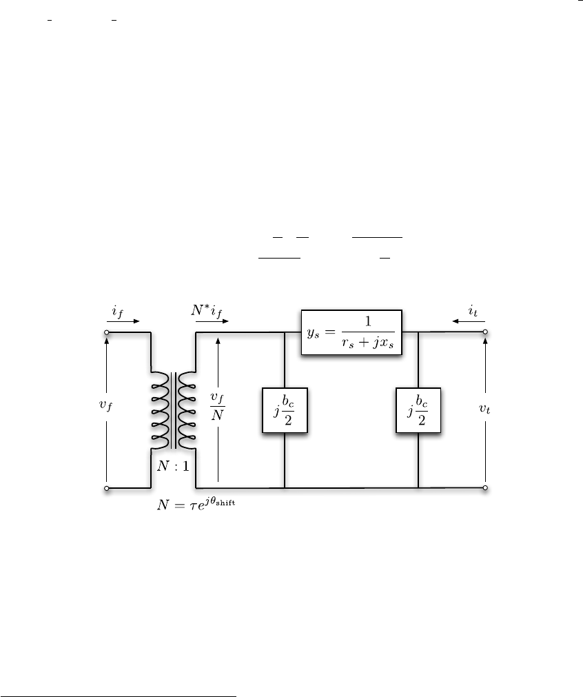
phase shift angle θshift, is located at the from end of the branch, as shown in Fig-
ure 3-1. The parameters rs,xs,bc,τand θshift are specified directly in columns BR R
(3), BR X (4), BR B (5), TAP (9) and SHIFT (10), respectively, of the corresponding row
of the branch matrix.15
The complex current injections ifand itat the from and to ends of the branch,
respectively, can be expressed in terms of the 2 ×2 branch admittance matrix Ybr
and the respective terminal voltages vfand vt
if
it=Ybr vf
vt.(3.1)
With the series admittance element in the πmodel denoted by ys= 1/zs, the branch
admittance matrix can be written
Ybr =ys+jbc
21
τ2−ys1
τe−jθshift
−ys1
τejθshift ys+jbc
2.(3.2)
Figure 3-1: Branch Model
If the four elements of this matrix for branch iare labeled as follows:
Yi
br =yi
ff yi
ft
yi
tf yi
tt (3.3)
then four nl×1 vectors Yff ,Yft,Ytf and Ytt can be constructed, where the i-th element
of each comes from the corresponding element of Yi
br. Furthermore, the nl×nbsparse
15A value of zero in the TAP column indicates that the branch is a transmission line and not a
transformer, i.e. mathematically equivalent to a transformer with tap ratio set to 1.
24
connection matrices Cfand Ctused in building the system admittance matrices can
be defined as follows. The (i, j)th element of Cfand the (i, k)th element of Ctare
equal to 1 for each branch i, where branch iconnects from bus jto bus k. All other
elements of Cfand Ctare zero.
3.3 Generators
A generator is modeled as a complex power injection at a specific bus. For generator i,
the injection is
si
g=pi
g+jqi
g.(3.4)
Let Sg=Pg+jQgbe the ng×1 vector of these generator injections. The MW and
MVAr equivalents (before conversion to p.u.) of pi
gand qi
gare specified in columns
PG (2) and QG (3), respectively of row iof the gen matrix. A sparse nb×nggenerator
connection matrix Cgcan be defined such that its (i, j)th element is 1 if generator j
is located at bus iand 0 otherwise. The nb×1 vector of all bus injections from
generators can then be expressed as
Sg,bus =Cg·Sg.(3.5)
A generator with a negative injection can also be used to model a dispatchable load.
3.4 Loads
Constant power loads are modeled as a specified quantity of real and reactive power
consumed at a bus. For bus i, the load is
si
d=pi
d+jqi
d(3.6)
and Sd=Pd+jQddenotes the nb×1 vector of complex loads at all buses. The
MW and MVAr equivalents (before conversion to p.u.) of pi
dand qi
dare specified in
columns PD (3) and QD (4), respectively of row iof the bus matrix. These fields can
also take on negative quantities to represent fixed (e.g. distributed) generation.
Constant impedance and constant current loads are not implemented directly,
but the constant impedance portions can be modeled as a shunt element described
below. Dispatchable loads are modeled as negative generators and appear as negative
values in Sg.
25
3.5 Shunt Elements
A shunt connected element such as a capacitor or inductor is modeled as a fixed
impedance to ground at a bus. The admittance of the shunt element at bus iis given
as
yi
sh =gi
sh +jbi
sh (3.7)
and Ysh =Gsh +jBsh denotes the nb×1 vector of shunt admittances at all buses.
The parameters gi
sh and bi
sh are specified in columns GS (5) and BS (6), respectively,
of row iof the bus matrix as equivalent MW (consumed) and MVAr (injected) at a
nominal voltage magnitude of 1.0 p.u and angle of zero.
A shunt element can also be used to model a constant impedance load and, though
correctly, Matpower does not currently report these quantities as “load”.
3.6 Network Equations
For a network with nbbuses, all constant impedance elements of the model are
incorporated into a complex nb×nbbus admittance matrix Ybus that relates the
complex nodal current injections Ibus to the complex node voltages V:
Ibus =YbusV. (3.8)
Similarly, for a network with nlbranches, the nl×nbsystem branch admittance
matrices Yfand Ytrelate the bus voltages to the nl×1 vectors Ifand Itof branch
currents at the from and to ends of all branches, respectively:
If=YfV(3.9)
It=YtV. (3.10)
If [ ·] is used to denote an operator that takes an n×1 vector and creates the
corresponding n×ndiagonal matrix with the vector elements on the diagonal, these
system admittance matrices can be formed as follows:
Yf= [Yff ]Cf+ [Yf t]Ct(3.11)
Yt= [Ytf ]Cf+ [Ytt]Ct(3.12)
Ybus =Cf
TYf+Ct
TYt+ [Ysh].(3.13)
The current injections of (3.8)–(3.10) can be used to compute the corresponding
26

complex power injections as functions of the complex bus voltages V:
Sbus(V) = [V]I∗
bus = [V]Y∗
busV∗(3.14)
Sf(V) = [CfV]I∗
f= [CfV]Y∗
fV∗(3.15)
St(V) = [CtV]I∗
t= [CtV]Y∗
tV∗.(3.16)
The nodal bus injections are then matched to the injections from loads and generators
to form the AC nodal power balance equations, expressed as a function of the complex
bus voltages and generator injections in complex matrix form as
gS(V, Sg) = Sbus(V) + Sd−CgSg= 0.(3.17)
3.7 DC Modeling
The DC formulation [17] is based on the same parameters, but with the following
three additional simplifying assumptions.
•Branches can be considered lossless. In particular, branch resistances rsand
charging capacitances bcare negligible:
ys=1
rs+jxs≈1
jxs
, bc≈0.(3.18)
•All bus voltage magnitudes are close to 1 p.u.
vi≈ejθi.(3.19)
•Voltage angle differences across branches are small enough that
sin(θf−θt−θshift)≈θf−θt−θshift.(3.20)
Substituting the first set of assumptions regarding branch parameters from (3.18),
the branch admittance matrix in (3.2) approximates to
Ybr ≈1
jxs1
τ2−1
τe−jθshift
−1
τejθshift 1.(3.21)
Combining this and the second assumption with (3.1) yields the following approxi-
mation for if:
if≈1
jxs
(1
τ2ejθf−1
τe−jθshift ejθt)
=1
jxsτ(1
τejθf−ej(θt+θshift)).(3.22)
27

The approximate real power flow is then derived as follows, first applying (3.19) and
(3.22), then extracting the real part and applying (3.20).
pf=<{sf}
=<vf·i∗
f
≈ <ejθf·j
xsτ(1
τe−jθf−e−j(θt+θshift))
=<j
xsτ1
τ−ej(θf−θt−θshift)
=<1
xsτsin(θf−θt−θshift) + j1
τ−cos(θf−θt−θshift)
≈1
xsτ(θf−θt−θshift) (3.23)
As expected, given the lossless assumption, a similar derivation for the power injec-
tion at the to end of the line leads to leads to pt=−pf.
The relationship between the real power flows and voltage angles for an individual
branch ican then be summarized as
pf
pt=Bi
br θf
θt+Pi
shift (3.24)
where
Bi
br =bi1−1
−1 1 ,
Pi
shift =θi
shiftbi−1
1
and biis defined in terms of the series reactance xi
sand tap ratio τifor branch ias
bi=1
xi
sτi.
For a shunt element at bus i, the amount of complex power consumed is
si
sh =vi(yi
shvi)∗
≈ejθi(gi
sh −jbi
sh)e−jθi
=gi
sh −jbi
sh.(3.25)
28
So the vector of real power consumed by shunt elements at all buses can be approx-
imated by
Psh ≈Gsh.(3.26)
With a DC model, the linear network equations relate real power to bus voltage
angles, versus complex currents to complex bus voltages in the AC case. Let the
nl×1 vector Bff be constructed similar to Yff , where the i-th element is biand let
Pf,shift be the nl×1 vector whose i-th element is equal to −θi
shiftbi. Then the nodal
real power injections can be expressed as a linear function of Θ, the nb×1 vector of
bus voltage angles
Pbus(Θ) = BbusΘ + Pbus,shift (3.27)
where
Pbus,shift = (Cf−Ct)TPf,shift.(3.28)
Similarly, the branch flows at the from ends of each branch are linear functions of
the bus voltage angles
Pf(Θ) = BfΘ + Pf,shift (3.29)
and, due to the lossless assumption, the flows at the to ends are given by Pt=−Pf.
The construction of the system Bmatrices is analogous to the system Ymatrices
for the AC model:
Bf= [Bff ] (Cf−Ct) (3.30)
Bbus = (Cf−Ct)TBf.(3.31)
The DC nodal power balance equations for the system can be expressed in matrix
form as
gP(Θ, Pg) = BbusΘ + Pbus,shift +Pd+Gsh −CgPg= 0 (3.32)
29

4 Power Flow
The standard power flow or loadflow problem involves solving for the set of voltages
and flows in a network corresponding to a specified pattern of load and generation.
Matpower includes solvers for both AC and DC power flow problems, both of
which involve solving a set of equations of the form
g(x) = 0,(4.1)
constructed by expressing a subset of the nodal power balance equations as functions
of unknown voltage quantities.
All of Matpower’s solvers exploit the sparsity of the problem and, except for
Gauss-Seidel, scale well to very large systems. Currently, none of them include any
automatic updating of transformer taps or other techniques to attempt to satisfy
typical optimal power flow constraints, such as generator, voltage or branch flow
limits.
4.1 AC Power Flow
In Matpower, by convention, a single generator bus is typically chosen as a refer-
ence bus to serve the roles of both a voltage angle reference and a real power slack.
The voltage angle at the reference bus has a known value, but the real power gen-
eration at the slack bus is taken as unknown to avoid overspecifying the problem.
The remaining generator buses are typically classified as PV buses, with the values
of voltage magnitude and generator real power injection given. These are specified
in the VG (6) and PG (3) columns of the gen matrix, respectively. Since the loads Pd
and Qdare also given, all non-generator buses are classified as PQ buses, with real
and reactive injections fully specified, taken from the PD (3) and QD (4) columns of
the bus matrix. Let Iref ,IPV and IPQ denote the sets of bus indices of the reference
bus, PV buses and PQ buses, respectively. The bus type classification is specified in
the Matpower case file in the BUS TYPE column (2) of the bus matrix. Any isolated
buses must be identified as such in this column as well.
In the traditional formulation of the AC power flow problem, the power balance
equation in (3.17) is split into its real and reactive components, expressed as functions
of the voltage angles Θ and magnitudes Vmand generator injections Pgand Qg, where
the load injections are assumed constant and given:
gP(Θ, Vm, Pg) = Pbus(Θ, Vm) + Pd−CgPg= 0 (4.2)
gQ(Θ, Vm, Qg) = Qbus(Θ, Vm) + Qd−CgQg= 0.(4.3)
30

For the AC power flow problem, the function g(x) from (4.1) is formed by taking
the left-hand side of the real power balance equations (4.2) for all non-slack buses
and the reactive power balance equations (4.3) for all PQ buses and plugging in the
reference angle, the loads and the known generator injections and voltage magnitudes:
g(x) = "g{i}
P(Θ, Vm, Pg)
g{j}
Q(Θ, Vm, Qg)#∀i∈ IPV ∪ IPQ
∀j∈ IPQ.(4.4)
The vector xconsists of the remaining unknown voltage quantities, namely the volt-
age angles at all non-reference buses and the voltage magnitudes at PQ buses:
x=θ{i}
v{j}
m∀i /∈ Iref
∀j∈ IPQ.(4.5)
This yields a system of nonlinear equations with npv + 2npq equations and un-
knowns, where npv and npq are the number of PV and PQ buses, respectively. After
solving for x, the remaining real power balance equation can be used to compute
the generator real power injection at the slack bus. Similarly, the remaining npv + 1
reactive power balance equations yield the generator reactive power injections.
Matpower includes four different algorithms for solving the general AC power
flow problem.16 The default solver is based on a standard Newton’s method [8] using a
polar form and a full Jacobian updated at each iteration. Each Newton step involves
computing the mismatch g(x), forming the Jacobian based on the sensitivities of
these mismatches to changes in xand solving for an updated value of xby factorizing
this Jacobian. This method is described in detail in many textbooks.
Also included are solvers based on variations of the fast-decoupled method [9],
specifically, the XB and BX methods described in [10]. These solvers greatly reduce
the amount of computation per iteration, by updating the voltage magnitudes and
angles separately based on constant approximate Jacobians which are factored only
once at the beginning of the solution process. These per-iteration savings, however,
come at the cost of more iterations.
The fourth algorithm is the standard Gauss-Seidel method from Glimm and
Stagg [11]. It has numerous disadvantages relative to the Newton method and is
included primarily for academic interest.
By default, the AC power flow solvers simply solve the problem described above,
ignoring any generator limits, branch flow limits, voltage magnitude limits, etc. How-
ever, there is an option (pf.enforce q lims) that allows for the generator reactive
16Three more that are specific to radial networks typical of distribution systems are described in
Section 4.3.
31
power limits to be respected at the expense of the voltage setpoint. This is done
in a rather brute force fashion by adding an outer loop around the AC power flow
solution. If any generator has a violated reactive power limit, its reactive injection is
fixed at the limit, the corresponding bus is converted to a PQ bus and the power flow
is solved again. This procedure is repeated until there are no more violations. Note
that this option is based solely on the QMAX and QMIN parameters for the generator,
from columns 4 and 5 of the gen matrix, and does not take into account the trape-
zoidal generator capability curves described in Section 6.4.3 and specifed in columns
PC1–QC2MAX (11–16). Note also that this option affects generators even if the bus
they are attached to is already of type PQ.
4.2 DC Power Flow
For the DC power flow problem [17], the vector xconsists of the set of voltage angles
at non-reference buses
x=θ{i},∀i /∈ Iref (4.6)
and (4.1) takes the form
Bdcx−Pdc = 0 (4.7)
where Bdc is the (nb−1) ×(nb−1) matrix obtained by simply eliminating from Bbus
the row and column corresponding to the slack bus and reference angle, respectively.
Given that the generator injections Pgare specified at all but the slack bus, Pdc can
be formed directly from the non-slack rows of the last four terms of (3.32).
The voltage angles in xare computed by a direct solution of the set of linear
equations. The branch flows and slack bus generator injection are then calculated
directly from the bus voltage angles via (3.29) and the appropriate row in (3.32),
respectively.
4.3 Distribution Power Flow
Distribution systems are different from transmission systems in a number of respects,
such as the xs/rsbranch ratio, magnitudes of xsand rsand most importantly the
typically radial structure. Due to these differences, a number of power flow solu-
tion methods have been developed to account for the specific nature of distribution
systems and most widely used are the backward/forward sweep methods [12,13].
Matpower includes an additional three AC power flow methods that are specific
to radial networks.
32
4.3.1 Radial Power Flow
When solving radial distribution networks it is practical to number branches with
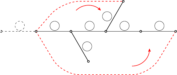
numbers that are equal to the receiving bus numbers. An example is given in Fig-
ure 4-1, where branches are drawn black. Furthermore, the oriented branch ordering
[14] offers a possibility for fast and efficient backward/forward sweeps. All branches
are always oriented from the sending bus to the receiving bus and the only re-
quirement is that the sending bus number should be smaller than the receiving bus
number. This means that i<kfor branch i–k. The indices of the sending nodes of
branches are stored in vector Fsuch that i=fk.
Loop 1
Loop 2
011223
3
4477PV2
6
6
5PV1
5
Figure 4-1: Oriented Ordering
As usual, the supply bus (slack bus) is given index 1, meaning that branch indices
should go from 2 to nbwhich is the number of buses in the network. Introducing a
fictitious branch with index 1 and zero impedance, given with dashed black line in
Figure 4-1, the number of branches nlbecomes equal to the number of buses nb.
For the example of Figure 4-1 vector Fis the following
F=0123324T,
and it offers an easy way to follow the path between any bus and bus 0. If we
consider bus 4, the path to the slack bus consists of following branches: branch 4,
since considered bus is their receiving bus; branch 3, since f4= 3; branch 2, since
f3= 2; and branch 1, since f2= 1.
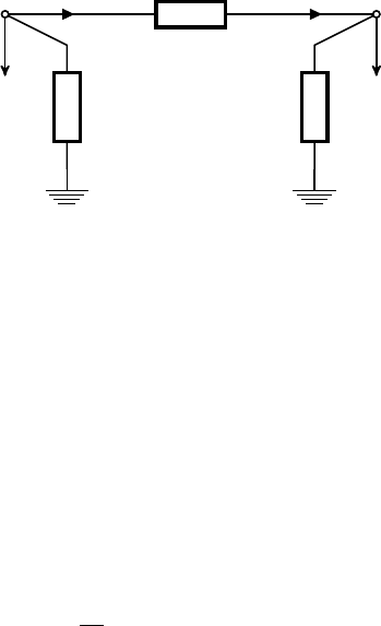
The representation of branch k, connecting buses iand k, is given in Figure 4-2,
where it is modeled with its serial impedance zk
s. At both ends there are load
demands si
dand sk
d, and shunt admittances yi
dand yk
dcomprised of admittances due
capacitance of all lines and shunt elements connected to buses iand k
yk
d=jXbk
lines +Xbk
shunt.
33
isk
fzk
ssk
tk
si
dyi
d
+
−
vi
sk
d
yk
d
+
−
vk
Figure 4-2: Branch Representation: branch kbetween buses i(sending) and k(re-
ceiving) and load demand and shunt admittances at both buses
4.3.2 Current Summation Method
The voltage calculation procedure with the Current Summation Method is performed
in 5 steps as follows [12,13].
1. Set all voltages to 1 p.u. (flat start). Set iteration count ν= 1.
2. Set branch current flow equal to the sum of current of the demand at receiving
end (sk
d) and the current drawn in the admittance (yk
d) connected to bus k
jk
b=sk
d
vk∗
+yk
d·vk, k = 1,2, . . . , nb.(4.8)
3. Backward sweep: Perform current summation, starting from the branch with
the biggest index and heading towards the branch whose index is equal to 1.
The current of branch kis added to the current of the branch whose index is
equal to i=fk.
ji
b,new =ji
b+jk
b, k =nl, nl−1,...,2 (4.9)
4. Forward sweep: The receiving end bus voltages are calculated with known
branch currents and sending bus voltages.
vk=vi−zk
s·jk
b, k = 2,3, . . . , nl(4.10)
5. Compare voltages in iteration νwith the corresponding ones from iteration
ν−1. If the maximum difference in magnitude is less than the specified toler-
ance
max
i=1...nbvν
i−vν−1
i< ε (4.11)
the procedure is finished. Otherwise go to step 2.
34

4.3.3 Power Summation Method
The voltage calculation procedure with the Power Summation Method is performed
in 5 steps as follows [14].
1. Set all voltages to 1 p.u. (flat start). Set iteration count ν= 1.
2. Set receiving end branch flow equal to the sum of the demand at receiving end
(sk
d) and the power drawn in the admittance (yk
d) connected to bus k
sk
t=sk
d+yk
d∗
v2
k
, k = 1,2, . . . , nb.(4.12)
3. Backward sweep: Calculate sending end branch power flows as a sum of re-
ceiving end branch power flows and branch losses via (4.13). Perform power
summation, starting from the branch with the biggest index and heading to-
wards the branch whose index is equal to 1. The sending power of branch kis
added to the receiving power of the branch whose index is equal to i=fkas
in (4.14).
sk
f=sk
t+zk
s·
sk
t
vk
2
k=nl, nl−1,...,2 (4.13)
si
t,new =si
t+sk
fk=nl, nl−1,...,2 (4.14)
4. Forward sweep: The receiving end bus voltages are calculated with known
sending powers and voltages.
vk=vi−zk
s· sk
f
vi!∗
k= 2,3, . . . , nl(4.15)
5. Compare voltages in iteration νwith the corresponding ones from iteration
ν−1, using (4.11). If the maximum difference in magnitude is less than the
specified tolerance the procedure is finished. Otherwise go to step 2.
4.3.4 Admittance Summation Method
For each node, besides the known admittance yk
d, we define the admittance yk
eas the
driving point admittance of the part of the network fed by node k, including shunt
35

admittance yk
d. We also define an equivalent current generator jk
efor the part of the
network fed by node k. The current of this generator consists of all load currents fed
by node k. The process of calculation of bus voltages with the admittance summation
method consists of the following 5 steps [15].
1. Set all voltages to 1 p.u. (flat start). Set iteration count ν= 1. Set initial
values
yk
e=yk
d, k = 1,2, . . . , nb.(4.16)
2. For each node k, calculate equivalent admittance yk
e. Perform admittance sum-
mation, starting from the branch with the biggest index and heading towards
the branch whose index is equal to 1. The driving point admittance of branch k
is added to the driving point admittance of the branch whose index is equal to
i=fkas in (4.18).
dk
b=1
1 + zk
s·yk
e
k=nl, nl−1,...,2 (4.17)
yi
e,new =yi
e+dk
b·yk
ek=nl, nl−1,...,2 (4.18)
3. Backward sweep: For each node kcalculate equivalent current generator jk
e, first
set it equal to load current jk
dand perform current summation over equivalent
admittances using factor dk
bas in (4.17).
jk
e=jk
d=sk
d
vk∗
k=nl, nl−1,...,2 (4.19)
ji
e,new =ji
e+dk
b·jk
ek=nl, nl−1,...,2 (4.20)
4. Forward sweep: The receiving end bus voltages are calculated with known
equivalent current generators and sending bus voltages.
vk=dk
b·(vi−zk
s·jk
e)k= 2,3, . . . , nl(4.21)
5. Compare voltages in iteration νwith the corresponding ones from iteration
ν−1, using (4.11). If the maximum difference in magnitude is less than the
specified tolerance the procedure is finished. Otherwise go to step 3.
36

4.3.5 Handling PV Buses
The methods explained in the previous three subsections are applicable to radial
networks without loops and PV buses. These methods can be used to solve the
power flow problem in weakly meshed networks if a compensation procedure based on
Thevenin equivalent impedance matrix is added [12,13]. In [14] a voltage correction
procedure is added to the process.
The list of branches is expanded by a set of npv fictitious links, corresponding to
the PV nodes. Each of these links starts at the slack bus and ends at a corresponding
PV bus, thus forming a loop in the network. A fictitious link going to bus kis
represented by a voltage generator with a voltage magnitude equal to the specified
voltage magnitude at bus k. Its phase angle is equal to the calculated phase angle
at bus k.
A loop impedance matrix Zlis formed for the loops made by the fictitious links
and it has the following properties
•Element zmm
lis equal to the sum of branch impedances off all branches related
to loop m,
•Element zmk
lis equal to the sum of branch impedances of mutual branches of
loops mand k.
As an illustration, in Figure 4-1 there a two PV generators at buses 5 and 7. The
fictitious links and loops orientation are drawn in red. The Thevenin matrix for this
case is
Zl=z2
b+z3
b+z5
bz2
b+z3
b
z2
b+z3
bz2
b+z3
b+z4
b+z7
b.
First column elements are equal to PV bus voltages when the current injection
at bus 5 is 1 p.u. and v1= 0. Bus voltages can be calculated with the current
summation method in a single iteration. By repeating the procedure for bus 7 one
can calculate the elements of second column.
By breaking all links the network becomes radial [13] and the three backward/forward
sweep methods are applicable. Since all link are fictitious, only the injected reactive
power at their receiving bus mis determined [14] by the following equation
∆qm
pv = ∆dm
pv
v2
m
<{vm},(4.22)
which is practically an increment in reactive power injection of the corresponding
PV generator for the current iteration.
37

The incremental changes of the imaginary part of PV generator current ∆dm
pv can
be obtained by solving the matrix equation
={Zl} · ∆Dpv = ∆Epv,(4.23)
where
∆em
pv =vm
g
|vm|−1· <{vm}, m = 1,2, . . . , npv.(4.24)
In order to ensure 90◦phase difference between voltage and current at PV gen-
erators in [16] it was suggested to calculate the real part of PV generator current
as
∆cm
pv = ∆dm
pv ={vm}
<{vm}.(4.25)
In such a way the PV generator will inject purely reactive power, as it is supposed
to do. Its active power is added before as a negative load.
Before proceeding with the next iteration, the bus voltage corrections are cal-
culated. In order to do that, the radial network is solved by applying incremental
current changes ∆Ipv = ∆Cpv +j∆Dpv at the PV buses as excitations and setting
v1= 0. After the backward/forward sweep is performed with the current summation
method, the voltage corrections at all buses are known. They are added to the latest
voltages in order to obtain the new bus voltages, which are used in the next iteration
[14].
4.4 runpf
In Matpower, a power flow is executed by calling runpf with a case struct or case
file name as the first argument (casedata). In addition to printing output to the
screen, which it does by default, runpf optionally returns the solution in a results
struct.
>> results = runpf(casedata);
The results struct is a superset of the input Matpower case struct mpc, with some
additional fields as well as additional columns in some of the existing data fields.
The solution values are stored as shown in Table 4-1.
Additional optional input arguments can be used to set options (mpopt) and
provide file names for saving the pretty printed output (fname) or the solved case
data (solvedcase).
38

Table 4-1: Power Flow Results
name description
results.success success flag, 1 = succeeded, 0 = failed
results.et computation time required for solution
results.iterations number of iterations required for solution
results.order see ext2int help for details on this field
results.bus(:, VM)†bus voltage magnitudes
results.bus(:, VA) bus voltage angles
results.gen(:, PG) generator real power injections
results.gen(:, QG)†generator reactive power injections
results.branch(:, PF) real power injected into “from” end of branch
results.branch(:, PT) real power injected into “to” end of branch
results.branch(:, QF)†reactive power injected into “from” end of branch
results.branch(:, QT)†reactive power injected into “to” end of branch
†AC power flow only.
>> results = runpf(casedata, mpopt, fname, solvedcase);
The options that control the power flow simulation are listed in Table 4-2 and those
controlling the output printed to the screen in Table 4-3.
By default, runpf solves an AC power flow problem using a standard Newton’s
method solver. To run a DC power flow, the model option must be set to 'DC'. For
convenience, Matpower provides a function rundcpf which is simply a wrapper
that sets the model option to 'DC'before calling runpf.
Internally, the runpf function does a number of conversions to the problem data
before calling the appropriate solver routine for the selected power flow algorithm.
This external-to-internal format conversion is performed by the ext2int function,
described in more detail in Section 7.3.1, and includes the elimination of out-of-service
equipment, the consecutive renumbering of buses and the reordering of generators
by increasing bus number. All computations are done using this internal indexing.
When the simulation has completed, the data is converted back to external format
by int2ext before the results are printed and returned.
4.5 Linear Shift Factors
The DC power flow model can also be used to compute the sensitivities of branch
flows to changes in nodal real power injections, sometimes called injection shift factors
(ISF) or generation shift factors [17]. These nl×nbsensitivity matrices, also called
39

Table 4-2: Power Flow Options
name default description
model 'AC'AC vs. DC modeling for power flow and OPF formulation
'AC'– use AC formulation and corresponding alg options
'DC'– use DC formulation and corresponding alg options
pf.alg 'NR'AC power flow algorithm:
'NR'– Newtons’s method
'FDXB'– Fast-Decoupled (XB version)
'FDBX'– Fast-Decouple (BX version)
'GS'– Gauss-Seidel
'PQSUM'– Power Summation (radial networks only)
'ISUM'– Current Summation (radial networks only)
'YSUM'– Admittance Summation (radial networks only)
pf.tol 10−8termination tolerance on per unit P and Q dispatch
pf.nr.max it 10 maximum number of iterations for Newton’s method
pf.nr.lin solver '' linear solver option for mplinsolve for computing Newton update step
(see mplinsolve for complete list of all options)
'' – default to '\'for small systems, 'LU3'for larger ones
'\'– built-in backslash operator
'LU'– explicit default LU decomposition and back substitution
'LU3'– 3 output arg form of lu, Gilbert-Peierls algorithm with
approximate minimum degree (AMD) reordering
'LU4'– 4 output arg form of lu, UMFPACK solver (same as
'LU')
'LU5'– 5 output arg form of lu, UMFPACK solver w/row scaling
pf.fd.max it 30 maximum number of iterations for fast-decoupled method
pf.gs.max it 1000 maximum number of iterations for Gauss-Seidel method
pf.radial.max it 20 maximum number of iterations for radial power flow methods
pf.radial.vcorr 0 perform voltage correction procedure in distribution power flow
0 – do not perform voltage correction
1 – perform voltage correction
pf.enforce q lims 0 enforce gen reactive power limits at expense of |Vm|
0 – do not enforce limits
1 – enforce limits, simultaneous bus type conversion
2 – enforce limits, one-at-a-time bus type conversion
power transfer distribution factors or PTDFs, carry an implicit assumption about
the slack distribution. If His used to denote a PTDF matrix, then the element in
row iand column j,hij , represents the change in the real power flow in branch i
given a unit increase in the power injected at bus j,with the assumption that the
additional unit of power is extracted according to some specified slack distribution:
∆Pf=H∆Pbus.(4.26)
40

Table 4-3: Power Flow Output Options
name default description
verbose 1 amount of progress info to be printed
0 – print no progress info
1 – print a little progress info
2 – print a lot of progress info
3 – print all progress info
out.all -1 controls pretty-printing of results
-1 – individual flags control what is printed
0 – do not print anything†
1 – print everything†
out.sys sum 1 print system summary (0 or 1)
out.area sum 0 print area summaries (0 or 1)
out.bus 1 print bus detail, includes per bus gen info (0 or 1)
out.branch 1 print branch detail (0 or 1)
out.gen 0 print generator detail (0 or 1)
out.force 0 print results even if success flag = 0 (0 or 1)
out.suppress detail -1 suppress all output but system summary
-1 – suppress details for large systems (>500 buses)
0 – do not suppress any output specified by other flags
1 – suppress all output except system summary section†
†Overrides individual flags, but (in the case of out.suppress detail) not out.all = 1.
This slack distribution can be expressed as an nb×1 vector wof non-negative
weights whose elements sum to 1. Each element specifies the proportion of the slack
taken up at each bus. For the special case of a single slack bus k,wis equal to the
vector ek. The corresponding PTDF matrix Hkcan be constructed by first creating
the nl×(nb−1) matrix
e
Hk=e
Bf·B−1
dc (4.27)
then inserting a column of zeros at column k. Here e
Bfand Bdc are obtained from Bf
and Bbus, respectively, by eliminating their reference bus columns and, in the case
of Bdc, removing row kcorresponding to the slack bus.
The PTDF matrix Hw, corresponding to a general slack distribution w, can be
obtained from any other PTDF, such as Hk, by subtracting Hk·wfrom each column,
equivalent to the following simple matrix multiplication:
Hw=Hk(I−w·1T).(4.28)
These same linear shift factors may also be used to compute sensitivities of branch
flows to branch outages, known as line outage distribution factors or LODFs [18].
41

Given a PTDF matrix Hw, the corresponding nl×nlLODF matrix Lcan be con-
structed as follows, where lij is the element in row iand column j, representing the
change in flow in branch i(as a fraction of the initial flow in branch j) for an outage
of branch j.
First, let Hrepresent the matrix of sensitivities of branch flows to branch endpoint
injections, found by multplying the PTDF matrix by the node-branch incidence
matrix:
H=Hw(Cf−Ct)T.(4.29)
Here the individual elements hij represent the sensitivity of flow in branch iwith
respect to injections at branch jendpoints, corresponding to a simulated increase in
flow in branch j. Then lij can be expressed as
lij =
hij
1−hjj
i6=j
−1i=j.
(4.30)
Matpower includes functions for computing both the DC PTDF matrix and
the corresponding LODF matrix for either a single slack bus kor a general slack
distribution vector w. See the help for makePTDF and makeLODF and Sections 9.5.5
and 9.5.4, respectively, for details.
42

5 Continuation Power Flow
Continuation methods or branch tracing methods are used to trace a curve given an
initial point on the curve. These are also called predictor-corrector methods since
they involve the prediction of the next solution point and correcting the prediction
to get the next point on the curve.
Consider a system of nnonlinear equations g(x) = 0, x ∈Rn. By adding a
continuation parameter λand one more equation to the system, xcan be traced by
varying λ. The resulting system f(x, λ) = 0 has n+ 1 dimensions. The additional
equation is a parameterized equation which identifies the location of the current
solution with respect to the previous or next solution.
The continuation process can be diagrammatically shown by (5.1).
xj, λjP redictor
−−−−−→ (ˆxj+1,ˆ
λj+1)Corrector
−−−−−→ xj+1, λj+1(5.1)
where, (xj, λj) represents the current solution at step j, (ˆxj+1,ˆ
λj+1) is the predicted
solution for the next step, and (xj+1, λj+1) is the next solution on the curve.
Continuation methods are employed in power systems to determine steady state
stability limits [19] in what is called a continuation power flow17. The limit is de-
termined from a nose curve where the nose represents the maximum power transfer
that the system can handle given a power transfer schedule. To determine the steady
state loading limit, the basic power flow equations
g(x) = P(x)−Pinj
Q(x)−Qinj = 0,(5.2)
are restructured as
f(x, λ) = g(x)−λb = 0 (5.3)
where x≡(Θ, Vm) and bis a vector of power transfer given by
b=Pinj
target −Pinj
base
Qinj
target −Qinj
base .(5.4)
The effects of the variation of loading or generation can be investigated using the
continuation method by composing the bvector appropriately.
17Thanks to Shrirang Abhyankar, Rui Bo, and Alexander Flueck for contributions to Mat-
power’s continuation power flow feature.
43
5.1 Parameterization
The values of (x, λ) along the solution curve can parameterized in a number of ways
[20,21]. Parameterization is a mathematical way of identifying each solution so that
the next solution or previous solution can be quantified. Matpower includes three
parameterization scheme options to quantify this relationship, detailed below, where
σis the continuation step size parameter.
•Natural parameterization simply uses λdirectly as the parameter, so the
new λis simply the previous value plus the step size.
pj(x, λ) = λ−λj−σj= 0 (5.5)
•Arc length parameterization results in the following relationship, where
the step size is equal to the 2-norm of the distance from one solution to the
next.
pj(x, λ) = X
i
(xi−xj
i)2+ (λ−λj)2−(σj)2= 0 (5.6)
•Pseudo arc length parameterization [23] is Matpower’s default pa-
rameterization scheme, where the next point (x, λ) on the solution curve is
constrained to lie in the hyperplane running through the predicted solution
(ˆxj+1,ˆ
λj+1) orthogonal to the tangent line from the previous corrected solution
(xj, λj). This relationship can be quantified by the function
pj(x, λ) = x
λ−xj
λjT
¯zj−σj= 0,(5.7)
where ¯zjis the normalized tangent vector at (xj, λj) and σjis the continuation
step size parameter.
5.2 Predictor
The predictor is used to produce an estimate for the next solution. The better the
prediction, the faster is the convergence to the solution point. Matpower uses a
tangent predictor for estimating the curve to the next solution. The tangent vector
zj=dx dλ j
Tat the current solution (xj, λj) is found by solving the linear
system fxfλ
pj−1
xpj−1
λzj=0
1.(5.8)
44

The matrix on the left-hand side is simply the standard power flow Jacobian with an
additional column and row added. The extra column fλis simply the negative of the
power transfer vector band the extra row, required to make the system non-singular
and define the magnitude of zj, is the derivative of the the parameterization function
at the previous solution point pj−1.
The resulting tangent vector is then normalized
¯zj=zj
||zj||2
(5.9)
and used to compute the predicted approximation (ˆxj+1,ˆ
λj+1) to the next solution
(xj+1, λj+1) using ˆxj+1
ˆ
λj+1 =xj
λj+σj¯zj,(5.10)
where σjis the continuation step size.
5.3 Corrector
The corrector stage finds the next solution (xj+1, λj+1) by correcting the approxi-
mation estimated by the predictor (ˆxj+1,ˆ
λj+1). Newton’s method is used to find
the next solution by solving the n+ 1 dimensional system in (5.11), where one of
(5.5)–(5.7) has been added as an additional constraint to the parameterized power
flow equations of (5.3). f(x, λ)
pj(x, λ)= 0 (5.11)
5.4 Step Length Control
Step length control is a key element affecting the computational efficiency of a contin-
uation method. It affects the continuation method with two issues: (1) speed – how
fast the corrector converges to a specified accuracy, and (2) robustness – whether
the corrector converges to a true solution given a predicted point. Matpower’s
continuation power flow can optionally use adaptive steps, where the step size σis
adjusted by a scaling factor αwithin the limits specified.
σj+1 =αjσj, σmin ≤σj+1 ≤σmax (5.12)
This scaling factor αjfor step jis limited to a maximum of 2 and is calculated from
an error estimation between the predicted and corrected solutions γjas follows,
αj= 1 + βcpf cpf
γj−1, αj≤2,(5.13)
45
where βcpf is a damping factor, cpf is a specified tolerance, and γjis given by
γj=
xj+1, λj+1−ˆxj+1,ˆ
λj+1
∞.(5.14)
5.5 Event Detection and Location
A continuation power flow event is triggered when the value of one of the elements
of an event function changes sign from one continuation step to the next. The
event occurs at the point where the corresponding value of the event function passes
through zero. Matpower provides event functions to detect the location at which
the continuation power flow reaches the following:
•a specified target λvalue
•the nose point
•the end of a full trace
•a generator reactive power limit
•a generator active power limit
•a bus voltage magnitude limit
•a branch flow limit
Each event function is registered with an event name, a flag indicating whether
or not the location of the event should be pinpointed, and if so, to within what
tolerance. For events that are to be located, when an event interval is detected, that
is, when an element of the event function value changes sign, Matpower adjusts
the continuation step size via a False Position or Regula Falsi method until it locates
the point of the zero-crossing to within the specified tolerance.
The detection of an event zero, or even an event interval, can be used to trigger
further actions. The CPF callback function capability was extended in Matpower
6.x to include the ability to handle events by including information about any event
intervals or zeros detected. For example, Matpower includes a callback that fixes
the reactive output of a generator and converts its bus from PV to PQ when the
corresponding event function indicates that its reactive power limit has been reached.
Another responds to the detection of the nose point by signaling the termination of
the continuation. In fact, continuation power flow termination for nose point, target
46

lambda or full trace modes are all based on CPF callback functions in conjunction
with event detection.
While Matpower does include a mechanism for supplying user defined callback
functions, it does not yet have a corresponding mechanism for user specified event
functions.
5.6 runcpf
In Matpower, a continuation power flow is executed by calling runcpf with two
Matpower cases (case structs or case file names) as the first two arguments,
basecasedata and targetcasedata, respectively. The first contains the base load-
ing/generation profile while the second contains the target loading/generation pro-
file. In addition to printing output to the screen, which it does by default, runcpf
optionally returns the solution in a results struct.
>> results = runcpf(basecasedata, targetcasedata);
Additional optional input arguments can be used to set options (mpopt) and
provide file names for saving the pretty printed output (fname) or the solved case
data (solvedcase).
>> results = runcpf(basecasedata, targetcasedata, mpopt, fname, solvedcase);
The results struct is a superset of the input Matpower case struct mpc, with
some additional fields as well as additional columns in some of the existing data
fields. In addition to the solution values included in the results for a simple power
flow, shown in Table 4-1 in Section 4.4, the following additional continuation power
flow solution values are stored in the cpf field as shown in Table 5-1.
The options that control the continuation power flow simulation are listed in
Table 5-2. All the power flow options for Newton’s method (tolerance, maximum
iterations) and for controlling the output on the screen (see Tables 4-2 and 4-3) are
also available with the continuation power flow.
47

Table 5-1: Continuation Power Flow Results
name description
results.cpf CPF output struct whose content depends on any user callback functions,
where default contains fields:
done msg string with message describing cause of continuation termination
events(eidx) a structure array of size ne, where neis the number of events located, with
fields:
kcontinuation step number at which event was located
name name of event
idx index(es) of critical elements in corresponding event function, e.g. index
of generator reaching VAr limit
msg descriptive text detailing the event
iterations nsteps, number of continuation steps performed
lam 1×nvector of λvalues from correction steps†
lam hat 1×nvector of λvalues from prediction steps†
max lam maximum value of λfound in results.cpf.lam
steps 1×nvector of step sizes for each continuation step performed†
Vnb×nmatrix of complex bus voltages from correction steps†
V hat nb×nmatrix of complex bus voltages from prediction steps†
†nis one more than the number of continuation steps, i.e. nsteps + 1, so the first element corresponds to the
starting point.
48

Table 5-2: Continuation Power Flow Options
name default description
cpf.parameterization 3 choice of parameterization
1 — natural
2 — arc length
3 — pseudo arc length
cpf.stop at 'NOSE'determines stopping criterion
'NOSE'— stop when nose point is reached
'FULL'— trace full nose curve
λstop — stop upon reaching target λvalue λstop
cpf.enforce p lims 0 enforce gen active power limits
0 — do not enforce limits
1 — enforce limits
cpf.enforce q lims 0 enforce gen reactive power limits at expense of Vm
0 — do not enforce limits
1 — enforce limits
cpf.enforce v lims 0 enforce bus voltage magnitude limits
0 — do not enforce limits
1 — enforce limits
cpf.enforce flow lims 0 enforce branch MVA flow limits
0 — do not enforce limits
1 — enforce limits
cpf.step 0.05 default value for continuation power flow step size σ
cpf.step min 10−4minimum allowed step size, σmin
cpf.step max 0.2 maximum allowed step size, σmax
cpf.adapt step 0 toggle adaptive step size feature
0 — adaptive step size disabled
1 — adaptive step size enabled
cpf.adapt step damping 0.7 damping factor βcpf from (5.13) for adaptive step sizing
cpf.adapt step tol 10−3tolerance cpf from (5.13) for adaptive step sizing
cpf.target lam tol 10−5tolerance for target lambda detection
cpf.nose tol 10−5tolerance for nose point detection (p.u.)
cpf.p lims tol 10−2tolerance for generator active power limit detection
(MW)
cpf.q lims tol 10−2tolerance for generator reactive power limit detection
(MVAr)
cpf.v lims tol 10−4tolerance for bus voltage magnitude limit detection (p.u)
cpf.flow lims tol 0.01 tolerance for branch flow limit detection (MVA)
cpf.plot.level 0 control plotting of nose curve
0 — do not plot nose curve
1 — plot when completed
2 — plot incrementally at each iteration
3 — same as 2, with pause at each iteration
cpf.plot.bus empty index of bus whose voltage is to be plotted
cpf.user callback empty string or cell array of strings with names of user callback
functions†
†See help cpf default callback for details. 49

5.6.1 CPF Callback Functions
Matpower’s continuation power flow provides a callback mechanism to give the
user access to the iteration process for executing custom code at each iteration,
for example, to implement custom incremental plotting of a PV nose curve or to
handle a detected event. This callback mechanism is used internally to handle de-
fault plotting functionality as well as to handle the standard CPF events. The
cpf default callback function, for example, is used to collect the λand Vresults
from each predictor and corrector iteration and optionally plot the PV nose curve.
The prototype for a CPF callback function is
function [nx, cx, done, rollback, evnts, cb_data, results] = ...
cpf_user_callback(k, nx, cx, px, done, rollback, evnts, ...
cb_data, cb_args, results)
and the input and output arguments are described in Tables 5-3 through 5-5 and in
the help for cpf default callback. Each registered CPF callback function is called in
three different contexts, distinguished by the value of the first argument kas follows:
1. initial – called with k= 0, without results input/output arguments, after base
power flow, before first CPF step.
2. iterations – called with k>0, without results input/output arguments, at
each iteration, after predictor-corrector step
3. final – called with k<0, with results input/output arguments, after exiting
predictor-corrector loop, inputs identical to last iteration call, except knegated
The user can define their own callback functions which take the same form and
are called in the same contexts as cpf default callback. User callback functions are
specified via the Matpower option cpf.user callback. This option can be a string
containing the name of the callback function, or a struct with the following fields,
where all but the first are optional:
•fcn - string with name of callback function
•priority - numerical value specifying callback priority,18 default = 20
•args - arbitrary value (any type) passed to the callback as cb args each time
it is invoked
Multiple user callbacks can be registered by assigning a cell array of such strings
and/or structs to the cpf.user callback option.
18See cpf register callback for details.
50

Table 5-3: Continuation Power Flow Callback Input Arguments
name description
kcontinuation step iteration count
nx next CPF state*
, corresponding to proposed next step
cx current CPF state*
, corresponding to most recent successful step
px previous CPF state*
, corresponding to last successful step prior to cx
done struct, with flag to indicate CPF termination and reason, with fields:
.flag termination flag, 1 →terminate, 0 →continue
.msg string containing reason for termination
rollback scalar flag to indicate that the current step should be rolled back and
retried with a different step size, etc.
evnts struct array listing any events detected for this step‡
cb data struct containing static data§
, with the following fields (all based on internal
indexing):
.mpc base Matpower case struct of base case
.mpc target Matpower case struct of target case
.Sbusb handle of function returning nb×1 vector of complex base case bus injec-
tions in p.u. and derivatives w.r.t. |V|
.Sbust handle of function returning nb×1 vector of complex target case bus
injections in p.u. and derivatives w.r.t. |V|
.Ybus bus admittance matrix
.Yf branch admittance matrix, “from” end of branches
.Yt branch admittance matrix, “to” end of branches
.pv list of indices of PV buses
.pq list of indices of PQ buses
.ref list of indices of reference buses
.idx pmax vector of gen indices of gens at PMAX
.mpopt Matpower options struct
cb args arbitrary data structure containing user-provided callback arguments
results initial value of output struct to be assigned to cpf field of results struct
returned by runcpf
*See Table 5-5 for details of the CPF state.
‡See cpf detect events for details of the evnts field.
§Please note that any callback that modifies the underlying problem is responsible to update the contents of
cb data accordingly. E.g. converting a bus from PV to PQ requires updates to mpc base,mpc target,Sbusb,
Sbust,pv,pq, and possibly ref. So, cb data should only be thought of as static for a fixed base and target
case pair.
51

Table 5-4: Continuation Power Flow Callback Output Arguments
name description
All are updated versions of the corresponding input arguments, see Table 5-3 for more details.
nx next CPF state*
, user state (cb field) should be updated here if rollback
is false
cx current CPF state*
, may contain updated this step or this parm values
to be used if rollback is true
done callback may have requested termination and set the msg field
rollback callback can request a rollback step, even if it was not indicated by an
event function†
evnts msg field for a given event may be updated‡
cb data this data should only be modified if the underlying problem has been
changed (e.g. generator limit reached), in which case it should always
be followed by a step of zero length, i.e. set nx.this step to 0§
results updated version of results input argument to be assigned to cpf field of
results struct returned by runcpf
*See Table 5-5 for details of the CPF state.
†In this case, the callback should also modify the step size or parameterization to be used for the re-try, by
setting the this step or this parm fields in cx.
‡See cpf detect events for details of the evnts field.
§It is the job of any callback modifying cb data to ensure that all data in cb data is kept consistent.
Table 5-5: Continuation Power Flow State
name description
lam hat value of λafter predictor step
V hat vector of complex bus voltages after predictor step
lam value of λafter corrector step
Vvector of complex bus voltages after corrector step
znormalized tangent predictor, ¯z
default step default step size
default parm default parameterization*
this step step size for this step only
this parm parameterization*for this step only
step current step size
parm current parameterization*
events event log
cb user state for callbacks†, a user-defined struct containing any information
a callback function would like to pass from one invokation to the next
ef cell array of event function values
*Corresponding to the cpf.parameterization option in Table 5-2.
†Replaces cb state from Matpower 5.
52
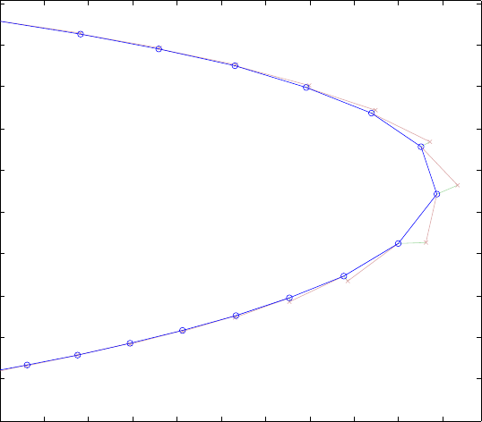
5.6.2 CPF Example
The following is an example of running a continuation power flow using a version of
the 9-bus system, looking at increasing all loads by a factor of 2.5. This example
plots the nose curve shown in Figure 5-1.
0 0.1 0.2 0.3 0.4 0.5 0.6 0.7 0.8 0.9 1
0
0.1
0.2
0.3
0.4
0.5
0.6
0.7
0.8
0.9
1
Voltage at Bus 9
λ
Voltage Magnitude
Figure 5-1: Nose Curve of Voltage Magnitude at Bus 9
53

define_constants;
mpopt = mpoption('out.all', 0, 'verbose', 2);
mpopt = mpoption(mpopt, 'cpf.stop_at', 'FULL', 'cpf.step', 0.2);
mpopt = mpoption(mpopt, 'cpf.plot.level', 2);
mpcb = loadcase(t_case9_pfv2); % load base case
mpct = mpcb; % set up target case with
mpct.gen(:, [PG QG]) = mpcb.gen(:, [PG QG]) * 2.5; % increased generation
mpct.bus(:, [PD QD]) = mpcb.bus(:, [PD QD]) * 2.5; % and increased load
results = runcpf(mpcb, mpct, mpopt);
This should result in something like the following output to the screen.
MATPOWER Version 7.0b1, 31-Oct-2018 -- AC Continuation Power Flow
step 0 : lambda = 0.000, 4 Newton steps
step 1 : stepsize = 0.2 lambda = 0.181 2 corrector Newton steps
step 2 : stepsize = 0.2 lambda = 0.359 2 corrector Newton steps
step 3 : stepsize = 0.2 lambda = 0.530 2 corrector Newton steps
step 4 : stepsize = 0.2 lambda = 0.693 3 corrector Newton steps
step 5 : stepsize = 0.2 lambda = 0.839 3 corrector Newton steps
step 6 : stepsize = 0.2 lambda = 0.952 3 corrector Newton steps
step 7 : stepsize = 0.2 lambda = 0.988 3 corrector Newton steps
step 8 : stepsize = 0.2 lambda = 0.899 3 corrector Newton steps
step 9 : stepsize = 0.2 lambda = 0.776 3 corrector Newton steps
step 10 : stepsize = 0.2 lambda = 0.654 3 corrector Newton steps
step 11 : stepsize = 0.2 lambda = 0.533 2 corrector Newton steps
step 12 : stepsize = 0.2 lambda = 0.413 2 corrector Newton steps
step 13 : stepsize = 0.2 lambda = 0.294 2 corrector Newton steps
step 14 : stepsize = 0.2 lambda = 0.176 2 corrector Newton steps
step 15 : stepsize = 0.2 lambda = 0.060 2 corrector Newton steps
step 16a : stepsize = 0.2 lambda = -0.054 2 corrector Newton steps ^ ROLLBACK
step 16 : stepsize = 0.0604 lambda = 0.000 3 corrector Newton steps
CPF TERMINATION: Traced full continuation curve in 16 continuation steps
The results of the continuation power flow are then found in the cpf field of the
returned results struct.
54

>> results.cpf
ans =
V_hat: [9x17 double]
lam_hat: [1x17 double]
V: [9x17 double]
lam: [1x17 double]
steps: [1x17 double]
iterations: 16
max_lam: 0.9876
events: [1x1 struct]
done_msg: 'Traced full continuation curve in 16 continuation steps'
55
6 Optimal Power Flow
Matpower includes code to solve both AC and DC versions of the optimal power
flow problem. The standard version of each takes the following form:
min
xf(x) (6.1)
subject to
g(x) = 0 (6.2)
h(x)≤0 (6.3)
xmin ≤x≤xmax .(6.4)
In both cases, the objective function f(x) consists of the polynomial cost of gener-
ator injections, the equality constraints g(x) are the power balance equations, the
inequality constraints h(x) are the branch flow limits, and the xmin and xmax bounds
include reference bus angles, voltage magnitudes (for AC) and generator injections.
6.1 Standard AC OPF
The optimization vector xfor the standard AC OPF problem consists of the nb×1
vectors of voltage angles Θ and magnitudes Vmand the ng×1 vectors of generator
real and reactive power injections Pgand Qg.
x=
Θ
Vm
Pg
Qg
(6.5)
The objective function f(x) in (6.1) is simply a summation of individual polynomial
cost functions fi
Pand fi
Qof real and reactive power injections, respectively, for each
generator:
f(Pg, Qg) =
ng
X
i=1
fi
P(pi
g) + fi
Q(qi
g).(6.6)
The equality constraints in (6.2) are simply the full set of 2 ·nbnonlinear real and
reactive power balance equations from (4.2) and (4.3).
gP(Θ, Vm, Pg) = Pbus(Θ, Vm) + Pd−CgPg= 0 (6.7)
gQ(Θ, Vm, Qg) = Qbus(Θ, Vm) + Qd−CgQg= 0 (6.8)
56

The inequality constraints (6.3) consist of two sets of nlbranch flow limits as non-
linear functions of the bus voltage angles and magnitudes, one for the from end and
one for the to end of each branch:
hf(Θ, Vm) = |Ff(Θ, Vm)| − Fmax ≤0 (6.9)
ht(Θ, Vm) = |Ft(Θ, Vm)| − Fmax ≤0.(6.10)
The flows are typically apparent power flows expressed in MVA, but can be real power
or current flows, yielding the following three possible forms for the flow constraints:
Ff(Θ, Vm) =
Sf(Θ, Vm),apparent power
Pf(Θ, Vm),real power
If(Θ, Vm),current
(6.11)
where Ifis defined in (3.9), Sfin (3.15), Pf=<{Sf}and the vector of flow limits
Fmax has the appropriate units for the type of constraint. It is likewise for Ft(Θ, Vm).
The values used by Matpower’s OPF for the flow limits Fmax are specified in the
RATE A column (6) of the branch matrix,19 and the selection of flow constraint type
in (6.11) is determined by the opf.flow lim option.
The variable limits (6.4) include an equality constraint on any reference bus angle
and upper and lower limits on all bus voltage magnitudes and real and reactive
generator injections:
θref
i≤θi≤θref
i, i ∈ Iref (6.12)
vi,min
m≤vi
m≤vi,max
m, i = 1 . . . nb(6.13)
pi,min
g≤pi
g≤pi,max
g, i = 1 . . . ng(6.14)
qi,min
g≤qi
g≤qi,max
g, i = 1 . . . ng.(6.15)
The voltage reference angle θref
iand voltage magnitude bounds vi,max
mand vi,min
mare
specified in columns VA (9), VMAX (12) and VMIN (13), respectively, of row iof the bus
matrix. Similarly, the generator bounds qi,max
g,qi,min
g,pi,max
gand pi,min
gare specfied in
columns QMAX (4), QMIN (5), PMAX (9) and PMIN (10), respectively, of row iof the gen
matrix.
6.1.1 Cartesian vs. Polar Coordinates for Voltage
Another variation of the standard AC OPF problem represents the bus voltages
in cartesian, rather than polar, coordinates. That is, instead of Θ and Vm, the
19Setting the RATE A column (6) of branch to zero is the preferred way to indicate a completely
unconstrained line.
57

optimization vector xincludes the real and imaginary parts of the complex voltage,
denoted respectively by Uand W, where V=U+jW .
x=
U
W
Pg
Qg
(6.16)
The objective function remains unchanged, but the nodal power balance con-
straints (6.7) and (6.8) and branch flow constraints (6.9) and (6.10) are implemented
as functions of Uand W.
gP(U, W, Pg) = Pbus(U, W ) + Pd−CgPg= 0 (6.17)
gQ(U, W, Qg) = Qbus(U, W ) + Qd−CgQg= 0 (6.18)
hf(U, W ) = |Ff(U, W )| − Fmax ≤0 (6.19)
ht(U, W ) = |Ft(U, W )| − Fmax ≤0.(6.20)
In this formulation, the voltage angle reference constraint (6.12) and voltage mag-
nitude limits (6.13) cannot be simply applied as bounds on optimization variables.
These constrained quantities also become functions of Uand W.
θref
i≤θi(ui, wi)≤θref
i, i ∈ Iref (6.21)
vi,min
m≤vi
m(ui, wi)≤vi,max
m, i = 1 . . . nb(6.22)
In Matpower setting the opf.v cartesian option to 1 (0 by default) selects the
cartesian representation for voltages when running an AC OPF.20
6.1.2 Current vs. Power for Nodal Balance Constraints
Another variation of the standard AC OPF problem uses current balance constraints
in place of the power balance constraints (6.7)–(6.8) or (6.17)–(6.18). If we let M
and Nrepresent the real and imaginary parts, respectively, of the current, we can
express the current balance functions for the polar form as
gM(Θ, Vm, Pg, Qg) = <{Ibus(Θ, Vm)+[V∗]−1(Sd−CgSg)∗}= 0 (6.23)
gN(Θ, Vm, Pg, Qg) = ={Ibus(Θ, Vm)+[V∗]−1(Sd−CgSg)∗}= 0 (6.24)
20This option only applies to solvers based on MIPS,fmincon,Ipopt and KNITRO.
58

and for the cartesian form as
gM(U, W, Pg, Qg) = <{Ibus(U, W )+[V∗]−1(Sd−CgSg)∗}= 0 (6.25)
gN(U, W, Pg, Qg) = ={Ibus(U, W )+[V∗]−1(Sd−CgSg)∗}= 0 (6.26)
where Sd=Pd+jQd,Sg=Pg+jQgand [V∗]−1is a diagonal matrix whose i-th
diagonal entry is 1/v∗
i, that is 1
vi
mejθior 1/(ui−jwi).
In this formulation, which can be selected by setting the opf.current balance
option to 1,21 the objective function and other constraints are not affected. This
option can be used in conjuntion with either the polar or cartesian representation of
bus voltages.
6.2 Standard DC OPF
When using DC network modeling assumptions and limiting polynomial costs to
second order, the standard OPF problem above can be simplified to a quadratic
program, with linear constraints and a quadratic cost function. In this case, the
voltage magnitudes and reactive powers are eliminated from the problem completely
and real power flows are modeled as linear functions of the voltage angles. The
optimization variable is
x=Θ
Pg(6.27)
and the overall problem reduces to the following form.
min
Θ,Pg
ng
X
i=1
fi
P(pi
g) (6.28)
subject to
gP(Θ, Pg) = BbusΘ + Pbus,shift +Pd+Gsh −CgPg= 0 (6.29)
hf(Θ) = BfΘ + Pf,shift −Fmax ≤0 (6.30)
ht(Θ) = −BfΘ−Pf,shift −Fmax ≤0 (6.31)
θref
i≤θi≤θref
i, i ∈ Iref (6.32)
pi,min
g≤pi
g≤pi,max
g, i = 1 . . . ng(6.33)
21This option only applies to solvers based on MIPS,fmincon,Ipopt and KNITRO.
59

6.3 Extended OPF Formulation
Matpower employs an extensible OPF structure to allow the user to modify or
augment the problem formulation without rewriting the portions that are shared
with the standard OPF formulation described above. The standard formulation is
modified by introducing additional variables, user-defined costs, and/or user-defined
constraints. The full extended formulation can be written as follows:
min
ˆxf(x) + fu(ˆx) (6.34)
subject to
ˆg(ˆx) = 0 (6.35)
ˆ
h(ˆx)≤0 (6.36)
ˆxmin ≤ˆx≤ˆxmax (6.37)
l≤Aˆx≤u(6.38)
The first difference to note is that the optimization variable xfrom the standard
OPF formulation has been augmented with additional variables zto form a new
optimization variable ˆx, and likewise with the lower and upper bounds.
ˆx=x
zˆxmin =xmin
zmin ˆxmax =xmax
zmax (6.39)
Second, there is an additional user-defined cost term fu(ˆx) in the objective function.
This cost consists of three pieces that will be described in more detail below.
fu(ˆx) = fq(ˆx) + fnln(ˆx) + flegacy(ˆx) (6.40)
Third, the nonlinear constraints gand hare augmented with user defined additions
guand huto give ˆgand ˆ
h.
ˆg(ˆx) = g(x)
gu(ˆx),ˆ
h(ˆx) = h(x)
hu(ˆx)(6.41)
And finally, a new set of linear constraints are included in (6.38).
Up through version 6.0 of Matpower, the OPF extensions were handled via op-
tional input parameters that define any additional variables,22 linear constraints,23
22Parameters zmin and zmax in (6.39).
23Parameters A,l,uin (6.38).
60

and costs of the pre-specified form defined by flegacy.24 This preserved the ability to
use solvers that employ pre-compiled MEX files to compute all of the costs and con-
straints. This is referred to as Matpower’s legacy extended OPF formulation [24].
For the AC OPF, subsequent versions also include the general nonlinear con-
straints guand hu, and the quadratic and general nonlinear costs fqand fnln. The
new quadratic cost terms can be handled by all of Matpower’s AC OPF solvers,
but the general nonlinear costs and constraints require a solver that uses Matlab
code to implement the function, gradient and Hessian evaluations.25
Section 7describes the mechanisms available to the user for taking advantage of
the extensible formulation described here.
6.3.1 User-defined Variables
The creation of additional user-defined zvariables can be done explicitly or implicitly
based on the difference between the number of columns in Aand the dimension of
the standard OPF optimization variable x. The optional vectors zmin and zmax are
available to impose lower and upper bounds on z, respectively.
6.3.2 User-defined Constraints
•Linear Constraints – The user-defined linear constraints (6.38) are general
linear restrictions involving all of the optimization variables and are specified
via matrix Aand lower and upper bound vectors land u. These parameters
can be used to create equality constraints (li=ui) or inequality constraints
that are bounded below (ui=∞), bounded above (li=∞) or bounded on
both sides.
•Nonlinear Constraints – The user-defined general nonlinear constraints take
the form
gj
u(x)=0 ∀j∈ Gu(6.42)
hj
u(x)≤0∀j∈ Hu,(6.43)
where Guand Huare sets of indices for user-defined equality and inequality
constraint sets, respectively.
Each of these constraint sets is defined by two M-file functions, similar to those
required by MIPS, one that computes the constraint values and their gradients
(Jacobian), and the other that computes Hessian values.
24Parameters H,C,N, ˆr,k,d,min (6.48)–(6.51).
25At the time of this writing, this includes solvers based on MIPS,fmincon,Ipopt and KNITRO.
61

6.3.3 User-defined Costs
The user-defined cost function fuconsists of three terms for three different types of
costs: quadratic, general nonlinear, and legacy. Each term is a simple summation
over all of the cost sets of that type.
fq(ˆx) = Pjfj
q(ˆx) (6.44)
fnln(ˆx) = Pjfj
nln(ˆx) (6.45)
flegacy(ˆx) = Pjfj
legacy(ˆx) (6.46)
•Quadratic Costs for a cost set jare specified by parameters Qj,cjand kj
that define a quadratic function of the optimization variable ˆx.
fj
q(ˆx) = ˆxTQjˆx+cj
Tˆx+kj(6.47)
•General Nonlinear Costs for a cost set jconsist of a cost function fj
nln(ˆx)
provided in the form of a function handle to an M-file function that evaluates
the cost and its gradients and Hessian for a given value of ˆx.
•Legacy Costs fj
legacy(ˆx) are specified in terms of parameters Hj,Cj,Nj, ˆrj,
kj,djand mj. For simplicity of presentation, we will drop the jsubscript for
the rest of this discussion. All of the parameters are nw×1 vectors except the
symmetric nw×nwmatrix Hand the nw×nˆxmatrix N. The legacy user cost
function takes the form
flegacy(ˆx) = 1
2wTHw +CTw(6.48)
where wis defined in several steps as follows. First, a new vector uis created
by applying a linear transformation Nand shift ˆrto the full set of optimization
variables
u=Nˆx−ˆr, (6.49)
then a scaled function with a “dead zone” is applied to each element of uto
produce the corresponding element of w.
wi=
mifdi(ui+ki), ui<−ki
0,−ki≤ui≤ki
mifdi(ui−ki), ui> ki
(6.50)
62
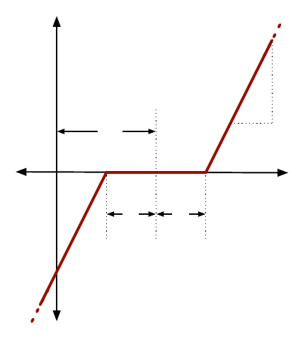
Here kispecifies the size of the “dead zone”, miis a simple scale factor and fdiis
a pre-defined scalar function selected by the value of di. Currently, Matpower
implements only linear and quadratic options:
fdi(α) = α, if di= 1
α2,if di= 2 (6.51)
as illustrated in Figure 6-1 and Figure 6-2, respectively.
wi
mi
ri
ˆri
ki
ki
Figure 6-1: Relationship of wito rifor di= 1 (linear option)
This form for flegacy provides the flexibility to handle a wide range of costs, from
simple linear functions of the optimization variables to scaled quadratic penal-
ties on quantities, such as voltages, lying outside a desired range, to functions
of linear combinations of variables, inspired by the requirements of price coor-
dination terms found in the decomposition of large loosely coupled problems
encountered in our own research.
Some limitations are imposed on the parameters in the case of the DC OPF
since Matpower uses a generic quadratic programming (QP) solver for the
optimization. In particular, ki= 0 and di= 1 for all i, so the “dead zone” is
not considered and only the linear option is available for fdi. As a result, for
the DC case (6.50) simplifies to wi=miui.
63
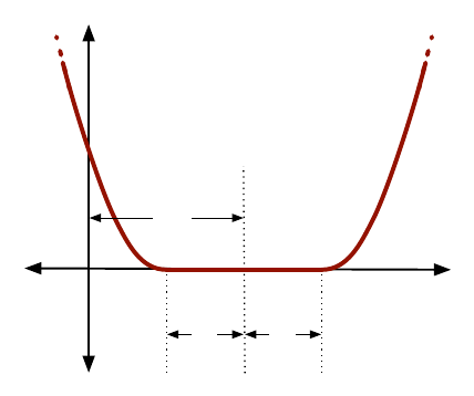
wi
ri
ˆri
ki
ki
Figure 6-2: Relationship of wito rifor di= 2 (quadratic option)
6.4 Standard Extensions
In addition to making this extensible OPF structure available to end users, Mat-
power also takes advantage of it internally to implement several additional capa-
bilities.
6.4.1 Piecewise Linear Costs
The standard OPF formulation in (6.1)–(6.4) does not directly handle the non-
smooth piecewise linear cost functions that typically arise from discrete bids and
offers in electricity markets. When such cost functions are convex, however, they
can be modeled using a constrained cost variable (CCV) method. The piecewise lin-
ear cost function c(x) is replaced by a helper variable yand a set of linear constraints
that form a convex “basin” requiring the cost variable yto lie in the epigraph of the
function c(x).
Figure 6-3 illustrates a convex n-segment piecewise linear cost function
c(x) =
m1(x−x1) + c1, x ≤x1
m2(x−x2) + c2, x1< x ≤x2
.
.
..
.
.
mn(x−xn) + cn, xn−1< x
(6.52)
defined by a sequence of points (xj, cj), j= 0 . . . n, where mjdenotes the slope of
64

x
x0
x1
x2
c
c0
c1
c2
y
cn
xn
Figure 6-3: Constrained Cost Variable
the j-th segment
mj=cj−cj−1
xj−xj−1
, j = 1 . . . n (6.53)
and x0< x1<··· < xnand m1≤m2≤ ··· < mn.
The “basin” corresponding to this cost function is formed by the following n
constraints on the helper cost variable y:
y≥mj(x−xj) + cj, j = 1 . . . n. (6.54)
The cost term added to the objective function in place of c(x) is simply the variable y.
Matpower uses this CCV approach internally to automatically generate the
appropriate helper variable, cost term and corresponding set of constraints for any
piecewise linear costs on real or reactive generation. All of Matpower’s OPF
solvers, for both AC and DC OPF problems, use the CCV approach with the ex-
ception of two that are part of the optional TSPOPF package [25], namely the
step-controlled primal/dual interior point method (SCPDIPM) and the trust region
based augmented Lagrangian method (TRALM), both of which use a cost smoothing
technique instead [26].
Note that Matpower (in opf setup) automatically converts any single-segment
piecewise linear costs into polynomial (linear) form to avoid unnecessarily creating
extra variables and constraints. It is this modified cost, rather than the original
piecewise linear equivalent, that is returned in the gencost field of the results struct.
65
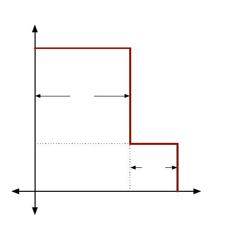
6.4.2 Dispatchable Loads
A simple approach to dispatchable or price-sensitive loads is to model them as nega-
tive real power injections with associated negative costs. This is done by specifying
a generator with a negative output, ranging from a minimum injection equal to the
negative of the largest possible load to a maximum injection of zero.
Consider the example of a price-sensitive load whose marginal benefit function is
shown in Figure 6-4. The demand pdof this load will be zero for prices above λ1,p1
for prices between λ1and λ2, and p1+p2for prices below λ2.
λ(marginal benefit)
$/MW
MW
λ1
λ2
p1
p2
p(load)
Figure 6-4: Marginal Benefit or Bid Function
This corresponds to a negative generator with the piecewise linear cost curve
shown in Figure 6-5. Note that this approach assumes that the demand blocks can
be partially dispatched or “split”. Requiring blocks to be accepted or rejected in
their entirety would pose a mixed-integer problem that is beyond the scope of the
current Matpower implementation.
It should be noted that, with this definition of dispatchable loads as negative
generators, if the negative cost corresponds to a benefit for consumption, minimizing
the cost f(x) of generation is equivalent to maximizing social welfare.
With an AC network model, there is also the question of reactive dispatch for
such loads. Typically the reactive injection for a generator is allowed to take on any
value within its defined limits. Since this is not normal load behavior, the model used
66
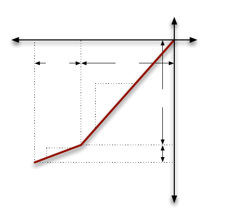
MW
2
1
p1
p2
$
p(injection)
c(total cost)
1p1
2p2
Figure 6-5: Total Cost Function for Negative Injection
in Matpower assumes that dispatchable loads maintain a constant power factor.
When formulating the AC OPF problem, Matpower will automatically generate
an additional equality constraint to enforce a constant power factor for any “negative
generator” being used to model a dispatchable load.
The power factor, which can be lagging or leading, is determined by the ratio of
reactive to active power for the load and is specified by the active and reactive limits
defining the nominal load in the gen matrix. For all dispatchable loads, the value
in the PMIN column is negative and defines the nominal active power of the load.
And PMAX is zero, allowing the load to be fully curtailed depending on the price.
The reactive limits, QMIN and QMAX, depend on whether the power flow is lagging
or leading. One defines the nominal reactive load and the other must be zero to
allow the load to be fully curtailed. The values of PG and QG must be defined to be
consistent with the nominal power factor.
•Lagging Power Factor – The reactive injection is negative, meaning that
reactive power is consumed by the load. Hence, QMIN is negative, QMAX is zero,
and PG and QG must be set so that QG is equal to PG * QMIN/PMIN.
•Leading Power Factor – The reactive injection is positive, that is, reactive
power is produced by the load. Hence, QMAX is positive, QMIN is zero, and PG
and QG must be set so that QG is equal to PG * QMAX/PMIN.
67
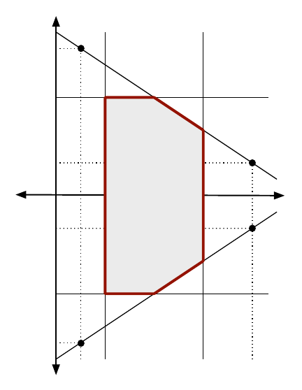
6.4.3 Generator Capability Curves
The typical AC OPF formulation includes box constraints on a generator’s real and
reactive injections, specified as simple lower and upper bounds on p(pmin and pmax)
and q(qmin and qmax). On the other hand, the true P-Qcapability curves of phys-
ical generators usually involve some tradeoff between real and reactive capability,
so that it is not possible to produce the maximum real output and the maximum
(or minimum) reactive output simultaneously. To approximate this tradeoff, Mat-
power includes the ability to add an upper and lower sloped portion to the standard
box constraints as illustrated in Figure 6-6, where the shaded portion represents the
feasible operating region for the unit.
qmax
1
qmax
2
qmin
2
qmin
1
qmin
qmax
pmax
pmin
p1
p2
q
p
Figure 6-6: Generator P-QCapability Curve
The two sloped portions are constructed from the lines passing through the two
pairs of points defined by the six parameters p1,qmin
1,qmax
1,p2,qmin
2, and qmax
2.
If these six parameters are specified for a given generator in columns PC1–QC2MAX
(11–16), Matpower automatically constructs the corresponding additional linear
inequality constraints on pand qfor that unit.
68

If one of the sloped portions of the capability constraints is binding for genera-
tor k, the corresponding shadow price is decomposed into the corresponding µPmax
and µQmin or µQmax components and added to the respective column (MU PMAX,MU QMIN
or MU QMAX) in the kth row of gen.
6.4.4 Branch Angle Difference Limits
The difference between the bus voltage angle θfat the from end of a branch and
the angle θtat the to end can be bounded above and below to act as a proxy for a
transient stability limit, for example. If these limits are provided in columns ANGMIN
(12) and ANGMAX (13) of the branch matrix, Matpower creates the corresponding
constraints on the voltage angle variables.26
6.5 Solvers
Early versions of Matpower relied on Matlab’s Optimization Toolbox [27] to
provide the NLP and QP solvers needed to solve the AC and DC OPF problems,
respectively. While they worked reasonably well for very small systems, they did not
scale well to larger networks. Eventually, optional packages with additional solvers
were added to improve performance, typically relying on Matlab extension (MEX)
files implemented in Fortran or C and pre-compiled for each machine architecture.
Some of these MEX files are distributed as optional packages due to differences in
terms of use. For DC optimal power flow, there is a MEX build [28] of the high
performance interior point BPMPD solver [29] for LP/QP problems. For the AC
OPF problem, the MINOPF [30] and TSPOPF [25] packages provide solvers suitable
for much larger systems. The former is based on MINOS [31] and the latter includes
the primal-dual interior point and trust region based augmented Lagrangian methods
described in [26]. Matpower version 4 and later also includes the option to use
the open-source Ipopt solver27 for solving both AC and DC OPFs, based on the
Matlab MEX interface to Ipopt28. It also includes the option to use CPLEX29 or
MOSEK30 for DC OPFs. Matpower 4.1 added the option to use KNITRO [32]31
26The voltage angle difference for branch kis taken to be unbounded below if branch(k, ANGMIN)
is less than or equal to −360 and unbounded above if branch(k, ANGMAX) is greater than or equal
to 360. If both parameters are zero, the voltage angle difference is unconstrained.
27Available from http://www.coin-or.org/projects/Ipopt.xml.
28See https://projects.coin-or.org/Ipopt/wiki/MatlabInterface.
29See http://www.ibm.com/software/integration/optimization/cplex-optimizer/.
30See http://www.mosek.com/.
31See http://www.ziena.com/.
69

for AC OPFs and the Gurobi Optimizer [33]32 for DC OPFs and Matpower 5
added GLPK [34] and 5.1 added CLP [35]. See Appendix Gfor more details on
these optional packages.
Beginnning with version 4, Matpower also includes its own primal-dual interior
point method implemented in pure-Matlab code, derived from the MEX implemen-
tation of the algorithms described in [26]. This solver is called MIPS (Matpower
Interior Point Solver) and is described in more detail in Appendix A. If no optional
packages are installed, MIPS will be used by default for both the AC OPF and
as the QP solver used by the DC OPF. The AC OPF solver also employs a unique
technique for efficiently forming the required Hessians via a few simple matrix opera-
tions [36–38]. This solver has application to general nonlinear optimization problems
outside of Matpower and can be called directly as mips. There is also a conve-
nience wrapper function called qps mips making it trivial to set up and solve LP and
QP problems, with an interface similar to quadprog from the Matlab Optimization
Toolbox.
6.6 runopf
In Matpower, an optimal power flow is executed by calling runopf with a case
struct or case file name as the first argument (casedata). In addition to printing
output to the screen, which it does by default, runopf optionally returns the solution
in a results struct.
>> results = runopf(casedata);
The results struct is a superset of the input Matpower case struct mpc, with
some additional fields as well as additional columns in some of the existing data
fields. In addition to the solution values included in the results for a simple power
flow, shown in Table 4-1 in Section 4.4, the following additional optimal power flow
solution values are stored as shown in Table 6-1.
32See http://www.gurobi.com/.
70

Table 6-1: Optimal Power Flow Results
name description
results.f final objective function value
results.x final value of optimization variables (internal order)
results.om OPF model object†
results.bus(:, LAM P) Lagrange multiplier on real power mismatch
results.bus(:, LAM Q) Lagrange multiplier on reactive power mismatch
results.bus(:, MU VMAX) Kuhn-Tucker multiplier on upper voltage limit
results.bus(:, MU VMIN) Kuhn-Tucker multiplier on lower voltage limit
results.gen(:, MU PMAX) Kuhn-Tucker multiplier on upper Pglimit
results.gen(:, MU PMIN) Kuhn-Tucker multiplier on lower Pglimit
results.gen(:, MU QMAX) Kuhn-Tucker multiplier on upper Qglimit
results.gen(:, MU QMIN) Kuhn-Tucker multiplier on lower Qglimit
results.branch(:, MU SF) Kuhn-Tucker multiplier on flow limit at “from” bus
results.branch(:, MU ST) Kuhn-Tucker multiplier on flow limit at “to” bus
results.mu shadow prices of constraints‡
results.g (optional) constraint values
results.dg (optional) constraint 1st derivatives
results.raw raw solver output in form returned by MINOS, and more‡
results.var.val final value of optimization variables, by named subset‡
results.var.mu shadow prices on variable bounds, by named subset‡
results.nle shadow prices on nonlinear equality constraints, by named subset‡
results.nli shadow prices on nonlinear inequality constraints, by named subset‡
results.lin shadow prices on linear constraints, by named subset‡
results.cost final value of user-defined costs, by named subset‡
†See help for opf model and opt model for more details.
‡See help for opf for more details.
71

Additional optional input arguments can be used to set options (mpopt) and
provide file names for saving the pretty printed output (fname) or the solved case
data (solvedcase).
>> results = runopf(casedata, mpopt, fname, solvedcase);
Some of the main options that control the optimal power flow simulation are listed
in Tables 6-2 and 6-3. There are many other options that can be used to control the
termination criteria and other behavior of the individual solvers. See Appendix C
or the mpoption help for details. As with runpf the output printed to the screen can
be controlled by the options in Table 4-3, but there are additional output options
for the OPF, related to the display of binding constraints that are listed Table 6-4,
along with an option that can be used to force the AC OPF to return information
about the constraint values and Jacobian and the objective function gradient and
Hessian.
For OPF problems, the preferred way to eliminate the flow limit on a branch is
to set the RATE A column (6) of the corresponding row in the branch matrix to zero.
This indicates a completely unconstrained flow (as opposed to zero flow).
By default, runopf solves an AC optimal power flow problem using a primal dual
interior point method. To run a DC OPF, the model option must be set to 'DC'. For
convenience, Matpower provides a function rundcopf which is simply a wrapper
that sets the model to 'DC'before calling runopf.
Internally, the runopf function does a number of conversions to the problem
data before calling the appropriate solver routine for the selected OPF algorithm.
This external-to-internal format conversion is performed by the ext2int function,
described in more detail in Section 7.3.1, and includes the elimination of out-of-service
equipment, the consecutive renumbering of buses and the reordering of generators
by increasing bus number. All computations are done using this internal indexing.
When the simulation has completed, the data is converted back to external format
by int2ext before the results are printed and returned. In addition, both ext2int
and int2ext can be customized via user-supplied callback routines to convert data
needed by user-supplied variables, constraints or costs into internal indexing.
72

Table 6-2: Optimal Power Flow Solver Options
name default description
opf.ac.solver 'DEFAULT'AC optimal power flow solver:
'DEFAULT'– choose default solver, i.e. 'MIPS'
'MIPS'– MIPS, Matpower Interior Point Solver,
primal/dual interior point method†
'FMINCON'–Matlab Optimization Toolbox, fmincon
'IPOPT'–Ipopt*
'KNITRO'– KNITRO*
'MINOPF'– MINOPF*
, MINOS-based solver
'PDIPM'– PDIPM*
, primal/dual interior point method‡
'SDPOPF'– SDPOPF*
, solver based on semidefinite relax-
ation
'TRALM'– TRALM*
, trust region based augmented Lan-
grangian method
opf.dc.solver 'DEFAULT'DC optimal power flow solver:
'DEFAULT'– choose default solver based on availability
in the following order: 'GUROBI','CPLEX',
'MOSEK','OT','GLPK'(linear costs only),
'BPMPD','MIPS'
'MIPS'– MIPS, Matpower Interior Point Solver,
primal/dual interior point method†
'BPMPD'– BPMPD*
'CLP'– CLP*
'CPLEX'– CPLEX*
'GLPK'– GLPK*(no quadratic costs)
'GUROBI'– Gurobi*
'IPOPT'–Ipopt*
'MOSEK'– MOSEK*
'OT'–Matlab Opt Toolbox, quadprog,linprog
*Requires the installation of an optional package. See Appendix Gfor details on the corresponding package.
†For MIPS-sc, the step-controlled version of this solver, the mips.step control option must be set to 1.
‡For SC-PDIPM, the step-controlled version of this solver, the pdipm.step control option must be set to 1.
73

Table 6-3: Other OPF Options
name default description
opf.current balance 0 use current, as opposed to power, balance formulation for
AC OPF, 0 or 1
opf.v cartesian 0 use cartesian, as opposed to polar, representation for volt-
ages for AC OPF, 0 or 1
opf.violation 5×10⁻⁶constraint violation tolerance
opf.use vg 0 respect generator voltage setpoint, 0 or 1†
0 – use voltage magnitude limits specified in bus, ig-
nore VG in gen
1 – replace voltage magnitude limits specified in bus
by VG in corresponding gen
opf.flow lim 'S'quantity to limit for branch flow constraints
'S'– apparent power flow (limit in MVA)
'P'– active power flow (limit in MW)
'I'– current magnitude (limit in MVA at 1 p.u.
voltage)
'2'– same as 'P', but implemented using square
of active flow, rather than simple max
opf.ignore angle lim 0 ignore angle difference limits for branches
0 – include angle difference limits, if specified
1 – ignore angle difference limits even if specified
opf.softlims.default 1 behavior of OPF soft limits for which parameters are not
explicitly provided
0 – do not include softlims if not explicitly specified
1 – include softlims with default values if not ex-
plicitly specified
opf.init from mpc*-1 specify whether to use the current state in Matpower
case to initialize OPF
-1 – Matpower decides based on solver/algorithm
0 – ignore current state in Matpower case‡
1 – use current state in Matpower case
opf.start 0 strategy for initializing OPF starting point
0 – default, Matpower decides based on solver,
(currently identical to 1)
1 – ignore current state in Matpower case‡
2 – use current state in Matpower case
3 – solve power flow and use resulting state
opf.return raw der 0 for AC OPF, return constraint and derivative info in
results.raw (in fields g,dg,df,d2f)
*Deprecated. Use opf.start instead.
†Using a value between 0 and 1 results in the limits being determined by the corresponding weighted average of
the 2 options.
‡Only applies to fmincon,Ipopt, KNITRO and MIPS solvers, which use an interior point estimate; others use
current state in Matpower case, as with opf.start = 2.
74

Table 6-4: OPF Output Options
name default description
out.lim.all -1 controls constraint info output
-1 – individual flags control what is printed
0 – do not print any constraint info†
1 – print only binding constraint info†
2 – print all constraint info†
out.lim.v 1 control output of voltage limit info
0 – do not print
1 – print binding constraints only
2 – print all constraints
out.lim.line 1 control output of line flow limit info‡
out.lim.pg 1 control output of gen active power limit info‡
out.lim.qg 1 control output of gen reactive power limit info‡
†Overrides individual flags.
‡Takes values of 0, 1 or 2 as for out.lim.v.
75
7 Extending the OPF
The extended OPF formulation described in Section 6.3 allows the user to modify the
standard OPF formulation to include additional variables, costs and/or constraints.
There are two primary mechanisms available for the user to accomplish this. The first
is by directly constructing the full parameters for the addional costs or constraints
and supplying them either as fields in the case struct or directly as arguments to
the opf function. The second, and more powerful, method is via a set of callback
functions that customize the OPF at various stages of the execution. Matpower
includes several examples of using the latter method, for example to add a fixed zonal
reserve requirement, to implement interface flow limits, dispatchable DC transmission
lines, or branch flow soft limits.
7.1 Direct Specification
This section describes the additional fields that can be added to mpc (the Matpower
case struct) or, alternatively, the input parameters that can be passed directly to the
opf function. The former is the preferred approach, as it allows the normal use of
runopf and related functions.
7.1.1 User-defined Variables
In the case of direct specification, additional variables are created implicitly based on
the difference between the number of columns in Aand the number nxof standard
OPF variables. If Ahas more columns than xhas elements, the extra columns are
assumed to correspond to a new zvariable. The initial value and lower and upper
bounds for zcan also be specified in the optional fields or arguments, z0,zl and zu,
respectively.
7.1.2 User-defined Constraints
•Linear Constraints can be added by specifying the A,land uparameters of
(6.38) directly as fields or arguments of the same names, A,land u, respectively,
where Ais sparse.
•Nonlinear Constraints for a constraint set j, that is, gj
u(x) or hj
u(x) from
(6.42) or (6.43), are implemented by defining two M-file functions, similar to
76

those required by MIPS. The first is a function to compute the constraint values
and their gradients (Jacobian),33 with calling syntax:
[g, dg] = my constraint fcn(x, <p1>, <p2>, ...)
Here <p1> and <p2> represent arbitrary optional input parameters that remain
constant for all calls to the function. The second is a function to compute the
Hessian of the corresponding term in the Lagrangian function, that is the term
corresponding to λTgj
u(x) or µThj
u(x). This function has the following calling
syntax:
d2G = my constraint hess(x, lambda, <p1>, <p2>, ...)
Once again this is similar to the form of the Hessian evaluation function ex-
pected by MIPS.34
In order to add a set of user-defined nonlinear constraints to the formula-
tion through direct specification, an entry must be added to the optional
user constraints.nle (nonlinear equality) or user constraints.nli (nonlin-
ear inequality) fields of the Matpower case struct. These fields are cell ar-
rays, in which each element (also a cell array) specifies a constraint set of the
corresponding kind. The format is as follows, where the details are described
in Table 7-1.
mpc.user_constraints.nle = {
{name, N, g_fcn, hess_fcn, varsets, params},
...
};
There is an example in the OPF testing code (e.g. t opf mips) near the end,
that implements a nonlinear relationship between three different generator out-
puts by adding the following line.
33The differences between this function and the one required by MIPS is that (1) this one repre-
sents a single set of equality constraints or inequality constraints, not both, (2) it returns in dg the
m×nJacobian (for mconstraints and nvariables), whereas MIPS expects the n×mtranspose,
(3) this function allows arbitrary additional parameters, and (4) xcan be a cell array of sub-vectors
of optimization variable ˆx(see varsets in Table 7-1).
34The differences between this function and the one required by MIPS is that (1) this one returns
the Hessian of a single term of the Lagrangian, not of the full Lagrangian, (2) the lambda argument
is a simple vector of multipliers (λor µ) corresponding just to this set of constraints, not a struct
containing the full λand µvectors, in fields eqnonlin and ineqnonlin, respectively, and (3) this
function allows arbitrary additional parameters, and (4) xcan be a cell array of sub-vectors of
optimization variable ˆx(see varsets in Table 7-1).
77

Table 7-1: User-defined Nonlinear Constraint Specification
name description
name string with name of constraint set, used to label multipliers in results struct
Nnumber of constraints, i.e. dimension of gj
u(x) (or hj
u(x) as the case may be)
g fcn string containing name of function to evaluate constraint and gradients (Jacobian)
hess fcn string containing name of function to evaluate Hessian of corresponding term of
Lagrangian
varsets cell array of variable set names, specifying sub-vectors of optimization vector ˆxto
be passed as inputs in x†
params cell array of optional, arbitrary parameters to pass to each call to the constraint and
Hessian evaluation functions
†If varsets is empty, xwill be the full optimization vector ˆx, otherwise it will be a cell array of sub-vectors of ˆxfor
the specified variable sets. Valid names include 'Va','Vm','Pg', and 'Qg'. It can include others depending on
the OPF extensions in use. See the variable names displayed by results.om for a complete list for your problem.
mpc.user_constraints.nle = {
{'Pg_usr', 1, 'opf_nle_fcn1', 'opf_nle_hess1', {'Pg'}, {}}
};
This adds a single constraint named 'Pg usr'as a function of the vector of
generator active injections (xwill be {Pg}, where Pg is a sub-vector of the
optimization vector ˆxcontaining only the generator active injections). The
constraints and gradients are evaluated by a function named 'opf nle fcn1'
and the Hessian of the corresponding term of the Lagrangian by a function
named 'opf nle hess1', neither of which expect any additional parameters.
7.1.3 User-defined Costs
•Quadratic Costs by direct specification are not currently supported.
•General Nonlinear Costs by direct specification are not currently supported.
•Legacy Costs – To add legacy costs directly, the parameters H,C,N, ˆr,k,
dand mof (6.48)–(6.51) described in Section 6.3.3 are specified as fields or
arguments H,Cw,Nand fparm, respectively, where fparm is the nw×4 matrix
fparm =dˆr k m .(7.1)
When specifying additional costs, Nand Cw are required, while Hand fparm are
optional. The default value for His a zero matrix, and the default for fparm is
78

such that dand mare all ones and ˆrand kare all zeros, resulting in simple
linear cost, with no shift or “dead-zone”. Nand Hshould be specified as sparse
matrices.
7.1.4 Additional Comments
For a simple formulation extension to be used for a small number of OPF cases, this
method has the advantage of being direct and straightforward. While Matpower
does include code to eliminate the columns of Aand Ncorresponding to Vmand Qg
when running a DC OPF35, as well as code to reorder and eliminate columns appro-
priately when converting from external to internal data formats, this mechanism still
requires the user to take special care in preparing the Aand Nmatrices to ensure
that the columns match the ordering of the elements of the optimization vectors x
and z. All extra constraints and variables must be incorporated into a single set of
parameters that are constructed before calling the OPF. The bookkeeping needed to
access the resulting variables and shadow prices on constraints and variable bounds
must be handled manually by the user outside of the OPF, along with any pro-
cessing of additional input data and processing, printing or saving of the additional
result data. Making further modifications to a formulation that already includes
user-supplied costs, constraints or variables, requires that both sets be incorporated
into a new single consistent set of parameters.
7.2 Callback Functions
The second method, based on defining a set of callback functions, offers several
distinct advantages, especially for more complex scenarios or for adding a feature
for others to use, such as the zonal reserve requirement or the interface flow limits
mentioned previously. This approach makes it possible to:
•define and access variable/constraint/cost sets as individual named blocks
•define constraints, costs only in terms of variables directly involved
•pre-process input data and/or post-process result data
•print and save new result data
•simultaneously use multiple, independently developed extensions (e.g. zonal
reserve requirements and interface flow limits)
35Only if they contain all zeros.
79

With this approach the OPF formulation is modified in the formulation callback,
which is described and illustrated below in Section 7.3.2. The modifications to the
formulation are handled by adding variables, costs and/or constraints to the OPF
Model object (om) using one of the add * methods. Please see the documentation for
each of these methods for more details.
7.2.1 User-defined Variables
Additional variables are added using the add var method.
om.add_var('myV', N, myV0, myV_min, myV_max);
Here myV is the name of the variable set, Nthe number of variables being added (i.e.
this is an N×1 vector being appended to the current optimization variable ˆx), and
myV0,myV min,myV max are vectors of initial values, lower bounds and upper bounds,
respectively.
7.2.2 User-defined Costs
•Quadratic Costs are added using the add quad cost method.
om.add_quad_cost('myQcost', Q, c, k, varsets);
Here myQcost is the name of the cost set, Q,cand kare the Qj,cjand kj
parameters from (6.47), respectively, and var sets is an optional cell array of
variable set names. If var sets is provided, the dimensions of Qand cwill
correspond, not to the full optimization vector ˆx, but to the subvector formed
by stacking only the variable sets specified in var sets.
•General Nonlinear Costs are added using the add nln cost method.
om.add_nln_cost('myNonlinCost', 1, fcn, varsets);
Here myNonlinCost is the name of the cost set, fcn is a function handle and
var sets is an optional cell array of variable set names. The function handle
fcn must point to a function that implements the fj
nln(ˆx) function from (6.46),
returning the value of the function, along with its gradient and Hessian. This
function has a format similar to that required by MIPS for its cost function.
If var sets is provided, instead of the full optimization vector ˆx, the xpassed
to the function fcn will be a cell array of sub-vectors of ˆxcorresponding to the
specified variable sets.
80

•Legacy Costs are added using the add legacy cost method.
om.add_legacy_cost('myLegacyCost', cp, varsets);
Here myLegacyCost is the name of the cost set, cp is a struct containing the cost
parameters H,C,N, ˆr,k,dand mfrom (6.48)–(6.51) in fields H,Cw,N,rh,kk,
dd and mm, respectively, and var sets is an optional cell array of variable set
names. If var sets is provided, the number of columns in Nwill correspond,
not to the full optimization vector ˆx, but to the subvector formed by stacking
only the variable sets specified in var sets.
7.2.3 User-defined Constraints
•Linear Constraints are added using the add lin constraint method.
om.lin_constraint('myLinCons', A, l, u, varsets);
Here myLinCons is the name of the constraint set, A,land ucorrespond to
additional rows to add to the A,land uparameters in (6.38), respectively, and
var sets is an optional cell array of variable set names. If var sets is provided,
the number of columns in Awill correspond, not to the full optimization vector
ˆx, but to the subvector formed by stacking only the variable sets specified in
var sets.
•Nonlinear Constraints are added using the add nln constraint method.
om.nln_constraint('myNonlinCons', N, iseq, fcn, hess, varsets);
Here myNonlinCons is the name of the constraint set, Nis the number of con-
straints being added, iseq is a true or false value indicating whether this is a set
of equality (or else inequality) constraints, fcn and hess are function handles
and var sets is an optional cell array of variable set names. The function han-
dle fcn must point to a function that implements the corresponding constraint
function gj
u(x) or hj
u(x) and its gradients, and hess to one that evaluates the
corresponding term in the Hessian of the Lagrangian function. This function
has a format similar to that required by MIPS for its cost function. See more
details in Section 7.1.2.
If var sets is provided, instead of the full optimization vector ˆx, the xpassed
to the function fcn will be a cell array of sub-vectors of ˆxcorresponding to the
specified variable sets.
81

7.3 Callback Stages and Example
Matpower defines five stages in the execution of a simulation where custom code
can be inserted to alter the behavior or data before proceeding to the next stage.
This custom code is defined as a set of “callback” functions that are registered via
add userfcn for Matpower to call automatically at one of the five stages. Each
stage has a name and, by convention, the name of a user-defined callback func-
tion ends with the name of the corresponding stage. For example, a callback for
the formulation stage that modifies the OPF problem formulation to add reserve
requirements could be registered with the following line of code.
mpc = add_userfcn(mpc, 'formulation', @userfcn_reserves_formulation);
The sections below will describe each stage and the input and output arguments
for the corresponding callback function, which vary depending on the stage. An
example that employs additional variables, constraints and costs will be used for
illustration.
Consider the problem of jointly optimizing the allocation of both energy and
reserves, where the reserve requirements are defined as a set of nrz fixed zonal MW
quantities. Let Zkbe the set of generators in zone kand Rkbe the MW reserve
requirement for zone k. A new set of variables rare introduced representing the
reserves provided by each generator. The value ri, for generator i, must be non-
negative and is limited above by a user-provided upper bound rmax
i(e.g. a reserve
offer quantity) as well as the physical ramp rate ∆i.
0≤ri≤min(rmax
i,∆i), i = 1 . . . ng(7.2)
If the vector ccontains the marginal cost of reserves for each generator, the user
defined cost term from (6.34) is simply
fu(ˆx) = cTr. (7.3)
There are two additional sets of constraints needed. The first ensures that, for
each generator, the total amount of energy plus reserve provided does not exceed the
capacity of the unit.
pi
g+ri≤pi,max
g, i = 1 . . . ng(7.4)
The second requires that the sum of the reserve allocated within each zone kmeets
the stated requirements.
X
i∈Zk
ri≥Rk, k = 1 . . . nrz (7.5)
82

Table 7-2: Names Used by Implementation of OPF with Reserves
name description
mpc Matpower case struct
reserves additional field in mpc containing input parameters for zonal reserves in
the following sub-fields:
cost ng×1 vector of reserve costs, cfrom (7.3)
qty ng×1 vector of reserve quantity upper bounds, ith element is rmax
i
zones nrz ×ngmatrix of reserve zone definitions
zones(k,j) =1 if gen jbelongs to reserve zone k(j∈Zk)
0 otherwise (j /∈Zk)
req nrz ×1 vector of zonal reserve requirements, kth element is Rkfrom (7.5)
om OPF model object, already includes standard OPF setup
results OPF results struct, superset of mpc with additional fields for output data
ng ng, number of generators
Rname for new reserve variable block, ith element is ri
Pg plus R name for new capacity limit constraint set (7.4)
Rreq name for new reserve requirement constraint set (7.5)
Table 7-2 describes some of the variables and names that are used in the example
callback function listings in the sections below.
7.3.1 ext2int Callback
Before doing any simulation of a case, Matpower performs some data conversion
on the case struct in order to achieve a consistent internal structure, by calling the
following.
mpc = ext2int(mpc, mpopt);
All isolated buses, out-of-service generators and branches are removed, along with
any generators or branches connected to isolated buses. The buses are renumbered
consecutively, beginning at 1, and the in-service generators are sorted by increasing
bus number. All of the related indexing information and the original data matrices
are stored in an order field in the case struct to be used later by int2ext to perform
the reverse conversions when the simulation is complete.
The first stage callback is invoked from within the ext2int function immediately
after the case data has been converted. Inputs are a Matpower case struct (mpc)
freshly converted to internal indexing, a Matpower options struct mpopt,36 and
36The mpopt may be empty if ext2int() is called manually without providing it.
83

any (optional) args value supplied when the callback was registered via add userfcn.
Output is the (presumably updated) mpc. This is typically used to reorder any input
arguments that may be needed in internal ordering by the formulation stage. The
example shows how e2i field can also be used, with a case struct that has already
been converted to internal indexing, to convert other data structures by passing in
2 or 3 extra parameters in addition to the case struct. In this case, it automatically
converts the input data in the qty,cost and zones fields of mpc.reserves to be
consistent with the internal generator ordering, where off-line generators have been
eliminated and the on-line generators are sorted in order of increasing bus number.
Notice that it is the second dimension (columns) of mpc.reserves.zones that is being
re-ordered. See the on-line help for e2i field and e2i data for more details on what
all they can do.
function mpc = userfcn_reserves_ext2int(mpc, mpopt, args)
mpc = e2i_field(mpc, {'reserves', 'qty'}, 'gen');
mpc = e2i_field(mpc, {'reserves', 'cost'}, 'gen');
mpc = e2i_field(mpc, {'reserves', 'zones'}, 'gen', 2);
This stage is also a good place to check the consistency of any additional input
data required by the extension and throw an error if something is missing or not as
expected.
7.3.2 formulation Callback
This stage is called at the end of opf setup after the OPF Model (om) object has been
initialized with the standard OPF formulation, but before calling the solver. This
is the ideal place for modifying the problem formulation with additional variables,
constraints and costs, using the add var,add lin constraint,add nln constraint,
add quad cost,add nln cost and add legacy cost methods of the OPF Model ob-
ject.37 Inputs are the om object, the Matpower options struct mpopt and any
(optional) args supplied when the callback was registered via add userfcn. Output
is the updated om object.
The om object contains both the original Matpower case data as well as all of
the indexing data for the variables and constraints of the standard OPF formulation.
37It is perfectly legitimate to register more than one callback per stage, such as when enabling
multiple independent OPF extensions. In this case, the callbacks are executed in the order they
were registered with add userfcn. E.g. when the second and subsequent formulation callbacks
are invoked, the om object will reflect any modifications performed by earlier formulation callbacks.
84

See the on-line help for opf model and opt model for more details on the OPF model
object and the methods available for manipulating and accessing it.
In the example code, a new variable block named Rwith ngelements and the
limits from (7.2) is added to the model via the add var method. Similarly, two linear
constraint blocks named Pg plus R and Rreq, implementing (7.4) and (7.5), respec-
tively, are added via the add lin constraint method. And finally, the add quad cost
method is used to add to the model a quadratic (actually linear) cost block corre-
sponding to (7.3).
Notice that the last argument to add lin constraint and add quad cost allows
the constraints and costs to be defined only in terms of the relevant parts of the
optimization variable ˆx. For example, the Amatrix for the Pg plus R constraint
contains only columns corresponding to real power generation (Pg) and reserves (R)
and need not bother with voltages, reactive power injections, etc. As illustrated in
Figure 7-1, this allows the same code to be used with both the AC OPF, where
ˆxincludes Vmand Qg, and the DC OPF where it does not. This code is also
independent of any additional variables that may have been added by Matpower
(e.g. yvariables from Matpower’s CCV handling of piece-wise linear costs) or by
the user via previous formulation callbacks. Matpower will place the constraint
and cost matrix blocks in the appropriate place when it constructs the aggregated
constraint and cost matrices at run-time. This is an important feature that enables
independently developed Matpower OPF extensions to work together.
85

function om = userfcn_reserves_formulation(om, mpopt, args)
%% initialize some things
define_constants;
mpc = om.get_mpc();
r = mpc.reserves;
ng = size(mpc.gen, 1); %% number of on-line gens
%% variable bounds
Rmin = zeros(ng, 1); %% bound below by 0
Rmax = r.qty; %% bound above by stated max reserve qty ...
k = find(mpc.gen(:, RAMP_10) > 0 & mpc.gen(:, RAMP_10) < Rmax);
Rmax(k) = mpc.gen(k, RAMP_10); %% ... and ramp rate
Rmax = Rmax / mpc.baseMVA;
%% constraints
I = speye(ng); %% identity matrix
Ar = [I I];
Pmax = mpc.gen(:, PMAX) / mpc.baseMVA;
lreq = r.req / mpc.baseMVA;
%% cost
Cw = r.cost * mpc.baseMVA; %% per unit cost coefficients
%% add them to the model
om.add_var('R', ng, [], Rmin, Rmax);
om.add_lin_constraint('Pg_plus_R', Ar, [], Pmax, {'Pg', 'R'});
om.add_lin_constraint('Rreq', r.zones, lreq, [], {'R'});
om.add_quad_cost('Rcost', [], Cw, 0, {'R'});
86

Va
A = 0A10 00 A2
A = 0A1 0A2
Ar = A1 A2
Va PgVm yQg R
Pg y R
AC OPF
DC OPF
Figure 7-1: Adding Constraints Across Subsets of Variables
87

7.3.3 int2ext Callback
After the simulation is complete and before the results are printed or saved, Mat-
power converts the case data in the results struct back to external indexing by
calling the following.
results = int2ext(results, mpopt);
This conversion essentially undoes everything that was done by ext2int. Generators
are restored to their original ordering, buses to their original numbering and all
out-of-service or isolated generators, branches and buses are restored.
This callback is invoked from int2ext immediately before the resulting case is
converted from internal back to external indexing. At this point, the simulation has
been completed and the results struct, a superset of the original Matpower case
struct passed to the OPF, contains all of the results. This results struct is passed to
the callback, along with the Matpower options struct mpopt,38 and any (optional)
args supplied when the callback was registered via add userfcn. The output of the
callback is the updated results struct. This is typically used to convert any results
to external indexing and populate any corresponding fields in the results struct.
The results struct contains, in addition to the standard OPF results, solution
information related to all of the user-defined variables, constraints and costs. Ta-
ble 7-3 summarizes where the various data is found. Each of the fields listed in
the table is actually a struct whose fields correspond to the named sets created by
add var,add lin constraint,add nln constraint,add quad cost,add nln cost and
add legacy cost.
In the example code below, the callback function begins by converting the reserves
input data in the resulting case (qty,cost and zones fields of results.reserves) back
to external indexing via calls to i2e field. See the help for i2e field and i2e data
for more details on how they can be used.
38The mpopt may be empty if int2ext() is called manually without providing it.
88

Table 7-3: Results for User-Defined Variables, Constraints and Costs
name description
results.var.val final value of user-defined variables
results.var.mu.l shadow price on lower limit of user-defined variables
results.var.mu.u shadow price on upper limit of user-defined variables
results.lin.mu.l shadow price on lower (left-hand) limit of linear constraints
results.lin.mu.u shadow price on upper (right-hand) limit of linear constraints
results.nle.lambda shadow price on nonlinear equality constraints
results.nli.mu shadow price on nonlinear inequality constraints
results.cost final value of legacy user costs
results.nlc final value of general nonlinear costs
results.qdc final value of quadratic costs
89

Then the reserves results of interest are extracted from the appropriate sub-fields
of results.var,results.lin and results.cost, converted from per unit to per MW
where necessary, and stored with external indexing for the end user in the chosen
fields of the results struct.
function results = userfcn_reserves_int2ext(results, mpopt, args)
%%----- convert stuff back to external indexing -----
%% convert all reserve parameters (zones, costs, qty, rgens)
results = i2e_field(results, {'reserves', 'qty'}, 'gen');
results = i2e_field(results, {'reserves', 'cost'}, 'gen');
results = i2e_field(results, {'reserves', 'zones'}, 'gen', 2);
r = results.reserves;
ng = size(results.gen, 1); %% number of on-line gens (internal)
ng0 = size(results.order.ext.gen, 1); %% number of gens (external)
%%----- results post-processing -----
%% get the results (per gen reserves, multipliers) with internal gen indexing
%% and convert from p.u. to per MW units
[R0, Rl, Ru] = results.om.params_var('R');
R = results.var.val.R * results.baseMVA;
Rmin = Rl * results.baseMVA;
Rmax = Ru * results.baseMVA;
mu_l = results.var.mu.l.R / results.baseMVA;
mu_u = results.var.mu.u.R / results.baseMVA;
mu_Pmax = results.lin.mu.u.Pg_plus_R / results.baseMVA;
%% store in results in results struct
z = zeros(ng0, 1);
results.reserves.R = i2e_data(results, R, z, 'gen');
results.reserves.Rmin = i2e_data(results, Rmin, z, 'gen');
results.reserves.Rmax = i2e_data(results, Rmax, z, 'gen');
results.reserves.mu.l = i2e_data(results, mu_l, z, 'gen');
results.reserves.mu.u = i2e_data(results, mu_u, z, 'gen');
results.reserves.mu.Pmax = i2e_data(results, mu_Pmax, z, 'gen');
results.reserves.prc = z;
for k = 1:ng0
iz = find(r.zones(:, k));
results.reserves.prc(k) = sum(results.lin.mu.l.Rreq(iz)) / results.baseMVA;
end
results.reserves.totalcost = results.cost.Rcost;
90

7.3.4 printpf Callback
The pretty-printing of the standard OPF output is done via a call to printpf after
the case has been converted back to external indexing. This callback is invoked from
within printpf after the pretty-printing of the standard OPF output. Inputs are
the results struct, the file descriptor to write to, a Matpower options struct, and
any (optional) args supplied via add userfcn. Output is the results struct. This is
typically used for any additional pretty-printing of results.
In this example, the out.all flag in the options struct is checked before printing
anything. If it is non-zero, the reserve quantities and prices for each unit are printed
first, followed by the per-zone summaries. An additional table with reserve limit
shadow prices might also be included.
91

function results = userfcn_reserves_printpf(results, fd, mpopt, args)
%% define named indices into data matrices
[GEN_BUS, PG, QG, QMAX, QMIN, VG, MBASE, GEN_STATUS, PMAX, PMIN, ...
MU_PMAX, MU_PMIN, MU_QMAX, MU_QMIN, PC1, PC2, QC1MIN, QC1MAX, ...
QC2MIN, QC2MAX, RAMP_AGC, RAMP_10, RAMP_30, RAMP_Q, APF] = idx_gen;
%%----- print results -----
r = results.reserves;
ng = length(r.R);
nrz = size(r.req, 1);
if mpopt.out.all ~= 0
fprintf(fd, '\n=======================================================');
fprintf(fd, '\n| Reserves |');
fprintf(fd, '\n=======================================================');
fprintf(fd, '\n Gen Bus Status Reserves Price');
fprintf(fd, '\n # # (MW) ($/MW)');
fprintf(fd, '\n---- ----- ------ -------- --------');
for k = 1:ng
fprintf(fd, '\n%3d %6d %2d ', k, results.gen(k, GEN_BUS), ...
results.gen(k, GEN_STATUS));
if results.gen(k, GEN_STATUS) > 0 && abs(results.reserves.R(k)) > 1e-6
fprintf(fd, '%10.2f', results.reserves.R(k));
else
fprintf(fd, ' - ');
end
fprintf(fd, '%10.2f ', results.reserves.prc(k));
end
fprintf(fd, '\n --------');
fprintf(fd, '\n Total:%10.2f Total Cost: $%.2f', ...
sum(results.reserves.R(r.igr)), results.reserves.totalcost);
fprintf(fd, '\n');
fprintf(fd, '\nZone Reserves Price ');
fprintf(fd, '\n # (MW) ($/MW) ');
fprintf(fd, '\n---- -------- --------');
for k = 1:nrz
iz = find(r.zones(k, :)); %% gens in zone k
fprintf(fd, '\n%3d%10.2f%10.2f', k, sum(results.reserves.R(iz)), ...
results.lin.mu.l.Rreq(k) / results.baseMVA);
end
fprintf(fd, '\n');
%% print binding reserve limit multipliers ...
end
92

7.3.5 savecase Callback
The savecase is used to save a Matpower case struct to an M-file, for example,
to save the results of an OPF run. The savecase callback is invoked from savecase
after printing all of the other data to the file. Inputs are the case struct, the file
descriptor to write to, the variable prefix (typically 'mpc.') and any (optional) args
supplied via add userfcn. Output is the case struct. The purpose of this callback is
to write any non-standard case struct fields to the case file.
In this example, the zones,req,cost and qty fields of mpc.reserves are written
to the M-file. This ensures that a case with reserve data, if it is loaded via loadcase,
possibly run, then saved via savecase, will not lose the data in the reserves field.
This callback could also include the saving of the output fields if present. The
contributed serialize function39 can be very useful for this purpose.
39http://www.mathworks.com/matlabcentral/fileexchange/1206
93

function mpc = userfcn_reserves_savecase(mpc, fd, prefix, args)
%
% mpc = userfcn_reserves_savecase(mpc, fd, mpopt, args)
%
% This is the 'savecase' stage userfcn callback that prints the M-file
% code to save the 'reserves' field in the case file. It expects a
% MATPOWER case struct (mpc), a file descriptor and variable prefix
% (usually 'mpc.'). The optional args are not currently used.
r = mpc.reserves;
fprintf(fd, '\n%%%%----- Reserve Data -----%%%%\n');
fprintf(fd, '%%%% reserve zones, element i, j is 1 iff gen j is in zone i\n');
fprintf(fd, '%sreserves.zones = [\n', prefix);
template = '';
for i = 1:size(r.zones, 2)
template = [template, '\t%d'];
end
template = [template, ';\n'];
fprintf(fd, template, r.zones.');
fprintf(fd, '];\n');
fprintf(fd, '\n%%%% reserve requirements for each zone in MW\n');
fprintf(fd, '%sreserves.req = [\t%g', prefix, r.req(1));
if length(r.req) > 1
fprintf(fd, ';\t%g', r.req(2:end));
end
fprintf(fd, '\t];\n');
fprintf(fd, '\n%%%% reserve costs in $/MW for each gen\n');
fprintf(fd, '%sreserves.cost = [\t%g', prefix, r.cost(1));
if length(r.cost) > 1
fprintf(fd, ';\t%g', r.cost(2:end));
end
fprintf(fd, '\t];\n');
if isfield(r, 'qty')
fprintf(fd, '\n%%%% max reserve quantities for each gen\n');
fprintf(fd, '%sreserves.qty = [\t%g', prefix, r.qty(1));
if length(r.qty) > 1
fprintf(fd, ';\t%g', r.qty(2:end));
end
fprintf(fd, '\t];\n');
end
%% save output fields for solved case ...
94

7.4 Registering the Callbacks
As seen in the fixed zonal reserve example, adding a single extension to the standard
OPF formulation is often best accomplished by a set of callback functions. A typical
use case might be to run a given case with and without the reserve requirements
active, so a simple method for enabling and disabling the whole set of callbacks as a
single unit is needed.
The recommended method is to define all of the callbacks in a single file containing
a “toggle” function that registers or removes all of the callbacks depending on whether
the value of the second argument is 'on'or 'off'. The state of the registration of any
callbacks is stored directly in the mpc struct. In our example, the toggle reserves.m
file contains the toggle reserves function as well as the five callback functions.
95

function mpc = toggle_reserves(mpc, on_off)
%TOGGLE_RESERVES Enable, disable or check status of fixed reserve requirements.
% MPC = TOGGLE_RESERVES(MPC, 'on')
% MPC = TOGGLE_RESERVES(MPC, 'off')
% T_F = TOGGLE_RESERVES(MPC, 'status')
if strcmp(upper(on_off), 'ON')
% <code to check for required 'reserves' fields in mpc>
%% add callback functions
mpc = add_userfcn(mpc, 'ext2int', @userfcn_reserves_ext2int);
mpc = add_userfcn(mpc, 'formulation', @userfcn_reserves_formulation);
mpc = add_userfcn(mpc, 'int2ext', @userfcn_reserves_int2ext);
mpc = add_userfcn(mpc, 'printpf', @userfcn_reserves_printpf);
mpc = add_userfcn(mpc, 'savecase', @userfcn_reserves_savecase);
mpc.userfcn.status.dcline = 1;
elseif strcmp(upper(on_off), 'OFF')
mpc = remove_userfcn(mpc, 'savecase', @userfcn_reserves_savecase);
mpc = remove_userfcn(mpc, 'printpf', @userfcn_reserves_printpf);
mpc = remove_userfcn(mpc, 'int2ext', @userfcn_reserves_int2ext);
mpc = remove_userfcn(mpc, 'formulation', @userfcn_reserves_formulation);
mpc = remove_userfcn(mpc, 'ext2int', @userfcn_reserves_ext2int);
mpc.userfcn.status.dcline = 0;
elseif strcmp(upper(on_off), 'STATUS')
if isfield(mpc, 'userfcn') && isfield(mpc.userfcn, 'status') && ...
isfield(mpc.userfcn.status, 'dcline')
mpc = mpc.userfcn.status.dcline;
else
mpc = 0;
end
else
error('toggle_dcline: 2nd argument must be ''on'', ''off'' or ''status''');
end
Running a case that includes the fixed reserves requirements is as simple as
loading the case, turning on reserves and running it.
mpc = loadcase('t_case30_userfcns');
mpc = toggle_reserves(mpc, 'on');
results = runopf(mpc);
96

7.5 Summary
The five callback stages currently defined by Matpower are summarized in Ta-
ble 7-4.
Table 7-4: Callback Functions
name invoked . . . typical use
ext2int . . . from ext2int immediately after
case data is converted from external
to internal indexing.
Check consistency of input data, con-
vert to internal indexing.
formulation . . . from opf after OPF Model (om)
object is initialized with standard
OPF formulation.
Modify OPF formulation, by adding
user-defined variables, constraints,
costs.
int2ext . . . from int2ext immediately before
case data is converted from internal
back to external indexing.
Convert data back to external index-
ing, populate any additional fields in
the results struct.
printpf . . . from printpf after pretty-printing
the standard OPF output.
Pretty-print any results not included
in standard OPF.
savecase . . . from savecase after printing all of
the other case data to the file.
Write non-standard case struct fields
to the case file.
7.6 Example Extensions
Matpower includes three OPF extensions implementing via callbacks, respectively,
the co-optimization of energy and reserves, interface flow limits and dispatchable DC
transmission lines.
7.6.1 Fixed Zonal Reserves
This extension is a more complete version of the example of fixed zonal reserve
requirements used for illustration above in Sections 7.3 and 7.4. The details of
the extensions to the standard OPF problem are given in equations (7.2)–(7.5) and
a description of the relevant input and output data structures is summarized in
Tables 7-5 and 7-6, respectively.
The code for implementing the callbacks can be found in toggle reserves. A
wrapper around runopf that turns on this extension before running the OPF is
97

Table 7-5: Input Data Structures for Fixed Zonal Reserves
name description
mpc Matpower case struct
reserves additional field in mpc containing input parameters for zonal reserves in the
following sub-fields:
cost (ngor ngr†)×1 vector of reserve costs in $/MW, cfrom (7.3)
qty (ngor ngr†)×1 vector of reserve quantity upper bounds in MW, ith element is
rmax
i
zones nrz ×ngmatrix of reserve zone definitions
zones(k,j) =1 if gen jbelongs to reserve zone k(j∈Zk)
0 otherwise (j /∈Zk)
req nrz ×1 vector of zonal reserve requirements in MW, kth element is Rkfrom (7.5)
†Here ngr is the number of generators belonging to at least one reserve zone.
Table 7-6: Output Data Structures for Fixed Zonal Reserves
name description
results OPF results struct, superset of mpc with additional fields for output data
reserves zonal reserve data, with results in the following sub-fields:‡
Rreserve allocation ri, in MW
Rmin lower bound of riin MW from (7.2), i.e. all zeros
Rmax upper bound of riin MW from (7.2), i.e. min(rmax
i,∆i)
mu shadow prices on constraints in $/MW
lshadow price on lower bound of riin (7.2)
ushadow price on upper bound of riin (7.2)
Pmax shadow price on capacity constraint (7.4)
prc reserve price in $/MW, computed for unit ias the sum of the shadow prices of
constraints kin (7.5) in which unit iparticipates (k|i∈Zk)
‡All zonal reserve result sub-fields are ng×1 vectors, where the values are set to zero for units not participating
in the provision of reserves.
provided in runopf w res, allowing you to run a case with an appropriate reserves
field, such as t case30 userfcns, as follows.
results = runopf_w_res('t_case30_userfcns');
See help runopf w res and help toggle reserves for more information. Exam-
ples of using this extension and a case file defining the necessary input data can be
found in t opf userfcns and t case30 userfcns, respectively. Additional tests for
runopf w res are included in t runopf w res.
98

7.6.2 Interface Flow Limits
This extension adds interface flow limits based on flows computed from a DC network
model. It is implemented in toggle iflims. A flow interface kis defined as a set Bk
of branch indices iand a direction for each branch. If pirepresents the real power
flow (“from” bus →“to” bus) in branch iand diis equal to 1 or −1 to indicate the
direction,40 then the interface flow fkfor interface kis defined as
fk(Θ) = X
i∈Bk
dipi(Θ),(7.6)
where each branch flow piis an approximation calculated as a linear function of the
bus voltage angles based on the DC power flow model from equation (3.29).
This extension adds to the OPF problem a set of nif doubly-bounded constraints
on these flows.
Fmin
k≤fk(Θ) ≤Fmax
k∀k∈ If(7.7)
where Fmin
kand Fmax
kare the specified lower and upper bounds on the interface flow,
and Ifis a the set indices of interfaces whose flow limits are to be enforced.
The data for the problem is specified in an additional if field in the Matpower
case struct mpc. This field is itself a struct with two sub-fields, map and lims, used
for input data, and two others, Pand mu, used for output data. The format of this
data is described in detail in Tables 7-7 and 7-8.
Table 7-7: Input Data Structures for Interface Flow Limits
name description
mpc Matpower case struct
if additional field in mpc containing input parameters for interface flow limits
in the following sub-fields:
map (Pknk)×2 matrix defining the interfaces, where nkis the number branches
that belong to interface k. The nkbranches of interface kare defined by
nkrows in the matrix, where the first column in each is equal to kand
the second is equal to the corresponding branch index imultiplied by di
to indicate the direction.
lims nif ×3 matrix of interface limits, where nif is the number of interface limits
to be enforced. The first column is the index kof the interface, and the
second and third columns are Fmin
kand Fmax
k, the lower and upper limits
respectively, on the DC model flow limits (in MW) for the interface.
40If di= 1, the definitions of the positive flow direction for the branch and the interface are the
same. If di=−1, they are opposite.
99

Table 7-8: Output Data Structures for Interface Flow Limits
name description
results OPF results struct, superset of mpc with additional fields for output data
if additional field in results containing output parameters for interface flow
limits in the following sub-fields:
Pnif ×1 vector of actual flow in MW across the corresponding interface (as
measured at the “from” end of associated branches)
mu.l nif ×1 vector of shadow prices on lower flow limits (u/MW)†
mu.u nif ×1 vector of shadow prices on upper flow limits (u/MW)†
†Here we assume the objective function has units u.
See help toggle iflims for more information. Examples of using this extension
and a case file defining the necessary input data for it can be found in t opf userfcns
and t case30 userfcns, respectively. Note that, while this extension can be used for
AC OPF problems, the actual AC interface flows will not necessarily be limited to the
specified values, since it is a DC flow approximation that is used for the constraint.
Running a case that includes the interface flow limits is as simple as loading the
case, turning on the extension and running it. Unlike with the reserves extension,
Matpower does not currently have a wrapper function to automate this.
mpc = loadcase('t_case30_userfcns');
mpc = toggle_iflims(mpc, 'on');
results = runopf(mpc);
7.6.3 DC Transmission Lines
Beginning with version 4.1, Matpower also includes a simple model for dispatchable
DC transmission lines. While the implementation is based on the extensible OPF
architecture described above, it can be used for simple power flow problems as well,
in which the case the (OPF only) formulation callback is skipped.
A DC line in Matpower is modeled as two linked “dummy” generators, as shown
in Figures 7-2 and 7-3, one with negative capacity extracting real power from the
network at the “from” end of the line and another with positive capacity injecting
power into the network at the “to” end. These dummy generators are added by the
ext2int callback and removed by the int2ext callback. The real power flow pfon
the DC line at the “from” end is defined to be equal to the negative of the injection
of corresponding dummy generator. The flow at the “to” end ptis defined to be
equal to the injection of the corresponding generator.
100
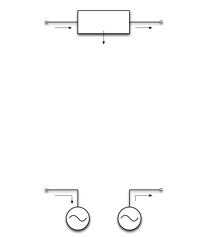
DC Line
pf
pt
“from”
bus
“to”
bus
ploss =l0+l1pf
Figure 7-2: DC Line Model
pt=(1−l1)pf−l0
“from”
bus
“to”
bus
pf
Figure 7-3: Equivalent “Dummy” Generators
101

Matpower links the values of pfand ptusing the following relationship, which
includes a linear approximation of the real power loss in the line.
pt=pf−ploss
=pf−(l0+l1pf)
= (1 −l1)pf−l0(7.8)
Here the linear coefficient l1is assumed to be a small (1) positive number. Ob-
viously, this is not applicable for bi-directional lines, where the flow could go either
direction, resulting in decreasing losses for increasing flow in the “to” →“from” di-
rection. There are currently two options for handling bi-directional lines. The first
is to use a constant loss model by setting l1= 0. The second option is to create
two separate but identical lines oriented in opposite directions. In this case, it is
important that the lower limit on the flow and the constant term of the loss model l0
be set to zero to ensure that only one of the two lines has non-zero flow at a time.41
Upper and lower bounds on the value of the flow can be specified for each DC
line, along with an optional operating cost. It is also assumed that the terminals of
the line have a range of reactive power capability that can be used to maintain a
voltage setpoint. Just as with a normal generator, the voltage setpoint is only used
for simple power flow; the OPF dispatches the voltage anywhere between the lower
and upper bounds specified for the bus. Similarly, in a simple power flow the input
value for pfand the corresponding value for pt, computed from (7.8), are used to
specify the flow in the line.
Most of the data for DC lines is stored in a dcline field in the Matpower
case struct mpc. This field is a matrix similar to the branch matrix, where each
row corresponds to a particular DC line. The columns of the matrix are defined in
Table B-5 and include connection bus indices, line status, flows, terminal reactive
injections, voltage setpoints, limits on power flow and VAr injections, and loss pa-
rameters. Also, similar to the branch or gen matrices, some of the columns are used
for input values, some for results, and some, such as PF can be either input or output,
depending on whether the problem is a simple power flow or an optimal power flow.
The idx dcline function defines a set of constants for use as named column indices
for the dcline matrix.
An optional dclinecost matrix, in the same form as gencost, can be used to
specify a cost to be applied to pfin the OPF. If the dclinecost field is not present,
the cost is assumed to be zero.
41A future version may make the handling of this second option automatic.
102

Matpower’s DC line handling is implemented in toggle dcline and examples
of using it can be found in t dcline. The case file t case9 dcline includes some
example DC line data. See help toggle dcline for more information.
Running a case that includes DC lines is as simple as loading the case, turning
on the extension and running it. Unlike with the reserves extension, Matpower
does not currently have a wrapper function to automate this.
mpc = loadcase('t_case9_dcline');
mpc = toggle_dcline(mpc, 'on');
results = runopf(mpc);
7.6.4 OPF Soft Limits
Matpower includes an extension that replaces limits (such as branch flow limits,
voltage magnitude bounds, generator limits, etc.) in an optimal power flow with
soft limits, that is, limits that can be violated with some linear penalty cost. This
can be useful in identifying the cause of infeasibility in some optimal power flow
problems. The extension is implemented in toggle softlims. A limited version for
branch flow constraints in a DC model only, was introduced in Matpower 5.0, with
a generalization to all of the standard OPF limits added in Matpower 7.0. The soft
AC branch flow limit implemention provides an example of user-defined nonlinear
constraints.
In general, replacing a hard constraint of the form
hi(x)≤0 (7.9)
with a soft limit involves introducing a new non-negative variable sito represent the
violation of the original constraint. The original hard constraint (7.9) is replaced by
one in which this violation variable is used to “relax” the constraint by adding it to
the right-hand.
si≥0 (7.10)
hi(x)≤si.(7.11)
Finally, a penalty cost on violations is implemented via a linear cost coefficient, ci
v,
applied to each violation variable si, so that the additional user defined cost term
from (6.47) for the set of soft limits looks like
fu(ˆx) = cv
Ts. (7.12)
103
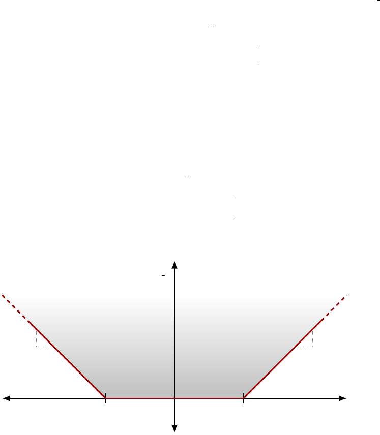
Take, as an example, branch flow limits. The flow constraints in (6.9) and (6.10)
are rewritten by replacing the right hand side with a flow violation variable si
rate a
si
rate a ≥0∀i(7.13)
hi
f(Θ, Vm) = fi
f(Θ, Vm)−fi,max ≤si
rate a∀i(7.14)
hi
t(Θ, Vm) = fi
t(Θ, Vm)−fi,max ≤si
rate a ∀i. (7.15)
In the case of AC flow constraints, the flow functions fi
fand fi
tare nonlinear and
can be either apparent power, active power, or current as shown in (6.11). In the case
of DC flow constraints, where there are no losses, these flows can be implemented in
terms of the flow at the from end of the line and its negative, both linear functions
of the bus voltage angles, based on (6.30) and (6.31).
si
rate a ≥0∀i(7.16)
Bi
fΘ + pi
f,shift −pi,max
f≤si
rate a ∀i(7.17)
−Bi
fΘ−pi
f,shift −pi,max
f≤si
rate a ∀i. (7.18)
The feasible area for the DC case is illustrated in Figure 7-4.
pi
f
si
rate a
−pi,max
fpi,max
f
−11
Figure 7-4: Feasible Region for Branch Flow Violation Constraints
Matpower implements soft limits for each of the types of constraints listed in
Table 7-9, where the formulation for each constraint type is shown.
The parameters for the problem are specified in an additional softlims field in
the Matpower case struct mpc. This field is itself a struct where each sub-field
104

Table 7-9: Soft Limit Formulation
name hard-limit formulation soft-limit formulation
VMIN,VMAX†vi
m≥vi,min
m,vi
m≤vi,max
mvi
m+si
vmin ≥vi,min
m,vi
m−si
vmax ≤vi,max
m
RATE A‡fi
f(Θ, Vm)≤fi
max fi
f(Θ, Vm)−srate a ≤fi
max
fi
t(Θ, Vm)≤fi
max fi
t(Θ, Vm)−srate a ≤fi
max
PMIN,PMAX pi
g≥pi,min
g,pi
g≤pi,max
gpi
g+spmin ≥pi,min
g,pi
g−spmax ≤pi,max
g
QMIN,QMAX†qi
g≥qi,min
g,qi
g≤qi,max
gqi
g+sqmin ≥qi,min
g,qi
g−sqmax ≤qi,max
g
ANGMIN θi
f−θi
t≥∆θi,min θi
f−θi
t+sangmin ≥∆θi,min
ANGMAX θi
f−θi
t≤∆θi,max θi
f−θi
t−sangmax ≤∆θi,max
†Only applicable for the AC OPF.
‡Example of a user-defined nonlinear constraint in the AC version.
corresponds to the name of one of the limits listed in Table 7-9. For each of the
limits, the input parameters are specified in the fields detailed in Table 7-10, with
defaults summarized in Table 7-11.
Depending on whether the original constraint in (7.10) is an upper bound or a
lower bound, it can be written as one of the following
hi(x) = (¯
hi(x)−hi,lim (upper bound)
hi,lim −¯
hi(x) (lower bound) (7.19)
where hi,lim is the actual value of the hard limit. When introducing a soft limit,
this original hard limit can be removed completely or modified to have a new value.
Matpower provides a several ways of modifying the original hard limit based on
fields hl mod (“hard limit modification”) and hl val (“hard limit value”) in the re-
spective limit structures. This new hard limit is implemented via an upper bound on
the corresponding violation variable si. Table 7-12 summarizes the new hard limits
and the corresponding bounds on the violation variable as functions of the values of
hl mod and hl val.
Unspecified limits in the mpc.softlims input parameters are handled differently,
depending on the value of the Matpower option 'opf.softlims.default'(see Ta-
ble C-5).
•If the opf.softlims.default option is 1 (default), each limit not explicitly spec-
ified, whether missing in mpc.softlims or present but empty, will be initialized
as in Table 7-11.
•If the opf.softlims.default option is 0, limits that are missing in mpc.softlims
are treated as though specified with hl mod ='none', that is, they are not
105

Table 7-10: Input Data Structures for OPF Soft Limits
name description
mpc Matpower case struct
softlims additional field in mpc containing OPF soft limit input parameters for the pos-
sible limits, each of which is optional.*
<LIM> <LIM> refers to the name of the limit, i.e. one of the following: ANGMIN,ANGMAX,
RATE A,PMIN,PMAX,QMIN,QMAX,VMIN,VMAX. Each of these is a struct with input
parameters defining the soft limits for this type of constraint in the following
optional fields (see Table 7-11 for defaults):
idx nsl ×1 vector of row indices for bus,branch or gen matrix, depending on <LIM>,
specifying the elements for which corresponding soft limits are to be applied†
busnum‡nsl ×1 vector of external bus numbers specifying the buses to which soft limits
are to be applied†
cost scalar or nsl ×1 vector cvof linear cost coefficients for limit violation costs
hl mod§string indicating type of modification to original hard limit:
'none'– do not add soft limit, no change to original hard limit
'remove'– add soft limit, relax hard limit by removing it completely
'replace'– add soft limit, relax hard limit by replacing original with value
specified in hl val
'scale'– add soft limit, relax hard limit by scaling original by value spec-
ified in hl val
'shift'– add soft limit, relax hard limit by shifting original by value spec-
ified in hl val
hl val§scalar or nsl ×1 vector value used to modify hard limit according to hl mod.
Ignored for 'none'and 'remove', required for 'replace', and optional, with
the following defaults, for 'scale'and 'shift':
'scale'– 2 for positive upper limits or negative lower limits, 0.5 otherwise
'shift'– 0.25 for VMAX and VMIN, 10 otherwise
*For fields not present, the value of the 'opf.softlims.defaults'option determines whether the corresponding
limit is unchanged (= 0) or converted (= 1, default) to a soft limit using default values from Table 7-11.
†For bus constraints, idx overrides busnum if both are provided.
‡Only applicable for bus constraints, i.e. <LIM> is VMIN or VMAX.
§Any new, relaxed hard limits are implemented via bounds on the violation variables. See Table 7-12 for details.
converted to soft limits at all. On the other hand, the default soft limits
of Table 7-11 are still applied to any limit that is present in mpc.softlims
but empty. For example, mpc.softlims.RATE A = struct() would result in the
default soft branch limits being applied.
Soft limit outputs, summarized in Table 7-13, include the amount and cost of
any overloads, that is, violations of the original hard limits. These can be found
as additional fields, overload and ov cost, under each limit in results.softlims.
The Kuhn-Tucker multipliers on the soft limit constraints are also included in the
106

Table 7-11: Default Soft Limit Values
name description
VMIN voltage magnitude lower bound
idx all buses
cost $100,000/p.u.†
hl mod 'replace'
hl val 0
VMAX voltage magnitude upper bound
idx all buses
cost $100,000/p.u.†
hl mod 'remove'
RATE A branch flow limit
idx all on-line branches with bounded flow limits
cost $1000/MVA, $1000/MW, or $1000/MA†depending on 'opf.flow lim'
hl mod 'remove'
PMIN generator active power lower bound
idx all on-line generators, excluding dispatchable loads
cost $1000/MW†
hl mod 'replace'
hl val 0 if Pi,min
g≥0, −∞ otherwise
PMAX,QMIN,QMAX generator active power upper bound, reactive power lower/upper bounds
idx all on-line generators, excluding dispatchable loads
cost $1000/MW or $1000/MVAr†
hl mod 'remove'
ANGMIN,ANGMAX branch angle difference lower/upper bounds
idx all on-line branches with angle difference limits, ∆θ, where |∆θ|<360◦
cost $1000/deg†
hl mod 'remove'
†Unless the maximum marginal cost at Pmax across all online generators, which we call cmax
g, exceeds
$1000/MWh, in which case the numerical value of the default cost is cmax
ginstead of 1000 (or 100 ·cmax
g
instead of 100,000, for VMIN or VMAX).
Table 7-12: Possible Hard-Limit Modifications
h mod new hard limit hi,lim
new upper bound on violation variable si
'remove'±∞†∞
'replace'hl val hl val −hi,lim
orig
'scale'hl val ·hi,lim
orig (hl val −1) ·hi,lim
orig
'shift'hi,lim
orig ±hl val†hl val
†Plus sign for upper bounds and minus sign for lower bounds.
107

usual columns of the corresponding matrix in the results, e.g. bus(:, MU VMAX),
branch(:, MU SF), etc. When there are no violations, these shadow prices are the
same as if hard limits were imposed. When there is a violation, they are equal to the
cost cvassociated with the violation variable, except in the case where a modified
hard limit is also binding, in which case it also reflects the shadow price on this
modified hard constraint.
Table 7-13: Output Data Structures for OPF Soft Limits
name description
results Matpower case struct
softlims additional field in results containing OPF soft limit outputs for
each limit type
<LIM> <LIM> refers to the name of the limit, i.e. one of the following:
ANGMIN,ANGMAX,RATE A,PMIN,PMAX,QMIN,QMAX,VMIN,VMAX. Each
of these is a struct with the following output fields:
overload†nb/l/g ×1 vector of overload quantities for this limit (amount of
original hard limit violation)
ov cost†nb/l/g ×1 vector of overload penalty costs for this limit
branch(:, MU ANGMIN) Kuhn-Tucker multipliers on angle difference lower bounds‡
branch(:, MU ANGMAX) Kuhn-Tucker multipliers on angle difference upper bounds‡
branch(:, MU SF) Kuhn-Tucker multipliers on branch flow limits (from end)‡
branch(:, MU ST) Kuhn-Tucker multipliers on branch flow limits (to end)‡
gen(:, MU PMIN) Kuhn-Tucker multipliers on active gen lower bounds‡
gen(:, MU PMAX) Kuhn-Tucker multipliers on active gen upper bounds‡
gen(:, MU QMIN) Kuhn-Tucker multipliers on reactive gen lower bounds‡
gen(:, MU QMAX) Kuhn-Tucker multipliers on reactive gen upper bounds‡
bus(:, MU VMIN) Kuhn-Tucker multipliers on voltage magnitude lower bounds‡
bus(:, MU VMAX) Kuhn-Tucker multipliers on voltage magnitude upper bounds‡
†The dimensions of overload and ov cost correspond to all buses, branches or generators (depending on <LIM>),
not just those whose limits were converted to soft limits. Entries corresponding to those not included (implicitly
or explicitly) in idx are set to zero.
†For limits that have been converted to soft limits, these are the shadow prices on the soft limit constraints. When
there is no violation of the soft limit, this shadow price is the same as it would be for the original hard limit.
When there is a violation, it is equal to the corresponding user-supplied violation cost ci
v, unless an updated
hard constraint is also binding.
108

See help toggle softlims for more information on this extension. Examples of
using this extension can be found in t opf softlims. Running a case that includes
the default soft limits is as simple as loading the case, turning on the extension and
running it. Unlike with the reserves extension, Matpower does not currently have
a wrapper function to automate this.
mpc = loadcase('case2383wp');
mpc = toggle_softlims(mpc, 'on');
results = runopf(mpc, mpopt);
109

8 Unit De-commitment Algorithm
The standard OPF formulation described in the previous section has no mechanism
for completely shutting down generators which are very expensive to operate. Instead
they are simply dispatched at their minimum generation limits. Matpower includes
the capability to run an optimal power flow combined with a unit de-commitment
for a single time period, which allows it to shut down these expensive units and find
a least cost commitment and dispatch. To run this for case30, for example, type:
>> runuopf('case30')
By default, runuopf is based on the AC optimal power flow problem. To run a DC
OPF, the model option must be set to 'DC'. For convenience, Matpower provides
a function runduopf which is simply a wrapper that sets the model option to 'DC'
before calling runuopf.
Matpower uses an algorithm similar to dynamic programming to handle the
de-commitment. It proceeds through a sequence of stages, where stage Nhas N
generators shut down, starting with N= 0, as follows:
Step 1: Begin at stage zero (N= 0), assuming all generators are on-line with all
limits in place.
Step 2: If the sum of the minimum generation limits for all on-line generators is less
than the total system demand, then go to Step 3. Otherwise, go to the next
stage, N=N+ 1, shut down the generator whose average per-MW cost of
operating at its minimum generation limit is greatest and repeat Step 2.
Step 3: Solve a normal OPF. Save the solution as the current best.
Step 4: Go to the next stage, N=N+ 1. Using the best solution from the previous
stage as the base case for this stage, form a candidate list of generators
with minimum generation limits binding. If there are no candidates, skip
to Step 6.
Step 5: For each generator on the candidate list, solve an OPF to find the total
system cost with this generator shut down. Replace the current best solu-
tion with this one if it has a lower cost. If any of the candidate solutions
produced an improvement, return to Step 4.
Step 6: Return the current best solution as the final solution.
110
It should be noted that the method employed here is simply a heuristic. It does
not guarantee that the least cost commitment of generators will be found. It is also
rather computationally expensive for larger systems and was implemented as a simple
way to allow an OPF-based “smart-market”, such as described in Appendix F, the
option to reject expensive offers while respecting the minimum generation limits on
generators.
111

9 Miscellaneous Matpower Functions
This section describes a number of additional Matpower functions that users may
find useful. The descriptions here are simply brief summaries, so please use the
Matlab help function to get the full details on each function.
9.1 Input/Output Functions
9.1.1 loadcase
mpc = loadcase(casefile)
The loadcase function provides the canonical way of loading a Matpower case
from a file or struct. It takes as input either a struct or the name of an M-file or
MAT-file in the Matlab path (casefile) and returns a standard Matpower case
struct (mpc). It can also convert from the older version 1 case file format to the
current format. This function allows a case to be loaded, and potentially modified,
before calling one of the main simulation functions such as runpf or runopf.
9.1.2 savecase
savecase(fname, mpc)
savecase(fname, mpc, version)
savecase(fname, comment, mpc)
savecase(fname, comment, mpc, version)
fname = savecase(fname, ...)
The savecase function writes out a Matpower case file, given a name for the
file to be created or overwritten (fname), and a Matpower case struct (mpc). If
fname ends with '.mat'it saves the case as a MAT-file, otherwise it saves it as an
M-file. Optionally returns the filename, with extension added if necessary. The
optional comment argument is either string (single line comment) or a cell array of
strings which are inserted as comments in the help section of the file. If the optional
version argument is '1'it will modify the data matrices to version 1 format before
saving.
112

9.1.3 cdf2mpc
mpc = cdf2mpc(cdf_file_name)
mpc = cdf2mpc(cdf_file_name, verbose)
mpc = cdf2mpc(cdf_file_name, mpc_name)
mpc = cdf2mpc(cdf_file_name, mpc_name, verbose)
[mpc, warnings] = cdf2mpc(cdf_file_name, ...)
The cdf2mpc function converts an IEEE Common Data Format (CDF) data file
into a Matpower case struct. Given an optional file name mpc name, it can save the
converted case to a Matpower case file. Warnings generated during the conversion
process can be optionally returned in the warnings argument.
Since the IEEE CDF format does not contain all of the data needed to run an
optimal power flow, some data, such as voltage limits, generator limits and generator
costs are created by cdf2mpc. See help cdf2mpc for details.
9.1.4 psse2mpc
mpc = psse2mpc(rawfile_name)
mpc = psse2mpc(rawfile_name, verbose)
mpc = psse2mpc(rawfile_name, verbose, rev)
mpc = psse2mpc(rawfile_name, mpc_name)
mpc = psse2mpc(rawfile_name, mpc_name, verbose)
mpc = psse2mpc(rawfile_name, mpc_name, verbose, rev)
[mpc, warnings] = psse2mpc(rawfile_name, ...)
The psse2mpc function converts a PSS/E RAW data file into a Matpower case
struct. Given an optional file name mpc name, it can save the converted case to a
Matpower case file. Warnings generated during the conversion process can be
optionally returned in the warnings argument. By default, psse2mpc attempts to
determine the revision of the PSS/E RAW file from the contents, but the user can
specify an explicit revision number to use in the optional rev argument.
113

9.1.5 save2psse
save2psse(fname, mpc)
fname_out = save2psse(fname, mpc)
The save2psse function saves a Matpower case struct mpc as a PSS/E RAW
file. The fname parameter is a string containing the name of the file to be created or
overwritten. If fname does not include a file extension, codeq.raw will be added. Op-
tionally returns the, possibly updated, filename. Currently exports to RAW format
Rev 33.
9.2 System Information
9.2.1 case info
case_info(mpc)
case_info(mpc, fd)
[groups, isolated] = case_info(mpc)
The case info function prints out detailed information about a Matpower case,
including connectivity information, summarizing the generation, load and other data
by interconnected island. It can optionally print the output to an open file, whose
file identifier (as returned by fopen) is specified in the optional second parameter fd.
Optional return arguments include groups and isolated buses, as returned by the
find islands function.
9.2.2 compare case
compare_case(mpc1, mpc2)
Compares the bus,branch and gen matrices of two Matpower cases and prints
a summary of the differences. For each column of the matrix it prints the maximum
of any non-zero differences.
114

9.2.3 find islands
groups = find_islands(mpc)
[groups, isolated] = find_islands(mpc)
The find islands function returns the islands in a network. The return value
groups is a cell array of vectors of the bus indices for each island. The second and
optional return value isolated is a vector of indices of isolated buses that have no
connecting branches.
9.2.4 get losses
loss = get_losses(results)
loss = get_losses(baseMVA, bus, branch)
[loss, chg] = get_losses(results)
[loss, fchg, tchg] = get_losses(results)
[loss, fchg, tchg, dloss_dv] = get_losses(results)
[loss, fchg, tchg, dloss_dv, dchg_dvm] = get_losses(results)
The get losses function computes branch series losses, and optionally reactive
injections from line charging, as functions of bus voltages and branch parameters,
using the following formulae for a branch, as described in Section 3.2, connecting
bus fto bus t:
lossi=vf
τejθshift −vt2
rs−jxs
(9.1)
fchg =vf
τejθshift
2bc
2(9.2)
tchg =|vt|2bc
2(9.3)
It can also optionally compute the partial derivatives of the line losses and reactive
charging injections with respect to voltage angles and magnitudes.
115

9.2.5 margcost
marginalcost = margcost(gencost, Pg)
The margcost function computes the marginal cost for generators given a matrix
in gencost format and a column vector or matrix of generation levels. The return
value has the same dimensions as Pg. Each row of gencost is used to evaluate the cost
at the output levels specified in the corresponding row of Pg. The rows of gencost
can specify either polynomial or piecewise linear costs and need not be uniform.
9.2.6 isload
TorF = isload(gen)
The isload function returns a column vector of 1’s and 0’s. The 1’s correspond
to rows of the gen matrix which represent dispatchable loads. The current test is
Pmin <0 and Pmax = 0.
9.2.7 loadshed
shed = loadshed(gen)
shed = loadshed(gen, ild)
The loadshed function returns a column vector of MW curtailments of dispatch-
able loads, computed as the difference between the PG and PMIN values in the corre-
sponding rows of the gen matrix. The optional ild argument is a column vector of
generator indices to the dispatchable loads of interest.
9.2.8 printpf
printpf(results, fd, mpopt)
The printpf function prints power flow and optimal power flow results, as re-
turned to fd, a file identifier which defaults to STDOUT (the screen). The details of
what gets printed are controlled by an optional Matpower options struct mpopt.
116

9.2.9 total load
Pd = total_load(mpc)
Pd = total_load(mpc, load_zone, opt, mpopt)
Pd = total_load(bus)
Pd = total_load(bus, gen, load_zone, opt, mpopt)
[Pd, Qd] = total_load(...)
The total load function returns a vector of total load in each load zone. The
opt argument controls whether it includes fixed loads, dispatchable loads or both,
and for dispatchable loads, whether to use the nominal or realized load values. The
load zone argument defines the load zones across which loads will be summed. It
uses the BUS AREA column (7) of the bus matrix by default. The string value 'all'can
be used to specify a single zone including the entire system. The reactive demands
are also optionally available as an output.
9.2.10 totcost
totalcost = totcost(gencost, Pg)
The totcost function computes the total cost for generators given a matrix in
gencost format and a column vector or matrix of generation levels. The return value
has the same dimensions as Pg. Each row of gencost is used to evaluate the cost at
the output levels specified in the corresponding row of Pg. The rows of gencost can
specify either polynomial or piecewise linear costs and need not be uniform.
9.3 Modifying a Case
9.3.1 extract islands
mpc_array = extract_islands(mpc)
mpc_array = extract_islands(mpc, groups)
mpc_k = extract_islands(mpc, k)
mpc_k = extract_islands(mpc, groups, k)
mpc_k = extract_islands(mpc, k, custom)
mpc_k = extract_islands(mpc, groups, k, custom)
The extract islands function extracts individual islands in a network that is not
fully connected. The original network is specified as a Matpower case struct (mpc)
and the result is returned as a cell array of case structs, or as a single case struct.
Supplying the optional group avoids the need to traverse the network again, saving
117

time on large systems. A final optional argument custom is a struct that can be used
to indicate custom fields of mpc from which to extract data corresponding to buses
generators, branches or DC lines.
9.3.2 load2disp
mpc = load2disp(mpc0)
mpc = load2disp(mpc0, fname)
mpc = load2disp(mpc0, fname, idx)
mpc = load2disp(mpc0, fname, idx, voll)
The load2disp function takes a Matpower case mpc0, converts fixed loads to
dispatchable loads, curtailable at a specific price, and returns the resulting case
struct mpc. It can optionally save the resulting case to a file (fname), convert loads
only at specific buses (idx), and set the value of lost load (voll) to be used as the
curtailment price (default is $5,000/MWh).
9.3.3 modcost
newgencost = modcost(gencost, alpha)
newgencost = modcost(gencost, alpha, modtype)
The modcost function can be used to modify generator cost functions by shifting
or scaling them, either horizontally or vertically. The alpha argument specifies the
numerical value of the modification, and modtype defines the type of modification
as a string that takes one of the following values: 'SCALE F'(default), 'SCALE X',
'SHIFT F', or 'SHIFT X'.
9.3.4 scale load
mpc = scale_load(load, mpc)
mpc = scale_load(load, mpc, load_zone)
mpc = scale_load(load, mpc, load_zone, opt)
bus = scale_load(load, bus)
[bus, gen] = scale_load(load, bus, gen, load_zone, opt)
[bus, gen, gencost] = ...
scale_load(load, bus, gen, load_zone, opt, gencost)
The scale load function is used to scale active (and optionally reactive) loads in
each zone by a zone-specific ratio, i.e. R(k) for zone k. The amount of scaling for
118

each zone, either as a direct scale factor or as a target quantity, is specified in load.
The load zones are defined by load zone, and opt specifies the type of scaling (factor
or target quantity) and which loads are affected (active, reactive or both and fixed,
dispatchable or both). The costs (gencost) associated with dispatchable loads can
also be optionally scaled with the loads.
9.3.5 apply changes
mpc_modified = apply_changes(label, mpc_original, chgtab)
The apply changes function implements a general mechanism to apply a set of
changes to a base Matpower case. This can be used, for example, to define and
apply a set of contingencies. There are three basic types of changes, those that
replace old values with new ones, those that scale old values by some factor, and
those that add a constant to existing values.
The change table matrix, chgtab, specifies modifications to be applied to an
existing case. These modifications are grouped into sets, designated change sets,
that are always applied as a group. A change set consists of one or more changes,
each specified in a separate row in the chgtab, where the rows share a common label
(integer ID).
For example, ncchange sets can be used to define nccontingencies via a single
chgtab with many rows, but only ncunique labels. The chgtab also optionally speci-
fies a probability πkof occurance associated with change set k. Table 9-1 summarizes
the meaning of the data in each column of chgtab. All of the names referenced in
Tables 9-1 through 9-4 are defined as constants by the idx ct function. Type help
idx ct at the Matlab prompt for more details. Use of the named constants when
constructing a chgtab matrix is encouraged to improve readability.
The value in the CT TABLE column of chgtab defines which data table is to be
modified and the options are given in Table 9-2. With the exception of load and cer-
tain generator cost changes, each individual change record specifies modification(s)
to a single column of a particular data matrix, either bus,gen,branch or gencost.
Some are changes to that column for an individual row in the matrix (or all rows, if
the row index is set to 0), while others are area-wide changes that modify all rows
corresponding to the specified area.42
Load changes are special and may modify multiple columns of the bus and/or gen
tables. They offer a more flexible and convenient means of specifying modifications
42Areas are defined by the BUS AREA column of the bus matrix.
119

Table 9-1: Columns of chgtab
name column description
CT LABEL 1 change set label, unique for each change set (integer)
CT PROB 2 change set probability (number between 0 and 1)†
CT TABLE 3 type of table to be modified (see Table 9-2 for possible values)
CT ROW 4 row index of data to be modified, 0 means all rows,
for area-wide changes this is the area index, rather than row index
CT COL 5 column index of data to be modified (see Table 9-4 for exceptions)
CT CHGTYPE 6 type of change, e.g. replace, scale or add (see Table 9-3 for details)
CT NEWVAL 7 new value used to replace or modify existing data
†The change set probability πkis taken from this column of the first row for change set k.
to loads (fixed, dispatchable, real and/or reactive) than directly including individ-
ual change specifications for each of the corresponding entries in the bus and gen
matrices. The row indices for load changes refer to bus numbers.
In addition to the normal direct modifications for generator cost parameters,
there is also the option to scale or shift an entire cost function, either vertically or
horizontally. This is often more convenient than manipulating the individual cost
parameters directly, especially when dealing with a mix of polynomial and piecewise
linear generator costs.
Table 9-2: Values for CT TABLE Column
name value description
CT TBUS 1bus table
CT TGEN 2gen table
CT TBRCH 3branch table
CT TAREABUS 4 area-wide change in bus table
CT TAREAGEN 5 area-wide change in gen table
CT TAREABRCH 6 area-wide change in branch table
CT TLOAD 7 per bus load change†
CT TAREALOAD 8 area-wide load change†
CT TGENCOST 9gencost table
CT TAREAGENCOST 10 area-wide change in gencost table
†Preferred method of modifying load, as opposed to manipulating bus and
gen tables directly.
Normally, the CT COL column contains the column index of the entry or entries in
the data tables to be modified. And the CT CHGTYPE and CT NEWVAL columns specify,
respectively, the type of change (replacement, scaling or adding) and the correspond-
120

ing replacement value, scale factor or constant to add, as shown in Table 9-3.
Table 9-3: Values for CT CHGTYPE Column
name value description
CT REP 1 replace old value by new one in CT NEWVAL column
CT REL 2 scale old value by factor in CT NEWVAL column
CT ADD 3 add value in CT NEWVAL column to old value
For load changes, the CT COL column is not a column index, but rather a code that
defines which loads at the specified bus(es) are to be modified, with the ability to
select fixed loads only, dispatchable loads only or both, and for each whether or not
to include the reactive load in the change. Similarly, the CT COL column for generator
cost modifications can be set to a special code to indicate a scaling or shifting of the
entire corresponding cost function(s). The various options for the CT COL column are
summarized in Table 9-4.
Table 9-4: Values for CT COL Column
name value description
for CT TABLE column = CT TLOAD or CT TAREALOAD
CT LOAD ALL PQ 1 modify all (fixed & dispatchable) loads, active and reactive
CT LOAD FIX PQ 2 modify fixed loads, active and reactive
CT LOAD DIS PQ 3 modify dispatchable loads, active and reactive
CT LOAD ALL P 4 modify all (fixed & dispatchable) loads, active power only
CT LOAD FIX P 5 modify fixed loads, active power only
CT LOAD DIS P 6 modify dispatchable loads, active power only
for CT TABLE column = CT TGENCOST or CT TAREAGENCOST
CT MODCOST F -1 scales or shifts the cost function vertically†
CT MODCOST X -2 scales or shifts the cost function horizontally†
otherwise‡
nindex of column in data matrix to be modified
†Use CT CHGTYPE column = CT REL to scale the cost and CT ADD to shift the cost.
‡Can also be used for CT TGENCOST or CT TAREAGENCOST in addition to the special codes above.
121

For example, setting up a chgtab matrix for the following four scenarios could be
done as shown below.
1. Turn off generator 2 (10% probability).
2. Reduce the line rating of all lines to 95% of their nominal values (0.2% proba-
bility).
3. Scale all loads in area 2 (real & reactive, fixed & dispatchable) up by 10%
(0.1% probability).
4. Decrease capacity of generator 3 and shift its cost function to the left both by
10 MW (5% probability).
chgtab = [ ...
1 0.1 CT_TGEN 2 GEN_STATUS CT_REP 0;
2 0.002 CT_TBRCH 0 RATE_A CT_REL 0.95;
3 0.001 CT_TAREALOAD 2 CT_LOAD_ALL_PQ CT_REL 1.1;
4 0.05 CT_TGEN 3 PMAX CT_ADD -10;
4 0.05 CT_TGENCOST 3 CT_MODCOST_X CT_ADD -10;
];
A change table can be used to easily create modified cases from an existing base
case with the apply changes function. Given the chgtab from the example above, a
new case with all lines derated by 5% can easily be created from an existing case mpc
with the following line of code.
mpc_new = apply_changes(2, mpc, chgtab);
9.3.6 savechgtab
savechgtab(fname, chgtab)
savechgtab(fname, chgtab, warnings)
fname = savechgtab(fname, ...)
This function can be used to save a change table matrix, chgtab, to a file specified
by fname. If the fname string ends with '.mat'it saves chgtab and warnings to a
MAT-file as the variables chgtab and warnings, respectively. Otherwise, it saves an
M-file function that returns the chgtab, with the optional warnings included in the
comments, where warnings is a cell array of warning messages such as those returned
by pssecon2chgtab.
122

9.4 Conversion between External and Internal Numbering
9.4.1 ext2int,int2ext
mpc_int = ext2int(mpc_ext)
mpc_int = ext2int(mpc_ext, mpopt)
mpc_ext = int2ext(mpc_int)
mpc_ext = int2ext(mpc_int, mpopt)
These functions convert a Matpower case struct from external to internal, and
from internal to external numbering, respectively. ext2int first removes all isolated
buses, off-line generators and branches, and any generators or branches connected
to isolated buses. Then the buses are renumbered consecutively, beginning at 1,
and the generators are sorted by increasing bus number. Any 'ext2int'callback
routines registered in the case are also invoked automatically. All of the related
indexing information and the original data matrices are stored in an 'order'field
in the struct to be used later by codeint2ext to perform the reverse conversions. If
the case is already using internal numbering it is returned unchanged. The optional
Matpower options struct (mpopt) input argument is only needed in conjunction
with callback routines that depend on it, e.g. when toggle softlims is on.
9.4.2 e2i data,i2e data
val = e2i_data(mpc, val, ordering)
val = e2i_data(mpc, val, ordering, dim)
val = i2e_data(mpc, val, oldval, ordering)
val = i2e_data(mpc, val, oldval, ordering, dim)
These functions can be used to convert other data structures from external to
internal indexing and vice versa. When given a case struct (mpc) that has already
been converted to internal indexing, e2i data can be used to convert other data
structures as well by passing in 2 or 3 extra parameters in addition to the case
struct. If the value passed in the second argument (val) is a column vector or cell
array, it will be converted according to the ordering specified by the third argument
(described below). If val is an n-dimensional matrix or cell array, then the optional
fourth argument (dim, default = 1) can be used to specify which dimension to reorder.
The return value in this case is the value passed in, converted to internal indexing.
The third argument, ordering, is used to indicate whether the data corresponds
to bus-, gen- or branch-ordered data. It can be one of the following three strings:
'bus','gen'or 'branch'. For data structures with multiple blocks of data, ordered
123

by bus, gen or branch, they can be converted with a single call by specifying ordering
as a cell array of strings.
Any extra elements, rows, columns, etc. beyond those indicated in ordering, are
not disturbed.
The function i2e data performs the opposite conversion, from internal back to
external indexing. It also assumes that mpc is using internal indexing, and the only
difference is that it also includes an oldval argument used to initialize the return
value before converting val to external indexing. In particular, any data correspond-
ing to off-line gens or branches or isolated buses or any connected gens or branches
will be taken from oldval, with val supplying the rest of the returned data.
9.4.3 e2i field,i2e field
mpc = e2i_field(mpc, field, ordering)
mpc = e2i_field(mpc, field, ordering, dim)
mpc = i2e_field(mpc, field, ordering)
mpc = i2e_field(mpc, field, ordering, dim)
These functions can be used to convert additional fields in mpc from external to
internal indexing and vice versa. When given a case struct that has already been
converted to internal indexing, e2i field can be used to convert other fields as well
by passing in 2 or 3 extra parameters in addition to the case struct.
The second argument (field) is a string or cell array of strings, specifying a
field in the case struct whose value should be converted by a corresponding call to
e2i data. The field can contain either a numeric or a cell array. The converted value
is stored back in the specified field, the original value is saved for later use and the
updated case struct is returned. If field is a cell array of strings, they specify nested
fields.
The third and optional fourth arguments (ordering and dim) are simply passed
along to the call to e2i data.
Similarly, i2e field performs the opposite conversion, from internal back to ex-
ternal indexing. It also assumes that mpc is using internal indexing and utilizes the
original data stored by e2i field, calling i2e data to do the conversion work.
124

9.5 Forming Standard Power Systems Matrices
9.5.1 makeB
[Bp, Bpp] = makeB(mpc, alg)
[Bp, Bpp] = makeB(baseMVA, bus, branch, alg)
The makeB function builds the two matrices B0and B00 used in the fast-decoupled
power flow. The alg, which can take values 'FDXB'or 'FDBX', determines whether the
matrices returned correspond to the XB or BX version of the fast-decoupled power
flow. Bus numbers must be consecutive beginning at 1 (i.e. internal ordering).
9.5.2 makeBdc
[Bbus, Bf, Pbusinj, Pfinj] = makeBdc(mpc)
[Bbus, Bf, Pbusinj, Pfinj] = makeBdc(baseMVA, bus, branch)
The function builds the Bmatrices, Bdc (Bbus) and Bf(Bf), and phase shift in-
jections, Pdc (Pbusinj) and Pf,shift (Pfinj), for the DC power flow model as described
in (3.29) and (4.7). Bus numbers must be consecutive beginning at 1 (i.e. internal
ordering).
9.5.3 makeJac
J = makeJac(mpc)
J = makeJac(mpc, fullJac)
[J, Ybus, Yf, Yt] = makejac(mpc)
The makeJac function forms the power flow Jacobian and, optionally, the system
admittance matrices. Bus numbers in the input case must be consecutive beginning
at 1 (i.e. internal indexing). If the fullJac argument is present and true, it returns
the full Jacobian (sensitivities of all bus injections with respect to all voltage angles
and magnitudes) as opposed to the reduced version used in the Newton power flow
updates.
125

9.5.4 makeLODF
PTDF = makePTDF(mpc)
LODF = makeLODF(mpc.branch, PTDF)
The makeLODF function forms the DC line outage distribution factor matrix for
a given PTDF. The matrix is nbr ×nbr, where nbr is the number of branches. See
Section 4.5 on Linear Shift Factors for more details.
9.5.5 makePTDF
H = makePTDF(mpc)
H = makePTDF(mpc, slack)
H = makePTDF(baseMVA, bus, branch)
H = makePTDF(baseMVA, bus, branch, slack)
The makePTDF function returns the DC PTDF matrix for a given choice of slack.
The matrix is nbr ×nb, where nbr is the number of branches and nbis the number
of buses. The slack can be a scalar (single slack bus) or an nb×1 column vector of
weights specifying the proportion of the slack taken up at each bus. If the slack is
not specified, the reference bus is used by default. Bus numbers must be consecutive
beginning at 1 (i.e. internal ordering). See Section 4.5 on Linear Shift Factors for
more details.
9.5.6 makeYbus
[Ybus, Yf, Yt] = makeYbus(mpc)
[Ybus, Yf, Yt] = makeYbus(baseMVA, bus, branch)
The makeYbus function builds the bus admittance matrix and branch admittance
matrices from (3.11)–(3.13). Bus numbers in the input case must be consecutive
beginning at 1 (i.e. internal indexing).
126

9.6 Miscellaneous
9.6.1 define constants
define_constants
The define constants script is a convenience script that defines a set of useful
constants, mostly to be used as named column indices into the bus,branch,gen
and gencost data matrices. The purpose is to avoid having to remember column
numbers and to allow code to be more robust against potential future changes to the
Matpower case data format. It also defines constants for the change tables used
by apply changes.
Specifically, it includes all of the constants defined by idx bus,idx brch,idx gen,
idx cost and idx ct.
9.6.2 feval w path
[y1, ..., yn] = feval_w_path(fpath, f, x1, ..., xn)
The feval w path function is identical to Matlab’s own feval, except that the
function fneed not be in the Matlab path if it is defined in a file in the path
specified by fpath. Assumes that the current working directory is always first in the
Matlab path.
9.6.3 have fcn
TorF = have_fcn(tag)
TorF = have_fcn(tag, toggle)
ver_str = have_fcn(tag, 'vstr')
ver_num = have_fcn(tag, 'vnum')
rdate = have_fcn(tag, 'date')
info = have_fcn(tag, 'all')
The have fcn function provides a unified mechanism for testing for optional func-
tionality, such as the presence of certain solvers, or to detect whether the code is
running under Matlab or Octave. Since its results are cached they allow for a very
quick way to check frequently for functionality that may initially be a bit more costly
to determine. For installed functionality, have fcn also determines the installed ver-
sion and release date, if possible. The optional second argument, when it is a string,
defines which value is returned, as follows:
127

•empty – 1 if optional functionality is available, 0 if not available
•'vstr'– version number as a string (e.g. '3.11.4')
•'vnum'– version number as numeric value (e.g. 3.011004)
•'date'– release date as a string (e.g. '20-Jan-2015')
•'all'– struct with fields named av (for “availability”), vstr,vnum and date,
and values corresponding to each of the above, respectively.
Alternatively, the optional functionality specified by tag can be toggled OFF or
ON by calling have fcn with a numeric second argument toggle with one of the
following values:
•0 – turn OFF the optional functionality
•1 – turn ON the optional functionality (if available)
•−1 – toggle the ON/OFF state of the optional functionality
9.6.4 mpopt2qpopt
qpopt = mpopt2qpopt(mpopt)
qpopt = mpopt2qpopt(mpopt, model)
qpopt = mpopt2qpopt(mpopt, model, alg)
The mpopt2qpopt function returns an options struct suitable for qps matpower,
miqps matpower or one of the solver specific equivalents. It is constructed from the
relevant portions of mpopt, a Matpower options struct. The model argument spec-
ifies whether the problem to be solved is an LP, QP, MILP or MIQP problem to
allow for the selection of a suitable default solver. The final alg argument allows
the solver to be set explicitly (in qpopt.alg). By default this value is taken from
mpopt.opf.dc.solver.
When the solver is set to 'DEFAULT', this function also selects the best available
solver that is applicable43 to the specific problem class, based on the following prece-
dence: Gurobi, CPLEX, MOSEK, Optimization Toolbox, GLPK, BPMPD, MIPS.
43GLPK is not available for problems with quadratic costs (QP and MIQP), BPMPD and MIPS
are not available for mixed integer problems (MILP and MIQP), and the Optimization Toolbox is
not an option for problems that combine the two (MIQP).
128

9.6.5 mpver
mpver
v = mpver
v = mpver('all')
The mpver function returns the current Matpower version number. With the
optional 'all'argument, it returns a struct with the fields 'Name','Version',
'Release'and 'Date'(all strings). Calling mpver without assigning the return value
prints the version and release date of the current installation of Matpower,Mat-
lab (or Octave), the Optimization Toolbox, MIPS and any optional Matpower
packages.
9.6.6 nested struct copy
ds = nested_struct_copy(d, s)
ds = nested_struct_copy(d, s, opt)
The nested struct copy function copies values from a source struct sto a desti-
nation struct din a nested, recursive manner. That is, the value of each field in s
is copied directly to the corresponding field in d, unless that value is itself a struct,
in which case the copy is done via a recursive call to nested struct copy. Certain
aspects of the copy behavior can be controled via the optional options struct opt,
including the possible checking of valid field names.
129
10 Acknowledgments
The authors would like to acknowledge contributions from others who have helped
make Matpower what it is today. First we would like to acknowledge the input
and support of Bob Thomas throughout the development of Matpower. Thanks to
Chris DeMarco, one of our PSerc associates at the University of Wisconsin, for the
technique for building the Jacobian matrix. Our appreciation to Bruce Wollenberg
for all of his suggestions for improvements to version 1. The enhanced output func-
tionality in version 2.0 is primarily due to his input. Thanks also to Andrew Ward
for code which helped us verify and test the ability of the OPF to optimize reactive
power costs. Thanks to Alberto Borghetti for contributing code for the Gauss-Seidel
power flow solver and to Mu Lin for contributions related to power flow reactive
power limits. Real power line limits were suggested by Pan Wei. Thanks to Roman
Korab for data for the Polish system. Some state estimation code was contributed
by James S. Thorp and Rui Bo contributed additional code for state estimation and
continuation power flow. Matpower was improved in various ways in response to
Doug Mitarotonda’s contributions and suggestions.
Thanks also to many others who have contributed code, testing time, bug reports
and suggestions over the years. And, last but not least, thanks to all of the many
users who, by using Matpower in their own work, have helped to extend the
contribution of Matpower to the field of power systems far beyond what we could
do on our own.
130

Appendix A MIPS – Matpower Interior Point Solver
Beginning with version 4, Matpower includes a new primal-dual interior point
solver called MIPS, for Matpower Interior Point Solver. It is implemented in pure-
Matlab code, derived from the MEX implementation of the algorithms described
in [26,41].
This solver has application outside of Matpower to general nonlinear optimiza-
tion problems of the following form:
min
xf(x) (A.1)
subject to
g(x) = 0 (A.2)
h(x)≤0 (A.3)
l≤Ax ≤u(A.4)
xmin ≤x≤xmax (A.5)
where f:Rn→R,g:Rn→Rmand h:Rn→Rp.
The solver is implemented by the mips function, which can be called as follows,
[x, f, exitflag, output, lambda] = ...
mips(f_fcn, x0, A, l, u, xmin, xmax, gh_fcn, hess_fcn, opt);
where the input and output arguments are described in Tables A-1 and A-2, respec-
tively. Alternatively, the input arguments can be packaged as fields in a problem
struct and passed in as a single argument, where all fields except f fcn and x0 are
optional.
[x, f, exitflag, output, lambda] = mips(problem);
The calling syntax is nearly identical to that used by fmincon from Matlab’s
Optimization Toolbox. The primary difference is that the linear constraints are
specified in terms of a single doubly-bounded linear function (l≤Ax ≤u) as opposed
to separate equality constrained (Aeqx=beq) and upper bounded (Ax ≤b) functions.
Internally, equality constraints are handled explicitly and determined at run-time
based on the values of land u.
The user-defined functions for evaluating the objective function, constraints and
Hessian are identical to those required by fmincon, with one exception described
131

Table A-1: Input Arguments for mips†
name description
f fcn Handle to a function that evaluates the objective function, its gradients and Hessian‡
for a given value of x. Calling syntax for this function:
[f, df, d2f] = f fcn(x)
x0 Starting value of optimization vector x.
A,l,uDefine the optional linear constraints l≤Ax ≤u. Default values for the elements of
land uare -Inf and Inf, respectively.
xmin,xmax Optional lower and upper bounds on the xvariables, defaults are -Inf and Inf,
respectively.
gh fcn Handle to function that evaluates the optional nonlinear constraints and their gra-
dients for a given value of x. Calling syntax for this function is:
[h, g, dh, dg] = gh fcn(x)
hess fcn Handle to function that computes the Hessian‡of the Lagrangian for given values
of x,λand µ, where λand µare the multipliers on the equality and inequality
constraints, gand h, respectively. The calling syntax for this function is:
Lxx = hess fcn(x, lam, cost mult),
where λ=lam.eqnonlin,µ=lam.ineqnonlin and cost mult is a parameter used
to scale the objective function
opt Optional options structure with fields, all of which are also optional, described in
Table A-3.
problem Alternative, single argument input struct with fields corresponding to arguments
above.
†All inputs are optional except f fcn and x0.
‡If gh fcn is provided then hess fcn is also required. Specifically, if there are nonlinear constraints, the Hessian
information must provided by the hess fcn function and it need not be computed in f fcn.
below for the Hessian evaluation function. Specifically, f fcn should return fas the
scalar objective function value f(x), df as an n×1 vector equal to ∇fand, unless
gh fcn is provided and the Hessian is computed by hess fcn,d2f as an n×nmatrix
equal to the Hessian ∂2f
∂x2. Similarly, the constraint evaluation function gh fcn must
return the m×1 vector of nonlinear equality constraint violations g(x), the p×1
vector of nonlinear inequality constraint violations h(x) along with their gradients
in dg and dh. Here dg is an n×mmatrix whose jth column is ∇gjand dh is n×p,
with jth column equal to ∇hj. Finally, for cases with nonlinear constraints, hess fcn
returns the n×nHessian ∂2L
∂x2of the Lagrangian function
L(x, λ, µ, σ) = σf(x) + λTg(x) + µTh(x) (A.6)
for given values of the multipliers λand µ, where σis the cost mult scale factor for
the objective function. Unlike fmincon,mips passes this scale factor to the Hessian
evaluation function in the 3rd argument.
132

Table A-2: Output Arguments for mips
name description
xsolution vector
ffinal objective function value
exitflag exit flag
1 – first order optimality conditions satisfied
0 – maximum number of iterations reached
-1 – numerically failed
output output struct with fields
iterations number of iterations performed
hist struct array with trajectories of the following: feascond,
gradcond,compcond,costcond,gamma,stepsize,obj,alphap,
alphad
message exit message
lambda struct containing the Langrange and Kuhn-Tucker multipliers on the con-
straints, with fields:
eqnonlin nonlinear equality constraints
ineqnonlin nonlinear inequality constraints
mu l lower (left-hand) limit on linear constraints
mu u upper (right-hand) limit on linear constraints
lower lower bound on optimization variables
upper upper bound on optimization variables
The use of nargout in f fcn and gh fcn is recommended so that the gradients
and Hessian are only computed when required.
A.1 Example 1
The following code shows a simple example of using mips to solve a 2-dimensional
unconstrained optimization of Rosenbrock’s “banana” function44
f(x) = 100(x2−x2
1)2+ (1 −x1)2.(A.7)
First, create a Matlab function that will evaluate the objective function, its
gradients and Hessian, for a given value of x. In this case, the coefficient of the first
term is defined as a paramter a.
44http://en.wikipedia.org/wiki/Rosenbrock_function
133

Table A-3: Options for mips†
name default description
opt.verbose 0 controls level of progress output displayed
0 – print no progress info
1 – print a little progress info
2 – print a lot of progress info
3 – print all progress info
opt.feastol 10−6termination tolerance for feasibility condition
opt.gradtol 10−6termination tolerance for gradient condition
opt.comptol 10−6termination tolerance for complementarity condition
opt.costtol 10−6termination tolerance for cost condition
opt.max it 150 maximum number of iterations
opt.step control 0 set to 1 to enable step-size control
opt.sc.red it 20 max number of step-size reductions if step-control is on
opt.cost mult 1 cost multiplier used to scale the objective function for improved
conditioning. Note: This value is also passed as the 3rd argu-
ment to the Hessian evaluation function so that it can appro-
priately scale the objective function term in the Hessian of the
Lagrangian.
opt.xi 0.99995 ξconstant used in αupdates in (A.46) and (A.47)
opt.sigma 0.1 centering parameter σused in γupdate in (A.52)
opt.z0 1 used to initialize elements of slack variable Z
opt.alpha min 10−8algorithm returns “Numerically Failed” if the αpor αdfrom
(A.46) and (A.47) become smaller than this value
opt.rho min 0.95 lower bound on ρtcorresponding to 1 −ηin Fig. 5 in [26]
opt.rho max 1.05 upper bound on ρtcorresponding to 1 + ηin Fig. 5 in [26]
opt.mu threshold 10−5Kuhn-Tucker multipliers smaller than this value for non-binding
constraints are forced to zero
opt.max stepsize 1010 algorithm returns “Numerically Failed” if the 2-norm of the New-
ton step ∆X
∆λfrom (A.45) exceeds this value
function [f, df, d2f] = banana(x, a)
f = a*(x(2)-x(1)^2)^2+(1-x(1))^2;
if nargout > 1 %% gradient is required
df = [ 4*a*(x(1)^3 - x(1)*x(2)) + 2*x(1)-2;
2*a*(x(2) - x(1)^2) ];
if nargout > 2 %% Hessian is required
d2f = 4*a*[ 3*x(1)^2 - x(2) + 1/(2*a), -x(1);
-x(1) 1/2 ];
end
end
134

Then, create a handle to the function, defining the value of the paramter ato be
100, set up the starting value of x, and call the mips function to solve it.
>> f_fcn = @(x)banana(x, 100);
>> x0 = [-1.9; 2];
>> [x, f] = mips(f_fcn, x0)
x =
1
1
f =
0
A.2 Example 2
The second example45 solves the following 3-dimensional constrained optimization,
printing the details of the solver’s progress:
min
xf(x) = −x1x2−x2x3(A.8)
subject to
x2
1−x2
2+x2
3−2≤0 (A.9)
x2
1+x2
2+x2
3−10 ≤0.(A.10)
First, create a Matlab function to evaluate the objective function and its gra-
dients,46
45From http://en.wikipedia.org/wiki/Nonlinear_programming#3-dimensional_example.
46Since the problem has nonlinear constraints and the Hessian is provided by hess fcn, this
function will never be called with three output arguments, so the code to compute d2f is actually
not necessary.
135

function [f, df, d2f] = f2(x)
f = -x(1)*x(2) - x(2)*x(3);
if nargout > 1 %% gradient is required
df = -[x(2); x(1)+x(3); x(2)];
if nargout > 2 %% Hessian is required
d2f = -[0 1 0; 1 0 1; 0 1 0]; %% actually not used since
end %% 'hess_fcn' is provided
end
one to evaluate the constraints, in this case inequalities only, and their gradients,
function [h, g, dh, dg] = gh2(x)
h = [ 1 -1 1; 1 1 1] * x.^2 + [-2; -10];
dh = 2 * [x(1) x(1); -x(2) x(2); x(3) x(3)];
g = []; dg = [];
and another to evaluate the Hessian of the Lagrangian.
function Lxx = hess2(x, lam, cost_mult)
if nargin < 3, cost_mult = 1; end %% allows to be used with 'fmincon'
mu = lam.ineqnonlin;
Lxx = cost_mult * [0 -1 0; -1 0 -1; 0 -1 0] + ...
[2*[1 1]*mu 0 0; 0 2*[-1 1]*mu 0; 0 0 2*[1 1]*mu];
Then create a problem struct with handles to these functions, a starting value for x
and an option to print the solver’s progress. Finally, pass this struct to mips to solve
the problem and print some of the return values to get the output below.
function example2
problem = struct( ...
'f_fcn', @(x)f2(x), ...
'gh_fcn', @(x)gh2(x), ...
'hess_fcn', @(x, lam, cost_mult)hess2(x, lam, cost_mult), ...
'x0', [1; 1; 0], ...
'opt', struct('verbose', 2) ...
);
[x, f, exitflag, output, lambda] = mips(problem);
fprintf('\nf = %g exitflag = %d\n', f, exitflag);
fprintf('\nx = \n');
fprintf(' %g\n', x);
fprintf('\nlambda.ineqnonlin =\n');
fprintf(' %g\n', lambda.ineqnonlin);
136

>> example2
MATPOWER Interior Point Solver -- MIPS, Version 1.3, 30-Oct-2018
(using built-in linear solver)
it objective step size feascond gradcond compcond costcond
---- ------------ --------- ------------ ------------ ------------ ------------
0 -1 0 1.5 5 0
1 -5.3250167 1.6875 0 0.894235 0.850653 2.16251
2 -7.4708991 0.97413 0.129183 0.00936418 0.117278 0.339269
3 -7.0553031 0.10406 0 0.00174933 0.0196518 0.0490616
4 -7.0686267 0.034574 0 0.00041301 0.0030084 0.00165402
5 -7.0706104 0.0065191 0 1.53531e-05 0.000337971 0.000245844
6 -7.0710134 0.00062152 0 1.22094e-07 3.41308e-05 4.99387e-05
7 -7.0710623 5.7217e-05 0 9.84879e-10 3.41587e-06 6.05875e-06
8 -7.0710673 5.6761e-06 0 9.73527e-12 3.41615e-07 6.15483e-07
Converged!
f = -7.07107 exitflag = 1
x =
1.58114
2.23607
1.58114
lambda.ineqnonlin =
0
0.707107
More example problems for mips can be found in t mips.m.
A.3 Quadratic Programming Solver
A convenience wrapper function called qps mips is provided to make it trivial to set
up and solve linear programming (LP) and quadratic programming (QP) problems
of the following form:
min
x
1
2xTHx +cTx(A.11)
subject to
l≤Ax ≤u(A.12)
xmin ≤x≤xmax.(A.13)
Instead of a function handle, the objective function is specified in terms of the
paramters Hand cof quadratic cost coefficients. Internally, qps mips passes mips
137

the handle of a function that uses these paramters to evaluate the objective function,
gradients and Hessian.
The calling syntax for qps mips is similar to that used by quadprog from the
Matlab Optimization Toolbox.
[x, f, exitflag, output, lambda] = qps_mips(H, c, A, l, u, xmin, xmax, x0, opt);
Alternatively, the input arguments can be packaged as fields in a problem struct and
passed in as a single argument, where all fields except H,c,Aand lare optional.
[x, f, exitflag, output, lambda] = qps_mips(problem);
Aside from Hand c, all input and output arguments correspond exactly to the same
arguments for mips as described in Tables A-1 and A-2.
As with mips and fmincon, the primary difference between the calling syntax
for qps mips and quadprog is that the linear constraints are specified in terms of a
single doubly-bounded linear function (l≤Ax ≤u) as opposed to separate equality
constrained (Aeqx=beq) and upper bounded (Ax ≤b) functions.
Matpower also includes another wrapper function qps matpower that provides
a consistent interface for all of the QP and LP solvers it has available. This interface
is identical to that used by qps mips with the exception of the structure of the opt
input argument. The solver is chosen according to the value of opt.alg. See the help
for qps matpower for details.
Several examples of using qps matpower to solve LP and QP problems can be
found in t qps matpower.m.
A.4 Primal-Dual Interior Point Algorithm
This section provides some details on the primal-dual interior point algorithm used
by MIPS and described in [26,41].
A.4.1 Notation
For a scalar function f:Rn→Rof a real vector X=x1x2··· xnT, we use
the following notation for the first derivatives (transpose of the gradient):
fX=∂f
∂X =h∂f
∂x1
∂f
∂x2··· ∂f
∂xni.(A.14)
138

The matrix of second partial derivatives, the Hessian of f, is:
fXX =∂2f
∂X2=∂
∂X ∂f
∂X T
=
∂2f
∂x2
1··· ∂2f
∂x1∂xn
.
.
.....
.
.
∂2f
∂xn∂x1··· ∂2f
∂x2
n
.(A.15)
For a vector function F:Rn→Rmof a vector X, where
F(X) = f1(X)f2(X)··· fm(X)T(A.16)
the first derivatives form the Jacobian matrix, where row iis the transpose of the
gradient of fi
FX=∂F
∂X =
∂f1
∂x1··· ∂f1
∂xn
.
.
.....
.
.
∂fm
∂x1··· ∂fm
∂xn
.(A.17)
In these derivations, the full 3-dimensional set of second partial derivatives of Fwill
not be computed. Instead a matrix of partial derivatives will be formed by computing
the Jacobian of the vector function obtained by multiplying the transpose of the
Jacobian of Fby a vector λ, using the following notation
FXX (λ) = ∂
∂X FX
Tλ.(A.18)
Please note also that [A] is used to denote a diagonal matrix with vector Aon
the diagonal and eis a vector of all ones.
A.4.2 Problem Formulation and Lagrangian
The primal-dual interior point method used by MIPS solves a problem of the form:
min
Xf(X) (A.19)
subject to
G(X) = 0 (A.20)
H(X)≤0 (A.21)
where the linear constraints and variable bounds from (A.4) and (A.5) have been
incorporated into G(X) and H(X). The approach taken involves converting the ni
139
inequality constraints into equality constraints using a barrier function and vector of
positive slack variables Z.
min
X"f(X)−γ
ni
X
m=1
ln(Zm)#(A.22)
subject to
G(X) = 0 (A.23)
H(X) + Z= 0 (A.24)
Z > 0 (A.25)
As the parameter of perturbation γapproaches zero, the solution to this problem
approaches that of the original problem.
For a given value of γ, the Lagrangian for this equality constrained problem is
Lγ(X, Z, λ, µ) = f(X) + λTG(X) + µT(H(X) + Z)−γ
ni
X
m=1
ln(Zm).(A.26)
Taking the partial derivatives with respect to each of the variables yields:
Lγ
X(X, Z, λ, µ) = fX+λTGX+µTHX(A.27)
Lγ
Z(X, Z, λ, µ) = µT−γeT[Z]−1(A.28)
Lγ
λ(X, Z, λ, µ) = GT(X) (A.29)
Lγ
µ(X, Z, λ, µ) = HT(X) + ZT.(A.30)
And the Hessian of the Lagrangian with respect to Xis given by
Lγ
XX (X, Z, λ, µ) = fXX +GXX (λ) + HXX (µ).(A.31)
A.4.3 First Order Optimality Conditions
The first order optimality (Karush-Kuhn-Tucker) conditions for this problem are
satisfied when the partial derivatives of the Lagrangian above are all set to zero:
F(X, Z, λ, µ) = 0 (A.32)
Z > 0 (A.33)
µ > 0 (A.34)
140
where
F(X, Z, λ, µ) =
Lγ
X
T
[µ]Z−γe
G(X)
H(X) + Z
=
fX
T+GX
Tλ+HX
Tµ
[µ]Z−γe
G(X)
H(X) + Z
.(A.35)
A.4.4 Newton Step
The first order optimality conditions are solved using Newton’s method. The Newton
update step can be written as follows:
FXFZFλFµ
∆X
∆Z
∆λ
∆µ
=−F(X, Z, λ, µ) (A.36)
Lγ
XX 0GX
THX
T
0 [µ] 0 [Z]
GX0 0 0
HXI0 0
∆X
∆Z
∆λ
∆µ
=−
Lγ
X
T
[µ]Z−γe
G(X)
H(X) + Z
.(A.37)
This set of equations can be simplified and reduced to a smaller set of equations
by solving explicitly for ∆µin terms of ∆Zand for ∆Zin terms of ∆X. Taking the
2nd row of (A.37) and solving for ∆µwe get
[µ] ∆Z+ [Z] ∆µ=−[µ]Z+γe
[Z] ∆µ=−[Z]µ+γe −[µ] ∆Z
∆µ=−µ+ [Z]−1(γe −[µ] ∆Z).(A.38)
Solving the 4th row of (A.37) for ∆Zyields
HX∆X+ ∆Z=−H(X)−Z
∆Z=−H(X)−Z−HX∆X. (A.39)
141
Then, substituting (A.38) and (A.39) into the 1st row of (A.37) results in
Lγ
XX ∆X+GX
T∆λ+HX
T∆µ=−Lγ
X
T
Lγ
XX ∆X+GX
T∆λ+HX
T(−µ+ [Z]−1(γe −[µ] ∆Z)) = −Lγ
X
T
Lγ
XX ∆X+GX
T∆λ
+HX
T(−µ+ [Z]−1(γe −[µ] (−H(X)−Z−HX∆X))) = −Lγ
X
T
Lγ
XX ∆X+GX
T∆λ−HX
Tµ+HX
T[Z]−1γe
+HX
T[Z]−1[µ]H(X) + HX
T[Z]−1[Z]µ+HX
T[Z]−1[µ]HX∆X=−Lγ
X
T
(Lγ
XX +HX
T[Z]−1[µ]HX)∆X+GX
T∆λ
+HX
T[Z]−1(γe + [µ]H(X)) = −Lγ
X
T
M∆X+GX
T∆λ=−N(A.40)
where
M≡ Lγ
XX +HX
T[Z]−1[µ]HX(A.41)
=fXX +GXX (λ) + HXX (µ) + HX
T[Z]−1[µ]HX(A.42)
and
N≡ Lγ
X
T+HX
T[Z]−1(γe + [µ]H(X)) (A.43)
=fX
T+GX
Tλ+HX
Tµ+HX
T[Z]−1(γe + [µ]H(X)).(A.44)
Combining (A.40) and the 3rd row of (A.37) results in a system of equations of
reduced size: M GX
T
GX0∆X
∆λ=−N
−G(X).(A.45)
The Newton update can then be computed in the following 3 steps:
1. Compute ∆Xand ∆λfrom (A.45).
2. Compute ∆Zfrom (A.39).
3. Compute ∆µfrom (A.38).
In order to maintain strict feasibility of the trial solution, the algorithm truncates
the Newton step by scaling the primal and dual variables by αpand αd, respectively,
142

where these scale factors are computed as follows:
αp= min ξmin
∆Zm<0−Zm
∆Zm,1(A.46)
αd= min ξmin
∆µm<0−µm
∆µm,1(A.47)
resulting in the variable updates below.
X←X+αp∆X(A.48)
Z←Z+αp∆Z(A.49)
λ←λ+αd∆λ(A.50)
µ←µ+αd∆µ(A.51)
The parameter ξis a constant scalar with a value slightly less than one. In MIPS,
ξis set to 0.99995.
In this method, during the Newton-like iterations, the perturbation parameter γ
must converge to zero in order to satisfy the first order optimality conditions of the
original problem. MIPS uses the following rule to update γat each iteration, after
updating Zand µ:
γ←σZTµ
ni
(A.52)
where σis a scalar constant between 0 and 1. In MIPS, σis set to 0.1.
143

Appendix B Data File Format
There are two versions of the Matpower case file format. Matpower versions 3.0.0
and earlier used the version 1 format internally. Subsequent versions of Matpower
have used the version 2 format described below, though version 1 files are still han-
dled, and converted automatically, by the loadcase and savecase functions.
In the version 2 format, the input data for Matpower are specified in a set of
data matrices packaged as the fields of a Matlab struct, referred to as a “Mat-
power case” struct and conventionally denoted by the variable mpc. This struct is
typically defined in a case file, either a function M-file whose return value is the mpc
struct or a MAT-file that defines a variable named mpc when loaded. The fields of
this struct are baseMVA,bus,branch,gen and, optionally, gencost. The baseMVA field
is a scalar and the rest are matrices. Each row in the data matrices corresponds to
a single bus, branch, or generator and the columns are similar to the columns in the
standard IEEE and PTI formats. The mpc struct also has a version field whose value
is a string set to the current Matpower case version, currently '2'by default. The
version 1 case format defines the data matrices as individual variables rather than
fields of a struct, and some do not include all of the columns defined in version 2.
Numerous examples can be found in the case files listed in Table D-18 in Ap-
pendix D. The case files created by savecase use a tab-delimited format for the data
matrices to make it simple to transfer data seamlessly back and forth between a text
editor and a spreadsheet via simple copy and paste.
The details of the Matpower case format are given in the tables below and
can also be accessed by typing help caseformat at the Matlab prompt. First,
the baseMVA field is a simple scalar value specifying the system MVA base used
for converting power into per unit quantities. For convenience and code portability,
idx bus defines a set of constants to be used as named indices into the columns of the
bus matrix. Similarly, idx brch,idx gen and idx cost define names for the columns
of branch,gen and gencost, respectively. The script define constants provides a
simple way to define all the usual constants at one shot. These are the names that
appear in the first column of the tables below.
144

The Matpower case format also allows for additional fields to be included in the
structure. The OPF is designed to recognize fields named A,l,u,H,Cw,N,fparm,z0,
zl and zu as parameters used to directly extend the OPF formulation as described
in Section 7.1. Additional standard optional fields include bus name,gentype and
genfuel.47 Other user-defined fields may also be included, such as the reserves
field used in the example code throughout Section 7.3. The loadcase function will
automatically load any extra fields from a case file and, if the appropriate 'savecase'
callback function (see Section 7.3.5) is added via add userfcn,savecase will also save
them back to a case file.
Table B-1: Bus Data (mpc.bus)
name column description
BUS I 1 bus number (positive integer)
BUS TYPE 2 bus type (1 = PQ, 2 = PV, 3 = ref, 4 = isolated)
PD 3 real power demand (MW)
QD 4 reactive power demand (MVAr)
GS 5 shunt conductance (MW demanded at V= 1.0 p.u.)
BS 6 shunt susceptance (MVAr injected at V= 1.0 p.u.)
BUS AREA 7 area number (positive integer)
VM 8 voltage magnitude (p.u.)
VA 9 voltage angle (degrees)
BASE KV 10 base voltage (kV)
ZONE 11 loss zone (positive integer)
VMAX 12 maximum voltage magnitude (p.u.)
VMIN 13 minimum voltage magnitude (p.u.)
LAM P†14 Lagrange multiplier on real power mismatch (u/MW)
LAM Q†15 Lagrange multiplier on reactive power mismatch (u/MVAr)
MU VMAX†16 Kuhn-Tucker multiplier on upper voltage limit (u/p.u.)
MU VMIN†17 Kuhn-Tucker multiplier on lower voltage limit (u/p.u.)
†Included in OPF output, typically not included (or ignored) in input matrix. Here we assume
the objective function has units u.
47All three of these are cell arrays of strings. See gentypes and genfuels for more information
on the corresponding fields.
145

Table B-2: Generator Data (mpc.gen)
name column description
GEN BUS 1 bus number
PG 2 real power output (MW)
QG 3 reactive power output (MVAr)
QMAX 4 maximum reactive power output (MVAr)
QMIN 5 minimum reactive power output (MVAr)
VG‡6 voltage magnitude setpoint (p.u.)
MBASE 7 total MVA base of machine, defaults to baseMVA
GEN STATUS 8 machine status, >0 = machine in-service
≤0 = machine out-of-service
PMAX 9 maximum real power output (MW)
PMIN 10 minimum real power output (MW)
PC1*11 lower real power output of PQ capability curve (MW)
PC2*12 upper real power output of PQ capability curve (MW)
QC1MIN*13 minimum reactive power output at PC1 (MVAr)
QC1MAX*14 maximum reactive power output at PC1 (MVAr)
QC2MIN*15 minimum reactive power output at PC2 (MVAr)
QC2MAX*16 maximum reactive power output at PC2 (MVAr)
RAMP AGC*17 ramp rate for load following/AGC (MW/min)
RAMP 10*18 ramp rate for 10 minute reserves (MW)
RAMP 30*19 ramp rate for 30 minute reserves (MW)
RAMP Q*20 ramp rate for reactive power (2 sec timescale) (MVAr/min)
APF*21 area participation factor
MU PMAX†22 Kuhn-Tucker multiplier on upper Pglimit (u/MW)
MU PMIN†23 Kuhn-Tucker multiplier on lower Pglimit (u/MW)
MU QMAX†24 Kuhn-Tucker multiplier on upper Qglimit (u/MVAr)
MU QMIN†25 Kuhn-Tucker multiplier on lower Qglimit (u/MVAr)
*Not included in version 1 case format.
†Included in OPF output, typically not included (or ignored) in input matrix. Here we assume the
objective function has units u.
‡Used to determine voltage setpoint for optimal power flow only if opf.use vg option is non-zero (0
by default). Otherwise generator voltage range is determined by limits set for corresponding bus
in bus matrix.
146

Table B-3: Branch Data (mpc.branch)
name column description
F BUS 1 “from” bus number
T BUS 2 “to” bus number
BR R 3 resistance (p.u.)
BR X 4 reactance (p.u.)
BR B 5 total line charging susceptance (p.u.)
RATE A 6 MVA rating A (long term rating), set to 0 for unlimited
RATE B 7 MVA rating B (short term rating), set to 0 for unlimited
RATE C 8 MVA rating C (emergency rating), set to 0 for unlimited
TAP 9 transformer off nominal turns ratio, if non-zero (taps at “from”
bus, impedance at “to” bus, i.e. if r=x=b= 0, tap =|Vf|
|Vt|;
tap = 0 used to indicate transmission line rather than transformer,
i.e. mathematically equivalent to transformer with tap = 1)
SHIFT 10 transformer phase shift angle (degrees), positive ⇒delay
BR STATUS 11 initial branch status, 1 = in-service, 0 = out-of-service
ANGMIN*12 minimum angle difference, θf−θt(degrees)
ANGMAX*13 maximum angle difference, θf−θt(degrees)
PF†14 real power injected at “from” bus end (MW)
QF†15 reactive power injected at “from” bus end (MVAr)
PT†16 real power injected at “to” bus end (MW)
QT†17 reactive power injected at “to” bus end (MVAr)
MU SF‡18 Kuhn-Tucker multiplier on MVA limit at “from” bus (u/MVA)
MU ST‡19 Kuhn-Tucker multiplier on MVA limit at “to” bus (u/MVA)
MU ANGMIN‡20 Kuhn-Tucker multiplier lower angle difference limit (u/degree)
MU ANGMAX‡21 Kuhn-Tucker multiplier upper angle difference limit (u/degree)
*Not included in version 1 case format. The voltage angle difference is taken to be unbounded below if
ANGMIN ≤ −360 and unbounded above if ANGMAX ≥360. If both parameters are zero, the voltage angle
difference is unconstrained.
†Included in power flow and OPF output, ignored on input.
‡Included in OPF output, typically not included (or ignored) in input matrix. Here we assume the
objective function has units u.
147

Table B-4: Generator Cost Data†(mpc.gencost)
name column description
MODEL 1 cost model, 1 = piecewise linear, 2 = polynomial
STARTUP 2 startup cost in US dollars*
SHUTDOWN 3 shutdown cost in US dollars*
NCOST 4 number of cost coefficients for polynomial cost function,
or number of data points for piecewise linear
COST 5 parameters defining total cost function f(p) begin in this column,
units of fand pare $/hr and MW (or MVAr), respectively
(MODEL = 1) ⇒p0, f0, p1, f1, . . . , pn, fn
where p0< p1<··· < pnand the cost f(p) is defined by
the coordinates (p0, f0), (p1, f1), . . . , (pn, fn)
of the end/break-points of the piecewise linear cost
(MODEL = 2) ⇒cn, . . . , c1, c0
n+ 1 coefficients of n-th order polynomial cost, starting with
highest order, where cost is f(p) = cnpn+··· +c1p+c0
†If gen has ngrows, then the first ngrows of gencost contain the costs for active power produced by the
corresponding generators. If gencost has 2ngrows, then rows ng+ 1 through 2ngcontain the reactive
power costs in the same format.
*Not currently used by any Matpower functions.
148

Table B-5: DC Line Data*(mpc.dcline)
name column description
F BUS 1 “from” bus number
T BUS 2 “to” bus number
BR STATUS 3 initial branch status, 1 = in-service, 0 = out-of-service
PF†4 real power flow at “from” bus end (MW), “from” →“to”
PT†5 real power flow at “to” bus end (MW), “from” →“to”
QF†6 reactive power injected into “from” bus (MVAr)
QT†7 reactive power injected into “to” bus (MVAr)
VF 8 voltage magnitude setpoint at “from” bus (p.u.)
VT 9 voltage magnitude setpoint at “to” bus (p.u.)
PMIN 10 if positive (negative), lower limit on PF (PT)
PMAX 11 if positive (negative), upper limit on PF (PT)
QMINF 12 lower limit on reactive power injection into “from” bus (MVAr)
QMAXF 13 upper limit on reactive power injection into “from” bus (MVAr)
QMINT 14 lower limit on reactive power injection into “to” bus (MVAr)
QMAXT 15 upper limit on reactive power injection into “to” bus (MVAr)
LOSS0 16 coefficient l0of constant term of linear loss function (MW)
LOSS1 17 coefficient l1of linear term of linear loss function (MW/MW)
(ploss =l0+l1pf, where pfis the flow at the “from” end)
MU PMIN‡18 Kuhn-Tucker multiplier on lower flow limit at “from” bus (u/MW)
MU PMAX‡19 Kuhn-Tucker multiplier on upper flow limit at “from” bus (u/MW)
MU QMINF‡20 Kuhn-Tucker multiplier on lower VAr limit at “from” bus (u/MVAr)
MU QMAXF‡21 Kuhn-Tucker multiplier on upper VAr limit at “from” bus (u/MVAr)
MU QMINT‡22 Kuhn-Tucker multiplier on lower VAr limit at “to” bus (u/MVAr)
MU QMAXT‡23 Kuhn-Tucker multiplier on upper VAr limit at “to” bus (u/MVAr)
*Requires explicit use of toggle dcline.
†Output column, value updated by power flow or OPF (except PF in case of simple power flow).
‡Included in OPF output, typically not included (or ignored) in input matrix. Here we assume the objective
function has units u.
149

Appendix C Matpower Options
Beginning with version 4.2, Matpower uses an options struct to control the many
options available. Earlier versions used an options vector with named elements.
Matpower’s options are used to control things such as:
•power flow algorithm
•power flow termination criterion
•power flow options (e.g. enforcing of reactive power generation limits)
•continuation power flow options
•OPF algorithm
•OPF termination criterion
•OPF options (e.g. active vs. apparent power vs. current for line limits)
•verbose level
•printing of results
•solver specific options
As with the old-style options vector, the options struct should always be created
and modified using the mpoption function to ensure compatibility across different
versions of Matpower. The default Matpower options struct is obtained by
calling mpoption with no arguments.
>> mpopt = mpoption;
Individual options can be overridden from their default values by calling mpoption
with a set of name/value pairs as input arguments. For example, the following runs
a fast-decoupled power flow of case30 with very verbose progress output:
>> mpopt = mpoption('pf.alg', 'FDXB', 'verbose', 3);
>> runpf('case30', mpopt);
For backward compatibility, old-style option names/values can also be used.
>> mpopt = mpoption('PF_ALG', 2, 'VERBOSE', 3);
150

Another way to specify option overrides is via a struct. Using the example above,
the code would be as follows.
>> overrides = struct('pf', struct('alg', 'FDXB'), 'verbose', 3);
>> mpopt = mpoption(overrides);
Finally, a string containing the name of a function that returns such a struct, can be
passed to mpoption instead of the struct itself.
>> mpopt = mpoption('verbose_fast_decoupled_pf_opts');
where the function verbose fast decoupled pf opts is defined as follows:
function ov = verbose_fast_decoupled_pf_opts()
ov = struct('pf', struct('alg', 'FDXB'), 'verbose', 3);
To make changes to an existing options struct (as opposed to the default options
struct), simply include it as the first argument. For example, to modify the previous
run to enforce reactive power limts, suppress the pretty-printing of the output and
save the results to a struct instead:
>> mpopt = mpoption(mpopt, 'pf.enforce_q_lims', 1, 'out.all', 0);
>> results = runpf('case30', mpopt);
This works when specifying the overrides as a struct or function name as well. For
backward compatibility, the first argument can be an old-style options vector, fol-
lowed by old-style option name/value pairs.
The available options and their default values are summarized in the following
tables and can also be accessed via the command help mpoption. Some of the options
require separately installed optional packages available from the Matpower website.
151

Table C-1: Top-Level Options
name default description
model 'AC'AC vs. DC modeling for power flow and OPF formulation
'AC'– use AC formulation and corresponding algs/options
'DC'– use DC formulation and corresponding algs/options
pf see Table C-2 power flow options
cpf see Table C-3 continuation power flow options
opf see Tables C-4,C-5 optimal power flow options
verbose 1 amount of progress info printed
0 – print no progress info
1 – print a little progress info
2 – print a lot of progress info
3 – print all progress info
out see Table C-6 pretty-printed output options
mips see Table C-7 MIPS options
clp see Table C-8 CLP options*
cplex see Table C-9 CPLEX options*
fmincon see Table C-10 fmincon options†
glpk see Table C-11 GLPK options*
gurobi see Table C-12 Gurobi options*
ipopt see Table C-13 Ipopt options*
knitro see Table C-14 KNITRO options*
minopf see Table C-15 MINOPF options*
mosek see Table C-16 MOSEK options*
pdipm see Table C-17 PDIPM options*
tralm see Table C-18 TRALM options*
*Requires the installation of an optional package. See Appendix Gfor details on the corresponding package.
†Requires Matlab’s Optimization Toolbox, available from The MathWorks, Inc (http://www.mathworks.com/).
152

Table C-2: Power Flow Options
name default description
pf.alg 'NR'AC power flow algorithm:
'NR'– Newtons’s method
'FDXB'– Fast-Decoupled (XB version)
'FDBX'– Fast-Decouple (BX version)
'GS'– Gauss-Seidel
'PQSUM'– Power Summation (radial networks only)
'ISUM'– Current Summation (radial networks only)
'YSUM'– Admittance Summation (radial networks only)
pf.tol 10−8termination tolerance on per unit P and Q dispatch
pf.nr.max it 10 maximum number of iterations for Newton’s method
pf.nr.lin solver '' linear solver option for mplinsolve for computing Newton update step
(see mplinsolve for complete list of all options)
'' – default to '\'for small systems, 'LU3'for larger ones
'\'– built-in backslash operator
'LU'– explicit default LU decomposition and back substitution
'LU3'– 3 output arg form of lu, Gilbert-Peierls algorithm with
approximate minimum degree (AMD) reordering
'LU4'– 4 output arg form of lu, UMFPACK solver (same as
'LU')
'LU5'– 5 output arg form of lu, UMFPACK solver w/row scaling
pf.fd.max it 30 maximum number of iterations for fast-decoupled method
pf.gs.max it 1000 maximum number of iterations for Gauss-Seidel method
pf.radial.max it 20 maximum number of iterations for radial power flow methods
pf.radial.vcorr 0 perform voltage correction procedure in distribution power flow
0 – do not perform voltage correction
1 – perform voltage correction
pf.enforce q lims 0 enforce gen reactive power limits at expense of |Vm|
0 – do not enforce limits
1 – enforce limits, simultaneous bus type conversion
2 – enforce limits, one-at-a-time bus type conversion
153

Table C-3: Continuation Power Flow Options
name default description
cpf.parameterization 3 choice of parameterization
1 — natural
2 — arc length
3 — pseudo arc length
cpf.stop at 'NOSE'determines stopping criterion
'NOSE'— stop when nose point is reached
'FULL'— trace full nose curve
λstop — stop upon reaching target λvalue λstop
cpf.enforce p lims 0 enforce gen active power limits
0 — do not enforce limits
1 — enforce limits
cpf.enforce q lims 0 enforce gen reactive power limits at expense of Vm
0 — do not enforce limits
1 — enforce limits
cpf.enforce v lims 0 enforce bus voltage magnitude limits
0 — do not enforce limits
1 — enforce limits
cpf.enforce flow lims 0 enforce branch MVA flow limits
0 — do not enforce limits
1 — enforce limits
cpf.step 0.05 default value for continuation power flow step size σ
cpf.step min 10−4minimum allowed step size, σmin
cpf.step max 0.2 maximum allowed step size, σmax
cpf.adapt step 0 toggle adaptive step size feature
0 — adaptive step size disabled
1 — adaptive step size enabled
cpf.adapt step damping 0.7 damping factor βcpf from (5.13) for adaptive step sizing
cpf.adapt step tol 10−3tolerance cpf from (5.13) for adaptive step sizing
cpf.target lam tol 10−5tolerance for target lambda detection
cpf.nose tol 10−5tolerance for nose point detection (p.u.)
cpf.p lims tol 10−2tolerance for generator active power limit detection
(MW)
cpf.q lims tol 10−2tolerance for generator reactive power limit detection
(MVAr)
cpf.v lims tol 10−4tolerance for bus voltage magnitude limit detection (p.u)
cpf.flow lims tol 0.01 tolerance for branch flow limit detection (MVA)
cpf.plot.level 0 control plotting of nose curve
0 — do not plot nose curve
1 — plot when completed
2 — plot incrementally at each iteration
3 — same as 2, with pause at each iteration
cpf.plot.bus empty index of bus whose voltage is to be plotted
cpf.user callback empty string or cell array of strings with names of user callback
functions†
†See help cpf default callback for details. 154

Table C-4: OPF Solver Options
name default description
opf.ac.solver 'DEFAULT'AC optimal power flow solver:
'DEFAULT'– choose default solver, i.e. 'MIPS'
'MIPS'– MIPS, Matpower Interior Point Solver,
primal/dual interior point method†
'FMINCON'–Matlab Optimization Toolbox, fmincon
'IPOPT'–Ipopt*
'KNITRO'– KNITRO*
'MINOPF'– MINOPF*
, MINOS-based solver
'PDIPM'– PDIPM*
, primal/dual interior point method‡
'SDPOPF'– SDPOPF*
, solver based on semidefinite relax-
ation
'TRALM'– TRALM*
, trust region based augmented Lan-
grangian method
opf.dc.solver 'DEFAULT'DC optimal power flow solver:
'DEFAULT'– choose default solver based on availability
in the following order: 'GUROBI','CPLEX',
'MOSEK','OT','GLPK'(linear costs only),
'BPMPD','MIPS'
'MIPS'– MIPS, Matpower Interior Point Solver,
primal/dual interior point method†
'BPMPD'– BPMPD*
'CLP'– CLP*
'CPLEX'– CPLEX*
'GLPK'– GLPK*(no quadratic costs)
'GUROBI'– Gurobi*
'IPOPT'–Ipopt*
'MOSEK'– MOSEK*
'OT'–Matlab Opt Toolbox, quadprog,linprog
*Requires the installation of an optional package. See Appendix Gfor details on the corresponding package.
†For MIPS-sc, the step-controlled version of this solver, the mips.step control option must be set to 1.
‡For SC-PDIPM, the step-controlled version of this solver, the pdipm.step control option must be set to 1.
155

Table C-5: General OPF Options
name default description
opf.current balance 0 use current, as opposed to power, balance formulation for
AC OPF, 0 or 1
opf.v cartesian 0 use cartesian, as opposed to polar, representation for volt-
ages for AC OPF, 0 or 1
opf.violation 5×10⁻⁶constraint violation tolerance
opf.use vg 0 respect generator voltage setpoint, 0 or 1†
0 – use voltage magnitude limits specified in bus, ig-
nore VG in gen
1 – replace voltage magnitude limits specified in bus
by VG in corresponding gen
opf.flow lim 'S'quantity to limit for branch flow constraints
'S'– apparent power flow (limit in MVA)
'P'– active power flow (limit in MW)
'I'– current magnitude (limit in MVA at 1 p.u.
voltage)
'2'– same as 'P', but implemented using square
of active flow, rather than simple max
opf.ignore angle lim 0 ignore angle difference limits for branches
0 – include angle difference limits, if specified
1 – ignore angle difference limits even if specified
opf.softlims.default 1 default behavior of implicit soft limits, where parameters
are not explicitly provided
0 – do not include softlims if not explicitly specified
1 – include softlims with default values if not ex-
plicitly specified
opf.init from mpc*-1 specify whether to use the current state in Matpower
case to initialize OPF
-1 – Matpower decides based on solver/algorithm
0 – ignore current state in Matpower case‡
1 – use current state in Matpower case
opf.start 0 strategy for initializing OPF starting point
0 – default, Matpower decides based on solver,
(currently identical to 1)
1 – ignore current state in Matpower case‡
2 – use current state in Matpower case
3 – solve power flow and use resulting state
opf.return raw der 0 for AC OPF, return constraint and derivative info in
results.raw (in fields g,dg,df,d2f)
*Deprecated. Use opf.start instead.
†Using a value between 0 and 1 results in the limits being determined by the corresponding weighted average of
the 2 options.
‡Only applies to fmincon,Ipopt, KNITRO and MIPS solvers, which use an interior point estimate; others use
current state in Matpower case, as with opf.start = 2.
156

Table C-6: Power Flow and OPF Output Options
name default description
verbose 1 amount of progress info to be printed
0 – print no progress info
1 – print a little progress info
2 – print a lot of progress info
3 – print all progress info
out.all -1 controls pretty-printing of results
-1 – individual flags control what is printed
0 – do not print anything†*
1 – print everything†
out.sys sum 1 print system summary (0 or 1)
out.area sum 0 print area summaries (0 or 1)
out.bus 1 print bus detail, includes per bus gen info (0 or 1)
out.branch 1 print branch detail (0 or 1)
out.gen 0 print generator detail (0 or 1)
out.lim.all -1 controls constraint info output
-1 – individual flags control what is printed
0 – do not print any constraint info†
1 – print only binding constraint info†
2 – print all constraint info†
out.lim.v 1 control output of voltage limit info
0 – do not print
1 – print binding constraints only
2 – print all constraints
out.lim.line 1 control output of line flow limit info‡
out.lim.pg 1 control output of gen active power limit info‡
out.lim.qg 1 control output of gen reactive power limit info‡
out.force 0 print results even if success flag = 0 (0 or 1)
out.suppress detail -1 suppress all output but system summary
-1 – suppress details for large systems (>500 buses)
0 – do not suppress any output specified by other flags
1 – suppress all output except system summary section†
*This setting is ignored for pretty-printed output to files specified as FNAME argument in calls to runpf,runopf,
etc.
†Overrides individual flags, but (in the case of out.suppress detail) not out.all = 1.
‡Takes values of 0, 1 or 2 as for out.lim.v.
157

Table C-7: OPF Options for MIPS
name default description
mips.linsolver '' linear system solver for update step
'' or '\'– built-in backslash \operator
'PARDISO'– PARDISO solver†
mips.feastol 0 feasibiliy (equality) tolerance
set to value of opf.violation by default
mips.gradtol 10−6gradient tolerance
mips.comptol 10−6complementarity condition (inequality) tolerance
mips.costtol 10−6optimality tolerance
mips.max it 150 maximum number of iterations
mips.step control 0 set to 1 to enable step-size control
mips.sc.red it‡20 maximum number of step size reductions per iteration
†Requires installation of the optional PARDISO package. See Appendix G.11 for details.
‡Only relevant when mips.step control is on.
Table C-8: OPF Options for CLP†
name default§description
clp.opts empty struct of native CLP options passed to clp options to override
defaults, applied after overrides from clp.opt fname‡
clp.opt fname empty name of user-supplied function passed as FNAME argument to
clp options to override defaults‡
†For opf.dc.solver option set to 'CLP'only. Requires the installation of the optional CLP package. See
Appendix G.2 for details.
‡For details, see help clp options or help clp.
158

Table C-9: OPF Options for CPLEX†
name default description
cplex.lpmethod 0 algorithm used by CPLEX for LP problems
0 – automatic; let CPLEX choose
1 – primal simplex
2 – dual simplex
3 – network simplex
4 – barrier
5 – sifting
6 – concurrent (dual, barrier, and primal)
cplex.qpmethod 0 algorithm used by CPLEX for QP problems
0 – automatic; let CPLEX choose
1 – primal simplex
2 – dual simplex
3 – network simplex
4 – barrier
cplex.opts empty struct of native CPLEX options (for cplexoptimset) passed to
cplex options to override defaults, applied after overrides from
cplex.opt fname‡
cplex.opt fname empty name of user-supplied function passed as FNAME argument to
cplex options to override defaults‡
cplex.opt 0 if cplex.opt fname is empty and cplex.opt is non-zero, the
value of cplex.opt fname is generated by appending cplex.opt
to 'cplex user options '(for backward compatibility with old
Matpower option CPLEX OPT)
†For opf.dc.solver option set to 'CPLEX'only. Requires the installation of the optional CPLEX package. See
Appendix G.3 for details.
‡For details, see help cplex options and the “Parameters of CPLEX” section of the CPLEX documentation
at http://www.ibm.com/support/knowledgecenter/SSSA5P.
159

Table C-10: OPF Options for fmincon†
name default description
fmincon.alg 4 algorithm used by fmincon in Matlab Opt Toolbox ≥4
1 – active-set‡
2 – interior-point, default “bfgs” Hessian approximation
3 – interior-point, “lbfgs” Hessian approximation
4 – interior-point, exact user-supplied Hessian
5 – interior-point, Hessian via finite-differences
6 – sqp, sequential quadratic programming‡
fmincon.tol x 10−4termination tolerance on x*
fmincon.tol f 10−4termination tolerance on f*
fmincon.max it 0 maximum number of iterations*
0⇒use solver’s default value
†Requires Matlab’s Optimization Toolbox, available from The MathWorks, Inc (http://www.mathworks.
com/).
‡Does not use sparse matrices, so not applicable for large-scale systems.
*Display is set by verbose,TolCon by opf.violation,TolX by fmincon.tol x,TolFun by fmincon.tol f,
and MaxIter and MaxFunEvals by fmincon.max it.
Table C-11: OPF Options for GLPK†
name default§description
glpk.opts empty struct of native GLPK options passed to glpk options to over-
ride defaults, applied after overrides from glpk.opt fname‡
glpk.opt fname empty name of user-supplied function passed as FNAME argument to
glpk options to override defaults‡
†For opf.dc.solver option set to 'GLPK'only. Requires the installation of the optional GLPK package. See
Appendix G.4 for details.
‡For details, see help glpk options or the “param” section of the GLPK documentation at http://www.gnu.
org/software/octave/doc/interpreter/Linear-Programming.html.
160

Table C-12: OPF Options for Gurobi†
name default§description
gurobi.method 0 algorithm used by Gurobi for LP/QP problems
0 – primal simplex
1 – dual simplex
2 – barrier
3 – concurrent (LP only)
4 – deterministic concurrent (LP only)
gurobi.timelimit ∞maximum time allowed for solver (secs)
gurobi.threads 0 (auto) maximum number of threads to use
gurobi.opts empty struct of native Gurobi options passed to gurobi options to
override defaults, applied after overrides from gurobi.opt fname‡
gurobi.opt fname empty name of user-supplied function passed as FNAME argument to
gurobi options to override defaults‡
gurobi.opt 0 if gurobi.opt fname is empty and gurobi.opt is non-zero,
the value of gurobi.opt fname is generated by appending
gurobi.opt to 'gurobi user options '(for backward compat-
ibility with old Matpower option GRB OPT)
†For opf.dc.solver option set to 'GUROBI'only. Requires the installation of the optional Gurobi package. See
Appendix G.5 for details.
§Default values in parenthesis refer to defaults assigned by Gurobi if called with option equal to 0.
‡For details, see help gurobi options and the “Parameters” section of the “Gurobi Optimizer Reference Manual”
at http://www.gurobi.com/documentation/6.0/refman/parameters.html.
Table C-13: OPF Options for Ipopt†
name default description
ipopt.opts empty struct of native Ipopt options (options.ipopt for ipopt)
passed to ipopt options to override defaults, applied after over-
rides from ipopt.opt fname‡
ipopt.opt fname empty name of user-supplied function passed as FNAME argument to
ipopt options to override defaults‡
ipopt.opt 0 if ipopt.opt fname is empty and ipopt.opt is non-zero, the
value of ipopt.opt fname is generated by appending ipopt.opt
to 'ipopt user options '(for backward compatibility with old
Matpower option IPOPT OPT)
†For opf.ac.solver or opf.dc.solver option set to 'IPOPT'only. Requires the installation of the optional
Ipopt package [49]. See Appendix G.6 for details.
‡For details, see help ipopt options and the options reference section of the Ipopt documentation at http:
//www.coin-or.org/Ipopt/documentation/.
161

Table C-14: OPF Options for KNITRO†
name default description
knitro.tol x 10−4termination tolerance on x
knitro.tol f 10−4termination tolerance on f
knitro.maxit 0 maximum number of iterations
0⇒use solver’s default value
knitro.opt fname empty name of user-supplied native KNITRO options file that overrides
other options‡
knitro.opt 0 if knitro.opt fname is empty and knitro.opt is a posi-
tive integer n, the value of knitro.opt fname is generated
as 'knitro user options n.txt'(for backward compatibility
with old Matpower option KNITRO OPT)
†For opf.ac.solver option set to 'KNITRO'only. Requires the installation of the optional KNITRO package [32].
See Appendix G.7 for details.
‡Note that KNITRO uses the opt fname option slightly differently from other optional solvers. Specifically, it is
the name of a text file processed directly by KNITRO, not a Matlab function that returns an options struct
passed to the solver.
162

Table C-15: OPF Options for MINOPF†
name default‡description
minopf.feastol 0 (10−3) primal feasibility tolerance
set to value of opf.violation by default
minopf.rowtol 0 (10−3) row tolerance
set to value of opf.violation by default
minopf.xtol 0 (10−4)xtolerance
minopf.majdamp 0 (0.5) major damping parameter
minopf.mindamp 0 (2.0) minor damping parameter
minopf.penalty 0 (1.0) penalty parameter
minopf.major it 0 (200) major iterations
minopf.minor it 0 (2500) minor iterations
minopf.max it 0 (2500) iteration limit
minopf.verbosity -1 amount of progress output printed by MEX file
-1 – controlled by verbose option
0 – do not print anything
1 – print only only termination status message
2 – print termination status & screen progress
3 – print screen progress, report file (usually fort.9)
minopf.core 0 memory allocation
defaults to 1200nb+ 2(nb+ng)2
minopf.supbasic lim 0 superbasics limit, defaults to 2nb+ 2ng
minopf.mult price 0 (30) multiple price
†For opf.ac.solver option set to 'MINOPF'only. Requires the installation of the optional MINOPF pack-
age [30]. See Appendix G.8 for details.
‡Default values in parenthesis refer to defaults assigned in MEX file if called with option equal to 0.
163

Table C-16: OPF Options for MOSEK†
name default§description
mosek.lp alg 0 solution algorithm used by MOSEK for continuous LP problems
(MSK IPAR OPTIMIZER)*
0 – automatic; let MOSEK choose
1 – interior point
3 – primal simplex
4 – dual simplex
5 – primal dual simplex
6 – automatic simplex (MOSEK chooses which simplex)
7 – network primal simplex
10 – concurrent
mosek.max it 0 (400) interior point maximum iterations
(MSK IPAR INTPNT MAX ITERATIONS)
mosek.gap tol 0 (10−8) interior point relative gap tolerance
(MSK DPAR INTPNT TOL REL GAP)
mosek.max time 0 (-1) maximum time allowed for solver (negative means ∞)
(MSK DPAR OPTIMIZER MAX TIME)
mosek.num threads 0 (1) maximum number of threads to use
(MSK IPAR INTPNT NUM THREADS)
mosek.opts empty struct of native MOSEK options (param struct normally passed
to mosekopt) passed to mosek options to override defaults, ap-
plied after overrides from mosek.opt fname‡
mosek.opt fname empty name of user-supplied function passed as FNAME argument to
mosek options to override defaults‡
mosek.opt 0 if mosek.opt fname is empty and mosek.opt is non-zero, the
value of mosek.opt fname is generated by appending mosek.opt
to 'mosek user options '(for backward compatibility with old
Matpower option MOSEK OPT)
†For opf.dc.solver option set to 'MOSEK'only. Requires the installation of the optional MOSEK package. See
Appendix G.9 for details.
§Default values in parenthesis refer to defaults assigned by MOSEK if called with option equal to 0.
*The values listed here correspond to those used by MOSEK version 7.x. Version 6.x was different. It is probably
safer to write your code using the symbolic constants defined by mosek symbcon rather than using explicit numerical
values.
‡For details, see help mosek options and the “Parameters” reference in “The MOSEK optimization toolbox for
MATLAB manual” at http://docs.mosek.com/7.1/toolbox/Parameters.html.
164

Table C-17: OPF Options for PDIPM†
name default description
pdipm.feastol 0 feasibiliy (equality) tolerance
set to value of opf.violation by default
pdipm.gradtol 10−6gradient tolerance
pdipm.comptol 10−6complementarity condition (inequality) tolerance
pdipm.costtol 10−6optimality tolerance
pdipm.max it 150 maximum number of iterations
pdipm.step control 0 set to 1 to enable step-size control
pdipm.sc.red it‡20 maximum number of step size reductions per iteration
pdipm.sc.smooth ratio‡0.04 piecewise linear curve smoothing ratio
†Requires installation of the optional TSPOPF package [25]. See Appendix G.13 for details.
‡Only relevant when pdipm.step control is on.
Table C-18: OPF Options for TRALM†
name default description
tralm.feastol 0 feasibiliy tolerance
set to value of opf.violation by default
tralm.primaltol 5×10⁻⁴primal variable tolerance
tralm.dualtol 5×10⁻⁴dual variable tolerance
tralm.costtol 10−5optimality tolerance
tralm.major it 40 maximum number of major iterations
tralm.minor it 100 maximum number of minor iterations
tralm.smooth ratio 0.04 piecewise linear curve smoothing ratio
†Requires installation of the optional TSPOPF package [25]. See Appendix G.13 for details.
165

C.1 Mapping of Old-Style Options to New-Style Options
AMatpower options struct can be created from an old-style options vector simply
by passing it to mpoption. The mapping of old-style options into the fields in the
option struct are summarized in Table C-19. An old-style options vector can also
be created from an options struct by calling mpoption with the struct and an empty
second argument.
mpopt_struct = mpoption(mpopt_vector);
mpopt_vector = mpoption(mpopt_struct, []);
Table C-19: Old-Style to New-Style Option Mapping
idx old option new option notes
1PF ALG pf.alg new option has string values
1→'NR'
2→'FDXB'
3→'FDBX'
4→'GS'
2PF TOL pf.tol
3PF MAX IT pf.nr.max it
4PF MAX IT FD pf.fd.max it
5PF MAX IT GS pf.gs.max it
6ENFORCE Q LIMS pf.enforce q lims
10 PF DC model new option has string values
0→'AC'
1→'DC'
11 OPF ALG opf.ac.solver new option has string values
0→'DEFAULT'
500 →'MINOPF'
520 →'FMINCON'
540 →'PDIPM'(and pdipm.step control = 0)
545 →'PDIPM'(and pdipm.step control = 1)
550 →'TRALM'
560 →'MIPS'(and mips.step control = 0)
565 →'MIPS'(and mips.step control = 1)
580 →'IPOPT'
600 →'KNITRO'
16 OPF VIOLATION opf.violation
17 CONSTR TOL X fmincon.tol x,
knitro.tol x
support for constr has been removed
18 CONSTR TOL F fmincon.tol f,
knitro.tol f
support for constr has been removed
19 CONSTR MAX IT fmincon.max it support for constr has been removed
continued on next page
166

Table C-19: Old-Style to New-Style Option Mapping – continued
idx old option new option notes
24 OPF FLOW LIM opf.flow lim new option has string values
0→'S'
1→'P'
2→'I'
25 OPF IGNORE ANG LIM opf.ignore angle lim
26 OPF ALG DC opf.dc.solver new option has string values
0→'DEFAULT'
100 →'BPMPD'
200 →'MIPS'(and mips.step control = 0)
250 →'MIPS'(and mips.step control = 1)
300 →'OT'
400 →'IPOPT'
500 →'CPLEX'
600 →'MOSEK'
700 →'GUROBI'
31 VERBOSE verbose
32 OUT ALL out.all
33 OUT SYS SUM out.sys sum
34 OUT AREA SUM out.area sum
35 OUT BUS out.bug
36 OUT BRANCH out.branch
37 OUT GEN out.gen
38 OUT ALL LIM out.lim.all
39 OUT V LIM out.lim.v
40 OUT LINE LIM out.lim.line
41 OUT PG LIM out.lim.pg
42 OUT QG LIM out.lim.qg
44 OUT FORCE out.force
52 RETURN RAW DER opf.return raw der
55 FMC ALG fmincon.alg
58 KNITRO OPT knitro.opt
60 IPOPT OPT ipopt.opt
61 MNS FEASTOL minopf.feastol
62 MNS ROWTOL minopf.rowtol
63 MNS XTOL minopf.xtol
64 MNS MAJDAMP minopf.majdamp
65 MNS MINDAMP minopf.mindamp
66 MNS PENALTY PARM minopf.penalty
67 MNS MAJOR IT minopf.major it
continued on next page
167

Table C-19: Old-Style to New-Style Option Mapping – continued
idx old option new option notes
68 MNS MINOR IT minopf.minor it
69 MNS MAX IT minopf.max it
70 MNS VERBOSITY minopf.verbosity
71 MNS CORE minopf.core
72 MNS SUPBASIC LIM minopf.supbasic lim
73 MNS MULT PRICE minopf.mult price
80 FORCE PC EQ P0 sopf.force Pc eq P0 for c3sopf (not part of Matpower)
81 PDIPM FEASTOL mips.feastol,
pdipm.feastol
82 PDIPM GRADTOL mips.gradtol,
pdipm.gradtol
83 PDIPM COMPTOL mips.comptol,
pdipm.comptol
84 PDIPM COSTTOL mips.costtol,
pdipm.costtol
85 PDIPM MAX IT mips.max it,
pdipm.max it
86 SCPDIPM RED IT mips.sc.red it,
pdipm.sc.red it
87 TRALM FEASTOL tralm.feastol
88 TRALM PRIMETOL tralm.primaltol
89 TRALM DUALTOL tralm.dualtol
90 TRALM COSTTOL tralm.costtol
91 TRALM MAJOR IT tralm.major it
92 TRALM MINOR IT tralm.minor it
93 SMOOTHING RATIO tralm.smooth ratio,
pdipm.sc.smooth ratio
95 CPLEX LPMETHOD cplex.lpmethod
98 CPLEX QPMETHOD cplex.qpmethod
97 CPLEX OPT cplex.opt
111 MOSEK LP ALG mosek.lp alg
112 MOSEK MAX IT mosek.max it
113 MOSEK GAP TOL mosek.gap tol
114 MOSEK MAX TIME mosek.max time
115 MOSEK NUM THREADS mosek.num threads
116 MOSEK OPT mosek.opt
continued on next page
168
Table C-19: Old-Style to New-Style Option Mapping – continued
idx old option new option notes
121 GRB METHOD gurobi.method
122 GRB TIMELIMIT gurobi.timelimit
123 GRB THREADS gurobi.threads
124 GRB OPT gurobi.opt
169
Appendix D Matpower Files and Functions
This appendix lists all of the files and functions that Matpower provides, with
the exception of those in the extras directory (see Appendix E). In most cases,
the function is found in a Matlab M-file of the same name in the lib directory
of the distribution, where the .m extension is omitted from this listing. For more
information on each, at the Matlab prompt, simply type help followed by the
name of the function. For documentation and data files, the filename extensions are
included.
D.1 Directory Layout and Documentation Files
Some of these files appear at the top level of the distribution and others in the docs
directory.
170

Table D-1: Matpower Directory Layout and Documentation Files
name description
data/ Matpower cases (see Section D.3)
docs/ Matpower documentation
MATPOWER-dev-guide.md Matpower Developer’s Guide
MATPOWER-manual.pdf Matpower User’s Manual†
relnotes/ Matpower release notes
src/ L
A
T
E
X source for Matpower User’s Manual
TN1-OPF-Auctions.pdf Matpower Technical Note 1 “Uniform Price
Auctions and Optimal Power Flow” [46]
TN2-OPF-Derivatives.pdf Matpower Technical Note 2 “AC Power Flows,
Generalized OPF Costs and their Derivatives us-
ing Complex Matrix Notation” [36]
TN3-More-OPF-Derivatives.pdf Matpower Technical Note 3 “Addendum to AC
Power Flows and their Derivatives using Complex
Matrix Notation: Nodal Current Balance” [37]
TN4-OPF-Derivatives-Cartesian.pdf Matpower Technical Note 4 “AC Power Flows
and their Derivatives using Complex Matrix No-
tation and Cartesian Coordinate Voltages” [38]
lib/ Matpower software (see Section D.2)
caseformat.m help file documenting Matpower case for-
mat (i.e. at the command prompt, type help
caseformat to see details)
t/ Matpower tests and examples (see Section D.4)
mips/ integrated MIPS distribution†
most/ integrated MOST distribution†
mptest/ integrated MP-Test distribution (see Table D-24)
AUTHORS list of Matpower authors
CHANGES.md Matpower change history
CONTRIBUTING.md Matpower Contributors Guide
LICENSE license file
README.md basic introduction to Matpower
†The MIPS User’s Manual and MOST User’s Manual are found in <MATPOWER>/mips/docs and
<MATPOWER>/most/docs, respectively.
171

D.2 Matpower Functions
All of the functions listed in this section are found in <MATPOWER>/lib, unless noted
otherwise.
Table D-2: Top-Level Simulation Functions
name description
runpf power flow†
runcpf AC continuation power flow
runopf optimal power flow†
runuopf optimal power flow with unit-decommitment†
rundcpf DC power flow‡
rundcopf DC optimal power flow‡
runduopf DC optimal power flow with unit-decommitment‡
runopf w res optimal power flow with fixed reserve requirements†
most MOST, Matpower Optimal Scheduling Tool §
†Uses AC model by default.
‡Simple wrapper function to set option to use DC model before calling the cor-
responding general function above.
§MOST and its supporting files and functions in the most/ sub-directory are
documented in the MOST User’s Manual and listed in its Appendix A.
Table D-3: Input/Output Functions
name description
cdf2mpc converts power flow data from IEEE Common Data Format (CDF) to
Matpower format
loadcase loads data from a Matpower case file or struct into data matrices or a
case struct
mpoption sets and retrieves Matpower options
printpf pretty prints power flow and OPF results
psse2mpc converts power flow data from PSS/E RAW format to Matpower format
save2psse exports Matpower case to PSS/E RAW format
savecase saves case data to a Matpower case file
172

Table D-4: Data Conversion Functions
name description
ext2int converts case from external to internal indexing
e2i data converts arbitrary data from external to internal indexing
e2i field converts fields in mpc from external to internal indexing
int2ext converts case from internal to external indexing
i2e data converts arbitrary data from internal to external indexing
i2e field converts fields in mpc from internal to external indexing
get reorder returns Awith one of its dimensions indexed
set reorder assigns Bto Awith one of the dimensions of Aindexed
Table D-5: Power Flow Functions
name description
calc v i sum implementation of current summation power flow solver†
calc v pq sum implementation of power summation power flow solver†
calc v y sum implementation of admittance summation power flow solver†
dcpf implementation of DC power flow solver
fdpf implementation of fast-decoupled power flow solver
gausspf implementation of Gauss-Seidel power flow solver
make vcorr calculate voltage corrections for radial power flow†
make zpv form loop impedance for PV bus handling in radial power flow†
newtonpf implementation of Newton-method power flow solver
order radial performs oriented ordering of buses and branches for radial power flow†
pfsoln computes branch flows, generator reactive power (and real power for slack
bus), updates bus,gen,branch matrices with solved values
radial pf wrapper for backward/forward sweep power flow solvers†
†For radial networks only.
173

Table D-6: Continuation Power Flow Functions
name description
cpf corrector computes Newton method corrector steps
cpf current mpc construct Matpower case struct for current continuation step
cpf default callback callback function that accumulates, and optionally plots, results
from each iteration
cpf detect events detects event intervals and zeros given previous and current event
function values
cpf flim event cb callback function to handle 'FLIM'events
cpf flim event event function for 'FLIM'events, to detect branch MVA flow
limits
cpf nose event cb callback function to handle 'NOSE'events
cpf nose event event function for 'NOSE'events, to detect nose point of contin-
uation curve
cpf p jac computes partial derivatives of parameterization function
cpf p computes value of parameterization function at current solution
cpf plim event cb callback function to handle 'PLIM'events
cpf plim event event function for 'PLIM'events, to detect generator active
power limits
cpf predictor computes the predicted solution from the current solution and
tangent direction
cpf qlim event cb callback function to handle 'QLIM'events
cpf qlim event event function for 'QLIM'events, to detect generator reactive
power limits
cpf register callback registers a CPF callback function to be called by runcpf
cpf register event registers a CPF event function to be called by runcpf
cpf tangent computes the normalized tangent vector at the current solution
cpf target lam event cb callback function to handle 'TARGET LAM'events
cpf target lam event event function for 'TARGET LAM'events, to detect end of contin-
uation curve or other target λvalue
cpf vlim event cb callback function to handle 'VLIM'events
cpf vlim event event function for 'VLIM'events, to detect bus voltage magni-
tude limits
174

Table D-7: OPF and Wrapper Functions
name description
opf†the main OPF function, called by runopf
dcopf‡calls opf with options set to solve DC OPF
fmincopf‡calls opf with options set to use fmincon to solve AC OPF
mopf‡calls opf with options set to use MINOPF to solve AC OPF§
uopf‡implements unit-decommitment heuristic, called by runuopf
†Can also be used as a top-level function, run directly from the command line. It provides more calling
options than runopf, primarly for backward compatibility with previous versions of mopf from MINOPF,
but does not offer the option to save the output or the solved case.
‡Wrapper with same calling conventions as opf.
§Requires the installation of an optional package. See Appendix Gfor details on the corresponding package.
175

Table D-8: OPF Model Objects
name description
@opf model/ OPF model object used to encapsulate OPF problem formulation
display called to display object when statement not ended with semicolon
get mpc returns the Matpower case struct
opf model constructor for the opf model class
@opt model/ optimization model object (@opf model base class)
add legacy cost adds a named subset of legacy user-defined costs to the model
add lin constraint adds a named subset of linear constraints to the model
add named set†adds a named subset of costs, constraints or variables to the model
add nln constraint adds a named subset of nonlinear constraints to the model
add nln cost adds a named subset of general nonlinear costs to the model
add quad cost adds a named subset of quadratic costs to the model
add var adds a named subset of optimization variables to the model
describe idx identifies variable, constraint or cost row indices
display called to display object when statement not ended with semicolon
eval legacy cost evaluates legacy user costs and derivatives
eval nln constraint returns full set of nonlinear equality or inequality constraints and
their gradients
eval nln constraint hess returns Hessian for full set of nonlinear equality or inequality con-
straints
eval nln cost evaluates general nonlinear costs and derivatives
eval quad cost evaluates quadratic costs and derivatives
get idx returns the idx struct for vars, lin/nln constraints, costs
get userdata returns values of user data stored in the model
getN returns the number of variables, constraints or cost rows‡
get returns the value of a field of the object
init indexed name initializes dimensions for indexed named set of costs, constraints
or variables
opt model constructor for the opt model class
params lin constraint returns individual or full set of linear constraint parameters
params legacy cost returns individual or full set of legacy user cost coefficients
params nln cost returns individual general nonlinear cost parameters
params quad cost returns individual or full set of quadratic cost coefficients
params var returns initial values, bounds and variable type for optimimization
vector ˆx‡
valid named set type†returns label for given named set type if valid, empty otherwise
varsets cell2struct†converts variable set list from cell array to struct array
varsets idx returns vector of indices into opt vector ˆxfor variable set list
varsets len returns total number of optimization variables for variable set list
varsets x assembles cell array of sub-vectors of opt vector ˆxspecified by
variable set list
†Private method for internal use only.
‡For all, or alternatively, only for a named (and possibly indexed) subset.
176

Table D-9: Deprecated @opt model Methods
name description
@opt model/ optimization model object (@opf model base class)
add constraints use add lin constraint or add nln constraint instead†
add costs use add legacy cost,add nln cost or add quad cost instead†
add vars use add var instead†
build cost params no longer needed
compute cost use eval legacy cost instead
get cost params use params legacy cost instead
getv use params var instead
linear constraints use params lin constraint instead
†Or init indexed name if simply initializing the dimensions for an indexed named set.
Table D-10: OPF Solver Functions
name description
dcopf solver sets up and solves DC OPF problem
fmincopf solver sets up and solves OPF problem using fmincon,Matlab Opt Toolbox
ipoptopf solver sets up and solves OPF problem using Ipopt†
ktropf solver sets up and solves OPF problem using KNITRO†
mipsopf solver sets up and solves OPF problem using MIPS
mopf solver sets up and solves OPF problem using MINOPF†
tspopf solver sets up and solves OPF problem using PDIPM, SC-PDIPM or TRALM†
†Requires the installation of an optional package. See Appendix Gfor details on the corresponding package.
177

Table D-11: Other OPF Functions
name description
margcost computes the marginal cost of generation as a function of gener-
ator output
makeAang forms linear constraints for branch angle difference limits
makeApq forms linear constraints for generator PQ capability curves
makeAvl forms linear constraints for dispatchable load constant power fac-
tor
makeAy forms linear constraints for piecewise linear generator costs (CCV)
opf args input argument handling for opf
opf setup constructs an OPF model object from a Matpower case
opf execute executes the OPF specified by an OPF model object
opf branch ang fcn†evaluates AC branch angle difference limit constraints and
gradients‡
opf branch ang hess†evaluates Hessian of AC branch angle difference limit constraints‡
opf branch flow fcn†evaluates AC branch flow limit constraints and gradients
opf branch flow hess†evaluates Hessian of AC branch flow limit constraints
opf consfcn†evaluates function and gradients for AC OPF nonlinear con-
straints
opf costfcn†evaluates function, gradients and Hessian for AC OPF objective
function
opf current balance fcn†evaluates AC current balance constraints and gradients
opf current balance hess†evaluates Hessian of AC current balance constraints
opf gen cost fcn†evaluates polynomial generator costs and derivatives
opf hessfcn†evaluates the Hessian of the Lagrangian for AC OPF
opf legacy user cost fcn†evaluates legacy user-defined costs and derivatives
opf power balance fcn†evaluates AC power balance constraints and gradients
opf power balance hess†evaluates Hessian of AC power balance constraints
opf veq fcn†evaluates voltage magnitude equality constraints and gradients‡
opf veq hess†evaluates Hessian of voltage magnitude equality constraints‡
opf vlim fcn†evaluates voltage magnitude limit constraints and gradients‡
opf vlim hess†evaluates Hessian of voltage magnitude limit constraints‡
opf vref fcn†evaluates reference voltage angle equality constraints and
gradients‡
opf vref hess†evaluates Hessian of reference voltage angle equality constraints‡
totcost computes the total cost of generation as a function of generator
output
update mupq updates generator limit prices based on the shadow prices on ca-
pability curve constraints
†Used by fmincon, MIPS, Ipopt and KNITRO for AC OPF.
‡Used with cartesian coordinate voltage representation only. I.e. opf.v cartesian option set to 1.
178

Table D-12: OPF User Callback Functions
name description
add userfcn appends a user callback function to the list of those to be called for a
given case
remove userfcn removes a user callback function from the list
run userfcn executes the user callback functions for a given stage
toggle dcline enable/disable or check the status of the callbacks implementing DC
lines
toggle iflims enable/disable or check the status of the callbacks implementing in-
terface flow limits
toggle reserves enable/disable or check the status of the callbacks implementing fixed
reserve requirements
toggle softlims enable/disable or check the status of the callbacks implementing DC
OPF branch flow soft limits
Table D-13: Power Flow Derivative Functions
name description†
dIbr dV evaluates the partial derivatives of If|twith respect to V
dSbr dV evaluates the partial derivatives of Sf|twith respect to V
dAbr dV evaluates the partial derivatives of |Ff|t|2with respect to V
dImis dV evaluates the partial derivatives of Imis with respect to V
dSbus dV evaluates the partial derivatives of Sbus with respect to V
d2Ibr dV2 evaluates the 2nd derivatives of If|twith respect to V
d2Sbr dV2 evaluates the 2nd derivatives of Sf|twith respect to V
d2Abr dV2 evaluates the 2nd derivatives of |Ff|t|2with respect to V
d2AIbr dV2*evaluates the 2nd derivatives of |If|t|2with respect to V
d2ASbr dV2*evaluates the 2nd derivatives of |Sf|t|2with respect to V
d2Imis dV2 evaluates the 2nd derivatives of Imis with respect to V
d2Imis dVdSg evaluates the 2nd derivatives of Imis with respect to Vand Sg.
d2Sbus dV2 evaluates the 2nd derivatives of Sbus with respect to V
*Deprecated. Please use d2Abr dV2 instead.
†Vrepresents complex bus voltages, Sgthe complex generator power injections, If|tcomplex branch current
injections, Sf|tcomplex branch power injections, Imis complex bus current injections, Sbus complex bus power
injections and Ff|trefers to branch flows, either If|tor Sf|t, depending on the inputs. The second derivatives
are all actually partial derivatives of the product of a first derivative matrix and a vector λ. Please see
Matpower Technical Note 2 [36], Matpower Technical Note 3 [37] and Matpower Technical Note 4 [38] for
the detailed derivations of the formulas implemented by these functions.
179

Table D-14: NLP, LP & QP Solver Functions
name description
clp options default options for CLP solver†
cplex options default options for CPLEX solver†
glpk options default options for GLPK solver†
gurobi options default options for Gurobi solver†
gurobiver prints version information for Gurobi/Gurobi MEX
ipopt options default options for Ipopt solver†
mips Matpower Interior Point Solver – primal/dual interior point solver for NLP
mipsver prints version information for MIPS
miqps matpower Mixed-Integer Quadratic Program Solver for Matpower, wrapper function
provides a common MIQP solver interface for various MIQP/MILP solvers
miqps cplex common MIQP/MILP solver interface to CPLEX (cplexmiqp and
cplexmilp)†
miqps glpk common MILP solver interface to GLPK†
miqps gurobi common MIQP/MILP solver interface to Gurobi†
miqps mosek common MIQP/MILP solver interface to MOSEK (mosekopt)†
miqps ot common QP/MILP solver interface to Matlab Opt Toolbox’s intlinprog,
quadprog,linprog
mosek options default options for MOSEK solver†
mosek symbcon symbolic constants to use for MOSEK solver options†
mplinsolve common linear system solver interface, used by MIPS
mpopt2qpopt create mi/qps matpower options struct from Matpower options struct
qps matpower Quadratic Program Solver for Matpower, wrapper function
provides a common QP solver interface for various QP/LP solvers
qps bpmpd common QP/LP solver interface to BPMPD MEX†
qps clp common QP/LP solver interface to CLP†
qps cplex common QP/LP solver interface to CPLEX (cplexqp and cplexlp)†
qps glpk common QP/LP solver interface to GLPK†
qps gurobi common QP/LP solver interface to Gurobi†
qps ipopt common QP/LP solver interface to Ipopt-based solver†
qps mips common QP/LP solver interface to MIPS-based solver
qps mosek common QP/LP solver interface to MOSEK (mosekopt)†
qps ot common QP/LP solver interface to Matlab Opt Toolbox’s quadprog,
linprog
†Requires the installation of an optional package. See Appendix Gfor details on the corresponding package.
180

Table D-15: Matrix Building Functions
name description
makeB forms the fast-decoupled power flow matrices, B0and B00
makeBdc forms the system matrices Bbus and Bfand vectors Pf,shift and Pbus,shift
for the DC power flow model
makeJac forms the power flow Jacobian matrix
makeLODF forms the line outage distribution factor matrix
makePTDF forms the DC PTDF matrix for a given choice of slack
makeSbus forms the vector of complex bus power injections
makeSdzip forms a struct w/vectors of nominal values for each component of ZIP load
makeYbus forms the complex bus and branch admittance matrices Ybus,Yfand Yt
181

Table D-16: Utility Functions
name description
apply changes modifies an existing Matpower case by applying changes defined
in a change table
bustypes creates vectors of bus indices for reference bus, PV buses, PQ buses
calc branch angle calcultes a vector of voltage angle differences for branches
case info checks a Matpower case for connectivity and prints a system
summary
compare case prints summary of differences between two Matpower cases
define constants convenience script defines constants for named column indices to
data matrices (calls idx bus,idx brch,idx gen and idx cost)
extract islands extracts islands in a network into their own Matpower case struct
feval w path same as Matlab’s feval function, except the function being eval-
uated need not be in the Matlab path
find islands finds islands and isolated buses in a network
genfuels list of standard values for generator fuel types, for mpc.genfuel
gentypes list of standard values for generator unit types, for mpc.gentype
get losses compute branch losses (and derivatives) as functions of bus voltage
hasPQcap checks for generator P-Q capability curve constraints
have fcn checks for availability of optional functionality
idx brch named column index definitions for branch matrix
idx bus named column index definitions for bus matrix
idx cost named column index definitions for gencost matrix
idx ct constant definitions for use with change tables and apply changes
idx dcline named column index definitions for dcline matrix
idx gen named column index definitions for gen matrix
isload checks if generators are actually dispatchable loads
load2disp converts fixed loads to dispatchable loads
loadshed computes MW curtailments of dispatchable loads
mpver prints version information for Matpower and optional packages
modcost modifies gencost by horizontal or vertical scaling or shifting
nested struct copy copies the contents of nested structs
poly2pwl creates piecewise linear approximation to polynomial cost function
polycost evaluates polynomial generator cost and its derivatives
pqcost splits gencost into real and reactive power costs
savechgtab saves a change table, such as used by apply changes, to a file
scale load scales fixed and/or dispatchable loads by load zone
total load returns vector of total load in each load zone
182

Table D-17: Other Functions
name description
connected components returns the connected components of a graph
mpoption info clp option information for CLP
mpoption info cplex option information for CPLEX
mpoption info fmincon option information for FMINCON
mpoption info glpk option information for GLPK
mpoption info gurobi option information for Gurobi
mpoption info intlinprog option information for INTLINPROG
mpoption info ipopt option information for Ipopt
mpoption info knitro option information for KNITRO
mpoption info linprog option information for LINPROG
mpoption info mips option information for MIPS
mpoption info mosek option information for MOSEK
mpoption info quadprog option information for QUADPROG
psse convert converts data read from PSS/E RAW file to Matpower format
psse convert hvdc called by psse convert to handle HVDC data
psse convert xfmr called by psse convert to handle transformer data
psse parse parses data from a PSS/E RAW data file
psse parse line called by psse parse to parse a single line
psse parse section called by psse parse to parse an entire section
psse read reads data from a PSS/E RAW data file
183

D.3 Example Matpower Cases
All of the functions listed in this section are found in <MATPOWER>/data, unless
noted otherwise.
Table D-18: Small Transmission System Test Cases
name description
case4gs 4-bus example case from Grainger & Stevenson
case5 modified 5-bus PJM example case from Rui Bo
case6ww 6-bus example case from Wood & Wollenberg
case9 9-bus example case from Chow
case9Q case9 with reactive power costs
case9target modified case9, target for example continuation power flow
case14 IEEE 14-bus case
case24 ieee rts IEEE RTS 24-bus case
case30 30-bus case, based on IEEE 30-bus case
case ieee30 IEEE 30-bus case
case30pwl case30 with piecewise linear costs
case30Q case30 with reactive power costs
case39 39-bus New England case
case57 IEEE 57-bus case
case RTS GMLC 96-machine, 73-bus Reliability Test System*
case118 IEEE 118-bus case
case145 IEEE 145-bus case, 50 generator dynamic test case
case300 IEEE 300-bus case
*Reliability Test System Grid Modernization Lab Consortium data from
https://github.com/GridMod/RTS-GMLC.
Table D-19: Small Radial Distribution System Test Cases
name description
case4 dist 4-bus example radial distribution system case
case18 18-bus radial distribution system from Grady, Samotyj and Noyola
case22 22-bus radial distribution system from Raju, Murthy and Ravindra
case33bw 33-bus radial distribution system from Baran and Wu
case69 69-bus radial distribution system from Das
case85 85-bus radial distribution system from Das, Kothari and Kalam
case141 141-bus radial distribution system from Khodr, Olsina, De Jesus and Yusta
184

Table D-20: ACTIV Synthetic Grid Test Cases
name description
case ACTIVSg200 200-bus Illinois synthetic model*
case ACTIVSg500 500-bus South Carolina synthetic model*
case ACTIVSg2000 2000-bus Texas synthetic model*
case ACTIVSg10k 10,000-bus US WECC synthetic model*
case ACTIVSg25k 25,000-bus US Northeast/Mid-Atlantic synthetic model*
case ACTIVSg70k 70,000-bus Eastern US synthetic model*
case SyntheticUSA 82,000-bus continental USA synthetic model*
contab ACTIVSg200 contingency table for case ACTIVSg200*
contab ACTIVSg500 contingency table for case ACTIVSg500*
contab ACTIVSg2000 contingency table for case ACTIVSg2000*
contab ACTIVSg10k contingency table for case ACTIVSg10k*
scenarios ACTIVSg200 one year of hourly zonal load scenarios for case ACTIVSg200*
scenarios ACTIVSg2000 one year of hourly area load scenarios for case ACTIVSg2000*
*These synthetic grid models are fictitious representations that are designed to be statistically and functionally
similar to actual electric grids while containing no confidential critical energy infrastructure information
(CEII). Please cite reference [42] when publishing results based on this data. More information about these
synthetic cases can be found at https://electricgrids.engr.tamu.edu.
Table D-21: Polish System Test Cases
name description
case2383wp Polish system - winter 1999-2000 peak*
case2736sp Polish system - summer 2004 peak*
case2737sop Polish system - summer 2004 off-peak*
case2746wop Polish system - winter 2003-04 off-peak*
case2746wp Polish system - winter 2003-04 evening peak*
case3012wp Polish system - winter 2007-08 evening peak*
case3120sp Polish system - summer 2008 morning peak*
case3375wp Polish system plus - winter 2007-08 evening peak*
*Contributed by Roman Korab.
185

Table D-22: PEGASE European System Test Cases
name description
case89pegase 89-bus portion of European transmission system from PEGASE project*
case1354pegase 1354-bus portion of European transmission system from PEGASE project*
case2869pegase 2869-bus portion of European transmission system from PEGASE project*
case9241pegase 9241-bus portion of European transmission system from PEGASE project*
case13659pegase 13659-bus portion of European transmission system from PEGASE project*
*Contributed by C´edric Josz and colleagues from the French Transmission System Operator. Please cite references
[43,44] when publishing results based on this data.
Table D-23: RTE French System Test Cases
name description
case1888rte 1888-bus snapshot of VHV French transmission system from RTE*
case1951rte 1951-bus snapshot of VHV French transmission system from RTE*
case2848rte 2848-bus snapshot of VHV French transmission system from RTE*
case2868rte 2868-bus snapshot of VHV French transmission system from RTE*
case6468rte 6468-bus snapshot of VHV and HV French transmission system from RTE*
case6470rte 6470-bus snapshot of VHV and HV French transmission system from RTE*
case6495rte 6495-bus snapshot of VHV and HV French transmission system from RTE*
case6515rte 6515-bus snapshot of VHV and HV French transmission system from RTE*
*Contributed by C´edric Josz and colleagues from the French Transmission System Operator. Please cite
reference [43] when publishing results based on this data.
186

D.4 Automated Test Suite
All of the functions and files listed in this section are found in <MATPOWER>/lib/t,
unless noted otherwise.
Table D-24: Automated Test Functions from MP-Test†
name description
mptest/lib/
t begin begin running tests
t end finish running tests and print statistics
t is tests if two matrices are identical to with a specified tolerance
t ok tests if a condition is true
t run tests run a series of tests
t skip skips a number of tests, with explanatory message
t/ MP-Test tests
test mptest runs full MP-Test test suite
t test fcns test t ok and t is
†These functions are part of MP-Test and are found in <MATPOWER>/mptest/lib.
Table D-25: MIPS Tests†
name description
mips/lib/
t/ MIPS tests
test mips runs full MIPS test suite
t mips runs tests for MIPS NLP solver
t mips pardiso runs tests for MIPS NLP solver, using PARDISO as linear solver
t mplinsolve tests for mplinsolve
t qps mips runs tests for qps mips
†These tests are part of MIPS and are found in <MATPOWER>/mips/lib/t.
187

Table D-26: Test Data
name description
opf nle fcn1.m user-defined nonlinear equality constraint function for OPF tests
opf nle hess1.m user-defined nonlinear equality constraint Hessian for OPF tests
pretty print acopf.txt pretty-printed output of an example AC OPF run
pretty print dcopf.txt pretty-printed output of an example DC OPF run
soln9 dcopf.mat solution data, DC OPF of t case9 opf
soln9 dcpf.mat solution data, DC power flow of t case9 pf
soln9 opf ang.mat solution data, AC OPF of t case9 opfv2 w/only branch angle
difference limits (gen PQ capability constraints removed)
soln9 opf extras1.mat solution data, AC OPF of t case9 opf w/extra cost/constraints
soln9 opf Plim.mat solution data, AC OPF of t case9 opf w/opf.flow lim ='P'
soln9 opf PQcap.mat solution data, AC OPF of t case9 opfv2 w/only gen PQ capabil-
ity constraints (branch angle diff limits removed)
soln9 opf vg.mat solution data, AC OPF of t case9 opf with option opf.use vg
soln9 opf.mat solution data, AC OPF of t case9 opf
soln9 pf.mat solution data, AC power flow of t case9 pf
t auction case.m case data used to test auction code
t case ext.m case data used to test ext2int and int2ext, external indexing
t case info eg.txt example output from case info, used by t islands
t case int.m case data used to test ext2int and int2ext, internal indexing
t case9 dcline.m same as t case9 opfv2 with additional DC line data
t case9 opf.m sample case file with OPF data, version 1 format
t case9 opfv2.m sample case file with OPF data, version 2 format, includes addi-
tional branch angle diff limits & gen PQ capability constraints
t case9 pf.m sample case file with only power flow data, version 1 format
t case9 pfv2.m sample case file with only power flow data, version 2 format
t case9 save2psse.m sample 9-bus case file used by t psse for testing save2psse
t case30 userfcns.m sample case file with OPF, reserves and interface flow limit data
t chgtab.m sample change table data, used by t apply changes
t psse case.raw sample PSS/E format RAW file used to test conversion code
t psse case2.m result of converting t psse case2.raw to Matpower format
t psse case2.raw sample PSS/E format RAW file used to test conversion code
t psse case3.m result of converting t psse case3.raw to Matpower format
t psse case3.raw sample PSS/E format RAW file used to test conversion code
188

Table D-27: Miscellaneous Matpower Tests
name description
test matpower runs full Matpower test suite
test most‡runs full MOST test suite
t apply changes runs tests for apply changes
t auction minopf runs tests for auction using MINOPF†
t auction mips runs tests for auction using MIPS
t auction tspopf pdipm runs tests for auction using PDIPM†
t cpf runs tests for AC continuation power flow
t cpf cb1 example CPF callback function for t cpf
t cpf cb2 example CPF callback function with cb args for t cpf
t dcline runs tests for DC line implementation in toggle dcline
t ext2int2ext runs tests for ext2int and int2ext
t get losses runs tests for get losses
t hasPQcap runs tests for hasPQcap
t hessian runs tests for 2nd derivative code
t islands runs test for find islands and extract islands
t jacobian runs test for partial derivative code
t load2disp runs tests for load2disp
t loadcase runs tests for loadcase
t makeLODF runs tests for makeLODF
t makePTDF runs tests for makePTDF
t margcost runs tests for margcost
t miqps matpower runs tests for miqps matpower
t modcost runs tests for modcost
t mpoption runs tests for mpoption
t nested struct copy runs tests for nested struct copy
t off2case runs tests for off2case
t opf model runs tests for opf model and opt model objects
t opf model legacy runs tests for opf model and opt model objects using legacy (dep-
recated) add constraints method
t printpf runs tests for printpf
t psse runs tests for psse2mpc and related functions
t qps matpower runs tests for qps matpower
t pf runs tests for AC and DC power flow
t pf radial runs tests for AC power flow for radial distribution systems
t runmarket runs tests for runmarket
t scale load runs tests for scale load
t total load runs tests for total load
t vdep load runs PF, CPF and OPF tests for voltage dependent (ZIP) loads
t totcost runs tests for totcost
†Requires the installation of an optional package. See Appendix Gfor details on the corresponding package.
‡While test most is listed here with other tests, it is actually located in <MATPOWER>/most/lib/t, not
<MATPOWER>/lib/t. MOST and its supporting files and functions in the most/ sub-directory are documented
in the MOST User’s Manual and listed in its Appendix A.
189

Table D-28: Matpower OPF Tests
name description
t opf dc bpmpd runs tests for DC OPF solver using BPMPD MEX†
t opf dc clp runs tests for DC OPF solver using CLP†
t opf dc cplex runs tests for DC OPF solver using CPLEX†
t opf dc glpk runs tests for DC OPF solver using GLPK†
t opf dc gurobi runs tests for DC OPF solver using Gurobi†
t opf dc ipopt runs tests for DC OPF solver using Ipopt†
t opf dc mosek runs tests for DC OPF solver using MOSEK†
t opf dc ot runs tests for DC OPF solver using Matlab Opt Toolbox
t opf dc mips runs tests for DC OPF solver using MIPS
t opf dc mips sc runs tests for DC OPF solver using MIPS-sc
t opf default runs tests for AC OPF solver using default solver
t opf fmincon runs tests for AC OPF solver using fmincon
t opf ipopt runs tests for AC OPF solver using Ipopt†
t opf knitro runs tests for AC OPF solver using KNITRO†
t opf minopf runs tests for AC OPF solver using MINOPF†
t opf mips runs tests for AC OPF solver using MIPS
t opf mips sc runs tests for AC OPF solver using MIPS-sc
t opf softlims runs tests for DC OPF with user callback functions for branch flow
soft limits
t opf tspopf pdipm runs tests for AC OPF solver using PDIPM†
t opf tspopf scpdipm runs tests for AC OPF solver using SC-PDIPM†
t opf tspopf tralm runs tests for AC OPF solver using TRALM†
t opf userfcns runs tests for AC OPF with user callback functions for reserves
and interface flow limits
t runopf w res runs tests for AC OPF with fixed reserve requirements
†Requires the installation of an optional package. See Appendix Gfor details on the corresponding package.
190

Appendix E Extras Directory
For a Matpower installation in <MATPOWER>, the contents of <MATPOWER>/extras
contains additional Matpower related code, some contributed by others. Some of
these could be moved into the main Matpower distribution in the future with a
bit of polishing and additional documentation. Please contact the developers if you
are interested in helping make this happen.
maxloadlim An optimal power flow extension, contributed by Camille Ha-
mon, for computing maximum loadability limits.48 Please see
extras/maxloadlim/manual/maxloadlim manual.pdf for details on
the formulation and implementation.
misc A number of potentially useful functions that are either not yet
fully implemented, tested, documented and/or supported. See the
help (and the code) in each individual file to understand what it
does.49
reduction A network reduction toolbox that performs a modifed Ward re-
duction and can be used to produce a smaller approximate equiv-
alent from a larger original system. Code contributed by Yu-
jia Zhu and Daniel Tylavsky. For more details, please see the
Network Reduction Toolbox.pdf file.
sdp pf Applications of a semidefinite programming programming relax-
ation of the power flow equations. Code contributed by Dan
Molzahn. See Appendix G.12 and the documentation in the
<MATPOWER>/extras/sdp pf/documentation directory, especially
the file sdp pf documentation.pdf, for a full description of the
functions in this package.
se State-estimation code contributed by Rui Bo. Type test se,
test se 14bus or test se 14bus err to run some examples. See
se intro.pdf for a brief introduction to this code.
smartmarket Code that implements a “smart market” auction clearing mech-
anism based on Matpower’s optimal power flow solver. See
Appendix Ffor details.
48Camille Hamon maintains a GitHub repository of this code at:
https://github.com/CamilleH/Max-Load-Lim-matpower
49For more information on qcqp opf, see [43]. For more information on plot mpc, see [45].
191

state estimator Older state estimation example, based on code by James S. Thorp.
192

Appendix F “Smart Market” Code
Matpower 3 and later includes in the extras/smartmarket directory code that
implements a “smart market” auction clearing mechanism. The purpose of this code
is to take a set of offers to sell and bids to buy and use Matpower’s optimal
power flow to compute the corresponding allocations and prices. It has been used
extensively by the authors with the optional MINOPF package [30] in the context of
PowerWeb50 but has not been widely tested in other contexts.
The smart market algorithm consists of the following basic steps:
1. Convert block offers and bids into corresponding generator capacities and costs.
2. Run an optimal power flow with decommitment option (uopf) to find generator
allocations and nodal prices (λP).
3. Convert generator allocations and nodal prices into set of cleared offers and
bids.
4. Print results.
For step 1, the offers and bids are supplied as two structs, offers and bids,
each with fields Pfor real power and Qfor reactive power (optional). Each of these
is also a struct with matrix fields qty and prc, where the element in the i-th row
and j-th column of qty and prc are the quantity and price, respectively of the j-th
block of capacity being offered/bid by the i-th generator. These block offers/bids are
converted to the equivalent piecewise linear generator costs and generator capacity
limits by the off2case function. See help off2case for more information.
Offer blocks must be in non-decreasing order of price and the offer must cor-
respond to a generator with 0 ≤PMIN <PMAX. A set of price limits can be speci-
fied via the lim struct, e.g. and offer price cap on real energy would be stored in
lim.P.max offer. Capacity offered above this price is considered to be withheld from
the auction and is not included in the cost function produced. Bids must be in non-
increasing order of price and correspond to a generator with PMIN <PMAX ≤0 (see
Section 6.4.2 on page 66). A lower limit can be set for bids in lim.P.min bid. See
help pricelimits for more information.
The data specified by a Matpower case file, with the gen and gencost matrices
modified according to step 1, are then used to run an OPF. A decommitment mech-
anism is used to shut down generators if doing so results in a smaller overall system
cost (see Section 8).
50See http://www.pserc.cornell.edu/powerweb/.
193

In step 3 the OPF solution is used to determine for each offer/bid block, how
much was cleared and at what price. These values are returned in co and cb, which
have the same structure as offers and bids. The mkt parameter is a struct used to
specify a number of things about the market, including the type of auction to use,
type of OPF (AC or DC) to use and the price limits.
There are two basic types of pricing options available through mkt.auction type,
discriminative pricing and uniform pricing. The various uniform pricing options are
best explained in the context of an unconstrained lossless network. In this context,
the allocation is identical to what one would get by creating bid and offer stacks
and finding the intersection point. The nodal prices (λP) computed by the OPF
and returned in bus(:,LAM P) are all equal to the price of the marginal block. This
is either the last accepted offer (LAO) or the last accepted bid (LAB), depending
which is the marginal block (i.e. the one that is split by intersection of the offer and
bid stacks). There is often a gap between the last accepted bid and the last accepted
offer. Since any price within this range is acceptable to all buyers and sellers, we end
up with a number of options for how to set the price, as listed in Table F-1.
Table F-1: Auction Types
auction type name description
0 discriminative price of each cleared offer (bid) is equal to the offered (bid)
price
1 LAO uniform price equal to the last accepted offer
2 FRO uniform price equal to the first rejected offer
3 LAB uniform price equal to the last accepted bid
4 FRB uniform price equal to the first rejected bid
5 first price uniform price equal to the offer/bid price of the marginal
unit
6 second price uniform price equal to min(FRO, LAB) if the marginal unit
is an offer, or max(FRB, LAO) if it is a bid
7 split-the-difference uniform price equal to the average of the LAO and LAB
8 dual LAOB uniform price for sellers equal to LAO, for buyers equal to
LAB
Generalizing to a network with possible losses and congestion results in nodal
prices λPwhich vary according to location. These λPvalues can be used to normalize
all bids and offers to a reference location by multiplying by a locational scale factor.
For bids and offers at bus i, this scale factor is λref
P/λi
P, where λref
Pis the nodal
price at the reference bus. The desired uniform pricing rule can then be applied to
the adjusted offers and bids to get the appropriate uniform price at the reference
194

bus. This uniform price is then adjusted for location by dividing by the locational
scale factor. The appropriate locationally adjusted uniform price is then used for all
cleared bids and offers.51 The relationships between the OPF results and the pricing
rules of the various uniform price auctions are described in detail in [46].
There are certain circumstances under which the price of a cleared offer deter-
mined by the above procedures can be less than the original offer price, such as
when a generator is dispatched at its minimum generation limit, or greater than
the price cap lim.P.max cleared offer. For this reason, all cleared offer prices are
clipped to be greater than or equal to the offer price but less than or equal to
lim.P.max cleared offer. Likewise, cleared bid prices are less than or equal to the
bid price but greater than or equal to lim.P.min cleared bid.
F.1 Handling Supply Shortfall
In single sided markets, in order to handle situations where the offered capacity is
insufficient to meet the demand under all of the other constraints, resulting in an
infeasible OPF, we introduce the concept of emergency imports. We model an import
as a fixed injection together with an equally sized dispatchable load which is bid in
at a high price. Under normal circumstances, the two cancel each other and have
no effect on the solution. Under supply shortage situations, the dispatchable load is
not fully dispatched, resulting in a net injection at the bus, mimicking an import.
When used in conjunction with the LAO pricing rule, the marginal load bid will not
set the price if all offered capacity can be used.
F.2 Example
The case file lib/t/t auction case.m, used for this example, is a modified version of
the 30-bus system that has 9 generators, where the last three have negative PMIN to
model the dispatchable loads.
•Six generators with three blocks of capacity each, offering as shown in Ta-
ble F-2.
•Fixed load totaling 151.64 MW.
•Three dispatchable loads, bidding three blocks each as shown in Table F-3.
51In versions of Matpower prior to 4.0, the smart market code incorrectly shifted prices instead
of scaling them, resulting in prices that, while falling within the offer/bid “gap” and therefore
acceptable to all participants, did not necessarily correspond to the OPF solution.
195

Table F-2: Generator Offers
Generator Block 1 Block 2 Block 3
MW @ $/MWh MW @ $/MWh MW @ $/MWh
1 12 @ $20 24 @ $50 24 @ $60
2 12 @ $20 24 @ $40 24 @ $70
3 12 @ $20 24 @ $42 24 @ $80
4 12 @ $20 24 @ $44 24 @ $90
5 12 @ $20 24 @ $46 24 @ $75
6 12 @ $20 24 @ $48 24 @ $60
Table F-3: Load Bids
Load Block 1 Block 2 Block 3
MW @ $/MWh MW @ $/MWh MW @ $/MWh
1 10 @ $100 10 @ $70 10 @ $60
2 10 @ $100 10 @ $50 10 @ $20
3 10 @ $100 10 @ $60 10 @ $50
To solve this case using an AC optimal power flow and a last accepted offer (LAO)
pricing rule, we use:
mkt.OPF = 'AC';
mkt.auction_type = 1;
196

and set up the problem as follows:
mpc = loadcase('t_auction_case');
offers.P.qty = [ ...
12 24 24;
12 24 24;
12 24 24;
12 24 24;
12 24 24;
12 24 24 ];
offers.P.prc = [ ...
20 50 60;
20 40 70;
20 42 80;
20 44 90;
20 46 75;
20 48 60 ];
bids.P.qty = [ ...
10 10 10;
10 10 10;
10 10 10 ];
bids.P.prc = [ ...
100 70 60;
100 50 20;
100 60 50 ];
[mpc_out, co, cb, f, dispatch, success, et] = runmarket(mpc, offers, bids, mkt);
197

The resulting cleared offers and bids are:
>> co.P.qty
ans =
12.0000 23.3156 0
12.0000 24.0000 0
12.0000 24.0000 0
12.0000 24.0000 0
12.0000 24.0000 0
12.0000 24.0000 0
>> co.P.prc
ans =
50.0000 50.0000 50.0000
50.2406 50.2406 50.2406
50.3368 50.3368 50.3368
51.0242 51.0242 51.0242
52.1697 52.1697 52.1697
52.9832 52.9832 52.9832
>> cb.P.qty
ans =
10.0000 10.0000 10.0000
10.0000 0 0
10.0000 10.0000 0
>> cb.P.prc
ans =
51.8207 51.8207 51.8207
54.0312 54.0312 54.0312
55.6208 55.6208 55.6208
198

In other words, the sales by generators and purchases by loads are as shown
summarized in Tables F-4 and Tables F-5, respectively.
Table F-4: Generator Sales
Generator Quantity Sold Selling Price
MW $/MWh
1 35.3 $50.00
2 36.0 $50.24
3 36.0 $50.34
4 36.0 $51.02
5 36.0 $52.17
6 36.0 $52.98
Table F-5: Load Purchases
Load Quantity Bought Purchase Price
MW $/MWh
1 30.0 $51.82
2 10.0 $54.03
3 20.0 $55.62
199

F.3 Smartmarket Files and Functions
Table F-6: Smartmarket Files and Functions
name description
extras/smartmarket/
auction clears set of bids and offers based on pricing rules and OPF results
case2off generates quantity/price offers and bids from gen and gencost
idx disp named column index definitions for dispatch matrix
off2case updates gen and gencost based on quantity/price offers and bids
pricelimits fills in a struct with default values for offer and bid limits
printmkt prints the market output
runmarket top-level simulation function, runs the OPF-based smart market
runmkt*top-level simulation function, runs the OPF-based smart market
smartmkt implements the smart market solver
SM CHANGES change history for the smart market software
*Deprecated. Will be removed in a subsequent version.
200

Appendix G Optional Packages
There are a number of optional packages, not included in the Matpower distribu-
tion, that Matpower can utilize if they are installed in your Matlab path. Each
of them is based on one or more MEX files pre-compiled for various platforms, some
distributed by PSerc, others available from third parties, and each with their own
terms of use.
G.1 BPMPD MEX – MEX interface for BPMPD
BPMPD MEX [28,29] is a Matlab MEX interface to BPMPD, an interior point
solver for quadratic programming developed by Csaba M´esz´aros at the MTA SZ-
TAKI, Computer and Automation Research Institute, Hungarian Academy of Sci-
ences, Budapest, Hungary. It can be used by Matpower’s DC and LP-based OPF
solvers and it improves the robustness of MINOPF. It is also useful outside of Mat-
power as a general-purpose QP/LP solver.
This MEX interface for BPMPD was coded by Carlos E. Murillo-S´anchez, while
he was at Cornell University. It does not provide all of the functionality of BPMPD,
however. In particular, the stand-alone BPMPD program is designed to read and
write results and data from MPS and QPS format files, but this MEX version does
not implement reading data from these files into Matlab.
The current version of the MEX interface is based on version 2.21 of the BPMPD
solver, implemented in Fortran.
Builds are available for Linux (32-bit), Mac OS X (PPC, Intel 32-bit) and Win-
dows (32-bit) at http://www.pserc.cornell.edu/bpmpd/.
When installed BPMPD MEX can be selected as the solver for DC OPFs by
setting the opf.dc.solver option to 'BPMPD'. It can also be used to solve general
LP and QP problems via Matpower’s common QP solver interface qps matpower
with the algorithm option set to 'BPMPD'(or 100 for backward compatibility), or by
calling qps bpmpd directly.
G.2 CLP – COIN-OR Linear Programming
The CLP [35] (COIN-OR Linear Programming) solver is an open-source linear pro-
gramming solver written in C++ by John Forrest. It can solve both linear program-
ming (LP) and quadratic programming (QP) problems. It is primarily meant to be
used as a callable library, but a basic, stand-alone executable version exists as well. It
is available from the COIN-OR initiative at http://www.coin-or.org/projects/
Clp.xml.
201

To use CLP with Matpower, a MEX interface is required52. For Microsoft
Windows users, a pre-compiled MEX version of CLP (and numerous other solvers,
such as GLPK and Ipopt) are easily installable as part of the OPTI Toolbox53 [47]
With the Matlab interface to CLP installed, it can be used to solve DC OPF
problems by setting the opf.dc.solver option equal to 'CLP'. The solution algo-
rithms and other CLP parameters can be set directly via Matpower’s clp.opts
option. A “CLP user options” function can also be specified via clp.opt fname to
override the defaults for any of the many CLP parameters. See help clp for details.
See Table C-8 for a summary of the CLP-related Matpower options.
CLP can also be used to solve general LP and QP problems via Matpower’s
common QP solver interface qps matpower with the algorithm option set to 'CLP',
or by calling qps clp directly.
G.3 CPLEX – High-performance LP and QP Solvers
The IBM ILOG CPLEX Optimizer, or simply CPLEX, is a collection of optimiza-
tion tools that includes high-performance solvers for large-scale linear programming
(LP) and quadratic programming (QP) problems, among others. More informa-
tion is available at http://www.ibm.com/software/integration/optimization/
cplex-optimizer/.
Although CPLEX is a commercial package, at the time of this writing the full
version is available to academics at no charge through the IBM Academic Initia-
tive program for teaching and non-commercial research. See http://www.ibm.com/
support/docview.wss?uid=swg21419058 for more details.
When the Matlab interface to CPLEX is installed, the CPLEX LP and QP
solvers, cplexlp and cplexqp, can be used to solve DC OPF problems by setting the
opf.dc.solver option equal to 'CPLEX'. The solution algorithms can be controlled
by Matpower’s cplex.lpmethod and cplex.qpmethod options. See Table C-9 for
a summary of the CPLEX-related Matpower options. A “CPLEX user options”
function can also be specified via cplex.opt fname to override the defaults for any
of the many CPLEX parameters. See help cplex options and the “Parameters of
52According to David Gleich at http://web.stanford.edu/~dgleich/notebook/2009/03/
coinor_clop_for_matlab.html, there was a Matlab MEX interface to CLP written by Jo-
han Lofberg and available (at some point in the past) at http://control.ee.ethz.ch/~joloef/
mexclp.zip. Unfortunately, at the time of this writing, it seems it is no longer available
there, but Davide Barcelli makes some precompiled MEX files for some platforms available here
http://www.dii.unisi.it/~barcelli/software.php, and the ZIP file linked as Clp 1.14.3 con-
tains the MEX source as well as a clp.m wrapper function with some rudimentary documentation.
53The OPTI Toolbox is available from http://www.i2c2.aut.ac.nz/Wiki/OPTI/.
202

CPLEX” section of the CPLEX documentation at http://www.ibm.com/support/
knowledgecenter/SSSA5P for details.
It can also be used to solve general LP and QP problems via Matpower’s com-
mon QP solver interface qps matpower, or MILP and MIQP problems via miqps matpower,
with the algorithm option set to 'CPLEX'(or 500 for backward compatibility), or by
calling qps cplex or miqps cplex directly.
G.4 GLPK – GNU Linear Programming Kit
The GLPK [34] (GNU Linear Programming Kit) package is intended for solving
large-scale linear programming (LP), mixed integer programming (MIP), and other
related problems. It is a set of routines written in ANSI C and organized in the form
of a callable library.
To use GLPK with Matpower, a MEX interface is required54. For Microsoft
Windows users, a pre-compiled MEX version of GLPK (and numerous other solvers,
such as CLP and Ipopt) are easily installable as part of the OPTI Toolbox55 [47].
When GLPK is installed, either as part of Octave or with a MEX interface for
Matlab, it can be used to solve DC OPF problems that do not include any quadratic
costs by setting the opf.dc.solver option equal to 'GLPK'. The solution algorithms
and other GLPK parameters can be set directly via Matpower’s glpk.opts option.
A “GLPK user options” function can also be specified via glpk.opt fname to override
the defaults for any of the many GLPK parameters. See help glpk options and the
parameters section the GLPK documentation at http://www.gnu.org/software/
octave/doc/interpreter/Linear-Programming.html for details. See Table C-11
for a summary of the GLPK-related Matpower options.
GLPK can also be used to solve general LP problems via Matpower’s common
QP solver interface qps matpower, or MILP problems via miqps matpower, with the
algorithm option set to 'GLPK', or by calling qps glpk or miqps glpk directly.
G.5 Gurobi – High-performance LP and QP Solvers
Gurobi [33] is a collection of optimization tools that includes high-performance solvers
for large-scale linear programming (LP) and quadratic programming (QP) problems,
54The http://glpkmex.sourceforge.net site and Davide Barcelli’s page http://www.dii.
unisi.it/~barcelli/software.php may be useful in obtaining the MEX source or pre-compiled
binaries for Mac or Linux platforms.
55The OPTI Toolbox is available from http://www.i2c2.aut.ac.nz/Wiki/OPTI/.
203

among others. The project was started by some former CPLEX developers. More
information is available at http://www.gurobi.com/.
Although Gurobi is a commercial package, at the time of this writing their is a
free academic license available. See http://www.gurobi.com/html/academic.html
for more details.
Beginning with version 5.0.0, Gurobi includes a native Matlab interface, which
is supported in Matpower version 4.2 and above.56
When Gurobi is installed, it can be used to solve DC OPF problems by setting
the opf.dc.solver option equal to 'GUROBI'. The solution algorithms can be con-
trolled by Matpower’s gurobi.method option. See Table C-12 for a summary of the
Gurobi-related Matpower options. A “Gurobi user options” function can also be
specified via gurobi.opt fname to override the defaults for any of the many Gurobi pa-
rameters. See help gurobi options and the “Parameters” section of the “Gurobi Op-
timizer Reference Manual” at http://www.gurobi.com/documentation/6.0/refman/
parameters.html for details.
It can also be used to solve general LP and QP problems via Matpower’s com-
mon QP solver interface qps matpower, or MILP and MIQP problems via miqps matpower,
with the algorithm option set to 'GUROBI'(or 700 for backward compatibility), or
by calling qps gurobi or miqps gurobi directly.
G.6 Ipopt – Interior Point Optimizer
Ipopt [49] (Interior Point OPTimizer, pronounced I-P-Opt) is a software package
for large-scale nonlinear optimization. It is is written in C++ and is released as
open source code under the Common Public License (CPL). It is available from the
COIN-OR initiative at http://www.coin-or.org/projects/Ipopt.xml. The code
has been written by Carl Laird and Andreas W¨achter, who is the COIN project
leader for Ipopt.
Matpower requires the Matlab MEX interface to Ipopt, which is included in
the Ipopt source distribution, but must be built separately. Additional information
on the MEX interface is available at https://projects.coin-or.org/Ipopt/wiki/
MatlabInterface. Please consult the Ipopt documentation, web-site and mailing
lists for help in building and installing the Ipopt Matlab interface. This inter-
face uses callbacks to Matlab functions to evaluate the objective function and its
gradient, the constraint values and Jacobian, and the Hessian of the Lagrangian.
56Matpower version 4.1 supported Gurobi version 4.x, which required a free third-party
Matlab MEX interface [48], available at http://www.convexoptimization.com/wikimization/
index.php/Gurobi_mex.
204

Precompiled MEX binaries for a high-performance version of Ipopt, using the
PARDISO linear solver [50,51], are available from the PARDISO project57. At the
time of this writing, these are the highest performing solvers available to Matpower
for very large scale AC OPF problems. For Microsoft Windows users, a pre-compiled
MEX version of Ipopt (and numerous other solvers, such as CLP and GLPK) are
easily installable as part of the OPTI Toolbox58 [47].
When installed, Ipopt can be used by Matpower to solve both AC and DC
OPF problems by setting the opf.ac.solver or opf.dc.solver options, respectively,
equal to 'IPOPT'. See Table C-13 for a summary of the Ipopt-related Matpower
options. The many algorithm options can be set by creating an “Ipopt user op-
tions” function and specifying it via ipopt.opt fname to override the defaults set
by ipopt options. See help ipopt options and the options reference section of the
Ipopt documentation at http://www.coin-or.org/Ipopt/documentation/ for de-
tails.
It can also be used to solve general LP and QP problems via Matpower’s
common QP solver interface qps matpower with the algorithm option set to 'IPOPT'
(or 400 for backward compatibility), or by calling qps ipopt directly.
G.7 KNITRO – Non-Linear Programming Solver
KNITRO [32] is a general purpose optimization solver specializing in nonlinear
problems, available from Ziena Optimization, LLC. As of version 9, KNITRO in-
cludes a native Matlab interface, knitromatlab59. More information is available at
http://www.ziena.com/ and http://www.ziena.com/knitromatlab.htm.
Although KNITRO is a commercial package, at the time of this writing there is
a free academic license available, with details on their download page.
When installed, KNITRO’s Matlab interface function, knitromatlab or ktrlink,
can be used by Matpower to solve AC OPF problems by simply setting the
opf.ac.solver option to 'KNITRO'. See Table C-14 for a summary of KNITRO-related
Matpower options. The knitromatlab function uses callbacks to Matlab func-
tions to evaluate the objective function and its gradient, the constraint values and
Jacobian, and the Hessian of the Lagrangian.
KNITRO options can be controlled directly by creating a standard KNITRO op-
57See http://www.pardiso-project.org/ for the download links.
58The OPTI Toolbox is available from http://www.i2c2.aut.ac.nz/Wiki/OPTI/.
59Earlier versions required the Matlab Optimization Toolbox from The MathWorks, which
includes an interface to the KNITRO libraries called ktrlink, but the libraries themselves still had
to be acquired directly from Ziena Optimization, LLC.
205

tions file in your working directory and specifying it via the knitro.opt fname (or,
for backward compatibility, naming it knitro user options n.txt and setting Mat-
power’s knitro.opt option to n, where nis some positive integer value). See the
KNITRO user manuals at http://www.ziena.com/documentation.htm for details
on the available options.
G.8 MINOPF – AC OPF Solver Based on MINOS
MINOPF [30] is a MINOS-based optimal power flow solver for use with Matpower.
It is for educational and research use only. MINOS [31] is a legacy Fortran-based
software package, developed at the Systems Optimization Laboratory at Stanford
University, for solving large-scale optimization problems.
While MINOPF is often Matpower’s fastest AC OPF solver on small problems,
as of Matpower 4, it no longer becomes the default AC OPF solver when it is in-
stalled. It can be selected manually by setting the opf.ac.solver option to 'MINOPF'
(see help mpoption for details).
Builds are available for Linux (32-bit), Mac OS X (PPC, Intel 32-bit) and Win-
dows (32-bit) at http://www.pserc.cornell.edu/minopf/.
G.9 MOSEK – High-performance LP and QP Solvers
MOSEK is a collection of optimization tools that includes high-performance solvers
for large-scale linear programming (LP) and quadratic programming (QP) problems,
among others. More information is available at http://www.mosek.com/.
Although MOSEK is a commercial package, at the time of this writing there is a
free academic license available. See http://mosek.com/resources/academic-license/
for more details.
When the Matlab interface to MOSEK is installed, the MOSEK LP and QP
solvers can be used to solve DC OPF problems by setting the opf.dc.solver op-
tion equal to 'MOSEK'. The solution algorithm for LP problems can be controlled
by Matpower’s mosek.lp alg option. See Table C-16 for other MOSEK-related
Matpower options. A “MOSEK user options” function can also be specified via
mosek.opt fname to override the defaults for any of the many MOSEK parame-
ters. For details see help mosek options and the “Parameters” reference in “The
MOSEK optimization toolbox for MATLAB manual” at http://docs.mosek.com/
7.1/toolbox/Parameters.html. You may also find it helpful to use the symbolic
constants defined by mosek symbcon.
206

It can also be used to solve general LP and QP problems via Matpower’s com-
mon QP solver interface qps matpower, or MILP and MIQP problems via miqps matpower,
with the algorithm option set to 'MOSEK'(or 600 for backward compatibility), or by
calling qps mosek or miqps mosek directly.
G.10 Optimization Toolbox – LP, QP, NLP and MILP Solvers
Matlab’s Optimization Toolbox [27,52], available from The MathWorks, provides
a number of high-performance solvers that Matpower can take advantage of.
It includes fmincon for nonlinear programming problems (NLP), and linprog and
quadprog for linear programming (LP) and quadratic programming (QP) problems,
respectively. For mixed-integer linear programs (MILP), it provides intlingprog.
Each solver implements a number of different solution algorithms. More information
is available from The MathWorks, Inc. at http://www.mathworks.com/.
When available, the Optimization Toolbox solvers can be used to solve AC or DC
OPF problems by setting the opf.ac.solver or opf.dc.solver options, respectively,
equal to 'OT'.
The solution algorithm used by fmincon for NLP problems can be controlled
by Matpower’s fmincon.alg option. See Table C-10 for other Matpower options
related to fmincon. For linprog,quadprog and intlingprog, the corresponding Mat-
power option can be used to pass in native Optimization Toolbox options directly
to the solver. For example, to set the LP solver to use a dual simplex method, simply
set Matpower’s 'linprog.Algorithm'option to 'dual-simplex'. For details on the
full set of Optimization Toolbox options, please refer to their documentation.60
The Optimization Toolbox can also be used to solve general LP and QP problems
via Matpower’s common QP solver interface qps matpower, or MILP problems
via miqps matpower, with the algorithm option set to 'OT', or by calling qps ot or
miqps ot directly.
G.11 PARDISO – Parallel Sparse Direct and Multi-Recursive
Iterative Linear Solvers
The PARDISO package is a thread-safe, high-performance, robust, memory efficient
and easy to use software for solving large sparse symmetric and non-symmetric linear
systems of equations on shared-memory and distributed-memory multiprocessor sys-
tems [50,51]. More information is available at http://www.pardiso-project.org.
60See http://www.mathworks.com/help/optim/ and [52].
207

When the Matlab interface to PARDISO is installed, PARDISO’s solvers can
be used to replace the built-in \operator for solving for the Newton update step
in Matpower’s default primal-dual interior point solver (MIPS) by setting the
mips.linsolver option equal to 'PARDISO'. The mplinsolve function can also be
called directly to solve Ax =bproblems via PARDISO or the built-in solver, de-
pending on the arguments supplied. This interface also gives access to the full range
of PARDISO’s options. For details, see help mplinsolve and the PARDISO User’s
Manual at http://www.pardiso-project.org/manual/manual.pdf.
When solving very large AC optimal power flow problems with MIPS, selecting
PARDISO as the linear solver can often dramtically improve both computation time
and memory use.
Also note that precompiled MEX binaries for a high-performance version of
Ipopt, using the PARDISO linear solver, are available. Refer to Section G.6 for
more details.
G.12 SDP PF – Applications of a Semidefinite Programming
Relaxation of the Power Flow Equations
This package is contributed by Dan Molzahn and is currently included with Mat-
power in the <MATPOWER>/extras/sdp pf directory. Complete documentation is
available in <MATPOWER>/extras/sdp pf/documentation directory, and especially in
the file sdp pf documentation.pdf.
G.13 TSPOPF – Three AC OPF Solvers by H. Wang
TSPOPF [25] is a collection of three high performance AC optimal power flow solvers
for use with Matpower. The three solvers are:
•PDIPM – primal/dual interior point method
•SCPDIPM – step-controlled primal/dual interior point method
•TRALM – trust region based augmented Lagrangian method
The algorithms are described in [26,41]. The first two are essentially C-language
implementations of the algorithms used by MIPS (see Appendix A), with the ex-
ception that the step-controlled version in TSPOPF also includes a cost smoothing
technique in place of the constrained-cost variable (CCV) approach for handling
piece-wise linear costs.
208
The PDIPM in particular is significantly faster for large systems than any previ-
ous Matpower AC OPF solver, including MINOPF. When TSPOPF is installed,
the PDIPM solver becomes the default optimal power flow solver for Matpower.
Additional options for TSPOPF can be set using mpoption (see help mpoption for
details).
Builds are available for Linux (32-bit, 64-bit), Mac OS X (PPC, Intel 32-bit, Intel
64-bit) and Windows (32-bit, 64-bit) at http://www.pserc.cornell.edu/tspopf/.
209

Appendix H Release History
The full release history can be found in docs/CHANGES or online at http://www.
pserc.cornell.edu/matpower/CHANGES.txt.
H.1 Pre 1.0 – released Jun 25, 1997
Work on Matpower began in 1996, with an optimal power flow based on Matlab’s
constr function.
H.2 Version 1.0 – released Sep 17, 1997
The Matpower 1.0 User’s Manual is available online.61
New Features
•Successive LP-based optimal power flow solver, by Deqiang Gan.
•Automatic conversion between possibly non-consecutive external bus numbers
and consecutive internal bus numbers.
•IEEE CDF to Matpower case conversion script, by Deqiang Gan.
Other Changes
•Top-level scripts converted to functions that take case file as input.
•Updated case file format. Generator costs moved to separate gencost table.
H.3 Version 1.0.1 – released Sep 19, 1997
Changes
•Bug fixes.
61http://www.pserc.cornell.edu/matpower/docs/MATPOWER-manual-1.pdf
210

H.4 Version 2.0 – released Dec 24, 1997
The Matpower 2.0 User’s Manual is available online.62
New Features
•greatly enhanced output options
•fast-decoupled power flow
•optional costs for reactive power generation in OPF
•consolidated parameters in Matpower options vector
Other Changes
•optimized building of Ybus and Jacobian matrices (much faster on large systems,
especially in Matlab 5)
•highly improved unit decommitment algorithm
•completely rewritten LP-based OPF solver
•various bug fixes
62http://www.pserc.cornell.edu/matpower/docs/MATPOWER-manual-2.0.pdf
211

H.5 Version 3.0 – released Feb 14, 2005
The Matpower 3.0 User’s Manual is available online.63
New Features
•Compatibility with Matlab 7 and Optimization Toolbox 3.
•DC power flow and DC OPF solvers added.
•Option to enforce generator reactive power limits in AC power flow solution.
•Gauss-Seidel power flow solver added.
•Support for MINOS-based OPF solver added (separate package, see
http://www.pserc.cornell.edu/minopf/ for more details)
•Multiple generators at a single bus.
•Saving of solved cases as M-files or MAT-files.
•Loading of input data from M-files, MAT-files, or structs.
•Improved decommitment algorithm.
•Added a very incomplete test suite.
•Handling of dispatchable loads in OPF, modeled as negative generators with
constant power factor constraint.
Bugs Fixed
•Phase shifters shifted the wrong direction.
•Minor fixes to IEEE CDF to Matpower format conversion (reported by D.
Devaraj and Venkat)
•Flows on out-of-service lines were not being zeroed out. (reported by Ramazan
Caglar)
•Reported total inter-tie flow values and area export values were incorrect.
•Several other bugs in solution printouts.
63http://www.pserc.cornell.edu/matpower/docs/MATPOWER-manual-3.0.pdf
212

H.6 Version 3.2 – released Sep 21, 2007
The Matpower 3.2 User’s Manual is available online.64
New Features
•AC OPF formulation enhancements
–new generalized cost model
–piece-wise linear generator PQ capability curves
–branch angle difference constraints
–simplified interface for specifying additional linear constraints
–option to use current magnitude for line flow limits (set OPF FLOW LIM to
2, fmincopf solver only)
•AC OPF solvers
–support for TSPOPF, a new optional package of three OPF solvers, im-
plemented as C MEX files, suitable for large scale systems
–ability to specify initial value and bounds on user variables z
•New (v. 2) case file format
–all data in a single struct
–generator PQ capability curves
–generator ramp rates
–branch angle difference limits
•New function makePTDF to build DC PDTF matrix
•Added 5 larger scale (>2000 bus) cases for Polish system (thanks to Roman
Korab).
•Improved identification of binding constraints in printout.
•Many new tests in test suite.
64http://www.pserc.cornell.edu/matpower/docs/MATPOWER-manual-3.2.pdf
213

Bugs Fixed
•Phase shifters shifted the wrong direction, again (v.2 had it right).
•Fixed bug in pfsoln which caused incorrect value for reactive generation when
Qmin =Qmax for all generators at a bus in power flow solution.
Incompatible Changes
•User supplied Amatrix for general linear constraints in OPF no longer includes
columns for helper variables for piecewise linear gen costs, and now requires
columns for all x(OPF) variables.
•Changed the sign convention used for phase shifters to be consistent with PTI,
PowerWorld, PSAT, etc. E.g. A phase shift of 10 deg now means the voltage
at the “to” end is delayed by 10 degrees.
•Name of option 24 in mpoption changed from OPF P LINE LIM to OPF FLOW LIM.
214

H.7 Version 4.0 – released Feb 7, 2011
The Matpower 4.0 User’s Manual is available online.65
New Features
•Licensed under the GNU General Public License (GPL).
•Added compatibility with GNU Octave, a free, open-source Matlab clone.
•Extensive OPF enhancements:
–Generalized, extensible OPF formulation applies to all solvers (AC and
DC).
–Improved method for modifying OPF formulation and output via a new
user-defined callback function mechanism.
–Option to co-optimize reserves based on fixed zonal reserve requirements,
implemented using new callback function mechanism.
–Option to include interface flow limits (based on DC model flows), imple-
mented using new callback function mechanism.
•New high performance OPF solvers:
–MIPS (Matpower Interior Point Solver), a new a pure-Matlab im-
plementation of the primal-dual interior point methods from the optional
package TSPOPF. MIPS is suitable for large systems and is used as Mat-
power’s default solver for AC and DC OPF problems if no other optional
solvers are installed. To select MIPS explicitly, use OPF ALG = 560/565 and
OPF ALG DC = 200/250 for AC and DC OPF, respectively. MIPS can also
be used independently of Matpower as a solver for general nonlinear
constrained optimization problems.
–Support for the Ipopt interior point optimizer for large scale nonlinear
optimization. Use OPF ALG = 580 and OPF ALG DC = 400 for AC and DC
OPF, respectively. Requires the Matlab MEX interface for Ipopt, avail-
able from https://projects.coin-or.org/Ipopt/.
–Support for CPLEX to solve LP and QP problems. Set option OPF ALG DC = 500
to use CPLEX to solve the DC OPF. Requires the Matlab interface to
65http://www.pserc.cornell.edu/matpower/docs/MATPOWER-manual-4.0.pdf
215

CPLEX, available from http://www.ibm.com/software/integration/
optimization/cplex-optimizer/. See help mpoption for more CPLEX
options.
–Support for MOSEK to solve LP and QP problems. Set option OPF ALG DC = 600
to use MOSEK to solve the DC OPF. Requires the Matlab interface to
MOSEK, available from http://www.mosek.com/. See help mpoption for
more MOSEK options.
–Updated support for MathWorks’ Optimization Toolbox solvers, fmincon(),
linprog() and quadprog().
•Improved documentation:
–New, rewritten User’s Manual (docs/manual.pdf).
–Two new Tech Notes, available from Matpower home page.
∗Uniform Price Auctions and Optimal Power Flow
∗AC Power Flows, Generalized OPF Costs and their Derivatives using
Complex Matrix Notation
–Help text updates to more closely match MathWorks conventions.
•New functions:
–load2disp() converts from fixed to dispatchable loads.
–makeJac() forms the power flow Jacobian. Optionally returns the system
admittance matrices too.
–makeLODF() computes line outage distribution factors.
–modcost() shifts/scales generator cost functions.
–qps matpower() provides a consistent, unified interface to all of Mat-
power’s available QP/LP solvers, serving as a single wrapper around
qps bpmpd(),qps cplex(),qps ipopt(),qps mips(), and qps ot() (Opti-
mization Toolbox, i.e. quadprog(),linprog()).
–scale load() conveniently modifies multiple loads.
–total load() retreives total load for the entire system, a specific zone or
bus, with options to include fixed loads, dispatchable loads or both.
•Option to return full power flow or OPF solution in a single results struct,
which is a superset of the input case struct.
216

•Ability to read and save generalized OPF user constraints, costs and variable
limits as well as other user data in case struct.
•Numerous performance optimizations for large scale systems.
•Perl script psse2matpower for converting PSS/E data files to Matpower case
format.
•Deprecated areas data matrix (was not being used).
•Many new tests in test suite.
Bugs Fixed
•Auction code in extras/smartmarket in all previous versions contained a design
error which has been fixed. Prices are now scaled instead of shifted when
modified according to specified pricing rule (e.g. LAO, FRO, LAB, FRB, split-
the-difference, etc.). Auctions with both real and reactive offers/bids must be
type 0 or 5, type 1 = LAO is no longer allowed.
•Branch power flow limits could be violated when using the option OPF FLOW LIM = 1.
Incompatible Changes
•Renamed functions used to compute AC OPF cost, constraints and hessian,
since they are used by more than fmincon:
costfmin →opf costfcn
consfmin →opf consfcn
hessfmin →opf hessfcn
•Input/output arguments to uopf() are now consistent with opf().
•dAbr dV() now gives partial derivatives of the squared magnitudes of flows
w.r.t. V, as opposed to the magnitudes.
217

H.8 Version 4.1 – released Dec 14, 2011
The Matpower 4.1 User’s Manual is available online.66
New Features
•More new high performance OPF solvers:
–Support for the KNITRO interior point optimizer for large scale nonlin-
ear optimization. Use OPF ALG = 600 for to select KNITRO to solve the
AC OPF. Requires the Matlab Optimization Toolbox and a license for
KNITRO, available from http://www.ziena.com/. See help mpoption
for more KNITRO options.
–Support for Gurobi to solve LP and QP problems. Set option OPF ALG DC = 700
to use Gurobi to solve the DC OPF. Requires Gurobi (http://www.
gurobi.com/) and the Gurobi MEX interface (http://www.convexoptimization.
com/wikimization/index.php/Gurobi_mex). See help mpoption for more
Gurobi options.
–Updated for compatibility with CPLEX 12.3.
–Changed options so that fmincon uses its interior-point solver by default.
Much faster on larger systems.
•Support for basic modeling of DC transmission lines.
•New case files with more recent versions of Polish system.
•Power flow can handle networks with islands.
Bugs Fixed
•Computation of quadratic user-defined costs had a potentially fatal error.
Thanks to Stefanos Delikaraoglou for finding this.
•Calculation of reserve prices in toggle reserves() had an error.
Incompatible Changes
•Optional packages TSPOPF and MINOPF must be updated to latest versions.
66http://www.pserc.cornell.edu/matpower/docs/MATPOWER-manual-4.1.pdf
218

H.9 Version 5.0 – released Dec 17, 2014
The Matpower 5.0 User’s Manual is available online.67
New Features
•Continuation power flow with tangent predictor and Newton method corrector,
based on code contributed by Shrirang Abhyankar and Alex Flueck.
•SDP PF, a set of applications of a semidefinite programming relaxation of the
power flow equations, contributed by Dan Molzahn (see extras/sdp pf):
–Globally optimal AC OPF solver (under certain conditions).
–Functions to check sufficient conditions for:
∗global optimality of OPF solution
∗insolvability of power flow equations
•PSS/E RAW data conversion to Matpower case format (experimental) based
on code contributed by Yujia Zhu.
•Brand new extensible Matpower options architecture based on options struct
instead of options vector.
•Utility routines to check network connectivity and handle islands and isolated
buses.
•New extension implementing DC OPF branch flow soft limits. See help toggle softlims
for details.
•New and updated support for 3rd party solvers:
–CPLEX 12.6
–GLPK
–Gurobi 5.x
–Ipopt 3.11.x
–KNITRO 9.x.x
–Optimization Toolbox 7.1
67http://www.pserc.cornell.edu/matpower/docs/MATPOWER-manual-5.0.pdf
219

•Numerous performance enhancements.
•New functions:
–runcpf() for continuation power flow.
–case info() for summarizing system information, including network con-
nectivity.
–extract islands() to extract a network island into a separate Mat-
power case.
–find islands() to detect network islands.
–@opt model/describe idx() to identify variable, constraint or cost row
indices to aid in debugging.
–margcost() for computing the marginal cost of generation.
–psse2mpc() to convert PSS/E RAW data into Matpower case format.
–get losses() to compute branch series losses and reactive charging injec-
tions and derivatives as functions of bus voltages.
–New experimental functions in extras/misc for computing loss factors,
checking feasibility of solutions, converting losses to negative bus injec-
tions and modifying an OPF problem to make it feasible.
•Added case5.m, a 5-bus, 5-generator example case from Rui Bo.
•New options:
–scale load() can scale corresponding gencost for dispatchable loads.
–makeJac() can return full Jacobian instead of reduced version used in
Newton power flow updates.
–modcost() can accept a vector of shift/scale factors.
–total load() can return actual or nominal values for dispatchable loads.
–runpf(),runopf(), etc. can send pretty-printed output to file without
also sending it to the screen.
–out.suppress detail option suppresses all output except system summary
(on by default for large cases).
–opf.init from mpc option forces some solvers to use user-supplied starting
point.
220

–MIPS 1.1 includes many new user-settable options.
•Reimplementated @opf model class as sub-class of the new @opt model class,
which supports indexed named sets of variables, constraints and costs.
•Many new tests in test suite.
Bugs Fixed
•Running a power flow for a case with DC lines but no gencost no longer causes
an error.
•Fixed a bug in runpf() where it was using the wrong initial voltage magnitude
for generator buses marked as PQ buses. Power flow of solved case was not
converging in zero iterations as expected.
•Fixed fatal bug in MIPS for unconstrained, scalar problems. Thanks to Han
Na Gwon.
•Fixed a bug in int2ext() where converting a case to internal ordering before
calling runpf() or runopf() could result in a fatal error due to mismatched
number of columns in internal and external versions of data matrices. Thanks
to Nasiruzzaman and Shiyang Li for reporting and detailing the issue.
•DC OPF now correctly sets voltage magnitudes to 1 p.u. in results.
•Fixed a bug in MIPS where a near-singular matrix could produce an extremely
large Newton step, resulting in incorrectly satisfying the relative feasibility
criterion for successful termination.
•Improved the starting point created for Ipopt, KNITRO and MIPS for vari-
ables that are only bounded on one side.
•Fixed bug in savecase() where the function name mistakenly included the path
when the fname input included a path.
•Fixed bugs in runpf() related to enforcing generator reactive power limits when
all generators violate limits or when the slack bus is converted to PQ.
•Fixed crash when using KNITRO to solve cases with all lines unconstrained.
221

•Fixed memory issue resulting from nested om fields when repeatedly running an
OPF using the results of a previous OPF as input. Thanks to Carlos Murillo-
S´anchez.
•Fixed fatal error when uopf() shuts down all gens attempting to satisfy Pmin
limits.
•Reactive power output of multiple generators at a PQ bus no longer get re-
allocated when running a power flow.
•Fixed a bug in savecase() where a gencost matrix with extra columns of zeros
resulted in a corrupted Matpower case file.
•Fixed bug in runpf() that caused a crash for cases with pf.enforce q lims
turned on and exactly two Q limit violations, one Qmax and one Qmin. Thanks
to Jose Luis Mar´ın.
Incompatible Changes
•Optional packages TSPOPF and MINOPF must be updated to latest versions.
•Renamed cdf2matp() to cdf2mpc() and updated the interface to be consistent
with psse2mpc().
•Removed ot opts field, replaced with linprog opts and quadprog opts fields in
the opt argument to qps matpower() and qps ot().
•The name of the mips() option used to specify the maximum number of step-
size reductions with step control on was changed from max red to sc.red it
for consistency with other Matpower options.
•Removed max it option from qps matpower() (and friends) args. Use algorithm
specific options to control iteration limits.
•Changed behavior of branch angle difference limits so that 0 is interpreted as
unbounded only if both ANGMIN and ANGMAX are zero.
•In results struct returned by an OPF, the value of results.raw.output.alg
is now a string, not an old-style numeric alg code.
222

•Removed:
–Support for Matlab 6.x.
–Support for constr() and successive LP-based OPF solvers.
–Support for Gurobi 4.x/gurobi mex() interface.
–extras/cpf, replaced by runcpf().
–extras/psse2matpower, replaced by psse2mpc().
223

H.10 Version 5.1 – released Mar 20, 2015
The Matpower 5.1 User’s Manual is available online.68
New License
•Switched to the more permissive 3-clause BSD license from the previously used
GNU General Public License (GPL) v3.0.
New Case Files
•Added four new case files, ranging from 89 up to 9421 buses, representing
parts of the European high voltage transmission network, stemming from the
Pan European Grid Advanced Simulation and State Estimation (PEGASE)
project. Thanks to C´edric Josz and colleagues from the French Transmission
System Operator.
New Documentation
•Added an online function reference to the website at http://www.pserc.
cornell.edu/matpower/docs/ref/.
New Features
•Added support for using PARDISO (http://www.pardiso-project.org/) as
linear solver for computing interior-point update steps in MIPS, resulting in
dramatic improvements in computation time and memory use for very large-
scale problems.
•Added support for LP/QP solver CLP (COIN OR Linear Programming, http:
//www.coin-or.org/projects/Clp.xml). Use opf.dc.solver option 'CLP'or
qps clp().
•Added support for OPTI Toolbox (http://www.i2c2.aut.ac.nz/Wiki/OPTI/)
versions of CLP, GLPK and Ipopt solvers, providing a very simple installation
path for some free high-performance solvers on Windows platforms.
•Network reduction toolbox for creating smaller approximate network equiv-
alents from a larger original case file. Contributed by Yujia Zhu and Daniel
Tylavsky.
68http://www.pserc.cornell.edu/matpower/docs/MATPOWER-manual-5.1.pdf
224

•Added unified interface to various solvers for mixed-integer linear and quadratic
programming (MILP/MIQP) problems.
•Major update to have fcn(), which now determines and caches version num-
bers and release dates for optional packages, and includes ability to toggle the
availability of optional functionality.
•New and updated support for 3rd party solvers:
–High-performance Ipopt-PARDISO solver builds from the PARDISO Project
http://www.pardiso-project.org (at time of release this is Matpower’s
highest performing solver for very large scale AC OPF problems)
–OPTI Toolbox versions of CLP, GLPK, Ipopt
–CLP
–Gurobi 6.x
–KNITRO 9.1
–MOSEK 7.1
–Optimization Toolbox 7.2
∗dual-simplex algorithm for linprog()
∗intlinprog() for MILP
•New functions:
–mplinsolve() provides unified interface for linear system solvers, including
PARDISO and built-in backslash operator
–miqps matpower() provides unified interface to multiple MILP/MIQP solvers.
–miqps clex() provides a unified MILP/MIQP interface to CPLEX.
–miqps glpk() provides a unified MILP interface to GLPK.
–miqps gurobi() provides a unified MILP/MIQP interface to Gurobi.
–miqps mosek() provides a unified MILP/MIQP interface to MOSEK.
–miqps ot() provides a unified MILP interface to intlingprog().
–mosek symbcon() defines symbolic constants for setting MOSEK options.
225

Other Improvements
•Cleaned up and improved consistency of output in printpf() for generation
and dispatchable load constraints.
•Modified runcpf() to gracefully handle the case when the base and target cases
are identical (as opposed to getting lost in an infinite loop).
•Optional generator and dispatchable load sections in pretty-printed output now
include off-line units.
Bugs Fixed
•Fixed fatal bug in case info() for islands with no generation.
•Fixed fatal bug in toggle dcline() when pretty-printing results. Thanks to
Deep Kiran for reporting.
•Fixed sign error on multipliers on lower bound on constraints in qps clp() and
qps glpk().
•Fixed bug in handling of interface flow limits, where multipliers on binding
interface flow limits were off by a factor of the p.u. MVA base.
•Fixed minor bug with poly2pwl(), affecting units with PMAX ≤0.
•Fixed error in qps mosek() in printout of selected optimizer when using MOSEK 7.
•Fixed bug in hasPQcap() that resulted in ignoring generator capability curves
for units whose reactive range increases as real power output increases. Thanks
to Irina Boiarchuk for reporting.
•Fixed several incompatibilities with Matlab versions <7.3.
226

H.11 Version 6.0 – released Dec 16, 2016
The Matpower 6.0 User’s Manual is available online.69
New Open Development Model
•Matpower development has moved to GitHub! The code repository is now
publicly available to clone and submit pull requests.70
•Public issue tracker for reporting bugs, submitting patches, etc.71
•Separate repositories for Matpower, MOST, MIPS, MP-Test, all available
from https://github.com/MATPOWER/.
•New developer e-mail list (MATPOWER-DEV-L) to facilitate communication
between those collaborating on Matpower-related development. Sign up at:
http://www.pserc.cornell.edu/matpower/mailinglists.html#devlist.
New Case Files
•Added 9 new case files, 8 cases ranging from 1888 to 6515 buses representing the
French system, and a 13,659-bus case representing parts of the of the European
high voltage transmission network, stemming from the Pan European Grid
Advanced Simulation and State Estimation (PEGASE) project. Thanks again
to C´edric Josz and colleagues from the French Transmission System Operator.
Please cite reference [43] when publishing results based on these cases.
•Added case145.m, IEEE 145 bus, 50 generator dynamic test case from the U
of WA Power Systems Test Case Archive72.
•Added case33bw.m, a 33-bus radial distribution system from Baran and Wu.
69http://www.pserc.cornell.edu/matpower/docs/MATPOWER-manual-6.0.pdf
70https://github.com/MATPOWER/matpower
71https://github.com/MATPOWER/matpower/issues
72http://www.ee.washington.edu/research/pstca/dyn50/pg_tcadd50.htm
227

New Features
•Matpower Optimal Scheduling Tool (MOST) 1.0b1 is a major new fea-
ture, implementing a full range of optimal power scheduling problems, from
a simple as a deterministic, single period economic dispatch problem with no
transmission constraints to as complex as a stochastic, security-constrained,
combined unit-commitment and multiperiod OPF problem with locational con-
tingency and load-following reserves, ramping costs and constraints, deferrable
demands, lossy storage resources and uncertain renewable generation. See
docs/MOST-manual.pdf for details.
•General mechanism for applying modifications to an existing Matpower case.
See apply changes() and idx ct().
•Redesigned CPF callback mechanism to handle CPF events such as generator
limits, nose point detection, etc. Included event log in CPF results.
•Added options 'cpf.enforce p lims'and 'cpf.enforce q lims'to enforce gen-
erator active and reactive power limts in the continuation power flow.
•Added OPF option 'opf.use vg'to provide a convenient way to have the OPF
respect the generator voltage setpoints specified in the gen matrix.
•Experimental foundation for handling of ZIP load models in power flow (New-
ton, fast-decoupled only), continuation power flow, and optimal power flow
(MIPS, fmincon, KNITRO, Ipopt solvers only). Currently, ZIP loads can only
be specified on a system-wide basis using the experimental options
'exp.sys wide zip loads.pw'and 'exp.sys wide zip loads.qw'.
•Support for quadprog() under GNU Octave.
•New contributed extras:
–Plot electrically meaningful drawings of a Matpower case using plot mpc()
in extras/misc, contributed by Paul Cuffe.
–Find the maximum loadability limit of a system via an optimal power
flow and dispatchable loads, using maxloadlim() in extras/maxloadlim,
contributed by Camille Hamon.
–Create a quadratically-constrained quadratic programming (QCQP) rep-
resentation of the AC power flow problem using using qcqp opf() in
extras/misc, contributed by C´edric Josz and colleagues.
228

•New functions:
–apply changes() and idx ct() provide a general mechanism for applying
modifications to an existing Matpower case.
–feval w path() evaluates a function located at a specified path, outside
of the Matlab path.
–mpopt2qpopt() provides a common interface for creating options struct for
mi/qps matpower() from a Matpower options struct.
•New function options:
–Option to call makeB(),makeBdc(),makePTDF(),scale load(), and total load()
with full case struct (mpc) instead of individual data matrices (bus,branch,
etc.).
–total load(), which now computes voltage-dependent load values, accepts
the values 'bus'and 'area'as valid values for 'load zone'argument.
Other Improvements
•Changed default solver order for LP, QP, MILP, MIQP problems to move
Gurobi before CPLEX and BPMPD after Optimization Toolbox and GLPK.
•Added some caching to mpoption() and made minor changes to nested struct copy()
to greatly decrease the overhead added by mpoption() when running many
small problems.
•Added option 'cpf.adapt step damping'to control oscillations in adaptive step
size control for continuation power flow.
•Added CPF user options for setting tolerances for target lambda detection and
nose point detection, 'cpf.target lam tol'and 'cpf.nose tol', respectively.
•Added support for Matlab Optimization Toolbox 7.5 (R2016b).
•Added support for MOSEK v8.x.
•Added tests for power flow with 'pf.enforce q lims'option.
•Updated network reduction code to handle cases with radially connected ex-
ternal buses.
229

•Updated versions of qcqp opf() and qcqp opf() in extras/misc,from C´edric
Josz.
•Added “Release History” section to Appendix of manual.
•Many new tests.
Bugs Fixed
•Fixed bug in toggle dclines() that resulted in fatal error when used with OPF
with reactive power costs. Thanks to Irina Boiarchuk.
•Fixed fatal bug in update mupq() affecting cases where QMIN is greater than or
equal to QC1MIN and QC2MIN (or QMAX is less than or equal to QC1MAX and QC2MAX)
for all generators. Thanks Jose Miguel.
•Copying a field containing a struct to a non-struct field with nested struct copy()
now overwrites rather than causing a fatal error.
•Fixed a bug in psse convert xfmr() where conversion of data for transformers
with CZ=3 was done incorrectly. Thanks to Jose Marin and Yujia Zhu.
•Fixed a fatal bug in psse convert xfmr() affecting transformers with CW
and/or CZ equal to 1. Thanks to Matthias Resch.
•Fixed a crash in have fcn() caused by changes in OPTI Toolbox v2.15 (or
possibly v2.12)
•Commented out isolated bus 10287 in case3375wp.m.
•Added code to DC OPF to return success = 0 for cases where the matrix is
singular (e.g. islanded system without slack).
•Fixed problem in have fcn() where SeDuMi was turning off and leaving off all
warnings.
•Fixed shadow prices on variable bounds for AC OPF for fmincon,Ipopt, and
KNITRO.
•In savecase() single quotes are now escaped properly in bus names.
•Generator capability curve parameters that define a zero-reactive power line
no longer cause a fatal error.
230

•Bad bus numbers no longer cause a fatal error (after reporting the bad bus
numbers) in case info().
Incompatible Changes
•Removed fairmax() from the public interface by moving it inside uopf(), the
only place it was used.
•Removed 'cpf.user callback args'option and modified 'cpf.user callback'.
•Changed name of 'cpf.error tol'option to 'cpf.adapt step tol'.
231

H.12 Version 7.0 – beta 1 released released Oct 31, 2018
The Matpower 7.0b1 User’s Manual is available online.73
New Features
•New Matpower installer script install matpower() automatically updates
Matlab or Octave paths or optionally provides the commands required to so.
•Support for additional user-defined general nonlinear constraints and costs in
AC OPF.
•Support for exporting Matpower case to PSS/E RAW data format.
•Three new variants of the standard AC OPF formulation, for a total of four,
including both nodal power and current balance constraints and both polar
and cartesian representations of voltage. See the new opf.current balance
and opf.v cartesian options. Thanks to Baljinnyam Sereeter.
•Three new power flow algorithms for radial distribution systems selected via
the three new options for pf.alg, namely 'PQSUM','ISUM','YSUM'. Also in-
cludes new Matpower options pf.radial.max it and pf.radial.vcorr. See
Section 4.3 on “Distribution Power Flow” for details. Thanks to Mirko Todor-
ovski.
•Major update to OPF soft limit functionality, supporting soft limits on all AC
and DC OPF inequality constraints, including branch flow constraints, bus
voltage bounds, generator active and reactive bounds, branch flow and branch
angle difference limits. Thanks to Eran Schweitzer.
•New options:
–pf.nr.lin solver controls the linear solver used to compute the Newton
update step in the Newton-Raphson power flow.
–pf.radial.max it and pf.radial.vcorr are options for the new radial
power flow algorithms. Thanks to Mirko Todorovski.
–cpf.enforce flow lims and cpf.enforce v lims control enforcement of
branch flow and bus voltage magnitude limits in the continuation power
73http://www.pserc.cornell.edu/matpower/docs/MATPOWER-manual-7.0b1.pdf
232

flow and cpf.flow lims tol and cpf.v lims tol control the respective de-
tection tolerances. Thanks to Ahmad Sadiq Abubakar and Shrirang Ab-
hyankar.
–opf.current balance and opf.v cartesian control formulation used for
AC OPF. Thanks to Baljinnyam Sereeter.
–opf.softlims.default determines whether or not to include soft lim-
its on constraints whose parameters are not specified explicitly in the
mpc.softlims struct. For use with enhanced toggle softlims() function-
ality. Thanks to Eran Schweitzer.
–opf.start replaces deprecated opf.init from mpc and adds a new possi-
bility to automatically run a power flow to initialize the starting state for
the OPF.
•New functions:
–calc branch angle calcultes voltage angle differences for branches.
–dImis dV() evaluates the partial derivatives of nodal current balance with
respect to bus voltages.
–d2Imis dV2() evaluates the 2nd derivatives of nodal current balance with
respect to bus voltages.
–d2Imis dVdSg() evaluates the 2nd derivatives of nodal current balance with
respect to bus voltages and generator injections.
–d2Abr dV2() evaluates the 2nd derivatives of squared branch flows with
respect to bus voltages.
–gentypes() and genfuels provide list of standard generator unit types
and fuel types, respectively.
–install matpower() installs Matpower by automatically modifying or,
alternatively, showing needed modifications to Matlab or Octave path.
–loadshed() computes MW curtailments of dispatchable loads.
–opf branch ang fcn() evaluates AC branch flow limit constraints and gra-
dients.
–opf branch ang hess() evaluates Hessian of AC branch flow limit con-
straints.
–opf current balance fcn() evaluates AC current balance constraints and
gradients.
233

–opf current balance hess() evaluates Hessian of AC current balance con-
straints.
–opf veq fcn() evaluates voltage magnitude equality constraints and gra-
dients.
–opf veq hess() evaluates Hessian of voltage magnitude equality constraints.
–opf vlim fcn() evaluates voltage magnitude limit constraints and gradi-
ents.
–opf vlim hess() evaluates Hessian of voltage magnitude limit constraints.
–opf vref fcn() evaluates reference voltage angle equality constraints and
gradients.
–opf vref hess() evaluates Hessian of reference voltage angle equality con-
straints.
–opt model/add lin constraint() to add linear constraints to an optimiza-
tion model.
–opt model/add nln constraint() to add nonlinear constraints to an opti-
mization model.
–opt model/init indexed name() to initialize the indices for an indexed
name set of constraints, costs or variables.
–save2psse() to export a Matpower case to PSS/E RAW data format.
–savechgtab() to save change tables, such as those used by apply changes,
to a file.
234

New Case Files
•Seven new purely synthetic cases from the ACTIVSg team (ASU, Cornell,
Texas A&M, U of Illinois, and VCU - Synthetic grids), resulting from work
supported by the ARPA-E GRID DATA program. Thanks to Adam Birchfield
and the ACTIVSg team.
–case ACTIVSg200 – 200-bus Illinois synthetic model
–case ACTIVSg500 – 500-bus South Carolina synthetic model
–case ACTIVSg2000 – 2000-bus Texas synthetic model
–case ACTIVSg10k – 10,000-bus US WECC synthetic model
–case ACTIVSg25k – 25,000-bus US Northeast/Mid-Atlantic synthetic model
–case ACTIVSg70k – 70,000-bus Eastern US synthetic model
–case SyntheticUSA – 82,000-bus continental USA synthetic model (ag-
gregation of case ACTIVSg70k,case ACTIVSg10k, and case ACTIVSg2000,
connected by 9 DC lines)
Some of these cases also include contingency tables and/or hourly load scenarios
for 1 year.
–contab ACTIVSg200
–contab ACTIVSg500
–contab ACTIVSg2000
–contab ACTIVSg10k
–scenarios ACTIVSg200
–scenarios ACTIVSg2000
•New RTS-GMLC case from https://github.com/GridMod/RTS-GMLC.
–case4 RTS GMLC
•Six new radial distribution system cases. Thanks to Mirko Todorovski.
–case4 dist
–case18
–case22
–case69
–case85
–case141
235

New Documentation
•Two new Tech Notes, available from Matpower home page.
–Matpower Technical Note 3 “Addendum to AC Power Flows and their
Derivatives using Complex Matrix Notation: Nodal Current Balance” [37]
–Matpower Technical Note 4 “AC Power Flows and their Derivatives
using Complex Matrix Notation and Cartesian Coordinate Voltages” [38]
•L
A
T
EX source code for Matpower User’s Manual included in docs/src, for
MIPS User’s Manual in mips/docs/src and for MOST User’s Manual in most/docs/src.
Other Improvements
•Update versions of included packages:
–MIPS 1.3.
–MOST 1.0.1.
–MP-Test 7.0b1.
•Continuous integration testing via GitHub and Travis-CI integration.
•Support added in core optimization model opt model for:
–general nonlinear constraints
–general nonlinear costs
–quadratic costs
•Refactor OPF code to take advantage of new opt model capabilities for nonlin-
ear constraints and quadratic and nonlinear costs.
•Derivative functions now support cartesian coordinates for voltage in addition
to polar coordinates.
•In the Newton power flow, for larger systems use explicit LU decomposition
with AMD reordering and the 3 output argument form of lu (to select the
Gilbert-Peierls algorithm), resulting in up to a 2x speedup in Matlab, 1.1x
in Octave. Thanks to Jose Luis Mar´ın.
•Support plotting of multiple nose curves in CPF by allowing option cpf.plot.bus
to take on vector values.
236

•Add line for curtailed load to case info() output.
•Change default implementation of active power line flow constraints (opf.flow lim
='P') to use flow directly, rather than square of flow, which is now a separate
option, namely opf.flow lim = '2'.Thanks to Nico Meyer-Huebner.
•Add genfuels and gentypes to establish standard set of values for optional
mpc.genfuel and mpc.gentype fields for generator fuel type and generator unit
type, respectively.
•Add support for gentype and genfuel fields of Matpower case struct in
extract islands,ext2int,int2ext,load2disp and savecase.
•Add support for bus name field of Matpower case struct to extract islands,
ext2int and int2ext.
•Deprecated functions:
–d2AIbr dV2() – use dA2br dV2() instead.
–d2ASbr dV2() – use dA2br dV2() instead.
–opt model/add constraints() – use the corresponding one of the follow-
ing methods instead: add lin constraint(),add nln constraint(), or
init indexed name().
–opt model/add costs() – use the corresponding one of the following meth-
ods instead: add quad cost(),add nln cost(),add legacy cost(), or
init indexed name().
–opt model/linear constraints() – use opt model/params lin constraint()
instead.
–opt model/build cost params() – no longer needed, incorporated into
opt model/params legacy cost().
–opt model/get cost params() – use opt model/params legacy cost() in-
stead.
237

Bugs Fixed
•Fix bug in conversion of older versions of Matpower options.
•Fix bug #4 where some Q limits were not being respected by CPF when buses
were converted to PQ by initial power flow run. Thanks to Shruti Rao.
•Fix fatal bug #8 when calling runcpf with base and target cases with identical
load and generation. Thanks to Felix.
•Fix fatal bug in get losses when computing derivatives of reactive branch
injections and fix some related tests.
•Fix #11 fatal error encountered when running test matpower with SDP PF and
YALMIP installed, but no SDP solver. Now checks for availability of SeDuMi,
SDP3 or MOSEK before attempting to run SDP PF tests that require solving
an SDP. Thanks to Felix.
•Fix bug #12 where the CPF could terminate early when requesting trace of
the full curve with P or Q limits enforced, if a limit becomes binding at the
base case. Thanks to Felix.
•Fix bug #13 where setting all buses to type NONE (isolated) resulted in a fatal
error for ext2int,runpf,runcpf and runopf.Thanks to SNPerkin.
•Fix bug #21 where a continuation power flow that failed the first corrector
step would produce a fatal error. Thanks to Elis Nycander.
•Fix bug #23 where the continuation power flow could switch directions unex-
pectedly when the operating point switched from stable to unstable manifold
or vice-versa after hitting a limit. Thanks to Elis Nycander and Shrirang Ab-
hyankar.
•Fix bug #26 where, in a continuation power flow, a reactive limit at a bus
could be detected in error if multiple generators at the bus had reactive ranges
of very different sizes. Thanks to Elis Nycander and Shrirang Abhyankar.
•Fix runpf handling of case where individual power flow fails during Q limit
enforcement.
238

Incompatible Changes
•Move included Matpower case files to new data subdirectory.
•Turning soft limits on without specifying any parameters explicitly in mpc.softlims
now implements soft limits for all constraints, by default, not just branch flow
limits. And the format of the input parameters in mpc.softlims has changed.
See help toggle softlims or Tables 7-9,7-10 and 7-11 for the details.
•Swap the order of the output arguments of dSbus dV()) for polar coordinate
voltages (angle before magnitude) for consistency.
•Correct signs of phase shifter angles in Polish system cases, since they were
based on the old sign convention used by Matpower prior to v3.2 (see change
on 6/21/07). Affects the following cases:
–case2383wp
–case2736sp
–case2737sop
–case2746wop
–case2746wp
–case3375wp
Thanks to Mikhail Khokhlov and Dr. Artjoms Obusevs for reporting.
•Remove nln.mu.l.<name> and nln.mu.u.<name> fields from OPF results struct.
Use nle.lambda.<name> and nli.mu.<name> fields instead for nonlinear con-
straint multipliers.
•Modify order of default output arguments of opt model/get idx().
•Add mpopt to input args for OPF 'ext2int','formulation', and 'int2ext'
callbacks.
239
References
[1] R. D. Zimmerman, C. E. Murillo-S´anchez, and R. J. Thomas, “Matpower:
Steady-State Operations, Planning and Analysis Tools for Power Systems Re-
search and Education,” Power Systems, IEEE Transactions on, vol. 26, no. 1,
pp. 12–19, Feb. 2011. DOI: 10.1109/TPWRS.2010.2051168 1.1,1.3
[2] C. E. Murillo-S´anchez, R. D. Zimmerman, C. L. Anderson, and R. J. Thomas,
“Secure Planning and Operations of Systems with Stochastic Sources, Energy
Storage and Active Demand,” Smart Grid, IEEE Transactions on, vol. 4, no. 4,
pp. 2220–2229, Dec. 2013. DOI: 10.1109/TSG.2013.2281001 1.1,1.3
[3] A. J. Lamadrid, D. Mu˜noz- ´
Alvarez, C. E. Murillo-S´anchez, R. D. Zimmerman,
H. D. Shin and R. J. Thomas, “Using the Matpower Optimal Scheduling Tool
to Test Power System Operation Methodologies Under Uncertainty,” Sustainable
Energy, IEEE Transactions on, 2018. DOI: 10.1109/TSTE.2018.2865454 1.1
[4] John W. Eaton, David Bateman, Søren Hauberg, Rik Wehbring (2015). GNU
Octave version 4.0.0 manual: a high-level interactive language for numer-
ical computations. Available: http://www.gnu.org/software/octave/doc/
interpreter/.5
[5] The BSD 3-Clause License. [Online]. Available: http://opensource.org/
licenses/BSD-3-Clause.1.2
[6] GNU General Public License. [Online]. Available: http://www.gnu.org/
licenses/.3
[7] F. Milano, “An Open Source Power System Analysis Toolbox,” Power Systems,
IEEE Transactions on, vol. 20, no. 3, pp. 1199–1206, Aug. 2005.
[8] W. F. Tinney and C. E. Hart, “Power Flow Solution by Newton’s Method,”
IEEE Transactions on Power Apparatus and Systems, vol. PAS-86, no. 11,
pp. 1449–1460, November 1967. 4.1
[9] B. Stott and O. Alsa¸c, “Fast Decoupled Load Flow,” IEEE Transactions on
Power Apparatus and Systems, vol. PAS-93, no. 3, pp. 859–869, May 1974. 4.1
[10] R. A. M. van Amerongen, “A General-Purpose Version of the Fast Decoupled
Load Flow,” Power Systems, IEEE Transactions on, vol. 4, no. 2, pp. 760–770,
May 1989. 4.1
240
[11] A. F. Glimm and G. W. Stagg, “Automatic Calculation of Load Flows,” AIEE
Transactions (Power Apparatus and Systems), vol. 76, pp. 817–828, October
1957. 4.1
[12] D. Shirmohammadi, H. W. Hong, A. Semlyen, and G. X. Luo, “A compensation-
based power flow method for weakly meshed distribution and transmission net-
works,” IEEE Transactions on Power Systems, vol. 3, no. 2, pp. 753–762, May
1988. DOI: 10.1109/59.192932 4.3,4.3.2,4.3.5
[13] G. X. Luo and A. Semlyen, “Efficient load flow for large weakly meshed net-
works,” IEEE Transactions on Power Systems, vol. 5, no. 4, pp. 1309–1316, Nov
1990. DOI: 10.1109/59.99382 4.3,4.3.2,4.3.5
[14] D. Rajiˇci´c, R. Ackovski, and R. Taleski, “Voltage correction power flow,”
IEEE Transactions on Power Delivery, vol. 9, no. 2, pp. 1056–1062, Apr 1994.
DOI: 10.1109/61.296308 4.3.1,4.3.3,4.3.5,4.3.5
[15] D. Rajiˇci´c and R. Taleski, “Two novel methods for radial and weakly meshed
network analysis,” Electric Power Systems Research, vol. 48, no. 2, pp. 79–87,
1998. [Online]. Available: //www.sciencedirect.com/science/article/pii/
S0378779698000674 4.3.4
[16] D. Rajiˇci´c and A. Dimitrovski, “A new method for handling pv nodes in back-
ward/forward power flow for radial and weakly meshed networks,” in 2001 IEEE
Porto Power Tech Proceedings (Cat. No.01EX502), vol. 3, 2001, 6 pp.
DOI: 10.1109/PTC.2001.964896 4.3.5
[17] A. J. Wood and B. F. Wollenberg, Power Generation, Operation, and Control,
2nd ed. New York: J. Wiley & Sons, 1996. 3.7,4.2,4.5
[18] T. Guler, G. Gross, and M. Liu, “Generalized Line Outage Distribution Fac-
tors,” Power Systems, IEEE Transactions on, vol. 22, no. 2, pp. 879–881, May
2007. 4.5
[19] V. Ajjarapu, C. Christy, “The Continuation Power Flow: A Tool for Steady
State Voltage Stability Analysis,” Power Systems, IEEE Transacations on,
vol. 7, no. 1, pp. 416–423, Feb. 1992. 5
[20] H.-D. Chiang, A. Flueck, K. Shah, and N. Balu, “CPFLOW: A Practical Tool
for Tracing Power System Steady-State Stationary Behavior Due to Load and
Generation Variations,” Power Systems, IEEE Transactions on, vol. 10, no. 2,
pp. 623–634, May 1995. 5.1
241

[21] S. H. Li and H. D. Chiang, “Nonlinear Predictors and Hybrid Corrector for
Fast Continuation Power Flow”, Generation, Transmission Distribution, IET,
2(3):341–354, 2008. 5.1
[22] A. J. Flueck, “Advances in Numerical Analysis of Nonlinear Dynamical Sys-
tems and the Application to Transfer Capability of Power Systems,” Ph. D.
Dissertation, Cornell University, August 1996.
[23] H. Mori and S. Yamada, “Continuation Power Flow with the Nonlinear Predictor
of the Lagrange’s Polynomial Interpolation Formula, ” In Transmission and
Distribution Conference and Exhibition 2002: Asia Pacific. IEEE/PES, vol. 2,
pp. 1133–1138, Oct 6–10, 2002. 5.1
[24] R. D. Zimmerman, C. E. Murillo-S´anchez, and R. J. Thomas, “Mat-
power’s Extensible Optimal Power Flow Architecture,” Power and En-
ergy Society General Meeting, 2009 IEEE, pp. 1–7, July 26–30 2009.
DOI: 10.1109/PES.2009.5275967 6.3
[25] TSPOPF. [Online]. Available: http://www.pserc.cornell.edu/tspopf/.
6.4.1,6.5,C-17,C-18,G.13
[26] H. Wang, C. E. Murillo-S´anchez, R. D. Zimmerman, and R. J. Thomas, “On
Computational Issues of Market-Based Optimal Power Flow,” Power Systems,
IEEE Transactions on, vol. 22, no. 3, pp. 1185–1193, August 2007. 6.4.1,6.5,
A,A-3,A.4,G.13
[27] Optimization Toolbox, The MathWorks, Inc. [Online]. Available: http://www.
mathworks.com/products/optimization/.6.5,G.10
[28] BPMPD MEX. [Online]. Available: http://www.pserc.cornell.edu/bpmpd/.
6.5,G.1
[29] C. M´esz´aros, The Efficient Implementation of Interior Point Methods for Linear
Programming and their Applications, Ph.D. thesis, E¨otv¨os Lor´and University of
Sciences, Budapest, Hungary, 1996. 6.5,G.1
[30] MINOPF. [Online]. Available: http://www.pserc.cornell.edu/minopf/.6.5,
C-15,F,G.8
[31] B. A. Murtagh and M. A. Saunders, MINOS 5.5 User’s Guide, Stanford Uni-
versity Systems Optimization Laboratory Technical Report SOL83-20R. 6.5,
G.8
242
[32] R. H. Byrd, J. Nocedal, and R. A. Waltz, “KNITRO: An Integrated Package for
Nonlinear Optimization”, Large-Scale Nonlinear Optimization, G. di Pillo and
M. Roma, eds, pp. 35–59 (2006), Springer-Verlag.
http://www.ziena.com/papers/integratedpackage.pdf 6.5,C-14,G.7
[33] Gurobi Optimization, Inc., “Gurobi Optimizer Reference Manual,” 2016. [On-
line]. Available: http://www.gurobi.com/.6.5,G.5
[34] GLPK. [Online]. Available: http://www.gnu.org/software/glpk/.6.5,G.4
[35] COIN-OR Linear Programming (CLP) Solver. [Online]. Available: http://www.
coin-or.org/projects/Clp.xml.6.5,G.2
[36] R. D. Zimmerman, AC Power Flows, Generalized OPF Costs and their Deriva-
tives using Complex Matrix Notation,Matpower Technical Note 2, Febru-
ary 2010. [Online]. Available: http://www.pserc.cornell.edu/matpower/
TN2-OPF-Derivatives.pdf 6.5,D-1,D-13
[37] B. Sereeter and R. D. Zimmerman, Addendum to AC Power Flows and their
Derivatives using Complex Matrix Notation: Nodal Current Balance,Mat-
power Technical Note 3, April 2018. [Online]. Available: http://www.pserc.
cornell.edu/matpower/TN3-More-OPF-Derivatives.pdf 6.5,D-1,D-13,
H.12
[38] B. Sereeter and R. D. Zimmerman, AC Power Flows and their Derivatives us-
ing Complex Matrix Notation and Cartesian Coordinate Voltages,Matpower
Technical Note 4, April 2018. [Online]. Available: http://www.pserc.cornell.
edu/matpower/TN4-OPF-Derivatives-Cartesian.pdf 6.5,D-1,D-13,H.12
[39] A. J. Lamadrid, S. Maneevitjit, T. D. Mount, C. E. Murillo-S´anchez,
R. J. Thomas, R. D. Zimmerman, “A ‘SuperOPF’ Framework”, CERTS
Report, December 2008. [Online]. Available: http://certs.lbl.gov/pdf/
superopf-framework.pdf
[40] C. E. Murillo-S´anchez, R. D. Zimmerman, C. L. Anderson, and R. J. Thomas,
“A Stochastic, Contingency-Based Security-Constrained Optimal Power Flow
for the Procurement of Energy and Distributed Reserve,” Decision Support Sys-
tems, Vol. 56, Dec. 2013, pp. 1–10. DOI: 10.1016/j.dss.2013.04.006
[41] H. Wang, On the Computation and Application of Multi-period Security-
constrained Optimal Power Flow for Real-time Electricity Market Operations,
243
Ph.D. thesis, Electrical and Computer Engineering, Cornell University, May
2007. A,A.4,G.13
[42] A.B. Birchfield, T. Xu, K.M. Gegner, K.S. Shetye, T.J. Overbye, “Grid Struc-
tural Characteristics as Validation Criteria for Synthetic Networks,” Power
Systems, IEEE Transactions on, vol. 32, no. 4, pp. 3258–3265, July 2017.
DOI: 10.1109/TPWRS.2016.2616385 D-20
[43] C. Josz, S. Fliscounakis, J. Maeght, and P. Panciatici, “AC Power Flow Data
in Matpower and QCQP Format: iTesla, RTE Snapshots, and PEGASE.”
Available: http://arxiv.org/abs/1603.01533.D-22,D-23,49,H.11
[44] S. Fliscounakis, P. Panciatici, F. Capitanescu, and L. Wehenkel, “Contingency
Ranking With Respect to Overloads in Very Large Power Systems Taking Into
Account Uncertainty, Preventive, and Corrective Actions,” Power Systems,
IEEE Transactions on, vol. 28, no. 4, pp. 4909–4917, Nov. 2013. D-22
[45] P. Cuffe and A. Keane, “Visualizing the Electrical Structure of Power Sys-
tems,” IEEE Systems Journal, vol. 11, no. 3, pp. 1810–1821, Sept. 2017.
DOI: 10.1109/JSYST.2015.2427994 49
[46] R. D. Zimmerman, Uniform Price Auctions and Optimal Power Flow,Mat-
power Technical Note 1, February 2010. [Online]. Available: http://www.
pserc.cornell.edu/matpower/TN1-OPF-Auctions.pdf D-1,F
[47] J. Currie and D. I. Wilson,“OPTI: Lowering the Barrier Between Open Source
Optimizers and the Industrial MATLAB User,” Foundations of Computer-Aided
Process Operations, Georgia, USA, 2012. G.2,G.4,G.6
[48] Wotao Yin. Gurobi Mex: A MATLAB interface for Gurobi, URL:
http://convexoptimization.com/wikimization/index.php/gurobi_mex,
2009-2011. 56
[49] A. W¨achter and L. T. Biegler, “On the implementation of a primal-dual inte-
rior point filter line search algorithm for large-scale nonlinear programming,”
Mathematical Programming, 106(1):25—57, 2006. C-13,G.6
[50] O. Shenk and K. G¨artner, “Solving unsymmetric sparse systems of linear
equations with PARDISO,” Journal of Future Generation Computer Systems,
20(3):475–487, 2004. G.6,G.11
244
[51] A. Kuzmin, M. Luisier and O. Shenk, “Fast methods for computing selected
elements of the Greens function in massively parallel nanoelectronic device sim-
ulations,” in F. Wolf, B. Mohr and D. Mey, editors, Euro-Par 2013 Parallel Pro-
cessing, Vol. 8097, Lecture Notes in Computer Science, pp. 533—544, Springer
Berlin Heidelberg, 2013. G.6,G.11
[52] Optimization Toolbox Users’s Guide, The MathWorks, Inc., 2016. [On-
line]. Available: http://www.mathworks.com/help/releases/R2016b/pdf_
doc/optim/optim_tb.pdf.G.10,60
245
