C:\WPWIN60\WPDOCS\1_DocCovers\C700\C701 MCNP4c2 Manual
MCNP4c2%20manual
User Manual:
Open the PDF directly: View PDF ![]() .
.
Page Count: 823 [warning: Documents this large are best viewed by clicking the View PDF Link!]
ccc-70 1
MCNP4C2
OAK RIDGE NATIONAL LABORATORY
managed by
UT-BATTELLE, LLC
for the
U.S. DEPARTMENT OF ENERGY
RSICC COMPUTER CODE COLLECTION
MCNP4C2
Monte Carlo N-Particle Transport Code System
Contributed by:
Los Alamos National Laboratory
Los Alamos, New Mexico
RADIATION SAFETY INFORMATION COMPUTATIONAL CENTER
Legal Notice: This material was prepared as an account of Government sponsored work and describes a code
system or data library which is one of a series collected by the Radiation Safety Information Computational
Center (RSICC). These codes/data were developed by various Government and private organizations who
contributed them to RSICC for distribution; they did not normally originate at RSICC. RSICC is informed that
each code system has been tested by the contributor, and, if practical, sample problems have been run by
RSICC. Neither the United States Government, nor the Department of Energy, nor UT-BATTELLE, LLC,
nor any person acting on behalf of the Department of Energy or UT-BATTELLE, LLC, makes any warranty,
expressed or implied, or assumes any legal liability or responsibility for the accuracy, completeness, usefulness
or functioning of any information code/data and related material, or represents that its use would not infringe
privately owned rights. Reference herein to any specific commercial product, process, or service by trade name,
trademark, manufacturer, or otherwise, does not necessarily constitute or imply its endorsement,
recommendation, or favoring by the United States Government, the Department of Energy, UT-BATTELLE,
LLC, nor any person acting on behalf of the Department of Energy or UT-BATTELLE, LLC.
Distribution Notice: This code/data package is a part of the collections of the Radiation Safety Information
Computational Center (RSICC) developed by various government and private organizations and contributed
to RSICC for distribution. Any further distribution by any holder, unless otherwise specifically provided for
is prohibited by the U.S. Department of Energy without the approval of RSICC, P.O. Box 2008, Oak Ridge,
TN 37831-6362.

i
Documentation for CCC-701/MCNP4C2 Code Package
PAGE
RSICC Computer Code Abstract ...................................................... iii
E. Selcow, LANL, “README4C2.txt” (June 6, 2001) .................................. Section 1
J. S. Hendricks, “MCNP4C2,” LANL Memo X-5:RN (U)-JSH-01-01 (30 January, 2001) ......... Section 2
J. F. Briesmeister, Ed., “MCNP - A General Monte Carlo N-Particle Transport Code, Version 4C,”
LA-13709-M (April 2000) ...................................................... Section 3
(June 2001)

iii
RSICC CODE PACKAGE CCC-701
1. NAME AND TITLE
MCNP4C2: Monte Carlo N-Particle Transport Code System.
AUXILIARY PROGRAMS
PRPR: Pre-processor for Extracting the Various Hardware Versions of MCNP and other
codes.
MAKXSF: Preparer of MCNP Cross-Section Libraries.
RELATED DATA LIBRARY
MCNP4C2 includes a test library of cross sections for running the sample problems. The DLC-
200/MCNPDATA code package includes data for use with MCNP and is distributed with the code for
the convenience of users. A new LA150U photonuclear library of particle emission data for nuclear
events from incident neutrons, protons and photons with energies up to 150 MeV is included in the
MCNP4C2 package. The following twelve isotopes have photonuclear evaluations in LA150U: C-12,
O-16, Al-27, Si-28, Ca-40, Fe-56, Cu-63, Ta-181, W-184, Pb-206, Pb-207, and Pb-208.
2. CONTRIBUTOR
Diagnostics Applications Group, Los Alamos National Laboratory, Los Alamos, New Mexico.
3. CODING LANGUAGE AND COMPUTERS
Fortran 77 or 90 and C; Unix workstations, Intel-based PCs, and Cray (C00701/ALLCP/00).
4. NATURE OF PROBLEM SOLVED
MCNP is a general-purpose, continuous-energy, generalized geometry, time-dependent, coupled
neutron-photon-electron Monte Carlo transport code system. MCNP4C2 is an interim release of
MCNP4C with distribution restricted to the Criticality Safety community and attendees of the LANL
MCNP workshops. The major new features of MCNP4C2 include:
* Photonuclear physics.
* Interactive plotting.
* Plot superimposed weight window mesh.
* Implement remaining macrobody surfaces.
* Upgrade macrobodies to surface sources and other capabilities.
* Revised summary tables.
* Weight window improvements
See the MCNP home page more information http://www-xdiv.lanl.gov/XCI/PROJECTS/MCNP
with a link to the MCNP Forum. See the Electronic Notebook at http://www-rsicc.ornl.gov/rsic.html
for information on user experiences with MCNP.
5. METHOD OF SOLUTION
MCNP treats an arbitrary three-dimensional configuration of materials in geometric cells bounded
by first- and second-degree surfaces and some special fourth-degree surfaces. Pointwise continuous-
energy cross section data are used, although multigroup data may also be used. Fixed-source adjoint
calculations may be made with the multigroup data option. For neutrons, all reactions in a particular
cross-section evaluation are accounted for. Both free gas and S(alpha, beta) thermal treatments are
used. Criticality sources as well as fixed and surface sources are available. For photons, the code takes
account of incoherent and coherent scattering with and without electron binding effects, the possibility
of fluorescent emission following photoelectric absorption, and absorption in pair production with local
emission of annihilation radiation. A very general source and tally structure is available. The tallies
have extensive statistical analysis of convergence. Rapid convergence is enabled by a wide variety of

iv
variance reduction methods. Energy ranges are 0-60 MeV for neutrons (data generally only available up
to 20 MeV) and 1 keV - 1 GeV for photons and electrons.
6. RESTRICTIONS OR LIMITATIONS
None noted.
7. TYPICAL RUNNING TIME
The 32 test cases ran in ~4 minutes on a Pentium III 550 MHz in a DOS window of WindowsNT
and in ~6 minutes on an IBM 43P-260.
8. COMPUTER HARDWARE REQUIREMENTS
MCNP is operable on Cray computers under UNICOS, workstations or PC’s running Unix or
Linux, and Windows-based PC’s. Executable files for Windows-based PC’s are provided for running
on Pentium computers. Expanding the code system requires 50 MB, and expanding the ASCII cross
sections require 880 MB of hard disk space.
9. COMPUTER SOFTWARE REQUIREMENTS
Compilation of MCNP requires both FORTRAN and ANSI C standard compilers for Unix and
under Windows for the dynamic memory option (pointer) with DVF. Executables are included for
Windows users. PVM is required for multiprocessing on a cluster of workstations and can be
downloaded from www.netlib.org. Scripts are provided for installation on both PC and Unix systems.
The PC Windows distribution includes MCNP and MAKXSF executables. For the PC Windows
systems, the supported operating systems are Windows NT/9x. The included executables also run under
Windows 2000. Both DVF and LF95 compilers are supported. The Lahey Fortran 95 5.50h LF95 PRO
v5.5 Professional Edition compiler was used to create an executable with MDAS=4,000,000. The
Digital Visual Fortran 6.0 Professional Edition and Microsoft Visual C++ 6.0 Professional Edition
compilers were used to create MCNP executables with the dynamic memory option (pointer). PC
executables linked with the standard DVF and Lahey graphics are included, and PC executables linked
with X11 graphics routines are also included. To use the later, X11 must be installed on your PC. An
X-windows server is required to display the X11 graphics. Suggested servers include ReflectionX,
Exceed, and X-Deep/32. RSICC tested this release on the following systems:
1. AIX 4.3.3 (IBM 43P-260) with XL C/C++ 4.4; XL Fortran 6.1
2. Redhat Linux Version 6.1 on 450 MHz Pentium III (9 nodes) with g77 0.5.24
(Case 14 fails; runs correctly with g77 0.5.25.)
3. Sun Solaris 2.6 on UltraSparc 60 using F77 Version 5.0 and C/C++ Version 5.0
4. HP B1000 (PA-8500) under HP-UX 10.20 with FORTRAN 77 V0.20 and HP C V10.32.00
5. DEC 500 AU under Digital Unix 4.0D with DEC Fortran 5.1-8 and DEC C 5.6-075
6. SGI MIPS R10000 (225MHz) under IRIX 6.5.5 with MIPS Fortran 77 Version 7.3
7. Pentium III 550MHz in a DOS window of Windows NT4 with Digital Visual Fortran
professional Edition 6.0 Fortran 90 compiler with QuickWin graphics
8. Pentium III 550MHz in a DOS window of Windows NT4 with Lahey/Fujitsu Fortran 95 --
LF95 Version 5.50h Fortran compiler with Winteracter graphics.
10. REFERENCES
The Adobe Acrobat Reader freeware is available from http://www.adobe.com to read and print the
electronic documentation.
a. included documentation in electronic format on the CD in DOC/C701DOC.PDF:
E. Selcow, LANL, “README4C2.txt” (June 6, 2001).
J. S. Hendricks, “MCNP4C2,” LANL Memo X-5:RN (U)-JSH-01-01 (30 January, 2001).
J. F. Briesmeister, Ed., “MCNP - A General Monte Carlo N-Particle Transport Code, Version 4C,”
LA-13709-M (April 2000).
v
b. background information:
D. J. Whalen, D. A. Cardon, J. L. Uhle, J. S. Hendricks, “MCNP: Neutron Benchmark Problems,”
LA-12212 (November 1993).
C. D. Harmon, II, R. D. Busch, J. F. Briesmeister, R. A. Forster, “Criticality Calculations with
MCNP: A Primer,” LA-12827-M (August 1994).
R. C. Little and R. E. Seamon, “Dosimetry/Activation Cross Sections for MCNP,” LANL Memo
(March 13, 1984).
11. CONTENTS OF CODE PACKAGE
Included are the referenced electronic documents in (10.a) and the source codes, test problems, PC
executables, and installation scripts transmitted on CD in Windows and UNIX format. The ASCII
DLC-200/MCNPDATA data library is included on the distribution media. See the README files for
details on package contents and installation.
12. DATE OF ABSTRACT
June 2001.
KEYWORDS: COMPLEX GEOMETRY; COUPLED; CROSS SECTIONS; ELECTRON;
GAMMA-RAY; MICROCOMPUTER; MONTE CARLO; NEUTRON;
WORKSTATION
S
E
C
T
I
O
N
1
___________________________________________________________________________
MCNP4C2 Notes LODDAT: 01/20/01
___________________________________________________________________________
___________________
1.0 Copyright
___________________
MCNP was prepared by the Regents of the University of
California at Los Alamos National Laboratory (the University) under
Contract number W-7405-ENG-36 with the U. S. Department of Energy
(DOE). The University has certain rights in the program pursuant to
the contract and the program should not be copied or distributed
outside your organization. All rights in the program are reserved by
the DOE and the University. Neither the U. S. government nor the
University makes any warranty, express or implied, or assumes any
liability or responsibility for the use of this software.
___________________
2.0 MCNP4C2
___________________
The major new features of MCNP4C2 include:
* Photonuclear physics;
* Interactive plotting;
* Plot superimposed weight window mesh;
* Implement remaining macrobody surfaces;
* Upgrade macrobodies to surface sources and other capabilities;
* Revised summary tables;
* Weight window improvements:
(a) Add weight window scaling factor;
(b) Allow 1 wwg coarse mesh per direction;
(c) Eliminate blanks when writing generated WWN card;
(d) Write out normalization constant for mesh windows.
In addition, there are 9 minor new features and 35 corrections.
___________________
3.0 User Support
___________________
A LIMITED amount of free user support is available from
Larry Cox, mcnp@lanl.gov. Users are encouraged to
communicate with other users via the list server,
mcnp-forum@lanl.gov. Our WWW Web site is:
http://www-xdiv.lanl.gov/XCI/PROJECTS/MCNP
________________________
4.0 DISTRIBUTION FILES
________________________
The following files should be present with the MCNP 4C2 distribution:
FILE DESCRIPTION
----------------------------------------------------------------------
Readme This file.
INSTALL Installation controller.
Named INSTALL.BAT for PC Windows systems.
INSTALL.FIX Installation fix file.
MCSETUP.ID Setup FORTRAN code.
PRPR.ID FORTRAN preprocessor code.
MAKXS.ID Cross-section processor source code.
MCNPC.ID MCNP C source code.
MCNPF.ID MCNP FORTRAN source code.
RUNPROB Script file for MCNP verification.
Named RUNPROB.BAT for PC Windows systems.
TESTINP.TAR Compressed input files for MCNP verification.
Named TESTINP.ZIP for PC Windows systems.
TESTMCTL.SYS Compressed tally output files for MCNP verification.
Named TESTMCTL.ZIP for PC Windows systems.
TESTOUTP.SYS Compressed MCNP output files for MCNP verification.
Named TESTOUTP.ZIP for PC Windows systems.
TESTDIR Cross-section directory for MCNP verification.
TESTLIB1 Cross-section data for MCNP verification.
Substitute the appropriate system identifier from the following table
for the "SYS" suffix.
SYSTEM IDENTIFIER SYSTEM IDENTIFIER
----------------------------------------------------------------------
Cray UNICOS ucos DEC ALPHA dec
PC DVF Windows n/a PC Lahey Windows n/a
IBM RS/6000 AIX aix Sun Solaris sun
HP-9000 HPUX hp SGI IRIX sgi
PC LINUX linux
The INSTALL.FIX file is used to implement corrections to either the MCNP
source or the MAKEMCNP script. The latter is important for future
changes/bugs in compilers and/or operating systems. The format of this
file is provided within INSTALL.FIX, and more details can be found in
Appendix C of the MCNP manual. The MCSETUP utility is a user-friendly
interface for creating system-dependent files. The remaining files in
the first group are MCNP related source code, and the second group of
files are used for MCNP verification (i.e. running the 32 MCNP test
problems).
For PC Windows systems, one additional utility has been included: the
archive utility PKUNZIP.EXE.
________________________
5.0 SYSTEM REQUIREMENTS
________________________
Software Requirements:
(1) A FORTRAN 77 compiler. The supported compiler for each system is
listed in the 1.1 MCSETUP menu (see below). The PC DVF compiler is
FORTRAN 90 and the PC Lahey compiler is FORTRAN 95.
(2) A C compiler with an ANSI C library is required for UNIX system timing,
as well as the X-Window graphics and dynamic memory allocation options.
On PC Windows systems, the Microsoft Visual C++ compiler is required
to implement the X-Window graphics and dynamic memory allocation options.
A Bourne-shell command interpreter is needed to execute the installation
Script on UNIX systems.
Hardware Requirements:
Minimum Recommended
RAM 2 Mbytes 16 Mbytes
Disk Space 50 Mbytes 100 Mbytes
________________________
6.0 GETTING STARTED
________________________
Before proceeding, read the "IMPORTANT ADDITIONAL INFORMATION" section below.
On all systems, initiate the installation controller with the following
commands:
COMMANDS COMMENT
---------------------------------------------------------------------
chmod a+x install UNIX systems - SYS keyword
./install SYS mcnp given in the table above.
---------------------------------------------------------------------
install mcnp PC Windows systems
The MCSETUP utility is initiated first. Simply alter the main menu
according to the MCNP options you desire. Note the following:
(1) Section 1.1 of the main menu SHOULD BE ALTERED FIRST.
This sets the appropriate computer system which in turn selects
suitable defaults for the remaining options.
(2) Default responses are indicated, and these will be activated
by typing a <CR>. Additional options are also included,
from which the user can select the desired configuration.
Several user-specific parameters, such as the cross section
data path, graphics library path, library name, and
include path may be also entered.
(3) If the dynamic memory option is turned "off", an appropriate value
for the MDAS parameter should be set (default is mdas=4000000).
In general MDAS should be greater than 100000 and less than
(R-2)/4 * 1000000, where R is your available RAM in Mbytes.
(4) More information on the setup options is available in the
MCNP manual. If you are unsure as to the graphics libraries
available on your system or their location, contact your system
administrator. Default library names and directory paths are
supplied by the MCSETUP utility; however these may not be
applicable to your system. An error message is displayed
if needed libraries could not be located. Included in
this error message is the expected library name and path.
When done altering the main menu, use the PROCESS command to continue
the installation. The MCSETUP utility creates three system dependent
files: the PRPR C patch file (PATCHC), the PRPR FORTRAN patch file (PATCHF),
and the MAKEMCNP script. PATCHF and PATCHC include the *define preprocessor
directives that reflect the options chosen in the execution of the MCSETUP
code. MCSETUP also creates an ANSWER file which contains the MCSETUP input
for future installations. This file reflects all options chosen during the
initial installation and can be used in future installations by
COMMAND(S) COMMENT
---------------------------------------------------------------------
./install mcnp SYS < answer UNIX systems
---------------------------------------------------------------------
install mcnp < answer PC Windows systems
Next, the installation controller initiates the MAKEMCNP script which
creates the MCNP executable. System differences can result in
compilation errors (e.g., unsatisfied externals). If this occurs,
contact MCNP@LANL.GOV regarding a fix. In most cases a two line fix
can be added to your INSTALL.FIX file to rectify the situation (the
INSTALL.FIX file included with the distribution contains examples of
such fixes).
The last section of the installation controller performs MCNP
verification by running the 32 MCNP test problems. If this step is
to be omitted, rename the RUNPROB file with some other name (e.g.,
RUNPROB.ORG).
On most dedicated systems, compilation time is roughly 15-30 minutes
and verification an additional 20-40 minutes.
___________________
7.0 UPON COMPLETION
___________________
A successful compilation generates an MCNP executable, called mcnp on
UNIX systems and mcnp.exe on PC Windows systems. The MCNP FORTRAN
source is split into subroutines, called subroutine.f on UNIX and
subroutine.for on PC Windows, and is placed in the flib directory.
The object code for individual subroutines is placed in the olib directory.
A normal completion results in the following message:
Installation complete - see Readme file.
A log of the installation process is written to the INSTALL.LOG file.
An abnormal completion results in one of the following messages:
SETUP ERROR OR USER ABORT.
COMPILATION ERROR - see INSTALL.LOG file.
VERIFICATION ERROR - see INSTALL.LOG file.
The cause of the error can be found in the INSTALL.LOG file.
Upon completion of MCNP verification, 32 difm?? files will exist
containing the MCNP tally differences between your runs and the
standard. Similarly, the 32 difo?? files will contain the MCNP output
file differences between your runs and the standard. Exact tracking
is required for MCNP verification, thus significant differences
(i.e. other than round-off in the last digit) may prove to be serious
(e.g. compiler bugs, etc.). In such cases the INSTALL.LOG file should
be reviewed to ensure that the 32 test problems ran successfully.
On all systems, EXACT tracking of ALL the test problems is required
to verify proper code installation. If you do not track exactly, or the code
crashes while running the test problems, try again using a lower optimization,
and eventually completely turn off all optimization. If verification errors
persist without optimization, try compiling without graphics.
Approximately 99% of installation problems are due to compiler
optimization bugs, compiler bugs, bad graphics libraries, or bad operating
system environments.
It should be noted that the results for a 32-bit compilation differ from
those for a 64-bit compilation.
_____________________________________
8.0 IMPORTANT ADDITIONAL INFORMATION
_______________________________________
The install.fix file contains directives to generate debuggable versions of
the code for all the supported systems. In order to activate this capability,
uncomment the specified lines for the system of interest. In particular,
delete the leading "c" plus one blank space for the indicated number of lines.
________________________
8.1 PC DVF Windows
________________________
For the PC Windows systems, the supported operating systems are
Windows NT/9x. The code can be installed and run from a DOS command
line prompt.
The following combination of software packages are required to achieve
full functionality with MCNP on the PC DVF Windows system:
___________________________________________________________________________
PACKAGE VERSION
------- -------
Digital Visual Fortran 6.0
Professional Edition
http://www5.compaq.com/fortran
This product is now known as
Compaq Visual Fortran.
Microsoft Visual C++ 6.0
Professional Edition
http://msdn.microsoft.com/visualc
___________________________________________________________________________
Two graphics systems are supported: X-windows graphics and DVF QuickWin.
It is important that your Path, Include, and Lib environment variables are
set accordingly. See the DVF and Microsoft Visual C++ manuals for appropriate
settings.
The X-windows library, X11, release 6.4, X11R6.4, can be downloaded
free-of-charge from the web-site "http://www.x.org".
This site contains the code needed to generate the X-windows libraries
to display MCNP geometry, cross section and tally plots. In addition, an
X-windows server is required to display the graphics. Suggested servers
include ReflectionX, Exceed, and X-Deep/32. It should be noted that the
development versions of the X-servers, which may be more expensive than the
standard versions, also include the additional software necessary to generate
the X11R6 development libraries. For this application, a custom installation
of the X-servers is recommended.
The following are guidelines for installing the X-Windows graphics
from the www.x.org download.
It is first necessary to unpack the X11R6.4 source code release
distribution (use WinZip), compile it, and then install it. The distribution
includes imake files, library files, fonts, language support files, auxiliary
programs, as well as detailed documentation. The imake utility, included in
the distribution, creates system-specific Makefiles from system-independent
Imakefiles. The system-dependent configuration parameters are defined in the
file site.def. There is a sample site.def (called site.sample) included in
the distribution. Copy this file to site.def and add the following as the
second line in the file:
#define RmTreeCmd del /q /s
When installing X11R6.4, is it necessary to create the following
subdirectories a priori:
\exports\include
\exports\lib
Follow the directions in the documentation to build the libraries, and type
the following line in your local directory:
nmake World.Win32 > world.log
After the build has had a successful completion, install the software
by typing:
nmake install > install.log
The generated files will include X11.lib and Xlib.h, which are required for
the X-Windows graphics version on PC Windows systems.
The MCSETUP utility will query the user on the graphics library path, library
filename, and include path only for the X-windows graphics option for the PC
Windows systems. There are default graphics paths, libraries, and include
paths which can be changed upon installation.
In addition, on all PC Windows systems, the graphics plots can be saved to
a postscript file using the FILE command at the PLOT or MCPLOT prompt.
These postscript files can be sent to any postscript-ready printer
for printing in color or black and white.
The archive utility PKUNZIP.EXE can also be downloaded free-of-charge as a
Shareware version:
http://www.pkware.com
________________________
8.2 PC LINUX
________________________
The dynamic memory option (pointer) is not currently available with
the LINUX system with the supported operating system and compiler.
For the LINUX system, using Redhat 6.0, there is a known bug
with the g77 compiler, version 05.24. Installation and execution
with this compiler version results in a verification error; the
code fails to execute test problem 14, which uses the
like-but construct. This bug has been rectified in version 05.25,
which we support.
For the LINUX system, the fsplit utility is available to be downloaded
free-of-charge from the following web-site.
http://imsb.au.dk/~mok/linux/dist/fsplit-5.5-1.i386.html
In order to download the fsplit utility from this site, simply click on
the title text: "fsplit-5.5-1 RPM for i386", and specify the desired path
for storage on your local computer system. This is a RPM (Red Hat Package
Manager) software tool that must subsequently be installed on your
local linux system. You must have rpm on your system, in addition to the
following files:
ld-linux.so.2
libc.so.6
Later versions of these shared object files will also be compatible with this
installation.
________________________
8.3 PC Lahey Windows
________________________
The following combination of software packages are required to achieve
full functionality with MCNP on PC Lahey Windows system:
___________________________________________________________________________
PACKAGE VERSION
------- -------
Lahey Fortran 95 5.50h
LF95 PRO v5.5
Professional Edition
http://www.lahey.com
This product is now known as
Lahey/Fujitsu Fortran 95.
Microsoft Visual C++ 6.0
Professional Edition
http://msdn.microsoft.com/visualc
___________________________________________________________________________
Two graphics systems are supported: X-windows graphics and Lahey Winteracter.
Please see the PC DVF Windows section for additional applicability to
the Lahey Fortran system.
For the Lahey Winteracter graphics, it is necessary to move all open windows
to the periphery of the windows screen in order to be enable visualization
of the plot. In addition, when executing the Lahey Winteracter version, it
is recommended to minimize the number of additional open windows in your
system.
The Lahey Fortran system does not include the fsplit utility.
For LF95, the Fortran 77 source code for the fsplit utility can
be downloaded free-of-charge from the following web-site:
http://members.aol.com/~Draine3/fsplit.html
After downloading the source, compile the source under the Lahey
Fortran 95 compiler, and specify name the executable as fsplit.exe.
Place this file in your local directory file-space when installing the code.
The dynamic memory option (pointer) is not currently available with
the PC Lahey Fortran system with the supported operating systems.
S
E
C
T
I
O
N
2
Los Alamos
NATIONAL LABORATORY
memorandum
Applied Physics Division
X-5: Diagnostics Applications
TO/MS: Distribution
From/MS:
John S. Hendricks/X-5 F663
Phone/FAX:
(505)667-6997
Symbol:
X-5:RN(U)-JSH-01-01
Date:
30 January, 2001
Subject: MCNP4C2
MCNP4C2TM1 ’
IS finished. The load date is Zoddat = 01/20/01. MCNP4C2 2 will be released to
RSICC for sponsors, such as the criticality safety community, and others whom we designate.
This MCNP4C2 documentation supersedes the preliminary version 3 released December 22, 2000.
The code has changed since then as required 4 by the MCNP Board of Directors (BoD) at their
January 9, 2001, meeting:
1. Revise interactive geometry plotting to make the “ROTATE”, “COLOR”, and ‘SCALES”
(both options 1 and 2) buttons into toggles rather than immediately redrawing. (JSH)
2. Implement “NoLines” option in interactive plotter so geometry plots can have any combina-
tion of lines for cell boundaries or the weight window mesh. (JSH)
3. Lee Carter’s patch 5 to extend macrobodies to MCTAL files, SSW and SSR surface sources,
event logs and PTRAK was integrated. (LLC)
Summary of New MCNP4C2 Features
Major New Features:
1. Photonuclear physics. (MCW)
2. Interactive plotting. (JSH)
3. Plot superimposed weight window mesh. (JSH)
4. Implement remaining macrobody surfaces. (LLC)
5. Upgrade macrobodies to surface sources and other capabilities. (LLC)
6. Revised summary tables. (MCW/JSH)
7. Weight window improvements:
(a) Add weight window scaling factor. (JSH)
‘MCNP is a trademark of the Regents of the University of California, Los Alamos National Laboratory
‘5. F. Briesmeister, Ed., “MCNP - A General Monte Carlo N-Particle Transport Code, Version 4C,” LA-13709-M,
Los Alamos National Laboratory (April 2000)
‘John S. Hendricks, “MCNP4C2,” X-S:RN(U)-JSH-00-48 (December 22, 2000)
4John S. Hendricks and Gregg C. Giesler, “Jan 9, 2001 MCNP BoD,” X-5:JSH-w-02 (January 9, 2001)
‘John S. Hendricks, “Macrobody Upgrade,” X-5:RN(U)-JSH-01-03 (January 31, ‘2001)
To Distribution
X-S:RN(U)-JSH-01-01
-2-
(b) Allow 1 wwg coarse mesh per direction. (JAF)
(c) Eliminate blanks when writing generated WWN card. (JSH)
(d) Write out normalization constant for mesh windows. (JSH)
30 January, 2001
Minor
New Features:
1. Remove 4B tracking fixes. (JSH)
2. Save particle attributes in stack. (JSH)
3. Shortcut for electrons below cutoff. (KJA)
4. Include bremsstrahlung produced below energy cutoff in photon summary table. Make elec-
tron summary balance. (AS)
5. Warn of unavailable delayed neutrons. (JSH)
6. Print random number index. (JSH)
7. Fatal error for CTME time cutoff and PVM. (JSH)
8. Fatal error if analog capture with alpha. (JSH)
9. Eliminate a DVF Qwin prompt inconvenience. (GWM)
Summary of MCNP4C2 Corrections
Significant Bugs:
1. Wrong record size causes PVM/SSW, SSR combination crash. (LJC)
2. KCODE source overwrites common in PVM mode. (JAF)
3. $20 PVM hangs with positive number of PVM tasks. (JSH)
4. $20 Bad pointers for unresolved resonance treatment. (JSH)
5. $20 Interrupts crash Lahey Fortran executables. (ECS)
6. $20 Bad energies with law 61 scatter and detectors. (JSH)
7. $20 Identical surfaces with reflection or white boundary fail. (LLC)
8. $4 Cannot read datapath on newer PC compilers. (JFB/GWM)
9. $4 Crash if inadequate space for FG:n,p tallies. (CJW/JSH)
10. $4 Torus will not translate. (LLC)
Lesser Bugs and corrections:
1. Corrected net multiplication. (REP)
2. Correct exponential transform. (JSH/TEB)
3. Perturbations wrong with P-group xsecs. (JAF)
4. Better diagnostics for failed source position sampling. (AS)
5. Faulty surface transformation initiation causes crash on tray. (JSH)
To Distribution
X-5:RN(U)-JSH-01-01
-3- 30 January, 2001
6. Multigroup adjoint puts upper weight cutoff in wrong place in summary table. (JSH)
7. Correct setting of DBCN(8). (REP)
8. Correct error messages (write hangs multitasking). (JSH)
9. Avoid infinite loop (unicos roundoff) if 1 azimuth bin of mesh-based weight window. (TEB)
10. Protect from floating to integer roundoff errors. (JSH)
11. Fix numerical weight window mesh tracking problems. (JAF)
12. Consistency between rectangular and cylindrical mesh tracking. (JAF)
13. Cleanup: unpack IEX in BANKIT. (JSH)
14. Wrong PVM line count. (GWM)
15. More precise error message (KPRINT). (JAF)
16. Solaris F90 bug workaround. (REP)
17. Solaris F90 problems with JSOURC ERPRNT. (REP)
18. Correct harmless 4B plot logic error. (JSH)
19. Remove unused variables. (JAF/TEB/JSH)
20. Typos in comments. (JSH/JAF)
21. Workarounds for Sun F90 compiler. (REP)
22. Correct weight window theta mesh indexing. (TEB/JAF/JSH)
23. Warn of missing material on BBREM (Bremsstrahlung biasing) card. (AS)
24. Print reaction number in event log and PTRAK. (GWM)
25. Eliminate overwrite in MCPLOT. (TBK/JSH)
Major New MCNP4C2 Features
1. Photonuclear Physics.
Morgan White’s Doctoral Dissertation 6 has been integrated into MCNP. 7 Morgan has pre-
pared a detailed description of the photonuclear interface ’ and a brief primer for simulating
photonuclear interactions. ’ Also available are the MCNP Manual Appendix F (data for-
mats) lo and Appendix G (data libraries). rp The photonuclear capability produces both
photoneutrons and photonuclear photons from photon collisions.
6M. C. White, “Development and Implementation of Photonuclear Cross-Section Data for Mutually Coupled Neutron-
Photon Transport Calculations in the Monte Carlo N-Particle (MCNP) Radiation Transport Code,” Los Alamos
National Laboratory report LA-13744-T (July 2000).
‘John S. Hendricks, “MCNP Photonuclear Physics,” X-5:RN(U)-JSH-00-19 (November 13, 2000)
‘Morgan C. White, “User Interface for Photonuclear Physics in MCNP(X),” X-5:MCW-00-88(U) (July 26, 2000)
‘Morgan C. White, A Brief Primer for Simulating Photonuclear Interactions with MCNP(X),” X-5:MCW-00-89(U)
(July 26,200O)
“Morgan C. White, “Class ‘u’ ACE Format - Photonuclear Data,” X-5:MCW-OO-86U (July 26, 2000)
‘lMorgan C. White, “Release of the LA150U Photonuclear Data Library,” X-S:MCW-00-87 (July 26, 2099)
To Distribution
X-5:RN(U)-JSH-01-01
-4- 30 January, 2001
User Interface Changes:
Mm card:
PNLIB = bd changes the default photonuclear table identifier to id.
Nevl MPNm Photon&ear material card:
MPNm ZApl~i ZApl~z . . .
The MPNm card allows different photonuclear ZAIDs than specified on the Mn card. For
example,
M23 1001.6OC 2 8016.60~ .9 8017.60~ .l
MPN23 0 8016 8016
PH YS: P cad:
Form: PHYS:P EMCPF IDES NOCOH PNB
PNB = -1 Analog photonuclear particle production
= 0 No photonuclear particle production
= 1 Biased photonuclear particle production
The user interface changes are described in more detail in References 2, 3 and 4.
2. Interactive Plotting.
MCNP4C2 introduces interactive point-and-click geometry plotting I2 for all systems with
XLIB graphics (basically, everything.) Figure 1 displays 3-cell macrobody geometry with
interactive geometry plot legends and buttons. The legend for the plot is in the upper left
hand corner and is unchanged from MCNP4C. All the other (red) markings in the margin
are commands for manipulating the plot.
On the top horizontal legend, UP, RT, DN, LF move the plot frame to the right, left, or up
or down. The origin (center) of the plot can be moved by clicking “Origin” and then clicking
the new location of the origin within the picture. “.l .2 Zoom 5. 10.” enables zooming in and
out. For example, if you click “5.” and then any point within the picture, the plot zooms in
to that point by a factor of 5.
The “Edit” command in the left legend provides information for the current plot cell quantity
at the cursor point. It is followed by black lettering identifying the present cell and coordinates
of wherever the last click was in the picture. The commands “CURSOR” and “SCALES”
are the same as MCNP4C, namely form a cursor to zoom into a part of the picture’ or add
scales showing the dimensions of the plot. “WW MESH” is described in the next section.
“ROTATE” rotates the picture 90”. “PostScript” creates a PostScript publication quality
picture in the file plotm.ps (“FILE” command in MCNP4C.) “COLOR” is a toggle to turn
off colors and produce a line drawing only. “XY YZ ZX” can be clicked to get MCNP4C PX,
PZ, or PY plots. “LABEL” controls surface and cell labels.
laJohn S. Hendricks, “Point-and-Click Plotting with MCNP,” Radiation Protection for Our National Priorities,
Spokane, Washington, p. 313-315 (September 17-21, 2000)
To Distribution
X-5:RN(U)-JSH-01-01
-5- 30 January, 2001
The right legend lists plot cell quantities. If “ccl” is clicked, then the cell labels (“LABEL”)
will be cell numbers, If “imp” is clicked then the cell labels will be importances. The particle
type is controlled by “PAR” in the right margin, and “N” in the right margin controls the
number on the cell quantity. For example, “wwn3:p” would provide photon weight windows
in the 3rd energy group and be clicked in using the “wwn”, “P”, and “N” in the right margin.
The lower legend controls the plots. ‘<Redraw” redraws the picture in case part of it got
cropped or otherwise needs to be refreshed. “Plot>” returns control to the command window
so that plot commands can be entered in the old MCNP4C command style. “End” terminates
the plot session. Command style commands can also be entered in the Plot Window by click-
ing in the lower left hand corner where it says “Click here or picture or menu.” The lower
left legend also suggests what further action is needed. For example, if you click “Zoom”
the lower left legend will change to tell you to either double click or make your next click
somewhere within the picture.
User Interface Change:
“Interact” is a new plot command to return from the command window mode to the point-
and-click mode.
3. Plot Superimposed Weight Window Meeh.
Figure 1 also shows the new plotting of the superimposed weight window mesh. In problems
where the weight window mesh is input from the WWINP file the point-and-click button
“MESH off” appears. It can be toggled to “WW MESH” to get the lines of the mesh-based
weight window boundaries. l3 i4 Both the XYZ rectangular and the RZ8 cylindrical meshes
can be plotted in any arbitrary combination of mesh and plot orientations. In the plot com-
mand window mode the PLOT) command is meshpl N where N = O/1/2/3 = No Lines /
CellLine / WW MESH/ WWSCell.
To plot the values of the mesh windows, click wwn in the right margin, toggle par and N in
the lower right margin to get the weight window particle type and number, and then click
the cell label entry (LABEL 2nd parameter, lower left).
User Interface Change:
“Meshpl N” is a new plot command for problems where a WWINP file is input. N = -l/O/l =
No Lines / MESH off / WW MESH. The interactive plotting buttons are No Lines / MESH
off / WW MESH which appear only if a WWINP file is read in.
4. Implement Remaining Macrobody Surfaces.
MCNP4C introduced five macrobodies: SPH, BOX, RPP, RCC, RHP/HEX. Lee Carter has
added five more I5 to MCNP4C2:
13John S. Hendricks, “Plotting Superimposed Meshes in MCNP,” X-5:RN(U)-JSH-01-04 (December 21, 2000)
l*John S. Hendricks, “Mathematics for Plotting Superimposed Meshes in MCNP,” X-5:RN(U)-JSH-01-04 (February
5, 2000)
“John S. Hendricks, “Extended Macrobodies,” X-5:RN(U)-JSH-00-32 (September 6, 2000)
To Distribution
X-ii:RN(U)-JSH-01-01
-6-
REC Right Elliptical Cylinder
TRC Truncated Right-angle Cone
ELL ELLipsoid
WED WEDge
ARB ARBitrary polyhedron
User Interface Change:
REC vx vy vz
Hx Hy Hz Vlx Vly VIZ v2x v2y v2z
30 January, 2001
where Vx Vy Vz = x,y,z coordinates of bottom cylinder
Hx Hy Hz = cylinder axis height vector
Vlx Vly Viz = ellipse major axis vector (normal to Hx Hy Hz)
v2x v2y v2z = ellipse minor axis vector (orthogonal to H and Vl)
If there are IO entries instead of 12, the 10th entry is the minor
axis radius, where the direction is determined from the cross product
of H and vi.
Example: REC 0 -5 0 0 10 0 4 0 0 2
a IO-cm high elliptical cylinder about the y-axis with
the center of the base at x,y,z=O,-5,0 and with
major radius 4 in the x-direction and minor radius 2
in the z-direction.
TRC: Truncated Right-angle Cone
TRC Vx Vy Vz Hx By Hz RI R2
where Vx Vy Vz = x,y,z coordinates of botto? of truncated cone
Hx Hy Hz = cone axis height vector
Rl = radius of lower cone base
R2 = radius of upper cone base
Example: TRC -500 1000 42
a IO-cm high truncated cone about the x-axis with the
center of the 4 cm radius base at x,y,z = -5,O,O and with
the 2 cm radius top at x,y,z = 5,0,0
ELL: ELLipsoid
ELL Vlx Vly Viz v2x v2y v2z Rm
If Rm > 0:
Vlx Vly VIZ = 1st foci coordinate
v2x v2y v2z = 2nd foci coordinate
Rm = length of major axis
To Distribution
X-S:RN(U)-JSH-01-01
If Rm < 0:
-7-
Vlx Vly Viz = center of ellipsoid
V2x V2y V2z = major axis vector (length = major radius)
Rm = minor radius length
30Januar~y 2001
Examples: ELL 00-2 002 006
ELL 0 0 0 003 2
an ellipsoid at the origin with major axis of length 6
in the z-direction and minor axis radius of length 4
normal to the z-axis
WED: Wedge
WED vx vy vz Vlx Vly VIZ
v2x v2y v2z v3x v3y v3z
Vx Vy Vz = vertex.
Vlx Vly Viz = vector of 1st side of triangular base
V2x V2y V2z = vector of 2nd side of triangular base
V3x V3y V3z = height vector
A right-angle wedge has a right triangle for a base defined
by VI and V2 and a height of V3.
The vectors Vl, V2, and V3 are orthogonal to each other.
Example: WED 00-6 400 030 0012
a 12 cm high wedge with vertex at x,y,z = O,O,-6.
The triangular base and top are a right triangle
with sides of length 4 (x-direction) and 3 (y-direction)
and hypotenuse of length 5.
ARB: ARBitrary polyhedron
ARB ax ay az bx by bz cx cy cz . . . hx hy hz Nl N2 N3 N4 N5 N6
There must be 8 triplets of entries input for the ARB to describe the (x,y,z) of the corners,
although some may not be used (just use zero triplets of entries). These are followed by six
more entries, N, which follow the prescription: each entry is a 4 digit integer that defines
a side of the ARB in terms of the corners for the side. For example, the entry 1278 would
define this plane surface to be bounded by the lst, 2nd, 7th, and 8th above triplets (corners).
Since three points are sufficient to determine the plane, only the lst, 2nd, and 7th corners
would be used in this example to determine the plane. The distance from the plane to the
fourth corner (corner 8 in the example) is determined by MCNP. If the absolute value of this
distance is greater than P.e-6, an error message is given and the distance is printed in the outp
file along with the (x,y,z) that would lie on the plane. If the 4th digit is zero, the fourth point
is ignored. For a four sided ARB, 4 non-zero 4-digit integers (last digit is zero for four sided
since there are only 3 corners for each side) are required to define the sides. For a five sided
ARB, 5 non-zero 4-digit integers are required, and 6 non-zero 4-digit integers are required for
a six sided ARB. Since there must be 30 entries altogether for an ARB (or MCNP gives an
To Distribution
jC-S:RN(U)-JSH-01-01
-8- 30 January, 2001
error message), the last two integers are zero for the four sided ARB and the last integer is
zero for a five sided ARB.
Example: ARB -5 -10 -5 -5 -IQ 5
5 -10 -5 5
-10 5
0 12 0 000
00 0 0 0 0 1234 1250 1350 2450 3450 0
a 5-sided polyhedron with corners at x,y,z = (-5,-IO,-59,
(-5,-10,5),(5,-IO,-5),(5,-10~5),(0,12,0) and planar facets
constructed from corners 1234, etc.
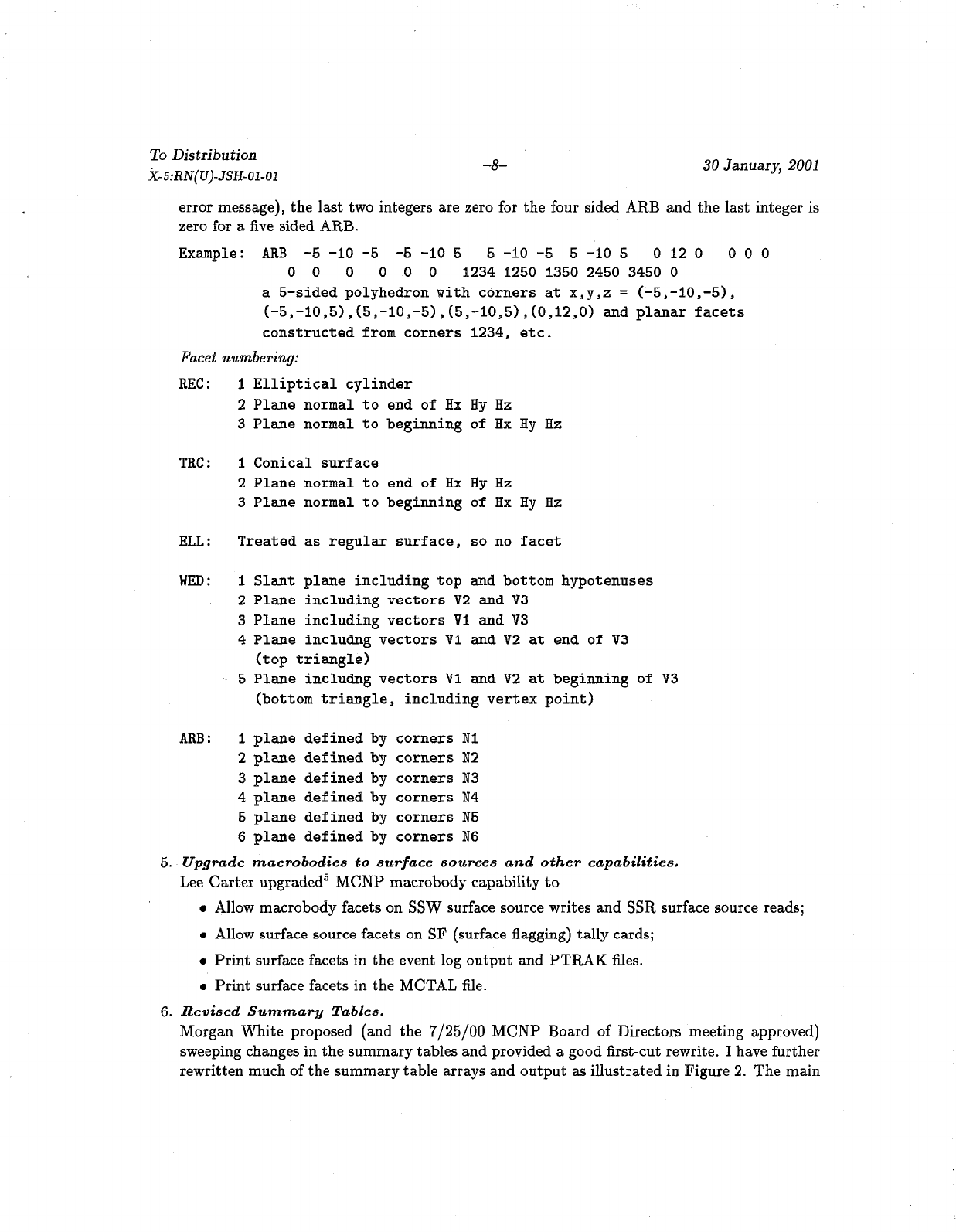
Facet numbering:
REC:
TRC:
ELL:
WED:
ARB:
I Elliptical cylinder
2 Plane normal to end of Hx Hy Hz
3 Plane normal to beginning of Hx Hy Hz
1 Conical surface
2 Plane normal to end of Hx Hy Hz
3 Plane normal to beginning of Hx Hy Hz
Treated as regular surface, so no facet
I Slant plane including top and bottom hypotenuses
2 Plane including vectors V2 and V3
3 Plane including vectors Vl and V3
4 Plane includng vectors VI and V2 at end of V3
(top triangle)
5 Plane includng vectors VI and V2 at beginning of V3
(bottom triangle, including vertex point)
I plane defined by corners Nl
2 plane defined by corners N2
3 plane defined by corners N3
4 plane defined by corners N4
5 plane defined by corners N5
6 plane defined by corners N6
5. Upgrade macrobodies to surface sources and other capabilities.
Lee Carter upgraded5 MCNP macrobody capability to
e Allow macrobody facets on SSW surface source writes and SSR surface source reads;
l
Allow surface source facets on SF (surface
flagging)
tally cards;
l
Print surface facets in the event log output and PTRAK files.
l
Print surface facets in the MCTAL file.
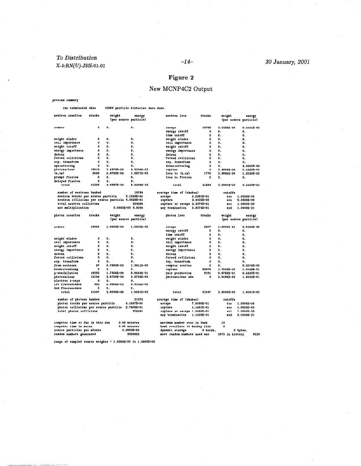
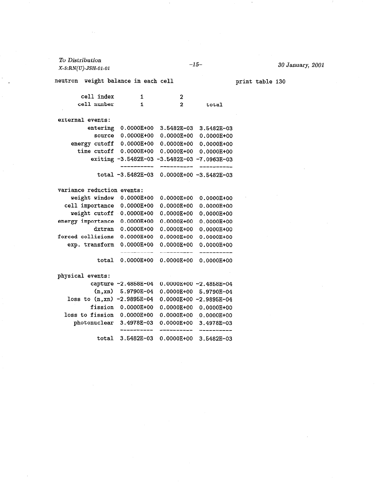
6. Revised Summary Tables.
Morgan White proposed (and the 7/25/00 MCNP Board of Directors meeting approved)
sweeping changes in the summary tables and provided a good first-cut rewrite. I have further
rewritten much ofthe summary table arrays and output asillustratedin Figure 2. The main

To Distribution
X-5:RN(U)-JSH-01-01
-4 30 January, 2001
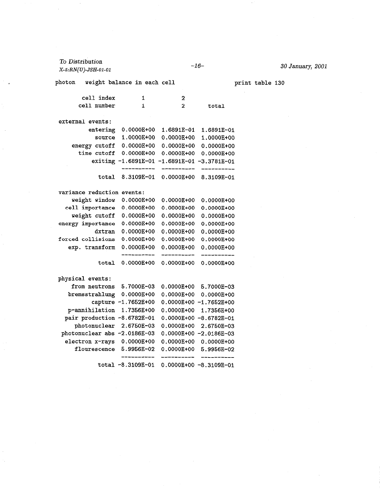
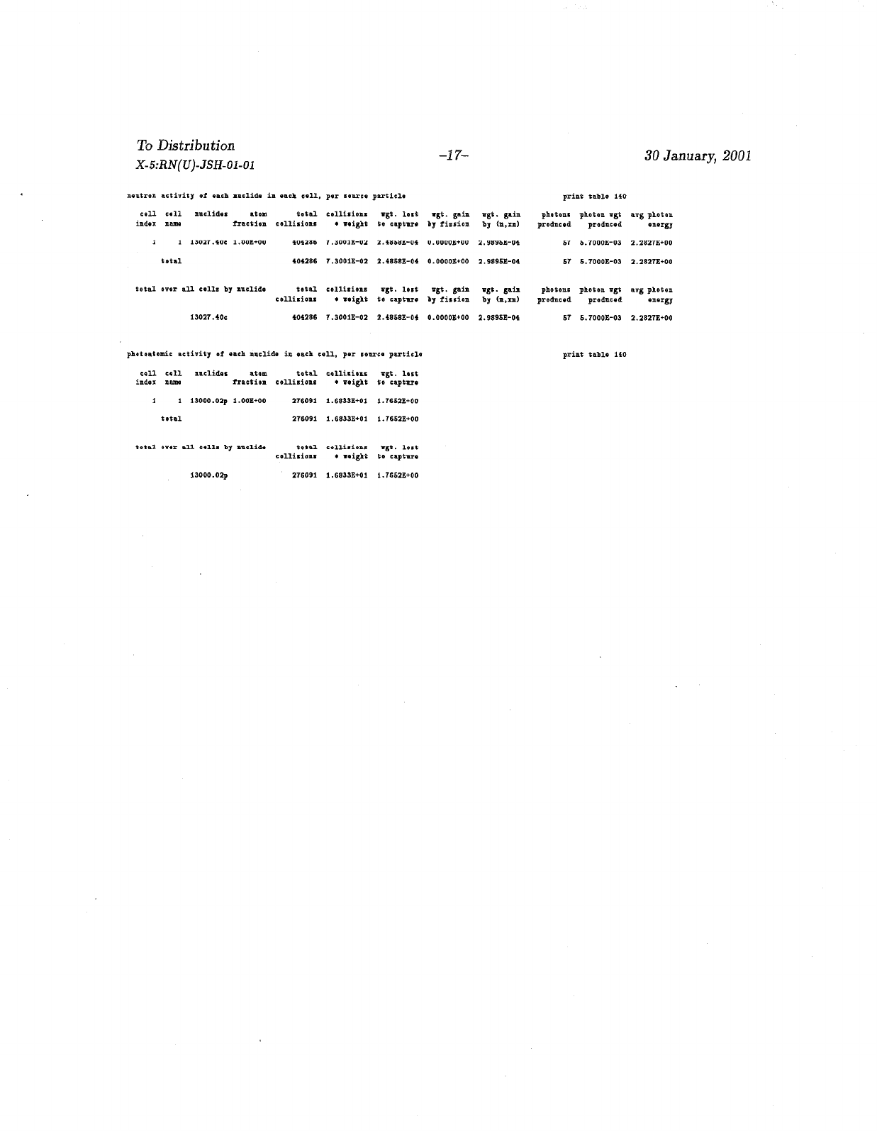
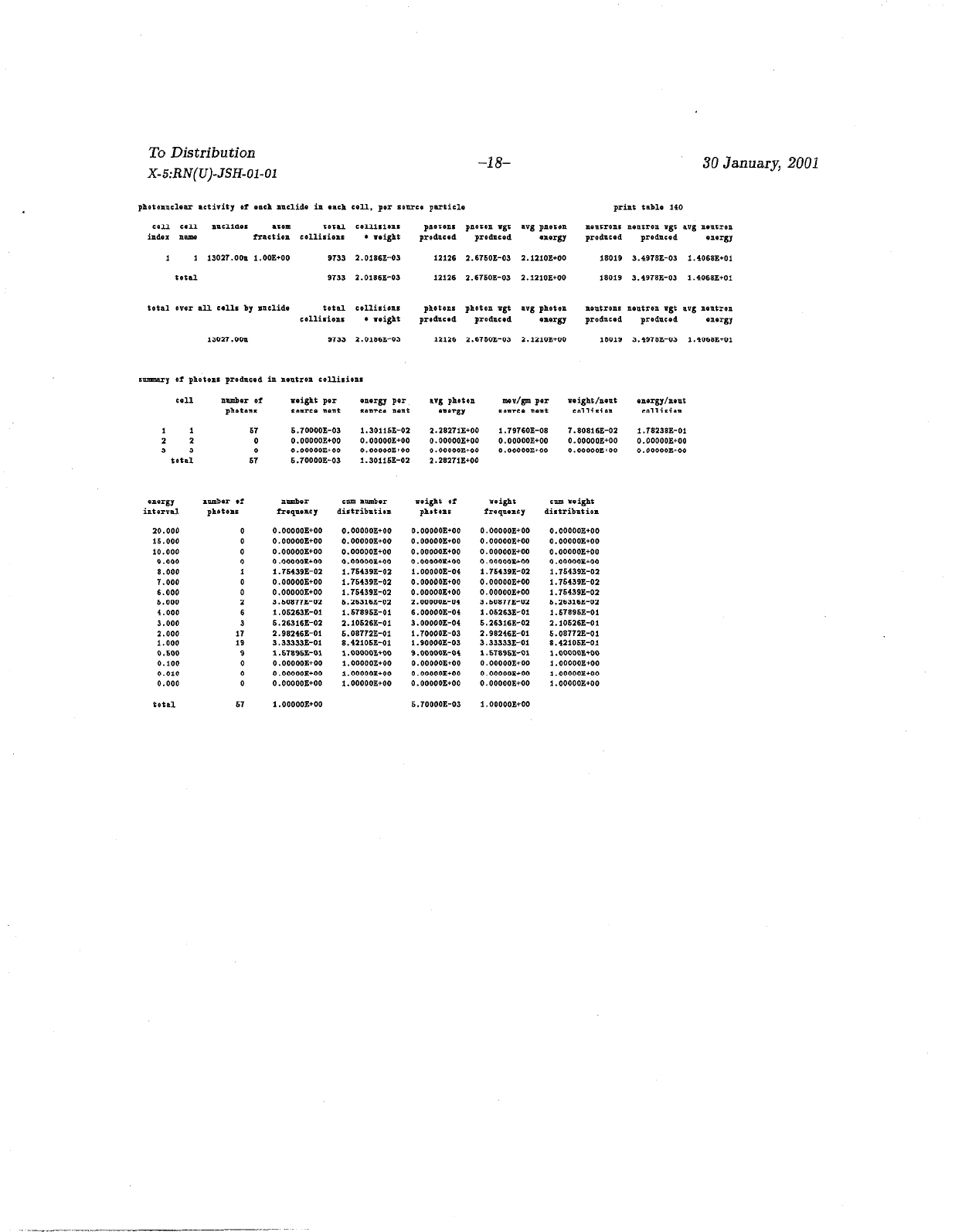
changes are Print Table 130 which has a new horizontal format for cells so that the increasing
number of events and reactions can be vertical. Print table 140 separates photonuclear and
photoatomic events. The problem summary also regroups events and adds photonuclear
interactions.
7. Weight Window Improvements.
The following improvements have been made for the weight window and weight window
generator variance reduction methods.
(a) Add weight window scaling factor. Now input windows may be multiplied by a user-
specified constant (7th entry on WWP card); l6
(b) Allow 1 superimposed mesh weight window coarse mesh per direction and make the
default 1 fine mesh in each direction; I7
(c) Eliminate blanks when writing generated WWN card to the OUTP file.
(d) Write out normalization constant used in generating weight windows (usually half the
average source weight) for mesh windows.
User Interface Changes:
WWP:n card, new 7th entry is multiplicative constant for all lower weight bounds on WWNim
cards or WWINP file mesh-based windows of particle type n.
WWG card 9th entry flags undocumented developmental recursive Monte Carlo feature.
MESH card defaults are now 1 fine mesh per coarse mesh and now 1 coarse mesh per direction
is allowed.
Description of Minor New Features
1. Remove 4B tracking fixes. The 20th entry on the DBCN card now causes MCNP4C2 to track
MCNP4C. (JSH)
2. Save particle attributes in stack. Morgan White in his photoneutron patch proposed a subrou-
tine to put particle descriptors (GPBLCM, JPBLCM and sometimes UDT arrays) in a stack
while photonuclear events took place. This functionality has been generalized and applied
wherever it is needed. (JSH)
3. Shortcut for electrons below cutoff. If electrons are below the electron energy cutoff they
do not produce bremsstrahlung photons as in MCNP4C. This speeds the code but affects
tracking of MCNP test problem 23. (KJA)
4. Include bremsstrahlung produced below energy cutoff in the photon summary table and make
electron summary balance. Ken Adams’ MCNP4C electron enhancements deliberately let
the electron summary table be out of balance in order to show energy lost to bremsstrahlung
production below the photon energy cutoff. (AS) l8 has put the electron table back in
balance and shows the bremsstrahlung photons not produced below the photon energy cutoff
‘sThomas E. Booth, “Theoretical and Practical Mesh-Based Weight Window Generator Suggestions for MCNP,”
X-5:RN(U)-TEB-00-40 (September 27, 2000)
17.Jef?rey A. Favorite, “Four Enhancements for the MCNP Mesh-Based Weight Window Generator,” X-5:RN(U)-JAF-
00-13
(May 25, 2000)
‘sAvneet Sood, “Electron Summary Table Balance,” X-5:AS-00-153 (U) (December 11, 2000)
To Distribution
X-5:RN(U)-JSH-01-01
-1 o- 30 January, 2001
as produced and captured in the photon summary table. (AS)
5. Warn of unavailable delayed neutrons. If delayed neutrons are requested and a fissionable
nuclide does not have delayed neutron data available a warning is issued. Approved at 2/10/00
MCNP BoD. (JSH)
6. Print random number index. In ERRPRN messages (warnings and fatal errors during the
transport of particles) and for large histories at point detectors the random number index
rather than the octal random number itself is printed. Approved at 7/25/00 MCNP BoD.
CJ w
7. Fatal error for CTME time cutoff and PVM. This caused wrong answers because of incomplete
accumulation of task data. Approved at 7/25/00 MCNP BoD. (JSH)
8. Fatal error if analog capture with alpha. With analog capture it was possible for alpha
time absorption to cause very low particle weights which, unchecked by weight cutoff, caused
underflow. Approved at 7/25/00 MCNP BoD. (JSH)
9. Eliminate a DVF Qwin prompt inconvenience that caused the code to wait for a user prompt
on PCs with DVF Qwin. (GWM)
Summary of MCNP4C2 Corrections
Significant Bugs:
1. Wrong record size causes PVM/SSW, SSR combination crash. Surface source reads and
writes simply do not work with PVM multiprocessing. (LJC)
2. KCODE source overwrites common in PVM mode. (JAF)
3. PVM hangs with positive number of PVM tasks. $20 to Neil1 Taylor (UKAEA Fusion,
Abingdon, UK) ls (JSH)
4. Bad pointers for unresolved resonance treatment. $20 to Alfred Hogenbirk, NRG, Petten,
Netherlands. 2o (JSH)
5. Interrupts crash Lahey Fortran executables. $20 to David Seagraves (ESH-4, LANL) 21 (ECS)
6. Bad energies with law 61 scatter and detectors. $20 to Chikara Konno (JAERI, Japan). 22
(JSH)
7. Identical surfaces with reflection or white boundary fail. $20 to Bruce Wilkin (AECL Re-
search, Chalk River, Ontario, Canada) 23 (LLC)
8. Cannot read datapath on newer PC compilers. $4 to Nick Savin (Westinghouse Savannah
River, Aiken, SC) 24 (JFB/GWM)
“John S. Hendricks, “MCNP Cash Award,” X-5:JSH-00-155 (December 20, 2000)
2030hn S. Hendricks, “MCNP Cash Award,,, X-5:JSH-00-53 (April 24, 2000)
‘lElizabeth C. Selcow, “MCNP Cash Award,” X-5:ECS-00-101 (August 10, 2000)
“John S. Hendicks, “MCNP Cash Award,,, X-5:JSH-00-127 (October 30, 2000)
23John S. Hendricks, “MCNP Cash Award,” X-5:JSH-00-152 (December 6, 2000)
24John S. Hendricks, “MCNP Cash Award,,’ X-5:JSH-00-150 (November 20, 2000)
‘To Distribution
X-5:RN(U)-JSH-01-01
-ll- 30 January, 2001
9. Crash if inadequate space for FG:n,p tallies. $4 to Frej Wasastjerna (VTT, Finland) 25
(CJW/JSH)
10. Torus will not translate. (LLC) $4 to Dennis Allen (BNFL, UK) 26 (LLC)
Lesser Bugs and corrections:
1. Correct the net multiplication in the problem summary table 27 (REP)
2. Correct exponential transform. 28 The following are wrong when the exponential transform
(EXP card) is used in MCNP4C: generated mesh-based weight windows, track length h,ff
estimate, track length cy perturbation estimates, summary accounts for the exponential trans-
form, multigroup weight window generation, and the DXTRAN weight cutoffs. Fortunately,
the exponential transform is seldom used for these applications. (JSH/TEB)
3. Perturbations are wrong with one-group multigroup cross section data. 2g (JAF)
4. Better diagnostics for failed source position sampling, namely, print the source distribution
number and the coordinates of the source point. so (AS)
5. Faulty surface transformation initiation causes crash on tray (subroutine TRFMAT). (JSH)
6. Multigroup adjoint puts upper weight cutoff in wrong summary table array. (subroutine
MGACOL) (JSH)
7. Correct setting of random number index (8th entry on DBCN card.) 31 (REP)
8. Error message corrections. Write statements during multitasking cause the code to hang
without proper multitasking lock settings. (JSH)
9. Avoid a UNICOS roundoff error which causes the code to hang in an infinite loop if there is
1 azimuthal bin in the mesh-based weight window. (TEB)
10. Protect from floating to integer roundoff errors by adding nint functions in appropriate places.
(Jfw
11. Fix numerical weight window mesh tracking problems.r7 (JAF)
12. Consistency between rectangular and cylindrical mesh tracking.17 (JAF)
13. Cleanup the unpacking of variable IEX in BANKIT for later use in PTRAK” (JSH)
14. Wrong PVM line count if *if de f,pvm compiler directives. (GWM)
15. More precise error message (subroutine KPRINT).2Q (JAF)
26Christopher J. Werner, “MCNP Cash Award,” X-5:CJW-00-93 (August 3, 2000)
26John S. Hendricks, “MCNP Cash Award,” X-5:JSH-00-128 (October 30, 2000)
27Richard E. Prael, “Reformulation of the New Multiplication Calculation,” X-5:REP-00-14 (January 26, 2000)
28Thomas E. Booth, “Correcting the Exponential Transform in MCNP4C,” X-5:RN(U)-TEB-00-42 (October 17,200O)
2gJefiey A. Favorite, LLAn Error in the MCNP4C Perturbation Capability for Eigenvalue Problems,” X-5:RH(U)-JAF-
00-39 (September 25, 2000)
“Avneet Sood, Ymproved Source Distribution Efficiency Message,” X-5:AS-00-104 (August 15,200O)
31Richard E. Prael, “Inconsistency in Setting Initial Conditions for Random Number Generator,” X-5:REP-00-117
(September 14, 2000)

To Distribution
X-5:RN(U)-JSH-01-01
-62- 30 January, 2001
16. Solaris F90 bug workaround (block data: n*’ ’ fails). (REP)
17. Solaris F90 problems with ERPRNT call in JSOURC. (REP)
18. Correct harmless 4B plot logic error (subroutine PTOST). (JSH)
19. Remove unused variables (subroutines AVRWGI, KSKCYC, etc.) (JAF/TEB/JSH)
20. Typos in comments (subroutine IPBC, ACALC, EXORDP, etc.). (JSH,JAF)
21. Workarounds for the Sun Solaris F90 compiler. (subroutines MAIN, GXAXIS) (REP)
22. Correct mesh-based weight window theta mesh indexing. (TEB/JAF/JSH)
23. Warn of missing material on BBREM (B remsstrahlung biasing) card. The 1st 49 entries are
energy bins, and the 50th entry onward is materials. If the count is off or the material(s)
omitted, MCNP4C would assume the 1st problem material, sometimes giving wrong answers
without warning. (AS)
24. Print reaction number (MTP) rather than type (NTYN) in event log and PTRAK. (GWM)
25. Eliminate overwrite in MCPLOT. If more than 100 Million histories were run then stars would
partially overwrite the legend NPS print field. (TBK/JSH)
File Location
The MCNP4C2 installation, test, and executable files are located on both open and closed systems
in directories install, test, exe under the following nodes:
cfs get dir=/x5code/mcnp4c2/. . .
hpss get /hpss/mcnp/mcnp4c2/...
Acknowledgement
MCNP4C2 is the collaborative effort of the X-5 Eolus Monte Carlo code development team:
Gregg W. McKinney (Team Leader), Thomas E. Booth, Judith F. Briesmeister, Leland L. Carter,
Lawrence J. Cox, R. Arthur Forster, William B. Hamilton, John S. Hendricks, Russell D. Mosteller,
Richard E. Prael, Elizabeth C. Selcow, Avneet Sood, Stephen White.

To Distribution
X-S:RN(U)-JSH-01-01
-13-
Figure B
MCNP4C2 Interactive Plotter
Plot shows the MCNP4C2 interactive geometry plot
with superimposed weight window mesh and mesh values.
30 January, 2001
To Distribution
X-ki:RN(U)-JSH-01-01
-14-
Fignse 2
New MCNP4C2 Output
prd.hn m.mury
rmn terminated when
10000 particle histories Pera doao.
UC1 1.0000H-10
=52 1.0000E-21
might energy
(per smr~e particle)
1.6891E-01 6.94693+00
0. 0.
0. 0.
0. 0.
0. 0.
0. 0.
0. 0.
0. 0.
0. 0.
0. 0.
0. *.20,8E+oo
1.76523+00 i..%o~E-o*
8.61823-01 *.6432E+Ol
2.0186E-03 1.833JE-01
2.*0*0E+00 1.0091E+02
cntot*r
(CO 1.0000E+3*
ece 1.0000E-03
PC1 1.ooooz-10
I752 S.OOOOE-21
II
0
30 January, 2001
rango of *ampled 10nrce weights = 1.0000E+OO to 1,0000E+OO
To Distribution
X-S:RN(U)-JSH-01-01
-%5-
neutron weight balance in each cell
30January, 2001
print table 130
cell index 1 2
cell number I 2 total
external events:
entering O.OOOOE+OO 3.5482E-03 3.5482E-03
source O.OOOOE+OO O.OOOOE+OO O.OOOOE+OO
energy cutoff O.OOOOE+OO O.OOOOE+OO O.OOOOE+OO
time cutoff O.OOOOE+OO O.OOOOE+OO O.OOOOE+OO
exiting -3.5482E-03 -3.5482E-03 -7.0963E-03
---_----_- ---------- ---_----__
total -3.5482E-03 O.OOOOE+OO -3.5482E-03
variance reduction events:
weight window O.OOOOE+OO
cell importance O.OOOOE+OO
weight cutoff O.OOOOE+OO
energy importance O.OOOOE+OO
dxtran O.OOOOE+OO
forced collisions O.OOOOE+OO
exp. transform O.OOOOE+OO
O.OOOOE+OO
O.OOOOE+OO
O.OOOOE+OO
0.0000E+00
O.OOOOE+OO
O.OOOOE+OO
O.OOOOE+OO
O.OOOOE+OO
O.OOOOE+OO
O.OOOOE+OO
O.OOOOE+OO
O.OOOOE+OO
O.OOOOE+OO
O.OOOOE+OO
total O.OOOOE+OO
physical events:
capture -2.4858E-04
(n,xn) 5.979OE-04
loss to (n,xn) -2.9895E-04
fission O.OOOOE+OO
loss to fission O.OOOOE+OO
photonuclear 3.4978E-03
----------
total 3.5482E-03
O.OOOOE+OO
O.OOOOE+OO
O.OOOOE+OO -2.4858E-04
O.OOOOE+OO 5.9790E-04
O.OOOOE+OO -2.9895E-04
O.OOOOE+OO O.OOOOE+OO
O.OOOOE+OO O.OOOOE+OO
O.OOOOE+OO 3.4978E-03
-------VW- ---------_
O.OOOOE+OO 3.5482E-03
To Distribution
X-s:RN(U)-JSH-01-01
photon weight balance in each cell
-16-
cell index 1 2
cell number f 2 total
external events:
entering O.OOOOE+OO 1.6891E-01 1.689lE-01
source l.OOOOE+OO O.OOOOE+OO 1.0000E+OO
energy cutoff O.OOOOE+OO O.OOOOE+OO O.OOOOE+OO
time cutoff O.OOOOE+OO O.OOOOE+OO O.OOOOE+OO
exiting -1.6891E-01 -1.689lE-01 -3.378fE-01
----__---- ---------- --------__
total 8.3109E-01 O.OOOOE+OO 8.3109E-01
variance reduction events:
weight window O.OOOOE+OO
cell importance O.OOOOE+OO
weight cutoff O.OOOOE+OO
energy importance O.OOOOE+OO
dxtran O.OOOOE+OO
forced collisions O.OOOOE+OO
exp. transform O.OOOOE+OO
O.OOOOE+OO
O.OOOOE+OO
O.OOOOE+OO
O.OOOOE+OO
O.OOOOE+OO
O.OOOOE+OO
O.OOOOE+OO
O.OOOOE+OO
O.OOOOE+OO
O.OOOOE+OO
O.OOOOE+OO
O.OOOOE+OO
O.OOOOE+OO
O.OOOOE+OO
total O.OOOOE+OO
physical events:
from neutrons 5.7000E-03
bremsstrahlung O.OOOOE+OO
capture -1.7652E+OO
p-annihilation 1.7356E+OO
pair production -8.6782E-01
photonuclear 2.6750E-03
photonuclear abs -2.0186E-03
electron x-rays O.OOOOE+OO
flourescence 5.9956E-02
----------
total -8.3109E-01
O.OOOOE+OO
O.OOOOE+OO
O.OOOOE+OO 5.7000E-03
O.OOOOE+OO O.OOOOE+OO
O.OOOOE+OO -1.7652E+OO
O.OOOOE+OO 1.7356E+OO
O.OOOOE+OO -8.6782E-01
O.OOOOE+OO 2.6750E-03
O.OOOOE+OO -2.0186E-03
O.OOOOE+OO O.OOOOE+OO
O.OOOOE+OO 5.9956E-02
---------- ---_----__
O.OOOOE+OO -8.3109E-01
30Januar35 2001
print table 130
To Distribution
X-C-C:RN(U)-ASH-01-01
3OJanuary, 2001
To Distribution
X-5:RN(U)-JSH-01-01
-18-
photmmlear activity e* each mclide in each 0011, par smrso particle
onorgy
interval
20.000
16.000
10.000
9.000
8.000
7.000
6.000
5.000
4.000
3.000
2.000
1.000
0.600
0.100
0.010
0.000
total
weight per onorgy par
soxr'co mlllt son?xe noat
6.700003-03 1.30116E-02
0.00000E+00 0.00000E+00
0.00000E+00 0.00000H+00
5.70000E-03 1.30ilSE-02
30January, 2001
1.1827iE+oo 1.797603-08 T.*0816E-01 i.78138B-01
0.00000B+00 0.00000E+00 0.00000E+00 0.00000E+00
0.00000E+00 0.00000E+00 0.00000E+00 0.00000E+00
1.2*2T1E+oo
cm might
dirtribation

To Distribution
X-C:RiV(U)-JSH-ol-01
JSH:jsh
Distribution:
X-5 File
A. R. Heath, X-5, MS F663
T. J. Seed, X-5, MS F663
G. W. McKinney, X-5, MS F663
T. E. Booth, X-5, MS F663
J. F. Briesmeister, X-5, MS F663
L. L. Carter, X-5, MS F663
L. J. Cox, X-5, MS F663
J. D. Court, X-5, MS F663
G. P. Estes, X-5, MS F663
J. A. Favorite, X-5, MS F663
S. C. Frankle, X-5, MS F663
R. A. Forster, X-5, MS F663
W. B. Hamilton, X-5, MS F663
J. S. Hendricks, X-5, MS F663
R. C. Little, X-5, MS F663
R. D. Mosteller, X-5, MS F663
R. E. Prael, X-5, MS F663
C. E. Ragan, X-5, MS F663
R. R. Roberts, X-5, MS F663
E. C. Selcow, X-5, MS F663
A. Sood, X-5, MS F663
C. J. Werner, X-5, MS F663
M. C. White, X-5, MS F663
S. W. White, X-5, MS F663
H. G. Hughes, CCS-4, MS D409
H. Lichtenstein, CCS-4, MS D409
G. C. Giesler, CIC-12, MS B295
D. A. Rutherford, NIS-8, MS B230
-19- 30 January, 2001
S
E
C
T
I
O
N
3

18 December 2000 i
LA–13709–M
Manual
MCNPTM–A General Monte Carlo
N–Particle Transport Code
Version 4C
Judith F. Briesmeister, Editor
UC abc
and
UC 700
Issued: March 2000

ii 18 December 2000
An Affirmative Action/Equal Opportunity Employer
DISCLAIMER
This report was prepared as an account of work sponsored by an agency of the United States
Government. Neither the United States Government nor any agency thereof, nor any of their
employees, makes any warranty, express or implied, or assumes any legal liability or
responsibility for the accuracy, completeness, or usefulness of any information, apparatus,
product, or process disclosed, or represents that its use would not infringe privately owned
rights. Reference herein to any specific commercial product, process, or service by trade name,
trademark, manufacturer, or otherwise, does not necessarily constitute or imply its
endorsement, recommendation, or favoring by the United States Government or any agency
thereof. The views and opinions of authors expressed herein do not necessarily state or reflect
those of the United States government or any agency thereof.

18 December 2000 iii
FOREWORD
This manual is a practical guide for the use of our general-purpose Monte Carlo code MCNP. The
first chapter is a primer for the novice user. The second chapter describes the mathematics, data,
physics, and Monte Carlo simulation found in MCNP. This discussion is not meant to be
exhaustive---details of the particular techniques and of the Monte Carlo method itself will have to
be found elsewhere. The third chapter shows the user how to prepare input for the code. The fourth
chapter contains several examples, and the fifth chapter explains the output. The appendices show
how to use MCNP on various computer systems and also give details about some of the code
internals.
The Monte Carlo method emerged from work done at Los Alamos duringWorld War II. The
invention is generally attributed to Fermi,von Neumann, Ulam, Metropolis, and Richtmyer. MCNP
is the successor to their work and represents over 450 person-years of development.
Neither the code nor the manual is static. The code is changed as the need arises and the manual
is changed to reflect the latest version of the code. This particular manual refers to Version 4C.
MCNP and this manual are the product of the combined effort of many people in the Diagnostics
Applications Group (X-5) in the Applied Physics Division (X Division) at the Los Alamos National
Laboratory.
The code and manual can be obtained from the Radiation Safety InformationComputational Center
(RSICC), P. O. Box 2008, Oak Ridge, TN, 37831-6362
J. F. Briesmeister
Editor
505-667-7277
email: mcnp@lanl.gov

iv 18 December 2000
COPYRIGHT NOTICE FOR MCNP VERSION 4C
Unless otherwise indicated, this information has been authored by anemployee or employees of the
University of California, operator of the Los Alamos National Laboratory under Contract No. W-
-7405--ENG--36 with the U.S. Department of Energy. The U.S. Government has rights to use,
reproduce, and distribute this information. The public maycopy and use this information without
charge, provided that this Notice and any statement of authorship are reproduced on all copies.
Neither the government nor the University makes any warranty, express or implied, or assumes any
liability or responsibility for the use of this information.

18 December 2000 v
TABLE OF CONTENTS
CHAPTER 1 . . . . . . . . . . . . . . . . . . . . . . . . . . . . . . . . . . . . . . . . . . . . . . . . . . . . . . . . . . . . . . . . 1
I. MCNP AND THE MONTE CARLO METHOD. . . . . . . . . . . . . . . . . . . . . . . . . . . 1
A. Monte Carlo Method vs Deterministic Method . . . . . . . . . . . . . . . . . . . . . . . . 2
B. The Monte Carlo Method . . . . . . . . . . . . . . . . . . . . . . . . . . . . . . . . . . . . . . . . . 3
II. INTRODUCTION TO MCNP FEATURES . . . . . . . . . . . . . . . . . . . . . . . . . . . . . . 4
A. Nuclear Data and Reactions . . . . . . . . . . . . . . . . . . . . . . . . . . . . . . . . . . . . . . . 4
B. Source Specification . . . . . . . . . . . . . . . . . . . . . . . . . . . . . . . . . . . . . . . . . . . . . 5
C. Tallies and Output. . . . . . . . . . . . . . . . . . . . . . . . . . . . . . . . . . . . . . . . . . . . . . . 6
D. Estimation of Monte Carlo Errors. . . . . . . . . . . . . . . . . . . . . . . . . . . . . . . . . . . 7
E. Variance Reduction. . . . . . . . . . . . . . . . . . . . . . . . . . . . . . . . . . . . . . . . . . . . . . 9
III. MCNP GEOMETRY . . . . . . . . . . . . . . . . . . . . . . . . . . . . . . . . . . . . . . . . . . . . . . . 13
A. Cells . . . . . . . . . . . . . . . . . . . . . . . . . . . . . . . . . . . . . . . . . . . . . . . . . . . . . . . . 14
B. Surface Type Specification. . . . . . . . . . . . . . . . . . . . . . . . . . . . . . . . . . . . . . . 19
C. Surface Parameter Specification. . . . . . . . . . . . . . . . . . . . . . . . . . . . . . . . . . . 19
IV. MCNP INPUT FOR SAMPLE PROBLEM. . . . . . . . . . . . . . . . . . . . . . . . . . . . . . 20
A. INP File. . . . . . . . . . . . . . . . . . . . . . . . . . . . . . . . . . . . . . . . . . . . . . . . . . . . . . 22
B. Cell Cards . . . . . . . . . . . . . . . . . . . . . . . . . . . . . . . . . . . . . . . . . . . . . . . . . . . . 23
C. Surface Cards . . . . . . . . . . . . . . . . . . . . . . . . . . . . . . . . . . . . . . . . . . . . . . . . . 24
D. Data Cards. . . . . . . . . . . . . . . . . . . . . . . . . . . . . . . . . . . . . . . . . . . . . . . . . . . . 25
V. HOW TO RUN MCNP. . . . . . . . . . . . . . . . . . . . . . . . . . . . . . . . . . . . . . . . . . . . . . 31
A. Execution Line . . . . . . . . . . . . . . . . . . . . . . . . . . . . . . . . . . . . . . . . . . . . . . . . 32
B. Interrupts. . . . . . . . . . . . . . . . . . . . . . . . . . . . . . . . . . . . . . . . . . . . . . . . . . . . . 35
C. Running MCNP . . . . . . . . . . . . . . . . . . . . . . . . . . . . . . . . . . . . . . . . . . . . . . . 35
VI. TIPS FOR CORRECT AND EFFICIENT PROBLEMS . . . . . . . . . . . . . . . . . . . . 36
A. Problem Setup. . . . . . . . . . . . . . . . . . . . . . . . . . . . . . . . . . . . . . . . . . . . . . . . . 36
B. Preproduction . . . . . . . . . . . . . . . . . . . . . . . . . . . . . . . . . . . . . . . . . . . . . . . . . 36
C. Production. . . . . . . . . . . . . . . . . . . . . . . . . . . . . . . . . . . . . . . . . . . . . . . . . . . . 37
VII. REFERENCES . . . . . . . . . . . . . . . . . . . . . . . . . . . . . . . . . . . . . . . . . . . . . . . . . . . . 38
CHAPTER 2 . . . . . . . . . . . . . . . . . . . . . . . . . . . . . . . . . . . . . . . . . . . . . . . . . . . . . . . . . . . . . . . . 1
I. INTRODUCTION . . . . . . . . . . . . . . . . . . . . . . . . . . . . . . . . . . . . . . . . . . . . . . . . . . 1
A. History. . . . . . . . . . . . . . . . . . . . . . . . . . . . . . . . . . . . . . . . . . . . . . . . . . . . . . . . 2
B. MCNP Structure . . . . . . . . . . . . . . . . . . . . . . . . . . . . . . . . . . . . . . . . . . . . . . . . 5
C. History Flow . . . . . . . . . . . . . . . . . . . . . . . . . . . . . . . . . . . . . . . . . . . . . . . . . . . 7
II. GEOMETRY . . . . . . . . . . . . . . . . . . . . . . . . . . . . . . . . . . . . . . . . . . . . . . . . . . . . . . 9
A. Complement Operator. . . . . . . . . . . . . . . . . . . . . . . . . . . . . . . . . . . . . . . . . . . . 9
B. Repeated Structure Geometry. . . . . . . . . . . . . . . . . . . . . . . . . . . . . . . . . . . . . 11

vi 18 December 2000
C. Surfaces. . . . . . . . . . . . . . . . . . . . . . . . . . . . . . . . . . . . . . . . . . . . . . . . . . . . . . 11
III. CROSS SECTIONS . . . . . . . . . . . . . . . . . . . . . . . . . . . . . . . . . . . . . . . . . . . . . . . . 16
A. Neutron Interaction Data: Continuous-Energy and Discrete-Reaction . . . . . 18
B. Photon Interaction Data . . . . . . . . . . . . . . . . . . . . . . . . . . . . . . . . . . . . . . . . . 21
C. Electron Interaction Data . . . . . . . . . . . . . . . . . . . . . . . . . . . . . . . . . . . . . . . . 23
D. Neutron Dosimetry Cross Sections. . . . . . . . . . . . . . . . . . . . . . . . . . . . . . . . . 23
E. Neutron Thermal S(α,β) Tables. . . . . . . . . . . . . . . . . . . . . . . . . . . . . . . . . . . . 24
F. Multigroup Tables. . . . . . . . . . . . . . . . . . . . . . . . . . . . . . . . . . . . . . . . . . . . . . 25
IV. PHYSICS . . . . . . . . . . . . . . . . . . . . . . . . . . . . . . . . . . . . . . . . . . . . . . . . . . . . . . . . 25
A. Particle Weight . . . . . . . . . . . . . . . . . . . . . . . . . . . . . . . . . . . . . . . . . . . . . . . . 26
B. Particle Tracks . . . . . . . . . . . . . . . . . . . . . . . . . . . . . . . . . . . . . . . . . . . . . . . . 27
C. Neutron Interactions . . . . . . . . . . . . . . . . . . . . . . . . . . . . . . . . . . . . . . . . . . . . 27
D. Photon Interactions . . . . . . . . . . . . . . . . . . . . . . . . . . . . . . . . . . . . . . . . . . . . . 55
E. Electron Interactions. . . . . . . . . . . . . . . . . . . . . . . . . . . . . . . . . . . . . . . . . . . . 63
V. TALLIES . . . . . . . . . . . . . . . . . . . . . . . . . . . . . . . . . . . . . . . . . . . . . . . . . . . . . . . . 76
A. Surface Current Tally . . . . . . . . . . . . . . . . . . . . . . . . . . . . . . . . . . . . . . . . . . . 78
B. Flux Tallies . . . . . . . . . . . . . . . . . . . . . . . . . . . . . . . . . . . . . . . . . . . . . . . . . . . 78
C. Track Length Cell Energy Deposition Tallies . . . . . . . . . . . . . . . . . . . . . . . . 80
D. Pulse Height Tallies . . . . . . . . . . . . . . . . . . . . . . . . . . . . . . . . . . . . . . . . . . . . 83
E. Flux at a Detector . . . . . . . . . . . . . . . . . . . . . . . . . . . . . . . . . . . . . . . . . . . . . . 85
F. Additional Tally Features . . . . . . . . . . . . . . . . . . . . . . . . . . . . . . . . . . . . . . . . 95
VI. ESTIMATION OF THE MONTE CARLO PRECISION . . . . . . . . . . . . . . . . . . . 99
A. Monte Carlo Means, Variances, and Standard Deviations . . . . . . . . . . . . . . . 99
B. Precision and Accuracy. . . . . . . . . . . . . . . . . . . . . . . . . . . . . . . . . . . . . . . . . 101
C. The Central Limit Theorem and Monte Carlo Confidence Intervals . . . . . . 103
D. Estimated Relative Errors in MCNP. . . . . . . . . . . . . . . . . . . . . . . . . . . . . . . 104
E. MCNP Figure of Merit . . . . . . . . . . . . . . . . . . . . . . . . . . . . . . . . . . . . . . . . . 108
F. Separation of Relative Error into Two Components. . . . . . . . . . . . . . . . . . . 109
G. Variance of the Variance . . . . . . . . . . . . . . . . . . . . . . . . . . . . . . . . . . . . . . . 111
H. Empirical History Score Probability Density Function f(x) . . . . . . . . . . . . . 113
I. Forming Statistically Valid Confidence Intervals. . . . . . . . . . . . . . . . . . . . . 119
J. A Statistically Pathological Output Example . . . . . . . . . . . . . . . . . . . . . . . . 123
VII. VARIANCE REDUCTION . . . . . . . . . . . . . . . . . . . . . . . . . . . . . . . . . . . . . . . . . 127
A. General Considerations. . . . . . . . . . . . . . . . . . . . . . . . . . . . . . . . . . . . . . . . . 127
B. Variance Reduction Techniques . . . . . . . . . . . . . . . . . . . . . . . . . . . . . . . . . . 132
VIII. CRITICALITY CALCULATIONS . . . . . . . . . . . . . . . . . . . . . . . . . . . . . . . . . . . 159
A. Criticality Program Flow . . . . . . . . . . . . . . . . . . . . . . . . . . . . . . . . . . . . . . . 159
B. Estimation of keff Confidence Intervals and Prompt Neutron Lifetimes . . . 162
C. Recommendations for Making a Good Criticality Calculation . . . . . . . . . . 178
IX. VOLUMES AND AREAS114. . . . . . . . . . . . . . . . . . . . . . . . . . . . . . . . . . . . . . . . 181
A. Rotationally Symmetric Volumes and Areas . . . . . . . . . . . . . . . . . . . . . . . . 181
B. Polyhedron Volumes and Areas . . . . . . . . . . . . . . . . . . . . . . . . . . . . . . . . . . 182

18 December 2000 vii
C. Stochastic Volume and Area Calculation . . . . . . . . . . . . . . . . . . . . . . . . . . . 183
X. PLOTTER. . . . . . . . . . . . . . . . . . . . . . . . . . . . . . . . . . . . . . . . . . . . . . . . . . . . . . . 183
XI. PSEUDORANDOM NUMBERS. . . . . . . . . . . . . . . . . . . . . . . . . . . . . . . . . . . . . 187
XII. PERTURBATIONS . . . . . . . . . . . . . . . . . . . . . . . . . . . . . . . . . . . . . . . . . . . . . . . 188
A. Derivation of the Operator . . . . . . . . . . . . . . . . . . . . . . . . . . . . . . . . . . . . . . 189
B. Limitations . . . . . . . . . . . . . . . . . . . . . . . . . . . . . . . . . . . . . . . . . . . . . . . . . . 195
C. Accuracy . . . . . . . . . . . . . . . . . . . . . . . . . . . . . . . . . . . . . . . . . . . . . . . . . . . . 196
XIII. REFERENCES . . . . . . . . . . . . . . . . . . . . . . . . . . . . . . . . . . . . . . . . . . . . . . . . . . . 197
CHAPTER 3 . . . . . . . . . . . . . . . . . . . . . . . . . . . . . . . . . . . . . . . . . . . . . . . . . . . . . . . . . . . . . . . . 1
I. INP FILE. . . . . . . . . . . . . . . . . . . . . . . . . . . . . . . . . . . . . . . . . . . . . . . . . . . . . . . . . . 1
A. Message Block . . . . . . . . . . . . . . . . . . . . . . . . . . . . . . . . . . . . . . . . . . . . . . . . . 1
B. Initiate-Run . . . . . . . . . . . . . . . . . . . . . . . . . . . . . . . . . . . . . . . . . . . . . . . . . . . . 2
C. Continue−Run . . . . . . . . . . . . . . . . . . . . . . . . . . . . . . . . . . . . . . . . . . . . . . . . . . 2
D. Card Format . . . . . . . . . . . . . . . . . . . . . . . . . . . . . . . . . . . . . . . . . . . . . . . . . . . 4
E. Particle Designators . . . . . . . . . . . . . . . . . . . . . . . . . . . . . . . . . . . . . . . . . . . . . 7
F. Default Values . . . . . . . . . . . . . . . . . . . . . . . . . . . . . . . . . . . . . . . . . . . . . . . . . 8
G. Input Error Messages . . . . . . . . . . . . . . . . . . . . . . . . . . . . . . . . . . . . . . . . . . . . 8
H. Geometry Errors . . . . . . . . . . . . . . . . . . . . . . . . . . . . . . . . . . . . . . . . . . . . . . . . 8
II. CELL CARDS . . . . . . . . . . . . . . . . . . . . . . . . . . . . . . . . . . . . . . . . . . . . . . . . . . . . 10
A. Shorthand Cell Specification . . . . . . . . . . . . . . . . . . . . . . . . . . . . . . . . . . . . . 12
III. SURFACE CARDS . . . . . . . . . . . . . . . . . . . . . . . . . . . . . . . . . . . . . . . . . . . . . . . . 12
A. Surfaces Defined by Equations. . . . . . . . . . . . . . . . . . . . . . . . . . . . . . . . . . . . 12
B. Axisymmetric Surfaces Defined by Points. . . . . . . . . . . . . . . . . . . . . . . . . . . 16
C. General Plane Defined by Three Points . . . . . . . . . . . . . . . . . . . . . . . . . . . . . 19
D. Surfaces Defined by Macrobodies . . . . . . . . . . . . . . . . . . . . . . . . . . . . . . . . . 19
IV. DATA CARDS . . . . . . . . . . . . . . . . . . . . . . . . . . . . . . . . . . . . . . . . . . . . . . . . . . . . 22
A. Problem Type (MODE) Card . . . . . . . . . . . . . . . . . . . . . . . . . . . . . . . . . . . . . 23
B. Geometry Cards . . . . . . . . . . . . . . . . . . . . . . . . . . . . . . . . . . . . . . . . . . . . . . . 23
C. Variance Reduction. . . . . . . . . . . . . . . . . . . . . . . . . . . . . . . . . . . . . . . . . . . . . 32
D. Source Specification . . . . . . . . . . . . . . . . . . . . . . . . . . . . . . . . . . . . . . . . . . . . 49
E. Tally Specification . . . . . . . . . . . . . . . . . . . . . . . . . . . . . . . . . . . . . . . . . . . . . 73
F. Material Specification Cards. . . . . . . . . . . . . . . . . . . . . . . . . . . . . . . . . . . . . 107
G. Energy and Thermal Treatment Specification . . . . . . . . . . . . . . . . . . . . . . . 116
H. Problem Cutoff Cards . . . . . . . . . . . . . . . . . . . . . . . . . . . . . . . . . . . . . . . . . . 123
I. User Data Arrays. . . . . . . . . . . . . . . . . . . . . . . . . . . . . . . . . . . . . . . . . . . . . . 126
J. Peripheral Cards . . . . . . . . . . . . . . . . . . . . . . . . . . . . . . . . . . . . . . . . . . . . . . 127
V. SUMMARY OF MCNP INPUT FILE . . . . . . . . . . . . . . . . . . . . . . . . . . . . . . . . . 146
A. Input Cards . . . . . . . . . . . . . . . . . . . . . . . . . . . . . . . . . . . . . . . . . . . . . . . . . . 146
B. Storage Limitations. . . . . . . . . . . . . . . . . . . . . . . . . . . . . . . . . . . . . . . . . . . . 150

viii 18 December 2000
CHAPTER 4 . . . . . . . . . . . . . . . . . . . . . . . . . . . . . . . . . . . . . . . . . . . . . . . . . . . . . . . . . . . . . . . . 1
I. GEOMETRY SPECIFICATION . . . . . . . . . . . . . . . . . . . . . . . . . . . . . . . . . . . . . . . 1
II. COORDINATE TRANSFORMATIONS . . . . . . . . . . . . . . . . . . . . . . . . . . . . . . . 15
A. TR1 and M = 1 Case: . . . . . . . . . . . . . . . . . . . . . . . . . . . . . . . . . . . . . . . . . . . 18
B. TR2 and M= −1 Case: . . . . . . . . . . . . . . . . . . . . . . . . . . . . . . . . . . . . . . . . . . . 19
III. REPEATED STRUCTURE AND LATTICE EXAMPLES . . . . . . . . . . . . . . . . . 20
IV. TALLY EXAMPLES . . . . . . . . . . . . . . . . . . . . . . . . . . . . . . . . . . . . . . . . . . . . . . . 37
A. FMn Examples (Simple Form) . . . . . . . . . . . . . . . . . . . . . . . . . . . . . . . . . . . . 37
B. FMn Examples (General Form) . . . . . . . . . . . . . . . . . . . . . . . . . . . . . . . . . . . 39
C. FSn Examples . . . . . . . . . . . . . . . . . . . . . . . . . . . . . . . . . . . . . . . . . . . . . . . . . 40
D. FTn Examples . . . . . . . . . . . . . . . . . . . . . . . . . . . . . . . . . . . . . . . . . . . . . . . . . 42
E. Repeated Structure/Lattice Tally Example. . . . . . . . . . . . . . . . . . . . . . . . . . . 44
F. TALLYX Subroutine Examples . . . . . . . . . . . . . . . . . . . . . . . . . . . . . . . . . . . 47
V. SOURCE EXAMPLES. . . . . . . . . . . . . . . . . . . . . . . . . . . . . . . . . . . . . . . . . . . . . . 50
VI. SOURCE SUBROUTINE . . . . . . . . . . . . . . . . . . . . . . . . . . . . . . . . . . . . . . . . . . . 53
VII. SRCDX SUBROUTINE. . . . . . . . . . . . . . . . . . . . . . . . . . . . . . . . . . . . . . . . . . . . . 55
CHAPTER 5 . . . . . . . . . . . . . . . . . . . . . . . . . . . . . . . . . . . . . . . . . . . . . . . . . . . . . . . . . . . . . . . . 1
I. DEMO PROBLEM AND OUTPUT . . . . . . . . . . . . . . . . . . . . . . . . . . . . . . . . . . . . 1
II. TEST1 PROBLEM AND OUTPUT. . . . . . . . . . . . . . . . . . . . . . . . . . . . . . . . . . . . . 9
III. CONC PROBLEM AND OUTPUT. . . . . . . . . . . . . . . . . . . . . . . . . . . . . . . . . . . . 48
IV. KCODE. . . . . . . . . . . . . . . . . . . . . . . . . . . . . . . . . . . . . . . . . . . . . . . . . . . . . . . . . . 61
V. EVENT LOG AND GEOMETRY ERRORS. . . . . . . . . . . . . . . . . . . . . . . . . . . . . 99
A. Event Log . . . . . . . . . . . . . . . . . . . . . . . . . . . . . . . . . . . . . . . . . . . . . . . . . . . . 99
B. Debug Print . . . . . . . . . . . . . . . . . . . . . . . . . . . . . . . . . . . . . . . . . . . . . . . . . . 102
APPENDIX B. . . . . . . . . . . . . . . . . . . . . . . . . . . . . . . . . . . . . . . . . . . . . . . . . . . . . . . . . . . . . . . 1
I. SYSTEM GRAPHICS INFORMATION. . . . . . . . . . . . . . . . . . . . . . . . . . . . . . . . . 1
A. X–Windows . . . . . . . . . . . . . . . . . . . . . . . . . . . . . . . . . . . . . . . . . . . . . . . . . . . 2
II. THE PLOT GEOMETRY PLOTTER . . . . . . . . . . . . . . . . . . . . . . . . . . . . . . . . . . . 3
A. PLOT Input and Execute Line Options . . . . . . . . . . . . . . . . . . . . . . . . . . . . . . 3
B. Plot Commands Grouped by Function . . . . . . . . . . . . . . . . . . . . . . . . . . . . . . . 5
C. Geometry Debugging and Plot Orientation . . . . . . . . . . . . . . . . . . . . . . . . . . . 9
III. THE MCPLOT TALLY AND CROSS SECTION PLOTTER . . . . . . . . . . . . . . . 10
A. Input for MCPLOT and Execution Line Options . . . . . . . . . . . . . . . . . . . . . . 11
B. Plot Conventions and Command Syntax . . . . . . . . . . . . . . . . . . . . . . . . . . . . 12
C. Plot Commands Grouped by Function . . . . . . . . . . . . . . . . . . . . . . . . . . . . . . 13
D. MCTAL Files . . . . . . . . . . . . . . . . . . . . . . . . . . . . . . . . . . . . . . . . . . . . . . . . . 20
E. Example of Use of COPLOT . . . . . . . . . . . . . . . . . . . . . . . . . . . . . . . . . . . . . 22
APPENDIX C. . . . . . . . . . . . . . . . . . . . . . . . . . . . . . . . . . . . . . . . . . . . . . . . . . . . . . . . . . . . . . . 1
I. INSTALLING MCNP . . . . . . . . . . . . . . . . . . . . . . . . . . . . . . . . . . . . . . . . . . . . . . . 1

18 December 2000 ix
A. On Supported Systems . . . . . . . . . . . . . . . . . . . . . . . . . . . . . . . . . . . . . . . . . . . 2
B. VMS System . . . . . . . . . . . . . . . . . . . . . . . . . . . . . . . . . . . . . . . . . . . . . . . . . . . 4
C. On Other Systems . . . . . . . . . . . . . . . . . . . . . . . . . . . . . . . . . . . . . . . . . . . . . . . 5
II. MODIFYING MCNP . . . . . . . . . . . . . . . . . . . . . . . . . . . . . . . . . . . . . . . . . . . . . . . . 8
A. Creating a PRPR Patch File . . . . . . . . . . . . . . . . . . . . . . . . . . . . . . . . . . . . . . . 8
B. Creating a New MCNP Executable . . . . . . . . . . . . . . . . . . . . . . . . . . . . . . . . 11
III. MCNP VERIFICATION . . . . . . . . . . . . . . . . . . . . . . . . . . . . . . . . . . . . . . . . . . . . 12
A. On Supported Systems . . . . . . . . . . . . . . . . . . . . . . . . . . . . . . . . . . . . . . . . . . 12
B. On VMS System . . . . . . . . . . . . . . . . . . . . . . . . . . . . . . . . . . . . . . . . . . . . . . . 13
IV. CONVERTING CROSS-SECTION FILES WITH MAKXSF . . . . . . . . . . . . . . . 14
APPENDIX D. . . . . . . . . . . . . . . . . . . . . . . . . . . . . . . . . . . . . . . . . . . . . . . . . . . . . . . . . . . . . . . 1
I. PREPROCESSORS . . . . . . . . . . . . . . . . . . . . . . . . . . . . . . . . . . . . . . . . . . . . . . . . . 1
II. PROGRAMMING LANGUAGE. . . . . . . . . . . . . . . . . . . . . . . . . . . . . . . . . . . . . . . 1
III. SYMBOLIC NAMES. . . . . . . . . . . . . . . . . . . . . . . . . . . . . . . . . . . . . . . . . . . . . . . . 2
IV. SYSTEM DEPENDENCE . . . . . . . . . . . . . . . . . . . . . . . . . . . . . . . . . . . . . . . . . . . . 3
V. COMMON BLOCKS . . . . . . . . . . . . . . . . . . . . . . . . . . . . . . . . . . . . . . . . . . . . . . . . 4
VI. DYNAMICALLY ALLOCATED STORAGE . . . . . . . . . . . . . . . . . . . . . . . . . . . . 5
VII. THE RUNTPE FILE. . . . . . . . . . . . . . . . . . . . . . . . . . . . . . . . . . . . . . . . . . . . . . . . . 6
VIII. C FUNCTIONS . . . . . . . . . . . . . . . . . . . . . . . . . . . . . . . . . . . . . . . . . . . . . . . . . . . . 7
IX. REFERENCES . . . . . . . . . . . . . . . . . . . . . . . . . . . . . . . . . . . . . . . . . . . . . . . . . . . . . 7
APPENDIX E . . . . . . . . . . . . . . . . . . . . . . . . . . . . . . . . . . . . . . . . . . . . . . . . . . . . . . . . . . . . . . . 1
I. DICTIONARY OF SYMBOLIC NAMES. . . . . . . . . . . . . . . . . . . . . . . . . . . . . . . . 1
II. SOME IMPORTANT COMPLICATED ARRAYS . . . . . . . . . . . . . . . . . . . . . . . 32
A. Source Arrays . . . . . . . . . . . . . . . . . . . . . . . . . . . . . . . . . . . . . . . . . . . . . . . . . 32
B. Transport Arrays . . . . . . . . . . . . . . . . . . . . . . . . . . . . . . . . . . . . . . . . . . . . . . . 33
C. Tally Arrays . . . . . . . . . . . . . . . . . . . . . . . . . . . . . . . . . . . . . . . . . . . . . . . . . . 35
D. Accounting Arrays . . . . . . . . . . . . . . . . . . . . . . . . . . . . . . . . . . . . . . . . . . . . . 41
E. KCODE Arrays. . . . . . . . . . . . . . . . . . . . . . . . . . . . . . . . . . . . . . . . . . . . . . . . 46
F. Alpha Arrays. . . . . . . . . . . . . . . . . . . . . . . . . . . . . . . . . . . . . . . . . . . . . . . . . . 48
G. Universe Map/ Lattice Activity Arrays for Table 128 . . . . . . . . . . . . . . . . . . 48
H. Weight Window Mesh Parameters . . . . . . . . . . . . . . . . . . . . . . . . . . . . . . . . . 49
I. Perturbation Parameters . . . . . . . . . . . . . . . . . . . . . . . . . . . . . . . . . . . . . . . . . 49
J. Macrobody and Identical Surface Arrays . . . . . . . . . . . . . . . . . . . . . . . . . . . . 51
APPENDIX F . . . . . . . . . . . . . . . . . . . . . . . . . . . . . . . . . . . . . . . . . . . . . . . . . . . . . . . . . . . . . . . 1
I. Data Types and Classes . . . . . . . . . . . . . . . . . . . . . . . . . . . . . . . . . . . . . . . . . . . . . . 1
II. XSDIR— Data Directory File . . . . . . . . . . . . . . . . . . . . . . . . . . . . . . . . . . . . . . . . . 2
III. Data Tables . . . . . . . . . . . . . . . . . . . . . . . . . . . . . . . . . . . . . . . . . . . . . . . . . . . . . . . . 4
A. Locating Data on a Type 1 Table . . . . . . . . . . . . . . . . . . . . . . . . . . . . . . . . . . . 5
B. Locating Data on a Type 2 Table . . . . . . . . . . . . . . . . . . . . . . . . . . . . . . . . . . 10

x 18 December 2000
C. Locating Data Tables in MCNP . . . . . . . . . . . . . . . . . . . . . . . . . . . . . . . . . . . 11
D. Individual Data Blocks . . . . . . . . . . . . . . . . . . . . . . . . . . . . . . . . . . . . . . . . . . 11
IV. Data Blocks for Continuous–Energy and Discrete Neutron Transport Tables. . . . 12
V. Data Blocks for Dosimetry Tables . . . . . . . . . . . . . . . . . . . . . . . . . . . . . . . . . . . . . 34
VI. Data Blocks for Thermal S(α,β) Tables . . . . . . . . . . . . . . . . . . . . . . . . . . . . . . . . . 35
VII. Data Blocks for Photon Transport Tables. . . . . . . . . . . . . . . . . . . . . . . . . . . . . . . . 38
VIII. Format for Multigroup Transport Tables . . . . . . . . . . . . . . . . . . . . . . . . . . . . . . . . 40
IX. Format for Electron Transport Tables. . . . . . . . . . . . . . . . . . . . . . . . . . . . . . . . . . . 52
Appendix G. . . . . . . . . . . . . . . . . . . . . . . . . . . . . . . . . . . . . . . . . . . . . . . . . . . . . . . . . . . . . . . . . 1
I. ENDF/B REACTION TYPES . . . . . . . . . . . . . . . . . . . . . . . . . . . . . . . . . . . . . . . . . 1
II. S(a,b) DATA FOR USE WITH THE MTm CARD . . . . . . . . . . . . . . . . . . . . . . . . 5
III. MCNP NEUTRON CROSS–SECTION LIBRARIES. . . . . . . . . . . . . . . . . . . . . . . 6
IV. MULTIGROUP DATA FOR MCNP . . . . . . . . . . . . . . . . . . . . . . . . . . . . . . . . . . . 29
V. DOSIMETRY DATA FOR MCNP . . . . . . . . . . . . . . . . . . . . . . . . . . . . . . . . . . . . 32
VI. REFERENCES . . . . . . . . . . . . . . . . . . . . . . . . . . . . . . . . . . . . . . . . . . . . . . . . . . . . 46
Appendix H. . . . . . . . . . . . . . . . . . . . . . . . . . . . . . . . . . . . . . . . . . . . . . . . . . . . . . . . . . . . . . . . . 1
I. CONSTANTS FOR FISSION SPECTRA . . . . . . . . . . . . . . . . . . . . . . . . . . . . . . . . 1
A. Constants for the Maxwell fission spectrum (neutron-induced). . . . . . . . . . . . 1
B. Constants for the Watt Fission Spectrum . . . . . . . . . . . . . . . . . . . . . . . . . . . . . 3
II. FlUX-TO-DOSE CONVERSION FACTORS . . . . . . . . . . . . . . . . . . . . . . . . . . . . . 3
A. Biological Dose Equivalent Rate Factors . . . . . . . . . . . . . . . . . . . . . . . . . . . . . 4
B. Silicon Displacement Kerma Factors . . . . . . . . . . . . . . . . . . . . . . . . . . . . . . . . 5
III. REFERENCES . . . . . . . . . . . . . . . . . . . . . . . . . . . . . . . . . . . . . . . . . . . . . . . . . . . . . 7
Appendix I . . . . . . . . . . . . . . . . . . . . . . . . . . . . . . . . . . . . . . . . . . . . . . . . . . . . . . . . . . . . . . . . . 1
Appendix J . . . . . . . . . . . . . . . . . . . . . . . . . . . . . . . . . . . . . . . . . . . . . . . . . . . . . . . . . . . . . . . . . 1

18 December 2000 xi
MCNP–A General Monte Carlo N–Particle Transport Code
Version 4C
Diagnostics Applications Group
Los Alamos National Laboratory
ABSTRACT
MCNP is a general-purpose Monte Carlo N–Particle code that can be used for neutron, photon,
electron, or coupled neutron/photon/electron transport, including the capability to calculate
eigenvalues for critical systems. The code treats an arbitrary three-dimensional configuration of
materials in geometric cells bounded by first- and second-degree surfaces and fourth-degree
elliptical tori.
Pointwise cross-section data are used. For neutrons, all reactions given in a particular cross-section
evaluation (such as ENDF/B-VI) are accounted for. Thermal neutrons are described by both the
free gas and S(α,β) models. For photons, the code takes account of incoherent and coherent
scattering, the possibility of fluorescent emission after photoelectric absorption, absorption in pair
production with local emission of annihilation radiation, and bremsstrahlung. A continuous-
slowing-down model is used for electron transport that includes positrons, k x-rays, and
bremsstrahlung but does not include external or self-induced fields.
Important standard features that make MCNP very versatile and easy to use include a powerful
general source, criticality source, and surface source; both geometry and output tally plotters; a rich
collection of variance reduction techniques; a flexible tally structure; and an extensive collection
of cross-section data.

xii 18 December 2000
CHAPTER 2
INP File
NOTES:

April 10, 2000 1-1
CHAPTER 1
MCNP AND THE MONTE CARLO METHOD
CHAPTER 1
PRIMER
WHAT IS COVERED IN CHAPTER 1
Brief explanation of the Monte Carlo method.
Summary of MCNP features.
Introduction to geometry.
Description of MCNP data input illustrated by a sample problem.
How to run MCNP.
Tips on problem setup.
Chapter 1 will enable the novice to start using MCNP, assuming very little knowledge of the Monte
Carlo method and no experience with MCNP. The primer begins with a short discussion of the
Monte Carlo method. Five features of MCNP are introduced: (1) nuclear data and reactions, (2)
source specifications, (3) tallies and output, (4) estimation of errors, and (5) variance reduction.
The third section explains MCNP geometry setup, including the concept of cells and surfaces. A
general description of an input deck is followed by a sample problem and a detailed description of
the input cards used in the sample problem. Section V tells how to run MCNP, VI lists tips for
setting up correct problems and running them efficiently, and VII is the references for Chapter 1.
The word “card” is used throughout this document to describe a single line of input up to 80
characters.
I. MCNP AND THE MONTE CARLO METHOD
MCNP is a general-purpose, continuous-energy, generalized-geometry, time-dependent, coupled
neutron/photon/electron Monte Carlo transport code. It can be used in several transport modes:
neutron only, photon only, electron only, combined neutron/photon transport where the photons are
produced by neutron interactions, neutron/photon/electron, photon/electron, or electron/photon.
The neutron energy regime is from 10-11 MeV to 20 MeV, and the photon and electron energy
regimes are from 1 keV to 1000 MeV. The capability to calculate keff eigenvalues for fissile
systems is also a standard feature.
The user creates an input file that is subsequently read by MCNP. This file contains information
about the problem in areas such as:
the geometry specification,
the description of materials and selection of cross-section evaluations,the location and
characteristics of the neutron, photon, or electron source,
the type of answers or tallies desired, and
any variance reduction techniques used to improve efficiency.

1-2 April 10, 2000
CHAPTER 1
MCNP AND THE MONTE CARLO METHOD
Each area will be discussed in the primer by use of a sample problem. Remember five “rules’’ when
running a Monte Carlo calculation. They will be more meaningful as you read this manual and
gain experience with MCNP, but no matter how sophisticated a user you may become, never forget
the following five points:
1. Define and sample the geometry and source well;
2. You cannot recover lost information;
3. Question the stability and reliability of results;
4. Be conservative and cautious with variance reduction biasing; and
5. The number of histories run is not indicative of the quality of the answer.
The following sections compare Monte Carlo and deterministic methods and provide a simple
description of the Monte Carlo method.
A. Monte Carlo Method vs Deterministic Method
Monte Carlo methods are very different from deterministic transport methods. Deterministic
methods, the most common of which is the discrete ordinates method, solve the transport equation
for the average particle behavior. By contrast, Monte Carlo does not solve an explicit equation, but
rather obtains answers by simulating individual particles and recording some aspects (tallies) of
their average behavior. The average behavior of particles in the physical system is then inferred
(using the central limit theorem) from the average behavior of the simulated particles. Not only are
Monte Carlo and deterministic methods very different ways of solving a problem, even what
constitutes a solution is different. Deterministic methods typically give fairly complete information
(for example, flux) throughout the phase space of the problem. Monte Carlo supplies information
only about specific tallies requested by the user.
When Monte Carlo and discrete ordinates methods are compared, it is often said that Monte Carlo
solves the integral transport equation, whereas discrete ordinates solves the integro-differential
transport equation. Two things are misleading about this statement. First, the integral and integro-
differential transport equations are two different forms of the same equation; if one is solved, the
other is solved. Second, Monte Carlo “solves” a transport problem by simulating particle histories
rather than by solving an equation. No transport equation need ever be written to solve a transport
problem by Monte Carlo. Nonetheless, one can derive an equation that describes the probability
density of particles in phase space; this equation turns out to be the same as the integral transport
equation.
Without deriving the integral transport equation, it is instructive to investigate why the discrete
ordinates method is associated with the integro-differential equation and Monte Carlo with the
integral equation. The discrete ordinates method visualizes the phase space to be divided into many
small boxes, and the particles move from one box to another. In the limit as the boxes get
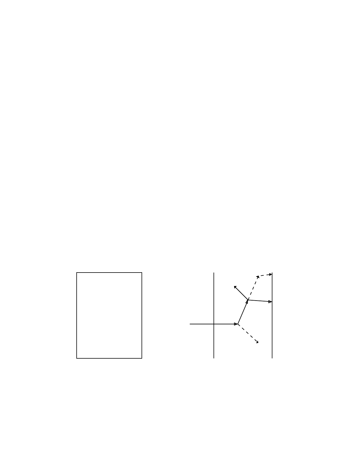
April 10, 2000 1-3
CHAPTER 1
MCNP AND THE MONTE CARLO METHOD
progressively smaller, particles moving from box to box take a differential amount of time to move
a differential distance in space. In the limit this approaches the integro-differential transport
equation, which has derivatives in space and time. By contrast, Monte Carlo transports particles
between events (for example, collisions) that are separated in space and time. Neither differential
space nor time are inherent parameters of Monte Carlo transport. The integral equation does not
have time or space derivatives.
Monte Carlo is well suited to solving complicated three-dimensional, time-dependent problems.
Because the Monte Carlo method does not use phase space boxes, there are no averaging
approximations required in space, energy, and time. This is especially important in allowing
detailed representation of all aspects of physical data.
B. The Monte Carlo Method
Monte Carlo can be used to duplicate theoretically a statistical process (such as the interaction of
nuclear particles with materials) and is particularly useful for complex problems that cannot be
modeled by computer codes that use deterministic methods. The individual probabilistic events
that comprise a process are simulated sequentially. The probability distributions governing these
events are statistically sampled to describe the total phenomenon. In general, the simulation is
performed on a digital computer because the number of trials necessary to adequately describe the
phenomenon is usually quite large. The statistical sampling process is based on the selection of
random numbers—analogous to throwing dice in a gambling casino—hence the name “Monte
Carlo.” In particle transport, the Monte Carlo technique is pre-eminently realistic (a theoretical
experiment). It consists of actually following each of many particles from a source throughout its
life to its death in some terminal category (absorption, escape, etc.). Probability distributions are
randomly sampled using transport data to determine the outcome at each step of its life.
Figure 1-1.
Event Log
1. Neutron scatter
Photon Production
2. Fission
Photon Production
3. Neutron Capture
4. Neutron Leakage
5. Photon Scatter
6. Photon Leakage
7. Photon Capture
Incident
Neutron
Void
Fissionable
Material Void
1
2
3
4
7
56

1-4 April 10, 2000
CHAPTER 1
INTRODUCTION TO MCNP FEATURES
Figure 1.1 represents the random history of a neutron incident on a slab of material that can
undergo fission. Numbers between 0 and 1 are selected randomly to determine what (if any) and
where interaction takes place, based on the rules (physics) and probabilities (transport data)
governing the processes and materials involved. In this particular example, a neutron collision
occurs at event 1. The neutron is scattered in the direction shown, which is selected randomly from
the physical scattering distribution. A photon is also produced and is temporarily stored, or banked,
for later analysis. At event 2, fission occurs, resulting in the termination of the incoming neutron
and the birth of two outgoing neutrons and one photon. One neutron and the photon are banked for
later analysis. The first fission neutron is captured at event 3 and terminated. The banked neutron
is now retrieved and, by random sampling, leaks out of the slab at event 4. The fission-produced
photon has a collision at event 5 and leaks out at event 6. The remaining photon generated at
event 1 is now followed with a capture at event 7. Note that MCNP retrieves banked particles such
that the last particle stored in the bank is the first particle taken out.
This neutron history is now complete. As more and more such histories are followed, the neutron
and photon distributions become better known. The quantities of interest (whatever the user
requests) are tallied, along with estimates of the statistical precision (uncertainty) of the results.
II. INTRODUCTION TO MCNP FEATURES
Various features, concepts, and capabilities of MCNP are summarized in this section. More detail
concerning each topic is available in later chapters or appendices.
A. Nuclear Data and Reactions
MCNP uses continuous-energy nuclear and atomic data libraries. The primary sources of nuclear
data are evaluations from the Evaluated Nuclear Data File (ENDF)1system, the Evaluated Nuclear
Data Library (ENDL)2 and the Activation Library (ACTL)3 compilations from Livermore, and
evaluations from the Applied Nuclear Science (T–2) Group4,5,6 at Los Alamos. Evaluated data are
processed into a format appropriate for MCNP by codes such as NJOY.7 The processed nuclear
data libraries retain as much detail from the original evaluations as is feasible to faithfully
reproduce the evaluator’s intent.
Nuclear data tables exist for neutron interactions, neutron-induced photons, photon interactions,
neutron dosimetry or activation, and thermal particle scattering S(α,β). Photon and electron data
are atomic rather than nuclear in nature. Each data table available to MCNP is listed on a directory
file, XSDIR. Users may select specific data tables through unique identifiers for each table, called
ZAIDs. These identifiers generally contain the atomic number Z, mass number A, and library
specifier ID.

April 10, 2000 1-5
CHAPTER 1
INTRODUCTION TO MCNP FEATURES
Over 500 neutron interaction tables are available for approximately 100 different isotopes and
elements. Multiple tables for a single isotope are provided primarily because data have been
derived from different evaluations, but also because of different temperature regimes and different
processing tolerances. More neutron interaction tables are constantly being added as new and
revised evaluations become available. Neutron−induced photon production data are given as part
of the neutron interaction tables when such data are included in the evaluations.
Photon interaction tables exist for all elements from Z = 1 through Z = 94. The data in the photon
interaction tables allow MCNP to account for coherent and incoherent scattering, photoelectric
absorption with the possibility of fluorescent emission, and pair production. Scattering angular
distributions are modified by atomic form factors and incoherent scattering functions.
Cross sections for nearly 2000 dosimetry or activation reactions involving over 400 target nuclei in
ground and excited states are part of the MCNP data package. These cross sections can be used as
energy-dependent response functions in MCNP to determine reaction rates but cannot be used as
transport cross sections.
Thermal data tables are appropriate for use with the S(α,β)scattering treatment in MCNP. The data
include chemical (molecular) binding and crystalline effects that become important as the
neutron’s energy becomes sufficiently low. Data at various temperatures are available for light and
heavy water, beryllium metal, beryllium oxide, benzene, graphite, polyethylene, and zirconium and
hydrogen in zirconium hydride.
B. Source Specification
MCNP’s generalized user-input source capability allows the user to specify a wide variety of
source conditions without having to make a code modification. Independent probability
distributions may be specified for the source variables of energy, time, position, and direction, and
for other parameters such as starting cell(s) or surface(s). Information about the geometrical extent
of the source can also be given. In addition, source variables may depend on other source variables
(for example, energy as a function of angle) thus extending the built-in source capabilities of the
code. The user can bias all input distributions.
In addition to input probability distributions for source variables, certain built-in functions are
available. These include various analytic functions for fission and fusion energy spectra such as
Watt, Maxwellian, and Gaussian spectra; Gaussian for time; and isotropic, cosine, and
monodirectional for direction. Biasing may also be accomplished by special built−in functions.
A surface source allows particles crossing a surface in one problem to be used as the source for a
subsequent problem. The decoupling of a calculation into several parts allows detailed design or
analysis of certain geometrical regions without having to rerun the entire problem from the

1-6 April 10, 2000
CHAPTER 1
INTRODUCTION TO MCNP FEATURES
beginning each time. The surface source has a fission volume source option that starts particles
from fission sites where they were written in a previous run.
MCNP provides the user three methods to define an initial criticality source to estimate keff, the
ratio of neutrons produced in successive generations in fissile systems.
C. Tallies and Output
The user can instruct MCNP to make various tallies related to particle current, particle flux, and
energy deposition. MCNP tallies are normalized to be per starting particle except for a few special
cases with criticality sources. Currents can be tallied as a function of direction across any set of
surfaces, surface segments, or sum of surfaces in the problem. Charge can be tallied for electrons
and positrons. Fluxes across any set of surfaces, surface segments, sum of surfaces, and in cells,
cell segments, or sum of cells are also available. Similarly, the fluxes at designated detectors (points
or rings) are standard tallies. Heating and fission tallies give the energy deposition in specified
cells. A pulse height tally provides the energy distribution of pulses created in a detector by
radiation. In addition, particles may be flagged when they cross specified surfaces or enter
designated cells, and the contributions of these flagged particles to the tallies are listed separately.
Tallies such as the number of fissions, the number of absorptions, the total helium production, or
any product of the flux times the approximately 100 standard ENDF reactions plus several
nonstandard ones may be calculated with any of the MCNP tallies. In fact, any quantity of the form
can be tallied, where is the energy-dependent fluence, and f(E) is any product or summation
of the quantities in the cross-section libraries or a response function provided by the user. The
tallies may also be reduced by line-of-sight attenuation. Tallies may be made for segments of cells
and surfaces without having to build the desired segments into the actual problem geometry. All
tallies are functions of time and energy as specified by the user and are normalized to be per starting
particle.
In addition to the tally information, the output file contains tables of standard summary information
to give the user a better idea of how the problem ran. This information can give insight into the
physics of the problem and the adequacy of the Monte Carlo simulation. If errors occur during the
running of a problem, detailed diagnostic prints for debugging are given. Printed with each tally is
also its statistical relative error corresponding to one standard deviation. Following the tally is a
detailed analysis to aid in determining confidence in the results. Ten pass/no pass checks are made
for the user-selectable tally fluctuation chart (TFC) bin of each tally. The quality of the confidence
interval still cannot be guaranteed because portions of the problem phase space possibly still have
not been sampled. Tally fluctuation charts, described in the following section, are also
CφE()fE()Ed
∫
=
φE()

April 10, 2000 1-7
CHAPTER 1
INTRODUCTION TO MCNP FEATURES
automatically printed to show how a tally mean, error, variance of the variance, and slope of the
largest history scores fluctuate as a function of the number of histories run.
Tally results can be displayed graphically, either while the code is running or in a separate
postprocessing mode.
D. Estimation of Monte Carlo Errors
MCNP tallies are normalized to be per starting particle and are printed in the output accompanied
by a second number R, which is the estimated relative error defined to be one estimated standard
deviation of the mean divided by the estimated mean . In MCNP, the quantities required for
this error estimate−−the tally and its second moment−−are computed after each complete Monte
Carlo history, which accounts for the fact that the various contributions to a tally from the same
history are correlated. For a well-behaved tally, R will be proportional to where N is the
number of histories. Thus, to halve R, we must increase the total number of histories fourfold. For
a poorly behaved tally, R may increase as the number of histories increases.
The estimated relative error can be used to form confidence intervals about the estimated mean,
allowing one to make a statement about what the true result is. The Central Limit Theorem states
that as N approaches infinity there is a 68% chance that the true result will be in the range
and a 95% chance in the range . It is extremely important to note that these
confidence statements refer only to the precision of the Monte Carlo calculation itself and not to
the accuracy of the result compared to the true physical value. A statement regarding accuracy
requires a detailed analysis of the uncertainties in the physical data, modeling, sampling
techniques, and approximations, etc., used in a calculation.
The guidelines for interpreting the quality of the confidence interval for various values of R are
listed in Table 1.1.
TABLE 1.1:
Guidelines for Interpreting the Relative Error R*
* and represents the estimated relative error at the 1σlevel.
These interpretations of Rassume that all portions of the problem phase
space are being sampled well by the Monte Carlo process.
Range of R Quality of the Tally
0.5 to 1.0 Not meaningful
0.2 to 0.5 Factor of a few
0.1 to 0.2 Questionable
< 0.10 Generally reliable
< 0.05 Generally reliable for point detectors
Sx x
1N⁄
x1R±() x12R±()
RS
xx⁄=

1-8 April 10, 2000
CHAPTER 1
INTRODUCTION TO MCNP FEATURES
For all tallies except next-event estimators, hereafter referred to as point detector tallies, the
quantity R should be less than 0.10 to produce generally reliable confidence intervals. Point
detector results tend to have larger third and fourth moments of the individual tally distributions,
so a smaller value of R, < 0.05, is required to produce generally reliable confidence intervals. The
estimated uncertainty in the Monte Carlo result must be presented with the tally so that all are
aware of the estimated precision of the results.
Keep in mind the footnote to Table 1.1. For example, if an important but highly unlikely particle
path in phase space has not been sampled in a problem, the Monte Carlo results will not have the
correct expected values and the confidence interval statements may not be correct. The user can
guard against this situation by setting up the problem so as not to exclude any regions of phase
space and by trying to sample all regions of the problem adequately.
Despite one’s best effort, an important path may not be sampled often enough, causing confidence
interval statements to be incorrect. To try to inform the user about this behavior, MCNP calculates
a figure of merit (FOM) for one tally bin of each tally as a function of the number of histories and
prints the results in the tally fluctuation charts at the end of the output. The FOM is defined as
where Tis the computer time in minutes. The more efficient a Monte Carlo calculation is, the larger
the FOM will be because less computer time is required to reach a given value of R.
The FOM should be approximately constant as Nincreases because R2is proportional to 1/N and
Tis proportional to N.Always examine the tally fluctuation charts to be sure that the tally appears
well behaved, as evidenced by a fairly constant FOM. A sharp decrease in the FOM indicates that
a seldom-sampled particle path has significantly affected the tally result and relative error estimate.
In this case, the confidence intervals may not be correct for the fraction of the time that statistical
theory would indicate. Examine the problem to determine what path is causing the large scores and
try to redefine the problem to sample that path much more frequently.
After each tally, an analysis is done and additional useful information is printed about the TFC tally
bin result. The nonzero scoring efficiency, the zero and nonzero score components of the relative
error, the number and magnitude of negative history scores, if any, and the effect on the result if the
largest observed history score in the TFC were to occur again on the very next history are given. A
table just before the TFCs summarizes the results of these checks for all tallies in the problem. Ten
statistical checks are made and summarized in table 160 after each tally, with a pass yes/no
criterion. The empirical history score probability density function (PDF) for the TFC bin of each
tally is calculated and displayed in printed plots.
FOM 1R2T()⁄≡

April 10, 2000 1-9
CHAPTER 1
INTRODUCTION TO MCNP FEATURES
The TFCs at the end of the problem include the variance of the variance (an estimate of the error
of the relative error), and the slope (the estimated exponent of the PDF large score behavior) as a
function of the number of particles started.
All this information provides the user with statistical information to aid in forming valid confidence
intervals for Monte Carlo results. There is no GUARANTEE, however. The possibility always
exists that some as yet unsampled portion of the problem may change the confidence interval if
more histories were calculated. Chapter 2 contains more information about estimation of Monte
Carlo precision.
E. Variance Reduction
As noted in the previous section, R(the estimated relative error) is proportional to , where
Nis the number of histories. For a given MCNP run, the computer time Tconsumed is proportional
to N. Thus , where Cis a positive constant. There are two ways to reduce R: (1)
increase Tand/or (2) decrease C. Computer budgets often limit the utility of the first approach. For
example, if it has taken 2 hours to obtain R=0.10, then 200 hours will be required to obtain R=0.01.
For this reason MCNP has special variance reduction techniques for decreasing C. (Variance is the
square of the standard deviation.) The constant Cdepends on the tally choice and/or the sampling
choices.
1. Tally Choice
As an example of the tally choice, note that the fluence in a cell can be estimated either by a
collision estimate or a track length estimate. The collision estimate is obtained by tallying 1/Σt
(Σt=macroscopic total cross section) at each collision in the cell and the track length estimate is
obtained by tallying the distance the particle moves while inside the cell. Note that as Σtgets very
small, very few particles collide but give enormous tallies when they do, a high variance situation
(see page 2–109). In contrast, the track length estimate gets a tally from every particle that enters
the cell. For this reason MCNP has track length tallies as standard tallies, whereas the collision
tally is not standard in MCNP, except for estimating keff.
2. Nonanalog Monte Carlo
Explaining how sampling affects C requires understanding of the nonanalog Monte Carlo model.
The simplest Monte Carlo model for particle transport problems is the analog model that uses the
natural probabilities that various events occur (for example, collision, fission, capture, etc.).
Particles are followed from event to event by a computer, and the next event is always sampled
(using the random number generator) from a number of possible next events according to the
natural event probabilities. This is called the analog Monte Carlo model because it is directly
analogous to the naturally occurring transport.
1N⁄
RCT⁄=

1-10 April 10, 2000
CHAPTER 1
INTRODUCTION TO MCNP FEATURES
The analog Monte Carlo model works well when a significant fraction of the particles contribute
to the tally estimate and can be compared to detecting a significant fraction of the particles in the
physical situation. There are many cases for which the fraction of particles detected is very small,
less than 10-6. For these problems analog Monte Carlo fails because few, if any, of the particles
tally, and the statistical uncertainty in the answer is unacceptable.
Although the analog Monte Carlo model is the simplest conceptual probability model, there are
other probability models for particle transport. They estimate the same average value as the analog
Monte Carlo model, while often making the variance (uncertainty) of the estimate much smaller
than the variance for the analog estimate. Practically, this means that problems that would be
impossible to solve in days of computer time can be solved in minutes of computer time.
A nonanalog Monte Carlo model attempts to follow “interesting” particles more often than
“uninteresting” ones. An “interesting” particle is one that contributes a large amount to the
quantity (or quantities) that needs to be estimated. There are many nonanalog techniques, and they
all are meant to increase the odds that a particle scores (contributes). To ensure that the average
score is the same in the nonanalog model as in the analog model, the score is modified to remove
the effect of biasing (changing) the natural odds. Thus, if a particle is artificially made q times as
likely to execute a given random walk, then the particle’s score is weighted by (multiplied by) .
The average score is thus preserved because the average score is the sum, over all random walks,
of the probability of a random walk multiplied by the score resulting from that random walk.
A nonanalog Monte Carlo technique will have the same expected tallies as an analog technique if
the expected weight executing any given random walk is preserved. For example, a particle can be
split into two identical pieces and the tallies of each piece are weighted by 1/2 of what the tallies
would have been without the split. Such nonanalog, or variance reduction, techniques can often
decrease the relative error by sampling naturally rare events with an unnaturally high frequency and
weighting the tallies appropriately.
3. Variance Reduction Tools in MCNP
There are four classes of variance reduction techniques8that range from the trivial to the esoteric.
Truncation Methods are the simplest of variance reduction methods. They speed up calculations
by truncating parts of phase space that do not contribute significantly to the solution. The simplest
example is geometry truncation in which unimportant parts of the geometry are simply not
modeled. Specific truncation methods available in MCNP are energy cutoff and time cutoff.
Population Control Methods use particle splitting and Russian roulette to control the number of
samples taken in various regions of phase space. In important regions many samples of low weight
are tracked, while in unimportant regions few samples of high weight are tracked. A weight
adjustment is made to ensure that the problem solution remains unbiased. Specific population
1q⁄

April 10, 2000 1-11
CHAPTER 1
INTRODUCTION TO MCNP FEATURES
control methods available in MCNP are geometry splitting and Russian roulette, energy splitting/
roulette, weight cutoff, and weight windows.
Modified Sampling Methods alter the statistical sampling of a problem to increase the number of
tallies per particle. For any Monte Carlo event it is possible to sample from any arbitrary
distribution rather than the physical probability as long as the particle weights are then adjusted to
compensate. Thus, with modified sampling methods, sampling is done from distributions that send
particles in desired directions or into other desired regions of phase space such as time or energy,
or change the location or type of collisions. Modified sampling methods in MCNP include the
exponential transform, implicit capture, forced collisions, source biasing, and neutron-induced
photon production biasing.
Partially-Deterministic Methods are the most complicated class of variance reduction methods.
They circumvent the normal random walk process by using deterministic-like techniques, such as
next event estimators, or by controlling the random number sequence. In MCNP these methods
include point detectors, DXTRAN, and correlated sampling.
Variance reduction techniques, used correctly, can greatly help the user produce a more efficient
calculation. Used poorly, they can result in a wrong answer with good statistics and few clues that
anything is amiss. Some variance reduction methods have general application and are not easily
misused. Others are more specialized and attempts to use them carry high risk. The use of weight
windows tends to be more powerful than the use of importances but typically requires more input
data and more insight into the problem. The exponential transform for thick shields is not
recommended for the inexperienced user; rather, use many cells with increasing importances (or
decreasing weight windows) through the shield. Forced collisions are used to increase the
frequency of random walk collisions within optically thin cells but should be used only by an
experienced user. The point detector estimator should be used with caution, as should DXTRAN.
For many problems, variance reduction is not just a way to speed up the problem but is absolutely
necessary to get any answer at all. Deep penetration problems and pipe detector problems, for
example, will run too slowly by factors of trillions without adequate variance reduction.
Consequently, users have to become skilled in using the variance reduction techniques in MCNP.
Most of the following techniques cannot be used with the pulse height tally.
The following summarizes briefly the main MCNP variance reduction techniques. Detailed
discussion is in Chapter 2, page 2–127.
1. Energy cutoff: Particles whose energy is out of the range of interest are terminated so
that computation time is not spent following them.
2. Time cutoff: Like the energy cutoff but based on time.

1-12 April 10, 2000
CHAPTER 1
INTRODUCTION TO MCNP FEATURES
3. Geometry splitting with Russian roulette: Particles transported from a region of higher
importance to a region of lower importance (where they will probably contribute little to
the desired problem result) undergo Russian roulette; that is, some of those particles will
be killed a certain fraction of the time, but survivors will be counted more by increasing
their weight the remaining fraction of the time. In this way, unimportant particles are
followed less often, yet the problem solution remains undistorted. On the other hand, if
a particle is transported to a region of higher importance (where it will likely contribute
to the desired problem result), it may be split into two or more particles (or tracks), each
with less weight and therefore counting less. In this way, important particles are followed
more often, yet the solution is undistorted because on average total weight is conserved.
4. Energy splitting/Russian roulette: Particles can be split or rouletted upon entering
various user−supplied energy ranges. Thus important energy ranges can be sampled
more frequently by splitting the weight among several particles and less important
energy ranges can be sampled less frequently by rouletting particles.
5. Weight cutoff/Russian roulette: If a particle weight becomes so low that the particle
becomes insignificant, it undergoes Russian roulette. Most particles are killed, and some
particles survive with increased weight. The solution is unbiased because total weight is
conserved, but computer time is not wasted on insignificant particles.
6. Weight window: As a function of energy, geometrical location, or both, low−weighted
particles are eliminated by Russian roulette and high−weighted particles are split. This
technique helps keep the weight dispersion within reasonable bounds throughout the
problem. An importance generator is available that estimates the optimal limits for a
weight window.
7. Exponential transformation: To transport particles long distances, the distance between
collisions in a preferred direction is artificially increased and the weight is
correspondingly artifically decreased. Because large weight fluctuations often result, it
is highly recommended that the weight window be used with the exponential transform.
8. Implicit capture: When a particle collides, there is a probability that it is captured by the
nucleus. In analog capture, the particle is killed with that probability. In implicit capture,
also known as survival biasing, the particle is never killed by capture; instead, its weight
is reduced by the capture probability at each collision. Important particles are permitted
to survive by not being lost to capture. On the other hand, if particles are no longer
considered useful after undergoing a few collisions, analog capture efficiently gets rid of
them.
9. Forced collisions: A particle can be forced to undergo a collision each time it enters a
designated cell that is almost transparent to it. The particle and its weight are
appropriately split into a collided and uncollided part. Forced collisions are often used to
generate contributions to point detectors, ring detectors, or DXTRAN spheres.
10. Source variable biasing: Source particles with phase space variables of more
importance are emitted with a higher frequency but with a compensating lower weight

April 10, 2000 1-13
CHAPTER 1
MCNP GEOMETRY
than are less important source particles. This technique can be used with pulse height
tallies.
11. Point and ring detectors: When the user wishes to tally a flux−related quantity at a point
in space, the probability of transporting a particle precisely to that point is vanishingly
small. Therefore, pseudoparticles are directed to the point instead. Every time a particle
history is born in the source or undergoes a collision, the user may require that a
pseudoparticle be tallied at a specified point in space. In this way, many pseudoparticles
of low weight reach the detector, which is the point of interest, even though no particle
histories could ever reach the detector. For problems with rotational symmetry, the point
may be represented by a ring to enhance the efficiency of the calculation.
12. DXTRAN: DXTRAN, which stands for deterministic transport, improves sampling in
the vicinity of detectors or other tallies. It involves deterministically transporting
particles on collision to some arbitrary, user−defined sphere in the neighborhood of a
tally and then calculating contributions to the tally from these particles. Contributions to
the detectors or to the DXTRAN spheres can be controlled as a function of geometric
cell or as a function of the relative magnitude of the contribution to the detector or
DXTRAN sphere.
The DXTRAN method is a way of obtaining large numbers of particles on user–specified
“DXTRAN spheres.” DXTRAN makes it possible to obtain many particles in a small
region of interest that would otherwise be difficult to sample. Upon sampling a collision
or source density function, DXTRAN estimates the correct weight fraction that should
scatter toward, and arrive without collision at, the surface of the sphere. The DXTRAN
method then puts this correct weight on the sphere. The source or collision event is
sampled in the usual manner, except that the particle is killed if it tries to enter the sphere
because all particles entering the sphere have already been accounted for
deterministically.
13. Correlated sampling: The sequence of random numbers in the Monte Carlo process is
chosen so that statistical fluctuations in the problem solution will not mask small
variations in that solution resulting from slight changes in the problem specification. The
ith history will always start at the same point in the random number sequence no matter
what the previous i−1 particles did in their random walks.
III. MCNP GEOMETRY
We will present here only basic information about geometry setup, surface specification, and cell
and surface card input. Areas of further interest would be the complement operator, use of
parentheses, and repeated structure and lattice definitions, found in Chapter 2. Chapter 4 contains
geometry examples and is recommended as a next step. Chapter 3 has detailed information about
the format and entries on cell and surface cards and discusses macrobodies.

1-14 April 10, 2000
CHAPTER 1
MCNP GEOMETRY
The geometry of MCNP treats an arbitrary three-dimensional configuration of user-defined
materials in geometric cells bounded by first- and second-degree surfaces and fourth-degree
elliptical tori. The cells are defined by the intersections, unions, and complements of the regions
bounded by the surfaces. Surfaces are defined by supplying coefficients to the analytic surface
equations or, for certain types of surfaces, known points on the surfaces.
MCNP has a more general geometry than is available in most combinatorial geometry codes.
Rather than combining several predefined geometrical bodies, as in a combinatorial geometry
scheme, MCNP gives the user the added flexibility of defining geometrical regions from all the first
and second degree surfaces of analytical geometry and elliptical tori and then of combining them
with Boolean operators. The code does extensive internal checking to find input errors. In addition,
the geometry-plotting capability in MCNP helps the user check for geometry errors.
MCNP treats geometric cells in a Cartesian coordinate system. The surface equations recognized
by MCNP are listed in Table 3.1 on page 3–14. The particular Cartesian coordinate system used is
arbitrary and user defined, but the right−handed system shown in Figure 1.2 is often chosen.
Figure 1-2.
Using the bounding surfaces specified on cell cards, MCNP tracks particles through the geometry,
calculates the intersection of a track’s trajectory with each bounding surface, and finds the
minimum positive distance to an intersection. If the distance to the next collision is greater than
this minimum distance and there are no DXTRAN spheres along the track, the particle leaves the
current cell. At the appropriate surface intersection, MCNP finds the correct cell that the particle
will enter by checking the sense of the intersection point for each surface listed for the cell. When
a complete match is found, MCNP has found the correct cell on the other side and the transport
continues.
A. Cells
When cells are defined, an important concept is that of the sense of all points in a cell with respect
to a bounding surface. Suppose that is the equation of a surface in the
Y
Z
X
sfxyz),,()0==
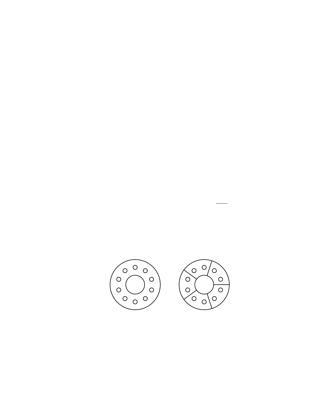
April 10, 2000 1-15
CHAPTER 1
MCNP GEOMETRY
problem. For any set of points (x,y,z), if s= 0 the points are on the surface. However, for points
not on the surface, if sis negative, the points are said to have a negative sense with respect to that
surface and, conversely, a positive sense if sis positive. For example, a point at x= 3 has a positive
sense with respect to the plane . That is, the equation is
positive for x= 3 (where D = constant).
Cells are defined on cells cards. Each cell is described by a cell number, material number, and
material density followed by a list of operators and signed surfaces that bound the cell. If the sense
is positive, the sign can be omitted. The material number and material density can be replaced by
a single zero to indicate a void cell. The cell number must begin in columns 1−5. The remaining
entries follow, separated by blanks. A more complete description of the cell card format can be
found on page 1–23. Each surface divides all space into two regions, one with positive sense with
respect to the surface and the other with negative sense. The geometry description defines the cell
to be the intersection, union, and/or complement of the listed regions.
The subdivision of the physical space into cells is not necessarily governed only by the different
material regions, but may be affected by problems of sampling and variance reduction techniques
(such as splitting and Russian roulette), the need to specify an unambiguous geometry, and the tally
requirements. The tally segmentation feature may eliminate most of the tally requirements.
Be cautious about making any one cell very complicated. With the union operator and disjointed
regions, a very large geometry can be set up with just one cell. The problem is that for each track
flight between collisions in a cell, the intersection of the track with each bounding surface of the
cell is calculated, a calculation that can be costly if a cell has many surfaces. As an example,
consider Figure 1.3a. It is just a lot of parallel cylinders and is easy to set up. However, the cell
containing all the little cylinders is bounded by fourteen surfaces (counting a top and bottom). A
much more efficient geometry is seen in Figure 1.3b, where the large cell has been broken up into
a number of smaller cells.
Figure 1-3.
x2–0=xD–32–s1===
a b
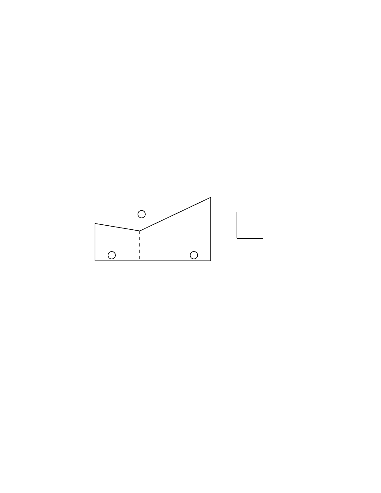
1-16 April 10, 2000
CHAPTER 1
MCNP GEOMETRY
1. Cells Defined by Intersections of Regions of Space
The intersection operator in MCNP is implicit; it is simply the blank space between two surface
numbers on the cell card.
If a cell is specified using only intersections,all points in the cell must have the same sense with
respect to a given bounding surface. This means that, for each bounding surface of a cell, all points
in the cell must remain on only one side of any particular surface. Thus, there can be no concave
corners in a cell specified only by intersections. Figure 1.4, a cell formed by the intersection of five
surfaces (ignore surface 6 for the time being), illustrates the problem of concave corners by
allowing a particle (or point) to be on two sides of a surface in one cell. Surfaces 3 and 4 form a
concave corner in the cell such that points p1and p2are on the same side of surface 4 (that is, have
the same sense with respect to 4) but point p3 is on the other side of surface 4 (opposite sense).
Points p2and p3have the same sense with respect to surface 3, but p1has the opposite sense. One
way to remedy this dilemma (and there are others) is to add surface 6 between the 3/4 corner and
surface 1 to divide the original cell into two cells.
Figure 1-4.
With surface 6 added to Figure 1.4, the cell to the right of surface 6 is number~1 (cells indicated
by circled numbers); to the left number 2; and the outside cell number 3. The cell cards (in two
dimensions, all cells void) are
101–2–36
201–6–45
Cell 1 is a void and is formed by the intersection of the region above (positive sense) surface 1 with
the region to the left (negative sense) of surface 2 intersected with the region below (negative sense)
surface 3 and finally intersected with the region to the right (positive sense) of surface 6. Cell 2 is
described similarly.
Cell 3 cannot be specified with the intersection operator. The following section about the union
operator is needed to describe cell 3.
1
2
3
4
56
Z
Y
p1
p2
p3
12
3
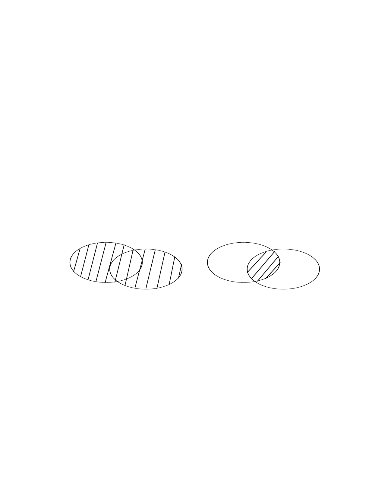
April 10, 2000 1-17
CHAPTER 1
MCNP GEOMETRY
2. Cells Defined by Unions of Regions of Space
The union operator, signified by a colon on the cell cards, allows concave corners in cells and also
cells that are completely disjoint. The intersection and union operators are binary Boolean
operators, so their use follows Boolean algebra methodology; unions and intersections can be used
in combination in any cell description.
Spaces on either side of the union operator are irrelevant, but remember that a space without the
colon signifies an intersection. In the hierarchy of operations, intersections are performed first and
then unions. There is no left to right ordering. Parentheses can be used to clarify operations and in
some cases are required to force a certain order of operations. Innermost parentheses are cleared
first. Spaces are optional on either side of a parenthesis. A parenthesis is equivalent to a space and
signifies an intersection.
For example, let A and B be two regions of space. The region containing points that belong to both
A and B is called the intersection of A and B. The region containing points that belong to A alone
or to B alone or to both A and B is called the union of A and B. The lined area in Figure 1.5a
represents the union of A and B (or A : B), and the lined area in Figure 1.5b represents the
intersection of A and B (or A B). The only way regions of space can be added is with the union
operator. An intersection of two spaces always results in a region no larger than either of the two
spaces. Conversely, the union of two spaces always results in a region no smaller than either of the
two spaces.
Figure 1-5.
A simple example will further illustrate the concept of Figure 1.5 and the union operator to solidify
the concept of adding and intersecting regions of space to define a cell. See also the second example
in Chapter 4. In Figure 1.6 we have two infinite planes that meet to form two cells. Cell 1 is easy
to define; it is everything in the universe to the right of surface 1 (that is, a positive sense) that is
also in common with (or intersected with) everything in the universe below surface 2 (that is, a
negative sense). Therefore, the surface relation of cell 1 is 1 –2.
A
B
a
A
B
b
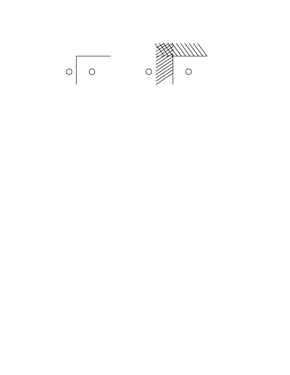
1-18 April 10, 2000
CHAPTER 1
MCNP GEOMETRY
Figure 1-6.
Cell 2 is everything in the universe to the left (negative sense) of surface 1 plus everything in the
universe above (positive sense) surface 2, or –1 : 2, illustrated in Figure 1.6b by all the shaded
regions of space. If cell 2 were specified as –1 2, that would represent the region of space common
to –1 and 2, which is only the cross-hatched region in the figure and is obviously an improper
specification for cell 2.
Returning to Figure 1.4 on page 1–16, if cell 1 is inside the solid black line and cell 2 is the entire
region outside the solid line, then the MCNP cell cards in two dimensions are (assuming both cells
are voids)
101–2(–3:–4)5
2 0 –5:–1:2:3 4
Cell 1 is defined as the region above surface 1 intersected with the region to the left of surface 2,
intersected with the union of regions below surfaces 3 and 4, and finally intersected with the region
to the right of surface 5. Cell 2 contains four concave corners (all but between surfaces 3 and 4),
and its specification is just the converse (or complement) of cell 1. Cell 2 is the space defined by
the region to the left of surface 5 plus the region below 1 plus the region to the right of 2 plus the
space defined by the intersections of the regions above surfaces 3 and 4.
A simple consistency check can be noted with the twocell cards above. All intersections for cell 1
become unions for cell 2 and vice versa. The senses are also reversed.
Note that in this example, all corners less than 180 degrees in a cell are handled by intersections
and all corners greater than 180 degrees are handled by unions.
To illustrate some of the concepts about parentheses, assume an intersection is thought of
mathematically as multiplication and a union is thought of mathematically as addition.
Parentheses are removed first, with multiplication being performed before addition. The cell cards
for the example cards above from Figure 1.4 may be written in the form
1
2
12
(a)
1
2
12
(b)

April 10, 2000 1-19
CHAPTER 1
MCNP GEOMETRY
1
2
Note that parentheses are required for the first cell but not for the second, although the second could
have been written as , etc.
Several more examples using the union operator are given in Chapter 4. Study them to get a better
understanding of this powerful operator that can greatly simplify geometry setups.
B. Surface Type Specification
The first- and second-degree surfaces plus the fourth-degree elliptical and degenerate tori of
analytical geometry are all available in MCNP. The surfaces are designated by mnemonics such as
C/Z for a cylinder parallel to the z-axis. A cylinder at an arbitrary orientation is designated by the
general quadratic GQ mnemonic. A paraboloid parallel to a coordinate axis is designated by the
special quadratic SQ mnemonic. The 29 mnemonics representing various types of surfaces are
listed in Table 3.1 on page 3–14.
C. Surface Parameter Specification
There are two ways to specify surface parameters in MCNP: (1) by supplying the appropriate
coefficients needed to satisfy the surface equation, and (2) by specifying known geometrical points
on a surface that is rotationally symmetric about a coordinate axis.
1. Coefficients for the Surface Equations
The first way to define a surface is to use one of the surface-type mnemonics from Table 3.1 on
page 3–14 and to calculate the appropriate coefficients needed to satisfy the surface equation. For
example, a sphere of radius 3.62-cm with the center located at the point (4,1,–3) is specified by
S41–33.62
An ellipsoid whose axes are not parallel to the coordinate axes is defined by the GQ mnemonic plus
up to 10 coefficients of the general quadratic equation. Calculating the coefficients can be (and
frequently is) nontrivial, but the task is greatly simplified by defining an auxiliary coordinate
system whose axes coincide with the axes of the ellipsoid. The ellipsoid is easily defined in terms
of the auxiliary coordinate system, and the relationship between the auxiliary coordinate system
and the main coordinate system is specified on a TRn card, described on page 3–30.
The use of the SQ (special quadratic) and GQ (general quadratic) surfaces is determined by the
orientation of the axes. One should always use the simplest possible surface in describing
ab c d+()e⋅⋅ ⋅
eabcd⋅+++
eab cd⋅()eab++()cd⋅()e() a() b() cd⋅()+++,+,+++

1-20 April 10, 2000
CHAPTER 1
MCNP INPUT FOR SAMPLE PROBLEM
geometries; for example, using a GQ surface instead of an S to specify a sphere will require more
computational effort for MCNP.
2. Points that Define a Surface
The second way to define a surface is to supply known points on the surface. This method is
convenient if you are setting up a geometry from something like a blueprint where you know the
coordinates of intersections of surfaces or points on the surfaces. When three or more surfaces
intersect at a point, this second method also produces a more nearly perfect point of intersection if
the common point is used in the surface specification. It is frequently difficult to get complicated
surfaces to meet at one point if the surfaces are specified by the equation coefficients. Failure to
achieve such a meeting can result in the unwanted loss of particles.
There are, however, restrictions that must be observed when specifying surfaces by points that do
not exist when specifying surfaces by coefficients. Surfaces described by points must be either
skew planes or surfaces rotationally symmetric about the x, y, or z axes. They must be unique, real,
and continuous. For example, points specified on both sheets of a hyperboloid are not allowed
because the surface is not continuous. However, it is valid to specify points that are all on one sheet
of the hyperboloid. (See the X,Y,Z, and P input cards description on page 3–16 for additional
explanation.)
IV. MCNP INPUT FOR SAMPLE PROBLEM
The main input file for the user is the INP (the default name) file that contains the input information
to describe the problem. We will present here only the subset of cards required to run the simple
fixed source demonstration problem. All input cards are discussed in Chapter 3 and summarized in
Table 3.8 starting on page 3–148.
MCNP does extensive input checking but is not foolproof. A geometry should be checked by
looking at several different views with the geometry plotting option. You should also surround the
entire geometry with a sphere and flood the geometry with particles from a source with an inward
cosine distribution on the spherical surface, using a VOID card to remove all materials specified in
the problem. If there are any incorrectly specified places in your geometry, this procedure will
usually find them. Make sure the importance of the cell just inside the source sphere is not zero.
Then run a short job and study the output to see if you are calculating what you think you are
calculating.
The basic constants used in MCNP are printed in optional print table 98 in the output file. The units
used are:
1. lengths in centimeters,
2. energies in MeV,
3. times in shakes (10-8 sec),

April 10, 2000 1-21
CHAPTER 1
MCNP INPUT FOR SAMPLE PROBLEM
4. temperatures in MeV (kT),
5. atomic densities in units of atoms/barn-cm,
6. mass densities in g/cm3,
7. cross sections in barns (10-24 cm2),
8. heating numbers in MeV/collision, and
9. atomic weight ratio based on a neutron mass of 1.008664967. In these units, Avogadro’s
number is 0.59703109 x 10⁻²⁴.
A simple sample problem illustrated in Figure 1.7 is referred to throughout the remainder of this
chapter. We wish to start 14-MeV neutrons at a point isotropic source in the center of a small sphere
of oxygen that is embedded in a cube of carbon. A small sphere of iron is also embedded in the
carbon. The carbon is a cube 10 cm on each side; the spheres have a 0.5-cm radius and are centered
between the front and back faces of the cube. We wish to calculate the total and energy-dependent
flux in increments of 1 MeV from 1 to 14 MeV, where bin 1 will be the tally from 0 to 1 MeV
1. on the surface of the iron sphere and
2. averaged in the iron sphere volume.
This geometry has four cells, indicated by circled numbers, and eight surfaces—six planes and two
spheres. Surface numbers are written next to the appropriate surfaces. Surface 5 comes out from
the page in the +x direction and surface 6 goes back into the page in the –x direction.
Figure 1-7.
With knowledge of the cell card format, the sense of a surface, and the union and intersection
operators, we can set up the cell cards for the geometry of our example problem. To simplify this
step, assume the cells are void, for now. Cells 1 and 2 are described by the following cards:
10–7
20–8
where the negative signs denote the regions inside (negative sense) surfaces 7 and 8. Cell 3 is
everything in the universe above surface 1 intersected with everything below surface 2 intersected
with everything to the left of surface 3 and so forth for the remaining three surfaces. The region in
Z
Y
1
2
1
3
2
4
7
8
3
4

1-22 April 10, 2000
CHAPTER 1
MCNP INPUT FOR SAMPLE PROBLEM
common to all six surfaces is the cube, but we need to exclude the two spheres by intersecting
everything outside surface 7 and outside surface 8. The card for cell 3 is
30 1–2–34–5678
Cell 4 requires the use of the union operator and is similar to the idea illustrated in Figure 1.6. Cell
4 is the outside world, has zero importance, and is defined as everything in the universe below
surface 1 plus everything above surface 2 plus everything to the right of surface 3 and so forth. The
cell card for cell 4 is
40–1:2:3:–4:5:–6
A. INP File
An input file has the following form:
All input lines are limited to 80 columns. Alphabetic characters can be upper, lower, or mixed case.
A $ (dollar sign) terminates data entry. Anything that follows the $ is interpreted as a comment.
Blank lines are used as delimiters and as an optional terminator. Data entries are separated by one
or more blanks.
Comment cards can be used anywhere in the INP file after the problem title card and before the
optional blank terminator card. Comment lines must have a C somewhere in columns 1-5 followed
by at least one blank and can be a total of 80 columns long.
Cell, surface, and data cards must all begin within the first five columns. Entries are separated by
one or more blanks. Numbers can be integer or floating point. MCNP makes the appropriate
conversion. A data entry item, e.g., IMP:N or 1.1e2, must be completed on one line.
Message Block
Blank Line Delimiter
One Line Problem Title Card
Cell Cards
.
.
Blank Line Delimiter
Surface Cards
Blank Line Delimiter
Data Cards
Blank Line Terminator (optional)
.
.
.
.
}Optional

April 10, 2000 1-23
CHAPTER 1
MCNP INPUT FOR SAMPLE PROBLEM
Blanks filling the first five columns indicate a continuation of the data from the last named card.
An & (ampersand) ending a line indicates data will continue on the following card, where data on
the continuation card can be in columns 1-80.
The optional message block, discussed in detail on page 3–1, is used to change file names and
specify running options such as a continuation run. On most systems these options and files may
alternatively be specified with an execution line message (see page 1–32). Message block entries
supersede execution line entries. The blank line delimiter signals the end of the message block.
The first card in the file after the optional message block is the required problem title card. If there
is no message block, this must be the first card in the INP file. It is limited to one 80-column line
and is used as a title in various places in the MCNP output. It can contain any information you
desire but usually contains information describing the particular problem.
MCNP makes extensive checks of the input file for user errors. A FATAL error occurs if a basic
constraint of the input specification is violated, and MCNP will terminate before running any
particles. The first fatal error is real; subsequent error messages may or may not be real because
of the nature of the first fatal message.
B. Cell Cards
The cell number is the first entry and must begin in the first five columns.
The next entry is the cell material number, which is arbitrarily assigned by the user. The material
is described on a material card (Mn) that has the same material number (see page 1–29). If the cell
is a void, a zero is entered for the material number. The cell and material numbers cannot exceed
5 digits.
Next is the cell material density. A positive entry is interpreted as atom density in units of 1024
atoms/cm3. A negative entry is interpreted as mass density in units of g/cm3. No density is entered
for a void cell.
A complete specification of the geometry of the cell follows. This specification includes a list of
the signed surfaces bounding the cell where the sign denotes the sense of the regions defined by the
surfaces. The regions are combined with the Boolean intersection and union operators. A space
indicates an intersection and a colon indicates a union.
Optionally, after the geometry description, cell parameters can be entered. The form is
keyword=value. The following line illustrates the cell card format:
11–0.0014 –7 IMP:N=1

1-24 April 10, 2000
CHAPTER 1
MCNP INPUT FOR SAMPLE PROBLEM
Cell 1 contains material 1 with density 0.0014 g/cm3, is bounded by only one surface (7), and has
an importance of 1. If cell 1 were a void, the cell card would be
10–7 IMP:N=1
The complete cell card input for this problem (with 2 comment cards) is
c cell cards for sample problem
11
–0.0014 –7
2 2 –7.86 –8
3 3 –1.60 1 –2 –34–5678
4 0 –1:2:3:–4:5:–6
c end of cell cards for sample problem
blank line delimiter
The blank line terminates the cell card section of the INP file. We strongly suggest that the cells be
numbered sequentially starting with one. A complete explanation of the cell card input is found in
Chapter 3, page 3–9.
C. Surface Cards
The surface number is the first entry. It must begin in columns 1-5 and not exceed 5 digits. The next
entry is an alphabetic mnemonic indicating the surface type. Following the surface mnemonic are
the numerical coefficients of the equation of the surface in the proper order. This simplified
description enables us to proceed with the example problem. For a full description of the surface
card see page 3–12.
Our problem uses planes normal to the x, y, and z axes and two general spheres. The respective
mnemonics are PX, PY, PZ, and S. Table 1.2 shows the equations that determine the sense of the
surface for the cell cards and the entries required for the surface cards. A complete list of available
surface equations is contained in Table 3.1 on page 3–14.
TABLE 1.2:
Surface Equations
Mnemonic Equation Card Entries
PX x - D = 0 D
PY y - D = 0 D
PZ x - D = 0 D
Sxx–()
2xy–()
2zz–()
2R2
–++ 0=xyzR

April 10, 2000 1-25
CHAPTER 1
MCNP INPUT FOR SAMPLE PROBLEM
For the planes, D is the point where the plane intersects the axis. If we place the origin in the center
of the 10-cm cube shown in Figure 1.7, the planes will be at x = –5, x = 5, etc. The two spheres are
not centered at the origin or on an axis, so we must give the x,y,z of their center as well as their
radii. The complete surface card input for this problem is shown below. A blank line terminates the
surface card portion of the input.
C Beginning of surfaces for cube
1 PZ −5
2 PZ 5
3 PY 5
4 PY −5
5 PX 5
6 PX −5
C End of cube surfaces
7 S 0 -4-2.5 .5 $ oxygen sphere
8 S 0 4 4 .5 $ iron sphere
blank line delimiter
D. Data Cards
The remaining data input for MCNP follows the second blank card delimiter, or third blank card if
there is a message block. The card name is the first entry and must begin in the first five columns.
The required entries follow, separated by one or more blanks.
Several of the data cards require a particle designator to distinguish between input data for
neutrons, data for photons, and data for electrons. The particle designator consists of the symbol :
(colon) and the letter N or P or E immediately following the name of the card. For example, to enter
neutron importances, use an IMP:N card; enter photon importances on an IMP:P card; enter
electron importances on an IMP:E card. No data card can be used more than once with the same
mnemonic, that is, M1 and M2 are acceptable, but two M1 cards are not allowed. Defaults have
been set for cards in some categories. A summary starting on page 3–147 shows which cards are
required, which are optional, and whether defaults exist and if so, what they are. The sample
problem will use cards in the following categories:
MCNP card name
1. mode, MODE
2. cell and surface parameters, IMP:N
3. source specification, SDEF
4. tally specification, Fn, En
5. material specification, and Mn
6. problem cutoffs. NPS

1-26 April 10, 2000
CHAPTER 1
MCNP INPUT FOR SAMPLE PROBLEM
A complete description of the data cards is found on page 3–22 in Chapter 3.
1. MODE Card
MCNP can be run in several different modes:
Mode N — neutron transport only (default)
N P — neutron and neutron-induced photon transport
P — photon transport only
E — electron transport only
P E — photon and electron transport
N P E — neutron, neutron-induced photon and electron transport
The MODE card consists of the mnemonic MODE followed by the choices shown above. If the
MODE card is omitted, mode N is assumed.
Mode N P does not account for photo-neutrons but only neutron-induced photons. Photon-
production cross sections do not exist for all nuclides. If they are not available for a Mode N P
problem, MCNP will print out warning messages. To find out whether a particular table for a
nuclide has photon-production cross sections available, check the Appendix G cross-section list.
Mode P or mode N P problems generate bremsstrahlung photons with a computationally expensive
thick-target bremsstrahlung approximation. This approximation can be turned off with the PHYS:E
card.
The sample problem is a neutron-only problem, so the MODE card can be omitted because MODE
N is the default.
2. Cell and Surface Parameter Cards
Most of these cards define values of cell parameters. Entries correspond in order to the cell or
surface cards that appear earlier in the INP file. A listing of all available cell and surface parameter
cards is found on page 3–32. A few examples are neutron and photon importance cards
(IMP:N,IMP:P), weight window cards (WWE:N, WWE:P, WWNi:N, WWNi:P), etc. Some
method of specifying relative cell importances is required; the majority of the other cell parameter
cards are for optional variance reduction techniques. The number of entries on a cell or surface
parameter card must equal the number of cells or surfaces in the problem or MCNP prints out a
WARNING or FATAL error message. In the case of a WARNING, MCNP assumes zeros.
The IMP:N card is used to specify relative cell importances in the sample problem. There are four
cells in the problem, so the IMP:N card will have four entries. The IMP:N card is used (a) for
terminating the particle’s history if the importance is zero and (b) for geometry splitting and

April 10, 2000 1-27
CHAPTER 1
MCNP INPUT FOR SAMPLE PROBLEM
Russian roulette to help particles move more easily to important regions of the geometry. An
IMP:N card for the sample problem is
IMP:N 1110
Cell parameters also can be defined on cell cards using the keyword=value format. If a cell
parameter is specified on any cell card, it must be specified only on cell cards and not at all in the
data card section.
3. Source Specification Cards
A source definition card SDEF is one of four available methods of defining starting particles.
Chapter 3 has a complete discussion of source specification. The SDEF card defines the basic
source parameters, some of which are
POS = x y z default is 0 0 0;
CEL = starting cell number
ERG = starting energy default is 14 MeV;
WGT = starting weight default is 1;
TME = time default is 0;
PAR = source particle type 1 for N, N P, N P E; 2 for P, P E; 3 for E.
MCNP will determine the starting cell number for a point isotropic source, so the CEL entry is not
always required. The default starting direction for source particles is isotropic.
For the example problem, a fully specified source card is
SDEF POS = 0 –4–2.5 CEL = 1 ERG = 14 WGT = 1 TME = 0 PAR = 1
Neutron particles will start at the center of the oxygen sphere (0 –4 –2.5), in cell 1, with an energy
of 14 MeV, and with weight 1 at time 0. All these source parameters except the starting position
are the default values, so the most concise source card is
SDEF POS = 0 –4 –2.5
If all the default conditions applied to the problem, only the mnemonic SDEF would be required.
4. Tally Specification Cards
The tally cards are used to specify what you want to learn from the Monte Carlo calculation,
perhaps current across a surface, flux at a point, etc. You request this information with one or more
tally cards. Tally specification cards are not required, but if none is supplied, no tallies will be

1-28 April 10, 2000
CHAPTER 1
MCNP INPUT FOR SAMPLE PROBLEM
printed when the problem is run and a warning message is issued. Many of the tally specification
cards describe tally “bins.” A few examples are energy (En), time (Tn), and cosine (Cn) cards.
MCNP provides six standard neutron, six standard photon, and four standard electron tallies, all
normalized to be per starting particle. Some tallies in criticality calculations are normalized
differently. Chapter 2, page 2–76, discusses tallies more completely, and Chapter 3, page 3–73, lists
all the tally cards and fully describes each one.
Tally Mnemonic Description
F1:N or F1:P or F1:E Surface current
F2:N or F2:P or F2:E Surface flux
F4:N or F4:P or F4:E Track length estimate of cell flux
F5a:N or F5a:P Flux at a point (point detector)
F6:N or F6:N,P Track length estimate of energy deposition
or F6:P
F7:N Track length estimate of fission energy deposition
F8:P or F8:E Energy distribution of pulses created
or F8:P,E in a detector
The tallies are identified by tally type and particle type. Tallies are given the numbers 1, 2, 4, 5, 6,
7, 8, or increments of 10 thereof, and are given the particle designator :N or :P or :E (or :N,P only
in the case of tally type 6 or P,E only for tally type 8). Thus you may have as many of any basic
tally as you need, each with different energy bins or flagging or anything else. F4:N, F14:N,
F104:N, and F234:N are all legitimate neutron cell flux tallies; they could all be for the same cell(s)
but with different energy or multiplier bins, for example. Similarly F5:P, F15:P, and F305:P are all
photon point detector tallies. Having both an F1:N card and an F1:P card in the same INP file is not
allowed. The tally number may not exceed three digits.
For our sample problem we will use Fn cards (Tally type) and En cards (Tally energy).
a. Tally (Fn) Cards: The sample problem has a surface flux tally and a track length cell flux
tally. Thus, the tally cards for the sample problem shown in Figure 1.7 are
F2:N 8 $ flux across surface 8
F4:N 2 $ track length in cell 2
Printed out with each tally bin is the relative error of the tally corresponding to one estimated
standard deviation. Read page 1−6 for an explanation of the relative error. Results are not reliable
until they become stable as a function of the number of histories run. Much information is provided
for one bin of each tally in the tally fluctuation charts at the end of the output file to help determine
tally stability. The user is strongly encouraged to look at this information carefully.

April 10, 2000 1-29
CHAPTER 1
MCNP INPUT FOR SAMPLE PROBLEM
b. Tally Energy (En) Card: We wish to calculate flux in increments of 1 MeV from 14 to 1
MeV. Another tally specification card in the sample input deck establishes these energy bins.
The entries on the En card are the upper bounds in MeV of the energy bins for tally n. The entries
must be given in order of increasing magnitude. If a particle has an energy greater than the last
entry, it will not be tallied, and a warning is issued. MCNP automatically provides the total over all
specified energy bins unless inhibited by putting the symbol NT as the last entry on the selected En
card.
The following cards will create energy bins for the sample problem:
E2 1234567891011121314
E4 1 12I 14
If no En card exists for tally n, a single bin over all energy will be used. To change this default, an
E0 (zero) card can be used to set up a default energy bin structure for all tallies. A specific En card
will override the default structure for tally n. We could replace the E2 and E4 cards with one E0
card for the sample problem, thus setting up identical bins for both tallies.
5. Materials Specification
The cards in this section specify both the isotopic composition of the materials and the cross-
section evaluations to be used in the cells. For a comprehensive discussion of materials
specification, see page 3–108.
a. Material (Mm) Card: The following card is used to specify a material for all cells
containing material m, where m cannot exceed 5 digits:
Mm ZAID1fraction1ZAID2 fraction2
The m on a material card corresponds to the material number on the cell card (see page 1–23). The
consecutive pairs of entries on the material card consist of the identification number (ZAID) of the
constituent element or nuclide followed by the atomic fraction (or weight fraction if entered as a
negative number) of that element or nuclide, until all the elements and nuclides needed to define
the material have been listed.
i. Nuclide Identification Number (ZAID). This number is used to identify the
element or nuclide desired. The form of the number is ZZZAAA.nnX, where
ZZZ is the atomic number of the element or nuclide,
AAA is the mass number of the nuclide, ignored for photons and electrons,
nn is the cross-section evaluation identifier; if blank or zero, a default
cross-section evaluation will be used, and
…

1-30 April 10, 2000
CHAPTER 1
MCNP INPUT FOR SAMPLE PROBLEM
X is the class of data: C is continuous energy; D is discrete reaction; T
is thermal; Y is dosimetry; P is photon; E is electron; and M is
multigroup.
For naturally occurring elements, AAA=000. Thus ZAID=74182 represents
the isotope W, and ZAID=74000 represents the element tungsten.
ii. Nuclide Fraction. The nuclide fractions may be normalized to 1 or left
unnormalized. For example, if the material is H2O, the fractions can be entered
as .667 and .333, or as 2 and 1 for H and O respectively. If the fractions are
entered with negative signs, they are weight fractions; otherwise they are
atomic fractions. Weight fractions and atomic fractions cannot be mixed on the
same Mm card.
The material cards for the sample problem are
M1 8016 1 $ oxygen 16
M2 26000 1 $ natural iron
M3 6000 1 $ carbon
b. VOID Card: The VOID card removes all materials and cross sections in a problem and
sets all nonzero importances to unity. It is very effective for finding errors in the geometry
description because many particles can be run in a short time. Flooding the geometry with many
particles increases the chance of particles going to most parts of the geometry—in particular, to an
incorrectly specified part of the geometry—and getting lost. The history of a lost particle often
helps locate the geometry error. The other actions of and uses for the VOID card are discussed on
page 3–113.
The sample input deck could have a VOID card while testing the geometry for errors. When you
are satisfied that the geometry is error-free, remove the VOID card.
6. Problem Cutoffs
Problem cutoff cards are used to specify parameters for some of the ways to terminate execution
of MCNP. The full list of available cards and a complete discussion of problem cutoffs is found on
page 3–124. For our problem we will use only the history cutoff (NPS) card. The mnemonic NPS
is followed by a single entry that specifies the number of histories to transport. MCNP will
terminate after NPS histories unless it has terminated earlier for some other reason.
182
74

April 10, 2000 1-31
CHAPTER 1
HOW TO RUN MCNP
7. Sample Problem Summary
The entire input deck for the sample problem follows. Recall that the input can be upper, lower, or
mixed case.
Sample Problem Input Deck
c cell cards for sample problem
1 1 -0.0014 -7
2 2 -7.86 -8
3 3 -1.60 1 -2 -3 4 -5 6 7 8
4 0 -1:2:3:-4:5:-6
c end of cell cards for sample problem
C Beginning of surfaces for cube
1PZ-5
2PZ5
3PY 5
4PY-5
5PX 5
6PX-5
C End of cube surfaces
7 S 0 -4 -2.5 .5 $ oxygen sphere
8 S 0 4 4.5 $ iron sphere
blank line delimiter
IMP:N1110
SDEF POS=0 -4 -2.5
F2:N 8 $ flux across surface 8
F4:N 2 $ track length in cell 2
E0 1 12I 14
M1 8016 1 $ oxygen 16
M2 26000 1 $ natural iron
M3 6000 1 $ carbon
NPS 100000
blank line delimiter (optional)
V. HOW TO RUN MCNP
This section assumes a basic knowledge of UNIX. Lines the user will type are shown in lower
case typewriter style type. Press the RETURN key after each input line. MCNP is the
executable binary file and XSDIR is the cross-section directory. If XSDIR is not in your current
directory, you may need to set the environmental variable:
setenv DATAPATH /ab/cd

1-32 April 10, 2000
CHAPTER 1
HOW TO RUN MCNP
where /ab/cd is the directory containing both XSDIR and the data libraries.
A. Execution Line
The MCNP execution line has the following form:
mcnp
Files Options
Files
and
Options
are described below. Their order on the execution line is irrelevant. If there
are no changes in default file names, nothing need be entered for
Files
and
Options
.
1. Files
MCNP uses several files for input and output. The file names cannot be longer than eight
characters. The files pertinent to the sample problem are shown in Table 1.3. File INP must be
present as a local file. MCNP will create OUTP and RUNTPE.
The default name of any of the files in Table 1.3 can be changed on the MCNP execution line by
entering
default_file_name=newname
For example, if you have an input file called MCIN and want the output file to be MCOUT and the
runtpe to be MCRUNTPE, the execution line is
mcnp inp=mcin outp=mcout runtpe=mcruntpe
Only enough letters of the default name are required to uniquely identify it. For example,
mcnp i=mcin o=mcout ru=mcrntpe
also works. If a file in your local file space has the same name as a file MCNP needs to create, the
file is created with a different unique name by changing the last letter of the name of the new file
TABLE 1.3:
MCNP Files
Default File Name Description
INP Problem input specification
OUTP BCD output for printing
RUNTPE Binary start-restart data
XSDIR Cross-section directory

April 10, 2000 1-33
CHAPTER 1
HOW TO RUN MCNP
to the next letter in the alphabet. For example, if you already have an OUTP, MCNP will create
OUTQ.
Sometimes it is useful for all files from one run to have similar names. If your input file is called
JOB1, the following line
mcnp name=job1
will create an OUTP file called JOB1O and a RUNTPE file called JOB1R. If these files already
exist, MCNP will NOT overwrite them, but will issue a message that JOB1O already exists and
then will terminate.
2. Options
There are two kinds of options: program module execution options and other options. Execution
options are discussed next.
MCNP consists of five distinct execution operations, each given a module name. These operations,
their corresponding module names, and a one-letter mnemonic for each operation are listed in
Table 1.4.
When
Options
are omitted, the default is ixr. The execution of the modules is controlled by
entering the proper mnemonic on the execution line. If more than one operation is desired, combine
the single characters (in any order) to form a string. Examples of use are as follows: i to look for
input errors, ip to debug a geometry by plotting, ixz to plot cross-section data, and z to plot tally
results from the RUNTPE file.
After a job has been run, the BCD print file OUTP can be examined with an editor on the computer
and/or sent to a printer. Numerous messages about the problem execution and statistical quality of
the results are displayed at the terminal.
TABLE 1.4:
Execution Options
Mnemonic Module Operation
i IMCN Process problem input file
p PLOT Plot geometry
x XACT Process cross sections
r MCRUN Particle transport
z MCPLOT Plot tally results or cross section data

1-34 April 10, 2000
CHAPTER 1
HOW TO RUN MCNP
The “other” options add more flexibility when running MCNP and are shown in Table 1.5.
The TASK option must be used to invoke multiprocessing on common or distributed memory
computer systems and is followed by the number of tasks or CPUs to be used for particle tracking.
The multiprocessing capability must be invoked at the time of compilation to create a compatible
executable. Two compilation options exist: common memory systems (UNICOS, etc.) and
distributed memory systems (workstation clusters, Cray T3D, etc.) While multiprocessing on
common memory systems is invoked and handled by the compiler with compiler directives, on
distributed memory systems it is performed by the software communications package Parallel
Virtual Machine9(PVM). Thus, using this capability on distributed memory systems requires the
installation and execution of PVM.10 On such systems, a negative entry following the TASKS
option will maximize efficiency for homogeneous dedicated systems (e.g., workstation with
multiple CPUs). For heterogeneous or multiuser systems, a positive entry should be used, in which
case load balancing and fault tolerance are enabled.11 In either case, the absolute value of this entry
indicates the number of hosts (or CPUs) available for use during particle tracking. On both
common and distributed memory systems, a table is provided in the output file that lists the number
of particles tracked by each host.
mcnp i=input o=output tasks 8
Indicates eight processors are to be used for particle tracking. On a common memory system, eight
tasks are initiated (if fewer processors are actually available, multiple tasks are run on each
processor.) On a distributed memory system, the master task and one subtask are initiated on the
primary host (i.e., machine from which the execution is initiated), and a subtask is initiated on each
of the seven secondary hosts.
TABLE 1.5:
Other Options
Mnemonic Operation
C m Continue a run starting with mth dump. If m is omitted, last dump is used.
See page 3–2
CN Like C, but dumps are written immediately after the fixed part of the
RUNTPE, rather than at the end. See page 3–2
DBUG n Write debug information every n particles. See DBCN card, page 3–130
NOTEK Indicates that your terminal has no graphics capability. PLOT output is in
PLOTM.PS. Equivalent to TERM=0. See
FATAL Transport particles and calculate volumes even if fatal errors are found.
PRINT Create the full output file; equivalent to PRINT card. See page 3–134
TASKS n Invokes multiprocessing on common or distributed memory systems.
n=number of processors to be used.
–n is allowed only on distributed memory systems to disable load
balancing and fault tolerance, increasing system efficiency.

April 10, 2000 1-35
CHAPTER 1
HOW TO RUN MCNP
mcnp name=inp tasks -4
A negative entry following the TASKS option is allowed only on a distributed memory system and
is recommended for homogeneous dedicated systems. As in the previous example, the master task
and one subtask are initiated on the primary host, and a subtask is initiated on each of the three
secondary hosts. The negative entry disables load balancing and fault tolerance, increasing system
efficiency.
B. Interrupts
MCNP allows four interactive interrupts while it is running:
(ctrl c)<cr> (default) MCNP status
(ctrl c)s MCNP status
(ctrl c)m Make interactive plots of tallies
(ctrl c)q Terminate MCNP normally after current history
(ctrl c)k Kill MCNP immediately
The (ctrl c)s interrupt prints the computer time used so far, the number of particles run so far, and
the number of collisions. In the IMCN module, it prints the input line being processed. In the
XACT module, it prints the cross section being processed.
The (ctrl c)q interrupt has no effect until MCRUN is executed. (Ctrl c)q causes the code to stop
after the current particle history, to terminate “gracefully,” and to produce a final print output file
and RUNTPE file.
The (ctrl c)k interrupt kills MCNP immediately, without normal termination. If (ctrl c)k fails, enter
(ctrl c) three or more times in a row.
C. Running MCNP
To run the example problem, have the input file in your current directory. For illustration, assume
the file is called SAMPLE. Type
mcnp n=sample
where n uniquely identifies NAME. MCNP will produce an output file SAMPLEO that you can
examine at your terminal, send to a printer, or both. To look at the geometry with the PLOT module
using an interactive graphics terminal, type in
mcnp ip n=sample

1-36 April 10, 2000
CHAPTER 1
TIPS FOR CORRECT AND EFFICIENT PROBLEMS
After the plot prompt plot > appears, type in
px=0 ex=20
This plot will show an intersection of the surfaces of the problem by the planeX=0with an extent
in the x-direction of 20 cm on either side of the origin. If you want to do more with PLOT, see the
instructions on page B-1. Otherwise type “end” after the next prompt to terminate the session.
VI. TIPS FOR CORRECT AND EFFICIENT PROBLEMS
This section has a brief checklist of helpful hints that apply to three phases of your calculation:
defining and setting up the problem, preparing for the long computer runs that you may require,
and making the runs that will give you results. Not everything mentioned in the checklist has been
covered in this chapter, but the list can serve as a springboard for further reading in preparation for
tackling more difficult problems.
A. Problem Setup
1. Model the geometry and source distribution accurately.
2. Use the best problem cutoffs.
3. Use zero (default) for the neutron energy cutoff (MODE N P).
4. Do not use too many variance reduction techniques.
5. Use the most conservative variance reduction techniques.
6. Do not use cells with many mean free paths.
7. Use simple cells.
8. Use the simplest surfaces.
9. Study warning messages.
10. Always plot the geometry.
11. Use the VOID card when checking geometry.
12. Use separate tallies for the fluctuation chart.
13. Generate the best output (consider PRINT card).
14. RECHECK the INP file (materials, densities, masses, sources, etc.).
15. GARBAGE into code = GARBAGE out of code.
B. Preproduction
1. Run some short jobs.
2. Examine the outputs carefully.
3. Study the summary tables.
4. Study the statistical checks on tally quality and the sources of variance.
5. Compare the figures of merit and variance of the variance.

April 10, 2000 1-37
CHAPTER 1
TIPS FOR CORRECT AND EFFICIENT PROBLEMS
6. Consider the collisions per source particle.
7. Examine the track populations by cell.
8. Scan the mean free path column.
9. Check detector diagnostic tables.
10. Understand large detector contributions.
11. Strive to eliminate unimportant tracks.
12. Check MODE N P photon production.
13. Do a back-of-the-envelope check of the results.
14. DO NOT USE MCNP AS A BLACK BOX.
C. Production
1. Save RUNTPE for expanded output printing, continue run, tally plotting.
2. Look at figure of merit stability.
3. Make sure answers seem reasonable.
4. Make continue runs if necessary.
5. See if stable errors decrease by (that is, be careful of the brute force approach).
6. Remember, accuracy is only as good as the nuclear data, modeling, MCNP sampling
approximations, etc.
1N⁄

1-38 April 10, 2000
CHAPTER 1
REFERENCES
VII. REFERENCES
1. R. Kinsey, “Data Formats and Procedures for the Evaluated Nuclear Data File, ENDF,”
Brookhaven National Laboratory report BNL-NCS-50496 (ENDF 102) 2nd Edition (ENDF/
B-V) (October 1979).
2. R. J. Howerton, D. E. Cullen, R. C. Haight, M. H. MacGregor, S. T. Perkins, and E. F.
Plechaty, “The LLL Evaluated Nuclear Data Library (ENDL): Evaluation Techniques,
Reaction Index, and Descriptions of Individual Reactions,” Lawrence Livermore National
Laboratory report UCRL-50400, Vol. 15, Part A (September 1975).
3. M. A. Gardner and R. J. Howerton, “ACTL: Evaluated Neutron Activation Cross–Section
Library-Evaluation Techniques and Reaction Index,” Lawrence Livermore National
Laboratory report UCRL-50400, Vol. 18 (October 1978).
4. E. D. Arthur and P. G. Young, “Evaluated Neutron-Induced Cross Sections for 54,56Fe to 40
MeV,” Los Alamos Scientific Laboratory report LA-8626-MS (ENDF-304) (December
1980).
5. D. G. Foster, Jr. and E. D. Arthur, “Average Neutronic Properties of “Prompt” Fission
Products,” Los Alamos National Laboratory report LA-9168-MS (February 1982).
6. E. D. Arthur, P. G. Young, A. B. Smith, and C. A. Philis, “New Tungsten Isotope Evaluations
for Neutron Energies Between 0.1 and 20 MeV,” Trans. Am. Nucl. Soc.39, 793 (1981).
7. R. E. MacFarlane, D. W. Muir, and R. M. Boicourt, “The NJOY Nuclear Data Processing
System, Volume I: User’s Manual,” Los Alamos National Laboratory report LA-9303-M,
Vol. I (ENDF-324) (May 1982).
R. E. MacFarlane, D. W. Muir, and R. M. Boicourt, “The NJOY Nuclear Data Processing
System, Volume II: The NJOY, RECONR, BROADR, HEATR, and THERMR Modules,”
Los Alamos National Laboratory report LA-9303-M, Vol. II (ENDF-324) (May 1982).
8. R. A. Forster, R. C. Little, J. F. Briesmeister, and J. S. Hendricks, “MCNP Capabilities For
Nuclear Well Logging Calculations,” IEEE Transactions on Nuclear Science,37 (3), 1378
(June 1990)
9. A. Geist et al, “PVM 3 User’s Guide and Reference Manual,” ORNL/TM-12187, Oak Ridge
National Laboratory (1993).
10. G. McKinney, “A Practical Guide to Using MCNP with PVM,” Trans. Am. Nucl. Soc. 71,
397 (1994).
11. G. McKinney, “MCNP4B Multiprocessing Enhancements Using PVM,” LANL memo
X-6:GWM-95-212 (1995).

April 10, 2000 2-1
CHAPTER 2
INTRODUCTION
CHAPTER 2
GEOMETRY, DATA, PHYSICS, AND MATHEMATICS
I. INTRODUCTION
Chapter 2 discusses the mathematics and physics of MCNP, including geometry, cross−section
libraries, sources, variance reduction schemes, Monte Carlo simulation of neutron and photon
transport, and tallies. This discussion is not meant to be exhaustive; many details of the particular
techniques and of the Monte Carlo method itself will be found elsewhere. Carter and Cashwell's
book Particle-Transport Simulation with the Monte Carlo Method,1a good general reference on
radiation transport by Monte Carlo, is based upon what is in MCNP. A more recent reference is
Lux and Koblinger's book, Monte Carlo Particle Transport Methods: Neutron and Photon
Calculations.2 Methods of sampling from standard probability densities are discussed in the
Monte Carlo samplers by Everett and Cashwell.3
MCNP was originally developed by the Monte Carlo Group, currently the Diagnostic
Applications Group, (Group X-5) in the Applied Physics Division (X Division) at the Los
Alamos National Laboratory. Group X-5 improves MCNP (releasing a new version every two
to three years), maintains it at Los Alamos and at other laboratories where we have collaborators
or sponsors, and provides limited free consulting and support for MCNP users. MCNP is
distributed to other users through the Radiation Safety Information Computational Center
(RSICC) at Oak Ridge, Tennessee, and the OECD/NEA data bank in Paris, France.
MCNP has approximately 48,000 lines of FORTRAN and 1000 lines of C source coding,
including comments, and with the COMMON blocks listed only once and not in every
subroutine. There are about 385 subroutines. There is only one source code; it is used for all
systems. At Los Alamos, there are about 250 active users. Worldwide, there are about 3000
active users at about 200 installations.
MCNP takes advantage of parallel computer architectures. It is supported in multitasking mode
on some mainframes and in multiprocessing mode on a cluster of workstations where the
distributed processing uses the Parallel Virtual Machine (PVM) software from Oak Ridge.
MCNP has not been successfully vectorized because the overhead required to set up and break
apart vector queues at random decision points is greater than the savings from vectorizing the
simple arithmetic between the decision points. MCNP (and any general Monte Carlo code) is
little more than a collection of random decision points with some simple arithmetic in between.
Because MCNP does not take advantage of vectorization, it is fairly inefficient on vectorized
computers. In particular, many workstations and PCs run MCNP as fast or faster than
mainframes. MCNP has been made as system independent as possible to enhance its portability,

2-2 April 10, 2000
CHAPTER 2
INTRODUCTION
and has been written to comply with the ANSI FORTRAN 77 standard. With one source code,
MCNP is maintained on many platforms.
A. History
The Monte Carlo method is generally attributed to scientists working on the development of
nuclear weapons in Los Alamos during the 1940s. However, its roots go back much farther.
Perhaps the earliest documented use of random sampling to solve a mathematical problem was
that of Compte de Buffon in 1772.4A century later people performed experiments in which they
threw a needle in a haphazard manner onto a board ruled with parallel straight lines and inferred
the value of π from observations of the number of intersections between needle and lines.5,6
Laplace suggested in 1786 that πcould be evaluated by random sampling.7Lord Kelvin appears
to have used random sampling to aid in evaluating some time integrals of the kinetic energy that
appear in the kinetic theory of gasses8 and acknowledged his secretary for performing
calculations for more than 5000 collisions.9
According to Emilio Segrè, Enrico Fermi's student and collaborator, Fermi invented a form of
the Monte Carlo method when he was studying the moderation of neutrons in Rome.9,10 Though
Fermi did not publish anything, he amazed his colleagues with his predictions of experimental
results. After indulging himself, he would reveal that his “guesses” were really derived from the
statistical sampling techniques that he performed in his head when he couldn't fall asleep.
During World War II at Los Alamos, Fermi joined many other eminent scientists to develop the
first atomic bomb. It was here that Stan Ulam became impressed with electromechanical
computers used for implosion studies. Ulam realized that statistical sampling techniques were
considered impractical because they were long and tedious, but with the development of
computers they could become practical. Ulam discussed his ideas with others like
John von Neumann and Nicholas Metropolis. Statistical sampling techniques reminded
everyone of games of chance, where randomness would statistically become resolved in
predictable probabilities. It was Nicholas Metropolis who noted that Stan had an uncle who
would borrow money from relatives because he “just had to go to Monte Carlo” and thus named
the mathematical method “Monte Carlo.”10
Meanwhile, a team of wartime scientists headed by John Mauchly was working to develop the
first electronic computer at the University of Pennsylvania in Philadelphia. Mauchly realized
that if Geiger counters in physics laboratories could count, then they could also do arithmetic
and solve mathematical problems. When he saw a seemingly limitless array of women cranking
out firing tables with desk calculators at the Ballistic Research Laboratory at Aberdeen, he
proposed10 that an electronic computer be built to deal with these calculations. The result was
ENIAC (Electronic Numerical Integrator and Computer), the world’s first computer, built for

April 10, 2000 2-3
CHAPTER 2
INTRODUCTION
Aberdeen at the University of Pennsylvania. It had 18,000 double triode vacuum tubes in a
system with 500,000 solder joints.10
John von Neumann was a consultant to both Aberdeen and Los Alamos. When he heard about
ENIAC, he convinced the authorities at Aberdeen that he could provide a more exhaustive test
of the computer than mere firing-table computations. In 1945 John von Neumann, Stan Frankel,
and Nicholas Metropolis visited the Moore School of Electrical Engineering at the University of
Pennsylvania to explore using ENIAC for thermonuclear weapon calculations with Edward
Teller at Los Alamos.10 After the successful testing and dropping of the first atomic bombs a few
months later, work began in earnest to calculate a thermonuclear weapon. On March 11, 1947,
John von Neumann sent a letter to Robert Richtmyer, leader of the Theoretical Division at Los
Alamos, proposing use of the statistical method to solve neutron diffusion and multiplication
problems in fission devices.10 His letter was the first formulation of a Monte Carlo computation
for an electronic computing machine. In 1947, while in Los Alamos, Fermi invented a
mechanical device called FERMIAC11 to trace neutron movements through fissionable materials
by the Monte Carlo Method.
By 1948 Stan Ulam was able to report to the Atomic Energy Commission that not only was the
Monte Carlo method being successfully used on problems pertaining to thermonuclear as well
as fission devices, but also it was being applied to cosmic ray showers and the study of partial
differential equations.10 In the late 1940s and early 1950s, there was a surge of papers describing
the Monte Carlo method and how it could solve problems in radiation or particle transport and
other areas.12,13,14 Many of the methods described in these papers are still used in Monte Carlo
today, including the method of generating random numbers15 used in MCNP. Much of the
interest was based on continued development of computers such as the Los Alamos MANIAC
(Mechanical Analyzer, Numerical Integrator, and Computer) in March, 1952.
The Atomic Energy Act of 1946 created the Atomic Energy Commission to succeed the
Manhattan Project. In 1953 the United States embarked upon the “Atoms for Peace” program
with the intent of developing nuclear energy for peaceful applications such as nuclear power
generation. Meanwhile, computers were advancing rapidly. These factors led to greater interest
in the Monte Carlo method. In 1954 the first comprehensive review of the Monte Carlo method
was published by Herman Kahn16 and the first book was published by Cashwell and Everett17
in 1959.
At Los Alamos, Monte Carlo computer codes developed along with computers. The first Monte
Carlo code was the simple 19−step computing sheet in John von Neumann's letter to Richtmyer.
But as computers became more sophisticated, so did the codes. At first the codes were written
in machine language and each code would solve a specific problem. In the early 1960s, better
computers and the standardization of programming languages such as FORTRAN made possible
more general codes. The first Los Alamos general−purpose particle transport Monte Carlo code
was MCS,18 written in 1963. Scientists who were not necessarily experts in computers and

2-4 April 10, 2000
CHAPTER 2
INTRODUCTION
Monte Carlo mathematical techniques now could take advantage of the Monte Carlo method for
radiation transport. They could run the MCS code to solve modest problems without having to
do either the programming or the mathematical analysis themselves. MCS was followed by
MCN19 in 1965. MCN could solve the problem of neutrons interacting with matter in a three−
dimensional geometry and used physics data stored in separate, highly−developed libraries.
In 1973 MCN was merged with MCG,20 a Monte Carlo gamma code that treated higher energy
photons, to form MCNG, a coupled neutron−gamma code. In 1977 MCNG was merged with
MCP,20 a Monte Carlo Photon code with detailed physics treatment down to 1 keV, to accurately
model neutron-photon interactions. The code has been known as MCNP ever since. Though at
first MCNP stood for Monte Carlo Neutron Photon, now it stands for Monte Carlo N−Particle.
Other major advances in the 70s included the present generalized tally structure, automatic
calculation of volumes, and a Monte Carlo eigenvalue algorithm to determine for nuclear
criticality (KCODE).
In 1983 MCNP3 was released, entirely rewritten in ANSI standard FORTRAN 77. MCNP3 was
the first MCNP version internationally distributed through the Radiation Shielding and
Information Center at Oak Ridge, Tennessee. Other 1980s versions of MCNP were MCNP3A
(1986) and MCNP3B (1988), that included tally plotting graphics (MCPLOT), the present
generalized source, surface sources, repeated structures/lattice geometries, and multigroup/
adjoint transport.
MCNP4 was released in 1990 and was the first UNIX version of the code. It accommodated N−
particle transport and multitasking on parallel computer architectures. MCNP4 added electron
transport (patterned after the Integrated TIGER Series (ITS) continuous−slowing−down
approximation physics),21 the pulse height tally (F8), a thick−target bremsstrahlung
approximation for photon transport, enabled detectors and DXTRAN with the S(α,β) thermal
treatment, provided greater random number control, and allowed plotting of tally results while
the code was running.
MCNP4A, released in 1993, featured enhanced statistical analysis, distributed processor
multitasking for running in parallel on a cluster of scientific workstations, new photon libraries,
ENDF/B−VI capabilities, color X−Windows graphics, dynamic memory allocation, expanded
criticality output, periodic boundaries, plotting of particle tracks via SABRINA, improved tallies
in repeated structures, and many smaller improvements.
MCNP4B, released in 1997, featured differential operator perturbations, enhanced photon
physics equivalent to ITS3.0, PVM load balance and fault tolerance, cross section plotting,
postscript file plotting, 64−bit workstation upgrades, PC X−windows, inclusion of LAHET
HMCNP, lattice universe mapping, enhanced neutron lifetimes, coincident−surface lattice
capability, and many smaller features and improvements.
keff

April 10, 2000 2-5
CHAPTER 2
INTRODUCTION
MCNP4C, released in 2000 features an unresolved resonance treatment, macrobodies,
superimposed importance mesh, perturbation enhancements, electron physics enhancements, an
alpha eigenvalue search, plotter upgrades, cumulative tallies, parallel enhancements and other
small features and improvements.
Large production codes such as MCNP have revolutionized science −− not only in the way it is
done, but also by becoming the repositories for physics knowledge. MCNP represents about 500
person-years of sustained effort. The knowledge and expertise contained in MCNP is
formidable.
Current MCNP development is characterized by a strong emphasis on quality control,
documentation, and research. New features continue to be added to the code to reflect new
advances in computer architecture, improvements in Monte Carlo methodology, and better
physics models. MCNP has a proud history and a promising future.
B. MCNP Structure
MCNP is written in the style of Dr. Thomas N. K. Godfrey, the principal MCNP programmer
from 1975−1989. Variable dimensions for arrays are achieved by massive use of
EQUIVALENCE statements and offset indexing. All variables local to a routine are no more
than two characters in length, and all COMMON variables are between three and six characters
in length. The code strictly complies with the ANSI FORTRAN 77 standard. The principal
characteristic of Tom Godfrey’s style is its terseness. Everything is accomplished in as few lines
of code as possible. Thus MCNP does more than some other codes that are more than ten times
larger. It was Godfrey’s philosophy that anyone can understand code at the highest level by
making a flow chart and anyone can understand code at the lowest level (one FORTRAN line);
it is the intermediate level that is most difficult. Consequently, by using a terse programming
style, subroutines could fit within a few pages and be most easily understood. Tom Godfrey’s
style is clearly counter to modern computer science programming philosophies, but it has served
MCNP well and is preserved to provide stylistic consistency throughout.
The general structure of MCNP is as follows:
Initiation (IMCN):
• Read input file (INP) to get dimensions (PASS1);
• Set up variable dimensions or dynamically allocated storage (SETDAS);
• Re-read input file (INP) to load input (RDPROB);
• Process source (ISOURC);
• Process tallies (ITALLY);
• Process materials specifications (STUFF) including masses without loadingthe data files;
• Calculate cell volumes and surface areas (VOLUME).

2-6 April 10, 2000
CHAPTER 2
INTRODUCTION
Interactive Geometry Plot (PLOT).
Cross Section Processing (XACT):
• Load libraries (GETXST);
• Eliminate excess neutron data outside problem energy range (EXPUNG);
• Doppler broaden elastic and total cross sections to the proper temperature if the problem
temperature is higher than the library temperature (BROADN);
• Process multigroup libraries (MGXSPT);
• Process electron libraries (XSGEN) including calculation of range tables, straggling tables,
scattering angle distributions, and bremsstrahlung.
MCRUN sets up multitasking and multiprocessing, runs histories (by calling TRNSPT, which
calls HSTORY), and returns to OUTPUT to print, write RUNTPE dumps, or process another
criticality (KCODE) cycle.
Under MCRUN, MCNP runs neutron, photon, or electron histories (HSTORY), calling
ELECTR for electron tracks:
• Start a source particle (STARTP);
• Find the distance to the next boundary (TRACK), cross the surface (SURFAC) and enter
the next cell (NEWCEL);
• Find the total neutron cross section (ACETOT) and process neutron collisions (COLIDN)
producing photons as appropriate (ACEGAM);
• Find the total photon cross section (PHOTOT) and process photon collisions (COLIDP)
producing electrons as appropriate (EMAKER);
• Use the optional thick−target bremsstrahlung approximation if no electron transport
(TTBR);
• Follow electron tracks (ELECTR);
• Process optional multigroup collisions (MGCOLN, MGCOLP, MGACOL);
• Process detector tallies (TALLYD) or DXTRAN;
• Process surface, cell, and pulse height tallies (TALLY).
Periodically write output file, restart dumps, update to next criticality (KCODE) cycle,
rendezvous for multitasking and updating detector and DXTRAN Russian roulette criteria, etc.
(OUTPUT):
• Go to the next criticality cycle (KCALC);
• Print output file summary tables (SUMARY, ACTION);
• Print tallies (TALLYP);
• Generate weight windows (OUTWWG).
Plot tallies, cross sections, and other data (MCPLOT).
GKS graphics simulation routines.
PVM distributed processor multiprocessing routines.
Random number generator and control (RANDOM).
Mathematics, character manipulation, and other slave routines.

April 10, 2000 2-7
CHAPTER 2
INTRODUCTION
C. History Flow
The basic flow of a particle history for a coupled neutron/photon/electron problem is handled in
subroutine HSTORY. HSTORY is called from TRNSPT after the random number sequence is
set up and the number of the history, NPS, is incremented. The flow of HSTORY is then as
follows.
First, STARTP is called. The flag IPT is set for the type of particle being run: 1 for a neutron, 2
for a photon, and 3 for an electron. Some arrays and variables (such as NBNK, the number of
particles in the bank) are initialized to zero. The starting random number is saved (RANB,
RANS, RNRTC0), and the branch of the history, NODE, is set to 1.
Next, the appropriate source routine is called. Source options are the standard fixed sources
(SOURCB), the surface source (SURSRC), the KCODE criticality source (SOURCK), or a user-
provided source (SOURCE). All of the parameters describing the particle are set in these source
routines, including position, direction of flight, energy, weight, time, and starting cell (and
possibly surface), by sampling the various distributions described on the source input control
cards. Several checks are made at this time to verify that the particle is in the correct cell or on
the correct surface, and directed toward the correct cell; then control is returned to STARTP.
Next in STARTP, the initial parameters of the first fifty particle histories are printed. Then some
of the summary information is incremented (see Appendix E for an explanation of these arrays).
Energy, time, and weight are checked against cutoffs. A number of error checks are made.
TALLYD is called to score any detector contributions, and then DXTRAN is called (if used in
the problem) to create particles on the spheres. The particles are saved with BANKIT for later
tracking. TALPH is called to start the bookkeeping for the pulse height cell tally energy balance.
The weight window game is played, with any additional particles from splitting put into the bank
and any losses to Russian roulette terminated. Control is returned to HSTORY.
Back in HSTORY, the actual particle transport is started. For an electron source, ELECTR is
called and electrons are run separately. For a neutron or photon source, TRACK is called to
calculate the intersection of the particle trajectory with each bounding surface of the cell. The
minimum positive distance DLS to the cell boundary indicates the next surface JSU the particle
is heading toward. The distance to the nearest DXTRAN sphere DXL is calculated, as is the
distance to time cutoff DTC, and energy boundary for multigroup charged particles DEB. The
cross sections for cell ICL are calculated using a binary table lookup in ACETOT for neutrons
and in PHOTOT for photons. The total cross section is modified in EXTRAN by the exponential
transformation if necessary. The distance PMF to the next collision is determined (if a forced
collision is required, FORCOL is called and the uncollided part is banked). The track length D
of the particle in the cell is found as the minimum of the distance PMF to collision, the distance
DLS to the surface JSU, the distance DXL to a DXTRAN sphere, the distance DTC to time
cutoff, or the distance DEB to energy boundary. TALLY then is called to increment any track

2-8 April 10, 2000
CHAPTER 2
INTRODUCTION
length cell tallies. Some summary information is incremented. The particle’s parameters (time,
position, and energy) are then updated. If the particle's distance DXL to a DXTRAN sphere (of
the same type as the current particle) is equal to the minimum track length D, the particle is
terminated because particles reaching the DXTRAN sphere are already accounted for by the
DXTRAN particles from each collision. If the particle exceeds the time cutoff, the track is
terminated. If the particle was detected leaving a DXTRAN sphere, the DXTRAN flag IDX is
set to zero and the weight cutoff game is played. The particle is either terminated to weight cutoff
or survives with an increased weight. Weight adjustments then are made for the exponential
transformation.
If the minimum track length D is equal to the distance-to-surface crossing DLS, the particle is
transported distance D to surface JSU and SURFAC is called to cross the surface and do any
surface tallies (by calling TALLY) and to process the particle across the surface into the next cell
by calling NEWCEL. It is in SURFAC that reflecting surfaces, periodic boundaries, geometry
splitting, Russian roulette from importance sampling, and loss to escape are treated. For
splitting, one bank entry of NPA particle tracks is made in BANKIT for an (NPA+1)-for-1 split.
The bank is the IBNK array, and entries or retrievals are made with the GPBLCM and JPBLCM
arrays (the bank operates strictly on a last-in, first-out basis). The history is continued by going
back to HSTORY and calling TRACK.
If the distance to collision PMF is less than the distance to surface DLS, or if a multigroup
charged particle reaches the distance to energy boundary DEB, the particle undergoes a
collision. Everything about the collision is determined in COLIDN for neutrons and COLIDP
for photons. COLIDN determines which nuclide is involved in the collision, samples the target
velocity of the collision nuclide by calling TGTVEL for the free gas thermal treatment,
generates and banks any photons (ACEGAM), handles analog capture or capture by weight
reduction, plays the weight cutoff game, handles thermal collisions (SABCOL) and
elastic or inelastic scattering (ACECOL). For criticality problems, COLIDK is called to store
fission sites for subsequent generations. Any additional tracks generated in the collision are put
in the bank. ACECAS and ACECOS determine the energies and directions of particles exiting
the collision. Multigroup and multigroup/adjoint collisions are treated separately in MGCOLN
and MGACOL that are called from COLIDN. The collision process and thermal treatments are
described in more detail later in this chapter (see page 2–28).
COLIDP for photons is similar to COLIDN, and it covers the simple or the detailed physics
treatments. The simple physics treatment is better for free electrons; the detailed treatment is the
default and includes form factors for electron binding effects, coherent (Thomson) scatter, and
fluorescence from photoelectric capture (see page 2–55). COLIDP samples for the collision
nuclide, treats photoelectric absorption, or capture (with fluorescence in the detailed physics
treatment), incoherent (Compton) scatter (with form factors in the detailed physics treatment to
account for electron binding), coherent (Thomson) scatter for the detailed physics treatment only
(again with form factors), and pair production. Electrons are generated (EMAKER) for
Sαβ,()

April 10, 2000 2-9
CHAPTER 2
GEOMETRY
incoherent scatter, pair production, and photoelectric absorption. These electrons may be
assumed to deposit all their energy instantly if IDES=1 on the PHYS:P card, or they may
produce electrons with the thick−target bremsstrahlung approximation (default for MODE P
problems, IDES=0 on the PHYS:P card), or they may undergo full electron transport (default for
MODE P E problems, IDES=0 on the PHYS:P card.) Multigroup or multigroup/adjoint photons
are treated separately in MGCOLP or MGACOL.
After the surface crossing or collision is processed, control returns to HSTORY and transport
continues by calling TRACK, where the distance to cell boundary is calculated. Or if the particle
involved in the collision was killed by capture or variance reduction, the bank is checked for any
remaining progeny, and if none exists, the history is terminated. Appropriate summary
information is incremented, the tallies of this particular history are added to the total tally data
by TALSHF, and a return is made to TRNSPT.
In TRNSPT, checks are made to see if output is required or if the job should be terminated
because enough histories have been run or too little time remains to continue. For continuation,
HSTORY is called again. Otherwise a return is made to MCRUN. MCRUN calls OUTPUT,
which calls SUMARY to print the summary information. Then SUMARY calls TALLYP to print
the tally data. Appendix E defines all of the MCNP variables that are in COMMON as well as
detailed descriptions of some important arrays.
II. GEOMETRY
The basic MCNP geometry concepts, discussed in Chapter 1, include the sense of a cell, the
intersection and union operators, and surface specification. Covered in this section are the
complement operator; the repeated structure capability; an explanation of two surfaces, the cone
and the torus; and a description of ambiguity, reflecting, white, and periodic boundary surfaces.
A. Complement Operator
This operator provides no new capability over the intersection and union operators; it is just a
shorthand cell-specifying method that implicitly uses the intersection and union operators.
The symbol # is the complement operator and can be thought of as standing for not in. There
are two basic uses of the operator:
#nmeans that the description of the current cell is the complement of the description of cell n.
#(...) means complement the portion of the cell description in the parentheses (usually just a
list of surfaces describing another cell).
In the first of the two above forms, MCNP performs five operations: (1) the symbol # is removed,
(2) parentheses are placed around n, (3) any intersections in nbecome unions, (4) any unions in

2-10 April 10, 2000
CHAPTER 2
GEOMETRY
nare replaced by back-to-back parentheses, “)(“, which is an intersection, and (5) the senses of
the surfaces defining nare reversed.
A simple example is a cube. We define a two−cell geometry with six surfaces, where cell 1 is the
cube and cell 2 is the outside world:
1 0 −1 2 −3 4 −5 6
2 0 1:−2: 3:−4: 5:−6
Note that cell 2 is everything in the universe that is not in cell 1, or
2 0 #1
The form #(n) is not allowed; it is functionally available as the equivalent of −n.
CAUTION: Using the complement operator can destroy some of the necessary conditions for
some cell volume and surface area calculations by MCNP. See page 4–15 for an example.
The complement operator can be easily abused if it is used indiscriminately. A simple example
can best illustrate the problems. Fig. 2-1 consists of two concentric spheres inside a box. Cell 4
can be described using the complement operator as
4 0 #3 #2 #1
Although cells 1 and 2 do not touch cell 4, to omit them would be incorrect. If they were omitted,
the description of cell 4 would be everything in the universe that is not in cell 3. Since cells 1
and 2 are not part of cell 3, they would be included in cell 4. Even though surfaces 1 and 2 do
not physically bound cell 4, using the complement operator as in this example causes MCNP to
think that all surfaces involved with the complement do bound the cell. Even though this
specification is correct and required by MCNP, the disadvantage is that when a particle enters
cell 4 or has a collision in cell 4, MCNP must calculate the intersection of the particle's trajectory
with all real bounding surfaces of cell 4 plus any extraneous ones brought in by the complement
operator. This intersection calculation is very expensive and can add significantly to the required
computer time.
Figure 2-1.
1
2
1
2
34

April 10, 2000 2-11
CHAPTER 2
GEOMETRY
A better description of cell 4 would be to complement the description of cell 3 (omitting surface
2) by reversing the senses and interchanging union and intersection operators as illustrated in the
cell cards that describe the simple cube in the preceding paragraphs.
B. Repeated Structure Geometry
The repeated structure geometry feature is explained in detail starting on page 3–25. The
capabilities are only introduced here. Examples are shown in Chapter 4. The cards associated
with the repeated structure feature are U (universe), FILL, TRCL, and LAT (lattice) and cell
cards with LIKE m BUT.
The repeated structure feature makes it possible to describe only once the cells and surfaces of
any structure that appears more than once in a geometry. This unit then can be replicated at other
xyz locations by using the “LIKE m BUT” construct on a cell card. The user specifies that a cell
is filled with something called a universe. The U card identifies the universe, if any, to which a
cell belongs. The FILL card specifies with which universe a cell is to be filled. A universe is
either a lattice or an arbitrary collection of cells. The two types of lattice shapes, hexagonal
prisms and hexahedra, need not be rectangular nor regular, but they must fill space exactly.
Several concepts and cards combine in order to use this capability.
C. Surfaces
1. Explanation of Cone and Torus
Two surfaces, the cone and torus, require more explanation. The quadratic equation for a cone
describes a cone of two sheets (just like a hyperboloid of two sheets)−one sheet is a cone of
positive slope, and the other has a negative slope. A cell whose description contains a two−
sheeted cone may require an ambiguity surface to distinguish between the two sheets. MCNP
provides the option to select either of the two sheets; this option frequently simplifies geometry
setups and eliminates any ambiguity. The +1 or the −1 entry on the cone surface card causes the
one sheet cone treatment to be used. If the sign of the entry is positive, the specified sheet is the
one that extends to infinity in the positive direction of the coordinate axis to which the cone axis
is parallel. The converse is true for a negative entry. This feature is available only for cones
whose axes are parallel to the coordinate axes of the problem.
The treatment of fourth degree surfaces in Monte Carlo calculations has always been difficult
because of the resulting fourth order polynomial (“quartic”) equations. These equations must be
solved to find the intersection of a particle’s line of flight with a toroidal surface. In MCNP these
equations must also be solved to find the intersection of surfaces in order to compute the volumes
and surface areas of geometric regions of a given problem. In either case, the quartic equation,

2-12 April 10, 2000
CHAPTER 2
GEOMETRY
is difficult to solve on a computer because of roundoff errors. For many years the MCNP toroidal
treatment required 30 decimal digits (CDC double-precision) accuracy to solve quartic
equations. Even then there were roundoff errors that had to be corrected by Newton-Raphson
iterations. Schemes using a single-precision quartic formula solver followed by a Newton-
Raphson iteration were inadequate because if the initial guess of roots supplied to the Newton-
Raphson iteration is too inaccurate, the iteration will often diverge when the roots are close
together.
The single-precision quartic algorithm in MCNP basically follows the quartic solution of
Cashwell and Everett.22 When roots of the quartic equation are well separated, a modified
Newton-Raphson iteration quickly achieves convergence. But the key to this method is that if
the roots are double roots or very close together, they are simply thrown out because a double
root corresponds to a particle’s trajectory being tangent to a toroidal surface, and it is a very good
approximation to assume that the particle then has no contact with the toroidal surface. In
extraordinarily rare cases where this is not a good assumption, the particle would become “lost.”
Additional refinements to the quartic solver include a carefully selected finite size of zero, the
use of a cubic rather than a quartic equation solver whenever a particle is transported from the
surface of a torus, and a gross quartic coefficient check to ascertain the existence of any real
positive roots. As a result, the single-precision quartic solver is substantially faster than double-
precision schemes, portable, and also somewhat more accurate.
In MCNP, elliptical tori symmetric about any axis parallel to a coordinate axis may be specified.
The volume and surface area of various tallying segments of a torus usually will be calculated
automatically.
2. Ambiguity Surfaces
The description of the geometry of a cell must eliminate any ambiguities as to which region of
space is included in the cell. That is, a particle entering a cell should be able to determine
uniquely which cell it is in from the senses of the bounding surfaces. This is not possible in a a
geometry such as shown in Fig. 2-2 unless an ambiguity surface is specified. Suppose the figure
is rotationally symmetric about the y−axis.
A particle entering cell 2 from the inner spherical region might think it was entering cell 1
because a test of the senses of its coordinates would satisfy the description of cell 1 as well as
that of cell 2. In such cases, an ambiguity surface is introduced such as a, the plane y = 0. An
ambiguity surface need not be a bounding surface of a cell, but it may be and frequently is. It
can also be the bounding surface of some cell other than the one in question. However, the
surface must be listed among those in the problem and must not be a reflecting surface (see page
2–14). The description of cells 1 and 2 in Fig. 2-2 is augmented by listing for each its sense
x4Bx3Cx2Dx E++++ 0=
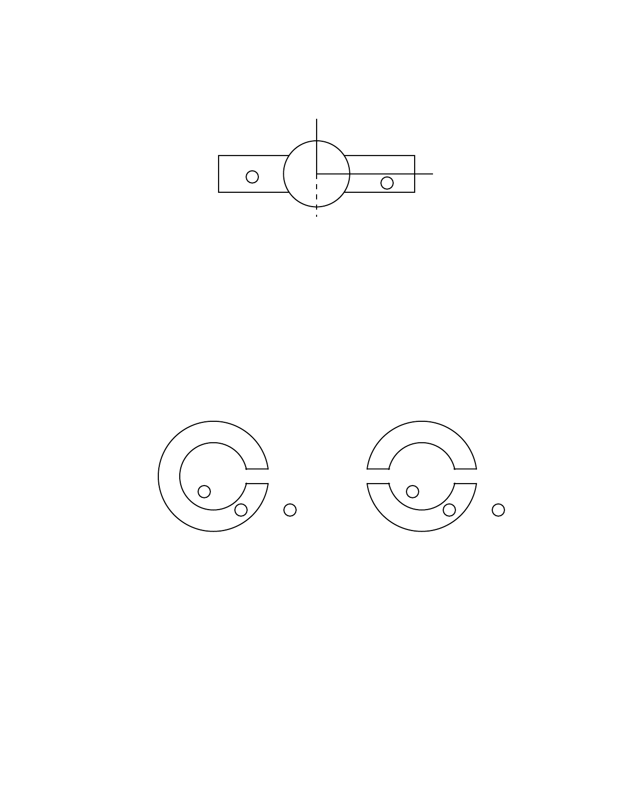
April 10, 2000 2-13
CHAPTER 2
GEOMETRY
Figure 2-2.
relative to surface aas well as that of each of its other bounding surfaces. A particle in cell 1
cannot have the same sense relative to surface a as does a particle in cell 2. More than one
ambiguity surface may be required to define a particular cell.
A second example may help to clarify the significance of ambiguity surfaces. We would like to
describe the geometry of Fig. 2-3a. Without the use of an ambiguity surface, the result will be
Fig. 2-3b. Surfaces 1 and 3 are spheres about the origin, and surface 2 is a cylinder around the
y−axis. Cell 1 is both the center and outside world of the geometry connected by the region
interior to surface 2.
Figure 2-3.
At first glance it may appear that cell 1 can easily be specified by −1 : −2 : 3 whereas cell 2 is
simply #1. This results in Figure 2.3b, in which cell 1 is everything in the universe interior to
surface 1 plus everything in the universe interior to surface 2 (remember the cylinder goes to plus
and minus infinity) plus everything in the universe exterior to surface 3.
An ambiguity surface (a plane at y=0) will solve the problem. Everything in the universe to the
right of the ambiguity surface (call it surface 4) intersected with everything in the universe
Z
Y
21
a
1
2
2
3
1
2 1
(a)
1
2
2
3
1
2 1
(b)

2-14 April 10, 2000
CHAPTER 2
GEOMETRY
interior to the cylinder is a cylindrical region that goes to plus infinity but terminates at y=0.
Therefore, −1 : (4 −2) : 3 defines cell 1 as desired in Figure 2.3a. The parentheses in this last
expression are not required because intersections are done before unions. Another expression for
cell 2 rather than #1 is 1 −3 #(4 −2).
For the user, ambiguity surfaces are specified the same way as any other surface–simply list the
signed surface number as an entry on the cell card. For MCNP, if a particular ambiguity surface
appears on cell cards with only one sense, it is treated as a true ambiguity surface. Otherwise, it
still functions as an ambiguity surface but the TRACK subroutine will try to find intersections
with it, thereby using a little more computer time.
3. Reflecting Surfaces
A surface can be designated a reflecting surface by preceding its number on the surface card with
an asterisk. Any particle hitting a reflecting surface is specularly (mirror) reflected. Reflecting
planes are valuable because they can simplify a geometry setup (and also tracking) in a problem.
They can, however, make it difficult (or even impossible) to get the correct answer. The user is
cautioned to check the source weight and tallies to ensure that the desired result is achieved. Any
tally in a problem with reflecting planes should have the same expected result as the tally in the
same problem without reflecting planes. Detectors or DXTRAN used with reflecting surfaces
give WRONG answers (see page 2–92).
The following example illustrates the above points and hopefully makes you very cautious in the
use of reflecting surfaces; they should never be used in any situation without a lot of thought.
Consider a cube of carbon 10 cm on a side sitting on top of a 5-MeV neutron source distributed
uniformly in volume. The source cell is a 1-cm-thick void completely covering the bottom of the
carbon cube and no more. The average neutron flux across any one of the sides (but not top or
bottom) is calculated to be 0.150 (±0.5%) per cm2per starting neutron from an MCNP F2 tally,
and the flux at a point at the center of the same side is 1.55e-03 n/cm2(±1%) from an MCNP F5
tally.
The cube can be modeled by half a cube and a reflecting surface. All dimensions remain the same
except the distance from the tally surface to the opposite surface (which becomes the reflecting
surface) is 5 cm. The source cell is cut in half also. Without any source normalization, the flux
across the surface is now 0.302 ( %), which is twice the flux in the nonreflecting geometry.
The detector flux is 2.58E −03 ( %), which is less than twice the point detector flux in the
nonreflecting problem.
The problem is that for the surface tally to be correct, the starting weight of the source particles
has to be normalized; it should be half the weight of the nonreflected source particles. The
detector results will always be wrong (and lower) for the reason discussed on page 2–92.
0.5±1±
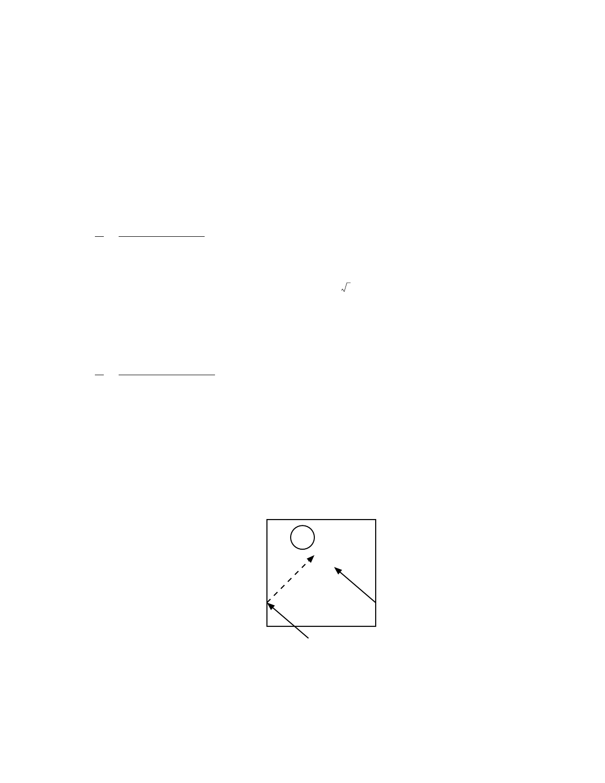
April 10, 2000 2-15
CHAPTER 2
GEOMETRY
In this particular example, the normalization factor for the starting weight of source particles
should be 0.5 because the source volume is half of the original volume. Without the
normalization, the full weight of source particles is started in only half the volume. These
normalization factors are problem dependent and should be derived very carefully.
Another way to view this problem is that the tally surface has doubled because of the reflecting
surface; two scores are being made across the tally surface when one is made across each of two
opposite surfaces in the nonreflecting problem. The detector has doubled too,except that the
contributions to it from beyond the reflecting surface are not being made, see page 2–92.
4. White Boundaries
A surface can be designated a white boundary surface by preceding its number on the surface
card with a plus. A particle hitting a white boundary is reflected with a cosine distribution,
p(µ)=µ, relative to the surface normal; that is, µ= , where ξ is a random number. White
boundary surfaces are useful for comparing MCNP results with other codes that have white
boundary conditions. They also can be used to approximate a boundary with an infinite scatterer.
They make absolutely no sense in problems with next-event estimators such as detectors or
DXTRAN (see page 2–92) and should always be used with caution.
5. Periodic Boundaries
Periodic boundary conditions can be applied to pairs of planes to simulate an infinite lattice.
Although the same effect can be achieved with an infinite lattice, the periodic boundary is easier
to use, simplifies comparison with other codes having periodic boundaries, and can save
considerable computation time. There is approximately a 55% run-time penalty associated with
repeated structures and lattices that can be avoided with periodic boundaries. However,
collisions and other aspects of the Monte Carlo random walk usually dominate running time, so
the savings realized by using periodic boundaries are usually much smaller. A simple periodic
boundary problem is illustrated in Figure 2.3c.
Figure 2-3(c).
ξ
12
3
4
5

2-16 April 10, 2000
CHAPTER 2
CROSS SECTIONS
It consists of a square reactor lattice infinite in the z direction and 10 cm on a side in the x and
y directions with an off-center 1 cm−radius cylindrical fuel pin. The MCNP surface cards are:
1−2px −5
2−1px 5
3−4py −5
4−3py 5
5 c/z −241
The negative entries before the surface mnemonics specify periodic boundaries. Card one says
that surface 1 is periodic with surface 2 and is a px plane. Card two says that surface 2 is periodic
with surface 1 and is a px plane. Card three says that surface 3 is periodic with surface 4 and is
a py plane. Card four says that surface 4 is periodic with surface 3 and is a py plane. Card five
says that surface 5 is an infinite cylinder parallel to the z−axis. A particle leaving the lattice out
the left side (surface 1) re-enters on the right side (surface 2). If the surfaces were reflecting, the
re-entering particle would miss the cylinder, shown by the dotted line. In a fully specified lattice
and in the periodic geometry, the re-entering particle will hit the cylinder as it should.
Much more complicated examples are possible, particularly hexagonal prism lattices. In all
cases, MCNP checks that the periodic surface pair matches properly and performs all the
necessary surface rotations and translations to put the particle in the proper place on the
corresponding periodic plane.
The following limitations apply:
• Periodic boundaries cannot be used with next event estimators such as detectors or
DXTRAN (see page 2–92);
• All periodic surfaces must be planes;
• Periodic planes cannot also have a surface transformation;
• The periodic cells may be infinite or bounded by planes on the top or bottom that must be
reflecting or white boundaries but not periodic;
• Periodic planes can only bound other periodic planes or top and bottom planes;
• A single zero-importance cell must be on one side of each periodic plane;
• All periodic planes must have a common rotational vector normal to the geometry top and
bottom.
III. CROSS SECTIONS
The MCNP code package is incomplete without the associated nuclear data tables. The kinds of
tables available and their general features are outlined in this section. The manner in which
information contained on nuclear data tables is used in MCNP is described in Sec. IV of this
chapter.

April 10, 2000 2-17
CHAPTER 2
CROSS SECTIONS
There are two broad objectives in preparing nuclear data tables for MCNP. First, it is our
responsibility to ensure that the data available to MCNP reproduce the original evaluated data as
much as is practical. Second, new data should be brought into the MCNP package in a timely
fashion, thereby giving users access to the most recent evaluations.
Eight classes of nuclear data tables exist for MCNP. They are: (1) continuous-energy neutron
interaction data, (2) discrete reaction neutron interaction data, (3) photon interaction data, (4)
neutron dosimetry cross sections, (5) neutron S(α,β) thermal data (6) multigroup neutron,
coupled neutron/photon, and charged particles masquerading as neutrons, (7) multigroup
photon, and (8) electron interaction data. It is understood that photon and electron data are
atomic rather than nuclear. In Mode N problems, one continuous-energy or discrete-reaction
neutron interaction table is required for each isotope or element in the problem. Likewise, one
photon interaction table is required for each element in a Mode P problem, and one electron
interaction table is required for each element in a Mode E problem. Dosimetry and thermal data
are optional. Cross sections from dosimetry tables can be used as response functions with the
FM card to determine reaction rates. Thermal S(α,β) tables are appropriate if the neutrons are
transported at sufficiently low energies where molecular binding effects are important.
MCNP can read from data tables in two formats. Data tables are transmitted between computer
installations in 80-column card-image BCD format (Type-1 format). An auxiliary processing
code, MAKXSF, converts the BCD files to standard unformatted binary files (Type-2 format),
allowing more economical access during execution of MCNP. The data contained on a table for
a specific ZAID (10-character name for a nuclear data table) are independent of the format of
the table.
The format of nuclear data tables is given in considerable detail in Appendix F. This appendix
may be useful for users making extensive modifications to MCNP involving cross sections or for
users debugging MCNP at a fairly high level.
The available nuclear data tables are listed in Appendix G. Each nuclear data table is identified
by a ZAID. The general form of a ZAID is ZZZAAA.nnX, where ZZZ is the atomic number,
AAA is the atomic weight, nn is the evaluation identifier, and X indicates the class of data. For
elemental evaluations AAA=000. Nuclear data tables are selected by the user with the Mn and
MTn cards.
In the remainder of this section we describe several characteristics of each class of data such as
evaluated sources, processing tools, and any differences between data on the original evaluation
and on the MCNP data tables. The means of accessing each class of data through MCNP input
will be detailed and some hints will be provided on how to select the appropriate data tables.

2-18 April 10, 2000
CHAPTER 2
CROSS SECTIONS
A. Neutron Interaction Data: Continuous-Energy and Discrete-Reaction
In neutron problems, one neutron interaction table is required for each isotope or element in the
problem. The form of the ZAIDs is ZZZAAA.nnC for a continuous-energy table and
ZZZAAA.nnD for a discrete reaction table. The neutron interaction tables available to MCNP
are listed in Table G.2 of Appendix G. (It should be noted that although all nuclear data tables
in Appendix G are available to users at Los Alamos, users at other installations will generally
have only a subset of the tables available.)
For most materials there are many cross-section sets available (represented by different values
of nn in the ZAIDs) because of multiple sources of evaluated data and different parameters used
in processing the data. An evaluated nuclear data set is produced by analyzing experimentally
measured cross sections and combining those data with the predictions of nuclear model
calculations in an attempt to extract the most accurate cross-section information. Preparing
evaluated cross-section sets has become a discipline in itself and has developed since the early
1960s. People in most of the national laboratories and several of the commercial reactor design
firms are involved in such work. American evaluators joined forces in the mid-1960s to create
the national ENDF system.23 The ENDF contributors collaborate through the Cross Section
Evaluation Working Group (CSEWG).
In recent years the primary evaluated source of neutron interaction data for MCNP has been the
ENDF/B system. Recently evaluated neutron interaction data tables are also extracted from two
other sources: Lawrence Livermore National Laboratory's Evaluated Nuclear Data Library
(ENDL),24 and supplemental evaluations performed in the Nuclear Theory and Applications
Group at Los Alamos.25,26,27 Older evaluations come from previous versions of ENDF/B and
ENDL, the Los Alamos Master Data File,28 and the Atomic Weapons Research Establishment
in Great Britain.
MCNP does not access evaluated data directly; these data must first be processed into ACE
format. The very complex processing codes used for this purpose include NJOY29 for evaluated
data in ENDF/B format and MCPOINT30 for ENDL data.
Data on the MCNP neutron interaction tables include cross sections and much more. Cross
sections for all reactions given in the evaluated data are specified. For a particular table, the cross
sections for each reaction are given on one energy grid that is sufficiently dense that linear-linear
interpolation between points reproduces the evaluated cross sections within a specified tolerance
that is generally 1% or less. Depending primarily on the number of resolved resonances for each
isotope, the resulting energy grid may contain as few as ∼250 points (for example, H-1) or as
many as ∼22,500 points (for example, the ENDF/B-V version of AU-197). Other information,
including the total absorption cross section, the total photon production cross section, and the
average heating number (for energy deposition calculations), is also tabulated on the same
energy grid.

April 10, 2000 2-19
CHAPTER 2
CROSS SECTIONS
Angular distributions of scattered neutrons are included in the neutron interaction tables for all
reactions emitting neutrons. The distributions are given in the center-of-mass system for elastic
scattering, discrete-level inelastic scattering, and for some ENDF/B-VI scattering laws, and are
given in the laboratory system for all other inelastic reactions. Angular distributions are given
on a reaction-dependent grid of incident neutron energies. These tables are sampled to conserve
energy for many collisions but will not necessarily conserve energy for a single collision; that is,
energy is conserved on average.
The sampled angle of scattering uniquely determines the secondary energy for elastic scattering
and discrete-level inelastic scattering. For other inelastic reactions, energy distributions of the
scattered neutrons are provided in the neutron interaction tables. As with angular distributions,
the energy distributions are given on a reaction-dependent grid of incident neutron energies.
When evaluations contain data about secondary photon production, that information appears in
the MCNP neutron interaction tables. Many processed data sets contain photon production cross
sections, photon angular distributions, and photon energy distributions for each neutron reaction
that produces secondary photons. The information is given in a manner similar to that described
in the last few paragraphs for neutron cross sections and secondary neutron distributions.
Other miscellaneous information on the neutron interaction tables includes the atomic weight
ratio of the target nucleus, the Q-values of each reaction, and nubar, , data (the average number
of neutrons per fission) for fissionable isotopes. In many cases both prompt and total are given.
Prompt is the default for all but KCODE criticality problems and total is the default for
KCODE criticality problems. The TOTNU input card can be used to change the default.
Approximations must be made when processing an evaluated data set into ACE format. As
mentioned above, cross sections are reproduced only within a certain tolerance, generally <1%;
to decrease it further would result in excessively large data tables. For many nuclides, a
“thinned” neutron interaction table is available with a coarse tolerance, > 1%, that greatly
reduces the library size. Smaller library sizes also can be obtained by using discrete reaction
tables or higher temperature data. Evaluated angular distributions for secondary neutrons and
photons are approximated on MCNP data tables by 32 equally probable cosine bins. This
approximation is clearly necessary when contrasted to the alternative that might involve
sampling from a 20th-order Legendre polynomial distribution. Secondary neutron energy
distributions given in tabular form by evaluators are sometimes approximated on MCNP data
tables by 32 equally probable energy bins. Older cross-section tables include a 30x20 matrix
approximation of the secondary photon energy spectra (described on page 2–34). On the whole,
the approximations are small, and MCNP neutron interaction data tables are extremely faithful
representations of evaluated data.
Discrete-reaction tables are identical to continuous-energy tables except that in the discrete
reaction tables all cross sections have been averaged into 262 groups. The averaging is done with
υ
υ
υ υ

2-20 April 10, 2000
CHAPTER 2
CROSS SECTIONS
a flat weighting function. This is not a multigroup representation; the cross sections are simply
given as histograms rather than as continuous curves. The remaining data (angular distributions,
energy distributions, , etc.) are identical in discrete-reaction and continuous-energy tables.
Discrete-reaction tables are provided primarily as a method of shrinking the required data
storage to enhance the ability to run MCNP on small machines or in a time-sharing environment.
The tables may also be useful for preliminary scoping studies or for isotopes that exist only in
trace quantities in a problem. They are not, however, recommended as a substitute for the
continuous-energy tables when performing final calculations, particularly for problems
involving transport through the resonance region.
The matter of how to select the appropriate neutron interaction tables for your calculation is now
discussed. Multiple tables for the same isotope are differentiated by the “nn” portion of the
ZAID. The easiest choice for the user, although by no means the recommended one, is not to
enter the nn at all. MCNP will select the first match found in the directory file XSDIR. The
default nnX can be changed for all isotopes of a material by the NLIB keyword entry on the Mm
card. The default will be overridden by fully specifying the ZAID. Default continuous-energy
neutron interaction tables are accessed by entering ZZZAAA for the ZAID\null. Including a
DRXS card in the input file will force MCNP to choose the default discrete reaction tables.
Careful users will want to think about what neutron interaction tables to choose. There is,
unfortunately, no strict formula for choosing the tables. The following guidelines and
observations are the best that can be offered:
1. Users should be aware of the differences between the “.50C” series of data tables and
the “.51C” series. Both are derived from ENDF/B-V. The “.50C” series is the most
faithful reproduction of the evaluated data. The “.51C” series, also called the
“thinned” series, has been processed with a less rigid tolerance than the “.50C” series.
As with discrete reaction data tables, although by no means to the same extent, users
should be careful when using the “thinned” data for transport through the resonance
region.
2. Consider differences in evaluators' philosophies. The Physical Data Group at
Livermore is justly proud of its extensive cross-section efforts; their evaluations
manifest a philosophy of reproducing the data with the fewest number of points.
Livermore evaluations are available mainly in the “.40C” series. We at Los Alamos
are particularly proud of the evaluation work being carried out in the Nuclear Theory
and Applications Group T-2; generally, these evaluations are the most complex
because they are the most thorough. Recent evaluations from Los Alamos are
available in the “.55C” series.
3. Be aware of the neutron energy spectrum in your problem. For high-energy problems,
the “thinned” and discrete reaction data are probably not bad approximations.
υ

April 10, 2000 2-21
CHAPTER 2
CROSS SECTIONS
Conversely, it is essential to use the most detailed continuous-energy set available for
problems influenced strongly by transport through the resonance region.
4. Check the temperature at which various data tables have been processed. Do not use
a set that is Doppler broadened to 12,000,000 K for a room temperature calculation.
5. Consider checking the sensitivity of the results to various sets of nuclear data. Try, for
example, a calculation with ENDF/B-V cross sections, and then another with ENDL
cross sections. If the results of a problem are extremely sensitive to the choice of
nuclear data, it is advisable to find out why.
6. For a coupled neutron/photon problem, be careful that the tables you choose have
photon production data available. If possible, use the more-recent sets that have been
processed into expanded photon production format.
7. In general, use the best data you can afford. It is understood that the latest evaluations
tend to be more complex and therefore require more memory and longer execution
times. If you are limited by available memory, try to use smaller data tables such as
thinned or discrete-reaction for the minor isotopes in the calculation. Discrete reaction
data tables might be used for a parameter study, followed by a calculation with the full
continuous-energy data tables for confirmation.
To select the neutron interaction data tables, the nn portion of the ZAIDs must be entered on the
Mn card(s). For a continuous-energy set, ZZZAAA.nn is equivalent to ZZZAAA.nnC. To use a
discrete-reaction table (unless there is a DRXS card in the input) the full ZAID, ZZZAAA.nnD,
must be entered.
If only the integer portion of the ZAID is entered (ZZZAAA), MCNP will choose the cross−
section table that it will use. Based on other cards (i.e., MODE, MGOPT, DRXS), MCNP knows
which class of data is required. The code then “reads” the cross-section directory file (XSDIR)
and selects the first table it finds that meets the ZZZAAA and class criteria. Thus, default cross
sections are based entirely on the ordering of the entries in the XSDIR file you are using at your
installation.
In conclusion, the additional time necessary to choose appropriate neutron interaction data tables
rather than simply to accept the defaults often will be rewarded by increased understanding of
your calculation.
B. Photon Interaction Data
Photon interaction cross sections are required for all photon problems. The form of the ZAID is
ZZZ000.nnP. There are two photon interaction data libraries: nn = 01 and nn = 02.
For the ZAID=ZZZ000.01P library, the photon interaction tables for Z = 84, 85, 87, 88, 89, 91,
and 93 are based on the compilation of Storm and Israel31 from 1 keV to 15 MeV. For all other
°

2-22 April 10, 2000
CHAPTER 2
CROSS SECTIONS
elements from Z = 1 through Z = 94 the photon interaction tables are based on evaluated data
from ENDF32 from 1 keV to 100 MeV. Fluorescence data are taken from work by Everett and
Cashwell.33 Energy grids are tailored specifically for each element and contain approximately
40 to 60 points.
The ZAID = ZZZ000.02P library is a superset of the ZAID = ZZZ000.01P library with pair
production thresholds added for the Storm-Israel data. Data above 15 MeV for the Storm-Israel
data and above 100 MeV for the ENDF data come from adaptation of the Livermore Evaluated
Photon Data Library (EPDL)34 and go up to 100 GeV. However, it usually is impractical to run
above 1 GeV with MCNP because electron data only go to 1 GeV. The energy grid for the ZAID
= ZZZ000.02P library contains approximately 100 points.
For each nuclide the photon interaction libraries contain an energy grid (logarithms of energies),
including the photoelectric edges and the pair production threshold. These energies are tailored
specifically for each element. The logarithmic energies are followed by tables of incoherent and
coherent form factors that are tabulated as a function of momentum transfer. The next tables are
logarithms of the incoherent scattering, coherent scattering, photoelectric, and pair production
cross sections, followed by the photon heating numbers. The total cross section is not stored, but
rather summed from the other cross sections during transport.
The determination of directions and energies of scattered photons requires information different
from the sets of angular and energy distributions found on neutron interaction tables. Angular
distributions of secondary photons are isotropic for photoelectric effect, fluorescence, and pair
production, and come from sampling the well-known Thomson and Klein-Nishina formulas for
coherent and incoherent scattering. The energy of an incoherently scattered photon is calculated
from the sampled scattering angle. Values of the integrated coherent form factor are tabulated on
the photon interaction tables for use with next event estimators such as point detectors.
Very few approximations are made in the various processing codes used to transfer photon data
from ENDF into the format of MCNP photon interaction tables. Cross sections are reproduced
exactly as given. Form factors and scattering functions are reproduced as given; however, the
momentum transfer grid on which they are tabulated may be different from that of the original
evaluation. Heating numbers are calculated values, not given in evaluated sets, but inferred from
them. Fluorescence data are not provided in ENDF; therefore the data for MCNP are extracted
from a variety of sources as described in Ref. 31.
To select photon interaction data, specific ZAID identifiers can be used, such as
ZAID = ZZZ000.02P, or selections from a library can be used by specifying PLIB=nnP on the
M card. The PLIB = specification on the M card is the preferred method because the ZAID
entries may already be used to specify neutron libraries and, unlike neutrons, it usually is
desirable to pick all photon data from the same library. A specification on the Mn card for a
neutron interaction table with ZAID = ZZZAAA.nnC or ZAID = ZZZAAA.nnD immediately

April 10, 2000 2-23
CHAPTER 2
CROSS SECTIONS
causes a photon interaction table with ZAID = ZZZ000.nnP to be accessed as well, where nn is
the first photon data encountered for ZZZ000 on the XSDIR cross section directory file or nn
comes from PLIB = nn. The data table required for ZAID = ZZZAAA.nnP is identical to that
required for ZAID = ZZZ000.nnP; however, the atomic weight used in the calculation will likely
be different.
C. Electron Interaction Data
Electron interaction data tables are required both for problems in which electrons are actually
transported, and for photon problems in which the thick-target bremsstrahlung model is used.
Electron data tables are identified by ZAIDs of the form ZZZ000.nnE, and are selected by
default when the problem mode requires them. There are two electron interaction data libraries:
nn=03 and nn = 01.
The electron library contains data on an element-by-element basis for atomic numbers Z=1–94.
As is the case with photons, there is no distinction between isotopes for a given element. The
library data contain energies for tabulation, radiative stopping power parameters,
bremsstrahlung production cross sections, bremsstrahlung energy distributions, K-edge
energies, Auger electron production energies, parameters for the evaluation of the Goudsmit-
Saunderson theory for angular deflections based on the Riley cross section calculation, and Mott
correction factors to the Rutherford cross sections also used in the Goudsmit-Saunderson theory.
The el03 database also includes the atomic data of Carlson used in the density effect calculation.
Internally, calculated data are electron stopping powers and ranges, K x-ray production
probabilities, knock-on probabilities, bremsstrahlung angular distributions, and the Landau-
Blunck-Leisegang theory of energy-loss fluctuations. The el03 evaluation is derived from the
ITS3.0 code system.35 Discussions of the theoretical basis for these data and references to the
relevant literature are presented in Section IV-E of this chapter.
The hierarchy rules for electron cross sections require that each material must use the same
electron library. If a specific ZAID is selected, such as ZZZ000.01E, that choice will override
any defaults. Alternatively, a default electron library for a given material can be chosen by
specifying ELIB = nnE on the M card. However, one can not specify different libraries, nn=01
and nn=03, by any means; overriding this with a fatal option will result in unreliable results. In
the absence of either of these specifications, MCNP will use the first electron data table listed in
the XSDIR cross section directory file for the relevant element.
D. Neutron Dosimetry Cross Sections
Dosimetry cross-section tables cannot be used for transport through material. These incomplete
cross-section sets provide energy-dependent neutron cross sections to MCNP for use as response

2-24 April 10, 2000
CHAPTER 2
CROSS SECTIONS
functions with the FM tally feature. ZAIDs of dosimetry tables are of the form ZZZAAA.nnY.
Remember, dosimetry cross-section tables have no effect on the particle transport of a problem.
The available dosimetry cross sections are from three sources: ENDF/B−V Dosimetry Tape 531,
ENDF/B−V Activation Tape 532, and ACTL36–an evaluated neutron activation cross-section
library from the Lawrence Livermore National Laboratory. Various codes have been used to
process evaluated dosimetry data into the format of MCNP dosimetry tables.
Data on dosimetry tables are simply energy-cross-section pairs for one or more reactions. The
energy grids for all reactions are independent of each other. Interpolation between adjacent
energy points can be specified as histogram, linear-linear, linear-log, log-linear, or log-log. With
the exception of the tolerance involved in any reconstruction of pointwise cross sections from
resonance parameters, evaluated dosimetry cross sections can be reproduced on the MCNP data
tables with no approximation.
ZAIDs for dosimetry tables must be entered on material cards that are referenced by FM cards,
not on Mm cards referenced by cell cards. The complete ZAID, ZZZAAA.nnY, must be given;
there are no defaults for dosimetry tables.
E. Neutron Thermal S(α,β) Tables
Thermal S(α,β) tables are not required, but they are absolutely essential to get correct answers
in problems involving neutron thermalization. Thermal tables have ZAIDs of the form
XXXXXX.nnT, where XXXXXX is a mnemonic character string. The data on these tables
encompass those required for a complete representation of thermal neutron scattering by
molecules and crystalline solids. The source of S(α,β) data is a special set of ENDF tapes.37 The
THERMR and ACER modules of the NJOY29 system have been used to process the evaluated
thermal data into a format appropriate for MCNP.
Data are for neutron energies generally less than 4 eV. Cross sections are tabulated on table-
dependent energy grids; inelastic scattering cross sections are always given and elastic scattering
cross sections are sometimes given. Correlated energy-angle distributions are provided for
inelastically scattered neutrons. A set of equally probable final energies is tabulated for each of
several initial energies. Further, a set of equally probable cosines or cosine bins is tabulated for
each combination of initial and final energies. Elastic scattering data can be derived from either
an incoherent or a coherent approximation. In the incoherent case, equally probable cosines or
cosine bins are tabulated for each of several incident neutron energies. In the coherent case,
scattering cosines are determined from a set of Bragg energies derived from the lattice
parameters. During processing, approximations to the evaluated data are made when
constructing equally probable energy and cosine distributions.

April 10, 2000 2-25
CHAPTER 2
PHYSICS
ZAIDs for the thermal tables are entered on an MTn card that is associated with an existing Mn
card. The thermal table generally will provide data for one component of a material–for
example, hydrogen in light water. Thermal ZAIDs may be entered on the MTn card(s) as
XXXXXX, XXXXXX.nn, or XXXXXX.nnT.
F. Multigroup Tables
Multigroup cross section libraries are the only libraries allowed in multigroup/adjoint problems.
Neutron multigroup problems cannot be supplemented with S(α,β) thermal libraries; the thermal
effects must be included in the multigroup neutron library. Photon problems cannot be
supplemented with electron libraries; the electrons must be part of the multigroup photon library.
The form of the ZAID is ZZZAAA.nnM or ZZZAAA.nnG for photons only.
Although continuous-energy data are more accurate than multigroup data, the multigroup option
is useful for a number of important applications: (1) comparison of deterministic (Sn) transport
codes to Monte Carlo; (2) use of adjoint calculations in problems where the adjoint method is
more efficient; (3) generation of adjoint importance functions; (4) cross section sensitivity
studies; (5) solution of problems for which continuous-cross sections are unavailable; and (6)
charged particle transport using the Boltzmann-Fokker-Planck algorithm in which charged
particles masquerade as neutrons.
Multigroup cross sections are very problem dependent. Some multigroup libraries are available
from the Transport Methods Group at Los Alamos but must be used with caution. Users are
encouraged to generate or get their own multigroup libraries and then use the supplementary
code CRSRD38 to convert them to MCNP format. Reference 38 describes the conversion
procedure. This report also describes how to use both the multigroup and adjoint methods in
MCNP and presents several benchmark calculations demonstrating the validity and
effectiveness of the multigroup/adjoint method.
To generate cross-section tables for electron/photon transport problems that will use the
multigroup Boltzmann-Fokker-Planck algorithm,39 the CEPXS40 code developed by Sandia
National Laboratory and available from RSICC can be used. The CEPXS manuals describe the
algorithms and physics database upon which the code is based; the physics package is essentially
the same as ITS version 2.1. The keyword “MONTE-CARLO” is needed in the CEPXS input
file to generate a cross-section library suitable for input into CRSRD; this undocumented feature
of the CEPXS code should be approached with caution.
IV. PHYSICS
The physics of neutron, photon, and electron interactions is the very essence of MCNP. This
section may be considered a software requirements document in that it describes the equations

2-26 April 10, 2000
CHAPTER 2
PHYSICS
MCNP is intended to solve. All the sampling schemes essential to the random walk are presented
or referenced. But first, particle weight and particle tracks, two concepts that are important for
setting up the input and for understanding the output, are discussed in the following sections.
A. Particle Weight
If MCNP were used only to simulate exactly physical transport, then each MCNP particle would
represent one physical particle and would have unit weight. However, for computational
efficiency, MCNP allows many techniques that do not exactly simulate physical transport. For
instance, each MCNP particle might represent a number w of particles emitted from a source.
This number w is the initial weight of the MCNP particle. The w physical particles all would
have different random walks, but the one MCNP particle representing these w physical particles
will only have one random walk. Clearly this is not an exact simulation; however, the true
number of physical particles is preserved in MCNP in the sense of statistical averages and
therefore in the limit of large particle numbers (of course including particle production or loss if
they occur). Each MCNP particle result is multiplied by the weight so that the full results of the
w physical particles represented by each MCNP particle are exhibited in the final results (tallies).
This procedure allows users to normalize their calculations to whatever source strength they
desire. The default normalization is to weight one per MCNP particle. A second normalization
to the number of Monte Carlo histories is made in the results so that the expected means will be
independent of the number of source particles actually initiated in the MCNP calculation.
The utility of particle weight, however, goes far beyond simply normalizing the source. Every
Monte Carlo biasing technique alters the probabilities of random walks executed by the
particles. The purpose of such biasing techniques is to increase the number of particles that
sample some part of the problem of special interest (1) without increasing (sometimes actually
decreasing) the sampling of less interesting parts of the problem, and (2) without erroneously
affecting the expected mean physical result (tally). This procedure, properly applied, increases
precision in the desired result compared to an unbiased calculation taking the same computing
time. For example, if an event is made times as likely to occur (as it would occur without
biasing), the tally ought to be multiplied by so that the expected average tally is unaffected.
This tally multiplication can be accomplished by multiplying the particle weight by
because the tally contribution by a particle is always multiplied by the particle weight in MCNP.
Note that weights need not be integers.
In short, particle weight is a number carried along with each MCNP particle, representing that
particle's relative contribution to the final tallies. Its magnitude is determined to ensure that
whenever MCNP deviates from an exact simulation of the physics, the expected physical result
nonetheless is preserved in the sense of statistical averages, and therefore in the limit of large
MCNP particle numbers. Its utility is in the manipulation of the number of particles, sampling
just a part of the problem to improve the precision of selected results obviating a full unbiased
calculation−with its added cost in computing time−to achieve the same results and precision.
212 12

April 10, 2000 2-27
CHAPTER 2
PHYSICS
B. Particle Tracks
When a particle starts out from a source, a particle track is created. If that track is split 2 for 1 at
a splitting surface, a second track is created and there are now two tracks from the original source
particle, each with half the single track weight. If one of the tracks has an (n,2n) reaction, one
more track is started for a total of three. A track refers to each component of a source particle
during its history. Track length tallies use the length of a track in a given cell to determine a
quantity of interest, such as fluence, flux, or energy deposition. Tracks crossing surfaces are used
to calculate fluence, flux, or pulse-height energy deposition (surface estimators). Tracks
undergoing collisions are used to calculate multiplication and criticality (collision estimators).
Within a given cell of fixed composition, the method of sampling a collision along the track is
determined using the following theory. The probability of a first collision for a particle between
l and l + dl along its line of flight is given by
,
where is the macroscopic total cross section of the medium and is interpreted as the
probability per unit length of a collision. Setting ξ the random number on [0,1), to be
,
it follows that
.
But, because is distributed in the same manner as ξand hence may be replaced by ξ,we
obtain the well-known expression for the distance to collision,
.
C. Neutron Interactions
When a particle (representing any number of neutrons, depending upon the particle weight)
collides with a nucleus, the following sequence occurs:
1. the collision nuclide is identified;
pl()dl e Σt
–Σt
=dl
Σt
ξeΣts–
0
l
∫
=Σtds 1eΣ–tl
–=
l1
Σt
-----ln 1ξ–()–=
1ξ–
l1
Σt
-----ξ()ln=

2-28 April 10, 2000
CHAPTER 2
PHYSICS
2. either the S(a,b) treatment is used or the velocity of the target nucleus is sampled for
low−energy neutrons;
3. photons are optionally generated for later transport;
4. neutron capture (that is, neutron disappearance by any process) is modeled;
5. unless the S(a,b) treatment is used, either elastic scattering or an inelastic reaction is
selected, and the new energy and direction of the outgoing track(s) are determined;
6. if the energy of the neutron is low enough and an appropriate S(a,b) table is present,
the collision is modeled by the S(a,b) treatment instead of by step 5.
1. Section of Collision Nuclide
If there are ndifferent nuclides forming the material in which the collision occurred, and if ξis
a random number on the unit interval [0,1), then the kth nuclide is chosen as the collision nuclide
if
where is the macroscopic total cross section of nuclide . If the energy of the neutron is low
enough (below about 4 eV) and the appropriate table is present, the total cross section is
the sum of the capture cross section from the regular cross-section table and the elastic and
inelastic scattering cross sections from the table. Otherwise, the total cross section is taken
from the regular cross-section table and is adjusted for thermal effects as described below.
2. Free Gas Thermal Treatment
A collision between a neutron and an atom is affected by the thermal motion of the atom, and in
most cases, the collision is also affected by the presence of other atoms nearby. The thermal
motion cannot be ignored in many applications of MCNP without serious error. The effects of
nearby atoms are also important in some applications. MCNP uses a thermal treatment based
on the free gas approximation to account for the thermal motion. It also has an explicit S(a,b)
capability that takes into account the effects of chemical binding and crystal structure for
incident neutron energies below about 4 eV, but is available for only a limited number of
substances and temperatures. The S(a,b) capability is described later on page 2–53.
The free gas thermal treatment in MCNP assumes that the medium is a free gas and also that, in
the range of atomic weight and neutron energy where thermal effects are significant, the elastic
scattering cross section at zero temperature is nearly independent of the energy of the neutron,
and that the reaction cross sections are nearly independent of temperature. These assumptions
allow MCNP to have a thermal treatment of neutron collisions that runs almost as fast as a
completely nonthermal treatment and that is adequate for most practical problems.
Σti
i1=
k1–
∑ξΣ
ti
i1=
n
∑
<Σ
ti
i1=
k
∑
≤
Σti i
Sαβ,()
Sαβ,()

April 10, 2000 2-29
CHAPTER 2
PHYSICS
With the above assumptions, the free gas thermal treatment consists of adjusting the elastic cross
section and taking into account the velocity of the target nucleus when the kinematics of a
collision are being calculated. Note that Doppler broadening of the inelastic cross sections is
assumed to have already been done in the processing of the cross section libraries. The free gas
thermal treatment effectively applies to elastic scattering only.
a. Adjusting the Elastic Cross Section: The first aspect of the free gas thermal treatment
is to adjust the zero-temperature elastic cross section by raising it by the factor
,
where , A = atomic weight, E= neutron energy, and T= temperature. For speed,
F is approximated by F=1+ 0.5/a2 when and by linear interpolation in a table of 51
values of aF when a < 2. Both approximations have relative errors less than 0.0001. The total
cross section also is increased by the amount of the increase in the elastic cross section.
The adjustment to the elastic and total cross sections is done partly in the setup of a problem and
partly during the actual transport calculation. No adjustment is made if the elastic cross section
in the data library was already processed to the temperature that is needed in the problem. If all
of the cells that contain a particular nuclide have the same temperature, constant in time, that is
different from the temperature of the library, the elastic and total cross sections for that nuclide
are adjusted to that temperature during the setup so that the transport will run a little faster.
Otherwise, these cross sections are reduced, if necessary, to zero temperature during the setup
and the thermal adjustment is made when the cross sections are used. For speed, the thermal
adjustment is omitted if the neutron energy is greater than 500 kT/A. At that energy the
adjustment of the elastic cross section would be less than 0.1%.
b. Sampling the Velocity of the Target Nucleus: The second aspect of the free gas thermal
treatment consists of taking into account the velocity of the target nucleus when the kinematics
of a collision are being calculated. The target velocity is sampled and subtracted from the
velocity of the neutron to get the relative velocity. The collision is sampled in the target-at-rest
frame and the outgoing velocities are transformed to the laboratory frame by adding the target
velocity.
There are different schools of thought as to whether the relative energy between the neutron and
target, Er, or the laboratory frame incident neutron energy (target-at-rest), Eo, should be used for
all the kinematics of the collision. Eois used in MCNP to obtain the distance-to-collision, select
the collision nuclide, determine energy cutoffs, generate photons, generate fission sites for the
next generation of a KCODE criticality problem, for S(α,β) scattering, and for capture. Er is
used for everything else in the collision process, namely elastic and inelastic scattering,
including fission and (n,xn) reactions. It is shown in Eqn. 2.1 that Er is based upon vrel that is
based upon the elastic scattering cross section, and, therefore, Er is truly valid only for elastic
F1 0.5 a2
⁄+()erf a() a2
–()aπ()⁄exp+=
aAEkT⁄=a2≥

2-30 April 10, 2000
CHAPTER 2
PHYSICS
scatter. However, the only significant thermal reactions for stable isotopes are absorption, elastic
scattering, and fission. 181Ta has a 6 keV threshold inelastic reaction; all other stable isotopes
have higher inelastic thresholds. Metastable nuclides like 242mAm have inelastic reactions all the
way down to zero, but these inelastic reaction cross sections are neither constant nor 1/v cross
sections and these nuclides are generally too massive to be affected by the thermal treatment
anyway. Furthermore, fission is very insensitive to incident neutron energy at low energies. The
fission secondary energy and angle distributions are nearly flat or constant for incident energies
below about 500 keV. Therefore, it makes no significant difference if Eris used only for elastic
scatter or for other inelastic collisions as well. At thermal energies, whether Eror Eois used only
makes a difference for elastic scattering.
If the energy of the neutron is greater than 400 kT and the target is not 1H, the velocity of the
target is set to zero. Otherwise, the target velocity is sampled as follows. The free-gas kernel is
a thermal interaction model that results in a good approximation to the thermal flux spectrum in
a variety of applications and can be sampled without tables. The effective scattering cross section
in the laboratory system for a neutron of kinetic energy E is
(E) = (2.1)
Here, vrel is the relative velocity between a neutron moving with a scalar velocity vnand a target nucleus moving
with a scalar velocity V, and µt is the cosine of the angle between the neutron and the target direction-of-flight
vectors. The equation for vrel is
The scattering cross section at the relative velocity is denoted by σs(vrel), and p(V) is the
probability density function for the Maxwellian distribution of target velocities,
with β defined as
,
where A is the mass of a target nucleus in units of the neutron mass, Mn is the neutron mass in
MeV-sh2/cm2, and kT is the equilibrium temperature of the target nuclei in MeV.
σs
eff 1
vn
-----σs
∫∫ vrel
()vrelpV()dvdµt
2
--------
vrel vn
2V22vnVµt–+()
1
2
---
=
pV() 4
π12⁄
-----------β3V2eβ–2V2
=
βAMn
2kT
------------
1
2
---
=

April 10, 2000 2-31
CHAPTER 2
PHYSICS
The most probable scalar velocity V of the target nuclei is 1/β, which corresponds to a kinetic
energy of kT for the target nuclei. This is not the average kinetic energy of the nuclei, which is
3kT/2. The quantity that MCNP expects on the TMPn input card is kT and not just T (see page
3–121). Note that kT is not a function of the particle mass and is therefore the kinetic energy at
the most probable velocity for particles of any mass.
Equation (2.1) implies that the probability distribution for a target velocity n and cosine is
.
It is assumed that the variation of with target velocity can be ignored. The justification
for this approximation is that (1) for light nuclei, is slowly varying with velocity, and
(2) for heavy nuclei, where can vary rapidly, the moderating effect of scattering is small
so that the consequences of the approximation will be negligible. As a result of the
approximation, the probability distribution actually used is
.
Note that the above expression can be written as
.
As a consequence, the following algorithm is used to sample the target velocity.
1. With probability , the target velocity Vis sampled from the
distribution . The transformation reduces this
distribution to the sampling distribution for . MCNP actually codes
.
2. With probability 1 − α, the target velocity is sampled from the distribution
. Substituting V = y/β reduces the distribution to the
sampling distribution for y: .
3. The cosine of the angle between the neutron velocity and the target velocity is sampled
uniformly on the interval + 1.
µt
PVµt
,()
σsvrel
()vrelPV()
2σs
eff E()vn
-----------------------------------------=
σsv() σsvrel
()
σsvrel
()
PVµt
,()ν
n
2V22Vνnµt
–V2eβ2V
2
–
∝
P
Vµt
,()
νn
2V22Vνnµt
–+
νnV+
----------------------------------------------- V3eβ2V2
–νnV2eβ2V
2
–
+(∝
α11 πβvn2⁄()+()⁄=
P1V() 2β4V3eβ2V2
–
=Vyβ⁄=
Py() ye y–
=
1α–
P2V() 4β3π⁄()V2eβ2V2
–
=
Py() 4π⁄()y2ey2
–
=
1µt
≤≤–

2-32 April 10, 2000
CHAPTER 2
PHYSICS
4. The rejection function R(V, µt) is computed using
.
With probability R(V,µt), the sampling is accepted; otherwise, the sampling is rejected and the
procedure is repeated. The minimum efficiency of this rejection algorithm averaged over µtis
68% and approaches 100% as either the incident neutron energy approaches zero or becomes
much larger than kT.
3. Optional Generation of Photons
Photons are generated if the problem is a combined neutron/photon run and if the collision
nuclide has a nonzero photon production cross section. The number of photons produced is a
function of neutron weight, neutron source weight, photon weight limits (entries on the PWT
card), photon production cross section, neutron total cross section, cell importance, and the
importance of the neutron source cell. No more than 10 photons may be born from any neutron
collision. In a KCODE calculation, secondary photon production from neutrons is turned off
during the inactive cycles.
Because of the many low-weight photons typically created by neutron collisions, Russian
roulette is played for particles with weight below the bounds specified on the PWT card,
resulting in fewer particles, each having a larger weight. The created photon weight before
Russian roulette is
,
where Wp= photon weight
Wn= neutron weight
= photon production cross section
σT= total neutron cross section.
Both and σTare evaluated at the incoming neutron energy without the effects of the thermal
free gas treatment because nonelastic cross sections are assumed independent of temperature.
The Russian roulette game is played according to neutron cell importances for the collision and
source cell. For a photon produced in cell iwhere the minimum weight set on the PWT card is
R
Vµt
,()
vn
2V22Vvnµt
–+
vnV+
----------------------------------------------=1≤
Wp
Wnσγ
σT
--------------=
σγ
σγ

April 10, 2000 2-33
CHAPTER 2
PHYSICS
, let Iibe the neutron importance in cell iand let Isbe the neutron importance in the source
cell. If , one or more photons will be produced. The number of photons
created is Np,where Np = (Wp∗ Ii)/(5 * ∗ Is)+1. . Each photon is stored in the
bank with weight Wp/Np. If ∗Is/Ii, Russian roulette is played and the photon
survives with probability Wp∗and is given the weight, ∗Is/Ii.
If weight windows are not used and if the weight of the starting neutrons is not unity, setting all
the on the PWT card to negative values will make the photon minimum weight relative to
the neutron source weight. This will make the number of photons being created roughly
proportional to the biased collision rate of neutrons. It is recommended for most applications that
negative numbers be used and be chosen to produce from one to four photons per source neutron.
The default values for on the PWT card are −1, which should be adequate for most
problems using cell importances.
If energy−independent weight windows are used, the entries on the PWT card should be the
same as on the WWN1:P card. If energy−dependent photon weight windows are used, the entries
on the PWT card should be the minimum WWNn:P entry for each cell, where n refers to the
photon weight window energy group. This will cause most photons to be born within the weight
window bounds.
Any photons generated at neutron collision sites are temporarily stored in the bank. There are
two methods for determining the exiting energies and directions, depending on the form in which
the processed photon production data are stored in a library. The first method has the evaluated
photon production data processed into an “expanded format.”41 In this format, energy−
dependent cross sections, energy distributions, and angular distributions are explicitly provided
for every photon−producing neutron interaction. In the second method, used with data
processed from older evaluations, the evaluated photon production data have been collapsed so
that the only information about secondary photons is in a matrix of 20 equally probable photon
energies for each of 30 incident neutron energy groups. The sampling techniques used in each
method are now described.
a. Expanded Photon Production Method: In the expanded photon production method,
the reaction n responsible for producing the photon is sampled from
where ξ is a random number on the interval (0,1), N is the number of photon production
reactions, and σiis the photon production cross section for reaction i at the incident neutron
energy. Note that there is no correlation between the sampling of the type of photon production
reaction and the sampling of the type of neutron reaction described on page 2–36.
Wi
min
WpWi
min IsIi
⁄> ∗
Wi
min Np10≤
WpWi
min
<
IiWi
min Is
()⁄∗Wi
min
Wi
min
Wi
min
σiξσ
iσi
i1=
n
∑
≤
i1=
N
∑
<
i1=
n1–
∑

2-34 April 10, 2000
CHAPTER 2
PHYSICS
Just as every neutron reaction (for example, (n,2n)) has associated energy-dependent angular and
energy distributions for the secondary neutrons, every photon production reaction (for example,
(n,pγ)) has associated energy-dependent angular and energy distributions for the secondary
photons. The photon distributions are sampled in much the same manner as their counterpart
neutron distributions.
All nonisotropic secondary photon angular distributions are represented by 32 equiprobable
cosine bins. The distributions are given at a number of incident neutron energies. All photon-
scattering cosines are sampled in the laboratory system. The sampling procedure is identical to
that described for secondary neutrons on page 2–37.
Secondary photon energy distributions are also a function of incident neutron energy. There are
two representations of secondary photon energy distributions allowed in ENDF/B format:
tabulated spectra and discrete (line) photons. Correspondingly, there are three laws used in
MCNP for the determination of secondary photon energies. Law 4 is an exact representation of
tabulated photon spectra. Law 2 is used for discrete photons. Law 44 is for discrete photon lines
with a continuous background. These laws are described beginning on page 2–41.
The expanded photon production method has clear advantages over the original 30 x 20 matrix
method described below. In coupled neutron/photon problems, users should attempt to specify
data sets that contain photon production data in expanded format. Such data sets are identified
by “YES P(E)” entries in the GPD column in Table G.2 in Appendix G.
b. 30 x 20 Photon Production Method: For lack of better terminology, we will refer to the
photon production data contained on older libraries as “30 x 20 photon production” data. In
contrast to expanded photon production data, there is no information about individual photon
production reactions in the 30 x 20 data.
The only secondary photon data are a 30 x 20 matrix of photon energies; that is, for each of 30
incident neutron energy groups there are 20 equally probable exiting photon energies. There is
no information regarding secondary photon angular distributions; therefore, all photons are
taken to be produced isotropically in the laboratory system.
There are several problems associated with 30 x 20 photon production data. The 30 x 20 matrix
is an inadequate representation of the actual spectrum of photons produced. In particular,
discrete photon lines are not well represented, and the high-energy tail of a photon continuum
energy distribution is not well sampled. Also, the multigroup representation is not consistent
with the continuous-energy nature of MCNP. Finally, not all photons should be produced
isotropically. None of these problems exists for data processed into the expanded photon
production format.

April 10, 2000 2-35
CHAPTER 2
PHYSICS
4. Capture
Capture is treated in one of two ways: analog or implicit. Either way, the incident incoming
neutron energy does not include the relative velocity of the target nucleus from the free gas
thermal treatment because nonelastic reaction cross sections are assumed to be nearly
independent of temperature. That is, only the scattering cross section is affected by the free gas
thermal treatment. In MCNP, “absorption” and “capture” are used interchangeably, both
meaning (n,0n), and σc and σa are used interchangeably also.
a. Analog Capture: In analog capture, the particle is killed with probability σa/σT, where
σaand σT are the absorption and total cross sections of the collision nuclide at the incoming
neutron energy. The absorption cross section is specially defined for MCNP as the sum of all
(n,x) cross sections, where xis anything except neutrons. Thus σais the sum of σn,g,σn,a,σn,d,
etc. For all particles killed by analog capture, the entire particle energy and weight are
deposited in the collision cell.
b. Implicit Capture: For implicit capture, the neutron weight Wn is reduced to Wn as
follows:
If the new weight Wnis below the problem weight cutoff (specified on the CUT card), Russian
roulette is played, resulting overall in fewer particles with larger weight.
For implicit capture, a fraction σa/σT of the incident particle weight and energy is deposited in
the collision cell corresponding to that portion of the particle that was captured. Implicit capture
is the default method of neutron capture in MCNP.
c. Implicit Capture Along a Flight Path: Implicit capture also can be done continuously
along the flight path of a particle trajectory as is the common practice in astrophysics. In this
case, the distance to scatter, rather than the distance to collision, is sampled. The distance to
scatter is
.
The particle weight at the scattering point is reduced by the capture loss,
,
…
Wn1σa
σT
------–
*Wn
=
‘
l
1
Σs
-----–1ξ–(
)
ln=
W′We Σal–
=

2-36 April 10, 2000
CHAPTER 2
PHYSICS
where W’ = reduced weight after capture loss,
W = weight before capture along flight path,
σa= absorption cross section,
σs= scattering cross section,
σt=σs + σa = total cross section,
l= distance to scatter, and
ξ= random number.
Implicit capture along a flight path is a special form of the exponential transformation coupled
with implicit capture at collisions. (See the description of the exponential transform on
page 2–141.) The path length is stretched in the direction of the particle, µ= 1, and the stretching
parameter is p = Σa/Σt. Using these values the exponential transform and implicit capture at
collisions yield the identical equations as does implicit capture along a flight path.
Implicit capture along a flight path is invoked in MCNP as a special option of the exponential
transform variance reduction method. It is most useful in highly absorbing media, that is, Σa/Σt
approaches 1. When almost every collision results in capture, it is very inefficient to sample
distance to collision. However, implicit capture along a flight path is discouraged. In highly
absorbing media, there is usually a superior set of exponential transform parameters. In
relatively nonabsorbing media, it is better to sample the distance to collision than the distance to
scatter.
5. Elastic and Inelastic Scattering
If the conditions for the S(α,β)treatment are not met, the particle undergoes either an elastic or
inelastic collision. The selection of an elastic collision is made with probability
where
σel is the elastic scattering cross section.
σin is the inelastic cross section; includes any neutron-out process−(n,n'), (n,f), (n,np), etc.
σais the absorption cross section; , that is, all neutron disappearing
reactions.
σTis the total cross section, σT=σel + σin + σa.
Both σel and σTare adjusted for the free gas thermal treatment at thermal energies.
The selection of an inelastic collision is made with the remaining probability
σel
σin σel
+
---------------------σel
σTσa
–
------------------=
Σσ nx,() n≠,
‘
‘

April 10, 2000 2-37
CHAPTER 2
PHYSICS
.
If the collision is determined to be inelastic, the type of inelastic reaction, n, is sampled from
,
where ξis a random number on the interval [0,1), Nis the number of inelastic reactions, and the
σi's are the inelastic reaction cross sections at the incident neutron energy.
For both elastic and inelastic scattering, the direction of exiting particles usually is determined
by sampling angular distribution tables from the cross-section files. This process is described
shortly. For elastic collisions and discrete inelastic scattering from levels, the exiting particle
energy is determined from two body kinematics based upon the center-of-mass cosine of the
scattering angle. For other inelastic processes, the energy of exiting particles is determined from
secondary energy distribution laws from the cross-section files, which vary according to the
particular inelastic collision modeled.
a. Sampling of Angular Distributions: The direction of emitted particles is sampled in
the same way for most elastic and inelastic collisions. The cosine of the angle between incident
and exiting particle directions, µ, is sampled from angular distribution tables in the collision
nuclide's cross-section library. The angular distribution tables consist of 32 equiprobable cosine
bins and are given at a number of different incident neutron energies. The cosines are either in
the center-of-mass or target-at-rest system, depending on the type of reaction. If Eis the incident
neutron energy, if Enis the energy of table n, and if En+1 is the energy of table n+1, then a value
of µ is sampled from table n+ 1 with probability (E−En)/(En + 1 −En) and from table nwith
probability (En + 1 −E)/(En+1 −En). A random number ξ on the interval [0,1) is then used to
select the ith cosine bin such that i= 32 ξ+ 1. The value of µ is then computed as
µ=µi+ (32ξ−i)(µi+1 −µ
i).
If, for some incident neutron energy, the emitted angular distribution is isotropic, µis chosen
from µ = ξ', where ξ' is a random number on the interval [−1,1). (Strictly, in MCNP random
numbers are always furnished on the interval [0,1). Thus, to compute ξ'on[−1,1) we calculate
ξ'= 2 ξ − 1, where ξ is a random number on [0,1).)
For elastic scattering, inelastic level scattering, and some ENDF/B−VI inelastic reactions, the
scattering cosine is chosen in the center-of-mass system. Conversion must then be made to µlab,
the cosine in the target-at-rest system. For other inelastic reactions, the scattering cosine is
sampled directly in the target-at-rest system.
σin
σTσa
–
------------------
σi
i1=
n1–
∑ξσ
i
i1=
N
∑σi
i1=
n
∑
≤<

2-38 April 10, 2000
CHAPTER 2
PHYSICS
The incident particle direction cosines, (uo,vo,wo), are rotated to new outgoing target-at-rest
system cosines, (u, v, w), through a polar angle whose cosine is µlab, and through an azimuthal
angle sampled uniformly. For random numbers ξ1 and ξ2 on the interval [−1,1) with rejection
criterion , the rotation scheme is (Ref. 2, pg. 54):
.
If , then
.
If the scattering distribution is isotropic in the target-at-rest system,it is possible to use an even
simpler formulation that takes advantage of the exiting direction cosines, (u,v,w), being
independent of the incident direction cosines, (uo,vo,wo). In this case,
ξ1
2ξ2
21≤
uu
oµlab
1µlab
2
–ξ1uowoξ2o–()
ξ1
2ξ2
2
+()1wo
2
–()
-------------------------------------------------------------+=
vv
oµlab
1ulab
2
–ξ1vowoξ2uo
+()
ξ1
2ξ2
2
+()1wo
2
–()
---------------------------------------------------------------+=
ww
oµlab
ξ11µlab
2
–()1wo
2
–()
ξ1
2ξ2
2
+()
----------------------------------------------------–=
1wo
20∼–
uu
oµlab
1µlab
2
–ξ1uovoξ2wo
+()
ξ1
2ξ2
2
+()1υo
2
–()
---------------------------------------------------------------+=
vv
oµlab
ξ11µlab
2
–()1vo
2
–()
ξ1
2ξ2
2
+()
-----------------------------------------------------–=
ww
oµlab
=1µlab
2
–ξ1wovoξ2uo
–()
ξ1
2ξ2
2
+()1vo
2
–()
---------------------------------------------------------------+
u2ξ1
22ξ2
21–+=
vξ11u2
–
ξ1
2ξ2
2
+
-----------------=

April 10, 2000 2-39
CHAPTER 2
PHYSICS
,
where ξ1 and ξ2 are rejected if .
b. Elastic Scattering: The particle direction is sampled from the appropriate angular
distributiontables, and the exiting energy, Eout, is dictated by two-body kinematics:
,
where Ein =incident neutron energy, µcm =center-of-mass cosine of the angle between incident
and exiting particle directions,
and A= mass of collision nuclide in units of the mass of a neutron (atomic weight ratio).
c. Inelastic Scattering: The treatment of inelastic scattering depends upon the particular
inelastic reaction chosen. Inelastic reactions are defined as (n,y) reactions such as (n,n'),(n,2n),
(n,f), (n,n'α) in which y includes at least one neutron.
For many inelastic reactions, such as (n,2n), more than one neutron can be emitted for each
incident neutron. The weight of each exiting particle is always the same as the weight of the
incident particle minus any implicit capture. The energy of exiting particles is governed by
various scattering laws that are sampled independently from the cross-section files for each
exiting particle. Which law is used is prescribed by the particular cross-section evaluation used.
In fact, more than one law can be specified, and the particular one used at a particular time is
decided with a random number. In an (n,2n) reaction, for example, the first particle emitted may
have an energy sampled from one or more laws, but the second particle emitted may have an
energy sampled from one or more different laws, depending upon specifications in the nuclear
data library. Because emerging energy and scattering angle is sampled independently for each
particle, there is no correlation between the emerging particles. Hence energy is not conserved
in an individual reaction because, for example, a 14-MeV particle could conceivably produce
two 12-MeV particles in a single reaction. But the net effect of many particle histories is
unbiased because on the average the correct amount of energy is emitted. Results are biased only
wξ21u2
–
ξ1
2ξ2
2
+
-----------------=
ξ1
2ξ2
21>+
Eout 1
2
---Ein 1α–()µ
cm 1α++[]=
Ein
1A22Aµcm
++
1A+()
2
---------------------------------------
=
αA1–
A1+
-------------
2
=

2-40 April 10, 2000
CHAPTER 2
PHYSICS
when quantities that depend upon the correlation between the emerging particles are being
estimated.
Users should note that MCNP follows a very particular convention. The exiting particle energy
and direction are always given in the target-at-rest (laboratory) coordinate system. For the
kinematical calculations in MCNP to be performed correctly, the angular distributions for
elastic, discrete inelastic level scattering, and some ENDF/B−VI inelastic reactions must be
given in the center-of-mass system, and the angular distributions for all other reactions {\it must}
be given in the target-at-rest system. MCNP does not stop if this convention is not adhered to,
but the results will be erroneous. In the checking of the cross-section libraries prepared for
MCNP at Los Alamos, however, careful attention has been paid to ensure that these conventions
are followed.
The exiting particle energy and direction in the target–at–rest (laboratory) coordinate system are
related to the center−of−mass energy and direction as follows:1
; and
,
where
= exiting particle energy (laboratory),
= exiting particle energy (center-of-mass),
E= incident particle energy (laboratory),
µcm = cosine of center−of−mass scattering angle,
µlab = cosine of laboratory scattering angle,
A= atomic weight ratio (mass of nucleus divided by mass of incident particle.)
For point detectors it is necessary to convert
,
where
E
′E′cm
E2µcm A1+()EE′cm
+
A1+()
2
-------------------------------------------------------------
+=
µlab µcm
E′cm
E′
-----------1
A1+
-------------E
E′
-----+=
E′
E′cm
pµlab
()pµcm
()
dµcm
dµlab
-------------
=

April 10, 2000 2-41
CHAPTER 2
PHYSICS
and1
d. Nonfission Inelastic Scattering and Emission Laws: Nonfission inelastic reactions are
handled differently from fission inelastic reactions. For each nonfission reaction Npparticles are
emitted, where Np is an integer quantity specified for each reaction in the cross-section data
library of the collision nuclide. The direction of each emitted particle is independently sampled
from the appropriate angular distribution table, as was described earlier. The energy of each
emitted particle is independently sampled from one of the following scattering or emission laws.
Energy and angle are correlated only for ENDF/B--VI laws 44 and 67. For completeness and
convenience we list all the laws together, regardless of whether the law is appropriate for
nonfission inelastic scattering (for example, Law~3), fission spectra (for example, Law 11), both
(for example, Law 9), or neutron-induced photon production (for example, Law 2). The
conversion from center−of−mass to target−at−rest (laboratory) coordinate systems is as above.
Law 1 (ENDF law 1): Equiprobable energy bins.
The index iand the interpolation fraction rare found on the incident energy grid for the
incident energy Ein such that
and
.
A random number on the unit interval ξ1is used to select an equiprobable energy bin k
from the K equiprobable outgoing energies Eik
.
Then scaled interpolation is used with random numbers ξ2 and ξ3 on the unit interval.
Let
and
µcm µlab E′
Ecm
′
--------- 1
A1+
-------------E
Ecm
′
---------–=
dµcm
dµlab
-------------E′E′cm
⁄
E′
E′cm
-----------µlab
A1+
-------------E
E′cm
-----------–
---------------------------------------------------=
E′
E′cm
-----------
1µlab
A1+
-------------E
E′
-----–
--------------------------------=
EiEin Ei1+
<<
Ein EirE
i1+ Ei
–()+=
kξiK1+=
E1Ei1,rE
i11,+Ei1,
–()+=

2-42 April 10, 2000
CHAPTER 2
PHYSICS
; and
if and
; then
.
Law 2 Discrete photon energy.
The value provided in the library is Eg. The secondary photon energy
Eout is either
Eout =Eg for non-primary photons or
Eout = Eg + [A/(A+1)]Ein for primary photons,
where A is the atomic weight to neutron weight ratio of the target and Ein
is the incident neutron energy.
Law 3 (ENDF law 3): Inelastic scattering (n,n') from nuclear levels.
The value provided in the library is Q.
.
Law 4 Tabular distribution (ENDF law 4).
For each incident neutron energy Ei there is a pointer to a table of secondary energies
Ei,k, probability density functions pi,k, and cumulative density functions ci,k. The index
i and the interpolation fraction r are found on the incident energy grid for the incident
energy Ein such that
and
.
A random number on the unit interval ξ1 is used to sample a secondary energy bin k
from the cumulative density function
EKEiK,rE
i1K,+EiK,
–()+=
liif ξ3ror>=
li1+= ξ3r<
E′Elk,ξ2Elk 1+,Elk,
–()+=
Eout E1
E′El1,
–()EKE1
–()
ElK,El1,
–
--------------------------------------------------+=
Eout A
A1+
-------------
2Ein QA 1+()
A
----------------------–=
EiEin Ei1+
<<
Ein EirE
i1+ Ei
–()+=
cik,rc
i1k,+cik,
–()ξ
1cik 1+,rc
i1k1+,+cik 1+,
–()+<<+
April 10, 2000 2-43
CHAPTER 2
PHYSICS
If these are discrete line spectra, then the sampled energy E' is interpolated between
incident energy grids as
.
It is possible to have all discrete lines, all continuous spectra, or a mixture of discrete
lines superimposed on a continuous background. For continuous distributions, the
secondary energy bin k is sampled from
,
where l=iifξ2>rand l=i+1if ξ2<r, and ξ2is a random number on the unit interval.
For histogram interpolation the sampled energy is
.
For linear-linear interpolation the sampled energy is
For neutron–induced photons, Eout = E' and the angle is selected as described on
page 2–37. That is, the photon secondary energy is sampled from either of the two
bracketing incident energy bins, l = i or l = i + 1.
The neutron secondary energy must be interpolated between the incident energy bins i
and i + 1 to properly preserve thresholds. Let
and
; then
.
E′Eik,rE
i1k,+Eik,
–()+=
clk,ξ1clk 1+,
<<
E′Elk,
ξ1clk,
–()
plk,
------------------------+=
E′Elk,
Plk,
22plk 1+,p–lk,
Elk 1+,Elk,
–
--------------------------------ξ1clk,
–()+plk,
–
plk 1+,plk,
–
Elk 1+,Elk,
–
--------------------------------
-----------------------------------------------------------------------------------------------------
+=
E1Ei1,rE
i11,+Ei1,
–()+=
EKEiK,rE
i1K,+EiK,
–()+=
Eout E1
E′El1,
–()EKE1
–()
ElK,El1,
–()
--------------------------------------------------+=

2-44 April 10, 2000
CHAPTER 2
PHYSICS
The outgoing neutron energy is then adjusted to the laboratory system, if it is in the
center-of-mass system, and the outgoing angle is selected as described on page 2–37.
Law 5 (ENDF law 5): General evaporation spectrum.
The function g(x) is tabulated versus χ and the energy is tabulated versus incident
energy Ein. The law is then
.
This density function is sampled by
Eout = χ(ξ) T(Ein),
where T(Ein) is a tabulated function of the incident energy and
c(ξ) is a table of equiprobable χ values.
Law 7 (ENDF law 7): Simple Maxwell Fission Spectrum.
*
The nuclear temperature T(Ein)is a tabulated function of the incident energy. The
normalization constant C is given by
U is a constant provided in the library and limits Eout to . In MCNP
this density function is sampled by the rejection scheme
,
where ξ1,ξ2,ξ3, and ξ4are random numbers on the unit interval. ξ1and ξ2are rejected
if
Law 9 (ENDF law 9): Evaporation spectrum.
,
fE
in Eout
→()gEout
TE
in
()
----------------
=
fE
in Eout
→()C=EouteE–out TE
in
()⁄
C1– T32⁄π
2
-------
erf Ein U–()
T
-----------------------
Ein U–()
T
-----------------------eEin U–()T⁄–
–=
0Eout Ein U–≤≤
Eout TE
in
()
ξ1
2ξ3
ln
ξ1
2ξ2
2
+
-----------------ξ4
ln+–=
ξ1
2ξ2
21>+
fE
in Eout
→()C=EouteEout TE
in
()⁄–

April 10, 2000 2-45
CHAPTER 2
PHYSICS
where the nuclear temperature T(Ein)is a tabulated function of the incident energy. The
energy U is provided in the library and is assigned so that Eout is limited by
. The normalization constant Cis given by
.
In MCNP this density function is sampled by
,
where ξ1and ξ2 are random numbers on the unit interval, and ξ1 and ξ2 are rejected if
Eout > Ein −U.
Law 11 (ENDF law 11): Energy Dependent Watt Spectrum.
.
The constants a and b are tabulated functions of incident energy and U is a constant
from the library. The normalization constant C is given by
where the constant U limits the range of outgoing energy so that .
This density function is sampled as follows. Let
. Then Eout = −ag ln ξ1.
Eout is rejected if
,
where ξ1 and ξ2 are random numbers on the unit interval.
0Eout Ein U–≤≤
C1– T21eEin U–()T⁄–1Ein U–()T⁄+()–[]=
Eout TE
in
()ξ
1ξ2
()ln–=
fE
in Eout
→()Ce Eout aE
in
()⁄–bE
in
()Eout
sinh=
c1– 1
2
---πa3b
4
------------ab
4
------
erf Ein U–()
a
-----------------------ab
4
------–
erf Ein U–()
a
-----------------------ab
4
------+
+
aEin U–()
a
-----------------------– bE
in U–()sinhexp–
exp=
,
0Eout Ein U–≤≤
g1ab
8
------+
21–1
ab
8
------+
+=
1g–()1ξ1
ln–()ξ
2
ln–[]
2bEout
>

2-46 April 10, 2000
CHAPTER 2
PHYSICS
Law 22 (UK law 2): Tabular linear functions of incident energy out.
Tables of Pij,Cij, and Tij are given at a number of incident energies Ei. If
then the ith Pij, Cij, and Tij tables are used.
,
where kis chosen according to
,
where ξ is a random number on the unit interval [0,1).
Law 24 (UK law 6): Equiprobable energy multipliers. The law is
.
The library provides a table of K equiprobable energy multipliers Ti,k for a grid of
incident neutron energies Ei. For incident energy Ein such that
,
the random numbers ξ1 and ξ2 on the unit interval are used to find T:
and then
.
Law 44 Tabular Distribution (ENDF/B-VI file 6 law=1 lang=2, Kalbach-87 correlated energy-
angle scattering). Law 44 is a generalization of law 4. For each incident neutron energy
Ei there is a pointer to a table of secondary energies Ei,k, probability density functions
pi,k, cumulative density functions ci,k, precompound fractions Ri,k, and angular
distribution slope values Ai,k. The index i and the interpolation fraction r are found on
the incident energy grid for the incident energy Ein such that
Ei < Ein < Ei+1 and
Ein = Ei + r(Ei + 1 − Ei ) .
A random number on the unit interval ξ1 is used to sample a secondary energy bin k
from the cumulative density function
EiEin Ei1+
<≤
Eout Cik Ein Tik
–()=
Pij ξPij
j1=
k1+
∑
≤<
j1=
k
∑
Eout EinTE
in
()=
EiEin Ei1+
<<
kξ1K1+=
TT
ik,ξ2Tik 1+,Tik,
–()+=
Eout EinT=
April 10, 2000 2-47
CHAPTER 2
PHYSICS
ci,k + r (ci+1,k − ci,k)<ξ
1< ci,k+1 + r (ci+1,k+1 − ci,k+1).
If these are discrete line spectra, then the sampled energy E' is interpolated between
incident energy grids as
.
It is possible to have all discrete lines, all continuous spectra, or a mixture of discrete
lines superimposed on a continuous background. For continuous distributions, the
secondary energy bin k is sampled from
,
where l=iifξ2>rand l=i+1if ξ2<r, and ξ2is a random number on the unit interval.
For histogram interpolation the sampled energy is
.
For linear-linear interpolation the sampled energy is
..
Unlike Law 4, the sampled energy is interpolated between the incident energy bins iand
i + 1 for both neutron-induced photons and neutrons. Let
and
; then
.
For neutron-induced photons, the outgoing angle is selected as described on
page 2–37. For neutrons, Eout is always in the center-of-mass system and must be
adjusted to the laboratory system. The outgoing neutron center-of-mass scattering angle
µ is sampled from the Kalbach-87 density function
E′Eik,rE
i1k,+Eik,
–()+=
clk,ξ1clk 1+,
<<
E′Elk,
ξ1clk,
–()
plk,
------------------------+=
E
′Elk,
plk,
22plk 1+,plk,
–
Elk 1+,Elk,
–
--------------------------------ξ1clk,
–()+plk,
–
plk 1+,plk,
–
Elk 1+,Elk,
–
--------------------------------
-----------------------------------------------------------------------------------------------------
+=
E1Ei1,rE
i11,+Ei1,
–()+=
EKEiK,rE
i1K,+EiK,
–()+=
Eout E1
E′El1,
–()EKE1
–()
ElK,El1,
–()
--------------------------------------------------+=

2-48 April 10, 2000
CHAPTER 2
PHYSICS
using the random numbers ξ3 and ξ4 on the unit interval as follows. If ξ3> R, then let
,
or if ξ3< R, then
.
R and A are interpolated on both the incident and outgoing energy grids. For discrete
spectra,
,
.
For continuous spectra with histogram interpolation,
For continuous spectra with linear-linear interpolation,
The Kalbach-87 formalism (Law 44) is also characterized by an energy-dependent
multiplicity in which the number of neutrons emerging from a collision varies. If the
number is less than one, Russian roulette is played and the collision can result in a
capture. If the number is greater than one, the usual MCNP approach is taken whereby
the additional particles are banked and only the first one contributes to detectors and
DXTRAN.
Law 66 N-body phase space distribution (ENDF/B-VI file 6 law 6).
The phase space distribution for particle i in the center-of-mass coordinate system is:
pµEin Eout
,,()
1
2
---= A
A()sinh
------------------- Aµ()RAµ()sinh+cosh[]
T2ξ41–()A()andsinh=
µTT
21++()A⁄ln=
µξ4eA1ξ4
–()eA–
+A⁄ln=
A
Aik,rA
i1k,+Aik,
–()+=
RR
ik,rR
i1k,+RIk,
–()+=
AA
lk,
R
,
Rlk,⋅
=
=
AA
lk,Alk 1+,Alk,
–()E′Elk,
–()Elk 1+,Elk,
–()⁄
R
,+
Rlk,Rlk 1+,Rlk,
–()E′Elk,
–()Elk 1+,Elk,
–()⁄⋅+
=
=

April 10, 2000 2-49
CHAPTER 2
PHYSICS
where all energies and angles are also in the center-of-mass system and is the
maximum possible energy for particle i,µand T.Tis used for calculating Eout. The Cn
normalization constants for n = 3, 4, 5 are:
and
Eimax is a fraction of the energy available, Ea,
where M is the total mass of the nparticles being treated, miis the mass of particle i, and
where mT is the target mass and mp is the projectile mass. For neutrons,
and for a total mass ratio Ap = M/mi,
.
Thus,
PiµEin T,,()CnTE
i
max T–()
3n24–⁄,=
Ei
max
C34
πEi
max
()
2
-----------------------,=
C4105
32 Ei
max
()
72⁄
-------------------------------,=
C5256
14πEi
max
()
5
-----------------------------⋅=
Ei
max Mm
i
–
M
-----------------Ea,=
Ea
mT
mpmT
+
-------------------- Ein Q,+=
mT
mpmT
+
-------------------- A
A1+
-------------=
Mm
i
–
M
-----------------Ap1–
Ap
---------------=
Ei
max Ap1–
Ap
--------------- A
A1+
-------------Ein Q+
⋅=

2-50 April 10, 2000
CHAPTER 2
PHYSICS
The total mass Apand the number of particles in the reaction nare provided in the data
library. The outgoing energy is sampled as follows.
Let ξi, i = 1,9 be random numbers on the unit interval. Then from rejection technique
R28 from the Monte Carlo Sampler,3 accept ξ1 and ξ2 if
and accept ξ3and ξ4 if
Then let
and
and let
and
then
The cosine of the scattering angle is always sampled isotropically in the center-of-mass
system using another random number ξ2 on the unit interval:
ξ1
2ξ2
2
+1≤
ξ3
2ξ4
21⋅≤+
pξ5if n3,==
pξ5ξ6if n4,==
pξ5ξ6ξ7ξ8if n5,==
xξ1ξ1
2ξ2
2
+()ln–
ξ1
2ξ2
2
+()
------------------------------------ ξ9,ln–=
yξ3ξ3
2ξ4
2
+()ln–
ξ3
2ξ4
2
+()
------------------------------------ pln ,–=
Tx
xy+
------------;=
Eout TEi
max ⋅=
µ2ξ21⋅–=

April 10, 2000 2-51
CHAPTER 2
PHYSICS
Law 67 Correlated energy-angle scattering (ENDF/B-VI file 6 law 7).
For each incident neutron energy, first the exiting particle direction µis sampled as
described on page 2–37. In other Law data, first the exiting particle energy is sampled
and then the angle is sampled. The index iand the interpolation fraction rare found on
the incident energy grid for the incident energy Ein, such that
For each incident energy Eithere is a table of exiting particle direction cosines µi,j and
locators Li,j. This table is searched to find which ones bracket µ, namely,
Then the secondary energy tables at Li,j and Li,j+1 are sampled for the outgoing particle energy.
The secondary energy tables consist of a secondary energy grid Ei,j,k, probability density
functions pi,j,k, and cumulative density functions ci,j,k. A random number ξ1on the unit interval
is used to pick between incident energy indices: if ξ1< r then l = i + 1; otherwise, l = i. Two
more random numbers ξ2and ξ3on the unit interval are used to determine interpolation energies.
If , then
Otherwise,
If ξ3 < (µ−µ
i+1,j)/(µi+1,j+1 −µ
i+1,j), then
Otherwise,
A random number ξ4 on the unit interval is used to sample a secondary energy bin k
from the cumulative density function
.
For histogram interpolation the sampled energy is
EiEin Ei1+ and<<
Ein EirE
i1+ Ei
–()⋅+=
µij,µµ
ij,1+ ⋅<<
ξ2µµ
1j,
–()µ
1j1+,µij,
–()⁄<
Eik,Eij 1k,+,and mj1,+==ifli⋅=
Eik,Eijk,, and mj,==ifli⋅=
Ei1k,+Ei1j1k,+,+and mj1,+==ifli1⋅+=
Ei1k,+Ei1jk,,+and mj if l,i1⋅+===
clmk,, ξ4clmk 1+,,
<<
2-52 April 10, 2000
CHAPTER 2
PHYSICS
For linear-linear interpolation the sampled energy is
.
The final outgoing energy Eout uses scaled interpolation. Let
.
e. Fission Inelastic Scattering: For any fission reaction a number of neutrons, Np, are
emitted according to the value of . The average number of neutrons per fission, ,
is either a tabulated function of energy or a polynomial function of energy. If I is the largest
integer less than , then
, where ξis a random number.
The type of emitted neutron, either delayed or prompt, is then determined from the ratio of
delayed to total as
, produce a delayed neutron, or
, produce a prompt neutron.
Each delayed fission neutron energy and time of emission is determined by sampling from the
abundance of each decay group and then the appropriate decay constant for time and tabular
emission distribution as specified in the evaluation is used.
E′Elmk,,
ξ4clmk,,
–()
plmk,,
------------------------------⋅+=
E′Elmk,,
Plmk,,
22plmk 1+,, plmk,,
–
Elmk 1+,, Elmk,,
–
-------------------------------------------ξ4clmk,,
–()+plmk,,
–
plmk 1+,, plmk,,
–
Elmk 1+,, Elmk,,
–
-------------------------------------------
--------------------------------------------------------------------------------------------------------------------------------
+=
E1Ei1,rE
i11,+Ei1,
–()+=
and EKEiK,rE
i1K,+EiK,
–()⋅+=
Then Eout E1
E′El1,
–()EKE1
–()
ElK,El1,
–()
--------------------------------------------------+=
νEin
() νEin
()
νEin
()
NpI–1ifξνEin
()1–≤+
NpIif ξνEin
()I–>=
νDEin
() νtot Ein
()
if ξν
DEin
()ν
tot
⁄Ein
()≤
if ξν
DEin
()ν
tot
⁄Ein
()>

April 10, 2000 2-53
CHAPTER 2
PHYSICS
The energy of each prompt fission neutron is determined from the emission law as specified in
the evaluation. The three laws used for prompt fission neutron spectra are 7, 9, and 11. These
laws are discussed in the preceding section, starting on page 2–44.
The direction of each emitted neutron is sampled independently from the appropriate angular
distribution table by the procedure described on page 2–37.
The energy of each fission neutron is determined from the appropriate (that is, as specified in the
evaluation) emission law. The three laws used for fission neutron spectra are 7, 9, and 11. These
laws are discussed in the preceding section, starting on page 2–44. MCNP then models the
transport of the first neutron out after storing all other neutrons in the bank.
6. The S(α,β) treatment
The S(α,β) thermal scattering treatment is a complete representation of thermal neutron
scattering by molecules and crystalline solids. Two processes are allowed: (1) inelastic scattering
with cross section σin and a coupled energy-angle representation derived from an
ENDF/B S(α,β) scattering law, and (2) elastic scattering with no change in the outgoing neutron
energy for solids with cross section σel and an angular treatment derived from lattice parameters.
The elastic scattering treatment is chosen with probability σel/(σel +σin). This thermal scattering
treatment also allows the representation of scattering by multiatomic molecules (for example,
BeO).
For the inelastic treatment, the distribution of secondary energies is represented by a set of
equally probable final energies (typically 16 or 32) for each member of a grid of initial energies
from an upper limit of typically 4 eV down to 10−5eV, along with a set of angular data for each
initial and final energy. The selection of a final energy E' given an initial energy E can be
characterized by sampling from the distribution
where Ei and Ei+1 are adjacent elements on the initial energy grid,
N is the number of equally probable final energies, and Eij is the jth discrete final energy for
incident energy Ei.
pE′EiEE
i1+
<<()
1
N
----δE′ρEij,1ρ–()Ei1j,+
––[],
i1=
N
∑
=
ρEi1+ E–
Ei1+ Ei
–
----------------------- ,=

2-54 April 10, 2000
CHAPTER 2
PHYSICS
There are two allowed schemes for the selection of a scattering cosine following selection of a
final energy and final energy index j. In each case, the (i,j)th set of angular data is associated with
the energy transition .
(1.) The data consist of sets of equally probable discrete cosines µi,j,k for k = 1,...,νwith ν
typically 4 or 8. An index k is selected with probability 1/ν, and µ is obtained by the relation
(2.) The data consist of bin boundaries of equally probable cosine bins. In this case,
random linear interpolation is used to select one set or the other, with ρbeing the probability of
selecting the set corresponding to incident energy Ei. The subsequent procedure consists of
sampling for one of the equally probable bins and then choosing µuniformly in the bin.
For elastic scattering, the above two angular representations are allowed for data derived by an
incoherent approximation. In this case, one set of angular data appears for each incident energy
and is used with the interpolation procedures on incident energy described above.
For elastic scattering, when the data have been derived in the coherent approximation, a
completely different representation occurs. In this case, the data actually stored are the set of
parameters Dk, where
and EBk are Bragg energies derived from the lattice parameters. For incident energy Esuch that
,
represents a discrete cumulative probability distribution that is sampled to obtain index i,
representing scattering from the ith Bragg edge. The scattering cosine is then obtained from the
relationship
Using next event estimators such as point detectors with S(α,β) scattering cannot be done
exactly because of the discrete scattering angles. MCNP uses an approximate scheme42,43 that
in the next event estimation calculation replaces discrete lines with histograms of width
< .1 .
See also page 2–95.
EE
iE′→ Eij,
==
µρµ
ijk,, 1ρ–()µ
i1jk,,+⋅+=
σeI DkEfor⁄Ebk EE
bk 1+
<≤=
σeI 0()Efor⁄EE
B1
<=
EBk EE
Bk 1+
≤≤
PiDiDk
⁄for i1…k,,==
µ12EBi E⁄⋅–=
δµ

April 10, 2000 2-55
CHAPTER 2
PHYSICS
7. Unresolved Resonance Range Probability Tables
Above the resonance range ( 2 - 25 keV for 235U in ENDF/B-VI, 10 - 300 keV for 238U in
ENDF/B-VI), continuous-energy neutron cross sections appear to be smooth as a function of
energy. This is not because the resonances end, but rather because the resonances are so close
together that they are unresolved. The cross section can, however, be represented by
probabilities. The unresolved resonance range probability table method provides a table of
probabilities for the cross sections in the unresolved resonance energy range. Properly sampling
unresolved resonances is important to properly model resonance self-shielding effects,
particularly for fast-spectra nuclear systems such as unmoderated critical assemblies.
Sampling cross sections from probability tables is straightforward. At each of a number of
incident energies there is a table of cumulative probabilities (typically 20) and the value of the
near-total, elastic, fission, and radiative capture cross sections and heat deposition numbers
corresponding to those probabilities. These data supplement the usual continuous data; if
probability tables are turned off (PHYS:N card), then the usual smooth cross section is used. But
if the probability tables are turned on (default), if they exist for the nuclide of a collision, and if
the energy of the collision is in the unresolved resonance energy range of the probability tables,
then the cross sections are sampled from the tables. The near-total is the total of the elastic,
fission, and radiative capture cross sections; it is not the total cross section, which may include
other absorption or inelastic scatter in addition to the near-total. The radiative capture cross
section is not the same as the usual MCNP capture cross section, which is more properly called
“destruction” or absorption and includes not only radiative capture but all other reactions not
emitting a neutron. Sometimes the probability tables are provided as factors (multipliers of the
average or underlying smooth cross section) which adds computational complexity but now
includes any structure in the underlying smooth cross section.
It is essential to maintain correlations in the random walk when using probability tables to
properly model resonance self-shielding. Suppose we sample the 17th level (probability) from
the table for a given collision. This position in the probability table must be maintained for the
neutron trajectory until the next collision, regardless of particle splitting for variance reduction
or surface crossings into various other materials whose nuclides may or may not have probability
table data. Correlation must also be retained in the unresolved energy range when two or more
cross-section sets for an isotope that utilize probability tables are at different temperatures.
D. Photon Interactions
Sampling of a collision nuclide, analog capture, implicit capture, and many other aspects of
photon interactions such as variance reduction, are the same as for neutrons. The collision
physics are completely different.
MCNP has two photon interaction models: simple and detailed.

2-56 April 10, 2000
CHAPTER 2
PHYSICS
The simple physics treatment ignores coherent (Thomson) scattering and fluorescent photons
from photoelectric absorption. It is intended for high-energy photon problems or problems
where electrons are free and is also important for next event estimators such as point detectors,
where scattering can be nearly straight ahead with coherent scatter. The simple physics treatment
uses implicit capture unless overridden with the CUT:P card, in which case it uses analog
capture.
The detailed physics treatment includes coherent (Thomson) scattering and accounts for
fluorescent photons after photoelectric absorption. Form factors are used to account for electron
binding effects. Analog capture is always used. The detailed physics treatment is used below
energy EMCPF on the PHYS:P card, and because the default value of EMCPF is 100 MeV, that
means it is almost always used by default. It is the best treatment for most applications,
particularly for high Z nuclides or deep penetration problems.
The generation of electrons from photons is handled three ways. These three ways are the same
for both the simple and detailed photon physics treatments. (1) If electron transport is turned on
(Mode P E), then all photon collisions except coherent scatter can create electrons that are
banked for later transport. (2) If electron transport is turned off (no E on the Mode card), then a
thick-target bremsstrahlung model (TTB) is used. This model generates electrons, but assumes
that they travel in the direction of the incident photon and that they are immediately annihilated.
Any bremsstrahlung photons produced by the nontransported electrons are then banked for later
transport. Thus electron-induced photons are not neglected, but the expensive electron transport
step is omitted. (3) If IDES = 1 on the PHYS:P card, then all electron production is turned off,
no electron-induced photons are created, and all electron energy is assumed to be locally
deposited.
The TTB approximation cannot be used in Mode P E problems, but it is the default for Mode P
problems.
1. Simple Physics Treatment
The simple physics treatment is intended primarily for higher energy photons. It is inadequate
for high Z nuclides or deep penetration problems. The physical processes treated are
photoelectric effect, pair production, and Compton scattering on free electrons. The
photoelectric effect is regarded as an absorption (without fluorescence), scattering (Compton) is
regarded to be on free electrons (without use of form factors), and the highly forward coherent
Thomson scattering is ignored. Thus the total cross section σt is regarded as the sum of three
components:
σtσpe σpp σs⋅++=

April 10, 2000 2-57
CHAPTER 2
PHYSICS
a. Photoelectric effect: This is treated as a pure absorption by implicit capture with a
corresponding reduction in the photon weight WGT, and hence does not result in the loss of a
particle history except for Russian roulette played on the weight cutoff. The noncaptured weight
WGT(1 −σ
pe/σt)is then forced to undergo either pair production or Compton scattering. The
captured weight either is assumed to be locally deposited or becomes a photoelectron for
electron transport or for the TTB approximation.
b. Pair production: In a collision resulting in pair production [probability σpp/(σt−σ
pe)],
either an electron-positron pair are created for further transport (or the TTB treatment) and the
photon disappears, or it is assumed that the kinetic energy WGT(E−1.022) MeV of the electron-
positron pair produced is deposited as thermal energy at the time and point of collision, with
isotropic production of one photon of energy 0.511 MeV headed in one direction and another
photon of energy 0.511 MeV headed in the opposite direction. The rare single 1.022−MeV
annihilation photon is ignored. The simple physics treatment for pair production is the same as
the detailed physics treatment that is described in detail below.
c. Compton scattering: The alternative to pair production is Compton scattering on a free
electron, with probabilityσs/(σt−σ
pe). In the event of such a collision, the objective is to
determine the energy E' of the scattered photon, and for the angle of deflection
from the line of flight. This yields at once the energy deposited at the point of
collision and the new direction of the scattered photon. The energy deposited at the point of
collision can then be used to make a Compton recoil electron for further transport or for the TTB
approximation.
The differential cross section for the process is given by the Klein-Nishina formula1
(2.2)
where rois the classical electron radius , αand are the incident and final
photon energies in units of 0.511 MeV , where mis the mass of the electron and
c is the speed of light], and .
The Compton scattering process is sampled exactly by Kahn's method44 below 1.5 MeV and by
Koblinger's method45 above 1.5 MeV as analyzed and recommended by Blomquist and
Gelbard.46
For next event estimators such as detectors and DXTRAN, the probability density for scattering
toward the detector point must be calculated:
µθcos=θ
WGT E E′–()
Kαµ,()dµπro
2α′
α
-----
2α′
α
----- α
α′
----- µ21–++ dµ,=
2.817938 10 13– cm×α′
α[ Emc
2
()⁄=
α′ α 1α1µ–()+[]⁄=

2-58 April 10, 2000
CHAPTER 2
PHYSICS
where is the total Klein-Nishina cross section obtained by integrating K(α,µ) over all
angles for energy α. This is a difficult integration, so the empirical formula of Hastings2is used:
,
where η = 1 + .222037a, c1 = 1.651035, c2 = 9.340220, c3 = -8.325004, d1 = 12.501332,
d2 = -14.200407, and d3 = 1.699075. Thus,
Above 100 MeV, where the Hastings fit is no longer valid, the approximation
is made so that
.
2. Detailed Physics Treatment
The detailed physics treatment includes coherent (Thomson) scattering and accounts for
fluorescent photons after photoelectric absorption. Form factors are used with coherent and
incoherent scattering to account for electron binding effects. Analog capture is always used, as
described below under photoelectric effect. The detailed physics treatment is used below energy
EMCPF on the PHYS:P card, and because the default value of EMCPF is 100 MeV, that means
it is almost always used by default. It is the best treatment for most applications, particularly for
high Z nuclides or deep penetration problems.
The detailed physics treatment for next event estimators such as point detectors is inadvisable,
as explained on page 2–62, unless the NOCOH=1 option is used on the PHYS:P card to turn off
coherent scattering.
a. Incoherent (Compton) scattering: To model Compton scattering it is necessary to
determine the angle θof scattering from the incident line of flight (and thus the new direction),
pµ() 1
σ1
KZα,()
---------------------- Kαµ,(),=
σt
KZα,()
σ1
KZα,()πro
2c1η2c2ηc3
++
η3d1η2d2ηd3
+++
----------------------------------------------------
=
pµ() η3d1η2d2ηd3
+++
c1η2c2ηc3
++
---------------------------------------------------- α′
α
-----
2α
α′
----- α′
α
----- µ21–++
⋅=
σ1
KZα,()σ
1Zα,()Z⁄=
pµ() Zπr0
2
σ1Zα,()
--------------------- α′
α
-----
2α
α′
----- α′
α
----- µ21–++
=
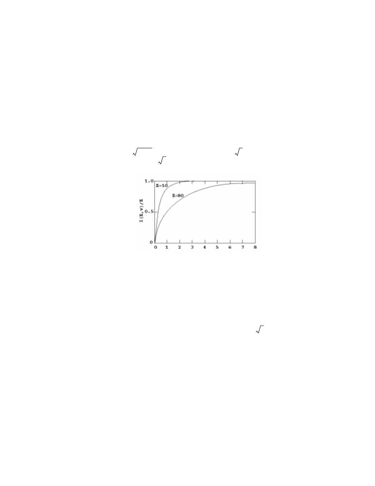
April 10, 2000 2-59
CHAPTER 2
PHYSICS
the new energy Eof the photon, and the recoil kinetic energy of the electron, E−E. The recoil
kinetic energy can be deposited locally, can be transported in Mode P E problems, or (default)
can be treated with the TTB approximation.
Incoherent scattering is assumed to have the differential cross section
, where I(Z,v) is an appropriate scattering factor
modifying the Klein-Nishina cross section in Eq. (2.2).
Qualitatively, the effect of I(Z,v) is to decrease the Klein-Nishina cross section (per electron)
more extremely in the forward direction, for low E and for high Z independently. For any Z,
I(Z,v) increases from to . The parameter v is the inverse length
. The
maximum value of νis at µ=−1. The essential features of I(Z,v) are
indicated in Fig. 2-4.
For hydrogen, an exact expression for the form factor is used:47
,
where f is the inverse fine structure constant, f = 137.0393, and .
The Klein-Nishina formula is sampled exactly by Kahn's method44 below 1.5 MeV and by
Koblinger's method45 above 1.5 MeV as analyzed and recommended by Blomquist and
Gelbard.46 The outgoing energy and angle µ are rejected according to the form factors.
For next event estimators such as detectors and DXTRAN, the probability density for scattering
toward the detector point must be calculated:
′′
σIZαµ,,()dµIZv()Kαµ,()dµ=
IZ0,()0= IZ∞,()Z=
vθ2⁄()λ⁄sin κα 1µ– where κ10 8– moch2()⁄29.1445cm 1–
== = =
m
ax kα2 41.2166
α
==
Figure 2-4.
I1v,()11
11
2
---f2v2
+
4
--------------------------------–=
f2⁄96.9014=
E'
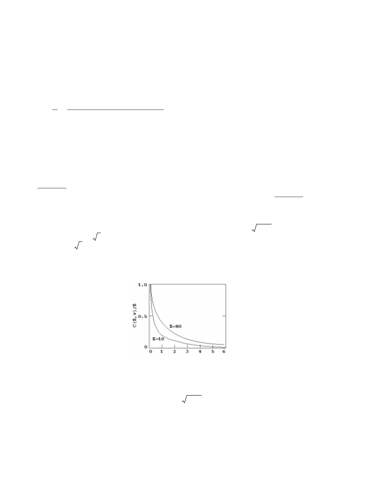
2-60 April 10, 2000
CHAPTER 2
PHYSICS
.
where and σ1(Z, α) and are looked up in the data library.
b. Coherent (Thomson) scattering: Thomson scattering involves no energy loss, and thus
is the only photon process that cannot produce electrons for further transport and that cannot use
the TTB approximation. Only the scattering angle θis computed, and then the transport of the
photon continues.
The differential cross section is σ2(Z, α,µ)dµ=C
2(Z, v)T(µ)dµ, where C(Z, v) is a form factor
modifying the energy-independent Thomson cross section .
The general effect of C2(Z, v)/Z2 is to decrease the Thomson cross section more extremely for
backward scattering, for high E, and low Z. This effect is opposite in these respects to the effect
of I(Z,v)/Z on K(α,µ)in incoherent (Compton) scattering. For a given Z, C(Z,v) decreases from
to . For example, C(Z, v) is a rapidly decreasing function of µas µ
varies from +1to−1, and therefore the coherent cross section is peaked in the forward direction.
At high energies of the incoming photon, coherent scattering is strongly forward and can be
ignored. The parameter v is the inverse length where
. The maximum value of v is
at µ = −1. The square of the maximum value is
. The qualitative features of C(Z,v) are shown in Fig. 2-5.
For next event estimators, one must evaluate the probability density function
for given µ. Here σ2(Z,α) is the integrated coherent
cross section. The value of at must be interpolated in the original
C2(Z,vi) tables separately stored on the cross-section library for this purpose.
pµ() 1
σ1Zα,()
--------------------- IZv,()Kαµ,() πro
2
σ1Zα,()
--------------------- IZv,()
α′
α
-----
2α
α′
----- α′
α
----- µ21–++
==
πro
22494351= IZv,()
Tµ() πr0
21µ2
+()dµ=
CZ0,()Z=CZ∞,()0=
υθ2⁄()λ⁄sin κα 1µ–==
κ10 8– moch2()⁄29.1445cm 1–
==
υmax κα 2 41.2166α==
υmax
21698.8038α2
=
Figure 2-5.
pµ() πr0
21µ2
+()C2Zv,()σ
2Zα,()⁄=C2Zv,()vκα 1µ–=

April 10, 2000 2-61
CHAPTER 2
PHYSICS
Note that at high energies, coherent scattering is virtually straight ahead with no energy loss;
thus, it appears from a transport viewpoint that no scattering took place. For a point detector to
sample this scattering, the point must lie on the original track , which is seldom the case.
Thus, photon point detector variances generally will be much greater with detailed photon
physics than with simple physics unless coherent scattering is turned off with NOCOH = 1 on
the PHYS:P card, as explained on page 2–62.
c. Photoelectric effect: The photoelectric effect consists of the absorption of the incident
photon of energy E, with the consequent emission of several fluorescent photons and the ejection
(or excitation) of an orbital electron of binding energy e<E, giving the electron a kinetic energy
of E−e. Zero, one, or two fluorescent photons are emitted. These three cases are now described.
(1) Zero photons greater than 1 keV are emitted. In this event, the cascade of
electrons that fills up the orbital vacancy left by the photoelectric ejection produces electrons and
low-energy photons (Auger effect). These particles can be followed in Mode P E problems, or
be treated with the TTB approximation, or be assumed to deposit energy locally. Because no
photons are emitted by fluorescence (some may be produced by electron transport or the TTB
model), the photon track is terminated. This photoelectric “capture” of the photon is scored like
analog capture in the summary table of the output file. Implicit capture is not possible.
(2) One fluorescent photon of energy greater than 1 keV is emitted. The photon
energy is the difference in incident photon energy E, less the ejected electron kinetic energy
E−e, less a residual excitation energy that is ultimately dissipated by further Auger processes.
This dissipation leads to additional electrons or photons of still lower energy. The ejected
electron and any Auger electrons can be transported or treated with the TTB approximation. In
general,
.
These primary transactions are taken to have the full fluorescent yield from all possible upper
levels , but are apportioned among the x−ray lines Kα1,,
(mean ); and , (mean ).
(3) Two fluorescence photons can occur if the residual excitation of process (2)
exceeds 1 keV. An electron of binding energy can fill the orbit of binding energy , emitting
a second fluorescent photon of energy . As before, the residual excitation is
dissipated by further Auger events and electron production that can be modeled with electron
transport in Mode P E calculations, approximated with the TTB model, or assumed to deposit
all energy locally. These secondary transitions come from all upper shells and go to Lshells.
Thus the primary transitions must be Kα1 or Kα2 to leave an L shell vacancy.
Each fluorescent photon born as discussed above is assumed to be emitted isotropically and is
transported, provided that , . The binding energies e, , and are very nearly
µ1≅()
E′e′
E′EEe–()–e′–ee′–==
e′L3K→()Kα2L2K→()Kβ′1
;,;
M
K
→kβ2
′NK→
e′
e′′ e′
E′′ e′e′′–= e′′
E′
E′′ 1keV>e′e′′

2-62 April 10, 2000
CHAPTER 2
PHYSICS
the x−ray absorption edges because the x−ray absorption cross section takes an abrupt jump as
it becomes energetically possible to eject (or excite) the electron of energy first , then ,
then e, etc. The jump can be as much as a factor of 20 (for example, K-carbon).
A photoelectric event is terminal for elements Z<12 because the possible fluorescence energy
is below 1 keV. The event is only a single fluorescence of energy above 1 keV for ,
but double fluorescence (each above 1 keV) is possible for . For , primary lines
Kα1,Kα2, and are possible and, in addition, for , the line is possible.
In all photoelectric cases where the photon track is terminated because either no fluorescent
photons are emitted or the ones emitted are below the energy cutoff, the termination is
considered to be caused by analog capture in the output file summary table (and not energy
cutoff).
d. Pair Production: This process is considered only in the field of a nucleus. The
threshold is MeV, where Mis the nuclear mass and m is the mass
of the electron. There are three cases:
(1) In the case of electron transport (Mode P E), the electron and positron are created
and banked and the photon track terminates.
(2) For Mode P problems with the TTB approximation, both an electron and positron
are produced but not transported. Both particles can make TTB approximation photons. If the
positron is below the electron energy cutoff, then it is not created and a photon pair is created as
in case (3).
(3) For Mode P problems when positrons are not created by the TTB approximation,
the incident photon of energy E vanishes. The kinetic energy of the created positron/electron
pair, assumed to be E− 2mc2, is deposited locally at the collision point. The positron is
considered to be annihilated with an electron at the point of collision, resulting in a pair of
photons, each with the incoming photon weight, and each with an energy of mc2=0.511 MeV.
The first photon is emitted isotropically, and the second is emitted in the opposite direction. The
very rare single-annihilation photon of 1.022 MeV is omitted.
e. Caution for detectors and coherent scattering: The use of the detailed photon physics
treatment is not recommended for photon next event estimators (such as point detectors and ring
detectors) nor for DXTRAN, unless coherent scatter is turned off with the NOCOH = 1 option
on the PHYS:P card. Alternatively, the simple physics treatment (EMCPF < .001 on the
PHYS:P card) can be used. Turning off coherent scattering can improve the figure of merit (see
page 2–108) by more than a factor of 10 for tallies with small relative errors because coherent
scattering is highly peaked in the forward direction. Consequently, coherent scattering becomes
undersampled because the photon must be traveling directly at the detector point and undergo a
Ee′′≅e′
31 Z12≥>
Z31≥Z31≥
Kβ′
1Z37≥Kβ2
‘
2mc
2
1mM⁄()+[]1.022≅

April 10, 2000 2-63
CHAPTER 2
PHYSICS
coherent scattering event. When the photon is traveling nearly in the direction of the point
detector or the chosen point on a ring detector or DXTRAN sphere, the PSC term, p(µ), of the
point detector (see page 2–85) becomes very large, causing a huge score for the event and
severely affecting the tally. Remember that p(µ) is not a probability (that can be no larger than
unity); it is a probability density function (the derivative of the probability) and can approach
infinity for highly forward-peaked scattering. Thus the undersampled coherent scattering event
is characterized by many low scores to the detector when the photon trajectory is away from the
detector (p(µ)= small) and a very few very large scores (p(µ)= huge) when the trajectory is
nearly aimed at the detector. Such undersampled events cause a sudden increase in both the tally
and the variance, a sudden drop in the figure of merit, and a failure to pass the statistical checks
for the tally as described on page 2–121.
E. Electron Interactions
The transport of electrons and other charged particles is fundamentally different from that of
neutrons and photons. The interaction of neutral particles is characterized by relatively
infrequent isolated collisions, with simple free flight between collisions. By contrast, the
transport of electrons is dominated by the long-range Coulomb force, resulting in large numbers
of small interactions. As an example, a neutron in aluminum slowing down from 0.5 MeV to
0.0625 MeV will have about 30 collisions, while a photon in the same circumstances will
experience fewer than ten. An electron accomplishing the same energy loss will undergo about
105 individual interactions. This great increase in computational complexity makes a single-
collision Monte Carlo approach to electron transport unfeasible for most situations of practical
interest.
Considerable theoretical work has been done to develop a variety of analytic and semi-analytic
multiple-scattering theories for the transport of charged particles. These theories attempt to use
the fundamental cross sections and the statistical nature of the transport process to predict
probability distributions for significant quantities, such as energy loss and angular deflection.
The most important of these theories for the algorithms in MCNP are the Goudsmit-
Saunderson48 theory for angular deflections, the Landau49 theory of energy-loss fluctuations,
and the Blunck-Leisegang50 enhancements of the Landau theory. These theories rely on a variety
of approximations that restrict their applicability, so that they cannot solve the entire transport
problem. In particular, it is assumed that the energy loss is small compared to the kinetic energy
of the electron.
In order to follow an electron through a significant energy loss, it is necessary to break the
electron's path into many steps. These steps are chosen to be long enough to encompass many
collisions (so that multiple-scattering theories are valid) but short enough that the mean energy
loss in any one step is small (so that the approximations necessary for the multiple-scattering
theories are satisfied). The energy loss and angular deflection of the electron during each of the
steps can then be sampled from probability distributions based on the appropriate multiple-

2-64 April 10, 2000
CHAPTER 2
PHYSICS
scattering theories. This subsumption of the effects of many individual collisions into single
steps that are sampled probabilistically constitutes the “condensed history” Monte Carlo
method.
The most influential reference for the condensed history method is the 1963 paper by Martin J.
Berger.51 Based on the techniques described in that work, Berger and Stephen M. Seltzer
developed the ETRAN series of electron/photon transport codes.52 These codes have been
maintained and enhanced for many years at the National Bureau of Standards (now the National
Institute of Standards and Technology). The ETRAN codes are also the basis for the Integrated
TIGER Series,53 a system of general-purpose, application-oriented electron/photon transport
codes developed and maintained by John A. Halbleib and his collaborators at Sandia National
Laboratories in Albuquerque, New Mexico. The electron physics in MCNP is essentially that of
the Integrated TIGER Series.
1. Electron Steps and Substeps
The condensed random walk for electrons can be considered in terms of a sequence of sets of
values
(0,E0,t0,u0,r0), (s1,E1,t1,u1,r1), (s2,E2,t2,u2,r2), ...
where sn,En,tn,un, and rn are the total path length, energy, time, direction, and position of the
electron at the end of n steps. On the average, the energy and path length are related by
, (2.3)
where −dE/ds is the total stopping power in energy per unit length. This quantity depends on
energy and on the material in which the electron is moving. ETRAN-based codes customarily
choose the sequence of path lengths {sn} such that
, (2.4)
for a constant k. The most commonly used value is k=2−1/8, which results in an average energy
loss per step of 8.3%.
Electron steps with (energy-dependent) path lengths s=s
n−sn-1 determined by Eqs. 2.3-2.4 are
called major steps or energy steps. The condensed random walk for electrons is structured in
terms of these energy steps. For example, all precalculated and tabulated data for electrons are
stored on an energy grid whose consecutive energy values obey the ratio in Eq. 2.4. In addition,
the Landau and Blunck-Leisegang theories for energy straggling are applied once per energy
En1– En
–sn1–
sn
∫
–= dE
ds
-------ds
En
En1–
-------------k=

April 10, 2000 2-65
CHAPTER 2
PHYSICS
step. For a single step, the angular scattering could also be calculated with satisfactory accuracy,
since the Goudsmit-Saunderson theory is valid for arbitrary angular deflections. However, the
representation of the electron's trajectory as the result of many small steps will be more accurate
if the angular deflections are also required to be small. Therefore, the ETRAN codes and MCNP
further break the electron steps into smaller substeps. A major step of path length s is divided
into m substeps, each of path length s/m. Angular deflections and the production of secondary
particles are sampled at the level of these substeps. The integer m depends only on material
(average atomic number Z). Appropriate values for m have been determined empirically, and
range from m= 2 for Z< 6 to m= 15 for Z> 91.
In some circumstances, it may be desirable to increase the value of mfor a given material. In
particular, a very small material region may not accommodate enough substeps for an accurate
simulation of the electron's trajectory. In such cases, the user can increase the value of m with
the ESTEP option on the material card. The user can gain some insight into the selection of m
by consulting Print Table 85 in the MCNP output. Among other information, this table presents
a quantity called DRANGE as a function of energy. DRANGE is the size of an energy step in
g/cm2. Therefore, DRANGE/mis the size of a substep in the same units, and if ρis the material
density in g/cm3, then DRANGE/(mρ) is the length of a substep in cm. This quantity can be
compared with the smallest dimension of a material region. A reasonable rule of thumb is that
an electron should make at least ten substeps in any material of importance to the transport
problem.
2. Condensed Random Walk
In the initiation phase of a transport calculation involving electrons, all relevant data are either
precalculated or read from the electron data file and processed. These data include the electron
energy grid, stopping powers, electron ranges, energy step ranges, substep lengths, and
probability distributions for angular deflections and the production of secondary particles.
Although the energy grid and electron steps are selected according to Eqs. 2.3-2.4, energy
straggling, the analog production of bremsstrahlung, and the intervention of geometric
boundaries and the problem time cutoff will cause the electron’s energy to depart from a simple
sequence sn satisfying Eq. 2.4. Therefore, the necessary parameters for sampling the random
walk will be interpolated from the points on the energy grid.
At the beginning of each major step, the collisional energy loss rate is sampled. In the absence
of energy straggling, this will be a simple average value based on the nonradiative stopping
power described in the next section. In general, however, fluctuations in the energy loss rate will
occur. The number of substeps m per energy step will have been preset, either from the
empirically-determined default values, or by the user, based on geometric considerations. At
most msubsteps will be taken in the current major step, i. e., with the current value for the energy
loss rate. The number of substeps may be reduced if the electron's energy falls below the
boundary of the current major step, or if the electron reaches a geometric boundary. In these

2-66 April 10, 2000
CHAPTER 2
PHYSICS
circumstances, or upon the completion of msubsteps, a new major step is begun, and the energy
loss rate is resampled.
Except for the energy loss and straggling calculation, the detailed simulation of the electron
history takes place in the sampling of the substeps. The Goudsmit-Saunderson48 theory is used
to sample from the distribution of angular deflections, so that the direction of the electron can
change at the end of each substep. Based on the current energy loss rate and the substep length,
the projected energy for the electron at the end of the substep is calculated. Finally, appropriate
probability distributions are sampled for the production of secondary particles. These include
electron-induced fluorescent X−rays, “knock-on” electrons (from electron-impact ionization),
and bremsstrahlung photons.
Note that the length of the substep ultimately derives from the total stopping power used in
Eq. 2.3, but the projected energy loss for the substep is based on the nonradiative stopping
power. The reason for this difference is that the sampling of bremsstrahlung photons is treated
as an essentially analog process. When a bremsstrahlung photon is generated during a substep,
the photon energy is subtracted from the projected electron energy at the end of the substep.
Thus the radiative energy loss is explicitly taken into account, in contrast to the collisional
(nonradiative) energy loss, which is treated probabilistically and is not correlated with the
energetics of the substep. Two biasing techniques are available to modify the sampling of
bremsstrahlung photons for subsequent transport. However, these biasing methods do not alter
the linkage between the analog bremsstrahlung energy and the energetics of the substep.
MCNP uses identical physics for the transport of electrons and positrons, but distinguishes
between them for tallying purposes, and for terminal processing. Electron and positron tracks
are subject to the usual collection of terminal conditions, including escape (entering a region of
zero importance), loss to time cutoff, loss to a variety of variance-reduction processes, and loss
to energy cutoff. The case of energy cutoff requires special processing for positrons, which will
annihilate at rest to produce two photons, each with energy m c2= 0.511008 MeV.
3. Stopping Power
3a. Collisional Stopping Power
Berger51 gives the restricted electron collisional stopping power, i. e., the energy loss per unit
path length to collisions resulting in fractional energy transfers εless than an arbitrary maximum
value εm, in the form
, (2.5)
dE
ds
-------
εm
–
NZC E2τ2+()
2I2
----------------------- f–τε
m
,()δ–+ln
=

April 10, 2000 2-67
CHAPTER 2
PHYSICS
where
(2.6)
+.
Here ε and εm represent energy transfers as fractions of the electron kinetic energy E;I is the
mean ionization potential in the same units as E;βis v/c;τis the electron kinetic energy in units
of the electron rest mass; δ is the density effect correction (related to the polarization of the
medium); Zis the average atomic number of the medium; Nis the atom density of the medium
in cm−3; and the coefficient C is given by
, (2.7)
where m,e, and vare the rest mass, charge, and speed of the electron, respectively. The density
effect correction δis calculated using the prescriptions of Sternheimer, Berger and Seltzer54 in
the el03 evaluation and using the method of Sternheimer and Peierls55 for the el1 evaluation.
The ETRAN codes and MCNP do not make use of restricted stopping powers, but rather treat
all collisional events in an uncorrelated, probabilistic way. Thus, only the total energy loss to
collisions is needed, and Eqs. 2.5-2-6 can be evaluated for the special value εm=1/2. The rea-
son for the 1/2 is the indistinguishability of the two outgoing electrons. The electron with the
larger energy is, by definition, the primary. Therefore, only the range ε< 1/2 is of interest. With
εm=1/2, Eq. 2.6 becomes
. (2.8)
On the right side of Eq. 2.5, we can express both Eand Iin units of the electron rest mass. Then
E can be replaced by τon the right side of the equation. We also introduce supplementary
constants
(2.9)
f–τε
m
,() 1– β2
–τ
τ1+
------------
2ε2
m
2
-------- 2τ1+
τ1+()
2
-------------------1εm
–()ln++=
4εm1εm
–()[]
1
1εm
–
---------------+ln
C2πe4
mv2
------------=
f–τε
m
,() β
2
–12ln–()
1
8
---2ln+
τ
τ1+
------------
2
++=
C22I2
(),ln=
C31 2,ln–=
C41
8
---2,ln+=

2-68 April 10, 2000
CHAPTER 2
PHYSICS
so that Eq. 2.5 becomes
(2.10)
This is the collisional energy loss rate in MeV/cm in a particular medium. In MCNP, we are
actually interested in the energy loss rate in units of MeV barns (so that different cells containing
the same material need not have the same density). Therefore, we divide Eq. 2.10 by N and
multiply by the conversion factor 1024 barns/cm2. We also use the definition of the fine structure
constant
,
where his Planck's constant, to eliminate the electronic charge efrom Eq. 2.10. The result is as
follows:
(2.11)
This is the form actually used in MCNP to preset the collisional stopping powers at the energy
boundaries of the major energy steps.
The mean ionization potential and density effect correction depend upon the state of the
material, either gas or solid. In the fit of Sternheimer and Peierls55 the physical state of the
material also modifies the density effect calculation. In the Sternheimer, Berger and Seltzer54
treatment, the calculation of the density effect uses the conduction state of the material to
determine the contribution of the outermost conduction electron to the ionization potential. The
occupation numbers and atomic binding energies used in the calculation are from Carlson.56
3b. Radiative Stopping Power
The radiative stopping power is
where is the scaled electron-nucleus radiative energy-loss cross section based upon
evaluations by Berger and Seltzer for either el1 and el03 (details of the numerical values of the
dE
ds
-------
–NZ2πe4
mv2
------------τ2τ2+()[]C2– C3β2
–C4τ
τ1+
------------
2δ–++ln
=
α2πe2
hc
------------=
dE
ds
-------
–1024α2h2c2
2πmc2
---------------------------- Zτ2τ2+()[]C2– C3β2
–C4τ
τ1+
------------
2δ–++ln
1
β2
-----
=
dE
ds
-------
rad
–10
24ZZ η+()αre
2
()Tmc
2
+()Φ
rad
n()
=
Φrad
n()

April 10, 2000 2-69
CHAPTER 2
PHYSICS
el03 evaluation can be found in Ref. 57, Ref. 58, and Ref. 59; is a parameter to account for
the effect of electron-electron bremsstrahlung (it is unity in the el1 evaluation and, in the el03
evaluation, it is based upon the work of S. Seltzer and M. Berger57,58,59 and can be different from
unity); α is the fine structure constant, mc2 is the mass energy of an electron, and re is the
classical electron radius. The dimensions of the radiative stopping power are the same as the
collisional stopping power.
4. Energy Straggling
Because an energy step represents the cumulative effect of many individual random collisions,
fluctuations in the energy loss rate will occur. Thus the energy loss will not be a simple average
; rather there will be a probability distribution f(s,∆)d∆from which the energy loss ∆for the
step of length s can be sampled. Landau49 studied this situation under the simplifying
assumptions that the mean energy loss for a step is small compared with the electron’s energy,
that the energy parameter ξdefined below is large compared with the mean excitation energy of
the medium, that the energy loss can be adequately computed from the Rutherford60 cross
section, and that the formal upper limit of energy loss can be extended to infinity. With these
simplifications, Landau found that the energy loss distribution can be expressed as
in terms of , a universal function of a single scaled variable
Here mand vare the mass and speed of the electron, δis the density effect correction, βis v/c,I
is the mean excitation energy of the medium, and γis Euler’s constant . The
parameter ξ is defined by
where eis the charge of the electron and NZis the number density of atomic electrons, and the
universal function is
where x is a positive real number specifying the line of integration.
η
∆
fs∆,()d∆φλ()dλ=
φλ()
λ∆
ξ
--- 2ξmv2
1β2
–()I2
------------------------ δβ
21– γ⋅++ +ln–=
γ0.5772157…=()
ξ2πe4NZ
mv2
-------------------- s,=
φλ() 1
2πi
-------- eµµλµ+ln µ,d
xi∞–
xi∞+
∫
=

2-70 April 10, 2000
CHAPTER 2
PHYSICS
For purposes of sampling, is negligible for , so that this range is ignored. B rsch -
Supan61 originally tabulated in the range , and derived for the range
the asymptotic form
in terms of the auxiliary variable w, where
.
Recent extensions62 of B rsch-Supan's tabulation have provided a representation of the function
in the range in the form of five thousand equally probable bins in λ. In MCNP, the
boundaries of these bins are saved in the array eqlm(mlam), where mlam =5001. Sampling from
this tabular distribution accounts for approximately 98.96% of the cumulative probability for
. For the remaining large-λ tail of the distribution, MCNP uses the approximate form
, which is easier to sample than (w2 + π2)−1, but is still quite accurate for λ> 100.
Blunck and Leisegang50 have extended Landau’s result to include the second moment of the
expansion of the cross section. Their result can be expressed as a convolution of Landau's
distribution with a Gaussian distribution:
.
Blunck and Westphal63 provided a simple form for the variance of the Gaussian:
.
Subsequently, Chechin and Ermilova64 investigated the Landau/Blunck-Leisegang theory, and
derived an estimate for the relative error
caused by the neglect of higher-order moments. Based on this work, Seltzer65 describes and
recommends a correction to the Blunck-Westphal variance:
φλ() λ 4–<o
˙˙
φλ() 4λ100≤≤–λ100>
φλ() 1
w2π2
+
------------------ ,≈
λwwγ3
2
---–+ln+=
o
˙˙
4λ100≤≤–
φλ()
φλ() w2–
≈
f∗s∆,() 1
2πσ
-------------- fs∆′,() ∆∆′–()
2
2σ2
----------------------
exp ∆′d
∞–
∞+
∫
=
σBW
210eV Z43⁄∆⋅=
εCE 10ξ
I
---------1ξ
10I
--------+
31
2
---–
≈

April 10, 2000 2-71
CHAPTER 2
PHYSICS
.
This value for the variance of the Gaussian is used in MCNP.
Examination of the asymptotic form for shows that unrestricted sampling of λ will not
result in a finite mean energy loss. Therefore, a material− and energy−dependent cutoff λcis
imposed on the sampling of λ. In the initiation phase of an MCNP calculation, the code makes
use of two preset arrays, flam(mlanc) and avlm(mlanc), with mlanc =1591. The array flam contains
candidate values for λcin the range ; the array avlm contains the corresponding
expected mean values for the sampling of λ. For each material and electron energy, the code uses
the known mean collisional energy loss , interpolating in this tabular function to select a
suitable value for λc, which is then stored in the dynamically-allocated array flc. During the
transport phase of the calculation, the value of flc applicable to the current material and electron
energy is used as an upper limit, and any sampled value of λgreater than the limit is rejected. In
this way, the correct mean energy loss is preserved.
5. Angular Deflections
The ETRAN codes and MCNP rely on the Goudsmit-Saunderson48 theory for the probability
distribution of angular deflections. The angular deflection of the electron is sampled once per
substep according to the distribution
,
where sis the length of the substep, is the angular deflection from the direction at the
beginning of the substep, Pl(µ) is the lth Legendre polynomial, and Gl is
,
in terms of the microscopic cross section , and the atom density N of the medium.
For electrons with energies below 0.256 MeV, the microscopic cross section is taken from
numerical tabulations developed from the work of Riley.66 For higher-energy electrons, the
microscopic cross section is approximated as a combination of the Mott67 and Rutherford60
cross sections, with a screening correction. Seltzer52 presents this “factored cross section” in the
form
σσBW
13εCE
+
---------------------=
φλ()
4λc50000≤≤–
∆
Fsµ,() l1
2
---+
sGl
–()Plµ()exp
l0=
∞
∑
=
µθcos=
Gl2πN1–
1+
∫dσ
dΩ
------- 1Plµ()–[]dµ=
dσdΩ⁄

2-72 April 10, 2000
CHAPTER 2
PHYSICS
,
where e,p, and v are the charge, momentum, and speed of the electron, respectively. The
screening correction was originally given by Molière68 as
,
where αis the fine structure constant, mis the rest mass of the electron, and β=v/c. MCNP now
follows the recommendation of Seltzer,52 and the implementation in the Integrated TIGER
Series, by using the slightly modified form
,
where τis the electron energy in units of electron rest mass. The multiplicative factor in the final
term is an empirical correction which improves the agreement at low energies between the
factored cross section and the more accurate partial-wave cross sections of Riley.
6. Bremsstrahlung
In the el1 evaluation, for the sampling of bremsstrahlung photons, MCNP relies primarily on the
Bethe-Heitler69 Born-approximation results that have been used until rather recently57 in
ETRAN. A comprehensive review of bremsstrahlung formulas and approximations relevant to
the present level of the theory in MCNP can be found in the paper of Koch and Motz.70 Particular
prescriptions appropriate to Monte Carlo calculations have been developed by Berger and
Seltzer.71 For the ETRAN-based codes, this body of data has been converted to tables including
bremsstrahlung production probabilities, photon energy distributions, and photon angular
distributions.
In the el03 evaluation, the production cross section for bremsstrahlung photons and energy
spectra are from the evaluation by Seltzer and Berger.57,58,59 We summarize the salient features
of the evaluation below; more details can be found in the evaluators’ documentation. The
evaluation uses detailed calculations of the electron-nucleus bremsstrahlung cross section for
electrons with energies below 2 MeV and above 50 MeV. The evaluation below 2 MeV uses the
results of Pratt, Tseng, and collaborators, based on numerical phase-shift calculations.72,73,74 For
50 MeV and above, the analytical theory of Davies, Bethe, Maximom, and Olsen75 is used and
is supplemented by the Elwert Coulomb76 correction factor and the theory of the high-frequency
limit or tip region given by Jabbur and Pratt.77 Screening effects are accounted for by the use of
Hartree-Fock atomic form factors.78 The values between these firmly grounded theoretical limits
dσ
dΩ
------- Z2e2
p2v21µ–2η+()
2
-------------------------------------------- dσdΩ⁄()
Mott
dσdΩ⁄()
Rutherford
----------------------------------------------
=
η
η1
4
---αmc
0.885p
-----------------
2Z23⁄1.13 3.76 αZβ⁄()
2
+[]=
η1
4
---αmc
0.885p
-----------------
2Z23⁄1.13 3.76 αZβ⁄()
24
τ1+
------------+=

April 10, 2000 2-73
CHAPTER 2
PHYSICS
are found by a cubic-spline interpolation as described in Ref. 57 and Ref. 58. Seltzer reports
good agreement between interpolated values and those calculated by Tseng and Pratt79 for 5 and
10 MeV electrons in aluminum and uranium. Electron-electron bremsstrahlung is also included
in the cross section evaluation based on the theory of Haug80 with screening corrections derived
from Hartree-Fock incoherent scattering factors.78 The energy spectra for the bremsstrahlung
photons are provided in the evaluation. No major changes were made to the tabular angular
distributions, which are internally calculated when using the el1 evaluation, except to make finer
energy bins over which the distribution is calculated.
MCNP addresses the sampling of bremsstrahlung photons at each electron substep. The tables
of production probabilities are used to determine whether a bremsstrahlung photon will be
created. In the el03 evaluation, the bremsstrahlung production is sampled according to a Poisson
distribution along the step so that none, one or more photons could be produced; the el1
evaluation allows for either none or one bremsstrahlung photon in a substep. If a photon is
produced, the new photon energy is sampled from the energy distribution tables. By default, the
angular deflection of the photon from the direction of the electron is also sampled from the
tabular data. The direction of the electron is unaffected by the generation of the photon, because
the angular deflection of the electron is controlled by the multiple scattering theory. However,
the energy of the electron at the end of the substep is reduced by the energy of the sampled
photon, because the treatment of electron energy loss, with or without straggling, is based only
on nonradiative processes.
There is an alternative to the use of tabular data for the angular distribution of bremsstrahlung
photons. If the fourth entry on the PHYS:E card is 1, then the simple, material-independent
probability distribution
, (2.12)
where and β=v/c, will be used to sample for the angle of the photon relative to the
direction of the electron according to the formula
,
where ξis a random number. This sampling method is of interest only in the context of detectors
and DXTRAN spheres. A set of source contribution probabilities p(µ) consistent with the tabular
data is not available. Therefore, detector and DXTRAN source contributions are made using
Eq. 2.12. Specifying that the generation of bremsstrahlung photons rely on Eq. 2.12 allows the
user to force the actual transport to be consistent with the source contributions to detectors and
DXTRAN.
pµ()dµ1β2
–
21 βµ–()
2
-------------------------- dµ=
µθcos=
µ2ξ1– β–
2ξβ 1– β–
----------------------------=

2-74 April 10, 2000
CHAPTER 2
PHYSICS
7. K-shell electron impact ionization and Auger transitions
The el03 evaluation does not change the K-shell impact ionization calculation (based upon
ITS1.0) except for how the emission of relaxation photons is treated; the el03 evaluation model
has been modified to be consistent with the photo-ionization relaxation model. In the el1
evaluation, a K-shell impact ionization event generated a photon with the average K-shell
energy. The el03 evaluation generates photons with energies given by Everett and Cashwell.33
Both el03 and el1 treatments only take into account the highest Z component of a material. Thus
inclusion of trace high Z impurities could mask K-shell impact ionization from other dominant
components.
Auger transitions are handled the same in the el03 and el1 evaluations. If an atom has undergone
an ionizing transition and can undergo a relaxation, if it does not emit a photon it will emit an
Auger electron. The difference between el1 and el03 is the energy with which an Auger electron
is emitted, given by or for el1 or e03, respectively. The el1
value is that of the highest energy Auger electron while the el03 value is the energy of the most
probable Auger electron. It should be noted that both models are somewhat crude.
8. Knock-On Electrons
The Møller cross section81 for scattering of an electron by an electron is
, (2.13)
where ∈,τ,E, and C have the same meanings as in Eqs. 2.5-2.7. When calculating stopping
powers, one is interested in all possible energy transfers. However, for the sampling of
transportable secondary particles, one wants the probability of energy transfers greater than
some εc representing an energy cutoff, below which secondary particles will not be followed.
This probability can be written
.
The reason for the upper limit of 1/2 is the same as in the discussion of Eq. 2.8. Explicit
integration of Eq. 2.13 leads to
.
EAEK
=
E
AEK2EL
–=
εd
dσC
E
----1
ε2
-----1
1ε–()
2
------------------ τ
τ1+
------------
22τ1+
τ1+()
2
-------------------1
ε1ε–()
-------------------
–++
=
σε
c
() εd
dσεd
εc
12⁄
∫
=
σε
c
() C
E
----1
εc
---- 1
1εc
–
-------------–τ
τ1+
------------
21
2
---εc
–
2τ1+
τ1+()
2
-------------------1εc
–
εc
-------------
ln–+
=

April 10, 2000 2-75
CHAPTER 2
PHYSICS
Then the normalized probability distribution for the generation of secondary electrons with
ε>ε
cis given by
. (2.14)
At each electron substep, MCNP uses σ(εc) to determine randomly whether knock-on electrons
will be generated. If so, the distribution of Eq. 2.14 is used to sample the energy of each
secondary electron. Once an energy has been sampled, the angle between the primary direction
and the direction of the newly generated secondary particle is determined by momentum
conservation. This angular deflection is used for the subsequent transport of the secondary
electron. However, neither the energy nor the direction of the primary electron is altered by the
sampling of the secondary particle. On the average, both the energy loss and the angular
deflection of the primary electron have been taken into account by the multiple scattering
theories.
9. Multigroup Boltzmann−Fokker−Planck Electron Transport
The electron physics described above can be implemented into a multigroup form using a hybrid
multigroup/continuous-energy method for solving the Boltzmann−Fokker−Planck equation as
described by Morel.39 The multigroup formalism for performing charged charged particle
transport was pioneered by Morel and Lorence40 for use in deterministic transport codes. With
a first order treatment for the continuous slowing down approximation (CSDA) operator, this
formalism is equally applicable to a standard Monte Carlo multigroup transport code as
discussed by Sloan.82 Unfortunately, a first order treatment is not adequate for many
applications. Morel, et.al. have addressed this difficulty by developing a hybrid multigroup/
continuousenergy algorithm for charged particles that retains the standard multigroup treatment
for large-angle scattering, but treats exactly the CSDA operator. As with standard multigroup
algorithms, adjoint calculations are performed readily with the hybrid scheme.
The process for performing an MCNP/MGBFP calculation for electron/photon transport
problems involves executing three codes. First the CEPXS40 code is used to generate coupled
electron−photon multigroup cross sections. Next the CRSRD code casts these cross sections into
a form suitable for use in MCNP by adjusting the discrete ordinate moments into a Radau
quadrature form that can be used by a Monte Carlo code. CRSRD also generates a set of
multigroup response functions for dose or charge deposition that can be used for response
estimates for a forward calculation or for sources in an adjoint calculation. Finally, MCNP is
executed using these adjusted multigroup cross sections. Some applications of this capability for
electron/photon transport have been presented in Ref. 83.
gεε
c
,()dε1
σε
c
()
------------- εd
dσεd=

2-76 April 10, 2000
CHAPTER 2
TALLIES
V. TALLIES
MCNP provides seven standard neutron tallies, six standard photon tallies, and four standard
electron tallies. These basic tallies can be modified by the user in many ways. All tallies are
normalized to be per starting particle except in KCODE criticality problems.
The above seven tally categories represent the basic MCNP tally types. To have many tallies of
a given type, add multiples of 10 to the tally number. For example, F1, F11, F21...F981, F991
are all type F1 tallies. Particle type is specified by appending a colon and the particle designator.
For example, F11:N and F96:N are neutron tallies and F2:P and F25:P are photon tallies. F6
tallies can be for both neutrons and photons − F16:N,P. F8 tallies are for both photons and
electrons: F8:P, F8:E, and F8:P,E are all identical. F8:N is also allowed, though not advised,
because MCNP neutron transport does not currently sample joint collision exit densities in an
analog way.
Thought should be given to selecting a tally and to comparing one tally with another. For
example, if the flux is varying as 1/R2in a cell, an average flux in the cell determined by the F4
tally will be higher than the flux at a point in the center of the cell determined by a detector. This
same consideration applies to the average flux provided by DXTRAN spheres (see page 2–150).
Standard summary information that gives the user a better insight into the physics of the problem
and the adequacy of the Monte Carlo simulation includes a complete accounting of the creation
and loss of all tracks and their energy; the number of tracks entering and reentering a cell plus
the track population in the cell; the number of collisions in a cell; the average weight, mean free
path, and energy of tracks in a cell; the activity of each nuclide in a cell; and a complete weight
balance for each cell.
Tally Mnemonic Description
F1:N or F1:P or F1:E Surface current
F2:N or F2:P or F2:E Surface flux
F4:N or F4:P or F4:E Track length estimate of cell flux
F5a:N or F5a:P Flux at a point or ring detector
F6:N or F6:P or F6:N,P Track length estimate of energy deposition
F7:N Track length estimate of fission energy deposition
F8:N or F8:P or F8:E Pulse height tally
or F8:P,E

April 10, 2000 2-77
CHAPTER 2
TALLIES
The quantities actually scored in MCNP before the final normalization per starting particle are
presented in Table 2.1. Note that adding an asterisk (∗Fn) changes the units and multiplies the
tally as indicated in the last column of Table 2.1. For an F8 pulse height tally the asterisk changes
the tally from deposition of pulses to an energy deposition tally. Table 2.1 also defines much of
the notation used in the remainder of this section.
Extensive statistical analysis of tally convergence also is applied to one bin of each tally. Ten
statistical checks are made, including the variance of the variance and the Pareto slope of the
tally density function. These are described in detail starting on page 2–99.
W=particle weight
Ws=source weight
E= particle energy (MeV)
|µ| = absolute value of cosine of angle between surface normal and particle trajectory.
If |µ| < .1, set |µ| = .05.
A= surface area (cm2)
Tl= track length (cm) = transit time ∗ velocity
V= volume (cm3)
p(µ) = probability density function: µ= cosine of angle between particle trajectory and
detector
λ= total mean free path to detector
R= distance to detector (cm)
σT(E) = microscopic total cross section (barns)
H(E) = heating number (MeV/collision)
ρa= atom density (atoms/barn-cm)
m= cell mass (gm)
TABLE 2.1:
Tally Quantities Scored
Tally Fn
Quantity Fn
Units ∗Fn
Multiplier ∗Fn
Units
F1 W E MeV
F2 W/(|µ| ∗ A) 1/cm2E MeV/cm2
F4 W∗ Tl/V1/cm2E MeV/cm2
F5 W∗ p(µ)∗ exp(−λ)/(2π R2) 1/cm2E MeV/cm2
F6 W ∗ Tl∗ σT(Ε) ∗ Η(Ε) ∗ ρa/m MeV/gm 1.60219E−22 jerks/gm
F7 W∗ Tl∗σ
f(E)*Q ∗ρ
a/mMeV/gm 1.60219E−22 jerks/gm
F8 Ws put in bin E∗ W/Wspulses E MeV

2-78 April 10, 2000
CHAPTER 2
TALLIES
σf(E) = microscopic fission cross section (barns)
Q= fission heating Q-value (MeV)
The following MCNP definitions of current and flux come from reactor theory but are related to
similar quantities in radiative transfer theory. The MCNP particle angular flux multiplied by the
particle energy is the same as the intensity in radiative transfer theory. The MCNP particle total
flux at energy Emultiplied by the particle energy equals the integrated energy density times the
speed of light in radiative transfer theory. The MCNP particle current multiplied by the particle
energy is analogous to the radiative flux crossing an area in radiative transfer theory. The MCNP
particle current uses |µ| in the definition, whereas the radiative transfer flux uses µ in its
definition. MCNP current is neither net nor positive nor negative current; it is the number of
particles crossing a surface in a particular direction. The MCNP particle fluence multiplied by
the particle energy is the same as the fluence in radiative transfer theory.
A. Surface Current Tally
The F1 surface current tally estimates the following quantity:
.
This tally is the number of particles (quantity of energy for ∗F1) crossing a surface. The scalar
current is related to the flux as . The range of integration over
area, energy, time, and angle (A,E,t,µ) can be controlled by FS, E, T, and C cards, respectively.
The FT card can be used to change the vector relative to which µis calculated (FRV option) or
to segregate electron current tallies by charge (ELC option).
B. Flux Tallies
The F2, F4 and F5 flux tallies are estimates of
∗
F1Jr Etµ,,,()
E
∫
t
∫
µ
∫
A
∫
=dE dt dµdA
∗F1ΕJr Etµ,,,()EdtdµAdd
E
∫
t
∫
µ
∫
A
∫
=∗
Jr Etµ,,,()µΦrEt,,()A=
F2ΦrEt,,()td Ad
A
------
E
∫
t
∫
A
∫
=
F2E∗ΦrEt,,()EdtdAd
A
------
E
∫
t
∫
A
∫
=

April 10, 2000 2-79
CHAPTER 2
TALLIES
∗
∗
The range of integration over energy and time is controlled by E and T cards. The F2 surface flux
and F4 cell flux tallies are discussed below. The F5 detector flux tally, a major topic, is discussed
on page 2–85.
The units of the flux tally are the units of the source. If the source has units of particles per unit
time, the tally is also particles per unit time. When the source has units of particles, this tally
represents a fluence tally. A steady-state flux solution can be obtained by having a source with
units of particles per unit time and integrating over all time (that is, omitting the Tn card). The
flux can be obtained from the fluence tally for a time-dependent source by dividing the tally by
the time bin width. These tallies can all be made per unit energy by dividing by the energy bin
width.
1. Track Length Estimate of Cell Flux (F4)
The definition of particle flux is , where v= particle velocity and
N=particle density = particle weight/unit volume. Roughly speaking, the time integrated flux is
.
More precisely, let ds = vdt. Then the time-integrated flux is
.
Because is a track length density, MCNP estimates this integral by summing
WTl/V for all particle tracks in the cell, time range, and energy range. Because of the track length
term Tlin the numerator, this tally is known as a track length estimate of the flux. It is generally
quite reliable because there are frequently many tracks in a cell (compared to the number of
collisions), leading to many contributions to this tally.
F4ΦrEt,,()EdtdVd
V
-------
E
∫
t
∫
V
∫
=
F4E∗ΦrEt,,()EdtdVd
V
-------
E
∫
t
∫
V
∫
=
F5ΦrEt,,()Edtd
E
∫
t
∫
=
F
5EΦrEt,,()Edtd
E
∫
t
∫
=∗
ΦrEt,,()vN r E t,,()=
ΦrEt,,()EdtdVd
V
-------
E
∫
t
∫
V
∫Wv t V⁄WTlV⁄==
ΦrEt,,()tdEdVd
V
-------
t
∫
E
∫
V
∫NrEt,,()sdEdVd
V
-------
s
∫
E
∫
v
∫
=
NrEt,,()ds
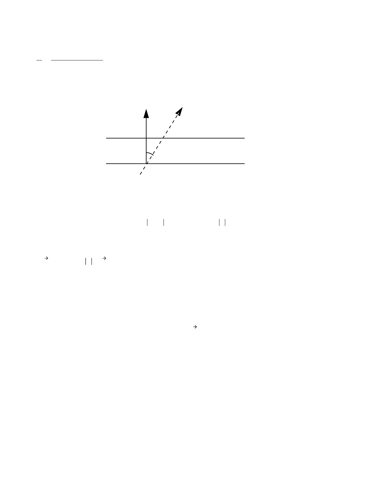
2-80 April 10, 2000
CHAPTER 2
TALLIES
2. Surface Flux (F2)
The surface flux is a surface estimator but can be thought of as the limiting case of the cell flux
or track length estimator when the cell becomes infinitely thin as illustrated in Fig. 2-6.
Figure 2-6.
As the cell thickness δapproaches zero, the volume approaches Aδand the track length
approaches δ/|µ|, where , the angle between the surface normal and the particle
trajectory. This definition of flux also follows directly from the relation between flux and current,
. MCNP sets |µ| = .05 when |µ| < .1. The F2 tally is essential for
stochastic calculation of surface areas when the normal analytic procedure fails.
C. Track Length Cell Energy Deposition Tallies
The F6 and F7 cell heating and energy deposition tallies are the following track length estimates
,
where
ρa=atom density (atoms/barn-cm)
ρg= gram density (grams/cm3)
H(E) =heating response (summed over nuclides in a material)
The units of the heating tally are MeV/gm. An asterisk (∗F6,7)changes the units to jerks/gm (1
MeV =1.60219E-22 jerks). The asterisk causes the F6,7 tally to be modified by a constant rather
Θ
δ
F2WTl
δ0→
lim V⁄=
Wδθcos⁄()Aδ()⁄=WAµ()⁄=
µθcos=
JrEtµ,,,()µΦrEt,,()A=
F
67,ρaρg
⁄HE()ΦrEt,,()EdtdVd
V
-------
E
∫
t
∫
V
∫
=

April 10, 2000 2-81
CHAPTER 2
TALLIES
than by energy as in other tallies. Note that the heating tallies are merely flux tallies (F4)
multiplied by an energy-dependent multiplier (FM card).
Energy deposition for photons and electrons can be computed with the ∗F8 tally, which is a
surface estimator rather than a track length estimator. See page 2–83 .
The F7 tally includes the gamma heating because the photons are deposited locally. The F6 tally
deposits the photons elsewhere, so it does not include gamma heating. Thus for fissionable
materials, the F7 result often will be greater than the F6 result even though F7 includes only
fission and F6 includes all reactions. The true heating is found by summing the neutron and
photon F6 tallies in a coupled neutron/photon calculation. In a neutron-only problem, F6 will
give the right heating of light materials only if all photons escape the geometry. F7 will give
about the right heating of fissionable materials only if no photons come from elsewhere, all
fission photons are immediately captured, and nonfission reactions can be ignored. The F7 tally
cannot be used for photons. Examples of combining the neutron and photon F6 tallies are F6:N,P
and F516:P,N
The heating response H(E) has different meanings, depending upon context as follows:
1. F6 Neutrons
H(E) =σ
T(E) Havg(E), where the heating number is
,
and
σT= total neutron cross section,
E= incident neutron energy,
pi(E) = probability of reaction i,
= average exiting neutron energy for reaction i,
Qi= Q-value of reaction i,
= average energy of exiting gammas for reaction i.
2. F6 Photons
H(E) =σ
T(E)Havg(E), where the heating number is
∗
H
avg E() Ep
iE()EoutiE() QiEγiE()+–[]
i
∑
–=
Eouti
Eγi
Havg E() piE()
i1=
3
∑
=EE
out
–()

2-82 April 10, 2000
CHAPTER 2
TALLIES
i= 1 incoherent (Compton) scattering with form factors
i= 2 pair production
i = 3 photoelectric.
All energy transferred to electrons is assumed to be deposited locally.
3. F7 Neutrons
,
where
σf(E) = total fission cross section and
Q= fission Q-value (MeV).
The Q-values as tabulated represent the total prompt energy release per fission and are printed
in optional PRINT TABLE 98. The total fission cross section is (n,f) + (n,nf) + .
4. F7 Photons
H(E) is undefined because photofission is not included in MCNP.
5. Equivalence of F4, F6, and F7 Tallies
The F6 and F7 heating tallies are special cases of the F4 track length estimate of cell flux with
energy-dependent multipliers. The following F4 and FM4 combinations give exactly the same
results as the F6 and F7 tallies. In this example, material 9 in cell 1 is 235U with an atom density
(ρa) of .02 atoms/barn-cm and a gram density (ρg) of 7.80612 g/cm3 for an atom/gram ratio of
.0025621.
F4:N 1
FM4 .0025621 9 1 4 gives the same result as F6:N 1
F14:N 1
FM14 .0025621 9 −6 8 gives the same result as F17:N 1
F24:P 1
FM24 .0025621 9 5 6 gives the same result as F26:P 1
For the photon results to be identical, both electron transport and the thick target bremsstrahlung
approximation must be turned off by PHYS:P j 1. In the F6 tally, if a photon produces an electron
that produces a photon, the second photon is not counted again. It is already tallied in the first
photon heating. In the F4 tally, the second photon track is counted, so the F4 tally will slightly
overpredict the tally.
Eout 1.022016 2moc2
==
HE() σ
fE()Q=
…

April 10, 2000 2-83
CHAPTER 2
TALLIES
The photon heating tally also can be checked against the ∗F8 energy deposition tally (divided by
cell mass to give answers in MeV per gram). Results will not be identical because the tallies are
totally independent and use different estimators.
The FM card can be used to make the surface flux tally (F2) and point and ring detector tallies
(F5) calculate heating as well.
D. Pulse Height Tallies
The pulse height tally provides the energy distribution of pulses created in a cell that models a
physical detector. It also can provide the energy deposition in a cell. Although the entries on the
F8 card are cells, this is not a track length cell tally. F8 tallies are made at source points and at
surface crossings.
The pulse height tally is analogous to a physical detector. The F8 energy bins correspond to the
total energy deposited in a detector in the specified channels by each physical particle. All the
other MCNP tallies record the energy of a scoring track in the energy bin.
In an experimental configuration, suppose a source emits 100 photons at 10 MeV, and ten of
these get to the detector cell. Further, suppose that the first photon (and any of its progeny created
in the cell) deposits 1 keV in the detector before escaping, the second deposits 2 keV, and so on
up to the tenth photon which deposits 10 keV. Then the pulse height measurement at the detector
would be one pulse in the 1 keV energy bin, 1 pulse in the 2 keV energy bin, and so on up to 1
pulse in the 10 keV bin.
In the analogous MCNP pulse height tally, the source cell is credited with the energy times the
weight of the source particle. When a particle crosses a surface, the energy times the weight of
the particle is subtracted from the account of the cell that it is leaving and is added to the account
of the cell that it is entering. The energy is the kinetic energy of the particle plus
2moc2=1.022016 if the particle is a positron. At the end of the history, the account in each tally
cell is divided by the source weight. The resulting energy determines which energy bin the score
is put in. The value of the score is the source weight for an F8 tally and the source weight times
the energy in the account for a ∗F8 tally. The value of the score is zero if no track entered the
cell during the history.
The pulse height tally is an inherently analog process. Therefore, it does not work well with
neutrons, which are inherently non analog, and it does not work at all with most variance
reduction schemes. The pulse height tally depends on sampling the joint density of all particles
exiting a collision event. MCNP does not currently sample this joint density for neutron
collisions. Thus neutron F8 tallies must be done with extreme caution when more than one
neutron can exit a collision. Suppose in the above example, the photon that deposited 10 keV in
the detector cell underwent a 2−for−1 split. Then if only one of the split halves entered the cell,

2-84 April 10, 2000
CHAPTER 2
TALLIES
the tally would be incorrectly put in the 5 keV bin rather than the 10 keV bin. Or if the particle
survived a Russian roulette event, its weight would be double and the score would be put into
the 20 keV bin. Similar scenarios can be given for other variance reduction methods. The MCNP
pulse height tally will not work with any variance reduction other than source biasing. It doesn't
work well with neutrons even without variance reduction because the MCNP neutron physics is
nonanalog (in the joint density sampling), particularly in the way that multiple neutrons exiting
a collision are totally uncorrelated and don't even conserve energy except in an average sense
over many neutron histories.
Another aspect of the pulse height tally that is different from other MCNP tallies is that F8:P,
F8:E and F8:P,E are all equivalent. All the energy from both photons and electrons, if present,
will be deposited in the cell, no matter which tally is specified.
When the pulse height tally is used with energy bins, care must be taken because of negative
scores from nonanalog processes and zero scores caused by particles passing through the pulse
height cell without depositing energy. In some codes, like the Integrated Tiger Series, these
events cause large contributions to the lowest energy bin pulse height score. In other codes no
contribution is made. MCNP compromises by counting these events in a zero bin and an epsilon
bin so that these scores can be segregated out. It is recommended that your energy binning for
an F8 tally be something like
E8 0 1 E -5 E1 E2 E3 E4 E5
Knock-on electrons in MCNP are nonanalog in that the energy loss is included in the multiple
scattering energy loss rate rather than subtracted out at each knock−on event. Thus knock−ons
can cause negative energy pulse height scores. These scores will be caught in the 0 energy bin.
If they are a large fraction of the total F8 tally, then the tally is invalid because of nonanalog
events. Another situation is differentiating zero contributions from particles not entering the cell
and particles entering the cell but not depositing any energy. These are differentiated in MCNP
by causing an arbitrary 1.E-12 energy loss for particles just passing through the cell. These will
appear in the 0-epsilon bin.
When the ∗F8 energy deposition tally is used and no energy bins are specified, variance
reduction of all kinds is allowed. The analog requirement to put a score in the proper energy bin
is removed in this special case of ∗F8 with no energy binning. If the tally had energy bins, the
total energy deposition is correct even though the tallies in the energy bins are wrong. When
Russian roulette is played at a surface bounding a pulse height tally, the variance can become
large because the roulette is played after the energy-times-weight entering the cell is recorded.
Particles terminated by roulette deposit all their energy in the cell. Particles surviving the roulette
have increased weight that can now record more energy-times-weight leaving the cell than
entered. On average, the total energy deposition is correct, but the negative and positive scores
cause an unbounded variance. Therefore, do not play roulette at pulse height cell boundaries.
…

April 10, 2000 2-85
CHAPTER 2
TALLIES
E. Flux at a Detector
Flux can be estimated at a point with either point or ring detector next-event estimators.
Detectors can yield anomalous statistics and must be used with caution. Detectors also have
special variance reduction features, such as a highly advantageous DD card Russian roulette
game. Whenever a user-supplied source is specified, a user-supplied source angle probability
density function must be provided also.
1. Point Detector
A point detector is a deterministic estimate (from the current event point) of the flux at a point
in space. Contributions to the point detector tally are made at source and collision events
throughout the random walk. Suppose is the probability of the particle’s scattering
or being born into the solid angle about the direction , where is the azimuthal angle
and µis the cosine of the angle between the incident particle direction and the direction from the
collision point to the detector. If R is the distance to the detector from the collision or source
point, then
yields the probability of scattering into about and arriving at the detector point with
no further collisions. The attenuation of a beam of monoenergetic particles passing through a
material medium is given by where sis measured along the direction from the
collision or source point to the detector and Σt(s) is the macroscopic total cross section at s. If
dA is an element of area normal to the scattered line of flight to the detector, and
therefore
is the expression giving the probability of scattering toward the detector and passing through the
element of area dA normal to the line of flight to the detector. Because the flux is by definition
the number of particles passing through a unit area normal to the scattered direction, the general
expression for the contribution to the flux is given by
.
In all the MCNP scattering distributions and in the standard sources, we assume azimuthal
symmetry. Therefore,
pµϕ,()dΩ
dΩµϕ,() ϕ
pµϕ,()dΩe
Σts()sd
0
R
∫
–
⋅
dΩµϕ,()
Σts()s
d
0
R
∫
–[]exp
dΩdA R2
⁄=
pµϕ,()
dA
R2
-------e
Σts()sd
0
R
∫
–
pµϕ,()
R2
------------------ eΣts()sd
0
R
∫
–

2-86 April 10, 2000
CHAPTER 2
TALLIES
and is sampled uniformly on (0,2π). That is, .
If is substituted in the expression for the flux, the expression used in
MCNP is arrived at:
,
when
W=particle weight;
λ= total number of mean free paths integrated over the trajectory
from the source or collision point to the detector;
R = distance from source or collision event to detector; and
p(µ)= value of probability density function at µ, the cosine of the angle between the
particle trajectory and the direction to the detector.
A point detector is known as a “next-event estimator” because it is a tally of the flux at a point
if the next event is a trajectory without further collision directly to the point detector.
A contribution to the point detector is made at every source or collision event. The e−λ term
accounts for attenuation between the present event and the detector point. The 1/2π R2 term
accounts for the solid angle effect. The p(µ) term accounts for the probability of scattering
toward the detector instead of the direction selected in the random walk. For an isotropic source
or scatter, p(µ)= 0.5 and the solid angle terms reduce to the expected 1/4π R2. (Note that p(µ)
can be larger than unity, because it is the value of a density function and not a probability.) Each
contribution to the detector can be thought of as the transport of a pseudoparticle to the detector.
The R2 term in the denominator of the point detector causes a singularity that makes the
theoretical variance of this estimator infinite. That is, if a source or collision event occurs near
the detector point, Rapproaches zero and the flux approaches infinity. The technique is still valid
and unbiased, but convergence is slower and often impractical. If the detector is not in a source
or scattering medium, a source or collision close to the detector is impossible. For problems
where there are many scattering events near the detector, a cell or surface estimator should be
used instead of a point detector tally. If there are so few scattering events near the detector that
cell and surface tallies are impossible, a point detector can still be used with a specified average
flux region close to the detector. This region is defined by a fictitious sphere of radius Ro
surrounding the point detector. Rocan be specified either in centimeters or in mean free paths. If
Rois specified in centimeters and if R<Ro, the point detector estimation inside Rois assumed to
be the average flux uniformly distributed in volume.
pµ() pµϕ,()ϕd
0
2π
∫
=
ϕpµϕ,()pµ()2π⁄=
pµϕ,()pµ()2π⁄=
ΦrEtµ,,,()Wp µ()eλ–2πR2
()⁄=
Σts()sd
0
R
∫=

April 10, 2000 2-87
CHAPTER 2
TALLIES
.
If Σt = 0, the detector is not in a scattering medium, no collision can occur, and
.
If the fictitious sphere radius is specified in mean free paths , then = Σt Ro and
.
The choice of Romay require some experimentation. For a detector in a void region or a region
with very few collisions (such as air), Rocan be set to zero. For a typical problem, setting Roto
a mean free path or some fraction thereof is usually adequate. If Rois in centimeters, it should
correspond to the mean free path for some average energy in the sphere. Be certain when
defining Ro that the sphere it defines does not encompass more than one material unless you
understand the consequences. This is especially true when defining Roin terms of mean free path
because Ro becomes a function of energy and can vary widely. In particular, if Ro is defined in
terms of mean free paths and if a detector is on a surface that bounds a void on one side and a
material on the other, the contribution to the detector from the direction of the void will be zero
even though the importance of the void is nonzero. The reason is simply that the volume of the
artificial sphere is infinite in a void. Contributions to the detector from the other direction (that
is, across the material) will be accounted for.
Detectors differing only in Ro are coincident detectors (see page 2–94), and there is little cost
incurred by experimenting with several detectors that differ only by Roin a single problem.
ΦRR
o
<()
ΦVd
∫
Vd
∫
---------------=
Wp µ() eΣtr–()
4πr2rd
0
Ro
∫4
3
---πRo
3
----------------------------------------
=
Wp µ()1eΣtRo
–
–()
2
3
---πRo
3Σt
---------------------------------------------=
ΦRR
oΣt0=,<()
Wp µ()Ro
2
3
---πRo
3
-----------------------=
λ0λ0
Φλ λ
0
<()
Wp µ()1eλ0
–
–()Σ
t
2
2
3
---πλ0
3
-----------------------------------------------=

2-88 April 10, 2000
CHAPTER 2
TALLIES
2. Ring Detector
A ring detector84 tally is a point detector tally in which the point detector location is not fixed
but rather sampled from some location on a ring. Most of the previous section on point detectors
applies to ring detectors as well. In MCNP three ring detector tallies FX, FY, and FZ correspond
to rings located rotationally symmetric about the x,y, and z coordinate axes. A ring detector
usually enhances the efficiency of point detectors for problems that are rotationally symmetric
about a coordinate axis. Ring detectors also can be used for problems where the user is interested
in the average flux at a point on a ring about a coordinate axis.
Although the ring detector is based on the point detector that has a 1/R2 singularity and an
unbounded variance, the ring detector has a finite variance and only a 1/Rmin singularity, where
Rmin is the minimum distance between the contributing point and the detector ring.85
In a cylindrically symmetric system, the flux is constant on a ring about the axis of symmetry.
Hence, one can sample uniformly for positions on the ring to determine the flux at any point on
the ring. The ring detector efficiency is improved by biasing the selection of point detector
locations to favor those near the contributing collision or source point. This bias results in the
same total number of detector contributions, but the large contributions are sampled more
frequently, reducing the relative error.
For isotropic scattering in the lab system, experience has shown that a good biasing function is
proportional to e−PR−2, where Pis the number of mean free paths and Ris the distance from the
collision point to the detector point. For most practical applications, using a biasing function
involving Ppresents prohibitive computational complexity except for homogeneous medium
problems. For air transport problems, a biasing function resembling e−Phas been used with good
results. A biasing function was desired that would be applicable to problems involving dissimilar
scattering media and would be effective in reducing variance. The function R−2 meets these
requirements.
In Fig. 2-7, consider a collision point, (xo,yo,zo) at a distance R from a point detector location
(x,y,z). The point (x,y,z) is to be selected from points on a ring of radius rthat is symmetric about
the y-axis in this case.
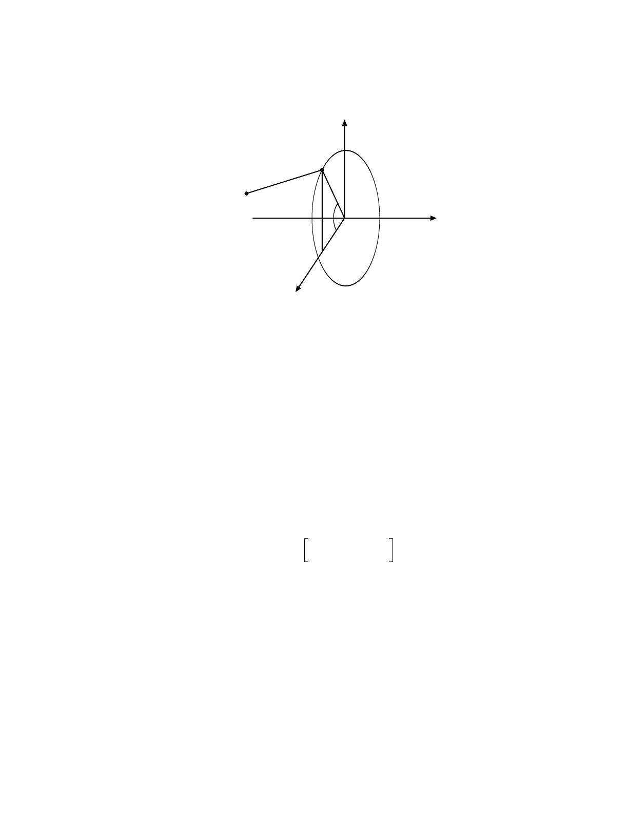
April 10, 2000 2-89
CHAPTER 2
TALLIES
Figure 2-7.
To sample a position (x,y,z) on the ring with a 1/R2 bias, we pick from the density function
, where C is a normalization constant. To pick from , let ξ be a
random number on the unit interval. Then
,
where
a=
b=−2rxo
c=−2rzo
C = (a2− b2 − c2)1/2.
Y
Z
X
(x ,y ,z )
ooo
(x,y,z)
Rr
ϕ
ϕ
pϕ() C2πR2
()⁄=ϕpϕ()
ξC
2π
------ ϕ′d
R2
--------
π–
ϕ
∫
=
C
2π
------ ϕ′d
xorϕ′cos–()
2yoy–()
2zorϕ′sin–()
2
++
--------------------------------------------------------------------------------------------------------
π–
ϕ
∫
=
C
2π
------ ϕ′d
ab ϕ′ cϕ′sin+cos+
--------------------------------------------------
π–
ϕ
∫
=
1
π
---1– 1
C
----ab–()
ϕ
2
--- c+tan
1
2
---+tan=
r2xo
2yy
o
–()
2zo
2
++ +

2-90 April 10, 2000
CHAPTER 2
TALLIES
The above expression is valid if a2> b2+ c2, which is true except for collisions exactly on the
ring.
Solving for tan ,
.
Letting ,
then x=r cos
y=y (fixed)
z=r sin .
For ring detectors, the 1/R2biasing has been supplemented when it is weak to include a biasing
based on angle to select the point on the ring. This angle is in the plane of the ring and is relative
to the shortest line from the collision point to the detector ring. The angle that would most likely
be selected would pick the same point on the ring as a straight line through the axis of the
problem, the collision point, and the ring. The angle least likely to be picked would choose the
point on the opposite side of the ring. This approach will thus make scores with smaller
attenuations more often. This supplemental biasing is achieved by requiring that
in the above equation.
If the radius of the ring is very large compared to the dimensions of the scattering media (such
that the detector sees essentially a point source in a vacuum), the ring detector is still more
efficient than a point detector. The reason for this unexpected behavior is that the individual
scores to the ring detector for a specific history have a mean closer to the true mean than to the
regular point detector contributions. That is, the point detector contributions from one history
will tend to cluster about the wrong mean because the history will not have collisions uniformly
in volume throughout the problem, whereas the ring detector will sample many paths through
the problem geometry to get to different points on the ring.
3. General Considerations of Point Detector Estimators
a. Pseudoparticles and detector reliability: Point and ring detectors are Monte Carlo
methods wherein the simulation of particle transport from one place to another is
deterministically short-circuited. Transport from the source or collision point to the detector is
replaced by a deterministic estimate of the potential contribution to the detector. This transport
between the source or collision point and the detector can be thought of as being via
ϕ
2
---
ϕ
2
---
tan 1
ab–
------------Cπξ 1
2
---–
c–tan
=
tϕ2⁄tan=
ϕr1t2
–()1t2
+()⁄=
ϕ2rt 1t2
+()⁄=
a32b2c2
+()⁄12⁄
≤

April 10, 2000 2-91
CHAPTER 2
TALLIES
“pseudoparticles.” Pseudoparticles undergo no further collisions. These particles do not reduce
the weight or otherwise affect the random walk of the particles that produced them. They are
merely estimates of a potential contribution. The only resemblance to Monte Carlo particles is
that the quantity they estimate requires an attenuation term that must be summed over the
trajectory from the source or collision to the detector. Thus most of the machinery for
transporting particles can also be used for the pseudoparticles. No records (for example, tracks
entering) are kept about pseudoparticle passage.
Because detectors rely on pseudoparticles rather than particle simulation by random walk, they
should be considered only as a very useful last resort. Detectors are unbiased estimators, but their
use can be tricky, misleading, and occasionally unreliable. Consider the problem illustrated in
Fig. 2-8.
The monoenergetic isotropic point source always will make the same contribution to the point
detector, so the variance of that contribution will be zero. If no particles have yet collided in the
scattering region, the detector tally will be converged to the source contribution, which is wrong
and misleading. But as soon as a particle collides in the scattering region, the detector tally and
its variance will jump. Then the detector tally and variance will steadily decrease until the next
particle collides in the scattering region, at which time there will be another jump.
These jumps in the detector score and variance are characteristic of undersampling important
regions. Next event estimators are prone to undersampling as already described on page 2–62
for the p(µ) term of photon coherent scattering. The jump discussed here is from the sudden
change in the R and possibly λ terms. Jumps in the tally caused by undersampling can be
eliminated only by better sampling of the undersampled scattering region that caused them.
Biasing Monte Carlo particles toward the tally region would cause the scattering region to be
sampled better, thus eliminating the jump problem. It is recommended that detectors be used
with caution and with a complete understanding of the nature of next event estimators. When
detectors are used, the tally fluctuation charts printed in the output file should be examined
closely to see the degree of the fluctuations. Also the detector diagnostic print tables should be
examined to see if any one pseudoparticle trajectory made an unusually large contribution to the
Monoenergetic
isotropic source Detector
Scattering
region
Figure 2-8.
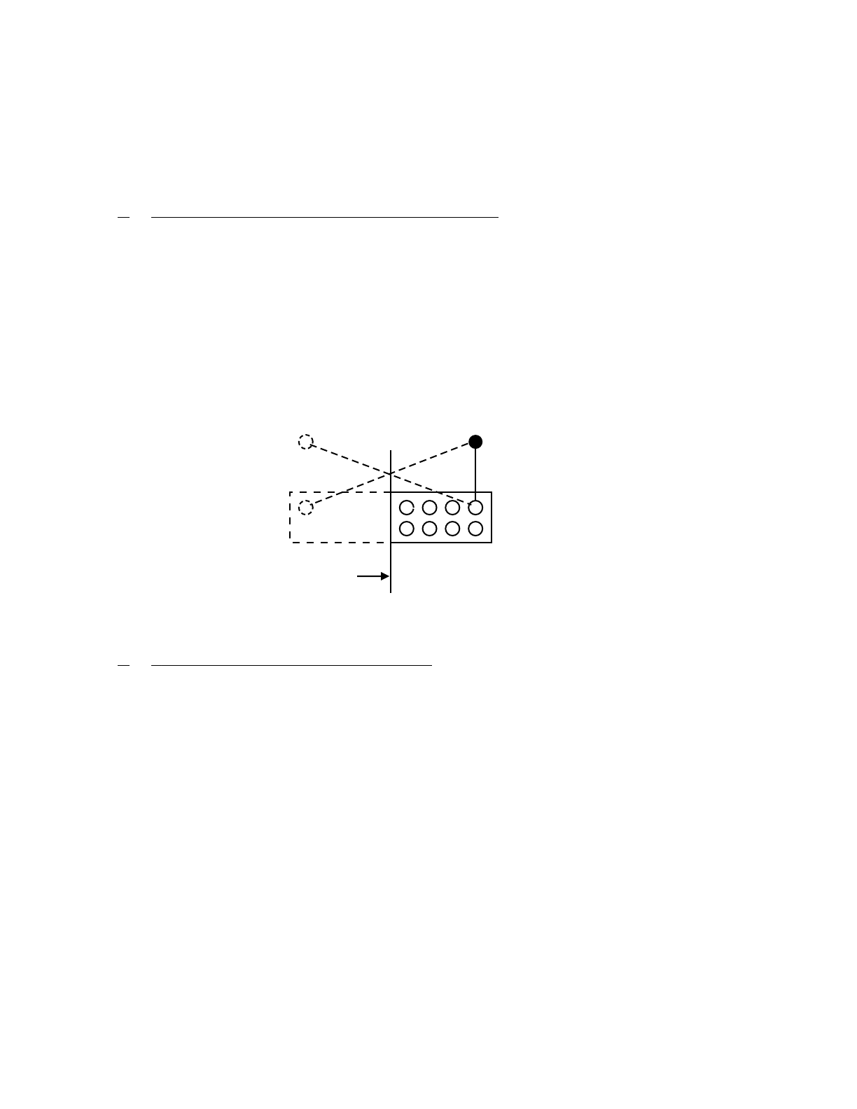
2-92 April 10, 2000
CHAPTER 2
TALLIES
tally. Detector results should be viewed suspiciously if the relative error is greater than 5%.
Close attention should be paid to the tally statistical analysis and the ten statistical checks
described on page 2–121.
b. Detectors and reflecting, white or periodic surfaces: Detectors used with reflecting,
white, or periodic surfaces give wrong answers because pseudoparticles travel only in straight
lines. Consider Fig. 2-9, with a point detector and eight source cells. The imaginary cells and
point detector are also shown on the other side of the mirror. The solid line shows the source
contribution from the indicated cell. MCNP does not allow for the dashed-line contribution on
the other side of the reflecting surface. The result is that contributions to the detector will always
be from the solid path instead of from a mixture of solid and dashed contributions. This same
situation occurs at every collision. Therefore, the detector tally will be lower (with the same
starting weight) than the correct answer and should not be used with reflecting, white, or periodic
surfaces. The effect is even worse for problems with multiple reflecting, white or periodic
surfaces.
c. Variance reduction schemes for detectors: Pseudoparticles of point detectors are not
subject to the variance reduction schemes applied to particles of the random walk. They do not
split according to importances, weight windows, etc., although they are terminated by entering
zero importance cells. However, two Russian roulette games are available specifically for
detector pseudoparticles.
The PD card can be used to specify the pseudoparticle generation probability for each cell. The
entry for each cell i is pi where . Pseudoparticles are created with probability piand
weight 1/pi. If pi= 1, which is the default, every source or collision event produces a
pseudoparticle. If pi=0, no pseudoparticle is produced. Setting pi=0in a cell that can actually
contribute to a detector erroneously biases the detector tally by eliminating such contributions.
Thus pi=0should be used only if the true probability of scoring is zero or if the score from cell
i is unwanted for some legitimate reason such as problem diagnostics. Fractional entries of pi
should be used with caution because the PD card applies equally to all pseudoparticles. The DD
card can be used to Russian roulette just the unimportant pseudoparticles. However, the DD card
Detector
Reflecting plane
Source cells
Figure 2-9.
0pi1≤≤

April 10, 2000 2-93
CHAPTER 2
TALLIES
roulette game often requires particles to travel some distance along their trajectory before being
killed. When cells are many mean free paths from the detector, the PD card may be preferable.
The DD card controls both the detector diagnostic printing and a Russian roulette game played
on pseudoparticles in transit to detectors. The Russian roulette game is governed by the input
parameter kthat controls a comparison weight wc internal to MCNP, such that
wc=−k if k < 0;
wc= 0 if k = 0;
wc= 0 if k > 0 and ;
wc= ifk > 0 and N > 200,
where N=number of histories run so far,
I=number of pseudoparticles started so far,
=Wp(µ)e−λ/(2πR2),
I=contribution of the ith pseudoparticle to the detector tally.
When each pseudoparticle is generated, W,p(µ), and Rare already known before the expensive
tracking process is undertaken to determine λ. If Wp(µ)/(2πR2)< wc, the pseudoparticle
contribution to the detector will be less than the comparison weight. Playing Russian roulette
on all pseudoparticles with < wcavoids the expensive tracking of unimportant
pseudoparticles. Most are never started. Some are started but are rouletted as soon as λ has
increased to the point where Wp(µ)e−λ/(2/πR2)<w
c. Rouletting pseudoparticles whose expected
detector contribution is small also has the added benefit that those pseudoparticles surviving
Russian roulette now have larger weights, so the disparity in particle weights reaching the
detector is reduced. Typically, using the DD card will increase the efficiency of detector
problems by a factor of ten. This Russian roulette is so powerful that it is one of two MCNP
variance reduction options that is turned on by default. The default value of k is 0.1. The other
default variance reduction option is implicit capture.
The DD card Russian roulette game is almost foolproof. Performance is relatively insensitive to
the input value of k. For most applications the default value of k = 0.1 is adequate. Usually,
choose kso that there are 1–5 transmissions (pseudoparticle contributions) per source history. If
k is too large, too few pseudoparticles are sampled; thus is a fatal error.
Because a random number is used for the Russian roulette game invoked by k>0, the addition
of a detector tally affects the random walk tracking processes. Detectors are the only tallies that
affect results. If any other tally type is added to a problem, the original problem tallies remain
unchanged. Because detectors use the default DD card Russian roulette game, and that game
affects the random number sequence, the whole problem will track differently and the original
tallies will agree only to within statistics. Because of this tracking difference, it is recommended
N200≤
kN⁄()Σ
i
Iϕi
ϕi
ϕi
ϕi
k1≥

2-94 April 10, 2000
CHAPTER 2
TALLIES
that k<0be used once a good guess at wccan be made. This is especially important if a problem
needs to be debugged by starting at some history past the first one. Also, k < 0 makes the first
200 histories run faster.
There are two cases when it is beneficial to turn off the DD card Russian roulette game by setting
k=0. First, when looking at the tail of a spectrum or some other low probability event, the DD
card roulette game will preferentially eliminate small scores and thus eliminate the very
phenomenon of interest. For example, if energy bias is used to preferentially produce high
energy particles, these biased particles will have a lower weight and thus preferentially will be
rouletted by the DD card game. Second, in very deep penetration problems, pseudoparticles will
sometimes go a long way before being rouletted. In this rare case it is wasteful to roulette a
pseudoparticle after a great deal of time has been spent following it and perhaps a fractional PD
card should be used or, if possible, a cell or surface tally.
d. Coincident detectors: Because tracking pseudoparticles is very expensive, MCNP uses
a single pseudoparticle for multiple detectors, known as coincident detectors, that must be
identical in: geometric location,
particle type (that is, neutron or photon),
upper time bin limit,
DD card Russian Roulette control parameter, k, and
PD card entries, if any.
Energy bins, time bins, tally multipliers, response functions, fictitious sphere radii, user-supplied
modifications (TALLYX), etc., can all be different. Coincident detectors require little additional
computational effort because most detector time is spent in tracking a pseudoparticle. Multiple
detectors using the same pseudoparticle are almost “free.”
e. Direct vs. total contribution: Unless specifically turned off by the user, MCNP
automatically prints out both the direct and total detector contribution. Recall that
pseudoparticles are generated at source and collision events. The direct contribution is that
portion of the tally from pseudoparticles born at source events. The total contribution is the total
tally from both source and collision events. For Mode N P problems with photon detectors, the
direct contribution is from pseudophotons born in neutron collisions. The direct contributions
for detailed photon physics will be smaller than the simple physics direct results because
coherent scattering is included in the detailed physics total cross section and omitted in the
simple physics treatment.
f. Angular distribution functions for point detectors: All detector estimates require
knowledge of the p(µ) term, the value of the probability density function at an angle , where µ
= cos . This quantity is available to MCNP for the standard source and for all kinds of
collisions. For user-supplied source subroutines, MCNP assumes an isotropic distribution
θ
θ

April 10, 2000 2-95
CHAPTER 2
TALLIES
.
Therefore, the variable PSC=p(µ) = 1/2. If the source distribution is not isotropic in a user-
supplied source subroutine, the user must also supply a subroutine SRCDX if there are any
detectors or DXTRAN spheres in the problem. In subroutine SRCDX, the variable PSC must be
set for each detector and DXTRAN sphere. An example of how this is done and also a
description of several other source angular distribution functions is in Chapter 4.
g. Detectors and the S(α,β) thermal treatment: The S(α,β) thermal treatment poses
special challenges to next event estimators because the probability density function for angle has
discrete lines to model Bragg scattering and other molecular effects. Therefore, MCNP has an
approximate model42 that, for the PSC calculation (not the transport calculation), replaces the
discrete lines with finite histograms of width µ< .1
This approximation has been demonstrated to accurately model the discrete line S(α,β) data. In
cases where continuous data is approximated with discrete lines, the approximate scheme
cancels the errors and models the scattering better than the random walk.43 Thus the S(α,β)
thermal treatment can be used with confidence with next event estimators like detectors and
DXTRAN.
F. Additional Tally Features
The standard MCNP tally types can be controlled, modified, and beautified by other tally cards.
These cards are described in detail in Chapter 3; an overview is given here.
1. Bin limit control
The integration limits of the various tally types are controlled by E, T, C, and FS cards. The E
card establishes energy bin ranges; the T card establishes time bin ranges; the C card establishes
cosine bin ranges; and the FS card segments the surface or cell of a tally into subsurface or
subcell bins.
2. Flagging
Cell and surface flagging cards, CF and SF, determine what portion of a tally comes from where.
Example: F4 1
CF4 2 3 4
The flux tally for cell 1 is output twice: first, the total flux in cell 1; and second, the flagged tally,
or that portion of the flux caused by particles having passed through cells 2, 3, or 4.
pµ()dµdΩ
4π
------- µϕdd
4π
-------------
0
2π
∫1
2
---µd== =

2-96 April 10, 2000
CHAPTER 2
TALLIES
3. Multipliers and modification
MCNP tallies can be modified in many different ways. The EM, TM, and CM cards multiply the
quantities in each energy, time, or cosine bin by a different constant. This capability is useful for
modeling response functions or changing units. For example, a surface current tally can have its
units changed to per steradian by entering the inverse steradian bin sizes on the CM card.
The DE and DF cards allow modeling of an energy-dependent dose function that is a continuous
function of energy from a table whose data points need not coincide with the tally energy bin
structure (E card). An example of such a dose function is the flux-to-radiation dose conversion
factor given in Appendix H.
The FM card multiplies the F1, F2, F4, and F5 tallies by any continuous-energy quantity
available in the data libraries. For example, average heating numbers Havg(E) and total cross
section σT(E) are stored on the MCNP data libraries. An F4 tally multiplied by σTHavg(E)ρa/ρg
converts it to an F6 tally, or an F5 detector tally multiplied by the same quantity calculates
heating at a point (see page 2–82). The FM card can modify any flux or current tally of the form
into , where R(E) is any combination of sums and products of energy-
dependent quantities known to MCNP.
The FM card can also model attenuation. Here the tally is converted to ,
where xis the thickness of the attenuator, ρais its atom density, and σtis its total cross section.
Double parentheses allow the calculation of . More complex
expressions of σt(E)ρaxare allowed so that many attenuators may be stacked. This is useful for
calculating attenuation in line-of-sight pipes and through thin foils and detector coatings,
particularly when done in conjunction with point and ring detector tallies. Beware, however, that
attenuation assumes that the attenuated portion of the tally is lost from the system by capture or
escape and cannot be scattered back in.
Two special FM card options are available. The first option sets R(E) =1/ϕ(E) to score tracks or
collisions. The second option sets R(E) = 1/velocity to score population or prompt removal
lifetime.
4. Special Treatments
A number of special tally treatments are available using the FT tally card. A brief description of
each one follows.
a. Change current tally reference vector: F1 current tallies measure bin angles relative to
the surface normal. They can be binned relative to any arbitrary vector with the FRV option.
ϕE()Ed
∫RE()ϕE()Ed
∫
ϕE()eσtE()ρ
ax–Ed
∫
ϕE()eσtE()ρ
ax–RE()Ed
∫

April 10, 2000 2-97
CHAPTER 2
TALLIES
b. Gaussian energy broadening: The GEB option can be used to better simulate a
physical radiation detector in which energy peaks exhibit Gaussian energy broadening. The
tallied energy is broadened by sampling from the Gaussian:
,
where E= the broadened energy;
Eo= the unbroadened energy of the tally;
C= a normalization constant; and
A= the Gaussian width.
The Gaussian width is related to the full width half maximum (FWHM) by
=.60056120439322 ∗FWHM
The desired FWHM is specified by the user–provided constants, a, b, and c, where
.
The FWHM is defined as FWHM = 2(EFWHM – Eo),
where EFWHM is such that f(EFWHM) = f(Eo)
and f(Eo) is the maximum value of f(E).
c. Time convolution: Because the geometry and material compositions are independent
of time, except in the case of time-dependent temperatures, the expected tally T(t,t + τ)at time
t+τfrom a source particle emitted at time tis identical to the expected tally T(0,τ)from a source
particle emitted at time 0. Thus, if a calculation is performed with all source particles started at
t=0, one has an estimate of T(0,τ)and the tallies from a number of time-distributed sources.
Qi(t) can be calculated at time as
,
by sampling tfrom Qi(t) and recording each particle’s tally (shifted by t), or after the calculation
by integrating Qi(t) multiplied by the histogram estimate of . The latter method is
used in MCNP to simulate a source as a square pulse starting at time a and ending at time b,
where a and b are supplied by the TMC option.
fE() Ce
EE
o
–
A
---------------
2
–
=
AFWHM
22ln
-------------------=
FWHM a b E cE2
++=
1
2
---
TQi
η
TQiη() Qit()Ttη,()td
a
b
∫Qit()T0ηt–,()td
a
b
∫
==
T0ηt–,()

2-98 April 10, 2000
CHAPTER 2
TALLIES
d. Binning by the number of collisions: Tallies can be binned by the number of collisions
that caused them with the INC option and an FU card. A current tally, for example, can be
subdivided into the portions of the total current coming from particles that have undergone zero,
one, two, three, ... collisions before crossing the surface. In a point detector tally, the user can
determine what portion of the score came from particles having their 1st, 2nd, 3rd, ... collision.
Collision binning is particularly useful with the exponential transform because the transform
reduces variance by reducing the number of collisions. If particles undergoing many collisions
are the major contributor to a tally, then the exponential transform is ill-advised. When the
exponential transform is used, the portion of the tally coming from particles having undergone
many collisions should be small.
e. Binning by detector cell: The ICD option with an FU card is used to determine what
portion of a detector tally comes from what cells. This information is similar to the detector
diagnostics print, but the FT card can be combined with energy and other binning cards. The
contribution to the normalized rather than unnormalized tally is printed.
f. Binning by source distribution: The SCX and SCD options are used to bin a tally score
according to what source distribution caused it.
g. Binning by multigroup particle type: The PTT option with an FU card is used to bin
multigroup tallies by particle type. The MCNP multigroup treatment is available for neutron,
coupled neutron/photon, and photon problems. However, charged particles or any other
combinations of particles can be run with the various particles masquerading as neutrons and are
printed out in the OUTP file as if they were neutrons. With the PTT option, the tallies can be
segregated into particle types by entering atomic weights in units of MeV on the FU card. The
FU atomic weights must be specified to within 0.1% of the true atomic weight in MeV units:
thus FU .511 specifies an electron, but .510 is not recognized.
h. Binning by particle charge: The ELC option allows binning F1 current tallies by
particle charge. There are three ELC options:
1. cause negative electrons to make negative scores and positrons to make positive
scores. Note that by tallying positive and negative numbers the relative error is
unbounded and this tally may be difficult to converge;
2. segregate electrons and positrons into separate bins plus a total bin. There will be three
bins (positron, electron, and total) all with positive scores. The total bin will be the
same as the single tally bin without the ELC option.
3. segregate electrons and positrons into separate bins plus a total bin, with the electron
bin scores being all negative to reflect their charge. The bins will be for positrons
(positive scores), electrons (negative scores), and total. The total bin will be the same
as the single bin with the first ELC option above (usually with negative scores because
there are more electrons than positrons).

April 10, 2000 2-99
CHAPTER 2
ESTIMATION OF THE MONTE CARLO PRECISION
5. User modification
If the above capabilities do not provide exactly what is desired, tallies can be modified by a user-
supplied TALLYX subroutine (FU card). As with a user-supplied SOURCE subroutine, which
lets the user provide his own specialized source, the TALLYX subroutine lets the user modify
any tally, with all the programming changes conveniently located in a single subroutine.
6. Tally output format
Not only can users change the contents of MCNP tallies, the output format can be modified as
well. Any desired descriptive comment can be added to the tally title by the tally comment (FC)
card. The printing order can be changed (FQ card) so that instead of, for instance, getting the
default output blocks in terms of time vs. energy, they could be printed in blocks of segment vs.
cosine. The tally bin that is monitored for the tally fluctuation chart printed at the problem end
and used in the statistical analysis of the tally can be selected (TF card). Detector tally diagnostic
prints are controlled with the DD card. Finally, the PRINT card controls what optional tables are
displayed in the output file.
VI. ESTIMATION OF THE MONTE CARLO PRECISION
Monte Carlo results represent an average of the contributions from many histories sampled
during the course of the problem. An important quantity equal in stature to the Monte Carlo
answer (or tally) itself is the statistical error or uncertainty associated with the result. The
importance of this error and its behavior vs. the number of histories cannot be overemphasized
because the user not only gains insight into the quality of the result, but also can determine if a
tally appears statistically well behaved. If a tally is not well behaved, the estimated error
associated with the result generally will not reflect the true confidence interval of the result and,
thus, the answer could be completely erroneous. MCNP contains several quantities that aid the
user in assessing the quality of the confidence interval.86
The purpose of this section is to educate MCNP users about the proper interpretation of the
MCNP estimated mean, relative error, variance of the variance, and history score probability
density function. Carefully check tally results and the associated tables in the tally fluctuation
charts to ensure a well-behaved and properly converged tally.
A. Monte Carlo Means, Variances, and Standard Deviations
Monte Carlo results are obtained by sampling possible random walks and assigning a score xi
(for example, xi= energy deposited by the ith random walk) to each random walk. Random walks
typically will produce a range of scores depending on the tally selected and the variance
reduction chosen.

2-100 April 10, 2000
CHAPTER 2
ESTIMATION OF THE MONTE CARLO PRECISION
Suppose f(x) is the history score probability density function for selecting a random walk that
scores xto the tally being estimated. The true answer (or mean) is the expected value of x,E(x),
where
= true mean.
The function f(x) is seldom explicitly known; thus, f(x) is implicitly sampled by the Monte Carlo
random walk process. The true mean then is estimated by the sample mean where
, (2.15)
where xi is the value of x selected from f(x) for the ith history and Nis the number of histories
calculated in the problem. The Monte Carlo mean is the average value of the scores xifor all
the histories calculated in the problem. The relationship between E(x) and is given by the
Strong Law of Large Numbers1 that states that if E(x) is finite, tends to the limit E(x) as N
approaches infinity.
The variance of the population of xvalues is a measure of the spread in these values and is given
by1
.
The square root of the variance is σ, which is called the standard deviation of the population of
scores. As with E(x),σis seldom known but can be estimated by Monte Carlo as S, given by (for
large N)
(2.16a)
and
. (2.16b)
The quantity Sis the estimated standard deviation of the population of xbased on the values of
xi that were actually sampled.
The estimated variance of is given by
Ex() xf x()xd
∫
=
x
x1
N
----xi
i1=
N
∑
=
xx
x
σ2xEx()–()
2fx()xd
∫Ex
2
() Ex()()
2
–==
S2Σi1=
Nxix–()
2
N1–
--------------------------------- x2x2
–∼=
x21
N
----xi
2
i1=
N
∑
=
x
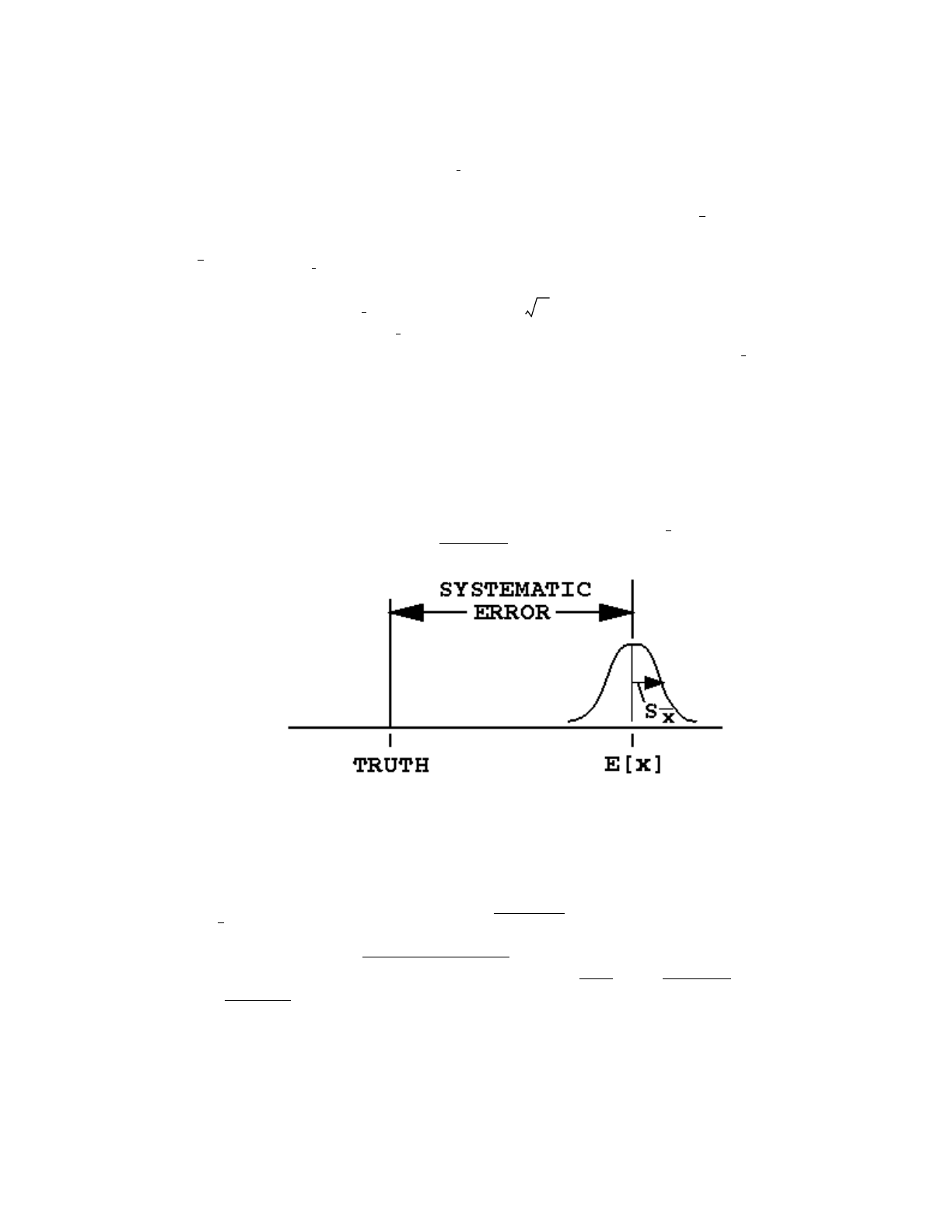
April 10, 2000 2-101
CHAPTER 2
ESTIMATION OF THE MONTE CARLO PRECISION
. (2.17)
These formulae do not depend on any restriction on the distribution of xor (such as normality)
beyond requiring that E(x) and σ2 exist and are finite. The estimated standard deviation of the
mean is given by .
It is important to note that is proportional to 1/ , which is the inherent drawback to the
Monte Carlo method. To halve , four times the original number of histories must be
calculated, a calculation that can be computationally expensive. The quantity can also be
reduced for a specified Nby making Ssmaller, reducing the inherent spread of the tally results.
This can be accomplished by using variance reduction techniques such as those discussed in
section VII of this chapter.
B. Precision and Accuracy
There is an extremely important difference between precision and accuracy of a Monte Carlo
calculation. As illustrated in Fig. 2-10, precision is the uncertainty in caused by the statistical
fluctuations of the xi’s for the portion of physical phase space sampled by the Monte Carlo
process. Important portions of physical phase space might not be sampled because of problem
cutoffs in time or energy, inappropriate use of variance reduction techniques, or an insufficient
sampling of important low-probability events. Accuracy is a measure of how close the expected
value of , E(x), is to the true physical quantity being estimated. The difference between this
true value and E(x) is called the systematic error, which is seldom known. Error or uncertainty
estimates for the results of Monte Carlo calculations refer only to the precision of the result and
not to the accuracy. It is quite possible to calculate a highly precise result that is far from the
physical truth because nature has not been modeled faithfully.
Sx
2S2
N
-----=
x
x Sx
SxN
SxSx
Figure 2-10.
x
x

2-102 April 10, 2000
CHAPTER 2
ESTIMATION OF THE MONTE CARLO PRECISION
1. Factors Affecting Problem Accuracy
Three factors affect the accuracy of a Monte Carlo result: (1) the code, (2) problem modeling,
and (3) the user. Code factors encompass: the physics features included in a calculation as well
as the mathematical models used; uncertainties in the data, such as the transport and reaction
cross sections, Avogadro's number, atomic weights, etc.; the quality of the representation of the
differential cross sections in energy and angle; and coding errors (bugs). All of the applicable
physics must be included in a calculation to produce accurate results. Even though the
evaluations are not perfect, more faithful representation of the evaluator's data should produce
more accurate results. The descending order of preference for Monte Carlo data for calculations
is continuous energy, thinned continuous energy, discrete reaction, and multigroup. Coding
errors can always be a problem because no large code is bug-free. MCNP, however, is a very
mature, heavily used production code. With steadily increasing use over the years, the likelihood
of a serious coding error continues to diminish.
The second area, problem-modeling factors, can quite often contribute to a decrease in the
accuracy of a calculation. Many calculations produce seemingly poor results because the model
of the energy and angular distribution of the radiation source is not adequate. Two other
problem-modeling factors affecting accuracy are the geometrical description and the physical
characteristics of the materials in the problem.
The third general area affecting calculational accuracy involves user errors in the problem input
or in user-supplied subroutines and patches to MCNP. The user can also abuse variance
reduction techniques such that portions of the physical phase space are not allowed to contribute
to the results. Checking the input and output carefully can help alleviate these difficulties. A last
item that is often overlooked is a user's thorough understanding of the relationship of the Monte
Carlo tallies to any measured quantities being calculated. Factors such as detector efficiencies,
data reduction and interpretation, etc., must be completely understood and included in the
calculation, or the comparison is not meaningful.
2. Factors Affecting Problem Precision
The precision of a Monte Carlo result is affected by four user-controlled choices: (1) forward vs.
adjoint calculation, (2) tally type, (3) variance reduction techniques, and (4) number of histories
run.
The choice of a forward vs. adjoint calculation depends mostly on the relative sizes of the source
and detector regions. Starting particles from a small region is easy to do, whereas transporting
particles to a small region is generally hard to do. Because forward calculations transport
particles from source to detector regions, forward calculations are preferable when the detector
(or tally) region is large and the source region is small. Conversely, because adjoint calculations
transport particles backward from the detector region to the source region, adjoint calculations
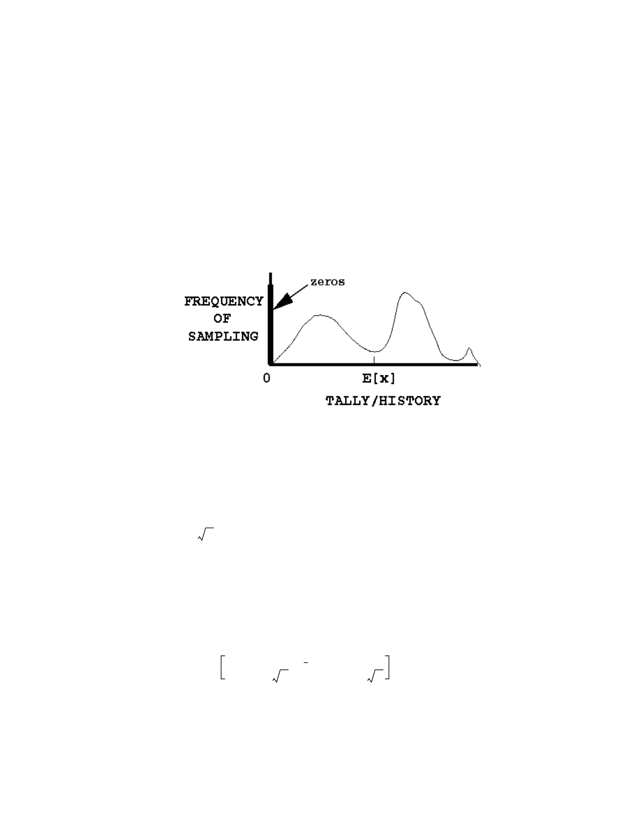
April 10, 2000 2-103
CHAPTER 2
ESTIMATION OF THE MONTE CARLO PRECISION
are preferable when the source (or tally) region is large and the detector region is small. MCNP
can be run in multigroup adjoint mode. There is no continuous-energy adjoint capability.
As alluded to above, the smaller the tally region, the harder it becomes to get good tally
estimates. An efficient tally will average over as large a region of phase space as practical. In this
connection, tally dimensionality is extremely important. A one-dimensional tally is typically 10
to 100 times easier to estimate than a two-dimensional tally, which is 10 to 100 times easier than
a three-dimensional tally. This fact is illustrated in Fig. 2-15 later in this section.
Variance reduction techniques can be used to improve the precision of a given tally by increasing
the nonzero tallying efficiency and by decreasing the spread of the nonzero history scores. These
two components are depicted in a hypothetical f(x) shown in Fig. 2-11. See page 2–113 for more
discussion about the empirical f(x) for each tally fluctuation chart bin. A calculation will be more
precise when the history-scoring efficiency is high and the variance of the nonzero scores is low.
The user should strive for these conditions in difficult Monte Carlo calculations. Examples of
these two components of precision are given on page 2–109.
More histories can be run to improve precision (see section Cfollowing). Because the precision
is proportional to 1/ , running more particles is often costly in computer time and therefore
is viewed as the method of last resort for difficult problems.
C. The Central Limit Theorem and Monte Carlo Confidence Intervals
To define confidence intervals for the precision of a Monte Carlo result, the Central Limit
Theorem1 of probability theory is used, stating that
,
Figure 2-11.
N
N∞–
lim Pr E x() ασ
N
-------- xEx() βσ
N
--------
+<<+1
2π
------ et22⁄–td
α
β
∫
=

2-104 April 10, 2000
CHAPTER 2
ESTIMATION OF THE MONTE CARLO PRECISION
where αand βcan be any arbitrary values and Pr[Z] means the probability of Z. In terms of the
estimated standard deviation of , , this may be rewritten in the following approximation for
large N:
.
This crucial theorem states that for large values of N (that is, as Ntends to infinity) and
identically distributed independent random variables xiwith finite means and variances, the
distribution of the ’s approaches a normal distribution. Therefore, for any distribution of tallies
(an example is shown in Fig. 2-11), the distribution of resulting ’s will be approximately
normally distributed, as shown in Fig. 2-10, with a mean of E(x).IfSis approximately equal to
σ, which is valid for a statistically significant sampling of a tally (i.e, Nhas tended to infinity),
then
~ 68% of the time and (2.18a)
, ~ 95% of the time (2.18b)
from standard tables for the normal distribution function. Eq. (2.18a) is a 68% confidence
interval and Eq. (2.18b) is a 95% confidence interval.
The key point about the validity of these confidence intervals is that the physical phase space
must be adequately sampled by the Monte Carlo process. If an important path in the geometry
or a window in the cross sections, for example, has not been well sampled, both and will
be unknowingly incorrect and the results will be wrong, usually tending to be too small. The user
must take great care to be certain that adequate sampling of the source, transport, and any tally
response functions have indeed taken place. Additional statistical quantities to aid in the
assessment of proper confidence intervals are described in later portions of section VI.
D. Estimated Relative Errors in MCNP
All standard MCNP tallies are normalized to be per starting particle history (except for some
criticality calculations) and are printed in the output with a second number, which is the
estimated relative error defined as
(2.19a)
The relative error is a convenient number because it represents statistical precision as a fractional
result with respect to the estimated mean.
xSx
Pr αSxxEx()–
σN
-------------------- βSx
<<1
2π
---------- et22⁄–td
α
β
∫
∼
xx
x2SxEx() xS
x,+<<–
x2SxEx() x2Sx
+<<–
x Sx
RS
xx⁄≡

April 10, 2000 2-105
CHAPTER 2
ESTIMATION OF THE MONTE CARLO PRECISION
Combining Eqs. (2.15), (2.16), and (2.17), R can be written (for large N) as
. (2.19b)
Several important observations about the relative error can be made from Eq. (2.19b). First, if
all the xi’s are nonzero and equal, Ris zero. Thus, low-variance solutions should strive to reduce
the spread in the xi’s. If the xi’s are all zero, Ris defined to be zero. If only one nonzero score is
made, Rapproaches unity as Nbecomes large. Therefore, for xi’s of the same sign, can never
be greater than because R never exceeds unity. For positive and negative xi’s, R can exceed
unity. The range of R values for xi’s of the same sign is therefore between zero and unity.
To determine what values of Rlead to results that can be stated with confidence using Eqs. (2.6),
consider Eq. (2.19b) for a difficult problem in which nonzero scores occur very infrequently. In
this case,
. (2.20a)
For clarity, assume that there are nout of nonzero scores that are identical and equal
to x. With these two assumptions, R for “difficult problems” becomes
RD.P. ~. (2.20b)
This result is expected because the limiting form of a binomial distribution with infrequent
nonzero scores and large Nis the Poisson distribution, which is the form in Eq. (2.20b) used in
detector “counting statistics.”
Through use of Eqs. (2.8), a table of Rvalues versus the number of tallies or “counts” can be
generated as shown in Table 2.2. A relative error of 0.5 is the equivalent of four counts, which
is hardly adequate for a statistically significant answer. Sixteen counts is an improvement,
TABLE 2.2:
Estimated Relative Error R vs. Number of Identical Tallies nfor Large N
n1 4 16 25 100 400
R1.0 0.5 0.25 0.20 0.10 0.05
R1
N
----x2
x2
-----1–
12⁄Σi1=
Nxi
2
Σi1=
Nxi
()
2
------------------------ 1
N
----–
12⁄
==
Sx
x
1
N
----Σi1=
Nxi
2
Σi1=
Nxi
()
2
------------------------«
Nn N«()
nx2
n2x2
-----------
12⁄1
n
-------nN«,=

2-106 April 10, 2000
CHAPTER 2
ESTIMATION OF THE MONTE CARLO PRECISION
reducing R to 0.25, but still is not a large number of tallies. The same is true for nequals 25.
When nis 100, Ris 0.10, so the results should be much improved. With 400 tallies, an Rof 0.05
should be quite good indeed.
Based on this qualitative analysis and the experience of Monte Carlo practitioners, Table 2.3
presents the recommended interpretation of the estimated 1σconfidence interval for
various values of R associated with an MCNP tally. These guidelines were determined
empirically, based on years of experience using MCNP on a wide variety of problems. Just
before the tally fluctuation charts, a “Status of Statistical Checks” table prints how many tally
bins of each tally have values of R exceeding these recommended guidelines.
Point detector tallies generally require a smaller value of R for valid confidence interval
statements because some contributions, such as those near the detector point, are usually
extremely important and may be difficult to sample well. Experience has shown that for R less
than 0.05, point detector results are generally reliable. For an Rof 0.10, point detector tallies may
only be known within a factor of a few and sometimes not that well (see the pathological
example on page 2–123.)
MCNP calculates the relative error for each tally bin in the problem using Eq. (2.19b). Each xi
is defined as the total contribution from the ith starting particle and all resulting progeny. This
definition is important in many variance reduction methods, multiplying physical processes such
as fission or (n,xn) neutron reactions that create additional neutrons, and coupled neutron/
photon/electron problems. The ith source particle and its offspring may thus contribute many
times to a tally and all of these contributions are correlated because they are from the same
source particle.
Figure 2.12 represents the MCNP process of calculating the first and second moments of each
tally bin and relevant totals using three tally storage blocks of equal length for each tally bin. The
TABLE 2.3:
Guidelines for Interpreting the Relative Error Ra
aand represents the estimated statistical relative error at the 1σlevel. These in-
terpretations of Rassume that all portions of the problem phase space have been well sam-
pled by the Monte Carlo process.
Range of RQuality of the Tally
0.5 to 1 Garbage
0.2 to 0.5 Factor of a few
0.1 to 0.2 Questionable
<0.10 Generally reliable except for point detector
<0.05 Generally reliable for point detector
x1R±()
RS
xx⁄=
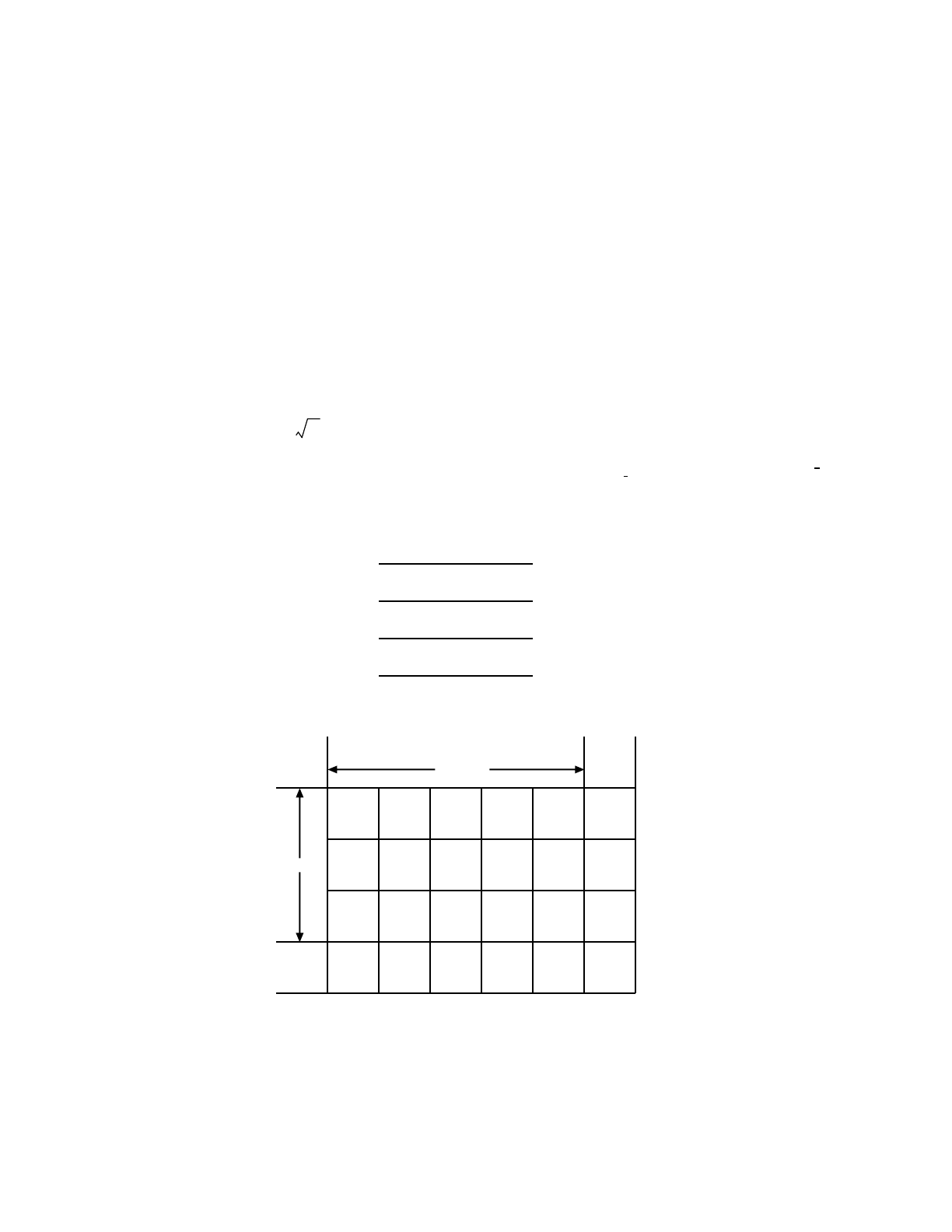
April 10, 2000 2-107
CHAPTER 2
ESTIMATION OF THE MONTE CARLO PRECISION
hypothetical grid of tally bins in the bottom half of Fig. 2-12 has 24 tally bins including the time
and energy totals. During the course of the ith history, sums are performed in the first MCNP tally
storage block. Some of the tally bins receive no contributions and others receive one or more
contributions. At the conclusion of the ith history, the sums are added to the second MCNP tally
storage block. The sums in the first MCNP tally storage block are squared and added to the third
tally storage block. The first tally storage block is then filled with zeros and history i+1begins.
After the last history N, the estimated tally means are computed using the second MCNP tally
storage block and Eq. (2.15). The estimated relative errors are calculated using the second and
third MCNP tally storage blocks and Eq. (2.19b). This method of estimating the statistical
uncertainty of the result produces the best estimate because the batch size is one, which
minimizes the variance of the variance.87,88
Note that there is no guarantee that the estimated relative error will decrease inversely
proportional to the as required by the Central Limit Theorem because of the statistical
nature of the tallies. Early in the problem, R will generally have large statistical fluctuations.
Later, infrequent large contributions may cause fluctuations in and to a lesser extent in and
therefore in R. MCNP calculates a FOM for one bin of each numbered tally to aid the user in
determining the statistical behavior as a function of N and the efficiency of the tally.
N
Sxx
Time
Energy
Time
Total Grand
Total
XXX X X XXXXX
XXXX
XX
XX XX
Energy
Total
HYPOTHETICAL TALLY GRID
X=Score from the present history
Particle batch size is one
MCNP TALLY BLOCKS
Σ
Σ
{
}
X2
i
Xi
Xi
Running
History
Scores
Sums performed
after each history
Figure 2-12.

2-108 April 10, 2000
CHAPTER 2
ESTIMATION OF THE MONTE CARLO PRECISION
E. MCNP Figure of Merit
The estimated relative error squared R2should be proportional to 1/N, as shown by Eq. (2.19a).
The computer time Tused in an MCNP problem should be directly proportional to N; therefore,
R2T should be approximately a constant within any one Monte Carlo run. It is convenient to
define a figure of merit (FOM) of a tally to be
. (2.21a)
MCNP prints the FOM for one bin of each numbered tally as a function of N, where the unit of
computer time T is minutes The table is printed in particle increments of 1000 up to 20,000
histories. Between 20,000 and 40,000 histories, the increment is doubled to 2000. This trend
continues, producing a table of up to 20 entries. The default increment can be changed by the
5th entry on the PRDMP card.
The FOM is a very important statistic about a tally bin and should be studied by the user. It is a
tally reliability indicator in the sense that if the tally is well behaved, the FOM should be
approximately a constant with the possible exception of statistical fluctuations very early in the
problem. An order-of-magnitude estimate of the expected fractional statistical fluctuations in the
FOM is 2R. This result assumes that both the relative statistical uncertainty in the relative error
is of the order of the relative error itself and the relative error is small compared to unity. The
user should always examine the tally fluctuation charts at the end of the problem to check that
the FOMs are approximately constant as a function of the number of histories for each tally.
The numerical value of the FOM can be better appreciated by considering the relation
(2.21b)
Table 2.4 shows the expected value of Rthat would be produced in a one-minute problem (T=1)
as a function of the value of the FOM. It is clearly advantageous to have a large FOM for a
problem because the computer time required to reach a desired level of precision is
proportionally reduced. Examination of Eq. (2.21b) shows that doubling the FOM for a problem
will reduce the computer time required to achieve the same R by a factor of two.
TABLE 2.4:
R Values as a Function of the FOM for T = 1 Minute
FOM 1 10 100 1000 10000
R 1.0 0.32 0.10 0.032 0.010
FOM 1
R2T
----------
≡
R1FOM T⁄=∗

April 10, 2000 2-109
CHAPTER 2
ESTIMATION OF THE MONTE CARLO PRECISION
In summary, the FOM has three uses. The most important use is as a tally reliability indicator.
If the FOM is not approximately a constant (except for statistical fluctuations early in the
problem), the confidence intervals may not overlap the expected score value, E(x), the expected
fraction of the time. A second use for the FOM is to optimize the efficiency of the Monte Carlo
calculation by making several short test runs with different variance reduction parameters and
then selecting the problem with the largest FOM. Remember that the statistical behavior of the
FOM (i.e., R) for a small number of histories may cloud the selection of techniques competing
at the same level of efficiency. A third use for the FOM is to estimate the computer time required
to reach a desired value of R by using T ~ 1/R2FOM.
F. Separation of Relative Error into Two Components
Three factors that affect the efficiency of a Monte Carlo problem are (1) history-scoring
efficiency, (2) dispersions in nonzero history scores, and (3) computer time per history. All three
factors are included in the FOM. The first two factors control the value of R; the third is T.
The relative error can be separated into two components: the nonzero history-scoring efficiency
component and the intrinsic spread of the nonzero xi scores . Defining qto be the
fraction of histories producing nonzero xi’s, Eq. 2.19b can be rewritten as
. (2.22a)
Note by Eq. 2.19b that the first two terms are the relative error of the qN nonzero scores. Thus
defining,
and (2.22b)
yields (2.22c)
. (2.22d)
For identical nonzero xi’s, is zero and for a 100% scoring efficiency, is zero. It is
usually possible to increase qfor most problems using one or more of the MCNP variance
reduction techniques. These techniques alter the random walk sampling to favor those particles
that produce a nonzero tally. The particle weights are then adjusted appropriately so that the
expected tally is preserved. This topic is described in Sec. VII (Variance Reduction) beginning
Reff
2Rint
2
R
Σi1=
Nxi
2
Σi1=
Nxi
()
2
------------------------ 1
N
----– Σxi0≠x2
i
Σxi0≠xi
()
2
------------------------- 1
N
----– Σxi0≠x2
i
Σxi0≠xi
()
2
--------------------------- 1
qN
-------–1q–
qN
------------+== =
Rint
2Σxi0≠x2
i
Σxi0≠xi
()
2
--------------------------- 1
qN
-------–=
Reff
21q–()qN()⁄=
R2Reff
2Rint
2
+=
Rint
2Reff
2

2-110 April 10, 2000
CHAPTER 2
ESTIMATION OF THE MONTE CARLO PRECISION
on page 2–127 . The sum of the two terms of Eq. (2.22d) produces the same result as Eq. (2.19b).
Both and are printed for the tally fluctuation chart bin of each tally so that the
dominant component of R can be identified as an aid to making the calculation more efficient.
These equations can be used to better understand the effects of scoring inefficiency; that is, those
histories that do not contribute to a tally. Table 2.5 shows the expected values of as a
function of qand the number of histories N. This table is appropriate for identical nonzero scores
and represents the theoretical minimum relative error possible for a specified q and N. It is no
surprise that small values of qrequire a compensatingly large number of particles to produce
precise results.
A practical example of scoring inefficiency is the case of infrequent high-energy particles in a
down-scattering-only problem. If only a small fraction of all source particles has an energy in
the highest energy tally bin, the dominant component of the relative error will probably be the
scoring efficiency because only the high-energy source particles have a nonzero probability of
contributing to the highest energy bin. For problems of this kind, it is often useful to run a
separate problem starting only high-energy particles from the source and to raise the energy
cutoff. The much-improved scoring efficiency will result in a much larger FOM for the high-
energy tally bins.
To further illustrate the components of the relative error, consider the five examples of selected
discrete probability density functions shown in Fig. 2-13. Cases I and II have no dispersion in
the nonzero scores, cases III and IV have 100% scoring efficiency, and case V contains both
elements contributing to R. The most efficient problem is case III. Note that the scoring
inefficiency contributes 75% to R in case V, the second worst case of the five.
TABLE 2.5:
Expected Values of Reff as a Function of q and N
q
N0.001 0.01 0.1 0.5
1030.999 0.315 0.095 0.032
1040.316 0.099 0.030 0.010
1050.100 0.031 0.009 0.003
1060.032 0.010 0.003 0.001
Rint
2Reff
2
Reff

April 10, 2000 2-111
CHAPTER 2
ESTIMATION OF THE MONTE CARLO PRECISION
G. Variance of the Variance
Previous sections have discussed the relative error R and figure of merit FOM as measures of the
quality of the mean. A quantity called the relative variance of the variance (VOV) is another
useful tool that can assist the user in establishing more reliable confidence intervals. The VOV
is the estimated relative variance of the estimated R. The VOV involves the estimated third and
fourth moments of the empirical history score probability density function (PDF) f(x) and is
much more sensitive to large history score fluctuations than is R. The magnitude and NPS
behavior of the VOV are indicators of tally fluctuation chart (TFC) bin convergence. Early work
was done by Estes and Cashwell87 and Pederson89 later reinvestigated this statistic to determine
its usefulness.
The VOV is a quantity that is analogous to the square of the R of the mean, except it is for R
instead of the mean. The estimated relative VOV of the mean is defined as
Vf
1/3
0 0.5 1
E[x]=0x1/3+1/3x1/2+1/3x1=0.5
R=0.82/sqrt(N)
R =0.41/sqrt(N) 25%
R =0.71/sqrt(N) 75%
eff
int
µ
IV f
0.5
0 1/4 3/4 1
E[x]=1/2x1/4+1/2x3/4=0.5
R=R =0.5/sqrt(N)
R =0
eff
int
µ
III f
0.5
0 1/3 2/3 1
E[x]=1/2x1/3+1/2x2/3=0.5
R=R =0.33/sqrt(N)
R =0
eff
int
µ
II f
0.75
0.25
02/3 1
E[x]=0x1/4+2/3x3/4=0.5
R=R =0.58/sqrt(N)
R =0
int
eff
µ
If
0.5
01
E[x]=0.5(0+1)=0.5
R=R =1/sqrt(N)
R =0
int
eff
µ
FIVE CASES WITH A MEAN OF 0.5
Figure 2-13.

2-112 April 10, 2000
CHAPTER 2
ESTIMATION OF THE MONTE CARLO PRECISION
where is the estimated variance of and is the estimated variance in . The VOV
is a measure of the relative statistical uncertainty in the estimated R and is important because S
must be a good approximation of σ to use the Central Limit Theorem to form confidence
intervals.
The VOV for a tally bin89 is
. (2.23)
This is the fourth central moment minus the second central moment squared normed by the
product of Nand the second central moment squared.
When Eq. (2.23) is expanded in terms of sums of powers of xi, it becomes
or
(2.24)
Now consider the truncated Cauchy formula for the following analysis. The truncated Cauchy is
similar in shape to some difficult Monte Carlo tallies. After numerous statistical experiments on
sampling a truncated positive Cauchy distribution
, (2.25)
it is concluded that the VOV should be below 0.1 to improve the probability of forming a reliable
confidence interval. The quantity 0.1 is a convenient value and is why the VOV is used for the
statistical check and not the square root of the VOV (R of the R). Multiplying numerator and
denominator of Eq. (2.24) by 1/N converts the terms into averages and shows that the VOV
is expected to decrease as 1/N.
It is interesting to examine the VOV for the nidentical history scores xthat were used
to analyze R in Table 2.2, page 2–105. The VOV behaves as 1/n in this limit. Therefore, ten
VOV S2Sx
2
()Sx
4
⁄=
Sx
2x S2Sx
2
() Sx
2
VOV Σxix–()
4
=Σxix–()
2
()⁄21N⁄–
VOV Σxi
44ΣxiΣxi
3N6Σxi
2Σxi
()
2N23Σxi
()
4N3
⁄–⁄+⁄–
Σxi
2Σxi
()
2N⁄–()
2
------------------------------------------------------------------------------------------------------------------------------ 1
N
----–=
VOV Σxi
44ΣxiΣxi
3N8Σxi
2Σxi
()
2N⁄24Σxi
()
4N⁄3
–Σxi
2
()
2N⁄–+⁄–
Σxi
2Σxi
()
2N⁄–()
2
-------------------------------------------------------------------------------------------------------------------------------------------------------------=
Cauchy f x() 2π1x2
+()0xx
max
≤≤,⁄=
xn
nN«()

April 10, 2000 2-113
CHAPTER 2
ESTIMATION OF THE MONTE CARLO PRECISION
identical history scores would be enough to satisfy the VOV criterion, a factor of at least ten less
than the R criterion. There are two reasons for this phenomenon: 1) it is more important to know
R well than the VOV in forming confidence intervals; and 2) the history scores will ordinarily
not be identical and thus the fourth moment terms in the VOV will increase rapidly over the
second moment terms in R.
The behavior of the VOV as a function of Nfor the TFC bin is printed in the OUTP file. Because
the VOV involves third and fourth moments, the VOV is a much more sensitive indicator to large
history scores than the R, which is based on first and second moments. The desired VOV
behavior is to decrease inversely with N. This criterion is deemed to be a necessary, but not
sufficient, condition for a statistically well-behaved tally result. A tally with a VOV that matches
this criteria is NOT guaranteed to produce a high quality confidence interval because
undersampling of high scores will also underestimate the higher score moments.
To calculate the VOV of every tally bin, put a nonzero 15th entry on the DBCN card. This option
creates two additional history score moment tables each of length MXF in the TAL array to sum
and (see Fig. 2-12). This option is not the default because the amount of tally storage will
increase by 2/5, which could be prohibitive for a problem with many tally bins. The magnitude
of the VOV in each tally bin is reported in the “Status of Statistical Checks” table. History–
dependent checks of the VOV of all tally bins can be done by printing the tallies to the output
file at some frequency using the PRDMP card.
H. Empirical History Score Probability Density Function f(x)
1. Introduction
This section discusses another statistic that is useful in assessing the quality of confidence
intervals from Monte Carlo calculations. Consider a generic Monte Carlo problem with difficult
to sample, but extremely important, large history scores. This type of problem produces three
possible scenarios.86
The first, and obviously desired, case is a correctly converged result that produces a statistically
correct confidence interval. The second case is the sampling of an infrequent, but very large,
history score that causes the mean and R to increase and the FOM to decrease significantly. This
case is easily detectable by observing the behavior of the FOM and the R in the TFCs.
The third and most troublesome case yields an answer that appears statistically converged based
on the accepted guidelines described previously, but in fact may be substantially smaller than the
correct result because the large history tallies were not well sampled. This situation of too few
large history tallies is difficult to detect. The following sections discuss the use of the empirical
history score probability density function (PDF) f(x) to gain insight into the TFC bin result. A
pathological example to illustrate the third case follows.
xi
3xi
4

2-114 April 10, 2000
CHAPTER 2
ESTIMATION OF THE MONTE CARLO PRECISION
2. The History Score Probability Density Function f(x)
A history score posted to a tally bin can be thought of as having been sampled from an
underlying and generally unknown history score PDF f(x), where the random variable x is the
score from one complete particle history to a tally bin. The history score can be either positive
or negative. The quantity f(x)dx is the probability of selecting a history score between x and
x+dx for the tally bin. Each tally bin will have its own f(x).
The most general form for expressing f(x) mathematically is
,
where fc(x) is the continuous nonzero part and represents the n different
discrete components occurring at xiwith probability pi.Anf(x) could be composed of either or
both parts of the distribution. A history score of zero is included in f(x) as the discrete component
δ(x − 0).
By the definition of a PDF,
.
As discussed on page 2–99, f(x) is used to estimate the mean, variance, and higher moment
quantities such as the VOV.
3. The Central Limit Theorem and f(x)
As discussed on page 2–103, the Central Limit Theorem (CLT) states that the estimated mean
will appear to be sampled from a normal distribution with a known standard deviation
when N approaches infinity. In practice, σ is NOT known and must be approximated by the
estimated standard deviation S. The major difficulty in applying the CLT correctly to a Monte
Carlo result to form a confidence interval is knowing when N has approached infinity.
The CLT requires the first two moments of f(x) to exist. Nearly all MCNP tally estimators
(except point detectors with zero neighborhoods in a scattering material and some exponential
transform problems) satisfy this requirement. Therefore, the history score PDF f(x) also exists.
One can also examine the behavior of f(x) for large history scores to assess if f(x) appears to have
been “completely” sampled. If “complete” sampling has occurred, the largest values of the
sampled x’s should have reached the upper bound (if such a bound exists) or should decrease
faster than 1/x3so that exists (σis assumed to be finite in the CLT).
fx() fcx() piδxx
i
–()
i1=
n
∑
+=
Σi1=
npiδxx
i
–()
fx()x1≡d
∞–
∞
∫
σN()⁄
Ex
2
() x2fx()xd
∞–
∞
∫
=

April 10, 2000 2-115
CHAPTER 2
ESTIMATION OF THE MONTE CARLO PRECISION
Otherwise, Nis assumed not to have approached infinity in the sense of the CLT. This is the basis
for the use of the empirical f(x) to assess Monte Carlo tally convergence.
The argument should be made that since S must be a good estimate of σ, the expected value of
the fourth history score moment should exist. It will be assumed that
only the second moment needs to exist so that the f(x) convergence criterion will be relaxed
somewhat. Nevertheless, this point should be kept in mind.
4. Analytic Study of f(x) for Two-State Monte Carlo Problems
Booth90,91 examined the distribution of history scores analytically for both an analog two-state
splitting problem and two exponential transform problems. This work provided the theoretical
foundation for statistical studies,92 on relevant analytic functions to increase understanding of
confidence interval coverage rates for Monte Carlo calculations.
It was found that the two–state splitting problem f(x) decreases geometrically as the score
increases by a constant increment. This is equivalent to a negative exponential behavior for a
continuous f(x). The f(x) for the exponential transform problem decreases geometrically with
geometrically increasing x. Therefore, the splitting problem produces a linearly decreasing f(x)
for the history score on a lin-log plot of the score probability versus score. The exponential
transform problem generates a linearly decreasing score behavior (with high score negative
exponential roll off) on a log-log plot of the score probability versus score plot. In general, the
exponential transform problem is the more difficult to sample because of the larger impact of the
low probability high scores.
The analytic shapes were compared with a comparable problem calculated with a modified
version of MCNP. These shapes of the analytic and empirical f(x)s were in excellent
agreement.92
5. Proposed Uses for the Empirical f(x) in Each TFC Bin
Few papers discuss the underlying or empirical f(x) for Monte Carlo transport problems.93,86
MCNP provides a visual inspection and analysis of the empirical f(x) for the TFC bin of each
tally. This analysis helps to determine if there are any unsampled regions (holes) or spikes in the
empirical history score PDF f(x) at the largest history scores.
The most important use for the empirical f(x) is to help determine if Nhas approached infinity
in the sense of the CLT so that valid confidence intervals can be formed. It is assumed that the
underlying f(x) satisfies the CLT requirements; therefore, so should the empirical f(x). Unless
there is a largest possible history score, the empirical f(x) must eventually decrease more steeply
than x−3 for the second moment to exist. It is postulated94 that if such
Ex
4
() x4fx()xd
∞–
∞
∫
=
x2fx()xd
∞–
∞
∫

2-116 April 10, 2000
CHAPTER 2
ESTIMATION OF THE MONTE CARLO PRECISION
decreasing behavior in the empirical f(x) with no upper bound has not been observed, then Nis
not large enough to satisfy the CLT because f(x) has not been completely sampled. Therefore, a
larger N is required before a confidence interval can be formed. It is important to note that this
convergence criterion is NOT affected by any correlations that may exist between the estimated
mean and the estimated R. In principle, this lack of correlation should make the f(x) diagnostic
robust in assessing “complete” sampling.
Both the analytic and empirical history score distributions suggest that large score fill-in and one
or more extrapolation schemes for the high score tail of the f(x) could provide an estimate of
scores not yet sampled to help assess the impact of the unsampled tail on the mean. The
magnitude of the unsampled tail will surely affect the quality of the tally confidence interval.
6. Creation of f(x) for TFC Bins
The creation of the empirical f(x) in MCNP automatically covers nearly all TFC bin tallies that
a user might reasonably be expected to make, including the effect of large and small tally
multipliers. A logarithmically spaced grid is used for accumulating the empirical f(x) because
the tail behavior is assumed to be of the form 1/xn,n>3(unless an upper bound for the history
scores exists). This grid produces an equal width histogram straight line for f(x) on a log-log plot
that decreases n decades in f(x) per decade increase in x.
Ten bins per x decade are used and cover the unnormalized tally range from 10−30 to 1030. The
term “unnormalized” indicates that normalizations that are not performed until the end of the
problem, such as cell volume or surface area, are not included in f(x). The user can multiply this
range at the start of the problem by the 16th entry on the DBCN card when the range is not
sufficient. Both history score number and history score for the TFC bin are tallied in the x grid.
With this x grid in place, the average empirical between xi and xi+1 is defined to be
= (number of history scores in ith score bin)/N(xi+1 −xi)) ,
where xi+1 = 1.2589 xi.The quantity 1.2589 is 100.1 and comes from 10 equally spaced log bins
per decade. The calculated s are available on printed plots or by using the “z” plot option
(MCPLOT) with the TFC command mnemonics. Any history scores that are outside the xgrid
are counted as either above or below to provide this information to the user.
Negative history scores can occur for some electron charge deposition tallies. The MCNP default
is that any negative history score will be lumped into one bin below the lowest history score in
the built-in grid (the default is ). If DBCN(16) is negative, f(−x) will be created from
the negative scores and the absolute DBCN(16) value will be used as the score grid multiplier.
Positive history scores then will be lumped into the lowest bin because of the sign change.
f
xi
()
fx
i
()
fx
i
()
110
30–
×
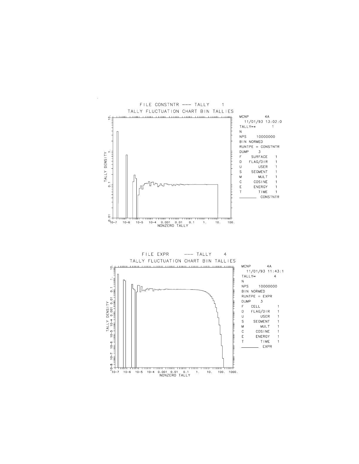
April 10, 2000 2-117
CHAPTER 2
ESTIMATION OF THE MONTE CARLO PRECISION
Figures 2.14 and 2.15 show two simple examples of empirical f(x)s from MCNP for 10 million
histories each. Figure 2.14 is from an energy leakage tally directly from a source that is uniform
in energy from 0 to 10 MeV. The analytic f(x) is a constant 0.1 between 0 and 10 MeV. The
empirical f(x) shows the sampling, which is 0.1 with statistical noise at the lower x bins where
fewer samples are made in the smaller bins.
Figure 2-14.
Figure 2-15.

2-118 April 10, 2000
CHAPTER 2
ESTIMATION OF THE MONTE CARLO PRECISION
Figure 2.15 shows the sampled distance to first collision in a material that has a macroscopic
cross section of about 0.1 cm−1. This analytic function is a negative exponential given by
f(x) = Σexp−Σ x(see page 2–27) with a mean of 10. The empirical f(x) transitions from a constant
0.1 at values of xless than unity to the expected negative exponential behavior.
7. Pareto Fit to the Largest History Scores for the TFC Bin
The slope nin 1/xnof the largest history tallies xmust be estimated to determine if and when the
largest history scores decrease faster than 1/x3. The 201 largest history scores for each TFC bin
are continuously updated and saved during the calculation. A generalized Pareto function95
Pareto f(x) = a−1(1 + kx/a)−(1/k)−1
is used to fit the largest x’s. This function fits a number of extreme value distributions including
1/xn,exponential (k=0), and constant (k=−1). The large history score tail fitting technique uses
the robust “simplex” algorithm,96 which finds the values of aand kthat best fit the largest history
scores by maximum likelihood estimation.
The number of history score tail points used for the Pareto fit is a maximum of 201 points
because this provides about 10% precision95 in the slope estimator at n=3. The precision
increases for smaller values of nand vice versa. The number of points actually used in the fit is
the lesser of 5% of the nonzero history scores or 201. The minimum number of points used for
a Pareto fit is 25 with at least two different values, which requires 500 nonzero history scores
with the 5% criterion. If less than 500 history scores are made in the TFC bin, no Pareto fit is
made.
From the Pareto fit, the slope of f(xlarge) is defined to be
.
A SLOPE value of zero is defined to indicate that not enough f(xlarge)tail information exists for
a SLOPE estimate. The SLOPE is not allowed to exceed a value of 10 (a “perfect score”), which
would indicate an essentially negative exponential decrease. If the 100 largest history scores all
have values with a spread of less than 1%, an upper limit is assumed to have been reached and
the SLOPE is set to 10. The SLOPE should be greater than 3 to satisfy the second moment
existence requirement of the CLT. Then, f(x) will appear to be “completely” sampled and hence
N will appear to have approached infinity.
A printed plot of f(x) is automatically generated in the OUTP file if the SLOPE is less than 3 (or
if any of the other statistical checks described in the next section do not pass). If
0 < SLOPE < 10, several “S’s” appear on the printed plot to indicate the Pareto fit, allowing the
quality of the fit to the largest history scores to be assessed visually. If the largest scores are not
Pareto in shape, the SLOPE value may not reflect the best estimate of the largest history score
SLOPE 1k⁄()1+≡

April 10, 2000 2-119
CHAPTER 2
ESTIMATION OF THE MONTE CARLO PRECISION
decrease. A new SLOPE can be estimated graphically. A blank or 162 on the PRINT card also
will cause printed plots of the first two cumulative moments of the empirical f(x) to be made.
Graphical plots of various f(x) quantities can be made using the “z” plot option (MCPLOT) with
the TFC plot command. These plots should be examined for unusual behavior in the empirical
f(x), including holes or spikes in the tail. MCNP tries to assess both conditions and prints a
message if either condition is found.
I. Forming Statistically Valid Confidence Intervals
The ultimate goal of a Monte Carlo calculation is to produce a valid confidence interval for each
tally bin. Section VI has described different statistical quantities and the recommended criteria
to form a valid confidence interval. Detailed descriptions of the information available in the
output for all tally bins and the TFC bins are now discussed.
1. Information Available for Forming Statistically Valid Confidence
The R is calculated for every user-specified tally bin in the problem. The VOV and the shifted
confidence interval center, discussed below, can be obtained for all bins with a nonzero entry for
the 15th entry on the DBCN card at problem initiation.
a. R Magnitude Comparisons With MCNP Guidelines: The quality of MCNP Monte
Carlo tallies historically has been associated with two statistical checks that have been the
responsibility of the user: 1) for all tally bins, the estimated relative error magnitude rules–of–
thumb that are shown in Fig. 2-3 (i.e., R<0.1 for nonpoint detector tallies and R<0.05 for point
detector tallies); and 2) a statistically constant FOM in the user-selectable (TFn card) TFC bin
so that the estimated R is decreasing by as required by the CLT.
In an attempt to make the user more aware of the seriousness of checking these criteria, MCNP
provides checks of the R magnitude for all tally bins. A summary of the checks is printed in the
“Status of Statistical Checks” table. Messages are provided to the user giving the results of these
checks.
b. Asymmetric Confidence Intervals: A correlation exists between the estimated mean
and the estimated uncertainty in the mean.89 If the estimated mean is below the expected value,
the estimated uncertainty in the mean will most likely be below its expected value. This
correlation is also true for higher moment quantities such as the VOV. The worst situation for
forming valid confidence intervals is when the estimated mean is much smaller than the expected
value, resulting in smaller than predicted coverage rates. To correct for this correlation and
improve coverage rates, one can estimate a statistic shift in the midpoint of the confidence
interval to a higher value. The estimated mean is unchanged.
1N⁄
Sx

2-120 April 10, 2000
CHAPTER 2
ESTIMATION OF THE MONTE CARLO PRECISION
The shifted confidence interval midpoint is the estimated mean plus a term proportional to the
third central moment. The term arises from an Edgeworth expansion89 to attempt to correct the
confidence interval for non-normality effects in the estimate of the mean. The adjustment term
is given by
.
Substituting for the estimated mean and expanding produces
.
The SHIFT should decrease as 1/N. This term is added to the estimated mean to produce the
midpoint of the now asymmetric confidence interval about the mean. This value of the
confidence interval midpoint can be used to form the confidence interval about the estimated
mean to improve coverage rates of the true, but unknown, mean E(x). The estimated mean plus
the SHIFT is printed automatically for the TFC bin for all tallies. A nonzero entry for the 15th
DBCN card entry produces the shifted value for all tally bins.
This correction approaches zero as Napproaches infinity, which is the condition required for the
CLT to be valid. Kalos97 uses a slightly modified form of this correction to determine if the
requirements of the CLT are “substantially satisfied.” His relation is
,
which is equivalent to
.
The user is responsible for applying this check.
c. Forming Valid Confidence Intervals for Non–TFC Bins: The amount of statistical
information available for non–TFC bins is limited to the mean and R. The VOV and the center
of the asymmetric confidence can be obtained for all tally bins with a nonzero 15th entry on the
DBCN card in the initial problem. The magnitude criteria for R (and the VOV, if available)
should be met before forming a confidence interval. If the shifted confidence interval center is
available, it should be used to form asymmetric confidence intervals about the estimated mean.
History dependent information about R (and the VOV, if available) for non–TFC bins can be
obtained by printing out the tallies periodically during a calculation using the PRDMP card. The
N–dependent behavior of R can then be assessed. The complete statistical information available
can be obtained by creating a new tally and selecting the desired tally bin with the TFn card.
SHIFT Σxix–()
32S2N()⁄=
SHIFT Σxi
33Σxi
2ΣxiN2Σxi
()
3N2
⁄+⁄–()2NΣxi
2Σxi
()
2
–()()⁄=
Σxix–()
3S3N«
SHIFT Sx2⁄«

April 10, 2000 2-121
CHAPTER 2
ESTIMATION OF THE MONTE CARLO PRECISION
2. Information Available for Forming Statistically Valid Confidence Intervals for TFC Bins
Additional information about the statistical behavior of each TFC bin result is available. A TFC
bin table is produced by MCNP after each tally to provide the user with detailed information
about the apparent quality of the TFC bin result. The contents of the table are discussed in the
following subsections, along with recommendations for forming valid confidence intervals using
this information.
a. TFC Bin Tally Information: The first part of the TFC bin table contains information
about the TFC bin result including the mean, R, scoring efficiency, the zero and nonzero history
score components of R (see page 2–109), and the shifted confidence interval center. The two
components of R can be used to improve the problem efficiency by either improving the history
scoring efficiency or reducing the range of nonzero history scores.
b. The Largest TFC Bin History Score Occurs on the Next History: There are occasions
when the user needs to make a conservative estimate of a tally result. Conservative is defined so
that the results will not be less than the expected result. One reasonable way to make such an
estimate is to assume that the largest observed history score would occur again on the very next
history, N + 1.
MCNP calculates new estimated values for the mean, R, VOV, FOM, and shifted confidence
interval center for the TFC bin result for this assumption. The results of this proposed occurrence
are summarized in the TFC bin information table. The user can assess the impact of this
hypothetical happening and act accordingly.
c. Description of the 10 Statistical Checks for the TFC Bin: MCNP prints the results of
ten statistical checks of the tally in the TFC bin at each print. In a “Status of Statistical Checks”
table, the results of these ten checks are summarized at the end of the output for all TFC bin
tallies. The quantities involved in these checks are the estimated mean, R, VOV, FOM, and the
large history score behavior of f(x). Passing all of the checks should provide additional assurance
that any confidence intervals formed for a TFC bin result will cover the expected result the
correct fraction of the time. At a minimum, the results of these checks provide the user with more
information about the statistical behavior of the result in the TFC bin of each tally.
The following 10 statistical checks are made on the TFCs printed at the end of the output for
desirable statistical properties of Monte Carlo solutions:
MEAN
(1) a nonmonotonic behavior (no up or down trend) in the estimated mean as a
function of the number histories N for the last half of the problem;

2-122 April 10, 2000
CHAPTER 2
ESTIMATION OF THE MONTE CARLO PRECISION
R
(2) an acceptable magnitude of the estimated R of the estimated mean (< 0.05 for a
point detector tally or < 0.10 for a non-point detector tally);
(3) a monotonically decreasing R as a function of the number histories Nfor the last
half of the problem;
(4) a decrease in the R as a function of N for the last half of the problem;
VOV
(5) the magnitude of the estimated VOV should be less than 0.10 for all types of
tallies;
(6) a monotonically decreasing VOV as a function of N for the last half of the
problem;
(7) a 1/N decrease in the VOV as a function of Nfor the last half of the problem;
FOM
(8) a statistically constant value of the FOM as a function of Nfor the last half of the
problem;
(9) a nonmonotonic behavior in the FOM as a function of N for the last half of the
problem; and
f(x)
(10) the SLOPE (see page 2–118) of the 25 to 201 largest positive (negative with a
negative DBCN(16) entry) history scores xshould be greater than 3.0 so that the
second moment will exist if the SLOPE is extrapolated to infinity.
The seven N-dependent checks for the TFC bin are for the last half of the problem. The last half
of the problem should be well behaved in the sense of the CLT to form the most valid confidence
intervals. “Monotonically decreasing” in checks 3 and 5 allows for some increases in both R and
the VOV. Such increases in adjacent TFC entries are acceptable and usually do not, by
themselves, cause poor confidence intervals. A TFC bin R that does not pass check 3, by
definition in MCNP, does not pass check 4. Similarly, a TFC bin VOV that does not pass check
6, by definition, does not pass check 7.
A table is printed after each tally for the TFC bin result that summarizes the results and the pass
or no-pass status of the checks. Both asymmetric and symmetric confidence intervals are printed
for the one, two, and three σlevels when all of the statistical checks are passed. These intervals
can be expected to be correct with improved probability over historical rules of thumb. This is
NOT A GUARANTEE, however; there is always a possibility that some as–yet–unsampled
portion of the problem would change the confidence interval if more histories were calculated.
1N⁄
x2fx()xd
∞–
∞
∫

April 10, 2000 2-123
CHAPTER 2
ESTIMATION OF THE MONTE CARLO PRECISION
A WARNING is printed if one or more of these ten statistical checks is not passed, and one page
of printed plot information about f(x) is produced for the user to examine.
An additional information-only check is made on the largest five f(x) score grid bins to determine
if there are bins that have no samples or if there is a spike in an f(x) that does not appear to have
an upper limit. The result of the check is included in the TFC summary table for the user to
consider. This check is not a pass or no-pass test because a hole in the tail may be appropriate
for a discrete f(x) or an exceptional sample occurred with so little impact that none of the ten
checks was affected. The empirical f(x) should be examined to assess the likelihood of
“complete” sampling.
d. Forming Valid TFC Bin Confidence Intervals: For TFC bin results, the highest
probability of creating a valid confidence interval occurs when all of the statistical checks are
passed. Not passing several of the checks is an indication that the confidence interval is less
likely to be correct. A monotonic trend in the mean for the last half of the problem is a strong
indicator that the confidence interval is likely to produce incorrect coverage rates. The
magnitudes of R and the VOV should be less than the recommended values to increase the
likelihood of a valid confidence interval. Small jumps in the R, VOV, and/or the FOM as a
function of Nare not threatening to the quality of a result. The slope of f(x) is an especially strong
indicator that Nhas not approached infinity in the sense of the CLT. If the slope appears too
shallow (< 3), check the printed plot of f(x) to see that the estimated Pareto fit is adequate. The
use of the shifted confidence interval is recommended, although it will be a small effect for a
well–converged problem.
The last half of the problem is determined from the TFC. The more information available about
the last half of the problem, the better the N-dependent checks will be. Therefore, a problem that
has run 40,000 histories will have 20 TFC N entries, which is more Nentries than a 50,000
history problem with 13 entries. It is possible that a problem that passes all tests at 40,000 may
not pass all the tests at 40,001. As is always the case, the user is responsible for deciding when
a confidence interval is valid. These statistical diagnostics are designed to aid in making this
decision.
J. A Statistically Pathological Output Example
A statistically pathological test problem is discussed in this section. The problem calculates the
surface neutron leakage flux above 12 MeV from an isotropic 14 MeV neutron point source of
unit strength at the center of a 30 cm thick concrete shell with an outer radius of 390 cm. Point
and ring detectors were deliberately used to estimate the surface neutron leakage flux with highly
inefficient, long-tailed f(x)s. The input is shown on page 5–50.
The variance reduction methods used were implicit capture with weight cutoff, low-score point
detector Russian roulette, and a 0.5 mean free path (4 cm) neighborhood around the detectors to

2-124 April 10, 2000
CHAPTER 2
ESTIMATION OF THE MONTE CARLO PRECISION
produce large, but finite, higher moments. Other tallies or variance reduction methods could be
used to make this calculation much more efficient, but that is not the object of this example. A
surface flux estimator would have been over a factor of 150 to 30,000 times more efficient than
ring and point detectors, respectively.
Figure 2.16 shows MCNP plots of the estimated mean, R, VOV and slope of the history score
PDF as a function of N values of 20,000 (left column) and 5 million (right column). The ring
detector results are shown as the solid line and the point detector result is the dashed line.
Column 1 shows the results as a function of N for 20,000 histories. The point detector result at
14,000 histories (not shown) was (R=0.041). The FOM varied somewhat
randomly between about 800 and 1160 for the last half of the problem. With no other
information, this result could be accepted by even a careful Monte Carlo practitioner. However,
the VOV never gets close to the required 0.1 value and the slope of the unbounded f(x) is less
than 1.4. This slope could not continue indefinitely because even the mean of f(x) would not
exist. Therefore, a confidence interval should not be formed for this tally. At 20,000 histories, R
increases substantially and the FOM crashes, indicating serious problems with the result.
The ring detector result is having problems of its own. The ring detector result for 14,000
histories was (R=0.17, VOV=0.35, slope=2.1, FOM=67). None of the
plotted quantities satisfies the required convergence criteria.The correct detector result, obtained
from a 5 million history ring detector tally, is (R=0.0169, VOV=0.023,
slope=4.6, FOM=19). The apparently converged 14,000 history point detector result is a factor
of four below the correct result!
If you were to run 200,000 histories, you would see the point detector result increasing to
(R=0.20, VOV=0.30, slope=1.6, FOM=1.8). The magnitudes of R and the
VOV are much too large for the point detector result to be accepted. The slope of f(x) is slowly
increasing, but has only reached a value of 1.6. This slope is still far too shallow compared to the
required value of 3.0.
The ring detector result of (R=0.0579, VOV=0.122, slope=2.8, FOM=22)
at 192,000 histories is interesting. All of these values are close to being acceptable, but just miss
the requirements. The ring detector result is more than two estimated standard deviations below
the correct result.
Column 2 shows the results as a function of Nfor 5 million histories. The ring detector result of
(R=0.0169, VOV=0.023, slope=4.6, FOM=19) now appears very well
behaved in all categories. This tally passed all 10 statistical checks. There appears to be no
reason to question the validity of this tally. The point detector result is
(R=0.11, VOV=0.28, slope=2.1, FOM=0.45). The result is clearly improving, but does not meet
the acceptable criteria for convergence. This tally did not pass 3 out 10 statistical checks.
1.41 10 8–
×ncm
2s⁄⁄
4.60 10 8–
×ncm
2s⁄⁄
5.72 10 8–
×ncm
2s⁄⁄
3.68 10 8–
×ncm
2s⁄⁄
5.06 10 8–
×ncm
2s⁄⁄
5.72 10 8–
×ncm
2s⁄⁄
4.72 10 8–
×ncm
2s⁄⁄
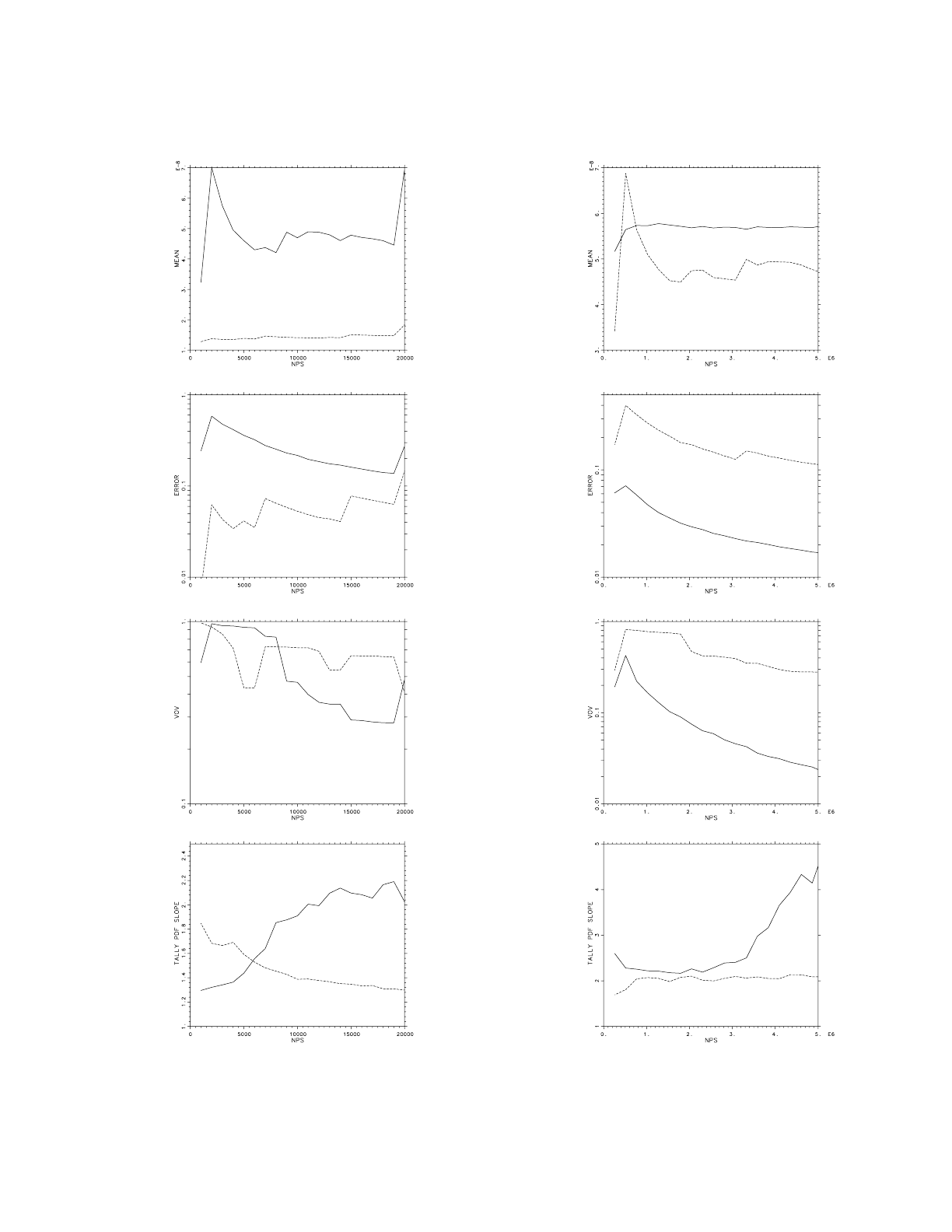
April 10, 2000 2-125
CHAPTER 2
ESTIMATION OF THE MONTE CARLO PRECISION
Figure 2-16.
Mean
RE
VOV
Slope

2-126 April 10, 2000
CHAPTER 2
ESTIMATION OF THE MONTE CARLO PRECISION
When you compare the empirical point detector f(x)s for 14,000 and 200 million histories you
see that the 14,000 history f(x) clearly has unsampled regions in the tail, indicating incomplete
f(x) sampling.94 For the point detector, seven decades of x have been sampled by 200 million
histories compared to only three decades for 14,000 histories. The largest x’s occur from the
extremely difficult to sample histories that have multiple small energy loss collisions close to the
detector. The 200 million history point detector result is (R=0.035,
VOV=0.60, slope=2.4, FOM=0.060). The point detector f(x) slope is increasing, but still is not
yet completely sampled. This tally did not pass 6 of 10 checks with 200 million histories. The
result is about 1.5 estimated standard deviations below the correct answer. It is important to note
that calculating a large number of histories DOES NOT guarantee a precise result. The more
compact empirical ring f(x) for 20 million histories appears to be completely sampled because
of the large slope. The results for 1 billion histories are shown in Ref. 86.
For difficult to sample problems such as this example, it is possible that an even larger history
score could occur that would cause the VOV and possibly the slope to have unacceptable values.
The mean and RE will be much less affected than the VOV. The additional running time required
to reach acceptable values for the VOV and the slope could be prohibitive. The large history
score should NEVER be discarded from the tally result. It is important that the cause for the large
history score be completely understood. If the score was created by a poorly sampled region of
phase space, the problem should be modified to provide improved phase space sampling. It is
also possible that the large score was created by an extremely unlikely set of circumstances that
occurred “early” in the calculation. In this situation, if the RE is within the guidelines, the
empirical f(x) appears to be otherwise completely sampled, and the largest history score appears
to be a once in a lifetime occurrence, a good confidence interval can still be formed. If a
conservative (large) answer is required, the printed result that assumes the largest history score
occurs on the very next history can be used.
Comparing several empirical f(x)s for the above problem with 200 million histories that have
been normalized so that the mean of each f(x) is unity, you see that the point detector at 390 cm
clearly is quite Cauchy–like (see Eq. (2.25) for many decades.93 The point detector at 4000 cm
is a much easier tally (by a factor of 10,000) as exhibited by the much more compact empirical
f(x). The large–score tail decreases in a manner similar to the negative exponential f(x). The
surface flux estimator is the most compact f(x) of all. The blip on the high–score tail is caused
by the average cosine approximation of 0.05 between cosines of 0 and 0.1 (see page 2–80). This
tally is 30,000 times more efficient than the point detector tally.
5.41 10 8–
×ncm
2s⁄⁄

April 10, 2000 2-127
CHAPTER 2
VARIANCE REDUCTION
VII. VARIANCE REDUCTION
A. General Considerations
1. Variance Reduction and Accuracy
Variance-reducing techniques in Monte Carlo calculations reduce the computer time required to
obtain results of sufficient precision. Note that precision is only one requirement for a good
Monte Carlo calculation. Even a zero variance calculation cannot accurately predict natural
behavior if other sources of error are not minimized. Factors affecting accuracy were discussed
in Section VI beginning on page 2–99.
2. Two Choices That Affect Efficiency
The efficiency of a Monte Carlo calculation is affected by two choices, tally type and random
walk sampling. The tally choice (for example, point detector flux tally vs. surface crossing flux
tally) amounts to trying to obtain the best results from the random walks sampled. The chosen
random walk sampling amounts to preferentially sampling “important” random walks at the
expense of “unimportant” random walks. (A random walk is important if it has a large affect on
a tally.) These two choices usually affect the time per history and the history variance as
described in Sec. 3 below. MCNP estimates tallies of the form
< T >
by sampling particle histories that statistically produce the correct particle density .
The tally function is zero except where a tally is required. For example, for a surface
crossing tally (F1),Twill be one on the surface and zero elsewhere. MCNP variance reduction
techniques allow the user to try to produce better statistical estimates of N where T is large,
usually at the expense of poorer estimates where T is zero or small.
There are many ways to statistically produce . Analog Monte Carlo simply samples
the events according to their natural physical probabilities. In this way, an analog Monte Carlo
calculation estimates the number of physical particles executing any given random walk.
Nonanalog techniques do not directly simulate nature. Instead, nonanalog techniques are free to
do anything if N, hence <T>, is preserved. This preservation is accomplished by adjusting the
weight of the particles. The weight can be thought of as the number of physical particles
represented by the MCNP particle (see page 2–26). Every time a decision is made, the nonanalog
techniques require that the expected weight associated with each outcome be the same as in the
analog game. In this way, the expected number of physical particles executing any given random
walk is the same as in the analog game.
rvtNrvt,,()Tr vt,,()d
∫
d
∫
d
∫
=
Nr vt,,()
Trvt,,()
Nr vt,,()

2-128 April 10, 2000
CHAPTER 2
VARIANCE REDUCTION
For example, if an outcome “A” is made qtimes as likely as in the analog game, when a particle
chooses outcome “A,” its weight must be multiplied by q−1to preserve the expected weight for
outcome “A.” Let p be the analog probability for outcome “A”; then pq is the nonanalog
probability for outcome “A.” If w0is the current weight of the particle, then the expected weight
for outcome “A” in the analog game is w0∗pand the expected weight for outcome “A” in the
nonanalog game is (w0/q)∗pq.
MCNP uses three basic types of nonanalog games: (1) splitting, (2) Russian roulette, and
(3) sampling from nonanalog probability density functions. The previous paragraph discusses
type 3. Splitting refers to dividing the particle's weight among two or more daughter particles
and following the daughter particles independently. Usually the weight is simply divided evenly
among kidentical daughter particles whose characteristics are identical to the parent except for
a factor 1/k in weight (for example, splitting in the weight window). In this case the expected
weight is clearly conserved because the analog technique has one particle of weight w0 at
, whereas the splitting results in k particles of weight w0/k at . In both cases
the outcome is weight w0 at .
Other splitting techniques split the parent particle into k, typically two, differing daughter
particles. The weight of the jth daughter represents the expected number of physical particles that
would select outcome jfrom a set of k mutually exclusive outcomes. For example, the MCNP
forced collision technique considers two outcomes: (1) the particle reaches a cell boundary
before collision, or (2) the particle collides before reaching a cell boundary. The forced collision
technique divides the parent particle representing w0physical particles into two daughter
particles, representing w1physical particles that are uncollided and w2 physical particles that
collide. The uncollided particle of weight w1is then put on the cell boundary. The collision site
of the collided particle of weight w2 is selected from a conditional distance-to-collision
probability density, the condition being that the particle must collide in the cell. This technique
preserves the expected weight colliding at any point in the cell as well as the expected weight
not colliding. A little simple mathematics is required to demonstrate this technique.
Russian roulette takes a particle at of weight w0 and turns it into a particle of weight
w1>w0with probability w0/w1and kills it (that is, weight=0) with probability (1−(w0/w1)). The
expected weight at is w1∗(w0/w1)+(1−(w0/w1)) ∗0=w0, the same as in the analog
game.
Some techniques use a combination of these basic games and DXTRAN uses all three.
3. Efficiency, Time per History, and History Variance
Recall from page 2–108 that the measure of efficiency for MCNP calculations is the
FOM: , where
rvt,,() rvt,,()
rvt,,()
rvt,,()
rvt,,()
FOM 1R2T()⁄≡

April 10, 2000 2-129
CHAPTER 2
VARIANCE REDUCTION
R2= sample relative standard deviation of the mean and
T= computer time for the calculation (in minutes).
Recall from Eqns. 2.17 and 2.19a that , where
S2=sample history variance,
N=number of particles, and
=sample mean.
Generally we are interested in obtaining the smallest R in a given time T. The equation above
indicates that to decrease Rit is desirable to: 1) decrease S and 2) increase N; that is, decrease
the time per particle history. Unfortunately, these two goals usually conflict. Decreasing S
normally requires more time because better information is required. Increasing Nnormally
increases Sbecause there is less time per history to obtain information. However, the situation
is not hopeless. It is often possible either to decrease S substantially without decreasing Ntoo
much or to increase N substantially without increasing Stoo much, so that Rdecreases.
Many variance reduction techniques in MCNP attempt to decrease Rby either producing or
destroying particles. Some techniques do both. In general, techniques that produce tracks work
by decreasing S(we hope much faster than Ndecreases) and techniques that destroy tracks work
by increasing N (we hope much faster than S increases).
4. Strategy
Successful use of MCNP variance reduction techniques is often difficult, tending to be more art
than science. The introduction of the weight window generator has improved things, but the user
is still fundamentally responsible for the choice and proper use of variance reducing techniques.
Each variance reduction technique has its own advantages, problems, and peculiarities.
However, there are some general principles to keep in mind while developing a variance
reduction strategy.
Not surprisingly, the general principles all have to do with understanding both the physical
problem and the variance reduction techniques available to solve the problem. If an analog
calculation will not suffice to calculate the tally, there must be something special about the
particles that tally. The user should understand the special nature of those particles that tally.
Perhaps, for example, only particles that scatter in particular directions can tally. After the user
understands why the tallying particles are special, MCNP techniques can be selected (or
developed by the user) that will increase the number of special particles followed.
After the MCNP techniques are selected the user typically has to supply appropriate parameters
to the variance reduction techniques. This is probably more difficult than is the selection of
RSN⁄()x⁄=
x

2-130 April 10, 2000
CHAPTER 2
VARIANCE REDUCTION
techniques. The first guess at appropriate parameters typically comes either from experience
with similar problems or from experience with an analog calculation of the current problem. It
is usually better to err on the conservative side; that is, too little biasing rather than too much
biasing. After the user has supplied parameters for the variance reduction techniques, a short
Monte Carlo run is done so that the effectiveness of the techniques and parameters can be
monitored with the MCNP output.
The MCNP output contains much information to help the user understand the sampling. This
information should be examined to ensure that
(1) the variance reduction techniques are improving the sampling of the particles that
tally;
(2) the variance reduction techniques are working cooperatively; that is, one is not
destructively interfering with another;
(3) the FOM table is not erratic, which would indicate poor sampling; and
(4) there is nothing that looks obviously ridiculous.
Unfortunately, analyzing the output information requires considerable thought and experience.
Reference 98 shows in detail strategies and analysis for a particular problem.
After ascertaining that the techniques are improving the calculation, the user makes a few more
short runs to refine the parameters until the sampling no longer improves. The weight window
generator can also be turned on to supply information about the importance function in different
regions of the phase space. This rather complex subject is described on page 2–139.
5. Erratic Error Estimates
Erratic error estimates are sometimes observed in MCNP calculations. In fact, the primary
reason for the Tally Fluctuation Chart (TFC) table in the MCNP output is to allow the user to
monitor the FOM and the relative error as a function of the number of histories. With few
exceptions, such as an analog point detector embedded in a scattering medium with Ro= 0 (a
practice highly discouraged), MCNP tallies are finite variance tallies. For finite variance tallies
the relative error should decrease roughly as so the FOM should be roughly constant and
the ten statistical checks of the tallies (see page 2–121) should all be passed. If the statistical
checks are not passed, the error estimates should be considered erratic and unreliable, no matter
how small the relative error estimate is.
Erratic error estimates occur typically because a high-weight particle tallies from an important
region of phase space that has not been well sampled. A high-weight particle in a given region
of phase space is a particle whose weight is some nontrivial fraction of \underbar{all} the weight
that has tallied from that region because of all previous histories. A good example is a particle
that collides very close to a point or ring detector. If not much particle weight has previously
N

April 10, 2000 2-131
CHAPTER 2
VARIANCE REDUCTION
collided that close to the detector, the relative error estimate will exhibit a jump for that history.
Another example is coherent photon scattering towards a point detector (see page 2–62).
To avoid high-weight particles in important regions, the user should try to ensure that these
regions are well sampled by many particles and try to minimize the weight fluctuation among
these particles. Thus the user should try to use biasing techniques that preferentially push
particles into important regions without introducing large weight fluctuations in these regions.
The weight window can often be very useful in minimizing weight fluctuations caused by other
variance reduction techniques.
If, despite a user's efforts, an erratic error estimate occurs, the user should obtain event logs for
those particles causing the estimate to be erratic. The event logs should be studied to learn what
is special about these particles. When the special nature of these particles is understood, the user
can adjust the variance reduction techniques to sample these particles more often. Thus their
weight will be smaller and they will not be as likely to cause erratic estimates. Under absolutely
no circumstances should these particles be discarded or ignored! The fact that these particles
contribute very heavily to the tally indicates that they are important to the calculation and the
user should try to sample more of them.
6. Biasing Against Random Walks of Presumed Low Importance
It was mentioned earlier that one should be cautious and conservative when applying variance
reduction techniques. Many more people get into trouble by overbiasing than by underbiasing.
Note that preferentially sampling some random walks means that some walks will be sampled
(for a given computer time) less frequently than they would have been in an analog calculation.
Sometimes these random walks are so heavily biased against that very few, or even none, are ever
sampled in an actual calculation because not enough particles are run.
Suppose that (on average) for every million histories only one track enters cell 23. Further
suppose that a typical run is 100,000 histories. On any given run it is unlikely that a track enters
cell~23. Now suppose that tracks entering cell 23 turn out to be much more important than a
user thought. Maybe 10% of the answer should come from tracks entering cell 23. The user
could run 100,000 particles and get 90% of the true tally with an estimated error of 1%, with
absolutely no indication that anything is amiss. However, suppose the biasing had been set such
that (on average) for every 10,000 particles, one track entered cell 23, about 10 tracks total. The
tally probably will be severely affected by at least one high weight particle and will hover closer
to the true tally with a larger and perhaps erratic error estimate. The essential point is this:
following ten tracks into cell 23 does not cost much computer time and it helps ensure that the
estimated error cannot be low when the tally is seriously in error. Always make sure that all
regions of the problem are sampled enough to be certain that they are unimportant.

2-132 April 10, 2000
CHAPTER 2
VARIANCE REDUCTION
B. Variance Reduction Techniques
There are four classes of variance reduction techniques99 that range from the trivial to the
esoteric.
Truncation Methods are the simplest of variance reduction methods. They speed up calculations
by truncating parts of phase space that do not contribute significantly to the solution. The
simplest example is geometry truncation in which unimportant parts of the geometry are simply
not modeled. Specific truncation methods available in MCNP are energy cutoff and time cutoff.
Population Control Methods use particle splitting and Russian roulette to control the number of
samples taken in various regions of phase space. In important regions many samples of low
weight are tracked, while in unimportant regions few samples of high weight are tracked. A
weight adjustment is made to ensure that the problem solution remains unbiased. Specific
population control methods available in MCNP are geometry splitting and Russian roulette,
energy splitting/roulette, weight cutoff, and weight windows.
Modified Sampling Methods alter the statistical sampling of a problem to increase the number of
tallies per particle. For any Monte Carlo event it is possible to sample from any arbitrary
distribution rather than the physical probability as long as the particle weights are then adjusted
to compensate. Thus with modified sampling methods, sampling is done from distributions that
send particles in desired directions or into other desired regions of phase space such as time or
energy, or change the location or type of collisions. Modified sampling methods in MCNP
include the exponential transform, implicit capture, forced collisions, source biasing, and
neutron-induced photon production biasing.
Partially-Deterministic Methods are the most complicated class of variance reduction methods.
They circumvent the normal random walk process by using deterministic-like techniques, such
as next event estimators, or by controlling of the random number sequence. In MCNP these
methods include point detectors, DXTRAN, and correlated sampling.
The available MCNP variance reduction techniques now are described.
1. Energy Cutoff
The energy cutoff in MCNP is either a single user-supplied, problem-wide energy level or a cell-
dependent energy level. Particles are terminated when their energy falls below the energy cutoff.
The energy cutoff terminates tracks and thus decreases the time per history. The energy cutoff
should be used only when it is known that low-energy particles are either of zero or almost zero
importance. An energy cutoff is like a Russian roulette game with zero survival probability. A
number of pitfalls exist.

April 10, 2000 2-133
CHAPTER 2
VARIANCE REDUCTION
1. Remember that low-energy particles can often produce high-energy particles (for
example, fission or low-energy neutrons inducing high-energy photons). Thus, even
if a detector is not sensitive to low-energy particles, the low-energy particles may be
important to the tally.
2. The CUT card energy cutoff is the same throughout the entire problem. Often low-
energy particles have zero importance in some regions and high importance in others,
and so a cell-dependent energy cutoff is also available with the ELPT card.
3. The answer will be biased (low) if the energy cutoff is killing particles that might
otherwise have contributed. Furthermore, as the apparent error will go to zero
and therefore mislead the unwary. Serious consideration should be given to two
techniques discussed later, energy roulette and space-energy weight window, that are
always unbiased.
The energy cutoff has one advantage not directly related to variance reduction. A lower energy
cutoff requires more cross sections so that computer memory requirements go up and interactive
computing with a timesharing system is degraded.
2. Time Cutoff
The time cutoff in MCNP is a single user-supplied, problem-wide time value. Particles are
terminated when their time exceeds the time cutoff. The time cutoff terminates tracks and thus
decreases the computer time per history. A time cutoff is like a Russian roulette game with zero
survival probability. The time cutoff should only be used in time-dependent problems where the
last time bin will be earlier than the cutoff.
Although the energy and time cutoffs are similar, more caution must be exercised with the
energy cutoff because low energy particles can produce high energy particles, whereas a late
time particle cannot produce an early time particle.
3. Geometry Splitting with Russian Roulette
Geometry splitting/Russian roulette is one of the oldest and most widely used variance-reducing
techniques in Monte Carlo codes. When used judiciously, it can save substantial computer time.
As particles migrate in an important direction, they are increased in number to provide better
sampling, but if they head in an unimportant direction, they are killed in an unbiased manner to
avoid wasting time on them. Oversplitting, however, can substantially waste computer time.
Splitting generally decreases the history variance but increases the time per history, whereas
Russian roulette generally increases the history variance but decreases the time per history.
Each cell in the problem geometry setup is assigned an importance Iby the user on the IMP input
card. The number I should be proportional to the estimated value that particles in the cell have
for the quantity being scored. When a particle of weight Wpasses from a cell of importance Ito
N∞→

2-134 April 10, 2000
CHAPTER 2
VARIANCE REDUCTION
one of higher importance , the particle is split into a number of identical particles of lower
weight according to the following recipe. If is an integer , the particle is split into
nidentical particles, each weighing W/n. Weight is preserved in the integer splitting process. If
is not an integer but still greater than 1, splitting is done probabilistically so that the
expected number of splits is equal to the importance ratio. Denoting to be the
largest integer in , is defined. Then with probability p,n+ 1 particles are
used, and with probability 1−p,n particles are used. For example, if is 2.75, 75% of the
time split 3 for 1 and 25% of the time split 2 for 1. The weight assigned to each particle is
, which is the expected weight, to minimize dispersion of weights.
On the other hand, if a particle of weight Wpasses from a cell of importance Ito one of lower
importance I', so that I'/I < 1, Russian roulette is played and the particle is killed with
probability 1−(I'/I), or followed further with probability I'/I and weight .
Geometry splitting with Russian roulette is very reliable. It can be shown that the weights of all
particle tracks are the same in a cell no matter which geometrical path the tracks have taken to
get to the cell, assuming that no other biasing techniques, e.g. implicit capture, are used. The
variance of any tally is reduced when the possible contributors all have the same weight.
The assigned cell importances can have any value—they are not limited to integers. However,
adjacent cells with greatly different importances place a greater burden on reliable sampling.
Once a sample track population has deteriorated and lost some of its information, large splitting
ratios (like 20 to 1) can build the population back up, but nothing can regain the lost information.
It is generally better to keep the ratio of adjacent importances small (for example, a factor of a
few) and have cells with optical thicknesses in the penetration direction less than about two mean
free paths. MCNP prints a warning message if adjacent importances or weight windows have a
ratio greater than 4. PRINT TABLE 120 in the OUTP file lists the affected cells and ratios.
Generally, in a deep penetration shielding problem the sample size (number of particles)
diminishes to almost nothing in an analog simulation, but splitting helps keep the size built up.
A good rule is to keep the population of tracks traveling in the desired direction more or less
constant—that is, approximately equal to the number of particles started from the source. A
good initial approach is to split the particles 2 for 1 wherever the track population drops by a
factor of 2. Near-optimum splitting usually can be achieved with only a few iterations and
additional iterations show strongly diminishing returns. Note that in a combined neutron/photon
problem, importances will probably have to be set individually for neutrons and for photons.
MCNP never splits into a void, although Russian roulette can be played entering a void.
Splitting into a void accomplishes nothing except extra tracking because all the split particles
must be tracked across the void and they all make it to the next surface. The split should be done
according to the importance ratio of the last nonvoid cell departed and the first nonvoid cell
entered.Note four more items:
I′I′I⁄nn 2≥()
I′I⁄nI′I⁄[]=
I′I⁄pI′In–⁄=I′I⁄
WII′⁄⋅
WII′⁄⋅

April 10, 2000 2-135
CHAPTER 2
VARIANCE REDUCTION
1. Geometry splitting/Russian roulette works well only in problems that do not have
extreme angular dependence. In the extreme case, splitting/Russian roulette can be
useless if no particles ever enter an important cell where the particles can be split.
2. Geometry splitting/Russian roulette will preserve weight variations. The technique is
“dumb” in that it never looks at the particle weight before deciding appropriate action.
An example is geometry splitting/Russian roulette used with source biasing.
3. Geometry splitting/Russian roulette are turned on or off together.
4. Particles are killed immediately upon entering a zero importance cell, acting as a
geometry cutoff.
4. Energy Splitting/Roulette
Energy splitting and roulette typically are used together, but the user can specify only one if
desired. Energy splitting/roulette is independent of spatial cell. If the problem has a space-
energy dependence, the space-energy dependent weight window is normally a better choice.
1. Splitting: In some cases, particles are more important in some energy ranges than in
others. For example, it may be difficult to calculate the number of 235U fissions
because the thermal neutrons are also being captured and not enough thermal neutrons
are available for a reliable sample. In this case, once a neutron falls below a certain
energy level it can be split into several neutrons with an appropriate weight
adjustment. A second example involves the effect of fluorescent emission after
photoelectric absorption. With energy splitting, the low-energy photon track
population can be built up rather than rapidly depleted, as would occur naturally with
the high photoelectric absorption cross section. Particles can be split as they move up
or down in energy at up to five different energy levels.
Energy splitting can increase as well as decrease tally variances. Currently, the MCNP
weight cutoff game does not take into account whether a particle has undergone
energy splitting or not. Consequently, particles undergoing energy splitting may then
be rouletted by the weight cutoff game, defeating any advantages of the energy
splitting.
With only a minor modification to MCNP, the mechanics for energy splitting can be
used for time splitting.
2. Russian roulette: In many cases the number of tracks increases with decreasing
energy, especially neutrons near the thermal energy range. These tracks can have
many collisions requiring appreciable computer time. They may be important to the
problem and cannot be completely eliminated with an energy cutoff, but their number
can be reduced by playing a Russian roulette game to reduce their number and
computer time.

2-136 April 10, 2000
CHAPTER 2
VARIANCE REDUCTION
If a track's energy drops through a prescribed energy level, the roulette game is played,
based on the input value of the survival probability. If the game is won, the track's
history is continued, but its weight is increased by the reciprocal of the survival
probability to conserve weight.
5. Weight Cutoff
In weight cutoff, Russian roulette is played if a particle's weight drops below a user-specified
weight cutoff. The particle is either killed or its weight is increased to a user-specified level. The
weight cutoff was originally envisioned for use with geometry splitting/Russian roulette and
implicit capture, see page 2–144. Because of this intent,
1. The weight cutoffs in cell j depend not only on WC1 and WC2 on the CUT card, but
also on the cell importances.
2. Implicit capture is always turned on (except in detailed photon physics) whenever a
nonzero WC1 is specified.
Referring to item 1 above, the weight cutoff is applied when the particle’s weight falls below
Rj∗WC2, where Rjis the ratio of the source cell importance (IMP card) to cell j’s importance.
With probability W/(WC1 ∗Rj) the particle survives with new weight WC1 ∗Rj; otherwise the
particle is killed. When WC1 and WC2 on the CUT card are negative, the weight cutoff is scaled
to the minimum source weight of a particle so that source particles are not immediately killed
by falling below the cutoff.
As mentioned earlier, the weight cutoff game was originally envisioned for use with geometry
splitting and implicit capture. To illustrate the need for a weight cutoff when using implicit
capture, consider what can happen without a weight cutoff. Suppose a particle is in the interior
of a very large medium and there are neither time nor energy cutoffs. The particle will go from
collision to collision, losing a fraction of its weight at each collision. Without a weight cutoff, a
particle's weight would eventually be too small to be representable in the computer, at which
time an error would occur. If there are other loss mechanisms (for example, escape, time cutoff,
or energy cutoff), the particle’s weight will not decrease indefinitely, but the particle may take
an unduly long time to terminate.
Weight cutoff's dependence on the importance ratio can be easily understood if one remembers
that the weight cutoff game was originally designed to solve the low-weight problem sometimes
produced by implicit capture. In a high-importance region, the weights are low by design, so it
makes no sense to play the same weight cutoff game in high- and low-importance regions.
Comments: Many techniques in MCNP cause weight change. The weight cutoff was really
designed with geometry splitting and implicit capture in mind. Care should be taken in the use
of other techniques.
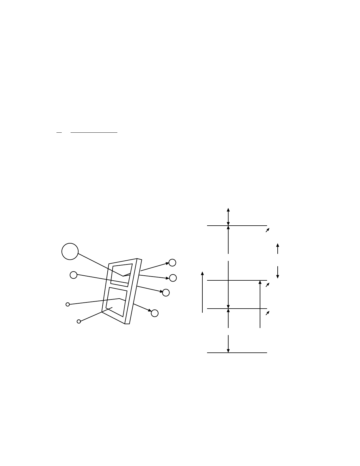
April 10, 2000 2-137
CHAPTER 2
VARIANCE REDUCTION
Weight cutoff games are unlike time and energy cutoffs. In time and energy cutoffs, the random
walk is always terminated when the threshold is crossed. Potential bias may result if the particle's
importance was not zero. A weight cutoff (weight roulette would be a better name) does not bias
the game because the weight is increased for those particles that survive.
Setting the weight cutoff is not typically an easy task and requires thought and experimentation.
Essentially the user must guess what weight is worth following and start experimenting with
weight cutoffs in that vicinity.
6. Weight Window
The weight window (Fig. 2-17) is a space-energy-dependent splitting and Russian roulette
technique. For each space-energy phase space cell, the user supplies a lower weight bound. The
upper weight bound is a user-specified multiple of the lower weight bound. These weight bounds
define a window of acceptable weights. If a particle is below the lower weight bound, Russian
roulette is played and the particle's weight is either increased to a value within the window or the
particle is terminated. If a particle is above the upper weight bound, it is split so that all the split
particles are within the window. No action is taken for particles within the window.
Figure 2.18 is a more detailed picture of the weight window. Three important weights define the
weight window in a space-energy cell
poof W
W
W
L
S
U
S
SL
UL
U
S
Particles here: play
roulette, kill,
or move to W
Particles within
window: do
nothing
Particles here: split
Increasing
Weight Lower weight bound
specified for each
space-energy cell
Survival weight
specified as a constant
C times W
Upper weight bound
specified as a constant
C times W
The constants C
and C are for
the entire problem
Figure 2-17. Figure 2-18.

2-138 April 10, 2000
CHAPTER 2
VARIANCE REDUCTION
1. WL, the lower weight bound,
2. WS, the survival weight for particles playing roulette, and
3. WU, the upper weight bound.
The user specifies WL for each space-energy cell on WWN cards. WS and WU are calculated
using two problem-wide constants, CS and CU (entries on the WWP card), as WS=CSWLand
WU=CUWL. Thus all cells have an upper weight bound CUtimes the lower weight bound and a
survival weight CS times the lower weight bound.
Although the weight window can be effective when used alone, it was designed for use with
other biasing techniques that introduce a large variation in particle weight. In particular, a
particle may have several “unpreferred” samplings, each of which will cause the particle weight
to be multiplied by a weight factor substantially larger than one. Any of these weight
multiplications by itself is usually not serious, but the cumulative weight multiplications can
seriously degrade calculational efficiency. Worse, the error estimates may be misleading until
enough extremely high-weight particles have been sampled. Monte Carlo novices are prone to
be mislead because they do not have enough experience reading and interpreting the summary
information on the sampling supplied by MCNP. Hence, a novice may put more faith in an
answer than is justified.
Although it is impossible to eliminate all pathologies in Monte Carlo calculations, a properly
specified weight window goes far toward eliminating the pathology referred to in the preceding
paragraph. As soon as the weight gets above the weight window, the particle is split and
subsequent weight multiplications will thus be multiplying only a fraction of the particle’s
weight (before splitting). Thus, it is hard for the tally to be severely perturbed by a particle of
extremely large weight. In addition, low-weight particles are rouletted, so time is not wasted
following particles of trivial weight.
One cannot ensure that every history contributes the same score (a zero variance solution), but
by using a window inversely proportional to the importance, one can ensure that the mean score
from any track in the problem isroughly constant. (A weight window generator exists to estimate
these importance reciprocals; see page 2–139.) In other words, the window is chosen so that the
track weight times the mean score (for unit track weight) is approximately constant. Under these
conditions, the variance is due mostly to the variation in the number of contributing tracks rather
than the variation in track score.
Thus far, two things remain unspecified about the weight window: the constant of inverse
proportionality and the width of the window. It has been observed empirically that an upper
weight bound five times the lower weight bound works well, but the results are reasonably
insensitive to this choice anyway. The constant of inverse proportionality is chosen so that the

April 10, 2000 2-139
CHAPTER 2
VARIANCE REDUCTION
lower weight bound in some reference cell is chosen appropriately. In most instances the
constant should be chosen so that the source particles start within the window.
1. Weight Window Compared to Geometry Splitting: Although both techniques use
splitting and Russian roulette, there are some important differences.
a. The weight window is space-energy dependent. Geometry splitting is only space
dependent.
b. The weight window discriminates on particle weight before deciding appropriate
action. Geometry splitting is done regardless of particle weight.
c. The weight window works with absolute weight bounds. Geometry splitting is
done on the ratio of the importance across a surface.
d. The weight window can be applied at surfaces, collision sites, or both. Geometry
splitting is applied only at surfaces.
e. The weight window can control weight fluctuations introduced by other biasing
techniques by requiring all particles in a cell to have weight WL<W<WU. The
geometry splitting will preserve any weight fluctuations because it is weight
independent.
f. In the rare case where no other weight modification schemes are present,
importances will cause all particles in a given cell to have the same weight.
Weight windows will merely bound the weight.
g. The weight windows can be turned off for a given cell or energy regime by
specifying a zero lower bound. This is useful in long or large regions where no
single importance function applies. Care should be used because when the weight
window is turned off at collisions, the weight cutoff game is turned on,
sometimes causing too many particles to be killed.
2. The Weight Window Generator: The generator is a method that automatically
generates weight window importance functions.100 The task of choosing importances
by guessing, intuition, experience, or trial and error is simplified and insight into the
Monte Carlo calculation is provided.
Although the window generator has proved very useful, two caveats are appropriate.
The generator is by no means a panacea for all importance sampling problems and
certainly is not a substitute for thinking on the user's part. In fact, in most instances,
the user will have to decide when the generator's results look reasonable and when
they do not. After these disclaimers, one might wonder what use to make of a

2-140 April 10, 2000
CHAPTER 2
VARIANCE REDUCTION
generator that produces both good and bad results. To use the generator effectively, it
is necessary to remember that the generated parameters are only statistical estimates
and that these estimates can be subject to considerable error. Nonetheless, practical
experience indicates that a user can learn to use the generator effectively to solve some
very difficult transport problems.
Examples of the weight window generator are given in Ref. 98 and Ref. 100 and
should be examined before using the generator. Note that this importance estimation
scheme works regardless of what other variance reduction techniques are used in a
calculation.
3. Theory: The importance of a particle at a point Pin phase space equals the expected
score a unit weight particle will generate. Imagine dividing the phase space into a
number of phase space “cells” or regions. The importance of a cell then can be defined
as the expected score generated by a unit weight particle after entering the cell. Thus,
with a little bookkeeping, the cell's importance can be estimated as
After the importances have been generated, MCNP assigns weight windows inversely
proportional to the importances. Then MCNP supplies the weight windows in an
output file suitable for use as an input file in a subsequent calculation. The spatial
portion of the phase space is divided using either standard MCNP cells or a
superimposed mesh grid, which can be either rectangular or cylindrical. The energy
portion of the phase space is divided using the WWGE card. The time portion of the
phase space can be divided also. The constant of proportionality is specified on the
WWG card.
4. Limitations of the Weight-Window Generator: The principal problem encountered
when using the generator is bad estimates of the importance function because of the
statistical nature of the generator. In particular, unless a phase space region is sampled
adequately, there will be either no generator importance estimate or an unreliable one.
The generator often needs a very crude importance guess just to get any tally; that is,
the generator needs an initial importance function to estimate a (we hope) better one
for subsequent calculations.
Fortunately, in most problems the user can guess some crude importance function
sufficient to get enough tallies for the generator to estimate a new set of weight
windows. Because the weight windows are statistical, several iterations usually are
Importance
(expected score)
total score because of particles (and
their progeny) entering the cell
total weight weight entering the cell
=

April 10, 2000 2-141
CHAPTER 2
VARIANCE REDUCTION
required before the optimum importance function is found for a given tally. The first
set of generated weight windows should be used in a subsequent calculation, which
generates a better set of windows, etc.
In addition to iterating on the generated weight windows, the user must exercise some
degree of judgment. Specifically, in a typical generator calculation, some generated
windows will look suspicious and will have to be reset. In MCNP, this task is
simplified by an algorithm that automatically scrutinizes cell-based importance
functions, either input by the user or generated by a generator. By flagging the
generated windows that are more than a factor of 4 different from those in adjacent
spatial regions, often it is easy to determine which generated weight windows are
likely to be statistical flukes that should be revised before the next generator iteration.
For example, suppose the lower weight bounds in adjacent cells were 0.5, 0.3, 0.9,
0.05, 0.03, 0.02, etc.; here the user would probably want to change the 0.9 to
something like 0.1 to fit the pattern, reducing the 18:1 ratio between cells 3 and 4.
The weight window generator also will fail when phase space is not sufficiently
subdivided and no single set of weight window bounds is representative of the whole
region. It is necessary to turn off the weight windows (by setting a lower bound of
zero) or to further subdivide the geometry or energy phase space. Use of a
superimposed importance mesh grid for weight window generation is a good way to
subdivide the spatial portion of the phase space without complicating the MCNP cell
geometry.
On the other hand, the weight window generator will also fail if the phase space is too
finely subdivided and subdivisions are not adequately sampled. Adequate sampling of
the important regions of phase space is always key to accurate Monte Carlo
calculations and the weight window generator is a tool to help the user determine the
important phase space regions. When using the mesh-based weight window generator,
resist the temptation to create mesh cells that are too small.
7. Exponential Transform
The exponential transform samples the distance to collision from a nonanalog probability
density function. Although many impressive results are claimed for the exponential transform,
it should be remembered that these results are usually obtained for one-dimensional geometries
and quite often for energy-independent problems. A review article by Clark101 gives theoretical
background and sample results for the exponential transform. Sarkar and Prasad102 have done a
purely analytical analysis for the optimum transform parameter for an infinite slab and one
energy group. The exponential transform allows particle walks to move in a preferred direction
by artificially reducing the macroscopic cross section in the preferred direction and increasing
the cross section in the opposite direction according to

2-142 April 10, 2000
CHAPTER 2
VARIANCE REDUCTION
,
where Σt*=fictitious transformed cross section,
Σt= true total cross section,
Σa= absorption cross section,
Σs= scattering cross section,
p= the exponential transform parameter used to vary the degree
of biasing |p|< 1. Can be a constant or p= Σa/Σt, in which case
Σt*= Σs, and
µ= cosine of the angle between the preferred direction and the
particle's direction. . The preferred direction can be
specified on a VECT card.
At a collision a particle's weight is multiplied by a factor wc(derived below) so that the expected
weight colliding at any point is preserved. The particle's weight is adjusted such that the weight
multiplied by the probability that the next collision is in ds about s remains constant.
The probability of colliding in ds about s is
,
where Σ is either Σtor Σt*, so that preserving the expected collided weight requires
,
or
.
If the particle reaches a cell surface, time cutoff, DXTRAN sphere, or tally segment instead of
colliding, the particle's weight is adjusted so that the weight, multiplied by the probability that
the particle travels a distance s to the surface, remains constant. The probability of traveling a
distance s without collision is
,
so that preserving the expected uncollided weight requires
, or
ΣtΣt1pµ–()=
*
µ1≤
ΣeΣs–sd
ΣteΣts–sdw
cΣteΣts–sd=*
wc
ΣteΣts–
ΣteΣts–
---------------- eρΣtµs–
1pµ–
----------------==
**
eΣs–
eΣts–wseΣts–
=*

April 10, 2000 2-143
CHAPTER 2
VARIANCE REDUCTION
.
For one–dimensional deep penetration through highly absorbing media, the variance typically
will decrease as p goes from zero to some p', and then increase as p goes from p' to one. For
p<p', the solution is “underbiased” and for p>p', the solution is “overbiased.”
Choosing p' is usually a matter of experience, although some insight may be gleaned by
understanding what happens in severely underbiased and severely overbiased calculations. For
illustration, apply the variance analysis of page 2–109 to a deep penetration problem when the
exponential transform is the only nonanalog technique used. In a severely underbiased
calculation , very few particles will score, but those that do will all contribute unity.
Thus the variance in an underbiased system is caused by a low scoring efficiency rather than a
large dispersion in the weights of the penetrating particles. In a severely overbiased system
particles will score, but there will be a large dispersion in the weights of the penetrating
particles with a resulting increase in variance.
Comments: MCNP gives a warning message if the exponential transform is used without a
weight window. There are numerous examples where an exponential transform without a weight
window gives unreliable means and error estimates. However, with a good weight window both
the means and errors are well behaved. The exponential transform works best on highly
absorbing media and very poorly on highly scattering media. For neutron penetration of concrete
or earth, experience indicates that a transform parameter p= 0.7 is about optimal. For photon
penetration of high-Z material, even higher values such as p= 0.9 are justified.
The following explains what happens with an exponential transform without a weight window.
For simplicity consider a slab of thickness T with constant Σt. Let the tally be a simple count
(F1 tally) of the weight penetrating the slab and let the exponential transform be the only
nonanalog technique used. Suppose for a given penetrating history that there are kflights, mthat
collide and n that do not collide. The penetrating weight is thus:
.
However, the particle's penetration of the slab means that
and hence
wseΣts–
eΣts–
-----------eρΣtµs–
==
p0→()
p1→()
wpeρΣtµisi
–
1pµi
–()
---------------------- eρΣtµjsj
–
jm1+=
k
∏
i1=
m
∏
=
µlsl
l1=
k
∑T=

2-144 April 10, 2000
CHAPTER 2
VARIANCE REDUCTION
.
The only variation in wpis because of the (1−pµ)−1 factors that arise only from collisions. For
a perfectly absorbing medium, every particle that penetrates scores exactly . If a particle
has only a few collisions, the weight variation will be small compared to a particle that has many
collisions. The weight window splits the particle whenever the weight gets too large, depriving
the particle of getting a whole series of weight multiplications upon collision that are
substantially greater than one.
By setting p=Σ
a/Σtand µ=1so that Σ*=Σ
s, we sample distance to scatter rather than distance
to collision. It is preferable to sample distance to scatter in highly absorbing media — in fact,
this is the standard procedure for astrophysics problems. Sampling distance to scatter is also
equivalent to implicit capture along a flight path (see page 2–35). However, in such highly
absorbing media there is usually a more optimal choice of transform parameter, p, and it is
usually preferable to take advantage of the directional component by not fixing µ = 1.
8. Implicit Capture
“Implicit capture,” “survival biasing,” and “absorption by weight reduction” are synonymous.
Implicit capture is a variance reduction technique applied in MCNP \underbar{after} the
collision nuclide has been selected. Let
σti = total microscopic cross section for nuclide i and
σai = microscopic absorption cross section for nuclide i.
When implicit capture is used rather than sampling for absorption with probability σai/σti, the
particle always survives the collision and is followed with new weight: W∗(1 − σai}/σti).
Implicit capture is a splitting process where the particle is split into absorbed weight (which need
not be followed further) and surviving weight.
Implicit capture can also be done along a flight path rather than at collisions when a special form
of the exponential transform is used. See page 2–35 for details.
Two advantages of implicit capture are
1. a particle that has finally, against considerable odds, reached the tally region is not
absorbed just before a tally is made, and
2. the history variance, in general, decreases when the surviving weight (that is, 0 or W)
is not sampled, but an expected surviving weight is used instead (see weight cutoff,
page 2–136).
w
peρΣtT–1pµi
–()
1–
i1=
m
∏
=
epΣt
–T
=

April 10, 2000 2-145
CHAPTER 2
VARIANCE REDUCTION
Two disadvantages are
1. a fluctuation in particle weight is introduced, and
2. the time per history is increased (see weight cutoff, page 2–136).
9. Forced Collisions
The forced collision method is a variance reduction scheme that increases sampling of collisions
in specified cells. Because detector contributions and DXTRAN particles arise only from
collisions and at the source, it is often useful in certain cells to increase the number of collisions
that can produce large detector contributions or large weight DXTRAN particles. Sometimes
we want to sample collisions in a relatively thin cell (a fraction of a mean free path) to improve
the estimate of quantities like a reaction rate or energy deposition or to cause collisions that are
important to some other part of the problem.
The forced collision method splits particles into collided and uncollided parts. The collided part
is forced to collide within the current cell. The uncollided part exits the current cell without
collision and is stored in the bank until later when its track is continued at the cell boundary. Its
weight is
,
where Wo= current particle weight before forced collision,
d= distance to cell surface in the particle's direction, and
Σt= macroscopic total cross section of the cell material.
That is, the uncollided part is the current particle weight multiplied by the probability of exiting
the cell without collision.
The collided part has weight , which is the current particle weight
multiplied by the probability of colliding in the cell. The uncollided part is always produced. The
collided part may be produced only a fraction fof the time, in which case the collided weight is
. This is useful when several forced collision cells are adjacent or when too
much time is spent producing and following forced collision particles.
The collision distance is sampled as follows. If P(x) is the unconditional probability of colliding
within a distance x,P(x)/P(d) is the conditional probability of colliding within a distance xgiven
that a collision is known to occur within a distance d. Thus the position xof the collision must
be sampled on the interval 0<x<d within the cell according to ξ=P(x)/P(d), where
and ξ is a random number. Solving for x, one obtains
WW
oeΣtd–
=
WW
01eΣtd–
–()=
Wo1eΣtd–
–()f⁄
Px() 1exΣt
–
–=

2-146 April 10, 2000
CHAPTER 2
VARIANCE REDUCTION
.
Because a forced collision usually yields a collided particle having a relatively small weight,
care must be taken with the weight-cutoff game (page 2–136), the weight-window game
(page 2–137), and subsequent collisions of the particle within the cell. The weight window game
is not played on the surface of a forced collision cell that the particle is entering. For collisions
inside the cell the user has two options.
Option 1: (negative entry for the cell on the forced collision card.) After the forced collision,
subsequent collisions of the particle are sampled normally. The weight cutoff game is turned off
and detector contributions and DXTRAN particles are made before the weight window game is
played. If weight windows are used, they should be set to the weight of the collided particle
weight or set to zero if detector contributions or DXTRAN particles are desired.
Option 2: (positive entry for the cell on the forced collision card.) After the forced collision,
detector contributions or DXTRAN particles are made and either the weight cutoff or weight
window game is played. Surviving collided particles undergo subsequent forced collisions. If
weight windows are used, they should bracket the weight of particles entering the cell.
10. Source Variable Biasing
Provision is made for biasing the MCNP sources in any or all of the source variables specified.
MCNP's source biasing, although not completely general, allows the production of more source
particles, with suitably reduced weights, in the more important regimes of each variable. For
example, one may start more “tracks” at high energies and in strategic directions in a shielding
problem while correcting the distribution by altering the weights assigned to these tracks.
Sizable variance reductions may result from such biasing of the source. Source biasing samples
from a nonanalog probability density function.
If negative weight cutoff values are used on the CUT card, the weight cutoff is made relative to
the lowest value of source particle weight generated by the biasing schemes.
Source biasing is the only variance reduction scheme allowed with F8 tallies having energy
binning (see page 2–83).
1. Biasing by Specifying Explicit Sampling Frequencies: The SB input card determines
source biasing for a particular variable by specifying the frequency at which source
particles will be produced in the variable regime. If this fictitious frequency does not
correspond to the fraction of actual source particles in a variable bin, the corrected
weight of the source particles in a particular bin is determined by the ratio of the actual
frequency (defined on the SP card) divided by the fictitious frequency (defined on the
x1
Σt
-----1ξ1edΣt
–
–()–[]ln–=
*

April 10, 2000 2-147
CHAPTER 2
VARIANCE REDUCTION
SB card) except for the lin-lin interpolation where it is defined to be the ratio of the
actual to fictitious frequency evaluated at the exact value of the interpolated variable.
The total weight of particles started in a given SI bin interval is thus conserved.
2. Biasing by Standard Prescription: Source biasing can use certain built-in prescriptions
similar in principle to built-in analytic source distributions. These biasing options are
detailed in the sections below for the appropriate source variables. The SB card input
is analogous to that of an SP card for an analytic source distribution; that is, the first
entry is a negative prescription number for the type of biasing required, followed by
one or more optional user-specified parameters, which are discussed in the following
sections.
a. Direction Biasing: The source direction can be biased by sampling from a continuous
exponential function or by using cones of fixed size and starting a fixed fraction of particles
within each cone. The user can bias particles in any arbitrary direction or combination of
directions.
In general, continuous biasing is preferable to fixed cone biasing because cone biasing can cause
problems from the discontinuities of source track weight at the cone boundaries. However, if the
cone parameters (cone size and fraction of particles starting in the cone) are optimized through
a parameter study and the paths that tracks take to contribute to tallies are understood, fixed cone
biasing sometimes can outperform continuous biasing. Unfortunately, it is usually time
consuming (both human and computer) and difficult to arrive at the necessary optimization.
Source directional biasing can be sampled from an exponential probability density function
p(µ)=CeKµ, where Cis a norming constant equal to K/(eK−e−K) and , where is an
angle relative to the biasing direction. Kis typically about 1; K= 3.5 defines the ratio of weight
of tracks starting in the biasing direction to tracks starting in the opposite direction to be 1/1097.
This ratio is equal to e−2K.
Table 2.6 may help to give you a feel for the biasing parameter K.r
TABLE 2.6:
Exponential Biasing Parameter
KCumulative
Probability Theta Weight K Cumulative
Probability Theta Weight
.01 0 0 0.990 2.0 0 0.245
.25 60 0.995 .25 31 .325
.50 90 1.000 .50 48 .482
.75 120 1.005 .75 70 .931
1.00 180 1.010 1.00 180 13.40
µθcos=θ

2-148 April 10, 2000
CHAPTER 2
VARIANCE REDUCTION
From this table for K=1, we see that half the tracks start in a cone of 64oopening about the axis,
and the weight of tracks at 64ois 0.762 times the unbiased weight of source particles. K= 0.01
is almost equivalent to no biasing, and K= 3.5 is very strong.
Cone directional biasing can be invoked by specifying cone cosines on the SI card, the true
distribution on the SP card, and the desired biasing probabilities on the SB card. Both histogram
and linear interpolation can be used. For example, consider the following case in which the true
distribution is isotropic:
The direction cosine relative to the reference direction, say v, is sampled uniformly within the
cone ν<v<1with probability p2and within −1 < v<νwith the complementary probability p1.
The weights assigned are W(1 − ν)/(2p2) and W(1 + ν)/(2p1), respectively. Note that for a very
small cone defined by νand a high probability p2>> p1for being within the cone, the few source
particles generated outside the cone will have a very high weight that can severely perturb a tally.
The sampling of the direction cosines azimuthal to the reference axis is not biased.
b. Covering Cylinder Extent Biasing: This biasing prescription for the SDEF EXT
variable allows the automatic spatial biasing of source particles in a cylindrical-source-covering-
volume along the axis of the cylinder. Such biasing can aid in the escape of source particles from
optically thick source regions and thus represents a variance reduction technique.
c. Covering Cylinder or Sphere Radial Biasing: This biasing prescription for the SDEF
RAD variable allows for the radial spatial biasing of source particles in either a spherical or
cylindrical source covering volume. Like the previous example of extent biasing, this biasing can
be used to aid in the escape of source particles from optically thick source regions.
1.0 0 0 .432 3.5 0 0 .143
.25 42 .552 .25 23 .190
.50 64 .762 .50 37 .285
.75 93 1.230 .75 53 .569
1.00 180 3.195 1.00 180 156.5
TABLE 2.6:
Exponential Biasing Parameter
SIn 1v1–
SPn 01v+
2
------------1v–
2
---------
SBn0p1p2

April 10, 2000 2-149
CHAPTER 2
VARIANCE REDUCTION
3. Biasing Standard Analytic Source Functions:103 The preceding examples discuss the
biasing of source variables by either input of specific sampling frequencies
corresponding to SP card entries or by standard analytic biasing functions. A third
biasing category can be used in conjunction with standard analytic source probability
functions (for example, a Watt fission spectrum).
A negative entry on an SP card, that is,
SPn −iab
causes MCNP to sample source distribution n from probability function i with input
variables a,b,... . Sampling schemes are typically unbiasable. For example, for
SPn −5a
the evaporation spectrum f(E) =CEexp(−E/a) is sampled according to the sampling
prescription E=−alog (\ξ1∗ξ2), where ξi1and ξi2are random numbers. Biasing this
sampling scheme is usually very difficult or impossible. Fortunately, there is an
approximate method available in MCNP for biasing any arbitrary probability
function.103 The code approximates the function as a table, then uses the usual SB card
biasing scheme to bias this approximate table function. The user inputs a coarse bin
structure to govern the bias and the code adds up to 300 additional equiprobable bins
to assure accuracy. For example, suppose we wish to sample the function
f(E) = C E exp(−E/a)
and suppose that we want half the source to be in the range .005 < E<.1and the other
half to be in the range .1 < E< 20. Then the input is
SPn -5 a
SIn .005 .1 20
SBn C 0 .5 1 .
MCNP breaks up the function into 150 equiprobable bins below E=.1and 150 more
equiprobable bins above E= .1. Half the time E is chosen from the upper set of bins
and half the time it is chosen from the lower set. Particles starting from the upper bins
have a different weight than that of particles starting from the lower bins to adjust for
the bias, and a detailed summarys provided when the PRINT option is used.
Note that in the above example the probability distribution function is truncated below
E= .005 and above E= 20. MCNP prints out how much of the distribution is lost in
this manner and reduces the weight accordingly.
It is possible for the user to choose a foolish biasing scheme. For example,
SPn -5 a
SIn .005 297I .1 20
SBn 0 1 298R

2-150 April 10, 2000
CHAPTER 2
VARIANCE REDUCTION
causes each of the 299 bins to be chosen with equal probability. This would be all right
except that since there are never more than 300 equiprobable bins, this allocates only
1 equiprobable bin per user-supplied bin. The single equiprobable bin for .1 < E<20
is inadequate to describe the distribution function over this range. Thus the table no
longer approximates the function and the source will be sampled erroneously. MCNP
issues an error message whenever too much of the source distribution is allocated to a
single equiprobable bin, alerting users to a poor choice of binning which might
inadequately represent the function. The coarse bins used for biasing should be chosen
so that the probability function is roughly equally distributed among them.
11. Point Detector Tally
The point detector is a tally and does not bias random walk sampling. Recall from Section VI,
however, that the tally choice affects the efficiency of a Monte Carlo calculation. Thus, a little
will be said here in addition to the discussion in the tally section.
Although flux is a point quantity, flux at a point cannot be estimated by either a track-length tally
(F4) or a surface flux tally (F2) because the probability of a track entering the volume or crossing
the surface of a point is zero. For very small volumes, a point detector tally can provide a good
estimate of the flux where it would be almost impossible to get either a track-length or surface-
crossing estimate because of the low probability of crossing into the small volume.
It is interesting that a DXTRAN sphere of vanishingly small size with a surface-crossing tally
across the diameter normal to the particle's trajectory is equivalent to a point detector. Thus,
many of the comments on DXTRAN are appropriate and the DXC cards essentially are identical
to the PD cards.
For a complete discussion of point detectors, see page 2–75.
12. DXTRAN
DXTRAN typically is used when a small region is being inadequately sampled because particles
have a very small probability of scattering toward that region. To ameliorate this situation, the
user can specify in the input file a DXTRAN sphere that encloses the small region. Upon
collision (or exiting the source) outside the sphere, DXTRAN creates a special “DXTRAN
particle” and deterministically scatters it toward the DXTRAN sphere and deterministically
transports it, without collision, to the surface of the DXTRAN sphere. The collision itself is
otherwise treated normally, producing a non-DXTRAN particle that is sampled in the normal
way, with no reduction in weight. However, the non-DXTRAN particle is killed if it tries to enter
the DXTRAN sphere. DXTRAN uses a combination of splitting, Russian roulette, and sampling
from a nonanalog probability density function.

April 10, 2000 2-151
CHAPTER 2
VARIANCE REDUCTION
The subtlety about DXTRAN is how the extra weight created for the DXTRAN particles is
balanced by the weight killed as non-DXTRAN particles cross the DXTRAN sphere. The non-
DXTRAN particle is followed without any weight correction, so if the DXTRAN technique is
to be unbiased, the extra weight put on the DXTRAN sphere by DXTRAN particles must
somehow (on average) balance the weight of non-DXTRAN particles killed on the sphere.
1. DXTRAN Viewpoint 1: One can view DXTRAN as a splitting process (much like the
forced collision technique) wherein each particle is split upon departing a collision (or
source point) into two distinct pieces:
a. the weight that does not enter the DXTRAN sphere on the next flight, either
because the particle is not pointed toward the DXTRAN sphere or because
the particle collides before reaching the DXTRAN sphere, and
b. the weight that enters the DXTRAN sphere on the next flight.
Let wobe the weight of the particle before exiting the collision, let p1be the analog probability
that the particle does not enter the DXTRAN sphere on its next flight, and let p2be the analog
probability that the particle does enter the DXTRAN sphere on its next flight. The particle must
undergo one of these mutually exclusive events, thus p1+p2= 1. The expected weight not
entering the DXTRAN sphere is w1=wop1, and the expected weight entering the DXTRAN
sphere is w2=wop2. Think of DXTRAN as deterministically splitting the original particle with
weight wointo two particles, a non-DXTRAN (particle 1) particle of weight w1and a DXTRAN
(particle 2) particle of weight w2. Unfortunately, things are not quite that simple.
Recall that the non-DXTRAN particle is followed with unreduced weight worather than weight
w1=wop1. The reason for this apparent discrepancy is that the non-DXTRAN particle (#1) plays
a Russian roulette game. Particle 1’s weight is increased from w1 to woby playing a Russian
roulette game with survival probability p1=w1/wo. The reason for playing this Russian roulette
game is simply that p1is not known, so assigning weight w1=p1woto particle 1 is impossible.
However, it is possible to play the Russian roulette game without explicitly knowing p1. It is not
magic, just slightly subtle.
The Russian roulette game is played by sampling particle 1 normally and keeping it only if it
does not enter (on its next flight) the DXTRAN sphere; that is, particle 1 survives (by definition
of p1) with probability p1. Similarly, the Russian roulette game is lost if particle 1 enters (on its
next flight) the DXTRAN sphere; that is, particle 1 loses the roulette with probability p2. To
restate this idea, with probability p1, particle 1 has weight woand does not enter the DXTRAN
sphere and with probability p2, the particle enters the DXTRAN sphere and is killed. Thus, the
expected weight not entering the DXTRAN sphere is wop1+0∗p2=w1, as desired.
So far, this discussion has concentrated on the non-DXTRAN particle and ignored exactly what
happens to the DXTRAN particle. The sampling of the DXTRAN particle will be discussed after
a second viewpoint on the non-DXTRAN particle.

2-152 April 10, 2000
CHAPTER 2
VARIANCE REDUCTION
2. DXTRAN Viewpoint 2: This second way of viewing DXTRAN does not see
DXTRAN as a splitting process but as an accounting process in which weight is both
created and destroyed on the surface of the DXTRAN sphere. In this view, DXTRAN
estimates the weight that should go to the DXTRAN sphere upon collision and creates
this weight on the sphere as DXTRAN particles. If the non-DXTRAN particle does
not enter the sphere, its next flight will proceed exactly as it would have without
DXTRAN, producing the same tally contributions and so forth. However, if the non-
DXTRAN particle's next flight attempts to enter the sphere, the particle must be killed
or there would be (on average) twice as much weight crossing the DXTRAN sphere
as there should be because the weight crossing the sphere has already been accounted
for by the DXTRAN particle.
3. The DXTRAN Particle: Although the DXTRAN particle does not confuse people
nearly as much as the non-DXTRAN particle, the DXTRAN particle is nonetheless
subtle.
The most natural approach for scattering particles toward the DXTRAN sphere would
be to sample the scattering angle proportional to the analog density. This approach
is not used because it is too much work to sample proportional to the analog density
and because it is sometimes useful to bias the sampling.
To sample in an unbiased fashion when it is known that points to the DXTRAN
sphere, one samples the conditional density
Pcon}( ) =P( )/ (the set S( ) points toward the sphere)
and multiplies the weight by , the probability of scattering into the
cone (see Fig. 2-19). However, it is too much work to calculate the above integral for
each collision. Instead, an arbitrary density function Parb( ) is sampled and the
weight is multiplied by
.
The total weight multiplication is the product of the fraction of the weight scattering
into the cone, , and the weight correction for sampling Parb( ) instead
of Pcon( ). Thus, the weight correction on scattering is
P()Parb().
Ω
ΩΩ
ΩΩ PΩ()Ωd
SΩ()
∫Ω
PΩ()Ω()d
SΩ()
∫
Ω
Pcon Ω()
Parb Ω()
-------------------- PΩ()
Parb Ω() PΩ()Ω()d
SΩ()
∫
------------------------------------------------------------=
PΩ()Ωd
SΩ()
∫Ω
Ω
ΩΩ

April 10, 2000 2-153
CHAPTER 2
VARIANCE REDUCTION
If µis the cosine of the angle between the scattering direction and the particle’s
incoming direction, then P()=P(µ)/(2π) because the scattering is symmetric in the
azimuthal angle. If is the cosine of the angle with respect to the cone axis (see
Fig. 2-19) and if the azimuthal angle about the cone axis is uniformly sampled, then
Parb()=Parb( )/(2π). Thus
= weight multiplier for DXTRAN particle.
This result can be obtained more directly, but the other derivation does not explain why
Pcon( ) is not sampled.
Because Parb( ) is arbitrary, MCNP can choose a scheme that samples from a two-
step density that favors particles within the larger interval. In fact, the inner
DXTRAN sphere has to do only with this arbitrary density and is not essential to the
DXTRAN concept. The DXTRAN particles are always created on the outside
DXTRAN sphere, with the inner DXTRAN sphere defining only the boundary
between the two steps in the density function.
After = cos has been chosen, the azimuthal angle is sampled uniformly on
[0,2π]; this completes the scattering. Recall, however, that the DXTRAN particle
arrives at the DXTRAN sphere without collision. Thus the DXTRAN particle also has
its weight multiplied by the negative exponential of the optical path between the
collision site and the sphere.
4. Inside the DXTRAN Sphere: So far, only collisions outside the DXTRAN sphere have
been discussed. At collisions inside the DXTRAN sphere, the DXTRAN game is not
played because first, the particle is already in the desired region, and second, it is
impossible to define the angular cone of Fig. 2-19. If there are several DXTRAN
spheres and the collision occurs in sphere i, DXTRAN will be played for all spheres
except sphere i.
5. Terminology—Real particle and Pseudoparticle: Sometimes the\break DXTRAN
particle is called a pseudoparticle and the non-DXTRAN particle is called the original
or real particle. The terms “real particle” and “pseudoparticle” are potentially
misleading. Both particles are equally real: both execute random walks, both carry
nonzero weight, and both contribute to tallies. The only sense in which the DXTRAN
particle should be considered “pseudo” or “not real” is during creation. A DXTRAN
particle is created on the DXTRAN sphere, but creation involves determining what
weight the DXTRAN particle should have upon creation. Part of this weight
determination requires calculating the optical path between the collision site and the
DXTRAN sphere. This is done in the same way as point detectors (see point detector
pseudoparticles on page 2–90.) MCNP determines the optical path by tracking a
Ω
η
Ωη
Pµ()
Parb η()
-------------------
Ω
ηη
η
ηθ ϕ
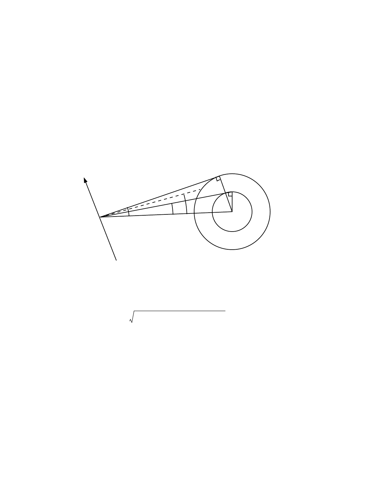
2-154 April 10, 2000
CHAPTER 2
VARIANCE REDUCTION
pseudoparticle from the collision site to the DXTRAN sphere. This pseudoparticle is
deterministically tracked to the DXTRAN sphere simply to determine the optical path.
No distance to collision is sampled, no tallies are made, and no records of the
pseudoparticle's passage are kept (for example, tracks entering). In contrast, once the
DXTRAN particle is created at the sphere's surface, the particle is no longer a
pseudoparticle. The particle has real weight, executes random walks, and contributes
to tallies.
6. DXTRAN Details: To explain how the scheme works, consider the neighborhood of
interest to be a spherical region surrounding a designated point in space. In fact,
consider two spheres of arbitrary radii about the point Po=(xo,yo,zo). Further, assume
that the particle having direction (u,v,w) collides at the point P1=(x,y,z), as shown in
Fig. 2-19.
The quantities I,O,I,O,RI, and Roare defined in the figure. Thus L, the
distance between the collision point and center of the spheres, is
.
On collision, a DXTRAN particle is placed at a point on the outer sphere of radius Ro
as described below. Provision is made for biasing the contributions of these DXTRAN
particles on the outer sphere within the cone defined by the inner sphere. The weight
of the DXTRAN particle is adjusted to account for the probability of scattering in the
direction of the point on the outer sphere and traversing the distance with no further
collision.
The steps in sampling the DXTRAN particles are outlined:
(u,v,w)
P1P0
RI
Ps
R0
θθθ
η
ηθ
θ
I= cos I
0= cos 0
0LI
Figure 2-19.
θθ ηη
Lxx
o
–()
2yy
o
–()
2zz
o
–()
2
++=

April 10, 2000 2-155
CHAPTER 2
VARIANCE REDUCTION
Sample =I+ξ(1 −I) uniformly in ( I,1) with probability
Q(1 − I)/[Q(1 − I) + I−O]
and with probability
(I−O)/[Q(1 − I) + I−O]
sample =O+ξ(I – O) uniformly in ( O,I). The quantity Q (equal to 5 in
MCNP) is a factor that measures the importance assigned to scattering in the inner
cone relative to the outer cone. Therefore, Q is also the ratio of weights for particles
put in the two different cones.
With = cos chosen, a new direction is computed by considering the
rotation through the polar angle (and a uniform azimuthal angle ) from the
reference direction
.
The particle is advanced in the direction to the surface of the sphere of
radius Ro. The new DXTRAN particle with appropriate direction and coordinates is
banked. The weight of the DXTRAN particle is determined by multiplying the weight
of the particle at collision by
and
where
µ=uu' +vv' +ww',
P(µ) = scattering probability density function for scattering through the angle
cos−1 µ in the lab system for the event sampled at (x,y,z),
ηIθI
cos L2RI
2
–()
12⁄L⁄==
ηOθO
cos L2Ro
2
–()
12⁄L⁄==
ηη η η
ηηηη
ηη η ηη
ηη η η ηη
ηθ u′v′w′,,()
θϕ
xox–
L
----------- yoy–
L
--------------zoz–
L
-------------
,,
u′v′w′,,()
νPµ()Q1ηI
–()η
IηO
–+{}e
σts()sd
PI
PS
∫
–
Q
---------------------------------------------------------------------------------------------- ηIη1≤≤,⋅
νPµ()Q1ηI
–()η
IηO
–+{}e
σts()sd
PI
PS
∫
–
ηOηη
I
≤≤,⋅

2-156 April 10, 2000
CHAPTER 2
VARIANCE REDUCTION
ν= number of particles emitted from the event, and
=the attenuation along the line between P1(x,y,z) and Ps, the point
on the sphere where the particle is placed.
In arriving at the weight factor, note that the density function for sampling is given
by
.
Thus the weight of the DXTRAN particle is the weight of the incoming particle at P1
modified by the ratio of the probability density function for actually scattering from
P1 and arriving at Pswithout collision to the density function actually sampled in
choosing Ps. Therefore, particles in the outer cone have weights Q=5times higher
than the weights of similar particles in the inner cone.
The attenuation is calculated at the energy obtained by scattering through the angle µ.
The energy is uniquely determined from µ in elastic scattering (and also in level
scattering), whereas for other nonelastic events, the energy is sampled from the
corresponding probability density function for energy, and may not depend on µ.
7. Auxiliary Games for DXTRAN: The major disadvantage to DXTRAN is the extra
time consumed following DXTRAN particles with low weights. Three special games
can control this problem:
1. DXTRAN weight cutoffs,
2. DXC games, and
3. DD game.
Particles inside a DXTRAN sphere are not subject to the normal MCNP weight cutoff
or weight window game. Instead DXTRAN spheres have their own weight cutoffs,
allowing the user to roulette DXTRAN particles that, for one reason or another, do not
have enough weight to be worth following.
Sometimes low-weighted DXTRAN particles occur because of collisions many free
paths from the DXTRAN sphere. The exponential attenuation causes these particles
to have extremely small weights. The DXTRAN weight cutoff will roulette these
particles only after much effort has been spent producing them. The DXC cards are
cell dependent and allow DXTRAN contributions to be taken only some fraction of
the time. They work just like the PD cards for detectors (see page 2–92). The user
e
Σts()sd
PI
PS
∫
–
η
QQ1ηI
–()η
IηO
–+[]⁄η
Iη1≤<,
1Q1ηI
–()η
IηO
–+[](),⁄η
Oηη
I
≤≤

April 10, 2000 2-157
CHAPTER 2
VARIANCE REDUCTION
specifies a probability pithat a DXTRAN particle will be produced at a given collision
or source sampling in cell i. The DXTRAN result remains unbiased because when a
DXTRAN particle is produced its weight is multiplied by . (The non-DXTRAN
particle is treated exactly as before, unaffected unless it enters the DXTRAN sphere,
whereupon it is killed.) To see the utility, suppose that the DXTRAN weight cutoff was
immediately killing 99% of the DXTRAN particles from cell i. Only 1% of the
DXTRAN particles survive anyway, so it might be appropriate to produce only 1%
(pi= .01) and have these not be killed immediately by the DXTRAN weight cutoff. Or
the pi’s can often be set such that all DXTRAN particles from all cells are created on
the DXTRAN sphere with roughly the same weight. Choosing the pi’s is often difficult
and the method works well typically when the material exponential attenuation is the
major source of the weight fluctuation.
Often the weight fluctuation arises because the probability P(µ) of scattering toward
the DXTRAN sphere varies greatly, depending on what nuclide is hit and what the
collision orientation is with respect to the DXTRAN sphere. For example, consider a
highly forward-peaked scattering probability density. If the DXTRAN sphere were
close to the particle’s precollision direction, P(µ) will be large; if the DXTRAN sphere
were at 105οto the precollision direction, P(µ) will be small. The DD game can be
used to reduce the weight fluctuation on the DXTRAN sphere caused by these
geometry effects, as well as the material exponential attenuation effects.
The DD game selectively roulettes the DXTRAN pseudoparticles during creation,
depending on the DXTRAN particles’ weight compared to some reference weight.
This is the same game that is played on detector contributions, and is described on
page 2–92 The reference weight can be either a fraction of the average of previous
DXTRAN particle weights or a user input reference weight. Recall that a DXTRAN
particle's weight is computed by multiplying the exit weight of the non-DXTRAN
particle by a weight factor having to do with the scattering probability and the negative
exponential of the optical path between collision site and DXTRAN sphere. The
optical path is computed by tracking a pseudoparticle from collision to DXTRAN
sphere. The weight of the pseudoparticle is monotonically decreasing, so the DD game
compares the pseudoparticle's weight at the collision site and, upon exiting each cell,
against the reference weight. A roulette game is played when the pseudoparticle's
weight falls below the reference weight. The DD card stops tracking a pseudoparticle
as soon as the weight becomes inconsequential, saving time by eliminating subsequent
tracking.
8. Final Comments:
a. DXTRAN should be used carefully in optically thick problems. Do not rely
on DXTRAN to do penetration.
pi1–

2-158 April 10, 2000
CHAPTER 2
VARIANCE REDUCTION
b. If the source is user supplied, some provision must be made for obtaining
the source contribution to particles on the DXTRAN sphere.
c. Extreme care must be taken when more than one DXTRAN sphere is in a
problem. Cross-talk between spheres can result in extremely low weights
and an excessive growth in the number of particle tracks.
d. Never put a zero on the DXC card. A zero will bias the calculation by not
creating DXTRAN particles but still killing the non-DXTRAN particle if it
enters the DXTRAN sphere.
e. Usually there should be a rough balance in the summary table of weight
created and lost by DXTRAN.
f. DXTRAN cannot be used with reflecting surfaces for the same reasons that
point detectors cannot be used with reflecting surfaces. See page 2–92 for
further explanation.
g. Both DXTRAN and point detectors track pseudoparticles to a point.
Therefore, most of the discussion about detectors applies to DXTRAN.
Refer to the section on detectors, page 2–85, for more information.
13. Correlated Sampling
Correlated sampling estimates the change in a quantity resulting from a small perturbation of
any type in the problem. This technique enables the evaluation of small quantities that would
otherwise be masked by the statistical errors of uncorrelated calculations. MCNP correlates a
pair of runs by providing each new history in the unperturbed and perturbed problems with the
same initial pseudorandom number. The same sequence of subsequent numbers is used, until a
perturbation causes the sequences to diverge. This sequencing is done by incrementing the
random number generator at the beginning of each history by a stride Sof random numbers from
the beginning of the previous history. The default value of S is 152,917. The stride should be a
quantity greater than would be needed by most histories (see page 2–187).
MCNP does not provide an estimate of the error in the difference. Reference 98 shows how the
error in the difference between two correlated runs can be estimated. A postprocessor code
would have to be written to do this.
Correlated sampling should not be confused with more elaborate Monte Carlo perturbation
schemes that calculate differences and their variances directly. MCNP has no such scheme at
present.

April 10, 2000 2-159
CHAPTER 2
CRITICALITY CALCULATIONS
VIII.CRITICALITY CALCULATIONS
Nuclear criticality, the ability to sustain a chain reaction by fission neutrons, is characterized by
keff, the eigenvalue to the neutron transport equation. In reactor theory, keff is thought of as the
ratio between the number of neutrons in successive generations, with the fission process
regarded as the birth event that separates generations of neutrons.104 For critical systems, keff =1
and the chain reaction will just sustain itself. For subcritical systems, keff <1and the chain
reaction will not sustain itself. For supercritical systems, keff >1 and the number of fissions in
the chain reaction will increase with time. In addition to the geometry description and material
cards, all that is required to run a criticality problem is a KCODE card, described below, and an
initial spatial distribution of fission points using either the KSRC card, the SDEF card, or an
SRCTP file.
Calculating keff consists of estimating the mean number of fission neutrons produced in one
generation per fission neutron started. A generation is the life of a neutron from birth in fission
to death by escape, parasitic capture, or absorption leading to fission. In MCNP, the
computational equivalent of a fission generation is a keff cycle; i.e., a cycle is a computed
estimate of an actual fission generation. Processes such as (n,2n) and (n,3n) are considered
internal to a cycle and do not act as termination. Because fission neutrons are terminated in each
cycle to provide the fission source for the next cycle, a single history can be viewed as continuing
from cycle to cycle. The effect of the delayed neutrons is included by using the total . The
spectrum of delayed neutrons is assumed to be the same as neutrons from prompt fission. In a
Mode N,P problem, secondary photon production from neutrons is turned off during inactive
cycles. MCNP uses three different estimators for keff. We recommend using, for the final keff
result, the statistical combination of all three.105
It is extremely important to emphasize that the result from a criticality calculation is a confidence
interval for keff that is formed using the final estimated keff and the estimated standard deviation.
A properly formed confidence interval from a valid calculation should include the true answer
the fraction of time used to define the confidence interval. There will always be some probability
that the true answer lies outside of a confidence interval.
Reference 106 is an introduction to using MCNP for criticality calculations, focusing on the
unique aspects of setting up and running a criticality problem and interpreting the results. A
quickstart chapter gets the new MCNP user on the computer running a simple criticality problem
as quickly as possible.
A. Criticality Program Flow
Because the calculation of keff entails running successive fission cycles, criticality calculations
have a different program flow than MCNP fixed source problems. They require a special
ν

2-160 April 10, 2000
CHAPTER 2
CRITICALITY CALCULATIONS
criticality source that is incompatible with the surface source and user-supplied sources. Unlike
fixed source problems, where the source being sampled throughout the problem never changes,
the criticality source changes from cycle to cycle.
1. Criticality Problem Definition
To set up a criticality calculation, the user initially supplies an INP file that includes the KCODE
card with the following information:
1. the nominal number of source histories, N, per keff cycle;
2. an initial guess of keff;
3. the number of source cycles, Ic, to skip before keff accumulation;
4. the total number of cycles, It, in the problem.
Other KCODE entries are discussed in Chapter 3, page 3–70. The initial spatial distribution of
fission neutrons can be entered by using (1) the KSRC card with sets of x,y,z point locations,
(2) the SDEF card to define points uniformly in volume, or (3) a file (SRCTP) from a previous
MCNP criticality calculation. If the SDEF card is used, the default WGT value should not be
changed. Any KSRC points in geometric cells that are void or have zero importance are rejected.
The remaining KSRC points are duplicated or rejected enough times so the total number of
points M in the source spatial distribution is approximately the nominal source size N. The
energy of each source particle for the first keff cycle is selected from a generic Watt thermal
fission distribution if it is not available from the SRCTP file.
2. Particle Transport for Each keff Cycle
In each keff cycle, M (varying with cycle) source particles are started isotropically. For the first
cycle, these Mpoints come from one of three user–selected source possibilities. For subsequent
cycles, these points are the ones written at collision sites from neutron transport in the previous
cycle. The total source weight of each cycle is a constant N. That is, the weight of each source
particle is N/M, so all normalizations occur as if Nrather than Mparticles started in each cycle.
Source particles are transported through the geometry by the standard random walk process,
except that fission is treated as capture, either analog or implicit as defined on the PHYS:N or
CUT:N card. At each collision point the following four steps are performed for the cycle:
1. the three prompt neutron lifetime estimates are accumulated;
2. if fission is possible, the three keff estimates are accumulated; and
3. if fission is possible, fission sites (including the sampled outgoing energy of the
fission neutron) at each collision are stored for use as source points in the next cycle,
n0≥

April 10, 2000 2-161
CHAPTER 2
CRITICALITY CALCULATIONS
where n=+ random number;
W= particle weight (before implicit capture weight reduction or
analog capture);
= average number of neutrons produced by fission at the
incident energy of this collision, with either prompt or
total (default) used;
σf= microscopic material fission cross section;
σt= microscopic material total cross section; and
keff = estimated collision keff from previous cycle.
For first cycle, the second KCODE card entry.
M=Σn= number of fission source points to be used in next cycle. The number of
fission sites n stored at each collision is rounded up or down to an integer (including
zero) with a probability proportional to its closeness to that integer. If the initial guess
of keff is too low or too high, the number of fission sites written as source points for the
next cycle will be, respectively, too high or too low relative to the desired nominal
number N. A bad initial guess of keff causes only this consequence.
Avery} poor initial guess for the spatial distribution of fissions can cause the first
cycle estimate of keff to be extremely low. This situation can occur when only a fraction
of the fission source points enter a cell with a fissionable material. As a result, one of
two error messages can be printed: (1) no new source points were generated, or (2)
the new source has overrun the old source. The second message occurs when the
MCNP storage for the fission source points is exceeded because the small keff that
results from a poor initial source causes n to become very large.
The fission energy of the next–cycle neutron is sampled separately for each source
point and stored for the next cycle. It is sampled from the same distributions as fissions
would be sampled in the random walk based on the incident neutron energy and
fissionable isotope. The geometric coordinates and cell of the fission site are also
stored.
4. The collision nuclide and reaction are sampled (after steps 1, 2, and 3) but the fission
reaction is not allowed to occur because fission is treated as capture. The fission
neutrons that would have been created are accrued in three different ways to estimate
keff for this cycle.
3. keff Cycle Termination
At the end of each keff cycle, a new set of M source particles has been written from fissions in
that cycle. The number Mvaries from cycle to cycle but the total starting weight in each cycle is
a constant N. These M particles are written to the SRCTP file at certain cycle intervals. The
Wνσ
fσt
⁄()1keff
⁄()
νν
ν

2-162 April 10, 2000
CHAPTER 2
CRITICALITY CALCULATIONS
SRCTP file can be used as the initial source in a subsequent criticality calculation with a similar,
though not identical, geometry. Also, keff quantities are accumulated, as is described below.
The first Iccycles in a criticality calculation are inactive cycles, where the spatial source changes
from the initial definition to the correct distribution for the problem. No keff accumulation,
summary table, activity table, or tally information is accrued for inactive cycles. Photon
production, perturbations, and DXTRAN are turned off during inactive cycles. Ic is an input
parameter on the KCODE card for the number of keff cycles to be skipped before keff and tally
accumulation. After the first Iccycles, the fission source spatial distribution is assumed to have
achieved equilibrium, active cycles begin, and keff and tallies are accumulated. Cycles are run
until either a time limit is reached or the total cycles on the KCODE card have been completed.
B. Estimation of keff Confidence Intervals and Prompt Neutron Lifetimes
The criticality eigenvalue keff and various prompt neutron lifetimes, along with their standard
deviations, are automatically estimated in every criticality calculation in addition to any user-
requested tallies. keff and the lifetimes are estimated for every active cycle, as well as averaged
over all active cycles. keff and the lifetimes are estimated in three different ways. These estimates
are combined105 using observed statistical correlations to provide the optimum final estimate of
keff and its standard deviation.
It is known107 that the power iteration method with a fixed source size produces a very small
negative bias ∆keff in keff that is proportional to 1/N. This bias is negligible107 for all practical
problems where N is greater than about 200 neutrons per cycle and as long as too many active
cycles are not used. It has been shown107 that this bias is less, probably much less, than one-half
of one standard deviation for 400 active cycles when the ratio of the true keff standard deviation
to keff is 0.0025 at the problem end.
In MCNP the definition of keff is:
,
where the phase-space variables are t, E, and for time, energy, direction, and implicitly rfor
position with incremental volume dV around r. The denominator is the loss rate, which is the sum
of leakage, capture (n,0n), fission, and multiplicity (n,xn) terms. By particle balance, the loss rate
is also the source rate, which is unity in a criticality calculation. If the number of fission neutrons
keff fission neutrons in generation i1+
fission neutrons in generation i
-------------------------------------------------------------------------------------=
ρaνσfΦVdtdEΩdd
Ω
∫
E
∫
0
∞
∫
V
∫
∇J•VtddEΩρ
aσcσfσm
++()ΦVtEΩdddd
Ω
∫
E
∫
0
∞
∫
V
∫
+dd
Ω
∫
E
∫
0
∞
∫
V
∫
-------------------------------------------------------------------------------------------------------------------------------------------------------------------------------=
Ω

April 10, 2000 2-163
CHAPTER 2
CRITICALITY CALCULATIONS
produced in one generation is equal to the number in the previous generation, then the system is
critical. If it is greater, the system is supercritical. If it is less, then the system is subcritical. The
multiplicity term is:
.
The above definition of keff comes directly from the time-integrated Boltzmann transport
equation (without external sources):
which may be rewritten to look more like the definition of keff as:
.
The loss rate is on the left and the production rate is on the right.
The neutron prompt removal lifetime is the average time from the emission of a prompt neutron
in fission to the removal of the neutron by some physical process such as escape, capture, or
fission. In MCNP “absorption” and “capture” are used interchangeably, both meaning (n,0n),
and σc and σa are used interchangeably. Also, even with the TOTNU card to produce delayed
neutrons as well as prompt neutrons (KCODE default), the neutrons are all born at time zero, so
ρaσmΦVtdd()EΩdd
Ω
∫
E
∫
0
∞
∫
V
∫
ρaσn2n,ΦVdtdEΩ2ρaσn2n,ΦVtEΩdddd
Ω
∫
E
∫
0
∞
∫
V
∫
–dd
Ω
∫
E
∫
0
∞
∫
V
∫
=
ρ
+
aσn3n,ΦVdtdEΩ3ρaσn3n,ΦVtEΩ…+dddd
Ω
∫
E
∫
0
∞
∫
V
∫
–dd
Ω
∫
E
∫
0
∞
∫
V
∫
∇JVtEΩρ
aσTΦVtEΩdddd
Ω
∫
E
∫
0
∞
∫
V
∫
+dddd•
Ω
∫
E
∫
0
∞
∫
V
∫
1
keff
-------- ρaνσfΦVtEΩρ
aσsΦ′ E′VtEΩddddd
E′
∫
Ω
∫
E
∫
0
∞
∫
V
∫
+dddd
Ω
∫
E
∫
0
∞
∫
V
∫
=‘
∇JVtEΩdddd•
Ω
∫
E
∫
0
∞
∫
V
∫
ρaσcσfσn2n,σn3n,…++ + +()ΦVtEΩdddd
Ω
∫
E
∫
0
∞
∫
V
∫
+
1
keff
-------- ρaνσfΦVtEΩdddd
Ω
∫
E
∫
0
∞
∫
V
∫
=
ρa2σn2n,3σn3n,…++()ΦVtEΩdddd
Ω
∫
E
∫
0
∞
∫
V
∫
+

2-164 April 10, 2000
CHAPTER 2
CRITICALITY CALCULATIONS
the removal lifetimes calculated in MCNP are prompt removal lifetimes, even if there are
delayed neutrons.
The definition of the prompt removal lifetime108 is
,
where is the population per unit volume per unit energy per unit solid angle. In a multiplying
system in which the population is increasing or decreasing on an asymptotic period, the
population changes in accordance with
,
where τr is the adjoint–weighted removal lifetime. MCNP calculates the nonadjoint–weighted
prompt removal lifetime τr that can be significantly different in a multiplying system. In a
nonmultiplying system, keff = 0 and , the population decays as
,
where the nonadjoint–weighted removal lifetime τris also the relaxation time.
Noting that the flux is defined as
,
where v is the speed, the MCNP nonadjoint–weighted prompt removal lifetime τr is defined as
.
The prompt removal lifetime is a fundamental quantity in the nuclear engineering point kinetics
equation. It is also useful in nuclear well-logging calculations and other pulsed source problems
because it gives the population time-decay constant.
1. Collision Estimators
The collision estimate for keff for any active cycle is:
τr
ηVtEΩdddd
Ω
∫
E
∫
0
∞
∫
V
∫
∇JVtEΩρ
aσcσfσm
++()ΦVtEΩdddd
Ω
∫
E
∫
0
∞
∫
V
∫
+dddd•
Ω
∫
E
∫
0
∞
∫
V
∫
-------------------------------------------------------------------------------------------------------------------------------------------------------------------------------=
η
ηη
0ekeff 1–()tτr
⁄
=+
τrτr
→+
ηη
0etτr
⁄–
=
Φηv=
τr
Φ
v
---- VtEΩdddd
Ω
∫
E
∫
0
∞
∫
V
∫
∇JVtEΩρ
aσcσfσm
++()ΦVtEΩdddd
Ω
∫
E
∫
0
∞
∫
V
∫
+dddd•
Ω
∫
E
∫
0
∞
∫
V
∫
-------------------------------------------------------------------------------------------------------------------------------------------------------------------------------=

April 10, 2000 2-165
CHAPTER 2
CRITICALITY CALCULATIONS
,
where iis summed over all collisions in a cycle where fission is possible;
kis summed over all nuclides of the material involved in the ith collision;
= total microscopic cross section;
= microscopic fission cross section;
= average number of prompt or total neutrons produced per fission by the
collision nuclide at the incident energy;
fk= atomic fraction for nuclide k;
N= nominal source size for cycle; and
Wi= weight of particle entering collision.
Because Wi represents the number of neutrons entering the ith collision,
is the expected number of neutrons to be produced from all fission processes in the collision.
Thus is the mean number of fission neutrons produced per cycle. The collision estimator
tends to be best, sometimes only marginally so, in very large systems.
The collision estimate of the prompt removal lifetime for any active cycle is the average time
required for a fission source neutron to be removed from the system by either escape, capture
(n,0n), or fission.
,
where Te and Tx are the times from the birth of the neutron until escape or collision. We is the
weight lost at each escape. Wc+Wf is the weight lost to (n,0n) and fission at each collision,
,
where is the microscopic capture (n,0n) cross section, and Wi is the weight entering the
collision.
keff
C1
N
----Wi
Σkfkvkσfk
ΣkfkσTk
-------------------------
i
∑
=
σTk
σfk
νk
WiΣkfkνkσfk
ΣkfkσTk
--------------------------
keff
C
τr
CΣWeTeΣWcWf
+()Tx
+
ΣWeΣWcWf
+()+
-------------------------------------------------------------=
WcWf
+Wi
Σkfkσckσfk
+()
ΣkfkσTk
--------------------------------------
=
σck

2-166 April 10, 2000
CHAPTER 2
CRITICALITY CALCULATIONS
2. Absorption Estimators
The absorption estimator for keff for any active cycle is made when a neutron interacts with a
fissionable nuclide. The estimator differs for analog and implicit capture. For analog capture,
,
where iis summed over each analog capture event in the kth nuclide. Note that in analog capture,
the weight is the same both before and after the collision. Because analog capture includes
fission in criticality calculations, the frequency of analog capture at each collision with nuclide
k is . The analog absorption keff estimate is very similar to the collision
estimator of keff except that only the kth absorbing nuclide, as sampled in the collision, is used
rather than averaging over all nuclides.
For implicit capture, the following is accumulated:
,
where iis summed over all collisions in which fission is possible and
is the weight absorbed in the implicit capture. The difference between the implicit absorption
estimator and the collision estimator is that only the nuclide involved in the collision
is used for the absorption keff estimate rather than an average of all nuclides in the material for
the collision keff estimator.
The absorption estimator with analog capture is likely to produce the smallest statistical
uncertainty of the three for systems where the ratio is nearly constant. Such
would be the case for a thermal system with a dominant fissile nuclide such that the 1/velocity
cross section variation would tend to cancel.
The absorption estimate differs from the collision estimate in that the collision estimate is based
upon the expected value at each collision, whereas the absorption estimate is based upon the
events actually sampled at a collision. Thus all collisions will contribute to the collision estimate
of and by the probability of fission (or capture for ) in the material. Contributions to
the absorption estimator will only occur if an actual fission (or capture for ) event occurs for
the sampled nuclide in the case of analog capture. For implicit capture, the contribution to the
absorption estimate will only be made for the nuclide sampled.
The absorption estimate of the prompt removal lifetime for any active cycle is again the average
time required for a fission source neutron to be removed from the system by either escape,
capture (n,0n), or fission.
keff
A1
N
----Wiνk
σfk
σckσfk
+
---------------------
i
∑
=
σckσfk
+()σ
Tk
⁄
keff
A1
N
----Wi′νk
σfk
σckσfk
+
---------------------
i
∑
=
Wi′Wiσckσfk
+()σ
Tk
⁄=
keff
Akeff
C
νkσfkσckσfk
+()⁄
keff
Cτr
Cτr
C
τr
A

April 10, 2000 2-167
CHAPTER 2
CRITICALITY CALCULATIONS
For implicit capture,
,
where
.
For analog capture,
,
where Te,Tc,Tf, and Txare the times from the birth of the neutron until escape, capture (n,0n),
fission, or collision. Weis the weight lost at each escape. Wcand Wfare the weights lost to capture
(n,0n) and fission at each capture (n,0n) or fission event with the nuclide sampled for the
collision.
3. Track Length Estimators
The track length estimator of keff is accumulated every time the neutron traverses a distance din
a fissionable material cell:
,
where iis summed over all neutron trajectories,
ρis the atomic density in the cell, and
dis the trajectory track length from the last event.
Because is the expected number of fission neutrons produced along trajectory d,
is a third estimate of the mean number of fission neutrons produced in a cycle per nominal
fission source neutron.
The track length estimator tends to display the lowest variance for optically thin fuel cells (e.g.,
plates) and fast systems where large cross–section variations because of resonances may cause
high variances in the other two estimators.
τ
r
AWeTeWcTcWfTf
+()T
x
∑
+
∑
WeWcWf
∑
+
∑
+
∑
-------------------------------------------------------------------------------
--
=
WcWf
+Wiσckσfk
+
σTk
-----------------------------=
τr
AWeTeWcTcWfT
f
∑
+
∑
+
∑
WeWcWf
∑
+
∑
+
∑
---------------------------------------------------------------------------
--
=
keff
TL 1
N
----Wiρdf
kνkσfk
k
∑
i
∑
=
ρdΣkfkνkσfk
keff
TL

2-168 April 10, 2000
CHAPTER 2
CRITICALITY CALCULATIONS
The track length estimator for the prompt removal lifetime for each cycle is accumulated every
time the neutron traverses a distance d in any material in any cell:
,
where Wsis the source weight summed over all histories in the cycle and vis the velocity. Note
that d/v is the time span of the track. Note further that:
,
and in criticality problems:
These relationships show how is related to the definition of τron page 2–164.
4. Other Lifetime Estimators
In addition to the collision, absorption, and track length estimators of the prompt removal
lifetime τr, MCNP provides the escape, capture (n,0n), and fission prompt lifespans and lifetimes
for all KCODE problems having a sufficient number of settle cycles. Further, the “average time
of” printed in the problem summary table is related to the lifespans, and track-length estimates
of many lifetimes can be computed using the 1/v tally multiplier option on the FM card for track-
length tallies.
In KCODE problems, MCNP calculates the lifespan of escape le, capture (n,0n) lc, fission lf, and
removal lr:
,
,
, and
τr
TL ΣiWidv⁄
Ws
----------------------=
Widv⁄
i
∑ρaΦ
v
---- VdtdEdΩd
Ω
∫
E
∫
0
∞
∫
V
∫
=
Ws1
keff
-------- ρaνσfΦVtEΩdddd
Ω
∫
E
∫
0
∞
∫
V
∫
=
∇J•VtEΩρ
aσcσfσm
++()ΦVtEΩdddd
Ω
∫
E
∫
0
∞
∫
V
∫
+dddd
Ω
∫
E
∫
0
∞
∫
V
∫
=
τr
TL
le
ΣWeTe
ΣWe
-----------------=
lc
ΣWcTc
ΣWc
-----------------=
lf
ΣWfTf
ΣWf
-------------------=

April 10, 2000 2-169
CHAPTER 2
CRITICALITY CALCULATIONS
.
These sums are taken over all the active histories in the calculation. (If KC8 = 0 on the KCODE
card, then the sums are over both active and inactive cycle histories, but KC8 = 1, the default, is
assumed for the remainder of this discussion.) The capture (n,0n) and fission contributions are
accumulated at each collision with a nuclide, so these are absorption estimates. Thus,
.
The difference is that is the average of the for each cycle and lr is the average over all
histories. lr= if there is precisely one active cycle, but then neither nor lris printed out
because there are too few cycles. The cycle average does not precisely equal the history
average lr because they are ratios.
le and lc are the “average time to” escape and capture (n,0n) that is printed in the problem
summary table for all neutron and photon problems.
, , and are the weight lost to escape, capture (n,0n), and fission in the
problem summary table.
The “fractions” Fx printed out below the lifespan in the KCODE summary table are, for
x=e,c,f,orr,
.
The prompt lifetimes108 for the various reactions τx are then
.
Both and the covariance-weighted combined estimator are used. Note again that
the slight differences between similar quantities are because lxand Fxare averaged over all active
histories whereas and are averaged within each active cycle, and then the final
values are the averages of the cycle values, i.e., history–averages vs. batch–averages.
The prompt removal lifetime can also be calculated using the F4 track-length tally with the 1/v
multiplier option on the FM card and using the volume divided by the average source weight Ws
as the multiplicative constant. The standard track length tally is then converted from
lr
ΣWeTeΣWcTcΣWfTf
++
ΣWeΣWcΣWf
++
-------------------------------------------------------------------=
lrτr
A
≈
τr
Aτr
A
τr
Aτr
A
τr
A
1
N
----ΣWe1
N
----ΣWc1
N
----ΣWf
Fx
Wx
ΣWeΣWcΣWf
++
------------------------------------------------=
τx
τr
Fx
------ρa
Φ
v
---- Vtdd
0
∞
∫
V
∫
σxΦVtdd
0
∞
∫
V
∫
------------------------------------
==
τr
AτrCAT⁄⁄()
τr
AτrCAT⁄⁄()

2-170 April 10, 2000
CHAPTER 2
CRITICALITY CALCULATIONS
to
.
Remember to multiply by volume, either by setting the FM card constant to the volume or
overriding the F4 volume divide by using segment divisors of unity on the SD card. Ws should
be unity for KCODE calculations. The only difference between and the modified F4 tally
will be any variations from unity in Ws and the error estimation, which will be batch-averaged
for and history-averaged for the F4 tally.
Lifetimes for all other processes also can be estimated by using the FM multiplier to calculate
reaction rates as well (the numerator and denominator are separate tallies that must be divided
by the user — see the examples in Chapter 4 and 5):
.
Note that the lifetimes are inversely additive:
.
5. Combined keff and τr Estimators
MCNP provides a number of combined keff and τrestimators that are combinations of the three
individual keff and τrestimators using two at a time or all three. The combined keff's and τr's are
computed by using a maximum likelihood estimate, as outlined by Halperin109 and discussed
further by Urbatsch.105 This technique, which is a generalization of the inverse variance
weighting for uncorrelated estimators, produces the maximum likelihood estimate for the
combined average keff and τr, which, for multivariate normality, is the almost–minimum variance
estimate. It is “almost” because the covariance matrix is not known exactly and must be
estimated. The three-combined keff and τrestimators are the best final estimates from an MCNP
calculation.105
This method of combining estimators can exhibit one feature that is disconcerting: sometimes
(usually with highly positively correlated estimators) the combined estimate will lie outside the
interval defined by the two or three individual average estimates. Statisticians at Los Alamos
have shown105 that this is the best estimate to use for a final keff and τr value. Reference 105
shows the results of one study of 500 samples from three highly positively correlated normal
F4Φtd
∫
=
F4V
Ws
-------Φ
v
---- td
∫
=
τr
TL
τr
TL
τx
TL 1v multiplier⁄()
reaction rate multiplier
------------------------------------------------------------------ ρa
Φ
v
---- Vtdd
0
∞
∫
V
∫
σxΦVtdd
0
∞
∫
V
∫
------------------------------------
==
1
τr
---- 1
τe
---- 1
τc
---- 1
τf
-----++=

April 10, 2000 2-171
CHAPTER 2
CRITICALITY CALCULATIONS
distributions, all with a mean of zero. In 319 samples, all three estimators fell on the same side
of the expected value. This type of behavior occurs with high positive correlation because if one
estimator is above or below the expected value, the others have a good probability of being on
the same side of the expected value. The advantage of the three–combined estimator is that the
Halperin algorithm correctly predicts that the true value will lie outside of the range.
6. Error Estimation and Estimator Combination
After the first Icinactive cycles, during which the fission source spatial distribution is allowed to
come into spatial equilibrium, MCNP begins to accumulate the estimates of keff and τrwith those
estimates from previous active (after the inactive) cycles. The relative error Rof each quantity is
estimated in the usual way as
where M= the number of active cycles,
,
where xm = a quantity, such as , from cycle m. This assumes that the cycle–to–cycle
estimates of each keff are uncorrelated. This assumption generally is good for keff, but not for the
eigenfunction (fluxes) of optically large systems.110
MCNP also combines the three estimators in all possible ways and determines the covariance
and correlations. The simple average of two estimators is defined as xij =(1/2)(xi+xj), where,
for example, ximay be the collision estimator and xjmay be the absorption estimator .
The “combined average” of two estimators is weighted by the covariances as
,
where the covariance Cij is
.
Note that for estimator i.
R1
x
---x2x2
–
M1–
----------------=
x1
M
-----xmand x2
,
m
∑1
M
-----xm
2
m
∑
==
keff
C
keff
Ckeff
A
xij xixixj
–()Cii Cij
–()
Cii Cjj 2Cij
–+()
---------------------------------------------–Cjj Cij
–()xiCii Cij
–()xj
+
Cii Cjj 2Cij
–+()
-------------------------------------------------------------------==
Cij 1
m
----xm
ixm
j1
M
-----xm
i
m
∑
1
M
-----xm
j
m
∑
–
m
∑
=
Cii x2x2
–=

2-172 April 10, 2000
CHAPTER 2
CRITICALITY CALCULATIONS
The “correlation” between two estimators is a function of their covariances and is given by
correlation = .
The correlation will be between unity (perfect positive correlation) and minus one (perfect anti
or negative correlation). If the correlation is one, no new information has been gained by the
second estimator. If the correlation is zero, the two estimators appear statistically independent
and the combined estimated standard deviation should be significantly less than either. If the
correlation is negative one, even more information is available because the second estimator will
tend to be low, relative to the expected value, when the first estimator is high and vice versa. Even
larger improvements in the combined standard deviation should occur.
The combined average estimator (keff or τr) and the estimated standard deviation of all three
estimators are based on the method of Halperin109 and is much more complicated than the two-
combination case. The improvements to the standard deviation of the three-combined estimator
will depend on the magnitude and sign of the correlations as discussed above. The details and
analysis of this method are given in Ref. 105.
For many problems, all three estimators are positively correlated. The correlation will depend on
what variance reduction (e.g., implicit or analog capture) is used. Occasionally, the absorption
estimator may be only weakly correlated with either the collision or track length estimator. It is
possible for the absorption estimator to be significantly anticorrelated with the other two
estimators for some fast reactor compositions and large thermal systems. Except in the most
heterogeneous systems, the collision and track length estimators are likely to be strongly
positively correlated.
There may be a negative bias107 in the estimated standard deviation of keff for systems with
dominance ratios (second largest to largest eigenvalue) close to unity. These systems are
typically large with small neutron leakage. The magnitude of this effect can be estimated by
batching the cycle keff values in batch sizes much greater than one cycle,107 which MCNP
provides automatically. For problems where there is a reason to suspect the results, a more
accurate calculation of this effect can be done by making several independent calculations of the
same problem (using different random number sequences) and observing the variance of the
population of independent keff’s. The larger the number of independent calculations that can be
made, the better the distribution of keff values can be assessed.
7. Creating and Interpreting keff Confidence Intervals
The result of a Monte Carlo criticality calculation (or any other type of Monte Carlo calculation)
is a confidence interval. For criticality, this means that the result is not just keff,butkeff plus and
minus some number of estimated standard deviations to form a confidence interval (based on the
Cij
CiiCjj
----------------------

April 10, 2000 2-173
CHAPTER 2
CRITICALITY CALCULATIONS
Central Limit Theorem) in which the true answer is expected to lie a certain fraction of the time.
The number of standard deviations used (e.g., from a Student's t Table) determines the fraction
of the time that the confidence interval will include the true answer, for a selected confidence
level. For example, a valid 99% confidence interval should include the true result 99% of the
time. There is always some probability (in this example, 1%) that the true result will lie outside
of the confidence interval. To reduce this probability to an acceptable level, either the confidence
interval must be increased according to the desired Student's t percentile, or more histories need
to be run to get a smaller estimated standard deviation.
MCNP uses three different estimators for keff. The advantages of each estimator vary with the
problem: no one estimator will be the best for all problems. All estimators and their estimated
standard deviations are valid under the assumption that they are unbiased and consistent,
therefore representative of the true parameters of the population. This statement has been
validated empirically105 for all MCNP estimators for small dominance ratios. The batched keff
results table should be used to estimate if the calculated batch-size-of-one keff standard deviation
appears to be adequate.
The confidence interval based on the three-statistically-combined keff estimator is the
recommended result to use for all final keff confidence interval quotations because all of the
available information has been used in the final result. This estimator often has a lower estimated
standard deviation than any of the three individual estimators and therefore provides the smallest
valid confidence interval as well. The final estimated keff value, estimated standard deviation, and
the estimated 68%, 95%, and 99% confidence intervals (using the correct number of degrees of
freedom) are presented in the box on the keff results summary page of the output. If other
confidence intervals are wanted, they can be formed from the estimated standard deviation of
keff. At least 30 active cycles need to be run for the final keff results box to appear. Thirty cycles
are required so that there are enough degrees of freedom to form confidence intervals using the
well-known estimated standard deviation multipliers. (When constructing a confidence interval
using any single keff estimator, its standard deviation, and a Student’s t Table, there are It−Ic−1
degrees of freedom. For the two- and three-combined keff estimators, there are It−Ic− 2 and
It−Ic−3 degrees of freedom, respectively.)
All of the keff estimators and combinations by two or three are provided in MCNP so that the user
can make an alternate choice of confidence interval if desired. Based on statistical studies, using
the individual keff estimator with the smallest estimated standard deviation is not recommended.
Its use can lead to confidence intervals that do not include the true result the correct fraction of
the time.105 The studies have shown that the standard deviation of the three-combined keff
estimator provides the correct coverage rates, assuming that the estimated standard deviations in
the individual keff estimators are accurate. This accuracy can be verified by checking the batched
keff results table. When significant anti-correlations occur among the estimators, the resultant
much smaller estimated standard deviation of the three-combined average has been verified105
by analyzing a number of independent criticality calculations.

2-174 April 10, 2000
CHAPTER 2
CRITICALITY CALCULATIONS
8. Analysis to Assess the Validity of a Criticality Calculation
The two most important requirements for producing a valid criticality calculation for a specified
geometry are sampling all of the fissionable material well and ensuring that the fundamental
spatial mode was achieved before and maintained during the active keff cycles. MCNP has checks
to assess the fulfillment of both of these conditions.
MCNP verifies that at least one fission source point was generated in each cell containing
fissionable material. A WARNING message is printed on the keff results summary page that
includes a list of cells that did not have any particles entering, and/or no collisions, and/or no
fission source points. For repeated structures geometries, a source point in any one cell that is
repeated will satisfy this test. For example, assume a problem with a cylinder and a cube that are
both filled with the same universe, namely a sphere of uranium and the space outside the sphere.
If a source point is placed in the sphere inside the cylinder but not in the sphere inside the cube,
the test will be satisfied.
One basic assumption that is made for a good criticality calculation is that the normal spatial
mode for the fission source has been achieved after Ic cycles were skipped. MCNP attempts to
assess this condition in several ways. The estimated combined keff and its estimated standard
deviation for the first and second active cycle halves of the problem are compared. A WARNING
message is issued if either the difference of the two values of combined col/abs/track-length keff
does not appear to be zero or the ratio of the larger-to-the-smaller estimated standard deviations
of the two col/abs/track-length keff is larger than expected. Failure of either or both checks
implies that the two active halves of the problem do not appear to be the same and the output
from the calculation should be inspected carefully.
MCNP checks to determine which number of cycles skipped produces the minimum estimated
standard deviation for the combined keff estimator. If this number is larger than Ic, it may indicate
that not enough inactive cycles were skipped. The table of combined keff–by–number–of–cycles
skipped should be examined to determine if enough inactive cycles were skipped.
It is assumed that N is large enough so that the collection of active cycle keff estimates for each
estimator will be normally distributed if the fundamental spatial mode has been achieved in Ic
cycles and maintained for the rest of the calculation. To test this assumption, MCNP performs
normality checks111,112 on each of the three keff estimator cycle data at the 95% and 99%
confidence levels. A WARNING message is issued if an individual keff data set does not appear
to be normally distributed at the 99% confidence level. This condition will happen to good data
about 1% of the time. Unless there is a high positive correlation among the three estimators, it
is expected to be rare that all three keff estimators will not appear normally distributed at the 99%
confidence level when the normal spatial mode has been achieved and maintained. When the
condition that all three sets of keff estimators do not appear to be normal at the 99% confidence
level occurs, the box with the final keff will not be printed. The final confidence interval results

April 10, 2000 2-175
CHAPTER 2
CRITICALITY CALCULATIONS
are available elsewhere in the output. Examine the calculation carefully to see if the normal
mode was achieved before the active cycles began. The normality checks are also made for the
batched-keff and keff-by- cycles-skipped tables so that normality behavior can be studied by batch
size and Ic.
These normality checks test the assumption that the individual cycle keff values behave in the
assumed way. Even if the underlying individual cycle keff values are not normally distributed, the
three average keff values and the combined keff estimator will be normally distributed if the
conditions required by the Central Limit Theorem are met for the average. If required, this
assumption can be tested by making several independent calculations to verify empirically that
the population of average keff’s appears to be normally distributed with the same population
variance as estimated by MCNP.
MCNP tests for a monotonic trend of the three-combined keff estimator over the last ten active
cycles. This type of behavior is not expected in a well converged solution for keff and could
indicate a problem with achieving or maintaining the normal spatial mode. A WARNING
message is printed if such a monotonic trend is observed.
9. Normalization of Standard Tallies in a Criticality Calculation
Track length fluxes, surface currents, surface fluxes, heating and detectors–all the standard
MCNP tallies—can be made during a criticality calculation. The tallies are for one fission
neutron generation. Biases may exist in these criticality results, but appear to be smaller than
statistical uncertainties.107 These tallied quantities are accumulated only after the Ic inactive
cycles are finished. The tally normalization is per active source weight w, where
w=N∗(It−Ic), and Nis the nominal source size (from the KCODE card); Itis the total number
of cycles in the problem; and Ic is the number of inactive cycles (from KCODE card). The
number w is appropriately adjusted if the last cycle is only partially completed. If the tally
normalization flag (on the KCODE card) is turned on, the tally normalization is the actual
number of starting particles during the active cycles rather than the nominal weight above. Bear
in mind, however, that the source particle weights are all set to W = N/M so that the source
normalization is based upon the nominal source size N for each cycle.
An MCNP tally in a criticality calculation is for one fission neutron being born in the system at
the start of a cycle. The tally results must be scaled either by the total number of neutrons in a
burst or by the neutron birth rate to produce, respectively, either the total result or the result per
unit time of the source. The scaling factor is entered on the Fm card.
The statistical errors that are calculated for the tallies assume that all the neutron histories are
independent. They are not independent because of the cycle–to–cycle correlations that become
worse as the dominance ratio approaches one. In this limit, each keff cycle effectively provides
no new source information. For extremely large systems (dominance ratio > 0.995), the

2-176 April 10, 2000
CHAPTER 2
CRITICALITY CALCULATIONS
estimated standard deviation for a tally that involves only a portion of the problem could be
underestimated by a factor of five or more (see Ref. 110, page 42–44). This value also is a
function of the size of the tally region. In the Ref. 110 slab reactor example, the entire problem
(i.e., keff) standard deviation was not underestimated at all. An MCNP study113 of the FFTF fast
reactor with a smaller dominance ratio indicates that 90% coverage rates for flux tallies are good,
but that 2 out of 300 tallies were beyond four estimated standard deviations. Independent runs
can be made to study the real eigenfunction distribution (i.e., tallies) and the estimated standard
deviations for difficult criticality calculations. This method is the only way to determine
accurately these confidence intervals for large dominance ratio problems.
10. Neutron Tallies and the MCNP Net Multiplication Factor
The MCNP net multiplication factor M printed out on the problem summary page differs from
the keff from the criticality code. We will examine a simple model to illustrate the approximate
relationship between these quantities and compare the tallies between standard and criticality
calculations.
Assume we run a standard MCNP calculation using a fixed neutron source distribution identical
in space and energy to the source distribution obtained from the solution of an eigenvalue
problem with keff <1. Each generation will have the same space and energy distribution as the
source. The contribution to an estimate of any quantity from one generation is reduced by a
factor of keff from the contribution in the preceding generation. The estimate Ekof a tally quantity
obtained in a criticality eigenvalue calculation is the contribution for one generation produced
by a unit source of fission neutrons. An estimate for a standard MCNP fixed source calculation,
Es, is the sum of contributions for all generations starting from a unit source.
. (2.26)
Note that 1/(1 −keff) is the true system multiplication. The above result depends on our
assumptions about the unit fission source used in the standard MCNP run. Usually, Eswill vary
considerably from the above result, depending on the difference between the fixed source and
the eigenmode source generated in the eigenvalue problem. Es will be a fairly good estimate if
the fixed source is a distributed source roughly approximating the eigenmode source. Tallies
from a criticality calculation are appropriate only for a critical system and the tally results can
be scaled to a desired fission neutron source (power) level or total neutron pulse strength.
In a fixed source MCNP problem, the net multiplication M is defined to be unity plus the gain
Gf in neutrons from fission plus the gain Gx from nonfission multiplicative reactions. Using
neutron weight balance (creation equals loss),
M=1 + Gf+ Gx= We + Wc, (2.27)
EsEkkeff Ekkeff
2Ekkeff
3Ek…++++Ek1keff
–()⁄==

April 10, 2000 2-177
CHAPTER 2
CRITICALITY CALCULATIONS
where Weis the weight of neutrons escaped per source neutron and Wcis the weight of neutrons
captured per source neutron. In a criticality calculation, fission is treated as an absorptive
process; the corresponding relationship for the net multiplication is then
, (2.28)
where the superscript odesignates results from the criticality calculation and is the weight
of neutrons causing fission per source neutron. Because keff is the number of fission neutrons
produced in a generation per source neutron, we can also write
, (2.29)
where is the average number of neutrons emitted per fission for the entire problem. Making
the same assumptions as above for the fixed source used in the standard MCNP calculation and
using equations (2.26), (2.27), and (2.28), we obtain
or, by using (2.28) and (2.29),
.
Often, the nonfission multiplicative reactions . This implies that keff can be approximated
by (from an appropriate Fixed Source calculation)
, (2.30)
when the two fission neutron source distributions are nearly the same. The average value of
in a problem can be calculated by dividing the fission neutrons gained by the fission neutrons
lost as given in the totals of the neutron weight balance for physical events. Note, however, that
the above estimate is subject to the same limitations as described in Eq. 2.26.
Mo1Gx
o
+We
oWc
oWf
o
++==
Wf
o
keff νWf
o
=
ν
MW
eWc
+We
oWc
o
+
1keff
–
----------------------MoWf
o
–
1keff
–
----------------------===
M
Mokeff
ν
--------–
1keff
–
----------------------
1keff
ν
--------–Gx
o
+
1keff
–
-------------------------------==
Gx
o1«
keff
FS
keff keff
FS
≈M1–
M1
ν
---–
--------------=
ν

2-178 April 10, 2000
CHAPTER 2
CRITICALITY CALCULATIONS
C. Recommendations for Making a Good Criticality Calculation
1. Problem Set-Up
As with any calculation, the geometry must be adequately and correctly specified to represent
the true physical situation. Plot the geometry and check cells, materials, and masses for
correctness. Specify the appropriate nuclear data, including S(α,β) thermal data, at the correct
material temperatures. Do as good a job as possible to put initial fission source points in every
cell with fissionable material. Try running short problems with both analog and implicit capture
(see the PHYS:N card) to improve the figure of merit for the combined keff and any tallies being
made. Follow the tips for good calculations listed at the end of Chapter 1.
2. Number of Neutrons per Cycle and Number of Cycles
Criticality calculations can suffer from two potential problems. The first is the failure to
sufficiently converge the spatial distribution of the fission source from its initial guess to a
distribution fluctuating around the fundamental eigenmode solution. It is recommended that you
make an initial run with a relatively small number of source particles per generation (perhaps
500) and generously allow a large enough number of cycles so that the eigenvalue appears to be
fluctuating about a constant value. You should examine the results and continue the calculation
if any trends in the eigenvalue are noticeable. The SRCTP file from the last keff cycle of the initial
run can then be used as the source for the final production run to be made with a larger number
of histories per cycle.
This convergence procedure can be extended for very slowly convergent problems–typically
large, thermal, low-leakage systems, where a convergence run might be made with 500 histories
per cycle. Then a second convergence run would be made with 1000 histories per cycle, using
the SRCTP file from the first run as an initial fission source guess. If the results from the second
run appear satisfactory, then a final run might be made using 4000 particles per cycle with the
SRCTP file from the second run as an initial fission source guess. In the final run, only a few
cycles should need to be skipped. The bottom line is this: skip enough cycles so that the normal
spatial mode is achieved.
The second potential problem arises from the fact that the criticality algorithm produces a very
small negative bias in the estimated eigenvalue. The bias depends upon 1/N, where N is the
number of source particles per generation. Thus it is desirable to make Nas large as possible.
Any value of N > 200 should be sufficient to reduce the bias to a small level.The eigenvalue bias
∆keff has been shown107 to be
, (2.31)∆keff
–ItIc
–()
2keff
-------------------σkeff
2σapprox
2
–()=

April 10, 2000 2-179
CHAPTER 2
CRITICALITY CALCULATIONS
where is the true standard deviation for the final keff,
σapprox is the approximate standard deviation computed assuming
the individual keff values are statistically independent, and
.
The standard deviations are computed at the end of the problem. Because the σ2s decrease as
1/(It−Ic),∆keff is independent of the number of active cycles. Recall that ∆keff is proportional to
1/N, the number of neutrons per keff cycle.
Eqn. (2.31) can be written107 as the following inequality:
. (2.32)
This inequality is useful for determining an upper limit to the number of active cycles that should
be used for a calculation without having ∆keff dominate . If is 0.0025, which is a
reasonable value for criticality calculations, and It−Icis 400, then and ∆keff
will not dominate the keff confidence interval. If is reasonably well approximated by
MCNP's estimated standard deviation, this ratio will be much less than 0.5.
The total running time for the active cycles is proportional to N(It−Ic), and the standard
deviation in the estimated eigenvalue is proportional to . From the results of the
convergence run, the total number of histories needed to achieve the desired standard deviation
can be estimated.
It is recommended that 200 to 400 active cycles be used, assuming that the above
is much less than unity in doing so. This large number of cycles will provide large batch sizes of
keff cycles (e.g., 40 batches of 10 cycles each for 400 active cycles) to compare estimated
standard deviations with those obtained for a batch size of one keff cycle. For example, for 400
active cycles, 40 batches of 10 keffs are created and analyzed for a new average keff and a new
estimated standard deviation. The behavior of the average keff by a larger number of cycles can
also be observed to ensure a good normal spatial mode. Fewer than 30 active cycles is not
recommended because trends in the average keff may not have enough cycles to develop.
3. Analysis of Criticality Problem Results
The goal of the calculation is to produce a keff confidence interval that includes the true result the
desired fraction of the time. Check all WARNING messages. Understand their significance to
σkeff
σkeff
2σapprox
2
>
∆keff
σkeff
--------------- ItIc
–()σ
keff
2keff
-----------------------------
<
σkeff σkeff keff
⁄
∆keff σkeff
⁄0.5<
σkeff
1NI
tIc
–()⁄
∆keff σkeff
⁄

2-180 April 10, 2000
CHAPTER 2
CRITICALITY CALCULATIONS
the calculation. Study the results of the checks that MCNP makes that were described starting
on page 2–174.
The criticality problem output contains a lot of useful information. Study it to make sure that:
1) the problem terminated properly; 2) enough cycles were skipped to ensure that the normal
spatial mode for fission sources was achieved; 3) all cells with fissionable material were
sampled; 4) the average combined keff appears to be varying randomly about the average value
for the active cycles; 5) the average combined keff–by–cycles–skipped does not exhibit a trend
during the latter stages of the calculation; 6) the confidence intervals for the batched (with at
least 30 batch values) combined keff do not differ significantly from the final result; 7) the impact
of having the largest of each of the three keff estimators occurring on the next cycle is not too
great on the final confidence interval; and 8) the combined keff figure of merit should be stable.
The combined keff figure of merit should be reasonably stable, but not as stable as a tally figure
of merit because the number of histories for each cycle is not exactly the same and combined keff
relative error may experience some changes because of changes in the estimated covariance
matrix for the three individual estimators.
Plots (using the z option) can be made of the three individual and average keff estimators by cycle,
as well as the three-estimator-combined keff. Use these plots to better understand the results.
If there is concern about a calculation, the keff–by–cycles–skipped table presents the results that
would be obtained in the final result box for differing numbers of cycles skipped. This
information can provide insight into fission source spatial convergence, normality of the keff data
sets, and changes in the 95% and 99% confidence intervals. If concern persists, a problem could
be run that tallies the track length estimator keff using an F4:n tally and an FM card using the −6
and −7 reaction multipliers (see Chapter 4 for an example). In the most drastic cases, several
independent calculations can be made and the variance of the keff values (and any other tallies)
could be computed from the individual values.
If a conservative (too large) keff confidence interval is desired, the results from the largest keff
occurring on the next cycle table can be used. This situation could occur with a maximum
probability of 1/(It−Ic) for highly positively correlated keff’s to 1/(It−Ic)3 for no correlation.
Finally, keep in mind the discussion in starting on page 2–175. For large systems with a
dominance ratio close to one, the estimated standard deviations for tallies could be much smaller
than the true standard deviation. The cycle–to–cycle correlations in the fission sources are not
taken into account, especially for any tallies that are not made over the entire problem. The only
way to obtain the correct statistical errors in this situation is to run a series of independent
problems using different random number sequences and analyze the sampled tally results to
estimate the statistical uncertainties.

April 10, 2000 2-181
CHAPTER 2
VOLUMES AND AREAS114
IX. VOLUMES AND AREAS114
The particle flux in Monte Carlo transport problems often is estimated as the track length per
unit volume or the number of particles crossing a surface per unit area. Therefore, knowing the
volumes and surface areas of the geometric regions in a Monte Carlo problem is essential.
Knowing volumes is useful in calculating the masses and densities of cells and thus in
calculating volumetric or mass heating. Furthermore, calculation of the mass of a geometry is
frequently a good check on the accuracy of the geometry setup when the mass is known by other
means.
Calculating volumes and surface areas in modern Monte Carlo transport codes is nontrivial.
MCNP allows the construction of cells from unions and/or intersections of regions defined by
an arbitrary combination of second-degree surfaces, toroidal fourth-degree surfaces, or both.
These surfaces can have different orientations or be segmented for tallying purposes. The cells
they form even can consist of several disjoint subcells. Cells can be constructed from
quadralateral or hexagonal lattices or can be embedded in repeated structures universes.
Although such generality greatly increases the flexibility of MCNP, computing cell volumes and
surface areas understandably requires increasingly elaborate computational methods.
MCNP automatically calculates volumes and areas of polyhedral cells and of cells or surfaces
generated by surfaces of revolution about any axis, even a skew axis. If a tally is segmented, the
segment volumes or areas are computed. For nonrotationally symmetric or nonpolyhedral cells,
a stochastic volume and surface area method that uses ray tracing is available. See page 2–182.
A. Rotationally Symmetric Volumes and Areas
The procedure for computing volumes and surface areas of rotationally symmetric bodies
follows:
1. Determine the common axis of symmetry of the cell.114 If there is none and if the cell
is not a polyhedron, MCNP cannot compute the volume (except stochastically) and the
area of each bounding surface cannot be computed on the side of the asymmetric cell.
2. Convert the bounding surfaces to q-form:
ar2+br +cs2+ds +e=0 ,
where s is the axis of rotational symmetry in the r-s coordinate system. All MCNP
surfaces except tori are quadratic surfaces and therefore can be put into q-form.
3. Determine all intersections of the bounding surfaces with each other in the r-s
coordinate system. This procedure generally requires the solution of a quartic
equation.22 For spheres, ellipses, and tori, extra intersection points are added so that

2-182 April 10, 2000
CHAPTER 2
VOLUMES AND AREAS114
these surfaces are not infinite. The list of intersections are put in order of increasing
s-coordinate. If no intersection is found, the surface is infinite; its volume and area on
one side cannot be computed.
4. Integrate over each bounding surface segment between intersections:
for volumes;
for surface areas.
A bounding surface segment lies between two intersections that bound the cell of interest.
A numerical integration is required for the area of a torroidal surface; all other integrals are
directly solved by integration formulas. The sense of a bounding surface to a cell determines the
sign of V. The area of each surface is determined cell-by-cell twice, once for each side of the
surface. An area will be calculated unless bounded on both sides by asymmetric or infinite cells.
B. Polyhedron Volumes and Areas
A polyhedron is a body bounded only by planes that can have an arbitrary orientation. The
procedure for calculating the volumes and surface areas of polyhedra is as follows:
1. For each facet side (planar surface), determine the intersections (ri,si) of the other
bounding planes in the r-scoordinate system. The r-scoordinate system is redefined
for each facet to be an arbitrary coordinate system in the plane of the facet.
2. Determine the area of the facet:
,
and the coordinates of its centroid, rc,sc:
.
.
The sums are over all bounding edges of the facet where i and i + 1 are the ends of
the bounding edge such that, in going from ito i+1, the facet is on the right side. As
with rotationally symmetric cells, the area of a surface is determined cell-by-cell
twice, once for each side. The area of a surface on one side is the sum over all facets
on that side.
Vπr2sd
∫
=
A2πr1rd
sd
-----
2
+sd
∫
=
a1
2
---si1+ si
–()
∑ri1+ ri
+()=
rc16a()⁄si1+ si
–()ri1+
2ri1+ riri
2
++()
∑
=
sc16a()⁄ri1+ ri
–()si1+
2si1+ sisi
2
++()
∑
=

April 10, 2000 2-183
CHAPTER 2
PLOTTER
3. The volume of a polyhedron is computed by using an arbitrary reference plane.
Prisms are projected from each facet normal to the reference plane, and the volume of
each prism is V = da cos where
d= distance from reference plane to facet centroid;
a= facet area; and
= angle between the external normal of the facet and the positive
normal of the reference plane.
The sum of the prism volumes is the polyhedron cell volume.
C. Stochastic Volume and Area Calculation
MCNP cannot calculate the volumes and areas of asymmetric, nonpolyhedral, or infinite cells.
Also, in very rare cases, the volume and area calculation can fail because of roundoff errors. For
these cases a stochastic estimation is possible by ray tracing. The procedure is as follows:
1. Void out all materials in the problem (VOID card).
2. Set all nonzero importances to one and all positive weight windows to zero.
3. Use a planar source with a source weight equal to the surface area to flood the
geometry with particles. This will cause the particle flux throughout the geometry to
statistically approach unity. Perhaps the best way to do a stochastic volume estimation
is to use an inward-directed, biased cosine source on a spherical surface with weight
equal to πr2.
4. Use the cell flux tally (F4) to tabulate volumes and the surface flux tally (F2) to
tabulate areas. The cell flux tally is inversely proportional to cell volume. Thus in cells
whose volumes are known, the unit flux will result in a tally of unity and in cells whose
volume is uncalculated, the unit flux will result in a tally of volumes. Similarly, the
surface flux tally is inversely proportional to area so that the unit flux will result in a
tally of unity wherever the area is known and a tally of area wherever it is unknown.
X. PLOTTER
The MCNP plotter draws cross-sectional views of the problem geometry according to
commands entered by the user. See Appendix B for the command vocabulary and examples of
use. The pictures can be drawn on the screen of a terminal or on some local or remote hard copy
graphics device, as directed by the user. The pictures are drawn in a square viewport on the
graphics device. The mapping between the viewport and the portion of the problem space to be
plotted, called the window, is user–defined. A plane in problem space, the plot plane, is defined
by specifying an origin and two perpendicular basis vectors and . The size of the window
in the plot plane is defined by specifying two extents. The picture appears in the viewport with
θ
θ
roa b
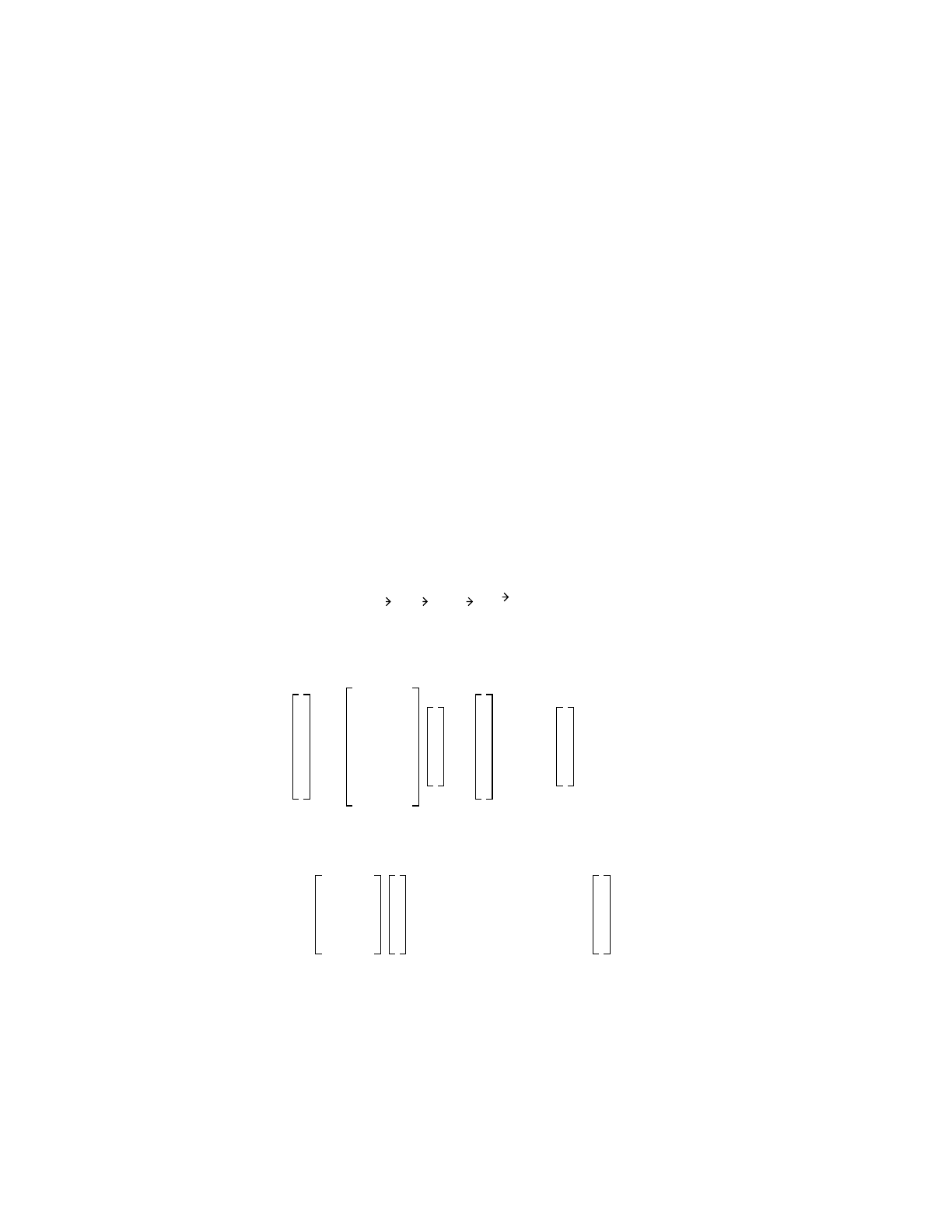
2-184 April 10, 2000
CHAPTER 2
PLOTTER
the origin at the center, the first basis vector pointing to the right and the second basis vector
pointing up. The width of the picture is twice the first extent and the height is twice the second
extent. If the extents are unequal, the picture is distorted. The central task of the plotter is to plot
curves representing the intersections of the surfaces of the geometry with the plot plane within
the window.
All plotted curves are conics, defined here to include straight lines. The intersection of a plane
with any MCNP surface that is not a torus is always a conic. A torus is plotted only if the plot
plane contains the torus axis or is perpendicular to it, in which cases the intersection curves are
conics. The first step in plotting the curves is to find equations for them, starting from the
equations for the surfaces of the problem. Equations are needed in two forms for each curve: a
quadratic equation and a pair of parametric equations. The quadratic equations are needed to
solve for the intersections of the curves. The parametric equations are needed for defining the
points on the portions of the curves that are actually plotted.
The equation of a conic is
As2 + 2Hst + Bt2+ 2Gs + 2Ft + C = 0 ,
where sand tare coordinates in the plot plane. They are related to problem coordinates (x,y,z) by
or in matrix form
.
In matrix form the conic equation is
.
Thus, finding the equation of a curve to be plotted is a matter of finding the QM matrix, given
the PL matrix and the coefficients of the surface.
Any surface in MCNP, if it is not a torus, can be readily written as
rr
osa tb++=
1
x
y
z
100
xoaxbx
yoayby
zoazbz
1
s
t
or
1
x
y
z
PL 1
s
t
==
1st[]
CGF
GAH
FHB
1
s
t
0or 1st[]QM 1
s
t
=

April 10, 2000 2-185
CHAPTER 2
PLOTTER
Ax2 + By2 + Cz2 + Dxy + Eyz + Fzx + Gx + Hy + Jz + K = 0 ,
or in matrix form as
,
or
.
The transpose of the transformation between (s,t) and (x,y,z) is
,
where PLT is the transpose of the PL matrix. Substitution in the surface equation gives
.
Therefore, QM = PLT AM PL.
A convenient set of parametric equations for conics is
straight line s = C1 + C2p
t=C4 + C5p
parabola s = C1 + C2p + C3p2
t=C4 + C5p + C6p2
ellipse s = C1+ C2 sin p+C
3 cos p
t=C4+ C5 sin p + C6 cos p
hyperbola s = C1+ C2 sinh p + C3 cosh p
t=C4+ C5 sinh p + C6 cosh p.
1xyz[]
KG2⁄H2⁄J2⁄
G2⁄AD2⁄F2⁄
H2⁄D2⁄BE2⁄
J2⁄F2⁄E2⁄C
1
x
y
z
0=
1xyz[]AM
1
x
y
z
0=
1xyz[]1st[]PLT
=
1st[]PLTAM PL 1
s
t
0=

2-186 April 10, 2000
CHAPTER 2
PLOTTER
The type of a conic is determined by examination of the conic invariants,115 which are simple
functions of the elements of QM. Some of the surfaces produce two curves, such as the two
branches of a hyperbola or two straight lines. A separate set of parametric coefficients, C1
through C6, is needed for each curve in such cases. The parametric coefficients are found by
transforming QM into yet another coordinate system where most of its elements are zero. The
parametric coefficients are then simple functions115 of the remaining elements. Finally, the
coefficients are transformed from that coordinate system back to the (s,t) system.
For a plottable torus, the curves are either a pair of identical ellipses or a pair of concentric
circles. The parametric coefficients are readily calculated from the surface coefficients and the
elements of QM are simple functions of the parametric coefficients.
The next step is to reject all curves that lie entirely outside the window by finding the
intersections of each curve with the straight line segments that bound the window, taking into
account the possibility that an ellipse may lie entirely inside the window.
The remaining curves are plotted one at a time. The intersections of the current curve with all of
the other remaining curves and with the boundaries of the window are found by solving the
simultaneous equations
,
where i = 1 is the current curve and i = 2 is one of the other curves. This process generally
requires finding the roots of a quartic. False roots and roots outside the window are rejected and
the value of the parameter pfor each remaining intersection is found. The intersections then are
arranged in order of increasing values of p.
Each segment of the curve–the portion of the curve between two adjacent intersections–is
examined to see whether and how it should be plotted. A point near the center of the segment is
transformed back to the (x,y,z) coordinate system. All cells immediately adjacent to the surface
at that point are found. If there is exactly one cell on each side of the surface and those cells are
the same, the segment is not plotted. If there is exactly one cell on each side and those cells are
different, the segment is plotted as a solid line. If anything else is found, the segment is plotted
as a dotted line, which indicates either that there is an error in the problem geometry or that some
other surface of the problem also intersects the plot plane along the segment.
If a curve to be plotted is not a straight line, it is plotted as a sequence of short straight lines
between selected points on the curve. The points are selected according to the criterion that the
middle of the line drawn between points must not lie farther from the nearest point on the true
1st[]QMi
1
s
t
0=

April 10, 2000 2-187
CHAPTER 2
PSEUDORANDOM NUMBERS
curve than the nominal resolution of the picture. The nominal resolution is fixed at 1/3000 of a
side of the viewport. This is a bit coarse for the best plotting devices and is quite a bit too fine
for the worst ones, but it produces adequate pictures at reasonable cost.
XI. PSEUDORANDOM NUMBERS
Like any other Monte Carlo program, MCNP uses a sequence of pseudorandom numbers to
sample from probability distributions. MCNP has always used the congruential scheme of
Lehmer,15 though the mechanics of implementation have been modified for portability to
different computer platforms. In particular, a method has been devised that multiplies two
64-bit words to get a 128-bit word without using more than 64-bit words for the 128-bit word.116
A pseudorandom sequence of integers In is generated by
In+1 = mod(M In, 248),
where Mis the random number multiplier, and 48-bit integers and 48-bit floating point mantissas
are assumed. The default value of M, which can be changed with the DBCN card, is
M = 519 = 19,073,486,328,125 .
The pseudorandom number is then
Rn= 2−48In.
The starting pseudorandom number of each history is
In+S = mod(MSIn,248),
where S is the pseudorandom number stride. Because each pseudorandom number is the least
significant (lower) 48 bits of Mmultiplied by the previous random number, the lower 48 bits of
In+S are the same as the lower 48 bits of MSIn. The default value of S, which can be changed
with the DBCN card, is
S = 15291710 = 4525258= 1001010101010101012.
The 01010101 pattern ensures that the bit pattern will change when the stride is multiplied by
almost anything.
The period P of the MCNP algorithm is
P246 7.04 1013
×≈=

2-188 April 10, 2000
CHAPTER 2
PERTURBATIONS
because the last two binary bits of the lower 48 bits of Mkare 012for all values of k. The period
could be increased from 246 to
by adding 1 as follows:
In= mod(M In-1, 248)+ 1 .
MCNP prints a WARNING and counts the number of histories for which the stride Sis exceeded.
MCNP also prints a WARNING if the period Pis exceeded. Exceeding the stride or the period
does not result in wrong answers but does result in an underestimate of the variance. However,
because the random numbers are used for very different purposes, MCNP seems quite
insensitive to overrunning either the stride or the period.116
Sometimes users wish to know how much of the variation between problems is purely statistical
and the variance is insufficient to provide this information. In correlated sampling (see
page 2–158) and criticality problems, the variances can be underestimated because of correlation
between histories. In this case, rerun the problems with a different random number sequence,
either by starting with a new random number or by changing the random number stride or
multiplier on the DBCN card. MCNP checks for and does not allow invalid choices, such as an
even numbered initial random number that, after a few pseudorandom numbers, would result in
all subsequent random numbers being zero.
XII. PERTURBATIONS
The evaluation of response or tally sensitivities to cross–section data involves finding the ratio
of the change in a tally to the infinitesimal change in the data, as given by the Taylor series
expansion. In deterministic methods, this ratio is approximated by performing two calculations,
one with the original data and one with the perturbed data. This approach is useful even when
the magnitude of the perturbation becomes very small. In Monte Carlo methods, however, this
approach fails as the magnitude of the perturbation becomes small because of the uncertainty
associated with the response. For this reason, the differential operator technique was developed.
The differential operator perturbation technique as applied in the Monte Carlo method was
introduced by Olhoeft117 in the early 1960’s. Nearly a decade after its introduction, this
technique was applied to geometric perturbations by Takahashi.118 A decade later, the method
was generalized for perturbations in cross–section data by Hall119,120 and later Rief.121 A
rudimentary implementation into MCNP followed shortly thereafter.122 With an enhancement of
the user interface and the addition of second order effects, this implementation has evolved into
a standard MCNP feature.
P248 2.81 1014
×≈=

April 10, 2000 2-189
CHAPTER 2
PERTURBATIONS
A. Derivation of the Operator
In the differential operator approach, a change in the Monte Carlo response c, due to changes in
a related data set (represented by the parameter v), is given by a Taylor series expansion
. . . + + . . . ,
where the nth order coefficient is
.
This can be written as
,
for the data set
,
where Kb(h) is some constant, Brepresents a set of macroscopic cross sections, and Hrepresents
a set of energies or an energy interval.
For a track-based response estimator
,
where tj is the response estimator and qj is the probability of path segment j (path segment j is
comprised of segment j− 1 plus the current track.) This gives
,
or
∆cdc
dv
------∆v1
2!
-----d2c
dv2
-------- ∆v2+⋅⋅+⋅=1
n!
-----dnc
dvn
-------- ∆vn
⋅⋅
un1
n!
-----dnc
dvn
--------
⋅=
un1
n!
-----xb
nh() ∂nc
∂xb
nh()
----------------
hH∈
∑
bB∈
∑
=
x
bh() Kkbh()evbBhH∈,∈;⋅=
ct
jqj
j
∑
=
un1
n!
-----xb
nh() ∂n
∂xb
nh()
---------------- tjqj
()
hH∈
∑
bB∈
∑
j
∑
=

2-190 April 10, 2000
CHAPTER 2
PERTURBATIONS
,
where
.
With some manipulations presented in Ref. 123, the path segment estimator γnjtj can be
converted to a particle history estimator of the form
,
where piis the probability of the ith history and Vni is the nth order coefficient estimator for history
i, given by
.
Note that this sum involves only those path segments j' in particle history i. The Monte Carlo
expected value of un becomes
,
for a sample of N particle histories.
The probability of path segment j is the product of the track probabilities,
,
where rk is the probability of track k and segment j contains m+ 1 tracks. If the kth track starts
with a neutron undergoing reaction type “a” at energy E' and is scattered from angle θ'to angle
θ and E, continues for a length λk, and collides, then
un1
n!
-----γnjtjqj
j
∑
=
γnj xb
nh() ∂n
∂xb
nh()
---------------- tjqj
()
1
tjqj
---------
hH∈
∑
bB∈
∑
≡
unVnipi
i
∑
Vni 1
n!
-----γnj′tj′
j
∑
≡
un
〈〉 1
N
----Vni
i
∑
=
1
Nn!
--------- γnj′tj′
j′
∑
i
∑
=
qjrk
k0=
m
∏
=

April 10, 2000 2-191
CHAPTER 2
PERTURBATIONS
,
where xa(E') is the macroscopic reaction cross section at energy E',xT(E') is the total cross
section at energy E', and is the probability distribution function in
phase space of the emerging neutron. If the track starts with a collision and ends in a boundary
crossing
.
If the track starts with a boundary crossing and ends with a collision,
And finally, if the track starts and ends with boundary crossings
1. First Order
For a first order perturbation, the differential operator becomes
whereas,
.
then
,
r
k
xaE′()
xTE′()
----------------
PaE′Eθ′ θ→;→()dEdτθ exTE()λ
k
–
()xTE()d
λ
=
PaE′Eθ′ θ→;→()dEdθ
rk
xae′()
xTE'()
----------------
PaE'Eθ′ θ→;→()dEdθexTE()λ
k
–
()=
rkexTE()λ
k
–
()xTE()dλ=
rkexTE()λ
k
–
=
γ1j′xbh() xbh()∂∂tj′qj′
()
1
tj′qj′
-----------
hH∈
∑
bB∈
∑
≡
xbh()
qj′
------------- qj′
∂
xbh()∂
---------------- xbh()
tj′
------------- tj′
∂
xbh()∂
----------------
+
hH∈
∑
bB∈
∑
=
1
qj′
------qj′
∂
xbh()∂
---------------- 1
rk
---- rk
∂
xbh()∂
----------------
k0=
m
∑
=
λ1j'βj'kR1j′
+
k0=
m
∑
=

2-192 April 10, 2000
CHAPTER 2
PERTURBATIONS
where
for a track segment k that starts with a particle undergoing reaction type “a” at energy E' and is
scattered to energy E and collides after a distance λk. Note that δhE and δba are unity if h=E and
b=a; otherwise they vanish. For other types of tracks (for which the various expressions for rk
were given in the previous section), i.e., collision to boundary, boundary to collision, and
boundary to boundary, derivatives of rkcan be taken leading to one or more of these four terms
for βj'k.
The second term of γ1j'is
,
where the tally response is a linear function of some combination of reaction cross sections, or
,
where cis an element of the tally cross sections, , and may be an element of the perturbed
cross sections, . Then,
.
R1j'is the fraction of the reaction rate tally involved in the perturbation. If none of the nuclides
participating in the tally is involved in the perturbation, then R1j' = 0, which is always the case
for F1, F2, and F4 tallies without FM cards. For F4 tallies with an FM card, if the FM card
multiplicative constant is positive (no flag to multiply by atom density) it is assumed that the FM
βj′k
xbh()
rk
-------------
rk
∂
xbh()∂
----------------
hH∈
∑
bB∈
∑
≡
δhEδba
δhE'xbE'()
xTE'()
-------------------------– δhExbE()λ
k
–δhExbE()
xTE()
-----------------------+
hH∈
∑
bB∈
∑
=
R1j'
xbh()
tj'
------------- ∂tj'
∂xbh()
----------------
hH∈
∑
bB∈
∑
=
tj'λkxcE()
cC∈
∑
=
cC∈
cB∈
R1j′
xbh()
xch()
cC∈
∑
----------------------------- ∂
∂xbh()
---------------- xch()
cC∈
∑
hH∈
∑
bB∈
∑
=
xcE()
EH∈
∑
cB∈
∑
xcE()
cC∈
∑
-------------------------------------=

April 10, 2000 2-193
CHAPTER 2
PERTURBATIONS
tally cross sections are unaffected by the perturbation and R1j' =0. For KCODE keff track length
estimates, F6 and F7 heating tallies, and F4 tallies with FM cards with negative multipliers
(multiply by atom density to get macroscopic cross sections), if the tally cross section is affected
by the perturbation, then R1j' > 0. For keff and F6 and F7 tallies in perturbed cells where all
nuclides are perturbed, generally R1j' = 1.
Finally, the expected value of the first order coefficient is
.
2. Second Order
For a second order perturbation, the differential operator becomes
.
Whereas tj' is a linear function of xb(h), then
and by taking first and second derivatives of the rkterms of qj' as for the first order perturbation,
,
where
.
The expected value of the second order coefficient is
u1
〈〉 1
N
----βj′kR1j′
+
k0=
m
∑
tj′
j′
∑
i
∑
=
γ2j′x2
bh() ∂2
∂x2
bh()
-------------------tj′qj′
()
1
tj′qj′
-----------
hH∈
∑
bB∈
∑
≡
x2
bh()
tj′qj′
----------------tj′
∂2qj′
∂x2
bh()
-------------------
2∂qj′
∂xbh()
---------------- ∂tj′
∂xbh()
---------------- qj′
∂2tj′
∂xbh()
----------------
++
hH∈
∑
bB∈
∑
=
∂2tj′
∂
xbh()
-
--------------- 0=
γ2j′αj′kβj′k
2
–()R1j′
2
–βj′kR1j′
+
k0=
m
∑
2
+
k0=
m
∑
=
αj′k
2δhE′xb
2E′()
xT
2E′()
----------------------------- 2δhE′δbaxbE′()
xTE′()
-------------------------------------–δhExb
2λk
22δhExb
2E()λ
k
xTE()
--------------------------------–+
hH∈
∑
bB∈
∑
=

2-194 April 10, 2000
CHAPTER 2
PERTURBATIONS
,
where βj'k and αj'k are given by one or more terms as described above for track kand R1j' is again
the fraction of the perturbation with nuclides participating in the tally.
3. Implementation in MCNP
The total perturbation printed in the MCNP output file is
.
For each history i and path j',
.
Let the first order perturbation with R1j' = 0 be
,
and let the second order perturbation with R1j' = 0 be
.
Then the Taylor series expansion for R1j' = 0 is
.
If then
u2
〈〉 1
2N
------- αj′kβj′k
2
–()R2
ij′
–βj′kR+1j′
k0=
m
∑
2
+
k0=
m
∑
tj′
j′
∑
i
∑
=
∆c〈〉 1
N
----∆cj′
j′
∑
i
∑
=
∆cj′
dcj′
dv
--------- ∆v1
2
---d2cj′
dv2
------------∆v2
⋅⋅+⋅=
P1j′βj′k
2
k0=
m
∑
tj′
j′
∑
=
P2j′αj′kβj′k
2
–()
k0=
m
∑
tj′
j′
∑
=
∆cj′P1j′∆v1
2
---P2j′P1j′
2
+()∆v2
+
tj′
=
R1j′0≠
∆cj′P1j′R1j′
+()∆v1
2
---P2j′R1j′
2
–P1j′R1j′
+()
2
+()∆v2
+tj′
=

April 10, 2000 2-195
CHAPTER 2
PERTURBATIONS
.
That is, the case is just a correction to the case.
In MCNP, P1j' and P2j' are accumulated along every track length through a perturbed cell. All
perturbed tallies are multiplied by
and then if the tally is further corrected by
R1j' ∆v+P1j' R1j' ∆v2.
R1j' is the fraction of the reaction rate tally involved in the perturbation. R1j' = 0 for F1, F2, F4
tallies without FM cards, and F4 tallies with FM cards with positive multiplicative constants.
B. Limitations
Although it is always a high priority to minimize the limitations of any MCNP feature, the
perturbation technique has the limitations given below. Chapter 3, page 3–144, has examples you
can refer to.
1. A fatal error is generated if a PERT card attempts to unvoid a region. The simple
solution is to include the material in the unperturbed problem and void the region of
interest with the PERT card. See Appendix B of Ref. 124.
2. A fatal error is generated if a PERT card attempts to alter a material composition in
such a way as to introduce a new nuclide. The solution is to set up the unperturbed
problem with a mixture of both materials and introduce PERT cards to remove each.
See Appendix B of Ref. 124.
3. The track length estimate of keff in KCODE criticality calculations assumes the
fundamental eigenvector (fission distribution) is unchanged in the perturbed
configuration.
4. DXTRAN, point detector tallies, and pulse height tallies are not currently compatible
with the PERT card.
5. While there is no limit to the number of perturbations, they should be kept to a
minimum, as each perturbation can degrade performance by 10–20%.
6. The METHOD keywork can indicate if a perturbation is so large that higher than
second order terms are needed to prevent inaccurate tallies.
P1j′∆v1
2
---P2j′P1j′
2
+( )∆v2R1j′∆vP
1j′R1j′∆v2
+++tj′
=
R1j′0≠R1j′0=
P1j′∆v1
2
---P2j′P2
1j′
+()∆v
2
+
R1j′0≠

2-196 April 10, 2000
CHAPTER 2
PERTURBATIONS
C. Accuracy
Analyzing the first and second order perturbation results presented in Ref. 124 leads to the
following rules of thumb. The first order perturbation estimator typically provides sufficient
accuracy for response or tally changes that are less than 5%. The default first and second order
estimator offers acceptable accuracy for response changes that are less than 20–30%. This upper
bound depends on the behavior of the response as a function of the perturbed parameter. The
magnitude of the second order estimator is a good measure of the range of applicability. If this
magnitude exceeds 30% of the first order estimator, it is likely that higher order terms are needed
for an accurate prediction. The METHOD keyword on the PERT card allows one to tally the
second order term separate from the first. See Chapter 3, page 3–142.

April 10, 2000 2-197
CHAPTER 2
REFERENCES
XIII.REFERENCES
1. L. L. Carter and E. D. Cashwell, Particle Transport Simulation with the Monte Carlo
Method, ERDA Critical Review Series, TID-26607 (1975).
2. Ivan Lux and Laszlo Koblinger, Monte Carlo Particle Transport Methods: Neutron and
Photon Calculations, CRC Press, Boca Raton (1991).
3. C. J. Everett and E. D. Cashwell, “A Third Monte Carlo Sampler,” Los Alamos National
Laboratory Report, LA-9721-MS, (March 1983).
4. G. Compte de Buffon, “Essai d'arithmetique morale,” Supplement a la Naturelle, Vol. 4,
1777.
5. A Hall, “On an Experimental Determination of Pi,” Messeng. Math., 2, 113-114 (1873).
6. J. M. Hammersley and D. C. Handscomb, Monte Carlo Methods, John Wiley & Sons, New
York (1964).
7. Marquis Pierre-Simon de Laplace, Theorie Analytique des Probabilities, Livre 2
pp. 356-366 contained in Oeuvres Completes de Laplace, de L'Aca\-demie des Sciences,
Paris, Vol. 7, part 2, 1786.
8. Lord Kelvin, “Nineteenth Century Clouds Over the Dynamical Theory of Heat and Light,”
Philosophical Magazine, series 6, 2, 1 (1901).
9. W. W. Wood, “Early History of Computer Simulations in Statistical Mechanics and
Molecular Dynamics,” International School of Physics “Enrico Fermi,” Varenna, Italy,
1985, Molecular-Dynamics Simulation of Statistical Mechanical Systems, XCVII Corso
(Soc. Italiana di Fisica, Bologna) (1986).
10. Necia Grant Cooper, Ed., From Cardinals to Chaos — Reflections on the Life and Legacy
of Stanislaw Ulam, Cambridge University Press, New York (1989).
11. “Fermi Invention Rediscovered at LASL,” The Atom, Los Alamos Scientific Laboratory
(October 1966).
12. N. Metropolis and S. Ulam, “The Monte Carlo Method,” J. Amer. Stat. Assoc., 44, 335
(1949).
13. Herman Kahn, “Modifications of the Monte Carlo Method,” Proceeding, Seminar on
Scientific Computation, Nov. 1949, IBM, New York, 20-27 (1950).
14. A. S. Householder, G. E. Forsythe, and H. H. Germond, Ed., Monte Carlo Methods, NBS
Applied Mathematics Series, Vol. 12, 6, (1951).
15. D. H. Lehmer, “Mathematical Methods in Large-Scale Computing Units,” Ann. Comp.
Lab., Harvard Univ. 26, 141-146 (1951).
16. Herman Kahn, “Applications of Monte Carlo,” AECU-3259 Report, Rand Corporation,
Santa Monica, CA, (1954).
17. E. D. Cashwell and C. J. Everett, A Practical Manual on the Monte Carlo Method for
Random Walk Problems, Pergamon Press, Inc., New York (1959).
18. Robert R. Johnston, “A General Monte Carlo Neutronics Code,” Los Alamos Scientific
Laboratory Report, LAMS–2856 (March 1963).
19. E. D. Cashwell, J. R. Neergaard, W. M. Taylor, and G. D. Turner, “MCN: A Neutron
Monte Carlo Code,” Los Alamos Scientific Laboratory Report, LA–4751 (January 1972).

2-198 April 10, 2000
CHAPTER 2
REFERENCES
20. E. D. Cashwell, J. R. Neergaard, C. J. Everett, R. G. Schrandt, W. M. Taylor, and
G. D. Turner, “Monte Carlo Photon Codes: MCG and MCP,” Los Alamos National
Laboratory Report, LA–5157–MS (March 1973).
21. J. A. Halblieb and T. A. Mehlhorn, “ITS: The Integrated TIGER Series of Coupled
Electron/Photon Monte Carlo Transport Codes,” Sandia National Laboratory Report,
SAND 84-0573 (1984).
22. E. D. Cashwell and C. J. Everett, “Intersection of a Ray with a Surface of Third of Fourth
Degree,” Los Alamos Scientific Laboratory Report, LA-4299 (December 1969).
23. R. Kinsey, “Data Formats and Procedures for the Evaluated Nuclear Data File, ENDF,”
Brookhaven National Laboratory Report, BNL-NCS-50496 (ENDF 102) 2nd Edition
(ENDF/B-V) (October 1979).
24. R. J. Howerton, D. E. Cullen, R. C. Haight, M. H. MacGregor, S. T. Perkins, and
E. F. Plechaty, “The LLL Evaluated Nuclear Data Library (ENDL): Evaluation
Techniques, Reaction Index, and Descriptions of Individual Reactions,” Lawrence
Livermore Scientific Laboratory Report UCRL-50400, Vol. 15, Part A (September 1975).
25. E. D. Arthur and P. G. Young, “Evaluated Neutron-Induced Cross Sections for 54,56Fe to
40 MeV,” Los Alamos National Laboratory report LA-8626-MS (ENDF-304) (December
1980).
26. D. G. Foster, Jr. and E. D. Arthur, “Average Neutronic Properties of “Prompt” Fission
Products,” Los Alamos National Laboratory report LA-9168-MS (February 1982).
27. E. D. Arthur, P. G. Young, A. B. Smith, and C. A. Philis, “New Tungsten Isotope
Evaluations for Neutron Energies Between 0.1 and 20 MeV,” Trans. Am. Nucl. Soc. 39,
793 (1981).
28. M. W. Asprey, R. B. Lazarus, and R. E. Seamon, “EVXS: A Code to Generate Multigroup
Cross Sections from the Los Alamos Master Data File,'' Los Alamos Scientific Laboratory
report LA-4855 (June 1974).
29. R. E. MacFarlane, D. W. Muir, and R. M. Boicourt, “The NJOY Nuclear Data Processing
System, Volume I: User's Manual,” Los Alamos National Laboratory report LA-9303-M,
Vol. I (ENDF-324) (May 1982).
R. E. MacFarlane, D. W. Muir, and R. M. Boicourt, “The NJOY Nuclear Data Processing
System, Volume II: The NJOY, RECONR, BROADR, HEATR, and THERMR Modules,”
Los Alamos National Laboratory report LA-9303-M, Vol. II (ENDF-324) (May 1982).
30. R. J. Howerton, R. E. Dye, P. C. Giles, J. R. Kimlinger, S. T. Perkins and E. F. Plechaty,
“Omega Documentation,” Lawrence Livermore National Laboratory report UCRL-50400,
Vol. 25 (August 1983).
31. E. Storm and H. I. Israel, “Photon Cross Sections from 0.001 to 100 Mev for Elements 1
through 100,” Los Alamos Scientific Laboratory report LA-3753 (November 1967).
32. J. H. Hubbell, W. J. Veigele, E. A. Briggs, R. T. Brown, D. T. Cromer and R. J. Howerton,
“Atomic Form Factors, Incoherent Scattering Functions, and Photon Scattering Cross
Sections,” J. Phys. Chem. Ref. Data 4, 471 (1975).
33. C. J. Everett and E. D. Cashwell, “MCP Code Fluorescence-Routine Revision,” Los
Alamos Scientific Laboratory report LA-5240-MS (May 1973).

April 10, 2000 2-199
CHAPTER 2
REFERENCES
34. D. E. Cullen, M. H. Chen, J. H. Hubbell, S. T. Perkins, E. F. Plechaty, J. A. Rathkopf, and
J. H. Schfield, “Tables and Graphs of Photon-Interaction Cross Sections from 10 eV to 100
GeV Derived from the LLNL Evaluated Photon Data Library (EPDL),” Lawrence
Livermore National Laboratory report UCRL-50400, Vol. 6 (October 31, 1989).
35. J. A. Halbleib, R. P. Kensek, T. A. Mehlhorn, G. D. Valdez, S. M. Seltzer, and M. J. Berger,
“ITS Version 3.0: Integrated TIGER Series of Coupled Electron/Photon Monte Carlo
Transport Codes,” SAND91-1634 (1992).
36. M. A. Gardner and R. J. Howerton, “ACTL: Evaluated Neutron Activation Cross-Section
Library—Evaluation Techniques and Reaction Index,” Lawrence Livermore National
Laboratory report UCRL-50400, Vol. 18 (October 1978).
37. J. U. Koppel and D. H. Houston, “Reference Manual for ENDF Thermal Neutron
Scattering Data,” General Atomics report GA-8744, Revised (ENDF-269) (July 1978).
38. J. C. Wagner, E. L. Redmond II, S. P. Palmtag, and J. S. Hendricks, “MCNP: Multigroup/
Adjoint Capabilities,” Los Alamos National Laboratory report, LA-12704 (December
1993).
39. J. E. Morel, L. J. Lorence, Jr., R. P. Kensek, J. A. Halbleib, and D. P. Sloan, “A Hybrid
Multigroup/Continuous–Energy Monte Carlo Method for Solving the Boltzmann–
Fokker–Planck Equation,” Nucl. Sci. Eng.,124, p. 369–389 (1996).
40. L. J. Lorence, Jr., J. E. Morel, G. D. Valdez, “Physics Guide to CEPXS: A Multigroup
Coupled Electron–Photon Cross–Section Generating Code, Version 1.0,” SAND89–1685
(1989) and “User's Guide to CEPXS/ONED--ANT: A One–Dimensional Coupled
Electron–Photon Discrete Ordinates Code Package, Version 1.0,” SAND89–1661 (1989)
and L. J. Lorence, Jr., W. E. Nelson, J. E. Morel, “Coupled Electron–Photon Transport
Calculations Using the Method of Discrete–Ordinates,” IEEE/NSREC, Vol. NS–32,
No. 6, Dec. 1985.
41. R. C. Little and R. E. Seamon, “Neutron-Induced Photon Production in MCNP,”
Proceedings of the Sixth International Conference on Radiation Shielding, Vol. I, 151,
(May 1983).
42. J. S. Hendricks and R. E. Prael, “Monte Carlo Next-Event Estimates from Thermal
Collisions,” Nucl. Sci. Eng.,109 (3) pp. 150-157 (October 1991).
43. J. S. Hendricks, R. E. Prael, “MCNP S(α,β) Detector Scheme,” Los Alamos National
Laboratory report, LA-11952 (October 1990).
44. H. Kahn, “Applications of Monte Carlo,” AEC-3259 The Rand Corporation (April 1956).
45. L. Koblinger, “Direct Sampling from the Klein-Nishina Distribution for Photon Energies
Above 1.4 MeV,'' Nucl. Sci. Eng.,56, 218 (1975).
46. R. N. Blomquist and E. M. Gelbard, “An Assessment of Existing Klein-Nishina Monte
Carlo Sampling Methods,” Nucl. Sci. Eng.,83, 380 (1983).
47. G. W. Grodstein, “X-Ray Attenuation Coefficients from 10 keV to 100 MeV,” National
Bureau of Standards, Circular No. 583 (1957).
48. S. Goudsmit and J. L. Saunderson, “Multiple Scattering of Electrons,” Phys. Rev. 57
(1940) 24.
49. L. Landau, “On the Energy Loss of Fast Particles by Ionization,” J. Phys. USSR 8(1944)

2-200 April 10, 2000
CHAPTER 2
REFERENCES
201.
50. O. Blunck and S. Leisegang, “Zum Energieverlust schneller Elektronen in d nnen
Schichten,” Z. Physik 128 (1950) 500.
51. M. J. Berger, “Monte Carlo Calculation of the Penetration and Diffusion of Fast Charged
Particles,” in Methods in Computational Physics, Vol. 1, edited by B. Alder, S. Fernbach,
and M. Rotenberg, (Academic Press, New York, 1963) 135.
52. Stephen M. Seltzer, “An Overview of ETRAN Monte Carlo Methods,” in Monte Carlo
Transport of Electrons and Photons, edited by Theodore M. Jenkins, Walter R. Nelson,
and Alessandro Rindi, (Plenum Press, New York, 1988) 153.
53. J. Halbleib, “Structure and Operation of the ITS Code System,” in Monte Carlo Transport
of Electrons and Photons, edited by Theodore M. Jenkins, Walter R. Nelson, and
Alessandro Rindi, (Plenum Press, New York, 1988) 249.
54. R. M. Sternheimer, M. J. Berger, and S. M. Seltzer, “Density Effect for the Ionization Loss
of Charged Particles in Various Substances,” Phys. Rev. B26 (1982) 6067.
55. R. M. Sternheimer and R. F. Peierls, “General Expression for the Density Effect for the
Ionization Loss of Charged Particles,” Phys. Rev. B3 (1971) 3681.
56. T. A. Carlson, Photoelectron and Auger Spectroscopy, Plenum Press, New York, N.Y.
1975.
57. Stephen M. Seltzer, “Cross Sections for Bremsstrahlung Production and Electron Impact
Ionization,” in Monte Carlo Transport of Electrons and Photons, edited by Theodore M.
Jenkins, Walter R. Nelson, and Alessandro Rindi, (Plenum Press, New York, 1988) 81.
58. S. M. Seltzer and M. J. Berger, “Bremsstrahlung Spectra from Electron Interactions with
Screened atomic Nuclei and Orbital Electrons”, Nucl. Instr. Meth. B12 (1985) 95.
59. S. M. Seltzer and M. J. Berger, “Bremsstrahlung Energy Spectra from Electrons with
Kinetic Energy 1 keV - 10 GeV Incident on Screened Nuclei and Orbital Electrons of
Neutral Atoms with Z=1 to 100", Atom. Data and Nuc. Data Tables 35, (1986) 345.
60. E. Rutherford, “The Scattering of α and β Particles by Matter and the Structure of the
Atom,'' Philos. Mag. 21 (1911) 669.
61. W. B rsch-Supan, “On the Evaluation of the Function for Real
Values of λ,” J. Res. National Bureau of Standards 65B (1961) 245.
62. J. A. Halbleib, R. P. Kensek, T. A. Mehlhorn, G. D. Valdez, S. M. Seltzer, and M. J.
Berger, “ITS Version 3.0: The Integrated TIGER Series of Coupled Electron/Photon
Monte Carlo Transport Codes,” Sandia National Laboratories report SAND91–1634
(March 1992).
63. O. Blunck and K. Westphal, “Zum Energieverlust energiereicher Elektronen in d nnen
Schichten,” Z. Physik 130 (1951) 641.
64. V. A. Chechin and V. C. Ermilova, “The Ionization-Loss Distribution at Very Small
Absorber Thickness,” Nucl. Instr. Meth. 136 (1976) 551.
65. Stephen M. Seltzer, “Electron–Photon Monte Carlo Calculations: The ETRAN Code,”
Appl. Radiat. Isot. Vol. 42, No. 10 (1991) pp. 917–941.
66. M. E. Riley, C. J. MacCallum, and F. Biggs, “Theoretical Electron-Atom Elastic
u˙˙
o˙˙ φλ() 1
2πi
-------- eµµln λµ+µd
σi∞–
σi∞+
∫
=
u˙˙

April 10, 2000 2-201
CHAPTER 2
REFERENCES
Scattering Cross Sections. Selected Elements, 1 keV to 256 keV,” Atom. Data and
Nucl. Data Tables 15 (1975) 443.
67. N. F. Mott, “The Scattering of Fast Electrons by Atomic Nuclei,” Proc. Roy. Soc.
(London) A124 (1929) 425.
68. G. Moliere, “Theorie der Streuung schneller geladener Teilchen II: Mehrfach- und
Vielfachstreuung,” Z. Naturforsch 3a (1948) 78.
69. H. A. Bethe and W. Heitler, “On Stopping of Fast Particles and on the Creation of Positive
Electrons,” Proc. Roy. Soc. (London) A146 (1934) 83.
70. H. W. Koch and J. W. Motz, “Bremsstrahlung Cross-Section Formulas and Related Data,
Rev. Mod. Phys. 31 (1959) 920.
71. Martin J. Berger and Stephen M. Seltzer, “Bremsstrahlung and Photoneutrons from Thick
Tungsten and Tantalum Targets,” Phys. Rev. C2 (1970) 621.
72. R. H. Pratt, H. K. Tseng, C. M. Lee, L. Kissel, C. MacCallum, and M. Riley,
“Bremsstrahlung Energy Spectra from Electrons of Kinetic Energy 1 keV <T< 2000 keV
Incident on Neutral Atoms 2 < Z <92,” Atom. Data and Nuc. Data Tables 20, (1977) 175;
errata in 26 (1981) 477.
73. H. K. Tseng and R. H. Pratt, “Exact Screened Calculations of Atomic-Field
Bremsstrahlung,” Phys. Rev. A3 (1971) 100.
74. H. K. Tseng and R. H. Pratt, “Electron Bremsstrahlung from Neutral Atoms,” Phys. Rev.
Lett. 33 (1974) 516.
75. H. Davies, H. A. Bethe, and L. C. Maximom, “Theory of Bremsstrahlung and Pair
Production. II. Integral Cross Section for Pair Production,” Phys. Rev. 93 (1954) 788; and
H. Olsen, “Outgoing and Ingoing Waves in Final States and Bremsstrahlung,” Phys. Rev.
99 (1955) 1335.
76. G. Elwert, “Verscharte Berechnung von Intensitat und Polarisation im Kontinuierlichen
Rontgenspektrum,” Ann. Physick 34 (1939)178.
77. R. J. Jabbur and R. H. Pratt, “High-Frequency Region of the Spectrum of Electron and
Positron Bremsstrahlung,” Phys. Rev. 129 (1963) 184; and “High-Frequency Region of the
Spectrum of Electron and Positron Bremsstrahlung II,” Phys. Rev. 133 (1964) 1090.
78. J. H. Hubbell, W. J. Veigele, E. A. Briggs, R. T. Brown, D. T. Cromer, and R. J. Howerton,
“Atomic Form Factors, Incoherent Scattering Functions, and Photon Scattering Cross
Sections,” J. Phys. Chem. Ref. Data 4 (1975) 471; and J. H. Hubbell and I. Overbo,
“Relativistic Atomic Form Factors and Photon Coherent Scattering Cross sections,” J.
Phys. Chem. Ref. Data 8 (1979) 69.
79. H. K. Tseng and R. H. Pratt, “Electron Bremsstrahlung Energy Spectra Above 2 MeV,”
Phys. Rev. A19 (1979) 1525.
80. E. Haug, “Bremsstrahlung and Pair Production in the field of free Electrons,” Z.
Naturforsch. 30a (1975) 1099.
81. C. Mοller, “Zur Theorie des Durchgang schneller Elektronen durch Materie,” Ann. Physik.
14 (1932) 568.
82. D. P. Sloan, “A New Multigroup Monte Carlo Scattering Algorithm Suitable for Neutral
and Charged–Particle Boltzmann and Fokker–Planck Calculations,” Ph.D. dissertation,

2-202 April 10, 2000
CHAPTER 2
REFERENCES
Sandia National Laboratories report SAND83–7094, (May 1983).
83. K. J. Adams and M. Hart, “Multigroup Boltzmann–Fokker–Planck Electron Transport
Capability in MCNP,” Trans. Am. Nucl. Soc.,73, 334 (1995).
84. J. E. Stewart, “A General Point-on-a-Ring Detector,” Transactions of the American
Nuclear Society,28, 643 (1978).
85. R. A. Forster, “Ring Detector and Angle Biasing,” Los Alamos Scientific Laboratory
technical memorandum TD-6-8-79 (July 1979).
86. S. P. Pederson, R. A. Forster, and T. E. Booth, “Confidence Interval Procedures for Monte
Carlo Transport Simulations,” Nucl. Sci. Eng.127, 54-77 (1997).
87. Guy Estes and Ed Cashwell, “MCNP1B Variance Error Estimator,” TD-6–27–78(8/31/
78).
88. A. Dubi, “On the Analysis of the Variance in Monte Carlo Calculations,” Nucl. Sci. Eng.,
72, 108 (1979). See also I. Lux, “On Efficient Estimation of Variances,” Nucl. Sci. Eng.,
92, 607 (1986).
89. Shane P. Pederson, “Mean Estimation in Highly Skewed Samples,” Los Alamos National
Laboratory Report LA–12114–MS (1991).
90. T. E. Booth, “Analytic Comparison of Monte Carlo Geometry Splitting and Exponential
Transform,” Trans. Am. Nucl. Soc.,64, 303 (1991).
91. T. E. Booth, “A Caution on Reliability Using “Optimal” Variance Reduction Parameters,”
Trans. Am. Nucl. Soc.,66, 278 (1991).
92. T. E. Booth, “Analytic Monte Carlo Score Distributions for Future Statistical Confidence
Interval Studies,” Nucl. Sci. Eng.,112, 159 (1992).
93. R. A. Forster, “A New Method of Assessing the Statistical Convergence of Monte Carlo
Solutions,” Trans. Am. Nucl. Soc.,64, 305 (1991).
94. R. A. Forster, S. P. Pederson, T. E. Booth, “Two Proposed Convergence Criteria for Monte
Carlo Solutions,” Trans. Am. Nucl. Soc.,64, 305 (1991).
95. J. R. M. Hosking and J. R. Wallis, “Parameter and Quantile Estimation for the Generalized
Pareto Distribution,” Technometrics,29, 339 (1987).
96. W. H. Press, B. P. Flannery, S. A. Teukolsky, and W. T. Vetterling, Numerical Recipes:
The Art of Scientific Computing (FORTRAN Version), Cambridge University Press (1990).
97. Malvin H. Kalos, Paula A Whitlock, Monte Carlo Methods, Volume I: Basics, John Wiley
& Sons, New York, 1987.
98. T. E. Booth, “A Sample Problem for Variance Reduction in MCNP,” Los Alamos National
Laboratory report LA–10363–MS (June 1985).
99. R. A. Forster, R. C. Little, J. F. Briesmeister, and J. S. Hendricks, “MCNP Capabilities For
Nuclear Well Logging Calculations,” IEEE Transactions on Nuclear Science,37 (3), 1378
(June 1990).
100. T. E. Booth and J. S. Hendricks, “Importance Estimation in Forward Monte Carlo
Calculations,” Nucl. Tech./Fusion,5 (1984).
101. F. H. Clark, “The Exponential Transform as an Importance-Sampling Device, A Review,”
ORNL-RSIC-14 (January 1966).
102. P. K. Sarkar and M. A. Prasad, “Prediction of Statistical Error and Optimization of Biased

April 10, 2000 2-203
CHAPTER 2
REFERENCES
Monte Carlo Transport Calculations,” Nucl. Sci. Eng.,70, 243-261, (1979).
103. J. S. Hendricks, “Construction of Equiprobable Bins for Monte Carlo Calculation,” Trans.
Am. Nucl. Soc.,35, 247 (1980).
104. G. Bell and S. Glasstone, Nuclear Reactor Theory, Litton Educational Publishing, Inc.,
1970.
105. T. J. Urbatsch, R. A. Forster, R. E. Prael, and R. J. Beckman, “Estimation and
Interpretation of keff Confidence Intervals in MCNP,” Los Alamos National Laboratory
report LA–12658, (November 1995).
106. C. D. Harmon II, R. D. Busch, J. F. Briesmeister, and R. A. Forster, “Criticality
Calculations with MCNP, A Primer,” Nuclear Criticality Safety Group, University of New
Mexico, Los Alamos National Laboratory, (December 1993).
107. E. M. Gelbard and R. Prael, “Computations of Standard Deviations in Eigenvalue
Calculations,” Progress in Nuclear Energy,24, p 237 (1990).
108. G. D. Spriggs, R. D. Busch, K. J. Adams, D. K. Parsons, L. Petrie, and J. S. Hendricks,
“On the Definition of Neutron Lifetimes in Multiplying and Nonmultiplying Systems,”
Los Alamos National Laboratory Report, LA–13260–MS, (March 1997).
109. M. Halperin, “Almost Linearly-Optimum Combination of Unbiased Estimates,” Amer.
Stat. Ass. J.,56, 36-43 (1961).
110. R. C. Gast and N. R. Candelore, “The Recap–12 Monte Carlo Eigenfunction Strategy and
Uncertainties,” WAPD–TM–1127 (L) (1974).
111. S. S. Shapiro and M. B. Wilk, “An Analysis of Variance Test for Normality,” Biometrika,
52, p. 591 (1965).
112. R. B. D'Agostino, “An Omnibus Test of Normality for Moderate and Large Size Samples,”
Biometrika,58, p. 341 (1971).
113. L. L. Carter, T. L. Miles, and S. E. Binney, “Quantifying the Reliability of Uncertainty
Predictions in Monte Carlo Fast Reactor Physics Calculations,” Nucl. Sci. Eng.,113,
p. 324 (1993).J. S. Hendricks, “Calculation of Cell Volumes and Surface Areas in
MCNP,” Los Alamos National Laboratory report LA–8113–MS (January 1980).
114. J. S. Hendricks, “Calculation of Cell Volumes and Surface Areas in MCNP,” Los Alamos
National Laboratory report LA–8113–MS (January 1980).
115. B. Spain, Analytical Conics, Pergamon, 1957.
116. J. S. Hendricks, “Effects of Changing the Random Number Stride in Monte Carlo
Calculations,” Nucl. Sci. Eng.,109 (1) pp. 86-91 (September 1991).
117. J. E. Olhoeft, “The Doppler Effect for a Non–Uniform Temperature Distribution in
Reactor Fuel Elements,” WCAP–2048, Westinghouse Electric Corporation, Atomic
Power Division, Pittsburgh (1962).
118. H. Takahashi, “Monte Carlo Method for Geometrical Perturbation and its Application to
the Pulsed Fast Reactor,” Nucl Sci. Eng. 41, p. 259 (1970).
119. M. C. Hall, “Monte Carlo Perturbation Theory in Neutron Transport Calculations,” PhD.
Thesis, University of London (1980).
120. M. C. Hall, “Cross–Section Adjustment with Monte Carlo Sensitivities: Application to the
Winfrith Iron Benchmark,” Nucl. Sci. Eng. 81, p. 423 (1982).

2-204 April 10, 2000
CHAPTER 2
REFERENCES
121. H. Rief, “Generalized Monte Carlo Perturbation Algorithms for Correlated Sampling and
a Second–Order Taylor Series Approach,” Ann. Nucl. Energy 11, p. 455 (1984).
122. G. McKinney, “A Monte Carlo (MCNP) Sensitivity Code Development and Application,”
M. S. Thesis, University of Washington, (1984).
123. G. W. McKinney, “Theory Related to the Differential Operator Perturbation Technique,”
Los Alamos National Laboratory Memo, X–6:GWM–94–124 (1994).
124. G. W. McKinney and J. L. Iverson, “Verification of the Monte Carlo Differential Operator
Technique for MCNP,” Los Alamos National Laboratory Report LA–13098, (February
1996).

April 10, 2000 3-1
CHAPTER 3
INP FILE
CHAPTER 3
DESCRIPTION OF MCNP INPUT
Input to MCNP consists of several files, but the main one supplied by the user is the INP (the
default name) file, which contains the input information necessary to describe the problem. Only a
small subset of all available input cards will be needed in any particular problem. The input cards
are summarized by card type on page 3–146. The word “card” is used throughout this manual to
describe a single line of input up to 80 characters.
Maximum dimensions exist for some MCNP input items; they are summarized on page 3–150. The
user can increase any of these maximum values by altering the code and recompiling.
All features of MCNP should be used with caution and knowledge. This is especially true of
detectors and variance reduction schemes; you are encouraged to read the appropriate sections of
Chapter 2 before using them.
The units used throughout MCNP are given in Chapter 1 on page 1–20.
I. INP FILE
The INP file can have two forms, initiate-run and continue-run. Either can contain an optional
message block that replaces or supplements the MCNP execution line information.
A. Message Block
A user has the option to use a message block before the problem identification title card in the INP
file. In computer environments where there are no execution line messages, the message block is
the only means for giving MCNP an execution message. Less crucially, it is a convenient way to
avoid retyping an often-repeated message. The message block starts with the string MESSAGE:
and is limited to columns 1−80. Alphabetic characters can be upper, lower, or mixed case. The
message block ends with a blank line delimiter before the title card.All cards before the blank line
delimiter are continuation cards. A $ and & in the message block are end−of−line markers. The
syntax and components of the message are the same as for the regular execution line message
discussed on page 1–32. Any filename substitution, program module execution option or keyword
entry on the execution line takes precedence over conflicting information in the message block.
INP = filename is not a legitimate entry in the message block. The name INP can be changed on
the execution line only.

3-2 April 10, 2000
CHAPTER 3
INP FILE
B. Initiate-Run
This form is used to set up a Monte Carlo problem (describe geometry, materials, tallies, etc.) and
run if message block is present. The initiate-run file has the following form:
The first card in the file after the optional message block is the required problem title card. It is
limited to one 80−column line and is used as a title in various places in the MCNP output.It can
contain any information the user desires (or can even be blank) and often contains information
describing the particular problem. Note that a blank card elsewhere is used as a delimiter or as a
terminator. Alphabetic characters can be upper, lower, or mixed case.
With a valid set of data cards MCNP will run with or without the blank line terminator. With the
terminator MCNP will stop reading the input file there even if additional lines are in the file. Some
users like to keep additional material, such as alternative versions of the problem or textual
information, associated with the input file itself. The terminator will prevent such additional lines
from being read.
C. Continue−Run
Continue-run is used to continue running histories in a problem that was terminated earlier−for
example, to run the job 2 hours and then to run it an additional hour later. It can also be used to
reconstruct the output of a previous run. A continue-run must contain C or CN in the MCNP
execution line or message block to indicate a continue-run. It will start with the last dump unless
C m is used to start with the mth dump.
Message Block
Blank Line Delimiter
Title Card
Cell Cards
⋅
⋅
Blank Line Delimiter
Surface Cards
⋅
⋅
Blank Line Delimiter
Data Cards
⋅
⋅
Blank Line Terminator
Anything Else Recommended
Optional
}Optional

April 10, 2000 3-3
CHAPTER 3
INP FILE
In addition to the C or CN option on the MCNP execution line, two files can be important for this
procedure: (1) the restart file (default name RUNTPE), and (2) an optional continue-run input file
(default name INP).
The run file, generated by MCNP in the initiate-run sequence, contains the geometry, cross
sections, problem parameters, tallies, and all other information necessary to restart the job. In
addition the problem results at various stages of the run are recorded in a series of dumps. See the
PRDMP card (page 3–127) for a discussion of the selection of dump times. As discussed below,
the run may be restarted from any of these dumps.
The CN execution message option differs from the C option only in that the dumps produced during
the continue-run are written immediately after the fixed data portion of the RUNTPE file rather
than after the dump from which the continue-run started. The new dumps overwrite the old dumps,
providing a way for the user to prevent unmanageable growth of RUNTPE files. RUNTPE growth
also can be controlled by the NDMP entry on the PRDMP card.
The optional continue-run input file must have the word CONTINUE as the first entry on the first
line (title card), or after the optional Message Block and its blank line delimiter. Alphabetic
characters can be upper, lower, or mixed case. This file has the following form:
The data cards allowed in the continue-run input file are a subset of the data cards available for an
initiate-run file. The allowed continue-run data cards are FQ, DD, NPS, CTME, IDUM, RDUM,
PRDMP, LOST, DBCN, PRINT, KCODE, MPLOT, ZA, ZB, and ZC.
A very convenient feature is that if none of the above items is to be changed (and if the computing
environment allows execution line messages), the continue-run input file is not required; only the
run file RUNTPE and the C option on the MCNP execution line are necessary. For example, if you
run a job for a minute but you want more particles run, execute with the C or CN message on the
execute line, and the job will pick up where it stopped and continue until another time limit or
particle cutoff is reached or until you stop it manually. This example assumes that a restart file
called RUNTPE from the initial run is in your current directory.
Message Block
Blank Line Delimiter
CONTINUE
Data Cards
Blank Line Terminator
Anything else
⋅
⋅
}Optional
Recommended
Optional

3-4 April 10, 2000
CHAPTER 3
INP FILE
The complete continue-run execution line option is C m or CN m, where m specifies which dump
to pick up from the RUNTPE and to continue with. If m is not specified, the last dump is taken by
default. If the initial run producing the RUNTPE was stopped because of particle cutoff (NPS card,
page 3–125), NPS must be increased for a continue-run. The NPS card refers to total histories to
be run, including preceding continue-runs and the initial run. CTME in a continue−run is the
number of minutes more to run, not cumulative total time. To run more KCODE cycles, only the
fourth entry KCT matters. Like NPS, KCT refers to total cycles to be run, including previous ones.
In a continue-run, a negative number entered on the NPS card produces a print output file at the
time of the requested dump. No more histories will be run. This can be useful when the printed
output has been lost or you want to alter the content of the output with the PRINT or FQ cards.
Be cautious if you use a FILES card in the initial run. See page 3–133.
D. Card Format
All input lines are limited to 80 columns. Alphabetic characters can be upper, lower, or mixed case.
Most input is entered in horizontal form; however, a vertical input format is allowed for data cards.
A comment can be added to any input card. A $ (dollar sign) terminates data entry and anything
that follows the $ is interpreted as a comment. Blank lines are used as delimiters and terminators.
Data entries are separated by one or more blanks.
Comment cards can be used anywhere in the INP file after the problem title card and before the last
blank terminator card. These cards must have a C anywhere in columns 1−5 followed by at least
one blank. Comment cards are printed only with the input file listing and not anywhere else in the
MCNP output file. The FCn input card is available for user comments and is printed as a heading
for tally n (as a tally title, for example). The SCn card is available for user comments and is printed
as a heading for source probability distribution n.
1. Horizontal Input Format
Cell, surface, and data cards all must begin within the first five columns. The card name or number
and particle designator is followed by data entries separated by one or more blanks. Blanks in the
first five columns indicate a continuation of the data from the last named card. An & (ampersand)
preceded by at least one blank ending a line indicates data will continue on the following card. Data
on the continuation card can be in columns 1−80. Completely blank cards are reserved as delimiters
between major sections of the input file. An individual entry must be entirely on one line. There
can be only one card of any given type for a given particle designation (see page 3–7). Integers must
be entered where integer input is required. Other numerical data can be entered as integer or
floating point and will be read properly by MCNP. (In fact noninteger numerical data can be entered
in any form acceptable to a FORTRAN E-edit descriptor.)

April 10, 2000 3-5
CHAPTER 3
INP FILE
Four features incorporated in the code facilitate input card preparation:
1. nR means repeat the immediately preceding entry on the card n times. For example, 2
4R is the same as 2 2 2 2 2.
2. nI means insert n linear interpolates between the entries immediately preceding and
following this feature. For example, 1.5 2I 3.0 on a card is the same as 1.5 2.0 2.5 3. In
the construct X nI Y, if X and Y are integers, and if Y − X is an exact multiple of n+1,
correct integer interpolates will be created. Otherwise only real interpolates will be
created, but Y will be stored directly in all cases. In the above example, the 2.0 may not
be exact, but in the example 1 4I 6 = 1 2 3 4 5 6, all interpolates are exact.
3. xM is a multiply feature and when used on an input card, it is replaced by the value of
the previous entry on the card multiplied by the factor x. For example, 1 1 2M 2M 2M
2M 4M 2M 2M is equivalent to 1 1 2 4 8 16 64 128 256.
4. nJ can be used on an input card to jump over the entry where used and take the default
value. As an example, the following two cards are identical in their effect:
DD .1 1000
DD J 1000
JJJisalso equivalent to 3J. You can jump to a particular entry on a card without having
to explicitly specify prior items on the card. This feature is convenient if you know you
want to use a default value but can’t remember it. DBCN 7J 5082 is another example.
These features apply to both integer and floating point quantities. If n (an integer) is omitted in the
constructs nR, nI, and nJ, then n is assumed to be 1. If x (integer or floating point) is omitted in xM,
it is a fatal error. The rules for dealing with adjacent special input items are as follows:
1. nR must be preceded by a number or by an item created by R or M.
2. nI must be preceded by a number or by an item created by R or M, and must be followed
by a number.
3. xM must be preceded by a number or by an item created by R or M.
4. nJ may be preceded by anything except I and may begin the card input list.
Examples: 1 3M 2R = 1 3 3 3
1 3M I 4 = 1 3 3.5 4
1 3M 3M = 1 3 9
1 2R 2I 2.5 = 1 1 1 1.5 2.0 2.5
1 R 2M = 1 1 2
1 R R = 1 1 1
1 2I 4 3M = 1 2 3 4 12
1 2I 4 2I 10 = 1 2 3 4 6 8 10

3-6 April 10, 2000
CHAPTER 3
INP FILE
3J 4R is illegal.
1 4I 3M is illegal.
1 4I J is illegal.
2. Vertical Input Format
Column input is particularly useful for cell parameters and source distributions. Cell importances
or volumes strung out on horizontal input lines are not very readable and often cause errors when
users add or delete cells. In column format, all the cell parameters for one cell can be on a single
line, labeled with the name of the cell. If a cell is deleted, the user deletes just one line of cell
parameters instead of hunting for the data item that belongs to the cell in each of several multiline
cell parameter cards. For source distributions, corresponding SI, SP, and SB values are side by side.
Source options, other than defaults, are on the next line and must all be entered explicitly. The &
continuation symbol is not needed, and if present, is ignored.
In column format, card names are put side by side on one input line and the data values are listed
in columns under the card names. A # is put somewhere in columns 1−5 on the line with the card
names. The card names must be all cell parameters, all surface parameters, or all something else.
If a card name appears on a # card, there must not be a regular horizontal card by that name in the
same input file. If there are more entries on data value lines than card names on the # line, the first
data entry is a cell or surface number. If any cell names are entered, all must be entered. If cell
names are entered, the cells don’t have to be in the same order as they are in the cell cards block.
If cell names are omitted, the default order is the order of the cells in the cell card block. The same
rules apply to surface parameters, but because we presently have only one surface parameter
(AREA), column input of surface parameters is less useful.
There can be more than one block of column data in an input file. Typically, there would be one
block for cell parameters and one for each source distribution. If a lot of cell parameter options are
being used, additional blocks of column data would be needed.
The entries in each column do not need to be precisely under the card name at the top of the column,
but you might want the columns to be reasonably neat for readability. The column format is
intended for input data that naturally fit into columns of equal length, but less tidy data are not
prohibited. If a longer column is to the right of a shorter column, the shorter column must be filled
with enough J entries to eliminate any ambiguity about which columns the data items are in.
Special syntax items (R, M, I, and J) are not as appropriate in column format as they are on
horizontal lines, but they are not prohibited. They are, of course, interpreted vertically instead of
horizontally. Multiple special syntax items, such as 9R, are not allowed if cell or surface names are
present.
The form of a column input block is

April 10, 2000 3-7
CHAPTER 3
INP FILE
#S
1S2Sm
K1D11 D12 D1m
K2D21 D22 D2m
.. .. .
.. .. .
.....
KnDn1 Dn2 Dnm
1. The # is somewhere in columns 1−5.
2. Each line can be only 80 columns wide.
3. Each column, Sithrough Dli, where lmay be less than n, represents a regular input card.
4. The Si must be valid MCNP card names. They must be all cell parameters, all surface
parameters, or all something else.
5. D1i through Dni must be valid entries for an Sicard, except that Dl+1,i through Dni may
be some J’s possibly followed by some blanks.
6. If Dji is nonblank, Dj,i-1 must also be nonblank. A J may be used if necessary to make
Dj,i-1 nonblank.
7. The Si must not appear anywhere else in the input file.
8. The Kj are optional integers. If any are nonblank, all must be nonblank.
9. If the Siare cell parameter card names, the Kj, if present, must be valid cell names. The
same is true with surface parameters.
10. If the Kj are present, the Dji must not be multiple special syntax items, such as 9R.
E. Particle Designators
Several of the input cards require a particle designator to distinguish between input data for
neutrons, for photons and for electrons. These cards are IMP, EXT, FCL, WWN, WWE, WWP,
WWGE, DXT, DXC, F, F5X, F5Y, F5Z, PHYS, ELPT, ESPLT, CUT and PERT. The particle
designator consists of the symbol : (colon) and the letter N, P or E immediately after the name of
the card. At least one blank must follow the particle designator. For example, to enter neutron
importances, use an IMP:N card; enter photon importances on an IMP:P card. To specify the same
value for more than one kind of particle, a single card can be used instead of several.
Example: IMP:E,P,N 1 1 0. With a tally card, the particle designator follows the card name
including tally number. For example, ∗F5:N indicates a neutron point detector energy tally. In the
heating tally case, both particle designators may appear. The syntax F6:N,P indicates the combined
heating tally for both neutrons and photons.
…
…
…
…

3-8 April 10, 2000
CHAPTER 3
INP FILE
F. Default Values
Many MCNP input parameters have default values that are summarized on page 3–146. Therefore
you do not always have to specify explicitly every input parameter every time if the defaults match
your needs. If an input card is left out, the default values for all parameters on the card are used.
However, if you want to change a particular default parameter on a card but that parameter is
preceded by others, you have to specify the others or use the nJ jump feature to jump over the
parameters for which you still want the defaults. CUT:P 3J −.10 is a convenient way to use the
defaults for the first three parameters on the photon cutoff card but change the fourth.
G. Input Error Messages
MCNP makes extensive checks (over 400) of the input file for user errors. A fatal error message is
printed, both at the terminal and in the OUTP file, if the user violates a basic constraint of the input
specification, and MCNP will terminate before running any particles. The first fatal error is real;
subsequent error messages may or may not be real because of the nature of the first fatal message.
The FATAL option on the MCNP execution line instructs MCNP to ignore fatal errors and run
particles, but the user should be extremely cautious about doing this.
Most MCNP error messages are warnings and are not fatal. The user should not ignore these
messages but should understand their significance before making important calculations.
In addition to FATAL and WARNING messages, MCNP issues BAD TROUBLE messages
immediately before any impending catastrophe, such as a divide by zero, which would otherwise
cause the program to “crash.” MCNP terminates as soon as the BAD TROUBLE message is issued.
User input errors in the INP file are the most common reason for issuing a BAD TROUBLE
message. These error messages indicate what corrective action is required.
H. Geometry Errors
There is one important kind of input error that MCNP will not detect while processing data from
the INP file. MCNP cannot detect overlapping cells or gaps between cells until a particle track
actually gets lost. Even then the precise nature of the error may remain unclear. However, there is
much that you can and should do to check your geometry before starting a long computer run.
Use the geometry-plotting feature of MCNP to look at the system from several directions and at
various scales. Be sure that what you see is what you intend. Any gaps or overlaps in the geometry
will probably show up as dashed lines. The intersection of a surface with the plot plane is drawn as
a dashed line if there is not exactly one cell on each side of the surface at each point. Dashed lines
can also appear if the plot plane happens to coincide with a plane of the problem, if there are any
cookie-cutter cells in the source, or if there are DXTRAN spheres in the problem.

April 10, 2000 3-9
CHAPTER 3
INP FILE
Set up and run a short problem in which your system is flooded with particle tracks from an external
source. The necessary changes in the INP file are as follows:
1. Add a VOID card to override some of the other specifications in the problem and make
all the cells voids, turn heating tallies into flux tallies, and turn off any FM cards.
2. Add another cell and a large spherical surface to the problem such that the surface
surrounds the system and the old outside world cell is split by the new surface into two
cells: the space between the system and the new surface, which is the new cell, and the
space outside the new surface, which is now the outside world cell. Be sure that the new
cell has nonzero importance. Actually, it is best to make all nonzero importances equal.
If the system is infinite in one or two dimensions, use one or more planes instead of a
sphere.
3. Replace the source specifications by an inward directed surface source to flood the
geometry with particles:
SDEF SUR=m NRM = −1
where m is the number of the new spherical surface added in Step 2. If the new surface
is a plane, you must specify the portion to be used by means of POS and RAD or possibly
X, Y, and Z source distributions.
Because there are no collisions, a short run will generate a great many tracks through your system.
If there are any geometry errors, they should cause some of the particles to get lost.
When a particle first gets lost, whether in a special run with the VOID card or in a regular
production run, the history is rerun to produce some special output on the OUTP file. Event-log
printing is turned on during the rerun. The event log will show all surface crossings and will tell
you the path the particle took to the bad spot in the geometry. When the particle again gets lost, a
description of the situation at that point is printed. You can usually deduce the cause of the lost
particle from this output. It is not possible to rerun lost particles in a multitasking run.
If the cause of the lost particle is still obscure, try plotting the geometry with the origin of the plot
at the point where the particle got lost and with the horizontal axis of the plot plane along the
direction the particle was moving. The cause of the trouble is likely to appear as a dashed line
somewhere in the plot or as some discrepancy between the plot and your idea of what it should look
like.

3-10 April 10, 2000
CHAPTER 3
CELL CARDS
II. CELL CARDS
Form: j m d geom params
or: j LIKE n BUT list
j=cell number; .
If cell has transformation, . See page 3–27.
m=0 if the cell is a void.
=material number if the cell is not a void. This indicates that the cell is to
contain material m, which is specified on the Mm card. See page 3–108.
d=absent if the cell is a void.
=cell material density. A positive entry is interpreted as the atomic density
in units of 1024 atoms/cm3. A negative entry is interpreted as the mass
density in units of g/cm3.
geom =specification of the geometry of the cell. It consists of signed surface
numbers and Boolean operators that specify how the regions bounded by
the surfaces are to be combined.
params =optional specification of cell parameters by entries in the
keyword = value form.
n=name of another cell
list =set of keyword =value specifications that define the attributes that differ
between cell n and j.
In the geometry specification, a signed surface number stands for the region on the side of the
surface where points have the indicated sense. The plus sign for positive sense is optional. The
regions are combined by Boolean operators: intersection (no symbol—implicit, like multiplication
in algebra); union, :; and complement, #. Parentheses can be used to control the order of the
operations. Parentheses and operator symbols also function as delimiters. Where they are present,
blank delimiters are not necessary. The default order of operations is complement first, intersection
second, and union last. A number immediately after a complement operator, without parentheses,
is interpreted as a cell number and is shorthand for the geometry specification of that cell number.
Example: 3 0 -1 2 -4 $ definition of cell 3
#3 $ equivalent to next line
#(-1 2 -4)
For a simple cell (no union or complement operators), the geometry specification is just a blank-
delimited list of the bounding surfaces and ambiguity surfaces of the cell with signs determined by
the sense of the cell with respect to each surface. See the Geometry sections of Chapters 1, 2, and
4 for complete explanations of how to specify the geometry of cells in MCNP.
Cell parameters can be defined on cell cards instead of in the data card section of the INP file. A
blank is equivalent to the equal sign. If a cell parameter is entered on any cell card, a cell-parameter
1j99999≤≤ 1j999≤≤

April 10, 2000 3-11
CHAPTER 3
CELL CARDS
card with that name can not be present, nor can the mnemonic appear on any column-format input
card. Some cell parameters can be specified on cell cards and a different subset on cell-parameter
or column-format cards. The form is keyword=value, where the allowed keywords are IMP, VOL,
PWT, EXT, FCL, WWN, DXC, NONU, PD, and TMP, with particle designators where necessary.
Four cell parameter cards associated with the repeated structures capability are U, TRCL, LAT and
FILL. Like any cell parameter card, these four cards can be placed in the data card section of the
INP file. Our recommendation is that the mnemonic and entry for each cell be placed on the cell
card line after the cell description. The entries on the TRCL card and the FILL card, in particular,
can be quite long and involved and it seems to be conceptually simpler when they are placed on the
cell card line.
The LIKE n BUT feature uses keywords for the cell material number and density. The mnemonics
are MAT and RHO, respectively. These keywords only can be used following the LIKE n BUT
construct. In a normal cell description, material number and density are still the second and third
entries on the cell card.
TMP and WWN data can be entered on cell cards in two ways. The keyword=value form
TMP1=value TMP2=value etc. can be used or a special syntax is available where the single
keyword TMP is followed by all the temperatures of the cell in an order corresponding to the times
on the THTME card. The form for the WWN card is analogous: WWN1:n=value or WWN:n
followed by all the lower weight bounds for the energy intervals of the cell.
Example: 10 16 −4.2 1 −2 3 IMP:N=4 IMP:P=8 EXT:N=−.4X
This says that cell 10 is to be filled with material 16 at a density of 4.2 g/cm3. The cell consists of
the intersections of the regions on the positive side of surface 1, the negative side of surface 2, and
the positive side of surface 3. The neutron importance in cell 10 is 4 and the photon importance is
8. Neutrons in cell 10 are subject to an exponential transform in the minus X direction with
stretching parameter 0.4.
Here are some precautions when you are preparing cell cards:
1. Avoid excessively complicated cells. MCNP runs faster when the problem geometry is
made up of many simpler cells rather than fewer more complicated cells.
2. Avoid adding unneeded surfaces to the geometry description of a cell through poor use
of the complement operator. The extra surfaces make the problem run slower and may
destroy the necessary conditions for volume and area calculations. See page 4–15.
3. Always use the geometry-plotting feature of MCNP to check the geometry of a problem.
See Appendix B.
4. Flood the system with particles from an outside source to find errors in the geometry.
See page 3–8.

3-12 April 10, 2000
CHAPTER 3
SURFACE CARDS
5. If you add or remove cells, change all your cell parameter cards accordingly. The
difficulty of this can be reduced if you use vertical format for your cell parameter cards.
See page 3–6. Alternatively, define the values of cell parameters on cell cards and
eliminate cell parameter cards entirely.
A. Shorthand Cell Specification
The LIKE n BUT feature is very useful in problems with a lot of repeated structures. Cell j inherits
from cell n the values of all attributes that are not specified in the list. The cell card for cell n must
be before the cell card for cell j in the INP file. Any card name that appears after the BUT is a cell
parameter on a cell card and, therefore, must appear on cell cards only, not on any cards in the data
block of the INP file.
Example: 2 3 −3.7 −1 IMP:N=2 IMP:P=4
3 LIKE 2 BUT TRCL=1 IMP:N=10
This says that cell 3 is the same as cell 2 in every respect except that cell 3 has a different location
(TRCL=1) and a different neutron importance. The material in cell 3, the density and the definition
are the same as cell 2 and the photon importance is the same.
III. SURFACE CARDS
A. Surfaces Defined by Equations
Form: j n a list
j=surface number: , with asterisk for a reflecting surface
or plus for a white boundary.
If surface defines a cell that is transformed with TRCL, .
See page 3–27.
n=absent or 0 for no coordinate transformation.
=>0, specifies number of a TRn card.
=< 0, specifies surface j is periodic with surface n.
a=equation mnemonic from Table 3.1
list =one to ten entries, as required.
The surface types, equations, mnemonics, and the order of the card entries are given in Table 3.1.
To specify a surface by this method, find the surface in Table 3.1 and determine the coefficients for
the equation (you may need to consult a book on analytical geometry). The information is entered
on a surface card according to the above form. Under certain conditions a surface can be defined
by specifying geometrical points, as discussed in sections B and C. Surfaces also can be produced
by combinatorial–geometry–like macrobodies, described in section D.
1j99999≤≤
1j999≤≤

April 10, 2000 3-13
CHAPTER 3
SURFACE CARDS
A point (x,y,z) is defined as having positive sense with respect to a surface when the expression for
that surface evaluated at (x,y,z) is positive. The expression for a surface is the left side of the
equation for the surface in Table 3.1. With the sphere, cylinder, cone, and torus, this definition is
identical to defining the sense to be positive outside the figure. With planes normal to axes (PX,
PY, or PZ), the definition gives positive sense for points with x,y, or zvalues exceeding the
intercept of the plane. For the P, SQ and GQ surfaces, the user supplies all of the coefficients for
the expression and thus can determine the sense of the surface at will. This is different from the
other cases where the sense, though arbitrary, is uniquely determined by the form of the expression.
Therefore, in a surface transformation (see the TRn card on page 3–30) a PX, PY, or PZ surface
will sometimes be replaced by a P surface just to prevent the sense of the surface from getting
reversed.
If the surface number is preceded by an asterisk, a reflecting surface is defined. A particle track that
hits a reflecting surface is reflected specularly. If the surface number is preceded by a plus, a white
boundary is defined. Detectors and DXTRAN (next–event estimators) usually should not be used
in problems that have reflecting surfaces or white boundaries. See page 2–92. Tallies in problems
with reflecting surfaces will need to be normalized differently. See page 2–14.
A negative second entry n specifies that surface j is periodic with surface k. The following
restrictions apply:
1. Surfaces j and k must be planes.
2. No surface transformation is allowed for the periodic planes.
3. The periodic cell(s) can be infinite or bounded by planes on the top and bottom that can
be reflecting or white, but cannot be periodic.
4. Periodic planes can only bound other periodic planes or top and bottom planes.
5. A single zero–importance cell must be on one side of each periodic plane.
6. All periodic planes must have a common rotational vector normal to the geometry top
and bottom.
7. Next–event estimators such as detectors and DXTRAN should not be used.
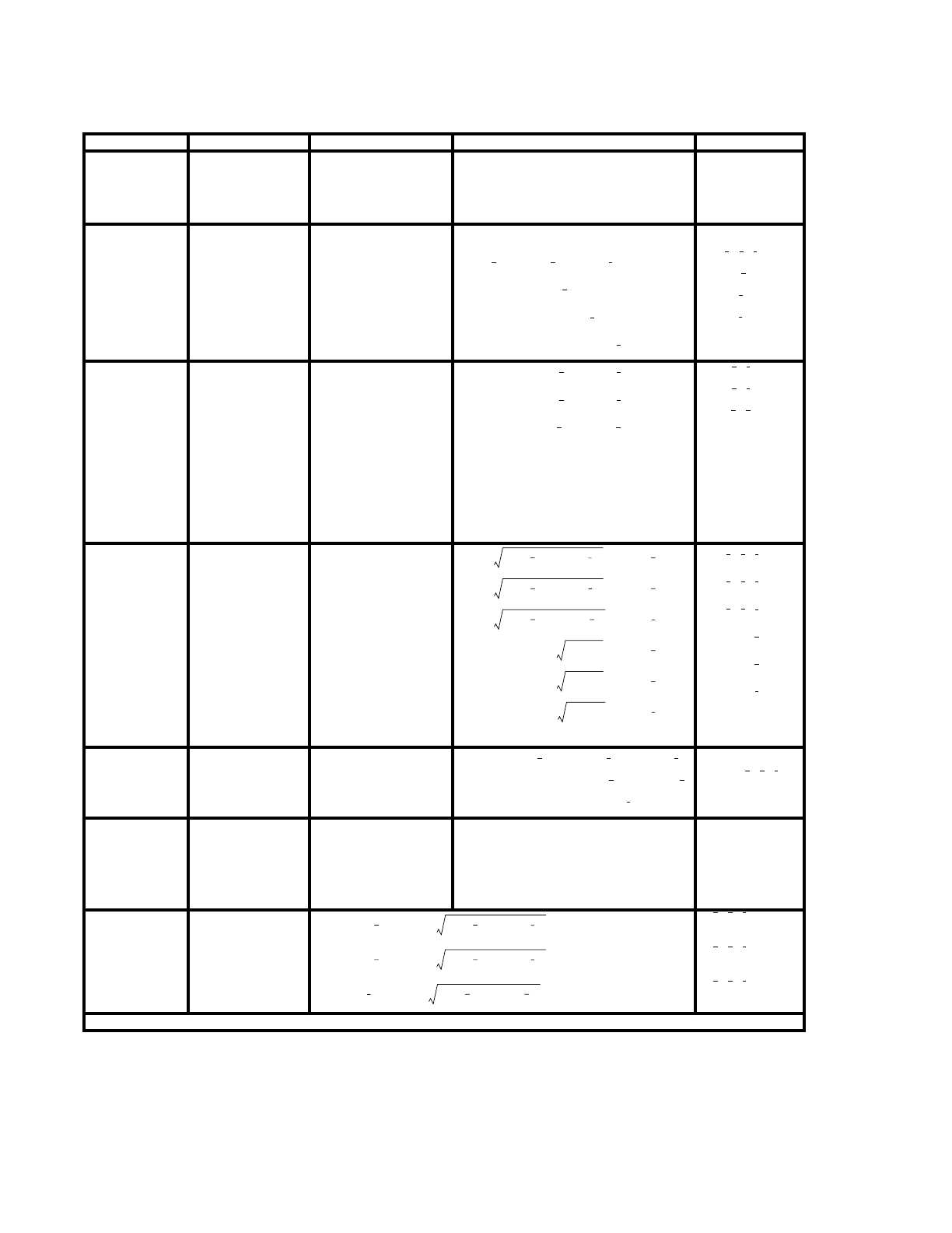
3-14 April 10, 2000
CHAPTER 3
SURFACE CARDS
TABLE 3.1: MCNP Surface Cards
Mnemonic Type Description Equation Card Entires
P
PX
PY
PZ
Plane General
Normal to X–axis
Normal to Y–axis
Normal to Z–axis
Ax + By + Cz – D = 0
x – D = 0
y – D = 0
z – D = 0
ABCD
D
D
D
SO
S
SX
SY
SZ
Sphere Centered at Origin
General
Centered on X–axis
Centered on Y–axis
Centered on Z–axis
R
C/X
C/Y
C/Z
CX
CY
CZ
Cylinder Parallel to X–axis
Parallel to Y–axis
Parallel to Z–axis
On X–axis
On Y–axis
On Z–axis
K/X
K/Y
K/Z
KX
KY
KZ
Cone Parallel to X–axis
Parallel to Y–axis
Parallel to Z–axis
On X–axis
On Y–axis
On Z–axis
used only
for 1 sheet cone
SQ Ellipsoid
Hyperboloid
Paraboloid
Axis not parallel
to X–, Y–, or Z–axis
A B C D E
F G
GQ Cylinder
Cone
Ellipsoid
Hyperboloid
Paraboloid
Axes not parallel
to X–, Y–, or Z–axis +
A B C D E
F G H J K
TX
TY
TZ
Elliptical or
circular torus.
Axis is
Parallel to
X–,Y–, or Z– axis
A B C
A B C
A B C
XYZP Surfaces defined by points See pages 3–16 and 3–18
x2y2z2R2
–++ 0=
xx–()
2yy–()
2zz–()
2R2
–++ 0=
xx–()
2y2z2R2
–++ 0=
x2yy–()
2z2R2
–++ 0=
y2y2zz–()
2R2
–++ 0=
R
xy z R
x
y R
zR
yy–()
2zz–()
2R2
–+0=
xx–()
2zz–()
2R2
–+0=
xx–()
2yy–()
2R2
–+0=
y2z2R2
–+0=
x2z2R2
–+0=
x2y2R2
–+0=
yz R
xz R
xy R
R
R
R
yy–()
2zz–()
2
+tx x–()–0=
xx–()
2zz–()
2
+ty y–()–0=
xx–()
2yy–()
2
+tz z–()–0=
y2z2
+tx x–()–0=
x2z2
+ty y–()–0=
x2y2
+tz z–()–0=
x y z t21±
x y z t21±
x y z t21±
xt21±
y t21±
z t21±
1±
Ax x–()
2By y–()
2Cz z–()
2
++
2Dx x–()2Ey y–()++
2Fz z–()G++0=
x y z
Ax2By2Cz2Dxy Eyz+++ +
Fzx Gz Hy Jz K++++ 0=
xx–()
2B2
⁄yy–()
2zz–()
2
+A–()
2C21–⁄+0=
yy–()
2B2
⁄xx–()
2zz–()
2
+A–()
2C2
⁄1–+0=
zz–()
2B2
⁄xx–()
2yy–()
2
+A–()
2C21–()⁄+0=
x y z
x y z
x y z

April 10, 2000 3-15
CHAPTER 3
SURFACE CARDS
Example 1: j PY 3
This describes a plane normal to the y–axis at y = 3 with positive sense for all points with y> 3.
Example 2: j K/Y 0 0 2 .25 1
This specifies a cone whose vertex is at (x,y,z) = (0,0,2) and whose axis is parallel to the y–axis.
The tangent tof the opening angle of the cone is 0.5 (note that t2is entered) and only the positive
(right hand) sheet of the cone is used. Points outside the cone have a positive sense.
Example 3: j GQ 1 .25 .75 0 –.866
0 –12 –2 3.464 39
This is a cylinder of radius 1 cm whose axis is in a plane normal to the x–axis at x=6, displaced 2
cm from the x–axis and rotated about the x–axis off the y–axis toward the z–axis. The sense is
positive for points outside the cylinder. Such a cylinder would be much easier to specify by first
defining it in an auxiliary coordinate system where it is symmetric about a coordinate axis and then
using the TRn input card (see page 3–30) to define the relation between the basic and auxiliary
coordinate systems. The input would then be
j 7 CX 1
*TR7 6 1 –1.732 0 30 60
See Chapter 4 for additional examples of the TRn card.
The TX, TY, and TZ input cards represent elliptical tori (fourth degree surfaces) rotationally
symmetric about axes parallel to the x,y, and z axes, respectively. A TY torus is illustrated in
Figure 3.1a. Note that the input parameters a b c specify the ellipse
rotated about the s–axis in the (r,s) cylindrical coordinate system (Figure 3.1b) whose origin is at
in the x,y,z system. In the case of a TY torus,
and
A torus is degenerate if |a|<c where 0< a < c produces the outer surface (Figure 3.1c), and
−c< a < 0 produces the inner surface (Figure 3.1d).
30°
xy z
s2
b2
-----ra–()
2
c2
------------------+1=
xy z
syy–()=
rxx–()
2zz–()
2
+=
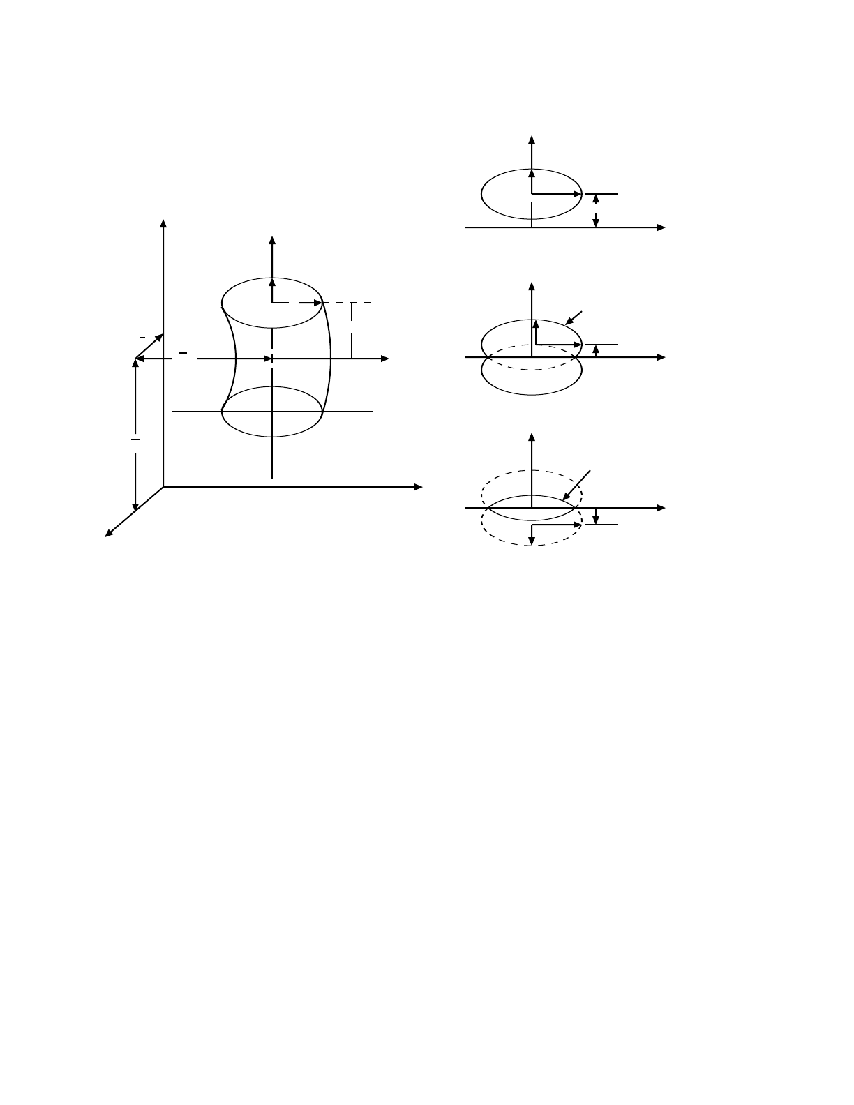
3-16 April 10, 2000
CHAPTER 3
SURFACE CARDS
Figure 3-1. Torus
Coordinate transformations for tori are limited to those in which each axis of the auxiliary
coordinate system is parallel to an axis of the main system.
B. Axisymmetric Surfaces Defined by Points
Form: j n a list
j=surface number: . If surface defines a cell that is
transformed with TRCL, . See page 3–27.
n=absent for no coordinate transformation, or number of TRn card.
a=the letter X, Y, or Z
list =one to three coordinate pairs.
Surface cards of type X, Y, and Z can be used to describe surfaces by coordinate points rather than
by equation coefficients as in the previous section. The surfaces described by these cards must be
Z
Y
X
z
xy s
c
r
b
a
Fig. a c
r
b
a
s
Fig. b
s
Fig. c
r
cb0< a< c
outer surface
s
Fig. d
r
cba< 0< c
inner surface
1j99999≤≤
1j999≤≤

April 10, 2000 3-17
CHAPTER 3
SURFACE CARDS
symmetric about the x−,y−, or z−axis, respectively, and, if the surface consists of more than one
sheet, the specified coordinate points must all be on the same sheet.
Each of the coordinate pairs defines a geometrical point on the surface. On the Y card, for example,
the entries may be
jYy1r1y2r2
where and yi is the coordinate of point i.
If one coordinate pair is used, a plane (PX, PY, or PZ) is defined.
If two coordinate pairs are used, a linear surface (PX, PY, PZ, CX, CY, CZ, KX, KY, or KZ) is
defined.
If three coordinate pairs are used, a quadratic surface (PX, PY, PZ, SO, SX, SY, SZ, CX, CY, CZ,
KX, KY, KZ, or SQ) is defined.
When a cone is specified by two points, a cone of only one sheet is generated.
The senses of these surfaces (except SQ) are determined by the code to be identical to the senses
one would obtain by specifying the surface by equations. For SQ, the sense is defined so that points
sufficiently far from the axis of symmetry have positive sense. Note that this is different from the
equation-defined SQ, where the user could choose the sense freely.
Example 1: j X 7 5 3 2 4 3
This describes a surface symmetric about the x–axis, which passes through the three (x,r) points
(7,5), (3,2), and (4,3). This surface is a hyperboloid of two sheets, converted in MCNP to its
equivalent
jSQ−.083333333 1 1 0 0 0 68.52083 −26.5 0 0.
Example 2: j Y 1 2 1 3 3 4
This describes two parallel planes at Y = 1 and Y = 3 and is a fatal error because the requirement
that all points be on the same sheet is not met.
Example 3: j Y 3 0 4 1 5 0
This describes a sphere of radius 1 with center at (x,y,z) = (0,4,0).
rixi
2zi
2
+()=

3-18 April 10, 2000
CHAPTER 3
SURFACE CARDS
Example 4: j Z 1 0 2 1 3 4
This surface is rejected because the points are on two different sheets of the hyperboloid
However, the surface
j Z 2 1 3 4 5 9.380832
which has the same surface equation as above is accepted because all coordinates lie on a single
surface, the right sheet of the hyperboloid.
Example 5: 1 0 1 −2 3 $ cell 1
1Y −32 21
2 Y 23 33 42
3 Y 21 31 42
This final example defines a cell bounded by a cone, hyperboloid, and an ellipsoid. The three
surfaces define the donut-like cell that is symmetric about the y−axis. A cross section of this cell is
seen in Figure 3.2. To plot this view, type PX = 0EX= 5. One surface goes through the points (-
3,2) and (2,1). The second surface goes through (2,3), (3,3), and (4,2). The last surface is defined
by the points (2,1), (3,1), and (4,2). These coordinate points are in the form (y,r). Using these cards,
MCNP indicates that surface 1 is a cone of one sheet, surface 2 is an ellipsoid, and surface 3 is a
hyperboloid of one sheet. The equation coefficients for the standard surface equations are printed
out for the various surfaces when the PRINT input card or execution option is used. For example,
an SQ card defining surface 3 is
3 SQ 1 -1.5 1000−.625 0 2.5 0
Figure 3-2.
x2y27z2
–20z13–++ 0=
Y
Z
2
1
33

April 10, 2000 3-19
CHAPTER 3
SURFACE CARDS
C. General Plane Defined by Three Points
Form: j n P X1Y1Z1X2Y2Z2X3Y3Z3
j=surface number: or if repeated structure.
n=absent or 0 for no coordinate transformation.
=> 0, specifies number of a TRn card.
=< 0, specifies surface j is periodic with surface n.
(Xi,Yi,Zi)=coordinates of points to define the plane.
If there are four entries on a P card, they are assumed to be the general plane equation coefficients
as in Table 3.1. If there are more than four entries, they give the coordinates of three points lying
in the desired plane. The code converts them to the required surface coefficients to produce the
plane
The sense of the plane is determined by requiring the origin to have negative sense. If the plane
passes through the origin (D = 0), the point has positive sense. If this fails (D =C=0),
the point has positive sense. If this fails (D =C=B=0), the point has positive
sense. If this fails, the three points lie in a line and a fatal error is issued.
D. Surfaces Defined by Macrobodies
Using a combinatorial–geometry–like macrobody capability is an alternative method of defining
cells and surfaces. The combinatorial geometry bodies available are similar to those in the
Integrated Tiger Series (ACCEPT) codes. The macrobodies can be mixed with the standard cells
and surfaces. The macrobody surface is decomposed internally into surface equations and the
facets are assigned individual numbers according to a predetermined sequence. The assigned
numbers are the number selected by the user followed by a decimal point and 1, 2, .... The facets
can be used for tallying, tally segmentation, other cell definitions, SDEF sources, etc. They cannot
be used on the SSR/SSW cards, the surface flagging card, PTRAC, or MCTAL files.
The space inside a body has a negative sense with respect to the macrobody surface and all its
facets. The space outside a body has a positive sense. The sense of a facet is the sense assigned to
it by the macrobody “master” cell and the facet retains that assigned sense if it appears in other cell
descriptions and must be properly annotated. See an example at the end of this section for an
illustration.
The following geometry bodies are available and their complete descriptions follow.
BOX Arbitrarily oriented orthogonal box
RPP Rectangular ParallelePiped
1j99999≤≤ 999≤
Ax By Cz D–++ 0=
00∞,,()
0∞0,,() ∞00,,()

3-20 April 10, 2000
CHAPTER 3
SURFACE CARDS
SPH Sphere
RCC Right Circular Cylinder
RHP or HEX Right Hexagonal Prism
BOX: Arbitrarily oriented orthogonal box (all corners are 90˚.)
BOX Vx Vy Vz A1x A1y A1z A2x A2y A2z A3x A3y A3z
where Vx Vy Vz = x,y,z coordinates of corner
A1x A1y A1z = vector of 1st side
A2x A2y A2z = vector of 2nd side
A2x A3y A3z = vector of 3rd side
Example: BOX –1 –1 –1 2 0 0 0 2 0 0 0 2
a cube centered at the origin, 2 cm on a side, sides parallel to the major axes.
RPP: Rectangular ParallelePiped, surfaces normal to major axes, x,y,z values relative to origin.
RPP Xmin Xmax Ymin Ymax Zmin Zmax
Example: RPP –1 1 –1 1 –1 1
equivalent to BOX above.
SPH: Sphere. Equivalent to surface equation for general sphere.
SPH Vx Vy Vz R
where Vx Vy Vz = x,y,z coordinates of center
R = radius
RCC: Right Circular Cylinder, can
RCC Vx Vy Vz Hx Hy Hz R
where Vx Vy Vz = center of base
Hx Hy Hz = cylinder axis vector
R = radius
Example: RCC 0 –5 0 0 10 0 4
a 10-cm high can about the y-axis, base plane at y=–5 with radius of 4 cm.
RHP or HEX: Right Hexagonal Prism. Differs from ITS (ACCEPT) format.
RHP v1 v2 v3 h2 h2 h3 r1 r2 r3 s1 s2 s3 t1 t2 t3
where v1 v2 v3 = x,y,z coordinates of the bottom of the hex
h1 h2 h3 = vector from the bottom to the top
for a z-hex with height h, h1,h2,h3 = 0 0 h
r1 r2 r3 = vector from the axis to the middle of the first facet
for a pitch 2p facet normal to y-axis, r1,r2,r3 = 0 p 0
s1 s2 s3 = vector to center of the 2nd facet

April 10, 2000 3-21
CHAPTER 3
SURFACE CARDS
t1 t2 t3 = vector to center of the 3rd facet
Example: RHP 0 0 –4 0 0 8 0 2 0
a hexagonal prism about the z-axis whose base plane is at z=–4 with a height
of 8-cm and whose first facet is normal to the y-axis at y=2.
The facets of the bodies are sequentially numbered and can be used on other MCNP cards. BOX
and RPP can be infinite in a dimension, in which case those two facets are skipped and the numbers
of the remaining facets are decreased by two. RHP can be infinite in the axial dimension in which
case facets 7 and 8 do not exist. The order of the facet numbering follows for each geometry body.
Facet numbering can be displayed graphically with MBODY=OFF in the geometry plotter.
BOX: 1 plane normal to end of A1x A1y A1z
2 plane normal to beginning of A1x A1y A1z
3 plane normal to end of A2x A2y A2z
4 plane normal to beginning of A2x A2y A2z
5 plane normal to end of A3x A3y A3z
6 plane normal to beginning of A3x A3y A3z
RPP: 1 Plane Xmax
2 Plane Xmin
3 Plane Ymax
4 Plane Ymin
5 Plane Zmax
6 Plane Zmin
SPH: treated as a regular surface so no facet
RCC: 1 Cylindrical surface of radius R
2 Plane normal to end of Hx Hy Hz
3 Plane normal to beginning of Hx Hy Hz
RHP or HEX 1 Plane normal to end of r1 r2 r3
2 Plane opposite facet 1
3 Plane normal to end of s1 s2 s3
4 Plane opposite facet 3
5 Plane normal to end of t1 t2 t3
6 Plane opposite facet 5
7 Plane normal to end of h1 h2 h3
8 Plane normal to beginning of h1 h2 h3
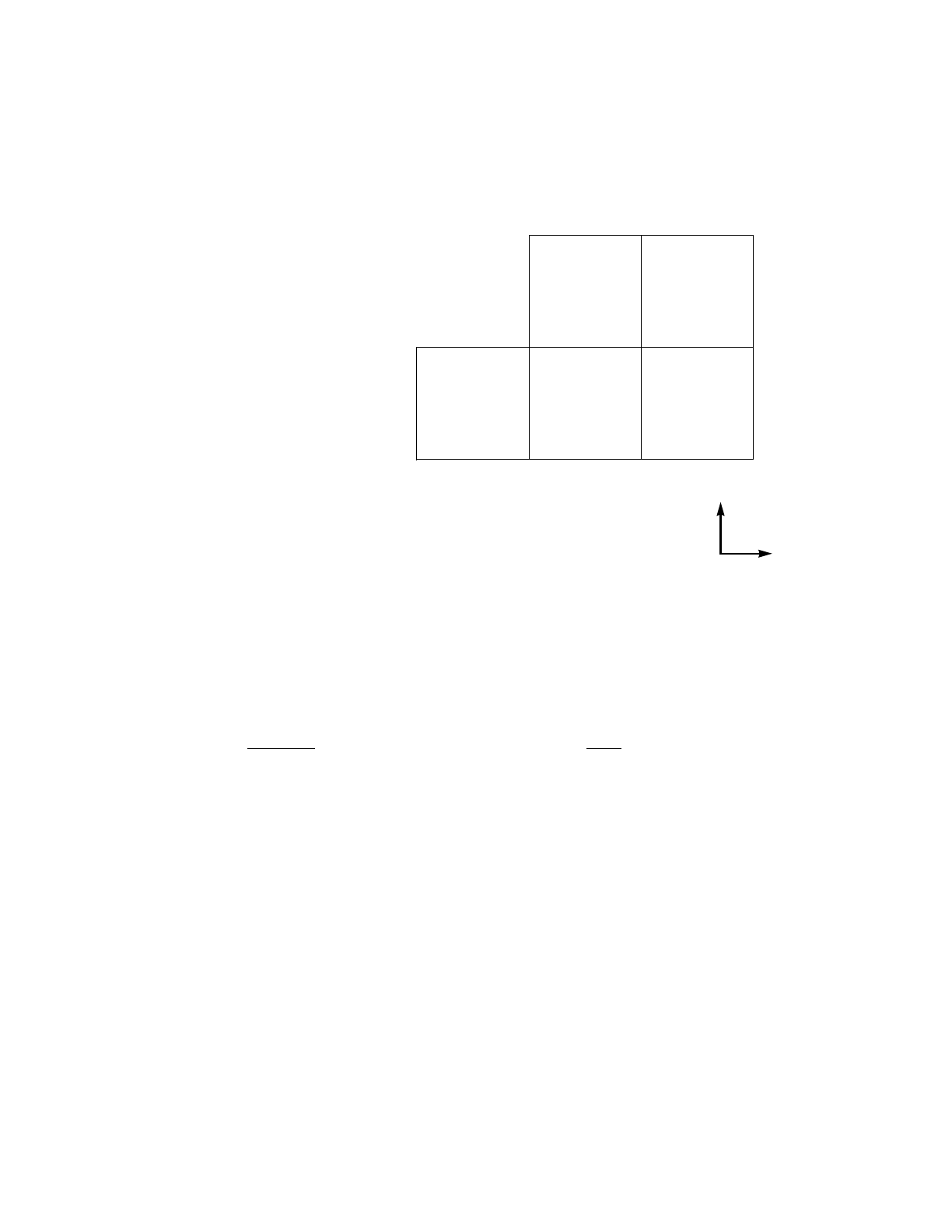
3-22 April 10, 2000
CHAPTER 3
DATA CARDS
The following input file describes five cells and illustrates a combination of the various body and
cell/surface descriptions. Surface numbers are in italics alongside the planes they define. Note that
the cell and surface numbers do not have to start with 1 or be consecutive.
IV. DATA CARDS
All MCNP input cards other than those for cells and surfaces are entered after the blank card
delimiter following the surface card block. The mnemonic must begin within the first five columns.
These cards fall into the following categories:
Category Page
(A) Problem type 3–23
(B) Geometry cards 3–23
(C) Variance reduction 3–32
(D) Source specification 3–49
(E) Tally specification 3–73
(F) Material and cross section specification 3–107
(G) Energy and thermal treatment 3–116
(H) Problem cutoffs 3–123
(I) User data arrays 3–126
(J) Peripheral cards 3–127
10–1
2 like 1 but trcl = (2 0 0)
4 0 1.1 –2001.1 –5.3 –5.5 –5.6 –5.4
9 0 (–5.1 : 1.3 : 2001.1 : –99 : 5.5 : 5.6) #5 cell 1 cell 2
cell 3 cell 4
cell 9
1.15.1
1.3
5.3
2001.1
99
x
y
5 rpp –2 0 –2 0 –1 1
99 py –2
1 rpp 0 2 0 2 –1 1
3 0 –1.2 –1.1 1.4 –1.5 –1.6 99
50 –5
cell 5
5.2
3 0 5.1 –1.1 1.4 –5.5 –5.6 –5.4
3 0 –1.2 –1.1 –5.3 –5.5 –5.6 –5.4
3 0 5.1 –1.1 –5.3 –5.5 –5.6 99
alternative descriptions of cell 3:

April 10, 2000 3-23
CHAPTER 3
DATA CARDS
These card categories are described below. Only the cards listed on page 3–3 are allowed in a
continue-run input file. No data card can be used more than once with the same number or particle
type designations. For example, M1 and M2 are acceptable, as are CUT:N and CUT:P, but two M1
cards or two CUT:N cards are disallowed.
A. Problem Type (MODE) Card
Form: MODE
xi=N for neutron transport
P for photon transport
E for electron transport
Default: If the MODE card is omitted, MODE N is assumed.
Use: A MODE card is required unless MODE=N. The entries are space delineated.
B. Geometry Cards
1. VOL Cell Volume Card
Form: VOL x1x2xi
or: VOL NO x1x2xi
xi= volume of cell i where i=1, 2, ... number of cells in the problem.
NO = no volumes or areas are calculated.
Default: MCNP attempts to calculate the volume of all cells unless “NO” appears on
the VOL card. If no value is entered for a cell on the VOL card, the calculated
volume is used.
Use: Optional card used to input cell volumes.
Mnemonic Card Type Page
VOL Cell volumes 3–23
AREA Surface areas 3–24
U Universes 3–26
TRCL Cell transformations 3–27
LAT Lattices 3–28
FILL Fill card 3–29
TR Coordinate transformation 3–30
x1…xi
…
…

3-24 April 10, 2000
CHAPTER 3
DATA CARDS
With the VOL card, if the number of entries does not equal the number of cells in the problem, it
is a fatal error. Use the nJ feature to skip over cells for which you do not want to enter values. The
entry NO on the VOL card will bypass the volume calculation altogether. The xientries following
NO are optional. If present, xientries are the volume values the code will use. For some problems
the NO option saves considerable computer time.
Volumes or masses of cells are required for some tallies. MCNP calculates the volumes of all cells
that are rotationally symmetric (generated by surfaces of revolution) about any axis, even a skew
axis. It will also calculate the volumes of polyhedral cells. As a byproduct of the volume
calculation, areas and masses are also calculated. These volumes, areas, and masses can be printed
in the OUTP file by using the PRINT card. The user can enter values on the VOL card for the
volume of any cell and these values, instead of the calculated values, will be used for tally purposes.
If a cell volume required for a tally cannot be calculated and is not entered on the VOL or SDn
cards, a fatal error message is printed.
The VOL card provides an alternative way to enter volumes required by tallies. Normally the SDn
card would be used. The VOL card can be used only for cell volumes, whereas the SDn card can
be used for cell and segment volumes or masses.
Volumes of cells or segments that cannot be calculated by MCNP or by the user can be obtained in
a separate MCNP run using the ray-tracing technique described on page 2–183.
2. AREA Surface Area Card
Form: AREA
xi= area of surface i where i=1, 2, ... number of surfaces in the problem.
Default: MCNP attempts to calculate the area of all surfaces. If no value is entered for a surface
on the AREA card, the calculated area, if any, is used.
Use: Optional card used to input surface areas.
This card is analogous to the VOL card. MCNP calculates the area of surfaces as a byproduct of
the volume calculation. If the volume of all cells on either side of the surface can be calculated, the
area of the surface will be calculated. Otherwise the area calculation will fail. A fatal error occurs
if an area is required for tallying purposes and is not available either from the MCNP calculation
or from an AREA or SDn card.
The AREA card provides an alternative way to enter areas required by tallies. Normally the SDn
card would be used. The AREA card can be used only for areas of whole surfaces, whereas the SDn
card can be used for areas of surface segments as well as whole surfaces.
x1…xi…xn

April 10, 2000 3-25
CHAPTER 3
DATA CARDS
3–6. Repeated Structures Cards
The primary goal of the repeated-structures capability is to make it possible to describe only once
the cells and surfaces of any structure that appears more than once in a geometry. The amount of
input data the user has to provide and the amount of computer memory needed by problems that
have a lot of geometrical repetition is reduced. Problems that would be impractical because they
take an unreasonable amount of work to set up or they use too much memory can be run. One
example of such a problem is a reactor core that has dozens of nearly identical fuel modules.
Another example is a room containing some complicated nearly identical objects arranged in some
not necessarily regular order. This feature reduces input and memory use but problems won’t run
any faster than with any other description. Examples of the use of repeated structures cards are in
Chapter 4.
The repeated structures capability extends the concept of an MCNP cell. The user can specify that
a cell is to be filled with something called a universe. A universe is either a lattice or an arbitrary
collection of cells. A single universe, described only once, can be designated to fill each of any
number of cells in the geometry. Some or all of the cells in a universe may themselves be filled with
universes. Several concepts and cards combine in order to use this capability.
• Remember that cell parameters can be defined on cell cards.
• The “LIKE m BUT” feature is a shorthand making it possible to make one cell equivalent to
another except for assorted attributes that can be specified with keyword=value entries. See
page 3–11.
• The universe card, the U card, is used to specify to what universe the cell belongs.
• The fill card is used to specify with which universe a cell is to be filled.
• The TRCL card makes it possible to define only once the surfaces that bound several cells
identical in size and shape but located at different places in the geometry. It follows the
transformation rules established for the TR card. See page 3–30.
• The lattice card, the LAT card, is used to define an infinite array of hexahedra or hexagonal
prisms. The order of specification of the surfaces of a lattice cell identifies which lattice
element lies beyond each surface.
• A general source description can be defined in a repeated structures part of the geometry.
Surface source surfaces must be regular MCNP surfaces, not surfaces associated with a
repeated structures part of the geometry. No check is made that this requirement is met. The
user must remember and this notification is your only warning.
• An importance in a cell that is in a universe is interpreted as a multiplier of the importance of
the filled cell. Weight–window lower bounds are handled the same way.

3-26 April 10, 2000
CHAPTER 3
DATA CARDS
Chapter 4 contains several examples that illustrate the repeated structures input and logic. The
reader is strongly encouraged to become familiar with these examples and to use them as teaching
aids to help understand the card descriptions that follow.
3. U Universe Card
As mentioned earlier, a universe can be either a lattice or a collection of ordinary cells. A nonzero
entry on the U card is the number of the universe that the corresponding cell belongs to. Lack of
a U card or a zero entry means that the cell does not belong to any universe. Universe numbers are
arbitrary integers chosen by the user. The FILL card, page 3–29, indicates that a cell is filled by all
the cells having a corresponding integer entry on the U card. The cells of a universe may be finite
or infinite, but they must fill all of the space inside any cell that the universe is specified to fill.
One way to think about the connection between a filled cell and the filling universe is that the filled
cell is a “window” that looks into a second level, like a window in a wall provides a view of the
outdoors. Cells in the second level can be infinite because they will be “ended” when they bump
into or intersect the surfaces of the “window.” The second level can have its own origin, in a primed
coordinate system, unrelated to the upper level origin. However, if the filled cell and filling universe
have all their surfaces in the same coordinate system, one TRCL card, explained on page 3–27, will
define the coordinate system of both filled and filling cells. The first repeated structures example
in Chapter 4 illustrates this fact.
A cell in a universe can be filled by another universe, in which case a third level is introduced.
There is a maximum of 10 levels, more than most problems will need. To clarify some jargon about
hierarchies, the highest to lowest level is in inverse order to the associated numerical value. The
highest level is level zero, lower is level one, lower still is level two, etc.
Planar surfaces of a filled cell and those in a filling universe CAN be coincident. In other words,
the cells of a universe can fit exactly into the filled cell. The following cell and surface cards
illustrate this feature. They represent a –cm box filled with a lattice of –
cm cubes, each of which is filled with a sphere.
A problem will run faster by preceding the U card entry with a minus sign for any cell that is not
truncated by the boundary of any higher level cell. The minus sign indicates that calculating
distances to boundary in higher level cells can be omitted. In the problem below, cell 3 has a
negative universe number. It is a finite cell and is not truncated by any other cell. Cell 4 cannot have
a negative universe number because it is an infinite region that is truncated by cell 2.
CAUTION: Use this capability AT YOUR OWN RISK. MCNP cannot detect errors in this feature
as the logic that enables detection is omitted by the presence of the negative universe. Extremely
wrong answers can be quietly calculated. Use this feature with EXTREME caution. Plot several
views of the geometry or run with the VOID card (see page 3–8) to check for errors.
50 20 10×× 10 10 10××

April 10, 2000 3-27
CHAPTER 3
DATA CARDS
10 1−2 –3 4 –5 6 fill=1
2 0 –7 1 –3 8 u=1 fill=2 lat=1
3 0 –11 u=−2
4 0 11 u=2
5 0 –1:2:3:–4:5:–6
1px 0
2px50
3py10
4 py –10
5pz 5
6pz –5
7px10
8py0
10 py 10
11 s 5504
Every cell in the problem is either part of the real world (universe level 0) or part of some universe,
but the surfaces of a problem are less restricted. A single planar surface can be used to describe
cells in more than one universe. Coincident surfaces can not be reflecting or periodic, source
surfaces, or tally surfaces. Materials are normally put into the cells of the lowest level universe, not
in the higher level but there is an exception in the case of a lattice.
The above example can be described with macrobodies as follows:
4. TRCL Cell Transformation Card
The TRCL card makes it possible to describe just once the surfaces that bound several cells
identical in size and shape but located at different places in the geometry. It is especially valuable
when these cells are filled with the same universe. If the surfaces of these filled cells and the
surfaces of the cells in the universe that fills them are all described in the same auxiliary coordinate
system, a single transformation will completely define the interior of all these filled cells because
the cells of the universe will inherit the transformation of the cells they fill.TRCL is intended to be
1 0 –20 fill=1
2 0 –30 u=1 fill=2 lat=1
3 0 –11 u=–2
4 0 11 u=2
50 20
20 rpp 0 50 –10 10 –5 5
30 rpp 0 10 0 10
11 s 5504

3-28 April 10, 2000
CHAPTER 3
DATA CARDS
used with LIKE BUT, LAT, etc. With a regular cell description, it is suggested the TR on the surface
cards be used.
The basic form of an entry is an integer that is interpreted as the number of a TR card that contains
a transformation for all of the surfaces of the cell and is located in the data card section of the INP
file. The absence of the TRCL card or zero means there is no transformation, the default. The actual
transformation can be entered following the TRCL mnemonic, enclosed by parentheses. If the
actual transformation is entered, all the rules applying to the TR card
(page 3–30) are valid. If the symbol ∗TRCL is used, the rotation matrix entries are angles in
degrees instead of cosines, the same as the ∗TR card.
If a cell has a transformation, a set of new surfaces with unique names is generated from the
original surfaces. The name of the generated surface is equal to the name of the original surface
plus 1000 times the name of the cell. This formula gives generated names that are predictable and
can be used on other cell cards and on tally cards. This method limits cell names and original
surface names to no more than three digits, however. These generated surfaces are only the
bounding surfaces of the transformed cell, not the surfaces of any universe that fills it. MCNP
requires only one full description of each universe, no matter how many times that universe is
referenced in the problem.
5. LAT Lattice Card
LAT=1 means the lattice is made of hexahedra, solids with six faces. LAT=2 means the lattice is
made of hexagonal prisms, solids with eight faces.A nonzero entry on the LAT card means that the
corresponding cell is the (0,0,0) element of a lattice. The cell description of a lattice cell has two
main purposes. It is a standard MCNP cell description and the order of specification of the surfaces
of the cell identifies which lattice element lies beyond each surface.
After you have designed your lattice, decide which element you want to be the (0,0,0) element and
in which directions in the lattice you want the three lattice indices to increase. In the case of a
hexagonal prism lattice you have two constraints: the first and second indices must increase across
adjacent surfaces and the third index must increase in one or the other direction along the length of
the prism. You will then enter the bounding surfaces of the (0,0,0) element on the cell card in the
right order, in accordance with the following conventions. For a hexahedral lattice cell, beyond the
first surface listed is the (1,0,0) element, beyond the second surface listed is the (-1,0,0) element,
then the (0,1,0), (0,-1,0), (0,0,1) and (0,0,-1) lattice elements in that order. This method provides
the order of arrangement of the lattice to the code so that when you specify element (7,9,3), the
code knows which one that is. For a hexagonal prism lattice cell, on the opposite side of the first
surface listed is element (1,0,0), opposite the second listed surface is
(-1,0,0), then (0,1,0), (0,-1,0), (-1,1,0), (1,-1,0), (0,0,1), and (0,0,-1). These last two surfaces must
be the base surfaces of the prism. Example 7, page 4–34, illustrates a hexagonal prism lattice cell.

April 10, 2000 3-29
CHAPTER 3
DATA CARDS
The hexahedra need not be rectangular and the hexagonal prisms need not be regular, but the
lattices made out of them must fill space exactly. This means that opposite sides have to be identical
and parallel. A hexahedral lattice cell may be infinite in one or two of its dimensions. A hexagonal
prism lattice cell may be infinite in the direction along the length of the prism. The cross section
must be convex (no butterflies). It does not matter whether the lattice is left-handed or right-handed.
A lattice must be the only thing in its universe. The real world (universe level 0) itself can be a
lattice. If a particle leaves the last cell of a real-world, limited-extent lattice (see the FILL card for
how the extent of a lattice can be limited), it is killed (escapes).
6. FILL Fill Card
A nonzero entry on the FILL card indicates the number of the universe that fills the corresponding
cell. The same number on the U card identifies the cells making up the filling universe. The FILL
entry may optionally be followed by, in parentheses, either a transformation number or the
transformation itself. This transformation is between the coordinate systems of the filled cell and
the filling universe, with the universe considered to be in the auxiliary coordinate system. If no
transformation is specified, the universe inherits the transformation, if any, of the filled cell. A
∗FILL may be used if the rotation matrix entries are angles in degrees rather than cosines. In the
data card section of the INP file you cannot have both a FILL and a ∗FILL entry. If you want to
enter some angles by degrees (∗FILL) and some angles by cosines (FILL), all FILL and ∗FILL data
must be placed on the cell cards of the INP file.
If the filled cell is a lattice, the FILL specification can be either a single entry, as described above,
or an array. If it is a single entry, every cell of the lattice is filled by the same universe. If it is an
array, the portion of the lattice covered by the array is filled and the rest of the lattice does not exist.
It is possible to fill various elements of the lattice with different universes, as shown below and in
examples in Chapter 4, section III,
The array specification for a cell filled by a lattice has three dimension declarators followed by the
array values themselves. The dimension declarators define the ranges of the three lattice indices.
They are in the same form as in FORTRAN, but both lower and upper bounds must be explicitly
stated with positive, negative, or zero integers, separated by a colon. The indices of each lattice
element are determined by its location with respect to the (0,0,0) element. Reread the LAT card
section, if needed, with particular emphasis on how the order of specification of the surfaces of the
cell identifies the ordering of the lattice elements. The first two surfaces listed on the cell card
define the direction the first lattice index must cover. The numerical range of the indices depends
on where in the lattice the (0,0,0) element is located. For example, −5:5, 0:10, and −10:0 all define
a range of 11 elements. The third and fourth surfaces listed in the cell description define the
direction of the second lattice index.
The array values follow the dimension declarators. Each element in the array corresponds to an
element in the lattice. Only those elements of the lattice that correspond to elements in the array

3-30 April 10, 2000
CHAPTER 3
DATA CARDS
actually exist. The value of each array element is the number of the universe that is to fill the
corresponding lattice. There are two values that can be used in the array that have special meanings.
A zero in a real world (level zero) lattice means that the lattice element does not exist, making it
possible, in effect, to specify a nonrectangular array. If the array value is the same as the number
of the universe of the lattice, that element is not filled with any universe but with the material
specified on the cell card for the lattice cell. A real world (level zero) lattice, by default, is universe
zero and only can be universe zero. Therefore, using the universe number of the lattice as an array
value to fill that element with the cell material is not possible. As with a single entry FILL
specification, any value in the array optionally can be followed by, in parentheses, a transformation
number or the transformation itself.
Example: FILL=0:2 1:2 0:1 4 42040433040
Only eight elements of this lattice exist. Elements (0,1,0), (1,1,0), (1,2,0), (0,1,1) and (1,2,1) are
filled with universe 4. Element (2,1,0) is filled with universe 2. Elements (1,1,1) and (2,1,1) are
filled with universe 3.
7. TRn Coordinate Transformation Card
Form: TRn O1O2O3B1B2B3B4B5B6B7B8B9M
n=number of the transformation: 1< n < 999.∗TRn means that the Bi
are angles in degrees rather than being the cosines of the angles.
O1O2O3=displacement vector of the transformation.
B1to B9=rotation matrix of the transformation.
M=1 (the default) means that the displacement vector is the location of
the origin of the auxiliary coordinate system, defined in the main
system.
=−1 means that the displacement vector is the location of the origin of
the main coordinate system, defined in the auxiliary system.
Default: TRn 0 0 0 1 0 0 0 1 0 0 0 1 1
The maximum number of transformations in a single problem is 999. A cone of one sheet can be
rotated only from being on or parallel to one coordinate axis to being on or parallel to another
coordinate axis (multiples of ). A cone of one sheet can have any origin displacement vector
appropriate to the problem. A cone of two sheets can be transformed anywhere. A cone of two
sheets with an ambiguity surface in the cell description to cut off one half (the cell looks like one
sheet) can be transformed. The ambiguity surface must have the same transformation number as
the cone of two sheets. Ambiguity surfaces are described on page 2–12.
90°

April 10, 2000 3-31
CHAPTER 3
DATA CARDS
The B matrix specifies the relationship between the directions of the axes of the two coordinate
systems. Bi is the cosine of the angle (or the angle itself, in degrees in the range from 0 to 180, if
the optional asterisk is used) between an axis of the main coordinate system (x,y,z) and an axis of
the auxiliary coordinate system as follows:
Element B1B2B3B4B5B6B7B8B9
Axes x,x' y,x' z,x' x,y' y,y' z,y' x,z' y,z' z,z'
The meanings of the Bido not depend on M. It is usually not necessary to enter all of the elements
of the B matrix. These patterns are acceptable:
1. All nine elements.
2. Two of the three vectors either way in the matrix (6 values). MCNP will create the third
vector by cross product.
3. One vector each way in the matrix (5 values). The component in common must be less
than 1. MCNP will fill out the matrix by the Eulerian angles scheme.
4. One vector (3 values). MCNP will create the other two vectors in some arbitrary way.
5. None. MCNP will create the identity matrix.
A vector consists of the three elements in either a row or a column in the matrix. In all cases MCNP
cleans up any small nonorthogonality and normalizes the matrix. In this process, exact vectors like
(1,0,0) are left unchanged. A warning message is issued if the nonorthogonality is more than about
0.001 radian.
Pattern #5 is appropriate when the transformation is a pure translation. Pattern #4 is appropriate
when the auxiliary coordinate system is being used to describe a set of surfaces that are all surfaces
of rotation about a common skew axis. Patterns 2 and 3 are about equally useful in more general
cases. Pattern #1 is required if one of the systems is right handed and the other is left handed.
Coordinate transformations in MCNP are used to simplify the geometrical description of surfaces
and to relate the coordinate system of a surface source problem to the coordinate system of the
problem that wrote the surface source file. See the surface source SSR card on page 3–66. Periodic
boundary surfaces cannot have surface transformations.
To use a transformation to simplify the description of a surface, choose an auxiliary coordinate
system in which the description of the surface is easy, include a transformation number n on the
surface card, and specify the transformation on a TRn card. See page 4–16 for an example showing
how much easier it is to specify a skewed cylinder this way than as a GQ surface. Often a whole
cluster of cells will have a common natural coordinate system. All of their surfaces can be
described in that system, which can then be specified by a single TRn card.
x′y′z′

3-32 April 10, 2000
CHAPTER 3
DATA CARDS
Example: 17 4 PX 5
TR4 7 .9 1.3 0 −10001−100
Surface 17 is set up in an auxiliary coordinate system that is related to the main coordinate system
by transformation number 4. (Presumably there are many other surfaces in this problem that are
using the same transformation, probably because they came from the input file of an earlier
problem. Otherwise there would be no reason to use a transformation to set up a surface as simple
as a plane perpendicular to a coordinate axis.) MCNP will produce coefficients in the main
coordinate system as if surface 17 had been entered as
17 P 0 −1 0 4.1
It will not produce
17 PY 4.1
that is located at the same place in space, because this PY surface has the wrong sense. More
examples of the transformation are in Chapter 4.
C. Variance Reduction
The following cards define parameters for variance reduction cards.
Mnemonic Card Type Page
IMP Cell importances 3–33
ESPLT Energy splitting and roulette 3–34
PWT Photon production weights 3–35
EXT Exponential transform 3–36
VECT Vector input 3–38
FCL Forced collision 3–38
WWE Weight window energies 3–40
WWN Weight window bounds 3–40
WWP Weight window parameter 3–41
WWG Weight window generation 3–43
WWGE Weight window generation energies 3–44
MESH Superimposed importance mesh for 3–44
mesh-based weight window generator
PD Detector contribution to tally 3–47
DXC DXTRAN cell contributions 3–48
BBREM Bremsstrahlung biasing 3–48

April 10, 2000 3-33
CHAPTER 3
DATA CARDS
Either an IMP or WWN card is required; most of the other cards are for optional variance reduction
techniques.
Entries on a cell or surface parameter card correspond in order to the cell or surface cards that
appear earlier in the INP file. To get to the particular cell(s) or surface(s) on a card, you must supply
the appropriate default values on the cards as spacers (the nR repeat or nJ jump features may help).
The number of entries on a cell or surface parameter card should always equal the number of cells
or surfaces in the problem or a FATAL error will result.
Many of these cards require a knowledge of both the Monte Carlo method and the particular
variance reduction technique being used. Chapter 2 and some of the references listed at the end of
the manual may provide some of this knowledge.
1. IMP Cell Importance Cards
Form: IMP:n x1x2xixI
n=N for neutrons, P for photons, E for electrons. N,P or P,E or N,P,E
is allowed if importances are the same for different particle types.
xi=importance for cell i
I=number of cells in the problem
Default: If an IMP:P card is omitted in a MODE N P problem, all photon cell importances
are set to unity unless the neutron importance is 0. Then the photon importance
is 0 also.
Use: An IMP:n card is required with an entry for every cell unless a WWN weight
window bound card is used.
The importance of a cell is used to terminate the particle’s history if the importance is zero, for
geometry splitting and Russian roulette as described on page 2–135 to help particles move to more
important regions of the geometry, and in the weight cutoff game described on page 3–124. An
importance in a cell that is in a universe is interpreted as a multiplier of the importance of the filled
cell.
Neutrons, photons, and electrons can be split differently by having separate IMP:N, IMP:P, and
IMP:E cards. It is a fatal error if the number of entries on any IMP:n card is not equal to the number
of cells in the problem. The nJ feature is allowed and provides the default importance of zero. The
nR repeat and nM multiply features are especially useful with this card.
Example: IMP:N 1 2 2M 0 1 20R
……

3-34 April 10, 2000
CHAPTER 3
DATA CARDS
The neutron importance of cell 1 is 1, cell 2 is 2, cell 3 is 4, cell 4 is 0, and cells 5 through 25 is 1.
A track will be split 2 for 1 going from cell 2 into cell 3, each new track having half the weight of
the original track before splitting. A track moving in the opposite direction will be terminated in
about half (that is, probability=0.5) the cases but followed in the remaining cases with twice the
weight.
Remember that both tracks and contributions to detectors and DXTRAN spheres are killed in cells
of zero importance.
A track will neither be split nor rouletted when it enters a void cell even if the importance ratio of
the adjacent cells would normally call for a split or roulette. However, the importance of the
nonvoid cell it left is remembered and splitting or Russian roulette will be played when the particle
next enters a nonvoid cell. As an example of the benefit of not splitting into a void, consider a long,
void pipe surrounded by a material like concrete where the importances are decreasing radially
away from the pipe. Considerable computer time can be wasted by tracks bouncing back and forth
across the pipe and doing nothing but splitting then immediately undergoing roulette. Splitting into
a void increases the time per history but has no counterbalancing effect on the expected history
variance. Thus the FOM is reduced by the increased time per history.
If a superimposed weight window mesh is used, the IMP card is required but splitting/Russian
roulette is not done at surfaces. Cell importances are only used for the weight cutoff game in zero–
window meshes.
2. ESPLT Energy Splitting and Roulette Card
Form: ESPLT:n N1E1... N5E5
n=N for neutrons, P for photons, E for electrons.
Ni= number of tracks into which a particle will be split.
Ei= energy (MeV) at which particles are to undergo splitting.
Default: Omission of this card means that energy splitting will not take place for those
particles for which the card is omitted.
Use: Optional; use energy-dependent weight windows instead.
The ESPLT card allows for splitting and Russian roulette in energy, as the IMP card allows for
splitting and Russian roulette as a function of geometry. Energy splitting can result in low weight
particles that are inadvertently killed by the weight cutoff game (CUT card). Because energy
dependent weight windows perform the same function as the ESPLT card, are not limited to five
energy groups, can have spatial dependence, and are more compatible with other variance
reduction features, use of the ESPLT card is discouraged.

April 10, 2000 3-35
CHAPTER 3
DATA CARDS
The entries on this card consist of pairs of energy-biasing parameters, Niand Ei, with a maximum
of five pairs allowed. Nican be noninteger and also can be between 0 and 1, in which case Russian
roulette on energy is played. For Nibetween 0 and 1 the quantity becomes the survival probability
in the roulette game.
If the particle’s energy falls below Ei, the specified splitting or roulette always occurs. If the
particle’s energy increases above Ei, the inverse game is normally played. For example, suppose
roulette is specified at 1 eV with survival probability 0.5; if a particle’s energy increases above 1
eV, it is split 2 for 1.
A neutron’s energy may increase by fission or from thermal up–scattering. There are cases when it
may not be desirable to have the inverse splitting or roulette game played on energy increases
(particularly in a fission-dominated problem). If N1<0, then splitting or roulette will be played
only for energy decreases and not for energy increases.
Example: ESPLT:N 2 .1 2 .01 .25 .001
This example specifies a 2 for 1 split when the neutron energy falls below 0.1 MeV, another 2 for
1 split when the energy falls below 0.01 MeV, and Russian roulette when the energy falls below
0.001 MeV with a 25% chance of surviving.
3. PWT Photon Weight Card
Form: PWT W1W2... Wi... WI
Wi=relative threshold weight of photons produced at neutron collisions in cell i
I=number of cells in the problem.
Use: Recommended for MODE N P and MODE N P E problems without weight windows.
The PWT card is used in Mode N P or ModeNPEproblems. Its purpose is to control the number
and weight of neutron-induced photons produced at neutron collisions. Only prompt photons are
produced from neutron collisions. Delayed gammas are neglected by MCNP. The PWT card
application is further discussed on page 2–33.
For each cell with a positive Wi entry, only neutron-induced photons with weights greater than
Wi∗Is/Iiare produced, where Isand Iiare the neutron importances of the collision and source cells,
respectively. Russian roulette is played to determine if a neutron-induced photon with a weight
below this value survives.
For each cell with a negative Wi entry, only neutron-induced photons with weights greater than −
Wi∗Ws∗Is/Ii are produced, where Ws is the starting weight of the neutron for the history being

3-36 April 10, 2000
CHAPTER 3
DATA CARDS
followed, and Isand Iiare the neutron importances of the collision and source cells, respectively.
Russian roulette is played to determine if a neutron-induced photon with weight below this value
survives.
If Wi= 0, exactly one photon will be generated at each neutron collision in cell i, provided that
photon production is possible. If Wi= −1.0E6, photon production in cell i is turned off.
The PWT card controls the production of neutron-induced photons by comparing the total weight
of photons produced with a relative threshold weight specified on the PWT card. This threshold
weight is relative to the neutron cell importance and, if Wi<0, to the source neutron weight. If more
neutron-induced photons are desired, the absolute value of Wi should be lowered to reduce the
weight and therefore increase the number of photons. If fewer neutron-induced photons are
desired, the absolute value of Wi should be increased.
For problems using photon cell importances (IMP:P), rather than photon weight windows
(WWNn:P), a good first guess for PWT card entries is either the default value, Wi= −1, or set Wi
in every cell to the average source weight.
For problems with photon weight windows, the PWT card is ignored and the correct number of
photons are produced to be born within the weight windows.
4. EXT Exponential Transform Card
Form: EXT:n A1A2... Ai... AI
n=N for neutrons, P for photons, not available for electrons.
Ai=entry for cell i. Each entry Ai is of the form A= QVm, where Q describes
the amount of stretching and Vm defines the stretching direction.
I=number of cells in the problem.
Default: No transform, Ai= 0.
Use: Optional. Use cautiously. Weight windows strongly recommended.
The exponential transform should not be used in the same cell as forced collisions or without good
weight control, such as the weight window. The transform works well only when the particle flux
has an exponential distribution, such as in highly absorbing problems.
The exponential transform method stretches the path length between collisions in a preferred
direction by adjusting the total cross section as follows:
, whereΣtΣt1pµ–()=
*

April 10, 2000 3-37
CHAPTER 3
DATA CARDS
=artificially adjusted total cross section;
Σt=true total cross section;
p=the stretching parameter; and
µ=cosine of angle between particle direction and stretching direction.
The stretching parameter p can be specified by the stretching entry Qthree ways:
Q= 0 ;p= 0 exponential transform not used
Q= p ;0< p < 1 constant stretching parameter
Q= S ; p=Σ
aΣt, where Σa is the capture cross section.
Letting p=Σ
a/Σt can be used for implicit capture along a flight path, as described on page 2–36.
The stretching direction is defined by the Vm part of each Ai entry on the EXT card with three
options.
1. Omit the Vm part of the Aientry; that is, enter only the stretching entry Ai=Qfor a given
cell. This causes the stretching to be in the particle direction (µ=1), independent of the
particle direction and is not recommended unless you want to do implicit capture along
a flight path, in which case Ai=Q=Sand the distance to scatter rather than the distance
to collision is sampled.
2. Specify the stretching direction as Vm, the line from the collision point to the point
(xm,ym,zm), where (xm,ym,zm)is specified on the VECT card (see next section). The
direction cosine µ is now the cosine of the angle between the particle direction and the
line drawn from the collision point to point (xm,ym,zm). The sign of Ai governs whether
stretching is toward or away from (xm,ym,zm).
3. Specify the stretching direction as Vm =X,Y,orZ, so the direction cosine µis the cosine
of the angle between the particle direction and the X−,Y−, or Z−axis, respectively. The
sign of Aigoverns whether stretching is toward or away from the
X−,Y−, or Z−axis.
Example: EXT:N 0 0 .7V2 S −SV2 −.6V9 0 .5V9 SZ −.4X
VECT V9 0 0 0 V2 1 1 1
The 10 entries are for the 10 cells in this problem. Path length stretching is not turned on for
photons or for cells 1, 2, and 7. Following is a summary of path length stretching in the other cells.
Σt
*

3-38 April 10, 2000
CHAPTER 3
DATA CARDS
5. VECT Vector Input Card
Form: VECT Vm xmymzm... Vn xnynzn...
m,n =any numbers to uniquely identify vectors Vm,Vn ...
xm ym zm= coordinate triplets to define vector Vm.
Default: None.
Use: Optional.
The entries on the VECT card are quadruplets which define any number of vectors for either the
exponential transform or user patches. See the EXT card (page 3–36) for a usage example.
6. FCL Forced Collision Card
Form: FCL:nx
1x2... xi... xI
n=N for neutrons, P for photons, not available for electrons.
xi= forced collision control for cell i.
I=number of cells in the problem.
Default: xi= 0, no forced collisions.
Use: Optional. Exercise caution.
The FCL card controls the forcing of neutron or photon collisions in each cell. This is particularly
useful for generating contributions to point detectors or DXTRAN spheres. The weight window
game at surfaces is not played when entering forced collision cells.
cell AiQVm stretching
parameter direction
3 .7V2 .7 V2 p= .7 toward point (1,1,1)
4SS p =Σ
a/Σtparticle direction
5−SV2 S −V2 p=Σ
a/Σtaway from point (1,1,1)
6−.6V9 .6 −V9 p= .6 away from origin
8 .5V9 .5 V9 p=.5 toward origin
9SZS Zp=Σ
a/Σtalong +Z-axis
10 −.4X .4 −Xp= .4 along −X-axis
1xi1≤≤–

April 10, 2000 3-39
CHAPTER 3
DATA CARDS
If , all particles entering cell iare split into collided and uncollided parts with the appropriate
weight adjustment (see page 2–147). If |xi|<1, Russian roulette is played on the collided parts with
survival probability |xi|to keep the number of collided histories from getting too large. Fractional
xi entries are recommended if a number of forced collision cells are adjacent to each other.
If xi< 0, the forced collision process applies only to particles entering the cell. After the forced
collision, the weight cutoff is ignored and all subsequent collisions are handled in the usual analog
manner. Weight windows are not ignored and are applied after contributions are made to detectors
and DXTRAN spheres.
If xi> 0, the forced collision process applies both to particles entering cell i and to the collided
particles surviving the weight cutoff or weight window games. Particles will continue to be split
into uncollided and (with probability |xi|) collided parts until killed by either weight cutoff or
weight windows.
Usage tips:
Let xi=1or−1 unless a number of forced collision cells are adjacent to each other or the number
of forced collision particles produced is higher than desired. Then fractional values are usually
needed.
When cell–based weight window bounds bracket the typical weight entering the cell, choose
xi> 0. When cell–based weight window bounds bracket the weight typical of forced collision
particles, choose xi< 0. For mesh–based windows, xi> 0 usually is recommended.
When using importances, use xi> 0 because xi< 0 turns off the weight cutoff game.
7–9. Weight Window Cards
Weight windows can be either cell–based or mesh–based. Mesh–based windows eliminate the need
to subdivide geometries finely enough for importance functions.
Weight windows provide an alternative means to importances (IMP:n cards) and energy splitting
(ESPLT:n cards) for specifying space and energy importance functions. They also can provide
time–dependent importance functions. The advantages of weight windows are that they (1) provide
an importance function in space and time or space and energy; (2) control particle weights; (3) are
more compatible with other variance reduction features such as the exponential transform (EXT:n
card); (4) can be applied at surface crossings, collisions, or both; (5) the severity of splitting or
Russian roulette can be controlled; (6) can be turned off in selected space or energy regions; and
(7) can be automatically generated by the weight window generator. The disadvantages are that (1)
weight windows are not as straightforward as importances; and (2) when the source weight is
xi0≠

3-40 April 10, 2000
CHAPTER 3
DATA CARDS
changed, the weight windows may have to be renormalized. You are strongly advised to read the
section on weight windows in Chapter 2.
A cell–based weight-window lower bound in a cell that is in a universe is interpreted as a multiplier
of the weight-window lower bound of the filled cell. Mesh–based windows are recommended in
repeated structures.
7. WWE Weight Window Energies or Times
Form: WWE:n E1E2... Ei... Ej; j 99
n=N for neutrons, P for photons, E for electrons
Ei=upper energy or time bound of ith window
Ei-1 =lower energy or time bound of ith window
E0= 0, by definition
Default: If this card is omitted and the weight window is used, a single energy or time
interval is established corresponding to the energy or time limits of the problem
being run.
Use: Optional. Use only with WWN card.
The WWE card defines the energy or time intervals for which weight window bounds will be
specified on the WWN card. The minimum energy, which is not entered on the WWE card, is zero.
The minimum time is –∞. Whether energy or time is specified is determined by the 6th entry on
the WWP card.
8. WWN Cell–Based Weight Window Bounds
Form: WWNi:n wi1 wi2 ... wij ... wiJ
n=N for neutrons, P for photons, E for electrons
wij =lower weight bound in cell j and energy or time interval Ei-1 < E < Ei,E
0= 0,
as defined on the WWE card. If no WWE card, i= 1.
J=number of cells in the problem.
Default: None.
Use: Weight windows (WWN and WWP cards) are required unless importances (IMP
card) or mesh–based windows are used.
The WWN card specifies the lower weight bound of the space and energy dependent weight
windows in cells. It must be used with the WWP card, and, if the weight windows are energy or
≤

April 10, 2000 3-41
CHAPTER 3
DATA CARDS
time dependent, with the WWE card. The IMP:n card should not be used if a WWN:n card, where
n is the same particle type, is used.
If wij < 0, any particle entering cell j is killed. That is, negative entries correspond to zero
importance. If negative entries are used for one energy group, they should be used for all the other
energy groups in the same cell.
If wij > 0, particles entering or colliding in cell j are split or rouletted according to the options on
the WWP card, described in the next section.
If wij =0, the weight window game is turned off in cell jfor energy bin iand the weight cutoff game
is turned on with a 1–for–2 roulette limit. Sometimes it is useful to specify the weight cutoffs on
the CUT card as the lowest permissible weights desired in the problem. Otherwise, too many
particles entering cells with wij =0 may be killed by the weight cutoff. Usually the
1–for–2 roulette limitation is sufficient to use the default weight cutoffs, but caution is needed and
the problem output file should be examined carefully. The capability to turn the weight window
game off in various energy and spatial regions is useful when these regions cannot be characterized
by a single importance function or set of weight window bounds.
In terms of the weight window, particle weight bounds are always absolute and not relative; you
have to explicitly account for weight changes from any other variance reduction techniques such
as source biasing. You must specify one lower weight bound per cell per energy interval. There
must be no holes in the specification; that is, if WWNi is specified, WWNj for 1< j < i must also
be specified.
Example 1: WWE:N E1E2E3
WWN1:N w11 w12 w13 w14
WWN2:N w21 w22 w23 w24
WWN3:N w31 w32 w33 w34
These cards define three energy or time intervals and the weight window bounds for a four-cell
neutron problem.
Example 2: WWN1:P w11 w12 w13
This card, without an accompanying WWE card, defines an energy or time independent photon
weight window for a three-cell problem.
9. WWP Weight Window Parameter Card
Form: WWP:n WUPN WSURVN MXSPLN MWHERE SWITCHN MTIME
n=N for neutrons, P for photons, E for electrons

3-42 April 10, 2000
CHAPTER 3
DATA CARDS
WUPN = If the particle weight goes above WUPN times the lower weight bound,
the particle will be split.
Required: WUPN .
WSURVN = If the particle survives the Russian roulette game, its weight becomes
MIN(WSURVN times the lower weight bound,WGT∗MXSPLN).
Required: 1 < WSURVN < WUPN.
MXSPLN = No particle will ever be split more than MXSPLN-for-one or be rouletted
more harshly than one-in-MXSPLN.
MXSPLN=2 in zero window cells or meshes.
Required: MXSPLN > 1.
MWHERE = decides where to check a particle’s weight.
−1 means check the weight at collisions only
0 means check the weight at surfaces and collisions
1 means check the weight at surfaces only
SWITCHN = decides where to get the lower weight window bounds.
< 0 means get them from an external WWINP file.
0 means get them from WWNi cards.
> 0 means set the lower weight window bounds equal to SWITCHN
divided by the cell importances from the IMP card.
MTIME = 0 energy dependent windows (WWE card)
1 time dependent windows (WWE card)
Defaults: WUPN=5; WSURVN=0.6∗WUPN; MXSPLN=5; MWHERE=0;
SWITCHN=0, MTIME=0
Use: Weight windows are required unless importances are used.
The WWP card contains parameters that control use of the weight window lower bounds specified
on the WWN cards, the IMP cards, or an external file, depending on the value of SWITCHN.
Having SWITCHN > 0 and also having WWNi cards is a fatal error. If SWITCHN is zero, the
lower weight window bounds must be specified with the WWNi cards. If SWITCHN < 0, an
external WWINP file with either cell- or mesh-based lower weight window bounds must exist.
This file name can be changed on the MCNP execution line using “WWINP = filename.” The
different formats of the WWINP file will indicate to the code whether the weight windows are cell
or mesh based. For mesh-based weight windows, the mesh geometry will also be read from the
WWINP file. The WWINP file format is provided in Appendix J.
Using Existing Cell Importances to Specify the Lower Weight Bound
An energy-independent weight window can be specified using existing importances from the IMP
card and setting the fifth entry (SWITCHN) on the WWP card to a positive constant C. If this
option is selected, the lower weight bounds for the cells become C/I, where I is the cell importance.
The remaining entries on the WWP card are entered as described above. A suggested value for C
2≥

April 10, 2000 3-43
CHAPTER 3
DATA CARDS
is one in which source particles start within the weight window such as .25 times the source weight.
If that is not possible, your window is probably too narrow or you need to respecify your source.
10–12. Weight Window Generation Cards
The weight window generator estimates the importances of the space-energy regions of phase
space specified by the user. The space-energy weight window parameters are then calculated
inversely proportional to the importances.
Recall that the cell–based generator estimates the average importance of a phase-space cell. If the
cells are too large, the importance variation inside the cell will be large and the average importance
will not represent the cell. Inadequate geometry specification also occurs with large importance
differences between adjacent cells. Fortunately, the generator provides information about whether
the geometry specification is adequate for sampling purposes. If geometries are inadequately
subdivided for importances, mesh–based weight windows should be used.
The user is advised to become familiar with the section on the weight window in Chapter 2 before
trying to use the weight window generator.
10. WWG Weight Window Generation
Form: WWG ItIcWgJJJJI
E
It= problem tally number (n of the Fn card). The particular tally bin for which
the weight window generator is optimized is defined by the TFn card.
Ic= invokes cell- or mesh-based weight window generator .
> 0 means use the cell-based weight window generator with Ic as the
reference cell (typically a source cell).
0 means use the mesh-based weight window generator. (MESH card.)
Wg= value of the generated lower weight window bound for cell Ic or for the
reference mesh (see MESH card).
0 means lower bound will be half the average source weight.
J= unused
IEtoggles energy- or time-dependent weight windows.
0 means interpret WWGE card as energy bins.
1 means interpret WWGE card as time bins.
Default: No weight window values are generated.
Use: Optional.
The WWG card causes the optimum importance function for tally Itto be generated. For the cell-
based weight window generator, the importance function is written on WWE and WWNi cards that

3-44 April 10, 2000
CHAPTER 3
DATA CARDS
are printed, evaluated, and summarized in the OUTP file and are also printed on the weight window
generator output file WWOUT. For the mesh-based weight window generator, the importance
function and the mesh description are written only on the WWOUT file. (The format of the mesh-
based WWOUT file is provided in Appendix J.) In either case, the generated weight window
importance function easily can be used in subsequent runs using SWITCHN < 0 on the WWP card.
For many problems, this importance function is superior to anything an experienced user can guess
on an IMP card. To generate energy- or time-dependent weight-windows, use the WWGE card
described below.
11. WWGE Weight Window Generation Energies or Times
Form: WWGE:n E1 E2... Ei ... Ej; j 15
n=N for neutrons, P for photons, E for electrons
Ei= upper energy or time bound for weight window group to be
generated, Ei+1 > Ei.
Default: If this card is omitted and the weight window is used, a single energy or time
interval will be established corresponding to the energy/time limits of the problem
being run. If the card is present but has no entries, ten energy/time bins will be
generated with energies/times of Ei=10
i-8 MeV/shake and j=10. Both the single
time/energy and the energy/time–dependent windows are generated.
Use: Optional.
If this card is present, time/energy-dependent weight windows are generated and written on the
WWOUT file and, for cell-based weight windows, on the OUTP file. If IE= 1 on the WWG card,
time-dependent windows are generated. In addition, single-group energy- or time-independent
weight windows are written on a separate output file, WWONE. Energy- and time-independent
weight windows are useful for trouble-shooting the energy- and time-dependent weight windows
on the WWOUT file. The WWONE file format is the same as that of the WWOUT file provided
in Appendix J.
12. MESH Superimposed Importance Mesh for Mesh-Based Weight Window Generator
Form: MESH mesh variable=specification
Use: Required if mesh-based weight windows are used or generated.
The equal sign is optional. Keywords can be entered in any order. Special input features I, M, and
R can be used except with GEOM. Table 3.2 summarizes the superimposed mesh variables and lists
their defaults. The default geometry is rectangular and the default ORIGIN point is (0,0,0). For a
cylindrical mesh, the default cylindrical axis is parallel to the MCNP geometry zaxis and the half-
≤

April 10, 2000 3-45
CHAPTER 3
DATA CARDS
plane defining θ=0 is the MCNP geometry positive x axis. The reference point must always be
specified.
TABLE 3.2: Superimposed Mesh Variables
The location of the n’th coarse mesh in the udirection (runin what follows) is given in terms of the
most positive surface in the udirection. For a rectangular mesh, the coarse mesh locations rxn,ryn,
and rzn are given as planes perpendicular to the x,y, and z axes, respectively, in the MCNP cell
coordinate system; thus, the ORIGIN point (x0,y0,z0) is the most negative point of the mesh. For
a cylindrical mesh, (r0,z0,θ0) = (0., 0., 0.), corresponds to the bottom center point, which is the
cylindrical ORIGIN point in MCNP cell geometry. The coarse mesh locations must increase
monotonically (beginning with the ORIGIN point for a rectangular mesh).
The fine meshes are evenly distributed within the n’th coarse mesh in the udirection. The mesh in
which the reference point lies becomes the reference mesh for the mesh-based weight window
Variable Meaning Default
GEOM Mesh geometry; either Cartesian (“xyz” or “rec”) or
cylindrical (“rzt” or “cyl”). xyz
REF x,y, and z coordinates of the reference point None (variable must be
present)
ORIGIN x,y, and z coordinates in MCNP cell geometry of the
origin (bottom center for cylindrical or bottom, left,
behind for rectangular) of the superimposed mesh
0., 0., 0.
AXS vector giving the direction of the axis of the
cylindrical mesh 0., 0., 1.
VEC vector defining, along with AXS, the plane for θ= 0 1., 0., 0.
IMESH locations of the coarse meshes in the x direction for
rectangular geometry or in the r direction for
cylindrical geometry
None
IINTS number of fine meshes within corresponding coarse
meshes in the xdirection for rectangular geometry or
in the r direction for cylindrical geometry
10 in each coarse mesh
JMESH locations of the coarse meshes in the y direction for
rectangular geometry or in the z direction for
cylindrical geometry
None
JINTS number of fine meshes within corresponding coarse
meshes in the ydirection for rectangular geometry or
in the z direction for cylindrical geometry
10 in each coarse mesh
KMESH locations of the coarse meshes in the z direction for
rectangular geometry or in the θ direction for
cylindrical geometry
None
KINTS number of fine meshes within corresponding coarse
meshes in the z direction for rectangular geometry or
in the θ direction for cylindrical geometry
10 in each coarse mesh

3-46 April 10, 2000
CHAPTER 3
DATA CARDS
generator; this reference mesh is analogous to the reference cell used by the cell-based weight
window generator.
For a cylindrical mesh, the AXS and VEC vectors need not be orthogonal but they must not be
parallel; the one half-plane that contains them and the ORIGIN point will define θ= 0. The AXS
vector will remain fixed. The length of the AXS or VEC vectors must not be zero. The θ coarse
mesh locations are given in revolutions and the last one must be 1.
At least two coarse meshes per coordinate direction must be specified using IMESH, JMESH, and
KMESH keywords, but the code uses a default value of 10 fine meshes per coarse mesh if IINTS,
JINTS, or KINTS keywords are omitted . If IINTS, JINTS, or KINTS keywords are present, the
number of entries must match the number of entries on the IMESH, JMESH, and KMESH
keywords, respectively. Entries on the IINTS, JINTS, and KINTS keywords must be greater than
zero. A reference point must be specified using the REF keyword.
A second method of providing a superimposed mesh is to use one that already exists, either written
on the WWOUT file or on the WWONE file. To implement this method, use the WWG card with
Ic=0 in conjunction with the MESH card where the only keyword is REF. The reference point must
be within the superimposed mesh and must be provided because there is no reference point in either
WWOUT or WWONE. If the mesh-based weight window generator is invoked by this method,
MCNP expects to read a file called WWINP. WWOUT or WWONE can be renamed in the local
filespace or the files can be equivalenced on the execution line using "WWINP=filename."
It is not necessary to use mesh-based weight windows from the WWINP file in order to use the
mesh from that file. Furthermore, previously generated mesh-based weight windows can be used
(WWP card with SWITCHN < 0 and WWINP file in mesh format) while the mesh-based weight
window generator is simultaneously generating weight windows for a different mesh (input on the
MESH card). However, it is not possible to read mesh-based weight windows from one file but a
weight-window generation mesh from a different file.
The superimposed mesh should fully cover the problem geometry; i.e., the outer boundaries of the
mesh should lie outside the outer boundaries of the geometry, rather than being coincident with
them. This requirement guarantees that particles remain within the weight window mesh. A line
or surface source should not be made coincident with a mesh surface. A point source should never
be coincident with the intersection of mesh surfaces. In particular, a line or point source should
never lie on the axis of a cylindrical mesh. These guidelines also apply to the WWG reference
point specified using the REF keyword.
If a particle does escape the weight-window generation mesh, the code prints a warning message
giving the coordinate direction and surface number (in that direction) from which the particle
escaped; for example, “warning. particle escaped wwg mesh in z direction” (the mesh index
number appears with NPS on the next line). The code prints the total number of particles escaping

April 10, 2000 3-47
CHAPTER 3
DATA CARDS
the mesh (if any) after the tally fluctuation charts in the standard output file. Similarly, if a track
starts outside the mesh, the code prints a warning message giving the coordinate direction that was
missed and which side of the mesh the particle started on; for example, “warning. track started
outside wwg mesh: x too great.” The code prints the total number of particles starting outside the
mesh (if any) after the tally fluctuation charts in the standard output file.
Ic= 0 on the WWG card with no MESH card is a fatal error. If AXS or VEC keywords are present
and the mesh is rectangular, a warning message is printed and the keyword is ignored. If there are
fatal errors and the FATAL option is on, weight-window generation is disabled.
Example: GEOM=cyl REF=1e–6 1e–7 0 ORIGIN=1 2 3
IMESH 2.55 66.34
IINTS 2 15 $ 2 fine bins from 0 to 2.55, 15 from 2.55 to 66.34
JMESH 33.1 42.1 53.4 139.7
JINTS 6 3 4 13
KMESH .5 1
KINTS 5 5
Example: GEOM=rec REF=1e–6 1e–7 0 ORIGIN=–66.34 –38.11 –60
IMESH –16.5 3.8 53.66
IINTS 10 3 8 $ 10 fine bins from –66.34 to –16.5, etc
13. PDn Detector Contribution Card
Form: PDn P1P2... Pi... PI
n= tally number
Pi= probability of contribution to detector n from cell i
I= number of cells in the problem.
Default: Pi = 1.
Use: Optional. Consider also using the DD card, page 3–102.
The PDn card reduces the number of contributions to detector tallies from selected cells that are
relatively unimportant to a given detector, thus saving computing time. At each collision in cell i,
the detector tallies are made with probability Pi. The tally is then increased by the
factor 1/Pito obtain unbiased results for all cells except those where Pi = 0. This enables you to
increase the running speed by setting Pi<1 for cells many mean free paths from the detectors. It
also selectively eliminates detector contributions from cells by setting the Pi’s to zero.
A default set of probabilities can be established for all tallies by use of a PD0 (zero) card. These
default values will be overridden for a specific tally n by values entered on a PDn card.
0Pi1≤≤()

3-48 April 10, 2000
CHAPTER 3
DATA CARDS
14. DXC DXTRAN Contribution Card
Form: DXCm:n P1P2... Pi... PI
m= which DXTRAN sphere the DXC card applies to. If 0 or absent,
the DXC card applies to all the DXTRAN spheres in the problem.
n=N for neutrons, P for photons, not available for electrons.
Pi= probability of contribution to DXTRAN spheres from cell i
I= number of cells in the problem
Default: m= 0, Pi=1.
Use: Optional. Consider also using the DD card, page 3–102.
This card is analogous to the above PDn card but is used for contributions to DXTRAN spheres.
15. BBREM Bremsstrahlung Biasing Card
Form: BBREM b1b2b3... b49 m1m2... mn
b1= any positive value (currently unused).
b2... b49 = bias factors for the bremsstrahlung energy spectrum.
m1... mn= list of materials for which the biasing is invoked.
Default: None.
Use: Optional.
The bremsstrahlung process generates many low-energy photons, but the higher-energy photons
are often of more interest. One way to generate more high-energy photon tracks is to bias each
sampling of a bremsstrahlung photon toward a larger fraction of the available electron energy. For
example, a bias such as
BBREM 1. 1. 46I 10. 888 999
would create a gradually increasing enhancement (from the lowest to the highest fraction of the
electron energy available to a given event) of the probability that the sampled bremsstrahlung
photon will carry a particular fraction of the electron energy. This biasing would apply to each
instance of the sampling of a bremsstrahlung photon in materials 888 and 999. The sampling in
other materials would remain unbiased. The bias factors are normalized by the code in a manner
that depends both on material and on electron energy, so that although the ratios of the photon
weight adjustments among the different groups are known, the actual number of photons produced
in any group is not easily predictable. For the el03 treatment, there are more than 49 relative photon
energy ratios so the lower energy bins have a linear interpolation between b1and b2for their values.

April 10, 2000 3-49
CHAPTER 3
DATA CARDS
In most problems the above prescription will increase the total number of bremsstrahlung photons
produced because there will be more photon tracks generated at higher energies. The secondary
electrons created by these photons will tend to have higher energies as well, and will therefore be
able to create more bremsstrahlung tracks than they would at lower energies. This increase in the
population of the electron-photon cascade will make the problem run more slowly. The benefits of
better sampling of the high-energy domain must be balanced against this increase in run time.
For a more detailed discussion of the bremsstrahlung energy biasing scheme, see Chapter 2.
D. Source Specification
Every MCNP problem has one of four sources: general source (SDEF card), surface source (SSR
card), criticality source (KCODE card), or user-supplied source (default if SDEF, SSR, and
KCODE are all missing). All can use source distribution functions, specified on SIn, SPn, SBn, and
DSn cards.
The following cards are used to specify the source.
The MODE card also serves as part of the source specification in some cases by implying the type
of particle to be started from the source.
The source has to define the values of the following MCNP variables for each particle it produces:
Mnemonic Card Type Page
SDEF General source 3–50
SIn Source information 3–57
SPn Source probability 3–58
SBn Source bias 3–58
DSn Dependent source 3–62
SCn Source comment 3–63
SSW Surface source write 3–65
SSR Surface source read 3–66
KCODE Criticality source 3–71
KSRC Source points 3–71
ACODE Alpha eigenvalue source 3–71
ERG the energy of the particle (MeV). See ∗ below
TME the time when the particle started (shakes)
UUU, VVV, WWW the direction of the flight of the particle
XXX, YYY, ZZZ the position of the particle

3-50 April 10, 2000
CHAPTER 3
DATA CARDS
Additional variables may have to be defined if there are point detectors or DXTRAN spheres in the
problem.
∗ERG has a different meaning in a special case. If there is a negative IGM on the MGOPT card,
which indicates a special electron–photon multigroup problem, ERG on the SDEF card is
interpreted as an energy group number, an integer.
1. SDEF General Source Card
Form: SDEF source variable = specification ...
Use: Required for problems using the general source. Optional for problems using
the criticality source.
The equal signs are optional. The source variables are not quite the same as MCNP variables that
the source must set. Many are intermediate quantities that control the sampling of the final
variables. All have default values. The specification of a source variable has one of these three
forms:
1. explicit value,
2. a distribution number prefixed by a D, or
3. the name of another variable prefixed by an F, followed by a distribution number
prefixed by a D. Var = Dn means that the value of source variable var is sampled from
distribution n. Var Fvar′Dn means that var is sampled from distribution n that depends
on the variable var′. Only one level of dependence is allowed. Each distribution may be
used for only one source variable.
The above scheme translates into three levels of source description. The first level exists when a
source variable has an explicit or default value (for example, a single energy) or a default
distribution (for example, an isotropic angular distribution). The second level occurs when a source
variable is given by a probability distribution. This level requires the SI and/or SP cards. The third
level occurs when a variable depends on another variable. This level requires the DS card.
MCNP samples the source variables in an order set up according to the needs of the particular
problem. Each dependent variable must be sampled after the variable it depends on has been
sampled. If the value of one variable influences the default value of another variable or the way it
IPT the type of the particle
WGT the statistical weight of the particle
ICL the cell where the particle started
JSU the surface where the particle started, or zero if
the starting point is not on any surface

April 10, 2000 3-51
CHAPTER 3
DATA CARDS
is sampled, as SUR influences DIR, they may have to be sampled in the right order. The scheme
used in MCNP to set up the order of sampling is complicated and may not always work. If it fails,
a message will be printed. The fix in such instances may be to use explicit values or distributions
instead of depending on defaults.
Table 3.3 summarizes the source variables and lists their defaults.
TABLE 3.3: Source Variables
Variable Meaning Default
CEL Cell Determined from XXX,YYY,ZZZ
and possibly UUU,VVV,WWW
SUR Surface Zero (means cell source)
ERG Energy (MeV) 14 MeV
TME Time (shakes) 0
DIR µ, the cosine of the angle between
VEC and UUU,VVV,WWW
(Azimuthal angle is always sampled
uniformly in 0oto 360o)
Volume case: µ is sampled
uniformly in −1 to 1 (isotropic)
Surface case: p(µ) = 2µ in 0 to 1
(cosine distribution)
VEC Reference vector for DIR Volume case: required unless
isotropic
Surface case: vector normal to the
surface with sign determined by
NRM
NRM Sign of the surface normal +1
POS Reference point for position sampling 0,0,0
RAD Radial distance of the position from
POS or AXS 0
EXT Cell case: distance from POS along
AXS
Surface case: Cosine of angle from
AXS
0
AXS Reference vector for EXT and RAD No direction
X x-coordinate of position No X
Y y-coordinate of position No Y
Z z-coordinate of position No Z
CCC Cookie-cutter cell No cookie-cutter cell

3-52 April 10, 2000
CHAPTER 3
DATA CARDS
The specification of WGT, EFF and PAR must be only an explicit value. A distribution is not
allowed. The allowed value for PAR is 1 for neutron, 2 for photon, or 3 for electron. The default
is the lowest of these three that corresponds to an actual or default entry on the MODE card. Only
one kind of particle is allowed in an SDEF source.
Most of the source variables are scalars. VEC, POS, and AXS are vectors. Where a value of a
source variable is required, as on SDEF, SI, or DS cards, usually a single number is appropriate,
but with VEC, POS, and AXS, the value must actually be a triplet of numbers, the x,y, and z
components of the vector.
The source variables SUR, POS, RAD, EXT, AXS, X, Y, Z, and CCC are used in various
combinations to determine the coordinates (x,y,z) of the starting positions of the source particles.
With them you can specify three different kinds of volume distributions and three different kinds
of distributions on surfaces. Degenerate versions of those distributions provide line and point
sources. More elaborate distributions can be approximated by combining several simple
distributions, using the S option of the SIn and DSn cards.
The three volume distributions are cartesian, spherical, and cylindrical. The value of the variable
SUR is zero for a volume distribution. A volume distribution can be used in combination with the
CEL variable to sample uniformly throughout the interior of a cell. A cartesian, spherical, or
cylindrical region that completely contains a cell is specified and is sampled uniformly in volume.
If the sampled point is found to be inside the cell, it is accepted. Otherwise it is rejected and another
point is sampled. If you use this technique, you must make sure that the sampling region really does
contain every part of the cell because MCNP has no way of checking for this. Cookie-cutter
rejection, described below, can be used instead of or in combination with CEL rejection.
A cartesian volume distribution is specified with the variables X,Y, and Z. A degenerate case of the
cartesian distribution, in which the three variables are constants, defines a point source. A single
point source can be specified by giving values to the three variables right on the SDEF card. If there
are several source points in the problem, it would usually be easier to use a degenerate spherical
ARA Area of surface (required only for
direct contributions to point detectors
from plane surface source.)
None
WGT Particle weight 1
EFF Rejection efficiency criterion for
position sampling .01
PAR Particle type source will emit 1=neutron if MODE N or
N P or N P E
2=photon if MODE P or P E
3=electron if MODE E

April 10, 2000 3-53
CHAPTER 3
DATA CARDS
distribution for each point. Other degenerate cases of the cartesian distribution are a line source and
a rectangular plane source. A cartesian distribution is an efficient shape for the CEL rejection
technique when the cell is approximately rectangular. It is much better than a cylindrical
distribution when the cell is a long thin slab. It is, however, limited in that its faces can only be
perpendicular to the coordinate axes.
A spherical volume distribution is specified with the variables POS and RAD. X,Y,Z, and AXS
must not be specified or it will be taken to be a cartesian or cylindrical distribution. The sampled
value of the vector POS defines the center of the sphere. The sampled value of RAD defines the
distance from the center of the sphere to the position of the particle. The position is then sampled
uniformly on the surface of the sphere of radius RAD. Uniform sampling in volume is obtained if
the distribution of RAD is a power law with a=2, which is the default in this case. A common use
of the spherical volume distribution is to sample uniformly in the volume between two spherical
surfaces. The two radii are specified on the SIn card for RAD and the effect of a SPn −21 2 card is
obtained by default (see page 3–58). If RAD is not specified, the default is zero. This is useful
because it specifies a point source at the position POS. A distribution for POS, with an L on the SIn
card, is the easiest way to specify a set of point sources in a problem.
A cylindrical volume distribution is specified with the variables POS, AXS, RAD, and EXT. The
axis of the cylinder passes through the point POS in the direction AXS. The position of the particles
is sampled uniformly on a circle whose radius is the sampled value of RAD, centered on the axis
of the cylinder. The circle lies in a plane perpendicular to AXS at a distance from POS which is the
sampled value of EXT. A common use of the cylindrical distribution is to sample uniformly in
volume within a cylindrical shell. The distances of the ends of the cylinder from POS are entered
on the SIn card for EXT and the inner and outer radii are entered on the SIn card for RAD. Uniform
sampling between the two values of EXT and power law sampling between the two values of RAD,
with a=1which gives sampling uniform in volume, are provided by default. A useful degenerate
case is EXT=0, which provides a source with circular symmetry on a plane.
Warning: Never position any kind of degenerate volume distribution in such a way that it lies on
one of the defined surfaces of the problem geometry. Even a bounding surface that extends into the
interior of a cell can cause trouble. If possible, use one of the surface distributions instead.
Otherwise, move to a position just a little way off of the surface. It will not make any detectable
difference in the answers, and it will prevent particles from getting lost.
The value of the variable SUR is nonzero for a distribution on a surface. If X,Y, and Zare specified,
their sampled values determine the position. You must in this case make sure that the point really
is on the surface because MCNP does not check. If X,Y, and Z are not specified, the position is
sampled on the surface SUR. The shape of the surface, which can be either a spheroid, sphere, or
plane, determines the way the position is sampled. Sampling with CEL rejection is not available,
but cookie-cutter rejection can be used to do anything that CEL rejection would do. Cylindrical
surface sources must be specified as degenerate volume sources.

3-54 April 10, 2000
CHAPTER 3
DATA CARDS
If the value of SUR is the name of a spheroidal surface, the position of the particle is sampled
uniformly in area on the surface. A spheroid is an ellipse revolved around one of its axes. A
spheroid for this purpose must have its axis parallel to one of the coordinate axes. There is presently
no provision for easy nonuniform or biased sampling on a spheroidal surface. A distribution of
cookie-cutter cells could be used to produce a crude nonuniform distribution of position.
If the value of SUR is the name of a spherical surface, the position of the particle is sampled on that
surface. If the vector AXS is not specified, the position is sampled uniformly in area on the surface.
If AXS is specified, the sampled value of EXT is used for the cosine of the angle between the
direction AXS and the vector from the center of the sphere to the position point. The azimuthal
angle is sampled uniformly in the range from to 360o. A nonuniform distribution of position,
in polar angle only, is available through a nonuniform distribution of EXT. A biased distribution of
EXT can be used to start more particles from the side of the sphere nearest the tallying regions of
the geometry. The exponential distribution function (−31; see page 3–61) is usually most
appropriate for this.
If the value of SUR is the name of a plane surface, the position is sampled on that plane. The
sampled value of POS must be a point on the plane. You must make sure that POS really is on the
plane because MCNP, for the sake of speed, does not check it. The sampled position of the particle
is at a distance from POS equal to the sampled value of RAD. The position is sampled uniformly
on the circle of radius RAD centered on POS. Uniform sampling in area is obtained if the
distribution of RAD is a power law with a= 1, which is the default in this case.
Cookie-cutter rejection is available for both cell and surface sources. If CCC is present, the position
sampled by the above procedures is accepted if it is within cell CCC and is resampled if it is not,
exactly like CEL rejection in the cell source case. You must be careful not to specify a cookie-cutter
cell such that MCNP mistakes it for a real cell. There should be no trouble if the cookie-cutter cells
are bounded by surfaces used for no other purpose in the problem and if the cookie-cutter cell cards
are at the end of the list of cell cards. Don’t make a cookie-cutter cell more complicated than it has
to be. For a surface source, the only thing that matters is the intersection of the cookie-cutter cell
with the source surface. An infinitely long cell of uniform cross section, bounded by planes and
cylinders, is usually adequate for a plane surface source.
Warning: The combination of either CEL or CCC rejection with biased sampling of the position is
nearly always an unfair game. If you use this combination, you must make sure that it really is a
fair game because MCNP is not able to detect the error.
The source variables SUR, VEC, NRM, and DIR are used to determine the initial direction of flight
of the source particles. The direction of flight is sampled with respect to the reference vector VEC,
which, of course, can itself be sampled from a distribution. The polar angle is the sampled value of
the variable DIR. The azimuthal angle is sampled uniformly in the range from 0 to 360o.IfVEC
and DIR are not specified for a volume distribution of position (SUR=0), an isotropic distribution
0°
°

April 10, 2000 3-55
CHAPTER 3
DATA CARDS
of direction is produced by default. If VEC is not specified for a distribution on a surface (SUR 0),
the vector normal to the surface, with the sign determined by the sign of NRM, is used by default.
If DIR is not specified for a distribution on a surface, the cosine distribution p(DIR)=2∗DIR,
0<DIR<1, is used by default. A biased distribution of DIR can be used to make more source
particles start in a direction towards the tallying regions of the geometry. The exponential
distribution function (−31; see page 3–61) is usually most appropriate for this.
Discrete values of DIR are allowed. DIR=1 gives a monodirectional source in the direction of VEC.
This is sometimes useful as an approximation to an actual source that is at a large distance from
the geometry of the problem. In most cases discrete values of DIR will prevent direct contributions
to point detectors from being scored. The direct contribution will be scored only if the source is on
a plane surface, is sampled uniformly in area within a circle (using RAD sampled from SP −21 1),
VEC is perpendicular to the surface (the default), and DIR=1. A cookie-cutter cell is allowed and
a value of ARA is necessary. Discrete values of DIR with DXTRAN are generally wrong because
p(µ)=.5 is assumed. See page 2–152.
The efficiency criterion EFF applies to both CCC and CEL rejection. If in any source cell or cookie-
cutter cell the acceptance rate is too low, the problem is terminated for inefficiency. The criterion
for termination is MAX(number of successes, 10) < EFF ∗ number of tries. The default value of
EFF, 0.01, lets a problem get by at rather low efficiency, but for the rare problem in which low
source efficiency is unavoidable, you may need to specify a lower value for EFF.
This section discusses a source in a geometry that we will call a repeated structure and is one that
includes FILL, U, or LAT cards. We strongly emphasize that print table 110 should be studied
carefully to ensure that the proper source path and position are being sampled when repeated
structures are used in a source description.
Warning: Defining a source on a lattice cell bounding plane or on a “window” cell plane coincident
with a lattice surface generally does not work and is not recommended.
The only part of the MCNP source specification that is different when the source is in a repeated
structure part of the geometry is the use of the CEL parameter on the SDEF card. CEL must have
a value that is a path from level 0 to level n, which is not necessarily the bottom:
c0 : c1 : ... : cn
ci is a cell in the universe that fills cell ci-1, or is zero, or is Dm for a distribution of cells in the
repeated structure case. Dm is not valid for a lattice. cican have a minus sign and is discussed more
below. Dm cannot have a minus sign. If ci=0, the cell at that level is searched for. Recall that level
n is not necessarily the bottom level in the problem. If ci is one specific element in a lattice, it is
indicated as: ... : ci (j1 j2 j3) : ...
≠

3-56 April 10, 2000
CHAPTER 3
DATA CARDS
The coordinate system for position and direction sampling (pds) is the coordinate system of the
first negative or zero ciin the source path. Each entry in the source path represents a geometry level,
where level zero is the first source path entry, level one the second, etc., and level zero is above
level one, level two is below level one. The pds level is the level associated with the pds cell or pds
coordinate system. All levels above the pds level must be included in the source path. Levels below
the pds level need not be specified, and when given, may include one or more zero entries. The
default pds level is the last entry in the source path when the path has no negative or zero entry.
Position rejection is done in cells at all levels where ci 0, but if any cihas a negative universe
number on its cell card and is at or above the pds level, higher level cells are not checked.
The following chart illustrates the idea of the pds level.
Lattice cell elements that are defined using the expanded FILL card (see page 3–29) can be
uniformly sampled automatically. This feature is applied to lattice cell entries in the source path
that lack an explicit lattice index AND that are at or above the pds level. Lattice cells not defined
by the expanded FILL card must include an explicit lattice index when at or above the pds level.
Rejection of automatically sampled lattice elements depends on the entry after the lattice cell
number in the source path.
Assume the following cell cards:
7 0 surfaces lat=1 u=1 fill=0:2 0:0 0:0 1 2 3
cells 8 and 9 belong to universe 2
cells 10 and 11 belong to universe 3
Cell 7 is a lattice with three existing elements: (0 0 0) is filled by itself [u=1], (1 0 0) is filled by
cells 8 and 9 [u=2], and (2 0 0) is filled by cells 10 and 11 [u=3]. The following combinations show
what elements are accepted and what are rejected.
CEL Source Path Cell of pds Level pds Level
8:7:6:5 5 3
8:−7:6 7 1
8:7:−6:0:4:0 6 2
8:−(1 0 0):6(0 0 0):0 7 1
8:7(1 0 0):6(0 0 0):0 Will be determined 3
CEL Source Path Accepted Rejected
7 All elements None
7:0 All elements None
7:8 (1 0 0) (0 0 0), (2 0 0)
7:10 (2 0 0) (0 0 0), (1 0 0)
≠

April 10, 2000 3-57
CHAPTER 3
DATA CARDS
The sampling efficiency for cell 7 in the OUTP file will reflect the element rejections. Lattice cell
entries that lack an explicit lattice index AND are below the pds level are not sampled. Instead, the
appropriate lattice element is determined by the input source position.
Lattice element sampling is independent from position sampling. First a lattice element is chosen,
then a position is chosen. If the sampled position is not in the sampled lattice element, the position
is resampled until it is in the specified source path and in the lattice element chosen or until an
efficiency error occurs. The lattice elements will not be resampled to accommodate the sampled
position. Lattice element rejection is done only as described above.
Using the previous description of lattice cell 7, add that cell 6 is filled by cell 7. The source path
becomes 6:7:0. Three elements of the lattice exist [fill=0:2 0:0 0:0] but element (0 0 0) now is cut
off by cell 6. Lattice element (0 0 0) still will be sampled 1/3 of the time. The first time element
(0 0 0) is sampled a fatal error will occur because the sampled position, no matter what it is, will
be rejected because element (0 0 0) does not exist. CAUTION: Implement automatic lattice
sampling carefully and ensure that all of the lattice elements specified on the expanded FILL card
really do exist.
See Chapter 4 for an example of specifying a source in a lattice geometry.
Example: SDEF (no entries)
This card specifies a 14-MeV isotropic point source at position 0,0,0 at time 0 with weight 1 (all
defaults).
2. SIn Source Information Card
3. SPn Source Probabiy Card
4. SBn Source Bias Card
Form: SIn option I1... Ik
n= distribution number (n= 1,999)
option = how the Ii’s are to be interpreted. Allowed values are:
omitted or H—bin boundaries for a histogram distribution,
for scalar variables only. This is the default.
L—discrete source variable values
A—points where a probability density distribution is defined
S—distribution numbers
I1... Ik=source variable values or distribution numbers
Default: SIn H Ii... Ik

3-58 April 10, 2000
CHAPTER 3
DATA CARDS
Form: SPn option P1... Pk
or: SPn fab
n= distribution number (n= 1,999)
option = how the Pi are to be interpreted. Allowed values are:
omitted—same as D for an H or L distribution. Probability
density for an A distribution on SI card.
D—bin probabilities for an H or L distribution on SI card.
This is the default.
C—cumulative bin probabilities for an H or L distribution
on SI card.
V—for cell distributions only. Probability is proportional
to cell volume (times Pi if the Pi are present).
Pi... Pk= source variable probabilities
f= designator (negative number) for a built-in function
a,b = parameters for the built-in function (see Table 3.4)
Default: SPn D P1...Pk
Form: SBn option B1... Bk
or: SBn fa b
n, option, f,a, and b are the same as for the SPn card, except that the
only values allowed for f are −21 and −31
Bi... Bk = source variable biased probabilities
Default: SBn D B1... Bk
The first form of the SP card, where the first entry is positive or nonnumeric, indicates that it and
its SI card define a probability distribution function. The entries on the SI card are either values of
the source variable or, when the S option is used, distribution numbers. The entries on the SP card
are probabilities that correspond to the entries on the SI card.
When the H option is used, the numerical entries on the SI card are bin boundaries and must be
monotonically increasing. The first numerical entry on the SP card must be zero and the following
entries are bin probabilities or cumulative bin probabilities, depending on whether the D or C
option is used. The probabilities need not be normalized. The variable is sampled by first sampling
a bin according to the bin probabilities and then sampling uniformly within the chosen bin.
When the A option is used, the entries on the SI card are values of the source variable at which the
probability density is defined. The entries must be monotonically increasing, and the lowest and
highest values define the range of the variable. The numerical entries on the SP card are values of
the probability density corresponding to the values of the variable on the SI card. They need not be
normalized. In the sampling process, the probability density is linearly interpolated between the

April 10, 2000 3-59
CHAPTER 3
DATA CARDS
specified values. The first and last entries on the SP card will typically be zero, but nonzero values
are also allowed.
When the L option is used, the numerical entries on the SI card are discrete values of the source
variable, such as cell numbers or the energies of photon spectrum lines. The entries on the SP card
are either probabilities of those discrete values or cumulative probabilities, depending on whether
the D or C option is used. The entries on the SI card need not be monotonically increasing.
The S option allows sampling among distributions, one of which is chosen for further sampling.
This feature makes it unnecessary to fold distributions together and is essential if some of the
distributions are discrete and others are linearly interpolated. The distributions listed on an SI card
with the S option can themselves also have the S option. MCNP can handle this structure to a depth
of about 20, which should be far more than necessary for any practical problem. Each distribution
number on the SI card can be prefixed with a D, or the D can be omitted. If a distribution number
is zero, the default value for the variable is used. A distribution can appear in more than one place
with an S option, but a distribution cannot be used for more than one source variable.
The V option on the SP card is a special case used only when the source variable is CEL. This
option is useful when the cell volume is a factor in the probability of particle emission. If MCNP
cannot calculate the volume of such a cell and the volume is not given on a VOL card, you have a
fatal error.
The SB card is used to provide a probability distribution for sampling that is different from the true
probability distribution on the SP card. Its purpose is to bias the sampling of its source variable to
improve the convergence rate of the problem. The weight of each source particle is adjusted to
compensate for the bias. All rules that apply to the first form of the SP card apply to the SB card.
The second form of the SP card, where the first entry is negative, indicates that a built-in analytic
function is to be used to generate a continuous probability density function for the source variable.
Built-in functions can be used only for scalar variables. See Table 3.3 for a description of these
functions.

3-60 April 10, 2000
CHAPTER 3
DATA CARDS
TABLE 3.4: Built-In Functions for Source Probability and Bias Specification
f= −2Maxwell fission energy spectrum: p(E) = C E1/2 exp(−E/a), where a is a temperature in
MeV.
Default: a= 1.2895 MeV
f= −3Watt fission energy spectrum: p(E) = C exp(−E/a) sinh(bE)1/2.
Defaults: a= 0.965 MeV, b= 2.29 MeV−1. See Appendix H for additional parameters
appropriate to neutron-induced fission in various materials and for spontaneous fission.
f= −4Gaussian fusion energy spectrum: p(E) =Cexp[−((E-b)/a)2], where ais the width in MeV
and bis the average energy in MeV. Width here is defined as the ∆Eabove bwhere the value of the
exponential is equal to e−1. If a< 0, it is interpreted as a temperature in MeV and b must also be
negative. If b= −1, the D–T fusion energy is calculated and used for b. If
b=−2, the D–D fusion energy is calculated and used for b. Note that a is not the “full-width-at-
half-maximum,” but is related to it by FWHM =a (ln 2)1/2.
Defaults: a= −0.01 MeV, b= −1 (DT fusion at 10 keV).
f= −5 Evaporation energy spectrum: p(E) = C E exp(−E/a).
Default: a= 1.2895 MeV.
f= −6 Muir velocity Gaussian fusion energy spectrum: p(E) = C exp − ((E1/2 − b1/2)/a)2,
where a is the width in MeV1/2, and b is the energy in MeV corresponding to the average speed.
Width here is defined as the change in velocity above the average velocity b1/2, where the value of
the exponential is equal to e−1. To get a spectrum somewhat comparable to f=−4, the width can be
determined by a= (b+a4)1/2 −b1/2, where a4 is the width used with the Gaussian fusion energy
spectrum. If a< 0, it is interpreted as a temperature in MeV. If b= −1, the D–T fusion energy is
calculated and used for b. If b=−2, the D–D fusion energy is calculated and used for b.
Defaults: a= −0.01 MeV, b= −1 (DT fusion at 10 keV).
SourceVariable Function No. and Input
Parameters Description
ERG −2aMaxwell fission spectrum
ERG −3ab Watt fission spectrum
ERG −4ab Gaussion fusion spectrum
ERG −5aEvaporation spectrum
ERG −6ab Muir velocity Gaussian fusion spectrum
ERG −7ab Spare
DIR, RAD, or EXT −21 aPower law p(x) = c|x|a
DIR or EXT −31 aExponential: p(µ)= ceaµ
TME −41 a b Gaussian distribution of time

April 10, 2000 3-61
CHAPTER 3
DATA CARDS
f= −7 Spare energy spectrum. The basic framework for another energy spectrum is in place to
make it easier for a user to add a spectrum of his own. The subroutines to change are SPROB,
SPEC, SMPSRC, and possibly CALCPS.
f= −21 Power law: p(x) = c|x|a.
The default depends on the variable. For DIR, a=1. For RAD, a=2, unless AXS is defined or JSU
0, in which case a= 1. For EXT, a= 0.
f= −31 Exponential: p(µ)=cea\µ.
Default: a= 0.
f= −41 Gaussian distribution of time: p(t) =cexp[−(1.6651092(t−b)/a)2], where ais the width at
half maximum in shakes and b is the mean in shakes.
Defaults: a=no default, b= 0.
The built-in functions can be used only for the variables shown in Table 3.3. Any of the built-in
functions can be used on SP cards, but only −21 and −31 can be used on SB cards. If a function is
used on an SB card, only that same function can be used on the corresponding SP card. The
combination of a regular table on the SI and SP cards with a function on the SB card is not allowed.
A built-in function on an SP card can be biased or truncated or both by a table on SI and SB cards.
The biasing affects only the probabilities of the bins, not the shape of the function within each bin.
If it is biased, the function is approximated within each bin by nequally probable groups such that
the product of nand the number of bins is as large as possible but not over 300. Unless the function
is −21 or −31, the weight of the source particle is adjusted to compensate for truncation of the
function by the entries on the SI card.
Special defaults are available for distributions that use built-in functions.
1. If SB f is present and SP f is not, an SP f with default input parameters is, in effect,
provided by MCNP.
2. If only an SI card is present for RAD or EXT, an SP −21 with default input parameters
is, in effect, provided.
3. If only SP −21 or SP −31 is present for DIR or EXT, an SI 0 1, for −21,orSI−1 1, for −
31, is, in effect, provided.
4. If SI x and SP −21 are present for RAD, the SI is treated as if it were SI 0 x.
5. If SI x and SP −21 or SP −31 are present for EXT, the SI is treated as if it were SI −x x.
≠

3-62 April 10, 2000
CHAPTER 3
DATA CARDS
5. DSn Dependent Source Distribution Card
Form: DSn option J1... Jk
or: DSn T I1J1... IkJk
or: DSn Q V1S1... VkSk
n= distribution number (n= 1,999)
option = how the Ji are to be interpreted. Allowed values are:
blank or H—source variable values in a continuous distribution, for scalar
variables only
L—discrete source variable values
S—distribution numbers
T= values of the dependent variable follow values of the independent variable,
which must be a discrete scalar variable
Ii= values of the independent variable
Ji= values of the dependent variable
Q= distribution numbers follow values of the independent variable, which must be
a scalar variable
Vi= monotonically increasing set of values of the independent variable
Si= distribution numbers for the dependent variable
Default: DSn H J1... Jk
The DS card is used instead of the SI card for a variable that depends on another source variable,
as indicated on the SDEF card. No SP or SB card is used. MCNP first determines the value of the
independent variable as usual by sampling the probability function of the independent variable.
Then the value of the dependent variable is determined according to the form of the DS card.
The first form of the DS card has several possibilities. If the SI card of the independent variable has
a histogram distribution of nbins (n+1entries) and the DS card has the blank or H option, the DS
card must have n+1entries to specify nbins. The first entry need not be zero. If the sampled value
of the independent variable is Ii+[f(Ii+1 −Ii)], then the value of the dependent variable is Ji+[f(Ji+1
−Ji)], where the terms in f are used only for continuous distributions. The interpolation factor f
always exists whether or not it is needed for the independent distribution.
If the L or S option is used on the DS card, nentries are required to specify ndiscrete values. It is
not necessary for the distributions of the independent and dependent variables to be both discrete
or both continuous. All combinations work correctly.
When the T option is used on a DS card, the sampled value of the independent variable is sought
among the Ii, and if a match is found, the independent variable gets the value Ji. If no match is
found, the dependent variable gets its default value. The purpose of the T option is to shorten the
input when a dependent variable should usually get the default value.

April 10, 2000 3-63
CHAPTER 3
DATA CARDS
When the Q option is used on a DS card, the Vi define a set of bins for the independent variable.
The sampled value of the independent variable is compared with the Vi, starting with V1, and if the
sampled value is less than or equal to Vi, the distribution Si is sampled for the value of the
dependent variable. The value of Vk must be greater than or equal to any possible value of the
independent variable. If a distribution number Siis zero, the default value for the variable is used.
The Q option is the only form of the DS card that can be used when the distribution of the
independent variable is a built-in function.
6. SCn Source Comment Card
Form: SCn comment
n = distribution number (n=1,999)
The comment is printed as part of the header of distribution nin the source distribution table
and in the source distribution frequency table. The & continuation symbol is considered as
part of the comment, not as a continuation command.
Default: No comment.
Examples of the General Source
Example 1: SDEF ERG=D1 POS=x y z WGT=w
SI1 H E1E2... Ek
SP1 D 0 P2... Pk
SB1 D 0 B2... Bk
This is a point isotropic source at x,y,z with a biased continuous-energy distribution and average
source particle weight w. The starting cell is not specified. MCNP will determine it from the values
of x,y, and z.
Example 2: SDEF SUR=mAXS=ijk EXT=D6
SB6 −31 1.5
This is a source on surface m. The presence of AXS and EXT implies that surface m is a sphere
because AXS and EXT are not otherwise used together for sources on a surface. By default, the
particles are emitted in a cosine distribution. They are emitted outward if the positive normal to the
sphere is outward, which it is for all the spherical surface types but might not be if the sphere is
specified as type SQ. The position on the surface is biased toward the direction i,j,k by an
exponential bias (specified by −31) such that the maximum and minimum source particle weights
are e1.5 = 4.48 and e−1.5 = 0.223. By default, MCNP provides the effect of two cards: SI6 −1 1 and
SP6 −31 0.

3-64 April 10, 2000
CHAPTER 3
DATA CARDS
Example 3: SDEF SUR=mNRM=−1 DIR=D1 WGT=w
SB1 −21 2
This is an inward-directed source on spherical surface m, assuming the positive normal of the
surface is directed outward. If w=πr2, where ris the radius of sphere m, this source in conjunction
with a VOID card, a VOL card, and type 2 and type 4 tallies, is suitable for estimating the areas of
surfaces and the volumes of cells. See page 2–183. By default, MCNP provides the effect of two
cards: SI1 0 1 and SP1 −21 1. The directional bias by the SB1 card causes higher track density
toward the center of the sphere, where presumably the cells of greatest interest lie, than it would be
if the unbiased cosine distribution were used. This bias, incidentally, provides a zero-variance
estimate of the (known) volume of the sphere m.
Example 4: SDEF ERG=D1 POS=x y z CEL=m RAD=D2
EXT=D3 AXS=i j k
SP1 −3
SI2 r1r2
SI3 l
This source is distributed uniformly in volume throughout cell m, which presumably approximates
a cylinder. The cell is enclosed by a sampling volume centered at x,y,z. The axis of the sampling
volume is the line through x,y,z in the direction i,j,k. The inner and outer radii of the sampling
volume are r1and r2, and it extends along i,j,k for a distance from x,y,z. The user has to make
sure that the sampling volume totally encloses cell m. The energies of the source particles are
sampled from the Watt fission spectrum using the default values of the two parameters, making it
a Cranberg spectrum. By default, MCNP interprets SI3 l as if it were actually SI3 −l+l and
provides the effect of two cards: SP2 −21 1 and SP3 −21 0.
Example 5: SDEF SUR=mPOS=x y z RAD=D1 DIR=1 CCC=n
SI1 r
This is a monodirectional source emitted from surface min the direction of the positive normal to
the surface. The presence of POS and RAD implies that surface mis a plane because POS and RAD
are not otherwise used together for sources on a surface. The position is sampled uniformly in area
on the surface within radius r of point x,y,z. The user must make sure that point x,y,z actually lies
on surface m. The sampled position is rejected and resampled if it is not within cookie-cutter cell
n. The starting cell is found from the position and the direction of the particle. By default, MCNP
interprets SI1 r as if it were actually SI1 0 rand provides the effect of card SP1 −21 1.
Example 6: SDEF POS D1 ERG FPOS D2
SI1 L 5 3.3 6 75 3.3 6
SP1 .3 .7
DS2 S 3 4
1±

April 10, 2000 3-65
CHAPTER 3
DATA CARDS
SI3 H21014
SP3 D012
SI4 −3 ab
This is a point isotropic source in two locations, shown by two x,y,z’s on the SI1 card. The code
will determine the starting cell. With probability .3 the first location will be picked and with
probability .7 the second location will be chosen. Each location has a different energy spectrum,
pointed to by the DS2 card. All other needed source variables will use their default values.
7. SSW Surface Source Write Card
Form: SSW S1S2 (C1Ck)S
3 Snkeyword=values
The = signs are optional.
Si= problem surface number, with the appropriate sense of inward or outward
particle direction, for which particle–crossing information is to be written to the
surface source file WSSA. Macrobody surfaces are not allowed.
Ci= problem cell number. A positive entry denotes an other–side cell. A negative
entry specifies a just–left cell.
SYM m symmetry option flag
m=0, no symmetry assumed.
m=1, spherical symmetry assumed. The list of problem surface numbers must
contain only one surface and it must be a sphere.
m=2, write particles to a surface bidirectionally. Otherwise, only particles going out
of a positive surface and into a negative surface are recorded.
PTY n1n2tracks to record
absent=record all tracks. This is the default.
ni=N, record neutron tracks
ni=P, record photon tracks
ni=E, record electron tracks
CEL C1C2Cn
list of names of all the cells from which KCODE fission source neutrons are to be
written, active cycles only.
Default: SYM=0 PTY absent=record all particle types
Use: Optional, as needed.
This card is used to write a surface source file or KCODE fission volume source file for use in a
subsequent MCNP calculation. Care must be taken to include enough geometry beyond the
specified surfaces to account for albedo effects. The card allows a list, in parentheses, of one or
more cell names, positive or negative, after any of the surface names. If the list of cells is absent,
any track that crosses the surface in the correct direction will be recorded. If the list is present, a
⋅⋅⋅
⋅⋅⋅
⋅⋅⋅

3-66 April 10, 2000
CHAPTER 3
DATA CARDS
track will be recorded if it crosses the surface in the correct direction and is either entering a cell
in the list whose entry is positive or leaving a cell in the list whose entry is negative.
If the SYM=1 option is used, the geometry inside the surface must be spherically symmetric and
the materials must be symmetric. In very few cases will the SYM=1 option apply. The user must
determine whether SYM=1 is appropriate for the problem. If the SYM=1 option is used, fewer
words per particle need to be written to the surface source file and certain biasing options become
available when reading the surface source file. In a KCODE calculation, particles are written only
for active cycles.
Example: SSW 4 −7 19 (45 −46)16−83 (49)
A track that crosses surface 19 in the correct direction will be recorded only if it is either entering
cell 45 or leaving cell 46. A track that crosses surface 83 in the correct direction will be recorded
only if it is entering cell 49. A track that crosses surface 4 or 7 or 16 in the correct direction will be
recorded regardless of what cells it happens to be leaving or entering.
Fission volume sources from a KCODE calculation can be written from active cycles only. The
fission neutrons and prompt photons can then be transported in a subsequent calculation using the
SSR surface source read fixed–source capability. In a KCODE criticality calculation the fission
neutron sources and prompt photons produced from fission during each cycle are written to the
WSSA surface source file if the SSW card has the CEL keyword followed by the names of all the
cells from which fission source neutrons are to be written. Particles crossing specified surfaces can
also be written by specifying Si. The SYM=1 option (spherically symmetric surface source) cannot
be used if CEL is specified.
Example: SSW 1 2 (3 4) CEL 8 9
A track that crosses surface 2 in the correct direction will be recorded only if it enters cell 3 or 4.
A track crossing surface 1 in the correct direction always will be recorded. And particles created
from fission events in cells 8 and 9 will be recorded.
During execution, surface source information is written to the scratch file WXXA. Upon normal
completion, WXXA becomes WSSA. If the run terminates abnormally, the WXXA file will appear
instead of WSSA and must be saved along with the RUNTPE file. The job must be continued for
at least one more history. At the subsequent normal termination, WXXA disappears and the correct
surface source file WSSA is properly written.
8. SSR Surface Source Read Card
Form: SSR keyword=values keyword=values
The = signs are optional.
⋅⋅⋅

April 10, 2000 3-67
CHAPTER 3
DATA CARDS
OLD S1S2... Sn
list of problem surface numbers, a subset of the surfaces on the SSW card that
created the file WSSA, now called RSSA. Macrobody surfaces are not allowed.
CEL C1C2... Cn
like OLD but for cells in which KCODE fission neutrons or photons were
written
NEW Sa1 Sa2 ... San Sb1 Sb2 ... Sbn
problem surface numbers upon which the surface source is to start particles in
this run. The n entries may be repeated to start the surface source in a,b,...
transformed locations.
COL m collision option flag
m= −1 start from the surface source file only those particles that came directly
from the source without a collision
m= 1 start from the surface source file only those particles that had collisions
before crossing the recording surface
m= 0 start particles without regard to collisions
WGT x Each particle weight is multiplied by the constant x as it is accepted for
transport.
TR n transformation number. Track positions and velocities are transformed from
the auxiliary coordinate system (the coordinate system of the problem that wrote
the surface source file) into the coordinate system of the current problem, using
the transformation on the TRn card, which must be present in the INP file of the
current problem.
TR Dn Distribution number for a set of SIn, SPn, and SBn cards. If the surface
source is transformed into several locations, the SIn card lists the transformation
numbers and the SPn and SBn cards give the probabilities and bias of each
transformation.
PSC c a nonnegative constant that is used in an approximation to the PSC evaluation
for the probability of the surface source emitting a particle into a specified angle
relative to the surface normal.
The following four keywords are used only with spherically symmetric surface sources, that is,
sources generated with SYM=1 on the SSW card.
AXS uvw Direction cosines that define an axis through the center of the surface
sphere in the auxiliary (original) coordinate system. This is the reference vector
for EXT.
EXT Dn n is the number of a distribution (SIn, SPn, and SBn cards) that will bias the
sampling of the cosine of the angle between the direction AXS and the vector
from the center of the sphere to the starting point on the sphere surface.
POA c Particles with a polar angle cosine relative to the source surface normal that
falls between 1 and c will be accepted for transport. All others are disregarded

3-68 April 10, 2000
CHAPTER 3
DATA CARDS
and no weight adjustment is made.
BCW rzbze 0 < zb <ze All particles with acceptable polar angles relative to the
surface normal are started so that they will pass through a cylindrical window
of radius r, starting at zb from the center of the source sphere, and ending at ze
from the center. The axis of the cylinder is parallel to the z-axis of the auxiliary
(original) coordinate system and contains the center of the source sphere. The
weight of each source particle is adjusted to compensate for this biasing of
position and direction.
Defaults: OLD accept all surfaces in the original run.
CEL accept all cells in the original run.
NEW the surfaces in the OLD list.
COL m= 0
WGT 1
TR no transformation
AXS no axis
EXT no position bias
POA c= 0
BCW no cylindrical window
PSC no default value
Use: Required for surface source problems.
The particle type is determined primarily by the type of the particle on the RSSA file, but particles
incompatible with the problem mode are rejected without weight adjustment.
An exact treatment of point detectors or DXTRAN spheres with a surface source is not possible
because the values required for the source contribution are not readily available. (See the
description of detector tallies in Chapter 2.) To use detectors or DXTRAN with a surface source,
an approximate must be specified on the SSR card. The most common azimuthally
symmetric approximation for an angular emission probability density function is given by
The PSC=value entered is n, the power to which is raised. Cnis a normalization constant
calculated in MCNP and is the angle between the direction vector to the point detector and the
surface normal at the point where the particle is to be started. Because surface crossings are
recorded in only one direction specified on the SSW card, the limits on µare always between 1 and
0. A PSC entry of zero specifies an isotropic angular distribution on the surface. An entry of 1
specifies a cosine angular distribution that produces an isotropic angular flux on the surface. In the
case of a 1D spherical surface source of radius R, a cosine distribution is adequate if the point
detector or DXTRAN sphere is more than 4R away from the source.
pθcos()
pθcos()
pθcos()Cnθcos()
nn0≥=
pθcos()
θ

April 10, 2000 3-69
CHAPTER 3
DATA CARDS
WARNING: Remember that the value entered is only an approximation. If the point detector or
DXTRAN sphere is close to the source sphere and the approximation is poor, the answers will be
WRONG.
Fission neutrons and photons written to the surface source file in a KCODE calculation can be used
as a volume–distributed source in a subsequent calculation. A NONU card should be used so that
fission neutrons and photons are not counted twice. Generally a TOTNU card also should be used.
Total is the default for KCODE sources but prompt is the default for non–KCODE sources.
Delayed gammas are ignored in MCNP. The keyword CEL specifies which fission cells to accept
of those from the KCODE calculation that wrote the RSSA file.
Example 1: Original run: SSW 1 2 3
Current run: SSR OLD 3 2 NEW 6 7 12 13 TR D5 COL 1
SI5 L 4 5
SP5 .4 .6
SB5 .3 .7
Particles starting on surface 1 in the original run will not be started in the current run because 1 is
absent from the list of OLD surface numbers. Particles recorded on surface 2 in the original run
will be started on surfaces 7 and 13 and particles recorded on surface 3 in the original run will be
started on surfaces 6 and 12, as prescribed by the mapping from the OLD to the NEW surface
numbers. The COL keyword causes only particles that crossed surfaces 2 and 3 in the original
problem after having undergone collisions to be started in the current problem. The TR entry
indicates that distribution function 5 describes the required surface transformations. According to
the SI5 card, surfaces 6 and 7 are related to surfaces 3 and 2, respectively, by transformation TR4;
surfaces 12 and 13 are related to 3 and 2 by TR5. The physical probability of starting on surfaces
6 and 7 is 40% according to the SP5 card, and the physical probability of starting on surfaces 12
and 13 is 60%. The SB5 card causes the particles from surfaces 3 and 2 to be started on surfaces 6
and 7 30% of the time with weight multiplier 4/3 and to be started on surfaces 12 and 13 70% of
the time with weight multiplier 6/7.
Example 2: Original run: SSW 3 SYM 1
Current run: SSR AXS001 EXTD99
SI99 −1 .5 1
SP99 C .75 1
SB99 .5 .5
All particles written to surface 3 in the original problem will be started on surface 3 in the new
problem, which must be exactly the same because no OLD, NEW, COL, or TR keywords are
present. Because this is a spherically symmetric problem, indicated by the SYM 1 flag in the
original run, the position on the sphere can be biased. It is biased in the z-direction with a cone
bias described by distribution 99.
υυ

3-70 April 10, 2000
CHAPTER 3
DATA CARDS
9. KCODE Criticality Source Card
Form: KCODE NSRCK RKK IKZ KCT MSRK KNRM MRKP KC8 ALPHA
NSRCK = number of source histories per cycle
RKK = initial guess for keff
IKZ = number of cycles to be skipped before beginning tally accumulation
KCT = number of cycles to be done
MSRK = number of source points to allocate storage for
KNRM = normalize tallies by 0=weight / 1=histories
MRKP = maximum number of cycle values on MCTAL or RUNTPE
KC8 = summary and tally information averaged over:
0 = all cycles
1 = active cycles only.
ALPHA = imposed value of alpha.
Defaults: NSRCK=1000; RKK=1.0; IKZ=30; KCT=IKZ+100; MSRK=4500 or 2*
NSRCK; KNRM=0; MRKP=6500;KC8=1; ALPHA=none.
Use: This card is required for criticality calculations.
The KCODE card specifies the MCNP criticality source that is used for determining keff. The
criticality source uses total fission nubar values unless overridden by a TOTNU NO card and
applies only to neutron problems. In a MODE N,P problem, secondary photon production from
neutrons is turned off during inactive cycles. SSW particles are not written during inactive cycles.
If alpha is positive, use default implicit capture. See Chapter 1 for further information.
The NSRCK entry is the nominal source size for each cycle. The IKZ entry is the number of cycles
to skip before beginning tally accumulation (this is important if the initial source guess is poor).
The KCT entry specifies the number of cycles to be done before the problem ends. A zero entry
means never terminate on the number of cycles but terminate on time. The MSRK is the maximum
number of source points for which storage will be allocated. If an SRCTP file with a larger value
of MSRK is read for the initial source, the larger value is used.
Fission sites for each cycle are those points generated by the previous cycle. For the initial cycle,
fission sites can come from an SRCTP file from a similar geometry, from a KSRC card, or from a
volume distribution specified by an SDEF card.
If in the first cycle the source being generated overruns the current source, the initial guess (RKK)
is probably too low. The code then proceeds to print a comment, continues without writing a new
source, calculates , reads the initial source back in, and begins the problem using instead
of RKK. If the generated source again overruns the current source after the first cycle, the job
terminates and either a better initial guess (RKK) or more source space (MSRK) should be
specified on the next try.
k′
eff k′
eff

April 10, 2000 3-71
CHAPTER 3
DATA CARDS
KC8=0 causes tallies and summary table information to be for both active and inactive cycles and
should not be used. KC8=0 also results in a strange MCTAL file normalization.
10. KSRC Source Points for KCODE Calculation
Form: KSRC x1y1z1x2y2z2...
xi,yi,zi = location of initial source points
Default: None. If this card is absent, an SRCTP source file or SDEF card must be supplied
to provide initial source points for a criticality calculation.
Use: Optional card for use with criticality calculations.
This card contains up to NSRCK (x,y,z) triplets that are locations of initial source points for a
KCODE calculation. At least one point must be in a cell containing fissile material and points must
be away from cell boundaries. It is not necessary to input all NSRCK coordinate points. MCNP
will start approximately (NSRCK/number of points) particles at each point. Usually one point in
each fissile region is adequate, because MCNP will quickly calculate and use the new fission source
distribution. The energy of each particle in the initial source is sampled from a Watt fission
spectrum hardwired into MCNP, with a= 0.965 MeV and b= 2.29 MeV−1.
An SRCTP file from a previous criticality calculation can be used instead of a KSRC card. If the
current problem has a lot in common with the previous problem, using the SRCTP file may save
some computer time. Even if the problems are quite different, the SRCTP file may still be usable
if some of the points in the SRCTP file are in cells containing fissile material in the current
problem. Points in void or zero importance cells will be deleted. The number of particles actually
started at each point will be such as to produce approximately NSRCK initial source particles.
An SDEF card also can be used to sample initial source points in fissile material regions. The SDEF
card parameters applicable to volume sampling can be used: CEL, POS, RAD, EXT, AXS, X, Y,
Z; and CCC, ERG, and EFF. If a uniform volume distribution is chosen, the early values of keff will
likely be low because too many particles are put near where they can escape, just the opposite of
the usual situation with the KSRC card. Do not change the default value of WGT for a KCODE
calculation.
11. ACODE Alpha Eigenvalue Source Card
Form: ACODE NSRCK RKK IKZ KCT MSRK KNRM KALPHA KALSAV
KALREG MRKP ALMIN
NSRCK = number of source histories per cycle
RKK = initial guess for keff
IKZ = number of cycles to be skipped before beginning tally accumulation

3-72 April 10, 2000
CHAPTER 3
DATA CARDS
KCT = number of cycles to be done
MSRK = number of source points to allocate storage for
KNRM = normalize tallies by 0=weight / 1=histories
KALPHA = alpha estimator: 1/2/3 = col/abs/trk
4 = differential operator perturbation estimator
KALSAV = cycle to start averaging alphas
KALREG = cycle to start ln-ln regression and reduce number of internal
settle cycles
MRKP = maximum number of cycle values on MCTAL or RUNTPE
ALPHA = initial guess of alpha
ALMIN = minimum floor value of alpha.
Defaults: NSRCK=1000; RKK=1.0; IKZ=30; KCT=IKZ+100; MSRK=4500 or 2*
NSRCK; KNRM=0; KALPHA=1; KALSAV=automatic;
KALREG=KALSAV+2; MRKP=6500; ALPHA=0; ALMIN=0
The alpha eigenvalue is , where Nis the neutron population at some time tthat builds
up from some initial population No.Alpha is of interest for comparison to benchmark calculations
and comparison to deterministic transport codes such as DANTSYS. The alpha capability allows
positive and negative alpha searches and a fixed positive or negative alpha value to be used in a keff
eigenvalue calculation. Negative values of alpha can result in a time creation (n,2n) delta scattering
reaction. Positive alpha is treated as time absorption. We recommend the use of default implicit
capture for positive alpha problems.
12. Subroutines SOURCE and SRCDX
If SDEF, SSR, or KCODE cards are not present in the INP file, a user supplied source is assumed
and is implemented by calling subroutine SOURCE, which the user must provide. Chapter 4 has
examples of a SOURCE subroutine and discusses the SRCDX subroutine. The parameters that
must be specified within the subroutine are listed and defined on page 3–49. Prior to calling
subroutine SOURCE, isotropic direction cosines u,v,w (UUU,VVV,WWW) are calculated and
need not be specified if you want an isotropic distribution.
The SIn, SPn, and SBn cards also can be used with the SOURCE subroutine, although
modifications to other parts of MCNP may be required for proper initialization and to set up
storage. A random number generator RANG( ) is available for use by SOURCE for generating
random numbers between 0 and 1. Up to 50 numerical entries can be entered on each of the IDUM
and RDUM cards for use by SOURCE. The IDUM entries must be integers and the RDUM entries
floating point numbers.
If you are using a detector or DXTRAN and your source has an anisotropic angular distribution,
you will need to supply an SRCDX subroutine to specify PSCs for each detector or DXTRAN
sphere (see Chapters 2 and 4).
NN
oeαt
=

April 10, 2000 3-73
CHAPTER 3
DATA CARDS
There are unused variables stored in the particle bank that are reserved for the user called
SPARE(M), M=1,MSPARE, where MSPARE=3. Depending on the application, you may need to
reset them to 0 in SOURCE for each history; MCNP does not reset them.
E. Tally Specification
The tally cards are used to specify what type of information the user wants to gain from the Monte
Carlo calculation; that is, current across a surface, flux at a point, heating in a region, etc. This
information is requested by the user by using a combination of the following cards. To obtain tally
results, only the Fn card is required; the other tally cards provide various optional features.
The nis a user-chosen tally number < 999; choices of nare given in the following section. When a
choice of nis made for a particular tally type, any other input card used with that tally (such as En
for energy bins) is given the same value of n by the user.
Much of the information on these cards is used to describe tally “bins,” subdivisions of the tally
space into discrete and contiguous increments such as cosine, energy, or time. Usually when the
user subdivides a tally into bins, MCNP can also provide the total tally summed over appropriate
bins (such as over energy bins). Absence of any bin specification card results in one unbounded bin
Mnemonic Card Type Page
Fna Tally type 3–74
FCn Tally comment 3–83
En Tally energies 3–83
Tn Tally times 3–84
Cn Tally cosines 3–85
FQn Tally print hierarchy 3–86
FMn Tally multiplier 3–87
DEn/DFn Dose energy/Dose function 3–91
EMn Energy multiplier 3–92
TMn Time multiplier 3–93
CMn Cosine multiplier 3–93
CFn Cell flagging 3–94
SFn Surface flagging 3–95
FSn Tally segment 3–95
SDn Segmented volume/area 3–97
FUn TALLYX input 3–98
TFn Tally fluctuation print 3–100
DD Detector and DXTRAN diagnostics 3–102
DXT DXTRAN 3–103
FTn Special treatments 3–105

3-74 April 10, 2000
CHAPTER 3
DATA CARDS
rather than one bin with a default bound. No information is printed about the limits on the
unbounded bin.
If there are reflecting surfaces or periodic boundaries in the problem, the user may have to
normalize the tallies in some special way (this can be done by setting the weight of the source
particles or by using the FMn card).
Printed with each tally bin is the relative error of the tally corresponding to one standard deviation.
These errors cannot be believed reliable (hence neither can the tally itself) unless the error is fairly
low. Results with errors greater than 50% are useless, results between 20% and 50% can be
believed to within a factor of a few, results between 10% and 20% are questionable, results less
than 10% are generally (but not always) reliable except for detectors, and detector results are
generally reliable below 5%. One bin of every tally is designated for the tally fluctuation charts at
the end of the output file. This bin is also used for the weight window generator. It also is subject
to ten statistical checks for tally convergence, including calculation of the variance of the variance
(VOV). The VOV can be printed for all bins in a tally by using the DBCN card.
1. Fna Tally Cards
Seven basic neutron tally types, six basic photon tally types, and four basic electron tally types are
available in MCNP as standard tallies. All are normalized to be per source particle unless changed
by the user with a TALLYX subroutine or normed by weight in a criticality (KCODE) calculation.
The tallies are identified by tally type and particle type as follows. Tallies are given the numbers 1,
2, 4, 5, 6, 7, 8, or increments of 10 thereof, and are given the particle designator :N, :P, or :E (or
Mnemonic Tally Description Fn units ∗Fn units
F1:N or F1:P or F1:E Current integrated over a surface particles MeV
F2:N or F2:P or F2:E Flux averaged over a surface particles/cm2MeV/cm2
F4:N or F4:P or F4:E Flux averaged over a cell particles/cm2MeV/cm2
F5a:N or F5a:P Flux at a point or ring detector particles/cm2MeV/cm2
F6:N or F6:N,P or F6:P Energy deposition averaged over
a cell MeV/g jerks/g
F7:N Fission energy deposition
averaged over a cell MeV/g jerks/g
F8:P or F8:E or F8:P,E
+F8:E
Energy distribution of pulses
created in a detector
Charge deposition
pulses
charge
MeV
N/A

April 10, 2000 3-75
CHAPTER 3
DATA CARDS
:N,P only in the case of tally type 6 or :P,E only in the case of tally type 8). Thus you may have as
many of any basic tally as you need, each with different energy bins or flagging or anything else.
F4:N, F14:N, F104:N, and F234:N are all legitimate neutron cell flux tallies; they could all be for
the same cell(s) but with different energy or multiplier bins, for example. Similarly F5:P, F15:P,
and *F305:P are all photon point detector tallies. Having both an F1:N card and an F1:P card in the
same INP file is not allowed. The tally number may not exceed three digits.
Tally types 1, 2, 4, and 5 are normally weight tallies (particles in the above table); however, if the
Fn card is flagged with an asterisk (for example, ∗F1:N), energy times weight will be tallied. The
asterisk flagging can also be used on tally types 6 and 7 to change the units from MeV/g to jerks/g
(1 jerk = 1 GJ = 109J). The asterisk on a tally type 8 converts from a pulse height tally to an energy
deposition tally. All of the units are shown in the above table.
Tally type 8 can also be flagged with a plus (+) to convert it from an energy deposition tally (flagged
with an asterisk) to a charge deposition tally. The tally is the negative particle weight for electrons
and the positive weight for positrons. The +F8 tally can be checked against an F1:E type surface
tally. See page 3–79 for an example.
Only the F2 surface flux tally requires the surface area. The area calculated is the total area of the
surface that may bound several cells, not a portion of the surface that bounds only a particular cell.
If you need only the segment of a surface, you might segment the full surface with the FSn card
(see page 3–95) and use the SDn card (see page 3–97) to enter the appropriate values. You can also
redefine the geometry as another solution to the problem. The detector total is restricted to 20. The
tally total is limited to 100. Note that a single type 5 tally may create more than one detector.
1. Surface and Cell Tallies (tally types 1, 2, 4, 6, and 7)
Simple Form: Fn:pl S1... Sk
General Form: Fn:pl S1 (S2... S3) (S4... S5)S6S7...
n = tally number.
pl = N or P or N,P or E
Si= problem number of surface or cell for tallying, or T.
Only surfaces bounding cells and listed in the cell card description can be used on F1 and F2 tallies.
Tally 6 does not allow E. Tally 7 allows N only.
In the simple form above, MCNP creates k surface or cell bins for the requested tally, listing the
results separately for each surface or cell. In the more general form, a bin is created for each surface
or cell listed separately and for each collection of surfaces or cells enclosed within a set of
parentheses. Entries within parentheses also can appear separately or in other combinations.
Parentheses indicate that the tally is for the union of the items within the parentheses. For
unnormalized tallies (tally type 1), the union of tallies is a sum, but for normalized tallies (types 2,

3-76 April 10, 2000
CHAPTER 3
DATA CARDS
4, 6, and 7), the union results in an average. See page 3–79 for an explanation of the repeated
structure and lattice tally format.
The symbol T entered on surface or cell Fn cards is shorthand for a region that is the union of all
of the other entries on the card. A tally is made for the individual entries on the Fn card plus the
union of all the entries.
If a tally label of the surfaces or cells in the output requires more than eleven characters, including
spaces, MCNP defines an alphabetical or numerical designator for printing purposes. The
designator [for example, G is (1 2 3 4 5 6)] is printed with the tally output. This labeling scheme is
usually required for tallies over the union of a long list of surfaces or cells.
Example 1: F2:N 1 3 6 T
This card specifies four neutron flux tallies, one across each of the surfaces 1, 3, and 6 and one
which is the average of the flux across all three of the surfaces.
Example 2: F1:P (1 2) (3 4 5) 6
This card provides three photon current tallies, one for the sum over surfaces 1 and 2; one for the
sum over surfaces 3, 4, and 5; and one for surface 6 alone.
Example 3: F371:N (1 2 3) (1 4) T
This card provides three neutron current tallies, one for the sum over surfaces 1, 2, and 3; one for
the sum over surfaces 1 and 4; and one for the sum over surfaces 1, 2, 3, and 4. The point of this
example is that the T bin is not confused by the repetition of surface 1.
Another case for study is in the DEMO example in Chapter 5.
2. Detector Tallies (tally type 5)
Form for point detectors: Fn:pl X Y Z
n= tally number.
pl = N for neutrons or P for photons,
X Y Z = location of the detector point.
= radius of the sphere of exclusion:
in centimeters, if Ro is entered as positive,
in mean free paths, if entered as negative. (Negative entry illegal in a void.)
Ro
±
Ro
±

April 10, 2000 3-77
CHAPTER 3
DATA CARDS
Form for ring detectors: Fna:pl aor
n= tally number.
a= the letter X, Y, or Z.
pl = N for neutrons or P for photons.
ao= distance along axis “a” where the ring plane intersects the axis.
r= radius of the ring in centimeters.
= same meaning as for point detectors, but describes a sphere about the point
selected on the ring.
Default: None.
Use: You are encouraged to read about detectors in Chapter 2 before using them because
they are very susceptible to unreliable results if used improperly. Remember that
contributions to a detector are not made through a region of zero importance. Ring
(rather than point) detectors should be used in all problems with axial symmetry. A
detector located right on a surface probably will cause trouble. Detectors and
DXTRAN can be used in problems with the S(α,β) thermal treatment, but the S(α,β)
contributions are approximate (see page 2–53. Detectors used with reflecting, white,
or periodic surfaces give wrong answers (see page 2–92). Consider using the PDn and
DDn cards.
For more than one detector with the same n or na designation, sets of the above input parameters
(quadruplets for Fn or triplets for Fna) are simply continued on the same Fn or Fna card. If more
than one detector of the same type (an F5:N and an F15:N, for example) are at the same location,
the time-consuming contribution calculation upon collision is made only once and not
independently for each detector, according to the rules in Chapter 2. Thus it is inexpensive to add
more than one detector (each with a different response function, for example) at the same location
as another.
The printout for detectors is normally in two parts: (1) the total of all contributions to the detector
(as a function of any defined bins such as energy) and (2) the direct (or uncollided) contribution to
the detector from the source. The direct contribution is always included in the total of all
contributions. Adding the symbol ND at the end of a type 5 detector tally card inhibits the separate
printing of the direct contribution for that tally. In coupled neutron/photon problems, the direct
contribution in photon tallies is from photons created at neutron collisions.
Rules of Thumb for Ro:Ro should be about 1/8 to 1/2 mean free path for particles of average
energy at the sphere and zero in a void. Supplying Roin terms of mean free path will increase the
variance and is not recommended unless you have no idea how to specify it in centimeters. Romust
not encompass more than one material. MCNP cannot check this and the consequences may be
wrong answers.
Ro
±
Ro
±

3-78 April 10, 2000
CHAPTER 3
DATA CARDS
3. Pulse Height Tally (tally type 8)
Simple Form: Fn:pl S1... Sk
General Form: Fn:pl S1 (S2... S3) (S4... S5)S6S7...
n= tally number.
pl = P, E or P,E
Si= problem number of cell for tallying, or T.
The F8 tally provides the energy distribution of pulses created in a detector by radiation and is
called a pulse height tally. See page 3–79 for an explanation of the repeated structure and lattice
tally format. The F8 card is used to list the cell bins, just like an F4 tally. The union of tallies
produces a tally sum, not an average. Cell, user, and energy bin cards are allowed. Flagging,
segment, multiplier, time, and cosine bins are not allowed. The energy bins accumulate the energy
deposited in a cell by all the tracks of a history rather than the energy of the scoring tracks. Both
photons and electrons will be tallied if present, even if only E or only P is on the F8 card. In other
words, the F8:P, F8:E, and F8:P,E are all equivalent tallies. An asterisk on the F8 card converts the
tally from a pulse height tally to an energy deposition tally. A plus on the F8 card converts the tally
from a pulse height tally to a charge deposition tally in units of electron charge. Energy binning is
not recommended.
If the F8 card has an asterisk or plus and there is no energy binning (E8 card), variance reduction
of all kinds is allowed. In this special case, the total energy deposition or charge is correct even
though the tallies in energy bins would not be correct. However, there still can be problems as
described on page 2–83.
Care must be taken when selecting energy bins for a pulse height tally. It is recommended that a
zero bin and an epsilon bin be included such as
E8 0 1E-5 1E-3 1E-1 ...
The zero bin will catch nonanalog knock–on electron negative scores. The epsilon (1E-5) bin will
catch scores from particles that travel through the cell without depositing energy. See page 2–83.
The pulse height tally is a radical departure from other MCNP tallies. All other tallies are estimates
of macroscopic variables, such as flux, whose values are determined by very large numbers of
microscopic events. The pulse height tally records the energy or charge deposited in a cell by each
source particle and its secondary particles. For other tallies it is not necessary to model microscopic
events realistically as long as the expectation values of macroscopic variables were correct. For the
pulse height tally, microscopic events must be modeled much more realistically.
The departures from microscopic realism in MCNP are everywhere. The number, energies, and
directions of the secondary neutrons and photons from a neutron collision are sampled without any

April 10, 2000 3-79
CHAPTER 3
DATA CARDS
correlation between the particles and with no regard for the conservation of energy. Modeling the
fluctuations in the number of fission neutrons is limited to choosing between the integer next larger
and the integer next smaller than the average number of fission neutrons. The fluctuations in the
energy loss rate of an electron are not correlated with the production of knock-ons and x rays. The
variance reduction schemes in MCNP create unrealistic histories that nevertheless give correct
results for macroscopic tallies.
Problems that give correct pulse height tallies are severely limited. The only possible variance
reduction scheme is biasing of the source itself. CAUTION: The pulse height tally does not work
well with neutrons (and is not allowed) because of the nonanalog nature of neutron transport that
departs from microscopic realism at every turn. One can have a neutron source in a MODE N,P or
N,P,E problem, but only the photons and electrons can be tallied on the F8 card. The F8 tally can
be used effectively in photon problems. Electron problems may give correct results as long as the
tally cells are thick enough for the errors in the energy loss rate to average out. MCNP tries to
detect conditions in a problem that would invalidate pulse height tallies, but it is not able to catch
all of them. The user must ascertain that his problem does not violate the necessary conditions for
obtaining correct answers.
Scoring the pulse height tally is done at the end of each history. A temporary account of energy is
kept for each pulse height tally cell bin during the history. At the source, the source cell is credited
with the energy times the weight of the source particle. When a particle crosses a surface, the
energy times the weight of the particle is subtracted from the account of the cell that it is leaving
and is added to the account of the cell that it is entering. The energy here is the kinetic energy of
the particle plus 1.022016 MeV if it is a positron. At the end of the history, the account in each tally
cell is divided by the source weight. The resulting energy determines which energy bin the score
is put in. The value of the score is the source weight, or, if there is an asterisk on the F8 card, the
source weight times the energy in the account. If there is a plus on the F8 card, the tally is the
negative particle weight for electrons and the positive weight for positrons. The +F8 charge
deposition tally can be checked against an electron F1:E surface tally with the FT ELC option if
the volume of the +F8 is exactly enclosed by the surfaces on the F1:E card. For example, if cell 1
is enclosed by spherical surface 2, then the following tallies give the same result provided the two
F1 current tally bins (in – out) are properly subtracted.
+F8:E and F1:E 2
FT1 ELC 1
C101
Note that the meaning of the energy bins of a pulse height tally is entirely different from the
meaning of the energy bins of the other tallies in MCNP. The normal meaning of energy bins is the
energy of a scoring track. The meaning of the energy bins of a pulse height tally is the energy
deposited in a cell bin by all the tracks of a history.

3-80 April 10, 2000
CHAPTER 3
DATA CARDS
4. Surface, Cell, and Pulse Height Tallies for Repeated Structures and Lattices
(tally types 1, 2, 4, 6, 7, and 8)
Simple Form: Fn:pl S1... Sk
General Form: Fn:pl S1 (S2... S3) ((S4S5)< (C1C2[I1... I2]) < (C3C4C5)) ...
n= tally number.
pl = N or P or N,P or E.
Si= problem number of a surface or cell for tallying, U=#, or T.
Ci= problem number of a cell filled with a universe, or U=#.
# = problem number of a universe used on a fill card.
Ii= index data for a lattice cell element, with three possible formats:
I1Indicating the I1th lattice element of cell C2,
as defined by the FILL array.
I1:I2I3:I4I5:I6Range of one or more lattice elements.
Use the same format as on the FILL card.
I1I2I3,I4I5I6Indicating lattice element (I1,I2,I3), (I4,I5,I6), etc
See LAT and FILL cards for indices explanation.
In the simple form, MCNP creates k surface or cell bins for the requested tally, listing the results
separately for each surface or cell. In the more general form, a bin is created for each surface or
cell listed separately and for each collection of surfaces or cells enclosed within a set of
parentheses. A tally bin can involve a single tally level or multiple tally levels. Tallies involving
repeated structure and lattice geometries can use either form.
If a tally label of the surface or cells in a given bin exceeds eleven characters, including spaces, an
alphabetical or numerical designator is defined for printing purposes. The designator
[G is (123456)], for example, would be printed with the tally output. This labeling scheme is
usually required for tallies over the union of a long list of surfaces or cells or with repeated structure
tallies.
Some operators and nomenclature need to be introduced before the explanation of repeated
structures and lattice tallies. The left arrow or less than symbol <is used to identify surfaces or cells
within levels of repeated structures. See page 3–26 for explanation of geometry levels. A tally bin
that includes one or more left arrows implies multiple levels, called a chain. Multiple entries
enclosed by parentheses at any level of a tally chain indicates the union of the items. Brackets [ ]
immediately following a filled lattice cell identify one or more elements of that lattice. The input
tally bin chain involving multiple levels MUST be enclosed by an outer set of parentheses.
F4:N (5 < 4 < 2 [1 0 0])
This example could specify an F4 tally in cell 5 when it is in cell 4, when cell 4 is in cell 2, which
is a lattice, and only in lattice element [1,0,0]. While any cell (lattice, filled, or simple) can be

April 10, 2000 3-81
CHAPTER 3
DATA CARDS
entered as a tally cell (e.g., S1 through S5), only cells filled with a universe can be used in higher
levels (e.g., C1 through C5.) See General Form, page 3–79.
Multiple bin format: In addition to multiple levels, multiple entries can be used in each level of the
tally chain resulting in multiple output bins. Within the parentheses required around the tally bin
chain, other sets of parentheses can be used to indicate the union of cells as in a simple tally
description, resulting in fewer output tally bins.
((S4S5)< (C1C2 [I1... I2]) < (C3C4C5))
This example results in one output tally bin and will be the union of the tally in S4plus S5that fill
C1or C2[elements I1... I2] and when C1or C2fills cells C3,C4,orC5. Removing the first and third
inner parentheses: (S4S5< (C1C2 [I1... I2]) <C3C4C5)
results in the creation of 2*1*3=6 bins as follows:
(S4< (C1C2 [I1... I2]) <C3), (S5< (C1C2 [I1... I2]) <C3),
(S4< (C1C2 [I1... I2]) <C4), (S5< (C1C2 [I1... I2]) <C4),
(S4<(C1C2[I1 ... I2]) <C5), (S5< (C1C2 [I1... I2]) <C5),
The repeated structure/lattice input tally bin format with levels that have multiple entries
automatically creates multiple output tally bins. The total number of bins generated is the product
of the number of entries at each level. If parentheses enclose all entries at a level, the number of
entries at that level is one and results in the union of all those entries. See Chapter 4, page 4–46,
for a caution when tallying a union of overlapping regions. For unnormalized tallies (type 1, 8), the
union is a sum. For normalized tallies (type 2, 4, 6, 7), the union is an average. A symbol Ton the
tally line creates an additional tally bin that is the union or total of all the other tally bins.
Brackets: Brackets [ ] enclose index data for lattice cell elements. Brackets make it possible to tally
on a cell or surface only when it is within the specified lattice elements. The brackets must
immediately follow a filled lattice cell. Listing a lattice cell without brackets will produce a tally
when the tally cell or surface is in any element of the lattice, provided the tally cell or surface fills
an entry at all other levels in the chain. The use of brackets is limited to levels after the first <in
the tally specification.
To tally within lattice elements of a real world (level zero) lattice cell, use the special syntax that
follows. Cell 3 contains material 1 and is bounded by four surfaces. The F4 card specifies a tally
only in lattice element (0,0,0). This syntax is required because brackets can only follow a <.
31−1.0 −1234lat=1
F4:N (3 <3 [0 0 0])
⋅

3-82 April 10, 2000
CHAPTER 3
DATA CARDS
Universe format: The universe format, U=#, is a shorthand method of including all cells and lattice
elements filled by universe #. This format can be used in any level of the tally chain. The following
example illustrates valid shorthand U=# descriptions in the left column. The right column shows
the tally after the shorthand has been expanded. Cells 4 and 5 are filled with universe 1.
shorthand expanded
F4:N u=1 4 5
(u=1) (4 5)
(u=1 < 2 < 3) (4 5 < 2 < 3)
((u = 1) <2<3) ((4 5)< 2 < 3)
(1 <u = 1 < 2 < 3)(1 < 4 5 < 2 < 3)
(1 < (u = 1)< 2 < 3)(1 < (4 5) < 2 < 3)
In complex geometries, the U=# format should be used sparingly, especially with the multiple bin
format. If 100 cells are filled by universe 1 and 10 cells are filled by universe 2, then the tally
F4:N (u = 1 < u= 2)
will create 1000 output tally bins. However,
F4:N ((u = 1) <(u = 2))
will create only one output tally bin.
Use of SDn card: When making tallies in repeated structure and lattice geometries, often a volume
or area is required and MCNP will be unable to calculate it. Possibly the geometry causes the
calculation to fail. A universe can be repeated a different number of times in different cells and the
code has no way to determine this. There are two distinct options for entries on the SDn card
relating to repeated structures and they cannot be mixed within a single tally.
The first option is to enter a value for each first level entry on the related F card. If the entry on the
F card is the union of cells, the SD card value will be the volume of the union of the cells. The
following examples illustrate Fn card tally descriptions in the left column. The right column shows
the SDn card entries.
F4:N (1 < 4 5 6 < 7 8) SD4 V1
(1 2 3 < 4 5 6 < 7 8)V
1 V2 V3
(1 2 3 < (4 5 6) < (7 8)) V1 V2 V3
((1 2 3) < 4 5 6 < 7 8)V
123L
Vi=volume of cell iand V123 =volume of the union of cells 1, 2, and 3. Even though the first line
creates six tally bins, only one SD value is entered. This divisor is applied to all bins generated by
the input tally bin. You do not need to know the number of bins generated by each input tally bin

April 10, 2000 3-83
CHAPTER 3
DATA CARDS
in order to use the SD card. The last line is the union of cells 1, 2, and 3 and only one divisor is
entered on the SD card.
The second option is to enter a value for each bin generated by the Fn card.
F4:N (1 < 4 5 6 < 7 8) SD4
(1 2 3 <4 5 6 <7 8) ...
(1 2 3 <(4 5 6) <(7 8))
((1 2 3) <4 5 6 <7 8)
=volume of cell ifor bin jand =volume of the union of cells 1, 2, and 3 for bin j. If cell
iis repeated the same number of times in all six bins generated by the first line above, then all six
SD values for this input bin will be the same ( ). However, if cell 1 is repeated a
different number of times in each bin, then different SD values should be entered. The volume is
multiplied by the number of times it is repeated. In these cases, the total cell 1 volume for each
generated bin will not be calculated. The bin generation order is explained previously in the Fn card
section. For the first line above, the bin order is (1<4<7), (1<5<7), (1<6<7), (1<4<8), (1<5<8), and
(1<6<8). The second line above generated 18 tally bins, and 18 SD values are required in the proper
sequence. This option requires the knowledge of both the number and sequence of bins generated
by each input tally bin.
2. FCn Tally Comment Card
Form: FCn any desired information
Default: No comment.
Use: Recommended for modified tally.
Anything entered after FCn will appear as the title heading of tally Fn. This card is particularly
useful when tallies are modified in some way, so later readers of the output will be warned of
modified or nonstandard tallies. The FCn card can be continued only by blanks in columns 1–5 on
suceeding lines. The & continuation symbol is considered as part of the comment, not as a
continuation command.
3. En Tally Energy Card
Form: En E1... Ek
n=tally number.
Ei= upper bound (in MeV) of the ith energy bin for tally n.
V1
1V1
2V1
3V1
4V1
5V1
6
V1
1V2
2V3
3V1
4V2
5V3
6V1
7V1
16 V2
17 V3
18
V1V2V3
V123
1V123
2V123
3V123
4V123
5V123
6
V1
jV123
j
V1
1V1
2V1
3…==

3-84 April 10, 2000
CHAPTER 3
DATA CARDS
Default: If the En card is absent, there will be one bin over all energies unless this
default has been changed by an E0 card.
Use: Required if EMn card is used.
The entries on the En card must be entered in the order of increasing magnitude. If a particle has
an energy greater than the last entry, it will not be tallied, but you will be warned that this has
happened. If the last entry is greater than the upper energy limit Emax specified on the PHYS card,
the last bin will be lowered to Emax. If there are several bins above Emax, the extra bins are
eliminated.
An E0 (zero) card can be used to set up a default energy bin structure for all tallies. A specific En
card will override the default structure for tally n.
MCNP automatically provides the total over all specified energy bins, but the total can be inhibited
for a given tally by putting the symbol NT at the end of the En card for that tally. The symbol C at
the end of the line causes the bin values to be cumulative and the last energy bin is also the total
over all energy.
Example: E11 .1 1 20
This will separate an F11 current tally into four energy bins: (1) from the energy cutoff to 0.1 MeV,
(2) from 0.1 to 1.0 MeV, (3) from 1.0 to 20.0 MeV, and (4) a total over all energy.
4. Tn Tally Time Card
Form: Tn T1... Tk
n=tally number.
Ti=upper bound (in shakes) of the ith time bin for tally n.
Default: If the Tn card is absent, there will be one bin over all times unless this default has
been changed by a T0 card.
Use: Required if TMn card is used. Consider FQn card.
The times on the Tn card must be entered in order of increasing magnitude. If a particle has a time
greater than the last entry on the Tn card, it will not be tallied, but you will be warned that this has
happened. The last time bin entry should always be less than or equal to the time cutoff (see CUT
card) except for point detectors. If time bins greater than the time cutoff are entered for tallies other
than point detectors, the first bin limit over the cutoff will be lowered to the cutoff. All higher bins
will be eliminated. For point detector tallies, time bins can exceed the time cutoff so that particles
will score at detectors remote from the main body of the system. Setting the time cutoff lower than

April 10, 2000 3-85
CHAPTER 3
DATA CARDS
the last time bin will inhibit unproductive transport of slow neutrons in the system and will increase
the efficiency of the problem.
A T0 (zero) card can be used to set up a default time bin structure for all tallies. A specific Tn card
will override the default structure for tally n.
MCNP automatically provides the total over all specified time bins, but the total can be inhibited
for a given tally by putting the symbol NT at the end of the Tn card for that tally. The symbol C at
the end of the line causes the bin values to be cumulative and the last time bin is also the total over
all time.
Example: T2 −1 1 1.0+37 NT
This will separate an F2 flux surface tally into three time bins: (1) from to −1.0 shake, (2) from
−1.0 shake to 1.0 shake, and (3) from 1.0 shake to 1.0e37 shakes, effectively infinity. No total bin
will be printed in this example.
5. Cn Cosine Card (tally type 1 only)
Form: Cn C1... Ck
n=tally number.
Ci=upper cosine limit of the ith angular bin for surface current tally n.
C1 > −1.Ck = 1.
Default: If the Cn card is absent, there will be one bin over all angles unless this default
has been changed by a C0 card.
Use: Tally type 1. Required if CMn card is used. Consider FQn card.
The angular limits described by the Cn card are defined with respect to the positive normal to the
surface at the particle point of entry. An FTn card with an FRVUVWoption can be used to make
the cosine bins relative to the vector u,v,w. The positive normal to the surface is always in the
direction of a cell that has positive sense with respect to that surface. The cosines must be entered
in increasing order, beginning with the cosine of the largest angle less than 180 to the normal and
ending with the normal (cos=1). A lower bound of −1 is set in the code and should not be entered
on the card. The last entry must always be 1.
A C0 (zero) card can be used to set up a default angular bin structure for all tallies. A specific Cn
card will override the default structure for tally n. Note that the selection of a single cosine bin for
an F1 tally gives the total and not the net current crossing a surface.
∞–
°

3-86 April 10, 2000
CHAPTER 3
DATA CARDS
MCNP does not automatically provide the total over all specified cosine bins, but the total can be
generated for a given tally by putting the symbol T at the end of the Cn card for that tally. The
symbol C at the end of the line causes the bin values to be cumulative and the last cosine bin is also
the total over all cosine bins.
Example: C1 −.866 −.5 0 .5 .866 1
This will tally currents within the angular limits (1) 180οto 150ο, (2) 150οto 120ο, (3) 120οto 90ο,
(4) 90ο to 60ο, (5) 60ο to 30ο, and (6) 30ο to 0ο with respect to the positive normal. No total will
be provided.
As an example of the relation between a surface normal and sense for the C1 card, consider a source
at the origin of a coordinate system and a plane (PY) intersecting the +yaxis. An entry of 0 and 1
on the C1 card will tally all source particles transmitted through the plane in the 0 to 1 cosine bin
(0οto 90ο) and all particles scattered back across the plane in the −1 to 0cosine bin (90οto 180ο).
A plane (PY) intersecting the −yaxis will result in a tally of all source particles transmitted through
the second plane in the −1 to 0 bin (90οto 180ο) and all particles scattered back across the plane in
the 0 to 1 bin (0ο to 90ο). Note that the positive normal direction for both planes is the same, the
+y axis.
6. FQn Print Hierarchy Card
Form: FQn a1a2... a8
n= tally number
ai= F—cell, surface, or detector
D—direct or flagged
U—user
S—segment
M—multiplier
C—cosine
E—energy
T—time
Default: Order as given above.
Use: Recommended where appropriate.
The ai’s are the letters representing all eight possible types of tally bins. This card can be used to
change the order in which the output is printed for the tallies. For a given tally, the default order is
changed by entering a different ordering of the letters, space delimited. An example of this card is
in the DEMO example in Chapter 5.

April 10, 2000 3-87
CHAPTER 3
DATA CARDS
A subset of the letters can be used, in which case MCNP places them at the end of the FQn card
and precedes them with the unspecified letters in the default order. The first letter is for the
outermost loop of the nest in the tally printout coding. The last two sets of bins make a table: the
next to last set goes vertically; the last set of bins goes horizontally in the table.
Note that the default order is a table in E and T; any other bins in a tally will be listed vertically
down the output page. Thus if you have a tally with only cell, user, and energy bins, the print for
that tally will be a hard-to-read vertical list. Specifying U E as the only entries or last two entries
on the FQn card will produce the same output, but in an easy-to-read table.
An FQ0 (zero) card can be used to change the default order for all tallies. A specific FQn card will
then override that order for tally number n.
An example of this card is in the DEMO example in Chapter 5.
7. FMn Tally Multiplier Card
Form: FMn (bin set 1) (bin set 2) ... T
n= tally number
(bin set i) = ((multiplier set 1) (multiplier set 2) ... (attenuator set))
T= absent for no total over bins
= present for total over all bins
C= cumulative tally bins
attenuator set = C −1 m1px1m2px2...
multiplier set i= C m (reaction list 1) (reaction list 2) ...
special multiplier set i=C−k
C= multiplicative constant
−1 = flag indicating attenuator rather than multiplier set
m= material number identified on an Mm card
px = density times thickness of attenuating material;
atom density if positive, mass density if negative
k= special multiplier option;
(reaction list i) = sums and products of ENDF or
special reaction numbers, described below.
Parentheses:
1. If a given multiplier set contains only one reaction list, the parentheses surrounding the
reaction list can be omitted. Parentheses within a reaction list are forbidden.

3-88 April 10, 2000
CHAPTER 3
DATA CARDS
2. If a given bin set consists of more than a single multiplier or attenuator set, each
multiplier or attenuator set must be surrounded by parentheses, and the combination
must also be surrounded by parentheses.
3. If the FMn card consists only of a single bin set, and that bin set consists only of a single
multiplier or attenuator bin, surrounding parentheses can be omitted.
Default: If the C entry is negative (for type 4 tally only), C is replaced by |C| times
the atom density of the cell where the tally is made.
Use: Optional. Use the attenuators only when they are thin. Use only the multiplicative
constant for tally types 6 and 7. Disallowed for tally type 8.
The FMn card is used to calculate any quantity of the form
,
where is the energy-dependent fluence (particles/cm2) and R(E) is an operator of additive
and/or multiplicative response functions from the MCNP cross-section libraries or specially
designated quantities. Note that some MCNP cross–section library reaction numbers are different
from ENDF/B reaction numbers. See below. The constant Cis any arbitrary scalar quantity that can
be used for normalization. The material number m must appear on an Mm card, but need not be
used in a geometrical cell of the problem.
A reaction list consists of one or more reaction numbers delimited by spaces and/or colons. A space
between reaction numbers means multiply the reactions. A colon means add the reactions. The
hierarchy of operation is multiply first and then add. One bin is created for each reaction list. Thus,
if R1,R2, and R3 are three reaction numbers, the form R1R2 : R3 represents one reaction list (one
bin) calling for reaction R3 to be added to the product of reactions R1 and R2. No parentheses are
allowed within the reaction list. The product of R1with the sum of R2and R3would be represented
by the form R1R2:R1R3rather than by the form R1(R2:R3). The latter form would produce two
bins with quite a different meaning (see Examples 1 and 2 below).
The reaction cross sections are microscopic (with units of barns) and not macroscopic. Thus, if the
constant Cis the atomic density (in atoms per barn cm), the results will include the normalization
“per cm3.” The examples in Chapter 4 illustrate the normalization.
Any number of ENDF/B or special reactions can be used in a multiplier set as long as they are
present in the MCNP cross-section libraries, or in special libraries of dosimetry data. If neither a
material nor any reactions are given, the tally is multiplied by the constant C.
A multiplier set that has only two entries, C−k, has special meaning. If k= −1, the tally is
multiplied by 1/weight and the tally is the number of tracks (or collisions for the F5 tally.) If
k= −2, the tally is multiplied by 1/velocity and the tally is the neutron population integrated over
CϕE()RmE()Ed
∫
ϕE()
c
⋅

April 10, 2000 3-89
CHAPTER 3
DATA CARDS
time, or the prompt removal lifetime. See Chapter 2 page 2–169, Chapter 4 example 3
page 4–39 and the KCODE problem in Chapter 5.
In addition to most of the approximately one hundred standard ENDF reaction numbers available
(for example, R = 1, 2, 16, representing σtot,σel,σn,2n), the following nonstandard special R
numbers may be used:
Neutrons: −1 total cross section without thermal
−2 absorption cross section
−3 elastic cross section without thermal
−4 average heating number (MeV/collision)
−5 gamma-ray production cross section, barns
−6 total fission cross section
−7 fission ν
−8 fission Q (MeV/fission)
Photons: −1 incoherent scattering cross section
−2 coherent scattering cross section
−3 photoelectric cross section
−4 pair production cross section
−5 total cross section
−6 photon heating number
Multigroup: −1 total cross section
−2 fission cross section
−3 nubar data
−4 fission chi data
−5 absorption cross section
−6 stopping powers
−7 momentum transfers
A list of many of the ENDF reaction numbers can be found in Appendix G. The total and elastic
cross sections, R= 1 and R= 2, are adjusted for temperature dependence. All other reactions are
interpolated directly from the library data tables. Note that for tritium production, the R number
differs from one nuclide to another. Note also that tally types 6 and 7 already include reactions, so
the FMn card makes little sense for n=6or 7. Only the constant-multiplier feature should be used
for these tally types, generally. Photon production reactions can be specified according to the
MTRP prescription in Table F.6 in Appendix F.
An attenuator set of the form C1mpx, where m is the material number and px is the product of
density and thickness, allows the tally to be modified by the factor representing an
exponential line-of-sight attenuator. This capability makes it possible to have attenuators without
eσtot
–px

3-90 April 10, 2000
CHAPTER 3
DATA CARDS
actually modeling them in the problem geometry. Caution: The assumption is made that the
attenuator is thin, so that simple exponential attenuation without buildup from scattering is valid.
The attenuator set can include more than one layer:
in which case the factor is . The attenuator set can also be part of a bin set, for
example,
((C1m1R1) (C2m2R2) (C3−1 m3px3))
in which case the attenuation factor is applied to every bin created by the multiplier sets. Note that
both the inner and the outer parentheses are required for this application.
Tallies are posted in all multiplier bins for each score. MCNP does not automatically provide the
total over all specified multiplier bins for a particular tally. The total is available for a tally,
however, by putting the symbol T at the end of the FMn card for that tally.
In perturbed problems (see PERT card, page 3–141), the perturbation keyword RXN can affect the
cross sections used with the FM card tally multipliers. If a tally in a cell is dependent on a cross
section that is perturbed, then and a correction is made to the R1j′= 0 case (see page 2-
XII.A.??.) For this required R1j′correction to be made, the user must ensure that the R reactions on
the FM card are the same as the RXN reactions on the PERT card AND that the FM card
multiplicative constant C is negative, indicating multiplication by the atom density to get
macroscopic cross sections. For example, if R = –6 for fission on the FM card, you should not use
RXN=18 for fission on the PERT card. If C > 0, the cross sections are not macroscopic, it is
assumed that there is no tally dependence on a perturbed cross section, R1j′=0, and no correction
is made. The same correction is automatically made for the F6 tally and the KCODE keff
calculation, and for an F7 tally if the perturbation reaction is fission because these three tallies all
have implicit associated FM cards
Example 1: FMn CmR
1R2 : R1R3
Example 2: FMn CmR
1 (R2 : R3)
These two examples reiterate that parentheses cannot be used for algebraic hierarchy within a
reaction list. The first example produces a single bin with the product of reaction R1with the sum
of reactions R2 and R3. The second case creates two bins, the first of which is reaction R1 alone;
the second is the sum of R2 and R3, without reference to R1.
C1m1px1m2px2
–
eσ1px1
–σ2px2
–
Rij′0≠
Rij′0≠

April 10, 2000 3-91
CHAPTER 3
DATA CARDS
Example 3: F2:N 1234
FM2 (C1)(C2)(C3)(C4)T
Example 4: F12:N 1234
FM12 C1
Example 5: F22:N (1 2 3) 4 T
FM22 (C1) (C2)(C3)(C4)
These three examples illustrate the syntax when only the constant-multiplier feature is used. All
parentheses are required in these examples. Tally 2 creates 20 bins: the flux across each of surfaces
1, 2, 3, and 4 with each multiplied by each constant C1,C2,C3,C4, and the sum of the four
constants. Tally 12 creates 4 bins: the flux across each of surfaces 1, 2, 3, and 4 with each multiplied
by the constant C1. Tally 22 creates 12 bins: the flux across surface 1 plus surface 2 plus surface 3,
the flux across surface 4, and the flux across all four surfaces with each multiplied by each constant
C1,C2,C3, and C4. An FQn card with an entry ofFMorMFwould print these bins of the tallies
in an easy-to-read table rather than strung out vertically down the output page.
Several more examples of the FMn card are in Chapter 4. The DEMO example in Chapter 5 also
illustrates the general form of the card.
Using MCNP tallies, there are two ways to obtain the energy deposited in a material in terms of
rads (1 rad = 100 ergs/g). When the actual material of interest is present in the MCNP model, the
simplest way is to use the heating tally with units MeV/g in conjunction with C=1.602E−08 on the
companion FMn card, where C=(1.602E−06 ergs/MeV)/(100 ergs/g). When the material is not
present in the model, rads can be obtained from type 1, 2, 4, and 5 tallies by using an FMn card
where C is equal to the factor above times , where No is Avogadro’s number and
ηand Aare the number of atoms/molecule and the atomic weight, respectively, of the material of
interest. This value of C equals as discussed on page 2–82. The implicit assumption when
the material is not present is that it does not affect the radiation transport significantly. In the
reaction list on the FM card, you must enter −4 1 for neutron heating and
−5 −6 for photon heating. See page 2–82 and 4–38 for examples. For both F4 and F6, if a heating
number from the data library is negative, it is set to zero by the code.
8. DEn Dose Energy Card
DFn Dose Function Card
Form: DEn A E1... Ek
DFn B F1... Fk
n= tally number.
Ei= an energy (in MeV).
Fi= the corresponding value of the dose function.
Noη10 24–
×A⁄
ρaρg
⁄

3-92 April 10, 2000
CHAPTER 3
DATA CARDS
A = LOG or LIN interpolation method for energy table.
B = LOG or LIN interpolation method for dose function table.
Defaults: If A or B is missing, LOG is chosen for that table.
Use: Tally comment recommended.
This feature allows you to enter a pointwise response function (such as flux-to-dose conversion
factors) as a function of energy to modify a regular tally. Both cards must have the same number
of numerical entries and they must be monotonically increasing in energy. Particle energies outside
the energy range defined on these cards use either the highest or lowest value.
By default MCNP uses log-log interpolation between the points rather than a histogram function
as is done for the EMn card. The energy points specified on the DEn card do not have to equal the
tally energy bins specified with the En card for the Fn tally. Unlike EMn card use, there can be
many points on the DEn and DFn cards, but the response can be tallied in only a few energy bins
such as one unbounded energy bin.
If nis zero on these two cards, the function will be applied to all tallies that do not have DEn and
DFn cards specifically associated with them.
LIN or LOG can be chosen independently for either table. Thus any combination of interpolation
(log-log, linear-linear, linear-log, or log-linear) is possible. The default log-log interpolation is
appropriate for the ANSI/ANS flux-to-dose rate conversion factors (they are listed in Appendix H);
kermas for air, water, and tissue; and energy absorption coefficients.
Example: DE5 E1E2E3E4... Ek
DF5 LIN F1F2F3F4... Fk
This example will cause a point detector tally to be modified according to the dose function F(E)
using logarithmic interpolation on the energy table and linear interpolation on the dose function
table.
9. EMn Energy Multiplier Card
Form: EMn M1... Mk
n= tally number.
Mi= multiplier to be applied to the ith energy bin.
Default: None.
Use: Requires En card. Tally comment recommended.

April 10, 2000 3-93
CHAPTER 3
DATA CARDS
This card can be used with any tally (specified by n) to scale the usual current, flux, etc. by a
response function. There should be one entry for each energy entry on the corresponding En card.
When a tally is being recorded within a certain energy bin, the regular contribution is multiplied
by the entry on the EMn card corresponding to that bin. For example, a dose rate can be tallied with
the appropriate response function entries. Tallies can also be changed to be per unit energy if the
entries are 1/∆ E for each bin. Note that this card modifies the tally by an energy-dependent
function that has the form of a histogram and not a continuous function. It also requires the tally to
have as many energy bins as there are histograms on the EMn card. If either of these two effects is
not desired, see the DEn and DFn cards.
A set of energy multipliers can be specified on an EM0 (zero) card that will be used for all tallies
for which there is not a specific EMn card.
10. TMn Time Multiplier Card
Form: TMn M1... Mk
n= tally number.
Mi= multiplier to be applied to the ith time bin.
Default: None.
Use: Requires Tn card. Tally comment recommended.
This card is just like the EMn card except that the entries multiply time bins rather than energy bins.
The Tn and TMn cards must have the same number of entries. Note that this card modifies the tally
by a time-dependent function that has the form of a histogram and not a continuous function.
A set of time multipliers can be specified on a TM0 (zero) card that will be used for all tallies for
which there is not a specific TMn card.
For example, if the entries are 1/∆ T, where ∆Tis the width of the corresponding time bin, the tally
will be changed to be per unit time with the units of 1/∆ T.
11. CMn Cosine Multiplier Card (tally type 1 only)
Form: CMn M1... Mk
n= tally number.
Mi= multiplier to be applied to the ith cosine bin.
Default: None.
Use: Tally type 1. Requires Cn card. Tally comment recommended.

3-94 April 10, 2000
CHAPTER 3
DATA CARDS
This card is just like the EMn and TMn cards except that the entries multiply cosine bins. The
number of entries on the CMn card must be the same as on the Cn card. Note that this card modifies
the tally by an angular-dependent function that has the form of a histogram and not a continuous
function.
A set of cosine multipliers can be specified on a CM0 (zero) card that will be used for all type 1
tallies for which there is not a specific CMn card.
For example, if you want the directionally dependent F1 tally results to be per steradian, the ith
entry on the CM1 card is
where is 180ο.
12. CFn Cell-Flagging Card (tally types 1, 2, 4, 6, 7)
Form: CFn C1... Ck
n= tally number.
Ci= problem cell numbers whose tally contributions are to be flagged.
Default: None.
Use: Not with detectors or pulse height tallies. Consider FQn card.
Particle tracks can be “flagged” when they leave designated cells and the contributions of these
flagged tracks to a tally are listed separately in addition to the normal total tally. This method can
determine the tally contribution from tracks that have passed through an area of interest.
Cell flagging cannot be used for detector tallies. The same purpose can be accomplished with an
FTn card with the ICD option.
The cell flag is turned on only upon leaving a cell. A source particle born in a flagged cell does not
turn the flag on until it leaves the cell.
In MODE N P the flagged neutron tallies are those caused by neutrons leaving the flagged cell, but
the flagged photon tallies can be caused by either a photon leaving a flagged cell or a neutron
leaving a flagged cell and then leading to a photon which is tallied.
1
2πθ
iθi1–
cos–cos()
---------------------------------------------------
θo

April 10, 2000 3-95
CHAPTER 3
DATA CARDS
Example: F4:N 6 10 13
CF4 3 4
In this example the flag is turned on when a neutron leaves cell 3 or 4. The print of Tally 4 is
doubled. The first print is the total track length tally in cells 6, 10, and 13. The second print is the
tally in these cells for only those neutrons that have left cell 3 or 4 at some time before making their
contribution to the cell 6, 10, or 13 tally.
13. SFn Surface-Flagging Card (tally types 1, 2, 4, 6, 7)
Form: SFn S1... Sk
n= tally number.
Si= problem surface numbers whose tally contributions are to be flagged.
Default: None.
Use: Not with detectors. Consider FQn card.
This feature is identical to cell flagging except that particles turn the flag on when they cross the
specified surfaces. Thus a second tally print is given for only those particles that have crossed one
or more of the surfaces specified on the SFn card.
Surface flagging cannot be used for detector tallies but an FTn card with the ICD option will do the
same thing.
The situation for photon tallies in MODENPislikethat for the CFn card: a photon can be flagged
either because it has crossed a flagged surface or because it was created by a neutron that crossed
a flagged surface.
Both a CFn and an SFn card can be used for the same tally. The tally is flagged if the track leaves
one or more of the specified cells or crosses one or more of the surfaces. Only one flagged output
for a tally is produced from the combined CFn and SFn card use.
14. FSn Tally Segment Card (tally types 1, 2, 4, 6, 7)
Form: FSn S1... Sk
n= tally number.
Si= signed problem number of a segmenting surface.
Default: No segmenting.
Use: Not with detectors. May require SDn card. Consider FQn card.

3-96 April 10, 2000
CHAPTER 3
DATA CARDS
This card allows you to subdivide a cell or a surface into segments for tallying purposes, the
advantage being that it is then not necessary to specify the problem geometry with extra cells just
for tallying. The segmenting surfaces specified on the FSn card are listed with the regular problem
surfaces, but they need not be part of the actual geometry and hence do not complicate the cell/
surface relationships.
If ksurfaces are entered on the FSn card, k+1surface or volume segments are created. Tally nis
subdivided into k + 1 segment bins according to the order and sense of the segmenting surfaces
listed on the FSn card. If the symbol Tis on the FSn card, there will be an additional total bin. The
symbol C at the end of the FS card causes the bin values to be cumulative. Segmenting is done
according to the following scheme:
Fn:N S(or C)
FSn S1... SkT (optional)
Tally n over surface S (or in cell C) will be subdivided into the following bins:
1. the portion with the same sense with respect to surface S1 as the sign given to S1,
2. the portion with the same sense with respect to surface S2 as the sign given to S2 but
excluding that already scored in a previously listed segment,
.
k the portion with the same sense with respect to surface Sk as the sign given to Sk but
excluding that already scored in a previously listed segment,
k+1 everything else,
k+2 entire surface or cell if Tis present on FSn card.
If the symbol T is absent from the FSn card, the (k+2)th bin is missing and MCNP calculates the
tally only for each segment (including the “everything else” segment). If multiple entries are on the
Fn card, each cell or surface in the tally is segmented according to the above rules. For tally types
1 or 2, the segmenting surfaces divide a problem surface into segments for the current or flux tallies.
The segmenting surfaces divide a problem cell into segments for tally types 4, 6, or 7. For
normalized tallies, the segment areas (for type 2), volumes (for type 4), or masses (for types 6 and
7) may have to be provided. See the discussion under the SDn card.
Example 1: F2:N 1
FS2 −3 −4
This example subdivides surface 1 into three sections and calculates the neutron flux across each
of them. There are three prints for the F2 tally: (1) the flux across that part of surface 1 that has
negative sense with respect to surface 3, (2) the flux across that part of surface 1 that has negative
sense with respect to surface 4 but that has not already been scored (and so must have positive sense
with respect to surface 3), (3) everything else (that is, the flux across surface 1 with positive sense
with respect to both surfaces 3 and 4).

April 10, 2000 3-97
CHAPTER 3
DATA CARDS
It is possible to get a zero score in some tally segments if the segmenting surfaces and their senses
are not properly specified. In Example 1 above, if all tallies that are positive with respect to surface
3 are also all positive with respect to surface 4, the second segment bin will have no scores.
Example 2: F2:N 1
FS2 −3 4
The order and sense of the surfaces on the FS2 card are important. This example produces the same
numbers as does Example 1 but changes the order of the printed flux. Bins two and three are
interchanged.
Example 3: F1:N 1 2 T
FS1 −3 T
This example produces three current tallies: (1) across surface 1, (2) across surface 2, and (3) the
sum across surfaces 1 and 2. Each tally will be subdivided into three parts: (1) that with a negative
sense with respect to surface 3, (2) that with a positive sense with respect to surface 3, and (3) a
total independent of surface 3.
Several additional examples of the FSn card are in Chapter 4.
15. SDn Segment Divisor Card (tally types 1, 2, 4, 6, 7)
Form: SDn (D11 82... D1m)(D21 D22 ... D2m)... (Dk1 Dk2 ... Dkm)
n= tally number. n cannot be zero.
k= number of cells or surfaces on Fn card, including T if present.
m= number of segmenting bins on the FSn card, including the
remainder segment, and the total segment if FSn has a T.
Dij = area, volume, or mass of jth segment of the ith surface or cell bin
for tally n.
The parentheses are optional.
Hierarchy for obtaining volume, area, or mass:
1. For cell or surface without segmenting (tally types 2, 4, 6, and 7):
a. nonzero entry on SDn card,
b. nonzero entry on VOL or AREA card,
c. volume, area or mass calculated by MCNP,
d. fatal error
2. For cell or surface with segmenting (tally types 2, 4, 6, and 7):
a. nonzero entry on SDn card,
b. volume, area or mass calculated by MCNP
c. fatal error

3-98 April 10, 2000
CHAPTER 3
DATA CARDS
3. For surface in a type 1 tally:
a. nonzero entry on SDn card,
b. no divisor.
Use: Not with detectors. May be required with FSn card. Can be used without FSn card.
For segmented cell volumes or surface areas defined by the FSn card that are not automatically
calculated by MCNP, the user can provide volumes, areas, or masses on this segment divisor card
to be used by tally n. This card is similar to the VOL and AREA cards but is used for specific tallies,
whereas the other two are used for the entire problem geometry. For tally type 2 the entry is area,
for tally type 4 the entry is volume, and for tally types 6 and 7 the entries are masses. Tally type 1
(the current tally) is not normally divided by anything, but with the SD1 card the user can introduce
any desired divisor, for example, area to tally surface current density.
Example F4:N 1 2 3 T
SD4 1 1 1 1
Note that the SDn card can be used to define tally divisors even if the tally is not segmented. In this
example the tally calculates the flux in the three cells plus the union of the three cells. The VOL
card can be used to set the volume divisor of the three cells (to unity, for example), but it cannot do
anything about the divisor for the union. Its divisor is the sum of the volumes (whether MCNP-
calculated or user-entered) of the three cells. But the divisors for all four of the cell bins can be set
to unity by means of the SDn card. These entries override entries on the VOL and AREA cards.
See page 3–82 for use with repeated structure tallies.
16. FUn TALLYX Input Card
Form: FUn X1X2... Xk
or: FUn blank
n= tally number.
Xi= input parameter establishing user bin i.
Default: If the FU card is absent, subroutine TALLYX is not called.
Use: Used with a user-supplied TALLYX subroutine or FTn card.
This card is used with a user-supplied tally modification subroutine TALLYX and some cases of
the FTn card. If the FUn card has no input parameters, TALLYX will be called but no user bins will
be created. The kentries on the FUn card serve three purposes: (1) each entry establishes a separate
user tally bin for tally n, (2) each entry can be used as an input parameter for TALLYX to define
the user bin it establishes, and (3) the entries appear in the output as labels for the user bins.
IPTAL(LIPT+3,1,ITAL) is the pointer to the location in the TDS array of the word preceding the
location of the data entries from the FUn card. Thus if the FUn card has the form shown above,

April 10, 2000 3-99
CHAPTER 3
DATA CARDS
TDS(L+1) = X1
TDS(L+2) = X2
.
.
.
TDS(L+k) = Xk
where L = IPTAL(LIPT+3,1,ITAL)
k= IPTAL(LIPT+3,4,ITAL) − 1
= IPTAL(LIPT+3,3,ITAL) − 1
n= JPTAL(LJPT+1,ITAL)
ITAL = program number of the tally
MCNP automatically provides the total over all specified user bins. The total can be inhibited for
a tally by putting the symbol NT at the end of the FUn card for that tally as follows:
FUn X1X2... XkNT
and there is one change in the preceding list of variables:
k= IPTAL(LIPT+3,4,ITAL) − 1
= IPTAL(LIPT+3,3,ITAL)
The symbol C at the end of the FU card causes the bin values to be cumulative in which case
IPTAL(LIPT+3,3,ITAL) = IPTAL(LIPT+3,4,ITAL)
IPTAL(LIPT+3,6,ITAL) = 1.
The discussion of the IPTAL and JPTAL arrays in Appendix E and the following description of
TALLYX may be useful.
SUBROUTINE TALLYX User-supplied Subroutine
Use: Called for tally n only if an FUn card is in the INP file.
TALLYX is called whenever a tally with an associated FUn card but no FTn card is scored. The
locations of the calls to TALLYX are such that TALLYX is the very last thing to modify a score
before it is posted in the tally. TALLYX calls can be initiated by more than one FUn card for
different values of n; a branch must be constructed inside the subroutine based on which tally Fn
is calling TALLYX, where n= JPTAL(LJPT+1,ITAL). TALLYX has the following form:
SUBROUTINE TALLYX(T,IB)
∗CALL CM
User-supplied FORTRAN statements

3-100 April 10, 2000
CHAPTER 3
DATA CARDS
RETURN
END
The quantity T (first argument of TALLYX) that is scored in a standard tally can be multiplied or
replaced by anything. The modified score T is then put into one of the k user bins established by
the FUn card. In TALLYX(T,IB) the second argument IB is defined to allow for more than one pass
through TALLYX per tally score. By default, IB=0, which means make one pass through the
MCNP coding where user bin tally scores are posted. If the user sets IB<0 in TALLYX, no score
will be made. If the user sets IB>0, passes through the user bin loop including TALLYX will be
made until IB is reset to zero. This scheme allows for tally modification and posting in more than
one user bin. The variable IBU is the variable designating the particular user bin established by the
FUn card. Its value is 1 before the first pass through the user bin loop. The indices of the current
user, segment, cosine, energy, and time bins (IBU, IBS, IBC, IBE, and IBT, respectively) and the
flag JBD that indicates flagged- or direct-versus-not are in Common for optional modification by
TALLYX. Note that the index of the multiplier bin is not available and cannot be modified. NTX
is a variable in blank Common. It is set equal to NX just before the CALL TALLYX in TALLYD
and TALLY. The variable NX is set to unity just before the start of the user bins loop and is
incremented after the CALL TALLYX, so NTX contains the number of the TALLYX call. An
example of using NTX to tally in every user bin before leaving the user bin loop follows:
SUBROUTINE TALLYX(T,IB)
∗CALL CM
T = whatever
IBU = NTX
IB = 1
IF(NTX.GE.IPTAL(LIPT+3,4,ITAL)-1) IB = 0
RETURN
END
If IBU is out of range, no score is made and a count of out-of-range scores is incremented. If
excessive loops through TALLYX are made, MCNP assumes IB has been incorrectly set and
terminates the job with a BAD TROUBLE error (excessive is greater than the product of the
numbers of bins of all kinds in the tally). Several examples of the FUn card and TALLYX are in
Chapter 4. The procedure for implementing a TALLYX subroutine is the same as for the user-
provided SOURCE subroutine.
17. TFn Tally Fluctuation Card
Form: TFn I1... I8
n= tally number. n cannot be zero.
Ii= bin number for bin type i.
last = IPTAL(LIPT+i,3,ITAL) 1Iilast≤≤

April 10, 2000 3-101
CHAPTER 3
DATA CARDS
= total number of bins in one of the eight bin types.
Default: 1 1 last last 1las last last
1. first cell, surface, or detector on Fn card
2. total rather than flagged or uncollided flux
3. last user bin
4. last segment bin
5. first multiplier bin on FMn card
6. last cosine bin
7. last energy bin
8. last time bin.
Use: Whenever one or more tally bins are more important than the default bin. Particularly
useful in conjunction with the weight window generator.
At the end of the output, one chart for each tally is printed to give an indication of tally fluctuations;
that is, how well the tally has converged. The tally mean, relative error, variance of the variance,
Pareto slope (see page 2–118), and figure of merit (FOM = 1/(σ2t), where σ is the relative error
printed with the tally and tis computer time in minutes) are printed as functions of the number of
histories run. The FOM should be roughly constant. The TF card determines for which bin in tally
nthe fluctuations are printed. It also determines which tally bin is optimized by the weight window
generator (WWE and WWG cards).
The TFn card allows you to change the default bin for a given tally and specify for which tally bin
the chart and all the statistical analysis output will be printed. The eight entries on the card
correspond (in order) to the list of bin indices for the eight dimensions of the tally bins array. The
order is fixed and not affected by an FQn card.
The mean printed in a chart will correspond to some number in the regular tally print. If you have
more than one surface listed on an F2 card, for example, the chart will be for the first surface only;
charts can be obtained for all surfaces by having a separate tally for each surface.
You may find the Jfeature useful to jump over last entries. Remember that totals are calculated for
energy, time, and user bins (unless inhibited by using NT), so that last for eight energy bins is 9. If
one segmenting surface divides a cell or surface into two segments, last in that case is 2, unless T
is used on the FS card, in which case last is 3. If there are no user bins or cosine bins, for example,
last is 1 for each; last is never less than 1.
Example: Suppose an F2 tally has four surface entries, is segmented into two segments (the
segment plus everything else) by one segmenting surface, and has eight energy bins. By default
one chart will be produced for the first surface listed, for the part outside the segment, and totaled
over energy. If we wish a chart for the fifth energy bin of the third surface in the first segment, we
would use TF2 3 2J 1 2J 5.

3-102 April 10, 2000
CHAPTER 3
DATA CARDS
18. DDn Detector Diagnostics Card
Form: DDn k1m1k2m2...
n= 1 for neutron DXTRAN spheres
= 2 for photon DXTRAN spheres
= tally number for specific detector tally
ki= criterion for playing Russian roulette for detector i
mi= criterion for printing large contributions
Defaults: If ki is not specified on a DDn card, ki on the DD card is used. If that is not
specified, k1on the DD card is used. If that is not specified, ki = 0.1 is used.
A similar sequence of defaults defines mi, with a final default of mi = 1000.
Use: Optional. Remember that Russian roulette will be played for detectors and
DXTRAN unless specifically turned off by use of the DD card. Consider
also using the PDn or DXC cards.
This card (1) using a Russian roulette game, can speed up calculations significantly by limiting
small contributions that are less than some fraction kof the average contribution per history to
detectors or DXTRAN spheres, and (2) can provide more information about the origin of large
contributions or the lack of a sufficient number of collisions close to the detector or DXTRAN
sphere. The information provided about large contributions can be useful for setting cell
importances or source-biasing parameters.
For a given detector or DXTRAN sphere, the Russian roulette criterion works as follows:
1. If ki is positive, all contributions to the detector or sphere are made for the first 200
histories. Then the average contribution per history is computed (and will be updated
from time to time throughout the problem). Thereafter, any contribution to the detector
or sphere larger than ki times this average contribution will always be made, but any
contribution smaller than ki times the average will be subject to the Russian roulette
game. (ki is not allowed to be greater than 1.)
2. If ki is negative, contributions larger than |ki|will always be made, and contributions
smaller than |ki|will be subject to Russian roulette. This rule applies to all histories from
the beginning of the problem, and the 200th history has no significance.
3. If ki is zero, no Russian roulette game will be played for the detector or sphere.
Probably, k= 0.5 is suitable for most problems; the nonzero default value 0.1 means that the game
is always played unless explicitly turned off by the user.
The second entry, mi, determines the condition for printing diagnostics for large contributions. If
the entry is zero, there is no diagnostic print. If the entry is positive, two possibilities exist.

April 10, 2000 3-103
CHAPTER 3
DATA CARDS
1. If the corresponding kiis positive or zero, no diagnostic prints will be made for the first
200 histories. Thereafter, the first 100 contributions larger than mitimes the average tally
per history will be printed.
2. If the corresponding kiis negative, the first 100 contributions larger than mitimes |ki|will
be printed.
Remember that when kiis positive the Russian roulette game is played on the basis of the estimated
average contribution per history. Because the estimate improves from time to time, the game is
based on different values for different histories. This can make debugging a problem more
complicated, and the variance estimate does not quite obey the Central Limit Theorem. A
procedure worth considering is to determine the average contribution per history in a preliminary
run and then to use some fraction of the negative of this value in subsequent longer runs. The
Russian roulette game is played without regard to particle time or energy; thus time and energy bins
for which the ultimate tally is small may lose a disproportionate share of scores by the roulette
game.
The DD card eliminates tracks with DXTRAN but only contributions with detectors.
Example: DXT:N x1y1z1RI1RO1
x2y2z2RI2RO2
x3y3z3RI3RO3
DXT:P x4y4z4RI4RO4
F15X:P a1r1R1
a2r2R2
DD .2 100 .15 2000
DD1 −1.1E25 3000 J J J 3000
DD15 .4 10
Detector/sphere k m
sphere 1 −1.1E25 3000
sphere 2 .15 2000
sphere 3 .2 3000
sphere 4 .2 100
detector 1 .4 10
detector 2 .15 2000
Another example of the DD card and a description of its output is in Chapter 5. For a more detailed
discussion of the Russian roulette game, see page 2–95 in Chapter 2.
19. DXT DXTRAN Card
Form: DXT:n x1y1z1RI1RO1x2y2z2RI2RO2... DWC1DWC2DPWT

3-104 April 10, 2000
CHAPTER 3
DATA CARDS
n=N for neutrons, P for photons, not available for electrons.
xiyizi= coordinates of the point at the center of the ith pair of spheres
RIi= radius of the ith inner sphere in cm
ROi= radius of the ith outer sphere in cm
DWC1= upper weight cutoff in the spheres
DWC2= lower weight cutoff in the spheres
DPWT = minimum photon weight. Entered on DXT:N card only.
Defaults: Zero for DWC1,DWC2, and DPWT.
Use: Optional. Consider using the DXC:N, DXC:P, or DD cards when using
DXTRAN.
DXTRAN is used to improve the particle sample in the vicinity of a tally (see page 2–152). It
should not be misconstrued as a tally itself, such as a detector; it is used in conjunction with tallies
as a variance reduction technique. DXTRAN spheres must not overlap. The inner sphere should
normally cover the tally region if possible. Specifying a tally cell or surface partly inside and partly
outside a DXTRAN sphere usually will make the mean of the tally erratic and the variance huge.
The technique is most effective when the geometry inside the spheres is very simple and can be
costly if the inside geometry is complicated, involving several surfaces. The inner sphere is
intended to surround the region of interest. The outer sphere should surround neighboring regions
that may scatter into the region of interest. In MCNP, the relative importance of the two regions is
five. That is, the probability density for scattering toward the inner sphere region is five times as
high as the probability density for scattering between the inner and outer spheres. The weight factor
is 1/5 for particles scattered toward the inner sphere.
Rule of Thumb for RI and RO: The inner radius RI should be at least as large as the tally region,
and RO–RI should be about one mean free path for particles of average energy at the spheres.
DXTRAN can be used around detectors, but the combination may be very sensitive to reliable
sampling.
There can be up to five sets of X Y Z RI RO on each DXT card. There is only one set of DWC1and
DWC2entries for each particle type. This pair is entered after conclusion of the other data and (with
DXT:N) before the one value of DPWT. The weight cutoffs apply to DXTRAN particle tracks
inside the outer radii and have default values of zero. The DXTRAN photon weight cutoffs have
no effect unless the simple physics is used, with one exception: upon leaving the sphere, track
weights (regardless of what physics is used) are checked against the cutoffs of the CUT:P card. The
DXTRAN weight cutoffs DWC and DWC2 are ignored when mesh-based weight windows are
used.
The minimum photon weight limit DPWT on the DXT:N card parallels almost exactly the
minimum photon weight entries on the PWT card. One slight difference is that in Russian roulette

April 10, 2000 3-105
CHAPTER 3
DATA CARDS
during photon production inside DXTRAN spheres, the factor for relating current cell importance
to source cell importance is not applied. Thus, the user must have some knowledge of the weight
distribution of the DXTRAN particles (from a short run with the DD card, for example) inside the
DXTRAN sphere, so the lower weight limit for photon production may be intelligently specified.
As in the case of the PWT entries, a negative entry will make the minimum photon weight relative
to the source particle starting weight. The default value is zero, which means photon production
will occur at each neutron DXTRAN particle collision in a material with nonzero photon
production cross section inside the DXTRAN sphere.
DXTRAN can be used in a problem with the S(α,β) thermal treatment, but contributions to the
DXTRAN spheres are approximate. DXTRAN should not be used with reflecting surfaces, white
boundaries, or periodic boundaries (see page 2–92). DXTRAN is incompatible with a
monodirectional source because direct contributions from the source are ignored.
If more than one set of DXTRAN spheres is used in the same problem, they can “talk” to each other
in the sense that collisions of DXTRAN particles in one set of spheres cause contributions to
another set of spheres. The contributions to the second set have, in general, extremely low weights
but can be numerous with an associated large increase in computer time. In this case the DXTRAN
weight cutoffs probably will be required to kill the very-low-weight particles. The DD card can
give you an indication of the weight distribution of DXTRAN particles.
20. FTn Special Treatments for Tallies
Form: FTn ID1P1,1 P1,2 P1,3 ... ID2P2,1 P2,2 P2,3 ...
n= tally number.
IDi= the alphabetic keyword identifier for a special treatment.
FRV fixed arbitrary reference direction for tally 1 cosine binning.
GEB Gaussian energy broadening.
TMC time convolution.
INC identify the number of collisions.
ICD identify the cell from which each detector score is made.
SCX identify the sampled index of a specified source distribution.
SCD identify which of the specified source distributions was used.
PTT put different multigroup particle types in different user bins.
ELC electron current tally.
Pi,j = parameters for that special treatment, either a number, a parenthesis
or a colon.
Default: If the FT card is absent, there is no special treatment for tally n.
Use: Optional; as needed.

3-106 April 10, 2000
CHAPTER 3
DATA CARDS
The syntax and meaning of the Pi,j is different for each IDi. A special treatment may cause a set of
user bins or possibly a set of some other kind of bins to be created. The information in the Pi,j
allows the number and kind of those bins to be inferred easily. More than one special treatment can
be specified by a given tally except for combinations of INC, ICD, SCX,SCD, PTT and ELC. Only
one of these special treatments can be used by a tally at one time because all require user bins,
making them mutually exclusive.
A description of the special treatments available follows with an explanation of the allowed
parameters for each.
FRV V1V2V3
The Vi are the xyz components of vector V, not necessarily normalized. If the FRV special
treatment is in effect for a type 1 tally, the direction V is used in place of the vector normal to the
surface as the reference direction for getting the cosine for binning.
GEB a b c
The parameters specify the full width at half maximum of the observed energy broadening in a
physical radiation detector: fwhm , where E is the energy of the particle. The
units of a, b, and c are MeV, MeV1/2, and none, respectively. The energy actually scored is sampled
from the Gaussian with that fwhm. See Chapter 2.
TMC a b
All particles should be started at time zero. The tally scores are made as if the source was actually
a square pulse starting at time a and ending at time b.
INC
No parameters follow the keyword but an FUn card is required. Its bin boundaries are the number
of collisions that have occurred in the track since the creation of the current type of particle,
whether at the source or at a collision where some other type of particle created it. If the INC
special treatment is in effect, the call to TALLYX that the presence of the FUn card would normally
trigger does not occur. Instead IBU is set by calling JBIN with the number of collisions as the
argument.
ICD
No parameters follow the keyword but an FUn card is required. Its bins are the names of some or
all of the cells in the problem. If the cell from which a detector score is about to be made is not in
the list on the FUn card, the score is not made. TALLYX is not called. The selection of the user bin
is done in TALLYD.
SCX k
abEcE
2
++=

April 10, 2000 3-107
CHAPTER 3
DATA CARDS
The parameter k is the name of one of the source distributions and is the k that appears on the SIk
card. One user bin is created for each bin of source distribution k plus a total bin. The scores for
tally n are then binned according to which bin of source distribution k the source particle came
from. The score of the total bin is the score you would see for tally n without the special treatment,
if source distribution k is not a dependent distribution.
CAUTION: For a dependent distribution, the score in the total bin is the subtotal portion of the
score from dependent distribution k.
SCD
No parameters follow the keyword but an FUn card is required. Its bins are a list of source
distribution numbers from SIk cards. The scores for tally n are then binned according to which
distribution listed on the FUn card was sampled. This feature might be used to identify which of
several source nuclides emitted the source particle. In this case, the source distributions listed on
the FUn card would presumably be energy distributions. Each energy distribution is the correct
energy distribution for some nuclide known to the user and the probability of that distribution being
sampled from is proportional to the activity of that nuclide in the source. The user might want to
include an FCn card that tells to what nuclide each energy distribution number corresponds.
CAUTION: If more than one of the source distributions listed on the FU card is used for a given
history, only the first one used will score.
PTT
No parameters follow the keyword but an FUn card is required. Its bins are a list of atomic weights
in units of MeV of particles masquerading as neutrons in a multigroup data library. The scores for
tally n are then binned according to the particle type as differentiated from the masses in the
multigroup data library. For example, .511 0 would be for electrons and photons masquerading
as neutrons.
ELC c
The single parameter c of ELC specifies how the charge on an electron is to affect the scoring of
an F1 tally. Normally, an electron F1 tally gives particle current without regard for the charges of
the particles. There are 3 possible values for c:
c=1 to cause negative electrons to make negative scores
c=2 to put positrons and negative electrons into separate user bins
c=3 for the effect of both c=1 and c=2
If c=2 or 3, three user bins, positrons, electrons and total are created.
F. Material Specification Cards
The cards in this section specify the isotopic composition of the materials in the cells and which
cross-section evaluations are to be used.

3-108 April 10, 2000
CHAPTER 3
DATA CARDS
1. Mm Material Card
Form: Mm ZAID1fraction1ZAID2fraction2... keyword=value ...
m corresponds to the material number on the cell cards
ZAIDi= either a full ZZZAAA.nnX or partial ZZZAAA element or
nuclide identifier for constituent i, where ZZZ is the atomic
number, AAA is the atomic mass, nn is the library identifier,
and X is the class of data
fractioni= atomic fraction (or weight fraction if entered as a negative
number) of constituent i in the material.
keyword = value, where = sign is optional. Keywords are:
GAS = mflag for density–effect correction to electron stopping power.
m = 0 calculation appropriate for material in the condensed
(solid or liquid) state used.
m = 1 calculation appropriate for material in the gaseous state
used.
ESTEP = ncauses the number of electron substeps per energy step to
be increased to n for the material. If n is smaller than the
built–in default found for this material, the entry is ignored.
Both the default value and the ESTEP value actually used
are printed in Table 85.
NLIB = id changes the default neutron table identifier to the string id.
The neutron default is a blank string, which selects the
first matching entry in XSDIR.
PLIB = id changes the default photon table identifier to id.
ELIB = id changes the default electron table identifier to id.
COND = id sets conduction state of a material only for el03 evaluation.
<0 nonconductor
=0 (default) nonconductor if at least one nonconducting
component; otherwise a conductor
>0 conductor if at least one conducting component.
Mnemonic Card Type Page
Mm Material 3–108
DRXS Discrete reaction 3–109
TOTNU Total fission 3–110
NONU Fission turnoff 3–111
AWTAB Atomic weight 3–112
XSn Cross-section files 3–112
VOID Negates materials 3–112
PIKMT Photon–production bias 3–113
MGOPT Multigroup card 3–114
υ

April 10, 2000 3-109
CHAPTER 3
DATA CARDS
Default: None for ZAID fraction; GAS=0; ESTEP internally set; NLIB, PLIB, and
ELIB=first match in XSDIR; COND=0.
Use: Optional, but required if you want materials in cells.
Neutrons. For naturally occurring elements, AAA = 000. Thus, ZAID = 74182.55 represents the
isotope 182W and ZAID = 74000.55 represents the element tungsten. Natural elements not
available from among those listed in Appendix G must be constructed on an Mm card by adding
together the individual isotopes if they are available. If the density for cells with AAA = 000 is
input in g/cm3, MCNP will assume the atomic weight for the natural element. The ZZZ and AAA
quantities are determined for neutrons by looking at the list of cross sections in Appendix G and
finding the appropriate ZAID associated with an evaluation that you want.
Photons and electrons. If neutrons are not being run, the AAA can be set to 000. Cross sections are
specified exactly like the neutron cross sections, but ZZZAAA.nnX equals ZZZ000. There is no
distinction between isotope and element for photons and electrons. However, if the isotopic
distribution for the element differs from the natural element, the atom density should be entered on
the cell cards to ensure the correct atom density for these cells.
Nuclide Fraction. The nuclide fractions can be normalized to 1.0 or left unnormalized. For
instance, if the material is H2O the atom fractions for H and O can be entered as 0.667 and 0.333
or as 2 and 1, respectively. If the fractions are entered with negative signs they are assumed to be
weight fractions. Weight fractions and atom fractions cannot be mixed on the same Mm card.
There is no limit to the number of “nuclide fraction” entries or the total number of different cross-
section tables allowed.
Default Library Hierarchy. When NLIB=id is included on an Mm card, the default neutron table
identifier for that material is changed to id. Fully specifying a ZAID on that Mm card,
ZZZAAA.nnX, overrides the NLIB=id default.
Example: M1 NLIB=50D 1001 2 8016.50C 1 6012 1
This material consists of three isotopes. Hydrogen (1001) and carbon (6012) are not fully specified
and will use the default neutron table that has been defined by the NLIB entry to be 50D, the
discrete reaction library. Oxygen (8016.50C) is fully specified and will use the continuous energy
library. The same default override hierarchy applies to photon and electron specifications.
2. DRXS Discrete Reaction Cross-Section Card
Form: DRXS ZAID1ZAID2... ZAIDi...
or blank

3-110 April 10, 2000
CHAPTER 3
DATA CARDS
ZAIDi= Identifying number of the form ZZAAA.nn, where ZZ is the
atomic number, AAA the mass number, and nn the neutron library
identifier.
Default: Continuous-energy cross-section treatment if DRXS is absent.
Use: Optional. Applies only to neutron cross sections.
Nuclides listed on the optional DRXS card are given a discrete energy treatment instead of the
regular fully continuous-energy cross-section treatment if the necessary discrete data are available.
Check the list in Appendix G for availability. If the DRXS card is present but has no entries after
the mnemonic, discrete cross sections will be used for every nuclide, if available.
All discrete reaction libraries are based on a 262 energy group structure. Groups below 1 eV make
the discrete treatment appropriate for thermal neutron problems near room temperature. All
discrete reaction libraries have photon production data given in expanded format.
It is not recommended that this card be used unless you are transporting neutrons in an energy
region where resonances and hence self-shielding are of little importance. However, if the problem
under consideration meets this criterion, using the DRXS card can reduce computer storage
requirements and enhance timesharing.
Use of these discrete cross sections will not result in the calculation being what is commonly
referred to as a multigroup Monte Carlo calculation because the only change is that the cross
sections are represented in a histogram form rather than a continuous-energy form. The angular
treatment used for scattering, energy sampling after scattering, etc., is performed using identical
procedures and data as in the continuous-energy treatment. The user wanting to make a truly
multigroup Monte Carlo calculation should use the MGOPT card multigroup capability.
3. TOTNU Total Fission Card
Form: TOTNU NO
or blank
Default: If the TOTNU card is absent, prompt is used for non-KCODE calculations
and total is used for KCODE calculations.
Use: All steady-state problems should use this card.
In a non-KCODE problem, prompt is used for all fissionable nuclides for which prompt values
are available if the TOTNU card is absent. If a TOTNU card is present but has no entry after it, total
sampling both prompt and delayed will be used for those fissionable nuclides for which
υ
υ
υ υ
υ,υ,

April 10, 2000 3-111
CHAPTER 3
DATA CARDS
prompt and delayed values are available. A TOTNU card with NO as the entry is the same as if the
card were absent, that is, prompt is used.
In a KCODE calculation, total including both prompt and delayed as available, is used for
all fissionable nuclides if the TOTNU card is absent. If a TOTNU card is present but has no entry
after it, total using both prompt and delayed is again used. A TOTNU card with NO as the
entry causes prompt to be used for all fissionable nuclides for which prompt values are available.
The nuclide list of Appendix G indicates data available for each fissionable nuclide. The MCNP
neutron cross-section summary print from XACT will show whether prompt or total was used.
4. NONU Fission Turnoff Card
Form: NONU a1a2... ai... amxa
or blank
ai= 0 fission in cell i treated as capture; gammas produced
= 1 fission in cell i treated as real; gammas produced
= 2 fission in cell i treated as capture; gammas not produced
mxa = number of cells in the problem
Default: If the NONU card is absent, fission is treated as real fission.
Use: Optional, as needed.
This card turns off fission in a cell. The fission is then treated as simple capture and is accounted
for on the loss side of the problem summary as the “Loss to fission” entry. If the NONU card is not
used, all cells are given their regular treatment of real fission, that is, the same as if all entries were
one. If the NONU card is present but blank, all ai’s are assumed to be zero and fission in all cells
is treated like capture. The NONU card cannot be added to a continue-run.
A value of 2 treats fission as capture and, in addition, no fission gamma rays are produced. This
option should be used with KCODE fission source problems written to surface source files.
Suppressing the creation of new fission neutrons and photons is important because they are already
accounted for in the source.
Sometimes it is desirable to run a problem with a fixed source in a multiplying medium. For
example, an operating reactor power distribution could be specified as a function of position in the
core either by an SDEF source description or by writing the fission source from a KCODE
calculation to a WSSA file with a CEL option on an SSW card. The non-KCODE calculation
would be impossible to run because of the criticality of the system and because fission neutrons
have already been accounted for. Using the NONU card in the non-KCODE mode allows this
problem to run correctly by treating fission as simple capture.
υ
υ,υ
υ,υ,
υ

3-112 April 10, 2000
CHAPTER 3
DATA CARDS
5. AWTAB Atomic Weight Card
Form: AWTAB ZAID1AW1ZAID2AW2...
ZAIDi=ZAID used on the Mm material card excluding the X for
class of data specification.
AWi= atomic weight ratios.
Default: If the AWTAB card is absent, the atomic weight ratios from the cross–section
directory file XSDIR and cross–section tables are used.
Use: Optional, as needed.
Entries on this card override the existing atomic weight ratios as contained in both the cross–
section directory file XSDIR and the cross–section tables. The AWTAB card is needed when
atomic weights are not available in an XSDIR file. Also, for fission products, ZAID=50120.35, the
atomic weight of tin ( ) will be used, so the following AWTAB card is needed:
AWTAB 50120.35 116.490609
WARNING: Using atomic weight ratios different from the ones in the cross–section tables in a
neutron problem can lead to negative neutron energies that will cause the problem to terminate
prematurely.
6. XSn Cross-Section File Card
n= 1 to 999
Use: Optional, as an alternative to the directory part of the XSDIR file.
The XSn card can be used to load cross–section evaluations not listed in the XSDIR file directory.
You can use XSn cards in addition to the XSDIR file. Each XSn card describes one cross section
table. The entries for the XSn card are identical to those in XSDIR except that
the +is not used for continuation. A detailed description of the required entries is provided in
Appendix F.
7. VOID Material Void Card
Form: VOID no entries
or: VOID C1C2... Ci
Ci= cell number
Default: None.
Use: Debugging geometry and calculating volumes.
50
120Sn

April 10, 2000 3-113
CHAPTER 3
DATA CARDS
The first form is used when calculating volumes stochastically (see page 2–183) and when
checking for geometry errors (see page 3–8). When the VOID card is blank, the material number
and density is set to zero for all cells, FM cards are turned off, heating tallies are turned into flux
tallies, and, if there is no NPS card, the effect of an NPS 100000 card is created. If there is a
TALLYX subroutine, it may need to be changed, too.
The second form is used to selectively void cells instead of setting the material number and density
to zero by hand on cell cards. It is a convenience if you want to check whether the presence of some
object in your geometry makes any significant difference in the answers.
8. PIKMT Photon–Production Bias Card
Form: PIKMT Z1IPIK1MT1,1 PMT1,1 ...
ZnIPIKnMTn,1 PMTn,1 ...
Zi= the ZAID of the ith entry. Full or partial ZAIDs can be specified;
that is, 29000 is equivalent to 29000.50.
IPIKi= the parameter that controls the biasing for ZAIDi.
0 = no biasing for ZAIDi; photons from ZAIDi are produced with the
normal sampling technique.
−1 = no photons are produced from ZAIDi.
> 0 = there is biasing for ZAIDi. The value of IPIKiis the number
of partial photon–production reactions to be sampled.
MTi,j and PMTi,j are only required for ZAIDs with IPIKi>0, where IPIKi
pairs of entries of MTs and PMTs are necessary. The MTs are the
identifiers for the partial photon–production reactions to be sampled.
The PMTs control, to a certain extent, the frequency with which the
specified MTs are sampled. The entries need not be normalized. For
a ZAID with a positive value of IPIK, any reaction that is not
identified with its MT on the PIKMT card will not be sampled.
Default: If the PIKMT card is absent, there is no biasing of neutron–induced photons.
If PIKMT is present, any ZAID not listed has a default value of IPIKi=−1.
Use: Optional; see caveats below.
For several classes of coupled neutron–photon calculations, the desired result is the intensity of a
small subset of the entire photon energy spectrum. Two examples are discrete–energy (line)
photons and the high–energy tail of a continuum spectrum. In such cases, it may be profitable to
bias the spectrum of neutron–induced photons to produce only those that are of interest.
1. WARNING: Use of the PIKMT card can cause nonzero probability events to be
completely excluded and the biasing game may be not necessarily a fair one. While
MT1IPIK1
,PMT1IPIK1
,
MTnIPIK
n
,PMTn IPIKn
,

3-114 April 10, 2000
CHAPTER 3
DATA CARDS
neutron tallies will be unaffected (within statistics), the only reliable photon tallies will
be those with energy bins immediately around the energies of the discrete photons
produced.
2. Users need information about the MT identifiers of the reactions that produce discrete--
energy photons. This information is available on the web.
3. The feature is also useful for biasing the neutron–induced photon spectrum to produce
very high energy photons (for example, ). Without biasing, these high–
energy photons are produced very infrequently; therefore, it is difficult to extract reliable
statistical information about them. An energy cutoff can be used to terminate a track
when it falls below the energy range of interest. Los Alamos users interested in using the
PIKMT card for this application should see X–5 regarding an internal code (NIPE) that
is useful for optimizing such problems.
Example: PIKMT 26000.55 1 102001 1 7014 0
29000 2 3001 2 3002 1
8016 −1
This example results in normal sampling of all photon–production reactions for 14N. All photons
from neutron collisions with Fe are from the reaction with MT identifier 102001. Two photon–
production reactions with Cu are allowed. Because of the PMT parameters the reaction with MT
identifier 3001 is sampled twice as frequently relative to the reaction with MT identifier 3002 than
otherwise would be the case. No photons are produced from 16O or from any other isotopes in the
problem that are not listed on the PIKMT card.
9. MGOPT Multigroup Adjoint Transport Option
Form: MGOPT MCAL IGM IPLT ISB ICW FNW RIM
MCAL = F for forward problem
A for adjoint problem
IGM = the total number of energy groups for all kinds of particles in the
problem. A negative total indicates a special electron–photon
problem.
IPLT = indicator of how weight windows are to be used.
= 0 means that IMP values set cell importances. Weight windows, if
any, are ignored for cell importance splitting and Russian roulette.
= 1 means that weight windows must be provided and are
transformed into energy–dependent cell importances. A zero
weight–window lower bound produces an importance equal to
the lowest nonzero importance for that energy group.
= 2 means that weight–windows do what they normally do.
ISB = Controls adjoint biasing for adjoint problems only (MCAL=A).
Eγ10 MeV≥

April 10, 2000 3-115
CHAPTER 3
DATA CARDS
= 0 means collisions are biased by infinite–medium fluxes.
= 1 means collisions are biased by functions derived from
weight–windows, which must be supplied.
= 2 means collisions are not biased.
ICW = name of the reference cell for generated weight windows.
= 0 means weight windows are not generated.
0 requires volumes be supplied or calculated for all cells of
nonzero importance.
FNW = normalization value for generated weight windows. The value of
the weight–window lower bound in the most important energy
group in cell ICW is set to FNW.
RIM = compression limit for generated weight windows. Before
generated weight windows are printed out, the weight
windows in each group separately are checked to see that
the ratio of the highest to the lowest is less than RIM.
If not, they are compressed.
Default: IPLT=0, ISB=0, ICW=0, FNW=1, RIM=1000. MCAL and IGM must be
specified.
Use: Required for multigroup calculation.
MCAL and IGM are required parameters. The others are optional. “J” is not an acceptable value
for any of the parameters.
At this time, the standard MCNP multigroup neutron cross sections are given in 30 groups and
photons are given in 12 groups. Thus, an existing continuous–energy input file can be converted to
a multigroup input file simply by adding one of the following cards:
MGOPT F 30 $MODE N
MGOPT F 42 $MODE N P
MGOPT F 12 $MODE P
A negative IGM value allows a single cross–section table to include data for more than one sort of
particle. This feature applies currently to electron/photon multigroup calculations only. A problem
with 50 electron groups followed by 30 photon groups in one table would have
IGM=−80. Also all tables must have the same group structure. A negative IGM value will use the
energy variable on the source or tally card as a group index unless it is associated with a
distribution. For an energy distribution on the source card, there should be IGM increasing integer
entries for each group on the SI card. On a tally energy card, if there are less than IGM entries, they
will be taken as energies in MeV; otherwise, the bins will be according to group index. The
particles can be separated in tallies by using the PTT option on the FTn tally card.
≠

3-116 April 10, 2000
CHAPTER 3
DATA CARDS
An input file for an adjoint problem can have both an IMP card and weight window cards
(IPLT=0 ISB=1). The entries on the weight window cards are not weight windows in the normal
sense but biasing functions. If IPLT=1 the values on a weight window card become energy–
dependent cell importances. Until now, importances have been energy independent.
See Appendix G for a more complete discussion of multigroup libraries.
G. Energy and Thermal Treatment Specification
The following cards control energy and other physics aspects of MCNP. All energies are in units
of MeV and all times are in shakes
.
1. PHYS Energy Physics Cutoff Card
a) Neutrons
Form: PHYS:N EMAX EMCNF IUNR DNB
EMAX = upper limit for neutron energy, MeV.
EMCNF = energy boundary above which neutrons are treated with implicit
capture and below which they are treated with analog capture.
IUNR = 0/1 = on/off unresolved resonance range probability tables.
DNB = number of delayed neutrons produced from fission
–1/0/>0 = natural sampling/no delayed neutrons produced/DNB
delayed neutrons per fission.
DNB > 0 not allowed in KCODE calculation.
Default: EMAX = very large; EMCNF = 0.0 MeV; IUNR = 0; DNB = –1
Use: Optional.
EMAX is the upper limit for neutron energy. All neutron cross-section data above EMAX are
expunged. If EMAX is not specified, there is no upper energy expunging of cross-section data to
save computer storage space. The physics of MCNP is such that if a neutron energy is greater than
the maximum energy in a table (typically 20 MeV), the cross section for the maximum energy is
Mnemonic Card Type Page
PHYS Energy physics cutoff 3–103
TMP Free-gas thermal temperature 3–108
THTME Thermal times 3–108
MTm S(α,β) material 3–109

April 10, 2000 3-117
CHAPTER 3
DATA CARDS
used with no extrapolation. If a particle is born above EMAX, either by source or collision, it is
rejected and the particle energy is resampled.
EMCNF controls the type of capture. Any neutron with energy greater than EMCNF will receive
the implicit capture treatment; below EMCNF, it will receive analog capture. This parameter is
analogous to EMCPF on the PHYS:P card and is useful in eliminating low-energy histories when
using a thermal treatment. Substantial computer time may be saved in a region of low absorption
(especially if the region is heterogeneous and bounded by a reflecting surface) simply by reducing
the number of tracks. EMCNF should be set to operate when a neutron enters a thermal regime,
typically a few kT. However, analog capture may undesirably kill important particles before they
are tallied or before they participate in physics important to the problem.
If EMCNF = EMAX, analog capture is used regardless of the value of WC1 on the CUT card. If
WC1 = 0, analog capture is used regardless of the value of EMCNF.
IUNR controls the treatment of cross sections in the unresolved energy range. The probability table
treatment (IUNR=0) should be left on for better physics but can be turned off (IUNR=1) to measure
the effect of the probability table treatment or to speed calculations when unresolved resonances
are unimportant.
DNB controls the number of delayed neutrons produced from fission and can be used only when
TOTNU is specified for fissionable nuclides for which delayed and prompt νvalues are available.
If DNB is not specified, the number of delayed neutrons produced per fission is determined from
the ratio of delayed ν to total ν. The nuclide list of Appendix G indicates data available for each
fissionable nuclide.
b) Photons
Form: PHYS:P EMCPF IDES NOCOH
EMCPF = upper energy limit for detailed photon physics treatment, MeV.
IDES = 0 photons will produce electrons in MODE E problems or
bremsstrahlung photons with the thick target bremsstrahlung
model.
= 1 photons will not produce electrons as above.
NOCOH = 0 coherent scattering occurs.
= 1 coherent scattering will not occur.
Default: EMCPF = 100 MeV; IDES = 0; NOCOH = 0.
Use: Optional.
Photons with energy greater than EMCPF will be tracked using the simple physics treatment. If
WC1 = 0 on the CUT:P card, analog capture is used in the energy region above EMCPF. Otherwise

3-118 April 10, 2000
CHAPTER 3
DATA CARDS
capture is simulated by weight reduction with Russian roulette on weight cutoff. Photons with
energy less than EMCPF will be treated with the more detailed physics that always includes analog
capture. For a detailed discussion of the simple and detailed photon physics treatments, see Chapter
2.
The simple physics treatment, intended primarily for higher energy photons, considers the
following physical processes: photoelectric effect without fluorescence, Compton scattering from
free electrons without the use of form factors, and pair production. The highly forward peaked
coherent Thomson scattering is ignored.
In the detailed physics treatment, photoelectric absorption can result in fluorescent emission, the
Thomson and Klein-Nishina differential cross sections are modified by appropriate form factors
taking electron binding effects into account, and coherent scattering is included.
To turn off the production of secondary electrons generated by photons, the switch IDES can be
set, either on the PHYS:P or on the PHYS:E card. If either of these cards sets IDES = 1, photons
will NOT produce electrons, even if IDES = 0 is set on the other. In a photon-only problem, turning
off secondary electrons causes the thick-target bremsstrahlung model to be bypassed. This option
should be exercised only with great care because it alters the physics of the electron-photon cascade
and will give erroneously low photon results when bremsstrahlung and electron transport are
significant.
NOCOH is a switch to allow coherent scattering to be turned off for photons with energies below
EMCPF. Thus, coherent scattering can be suppressed within the detailed physics treatment without
losing the other advantages of the detailed model. When NOCOH = 1, the cross section for
coherent scattering will be set to zero. This approximation can be useful in problems with bad
point detector variances.
c) Electrons
Form: PHYS:E EMAX IDES IPHOT IBAD ISTRG BNUM XNUM RNOK ENUM
NUMB
EMAX = upper limit for electron energy in MeV.
IDES = 0/1 = photons will/will not produce electrons.
IPHOT = 0/1 = electrons will/will not produce photons.
IBAD = 0 full bremsstrahlung tabular angular distribution.
= 1 simple bremsstrahlung angular distribution approximation.
ISTRG = 0 sampled straggling for electron energy loss.
= 1 expected-value straggling for electron energy loss.
BNUM <0 only applicable for el03 evaluation. See below for details.
= 0 bremsstrahlung photons will not be produced
>0 produce BNUM times the analog number of bremsstrahlung

April 10, 2000 3-119
CHAPTER 3
DATA CARDS
photons. Radiative energy loss uses the bremsstrahlung energy
of the first sampled photon.
XNUM >0 produce XNUM times the analog number of electron-induced
x–rays.
= 0 x-ray photons will not be produced by electrons.
RNOK >0 produce RNOK times the analog number of knock-on electrons.
= 0 knock-on electrons will not be produced.
ENUM >0 produce ENUM times the analog number of photon-induced
secondary electrons.
= 0 photon-induced secondary electrons will not be produced.
NUMB > 0 produce bremsstrahlung on each substep
= 0 nominal bremsstrahlung production
Defaults: EMAX = 100 MeV; IDES, IPHOT, IBAD, ISTRG = 0;
BNUM, XNUM, RNOK, ENUM = 1., NUMB = 0
Use: Optional.
EMAX is the upper electron energy limit in MeV. Electron cross sections and related data are
generated on a logarithmic energy grid from EMAX down to an energy at least as low as the global
energy cutoff for electrons. Setting the value of EMAX too high results in longer processing times
and larger storage requirements for electron data. EMAX should be set to the highest electron
energy encountered in your problem.
IDES is a switch to turn off electron production by photons. The default (IDES = 0) is for photons
to create electrons in all photon-electron problems and for photons to produce bremsstrahlung
photons using the thick-target bremsstrahlung approximation in photon problems run without
electrons. In either case the electron default cross section library will be read, which requires
considerable processing time. Electron transport is also very slow. However, the neglect of electron
transport and bremsstrahlung production will cause erroneously low photon results when these
effects are important. IDES = 1 turns off electron production, but it does not turn off the pair
production--produced annihilation photons. See ENUM.
IPHOT is a switch to turn off photon production by electrons. Because photon transport is fast
relative to electron transport and is usually required for an accurate physical model, the default
(IPHOT = 0, which leaves photon production on) is recommended.
IBAD is a switch to turn on the simple approximate bremsstrahlung angular distribution treatment
and turn off the full, more detailed model. The electron transport random walk can be done with
either the simple or full treatment, but photon contributions to detectors and DXTRAN can use
only the simple treatment. The full detailed physics model is more accurate and just as fast as the
simple approximate treatment for the electron transport random walk, and is therefore the default

3-120 April 10, 2000
CHAPTER 3
DATA CARDS
(IBAD = 0) even though it is inconsistent with the way bremsstrahlung photons contribute to
detectors and DXTRAN spheres. Setting IBAD = 1 causes the simple treatment to be used for
detectors and DXTRAN and the electron random walk, which is self-consistent.
ISTRG is a switch to control the electron continuous-energy slowing down treatment. If
ISTRG = 1, the expected value for each collision is used; if ISTRG = 0 (default), the more realistic
sampled value is used. The option of using the expected value is useful for some comparisons to
deterministic electron transport calculations.
BNUM, XNUM, RNOK, and ENUM are biasing parameters for specific classes of electron or
photon production processes. For each parameter the default is 1.0, which invokes an analog
treatment for the associated process. Other values allow biasing of the sampling of the processes.
The processes associated with the four parameters follow.
BNUM is used to control the sampling of bremsstrahlung photons produced along electron
substeps. The default value (BNUM = 1) results in the analog number of bremsstrahlung tracks
being sampled. If BNUM >0, the number of bremsstrahlung photons produced is BNUM times
the number that would be produced in the analog case. If the number of tracks is increased, an
appropriate weight reduction is made; if the biasing reduces the number of tracks, the weight is
increased. If BNUM = 0, the production of bremsstrahlung photons is turned off. In the el1
treatment, BNUM > 0 produces BNUM times the number of analog identical photons with
appropriately modified weights. In the el03 treatment, BNUM > 0 produces BNUM times the
number of analog photons, each sampled independently for energy and angle with appropriately
modified weights. Such a scheme is similar to the one used in ITS3.0 and recommended by
Bielajew, et. al. (A. F. Bielajew, R. Mohan, and C. S. Chui, “Improved Bremsstrahlung Photon
Angular Aampling in the EGS4 Code System,” Nov. 1989, PIR-0203.) In either case radiative
energy loss uses the bremsstrahlung energy of the first sampled photon. BNUM < 0 (only for el03)
produces BNUMtimes the number of analog photons, each sampled independently for energy
and angle with appropriately modified weights. However, the radiative energy loss uses the average
energy of all the bremsstrahlung photons sampled. Such a scheme conserves energy more closely
but becomes more like a continuous slowing down approximation energy loss model.
XNUM is used to control the sampling of x-ray photons produced along electron substeps. The
default value (XNUM = 1) results in the analog number of tracks being sampled. If
XNUM >0, the number of photons produced is XNUM times the number that would be produced
in the analog case, and an appropriate weight adjustment is made. If XNUM = 0, the production
of x-ray photons by electrons is turned off.
RNOK is used to control the number of knock-on electrons produced in electron interactions. The
default value (RNOK = 1) results in the analog number of tracks being sampled. If RNOK >0, the
number of knock-on electrons produced is RNOK times the analog number, and an appropriate
weight adjustment is made. If RNOK = 0, the production of knock-on electrons is turned off.

April 10, 2000 3-121
CHAPTER 3
DATA CARDS
ENUM is used to control the generation of photon-induced secondary electrons. The default value
(ENUM = 1) results in an analog treatment. If ENUM > 0, ENUM times the analog number of
secondaries will be produced, and an appropriate weight adjustment is made. If ENUM = 0, the
generation of secondary electrons by photons will be turned off. ENUM = 0 differs from IDES =
1. If ENUM = 0, pair production is totally turned off. If IDES = 1, the pair production–produced
annihilation photons are still produced.
NUMB generates bremsstrahlung on each electron substep. Only a real event, one that has been
sampled to have a bremsstrahlung interaction, causes energy loss. The weights of the
bremsstrahlung photons are multiplied by the probability of interaction in a substep. If two or more
photons are produced in a real event, the weight of the second or more photons is the unadjusted
value because there is no Poisson sampling, except for real events.
In any of these biasing schemes, increasing the population of photons also increases the population
of electrons because the additional photon tracks create photoelectrons, Compton recoil electrons,
pair production electrons, etc. Similarly, increasing the number of electrons will propagate an
increase in the population of subsequent generations of the cascade. Because electron transport is
slow, a judicious use of ENUM < 1 may often be appropriate. When BNUM is set by the user,
ENUM=1/BNUM in the el03 treatment unless the user sets ENUM. When NUMB>0, ENUM=1%
by default.
The use of the switches, or of zero values for the biasing parameters, to turn off various processes
goes beyond biasing, and actually changes the physics of the simulation. Therefore such actions
should be taken with extreme care. These options are provided primarily for purposes of
debugging, code development, and special-purpose studies of the cascade transport process.
2. TMP Free-Gas Thermal Temperature Card
Form: TMPn T1n T2n ... Tin ... TIn
n= index of time on the THTME card.
Tin = temperature of ith cell at time n, in MeV.
I= number of cells in the problem.
Default: 2.53 x 10⁻⁸ MeV, room temperature.
Use: Optional. Required when THTME card is used. Needed for low-energy
neutron transport at other than room temperature. A fatal error occurs if a
zero temperature is specified for a nonvoid cell.
The TMP cards provide MCNP the time-dependent thermal cell temperatures that are necessary
for the free-gas thermal treatment of low-energy neutron transport described on page 2–28. This
treatment becomes important when the neutron energy is less than about 4 times the temperature

3-122 April 10, 2000
CHAPTER 3
DATA CARDS
of heavy nuclei or less than about 400 times the temperature of light nuclei. Thus the TMP cards
should be used when parts of the problem are not at room temperature and neutrons are transported
with energies within a factor of 400 from the thermal temperature.
Thermal temperatures are entered as a function of time with a maximum of 99 time entries allowed.
These times are entered on a thermal time (THTME) card. The thermal temperatures at time t1n are
listed, cell by cell, on the TMP1 card; the cell thermal temperatures at time t2n are listed on the
TMP2 card, etc. A linear interpolation is used to determine the cell thermal temperatures at times
between two entries. Time values before t1n or after tIn use the thermal temperatures at the nearest
time entry.
We use kT to denote the thermal temperature of a cell and use units of MeV. The following formulas
can be used to provide the values of kT for temperatures in degrees Kelvin, Celsius, Rankine, and
Fahrenheit.
kT(MeV) = 8.617 10−11T where T is in degrees K
=8.617 10−11(T+ 273.15) where Tis in degrees C
=4.787 10−11Twhere Tis in degrees R
=4.787 10−11(T+ 459.67) where Tis in degrees F
3. THTME Thermal Times Card
Form: THTME t1t2... tn... tN
tn= time in shakes at which thermal temperatures are specified on
the TMP card.
N= total number of thermal times specified.
Default: Zero; temperature is not time dependent.
Use: Optional. Use with TMP card.
The THTME card specifies the times at which the thermal temperatures on the TMPn cards are
provided. The temperatures on the TMP1 card are at time t1on the THTME card, the temperatures
on the TMP2 card are at time t2on the THTME card, etc. The times must be monotonically
increasing: tn<tn+1. For each entry on the THTME card there must be a TMPn card.
4. MTm S(α,β) Material Card
Form: MTm X1X2...
Xi=S(α,β) identifier corresponding to a particular component on the
Mm card.
Default: None.
Use: Optional, as needed.
×
×
×
×

April 10, 2000 3-123
CHAPTER 3
DATA CARDS
For any material defined on an Mn card, a particular component of that material (represented by a
ZAID number) can be associated through an MTm card with an S(α,β) data set if that data set
exists. The S(α,β) data for that ZAID are used in every cell in which that material is specified. For
a particular ZAID in a material, the free-gas treatment can be used down to the energy where S(α,β)
data are available. At that point, the S(α,β) treatment automatically overrides the free-gas treatment
(that is, there is no mixing of the two treatments for the same ZAID in the same material at a given
energy). Typically the free-gas model is used for a particular ZAID of a material down to 4 eV and
then the S(α,β) treatment will take over. In general, S(α,β) effects are most significant below 2 eV.
The S(α,β) treatment is invoked by identifiers on MTm cards. The mrefers to the material m
defined on a regular Mm card. The appearance of an MTm card will cause the loading of the
corresponding S(α,β) data from the thermal data file. The currently available S(α,β) identifiers for
the MTm card are listed in Table G.1 of Appendix G. S(α,β) contributions to detectors or
DXTRAN spheres are approximate.
Examples: M1 1001 2 8016 1 $ light water
MT1 LWTR.07
M14 1001 2 6012 1 $ polyethylene
MT14 POLY.03
M8 6012 1 $ graphite
MT8 GRPH.01
H. Problem Cutoff Cards
The following cards can be used in an initiate-run or a continue-run input file to specify parameters
for some of the ways to terminate tracks in MCNP.
1. CUT Cutoffs Card
Form: CUT:n T E WC1 WC2 SWTM
n=N for neutrons, P for photons, E for electrons.
T= time cutoff in shakes, 1 shake=10−8 sec.
E= lower energy cutoff in MeV.
WC1 and WC2 = weight cutoffs.
Mnemonic Card Type Page
CUT Cutoffs 3–123
ELPT Cell–by–cell energy cutoff 3–125
NPS History cutoff 3–125
CTME Computer time cutoff 3–126

3-124 April 10, 2000
CHAPTER 3
DATA CARDS
SWTM = minimum source weight.
Use: Optional, as needed.
Neutron default: T=very large, E=0.0 MeV, WC1 = −0.50,WC2 = −0.25,
SWTM=minimum source weight if the general source is used.
If a neutron’s time becomes greater than T, its transport is stopped and it is killed. Even though
MCNP is time dependent, neutron decay is not considered. Any neutron with energy lower than E
is killed.
If a neutron’s weight WGT falls below WC2 times the ratio Rof the source cell importance to the
current cell importance, then with probability WGT/(WC1 ∗R), the neutron survives and is
assigned WGT =WC1 ∗R. If negative values are entered for the weight cutoffs, the values
∗Ws and |WC2| ∗ Ws
will be used for WC1 and WC2, respectively, where Wsis the minimum weight assigned to a source
neutron from an MCNP general source. These negative entries are recommended for most
problems. If only WC1 is specified, then WC2 = 0.5 ∗ WC1. See page 2–139 for a discussion of
weight cutoffs.
In a coupled neutron/photon problem, photons are generated before the neutron weight cutoff game
is played.
If WC1 is set to zero, capture is treated explicitly by analog rather than implicitly by reducing the
neutrons’s weight according to the capture probability. If EMCNF =Emax on the PHYS card,
analog capture is used regardless of the value of WC1 except for neutrons leaving a DXTRAN
sphere.
SWTM (source weight minimum) can be used to make the weight cutoffs relative to the minimum
starting weight of a source particle for user source as is done automatically for the general source.
The entry will in general be the minimum starting weight of all source particles, including the
effects of energy and direction biasing. The entry is also effective for the general source as well.
Then SWTM is multiplied by the W entry on the SDEF card but is unaffected by any directional or
energy biasing. This entry is ignored for a KCODE calculation.
Photon default: T=neutron cutoff, E=0.001 MeV, WC1 = −0.50,WC2 = −0.25,
SWTM=minimum source weight if the general source is used.
If there are pulse height tallies, WC1 =WC2 = 0.
The CUT:P weight cutoffs are analogous to the CUT:N card except that they are used only for
energies above the EMCPF entry on the PHYS:P card (see page 3–117). If WC1=0, analog capture
is specified for photons of energy greater than EMCPF, just as it is for neutrons. For energies below
EMCPF, analog capture is the only choice with one exception: photons leaving a DXTRAN
WC1

April 10, 2000 3-125
CHAPTER 3
DATA CARDS
sphere. Their weight is always checked against the CUT:P weight cutoff upon exiting. If only WC1
is specified, then WC2 = 0.5 ∗ WC1.
In a coupled neutron/photon problem, the photon weight cutoffs are the same as the neutron weight
cutoffs unless overridden by a CUT:P card. Again, the photon weight cutoffs have no effect at
energies below EMPCF (except with DXTRAN as noted above).
MCNP allows only analog capture below 0.001 MeV. Because the photoelectric cross section is
virtually 100% of the total cross section below that energy for all isotopes, tracks will be quickly
captured and terminated.
Electron default: T=neutron cutoff, E=0.001 MeV, WC1 = 0,WC2 = 0,
SWTM=minimum source weight if the general source is used.
The CUT:E weight cutoff entries have the same meaning as the neutron entries have.
2. ELPT Cell–by–cell Energy Cutoff
Form: ELPT:n x1x2... xi... xI
n=N for neutrons, P for photons, E for electrons.
xi= lower energy cutoff of cell i
I= number of cells in the problem.
A separate lower energy cutoff can be specified for each cell in the problem. The higher of either
the value on the ELPT:n card or the global value E on the CUT:n card applies.
3. NPS History Cutoff Card
Form: NPS N
N= number of particle histories.
Default: None.
Use: As needed to terminate the calculation. In a criticality calculation, the NPS
card has no meaning and a warning error message is issued if it is used.
The single entry N on this card is used to terminate the Monte Carlo calculation after Nhistories
have been transported—unless the calculation is terminated earlier for some other reason such as
computer time cutoff.

3-126 April 10, 2000
CHAPTER 3
DATA CARDS
In a continue-run, NPS is the total number of particles including runs before the continue-run; it is
cumulative. However, a negative NPS entry means to print an output file at the time of the last
history run and then stop.
In a surface source problem, either more or less than all of the particle histories on the RSSA
surface source file will be run, depending on the value N entered on the NPS card. If N<NP1,
where NP1 is the number of original histories, Russian roulette with weight adjustment will be
played with each history in the file, using a survival probability of N/NP1.IfN>NP1, the histories
will be split N/NP1 to 1, and the fractional part is taken care of by sampling. This can be done
equally well for nonspherical sources by cell importance splitting. With a spherical source, each
multiple occurrence of the history is sampled for a different starting location on the source sphere,
possibly improving the spatial statistics of the results. In either case, the use of the NPS card will
not provide additional information about the original source distributions or the transport to the
recording surface crossing.
4. CTME Computer Time Cutoff Card
Form: CTME x
x= maximum amount of computer time (in minutes) to be spent in the
Monte Carlo calculation.
Default: None.
Use: As needed.
For a continue-run job the time on the CTME card is the time relative to the start of the continue-
run; it is not cumulative.
Five normal ways to terminate an MCNP calculation are the NPS card, the CTME card, the job
time limit, the end of a surface source file, and the number of cycles on a KCODE card. If more
than one is in effect, the one encountered first will control. MCNP checks the computer time
remaining in a running problem and will terminate the job itself, leaving enough time to wrap up
and terminate gracefully.
I. User Data Arrays
Two arrays, IDUM and RDUM, are in MCNP variable COMMON and are available to the user.
They are included in the dumps on the RUNTPE file and can therefore be used for any purpose,
including accumulating information over the entire course of a problem through several continue-
runs. Each array is dimensioned 50, and they can be filled by cards in the input file. IDUM is an
integer array and RDUM is a floating point array.

April 10, 2000 3-127
CHAPTER 3
DATA CARDS
1. IDUM Integer Array Card
Form: IDUM I1... In,
Default: All array values zero.
Use: Useful only in user-modified versions of MCNP.
Entries (up to 50) fill the IDUM array with integer numbers. If floating point numbers are entered,
they will be truncated and converted to integers.
2. RDUM Floating Point Array Card
Form: RDUM R1... Rn,
Default: All array values zero.
Use: Useful only in user-modified versions of MCNP.
Entries (up to 50) fill the RDUM array with floating point numbers.
J. Peripheral Cards
The following cards offer a variety of conveniences:
1. PRDMP Print and Dump Cycle Card
Form: PRDMP NDP NDM MCT NDMP DMMP
NDP = increment for printing tallies
NDM = increment for dumping to RUNTPE file
MCT = flag to write MCTAL file and for OUTP comparisons
Mnemonic Card Type Page
PRDMP Print and dump cycle 3–127
LOST Lost particle 3–129
DBCN Debug information 3–129
FILES Create user files 3–133
PRINT Printing control 3–134
MPLOT Plot tally while problem is running 3–136
PTRAC Particle track output card 3–137
PERT Perturbation Card 3–141
1n50≤≤
1n50≤≤

3-128 April 10, 2000
CHAPTER 3
DATA CARDS
NDMP = maximum number of dumps on RUNTPE file
DMMP Sequential MCNP Multiprocessing MCNP
TFC entries every TFC entries and
rendezvous every
< 0 1000 particles 1000 particles
= 0 1000 particles 10 during the run
(see discussion below)
> 0 DMMP particles DMMP particles
Default: Print only after the calculation has successfully ended. Dump every
15 minutes and at the end of the problem. Do not write a MCTAL file.
Write all dumps to the RUNTPE file. DMMP=0 (see table above).
Use: Recommended, especially for complex problems.
The PRDMP card allows the user to control the interval at which tallies are printed to the OUTP
file and information is dumped to the RUNTPE file. Positive entries mean that after every NDP
histories the summary and tallies are printed to the output file, and after every NDM histories a
dump is written to the run file. A negative entry changes the unit from histories to minutes of
computer time.In a criticality calculation, positive entries for NDP and NDM on the PRDMP card
are interpreted as the number of cycles rather than the number of particles started. Printing and
dumping are done only at the ends of cycles.
If the third entry MCT on the PRDMP card is nonzero, a MCTAL file is written at the problem end.
The MCTAL file is an ASCII file of tallies that can be subsequently plotted with the MCNP
MCPLOT option (see description elsewhere). The MCTAL file is also a convenient way to store
tally information in a format that is stable for use in the user’s own auxiliary programs. For
example, if the user is on a system that cannot use the MCNP MCPLOT option, the MCTAL file
can be manipulated into whatever format is required by the user’s own local plotting algorithms. If
MCT=−1, references to code name, version number, problem ID, figure of merit, and anything else
having to do with running time are omitted from MCTAL and OUTP so that tracking runs (identical
random walks) yield identical MCTAL and OUTP files. MCT=−2 turns off additional prints in
OUTP to assist in comparing multitasking output.
The PRDMP card also allows the user to control the size of the RUNTPE file by specifying the
maximum number of dumps, NDMP, to be written. The RUNTPE file will contain the last NDMPs
that were written. For example, if NDMP = 4, after dump 20 is written only dumps 17, 18, 19, and
20 will be on the RUNTPE file. In all cases, the fixed data and cross section data at the front of the
RUNTPE file are preserved.
The fifth entry DMMP has several possible meanings. For sequential MCNP, a value of
DMMP~ results in TFC entries every 1000 particles initially. This value doubles to 2000 after0≤

April 10, 2000 3-129
CHAPTER 3
DATA CARDS
20 TFC entries. A positive value of DMMP produces TFC entries every DMMP particles initially.
For distributed memory multiprocessing, DMMP < 0 produces TFC entries and task rendezvous
every 1000 particles initially, the same as does the sequential version. DMMP=0, the default value,
produces ten TFC entries and task rendezvous, rounded to the nearest 1000 particles, based on
other cutoffs such as NPS, CTME, etc. This selection optimizes speedup in conjunction with TFC
entries. If detectors/DXTRAN are used with default Russian roulette criteria (DD card default), the
DMMP=0 entry is changed by MCNP to < 0, ensuring tracking with the sequential version (i.e.,
TFC entries and rendezvous every 1000 particles). As with the sequential version, DMMP > 0
produces TFC entries and task rendezvous every DMMP particles, even with detectors/DXTRAN
with default Russian roulette criteria. Setting DMMP to a large positive number minimizes
communication time and maximizes speedup. However, the TFC may not have many entries,
possibly only one, if DMMP=NPS.
2. LOST Lost Particle Card
Form: LOST LOST(1) LOST(2)
LOST(1) = number of particles which can be lost before the job
terminates with BAD TROUBLE
LOST(2) = maximum number of debug prints that will be made for
lost particles
Defaults: 10 lost particles and 10 debug prints.
Use: Discouraged. Losing more than 10 particles is rarely justifiable.
The word “lost” means that a particle gets to an ill-defined section of the geometry and does not
know where to go next. This card should be used cautiously: you should know why the particles
are being lost, and the number lost should be statistically insignificant out of the total sample. Even
if only one of many particles gets lost, there could be something seriously wrong with the geometry
specification. Geometry plots in the area where the particles are being lost can be extremely useful
in isolating the reason that particles are being lost. See page 3–8.
3. DBCN Debug Information Card
Form: DBCN X1X2X3... X20
X1= the starting pseudorandom number. Default =(519)152917;
X2= debug print interval;
X3 and X4= history number limits for event log printing;
X5= maximum number of events in the event log to print per history.
Default = 600;
X6= unused.
X7= 1 produces a detailed print from the volume and surface area

3-130 April 10, 2000
CHAPTER 3
DATA CARDS
calculations;
X8= number of the history whose starting pseudorandom number
is to be used to start the first history of this problem;
X9= closeness of coincident repeated structures surfaces.
Default = 1.E-4;
X10 = seconds between time interrupts. Default = 100 seconds;
X11 = 1 causes collision lines to print in lost particle event log;
X12 = expected number of random numbers;
X13 = random number stride. Default = 152917;
X14 = random number multiplier. Default = 519;
X15 = 1 prints the shifted confidence interval and the variance of
the variance for all tally bins;
X16 = scale the score grid for the accumulation of the empirical
f(x) in print tables 161 and 162;
X17 = 0 default angular treatment for partial substeps to generation
sites of secondary particles;
>0 alternate angular treatment for secondary generation;
<0 MCNP4A treatment of electron angles at secondary
generation sites;
X18 = 0 default “MCNP–style” energy indexing algorithm;
1 “ITS–style” energy indexing algorithm;
X20 = track previous version.
Use: Optional.
The entries on this card are used primarily for debugging problems and the code itself. The first 12
can be changed in a continue run which is useful for diagnosing troubles that occur late in a long-
running problem.
1. X1 is the random number used for starting the transport of the first particle history in a
run. See also entry X8, which for repeating particle histories, is the preferred method of
changing the pseudorandom number sequence. See the caution after the last DBCN item
listed below.
2. X2 is used to print out information about every X2th particle. The information consists
of: (a) the particle history number, (b) the total number of neutron, photon, and electron
collisions, (c) the total number of random numbers generated, and (d) the random
number at the beginning of the history. This information is printed at the beginning of
the history and is preceded by the letters DBCN in the output to aid in a pattern search.
3. and 4. Event log printing is done for histories X3 through X4, inclusively. The
information includes a step-by-step account of each history, such as where and how a
particle is born, which surface it crosses and which cell it enters, what happens to it in a
cell, etc. See X11.

April 10, 2000 3-131
CHAPTER 3
DATA CARDS
5. X5is the maximum number of events the event log will print per history. The default is
600.
6. Unused.
7. X7 = 1 will cause a detailed print from the volume and surface area calculations and is
useful only to MCNP code developers.
8. The X8th entry causes the starting random number of the problem to be the random
number that would normally be picked for the X8th history. If a surface source is used,
the X8th surface source history will be taken from the RSSA file at the problem start. The
purpose of this entry is to let the X8th history be the first history of a problem for
debugging purposes or to select a random number sequence different from that in an
identical problem to compare statistical convergence. See the caution after the last
DBCN item listed below.
9. X9defines the distance allowed between coincident repeated structures surfaces for them
still to be considered coincident. The default is 1.E−4. A value of 1.E−30 reproduces the
earlier treatment where coincident repeated structures surfaces was not allowed. X9
should not have to be changed unless geometries have dimensions greater than 1.E5 or
unless surfaces at different levels are intended to be closer than 2.E−4.
10. X10 is the seconds between time interrupts for checking if a history has run too long or
is in an infinite loop. The default is 100 seconds. If in two consecutive time interrupts the
random walk is in the same history, MCNP assumes that something is wrong and stops
the job. If histories should legitimately take longer than X10 seconds the job can be
continued with a larger value for X10 specified on the DBCN card in the continue-run
INP file. This entry also affects the time increment MCNP reserves for itself to terminate
a job before the job time limit is reached. The increment for interactive jobs is 2X10 or
1% of the time limit, whichever is greater.
11. X11 = 1 causes collision lines to print in the lost particle event log.
12. X12 is the expected number of random numbers for this calculation. Entering X12 will
cause the last line of the output file to print X12 and the actual number of random numbers
used so that a quick comparison can be made to see if two problems tracked each other.
13. X13 is the random number stride, S. The default is S = X13 = 152917. Each source history
starts with a random number S numbers up the pseudorandom number sequence from the
random number of the previous history. If any history requires more than S random
numbers, the number of times S was exceeded is printed in the problem summary of the
OUTP file. The maximum number of random numbers required for a history is always
printed in the problem summary. Exceeding the random number stride will cause a
correlation between histories and should be avoided because variances may be
underestimated. However, if the stride is too large, the period of the random number
sequence, E13, will be exceeded.246 7.04≈

3-132 April 10, 2000
CHAPTER 3
DATA CARDS
S should be chosen so that NPS∗S< 246. Exceeding the period will underestimate
variances, particularly if S is a power of 2.
14. X14 is the random number multiplier. The default is X14 =5
19 =19073486328125, which
is adequate for all known problems. If a new entry is such that the sum of its left and right
24-bit halves is not less than 224 then the input value is rejected. If X14 is even it is
rejected because the random number sequence rapidly converges to zero.
15. A nonzero X15th entry causes the shifted confidence interval and the variance of the
variance (VOV) to be calculated and printed for all tally bins. An extra line of tally
output is created for each tally that contains nonzero information. The shifted confidence
interval center is followed by the estimated VOV. If the tally mean and relative error
(RE) are all zeros, the VOV line is not printed because it is all zero also. Changing X15
from nonzero to zero in a CONTINUE run will cause the VOV information not to be
printed. X15 cannot be changed from zero to nonzero in a CONTINUE run.
16. MCNP uses a logarithmically spaced history score grid in print table 161 for f(x),
producing a straight line for f(x) on a log–log plot for 1/xnbehavior, covering 60 decades
of unnormalized tally magnitudes from 1E−30 to 1E30. This range can be multiplied by
the X16th entry when the range is not sufficient. A negative entry means that negative
history scores will be accrued in the score grid f(−x) and the absolute value of X16 will
be used as the score grid multiplier. Positive history scores will then be lumped into the
lowest bin with this option. This scaling can be done only in the original problem, not
in a CONTINUE run.
17. If 0, the default angular treatment for partial substeps to generation sites of secondary
particles is invoked. This treatment accounts for the probability of the delta function first,
then interpolates in the cosine of the deflection angle. It does not preserve the plane in
which the deflection angle will lie at the end of the full substep.
If > 0, an angular treatment for secondary generation is invoked as follows. The cosine
of the electron angle is interpolated and the end–of–substep plane is preserved, but the
changing probability of the delta function along the substep is ignored. This option is
preserved for further testing of angular algorithms because results have been known to
be sensitive to these details.
If < 0, the MCNP4A treatment of electron angles at secondary generation sites is
invoked. Used with dbcn(20)=0, comparisons to the earlier treatment can be made.
18. If 0, the default “MCNP–style” energy indexing algorithm is used, also called the “bin–
centered” treatment.
If , the “ITS–style” energy algorithm is used, also called the “nearest group
boundary” treatment. Allows us to match ITS results as closely as possible.
19. A nonzero X20th entry causes MCNP to track the previous version of the code, except in
the few cases when bugs are too hard to duplicate with this option. Because bug
corrections, new features, and enhanced physics must be undone, should be
used only for debugging purposes.
0≠
X20 0≠

April 10, 2000 3-133
CHAPTER 3
DATA CARDS
CAUTION: When trying to duplicate a particle history by setting the starting random number with
either X1 or X8, the random number sequence may be altered by a default Russian Roulette game
on contributions to detectors or DXTRAN spheres. If a problem has detectors or DXTRAN, the
only ways to reproduce histories with X1 or X8are: (a) turn off the Russian Roulette game on the
DD card by setting k = 0; (b) play the roulette game with a fixed criterion by setting k < 0 on the
DD card; or (c) reproduce a history with NPS < 200.
4. FILES File Creation Card
Form: FILES unit no. filename access form record length
unit no. = 1 to 99
filename = name of the file
access = sequential or direct
form = formatted or unformatted
record length = record length in a direct access file
Default: None; none; sequential; formatted if sequential, unformatted if direct; not
required if sequential, no default if direct.
Use: When a user-modified version of MCNP needs files whose characteristics
may vary from run to run. Not legal in a continue-run.
If this card is present, the first two entries are required and must not conflict with existing MCNP
units and files. The words “sequential,” “direct,” “formatted,” and “unformatted” can be
abbreviated. If more than one file is on the FILES card, the defaults are not much help but the
abbreviations will keep it brief. The maximum number of files allowed is six, unless the dimension
of the KUFIL array in Fixed Common is increased.
Example: FILES 21 ANDYSF022 MIKE D U 512
If the filename is DUMN1 or DUMN2, the user can optionally use the execution line message to
designate a file whose name might be different from run to run, for instance in a continue-run.
Example: FILES 17 DUMN1
MCNP INP=TEST3 DUMN1=POST3
Caution: The names of any user files in a continue-run will be the same as in the initial run. The
names are not automatically sequenced if a file of the same name already exists; therefore, a second
output file from a continue-run will clobber an existing file of the same name. If you are using the
FILES card for an input file and do a continue-run, you will have to provide the coding for keeping
track of the record number and then positioning the correct starting location on the file when you
continue or MCNP will start reading the file at the beginning.

3-134 April 10, 2000
CHAPTER 3
DATA CARDS
5. PRINT Output Print Tables
Form: PRINT x
x= no entry gives the full output print
x=x1x2... prints basic output plus the tables specified by the table
numbers x1,x2,...
x=−x1−x2... prints full output except the tables specified by x1,x2,...
Default: No PRINT card in the INP file or no PRINT option on the execution line will
result in a reduced output print.
Use: Optional.
The following output will be printed automatically, as applicable:
• a listing of the input file,
• the problem summary of particle creation and loss,
• KCODE cycle summaries,
• tallies,
• tally fluctuation charts, and
• the tables listed below marked basic and default.
You will always get the information indicated by the first five bullets above and the tables labelled
“basic” below. They cannot be turned off. Tables marked “default” will be printed automatically
but they can be turned off with the PRINT card.
To get all optional print tables applicable to your problem, indicated in the table below as blank
type, use the PRINT card in the INP file or the PRINT option on the execute line. The execute line
takes precedence over the input card. Absence of a PRINT card or a PRINT option produces only
the tables marked “basic,” “default,” and “shorten.” Entries are allowed only on the PRINT card,
not following the PRINT option. Entries on the PRINT card can be in any order.
The PRINT card entries are table numbers of optional and default tables, and control turning the
table off or on. If all the entries are positive, you will get the “basic” tables plus the tables requested
on the PRINT card. If any entry is negative, you will get all tables applicable to your problem
except those turned off by the negative entries.
The table number appears in the upper righthand corner of the table, providing a convenient pattern
when scanning the output file with an editor. The pattern is PRINT TABLE n, where nis preceded
always by one space and is a two- or three-digit number. The table numbers and titles and type are
summarized in the table below. Tables that can not be controlled by the PRINT card are marked as
type “basic.” Tables that are automatically printed but can be turned off are marked as type
“default.” Tables with no type (blank) can be turned off and on with the PRINT card or option.

April 10, 2000 3-135
CHAPTER 3
DATA CARDS
Tables 160, 161, and 162 are different from the other tables. If you turn off table 160, tables 161
and 162 will not appear either. If table 160 is printed, they will all be printed. They are all
automatically printed if there is no PRINT card or if there is a blank PRINT card. If a PRINT card
has a positive entry, tables 160, 161, and 162 will not appear, unless table 160 is explicitly
requested. If the entry is negative, they will appear, unless table 160 is explicitly turned off.
Table 175 can not be turned off completely, but the output can be greatly shortened to every 100
cycles plus the last five cycles. PRINT −175 and PRINT 110 both will produce the short version of
Table 175.
Table 128, the repeated structure universe map, is special. If table 128 is not turned on in an initial
run, it CANNOT be turned on in a subsequent continue–run because the (often large) storage arrays
have not been set up. Table 128 is the only print table that affects storage. The information in the
other tables is always stored, whether or not it is printed. A warning will be printed in a repeated
structures problem if you do not request the universe map/lattice activity table in the original run.
The PRINT control can be used in a continue–run to recover all or any applicable print tables, even
if they were not requested in the original run. A continue file with NPS −1 and PRINT will create
the output file for the initial run starting with the Problem Summary (located after table 110). Table
128 can never be printed if it was not requested in the original run.
Table Number Type Table Description
10 Source coefficients and distribution
20 Weight window information
30 Tally description
35 Coincident detectors
40 Material composition
50 Cell volumes and masses, surface areas
60 basic Cell importances
62 basic Forced collision and exponential transform
70 Surface coefficients
72 basic Cell temperatures
85 Electron range and straggling tables
multigroup: flux values for biasing adjoint calcs
86 Electron bremsstrahlung and secondary production
90 KCODE source data
98 Physical constants and compile options
100 basic Cross section tables
102 Assignment of S(α,β) data to nuclides
110 First 50 starting histories

3-136 April 10, 2000
CHAPTER 3
DATA CARDS
Example: PRINT 110 40 150
The output file will contain the “basic” tables plus tables 40, 110, and 150, not 160, 161, 162 (the
“default” tables), and the shortened version of 175.
Example: PRINT 170 −70 −110
The output file will contain all the “basic” tables, all the “default” tables, the long version of table
175, and all the optional tables except tables 70, 110, and 170 applicable to your problem.
6. MPLOT Plot tally while problem is running
Form: MPLOT MCPLOT keyword=parameter
Default: None.
Use: Optional.
This card specifies a plot of intermediate tally results that is to be produced periodically during the
run. The entries are MCPLOT commands for one picture. The = sign is optional. During the run,
as determined by the FREQ n entry, MCRUN will call MCPLOT to display the current status of
one or more of the tallies in the problem. If a FREQ n command is not included on the MPLOT
card, n will be set to 5000. The following commands can not appear on the MPLOT card:
RMCTAL, RUNTPE, DUMP, and END. All of the commands on the MPLOT card are executed
for each displayed picture, so coplots of more than one bin or tally are possible. No output is sent
120 Analysis of the quality of your importance function
126 basic Particle activity in each cell
128 Universe map
130 Neutron/photon/electron weight balance
140 Neutron/photon nuclide activity
150 DXTRAN diagnostics
160 default TFC bin tally analysis
161 default f(x) tally density plot
162 default Cumulative f(x) and tally density plot
170 Source distribution frequency tables, surface source
175 shorten Estimated keff results by cycle
178 Estimated keff results by batch size
180 Weight window generator bookkeeping summary
controlled by WWG(7), not print card
190 basic Weight window generator summary
198 Weight windows from multigroup fluxes
200 basic Weight window generated windows

April 10, 2000 3-137
CHAPTER 3
DATA CARDS
to COMOUT. MCPLOT will not take plot requests from the terminal and returns to MCRUN after
each plot is displayed. See Appendix B for a complete list of MCPLOT commands available.
Another way to plot intermediate tally results is to use the TTY interrupt <ctrl–c>IMCPLOT or
<ctrl–c>IM that allows interactive plotting during the run. At the end of the history that is running
when the interrupt occurs, MCRUN will call MCPLOT, which will take plot requests from the
terminal. No output is sent to the COMOUT file. The following commands can not be used:
RMCTAL, RUNTPE, DUMP and END.
7. PTRAC Particle Track Output Card
Form: PTRAC keyword=parameter(s) keyword=parameter(s)
Default: See Table 3.5.
Use: Optional.
This card generates an output file, default name PTRAC, of user–filtered particle events. The name
PTRAC can be changed on the execution line or within the message block. Using this card without
any keywords causes all particle events to be written to the PTRAC file. CAUTION: an extremely
large file likely will be created unless NPS is small. Use of one or more keywords listed in Table
3.5 will reduce significantly the PTRAC file size. In Table 3.5 the keywords are arranged into three
categories: output control keywords, event filter keywords, and history filter keywords. The output
control keywords provide user control of the PTRAC file and I/O. The event filter keywords filter
particle events on an event–by–event basis. That is, if the history meets the filter criteria, all filtered
events for that history are written to file PTRAC. The PTRAC card keywords can be entered in any
order and, in most cases, the corresponding parameter values can appear in any order (exceptions
noted below.) The PTRAC card is not legal in a continue–run input file because a change in the
PTRAC input would require a readjustment in dynamically allocated storage.
When multiple keywords are entered on the PTRAC card, the filter criteria for each keyword must
be satisfied to obtain an output event. For example:
PTRAC FILTER=8,9,erg EVENT=sur NPS=1,50 TYPE=e CELL=3,4
will write only surface crossing events for 8–9 MeV electrons generated by histories 1–50 that have
entered cells 3 or 4.

3-138 April 10, 2000
CHAPTER 3
DATA CARDS
BUFFER Determines the amount of storage available for filtered events. A small value
results in increased I/O and a decrease in required memory, whereas a large
value minimizes I/O and increases memory requirements.
FILE Controls file type. One of the following values can be entered:
asc—generates an ASCII output file.
bin—generates a binary output file. This is the default.
MAX Sets the maximum number of events to write to the PTRAC file. A negative
value terminates MCNP when this value is reached.
MEPH Determines the maximum number of events per history to write to the PTRAC
Default: write all events.
WRITE Controls what particle parameters are written to the PTRAC file.
pos—only x, y, z location with related cell and material numbers.
all—additionally, u, v, w direction cosines, energy, weight, and time.
If the size of the PTRAC file is a concern and the additional parameters are not
needed, the default value of “pos” is recommended.
EVENT Specifies the type of events written to PTRAC. One or more of the
following parameter values can be entered:
src—initial source events
bnk—bank events
TABLE 3.5: PTRAC Keywords, Parameter Values, and Defaults
Keyword Parameter Values Default Entries
OUTPUT CONTROL KEYWORDS
BUFFER Integer > 0 100 1
FILE asc, bin bin 1
MAX Integer 10000 1
MEPH Integer >0 ∗ 1
WRITE pos, all pos 1
EVENT FILTER KEYWORDS
EVENT src, bnk, sur, col, ter ∗1–5
FILTER Real, Integer, Mnemonic ∗2–72
TYPE n, p, e ∗1–3
HISTORY FILTER KEYWORDS
NPS Integer > 0 ∗ 1–2
CELL Integer > 0 ∗ Unlimited
SURFACE Integer > 0 * Unlimited
TALLY Integer ∗Unlimited
VALUE Real, Integer ∗Unlimited
0≠
0≠

April 10, 2000 3-139
CHAPTER 3
DATA CARDS
sur—surface events
col—collision events
ter—termination events
The bank events include secondary sources, e.g., photons produced by
neutrons, as well as particles created by variance reduction techniques, e.g.,
DXTRAN and energy splitting. See page I-5 for a complete list.
FILTER Specifies additional MCNP variables for filtering. The parameter
values consist of one or two numerical entries and a variable mnemonic that
corresponds to a variable in the PBLCOM common block. See Table 3.6 for
available mnemonics. A single numerical entry requires an exact value.
EXAMPLE: FILTER=2,icl writes only those events that occur in cell 2.
Two numerical entries represent a range.
EXAMPLE: FILTER=0,10,x writes only those events in which
the particle’s x–coordinate is between 0 and 10 cm. When a range is
specified, the first entry must be less than or equal to the second. Multiple
sets of numerical entries and mnemonics are also allowed.
EXAMPLE: FILTER=0.0,10.0,x 0,1,u 1.0,2,erg writes only those
events in which the particle’s x–coordinate is between 0 and 10 cm
and the particle’s x–axis cosine in between 0 and 1 and the particle’s
energy is between 1 and 2 MeV.
Default: No additional filtering.
TYPE Filters events based on particle type. One or more of the following parameter
values can be entered:
n—neutron events; p—photon events; e—electron events
EXAMPLE: TYPE=p,e writes only photon and electron events.
Default: Events for all particle types are written.
NPS Sets the range of particle histories for which events will be output. A single
value produces filtered events only for the specified history.
EXAMPLE: NPS=10 writes events only for particle number 10.
Two entries indicate a range and will produce filtered events for all histories
within that range. The first entry must be less than or equal to the second.
EXAMPLE: NPS=10,20 writes events for particles 10 through 20.
Default: Events for all histories.
CELL, SURFACE, TALLY The cell, surface, or tally numbers entered after these
keywords are used for history filtering. If any track of the history enters listed
cells or crosses listed surfaces or contributes to the TFC bin of listed tallies,
all filtered events for the history are written to the PTRAC file. See page 3–100
for specification of the TFC bin.
EXAMPLE: CELL=1,2 writes all filtered events for those histories that
enter cell 1 or 2.

3-140 April 10, 2000
CHAPTER 3
DATA CARDS
EXAMPLE: TALLY=4 writes all filtered events for those histories that
contribute to tally 4 (see VALUE keyword for filter criteria.) The number of
entries following CELL, SURFACE, and TALLY is unlimited. A negative
TALLY entry indicates that the corresponding VALUE entry is a multiplier
rather than an absolute value.
Default: No history filtering.
VALUE Specifies the tally cutoff above which history events will be written.
The number of entries must match those of the TALLY keyword.
EXAMPLE: Tally=4 VALUE=2.0 writes all filtered events of any history
that contributes 2.0 or more to the TFC bin of tally 4. A negative TALLY
value indicates that the corresponding VALUE entry is a multiplier.
EXAMPLE: TALLY=–4 VALUE=2.0 writes all filtered events of any
history that contributes more than 2.0∗Ta to tally 4, where Ta is the
average tally of the TFC bin. The values for Ta are updated every DMMP
histories. Typically, DMMP=1000. See the PRDMP card, page 3–127.
Filtering based on the Ta values will occur only when they become nonzero.
Thus, when using a multiplier, PTRAC events may not be written for several
thousand particles, or at all, if scores are seldom or never made to the TFC bin
of the specified tally. In such cases, it is best to enter an absolute value.
EXAMPLE: TALLY=4 VALUE=0.0 writes all filtered events of every
history that scores to tally 4.
Default: A multiplier of 10.0 for each tally associated with the TALLY
keyword .

April 10, 2000 3-141
CHAPTER 3
DATA CARDS
8. PERTn Perturbation Card
Form: PERTn:pl keyword=parameter(s) keyword=parameter(s)
n= unique, arbitrary perturbation number.
pl = N, P, or N,P. Not available for electrons.
keyword = See Table 3.7.
Default: Some keywords are required. See Table 3.7.
Use: Optional.
This card allows perturbations in cell material density, composition, or reaction cross-section data.
The perturbation analysis uses the first and second order differential operator technique described
TABLE 3.6: Mnemonic Values for the FILTER Keyword
Mnemonic MCNP Variable Description
X XXX X–coordinate of particle position (cm)
Y YYY Y–coordinate of particle position (cm)
Z ZZZ Z–coordinate of particle position (cm)
U UUU Particle X–axis direction cosine
V VVV Particle Y–axis direction cosine
W WWW Particle Z–axis direction cosine
ERG ERG Particle energy (MeV)
WGT WGT Particle weight
TME TME Time at the particle position (shakes)
VEL VEL Speed of the particle (cm/shake)
IMP1 FIML(1) Neutron cell importance
IMP2 FIML(2) Photon cell importance
IMP3 FIML(3) Electron cell importance
SPARE1 SPARE(1) Spare banked variable
SPARE2 SPARE(2) Spare banked variable
SPARE3 SPARE(3) Spare banked variable
ICL ICL Problem number of current cell
JSU JSU Problem number of current surface
IDX IDX Number of current DXTRAN sphere
NCP NCP Count of collisions for current branch
LEV LEV Geometry level of particle location
III III 1st lattice index of particle location
JJJ JJJ 2nd lattice index of particle location
KKK KKK 3rd lattice index of particle location

3-142 April 10, 2000
CHAPTER 3
DATA CARDS
in Chapter 2, page 2–191. Using this technique, the perturbation estimates are made without
actually changing the input material specifications. Multiple perturbations can be applied in the
same run, each specified by a separate PERT card. There is no limit to the number of perturbations
because dynamic memory is used for perturbation storage. The entire tally output is repeated for
each perturbation, giving the estimated differential change in the tally or this change can be added
to the unperturbed tally (see the METHOD keyword). For this reason, the number of tallies and
perturbations should be kept to a minimum. A track length estimate of perturbations to keff is
automatically estimated and printed for KCODE problems. The CELL keyword that identifies one
or more perturbed problem cells is required. Also, either the MAT or RHO keyword must be
specified.
CELL Indicates which cells are perturbed. At least one entry is required, and there is
no limit to the number of entries. A comma or space delimiter is required
between entries:
CELL=1,2,3,4
CELL=1 10i 12
MAT Specifies the perturbation material number, which must have a corresponding
M card. Composition changes can only be made through the use of this
keyword. If the RHO keyword is omitted, the MAT keyword is required. Note
in the CAUTIONS below that certain composition changes are prohibited.
RHO Specifies the perturbed density of the cells listed after the CELL keyword. A
positive entry indicates units of atoms/cm3 and a negative entry indicates units
of g/cm3. If the MAT keyword is omitted, the RHO keyword is required.
METHOD Specifies the number of terms to include in the perturbation estimate.
1 — include first and second order (default)
2 — include only first order
TABLE 3.7: PERT Keywords, Parameter Values, and Defaults
Keyword Parameter Values Default Entries
BASIC KEYWORDS
CELL Integer > 0 Required Unlimited
MAT Integer > 0 ∗ 1
RHO Real, integer ∗1
ADVANCED KEYWORDS
METHOD 1 1
ERG Real, Integer > 0 All Energies 2
RXN Integer 1 Unlimited
123,,±

April 10, 2000 3-143
CHAPTER 3
DATA CARDS
3 — include only second order
A positive entry produces perturbation tallies that give the estimated
differential change in the unperturbed tally (default). A negative entry adds
this change to the unperturbed tally. The ability to produce first and second
order terms separately enables the user to determine the significance of
including the second-order estimator for subsequent runs. If the second-order
results are a significant fraction (20-30%) of the total, then higher order terms
are necessary to accurately predict the change in the unperturbed tally. In such
cases, the magnitude of the perturbation should be reduced to satisfy this
condition. Typically, this technique is accurate to within a few percent for
up to 30% changes in the unperturbed tally. It is strongly recommended
that the magnitude of the second order term be determined before the user
continues with this capability.
ERG The two entries specify an energy range in which the perturbation is applied.
The default range includes all energies. This keyword is usually used with
the RXN keyword to perturb a specific cross-section over a particular energy
range.
RXN Entries must be ENDF/B reaction types that identify one or more specific
reaction cross-sections to perturb. A list of available ENDF/B reaction types
is given in Table I, Appendix G. This keyword allows the user to perturb a
single reaction cross-section of a single nuclide in a material, all reaction
types of a single nuclide, a single reaction for all nuclides in a material, and
a set of cross-sections for all nuclides in a material. The default reaction is the
total cross section (RXN=1 for neutrons and multigroup, RXN=-5 for
photons.) Relevant nonstandard special R numbers on page 3–88 can be used.
Those that cannot be used are −4,−5,−7, and −8 for neutrons; −6 for photons;
and −3,−4,−6, and −7 for multigroup problems. If these irrevelant R numbers
are used, the following fatal error will be printed: “fatal error. reaction # illegal
in perturbation #.”
RXN=2 elastic cross section
RXN=−2 absorption cross section
RXN reaction numbers must be consistent with FM card reaction numbers (see page 3–88) if the
perturbation affects the tally cross section. RXN=−6 is most efficient for fission, although MT=18,
MT=19, or MT=−2 (multigroup) also work for keff and F7 tallies.

3-144 April 10, 2000
CHAPTER 3
DATA CARDS
CAUTIONS
1. There is no limit to the number of perturbations, but they should be kept to a minimum as each
perturbation can degrade performance by 10-20%.
2. It is not possible to take a region originally specified as void and put in a material with the
perturbation technique. However, you can specify a region as containing a material and use
the PERT card to make it void by setting RHO=0.
3. It is not possible to introduce a new nuclide into a material composition. However, you can
set up the problem with a mixture of all nuclides of interest and use PERT cards to remove
one or more (see the examples below).
4. The track length estimate of keff in KCODE criticality calculations assumes the fundamental
eigenvector (fission distribution) is unchanged in the perturbed configuration.
5. Use caution in selecting the multiplicative constant and reaction number on FM cards used
with F4 tallies in perturbation problems. The track length correction term R1j′is made only if
the multiplicative constant on the FM card is negative (indicating macroscopic cross sections
with multiplication by the atom density of the cell). If the multiplicative constant on the FM
card is positive, it is assumed that any FM card cross sections are independent of the perturbed
cross sections. If there is a reaction (RXN) specified on the PERT card, the track length
correction term R1j is set only if the exact same reaction is specified on the FM card. For
example, an entry of RXN=2 on the PERT card is not equivalent to the special elastic reaction
−3 on the FM card (should either enter 2 and 2 or −3 and −3).
6. DXTRAN, F5 point detector tallies, and F8 pulse height tallies are not compatible with the
PERT card. DXTRAN will give a fatal error; F5 and F8 will give zero perturbations.
7. Large perturbations require higher than second order terms to avoid inaccurate tallies. Refer
to the METHOD keyword for a more complete discussion.
Examples of the PERT Card
Example 1: PERT1:n,p CELL=1 RHO=0.03
This perturbation specifies a density change to 0.03 atoms/cm3in cell 1. This change is applied to
both neutron and photon interactions.
Example 2: 3 1 −1 −1 2−34−5 6 $ mat 1 at 1 g/cm3
12 1 −1 −7 8−9 10 −11 12 $ mat 1 at 1 g/cm3
…

April 10, 2000 3-145
CHAPTER 3
DATA CARDS
C M1 material is semiheavy water
M1 1001 .334 1002 .333 8016 .333
C M8 material is heavy water
M8 1002 .667 8016 .333
PERT2:n CELL=3,12 MAT=8 RHO=−1.2
This perturbation changes the material composition of cells 3 and 12 from material 1 to material 8.
The MAT keyword on the PERT card specifies the perturbation material. The material density was
also changed from 1.0 to 1.2 g/cm3 to change from water to heavy water.
Example 3: PERT3:n,p CELL=1 10i 12 RHO=0 METHOD=−1
This perturbation makes cells 1 through 12 void for both neutrons and photons. The estimated
changes will be added to the unperturbed tallies.
Example 4: 60 13 −2.34 105 −106 −74 73 $ mat 13 at 2.34 g/cm3
M13 1001 −.2 8016 −.2 13027 −.2 26000 −.2 29000 −.2
M15 1001 −.2 8016 −.2 13027 −.2 26000 −.2 29000 −.4
PERT1:p CELL=60 MAT=15 RHO=−2.808 RXN=51 9i 61,91
ERG=1,20
PERT2:p CELL=60 RHO=−4.68 RXN=2
This example illustrates sensitivity analysis. The first PERT card generates estimated changes in
tallies caused by a 100% increase in the Cu (n,n’) cross section (ENDF/B reaction types 51–61 and
91) above 1 MeV. To effect a 100% increase, double the composition fraction (−.2 to −.4) and
multiply the ratio of this increase by the original cell density
(RHO=[1.2/1.0] ∗ −2.34 =−2.808 g/cm3, where the composition fraction for material 13 is 1.0 and
that for material 15 is 1.2.) A change must be made to RHO to maintain the other nuclides in their
original amounts. Otherwise, after MCNP normalizes the M15 card, it would be as follows, which
is different from the composition of the original material M13:
M15 1001 −.167 8016 −.167 13027 −.167 26000 −.167 29000 −.333
The second PERT card (PERT2:p) gives the estimated tally change for a 100% increase in the
elastic (RXN=2) cross section of material 13. RHO=−2.34 ∗ 2 = −4.68 g/cm3
Example 5: M4 6000.60C .5 6000.50C .5
M6 6000.60C 1
M8 6000.50C 1
PERT1:n CELL=3 MAT=6 METHOD=−1
PERT2:n CELL=3 MAT=8 METHOD=−1
…

3-146 April 10, 2000
CHAPTER 3
SUMMARY OF MCNP INPUT FILE
The perturbation capability can be used to determine the difference between one cross–section
evaluation and another. The difference between these perturbation tallies will give an estimate of
the effect of using different cross section evaluations.
Example 6: 1 1 0.05 −12−3 $ mat 1 at 0.05 x 1024 atoms/cm3
M1 1001 .1 8016 .2 92235 .7
M9 1001 .1 8016 .22 92235 .7
F14:n 1
FM14 (−11−6 −7 $ keff estimator for cell 1
PERT1:n CELL=1 MAT=9 RHO=0.051 METHOD=1
PERT2:n CELL=1 MAT=9 RHO=0.051 METHOD=−1
These perturbations involve a 10% increase in the oxygen atom fraction of material 1 (RHO=0.05
x [1.02/1.0] = 0.051). The effect of this perturbation on tally 14, which is a track length estimate
of keff, will be provided as a differential change (PERT1) as well as with this change added to the
unperturbed estimate of keff (PERT2). Note: if the RHO keyword is omitted from the PERT cards,
the 235U composition will be perturbed, which can produce invalid results (see Caution #4.)
Example 7: 1 1 −1.5 −12−34−5 6 $ mat 1 at 1.5 g/cm3
M1 1001 −.4333 6000 −.2000 8016 −.3667 $ half water
$ half plastic
M2 1001 −.6666 8016 −.3334 $ water
M3 1001 −.2000 6000 −.4000 8016 −.4000 $ plastic
PERT1:n CELL=1 MAT=2 RHO=−1.0 METHOD=−1
PERT2:n CELL=1 MAT=3 RHO=−2.0 METHOD=−1
This example demonstrates how to make significant composition changes (e.g., changing a region
from water to plastic.) The unperturbed material is made from a combination of the two desired
materials, typically half of each. PERT1 gives the predicted tally as if cell 1 were filled with water
and PERT2 gives the predicted tally as if cell 1 were filled with plastic. The difference between
these perturbation tallies is an estimate of the effect of changing cell 1 from water to plastic.
V. SUMMARY OF MCNP INPUT FILE
A. Input Cards
The following table lists the various input cards and when they are required. Two kinds of defaults
are involved in the following table: (1) if a particular entry on a given card has a default value, that
…
…

April 10, 2000 3-147
CHAPTER 3
SUMMARY OF MCNP INPUT FILE
value is listed in the appropriate location on the card, and (2) the omission of a card from the input
file sometimes has a default meaning, and if so, the default description is preceded by an asterisk.
TABLE 3.8: Summary of MCNP Input Cards
Use Card and Defaults
General Categories Page
optional Message block plus blank terminator 3–1
required Problem title card 3–2
required Cell cards plus blank terminator 3–10
required Surface cards plus blank terminator 3–12
required Data cards plus blank terminator 3–22
optional C Comment card 3–4
Problem type card page 3–23
(a) MODE N
(a) Required for all but MODE N
Geometry cards page 3–23
optional VOL 0
optional AREA 0
optional U 0
optional TRCL 0
optional LAT 0
optional FILL 0
optional TRn none
Variance reduction cards page 3–32
required IMP required unless weight windows used
optional ESPLT *no energy splitting or roulette
optional PWT −1 MODE N P or N P E only
optional EXT 0
optional VECT none
optional FCL 0
optional WWE none
required WWN required unless importances used
optional WWP 5 3 5 0 0 0
optional WWG none
optional WWGE single energy or time interval

3-148 April 10, 2000
CHAPTER 3
SUMMARY OF MCNP INPUT FILE
optional MESH none
optional PDn 1
optional DXC 1
optional BBREM none electron photon transport only
Source specification cards page 3–49
optional SDEF ERG=14 TME=0 POS=0,0,0 WGT=1
optional SIn H Ii ... Ik
optional SPn D Pi... Pk
optional SBn D Bi... Bk
optional DSn H Ji... Jk
optional SCn none
optional SSW SYM 0
optional SSR OLD NEW COL m=0
(b) KCODE 1000 1 30 130 MAX(4500,2∗NSRCK) 0
6500 1 none
(c) KSRC none
(b) ACODE 1000 1 30 130 MAX(4500,2∗NSRCK) 0
1 automatic KALSAV+2 6500 0 0
(b) neutron criticality problems only
(c) KCODE or ACODE only
Tally specification cards page 3–73
optional FnaR
o = 0 for n = 5
optional FCn none
optional En very large
optional Tn very large
optional Cn 1
optional FQn F D U S M C E T
optional FMn 1
optional DEn/DFn none
optional EMn 1
optional TMn 1
optional CMn 1
optional CFn none
optional SFn none
optional FSn none
optional SDn 0
TABLE 3.8: Summary of MCNP Input Cards

April 10, 2000 3-149
CHAPTER 3
SUMMARY OF MCNP INPUT FILE
optional FUn (Requires SUBROUTINE TALLYX)
optional TFn 1 1 last last 1 last last last
optional DD 0.1 1000
optional DXT – – – – – 0 0 0
optional FTn none
Material specification cards page 3–107
optional Mm no ZAID default; 0; set internally; first match in
XSDIR; .01p; .01e
(d) DRXS ∗fully continuous
(d) TOTNU *prompt for non-KCODE; total for KCODE
(d) NONU *fission treated as real fission
optional AWTAB *atomic weights from cross-section tables
optional XSn none
optional VOID none
optional PIKMT *no photon–production biasing
optional MGOPT *fully continuous
(d) neutron problems only
Energy and Thermal cards page 3–116
optional PHYS:N *very large 0 0
optional PHYS:P *100 0 0
optional PHYS:E *10000001111
(e) TMP 2.53 x 10⁻⁸
(e) THTME 0
(e) MTm none
(e) neutron problems only
Problem cutoffs page 3–123
optional CUT:N very large 0 −0.5 −0.25 SWTM
optional CUT:P very large .001 −0.5 −0.25 SWTM
optional CUT:E very large .001 0 0 SWTM
optional EPLT cut card energy cutoff
optional NPS none
optional CTME none
TABLE 3.8: Summary of MCNP Input Cards
ν ν

3-150 April 10, 2000
CHAPTER 3
SUMMARY OF MCNP INPUT FILE
B. Storage Limitations
Table 3.9 summarizes some of the more important limitations that have to be considered when
setting up a problem. It may be necessary to modify MCNP to change one or more of these
restrictions for a particular problem.
User arrays page 3–126
optional IDUM 0
optional RDUM 0
Peripheral cards page 3–127
optional PRDMP end −15 0 all 10 rendezvous points
optional LOST 10 10
optional DBCN (1519)152917 0006000001.E−410000
152917 519 000000
optional FILES none none sequential formatted –
optional PRINT *short output
optional MPLOT none
optional PTRAC none
optional PERT none
*This describes the effect of not using this particular card.
TABLE 3.9: Storage Limitations
Entries in the description of a cell *1000 after processing
Total number of tallies NTALMX = 100
Detectors MXDT = 20
Neutron DXTRAN spheres MXDX = 5
Photon DXTRAN spheres MXDX = 5
NSPLT or PSPLT card entries *10
Entries on IDUM card *50
Entries on RDUM card *50
*Set as a dimension in an array
TABLE 3.8: Summary of MCNP Input Cards

18 December 2000 4-1
CHAPTER 4
GEOMETRY SPECIFICATION
CHAPTER 4
EXAMPLES
In this chapter, cookbook examples of several topics provide instructive, real examples that you can
follow and learn from. They should be studied in conjunction with the theory and instructions of
Chapters 1, 2, and 3. You must understand the geometry discussions in Chapters 1 and 2 before
studying the following examples. The concept of combining regions of space bounded by surfaces
to make a cell must be fully appreciated; the following examples should help solidify this concept.
The use of macrobodies will simplify many geometry definition situations.
Following the geometry specification examples are examples of coordinate transformation,
repeated structure and lattice geometries, tally options, source specifications, a SOURCE
subroutine, and SRCDX subroutines for point detectors and/or DXTRAN spheres. The tally
examples include the FMn, FSn, and FTn cards and the TALLYX subroutine for user-defined
tallies using the FUn card.
I. GEOMETRY SPECIFICATION
Several more examples of the union and complement operators are given to help you understand
these features. In all examples, the cell numbers will be circled; the surface numbers will not be
circled but will appear next to the surface they represent. All cells are voids.
All examples in this chapter are available at Los Alamos from CFS under the /x6code/manual/
examples/chap4 node. The input file for the first example is called exp1, etc. You are encouraged
to experiment with these files by plotting and modifying them.
The next several examples become progressively more difficult and usually take advantage of what
you learned in the preceding ones. Remember that unless altered by parentheses, the hierarchy of
operations is that intersections are performed first and then unions.
Example 1: In Figure 4.1a, surfaces 2 and 4 are cylinders and the others are planes with their
positive sides to the right. Cells 1 and 2 are easy to specify:
101−2−3
203−4−5
Cell 3 is harder, and you need to have in mind Figure 1.5 and its explanation. Remember that a
union adds regions and an intersection gives you only the areas that overlap or are common to both
regions. Regions can be added together more than once–or duplicated–with the union operator.
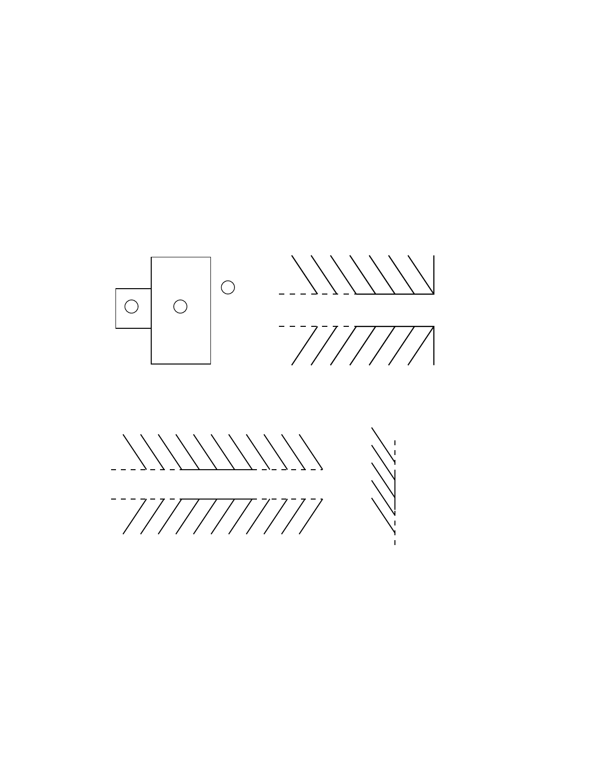
4-2 18 December 2000
CHAPTER 4
GEOMETRY SPECIFICATION
Let us start the definition of cell 3 at surface 2 (this is not a requirement). The expression 2 −3
defines the following region: everything in the world outside surface 2 intersected with everything
to the left of surface 3. This region is hatched in Figure 4.1b. Let us examine in detail how
Figure 4.1b was derived. First look at each region separately. The area with a positive sense with
respect to surface 2 is shown in Figure 4.1c. It includes everything outside surface 2 extending to
infinity in all directions. The area with negative sense with respect to surface 2 is undefined so far.
The area with negative sense with respect to surface 3 is shown in Figure 4.1d. It includes
everything to the left of surface 3 extending to infinity, or half the universe. Recall that an
intersection of two regions gives only the area common to both regions or the areas that overlap.
Superimposing Figures 4.1c and 4.1d results in Figure 4.1e. The cross-hatched regions show the
space common to both regions. This is the same area hatched in Figure 4.1b.
Figure 4-1a. Figure 4.1b
Figure 4.1c Figure 4.1d
Let us now deal with surface 1. To the quantity 2 −3 we will add everything with a negative sense
with respect to surface 1 as indicated by the expression 2 −3: −1, or (2 −3): −1 if you prefer. Recall
(1) that in the hierarchy of operations, intersections are performed first and then unions (so the
parentheses are unnecessary in the previous expression), and (2) that a union of two regions results
5
4
13
2
3
21
2
3
2
3
2
23

18 December 2000 4-3
CHAPTER 4
GEOMETRY SPECIFICATION
in a space containing everything in the first region plus everything in the second region; this
includes everything common to both regions. Superimposing the region shown in Figure 4.1b and
the region to the left of surface 1 results in Figure 4.1f. Our geometry now includes everything
hatched plus everything crosshatched and has added part of the tunnel which is interior to surface 2.
By the same method we will deal with surface 4. To the quantity 2 −3: −1 we will add everything
with a positive sense with respect to surface 4, written as 2 −3: −1: 4. Figure 4.1g shows our new
geometry. It includes everything in Figure 4.1f plus everything outside surface 4.
Our final step is to block off the large tunnel extending to infinity to the right by adding the region
with a positive sense with respect to surface 5 to the region shown in Figure 4.1g. The final
expression that defines cell 3 of Figure 4.1a is 2 −3: −1: 4: 5.
Figure 4.1e Figure 4.1f
Figure 4-1g.
There is more than one way to define cell 3. Starting with surface 1, we can add the region to the
left of 1 to the region outside surface 2 or −1: 2, which is illustrated in Figure 4.1h. We wish to
intersect this space with the space having a negative sense with respect to surface 3. Superimposing
3
3
2
21
2
2
3
3
4
4
3
3
2
2
1

4-4 18 December 2000
CHAPTER 4
GEOMETRY SPECIFICATION
Figure 4.1h and the region to the left of surface 3 results in Figure 4.1i. The cross-hatched area
indicates the area common to both regions and is the result of the intersection. Note that the cross-
hatched area of Figure 4.1i is identical to the entire hatched plus crosshatched area of Figure 4.1f.
Therefore, we have defined the same geometry in both figures but have used two different
approaches to the problem. To ensure that the intersection of −3 is with the quantity −1: 2 as we
have illustrated, we must use parentheses giving the expression (−1: 2) −3. Remember the order in
which the operations are performed. Intersections are done before unions unless parentheses alter
the order. The final expression is (−1: 2) −3: 4: 5.
Figure 4.1h Figure 4.1i
Another tactic uses a somewhat different approach. Rather than defining a small region of the
geometry as a starting point and adding other regions until we get the final product, we shall start
by defining a block of space and adding to or subtracting from that block as necessary. We
arbitrarily choose our initial block to be represented by 4: −1: 5, illustrated in Figure 4.1j.
Figure 4-1j.
To this block we need to add the space in the upper and lower left corners. The expression 2 −3
isolates the space we need to add. Adding 2 −3 to our original block, we have 4: −1: 5: (2 −3). The
parentheses are not required for correctness in this case but help to illustrate the path our reasoning
has followed. Figure 4.1k depicts the union of 2 −3 with the block of space we originally chose.
1
2
2
1
2
2
3
3
1
4
4
5

18 December 2000 4-5
CHAPTER 4
GEOMETRY SPECIFICATION
Figure 4-1k.
Let us arbitrarily choose a different initial block, 4: 5: −3, all the world except cell 2. From this
region we need to subtract cell 1. If we intersect the region (2: −1) with (4: 5: −3), as shown in
Figure 4.1l, we will have introduced an undefined tunnel to the right of surface 5. To correct this
error, define an area (2: −1: 3) or (2: −1: 5) and intersect this region with the initial block.
Figure 4.1l.
Another approach is to intersect the two regions −1: 2 and −3: 4, then add that to the region to the
right of surface 5 by (−1: 2)(−3: 4): 5. In the above paragraph the expression
(4:5:−3)(2 : −1: 5) can have the common quantity: 5 factored out, also resulting in
(−1: 2)(−3 : 4): 5.
Finally, another approach is to forget about the reality of the geometry and for cell 3 take the inverse
(or complement) of all the cells bounding cell 3, which is cells 1 and 2. This says that cell 3 is all
of the world excluding that which has already been defined to be in cells 1 and 2. The advantage
of this is that cells 1 and 2 are easy to specify and you don’t get bogged down in details for cell 3.
Cell 3 thus becomes (−1:2:3)(−3:4:5).Note that the specifications for cells 1 and 2 are reversed.
Intersections become unions. Positive senses become negative. Then each piece is intersected with
the other. There is a complement operator in MCNP that is a shorthand notation for the above
1
2
2
3
34
4
5
12
2
3
34
4
5
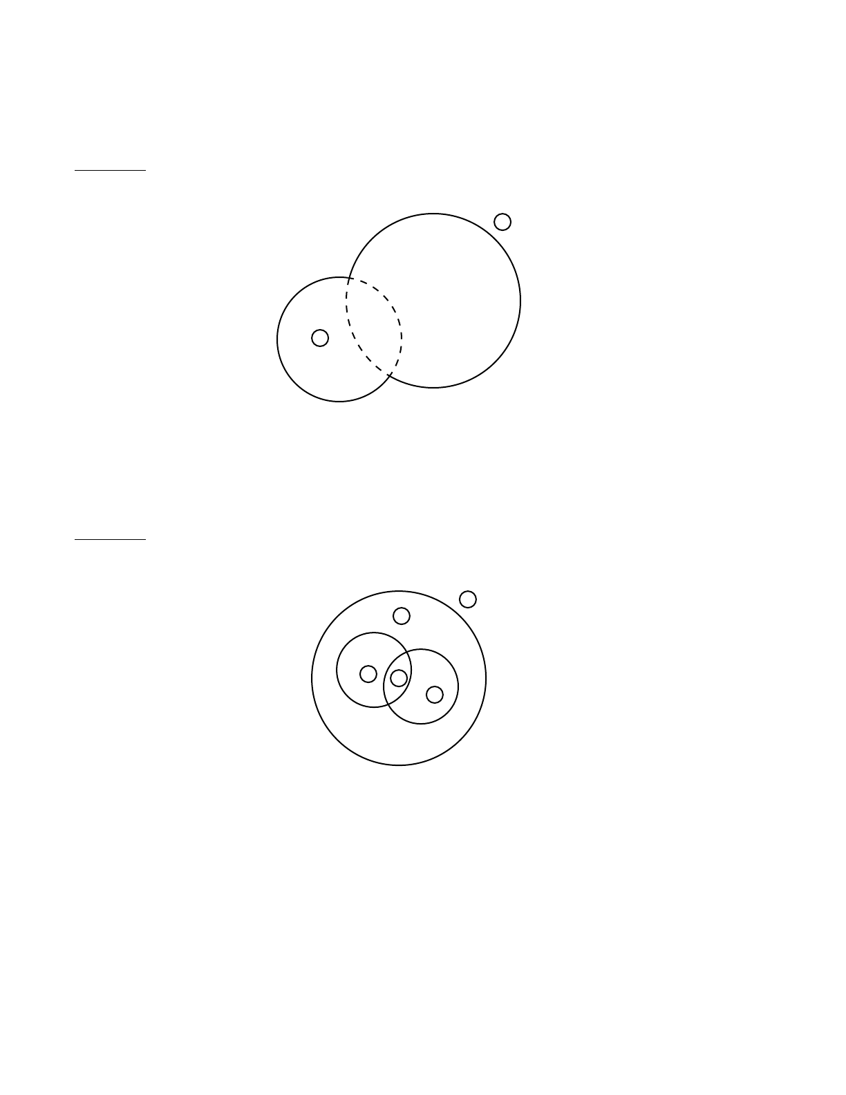
4-6 18 December 2000
CHAPTER 4
GEOMETRY SPECIFICATION
expression; it is the symbol #, which can be thought of as meaning not in. Therefore, cell 3 is
specified by #1 #2, translated as everything in the world that is not in cell 1 and not in cell 2.
Example 2:
Figure 4-2.
Cell 1 is everything interior to the surfaces 1 and 2:
10−1: −2
201 2
Example 3:
Figure 4-3.
In this geometry of four cells defined by three spheres, cell 3 is disconnected. Cell 3 is the region
inside surface 3 but outside surfaces 1 and 2 plus the region enclosed between surfaces 1 and 2:
10−12
20−21
1
1
22
34
1
13
2
2
3

18 December 2000 4-7
CHAPTER 4
GEOMETRY SPECIFICATION
30−312:−2−1
403
Cell 3 could also be written as
30(−312):(−2−1) The parentheses are not required.
Example 4:
Figure 4-4.
In this example all vertical lines are planes with their positive sides to the right and all horizontal
lines are cylinders. Cells 1, 2, and 3 are simple; they are defined by 1 -2 -3, 3 −4−5, and 5 −6−7,
respectively. Cell 4 is simple if the complement operator is used; it is #1 #2 #3 #5 or #1 #2 #3 −8.
Cell 5 is also simple; it is no more than 8 (or verbally, everything in the world with a positive sense
with respect to surface 8).
If cell 5 were defined as just #4, it would be incorrect. That says cell 5 is everything in the universe
not in cell 4, which includes cells 1, 2, and 3. The specification #4 #1 #2 #3 is correct but should
not be used because it tells MCNP that cell 5 is bounded by surfaces 1 through 7 in addition to
surface 8. This will cause MCNP to run significantly more slowly than it should because anytime
a particle enters cell 5 or has a collision in it, the intersection of the particle’s trajectory with each
bounding surface has to be calculated.
Specifying cell 4 exclusively with the complement operator is very convenient and
computationally efficient in this case. However, it will be instructive to set up cell 4 explicitly
without complements. There are many different ways to specify cell 4; the following approach
should not be considered to be the way.
First consider cell 4 to be everything outside the big cylinder of surface 4 that is bounded on each
end by surfaces 1 and 7. This is specified by (−1:4:7). The parentheses are not necessary but may
1
2
3
4
6
7
5
6
4
2
8
1 2 3 4 5

4-8 18 December 2000
CHAPTER 4
GEOMETRY SPECIFICATION
add clarity. Now all that remains is to add the corners outside cylinders 2 and 6. The corner outside
cylinder 2 is (2 −3), whereas it is (5 6) outside cylinder 6. Again the parentheses are optional. These
corners are then added to what we already have outside cylinder 4 to get
(−1:4:7):(2 −3):(5 6)
The region described so far does not include cells 1, 2, or 3 but extends to infinity in all directions.
This region needs to be terminated at the spherical surface 8. In other words, cell 4 is everything
we have defined so far that is also common with everything inside surface 8 (that is, everything so
far intersected with −8). So as a final result,
((−1:4:7):(2 −3):(5 6)) −8
The inner parentheses can be removed, but the outer ones are necessary (remember the hierarchy
of operations) to give us
(−1:4:7:2 −3:5 6) −8
If the outer parentheses are removed, the intersection of −8 will occur only with 5 and 6, an event
that is clearly incorrect.
Example 5:
Figure 4-5.
This example is similar to the previous one except that a vertical cylinder (surface 4) is added to
one side of the horizontal cylinder (surface 3).
Cell 1 is (1 −3−2), cell 3 is #1 #2 #4, and cell 4 is just 6.
4
5
4
3
12
3
6
1
2
3 4
Z
Y

18 December 2000 4-9
CHAPTER 4
GEOMETRY SPECIFICATION
Cell 2 is more than might initially meet the eye. It might appear to be simply (−5−4 3), but this
causes a mirror image of the cell 2 we want to show up on the bottom half of cell 1, as represented
by the dashed lines in Figure 4.5. We need to add an ambiguity surface to keep cell 2 above the y-
axis. Let surface 7 be an ambiguity surface that is a plane at z= 0. This surface appears in the
MCNP input file as any other surface. Then cell 2 becomes (−5−4 3 7) for the final result. You
should convince yourself that the region above surface 7 intersected with the region defined by −5
−4 3 is cell 2 (don’t even think of surface 7 as an ambiguity surface but just another surface defining
some region in space). The mirror problem can also be avoided by defining cells 1 and 2 as a right
circular cylinder (rcc) macrobodies. The necessary cards for defining the macrobodies would be
1 rcc 0 -2 0 0 4 0 4
2 rcc 0 0 0 0 0 7 1
In this case cells 1,2 and 3 would simply be (-1), (-2 1), and (1 2 -6) respectively. Notice that to get
the interface between the cylinders correct macrobody 2 extends into cell 1 and is then truncated
by the definition of cell 1.
Example 6:
Figure 4-6.
This is three concentric spheres with a box cut out of cell 3. Surface 8 is the front of the box and 9
is the back of the box. The cell cards are
10−1
20−21
30−32 (−4:5:−6:7:8:−9) $ These parentheses are required.
3
2
1
67
5
4
123
4
5
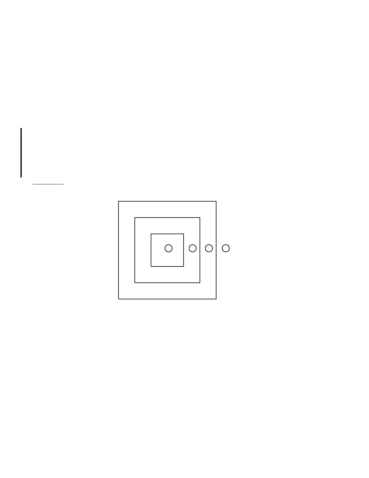
4-10 18 December 2000
CHAPTER 4
GEOMETRY SPECIFICATION
403
504−5 6 −7−8 9
Cell 3 is everything inside surface 3 intersected with everything outside surface 2 but not in cell 5.
Therefore, cell 3 could be written as
30−3 2 #(4 −5 6 −7−8 9)
or 3 0 −3 2#5
or 3 0 −3 2(−4:5:−6:7:8:−9)
Cell 5 could also be specified using a RPP macrobody. The correct cell and surface cards for this
would be
5 0 -4 $
4 rrp 2 4 7.5 8.5 -2 2
Example 7:
Figure 4-7.
This is three concentric boxes, a geometry very challenging to set up using only intersections,
easier with unions, and almost trivial with the BOX macrobody. Surfaces 5, 11, and 17 are the back
sides of the boxes (smaller to larger, respectively); 6, 12, and 18 are the fronts:
10−2 −3 41 5 −6
20−7 −8 910 11−12
(2 : 3 : −4 :−1 :−5 :6)
30−13 −14 15 16 17 −18
(7 : 8 : −9 :−10 :−11 : 12)
4013:14:−15:−16 :−17 :18
1
3
2
4
10
8
7
9
16
14
13
15 1 2 3 4
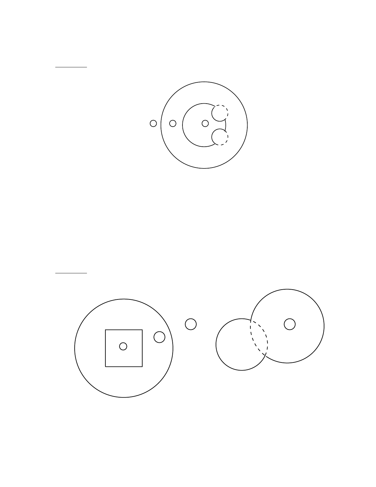
18 December 2000 4-11
CHAPTER 4
GEOMETRY SPECIFICATION
Example 8:
Figure 4-8.
This is two concentric spheres with a torus attached to cell 2 and cut out of cell 1:
10−1 4
20−2 (1 : −4)
302
If the torus were attached to cell 1 and cut out of cell 2, this bug-eyed geometry would be:
10−1 :−4
20−2 14
302
Example 9:
1
2
4
123
12
3
4
5
6
7
9
17
1722

4-12 18 December 2000
CHAPTER 4
GEOMETRY SPECIFICATION
Figure 4-9.
Cell 9 is a box cut out of the left part of spherical cell 17; surface 9 is the front of the box and 8 is
the rear. Cell 17 is disconnected; the right part is the space interior to the spheres 6 and 7. An F4
tally in cell 17 would be the average flux in all parts of cell 17. An F2 surface tally on surface 7
would be the flux across only the solid portion of surface 7 in the figure. The cell specifications are:
90−3 −2 4 1 8 −9
170−5 (3 : −4 : −1 : 2 : 9 : −8) : −6 : −7
22 0 5 6 7
A variation on this problem is for the right portion of cell 17 to be the intersection of the interiors
of surfaces 6 and 7 (the region bounded by the dashed lines in the above figure):
90−3 −2 4 1 8 −9
170−5 (3 : −4 : −1 : 2 : 9 : −8) : −6 −7
22 0 5 (6 : 7)
Example 10:
Figure 4-10.
This is a box with a cone sitting on top of it. Surface 6 is the front of the box and 7 is the rear. You
should understand this example before going on to the next one.
1012−3 (-4 : −5)−6 7
20−1 : −2 : 3 : 4 5 : 6 : −7
This problem could be simplified by replacing surfaces 1-6 with a BOX macrobody. The resulting
cell and surface cards would be
c cell cards
1 0 -8:(-5 8.5)
2 0 #1 $ or -8.4:-8.6:8.3:(8.5 5):8.1:-8.2
13
2
4
5
1
2
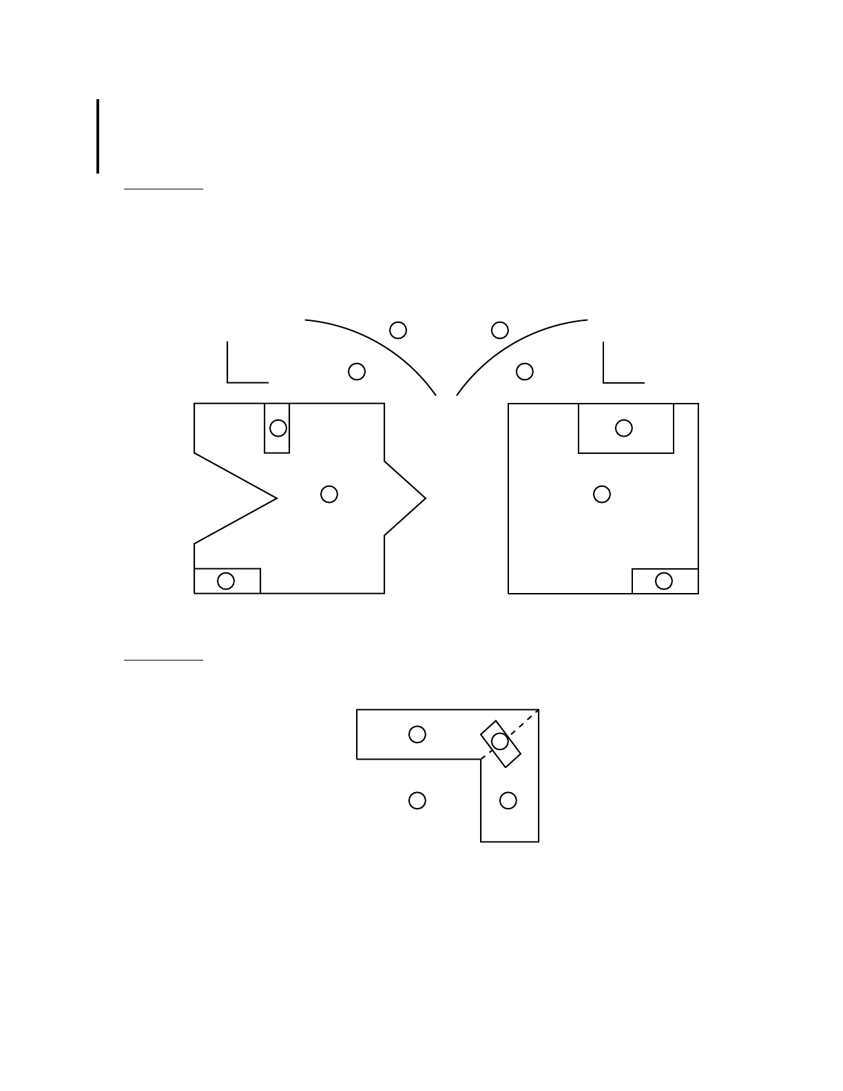
18 December 2000 4-13
CHAPTER 4
GEOMETRY SPECIFICATION
c surface cards
5 kz 8 0.25 -1
8 box -2.5 -2.5 0 5 0 0 0 5 0 0 0 5
Example 11: Surfaces 15 and 16 are cones, surface 17 is a sphere, and cell 2 is disconnected.
10−1 23 (−4 :−16) 5 −6 (12 : 13 : −14)
(10 : −9 :−11 :−7 : 8) 15
20−10 9117−8 −1 : 2 −12 14 −6 −13 3
30−17 (1 : −2 :−5 : 6 : −3 :−15 : 16 4)
4017
Figure 4-11.
Example 12:
Figure 4-12.
Z
Y
1
2
34
13
12
15
910
11 16
17
1
2
2
3
4Z
X
1
2
56
14
12
78
11
17
1
2
2
3
4
4
3
a1
2
1b
3
6
87
8
1
1
3
2

4-14 18 December 2000
CHAPTER 4
GEOMETRY SPECIFICATION
Cell 1 consists of two cylinders joined at a 45° angle. Cell 2 is a disk consisting of a cylinder
(surface 8) bounded by two planes. Surface 5 is a diagonal plane representing the intersection of
the two cylinders. The problem is to specify the disk (cell 2) in one cell formed by the two cylinders
(cell 1). A conflict arises in specifying cell 1 since, from the outside cell 3, corner abetween
surfaces 1 and 3 is convex, but on the other side of the cell the same two surfaces form a concave
corner at b. The dilemma is solved by composing cell 1 of two disconnected cells, each bounded
by surface 5 between the corners aand b. Surface 5 must be included in the list of surface cards in
the MCNP input file. When the two parts are joined to make cell 1, surface 5 does not appear.
Convince yourself by plotting it using an origin of 0 0 24 and basis vectors 0 1 1 0 −1 1. See
Appendix B for an explanation of plotting commands.
10(2−1 −5 (7:8:−6)):(4 −3 5(−6:8:7))
20−8 6−7
30(−2:1:5)(−4:3:−5)
A more efficient expression for cell 1 is
10(2−1 −5:4 −3 5)(−6:8:7)
Example 13:
This example has the most complicated geometry so far, but it can be described very simply. The
input file is called antares and is available from the /x6code/manual/examples/chap4 node.
You can see that Example 13 is similar to Example 1. There is just a lot more of it.It is possible to
set this geometry up by any of the ways mentioned in Example 1. However, going around the outer
surfaces of the cells inside cell 10 is tedious. There is a problem of visualization and also the
problem of coming up with undefined tunnels going off to infinity as in Example 1.
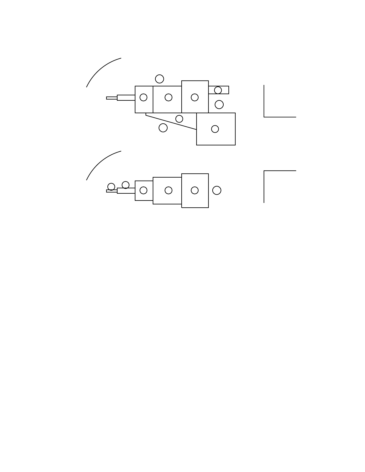
18 December 2000 4-15
CHAPTER 4
GEOMETRY SPECIFICATION
Figure 4-13.
The way to handle this geometry is by the last method in Example 1. Set up the cell/surface
relations for each interior cell, then just take the complement for cell 10. For the interior cells,
101−2 −23
20−3 25 −24 2
303−5 12 −15 16 −11
405−6 12 −17 18 −11
506 −8 12 −13 −19 20
608 −9 −26
70−12 4 −7 −27
80−12 7−10 14 −21 22
902−3 −25
Cell 10 is surrounded by the spherical surface 28. Considering cell 10 to be everything outside cells
1 through 9 but inside surface 28, one can reverse the senses and replace all intersections with
unions to produce
X
Y
Z
Y
35 6 8
15 17 19
16 18 20
28
123 4 5 10
35 6 8
11
12
13 26
9
26
107
14
27
28
3 4 5
8
6
7
10
10
10
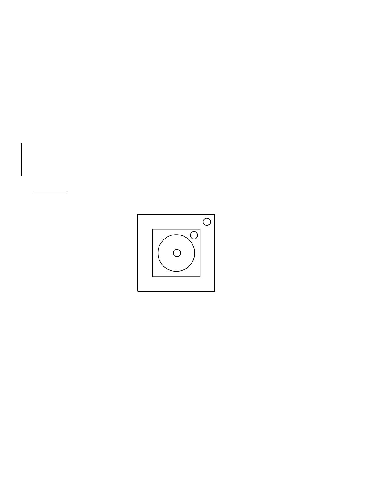
4-16 18 December 2000
CHAPTER 4
GEOMETRY SPECIFICATION
100(−1:2:23)(3:−25:24:−2)
(−3:5:−12:15:−16:11)
(−5:6:−12:17:−18:11)
(−6:8:−12:13:19:−20)
(−8:9:26)(12:−4:7:27)
(12:−7:10:−14:21:−22)
(−2:3:25) −28
Note how easy cell 10 becomes when the complement operator is used:
10 0 #1 #2 #3 #4 #5 #6 #7 #8 #9 −28
Once again this example can be greatly simplified by replacing all but cell 7 with macrobodies.
However the definition of cell 7 must then be changed to use the facets of the surrounding
macrobodies instead of surfaces 12 and 7. The facets of macrobodies can be visualized using the
MBODY OFF option of the geometry plotter.
Example 14:
Figure 4-14.
This example illustrates some necessary conditions for volume and area calculations. The
geometry has three cells, an outer cube, an inner cube, and a sphere at the center. If cell 3 is
described as
308−9 −10 11 −12 13 #2 #1
(and #1 must be included to be correct), the volume of cell 3 cannot be calculated. As described, it
is not bounded by all planes so it is not a polyhedron, nor is it rotationally symmetric. If cell 3 is
described by listing all 12 bounding surfaces explicitly, the volume can be calculated.
11
10
89
1
2
3
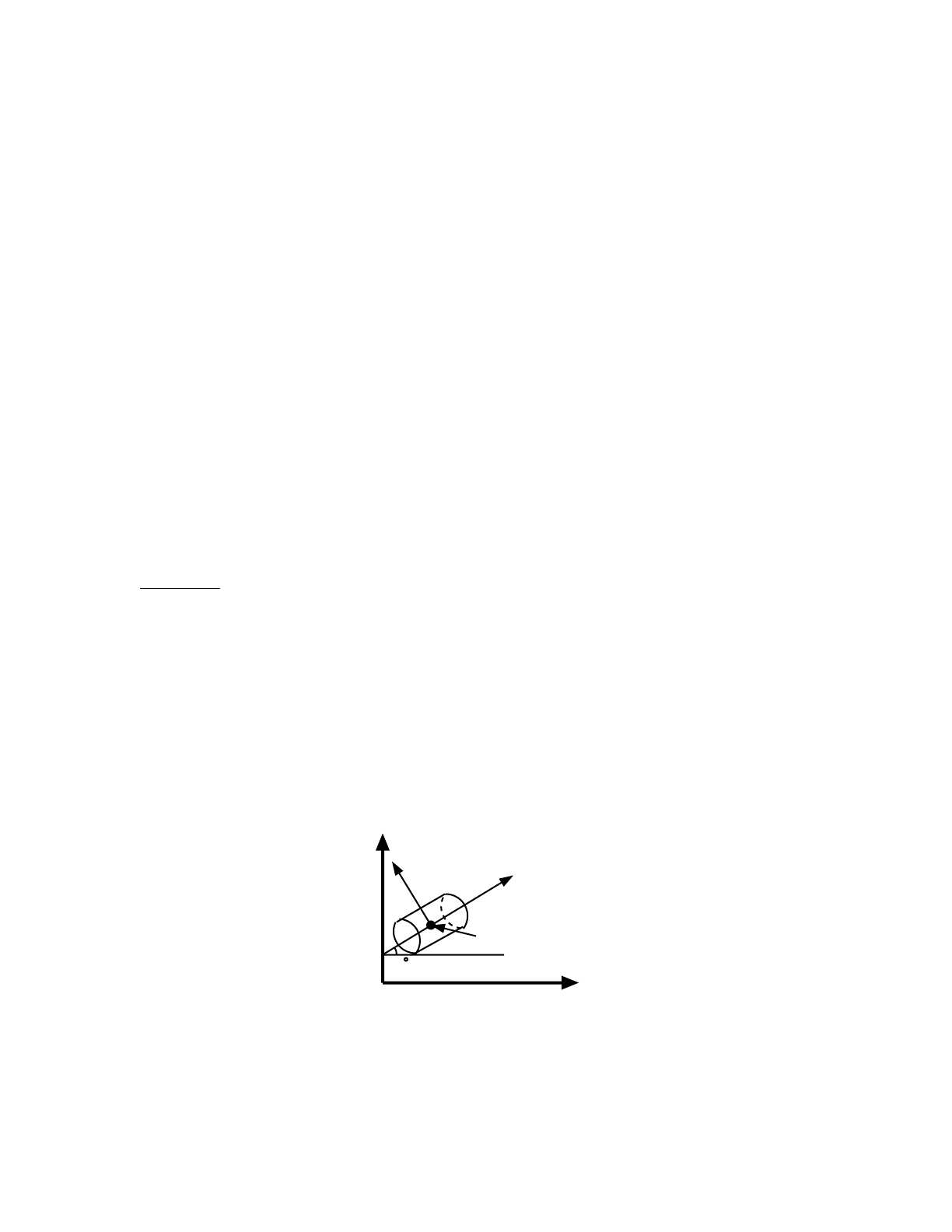
18 December 2000 4-17
CHAPTER 4
COORDINATE TRANSFORMATIONS
II. COORDINATE TRANSFORMATIONS
In most problems, the surface transformation feature of the TRn card will be used with the default
value of 1 for M. When M= 1 applies, most of the geometry can be set up easily in an (x,y,z)
coordinate system and only a small part of the total geometry will be difficult to specify. For
example, a box with sides parallel to the (x,y,z) coordinate system is simple to describe, but inside
might be a tilted object consisting of a cylinder bounded by two planes. Since the axis of the
cylinder is neither parallel to nor on the x,y,orzaxis, a general quadratic must be used to describe
the surface of the cylinder. The GQ surface card has 10 entries that are usually difficult to
determine. On the other hand, it is simple to specify the entries for the surface card for a cylinder
centered on the y-axis. Therefore, we define an auxiliary coordinate system (x′,y′,z′) so the axis of
the cylinder is one of the primed axes, y′ for example. Now we will use the TRn card to describe
the relationship between one coordinate system and the other. M=1requires that the coordinates
of a vector from the (x,y,z) origin to the (x′,y′,z′) origin be given in terms of (x,y,z).
Only in rare instances will M=−1be needed. Some unusual circumstances may require that a small
item of the geometry must be described in a certain system which we will call (x,y,z), and the
remainder of the surfaces would be easily described in an auxiliary system (x′,y′,z′). The Oientries
on the TRn card are then the coordinates of a vector from the (x′,y′,z′) origin to the (x,y,z) origin
given in terms of the primed system.
Example 1: The following example consists of a can whose axis is in the yz plane and is tilted 30°
from the y-axis and whose center is at (0,10,15) in the (x,y,z) coordinate system. The can is bounded
by two planes and a cylinder, as shown in Figure 4.15.
The surface cards that describe the can in the simple (x′,y′,z′) system are:
11CY 4
21PY−7
31PY 7
Figure 4-15.
Y
Z
Y’
Z’
(X,Y,Z)=(0,10,15)
1
1
3
2
30

4-18 18 December 2000
CHAPTER 4
COORDINATE TRANSFORMATIONS
The 1 before the surface mnemonics on the cards is the n that identifies which TRn card is to be
associated with these surface cards. The TRn card indicates the relationship of the primed
coordinate system to the basic coordinate system.
We will specify the origin vector as the location of the origin of the (x′,y′,z′) coordinate system with
respect to the (x,y,z) system; therefore, M= 1. Since we wanted the center of the cylinder at
(0,10,15), the Oientries are simply 0 10 15. If, however, we had wanted surface 2 to be located at
(x,y,z) = (0,10,15), a different set of surface cards would accomplish it. If surface 2 were at y′=0
and surface 3 at y′=14 the Oi entries would remain the same. The significant fact to remember
about the origin vector entries is that they describe one origin with respect to the other origin. The
user must locate the surfaces about the auxiliary origin so that they will be properly located in the
main coordinate system.
The Bi entries on the TRn card are the cosines of the angles between the axes as listed on page 3–
26 in Chapter 3. In this example, the x-axis is parallel to the x′-axis. Therefore, the cosine of the
angle between them is 1. The angle between yand x′is 90° with a cosine of 0. The angle between
zand x′and also between xand y′is 90° with a cosine of 0. The angle between yand y′is 30° with
a cosine of 0.866. The angle between z and y′is 60° with 0.5 being the cosine. Similarly, 90° is
between xand z′;120° is between yand z′; and 30° is between zand z′. The complete TRn card is
TR1 0 10 15 1 0 0 0 .866 .5 0 −.5 .866
An asterisk preceding TRn indicates that the Bi entries are the angles in degrees between the
appropriate axes. The entries using the ∗TRn mnemonic are
∗TR1 0 10 15 0 90 90 90 30 60 90 120 30
The default value of 1 for M, the thirteenth entry, has been used and is not explicitly specified.
The user need not enter values for all of the Bi. As shown on page 3–26, Bimay be specified in any
of five patterns. Pattern #1 was used above, but the simplest form for this example is pattern #4
since all the skew surfaces are surfaces of revolution about some axis. The complete input card then
becomes
∗TR1 0 10 15 3J 90 30 60
Example 2: The following example illustrates another use of the TRn card. The first part of the
example uses the TR1 card and an M=1transformation; the second part with the TR2 card uses
an M=−1 transformation. Both parts and transformations are used in the following input file.
EXAMPLE OF SURFACE TRANSFORMATIONS
20 −4 3−5
60 −14 −13 :−15 41 −42
31 PX−14
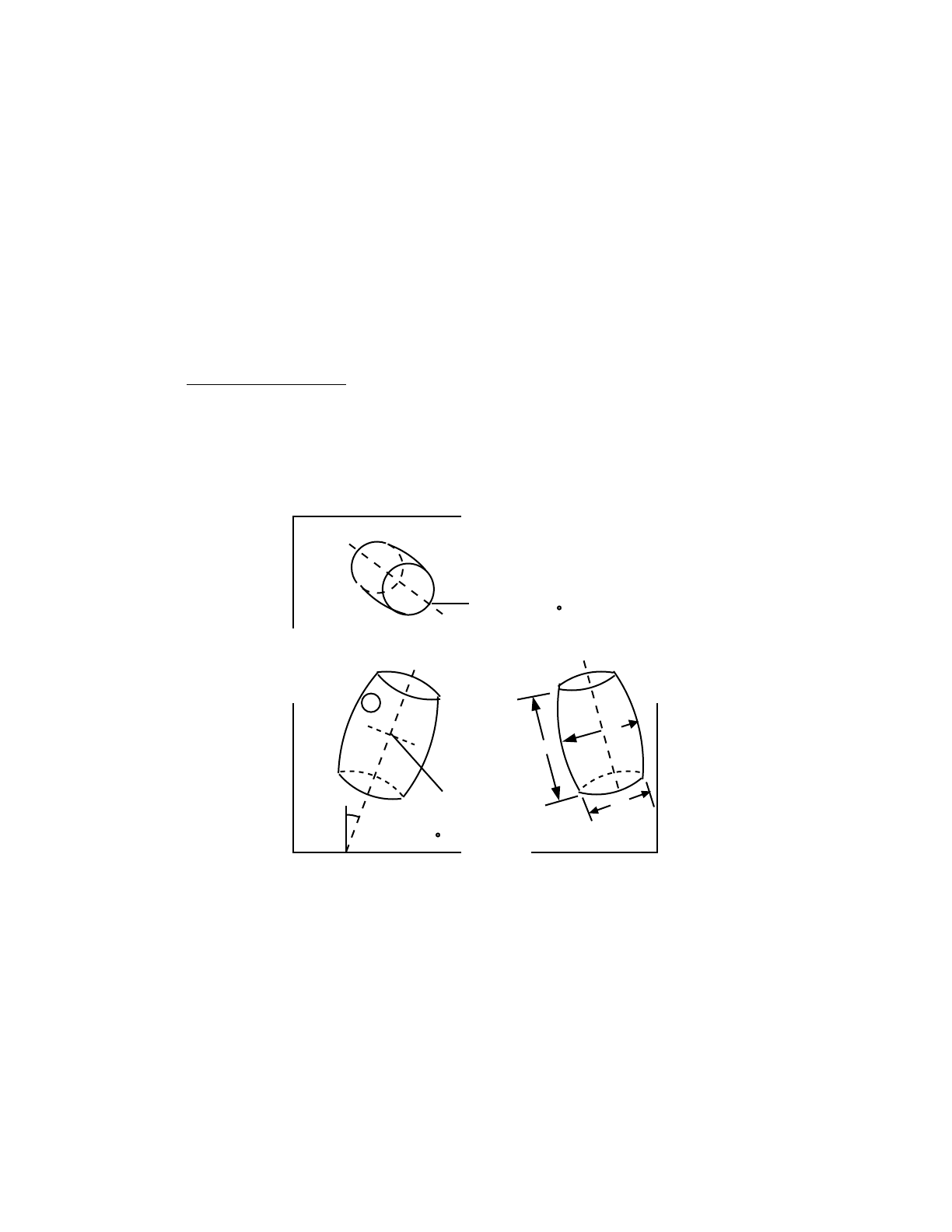
18 December 2000 4-19
CHAPTER 4
COORDINATE TRANSFORMATIONS
41 X −14 10 0 12 14 10
5 1 PX 14
13 2 SX −15 70
14 2 CX 30
15 2 Y 75 0 30 16
41 2 PY 0
42 2 PY 75
TR1 20 31 37 .223954 .358401 .906308
TR2 −250 −100 −65 .675849 .669131 .309017
J J .918650 J J −.246152 −1
A. TR1 and M = 1 Case:
Cell 2 is bounded by the plane surfaces 3 and 5 and the spheroid surface 4, which is a surface of
revolution about the skew axis x’ in Figure 4.16.
Figure 4-16.
To get the coefficients of surfaces 3, 4, and 5, define the x′axis as shown in the drawings (since the
surfaces are surfaces of revolution about the x′ axis, the orientation of the y′ and z′ axes does not
matter), then set up cell 2 and its surfaces, with coefficients defined in the x′y′z′coordinate system.
On the TR1 card, the origin vector is the location of the origin of the x′y′z′coordinate system with
respect to the main xyz system of the problem. The pattern #4 on page 3–26 in Chapter 3 is
Z
XY
Z(up)
X
Y
x’
3
4
5
2
center is at
(X,Y,Z)=(20,31,37)
tilted 25 from vertical
x’
28 24
20
x’
vertical plane containing x’
axis is 32 from YZ plane
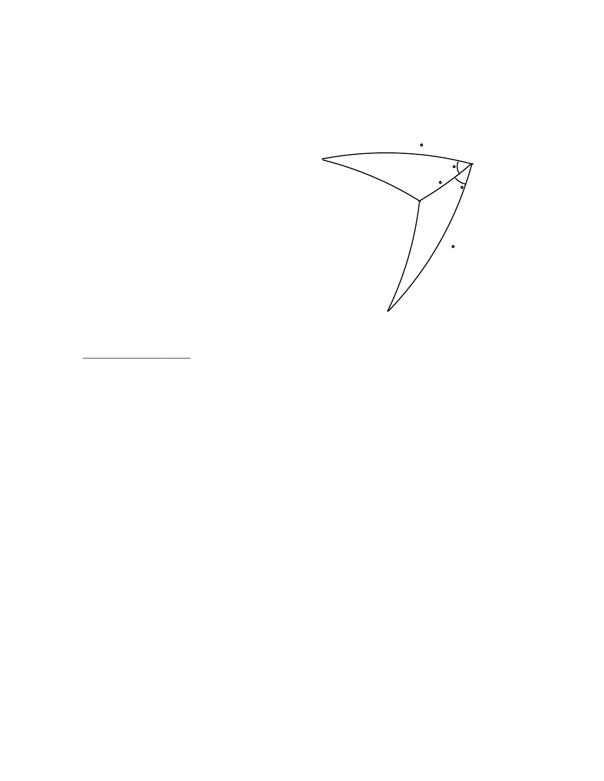
4-20 18 December 2000
CHAPTER 4
COORDINATE TRANSFORMATIONS
appropriate since the surfaces are all surfaces of revolution about the x′ axis. The components of
one vector of the transformation matrix are the cosines of the angles between x′and the x,y, and z
axes. They are obtained from spherical trigonometry:
B. TR2 and M = −1 Case:
Cell 6 is the union of a can bounded by spherical surface 13 and cylindrical surface 14 and a conical
piece bounded by conical surface 15 and ambiguity surfaces 41 and 42, which are planes. (Surface
42 is required because when surface 15 is defined in x′y′z′it is as a type Y surface, which becomes
a cone of one sheet; when it is transformed into the xyz system it becomes a type GQ surface, which
in this case is a cone of two sheets. Weird, but that’s the way it has to be.) Surfaces 13 and 14 are
surfaces of revolution about one axis, and surfaces 15, 41, and 42 are surfaces of revolution about
an axis perpendicular to the first axis. Both axes are skewed with respect to the xyz coordinate
system of the rest of the geometry.
Define the auxiliary x′y′z′coordinate system as shown in Figure 4.17. Set up cell 6 with its surfaces
specified in the x′y′z′ coordinate system as part of the input file and add a second transformation
card, TR2.
Because the location of the origin of the xyz coordinate system is known relative to the x′y′z′system
(rather than the other way around, as in the first part of the example), it is necessary to use the
reverse mapping. This is indicated by setting M= −1. In this reverse mapping the origin vector (−
250,−100,−65) is the location of the origin of the xyz system with respect to the x′y′z′system. For
the components of the transformation matrix, pattern #3 out of the four possible choices from
Chapter 3 is most convenient here. The xyz components of z′and the x′y′z′components of zare easy
to get. The components of xand of yare not. The whole transformation matrix is shown here with
XZ
90
X’
E
Y
90F
58
32
G=25
cos E = cos 58˚ x sin 25˚ = .223954
cos F = cos 32˚ x sin 25˚ = .358401
cos G = cos 25˚ = .906308
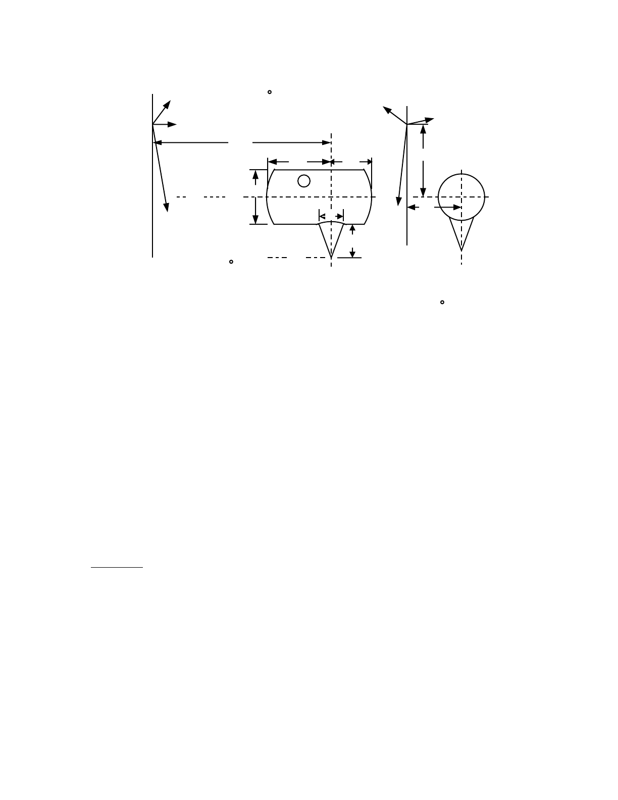
18 December 2000 4-21
CHAPTER 4
REPEATED STRUCTURE AND LATTICE EXAMPLES
Figure 4-17.
the components that are obtained from Figure 4.17 written in:
The zz′component is −SQRT(1. −.309107∗∗2−.918650∗∗2) = −.246152, and the xx′component
is SQRT(1. − .669131∗∗2− .309017∗∗2) = .675849, with the signs determined by inspection of the
figure.
III. REPEATED STRUCTURE AND LATTICE EXAMPLES
Example 1: This example illustrates the use of transformations with simple repeated structures.
The geometry consists of a sphere enclosing two boxes that each contain a cylindrical can. Cell 2
is filled by universe 1. Two cells are in universe 1—the cylindrical can, cell 3, and the space outside
the can, cell 4. Cell 2 is defined and the LIKE m BUT card duplicates the structure at another
location. The TRCL entry identifies a TRn card that defines the displacement and rotational axis
transformation for cell 5. To plot type:
b100 010 ex11 or3.53.50
xy z
x′.675849 cos 48° = .669131 cos 72° = .309017
y′cos 15° × cos 18° = .918650
z′ −.246152
Z axis is 18 from
the Y’Z’ plane
YY axis is 42 from
the Y’Z’ plane
X
Z
250
41 X’
Y’
60 6
13 13
14
85 55
32
45
42
Z’
Y’
15
14
X
Y
Z
projection
of the Z axis
on the Y’Z’
plane is 15
from the X’Y’plane
100
65
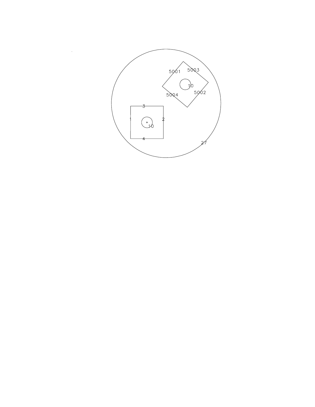
4-22 18 December 2000
CHAPTER 4
REPEATED STRUCTURE AND LATTICE EXAMPLES
simple repeated structures
1 0 -27 #2 #5 imp:n=1
2 0 1 -2 -3 4 -5 6 fill=1 imp:n=1
3 0 -10 -11 12 u=1 imp:n=1
4 0 #3 u=1 imp:n=1
5 like 2 but trcl=3
7 0 27 imp:n=0
1px−3
2px 3
3py 3
4py−3
5 pz 4.7
6 pz –4.7
10 cz 1
11 pz 4.5
12 pz –4.5
27 s 3.5 3.5 0 11
sdef pos 3.5 3.5 0
f2:n 1
tr3∗7 7 0 40 130 90 50 40 90 90 90 0
nps 10000
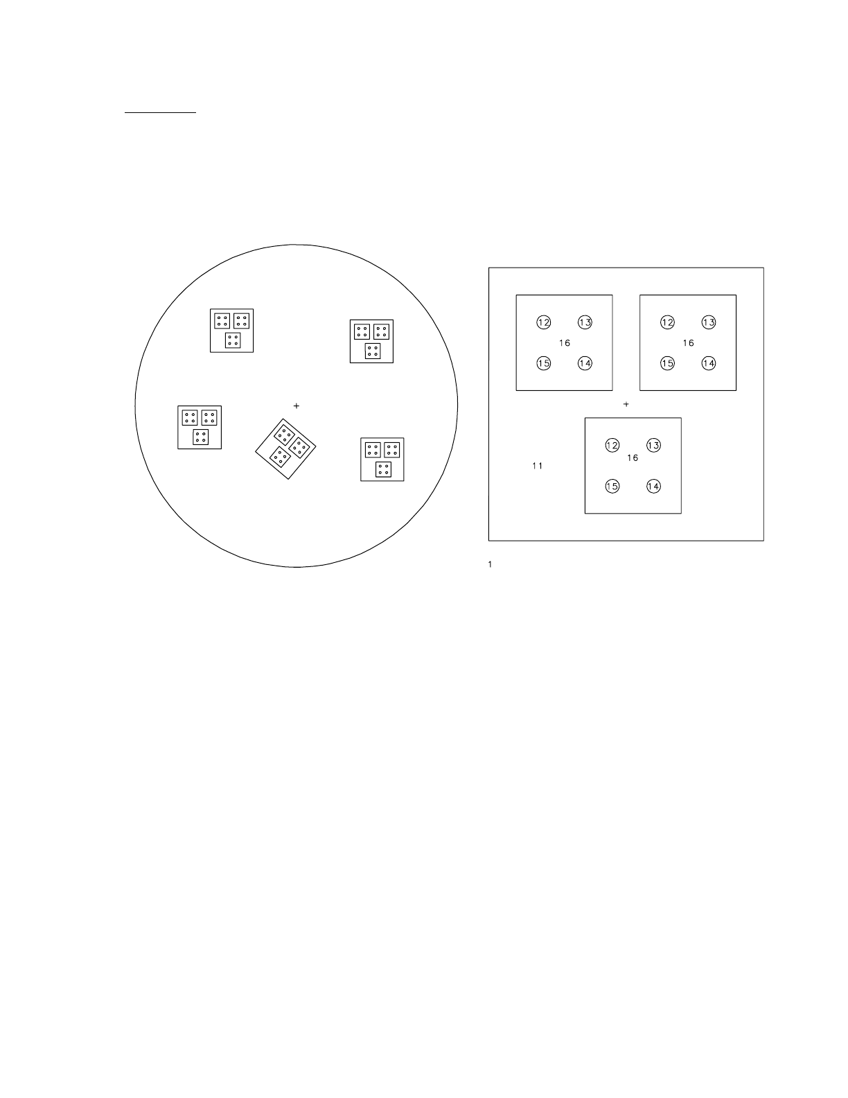
18 December 2000 4-23
CHAPTER 4
REPEATED STRUCTURE AND LATTICE EXAMPLES
Example 2: This example illustrates the LIKE m BUT construct, the FILL card, the U card, two
forms of the TRCL card, and a multiple source cell definition. The following line will plot the view
shown on the left:
b100 010 ex21 la0
In this example five cells, numbers 2 through 6, are identical except for their locations. Cell 2 is
described fully and the other four are declared to be like cell 2 but in different locations. Cell 2 is
defined in an auxiliary coordinate system that is centered in the cell for convenience. That
coordinate system is related to the main coordinate system of the problem by transformation
number 2, as declared by the TRCL = 2 entry and the TR2 card. Cells 2 through 6 are all filled with
universe number 1. Because no transformation is indicated for that filling, universe 1 inherits the
transformation of each cell that it fills, thereby establishing its origin in the center of each of those
five cells. Universe 1 contains three infinitely long tubes of square cross section embedded in cell
11, which is unbounded. All four of these infinitely large cells are truncated by the bounding
surfaces of each cell that is filled by universe 1, thus making them effectively finite. The
transformations that define the locations of cells 8, 9 and 10 are entered directly on the cell cards
after the TRCL symbol rather than indirectly through TR cards as was done for cells 2 through 6
to illustrate the two possible ways of doing this. Cells 8, 9 and 10 are each filled with universe 2,
which consists of five infinite cells that are truncated by the boundaries of higher level cells. The
simplicity and lack of repetition in this example were achieved by careful choice of the auxiliary
cell 8 cell 9
cell 10
cell 2
cell 3
cell 4cell 5
cell 6

4-24 18 December 2000
CHAPTER 4
REPEATED STRUCTURE AND LATTICE EXAMPLES
coordinate systems at all levels. All of the location information is contained in just a few TRCL
entries, some direct and some pointing to a few TR cards.
The source definition is given on the SDEF, SIn and SPn cards. The source desired is a cylindrical
volume distribution, equally probable in all the cylindrical rods. The energies are given by
distribution 1. The entry for CEL shows that level 0 cells are given by distribution 2 and level 1
cells by distribution 3. The zero means that cells are searched for at level 2 and also that the
sampled position and direction will apply to the universe indicated by the entry just preceding the
first entry that is ≤0. In this case the position and direction will be defined in the coordinate system
of the cell sampled by distribution 3 at level 1. The SI2 card lists all the cells at level 0 that will
contain the source. SP2 indicates equal probability. SI3 lists the cells in level 1 and the positions
on the SI7 card are given in the coordinates of this level. A cylindrical volume distribution is
specified by RAD, EXT, AXS, and POS. The radius on the SI5 card is from 0 to .1. The ends of the
cylinder are at -2 and 2 (SI6) and the four sets of entries on the SI7 card are the origins of the four
cylinders of cells 12–15. These parameters describe exactly the four cells 12–15.
chapter 4 example 2
11−.5 −7 #2 #3 #4 #5 #6 imp:n=1
2 0 1 -2 -3 4 5 -6 imp:n=2 trcl=2 fill=1
3 like 2 but trcl=3
4 like 2 but trcl=4
5 like 2 but trcl=5 imp:n=1
6 like 2 but trcl=6
7 0 7 imp:n=0
8 0 8 -9 -10 11 imp:n=1 trcl=(−.9 .9 0) fill=2 u=1
9 like 8 but trcl=(.9 .9 0)
10 like 8 but trcl=(.1 -.9 0)
11 2 −18 #8 #9 #10 imp:n=1 u=1
12 2 -18 -12 imp:n=1 trcl=(-.3 .3 0) u=2
13 like 12 but trcl=(.3 .3 0)
14 like 12 but trcl=(.3 -.3 0)
15 like 12 but trcl=(-.3 -.3 0)
16 1 -.5 #12 #13 #14 #15 u=2 imp:n=1
1 px -2
2 py 2
3 px 2
4py−2
5pz−2
6 pz 2
7 so 15
8px−.7

18 December 2000 4-25
CHAPTER 4
REPEATED STRUCTURE AND LATTICE EXAMPLES
9py.7
10 px .7
11 py −.7
12 cz .1
sdef erg=d1 cel=d2:d3:0 rad=d5 ext=d6 axs=0 0 1 pos=d7
# si1 sp1 sb1
100
3 .22 .05
4 .08 .05
5 .25 .1
6 .18 .1
7 .07 .2
8.1.2
9 .05 .1
11 .05 .2
si2 l 2 3 4 5 6
sp2 1 1 1 1
si3 l 8 9 10
sp3 1 1 1
si5 0 .1
sp5 -21 1
si6 -2 2
sp6 0 1
si7 l .3 .3 0 .3 -.3 0 -.3 .3 0 -.3 -.3 0
sp7 1 1 1 1
m1 6000 1
m2 92235 1
drxs
tr2 -6 7 1.2
tr3 7 6 1.1
tr4 8 -5 1.4
tr5∗-1 -4 1 40 130 90 50 40 90 90 90 0
tr6 -9 -2 1.3
f4:n 2 3 4 5 6 12 13 14 15
e4 1 3 5 7 9 11 13
sd4 5j 1.8849555921 3r
fq f e
cut:n 1e20 .1
nps 100000
print
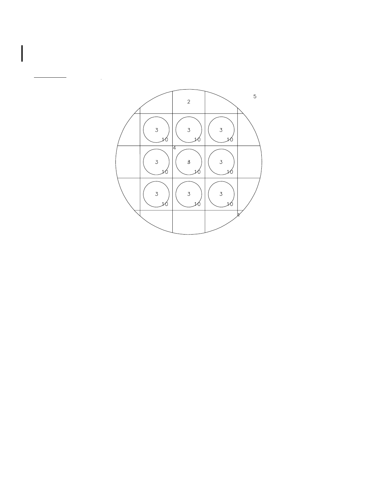
4-26 18 December 2000
CHAPTER 4
REPEATED STRUCTURE AND LATTICE EXAMPLES
Cell 2 could be replaced with a RPP macrobody that can then be replicated and translated
identically to cell 2 above.
Example 3:
This is a simple example illustrating the use of the FILL, U, and LAT cards to create an object
within several cells of a lattice. A hexahedral lattice is contained within a cylinder of radius 45 cm.
Cell 1 is the interior of the cylinder, and cell 5 is everything outside (all surfaces are infinite in the
z-direction). Cell 1 is filled by universe 1. Cell 2 is defined to be in universe 1. Surfaces 301-304
define the dimensions of the square lattice.
When filling the cells of a lattice, all cells visible, even partially, must be specified by the FILL
card. In this case, the “window” created by the cylinder reveals portions of 25 cells (5x5 array). A
FILL card with indices of –2 to 2 in the x- and y-directions will place the [0,0,0] element at the
center of the array. Universe 2, described by cells 3 and 4, is the interior and exterior, respectively,
of an infinite cylinder of radius 8 cm. The cells in universe 1 not filled by universe 2 are filled by
universe 1, in effect they are filled by themselves. The following file describes a cylinder that
contains a square lattice, with the inner 3x3 array of cells containing a small cylinder in each cell.
simple lattice
1 0 –1 fill=1 imp:n=1
2 0 –301 302 –303 304 lat=1 u=1 imp:n=1 fill=-2:2 –2:2 0:0
1 1 1 1 1 1 2 2 2 1 1 2 2 2 1 1 2 2 2 1 1 1 1 1 1
18 December 2000 4-27
CHAPTER 4
REPEATED STRUCTURE AND LATTICE EXAMPLES
3 0 –10 u=2 imp:n=1
4 0 #3 imp:n=1 u=2
5 0 1 imp:n=0
1 cz 45
10 cz 8
301 px 10
302 px –10
303 py 10
304 py –10
Example 4:
This example illustrates a lattice geometry and uses the FILL entries followed by transformations,
the U card, and the LAT card. Cell 2 is the bottom half of the large sphere outside the small sphere
(cell 1), is filled by universe 1, and the transformation between the filled cell and the filling universe
immediately follows in parentheses.
Cell 6 describes a hexahedral lattice cell (LAT=1) and by the order of specification of its surfaces,
also describes the order of the lattice elements. The (0,0,0) element has its center at
(–6 –6.5 0) according to the transformation information on the card for cell 2. Element (1,0,0) is
0,0,0
0,0,0
0,0,0
cell 9
cell 8
cell 7 cell 7

4-28 18 December 2000
CHAPTER 4
REPEATED STRUCTURE AND LATTICE EXAMPLES
beyond surface 5, element (–1,0,0) beyond surface 6, (0,1,0) beyond surface 7, etc. Cell 6 is filled
by universe 3, which consists of two cells: cell 8 inside the ellipsoid and cell 9 outside the ellipsoid.
When a lattice cell is defined with a macrobody, the lattice element indexing is somewhat
predetermined. The first, third and fifth facets are used to define the direction of increasing indices.
For the RPP, the second index increases in the positive y direction and the third index increases in
the positive z direction. For the BOX, the order of defining the three vectors will determine the axis
each index will increase in a positive direction.
Cell 3 is the top left-hand quarter of the sphere; cell 4 is the top right-hand quarter. Both are filled
by universe 2. Both FILL entries are followed by a transformation. The interorigin vector portion
of the transformation is between the origin of the filled cell and the origin of the filling universe,
with the universe considered to be in the auxiliary coordinate system. The (0,0,0) lattice element is
located around the auxiliary origin and the lattice elements are identified by the ordering of the
surfaces describing cell 7. The skewed appearance is caused by the rotation part of the
transformation.
The source is centered at (0,–5,0) (at the center of cell 1). It is a volumetric source filling cell 1,
and the probability of a particle being emitted at a given radius is given by the power law function.
For RAD the exponent defaults to 2, so the probability increases as the square of the radius,
resulting in a uniform volumetric distribution.
example 4
11
–
.6
–
1 imp:n=1
20 1
–
2
–
4 fill=1 (
–
6
–6
.5 0) imp:n=1
30 2
−
3
−
4
∗
fill=2 (
−
7 5 0 30 60 90 120 30 90) imp:n=1
4 0 2 3
−
4
∗
fill=2 (4 8 0 15 105 90 75 15 90) imp:n=1
5 0 4 imp:n=1
60
−
5 6
−
$7 8
−
9 10 fill=3 u=1 lat=1 imp:n=1
73
−
2.7
−
11 12
−
13 14
−
15 16 u=2 lat=1 imp:n=1
82
−
.8
−
17 u=3
9 0 17 u=3
1sy
−
5 3
2 py 0
3 px 0
4 so 15
5 px 1.5
6px
−
1.5
7 py 1
8py
−
1
9 pz 3

18 December 2000 4-29
CHAPTER 4
REPEATED STRUCTURE AND LATTICE EXAMPLES
10
−
3
11 p 1
−
.5 0 1.3
12 p 1
−
.5 0
−
1.3
13 py .5
14 py
−
.5
15 pz 3
16 pz
−
3
17 sq 1 2 0 0 0 0
−
1 .2 0 0
sdef pos 0
−
5 0 erg d1 rad d2
si1 0 10
sp1 0 1
si2 3
sp2
−
21
e0 1 2 3 4 5 6 7 8 9 10 11 12
f2:n 3
sd2 1
f4:n 8 9
sd4 1 1
m1 4009 1
m2 6000 1
m3 13027 1
nps 100000
print
dbcn 0 0 1 4
4-30 18 December 2000
CHAPTER 4
REPEATED STRUCTURE AND LATTICE EXAMPLES
Example 5:
This example illustrates a more complicated lattice geometry and uses the FILL card followed by
the array specification. It builds on the expertise from example 4. There are three “main” cells: cell
1 is inside surface 5, cell 3 is the outside world, and cell 2 is the large square (excluding cell 1) that
is filled with a lattice, some of whose elements are filled with 3 different universes.
Universe 1 is a hexahedral lattice cell infinite in the z direction. Looking at the FILL parameters,
we see that the lattice has five elements in the first direction numbered from -2 to 2, nine elements
in the second direction numbered from -4 to 4 and one element in the third direction. The remaining
entries on the card are the array that identifies what universe is in each element, starting in the lower
left hand corner with (-2,-4,0), (-1,-4,0), (0,-4,0), etc. An array entry, in this case 1, the same as the
number of the universe of the lattice means that element is filled by the material specified for the
lattice cell itself. Element (1,-3,0) is filled by universe 2, which is located within the element in
accordance with the transformation defined on the TR3 card. Element (-1,-2,0) is filled by universe
3. Cell 7, part of universe 3, is filled by universe 5, which is also a lattice. Note the use of the X
card to describe surface 13. The quadratic surface, which is symmetric about the x-axis, is defined
by specifying three coordinate pairs on the surface.
The source is a volumetric source of radius 3.6 which is centered in and completely surrounds cell
1. CEL rejection is used to uniformly sample throughout the cell. That is, the source is sampled
uniformly in volume and any points outside cell 1 are rejected. The same effect could have been

18 December 2000 4-31
CHAPTER 4
REPEATED STRUCTURE AND LATTICE EXAMPLES
achieved using cookie-cutter rejection. The PRINT card results in a full output print, and the VOL
card sets the volumes of all the cells to unity.
example 5
1 1 -.6 -5 imp:n=1
2 0 -1 2 -3 4 5 -22 23 imp:n=1 fill=1
3 0 1:-2:3:-4:22:-23 imp:n=0
4 2 -.8 -6 7 -8 9 imp:n=1 lat=1 u=1
fill=-2:2 -4:4 0:0 1 1111 1112(3) 1 1 3111
1 2 3 2 1 1 1 1 1 1 1 4(2) 2 1 1 1 1 3 4(1) 1
1 2 3 1 1 1 1 1 1 1
5 3 -.5 -11 10 12 imp:n=1 u=2
6 4 -.4 11:-10:-12 imp:n=1 u=2
7 0 -13 imp:n=1 u=3 fill=5
8 3 -.5 13 imp:n=1 u=3
9 4 -.4 -14 15 -16 17 imp:n=1 lat=1 u=5
10 3 -.5 -18 19 -20 21 imp:n=1 u=4
11 4 -.4 18:-19:20:-21 imp:n=1 u=4
1 px 15
2 px -15
3 py 15
4 py -15
5 s 7 2.1 0 3.5
6 px 4
7 px -5
8 py 2
9 py -2
10 p .7 −.7 0 −2.5
11 p .6 .8 0 .5
12 py −1
13 x −4.5 0 −.5 1.7 3.5 0
14 px 1.6
15 px −1.4
16 py 1
17 py −1.2
18 px 3
19 px −3
20 py .5
21 py −.6
22 pz 6
23 pz −7

4-32 18 December 2000
CHAPTER 4
REPEATED STRUCTURE AND LATTICE EXAMPLES
sdef erg d1 pos 7 2 0 cel=1 rad d2
si2 3.6
si1 0 10
sp1 0 1
f4:n 10
e4 1 3 5 7 9 11
m1 4009 1
m2 6000 1
m3 13027 1
m4 1001 2 8016 1
nps 100000
dbcn 0 0 1 4
*tr 0 0 0 10 80 90 100 10 90
*tr2 1 0 0 2 88 90 92 2 90
tr3 3 0 0
vol 1 10r
print
Example 6: This example primarily illustrates a fairly complex source description in a lattice
geometry. The geometry consists of two “main” cells, each filled with a different lattice. Cell 2, the
left half, is filled with a hexahedral lattice, which is in turn filled with a universe consisting of a cell
of rectangular cross section and a surrounding cell. The relation of the origin of the filling universe,
1, to the filled cell, 2, is given by the transformation in parentheses following FILL=1. Cell 3, the
right half, is filled with a different hexahedral lattice, in turn filled by universes 4 and 5. Lattice
cells must be completely specified by an expanded FILL card if the lattice contains a source (cell
5) or by selecting a coordinate system of a higher level universe (SI7 L –2:4:8). Check print table
110 to see the lattice elements that are being sampled. Become familiar with the geometry before
proceeding to the source description.
18 December 2000 4-33
CHAPTER 4
REPEATED STRUCTURE AND LATTICE EXAMPLES
In brief, a volume distributed source located in each of the ten boxes and eight circles (in two
dimensions) is desired. The cells involved are given by distribution 6. The S on the SI6 card
indicates distribution numbers will follow. The four distributions will describe the cells further. The
probabilities for choosing each distribution of cells is given by the SP6 card.
The SI7 card shows the entire path from level 0 to level n for the nine boxes on the left. The
expanded FILL notation is used on the cell 4 card to describe which elements of the lattice exist
and what universe each one is filled with. All nine are filled by universe 3. SI12 says x is sampled
from –4 to 4 and SI14 says y is sampled from –3 to 3. Used together with the expanded FILL,
MCNP will sample source points from all nine lattice elements. Without the expanded FILL, only
the [0,0,0] element would have source points. Another method would be to use the following input
cards:
40−11 12 –14 13 imp:n=1 lat=1 u=1 fill=3
si7 l –2:4:8
si12 –46 –4
si14 –17 17
The minus sign by the 2 means the sampled position and direction will be in the coordinate system
of the level preceding the entry ≤0. There is no preceding entry so they will be in the coordinate
system of cell 2. If a point is chosen that is not is cell 8, it is rejected and the variable is resampled.
SI8 describes a path from cell 3 to element (0,0,0) of cell 5 to cell 11, from cell 3 to element (1,0,0)
to cell 11, etc. Element (1,2,0) is skipped over and will be treated differently. SI9 is the path to cell
13, the circle in element (1,2,0) and SI10 is the path to cell 15, the box in element (1,2,0). All the
other source variables are given as a function of cell and follow explanations given in the manual.
cell 2 cell 3
[0,0,0]
[0,0,0]

4-34 18 December 2000
CHAPTER 4
REPEATED STRUCTURE AND LATTICE EXAMPLES
example 6
1 0 1:$-$3:–4:5:6:$-$7 imp:n=0
2 0 –2 3 4 –5 –6 7 imp:n=1 fill=1 (–25 0 0)
3 0 –1 2 4 –5 –6 7 imp:n=1 fill=2 (0 –20 0)
4 0 –11 12 –14 13 imp:n=1 lat=1 u=1 fill=-1:1 -1:1 0:0 3 8r
5 0 –15 2 –18 17 imp:n=1 lat=1 u=2
fill=0:1 0:3 0:0 4 4 4(5 0 0) 4 4 5 4 4
6 1 –.9 21:–22:–23:24 imp:n=1 u=3
7 1 –.9 19 imp:n=1 u=4
8 2 –18 –21 22 23 –24 imp:n=1 u=3
9 1 –.9 20(31:–32:–33:34) imp:n=1 u=5
11 2 –18 –19 imp:n=1 u=4
13 2 –18 –20 imp:n=1 u=5
15 2 –18 –31 32 33 –34 imp:n=1 u=5
1 px 50
2 px 0
3 px –50
4 py –20
5 py 20
6 pz 60
7 pz –60
11 px 8.334
12 px –8.334
13 py –6.67
14 py 6.67
15 px 25
17 py 0
18 py 10
19 c/z 10 5 3
20 c/z 10 5 3
21 px 4
22 px –4
23 py –3
24 py 3
31 px 20
32 px 16
33 py 3
34 py 6
m1 6000 .4 8016 .2 11023 .2 29000 .2
m2 92238 .98 92235 .02
sdef erg fcel d1 cel d6 x fcel d11 y fcel d13 z fcel d15

18 December 2000 4-35
CHAPTER 4
REPEATED STRUCTURE AND LATTICE EXAMPLES
rad fcel d17 ext fcel d19 pos fcel d21 axs fcel d23
ds1 s d2 d3 d4 d5
sp2 –2 1.2
sp3 –2 1.3
sp4 –2 1.4
sp5 –2 1.42
si6 s d7 d8 d9 d10
sp6 .65 .2 .1 .05
si7 l 2:4:8
sp7 1
si8 l 3:5(0 0 0):11 3:5(1 0 0):11 3:5(0 1 0):11 3:5(1 1 0):11
3:5(0 2 0):11 3:5(0 3 0):11 3:5(1 3 0):11
sp8 1 1 1 1 1 1 1
si9 l 3:5(1 2 0):13
sp9 1
si10 l 3:5(1 2 0):15
sp10 1
ds11 s d12 0 0 d25
si12 –4 4
sp12 0 1
ds13 s d14 0 0 d26
si14 –3 3
sp14 0 1
ds15 s d16 0 0 d16
si16 –60 60
sp16 0 1
ds17 s 0 d18 d18 0
si18 0 3
sp18 –21 1
ds19 s 0 d20 d20 0
si20 –60 60
sp20 0 1
ds21 s 0 d22 d22 0
si22 l 10 5 0
sp22 1
ds23 s 0 d24 d24 0
si24 l 0 0 1
sp24 1
si25 16 20
sp25 0 1
si26 3 6
sp26 0 1
4-36 18 December 2000
CHAPTER 4
REPEATED STRUCTURE AND LATTICE EXAMPLES
f2:n 1
e2 .1 1 20
f6:n 2 4 6 8 3 5 7 9 11 13 15
sd6 1 1 1 1 1 1 1 1 1 1 1
print
nps 5000
Example 7:
This example illustrates a hexagonal prism lattice and shows how the order of specification of the
surfaces on a cell card identifies the lattice elements beyond each surface. The (0,0,0) element is
the space described by the surfaces on the cell card, perhaps influenced by a TRCL entry. The user
chooses where the (0,0,0) element will be. The user chooses the location of the (1,0,0) element—
it is beyond the first surface entered on the cell card. The (–1,0,0) element MUST be in the opposite
direction from (1,0,0) and MUST be beyond the second surface listed. The user then chooses where
the (0,1,0) element will be—it must be adjacent to the (1,0,0) element—and that surface is listed
next. The (0,–1,0) element MUST be diagonally opposite from (0,1,0) and is listed fourth. The fifth
and sixth elements are defined based on the other four and must be listed in the correct order:
(–1,1,0) and (1,–1,0). Pairs can be picked in any order but the pattern must be adhered to once set.
Illustrated is one pattern that could be selected and shows how the numbering of elements in this
example progresses out from the center.
hexagonal prism lattice
1 0 –1 –19 29 fill=1 imp:n=1
2 0 –301 302 –303 305 –304 306 lat=2 u=1 imp:n=1
302
305 303
301
306304
[0,0,0]
[-1,0,0][-2,0,0] [1,0,0] [2,0,0]
[-2,1,0] [-1,1,0] [0,1,0] [1,1,0] [2,1,0]
[-2,2,0] [-1,2,0] [0,2,0]
[-1,-1,0] [0,-1,0] [1,-1,0] [2,-1,0]
[-1,-2,0] [0,-2,0] [1,-2,0] [2,-2,0] [3,-2,0]
‘

18 December 2000 4-37
CHAPTER 4
REPEATED STRUCTURE AND LATTICE EXAMPLES
3 0 1:19:-29 imp:n=0
1 cz 20
19 pz 31.75
29 pz –31.75
301 px 1
302 px -1
303 p 1 1.7320508076 0 2
304 p -1 1.7320508076 0 2
305 p 1 1.7320508076 0 -2
306 p –1 1.7320508076 0 -2
sdef
f1:n 1
nps 2000
One of the most powerful uses of macrobodies is for the specification of hexagonal prisms. The
example above can be simplified by using the RHP (also caled HEX) macrobody as follows:
hexagonal prism lattice
C Cell Cards
1 0 -2 fill=1 imp:n=1
2 0 -1 lat=2 u=1 imp:n=1
3 0 2 imp:n=0
C Surface Cards
1 rhp 0 0 -31.75 0 0 63.5 2 0 0
2 rcc 0 0 -31.75 0 0 63 20
4-38 18 December 2000
CHAPTER 4
REPEATED STRUCTURE AND LATTICE EXAMPLES
Example 8:
This example shows how the LIKE m BUT and TRCL cards can be used to create an array of
nonidentical objects within each cell of a lattice. Only one lattice element is shown in the plot
above. A lattice of hexahedral subassemblies, each holding an array of 25 cylindrical rods, is
contained within a cylindrical cell. Cell 1 is the space inside the large cylinder and is filled with
universe 1. Cell 2 is the only cell in universe 1 and is the hexahedral lattice that fills cell 1. The
lattice is a 7x7x1 array, indicated by the array indices on the FILL card, and is filled either by
universe 2 or by itself, universe 1. Cell 3, a fuel rod, is in universe 2 and is the space inside the
cylindrical rod. The other fuel cells, 5–24, are like cell 3 but at different x,y locations. The material
in these 21 fuel cells is slightly enriched uranium. Cells 25–28 are control rods. Cell 25 is like 3
but the material is changed to cadmium, and the density and the x,y location are different. Cells
26–28 are like cell 25 but at different x,y locations. Cell 4 is also in universe 2 and is the space
outside all 25 rods. To describe cell 4, each cell number is complimented. Notice in the plot that all
the surfaces except for the center one have a new predictable surface number—1000 * cell no +
surface no. These numbers could be used in the description of cell 4 if you wanted.
The KCODE and KSRC cards specify the criticality source used in calculating keff. There are 1000
particles per cycle, the initial guess for keff is 1, 5 cycles are skipped before the tally accumulation
begins, and a total of 10 cycles is run.
example of pwrlat
1 0 -1 -19 29 fill=1 imp:n=1
2 2 -1 -301 302 -303 304 lat=1 u=1 imp:n=1 fill=-3:3 -3:3 0:0

18 December 2000 4-39
CHAPTER 4
REPEATED STRUCTURE AND LATTICE EXAMPLES
1111111 1122211 1222221 1222221
1 2 2 2 2 2 1 1 1 2 2 2 1 1 1 1 1 1 1 1 1
3 1 -18 -10 u=2 imp:n=1
4 2 -1 #3 #5 #6 #7 #8 #9 #10 #11 #12 #13 #14 #15 #16 #17 #18
#19 #20 #21 #22 #23 #24 #25 #26 #27 #28 imp:n=1 u=2
5 like 3 but trcl=(-6 6 0)
6 like 3 but trcl=(-3 6 0)
7 like 3 but trcl=(0 6 0)
8 like 3 but trcl=(3 6 0)
9 like 3 but trcl=(6 6 0)
10 like 3 but trcl=(-6 3 0)
11 like 3 but trcl=(0 3 0)
12 like 3 but trcl=(6 3 0)
13 like 3 but trcl=(-6 0 0)
14 like 3 but trcl=(-3 0 0)
15 like 3 but trcl=(3 0 0)
16 like 3 but trcl=(6 0 0)
17 like 3 but trcl=(-6 -3 0)
18 like 3 but trcl=(0 -3 0)
19 like 3 but trcl=(6 -3 0)
20 like 3 but trcl=(-6 -6 0)
21 like 3 but trcl=(-3 -6 0)
22 like 3 but trcl=(0 -6 0)
23 like 3 but trcl=(3 -6 0)
24 like 3 but trcl=(6 -6 0)
25 like 3 mat=3 rho=-9 trcl=(-3 3 0)
26 like 25 but trcl=(3 3 0)
27 like 25 but trcl=(-3 -3 0)
28 like 25 but trcl=(3 -3 0)
50 0 1:19:-29 imp:n=0
1 cz 60
10 cz 1.4
19 pz 60
29 pz -60
301 px 10
302 px -10
303 py 10
304 py -10
kcode 1000 1 5 10
ksrc 0 0 0

4-40 18 December 2000
CHAPTER 4
TALLY EXAMPLES
m1 92235 .02 92238 .98
m2 1001 2 8016 1
m3 48000 1
IV. TALLY EXAMPLES
This section contains examples of the FMn, FSn, and FTn tally cards, a complicated repeated
structures/lattice example, and the TALLYX subroutine. Refer also to page 3–75 for the FMn card,
to page 3–83 for the FSn card, to page 3–93 for the FTn card, to page 3–69 for the basic repeated
structure/lattice tally, and to page 3–87 for TALLYX before trying to understand these examples.
A. FMn Examples (Simple Form)
Example 1: Consider the following input cards.
F4:N 10
FM4 0.04786 999 102
M999 92238.13 1
The F4 neutron tally is the track length estimate of the average fluence in cell 10. Material 999 is
238U with an atomic fraction of 100%.
C = 0.04786 normalization factor (such as atom/barn ⋅cm)
M= 999 material number for 238U as defined on the material card
(with an atom density of 0.04786 atom/barn⋅cm)
R1= 102 ENDF reaction number for radiative capture
cross section (microscopic)
The average fluence is multiplied by the microscopic (n,γ) cross section of 238U (with an atomic
fraction of 1.0) and then by the constant 0.04786 (atom/barn⋅cm). Thus the tally 4 printout will
indicate the number of 239U atoms/cm3produced as a result of (n,γ) capture with 238U.
Standard F6 and F7 tallies can be duplicated by F4 tallies with appropriate FM4 cards. The FM4
card to duplicate F6 is
FM4 C M 1 –4.
For F7 it is
FM4 C M –6 –8.
C=10−24 x number of atoms per gram
R1= 1 ENDF reaction number for total cross section (barns)
R2=−4 reaction number for average heating number (MeV/collision)
R1=−6 reaction number for total fission cross section (barns)
R2=−8 reaction number for fission Q (MeV/fission)

18 December 2000 4-41
CHAPTER 4
TALLY EXAMPLES
This technique applied to F2 tallies can be used to estimate the average heating over a surface rather
than over a volume. It provides the surface equivalents of F6 and F7 tallies, which are not available
as standard tallies in MCNP.
Example 2: Consider a point detector.
F25:N 0 0 0 0
FM25 0.00253 1001 –6 –8
M1001 92238.60 .9 92235.60 .1
This F25 neutron tally is the fission heating per unit volume of material 1001 at the origin. Material
1001 does not actually have to be in a cell at the origin. The FM25 card constants are:
C= 0.00253 atoms per barn⋅cm (atomic density) of material 1001
M= 1001 material number for material being heated
R1=−6 reaction number for total fission cross section (barn)
R2=−8 reaction number for fission Q (MeV/fission)
Example 3: Lifetime calculation
F4:N 1
SD4 1
FM4 (-1 1 16:17) $ bin 1 = (n,xn) reaction rate
(-1 1 -2) $ bin 2 = capture (n,0n) reaction rate
(-1 1 -6) $ bin 3 = fission reaction rate
(-1 -2) $ bin 4 = prompt removal lifetime=flux/velocity
M1 92235 –94.73 92238 –5.27
This F4 neutron flux tally from a Godiva criticality problem is multiplied by four FM bins and will
generate four separate tally quantities. The user can divide bins 1, 2, and 3 by bin 4 to obtain the
(n,xn) lifetime, the (n,0n) lifetime, and the (n,f) lifetime, respectively. The FM4 card entries are:
C=−1 multiply by atomic density of material 1
M= 1 material number on material card
R1= 16:17 reaction number for (n,2n) cross section plus
reaction number for (n,3n) cross section
R2=−2 reaction number for capture cross section
R3= –6 reaction number for total fission cross section
=1–2prompt removal lifetime = flux/velocity = time integral of population
More examples: (Remember C= –1 =ρfor type 4 tally)
F5:N 0000 Neutron heating per cm3 with an atom density of
FM5 ρM1−4 ρ of material M at a point detector

4-42 18 December 2000
CHAPTER 4
TALLY EXAMPLES
F5Y:P 10 5 0 Photon heating per cm3 of material M
FM5 ρM−5 −6 with an atom density ρ at a ring detector
F1:N 1 2 3 Number of neutron tracks crossing surfaces 1, 2, and 3
FM1 1 0 per neutron started
F35:P 0000 Number of photon collisions per source particle
FM35 1 0 that contribute to point detector
M99 3007 1 7Li tritium production per cm3 in cell 10
F4:N 10
FM4 −1 99 91
F104:N 8 Number of reactions per cm3 of type R in cell 8
FM104 −1 MR of material M of atom density ρ
B. FMn Examples (General Form)
Remember that the hierarchy of operation is multiply first and then add and that this hierarchy can
not be superseded by the use of parentheses.
Example 1:
F4:N 1
FM4 (ρ 1 (1 –4)(–2)) (ρ 1 1) where C = ρ= atomic density (atom/barn⋅cm)
M1 6012.10 1
In this example there are three different tallies, namely
(a) ρ11−4
(b) ρ1−2
(c) ρ11
Thus tally (a) will yield the neutron heating in MeV/cm3 from 12C in cell 1. The advantage in
performing the multiplication 1 −4 in tally (a) is that the correct statistics are determined for the
desired product. This would not be true if tally (a) were to be done as two separate tallies and the
product formed by hand after the calculation.
Example 2: F4:N 1
FM4 (0.04635 1 (105:91))
M1 3006.50 0.0742 3007.50 0.9258
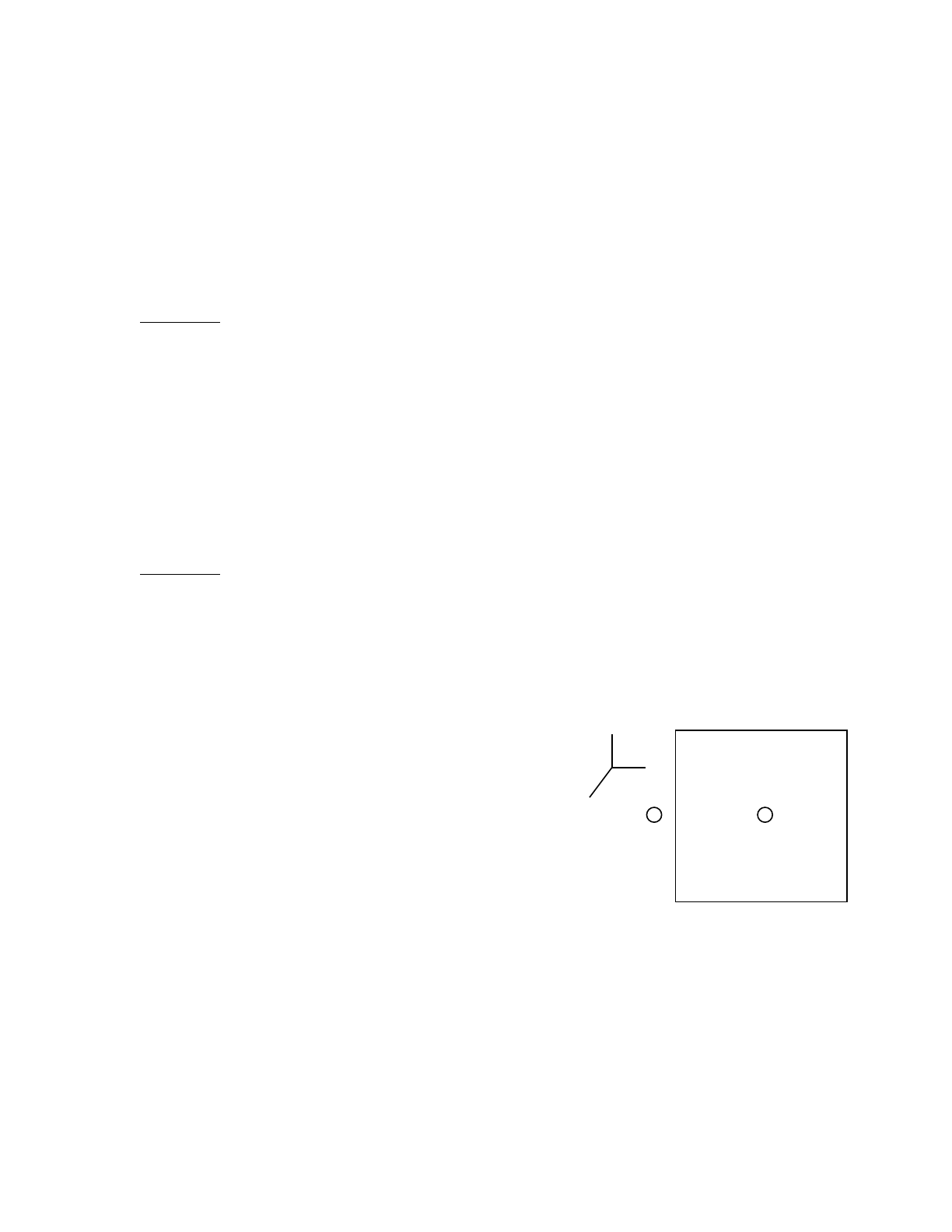
18 December 2000 4-43
CHAPTER 4
TALLY EXAMPLES
In this example we obtain the total tritium production per cm3 from natural lithium (ENDF/B-V
evaluation) in cell 1. The constant C on the FM4 card is the atomic density of natural lithium. A
subtle point is that the R = 105 reaction number contains the reaction data for just the 6Li reaction
and R = 91 contains the reaction data for the 7Li reaction (p.524 Appendix G). However, this
examples uses both sets of reaction data in the FM4 card to calculate the tritium production in a
media composed of both 6Li and 7Li. Thus, four calculations are carried out (two for 6Li using
R = 91,105, and two for 7Li using R = 91,105). Note that two of these calculations (6Li with
R = 91, and 7Li with R = 105) will contribute nothing to the total tritium production.
Example 3: Suppose we have three reactions—R1,R2, and R3—and wish to add R2 and R3and
multiply the result by R1. The following would NOT be valid: FMn (C m R1 (R2:R3)).
The correct card is: FMn (C m (R1R2:R1R3)).
C. FSn Examples
The FSn card allows you to subdivide your tally into geometry segments, avoiding overspecifying
the problem geometry with unnecessary cells.
The entries on the FS card are the names and senses of surfaces that define how to segment any
surface or cell tally.
Example 1: Consider a 1-MeV point isotropic source at the center of a 2 cm cube of carbon. We
wish to calculate the flux through a 1-cm2window in the center of one face on the cube. The input
file calculating the flux across one entire face is shown in Figure 4.18.
EXAMPLE 1, SIMPLE CUBE
11−2.22 1 2 −3 −4 −5 6 IMP:N=1
2 0 #1 IMP:N=0
1 PY 0
2PZ−1
3 PY 2
4 PZ 1
5PX1
6 PX –1
SDEF POS = 0 1 0 ERG = 1
M1 6012.60 –1
F2:N 3
The FS card retains the simple cube geometry and four more surface cards are required,
z
y
x121 3
2
6B
4
5F
Figure 4-18.
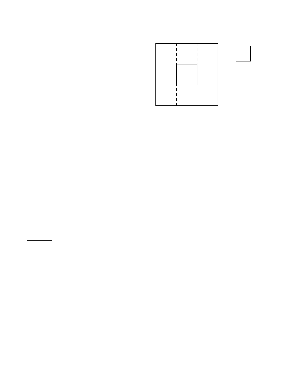
4-44 18 December 2000
CHAPTER 4
TALLY EXAMPLES
7PX.5
8PX−.5
9PZ.5
10 PZ −.5
FS2 7 −10 −8 9
The four segmenting surface cards are
listed with the other surface cards, but they
are not part of the actual geometry and
hence do not complicate the cell-surface
relationships.
The F2 tally is subdivided into five separate
tallies as shown in Figure 4.19: (1) the first is the flux of particles crossing surface 3 but with a
positive sense to surface 7; (2) the second is the remaining flux with negative sense to surface 7
crossing surface 3 but with a negative sense to surface 10; (3) the third is the remaining flux
(negative sense to 7 and positive sense to 10) crossing 3 but with a negative sense to 8; (4) the
remaining flux with positive sense to 9; and (5) everything else. In this example, the desired flux in
the window is in the fifth subtally—the “everything else” portion.
The FS segmenting card could have been set up other ways. For example:
FS2 −10 79 −8 and
FS2 −8 9−10 7
Each works, but the order of the subtallies is changed. A way to avoid the five subtallies and to get
only the window of interest is to use the TALLYX subroutine described later.
Example 2: Consider a source at the center of a 10-cm radius sphere called cell 1. We want to
determine the fission heating in a segment of the sphere defined by the intersection of the 10-cm
sphere, an 8-cm inner sphere, and a 20°cone whose vertex is at the source and is about the Y-axis.
This is accomplished by using
F7:N 1
FS7 −2 −3
where surface 2 is the 8-cm surface and surface 3 is the cone. This breaks the F7 tally up into three
portions: (1) the heating inside the 8-cm sphere; (2) the heating outside the 8-cm sphere but within
the cone—this is the desired portion; and (3) everything else, which is a 2-cm shell just inside the
10-cm sphere but outside the cone.
x
z
2
4
5678
9
10
I
II
III
IV
V
Figure 4-19.

18 December 2000 4-45
CHAPTER 4
TALLY EXAMPLES
D. FTn Examples
Example 1: Consider the following input cards.
F1:N 2
FT1 FRV V1V2V3
The FTn card is the special treatment for tallies card. Various tally treatments are available for
certain specific tally requirements. The FTn tally with the FRV card used in conjunction with tally
type 1 will redefine the vector normal to the tally surface. In this case, the current over surface 2
(tally type 1) uses the vector V as its reference vector for getting the cosine for binning.
Example 2:
F5:P 4
FT5 ICD
FU5 1 3
In this example the photon flux at detector 5 is being tallied. However, only the contributions to the
detector tally from cells 1 and 3 are of interest. The ICD keyword allows the user to create a
separate bin for each cell, and only contributions from one of the specified cells are scored. The
FUn card specifies the cells from which tallies are to be made, but TALLYX is not called.
Example 3: When keeping track of charged particle current across a surface, it is sometimes
desirable to track both positive and negative score contributions, applicable in cases that include
electrons and positrons. Consider a photon source that is enclosed in a spherical shell of lead. If a
surface current tally is taken over the sphere and it is desirable to tally both the positron and
electron current separately, then the special treatment card option is invoked.
11−.001124 −11 imp:e=1 imp:p=1
22−11.0 11 −21 imp:e=1 imp:p=1
3 0 21 imp:e=0 imp:p=0
11 so 30
21 so 32
m1 6012 .000125 7014 .6869 8016 .301248 18040 .011717
m2 82000 1.
mode p e
sdef pos = 0. 0. 0. erg = 2.5
f1:e 21
ft1 elc 2
f2:p 21

4-46 18 December 2000
CHAPTER 4
TALLY EXAMPLES
e2 1e-3 1e-2 0.1 0.5 1.0 1.5 2.0 2.5 C
nps 10000
The input deck shown above models a sphere filled with dry air surrounded by a spherical shell of
lead. The centrally located source emits 2.5 MeV photons that travel through the air into the lead
shell. The F1 surface current tally has been modified with the ELC special tally option. The
parameter value of 2 that follows the ELC keyword specifies that positrons and electrons be placed
into separate tally user bins. Once this option has been invoked, the user can inspect the output tally
bins for the respective scoring of either particle.
The F2 tally scores photon flux crossing surface 21, scored into energy bins defined on the E2 card.
The C at the end of the energy bin card indicates that the bins are cumulative. Therefore the bin
with an upper limit of 1 MeV would contain scores from particles that cross surface 21 with energy
less than or equal to 1 MeV.
Example 4: Consider the following two point sources, each with a different energy distribution:
sdef pos=d1 erg=fpos d2
si1 L 536 7536
sp1 .3 .7
ds2 S 3 4
si3 H21014
sp3 D 0 1 2
si4 H.528
sp4 D0 31
f2:n 2
ft2 scd
fu2 3 4
The SCD option causes tallies to be binned according to which source distribution was sampled.
The FUn card is used to list the distribution numbers of interest. Thus, the tallies in this example
are placed in one of two bins, depending on which of the two sources emitted the particle. The two
sources may represent two nuclides with different energy distributions, for instance, with the use
of the SCD option allowing the user to determine each nuclide’s contribution to the final tally.
E. Repeated Structure/Lattice Tally Example
An explanation of the basic repeated structure/lattice tally format can be found on page 3–69 in
Chapter 3. The example shown here illustrates more complex uses. Figures 4.20(a–f) indicate the
tally regions for each tally line. The number of bins generated by MCNP is shown at the end of
each tally line following the $.

18 December 2000 4-47
CHAPTER 4
TALLY EXAMPLES
example 1 – repeated structure lattice tally example
1 0 –1 –2 3 13 fill=4
2 0 –1 –2 3 –13 fill=1
3 0 –4 5 –6 7 u=1 lat=1
fill=–2:2 –2:0 0:0 1 1 3 1 1 1 3 2 3 1 3 2 3 2 3
4 0 –8 9 –10 11 u=2 fill=3 lat=1
5 1 –0.1 –12 u=3
6 0 12 u=3
7 0 –14 –2 3 u=4 fill=3 trcl=(-60 40 0)
8 like 7 but trcl=(-30 40 0)
9 like 7 but trcl=(0 40 0)
10 like 7 but trcl=(30 40 0)
11 like 7 but trcl=(60 40 0)
12 0 #7 #8 #9 #10 #11 u=4
13 0 1:2:-3
1 cz 100
2 pz 100
3 pz -100
4 px 20
5 px -20
6 py 20
7 py -20
8 px 10
9 px -10
10 py 10
11 py -10
12 cz 5
13 py 19.9
14 cz 10
f4:n 5 6 (5 6 3) $ 3 bins
(5<3) (5<(3[–2:2 –2:0 0:0])) $ 2 bins
(5<(7 8 9 10 11)) (5<7 8 9 10 11<1) (5<1) $ 7 bins
((5 6)<3[0 –1 0]) ((5 6)<3[0:0 –1:-1 0:0]) ((5 6)<3[8]) $ 3 bins
(5<(4[0 0 0]3[8]))(5<4[0 0 0]<3[8])
(3<(3[1]3[2]3[4]3[5]3[6]3[10])) $ 3 bins
5<u=3) $ 12 bins
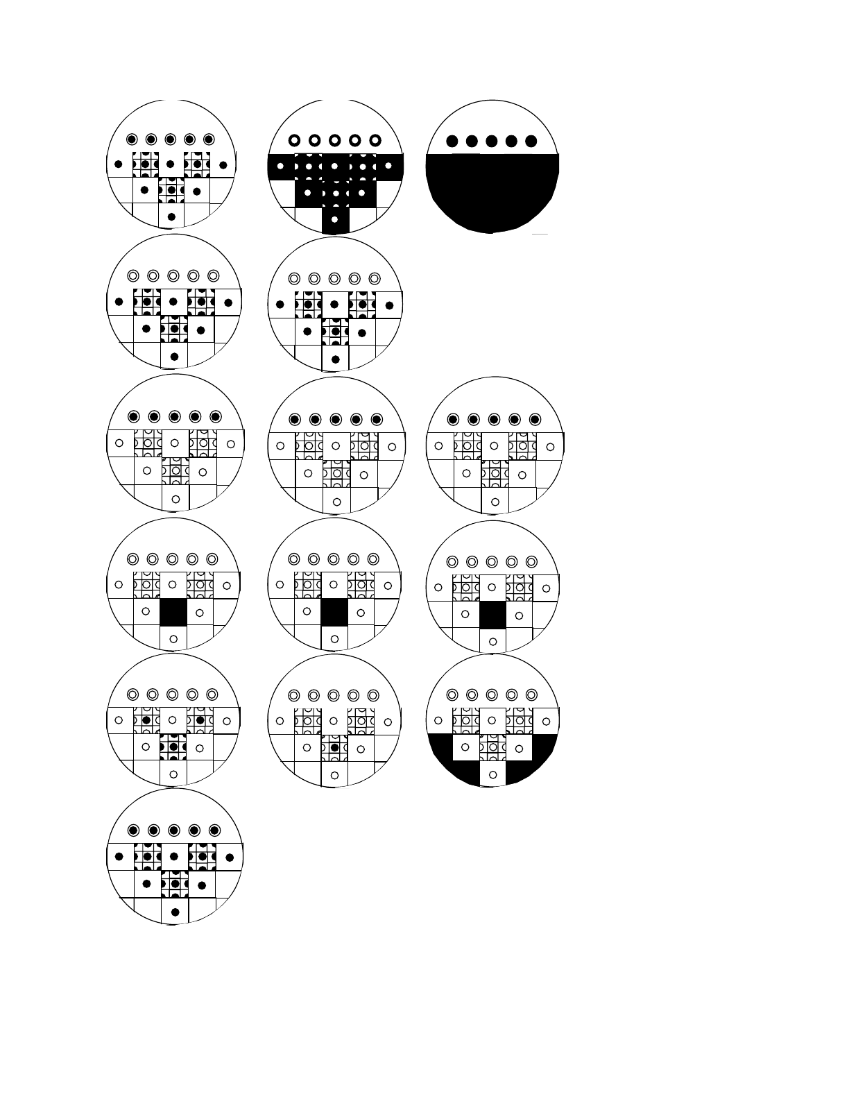
4-48 18 December 2000
CHAPTER 4
TALLY EXAMPLES
Figure 4-20.
Fig 4.20a
Fig 4.20b
Fig 4.20c
Fig 4.20d
Fig 4.20e
Fig 4.20f

18 December 2000 4-49
CHAPTER 4
TALLY EXAMPLES
Tally line 1: This first line creates three tally output bins: cell 5, cell 6, and the union of cells 5, 6,
and 3, indicated in Figure 4.20a. Notice that cell 3 is filled entirely by cells 5 and 6. Cell 5 plus cell
6 equals cell 3. If a particle is tallied in cell 5 and tallied in cell 3, it will be tallied twice in the bin
(5 6 3). CAUTION: A true union IS performed when first level cells overlap (or fill) another cell.
This probably is NOT a tally you often want. If an average of cell 3 and region (5 6) outside cell 3
is desired, separate bins must be defined and properly combined using correct volume weighting.
Tally line 2: These two input tally bins result in identical output tallies and demonstrate the use of
lattice index brackets that include all existing lattice elements, thereby making the two tallies
equivalent. The simpler format will execute faster. Tally region shown in Fig. 4.20b.
Tally line 3: This line illustrates omission of geometry levels and a single output bin vs. multiple
bins. All three input bins tally cell 5 within cells 7 through 11. The second bin specifies the entire
path explicitly. Because the only place cell 5 exists within cell 1 is in cells 7–11, the 7–11
specification can be omitted, as in the third input bin. In the second input bin, the parentheses
around cells 7–11 are omitted, creating multiple output bins. Five tally bins are produced: (5<7<1),
(5<8<1), (5<9<1), (5<10<1), and (5<11<1). The sum of these five bins should equal the tally in the
first and last output bins on this line. Tally region shown in Fig. 4.20c.
Tally line 4: This line illustrates the union of multiple tally cells, (5 6), and various ways of
specifying lattice index data. The three input tally bins create three output tally bins with identical
values because the three different lattice descriptions refer to the same lattice element, the eighth
entry on the FILL array. If the parentheses around (5 6) were removed, two output bins would be
created for each input bin, namely (5<3[0 –1 0]) and (6<3[0 –1 0]), etc. Tally region shown in Fig.
4.20d.
Tally line 5: This line illustrates tallys in overlapping regions in repeated structures in a lattice and
a tally in lattice elements filled with themselves. Three tally output bins are produced. In the first
input bin, a particle is tallied only once when it is in cell 5 and in 4[0 0 0] and in 3[0 –1 0]. Figure
4.20f shows all the cell 5’s included in this tally bin. This tally is probably more useful than the
overlapping regions in tally line 1. Input bin two demonstrates a tally for a nested lattice. A tally is
made when a particle is in cell 5 and in cell 4, element [0 0 0] and in cell 3, element [0 –1 0]. Note
that 3[0 –1 0] is indeed filled with cell 4 (u=2). If that were not true, a zero tally would result in
this bin. The final input tally bin demonstrated a tally in lattice elements that are filled with their
own universe number. This method is the only way to tally in these elements separate from the rest
of cell 3. Tally region shown in Fig. 4.20e.
Tally line 6: This line illustrates the universe format. The single input bin includes all possible
chains involving cell 5. Because u=3 is not within parentheses, the input is expanded into twelve
output bins: (5<3[3], etc. The format 3[3] indicates the third lattice element of cell 3 as entered on
the cell 3 FILL array. Note that the third element is filled by universe 3, consisting of cells 5 and 6.
Tally region shown in Fig. 4.20f.

4-50 18 December 2000
CHAPTER 4
TALLY EXAMPLES
F. TALLYX Subroutine Examples
An explanation of the TALLYX subroutine arguments can be found on page 3–87 in Chapter 3.
Only examples illustrating some uses of TALLYX will be found here.
Example 1: In the example of the FSn card to get the flux through a window on the face of a cube,
instead of using the FS2 card, which established five sub tallies, TALLYX could have been used to
get only the desired window tally. Two input cards are used:
FU2 1
RDUM −.5 .5 −.5 .5
The following subroutine (which is implemented just like a user-provided SOURCE subroutine by
replacing lines TX.2 through TX.18) does the job. Note that IB=0 and IBU=1 upon entry into
TALLYX.
SUBROUTINE TALLYX(T,IB)
∗CALL CM
IF(X.LT.RDUM(1).OR.X.GT.RDUM(2))IB = –1
IF(Z.LT.RDUM(3).OR.Z.GT.RDUM(4))IB = –1
RETURN
END
The subroutine was generalized a bit by using the RDUM input card, although the card could have
been avoided by hard wiring the dimensions of the window into TALLYX.
Example 2: Dump 18 words of the GPBLCM array to a BCD file called UOUT each time a
neutron crosses surface 15. The input cards are
F2:N 15
FU2 1
FILES 7 UOUT
The user-provided subroutine is
SUBROUTINE TALLYX(T,IB)
∗CALL CM
WRITE(7,20) (GPBLCM(I),I=1,10),NPA,ICL,JSU,IPT,IEX,NODE,IDX,NCP
20 FORMAT(5E14.6/5E14.6/7I10/2I10)
RETURN
END

18 December 2000 4-51
CHAPTER 4
TALLY EXAMPLES
Every time surface 15 is crossed and the F2 tally is scored, TALLYX is called and part of the
GPBLCM array is written to the file UOUT. If more discrimination is desired, such as dump the
GPBLCM array only for neutrons with energy between 2.5 and 4.5 MeV and crossing surface 15
at less than 30° with respect to the normal (assume surface 15 has been defined by a PY card), add
the following two lines before the WRITE statement:
IF(VVV.LT.0.866)RETURN
IF(ERG.LT.2.5.OR.ERG.GT.4.5)RETURN
To write a binary file, the FILES card entries are 7 UOUT S U and the WRITE statement in
TALLYX is unformatted:
SUBROUTINE TALLYX(T,IB)
∗CALL CM
WRITE(7) (GPBLCM(I),I=1,10),NPA,ICL,JSU,IPT,IEX,NODE,IDX,NCP
RETURN
END
The advantage of a BCD file is that it is easy to look at and manipulate, but it requires more I/O
time and a larger file. A binary file is more compact than a BCD file and requires less I/O time to
write; however, it may be more difficult to use.
Example 3: Calculate the number of neutron tracks exiting cell 20 per source neutron. This is also
done in Chapter 5 with the TEST1 example using the FMn card. The input cards are
F4:N 20
FU4 1
SD4 1
and TALLYX becomes
SUBROUTINE TALLYX(T,IB)
∗CALL CM
T=1.0
IF(PMF.LT.DLS) IB = –1
RETURN
END
The quantity T=1.0 is scored every time a track exits cell 20. The variables used in this subroutine,
PMF (the distance to collision) and DLS (distance to the boundary), are available to TALLYX from
the MCNP COMMON.

4-52 18 December 2000
CHAPTER 4
TALLY EXAMPLES
Example 4: Divide the point detector scores into separate tallies (that is, user bins) depending upon
which of the 20 cells in a problem geometry caused the contributions. The input cards are
F5:N 0 0 0 0
FU5 1 18I 20
and TALLYX is
SUBROUTINE TALLYX(T,IB)
∗CALL CM
IBU=ICL9
RETURN
END
The FU5 card establishes 20 separate user bins, one for each cell in the problem. Note the use of
the “nI” input format, described in Chapter 3, which creates 18 linear interpolates between 1 and
20. The variable ICL9 contains, for the current history, the number of the cell which produced the
original particle.
Example 5: Determine the quantity ∫ϕ(E)f(E)dE in cell 14 where f(E)=eαt. The input cards are
F4:N 14
FU4 α
where α is a numerical value and TALLYX is
SUBROUTINE TALLYX(T,IB)
∗CALL CM
T=T*EXP(TDS(IPTAL(LIPT+3,1,ITAL)+1)*TME)
RETURN
END
The FU4 card establishes a single user bin, and the value of αis stored in
TDS(IPTAL(LIPT+3,1,ITAL)+1) and used for the tally label.
Example 6: Tally the number of neutrons passing through cell 16 which have had 0, 1, 2, 3, or 4
collisions. The input cards are
F4:N 16
FU4 0 1 2 3 4
SD4 1
and TALLYX is

18 December 2000 4-53
CHAPTER 4
SOURCE EXAMPLES
SUBROUTINE TALLYX(T,IB)
∗CALL CM
IBU=INT(SPARE1)+1
IF(IBU.GT.5)IB = –1
T=WGT
RETURN
END
The subroutine can be generalized by replacing the 5 in the IF statement with
IPTAL(LIPT+3,3,ITAL), which is the number of entries on the FU4 card.
If no tracks were put into the bank (from fission, geometry splitting, etc.,), INT(SPARE1) could
be replaced by NCH(1), the number of neutron collisions per history. However, to be general, use
the quantity SPARE1, which goes into the bank with the rest of the banked track parameters.
SPARE1 must be set to 0 when a source particle is started and then incremented at collisions. This
is done with the following patch in the STARTP and HSTORY subroutines:
∗I,SP.30
SPARE1=0.
∗I,HS.184
SPARE1=SPARE1+1.
If the IF statement in this TALLYX is omitted, a count will be made of the cases of five or more
collisions, and in these cases no score will be tallied but a count will be printed of the times that
the tally was unable to be made because IBU was a value where no bin existed.
In the five user bins, T is the number of neutrons per source neutron passing through cell 16 that
has undergone 0, 1, 2, 3, or 4 collisions, respectively. Note that the FU4 card has five entries to
establish the five user bins and provide labels. Note also that in this example, the neutrons are
calculated so that T=T∗ renormalization factor (which preserves the weight associated with the
tracks), where in Example 3 the neutron tracks are calculated so that T=1. Again the value of
SPARE1 is available from COMMON. Finally, note that if SPARE1 >5 (six or more collisions) no
tally is made because IB is set to be less than zero. If an E4 card were added, the neutrons would
be tallied as a function of energy for each user bin.
V. SOURCE EXAMPLES
Some examples of the general source are given here to illustrate the power and complexity of this
feature. Refer to Chapter 3 for the more complete explanation and other examples.
Example 1: SDEF ERG = D1 DIR FERG D2
SUR=1 CEL=2 POS=X Y Z RAD D5 VEC = U V W
SI1 H 10−7 10−5 …13.5 14 …20 $ Level 1
SP1 D 0 10−4 …10−2 10−1 ….3

4-54 18 December 2000
CHAPTER 4
SOURCE EXAMPLES
DS2 S 3 …34…4
SI3 0 .2 …1 $ Level 2
SP3 D 0 10−4….1
SI4 0 .1 … 1
SP4 D 0 10−2 … .1
SI5 37
SP5 −21 1 $ Optional card
This example of the general source illustrates two levels of dependency. Let us assume a duct
streaming problem where the source at the duct opening has been obtained from a reactor
calculation. Energies above 13.5 MeV have one angular distribution and energies below 13.5 MeV
have a different angular distribution. The source has a uniform spatial distribution on a circular disk
of radius 37 cm centered at x,y,z on planar surface 1 going into cell 2.
This example can be expanded by having the source in two ducts instead of one (with the same
energy and angular distribution as before). The SI1, SP1, DS2, SI3, SP3, SI4, and SP4 cards remain
unchanged. The SDEF card is changed as shown below and the other cards are added.
SDEF ERG = D1 DIR FERG D2 SUR = D6 CEL FSUR D7
POS FSUR D8 RAD FSUR D9 VEC FSUR D10
SI6 L 1 7
SP6 D .6 .4
DS7 L 2 8
DS8 L x1 y1 z1x2 y2 z2
DS9 S 11 12
DS10 L u1 v1 w1u2 v2 w2
SI11 0 37
SP11 −21 1
SI12 0 25
SP12 −21 1
Example 2: This example is a two-source-cell problem where the material in one cell is uranium
and in the other is thorium. The uranium cell has two isotopes, 235U and 238U, and the thorium has
one, 232Th. Each isotope has many photon lines from radioactive decay. The following input cards
describe this source.
SDEF CEL = D1 ERG FCEL D2 …
SC1 source cells $ Level 1
SI1 L 1 2
SP1 D 2 1
SC2 source “spectra”
DS2 S 3 4
SC3 uranium nuclides $ Level 2

18 December 2000 4-55
CHAPTER 4
SOURCE EXAMPLES
SI3 S 5 6
SP3 D 1 3
SC4 thorium nuclide
SI4 S 7
SP4 D 1
SC5 U235 photon lines $ Level 3
SI5 L E1…EI
SP5 D I1…II
SC6 U238 photon lines
SI6 L E1…EJ
SP6 D I1…IJ
SC7 Th232 photon lines
SI7 L E1…EK
SP7 D I1…IK
Example 3: SDEF SUR = D1 CEL FSUR D2 ERG FSUR D6
X FSUR D3 Y FSUR D4 Z FSUR D5
SI1 L 10 0
SP1 .8 .2
DS2 L 0 88
DS6 S 61 62
SP61 −3 .98 2.2
SP62 −3 1.05 2.7
DS3 S 0 31
SI31 20 30
SP31 0 1
DS4 S 0 41
SI41 −17 36
SP41 0 1
DS5 S 0 51
SI51 −10 10
SP51 0 1
Of the particles from this source, 80% start on surface 10, and the rest start in cell 88. When a
particle starts in cell 88, its position is sampled, with rejection, in the rectangular polyhedron
bounded by x=20to 30, y= −17 to 36, and z= −10 to 10. When a particle starts on surface 10, its
cell is found from its position and direction. The energy spectrum of the particles from surface 10
is different from the energy spectrum of the particles from cell 88. A zero after the S option invokes
the default variable value.
Example 4: SDEF ERG=D1 DIR FERG D2 SUR=m
SI1 E1E2…Ek
SP1 0 P2…Pk

4-56 18 December 2000
CHAPTER 4
SOURCE SUBROUTINE
DS2 Q .3 21 .8 22 1.7 23 20. 24
SP21 −21 1
SP22 −21 1.1
SP23 −21 1.3
SP24 −21 1.8
This is an example of using the Q option. The low-energy particles from surface mcome out with
a cosine distribution of direction, but the higher-energy particles have a more nearly radial
distribution. The energy values on the DS2 card need not be the same as any of the Ei on the SI1
card.
VI. SOURCE SUBROUTINE
When possible, you should take advantage of the standard sources provided by the code rather than
write a source subroutine. When you write your own source subroutine, you lose features such as
sampling from multiple distributions, using dependent distributions, and having frequency prints
for each tabular distribution. Also, subroutine SRCDX is needed.
The standard sources, however, cannot handle all problems. If the general source (SDEF card),
surface source (SSR), or criticality source (KCODE card) is unsuitable for a particular application,
MCNP provides a mechanism to furnish your own source-modeling capability. The absence of
SDEF, SSR, or KCODE cards causes MCNP to call subroutine SOURCE, which you must supply.
Subroutine SOURCE specifies the coordinates, direction, weight, energy, and time of source
particles as listed and defined on page 3–40. If the value of IPT (particle type) set by STARTP,
which calls SOURCE, is not satisfactory, SOURCE must also specify IPT. STARTP sets IPT=1
(neutron) for MODE N, N P, and N P E; sets IPT=2 (photon) for MODE P and P E; and sets IPT=3
(electron) for MODE E. MCNP checks the user’s source for consistency of cell, surface, direction,
and position. If the source direction is anisotropic and there are point detectors or DXTRAN
spheres, an SRCDX subroutine is also required (see page 4–52). The SOURCE subroutine can be
put into MCNP with PRPR.
The following example of a subroutine SOURCE uses SIn, SPn, and SBn cards and demonstrates
the use of MCNP subroutines SMPSRC, ROTAS, CHKCEL, and the function NAMCHG. The
geometry is a 5-cm-long cylinder centered about the y-axis, divided into 5 cells by PY planes at 1-
cm intervals. The 1-MeV monoenergetic source is a biased isotropic distribution that is also biased
along the y-axis. The input distribution cards are
SI1 –1 0 1 $ These 3 cards
SP1 0 1 1 $ represent a biased
SB1 0 1 2 $ isotropic distribution.
SI2 012345$ These 3 cards
SP2 042211$ represent a biased

18 December 2000 4-57
CHAPTER 4
SOURCE SUBROUTINE
SB2 011224$ distribution in y.
RDUM 1 $ cylindrical radius
IDUM 246810 $ source cells
This problem can be run with the general source by removing the RDUM and IDUM cards and
adding:
SDEF ERG=1 VEC=0 1 0 AXS=0 1 0 DIR=D1 EXT=D2 RAD=D3
SI3 0 1 $ represents a covering surface of radius 1
SP3 −21 1 $ samples from the power law with k=1
∗IDENT SRCEX
∗D,SO.11
DIMENSION A(3)
WGT=1.
C RDUM(1)--RADIUS OF SOURCE CYLINDER.
C SAMPLE RADIUS UNIFORM IN AREA.
R=RDUM(1)*SQRT(RANG())
C Y COORDINATE POSITION, PROBABILITY AND BIAS ARE
C DEFINED IN DISTRIBUTION 2 BY THE SI2, SP2, SB2 CARDS.
C SAMPLE FOR Y.
C IB RETURNS THE INDEX SAMPLED AND FI THE INTERPOLATED FRACTION.
C NEITHER ARE USED IN THIS EXAMPLE.
CALL SMPSRC(YYY,2,IX]B,FI)
C SAMPLE FOR X AND Z.
TH=2.*PIE*RANG()
XXX=-R*SIN(TH)
ZZZ=R*COS(TH)
C DIRECTION IS ISOTROPIC BUT BIASED IN CONE ALONG Y-AXIS
C DEFINED AS DISTRIBUTION 1 BY THE SI1, SP1, SB1 CARDS.
C SAMPLE FOR CONE OPENING C=COS(NU).
C ROTAS SAMPLES A DIRECTION U,V,W at AN ANGLE ARCCOS(C)
C FROM THE REFERENCE VECTOR UOLD(3)
C AND AT AN AZIMUTHAL ANGLE SAMPLED UNIFORMLY.
CALL SMPSRC(C,1,IB,FI)
UOLD(1)=0.
UOLD(2)=1.
UOLD(3)=0.
CALL ROTAS(C,UOLD,A,LEV,IRT)
UUU=A(1)
VVV=A(2)
WWW=A(3)
C CELL SOURCE - FIND STARTING CELL.

4-58 18 December 2000
CHAPTER 4
SRCDX SUBROUTINE
C IDUM(1)-IDUM(5)--LIST OF SOURCE CELLS (PROGRAM NAME).
JSU=0
DO 10 I=1,5
ICL=NAMCHG(1,IDUM(I))
CALL CHKCEL(ICL,2,J)
IF(J.EQ.0) GO TO 20
10 CONTINUE
CALL EXPIRE(1,’SOURCE’,
1 ’SOURCE IS NOT IN ANY CELLS ON THE IDUM CARD.’)
20 ERG=1.
TME=0.
VII. SRCDX SUBROUTINE
If a user has supplied a subroutine SOURCE that does not emit particles isotropically (uniform
emission in all directions) and is using either a detector tally or DXTRAN in the calculations, then
subroutine SRCDX must also be supplied to MCNP. The structure of this subroutine is the same as
for subroutine SOURCE, except that usually only a single parameter, PSC, needs to be specified
for each detector or set of DXTRAN spheres. PSC as defined in SRCDX is used to calculate the
direct contribution from the source to a point detector, to the point selected for the ring detector, or
DXTRAN sphere. Other parameters may also be specified in SRCDX. For example, if a quantity
such as particle energy and/or weight is directionally dependent, its value must be specified in both
subroutine SOURCE and SRCDX. When using detectors and a subroutine SOURCE with an
anisotropic distribution, check the direct source contribution to the detectors carefully to see if it is
close to the expected result.
In general, it is best to have as few directionally-dependent parameters as possible in subroutine
SOURCE. Directionally dependent parameters must also be dealt with in subroutine SRCDX.
The most general function for emitting a particle from the source in the laboratory system can be
expressed as p(µ,ϕ), where µ is the cosine of the polar angle and ϕ is the azimuthal angle in the
coordinate system of the problem. Most anisotropic sources are azimuthally symmetric and p(µ,ϕ)
=p(µ)/2π. The quantity p(µ) is the probability density function for the µvariable only (that is, ∫
p(µ) dµ = 1,p(µ)≥0). PSC is p(µo), where µois the cosine of the angle between the direction
defining the polar angle for the source and the direction to a detector or DXTRAN sphere point in
the laboratory system. (MCNP includes the 2π in the calculation automatically.) Note that p(µo)
and hence PSC may have a value greater than unity and must be non-negative. It is valuable to point
out that every source must have a cumulative distribution function based on p(µ,ϕ) from which to
sample angular dependence. The probability density function p(µ,ϕ) needs only to be considered
explicitly for those problems with detectors or DXTRAN.

18 December 2000 4-59
CHAPTER 4
SRCDX SUBROUTINE
Table 4.1 gives the equations for PSC for six continuous source probability density functions. More
discussion of probability density functions is given in the detector theory section of Chapter 2 (see
page 2–75). The isotropic case is assumed in MCNP; therefore SRCDX is required only for the
anisotropic case.
As an example of calculating µo, consider a spherical surface cosine source (type 2 in Table 4.1)
with several point detectors in the problem. Assume that a point on the spherical surface has been
selected at which to start a particle. The value of µofor a detector is given by the scalar (or dot)
product of the two directions; that is,
TABLE 4.1:
Continuous Source Distributions and their Associated PSC’s
Source
Description Source
Distribution PSC Range of µo
1.
2. Isotropic
Surface Cosine Uniform
µ0.5
2|µo|−1≤µ
o≤1
0≤µ
o≤ 1
(or −1 ≤ µo≤0)
0 −1≤µ
o< 0
(or 0 < µ ≤ 1)
3.
4. Point Cosine
Point Cosine*
*The quantities aand bmust have values such that PSC is always nonnegative and finite over the range
of µo.
|µ|
a+bµ|µo| −1≤µ
o≤1
0 ≤ µo≤ 1
(−1 ≤ µo≤ 0)
0 −1 ≤ µo< 0
(or 0 < µo≤ 1)
5. Point Cosine* a+bµ,a≠ 0 −1≤µ
o≤ 1
6. Point Cosine* a + b|µ| −1 ≤ µo≤ 1
2abµo
+()
2ab+
--------------------------
2abµo
+()
2ab–
--------------------------
abµo
+
2a
------------------
abµo
+
2ab+
---------------------

4-60 18 December 2000
CHAPTER 4
SRCDX SUBROUTINE
(4.1)
where u,v, and w are the direction cosines of the line from the source point to the point detector
location and u’,v’, and w’are the direction cosines for either the outward normal if the surface
source is outward or the inward normal if the source is inward.
If u=u’,v=v’, and w=w’, then µo=1, indicating that the point detector lies on the normal line.
The value of PSC for the detector point is
where the parenthetical values of µo are for the inward-directed cosine distribution.
For |µo|less than 0.25 in case 2 of Table 4.1, PSC is less than 0.5, which is the value for an isotropic
source. This means that source emissions for these values of |µo|are less probable than the isotropic
case for this source distribution. The converse is also true. Note that if |µo|is greater than 0.5, PSC
is greater than one, which is perfectly valid.
An example of a subroutine SRCDX with appropriate PRPR lines for a surface outward cosine
distribution is shown in Figure 4.21. This is basically the technique that is used in MCNP to
calculate PSC for a spherical surface source in a cosine distribution; the only difference is that
MCNP uses the cosines of the direction from the center of the sphere used to select the source point
because this is the normal to the spherical surface. The primed direction cosines were calculated in
Figure 4.21 to aid in illustrating this example. The direction cosines u,v, and was defined in
Equation (4.1) have already been calculated in subroutine DDDET when SRCDX is called and are
available through COMMON.
∗I,SX.5
C CALCULATE PSC FOR A SURFACE (SPHERE) OUTWARD COSINE DIST
C FIND THE DIRECTION COSINES FOR THIS EXAMPLE BASED
C ON THE SOURCE POINT ON THE SPHERE (X,Y,Z).
UP = (XXX - RDUM(1))/RDUM(4)
VP = (YYY - RDUM(2))/RDUM(4)
WP = (ZZZ - RDUM(3))/RDUM(4)
C (RDUM(1),RDUM(2),RDUM(3)) ARE THE COORDINATES OF THE CENTER
C OF THE SPHERE FROM THE RDUM CARD. RDUM(4) IS THE RADIUS.
C U, V, AND W HAVE BEEN CALCULATED FOR THE CURRENT
C POINT DETECTOR IN SUBROUTINE DDDET
PSC=2.*MAX(ZERO,UUU*UP+VVV*VP+WWW*WP)
Figure 4-21.
µouu′vv′ww′,++=
PSC 2µo,µo0µo0<()>=
0, µo0µo0≥(),≤=

18 December 2000 4-61
CHAPTER 4
SRCDX SUBROUTINE
The PRPR cards in Figures 4.21 and 4.22 are the recommended procedure for replacing the
existing dummy SRCDX subroutine.
For many sources, a discrete probability density function will be used. In this situation, a
cumulative distribution function P(µ) is available and is defined as
where pjis an average value of the probability density function in the interval ∆µj. Thus, the
probability density function is a constant pjin the interval ∆µj. For this case, there are Nvalues of
Pi with Each value of Pihas an associated value of µi.
Because PSC is the derivative of P(µo), then
(4.2)
This is an average PSC between µi-1 and µi and is also an average value of p(µ) in the specified
range of µ.
Frequently, the cumulative distribution function is divided into Nequally probable intervals. For
this case,
This is precisely the form used in MCNP for calculating contributions to the point detector for
elastic scattering with N= 32.
An example of a subroutine SRCDX for a discrete probability density function is shown in
Figure 4.22. This subroutine would work with the subroutine SOURCE example on page 4–51, and
would calculate PSC = 1/2 for the isotropic distribution.
A biased anisotropic distribution can also be represented by
SIn µoµ1…µ
n
SPn 0 p1…pn
SBn 0 q1…qn
A reference vector u’,v’,w’ for this distribution is also needed.
Pµ() pµ′()µ′andP
i1+
d
1–
µ
∫pj∆µj,
j1i,=
∑
==
P10PN1+
,1.0 and Pi1– Pi.<==
PSC PiPi1–
–
µiµi1–
–
-----------------------µi1– µoµi.<≤,=
PSC 1
N
----1
µiµi1–
–
---------------------- .=

4-62 18 December 2000
CHAPTER 4
SRCDX SUBROUTINE
The subroutine SOURCE input cards can be modified for this case by changing the SI1, SP1, SB1,
and RDUM cards as follows:
SI1 −1 0 1 $ These 3 cards
SP1 0 2 1 $ represent a biased
SB1 0 1 2 $ anisotropic distribution.
RDUM 1 0 1 0 $ cylindrical radius and reference vector
SOURCE would sample this anisotropic distribution and SRCDX would calculate the appropriate
PSC.
∗I,SX.5
C THE VARIABLY DIMENSIONED BLOCK SPF HOLDS THE SI, SP, SB ARRAYS.
C THE KSD ARRAY IS A POINTER BLOCK TO THE SPF ARRAY.
C THE FOLLOWING STATEMENT FUNCTION IS DEFINED.
K(I,J)=KSD(LKSD+I,J)
C RDUM(2),RDUM(3),RDUM(4)--DIRECTION COSINES
C FOR THE SOURCE REFERENCE DIRECTION.
AM=UUU*RDUM(2)+VVV*RDUM(3)+WWW*RDUM(4)
C K(4,1) IS THE LENGTH OF THE DISTRIBUTION.
C K(13,1) IS THE OFFSET INTO THE SPF BLOCK.
DO 10 I=1,K(4,1)-1
10 IF(SPF(K(13,1)+1,I).LE.AM.AND.SPF(K(13,1)+1,I+1).GE.AM)
1 GO TO 20
GO TO 30
20 PSC=(SPF(K(13,1)+2,I+1)-SPF(K(13,1)+2,I))/
1 (SPF(K(13,1)+1,I+1)-SPF(K(13,1)+1,I))
PSC=PSC*SPF(K(13,1)+3,I+1)
RETURN
30 PSC=0.
Figure 4-22.
It is extremely important to note that the above case applies only when the source is anisotropic
with azimuthal symmetry. For the general case,
The 2π factor must be applied by the user because MCNP assumes azimuthal symmetry and, in
effect, divides the user-defined PSC by 2π.
For a continuous p(µ,ϕ) function, PSC is calculated as above. In the case of a discrete probability
density function,
PSC 2πpµoϕo
,().=

18 December 2000 4-63
CHAPTER 4
SRCDX SUBROUTINE
where is an average probability density function in
the specified values of µoand µoand Pi−Pi-1 is the probability of selecting µoand µoin these
intervals. For N equally probable bins and n equally spaced ∆ϕ’s, each 2π/n wide,
Another way to view this general case is by considering solid angles on the unit sphere. For an
isotropic source, the probability (Pi−Pi-1) of being emitted into a specified solid angle is the ratio
of the total solid angle (4π) to the specified solid angle (∆ϕ∆µ). Then, PSC ≡ 0.5. Thus, for the
general case (normed to PSC ≡ 0.5 for an isotropic source)
Note that PSC is greater than 0.5 if the specified solid angle ∆µ∆ϕiis less than (Pi−Pi-1)4π. This
is the same as the previous general expression.
CAUTIONS:
You are cautioned to be extremely careful when using your own subroutine SOURCE with either
detectors or DXTRAN. This caution applies to the calculation of the direct contribution from the
source to a point detector, point on a ring, or point on a DXTRAN sphere. Not only is there the
calculation of the correct value of PSC for an anisotropic source, but there may also be problems
with a biased source.
For example, if an isotropic source is biased to start only in a cone of a specified angle (for example,
ψ), the starting weight of each particle should be WGT∗(1−cos ψ)/2, where WGT is the weight of
the unbiased source (that is, WGT is the expected weight from a total source). The weight in
SRCDX must be changed to the expected weight WGT to calculate the direct contribution to a point
detector correctly if PSC is defined to be 0.5.
This example can be viewed in a different way. The probability density function for the above
biased source is
PSC 2πpµoϕo
,()⋅2πPiPi1–
–()
µiµi1–
–()ϕ
iϕi1–
–()
-------------------------------------------------------
2πPiPi1–
–()
∆µi∆ϕi
----------------------------------
==
=
µi1– µoµiϕ, i1– ϕoϕiand pµoϕo
,()<≤<≤
PSC n
N
----1
∆µi
-------- .=
PSC 0.5()PiPi1–
–()4π
∆µ∆ϕi
----------------------------------------------- 2πPiPi1–
–()
∆µi∆ϕi
---------------------------------- .==

4-64 18 December 2000
CHAPTER 4
SRCDX SUBROUTINE
Thus, PSC is this constant everywhere in the cone and zero elsewhere. Multiplying this PSC and
biased starting weight gives
WGT ∗ (1 − cos ψ) ∗ 0.5/(1 − cos ψ)
or WGT ∗ 0.5, which is the expected result for an isotropic source.
Another source type that requires caution is for a user supplied source that is energy-angle
correlated. For example, assume a source has a Gaussian distribution in energy where the mean of
the Gaussian is correlated in some manner with µ. In subroutine SRCDX, the µoto a point detector
must be calculated and the energy of the starting particle must be sampled from the Gaussian based
on this µo. This must be done for each point detector in the problem, thus guaranteeing that the
direct source contribution to each detector will be from the proper energy spectrum. The original
energy of the starting particle, as well as all of the other starting parameters, selected in subroutine
SOURCE are automatically restored after the direct source contribution to detectors is made. Thus,
the subroutine SOURCE is still sampled correctly.
pµ() 1
1Ψcos–
---------------------- , for Ψµ1≤≤cos=
0 for 1 µΨ.cos<≤–=

18 December 2000 5-1
CHAPTER 5
DEMO PROBLEM AND OUTPUT
CHAPTER 5
OUTPUT
WHAT IS COVERED IN CHAPTER 5
This chapter shows annotated output from four test problems and an event log print:
DEMO illustrates tally flexibility
TEST1 annotated tables produced by PRINT card
CONC output associated with detectors and detector diagnostics
KCODE output from a criticality calculation (GODIVA)
Event log event log and debug prints
Portions of the complete output have been excluded. The line “SKIP nnn LINES IN OUTPUT”
indicates these omissions.
The event log and debug prints help find errors if you set up a geometry improperly or modify
the code. The DBCN input card also is useful when finding errors but is not discussed here.
MCNP prints out warning messages if needed. Do not ignore these warning messages. Look up
the pertinent section in the manual if you need explanation to help you understand what you are
being warned about.
I. DEMO PROBLEM AND OUTPUT
DEMO has a point isotropic neutron source (SDEF) in the center of a tungsten cube (M2), with
energy uniformly distributed from 0.1 to 10 MeV (SI1,SP1). Flux is calculated across each facet
of the cube (F2), across the sum of all facets (F22), and across the sum of some of the facets
(F12). A pulse height tally (F8) is made in the tungsten cell. Selected pages of the output file
follow.
The FQ card in the DEMO input file changes the printing order. Depending upon what you are
interested, the tally output can be made more readable. FQ2 causes energy to be printed as a
function of surface. FQ22 causes surface to be printed as a function of energy. FQ62 prints
multiplier bins as a function of energy for the two surfaces desired. The NT and T features also
are illustrated in tallies 62 and 22, respectively. The generalized FM62 card used with the F62:N
tally is a useful feature for normalization, unit conversion, reaction rate, etc., and has three
multipliers instead of one. Finally, the TF62 card causes the tally fluctuation chart for the second
surface, the first multiplier bin, and the second energy bin to be printed. By default the
fluctuation chart for tally 62 would contain information for the first surface, the first multiplier
bin, and the last energy bin.

5-2 18 December 2000
CHAPTER 5
DEMO PROBLEM AND OUTPUT
The F8:E card provides a pulse height tally in cell 1. The F8 tally capability is limited to an
analog problem. The default implicit capture is turned off by the CUT:N card. Analog capture is
the default for photons and electrons, so CUT:P and CUT:E cards are not required. The pulse
height tally tracks the energy deposited in a cell by both photons and electrons, even if only E or
P is on the F8 card. The F8 tally is not available for neutrons and will return an error if
attempted. In the following output is a warning that “f8 tally unreliable since neutron transport
nonanalog”. This message means some nonanalog events such as (n,2n) may have occured to the
neutron from the source to the production of a photon, not that there is an F8:N tally or that there
is some neutron variance reduction in the definition of the problem.
A tally fluctuation chart bin analysis follows each tally. Only an analysis for tally 8 is shown in
this example. This analysis checks the variance of the variance as well as the general behavior of
the probability density function of each tally and provides an additional set of checks to ensure
the reliability of a tally. Ten different statistical checks are run for the tally and presented in
tabular form. The results of the ten checks are presented in pass?yes/no table format. These
checks do not guarantee the absolute reliability of the tally, but they provide a better method of
identifying problems that have not been sampled well. A more complete description of the
significance of each entry in the tally fluctuation section is presented in TEST1.
There are three possible physics treatments for problems involving photons. The first is the
explicit p,e treatment where photons generate electrons that are the tracked and generate photons
(ad infinium). This is the most accurate model but is costly in terms of runtime. The second
physics treatment is mode p only that uses the default ‘thick target bremsstrahlung’ (TTB) model
where electrons are generated in the direction of the incident photon and are immediately
annihilated after generating bremsstrahlung photons. The third photon physics treatment is a
mode p only with the thick target bremsstrahlung turned off (IDES=1 on the PHYS card). Then
electrons are completely ignored.
The choice of which physics treatment to use depends on the objective of the problem being
solved. Using a test problem similar to the cube above it was found that F4 photon tallies for the
three treatments agreed reasonably well above 2 MeV. Below 1 MeV the results from the
simplest model (photon mode no bremstrahlung) began to diverge from the full physics model
results. Below the annihilation photon peak, the TTB treatment also begins to diverge from the
mode p,e results. The choice of physics treatment had a drastic impact on the runtime of the
problem. To run 1E6 particles on a SGI 2000 mode p with and without thick target
bremstrahlung took 2.25 and 1.70 minutes respectively, while the full physics mode p,e problem
took just over 17 hours. If it is necessary to model photon generation and transport below 0.5
MeV then the full physics model should be used. However if these low energy photons are not
important or if the calculation is for diagnostic purposes, then the mode p with or without thick
target bremstrahlung model is sufficient.

18 December 2000 5-3
CHAPTER 5
DEMO PROBLEM AND OUTPUT
The small table preceding the summary of statistical checks indicates that some of the tally
scores were not made for some reason. In the case of tally 2, 93547 particles did not score in any
of the bins because their energy was greater than that of the upper limit of the highest energy bin.
Tallies 12, 22, and 62 also had significant numbers of particles that had energies above the
highest energy bin. This is concerning since for tally 2 the number of particles not scored is
nearly 90% of the initial source particles. This can be fixed by simple increasing the upper limit
of the last energy bin, or adding more bins to cover the energy range up to the maximum energy
of the source (10 MeV).

CHAPTER 5
DEMO PROBLEM AND OUTPUT
5-4 18 December 2000
1mcnp version 4c ld=01/20/00 07/19/00 14:32:23
************************************************************************* probid = 07/19/00 14:32:23
i=demo name=demo.
1- demo: a box with flux across surfaces in various combinations
2- 1 2 -1.6 -1
3- 2 0 1
4-
5- 1 rpp -1 1 -1 1 -1 1
6-
7- cut:n 10000 0.0 0.0 0.0
8- mode n p e
9- sdef pos=0 0 0 cel=1 wgt=1 erg=d1
10- si1 0.1 10
11- sp1 0 1
12- imp:n,p,e 1 0
13- e0 0.2 0.4 0.6 0.8 1
14- f2:n 1.1 1.2 1.3 1.4 1.5 1.6
15- fq2 e f
16- f12:n (1.3 1.5) (1.4 1.6) (1.2 1.1)
17- f22:n 1.1 1.2 1.3 1.4 1.5 1.6 t
18- fq22 f e
19- m1 6000.50c 1
warning. material 1 is used only for a perturbation or tally.
20- m2 74000.55c 1
21- f62:n 1.3 1.4
22- fm62 (1 2(1 -4)(-2))(1 1 1)
23- e62 0.2 0.4 0.6 0.8 1 nt $
24- fq62 m e
25- tf62 2 5j 2
26- f8:e 1
warning. f8 tally unreliable since neutron transport nonanalog.
27- e8 0.001 10i 20 $
28- nps 104000
warning. tally 8 needs zero energy bin for negative f8 scores.
SKIP 482 LINES IN OUTPUT
1tally 22 nps = 104000
tally type 2 particle flux averaged over a surface. units 1/cm**2

18 December 2000 5-5
CHAPTER 5
DEMO PROBLEM AND OUTPUT
tally for neutrons
areas
surface: 1.1 1.2 1.3 1.4 1.5 1.6 total
4.00000E+00 4.00000E+00 4.00000E+00 4.00000E+00 4.00000E+00 4.00000E+00 2.40000E+01
energy: 2.0000E-01 4.0000E-01 6.0000E-01 8.0000E-01 1.0000E+00
surface
1.1 7.30357E-04 0.0942 1.29205E-03 0.0513 1.18025E-03 0.0653 1.17268E-03 0.0651 1.16323E-03 0.0534
1.2 6.57953E-04 0.0686 1.15327E-03 0.0508 1.05268E-03 0.0545 1.13600E-03 0.0519 1.18122E-03 0.0643
1.3 6.33307E-04 0.0756 1.27882E-03 0.0717 1.13639E-03 0.0528 1.17168E-03 0.0521 1.13825E-03 0.0524
1.4 6.52386E-04 0.0705 1.07859E-03 0.0576 1.21496E-03 0.0528 1.25657E-03 0.0495 1.05426E-03 0.0537
1.5 6.11844E-04 0.0711 1.21984E-03 0.0522 1.25661E-03 0.0487 1.26987E-03 0.0496 1.15210E-03 0.0516
1.6 6.60230E-04 0.0686 1.15995E-03 0.0522 1.19812E-03 0.0515 1.10335E-03 0.0526 1.07351E-03 0.0543
total 6.57680E-04 0.0312 1.19709E-03 0.0231 1.17317E-03 0.0221 1.18503E-03 0.0217 1.12710E-03 0.0224
energy: total
surface
1.1 5.53857E-03 0.0284
1.2 5.18112E-03 0.0258
1.3 5.35846E-03 0.0273
1.4 5.25677E-03 0.0248
1.5 5.51027E-03 0.0237
1.6 5.19516E-03 0.0244
total 5.34006E-03 0.0102
SKIP 227 LINES OF OUTPUT
1tally 8 nps = 104000
tally type 8 pulse height distribution. units number
tally for photons electrons
cell 1
energy
1.0000E-03 1.88365E-02 0.0224
1.8191E+00 1.50962E-02 0.0250
3.6372E+00 2.59615E-04 0.1924
5.4553E+00 7.69231E-05 0.3535
7.2734E+00 4.80769E-05 0.4472
9.0915E+00 1.92308E-05 0.7071
1.0910E+01 0.00000E+00 0.0000
1.2728E+01 0.00000E+00 0.0000
1.4546E+01 0.00000E+00 0.0000
1.6364E+01 0.00000E+00 0.0000
1.8182E+01 0.00000E+00 0.0000
2.0000E+01 0.00000E+00 0.0000
total 3.43365E-02 0.0164
1analysis of the results in the tally fluctuation chart bin (tfc) for tally 8 with nps = 104000 print table 160
normed average tally per history = 3.43365E-02 unnormed average tally per history = 3.43365E-02

CHAPTER 5
DEMO PROBLEM AND OUTPUT
5-6 18 December 2000
estimated tally relative error = 0.0164 estimated variance of the variance = 0.0003
relative error from zero tallies = 0.0164 relative error from nonzero scores = 0.0000
number of nonzero history tallies = 3571 efficiency for the nonzero tallies = 0.0343
history number of largest tally = 13 largest unnormalized history tally = 1.00000E+00
(largest tally)/(average tally) = 2.91235E+01 (largest tally)/(avg nonzero tally)= 1.00000E+00
(confidence interval shift)/mean = 0.0001 shifted confidence interval center = 3.43410E-02
if the largest history score sampled so far were to occur on the next history, the tfc bin quantities would change as follows:
estimated quantities value at nps value at nps+1 value(nps+1)/value(nps)-1.
mean 3.43365E-02 3.43458E-02 0.000270
relative error 1.64444E-02 1.64420E-02 -0.000145
variance of the variance 2.51529E-04 2.51451E-04 -0.000310
shifted center 3.43410E-02 3.43410E-02 0.000000
figure of merit 1.28091E+03 1.28128E+03 0.000290
the 100 largest history tallies appear to have a maximum value of about 1.00000E+00
the large score tail of the empirical history score probability density function appears to have no unsampled regions.
===================================================================================================================================
results of 10 statistical checks for the estimated answer for the tally fluctuation chart (tfc) bin of tally 8
tfc bin --mean-- ---------relative error--------- ----variance of the variance---- --figure of merit-- -pdf-
behavior behavior value decrease decrease rate value decrease decrease rate value behavior slope
desired random <0.10 yes 1/sqrt(nps) <0.10 yes 1/nps constant random >3.00
observed random 0.02 yes yes 0.00 yes yes constant random 10.00
passed? yes yes yes yes yes yes yes yes yes yes
===================================================================================================================================
this tally meets the statistical criteria used to form confidence intervals: check the tally fluctuation chart to verify.
the results in other bins associated with this tally may not meet these statistical criteria.
estimated asymmetric confidence interval(1,2,3 sigma): 3.3776E-02 to 3.4906E-02; 3.3212E-02 to 3.5470E-02; 3.2647E-02 to 3.6035E-02
estimated symmetric confidence interval(1,2,3 sigma): 3.3772E-02 to 3.4901E-02; 3.3207E-02 to 3.5466E-02; 3.2643E-02 to 3.6030E-02
fom = (histories/minute)*(f(x) signal-to-noise ratio)**2 = (3.602E+04)*( 1.886E-01)**2 = (3.602E+04)*(3.556E-02) = 1.281E+03
1 some tally scores were not made for various reasons:

18 December 2000 5-7
CHAPTER 5
DEMO PROBLEM AND OUTPUT
beyond last bin not in
tally angle energy time user
2 0 93547 0 0
12 0 93547 0 0
22 0 93547 0 0
62 0 31134 0 0
1status of the statistical checks used to form confidence intervals for the mean for each tally bin
tally result of statistical checks for the tfc bin (the first check not passed is listed) and error magnitude check for all bins
2 missed 2 of 10 tfc bin checks: the figure of merit has a trend during the last half of the problem
passed all bin error check: 36 tally bins all have relative errors less than 0.10 with no zero bins
12 missed 3 of 10 tfc bin checks: the variance of the variance does not monotonically decrease over the last half of problem
passed all bin error check: 18 tally bins all have relative errors less than 0.10 with no zero bins
22 missed 2 of 10 tfc bin checks: the figure of merit has a trend during the last half of the problem
passed all bin error check: 42 tally bins all have relative errors less than 0.10 with no zero bins
62 missed 1 of 10 tfc bin checks: there is insufficient tfc bin tally information to estimate the large tally slope reliably
passed all bin error check: 30 tally bins all have relative errors less than 0.10 with no zero bins
8 passed the 10 statistical checks for the tally fluctuation chart bin result
missed all bin error check: 13 tally bins had 6 bins with zeros and 4 bins with relative errors exceeding 0.10
the 10 statistical checks are only for the tally fluctuation chart bin and do not apply to other tally bins.
the tally bins with zeros may or may not be correct: compare the source, cutoffs, multipliers, et cetera with the tally bins.
warning. 4 of the 5 tally fluctuation chart bins did not pass all 10 statistical checks.
warning. 1 of the 5 tallies had bins with relative errors greater than recommended.
1tally fluctuation charts
tally 2 tally 12 tally 22
nps mean error vov slope fom mean error vov slope fom mean error vov slope fom
8000 4.6911E-03 0.0945 0.0153 0.0 648 5.6745E-03 0.0580 0.0033 0.0 1719 4.6911E-03 0.0945 0.0153 0.0 648
16000 4.8398E-03 0.0645 0.0059 0.0 605 5.6055E-03 0.0416 0.0020 3.2 1458 4.8398E-03 0.0645 0.0059 0.0 605
24000 5.2302E-03 0.0505 0.0035 0.0 600 5.5189E-03 0.0342 0.0013 3.5 1313 5.2302E-03 0.0505 0.0035 0.0 600
32000 5.2548E-03 0.0433 0.0025 2.0 593 5.5052E-03 0.0299 0.0013 2.2 1247 5.2548E-03 0.0433 0.0025 2.0 593
40000 5.3488E-03 0.0401 0.0074 1.7 561 5.3085E-03 0.0272 0.0011 2.4 1215 5.3488E-03 0.0401 0.0074 1.7 561
48000 5.3088E-03 0.0364 0.0056 1.7 558 5.3638E-03 0.0248 0.0009 2.3 1209 5.3088E-03 0.0364 0.0056 1.7 558
56000 5.5486E-03 0.0425 0.0630 1.5 347 5.3419E-03 0.0231 0.0009 2.1 1175 5.5486E-03 0.0425 0.0630 1.5 347
64000 5.6121E-03 0.0383 0.0534 1.6 378 5.3601E-03 0.0216 0.0008 2.0 1194 5.6121E-03 0.0383 0.0534 1.6 378
72000 5.5574E-03 0.0355 0.0468 1.6 391 5.3959E-03 0.0203 0.0007 2.0 1198 5.5574E-03 0.0355 0.0468 1.6 391
80000 5.5380E-03 0.0332 0.0408 1.6 411 5.3570E-03 0.0193 0.0006 2.1 1223 5.5380E-03 0.0332 0.0408 1.6 411
88000 5.5665E-03 0.0316 0.0340 1.6 415 5.3594E-03 0.0192 0.0064 1.9 1127 5.5665E-03 0.0316 0.0340 1.6 415
96000 5.5762E-03 0.0298 0.0302 1.6 422 5.3934E-03 0.0188 0.0091 1.9 1054 5.5762E-03 0.0298 0.0302 1.6 422

CHAPTER 5
DEMO PROBLEM AND OUTPUT
5-8 18 December 2000
104000 5.5386E-03 0.0284 0.0274 1.7 431 5.4344E-03 0.0179 0.0078 1.9 1079 5.5386E-03 0.0284 0.0274 1.7 431
tally 62 tally 8
nps mean error vov slope fom mean error vov slope fom
8000 2.2306E-05 0.2087 0.0992 0.0 133 3.3500E-02 0.0601 0.0034 0.0 1604
16000 2.0345E-05 0.1462 0.0436 0.0 118 3.2250E-02 0.0433 0.0018 10.0 1344
24000 1.9682E-05 0.1195 0.0259 0.0 107 3.2708E-02 0.0351 0.0012 10.0 1243
32000 2.0456E-05 0.1000 0.0167 0.0 111 3.2594E-02 0.0305 0.0009 10.0 1201
40000 2.1405E-05 0.0960 0.0550 0.0 98 3.2850E-02 0.0271 0.0007 10.0 1225
48000 2.1120E-05 0.0866 0.0429 0.0 99 3.3104E-02 0.0247 0.0006 10.0 1217
56000 2.1137E-05 0.0793 0.0335 0.0 100 3.3304E-02 0.0228 0.0005 10.0 1208
64000 2.1388E-05 0.0732 0.0264 0.0 104 3.3734E-02 0.0212 0.0004 10.0 1239
72000 2.2092E-05 0.0691 0.0232 0.0 103 3.4250E-02 0.0198 0.0004 10.0 1259
80000 2.1131E-05 0.0666 0.0212 0.0 102 3.4000E-02 0.0188 0.0003 10.0 1278
88000 2.0994E-05 0.0634 0.0184 0.0 103 3.4284E-02 0.0179 0.0003 10.0 1292
96000 2.1022E-05 0.0602 0.0160 0.0 103 3.4656E-02 0.0170 0.0003 10.0 1286
104000 2.1130E-05 0.0574 0.0140 0.0 105 3.4337E-02 0.0164 0.0003 10.0 1281
***********************************************************************************************************************
dump no. 2 on file demo.r nps = 104000 coll = 9352864 ctm = 2.89 nrn = 46800292
15 warning messages so far.
run terminated when 104000 particle histories were done.
computer time = 2.94 minutes
mcnp version 4c 01/20/00 07/19/00 14:35:44 probid = 07/19/00 14:32:23
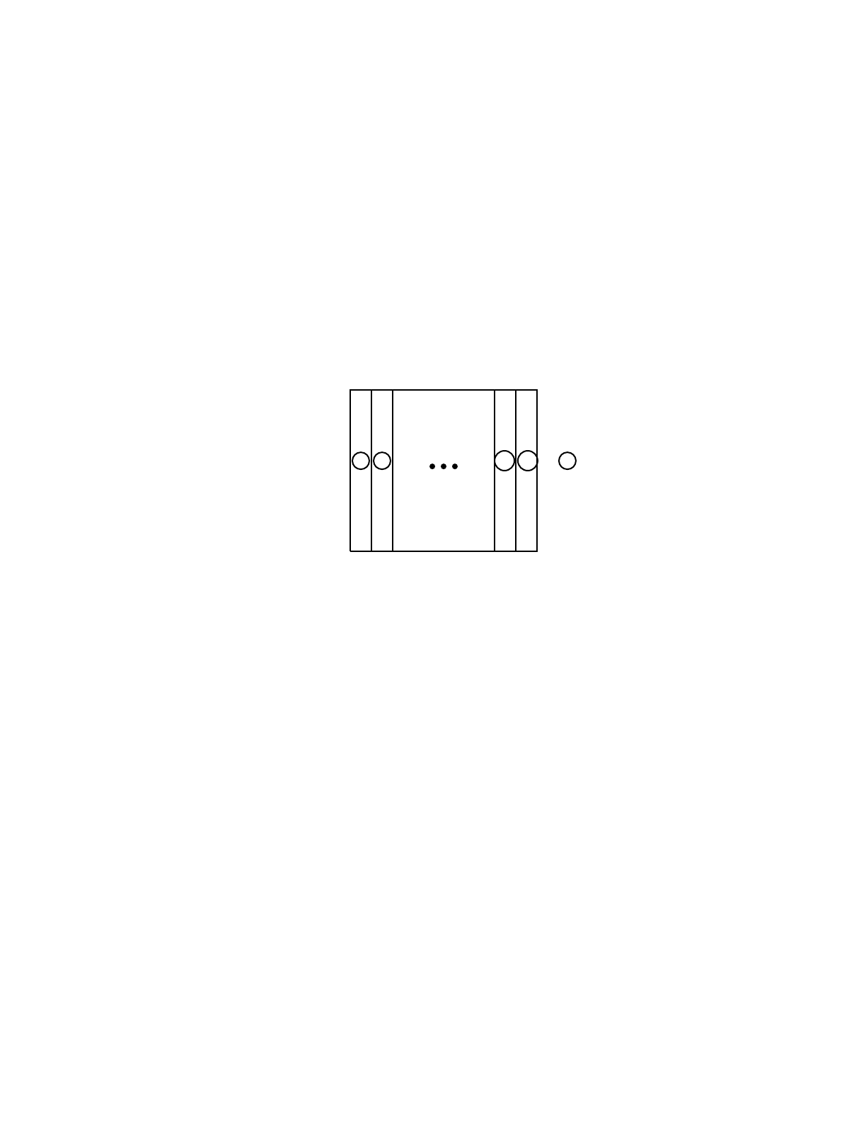
18 December 2000 5-9
CHAPTER 5
TEST1 PROBLEM AND OUTPUT
II. TEST1 PROBLEM AND OUTPUT
TEST 1 defines a disk of concrete 100 cm thick, with a 75-cm radius. A 14.19 MeV neutron
source is incident at a point in the center of a face of the disk and normal to it. Several neutron
and photon tallies are made on surface 18 and in cell 17. There is no energy cutoff and the simple
physics treatment that includes implicit capture is used for photons with energy greater than
0.001 MeV.
The disk is divided into 16 slabs, each 6.25 cm thick, as seen in Fig. 5.1. The neutron importance
of each slab, or cell, varies from 0 in cell 1 to 32 in cell 17. Photon importances are set equal to
neutron importances. The problem ran 10,000 particles and the tally means, errors, and FOMs
shown in the tally fluctuation charts seem to be stable.
Figure 5.1
The weight window generator was used to generate a better importance function for subsequent
runs. The resulting cards are printed at the end of the TEST1 output file and can be copied into
an input file to be run a second time. Generation of weight windows did not affect the results of
TEST1 but did slow down the calculation by 14%. When the importances in TEST1 were
replaced by the generated weight windows (WWP and WWN cards), the problem took 14.27
minutes to run 10000 particles vs 10.01 minutes for TEST1. However, the photon FOMs
increased by a factor of 2 to 3 and the errors decreased by half, while the means appeared to stay
stable. The neutron means, errors, and FOMs stayed approximately the same, indicating that they
were already well chosen to optimize tally 12. The use of the mesh-based weight window
generator instead of the cell-based weight window generator for this problem did not
significantly improve the FOM because the cell-based weight windows were quite good.
Following is a partial output from TEST1. The symbol Xappearing left of the table title indicates
that table does not appear unless the PRINT option or card is used. If Nn, where n is an integer,
appears before an item on a page or below a column, that item is explained or discussed in Note
Nn in the text following the output.
2 3 4 16 17 18
1
2 3 16 17 1

CHAPTER 5
TEST1 PROBLEM AND OUTPUT
5-10 18 December 2000
N11mcnp version 4c ld=01/20/00 06/23/00 11:30:40
************************************************************************* probid = 06/23/00 11:30:40
N2i=test1 name=test1.
N31- test1: 100 cm thick concrete disk with 15 splitting surfaces
2- c
3- 1 0 1 : -2 : 18
4- 2 1 -2.2505 -1 -3 2
5- 3 1 -2.2505 -1 -4 3
6- 4 1 -2.2505 -1 -5 4
7- 5 1 -2.2505 -1 -6 5
8- 6 1 -2.2505 -1 -7 6
9- 7 1 -2.2505 -1 -8 7
10- 8 1 -2.2505 -1 -9 8
11- 9 1 -2.2505 -1 -10 9
12- 10 1 -2.2505 -1 -11 10
13- 11 1 -2.2505 -1 -12 11
14- 12 1 -2.2505 -1 -13 12
15- 13 1 -2.2505 -1 -14 13
16- 14 1 -2.2505 -1 -15 14
17- 15 1 -2.2505 -1 -16 15
18- 16 1 -2.2505 -1 -17 16
19- 17 1 -2.2505 -1 -18 17
20-
21- 1 cy 75
22- 2 py 0
23- 3 py 6.25
24- 4 py 12.50
25- 5 py 18.75
26- 6 py 25.00
27- 7 py 31.25
28- 8 py 37.50
29- 9 py 43.75
30- 10 py 50.00
31- 11 py 56.25
32- 12 py 62.50
33- 13 py 68.75
34- 14 py 75.00
35- 15 py 81.25
36- 16 py 87.50
37- 17 py 93.75
38- 18 py 100.00
39-
40- mode n p
41- c the following is los alamos concrete
42- m1 1001.60c 8.47636e-2

18 December 2000 5-11
CHAPTER 5
TEST1 PROBLEM AND OUTPUT
43- 8016.60c 6.04086e-1
44- 11023.60c 9.47250e-3
45- 12000.60c 2.99826e-3
46- 13027.60c 2.48344e-2
47- 14000.60c 2.41860e-1
48- 19000.60c 6.85513e-3
49- 20000.60c 2.04808e-2
50- 26054.60c 2.74322e-4
51- 26056.60c 4.26455e-3
52- 26057.60c 9.76401e-5
53- 26058.60c 1.30187e-5
N454- sdef pos=0 0 0 cel=2 wgt=1 vec=0 1 0 sur=2 dir=1 erg=14.19
55- imp:n 0 1 5r 2 2 2 4 4 4 8 8 16 32
56- imp:p 0 1 5r 2 2 2 4 4 4 8 8 16 32
N557- pwt 0 -10 -9 -8 -7 -6 -5 -4 -3 -2 -1.7 -1.4 -1.0 -0.7 -0.4 -0.3 -0.2
58- f1:p 18
59- f11:n 18
60- fc12 optimize weight window generator on tally 12
61- f12:p 18
62- e12 20
63- wwg 12 2
64- f6:n,p 17
65- e6 .00001 .0001 .001 .01 .05 .1 .5 1 13i 15 20
66- f16:n 17
67- f26:p 17
68- f34:n 17
69- fm34 -1 1 1 -4
N670- e0 .0001 .001 .01 .05 .1 .5 1 13i 15 20
71- phys:n 15 0
72- phys:p .001
73- nps 10000
74- print
X 1source print table 10
N7values of defaulted or explicitly defined source variables
cel 2.0000E+00
sur 2.0000E+00
erg 1.4190E+01
tme 0.0000E+00
dir 1.0000E+00
pos 0.0000E+00 0.0000E+00 0.0000E+00
x 0.0000E+00
y 0.0000E+00
z 0.0000E+00
rad 0.0000E+00
ext 0.0000E+00
axs 0.0000E+00 0.0000E+00 0.0000E+00

CHAPTER 5
TEST1 PROBLEM AND OUTPUT
5-12 18 December 2000
vec 0.0000E+00 1.0000E+00 0.0000E+00
ccc 0.0000E+00
nrm 1.0000E+00
ara 0.0000E+00
wgt 1.0000E+00
eff 1.0000E-02
par 0.0000E+00
order of sampling source variables.
cel sur pos vec dir erg tme
X 1tally 11 print table 30
N8 tally type 1 number of particles crossing a surface.
tally for neutrons
N9warning. energy bin limits adjusted for tally 11
surfaces 18
N10 energy bins
0.00000E+00 to 1.00000E-04 mev
1.00000E-04 to 1.00000E-03 mev
1.00000E-03 to 1.00000E-02 mev
1.00000E-02 to 5.00000E-02 mev
5.00000E-02 to 1.00000E-01 mev
1.00000E-01 to 5.00000E-01 mev
5.00000E-01 to 1.00000E+00 mev
1.00000E+00 to 2.00000E+00 mev
2.00000E+00 to 3.00000E+00 mev
3.00000E+00 to 4.00000E+00 mev
4.00000E+00 to 5.00000E+00 mev
5.00000E+00 to 6.00000E+00 mev
6.00000E+00 to 7.00000E+00 mev
7.00000E+00 to 8.00000E+00 mev
8.00000E+00 to 9.00000E+00 mev
9.00000E+00 to 1.00000E+01 mev
1.00000E+01 to 1.10000E+01 mev
1.10000E+01 to 1.20000E+01 mev
1.20000E+01 to 1.30000E+01 mev
1.30000E+01 to 1.40000E+01 mev
1.40000E+01 to 1.50000E+01 mev
total bin
SKIP 158 LINES IN OUTPUT
X 1material composition print table 40
material
number component nuclide, atom fraction
1 1001, 8.47636E-02 8016, 6.04086E-01 11023, 9.47250E-03 12000, 2.99826E-03

18 December 2000 5-13
CHAPTER 5
TEST1 PROBLEM AND OUTPUT
13027, 2.48344E-02 14000, 2.41860E-01 19000, 6.85513E-03 20000, 2.04808E-02
26054, 2.74322E-04 26056, 4.26455E-03 26057, 9.76401E-05 26058, 1.30187E-05
material
number component nuclide, mass fraction
1 1001, 4.53200E-03 8016, 5.12597E-01 11023, 1.15530E-02 12000, 3.86599E-03
13027, 3.55480E-02 14000, 3.60364E-01 19000, 1.42190E-02 20000, 4.35460E-02
26054, 7.84990E-04 26056, 1.26547E-02 26057, 2.94921E-04 26058, 4.00121E-05
X 1cell volumes and masses print table 50
N11
cell atom gram input calculated reason volume
density density volume volume mass pieces not calculated
1 1 0.00000E+00 0.00000E+00 0.00000E+00 0.00000E+00 0.00000E+00 0 infinite
2 2 7.18983E-02 2.25050E+00 0.00000E+00 1.10447E+05 2.48560E+05 1
3 3 7.18983E-02 2.25050E+00 0.00000E+00 1.10447E+05 2.48560E+05 1
4 4 7.18983E-02 2.25050E+00 0.00000E+00 1.10447E+05 2.48560E+05 1
5 5 7.18983E-02 2.25050E+00 0.00000E+00 1.10447E+05 2.48560E+05 1
6 6 7.18983E-02 2.25050E+00 0.00000E+00 1.10447E+05 2.48560E+05 1
7 7 7.18983E-02 2.25050E+00 0.00000E+00 1.10447E+05 2.48560E+05 1
8 8 7.18983E-02 2.25050E+00 0.00000E+00 1.10447E+05 2.48560E+05 1
9 9 7.18983E-02 2.25050E+00 0.00000E+00 1.10447E+05 2.48560E+05 1
10 10 7.18983E-02 2.25050E+00 0.00000E+00 1.10447E+05 2.48560E+05 1
11 11 7.18983E-02 2.25050E+00 0.00000E+00 1.10447E+05 2.48560E+05 1
12 12 7.18983E-02 2.25050E+00 0.00000E+00 1.10447E+05 2.48560E+05 1
13 13 7.18983E-02 2.25050E+00 0.00000E+00 1.10447E+05 2.48560E+05 1
14 14 7.18983E-02 2.25050E+00 0.00000E+00 1.10447E+05 2.48560E+05 1
15 15 7.18983E-02 2.25050E+00 0.00000E+00 1.10447E+05 2.48560E+05 1
16 16 7.18983E-02 2.25050E+00 0.00000E+00 1.10447E+05 2.48560E+05 1
17 17 7.18983E-02 2.25050E+00 0.00000E+00 1.10447E+05 2.48560E+05 1
X 1surface areas print table 50
surface input calculated reason area
area area not calculated
1 1 0.00000E+00 4.71239E+04
2 2 0.00000E+00 1.76715E+04
3 3 0.00000E+00 1.76715E+04
4 4 0.00000E+00 1.76715E+04
5 5 0.00000E+00 1.76715E+04
6 6 0.00000E+00 1.76715E+04
7 7 0.00000E+00 1.76715E+04
8 8 0.00000E+00 1.76715E+04

CHAPTER 5
TEST1 PROBLEM AND OUTPUT
5-14 18 December 2000
9 9 0.00000E+00 1.76715E+04
10 10 0.00000E+00 1.76715E+04
11 11 0.00000E+00 1.76715E+04
12 12 0.00000E+00 1.76715E+04
13 13 0.00000E+00 1.76715E+04
14 14 0.00000E+00 1.76715E+04
15 15 0.00000E+00 1.76715E+04
16 16 0.00000E+00 1.76715E+04
17 17 0.00000E+00 1.76715E+04
18 18 0.00000E+00 1.76715E+04
X 1cells print table 60
atom gram neutron photon photon wt
cell mat density density volume mass pieces importance importance generation
1 1 0 0.00000E+00 0.00000E+00 0.00000E+00 0.00000E+00 0 0.0000E+00 0.0000E+00 0.000E+00
2 2 1 7.18983E-02 2.25050E+00 1.10447E+05 2.48560E+05 1 1.0000E+00 1.0000E+00 -1.000E+01
3 3 1 7.18983E-02 2.25050E+00 1.10447E+05 2.48560E+05 1 1.0000E+00 1.0000E+00 -9.000E+00
4 4 1 7.18983E-02 2.25050E+00 1.10447E+05 2.48560E+05 1 1.0000E+00 1.0000E+00 -8.000E+00
5 5 1 7.18983E-02 2.25050E+00 1.10447E+05 2.48560E+05 1 1.0000E+00 1.0000E+00 -7.000E+00
6 6 1 7.18983E-02 2.25050E+00 1.10447E+05 2.48560E+05 1 1.0000E+00 1.0000E+00 -6.000E+00
7 7 1 7.18983E-02 2.25050E+00 1.10447E+05 2.48560E+05 1 1.0000E+00 1.0000E+00 -5.000E+00
8 8 1 7.18983E-02 2.25050E+00 1.10447E+05 2.48560E+05 1 2.0000E+00 2.0000E+00 -4.000E+00
9 9 1 7.18983E-02 2.25050E+00 1.10447E+05 2.48560E+05 1 2.0000E+00 2.0000E+00 -3.000E+00
10 10 1 7.18983E-02 2.25050E+00 1.10447E+05 2.48560E+05 1 2.0000E+00 2.0000E+00 -2.000E+00
11 11 1 7.18983E-02 2.25050E+00 1.10447E+05 2.48560E+05 1 4.0000E+00 4.0000E+00 -1.700E+00
12 12 1 7.18983E-02 2.25050E+00 1.10447E+05 2.48560E+05 1 4.0000E+00 4.0000E+00 -1.400E+00
13 13 1 7.18983E-02 2.25050E+00 1.10447E+05 2.48560E+05 1 4.0000E+00 4.0000E+00 -1.000E+00
14 14 1 7.18983E-02 2.25050E+00 1.10447E+05 2.48560E+05 1 8.0000E+00 8.0000E+00 -7.000E-01
15 15 1 7.18983E-02 2.25050E+00 1.10447E+05 2.48560E+05 1 8.0000E+00 8.0000E+00 -4.000E-01
16 16 1 7.18983E-02 2.25050E+00 1.10447E+05 2.48560E+05 1 1.6000E+01 1.6000E+01 -3.000E-01
17 17 1 7.18983E-02 2.25050E+00 1.10447E+05 2.48560E+05 1 3.2000E+01 3.2000E+01 -2.000E-01
N12total 1.76715E+06 3.97696E+06
X 1surfaces print table 70
N13 surface trans type surface coefficients
1 1 cy 7.5000000E+01
2 2 py 0.0000000E+00
3 3 py 6.2500000E+00
4 4 py 1.2500000E+01
5 5 py 1.8750000E+01
6 6 py 2.5000000E+01
7 7 py 3.1250000E+01
8 8 py 3.7500000E+01
9 9 py 4.3750000E+01
10 10 py 5.0000000E+01
11 11 py 5.6250000E+01

18 December 2000 5-15
CHAPTER 5
TEST1 PROBLEM AND OUTPUT
12 12 py 6.2500000E+01
13 13 py 6.8750000E+01
14 14 py 7.5000000E+01
15 15 py 8.1250000E+01
16 16 py 8.7500000E+01
17 17 py 9.3750000E+01
18 18 py 1.0000000E+02
1 cell temperatures in mev for the free-gas thermal neutron treatment. print table 72
N14 all non-zero importance cells with materials have a temperature for thermal neutrons of 2.5300E-08 mev.
minimum source weight = 1.0000E+00 maximum source weight = 1.0000E+00
3 warning messages so far.
N151physical constants print table 98
name value description
huge 1.0000000000000E+37 infinity
pie 3.1415926535898E+00 pi
euler 5.7721566490153E-01 euler constant
avogad 6.0220434469282E+23 avogadro number (molecules/mole)
aneut 1.0086649670000E+00 neutron mass (amu)
avgdn 5.9703109000000E-01 avogadro number/neutron mass (1.e-24*molecules/mole/amu)
slite 2.9979250000000E+02 speed of light (cm/shake)
planck 4.1357320000000E-13 planck constant (mev shake)
fscon 1.3703930000000E+02 inverse fine structure constant h*c/(2*pi*e**2)
gpt(1) 9.3958000000000E+02 neutron mass (mev)
gpt(3) 5.1100800000000E-01 electron mass (mev)
fission q-values: nuclide q(mev) nuclide q(mev)
90232 171.91 91233 175.57
92233 180.84 92234 179.45
92235 180.88 92236 179.50
92237 180.40 92238 181.31
92239 180.40 92240 180.40
93237 183.67 94238 186.65
94239 189.44 94240 186.36
94241 188.99 94242 185.98
94243 187.48 95241 190.83
95242 190.54 95243 190.25
96242 190.49 96244 190.49
other 180.00
the following compilation options were used:
pointer

CHAPTER 5
TEST1 PROBLEM AND OUTPUT
5-16 18 December 2000
cheap
unix
sun
plot
mcplot
gkssim
xlib
xs64
default datapath: /usr/local/codes/data/mc/type2/unix64
N161cross-section tables print table 100
table length
tables from file endf602
1001.60c 2322 1-h-1 from endf-vi.1 mat 125 11/25/93
8016.60c 50346 8-o-16 from endf/b-vi mat 8 25 11/25/93
11023.60c 48471 11-na-23 from endf/b-vi.1 mat1125 11/25/93
12000.60c 52785 12-mg-nat from endf/b-vi mat1200 11/25/93
13027.60c 49407 13-al-27 from endf/b-vi mat1325 11/25/93
14000.60c 100118 14-si-nat from endf/b-vi mat1400 11/25/93
19000.60c 23390 19-k-nat from endf/b-vi mat1900 11/25/93
20000.60c 70573 20-ca-nat from endf/b-vi mat2000 11/25/93
26054.60c 120443 endf/b-vi.1 fe54a mat2625 11/25/93
26056.60c 172174 endf/b-vi.1 fe56a mat2631 11/25/93
26057.60c 133044 endf/b-vi.1 fe57a mat2634 11/25/93
26058.60c 92535 endf/b-vi.1 fe58a mat2637 11/25/93
tables from file mcplib022
1000.02p 623 01/15/93
8000.02p 623 01/15/93
11000.02p 635 01/15/93
12000.02p 643 01/15/93
13000.02p 643 01/15/93
14000.02p 643 01/15/93
19000.02p 643 01/15/93
20000.02p 651 01/15/93
26000.02p 651 01/15/93
total 921363
N17 any neutrons with energy greater than emax = 1.50000E+01 from the source or from a collision will be resampled.
N18 neutron cross sections outside the range from 0.0000E+00 to 1.5000E+01 mev are expunged.
maximum photon energy set to 100.0 mev (maximum electron energy)

18 December 2000 5-17
CHAPTER 5
TEST1 PROBLEM AND OUTPUT
tables from file el032
1000.03e 2329 6/6/98
8000.03e 2333 6/6/98
11000.03e 2337 6/6/98
12000.03e 2337 6/6/98
13000.03e 2337 6/6/98
14000.03e 2339 6/6/98
19000.03e 2343 6/6/98
20000.03e 2343 6/6/98
26000.03e 2345 6/6/98
X 1range table for material 1 (condensed) print table 85
electron substeps per energy step = 4, default = 4. mean ionization energy = 1.41099E+02 ev.
N19X density effect data
non-conductor
z = 1
occ no, be(ev) pairs
1. 13.600
z = 8
occ no, be(ev) pairs
2. 538.000 2. 28.480 4. 13.620
z = 11
occ no, be(ev) pairs
2. 1075.000 2. 66.000 2. 34.000 4. 34.000 -1. 5.139
z = 12
occ no, be(ev) pairs
2. 1308.000 2. 92.000 2. 54.000 4. 54.000 -2. 7.646
z = 13
occ no, be(ev) pairs
2. 1564.000 2. 121.000 2. 77.000 4. 77.000 -3. 9.075
z = 14
occ no, be(ev) pairs
2. 1844.000 2. 154.000 2. 104.000 4. 104.000 2. 13.460 -2. 8.151
z = 19
occ no, be(ev) pairs
2. 3610.000 2. 381.000 2. 299.000 4. 296.000 2. 37.000 2. 19.000
4. 18.700 -1. 4.341
z = 20
occ no, be(ev) pairs
2. 4041.000 2. 441.000 2. 353.000 4. 349.000 2. 46.000 2. 28.000
4. 28.000 -2. 6.113
z = 26
occ no, be(ev) pairs
2. 7117.000 2. 851.000 2. 726.000 4. 713.000 2. 98.000 2. 61.000
4. 59.000 6. 9.000 -2. 7.870
z = 26

CHAPTER 5
TEST1 PROBLEM AND OUTPUT
5-18 18 December 2000
occ no, be(ev) pairs
2. 7117.000 2. 851.000 2. 726.000 4. 713.000 2. 98.000 2. 61.000
4. 59.000 6. 9.000 -2. 7.870
z = 26
occ no, be(ev) pairs
2. 7117.000 2. 851.000 2. 726.000 4. 713.000 2. 98.000 2. 61.000
4. 59.000 6. 9.000 -2. 7.870
z = 26
occ no, be(ev) pairs
2. 7117.000 2. 851.000 2. 726.000 4. 713.000 2. 98.000 2. 61.000
4. 59.000 6. 9.000 -2. 7.870
plas(ev) wt tmin(mev)
30.57106 2.35209 0.36478
N20 energy stopping power range radiation beta**2 density rad/col drange dyield
n collision radiation total yield corr
mev mev cm2/g mev cm2/g mev cm2/g g/cm2 mev cm2/g g/cm2
133 1.0790E-03 7.975E+01 3.695E-03 7.976E+01 7.021E-06 3.708E-06 4.210E-03 0.000E+00 4.633E-05 1.098E-06 4.000E-09
132 1.1766E-03 7.605E+01 3.798E-03 7.605E+01 8.276E-06 7.395E-06 4.589E-03 0.000E+00 4.994E-05 1.254E-06 4.700E-09
131 1.2831E-03 7.241E+01 3.900E-03 7.242E+01 9.711E-06 1.109E-05 5.003E-03 0.000E+00 5.386E-05 1.435E-06 5.527E-09
130 1.3992E-03 6.886E+01 4.003E-03 6.887E+01 1.136E-05 1.482E-05 5.454E-03 0.000E+00 5.813E-05 1.645E-06 6.502E-09
129 1.5259E-03 6.540E+01 4.105E-03 6.541E+01 1.324E-05 1.860E-05 5.945E-03 0.000E+00 6.276E-05 1.888E-06 7.655E-09
128 1.6640E-03 6.205E+01 4.207E-03 6.205E+01 1.541E-05 2.248E-05 6.481E-03 0.000E+00 6.780E-05 2.169E-06 9.015E-09
127 1.8146E-03 5.880E+01 4.308E-03 5.881E+01 1.791E-05 2.646E-05 7.064E-03 0.000E+00 7.327E-05 2.494E-06 1.062E-08
SKIP 122 LINES IN OUTPUT
4 7.7111E+01 1.906E+00 2.563E+00 4.469E+00 2.757E+01 3.582E-01 1.000E+00 4.644E-01 1.344E+00 1.471E+00 3.600E+00
3 8.4090E+01 1.914E+00 2.814E+00 4.728E+00 2.909E+01 3.769E-01 1.000E+00 4.770E-01 1.471E+00 1.518E+00 4.079E+00
2 9.1700E+01 1.921E+00 3.089E+00 5.010E+00 3.065E+01 3.960E-01 1.000E+00 4.898E-01 1.608E+00 1.564E+00 4.613E+00
1 1.0000E+02 1.928E+00 3.390E+00 5.318E+00 3.226E+01 4.152E-01 1.000E+00 5.025E-01 1.759E+00 1.608E+00 5.206E+00
N211electron secondary production for material 1 print table 86
energy stopping power brems thick tgt k x-ray knock-on
n collision radiation total brems
mev mev barn mev barn mev barn barn barn barn
133 1.0790E-03 2.496E+03 1.157E-01 2.496E+03 1.398E+03 5.031E-05 0.000E+00 0.000E+00
132 1.1766E-03 2.380E+03 1.189E-01 2.381E+03 1.327E+03 1.049E-04 0.000E+00 0.000E+00
131 1.2831E-03 2.267E+03 1.221E-01 2.267E+03 1.259E+03 1.642E-04 0.000E+00 0.000E+00
130 1.3992E-03 2.155E+03 1.253E-01 2.156E+03 1.193E+03 2.286E-04 0.000E+00 0.000E+00
129 1.5259E-03 2.047E+03 1.285E-01 2.047E+03 1.130E+03 2.987E-04 0.000E+00 0.000E+00
128 1.6640E-03 1.942E+03 1.317E-01 1.942E+03 1.070E+03 3.749E-04 0.000E+00 0.000E+00
127 1.8146E-03 1.841E+03 1.349E-01 1.841E+03 1.012E+03 4.578E-04 0.000E+00 0.000E+00
SKIP 122 LINES in OUTPUT
4 7.7111E+01 5.967E+01 8.022E+01 1.399E+02 2.275E+01 1.986E+01 1.596E+00 2.409E+03
3 8.4090E+01 5.990E+01 8.808E+01 1.480E+02 2.275E+01 2.097E+01 1.613E+00 2.409E+03
2 9.1700E+01 6.012E+01 9.670E+01 1.568E+02 2.274E+01 2.210E+01 1.629E+00 2.409E+03
1 1.0000E+02 6.035E+01 1.061E+02 1.665E+02 2.274E+01 2.327E+01 1.645E+00 2.409E+03

18 December 2000 5-19
CHAPTER 5
TEST1 PROBLEM AND OUTPUT
1decimal words of dynamically allocated storage
general 148616
tallies 47160
bank 46724
cross sections 1842726
total 2058178 = 8232712 bytes
***********************************************************************************************************************
N22 dump no. 1 on file test1.r nps = 0 coll = 0 ctm = 0.00 nrn = 0
3 warning messages so far.
X 1 starting mcrun. dynamic storage = 2058182 words, 8232728 bytes. cp0 = 0.12 print table 110
N23 test1: 100 cm thick concrete disk with 15 splitting surfaces
nps x y z cell surf u v w energy weight time
1 0.000E+00 0.000E+00 0.000E+00 2 2 0.000E+00 1.000E+00 0.000E+00 1.419E+01 1.000E+00 0.000E+00
2 0.000E+00 0.000E+00 0.000E+00 2 2 0.000E+00 1.000E+00 0.000E+00 1.419E+01 1.000E+00 0.000E+00
3 0.000E+00 0.000E+00 0.000E+00 2 2 0.000E+00 1.000E+00 0.000E+00 1.419E+01 1.000E+00 0.000E+00
4 0.000E+00 0.000E+00 0.000E+00 2 2 0.000E+00 1.000E+00 0.000E+00 1.419E+01 1.000E+00 0.000E+00
5 0.000E+00 0.000E+00 0.000E+00 2 2 0.000E+00 1.000E+00 0.000E+00 1.419E+01 1.000E+00 0.000E+00
6 0.000E+00 0.000E+00 0.000E+00 2 2 0.000E+00 1.000E+00 0.000E+00 1.419E+01 1.000E+00 0.000E+00
7 0.000E+00 0.000E+00 0.000E+00 2 2 0.000E+00 1.000E+00 0.000E+00 1.419E+01 1.000E+00 0.000E+00
8 0.000E+00 0.000E+00 0.000E+00 2 2 0.000E+00 1.000E+00 0.000E+00 1.419E+01 1.000E+00 0.000E+00
9 0.000E+00 0.000E+00 0.000E+00 2 2 0.000E+00 1.000E+00 0.000E+00 1.419E+01 1.000E+00 0.000E+00
10 0.000E+00 0.000E+00 0.000E+00 2 2 0.000E+00 1.000E+00 0.000E+00 1.419E+01 1.000E+00 0.000E+00
11 0.000E+00 0.000E+00 0.000E+00 2 2 0.000E+00 1.000E+00 0.000E+00 1.419E+01 1.000E+00 0.000E+00
12 0.000E+00 0.000E+00 0.000E+00 2 2 0.000E+00 1.000E+00 0.000E+00 1.419E+01 1.000E+00 0.000E+00
13 0.000E+00 0.000E+00 0.000E+00 2 2 0.000E+00 1.000E+00 0.000E+00 1.419E+01 1.000E+00 0.000E+00
14 0.000E+00 0.000E+00 0.000E+00 2 2 0.000E+00 1.000E+00 0.000E+00 1.419E+01 1.000E+00 0.000E+00
15 0.000E+00 0.000E+00 0.000E+00 2 2 0.000E+00 1.000E+00 0.000E+00 1.419E+01 1.000E+00 0.000E+00
16 0.000E+00 0.000E+00 0.000E+00 2 2 0.000E+00 1.000E+00 0.000E+00 1.419E+01 1.000E+00 0.000E+00
17 0.000E+00 0.000E+00 0.000E+00 2 2 0.000E+00 1.000E+00 0.000E+00 1.419E+01 1.000E+00 0.000E+00
18 0.000E+00 0.000E+00 0.000E+00 2 2 0.000E+00 1.000E+00 0.000E+00 1.419E+01 1.000E+00 0.000E+00
19 0.000E+00 0.000E+00 0.000E+00 2 2 0.000E+00 1.000E+00 0.000E+00 1.419E+01 1.000E+00 0.000E+00
20 0.000E+00 0.000E+00 0.000E+00 2 2 0.000E+00 1.000E+00 0.000E+00 1.419E+01 1.000E+00 0.000E+00
21 0.000E+00 0.000E+00 0.000E+00 2 2 0.000E+00 1.000E+00 0.000E+00 1.419E+01 1.000E+00 0.000E+00
22 0.000E+00 0.000E+00 0.000E+00 2 2 0.000E+00 1.000E+00 0.000E+00 1.419E+01 1.000E+00 0.000E+00
23 0.000E+00 0.000E+00 0.000E+00 2 2 0.000E+00 1.000E+00 0.000E+00 1.419E+01 1.000E+00 0.000E+00
24 0.000E+00 0.000E+00 0.000E+00 2 2 0.000E+00 1.000E+00 0.000E+00 1.419E+01 1.000E+00 0.000E+00
25 0.000E+00 0.000E+00 0.000E+00 2 2 0.000E+00 1.000E+00 0.000E+00 1.419E+01 1.000E+00 0.000E+00
26 0.000E+00 0.000E+00 0.000E+00 2 2 0.000E+00 1.000E+00 0.000E+00 1.419E+01 1.000E+00 0.000E+00
27 0.000E+00 0.000E+00 0.000E+00 2 2 0.000E+00 1.000E+00 0.000E+00 1.419E+01 1.000E+00 0.000E+00

CHAPTER 5
TEST1 PROBLEM AND OUTPUT
5-20 18 December 2000
28 0.000E+00 0.000E+00 0.000E+00 2 2 0.000E+00 1.000E+00 0.000E+00 1.419E+01 1.000E+00 0.000E+00
29 0.000E+00 0.000E+00 0.000E+00 2 2 0.000E+00 1.000E+00 0.000E+00 1.419E+01 1.000E+00 0.000E+00
30 0.000E+00 0.000E+00 0.000E+00 2 2 0.000E+00 1.000E+00 0.000E+00 1.419E+01 1.000E+00 0.000E+00
31 0.000E+00 0.000E+00 0.000E+00 2 2 0.000E+00 1.000E+00 0.000E+00 1.419E+01 1.000E+00 0.000E+00
32 0.000E+00 0.000E+00 0.000E+00 2 2 0.000E+00 1.000E+00 0.000E+00 1.419E+01 1.000E+00 0.000E+00
33 0.000E+00 0.000E+00 0.000E+00 2 2 0.000E+00 1.000E+00 0.000E+00 1.419E+01 1.000E+00 0.000E+00
34 0.000E+00 0.000E+00 0.000E+00 2 2 0.000E+00 1.000E+00 0.000E+00 1.419E+01 1.000E+00 0.000E+00
35 0.000E+00 0.000E+00 0.000E+00 2 2 0.000E+00 1.000E+00 0.000E+00 1.419E+01 1.000E+00 0.000E+00
36 0.000E+00 0.000E+00 0.000E+00 2 2 0.000E+00 1.000E+00 0.000E+00 1.419E+01 1.000E+00 0.000E+00
37 0.000E+00 0.000E+00 0.000E+00 2 2 0.000E+00 1.000E+00 0.000E+00 1.419E+01 1.000E+00 0.000E+00
38 0.000E+00 0.000E+00 0.000E+00 2 2 0.000E+00 1.000E+00 0.000E+00 1.419E+01 1.000E+00 0.000E+00
39 0.000E+00 0.000E+00 0.000E+00 2 2 0.000E+00 1.000E+00 0.000E+00 1.419E+01 1.000E+00 0.000E+00
40 0.000E+00 0.000E+00 0.000E+00 2 2 0.000E+00 1.000E+00 0.000E+00 1.419E+01 1.000E+00 0.000E+00
41 0.000E+00 0.000E+00 0.000E+00 2 2 0.000E+00 1.000E+00 0.000E+00 1.419E+01 1.000E+00 0.000E+00
42 0.000E+00 0.000E+00 0.000E+00 2 2 0.000E+00 1.000E+00 0.000E+00 1.419E+01 1.000E+00 0.000E+00
43 0.000E+00 0.000E+00 0.000E+00 2 2 0.000E+00 1.000E+00 0.000E+00 1.419E+01 1.000E+00 0.000E+00
44 0.000E+00 0.000E+00 0.000E+00 2 2 0.000E+00 1.000E+00 0.000E+00 1.419E+01 1.000E+00 0.000E+00
45 0.000E+00 0.000E+00 0.000E+00 2 2 0.000E+00 1.000E+00 0.000E+00 1.419E+01 1.000E+00 0.000E+00
46 0.000E+00 0.000E+00 0.000E+00 2 2 0.000E+00 1.000E+00 0.000E+00 1.419E+01 1.000E+00 0.000E+00
47 0.000E+00 0.000E+00 0.000E+00 2 2 0.000E+00 1.000E+00 0.000E+00 1.419E+01 1.000E+00 0.000E+00
48 0.000E+00 0.000E+00 0.000E+00 2 2 0.000E+00 1.000E+00 0.000E+00 1.419E+01 1.000E+00 0.000E+00
49 0.000E+00 0.000E+00 0.000E+00 2 2 0.000E+00 1.000E+00 0.000E+00 1.419E+01 1.000E+00 0.000E+00
50 0.000E+00 0.000E+00 0.000E+00 2 2 0.000E+00 1.000E+00 0.000E+00 1.419E+01 1.000E+00 0.000E+00
1problem summary
run terminated when 10000 particle histories were done.
+ 06/23/00 11:34:29
test1: 100 cm thick concrete disk with 15 splitting surfaces probid = 06/23/00 11:30:40
0
N24neutron creation tracks weight energy neutron loss tracks weight energy
(per source particle) (per source particle)
source 10000 1.0000E+00 1.4190E+01 N27escape 13411 4.0545E-01 9.9156E-01
energy cutoff 0 0. 0.
time cutoff 0 0. 0.
weight window 0 0. 0. weight window 0 0. 0.
N25cell importance 35681 2.5286E-01 9.6306E-02 N28cell importance 23893 2.5427E-01 1.0282E-01
N26weight cutoff 0 8.1018E-02 5.4609E-02 N29weight cutoff 8625 8.0533E-02 5.5477E-02
energy importance 0 0. 0. energy importance 0 0. 0.
dxtran 0 0. 0. dxtran 0 0. 0.
forced collisions 0 0. 0. forced collisions 0 0. 0.
exp. transform 0 0. 0. exp. transform 0 0. 0.
upscattering 0 0. 1.0851E-07 N30downscattering 0 0. 8.2722E+00
delayed fission 0 0. 0. N31capture 0 6.0858E-01 4.7835E+00
(n,xn) 496 2.9921E-02 7.3027E-02 loss to (n,xn) 248 1.4960E-02 2.0833E-01
prompt fission 0 0. 0. loss to fission 0 0. 0.
total 46177 1.3638E+00 1.4414E+01 N32 total 46177 1.3638E+00 1.4414E+01

18 December 2000 5-21
CHAPTER 5
TEST1 PROBLEM AND OUTPUT
number of neutrons banked 35929 N33average time of (shakes) cutoffs
neutron tracks per source particle 4.6177E+00 escape 6.2490E+03 tco 1.0000E+34
neutron collisions per source particle 1.1440E+02 capture 1.6237E+04 eco 0.0000E+00
total neutron collisions 1143962 capture or escape 1.2243E+04 wc1 -5.0000E-01
N34net multiplication 1.0150E+00 0.0010 any termination 1.7300E+04 wc2 -2.5000E-01
0
photon creation tracks weight energy photon loss tracks weight energy
(per source particle) (per source particle)
source 0 0. 0. escape 7391 5.1898E-01 1.0525E+00
energy cutoff 0 0. 0.
time cutoff 0 0. 0.
weight window 0 0. 0. weight window 0 0. 0.
cell importance 9943 1.3568E-01 1.4838E-01 cell importance 6205 1.4357E-01 1.6084E-01
weight cutoff 0 4.8911E-02 4.7908E-03 weight cutoff 32220 5.0010E-02 4.9142E-03
energy importance 0 0. 0. energy importance 0 0. 0.
dxtran 0 0. 0. dxtran 0 0. 0.
forced collisions 0 0. 0. forced collisions 0 0. 0.
exp. transform 0 0. 0. exp. transform 0 0. 0.
from neutrons 14595 1.9430E+00 6.1915E+00 compton scatter 0 0. 4.4296E+00
bremsstrahlung 20279 9.0128E-01 8.9382E-02 capture 0 2.4540E+00 1.4688E-01
N35p-annihilation 1998 2.7534E-01 1.4070E-01 pair production 999 1.3767E-01 7.8001E-01
electron x-rays 0 0. 0.
1st fluorescence 0 0. 0.
2nd fluorescence 0 0. 0.
total 46815 3.3043E+00 6.5747E+00 total 46815 3.3043E+00 6.5747E+00
number of photons banked 45816 N36 average time of (shakes) cutoffs
photon tracks per source particle 4.6815E+00 escape 7.1788E+03 tco 1.0000E+34
photon collisions per source particle 1.7059E+01 capture 1.1333E+04 eco 1.0000E-03
total photon collisions 170585 capture or escape 1.0608E+04 wc1 -5.0000E-01
any termination 1.0995E+04 wc2 -2.5000E-01
computer time so far in this run 6.70 minutes maximum number ever in bank 30
computer time in mcrun 3.29 minutes bank overflows to backup file 0
source particles per minute 3.0400E+03 dynamic storage 2058182 words, 8232728 bytes.
random numbers generated 20699414 most random numbers used was 49909 in history 7348
range of sampled source weights = 1.0000E+00 to 1.0000E+00
1neutron activity in each cell print table 126
tracks population collisions collisions number flux average average
cell entering * weight weighted weighted track weight track mfp
(per history) energy energy (relative) (cm)
2 2 18335 10493 43171 2.8559E+00 4.3317E-03 6.7719E+00 7.2919E-01 6.4461E+00
3 3 21618 9090 64201 3.8597E+00 1.8065E-03 4.4117E+00 6.4965E-01 5.5031E+00

CHAPTER 5
TEST1 PROBLEM AND OUTPUT
5-22 18 December 2000
4 4 22171 8049 74156 4.1862E+00 1.0093E-03 3.1694E+00 6.0279E-01 4.9011E+00
5 5 21004 7371 76022 4.1000E+00 6.3848E-04 2.4071E+00 5.6861E-01 4.5125E+00
6 6 18634 7005 70710 3.6435E+00 4.2679E-04 1.8468E+00 5.3952E-01 4.1749E+00
7 7 15941 7715 62015 3.0870E+00 3.1639E-04 1.4970E+00 5.1823E-01 3.9409E+00
8 8 25940 13029 103223 2.4867E+00 2.3767E-04 1.2220E+00 4.9832E-01 3.7443E+00
9 9 20450 8738 83591 1.9533E+00 1.9586E-04 1.0554E+00 4.8175E-01 3.6338E+00
10 10 16178 8132 67245 1.5263E+00 1.5952E-04 8.8762E-01 4.6817E-01 3.5113E+00
11 11 24770 12543 104079 1.1670E+00 1.3360E-04 7.5248E-01 4.6093E-01 3.4174E+00
12 12 18448 7887 78368 8.6360E-01 1.1375E-04 6.5578E-01 4.5158E-01 3.3338E+00
13 13 13562 7038 57418 6.1837E-01 9.7234E-05 5.8251E-01 4.4111E-01 3.2583E+00
14 14 19237 10654 81605 4.3278E-01 8.6184E-05 5.2830E-01 4.3273E-01 3.2085E+00
15 15 12669 7187 53795 2.8142E-01 8.2713E-05 5.0187E-01 4.2634E-01 3.1945E+00
16 16 15238 10976 65726 1.7060E-01 8.7605E-05 5.2869E-01 4.2251E-01 3.2366E+00
17 17 13964 11774 58637 7.6169E-02 1.0658E-04 6.3919E-01 4.2288E-01 3.3528E+00
total 298159 147681 1143962 3.1309E+01
N37 N38 N39 N40 N41 N42 N43 N44
1photon activity in each cell print table 126
tracks population collisions collisions number flux average average
cell entering * weight weighted weighted track weight track mfp
(per history) energy energy (relative) (cm)
2 2 685 1412 3165 1.9102E+00 1.7128E+00 1.7128E+00 7.7437E+00 7.5138E+00
3 3 1163 1722 5257 2.8973E+00 1.5538E+00 1.5538E+00 7.1560E+00 7.0346E+00
4 4 1330 1703 5440 2.7612E+00 1.4754E+00 1.4754E+00 6.5959E+00 6.8331E+00
5 5 1321 1700 5157 2.3396E+00 1.4202E+00 1.4202E+00 5.8593E+00 6.7537E+00
6 6 1236 1550 4819 1.9547E+00 1.3651E+00 1.3651E+00 5.1434E+00 6.6591E+00
7 7 1101 1522 4174 1.4558E+00 1.5056E+00 1.5056E+00 4.3974E+00 6.9473E+00
8 8 2064 2831 8015 1.2345E+00 1.3998E+00 1.3998E+00 3.7583E+00 6.6404E+00
9 9 1898 2515 7305 8.8062E-01 1.3206E+00 1.3206E+00 2.9399E+00 6.5022E+00
10 10 1723 2444 6274 6.2921E-01 1.3613E+00 1.3613E+00 2.3435E+00 6.5900E+00
11 11 3428 4744 12135 4.7280E-01 1.3471E+00 1.3471E+00 1.8650E+00 6.5684E+00
12 12 3158 4225 11015 3.7026E-01 1.3603E+00 1.3603E+00 1.5276E+00 6.6002E+00
13 13 2994 4232 10925 2.9309E-01 1.3062E+00 1.3062E+00 1.2124E+00 6.4108E+00
14 14 5483 8048 19249 1.9942E-01 1.3322E+00 1.3322E+00 9.3212E-01 6.5211E+00
15 15 4490 7131 16119 1.3955E-01 1.3791E+00 1.3791E+00 7.4475E-01 6.6435E+00
16 16 6871 11772 23766 8.7332E-02 1.3893E+00 1.3893E+00 6.2711E-01 6.7138E+00
17 17 8744 15809 27770 4.8320E-02 1.4586E+00 1.4586E+00 5.8386E-01 6.9410E+00
total 47689 73360 170585 1.7674E+01 N45
X 1neutron weight balance in each cell -- external events print table 130
N46 cell entering source energy time exiting other total
cutoff cutoff
2 2 5.0025E-01 1.0000E+00 0.0000E+00 0.0000E+00 -1.3773E+00 0.0000E+00 1.2300E-01
3 3 1.5253E+00 0.0000E+00 0.0000E+00 0.0000E+00 -1.4235E+00 0.0000E+00 1.0178E-01
4 4 1.4169E+00 0.0000E+00 0.0000E+00 0.0000E+00 -1.3346E+00 0.0000E+00 8.2296E-02

18 December 2000 5-23
CHAPTER 5
TEST1 PROBLEM AND OUTPUT
5 5 1.2472E+00 0.0000E+00 0.0000E+00 0.0000E+00 -1.1795E+00 0.0000E+00 6.7740E-02
6 6 1.0434E+00 0.0000E+00 0.0000E+00 0.0000E+00 -9.9146E-01 0.0000E+00 5.1938E-02
7 7 8.5224E-01 0.0000E+00 0.0000E+00 0.0000E+00 -8.0834E-01 0.0000E+00 4.3898E-02
8 8 6.6384E-01 0.0000E+00 0.0000E+00 0.0000E+00 -6.3099E-01 0.0000E+00 3.2856E-02
9 9 5.0444E-01 0.0000E+00 0.0000E+00 0.0000E+00 -4.7817E-01 0.0000E+00 2.6266E-02
10 10 3.8652E-01 0.0000E+00 0.0000E+00 0.0000E+00 -3.6796E-01 0.0000E+00 1.8566E-02
11 11 2.9006E-01 0.0000E+00 0.0000E+00 0.0000E+00 -2.7559E-01 0.0000E+00 1.4468E-02
12 12 2.1097E-01 0.0000E+00 0.0000E+00 0.0000E+00 -2.0013E-01 0.0000E+00 1.0842E-02
13 13 1.5138E-01 0.0000E+00 0.0000E+00 0.0000E+00 -1.4351E-01 0.0000E+00 7.8751E-03
14 14 1.0557E-01 0.0000E+00 0.0000E+00 0.0000E+00 -9.9876E-02 0.0000E+00 5.6967E-03
15 15 6.8826E-02 0.0000E+00 0.0000E+00 0.0000E+00 -6.4757E-02 0.0000E+00 4.0695E-03
16 16 4.0784E-02 0.0000E+00 0.0000E+00 0.0000E+00 -3.8564E-02 0.0000E+00 2.2201E-03
17 17 1.8644E-02 0.0000E+00 0.0000E+00 0.0000E+00 -1.7607E-02 0.0000E+00 1.0373E-03
total 9.0263E+00 1.0000E+00 0.0000E+00 0.0000E+00 -9.4317E+00 0.0000E+00 5.9455E-01
X 1neutron weight balance in each cell -- variance reduction events print table 130
cell weight cell weight energy dxtran forced exponential total
window importance cutoff importance collision transform
2 2 0.0000E+00 0.0000E+00 -8.1706E-05 0.0000E+00 0.0000E+00 0.0000E+00 0.0000E+00 -8.1706E-05
3 3 0.0000E+00 0.0000E+00 3.4900E-04 0.0000E+00 0.0000E+00 0.0000E+00 0.0000E+00 3.4900E-04
4 4 0.0000E+00 0.0000E+00 8.6370E-05 0.0000E+00 0.0000E+00 0.0000E+00 0.0000E+00 8.6370E-05
5 5 0.0000E+00 0.0000E+00 4.4060E-04 0.0000E+00 0.0000E+00 0.0000E+00 0.0000E+00 4.4060E-04
6 6 0.0000E+00 0.0000E+00 7.8845E-04 0.0000E+00 0.0000E+00 0.0000E+00 0.0000E+00 7.8845E-04
7 7 0.0000E+00 -1.9599E-03 -4.1174E-04 0.0000E+00 0.0000E+00 0.0000E+00 0.0000E+00 -2.3716E-03
8 8 0.0000E+00 0.0000E+00 -1.1306E-04 0.0000E+00 0.0000E+00 0.0000E+00 0.0000E+00 -1.1306E-04
9 9 0.0000E+00 0.0000E+00 -5.4611E-04 0.0000E+00 0.0000E+00 0.0000E+00 0.0000E+00 -5.4611E-04
10 10 0.0000E+00 8.1516E-04 -3.5028E-05 0.0000E+00 0.0000E+00 0.0000E+00 0.0000E+00 7.8013E-04
11 11 0.0000E+00 0.0000E+00 6.2059E-05 0.0000E+00 0.0000E+00 0.0000E+00 0.0000E+00 6.2059E-05
12 12 0.0000E+00 0.0000E+00 2.2170E-05 0.0000E+00 0.0000E+00 0.0000E+00 0.0000E+00 2.2170E-05
13 13 0.0000E+00 7.2159E-05 -7.6281E-05 0.0000E+00 0.0000E+00 0.0000E+00 0.0000E+00 -4.1214E-06
14 14 0.0000E+00 0.0000E+00 -2.6033E-05 0.0000E+00 0.0000E+00 0.0000E+00 0.0000E+00 -2.6033E-05
15 15 0.0000E+00 -3.4469E-04 -1.1228E-05 0.0000E+00 0.0000E+00 0.0000E+00 0.0000E+00 -3.5592E-04
16 16 0.0000E+00 4.7893E-06 4.8176E-05 0.0000E+00 0.0000E+00 0.0000E+00 0.0000E+00 5.2965E-05
17 17 0.0000E+00 0.0000E+00 -1.1216E-05 0.0000E+00 0.0000E+00 0.0000E+00 0.0000E+00 -1.1216E-05
total 0.0000E+00 -1.4125E-03 4.8443E-04 0.0000E+00 0.0000E+00 0.0000E+00 0.0000E+00 -9.2803E-04
X 1neutron weight balance in each cell -- physical events print table 130
cell (n,xn) fission capture loss to loss to total
(n,xn) fission
2 2 1.2693E-02 0.0000E+00 -1.2926E-01 -6.3465E-03 0.0000E+00 -1.2292E-01
3 3 7.3045E-03 0.0000E+00 -1.0578E-01 -3.6522E-03 0.0000E+00 -1.0213E-01
4 4 4.5440E-03 0.0000E+00 -8.4654E-02 -2.2720E-03 0.0000E+00 -8.2382E-02
5 5 1.5039E-03 0.0000E+00 -6.8933E-02 -7.5196E-04 0.0000E+00 -6.8181E-02
6 6 1.0648E-03 0.0000E+00 -5.3259E-02 -5.3242E-04 0.0000E+00 -5.2727E-02

CHAPTER 5
TEST1 PROBLEM AND OUTPUT
5-24 18 December 2000
7 7 1.2633E-03 0.0000E+00 -4.2158E-02 -6.3164E-04 0.0000E+00 -4.1526E-02
8 8 6.6219E-04 0.0000E+00 -3.3074E-02 -3.3109E-04 0.0000E+00 -3.2743E-02
9 9 4.0116E-04 0.0000E+00 -2.5921E-02 -2.0058E-04 0.0000E+00 -2.5720E-02
10 10 1.6792E-04 0.0000E+00 -1.9430E-02 -8.3959E-05 0.0000E+00 -1.9346E-02
11 11 6.9211E-05 0.0000E+00 -1.4564E-02 -3.4606E-05 0.0000E+00 -1.4530E-02
12 12 1.1235E-04 0.0000E+00 -1.0921E-02 -5.6173E-05 0.0000E+00 -1.0865E-02
13 13 3.3433E-05 0.0000E+00 -7.8877E-03 -1.6716E-05 0.0000E+00 -7.8710E-03
14 14 2.8198E-05 0.0000E+00 -5.6848E-03 -1.4099E-05 0.0000E+00 -5.6707E-03
15 15 4.5747E-05 0.0000E+00 -3.7364E-03 -2.2874E-05 0.0000E+00 -3.7135E-03
16 16 1.1042E-05 0.0000E+00 -2.2786E-03 -5.5208E-06 0.0000E+00 -2.2731E-03
17 17 1.6120E-05 0.0000E+00 -1.0342E-03 -8.0602E-06 0.0000E+00 -1.0261E-03
total 2.9921E-02 0.0000E+00 -6.0858E-01 -1.4960E-02 0.0000E+00 -5.9362E-01
X 1photon weight balance in each cell -- external events print table 130
cell entering source energy time exiting other total
cutoff cutoff
2 2 4.7473E-01 0.0000E+00 0.0000E+00 0.0000E+00 -8.3535E-01 0.0000E+00 -3.6062E-01
3 3 7.9509E-01 0.0000E+00 0.0000E+00 0.0000E+00 -9.7217E-01 0.0000E+00 -1.7708E-01
4 4 8.5367E-01 0.0000E+00 0.0000E+00 0.0000E+00 -9.0146E-01 0.0000E+00 -4.7792E-02
5 5 7.7300E-01 0.0000E+00 0.0000E+00 0.0000E+00 -7.9943E-01 0.0000E+00 -2.6432E-02
6 6 6.5537E-01 0.0000E+00 0.0000E+00 0.0000E+00 -6.3816E-01 0.0000E+00 1.7204E-02
7 7 5.0124E-01 0.0000E+00 0.0000E+00 0.0000E+00 -4.9142E-01 0.0000E+00 9.8151E-03
8 8 3.9429E-01 0.0000E+00 0.0000E+00 0.0000E+00 -3.8071E-01 0.0000E+00 1.3571E-02
9 9 2.9763E-01 0.0000E+00 0.0000E+00 0.0000E+00 -2.8463E-01 0.0000E+00 1.3007E-02
10 10 2.2210E-01 0.0000E+00 0.0000E+00 0.0000E+00 -2.1339E-01 0.0000E+00 8.7039E-03
11 11 1.7411E-01 0.0000E+00 0.0000E+00 0.0000E+00 -1.6764E-01 0.0000E+00 6.4640E-03
12 12 1.3066E-01 0.0000E+00 0.0000E+00 0.0000E+00 -1.2545E-01 0.0000E+00 5.2095E-03
13 13 9.9406E-02 0.0000E+00 0.0000E+00 0.0000E+00 -9.2106E-02 0.0000E+00 7.2993E-03
14 14 7.2720E-02 0.0000E+00 0.0000E+00 0.0000E+00 -6.8691E-02 0.0000E+00 4.0291E-03
15 15 5.0601E-02 0.0000E+00 0.0000E+00 0.0000E+00 -4.6222E-02 0.0000E+00 4.3796E-03
16 16 3.2973E-02 0.0000E+00 0.0000E+00 0.0000E+00 -3.0825E-02 0.0000E+00 2.1479E-03
17 17 1.9081E-02 0.0000E+00 0.0000E+00 0.0000E+00 -1.7969E-02 0.0000E+00 1.1125E-03
total 5.5467E+00 0.0000E+00 0.0000E+00 0.0000E+00 -6.0656E+00 0.0000E+00 -5.1898E-01
X 1photon weight balance in each cell -- variance reduction events print table 130
cell weight cell weight energy dxtran forced exponential total
window importance cutoff importance collision transform
2 2 0.0000E+00 0.0000E+00 1.6185E-04 0.0000E+00 0.0000E+00 0.0000E+00 0.0000E+00 1.6185E-04
3 3 0.0000E+00 0.0000E+00 -5.6439E-04 0.0000E+00 0.0000E+00 0.0000E+00 0.0000E+00 -5.6439E-04
4 4 0.0000E+00 0.0000E+00 -3.1260E-04 0.0000E+00 0.0000E+00 0.0000E+00 0.0000E+00 -3.1260E-04
5 5 0.0000E+00 0.0000E+00 -8.6533E-04 0.0000E+00 0.0000E+00 0.0000E+00 0.0000E+00 -8.6533E-04
6 6 0.0000E+00 0.0000E+00 -4.1528E-04 0.0000E+00 0.0000E+00 0.0000E+00 0.0000E+00 -4.1528E-04
7 7 0.0000E+00 -5.5121E-03 6.4045E-04 0.0000E+00 0.0000E+00 0.0000E+00 0.0000E+00 -4.8716E-03
8 8 0.0000E+00 0.0000E+00 1.0003E-04 0.0000E+00 0.0000E+00 0.0000E+00 0.0000E+00 1.0003E-04

18 December 2000 5-25
CHAPTER 5
TEST1 PROBLEM AND OUTPUT
9 9 0.0000E+00 0.0000E+00 -1.0854E-04 0.0000E+00 0.0000E+00 0.0000E+00 0.0000E+00 -1.0854E-04
10 10 0.0000E+00 -2.5548E-03 1.0642E-05 0.0000E+00 0.0000E+00 0.0000E+00 0.0000E+00 -2.5442E-03
11 11 0.0000E+00 0.0000E+00 -2.3652E-04 0.0000E+00 0.0000E+00 0.0000E+00 0.0000E+00 -2.3652E-04
12 12 0.0000E+00 0.0000E+00 1.6010E-04 0.0000E+00 0.0000E+00 0.0000E+00 0.0000E+00 1.6010E-04
13 13 0.0000E+00 3.7151E-04 3.7336E-04 0.0000E+00 0.0000E+00 0.0000E+00 0.0000E+00 7.4487E-04
14 14 0.0000E+00 0.0000E+00 -7.7834E-05 0.0000E+00 0.0000E+00 0.0000E+00 0.0000E+00 -7.7834E-05
15 15 0.0000E+00 -1.5345E-04 9.8355E-05 0.0000E+00 0.0000E+00 0.0000E+00 0.0000E+00 -5.5098E-05
16 16 0.0000E+00 -4.6109E-05 -2.6627E-05 0.0000E+00 0.0000E+00 0.0000E+00 0.0000E+00 -7.2736E-05
17 17 0.0000E+00 0.0000E+00 -3.6924E-05 0.0000E+00 0.0000E+00 0.0000E+00 0.0000E+00 -3.6924E-05
total 0.0000E+00 -7.8949E-03 -1.0993E-03 0.0000E+00 0.0000E+00 0.0000E+00 0.0000E+00 -8.9942E-03
X 1photon weight balance in each cell -- physical events print table 130
cell from brems- p-annihi- electron fluorescence capture pair total
neutrons strahlung lation x-rays production
2 2 4.6576E-01 1.3117E-01 4.3772E-02 0.0000E+00 0.0000E+00 -2.5835E-01 -2.1886E-02 3.6046E-01
3 3 3.9309E-01 1.6619E-01 4.6183E-02 0.0000E+00 0.0000E+00 -4.0474E-01 -2.3092E-02 1.7764E-01
4 4 2.7820E-01 1.2576E-01 3.7790E-02 0.0000E+00 0.0000E+00 -3.7475E-01 -1.8895E-02 4.8105E-02
5 5 2.2175E-01 1.2742E-01 3.6338E-02 0.0000E+00 0.0000E+00 -3.4004E-01 -1.8169E-02 2.7297E-02
6 6 1.5651E-01 7.8617E-02 2.7130E-02 0.0000E+00 0.0000E+00 -2.6548E-01 -1.3565E-02 -1.6789E-02
7 7 1.1943E-01 6.9034E-02 1.9332E-02 0.0000E+00 0.0000E+00 -2.0307E-01 -9.6661E-03 -4.9435E-03
8 8 8.9937E-02 6.1268E-02 1.7977E-02 0.0000E+00 0.0000E+00 -1.7386E-01 -8.9885E-03 -1.3671E-02
9 9 6.4458E-02 3.9925E-02 1.5964E-02 0.0000E+00 0.0000E+00 -1.2526E-01 -7.9818E-03 -1.2899E-02
10 10 4.6276E-02 2.8892E-02 8.8699E-03 0.0000E+00 0.0000E+00 -8.5763E-02 -4.4349E-03 -6.1597E-03
11 11 3.4747E-02 2.1394E-02 6.0028E-03 0.0000E+00 0.0000E+00 -6.5370E-02 -3.0014E-03 -6.2274E-03
12 12 2.6405E-02 1.6839E-02 4.9917E-03 0.0000E+00 0.0000E+00 -5.1109E-02 -2.4958E-03 -5.3696E-03
13 13 1.7351E-02 1.3353E-02 3.8170E-03 0.0000E+00 0.0000E+00 -4.0656E-02 -1.9085E-03 -8.0441E-03
14 14 1.3261E-02 8.8015E-03 3.4989E-03 0.0000E+00 0.0000E+00 -2.7763E-02 -1.7495E-03 -3.9513E-03
15 15 8.3679E-03 6.1235E-03 1.7251E-03 0.0000E+00 0.0000E+00 -1.9678E-02 -8.6255E-04 -4.3245E-03
16 16 5.1510E-03 3.9539E-03 1.2204E-03 0.0000E+00 0.0000E+00 -1.1790E-02 -6.1019E-04 -2.0752E-03
17 17 2.3495E-03 2.5404E-03 7.2662E-04 0.0000E+00 0.0000E+00 -6.3288E-03 -3.6331E-04 -1.0755E-03
total 1.9430E+00 9.0128E-01 2.7534E-01 0.0000E+00 0.0000E+00 -2.4540E+00 -1.3767E-01 5.2798E-01
X 1neutron activity of each nuclide in each cell, per source particle print table 140
N47 cell nuclides atom total collisions weight lost weight gain weight gain
fraction collisions * weight to capture by fission by (n,xn)
2 2 1001.60c 8.4764E-02 10340 5.9405E-01 2.1850E-03 0.0000E+00 0.0000E+00
8016.60c 6.0409E-01 22198 1.5088E+00 6.1243E-02 0.0000E+00 0.0000E+00
11023.60c 9.4725E-03 468 3.1718E-02 1.1632E-03 0.0000E+00 0.0000E+00
12000.60c 2.9983E-03 137 9.0702E-03 4.5896E-04 0.0000E+00 0.0000E+00
13027.60c 2.4834E-02 783 5.5924E-02 2.6602E-03 0.0000E+00 3.4810E-04
14000.60c 2.4186E-01 7891 5.6185E-01 5.0501E-02 0.0000E+00 5.5828E-03
19000.60c 6.8551E-03 273 1.9129E-02 3.3765E-03 0.0000E+00 0.0000E+00
20000.60c 2.0481E-02 734 5.2808E-02 6.4912E-03 0.0000E+00 6.9295E-05
26054.60c 2.7432E-04 15 9.5659E-04 9.5529E-05 0.0000E+00 0.0000E+00

CHAPTER 5
TEST1 PROBLEM AND OUTPUT
5-26 18 December 2000
26056.60c 4.2645E-03 329 2.1357E-02 1.0886E-03 0.0000E+00 3.4627E-04
26057.60c 9.7640E-05 3 2.4055E-04 1.4268E-06 0.0000E+00 0.0000E+00
26058.60c 1.3019E-05 0 0.0000E+00 0.0000E+00 0.0000E+00 0.0000E+00
SKIP 182 LINES IN OUTPUT
17 17 1001.60c 8.4764E-02 22594 2.8629E-02 2.1287E-04 0.0000E+00 0.0000E+00
8016.60c 6.0409E-01 26465 3.4788E-02 7.6736E-05 0.0000E+00 0.0000E+00
11023.60c 9.4725E-03 507 6.7990E-04 3.9230E-05 0.0000E+00 0.0000E+00
12000.60c 2.9983E-03 158 2.1435E-04 2.4640E-06 0.0000E+00 0.0000E+00
13027.60c 2.4834E-02 543 7.3032E-04 4.3007E-05 0.0000E+00 0.0000E+00
14000.60c 2.4186E-01 6684 8.9450E-03 3.4309E-04 0.0000E+00 8.0602E-06
19000.60c 6.8551E-03 295 3.8275E-04 1.3559E-04 0.0000E+00 0.0000E+00
20000.60c 2.0481E-02 758 9.9921E-04 8.1763E-05 0.0000E+00 0.0000E+00
26054.60c 2.7432E-04 14 1.8735E-05 4.4469E-06 0.0000E+00 0.0000E+00
26056.60c 4.2645E-03 613 7.7358E-04 9.2645E-05 0.0000E+00 0.0000E+00
26057.60c 9.7640E-05 6 7.1280E-06 2.3103E-06 0.0000E+00 0.0000E+00
26058.60c 1.3019E-05 0 0.0000E+00 0.0000E+00 0.0000E+00 0.0000E+00
total 1143962 3.1309E+01 6.0858E-01 0.0000E+00 1.4960E-02
N48total over all cells for each nuclide total collisions weight lost weight gain weight gain
collisions * weight to capture by fission by (n,xn)
1001.60c 408622 9.7833E+00 5.5216E-02 0.0000E+00 0.0000E+00
8016.60c 532245 1.5216E+01 1.9888E-01 0.0000E+00 0.0000E+00
11023.60c 10922 3.4009E-01 1.2149E-02 0.0000E+00 1.7272E-04
12000.60c 2698 8.2127E-02 1.6235E-03 0.0000E+00 8.0808E-05
13027.60c 13111 4.4408E-01 1.9264E-02 0.0000E+00 5.1297E-04
14000.60c 144029 4.5450E+00 2.2217E-01 0.0000E+00 1.2428E-02
19000.60c 5627 1.5700E-01 3.6066E-02 0.0000E+00 6.6908E-05
20000.60c 15525 4.5637E-01 3.8979E-02 0.0000E+00 6.9295E-05
26054.60c 329 1.0683E-02 1.2161E-03 0.0000E+00 0.0000E+00
26056.60c 10728 2.6969E-01 2.2624E-02 0.0000E+00 1.5756E-03
26057.60c 113 3.3625E-03 3.5985E-04 0.0000E+00 5.4288E-05
26058.60c 13 6.5846E-04 3.8437E-05 0.0000E+00 0.0000E+00
X 1photon activity of each nuclide in each cell, per source particle print table 140
cell nuclides atom total collisions weight lost total from weight from avg photon
fraction collisions * weight to capture neutrons neutrons energy
2 2 1000.02p 8.4764E-02 15 1.1098E-02 1.8345E-08 2 2.0000E-03 2.2246E+00
8000.02p 6.0409E-01 1285 8.5473E-01 3.0457E-02 174 1.7400E-01 4.4156E+00
11000.02p 9.4725E-03 42 2.4661E-02 2.3057E-03 6 6.0000E-03 1.3193E+00
12000.02p 2.9983E-03 19 1.3428E-02 1.8033E-03 3 3.0000E-03 1.9604E+00
13000.02p 2.4834E-02 118 7.0548E-02 1.0100E-02 14 1.4000E-02 2.8540E+00
14000.02p 2.4186E-01 1244 7.2981E-01 1.2357E-01 231 2.3076E-01 2.6378E+00
19000.02p 6.8551E-03 62 2.9799E-02 9.6794E-03 9 9.0000E-03 2.6985E+00
20000.02p 2.0481E-02 252 1.2116E-01 4.6341E-02 16 1.6000E-02 2.2538E+00

18 December 2000 5-27
CHAPTER 5
TEST1 PROBLEM AND OUTPUT
26000.02p 2.7432E-04 10 4.0221E-03 1.0467E-03 1 1.0000E-03 2.0484E+00
26000.02p 4.2645E-03 116 5.0704E-02 3.2799E-02 10 9.9948E-03 3.3209E+00
26000.02p 9.7640E-05 2 2.5624E-04 2.5467E-04 0 0.0000E+00 0.0000E+00
26000.02p 1.3019E-05 0 0.0000E+00 0.0000E+00 0 0.0000E+00 0.0000E+00
SKIP 182 LINES IN OUTPUT
17 17 1000.02p 8.4764E-02 175 3.7967E-04 1.1179E-09 362 2.2625E-04 2.2246E+00
8000.02p 6.0409E-01 12302 2.2518E-02 8.4831E-04 209 1.4640E-04 4.4367E+00
11000.02p 9.4725E-03 272 5.0251E-04 3.2896E-05 229 1.6335E-04 1.9765E+00
12000.02p 2.9983E-03 99 1.5427E-04 1.2841E-05 13 1.0031E-05 2.1827E+00
13000.02p 2.4834E-02 1001 1.5484E-03 2.0988E-04 173 1.2242E-04 3.2435E+00
14000.02p 2.4186E-01 10719 1.8202E-02 2.9834E-03 1329 9.4460E-04 3.3940E+00
19000.02p 6.8551E-03 505 8.1839E-04 2.8755E-04 252 2.8214E-04 3.0306E+00
20000.02p 2.0481E-02 1847 2.8742E-03 1.1173E-03 296 2.0028E-04 3.1209E+00
26000.02p 2.7432E-04 49 5.8109E-05 3.5484E-05 9 1.2335E-05 4.1360E+00
26000.02p 4.2645E-03 783 1.2441E-03 7.8711E-04 333 2.3524E-04 3.0109E+00
26000.02p 9.7640E-05 17 1.7974E-05 1.2444E-05 3 6.4338E-06 6.2223E-01
26000.02p 1.3019E-05 1 1.7165E-06 1.6131E-06 0 0.0000E+00 0.0000E+00
total 170585 1.7674E+01 2.4540E+00 14595 1.9430E+00 3.1865E+00
total over all cells for each nuclide total collisions weight lost total from weight from avg photon
N49 collisions * weight to capture neutrons neutrons energy
1000.02p 1190 1.3776E-01 4.8485E-07 1298 5.8148E-02 2.2246E+00
8000.02p 73520 8.1008E+00 3.0358E-01 1480 5.1081E-01 4.3640E+00
11000.02p 1857 2.1492E-01 1.7868E-02 954 5.8290E-02 1.5248E+00
12000.02p 585 5.6857E-02 5.8439E-03 54 7.4416E-03 2.7424E+00
13000.02p 6033 6.1133E-01 8.6939E-02 752 9.0933E-02 3.2459E+00
14000.02p 65585 6.6356E+00 1.1714E+00 6255 9.5711E-01 2.8011E+00
19000.02p 3490 3.0481E-01 1.0940E-01 1248 8.4874E-02 2.9592E+00
20000.02p 12398 1.1039E+00 4.5537E-01 1199 9.0651E-02 2.7107E+00
26000.02p 5927 5.0785E-01 3.0363E-01 1355 8.4797E-02 2.9565E+00
N501summary of photons produced in neutron collisions
cell number of weight per energy per avg photon mev/gm per weight/neut energy/neut
photons source neut source neut energy source neut collision collision
1 1 0 0.00000E+00 0.00000E+00 0.00000E+00 0.00000E+00 0.00000E+00 0.00000E+00
2 2 466 4.65757E-01 1.53080E+00 3.28668E+00 6.15865E-06 1.63086E-01 5.36011E-01
3 3 437 3.93094E-01 1.22727E+00 3.12206E+00 4.93750E-06 1.01845E-01 3.17965E-01
4 4 348 2.78202E-01 8.53895E-01 3.06934E+00 3.43537E-06 6.64563E-02 2.03977E-01
5 5 317 2.21749E-01 7.08568E-01 3.19536E+00 2.85069E-06 5.40855E-02 1.72823E-01
6 6 261 1.56515E-01 4.62941E-01 2.95781E+00 1.86249E-06 4.29571E-02 1.27059E-01
7 7 239 1.19427E-01 4.20886E-01 3.52423E+00 1.69330E-06 3.86872E-02 1.36342E-01
8 8 450 8.99374E-02 2.93122E-01 3.25918E+00 1.17928E-06 3.61670E-02 1.17875E-01
9 9 430 6.44581E-02 2.00949E-01 3.11751E+00 8.08451E-07 3.30002E-02 1.02878E-01
10 10 463 4.62759E-02 1.45762E-01 3.14986E+00 5.86427E-07 3.03195E-02 9.55022E-02

CHAPTER 5
TEST1 PROBLEM AND OUTPUT
5-28 18 December 2000
11 11 818 3.47471E-02 1.13936E-01 3.27900E+00 4.58383E-07 2.97751E-02 9.76326E-02
12 12 755 2.64048E-02 8.84458E-02 3.34961E+00 3.55833E-07 3.05754E-02 1.02416E-01
13 13 694 1.73507E-02 5.18621E-02 2.98905E+00 2.08650E-07 2.80586E-02 8.38685E-02
14 14 1510 1.32609E-02 4.28907E-02 3.23436E+00 1.72556E-07 3.06414E-02 9.91053E-02
15 15 1619 8.36792E-03 2.64074E-02 3.15579E+00 1.06241E-07 2.97350E-02 9.38374E-02
16 16 2580 5.15099E-03 1.64214E-02 3.18801E+00 6.60661E-08 3.01936E-02 9.62574E-02
17 17 3208 2.34947E-03 7.34408E-03 3.12584E+00 2.95465E-08 3.08457E-02 9.64187E-02
total 14595 1.94305E+00 6.19149E+00 3.18649E+00
energy number of number cum number weight of weight cum weight
interval photons frequency distribution photons frequency distribution
20.000 0 0.00000E+00 0.00000E+00 0.00000E+00 0.00000E+00 0.00000E+00
15.000 0 0.00000E+00 0.00000E+00 0.00000E+00 0.00000E+00 0.00000E+00
10.000 22 1.50737E-03 1.50737E-03 6.13839E-03 3.15916E-03 3.15916E-03
9.000 40 2.74066E-03 4.24803E-03 5.44764E-03 2.80366E-03 5.96282E-03
8.000 93 6.37205E-03 1.06201E-02 1.89398E-02 9.74749E-03 1.57103E-02
7.000 758 5.19356E-02 6.25557E-02 9.52411E-02 4.90163E-02 6.47266E-02
6.000 1265 8.66735E-02 1.49229E-01 2.56124E-01 1.31816E-01 1.96543E-01
5.000 475 3.25454E-02 1.81775E-01 5.94310E-02 3.05865E-02 2.27129E-01
4.000 1752 1.20041E-01 3.01816E-01 1.48707E-01 7.65330E-02 3.03662E-01
3.000 2345 1.60671E-01 4.62487E-01 2.67643E-01 1.37744E-01 4.41406E-01
2.000 3014 2.06509E-01 6.68996E-01 3.02696E-01 1.55784E-01 5.97190E-01
1.000 2646 1.81295E-01 8.50291E-01 4.24335E-01 2.18387E-01 8.15577E-01
0.500 903 6.18705E-02 9.12162E-01 1.55504E-01 8.00312E-02 8.95608E-01
0.100 631 4.32340E-02 9.55396E-01 1.22427E-01 6.30077E-02 9.58616E-01
0.010 571 3.91230E-02 9.94519E-01 7.22862E-02 3.72025E-02 9.95818E-01
0.000 80 5.48133E-03 1.00000E+00 8.12513E-03 4.18165E-03 1.00000E+00
total 14595 1.00000E+00 1.94305E+00 1.00000E+00
N511tally 11 nps = 10000
tally type 1 number of particles crossing a surface.
tally for neutrons
surface 18
energy
1.0000E-04 4.73427E-03 0.0428
1.0000E-03 3.41844E-04 0.0949
1.0000E-02 2.66169E-04 0.1057
5.0000E-02 2.08038E-04 0.1153
1.0000E-01 1.43064E-04 0.1545
5.0000E-01 3.19056E-04 0.1002
1.0000E+00 2.80542E-04 0.0978
2.0000E+00 4.25783E-04 0.0941
3.0000E+00 4.56545E-04 0.0992
4.0000E+00 1.52545E-04 0.1326
5.0000E+00 1.50381E-04 0.1501

18 December 2000 5-29
CHAPTER 5
TEST1 PROBLEM AND OUTPUT
6.0000E+00 7.57808E-05 0.2022
7.0000E+00 9.91571E-05 0.1866
8.0000E+00 4.22977E-05 0.2764
9.0000E+00 3.08416E-05 0.3153
1.0000E+01 2.63550E-05 0.3440
1.1000E+01 4.98461E-05 0.2830
1.2000E+01 1.77223E-05 0.3324
1.3000E+01 3.75968E-05 0.2468
1.4000E+01 1.67052E-04 0.1568
1.5000E+01 9.08942E-05 0.3073
total 8.11579E-03 0.0393
1analysis of the results in the tally fluctuation chart bin (tfc) for tally 11 with nps = 10000 print table 160
N52normed average tally per history = 8.11579E-03 N53unnormed average tally per history = 8.11579E-03
estimated tally relative error = 0.0393 N54estimated variance of the variance = 0.0050
N55relative error from zero tallies = 0.0278 N56relative error from nonzero scores = 0.0278
number of nonzero history tallies = 1143 N57efficiency for the nonzero tallies = 0.1143
history number of largest tally = 9766 N58largest unnormalized history tally = 5.04052E-01
(largest tally)/(average tally) = 6.21076E+01 (largest tally)/(avg nonzero tally)= 7.09889E+00
N59(confidence interval shift)/mean = 0.0012 shifted confidence interval center = 8.12539E-03
N60if the largest history score sampled so far were to occur on the next history, the tfc bin quantities would change as follows:
estimated quantities value at nps value at nps+1 value(nps+1)/value(nps)-1.
mean 8.11579E-03 8.16537E-03 0.006110
relative error 3.93120E-02 3.95385E-02 0.005761
variance of the variance 4.95966E-03 5.27658E-03 0.063899
shifted center 8.12539E-03 8.12574E-03 0.000043
figure of merit 1.96707E+02 1.94460E+02 -0.011424
N61the estimated slope of the 57 largest tallies starting at 1.99571E-01 appears to be decreasing at least exponentially.
the large score tail of the empirical history score probability density function appears to have no unsampled regions.
===================================================================================================================================
N62 results of 10 statistical checks for the estimated answer for the tally fluctuation chart (tfc) bin of tally 11
tfc bin --mean-- ---------relative error--------- ----variance of the variance---- --figure of merit-- -pdf-
behavior behavior value decrease decrease rate value decrease decrease rate value behavior slope
desired random <0.10 yes 1/sqrt(nps) <0.10 yes 1/nps constant random >3.00
observed random 0.04 yes yes 0.00 yes yes constant random 10.00
passed? yes yes yes yes yes yes yes yes yes yes
N63 N64 N65 N66 N67 N68 N69 N70 N71 N72
=================================================================================================================================
N73this tally meets the statistical criteria used to form confidence intervals: check the tally fluctuation chart to verify.

CHAPTER 5
TEST1 PROBLEM AND OUTPUT
5-30 18 December 2000
the results in other bins associated with this tally may not meet these statistical criteria.
estimated asymmetric confidence interval(1,2,3 sigma): 7.8060E-03 to 8.4448E-03; 7.4865E-03 to 8.7642E-03; 7.1671E-03 to 9.0837E-03
estimated symmetric confidence interval(1,2,3 sigma): 7.7967E-03 to 8.4348E-03; 7.4777E-03 to 8.7539E-03; 7.1586E-03 to 9.0729E-03
fom = (histories/minute)*(f(x) signal-to-noise ratio)**2 = (3.040E+03)*( 2.544E-01)**2 = (3.040E+03)*(6.471E-02) = 1.967E+02
N741unnormed tally density for tally 11 nonzero tally mean(m) = 7.100E-02 nps = 10000 print table 161
abscissa ordinate log plot of tally probability density function in tally fluctuation chart bin(d=decade,slope=10.0)
tally number num den log den:d--------------------------d---------------------------d----------------------------d---------------
7.94-03 5 3.06-01 -0.514 ***************************|***************************|****************** |
1.00-02 51 2.48+00 0.394 ***************************|***************************|****************************|***************
1.26-02 46 1.78+00 0.250 ***************************|***************************|****************************|***********
1.58-02 50 1.53+00 0.186 ***************************|***************************|****************************|*********
2.00-02 54 1.32+00 0.119 ***************************|***************************|****************************|*******
2.51-02 80 1.55+00 0.190 ***************************|***************************|****************************|*********
3.16-02 81 1.25+00 0.095 ***************************|***************************|****************************|*******
3.98-02 110 1.34+00 0.128 ***************************|***************************|****************************|*******
5.01-02 102 9.90-01 -0.005 ***************************|***************************|****************************|****
6.31-02 100 7.71-01 -0.113 ***************************|***************************|****************************|*
7.94-02 106 6.49-01 -0.188 mmmmmmmmmmmmmmmmmmmmmmmmmmm|mmmmmmmmmmmmmmmmmmmmmmmmmmm|mmmmmmmmmmmmmmmmmmmmmmmmmmmm|
1.00-01 98 4.76-01 -0.322 ***************************|***************************|************************ |
1.26-01 78 3.01-01 -0.521 ***************************|***************************|****************** |
1.58-01 71 2.18-01 -0.662 ***************************|***************************|************** |
2.00-01 54 1.32-01 -0.881 ***************************|***************************|******** |
2.51-01 27 5.23-02 -1.282 ***************************|************************* | |
3.16-01 15 2.31-02 -1.637 ***************************|*************** | |
3.98-01 11 1.34-02 -1.872 ***************************|******** | |
5.01-01 3 2.91-03 -2.536 ***************** | | |
6.31-01 1 7.71-04 -3.113 * | | |
total 1143 1.14-01 d--------------------------d---------------------------d----------------------------d---------------
N75 cumulative tally number for tally 11 nonzero tally mean(m) = 7.100E-02 nps = 10000 print table 162
abscissa cum ordinate plot of the cumulative number of tallies in the tally fluctuation chart bin from 0 to 100 percent
tally number cum pct:--------10--------20--------30--------40--------50--------60--------70--------80--------90-------100
7.94328E-03 5 0.437| | | | | | | | | | |
1.00000E-02 56 4.899|***** | | | | | | | | | |
1.25893E-02 102 8.924|*********| | | | | | | | | |
1.58490E-02 152 13.298|*********|*** | | | | | | | | |
1.99527E-02 206 18.023|*********|******** | | | | | | | | |
2.51188E-02 286 25.022|*********|*********|***** | | | | | | | |
3.16228E-02 367 32.108|*********|*********|*********|** | | | | | | |
3.98108E-02 477 41.732|*********|*********|*********|*********|** | | | | | |
5.01188E-02 579 50.656|*********|*********|*********|*********|*********|* | | | | |
6.30959E-02 679 59.405|*********|*********|*********|*********|*********|*********| | | | |
7.94328E-02 785 68.679|mmmmmmmmm|mmmmmmmmm|mmmmmmmmm|mmmmmmmmm|mmmmmmmmm|mmmmmmmmm|mmmmmmmmm| | | |
1.00000E-01 883 77.253|*********|*********|*********|*********|*********|*********|*********|******* | | |
1.25893E-01 961 84.077|*********|*********|*********|*********|*********|*********|*********|*********|**** | |
1.58490E-01 1032 90.289|*********|*********|*********|*********|*********|*********|*********|*********|*********| |

18 December 2000 5-31
CHAPTER 5
TEST1 PROBLEM AND OUTPUT
1.99527E-01 1086 95.013|*********|*********|*********|*********|*********|*********|*********|*********|*********|***** |
2.51188E-01 1113 97.375|*********|*********|*********|*********|*********|*********|*********|*********|*********|******* |
3.16228E-01 1128 98.688|*********|*********|*********|*********|*********|*********|*********|*********|*********|*********|
3.98108E-01 1139 99.650|*********|*********|*********|*********|*********|*********|*********|*********|*********|*********|
5.01188E-01 1142 99.913|*********|*********|*********|*********|*********|*********|*********|*********|*********|*********|
6.30959E-01 1143 100.000|*********|*********|*********|*********|*********|*********|*********|*********|*********|*********|
total 1143 100.000:--------10--------20--------30--------40--------50--------60--------70--------80--------90-------100
1cumulative unnormed tally for tally 11 nonzero tally mean(m) = 7.100E-02 nps = 10000 print table 162
abscissa cum ordinate plot of the cumulative tally in the tally fluctuation chart bin from 0 to 100 percent
tally tally/nps cum pct:--------10--------20--------30--------40--------50--------60--------70--------80--------90-------100
7.943E-03 3.930E-06 0.048| | | | | | | | | | |
1.000E-02 4.894E-05 0.603|* | | | | | | | | | |
1.259E-02 1.004E-04 1.237|* | | | | | | | | | |
1.585E-02 1.713E-04 2.111|** | | | | | | | | | |
1.995E-02 2.686E-04 3.310|*** | | | | | | | | | |
2.512E-02 4.505E-04 5.551|****** | | | | | | | | | |
3.162E-02 6.771E-04 8.343|******** | | | | | | | | | |
3.981E-02 1.069E-03 13.170|*********|*** | | | | | | | | |
5.012E-02 1.530E-03 18.848|*********|*********| | | | | | | | |
6.310E-02 2.093E-03 25.783|*********|*********|****** | | | | | | | |
7.943E-02 2.841E-03 35.007|mmmmmmmmm|mmmmmmmmm|mmmmmmmmm|mmmmm | | | | | | |
1.000E-01 3.712E-03 45.742|*********|*********|*********|*********|****** | | | | | |
1.259E-01 4.587E-03 56.525|*********|*********|*********|*********|*********|******* | | | | |
1.585E-01 5.594E-03 68.922|*********|*********|*********|*********|*********|*********|*********| | | |
1.995E-01 6.539E-03 80.574|*********|*********|*********|*********|*********|*********|*********|*********|* | |
2.512E-01 7.133E-03 87.889|*********|*********|*********|*********|*********|*********|*********|*********|******** | |
3.162E-01 7.551E-03 93.038|*********|*********|*********|*********|*********|*********|*********|*********|*********|*** |
3.981E-01 7.943E-03 97.867|*********|*********|*********|*********|*********|*********|*********|*********|*********|******** |
5.012E-01 8.065E-03 99.379|*********|*********|*********|*********|*********|*********|*********|*********|*********|*********|
6.310E-01 8.116E-03 100.000|*********|*********|*********|*********|*********|*********|*********|*********|*********|*********|
total 8.11579E-03 100.000:--------10--------20--------30--------40--------50--------60--------70--------80--------90-------100
SKIP 1220 LINES OF OUTPUT
N76tally result of statistical checks for the tfc bin (the first check not passed is listed) and error magnitude check for all bins
11 passed the 10 statistical checks for the tally fluctuation chart bin result
missed all bin error check: 22 tally bins had 0 bins with zeros and 16 bins with relative errors exceeding 0.10
16 missed 1 of 10 tfc bin checks: the estimated mean has a trend during the last half of the problem
missed all bin error check: 22 tally bins had 0 bins with zeros and 13 bins with relative errors exceeding 0.10
34 missed 1 of 10 tfc bin checks: the estimated mean has a trend during the last half of the problem
missed all bin error check: 22 tally bins had 0 bins with zeros and 13 bins with relative errors exceeding 0.10
1 passed the 10 statistical checks for the tally fluctuation chart bin result
missed all bin error check: 22 tally bins had 6 bins with zeros and 9 bins with relative errors exceeding 0.10
12 passed the 10 statistical checks for the tally fluctuation chart bin result
passed all bin error check: 1 tally bins all have relative errors less than 0.10 with no zero bins

CHAPTER 5
TEST1 PROBLEM AND OUTPUT
5-32 18 December 2000
26 missed 1 of 10 tfc bin checks: the slope of decrease of largest tallies is less than the minimum acceptable value of 3.0
missed all bin error check: 22 tally bins had 5 bins with zeros and 8 bins with relative errors exceeding 0.10
6 passed the 10 statistical checks for the tally fluctuation chart bin result
missed all bin error check: 23 tally bins had 0 bins with zeros and 10 bins with relative errors exceeding 0.10
the 10 statistical checks are only for the tally fluctuation chart bin and do not apply to other tally bins.
the tally bins with zeros may or may not be correct: compare the source, cutoffs, multipliers, et cetera with the tally bins.
warning. 3 of the 7 tally fluctuation chart bins did not pass all 10 statistical checks.
warning. 6 of the 7 tallies had bins with relative errors greater than recommended.
N771tally fluctuation charts
tally 11 tally 16 tally 34
nps mean error vov slope fom mean error vov slope fom mean error vov slope fom
1000 7.2180E-03 0.1255 0.0365 0.0 197 7.2179E-09 0.2134 0.0889 0.0 68 1.6244E-08 0.2134 0.0889 0.0 68
2000 6.8028E-03 0.0929 0.0303 0.0 179 6.9752E-09 0.1661 0.0630 0.0 56 1.5698E-08 0.1661 0.0630 0.0 56
3000 7.4265E-03 0.0742 0.0174 0.0 189 8.2071E-09 0.1351 0.0471 0.0 57 1.8470E-08 0.1351 0.0471 0.0 57
4000 7.0511E-03 0.0655 0.0143 0.0 183 7.5738E-09 0.1168 0.0383 0.0 58 1.7045E-08 0.1168 0.0383 0.0 58
5000 7.4809E-03 0.0575 0.0107 10.0 188 8.5002E-09 0.1012 0.0359 10.0 61 1.9130E-08 0.1012 0.0359 10.0 61
6000 7.7297E-03 0.0515 0.0084 10.0 194 9.7427E-09 0.0901 0.0248 10.0 63 2.1926E-08 0.0901 0.0248 10.0 63
7000 7.9401E-03 0.0473 0.0070 10.0 196 9.9476E-09 0.0848 0.0267 10.0 61 2.2387E-08 0.0848 0.0267 10.0 61
8000 8.0837E-03 0.0436 0.0058 10.0 201 1.0507E-08 0.0783 0.0218 10.0 62 2.3646E-08 0.0783 0.0218 10.0 62
9000 8.1393E-03 0.0413 0.0052 10.0 198 1.0646E-08 0.0738 0.0185 10.0 62 2.3960E-08 0.0738 0.0185 10.0 62
10000 8.1158E-03 0.0393 0.0050 10.0 197 1.0908E-08 0.0702 0.0170 10.0 62 2.4549E-08 0.0702 0.0170 10.0 62
tally 1 tally 12 tally 26
nps mean error vov slope fom mean error vov slope fom mean error vov slope fom
1000 1.1542E-02 0.1630 0.1624 0.0 117 1.0229E-06 0.1433 0.0886 0.0 151 5.4916E-08 0.1475 0.1010 0.0 143
2000 1.1783E-02 0.1181 0.0755 0.0 111 1.0670E-06 0.1111 0.0740 0.0 125 5.7742E-08 0.1073 0.0392 0.0 134
3000 1.0625E-02 0.0942 0.0573 0.0 117 9.7872E-07 0.0886 0.0527 0.0 132 5.2554E-08 0.0861 0.0286 0.0 140
4000 1.0378E-02 0.0798 0.0404 0.0 123 9.5219E-07 0.0760 0.0364 0.0 136 5.0781E-08 0.0747 0.0210 0.0 141
5000 1.1485E-02 0.0714 0.0283 4.7 122 1.0385E-06 0.0680 0.0252 3.4 134 5.6158E-08 0.0706 0.0473 3.6 125
6000 1.1698E-02 0.0642 0.0228 5.0 125 1.0537E-06 0.0610 0.0200 3.8 138 5.7865E-08 0.0647 0.0375 3.3 123
7000 1.1569E-02 0.0603 0.0198 10.0 121 1.0470E-06 0.0572 0.0173 3.6 134 5.6676E-08 0.0598 0.0312 3.5 123
8000 1.1624E-02 0.0552 0.0166 8.9 125 1.0481E-06 0.0526 0.0147 5.8 138 5.7311E-08 0.0545 0.0256 2.9 128
9000 1.2111E-02 0.0536 0.0195 4.8 117 1.0966E-06 0.0509 0.0163 4.2 130 5.9588E-08 0.0523 0.0219 2.9 123
10000 1.1784E-02 0.0509 0.0179 4.0 117 1.0654E-06 0.0483 0.0150 5.3 130 5.8153E-08 0.0495 0.0199 2.9 124
tally 6
nps mean error vov slope fom
1000 6.2134E-08 0.1377 0.0837 0.0 164
2000 6.4718E-08 0.1017 0.0349 0.0 149
3000 6.0761E-08 0.0812 0.0236 0.0 158

18 December 2000 5-33
CHAPTER 5
TEST1 PROBLEM AND OUTPUT
4000 5.8355E-08 0.0707 0.0179 10.0 157
5000 6.4658E-08 0.0656 0.0372 4.7 144
6000 6.7607E-08 0.0599 0.0289 4.0 144
7000 6.6623E-08 0.0552 0.0239 4.0 144
8000 6.7818E-08 0.0504 0.0192 4.1 150
9000 7.0235E-08 0.0482 0.0166 4.2 145
10000 6.9061E-08 0.0458 0.0147 4.2 145
N781neutron weight-window lower bounds from the weight-window generator print table 190
energy: 1.000E+02
cell
1 -1.000E+00
2 5.000E-01
3 3.886E-01
4 3.065E-01
5 2.441E-01
6 1.960E-01
7 1.576E-01
8 1.274E-01
9 9.844E-02
10 7.579E-02
11 5.991E-02
12 4.737E-02
13 3.811E-02
14 3.181E-02
15 2.758E-02
16 2.483E-02
17 2.831E-02
1photon weight-window lower bounds from the weight-window generator print table 190
energy: 1.000E+02
cell
1 -1.000E+00
2 1.155E+02
3 3.156E+01
4 1.538E+01
5 6.782E+00
6 4.129E+00
7 2.122E+00
8 1.243E+00
9 7.722E-01
10 4.657E-01
11 2.671E-01
12 1.528E-01
13 9.071E-02
14 5.465E-02
15 3.162E-02
16 1.733E-02
17 9.827E-03

CHAPTER 5
TEST1 PROBLEM AND OUTPUT
5-34 18 December 2000
N791weight-window cards from the weight-window generator print table 200
each card has ten leading blanks that must be removed by a text editor.
wwp:n 5 3 5 0 0 0
wwe:n 1.0000E+02
wwn 1:n -1.0000E+00 5.0000E-01 3.8863E-01 3.0648E-01 2.4414E-01
1.9598E-01 1.5757E-01 1.2742E-01 9.8439E-02 7.5788E-02
5.9910E-02 4.7368E-02 3.8112E-02 3.1809E-02 2.7585E-02
2.4827E-02 2.8306E-02
wwp:p 5 3 5 0 0 0
wwe:p 1.0000E+02
wwn 1:p -1.0000E+00 1.1548E+02 3.1561E+01 1.5376E+01 6.7818E+00
4.1291E+00 2.1218E+00 1.2429E+00 7.7217E-01 4.6575E-01
2.6710E-01 1.5285E-01 9.0710E-02 5.4652E-02 3.1623E-02
1.7327E-02 9.8268E-03
***********************************************************************************************************************
N80dump no. 2 on file test1.r nps = 10000 coll = 1314547 ctm = 3.29 nrn = 20699414
8 warning messages so far.
N80run terminated when 10000 particle histories were done.
computer time = 3.42 minutes
mcnp version 4c 01/20/00 06/23/00 11:34:30 probid = 06/23/00 11:30:40

18 December 2000 5-35
CHAPTER 5
TEST1 PROBLEM AND OUTPUT
Notes:
N1: The first line of the output file indentifies the code name and version. LD=xx identifies
the code version date. The last two entries are the date and time the run was made.
N2: This is an echo of the execution line.
N3: The numbers in this first column are sequential line numbers for the input file. They may
be useful if you make changes to the file with an editor.
N4: Defines a source at the point 0,0,0 on surface 2. The particles will enter cell 2. The entry
CEL=2 is not needed, but if you choose to use it and type in the wrong cell number, the
code will give you an error message. The weight of each source particle is 1, the default.
VEC and DIR determine the starting direction. In this problem, the source is
monodirectional in the y direction. All source particles have a starting energy of 14.19
MeV.
N5: The PWT card controls the number and weight of neutron−induced photons produced at
neutron collisions.
N6: Energy bins for all tallies but F6 and F12. 13I means put 13 interpolates between 1 and
15 MeV. These energy bins are printed in PRINT TABLE 30.
−Table 10−
N7: All source variables defined explicitly or by default are printed. The order of sampling of
the source variables is also printed, which is important for sources that are dependent
upon functions.
−Table 30−
N8: This entry identifies which particle type and tally type is used (neutron, photon, or
electron).
N9: This warning is generated because the upper limit of the E0 card of 20 MeV is higher
than the maximum energy specified on the PHYS:N card.
N10: The energy bins are specified by the E0, E6, and E12 cards. Tallies F1, F11, F16, F26,
and F34 have energy bins specified by the E0 card. F6 and F12 have energy bins specified
by the E6 and E12 cards.

5-36 18 December 2000
CHAPTER 5
TEST1 PROBLEM AND OUTPUT
−Table 50−
N11: A cell can be composed of physically separate regions or pieces joined with the union
operator. Improperly defined cells can be composed unintentionally of more than one
piece (for example, a surface is extended unknowingly and forms a cell). If a cell is
composed of more than one piece, a warning message is given and you should verify that
the number of pieces is correct or incorrect.
−Table 60−
N12: If you know the mass or volume of a geometry or parts of it, you can compare the known
volume or mass with what MCNP calculates to verify the correctness of your geometry.
Be careful, however, that volumes or masses that MCNP cannot calculate (but supplies a
value such as unity) do not affect the totals.
−Table 70−
N13: These entries are the surface coefficients used by the code and are not necessarily the
entries on the surface cards.
−Table 72−
N14: This is the temperature calculated by MCNP for cells 2−17. Because there was not a
TMPn:N card in the input file, room temperature (2.53E−08 MeV) is assumed. Cell 1 has
zero importance and is therefore not affected. The minimum and maximum source
weights are also printed here because they are sometimes dependent upon cell volumes
and cannot be printed earlier. When the source is biased in any way, there will be a
fluctuation in starting source weights. The minimum source weight is used in the weight
cutoff game when negative weight cutoffs are entered on the CUT cards. By playing the
weight cutoff game relative to the minimum source weight, the weight cutoff in each cell
is the same regardless of starting source wight. Note that if the source weight can go to
zero, the miniumum source weight is set to 1.E-10 times the value of the WGT parameter
on the SDEF card.
−Table 98−
N15: The physical constants used in MCNP and changeable in parameter statements in
COMMON blocks are listed here. The compilation options are also listed. Knowing how
the code was compiled is very useful if it runs slowly (pointer option), runs out of space
(pointer option not used), doesn't plot (plot option wrong for your machine or run−time
libraries for plotting located differently on your machine), or can't find the data libraries
(wrong datapath−so you must use “setenv DATAPATH ...” on Unix systems).

18 December 2000 5-37
CHAPTER 5
TEST1 PROBLEM AND OUTPUT
−Table 100−
N16: The cross-section table list shows the nuclear data used in the problem. The C appended
to the neutron data indicates continuous energy. A D would indicate discrete reactions. A
P indicates photon data, and an E indicates electron data. Note that photon and electron
data are all elemental (1000.02P) rather than isotopic (1001.60C). Warnings are printed
in MODE N P problems if the photon production cross sections are unavailable or are in
the less accurate equiprobable bin format. Note that electron data are loaded even though
electrons are not transported in this MODE N P problem. The electron data are used for
the thick target Bremsstrahlung model.
N17: If a neutron is born at an energy greater than Emax as set by the PHYS:N card, that
neutron is rejected and the event (such as fission) is resampled until an energy below Emax
is obtained.
N18: Any neutron cross sections outside the energy range of the problem as specified by the
PHYS:N and CUT:N cards are deleted.
N19: The ‘Density Effect Data’ Table contains the material data necesary to correct the
stopping power term for the polarization of the media. If a fast electron passes through
an equal linear density of two materials it will lose more energy in a sparse material than
in a dense material. This effect is very small for heavier particles but for electrons with
relativistic velocities transversing dielectrics media it can be significant. For 1 MeV
electrons in water this correction can be as large as 5%.
N20: This is the electron range and straggling table for material 1 (Los Alamos concrete). It
lists 133 electron energies in ascending order (only some are shown in this listing) and
gives the respective stopping powers due to collision and radiation and the range of the
electron in the material. Radiation yield is the fraction of the electron's kinetic energy
which is converted into bremsstrahlung energy. The electron physics is turned on in this
MODE N P problem for the thick target bremsstrahlung model.
N21: The table entitled “Secondary electron production for material 1” contains a list of 133
electron energies in ascending order (only some are shown in this listing) and gives the
respective stopping powers due to collision and radiation and the range of the secondary
electron created in the electron in the material.
N22: At the end of the cross section processing, and before histories are started, the first dump
is made to the RUNTPE file. This dump contains all the fixed information about the
problem, namely the problem specification and all nuclear data. Subsequent dumps to
RUNTPE will contain only information that accumulates as histories are run, such as
tally information and particle statistics for summary and ledger tables.

5-38 18 December 2000
CHAPTER 5
TEST1 PROBLEM AND OUTPUT
−Table 110−
N23: This table gives starting information about the first 50 source particles. X, Y, and Z tells
the initial position. CELL identifies what cell the particle started in or was directed into.
SURF identifies what surface the particle started on, if any. U, V, and W identifies the
starting direction cosines. The starting time, weight and energy of the particles are also
given.
−Problem Summary−
N24: This is the summary page of the problem. It is a balance sheet with the left side showing
how particle tracks, weight, and energy were created and right side showing how they
were lost. The problem summary is for accounting only, because most entries, such as
“tracks,” have no physical meaning and trying to give physical interpretation to these
numerical quantities may be dangerous. The weight and energy columns contain the
physical results. Because the summary contains net creation and loss, physical
interpretation must be done with care.
N25: 35681 represents the increased number of tracks obtained and banked from cell splitting,
which occurs when the ratio of importances of the cell entered to the cell exited is greater
than one. If the ratio is less than one, Russian roulette is played. If the track survives the
roulette, its increase in weight and energy are recorded as a gain. If it loses, it is recorded
as a loss in all three categories on the loss side of the table.
N26: The creation from weight cutoff represents the weight and energy gained from winning
the weight cutoff Russian roulette game. No tracks are created because the original track
continues with an increased weight.
N27: Any tracks that enter a cell of zero importance are considered to have escaped the
geometry and are recorded here. This is the physical leakage from the system. The
precision of this result is unknown because no relative error is calculated as is with a
tally.
N28: Loss to importance sampling results from losing the Russian roulette game played when
crossing a surface into a cell of lower importance. The weight and energy losses should
agree with gains in N25 with perfect sampling.
N29: Loss to weight cutoff comes from losing the weight cutoff Russian roulette game. With
perfect sampling, the weight and energy lost here should equal the weight and energy
gained in N26. What is accumulated in the three loss entries is the number, weight, and
weight times energy of the tracks lost to weight cutoff. The weight entry in the table is
normalized by the number of source particles and the energy entry by the total weight of

18 December 2000 5-39
CHAPTER 5
TEST1 PROBLEM AND OUTPUT
source particles. Thus the average weight of each track lost to the weight cutoff is: weight
entry ∗NPS/number of tracks lost: 0.080533 * 10000 / 8625 = 0.09337. The small
average track weight is caused by the scaling of the weight cutoff criteria by the ratio of
the source cell importance to the collision cell importance. The average energy of a
particle lost to weight cutoff per source particle is: energy entry/weight entry ∗ average
source starting weight: (0.055477/0.080533) ∗ 1.0 = 0.68889. The same normalizing
procedure applies to all energy entries in both the creation and loss columns of this table.
N30: In a scattering event only energy is changed. Energy difference = energy in − energy out.
If this difference is positive, it is entered as downscattering on the loss side; if negative, as
in a thermal neutron upscatter, it is entered on the creation side as upscattering. Thermal
neutron scatter always results in a small energy gain or loss. (Elastic collisions in the
center−of−mass system gain or lose energy in the laboratory system.) Higher energy
scatter usually is an energy loss mechanism. This energy is only for the track being
followed. If the collision is a fission or (x,xn), the tracks in addition to one outgoing track
are recorded in the three creation columns of the fission and (x,xn) rows.
N31: Tracks are lost to capture only if the analog capture option is used (PHYS or CUT card).
In this problem, implicit capture was used to remove a fraction of each particle's weight
at each collision. The energy lost is the incident energy of the particle times the weight
lost to capture. The weight lost to absorption (n,0n) is a physically meaningful quantity.
No relative error is calculated.
N32: Note that the total gain and the total loss of the track quantities balance exactly in all
problems.
N33: Whereas all neutrons in this problem started at time zero, the average time of escape is
also the prompt neutron escape lifespan and the average time of capture is also the
prompt capture (n,0n) lifespan. As there is no fission in the problem, escape and capture
are the only two physical removal mechanisms; thus the average time to capture or escape
is both the prompt removal lifespan and the prompt removal lifetime. See Chapter 2, page
2-164. These quantities are absorption estimates averaged over all histories; track length
estimates can be calculated with the FM card. The “average time of” is always measured
relative to time zero and is mostly of use in setting a time cutoff, time bins, or getting a
better feel for what is happening in the problem.
N34: The second entry of the net multiplication is the relative error or the multiplication
corresponding to one standard deviation. In this problem, the net multiplication, which is
the sum of the source weight and the weight from (x,xn) reactions, is 1.0150 +/- %. The
net multiplication is not the criticality eigenvalue keff of the system. See page 2-176 for
further discussion of this subject.

5-40 18 December 2000
CHAPTER 5
TEST1 PROBLEM AND OUTPUT
N35: Pair production caused the loss of 999 tracks with a weight of 0.13767. The electron from
pair production is assumed to immediately annihilate and lose all its energy in the cell,
unless it is followed in MODE P E. The positron is annihilated (p−annihilation),
producing two photons (1998 tracks with weight 0.27534), each with energy 0.511 MeV
isotropic in direction.
N36: For a MODE N P problem, the “average time of” for a photon is relative to zero time, and
not the time when the photon was produced. Thus the “average time of” escape or capture
includes the mean time to creation.
−Table 126−
N37: Tracks entering a cell refers to all tracks entering a cell, including source particles. If a
track leaves a cell and later reenters that same cell, it is counted again. Does not include
particles from the bank (from variance reduction events at collisions or physical events at
collisions.)
N38: Population in a cell is the number of tracks entering a cell plus source particles plus
particles from the bank (from variance reduction or physical events at collisions.)
Population does not include reentrant tracks. Comparing N37 to N38 will indicate the
amount of back scattering in the problem. An often successful rule of thumb for choosing
importances is to select them so that population is kept roughly constant in all cells
between the source and tally regions. Information, once lost, cannot be regained. The
13029 particles in cell 8 can contain no more information than the 7005 particles in cell 6
because all particles in cell 8 are progeny of the particles in cell 6. Oversplitting or
undersplitting has occurred between cell 6 and cell 8.
N39: The number of collisions in a cell is important for a detector tally or anything involving
collision rate. A lack of collisions may indicate a need to force them. This quantity is not
normalized by cell volume. In some problems most of the computer time is spent
modeling collisions. Cells with excessive numbers of collisions are possibly oversampled.
This often happens when many thermal neutrons rattle around and contribute little of
significance to the problem solution. In such cases energy−dependent weight windows
are most effective, followed by energy roulette, exponential transform, time cutoff, or
energy cutoff. Note that the last two methods may introduce a bias into the problem.
Subdividing the cell into smaller cells with different importances also is effective.
N40: The collision times the weight of the particles having the collisions is an indication of
how important the collisions were.
N41: The next four items are determined from the distance D to the next collision or surface.
The time DT to traverse this distance is determined from DT=D/VEL where VEL is the

18 December 2000 5-41
CHAPTER 5
TEST1 PROBLEM AND OUTPUT
speed of the particle. Furthermore, the flux Φis equal to the number density n(E) times
the speed.
The energy ERG averaged over the number density of particles is determined by
or
N42: The energy averaged over the flux density is
or
It is very difficult, and perhaps meaningless, to determine an average energy because a
large spectrum involving several orders of magnitude is frequently involved leading to the
problem of representing this by one number. That is why it has been calculated by the
two methods of items N41 and N42. If the number−averaged energy is significantly lower
than the flux−averaged energy (as is true in this problem), it indicates a large number of
low-energy particles. As the energy cutoff in this problem is raised, these two average
energies come into closer agreement.
N43: The relative average track weight is , where Ic and Is are the
importances of the cell and the source cell. By making the average track weight relative
to the cell importance, the weight reduction from importance splitting is removed. For
most problems with proper cell importances, the average track weight is constant from
cell to cell and deviations indicate a poor importance function. The variation in average
track weight for the photons in the following table suggests that the photon importances
(same as neutrons) are poor. With weight windows, the average track weight should be
within the weight window bounds.
N44: The average track mean free path is
,
where TOTM = Σt(E) is the total macroscopic cross section. The mean free path is
strongly dependent upon energy and so this average mean free path may be meaningless.
A rule of thumb for guessing at importances is that they should double approximately
nEt,()E⋅Edtd
∫∫
nEt,()Edtd
∫∫
------------------------------------------- WGT∗DT∗ERG()
∑WGT∗D()
∑
------------------------------------------------------
ΦEt,()E⋅Edtd
∫∫ ΦEt,()Edtd
∫∫
---------------------------------------------WGT∗D∗ERG()
∑WGT∗D()
∑
-------------------------------------------------
IcΣWGT∗D()IsΣD()⁄
ΦE()Σ
t
⁄E()Ed
∫ΦE()Ed
∫
----------------------------------------- W
∑GT∗DT⁄OTM
WGT∗D
∑
---------------------------------------------------=

5-42 18 December 2000
CHAPTER 5
TEST1 PROBLEM AND OUTPUT
every mean free path. This is usually a very poor rule, but it is sometimes better than
nothing. The average track mean free path is thus useful for making poor guesses at cell
importances. It is also useful for determining the ficticious radius of point detectors, the
outer radius of DXTRAN spheres, exponential transform stretching parameters, the
necessity of forced collisions, etc. Occasionally this quantity may even provide physical
insight into your problem.
N45: For photons, the number−weighted energy and flux−weighted energy are equal because a
photon has a constant velocity regardless of energy. See N37 −− N44.
−Table 130−
N46: The next six tables (three for neutrons and three for photons) show all possible ways a
particle's weight may be changed in each cell. In addition to telling you what is
happening to the particle and where, this information can be useful in debugging a
problem. The totals agree with the problem summary.
Note that the neutron weight entering cell 17 is 0.018644, whereas in Table 126 the
average relative track weight in cell 17 is 0.41987. This apparent discrepancy is resolved
by realizing that the average weight in Table 126 is for a track, while it is for a history in
Table 130. Furthermore, in Table 126 the weight is relative, whereas it is absolute here in
Table 130. If the average track weight is multiplied by the tracks entering cell 17 (13964)
and then divided by both the number of source particles (10,000) and the importance ratio
(32), the two weights are in close agreement. Most of the totals over the cells can be
compared directly with the weight gain, loss or difference in the Problem Summary. The
average value of in a problem with fissionable material can be obtained by taking the
ratio of fission neutrons to fission loss in the neutron physical events table.
−Table 140−
N47: The activity of each nuclide per cell can tell you how important various nuclides, such as
trace elements, are to the problem and may aid in selecting cross-section libraries when
memory is limited. This chapter only shows a partial listing of this table.
N48: This table is the activity summed over all cells in the problem.
N49: This column shows the total number of photons produced by each isotope in the problem.
The earlier entries in this column show photon production per isotope in each cell.
N50: This table is printed only for MODE N P or MODE N P E. It gives you an idea of how
many photons were produced in each cell and the energy spectrum of the photons
averaged over the problem. Because photons are produced only at neutron collisions,
ν

18 December 2000 5-43
CHAPTER 5
TEST1 PROBLEM AND OUTPUT
there is a correlation between the number of collisions in a cell, the PWT card, and this
table. The previous table showing the photon activity for the problem includes isotope−
dependent neutron−induced photon production information.
TALLY AND TALLY FLUCTUATION CHARTS
N51: All tallies here are caused by the F1, F11, F12, F6, F16, F26, and F34 cards in the input
file. Only the F11 results are shown. The F11 tally gives the neutron current summed in
both directions integrated over a surface. This tally says that between 13 and 14 MeV, the
current is 1.67052E−04 ± 15.68% within one standard deviation.
N52: The normed average tally per history describes the average tally normalized over the tally
surface or volume. It includes energy- and time-dependent mutlipliers and some constant
multipliers,but excludes most constant multipliers. This is always equal to the total tally.
N53: The unnormed average tally per history does not always include all multipliers. It is the
tally used for statistical analysis and is for the same TFC bin as the normed tally.
N54: This is the variance of the variance which checks the tally for any effects of inadequately
sampled problems. It can pick up tally errors due to insufficient sampling of high weight
scores which can cause an underestimated mean and RE. The typical acceptable VOV is
0.1 or less in order to provide a reliable confidence interval.
N55: This is the relative error component from histories which do not contribute to the tally
(zero history scores).
N56: This is the relative error from only the non zero history scores.
N57: This is the fraction of total NPS that resulted in nonzero score tallies.
N58: If there was a great difference between the largest and average tally, the large weight
particles would represent important phenomena that have been undersampled and/or poor
variance reduction technique selection. To understand what causes the large weight
particles, the history number of the largest is printed so that this history can be rerun to
get its event log. When the undersampled event is identified, the variance reduction
should be modified and the problem rerun. Improved variance reduction usually causes
fewer source histories to be run per minute because more time is spent sampling the
formerly undersampled important phenomena outside the source. The final result will be
an improved (higher) FOM and a lower largest/average tally ratio. As the largest/average
tally ratio approaches unity, the problem approaches an ideal zero variance solution. In
practice, performing the steps discussed above is an art usually beyond all but the most
experienced users and is often difficult, time-consuming, frustrating, and sometimes

5-44 18 December 2000
CHAPTER 5
TEST1 PROBLEM AND OUTPUT
unsuccessful. An alternative is to let MCNP determine the better importance function for
the next run with the weight window generator, as has been done in this problem. Use of
the generated weight windows printed in PRINT TABLE 190 caused a factor of three
improvement in problem efficiency when the problem was rerun.
N59: This ratio expresses the confidence interval shift as a fraction of the mean. The
confidence interval is shifted in the case of an asymmetric probability density function.
N60: This table provides the user with the information on how the TFC bins would be effected
by a high magnitude score occurring on the next history. This can reveal the impact of an
infrequent high weight score distorting the TFC bin quantities. The three columns show
the value at the current NPS, the value at the next NPS (which is the value of the highest
past score), and the ratio of the highest value over the previous lower value.
N61: These two lines summarize briefly the behavior of the tail of the probability density
function. MCNP checks the slope of the high score tail in order to discern whether the
problem has been sampled well. If the tail of the probability density function is not
decreasing at a fast enough rate, then MCNP will flag this as an insufficiently sampled
problem.
N62: This is the TFC statistical check table which provides the results of ten checks that are
used to test the tally for reliability. MCNP checks the behavior of the mean, relative
error, variance of the variance, figure of merit and the probability density function. The
table presents the desired, observed and actual results along with the pass/no pass
message for each test.
N63: This column shows the desired, observed, and actual behavior of the mean. Random
behavior of the mean is desired because an ideal random quantity should exhibit a normal
distribution of values around an average value. MCNP checks for non-monotonic (no
increasing or decreasing trend) behavior of the mean for the last half of the problem. If
the behavior of the mean meets this criteria, then it passes this test. The tally was random
over the last half of the problem so it passed this check.
N64: This column checks if the relative error is below the limit required to provide a reliable
confidence interval.
N65: This column checks if the relative error is decreasing over the length of the problem.
N66: This column checks for the decrease rate of the relative error as a function of the number
of histories(NPS). If the relative error is decreasing at the desired rate for the last half of
the problem, then it passes this check.

18 December 2000 5-45
CHAPTER 5
TEST1 PROBLEM AND OUTPUT
N67: This column checks if the variance of the variance (VOV) is below the prescribed value
of 0.1.
N68: This column checks for a monotonically decreasing VOV for the last half of the problem.
N69: This column is the check for the rate of decrease of the VOV for the last half of the
problem.
N70: This column checks for a statistically constant value of the figure of merit (FOM) for the
last half of the problem.
N71: This column checks the FOM for random behavior.
N72: This column checks the probability density function (PDF) for the slope of the 25 to 200
largest history scores. If the slope is greater than 3 then the second moment of the PDF
exists and the central limit theorem is satisfied. Basically, this means that as the slope
increases, a more reliable confidence interval is formed because the problem is sampled
more.
N73: All of the statistical checks were passed, therefore a range of confidence intervals for the
unshifted asymmetric distribution is provided. Three ranges are given for the confidence
intervals of 1, 2, and 3 standard deviations. The second line displays the ranges for the
shifted symmetric confidence intervals. If the checks had not been satisfied, a warning
would have been provided.
N74: This plot is the unnormed probability density for the tally flucuation chart bin of tally 11.
The probability density is the number of tallies plotted (horizontal) against the value of
the tally (vertical). The central mean is denoted by the line of m's. If a problem has been
undersampled, this plot will often show “holes,” or unsampled regions of the PDF. If the
slope is less than 10, this plot will also show a curve of S's which represent the Pareto
curve fit to the PDF. This allows the user to visually compare the curve fit to the
calculated distribution. The total 1.14E-1 is 1143 tallies from 10000 histories.
−Table 162−
N75: This plot is the cumulative number of tallies in the tally fluctuation chart bin of tally 11.
It is simply the cumulative version of table 161, or the cumulative probability density
function. The ordinate and abscissa values are printed in the left-hand columns and are
read as, “785 scores were made with a value of 7.94328E-02 or less and these 785 scores
accounted for 68.679% of the total tally.” This plot is followed by a plot of the cumulative
tally in the tally fluctuation chart bin. These entries are read as “Of the total tally value
8.11579E-03, 2.841E-3 (or 35.007%) was from tallies with values less than 7.943E-02.”

5-46 18 December 2000
CHAPTER 5
TEST1 PROBLEM AND OUTPUT
N76: Only tally 11 was shown to save space. After all the tallies are printed a summary of
statistical checks for all of the tallies is given.
N77: The tally fluctuation charts always should be studied to see how stable or reliable the tally
mean, relative error, variance of the variance, slope, and FOM are, indicating how the
problem is converging as a function of history number, NPS. The FOM is defined as 1/σ2t,
where σ is the relative error and t is the computer time in minutes. In a well-behaved
problem, tis proportional to the number of histories run, N, and σ is proportional to
. Thus the FOM should rapidly approach a constant value as it does in this problem.
Big changes in the FOM indicate sampling problems that need attention.
The order of printing tallies is: neutron, photon, combined neutron/photon, electron, and
combined photon/electron. Notice that the combined heating tally F6 is exactly the sum
of the neutron, F16, and photon, F26, heating tallies.
−Table 190−
N78: This table is a list of the lower weight window bounds generated by the WWG card.
These window bounds are themselves estimated quantities and must be well converged or
they can cause more harm than good. When well converged, they can improve efficiency
dramatically. Use of these printed weight windows results in an increase of three in the
FOM for tally 12 when the problem was rerun. Note that the number of histories per
minute is often lower in the more efficient problem because more time is spent sampling
important regions of the problem phase space.
These weight windows were chosen to optimize tally 12 as specified on the WWG card.
In the subsequent run using these weight windows, the FOM of tally 12 improved by three
as did the other photon tallies, and tallies 16 and 34 were slightly degraded. The weight
window generator optimizes the importance function for one tally at the expense of all
others, if necessary.
Sometimes the calculated lower bound for the photon weight window in a cell is zero,
meaning that no photon in that cell ever contributed to the tally of interest in that run. If
the zero is unchanged in the run using these windows, the weight cutoff game will be
played that cell, sometimes with disastrous consequences. Thus a guess should be made
for a lower bound rather than leaving the zero value. A good guess is 10, which is several
times higher than the weight window generated for its nearest neighboring cell.
The generated weight windows may be thought of as a forward adjoint solution and thus
can provide considerable insight into the physics of a problem. Low weight windows
indicate important regions. A low window on a cell bounding the outside world often
1N⁄

18 December 2000 5-47
CHAPTER 5
TEST1 PROBLEM AND OUTPUT
indicates that the geometry was truncated and more cells need to be added outside the
present geometry. Weight windows that differ greatly between adjacent cells indicate
poor weight window convergence or, more likely, a need to subdivide the geometry into
smaller phase space units that will have different importances.
Energy dependent weight windows are also available.
−Table 200−
N79: The weight window cards from the weight window generator can, with some file editing,
be used instead of the IMP:N and IMP:P cards in the next run of this problem. Zero
windows should be replaced with a good guess. Windows differing greatly from those in
neighboring cells should be replaced (there are no such cases in this problem). The space
between WWN and 1:N must be removed.
We suggest the user read these generated window values from the WWOUT file rather
than the editing method just discussed (WWG card, WWINP=WWOUT on the execute
line).
N80: With this initial run there are two dumps on the RUNTPE. The first dump occurs at the
end of XACT. The second dump is done at the problem end. A continue−run will pick up
from this second dump and add a third dump to the RUNTPE when it finishes. CTM =
3.29 is the computer time in minutes used in the transport portion of the problem.
N81: One or more reasons are always given as to why the run was terminated. If there are no
errors, most runs terminate after the desired number of particles are run or by a time limit.
Computer time = 3.29 minutes is the total time for the problem, including initiation,
output, etc.

5-48 18 December 2000
CHAPTER 5
CONC PROBLEM AND OUTPUT
III. CONC PROBLEM AND OUTPUT
This simple problem illustrates how to use and interpret results from detectors. It also shows
how the statistical checks can reveal deficiencies in the output of an otherwise well−behaved
problem. The problem consists of a spherical shell of concrete with a 390-cm outer radius and a
360−cm inner radius. A 14 MeV point isotropic neutron source is at 0,0,0, the center of the void
region. It is a neutron−only problem (MODE N), with a neutron lower energy cutoff at 12 MeV.
A surface flux tally is used in addition to point and ring detectors.
Even though this is a simple problem, it is difficult, and even inappropriate, for the F65 point
detector. Detectors are inappropriate when particles can be transported readily to the region of
interest and another type of tally, such as the F2 surface flux tally, can be used. Also, detectors do
not work well close to or in scattering regions. A detailed discussion of this problem is presented
in Chapter 2, page 2−150.
The following notes on the output describe the pertinent details dealing with the point detector
results. The notes will provide a description of the TFC bin checks that test the tally for its
reliability. This problem dramatically illustrates the importance of the VOV (variance of the
variance) and the PDF (probability density function) slope checks in determining the reliability
of the results.
The following notes apply to the CONC problem output file. Only the default print tables appear
because there is no PRINT card.

18 December 2000 5-49
CHAPTER 5
CONC PROBLEM AND OUTPUT
1mcnp version 4c ld=01/20/00 07/18/00 12:56:34
************************************************************************* probid = 07/18/00 12:56:34
N1inp=conc name=conc.
1- conc: 30 concrete shell with a point 14 MeV source in the center
2- C ex=500
3- 1 0 -1
4- 2 1 -2.3 1 -2
5- 3 0 2 -3
6- 4 0 3 -4
7- 5 0 4
8-
9- 1 so 360
10- 2 so 390
11- 3 so 420
12- 4 so 4000
13-
14- sdef
15- imp:n 1 3r 0
16- m1 1001.60c 1.68756E-01
17- 8016.60c 5.62493E-01
18- 11023.60c 1.18366E-02
19- 12000.60c 1.39951E-03
20- 13027.60c 2.14316E-02
21- 14000.60c 2.04076E-01
22- 19000.60c 5.65495E-03
23- 20000.60c 1.86720E-02
24- 26054.60c 2.47295E-04
25- 26056.60c 3.91067E-03
26- 26057.60c 9.38014E-05
27- 26058.60c 1.19384E-05
28- 6012.50c 1.41730E-03
29- c
30- c surface, point, and ring tallies
31- f2:n 4
32- e2 12.5 2i 14. c
33- f12:n 3
34- f22:n 2
35- f25:n 0 -4000 0 0
36- f35:n 0 4000 0 0
37- f45:n 0 -420 0 0
38- f55:n 0 420 0 0
N239- f65:n 0 -390 0 -0.5
40- f75:n 0 390 0 -0.5
41- f85y:n 0 4000 0
N342- f95y:n 0 420 0
43- f105y:n 0 390 -0.5
44- e0 12.5 2i 14.

CHAPTER 5
CONC PROBLEM AND OUTPUT
5-50 18 December 2000
N445- dd 0.1 1e100
46- c
47- c cutoff the neutrons at 12 MeV
N548- cut:n j 12.0
49- nps 14000
1cells print table 60
atom gram neutron
cell mat density density volume mass pieces importance
1 1 0 0.00000E+00 0.00000E+00 1.95432E+08 0.00000E+00 1 1.0000E+00
2 2 1 8.14382E-02 2.30000E+00 5.30427E+07 1.21998E+08 1 1.0000E+00
3 3 0 0.00000E+00 0.00000E+00 6.18642E+07 0.00000E+00 1 1.0000E+00
4 4 0 0.00000E+00 0.00000E+00 2.67772E+11 0.00000E+00 1 1.0000E+00
5 5 0 0.00000E+00 0.00000E+00 0.00000E+00 0.00000E+00 0 0.0000E+00
total 2.68083E+11 1.21998E+08
minimum source weight = 1.0000E+00 maximum source weight = 1.0000E+00
1cross-section tables print table 100
table length
tables from file endf602
1001.60c 488 1-h-1 from endf-vi.1 mat 125 11/25/93
8016.60c 7725 8-o-16 from endf/b-vi mat 8 25 11/25/93
11023.60c 1433 11-na-23 from endf/b-vi.1 mat1125 11/25/93
12000.60c 5743 12-mg-nat from endf/b-vi mat1200 11/25/93
13027.60c 5790 13-al-27 from endf/b-vi mat1325 11/25/93
14000.60c 7846 14-si-nat from endf/b-vi mat1400 11/25/93
19000.60c 1981 19-k-nat from endf/b-vi mat1900 11/25/93
20000.60c 8534 20-ca-nat from endf/b-vi mat2000 11/25/93
26054.60c 6047 endf/b-vi.1 fe54a mat2625 11/25/93
26056.60c 17615 endf/b-vi.1 fe56a mat2631 11/25/93
26057.60c 7045 endf/b-vi.1 fe57a mat2634 11/25/93
26058.60c 5702 endf/b-vi.1 fe58a mat2637 11/25/93
tables from file rmccs2
6012.50c 3844 njoy ( 1306) 79/07/31.
total 79793
neutron cross sections outside the range from 1.2000E+01 to 1.0000E+37 mev are expunged.

18 December 2000 5-51
CHAPTER 5
CONC PROBLEM AND OUTPUT
decimal words of dynamically allocated storage
general 10092
tallies 79288
bank 46724
cross sections 159586
total 249322 = 997288 bytes
***********************************************************************************************************************
dump no. 1 on file conc.r nps = 0 coll = 0 ctm = 0.00 nrn = 0
N61problem summary
run terminated when 14000 particle histories were done.
+ 07/18/00 12:57:14
conc: 30 concrete shell with a point 14 MeV source in the center probid = 07/18/00 12:56:34
0
neutron creation tracks weight energy neutron loss tracks weight energy
(per source particle) (per source particle)
source 14000 1.0000E+00 1.4000E+01 escape 1568 8.6876E-02 1.1939E+00
energy cutoff 12673 6.7294E-01 3.6320E+00
time cutoff 0 0. 0.
weight window 0 0. 0. weight window 0 0. 0.
cell importance 0 0. 0. cell importance 0 0. 0.
weight cutoff 0 1.5341E-04 1.9648E-03 weight cutoff 16 2.6504E-04 3.3844E-03
energy importance 0 0. 0. energy importance 0 0. 0.
dxtran 0 0. 0. dxtran 0 0. 0.
forced collisions 0 0. 0. forced collisions 0 0. 0.
exp. transform 0 0. 0. exp. transform 0 0. 0.
upscattering 0 0. 0. downscattering 0 0. 5.5765E+00
delayed fission 0 0. 0. capture 0 2.5297E-01 3.4795E+00
(n,xn) 514 2.5795E-02 6.2067E-02 loss to (n,xn) 257 1.2898E-02 1.7868E-01
prompt fission 0 0. 0. loss to fission 0 0. 0.
total 14514 1.0259E+00 1.4064E+01 total 14514 1.0259E+00 1.4064E+01
number of neutrons banked 0 average time of (shakes) cutoffs
neutron tracks per source particle 1.0367E+00 escape 7.9538E+01 tco 1.0000E+34
neutron collisions per source particle 1.8890E+00 capture 7.2934E+00 eco 1.2000E+01
total neutron collisions 26446 capture or escape 2.5762E+01 wc1 -5.0000E-01
net multiplication 1.0129E+00 0.0008 any termination 1.3250E+01 wc2 -2.5000E-01
computer time so far in this run 0.61 minutes maximum number ever in bank 0
computer time in mcrun 0.28 minutes bank overflows to backup file 0
source particles per minute 4.9296E+04 dynamic storage 249326 words, 997304 bytes.
random numbers generated 421786 most random numbers used was 160 in history 4334

CHAPTER 5
CONC PROBLEM AND OUTPUT
5-52 18 December 2000
range of sampled source weights = 1.0000E+00 to 1.0000E+00
1neutron activity in each cell print table 126
tracks population collisions collisions number flux average average
cell entering * weight weighted weighted track weight track mfp
(per history) energy energy (relative) (cm)
1 1 14145 14000 0 0.0000E+00 1.3989E+01 1.3989E+01 9.9715E-01 0.0000E+00
2 2 14145 14000 26446 1.6648E+00 1.3745E+01 1.3755E+01 8.8157E-01 8.0847E+00
3 3 1568 1568 0 0.0000E+00 1.3679E+01 1.3687E+01 7.5956E-01 0.0000E+00
4 4 1568 1568 0 0.0000E+00 1.3733E+01 1.3740E+01 7.7460E-01 0.0000E+00
total 31426 31136 26446 1.6648E+00
1tally 2 nps = 14000
tally type 2 particle flux averaged over a surface. units 1/cm**2
tally for neutrons
N7 energy bins are cumulative.
areas
surface: 4
2.01062E+08
surface 4
energy
1.2500E+01 1.43092E-11 0.1277
1.3000E+01 3.32372E-11 0.0848
1.3500E+01 6.70291E-11 0.0593
1.4000E+01 4.32412E-10 0.0244
SKIP 703 LINES OF OUTPUT
1tally 65 nps = 14000
tally type 5 particle flux at a point detector. units 1/cm**2
tally for neutrons
detector located at x,y,z = 0.00000E+00-3.90000E+02 0.00000E+00
energy
1.2500E+01 6.95657E-10 0.7722
1.3000E+01 9.43523E-10 0.6869
1.3500E+01 2.27344E-10 0.4054
1.4000E+01 1.31533E-08 0.0096
total 1.50198E-08 0.0620
detector located at x,y,z = 0.00000E+00-3.90000E+02 0.00000E+00
uncollided neutron flux
energy
1.2500E+01 0.00000E+00 0.0000
1.3000E+01 0.00000E+00 0.0000
1.3500E+01 0.00000E+00 0.0000
1.4000E+01 1.29226E-08 0.0000

18 December 2000 5-53
CHAPTER 5
CONC PROBLEM AND OUTPUT
total 1.29226E-08 0.0000
N8 detector score diagnostics cumulative tally cumulative
fraction of per fraction of
times average score transmissions transmissions history total tally
*a* 1.00000E-01 4071 0.22336 1.91294E-11 0.00127
*b* 1.00000E+00 13841 0.98277 1.27537E-08 0.85040
2.00000E+00 12 0.98343 1.78407E-11 0.85158
5.00000E+00 6 0.98376 2.03013E-11 0.85294
1.00000E+01 7 0.98414 5.12260E-11 0.85635
1.00000E+02 23 0.98541 8.76880E-10 0.91473
1.00000E+03 2 0.98552 1.09590E-09 0.98769
1.00000E+38 0 0.98552 0.00000E+00 0.98769
1st 200 histories 264 1.00000 1.84875E-10 1.00000
average tally per history = 1.50198E-08 largest score = 7.92170E-06
(largest score)/(average tally) = 5.27417E+02 nps of largest score = 6698
score contributions by cell
cell misses hits tally per history weight per hit
1 1 0 *c* 14000 1.29226E-08 1.29226E-08
2 2 19611 *d* 4226 2.09721E-09 6.94769E-09
total 19611 *e* 18226 1.50198E-08 1.15372E-08
score misses
russian roulette on pd 0
psc=0. 1929
russian roulette in transmission 562
underflow in transmission 0
hit a zero-importance cell 0
energy cutoff 17120
1analysis of the results in the tally fluctuation chart bin (tfc) for tally 65 with nps = 14000 print table 160
normed average tally per history = 1.50198E-08 unnormed average tally per history = 1.50198E-08
estimated tally relative error = 0.0620 estimated variance of the variance = 0.4479
relative error from zero tallies = 0.0000 relative error from nonzero scores = 0.0620
number of nonzero history tallies = 14000 efficiency for the nonzero tallies = 1.0000
history number of largest tally = 6698 largest unnormalized history tally = 9.96753E-06
*f*(largest tally)/(average tally) = 6.63626E+02 (largest tally)/(avg nonzero tally)= 6.63626E+02
(confidence interval shift)/mean = 0.0199 shifted confidence interval center = 1.53193E-08
N9if the largest history score sampled so far were to occur on the next history, the tfc bin quantities would change as follows:
estimated quantities value at nps value at nps+1 value(nps+1)/value(nps)-1.

CHAPTER 5
CONC PROBLEM AND OUTPUT
5-54 18 December 2000
mean 1.50198E-08 1.57306E-08 0.047327
relative error 6.19530E-02 7.44344E-02 0.201465
variance of the variance 4.47855E-01 3.14281E-01 -0.298254
shifted center 1.53193E-08 1.53395E-08 0.001322
figure of merit 9.17397E+02 6.35528E+02 -0.307248
the estimated inverse power slope of the 193 largest tallies starting at 1.32362E-08 is 1.3691
the history score probability density function appears to have an unsampled region at the largest history scores: please examine.
===================================================================================================================================
results of 10 statistical checks for the estimated answer for the tally fluctuation chart (tfc) bin of tally 65
N10tfc bin --mean-- ---------relative error--------- ----variance of the variance---- --figure of merit-- -pdf-
behavior behavior value decrease decrease rate value decrease decrease rate value behavior slope
desired random <0.05 yes 1/sqrt(nps) <0.10 yes 1/nps constant random >3.00
observed random 0.06 yes yes 0.45 yes no constant increase 1.37
passed? yes no yes yes no yes no yes no no
===================================================================================================================================
warning. the tally in the tally fluctuation chart bin did not pass 5 of the 10 statistical checks.
fom = (histories/minute)*(f(x) signal-to-noise ratio)**2 = (4.930E+04)*( 1.364E-01)**2 = (4.930E+04)*(1.861E-02) = 9.174E+02
N111unnormed tally density for tally 65 nonzero tally mean(m) = 1.502E-08 nps = 14000 print table 161
abscissa ordinate log plot of tally probability density function in tally fluctuation chart bin(d=decade,slope= 1.4)
tally number num den log den:d------------d--------------d-------------d-------------d-------------d--------------d-------------d
1.58-08 13946 3.06+08 8.485 mmmmmmmmmmmmm|mmmmmmmmmmmmmm|mmmmmmmmmmmmm|mmmmmmmmmmmmm|mmmmmmmmmmmmm|mmmmmmmmmmmmmm|mmmmmmmmmmmms|
2.00-08 12 2.09+05 5.320 *************|**************|*************|************ | | | s |
2.51-08 8 1.11+05 5.044 *************|**************|*************|******** | | | s |
3.16-08 5 5.49+04 4.740 *************|**************|*************|**** | | | s |
3.98-08 5 4.36+04 4.640 *************|**************|*************|** | | | s |
5.01-08 2 1.39+04 4.142 *************|**************|********* | | | | s |
6.31-08 1 5.50+03 3.741 *************|**************|*** | | | |s |
7.94-08 0 0.00+00 0.000 | | | | | s| |
1.00-07 2 6.95+03 3.842 *************|**************|***** | | | s | |
1.26-07 2 5.52+03 3.742 *************|**************|*** | | | s | |
1.58-07 1 2.19+03 3.341 *************|************* | | | | s | |
2.00-07 1 1.74+03 3.241 *************|*********** | | | | s | |
2.51-07 4 5.53+03 3.743 *************|**************|*** | | | s | |
3.16-07 1 1.10+03 3.041 *************|******** | | | | s | |
3.98-07 0 0.00+00 0.000 | | | | |s | |
5.01-07 3 2.08+03 3.318 *************|************ | | | s| | |

18 December 2000 5-55
CHAPTER 5
CONC PROBLEM AND OUTPUT
6.31-07 0 0.00+00 0.000 | | | | s | | |
7.94-07 0 0.00+00 0.000 | | | | s | | |
1.00-06 0 0.00+00 0.000 | | | | s | | |
1.26-06 2 5.52+02 2.742 *************|**** | | | s | | |
1.58-06 1 2.19+02 2.341 ************ | | | | s | | |
2.00-06 1 1.74+02 2.241 *********** | | | |s | | |
2.51-06 0 0.00+00 0.000 | | | s| | | |
3.16-06 1 1.10+02 2.041 ******** | | | s | | | |
3.98-06 0 0.00+00 0.000 | | | s | | | |
5.01-06 0 0.00+00 0.000 | | | s | | | |
6.31-06 0 0.00+00 0.000 | | | s | | | |
7.94-06 1 4.37+01 1.641 ** | | | s | | | |
1.00-05 1 3.47+01 1.541 * | | |s | | | |
total 14000 1.00+00 d------------d--------------d-------------d-------------d-------------d--------------d-------------d
SKIP 554 LINES OF OUTPUT
N121tally fluctuation charts
tally 2 tally 12 tally 22
nps mean error vov slope fom mean error vov slope fom mean error vov slope fom
1000 4.7068E-10 0.0876 0.0068 0.0 7313 4.7567E-08 0.0876 0.0075 0.0 7308 5.8922E-08 0.0971 0.0685 0.0 5947
2000 4.2275E-10 0.0653 0.0039 0.0 6375 4.2930E-08 0.0656 0.0046 0.0 6316 5.3176E-08 0.0715 0.0290 0.0 5314
3000 4.3409E-10 0.0525 0.0025 0.0 6470 4.3773E-08 0.0526 0.0028 0.0 6451 5.3670E-08 0.0562 0.0154 0.0 5657
4000 4.4451E-10 0.0448 0.0018 0.0 6589 4.5086E-08 0.0449 0.0020 0.0 6555 5.5571E-08 0.0481 0.0109 0.0 5701
5000 4.3402E-10 0.0407 0.0015 10.0 6179 4.3893E-08 0.0408 0.0017 10.0 6149 5.3928E-08 0.0434 0.0081 6.1 5419
6000 4.3257E-10 0.0373 0.0013 10.0 6111 4.3604E-08 0.0373 0.0014 10.0 6084 5.3513E-08 0.0397 0.0064 4.5 5376
7000 4.3106E-10 0.0346 0.0011 10.0 5997 4.3644E-08 0.0347 0.0012 10.0 5957 5.3608E-08 0.0368 0.0051 5.8 5297
8000 4.2402E-10 0.0327 0.0010 10.0 5858 4.2792E-08 0.0328 0.0011 10.0 5818 5.2434E-08 0.0346 0.0043 6.8 5207
9000 4.2702E-10 0.0307 0.0009 10.0 5905 4.3025E-08 0.0308 0.0010 10.0 5873 5.2555E-08 0.0324 0.0036 4.9 5306
10000 4.2944E-10 0.0290 0.0008 10.0 5886 4.3157E-08 0.0291 0.0008 10.0 5864 5.2550E-08 0.0305 0.0030 3.6 5344
11000 4.3427E-10 0.0275 0.0007 10.0 5953 4.3540E-08 0.0276 0.0007 10.0 5942 5.2867E-08 0.0288 0.0026 4.3 5458
12000 4.3401E-10 0.0264 0.0006 10.0 5953 4.3602E-08 0.0264 0.0007 10.0 5945 5.2961E-08 0.0275 0.0023 5.3 5481
13000 4.3445E-10 0.0253 0.0006 10.0 5953 4.3746E-08 0.0253 0.0006 10.0 5938 5.3617E-08 0.0276 0.0109 3.2 5015
14000 4.3241E-10 0.0244 0.0005 10.0 5899 4.3519E-08 0.0244 0.0006 10.0 5891 5.3284E-08 0.0265 0.0098 3.5 5012
tally 25 tally 35 tally 45
nps mean error vov slope fom mean error vov slope fom mean error vov slope fom
1000 4.3003E-10 0.1894 0.3080 2.2 1563 4.4792E-10 0.1596 0.1612 2.6 2201 1.5987E-08 0.1572 0.4035 1.3 2269
2000 4.9422E-10 0.1342 0.1158 2.0 1508 3.9840E-10 0.1174 0.1139 2.3 1971 2.2806E-08 0.3296 0.8828 1.3 250
3000 4.6236E-10 0.1055 0.0852 2.0 1604 4.3304E-10 0.0968 0.0813 2.3 1905 5.1530E-08 0.6212 0.9507 1.2 46
4000 4.6662E-10 0.0921 0.0610 2.1 1557 4.5852E-10 0.0905 0.0804 2.2 1614 4.2554E-08 0.5646 0.9482 1.2 41
5000 4.4901E-10 0.0802 0.0520 2.0 1589 4.5054E-10 0.0778 0.0664 2.4 1688 3.8499E-08 0.5004 0.9401 1.2 41
6000 4.3176E-10 0.0711 0.0479 2.4 1681 4.3363E-10 0.0689 0.0611 2.7 1790 3.4036E-08 0.4717 0.9401 1.3 38
7000 4.5114E-10 0.0658 0.0388 2.7 1653 4.3277E-10 0.0621 0.0514 2.9 1856 4.6830E-08 0.4339 0.4898 1.3 38
8000 4.3486E-10 0.0610 0.0362 2.9 1681 4.3543E-10 0.0587 0.0403 3.4 1813 4.2681E-08 0.4166 0.4898 1.4 36
9000 4.2029E-10 0.0572 0.0339 3.1 1699 4.3790E-10 0.0553 0.0347 3.7 1816 3.9306E-08 0.4021 0.4898 1.4 34
10000 4.1498E-10 0.0541 0.0308 3.1 1699 4.2707E-10 0.0520 0.0326 4.1 1838 3.6630E-08 0.3884 0.4898 1.4 33
11000 4.1164E-10 0.0515 0.0284 3.1 1703 4.4293E-10 0.0494 0.0268 4.4 1851 3.4458E-08 0.3753 0.4897 1.5 32
12000 4.1067E-10 0.0487 0.0257 3.9 1744 4.4056E-10 0.0468 0.0244 4.6 1884 3.3080E-08 0.3587 0.4883 1.4 32

CHAPTER 5
CONC PROBLEM AND OUTPUT
5-56 18 December 2000
13000 4.0983E-10 0.0459 0.0239 4.5 1804 4.3922E-10 0.0458 0.0241 5.1 1815 3.2244E-08 0.3400 0.4862 1.3 33
14000 4.1441E-10 0.0444 0.0210 4.6 1788 4.3043E-10 0.0438 0.0232 5.2 1833 3.1520E-08 0.3237 0.4823 1.4 34
tally 55 tally 65 tally 75
nps mean error vov slope fom mean error vov slope fom mean error vov slope fom
1000 1.2948E-08 0.0640 0.4349 1.3 13703 1.3031E-08 0.0062 0.9837 1.8 1458748 1.2970E-08 0.0018 0.9031 2.0 1.7E+07
2000 1.6116E-08 0.1796 0.5871 1.3 842 1.3893E-08 0.0567 0.9588 1.7 8444 1.3262E-08 0.0162 0.5148 1.9 103449
3000 2.0729E-08 0.1568 0.1859 1.3 727 1.3747E-08 0.0391 0.8777 1.7 11696 1.3798E-08 0.0351 0.7769 1.6 14454
4000 1.9257E-08 0.1297 0.1702 1.4 786 1.3659E-08 0.0306 0.7616 1.7 14103 1.5296E-08 0.1119 0.9120 1.6 1055
5000 1.8678E-08 0.1139 0.1421 1.4 787 1.3993E-08 0.0351 0.4095 1.6 8298 1.4827E-08 0.0924 0.9121 1.5 1198
6000 1.9004E-08 0.1117 0.1478 1.4 680 1.3822E-08 0.0296 0.4095 1.6 9678 1.4793E-08 0.0789 0.8353 1.5 1362
7000 1.8810E-08 0.1009 0.1282 1.5 703 1.6194E-08 0.1116 0.5009 1.5 575 1.4715E-08 0.0684 0.8145 1.5 1529
8000 2.1095E-08 0.1475 0.5038 1.3 287 1.5802E-08 0.1001 0.5010 1.5 624 1.5333E-08 0.0791 0.4496 1.4 999
9000 2.2176E-08 0.1323 0.4022 1.3 318 1.5509E-08 0.0907 0.5007 1.4 676 1.5320E-08 0.0713 0.4263 1.4 1093
10000 2.1091E-08 0.1252 0.4022 1.2 317 1.5300E-08 0.0828 0.4994 1.4 725 1.5084E-08 0.0652 0.4263 1.4 1169
11000 2.2194E-08 0.1247 0.2687 1.2 290 1.5096E-08 0.0763 0.4994 1.4 776 1.5189E-08 0.0616 0.3624 1.4 1189
12000 2.2296E-08 0.1184 0.2341 1.3 295 1.5018E-08 0.0706 0.4906 1.4 830 1.5033E-08 0.0571 0.3618 1.4 1268
13000 2.4274E-08 0.1530 0.3679 1.3 163 1.5158E-08 0.0661 0.4480 1.4 872 1.6616E-08 0.1152 0.6972 1.4 287
14000 2.4154E-08 0.1456 0.3420 1.4 166 1.5020E-08 0.0620 0.4479 1.4 917 1.6359E-08 0.1087 0.6972 1.4 298
1tally fluctuation charts
tally 85 tally 95 tally 105
nps mean error vov slope fom mean error vov slope fom mean error vov slope fom
1000 4.6893E-10 0.1150 0.0940 3.1 4237 3.7894E-08 0.3062 0.6184 1.7 598 3.1655E-08 0.2324 0.5702 1.3 1038
2000 4.5072E-10 0.0754 0.0503 3.3 4773 3.1910E-08 0.1915 0.5058 1.8 741 7.0026E-08 0.5600 0.9385 1.3 87
3000 4.5901E-10 0.0597 0.0296 4.2 5012 2.8192E-08 0.1470 0.4726 1.9 826 5.7102E-08 0.4603 0.9189 1.3 84
4000 4.7243E-10 0.0551 0.0277 2.9 4351 2.8978E-08 0.1196 0.3186 1.9 924 4.8966E-08 0.4030 0.9156 1.4 81
5000 4.6252E-10 0.0503 0.0241 2.9 4034 3.4948E-08 0.1418 0.3532 1.9 508 4.9120E-08 0.3254 0.8720 1.4 97
6000 4.5707E-10 0.0467 0.0221 3.7 3898 3.6619E-08 0.1239 0.2512 2.0 553 4.5316E-08 0.2943 0.8673 1.5 98
7000 4.4496E-10 0.0430 0.0201 3.8 3872 3.5555E-08 0.1108 0.2390 2.2 584 4.7860E-08 0.2480 0.7483 1.6 116
8000 4.3427E-10 0.0397 0.0182 4.3 3969 3.6111E-08 0.1029 0.1883 2.4 590 4.4972E-08 0.2312 0.7456 1.7 117
9000 4.3578E-10 0.0376 0.0157 4.6 3937 3.5384E-08 0.0944 0.1804 2.6 624 5.1731E-08 0.2129 0.4267 1.9 123
10000 4.3122E-10 0.0353 0.0143 4.9 3977 3.8466E-08 0.1031 0.1700 2.4 468 5.0118E-08 0.1987 0.4189 1.9 126
11000 4.3632E-10 0.0339 0.0130 5.6 3919 3.8983E-08 0.0956 0.1499 2.4 494 4.9698E-08 0.1836 0.4060 2.0 134
12000 4.3565E-10 0.0325 0.0119 7.5 3915 3.8267E-08 0.0900 0.1450 2.5 510 4.9341E-08 0.1737 0.3705 2.0 137
13000 4.3031E-10 0.0310 0.0112 8.9 3955 3.8663E-08 0.0851 0.1280 2.6 526 5.0503E-08 0.1675 0.2987 2.0 136
14000 4.3184E-10 0.0297 0.0102 10.0 3980 3.8499E-08 0.0801 0.1235 2.8 549 4.8699E-08 0.1614 0.2976 2.1 135
***********************************************************************************************************************
dump no. 2 on file conc.r nps = 14000 coll = 26446 ctm = 0.28 nrn = 421786
9 warning messages so far.
run terminated when 14000 particle histories were done.
computer time = 0.33 minutes
mcnp version 4c 01/20/00 07/18/00 12:57:14 probid = 07/18/00 12:56:34

18 December 2000 5-57
CHAPTER 5
CONC PROBLEM AND OUTPUT
Notes:
N1: MCNP was run with the name execute line option that renames the output file conc.o and
the continue−run file conc.r.
N2: The point detector for tally 65 is placed on surface 2 (at 0,-390,0) with a sphere of
exclusion of .5 mean free paths. This tally is a good example of what NOT to do when
using point detectors. First of all, the point detector (or ring detector) should not be
placed directly on a surface, especially if the cell on one side has a zero importance. As a
rule of thumb, the point detector should lie just inside or outside a surface. Another
significant item about this tally is that the radius of the sphere of exclusion is expressed as
0.5 mean free paths. It is generally not recommended to use a radius expressed in mean
free paths because this increases the variance of the tally. However, the radius can be
entered in mean free paths if the user does not know what other value to use. The
fictitious sphere radius of 0.5 mean free paths (approximately 4.3 cm) assumes a uniform
isotropic flux within the sphere. Although this assumption will smooth out the detector
response, it is false. The fictitious sphere should never be in more than one material
medium as it is here because the material is assumed to be uniform throughout the sphere.
This point detector is included in the example to demonstrate how MCNP can sometimes
be fooled into giving supposedly accurate results.
N3: The ring detector for tally 95 is about the y-axis centered at the origin. The radius of the
ring is 420 cm and it is coincident with surface 3. The radius of the sphere of exclusion
for this detector is set to 0. Because the detector lies in a void region, it will not produce
erroneous results if concident with a geometric surface.
N4: The DD card controls the Russian roulette games that are played for all detector
problems unless explicitly turned off. The first entry of this card, 0.1, designates the level
at which Russian roulette will be played. For the first 200 histories, all contributions to
the detector are counted. The average then is computed and is updated whenever the tally
fluctuation chart entry is computed. Russian roulette is played on all contributions below
0.1 times the computed average. This Russian roulette game is one of the few default
MCNP variance reduction schemes and typically speeds up detector problems by an order
of magnitude. The second entry on the DD card causes a diagnostic message to be
printed if a tally greater than 0.1 * 1e100 is reached (which in this case is never). If this
second entry is too high, the diagnostic messages will never be printed, conversely, if this
number is too low, the output will be cluttered with these messages.
N5: The cutoff card for this problem uses the default time cutoff value and an energy cutoff
of 12.0 MeV. If a neutron time is greater than the time entry or if the neutron energy is
below 12 MeV, the particle is terminated. These cutoff parameters can reduce
computational time, but they should be used with caution. In some applications, ignoring

5-58 18 December 2000
CHAPTER 5
CONC PROBLEM AND OUTPUT
neutrons and photons beneath a certain energy cutoff will not significantly affect the tally.
But, if these lower energy interactions are important (fission and photon interactions) then
the final result may be truncated.
N6: The problem summary table provides an accounting of particle track, weight, and energy
creation and loss. For this problem, the largest neutron loss was caused by energy cutoff.
There is a total of 26,446 collisions for 14,000 source histories. The net multiplication of
1.0129 is caused by (n,xn) reactions; the system is clearly not supercritical because there
is no fissionable material. The weight per escaping source particle is 0.086876, meaning
that the flux on the shell of radius 4000 cm is approximately 0.086876/(4∗π∗40002) =
4.321E−10 neutrons/cm2. The energy cutoff terminated 12673 tracks out of 14000
starting particles, making for a very fast problem run time.
N7: The energy bins for tally 2 are cummulative so that any particle with energy less than or
equal to the energy of a bin scores in that bin.
N8: The letters *a*, etc, throughout the diagnostics table correspond to the notes, (a),(b), etc.
There were 18226 detector contributions (e). 14000 were from the source (there were
14000 hits from cell 1)(c) and 4226 from collisions inside cell 2 (d). According to the
problem summary there were 26,446 collisions. Thus the DD card roulette game
eliminated 84% of the collision contributions. Of the 4226 collisions that did contribute
to the tally, 4071 (a) made a tally less than the 1E−1 cutoff (it was conservatively
estimated that their contributions would be higher so that they would not be rouletted).
These 4071 transmissions to the detector contributed only 0.127% of the cumulative
fraction of total tally(a). The majority of the total tally was contributed by transmissions
with an average score of 1.0 or less (b); these scores accounted for 85.04% of the total
tally. The remaining fraction of the tally was contributed by the transmissions with scores
greater than 1.0. The largest tally is 663.63 times larger than the average tally(f).
N9: This section describes how the TFC bins would be affected if the largest previously
sampled score was encountered on the next history. The “value at nps” column shows the
TFC bin values of the current history, while the “value at nps+1” column shows the
results after the largest previous history has been added to the tally. The last column
shows the relative change of the TFC bin values from the NPS value to the NPS+1 value.
The effect of having a very large score on the next history appears to have an overall
detrimental effect on these TFC values. The relative error increased by 20% while the
figure of merit decreased by 31%. One positive effect is that the VOV decreased by
29.8% (to 0.314281), however, it was still not beneath the required value of 0.1.
N10: This problem passed only five of the ten TFC bin statistical checks, clearly a bad sign.
The relative error (RE) was more than 5%. The VOV was not below the required 0.1
maximum and is not decreasing as 1/NPS. The probability density function (PDF) slope

18 December 2000 5-59
CHAPTER 5
CONC PROBLEM AND OUTPUT
was not greater than 3. Both indicate that the problem was not sampled adequately.
Undersampling of infrequent high scoring tallies gives a result with an underpredicted RE
and variance. The VOV is more sensitive to large tally score fluctuations than the RE, and
is one good indicator of confidence interval reliability. The PDF slope check confirms
whether the PDF function's high score tail is decreasing with at least a 1/x3 dependence.
If the high score tail follows this criteria, then the Central Limit Theorem is satisfied and
the distribution should converge to a normal distribution if enough histories are run. It can
be seen that a low relative error and variance do not always guarantee a reliable result.
These ten statistical checks do not ensure a totally reliable result; they just provide a more
rigorous check of the tally reliability.
N11: This plot is the unnormed probability density for tally 65. It is a log−log plot of the PDF
that is shown by asterisks, along with the central mean (denoted by the line of m's). The
curve of S's denotes the Pareto curve fit to the PDF distribution. This curve is included so
that the user can see if the fit is fairly accurate when compared to the calculated
distribution. To the left of the plot are the columns that show the abscissa, number,
number density and the ordinate of the PDF.
N12: These are the TFC bin results all of the tallies. For the tally 65 point detector, the RE is
just above 5%, the FOM is decent, and the answer is wrong. To ensure a reliable
confidence interval, the acceptable value of the VOV is 0.1. As mentioned previously, the
VOV checks the higher moments (3rd and 4th) of the PDF because they are more
sensitive to any aberrations in the PDF caused by insufficient sampling. For this tally, the
VOV of 0.4479 clearly does not fall below the acceptable limit of 0.1. To achieve a
reliable confidence interval, the slope of the PDF must be greater than or equal to three in
order to produce a distribution that has a 1/x3 behavior. The tally also fails this criterion,
indicating that the Central Limit Theorem is not satisfied. Tally 65 appears to have
converged to a flux of 1.5020E-08. However, surface tally 22 at 390 cm is 5.3284E-08
and the still−unconverged ring detector tally 105 at 390 cm is 4.8699E-08. Tally 65
appears from its relative error to be close to convergence but it is actually low by a factor
of 4! Tallies 25 and 35 at 4000 cm agree with to the flux extracted from the problem
summary (see note N6), namely 4.321E-10.
COMMENTS:
How should the CONC problem be better specified? First, detectors are inappropriate for
this problem and should not be used. The shell should be divided into four spherically
concentric geometrical regions with outwardly increasing importances of 1, 2, 4 and 8.
Then for every source particle, approximately one particle would cross the outer surface
of the shell and score, instead of the present 14381 out of 100000.

5-60 18 December 2000
CHAPTER 5
CONC PROBLEM AND OUTPUT
How could detectors be made to work better in this problem? In any problem with
symmetry, a ring detector rather than a point detector should be used to at least take
advantage of the symmetry. The fictitious sphere radius could be made smaller so that the
1/r2singularity made about as much difference as the fluctuation in PSC value. Perhaps
this fictitious sphere radius would be 1 cm. Most importantly, the source direction could
be biased to direct particles at the ring, causing a lot more collisions in the vicinity of the
detector.

18 December 2000 5-61
CHAPTER 5
KCODE
IV. KCODE
The problem selected to illustrate the output from a criticality calculation is the one−dimensional
model of the GODIVA critical assembly, composed of about 94% 235U. This assembly is one of
several fast neutron critical assemblies discussed in LA-4208 entitled “Reevaluated Critical
Specifications of Some Los Alamos Fast−Neutron Systems” by G. E. Hansen and H. C. Paxton
(September 1964).
An MCNP input file that models GODIVA and performs only the criticality calculation with no
separate tallies would be only 11 lines long. The KCODE card indicates that the problem is a
criticality calculation for the keff eigenvalue. To perform this same calculation with neutron-
induced photon production, add the MODE N P card. Any tallies that are made in a criticality
problem are normalized to the starting weight (default) or number of particles as defined by the
user (see Chapter 2, section VIII for details). Tallies should be scaled for the appropriate steady
state neutron generation rate.
Following is a partial listing of the output from a KCODE calculation. The pages selected
emphasize the criticality aspects of the problem.

CHAPTER 5
KCODE
5-62 18 December 2000
N11mcnp version 4c ld=01/20/00 07/31/00 12:11:37
************************************************************************* probid = 07/31/00 12:11:37
inp=kcode name=kcode.
1- bare u(94) sphere ref. la-4208, g. e. hansen and h. c. paxton, 1969, page 4
2- 1 10 -18.74 -1
3- 2 0 1
4-
5- 1 so 8.7037
6-
7- imp:n 1 0
N2 8- m10 92235.61c 0.045217 92238.61c 0.0024355 92234.61c 0.0004935
N3 9- kcode 3000 1. 5 35
N410- ksrc 0 0 0
11- print
12- C
13- C Pertubations
N514- pert1:n cell=1 rho=-20.0 method=-1 $ perterb density and give changes
15- c
16- c tallies
17- c
18- f1:n 1
19- f14:n 1
20- fc14 total total fission neutrons (track-lenght Keff), total loss to (n,xn)
21- total neutron absorptions,total fission,and neutron heating (mev/gram)
22- fq14 e m
N623- fm14 (132.534 10 (-6 -7) (16:17) (-2) (-6)) (0.002560689 10 1 -4)
24- f6:n 1
25- f7:n 1
26- c
27- c use the sixteen group hansen-roach energy structure as the default
28- c
N729- e0 1-7 4-7 1-6 3-6 1-5 3-5 1-4 5.5-4 3-3 1.7-2 0.1 0.4 0.9 1.4 3 20
N830- f34:n 1
31- sd34 1
32- fq34 m f
33- fm34 (-1 10 -6 -7) (-1 10 16:17) (-1 10 -2) (-1 10 -6) (-0.000019321 10 1 -4)
34- e34 20 nt
35-
1 initial source from ksrc card. print table 90
N9
original number of points 1
points not in any cell 0
points in cells of zero importance 0
points in void cells 0
points in ambiguous cells 0

18 December 2000 5-63
CHAPTER 5
KCODE
total points rejected 0
points remaining 1
points after expansion or contraction 3000
nominal source size 3000
initial guess for k(eff.) 1.000000
cycles to skip before tallying 5
number of keff cycles that can be stored 6500
total fission nubar data are being used.
SKIP 69 LINES in OUTPUT
1tally 14 print table 30
+ total total fission neutrons (track-lenght Keff), total loss to (n,xn)
total neutron absorptions,total fission,and neutron heating (mev/gram)
tally type 4 track length estimate of particle flux.
tally for neutrons
N10 warning. perturbation may require negative fm constant. tally 14
warning. perturbation may require negative fm constant. tally 14
warning. perturbation may require negative fm constant. tally 14
warning. perturbation may require negative fm constant. tally 14
warning. perturbation may require negative fm constant. tally 14
SKIP 47 LINES IN OUTPUT
1material composition print table 40
the sum of the fractions of material 10 was 4.814600E-02
material
number component nuclide, atom fraction
10 92235, 9.39164E-01 92238, 5.05857E-02 92234, 1.02501E-02
material
number component nuclide, mass fraction
10 92235, 9.38598E-01 92238, 5.12020E-02 92234, 1.02002E-02
N11 warning. 1 materials had unnormalized fractions. print table 40.
N12 warning. perturbation correction not applied to tally 6
warning. perturbation correction not applied to tally 7

CHAPTER 5
KCODE
5-64 18 December 2000
1cell volumes and masses print table 50
N13
cell atom gram input calculated reason volume
density density volume volume mass pieces not calculated
1 1 4.79847E-02 1.87400E+01 0.00000E+00 2.76185E+03 5.17571E+04 1
2 2 0.00000E+00 0.00000E+00 0.00000E+00 0.00000E+00 0.00000E+00 0 infinite
SKIP 70 LINES IN OUTPUT
1cross-section tables print table 100
N14
table length
tables from file endf6dn2
92234.61c 82031 92-u-234 from endf-vi total nu mat9225 11/27/93
92235.61c 234221 92-u-235 from lanl proposed endf-vi.2 total nu mat9228 11/27/93
92238.61c 184612 92-u-238 from endf-vi.2 total nu mat9237 11/27/93
total 500864
decimal words of dynamically allocated storage
N15
general 532058
tallies 35996
bank 58244
cross sections 1001728
total 1621886 = 6487544 bytes
***********************************************************************************************************************
dump no. 1 on file kcode.r nps = 0 coll = 0 ctm = 0.00 nrn = 0
N16
source distribution written to file kcode.s cycle = 0
8 warning messages so far.
1 starting mcrun. dynamic storage = 1621890 words, 6487560 bytes. cp0 = 0.03 print table 110
bare u(94) sphere ref. la-4208, g. e. hansen and h. c. paxton, 1969, page 4
N17
nps x y z cell surf u v w energy weight time
1 0.000E+00 0.000E+00 0.000E+00 1 0 5.085E-01 4.733E-01 7.193E-01 2.209E+00 1.000E+00 0.000E+00
2 0.000E+00 0.000E+00 0.000E+00 1 0 8.952E-01 -4.447E-01 -2.944E-02 4.904E+00 1.000E+00 0.000E+00
3 0.000E+00 0.000E+00 0.000E+00 1 0 -6.184E-01 -4.495E-01 6.446E-01 3.809E-01 1.000E+00 0.000E+00
4 0.000E+00 0.000E+00 0.000E+00 1 0 9.710E-01 -5.665E-02 -2.323E-01 1.331E+00 1.000E+00 0.000E+00
5 0.000E+00 0.000E+00 0.000E+00 1 0 5.861E-01 1.496E-01 -7.963E-01 1.902E+00 1.000E+00 0.000E+00

18 December 2000 5-65
CHAPTER 5
KCODE
6 0.000E+00 0.000E+00 0.000E+00 1 0 -6.489E-02 -1.626E-01 9.845E-01 4.410E-01 1.000E+00 0.000E+00
7 0.000E+00 0.000E+00 0.000E+00 1 0 -7.068E-02 3.263E-02 -9.970E-01 4.750E-01 1.000E+00 0.000E+00
8 0.000E+00 0.000E+00 0.000E+00 1 0 -3.915E-01 4.664E-01 -7.932E-01 4.136E+00 1.000E+00 0.000E+00
9 0.000E+00 0.000E+00 0.000E+00 1 0 -2.368E-01 9.215E-01 -3.079E-01 7.453E-02 1.000E+00 0.000E+00
10 0.000E+00 0.000E+00 0.000E+00 1 0 1.946E-01 -3.204E-01 9.271E-01 3.128E+00 1.000E+00 0.000E+00
11 0.000E+00 0.000E+00 0.000E+00 1 0 -6.698E-01 -7.177E-01 -1.905E-01 1.014E+00 1.000E+00 0.000E+00
12 0.000E+00 0.000E+00 0.000E+00 1 0 -8.398E-01 -4.129E-01 3.524E-01 1.395E+00 1.000E+00 0.000E+00
13 0.000E+00 0.000E+00 0.000E+00 1 0 -1.714E-01 -8.572E-01 4.857E-01 7.748E-01 1.000E+00 0.000E+00
14 0.000E+00 0.000E+00 0.000E+00 1 0 -2.489E-01 -5.118E-01 -8.222E-01 1.101E+00 1.000E+00 0.000E+00
15 0.000E+00 0.000E+00 0.000E+00 1 0 -2.959E-01 2.119E-01 9.314E-01 1.951E+00 1.000E+00 0.000E+00
16 0.000E+00 0.000E+00 0.000E+00 1 0 1.395E-01 -9.829E-01 1.202E-01 2.186E+00 1.000E+00 0.000E+00
17 0.000E+00 0.000E+00 0.000E+00 1 0 6.909E-01 -7.110E-01 1.307E-01 1.865E+00 1.000E+00 0.000E+00
18 0.000E+00 0.000E+00 0.000E+00 1 0 -6.580E-01 5.320E-01 -5.329E-01 1.229E+00 1.000E+00 0.000E+00
19 0.000E+00 0.000E+00 0.000E+00 1 0 -9.903E-01 -1.380E-01 1.353E-02 1.305E+00 1.000E+00 0.000E+00
20 0.000E+00 0.000E+00 0.000E+00 1 0 7.462E-01 4.859E-01 -4.551E-01 1.000E+00 1.000E+00 0.000E+00
21 0.000E+00 0.000E+00 0.000E+00 1 0 -1.977E-01 9.797E-01 3.360E-02 3.990E+00 1.000E+00 0.000E+00
22 0.000E+00 0.000E+00 0.000E+00 1 0 -9.117E-01 -3.647E-01 -1.891E-01 2.665E-01 1.000E+00 0.000E+00
23 0.000E+00 0.000E+00 0.000E+00 1 0 -4.287E-01 8.361E-01 -3.423E-01 1.156E+00 1.000E+00 0.000E+00
24 0.000E+00 0.000E+00 0.000E+00 1 0 1.080E-01 3.412E-01 -9.338E-01 2.669E+00 1.000E+00 0.000E+00
25 0.000E+00 0.000E+00 0.000E+00 1 0 -9.111E-01 -9.012E-03 -4.122E-01 2.185E+00 1.000E+00 0.000E+00
26 0.000E+00 0.000E+00 0.000E+00 1 0 -2.568E-01 -6.391E-01 -7.249E-01 4.225E+00 1.000E+00 0.000E+00
27 0.000E+00 0.000E+00 0.000E+00 1 0 -2.912E-01 8.086E-01 5.113E-01 1.079E+00 1.000E+00 0.000E+00
28 0.000E+00 0.000E+00 0.000E+00 1 0 1.472E-01 -9.514E-01 2.705E-01 3.461E+00 1.000E+00 0.000E+00
29 0.000E+00 0.000E+00 0.000E+00 1 0 -6.135E-01 -7.645E-01 -1.978E-01 1.836E+00 1.000E+00 0.000E+00
30 0.000E+00 0.000E+00 0.000E+00 1 0 -5.702E-01 5.651E-01 -5.963E-01 4.556E-01 1.000E+00 0.000E+00
31 0.000E+00 0.000E+00 0.000E+00 1 0 -6.607E-01 5.373E-01 -5.242E-01 6.415E-01 1.000E+00 0.000E+00
32 0.000E+00 0.000E+00 0.000E+00 1 0 -9.742E-02 -3.639E-01 -9.263E-01 2.764E+00 1.000E+00 0.000E+00
33 0.000E+00 0.000E+00 0.000E+00 1 0 -1.965E-01 -3.145E-01 -9.287E-01 2.785E-01 1.000E+00 0.000E+00
34 0.000E+00 0.000E+00 0.000E+00 1 0 4.097E-01 8.465E-01 -3.399E-01 9.097E-01 1.000E+00 0.000E+00
35 0.000E+00 0.000E+00 0.000E+00 1 0 -4.048E-02 8.831E-01 4.675E-01 3.360E-01 1.000E+00 0.000E+00
36 0.000E+00 0.000E+00 0.000E+00 1 0 3.371E-01 -9.269E-01 -1.652E-01 6.376E-01 1.000E+00 0.000E+00
37 0.000E+00 0.000E+00 0.000E+00 1 0 -1.867E-01 9.756E-01 -1.155E-01 2.186E+00 1.000E+00 0.000E+00
38 0.000E+00 0.000E+00 0.000E+00 1 0 -2.616E-01 2.336E-01 -9.365E-01 7.314E-01 1.000E+00 0.000E+00
39 0.000E+00 0.000E+00 0.000E+00 1 0 9.780E-01 -7.641E-02 -1.939E-01 2.997E-01 1.000E+00 0.000E+00
40 0.000E+00 0.000E+00 0.000E+00 1 0 2.580E-01 -7.076E-01 6.578E-01 1.444E+00 1.000E+00 0.000E+00
41 0.000E+00 0.000E+00 0.000E+00 1 0 -3.212E-01 -7.678E-01 -5.543E-01 1.914E+00 1.000E+00 0.000E+00
42 0.000E+00 0.000E+00 0.000E+00 1 0 5.039E-01 -1.460E-01 8.513E-01 1.502E+00 1.000E+00 0.000E+00
43 0.000E+00 0.000E+00 0.000E+00 1 0 6.080E-01 5.487E-01 5.738E-01 5.971E+00 1.000E+00 0.000E+00
44 0.000E+00 0.000E+00 0.000E+00 1 0 -2.932E-01 9.304E-01 -2.199E-01 1.827E+00 1.000E+00 0.000E+00
45 0.000E+00 0.000E+00 0.000E+00 1 0 -8.475E-01 -3.993E-01 -3.497E-01 1.928E+00 1.000E+00 0.000E+00
46 0.000E+00 0.000E+00 0.000E+00 1 0 1.200E-01 -9.195E-01 -3.743E-01 1.351E+00 1.000E+00 0.000E+00
47 0.000E+00 0.000E+00 0.000E+00 1 0 7.085E-01 5.879E-01 3.904E-01 2.288E+00 1.000E+00 0.000E+00
48 0.000E+00 0.000E+00 0.000E+00 1 0 4.261E-01 9.046E-01 9.254E-03 1.230E+00 1.000E+00 0.000E+00
49 0.000E+00 0.000E+00 0.000E+00 1 0 5.431E-01 4.270E-01 -7.230E-01 1.433E+00 1.000E+00 0.000E+00
50 0.000E+00 0.000E+00 0.000E+00 1 0 -1.053E-01 -9.805E-01 1.658E-01 6.572E-01 1.000E+00 0.000E+00
1estimated keff results by cycle print table 175
N18
cycle 1 k(collision) 1.358125 prompt removal lifetime(abs) 9.1005E-01 source points generated 4119

CHAPTER 5
KCODE
5-66 18 December 2000
cycle 2 k(collision) 1.154061 prompt removal lifetime(abs) 7.1727E-01 source points generated 2562
cycle 3 k(collision) 1.064506 prompt removal lifetime(abs) 6.6305E-01 source points generated 2784
cycle 4 k(collision) 1.021321 prompt removal lifetime(abs) 6.4986E-01 source points generated 2867
cycle 5 k(collision) 1.023708 prompt removal lifetime(abs) 6.5835E-01 source points generated 2971
cycle 6 k(collision) 0.986612 prompt removal lifetime(abs) 6.2340E-01 source points generated 2887
estimator cycle 7 ave of 2 cycles combination simple average combined average corr
k(collision) 1.017630 1.002121 0.0155 k(col/abs) 0.000000 0.0000 0.000000 0.0000 0.0000
k(absorption) 1.016863 1.000145 0.0167 k(abs/tk ln) 0.000000 0.0000 0.000000 0.0000 0.0000
k(trk length) 1.000350 0.996914 0.0034 k(tk ln/col) 0.000000 0.0000 0.000000 0.0000 0.0000
rem life(col) 6.2033E-01 6.2210E-01 0.0029
rem life(abs) 6.2043E-01 6.2191E-01 0.0024 life(col/abs) 0.0000E+00 0.0000 0.0000E+00 0.0000 0.0000
source points generated 3110
estimator cycle 8 ave of 3 cycles combination simple average combined average corr
k(collision) 0.984670 0.996304 0.0107 k(col/abs) 0.995820 0.0108 0.996554 0.0173 0.9935
k(absorption) 0.985717 0.995336 0.0108 k(abs/tk ln) 0.995518 0.0066 0.995799 0.0004 0.9962
k(trk length) 0.993270 0.995699 0.0023 k(tk ln/col) 0.996002 0.0065 0.995531 0.0001 0.9996
rem life(col) 6.1084E-01 6.1835E-01 0.0063
rem life(abs) 6.1184E-01 6.1856E-01 0.0056 life(col/abs) 6.1845E-01 0.0059 6.2020E-01 0.0012 0.9999
source points generated 2891
estimator cycle 9 ave of 4 cycles combination simple average combined average corr
k(collision) 0.978535 0.991862 0.0088 k(col/abs) 0.991791 0.0087 0.991518 0.0102 0.9910
k(absorption) 0.980872 0.991720 0.0085 k(abs/tk ln) 0.990160 0.0072 0.989571 0.0089 0.6206
k(trk length) 0.967305 0.988601 0.0074 k(tk ln/col) 0.990231 0.0075 0.989312 0.0092 0.6885
rem life(col) 6.0996E-01 6.1625E-01 0.0056 k(col/abs/tk ln) 0.990728 0.0076 0.988013 0.0101
rem life(abs) 6.0986E-01 6.1638E-01 0.0053 life(col/abs/tl) 6.1588E-01 0.0072 6.1774E-01 0.0011
source points generated 3042
estimator cycle 10 ave of 5 cycles combination simple average combined average corr
k(collision) 1.011025 0.995694 0.0078 k(col/abs) 0.995962 0.0079 0.995489 0.0093 0.9895
k(absorption) 1.014266 0.996229 0.0080 k(abs/tk ln) 0.994777 0.0072 0.994330 0.0086 0.7562
k(trk length) 1.012225 0.993326 0.0074 k(tk ln/col) 0.994510 0.0072 0.994211 0.0085 0.7753
rem life(col) 6.4614E-01 6.2223E-01 0.0105 k(col/abs/tk ln) 0.995083 0.0073 0.994205 0.0106
rem life(abs) 6.4614E-01 6.2233E-01 0.0104 life(col/abs/tl) 6.2165E-01 0.0108 6.2336E-01 0.0148
source points generated 3073
SKIP 185 LINES IN OUTPUT
estimator cycle 34 ave of 29 cycles combination simple average combined average corr
k(collision) 1.012300 0.992941 0.0032 k(col/abs) 0.992787 0.0032 0.992883 0.0034 0.9945
k(absorption) 1.013670 0.992633 0.0033 k(abs/tk ln) 0.993246 0.0027 0.994279 0.0023 0.8487
k(trk length) 1.006845 0.993858 0.0023 k(tk ln/col) 0.993399 0.0027 0.994190 0.0022 0.8539
rem life(col) 6.2892E-01 6.1948E-01 0.0045 k(col/abs/tk ln) 0.993144 0.0028 0.994148 0.0023
rem life(abs) 6.2883E-01 6.1972E-01 0.0044 life(col/abs/tl) 6.1933E-01 0.0041 6.1870E-01 0.0040
source points generated 3073

18 December 2000 5-67
CHAPTER 5
KCODE
N19
estimator cycle 35 ave of 30 cycles combination simple average combined average corr
k(collision) 1.014312 0.993653 0.0032 k(col/abs) 0.993520 0.0032 0.993675 0.0033 0.9947
k(absorption) 1.015224 0.993386 0.0032 k(abs/tk ln) 0.993694 0.0026 0.994208 0.0022 0.8387
k(trk length) 0.998200 0.994003 0.0022 k(tk ln/col) 0.993828 0.0026 0.994125 0.0022 0.8453
rem life(col) 6.1576E-01 6.1935E-01 0.0043 k(col/abs/tk ln) 0.993681 0.0028 0.994084 0.0022
rem life(abs) 6.1562E-01 6.1959E-01 0.0043 life(col/abs/tl) 6.1924E-01 0.0040 6.1875E-01 0.0038
source points generated 2856
source distribution written to file kcode.s cycle = 35
1problem summary (active cycles only) source particle weight for summary table normalization = 90000.00
N20
run terminated when 35 kcode cycles were done.
+ 07/31/00 12:16:01
bare u(94) sphere ref. la-4208, g. e. hansen and h. c. paxton, 1969, page 4 probid = 07/31/00 12:11:37
0
neutron creation tracks weight energy neutron loss tracks weight energy
(per source particle) (per source particle)
source 89903 1.0000E+00 2.0594E+00 escape 77458 5.7633E-01 9.2165E-01
energy cutoff 0 0. 0.
time cutoff 0 0. 0.
weight window 0 0. 0. weight window 0 0. 0.
cell importance 0 0. 0. cell importance 0 0. 0.
weight cutoff 0 3.3230E-02 1.2081E-02 weight cutoff 12845 3.2561E-02 1.1439E-02
energy importance 0 0. 0. energy importance 0 0. 0.
dxtran 0 0. 0. dxtran 0 0. 0.
forced collisions 0 0. 0. forced collisions 0 0. 0.
exp. transform 0 0. 0. exp. transform 0 0. 0.
upscattering 0 0. 0. downscattering 0 0. 5.2490E-01
delayed fission 0 0. 0. capture 0 4.4700E-02 2.7392E-02
(n,xn) 798 5.5379E-03 3.7998E-03 loss to (n,xn) 398 2.7615E-03 2.1751E-02
prompt fission 0 0. 0. loss to fission 0 3.8242E-01 5.6810E-01
total 90701 1.0388E+00 2.0752E+00 total 90701 1.0388E+00 2.0752E+00
number of neutrons banked 471 average time of (shakes) cutoffs
neutron tracks per source particle 1.0078E+00 escape 6.0468E-01 tco 1.0000E+34
neutron collisions per source particle 4.0471E+00 capture 1.0174E+00 eco 0.0000E+00
total neutron collisions 364239 capture or escape 6.3438E-01 wc1 -5.0000E-01
net multiplication 1.0028E+00 0.0002 any termination 6.7341E-01 wc2 -2.5000E-01
computer time so far in this run 7.66 minutes maximum number ever in bank 2
computer time in mcrun 3.81 minutes bank overflows to backup file 0
source particles per minute 2.7621E+04 dynamic storage 1621890 words, 6487560 bytes.
random numbers generated 5379507 most random numbers used was 445 in history 98676
range of sampled source weights = 7.2833E-01 to 1.1710E+00
1neutron activity in each cell print table 126

CHAPTER 5
KCODE
5-68 18 December 2000
tracks population collisions collisions number flux average average
cell entering * weight weighted weighted track weight track mfp
(per history) energy energy (relative) (cm)
1 1 89903 90303 364239 2.6395E+00 8.5689E-01 1.4906E+00 6.7470E-01 2.6346E+00
total 89903 90303 364239 2.6395E+00
1neutron weight balance in each cell -- external events print table 130
cell entering source energy time exiting other total
cutoff cutoff
1 1 0.0000E+00 1.0000E+00 0.0000E+00 0.0000E+00 -5.7633E-01 0.0000E+00 4.2367E-01
total 0.0000E+00 1.0000E+00 0.0000E+00 0.0000E+00 -5.7633E-01 0.0000E+00 4.2367E-01
1neutron weight balance in each cell -- variance reduction events print table 130
cell weight cell weight energy dxtran forced exponential total
window importance cutoff importance collision transform
1 1 0.0000E+00 0.0000E+00 6.6914E-04 0.0000E+00 0.0000E+00 0.0000E+00 0.0000E+00 6.6914E-04
total 0.0000E+00 0.0000E+00 6.6914E-04 0.0000E+00 0.0000E+00 0.0000E+00 0.0000E+00 6.6914E-04
1neutron weight balance in each cell -- physical events print table 130
cell (n,xn) fission capture loss to loss to total
(n,xn) fission
1 1 5.5379E-03 0.0000E+00 -4.4700E-02 -2.7615E-03 -3.8242E-01 -4.2434E-01
total 5.5379E-03 0.0000E+00 -4.4700E-02 -2.7615E-03 -3.8242E-01 -4.2434E-01
1neutron activity of each nuclide in each cell, per source particle print table 140
cell nuclides atom total collisions weight lost weight loss weight gain
fraction collisions * weight to capture to fission by (n,xn)
1 1 92235.61c 9.3916E-01 341484 2.4732E+00 4.2463E-02 3.7584E-01 2.6519E-03
92238.61c 5.0586E-02 18718 1.3668E-01 1.5079E-03 3.3677E-03 1.1715E-04
92234.61c 1.0250E-02 4037 2.9556E-02 7.2938E-04 3.2123E-03 7.3822E-06
total 364239 2.6395E+00 4.4700E-02 3.8242E-01 2.7764E-03
total over all cells for each nuclide total collisions weight lost weight loss weight gain
collisions * weight to capture to fission by (n,xn)
92234.61c 4037 2.9556E-02 7.2938E-04 3.2123E-03 7.3822E-06
92235.61c 341484 2.4732E+00 4.2463E-02 3.7584E-01 2.6519E-03

18 December 2000 5-69
CHAPTER 5
KCODE
92238.61c 18718 1.3668E-01 1.5079E-03 3.3677E-03 1.1715E-04
1keff results for: bare u(94) sphere ref. la-4208, g. e. hansen and h. c. paxton, 1969, page 4 probid = 07/31/00 12:11:37
the initial fission neutron source distribution used the 1 source points that were input on the ksrc card.
the criticality problem was scheduled to skip 5 cycles and run a total of 35 cycles with nominally 3000 neutrons per cycle.
this problem has run 5 inactive cycles with 15332 neutron histories and 30 active cycles with 89903 neutron histories.
this calculation has completed the requested number of keff cycles using a total of 105235 fission neutron source histories.
all cells with fissionable material were sampled and had fission neutron source points.
the results of the w test for normality applied to the individual collision, absorption, and track-length keff cycle values are:
the k( collision) cycle values appear normally distributed at the 95 percent confidence level
the k(absorption) cycle values appear normally distributed at the 95 percent confidence level
the k(trk length) cycle values appear normally distributed at the 95 percent confidence level
N21
-----------------------------------------------------------------------------------------------------------------------------------
| |
| the final estimated combined collision/absorption/track-length keff = 0.99408 with an estimated standard deviation of 0.00220 |
| |
| the estimated 68, 95, & 99 percent keff confidence intervals are 0.99185 to 0.99632, 0.98956 to 0.99861, and 0.98797 to 1.00019 |
| |
| the final combined (col/abs/tl) prompt removal lifetime = 6.1875E-09 seconds with an estimated standard deviation of 2.3789E-11 |
| |
-----------------------------------------------------------------------------------------------------------------------------------
the estimated average keffs, one standard deviations, and 68, 95, and 99 percent confidence intervals are:
keff estimator keff standard deviation 68% confidence 95% confidence 99% confidence corr
collision 0.99365 0.00319 0.99042 to 0.99689 0.98712 to 1.00019 0.98485 to 1.00246
absorption 0.99339 0.00321 0.99013 to 0.99664 0.98681 to 0.99996 0.98452 to 1.00225
track length 0.99400 0.00219 0.99178 to 0.99622 0.98951 to 0.99849 0.98795 to 1.00005
col/absorp 0.99367 0.00329 0.99034 to 0.99700 0.98694 to 1.00041 0.98459 to 1.00276 0.9947
abs/trk len 0.99421 0.00215 0.99203 to 0.99639 0.98980 to 0.99861 0.98826 to 1.00015 0.8387
col/trk len 0.99413 0.00214 0.99196 to 0.99630 0.98974 to 0.99851 0.98820 to 1.00005 0.8453
col/abs/trk len 0.99408 0.00220 0.99185 to 0.99632 0.98956 to 0.99861 0.98797 to 1.00019
N22
if the largest of each keff occurred on the next cycle, the keff results and 68, 95, and 99 percent confidence intervals would be:
keff estimator keff standard deviation 68% confidence 95% confidence 99% confidence
collision 0.99452 0.00321 0.99128 to 0.99777 0.98797 to 1.00108 0.98570 to 1.00335

CHAPTER 5
KCODE
5-70 18 December 2000
absorption 0.99416 0.00320 0.99092 to 0.99741 0.98762 to 1.00071 0.98535 to 1.00298
track length 0.99476 0.00225 0.99248 to 0.99705 0.99016 to 0.99937 0.98856 to 1.00097
col/abs/trk len 0.99459 0.00226 0.99229 to 0.99688 0.98995 to 0.99921 0.98833 to 1.00081
N23
the estimated average prompt removal lifetimes, one standard deviations, and 68, 95, and 99 percent confidence intervals are (sec):
estimator lifetime std. dev. 68% confidence 95% confidence 99% confidence corr
collision 6.19351E-09 2.66771E-11 6.1665E-09 to 6.2205E-09 6.1390E-09 to 6.2480E-09 6.1201E-09 to 6.2669E-09
absorption 6.19586E-09 2.66582E-11 6.1689E-09 to 6.2228E-09 6.1414E-09 to 6.2503E-09 6.1226E-09 to 6.2692E-09
track length 6.18776E-09 2.16289E-11 6.1659E-09 to 6.2096E-09 6.1436E-09 to 6.2319E-09 6.1283E-09 to 6.2472E-09
col/absorp 6.19578E-09 2.94182E-11 6.1660E-09 to 6.2256E-09 6.1355E-09 to 6.2561E-09 6.1145E-09 to 6.2771E-09 0.9992
abs/trk len 6.18454E-09 2.16832E-11 6.1626E-09 to 6.2065E-09 6.1401E-09 to 6.2290E-09 6.1246E-09 to 6.2445E-09 0.9045
col/trk len 6.18542E-09 2.15725E-11 6.1636E-09 to 6.2073E-09 6.1412E-09 to 6.2296E-09 6.1258E-09 to 6.2450E-09 0.9056
col/abs/trk len 6.18747E-09 2.37889E-11 6.1634E-09 to 6.2116E-09 6.1387E-09 to 6.2362E-09 6.1217E-09 to 6.2532E-09
absorption estimates of prompt lifetimes (sec):
escape capture fission removal
lifespan 6.04675E-09 1.01744E-08 5.95603E-09 6.19605E-09
fraction 5.74348E-01 4.45467E-02 3.81105E-01 1.00000E+00
lifetime(abs) 1.07876E-08 1.39087E-07 1.62576E-08 6.19586E-09
lifetime(c/a/t) 1.07730E-08 1.38899E-07 1.62356E-08 6.18747E-09
N24
=========================================================================================================================
= =
= the following output gives the predicted changes in keff (track length estimator) for the perturbations. =
= the differential operator method was used to obtain these results (1st and/or 2nd order). =
= warning: fundamental eigenvector (fission distribution) approximated as unperturbed. =
= =
=========================================================================================================================
perturbation k(trk ln) std. dev.
1 1.04614 0.00234
1average keff results summed over 2 cycles each to form 15 batch values of keff print table 178
N25
batch start end keff estimators by batch average keff estimators and deviations col/abs/tl keff
number cycle cycle k(coll) k(abs) k(track) k(coll) st dev k(abs) st dev k(track) st dev k(c/a/t) st dev
1 6 7 1.00212 1.00015 0.99691
2 8 9 0.98160 0.98329 0.98029 0.99186 0.01026 0.99172 0.00843 0.98860 0.00831
3 10 11 0.99780 0.99946 1.00115 0.99384 0.00624 0.99430 0.00551 0.99278 0.00637
4 12 13 0.98606 0.98403 0.99690 0.99190 0.00483 0.99173 0.00466 0.99381 0.00462 0.99291 0.00744
5 14 15 0.98197 0.98098 0.99300 0.98991 0.00423 0.98958 0.00420 0.99365 0.00358 0.99255 0.00536

18 December 2000 5-71
CHAPTER 5
KCODE
6 16 17 0.99533 0.99559 0.99768 0.99081 0.00357 0.99058 0.00358 0.99432 0.00300 0.99350 0.00421
7 18 19 0.98969 0.98927 0.99566 0.99065 0.00302 0.99040 0.00303 0.99451 0.00254 0.99358 0.00354
8 20 21 0.99881 1.00126 0.99601 0.99167 0.00281 0.99175 0.00295 0.99470 0.00221 0.99449 0.00298
9 22 23 1.00451 1.00256 1.00154 0.99310 0.00286 0.99295 0.00287 0.99546 0.00209 0.99542 0.00246
10 24 25 1.00098 0.99824 0.99327 0.99389 0.00268 0.99348 0.00262 0.99524 0.00188 0.99480 0.00217
-----------------------------------------------------------------------------------------------------------------------------------
11 26 27 0.99197 0.99192 0.99288 0.99371 0.00243 0.99334 0.00237 0.99503 0.00172 0.99461 0.00194
12 28 29 0.97730 0.97666 0.98363 0.99235 0.00260 0.99195 0.00257 0.99408 0.00183 0.99389 0.00213
13 30 31 1.00089 1.00059 0.99503 0.99300 0.00248 0.99262 0.00246 0.99415 0.00169 0.99395 0.00190
14 32 33 0.98246 0.98234 0.98356 0.99225 0.00242 0.99188 0.00239 0.99339 0.00174 0.99317 0.00194
15 34 35 1.01331 1.01445 1.00252 0.99365 0.00265 0.99339 0.00269 0.99400 0.00173 0.99396 0.00184
average keff results summed over 3 cycles each to form 10 batch values of keff
batch start end keff estimators by batch average keff estimators and deviations col/abs/tl keff
number cycle cycle k(coll) k(abs) k(track) k(coll) st dev k(abs) st dev k(track) st dev k(c/a/t) st dev
1 6 8 0.99630 0.99534 0.99570
2 9 11 0.99138 0.99326 0.98987 0.99384 0.00246 0.99430 0.00104 0.99278 0.00292
3 12 14 0.97881 0.97657 0.99144 0.98883 0.00521 0.98839 0.00594 0.99234 0.00174
4 15 17 0.99677 0.99717 1.00028 0.99081 0.00418 0.99058 0.00474 0.99432 0.00234 0.99494 0.00506
5 18 20 0.99579 0.99651 0.99666 0.99181 0.00339 0.99177 0.00386 0.99479 0.00187 0.99544 0.00343
6 21 23 0.99955 0.99888 0.99881 0.99310 0.00305 0.99295 0.00337 0.99546 0.00167 0.99621 0.00229
7 24 26 0.99835 0.99620 0.99345 0.99385 0.00269 0.99342 0.00288 0.99517 0.00144 0.99531 0.00186
8 27 29 0.98182 0.98168 0.98640 0.99235 0.00277 0.99195 0.00290 0.99408 0.00166 0.99437 0.00206
9 30 32 0.99038 0.99041 0.99133 0.99213 0.00245 0.99178 0.00256 0.99377 0.00149 0.99402 0.00181
10 33 35 1.00739 1.00784 0.99608 0.99365 0.00267 0.99339 0.00280 0.99400 0.00136 0.99400 0.00151
average keff results summed over 5 cycles each to form 6 batch values of keff
batch start end keff estimators by batch average keff estimators and deviations col/abs/tl keff
number cycle cycle k(coll) k(abs) k(track) k(coll) st dev k(abs) st dev k(track) st dev k(c/a/t) st dev
1 6 10 0.99569 0.99623 0.99333
2 11 15 0.98413 0.98293 0.99397 0.98991 0.00578 0.98958 0.00665 0.99365 0.00032
3 16 20 0.99561 0.99614 0.99707 0.99181 0.00384 0.99177 0.00442 0.99479 0.00116
4 21 25 1.00012 0.99863 0.99659 0.99389 0.00342 0.99348 0.00356 0.99524 0.00093 0.99526 0.00167
5 26 30 0.98972 0.98902 0.99012 0.99305 0.00278 0.99259 0.00290 0.99422 0.00125 0.99433 0.00202
6 31 35 0.99665 0.99736 0.99293 0.99365 0.00235 0.99339 0.00250 0.99400 0.00105 0.99397 0.00141
average keff results summed over 6 cycles each to form 5 batch values of keff
batch start end keff estimators by batch average keff estimators and deviations col/abs/tl keff

CHAPTER 5
KCODE
5-72 18 December 2000
number cycle cycle k(coll) k(abs) k(track) k(coll) st dev k(abs) st dev k(track) st dev k(c/a/t) st dev
1 6 11 0.99384 0.99430 0.99278
2 12 17 0.98779 0.98687 0.99586 0.99081 0.00303 0.99058 0.00372 0.99432 0.00154
3 18 23 0.99767 0.99770 0.99774 0.99310 0.00288 0.99295 0.00320 0.99546 0.00144
4 24 29 0.99008 0.98894 0.98993 0.99235 0.00217 0.99195 0.00247 0.99408 0.00172 0.99430 0.00243
5 30 35 0.99889 0.99912 0.99371 0.99365 0.00213 0.99339 0.00239 0.99400 0.00133 0.99469 0.00150
average keff results summed over 10 cycles each to form 3 batch values of keff
batch start end keff estimators by batch average keff estimators and deviations
number cycle cycle k(coll) k(abs) k(track) k(coll) st dev k(abs) st dev k(track) st dev
1 6 15 0.98991 0.98958 0.99365
2 16 25 0.99786 0.99739 0.99683 0.99389 0.00398 0.99348 0.00390 0.99524 0.00159
3 26 35 0.99318 0.99319 0.99153 0.99365 0.00231 0.99339 0.00226 0.99400 0.00154
average keff results summed over 15 cycles each to form 2 batch values of keff
batch start end keff estimators by batch average keff estimators and deviations
number cycle cycle k(coll) k(abs) k(track) k(coll) st dev k(abs) st dev k(track) st dev
1 6 20 0.99181 0.99177 0.99479
2 21 35 0.99550 0.99500 0.99322 0.99365 0.00184 0.99339 0.00162 0.99400 0.00079
1average individual and combined collision/absorption/track-length keff results for 5 different batch sizes
N26
cycles per number of average keff estimators and deviations normality average k(c/a/t) k(c/a/t) confidence intervals
keff batch k batches k(col) st dev k(abs) st dev k(trk) st dev co/ab/trk k(c/a/t) st dev 95% confidence 99% confidence
1 30 | 0.9937 0.0032 0.9934 0.0032 0.9940 0.0022 |95/95/95| 0.99408 0.00220 0.98956-0.99861 0.98797-1.00019
2 15 | 0.9937 0.0027 0.9934 0.0027 0.9940 0.0017 |95/95/95| 0.99396 0.00184 0.98995-0.99797 0.98834-0.99958
3 10 | 0.9937 0.0027 0.9934 0.0028 0.9940 0.0014 |95/95/95| 0.99400 0.00151 0.99042-0.99758 0.98871-0.99930
5 6 | 0.9937 0.0023 0.9934 0.0025 0.9940 0.0010 |95/95/95| 0.99397 0.00141 0.98949-0.99844 0.98575-1.00218
6 5 | 0.9937 0.0021 0.9934 0.0024 0.9940 0.0013 |95/95/95| 0.99469 0.00150 0.98823-1.00116 0.97979-1.00960
1individual and average keff estimator results by cycle
N27
keff neutron keff estimators by cycle average keff estimators and deviations average k(c/a/t)
cycle histories k(coll) k(abs) k(track) k(coll) st dev k(abs) st dev k(track) st dev k(c/a/t) st dev fom
1 3000 | 1.35813 1.35567 1.34299 |
2 4119 | 1.15406 1.15263 1.14618 |
3 2562 | 1.06451 1.06650 1.06327 |
4 2784 | 1.02132 1.02362 1.01860 |
5 2867 | 1.02371 1.02286 1.03020 |

18 December 2000 5-73
CHAPTER 5
KCODE
------------------- begin active keff cycles ------------------------------------------------------------------------------------
6 2971 | 0.98661 0.98343 0.99348 |
7 2887 | 1.01763 1.01686 1.00035 | 1.00212 0.01551 1.00015 0.01672 0.99691 0.00344 |
8 3110 | 0.98467 0.98572 0.99327 | 0.99630 0.01068 0.99534 0.01078 0.99570 0.00233 |
9 2891 | 0.97854 0.98087 0.96731 | 0.99186 0.00876 0.99172 0.00844 0.98860 0.00729 | 0.98801 0.00996 19883
10 3042 | 1.01102 1.01427 1.01223 | 0.99569 0.00779 0.99623 0.00794 0.99333 0.00736 | 0.99420 0.01052 14421
-----------------------------------------------------------------------------------------------------------------------------------
11 3073 | 0.98457 0.98465 0.99008 | 0.99384 0.00663 0.99430 0.00677 0.99278 0.00603 | 0.99308 0.00780 21812
12 2925 | 0.95715 0.95549 0.97617 | 0.98860 0.00767 0.98876 0.00796 0.99041 0.00563 | 0.99045 0.00696 23358
13 2886 | 1.01497 1.01256 1.01762 | 0.99190 0.00742 0.99173 0.00751 0.99381 0.00594 | 0.99395 0.00703 20390
14 3148 | 0.96430 0.96165 0.98053 | 0.98883 0.00722 0.98839 0.00742 0.99234 0.00544 | 0.99305 0.00648 21229
15 2812 | 0.99964 1.00031 1.00547 | 0.98991 0.00655 0.98958 0.00674 0.99365 0.00504 | 0.99443 0.00600 22558
16 3090 | 1.01165 1.01124 1.00505 | 0.99189 0.00625 0.99155 0.00641 0.99469 0.00468 | 0.99542 0.00531 26204
17 3078 | 0.97902 0.97995 0.99031 | 0.99081 0.00580 0.99058 0.00593 0.99432 0.00429 | 0.99535 0.00488 28459
18 2831 | 1.00428 1.00388 1.00553 | 0.99185 0.00544 0.99161 0.00555 0.99518 0.00404 | 0.99620 0.00454 30555
19 3049 | 0.97510 0.97467 0.98579 | 0.99065 0.00517 0.99040 0.00528 0.99451 0.00380 | 0.99584 0.00429 31745
20 2899 | 1.00799 1.01099 0.99867 | 0.99181 0.00495 0.99177 0.00510 0.99479 0.00354 | 0.99594 0.00387 36437
-----------------------------------------------------------------------------------------------------------------------------------
21 3105 | 0.98962 0.99153 0.99335 | 0.99167 0.00464 0.99175 0.00477 0.99470 0.00332 | 0.99594 0.00365 38456
22 2974 | 1.00901 1.00760 1.00932 | 0.99269 0.00447 0.99269 0.00458 0.99556 0.00323 | 0.99683 0.00347 40099
23 3073 | 1.00001 0.99752 0.99377 | 0.99310 0.00424 0.99295 0.00433 0.99546 0.00305 | 0.99626 0.00322 43706
24 2971 | 1.02064 1.01748 1.01019 | 0.99455 0.00426 0.99425 0.00429 0.99624 0.00299 | 0.99670 0.00304 46545
25 2976 | 0.98132 0.97900 0.97634 | 0.99389 0.00410 0.99348 0.00414 0.99524 0.00300 | 0.99558 0.00316 40777
26 2917 | 0.99309 0.99212 0.99382 | 0.99385 0.00390 0.99342 0.00394 0.99517 0.00286 | 0.99550 0.00301 42849
27 3084 | 0.99086 0.99172 0.99193 | 0.99371 0.00372 0.99334 0.00376 0.99503 0.00273 | 0.99535 0.00286 45487
28 3002 | 0.98990 0.98813 0.99055 | 0.99355 0.00356 0.99311 0.00360 0.99483 0.00261 | 0.99516 0.00275 46746
29 3123 | 0.96469 0.96520 0.97671 | 0.99235 0.00361 0.99195 0.00363 0.99408 0.00261 | 0.99463 0.00271 45816
30 2908 | 1.01006 1.00794 0.99760 | 0.99305 0.00353 0.99259 0.00354 0.99422 0.00251 | 0.99451 0.00260 47825
-----------------------------------------------------------------------------------------------------------------------------------
31 3169 | 0.99172 0.99324 0.99247 | 0.99300 0.00340 0.99262 0.00341 0.99415 0.00241 | 0.99446 0.00247 50814
32 2839 | 0.96936 0.97006 0.98392 | 0.99213 0.00338 0.99178 0.00338 0.99377 0.00235 | 0.99431 0.00239 52343
33 2919 | 0.99556 0.99462 0.98321 | 0.99225 0.00326 0.99188 0.00326 0.99339 0.00230 | 0.99364 0.00237 51345
34 3078 | 1.01230 1.01367 1.00685 | 0.99294 0.00322 0.99263 0.00323 0.99386 0.00227 | 0.99415 0.00230 52575
35 3073 | 1.01431 1.01522 0.99820 | 0.99365 0.00319 0.99339 0.00321 0.99400 0.00219 | 0.99408 0.00220 55321
N28
the largest active cycle keffs by estimator are: the smallest active cycle keffs by estimator are:
collision 1.02064 on cycle 24 collision 0.95715 on cycle 12
absorption 1.01748 on cycle 24 absorption 0.95549 on cycle 12
track length 1.01762 on cycle 13 track length 0.96731 on cycle 9
1plot of the estimated col/abs/track-length keff one standard deviation interval versus cycle number (| = final keff = 0.99408)
N29
cycle active 0.98 0.99 1.00 1.01
number cycles |-------------------------------|--------------------------------|--------------------------------|
11 6 | (-------------------------k--|----------------------) |
12 7 | (----------------------k-----------|-----------) |
13 8 | (----------------------k----------------------) |

CHAPTER 5
KCODE
5-74 18 December 2000
14 9 | (---------------------k--|------------------) |
15 10 | (-----------------|-k-------------------) |
16 11 | (------------|----k-----------------) |
17 12 | (-----------|----k---------------) |
18 13 | (-------|-------k--------------) |
19 14 | (-------|-----k--------------) |
20 15 + (-----|------k------------) +
21 16 | (-----|------k-----------) |
22 17 | (-|---------k----------) |
23 18 | (--|-------k---------) |
24 19 | (|--------k---------) |
25 20 | (----|----k----------) |
26 21 | (----|----k---------) |
27 22 | (----|----k--------) |
28 23 | (----|---k--------) |
29 24 | (------|-k--------) |
30 25 + (------|-k--------) +
31 26 | (------|-k-------) |
32 27 | (------|k-------) |
33 28 | (-------k|------) |
34 29 | (------|k------) |
35 30 | (------k-------) |
|-------------------------------|--------------------------------|--------------------------------|
0.98 0.99 1.00 1.01
1individual and collision/absorption/track-length keffs for different numbers of inactive cycles skipped for fission source settling
N30
skip active active average keff estimators and deviations normality average k(c/a/t) k(c/a/t) confidence intervals
cycles cycles neutrons k(col) st dev k(abs) st dev k(trk) st dev co/ab/tl k(c/a/t) st dev 95% confidence 99% confidence
0 35 105235| 1.0123 0.0117 1.0121 0.0116 1.0120 0.0110 |no/no/no| 1.00981 0.01058 0.98826-1.03135 0.98083-1.03878
1 34 102235| 1.0022 0.0059 1.0020 0.0059 1.0023 0.0053 |no/no/no| 1.00237 0.00537 0.99141-1.01333 0.98762-1.01712
2 33 98116| 0.9975 0.0038 0.9974 0.0038 0.9979 0.0031 |95/95/no| 0.99828 0.00316 0.99182-1.00474 0.98958-1.00698
3 32 95554| 0.9955 0.0032 0.9953 0.0033 0.9959 0.0025 |95/95/95| 0.99608 0.00251 0.99095-1.00120 0.98917-1.00298
4 31 92770| 0.9946 0.0032 0.9943 0.0033 0.9952 0.0024 |95/95/95| 0.99522 0.00249 0.99011-1.00032 0.98833-1.00211
5 30* 89903| 0.9937 0.0032 0.9934 0.0032 0.9940 0.0022 |95/95/95| 0.99408 0.00220 0.98956-0.99861 0.98797-1.00019
6 29 86932| 0.9939 0.0033 0.9937 0.0033 0.9940 0.0023 |95/95/95| 0.99405 0.00227 0.98938-0.99871 0.98774-1.00035
7 28 84045| 0.9930 0.0033 0.9929 0.0033 0.9938 0.0023 |95/95/95| 0.99404 0.00236 0.98918-0.99890 0.98747-1.00062
8 27 80935| 0.9934 0.0034 0.9932 0.0034 0.9938 0.0024 |95/95/95| 0.99395 0.00245 0.98889-0.99901 0.98710-1.00081
9 26 78044| 0.9939 0.0035 0.9936 0.0035 0.9948 0.0023 |95/95/95| 0.99558 0.00218 0.99108-1.00009 0.98947-1.00170
10 25 75002| 0.9932 0.0036 0.9928 0.0036 0.9941 0.0023 |95/95/95| 0.99466 0.00221 0.99008-0.99923 0.98844-1.00088
-----------------------------------------------------------------------------------------------------------------------------------
11 24 71929| 0.9936 0.0037 0.9932 0.0037 0.9943 0.0024 |95/95/95| 0.99473 0.00230 0.98994-0.99952 0.98821-1.00125
12 23 69004| 0.9952 0.0035 0.9948 0.0035 0.9951 0.0023 |95/95/95| 0.99501 0.00234 0.99013-0.99990 0.98835-1.00168
13 22 66118| 0.9943 0.0035 0.9940 0.0035 0.9941 0.0022 |95/95/95| 0.99420 0.00209 0.98983-0.99857 0.98823-1.00017
14 21 62970| 0.9957 0.0034 0.9955 0.0033 0.9947 0.0022 |95/95/95| 0.99438 0.00217 0.98982-0.99893 0.98813-1.00062
15 20 60158| 0.9955 0.0036 0.9953 0.0035 0.9942 0.0022 |95/95/95| 0.99360 0.00217 0.98902-0.99818 0.98730-0.99989
16 19 57068| 0.9947 0.0036 0.9944 0.0036 0.9936 0.0023 |95/95/95| 0.99319 0.00223 0.98846-0.99792 0.98668-0.99970
17 18 53990| 0.9955 0.0037 0.9953 0.0037 0.9938 0.0024 |95/95/95| 0.99303 0.00240 0.98792-0.99815 0.98596-1.00010
18 17 51159| 0.9950 0.0039 0.9947 0.0039 0.9931 0.0024 |95/95/95| 0.99220 0.00239 0.98707-0.99733 0.98509-0.99932

18 December 2000 5-75
CHAPTER 5
KCODE
19 16 48110| 0.9963 0.0040 0.9960 0.0039 0.9936 0.0025 |95/95/95| 0.99226 0.00262 0.98661-0.99791 0.98438-1.00014
20 15 45211| 0.9955 0.0042 0.9950 0.0040 0.9932 0.0027 |95/95/95| 0.99223 0.00282 0.98608-0.99837 0.98361-1.00084
-----------------------------------------------------------------------------------------------------------------------------------
21 14 42106| 0.9959 0.0044 0.9953 0.0043 0.9932 0.0029 |95/95/95| 0.99193 0.00317 0.98496-0.99891 0.98209-1.00178
22 13 39132| 0.9949 0.0047 0.9943 0.0046 0.9920 0.0028 |95/95/95| 0.99066 0.00289 0.98422-0.99711 0.98149-0.99983
23 12 36059| 0.9945 0.0051 0.9940 0.0050 0.9918 0.0031 |95/95/95| 0.99059 0.00308 0.98361-0.99757 0.98057-1.00061
24 11 33088| 0.9921 0.0049 0.9919 0.0049 0.9901 0.0028 |95/95/95| 0.98968 0.00250 0.98392-0.99544 0.98130-0.99805
25 10 30112| 0.9932 0.0053 0.9932 0.0052 0.9915 0.0027 |95/95/95| 0.99061 0.00244 0.98483-0.99639 0.98206-0.99916
26 9 27195| 0.9932 0.0059 0.9933 0.0059 0.9913 0.0030 |95/95/95| 0.98990 0.00269 0.98331-0.99649 0.97991-0.99989
27 8 24111| 0.9935 0.0067 0.9935 0.0066 0.9912 0.0034 |95/95/95| 0.98981 0.00312 0.98179-0.99782 0.97723-1.00238
28 7 21109| 0.9940 0.0077 0.9943 0.0076 0.9913 0.0040 |95/95/95| 0.98855 0.00371 0.97826-0.99885 0.97148-1.00562
29 6 17986| 0.9989 0.0070 0.9991 0.0069 0.9937 0.0037 |95/95/95| 0.99051 0.00465 0.97572-1.00531 0.96336-1.01766
30 5 15078| 0.9967 0.0081 0.9974 0.0082 0.9929 0.0045 |95/95/95| 0.98499 0.00423 0.96680-1.00318 0.94304-1.02694
-----------------------------------------------------------------------------------------------------------------------------------
31 4 11909| 0.9979 0.0104 0.9984 0.0105 0.9930 0.0058 |95/95/95| 0.98556 0.00438 0.92987-1.04126 0.70661-1.26452
32 3 9070| 1.0074 0.0059 1.0078 0.0066 0.9961 0.0069 |
33 2 6151| 1.0133 0.0010 1.0144 0.0008 1.0025 0.0043 |
N31
the minimum estimated standard deviation for the col/abs/tl keff estimator occurs with 4 inactive cycles and 31 active cycles.
N32
the first active half of the problem skips 5 cycles and uses 15 active cycles; the second half skips 20 and uses 15 cycles.
the col/abs/trk-len keff, one standard deviation, and 68, 95, and 99 percent intervals for each active half of the problem are:
problem keff standard deviation 68% confidence 95% confidence 99% confidence
first half 0.99594 0.00387 0.99192 to 0.99995 0.98751 to 1.00437 0.98412 to 1.00776
second half 0.99223 0.00282 0.98930 to 0.99515 0.98608 to 0.99837 0.98361 to 1.00084
final result 0.99408 0.00220 0.99185 to 0.99632 0.98956 to 0.99861 0.98797 to 1.00019
the first and second half values of k(collision/absorption/track length) appear to be the same at the 68 percent confidence level.
1plot of the estimated col/abs/track-length keff one standard deviation interval by active cycle number (| = final keff = 0.99408)
N33
inactive active 0.98 0.99 1.00 1.01 1.02 1.03
cycles cycles |------------------|-------------------|-------------------|-------------------|-------------------|
0 35 | | (--------------------k--------------------) |
1 34 | | (----------k----------) |
2 33 | | (-----k-----) |
3 32 | (|---k----) |
4 31 | (--|-k----) |
5 30 * (----k---) *
6 29 | (----k---) |
7 28 | (----k---) |
8 27 | (---k|---) |
9 26 + (-|--k---) +
10 25 | (---|k---) |
11 24 | (---|k----) |

CHAPTER 5
KCODE
5-76 18 December 2000
12 23 | (--|-k---) |
13 22 | (---k---) |
14 21 | (---k----) |
15 20 | (----k|--) |
16 19 | (----k-|-) |
17 18 | (----k-|-) |
18 17 | (----k---|) |
19 16 + (----k---|) +
20 15 | (-----k---|-) |
21 14 | (-----k----|-) |
22 13 | (-----k-----)| |
23 12 | (-----k-----)| |
24 11 | (----k----) | |
25 10 | (----k----) | |
|------------------|-------------------|-------------------|-------------------|-------------------|
0.98 0.99 1.00 1.01 1.02 1.03
N34 1tally 1 nps = 105235
tally type 1 number of particles crossing a surface.
tally for neutrons
number of histories used for normalizing tallies = 90000.00
surface 1
energy
1.0000E-07 0.00000E+00 0.0000
4.0000E-07 0.00000E+00 0.0000
1.0000E-06 0.00000E+00 0.0000
3.0000E-06 0.00000E+00 0.0000
1.0000E-05 0.00000E+00 0.0000
3.0000E-05 0.00000E+00 0.0000
1.0000E-04 0.00000E+00 0.0000
5.5000E-04 0.00000E+00 0.0000
3.0000E-03 1.93456E-05 0.5056
1.7000E-02 5.56838E-04 0.1069
1.0000E-01 1.43341E-02 0.0202
4.0000E-01 9.50148E-02 0.0077
9.0000E-01 1.41255E-01 0.0067
1.4000E+00 9.03271E-02 0.0093
3.0000E+00 1.44701E-01 0.0073
2.0000E+01 9.01202E-02 0.0097
total 5.76327E-01 0.0019
1analysis of the results in the tally fluctuation chart bin (tfc) for tally 1 with nps = 105235 print table 160
normed average tally per history = 5.76327E-01 unnormed average tally per history = 5.76327E-01
estimated tally relative error = 0.0019 estimated variance of the variance = 0.0000
relative error from zero tallies = 0.0014 relative error from nonzero scores = 0.0013
number of nonzero history tallies = 77248 efficiency for the nonzero tallies = 0.8583
history number of largest tally = 27863 largest unnormalized history tally = 1.69041E+00

18 December 2000 5-77
CHAPTER 5
KCODE
(largest tally)/(average tally) = 2.93307E+00 (largest tally)/(avg nonzero tally)= 2.51749E+00
(confidence interval shift)/mean = 0.0000 shifted confidence interval center = 5.76327E-01
if the largest history score sampled so far were to occur on the next history, the tfc bin quantities would change as follows:
nps = 89903 for this table because 5 keff cycles and 15332 histories were skipped before tally accumulation.
estimated quantities value at nps value at nps+1 value(nps+1)/value(nps)-1.
mean 5.76327E-01 5.76340E-01 0.000022
relative error 1.86279E-03 1.85963E-03 -0.001695
variance of the variance 1.30178E-05 1.30942E-05 0.005862
shifted center 5.76327E-01 5.76327E-01 0.000000
figure of merit 7.93646E+04 7.96343E+04 0.003399
the estimated slope of the 70 largest tallies starting at 1.06982E+00 appears to be decreasing at least exponentially.
the empirical history score probability density function appears to be increasing at the largest history scores: please examine.
the large score tail of the empirical history score probability density function appears to have no unsampled regions.
===================================================================================================================================
results of 10 statistical checks for the estimated answer for the tally fluctuation chart (tfc) bin of tally 1
tfc bin --mean-- ---------relative error--------- ----variance of the variance---- --figure of merit-- -pdf-
behavior behavior value decrease decrease rate value decrease decrease rate value behavior slope
desired random <0.10 yes 1/sqrt(nps) <0.10 yes 1/nps constant random >3.00
observed random 0.00 yes yes 0.00 yes yes constant random 10.00
passed? yes yes yes yes yes yes yes yes yes yes
===================================================================================================================================
this tally meets the statistical criteria used to form confidence intervals: check the tally fluctuation chart to verify.
the results in other bins associated with this tally may not meet these statistical criteria.
estimated asymmetric confidence interval(1,2,3 sigma): 5.7525E-01 to 5.7740E-01; 5.7418E-01 to 5.7847E-01; 5.7311E-01 to 5.7955E-01
estimated symmetric confidence interval(1,2,3 sigma): 5.7525E-01 to 5.7740E-01; 5.7418E-01 to 5.7847E-01; 5.7311E-01 to 5.7955E-01
fom = (histories/minute)*(f(x) signal-to-noise ratio)**2 = (2.479E+04)*( 1.789E+00)**2 = (2.479E+04)*(3.202E+00) = 7.936E+04
SKIP 49 LINES IN OUTPUT
N35 1tally 6 nps = 105235
tally type 6 track length estimate of heating. units mev/gram
tally for neutrons
number of histories used for normalizing tallies = 90000.00

CHAPTER 5
KCODE
5-78 18 December 2000
masses
cell: 1
5.17571E+04
cell 1
energy
1.0000E-07 0.00000E+00 0.0000
4.0000E-07 0.00000E+00 0.0000
1.0000E-06 0.00000E+00 0.0000
3.0000E-06 0.00000E+00 0.0000
1.0000E-05 0.00000E+00 0.0000
3.0000E-05 0.00000E+00 0.0000
1.0000E-04 4.21331E-08 1.0000
5.5000E-04 7.99328E-08 0.5976
3.0000E-03 5.02019E-07 0.2414
1.7000E-02 4.40209E-06 0.0678
1.0000E-01 6.29932E-05 0.0168
4.0000E-01 2.56615E-04 0.0071
9.0000E-01 2.77559E-04 0.0060
1.4000E+00 1.74875E-04 0.0079
3.0000E+00 3.00692E-04 0.0058
2.0000E+01 1.69072E-04 0.0081
total 1.24683E-03 0.0020
1analysis of the results in the tally fluctuation chart bin (tfc) for tally 6 with nps = 105235 print table 160
normed average tally per history = 1.24683E-03 unnormed average tally per history = 6.45325E+01
estimated tally relative error = 0.0020 estimated variance of the variance = 0.0000
relative error from zero tallies = 0.0001 relative error from nonzero scores = 0.0020
number of nonzero history tallies = 89903 efficiency for the nonzero tallies = 0.9989
history number of largest tally = 101153 largest unnormalized history tally = 3.31676E+02
(largest tally)/(average tally) = 5.13968E+00 (largest tally)/(avg nonzero tally)= 5.13414E+00
(confidence interval shift)/mean = 0.0000 shifted confidence interval center = 1.24684E-03
if the largest history score sampled so far were to occur on the next history, the tfc bin quantities would change as follows:
nps = 89903 for this table because 5 keff cycles and 15332 histories were skipped before tally accumulation.
estimated quantities value at nps value at nps+1 value(nps+1)/value(nps)-1.
mean 1.24683E-03 1.24689E-03 0.000046
relative error 1.99134E-03 1.98875E-03 -0.001303
variance of the variance 3.81875E-05 3.85391E-05 0.009208
shifted center 1.24684E-03 1.24684E-03 0.000000
figure of merit 6.94483E+04 6.96296E+04 0.002611

18 December 2000 5-79
CHAPTER 5
KCODE
the estimated slope of the 198 largest tallies starting at 2.21201E+02 appears to be decreasing at least exponentially.
the large score tail of the empirical history score probability density function appears to have no unsampled regions.
===================================================================================================================================
results of 10 statistical checks for the estimated answer for the tally fluctuation chart (tfc) bin of tally 6
tfc bin --mean-- ---------relative error--------- ----variance of the variance---- --figure of merit-- -pdf-
behavior behavior value decrease decrease rate value decrease decrease rate value behavior slope
desired random <0.10 yes 1/sqrt(nps) <0.10 yes 1/nps constant random >3.00
observed random 0.00 yes yes 0.00 yes yes constant random 10.00
passed? yes yes yes yes yes yes yes yes yes yes
===================================================================================================================================
this tally meets the statistical criteria used to form confidence intervals: check the tally fluctuation chart to verify.
the results in other bins associated with this tally may not meet these statistical criteria.
estimated asymmetric confidence interval(1,2,3 sigma): 1.2444E-03 to 1.2493E-03; 1.2419E-03 to 1.2518E-03; 1.2394E-03 to 1.2543E-03
estimated symmetric confidence interval(1,2,3 sigma): 1.2444E-03 to 1.2493E-03; 1.2419E-03 to 1.2518E-03; 1.2394E-03 to 1.2543E-03
fom = (histories/minute)*(f(x) signal-to-noise ratio)**2 = (2.479E+04)*( 1.674E+00)**2 = (2.479E+04)*(2.802E+00) = 6.945E+04
SKIP TABLES 161 AND 162 IN OUTPUT
N36 1tally 7 nps = 105235
tally type 7 track length estimate of fission heating. units mev/gram
tally for neutrons
number of histories used for normalizing tallies = 90000.00
masses
cell: 1
5.17571E+04
cell 1
energy
1.0000E-07 0.00000E+00 0.0000
4.0000E-07 0.00000E+00 0.0000
1.0000E-06 0.00000E+00 0.0000
3.0000E-06 0.00000E+00 0.0000
1.0000E-05 0.00000E+00 0.0000
3.0000E-05 0.00000E+00 0.0000
1.0000E-04 4.50318E-08 1.0000
5.5000E-04 8.55183E-08 0.5978
3.0000E-03 5.36601E-07 0.2413
1.7000E-02 4.70495E-06 0.0678

CHAPTER 5
KCODE
5-80 18 December 2000
1.0000E-01 6.72758E-05 0.0168
4.0000E-01 2.74136E-04 0.0071
9.0000E-01 2.96092E-04 0.0060
1.4000E+00 1.87357E-04 0.0079
3.0000E+00 3.23609E-04 0.0058
2.0000E+01 1.83378E-04 0.0081
total 1.33722E-03 0.0020
1analysis of the results in the tally fluctuation chart bin (tfc) for tally 7 with nps = 105235 print table 160
normed average tally per history = 1.33722E-03 unnormed average tally per history = 6.92107E+01
estimated tally relative error = 0.0020 estimated variance of the variance = 0.0000
relative error from zero tallies = 0.0001 relative error from nonzero scores = 0.0020
number of nonzero history tallies = 89903 efficiency for the nonzero tallies = 0.9989
history number of largest tally = 101153 largest unnormalized history tally = 3.54596E+02
(largest tally)/(average tally) = 5.12343E+00 (largest tally)/(avg nonzero tally)= 5.11791E+00
(confidence interval shift)/mean = 0.0000 shifted confidence interval center = 1.33722E-03
if the largest history score sampled so far were to occur on the next history, the tfc bin quantities would change as follows:
nps = 89903 for this table because 5 keff cycles and 15332 histories were skipped before tally accumulation.
estimated quantities value at nps value at nps+1 value(nps+1)/value(nps)-1.
mean 1.33722E-03 1.33728E-03 0.000046
relative error 1.98857E-03 1.98597E-03 -0.001308
variance of the variance 3.80138E-05 3.83625E-05 0.009174
shifted center 1.33722E-03 1.33722E-03 0.000000
figure of merit 6.96421E+04 6.98246E+04 0.002621
the estimated slope of the 200 largest tallies starting at 2.36318E+02 appears to be decreasing at least exponentially.
the large score tail of the empirical history score probability density function appears to have no unsampled regions.
===================================================================================================================================
results of 10 statistical checks for the estimated answer for the tally fluctuation chart (tfc) bin of tally 7
tfc bin --mean-- ---------relative error--------- ----variance of the variance---- --figure of merit-- -pdf-
behavior behavior value decrease decrease rate value decrease decrease rate value behavior slope
desired random <0.10 yes 1/sqrt(nps) <0.10 yes 1/nps constant random >3.00
observed random 0.00 yes yes 0.00 yes yes constant random 10.00
passed? yes yes yes yes yes yes yes yes yes yes
===================================================================================================================================

18 December 2000 5-81
CHAPTER 5
KCODE
this tally meets the statistical criteria used to form confidence intervals: check the tally fluctuation chart to verify.
the results in other bins associated with this tally may not meet these statistical criteria.
estimated asymmetric confidence interval(1,2,3 sigma): 1.3346E-03 to 1.3399E-03; 1.3319E-03 to 1.3425E-03; 1.3292E-03 to 1.3452E-03
estimated symmetric confidence interval(1,2,3 sigma): 1.3346E-03 to 1.3399E-03; 1.3319E-03 to 1.3425E-03; 1.3292E-03 to 1.3452E-03
fom = (histories/minute)*(f(x) signal-to-noise ratio)**2 = (2.479E+04)*( 1.676E+00)**2 = (2.479E+04)*(2.810E+00) = 6.964E+04
SKIP TABLES 161 AND 162 IN OUTPUT
N37 1tally 14 nps = 105235
+ total total fission neutrons (track-lenght Keff), total loss to (n,xn)
total neutron absorptions,total fission,and neutron heating (mev/gram)
tally type 4 track length estimate of particle flux.
tally for neutrons
number of histories used for normalizing tallies = 90000.00
multiplier bin 1: 1.32534E+02 10 -6 -7
multiplier bin 2: 1.32534E+02 10 16 : 17
multiplier bin 3: 1.32534E+02 10 -2
multiplier bin 4: 1.32534E+02 10 -6
multiplier bin 5: 2.56069E-03 10 1 -4
volumes
cell: 1
2.76185E+03
cell 1
mult bin: 1 2 3 4 5
energy
1.0000E-07 0.00000E+00 0.0000 0.00000E+00 0.0000 0.00000E+00 0.0000 0.00000E+00 0.0000 0.00000E+00 0.0000
4.0000E-07 0.00000E+00 0.0000 0.00000E+00 0.0000 0.00000E+00 0.0000 0.00000E+00 0.0000 0.00000E+00 0.0000
1.0000E-06 0.00000E+00 0.0000 0.00000E+00 0.0000 0.00000E+00 0.0000 0.00000E+00 0.0000 0.00000E+00 0.0000
3.0000E-06 0.00000E+00 0.0000 0.00000E+00 0.0000 0.00000E+00 0.0000 0.00000E+00 0.0000 0.00000E+00 0.0000
1.0000E-05 0.00000E+00 0.0000 0.00000E+00 0.0000 0.00000E+00 0.0000 0.00000E+00 0.0000 0.00000E+00 0.0000
3.0000E-05 0.00000E+00 0.0000 0.00000E+00 0.0000 0.00000E+00 0.0000 0.00000E+00 0.0000 0.00000E+00 0.0000
1.0000E-04 3.13391E-05 1.0000 0.00000E+00 0.0000 9.43974E-06 1.0000 1.28862E-05 1.0000 4.21354E-08 1.0000
5.5000E-04 5.95150E-05 0.5978 0.00000E+00 0.0000 8.30220E-06 0.6257 2.44716E-05 0.5978 7.99372E-08 0.5976
3.0000E-03 3.73438E-04 0.2413 0.00000E+00 0.0000 7.82420E-05 0.2710 1.53552E-04 0.2413 5.02047E-07 0.2414
1.7000E-02 3.27337E-03 0.0678 0.00000E+00 0.0000 4.94682E-04 0.0675 1.34635E-03 0.0678 4.40234E-06 0.0678
1.0000E-01 4.67088E-02 0.0168 0.00000E+00 0.0000 6.04415E-03 0.0170 1.92515E-02 0.0168 6.29967E-05 0.0168
4.0000E-01 1.92544E-01 0.0071 0.00000E+00 0.0000 1.67116E-02 0.0073 7.84466E-02 0.0071 2.56629E-04 0.0071
9.0000E-01 2.11200E-01 0.0060 0.00000E+00 0.0000 1.14261E-02 0.0061 8.47343E-02 0.0060 2.77575E-04 0.0060
1.4000E+00 1.36490E-01 0.0079 0.00000E+00 0.0000 4.89812E-03 0.0079 5.36179E-02 0.0079 1.74885E-04 0.0079
3.0000E+00 2.45846E-01 0.0058 0.00000E+00 0.0000 4.47338E-03 0.0061 9.26079E-02 0.0058 3.00709E-04 0.0058
2.0000E+01 1.57533E-01 0.0082 2.64782E-03 0.0239 5.58023E-04 0.0095 5.24771E-02 0.0081 1.69082E-04 0.0081
total 9.94059E-01 0.0020 2.64782E-03 0.0239 4.47020E-02 0.0037 3.82672E-01 0.0020 1.24690E-03 0.0020
1analysis of the results in the tally fluctuation chart bin (tfc) for tally 14 with nps = 105235 print table 160

CHAPTER 5
KCODE
5-82 18 December 2000
normed average tally per history = 9.94059E-01 unnormed average tally per history = 2.74544E+03
estimated tally relative error = 0.0020 estimated variance of the variance = 0.0000
relative error from zero tallies = 0.0001 relative error from nonzero scores = 0.0020
number of nonzero history tallies = 89903 efficiency for the nonzero tallies = 0.9989
history number of largest tally = 84240 largest unnormalized history tally = 1.58138E+04
(largest tally)/(average tally) = 5.76003E+00 (largest tally)/(avg nonzero tally)= 5.75382E+00
(confidence interval shift)/mean = 0.0000 shifted confidence interval center = 9.94062E-01
if the largest history score sampled so far were to occur on the next history, the tfc bin quantities would change as follows:
nps = 89903 for this table because 5 keff cycles and 15332 histories were skipped before tally accumulation.
estimated quantities value at nps value at nps+1 value(nps+1)/value(nps)-1.
mean 9.94059E-01 9.94112E-01 0.000053
relative error 1.97345E-03 1.97099E-03 -0.001245
variance of the variance 3.80437E-05 3.86107E-05 0.014903
shifted center 9.94062E-01 9.94062E-01 0.000000
figure of merit 7.07134E+04 7.08898E+04 0.002494
the estimated slope of the 200 largest tallies starting at 9.32151E+03 appears to be decreasing at least exponentially.
the large score tail of the empirical history score probability density function appears to have no unsampled regions.
===================================================================================================================================
results of 10 statistical checks for the estimated answer for the tally fluctuation chart (tfc) bin of tally 14
tfc bin --mean-- ---------relative error--------- ----variance of the variance---- --figure of merit-- -pdf-
behavior behavior value decrease decrease rate value decrease decrease rate value behavior slope
desired random <0.10 yes 1/sqrt(nps) <0.10 yes 1/nps constant random >3.00
observed random 0.00 yes yes 0.00 yes yes constant random 10.00
passed? yes yes yes yes yes yes yes yes yes yes
===================================================================================================================================
this tally meets the statistical criteria used to form confidence intervals: check the tally fluctuation chart to verify.
the results in other bins associated with this tally may not meet these statistical criteria.
estimated asymmetric confidence interval(1,2,3 sigma): 9.9210E-01 to 9.9602E-01; 9.9014E-01 to 9.9799E-01; 9.8818E-01 to 9.9995E-01
estimated symmetric confidence interval(1,2,3 sigma): 9.9210E-01 to 9.9602E-01; 9.9014E-01 to 9.9798E-01; 9.8817E-01 to 9.9994E-01

18 December 2000 5-83
CHAPTER 5
KCODE
fom = (histories/minute)*(f(x) signal-to-noise ratio)**2 = (2.479E+04)*( 1.689E+00)**2 = (2.479E+04)*(2.853E+00) = 7.071E+04
SKIP TABLES 161 AND 162 IN OUTPUT
N38 1tally 34 nps = 105235
tally type 4 track length estimate of particle flux.
tally for neutrons
number of histories used for normalizing tallies = 90000.00
multiplier bin 1: -1.00000E+00 10 -6 -7
multiplier bin 2: -1.00000E+00 10 16 : 17
multiplier bin 3: -1.00000E+00 10 -2
multiplier bin 4: -1.00000E+00 10 -6
multiplier bin 5: -1.93210E-05 10 1 -4
volumes
cell: 1
1.00000E+00
energy bin: 0. to 2.00000E+01
cell: 1
mult bin
1 9.94003E-01 0.0020
2 2.64767E-03 0.0239
3 4.46995E-02 0.0037
4 3.82651E-01 0.0020
5 1.24683E-03 0.0020
1analysis of the results in the tally fluctuation chart bin (tfc) for tally 34 with nps = 105235 print table 160
normed average tally per history = 9.94003E-01 unnormed average tally per history = 9.94003E-01
estimated tally relative error = 0.0020 estimated variance of the variance = 0.0000
relative error from zero tallies = 0.0001 relative error from nonzero scores = 0.0020
number of nonzero history tallies = 89903 efficiency for the nonzero tallies = 0.9989
history number of largest tally = 84240 largest unnormalized history tally = 5.72548E+00
(largest tally)/(average tally) = 5.76003E+00 (largest tally)/(avg nonzero tally)= 5.75382E+00
(confidence interval shift)/mean = 0.0000 shifted confidence interval center = 9.94006E-01
if the largest history score sampled so far were to occur on the next history, the tfc bin quantities would change as follows:
nps = 89903 for this table because 5 keff cycles and 15332 histories were skipped before tally accumulation.
estimated quantities value at nps value at nps+1 value(nps+1)/value(nps)-1.
mean 9.94003E-01 9.94055E-01 0.000053
relative error 1.97345E-03 1.97099E-03 -0.001245
variance of the variance 3.80437E-05 3.86107E-05 0.014903
shifted center 9.94006E-01 9.94006E-01 0.000000
figure of merit 7.07134E+04 7.08898E+04 0.002494

CHAPTER 5
KCODE
5-84 18 December 2000
the estimated slope of the 200 largest tallies starting at 3.37490E+00 appears to be decreasing at least exponentially.
the large score tail of the empirical history score probability density function appears to have no unsampled regions.
===================================================================================================================================
results of 10 statistical checks for the estimated answer for the tally fluctuation chart (tfc) bin of tally 34
tfc bin --mean-- ---------relative error--------- ----variance of the variance---- --figure of merit-- -pdf-
behavior behavior value decrease decrease rate value decrease decrease rate value behavior slope
desired random <0.10 yes 1/sqrt(nps) <0.10 yes 1/nps constant random >3.00
observed random 0.00 yes yes 0.00 yes yes constant random 10.00
passed? yes yes yes yes yes yes yes yes yes yes
===================================================================================================================================
this tally meets the statistical criteria used to form confidence intervals: check the tally fluctuation chart to verify.
the results in other bins associated with this tally may not meet these statistical criteria.
estimated asymmetric confidence interval(1,2,3 sigma): 9.9204E-01 to 9.9597E-01; 9.9008E-01 to 9.9793E-01; 9.8812E-01 to 9.9989E-01
estimated symmetric confidence interval(1,2,3 sigma): 9.9204E-01 to 9.9596E-01; 9.9008E-01 to 9.9793E-01; 9.8812E-01 to 9.9989E-01
fom = (histories/minute)*(f(x) signal-to-noise ratio)**2 = (2.479E+04)*( 1.689E+00)**2 = (2.479E+04)*(2.853E+00) = 7.071E+04
SKIP TABLES 161 AND 162 IN OUTPUT
=========================================================================================================================
= N39 =
= the following output gives the predicted change in a tally for perturbation 1. =
= the differential operator method was used to obtain these results (1st and/or 2nd order). =
= =
=========================================================================================================================
N40
1tally 1 nps = 105235
tally type 1 number of particles crossing a surface.
tally for neutrons
number of histories used for normalizing tallies = 90000.00
surface 1
energy
1.0000E-07 0.00000E+00 0.0000
4.0000E-07 0.00000E+00 0.0000
1.0000E-06 0.00000E+00 0.0000
3.0000E-06 0.00000E+00 0.0000
1.0000E-05 0.00000E+00 0.0000
3.0000E-05 0.00000E+00 0.0000

18 December 2000 5-85
CHAPTER 5
KCODE
1.0000E-04 0.00000E+00 0.0000
5.5000E-04 0.00000E+00 0.0000
3.0000E-03 1.65701E-05 0.5047
1.7000E-02 5.53326E-04 0.1064
1.0000E-01 1.40325E-02 0.0202
4.0000E-01 9.27035E-02 0.0076
9.0000E-01 1.36687E-01 0.0066
1.4000E+00 8.63582E-02 0.0092
3.0000E+00 1.37120E-01 0.0073
2.0000E+01 8.55312E-02 0.0096
total 5.53003E-01 0.0018
SKIP 102 LINES IN OUTPUT
1tally 6 nps = 105235
tally type 6 track length estimate of heating. units mev/gram
tally for neutrons
number of histories used for normalizing tallies = 90000.00
masses
cell: 1
5.17571E+04
cell 1
energy
1.0000E-07 0.00000E+00 0.0000
4.0000E-07 0.00000E+00 0.0000
1.0000E-06 0.00000E+00 0.0000
3.0000E-06 0.00000E+00 0.0000
1.0000E-05 0.00000E+00 0.0000
3.0000E-05 0.00000E+00 0.0000
1.0000E-04 3.78522E-08 1.0000
5.5000E-04 7.88833E-08 0.5905
3.0000E-03 4.77198E-07 0.2340
1.7000E-02 4.49400E-06 0.0661
1.0000E-01 6.37347E-05 0.0165
4.0000E-01 2.58753E-04 0.0069
9.0000E-01 2.75932E-04 0.0059
1.4000E+00 1.71299E-04 0.0077
3.0000E+00 2.91938E-04 0.0057
2.0000E+01 1.63937E-04 0.0079
total 1.23068E-03 0.0019
SKIP 214 LINES IN OUTPUT
1tally 7 nps = 105235
tally type 7 track length estimate of fission heating. units mev/gram
tally for neutrons
number of histories used for normalizing tallies = 90000.00
masses
cell: 1
5.17571E+04

CHAPTER 5
KCODE
5-86 18 December 2000
cell 1
energy
1.0000E-07 0.00000E+00 0.0000
4.0000E-07 0.00000E+00 0.0000
1.0000E-06 0.00000E+00 0.0000
3.0000E-06 0.00000E+00 0.0000
1.0000E-05 0.00000E+00 0.0000
3.0000E-05 0.00000E+00 0.0000
1.0000E-04 4.04563E-08 1.0000
5.5000E-04 8.43930E-08 0.5907
3.0000E-03 5.10073E-07 0.2340
1.7000E-02 4.80318E-06 0.0661
1.0000E-01 6.80677E-05 0.0165
4.0000E-01 2.76420E-04 0.0069
9.0000E-01 2.94357E-04 0.0059
1.4000E+00 1.83525E-04 0.0077
3.0000E+00 3.14188E-04 0.0057
2.0000E+01 1.77808E-04 0.0079
total 1.31980E-03 0.0019
SKIP 217 LINES IN OUTPUT
N41 1tally 14 nps = 105235
+ total total fission neutrons (track-lenght Keff), total loss to (n,xn)
total neutron absorptions,total fission,and neutron heating (mev/gram)
tally type 4 track length estimate of particle flux.
tally for neutrons
number of histories used for normalizing tallies = 90000.00
multiplier bin 1: 1.32534E+02 10 -6 -7
multiplier bin 2: 1.32534E+02 10 16 : 17
multiplier bin 3: 1.32534E+02 10 -2
multiplier bin 4: 1.32534E+02 10 -6
multiplier bin 5: 2.56069E-03 10 1 -4
volumes
cell: 1
2.76185E+03
cell 1
mult bin: 1 2 3 4 5
energy
1.0000E-07 0.00000E+00 0.0000 0.00000E+00 0.0000 0.00000E+00 0.0000 0.00000E+00 0.0000 0.00000E+00 0.0000
4.0000E-07 0.00000E+00 0.0000 0.00000E+00 0.0000 0.00000E+00 0.0000 0.00000E+00 0.0000 0.00000E+00 0.0000
1.0000E-06 0.00000E+00 0.0000 0.00000E+00 0.0000 0.00000E+00 0.0000 0.00000E+00 0.0000 0.00000E+00 0.0000
3.0000E-06 0.00000E+00 0.0000 0.00000E+00 0.0000 0.00000E+00 0.0000 0.00000E+00 0.0000 0.00000E+00 0.0000
1.0000E-05 0.00000E+00 0.0000 0.00000E+00 0.0000 0.00000E+00 0.0000 0.00000E+00 0.0000 0.00000E+00 0.0000
3.0000E-05 0.00000E+00 0.0000 0.00000E+00 0.0000 0.00000E+00 0.0000 0.00000E+00 0.0000 0.00000E+00 0.0000
1.0000E-04 2.81549E-05 1.0000 0.00000E+00 0.0000 8.48061E-06 1.0000 1.15769E-05 1.0000 3.78543E-08 1.0000
5.5000E-04 5.87319E-05 0.5907 0.00000E+00 0.0000 8.17629E-06 0.6181 2.41496E-05 0.5907 7.88876E-08 0.5905
3.0000E-03 3.54977E-04 0.2340 0.00000E+00 0.0000 7.44051E-05 0.2606 1.45961E-04 0.2340 4.77224E-07 0.2340

18 December 2000 5-87
CHAPTER 5
KCODE
1.7000E-02 3.34170E-03 0.0661 0.00000E+00 0.0000 5.05434E-04 0.0660 1.37446E-03 0.0661 4.49425E-06 0.0661
1.0000E-01 4.72587E-02 0.0165 0.00000E+00 0.0000 6.11329E-03 0.0166 1.94780E-02 0.0165 6.37382E-05 0.0165
4.0000E-01 1.94145E-01 0.0069 0.00000E+00 0.0000 1.68603E-02 0.0071 7.91001E-02 0.0069 2.58767E-04 0.0069
9.0000E-01 2.09957E-01 0.0059 0.00000E+00 0.0000 1.13657E-02 0.0060 8.42378E-02 0.0059 2.75947E-04 0.0059
1.4000E+00 1.33697E-01 0.0077 0.00000E+00 0.0000 4.79891E-03 0.0077 5.25212E-02 0.0077 1.71309E-04 0.0077
3.0000E+00 2.38680E-01 0.0057 0.00000E+00 0.0000 4.34611E-03 0.0060 8.99118E-02 0.0057 2.91954E-04 0.0057
2.0000E+01 1.52744E-01 0.0080 2.56445E-03 0.0234 5.41123E-04 0.0093 5.08832E-02 0.0079 1.63946E-04 0.0079
total 9.80264E-01 0.0019 2.56445E-03 0.0234 4.46220E-02 0.0036 3.77688E-01 0.0019 1.23075E-03 0.0019
SKIP 214 LINES IN OUTPUT
N42 1tally 34 nps = 105235
tally type 4 track length estimate of particle flux.
tally for neutrons
number of histories used for normalizing tallies = 90000.00
multiplier bin 1: -1.00000E+00 10 -6 -7
multiplier bin 2: -1.00000E+00 10 16 : 17
multiplier bin 3: -1.00000E+00 10 -2
multiplier bin 4: -1.00000E+00 10 -6
multiplier bin 5: -1.93210E-05 10 1 -4
volumes
cell: 1
1.00000E+00
energy bin: 0. to 2.00000E+01
cell: 1
mult bin
1 1.04614E+00 0.0019
2 2.73727E-03 0.0234
3 4.76183E-02 0.0036
4 4.03067E-01 0.0019
5 1.31345E-03 0.0019
SKIP 214 LINES IN OUTPUT
1status of the statistical checks used to form confidence intervals for the mean for each tally bin
N43
tally result of statistical checks for the tfc bin (the first check not passed is listed) and error magnitude check for all bins
1 passed the 10 statistical checks for the tally fluctuation chart bin result
missed all bin error check: 17 tally bins had 8 bins with zeros and 2 bins with relative errors exceeding 0.10
6 passed the 10 statistical checks for the tally fluctuation chart bin result
missed all bin error check: 17 tally bins had 6 bins with zeros and 3 bins with relative errors exceeding 0.10
7 passed the 10 statistical checks for the tally fluctuation chart bin result
missed all bin error check: 17 tally bins had 6 bins with zeros and 3 bins with relative errors exceeding 0.10
14 passed the 10 statistical checks for the tally fluctuation chart bin result
missed all bin error check: 85 tally bins had 39 bins with zeros and 12 bins with relative errors exceeding 0.10
34 passed the 10 statistical checks for the tally fluctuation chart bin result
passed all bin error check: 5 tally bins all have relative errors less than 0.10 with no zero bins
for perturbation 1
1 missed 1 of 10 tfc bin checks: the slope of decrease of largest tallies is less than the minimum acceptable value of 3.0
missed all bin error check: 17 tally bins had 8 bins with zeros and 2 bins with relative errors exceeding 0.10

CHAPTER 5
KCODE
5-88 18 December 2000
6 passed the 10 statistical checks for the tally fluctuation chart bin result
missed all bin error check: 17 tally bins had 6 bins with zeros and 3 bins with relative errors exceeding 0.10
7 passed the 10 statistical checks for the tally fluctuation chart bin result
missed all bin error check: 17 tally bins had 6 bins with zeros and 3 bins with relative errors exceeding 0.10
14 passed the 10 statistical checks for the tally fluctuation chart bin result
missed all bin error check: 85 tally bins had 39 bins with zeros and 12 bins with relative errors exceeding 0.10
34 passed the 10 statistical checks for the tally fluctuation chart bin result
passed all bin error check: 5 tally bins all have relative errors less than 0.10 with no zero bins
the 10 statistical checks are only for the tally fluctuation chart bin and do not apply to other tally bins.
the tally bins with zeros may or may not be correct: compare the source, cutoffs, multipliers, et cetera with the tally bins.
warning. 1 of the 10 tally fluctuation chart bins did not pass all 10 statistical checks.
warning. 8 of the 10 tallies had bins with relative errors greater than recommended.
1tally fluctuation charts
tally 1 tally 6 tally 7
nps mean error vov slope fom mean error vov slope fom mean error vov slope fom
8000 0.0000E+00 0.0000 0.0000 0.0 0.0E+00 0.0000E+00 0.0000 0.0000 0.0 0.0E+00 0.0000E+00 0.0000 0.0000 0.0 0.0E+00
16000 5.7636E-01 0.0220 0.0017 10.0 76858 1.2343E-03 0.0227 0.0044 10.0 72080 1.3237E-03 0.0227 0.0044 10.0 72249
24000 5.7248E-01 0.0061 0.0001 10.0 75567 1.2495E-03 0.0063 0.0004 8.5 70107 1.3401E-03 0.0063 0.0004 10.0 70311
32000 5.7518E-01 0.0044 0.0001 10.0 77371 1.2448E-03 0.0046 0.0002 10.0 68130 1.3351E-03 0.0046 0.0002 10.0 68332
40000 5.7706E-01 0.0036 0.0000 10.0 77562 1.2460E-03 0.0038 0.0001 10.0 67617 1.3364E-03 0.0038 0.0001 10.0 67803
48000 5.7668E-01 0.0031 0.0000 10.0 78019 1.2472E-03 0.0033 0.0001 10.0 68177 1.3376E-03 0.0033 0.0001 10.0 68368
56000 5.7678E-01 0.0028 0.0000 10.0 77961 1.2480E-03 0.0030 0.0001 10.0 68180 1.3384E-03 0.0030 0.0001 10.0 68374
64000 5.7714E-01 0.0025 0.0000 10.0 78904 1.2476E-03 0.0027 0.0001 10.0 68777 1.3381E-03 0.0027 0.0001 10.0 68967
72000 5.7609E-01 0.0024 0.0000 10.0 78986 1.2496E-03 0.0025 0.0001 10.0 69264 1.3402E-03 0.0025 0.0001 10.0 69451
80000 5.7661E-01 0.0022 0.0000 10.0 79180 1.2479E-03 0.0024 0.0001 10.0 69182 1.3384E-03 0.0024 0.0001 10.0 69370
88000 5.7666E-01 0.0021 0.0000 10.0 79299 1.2469E-03 0.0022 0.0000 10.0 69127 1.3373E-03 0.0022 0.0000 10.0 69318
96000 5.7677E-01 0.0020 0.0000 10.0 79328 1.2469E-03 0.0021 0.0000 10.0 69275 1.3373E-03 0.0021 0.0000 10.0 69469
104000 5.7640E-01 0.0019 0.0000 10.0 79295 1.2468E-03 0.0020 0.0000 10.0 69328 1.3372E-03 0.0020 0.0000 10.0 69523
105235 5.7633E-01 0.0019 0.0000 10.0 79365 1.2468E-03 0.0020 0.0000 10.0 69448 1.3372E-03 0.0020 0.0000 10.0 69642
tally 14 tally 34
nps mean error vov slope fom mean error vov slope fom
8000 0.0000E+00 0.0000 0.0000 0.0 0.0E+00 0.0000E+00 0.0000 0.0000 0.0 0.0E+00
16000 9.8103E-01 0.0225 0.0041 10.0 73626 9.8097E-01 0.0225 0.0041 10.0 73626
24000 9.9532E-01 0.0063 0.0004 10.0 71707 9.9526E-01 0.0063 0.0004 10.0 71707
32000 9.9222E-01 0.0046 0.0002 10.0 69730 9.9217E-01 0.0046 0.0002 10.0 69730
40000 9.9339E-01 0.0038 0.0001 10.0 68937 9.9333E-01 0.0038 0.0001 10.0 68937
48000 9.9424E-01 0.0033 0.0001 10.0 69552 9.9419E-01 0.0033 0.0001 10.0 69552
56000 9.9483E-01 0.0030 0.0001 10.0 69584 9.9477E-01 0.0030 0.0001 10.0 69584
64000 9.9469E-01 0.0027 0.0001 10.0 70062 9.9464E-01 0.0027 0.0001 10.0 70062
72000 9.9616E-01 0.0025 0.0001 10.0 70471 9.9610E-01 0.0025 0.0001 10.0 70471
80000 9.9485E-01 0.0023 0.0001 10.0 70410 9.9479E-01 0.0023 0.0001 10.0 70410
88000 9.9395E-01 0.0022 0.0000 10.0 70371 9.9390E-01 0.0022 0.0000 10.0 70371
96000 9.9391E-01 0.0021 0.0000 10.0 70596 9.9386E-01 0.0021 0.0000 10.0 70596
104000 9.9396E-01 0.0020 0.0000 10.0 70644 9.9390E-01 0.0020 0.0000 10.0 70644

18 December 2000 5-89
CHAPTER 5
KCODE
105235 9.9406E-01 0.0020 0.0000 10.0 70713 9.9400E-01 0.0020 0.0000 10.0 70713
1tally fluctuation charts - for perturbation 1
tally 1 tally 6 tally 7
nps mean error vov slope fom mean error vov slope fom mean error vov slope fom
8000 0.0000E+00 0.0000 0.0000 0.0 0.0E+00 0.0000E+00 0.0000 0.0000 0.0 0.0E+00 0.0000E+00 0.0000 0.0000 0.0 0.0E+00
16000 5.5289E-01 0.0213 0.0020 4.2 81934 1.2189E-03 0.0220 0.0037 10.0 76853 1.3070E-03 0.0220 0.0037 10.0 77072
24000 5.4933E-01 0.0059 0.0001 5.6 80248 1.2337E-03 0.0062 0.0004 9.5 73800 1.3230E-03 0.0062 0.0004 8.0 74057
32000 5.5230E-01 0.0042 0.0001 3.0 81931 1.2289E-03 0.0045 0.0002 10.0 72015 1.3179E-03 0.0045 0.0002 10.0 72265
40000 5.5367E-01 0.0035 0.0001 2.2 81947 1.2295E-03 0.0037 0.0001 10.0 71253 1.3186E-03 0.0037 0.0001 10.0 71490
48000 5.5319E-01 0.0030 0.0000 1.9 82486 1.2306E-03 0.0033 0.0001 10.0 71667 1.3197E-03 0.0032 0.0001 10.0 71910
56000 5.5326E-01 0.0027 0.0000 2.2 82439 1.2316E-03 0.0029 0.0001 10.0 71593 1.3208E-03 0.0029 0.0001 10.0 71838
64000 5.5359E-01 0.0025 0.0000 2.1 83450 1.2313E-03 0.0027 0.0001 10.0 72235 1.3205E-03 0.0027 0.0001 10.0 72475
72000 5.5262E-01 0.0023 0.0000 2.0 83596 1.2333E-03 0.0025 0.0001 10.0 72807 1.3226E-03 0.0024 0.0001 10.0 73046
80000 5.5314E-01 0.0021 0.0000 1.9 83789 1.2317E-03 0.0023 0.0001 10.0 72725 1.3209E-03 0.0023 0.0001 10.0 72965
88000 5.5326E-01 0.0020 0.0000 1.8 83945 1.2306E-03 0.0022 0.0001 10.0 72812 1.3197E-03 0.0022 0.0001 10.0 73055
96000 5.5335E-01 0.0019 0.0000 1.7 83990 1.2305E-03 0.0021 0.0000 10.0 72996 1.3196E-03 0.0020 0.0000 10.0 73243
104000 5.5306E-01 0.0018 0.0000 1.6 83958 1.2306E-03 0.0020 0.0000 10.0 73049 1.3197E-03 0.0020 0.0000 10.0 73296
105235 5.5300E-01 0.0018 0.0000 1.6 84048 1.2307E-03 0.0019 0.0000 10.0 73175 1.3198E-03 0.0019 0.0000 10.0 73421
tally 14 tally 34
nps mean error vov slope fom mean error vov slope fom
8000 0.0000E+00 0.0000 0.0000 0.0 0.0E+00 0.0000E+00 0.0000 0.0000 0.0 0.0E+00
16000 9.6798E-01 0.0217 0.0035 10.0 79053 1.0331E+00 0.0217 0.0035 10.0 79027
24000 9.8182E-01 0.0061 0.0004 8.6 76054 1.0478E+00 0.0061 0.0004 8.7 76067
32000 9.7869E-01 0.0045 0.0002 10.0 74184 1.0445E+00 0.0045 0.0002 10.0 74200
40000 9.7932E-01 0.0037 0.0001 10.0 73217 1.0451E+00 0.0037 0.0001 10.0 73235
48000 9.8008E-01 0.0032 0.0001 10.0 73711 1.0459E+00 0.0032 0.0001 10.0 73731
56000 9.8083E-01 0.0029 0.0001 10.0 73670 1.0467E+00 0.0029 0.0001 10.0 73692
64000 9.8073E-01 0.0026 0.0001 10.0 74161 1.0466E+00 0.0026 0.0001 10.0 74181
72000 9.8224E-01 0.0024 0.0001 10.0 74698 1.0482E+00 0.0024 0.0001 10.0 74718
80000 9.8096E-01 0.0023 0.0001 10.0 74636 1.0469E+00 0.0023 0.0001 10.0 74655
88000 9.8006E-01 0.0021 0.0000 10.0 74758 1.0459E+00 0.0021 0.0000 10.0 74776
96000 9.7991E-01 0.0020 0.0000 10.0 75006 1.0458E+00 0.0020 0.0000 10.0 75023
104000 9.8013E-01 0.0019 0.0000 10.0 75052 1.0460E+00 0.0019 0.0000 10.0 75070
105235 9.8026E-01 0.0019 0.0000 10.0 75139 1.0461E+00 0.0019 0.0000 10.0 75156
***********************************************************************************************************************
dump no. 2 on file kcode.r nps = 105235 coll = 364239 ctm = 3.81 nrn = 5379507
11 warning messages so far.
run terminated when 35 kcode cycles were done.
computer time = 3.86 minutes
mcnp version 4c 01/20/00 07/31/00 12:16:05 probid = 07/31/00 12:11:37

5-90 18 December 2000
CHAPTER 5
KCODE
Notes:
N1: This model of Godiva was suggested by the LANL Nuclear Criticality Safety Group
ESH−6 and is from LA−4208.
N2: The ZAID.61c cross sections are used to include the proper delayed neutron data from
ENDF6.
N3: The KCODE card indicates this is a criticality calculation with a nominal source size of
3000 particles per cycle, an estimate of keff of 1.0, skip 5 cycles before averaging keff or
tallying, and run a total of 35 cycles if computer time permits. A tally batch size of 30 is
large enough to ensure that the standard normal distribution confidence interval
statements at the 1σ and 2σ levels should apply. A total of 3000 particles was selected to
run the problem in less than 5 minutes. Tally normalization will be by the starting source
weight by default.
To normalize a criticality calculation by the steady−state power level of a reactor, use the
following conversion:
Therefore, to produce P watts of power, one needs 3.467E10P fissions per second. This
produces 3.467E10 x P x neutrons/s, which is the source strength for this power level,
or a source strength of 9E10P neutrons/s. The normalization should be in the tally on the
FM card and NOT in the source on an SDEF card.
The tallies must be scaled by the steady state power level of the critical system in units of
fission neutrons per unit time. For example, if Godiva is operating at a power level of 100
watts, the tally scaling factor would be (100 x 3.467 x 1010 fission/s) (2.5977 neutrons/
fission) = 9.0 x 10¹² neutrons/s. (The value comes from the 1st and 4th bins of tally
14, = .994059/.382672.) The tallies will then have the same time units. Tallies for
subcritical systems do not include any multiplication effects because fission is treated as
an absorption. Tallies can be estimated for subcritical systems by multiplying the results
by the system multiplication 1/(1-keff). See Chapter 2 Sec. VIII for further discussion.
N4: One source location at the center of the 94% enriched uranium sphere is used to begin the
first cycle. When an SRCTP file is used, the KSRC card should be removed.
The sources for each generation are the fission locations and neutron energies from
fission found in the previous generation. Therefore, in a keff calculation the fission
1joule/sec
watt
-----------------------------
1MeV
1.602 E13 joules–
--------------------------------------------------
fission
180 MeV
-----------------------
3.467E10 fission/watt sec–=
υ
υ
υ

18 December 2000 5-91
CHAPTER 5
KCODE
distribution converges to a stable distribution as a function of space. For complicated
problem geometries, the fission distribution must converge for the calculated keff to
converge. This effect is minimized by sampling a larger number of particles per
generation. Usually the first generation source is not too important because subsequent
later sources will have converged. If the user source selects good source points on the
KSRC card, the problem will converge to a stable keff in fewer generations. It is critical
that the source points have converged before keffs and tallies are calculated to ensure
proper mean keffs and confidence intervals.
The correct source distribution is proportional to the product of the macroscopic fission
cross-section and the neutron flux that, in turn, is proportional to the power. The
approximate power distribution is often known and can provide guidance for the initial
source definition. The closer the initial source definition is to the correct distribution
the faster the convergence of keff will be.
N5: The PERT card perturbs the density of cell 1. The effect of increasing the density from
18.74 g/cc to 20.0 g/cc will be estimated for each of the tallies in the problem using the
differential operator technique, including the k eigenvalue estimated by KCODE. The
METHOD = –1 causes the estimated change to be combined with the unperturbed
value to give the perturbed value directly. Because large perturbations can cause the
differential operator technique to break down, it is suggested that the perturbation not
exceed 25%. The perturbation capability also assumes that the underlying fundamental
mode (flux shape) is not affected significantly.
N6: This note shows the use of the FM card to calculate the quantities described by the
FC14 comment card. The atom density times the volume of the sphere is 132.534
atoms-cm3/barn-cm and is used as a multiplier to obtain reaction rates. Tallies 14 and
34 achieve the same tallies in two different ways. The first multiplier bin is the total
number of neutrons created by fission per source neutron. This value is equal to the
track length estimate of keff . The second multiplier bin is the total number of neutrons
lost to (n,xn) reactions. The third multiplier bin is the total number of absorptions.
This value is slightly different from the total capture in the problem summary because
the tally is a track length estimator and the summary table uses an absorption estimator.
The fourth multiplier bin is an estimate of the total number of fissions. The fifth
multiplier bin is the total neutron heating tally. The multiplier for the fifth bin is the
atom density divided by the gram density of cell 1 to calculate heating in units of MeV/
gram. (The two constants are slightly wrong but do not affect overall results.)
N7: The E0 card uses the Hansen-Roach energy structure as the energy bins for all tallies
except tally 34 because an E34 card exists.

5-92 18 December 2000
CHAPTER 5
KCODE
N8: Tally 34 demonstrates an alternate way to specify the tallies listed in tally 14. The
SD34 card divides the tally by a volume of one instead of by the real volume, which is
equivalent to multiplying the tally by the volume. The constant on multiplier bin 5
(heating tally) is 1/gram density of cell 1/cell volume. Remember that the SD34 card
replaced the real volume by a value of one, effectively multiplying by the volume. In
the unperturbed case the bin 5 tally gives the same results as tally 14. See other notes
discussing the perturbed tallies.
N9: Print Table 90 gives detailed information about the criticality source from the KSRC
card, including points accepted and rejected. Entries from the KCODE card are
echoed. Table 90 shows that total (as opposed to prompt) fission data are being used
by default to account for the effect of delayed neutrons. Delayed neutrons are
generated according to the proper delayed neutron fraction for a fissile material and
their energy is sampled from the appropriate delayed neutron spectrum. The delayed
neutron libriaries are contained in the ZAID.61c cross sections, therefore these cross
sections must be specified in order to properly model delayed neutrons. Delayed
neutrons typically have a softer spectrum than prompt neutrons; neglecting this
difference in energy can have a small affect. Delayed neutron production can be turned
off using the TOTNU card.
N10: These warnings alert the user to the fact that tallies with positive multipliers (tally 14)
may not be properly perturbed, and the results reported may be erroneous. Generally,
negative multipliers are needed if tallies involve perturbed materials. Tallies not
involving materials, or only involving unperturbed nuclides, are generally safe.
N11: A warning of unnormalized fractions was issued because the sum of the material
fractions from the M10 card is not the same as the density in cell 1 and was also not
unity. Generally F6 and F7 tallies are correctly perturbed and this warning is
unnecessary.
N12: These warnings indicate that the density perturbation may not be properly corrected for
the neutron energy deposition tally (tally 6) or the fission energy deposition tally (tally
7). Generally the F6 and F7 tallies are correctly perturbed.
N13: These densities and volumes were used in determining the multipliers for the FM card.
N14: The cross-section tables show that all three isotopes use the total . These particular
evaluations also have the full delayed neutron energy-time distributions.
N15: If cross-section space required is too large, thinned or discrete reaction cross-section
sets can be used for isotopes with small atom fractions (see Print Table 40), although
ν
ν

18 December 2000 5-93
CHAPTER 5
KCODE
we recommend just buying more disk space. Note that the required dynamically−
allocated storage is given in both decimal words and bytes, but the fixed−dimension
storage and code executable sizes are not given.
N16: An SRCTP file has been generated (kcode.s) for possible use as a source in future
versions of the problem.
N17: Print Table 110 shows starting information about the first 50 histories and indicates that
all source points are at the origin as specified on the KSRC card. The directions are
isotropic and the energy is sampled from a Watt fission spectrum for the first cycle.
N18: Five cycles are skipped before averaging of keff and prompt removal lifetimes. Tallies,
photon production, DXTRAN summary and activity tables, and other options are also
turned off during the first five cycles. Cycle 6 is the first active cycle. Cycle 7 begins
simple averages over active cycles. Cycle 8 begins 2−combined estimators that require
a minimum of three active cycles. Cycle 9 begins 3−combined estimators of keff and
prompt removal lifetimes.
N19: There are three keff and prompt removal lifetime estimators, and they use the collision,
absorption, and track length methods discussed in Chapter 2.VIII.B. All combinations
of these estimators are included. The positive correlations of the various keff and
prompt removal lifetime estimators result in almost no reduction in the relative errors
for the combined estimators. The estimator with the smallest relative error is generally
selected. After 35 total cycles and 30 averaging cycles, all of the keff values agree well
at ~0.9935 and have an estimated relative error at the 1σlevel of 0.0022 to 0.0032. File
SRCTP contains the 2856 source points that were generated during cycle 35.
N20: The problem summary provides information for the 30 active cycles. The source
particle weight for summary table normalization is the requested 30 cycles x 3000
histories/cycle = 90,000 histories. Whenever the default tally normalization by source
particle weight is used, the source weight is always exactly 1.000. The neutrons created
from both prompt and delayed fission are zero because the actual fission neutrons
produced are written to the source for the next cycle. In a noncriticality problem with a
point source, both these values would be nonzero provided that the proper cross
sections were used. The loss side of the table gives general guidelines about what
happened in the problem. The values will not agree exactly with separate tallies in the
problem because collision estimators are used for the summary table and track lenght
estimators are used for the tallies. The loss to fission category is for the weight lost to
fission, which is treated as a terminal event for the criticality calculation. Parasitic
capture is listed separately. No tracks were lost to either the capture or fission

5-94 18 December 2000
CHAPTER 5
KCODE
categories because implicit capture is being used (the default for EMCNF with no
PHYS:N card present is 0). Capture and absorption both mean (n,0n).
N21: Hundreds, often thousands, of values of keff are printed in a single KCODE problem.
This page is the summary page which features the single best estimate of keff clearly
outlined: “the final estimated combined collision/absorption/track-length keff =
0.99408 with an estimated standard deviation of 0.00220.” This summary page also
includes a check to determine if each cell with fissionable material had tracks entering,
collisions, and fission source points to assess problem sampling. Fissionable cells that
have no entering tracks may indicate geometry errors on the part of the user, excessive
detail in the user's problem setup, or undersampling that can lead to an underestimate
of keff. Normality tests are made of the active keff values for each estimator. If the keff
estimates are not normally distributed, then all the Monte Carlo assumptions based
upon the Central Limit Theorem may be suspect. In particular, the estimated relative
errors and confidence intervals may be underestimated. See the discussion in Chapter
2. Note that all error estimators for keff are standard deviations, not relative errors.
N22: The summary page also gives a table of keff and confidence intervals if the largest value
of keff for each estimator were to occur on the next cycle. This information provides an
indication of the “upper bound” of keff in a worst-case sampling scenario. This is one
of the more useful indicators of how well converged the estimation of keff is.
N23: Three estimates (col/abs/trk len) and all combinations are made of the prompt removal
lifetimes, including standard deviations, just as is done for keff. Lifetimes are quoted in
seconds rather than shakes. Then the lifespans and lifetimes are summarized. The
escape and capture lifespans are exactly the same as the “average time of” in the
summary table because all KCODE source particles start at time zero. The removal
lifespan is identical to the prompt removal lifetime. The slight difference between
removal lifespan and removal lifetime (abs) is because the lifespan is history averaged
and the removal lifetime (abs) is batch averaged. The removal lifetime (c/a/t) is
slightly different because the collision and track length estimators are included. The
“fraction” fi, where i = escape, capture (n,0n), and fission, is the weight lost per source
particle from the summary table normalized so that fe + fc + ff= 1.0. In the present
example ~57% of the source neutrons escape, this is to be expected for such a small
assembly where the neutron mean free path is within a few factors of the radius of the
sphere. The lifetimes are defined as τx = τr/fx where x = e,c,f. That is, the escape,
capture, and fission lifetimes are defined in terms of their loss fractions fx and the
removal lifetime τr, and have nothing to do with their respective lifespans. The
lifespans are the average time from source to an event; the lifetimes are the average
time between fission or the mean time between captures (n,0n). An absorption

18 December 2000 5-95
CHAPTER 5
KCODE
estimator is used to calculate the lifespans. Thus the absorption estimate of the lifetime
is presented for consistency. The best lifetime estimator is the 3−combined
covariance−weighted lifetime (c/a/t).
N24: This section gives the value of keff that was estimated for a density of 20.0 g/cc using
the differential operator perturbation technique on the track length estimator of keff .
This technique estimates that a Godiva with a density of 20.0 g/cc would have an
eigenvalue of 1.04614 with a standard deviation of 0.00234. This value compares very
well with the result obtained from running a separate problem with the increased
density ( keff =1.04393 +/-0.00255).
N25: The batch table approximates alternate batch size values. It shows keff and its variance
as it would have been calculated with a different number of keff cycles per batch to
assess keff correlation effects. This table saves making dozens of independent MCNP
calculations to get the same information. For this problem there are seven different
batch combinations: 30 batches of 1 cycle, 15 batches of 2 cycles, 10 batches of 3
cycles, 6 batches of 5 cycles, 5 batches of 6 cycles, 3 batches of 10 cycles, and 2
batches of 15 cycles. The batch size table is not the same as running 15 active cycles
with 6000 histories each or 10 active cycles with 9000 histories each. It is approximate
because each cycle is still generated from the previous cycle rather than each batch
being generated from the previous batch. The batch table is intended to see if the
variance (and confidence interval) changes much by averaging over cycles to reduce
the cycle-to-cycle correlation. If there is a significant change in the variance (over
30%) then there may be too much correlation between cycles. In that case the more
conservative variance and confidence interval may be the larger values of the variance
and confidence interval from the batch size table summary (N26).
N26: The above alternate batch size results are summarized with confidence intervals and a
normality check. The confidence intervals can be compared to assess if there appears to
be a substantial cycle−to−cycle correlation effect. Because the estimated standard
deviation itself has a statistical uncertainty, it is recommended to use collapses that
produce at least 30 batches.
N27: This is the keff−by−cycle table. The individual and average keff estimator results by
cycle repeats the information printed while the run was in progress (see notes N18 and
N19) in a more readable format. A keff figure of merit is also included.
N28: The largest and smallest values for each of the three keff estimators and the cycle at
which they occurred is provided.

5-96 18 December 2000
CHAPTER 5
KCODE
N29: The keff−by−cycle table results for the combined col/abs/track−length estimator are
plotted. The final keff value (0.99408) is marked with the vertical line. This plot should
be examined for any trends in the average keff. The plot shown appears to have such a
trend, indicating the problem requires more settle cycles or should be run farther.
N30: This is the keff−by−number−of−active−cycles table. It provides a summary of what the
results for each estimator and the combined col/abs/track-length would be had there
been a different number of settle or skip cycles and active cycles. The combination
actually used in this problem, 5 settle cycles and 30 active cycles, is marked with an
asterisk (*). Unlike the approximate batch table, the skip/active cycle table provides
exactly the results you would have had by changing the number of skip/active cycles.
N31: The skip/active cycle resulting in the minimum keff error is identified. In this problem
it is for 4 settle cycles and 31 active cycles rather than 5 and 30. If the best
combination is significantly greater than the number of cycles actually skipped, the
normal spatial mode may not have been achieved in the skipped cycles and the
problem should be rerun with more settle cycles.
N32: The keff and its estimated standard deviation for the first and second active halves of the
problem are are checked to see if they appear to be statistically the same value.
N33: The active cycle table (N30) is plotted. The final keff value (0.99408) is marked with
the vertical line. This plot also exhibits an obvious trend indicating that the problem is
poorly converged. The estimation of keff clearly decreases with decreasing number of
active cycles, caused by placing the KSRC source in the center of the assembly. A
neutron born in the center of the sphere has a much larger probability of causing fission
and therefore over estimates keff . The initial cycles have a source that is biased toward
the center and as the source updates from cycle to cycle the source spreads outward
toward the correct distribution, lowering keff .
N34: The F1 total leakage tally agrees exactly with the total weight lost to escape in the
problem summary table, see note N20.
N35: The F6 heating tally in the uranium sphere does not include any estimate from photons.
To account for photons, a coupled neutron/photon criticality problem must be run using
a MODE N P card. An F7 fission heating tally may give a good approximation, see
note N36.
N36: The F7 fission heating tally is larger than the F6 total heating tally because the F7 tally
includes photons and the F6 tally does not. The fission heating estimate assumes that
all photons are deposited locally. The difference between the F6 and F7 tally is

18 December 2000 5-97
CHAPTER 5
KCODE
discussed on page 2-81. Because Godiva is an optically thick system to photons, the F7
tally should be a good approximation to the total heating. A MODE N P calculation of
this problem produced a neutron heating (F6) of 1.242 x 10⁻³ (0.0020) MeV/g and a
photon heating of 6.491 x 10⁻⁵ (0.0038), which adds to about the estimate of the F7
tally, 1.337 x 10⁻³ (0.0020) (the estimated relative errors are listed in parentheses). If
the 100 watt power level normalization in note 3 is used to scale tally 7,
(100 Watts) (1.337 x 10⁻³ MeV/g) (51931 g) (9.0 x 10¹⁰ neutrons/s) (1.602 x 10⁻¹³
W/MeV/s) = 100.106 watts. Thus, the source normalization and tally are consistent
with the 100 watt assumed power level.
N37: The F14 flux tally has five multiplier bins. The tallies below 0.1 MeV are small
because there is no moderator. Multiplier bin 1 is the total number of fission neutrons
produced, per source neutron, and agrees exactly with the track length keff estimator
described in notes N19 and N21. The estimated errors differ because keff (track length) is
a batch averaged standard deviation while the tally is a history averaged relative error.
Bin 2 estimates the number of neutrons lost to (n,xn) reactions. The difference
between this track length tally and the collision estimate in the problem summary (N20)
is purely statistical. Multiplier bin 3 estimates absorption (n,0n), which agrees with the
problem summary weight lost to capture (n,0n) with a slight difference between the
tally track length estimator and the problem summary absorption estimator. Multiplier
bin 4 gives the total number of fissions, as opposed to the total number of fission
neutrons in bin 1. Dividing multiplier bin 1 by multiplier bin 4 gives the average value
of of 2.5977 neutrons produced per fission. Multiplier bin 5 is the total neutron
heating tally that agrees exactly with the F6 tally.
N38: Tally 34 illustrates a different way of doing tally 14 using the SD card. The SD card
sets the tally divisor to one, not the volume, which has the same effect as multiplying
by the volume. Note how the first multiplier bin, the track length estimate of keff, is
identical to the first multiplier bin in tally 14, which is multiplied by the atom density
times the volume. The second multiplier bin is the (n,2n) + (n,3n) reaction rate; that is,
the track length estimate of the total loss to (n,xn), and is in good agreement with the
(n,xn) estimate in the problem summary table. Multiplier bins 3 and 4 are the
absorption (n,0n) and fission rates, which agree exactly with multiplier bins 3 and 4 in
tally 14 and differ from the weight lost to capture (n,0n) and fission in the problem
summary table only by the difference between track length estimators and absorption
estimators. Multiplier bin 5 is the heating tally and it agrees exactly with bin 5 of tally
14 and also tally 6. Tally 14 and tally 34 agree to within the precision of the constants
specified on the FM card.
ν

5-98 18 December 2000
CHAPTER 5
KCODE
N39: The tallies that follow have been corrected for the perturbation. The perturbation
capability assumes that the underlying fundamental mode (flux shape) is not affected
significantly.
N40: This table lists the perturbed result of tally 1, the total leakage (escape) from the
assembly when the density was increased to 20 g/cc. As expected, increasing the
material density decreases the mean free path of a neutron and decreases the leakage
from the assembly.
N41: The perturbed results of tally 14 should be immediately questioned because the track
length estimate of keff (multiplier bin 1) is not equal to the perturbed keff track length
estimate in N24. The positive bin multiplier caused this error. Perturbation of a cross-
section-dependent tally requires a negative multiplier so that a needed correction is
made--see page 2-189. Bins 1–4 are wrong. Bin 5 is correct because it is a cross-
section-independent tally that does NOT need the correction, so a positive multiplier is
correctly used. See note N10.
N42: Since tally 34 used negative bin multipliers the perturbed values for this tally are
correct. Note that bin 1 is equal to the perturbed track length estimate in N24 (keff =
1.04614).
N43: The tally fluctuation charts confirm stable, efficient tallies in the bins monitored. The
charts confirm that the first five cycles (15231 histories) were skipped because of the
zeros after 8000 particles were run and the large reduction in the estimated relative
error between 16000 and 24000 histories. These charts include both the perturbed and
unperturbed results for the selected bins.
A few final points should be made about KCODE calculations. To make a KCODE
calculation using the SRCTP source points file produced by a previous run, remove the
KSRC card from the input file. To do a continue−run, the standard MCNP rules apply.
Having an input file beginning with CONTINUE may be needed. If the previous run
terminated because all the cycles requested by the KCODE card were completed,
another KCODE card in a continue−run input file with a new total (not how many
more) number of cycles to run is needed. Otherwise, only one more cycle will be run
and the code will stop again. If the previous run was interrupted and stopped before all
KCODE card cycles were completed, a continue-run input file is not needed. The code
will start where it was stopped and continue until it is finished. The SRCTP file is not
required for a KCODE continue−run because the source points information is
contained on the RUNTPE file.

18 December 2000 5-99
CHAPTER 5
EVENT LOG AND GEOMETRY ERRORS
V. EVENT LOG AND GEOMETRY ERRORS
MCNP cannot detect a geometry error while processing data from the INP file. Particles must
actually be run and when a particle gets to a place in the geometry that is not correctly
specified, it gets lost−−it simply does not know where to go next. When ten particles get lost,
MCNP stops. If this happens, you will get in the output file a debug print and event-log print
for each of ten lost particles. The default of ten lost particles for printing and termination can
be changed with the LOST card but is generally an unwise thing to do. See page 3-8 for a
more complete discussion of how to use the plotter and set up a problem to flood the geometry
with particles to check for geometry errors.
A. Event Log
An event−log print is produced by a lost particle and also by the third and fourth entries on the
DBCN card. When a particle gets lost, the history is rerun and event−log printing is turned on
during the rerun, making some of the summary information slightly incorrect. The following
example is from the file CONC2, which is the same as the CONC problem with all of the
tallies taken out. CONC2 runs only two histories (nps 2) and an event log is forced by a
DBCN card (dbcn 2j 1 2). The shell is given an importance of two to cause particles to split
when they leave the source cell and enter the shell. The event log is reproduced on the next
page. In column 1 of the event log, SRC is source, S is surface, Cis collison, T is termination,
BNK is return a track from the bank, and Rrefers to the reaction type used. See TABLE F-8 in
Appendix F for a full description of the TYR Block, which explains the value for R.

CHAPTER 5
EVENT LOG AND GEOMETRY ERRORS
5-100 18 December 2000
1 event log for particle history no. 1 ijk = 6647299061401
cell x y z u v w erg wgt nch nrn
src 1 0.000+00 0.000+00 0.000+00 5.085-01 4.733-01 7.193-01 1.400+01 1.000+00 2
s 2 1.831+02 1.704+02 2.590+02 5.085-01 4.733-01 7.193-01 1.400+01 5.000-01 surf= 1 npa= 1 2
c 2 1.841+02 1.714+02 2.604+02 -2.302-01 9.676-01 1.039-01 5.760+00 3.832-01 14000.60c r= -1 1 10
t 2 1.841+02 1.714+02 2.604+02 -2.302-01 9.676-01 1.039-01 5.760+00 3.832-01 energy cutoff 10
bnk 2 1.831+02 1.704+02 2.590+02 5.085-01 4.733-01 7.193-01 1.400+01 5.000-01 n imp split 2 10
c 2 1.837+02 1.709+02 2.598+02 -6.893-02 5.267-01 8.473-01 1.369+01 4.315-01 8016.60c r= -99 2 17
c 2 1.826+02 1.786+02 2.722+02 -7.468-01 6.133-01 2.574-01 6.209+00 3.706-01 8016.60c r= -1 3 25
t 2 1.826+02 1.786+02 2.722+02 -7.468-01 6.133-01 2.574-01 6.209+00 3.706-01 energy cutoff 25
1 event log for particle history no. 2 ijk = 130407176137285
cell x y z u v w erg wgt nch nrn
src 1 0.000+00 0.000+00 0.000+00 8.952-01 -4.447-01 -2.944-02 1.400+01 1.000+00 27
s 2 3.223+02 -1.601+02 -1.060+01 8.952-01 -4.447-01 -2.944-02 1.400+01 5.000-01 surf= 1 npa= 1 27
c 2 3.239+02 -1.609+02 -1.065+01 4.894-01 -4.941-01 7.186-01 1.337+01 4.315-01 8016.60c r= -99 1 34
c 2 3.268+02 -1.638+02 -6.379+00 3.521-02 -5.238-01 8.511-01 1.318+01 3.666-01 8016.60c r= -99 2 41
c 2 3.273+02 -1.706+02 4.542+00 -8.751-01 4.809-01 5.465-02 1.206+01 2.788-01 14000.60c r= -99 3 48
s 1 3.193+02 -1.662+02 5.039+00 -8.751-01 4.809-01 5.465-02 1.206+01 2.788-01 surf= 1 npa= 0 49
s 2 -3.091+02 1.791+02 4.429+01 -8.751-01 4.809-01 5.465-02 1.206+01 2.788-01 surf= 1 npa= 0 49
c 2 -3.118+02 1.806+02 4.445+01 -8.487-01 4.124-01 -3.311-01 1.199+01 2.422-01 13027.60c r= -99 4 56
t 2 -3.118+02 1.806+02 4.445+01 -8.487-01 4.124-01 -3.311-01 1.199+01 2.422-01 energy cutoff 56
bnk 2 3.223+02 -1.601+02 -1.060+01 8.952-01 -4.447-01 -2.944-02 1.400+01 5.000-01 n imp split 27 56
c 2 3.228+02 -1.603+02 -1.062+01 7.289-01 -6.728-01 -1.264-01 1.392+01 4.315-01 8016.60c r= -99 5 63
c 2 3.319+02 -1.688+02 -1.220+01 8.532-01 -5.113-01 -1.026-01 1.391+01 3.441-01 20000.60c r= -99 6 70
c 2 3.349+02 -1.705+02 -1.256+01 8.348-01 -5.275-01 -1.580-01 1.390+01 3.035-01 11023.60c r= -99 7 77
c 2 3.364+02 -1.715+02 -1.285+01 9.181-01 -3.018-01 2.570-01 1.089+01 3.035-01 1001.60c r= -99 8 97
t 2 3.364+02 -1.715+02 -1.285+01 9.181-01 -3.018-01 2.570-01 1.089+01 3.035-01 energy cutoff 97

18 December 2000 5-101
CHAPTER 5
EVENT LOG AND GEOMETRY ERRORS
The first neutron starts with the correct parameters and immediately crosses surface 1 into cell
2 as we would expect because cell 1 is a void. The cell importance increases to 2 in cell 2 and
the original particle is split into two tracks, one of which is put in the bank (NPA=1) and the
other followed. If there had been a four-for-one split instead of two−for−one as we have here,
NPA would be 3 indicating one entry into the bank representing three tracks.
The next event is a collision for the track that is being followed. It has an inelastic collision in
the center of mass system with silicon (14000.60c) in cell 2. Its energy after the
collision is 5.760 MeV, which results in a termination because the energy cutoff in the problem
is 12 MeV.
At this point the bank is checked for any tracks and one is found that got there as a result of
importance sampling.
“n imp split” means the particle was put in the bank at random number nrn = 2 from a split
occurring at a surface. That track is started at the point where it was created and it has an
elastic collision in the center of mass system with oxygen (8016.60c). It's energy
after the collision is 13.69 MeV. A second collision with oxygen follows in the center of mass
system, but this time it is inelastic with one neutron out. The energy after collision is 6.209
MeV, resulting in its termination due to energy cutoff.
The second source particle is started. It is split, has two collisions with oxygen, one collision
with silicon, and crosses surface 1 back into cell 1. The particle then crosses back into cell 2,
has one collision and is terminated because of energy cutoff. The second track of this second
source neutron is returned from the bank. It has four collisions, falls below the energy cutoff,
and is terminated.
By default only 600 lines of the event log are printed for each history. This value can be
changed by the fifth entry on the DBCN card.
r1–=()
r99–=()

5-102 18 December 2000
CHAPTER 5
EVENT LOG AND GEOMETRY ERRORS
B. Debug Print
In addition to getting the event-log print for a lost particle, you will also get a debug print that
gives you additionalinformation. It tells you what the geometry description is in terms of cell/
surface relations at the point the particle got lost. Sometimes the problem is an incorrectly
specified sense.
If the geometry of Figure 4.1l in Chapter 4, page 4−5, is specified incorrectly such that the
undefined tunnel going off to the right of surface 5 remains, you will get the following debug
print:
1 lost particle no. 1 no cell found in subroutine newcel history no. 21
the neutron currently being tracked has reached surface 5. there
appears to be no cell on the other side of the surface from cell 2
at that point.
the neutron is in cell 2.
x,y,z coordinates: -9.88564E-01 5.00000E+00 1.68033E-01
u,v,w direction cosines: -1.97652E-01 9.79696E-01 3.35962E-02
energy = 1.40000E+01 weight = 1.00000E+00 time = 9.77199E-02
sqrt(z**2+x**2) = 1.00274E+00
the distance to surface 5 from the last event is 2.04145E+00
the distance to collision from the last event is 1.00000E+37
the number of neutron collisions so far in this history is 0.
the cells so far found on the other side of surface 5 of cell 2
(and the surface with respect to which the point x,y,z had the wrong sense) are:
(see chapter 5 of the mcnp manual.)
3
The x,y,z coordinates give the location of the particle when it got lost. If the geometry is
plotted with x,y,z as the origin, the geometry in the vicinity of the lost particle can be
examined. Dashed lines in the plot indicate the improperly specified portion of the geometry
(see page 3-8).
The last paragraph of the debug print pinpoints the geometry error. The particle has just exited
cell 2 by crossing surface 5. The only known cell on the other side of surface 5 from cell 2 is
cell 3. However, cell 3 has been defined as (2:−1) (4:5:−3). The particle is in the undefined
tunnel region (−2 5), not in cell 3. If cell 3 were only the area to the right of surface 5 and
defined without the union operator, the debug print would be even more specific, listing 3 (2)
to indicate that the particle has the wrong sense with respect to surface 2 of cell 3.

18 December 2000 5-103
CHAPTER 5
EVENT LOG AND GEOMETRY ERRORS

5-104 18 December 2000
CHAPTER 5
EVENT LOG AND GEOMETRY ERRORS

April 10, 2000 B-1
APPENDIX B
SYSTEM GRAPHICS INFORMATION
APPENDIX B
MCNP GEOMETRY AND TALLY PLOTTING
MCNP has two plotting capabilities. The first, PLOT, is used to plot two-dimensional slices of a
problem geometry specified in the INP file. The second, MCPLOT, plots tally results produced by
MCNP and cross-section data used by MCNP. Section I of this appendix addresses system issues
external to MCNP related to graphics. Section II discusses how to invoke the PLOT features.
Section III discusses how to invoke the MCPLOT features. A complete explanation of each set of
input commands is given. Lines the user will type are shown in lower case typewriter
type. Press the RETURN key after each input line.
I. SYSTEM GRAPHICS INFORMATION
The implementation of plotting in MCNP may differ slightly from installation to installation. Table
B-1 lists the graphics systems and features supported by MCNP. These graphics libraries are
device-independent in general and give considerable flexibility in processing graphical output.
Table B-2 shows supported graphics/computer system combinations.
TABLE B-1:
Supported Graphics Feature
Metafile Color
Locate and
Cursor
commands
Auto Sizing
X-window p x x x
CGS x x
GKS x x x
DVF Quickwin p x
LAHEY Winteractor p x
x=supported p=metafile is standard postscript file
TABLE B-2:
Graphics/Computer System Combinations
X–window GKS DVF
Quickwin LAHEY
Winteractor CGS
UNICOS s s u u
Sun Solaris s u u
IRIX s u u
AIX s s u u
HPUX s u u
ULTRIX s u u

B-2 April 10, 2000
APPENDIX B
SYSTEM GRAPHICS INFORMATION
MCNP uses the ANSI GKS (Graphics Kernel System1) standard for graphics. If GKS is not
available or is defective, subroutines that simulate GKS can be called. This is done for all other
graphics systems listed in Table B–1, of which most use routines compatible with Tektronix output
devices. (The TERM command sets the output device type.) See also Appendix C.
A. X–Windows
The X-window graphics library allows the user to send/receive graphics output to/from remote
hosts as long as the window manager on the display device supports the X protocol (e.g.,
OPENWINDOWS, MOTIF, etc.). Prior to running MCNP, perform the following steps to use these
capabilities. Note that these steps use UNIX C-shell commands.
1. On the host that will execute MCNP, enter:
setenv DISPLAY
displayhost:0
where displayhost is the name of the host that will receive the graphics.
2. In the CONSOLE window of the display host enter:
xhost executehost
where executehost is the name of the host that will execute MCNP.
With either the ‘setenv’ or ‘xhost’ commands, the host IP address can be used in place of the host
name, useful when one remote system does not recognize the host name of another.; for example,
setenv DISPLAY 128.10.1:0
REFERENCE
1. “American National Standard for Information Systems–Computer Graphics–Graphical
Kernel System (GKS) Functional Description,” ANSI X3.124--1985, ANSI, INC.
PC Linux s u u
PC Windows DVF s s u
PC Windows LF s u s
VMS u u u
s=supported u=unavailable blank=not tested
TABLE B-2: (Cont.)
Graphics/Computer System Combinations

April 10, 2000 B-3
APPENDIX B
THE PLOT GEOMETRY PLOTTER
II. THE PLOT GEOMETRY PLOTTER
The geometry plotter is used to plot two-dimensional slices of a problem geometry specified in the
INP file. This feature of MCNP is invaluable for debugging geometries. You should first verify your
geometry model with the MCNP geometry plotter before running the transport part of MCNP,
especially with a complicated geometry in which it is easy to make mistakes. The time required to
plot the geometry model is small compared with the potential time lost working with an erroneous
geometry.
In this appendix, plot options and keywords are shown in upper case, but are usually typed by the
user in lower case.
A. PLOT Input and Execute Line Options
To plot geometries with MCNP, enter the following command:
mcnp ip inp=
filename options
where ‘ip’ stands for initiate and plot. “Options” is explained in the next paragraph. The most
common method of plotting is with an interactive graphics terminal. MCNP will read the input file,
perform the normal checks for consistency, and then the plot prompt plot> appears.
The following four options can be entered on the execution line:
NOTEK Suppress plotting at the terminal and send all plots to the graphics metafile,
PLOTM. For production and batch situations and when the user’s terminal
has no graphics capability. Available only with certain graphics systems.
COM=aaaa Use file aaaa as the source of plot requests. When an EOF is read, control
is transferred to the terminal. In a production or batch situation, end the file
with an END command to prevent transfer of control. Never end the COM
file with a blank line. If COM is absent, the terminal is used as the source
of plot requests.
PLOTM=aaaa Name the graphics metafile aaaa. The default name is PLOTM. For some
systems (see Table B–1) this metafile is a standard postscript file and is
named PLOTM.PS. When CGS is being used, there can be no more than
six characters in aaaa.
COMOUT=aaaa Write all plot requests to file aaaa. The default name is COMOUT.
MCPLOT writes the COMOUT file in order to give the user the

B-4 April 10, 2000
APPENDIX B
THE PLOT GEOMETRY PLOTTER
opportunity to do the same plotting at some later time, using all or part of
the old COMOUT file as the COM file in the second run.
Unique names for the output files, PLOTM and COMOUT, will be chosen by MCNP to avoid
overwriting existing files.
MCNP can be run in a batch environment without much difficulty, but the user interaction with the
plotter is significantly reduced. If you are not using an interactive graphics terminal, use the
NOTEK option on the MCNP execution line or set TERM=0 along with other PLOT commands
when first prompted by PLOT. Every view you plot will be put in a local graphics metafile or
postscript file called PLOTn where n begins at M and goes to the next letter in the alphabet if
PLOTM exists. In the interactive mode, plots can be sent to this graphics metafile with the FILE
keyword (see the keyword description in section B for a complete explanation.) At Los Alamos,
the metafile can be sent to various hard copy devices with PPAGES. For some graphics systems
(see Table B–1), the PLOTn.PS file is a postscript file that can be sent to a postscript printer.
A plot request consists of a sequence of commands terminated by a carriage return. A command
consists of a keyword, usually followed by some parameters. Lines can be continued by typing an
& before the carriage return but each keyword and its parameters must be complete on one line.
Keywords and parameters are blank-delimited, no more than 80 characters per line. Commas and
equal signs are interpreted as blanks. Keywords can be shortened to any degree not resulting in
ambiguity but must be spelled correctly. Parameters following the keywords cannot be abbreviated.
Numbers can be entered in free form format and do not require a decimal point for floating point
data. Keywords and parameters remain in effect until you change them.
Before describing the individual plotting commands, it may help to explain the mechanics of two-
dimensional plotting. To obtain a two-dimensional slice of a geometry, you must decide where the
slice should be taken and how much of the slice should be viewed on the terminal screen. The slice
is actually a two-dimensional plane that may be arbitrarily oriented in space; therefore, the first
problem is to decide the plane position and orientation. In an orthogonal three-dimensional
coordinate system the three axes are perpendicular to each other. An orthogonal axis system is
defined with a set of BASIS vectors on the two-dimensional plane used to slice the geometry to
determine the plot orientation. The first BASIS vector is the horizontal direction on the screen. The
second BASIS vector is the vertical direction on the screen. The surface normal for the plane being
viewed is perpendicular to the two BASIS vectors.
How much of the slice to view is determined next. The center of the view plane is set with ORIGIN,
which serves two purposes: first, for planes not corresponding to simple coordinate planes, it
determines the position of the plane being viewed, and second, the origin becomes the center of the
cross-sectional slice being viewed. For example, for a Y-Z plot, the X-coordinate given with the PX
command determines the location of the PX plane. The ORIGIN is given as an X, Y, and Z
coordinate and is the center of the plot displayed. Because planes are infinite and only a finite area

April 10, 2000 B-5
APPENDIX B
THE PLOT GEOMETRY PLOTTER
can be displayed at any given time, you must limit the extent of the cross-sectional plane being
displayed with the EXTENT command. For instance, a plane defined with PX=X1at an ORIGIN
of X1, Y1, and Z1 would produce a Y-Z plane at X=X1, centered at Y1and Z1 using the default
BASIS vectors for a PX plane of 0 1 0 and 0 0 1. If the EXTENT entered is Y2 and Z2, the plot
displayed would have a horizontal extent from Y1−Y2to Y1+Y2and a vertical extent of Z1−Z2
to Z1+ Z2.
The BASIS vectors are arbitrary vectors in space. This may seem confusing to the new user, but
the majority of plots are PX, PY, or PZ planes where the BASIS vectors are defaulted. For the
majority of geometry plots, these simple planes are sufficient and you do not have to enter BASIS
vectors.
All the plot parameters for the MCNP plotter have defaults. You can respond to the first MCNP
prompt with a carriage return and obtain a plot. The default plot is a PX plane centered at 0,0,0 with
an extent of −100 to +100 on Y and −100 to +100 on Z. The Y axis will be the horizontal axis of
the plot, and the Z axis will be the vertical axis. Surface labels are printed. This default is the
equivalent of entering the command line:
origin 0 0 0 extent 100 100 basis 0 1 0 0 0 1 label 1 0
By resetting selected plot parameters, you can obtain any desired plot. Most parameters remain set
until you change them, either by the same command with new values or by a conflicting command.
Warning: Placing the plot plane exactly on a surface of the geometry is not a good idea. Several
things can result. Some portion of the geometry may be displayed in dotted lines, which usually
indicates a geometry error. Some portion of the geometry may simply not show up at all. Very
infrequently the code may crash with an error. To prevent all these unpleasantries, move the plot
plane some tiny amount away from surfaces.
B. Plot Commands Grouped by Function
This section is a detailed description of each of the PLOT keywords and its parameters. You only
have to type enough of the keyword so that it is unique but as much as you type must be spelled
correctly. The parameters must be typed in full as given here.
1. Device–control Commands
Normally PLOT draws plots on the user’s terminal and nowhere else. By means of the following
commands the user can specify that plots not be drawn on his terminal and/or that they be sent to
a graphics metafile or postscript file for processing later by a graphics utility program that will send
the plots to other graphics devices.

B-6 April 10, 2000
APPENDIX B
THE PLOT GEOMETRY PLOTTER
TERM n m The first parameter of this command sets the output device type.
Values for this parameter are not consistent from one graphics vendor
to another. The n parameter is not used with any graphics systems
other than those shown below. The following values are allowed for n:
0 terminal with no graphics capability. No plots will be drawn on the
terminal, and all plots will be sent to the graphic metafile. TERM 0 is
equivalent to putting NOTEK on MCNP’s execute line.
1 Tektronix 4010 using CGS.
2 Tektronix 4014 using CGS.
3 Tektronix 4014E using CGS. This is the default.
4115 Tektronix using GKS and UNICOS. This is the default.
1 Tektronix using the AIX PHIGS GKS library. This is the default.
Check with your vendor for the proper terminal type if you are using
a GKS library.
The optional parameter m is the baud rate of the terminal. The default
value is 9600.
FILE aa Send or don’t send plots to the graphics metafile PLOTM or postscript
file PLOTM.PS according to the value of the parameter aa. The
graphics metafile is not created until the first FILE command is
entered. FILE has no effect in the NOTEK or TERM~0 cases. The
allowed values of aa are:
blank only the current plot is sent to the graphics metafile.
ALL the current plot and all subsequent plots are sent to the metafile until
another FILE command is entered.
NONE the current plot is not sent to the metafile nor are any subsequent plots
until another FILE command is entered.
VIEWPORT aa Make the viewport rectangular or square according to the value of aa.
The default is RECT. This option does not affect the appearance of the
plot. It only determines whether space is provided beside the plot for
a legend and around the plot for scales. The allowed values of aa are:
RECT allows space beside the plot for a legend and around the plot for
scales.
SQUARE the legend area, the legend and scales are omitted, making it possible
to print a sequence of plots on some sort of strip medium so as to
produce one long picture free from interruptions by legends.
2. General Commands
& Continue reading commands for the current plot from the next input line. The &
must be the last thing on the line.
RETURN If PLOT was called by MCPLOT, control returns to MCPLOT. Otherwise
RETURN has no effect.
MCPLOT Call or return to MCPLOT.

April 10, 2000 B-7
APPENDIX B
THE PLOT GEOMETRY PLOTTER
PAUSE n Use with COM=aaaa option. Hold each picture for n seconds. If no n value is
provided, each picture remains until the return key is pressed.
END Terminate execution of PLOT.
3. Inquiry Commands
When one of these commands is encountered, the requested display is made and then PLOT waits
for the user to enter another line, which can be just a carriage return, before resuming. The same
thing will happen if PLOT sends any kind of warning or comment to the user as it prepares the data
for a plot.
OPTIONS Display a list of the PLOT command keywords and available colors.
or ? or HELP
STATUS Display the current values of the plotting parameters.
4. Plot Commands
Plot commands define the values of the parameters used in drawing the next plot. Parameters
entered for one plot remain in effect for subsequent plots until they are overridden, either by the
same command with new values or by a conflicting command.
BASIS X1 Y1 Z1X2 Y2 Z2
Orient the plot so that the direction (X1Y1Z1) points to the right and the direction
(X2Y2Z2) points up. The default values are 0 1 0 0 0 1,causing the Y-axis to point
to the right and the Z-axis to point up.
ORIGIN VX VY VZ
Position the plot so that the origin, which is in the middle of the plot, is at the point
(VX,VY,VZ). The default values are 0 0 0.
EXTENT EH EV
Set the scale of the plot so that the horizontal distance from the origin to either side
of the plot is EH and the vertical distance from the origin to the top or bottom is EV.
If EV is omitted, it will be set equal to EH. If EV is not equal to EH, the plot will
be distorted. The default values are 100 and 100.
PX VX Plot a cross section of the geometry in a plane perpendicular to the X-axis at a
distance VX from the origin. This command is a shortcut equivalent of
BASIS 0 1 0 0 0 1 ORIGIN VX vy vz, where vy and vz are the current values
of VY and VZ.
PY VY Plot a cross section of the geometry in a plane perpendicular to the Y-axis at a
distance VY from the origin.
PZ VZ Plot a cross section of the geometry in a plane perpendicular to the Z-axis at a
distance VZ from the origin.
LABEL S C DES

B-8 April 10, 2000
APPENDIX B
THE PLOT GEOMETRY PLOTTER
Put labels of size S on the surfaces and labels of size C in the cells. Use the quantity
indicated by DES for the cell labels. C and DES are optional parameters. The sizes
are relative to 0.01 times the height of the view surface. If S or C is zero, that kind
of label will be omitted. If S or C is not zero, it must be in the range from 0.2 to 100.
The defaults are S=1, C=0 and DES=CEL. The values of DES follow, where “:p”
can be :N for neutrons, :P for photons and :E for electrons.
CEL cell names
IMP:p importances
RHO atom density
DEN mass density
VOL volume
FCL:p forced collision
MAS mass
PWT photon--production weight
MAT material number
TMPn temperature (n=index of time)
WWNn:p weight window lower bound (n=energy interval)
EXT:p exponential transform
PDn detector contribution (n=tally number)
DXC:p DXTRAN contribution
U universe
LAT lattice type
FILL filling universe
NONU fission turnoff
LEVEL n Plot only the nth level of a repeated structure geometry. A negative entry (default)
plots the geometry at all levels.
MBODY on display only the macrobody surface number. This is the default.
off display the macrobody surface facet numbers.
SCALES n Put scales and a grid on the plot. Scales and grids are incompatible with
VIEWPORT SQUARE. n can have the following values:
0 neither scales nor a grid. This is the default.
1 scales on the edges.
2 scales on the edges and a grid on the plot.
COLOR n Turn color on or off and set the resolution. n can have the following values:
on turn color on.
off turn color off.
50 ≤ n≤ 3000 set the color resolution to n. A larger value increases resolution and drawing time.
SHADE M1 = parameter M2 = parameter …
Make the cells containing problem material number Mi a particular color. Use the
LABEL command to display material numbers. Parameter designates the desired
color (e.g., green, blue, etc.).OPTIONS will list available colors if your display is a
color monitor.

April 10, 2000 B-9
APPENDIX B
THE PLOT GEOMETRY PLOTTER
See page B–1 for supported graphics systems.
5. Zoom Commands
Zoom commands redefine the origin, basis and extent relative to the current origin, basis and
extent. The new origin, basis and extent will be used for all subsequent plots until they are again
redefined, either by zoom commands or by plot commands. The zoom commands are usually used
to zoom in on some feature of the plot.
CENTER DH DV
Change the origin of the plot by the amount DH in the horizontal direction and by
the amount DV in the vertical direction. This command is usually used to define the
center of a portion of the current plot that the user wants to enlarge.
FACTOR F Enlarge the plot by the factor 1/F. F must be greater than 10−6.
THETA TH Rotate the plot counterclockwise by the angle TH, in degrees.
CURSOR Present the graphics cursor and prepare to receive cursor input from the user. This
command is available only if the terminal has a graphics cursor capability. The user
defines a rectangular area to be enlarged by moving the cursor to one corner of the
rectangle and entering the cursor trigger, then moving it to the diagonally opposite
corner of the rectangle and entering the cursor trigger again. On most terminals the
cursor trigger is any key other than the carriage return followed by a carriage return.
If the extents were equal before the cursor command was entered, the smaller of the
two extents defined by the cursor input is made equal to the larger one. The
CURSOR command should be the only command on the input line.
RESTORE Restore the origin and extent to the values they had before the most recent
CURSOR command. The RESTORE command should be the only command on the
input line. It cannot be used to undo the effects of the CENTER, FACTOR and
THETA commands.
LOCATE Present the graphics cursor and prepare to receive cursor input from the user. This
command is available only if the terminal has a graphics cursor capability. The user
moves the cursor to a point in the picture and enters the cursor trigger. The x,y,z
coordinates of the point are displayed. The LOCATE command should be the only
command on the input line.
C. Geometry Debugging and Plot Orientation
Surfaces appearing on a plot as dashed lines usually indicate that adjoining space is improperly
defined. Dashed lines caused by a geometry error can indicate space that has been defined in more
than one cell or space that has never been defined. These geometry errors need to be corrected.
Dashed lines can occur because the plot plane corresponds to a bounding planar surface. The plot
plane should be moved so it is not coincident with a problem surface. Dashed lines can indicate a

B-10 April 10, 2000
APPENDIX B
THE MCPLOT TALLY AND CROSS SECTION PLOTTER
cookie cutter cell or a DXTRAN sphere. These are not errors. The reason for the presence of
dashed lines on an MCNP plot should be understood before running a problem.
When checking a geometry model, errors may not appear on the two–dimensional slice chosen, but
one or more particles will get lost in tracking. To find the modeling error, use the coordinates and
trajectory of the particle when it got lost. Entering the particle coordinates as the ORIGIN and the
particle trajectory as the first basis vector will result in a plot displaying the problem space.
The ORIGIN, EXTENT, and BASIS vectors all define a space called the plot window (in particular,
the window that appears on the terminal screen). The window is a rectangular plane twice the
length and width of EXTENT, centered about the point defined by ORIGIN. The first BASIS vector
B1 is along the horizontal axis of the plot window and points toward the right side of the window.
The second BASIS vector B2 is along the vertical axis of the plot window and points toward the
top of the window.
The signs are determined by the direction of the vectors; in particular, do the vector components
point in the ±x, ±y, or ±z direction? After signs have been fixed, determine the magnitudes of the
vector components. Assume the vector is parallel to the x-axis. It has no y-component and no z-
component so the vector would be 1 0 0. If there is no x-component but both y and z, and y and z
have equal magnitudes, the vector would be 0 1 1. The vector does not have to be normalized. If
the angle between the vector and the axes is known, the user can use the sine and cosine of the angle
to determine the magnitude of the components. A rough approximation will probably be sufficient.
III. THE MCPLOT TALLY AND CROSS SECTION PLOTTER
MCPLOT plots tally results produced by MCNP and cross-section data used by MCNP. It can draw
ordinary two-dimensional x-y plots, contour tally plots, and three-dimensional surface tally plots,
and supports a wide variety of plot options. More than one curve can be plotted on a single x-y plot.
MCPLOT plots cross-section data specified in an INP file: either individual nuclides or the
complete material composed of constituent nuclei properly weighted by atomic fraction. The data
plotted reflect adjustments to the cross sections made by MCNP such as energy cutoffs, neutron
cross–section temperatures, S(α,β) treatment, summation of photon reactions to provide a total
photon cross section, simple physics treatment for photon data, generation of electron stopping
powers and other electron data, and more. Cross-section plots can not be made from a RUNTPE
file.
This section covers these general topics in the following order: execute line options, plot
conventions and command syntax, plot commands grouped by function, and MCTAL files.
MCPLOT options and keywords are shown in upper case but are usually typed by the user in lower
case.

April 10, 2000 B-11
APPENDIX B
THE MCPLOT TALLY AND CROSS SECTION PLOTTER
Final tally results can be plotted after particle transport has finished. The temporary status of one
or more tallies can be displayed during the run as transport is ongoing. After transport is finished,
MCPLOT is invoked by typing a zon the MCNP execute line, either as a separate procedure using
existing RUNTPE or MCTAL files or as part of a regular uninterrupted MCNP run. There are two
ways to request that a plot be produced periodically during the run: use a MPLOT card in the INP
file or use the TTY interrupt feature. See Chapter 3 for an explanation of the MPLOT card. A TTY
interrupt <ctrl–c> m causes MCNP to pause at the end of the history that is running when the
interrupt occurs and allows plots to be made by calling MCPLOT, which takes plot requests from
the terminal. No output is sent to the COMOUT file. The following commands can not be used:
RMCTAL, RUNTPE, DUMP and END. Cross-section data cannot be displayed after a TTY
interrupt or by use of the MPLOT card.
MCPLOT can make tally plots on a machine different from the one on which the problem was run
by using the MCTAL file. When the INP file has a PRDMP card with a nonzero third entry, a
MCTAL file is created at the end of the run. The MCTAL file contains all the tally data in the last
RUNTPE dump and it is a coded ASCII file that can be converted and moved from one kind of
machine to another. When the MCTAL file is created, its name can be specified by:
mcnp i=
inpfile
mctal=
filename
in the execute line. The default name is a unique
name based on MCTAL.
A. Input for MCPLOT and Execution Line Options
To run only MCPLOT and plot tallies after termination of MCNP, enter the following command:
mcnp z
options
where ‘z’ invokes MCPLOT. “
Options
” is explained in the next paragraph. Cross-section data
cannot be plotted by this method.
The execute line command
mcnp inp=
filename
ixrz
options
causes MCNP to run the problem specified in
filename
and then the prompt mcplot >appears
for MCPLOT commands. Both cross-section data and tallies can be plotted. Cross-section data
cannot be plotted after a TTY interrupt or by use of the MPLOT card.
The execute line command
mcnp inp=
filename
ixz
options
is the most common way to plot cross-section data. The problem cross sections are read in but no
transport occurs. The following commands cannot be used: 3D, BAR, CONTOUR, DUMP, FREQ,
HIST, PLOT, RETURN, RMCTAL, RUNTPE, SPLINE, VIEW, and WMCTAL.
The following options can be entered on the execution line:

B-12 April 10, 2000
APPENDIX B
THE MCPLOT TALLY AND CROSS SECTION PLOTTER
NOTEK Suppress plotting at the terminal and send all plots to the graphics metafile,
PLOTM. NOTEK is for production and batch situations and for when the user’s
terminal has no graphics capability.
COM=aaaa Use file aaaa as the source of plot requests. When an EOF is read, control is
transferred to the terminal. In a production or batch situation, end the file with an
END command to prevent transfer of control. Never end the COM file with a blank
line. If COM is absent, the terminal is used as the source of plot requests.
RUNTPE=aaaaRead file aaaa as the source of MCNP tally data. The default is RUNTPE, if it
exists. If the default RUNTPE file does not exist, the user will be prompted for an
RMCTAL or RUNTPE command.
PLOTM=aaaa Name the graphics metafile aaaa. The default name is PLOTM. For some systems
(see Table B–1) this metafile is a standard postscript file and is named PLOTM.PS.
When CGS is being used, there can be no more than six characters in aaaa.
COMOUT=aaaaWrite all plot requests to file aaaa. The default name is COMOUT. MCPLOT
writes the COMOUT file in order to give the user the opportunity to do the same
plotting at some later time, using all or part of the old COMOUT file as the COM
file in the second run.
Unique names for the output files, PLOTM and COMOUT, will be chosen by MCNP to avoid
overwriting existing files.
Plot requests are normally entered from the keyboard of a terminal but alternatively can be entered
from a file. A plot is requested by entering a sequence of plot commands following a prompt
character. The request is terminated by a carriage return not immediately preceded by an & or by
a COPLOT command. Commands consist of keywords, usually followed by some parameters,
entered space or comma delimited.
Defaults are available for nearly everything. If MCNP is run with Z as the execute line message,
and if file RUNTPE is present with more than one energy bin in the first tally, and if a carriage
return is entered in response to the MCPLOT prompt, a lin-log histogram plot of tally/MeV vs.
energy, with error bars and suitable labels, will appear on the screen.
B. Plot Conventions and Command Syntax
1. 2D plot
The origin of coordinates is at the lower left corner of the picture. The horizontal axis is called
the x axis. It is the axis of the independent variable such as user bin or cell number or energy.
The vertical axis is called the y axis. It is the axis of the dependent variable such as flux or
current or dose. Each axis can be either linear or logarithmic.

April 10, 2000 B-13
APPENDIX B
THE MCPLOT TALLY AND CROSS SECTION PLOTTER
2. Contour plot
The origin of coordinates is at the lower left corner of the picture. The horizontal axis is called the
x axis. It is the axis of the first of the two independent variables. The vertical axis is called the
y axis. It is the axis of the second independent variable. The contours represent the values of the
dependent variable. Only linear axes are available.
3. Command syntax
Each command consists of a command keyword, in most cases followed by some parameters.
Keywords and parameters are entered blank delimited, no more than 80 characters per line.
Commas and equal signs are interpreted as blanks. A plot request can be continued onto another
line by typing an & before the carriage return, but each command (the keyword and its parameters)
must be complete on one line. Command keywords, but not parameters, can be abbreviated to any
degree not resulting in ambiguity but must be correctly spelled. The term “current plot” means the
plot that is being defined by the commands currently being typed in, which might not be the plot
that is showing on the screen. Only those commands marked with an ∗in the list in section C can
be used after the first COPLOT command in a plot request because the others all affect the
framework of the plot or are for contour or 3D plots only.
C. Plot Commands Grouped by Function
1. Device–control Commands
Normally MCPLOT draws plots on the user’s terminal and nowhere else. By means of the
following commands the user can specify that plots not be drawn on his terminal and/or that they
be sent to a graphics metafile or postscript file for processing later by a graphics utility program
that will send the plots to other graphics devices.
TERM n m The first parameter of this command sets the output device type. Values for this
parameter are not consistent from one graphics vendor to another. The n parameter
is not used with any graphics systems other than those shown below. The following
values are allowed for n:
0 for a terminal with no graphics capability. No plots will be drawn on the
terminal, and all plots will be sent to the graphics metafile. TERM 0 is
equivalent to putting NOTEK on MCNP’s execute line.
1 Tektronix 4010 using CGS.
2 Tektronix 4014 using CGS.
3 Tektronix 4014E using CGS. This is the default.
4115 Tektronix using GKS and UNICOS. This is the default.
1 Tektronix using the AIX PHIGS GKS library. This is the default.

B-14 April 10, 2000
APPENDIX B
THE MCPLOT TALLY AND CROSS SECTION PLOTTER
Check with your vendor for the proper terminal type if you are using a
GKS library.
The optional parameter m is the baud rate of the terminal. The default
value is 9600.
FILE aa Send or don’t send plots to the graphics metafile PLOTM or postscript file
PLOTM.PS according to the value of the parameter aa. The graphics metafile is not
created until the first FILE command is entered. FILE has no effect in the NOTEK
or TERM 0 cases. The allowed values of aa are:
blank only the current plot is sent to the graphics metafile.
ALL the current plot and all subsequent plots are sent to the metafile until
another FILE command is entered.
NONE the current plot is not sent to the metafile nor are any subsequent plots
until another FILE command is entered.
2. General Commands
∗ & Continue reading commands for the current plot from the next input line. The &
must be the last thing on the line.
∗ COPLOT Plot a curve according to the commands entered so far and keep the plot open for
coplotting one or more additional curves. COPLOT is effective for 2D plots only. If
COPLOT is the last command on a line, it functions as if it were followed by an &.
FREQ n Specifies the interval between calls to MCPLOT to be every n histories. In KCODE
calculation, interval is every n cycles. If n is negative, the interval is in CPU
minutes. If n=0, MCPLOT is not called while MCNP is running histories. The
default is n=0.
RETURN If MCPLOT was called by MCNP while running histories or by PLOT while doing
geometry plotting, control returns to the calling subroutine. Otherwise RETURN
has no effect.
PLOT Call or return to the PLOT geometry plotter.
PAUSE n Use with COM=aaaa option. Hold each picture for n seconds. If no n value is
provided, each picture remains until the return key is pressed.
∗ END Terminate execution of MCPLOT.
∗ = available with COPLOT
3. Inquiry Commands
When one of these commands is encountered, the requested display is made and then MCPLOT
waits for the user to enter another line, which can be just a carriage return, before resuming. The
same thing will happen if MCPLOT sends any kind of warning or comment to the user as it
prepares the data for a plot.
∗ OPTIONS Display a list of the MCPLOT command keywords.

April 10, 2000 B-15
APPENDIX B
THE MCPLOT TALLY AND CROSS SECTION PLOTTER
∗ or ? or HELP
∗ STATUS Display the current values of the plotting parameters.
∗PRINTAL Display the numbers of the tallies in the current RUNTPE or MCTAL file.
∗ IPTAL Display the IPTAL array for the current tally. This array (see Appendix E) tells how
many elements are in each dimension of the current 8–dimensional tally.
PRINTPTS Display the x–y coordinates of the points in the current plot. PRINTPTS is not
available for coplots or contour or 3D plots.
∗ = available with COPLOT
4. File Manipulation Commands
∗ RUNTPE aa n Read dump n from RUNTPE file aa. If the parameter n is omitted, the last dump
in the file is read.
∗ DUMP n Read dump n of the current RUNTPE file.
∗ WMCTAL aa Write the tally data in the current RUNTPE dump to MCTAL file aa.
* RMCTAL aa Read MCTAL file aa.
∗= available with COPLOT
5. Parameter–setting Commands
Parameters entered for one curve or plot remain in effect for subsequent curves and plots until they
are either reset to their default values with the RESET command or are overridden, either by the
same command with new values, by a conflicting command, or by the FREE command that resets
many parameters. There are two exceptions: FACTOR and LABEL are effective for the current
curve only. An example of a conflicting command is BAR, which turns off HIST, PLINEAR, and
SPLINE.
a. General
∗ TALLY n Define tally n as the current tally. n is the n on the Fn card in the INP file of the
problem represented by the current RUNTPE or MCTAL file. The default is the first
tally in the problem, which is the lowest numbered neutron tally or, if none, then the
lowest numbered photon tally or, if none, then the lowest numbered electron tally.
∗ PERT n Plot a perturbation associated with a tally, where n is a number on a PERTn card.
PERT 0 will reset PERT n.
NONORM Suppress bin normalization. The default in a 2D plot is to divide the tallies by the
bin widths if the independent variable is cosine, energy, or time. However, also see
the description of the MCTAL file in section B.II.D. Bin normalization is not done
in 3D or contour plots.
∗ FACTOR a f s Multiply the data for axis a by the factor f and then add the term s. a is x, y, or
z. s is optional. If s is omitted, it is set to zero. For the initial curve of a 2D plot, reset

B-16 April 10, 2000
APPENDIX B
THE MCPLOT TALLY AND CROSS SECTION PLOTTER
the axis limits (XLIMS or YLIMS) to the default values. FACTOR affects only the
current curve or plot.
∗ RESET aa Reset the parameters of command aa to their default values. aa can be a parameter–
setting command, COPLOT, or ALL. If aa is ALL, the parameters of all parameter–
setting commands are reset to their default values. After a COPLOT command, only
COPLOT, ALL, or any of the parameter-setting commands that are marked with an
∗ in this list may be reset. Resetting COPLOT or ALL while COPLOT is in effect
causes the next plot to be an initial plot.
∗ = available with COPLOT
b. Titling commands. The double quotes are required.
TITLE n “aa” Use aa as line n of the main title at the top of the plot. The allowed values of n
are 1 and 2. The maximum length of aa is 40 characters. The default is the
comment on the FC card for the current tally, if any. Otherwise it is the name of
the current RUNTPE or MCTAL file plus the name of the tally. KCODE plots
have their own special default title.
BELOW Put the title below the plot instead of above it. BELOW has no effect on 3D plots.
SUBTITLE x y “aa” Write subtitle aa at location x,y, which can be anywhere on the plot
including in the margins between the axes and the limits of the screen.
XTITLE “aa” Use aa as the title for the x axis. The default is the name of the variable
represented by the x axis.
YTITLE “aa” Use aa as the title for the y axis. The default is the name of the variable
represented by the y axis.
ZTITLE “aa” Use aa as the title for the z axis in 3D plots. The default is the name of the variable
represented by the z axis.
∗ LABEL “aa” Use aa as the label for the current curve. It is printed in the legend beside a short
piece of the kind of line used to plot the curve. The value of LABEL reverts to its
default value, blank, after the current curve is plotted. If LABEL is blank, the
name of the RUNTPE or MCTAL file being plotted is printed as the label for the
curve.
∗= available with COPLOT
c. Commands that specify what is to be plotted.
Tallies in MCNP are binned according to the values of eight different independent variables.
Because only one or two of those variables can be used as independent variables in any one plot,
one or two of the eight independent variables have to be designated as free variables, and the rest
become fixed variables. Fixed values (bin numbers) have to be defined, explicitly or by default, for
all of the fixed variables. The default value for each fixed variable is the first bin unless a total bin
exists in which case it is used instead.

April 10, 2000 B-17
APPENDIX B
THE MCPLOT TALLY AND CROSS SECTION PLOTTER
FREE xy Use variable x (y blank) or variables x and y as the independent variable or variables
in the plot. If only x is specified, 2D plots are made. If both x and y are specified,
either contour or 3D plots are made, depending on whether 3D is in effect. See
keyword FIXED for the list of the symbols that can be used for x and y. The default
value of xy is E, and gives a 2D plot in which the independent variable is energy.
The FREE command resets XTITLE, YTITLE, ZTITLE, XLIMS, YLIMS, HIST,
BAR, PLINEAR, and SPLINE to their defaults.
∗ FIXED q n Set n as the bin number for fixed variable q. The symbols that can be used for q, and
the kinds of bins they represent are:
F cell, surface, or detector
D total vs. direct or flagged vs. unflagged
U user–defined
S segment
M multiplier
C cosine
E energy
T time
SET f d u s m c e t
Define which variables are free and define the bin numbers of the fixed variables.
SET does the job of the FREE and several FIXED commands in one compact
command. The value of each parameter can be a bin number (the corresponding
variable is then a fixed variable) or an ∗ (the corresponding variable is then a free
variable). If there is only one ∗,2D plots are made. If there are two, contour or 3D
plots are made. SET does the same resetting of parameters that FREE does.
TFC x Plot the tally fluctuation chart of the current tally. The independent variable is NPS.
Allowed values of x are:
M mean
E relative error
F figure of merit
L 201 largest tallies vs x
(NONORM for frequency vs x)
N cumulative number fraction of f(x) vs x
P probability f(x) vs x
(NONORM for number frequency vs x)
S SLOPE of the high tallies as a function of NPS
T cumulative tally fraction of f(x) vs x
V VOV as a function of NPS
1–8 1 to 8 moments of f(x)∗x1to8 vs x
(NONORM for f(x)∗∆ x ∗ x1to8 vs x)
1c–8c 1 to 8 cumulative moments of f(x)∗x1to8 vs x

B-18 April 10, 2000
APPENDIX B
THE MCPLOT TALLY AND CROSS SECTION PLOTTER
∗ KCODE i The independent variable is the KCODE cycle. The individual estimator plots start
with cycle one. The average col/abs/trk-len plots start with the fourth active
cycle.
Plot keff or removal lifetime according to the value of i:
1 k (collision)
2 k (absorption)
3 k (track)
4 prompt removal lifetime (collision)
5 prompt removal lifetime (absorption)
11–15 the quantity corresponding to i−10, averaged over the cycles
so far in the problem.
16 average col/abs/trk-len keff and one estimated standard deviation
17 average col/abs/trk-len keff and one estimated standard deviation
by cycle skipped. Can not plot fewer than 10 active cycles.
18 average col/abs/trk-len keff figure of merit
19 average col/abs/trk-len keff relative error
∗= available with COPLOT
d. Commands for cross section plotting.
∗ XS m Plot a cross section according to the value of m:
Mn a material card in the INP file. Example: XS M15. The available materials
will be listed if a material is requested that does not exist in the INP file.
z a nuclide ZAID. Example: XS 92235.50C. The full ZAID must be provided.
The available nuclides will be listed if a nuclide is requested that does not
exist in the INP file.
? Print out a cross section plotting primer.
∗ MT n Plot reaction n of material XS m. The default is the total cross section. The available
reaction numbers are listed in Appendix G Section I page G–1. If an invalid reaction
number is requested, the available reactions in the data file will be listed.
∗ PAR p Plot the data for particle type p, where p can be n, p, or e of material Mn. The default
is the source particle type for XS=Mn. For XS=z, the particle type is determined
from the data library type. For example, 92000.01g defines PAR=p. Must be first
entry on line.
∗= available with COPLOT
e. Commands that specify the form of 2D plots.
LINLIN Use linear x axis and linear y axis.
LINLOG Use linear x axis and logarithmic y axis. This is the default.
LOGLIN Use logarithmic x axis and linear y axis.
LOGLOG Use logarithmic x axis and logarithmic y axis.

April 10, 2000 B-19
APPENDIX B
THE MCPLOT TALLY AND CROSS SECTION PLOTTER
XLIMS min max nsteps
YLIMS min max nsteps
Define the lower limit, upper limit, and number of subdivisions on the x or y axis.
nsteps is optional for a linear exis and is ineffective for a logarithmic axis. In the
absence of any specification by the user, the values of min, max, and nsteps are
defined by an algorithm in MCNP.
SCALES n Put scales on the plots according to the value of n:
0 no scales on the edges and no grid.
1 scales on the edges (the default).
2 scales on the edges and a grid on the plot.
∗ HIST Make histogram plots. This is the default if the independent variable is cosine,
energy, or time.
∗ PLINEAR Make piecewise–linear plots. This is the default if the independent variable is not
cosine, energy, or time.
∗ SPLINE x Use spline curves in the plots. If the parameter x is included, rational splines of
tension x are plotted. Otherwise Stineman cubic splines are plotted. Rational splines
are available only with the DISSPLA graphics system.
∗ BAR Make bar plots.
∗ NOERRBAR Suppress error bars. The default is to include error bars.
∗ THICK x Set the thickness of the plot curves to the value x. The legal values lie in the range
from 0.01 to 0.10. The default value of THICK is 0.02.
∗ THIN Set the thickness of the plot curves to the legal minimum of 0.01.
LEGEND x y Include or omit the legend according to the values of optional parameters x and y.
no x and no y: put the legend in its normal place. (the default).
x=0 and no y: omit the legend.
x and y defined: for 2D plots only, put most of the legend in its usual place but put
the part that labels the plot lines at location x,y.
∗= available with COPLOT
f. Commands that specify the form of contour plots.
CONTOUR cmin cmax cstep %
Define cmin, cmax, and cstep as the minimum, maximum, and step values for
contours. If the optional % symbol is included, the first three parameters are
interpreted as percentages of the minimum and maximum values of the dependent
variable. The default values are 5 95 10 %

B-20 April 10, 2000
APPENDIX B
THE MCPLOT TALLY AND CROSS SECTION PLOTTER
D. MCTAL Files
A MCTAL file contains the tally data of one dump of a RUNTPE file. It can be written by the
MCRUN module of MCNP or by the MCPLOT module, by other codes, or even by hand in order
to send data to MCPLOT for coplotting with MCNP tally data.
As written by MCNP, a MCTAL file has the form shown below, but only as much of it as is essential
to contain the information of real substance is necessary. Furthermore the numerical items do not
need to be in the columns implied by the formats as long as they are in the right order, are blank
delimited, and have no imbedded blanks. For example, to give MCPLOT a table of something
versus energy, the user might write a file as simple as:
E71
.2.4.713812
VALS
4.00E-5 .022 5.78E-4 .054 3.70E-5 .079 1.22E-5 .122
7.60E-6 .187 2.20E-6 .245 9.10E-7 .307
If more than one independent variable is wanted, other lines such as a T line followed by a list of
time values would be needed and the table of tally/error values would need to be expanded. If more
than one table of tally/error values is wanted, the file would have to include an NTAL line followed
by a list of arbitrarily chosen tally numbers, a TALLY line, and lines to describe all of the pertinent
independent variables would have to be added for each table.
Form of the MCTAL file as written by MCNP.
kod, ver, probid, knod, nps, rnr (2A8,A19,15,I11,I15)
kod is the name of the code, MCNP.
ver is the version, 4A.
probid is the date and time when the problem was run and, if it is available,
the designator of the machine that was used.
knod is the dump number.
nps is the number of histories that were run.
rnr is the number of pseudorandom numbers that were used.
One blank followed by columns 1–79 of the problem identification (1x,A79)
line, which is the first line in the problem’s INP file.
NTAL n NPERT m (A4,I6,1X,A5,I6)
n is the number of tallies in the problem.
m is the number of perturbations in the problem.
List of the tally numbers, on as many lines as necessary. (16I5)
The following information is written for each tally in the problem.

April 10, 2000 B-21
APPENDIX B
THE MCPLOT TALLY AND CROSS SECTION PLOTTER
TALLY m i (A5,2I5)
m is the problem name of the tally, one of the numbers in
the list after the NTAL line.
i is the particle type: 1=N, 2=P, 3=N+P, 4=E, 5=N+E, 6=P+E,
7=N+P+E, where N=neutron, P=photon, E=electron.
The FC card lines, if any, each starting with 5 blanks} (5x,A75)
F n (A2,I8)
n is the number of cell, surface, or detector bins.
List of the cell or surface numbers, on as many lines as necessary. (11I7)
If a cell or surface bin is made up of several cells or surfaces,
a zero is written. This list is omitted if the tally is a detector tally.
D n (A2,I8)
n is the number of total vs. direct or flagged vs. unflagged bins.
For detectors, n=2 unless there is an ND on the F5 card; for cell
and surface tallies, n=1 unless there is an SF or CF card.
U n or UT n or UC n (A2,I8)
n is the number of user bins, including the total bin if there is one.
But if there is only one unbounded bin, n=0 instead of 1.
If there is a total bin, the character U at the beginning of the line is
followed by the character T. If there is cumulative binning, the character
U at the beginning of the line is followed by the character C.
These conventions concerning a single unbounded bin and the total bin
also apply to the S, M, C, E, and T lines below.
S n or ST n or SC n (A2,I8)
n is the number of segment bins.
M n or MT n or MC n (A2,I8)
n is the number of multiplier bins.
C n f or CT n f or CC n f (A2,I8,I4)
n is the number of cosine bins. f is an integer flag: if f=0 or is absent,
the cosine values in the list next below are bin boundaries. Otherwise
they are the points where the tally values ought to be plotted, and the
tally values are not under any circumstances to be divided by the
widths of cosine bins. The E and T lines below have similar flags.
List of cosine values, on as many lines as necessary. 1P6E13.5
E n f or ET n f or EC n f A2,I8,I4
n is the number of energy bins.
List of energy values, on as many lines as necessary. (1P6E13.5)
T n f or TT n f or TC n f (A2,I8,I4)
n is the number of time bins.
List of time values, on as many lines as necessary. (1P6E13.5)
VALS (A4)
List of tally/error data pairs, on as many lines as necessary. (4(1PE13.5,0PF7.4))

B-22 April 10, 2000
APPENDIX B
THE MCPLOT TALLY AND CROSS SECTION PLOTTER
The order is what a 9-dimensional FORTRAN array would
have if it were dimensioned (2,NT,NE,...,NF), where NT is the
# of time bins, NE is the # of energy bins, ..., and NF is the # of
cell, surface, or detector bins. The values here are exactly the same
as are printed for each tally in the OUTP file.
TFC n jtf (A3,I5,8I8)
n is the number of sets of tally fluctuation data. jtf is a list of
8 numbers, the bin indexes of the tally fluctuation chart bin.
List of four numbers for each set of tally fluctuation (I11,1P3E13.5)
chart data, NPS, tally, error, figure of merit.
This is the end of the information written for each tally.
KCODE nc ikz mk (A5,I5)
nc is the number of recorded KCODE cycles. ikz is the number
of settle cycles. mk is the number of variables provided for each cycle.
List of 3 keff and 2 removal lifetime values for each recorded KCODE cycle (5F12.6)
if mk=0 or 5; if mk=19, the whole RKPL(19,MRKP) array is
given (see page E–40).
E. Example of Use of COPLOT
runtpe a coplot runtpe b
Assume all parameter-setting commands have been previously defined. The input above will put
two curves on one plot. The first curve will display tally data from RUNTPE a and the second
curve will display tally data from RUNTPE bfor the same tally number. Unless reset somehow,
MCPLOT will continue to read from RUNTPE b. Next we might type
xlims min max tally 11 coplot rmctal aux tally 41 &
coplot runtpe a tally 1
changing the upper and lower limit of the x-axis, defining tally 11 as the current tally, plotting the
first curve from RUNTPE b, the second curve from tally 41 data on MCTAL file aux, and the third
curve from tally 1 data on RUNTPE a. Future plots will display data from RUNTPE aunless
reset.
tally 24 nonorm file coplot tally 44
will send a frame with two curves to the graphics metafile.

April 10, 2000 C-1
APPENDIX C
INSTALLING MCNP
APPENDIX C
INSTALLING MCNP ON VARIOUS SYSTEMS
The following topics are addressed in this appendix: MCNP installation, modifying MCNP,
MCNP verification, and converting cross-section files.
I. INSTALLING MCNP
The following files are provided with the MCNP4C distribution:
FILE DESCRIPTION
Readme Installation instructions
INSTALL Installation controller. Named INSTALL.BAT for PC Windows systems
INSTALL.FIX Installation fix file
MCSETUP.ID Setup FORTRAN code
PRPR.ID FORTRAN preprocessor code
MAKXS.ID Cross-section processor source code
MCNPC.ID MCNP C source code
MCNPF.ID MCNP FORTRAN source code
RUNPROB Script file for MCNP verification. Named RUNPROB.BAT for PC
Windows systems
TESTINP.TAR Compressed input files for MCNP verification
Named TESTINP.ZIP for PC Windows systems
TESTMCTL.SYS Compressed tally output files for MCNP verification
Named TESTMCTL.ZIP for PC Windows systems
TESTOUTP.SYS Compressed MCNP output files for MCNP verification
Named TESTOUTP.ZIP for PC Windows systems
TESTDIR Cross-section directory for MCNP verification
TESTLIB1 Cross-section data for MCNP verification
Substitute the appropriate system identifier from Table C.1 for the “SYS” suffix.
TABLE C.1:
SYSTEM IDENTIFIER SYSTEM IDENTIFIER
Cray UNICOS ucos DEC Alpha ULTRIX dec
Sun Solaris sun PC Linux linux
IBM RS/6000 AIX aix PC Windows (DVF) n/a
HP-9000 HPUX hp PC Windows (Lahey) n/a
SGI IRIX sgi DEC VMS vms

C-2 April 10, 2000
APPENDIX C
INSTALLING MCNP
The INSTALL.FIX file is used to implement corrections to either the MCNP source or the
MAKEMCNP script. The latter is important for future changes and/or bugs in compilers and/or
operating systems. The format of this file is provided within INSTALL.FIX and additional details
can be found on page C-11. The MCSETUP utility is a user-friendly interface for creating system
dependent files. The remaining files in the first group are MCNP related source code, and the
second group of files are used for MCNP verification (i.e., running the 29 MCNP test problems).
For Windows systems, one additional utility is included: the archive utility PKUNZIP.EXE.
The following software/hardware requirements exist:
1. A FORTRAN 77 compiler. The supported compiler for each system is listed in the 1.1
MCSETUP menu (see below). The PC DVF compiler is FORTRAN 90 and the PC Lahey compiler
is FORTRAN 95.
2. On Unix systems, a C compiler with an ANSI C library is required for X-Window
graphics and dynamic memory allocation options. A Bourne-shell command interpreter is needed
to execute the installation script. On PC Windows systems, the Microsoft Visual C++ compiler is
required to implement these options.
3. A minimum of 2 Mbytes of RAM (16 Mbytes recommended) and 50 Mbytes of disk
space (100 Mbytes recommended).
A. On Supported Systems
The supported systems are those included in Table C.1. Installation on other systems should follow
the procedure described in Section I. C on page C-5.
1. Getting Started
To initiate the installation controller, enter the appropriate commands from Table C.2.
The MCSETUP utility is initiated first. Alter the main menu according to the MCNP options you
desire. Note the following:
TABLE C.2:
COMMANDS COMMENT
chmod a+x install
./install SYS UNIX systems - SYS keyword
given in the table C.1
INSTALL Windows systems

April 10, 2000 C-3
APPENDIX C
INSTALLING MCNP
1 . Default responses are included within brackets, [ ], (i.e., a <CR>will produce the default
response) and additional options are included within parentheses.
2. Section 1.1 of the main menu should be altered first because it sets the appropriate
computer system with suitable option defaults.
3. If the dynamic memory option is turned “off”, an appropriate value for the MDAS
parameter should be set (default is mdas=4000000). In general, MDAS should be greater than
100000 and less than (R-2)/4 * 1000000, where R is your available RAM in Mbytes.
4. If you are uncertain as to the availability or location of graphics libraries on your system,
contact your system administrator. Default library names and directory paths are supplied by the
MCSETUP utility; however these may not be applicable to your system. A FATAL error message
is displayed if needed libraries can not be located. Included in this message is the expected library
name and path.
When done altering the MCSETUP menu, use the PROCESS command to continue the
installation. The MCSETUP utility creates three system-dependent files: the PRPR C patch file
PATCHC, the PRPR FORTRAN patch file PATCHF, and the MAKEMCNP script. PATCHF and
PATCHC include *define preprocessor directives that reflect the options chosen in the execution of
the MCSETUP code. MCSETUP also creates an ANSWER file that contains the MCSETUP input
for future installations. This file reflects all options chosen during the initial installation and can
be used in future installations by entering the appropriate command from Table C.3.
Next, INSTALL initiates the MAKEMCNP script that creates the MCNP executable. System
differences can result in compilation errors such as unsatisfied externals. If errors occur, contact
MCNP@LANL.GOV regarding a fix. In many cases a short fix can be added to your
INSTALL.FIX file to rectify the situation.
The last section of INSTALL performs MCNP verification by running the 29 MCNP test problems.
If this step is to be omitted, rename the RUNPROB file to some other name.
On most dedicated systems, compilation time is roughly 15-30 minutes and verification an
additional 20-40 minutes.
TABLE C.3:
COMMANDS COMMENT
./install SYS < answer UNIX systems
INSTALL ANSWER DOS systems

C-4 April 10, 2000
APPENDIX C
INSTALLING MCNP
2. Upon Completion
A successful compilation generates an MCNP executable called mcnp on UNIX systems and
MCNP.EXE on Windows sytems. The MCNP FORTRAN source is placed in the flib directory and
split into subroutines called subroutine.f on UNIX and subroutine.for on Windows. The object
code is split and placed in the olib directory. A normal completion results in the following message:
Installation complete - see Readme file.
A log of the installation process and the cause of an error are written to the INSTALL.LOG file.
An abnormal completion results in one of the following messages:
SETUP ERROR OR USER ABORT.
COMPILATION ERROR - see INSTALL.LOG file.
VERIFICATION ERROR - see INSTALL.LOG file.
Upon completion of MCNP verification, 29 difm?? files (??=01,02,etc.) will exist containing the
MCNP tally differences between your runs and the standard. Similarly, the 29 difo?? files will
contain the MCNP output file differences between your runs and the standard. Exact tracking is
required for MCNP verification. Significant differences, that is, other than round-off in the last
digit, may prove to be serious (e.g., compiler bugs). In such cases the INSTALL.LOG file should
be reviewed to ensure that the 29 test problems ran successfully. See Section III on page C-12 for
further details.
B. VMS System
On VMS systems, enter the following line in your LOGIN.COM file to enable argument passing
on the MCNP execution line:
MCNP :== $MCNP\_DISK:[MCNP\_PATH]MCNP.EXE
where MCNP_DISK and MCNP\_PATH are the disk and directory path to be used for the MCNP
installation. To update this change, log back in or type @LOGIN.
To initiate the installation controller, enter COPY INSTALL.VMS INSTALL.COM@INSTALL
MCSETUP creates an ANSWER file that contains the MCSETUP input for future installations.
This file reflects all options chosen during the initial installation and can be used in future
installations by entering ASSIGN ANSWER.DAT SYS$COMMAND@INSTALL
A successful compilation generates an MCNP executable called MCNP.EXE on VMS. The MCNP
FORTRAN source will be called MCNP.FOR.

April 10, 2000 C-5
APPENDIX C
INSTALLING MCNP
C. On Other Systems
For systems not included in Table C.1, the installation process is somewhat more complex,
involving three general steps: (1) create a PRPR patch file for MCNP; (2) create PRPR, MAKXSF,
and MCNP executables; and (3) execute the 29 MCNP test problems. Discussion for the first two
steps follows, while step (3) is discussed in Section III on page C-12.
1. Creating a PRPR Patch File for MCNP
The MCNP source file must be preprocessed before it can be compiled. The preprocessor inserts
comdecks and deletes the sections of system dependent code that are not appropriate for your
particular computer system. Also the preprocessor can modify MCNP to set a search path for data,
to set the maximum size of variably dimensioned storage for machines without dynamic memory
allocation, or to make any other modification desired. The MCNP preprocessor is called PRPR.
PRPR is short, is written in pure FORTRAN 77, and contains no system dependent features. It
should compile easily on all systems.
All changes to MCNP, both for the initial compilation and any subsequent modifications, should
be done with the preprocessor. The MCNP source file, MCNPF.ID, should not be altered; LANL
X-5 will not support any modifications once the MCNP source file is altered. You no longer
have MCNP but your own code, which we do not support. Only changes implemented by a patch
file and PRPR will be supported.
PRPR requires the FORTRAN source file and usually a correction or modification file known as a
patch file. These files must be named CODEF and PATCH, respectively. PRPR retains or deletes
sections of code according to *DEFINE, *IF DEF, and *ENDIF directives in the MCNP source file.
The *DEFINE directive must be the first line(s) of the patch file. If no other changes are specified
in the patch file, then the *DEFINE directive can be the first line in the CODEF file and the patch
file can be omitted. In either case, *DEFINE must start in column 1.
The *DEFINE directive has the form *DEFINE name1,name2,…,.The names are chosen from the
list below.
Names for hardware
CHEAP 32-bit floats and 32--bit integers
Names for operating systems
UNIX Unix operating system.
UNICOS Cray Unix time-sharing system. Don't use with UNIX.
SUN Sun Solaris. Requires UNIX.
HPUX HP operating system. Requires UNIX.
DEC DEC Alpha Unix and SGI IRIX operating systems. Requires UNIX.
PC Windows with DVF compiler. Do not use UNIX.

C-6 April 10, 2000
APPENDIX C
INSTALLING MCNP
AIX IBM RS/6000. Requires UNIX.
PCDOS PC Windows with Lahey compiler. Do not use UNIX.
LINUX Linux operating system. Replicates UNIX system.
VMS Digital Equipment VMS operating system.
Names for optional features
POINTER Dynamic memory allocation.
MULTT Shared memory multitasking.
MULTP Distributed memory multiprocessing. Requires one of following directives.
PVM With Parallel Virtual Machine software.
MPI With Message Passing Interface software. Under development.
XS64 Use 64-bit cross sections on CHEAP computers.
LP64 Long pointers (64–bit) on workstations.
Names for plotting features
PLOT Geometry plotting.
MCPLOT Plotting tally results. Requires PLOT.
GKSSIM Simulation of GKS by subroutines provided in MCNP. Requires one of the
following graphics libraries
XLIB X-Window graphics.
LAHEY Lahey PC graphics (Winteractor).
QWIN Digital Visual Fortran PC graphics (QuickWin).
For example, the following PATCH file will extract the appropriate MCNP code for the Sun Solaris
system:
*define sun,unix,cheap,pointer,plot,mcplot,gkssim,xlib,xs64
Section II on page C-9 discusses other PRPR commands that can be used within the PATCH file
to modify MCNP (e.g., set the variably dimensioned storage, the cross-section data path, etc.).
2. Creating PRPR, MAKXSF, and MCNP executables
On most systems a script (or batch) file can be written to perform the necessary steps in creating
PRPR, MAKXSF, and MCNP executables. This script file is called MAKEMCNP. For systems
supported by the installation package, this file is created automatically. A description of the
necessary steps follows and the order of these steps is important:
1. Copy PATCH to PATCHF
2. Copy PRPR.ID to PRPR.F
3. Compile and link PRPR.F
4. Remove files PRPR.F, NEWID, and COMPILE
5. Copy the *define line from PATCHF to PATCH
6. Copy MAKXS.ID to CODEF

April 10, 2000 C-7
APPENDIX C
INSTALLING MCNP
7. Run PRPR
8. Rename COMPILE to MAKXSF.F
9. Compile and link MAKXSF.F
10. Remove files MAKXSF.F, CODEF, and NEWID
11. Copy MCNPC.ID to CODEF
12. Run PRPR
13. Rename COMPILE to MCNPC.C
14. Using a C compiler, compile (but don't link) MCNPC.C
15. Remove file CODEF
16. Rename NEWID to NEWDIC
17. Copy PATCHF to PATCH
18. Copy MCNPF.ID to CODEF
19. Run PRPR
20. FSPLIT COMPILE into SUBROUTINE.F
21. Remove files CODEF and PATCH
22. Rename NEWID to NEWIDF
23. Using a FORTRAN compiler, compile (but don't link) SUBROUTINE.F
24. Link the MCNP object files (SUBROUTINE.O and MCNPC.O) with the appropriate
system libraries
The upper-case file names are for clarity. Use the case appropriate for your operating system. On
some systems the FORTRAN file suffix is .FOR rather than .F, and the object file suffix .OBJ rather
than .O. The following example is MAKEMCNP for the Sun Solaris system:
#!/bin/sh
# Script file to make MCNP 4C on the Sun Solaris.
# Files needed: prpr.id,makxs.id,patch?,mcnpc.id,mcnpf.id.
set -ex
rm -f compile newid patch newidc newidf
cp prpr.id prpr.f
f77 -o prpr prpr.f
cp makxs.id codef
grep *define patchc > patch
./prpr
mv compile makxsf.f
f77 -o makxsf makxsf.f
rm -f newid *.f *.o
cp mcnpc.id codef
cp patchc patch
./prpr
mv compile mcnpc.c
cc -dalign -c -I/usr/openwin/include mcnpc.c

C-8 April 10, 2000
APPENDIX C
MODIFYING MCNP
rm -f codef patch
mv newid newidc
cp mcnpf.id codef
cp patchf patch
./prpr
mv compile compile.f
fsplit compile.f > clog
rm -f compile.f codef patch clog
mv newid newidf
mkdir flib
mkdir olib
f77 -O3 -Nn6000 -Nq6000 -Ns6000 -Nx2000 -dalign -c *.f
f77 -o mcnp *.o -L/usr/openwin/lib -lX11
mv *.f *.c flib
mv *.o olib
Note the MCNP FORTRAN routines are split into separate files for compilation (your compiler
may or may not support this). This script links MCNP with the X-Window graphics library
(libX11.a in /usr/openwin/lib).
II. MODIFYING MCNP
After the initial compilation of MCNP you may want to make minor modifications to the code. You
should avoid the temptation to text edit the MCNP source file or routines that have already been
compiled. Instead you should modify the code with PRPR and a patch file, using the ∗edit
command to modify only the affected subroutines if you don't want to recompile the entire code.
LANL X-5 will not support any version of MCNP that has been modified in any other way.
A. Creating a PRPR Patch File
The preprocessor PRPR provided with MCNP makes it possible to maintain codes with the
convenience of update patches on workstations where vendor supplied products are unavailable.
Unlike other update emulators PRPR uses no binary files and is written in portable standard Fortran
77. PRPR reads a standard Fortran 77 source code that must be named CODEF, spreads common
(∗comdeck and ∗call commands) and keeps or deletes conditional code (∗define, ∗if def, ∗endif
commands), and then writes a compile file that will be called COMPILE. If an optional PATCH file
is present with more than ∗define directives, a new CODEF file called NEWID is written according
to ∗insert, ∗delete, ∗before, ∗ident, ∗addfile, ∗deck, and ∗define directives in the PATCH file. The
COMPILE file is written when ∗define directives are present in either the PATCH or CODEF files.
The ∗edit command can be used to recompile single subroutines for minor modifications of MCNP.

April 10, 2000 C-9
APPENDIX C
MODIFYING MCNP
PRPR is used to maintain both MCNP and MAKXSF. Patches, in the form of PATCH files, can be
developed, maintained, and tested with interim codes obtained from the NEWID and COMPILE
files. Temporary fixes, such as compiler bug errors, are particularly attractive to correct with
PATCH files rather than embedding lines into the source file where they are hard to remove later.
Various PATCH files can be combined to form a new version of the source code by letting a
NEWID file become the new CODEF source file.
The principal advantage of PRPR is that it can be used wherever Fortran 77, Fortran 90 or Fortran
95 is supported. Other advantages of PRPR are that it is machine-portable, simple (only 175 lines
of Fortran plus 75 lines of comments), and operates directly on source code, not on an earlier
program library.
The disadvantages and restrictions are shown below.
1. Available commands are limited to those listed in Table C.4.
2. All commands in PATCH must be in the same order as the corresponding code in
CODEF. For example, changes to deck IM must come before changes to deck HS in
PATCH because IM comes before HS in CODEF.
3. There are very few error traps. If your PATCH or CODEF files are wrong, PRPR will
fail without warning. The few error messages provided are printed at the end of the
NEWID file.
4. The FORTRAN source file must be named CODEF and the patch file must be named
PATCH.
5. Files named NEWID and COMPILE must not be present when PRPR is executed.
6. The number of lines in a COMDECK and other dimensions are fixed by parameter
statements and must be increased if exceeded.
7. ∗define directives must be the first line(s) of either the PATCH or CODEF file.
8. ∗addfile should be immediately followed by ∗deck on the next line;
9. Either an ∗ident or an ∗addfile/∗deck must precede ∗insert, ∗delete, ∗before, ∗edit
commands.
10. Nothing can be added after the last line of CODEF.
PRPR recognizes the directives shown in Table C.4.
TABLE C.4:
Long Directive Short Directive Function
*/ */ comment
*define,c *df,c set condition
*ident,a *id,a change patch identifier to a
*edit,a *e,a process only deck a
*addfile ,b *af ,b add subroutine after deck b
*deck,a *dk,a change deck identifier to a

C-10 April 10, 2000
APPENDIX C
MODIFYING MCNP
All commas above are optional except on the ∗addfile directive, where the blank before the comma
also is required. After each command a comment can be entered as shown in Example 1.
Rules of operation:
1. If the PATCH file does not exist, COMPILE is produced from CODEF.
2. If the PATCH file exists and contains more than ∗define directives, both NEWID and
COMPILE files will be generated.
3. If no ∗define directives are present, only NEWID is produced from CODEF.
For systems that do not have virtual memory or dynamic memory allocation, it is necessary to set
the size of variable common in MCNP using the variable MDAS. MCNP will issue a warning
message when a problem is too large for the MDAS value. One of the ways MCNP finds its cross-
section data is by searching the path HDPATH that is set in a data statement at compilation time.
Many workstations have faulty FORTRAN compilers that do not adhere to the full ANSI standard
FORTRAN. Changes in the code may be necessary in the situations mentioned. All changes should
be made with a patch file when MCNP is preprocessed. A sample patch file for setting *DEFINE,
changing MDAS to 2,500,000 words, and setting the default datapath to /home/yourpath on a Sun
Unix system is shown in Example 1.
*insert,a.n *i,a.n insert lines after a.n
*delete,a.m,a.n *d,a.m,a.n delete or replace lines a.m through a.n
*before,a.n *b,a.n insert lines before a.n
*comdeck,a *cd,a define common deck a
*call,a *ca,a insert comdeck a
*if def,c,n keep following n lines if condition c met
*endif *ei end conditional if
TABLE C.4:
Example 1
*define sun,unix,cheap,plot,mcplot,gkssim,xlib,xs64
*ident sunfix
*/ comdeck zc
*delete,zc4c.4 line 22
parameter (hdpth0=’/home/yourpath’)
*delete,zc4c.5 line 31
parameter (mdas=2500000)

April 10, 2000 C-11
APPENDIX C
MODIFYING MCNP
One line of this example is a comment. Without comments and with short directives it looks like:
B. Creating a New MCNP Executable
After preparing a PRPR patch file, a new MCNP executable must be created. If your system is one
of those supported by the installation package, see section 1 below; otherwise, see section 2.
1. Using the INSTALL.FIX File
The INSTALL.FIX file can be used to incorporate your patch into the MCNP source. Add the
following to your INSTALL.FIX file:
0 1 10 2
⋅
⋅ ***** Enter your patch here, followed by a blank line *****
⋅
Omit the *define line from your patch (the installer adds this for you). A blank line indicates the
end of your patch. The meaning of the first line of numbers is explained in the INSTALL.FIX file
supplied with the MCNP distribution. Having modified the fix file, rerun the install script as
explained in Section I.A.1 on page C-2 (see Table C.3).
If your patch makes changes to any of the MCNP common blocks (i.e., ZC, VV, CM, GS, MB, or
BD decks), then the MAKEMCNP and RUNPROB scripts must be run manually as described in
sections 2 following and III.
2. Using the MAKEMCNP Script
Assuming a MAKEMCNP script is available or has been developed (see Section I.C.2 on page C-
6), this script can be executed using the PRPR patch file containing your modifications. While this
method may not be the most efficient means of recreating an executable (i.e., all subroutines will
be recompiled), it is the most straightforward. Once completed, the test problems should be
executed to help ensure the accuracy of your modifications (see below).
*define sun,unix,cheap,plot,mcplot,gkssim,xlib,xs64
*id sunfix
*d,zc4c.4
parameter (hdpth0=’/home/yourpath’)
*d,zc4c.5
parameter (mdas=2500000)

C-12 April 10, 2000
APPENDIX C
MCNP VERIFICATION
III. MCNP VERIFICATION
A. On Supported Systems
MCNP comes with 29 test problems (TESTINP.TAR) and the other files shown below.
Substitute the appropriate system identifier from Table C.1 for the “SYS” suffix. The following
commands will uncompress the input/output files and execute the test problem script:
For other systems, a request must be made for the ASCII format of these files and a RUNPROB
script file must be developed. This script performs the following steps for each of the 29 test
problems:
1. Execute MCNP for the 1st test problem
2. Compare the tally output file (inp01m) with the standard (mctl01)
3. Compare the output file (inp01o) with the standard (outp01)
4. Remove the RUNTPE file (inp01r)
FILE DESCRIPTION
RUNPROB Script file for MCNP verification.
Named RUNPROB.BAT for PC Windows systems.
TESTINP.TAR Compressed input files for MCNP verification.
Named TESTINP.ZIP for PC Windows systems.
TESTMCTL.SYS Compressed tally output files for MCNP verification.
Named TESTMCTL.ZIP for PC Windows systems.
TESTOUTP.SYS Compressed MCNP output files for MCNP verification.
Named TESTOUTP.ZIP for PC Windows systems.
TESTDIR Cross-section directory for MCNP verification.
TESTLIB1 Cross-section data for MCNP verification.
COMMANDS COMMENT
tar -xf testinp.tar UNIX systems - SYS keyword
tar -xf testmctl.SYS given in the table C.1
tar -xf testoutp.SYS
chmod a+x runprob
runprob
PKUNZIP -O TESTINP.ZIP Windows systems
PKUNZIP -O TESTMCTL.ZIP
PKUNZIP -O TESTOUTP.ZIP
RUNPROB

April 10, 2000 C-13
APPENDIX C
MCNP VERIFICATION
The following is a partial listing of the UNIX RUNPROB file:
#! /bin/sh
# script for MCNP verification
set -x
./mcnp name=inp01
diff inp01m mctl01 $>$ difm01
diff inp01o outp01 $>$ difo01
rm -f inp01r
./mcnp name=inp02
diff inp02m mctl02 $>$ difm02
diff inp02o outp02 $>$ difo02
rm -f inp02r
.
.
Upon completion, there should be 29 inp??m and inp??o files (?? = 01, 02, etc.). If any of these
files are missing, test?? failed. Differences between these runs and the standard show up in the
DIF?? files. Exact tracking is required for MCNP verification. Significant differences, that is, other
than round-off in the last digit, may prove to be serious (e.g., compiler bugs). In such cases, the
cause of the difference should be fully understood.
The test problems are neither good nor typical examples of MCNP problems. Rather, they are
bizarre test configurations designed to exercise as many features as possible. The test set is
constantly changed as new capabilities are added to MCNP and as bugs are corrected. The INPnn
files are the same for all systems, but the answers, MCTL??, differ slightly from system to system
because of differences in arithmetic processors. The test set works on the basis of “particle
tracking” in which the random walks must be identical. The test problem data library TESTLIB1
is also only for testing purposes because it contains bad data used to test the code. The TESTLIB1
data should not be used for real transport problems.
B. On VMS System
The following commands will uncompress the input/output files and execute the test problem
script:
COMMANDS COMMENT
BACKUP TESTINP.VMS/SAVE * VMS systems
BACKUP TESTOUTP.VMS/SAVE *
BACKUP TESTMCTL.VMS/SAVE *
COPY RUNPROB.VMS RUNPROB.COM
@RUNPROB

C-14 April 10, 2000
APPENDIX C
CONVERTING CROSS-SECTION FILES WITH MAKXSF
IV. CONVERTING CROSS-SECTION FILES WITH MAKXSF
The auxiliary code MAKXSF can be used to convert cross-section libraries from one format to
another and to construct custom-designed cross-section libraries.
MCNP can read cross-section data from two types of files. Type 1 files are formatted and have
sequential access. Type 2 files are unformatted and have direct access. The cross-section files
distributed by RSICC are all Type 1 files because Type 1 files are portable. But reading large
formatted files is slow and formatted files are more bulky than unformatted files. The portable
auxiliary program MAKXSF has been provided for translating big, slow, portable, Type 1 files into
compact, fast, unportable (but still in compliance with Fortran 77, 90, and 95), Type 2 files. You
can also use MAKXSF to delete cross-section tables that you do not need and to reorganize the
cross-section tables into custom-designed cross-section libraries.
MAKXSF must be preprocessed and compiled in a manner similar to that described for MCNP.
Examples of compiling MAKXSF are given in Section I.C.2 on page C-6. The PATCH file consists
only of the same *DEFINE directive used for MCNP.
The input files to MAKXSF are one or more existing cross-section libraries, a directory file that
describes the input cross-section libraries, and a file called SPECS that tells MAKXSF what it is
supposed to do. The output files are one or more new cross-section libraries, a new directory file
that describes the new cross-section libraries, and a file called TPRINT that contains any error
messages generated during the run. The input and output cross-section libraries can be any
combination of Type 1 and Type 2 files. The various types of cross-section libraries and the form
and contents of the cross-section directory file are described in detail in Appendix Fl. The directory
file XSDIR in the MCNP code package contains complete descriptions of all of the cross-section
files in that package. You might print XSDIR and keep the listing as a reference that will tell you
what cross-section tables you actually have on hand. The sample SPECS file in the MCNP code
package is provided not only as an example of the correct form for a SPECS file but also as one
that will be immediately useful to many users. With SPECS and MAKXSF you can create a
complete set of Type 2 files from the Type 1 files in the MCNP code package.
The SPECS file is a formatted sequential file with records not exceeding 80 characters in length.
The data items in each record may start in any column and are delimited by blanks. The contents
of the file are given in Table C.5.

April 10, 2000 C-15
APPENDIX C
CONVERTING CROSS-SECTION FILES WITH MAKXSF
Records 2 through 4+ can be repeated any number of times with data for additional new cross-
section libraries. The SPECS file ends with a blank record. If “name of old cross–section library”
exists on record 2, all nuclides from that library will be converted.
In Table C.6, the SPECS file starts with Type 1 directory XSDIR1, electron library EL1, and
neutron libraries RMCCSA1 and RMCCS1. All nuclides on the electron data file EL1 are to be
converted to a Type 2 file called EL2. For electron files only, all data is double precision, so for 512
entries per record (Epr) the record length (Recl) will be 4096 on both Cray and Unix systems.
Records 4–7 tell MAKXSF to search all libraries listed in XSDIR1 until it finds nuclides 7015.55c
and 1001.50c (which happen to be on RMCCSA1 and RMCCS1, respectively) and construct a new
Type 2 library RMCCSAB2 consisting only of these nuclides. The entries per record (Epr) and
record length (Recl) will be defaulted. The new directory file XSDIR2 will tell MCNP to look for
the the electron cross sections in /home/scratch/el2 and for the neutron cross sections in /datalib/
rmccsab2.
If the Type of the new cross-section file is specified to be 1 in record 2, only the name of the new
cross-section file and the 1 for the Type are read in that record. If the Type in record 2 is 2, the
TABLE C.5:
Record Contents
1 name of old dir file name of new dir file
2 name of old xs lib* name of new xs lib Type Recl* Epr*
3 access route* entered into new directory file
(or blank line)
4 + nuclide list, if old xs lib is absent
Blank record
where * = optional
Recl = record length; default is 4096, 2048, or 512, depending on system
Epr = entries per record; default is 512
TABLE C.6:
Record Contents
1 xsdir1 xsdir2
2 el1 el2 2 4096 512
3 home/scratch/el2
4 rmccsab2 2
5 datalib/rmccsab2
6 7015.55c
7 1001.50c
8 blank record

C-16 April 10, 2000
APPENDIX C
CONVERTING CROSS-SECTION FILES WITH MAKXSF
record length and the number of entries per record can be specified in case the defaults in
MAKXSF are wrong for your system. The record length is in 8-bit bytes on the CRAY, and in
words on VMS. If the record length is in words, it must be set equal to the number of entries per
record (Recl = Epr). If the record length is in bytes, Recl = 4∗Epr for CHEAP systems with 32-bit
numeric storage units (except for electrons) and Recl = 8∗Epr for electron data and systems with
64-bit numeric storage units. The best value to use for the number of entries per record depends
on the characteristics of the secondary storage, usually disks, on your computer system. If the
number of entries is too large, there will be a lot of wasted space in the file because of the partial
record at the end of each cross-section table. If the number of entries is too small, reading may be
slow because of the large number of accesses. For many systems the default value, Epr = 512, is a
good value. If you intend to use the SPECS file from the MCNP code package, be sure that the
values of the record length and number of entries per record are suitable for your system. The
default is Epr = 512 and Recl = 4096, 2048 or 512 depending upon the kind of system as
determined in the *DEFINE command when MAKXSF is preprocessed by PRPR.
The access route on record 3 of the SPECS file is a concatenation of either a Los Alamos Common
File System path or a Unix data path with the library name and becomes the fourth entry for each
nuclide in the library in the XSDIR file.
It is not necessary to generate all the cross-section files that you will ever need in one MAKXSF
run. You can combine and edit directory files at any time with a text editor or with another
MAKXSF run. The only requirement is that you must give MCNP a directory file that points to all
the cross-section tables that are needed by the current problem. If you plan to run a long series of
MCNP problems that all use the same small set of cross-section tables, it might be convenient to
generate with MAKXSF a small special-purpose cross-section file and directory file just for your
project.
There is another good use for MAKXSF that has nothing to do with cross-section tables, which is
to use it as a test code to see whether your computer system fully supports Fortran 77. You might
compile MAKXSF and convert the Type 1 cross–section files to Type 2 before tackling MCNP. The
small size of MAKXSF makes it more convenient than MCNP for this testing purpose.

April 10, 2000 D-1
APPENDIX D
PREPROCESSORS
APPENDIX D
MODIFYING MCNP
Users sometimes have to modify MCNP for particular applications. In the past, most user
modifications were for special sources or special tallies. The need for tally modifications has been
greatly reduced by the generalization of the standard tallies in MCNP Versions 2 and 2B. The
generalization of the standard sources in Version 3A has done the same for source modifications.
However, users continue to find new applications for MCNP and will find new reasons to modify it.
This appendix contains information that users will need when they write modifications to MCNP.
Other sections of this manual are also applicable, especially Chapter 2 for theory, Appendix E for
variables and arrays in common, and Appendix F for the details of the cross-section tables.
This appendix is written with the assumption that the reader has a listing of MCNP, such as the files
MCNPF.ID and MCNPC.ID, open in front of him so he can look at the sections of code referred to
in the text.
I. PREPROCESSORS
Before MCNP is compiled, it must be preprocessed to distribute the comdecks and to delete
inappropriate system-dependent sections of code. The MCNP preprocessor is PRPR, a
FORTRAN771 program that comes with the MCNP installation package. See Appendix C for
information on the *DEFINE directive required for selecting the appropriate system-dependent
code and on how to load MCNP on the various systems.
II. PROGRAMMING LANGUAGE
MCNP is written mostly in standard FORTRAN77. Deviations from the standard are avoided
because they make it more difficult to maintain portability. MCNP programming currently deviates
from the standard in the following areas: system-dependent features, system peculiarities, timing
CONTENTS OF APPENDIX D
I. Preprocessors page D–1
II. Programming Language page D–1
III. Symbolic Names page D–2
IV. System Dependence page D–3
V. Common Blocks page D–4
VI. Dynamically Allocated Storage page D–5
VII. The RUNTPE File page D–6
VIII. C Functions page D–7

D-2 April 10, 2000
APPENDIX D
SYMBOLIC NAMES
routines, X-window graphics, and dynamically allocated storage. The last three are implemented
using C routines found in the distribution file MCNPC.ID.
Every dynamically allocated storage array in MCNP has an offset that is added to the first subscript
expression in every reference to the array. This causes the value of the subscript expression to
exceed the corresponding upper dimension bound for the array, which violates a FORTRAN rule.
So far this has not caused trouble because the systems that MCNP currently runs on do not enforce
the rule dynamically. The rule can not be enforced at compile time because the offset is a variable.
Common block PBLCOM, containing both floating-point and integer quantities, is equivalenced
to an integer array that is used in some DO-loops that copy it to similar arrays. This is illegal in
FORTRAN but works because the equivalenced arrays and variables are actually stored in the same
places in memory.
Some special features of MCNP cannot be provided within the FORTRAN language. The special
features are implemented by calling subroutines in the local libraries in the various computing
facilities where MCNP is used. Some of the subroutine calls or preparations for the calls require
nonstandard language. For example, the statement that fetches the execute-line message in the
DEC VMS system is CALL LIB$GET_FOREIGN(HM,,). There are too many characters in the
name of this subroutine, it contains some illegal characters, and two of the arguments are void.
While the FORTRAN standard is not specific as to the case of the source characters, MCNP source
files are distributed primarily in lower case. The few exceptions to this are predicated by the
following comment : “CCCC …must be upper case.” Changing the case of the source files should
be avoided. Input to MCNP (via input files or the terminal) is now case insensitive. Case conversion
is provided in subroutine NXTSYM.
III. SYMBOLIC NAMES
In MCNP, the name of every entity in COMMON and the name of every function subprogram is at
least three characters long. The name of every local entity, including statement functions, is less
than three characters long. Thus, the local or global status of a symbolic name can be determined
at a glance.
The default implicit typing of FORTRAN is used for all integer and real entities in MCNP. When
MCNP is compiled on any 32-bit computer, the statement IMPLICIT DOUBLE PRECISION
(A-H,O-Z) is included in all program units. There are no complex entities in MCNP nor are there
any double-precision entities other than when double precision is used instead of real on 32-bit
machines. Logical entities are rare and are always local. The names of most, not all, character
entities begin with the letter H.

April 10, 2000 D-3
APPENDIX D
SYSTEM DEPENDENCE
IV. SYSTEM DEPENDENCE
The use of standard FORTRAN goes a long way by itself toward making MCNP run on many
different computer systems. However, differences between the systems still have to be allowed for
to some extent.
The most important difference between hardware systems is that some have 60-bit or 64-bit words,
whereas others, such as IBM and SUN machines, have 32-bit words. MCNP assumes that no more
than 32 bits are available for integer quantities. MCNP assumes that at least 48 bits of precision are
available for floating-point quantities. This requires double precision on 32-bit machines.
Geometry tracking in MCNP uses floating-point quantities without any special allowance for the
fact that they are only approximations to the mathematical real numbers that they represent. This
turns out to be a safe practice if the floating-point numbers have 48 bits of precision but not with
much less than 48. The accuracy of cross-section data is so low that they could be represented
adequately by 32-bit floating-point values, and because most of the memory used by a typical
MCNP problem is filled with cross-section tables, one can use 32-bit words for them. We
recommend use of 64-bit data to avoid problems on some systems. MCNP issues a fatal error if 32-
bit data are inadequate. When 32-bit words are used for cross sections, problems fail to track 64-
bit–data problems.
The magnitude of a floating-point number cannot exceed about 1038 in most 32-bit machines;
therefore, intermediate values do not exceed that limit. There are probably still sections of MCNP
that can fail by trying to generate numbers greater than 1038.
The vector capability of Cray computers is a major hardware peculiarity that might speed up
MCNP if we could find a way to exploit it. The attempts made so far to vectorize MCNP have not
been successful and, in fact, have made it run more slowly. Part of the trouble is that Monte Carlo
itself resists vectorization, especially with continuous-energy cross-section tables. Part of the
trouble is that MCNP is a general-purpose program with a great many options that are implemented
in hordes of IF statements. The one place in MCNP where there is some system-dependent code to
facilitate vectorization is in subroutine TALSHF. The list-scoring parameter FTLS is affected by
this bit of vectorization and has a special value in the Cray case. Only in rare problems does any of
this make any significant difference.
The FORTRAN standard allows I/O units to be preconnected, which means that MCNP must avoid
using certain unit numbers. Fortunately the preconnected unit numbers in all systems that MCNP
currently runs on are numbers less than 10 or greater than 99. To avoid them, MCNP uses unit
numbers in the thirties, forties, and fifties. VMS uses SYS$INPUT and SYS$OUTPUT to
represent the user's terminal.
The FORTRAN standard does not specify the units for the length of the records of a direct-access
file. Some systems define the length in bytes, some in words. This inconsistency does not affect the

D-4 April 10, 2000
APPENDIX D
COMMON BLOCKS
portability of MCNP. Direct access is used only for Type 2 cross-section files. The record length is
read from the cross-section directory file and is entered explicitly in the input file to the auxiliary
program MAKXSF, which writes the Type 2 files and the cross-section directory file. The question
of the units occurs at the same time that the user chooses the size of the records, all in the context
of the local system.
Some features of MCNP cannot be provided within the FORTRAN language. They are
implemented by calling subroutines in local system libraries. Not all system-dependent features are
available in all systems. The geometry-plotting feature is a special case. Its availability depends
more on the local availability of GKS or of one of the other plotting packages – CGS, X-window,
Lahey Winteractor, or DVF Quickwin – than on the nature of the computer system.
We have encountered bugs in compilers. Some of the comments in MCNP have CA in columns 1
and 2. These comments identify places where unusual programming has been done to get around
compiler bugs.
System-dependent sections of code are set off by the preprocessor directives
*IF DEF,name ... *ENDIF or *IF DEF,name,n
See Appendix C for the names that are used and for how to use the preprocessors. As much as
possible, we have tried to gather the system-dependent code in MCNP into only a few places, away
from heavily mathematical parts of the program. One technique, exemplified by subroutine
SETIDT, is to write a subroutine to do just one or several closely related system-dependent tasks.
A subroutine of this sort consists of several alternative sections of code, one for each of the different
systems. When that technique is impractical, we have tried to concentrate system-dependent code
into the main program and into the top subroutines of the main sections. However, some system-
dependent code is to be found almost anywhere. Finally, coding practices forced on us by the
limitations of certain systems, such as keeping all integer values within 32 bits, affect the entire
program.
V. COMMON BLOCKS
Most of the common storage is in comdeck CM that is used by all MCNP program units except
some short mathematical or system-oriented subprograms. This common storage is divided into
nine separate common blocks. Dynamically allocated storage is in common block /DAC/, separate
from statically allocated storage. Fixed, variable, and ephemeral data are separated to simplify
maintenance of subroutine TPEFIL that writes and reads the RUNTPE file. Fixed data are defined
in setting up the problem, are written to RUNTPE only once, and are not changed during transport.
Variable data are changed during transport and have to be written to RUNTPE for each restart
dump. Ephemeral data, in common blocks /EPHCOM/ and /TSKCOM/, are needed only during
problem setup or only during the current history and are not written to RUNTPE. The particle

April 10, 2000 D-5
APPENDIX D
DYNAMICALLY ALLOCATED STORAGE
description variables that have to be saved when a detector tally is made, when a DXTRAN particle
is generated, and when a particle is banked are in common block /PBLCOM/ that is separate from
the rest of the ephemeral data. Character data are in a common block /CHARCM/ separate from
the numerical data in accordance with the rules of FORTRAN. Tables of hard-wired data are in a
separate block called /TABLES/.
If any of the following common blocks is changed, the marker variables at the ends of the floating
point and integer portions of the block must remain in those places. The length parameters
associated with the block may need to be changed. The values of the length parameters are the
numbers of numeric storage units in the floating point and integer portions of the common block.
The expressions for some of the length parameters include the parameter NDP2 that is the number
of numeric storage units needed for a floating-point quantity. It has the value 1 on 60-bit and 64-
bit machines and 2 on 32-bit machines. If any changes are made to /PBLCOM/ before the real
variable ZPBLCM or between the integer variables NPA and MPBLCM, those changes must be
echoed in the section of duplicate variables ending in “9” (XXX9, YYY9, etc.). The last two small
common blocks, /GKSSIM/ and /MSGCOM/, are used in graphics routines and message passing
routines, respectively.
VI. DYNAMICALLY ALLOCATED STORAGE
MCNP uses a limited form of dynamically allocated storage. The lengths and locations of all
dynamically allocated arrays are defined during problem setup and are not changed during
transport and output. All dynamically allocated storage, for both real (double-precision on 32-bit
machines) and integer arrays, is in common block /DAC/. /DAC/ contains only one declared array,
DAS. All of the dynamically allocated arrays are equivalenced to DAS. When any dynamically
allocated array is referenced, an offset is included in the first subscript expression. The offset for
each array is equal to the offset of the previous array plus the length of the previous array. Most of
the arrays are included in three sets of arrays, one each for fixed, variable, and ephemeral data. The
arrays used for statistics (SHSD, STT, NHSD), tallying (TAL), and for nuclear data tables (XSS,
EXS) follow at the end. The space these arrays occupy is also used for some temporary arrays
common block marker variables length parameters
/FIXCOM/ ZFIXCM, MFIXCM NFIXCM, LFIXCM
/VARCOM/ ZVZRCM, MVARCM NVARCM, LVARCM
/EPHCOM/ ZEPHCM, MEPHCM NEPHCM, LEPHCM
/PBLCOM/ ZPBLCM, MPBLCM NPBLCM, LPBLCM
ZPB9CM, MPB9CM
/TSKCOM/ ZTSKCM, MTSKCM NTSKCM,LTSKCM

D-6 April 10, 2000
APPENDIX D
THE RUNTPE FILE
during problem setup and geometry plotting. The lengths of most of the arrays are determined
during the course of a preliminary reading of the INP file by subroutine PASS1. The offsets of those
arrays are calculated in subroutine SETDAS. The INP file is then rewound and is read again by
subroutine RDPROB. This time the data from INP are actually stored. The length of TAL is
calculated in subroutine ITALLY. The length of XSS is calculated in subroutines under XACT.
The parameter NDP2 is used to make the appropriate adjustments to the offsets where an integer
array follows a floating-point array or vice versa.
On systems that provide dynamic memory size adjustment, DAS is dimensioned relatively small,
and /DAC/ is loaded as the last thing in memory. At several points during the problem setup, the
memory size is adjusted to make /DAC/ big enough to hold the arrays whose lengths have been
defined. This is done on most systems using the FORTRAN POINTER statement and the C
routines MALLOC and REALLOC (see page D–7 and the MCNPC.ID file). On systems without
dynamic memory size adjustment, mostly virtual-memory systems, the parameter MDAS, which
is the length of DAS, has to be set before compilation to be large enough for the biggest problem
planned to be run but not so large as to violate whatever technical or administrative constraints may
exist at the site.
VII. THE RUNTPE FILE
The RUNTPE file contains all the information needed to restart a problem in the continue-run
mode. It can be used either to run more histories or to postprocess and plot tallies (see Appendix B.)
The RUNTPE file is sequential and unformatted. It is written and read by subroutine TPEFIL in
conjunction with subroutines RUNTPR and RUNTPW. The first part of RUNTPE is a sequence of
records containing fixed data for the problem. The rest of RUNTPE is a sequence of restart dumps,
each consisting of a sequence of records containing variable data. The first dump is written
immediately after the records of fixed data are written, before any transport calculations are done.
Subsequent dumps are written from time to time during the initial run and during any continue-
runs. If a continue-run is done with execute message item C, its dumps are written after the dump
from which it started. If a continue-run is done with execute message item CN, its dumps are
written after the fixed-data records. In either case, the number of dumps on the RUNTPE file can
be limited by the fourth entry on the PRDMP card, see page 3–113.
Records in the Fixed-Data Part of the RUNTPE File
Identification Record
KOD*8 name of the code
VER*5 version identification
LODDAT*8 load date of the code
IDTM*19 machine designator, date and time

April 10, 2000 D-7
APPENDIX D
C FUNCTIONS
CHCD*10 charge code
PROBID*19 problem identification
PROBS*19 problem identification of surface source
AID*80 problem title
UFIL(3,6)*11 characteristics of user files
MXE number of cross–section tables in the problem
Cross-section tables, MXE of them, one per record.
The contents of /FIXCOM/.
The part of /DAC/ that contains fixed data.
Records in a Restart Dump
Dump Identification Record
Current values of KOD, VER, LODDAT, IDTM, CHCD, and PROBID.
PROBID is always the same as in the initial identification record.
The contents of /VARCOM/.
The part of /DAC/ that contains variable data.
The part of /DAC/ that contains tally information, if any.
Endfile record, which is overwritten by the next dump.
VIII.C FUNCTIONS
The MCNP source includes a file (MCNPC.ID) of C functions that are implemented on most UNIX
and PC systems. These functions can be grouped into three features: UNIX system timing, X-
window graphics, and dynamic memory allocation. Use of these features requires an ANSI C
compiler. At the top of the MCNPC.ID file are the standard include files followed by the bitmap
description of the MCNP graphics X-window icon and the related XLIB variable structures and
global variable definitions. The function ETIME provides a standard UNIX timing routine. The
functions MALLOF and REALLF provide dynamic memory allocation. The remaining routines
comprise MCNP/X-window interface functions. The terseness of these C routines is not typical of
code written by C experts; however, it is consistent with the MCNP FORTRAN programming style.
Note also the use of 6 characters or less in those C function names referenced from the FORTRAN.
Other function names and variables reflect standard C programming.
IX. REFERENCES
1. American National Standards Institute, Inc., American National Standard Programming
Language FORTRAN, ANSI X3.9-1978., (New York, 1978).

D-8 April 10, 2000
APPENDIX C
INP File

April 10, 2000 E-1
APPENDIX E
DICTIONARY OF SYMBOLIC NAMES
APPENDIX E
GLOBAL CONSTANTS, VARIABLES, AND ARRAYS
This appendix contains information for users who need to modify MCNP. The first section is a
dictionary of the symbolic names of the global entities in MCNP. The second section contains
descriptions of some complicated arrays.
I. DICTIONARY OF SYMBOLIC NAMES
The global variables and arrays in MCNP are declared in COMMON statements that are in
comdecks to reduce the bulk of the code and to simplify maintenance. The comdecks are copied
into the MCNP program units in a preprocessor run before compilation. Some comdecks also
contain PARAMETER statements that declare global named constants. Associated with each
comdeck that has any common blocks is a BLOCK DATA subprogram that provides initial
definitions for some of the entities in the common blocks. The arrangement of the common blocks
and named constants in the comdecks and their related BLOCK DATA subprograms is as follows.
COMDECK LX Copyright notice
COMDECK ZC Double precision declaration and named constants
COMDECK VV Tables and character common
/TABLES/ Tables of constant data
/CHARCM/ Character variables and arrays
COMDECK CM with BLKDAT Common blocks for all program units
Includes comdeck ZC and VV
/FIXCOM/ Fixed common; unchanged after problem initiation.
/VARCOM/ Variable common; changes throughout random walk and is
needed for continue run.
/EPHCOM/ Ephemeral common; not used in continue run.
/PBLCOM/ Particle description required for banking particles.
/TSKCOM/ Variable common repeated on each multitasking processor.
/ITSKPT/ Pointers to dynamically allocated variable and ephemeral
common on each processor.
/DAC/ Dynamically allocated common; variably dimensioned arrays.
COMDECK GS Common block /GKSSIM/ for GKS simulation subroutines
COMDECK MB Common block /MSGCOM/ for multiprocessing message passing
subroutines
COMDECK LKON Turn on multitasking lock

E-2 April 10, 2000
APPENDIX E
DICTIONARY OF SYMBOLIC NAMES
COMDECK LKOFF Turn off multitasking lock
COMDECK JC with IBLDAT Common blocks for the IMCN program unit
Named constants
/IMCCOM/ Constants and ephemeral data
/JMCCOM/ Character variables and arrays
COMDECK PC with PBLDAT Common blocks for the PLOT geometry plotting section
Named constants
/PLTCOM/ Constants and ephemeral data
/QLTCOM/ Character variables and arrays
COMDECK LT with LANDCT Common block for XACT electron data
/LANCUT/ Ephemeral data
COMDECK LM with LANDAU Common block for MCRUN electron Landau treatment
/LANCOM/ Ephemeral data
COMDECK MP with ZBLDAT Common blocks for the MCPLOT tally and cross section
plotting section
/MPLCOM/ Constants and ephemeral data
/ZCHAR/ Character variables and arrays
The symbolic names of the global constants, variables, and arrays are listed alphabetically below.
The dimension bounds (for arrays), the location, and a brief description is given for each entry. The
adjustable dimension bound of each dynamically allocated array is indicated by a ∗. The location
of each variable or array is the name of its common block with the slashes omitted. The location
of each global named constant is given as the comdeck designator followed by -par.
The names of the entities in /PBLCOM/ that end in 9 are not included in the dictionary. They are
used only for saving temporarily the other entities in /PBLCOM/. The names of variables ending
in TC are not included in the dictionary. They are the /TSKCOM/ equivalents of some variables in
/VARCOM/.
AAAFD(2) DAC Array name for real fixed /DAC/
AAAVD(*) DAC Array name for real variable /DAC/
AB1(*) DAC X-coordinates of points to be plotted
AB2(*) DAC Y-coordinates of points to be plotted
ABHI(2) MPLCOM Upper x-axis limit of plot data
ABLO(2) MPLCOM Lower x-axis limit of plot data
AID*80 CHARCM Title card of the initial run
AID1*80 CHARCM Title card of the current run
AIDS*80 CHARCM Title card of the surface source write run
AJSH IMCCOM Coefficient for surface area of a torus

April 10, 2000 E-3
APPENDIX E
DICTIONARY OF SYMBOLIC NAMES
ALFA(3) VARCOM Collision estimate of alpha. See page E–48
1=collision estimate of alpha generation time; 2=1st order change in
alfa(1) (<0); 3=2nd order change in alfa(1) (>0)
ALFAP(2) PBLCOM Alpha eigenvalue by 2nd order perturbation method
ALMIN FIXCOM Minimum allowed value of alpha
ALPHA(13) VARCOM Linear alpha moments. See page E–48
ALS GKSSIM Current distance along a polyline
AMFP TSKCOM Mean free paths to detector or DXTRAN sphere
AMX(4,4,*) DAC Matrices of surface coefficients from SCF
ANEUT ZC-par Neutron mass in a.m.u.
ANG(3) TSKCOM Surface normal and cosine of track direction
ARA(*) DAC Areas of the surfaces in the problem
ARAS(2,*) DAC Area calculated for each side of each surface
ASM(3,*) DAC Mesh indices of superimposed mesh
ASP(*) DAC Ionization loss straggling coefficients
ATSA(2,*) DAC Segment volume or area (for each side) of segment surface
AVGDN ZC-par 1.e-24*Avogadro's number/neutron mass
AVLM(MLANC) LANCUT Average electron Landau scattering lambda cutoff
AVOGAD ZC-par Avogadro's number
AVRM(6)*1 CHARCM x,y,z,r,z,t identifier of superimposed mesh
AWC(*) DAC Atomic weights for density conversions
AWN(*) DAC Atomic weights for neutron kinematics
AWT(*) DAC Atomic weights from AWTAB card
BASIS(9) PLTCOM Basis vectors for plotting
BBB(4,4) IMCCOM Transformation matrix in volume calculator
BBREM(MTOP) FIXCOM Bremsstrahlung energy bias factors
BBV(*) DAC Equiprobable bins of a source function
BCW(2,3) VARCOM Coefficients of surface source biasing cylinder
BNUM FIXCOM Bremsstrahlung bias number
CALPH(MAXI) FIXCOM Cosines of electron scattering group boundaries
CBWF TSKCOM Weight multiplier for source direction bias
CHCD*10 CHARCM Charge code
CHITE(5) GKSSIM Character height parameters
CHUP(2) GKSSIM Character up vector
CLEV(MCLEVS) MPLCOM Contour levels
CMG(*) DAC Energy-dependent importances
CMULT TSKCOM Collision multiplicity
CNM(NKCD)*5 JMCCOM List of all legal input-card names
COE(6,2,*) DAC Parametric coefficients of plot curves
COINCD FIXCOM Distance of coincidence. See DBCN(9)
COLL(MIPT) VARCOM Number of collisions in problem
COLOUT(3,11) TSKCOM Energy, cosine, time (delayed neutrons) of particles from collisions
COM*8 CHARCM Name of plot command input file
COMOUT*8 CHARCM Name of plot command output file
CONTUR(3) MPLCOM Contour level limits and interval
CP0 EPHCOM Computer time used to start of MCRUN
CP1 EPHCOM Computer time used after beginning MCRUN
CP2(MCPU) EPHCOM Computer time used so far for each processor
CP3 EPHCOM Computer time of multiprocessing subtasks

E-4 April 10, 2000
APPENDIX E
DICTIONARY OF SYMBOLIC NAMES
CPA EPHCOM Computer time used up to start of MCNP
CPK VARCOM Computer time for settling in a KCODE problem
CPV TSKCOM Current time for time interrupt in VMS
CRS(*) DAC Intersections of plot curves
CTHICK MPLCOM Thickness of plot line
CTM EPHCOM Computer time cutoff from CTME card
CTS VARCOM Computer time used for transport in current problem including previous
runs, if any
DAS(MDAS/NDP2) DAC Dynamically allocated storage
DBCN(30) VARCOM Debug controls from DBCN card
DDET TSKCOM Distance from collision point to detector
DDG(2,MXDT) FIXCOM Controls for detector diagnostics
DDM(2,*) DAC Size and history of largest score of each tally
DDN(24,*) DAC Detector diagnostics
DDX(MIPT,2,MXDX) FIXCOM Controls for DXTRAN diagnostics
DEB TSKCOM Distance to energy-group boundary
DEC(3,*) DAC Detector contributions by cell
DEN(*) DAC Mass densities of the cells
DFDMP ZC-par Default dump interval
DFTINT ZC-par Default interval between time interrupts
DISSF(3) MPLCOM Scaling factors due to DISSPLA limitation
DLS PBLCOM Distance to next boundary
DMP VARCOM Dump control from PRDMP card
DNB FIXCOM Delayed neutron bias (4th PHYS:N entry)
DPTB(3,*) DAC PERT card density change. See page page E–49
DRC(18,*) DAC Data saved for coincident detectors
DRS(*) DAC Electron energy substep range
DTC PBLCOM Distance to time cutoff
DTI(MLGC) TSKCOM Positive distances to surfaces
DUMN1*8 CHARCM Dummy name for user-specified file
DUMN2*8 CHARCM Dummy name for user-specified file
DUMN(15)*8 CHARCM Spare file names
DXC(3,*) DAC DXTRAN contributions by cell
DXCP(0:MXDX,MIPT,*) DAC DXTRAN cell probabilities
DXD(MIPT,24,MXDX) DAC DXTRAN diagnostics
DXL PBLCOM Distance to nearest DXTRAN sphere
DXW(MIPT,3) FIXCOM DXTRAN weight cutoffs
DXX(MIPT,5,MXDX) FIXCOM DXTRAN sphere parameters
EAA(*) DAC Average values of source distributions
EACC(4) VARCOM Weight and energy of electrons above EMAX
EAR(*) DAC Ionization loss straggling coefficients
EBA(MTOP,*) DAC Unbiased cumulative prob. for photon/elec bremsstrahlung energy loss
fractions.
EBD(MTOP,*) DAC Bremsstrahlung energy distributions
EBL(*) DAC Energy group bounds for photon production
EBT(MTOP,*) DAC Thick-target bremsstrahlung distributions
ECF(MIPT+1) FIXCOM Particle energy cutoffs
ECH(MPNG,MWNG,*) DAC Bremsstrahlung angular distributions
EDG(*) DAC K-edge energies

April 10, 2000 E-5
APPENDIX E
DICTIONARY OF SYMBOLIC NAMES
EEE(*) DAC Energy grid for electron cross-section tables
EEK(*) DAC K x-ray energies
EFAC FIXCOM Ratio of adjacent energies in array EEE
EG0 TSKCOM Energy of the particle before last collision
EGG(MAXI,*) DAC Electron scattering angle distribution
ELC(MIPT) PBLCOM Energy cutoffs in the current cell
ELP(MIPT,*) DAC Cell-dependent energy cutoffs
EMCF(MIPT) FIXCOM Cutin energy for analog capture (n,p) and for detailed photon physics (p)
EMX(MIPT) FIXCOM Maximum energy in problem for particle type
ENUM FIXCOM Secondary electron production bias number
EQLM(MLAM) LANCOM Landau electron scattering equiprobable bins
ERB(*) DAC Error bars for plot points
ERG PBLCOM Particle energy
ERGACE TSKCOM Raw energy extracted from cross–section table
ESA(*) DAC Cut-in energies for thermal S(A,B) tables
ESPL(MIPT,10) FIXCOM Controls for energy splitting
EULER ZC-par Euler constant used in electron transport
EWWG(*) DAC Energy bins for weight-window generator
EXMS*80 CHARCM Execute message
EXS(*) DAC Electron cross sections
EXSAV(2) PLTCOM Saved extents
EXTENT(2) PLTCOM Extents for plotting
FDD(2,*) DAC Inhibitors of source frequency duplication
FEBL(2,*) DAC Number, weight of photons produced in each energy group
FES(33) IMCCOM Fission energy spectrum for KCODE source
FIM(MIPT+1,*) DAC Particle cell importances
FIML(MIPT) PBLCOM Importance of the current cell
FISMG PBLCOM Multigroup importance
FLAM(MLANC) LANCUT Landau electron scatter cutoff
FLC(*) DAC Electron landau scattering energy cutoff
FLX(*) DAC Tally of multigroup cell fluxes
FME(*) DAC Atom fractions from M cards
FMG(*) DAC Table for biased adjoint sampling
FNW FIXCOM Normalization of generated weight windows
FOR(MIPT,*) DAC Controls for forced collisions
FPI EPHCOM Reciprocal of number of histories
FRC(*) DAC Fraction of source cut off by energy limits
FREQ EPHCOM Interval between MCRUN calls of MCPLOT
FSCON ZC-par Inverse fine-structure constant
FSO(*) DAC Fission source for KCODE
FST(*) DAC Bremsstrahlung bias correction factors
FTT(*) DAC TTB bremsstrahlung bias correction factors
GBNK(*) DAC The floating-point part of the bank
GEPHCM(NEPHCM) EPHCOM Array name of floating-point part of /EPHCOM/
GFIXCM(NFIXCM) FIXCOM Array name of floating-point part of /FIXCOM/
GMG(*) DAC Other-way fluxes for biased adjoint sampling
GPB9CM(MPB,NPBLCM+1) PBLCOM Floating-point stack in /PBLCOM/
GPBLCM(NPBLCM+1) PBLCOM Array name of floating-point part of /PBLCOM/
GPT(MIPT) TABLES Masses of particles

E-6 April 10, 2000
APPENDIX E
DICTIONARY OF SYMBOLIC NAMES
GTSKCM(NTSKCM) TSKCOM Array name of floating-point part of /TSKCOM/
GVARCM(NVARCM) VARCOM Array name of floating-point part of /VARCOM/
GVL(*) DAC Group-center velocities
GWT(*) DAC Minimum gamma production weights
HBLN(MAXV,4)*3 CHARCM Names of SDEF and SSR source variables
HBLW(MAXW)*3 CHARCM Names of SSW source variables
HCOLOR(NCOLOR)*12 QLTCOM Color keywords of geometry plot
HCS(2)*7 CHARCM “cell” and “surface”
HDPATH*80 CHARCM Block data UNIX path to XSDIR and/or libraries
HDPTH0 ZC-par Default value of cross section DATAPATH
HDPTH*80 CHARCM UNIX path set other ways
HFT(MKFT)*3 CHARCM Names of FT-card special treatments
HFU(2)*11 CHARCM Legal values of file attribute FORM
HIP*(MIPT+1) CHARCM Initials of particle names
HITM*67 JMCCOM Current item from input card
HLBL(43)*40 ZCHAR Cross section plot reaction labels
HLIN*80 JMCCOM Initial storage for newly read input line
HMES*69 CHARCM Expire (bad trouble) message
HMOPT(MOPTS)*5 JMCCOM M card options (gas, estep, plib, etc.)
HMSH(NMKEY)*7 JMCCOM MESH card keywords
HNP(MIPT)*8 CHARCM Names of particles
HOVR*8 CHARCM Name of the current code section
HPBL(24)*7 JMCCOM PTRAC keyword filters (x, y, z, etc.)
HPTB(NPKEY)*7 JMCCOM PERT card key words
HPTR(NPTR)*7 JMCCOM PTRAC keywords (buffer, cell, event, etc.)
HSB(NSP) FIXCOM Statistical analysis history score grid
HSD(2)*10 CHARCM Legal values of file attribute ACCESS
HSLL ZC-PAR History score lower bin bound
HSUB*6 CHARCM Subroutine where expire (bad trouble) occurred
HUGE ZC-par A very large number
HXSPU(15)*40 ZCHAR Cross section plot ordinate labels
IAFG(*) DAC Reentrant particle weight window generator flag
IAP PBLCOM Program number of the next cell
IAX TSKCOM Flag for presence of AXS vector
IBAD FIXCOM Flag for simple bremsstrahlung distribution
IBC TSKCOM Index of the tally cosine bin
IBE TSKCOM Index of the tally energy bin
IBIN*9 CHARCM Tally-bin type symbols
IBL(8,2) MPLCOM Bin range for plotting each tally bin type
IBNK(*) DAC The integer part of the bank
IBS TSKCOM Index of the tally segment bin
IBT TSKCOM Index of the tally time bin
IBU TSKCOM Index of the tally user bin
IC0 TSKCOM Index for sampling ENDF law 67 neutrons
ICA IMCCOM Index of the type of the current input card
ICH*5 JMCCOM Name in columns 1-5 of the current input card
ICHAN EPHCOM Terminal channel for TTY interupt on VMS
ICL PBLCOM Program number of the current cell
ICLP(5,0:MXLV) TSKCOM Multilevel source cell and lattice indices

April 10, 2000 E-7
APPENDIX E
DICTIONARY OF SYMBOLIC NAMES
ICN IMCCOM Number in columns 1-5 of current input card
ICOL GKSSIM GKS graphics color
ICOLOR(MPLM) PLTCOM Shading index for materials in plot
ICRN(3,*) DAC Surfaces and label of each cell corner
ICS EPHCOM Flag for error on current input card
ICURS PLTCOM Cursor flag
ICURS1 PLTCOM Flag for saving initial conditions for cursor
ICUT(2) MPLCOM Index of lower x-axis limit of plot data
ICW FIXCOM Reference cell for generated weight windows
ICX IMCCOM Flag for asterisk on current input card
ID0 TSKCOM Data index for neutron scattering ENDF law 67
IDBUF MSGCOM Buffer for PVM message passing
IDEFV(MAXV) FIXCOM Flags for presence of variable names on SDEF
IDES FIXCOM Flag to inhibit electron production by photons
IDET TSKCOM Index of the current detector
IDMP EPHCOM Number of the dump to start a continue run from
IDNA(*) DAC Macrobody surface facet names. See page E–51
IDNE(*) DAC List of identical surfaces. See page E–51
IDNS(*) DAC Locator in IDNE for list of identical surfaces. See page E–51
IDNT(*) DAC Program surface number of master identical surfaces. See page E–51
IDRC(MXDT) FIXCOM Links between master and slave detectors
IDTM*19 CHARCM Machine designator and current date and time
IDTMS*19 CHARCM IDTM of the surface source write run
IDUM(50) VARCOM Data from IDUM input card
IDX PBLCOM Number of the current DXTRAN sphere
IET TSKCOM Index of the current S(α,β) table
IEX PBLCOM Index of the current cross section table
IEXP PBLCOM IEX from previous collision
IFFT FIXCOM Flag for FT-card treatments SCX or SCD
IFILE EPHCOM I/O unit of current plot input file
IFIP(MIPT+1) IMCCOM Flag for presence of IP card
IFL(*) DAC Nodes at cell leavings, for tally flagging
IFREE(2) MPLCOM Indices of current free variables
IGM FIXCOM Total number of energy groups
III PBLCOM First lattice index of particle location
IIIFD(*) DAC Array name for integer fixed /DAC/
IIIVD(*) DAC Array name for integer variable /DAC/
IINT(*) DAC Surfaces crossed at the intersections
IITM IMCCOM Integer form of current item from input card
IKZ FIXCOM Number of KCODE cycles to skip before tallying
ILBL(9)*8 CHARCM Names of the 8 kinds of tally bins
ILN EPHCOM Count of lines of input data
ILN1 EPHCOM Saved count of lines of input data
IMD TSKCOM Indicator of monodirectional plane source
IMESH(NMKEY) FIXCOM Counts number of entrys on each MESH card keyword
IMG FIXCOM Flag for electron-photon multigroup problem
IMT FIXCOM Number of times the surface source will occur
INAME*8 CHARCM Name from name option on execution line
INDT FIXCOM Count of entries on MT cards

E-8 April 10, 2000
APPENDIX E
DICTIONARY OF SYMBOLIC NAMES
INFORM EPHCOM Flag for output to plot user
INIF VARCOM Flag to advance starting random number
INK(MINK) FIXCOM Output controls from PRINT card
INP*8 CHARCM Name of problem input file
INPD EPHCOM TFC rendezvous frequency (5th PRDMP entry)
IOID IMCCOM Flag for VOID card
IOVR EPHCOM Index of the current code section
IPAC2(*) DAC Flags used to distinguish between population and tracks entering cell
IPAN(*) DAC Pointers into PAN for all the cells
IPCT MPLCOM Flag for percent contours
IPER TSKCOM Current perturbation index
IPERT FIXCOM Perturbation flag
IPHOT FIXCOM PHYS:E flag for electrons to produce photons
IPL IMCCOM Pointer into RTP for current tally card
IPLT FIXCOM Indicator how weight windows are to be used
IPNT(2,MKTC,0:*) DAC Pointers into RTP. See page E–41
IPRPTS MPLCOM Flag for printing instead of plotting points
IPSC TSKCOM Type of PSC calculation to make
IPT PBLCOM Type of particle
IPTAL(8,6,*) DAC Guide to tally bins. See page E–36
IPTB(2+2*NPKEY,*) DAC Pointers to RPTB array. See page E–50
IPTR EPHCOM PTRAC option flag
IPTRA(NPTR) EPHCOM Pointer to PTR() for each PTRAC keyword
IPTY(MIPT) FIXCOM Particle types to be written to surface source
IQC PLTCOM Index of current curve of current surface
IRC IMCCOM First column of data field of input line
IRS IMCCOM Index of the current source distribution
IRT TSKCOM Counter for renormalizing direction cosines
IRUP EPHCOM Flag set by user with ctrl-c interrupt
ISB FIXCOM Control parameter for adjoint biasing
ISBM MP-par X-dimension of contour or 3D sub-block
ISEF(2,*) DAC Source position tries and rejections
ISIC(MAXF) TSKCOM Distribution used for each source variable
ISM(3) FIXCOM Number of fine mesh surfaces in x,y,z or r,z,t
ISS(MXSS*) DAC Surfaces where input surface source is to start
ISSW FIXCOM Flag to cause surface source file to be written
IST VARCOM Where in FSO to store next KCODE source neutron
IST0 VARCOM Saved IST value to rerun lost history
ISTERN FIXCOM Memory offset for ITS3.0 Sternhiemer, Berger, Seltzer electron density
effect treatment option
ISTRG FIXCOM Flag to inhibit electron energy straggling
ISUB(NDEF)*8 CHARCM Names of I/O files
ITAL TSKCOM Index of the current tally
ITASK EPHCOM Number of active tasks
ITDS(*) DAC Tally specifications. See page E–37
ITERM EPHCOM Type of computer terminal
ITFC MPLCOM Type of TFC or KCODE plot
ITFXS EPHCOM Flag to indicate need for total-fission tables
ITI(MLGC) TSKCOM Surface numbers associated with DTI values

April 10, 2000 E-9
APPENDIX E
DICTIONARY OF SYMBOLIC NAMES
ITID(MCPU) MSGCOM PVM pid mapping to subtask (0:ltasks)
ITIK(2) MPLCOM Number of divisions in each axis
ITS30 FIXCOM Flag for ITS3.0 electron treatment
ITITLE(7) MPLCOM Flags for existence of titles
ITOTNU EPHCOM Flag for total vs prompt nubar
ITTY TABLES I/O unit for terminal keyboard
IU1 ZC-par I/O unit for a scratch file
IU2 ZC-par I/O unit for another scratch file
IU3 ZC-par I/O unit for another scratch file
IU4 ZC-par I/O unit for another scratch file
IUB ZC-par I/O unit for bank backup file
IUC ZC-par I/O unit for output plot command file
IUD ZC-par I/O unit for directory of cross section tables
IUI ZC-par I/O unit for problem input file
IUK ZC-par I/O unit for input plot command file
IUNR FIXCOM Number of nuclides with probability tables (negative if temperature
correlations)
IUO ZC-par I/O unit for problem output file
IUOU EPHCOM Indicator that OUTP has been opened
IUP ZC-par I/O unit for intermediate file of plots
IUPC ZC-par PTRAC scratch file
IUPW ZC-par PTRAC output file
IUPX ZC-par Unit number of file for writing plot print points
IUR ZC-par I/O unit for file of restart dumps
IUS ZC-par I/O unit for KCODE source file
IUSC ZC-par I/O unit for surface source scratch file
IUSR ZC-par I/O unit for surface source input file
IUSW ZC-par I/O unit for surface source output file
IUT ZC-par I/O unit for output MCTAL file
IUW ZC-par I/O unit for input WWINP file
IUW1 ZC-par I/O unit for output WWONE file
IUWE ZC-par I/O unit for output WWOUT file
IUX ZC-par I/O unit for files of cross section tables
IUZ ZC-par I/O unit for tally input file
IVDD(MAXF) FIXCOM For each dependent source variable, the number of the source variable
depended upon
IVDIS(MAXV) FIXCOM Distribution number for each source variable
IVORD(MAXF) FIXCOM Source variable numbers in sampling order
IW0 TSKCOM Index for sampling ENDF law 67 neutrons
IWWG FIXCOM Weight window generator flag
=-1 fatal error on WWG or MESH cards
= 0 no weight window generation
= 1 cell-based generator or mesh-based generator with mesh from
MESH card
= 2 mesh-based generator with mesh from WWINP file
IXAK VARCOM Where in FSO to get next KCODE source neutron
IXAK0 VARCOM Saved IXAK value to rerun lost history
IXC(61,*) DAC Encoded cross-section directory entries
IXCOS TSKCOM Pointer to cosine table for PSC calculation

E-10 April 10, 2000
APPENDIX E
DICTIONARY OF SYMBOLIC NAMES
IXL(3,*) DAC Encoded ZAIDs
IXRE TSKCOM Index of the collision reaction
IZA(*) DAC ZAs from M cards
J3D MPLCOM Flag: if 2 free variables, plot is 3D not 2D
JAP TSKCOM Program number of the next surface
JASR(MXSS*) DAC Input surface source surfaces to be used
JASW(*) DAC Surfaces from surface source input file
JBD TSKCOM Indicator for scoring flagged (or direct) bin
JBNK TSKCOM Number of particles in the bank in memory
JCHAR EPHCOM Current character position in input line
JCOND DAC Flags for M card COND option
JEMI DAC Flags for M card GAS option
JEPHCM(LEPHCM) EPHCOM Array name for integer part of /EPHCOM/
JEV TSKCOM Count of event-log lines printed
JFCN EPHCOM Flag indicating CN is in the execute message
JFIXCM(LFIXCM) FIXCOM Array name for integer part of /FIXCOM/
JFL(*) DAC Nodes of surface crossings, for tally flagging
JFQ(8,0:*) DAC Order for printing tally results
JFT(*) DAC User bin indexes for special tally treatments
JGF EPHCOM Indicator that plot goes to graphics metafile
JGM(MIPT) FIXCOM Number of energy groups for each particle
JGP PBLCOM Neutron: particle energy group number
Photon: flag for photon generated electron progeny
Electron: flag for positron
JGXA(2) EPHCOM Flag for active workstations
JGXO(2) EPHCOM Flag for open workstations
JJJ PBLCOM Second lattice index of particle location
JLBL(2,8) MPLCOM Key to cross section plot labels
JLIM(2) MPLCOM Flag that user-supplied limits are in effect
JLOC PLTCOM Flag for LOCATE command
JLOCK TSKCOM Status variable for multithreading memory/io lock
0=not used (ntasks=1); –1=lock not held by current task; 1=lock
held by current task; 2=lock doubly held by current task
JMD(*) DAC Material mixture number pointer
JMT(*) DAC S(α,β) material number pointer
JOVR(NOVR) EPHCOM Flags for cross sections to be executed
JPB9CM(MPB,LPBLCM+1) PB9COM Stored values of JPBLCM
JPBLCM(LPBLCM+1) PBLCOM Array name for the common block. See page E–33
JPTAL(18,*) DAC Basic tally information. See page E–36
JPTB(*) DAC Flag if perturbation correction R1j' required
JRAD VARCOM Latch for warning of unusual radius sampling
JRWB(16,MIPT) TABLES PWB columns corresponding to values of NTER
JSBM MP-par Y-dimension of contour or 3D sub-block
JSCAL PLTCOM Indicator of type of scales wanted on plot
JSCN(*) DAC Source comments
JSD(4,33) IMCCOM Flags for distributions that need space in SSO
JSF(MJSF) TABLES Numerical names of built-in source functions
JSS(*) DAC Surfaces for surface source output file
JST(2,*) DAC Stack of points in the current piece of cell

April 10, 2000 E-11
APPENDIX E
DICTIONARY OF SYMBOLIC NAMES
JSU PBLCOM Program number of the current surface
JTA(2) GKSSIM Flag for active workstations
JTASKS EPHCOM Number of PVM subtasks, >0 for load balancing
JTF(8,*) DAC Indices for fluctuation charts. See page E–35
JTFC EPHCOM Flag to indicate TFC update is due
JTLS TSKCOM Count of the scores in the current history
JTLX FIXCOM Latch for the TALLYX warning message
JTR(*) DAC Transformation numbers from surface cards
JTSKCM(LTSKCM) TSKCOM Array name of integer part of /TSKCOM/
JTTY TABLES I/O unit for terminal printer or CRT
JUI IMCCOM Unit number of the current input file
JUN(*) DAC Universe number of each cell
JUNF FIXCOM Flag for repeated structures
JVARCM(LVARCM) VARCOM Array name for integer part of /VARCOM/
JVC(*) DAC Vector numbers from the VECT card
JVP EPHCOM Flag for square viewport
JXS(32,*) DAC Blocks of pointers into cross section tables
KALINT VARCOM Internal alpha settle cycle control
KALMAX VARCOM Internal alpha settle cycles per keff cycle
KALPHA FIXCOM Specifies keff estimator to use in alpha search
KALREG VARCOM keff cycle to start ln-ln regression (default = kalsav+2)
KALSAV VARCOM keff cycle to start accrual of average alpha
KAW(*) DAC Values of Z*1000+A from the AWTAB card
KBIN(8,2) MPLCOM Bin range for plotting each tally bin type
KBNK ITSKPT Task offset for IBNK array
KBP EPHCOM Interrupt flag for multitasking mode
KC8 VARCOM -1/0/1 KCODE cycle: settle/not KCODE/active
KCL(102,*) DAC Cell numbers of grid points in the plot window
KCOLOR(NCOLOR+7) EPHCOM Color indices for geometry plot
KCP(*) DAC Descriptions of multi-level source cells
KCSF VARCOM Flag for KCODE source overlap
KCT VARCOM Number of KCODE cycles to run
KCY VARCOM Current KCODE cycle
KCZ VARCOM The last KCODE cycle completed
KDB TSKCOM Flag for lost particle or long history
KDBNPS EPHCOM NPS of bad trouble history in multitasking
KDDM ITSKPT Task offset for DDM array
KDDN ITSKPT Task offset for DDN array
KDEC ITSKPT Task offset for DEC array
KDR(*) DAC ZAs from DRXS card
KDRC ITSKPT Task offset for DRC array
KDUP(*) DAC List of input cards for detecting duplicates
KDXC ITSKPT Task offset for DXC array
KDXD ITSKPT Task offset for DXD array
KDY DAC Pointer for dynamic arrays under FORTLIB
KEYP(NKEYP)*8 QLTCOM Command keywords of PLOT
KEYS(NKEYS)*8 ZCHAR Command keywords of MCPLOT
KF8 FIXCOM Indicator of presence of F8 tallies
KFDD ITSKPT Task offset for FDD array

E-12 April 10, 2000
APPENDIX E
DICTIONARY OF SYMBOLIC NAMES
KFEB ITSKPT Pointer to FEBL array
KFL FIXCOM Flag for cell or surface tally flagging
KFLX ITSKPT Task offset for FLX array
KFM(*) DAC Type of curve each surface makes in plot plane
KFME ITSKPT Task offset for FME array
KFSO ITSKPT Task offset for FSO array
KFQ FIXCOM Facet number of macrobody surface
KGBN ITSKPT Task offset for GBNK array
KIFG ITSKPT Task offset for IAFG array
KIFL ITSKPT Task offset for IFL array
KISE ITSKPT Task offset for ISEF array
KITM IMCCOM Type of current item from input card
KJFL ITSKPT Task offset for JFL array
KJFT ITSKPT Task offset for JFT array
KJPB ITSKPT Task offset for JPTB array
KKK PBLCOM Third lattice index of particle location
KKTC ITSKPT Task offset for KTC array
KLAJ ITSKPT Task offset for LAJ array
KLBL(43) MPLCOM Key to cross section plot reaction labels
KLCJ ITSKPT Task offset for LCAJ array
KLIN*80 CHARCM Input line currently being processed
KLS GKSSIM Phase of interrupted-line pattern
KLSE ITSKPT Task offset for LSE array
KMAZ ITSKPT Task offset for maze array
KMM(*) DAC Encoded IDs from M cards
KMPLOT EPHCOM Indicator of < ctrl-e > IMCPLOT interrupt
KMT(3,*) DAC Encoded ZAIDs from MT cards
KNDP ITSKPT Task offset for NDPF array
KNDR ITSKPT Task offset for NDR array
KNHS ITSKPT Task offset for NHSD array
KNMC ITSKPT Task offset for NMCP array
KNOD VARCOM Dump number
KNODS FIXCOM Last dump in the surface source write run
KNRM FIXCOM Type of normalization of KCODE tallies
KOD*8 ZC-par Name of the code (MCNP)
KODS*8 CHARCM Name of the code that wrote surface source file
KOMOUT EPHCOM Indicator that COMOUT has been created
KONRUN EPHCOM Continue-run flag
KOPLOT MPLCOM Flag for coplot
KPAC ITSKPT Task offset for PAC array
KPAN ITSKPT Task offset for PAN array
KPC2 ITSKPT Task offset for IPAC2 array
KPCC ITSKPT Task offset for PCC array
KPIK ITSKPT Task offset for PIK array
KPROD EPHCOM Flag for production status
KPT(MIPT) FIXCOM Indicators of particle types in problem
KPTB ITSKPT Task offset for PTB array
KPWB ITSKPT Task offset for PWB array
KQSS TSKCOM Latch for incrementing NQSW

April 10, 2000 E-13
APPENDIX E
DICTIONARY OF SYMBOLIC NAMES
KRFLG EPHCOM Flag to do event printing
KRHO ITSKPT Task offset for RHO array
KRQ(7,NKCD) IMCCOM Attributes of all types of input data cards
KRTC ITSKPT Task offset for RTC array
KRTM EPHCOM Flag for run-time monitor
KSC(*) DAC 0=nonplanar, 2=PX, 3=PY, 4=PZ, N=P plane with orientation N.
Parallel planes have same value.
KSD(21,*) DAC Source distribution information. See page E–32
KSDEF VARCOM Flag for KCODE SDEF source
KSF(39)*3 CHARCM List of all legal surface-type symbols
KSHS ITSKPT Pointer to SHSD array
KSM DAC Macrobody surface flag
= master surface of facet
= -surface type of master surface
KSR EPHCOM Number of sacrobody surface flag:econds left before job time limit
KST(*) DAC Surface-type numbers of all the surfaces
KSTT ITSKPT Task offset for STT array
KSU(*) DAC White (-2), reflecting (-1) or periodic (>0) surface boundary
KSUM ITSKPT Task offset for SUMP array
KSWW ITSKPT Task offset for the SWWFA array
KTAL ITSKPT Task offset for TAL array
KTASK TSKCOM Index of the current task
KTC(2,*) DAC Current indices of energy grids. See page E–33
KTFILE FIXCOM Tally file open: none, RUNTPE, or MCTAL
KTGP ITSKPT Task offset for TGP array
KTL(NTALMX,2) IMCCOM Amount of storage needed for segment divisors
KTLS FIXCOM Length of list scoring space
KTMP ITSKPT Task offset for TMP array
KTP(MIPT,*) DAC Particle types included in each tally
KTR(*) DAC Cell transformation numbers from TRCL card
KTSKPT(LTSKPT) ITSKPT Array name of pointers in /ITSKPT/
KUFIL(2,6) FIXCOM Unit numbers and record lengths of user files
KURV MPLCOM Type of plot: histogram, plinear, etc.
KWFA ITSKPT Task offset for the WWFA array
KWNS ITSKPT Task offset for WNS array
KXD(*) DAC Encoded dates of XSDIR entries
KXS(*) DAC Indices of the cross section tables on RUNTPE
KXSMAT MPLCOM Cross section plot first material number in MAT array
KXSPAR MPLCOM Cross section plot source particle type number
KXSPEN(*) DAC Cross section plot xss array energy pointer
KXSPIE(*) DAC Cross section plot iex material indices
KXSPKM MPLCOM Cross section plot pointer to zaids in a material
KXSPLT MPLCOM Cross section plot number of nuclides in mat
KXSPMA MPLCOM Cross section plot material number from input file
KXSPMT MPLCOM Cross section plot reaction number
KXSPNX(*) DAC Cross section plot xss array number of energies
KXSPTP MPLCOM Cross section plot data type
KXSPU(43) MPLCOM Cross section plot reaction label indices
KXSPXS(*) DAC Cross section plot xss array cross section pointer

E-14 April 10, 2000
APPENDIX E
DICTIONARY OF SYMBOLIC NAMES
LAB1 MPLCOM Offset for AB1 array
LAB2 MPLCOM Offset for AB2 array
LAF(3,3) DAC Fill data for lattice elements
LAJ(*) DAC Cells on the other sides of the surfaces in LJA
LALPHA(6) FIXCOM Alpha pointers to PAC, PAN and PWB summary arrays to avoid
accumulation in inactive cycles
LAMX PLTCOM Offset for AMX array
LARA FIXCOM Offset for ARA array
LARS IMCCOM Offset for ARAS array
LASM FIXCOM Offset for ASM array
LASP FIXCOM Offset for ASP array
LAT(2,*) DAC Lattice type and VCL pointer for each cell
LATS IMCCOM Offset for ATSA array
LAWC FIXCOM Offset for AWC array
LAWN FIXCOM Offset for AWN array
LAWT IMCCOM Offset for AWT array
LAX MPLCOM Indicator of which axes are logarithmic
LBB(*) DAC Size of records in bank backup file
LBBV IMCCOM Offset for BBV array
LBNK FIXCOM Offset for IBNK array
LCA(*) DAC For each cell, a pointer into LJA and LCAJ
LCAJ(*) DAC For each surface in LJA, a pointer into the list of other-side cells in LAJ
LCHNK EPHCOM Buffer size for passing PVM data
LCL(*) DAC List of cells bounded by the current surface
LCMG FIXCOM Offset for CMG array
LCOE PLTCOM Offset for COE array
LCOLOR PLTCOM Resolution of coloring for geometry plots
LCRS PLTCOM Offset for CRS array
LDDM FIXCOM Offset for DDM array
LDDN FIXCOM Offset for DDN array
LDEC FIXCOM Offset for DEC array
LDEN FIXCOM Offset for DEN array
LDPT FIXCOM Offset for DPTB array
LDRC FIXCOM Offset for DRC array
LDRS FIXCOM Offset for DRS array
LDUP IMCCOM Offset for KDUP array
LDXC FIXCOM Offset for DXC array
LDXD FIXCOM Offset for DXD array
LDXP FIXCOM Offset for DXCP array
LEAA FIXCOM Offset for EAA array
LEAR FIXCOM Offset for EAR array
LEBA FIXCOM Offset for EBA array
LEBD FIXCOM Offset for EBD array
LEBL FIXCOM Offset for EBL array
LEBT FIXCOM Offset for EBT array
LECH FIXCOM Offset for ECH array
LEDG FIXCOM Offset for EDG array
LEEE FIXCOM Offset for EEE array
LEEK FIXCOM Offset for EEK array

April 10, 2000 E-15
APPENDIX E
DICTIONARY OF SYMBOLIC NAMES
LEGALC(NKEYS) MPLCOM Indicators of legal coplot commands
LEGALM(NKEYS) MPLCOM Indicators of legal runtime monitor commands
LEGALX(NKEYS) MPLCOM Cross section plot tag for legal plot commands
LEGEND MPLCOM Indicator of type of legend specified
LEGG FIXCOM Offset for EGG array
LELP FIXCOM Offset for ELP array
LLEPHCM CM-par Size of integer part of /EPHCOM/
LERB MPLCOM Offset for ERB array
LESA FIXCOM Offset for ESA array
LEV PBLCOM Level of the current particle
LEVP TSKCOM Level of the next boundary
LEVPLT PLTCOM Geometry plot level command level
LEWG FIXCOM Offsets for EWWG array
LEXS FIXCOM Length of electron cross section tables
LFATL EPHCOM Flag to run in spite of fatal errors
LFCDG FIXCOM End of floating-point fixed /DAC/
LFCDJ FIXCOM End of integer fixed /DAC/
LFCL(*) DAC Cells where fission is treated like capture
LFDD FIXCOM Offset for FDD array
LFEB FIXCOM Offset for FEBL array
LFIM FIXCOM Offset for FIM array
LFIXCM CM-par Size of integer part of /FIXCOM/
LFLC FIXCOM Offset for FLC array
LFLL EPHCOM Current length of /DAC/
LFLX FIXCOM Offset for FLX array
LFME FIXCOM Offset for FME array
LFMG FIXCOM Offset for FMG array
LFOR FIXCOM Offset for FOR array
LFRC FIXCOM Offset for FRC array
LFSO FIXCOM Offset for FSO array
LFST FIXCOM Offset for FST array
LFT(MKFT,*) DAC Pointers to FT-card data
LFTT FIXCOM Offset for FTT array
LGBN FIXCOM Offset for GBNK array
LGC(MLGC+1) TSKCOM Logical expression for the current point with respect to a particular cell
LGMG FIXCOM Offset for GMG array
LGVL FIXCOM Offset for GVL array
LGWT FIXCOM Offset for GWT array
LICC IMCCOM Length of /DAC/ during execution of IMCN
LICR IMCCOM Offset for ICRN array
LIDA FIXCOM Offset for IDNA array
LIDE FIXCOM Offset for IDNE array
LIDS FIXCOM OFfset for IDNS array
LIDT FIXCOM Offset for IDNT array
LIFG FIXCOM OFfset for IAFG array
LIFL FIXCOM Offset for IFL array
LIIN IMCCOM Offset for IINT array
LIKEF IMCCOM Flag for “LIKE m BUT” on cell card
LIPA FIXCOM Offset for IPAN array

E-16 April 10, 2000
APPENDIX E
DICTIONARY OF SYMBOLIC NAMES
LIPB FIXCOM Offset for IPTB array
LIPN IMCCOM Offset for IPNT array
LIPT FIXCOM Offset for IPTAL array
LISE FIXCOM Offset for ISEF array
LISS FIXCOM Offset for ISS array
LIT IMCCOM Length of ITDS array
LITD FIXCOM Offset for ITDS array
LIXC FIXCOM Offset for IXC array
LIXL FIXCOM Offset for IXL array
LIZA FIXCOM Offset for IZA array
LJA(*) DAC Logical geometrical definitions of all cells
LJAR FIXCOM Offset for JASR array
LJAV(*) DAC Logical geometrical definition of current cell
LJAW IMCCOM Offset for JASW array
LJCO FIXCOM Offset for JCOND array
LJEM FIXCOM Offset for JEMI array
LJFL FIXCOM Offset for JFL array
LJFQ FIXCOM Offset for JFQ array
LJFT FIXCOM Offset for JFT array
LJMD FIXCOM Offset for JMD array
LJMT FIXCOM Offset for JMT array
LJPB FIXCOM Offset for JPTB array
LJPT FIXCOM Offset for JPTAL array
LJSC FIXCOM Offset for JSCN array
LJSS FIXCOM Offset for JSS array
LJST PLTCOM Offset for JST array
LJSV(*) DAC List of the surfaces of the current cell
LJTF FIXCOM Offset for JTF array
LJTR IMCCOM Offset for JTR array
LJUN FIXCOM Offset for JUN array
LJVC FIXCOM Offset for JVC array
LJXS FIXCOM Offset for JXS array
LKAW IMCCOM Offset for KAW array
LKCL PLTCOM Offset for KCL array
LKCP FIXCOM Offset for KCP array
LKDR IMCCOM Offset for KDR array
LKFM PLTCOM Offset for KFM array
LKMM FIXCOM Offset for KMM array
LKMT IMCCOM Offset for KMT array
LKSC FIXCOM Offset for KSC array
LKSD FIXCOM Offset for KSD array
LKSM FIXCOM Offset for KSM array
LKST FIXCOM Offset for KST array
LKSU FIXCOM Offset for KSU array
LKTC FIXCOM Offset for KTC array
LKTP FIXCOM Offset for KTP array
LKTR IMCCOM Offset for KTR array
LKXD FIXCOM Offset for KXD array
LKXS FIXCOM Offset for KXS array

April 10, 2000 E-17
APPENDIX E
DICTIONARY OF SYMBOLIC NAMES
LLAF FIXCOM Offset for LAF array
LLAJ FIXCOM Offset for LAJ array
LLAT FIXCOM Offset for LAT array
LLAV IMCCOM Offset for LJAV array
LLBB FIXCOM Offset for LBB array
LLCA FIXCOM Offset for LCA array
LLCJ FIXCOM Offset for LCAJ array
LLCL PLTCOM Offset for LCL array
LLCT FIXCOM Offset for LOCCT array
LLFC FIXCOM Offset for LFCL array
LLFT FIXCOM Offset for LFT array
LLGTSK FIXCOM Offset for floating-point task arrays
LLJA FIXCOM Offset for LJA array
LLJTSK FIXCOM Offset for integer task arrays
LLME FIXCOM Offset for LME array
LLMT FIXCOM Offset for LMT array
LLPH FIXCOM Offset for LOCPH array
LLSA IMCCOM Offset for LSAT array
LLSC FIXCOM Offset for LSC array
LLSE FIXCOM Offset for LSE array
LLSG PLTCOM Offset for LSG array
LLST FIXCOM Offset for LOCST array
LLSV IMCCOM Offset for LJSV array
LLXD IMCCOM Offset for LXD array
LMAT FIXCOM Offset for MAT array
LMAZ FIXCOM Offset for MAZE array
LMB FIXCOM Location of temporary electron arrays
LMBD FIXCOM Offset for MBD array
LMBI FIXCOM Offset for MBI array
LMCC MPLCOM Offset for MCC array
LME(MIPT,*) DAC For each material, a list of the indices of the cross section tables
LMFL FIXCOM Offset for MFL array
LMFM IMCCOM Offset for MFM array
LMT(*) DAC For each material, a list of the indices of the applicable S(α,β) tables
LMZP FIXCOM Offset for MAZP array
LMZU FIXCOM Offset for MAZU array
LNCL FIXCOM Offset for NCL array
LNCS PLTCOM Offset for NCS array
LNDP FIXCOM Offset for NDPF array
LNDR FIXCOM Offset for NDR array
LNGM FIXCOM Offset for NGMFL array
LNHS FIXCOM Offset for NHSD array
LNHT FIXCOM Offset for NHTFL array
LNLV IMCCOM Offset for NLV array
LNMC FIXCOM OFfset for NMCP array
LNMT FIXCOM Offset for NMT array
LNPQ FIXCOM Offset for NPQ array
LNPT FIXCOM Offset for NPTB array
LNPW FIXCOM Offset for NPSW array

E-18 April 10, 2000
APPENDIX E
DICTIONARY OF SYMBOLIC NAMES
LNSB FIXCOM Offset for NSB array
LNSF FIXCOM Offset for NSFM array
LNSL FIXCOM Offset for NSL array
LNSR FIXCOM Offset for NSLR array
LNSTYL MPLCOM Line type
LNTB FIXCOM Offset for NTBB array
LNTY FIXCOM Offset for NTY array
LNXS FIXCOM Offset for NXS Array
LOCCT(MIPT,*) DAC Cell-tally locators. See page E–38
LOCDT(2,MXDT) FIXCOM Detector-tally locators. See page E–37
LOCKI EPHCOM Integer lock variable
LOCKL EPHCOM Logical lock variable
LOCPH(*) DAC Pulse-height-tally locators
LOCST(MIPT,*) DAC Surface-tally locators. See page E–38
LODDAT*8 CHARCM Date when the code was loaded
LODS*8 CHARCM LODDAT of code that wrote surface source file
LORD MPLCOM Offset for ORD array
LOST(2) VARCOM Controls for handling lost particles
LPAC FIXCOM Offset for PAC array
LPAN FIXCOM Offset for PAN array
LPBLCM CM-par Length of /PBLCOM/
LPBR FIXCOM Offset for PBR array
LPBT FIXCOM Offset for PBT array
LPC2 FIXCOM Offset for IPAC2 array
LPCC FIXCOM Offset for PCC array
LPERT MPLCOM Perturbation number for MCPLOT
LPIK FIXCOM Offset for PIK array
LPKN FIXCOM Offset for PKN array
LPLB PLTCOM Offset for PLB array
LPMG FIXCOM Offsets for PMG array
LPNTCM(LTSKPT) FIXCOM Equivalence array of k and l offsets for nonmultitasking problems
LPRB IMCCOM Offset for PRB array
LPRU FIXCOM Offset for PRU array
LPTB FIXCOM Offset for PTB array
LPTR FIXCOM Offset for PTR array
LPTS FIXCOM Offset for PTS array
LPUT MPLCOM Flag for title below plot
LPWB FIXCOM Offset for PWB array
LPXR FIXCOM Offset for PXR array
LQAV FIXCOM Offset for QAV array
LQAX FIXCOM Offset for QAX array
LQCN FIXCOM Offset for QCN array
LQMX PLTCOM Offset for QMX array
LRHO FIXCOM Offset for RHO array
LRKP FIXCOM Offset for RKPL array
LRNG FIXCOM Offset for RNG array
LRPT FIXCOM Offset for RPTB array
LRSC IMCCOM Offset for RSCRN array
LRSN IMCCOM Offset for RSINT array

April 10, 2000 E-19
APPENDIX E
DICTIONARY OF SYMBOLIC NAMES
LRT IMCCOM Length of RTP array
LRTC FIXCOM Offset for RTC array
LRTP IMCCOM Offset for RTP array
LSAT(*) DAC For each segmented tally, a pointer into ATSA
LSB TSKCOM Latch for the count of bank overflows
LSC(*) DAC For each surface, a pointer into SCF
LSCF FIXCOM Offset for SCF array
LSCQ IMCCOM Offset for SCFQ array
LSCR FIXCOM Offset for SCR array
LSE(*) DAC Cells where source particles have appeared
LSFB IMCCOM Offset for SFB array
LSG(*) DAC Kind of line to plot for each segment of curve
LSHS FIXCOM Offset for SHSD array
LSMG FIXCOM Offset for SMG array
LSPEED EPHCOM Baud rate of the plotting terminal display
LSPF FIXCOM Offset for SPF array
LSQQ FIXCOM Offset for SQQ array
LSSO FIXCOM Offset for SSO array
LSTT FIXCOM Offset for STT array
LSUM FIXCOM Offset for SUMP array
LSWW FIXCOM Offset for SWWFA array
LTAL FIXCOM Offset for TAL array
LTASKS EPHCOM Number of PVM tasks =JTASKS
LTBT FIXCOM Offset for TBT array
LTD IMCCOM Length of TDS array
LTDS FIXCOM Offset for TDS array
LTFC FIXCOM Offset for TFC array
LTGP FIXCOM Offset for TGP array
LTMP FIXCOM Offset for TMP array
LTRF FIXCOM Offset for TRF array
LTSKCM CM-par Size of integer part of /TSKCOM/
LTSKPT CM-par Number of pointers in /ITSKPT/
LTTH FIXCOM Offset for TTH array
LTYPE GKSSIM Line type
LVARCM CM-par Size of integer part of /VARCOM/
LVARSW CM-par Number of swept variable common integers
LVCDG FIXCOM End of floating-point variable /DAC/
LVCDJ FIXCOM End of integer variable /DAC/
LVCL FIXCOM Offset for VCL array
LVD GKSSIM DISSPLA level
LVEC FIXCOM Offset for VEC array
LVLS IMCCOM Offset for VOLS array
LVOL FIXCOM Offset for VOL array
LWFA FIXCOM Offset for WWFA array
LWGA FIXCOM Offset for WGMA array
LWGM FIXCOM Offset for WGM array
LWNS FIXCOM Offset for WNS array
LWWE FIXCOM Offset for WWE array
LWWF FIXCOM Offset for WWF array

E-20 April 10, 2000
APPENDIX E
DICTIONARY OF SYMBOLIC NAMES
LWWK FIXCOM Offset for WWK array
LXCC MPLCOM Offset for XCC array
LXD(MIPT,*) DAC Encoded ZAID extension from M cards
LXEN MPLCOM Offset for KXSPEN array
LXIE MPLCOM Offset for KXSPIE array
LXLK FIXCOM Offset for XLK array
LXNM FIXCOM Offset for XNM array
LXNX MPLCOM Offset for KXSPNX array
LXRR MPLCOM Offset for XRR array
LXS FIXCOM Length of XSS array
LXSS FIXCOM Offset for XSS array
LXXS MPLCOM Offset for KXSPXS array
LX85 MPLCOM Offset for XSE85 array
LYCC MPLCOM Offset for YCC array
LYLA FIXCOM Offset for YLA array
LYLK FIXCOM Offset for YLK array
LYRR MPLCOM Offset for YRR array
LZST PLTCOM Offset for ZST array
M1C IMCCOM General purpose variable for PASS1 and RDPROB
M2C IMCCOM General purpose variable for PASS1 and RDPROB
M3C IMCCOM General purpose variable for PASS1 and RDPROB
M4C IMCCOM General purpose variable for PASS1 and RDPROB
M5C IMCCOM General purpose variable for PASS1 and RDPROB
M6C IMCCOM General purpose variable for PASS1 and RDPROB
M7C IMCCOM General purpose variable for PASS1 and RDPROB
M8C IMCCOM General purpose variable for PASS1 and RDPROB
M9C IMCCOM General purpose variable for PASS1 and RDPROB
M10C IMCCOM General purpose variable for PASS1 and RDPROB
MAI FIXCOM Index number of reference mesh in mesh-based weight window
generator
MAT(*) DAC Material numbers of the cells
MAXF ZC-par Number of sampleable source variables
MAXI ZC-par Number of electron scattering angle groups
MAXV ZC-par Number of SDEF source variables
MAXW ZC-par Number of SSW source variables
MAZE(*) DAC Universe/lattice map values. See page E–48
MAZF(3) EPHCOM Total source, entering, collisions in maze
MAZP(3,*) DAC Universe/lattice map addresses. See page E–48
MAZU(*) DAC Universe/lattice map pointers. See page E–49
MBB TSKCOM Size of the part of bank currently in memory
MBD(*) DAC Flags for cells for which DBMIN is inappropriate
MBI(*) DAC Which materials have bremmstrahlung biasing
MBNG ZC-par Number of possible photon/electron ratio values
MBNK FIXCOM Size of the bank
MCAL FIXCOM Type of multigroup problem
MCC(*) DAC Scratch array for MCPLOT
MCLB PC-par Number of LABEL command keywords
MCLEVS MP-par Maximum number of contour levels allowed for
MCOH ZC-par Number of WCO coherent form factors

April 10, 2000 E-21
APPENDIX E
DICTIONARY OF SYMBOLIC NAMES
MCOLOR EPHCOM Number of colors available for geometry plots
MCPU ZC-par Maximum number of tasks allowed for
MCT FIXCOM Flag to write MCTAL file at end of the run
MCTAL*8 CHARCM Name of output MCTAL file
MDAS ZC-par Initial length of /DAC/
MDC EPHCOM Flag indicating a dump is due to be written
MEPHCM EPHCOM Marker variable at end of /EPHCOM/
MFISS(22) TABLES Fission ZAIDS for BLKDAT fission Q-values
MFIXCM FIXCOM Marker variable at end of /FIXCOM/
MFL(3,*) DAC Fill data for each cell
MFM(*) DAC FM-card material numbers
MGEGBT(MIPT) FIXCOM Index of a multigroup table for each particle
MGM(MIPT+1) FIXCOM Cumulative number of multigroup groups
MGWW(MIPT+1) FIXCOM Cumulative sum of NGWW
MINC ZC-par Number of VIC incoherent form factors
MINK ZC-par Length of INK array
MIPT ZC-par Number of kinds of particles the code can run
MIPTS IMCCOM Source particle type
MIX FIXCOM Number of entries in KMM and FME
MJSF ZC-par Length of JSF array
MJSS FIXCOM Space needed for surfaces and cells from SSW
MKC TSKCOM Index of the current material
MKCP IMCCOM Size of array KCP
MKFT ZC-par Number of kinds of FT card special treatments
MKPL ZC-par No. of entries in RKPL array for kcode tally plots
MKTC ZC-par Number of kinds of tally cards
MLAF IMCCOM Space required for LAF
MLAJ FIXCOM Length of LAJ array
MLAM LM-par Landau electron scattering eqlm bins
MLANC LT-par Electron Landau lambda cutoff values
MLGC ZC-par Size of logical arrays for complicated cells
MLJA FIXCOM Length of LJA array
MLOLD LM-par MCNP4A electron scattering told array size
MMKDB EPHCOM Print history info flag for EXPIRE
MNK EPHCOM Flag to indicate maximum printing is wanted
MNNM FIXCOM Maximum number of nuclides on M card
MOPTS IMCCOM Number of M card options (gas, estep, etc.)
MPAN TSKCOM Index in PAN of collision material/nuclide
MPB ZC-par Depth of the /PBLCOM/
MPB9CM(MPB) PBLCOM Marker variable in /PBLCOM/
MPBLCM PBLCOM Marker variable at end of /PBLCOM/
MPC EPHCOM Flag indicating that printing is due to be done
MPLM PC-par Number of material color shadings in plot
MPNG ZC-par Number of angle groups in ECH
MRKP FIXCOM Number of KCODE cycles kept for plotting
MRL FIXCOM Number of source points in FSO
MRM EPHCOM Flag indicating that plotting is due to be done
MSCAL MPLCOM Indicator of type of scales wanted on plot
MSD FIXCOM Number of source distributions

E-22 April 10, 2000
APPENDIX E
DICTIONARY OF SYMBOLIC NAMES
MSEB ZC-par Maximum number of equiprobable source bins
MSPARE ZC-par Number of spare entries in / PBLCOM/
MSRK FIXCOM Maximum number of source points in FSO
MSSC IMCCOM Length of source comments array JSCN
MSTP ZC-par Coarsening factor for electron energy grids
MSUB(NDEF)*8 CHARCM Default names of files
MTAL MPLCOM Index of the current tally
MTASKS FIXCOM Multi-threading parallel offset, usually MTASKS+1
MTOP ZC-par Number of bremsstrahlung energy groups + 1
MTP PBLCOM Reaction MT from previous collision
MTSKCM TSKCOM Marker after integer part of /TSKCOM/
MTSKPT ITSKPT Marker after /ITSKPT/
MUNIT GKSSIM Postscript file unit number
MVARCM VARCOM Marker variable at end of /VARCOM/
MWNG ZC-par Number of photon energy groups in ECH
MWW(MIPT+1) FIXCOM Cumulative sum of NWW
MXA FIXCOM Number of cells in the problem
MXAFS FIXCOM Number of cells plus pseudocells for FS cards
MXDT ZC-par Maximum number of detectors
MXDX ZC-par Maximum number of DXTRAN spheres
MXE FIXCOM Number of cross section tables in the problem
MXE1 FIXCOM First estimate (usually too big) of MXE
MXF FIXCOM Total number of tally bins
MXFP FIXCOM Number of tally bins without perturbations
MXIT IMCCOM Longest input geometry definition for any cell
MXJ FIXCOM Number of surfaces in the problem
MXLV ZC-par Maximum number of levels allowed for
MXSS ZC-par Spare dimension of surface source arrays
MXT FIXCOM Number of cell-temperature time bins
MXTR FIXCOM Number of surface transformations
MXXS FIXCOM Length of SPF and WNS
MYNUM EPHCOM PVM index (=0 for master task)
NACI VARCOM Number of inactive alpha cycles
NAW IMCCOM Number of atomic weights from AWTAB card
NBAL(MCPU) VARCOM Number of histories processed by each task
NBHWM VARCOM Largest number of particles ever in the bank
NBMX ZC-par Number of particles IBNK has room for
NBNK TSKCOM Number of particles in the bank
NBOV VARCOM Count of bank overflows
NBT(MIPT) VARCOM Total numbers particles banked
NCEL PLTCOM Number of cells bounded by the current surface
NCH(MIPT) TSKCOM Counts of neutron and photon collisions or electron substeps
NCL(*) DAC Problem numbers of the cells
NCLEV MPLCOM Number of contour levels
NCOLOR ZC-par Basic colors for plotting
NCOMP IMCCOM Count of # characters on cell cards
NCP PBLCOM Count of collisions per track
NCPAR(MIPT,NKCD) IMCCOM Largest cell parameter n, −1 if none
NCPARF IMCCOM Number of cell parameter cards on cell cards

April 10, 2000 E-23
APPENDIX E
DICTIONARY OF SYMBOLIC NAMES
NCRN IMCCOM Number of corners in the current cell
NCRS PLTCOM Length of LSG and CRS arrays
NCS(*) DAC Number of curves where surface meets plot plane
NCTEXT GKSSIM GKS graphics color index
NDE EPHCOM Value of execute-message item DBUG n
NDEF ZC-par Number of file names
NDET(MIPT) FIXCOM Numbers of neutron and photon detectors
NDMP VARCOM Maximum number of dumps on RUNTPE
NDND FIXCOM Number of detectors in the problem
NDP(NTALMX) IMCCOM Tally numbers appearing with PD on cell cards
NDP2 ZC-par Number of numeric storage units needed to store a floating-point value
NDPF(6,*) DAC Accounts of detector scores that failed
NDR DAC List of discrete-reaction rejections
NDTT FIXCOM Total number of detectors in the problem
NDUP(3) IMCCOM Number of cards in each input data block
NDX(MIPT) FIXCOM Numbers of neutron and photon DXTRAN spheres
NEE FIXCOM Number of energies in EEE (0 if no electrons)
NEPHCM CM-par Size of floating-point part of /EPHCOM/
NERR VARCOM Count of lost particles
NESM VARCOM Number of tracks that escape the superimposed mesh in mesh-based
weight window generation
NETB(2) VARCOM Counts of numbers of times energy > EMX
NFER VARCOM Count of fatal errors found by IMCN or XACT
NFIXCM CM-par Size of floating-point part of /FIXCOM/
NFREE MPLCOM Number of free variables in current plot
NGMFL(*) DAC Gamma production flag for material iex for xs plot
NGP TSKCOM Electron energy group
NGWW(MIPT) FIXCOM Number of weight-window-generator energy bins
NHB FIXCOM Number of history bin computed from DBCN(16)
NHSD(NSP12,*) DAC Number in history score distribution which counts nonzero scores for
statistical analysis
NHTFL(*) DAC Heating number flag for material iex for xs plot
NII IMCCOM Number of interpolated values to make; −1 for J
NILR(MXSS) FIXCOM Number of cells on SSR card
NILW FIXCOM Number of cells on SSW card
NIPS FIXCOM Source particle type
NISS FIXCOM Number of histories in input surface source
NITM IMCCOM Length of current item from input card
NIWR IMCCOM Number of cells in RSSA file
NJSR(MXSS) FIXCOM Number of surfaces in JASR
NJSS FIXCOM Number of surfaces in JSS
NJSW IMCCOM Number of surfaces in JASW
NJSX(MXSS) FIXCOM Number of surfaces in ISS
NKCD JC-par Number of different types of input cards
NKEYP PC-par Number of PLOT commands
NKEYS MP-par Number of MCPLOT commands
NKRP EPHCOM Latch for warning in CALCPS
NKXS FIXCOM Count of cross section tables written on RUNTPE
NLAJ TSKCOM Number of other-side cells in LAJ

E-24 April 10, 2000
APPENDIX E
DICTIONARY OF SYMBOLIC NAMES
NLAT FIXCOM Number of lattice universes in the problem
NLB PLTCOM Number of surface labels on the plot
NLEV FIXCOM Number of levels in the problem
NLJA FIXCOM Number of entries in LJA
NLSE TSKCOM Number of cells in the LSE list
NLT TSKCOM Number of entries in DTI
NLTEXT GKSSIM GKS graphics color index
NLV(*) DAC Number of levels in each cell
NMAT FIXCOM Number of materials in the problem
NMAT1 IMCCOM First estimate (usually too big) of NMAT
NMAZ FIXCOM Length of maze array. (0 in 1st pass)
NMC TSKCOM Counter for weight window generator tracking
NMCO PBLCOM Stores value of NMC as it is updated
NMCP(4,1) DAC Track record array for weight window generator
NMFM IMCCOM 2*number of materials on FM cards
NMIP FIXCOM No. of particle types for lattice/universe maze
NMKEY ZC-par Number of MESH keywords
NMRKP ZC-par Maximum number of kcode cycles to plot (mrkp)
NMT(*) DAC Names of the materials
NMXF FIXCOM Number of tally blocks =3 or =5 if DBCN(15) set to give VOV in all bins
NMZU FIXCOM Length of MAZU array
NNAL VARCOM Number of times alpha reset to almin
NNPOS FIXCOM Index of first position variable to be sampled
NOCOH FIXCOM Flag to inhibit coherent photon scattering
NODE PBLCOM Number of nodes in track from source to here
NOERBR MPLCOM Flag for no error bars
NOMORE EPHCOM Flag for exhausted surface-source file
NONORM MPLCOM Flag for no normalization
NORD FIXCOM Number of source variables to be sampled
NOVOL IMCCOM Flag to inhibit volume calculation
NOVR ZC-par Number of main code sections
NP1 FIXCOM Number of histories in surface source write run
NPA PBLCOM Number of tracks in the same bank location
NPAGES GKSSIM Number of postscript file pages
NPB TSKCOM Number of saved particles in GPB9CM
NPBLCM CM-par Size of floating-point part of /PBLCOM/
NPC(20) VARCOM NPS for tally fluctuation charts. See page E–40
NPD VARCOM NPS step in tally fluctuation chart
NPERT FIXCOM Number of perturbations
NPIKMT FIXCOM Number of PIKMT entries
NPKEY ZC-par Number of PERT keywords
NPLB PLTCOM Length of PLB array
NPN FIXCOM Length of adjustable dimension of PAN
NPNM VARCOM Count of times neutron-reaction MT not found
NPP VARCOM Number of histories to run, from NPS card
NPPM VARCOM Count of times photon-production MT not found
NPQ(*) DAC Number of components in each material
NPS VARCOM Count of source particles started
NPSOUT EPHCOM NPS when output was last done

April 10, 2000 E-25
APPENDIX E
DICTIONARY OF SYMBOLIC NAMES
NPSR VARCOM History number last read from surface source
NPSW(*) DAC For each surface source surface, the last history in which a track crossed
it
NPT(2) MPLCOM Number of points to plot in each direction
NPTB(*) DAC Pointers to DPTB and RPTB arrays. See page E–50
NPTR ZC-par Number of PTRAC keywords (HPTR)
NQP(MIPT+1) IMCCOM Flags for particle-type indicators on card
NQSS VARCOM Number of histories read from surface source
NQSW VARCOM Number of histories written to surface source
NQW IMCCOM Particle type of input card. See JPTAL array page E–36
NRC EPHCOM Count of restarts in the run
NRCD FIXCOM Number of values in a surface-source record
NRNH(3) VARCOM Information about number of random numbers used
NRRS VARCOM Number of tracks read from surface source
NRSS FIXCOM Number of tracks on input surface source file
NRSW VARCOM Number of tracks written to surface source
NSA VARCOM Source particles yet to be done in this cycle
NSA0 VARCOM Saved NSA value to rerun lost history
NSB(*) DAC Substeps per step for each material
NSC IMCCOM Number of surface coefficients in SCF
NSFM(*) DAC Problem names of surfaces
NSJV IMCCOM Length of cell definition in LJAV
NSKK VARCOM Number of histories in first IKZ KCODE cycles
NSL(2+4*MIPT,*) DAC Summary information for surface source file
NSLR(2+4*MIPT,*) DAC Summary information from surface source file
NSOM VARCOM Number of tracks that start outside superimposed mesh in mesh-based
weight window generation
NSP ZC-par Number of points in history score distribution grid
NSP12 ZC-par NSP+12
NSPH FIXCOM Flag for spherical output surface source
NSPT ZC-par NSP+NTP+7
NSR FIXCOM Source type
NSRC IMCCOM Number of entries on SRC card
NSRCK FIXCOM Nominal size of the KCODE source
NSS VARCOM Count of source points stored for the next cycle
NSS0 VARCOM Saved NSS value to rerun lost history
NSSI(10) VARCOM Numbers of rejected surface source tracks
NST EPHCOM Reasons why the run is terminating
NSTP FIXCOM Value of MSTP for current electron library
NSTRID FIXCOM Random number stride, 152917 or DBCN(13)
NSUB MSGCOM Total number of PVM tasks (1+ltasks; private to PVM routines)
NSV IMCCOM Number of surfaces in LJSV
NTAL FIXCOM Number of tallies in the problem
NTALMX JC-par Maximum number of tallies
NTASKS EPHCOM Number of threads for multitasking or for each PVM subtask
NTBB(5,*) DAC Counts of scores beyond the last bin
NTC VARCOM Control variable for time check
NTC1 VARCOM Second control variable for time check
NTER TSKCOM Type of termination of the track

E-26 April 10, 2000
APPENDIX E
DICTIONARY OF SYMBOLIC NAMES
NTII TSKCOM Indicator of multiple time interrupts
NTL(0:NTALMX) IMCCOM Tally numbers from tally input cards
NTOP FIXCOM MTOP value for current electron library
NTP ZC-par Number of tail points in history score distribution statistical analysis
table
NTSKCM CM-par Size of floating-point part of /TSKCOM/
NTSS VARCOM Number of surface source tracks accepted
NTX TSKCOM Number of calls of TALLYX in user bins loop
NTY(*) DAC Type of each cross section table
NTYN TSKCOM Type of reaction in current collision
NUMB FIXCOM Flag for biasing bremsstrahlung production in each step
NVARCM CM-par Size of floating-point part of /VARCOM/
NVARSW CM-par Number of swept variable common float words
NVEC FIXCOM Number of vectors on VECT card
NVS(MAXV) TABLES Number of values for each source variable
NWANG FIXCOM Weight window mesh file type and adjoint current flag
NWC IMCCOM Count of items on current input card
NWER VARCOM Count of warning messages printed
NWGEOA FIXCOM For weight window generation on: 1/2/3=a superimposed rectangular
mesh/a superimposed cylindrical mesh/cells
NWGEOM FIXCOM For weight windows from the WWINP file for: 1/2/3=rectangular mesh/
cylindrical mesh/cells
NWGM FIXCOM Weight window mesh coarse meshes + 9 0th index entries
NWGMA FIXCOM Number of coarse mesh cells in superimposed grid for mesh-based
weight window generation
NWNG FIXCOM Current number of ratios for bremsstrahlung angular distributions
NWWM FIXCOM Number of weight window mesh fine mesh cells
NWWMA FIXCOM Number of fine mesh cells in superimposed grid for mesh-based weight
window generation
NWSB VARCOM Count of source weights below cutoff
NWSE VARCOM Count of source energies below cutoff
NWSG(3) VARCOM Count of source weights above weight window
NWST VARCOM Count of source times greater than cutoff
NWW(MIPT) FIXCOM Number of weight-window energy bins
NWWS(2,99) VARCOM Like NWSG and NWSL but binned
NXNORM GKSSIM Postscript file plot normalization
NXNX FIXCOM Number of DXTRAN spheres in the problem
NXP PLTCOM Number of intersections in CRS
NXS(16,*) DAC Blocks of descriptors of cross section tables
NXSC IMCCOM Number of XSn cards
NYNORM GKSSIM Postscript file plot normalization
NZIY(8,MXDX,MIPT) VARCOM DXTRANs lost to zero importance
ONE ZC-par Floating-point constant 1. for arguments
ORD(*) DAC Ordinates of points to be plotted
ORIGIN(3) PLTCOM Origin for plotting
ORSAV(3) PLTCOM Saved origin
OSUM(3) VARCOM keff, cumulative. See page E–46
OSUM2(3,3) VARCOM keff covariances, cumulativ. See page E–46
OUTP*8 CHARCM Name of problem output file

April 10, 2000 E-27
APPENDIX E
DICTIONARY OF SYMBOLIC NAMES
PAC(MIPT,10,*) DAC Activity in each cell. See page E–43
PAN(2,6,*) DAC Activity of each nuclide. See page E–44
PAX(6,20,MIPT) VARCOM Ledger of creation and loss. See page E–41
PBR(*) DAC Bremsstrahlung production cross sections
PBT(5,*) DAC Thick-target bremsstrahlung probabilities
PCC(3,*) DAC Neutron-induced photons, by cell. See page E–45
PFP TSKCOM Probability of electron scatter
PHT(2) MPLCOM View angles for 3D plot
PIE ZC-par π
PIK(*) DAC Entries from PIKMT card
PIM(10:100) LANCUT Landau electron mean ionization potentials
PIMPH(9,4) LANCUT Landau electron mean ionization potentials
PKN(*) DAC Knock-on production cross sections
PLANCK ZC-par Planck constant
PLB(*) DAC Locations and widths of surface labels
PLE TSKCOM Macroscopic cross section of current cell
PLIM(4) MPLCOM Limits of the plot
PLMX(4,4) PLTCOM Plot matrix
PLOTM*8 CHARCM Name of the graphics metafile
PMF TSKCOM Distance to next collision
PMG(*) DAC Table for biased adjoint sampling
PPTME(4) VARCOM Wall clock times for multiprocessing
PRB(*) DAC Probabilities for equiprobable-bin iteration
PRN VARCOM Print control from PRDMP card
PROBID*19 CHARCM Problem identification
PROBS*19 CHARCM PROBID of the surface source write run
PRU(*) DAC Part of the knock-on angular distribution
PSC TSKCOM Probability density for scattering toward a detector or DXTRAN sphere
PSIZE(4) GKSSIM Postscript file scale factor
PTB(5,*) DAC Perturbation coefficients. See page E–50
PTBTC TSKCOM Total perturbed tally score. See page E–51
PTR(*) DAC PTRAC input parameters
PTRAC*8 CHARCM Name of the PTRAC file
PTS(*) DAC PTRAC track descriptions
PWB(MIPT,20,*) DAC Weight-balance tables. See page E–43
PXR(*) DAC X-ray production cross sections
PXX(4,4) PLTCOM Plot matrix transformed for all levels
QAV(*) DAC Ionization loss straggling coefficients
QAX(MIPT,*) DAC Exponential transform parameters for each cell
QCN(*) DAC Ionization loss straggling coefficients
QFISS(23) TABLES Fission Q-values
QMX(3,3,2,*) DAC Curves where surfaces intersect the plot plane
QPL TSKCOM Adjusted macroscopic cross section
RANB TSKCOM Upper part of pseudorandom number
RANI VARCOM Upper part of RIJK
RANJ VARCOM Lower part of RIJK
RANS TSKCOM Lower part of pseudorandom number
RDUM(50) VARCOM Data from RDUM input card
RES PC-par Plot resolution

E-28 April 10, 2000
APPENDIX E
DICTIONARY OF SYMBOLIC NAMES
RFQ(15)*57 CHARCM Partial formats for termination messages
RGB(100) GKSSIM Triplets for colors in postscript files
RHO(*) DAC Atom densities of the cells
RIJK VARCOM Starting random number for the current history
RIM FIXCOM Compression limit for weight windows
RITM IMCCOM Real form of current item from input card
RKA(MBNG) FIXCOM Photon/electron energy ratios for angular distributions
RKK VARCOM Collision estimate of keff
RKPL(MKPL,*) DAC KCODE quantities for plotting. See page E–46
RKT(MTOP) FIXCOM Bremsstrahlung photon/electron energy ratios for current electron library
RKTC(MTOP) TABLES Bremsstrahlung photon/electron energy ratios for current electron library
RLT(4,2) VARCOM Removal lifetimes, current cycle. See page E–46
RNB(5) TSKCOM Saved random numbers for ENDF law 67 neutrons
RNFB FIXCOM Upper (big) 24 bits of RNMULT*NSTRID
RNFS FIXCOM Lower (small) 24 bits of RNMULT*NSTRID
RNG(*) DAC Electron ranges
RNGB FIXCOM Upper (big) 24 bits of RNMULT
RNGS FIXCOM Lower (small) 24 bits of RNMULT
RNK PBLCOM RNR at point where new track was created
RNMULT FIXCOM Random number multiplier = 519 or DBCN(14r)
RNOK FIXCOM Knock-on electron production bias
RNR VARCOM Count of pseudorandom numbers generated
RNRTC0 TSKCOM Initial random number of a history
RPTB(*) DAC PERT card keyword entries. See page E–51
RR0 TSKCOM Interpolation fraction for ENDF law 67 neutrons
RSCRN(2,*) DAC R and S coordinates of cell corners
RSINT(2,*) DAC R and S coordinates of surface intersections
RSSA*8 CHARCM Name of surface source input file
RSSP VARCOM Radius of spherical surface source
RSUM(3) VARCOM Removal lifetimes, cumulative. See page E–47
RSUM2(3,3) VARCOM Removal lifetime covariances, cumulative. See page E–47
RTC(15,*) DAC Current interpolated cross sections. See page E–33
RTP(*) DAC Tally-card data. See page E–41
RUNTPE*8 CHARCM Name of file of restart dumps
SCALF(2,3) MPLCOM Scale factors for plot data
SCF(*) DAC Surface coefficients for all surfaces
SCFQ(5,*) DAC Q-form of surface coefficients
SCH PLTCOM Scale factor for geometry plots
SCLABL(4) PLTCOM LABEL parameters
SCR(*) DAC Scratch storage for GMGWW
SFB(*) DAC Probabilities of the source input groups
SFF(3,MAXF) TSKCOM Current values of source variables
SHSD(NSPT,*) DAC Score in the history score distribution for statistical analysis.
SIGA TSKCOM Capture cross section
SLITE ZC-par Speed of light
SMG(*) DAC Table for biased adjoint sampling
SMUL(3) VARCOM Tally of neutron multiplication
SNIT VARCOM Surface source splitting or RR factor
SPARE(MSPARE) PBLCOM Spare banked array for user modifications

April 10, 2000 E-29
APPENDIX E
DICTIONARY OF SYMBOLIC NAMES
SPF(4,2) DAC Source probability distributions. See page E–32
SQQ(12,*) DAC Coefficients of the built-in source functions
SRCTP*8 CHARCM Name of KCODE source file
SRV(3,MAXV) FIXCOM Explicit or default values of source variables
SSB(11) EPHCOM Surface source input buffer
SSO(*) DAC Equiprobable bins for source distributions
SSR TSKCOM Neutron speed relative to target nucleus
STP TSKCOM Electron stopping power
STT(NTP,*) DAC Big and small tally scores for statistical analysis
SUMK(3) VARCOM Sums of KCODE fission weight. See page E–48
SUMP(*) DAC Perturbed track length keff. See page E–48
SWTM VARCOM Minimum weight of source particles
SWTX IMCCOM Minimum source weight for obsolete sources
SWWFA DAC Weight window generator scoring weight array
TAL(*) DAC Tally scores accumulation. See page E–35
TALB(8,2) TABLES Bins for detector and DXTRAN diagnostics
TBT(*) DAC Temperatures of the cross section tables
TCO(MIPT) FIXCOM Particle time cutoffs
TDC EPHCOM Time of writing latest dump to RUNTPE
TDS(*) DAC Tally specifications. See page E–38
TENSN MPLCOM Tension of a rational spline
TFC(6,20,*) DAC Tally fluctuation charts. See page E–40
TGP(*) DAC PIKMT biased photon production probability; or temporary KCODE
fission production
THGF(0:50) FIXCOM Table of the thermal cross section function
THIRD ZC-par Floating-point constant 1/3
TITLES(7)*40 ZCHAR Titles, legends, and labels
TLC EPHCOM Time of writing latest problem summary to OUTP
TMAV(MIPT,3) VARCOM Tallies of time to termination
TME PBLCOM Time at the particle position
TMP(*) DAC Temperatures of the cells
TOLD(MLOLD) LANCOM MCNP4A electron scattering lambda data
TOTGP1 TSKCOM Total biased gamma-production cross section
TOTM TSKCOM Total microscopic cross section
TOTMP PBLCOM Total cross section for previous track
TPD(7) TSKCOM Stored collision data for PSC calculation
TPP(64) TSKCOM General-purpose scratch storage
TRF(17,0:1) DAC Geometry transformations
TRM EPHCOM Time of latest updata of MCPLOT display
TTH(*) DAC Time bins for cell temperatures
TTN TSKCOM Temperature of the current cell
TWAC VARCOM Total weight accepted from surface source file
TWSS VARCOM Total weight read from surface source file
UDT(10,0:MXLV) TSKCOM Particle location, direction at higher levels
UDT1(10*MXLV+10) TSKCOM Synonym for UDT, for fast copying
UDTR(10*MXLV+10) TSKCOM Saves UDT for electron generation
UDTS(10*MXLV+10) TSKCOM Saves UDT for detectors and DXTRAN
UDTT(10*MXLV+10) TSKCOM Another array for saving UDT in
UFIL(3,6)*11 CHARCM Name, access, and form of each user file

E-30 April 10, 2000
APPENDIX E
DICTIONARY OF SYMBOLIC NAMES
UOLD(3) TSKCOM Old direction cosines of track prior to collision
UUU PBLCOM Particle direction cosine with X-axis
VCL(3,7,*) DAC Lattice vectors and search constants
VCO(MCOH) TABLES Form factors for photon scattering
VEC(3,*) DAC Vectors from the VECT carr
VEL PBLCOM Speed of the particle
VER*5 ZC-par Code version identification
VERS*5 CHARCM Version of code that wrote surface source file
VIC(MINC) TABLES Form factors for photon scattering
VOL(*) DAC Volumes of the cells in the problem
VOLS(2,*) DAC Calculated volumes of the cells
VTR(3) TSKCOM Velocity of the target nucleus
VVV PBLCOM Particle direction cosine with Y-axis
WC1(MIPT) FIXCOM First weight cutoff
WC2(MIPT) FIXCOM Second weight cutoff
WCO(MCOH) TABLES Form factors for photon scattering
WCS1(MIPT) VARCOM First weight cutoff modified by SWTM
WCS2(MIPT) VARCOM Second weight cutoff modified by SWTM
WGM(*) DAC Geometry data for superimposed weight window mesh. See page E–49
WGMA(*) DAC Geometry data for superimposed weight window generator mesh. See
page E–49
WGT PBLCOM Particle weight
WGTS(2) VARCOM Range of actual source weights
WNS(2,*) DAC Actual frequencies of source sampling
WNVP(4) EPHCOM Window and viewport limits
WSF GKSSIM Linewidth scale factor
WSSA*8 CHARCM Name of surface source output file
WSSI(10) VARCOM Weights of rejected surface source tracks
WT0 VARCOM Weight of each KCODE source point
WTFASV PBLCOM Accumulated weight of adjoint particle
WWE(*) DAC Weight-window energy bins
WWF(*) DAC Lower weight bounds for weight window
WWFA(*) DAC Weight window generator entering weight array
WWG(8) FIXCOM Controls for the weight window generator
WWINP*8 CHARCM Weight window mesh input file name
WWK(*) DAC Auger electron generation probability
WWM(26) FIXCOM Weight window mesh parameters. See page E–49
WWMA(26) FIXCOM Weight window generator mesh parameters. See page page E–49
WWONE*8 CHARCM Name of single-group weight window generator. output file
WWOUT*8 CHARCM Name of standard weight window generator output file
WWP(MIPT,7) FIXCOM Weight-window controls
WWW PBLCOM Particle direction cosine with Z-axis
XCC(*) DAC Scratch array for MCPLOT
XHOM EPHCOM Horizontal coordinate of home position
XLF GKSSIM Postscript plotting left x-axis tick
XLG MPLCOM Horizontal coordinate of legend
XLK(*) DAC ln of keff vs. cycle number
XNM(*) DAC X-ray production bias factors
XNUM EPHCOM X-ray bias number

April 10, 2000 E-31
APPENDIX E
DICTIONARY OF SYMBOLIC NAMES
XRR(*) DAC Real scratch array
XRT GKSSIM Postscript plotting right x-axis tick
XSDIR*8 CHARCM Name of directory of cross section tables
XSE85(10,*) DAC Electron data by cell: 10 columns of print table 85
XSPTTL*10 MPLCOM Cross section plot title
XSS(*) DAC Cross section tables
XST MPLCOM Horizontal coordinate of subtitle
XUNRL FIXCOM Lowest energy of any unresolved resonance probability table
XUNRU FIXCOM Highest energy of any unresolved resonance probability table
XXX PBLCOM X-coordinate of the particle position
XYZMN(3) MPLCOM Lower ends of plot axes
XYZMX(3) MPLCOM Upper ends of plot axes
YBT GKSSIM Postscript plotting top y-axis tick
YCC(*) DAC Scratch array for MCPLOT
YCN TSKCOM Temperature-normalized neutron velocity
YHOM EPHCOM Vertical coordinate of home position
YLG MPLCOM Vertical coordinate of legend
YLA(*) DAC ln of alpha vs. cycle number
YRR(*) DAC Real scratch array
YST MPLCOM Vertical coordinate of subtitle
YTP GKSSIM Postscript plotting bottom y-axis tick
YVAL MPLCOM Current location in plot legend area
YYY PBLCOM Y-coordinate of the particle position
ZEPHCM EPHCOM Marker after floating-point part of /EPHCOM/
ZERO ZC-par Floating-point constant 0. for arguments
ZFIXCM FIXCOM Marker after floating-point part of /FIXCOM/
ZPB9CM(MPB) PBLCOM Marker after floating-point part of /PBLCOM/
ZPBLCM PBLCOM Marker after floating-point part of /PBLCOM/
ZST(*) DAC Data buffer for PIX file
ZTSKCM TSKCOM Marker after floating-point part of /TSKCOM/
ZVARCM VARCOM Marker after floating-point part of /VARCOM/
ZZZ PBLCOM Z-coordinate of the particle position

E-32 April 10, 2000
APPENDIX E
SOME IMPORTANT COMPLICATED ARRAYS
II. SOME IMPORTANT COMPLICATED ARRAYS
A. Source Arrays
KSD(21,MSD) Array Information About Each Source Distribution
KSD(LKSD+J,K) contains information of type J about source probability distribution K, as listed
below.
J1 problem name of the distribution
2 index of built-in function, if any
3 length of comment in JSCN
4 number of value sets from SI or DS card
5 flag for discrete distribution: L, S, F, Q, or T option
6 flag for distribution of distributions: S or Q option
7 flag for dependent distribution: DS rather than SI
8 flag for DS Q
9 flag for DS T
10 flag for SP V
11 flag for SI F
12 index of the variable of the distribution
13 offset into SPF
14 offset into SSO
15 offset into JSCN
16 offset into WNS
17 number of equiprobable bins in each group, if any
18 flag for biased distribution: SB card present
19 flag for interpolated distribution: A option
20 number of values on SP and/or SB card
21 number of values per bin, including tag from Q or T option
SPF(4,MXXS) Array Source Probability Distributions
Each source distribution that is not just an unbiased function has a section of SPF. For a histogram
distribution, the four rows of SPF contain
row
1 values of the variable (triples for POS, AXS, or VEC)
2 cumulative probability of each bin, possibly biased
3 weight factor to compensate for the bias
4 not used

April 10, 2000 E-33
APPENDIX E
SOME IMPORTANT COMPLICATED ARRAYS
If the distribution is linearly interpolated, the four rows contain
row
1 values of the variable (never triple)
2 unbiased probability density
3 biased probability density, if any
4 cumulative probability for sampling which bin
The above definitions are for the final SPF table as used in MCRUN. In IMCN the cumulative
probabilities start out as probability per bin and the distributions may not yet be normalized.
B. Transport Arrays
GPBLCM(NPBLCM+1) and JPBLCM(LPBLCM+1) Arrays Particle and Collision Descriptors
GPBLCM and JPBLCM are are the floating point and integer variables describing the state of a
particle at any given time. GPBLCM is equivalenced to XXX, YYY, ZZZ, UUU, VVV, WWW,
ERG, WGT, TME, etc., that describe a particle's x, y, and z-coordinates, u, v, and w-direction
cosines, energy, weight, and time. JPBLCM is equivalenced to NPA, ICL, JSU, IPT, IEX, etc., that
describe a particle's multiplicity, cell number, surface number, particle type, collision material
index, etc. Having all the attributes of a particle in an array form is convenient for storing them
temporarily in the GPB9CM and JPB9CM arrays at the start of a history, when generating
secondary particles such as neutrons or photons, when generating “pseudo particles” for detectors
and DXTRAN, and for banking particles. Banking a particle consists of copying the GPBLCM and
JPBLCM arrays to the next block of space in IBNK, and getting a particle from the bank is the
reverse. (Banking also consists of coping the UDT1 array if there are repeated structures and the
GENR array if there is a weight window generator.)
KTC(2,MXE) and RTC(10,MXE) Arrays Interpolated Cross Sections
When interpolated values of cross sections are calculated at the current particle energy, they are
stored in KTC and RTC for possible use later in the calculation of the details of the collision. The
values stored in KTC(I,J) and RTC(I,J) are as follows:
For neutron cross sections, class C, D, or Y
EGO = neutron energy in laboratory frame
ERG = neutron energy in target-at-rest frame
KTC
1 index in cross-section table for EGO
2 index in cross-section table for ERG
RTC
1 table interpolation factor for EGO
2 table interpolation factor for ERG

E-34 April 10, 2000
APPENDIX E
SOME IMPORTANT COMPLICATED ARRAYS
3 absorption (n,0n) cross section for EGO
4 total cross section for EGO at temperature of table
5 total cross section for EGO at cell temperature
6 EGO
7 cell temperature
8 fission cross section
9
10 number of neutrons emitted by fission
11 probability table elastic cross section (-1 if not in unresolved range)
12 probability table fission cross section
13 probability table neutron heating number
14 probability table (n,γ) radiative capture cross section
15 random number used to sample probability table cross sections
For neutron S(α,β) cross sections, class T
KTC
1 index in inelastic cross-section table
2 index in elastic cross-section table
RTC
1 inelastic interpolation factor
2
3
4 elastic interpolation factor
5
6 neutron energy
7 inelastic cross section plus elastic cross section
8 inelastic cross section
9
10
For photon cross sections, class P
RTC
1 incoherent scattering cross section
2 incoherent plus coherent scattering cross section
3 incoherent plus coherent plus photoelectric cross section
4 total cross section
5 photon heating number
6 photon energy
7
8
9
10

April 10, 2000 E-35
APPENDIX E
SOME IMPORTANT COMPLICATED ARRAYS
For multigroup neutron cross sections, class M
RTC
3 absorption (n,0n) cross section for EGO
5 total cross section for EGO at cell temperature
8 fission cross section
10 number of neutrons emitted by fission
For multigroup photon cross sections, class G
RTC
4 total cross section
C. Tally Arrays
The tallying facilities in MCNP are very flexible. The places in the code where tally scoring is done
are very heavily used. The arrays required for flexible and efficient tallying are numerous and
complicated. The main tally arrays, grouped by function, are listed below. Arrays in parentheses
are not discussed separately but are mentioned in the discussion of the preceding array.
Accumulation of scores: TAL
Controls: JPTAL, IPTAL, LOCDT, ITDS (LOCCT, LOCST), TDS
Fluctuation charts: TFC (JTF, NPC)
Initiation: RTP (IPNT)
TAL(*) Array Tally Scores Accumulation
TAL is in dynamically allocated storage with offset LTAL. LTAL is usually not explicit in the
subscript of TAL because the values of the various pointers into TAL include LTAL. TAL is usually
divided into three blocks, each of length MXF. If the 15th DBCN card entry is nonzero, then all
tallies have the variance of the variance computed and TAL is divided into five blocks. Unless list
scoring is in effect (see below), tally scores made during the course of a history are added into tally
bins in the first block. At the end of each history the scores in the first block are added into
corresponding places in the second block, their squares are added into the third block, and the first
block is zeroed. The fourth and fifth blocks carry the cumulative cubes and fourth-powers of the
tally to compute the variance of the variance when applicable. Whenever printed output is called
for, the sums in the second block and the sums of squares in the third block are used to calculate
and print the tally estimates and their estimated errors.
Each of the blocks in TAL is divided into sections of various lengths, one for each tally in the
problem. Each section is an eight-dimensional array of tally bins. The storage sequence is as if the
section of TAL were an eight-dimensional FORTRAN array. The order of the eight dimensions,
corresponding to a right-to-left reading of the dimensions of a FORTRAN array, the kind of bins
each dimension represents, and the input cards that define them are as follows.

E-36 April 10, 2000
APPENDIX E
SOME IMPORTANT COMPLICATED ARRAYS
1 cell, surface, or detector bins F
2 all vs flagged or all vs direct CF, SF or F
3 user bins FU
4 segment bins FS
5 multiplier bins FM
6 cosine bins C
7 energy bins E
8 time bins T
The number of bins in each dimension is determined by rules set forth in the descriptions of the
input cards in Chapter 3.
An alternative way of entering scores into the first block is automatically used if the number of
scores per history is sufficiently small compared to the size of the block. Only the first of the three
(or five) blocks in TAL is affected. The procedure is as follows. Index JTLS is incremented by 2,
the score is entered at TAL(LTAL+JTLS−1), and the location where the score would otherwise
have gone is entered at TAL(LTAL+JTLS). At the end of the history, scores with the same location
are consolidated, the scores and their squares are added into the second and third blocks, and JTLS
is set to zero. This technique is called list scoring. The scoring described previously is called table
scoring. The reason for using list scoring is speed. It is used in only a small minority of problems
but can in some cases make a big difference in running time.
JPTAL(8,NTAL) Array Basic Tally Information
JPTAL(LJPT+J,K) contains integer information of type J about tally K. Each pointer in JPTAL
includes the offset of the array pointed into.
J
1 problem number of the tally
2 tally type: 1, 2, 4, 5, 6, 7, or 8
3 NQW particle type: 1=N, 2=P, 3=P,N, 4=E, 6=E,P, 7=E,P,N
4 0 if nothing, 1 if asterisk, 2 if plus, on F card
5 offset in the first block in TAL of the section for tally K
6 location of the tally comment in ITDS
7 location in TAL of the tally fluctuation chart bin
8 1 for a point detector, 2 for a ring detector, 0 if not a detector tally
IPTAL(8,6,NTAL) Array Guide to Tally Bins
IPTAL(LIPT+I,J,K) contains information of type J about the bins of type I of tally K\null. The eight
bin types I are defined above under TAL. The information types J are listed below, subject to the
exceptions noted. Each pointer in IPTAL includes the offset of the array pointed into.

April 10, 2000 E-37
APPENDIX E
SOME IMPORTANT COMPLICATED ARRAYS
J
1 offset in TDS or ITDS of specifications for the bins. If there is just one unbounded
bin, the value is zero.
Exceptions
I=2: for cell or surface tally, location in ITDS of flagging cells
for detector tally, the number of direct bins (0 or 1)
I=4: program number of pseudocell for segmenting surfaces
2 offset in TDS of bin multipliers
Exceptions
I=1: no meaning
I=2: cell or surface tally: location in ITDS of flagging surfaces detector tally: offset
in TDS of cell contributions
I=3: location in TDS of the dose function
I=4: offset in TDS of the table of segment divisors
3 number of bins, which is never less than one
4 number of bins including a total bin whether there actually is a total bin or not
Exceptions
I=1 and I=2 have no meaning.
5 coefficients for calculating the location of a bin, given the eight bin indices
6 flag (0/1 = no/yes) cumulative tally bin
LOCDT(2,MXDT) Array Detector–Tally Locators
LOCDT(1,J) is the program number of the tally of which detector J is a part. LOCDT(2,J) is the
offset in the first block of TAL of the seven-dimensional array where scores for detector J are made.
ITDS(LIT) Array Tally Specifications
ITDS contains blocks, in no particular order and accessed only through pointers, that contain some
of the specifications of the tallies of the problem. ITDS is in dynamically allocated storage with
offset LITD. LITD is usually not explicit in the subscript of ITDS because the values of the various
pointers into ITDS include LITD.
Tally Comment
The value of JPTAL(LJPT+6,K) is the location in ITDS of the comment for tally K. The first
element of the comment is the number of additional elements in the comment. Each line of 67
characters is contained in 23 elements of ITDS, packed 3 characters per element. The packing uses
the ICHAR function and a shift factor of 256. The characters are unpacked and processed by the
CHAR function before being printed.
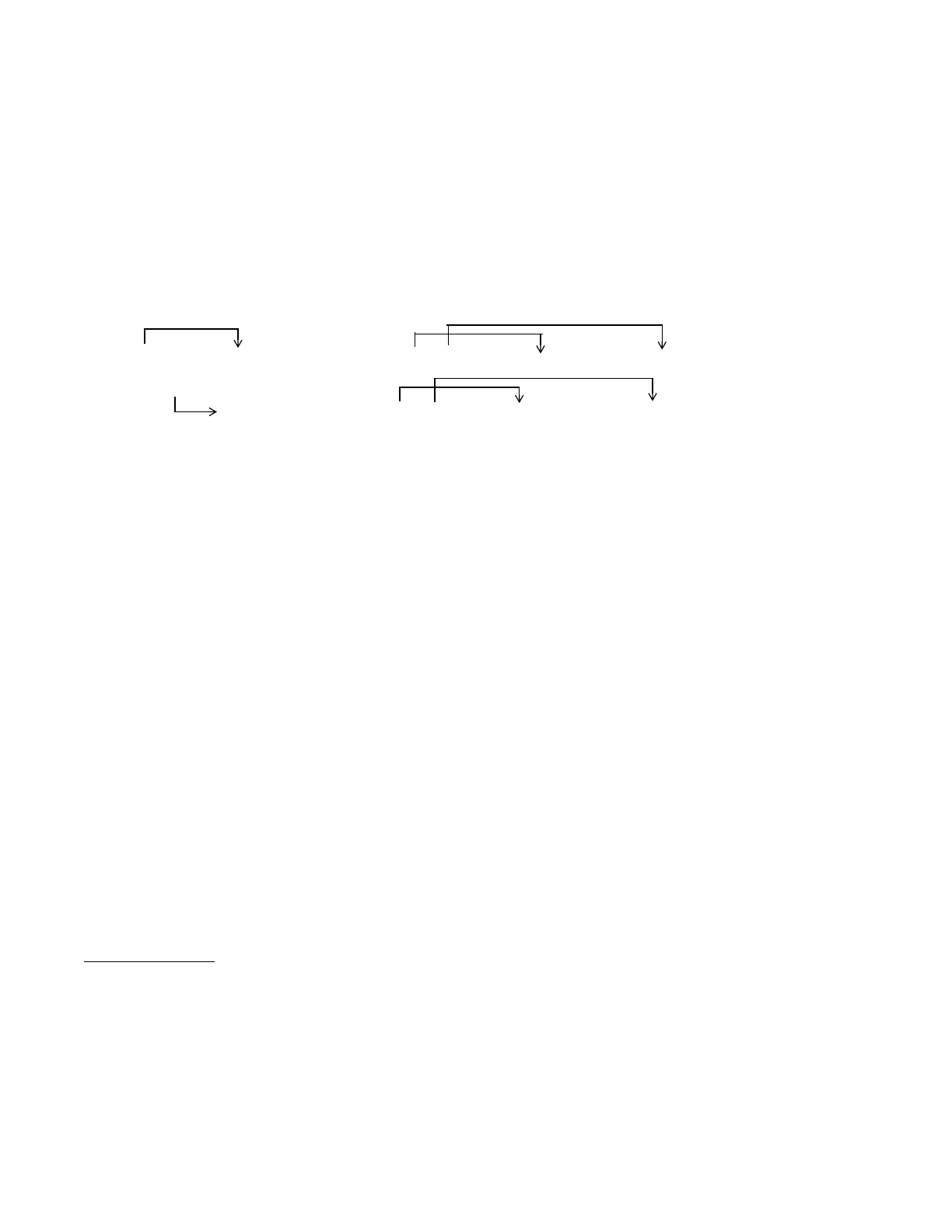
E-38 April 10, 2000
APPENDIX E
SOME IMPORTANT COMPLICATED ARRAYS
Flagging Cells and Surfaces
The values of IPTAL(LIPT+2,1,K) and the values of IPTAL(LIPT+2,2,K) are the locations in
ITDS of lists of the program numbers of flagging cells and flagging surfaces, respectively, for tally
K. The first item of each list is the number of cells or surfaces in the list.
Cell and Surface Bins
The value of IPTAL(LIPT+1,1,K) is the offset in ITDS of the description of the cell or surface bins
of cell or surface tally K. The structure of the description is
where
N= number of cell or surface bins in tally K
Pi= pointer to specifications for bin i
nij = number of cells or surfaces in level j of bin i
Iij = program number of a cell or surface in level j. If negative, it is a lattice cell and the
following three entries are element indices I,J,K).
Mi= number of levels in bin i minus one. If zero, no remaining data follows for this bin.
Lij = pointer to specifications for level j of bin i
Cell and Surface Tally Pointers
The value of LOCCT(I,J) if J is a cell—or LOCST(I,J) if J is a surface—is the location in ITDS of
a table which locates the sections of TAL where tally scoring is done when a particle of type I
passes through cell or surface J. The table is organized this way:
where
N= number of tallies for particle type I which include cell or surface J
Ti= program number of a tally
mi= number of bins that involve cell or surface J
Lji = cell or surface bin number
TDS(LTD) Array Tally Specifications
TDS contains blocks, in no particular order and accessed only through pointers, that contain some
of the specifications of the tallies of the problem. TDS is in dynamically allocated storage with
P1P2…PNn11 I11 I21…InI M1L12 L13…L1Mn12 I12I22…In2n13 I13 I23…
n21 I11 I21…In1M2L22 L23…L2Mn22 I12 I22…In2n23 I13 I23…
NT
1m1L11 L21…Lm1…TNmNL1NL2N…LmN

April 10, 2000 E-39
APPENDIX E
SOME IMPORTANT COMPLICATED ARRAYS
offset LTDS\null. LTDS is usually not explicit in the subscript of TDS because the values of the
various pointers into TDS include LTDS.
Detector Bins
For detector tally K, the value of IPTAL(LIPT+1,1,K) is the offset in TDS of the description of the
detector bins. The description contains the information from the F card, modified for faster use in
TALLYD. Five elements of TDS are used for each detector:
Point detector Ring detector
1X a
2Y r
3 Z 1, 2, or 3 for x, y, or z
4R R
5|2π R3/3| |2π R3/3|
Cell Contributions
For detector tally K, the value of IPTAL(LIPT+2,2,K) is the offset in TDS of the table of cell
contributions. The information in the table is exactly as it is on the PD card.
Simple Bins and Multipliers
The value of IPTAL(LIPT+I,1,K) for I = 3, 6, 7, or 8 is the offset in TDS of a table of bins for tally
K. The information in the table is as it came from the corresponding input card except that any T
or NT on the card does not appear in the table. The value of IPTAL(LIPT+I,2,K) for I = 6, 7, or 8
is the offset in TDS of a table of bin multipliers for tally K. The information in the table is exactly
as it is on the input card.
Segment Bin Divisors
For cell or surface tally K, the value of IPTAL(LIPT+4,2,K) is the offset in TDS of the table of
segment bin divisors. Except for a type 1 tally without any SD card, the table exists even if there is
no FS card. The table is a two-dimensional array. One dimension is for cell or surface bins and the
other is for the segment bins. The segment bin index changes faster. If segment bin divisors are not
provided on an SD card, they are calculated or derived from VOL or AREA data, if possible, by
MCNP according to the tally type:
tally type 2 4 6 7
divisor area volume mass mass
Multiplier Bins
The value of IPTAL(LIPT+5,2,K) is the offset in TDS of a table of the constant multipliers for the
multiplier bins from the FM card of tally K\null. If there is anything more on the FM card than just
a constant multiplier for each bin, the value of IPTAL(LIPT+5,1,K) is the offset in TDS of a table
of bin descriptions:

E-40 April 10, 2000
APPENDIX E
SOME IMPORTANT COMPLICATED ARRAYS
where
N= number of P's.
Pi= pointer to the description of a bin or attenuator. If the FM card has only a constant
for some bin, then Pi= 0 for that bin. If the FM card has C m but nothing more for a
bin, (which makes it a track-count bin), then Pi= −1. If Pi points to an attenuator
which appears inside parentheses on the FM card, it is negative.
Ii= for a regular bin, the program number of the material m specified on the FM card.
For an attenuator, Ii= −1.
ni= for a regular bin, the number of entries, including both reaction numbers and
operators, in the bin description. If the list of reaction numbers in the bin includes the
elastic or the total cross section, ni is negative. For an attenuator, ni is the number of
entries, including material numbers and superficial-density values. If a regular bin
appears on the FM card within parentheses that also contain an attenuator, ni has
10000000 added to it for an attenuator to the right of the bin and 20000000 for an
attenuator to the left.
Rji = for a regular bin, a reaction number or operator. The sum operator, indicated by a
colon on the FM card, is stored here as the value 100003. For an attenuator, the Rji are
alternating cell numbers and superficial-density values.
Dose Function
The value of IPTAL(LIPT+3,2,K) is the location in TDS of the dose function table for tally K. The
first element in the table is the length N. It is followed by the N values of the energy and then the
N values of the function. N is preceded by an indicator of the type of interpolation: 0 for log-log,
1 for lin-log, 2 for log-lin, and 3 for lin-lin.
TFC(6,20,NTAL) Array Tally Fluctuation Charts
The value of TFC(LTFC+I,J,K) is the tally value (I=1), the error (I=2), the figure of merit (I=3),
the variance of the variance (I=4), the Pareto slope (I=5), and a locator for the Pareto tail plot (I=6)
for line J of the tally fluctuation chart for tally K. The tally bin involved is designated by the eight
indices in JTF(LJTF+I,K) forI=1to8.Thenumber of histories run at the point where the entries
for a line were calculated is stored in NPC(J). Initially a line is calculated every 1000 histories.
When the 20th line is generated, the history increment is doubled. When the time comes to generate
the 21st line, the odd-numbered lines are eliminated, the data in line J are moved to line J/2 for
J = 2 to 20 by 2, and the new data are put in line 11.
NP
1P2…PNI1n1R11 R21…Rn1I2n2R12 R22…Rn2…

April 10, 2000 E-41
APPENDIX E
SOME IMPORTANT COMPLICATED ARRAYS
RTP(LRT) Array Information from Tally Input Cards
The information from most tally input cards is stored without much modification in temporary
array RTP. Numbers are stored as is. Special characters are encoded. After all the input cards have
been read, subroutine ITALLY sets up the permanent tally control arrays from the information in
RTP. The main reason for this two-step process is that some of the control arrays depend in a
complicated way on information from more than one input card. It is simpler to generate the
control arrays with all the input data available at the same time than to do it as the cards are read.
Pointer array IPNT(2,21,0:NTAL) is defined as the tally cards are read. The information from tally
card type J of tally K begins at RTP(LRTP+ \break IPNT(LIPN+1,J,K)) and occupies
IPNT(LIPN+2,J,K) elements of RTP. The tally card type numbers J are given in KRQ(3,N) for each
type N of input card. KRQ(3,N) is defined by DATA statements in block data subprogram
IBLDAT\null. KRQ(3,N) is zero for nontally input cards. There is no tally card type 1.
IPNT(LIPN+1,1,K) is used for bits that reflect T or NT on certain cards and indicate whether a total
bin needs to be included. The value of IPNT(LIPN+1,2,K) is 1, 2, 3, 4, or 5, depending on whether
the F card for the tally has blank, X, Y, Z, or W with the F, and it is negative if there is an asterisk
on that card.
D. Accounting Arrays
MCNP regularly collects and prints data on the behavior of the particles transported through the
problem geometry. This is accounting information which shows what MCNP actually did, in
contrast to the tallies which are estimates of physically measurable quantities. The accounting
information is essential to a user who is trying to make his problem run faster. The arrays where
the accounting data are collected and the titles of the tables where they are printed are as follows.
PAX Problem Summary
PAC Problem Activity in Each Cell (Print Table 126)
PWB Weight Balance in Each Cell (Print Table 130)
PAN Activity of Each Nuclide in Each Cell (Print Table 140)
PAX(6,20,MIPT) Array Problem Summary
The value of PAX(J,K,I) is the total of type I data for mechanism J and particle type K.
I
1 number of tracks created
2 weight created
PCC
FEBL Summary of Photons Produced in Neutron Collisions
}

E-42 April 10, 2000
APPENDIX E
SOME IMPORTANT COMPLICATED ARRAYS
3 energy created
4 number of tracks terminated
5 weight terminated
6 energy terminated
J Particle Creation Mechanism Loss Mechanism}
1 NPE source escape
2 NPE energy cutoff
3 NPE time cutoff
4 NPE weight window weight window
5 NPE cell importance cell importance
6 NPE weight cutoff weight cutoff
7 NPE energy importance energy importance
8 NP DXTRAN DXTRAN
9 NP forced collisions forced collisions
10 NP exponential transform exponential transform
For neutrons only
11 N upscattering downscattering
12 N capture
13 N (n,xn) loss to (n,xn)
14 N fission loss to fission
16 N alpha <0 time creation alpha >0 absorption
For photons only
11 P from neutrons Compton scatter
12 P bremsstrahlung capture
13 P p-annihilation pair production
14 P electron x-rays
15 P 1st fluorescence
16 P 2nd fluorescence
For electrons only
11 E pair production scattering
12 E Compton recoil bremsstrahlung
13 E photo-electric
14 E photon auger
15 E electron auger
16 E knock-on
For the printed table, the weight totals are divided by the number of histories and the energy totals
are divided by the total weight of source particles.

April 10, 2000 E-43
APPENDIX E
SOME IMPORTANT COMPLICATED ARRAYS
PAC(MIPT,10,MXA) Array Problem Activity in Each Cell
The value of PAC(LPAC+I,J,K) is the total of type J data for particle type I in cell K. If a particle
becomes lost, a small amount of erroneous information gets added into PAC.
J
1 number of tracks entering cell K
2 population of cell K: the number of tracks, including source tracks,, entering for the
first time
3 number of collisions in cell K
4 weight entering collisions
5 energy * time interval in cell K * weight
6 energy * path length * weight
7 path length in cell K
8 mean free path * path length * weight
9 time interval * weight
10 path length * weight
The quantities printed are
Tracks Entering = PAC(LPAC+I,1,K)
Population = PAC(LPAC+I,2,K)
Collisions = PAC(LPAC+I,3,K)
Collisions * weight (per history) = PAC(LPAC+I,4,K) / number of histories
Number Weighted Energy = PAC(LPAC+I,5,K) / PAC(LPAC+I,9,K)
Flux Weighted Energy = PAC(LPAC+I,6,K) / PAC(LPAC+I,10,K)
Average Track Weight (Relative) = PAC(LPAC+I,10,K) * importance of cell K /
[PAC(LPAC+I,7,K) * importance of source cell]
Average Track MFP = PAC(LPAC+I,8,K) / PAC(LPAC+I,10,K)
PWB(MIPT,20,MXA) Array Weight Balance in Each Cell
The value of PWB(LPWB+I,J,K) is the net weight change of type J for particle type I in cell K. If
a particle becomes lost, a small amount of erroneous information gets added into PWB. Table
values are divided by the number of histories before being printed.
J Table Heading
External
1 Entering weight of particles entering cell K
2 Source weight of created source particles
3 Time Cutoff weight of particles killed by time cutoff
4 Energy Cutoff weight of particles killed by energy cutoff
5 Exiting weight of particles exiting cell K
20 Alpha weight of alpha time creation/absorption

E-44 April 10, 2000
APPENDIX E
SOME IMPORTANT COMPLICATED ARRAYS
Variance Reduction
6 Weight Window net weight change due to weight-window Russian roulette
7 Cell Importance net weight change due to splitting and Russian roulette in
importance sampling
8 Weight Cutoff net weight change due to weight cutoff
9 Energy Importance net weight change due to energy splitting and Russian roulette
10 DXTRAN net weight change due to DXTRAN
11 Forced Collision net weight change due to forced collision
12 Exponential net weight change due to exponential transform
Transform
Physical (neutrons)
13 (n,xn) weight of new tracks produced by other nonfission processes
14 Fission weight of fission neutrons produced
15 Capture weight lost to capture
16 Loss to (n,xn) weight of neutrons lost to (n,xn)
17 Loss to Fission weight of neutrons lost to fission
Physical (photons)
13 From Neutrons weight of neutron-induced photons
14 Bremsstrahlung net weight created by bremsstrahlung
15 P-annihilation net weight created by p-annihilation
16 Electron x-rays net weight created by electron x-rays
17 Fluorescence net weight created by double fluorescence
18 Capture weight lost to capture
19 Pair Production net weight created by pair production
Physical (electrons)
13 Pair production net weight created by pair producction
14 Compton recoil net weight created by Compton scatter
15 Photo-electron net weight created by photo-electrons
16 Photon Auger net weight created by photon auger
17 Electron Auger net weight created by electron auger
18 Knock-on net weight created by knock-ons
PAN(2,6,NPN) Array Activity of Each Nuclide in Each Cell
The value of PAN(LPAN+I,J,IPAN(LIPA+K)+N–1) is the total of type J data for particle type I for
the Nth nuclide in cell K. IPAN(LIPA+M+1) = IPAN(LIPA+M) + number of nuclides in the
material of cell M. IPAN(LIPA+1) = 1 and NPN = IPAN(LIPA+MXA+1) −1. If a particle becomes
lost, a small amount of erroneous information gets added into PAN.

April 10, 2000 E-45
APPENDIX E
SOME IMPORTANT COMPLICATED ARRAYS
J (for neutrons)
1 number of collisions with Nth nuclide of cell K
2 weight entering collisions
3 weight lost to capture
4 weight gain by fission
5 weight gain by other inelastic processes
6 unused
J (for photons)
1 number of collisions with Nth nuclide of cell K
2 weight entering collisions
3 weight lost to capture
4 number of neutron-induced photons
5 weight of neutron-induced photons
6 energy * weight of neutron-induced photons
The quantities printed are
Total Collisions = PAN(LPAN+I,1,L)
Collisions * Weight = PAN(LPAN+I,2,L) / number of histories
Weight Lost to Capture = PAN(LPAN+I,3,L) / number of histories
Weight Gain by Fission = PAN(LPAN+1,4,L) / number of histories
Weight Gain by (n,xn) = PAN(LPAN+1,5,L) / number of histories
Total From Neutrons = PAN(LPAN+2,4,L)
Weight from Neutrons = PAN(LPAN+2,5,l) / number of histories
Avg Photon Energy = PAN(LPAN+2,6,L) / PAN(LPAN+2,5,L)
PCC(3,MXA) Array Summary of Photons Produced in Neutron Collisions
The value of PCC(LPCC+J,K) is the total of type J data for cell K. If a particle becomes lost, a
small amount of erroneous information may be added into PCC.
J
1 number of neutron-induced photons
2 weight of neutron-induced photons
3 weight * energy of neutron-induced photons
The quantities printed are
Number of Photons = PCC(LPCC+1,K)
Weight Per Source Neutron = PCC(LPCC+2,K) / number of histories
Energy Per Source Neutron = PCC(LPCC+3,K) / number of histories
Avg Photon Energies = PCC(LPCC+3,K) /PCC(LPCC+2,K)
Energy/Gram Per Source Neutron = PCC(LPCC+3,K) /
[cell mass * number of histories]
Weight/Neutron Collision = PCC(LPCC+2,K) / PAC(LPAC+1,4,K)
Energy/Neutron Collision = PCC(LPCC+3,K) / PAC(LPAC+1,4,K)

E-46 April 10, 2000
APPENDIX E
SOME IMPORTANT COMPLICATED ARRAYS
FEBL(2,K) Array Summary of Photons Produced in Neutron Collisions
The value of FEBL(J,K) is the total of type J data for photon energy bin K, where K=16 for
continuous energy problems and K=IGM=number of multigroup energy groups. The energy bin
bounds are in array EBL(K) in common block /TABLES/.
J
1 number of neutron-induced photons
2 weight of neutron-induced photons
The quantities printed are
Number of Photons = FEBL(1,K)
Number Frequency = FEBL(1,K) / PAX(2,1,3)
Weight of Photons = FEBL(2,K) / number of histories
Weight Frequency = FEBL(2,K) / PAX(2,2,3)
E. KCODE Arrays
OSUM(I) Array Cumulative keff over active cycles
OSUM(I) = OSUM(I) + SUMK(I)/NSRCK, I=1,3.
OSUM2(I,J) Array Cumulative keff covariance quantities
OSUM2(I,J) = OSUM2(I,J) + ZZ(I) * ZZ(J)
where ZZ(K) = SUMK(K)/NSRCK.
RLT(I,J) Array Prompt removal lifetimes for current active cycle
RLT(I,J) Prompt removal lifetimes for current active cycle.
I = 1/2/3/4 = collision/absorption/track length/fission
J = 1 sum of WGT*TME over cycle
J = 2 sum of WGT over cycle
Note: RLT(4,1) is summed over all histories and used only for the fission lifespan.
RLT(4,2) unused.
RKPL(19,MRKP) Array KCODE Quantities for Plotting
The value of RKPL(LRKP+I,J) for the Jth cycle of a KCODE or ACODE problem:
J
1keff (collision)
2keff (absorption)
3keff (track length)
4 prompt removal life (collision)

April 10, 2000 E-47
APPENDIX E
SOME IMPORTANT COMPLICATED ARRAYS
5 prompt removal life (absorption)
6 average collision keff
7 average collision keff standard deviation
8 average absorption keff
9 average absorption keff standard deviation
10 average track length keff
11 average track length keff standard deviation
12 average col/abs/trk-len keff
13 average col/abs/trk-len keff standard deviation
14 average col/abs/trk-len keff by cycles skipped
15 average col/abs/trk-len keff by cycles skipped standard deviation
16 prompt removal lifetime (col/abs/trk-len)
17 prompt removal lifetime (col/abs/trk-len) standard deviation
18 number of histories used in each cycle
19 col/abs/trk-len keff figure of merit
The value of RKPL(LRKP+I,J) for the Jth cycle of an ACODE problem:
20 imposed alphas vs. cycle number
21 imposed delta alpha vs cycle number (i.e., how much alpha is incremented each cycle)
22 average imposed alpha vs. cycle
23 relative error on average alpha vs. cycle number
24 average delta alpha vs. cycle number (should approach zero)
25 standard deviation of delta alpha vs. cycle number
26 ln-ln regression fit alpha vs. cycle number
27 linear regression fit alpha using alpha=a+b*keff vs. cycle number
28 linear regression fit alpha using keff=a+b*alpha vs. cycle number
29 alpha figure of merit (fom) vs. cycle number
30 alpha vs. the keff estimator used to estimate alpha
31 keff estimator to estimate alpha vs. alpha
32 linear estimate of dalpha/dkeff (should be negative) vs. cycle number
33 ln-ln estimate of dalpha/dkeff (should be negative) vs. cycle number
34 alpha values by alpha cycles skipped vs. cycles skipped (keff cycle kalsav+1 is zero
alpha cycles skipped)
35 alpha relative error by cycles skipped vs cycles skipped
RSUM(I) Array Cumulative prompt removal lifetimes over active cycles
RSUM(I) = RSUM(I) + RLT(I,1)/RLT(I,2), I=1,3.
RSUM2(I,J) Array Cumulative prompt removal lifetime covariance quantities
RSUM2(I,J) = RSUM2(I,J) + RL(I) * RL(J)
where RL(K) = RLT(K,1)/RLT(K,2).\cr}

E-48 April 10, 2000
APPENDIX E
SOME IMPORTANT COMPLICATED ARRAYS
SUMK(I) Array SUMK(I)/NSRCK is keff for current cycle
I = 1/2/3 = collision/absorption/track length
SUMP(3*NPERT) Array Track length estimate of keff for each perturbation, IP=1,NPERT
SUMP(IP) track length estimate of keff for current cycle
SUMP(NPERT+IP) cumulative SUMP(IP) over all cycles
SUMP(2*NPERT+IP) cumulative SUMP(IP)**2 to get standard deviations
SUMP(LSUM+IP),IP=1,NPERT is like SUMK(3)
SUMP(LSUM+NPERT+IP) is like OSUM(3)
SUMP(LSUM+2*NPERT+IP) is like OSUM2(3,3)
In multitasking, SUMP(KSUM+IP) is accumulated into SUMP(LSUM+IP), but there is no
need for nor space saved for SUMP(KSUM+NPERT+IP) or SUMP(KSUM+2*NPERT+IP).
F. Alpha Arrays
ALFA(1) Collision estimate of alpha generation time
ALFA(2) 1st order change in alfa(1) (<0)
ALFA(3) 2nd order change in alfa(1) (>0)
ALPHA(1) Imposed alpha for current cycle
ALPHA(2) Unused
ALPHA(3) Sum of keff (alpha)
ALPHA(4) Sum of alpha(1)
ALPHA(5) Sum of alpha(1) * keff (alpha)
ALPHA(6) Sum of keff (alpha)**2
ALPHA(7) Sum of alpha(1)**2
ALPHA(8) Sum of delta alpha
ALPHA(9) Sum of (delta alpha)**2
ALPHA(10) Sum of xl; xl = log(keff (alpha))
ALPHA(11) Sum of al; al = max(log(alpha(1)),log(1e–3))
ALPHA(12) Sum of al*xl
ALPHA(13) Sum of xl**2
G. Universe Map/ Lattice Activity Arrays for Table 128
MAZP(3,MXA) Array Used in RSLMAZ to point inside MAZE array.
MAZP(1,IC) = I, index of cell IC in MAZU(j) list.
MAZP(2,IC) = universe address J of cell IC.
MAZP(3,IC) = address J of universe filling cell IC.

April 10, 2000 E-49
APPENDIX E
SOME IMPORTANT COMPLICATED ARRAYS
MAZU(NMZU) Array Used in RSLMAZ to point inside MAZE array. The MAZE(NMAZ)
array cointains the number of sources, tracks entering and collisions in each repeated structures/
lattice element for each
MAZU(J-3) = I = universe name.
MAZU(J-2) = finite lattice cell filling universe I.
MAZU(J-1) = total number of lowest level elements below U=I.
MAZU(J) = NE = number of cells/elements in universe I.
MAZU(J+K) = number of elements below Kth cell/universe.
MAZU(J+NE+K) = Kth cell in universe I (repeated structures).
MAZU(J+NE+K) = first cell of universe filling Kth lattice element.
H. Weight Window Mesh Parameters
WWM(1-3) total number of fine meshes in x,y,z or r,z,theta directions
WWM(4-6) origin (corner of box for rectangular geometry, bottom & center point for
cylindrical geometry)
WWM(7-9) number of coarse meshes in each direction
WWM(10-12) cylindrical geometry top center point
WWM(13-15) cylindrical geometry point on radius and bottom plane
WWM(16-18) cylindrical geometry direction cosines from bottom center point to point
on radius
WWM(19) cylindrical geometry radius
WWM(20-22) cylindrical geometry cosines of axis
WWM(23) cylindrical geometry axis length
WWM(24-26) cylindrical geometry direction cosines of the cross product of the radial
direction and axial direction; necessary for full revolution theta
determination
WGM(NWGM) weight window mesh geometric data with the inclusion of 0th index entries
for each dimension. The data are stored as cumulative values.
I. Perturbation Parameters
DPTB(3,NPERT*MNNM) Array PERT card density changes which become the perturbation
coefficients fixed at code initiation. For each nuclide, J, of perturbation IP where
J=NPTB(IP),NPTB(IP+1)+1, DPTB(LDPT+I,J) has the following values:
I Description
1 nuclide index, IEX
2δ1∆v
3δ2∆v

E-50 April 10, 2000
APPENDIX E
SOME IMPORTANT COMPLICATED ARRAYS
where ∆v is the density change term (see page 2–192) of the Taylor Series expansion. δ1= 1/0 if
the 1st order perturbation is on (METHOD=1,2) or off. δ2= 1/0 if the 2nd order perturbation is on
(METHOD=1,3) or off.
IPTB(2+2*NPKEY,NPERT) Array Pointers to RPTB array and other perturbation parameters
from PERT card.
The 6 NPKEY perturbation key words are CELL, MAT, RHO, RXN, ERG and METHOD. For
perturbation IP=1,NPERT,
IPTB(LIPB+1,IP) = perturbation number from PERT card
IPTB(LIPB+2,IP) = particle type from PERT card
IPTB(LIPB+1+2*K,IP) = number of entries for keyword K
IPTB(LIPB+2+2*K,IP) = location in RPTB of PERT card data for keyword K
Exception:
IPTB(LIPB+13,IP) = 1/2/3 = METHOD
IPTB(LIPB+14,IP) = 0 for method = 1/2/3;
= 1 for METHOD = -1/–2/–3
Example: PERT6:N,P CELL78912 METHOD = −2
IPTB = 6 3 4 12345 0 0 0 0 0 0 0 0 2 1
RPTB(12345) = 7. 8. 9. 12.
NPTB(NPERT+1) Array Cumulative number of perturbed cross sections used as pointers to
DPTB and PTB arrays. NPTB(IP) points to the first nuclide data in DPTB and PTB for the material
of perturbation IP. Thus perturbation IP has NPTB(IP+1) – NPTB(IP) ≤ MNNM nuclides in its
perturbed material, and the entries in the PTB and RPTB arrays for these nuclides are stored from
NPTB(IP) to NPTB(IP+1) –1.
PTB(5,NPERT*MNNM) Array Perturbation coefficients. The perturbation coefficients P1j' and
P2j' described in Chapter 2 (see page 2–198) are stored in the PTB(LPTB+I,J) array where
J=NPTB(IP),NPTB(IP+1) –P1 for the NPTB(IP+1) – NPTB(IP) nuclides of perturbation IP.
PTB(KPTB+1,J) = P1j'
PTB(KPTB+2,J) = P2j'
PTB(KPTB+3,J) = xb(E′)the macroscopic cross section nuclide J at E′
PTB(KPTB+4,IP) = P1j' ∆v+ (P2j' +
PTB(KPTB+5,J) = xc(E)
1
2
---P1j′
2∆v2

April 10, 2000 E-51
APPENDIX E
SOME IMPORTANT COMPLICATED ARRAYS
The perturbed value of keff or a tally is then the unperturbed value times PTB(KPTB+4,IP). If the
nuclides in the perturbation are also in the tally (F6, F7, or F4 with FM card with negative constant
for atom density multiplier), then PTB(KPTB+4,IP) is corrected by adding R1j'∆v+P1j'R1j'∆v2
where
Note that xb(E) at collision kis saved as PTB(KPTB+3,J) to be used as xb(E′)at collision k+1. Also
note that PTB(KPTB+4,IP) is stored by perturbation number IP, not J like the rest of the PTB array,
leaving NPERT*MNNM - NPERT words unused.
RPTB(IPERT) Array Perturbation parameters from PERT card. RPTB(LRPT+I) stores the
keywords read from the PERT card as pointed by the IPTB array (see above).
J. Macrobody and Identical Surface Arrays
IDNA(K) exactly parallels the LJA(K) array for cell cards
= 0 when slot k does not involve a macrobody surface
= n with n>o, is facet n of macrobody
=-n is facet, but cell card is only using this one facet
IDNT(J) program surface number of master identical surface
= 0, j is not an identical surface
=j′,|j′|is the master surface of identical surfaces. The sense gives the sense of
surface j with respect to the sense of the master surface j′
IDNS(J) locator in IDNE for list of identical surfaces
=0 no identical surfaces
=m with m locator in IDNE
IDNE(M) list of identical surfaces
=n number of identical surfaces for surface j
next n entries are the identical program surfaces (j’s)
IDNE(1) is the number of identical surface sets
IDNE(2) is the total length of IDNE
R1j′
xcE()
EH∈
∑
cB∈
∑
xcE()
cC∈
∑
----------------------------------------
PTB(KPTB+5,J)
J
∑
PTBTC
--------------------------------------------------==

18 December 2000 F–1
APPENDIX F
DATA TYPES AND CLASSES
APPENDIX F
DATA TABLE FORMATS
MCNP has two types and eight classes of data. These data are kept in individual tables that are
often organized into libraries. These tables are located with the XSDIR data directory file. These
terms, tables, and the basic data table formats are described in this appendix in the following
sections:
I. DATA TYPES AND CLASSES
MCNP reads eight classes of data from two types of data tables. The two types of data tables are:
1. Type 1—standard formatted tables (sequential, 80 characters per record). These portable
libraries are used to transmit data from one installation to another. They are bulky and
slow to read. Few installations use Type 1 tables in MCNP directly. Most generate Type
2 tables from Type 1 tables using the MAKXSF code (see Appendix C).
2. Type 2—standard unformatted tables (direct-access, binary) locally generated from
Type 1 tables. They are not portable except between similar systems such as various
UNIX platforms. Type 2 tables are used most because they are more compact and faster
to read than Type 1 tables.
Data tables exist for eight classes of data: continuous-energy neutron, discrete-reaction neutron,
continuous-energy photon interaction, continuous-energy electron interaction, neutron dosimetry,
S(α,β) thermal, neutron multigroup, and photon multigroup. A user should think of a data table as
an entity that contains evaluation-dependent information about one of the eight classes of data for
a specific target isotope, element, or material. For how the data are used in MCNP, a user does not
need to know whether a particular table is in Type 1 or Type 2. For any ZAID, the data contained
Page
I. Data Types and Classes F–1
II. XSDIR – Data Directory File F–2
III. Data Tables F–4
IV. Data Blocks for Neutron Continuous–Energy and Discrete
Transport Tables F–12
V. Data Blocks for Dosimetry Tables F–34
VI. Data Blocks for Thermal S(α,β Tables F–35
VII. Data Blocks for Photon Transport Tables F–38
VIII. Format for Multigroup Transport Tables F–40
IX. Data Blocks for Electron Transport Tables F–52

F–2 18 December 2000
APPENDIX F
XSDIR— DATA DIRECTORY FILE
on Type 1 and Type 2 tables are identical. Problems run with one data type will track problems run
with the same data in another format type.
When we refer to data libraries, we are talking about a series of data tables concatenated into one
file. All tables on a single library must be of the same type but not necessarily of the same class.
For example, the Type 1 library for the MCNP test set contains six classes of data. There is no
reason, other than convenience, for having data libraries; MCNP could read exclusively from
individual data tables not in libraries.
II. XSDIR— DATA DIRECTORY FILE
MCNP determines where to find data tables for each ZAID in a problem based on information
contained in a system-dependent directory file XSDIR. The directory file is a sequential formatted
ASCII file with 80-character records (lines) containing free-field entries delimited by blanks.
The XSDIR file has three sections. In the first section, the first line is an optional entry of the form:
DATAPATH = datapath
where the word DATAPATH (optionally capitalized) must start in column 1.
The = sign is optional. The directory where the data libraries are stored is datapath. The xsdir
directory file can be renamed by item 1. The search hierarchy to find the data libraries is:
1. xsdir= cross-section directory file name on the MCNP execution line;
2. DATAPATH = datapath in the INP file message block;
3. the current directory;
4. the DATAPATH entry on the first line of the XSDIR file;
5. the unix environmental variable setenv DATAPATH datapath;
6. the individual data table line in the XSDIR file (see below under Access route); or
7. the directory specified at MCNP compile time in the BLOCK DATA subroutine.
The second section of the XSDIR file is the atomic weight ratios. This section starts with the words
“ATOMIC WEIGHT RATIOS” (capitalization optional) beginning in column 1. The following
lines are free-format pairs of ZAID AWR, where ZAID is an integer of the form ZZAAA and AWR
is the atomic weight ratio. These atomic weight ratios are used for converting from weight fractions
to atom fractions and for getting the average Z in computing electron stopping powers. If the
atomic weight ratio is missing for any nuclide requested on an Mn card, it must be provided on the
AWTAB card.

18 December 2000 F–3
APPENDIX F
XSDIR— DATA DIRECTORY FILE
The third section of the XSDIR file is the listing of available data tables. This section starts with
the word “DIRECTORY” (capitalization optional) beginning in column 1. The lines following
consist of the seven– to ten–entry description of each table. The ZAID of each table must be the
first entry. If a table requires more than one line, the continuation is indicated by a +at the end of
the line. A zero indicates the entry is inapplicable. Unneeded entries at the end of the line can be
omitted.
The directory file has seven to eleven entries for each table. They are:
1. Name of the table character * 10
2. Atomic weight ratio real
3. File name character
4. Access route character * 70
5. File type integer
6. Address integer
7. Table length integer
8. Record length integer
9. Number of entries per record integer
10. Temperature real
11. Probability table flag character
1. Name of the Table. This is usually the ZAID: 3 characters for Z, 3 characters for A, a decimal
point, 2 characters for evaluation identification, and a tenth character used to identify
continuous energy tables by the letter C, discrete-reaction tables by D, dosimetry tables by Y,
S(α,β) thermal tables by T, continuous-energy photon tables by P, continuous-energy
electron tables by E, multigroup neutron tables by M, and multigroup photon tables by G. For
the S(α,β) tables, the first 6 characters contain a mnemonic character string, such as
LWTR.01T.
2. Atomic Weight Ratio. This is the atomic mass divided by the mass of a neutron. The atomic
weight ratio here is used only for neutron kinematics and should be the same as it appears in
the cross-section table so that threshold reactions are correct. It is the quantity Aused in all
the neutron interaction equations of Chapter 2. This entry is used only for neutron tables.
3. File Name. The file name is the name of the library that contains the table and is a string of
eight characters in a form allowed by the local installation.
4. Access Route. The access route is a string of up to 70 characters that tells how to get ahold of
the file if it is not already accessible. At Los Alamos on UNICOS, it is a CFS path name. On
other systems it might be a UNIX directory path. If there is no access route, this entry is zero.
5. File Type. 1 or 2.
6. Address. For Type 1 files the address is the line number in the file where the table starts. For
Type 2 files, it is the record number of the first record of the table.

F–4 18 December 2000
APPENDIX F
DATA TABLES
7. Table Length. A data table consists of two blocks of information. The first block is a
collection of pointers, counters, and character information. The second block is a solid
sequence of numbers. For Type 1 and Type 2 tables, the table length is the length (total
number of words) of the second block.
8. Record Length. This entry is unused for Type 1 files and therefore is zero. For Type 2 direct
access files it is the processor-dependent attribute called the record length. The record length
is a multiple of the number of entries per record where the multiple is 1 for VMS and the
multiple is the number of 8-bit bytes in the record for most other systems. Thus for 512 entries
per record, the record length is 4096 for UNICOS, 4096 for double-precision data on unix
workstations (electron data are always double precision on single-precision platforms), 2048
for single-precision data on unix workstations, etc.
9. Number of Entries per Record. This is unused for Type 1 files and therefore is zero. For Type
2 files it is the number of items per record in the second block of the table. Usually this entry
is set to 512.
10. Temperature. The temperature in MeV at which a neutron table was processed. This entry is
used only for neutron data.
11. Probability table flag. The character word “ptable” indicates a continuous-energy neutron
nuclide has unresolved resonance range probability tables.
III. DATA TABLES
The remainder of this Appendix is designed for the user who wishes to know a great deal about
how data are stored in data tables and in MCNP. First we describe how to find a specific table on a
Type 1 or Type 2 library. Then we document the detailed format of the various blocks of
information for each class of data.
Three arrays are associated with each data table. The NXS array contains various counters and
flags. The JXS array contains pointers. The XSS array contains all of the data. These arrays are the
same regardless of the type of a specific table. The arrays are manipulated internally by MCNP.
Within a data table, the counter and pointer arrays are dimensioned to NXS(16) and JXS(32). In
MCNP the same arrays are dimensioned to NXS(16,IEX) and JXS(32,IEX), where IEX is the
index of the particular table in the problem. There is no limit to the number of tables or their size
other than available space on a particular computing platform.
To locate data for a specific table (external to MCNP) it is necessary to extract several parameters
associated with that table from the directory file XSDIR. The file name obviously indicates the
name of the library that the table is stored on. Other important parameters from the viewpoint of
this Appendix are file type (NTY), address (IRN), table length (ITL), and number of entries per
record (NER).

18 December 2000 F–5
APPENDIX F
DATA TABLES
A. Locating Data on a Type 1 Table
Because Type 1 tables are 80-character card-image files, the XSDIR address IRN is the line number
of the first record, or the beginning, of the table. The first 12 records (lines) contain miscellaneous
information as well as the NXS and JXS arrays. The format follows.
The variables are defined in Tables F.1–F.3 for neutron, photon, dosimetry and S(α,β) thermal
libraries. These variables are defined in TABLE F-32 and TABLE F-33 for multigroup data.
The XSS array immediately follows the JXS array. All data from the XSS array are read into
MCNP with a 4E20.0 format. (When Type 1 tables are created, floating-point numbers are written
in 1PE20.12 format and integers are written in I20 format.) The length of the XSS array is given
by the table length, ITL, in the directory (also by NXS(1) in the table itself). The number of records
required for the XSS array is (ITL+3)/4. A Type 1 library is shown in Figure F-1.
Figure F-1.
Address
Relative Absolute Contents Format
1 IRN HZ,AW(0),TZ,HD A10,2E12.0,1X,A10
2 IRN+1 HK,HM A70,A10
3–6 IRN+2 (IZ(I),AW(I),I=1,16) 4(I7,F11.0)
7–8 IRN+6 (NXS(I),I=1,16) 8I9
9–12 IRN+8 (JXS(I),I=1,32) 8I9
Layout of a Type 1 Library
Starting Address
(Line Number) Number of Records Contents
IRN1=1
IRNi, ITLi are the addresses and tables lengths from XSDIR
12 misc. including NXS1, JXS1
IRN1+12 (ITL1+3)/4 XSS1
IRN212 misc. including NXS2, JXS2
IRN2+12 (ITL2+3)/4 XSS2
.
..
..
.
IRNn12 misc. including NXSn, JXSn
n=number of tables contained on library
IRNn+12 (ITLn+3)/4 XSSn

F–6 18 December 2000
APPENDIX F
DATA TABLES
TABLE F-1
Definition of the NXS Array
NTY 1 or 2
Continuous energy
or Discrete reaction
Neutron
3
Dosimetry 4
Thermal 5
Continuous energy
Photon
NXS(1) Length of second
block of data Length of second
block of data Length of second
block of data Length of second
block of data
NXS(2) ZA=1000*Z+A ZA=1000*Z+A IDPNI=inelastic
scattering mode Z
NXS(3) NES=number of
energies NIL=inelastic
dimensioning
parameter
NES=number of
energies
NXS(4) NTR=number of
reactions excluding
elastic
NTR=number
of reactions NIEB=number of
inelastic exiting
energies
NFLO=length of
the fluorescence
data divided by 4
NXS(5) NR=number of
reactions having
secondary neutrons
excluding elastic
IDPNC=elastic
scattering mode
NXS(6) NTRP=number of
photon production
reactions
NCL=elastic
dimensioning
parameter
NXS(7) IFENG=secondary
energy mode
NXS(8) NPCR=number of
delayed neutron
precursor families
......
......
......
NXS(15) NT=number of PIKMT reactions
NXS(16) 0=normal photon production
–1=do not produce photons
Note that many variables are not used, allowing for expansion in the future.

18 December 2000 F–7
APPENDIX F
DATA TABLES
TABLE F-2
Definition of the JXS Array
NTY 1 or 2
Continuous energy
or Discrete reaction
Neutron
3
Dosimetry 4
Thermal 5
Continuous energy
Photon
JXS(1) ESZ=location of energy
table LONE=location
of first word of
table
ITIE=location of
inelastic energy
table
ESZG=location of
energy table
JXS(2) NU=location of fission
nu data ITIX=location of
inelastic cross
sections
JINC=location of
incoherent form
factors
JXS(3) MTR=location of
MT array MTR=location of
MT array ITXE=location
of inelastic
energy/angle
distributions
JCOH=location of
coherent form
factors
JXS(4) LQR=location of
Q-value array ITCE=location of
elastic energy
table
JFLO=location of
fluorescence data
JXS(5) TYR=location of
reaction type array ITCX=location of
elastic cross
sections
LHNM=location of
heating numbers
JXS(6) LSIG=location of table
of cross-section locators LSIG=location of
table of cross-
section locators
ITCA=location of
elastic angular
distributions
JXS(7) SIG=location of cross
sections SIGD=location of
cross sections
JXS(8) LAND=location of table
of angular distribution
locators
JXS(9) AND=location of
angular distributions
JXS(10) LDLW=location of table
of energy distribution
locators
JXS(11) DLW=location of energy
distributions

F–8 18 December 2000
APPENDIX F
DATA TABLES
JXS(12) GPD=location of photon
production data
JXS(13) MTRP=location of
photon production MT
array
JXS(14) LSIGP=location of table
of photon production
cross-section locators
JXS(15) SIGP=location of photon
production cross
sections
NXS(16) LANDP=location of
table of photon
production angular
distribution locators
JXS(17) ANDP=location of
photon production
angular distributions
JXS(18) LDLWP=location of
table of photon
production energy
distribution locators
JXS(19) DLWP=location of
photon production
energy distributions
JXS(20) YP=location of table of
yield multipliers
JXS(21) FIS=location of total
fission cross section
JXS(22) END=location of last
word of this table END=location of
last word of this
table
JXS(23) LUNR=location of
probability tables
JXS(24) DNU=location of
delayed nubar data
TABLE F-2 (Cont.)
Definition of the JXS Array

18 December 2000 F–9
APPENDIX F
DATA TABLES
JXS(25) BDD=location of basic
delayed data (λ’s,
probabilities)
JXS(26) DNEDL=location of
table of energy
distribution locators
JXS(27) DNED=location of
energy distributions
......
JXS(32)
Note that many variables are not used, allowing for easy expansion in the future.
All pointers in the JXS array refer to locations in the XSS array.
JXS(1) always points to the first entry in the second block of data.
TABLE F-3
Definition of Miscellaneous Variables on Data Tables
HZ—10 character name (ZAID) of table. The form of HZ is
ZZZAAA.nnC continuous-energy neutron
ZZZAAA.nnD discrete-reaction neutron
ZZZAAA.nnY dosimetry
XXXXXX.nnT thermal S(α, β)
ZZZ000.nnP continuous-energy photon
ZZZ000.nnM neutron multigroup
ZZZ000.nnG photon multigroup
ZZZ000.nnE continuous-energy electron
where ZZZ is the atomic number
AAA is the mass number
XXXXXX for thermal data is a Hollerith name or abbreviation of the material
nn is the evaluation identifier
AW(0)—atomic weight ratio; the atomic weight divided by the mass of a neutron
TZ—temperature at which the data were processed (in MeV)
HD—10-character date when data were processed
HK—70-character comment
HM—10-character MAT identifier
TABLE F-2 (Cont.)
Definition of the JXS Array

F–10 18 December 2000
APPENDIX F
DATA TABLES
B. Locating Data on a Type 2 Table
A standard unformatted file consists of many records, each with NER entries, where NER is the
number of entries per record defined on XSDIR. A Type 2 data table consists of one record that
contains pointers, counters, and character information, followed by one or more records containing
the XSS array.
The information contained in the first record for each table is the same as that contained in the first
twelve lines of a Type 1 table described above. The variables, in order, are HZ, AW(0), TZ, HD,
HK, HM, (IZ(I),AW(I),I=1,16), (NXS(I),I=1,16), (JXS(I),I=1,32). The variables are defined in
Tables F.1–F.3. HZ, HD, and HM are 10-character variables and HK is a 70-character variable.
Floating-point variables may be double precision in some cases. The number of words contained
in this “package” of information is therefore different for different computing systems. The
remainder of the first record is empty. The next NREC records (NREC ≥1) contain the XSS data
array, with NREC=(ITL+NER−1)/NER, where ITL is the table length.A Type 2 library is shown
in Figure F-2.
Figure F-2.
(IZ(I),AW(I),I=1,16)—16 pairs of ZZZAAAs and atomic weight ratios. In the past these
were needed for photon tables but are now ignored. The IZ entries are still needed for
thermal tables to indicate for which isotope(s) the scattering data are appropriate.
Address
Layout of a Type 2 Library
Contents
IRN1= 1 misc. including NXS1, JXS1
2 XSS1NER <ITL1≤2*NER
3 XSS1 (cont)
IRN2 = 4 misc. including NXS2, JXS2
5 XSS2ITL2≤NER
.
..
..
IRNn = MAX–3 misc. including NXSn, JXSn
MAX–2 XSSn
MAX–1 XSSn (cont) 2*NER <ITLn≤3*NER
MAX XSSn (cont)
(Records per table are examples only)
n=number of tables contained on library
MAX=number of records contained on library
IRNi, ITLi, NER are the addresses, table lengths, and entries per record from XSDIR
TABLE F-3 (Cont.)
Definition of Miscellaneous Variables on Data Tables

18 December 2000 F–11
APPENDIX F
DATA TABLES
C. Locating Data Tables in MCNP
The NXS and JXS arrays exist in MCNP for each data table. The information contained in the
(2-dimensional) arrays in MCNP mirrors the information contained in NXS and JXS
(1-dimensional) on the individual tables. The current dimensions are NXS(16) and JXS(32) on the
data tables and NXS(16,∞) and JXS(32,∞) in MCNP, where ∞indicates variable dimensioning. In
the code, the arrays are usually referenced as NXS(I,IEX) and JXS(I,IEX), where IEX is the index
to a particular table.
The data from all cross-section tables used in an MCNP problem are in the XSS array, a part of
dynamically allocated common. The data from the first table appear first, followed by the data from
the second table, etc., as shown in Figure F-3. The pointers in the JXS array indicate absolute
locations in the XSS array.
Diagram of Data Storage in MCNP
XSS
Figure F-3.
The definitions of the variables in the NXS and JXS arrays (TABLE F-1 and TABLE F-2) are the
same in MCNP as on a data table with one exception. For discrete-reaction neutron tables,
NXS(16,IEX) is used in MCNP as an indicator of whether discrete tables in a problem have cross
sections tabulated on identical energy grids. Although the definitions of the variables are the same,
the contents are generally not. Pointers in the JXS array are pointing to locations in the MCNP
internal XSS array that are different from the locations in the data table XSS array. Flags in the
NXS array will generally retain the same value in MCNP. Counters in the NXS array may retain
the same value, primarily depending on the degree to which MCNP is able to expunge data for a
particular problem.
D. Individual Data Blocks
Several blocks of data exist for every cross-section table. The format of an individual block is
essentially the same in MCNP as on a data table. In either case, the absolute location of a data block
in the XSS array is determined by pointers in the JXS array. The specific data blocks available for
a particular table are a function of the class of data. We next describe the detailed format of
individual data blocks for each class of data.
common shared
with other
information
Data
Table
1
Data
Table
2…Data
Table
n

F–12 18 December 2000
APPENDIX F
DATA BLOCKS FOR CONTINUOUS/DISCRETE NEUTRON TRANSPORT TABLES
IV. DATA BLOCKS FOR CONTINUOUS/DISCRETE NEUTRON
TRANSPORT TABLES
The format of individual data blocks found on neutron transport tables is identical for continuous-
energy (NTY=1) and discrete-reaction (NTY=2) tables. Therefore, the format for both are
described in this section. All data blocks are now listed with a brief description of their contents
and the table numbers in which their formats are detailed.
**Note: In the tables that follow these descriptions, it is understood that NXS(I) or
JXS(I) really means NXS(I,IEX) or JXS(I,IEX) when locating data blocks in MCNP.
1. ESZ Block—contains the main energy grid for the table and the total, absorption, and elastic
cross sections as well as the average heating numbers. The ESZ Block always exists. See
TABLE F-4.
2. NU Block—contains prompt, delayed and/or total as a function of incident neutron energy.
The NU Block exists only for fissionable isotopes (that is, if JXS(2) ≠ 0). See TABLE F-5.
3. MTR Block—contains list of ENDF/B MT numbers for all neutron reactions other than
elastic scattering. The MTR Block exists for all isotopes that have reactions other than elastic
scattering (that is, all isotopes with NXS(4) ≠0). See TABLE F-6.
4. LQR Block—contains list of kinematic Q-values for all neutron reactions other than elastic
scattering. The LQR Block exists if NXS(4) ≠0. See TABLE F-7.
5. TYR Block—contains information about the type of reaction for all neutron reactions other
than elastic scattering. Information for each reaction includes the number of secondary
neutrons and whether secondary neutron angular distributions are in the laboratory or center-
of-mass system. The TYR Block exists if NXS(4) ≠0. See TABLE F-8.
6. LSIG Block—contains list of cross-section locators for all neutron reactions other than elastic
scattering. The LSIG Block exists if NXS(4) ≠0. See TABLE F-9.
7. SIG Block—contains cross sections for all reactions other than elastic scattering. The SIG
Block exists if NXS(4) ≠ 0. See TABLE F-10.
8. LAND Block—contains list of angular-distribution locators for all reactions producing
secondary neutrons. The LAND Block always exists. See TABLE F-11.
9. AND Block—contains angular distributions for all reactions producing secondary neutrons.
The AND Block always exists. See TABLE F-12.
10. LDLW Block—contains list of energy distribution locators for all reactions producing
secondary neutrons except for elastic scattering. The LDLW Block exists if NXS(5) ≠0. See
TABLE F-13.
11. DLW Block—contains energy distributions for all reactions producing secondary neutrons
except for elastic scattering. The DLW Block exists if NXS(5) ≠0. See TABLE F-14.
ν

18 December 2000 F–13
APPENDIX F
DATA BLOCKS FOR CONTINUOUS/DISCRETE NEUTRON TRANSPORT TABLES
12. GPD—contains the total photon production cross section tabulated on the ESZ energy grid
and a 30X20 matrix of secondary photon energies. The GPD Block exists only for those older
evaluations that provide coupled neutron/photon information (that is, if JXS(12) ≠0). See
TABLE F-15.
13. MTRP Block—contains list of MT numbers for all photon production reactions. (We will use
the term “photon production reaction” for any information describing a specific neutron-in
photon-out reaction.) The MTRP Block exists if NXS(6) ≠0. See TABLE F-6.
14. LSIGP Block—contains list of cross-section locators for all photon production reactions. The
LSIGP Block exists if NXS(6) ≠0. See TABLE F-9.
15. SIGP Block —contains cross sections for all photon production reactions. The SIGP Block
exists if NXS(6) ≠0. See TABLE F-16.
16. LANDP Block—contains list of angular-distribution locators for all photon production
reactions. The LANDP Block exists if NXS(6 ) ≠0. See TABLE F-17.
17. ANDP Block—contains photon angular distributions for all photon production reactions. The
ANDP Block exists if NXS(6) ≠0. See TABLE F-18.
18. LDLWP Block—contains list of energy-distribution locators for all photon production
reactions. The LDLWP Block exists if NXS(6) ≠0. See TABLE F-13.
19. DLWP Block—contains photon energy distributions for all photon production reactions. The
DLWP Block exists if NXS(6) ≠0. See TABLE F-14.
20. YP Block—contains list of MT identifiers of neutron reaction cross sections required as
photon production yield multipliers. The YP Block exists if NXS(6) ≠0. See TABLE F-19.
21. FIS Block—contains the total fission cross section tabulated on the ESZ energy grid. The FIS
Block exists if JXS(21) ≠0. See TABLE F-20.
22. UNR Block—contains the unresolved resonance range probability tables. The UNR block
exists if JXS(23) ≠0. See TABLE F-21.
TABLE F-4
ESZ Block
Location in XSS Parameter Description
JXS(1) E(I),I=1,NXS(3) Energies
JXS(1)+NXS(3) σt(I),I=1,NXS(3) Total cross sections
JXS(1)+2*NXS(3) σa(I),I=1,NXS(3) Total absorption cross sections
JXS(1)+3*NXS(3) σel(I),I=1,NXS(3) Elastic cross sections
JXS(1)+4*NXS(3) Have(I),I=1,NXS(3) Average heating numbers

F–14 18 December 2000
APPENDIX F
DATA BLOCKS FOR CONTINUOUS/DISCRETE NEUTRON TRANSPORT TABLES
TABLE F-5
NU Block
There are four possibilities for the NU Block:
1. JXS(2)=0 no NU Block
2. XSS(JXS(2))>0 either prompt or total is given. The NU array begins at
location XSS(KNU) where KNU=JXS(2).
3. XSS(JXS(2))<0 both prompt and total are given. The prompt NU Array
begins at XSS(KNU) where KNU=JXS(2)+1; the total NU
array begins at XSS(KNU), where
KNU=JXS(2)+ABS(XSS(JXS(2)))+1.
4. JXS(24)>0 delayed is given. The array begins at XSS(KNU) where
KNU=JXS(24). Delayed data must be given in form b).
The NU Array has two forms if it exists:
a) Polynomial function form of NU Array:
Location in XSS Parameter Description
KNU LNU=1 Polynomial function flag
KNU+1 NC Number of coefficients
KNU+2 C(I),I=1,NC Coefficients
b) Tabular data form of NU array
Location in XSS Parameter Description
KNU LNU=2 Tabular data flag
KNU+1 NR Number of interpolation regions
KNU+2 NBT(I),I=1,NR ENDF interpolation parameters
KNU+2+NR INT(I),I=1,NR If NR=0, NBT and INT are omitted
and linear-linear interpolation is used.
KNU+2+2*NR NE Number of energies
KNU+3+2*NR E(I),I=1,NE Tabular energy points
KNU+3+2*NR+NE (I),I=1,NE Corresponding values of
If delayed data exist, the precursor distribution format is given below. The energy
distribution for delayed fission neutrons is given by data that follows the format in
TABLE F-13 and TABLE F-14, whee LED=JXS(26) and LDIS=JXS(27).
JXS(25) DEC1Decay constant for this group
JXS(25)+1 NR Number of interpolation regions
JXS(25)+2 NBT(I),I=1,NR ENDF interpolation parameters
νν
ν ν
ν ν
ν
νE() CI()*EI1– EinMeV
I1=
NC
∑
=
ν ν
ν

18 December 2000 F–15
APPENDIX F
DATA BLOCKS FOR CONTINUOUS/DISCRETE NEUTRON TRANSPORT TABLES
JXS(25)+2+NR INT(I),I=1,NR If NR=0, NBT and INT are omitted
and linear-linear interpolation is used.
JXS(25)+2+2*NR NE Number of energies
JXS(25)+3+2*NR E(I),I=1,NE Tabular energy points
JXS(25)+3+2*NR+NE P(I),I=1,NE Corresponding probabilities
JXS(25)+3+2*NR+2NE DEC2Decay constant for this group
.
.
TABLE F-6
MTR, MTRP Blocks
Location in XSS
Note: For MTR Block: MT1,MT
2, ... are standard ENDF MT numbers, that is, MT=16=(n,2n);
MT=17=(n,3n); etc.
For MTRP Block: the MT values are somewhat arbitrary. To understand the scheme used for num-
bering the photon production MTs, it is necessary to realize that in ENDF/B format, more than one
photon can be produced by a particular neutron reaction that is itself specified by a single MT. Each
of these photons is produced with an individual energy-dependent cross section. For example, MT 102
(radiative capture) might be responsible for 40 photons, each with its own cross section, angular dis-
tribution, and energy distribution. We need 40 photon MTs to represent the data; the MTs are num-
bered 102001, 102002, ... , 102040. Therefore, if ENDF/B MT “N” is responsible for “M” photons,
we shall number the photon MTs 1000*N+1, 1000*N+2, ... , 1000*N+M.
Parameter Description
LMT MT1First ENDF reaction available
LMT+1 MT2Second ENDF reaction available
.
.
.
.
.
.
.
.
.
LMT+NMT−1MT
NMT Last ENDF reaction available
where LMT=JXS(3) for MTR Block
LMT=JXS(13) for MTRP Block
NMT=NXS(4) for MTR Block
NMT=NXS(6) for MTRP Block
TABLE F-5
NU Block

F–16 18 December 2000
APPENDIX F
DATA BLOCKS FOR CONTINUOUS/DISCRETE NEUTRON TRANSPORT TABLES
TABLE F-7
LQR Block
Location in XSS Parameter Description
JXS(4) Q1Q-value of reaction MT1
JXS(4)+1 Q2Q-value of reaction MT2
.
.
.
.
.
.
.
.
.
JXS(4)+NXS(4)−1Q
NXS(4) Q-value of reaction MTNXS(4)
Note: The MTi’s are given in the MTR Block.
TABLE F-8
TYR Block
Location in XSS
Note: The possible values of TYiare ±1, ±2, ±3, ±4, 19, 0 and integers greater than 100 in absolute value.
The sign indicates the system for scattering: negative = CM system; positive = LAB system. Thus if
TYi= +3, three neutrons are released for reaction MTi, and the data on the cross-section tables used
to determine the exiting neutrons' angles are given in the LAB system.
TYi=19 indicates fission. The number of secondary neutrons released is determined from the fission
data found in the NU Block.
TYi=0 indicates absorption (ENDF reactions MT > 100); no neutrons are released.
signifies reactions other than fission that have energy–dependent neutron multiplici-
ties. The number of secondary neutrons released is determined from the yield data found in the DLW
Block.The MTi's are given in the MTR Block.
Parameter Description
JXS(5) TY1Neutron release for reaction MT1
JXS(5)+1 TY2Neutron release for reaction MT2
.
.
.
.
.
.
.
.
.
JXS(5)+NXS(4)–1 TYNXS(4) Neutron release for reaction MTNXS(4)
ν
TYi100>

18 December 2000 F–17
APPENDIX F
DATA BLOCKS FOR CONTINUOUS/DISCRETE NEUTRON TRANSPORT TABLES
TABLE F-9
LSIG, LSIGP Blocks
Location in XSS Parameter Description
LXS LOCA1=1 Loc. of cross sections for reaction MT1
LXS+1 LOCA2Loc. of cross sections for reaction MT2
.
.
.
.
.
.
.
.
.
LXS+NMT–1 LOCANMT Loc. of cross sections for reaction MTNMT
where LXS=JXS(6) for LSIG Block
LXS=JXS(14) for LSIGP Block
NMT=NXS(4) for LSIG Block
NMT=NXS(6) for LSIGP Block
Note: All locators are relative to JXS(7) for LSIG or JXS(15) for LSIGP. The MTi's are given in the MTR
Block for LSIG or the MTRP Block for LSIGP. LOCA−ivalues must be monotonically increasing
or data will be overwritten in subroutine EXPUNG.
TABLE F-10
SIG Block
Location in XSS
Note: The values of LOCAiare given in the LSIG Block. The energy grid E(K) is given in the ESZ Block.
The energy grid index IEicorresponds to the first energy in the grid at which a cross section is given.
The MTi's are defined in the MTR Block.
Description
JXS(7)+LOCA1–1 Cross-section array* for reaction MT1
JXS(7)+LOCA2–1 Cross-section array* for reaction MT2
.
.
.
.
.
.
JXS(7)+LOCANXS(4)−1 Cross-section array* for reaction MTNXS(4)
*The ith array has the form:
Location in XSS Parameter Description
JXS(7)+LOCAi−1 IEiEnergy grid index for reaction MTi
JXS(7)+LOCAiNEiNumber of consecutive entries for MTi
JXS(7)+LOCAi+1 σi[E(K)],K=IEi,
IEi+NEi−1
Cross sections for reaction MTi

F–18 18 December 2000
APPENDIX F
DATA BLOCKS FOR CONTINUOUS/DISCRETE NEUTRON TRANSPORT TABLES
*The ith array has the form:
TABLE F-11
LAND Block
Location in XSS Parameter Description
Loc. of angular dist. data for:
JXS(8) LOCB1=1 elastic scattering
JXS(8)+1 LOCB2reaction MT1
.
.
.
.
.
.
.
.
.
JXS(8)+NXS(5) LOCBNXS(5)+1 reaction MTNXS(5)
Note: All locators (LOCBi) are relative to JXS(9). If LOCBi=0, no angular distribution data are given for
this reaction, and isotropic scattering is assumed in either the LAB or CM system. Choice of LAB or
CM system depends upon value for this reaction in the TYR Block. The MTi's are given in the MTR
Block.
If LOCBi= –1, no angular distribution data are given for this reaction in the AND Block. Angular
distribution data are specified through LAWi=44 in the DLW Block.
The LOCBilocators must be monotonically increasing or data will be overwritten in subroutine EX-
PUNG.
TABLE F-12
AND Block
Location in XSS
Note: The values of LOCBiare given in the LAND Block. If LOCBi= 0, no angular distribution array is
given and scattering is isotropic in either the LAB or CM system. Choice of LAB or CM system de-
pends on value in the TYR Block. The MTi's are given in the MTR Block.
Description
JXS(9)+LOCB1–1 Angular distribution array* for elastic scattering
JXS(9)+LOCB2–1 Angular distribution array* for reaction MT1
.
.
.
.
.
.
JXS(9)+LOCBNXS(5)+1−1 Angular distribution array* for reaction MTNXS(5)
Location in XSS Parameter Description
JXS(9)+LOCBi−1 NE Number of energies at which angular
distributions are tabulated.
JXS(9)+LOCBiE(J),J=1,NE Energy grid
JXS(9)+LOCBi+NE LC(J),J=1,NE Location of tables* associated with
energies E(J)

18 December 2000 F–19
APPENDIX F
DATA BLOCKS FOR CONTINUOUS/DISCRETE NEUTRON TRANSPORT TABLES
If LC(J) is positive, it points to 32 equiprobable bin distribution.
If LC(J) is negative, it points to a tabular angular distribution.
If LC(J)=0=isotropic and no further information is needed.
*The Jth array for a 32 equiprobable bin distribution has the form:
JXS(9)+|LC(J)|−1 P(1,K),K=1,33 32 equiprobable cosine bins for scattering
at energy E(1)
*The Jth array for a tabular angular distribution has the form:
JXS(9)+|LC(J)|−1 is now defined to be:
LDAT(K+1) JJ Interpolation flag: 0=histogram
1=lin-lin
LDAT(K+2) NP Number of points in the distribution
LDAT(K+3) CSOUT(I),I=1,NP Cosine scattering angular grid
LDAT(K+3+NP) PDF(I),I=1,NP Probability density function
LDAT(K+3+2*NP) CDF(I),I=1,NP Cumulative density function
Note: All values of LC(J) are relative to JXS(9). If LC(J) = 0, no table is given for energy E(J) and scattering
is isotropic in the coordinate system indicated by entry in the TYR Block
TABLE F-13
LDLW, LDLWP Block
Location in XSS
Note: All locators are relative to JXS(11) for LDLW or JXS(19) for LDLWP. The MTi's are given in the
MTR Block for LDLW or MTRP Block for LDLWP. The LOCCilocators must be monotonically
increasing or data will be overwritten in subroutine EXPUNG. For delayed neutrons, the LOCCival-
ues are relative to JXS(27).
Parameter Description
LED LOCC1Loc. of energy distribution data for reaction MT1or
group 1 if delayed neutron
LED+1 LOCC2Loc. of energy distribution data for reaction MT2or
group 2 if delayed neutron
.
..
..
.
LED+NMT–1 LOCCNMT Loc. of energy distribution data for reaction MTNMT
or group NMT if delayed neutron
where LED=JXS(10) for LDLW Block NMT=NXS(5) for LDLW Block
LED=JXS(18) for LDLWP Block NMT=NXS(6) for LDLWP Block
LED=JXS(26) for delayed neutron NMT=NXS(8) for delayed neutrons

F–20 18 December 2000
APPENDIX F
DATA BLOCKS FOR CONTINUOUS/DISCRETE NEUTRON TRANSPORT TABLES
*The ith array has the form:
TABLE F-14
DLW, DLWP Block
Location in XSS Description
JED+LOCC1–1 Energy distribution array* for reaction MT1
JED+LOCC2–1 Energy distribution array* for reaction MT2
.
.
.
.
.
.
JED+LOCCNMT −1 Energy distribution array* for reaction MTNMT
where JED=JXS(11) for DLW
JED=JXS(19) for DLWP
NMT=NXS(5) for DLW
NMT=NXS(6) for DLWP
Note: Values of LOCCiare given in the LDLW and LDLWP Blocks. Values of MTiare given in the MTR
and MTRP Blocks.
Location in XSS Parameter Description
LDIS+LOCCi−1 LNW1Location of next law. If LNWi=0, then law
LAW1 is used regardless of other
circumstances.
LDIS+LOCCiLAW1Name of this law
LDIS+LOCCi+1 IDAT1Location of data for this law relative to
LDIS
LDIS+LOCCi+2 NR Number of interpolation regions to define
law applicability regime
LDIS+LOCCi+3 NBT(I),I=1,NR ENDF interpolation parameters.
LDIS+LOCCi+3+NR INT(I),I=1,NR If NR=0, NBT and INT are omitted and
linear-linear interpolation is used.
LDIS+LOCCi+3+2*NR NE Number of energies
LDIS+LOCCi+4+2*NR E(I),I=NE Tabular energy points
LDIS+LOCCi+4+2*NR+NE P(I),I=1,NE Probability of law validity.
If the particle energy E is E<E(1), then
P(E)=P(1).
If E>E(NE), then P(E)=P(NE).
If more than l law is given, then LAW1 is
used only if ξ< P(E) where ξ is a random
number between 0 and 1.

18 December 2000 F–21
APPENDIX F
DATA BLOCKS FOR CONTINUOUS/DISCRETE NEUTRON TRANSPORT TABLES
**We now define the format of the LDAT array for each law. Laws 2 and 4 are used to describe the
spectra of secondary photons from neutron collisions. All laws except for Law 2 are used to
describe the spectra of scattered neutrons. In the following tables we provide relative locations of
data in the LDAT array rather than absolute locations in the XSS array. The preceding table defines
the starting location of the LDAT array within the XSS array.
a. LAWi=1 Tabular Equiprobable Energy Bins (From ENDF Law 1)
LDIS+IDAT1–1 LDAT(I),I=1,L** Law data array for LAW1. The length L of
the law data array LDAT is determined
from parameters within LDAT. The
various law data arrays LDAT for each
law LAWi are given in the following
tables.
LDIS+LNW1–1 LNW2Location of next law
LDIS+LNW1LAW2Name of this law
LDIS+LNW1+1 IDAT2Location of data for this law
.
.
.
.
.
.
.
.
.
where LDIS=JXS(11) for DLW
LDIS=JXS(19) for DLWP
LDIS=JXS(27) for delayed neutrons
Note: The locators LOCCiare defined in the LDLW Block or the LDLWP Block. All locators (LNWi,
IDATi) are relative to LDIS.
Location Parameter Description
LDAT(1)
LDAT(2)
LDAT(2+NR)
NR
NBT(I),I=1,NR
INT(I),I=1,NR
Interpolation scheme between tables of Eout.If
NR=0 or if INT(I) ±1 (histogram), linear-
linear interpolation is used
LDAT(2+2*NR)
LDAT(3+2*NR) NE
Ein(I),I=1,NE Number of incident energies tabulated
List of incident energies for which Eout is
tabulated
LDAT(3+2*NR+NE) NET Number of outgoing energies in each Eout table
LDAT(4+2*NR+NE) (I),I=1,NET
(I),I=1,NET
(I),I=1,NET
Eout tables are NET boundaries of NET−1
equally likely energy intervals. Linear-linear
interpolation is used between intervals
Eout1
Eout2
EoutNE

F–22 18 December 2000
APPENDIX F
DATA BLOCKS FOR CONTINUOUS/DISCRETE NEUTRON TRANSPORT TABLES
b. LAWi= 2 Discrete Photon Energy
c. LAWi= 3 Level Scattering (From ENDF Law 3)
∗ (Ε − LDΑΤ(1))
where = outgoing center-of-mass energy
E = incident energy
A = atomic weight ratio
Q = Q-value
The outgoing neutron energy in the laboratory system, , is
,
where µcm = cosine of the center-of-mass scattering angle.
d. LAWi=4 Continuous Tabular Distribution (From ENDF Law 1)
Location Parameter Description
LDAT(1) LP Indicator of whether the photon is a
primary or nonprimary photon
LDAT(2) EG Photon energy (if LP=0 or LP=1), or
Binding energy (if LP=2)
If LP=0 or LP=1, the photon energy is EG
If LP=2, the photon energy is EG+(AWR)/(AWR+1)*EN, where AWR is the atomic weight
ratio and EN is the neutron energy
Location Parameter Description
LDAT(1)
LDAT(2)
LDAT(2+NR)
NR
NBT(I),I=1,NR
INT(I),I=1,NR
Number of interpolation regions
ENDF interpolation parameters. If NR=0,
NBT and INT are omitted and linear-
linear interpolation is used.
LDAT(2+2*NR) NE Number of energies at which distributions
are tabulated
LDAT(3+2*NR)
LDAT(3+2*NR+NE) E(I),I=1,NE
L(I),I=1,NE Incident neutron energies
Locations of distributions (relative to
JXS(11) or JXS(19))
LDAT 1() A1+
A
-------------
Q LDAT 2() A
A1+
-------------
2
==
Eout
CM LDAT 2()=
Eout
CM
Eout
LAB
Eout
LAB Eout
CM E2µcm A1+()EEout
CM
()
12⁄
+
A1+()
2
⁄+=

18 December 2000 F–23
APPENDIX F
DATA BLOCKS FOR CONTINUOUS/DISCRETE NEUTRON TRANSPORT TABLES
e. LAWi=5 General Evaporation Spectrum (From ENDF Law 5)
f. LAWi=7 Simple Maxwell Fission Spectrum (From ENDF Law 7)
Data for E(1) (let K=3+2*NR+2*NE):
LDAT(K) INTT′Combination of the number of discrete
photon lines, ND, and the interpolation
scheme for subsequest data,
INTT=1 histogram distribution
INTT=2 linear-linear distribution
LDAT(K+1) NP Number of points in the distribution
LDAT(K+2) EOUT(I),I=1,NP Outgoing energy grid
LDAT(K+2+NP) PDF(I),I=1,NP Probability density function
LDAT(K+2+2*NP) CDF(I),I=1,NP Cumulative density function
Data for E(2):
.
..
..
.
If the value of LDAT(K) is INTT′> 10, then
INTT′ = (ND*10) + INTT
where INTT is the interpolation scheme and the first ND values of NP points describe discrete
photon lines. The remaining NP − ND values describe a continuous distribution. In this way
the distribution may be discrete, continuous, or a discrete distribution superimposed upon a
continuous background.
Location Parameter Description
LDAT(1) NR
NBT(I),I=1,NR
INT(I),I=1,NR
LDAT(2) Interpolation scheme between T’s
LDAT(2+NR)
LDAT(2+2*NR) NE Number of incident energies tabulated
LDAT(3+2*NR) E(I),I=1,NE Incident energy table
LDAT(3+2*NR+NE) T(I),I=1,NE Tabulated function of incident energies
LDAT(3+2*NR+2*NE) NET Number of X’s tabulated
LDAT(4+2*NR+2*NE) X(I),I=1,NET Tabulated probabilistic function
Eout =X(ξ)*T(E), where X(ξ) is a randomly sampled table of X's, and E is the incident energy.
Location Parameter Description
LDAT(1) NR
LDAT(2) NBT(I),I=1,NR Interpolation scheme between T’s
LDAT(2+NR) INT(I),I=1,NR
LDAT(2+2*NR) NE Number of incident energies tabulated
}
}

F–24 18 December 2000
APPENDIX F
DATA BLOCKS FOR CONTINUOUS/DISCRETE NEUTRON TRANSPORT TABLES
with restriction 0 ≤Eout ≤E− U
g. LAWi=9 Evaporation Spectrum (From ENDF Law 9)
with restriction 0 ≤ Eout ≤ E −U
h. LAWi=11 Energy Dependent Watt Spectrum (From ENDF Law 11)
LDAT(3+2*NR) E(I),I=1,NE Incident energy table
LDAT(3+2*NR+NE) T(I),I=1,NE Tabulated T’s
LDAT(3+2*NR+2*NE) U Restriction energy
Location Parameter Description
LDAT(1) NR
LDAT(2) NBT(I),I=1,NR Interpolation scheme between T's
LDAT(2+NR) INT(I),I=1,NR
LDAT(2+2*NR) NE Number of incident energies tabulated
LDAT(3+2*NR) E(I),I=1,NE Incident energy table
LDAT(3+2*NR+NE) T(I),I=1,NE Tabulated T’s
LDAT(3+2*NR+2*NE) U Restriction energy
Location Parameter Description
LDAT(1) NRa
LDAT(2) NBTa(I),I=1,NRaInterpolation scheme between a’s
LDAT(2+NRa) INTa(I),I=1,NRa
LDAT(2+2*NRa)NE
aNumber of incident energies
tabulated for a(Ein) table
LDAT(3+2*NRa)E
a(I),I=1,NEaIncident energy table
LDAT(3+2*NRa+NEa) a(I),I=1,NEaTabulated a’s
let L=3+2*(NRa+NEa)
fE E
out
→()CE
out eEout TE()⁄–
=
CT
32⁄–π
2
------- erf E U–()T⁄()EU–()T⁄–eEU–()T⁄–
+1–
=
}
fE E
out
→()CEouteEout TE()⁄–
=
CT
2– 1eEU–()T⁄1EU–()T⁄+()–
1–
=
}

18 December 2000 F–25
APPENDIX F
DATA BLOCKS FOR CONTINUOUS/DISCRETE NEUTRON TRANSPORT TABLES
i. LAWi=22 Tabular Linear Functions (from UK Law 2)
j. LAWi=24 (From UK Law 6)
LDAT(L) NRb
LDAT(L+1) NBTb(I),I=1,NRbInterpolation scheme between b’s
LDAT(L+1+NRb) INTb(I),I=1,NRb
LDAT(L+1+2*NRb)NE
bNumber of incident energies
tabulated for b(Ein) table
LDAT(L+2+2*NRb)E
b(I),I=1,NEbIncident energy table
LDAT(L+2+2*NRb+NEb) b(I),I=1,NEbTabulated b’s
LDAT(L+2+2*NRb+2*NEb) U Rejection energy
with restriction 0≤Eout <E−U
This law is sampled by the rejection scheme in LA-5061-MS (R11, pg. 45).
Location in XSS Parameter Description
LDAT(1) NR Interpolation parameters that are not used by
LDAT(2) NBT(I),I=1,NR MCNP
LDAT(2+NR) INT(I),I=1,NR (histogram interpolation is assumed)
LDAT(2+2*NR) NE
LDAT(3+2*NR) Ein(I),I=1,NE Number of incident energies tabulated
LDAT(3+2*NR+NE) LOCE(I),I=1,NE List of incident energies for Eout tables
Data for Ein(1) (Let L=3+2*NR+2*NE): Locators of Eout tables (relative to JXS(11))
LDAT(L) NF1if Ein(I)iE< Ein(I+1) and ξ is a
random number [0,1] then ifLDAT(L+1) P1(K),K=1,NF1
LDAT(L+1+NF1)
LDAT(L+1+2*NF1)
Data for Ein(2):
T1(K),K=1,NF1
C1(K),K=1,NF1
..E
out = CI(K)*(E–TI(K))
Location in XSS Parameter Description
LDAT(1) NR Interpolation parameters that are not used
LDAT(2) NBT(I),I=1,NR by MCNP
LDAT(2+NR) INT(I),I=1,NR (histogram interpolation is assumed)
LDAT(2+2*NR) NE Number of incident energies
LDAT(3+2*NR) Ein(I),I=1,NE List of incident energies for which T is
tabulated
LDAT(3+2*NR+NE) NET Number of outgoing values in each table
}
fE E
out
→()CoEout aE()⁄–[]bE()Eout
[]
12⁄
sinhexp=
}
}
PIK() ξ PIK()
k1=
kK=
∑
≤<
k1=
kK=
∑
}

F–26 18 December 2000
APPENDIX F
DATA BLOCKS FOR CONTINUOUS/DISCRETE NEUTRON TRANSPORT TABLES
k. LAWi=44 Kalbach-87 Formalism (From ENDF File 6 Law 1, LANG=2)
where INTT is the interpolation scheme and the first ND values of NP describe discrete photon
lines. The remaining NP − ND values describe a continuous distribution. In this way the
distribution may be discrete, continuous, or a discrete distribution superimposed upon a continuous
background.
LDAT(4+2*NR+NE) T1(I),I=1,NET
T2(I),I=1,NET
.
.
TNE(I),I=1,NET
Tables are NET boundaries
of NET−1 equally likely
intervals. Linear-linear
interpolation is used between
intervals.
Eout = TK(I)*E
where TK(I) is sampled from the above tables
E is the incident neutron energy
Location Parameter Description
LDAT(1) NR Number of interpolation regions
LDAT(2) NBT(I),I=1,NR ENDF interpolation parameters. If NR=0,
LDAT(2+NR) INT(I),I=1,NR NBT and INT are omitted and
linear-linear interpolation is used.
LDAT(2+2*NR) NE Number of energies at which distributions
are tabulated
LDAT(3+2*NR) E(I),I=1,NE Incident neutron energies
LDAT(3+2*NR+NE) L(I),I=1,NE Locations of distributions (relative to
JXS(11) or JXS(19))
Data for E(1) (let K=3+2*NR+2*NE):
LDAT(K) INTT′Interpolation scheme for subsequent data
INTT=1 histogram distribution
INTT=2 linear-linear distribution
LDAT(K+1) NP Number of points in the distribution
LDAT(K+2) EOUT(I),I=1,NP Outgoing energy grid
LDAT(K+2+NP) PDF(I),I=1,NP Probability density function
LDAT(K+2+2*NP) CDF(I),I=1,NP Cumulative density function
LDAT(K+2+3*NP) R(I),I=1,NP Precompound fraction r
LDAT(K+2+4*NP) A(I),I=1,NP Angular distribution slope value a
Data for E(2):
.
..
..
.
If the value of LDAT(K) is INTT′ > 10, then
INTT′ = 10 ∗ ND +INTT

18 December 2000 F–27
APPENDIX F
DATA BLOCKS FOR CONTINUOUS/DISCRETE NEUTRON TRANSPORT TABLES
The angular distributions for neutrons are then sampled from
as described in Chapter 2.
l. LAWi=61 Like LAW 44 but tabular angular distribution instead of Kalbach-87
Location Parameter Description
LDAT(1) NR Number of interpolation regions
LDAT(2) NBT(I),I=1,NR ENDF interpolation parameters. If NR=0,
LDAT(2+NR) INT(I),I=1,NR NBT and INT are omitted and
linear-linear interpolation is used.
LDAT(2+2*NR) NE Number of energies at which distributions
are tabulated
LDAT(3+2*NR) E(I),I=1,NE Incident neutron energies
LDAT(3+2*NR+NE) L(I),I=1,NE Locations of distributions (relative to
JXS(11) or JXS(19))
Data for E(1) (let K=3+2*NR+2*NE):
LDAT(K) INTT′Interpolation scheme for subsequent data
INTT=1 histogram distribution
INTT=2 linear-linear distribution
LDAT(K+1) NP Number of points in the distribution
LDAT(K+2) EOUT(I),I=1,NP Outgoing energy grid
LDAT(K+2+NP) PDF(I),I=1,NP Probability density function
LDAT(K+2+2*NP) CDF(I),I=1,NP Cumulative density function
LDAT(K+2+3*NP) LC(I),I=1,NP Location of tables* associated with
energies E(I)
If LC(I) is positive, it points to a tabular angular distribution.
If LC(I)=0=isotropic and no further information is needed.
32 equiprobable bin distribution is not allowed.
*The Jth array for a tabular angular distribution has the form::
JXS(11) or JXS(19)+|LC(J)|−1 is now defined to be:
LDAT(L+1) JJ Interpolation flag: 0=histogram
1=lin-lin
LDAT(L+2) NP Number of points in the distribution
LDAT(L+3) CSOUT(I),I=1,NP Cosine scattering angular grid
LDAT(L+3+NP) PDF(I),I=1,NP Probability density function
LDAT(L+3+2*NP) CDF(I),I=1,NP Cumulative density function
Data for E(2):
pµEin Eout
,,()
1
2
---A
A()sinh
------------------- Aµ()RAµ()sinh+cosh[]=

F–28 18 December 2000
APPENDIX F
DATA BLOCKS FOR CONTINUOUS/DISCRETE NEUTRON TRANSPORT TABLES
m. LAWi=66 N-body phase space distribution (From ENDF File 6 Law 6)
∗
where
and T(ξ) is sampled from
where the sampling scheme is from R28 of LA-9721-MS and is described in Chapter 2,
page 2–50.
n. LAWi=67 Laboratory Angle–Energy Law (From ENDF File 6 Law 7)
.
..
..
.
If the value of LDAT(K) is INTT′ > 10, then
INTT′ = 10 ∗ ND +INTT
Location Parameter Description
LDAT(1)
LDAT(2) NPSX
Ap
Number of bodies in the phase space
Total mass ratio for the NPSX particles
Location Parameter Description
LDAT(1) NR Number of interpolation regions
LDAT(2) NBT(I),I=1,NR ENDF interpolation parameters. If NR=0,
LDAT(2+NR) INT(I),I=1,NR NBT and INT are omitted and
linear-linear interpolation is used.
LDAT(2+2*NR) NE Number of energies at which distributions
are tabulated
LDAT(3+2*NR) E(I),I=1,NE Incident neutron energies
LDAT(3+2*NR+NE) L(I),I=1,NE Locations of distributions (relative to
JXS(11) or JXS(19))
Data for E(1) (let K=3+2*NR+2*NE):
LDAT(K) INTMU Interpolation scheme for secondary cosines
INTMU=1 histogram distribution
INTMU=2 linear-linear distribution
LDAT(K+1) NMU Number of secondary cosines
LDAT(K+2) XMU(I),I=1,NMU Secondary cosines
Eout Tξ()=Ei
max
Ei
max Ap1–
Ap
--------------- A
A1+
-------------Ein Q+
=
PiµEin T,,()CnTE
i
max T–()
3n24–⁄
=

18 December 2000 F–29
APPENDIX F
DATA BLOCKS FOR CONTINUOUS/DISCRETE NEUTRON TRANSPORT TABLES
o. Energy–Dependent Neutron Yields
There are additional numbers to be found for neutrons in the DLW array. For those reactions with
entries in the TYR block that are greater than 100 in absolute value, there must be neutron yields
Y(E) provided as a function of neutron energy. The neutron yields are handled similar to the
average number of neutrons per fission (E) that is given for the fission reactions. These yields are
a part of the coupled energy–angle distributions given in File 6 of ENDF–6 data.
Location in XSS
JED + |TYi|– 101 Neutron yield data for reaction MTi
where JED=JXS(11)=DLW
i≤ number of reactions with negative angular distributions locators
The ith array has the form
LDAT(K+2+NMU) LMU(I),I=1,NMU) Location of data for each secondary cosine
(relative to JXS(11) or JXS(19))
Data for XMU(1) (let J=K+2+2*NMU):
LDAT(J) INTEP Interpolation parameter between secondary
energies (INTEP=1 is histogram,
INTEP=2 is linear-linear)
LDAT(J+1) NPEP Number of secondary energies
LDAT(J+2) EP(I),I=1,NPEP Secondary energy grid
LDAT(J+2+NPEP) PDF(I),I=1,NPEP Probability density function
LDAT(J+2+2*NPEP) CDF(I),I=1,NPEP Cumulative density function
Data for XMU(2)
.
.
Data for XMU(NMU)
.
.
Data for E(2)
.
.
Data for E(NE)
.
.
ν

F–30 18 December 2000
APPENDIX F
DATA BLOCKS FOR CONTINUOUS/DISCRETE NEUTRON TRANSPORT TABLES
Location in XSS Parameter Description
KY NR Number of interpolation regions
KY+1 NBT(I),I=1,NR ENDF interpolation parameters. If NR=0
KY+1+NR INT(I),I=1,NR NBT and INT are omitted and
linear-linear interpolation is used.
KY+1+2*NR NE Number of energies
KY+2+2*NR E(I),I=1,NE Tabular energy points
KY+2+2*NR+NE Y(I),I=1,NE Corresponding Y(E) values
where KY=JED+|TYi|–101
TABLE F-15
GPD Block
Location in XSS
Notes: (1) The discrete incident neutron energy array in MeV is EN(J),J=1,30: 1.39E-10, 1.52E-7, 4.14E−7,
1.13E−6, 3.06E−6, 8.32E−6, 2.26E−5, 6.14E−5, 1.67E−4, 4.54E−4, 1.235E−3, 3.35E−3, 9.23E−3,
2.48E−2, 6.76E−2, .184, .303, .500, .823, 1.353, 1.738, 2.232, 2.865, 3.68, 6.07, 7.79, 10., 12., 13.5,
15.
(2) The equiprobable photon energy matrix is used only for those older tables that do not provide ex-
panded photon production data, and no currently–supported libraries use this data.
Parameter Description
JXS(12) (I),I=1,NXS(3) Total photon production cross section
JXS(12)+NXS(3) EG(1,K),K=1,20 20 equally likely outgoing photon energies
for incident neutron energy E < EN(2)
JXS(12)+NXS(3)+20 EG(2,K),K=1,20 20 equiprobable outgoing photon energies
for incident neutron energy
EN(2) ≤ E < EN(3)
.
.
.
.
.
.
.
.
.
JXS(12)+NXS(3)+580 EG(30,K),K=1,20 20 equiprobable outgoing photon
energies for incident neutron
energy E ≥ EN(30)
σγ

18 December 2000 F–31
APPENDIX F
DATA BLOCKS FOR CONTINUOUS/DISCRETE NEUTRON TRANSPORT TABLES
(a) If MFTYPE=12 (Yield Data taken from ENDF File 12) or
If MFTYPE=16 (Yield Data taken from ENDF File 6)
*
(b) If MFTYPE=13 (Cross-Section Data from ENDF File 13)
TABLE F-16
SIGP Block
Location in XSS Description
JXS(15)+LOCA1−1 Cross-section array* for reaction MT1
JXS(15)+LOCA2−1 Cross-section array* for reaction MT2
.
..
.
JXS(15)+LOCANXS(6)−1 Cross-section array* for reaction MTNXS(6)
*The ith array has three possible forms, depending on the first word in the array:
Location in XSS Parameter Description
JXS(15)+LOCAi−1 MFTYPE 12 or 16
JXS(15)+LOCAiMTMULT Neutron MT whose cross section
should multiply the yield
JXS(15)+LOCAi+1 NR Number of interpolation regions
JXS(15)+LOCAi+2 NBT(I),I=1,NR ENDF interpolation parameters. If
NR=0, NBT and INT are omitted and
JXS(15)+LOCAi+2+NR INT(I),I=1,NR linear-linear interpolation is used.
JXS(15)+LOCAi+2+2*NR NE Number of energies at which the
yield is tabulated
JXS(15)+LOCAi+3+2*NR E(I),I=1,NE Energies
JXS(15)+LOCAi+3 +2*NR+NE Y(I),I=1,NE Yields
Location in XSS
Note: The values of LOCAiare given in the LSIGP Block. The energy grid E(K) is given in the ESZ Block.
The MTi’s are defined in the MTRP Block.
Parameter Description
JXS(15)+LOCAi−1 MFTYPE 13
JXS(15)+LOCAiIE Energy grid index
JXS(15)+LOCAi+1 NE Number of consecutive entries
JXS(15)+LOCAi+2 = +NE−1 Cross sections for reaction MTi
σγi,YE()=σMTMULT E()
σγi,EK()[]K,IE IE,

F–32 18 December 2000
APPENDIX F
DATA BLOCKS FOR CONTINUOUS/DISCRETE NEUTRON TRANSPORT TABLES
*The ith array has the form:
TABLE F-17
LANDP Block
Location in XSS Parameter Description
JXS(16) LOCB1=1 Loc. of angular dist. data for reaction MT1
JXS(16)+1 LOCB2Loc. of angular dist. data for reaction MT2
.
.
.
.
.
.
.
.
.
JXS(16)+NXS(6) − 1 LOCBNXS(6) Loc. of angular dist. data for reaction MTNXS(6)
Note: All locators (LOCBi) are relative to JXS(17). If LOCBi=0, there are no angular distribution data given
for this reaction and isotropic scattering is assumed in the LAB system. MTi’s are defined in the
MTRP Block.
TABLE F-18
ANDP Block
Location in XSS
Note: The values of LOCBiare given in the LANDP Block. If LOCBi=0, then no angular distribution array
is given and scattering is isotropic in the LAB system. The MTi's are given in the MTRP Block.
Description
JXS(17)+LOCB1−1 Angular distribution array* for reaction MT1
JXS(17)+LOCB2−1 Angular distribution array* for reaction MT2
JXS(17)+LOCBNXS(6)−1 Angular distribution array* for reaction MTNXS(6)
Location in XSS
Note: All values of LC(J) are relative to JXS(17). If LC(J)=0, no table is given for energy E(J) and scattering
is isotropic in the LAB system.
Parameter Description
JXS(17)+LOCBi−1 NE Number of energies at which angular
distributions are tabulated.
JXS(17)+LOCBiE(J),J=1,NE Energy grid
JXS(17)+LOCBi+NE LC(J),J=1,NE Location of tables associated with energies E(J)
JXS(17)+LC(1)−1 P(1,K),K=1,33 32 equiprobable cosine bins for scattering at
energy E(1)
JXS(17)+LC(2)−1 P(2,K),K=1,33 32 equiprobable cosine bins for scattering at
energy E(2)
.
...
..
.
JXS(17)+LC(NE)−1 P(NE,K),K=1,33 32 equiprobable cosine bins for scattering at
energy E(NE)

18 December 2000 F–33
APPENDIX F
DATA BLOCKS FOR CONTINUOUS/DISCRETE NEUTRON TRANSPORT TABLES
TABLE F-19
YP Block
Location in XSS Parameter Description
JXS(20) NYP Number of neutron MTs to follow
JXS(20)+1 MTY(I),I=1,NYP Neutron MTs
Note: The MTY array contains all neutron MTs that are required as photon-production yield multipliers (See
TABLE F-16). MCNP needs this information when expunging data
TABLE F-20
FIS Block
Location in XSS
Note: The FIS Block generally is not provided on individual data tables because the total fission cross sec-
tion is a redundant quantity [that is, σf,tot(E) = σn,f(E) + σn,n'f(E) + σn,2nf(E) + σn,3nf(E)]. MCNP
forms the FIS Block if conditions warrant (for example, for KCODE calculations, coupled neutron/
photon calculations, etc.). The energy grid E(K) is given in the ESZ Block.
Parameter Description
JXS(21) IE Energy grid index
JXS(21)+1 NE Number of consecutive entries
JXS(21)+2 =+NE−1 Total fission cross sections
TABLE F-21
UNR Block
Location in XSS
Note: ILF is the inelastic competition flag. If this flag is less than zero, the inelastic cross section is zero
within the entire unresolved energy range. If this flag is more than zero, then its value is a special MT
number whose tabulation is the sum of the inelastic levels. An exception to this scheme is typically
made when there is only one inelastic level within the unresolved energy range, because the flag can
then just be set to its MT number and the special tabulation is not needed. The flag can also be set to
zero, which means that the sum of the contribution of the inelastic reactions will be made using a bal-
ance relationship involving the smooth cross sections.
Parameter Description
JXS(23) N Number of incident energies where there is a
probability table
JXS(23)+1 M Length of table; i.e., number of probabilities,
typically 20
JXS(23)+2 INT Interpolation parameter between tables
=2 lin-lin; =5 log-log
JXS(23)+3 ILF Inelastic competition flag (see below)
JXS(23)+4 IOA Other absorption flag (see below)
JXS(23)+5 IFF Factors flag (see below)
JXS(23)+6 E(I),I=1,N Incident energies
JXS(23)+6+N P(I,J,K) Probability tables (see below)
σfEK()[]K,IE IE,

F–34 18 December 2000
APPENDIX F
DATA BLOCKS FOR DOSIMETRY TABLES
IOA is the other absorption flag for determining the contribution of “other absorptions” (no neutron out
or destruction reactions). If this flag is less than zero, the “other absorption” cross section is zero within
the entire unresolved energy range. If this flag is more than zero, then its value is a special MT number
whose tabulation is the sum of the “other absorption” reactions. An exception to this scheme is typically
made when there is only one “other absorption” reaction within the unresolved energy range, because the
flag can then just be set to its MT number and the special tabulation is not needed. The flag can also be
set to zero, which means that the sum of the contribution of the “other absorption” reactions will be made
using a balance relationship involving the smooth cross sections.
IFF is the factors flag. If this flag is zero, then the tabulations in the probability tables are cross sections.
If the flag is one, the tabulations in the probability tables are factors that must be multiplied by the cor-
responding “smooth” cross sections to obtain the actual cross sections.
P(I,J,K), where I=1,N, J=1,6 , and K=1,M, are the tables at N incident energies for M cumulative prob-
abilities. For each of these probabilities the J values are:
Notes: The cumulative probabilities are monotonically increasing from an implied lower value of zero
to the upper value of P(I,1,K=M) = 1.0. The total cross section, P(I,2,J), is not used in MCNP; the total
is recalculated from sampled partials to avoid round-off error. The (n,γ) cross section is radiative capture
only; it is not the usual MCNP “capture” cross section, which is really absorption or destruction with oth-
er no-neutron-out reactions.
V. DATA BLOCKS FOR DOSIMETRY TABLES
Dosimetry tables (NTY=3) provide cross sections that are useful as response functions with the FM
feature in MCNP. They can never be used for actual neutron transport. Therefore, there is a more
limited set of information available on dosimetry tables than on neutron transport tables (NTY=1
or 2). Only three blocks of data exist on dosimetry tables. The three blocks follow, with the table
numbers in which their formats are detailed.
J Description
1 cumulative probability
2 total cross section or total factor
3 elastic cross section or elastic factor
4 fission cross section or fission factor
5(n,γ) cross section or (n,γ) factor
6 neutron heating number or heating factor
The ordering of the probability-table entries is as follows
M cumulative probabilities for energy I=1 (K=1 through K=M
M total cross sections (or factors) for energy I=1 (K=1 through K=M)
...
M cumulative probabilities for energy I=2 (K=1 through K=M)
...
M neutron heating numbers (or factors) for energy I=N (K=1 through K=M)

18 December 2000 F–35
APPENDIX F
DATA BLOCKS FOR THERMAL S(α,β) TABLES
1. MTR Block—contains a list of the MT numbers for all reactions provided on the table. The
MTR Block always exists on dosimetry tables. The format of the block is identical to that of
the MTR Block previously described for neutron transport tables. See TABLE F-6.
2. LSIG Block—contains a list of cross-section locators for all reactions provided on the table.
The LSIG Block always exists on dosimetry tables. The format of the block is identical to that
of the LSIG Block previously described for neutron transport tables. See TABLE F-9.
3. SIGD Block—contains (energy, cross-section) pairs for all reactions provided on the table.
The SIGD Block always exists on dosimetry tables. See TABLE F-22.
*The ith array is of the form:
VI. DATA BLOCKS FOR THERMAL S(α,β) TABLES
Data from thermal S(α,β) tables (NTY=4) provide a complete representation of thermal neutron
scattering by molecules and crystalline solids. Cross sections for elastic and inelastic scattering are
found on the tables (typically for neutron energies below 4 eV). A coupled energy/angle
representation is used to describe the spectra of inelastically scattered neutrons. Angular
distributions for elastic scattering are also provided.
TABLE F-22
SIGD Block
Loctzation in XSS Description
JXS(7)+LOCA1−1 Cross-section array* for reaction MT1
JXS(7)+LOCA2−1 Cross-section array* for reaction MT2
.
..
.
JXS(7)+LOCANXS(4)−1 Cross-section array* for reaction MTNXS(4)
Location in XSS
Note: The locators (LOCAi) are provided in the LSIG Block. The MTi’s are given in the MTR Block.
Parameter Description
JXS(7)+LOCAi−1 NR Number of interpolation regions
JXS(7)+LOCAiNBT(I),I=1,NR ENDF interpolation parameters. If NR=0,
JXS(7)+LOCAi+NR INT(I),I=1,NR NBT and INT are omitted and
linear-linear interpolation is assumed.
JXS(7)+LOCAi+2*NR NE Number of (energy,cross section) pairs
JXS(7)+LOCAi+1 +2*NR E(I),I=1,NE Energies
JXS(7)+LOCAi+1+2*NR+NE σ(I),I=1,NE Cross sections

F–36 18 December 2000
APPENDIX F
DATA BLOCKS FOR THERMAL S(α,β) TABLES
Four unique blocks of data are associated with S(α,β) tables. We now briefly describe each of the
four data blocks and give the table numbers in which their formats are detailed.
1. ITIE Block—contains the energy-dependent inelastic scattering cross sections. The ITIE
Block always exists. See TABLE F-23.
2. ITCE Block—contains the energy-dependent elastic scattering cross sections. The ITCE
Block exists if JXS(4) ≠ 0. See TABLE F-24.
3. ITXE Block—contains coupled energy/angle distributions for inelastic scattering. The ITXE
Block always exists. See TABLE F-25.
4. ITCA Block—contains angular distributions for elastic scattering.
The ITCA Block exists if JXS(4) ≠ 0 and NXS(6) ≠ −1. See TABLE F-26.
TABLE F-23
ITIE Block
Location in XSS
Note: JXS(2)=JXS(1)+1+NEin . Linear-linear interpolation is assumed between adjacent energies.
Parameter Description
JXS(1) NEin Number of inelastic energies
JXS(1)+1 Ein(I),I=1,NEin Energies
JXS(1)+1+NEin σin(I),I=1,NEin Inelastic cross sections
TABLE F-24
ITCE Block
Location in XSS Parameter Description
JXS(4) NEel Number of elastic energies
JXS(4)+1 Eel(I),I=1,NEel Energies
JXS(4)+1+NEel P(I),I=1,NEel (See Below)
If NXS(5) ≠ 4: σel(I)=P(I), with linear-linear interpolation between points
If NXS(5)=4: σel(E)=P(I)/E, for Eel(I)i< E <Eel(I+1)
Note: JXS(5)=JXS(3)+1+NEel

18 December 2000 F–37
APPENDIX F
DATA BLOCKS FOR THERMAL S(α,β) TABLES
TABLE F-25
ITXE Block
For NXS(2)=3 (equally-likely cosines; currently the only scattering mode allowed for
inelastic angular distributions)
Location in XSS Parameter Description
JXS(3) First of NXS(4) equally-likely outgoing
energies for inelastic scattering at Ein(1)
JXS(3)+1 ,
I=1,NXS(3)+1
Equally-likely discrete cosines for
scattering from Ein(1) to
JXS(3)+2+NXS(3) Second of NXS(4) equally-likely outgoing
energies for inelastic scattering at Ein(1)
JXS(3)+3+NXS(3) ,
I=1,NXS(3)+1
Equally-likely discrete cosines for
scattering from Ein(1) to
.
..
..
.
JXS(3)+(NXS(4)−1)*
(NXS(3)+2) Last of NXS(4) equally-likely outgoing
energies for inelastic scattering at Ein(1)
JXS(3)+(NXS(4)−1)*
(NXS(3)+2)+1 ,
I=1,NXS(3)+1
Equally-likely discrete cosines for
scattering from Ein(1) to
.. .
(Repeat for all remaining values of Ein).
.. .
Note: Incident inelastic energy grid Ein(I) is given in ITIE Block. Linear-linear interpolation is assumed be-
tween adjacent values of Ein.
TABLE F-26
ITCA Block
Location in XSS
Note: Incident elastic energy grid Eel(I) and number of energies NEel are given in ITCE Block. Linear-linear
interpolation is assumed between adjacent values of Eel.
Parameter Description
JXS(6) µI[Eel(1)],
I=1,NXS(6)+1
Equally-likely discrete cosines for elastic
scattering at Eel(1)
JXS(6)+NXS(6)+1 µI[Eel(2)],
I=1,NXS(6)+1
Equally-likely discrete cosines for elastic
scattering at Eel(2)
.
..
..
.
JXS(6)+(NEel−1)*
(NXS(6)+1)
µI[Eel(NEel)],
I=1,NXS(6)+1
Equally-likely discrete cosines for elastic
scattering at Eel(NEel)
E1
OUT Ein 1()[]
µI11→()
E1
OUT Ein 1()[]
E2
OUT Ein 1()[]
µI12→()
E2
OUT Ein 1()[]
ENXS 4()
OUT Ein 1()[]
µI1NXS 4()→()
ENXS 4()
OUT Ein 1()[]

F–38 18 December 2000
APPENDIX F
DATA BLOCKS FOR PHOTON TRANSPORT TABLES
VII. DATA BLOCKS FOR PHOTON TRANSPORT TABLES
Only five data blocks are found on photon transport tables (NTY=5). Information contained on the
blocks includes: cross sections for coherent and incoherent scattering, pair production, and the
photoelectric effect; scattering functions and form factors that modify the differential Klein-
Nishina and Thomson cross sections; energy deposition data; and fluorescence data. The five data
blocks follow, with brief descriptions and table numbers where detailed formats may be found.
1. ESZG Block—contains the coherent, incoherent, photoelectric, and pair production cross
sections, all tabulated on a common energy grid. The ESZG Block always exists. See TABLE
F-27.
2. JINC Block—contains the incoherent scattering functions that are used to modify the
differential Klein-Nishina cross section. The JINC Block always exists. See TABLE F-28.
3. JCOH Block—contains the coherent form factors that are used to modify the differential
Thomson cross section. The JCOH Block always exists. See TABLE F-29.
4. JFLO Block—contains fluorescence data. The JFLO Block exists if NXS(4) ≠ 0.
See TABLE F-30.
5. LHNM Block—contains average heating numbers. The LHNM Block always exists.
See TABLE F-31.
TABLE F-27
ESZG Block
Location in XSS
Note: Linear-linear interpolation is performed on the logarithms as stored, resulting in effective log-log in-
terpolation for the cross sections. If a cross section is zero, a value of 0.0 is stored on the data table.
Parameter Description
JXS(1) ln[E(I),I=1,NXS(3)] Logarithms of energies
JXS(1)+NXS(3) ln[σIN(I),I=1,NXS(3)] Logarithms of incoherent cross sections
JXS(1)+2∗NXS(3) ln[σCO(I),I=1,NXS(3)] Logarithms of coherent cross sections
JXS(1)+3∗NXS(3) ln[σPE(I),I=1,NXS(3)] Logarithms of photoelectric cross sections
JXS(1)+4∗NXS(3) ln[σPP(I),I=1,NXS(3)] Logarithms of pair production cross sections
TABLE F-28
JINC Block
Location in XSS Parameter Description
JXS(2) FFINC(I),I=1,21 Incoherent scattering functions

18 December 2000 F–39
APPENDIX F
DATA BLOCKS FOR PHOTON TRANSPORT TABLES
Note: The scattering functions for all elements are tabulated on a fixed set of v(I), where v is the momentum
of the recoil electron (in inverse angstroms). The grid is: v(I),I=1,21 / 0. , .005 , .01 , .05 , .1 , .15 , .2 ,
.3 , .4 , .5 , .6 , .7 , .8 , .9 , 1. , 1.5 , 2. , 3. , 4. , 5. , 8. /
Linear-linear interpolation is assumed between adjacent v(I).
The constants v(I) are stored in the VIC array in common block RBLDAT.
TABLE F-29
JCOH Block
Location in XSS
Note: The form factors for all elements are tabulated on a fixed set of v(I), where v is the momentum transfer
of the recoil electron (in inverse angstroms). The grid is: v(I),I=1,55 / 0., .01, .02, .03, .04, .05, .06, .08,
.10, .12, .15, .18, .20, .25, .30, .35, .40, .45, .50, .55, .60, .70, .80, .90, 1.0, 1.1, 1.2, 1.3, 1.4, 1.5, 1.6,
1.7, 1.8, 1.9, 2.0, 2.2, 2.4, 2.6, 2.8, 3.0, 3.2, 3.4, 3.6, 3.8, 4.0, 4.2, 4.4, 4.6, 4.8, 5.0, 5.2, 5.4, 5.6, 5.8, 6.0 /
The integrated form factors are tabulated on a fixed set of v(I)2, where the v(I) are those defined above.
See LA-5157-MS for a description of the integrated form factors and the sampling technique used in
MCNP. The constants v(I) are stored in the VCO array. The constants v(I)2are stored in the WCO ar-
ray. Both arrays are in common block RBLDAT.
Parameter Description
JXS(3) FFINTCOH(I),I=1,55 Integrated coherent form factors
JXS(3)+55 FFCOH(I),I=1,55 Coherent form factors
TABLE F-30
JFLO Block
Location in XSS Parameter Description
JXS(4) e(1),...,e(NXS(4)) (See Below)
JXS(4) + NXS(4) Φ(1),...,Φ(NXS(4)) (See Below)
JXS(4) + 2∗NXS(4) Y(1),...,Y(NXS(4)) (See Below)
JXS(4) + 3∗NXS(4) F(1),...,F(NXS(4)) (See Below)
.
.
.
.
.
.
.
.
.
A complete description of the parameters given in this block can be found in LA-5240-MS.
Briefly:
e(I) are the edge energies
Φ(I) are relative probabilities of ejection from various shells
Y(I) are yields and
F(I) are fluorescent energies.

F–40 18 December 2000
APPENDIX F
FORMAT FOR MULTIGROUP TRANSPORT TABLES
VIII.FORMAT FOR MULTIGROUP TRANSPORT TABLES
TABLE F-31
LHNM Block
Location in XSS Parameter Description
JXS(5) Have(I),I=1,NXS(3) Average heating numbers
Note: Log-log interpolation is performed between adjacent heating numbers. The units of Have are MeV per
collision. Heating numbers are tabulated on the energy grid given in the ESZG Block.
TABLE F-32
NXS Array
Parameter Description
NXS(1) LDB Length of second block of data
NXS(2) ZA 1000*Z+A for neutrons, 1000*Z for photons
NXS(3) NLEG Number of angular distribution variables
NXS(4) NEDIT Number of edit reactions
NXS(5) NGRP Number of groups
NXS(6) NUS Number of upscatter groups
NXS(7) NDS Number of downscatter groups
NXS(8) NSEC Number of secondary particles
NXS(9) ISANG Angular distribution type
ISANG=0 for equiprobable cosines bins
ISANG=1 for discrete cosines
NXS(10) NNUBAR Number of nubars given
NXS(11) IBFP Boltzmann-Fokker-Planck indicator
IBFP=0 for Boltzmann only
IBFP=1 for Boltzmann-Fokker-Planck
IBFP=2 for Fokker-Planck only
NXS(12) IPT Identifier for incident particle
IPT=1 for neutrons
IPT=2 for photons
IPT=0 for other particles (temporary)
NXS(13)–NXS(16) are presently unused
All data in the NXS Array is appropriate for the incident particle only.

18 December 2000 F–41
APPENDIX F
FORMAT FOR MULTIGROUP TRANSPORT TABLES
TABLE F-33
JXS Array
Parameter Description
JXS(1) LERG Location of incident particle group structure=1
JXS(2) LTOT Location of total cross sections
JXS(3) LFISS Location of fission cross sections
JXS(4) LNU Location of nubar data
JXS(5) LCHI Location of fission chi data
JXS(6) LABS Location of absorption cross sections
JXS(7) LSTOP Location of stopping powers
JXS(8) LMOM Location of momentum transfers
JXS(9) LMTED Location of edit reaction numbers
JXS(10) LXSED Location of edit cross sections
JXS(11) LIPT Location of secondary particle types
JXS(12) LERG2L Location of secondary group structure locators
JXS(13) LPOL Location of P0 locators
JXS(14) LSANG2 Location of secondary angular distribution types
JXS(15) LNLEG2 Location of number of angular distribution
variables for secondaries
JXS(16) LXPNL Location of XPN locators
JXS(17) LPNL Location of PN locators
JXS(18) LSIGMA Location of SIGMA Block locators
JXS(19) LSIGSC Location of cumulative P0 scattering cross sections
JXS(20) LSIGSCS Location of cumulative P0 scattering cross sections
to secondary particle
Notes: JXS(18)–JXS(20) are calculated and used internally in MCNP. These parameters have a value of 0 on
the cross-section file.
JXS(21)–JXS(32) are presently unused.
TABLE F-34
ERG Block
Location Parameter Description
JXS(1)
.
.
ECENT(1)
.
.
Center energy of group 1
.
.
JXS(1)+NXS(5)−1 ECENT(NXS(5)) Center energy of Group NXS(5)
JXS(1)+NXS(5)
.
.
EWID(1)
.
.
Width of Group 1
.
.
JXS(1)+2∗NXS(5)−1 EWID(NXS(5)) Width of Group NXS(5)

F–42 18 December 2000
APPENDIX F
FORMAT FOR MULTIGROUP TRANSPORT TABLES
JXS(1)+2∗NXS(5)
.
.
GMASS(1)
.
.
Mass of Group-1 particle
.
.
JXS(1)+3∗NXS(5)−1 GMASS(NXS(5)) Mass of Group – NXS(5) particle
Notes: Group masses are given only if NXS(12)=0.
All entries are in MeV.
Group energies are descending, unless NXS(12)=0, in which case there may be discontinuities.
Length: 2∗NXS(5) if NXS(12) ≠0; 3∗NXS(5) if NXS(12)=0
Exists: Always
TABLE F-35
TOT Block
Location Parameter Description
JXS(2)
.
.
SIGTOT(1)
.
.
Total cross section in Group 1
.
.
JXS(2)+NXS(5)−1 SIGTOT(NXS(5))Total cross section in Group NXS(5)
Length: NXS(5)
Exists: If JXS(2) ≠ 0
TABLE F-36
FISS Block
Location Parameter Description
JXS(3)
.
.
SIGFIS(1)
.
.
Fission cross section in Group 1
.
.
JXS(3)+NXS(5)−1 SIGFIS(NXS(5)) Fission cross section in Group NXS(5)
Length: NXS(5)
Exists: If JXS(3) ≠ 0
TABLE F-34 (Cont.)
ERG Block

18 December 2000 F–43
APPENDIX F
FORMAT FOR MULTIGROUP TRANSPORT TABLES
TABLE F-37
NU Block
Location Parameter Description
JXS(4)
.
.
NUBAR(1)
.
.
See below
.
.
JXS(4)+NXS(10)∗NXS(5)−1 NUBAR(NXS(10)∗NXS(5)) See below
Note: If NXS(10)=1, then one set of nubars is given (NUBAR(1) →NUBAR(NXS(5))).
The nubars may be either prompt or total.
If NXS(10) = 2, then both prompt and total nubars are given. In this case, NUBAR(1) →
NUBAR(NXS(5)) are prompt nubars and NUBAR(NXS(5)+1) →NUBAR (2∗NXS(5)) are
total nubars.
Length: NXS(5)∗NXS(10)
Exists: If JXS(3) ≠0
TABLE F-38
CHI Block
Location Parameter Description
JXS(5)
.
.
FISFR(1)
.
.
Group 1 fission fraction
.
.
JXS(5)+NXS(5)−1 FISFR(NXS(5)) Group NXS(5) fission fraction
Note: The fission fractions are normalized so that their sum is 1.0.
Length: NXS(5)
Exists: If JXS(3) ≠0

F–44 18 December 2000
APPENDIX F
FORMAT FOR MULTIGROUP TRANSPORT TABLES
TABLE F-39
ABS Block
Location Parameter Description
JXS(6)
.
.
SIGABS(1)
.
.
Absorption cross section in Group 1
.
.
JXS(6)+NXS(5)−1 SIGABS(NXS(5)) Absorption cross section in Group NXS(5)
Length: NXS(5)
Exists: If JXS(6) ≠0
TABLE F-40
STOP Block
Location Parameter Description
JXS(7)
.
.
SPOW(1)
.
.
Stopping power in Group 1
.
.
JXS(7)+NXS(5)−1 SPOW(NXS(5)) Stopping power in Group NXS(5)
Length: NXS(5)
Exists: If JXS(7) ≠0
TABLE F-41
MOM Block
Location Parameter Description
JXS(8)
..
.
MOMTR(1)
.
.
Momentum transfer in Group 1
.
.
JXS(8)+NXS(5)−1 MOMTR(NXS(5)) Momentum transfer in Group NXS(5)
Length: NXS(5)
Exists: If JXS(8) ≠0

18 December 2000 F–45
APPENDIX F
FORMAT FOR MULTIGROUP TRANSPORT TABLES
TABLE F-42
MTED Block
Location Parameter Description
JXS(9)
.
.
MT(1)
.
.
Identifier for edit reaction 1
..
.
JXS(9)+NXS(4)−1 MT(NXS(4)) Identifier for edit reaction NXS(4)
Length: NXS(4)
Exists: If JXS(4) ≠0
TABLE F-43
XSED Block
Location Parameter Description
JXS(10)
.
.
XS(1,1)
.
.
Edit cross section for reaction 1, Group 1
.
.
JXS(10)+NXS(5)−1
.
.
XS(1,NXS(5))
.
.
Edit cross section for reaction 1, Group
NXS(5)
.
.
JXS(10)+(NXS(4)−1)
*(NXS(5))
.
.
XS(NXS(4),1)
.
.
Edit cross section for reaction NXS(4),
Group 1
.
.
JXS(10)+NXS(4)∗NXS(5)−1 XS(NXS(4),
NXS(5)) Edit cross section for reaction NXS(4),
Group NXS(5)
Length: NXS(4)∗NXS(5)
Exists: If NXS(4) ≠0

F–46 18 December 2000
APPENDIX F
FORMAT FOR MULTIGROUP TRANSPORT TABLES
*The ERG2 Block for secondary particle i is of the form:
TABLE F-44
IPT Block
Location Parameter Description
JXS(11)
.
.
.
IPT(1)
.
.
.
Identifier for secondary particle 1
.
.
.
JXS(11)+NXS(8)−1 IPT(NXS(8)) Identifier for secondary particle NXS(8)
Note: Present values of IPT are:
IPT=1 for neutrons,
IPT=2 for photons
Length: NXS(8)
Exists: If NXS(8) ≠0
TABLE F-45
ERG2L Block
Location Parameter Description
JXS(12)
.
.
LERG2(1)
.
.
Location of ERG2 Block* for secondary
particle 1
.
.
JXS(12)+NXS(8)−1 LERG2(NXS(8)) Location of ERG2 Block* for secondary
particle NXS(8)
Length: NXS(8)
Exists: If NXS(8) ≠0
Location Parameter Description
LERG2(i) NERG(i) Number of energy groups for secondary
particle i
LERG2(i)+1
.
.
ECENT2(1)
.
.
Center energy of Group 1 for secondary
particle i
.
.

18 December 2000 F–47
APPENDIX F
FORMAT FOR MULTIGROUP TRANSPORT TABLES
*The PO Block for particle i is of the form:
LERG2(i)+NERG(i) ECENT2(NERG(i)) Center energy of Group NERG(i) for
secondary particle i
LERG2(i)+NERG(i)+1
.
.
EWID2(1)
.
.
Width of Group 1 for secondary particle i
.
.
LERG2(i)+2∗NERG(i) EWID2(NERG(i)) Width of Group NERG(i) for secondary
particle i
Note: Values of LERG2(i) are from ERG2L Block. Group energies are descending.
Length: 2∗NERG(i)+1
Exists: If NXS(8) ≠ 0, then ERG2 Block is repeated NXS(8) times.
TABLE F-46
POL Block
Location Parameter Description
JXS(13)
.
.
JXS(13)+NXS(8)
LPO(1)
.
.
LPO(NXS(8)+1)
Location of P0 Block* for incident particle
.
.
Location of P0 Block* for secondary
particle NXS(8)
Length: NXS(8)+1
Exists: If JXS(13) ≠ 0
Location Parameter Description
LPO(i)
.
.
LPO(i+L – 1)
SIG(1 → 1)
.
.
SIG(NXS(5) → K)
P0 cross section for scattering from incident
particle Group 1 to exiting particle Group 1
.
.
P0 cross section for scattering from incident
particle group NXS(5) to exiting particle
Group K
Note: See TABLE F-54 for a complete description of the ordering and length of the P0 block.
Exists: If JXS(13) ≠ 0, then the P0 Block is repeated NXS(8)+1 times.

F–48 18 December 2000
APPENDIX F
FORMAT FOR MULTIGROUP TRANSPORT TABLES
TABLE F-47
SANG2 Block
Location Parameter Description
JXS(14)
.
.
JXS(14)+NXS(8)−1
ISANG2(1)
.
.
ISANG2(NXS(8))
Angular distribution type for secondary
particle 1
.
.
Angular distribution type for secondary
particle NXS(8)
Note: ISANG2(i)=0 for equiprobable cosine bins; ISANG2(i)=1 for discrete cosines.
Length: NXS(8)
Exists: If NXS(8) ≠ 0
TABLE F-48
NLEG2 Block
Location Parameter Description
JXS(15)
.
.
JXS(15)+NXS(8)−1
NLEG2(1)
.
.
NLEG2(NXS(8))
Number of angular distribution variables
for secondary particle 1
.
.
Number of angular distribution variables
for secondary particle NXS(8)
Length: NXS(8)
Exists: If NXS(8) ≠ 0

18 December 2000 F–49
APPENDIX F
FORMAT FOR MULTIGROUP TRANSPORT TABLES
*The XPN Block for particle i is of the form:
TABLE F-49
XPNL Block
Location Parameter Description
JXS(16)
.
.
JXS(16)+NXS(8)
LXPN(1)
.
.
LXPN(NXS(8)+1)
Location of XPN Block* for incident
particle
.
.
Location of XPN Block* for secondary
particle NXS(8)
Note: If LXPN(i)=0, then all possible scattering is isotropic and no XPN block exists.
Length: NXS(8)+1
Exists: If JXS(13) ≠0
Location Parameter Description
LXPN(i)
.
.
LXPN(i+L – 1)
LPND(1 → 1)
.
.
LPND(NXS(5) → K)
Location of PND Block for scattering
from incident particle Group 1 to exiting
particle Group 1
.
.
Location of PND Block for scattering
from incident particle Group NXS(5) to
exiting particle Group K
See TABLE F-50 for a description of the PND Block
Note: See TABLE F-54 for a complete description of the ordering and length of the XPN
Block. Also see the notes to the PN Block in TABLE F-50 for more complete
description of the meanings of the LPND parameters.
Exists: If JXS(13) ≠ 0, then the XPN Block is repeated NXS(8)+1 times.
†
†
†

F–50 18 December 2000
APPENDIX F
FORMAT FOR MULTIGROUP TRANSPORT TABLES
*The PN Block for particle i is of the form:
TABLE F-50
PNL Block
Location Parameter Description
JXS(17)
.
.
JXS(17)+NXS(8)
LPN(1)
.
.
LPN(NXS(8)+1)
Location of PN Block* for incident
particle
.
.
Location of PN Block* for secondary
particle NXS(8)
Note: If LPN(i)=0, then all possible scattering is isotropic and no PN Block exists.
Length: NXS(8)+1
Exists: If JXS(13) ≠0.
Location Parameter Description
LPN(i)+LPND(1 → 1)−1
.
.
LPN(i)+LPND(NXS(5)
→ K)−1
PND(1 → 1,I)
I=1,NLEG(i)
.
.
PND(NXS(5)
→K,I), I=1,
NLEG(i)
Angular distribution data for
scattering from incident particle
Group 1 to exiting particle Group 1
.
.
Angular distribution data for
scattering from incident particle
Group NXS(5) to exiting particle
Group K
Note: Values of LPND are from the XPN Block (see TABLE F-49). Values of LPN(i) are
from the PNL Block. If LPND>0, then data exists in the PN Block as described
above. If LPND=0, scattering is isotropic in the laboratory system and no data exist
in the PN Block. If LPND=−1, then scattering is impossible for the combination of
incident and exiting groups; again no data exist in the PN Block. The appropriate
value of NLEG is found in TABLE F-32 or TABLE F-48. The value of ISANG
(from TABLE F-32 or TABLE F-47) determines what data are found in the PND
array. If ISANG=0, then PND contains NLEG cosines, which are boundaries of
NLEG–1 equiprobable cosine bins. If ISANG=1, then PND contains (NLEG–1)/2
cumulative probabilities followed by (NLEG+1)/2 discrete cosines. The cumulative
probability corresponding to the final discrete cosine is defined to be 1.0.
Exists: If JXS(13) ≠ 0, then the PN Block is repeated NXS(8)+1 times.

18 December 2000 F–51
APPENDIX F
FORMAT FOR MULTIGROUP TRANSPORT TABLES
*The SIGMA, SIGSC and SIGSCS Blocks are calculated and used internally within MCNP
and do not actually appear on the cross-section file.
TABLE F-51
SIGMA Block*
Location Parameter Description
JXS(18)
.
.
SCATgg(1)
.
.
Location of the within–group scattering
cross section for group 1 within the P0
Block
.
.
JXS(18)+NXS(5)−1 SCATgg(NXS(5)) Location of the within–group scattering
cross section for group NXS(5) in the
P0 Block
TABLE F-52
SIGSC Block*
Location Parameter Description
JXS(19)
.
.
SIGSC(1)
.
.
Total P0 scattering cross section for
group 1 excluding scattering to
secondary particle
.
.
JXS(19)+NXS(5)−1 SIGSC(NXS(5)) Total P0 scattering cross section for
group NXS(5) excluding scattering to
secondary particle
TABLE F-53
SIGSCS Block*
Location Parameter Description
JXS(20)
.
.
SIGSCS(1)
.
.
Total P0 scattering cross section to a
secondary particle for group 1
.
.
JXS(20)+NXS(5)−1 SIGSCS(NXS(5)) Total P0 scattering cross section to a
secondary particle for group NXS(5)

F–52 18 December 2000
APPENDIX F
FORMAT FOR ELECTRON TRANSPORT TABLES
TABLE F-54
Additional Information for P0 and XPN Blocks
1. Ordering
Entries in these blocks always start with data for scattering from the highest energy group of
the incident particle to the highest energy group of the exiting particle.The last entry is always
data for scattering from the lowest energy group of the exiting particle. The remaining entries
are ordered according to the following prescription:
X(1→J), J=I1(1), I2(1),
X(2→J), J=I1(2), I2(2),
.
.
.
X(NXS(5)→J), J=I1(NXS(5)), I2(NXS(5)).
If the incident and exiting particles are the same:
I1(K)=MAX(1,K–NXS(6)),
I2(K)=MIN(NXS(5),K+NXS(7)).
If the incident and exiting particles are different:
I1(K)=1,
I2(K)=NERG(i) for the appropriate secondary particle from TABLE F-45.
2. Length
If the incident and exiting particles are the same:
L=NXS(5)*(1+NXS(7)+NXS(6)) −
If the incident and exiting particles are different:
L = NXS(5)*NERG(i), where NERG(i) is for the appropriate secondary particle from TABLE
F-45.
IX. FORMAT FOR ELECTRON TRANSPORT TABLES
This Section not written yet.
NXS 7() NXS 7() 1+()•()NXS 6() NSX 6() 1+()•()+
2
---------------------------------------------------------------------------------------------------------------------------------------

18 December 2000 G–1
APPENDIX G
ENDF/B REACTION TYPES
APPENDIX G
NEUTRON CROSS-SECTION LIBRARIES
This appendix is divided into five sections. Section I lists some of the more frequently used ENDF/
B reaction types that can be used with the FMn input card. TABLE G-1 in Section II lists the
currently available S(α,β) data available for use with the MTm card. Section III provides a brief
description of the available continuous-energy and discrete neutron data libraries. TABLE G-2 in
Section III is a list of the continuous-energy and discrete neutron data libraries maintained by X-5.
Section IV describes the multigroup data library MGXSNP (TABLE G-3), and Section V describes
the dosimetry data libraries (TABLE G-4).
I. ENDF/B REACTION TYPES
The following partial list includes some of the more useful reactions for use with the FMn input
card and with the cross–section plotter (see pages 3–87 and B–10.) The complete ENDF/B list can
be found in the ENDF/B manual.1The MT column lists the ENDF/B reaction number. The FM
column lists special MCNP reaction numbers that can be used with the FM card and cross-section
plotter.
Generally only a subset of reactions are available for a particular nuclide. Some reaction data are
eliminated by MCNP in cross–section processing if they are not required by the problem.
Examples are photon production in a MODE N problem, or certain reaction cross sections not
requested on an FM card. FM numbers should be used when available, rather than MT numbers.
If an MT number is requested, the equivalent FM number will be displayed on the legend of cross-
section plots.
Neutron Continuous-energy and Discrete:
MT FM Microscopic Cross–Section Description
1 –1 Total (see note 1 following)
2 –3 Elastic (see note 1 following)
16 (n,2n)
17 (n,3n)
18 Total fission (n,fx) if and only if MT=18 is used to specify fission in
the original evaluation.
–6 Total fission cross section. (equal to MT=18 if MT=18 exists;
otherwise equal to the sum of MTs 19, 20, 21, and 38.)
19 (n,f)
20 (n,n’f)
21 (n,2nf)
22 (n,n’α)

G–2 18 December 2000
APPENDIX G
ENDF/B REACTION TYPES
In addition, the following special reactions are available for many nuclides:
S(α,β):
Neutron and Photon Multigroup:
28 (n,n’p)
32 (n,n’d)
33 (n,n’t)
38 (n,3nf)
51 (n,n’) to 1st excited state
52 (n,n’) to 2nd excited state
⋅⋅
90 (n,n’) to 40th excited state
91 (n,n’) to continuum
101 −2 Absorption: sum of MT=102-117
(neutron disappearance; does not include fission)
102 (n,γ)
103 (n,p)
104 (n,d)
105 (n,t)
106 (n,3He)
107 (n,α)
202 −5 total photon production
203 total proton production (see note 3 following)
204 total deuterium production (see note 3 following)
205 total tritium production (see note 3 following)
206 total 3He production (see note 3 following)
207 total alpha production (see note 3 following)
301 −4 average heating numbers (MeV/collision)
−7 nubar (prompt or total)
−8 fission Q (in print table 98, but not plots)
MT FM Microscopic Cross–Section Description
1 Total cross section
2 Elastic scattering cross–section
4 Inelastic scattering cross–section
MT FM Microscopic Cross–Section Description
1−1 Total cross section
18 −2 Fission cross section

18 December 2000 G–3
APPENDIX G
ENDF/B REACTION TYPES
Photons (see note 4 following):
Electrons (see note 5 following):
−3 Nubar data
−4 Fission chi data
101 −5 Absorption cross section
−6 Stopping powers
−7 Momentum transfers
n Edit reaction n
202 Photon production
301 Heating number
318 Fission Q
401 Heating number times total cross section
MT FM Microscopic Cross–Section Description
501 −5 Total
504 −1 Incoherent (Compton + Form Factor)
502 −2 Coherent (Thomson + Form Factor)
522 −3 Photoelectric with fluorescence
516 −4 Pair production
301 −6 Heating number
MT FM Microscopic Cross–Section Description
1 de/dx electron collision stopping power
2 de/dx electron radiative stopping power
3 de/dx total electron stopping power
4 electron range
5 electron radiation yield
6 relativistic β2
7 stopping power density correction
8 ratio of rad/col stopping powers
9 drange
10 dyield
11 rng array values
12 qav array values
13 ear array values

G–4 18 December 2000
APPENDIX G
ENDF/B REACTION TYPES
Notes:
1. At the time they are loaded, the total and elastic cross sections from the data library are
thermally adjusted by MCNP to the temperature of the problem, if that temperature is
different from the temperature at which the cross–section set was processed (see page 2–
29.) If different cells have different temperatures, the cross sections first are adjusted to
zero degrees and adjusted again to the appropriate cell temperatures during transport.
The cross-section plot will never display the transport adjustment. Therefore, for
plotting, reactions 1 and −1 are equivalent and reactions 2 and −3 are equivalent. But for
the FM card, reactions −1 and −3 will use the zero degree data and reactions 1 and 2 will
use the transport–adjusted data.
For example, if a library evaluated at 300° is used in a problem with cells at 400° and
500°, the cross–section plotter and MT=−1 and MT=−3 options on the FM card will use
0° data. The MT=1 and MT=2 options on the FM card will use 400° and 500° data.
2. The nomenclature between MCNP and ENDF/B is sometimes inconsistent in that
MCNP often refers to the number of the reaction type as R whereas ENDF/B uses MT.
They are one and the same, however. The problem arises because MCNP has an MT
input card used for the S(α,β) thermal treatment.
3. The user looking for total production of p, d, t, 3He and 4He should be warned that in
some evaluations, such processes are represented using reactions with MT (or R)
numbers other than the standard ones given in the above list. This is of particular
importance with the so-called “pseudolevel” representation of certain reactions which
take place in light isotopes. For example, the ENDF/B-V evaluation of carbon includes
cross sections for the (n,n’3α) reaction in MT = 52 to 58. The user interested in particle
production from light isotopes should check for the existence of pseudolevels and thus
possible deviations from the above standard reaction list.
4. There are two photon transport libraries maintained by X-5, MCPLIB and
MCPLIB02.2,3The photon library MCPLIB provides data for transporting photons with
energies from 1 keV to 100 MeV. The default photon library MCPLIB02 provides data
up to 100 GeV. Photon transport data are not provided for Z >94, and coupled neutron-
photon problems cannot be run for these nuclides.
5. X-5 maintains one electron transport library, EL. The MT numbers used for xs plotting
are taken from Print Table 85 columns and are not from ENDF.

18 December 2000 G–5
APPENDIX G
S(a,b) DATA FOR USE WITH THE MTm CARD
II. S(α,β) DATA FOR USE WITH THE MTm CARD
TABLE G-1
Thermal S(α,β) Cross–Section Libraries
ZAID Date of
Processing Material Description Nuclides* Temp
(°K)
THERXS1 (Source: LANL)
smeth.01t 04/10/88 Solid methane 1001 22
lmeth.01t 04/10/88 Liquid methane 1001 100
hpara.01t 03/03/89 Para H 1001 20
hortho.01t 03/03/89 Ortho H 1001 20
dpara.01t 05/30/89 Para D 1002 20
dortho.01t 05/30/89 Ortho D 1002 20
TMCCS1 (Source: ENDF)
lwtr.01t 10/22/85 H in light water 1001 300
lwtr.02t 10/22/85 H in light water 1001 400
lwtr.03t 10/22/85 H in light water 1001 500
lwtr.04t 10/22/85 H in light water 1001 600
lwtr.05t 10/22/85 H in light water 1001 800
poly.01t 10/22/85 H in polyethylene 1001 300
h/zr.01t 10/22/85 H in Zr-hydride 1001 300
h/zr.02t 10/22/85 H in Zr-hydride 1001 400
h/zr.04t 10/22/85 H in Zr-hydride 1001 600
h/zr.05t 10/22/85 H in Zr-hydride 1001 800
h/zr.06t 10/22/85 H in Zr-hydride 1001 1200
benz.01t 09/08/86 Benzene 1001, 6000, 6012 300
benz.02t 09/08/86 Benzene 1001, 6000, 6012 400
benz.03t 09/08/86 Benzene 1001, 6000, 6012 500
benz.04t 09/08/86 Benzene 1001, 6000, 6012 600
benz.05t 09/08/86 Benzene 1001, 6000, 6012 800
hwtr.01t 10/22/85 D in heavy water 1002 300
hwtr.02t 10/22/85 D in heavy water 1002 400
hwtr.03t 10/22/85 D in heavy water 1002 500
hwtr.04t 10/22/85 D in heavy water 1002 600
hwtr.05t 10/22/85 D in heavy water 1002 800

G–6 18 December 2000
APPENDIX G
MCNP NEUTRON CROSS–SECTION LIBRARIES
III. MCNP NEUTRON CROSS–SECTION LIBRARIES
TABLE G-2 lists all the continuous-energy and discrete neutron data libraries maintained by X-5.
The entries in each of the columns of TABLE G-2 are described as follows:
ZAID – The nuclide identification number with the form ZZZAAA.nnX
where ZZZ is the atomic number,
AAA is the mass number (000 for naturally occurring elements),
nn is the neutron cross-section identifier
X=C for continuous-energy neutron tables
X=D for discrete-reaction tables
ATOMIC – The atomic weight ratio (AWR) is the ratio of the atomic mass of the
be.01t 10/24/85 Be metal 4009 300
be.04t 10/24/85 Be metal 4009 600
be.05t 10/24/85 Be metal 4009 800
be.06t 10/24/85 Be metal 4009 1200
beo.01t 09/08/86 Be oxide 4009, 8016 300
beo.04t 09/08/86 Be oxide 4009, 8016 600
beo.05t 09/08/86 Be oxide 4009, 8016 800
beo.06t 09/08/86 Be oxide 4009, 8016 1200
grph.01t 09/08/86 Graphite 6000, 6012 300
grph.04t 09/08/86 Graphite 6000, 6012 600
grph.05t 09/08/86 Graphite 6000, 6012 800
grph.06t 09/08/86 Graphite 6000, 6012 1200
grph.07t 09/08/86 Graphite 6000, 6012 1600
grph.08t 09/08/86 Graphite 6000, 6012 2000
zr/h.01t 09/08/86 Zr in Zr-hydride 40000 300
zr/h.02t 09/08/86 Zr in Zr-hydride 40000 400
zr/h.04t 09/08/86 Zr in Zr-hydride 40000 600
zr/h.05t 09/08/86 Zr in Zr-hydride 40000 800
zr/h.06t 09/08/86 Zr in Zr-hydride 40000 1200
*Nuclides for which the S(α,β) data are valid. For example, lwtr.01t provides scattering data only for 1H;
16O would still be represented by the default free-gas treatment.
TABLE G-1 (Cont.)
Thermal S(α,β) Cross–Section Libraries
ZAID Date of
Processing Material Description Nuclides* Temp
(°K)

18 December 2000 G–7
APPENDIX G
MCNP NEUTRON CROSS–SECTION LIBRARIES
WEIGHT – nuclide to a neutron. This is the AWR that is contained in the original
RATIO – evaluation and that was used in the NJOY processing of the evaluation.
LIBRARY – Name of the library that contains the data file for that ZAID. The number
in brackets following a file name refers to one of the special notes at the
end of TABLE G-2.
SOURCE – Indicates the originating evaluation for that data file.
ENDF/B-V.# or ENDF/B-VI.# ( such as B–V.0 and B–VI.1) are the
Evaluated Nuclear Data Files, a US effort coordinated by the National
Nuclear Data Center at Brookhaven National Laboratory. The
evaluations are updated periodically by evaluators from all over the
country, and the release number of the evaluation is given. This is not
necessarily the same as the ENDF revision number for that evaluation.
For example, Pu-242 is noted as ENDF/B-VI.2 as it is from release 2 of
ENDF/B-VI, but it is revision 1 of that evaluation.
LLNL – evaluated nuclear data libraries compiled by the Nuclear
Data Group at Lawrence Livermore National Laboratory. The number in
the library name indicates the year the library was produced or received.
T–2 – evaluations from the Nuclear Theory and Applications group
T–2 at Los Alamos National Laboratory.
—:T-2 or —:X-5 – indicates the original evaluation has been
modified by the Los Alamos National Laboratory groups T–2 or X-5.
DATE of - Denotes the year that the evaluation was completed or accepted. In
EVALUATION – cases where this information is not known, the date that data library was
produced is given. If minor corrections were made to an evaluation, the
original evaluation date was kept. The notation “<1985” means “before”
1985.
TEMP – Indicates the temperature (°K) at which the data were processed. The
temperature enters into the processing of the evaluation into a data file
only through the Doppler broadening of cross sections. The user must
be aware that without the proper use of the TMP card, MCNP will
attempt to correct the data libraries to the default 300°K by modifying
the elastic and total cross sections only.
Doppler broadening refers to a change in cross section resulting
from thermal motion (translation, rotation and vibration) of nuclei in a
target material. Doppler broadening is done on all cross sections for
incident neutrons (nonrelativistic energies) on a target at some
temperature (TEMP) in which the free-atom approximation is valid. In

G–8 18 December 2000
APPENDIX G
MCNP NEUTRON CROSS–SECTION LIBRARIES
general an increase in the temperature of the material containing
neutron-absorbing nuclei in a homogeneous system results in Doppler
broadening of resonances and an increase in resonance absorption.
Furthermore, a constant cross section at zero °K goes to 1/v behavior as
the temperature increases. You should not only use the best evaluations
but also use evaluations that are at temperatures approximating the
temperatures in your application.
LENGTH – The total length of a particular cross-section file in words. It is
understood that the actual storage requirement in an MCNP problem
will often be less because certain data that are not needed for a problem
may be expunged.
NUMBER of – The number of energy points on the grid used for the neutron cross
ENERGIES – section for that data file. In general, a finer energy grid (or greater
number of points) indicates a more accurate representation of the cross
sections, particularly through the resonance region.
Emax – The maximum incident neutron energy for that data file. For all incident
neutron energies greater than Emax, MCNP assumes the last cross
section value given.
GPD – “yes” means that photon-production data are included;
“no” means that such data are not included.
– for fissionable material, indicates the type of fission nu data available.
“pr” means that only prompt nu data are given;
“tot” means that only total nu data are given;
“both” means that prompt and total nu are given.
CP “yes” means that secondary charged-particles data are present;
“no” means that such data are not present.
DN “yes” means that delayed neutron data are present;
“no” means that such data are not present.
UR “yes” means that unresolved resonance data are present;
“no” means that such data are not present.
TABLE G-2 contains no indication of a “recommended” library for each isotope. Because of the
wide variety of applications, no one set is “best.” The default cross–section set for each isotope is
determined by the XSDIR file being used (see page 2–21.)
Finally, you can introduce a cross-section library of your own by using the XS input card.
υυ

18 December 2000 G–9
APPENDIX G
MCNP NEUTRON CROSS–SECTION LIBRARIES
TABLE G-2
Continuous-Energy and Discrete Neutron Data Libraries Maintained by X-5
ZAID AWR
Library
Name Source
Eval
Date
Temp
(°K)
Length
words NE
Emax
MeV GPD CP DN UR
Z = 1 ************** Hydrogen ***********************************************
** H-1 **
1001.35c 0.9992 endl85 LLNL <1985 0.0 3506 330 20.0 yes no no no no
1001.42c 0.9992 endl92 LLNL <1992 300.0 1968 121 30.0 yes no no no no
1001.50c 0.9992 rmccs B-V.0 1977 293.6 2766 244 20.0 yes no no no no
1001.50d 0.9992 drmccs B-V.0 1977 293.6 3175 263 20.0 yes no no no no
1001.53c 0.9992 endf5mt[1] B-V.0 1977 587.2 4001 394 20.0 yes no no no no
1001.60c 0.9992 endf60 B-VI.1 1989 293.6 3484 357 100.0 yes no no no no
** H-2 **
1002.35c 1.9968 endl85 LLNL <1985 0.0 2507 135 20.0 yes no no no no
1002.50c 1.9968 endf5p B-V.0 1967 293.6 3987 214 20.0 yes no no no no
1002.50d 1.9968 dre5 B-V.0 1967 293.6 4686 263 20.0 yes no no no no
1002.55c 1.9968 rmccs T-2 1982 293.6 5981 285 20.0 yes no no no no
1002.55d 1.9968 drmccs T-2 1982 293.6 5343 263 20.0 yes no no no no
1002.60c 1.9968 endf60 B-VI.0 1967[2] 293.6 2704 178 20.0 yes no no no no
** H-3 **
1003.35c 2.9901 endl85 LLNL <1985 0.0 1269 76 20.0 no no no no no
1003.42c 2.9901 endl92 LLNL <1992 300.0 2308 52 30.0 no no no no no
1003.50c 2.9901 rmccs B-V.0 1965 293.6 2428 184 20.0 no no no no no
1003.50d 2.9901 drmccs B-V.0 1965 293.6 2807 263 20.0 no no no no no
1003.60c 2.9901 endf60 B-VI.0 1965 293.6 3338 180 20.0 no no no no no
Z = 2 ************** Helium *************************************************
** He-3 **
2003.35c 2.9901 endl85 LLNL <1985 0.0 2481 182 20.0 yes no no no no
2003.42c 2.9901 endl92 LLNL <1992 300.0 1477 151 30.0 yes no no no no
2003.50c 2.9901 rmccs B-V.0 1971 293.6 2320 229 20.0 no no no no no
2003.50d 2.9901 drmccs B-V.0 1971 293.6 2612 263 20.0 no no no no no
2003.60c 2.9890 endf60 B-VI.1 1990 293.6 2834 342 20.0 no no no no no
** He-4 **
2004.35c 3.9682 endl85 LLNL <1985 0.0 1442 78 20.0 no no no no no
2004.42c 3.9682 endl92 LLNL <1992 300.0 1332 49 30.0 no no no no no
2004.50c 4.0015 rmccs B-V.0 1973 293.6 3061 345 20.0 no no no no no
2004.50d 4.0015 drmccs B-V.0 1973 293.6 2651 263 20.0 no no no no no
2004.60c 4.0015 endf60 B-VI.0 1973 293.6 2971 327 20.0 no no no no no
Z = 3 ************** Lithium ************************************************
** Li-6 **
3006.42c 5.9635 endl92 LLNL <1992 300.0 7805 294 30.0 yes no no no no
3006.50c 5.9634 rmccs B-V.0 1977 293.6 9932 373 20.0 yes no no no no
3006.50d 5.9634 drmccs B-V.0 1977 293.6 8716 263 20.0 yes no no no no
3006.60c 5.9634 endf60 B-VI.1 1989 293.6 12385 498 20.0 yes no no no no
** Li-7 **
3007.42c 6.9557 endl92 LLNL <1992 300.0 5834 141 30.0 yes no no no no
3007.50c 6.9557 endf5p B-V.0 1972 293.6 4864 343 20.0 yes no no no no
3007.50d 6.9557 dre5 B-V.0 1972 293.6 4935 263 20.0 yes no no no no
3007.55c 6.9557 rmccs B-V.2 1979 293.6 13171 328 20.0 yes no no no no
3007.55d 6.9557 drmccs B-V.2 1979 293.6 12647 263 20.0 yes no no no no
3007.60c 6.9557 endf60 B-VI.0 1988 293.6 14567 387 20.0 yes no no no no
Z = 4 ************** Beryllium **********************************************
** Be-7 **
4007.35c 6.9567 endl85 LLNL <1985 0.0 1834 180 20.0 no no no no no
4007.42c 6.9567 endl92 LLNL <1992 300.0 1544 127 30.0 yes no no no no
** Be-9 **
4009.21c 8.9348 100xs[3] T-2:X-5 1989 300.0 28964 316 100.0 yes no no no no
4009.50c 8.9348 rmccs B-V.0 1976 293.6 8886 329 20.0 yes no no no no
4009.50d 8.9348 drmccs B-V.0 1976 293.6 8756 263 20.0 yes no no no no
4009.60c 8.9348 endf60 B-VI.0 1986 293.6 64410 276 20.0 yes no no no no
Z = 5 ************** Boron **************************************************
υ

G–10 18 December 2000
APPENDIX G
MCNP NEUTRON CROSS–SECTION LIBRARIES
** B-10 **
5010.42c 9.9269 endl92 LLNL <1992 300.0 4733 175 30.0 yes no no no no
5010.50c 9.9269 rmccs B-V.0 1977 293.6 20200 514 20.0 yes no no no no
5010.50d 9.9269 drmccs B-V.0 1977 293.6 12322 263 20.0 yes no no no no
5010.53c 9.9269 endf5mt[1] B-V.0 1977 587.2 23676 700 20.0 yes no no no no
5010.60c 9.9269 endf60 B-VI.1 1989 293.6 27957 673 20.0 yes no no no no
** B-11 **
5011.35c 10.9147 endl85 LLNL <1985 0.0 4289 247 20.0 yes no no no no
5011.42c 10.9147 endl92 LLNL <1992 300.0 4285 244 30.0 yes no no no no
5011.50c 10.9150 endf5p B-V.0 1974 293.6 4344 487 20.0 no no no no no
5011.50d 10.9150 dre5 B-V.0 1974 293.6 2812 263 20.0 no no no no no
5011.55c 10.9150 rmccsa B-V.0:T-2 1971[4] 293.6 12254 860 20.0 yes no no no no
5011.55d 10.9150 drmccs B-V.0:T-2 1971[4] 293.6 7106 263 20.0 yes no no no no
5011.56c 10.9147 newxs T-2 1986 293.6 56929 1762 20.0 yes no no no no
5011.56d 10.9147 newxsd T-2 1986 293.6 17348 263 20.0 yes no no no no
5011.60c 10.9147 endf60 B-VI.0 1989 293.6 108351 2969 20.0 yes no no no no
Z = 6 ************** Carbon *************************************************
** C-nat **
6000.50c 11.8969 rmccs B-V.0 1977 293.6 23326 875 20.0 yes no no no no
6000.50d 11.8969 drmccs B-V.0 1977 293.6 16844 263 20.0 yes no no no no
6000.60c 11.8980 endf60 B-VI.1 1989 293.6 22422 978 32.0 yes no no no no
** C-12 **
6012.21c 11.8969 100xs[3] T-2:X-5 1989 300.0 28809 919 100.0 yes no no no no
6012.35c 11.8969 endl85 LLNL <1985 0.0 5154 225 20.0 yes no no no no
6012.42c 11.8969 endl92 LLNL <1992 300.0 6229 191 30.0 yes no no no no
6012.50c 11.8969 rmccs[5] B-V.0 1977 293.6 23326 875 20.0 yes no no no no
6012.50d 11.8969 drmccs[5] B-V.0 1977 293.6 16844 263 20.0 yes no no no no
** C-13 **
6013.35c 12.8916 endl85 LLNL <1985 0.0 4886 395 20.0 yes no no no no
6013.42c 12.8916 endl92 LLNL <1992 300.0 5993 429 30.0 yes no no no no
Z = 7 ************** Nitrogen ***********************************************
** N-14 **
7014.42c 13.8828 endl92 LLNL <1992 300.0 20528 770 30.0 yes no no no no
7014.50c 13.8830 rmccs B-V.0 1973 293.6 45457 1196 20.0 yes no no no no
7014.50d 13.8830 drmccs B-V.0 1973 293.6 26793 263 20.0 yes no no no no
7014.60c 13.8828 endf60 T-2 1992 293.6 60397 1379 20.0 yes no no no no
** N-15 **
7015.42c 14.8713 endl92 LLNL <1992 300.0 22590 352 30.0 yes no no no no
7015.55c 14.8710 rmccsa T-2 1983 293.6 20920 744 20.0 yes no no no no
7015.55d 14.8710 drmccs T-2 1983 293.6 15273 263 20.0 yes no no no no
7015.60c 14.8710 endf60 B-VI.0 1993 293.6 24410 653 20.0 yes no no no no
Z = 8 ************** Oxygen *************************************************
** O-16 **
8016.21c 15.8575 100xs[3] T-2:X-5 1989 300.0 45016 1427 100.0 yes no no no no
8016.35c 15.8575 endl85 LLNL <1985 0.0 10357 465 20.0 yes no no no no
8016.42c 15.8575 endl92 LLNL <1992 300.0 9551 337 30.0 yes no no no no
8016.50c 15.8580 rmccs B-V.0 1972 293.6 37942 1391 20.0 yes no no no no
8016.50d 15.8580 drmccs B-V.0 1972 293.6 20455 263 20.0 yes no no no no
8016.53c 15.8580 endf5mt[1] B-V.0 1972 587.2 37989 1398 20.0 yes no no no no
8016.54c 15.8580 endf5mt[1] B-V.0 1972 880.8 38017 1402 20.0 yes no no no no
8016.60c 15.8532 endf60 B-VI.0 1990 293.6 58253 1609 20.0 yes no no no no
** O-17 **
8017.60c 16.8531 endf60 B-VI.0 1978 293.6 4200 335 20.0 no no no no no
Z = 9 ************** Fluorine ***********************************************
** F-19 **
9019.35c 18.8352 endl85 LLNL <1985 0.0 31547 1452 20.0 yes no no no no
9019.42c 18.8352 endl92 LLNL <1992 300.0 37814 1118 30.0 yes no no no no
9019.50c 18.8350 endf5p B-V.0 1976 293.6 44130 1569 20.0 yes no no no no
TABLE G-2 (Cont.)
Continuous-Energy and Discrete Neutron Data Libraries Maintained by X-5
ZAID AWR
Library
Name Source
Eval
Date
Temp
(°K)
Length
words NE
Emax
MeV GPD CP DN URυ

18 December 2000 G–11
APPENDIX G
MCNP NEUTRON CROSS–SECTION LIBRARIES
9019.50d 18.8350 dre5 B-V.0 1976 293.6 23156 263 20.0 yes no no no no
9019.51c 18.8350 rmccs B-V.0 1976 293.6 41442 1541 20.0 yes no no no no
9019.51d 18.8350 drmccs B-V.0 1976 293.6 23156 263 20.0 yes no no no no
9019.60c 18.8350 endf60 B-VI.0 1990 300.0 93826 1433 20.0 yes no no no no
Z = 10 ************** Neon **************************************************
** Ne-20 **
10020.42c 19.8207 endl92 LLNL <1992 300.0 14286 1011 30.0 yes no no no no
Z = 11 ************** Sodium *************************************************
** Na-23 **
11023.35c 22.7923 endl85 LLNL <1985 0.0 22777 1559 20.0 yes no no no no
11023.42c 22.7923 endl92 LLNL <1992 300.0 19309 1163 30.0 yes no no no no
11023.50c 22.7920 endf5p B-V.0 1977 293.6 52252 2703 20.0 yes no no no no
11023.50d 22.7920 dre5 B-V.0 1977 293.6 41665 263 20.0 yes no no no no
11023.51c 22.7920 rmccs B-V.0 1977 293.6 48863 2228 20.0 yes no no no no
11023.51d 22.7920 drmccs B-V.0 1977 293.6 41665 263 20.0 yes no no no no
11023.60c 22.7920 endf60 B-VI.1 1977 293.6 50294 2543 20.0 yes no no no no
Z = 12 ************** Magnesium **********************************************
** Mg-nat **
12000.35c 24.0962 endl85 LLNL <1985 0.0 9686 675 20.0 yes no no no no
12000.42c 24.0962 endl92 LLNL <1992 300.0 9288 468 30.0 yes no no no no
12000.50c 24.0963 endf5u B-V.0 1978 293.6 56334 2430 20.0 yes no no no no
12000.50d 24.0963 dre5 B-V.0 1978 293.6 14070 263 20.0 yes no no no no
12000.51c 24.0963 rmccs B-V.0 1978 293.6 48917 1928 20.0 yes no no no no
12000.51d 24.0963 drmccs B-V.0 1978 293.6 14070 263 20.0 yes no no no no
12000.60c 24.0963 endf60 B-VI.0 1978 293.6 55776 2525 20.0 yes no no no no
Z = 13 ************** Aluminum ***********************************************
** Al-27 **
13027.21c 26.7498 100xs[3] T-2:X-5 1989 300.0 35022 1473 100.0 yes no no no no
13027.35c 26.7498 endl85 LLNL <1985 0.0 36895 2038 20.0 yes no no no no
13027.42c 26.7498 endl92 LLNL <1992 300.0 32388 1645 30.0 yes no no no no
13027.50c 26.7500 rmccs B-V.0 1973 293.6 54162 2028 20.0 yes no no no no
13027.50d 26.7500 drmccs B-V.0 1973 293.6 41947 263 20.0 yes no no no no
13027.60c 26.7500 endf60 B-VI.0 1973 293.6 55427 2241 20.0 yes no no no no
Z = 14 ************** Silicon ************************************************
** Si-nat **
14000.21c 27.8440 100xs[3] T-2:X-5 1989 300.0 76399 2883 100.0 yes no no no no
14000.35c 27.8442 endl85 LLNL <1985 0.0 19016 1012 20.0 yes no no no no
14000.42c 27.8442 endl92 LLNL <1992 300.0 16696 855 30.0 yes no no no no
14000.50c 27.8440 endf5p B-V.0 1976 293.6 98609 2440 20.0 yes no no no no
14000.50d 27.8440 dre5 B-V.0 1976 293.6 69498 263 20.0 yes no no no no
14000.51c 27.8440 rmccs B-V.0 1976 293.6 88129 1887 20.0 yes no no no no
14000.51d 27.8440 drmccs B-V.0 1976 293.6 69498 263 20.0 yes no no no no
14000.60c 27.8440 endf60 B-VI.0 1976 293.6 104198 2824 20.0 yes no no no no
Z = 15 ************** Phosphorus *********************************************
** P-31 **
15031.35c 30.7077 endl85 LLNL <1985 0.0 5875 303 20.0 yes no no no no
15031.42c 30.7077 endl92 LLNL <1992 300.0 6805 224 30.0 yes no no no no
15031.50c 30.7080 endf5u B-V.0 1977 293.6 5733 326 20.0 yes no no no no
15031.50d 30.7080 dre5 B-V.0 1977 293.6 5761 263 20.0 yes no no no no
15031.51c 30.7080 rmccs B-V.0 1977 293.6 5732 326 20.0 yes no no no no
15031.51d 30.7080 drmccs B-V.0 1977 293.6 5761 263 20.0 yes no no no no
15031.60c 30.7080 endf60 B-VI.0 1977 293.6 6715 297 20.0 yes no no no no
TABLE G-2 (Cont.)
Continuous-Energy and Discrete Neutron Data Libraries Maintained by X-5
ZAID AWR
Library
Name Source
Eval
Date
Temp
(°K)
Length
words NE
Emax
MeV GPD CP DN URυ

G–12 18 December 2000
APPENDIX G
MCNP NEUTRON CROSS–SECTION LIBRARIES
Z = 16 ************** Sulfur *************************************************
** S-nat **
16000.60c 31.7882 endf60 B-VI.0 1979 293.6 108683 8382 20.0 yes no no no no
** S-32 **
16032.35c 31.6974 endl85 LLNL <1985 0.0 7054 357 20.0 yes no no no no
16032.42c 31.6974 endl92 LLNL <1992 300.0 6623 307 30.0 yes no no no no
16032.50c 31.6970 endf5u B-V.0 1977 293.6 6789 363 20.0 yes no no no no
16032.50d 31.6970 dre5 B-V.0 1977 293.6 6302 263 20.0 yes no no no no
16032.51c 31.6970 rmccs B-V.0 1977 293.6 6780 362 20.0 yes no no no no
16032.51d 31.6970 drmccs B-V.0 1977 293.6 6302 263 20.0 yes no no no no
16032.60c 31.6970 endf60 B-VI.0 1977 293.6 7025 377 20.0 yes no no no no
Z = 17 ************** Chlorine ***********************************************
** Cl-nat **
17000.35c 35.1484 endl85 LLNL <1985 0.0 12903 1014 20.0 yes no no no no
17000.42c 35.1484 endl92 LLNL <1992 300.0 12012 807 30.0 yes no no no no
17000.50c 35.1480 endf5p B-V.0 1967 293.6 23313 1499 20.0 yes no no no no
17000.50d 35.1480 dre5 B-V.0 1967 293.6 18209 263 20.0 yes no no no no
17000.51c 35.1480 rmccs B-V.0 1967 293.6 21084 1375 20.0 yes no no no no
17000.51d 35.1480 drmccs B-V.0 1967 293.6 18209 263 20.0 yes no no no no
17000.60c 35.1480 endf60 B-VI.0 1967 293.6 24090 1816 20.0 yes no no no no
Z = 18 ************** Argon **************************************************
** Ar-nat **
18000.35c 39.6048 rmccsa LLNL <1985 0.0 5585 259 20.0 yes no no no no
18000.35d 39.6048 drmccs LLNL <1985 0.0 14703 263 20.0 yes no no no no
18000.42c 39.6048 endl92 LLNL <1992 300.0 5580 152 30.0 yes no no no no
18000.59c 39.6048 misc5xs[6,7] T-2 1982 293.6 3473 252 20.0 yes no no no no
Z = 19 ************** Potassium **********************************************
** K-nat **
19000.35c 38.7624 endl85 LLNL <1985 0.0 11130 714 20.0 yes no no no no
19000.42c 38.7624 endl92 LLNL <1992 300.0 11060 544 30.0 yes no no no no
19000.50c 38.7660 endf5u B-V.0 1974 293.6 22051 1243 20.0 yes no no no no
19000.50d 38.7660 dre5 B-V.0 1974 293.6 23137 263 20.0 yes no no no no
19000.51c 38.7660 rmccs B-V.0 1974 293.6 18798 1046 20.0 yes no no no no
19000.51d 38.7660 drmccs B-V.0 1974 293.6 23137 263 20.0 yes no no no no
19000.60c 38.7660 endf60 B-VI.0 1974 293.6 24482 1767 20.0 yes no no no no
Z = 20 ************** Calcium ************************************************
** Ca-nat **
20000.35c 39.7357 endl85 LLNL <1985 0.0 12933 974 20.0 yes no no no no
20000.42c 39.7357 endl92 LLNL <1992 300.0 13946 1002 30.0 yes no no no no
20000.50c 39.7360 endf5u B-V.0 1976 293.6 62624 2394 20.0 yes no no no no
20000.50d 39.7360 dre5 B-V.0 1976 293.6 29033 263 20.0 yes no no no no
20000.51c 39.7360 rmccs B-V.0 1976 293.6 53372 1796 20.0 yes no no no no
20000.51d 39.7360 drmccs B-V.0 1976 293.6 29033 263 20.0 yes no no no no
20000.60c 39.7360 endf60 B-VI.0 1980 293.6 76468 2704 20.0 yes no no no no
** Ca-40 **
20040.21c 39.6193 100xs[3] T-2:X-5 1989 300.0 53013 2718 100.0 yes no no no no
Z = 21 ************** Scandium ***********************************************
** Sc-45 **
21045.60c 44.5679 endf60 B-VI.2 1992 293.6 105627 10639 20.0 yes no no no no
Z = 22 ************** Titanium ***********************************************
** Ti-nat **
22000.35c 47.4885 endl85 LLNL <1985 0.0 13421 1337 20.0 yes no no no no
22000.42c 47.4885 endl92 LLNL <1992 300.0 8979 608 30.0 yes no no no no
TABLE G-2 (Cont.)
Continuous-Energy and Discrete Neutron Data Libraries Maintained by X-5
ZAID AWR
Library
Name Source
Eval
Date
Temp
(°K)
Length
words NE
Emax
MeV GPD CP DN URυ

18 December 2000 G–13
APPENDIX G
MCNP NEUTRON CROSS–SECTION LIBRARIES
22000.50c 47.4676 endf5u B-V.0 1977 293.6 54801 4434 20.0 yes no no no no
22000.50d 47.4676 dre5 B-V.0 1977 293.6 10453 263 20.0 yes no no no no
22000.51c 47.4676 rmccs B-V.0 1977 293.6 31832 1934 20.0 yes no no no no
22000.51d 47.4676 drmccs B-V.0 1977 293.6 10453 263 20.0 yes no no no no
22000.60c 47.4676 endf60 B-VI.0 1977 293.6 76454 7761 20.0 yes no no no no
Z = 23 ************** Vanadium ***********************************************
** V-nat **
23000.50c 50.5040 endf5u B-V.0 1977 293.6 38312 2265 20.0 yes no no no no
23000.50d 50.5040 dre5 B-V.0 1977 293.6 8868 263 20.0 yes no no no no
23000.51c 50.5040 rmccs B-V.0 1977 293.6 34110 1899 20.0 yes no no no no
23000.51d 50.5040 drmccs B-V.0 1977 293.6 8868 263 20.0 yes no no no no
23000.60c 50.5040 endf60 B-VI.0 1988 293.6 167334 8957 20.0 yes no no no no
** V-51 **
23051.42c 50.5063 endl92 LLNL <1992 300.0 94082 5988 30.0 yes no no no no
Z = 24 ************** Chromium ***********************************************
** Cr-nat **
24000.35c 51.5493 endl85 LLNL <1985 0.0 9218 358 20.0 yes no no no no
24000.42c 51.5493 endl92 LLNL <1992 300.0 12573 377 30.0 yes no no no no
24000.50c 51.5490 rmccs B-V.0 1977 293.6 134454 11050 20.0 yes no no no no
24000.50d 51.5490 drmccs B-V.0 1977 293.6 30714 263 20.0 yes no no no no
** Cr-50 **
24050.60c 49.5170 endf60 B-VI.1 1989 293.6 119178 11918 20.0 yes no no no no
** Cr-52 **
24052.60c 51.4940 endf60 B-VI.1 1989 293.6 117680 10679 20.0 yes no no no no
** Cr-53 **
24053.60c 52.4860 endf60 B-VI.1 1989 293.6 114982 10073 20.0 yes no no no no
** Cr-54 **
24054.60c 53.4760 endf60 B-VI.1 1989 293.6 98510 9699 20.0 yes no no no no
Z = 25 ************** Manganese **********************************************
** Mn-55 **
25055.35c 54.4661 endl85 LLNL <1985 0.0 7493 446 20.0 yes no no no no
25055.42c 54.4661 endl92 LLNL <1992 300.0 10262 460 30.0 yes no no no no
25055.50c 54.4661 endf5u B-V.0 1977 293.6 105093 12525 20.0 yes no no no no
25055.50d 54.4661 dre5 B-V.0 1977 293.6 9681 263 20.0 yes no no no no
25055.51c 54.4661 rmccs B-V.0 1977 293.6 25727 1578 20.0 yes no no no no
25055.51d 54.4661 drmccs B-V.0 1977 293.6 9681 263 20.0 yes no no no no
25055.60c 54.4661 endf60 B-VI.0 1988 293.6 184269 8207 20.0 yes no no no no
Z = 26 ************** Iron ***************************************************
** Fe-nat **
26000.21c 55.3650 100xs[3] T-2:X-5 1989 300.0 149855 15598 100.0 yes no no no no
26000.35c 55.3672 endl85 LLNL <1985 0.0 30983 2772 20.0 yes no no no no
26000.42c 55.3672 endl92 LLNL <1992 300.0 38653 3385 30.0 yes no no no no
26000.50c 55.3650 endf5p B-V.0 1978 293.6 115447 10957 20.0 yes no no no no
26000.50d 55.3650 dre5 B-V.0 1978 293.6 33896 263 20.0 yes no no no no
26000.55c 55.3650 rmccs T-2 1986 293.6 178392 6899 20.0 yes no no no no
26000.55d 55.3650 drmccs T-2 1986 293.6 72632 263 20.0 yes no no no no
** Fe-54 **
26054.60c 53.4760 endf60 B-VI.1 1989 293.6 121631 10701 20.0 yes no no no no
** Fe-56 **
26056.60c 55.4540 endf60 B-VI.1 1989 293.6 174517 11618 20.0 yes no no no no
** Fe-57 **
26057.60c 56.4460 endf60 B-VI.1 1989 293.6 133995 7606 20.0 yes no no no no
** Fe-58 **
26058.60c 57.4360 endf60 B-VI.1 1989 293.6 93450 6788 20.0 yes no no no no
Z = 27 ************** Cobalt *************************************************
** Co-59 **
TABLE G-2 (Cont.)
Continuous-Energy and Discrete Neutron Data Libraries Maintained by X-5
ZAID AWR
Library
Name Source
Eval
Date
Temp
(°K)
Length
words NE
Emax
MeV GPD CP DN URυ

G–14 18 December 2000
APPENDIX G
MCNP NEUTRON CROSS–SECTION LIBRARIES
27059.35c 58.4269 endl85 LLNL <1985 0.0 38958 4177 20.0 yes no no no no
27059.42c 58.4269 endl92 LLNL <1992 300.0 119231 13098 30.0 yes no no no no
27059.50c 58.4269 endf5u B-V.0 1977 293.6 117075 14502 20.0 yes no no no no
27059.50d 58.4269 dre5 B-V.0 1977 293.6 11769 263 20.0 yes no no no no
27059.51c 58.4269 rmccs B-V.0 1977 293.6 28355 1928 20.0 yes no no no no
27059.51d 58.4269 drmccs B-V.0 1977 293.6 11769 263 20.0 yes no no no no
27059.60c 58.4269 endf60 B-VI.2 1992 293.6 186618 11838 20.0 yes no no no no
Z = 28 ************** Nickel *************************************************
** Ni-nat **
28000.42c 58.1957 endl92 LLNL <1992 300.0 44833 3116 30.0 yes no no no no
28000.50c 58.1826 rmccs B-V.0 1977 293.6 139913 8927 20.0 yes no no no no
28000.50d 58.1826 drmccs B-V.0 1977 293.6 21998 263 20.0 yes no no no no
** Ni-58 **
28058.35c 57.4376 endl85 LLNL <1985 0.0 42744 4806 20.0 yes no no no no
28058.42c 57.4376 endl92 LLNL <1992 300.0 38930 4914 30.0 yes no no no no
28058.60c 57.4380 endf60 B-VI.1 1989 293.6 172069 16445 20.0 yes no no no no
** Ni-60 **
28060.60c 59.4160 endf60 B-VI.1 1991 293.6 110885 10055 20.0 yes no no no no
** Ni-61 **
28061.60c 60.4080 endf60 B-VI.1 1989 293.6 93801 5882 20.0 yes no no no no
** Ni-62 **
28062.60c 61.3960 endf60 B-VI.1 1989 293.6 82085 7230 20.0 yes no no no no
** Ni-64 **
28064.60c 63.3790 endf60 B-VI.1 1989 293.6 66656 6144 20.0 yes no no no no
Z = 29 ************** Copper *************************************************
** Cu-nat **
29000.35c 63.0001 endl85 LLNL <1985 0.0 7039 293 20.0 yes no no no no
29000.50c 63.5460 rmccs B-V.0 1978 293.6 51850 3435 20.0 yes no no no no
29000.50d 63.5460 drmccs B-V.0 1978 293.6 12777 263 20.0 yes no no no no
** Cu-63 **
29063.60c 62.3890 endf60 B-VI.2 1989 293.6 119097 11309 20.0 yes no no no no
** Cu-65 **
29065.60c 64.3700 endf60 B-VI.2 1989 293.6 118385 11801 20.0 yes no no no no
Z = 30 ************** Zinc ***************************************************
** Zn-nat **
30000.40c 64.8183 endl92 LLNL <1992 300.0 271897 33027 30.0 yes no no no no
30000.42c 64.8183 endl92 LLNL:X-5 <1992 300.0 271897 33027 30.0 yes no no no no
Z = 31 ************** Gallium ************************************************
** Ga-nat **
31000.35c 69.1211 endl85 LLNL <1985 0.0 7509 469 20.0 yes no no no no
31000.42c 69.1211 endl92 LLNL <1992 300.0 6311 219 30.0 yes no no no no
31000.50c 69.1211 rmccs B-V.0 1980 293.6 7928 511 20.0 yes no no no no
31000.50d 69.1211 drmccs B-V.0 1980 293.6 6211 263 20.0 yes no no no no
31000.60c 69.1211 endf60 B-VI.0 1980 293.6 9228 566 20.0 yes no no no no
Z = 33 ************** Arsenic ************************************************
** As-74 **
33074.35c 73.2889 endl85 LLNL <1985 0.0 50881 6424 20.0 yes no no no no
33074.42c 73.2889 endl92 LLNL <1992 300.0 55752 6851 30.0 yes no no no no
** As-75 **
33075.35c 74.2780 rmccsa B-V.0 1974 0.0 50931 6421 20.0 yes no no no no
33075.35d 74.2780 drmccs B-V.0 1974 0.0 8480 263 20.0 yes no no no no
33075.42c 74.2780 endl92 LLNL <1992 300.0 56915 6840 30.0 yes no no no no
Z = 35 ************** Bromine ************************************************
** Br-79 **
TABLE G-2 (Cont.)
Continuous-Energy and Discrete Neutron Data Libraries Maintained by X-5
ZAID AWR
Library
Name Source
Eval
Date
Temp
(°K)
Length
words NE
Emax
MeV GPD CP DN URυ

18 December 2000 G–15
APPENDIX G
MCNP NEUTRON CROSS–SECTION LIBRARIES
35079.55c 78.2404 misc5xs[6,8] T-2 1982 293.6 10431 1589 20.0 no no no no no
** Br-81 **
35081.55c 80.2212 misc5xs[6,8] T-2 1982 293.6 5342 831 20.0 no no no no no
Z = 36 ************** Krypton ************************************************
** Kr-78 **
36078.50c 77.2510 rmccsa B-V.0 1978 293.6 9057 939 20.0 no no no no no
36078.50d 77.2510 drmccs B-V.0 1978 293.6 4358 263 20.0 no no no no no
** Kr-80 **
36080.50c 79.2298 rmccsa B-V.0 1978 293.6 10165 1108 20.0 no no no no no
36080.50d 79.2298 drmccs B-V.0 1978 293.6 4276 263 20.0 no no no no no
** Kr-82 **
36082.50c 81.2098 rmccsa B-V.0 1978 293.6 7220 586 20.0 no no no no no
36082.50d 81.2098 drmccs B-V.0 1978 293.6 4266 263 20.0 no no no no no
36082.59c 81.2098 misc5xs[6,7] T-2 1982 293.6 7010 499 20.0 yes no no no no
** Kr-83 **
36083.50c 82.2018 rmccsa B-V.0 1978 293.6 8078 811 20.0 no no no no no
36083.50d 82.2018 drmccs B-V.0 1978 293.6 4359 263 20.0 no no no no no
36083.59c 82.2018 misc5xs[6,7] T-2 1982 293.6 8069 704 20.0 yes no no no no
** Kr-84 **
36084.50c 83.1906 rmccsa B-V.0 1978 293.6 9364 944 20.0 no no no no no
36084.50d 83.1906 drmccs B-V.0 1978 293.6 4463 263 20.0 no no no no no
36084.59c 83.1906 misc5xs[6,7] T-2 1982 293.6 10370 954 20.0 yes no no no no
** Kr-86 **
36086.50c 85.1726 rmccsa B-V.0 1975 293.6 10416 741 20.0 no no no no no
36086.50d 85.1726 drmccs B-V.0 1975 293.6 4301 263 20.0 no no no no no
36086.59c 85.1726 misc5xs[6,7] T-2 1982 293.6 8740 551 20.0 yes no no no no
Z = 37 ************** Rubidium ***********************************************
** Rb-85 **
37085.55c 84.1824 misc5xs[6,8] T-2 1982 293.6 27304 4507 20.0 no no no no no
** Rb-87 **
37087.55c 86.1626 misc5xs[6,8] T-2 1982 293.6 8409 1373 20.0 no no no no no
Z = 39 ************** Yttrium ************************************************
** Y-88 **
39088.35c 87.1543 endl85 LLNL <1985 0.0 11299 272 20.0 yes no no no no
39088.42c 87.1543 endl92 LLNL <1992 300.0 11682 181 30.0 yes no no no no
** Y-89 **
39089.35c 88.1421 misc5xs[6] LLNL <1985 0.0 49885 6154 20.0 yes no no no no
39089.42c 88.1421 endl92 LLNL <1992 300.0 69315 8771 30.0 yes no no no no
39089.50c 88.1421 endf5u B-V.0[9] 1985 293.6 18631 3029 20.0 no no no no no
39089.50d 88.1421 dre5 B-V.0[9] 1985 293.6 2311 263 20.0 no no no no no
39089.60c 88.1420 endf60 B-VI.0 1986 293.6 86556 9567 20.0 yes no no no no
Z = 40 ************** Zirconium **********************************************
** Zr-nat **
40000.35c 90.4364 endl85 LLNL <1985 0.0 14738 1292 20.0 yes no no no no
40000.42c 90.4364 endl92 LLNL <1992 300.0 131855 17909 30.0 yes no no no no
40000.56c 90.4360 misc5xs[6,10] B-V:X-5 1976 300.0 52064 7944 20.0 no no no no no
40000.56d 90.4360 misc5xs[6,10] B-V:X-5 1976 300.0 5400 263 20.0 no no no no no
40000.57c 90.4360 misc5xs[6,10] B-V:X-5 1976 300.0 16816 2116 20.0 no no no no no
40000.57d 90.4360 misc5xs[6,10] B-V:X-5 1976 300.0 5400 263 20.0 no no no no no
40000.58c 90.4360 misc5xs[6,10] B-V:X-5 1976 587.2 57528 8777 20.0 no no no no no
40000.60c 90.4360 endf60 B-VI.1 1976[10] 293.6 66035 10298 20.0 no no no no no
** Zr-93 **
40093.50c 92.1083 kidman B-V.0 1974 293.6 2579 236 20.0 no no no no no
Z = 41 ************** Niobium ************************************************
** Nb-93 **
41093.35c 92.1083 endl85 LLNL <1985 0.0 50441 6095 20.0 yes no no no no
TABLE G-2 (Cont.)
Continuous-Energy and Discrete Neutron Data Libraries Maintained by X-5
ZAID AWR
Library
Name Source
Eval
Date
Temp
(°K)
Length
words NE
Emax
MeV GPD CP DN URυ

G–16 18 December 2000
APPENDIX G
MCNP NEUTRON CROSS–SECTION LIBRARIES
41093.42c 92.1083 endl92 LLNL <1992 300.0 73324 9277 30.0 yes no no no no
41093.50c 92.1051 endf5p B-V.0 1974 293.6 128960 17279 20.0 yes no no no no
41093.50d 92.1051 dre5 B-V.0 1974 293.6 10332 263 20.0 yes no no no no
41093.51c 92.1051 rmccs B-V.0 1974 293.6 14675 963 20.0 yes no no no no
41093.51d 92.1051 drmccs B-V.0 1974 293.6 10332 263 20.0 yes no no no no
41093.60c 92.1051 endf60 B-VI.1 1990 293.6 110269 10678 20.0 yes no no no no
Z = 42 ************** Molybdenum *********************************************
** Mo-nat **
42000.35c 95.1158 endl85 LLNL <1985 0.0 8628 573 20.0 yes no no no no
42000.42c 95.1158 endl92 LLNL <1992 300.0 9293 442 30.0 yes no no no no
42000.50c 95.1160 endf5u B-V.0 1979 293.6 35634 4260 20.0 yes no no no no
42000.50d 95.1160 dre5 B-V.0 1979 293.6 7754 263 20.0 yes no no no no
42000.51c 95.1160 rmccs B-V.0 1979 293.6 10139 618 20.0 yes no no no no
42000.51d 95.1160 drmccs B-V.0 1979 293.6 7754 263 20.0 yes no no no no
42000.60c 95.1160 endf60 B-VI.0 1979 293.6 45573 5466 20.0 yes no no no no
** Mo-95 **
42095.50c 94.0906 kidman B-V.0 1980 293.6 15411 2256 20.0 no no no no no
Z = 43 ************** Technetium *********************************************
** Tc-99 **
43099.50c 98.1500 kidman B-V.0 1978 293.6 12152 1640 20.0 no no no no no
43099.60c 98.1500 endf60 B-VI.0 1978 293.6 54262 8565 20.0 no no no no no
Z = 44 ************** Ruthenium **********************************************
** Ru-101 **
44101.50c 100.0390 kidman B-V.0 1980 293.6 5299 543 20.0 no no no no no
** Ru-103 **
44103.50c 102.0220 kidman B-V.0 1974 293.6 3052 235 20.0 no no no no no
Z = 45 ************** Rhodium ************************************************
** Rh-103 **
45103.50c 102.0210 rmccsa B-V.0 1978 293.6 18870 2608 20.0 no no no no no
45103.50d 102.0210 drmccs B-V.0 1974 293.6 4663 263 20.0 no no no no no
** Rh-105 **
45105.50c 104.0050 kidman B-V.0 1974 293.6 1591 213 20.0 no no no no no
Z = 45 ********* Average fission product from Uranium-235 ********************
** U-235 fp **
45117.90c 115.5446 rmccs T-2 1982 293.6 10314 399 20.0 yes no no no no
45117.90d 115.5446 drmccs T-2 1982 293.6 9507 263 20.0 yes no no no no
Z = 46 ************** Palladium **********************************************
** Pd-105 **
46105.50c 104.0040 kidman B-V.0 1980 293.6 4647 505 20.0 no no no no no
** Pd-108 **
46108.50c 106.9770 kidman B-V.0 1980 293.6 4549 555 20.0 no no no no no
Z = 46 ********* Average fission product from Plutonium-239 ******************
** Pu-239 fp **
46119.90c 117.5255 rmccs T-2 1982 293.6 10444 407 20.0 yes no no no no
46119.90d 117.5255 drmccs T-2 1982 293.6 9542 263 20.0 yes no no no no
Z = 47 ************** Silver ************************************************
** Ag-nat **
47000.55c 106.9420 rmccsa T-2 1984 293.6 29092 2350 20.0 yes no no no no
47000.55d 106.9420 drmccs T-2 1984 293.6 12409 263 20.0 yes no no no no
TABLE G-2 (Cont.)
Continuous-Energy and Discrete Neutron Data Libraries Maintained by X-5
ZAID AWR
Library
Name Source
Eval
Date
Temp
(°K)
Length
words NE
Emax
MeV GPD CP DN URυ

18 December 2000 G–17
APPENDIX G
MCNP NEUTRON CROSS–SECTION LIBRARIES
** Ag-107 **
47107.35c 105.9867 endl85 LLNL <1985 0.0 13134 994 20.0 yes no no no no
47107.42c 105.9867 endl92 LLNL <1992 300.0 27108 2885 30.0 yes no no no no
47107.50c 105.9870 rmccsa B-V.0 1978 293.6 12111 1669 20.0 no no no no no
47107.50d 105.9870 drmccs B-V.0 1978 293.6 4083 263 20.0 no no no no no
47107.60c 105.9870 endf60 B-VI.0 1983 293.6 64008 10101 20.0 no no no no no
** Ag-109 **
47109.35c 107.9692 endl85 LLNL <1985 0.0 13452 1094 20.0 yes no no no no
47109.42c 107.9692 endl92 LLNL <1992 300.0 33603 3796 30.0 yes no no no no
47109.50c 107.9690 rmccsa B-V.0 1978 293.6 14585 2120 20.0 no no no no no
47109.50d 107.9690 drmccs B-V.0 1978 293.6 3823 263 20.0 no no no no no
47109.60c 107.9690 endf60 B-VI.0 1983 293.6 76181 11903 20.0 no no no no no
Z = 48 ************** Cadmium ************************************************
** Cd-nat **
48000.35c 111.4443 endl85 LLNL <1985 0.0 12283 1115 20.0 yes no no no no
48000.42c 111.4443 endl92 LLNL <1992 300.0 211537 29369 30.0 yes no no no no
48000.50c 111.4600 endf5u B-V.0 1974 293.6 19714 2981 20.0 no no no no no
48000.50d 111.4600 dre5 B-V.0 1974 293.6 3026 263 20.0 no no no no no
48000.51c 111.4600 rmccs B-V.0 1974 293.6 6734 818 20.0 no no no no no
48000.51d 111.4600 drmccs B-V.0 1974 293.6 3026 263 20.0 no no no no no
Z = 49 ************** Indium *************************************************
** In-nat **
49000.42c 113.8336 endl92 LLNL <1992 300.0 65498 7870 30.0 yes no no no no
49000.60c 113.8340 endf60 B-VI.0 1990 293.6 93662 10116 20.0 yes no no no no
Z = 49-50 ********* Fission products *****************************************
** Ave fp **
49120.42c 116.4906 endl92fp[11] LLNL <1992 300.0 12755 164 30.0 yes no no no no
49125.42c 116.4906 endl92fp[11] LLNL <1992 300.0 9142 119 30.0 yes no no no no
50120.35c 116.4906 rmccs LLNL <1985 0.0 8366 232 20.0 yes no no no no
50120.35d 116.4906 drmccs LLNL <1985 0.0 8963 263 20.0 yes no no no no
Z = 50 ************** Tin ****************************************************
** Sn-nat **
50000.35c 117.6704 endl85 LLNL <1985 0.0 5970 205 20.0 yes no no no no
50000.40c 117.6704 endl92 LLNL <1992 300.0 248212 34612 30.0 yes no no no no
50000.42c 117.6704 endl92 LLNL:X-5 <1992 300.0 248212 34612 30.0 yes no no no no
Z = 51 ************** Antimony ***********************************************
** Sb-nat **
51000.42c 120.7041 endl92 LLNL <1992 300.0 95953 10721 30.0 yes no no no no
Z = 53 ************** Iodine *************************************************
** I-127 **
53127.42c 125.8143 endl92 LLNL <1992 300.0 76321 10 30.0 yes no no no no
53127.55c 125.8140 misc5xs[6,8] T-2 1982 293.6 59725 9423 20.0 no no no no no
53127.60c 125.8143 endf60[12] T-2 1991 293.6 399760 7888 30.0 yes no no no no
** I-129 **
53129.60c 127.7980 endf60 B-VI.0 1980 293.6 8792 1237 20.0 no no no no no
** I-135 **
53135.50c 133.7510 kidman B-V.0 1974 293.6 1232 194 20.0 no no no no no
Z = 54 ************** Xenon **************************************************
** Xe-nat **
54000.35c 130.1721 endl85 LLNL <1985 0.0 41432 5228 20.0 yes no no no no
54000.42c 130.1721 endl92 LLNL <1992 300.0 43411 5173 30.0 yes no no no no
TABLE G-2 (Cont.)
Continuous-Energy and Discrete Neutron Data Libraries Maintained by X-5
ZAID AWR
Library
Name Source
Eval
Date
Temp
(°K)
Length
words NE
Emax
MeV GPD CP DN URυ

G–18 18 December 2000
APPENDIX G
MCNP NEUTRON CROSS–SECTION LIBRARIES
** Xe-131 **
54131.50c 129.7810 kidman B-V.0 1978 293.6 22572 3376 20.0 no no no no no
** Xe-134 **
54134.35c 132.7551 endl85 LLNL <1985 0.0 7463 359 20.0 yes no no no no
54134.42c 132.7551 endl92 LLNL <1992 300.0 8033 192 30.0 yes no no no no
** Xe-135 **
54135.50c 133.7480 endf5mt[1] B-V 1975 293.6 5529 704 20.0 no no no no no
54135.53c 133.7480 endf5mt[1] B-V 1975 587.2 5541 706 20.0 no no no no no
54135.54c 133.7480 endf5mt[1] B-V 1975 880.8 5577 712 20.0 no no no no no
Z = 55 ************** Cesium *************************************************
** Cs-133 **
55133.50c 131.7640 kidman B-V.0 1978 293.6 26713 4142 20.0 no no no no no
55133.55c 131.7640 misc5xs[6,8] T-2 1982 293.6 67893 11025 20.0 no no no no no
55133.60c 131.7640 endf60 B-VI.0 1978 293.6 54723 8788 20.0 no no no no no
** Cs-134 **
55134.60c 132.7570 endf60 B-VI.0 1988 293.6 10227 1602 20.0 no no no no no
** Cs-135 **
55135.50c 133.7470 kidman B-V.0 1974 293.6 1903 199 20.0 no no no no no
55135.60c 133.7470 endf60 B-VI.0 1974 293.6 3120 388 20.0 no no no no no
** Cs-136 **
55136.60c 134.7400 endf60 B-VI.0 1974 293.6 10574 1748 20.0 no no no no no
** Cs-137 **
55137.60c 135.7310 endf60 B-VI.0 1974 293.6 2925 369 20.0 no no no no no
Z = 56 ************** Barium *************************************************
** Ba-138 **
56138.35c 136.7206 endl85 LLNL <1985 0.0 5985 262 20.0 yes no no no no
56138.50c 136.7150 rmccs B-V.0 1978 293.6 6018 292 20.0 yes no no no no
56138.50d 136.7150 drmccs B-V.0 1978 293.6 6320 263 20.0 yes no no no no
56138.60c 136.7150 endf60 B-VI.0 1978 293.6 7347 267 20.0 yes no no no no
Z = 59 ************** Praseodymium *******************************************
** Pr-141 **
59141.50c 139.6970 kidman B-V.0 1980 293.6 15620 1354 20.0 no no no no no
Z = 60 ************** Neodymium **********************************************
** Nd-143 **
60143.50c 141.6820 kidman B-V.0 1980 293.6 17216 1701 20.0 no no no no no
** Nd-145 **
60145.50c 143.6680 kidman B-V.0 1980 293.6 38473 3985 20.0 no no no no no
** Nd-147 **
60147.50c 145.6540 kidman B-V.0 1979 293.6 1816 251 20.0 no no no no no
** Nd-148 **
60148.50c 146.6460 kidman B-V.0 1980 293.6 10867 1054 20.0 no no no no no
Z = 61 ************** Promethium *********************************************
** Pm-147 **
61147.50c 145.6530 kidman B-V.0 1980 293.6 9152 825 20.0 no no no no no
** Pm-148 **
61148.50c 146.6470 kidman B-V.0 1979 293.6 1643 257 20.0 no no no no no
** Pm-149 **
61149.50c 147.6390 kidman B-V.0 1979 293.6 2069 238 20.0 no no no no no
Z = 62 ************** Samarium ***********************************************
** Sm-147 **
62147.50c 145.6530 kidman B-V.0 1980 293.6 33773 2885 20.0 no no no no no
** Sm-149 **
62149.49c 147.6380 ures B-VI.0 1978 300.0 57787 7392 20.0 no no no no yes
62149.50c 147.6380 endf5u B-V.0 1978 293.6 15662 2008 20.0 no no no no no
TABLE G-2 (Cont.)
Continuous-Energy and Discrete Neutron Data Libraries Maintained by X-5
ZAID AWR
Library
Name Source
Eval
Date
Temp
(°K)
Length
words NE
Emax
MeV GPD CP DN URυ

18 December 2000 G–19
APPENDIX G
MCNP NEUTRON CROSS–SECTION LIBRARIES
62149.50d 147.6380 dre5 B-V.0 1978 293.6 4429 263 20.0 no no no no no
** Sm-150 **
62150.49c 148.6290 ures B-VI.2 1992 300.0 60992 8183 20.0 no no no no yes
62150.50c 148.6290 kidman B-V.0 1974 293.6 9345 1329 20.0 no no no no no
** Sm-151 **
62151.50c 149.6230 kidman B-V.0 1980 293.6 7303 605 20.0 no no no no no
** Sm-152 **
62152.49c 150.6150 ures B-VI.2 1992 300.0 203407 19737 20.0 no no no no yes
62152.50c 150.6150 kidman B-V.0 1980 293.6 41252 4298 20.0 no no no no no
Z = 63 ************** Europium ***********************************************
** Eu-nat **
63000.35c 150.6546 rmccsa LLNL <1985 0.0 6926 364 20.0 yes no no no no
63000.35d 150.6546 drmccs LLNL <1985 0.0 6654 263 20.0 yes no no no no
63000.42c 150.6546 endl92 LLNL <1992 300.0 37421 4498 30.0 yes no no no no
** Eu-151 **
63151.49c 149.6230 ures B-VI.0 1986 300.0 147572 10471 20.0 yes no no no yes
63151.50c 149.6230 rmccs B-V.0 1977 293.6 68057 5465 20.0 yes no no no no
63151.50d 149.6230 drmccs B-V.0 1977 293.6 10013 263 20.0 yes no no no no
63151.55c 149.6230 newxs T-2 1986 293.6 86575 4749 20.0 yes no no no no
63151.55d 149.6230 newxsd T-2 1986 293.6 35199 263 20.0 yes no no no no
63151.60c 149.6230 endf60 B-VI.0 1986 293.6 96099 7394 20.0 yes no no no no
** Eu-152 **
63152.49c 150.6200 ures B-VI.0 1975 300.0 81509 6540 20.0 no no no no yes
63152.50c 150.6200 endf5u B-V.0 1975 293.6 49313 4553 20.0 no no no no no
63152.50d 150.6200 dre5 B-V.0 1975 293.6 5655 263 20.0 no no no no no
** Eu-153 **
63153.49c 151.6080 ures B-VI.0 1986 300.0 129446 8784 20.0 yes no no no yes
63153.50c 151.6070 rmccs B-V.0 1978 293.6 55231 4636 20.0 yes no no no no
63153.50d 151.6070 drmccs B-V.0 1978 293.6 11244 263 20.0 yes no no no no
63153.55c 151.6080 newxs T-2 1986 293.6 72971 4174 20.0 yes no no no no
63153.55d 151.6080 newxsd T-2 1986 293.6 36372 263 20.0 yes no no no no
63153.60c 151.6080 endf60 B-VI.0 1986 293.6 86490 6198 20.0 yes no no no no
** Eu-154 **
63154.49c 152.6000 ures B-VI.0 1975 300.0 72804 6627 20.0 no no no no yes
63154.50c 152.6000 endf5u B-V.0 1975 293.6 37008 4030 20.0 no no no no no
63154.50d 152.6000 dre5 B-V.0 1975 293.6 5458 263 20.0 no no no no no
** Eu-155 **
63155.50c 153.5920 kidman B-V.0 1974 293.6 4532 273 20.0 no no no no no
Z = 64 ************** Gadolinium *********************************************
** Gd-nat **
64000.35c 155.8991 rmccsa LLNL <1985 0.0 7878 454 20.0 yes no no no no
64000.35d 155.8991 drmccs LLNL <1985 0.0 6833 263 20.0 yes no no no no
** Gd-152 **
64152.50c 150.6150 endf5u B-V.0 1977 293.6 26251 3285 20.0 no no no no no
64152.50d 150.6150 dre5 B-V.0 1977 293.6 5899 263 20.0 no no no no no
64152.55c 150.6150 misc5xs[6,13] B-V.0:T-2 1986 293.6 32590 3285 20.0 yes no no no no
64152.60c 150.6150 endf60 B-VI.0 1977 293.6 32760 4391 20.0 no no no no no
** Gd-154 **
64154.50c 152.5990 endf5u B-V.0 1977 293.6 49572 7167 20.0 no no no no no
64154.50d 152.5990 dre5 B-V.0 1977 293.6 5930 263 20.0 no no no no no
64154.55c 152.5990 misc5xs[6,13] B-V.0:T-2 1986 293.6 59814 7167 20.0 yes no no no no
64154.60c 152.5990 endf60 B-VI.0 1977 293.6 67662 10189 20.0 no no no no no
** Gd-155 **
64155.50c 153.5920 endf5u B-V.0 1977 293.6 44965 6314 20.0 no no no no no
64155.50d 153.5920 dre5 B-V.0 1977 293.6 6528 263 20.0 no no no no no
64155.55c 153.5920 misc5xs[6,13] B-V.0:T-2 1986 293.6 54346 6314 20.0 yes no no no no
64155.60c 153.5920 endf60 B-VI.0 1977 293.6 61398 9052 20.0 no no no no no
** Gd-156 **
64156.50c 154.5830 endf5u B-V.0 1977 293.6 37371 3964 20.0 no no no no no
64156.50d 154.5830 dre5 B-V.0 1977 293.6 6175 263 20.0 no no no no no
64156.55c 154.5830 misc5xs[6,13] B-V.0:T-2 1986 293.6 44391 3964 20.0 yes no no no no
64156.60c 154.5830 endf60 B-VI.0 1977 293.6 42885 5281 20.0 no no no no no
TABLE G-2 (Cont.)
Continuous-Energy and Discrete Neutron Data Libraries Maintained by X-5
ZAID AWR
Library
Name Source
Eval
Date
Temp
(°K)
Length
words NE
Emax
MeV GPD CP DN URυ

G–20 18 December 2000
APPENDIX G
MCNP NEUTRON CROSS–SECTION LIBRARIES
** Gd-157 **
64157.50c 155.5760 endf5u B-V.0 1977 293.6 38975 5370 20.0 no no no no no
64157.50d 155.5760 dre5 B-V.0 1977 293.6 6346 263 20.0 no no no no no
64157.55c 155.5760 misc5xs[6,13] B-V.0:T-2 1986 293.6 47271 5370 20.0 yes no no no no
64157.60c 155.5760 endf60 B-VI.0 1977 293.6 56957 8368 20.0 no no no no no
** Gd-158 **
64158.50c 156.5670 endf5u B-V.0 1977 293.6 95876 15000 20.0 no no no no no
64158.50d 156.5670 dre5 B-V.0 1977 293.6 5811 263 20.0 no no no no no
64158.55c 156.5670 misc5xs[6,13] B-V.0:T-2 1986 293.6 113916 15000 20.0 yes no no no no
64158.60c 156.5670 endf60 B-VI.0 1977 293.6 59210 8909 20.0 no no no no no
** Gd-160 **
64160.50c 158.5530 endf5u B-V.0 1977 293.6 53988 8229 20.0 no no no no no
64160.50d 158.5530 dre5 B-V.0 1977 293.6 5030 263 20.0 no no no no no
64160.55c 158.5530 misc5xs[6,13] B-V.0:T-2 1986 293.6 65261 8229 20.0 yes no no no no
64160.60c 158.5530 endf60 B-VI.0 1977 293.6 54488 8304 20.0 no no no no no
Z = 67 ************** Holmium ************************************************
** Ho-165 **
67165.35c 163.5135 rmccsa LLNL <1985 0.0 54279 7075 20.0 yes no no no no
67165.35d 163.5135 drmccs LLNL <1985 0.0 7019 263 20.0 yes no no no no
67165.42c 163.5135 endl92 LLNL <1992 300.0 103467 13884 30.0 yes no no no no
67165.55c 163.5130 newxs T-2 1986 293.6 56605 2426 30.0 yes no no no no
67165.55d 163.5130 newxsd T-2 1986 293.6 42266 263 20.0 yes no no no no
67165.60c 163.5130 endf60 B-VI.0 1988 293.6 75307 4688 30.0 yes no no no no
Z = 69 ************** Thulium ************************************************
** Tm-169 **
69169.55c 167.4830 misc5xs[6] T-2 1986 300.0 47941 4738 20.0 no no no no no
Z = 72 ************** Hafnium ************************************************
** Hf-nat **
72000.35c 176.9567 endl85 LLNL <1985 0.0 75862 9636 20.0 yes no no no no
72000.42c 176.9567 endl92 LLNL <1992 300.0 108989 14113 30.0 yes no no no no
72000.50c 176.9540 newxs B-V.0 1976 293.6 52231 8270 20.0 no no no no no
72000.50d 176.9540 newxsd B-V.0 1976 293.6 4751 263 20.0 no no no no no
72000.60c 176.9540 endf60 B-VI.0 1976 293.6 84369 13634 20.0 no no no no no
Z = 73 ************** Tantalum ***********************************************
** Ta-181 **
73181.35c 179.3936 endl85 LLNL <1985 0.0 33547 2812 20.0 yes no no no no
73181.42c 179.3936 endl92 LLNL <1992 300.0 47852 4927 30.0 yes no no no no
73181.50c 179.4000 endf5u B-V.0 1972 293.6 60740 6341 20.0 yes no no no no
73181.50d 179.4000 dre5 B-V.0 1972 293.6 16361 263 20.0 yes no no no no
73181.51c 179.4000 rmccs B-V.0 1972 293.6 21527 753 20.0 yes no no no no
73181.51d 179.4000 drmccs B-V.0 1972 293.6 16361 263 20.0 yes no no no no
73181.60c 179.4000 endf60 B-VI.0 1972 293.6 91374 10352 20.0 yes no no no no
** Ta-182 **
73182.49c 180.3870 ures B-VI.0 1971 300.0 20850 2463 20.0 no no no no yes
73182.60c 180.3870 endf60 B-VI.0 1971 293.6 12085 1698 20.0 no no no no no
Z = 74 ************** Tungsten ***********************************************
** W-nat **
74000.21c 182.2706 100xs[3] T-2:X-5 1989 300.0 194513 21386 100.0 yes no no no no
74000.55c 182.2770 rmccs B-V.2 1982 293.6 50639 1816 20.0 yes no no no no
74000.55d 182.2770 drmccs B-V.2 1982 293.6 34272 263 20.0 yes no no no no
** W-182 **
74182.49c 180.3900 ures B-VI.0 1980 300.0 150072 16495 20.0 yes no no no yes
74182.50c 180.3900 endf5p B-V.0 1973 293.6 94367 11128 20.0 yes no no no no
74182.50d 180.3900 dre5 B-V.0 1973 293.6 17729 263 20.0 yes no no no no
74182.55c 180.3900 rmccsa B-V.2 1980 293.6 122290 13865 20.0 yes no no no no
74182.55d 180.3900 drmccs B-V.2 1980 293.6 26387 263 20.0 yes no no no no
TABLE G-2 (Cont.)
Continuous-Energy and Discrete Neutron Data Libraries Maintained by X-5
ZAID AWR
Library
Name Source
Eval
Date
Temp
(°K)
Length
words NE
Emax
MeV GPD CP DN URυ

18 December 2000 G–21
APPENDIX G
MCNP NEUTRON CROSS–SECTION LIBRARIES
74182.60c 180.3900 endf60 B-VI.0 1980 293.6 113177 12283 20.0 yes no no no no
** W-183 **
74183.49c 181.3800 ures B-VI.0 1980 300.0 119637 12616 20.0 yes no no no yes
74183.50c 181.3800 endf5p B-V.0 1973 293.6 58799 5843 20.0 yes no no no no
74183.50d 181.3800 dre5 B-V.0 1973 293.6 19443 263 20.0 yes no no no no
74183.55c 181.3800 rmccsa B-V.2 1980 293.6 79534 8083 20.0 yes no no no no
74183.55d 181.3800 drmccs B-V.2 1980 293.6 26320 263 20.0 yes no no no no
74183.60c 181.3800 endf60 B-VI.0 1980 293.6 89350 9131 20.0 yes no no no no
** W-184 **
74184.49c 182.3700 ures B-VI.0 1980 300.0 97118 9794 20.0 yes no no no yes
74184.50c 182.3700 endf5p B-V.0 1973 293.6 58870 6173 20.0 yes no no no no
74184.50d 182.3700 dre5 B-V.0 1973 293.6 17032 263 20.0 yes no no no no
74184.55c 182.3700 rmccsa B-V.2 1980 293.6 80006 7835 20.0 yes no no no no
74184.55d 182.3700 drmccs B-V.2 1980 293.6 26110 263 20.0 yes no no no no
74184.60c 182.3700 endf60 B-VI.0 1980 293.6 78809 7368 20.0 yes no no no no
** W-186 **
74186.49c 184.3600 ures B-VI.0 1980 300.0 102199 10485 20.0 yes no no no yes
74186.50c 184.3600 endf5p B-V.0 1973 293.6 63701 6866 20.0 yes no no no no
74186.50d 184.3600 dre5 B-V.0 1973 293.6 17018 263 20.0 yes no no no no
74186.55c 184.3600 rmccsa B-V.2 1980 293.6 83618 8342 20.0 yes no no no no
74186.55d 184.3600 drmccs B-V.2 1980 293.6 26281 263 20.0 yes no no no no
74186.60c 184.3600 endf60 B-VI.0 1980 293.6 82010 7793 20.0 yes no no no no
Z = 75 ************** Rhenium ************************************************
** Re-185 **
75185.32c 183.3612 misc5xs[6] LLNL <1985 0.0 13650 1488 20.0 yes no no no no
75185.35c 183.3641 endl85 LLNL <1985 0.0 16038 1487 20.0 yes no no no no
75185.42c 183.3641 endl92 LLNL <1992 300.0 23715 2214 30.0 yes no no no no
75185.50c 183.3640 rmccsa B-V.0 1968 293.6 9190 1168 20.0 no no no no no
75185.50d 183.3640 drmccs B-V.0 1968 293.6 4252 263 20.0 no no no no no
75185.60c 183.3640 endf60 B-VI.0 1990 293.6 102775 16719 20.0 no no no no no
** Re-187 **
75187.32c 185.3539 misc5xs[6] LLNL <1985 0.0 12318 1296 20.0 yes no no no no
75187.35c 185.3497 endl85 LLNL <1985 0.0 14769 1295 20.0 yes no no no no
75187.42c 185.3497 endl92 LLNL <1992 300.0 20969 1821 30.0 yes no no no no
75187.50c 185.3500 rmccsa B-V.0 1968 293.6 8262 959 20.0 no no no no no
75187.50d 185.3500 drmccs B-V.0 1968 293.6 4675 263 20.0 no no no no no
75187.60c 185.3500 endf60 B-VI.0 1990 293.6 96989 15624 20.0 no no no no no
Z = 77 ************** Iridium ***********************************************
** Ir-nat **
77000.55c 190.5630 misc5xs[6] T-2 1986 300.0 43071 3704 20.0 no no no no no
** Ir-191 **
77191.49c 189.3200 ures B-VI.4 1995 300.0 83955 8976 20.0 yes no no no yes
** Ir-193 **
77193.49c 191.3050 ures B-VI.4 1995 300.0 82966 8943 20.0 yes no no no yes
Z = 78 ************** Platinum ***********************************************
** pt-nat **
78000.35c 193.4141 rmccsa LLNL <1985 0.0 15371 1497 20.0 yes no no no no
78000.35d 193.4141 drmccs LLNL <1985 0.0 6933 263 20.0 yes no no no no
78000.40c 193.4141 endl92 LLNL <1992 300.0 43559 5400 30.0 yes no no no no
78000.42c 193.4141 endl92 LLNL:X-5 <1992 300.0 43559 5400 30.0 yes no no no no
Z = 79 ************** Gold ***************************************************
** Au-197 **
79197.35c 195.2745 endl85 LLNL <1985 0.0 31871 3781 20.0 yes no no no no
79197.50c 195.2740 endf5p B-V.0 1977 293.6 139425 22632 20.0 no no no no no
79197.50d 195.2740 dre5 B-V.0 1977 293.6 4882 263 20.0 no no no no no
79197.55c 195.2740 rmccsa T-2 1983[4] 293.6 134325 17909 20.0 yes no no no no
79197.55d 195.2740 drmccs T-2 1983[4] 293.6 7883 263 20.0 yes no no no no
79197.56c 195.2740 newxs T-2 1984 293.6 122482 11823 30.0 yes no no no no
TABLE G-2 (Cont.)
Continuous-Energy and Discrete Neutron Data Libraries Maintained by X-5
ZAID AWR
Library
Name Source
Eval
Date
Temp
(°K)
Length
words NE
Emax
MeV GPD CP DN URυ

G–22 18 December 2000
APPENDIX G
MCNP NEUTRON CROSS–SECTION LIBRARIES
79197.56d 195.2740 newxsd T-2 1984 293.6 38801 263 20.0 yes no no no no
79197.60c 195.2740 endf60 B-VI.1 1984 293.6 161039 17724 30.0 yes no no no no
Z = 80 ************** Mercury ************************************************
** Hg-nat **
80000.40c 198.8668 endl92 LLNL <1992 300.0 29731 2507 30.0 yes no no no no
80000.42c 198.8668 endl92 LLNL:X-5 <1992 300.0 29731 2507 30.0 yes no no no no
Z = 82 ************** Lead ***************************************************
** Pb-nat **
82000.35c 205.4200 endl85 LLNL <1985 0.0 6639 349 20.0 yes no no no no
82000.42c 205.4200 endl92 LLNL <1992 300.0 270244 18969 30.0 yes no no no no
82000.50c 205.4300 rmccs B-V.0 1976 293.6 37633 1346 20.0 yes no no no no
82000.50d 205.4300 drmccs B-V.0 1976 293.6 20649 263 20.0 yes no no no no
** Pb-206 **
82206.60c 204.2000 endf60 B-VI.0 1989 293.6 148815 12872 20.0 yes no no no no
** Pb-207 **
82207.60c 205.2000 endf60 B-VI.1 1991 293.6 111750 7524 20.0 yes no no no no
** Pb-208 **
82208.60c 206.1900 endf60 B-VI.0 1989 293.6 70740 5105 20.0 yes no no no no
Z = 83 ************** Bismuth ************************************************
** Bi-209 **
83209.35c 207.1851 endl85 LLNL <1985 0.0 18316 1303 20.0 yes no no no no
83209.42c 207.1851 endl92 LLNL <1992 300.0 20921 1200 30.0 yes no no no no
83209.50c 207.1850 endf5u B-V.0 1980 293.6 14939 1300 20.0 yes no no no no
83209.50d 207.1850 dre5 B-V.0 1980 293.6 7516 263 20.0 yes no no no no
83209.51c 207.1850 rmccs B-V.0 1980 293.6 13721 1186 20.0 yes no no no no
83209.51d 207.1850 drmccs B-V.0 1980 293.6 7516 263 20.0 yes no no no no
83209.60c 207.1850 endf60 B-VI.0 1989 293.6 100138 8427 20.0 yes no no no no
Z = 90 ************** Thorium ************************************************
** Th-230 **
90230.60c 228.0600 endf60 B-VI.0 1977 293.6 35155 5533 20.0 no tot no no no
** Th-231 **
90231.35c 229.0516 endl85 LLNL <1985 0.0 9157 308 20.0 yes pr no no no
90231.42c 229.0516 endl92 LLNL <1992 300.0 15712 187 30.0 yes both no no no
** Th-232 **
90232.35c 230.0447 endl85 LLNL <1985 0.0 56091 6169 20.0 yes pr no no no
90232.42c 230.0447 endl92 LLNL <1992 300.0 109829 13719 30.0 yes both no no no
90232.49c 230.0400 ures B-VI.0 1977 300.0 305942 41414 20.0 yes both no no yes
90232.50c 230.0400 endf5u B-V.0 1977 293.6 152782 17901 20.0 yes both no no no
90232.50d 230.0400 dre5 B-V.0 1977 293.6 11937 263 20.0 yes both no no no
90232.51c 230.0400 rmccs B-V.0 1977 293.6 17925 1062 20.0 yes both no no no
90232.51d 230.0400 drmccs B-V.0 1977 293.6 11937 263 20.0 yes both no no no
90232.60c 230.0400 endf60 B-VI.0 1977 293.6 127606 16381 20.0 yes both no no no
90232.61c 230.0400 endf6dn B-VI.0 1977 293.6 132594 16381 20.0 yes both no yes no
** Th-233 **
90233.35c 231.0396 endl85 LLNL <1985 0.0 9352 348 20.0 yes pr no no no
90233.42c 231.0396 endl92 LLNL <1992 300.0 16015 206 30.0 yes both no no no
Z = 91 ************** Protactinium *******************************************
** Pa-231 **
91231.60c 229.0500 endf60 B-VI.0 1977 293.6 19835 2610 20.0 no both no no no
91231.61c 229.0500 endf6dn B-VI.0 1977 293.6 24733 2610 20.0 no both no yes no
** Pa-233 **
91233.35c 231.0383 endl85 LLNL <1985 0.0 19170 1910 20.0 yes pr no no no
91233.42c 231.0383 endl92 LLNL <1992 300.0 27720 1982 30.0 yes both no no no
91233.50c 231.0380 endf5u B-V.0 1974 293.6 19519 2915 20.0 no tot no no no
91233.50d 231.0380 dre5 B-V.0 1974 293.6 3700 263 20.0 no tot no no no
91233.51c 231.0380 rmccs B-V.0 1974 293.6 5641 637 20.0 no tot no no no
TABLE G-2 (Cont.)
Continuous-Energy and Discrete Neutron Data Libraries Maintained by X-5
ZAID AWR
Library
Name Source
Eval
Date
Temp
(°K)
Length
words NE
Emax
MeV GPD CP DN URυ

18 December 2000 G–23
APPENDIX G
MCNP NEUTRON CROSS–SECTION LIBRARIES
91233.51d 231.0380 drmccs B-V.0 1974 293.6 3700 263 20.0 no tot no no no
Z = 92 ************** Uranium ************************************************
** U-232 **
92232.49c 230.0400 ures B-VI.0 1977 300.0 21813 2820 20.0 no both no no yes
92232.60c 230.0400 endf60 B-VI.0 1977 293.6 13839 1759 20.0 no both no no no
92232.61c 230.0400 endf6dn B-VI.0 1977 293.6 18734 1759 20.0 no both no yes no
** U-233 **
92233.35c 231.0377 endl85 LLNL <1985 0.0 29674 2924 20.0 yes pr no no no
92233.42c 231.0377 endl92 LLNL <1992 300.0 29521 2163 30.0 yes both no no no
92233.49c 231.0430 ures B-VI.0 1978 300.0 47100 4601 20.0 yes both no no yes
92233.50c 231.0430 rmccs B-V.0 1978 293.6 18815 2293 20.0 no both no no no
92233.50d 231.0430 drmccs B-V.0 1978 293.6 4172 263 20.0 no both no no no
92233.60c 231.0430 endf60[14] B-VI.0 1978 293.6 32226 3223 20.0 yes both no no no
92233.61c 231.0430 endf6dn B-VI.0 1978 293.6 37218 3223 20.0 yes both no yes no
** U-234 **
92234.35c 232.0304 endl85 LLNL <1985 0.0 8557 237 20.0 yes pr no no no
92234.42c 232.0304 endl92 LLNL <1992 300.0 13677 149 30.0 yes both no no no
92234.49c 232.0300 ures B-VI.0 1978 300.0 161296 22539 20.0 no both no no yes
92234.50c 232.0300 endf5p B-V.0 1978 293.6 89433 12430 20.0 no tot no no no
92234.50d 232.0300 dre5 B-V.0 1978 293.6 4833 263 20.0 no tot no no no
92234.51c 232.0300 rmccs B-V.0 1978 293.6 6426 672 20.0 no tot no no no
92234.51d 232.0300 drmccs B-V.0 1978 293.6 4833 263 20.0 no tot no no no
92234.60c 232.0300 endf60 B-VI.0 1978 293.6 77059 10660 17.5 no both no no no
92234.61c 232.0300 endf6dn B-VI.0 1978 293.6 82047 10660 17.5 no both no yes no
** U-235 **,
92235.01c 233.0250 endfht B-VI.2 1989 1.2e4 234381 18913 20.0 yes both no no no
92235.02c 233.0250 endfht B-VI.2 1989 1.2e5 138369 8245 20.0 yes both no no no
92235.03c 233.0250 endfht B-VI.2 1989 1.2e6 102567 4267 20.0 yes both no no no
92235.04c 233.0250 endfht B-VI.2 1989 1.2e7 85917 2417 20.0 yes both no no no
92235.05c 233.0250 endfht B-VI.2 1989 1.2e8 79635 1719 20.0 yes both no no no
92235.06c 233.0250 endfht B-V.0 1977 1.2e4 47562 3712 20.0 yes both no no no
92235.07c 233.0250 endfht B-V.0 1977 1.2e5 32721 2063 20.0 yes both no no no
92235.08c 233.0250 endfht B-V.0 1977 1.2e6 28905 1639 20.0 yes both no no no
92235.09c 233.0250 endfht B-V.0 1977 1.2e7 27627 1497 20.0 yes both no no no
92235.10c 233.0250 endfht B-V.0 1977 1.2e8 27312 1462 20.0 yes both no no no
92235.11c 233.0250 endf62mt[15] B-VI.2 1989 77.0 696398 78912 20.0 yes both no no no
92235.12c 233.0250 endf62mt[15] B-VI.2 1989 400.0 411854 43344 20.0 yes both no no no
92235.13c 233.0250 endf62mt[15] B-VI.2 1989 500.0 379726 39328 20.0 yes both no no no
92235.14c 233.0250 endf62mt[15] B-VI.2 1989 600.0 353678 36072 20.0 yes both no no no
92235.15c 233.0250 endf62mt[15] B-VI.2 1989 800.0 316622 31440 20.0 yes both no no no
92235.16c 233.0250 endf62mt[15] B-VI.2 1989 900.0 300278 29397 20.0 yes both no no no
92235.17c 233.0250 endf62mt[15] B-VI.2 1989 1200 269062 25495 20 yes both no no no
92235.42c 233.0248 endl92 LLNL <1992 300.0 72790 5734 30.0 yes both no no no
92235.49c 233.0250 ures B-VI.4 1996 300.0 647347 72649 20.0 yes both no no yes
92235.50c 233.0250 rmccs B-V.0 1977 293.6 60489 5725 20.0 yes both no no no
92235.50d 233.0250 drmccs B-V.0 1977 293.6 11788 263 20.0 yes both no no no
92235.52c 233.0250 endf5mt[1] B-V.0 1977 587.2 65286 6320 20.0 yes both no no no
92235.53c 233.0250 endf5mt[1] B-V.0 1977 587.2 36120 2685 20.0 yes both no no no
92235.54c 233.0250 endf5mt[1] B-V.0 1977 880.8 36008 2671 20.0 yes both no no no
92235.56c 233.0250 endf5ht B-V.0 1977 1.2e4 28494 1729 20.0 yes both no no no
92235.57c 233.0250 endf5ht B-V.0 1977 1.2e5 25214 1319 20.0 yes both no no no
92235.58c 233.0250 endf5ht B-V.0 1977 1.2e6 22966 1038 20.0 yes both no no no
92235.59c 233.0250 endf5ht B-V.0 1977 1.2e7 22406 968 20.0 yes both no no no
92235.60c 233.0250 endf60 B-VI.2 1989 293.6 289975 28110 20.0 yes both no no no
92235.61c 233.0250 endf6dn B-VI.2 1989 293.6 294963 28110 20.0 yes both no yes no
** U-236 **
92236.35c 234.0178 endl85 LLNL <1985 0.0 8699 224 20.0 yes pr no no no
92236.42c 234.0178 endl92 LLNL <1992 300.0 14595 311 30.0 yes both no no no
92236.49c 234.0180 ures B-VI.0 1989 300.0 159074 20865 20.0 no both no no yes
92236.50c 234.0180 endf5p B-V.0 1978 293.6 138715 19473 20.0 no tot no no no
92236.50d 234.0180 dre5 B-V.0 1978 293.6 4838 263 20.0 no tot no no no
92236.51c 234.0180 rmccs B-V.0 1978 293.6 7302 800 20.0 no tot no no no
92236.51d 234.0180 drmccs B-V.0 1978 293.6 4838 263 20.0 no tot no no no
92236.60c 234.0180 endf60 B-VI.0 1989 293.6 82819 10454 20.0 no both no no no
TABLE G-2 (Cont.)
Continuous-Energy and Discrete Neutron Data Libraries Maintained by X-5
ZAID AWR
Library
Name Source
Eval
Date
Temp
(°K)
Length
words NE
Emax
MeV GPD CP DN URυ

G–24 18 December 2000
APPENDIX G
MCNP NEUTRON CROSS–SECTION LIBRARIES
92236.61c 234.0180 endf6dn B-VI.0 1989 293.6 87807 10454 20.0 no both no yes no
** U-237 **
92237.35c 235.0123 endl85 LLNL <1985 0.0 9364 353 20.0 yes pr no no no
92237.42c 235.0123 endl92 LLNL <1992 300.0 13465 210 30.0 yes both no no no
92237.50c 235.0120 endf5p B-V.0 1976 293.6 32445 3293 20.0 yes tot no no no
92237.50d 235.0120 dre5 B-V.0 1976 293.6 8851 263 20.0 yes tot no no no
92237.51c 235.0120 rmccs B-V.0 1976 293.6 10317 527 20.0 yes tot no no no
92237.51d 235.0120 drmccs B-V.0 1976 293.6 8851 263 20.0 yes tot no no no
** U-238 **
92238.01c 236.0060 endfht B-VI.2 1993 1.2e4 296788 30203 20.0 yes both no no no
92238.02c 236.0060 endfht B-VI.2 1993 1.2e5 138937 12664 20.0 yes both no no no
92238.03c 236.0060 endfht B-VI.2 1993 1.2e6 77638 5853 20.0 yes both no no no
92238.04c 236.0060 endfht B-VI.2 1993 1.2e7 54625 3296 20.0 yes both no no no
92238.05c 236.0060 endfht B-VI.2 1993 1.2e8 44356 2155 20.0 yes both no no no
92238.06c 236.0060 endfht B-V.0 1979 1.2e4 185164 18732 20.0 yes both no no no
92238.07c 236.0060 endfht B-V.0 1979 1.2e5 85705 7681 20.0 yes both no no no
92238.08c 236.0060 endfht B-V.0 1979 1.2e6 46123 3283 20.0 yes both no no no
92238.09c 236.0060 endfht B-V.0 1979 1.2e7 34774 2022 20.0 yes both no no no
92238.10c 236.0060 endfht B-V.0 1979 1.2e8 30193 1513 20.0 yes both no no no
92238.11c 236.0060 endf62mt[15] B-VI.2 1993 77.0 621385 74481 20.0 yes both no no no
92238.12c 236.0060 endf62mt[15] B-VI.2 1993 400.0 456593 53882 20.0 yes both no no no
92238.13c 236.0060 endf62mt[15] B-VI.2 1993 500.0 433681 51018 20.0 yes both no no no
92238.14c 236.0060 endf62mt[15] B-VI.2 1993 600.0 414185 48581 20.0 yes both no no no
92238.15c 236.0060 endf62mt[15] B-VI.2 1993 800.0 386305 45096 20.0 yes both no no no
92238.16c 236.0060 endf62mt[15] B-VI.2 1993 900.0 372625 43386 20.0 yes both no no no
92238.17c 236.0060 endf62mt[15] B-VI.2 1993 1200.0 348137 40325 20.0 yes both no no no
92238.21c 236.0060 100xs[3] T-2:X-5 1989 300.0 279245 30911 100.0 yes both no no no
92238.35c 236.0058 endl85 LLNL <1985 0.0 27168 1845 20.0 yes pr no no no
92238.42c 236.0058 endl92 LLNL <1992 300.0 107739 7477 30.0 yes both no no no
92238.49c 236.0060 ures B-VI.2 1993 300.0 705623 85021 20.0 yes both no no yes
92238.50c 236.0060 rmccs B-V.0 1979 293.6 88998 9285 20.0 yes both no no no
92238.50d 236.0060 drmccs B-V.0 1979 293.6 16815 263 20.0 yes both no no no
92238.52c 236.0060 endf5mt[1] B-V.0 1979 587.2 123199 8454 20.0 yes both no no no
92238.53c 236.0060 endf5mt[1] B-V.0 1979 587.2 160107 17876 20.0 yes both no no no
92238.54c 236.0060 endf5mt[1] B-V.0 1979 880.8 160971 17984 20.0 yes both no no no
92238.56c 233.0250 endf5ht B-V.0 1979 1.2e4 82470 8176 20.0 yes both no no no
92238.57c 233.0250 endf5ht B-V.0 1979 1.2e5 47206 3768 20.0 yes both no no no
92238.58c 233.0250 endf5ht B-V.0 1979 1.2e6 27814 1344 20.0 yes both no no no
92238.59c 233.0250 endf5ht B-V.0 1979 1.2e7 22078 627 20.0 yes both no no no
92238.60c 236.0060 endf60 B-VI.2 1993 293.6 206322 22600 20.0 yes both no no no
92238.61c 236.0060 endf6dn B-VI.2 1993 293.6 211310 22600 20.0 yes both no yes no
** U-239 **
92239.35c 237.0007 rmccsa LLNL <1985 0.0 9809 394 20.0 yes pr no no no
92239.35d 237.0007 drmccs LLNL <1985 0.0 9286 263 20.0 yes pr no no no
92239.42c 237.0007 endl92 LLNL <1992 300.0 14336 205 30.0 yes both no no no
** U-240 **
92240.35c 237.9944 endl85 LLNL <1985 0.0 8495 218 20.0 yes pr no no no
92240.42c 237.9944 endl92 LLNL <1992 300.0 14000 128 30.0 yes both no no no
Z = 93 ************** Neptunium *********************************************
** Np-235 **
93235.35c 233.0249 endl85 LLNL <1985 0.0 9490 364 20.0 yes pr no no no
93235.42c 233.0249 endl92 LLNL <1992 300.0 17717 660 30.0 yes both no no no
** Np-236 **
93236.35c 234.0188 endl85 LLNL <1985 0.0 8821 284 20.0 yes pr no no no
93236.42c 234.0188 endl92 LLNL <1992 300.0 13464 179 30.0 yes both no no no
** Np-237 **
93237.35c 235.0118 endl85 LLNL <1985 0.0 20225 1678 20.0 yes pr no no no
93237.42c 235.0118 endl92 LLNL <1992 300.0 31966 2477 30.0 yes both no no no
93237.50c 235.0120 endf5p B-V.0 1978 293.6 63223 8519 20.0 no tot no no no
93237.50d 235.0120 dre5 B-V.0 1978 293.6 5267 263 20.0 no tot no no no
93237.55c 235.0120 rmccsa T-2 1984 293.6 32558 1682 20.0 no both no no no
93237.55d 235.0120 drmccs T-2 1984 293.6 20484 263 20.0 no both no no no
93237.60c 235.0118 endf60 B-VI.1 1990 293.6 105150 7218 20.0 yes both no no no
93237.61c 235.0118 endf6dn B-VI.1 1990 293.6 110048 7218 20.0 yes both no yes no
TABLE G-2 (Cont.)
Continuous-Energy and Discrete Neutron Data Libraries Maintained by X-5
ZAID AWR
Library
Name Source
Eval
Date
Temp
(°K)
Length
words NE
Emax
MeV GPD CP DN URυ

18 December 2000 G–25
APPENDIX G
MCNP NEUTRON CROSS–SECTION LIBRARIES
** Np-238 **
93238.35c 236.0060 endl85 LLNL <1985 0.0 8878 282 20.0 yes pr no no no
93238.42c 236.0060 endl92 LLNL <1992 300.0 13445 165 30.0 yes both no no no
** Np-239 **
93239.60c 236.9990 endf60 B-VI.0 1988 293.6 7406 562 20.0 no tot no no no
Z = 94 ************** Plutonium **********************************************
** Pu-236 **
94236.60c 234.0180 endf60 B-VI.0 1978 293.6 33448 4610 20.0 no tot no no no
** Pu-237 **
94237.35c 235.0120 endl85 LLNL <1985 0.0 11300 202 20.0 yes pr no no no
94237.42c 235.0120 endl92 LLNL <1992 300.0 17284 279 30.0 yes both no no no
94237.60c 235.0120 endf60 B-VI.0 1978 293.6 3524 257 20.0 no tot no no no
** Pu-238 **
94238.35c 236.0046 endl85 LLNL <1985 0.0 15619 958 20.0 yes pr no no no
94238.42c 236.0046 endl92 LLNL <1992 300.0 30572 2177 30.0 yes both no no no
94238.49c 236.0045 ures B-VI.0 1978 300.0 41814 5337 20.0 no both no no yes
94238.50c 236.1670 endf5p B-V.0 1978 293.6 18763 2301 20.0 no tot no no no
94238.50d 236.1670 dre5 B-V.0 1978 293.6 5404 263 20.0 no tot no no no
94238.51c 236.1670 rmccs B-V.0 1978 293.6 6067 537 20.0 no tot no no no
94238.51d 236.1670 drmccs B-V.0 1978 293.6 5404 263 20.0 no tot no no no
94238.60c 236.0045 endf60 B-VI.0 1978 293.6 29054 3753 20.0 no both no no no
94238.61c 236.0045 endf6dn B-VI.0 1978 293.6 33952 3753 20.0 no both no yes no
** Pu-239 **
94239.01c 236.9986 endfht B-VI.2 1993 1.2e4 229878 18004 20.0 yes both no no no
94239.02c 236.9986 endfht B-VI.2 1993 1.2e5 126018 6464 20.0 yes both no no no
94239.03c 236.9986 endfht B-VI.2 1993 1.2e6 97362 3280 20.0 yes both no no no
94239.04c 236.9986 endfht B-VI.2 1993 1.2e7 85788 1994 20.0 yes both no no no
94239.05c 236.9986 endfht B-VI.2 1993 1.2e8 81423 1509 20.0 yes both no no no
94239.06c 236.9990 endfht B-V.2 1983 1.2e4 76790 6005 20.0 yes both no no no
94239.07c 236.9990 endfht B-V.2 1983 1.2e5 45461 2524 20.0 yes both no no no
94239.08c 236.9990 endfht B-V.2 1983 1.2e6 36236 1499 20.0 yes both no no no
94239.09c 236.9990 endfht B-V.2 1983 1.2e7 33797 1228 20.0 yes both no no no
94239.10c 236.9990 endfht B-V.2 1983 1.2e8 33230 1165 20.0 yes both no no no
94239.11c 236.9986 endf62mt[15] B-VI.2 1993 77.0 568756 62522 20.0 yes both no no no
94239.12c 236.9986 endf62mt[15] B-VI.2 1993 400.0 418556 43747 20.0 yes both no no no
94239.13c 236.9986 endf62mt[15] B-VI.2 1993 500.0 395964 40923 20.0 yes both no no no
94239.14c 236.9986 endf62mt[15] B-VI.2 1993 600.0 377116 38567 20.0 yes both no no no
94239.15c 236.9986 endf62mt[15] B-VI.2 1993 800.0 350292 35214 20.0 yes both no no no
94239.16c 236.9986 endf62mt[15] B-VI.2 1993 900.0 338236 33707 20.0 yes both no no no
94239.17c 236.9986 endf62mt[15] B-VI.2 1993 1200.0 312572 30499 20 yes both no no no
94239.42c 236.9986 endl92 LLNL <1992 300.0 93878 6827 30.0 yes both no no no
94239.49c 236.9986 ures B-VI.2 1993 300.0 595005 64841 20.0 yes both no no yes
94239.50c 236.9990 endf5p B-V.0 1976 293.6 74049 7809 20.0 yes both no no no
94239.50d 236.9990 dre5 B-V.0 1976 293.6 12631 263 20.0 yes both no no no
94239.55c 236.9990 rmccs B-V.2 1983 293.6 102099 10318 20.0 yes both no no no
94239.55d 236.9990 drmccs B-V.2 1983 293.6 20727 263 20.0 yes both no no no
94239.56c 236.9990 endf5ht B-V.2 1983 1.2e4 45529 2547 20.0 yes both no no no
94239.57c 236.9990 endf5ht B-V.2 1983 1.2e5 36201 1381 20.0 yes both no no no
94239.58c 236.9990 endf5ht B-V.2 1983 1.2e6 31049 737 20.0 yes both no no no
94239.59c 236.9990 endf5ht B-V.2 1983 1.2e7 29761 576 20.0 yes both no no no
94239.60c 236.9986 endf60 B-VI.2 1993 293.6 283354 26847 20.0 yes both no no no
94239.61c 236.9986 endf6dn B-VI.2 1993 293.6 288252 26847 20.0 yes both no yes no
** Pu-240 **
94240.42c 237.9916 endl92 LLNL <1992 300.0 198041 16626 30.0 yes both no no no
94240.49c 237.9920 ures B-VI.2 1986 300.0 341542 41596 20.0 yes both no no yes
94240.50c 237.9920 rmccs B-V.0 1977 293.6 58917 6549 20.0 yes both no no no
94240.50d 237.9920 drmccs B-V.0 1977 293.6 9569 263 20.0 yes both no no no
94240.60c 237.9920 endf60 B-VI.2 1986 293.6 133071 15676 20.0 yes both no no no
94240.61c 237.9920 endf6dn B-VI.2 1986 293.6 137969 15676 20.0 yes both no yes no
** Pu-241 **
94241.35c 238.9860 endl85 LLNL <1985 0.0 8844 257 20.0 yes pr no no no
94241.42c 238.9860 endl92 LLNL <1992 300.0 14108 203 30.0 yes both no no no
94241.49c 238.9780 ures B-VI.3 1994 300.0 155886 17753 20.0 yes both no no yes
94241.50c 238.9780 endf5p B-V.0 1977 293.6 38601 3744 20.0 yes both no no no
TABLE G-2 (Cont.)
Continuous-Energy and Discrete Neutron Data Libraries Maintained by X-5
ZAID AWR
Library
Name Source
Eval
Date
Temp
(°K)
Length
words NE
Emax
MeV GPD CP DN URυ

G–26 18 December 2000
APPENDIX G
MCNP NEUTRON CROSS–SECTION LIBRARIES
94241.50d 238.9780 dre5 B-V.0 1977 293.6 11575 263 20.0 yes both no no no
94241.51c 238.9780 rmccs B-V.0 1977 293.6 13403 623 20.0 yes both no no no
94241.51d 238.9780 drmccs B-V.0 1977 293.6 11575 263 20.0 yes both no no no
94241.60c 238.9780 endf60 B-VI.1 1988 293.6 76453 8112 20.0 yes both no no no
94241.61c 238.9780 endf6dn B-VI.1 1988 293.6 81351 8112 20.0 yes both no yes no
** Pu-242 **
94242.35c 239.9793 endl85 LLNL <1985 0.0 21159 1724 20.0 yes pr no no no
94242.42c 239.9793 endl92 LLNL <1992 300.0 48688 4287 30.0 yes both no no no
94242.49c 239.9790 ures B-VI.0 1978 300.0 130202 14922 20.0 yes both no no yes
94242.50c 239.9790 endf5p B-V.0 1978 293.6 71429 7636 20.0 yes both no no no
94242.50d 239.9790 dre5 B-V.0 1978 293.6 12463 263 20.0 yes both no no no
94242.51c 239.9790 rmccs B-V.0 1978 293.6 15702 728 20.0 yes both no no no
94242.51d 239.9790 drmccs B-V.0 1978 293.6 12463 263 20.0 yes both no no no
94242.60c 239.9790 endf60 B-VI.0 1978 293.6 73725 7896 20.0 yes both no no no
94242.61c 239.9790 endf6dn B-VI.0 1978 293.6 78623 7896 20.0 yes both no yes no
** Pu-243 **
94243.35c 240.9740 endl85 LLNL <1985 0.0 10763 485 20.0 yes pr no no no
94243.42c 240.9740 endl92 LLNL <1992 300.0 20253 745 30.0 yes both no no no
94243.60c 240.9740 endf60 B-VI.2 1976 293.6 45142 4452 20.0 yes tot no no no
** Pu-244 **
94244.60c 241.9680 endf60 B-VI.0 1978 293.6 23654 3695 20.0 no tot no no no
Z = 95 ************** Americium **********************************************
** Am-241 **
95241.35c 238.9860 endl85 LLNL <1985 0.0 25290 1982 20.0 yes pr no no no
95241.42c 238.9860 endl92 LLNL <1992 300.0 32579 2011 30.0 yes both no no no
95241.50c 238.9860 endf5u B-V.0 1978 293.6 42084 4420 20.0 yes tot no no no
95241.50d 238.9860 dre5 B-V.0 1978 293.6 9971 263 20.0 yes tot no no no
95241.51c 238.9860 rmccs B-V.0 1978 293.6 12374 713 20.0 yes tot no no no
95241.51d 238.9860 drmccs B-V.0 1978 293.6 9971 263 20.0 yes tot no no no
95241.60c 238.9860 endf60 T-2 1994 300.0 168924 13556 30.0 yes both no no no
95241.61c 238.9860 endf6dn T-2 1994 300.0 173822 13556 30.0 yes both no yes no
** Am-242 ms **
95242.35c 239.9801 endl85 LLNL <1985 0.0 20908 1817 20.0 yes pr no no no
95242.42c 239.9801 endl92 LLNL <1992 300.0 21828 1368 20.0 yes both no no no
95242.50c 239.9800 endf5u B-V.0 1978 293.6 8593 323 20.0 yes tot no no no
95242.50d 239.9800 dre5 B-V.0 1978 293.6 9048 263 20.0 yes tot no no no
95242.51c 239.9800 rmccs B-V.0 1978 293.6 8502 317 20.0 yes tot no no no
95242.51d 239.9800 drmccs B-V.0 1978 293.6 9048 263 20.0 yes tot no no no
** Am-243 **
95243.35c 240.9733 endl85 LLNL <1985 0.0 39400 4093 20.0 yes pr no no no
95243.42c 240.9733 endl92 LLNL <1992 300.0 52074 4867 30.0 yes both no no no
95243.50c 240.9730 endf5u B-V.0 1978 293.6 92015 11921 20.0 yes tot no no no
95243.50d 240.9730 dre5 B-V.0 1978 293.6 11742 263 20.0 yes tot no no no
95243.51c 240.9730 rmccs B-V.0 1978 293.6 13684 757 20.0 yes tot no no no
95243.51d 240.9730 drmccs B-V.0 1978 293.6 11742 263 20.0 yes tot no no no
95243.60c 240.9730 endf60 B-VI.0 1988 293.6 104257 11984 20.0 yes both no no no
95243.61c 240.9730 endf6dn B-VI.0 1988 293.6 109155 11984 20.0 yes both no yes no
Z = 96 ************** Curium *************************************************
** Cm-241 **
96241.60c 238.9870 endf60 B-VI.0 1978 293.6 3132 278 20.0 no tot no no no
** Cm-242 **
96242.35c 239.9794 endl85 LLNL <1985 0.0 21653 1891 20.0 yes pr no no no
96242.42c 239.9794 endl92 LLNL <1992 300.0 37766 3141 30.0 yes both no no no
96242.50c 239.9790 endf5u B-V.0 1978 293.6 30897 3113 20.0 yes tot no no no
96242.50d 239.9790 dre5 B-V.0 1978 293.6 8903 263 20.0 yes tot no no no
96242.51c 239.9790 rmccs B-V.0 1978 293.6 9767 472 20.0 yes tot no no no
96242.51d 239.9790 drmccs B-V.0 1978 293.6 8903 263 20.0 yes tot no no no
96242.60c 239.9790 endf60 B-VI.0 1978 293.6 34374 3544 20.0 yes both no no no
96242.61c 239.9790 endf6dn B-VI.0 1978 293.6 39269 3544 20.0 yes both no yes no
** Cm-243 **
96243.35c 240.9733 endl85 LLNL <1985 0.0 21577 1880 20.0 yes pr no no no
96243.42c 240.9733 endl92 LLNL <1992 300.0 21543 1099 30.0 yes both no no no
TABLE G-2 (Cont.)
Continuous-Energy and Discrete Neutron Data Libraries Maintained by X-5
ZAID AWR
Library
Name Source
Eval
Date
Temp
(°K)
Length
words NE
Emax
MeV GPD CP DN URυ

18 December 2000 G–27
APPENDIX G
MCNP NEUTRON CROSS–SECTION LIBRARIES
Not all libraries listed in this table are publically available.
96243.60c 240.9730 endf60 B-VI.0 1978 293.6 18860 1445 20.0 yes tot no no no
** Cm-244 **
96244.35c 241.9661 endl85 LLNL <1985 0.0 21196 1815 20.0 yes pr no no no
96244.42c 241.9661 endl92 LLNL <1992 300.0 46590 4198 30.0 yes both no no no
96244.49c 241.9660 ures B-VI.0 1978 300.0 97975 11389 20.0 yes pr no no yes
96244.50c 241.9660 endf5u B-V.0 1978 293.6 45991 4919 20.0 yes tot no no no
96244.50d 241.9660 dre5 B-V.0 1978 293.6 9509 263 20.0 yes tot no no no
96244.51c 241.9660 rmccs B-V.0 1978 293.6 10847 566 20.0 yes tot no no no
96244.51d 241.9660 drmccs B-V.0 1978 293.6 9509 263 20.0 yes tot no no no
96244.60c 241.9660 endf60 B-VI.0 1978 293.6 73001 8294 20.0 yes tot no no no
** Cm-245 **
96245.35c 242.9602 endl85 LLNL <1985 0.0 24128 2230 20.0 yes pr no no no
96245.42c 242.9602 endl92 LLNL <1992 300.0 25678 1564 30.0 yes both no no no
96245.60c 242.9600 endf60 B-VI.2 1979 293.6 29535 2636 20.0 yes both no no no
96245.61c 242.9600 endf6dn B-VI.2 1979 293.6 34433 2636 20.0 yes both no yes no
** Cm-246 **
96246.35c 243.9534 endl85 LLNL <1985 0.0 12489 711 20.0 yes pr no no no
96246.42c 243.9534 endl92 LLNL <1992 300.0 24550 1376 30.0 yes both no no no
96246.60c 243.9530 endf60 B-VI.2 1976 293.6 37948 3311 20.0 yes tot no no no
** Cm-247 **
96247.35c 244.9479 endl85 LLNL <1985 0.0 20265 1654 20.0 yes pr no no no
96247.42c 244.9479 endl92 LLNL <1992 300.0 39971 3256 30.0 yes both no no no
96247.60c 244.9500 endf60 B-VI.2 1976 293.6 38800 3679 20.0 yes tot no no no
** Cm-248 **
96248.35c 245.9413 endl85 LLNL <1985 0.0 18178 1425 20.0 yes pr no no no
96248.42c 245.9413 endl92 LLNL <1992 300.0 40345 3355 30.0 yes both no no no
96248.60c 245.9410 endf60 B-VI.0 1978 293.6 83452 9706 20.0 yes tot no no no
Z = 97 ************** Berkelium **********************************************
** Bk-249 **
97249.35c 246.9353 endl85 LLNL <1985 0.0 11783 633 20.0 yes pr no no no
97249.42c 246.9353 endl92 LLNL <1992 300.0 19573 809 30.0 yes both no no no
97249.60c 246.9400 endf60 B-VI:X-5 1986 293.6 50503 5268 20.0 no both no no no
Z = 98 ************** Californium *******************************************
** Cf-249 **
98249.35c 246.9352 endl85 LLNL <1985 0.0 28055 2659 20.0 yes pr no no no
98249.42c 246.9352 endl92 LLNL <1992 300.0 49615 4554 30.0 yes both no no no
98249.60c 246.9400 endf60 B-VI:X-5 1989 293.6 41271 4329 20 no both no no no
98249.61c 246.9400 endf6dn B-VI:X-5 1989 293.6 46154 4329 20.0 no both no yes no
** Cf-250 **
98250.35c 247.9281 endl85 LLNL <1985 0.0 10487 457 20.0 yes pr no no no
98250.42c 247.9281 endl92 LLNL <1992 300.0 17659 574 30.0 yes both no no no
98250.60c 247.9280 endf60 B-VI.2 1976 293.6 47758 5554 20.0 yes tot no no no
** Cf-251 **
98251.35c 248.9227 endl85 LLNL <1985 0.0 10969 516 20.0 yes pr no no no
98251.42c 248.9227 endl92 LLNL <1992 300.0 17673 545 30.0 yes both no no no
98251.60c 248.9230 endf60 B-VI.2 1976 293.6 42817 4226 20.0 yes both no no no
98251.61c 248.9230 endf6dn B-VI.2 1976 293.6 47715 4226 20.0 yes both no yes no
** Cf-252 **
98252.35c 249.9161 endl85 LLNL <1985 0.0 17908 1535 20.0 yes pr no no no
98252.42c 249.9161 endl92 LLNL <1992 300.0 21027 1210 30.0 yes both no no no
98252.60c 249.9160 endf60 B-VI.2 1976 293.6 49204 5250 20.0 yes both no no no
TABLE G-2 (Cont.)
Continuous-Energy and Discrete Neutron Data Libraries Maintained by X-5
ZAID AWR
Library
Name Source
Eval
Date
Temp
(°K)
Length
words NE
Emax
MeV GPD CP DN URυ

G–28 18 December 2000
APPENDIX G
MCNP NEUTRON CROSS–SECTION LIBRARIES
SPECIAL NOTES
note 1. The data libraries previously known as EPRIXS and U600K are now a part of the data
library ENDF5MT.
note 2. Data translated to ENDF/B-VI format with some modifications by LANL.
note 3. The 100XS data library contains data for 9 nuclides up to 100 MeV. Heating numbers on
this data library are known to be incorrect, overestimating the energy deposition.4
note 4. Photon production data were added to the existing ENDF evaluation in 1984. A complete
new evaluation was performed in 1986.
note 5. The natural carbon data 6000.50c are repeated here with the ZAID of 6012.50c for the
user's convenience. Both are based on the natural carbon ENDF/B-V.0 evaluation.
note 6. The data libraries previously known as ARKRC, GDT2GP, IRNAT, MISCXS, TM169,
and T2DDC are now a part of the data library MISC5XS.
note 7. Photon production added to ENDF/B-V.0 neutron files by T-2, with the intent to estimate
photon heating roughly.5
note 8. These data were taken from incomplete fission-product evaluations.6
note 9. This is ENDF/B-V.0 after modification by evaluator to get better agreement with
ENDL85.7,8
note 10. The following files for Zr have been replaced by the indicated ZAID, eliminating the rare
problem of having a secondary neutron energy greater than the incident neutron energy
caused by an ENDF/B-V.0 evaluation problem.9Note that this correction has been made
for the ENDF/B-VI evaluation.
note 11. The ZAIDs for ENDL-based average fission product data files have been changed for the
latest library, ENDL92, to 49120.42c and 49125.42c. Z is now set to 49 to ensure that the
appropriate atomic fraction and photon transport library is used. You may need to update
the atomic weight ratio table in your XSDIR file to include these entries.10,11 The
ENDL92FP library is not publically available.
note 12. The LANL/T-2 evaluation for I-127 was accepted for ENDF/B-VI.2 with modifications.
These data are processed from the original LANL/T-2 evaluation.
note 13. Photon production data for Gd were added to the ENDF/B-V.0 neutron cross sections by
T-2. These data are valid only to 1 MeV.12
note 14. Photon production data added to original evaluation in 1981 by LANL.
note 15. The multitemperature data library ENDF62MT is still under development and is not
publically available.13
40000.50c rmccs –>40000.56c misc5xs
40000.50d drmccs –>40000.56d misc5xs
40000.51c endf5p –>40000.57c misc5xs
40000.51d dre5 –>40000.57d misc5xs
40000.53c eprixs –>40000.58c misc5xs

18 December 2000 G–29
APPENDIX G
MULTIGROUP DATA FOR MCNP
IV. MULTIGROUP DATA FOR MCNP
Currently, only one coupled neutron-photon multigroup library is supported by X-5, MGXSNP.14
MGXSNP is comprised of 30-group neutron and 12-group photon data primarily based on ENDF/
B-V for 95 nuclides. The MCNP-compatible multigroup data library was produced from the
original Sn multigroup libraries MENDF5 and MENDF5G using the code CRSRD in April
1987.15,16 The original neutron data library MENDF5 was produced using the “TD-Division
Weight Function,” also called “CLAW” by the processing code NJOY.17,18,19 This weight function
is a combination of a Maxwellian thermal + 1/E + fission + fusion peak at 14.0 MeV. The data
library contains no upscatter groups or self-shielding, and is most applicable for fast systems. All
cross-sections are for room temperature, 300°K. P0 through P4 scattering matrices from the
original library were processed by CRSRD into angular distributions for MCNP using the Carter-
Forest equiprobable bin treatment. When available, both total and prompt nubar data are provided.
The edit reactions available for each ZAID are fully described in reference 14.
TABLE G-3 describes the MGXSNP data library. The ZAIDs used for this library correspond to
the source evaluation in the same manner as the ZAID for the continuous-energy and discrete data;
as an example the same source evaluation for natural iron was used to produce 26000.55c,
26000.55d and 26000.55m. For coupled neutron-photon problems, specifying a particular isotope
on a material card will invoke the neutron set for that isotope and the corresponding photon set for
that element. For example, an entry of “1003” on a material card will cause MCNP to use
ZAID=1003.50m for neutron data and 1000.01g for photon data.
TABLE G-3
MGXSNP: A Coupled Neutron-Photon Multigroup Data Library
ZAID Neutron
AWR Length ZAID Photon
AWR Length
1001.50m 0.999172 3249 1000.01g 0.999317 583
1002.55m 1.996810 3542
1003.50m 2.990154 1927
2003.50m 2.990134 1843 2000.01g 3.968217 583
2004.50m 3.968238 1629
3006.50m 5.963479 3566 3000.01g 6.881312 583
3007.55m 6.955768 3555
4007.35m 6.949815 1598 4000.01g 8.934763 557
4009.50m 8.934807 3014
5010.50m 9.926970 3557 5000.01g 10.717168 583
5011.56m 10.914679 2795
6000.50m [1] 11.896972 2933 6000.01g 11.907955 583
6012.50m [1] 11.896972 2933
7014.50m 13.882849 3501 7000.01g 13.886438 583

G–30 18 December 2000
APPENDIX G
MULTIGROUP DATA FOR MCNP
7015.55m 14.871314 2743
8016.50m 15.857588 3346 8000.01g 15.861942 583
9019.50m 18.835289 3261 9000.01g 18.835197 583
11023.50m 22.792388 2982 11000.01g 22.792275 583
12000.50m 24.096375 3802 12000.01g 24.096261 583
13027.50m 26.749887 3853 13000.01g 26.749756 583
14000.50m 27.844378 3266 14000.01g 27.844241 583
15031.50m 30.707833 2123 15000.01g 30.707682 583
16032.50m 31.697571 2185 16000.01g 31.788823 583
17000.50m 35.148355 2737 17000.01g 35.148180 583
18000.35m 39.605021 2022 18000.01g 39.604489 557
19000.50m 38.762616 2833 19000.01g 38.762423 583
20000.50m 39.734053 3450 20000.01g 39.733857 583
22000.50m 47.455981 3015 22000.01g 47.455747 583
23000.50m 50.504104 2775 23000.01g 50.503856 583
24000.50m 51.549511 3924 24000.01g 51.549253 583
25055.50m 54.466367 2890 25000.01g 54.466099 583
26000.55m 55.366734 4304 26000.01g 55.366466 583
27059.50m 58.427218 2889 27000.01g 58.426930 583
28000.50m 58.182926 3373 28000.01g 58.182641 583
29000.50m 62.999465 2803 29000.01g 62.999157 583
31000.50m 69.124611 2084 31000.01g 69.124270 583
33075.35m 74.278340 2022 33000.01g 74.277979 557
36078.50m 77.251400 2108 36000.01g 83.080137 583
36080.50m 79.230241 2257
36082.50m 81.210203 2312
36083.50m 82.202262 2141
36084.50m 83.191072 2460
36086.50m 85.173016 2413
40000.50m 90.440039 2466 40000.01g 90.439594 583
41093.50m 92.108717 2746 41000.01g 92.108263 583
42000.50m 95.107162 1991 42000.01g 95.106691 583
45103.50m 102.021993 2147 45000.01g 102.021490 583
45117.90m 115.544386 2709
46119.90m 117.525231 2629 46000.01g 105.513949 557
47000.55m 106.941883 2693 47000.01g 106.941685 583
47107.50m 105.987245 2107
47109.50m 107.969736 1924
48000.50m 111.442911 1841 48000.01g 111.442363 583
50120.35m 115.995479 1929 50000.01g 117.667336 557
50998.99m 228.025301 1382
50999.99m 228.025301 1413
54000.35m 130.171713 1929 54000.01g 130.165202 557
56138.50m 136.721230 2115 56000.01g 136.146809 583
TABLE G-3 (Cont.)
MGXSNP: A Coupled Neutron-Photon Multigroup Data Library
ZAID Neutron
AWR Length ZAID Photon
AWR Length

18 December 2000 G–31
APPENDIX G
MULTIGROUP DATA FOR MCNP
note 1. The neutron transport data for ZAID's 6012.50m and 6000.50m are the same.
note 2. Photon transport data are not provided for Z>94.
63000.35m 150.654333 1933 63000.01g 150.657141 557
63151.55m 149.623005 2976
63153.55m 151.608005 2691
64000.35m 155.898915 1929 64000.01g 155.900158 557
67165.55m 163.512997 2526 67000.01g 163.513493 583
73181.50m 179.394458 2787 73000.01g 179.393456 583
74000.55m 182.270446 4360 74000.01g 182.269548 583
74182.55m 180.386082 3687
74183.55m 181.379499 3628
74184.55m 182.371615 3664
74186.55m 184.357838 3672
75185.50m 183.365036 1968 75000.01g 184.607108 583
75187.50m 185.350629 2061
78000.35m 193.415026 1929 78000.01g 193.404225 557
79197.56m 195.274027 3490 79000.01g 195.274513 583
82000.50m 205.437162 3384 82000.01g 205.436151 583
83209.50m 207.186158 2524 83000.01g 207.185136 583
90232.50m 230.045857 2896 90000.01g 230.044724 583
91233.50m 231.039442 1970 91000.01g 229.051160 479
92233.50m 231.038833 1988 92000.01g 235.984125 583
92234.50m 232.031554 2150
92235.50m 233.025921 3164
92236.50m 234.018959 2166
92237.50m 235.013509 2174
92238.50m 236.006966 3553
92239.35m 236.997601 2147
93237.55m 235.012957 2812 93000.01g 235.011799 479
94238.50m 236.005745 2442 94000.01g [2] 241.967559 583
94239.55m 236.999740 3038
94240.50m 237.992791 3044
94241.50m 238.987218 2856
94242.50m 239.980508 2956
95241.50m 238.987196 2535
95242.50m 239.981303 2284
95243.50m 240.974535 2480
96242.50m 239.980599 1970
96244.50m 241.967311 1950
TABLE G-3 (Cont.)
MGXSNP: A Coupled Neutron-Photon Multigroup Data Library
ZAID Neutron
AWR Length ZAID Photon
AWR Length

G–32 18 December 2000
APPENDIX G
DOSIMETRY DATA FOR MCNP
V. DOSIMETRY DATA FOR MCNP
The tally multiplier (FM) feature in MCNP allows users to calculate quantities of the form:
C∫φ(E) R(E) dE, where C is a constant, φ(E) is the fluence (n/cm2), and R(E) is a response
function. If R(E) is a cross section, and with the appropriate choice of units for C [atom/b⋅cm], the
quantity calculated becomes the total number of some type of reaction per unit volume. If the tally
is made over a finite time interval, it becomes a reaction rate per unit volume. In addition to using
the standard reaction cross-section information available in our neutron transport libraries,
dosimetry or activation reaction data may also be used as a response function. Often only dosimetry
data is available for rare nuclides.
A full description of the use of dosimetry data can be found in reference 20. This memorandum
also gives a listing of all reaction data that is available for each ZAID. There have been no major
revisions of the LLNL/ACTL data since LLLDOS was produced. Users need to remember that
dosimetry data libraries are appropriate only when used as a source of R(E) for FM tally
multipliers. Dosimetry data libraries can not be used as a source of data for materials through which
actual transport is required. TABLE G-4 lists the available dosimetry data libraries for use with
MCNP, the evaluation source and date, and the length of the data in words.
TABLE G-4
Dosimetry Data Libraries for MCNP Tallies
ZAID AWR Library Source Date Length
Z = 1 ******************* Hydrogen *************************************
1001.30y 1.00782 llldos LLNL/ACTL <1983 209
1002.30y 2.01410 llldos LLNL/ACTL <1983 149
1003.30y 3.01605 llldos LLNL/ACTL <1983 27
Z = 2 ****************** Helium ***************************************
2003.30y 3.01603 llldos LLNL/ACTL <1983 267
Z = 3 ******************* Lithium **************************************
3006.24y 5.96340 531dos ENDF/B-V 1978 735
3006.26y 5.96340 532dos ENDF/B-V 1977 713
3006.30y 6.01512 llldos LLNL/ACTL <1983 931
3007.26y 6.95570 532dos ENDF/B-V 1972 733
3007.30y 7.01601 llldos LLNL/ACTL <1983 201
Z = 4 ******************* Beryllium ************************************
4007.30y 7.01693 llldos LLNL/ACTL <1983 253
4009.30y 9.01218 llldos LLNL/ACTL <1983 335
Z = 5 ****************** Boron ****************************************

18 December 2000 G–33
APPENDIX G
DOSIMETRY DATA FOR MCNP
5010.24y 9.92690 531dos ENDF/B-V 1979 769
5010.26y 9.92690 532dos ENDF/B-V 1976 589
5010.30y 10.01290 llldos LLNL/ACTL <1983 381
5011.30y 11.00930 llldos LLNL/ACTL <1983 119
Z = 6 ****************** Carbon ***************************************
6012.30y 12.00000 llldos LLNL/ACTL <1983 97
6013.30y 13.00340 llldos LLNL/ACTL <1983 479
6014.30y 14.00320 llldos LLNL/ACTL <1983 63
Z = 7 ******************* Nitrogen *************************************
7014.26y 13.88300 532dos ENDF/B-V 1973 1013
7014.30y 14.00310 llldos LLNL/ACTL <1983 915
Z = 8 ****************** Oxygen ***************************************
8016.26y 15.85800 532dos ENDF/B-V 1973 95
8016.30y 15.99490 llldos LLNL/ACTL <1983 215
8017.30y 16.99910 llldos LLNL/ACTL <1983 239
Z = 9 ************** Fluorine *************************************
9019.26y 18.83500 532dos ENDF/B-V 1979 31
9019.30y 18.99840 llldos LLNL/ACTL <1983 517
Z = 11 ***************** Sodium ***************************************
11023.30y 22.98980 llldos LLNL/ACTL <1983 621
Z = 12 ************** Magnesium ************************************
12023.30y 22.99410 llldos LLNL/ACTL <1983 333
12024.26y 23.98500 532dos ENDF/B-V 1979 165
12024.30y 23.98500 llldos LLNL/ACTL <1983 309
12025.30y 24.98580 llldos LLNL/ACTL <1983 309
12026.30y 25.98260 llldos LLNL/ACTL <1983 321
12027.30y 26.98430 llldos LLNL/ACTL <1983 309
Z = 13 ***************** Aluminum *************************************
13026.30y 25.98690 llldos LLNL/ACTL <1983 447
13027.24y 26.75000 531dos ENDF/B-V 1973 1165
13027.26y 26.75000 532dos ENDF/B-V 1973 1753
13027.30y 26.98150 llldos LLNL/ACTL <1983 491
TABLE G-4 (Cont.)
Dosimetry Data Libraries for MCNP Tallies
ZAID AWR Library Source Date Length

G–34 18 December 2000
APPENDIX G
DOSIMETRY DATA FOR MCNP
Z = 14 ******************* Silicon **************************************
14027.30y 26.98670 llldos LLNL/ACTL <1983 401
14028.30y 27.97690 llldos LLNL/ACTL <1983 377
14029.30y 28.97650 llldos LLNL/ACTL <1983 389
14030.30y 29.97380 llldos LLNL/ACTL <1983 395
14031.30y 30.97540 llldos LLNL/ACTL <1983 337
Z = 15 ******************* Phosphorus ***********************************
15031.26y 30.70800 532dos ENDF/B-V 1977 65
15031.30y 30.97380 llldos LLNL/ACTL <1983 263
Z = 16 ******************* Sulfur ***************************************
16031.30y 30.97960 llldos LLNL/ACTL <1983 393
16032.24y 31.69740 531dos ENDF/B-V 1979 145
16032.26y 31.69700 532dos ENDF/B-V 1977 35
16032.30y 31.97210 llldos LLNL/ACTL <1983 417
16033.30y 32.97150 llldos LLNL/ACTL <1983 435
16034.30y 33.96790 llldos LLNL/ACTL <1983 437
16035.30y 34.96900 llldos LLNL/ACTL <1983 339
16036.30y 35.96710 llldos LLNL/ACTL <1983 293
16037.30y 36.97110 llldos LLNL/ACTL <1983 279
Z = 17 ******************* Chlorine *************************************
17034.30y 33.97380 llldos LLNL/ACTL <1983 401
17035.30y 34.96890 llldos LLNL/ACTL <1983 459
17036.30y 35.96830 llldos LLNL/ACTL <1983 563
17037.30y 36.96590 llldos LLNL/ACTL <1983 407
7038.30y 37.96800 llldos LLNL/ACTL <1983 33
Z = 18 ****************** Argon ****************************************
18036.30y 35.96750 llldos LLNL/ACTL <1983 309
18037.30y 36.96680 llldos LLNL/ACTL <1983 311
18038.30y 37.96270 llldos LLNL/ACTL <1983 311
18039.30y 38.96430 llldos LLNL/ACTL <1983 337
18040.26y 39.61910 532dos ENDF/B-V 1979 3861
18040.30y 39.96240 llldos LLNL/ACTL <1983 347
18041.30y 40.96450 llldos LLNL/ACTL <1983 317
18042.30y 41.96300 llldos LLNL/ACTL <1983 291
18043.30y 42.96570 llldos LLNL/ACTL <1983 295
Z = 19 ******************* Potassium ************************************
19038.30y 37.96910 llldos LLNL/ACTL <1983 603
19039.30y 38.96370 llldos LLNL/ACTL <1983 405
TABLE G-4 (Cont.)
Dosimetry Data Libraries for MCNP Tallies
ZAID AWR Library Source Date Length

18 December 2000 G–35
APPENDIX G
DOSIMETRY DATA FOR MCNP
19040.30y 39.96400 llldos LLNL/ACTL <1983 675
19041.26y 40.60990 532dos ENDF/B-V 1979 33
19041.30y 40.96180 llldos LLNL/ACTL <1983 369
19042.30y 41.96240 llldos LLNL/ACTL <1983 343
19043.30y 42.96070 llldos LLNL/ACTL <1983 277
19044.30y 43.96160 llldos LLNL/ACTL <1983 275
19045.30y 44.96070 llldos LLNL/ACTL <1983 283
19046.30y 45.96200 llldos LLNL/ACTL <1983 283
Z = 20 ****************** Calcium **************************************
20039.30y 38.97070 llldos LLNL/ACTL <1983 601
20040.30y 39.96260 llldos LLNL/ACTL <1983 309
20041.30y 40.96230 llldos LLNL/ACTL <1983 313
20042.30y 41.95860 llldos LLNL/ACTL <1983 285
20043.30y 42.95880 llldos LLNL/ACTL <1983 295
20044.30y 43.95550 llldos LLNL/ACTL <1983 269
20045.30y 44.95620 llldos LLNL/ACTL <1983 271
20046.30y 45.95370 llldos LLNL/ACTL <1983 255
20047.30y 46.95450 llldos LLNL/ACTL <1983 243
20048.30y 47.95250 llldos LLNL/ACTL <1983 239
20049.30y 48.95570 llldos LLNL/ACTL <1983 229
Z = 21 ***************** Scandium *************************************
21044.30y 43.95940 llldos LLNL/ACTL <1983 313
21044.31y 43.95940 llldos LLNL/ACTL <1983 311
21045.24y 44.56790 531dos ENDF/B-V 1979 20179
21045.26y 44.56790 532dos ENDF/B-V 1979 20211
21045.30y 44.95590 llldos LLNL/ACTL <1983 547
21046.30y 45.95520 llldos LLNL/ACTL <1983 323
21046.31y 45.95520 llldos LLNL/ACTL <1983 323
21047.30y 46.95240 llldos LLNL/ACTL <1983 331
21048.30y 47.95220 llldos LLNL/ACTL <1983 325
Z = 22 ******************* Titanium *************************************
22045.30y 44.95810 llldos LLNL/ACTL <1983 449
22046.24y 45.55780 531dos ENDF/B-V 1977 53
22046.26y 45.55780 532dos ENDF/B-V 1977 53
22046.30y 45.95260 llldos LLNL/ACTL <1983 391
22047.24y 46.54800 531dos ENDF/B-V 1977 209
22047.26y 46.54800 532dos ENDF/B-V 1977 209
22047.30y 46.95180 llldos LLNL/ACTL <1983 419
22048.24y 47.53600 531dos ENDF/B-V 1977 145
22048.26y 47.53600 532dos ENDF/B-V 1977 177
22048.30y 47.94790 llldos LLNL/ACTL <1983 415
22049.30y 48.94790 llldos LLNL/ACTL <1983 409
22050.26y 49.57000 532dos ENDF/B-V 1979 33
TABLE G-4 (Cont.)
Dosimetry Data Libraries for MCNP Tallies
ZAID AWR Library Source Date Length

G–36 18 December 2000
APPENDIX G
DOSIMETRY DATA FOR MCNP
22050.30y 49.94480 llldos LLNL/ACTL <1983 345
22051.30y 50.94660 llldos LLNL/ACTL <1983 389
Z = 23 ****************** Vanadium *************************************
23047.30y 46.95490 llldos LLNL/ACTL <1983 209
23048.30y 47.95230 llldos LLNL/ACTL <1983 399
23049.30y 48.94850 llldos LLNL/ACTL <1983 423
23050.30y 49.94720 llldos LLNL/ACTL <1983 407
23051.30y 50.94400 llldos LLNL/ACTL <1983 357
23052.30y 51.94480 llldos LLNL/ACTL <1983 401
Z = 24 ***************** Chromium *************************************
24049.30y 48.95130 llldos LLNL/ACTL <1983 377
24050.26y 49.51650 532dos ENDF/B-V 1979 7405
24050.30y 49.94600 llldos LLNL/ACTL <1983 435
24051.30y 50.94480 llldos LLNL/ACTL <1983 377
24052.26y 51.49380 532dos ENDF/B-V 1979 27
24052.30y 51.94050 llldos LLNL/ACTL <1983 417
24053.30y 52.94060 llldos LLNL/ACTL <1983 425
24054.30y 53.93890 llldos LLNL/ACTL <1983 461
24055.30y 54.94080 llldos LLNL/ACTL <1983 419
24056.30y 55.94070 llldos LLNL/ACTL <1983 297
Z = 25 ****************** Manganese ************************************
25051.30y 50.94820 llldos LLNL/ACTL <1983 417
25052.30y 51.94560 llldos LLNL/ACTL <1983 379
25053.30y 52.94130 llldos LLNL/ACTL <1983 425
25054.30y 53.94040 llldos LLNL/ACTL <1983 391
25055.24y 54.46610 531dos ENDF/B-V 1977 119
25055.30y 54.93800 llldos LLNL/ACTL <1983 435
25056.30y 55.93890 llldos LLNL/ACTL <1983 423
25057.30y 56.93830 llldos LLNL/ACTL <1983 419
25058.30y 57.93970 llldos LLNL/ACTL <1983 285
Z = 26 ****************** Iron *****************************************
26053.30y 52.94530 llldos LLNL/ACTL <1983 387
26054.24y 53.47620 531dos ENDF/B-V 1979 517
26054.26y 53.47600 532dos ENDF/B-V 1978 21563
26054.30y 53.93960 llldos LLNL/ACTL <1983 457
26055.30y 54.93830 llldos LLNL/ACTL <1983 373
26056.24y 55.45400 531dos ENDF/B-V 1978 449
26056.26y 55.45400 532dos ENDF/B-V 1978 581
26056.30y 55.93490 llldos LLNL/ACTL <1983 415
26057.30y 56.93540 llldos LLNL/ACTL <1983 447
26058.24y 57.43560 531dos ENDF/B-V 1979 7077
TABLE G-4 (Cont.)
Dosimetry Data Libraries for MCNP Tallies
ZAID AWR Library Source Date Length

18 December 2000 G–37
APPENDIX G
DOSIMETRY DATA FOR MCNP
26058.26y 57.43560 532dos ENDF/B-V 1979 7097
26058.30y 57.93330 llldos LLNL/ACTL <1983 431
26059.30y 58.93490 llldos LLNL/ACTL <1983 397
26060.30y 59.93400 llldos LLNL/ACTL <1983 285
Z = 27 ****************** Cobalt ***************************************
27057.30y 56.93630 llldos LLNL/ACTL <1983 629
27058.30y 57.93580 llldos LLNL/ACTL <1983 531
27058.31y 57.93580 llldos LLNL/ACTL <1983 569
27059.30y 58.93320 llldos LLNL/ACTL <1983 657
27060.30y 59.93380 llldos LLNL/ACTL <1983 435
27060.31y 59.93380 llldos LLNL/ACTL <1983 499
27061.30y 60.93250 llldos LLNL/ACTL <1983 613
27062.30y 61.93400 llldos LLNL/ACTL <1983 463
27062.31y 61.93400 llldos LLNL/ACTL <1983 519
27063.30y 62.93360 llldos LLNL/ACTL <1983 339
27064.30y 63.93580 llldos LLNL/ACTL <1983 323
Z = 28 ******************* Nickel ***************************************
28057.30y 56.93980 llldos LLNL/ACTL <1983 441
28058.24y 57.43760 531dos ENDF/B-V 1977 411
28058.26y 57.43760 532dos ENDF/B-V 1978 4079
28058.30y 57.93530 llldos LLNL/ACTL <1983 509
28059.30y 58.93430 llldos LLNL/ACTL <1983 513
28060.24y 59.41590 531dos ENDF/B-V 1977 435
28060.26y 59.41590 532dos ENDF/B-V 1978 479
28060.30y 59.93080 llldos LLNL/ACTL <1983 503
28061.30y 60.93110 llldos LLNL/ACTL <1983 489
28062.26y 61.39630 532dos ENDF/B-V 1978 3847
8062.30y 61.92830 llldos LLNL/ACTL <1983 459
28063.30y 62.92970 llldos LLNL/ACTL <1983 375
28064.30y 63.92800 llldos LLNL/ACTL <1983 397
28065.30y 64.93010 llldos LLNL/ACTL <1983 345
Z = 29 ****************** Copper ***************************************
29062.30y 61.93260 llldos LLNL/ACTL <1983 507
29063.24y 62.93000 531dos ENDF/B-V 1978 3375
29063.26y 62.93000 532dos ENDF/B-V 1978 3615
29063.30y 62.92960 llldos LLNL/ACTL <1983 513
29064.30y 63.92980 llldos LLNL/ACTL <1983 437
29065.24y 64.92800 531dos ENDF/B-V 1978 49
29065.26y 64.92800 532dos ENDF/B-V 1978 49
29065.30y 64.92780 llldos LLNL/ACTL <1983 563
29066.30y 65.92890 llldos LLNL/ACTL <1983 397
Z = 30 ****************** Zinc *****************************************
TABLE G-4 (Cont.)
Dosimetry Data Libraries for MCNP Tallies
ZAID AWR Library Source Date Length

G–38 18 December 2000
APPENDIX G
DOSIMETRY DATA FOR MCNP
30064.30y 63.92910 llldos LLNL/ACTL <1983 555
30066.30y 65.92600 llldos LLNL/ACTL <1983 561
30067.30y 66.92710 llldos LLNL/ACTL <1983 411
30068.30y 67.92480 llldos LLNL/ACTL <1983 643
30070.30y 69.92530 llldos LLNL/ACTL <1983 619
Z = 31 ****************** Gallium **************************************
31069.30y 68.92560 llldos LLNL/ACTL <1983 197
31071.30y 70.92470 llldos LLNL/ACTL <1983 419
Z = 32 ***************** Germanium ************************************
32070.30y 69.92420 llldos LLNL/ACTL <1983 405
32072.30y 71.92210 llldos LLNL/ACTL <1983 423
32073.30y 72.92350 llldos LLNL/ACTL <1983 431
32074.30y 73.92120 llldos LLNL/ACTL <1983 629
32076.30y 75.92140 llldos LLNL/ACTL <1983 623
Z = 33 ******************* Arsenic **************************************
33075.30y 74.92160 llldos LLNL/ACTL <1983 987
Z = 34 ****************** Selenium *************************************
34074.30y 73.92250 llldos LLNL/ACTL <1983 159
34076.30y 75.91920 llldos LLNL/ACTL <1983 177
34080.30y 79.91650 llldos LLNL/ACTL <1983 205
34082.30y 81.91670 llldos LLNL/ACTL <1983 223
Z = 35 ****************** Bromine **************************************
35079.30y 78.91830 llldos LLNL/ACTL <1983 263
35081.30y 80.91630 llldos LLNL/ACTL <1983 695
Z = 37 ****************** Rubidium *************************************
37085.30y 84.91180 llldos LLNL/ACTL <1983 193
37087.30y 86.90920 llldos LLNL/ACTL <1983 199
Z = 38 ******************* Strontium ************************************
38084.30y 83.91340 llldos LLNL/ACTL <1983 163
38086.30y 85.90930 llldos LLNL/ACTL <1983 33
Z = 39 ************** Yttrium **************************************
39089.30y 88.90590 llldos LLNL/ACTL <1983 419
TABLE G-4 (Cont.)
Dosimetry Data Libraries for MCNP Tallies
ZAID AWR Library Source Date Length

18 December 2000 G–39
APPENDIX G
DOSIMETRY DATA FOR MCNP
Z = 40 ****************** Zirconium ************************************
40089.30y 88.90890 llldos LLNL/ACTL <1983 321
40090.26y 89.13200 532dos ENDF/B-V 1976 37
40090.30y 89.90470 llldos LLNL/ACTL <1983 385
40091.30y 90.90560 llldos LLNL/ACTL <1983 407
40092.26y 91.11200 532dos ENDF/B-V 1976 3821
40092.30y 91.90500 llldos LLNL/ACTL <1983 431
40093.30y 92.90650 llldos LLNL/ACTL <1983 371
40094.26y 93.09600 532dos ENDF/B-V 1976 5255
40094.30y 93.90630 llldos LLNL/ACTL <1983 417
40095.30y 94.90800 llldos LLNL/ACTL <1983 375
40096.30y 95.90830 llldos LLNL/ACTL <1983 57
40097.30y 96.91090 llldos LLNL/ACTL <1983 339
Z = 41 ****************** Niobium **************************************
41091.30y 90.90700 llldos LLNL/ACTL <1983 491
41091.31y 90.90700 llldos LLNL/ACTL <1983 491
41092.30y 91.90720 llldos LLNL/ACTL <1983 285
41092.31y 91.90720 llldos LLNL/ACTL <1983 285
41093.30y 92.90640 llldos LLNL/ACTL <1983 493
41094.30y 93.90730 llldos LLNL/ACTL <1983 331
41095.30y 94.90680 llldos LLNL/ACTL <1983 333
41096.30y 95.90810 llldos LLNL/ACTL <1983 335
41097.30y 96.90810 llldos LLNL/ACTL <1983 339
41098.30y 97.91030 llldos LLNL/ACTL <1983 341
41100.30y 99.91420 llldos LLNL/ACTL <1983 349
Z = 42 ***************** Molybdenum ***********************************
42090.30y 89.91390 llldos LLNL/ACTL <1983 261
42091.30y 90.91180 llldos LLNL/ACTL <1983 281
42092.26y 91.21000 532dos ENDF/B-V 1980 7815
42092.30y 91.90680 llldos LLNL/ACTL <1983 537
42093.30y 92.90680 llldos LLNL/ACTL <1983 429
42093.31y 92.90680 llldos LLNL/ACTL <1983 461
42094.30y 93.90510 llldos LLNL/ACTL <1983 443
42095.30y 94.90580 llldos LLNL/ACTL <1983 523
42096.30y 95.90470 llldos LLNL/ACTL <1983 501
42097.30y 96.90600 llldos LLNL/ACTL <1983 427
42098.26y 97.06440 532dos ENDF/B-V 1980 6489
42098.30y 97.90540 llldos LLNL/ACTL <1983 421
42099.30y 98.90770 llldos LLNL/ACTL <1983 445
42100.26y 99.04920 532dos ENDF/B-V 1980 4971
42100.30y 99.90750 llldos LLNL/ACTL <1983 427
42101.30y 100.91000 llldos LLNL/ACTL <1983 447
TABLE G-4 (Cont.)
Dosimetry Data Libraries for MCNP Tallies
ZAID AWR Library Source Date Length

G–40 18 December 2000
APPENDIX G
DOSIMETRY DATA FOR MCNP
Z = 43 ****************** Technetium ***********************************
43099.30y 98.90620 llldos LLNL/ACTL <1983 469
43099.31y 98.90620 llldos LLNL/ACTL <1983 469
Z = 45 ***************** Rhodium **************************************
45103.30y 102.90600 llldos LLNL/ACTL <1983 275
Z = 46 ****************** Palladium ************************************
46110.30y 109.90500 llldos LLNL/ACTL <1983 417
Z = 47 ******************* Silver ***************************************
47106.30y 105.90700 llldos LLNL/ACTL <1983 263
47106.31y 105.90700 llldos LLNL/ACTL <1983 265
47107.30y 106.90500 llldos LLNL/ACTL <1983 517
47108.30y 107.90600 llldos LLNL/ACTL <1983 275
47108.31y 107.90600 llldos LLNL/ACTL <1983 275
47109.30y 108.90500 llldos LLNL/ACTL <1983 583
47110.30y 109.90600 llldos LLNL/ACTL <1983 277
47110.31y 109.90600 llldos LLNL/ACTL <1983 281
Z = 48 ***************** Cadmium **************************************
48106.30y 105.90600 llldos LLNL/ACTL <1983 177
48111.30y 110.90400 llldos LLNL/ACTL <1983 317
48112.30y 111.90300 llldos LLNL/ACTL <1983 221
48116.30y 115.90500 llldos LLNL/ACTL <1983 231
Z = 49 ****************** Indium ***************************************
49113.30y 112.90400 llldos LLNL/ACTL <1983 861
49115.24y 113.92000 531dos ENDF/B-V 1978 26009
49115.26y 113.92000 532dos ENDF/B-V 1978 26009
49115.30y 114.90400 llldos LLNL/ACTL <1983 1265
Z = 50 ****************** Tin ******************************************
50112.30y 111.90500 llldos LLNL/ACTL <1983 789
50114.30y 113.90300 llldos LLNL/ACTL <1983 435
50115.30y 114.90300 llldos LLNL/ACTL <1983 389
50116.30y 115.90200 llldos LLNL/ACTL <1983 603
50117.30y 116.90300 llldos LLNL/ACTL <1983 313
50118.30y 117.90200 llldos LLNL/ACTL <1983 745
50119.30y 118.90300 llldos LLNL/ACTL <1983 311
50120.26y 118.87200 532dos ENDF/B-V 1974 12881
50120.30y 119.90200 llldos LLNL/ACTL <1983 309
TABLE G-4 (Cont.)
Dosimetry Data Libraries for MCNP Tallies
ZAID AWR Library Source Date Length

18 December 2000 G–41
APPENDIX G
DOSIMETRY DATA FOR MCNP
50122.26y 120.85600 532dos ENDF/B-V 1974 1891
50122.30y 121.90300 llldos LLNL/ACTL <1983 275
50124.26y 122.84100 532dos ENDF/B-V 1974 1693
50124.30y 123.90500 llldos LLNL/ACTL <1983 485
Z = 51 ****************** Antimony *************************************
51121.30y 120.90400 llldos LLNL/ACTL <1983 811
51123.30y 122.90400 llldos LLNL/ACTL <1983 1013
Z = 53 ******************* Iodine ***************************************
53127.24y 125.81400 531dos ENDF/B-V 1972 115
53127.26y 125.81400 532dos ENDF/B-V 1980 14145
53127.30y 126.90400 llldos LLNL/ACTL <1983 221
Z = 55 ********************* Cesium ************************************
55133.30y 132.90500 llldos LLNL/ACTL <1983 215
Z = 57 ****************** Lanthanum ************************************
57139.26y 137.71300 532dos ENDF/B-V 1980 15475
Z = 58 ****************** Cerium ***************************************
58140.30y 139.90500 llldos LLNL/ACTL <1983 427
58142.30y 141.90900 llldos LLNL/ACTL <1983 265
Z = 59 ****************** Praseodymium *********************************
59141.30y 140.90800 llldos LLNL/ACTL <1983 215
Z = 60 ***************** Neodymium ************************************
60142.30y 141.90800 llldos LLNL/ACTL <1983 207
60148.30y 147.91700 llldos LLNL/ACTL <1983 255
60150.30y 149.92100 llldos LLNL/ACTL <1983 259
Z = 62 ****************** Samarium *************************************
62144.30y 143.91200 llldos LLNL/ACTL <1983 189
62148.30y 147.91500 llldos LLNL/ACTL <1983 245
62152.30y 151.92000 llldos LLNL/ACTL <1983 237
62154.30y 153.92200 llldos LLNL/ACTL <1983 247
Z = 63 ****************** Europium *************************************
63151.30y 150.92000 llldos LLNL/ACTL <1983 731
TABLE G-4 (Cont.)
Dosimetry Data Libraries for MCNP Tallies
ZAID AWR Library Source Date Length

G–42 18 December 2000
APPENDIX G
DOSIMETRY DATA FOR MCNP
63153.30y 152.92100 llldos LLNL/ACTL <1983 565
Z = 64 ****************** Gadolinium ***********************************
64150.30y 149.91900 llldos LLNL/ACTL <1983 237
64151.30y 150.92000 llldos LLNL/ACTL <1983 241
Z = 66 ****************** Dysprosium ***********************************
66164.26y 162.52000 532dos ENDF/B-V 1967 581
Z = 67 ***************** Holmium **************************************
67163.30y 162.92900 llldos LLNL/ACTL <1983 533
67164.30y 163.93000 llldos LLNL/ACTL <1983 327
67164.31y 163.93000 llldos LLNL/ACTL <1983 327
67165.30y 164.93000 llldos LLNL/ACTL <1983 589
67166.30y 165.93200 llldos LLNL/ACTL <1983 333
67166.31y 165.93200 llldos LLNL/ACTL <1983 333
Z = 69 ****************** Thulium **************************************
69169.30y 168.93400 llldos LLNL/ACTL <1983 453
Z = 71 ****************** Lutetium *************************************
71173.30y 172.93900 llldos LLNL/ACTL <1983 587
71174.30y 173.94000 llldos LLNL/ACTL <1983 417
71174.31y 173.94000 llldos LLNL/ACTL <1983 465
71175.30y 174.94100 llldos LLNL/ACTL <1983 559
71176.30y 175.94300 llldos LLNL/ACTL <1983 621
71176.31y 175.94300 llldos LLNL/ACTL <1983 637
71177.30y 176.94400 llldos LLNL/ACTL <1983 573
71177.31y 176.94400 llldos LLNL/ACTL <1983 573
Z = 72 ****************** Hafnium **************************************
72174.30y 173.94000 llldos LLNL/ACTL <1983 147
72175.30y 174.94100 llldos LLNL/ACTL <1983 121
72176.30y 175.94100 llldos LLNL/ACTL <1983 153
72177.30y 176.94300 llldos LLNL/ACTL <1983 157
72178.30y 177.94400 llldos LLNL/ACTL <1983 153
72179.30y 178.94600 llldos LLNL/ACTL <1983 433
72180.30y 179.94700 llldos LLNL/ACTL <1983 409
72181.30y 180.94900 llldos LLNL/ACTL <1983 365
72183.30y 182.95400 llldos LLNL/ACTL <1983 373
Z = 73 ****************** Tantalum *************************************
TABLE G-4 (Cont.)
Dosimetry Data Libraries for MCNP Tallies
ZAID AWR Library Source Date Length

18 December 2000 G–43
APPENDIX G
DOSIMETRY DATA FOR MCNP
73179.30y 178.94600 llldos LLNL/ACTL <1983 629
73180.30y 179.94700 llldos LLNL/ACTL <1983 523
73180.31y 179.94700 llldos LLNL/ACTL <1983 435
73181.30y 180.94800 llldos LLNL/ACTL <1983 715
73182.30y 181.95000 llldos LLNL/ACTL <1983 435
73182.31y 181.95000 llldos LLNL/ACTL <1983 447
73183.30y 182.95100 llldos LLNL/ACTL <1983 425
73184.30y 183.95400 llldos LLNL/ACTL <1983 371
73186.30y 185.95900 llldos LLNL/ACTL <1983 377
Z = 74 ****************** Tungsten *************************************
74179.30y 178.94700 llldos LLNL/ACTL <1983 263
74180.30y 179.94700 llldos LLNL/ACTL <1983 397
74181.30y 180.94800 llldos LLNL/ACTL <1983 263
74182.30y 181.94800 llldos LLNL/ACTL <1983 415
74183.30y 182.95000 llldos LLNL/ACTL <1983 499
74184.30y 183.95100 llldos LLNL/ACTL <1983 443
74185.30y 184.95300 llldos LLNL/ACTL <1983 267
74186.30y 185.95400 llldos LLNL/ACTL <1983 413
74187.30y 186.95700 llldos LLNL/ACTL <1983 279
74188.30y 187.95800 llldos LLNL/ACTL <1983 271
Z = 75 ****************** Rhenium **************************************
75184.30y 183.95300 llldos LLNL/ACTL <1983 331
75184.31y 183.95300 llldos LLNL/ACTL <1983 335
75185.30y 184.95300 llldos LLNL/ACTL <1983 373
75186.30y 185.95500 llldos LLNL/ACTL <1983 381
75187.30y 186.95600 llldos LLNL/ACTL <1983 547
75188.30y 187.95800 llldos LLNL/ACTL <1983 339
75188.31y 187.95800 llldos LLNL/ACTL <1983 341
Z = 77 ******************* Iridium *************************************
77191.30y 190.96100 llldos LLNL/ACTL <1983 237
77193.30y 192.96300 llldos LLNL/ACTL <1983 243
77194.30y 193.96500 llldos LLNL/ACTL <1983 421
Z = 78 ******************** Platinum *************************************
78190.30y 189.96000 llldos LLNL/ACTL <1983 151
78192.30y 191.96100 llldos LLNL/ACTL <1983 153
78193.30y 192.96300 llldos LLNL/ACTL <1983 123
78193.31y 192.96300 llldos LLNL/ACTL <1983 123
78194.30y 193.96300 llldos LLNL/ACTL <1983 211
78195.30y 194.96500 llldos LLNL/ACTL <1983 157
78196.30y 195.96500 llldos LLNL/ACTL <1983 157
78197.30y 196.96700 llldos LLNL/ACTL <1983 427
TABLE G-4 (Cont.)
Dosimetry Data Libraries for MCNP Tallies
ZAID AWR Library Source Date Length

G–44 18 December 2000
APPENDIX G
DOSIMETRY DATA FOR MCNP
78197.31y 196.96700 llldos LLNL/ACTL <1983 129
78198.30y 197.96800 llldos LLNL/ACTL <1983 183
78199.30y 198.97100 llldos LLNL/ACTL <1983 99
78199.31y 198.97100 llldos LLNL/ACTL <1983 99
Z = 79 ****************** Gold *****************************************
79193.30y 192.96400 llldos LLNL/ACTL <1983 209
79194.30y 193.96500 llldos LLNL/ACTL <1983 261
79195.30y 194.96500 llldos LLNL/ACTL <1983 261
79196.30y 195.96700 llldos LLNL/ACTL <1983 265
79196.31y 195.96700 llldos LLNL/ACTL <1983 265
79197.30y 196.96700 llldos LLNL/ACTL <1983 307
79198.30y 197.96800 llldos LLNL/ACTL <1983 265
79199.30y 198.96900 llldos LLNL/ACTL <1983 269
79200.30y 199.97100 llldos LLNL/ACTL <1983 39
Z = 80 ****************** Mercury **************************************
80202.30y 201.97100 llldos LLNL/ACTL <1983 381
80203.30y 202.97300 llldos LLNL/ACTL <1983 379
80204.30y 203.97300 llldos LLNL/ACTL <1983 365
Z = 81 ******************* Thallium *************************************
81202.30y 201.97200 llldos LLNL/ACTL <1983 377
81203.30y 202.97200 llldos LLNL/ACTL <1983 375
81204.30y 203.97400 llldos LLNL/ACTL <1983 373
81205.30y 204.97400 llldos LLNL/ACTL <1983 369
Z = 82 ****************** Lead *****************************************
82203.30y 202.97300 llldos LLNL/ACTL <1983 257
82204.30y 203.97300 llldos LLNL/ACTL <1983 405
82205.30y 204.97400 llldos LLNL/ACTL <1983 257
82206.30y 205.97400 llldos LLNL/ACTL <1983 347
82207.30y 206.97600 llldos LLNL/ACTL <1983 333
82208.30y 207.97700 llldos LLNL/ACTL <1983 263
82209.30y 208.98100 llldos LLNL/ACTL <1983 279
82210.30y 209.98400 llldos LLNL/ACTL <1983 351
Z = 83 ****************** Bismuth **************************************
83208.30y 207.98000 llldos LLNL/ACTL <1983 409
83209.30y 208.98000 llldos LLNL/ACTL <1983 551
83210.30y 209.98400 llldos LLNL/ACTL <1983 421
83210.31y 209.98400 llldos LLNL/ACTL <1983 421
TABLE G-4 (Cont.)
Dosimetry Data Libraries for MCNP Tallies
ZAID AWR Library Source Date Length

18 December 2000 G–45
APPENDIX G
DOSIMETRY DATA FOR MCNP
Z = 84 ****************** Polonium *************************************
84210.30y 209.98300 llldos LLNL/ACTL <1983 441
Z = 90 ****************** Thorium **************************************
90230.30y 230.03300 llldos LLNL/ACTL <1983 209
90231.30y 231.03600 llldos LLNL/ACTL <1983 599
90232.30y 232.03800 llldos LLNL/ACTL <1983 347
90233.30y 233.04200 llldos LLNL/ACTL <1983 561
90234.30y 234.04400 llldos LLNL/ACTL <1983 37
Z = 91 ******************** Protactinium *********************************
91231.26y 229.05000 532dos ENDF/B-V 1978 2861
91233.26y 231.03800 532dos ENDF/B-V 1978 73
91233.30y 233.04000 llldos LLNL/ACTL <1983 361
Z = 92 ****************** Uranium **************************************
92233.26y 231.04300 532dos ENDF/B-V 1978 75
92233.30y 233.04000 llldos LLNL/ACTL <1983 461
92234.30y 234.04100 llldos LLNL/ACTL <1983 393
92235.30y 235.04400 llldos LLNL/ACTL <1983 4629
92236.30y 236.04600 llldos LLNL/ACTL <1983 395
92237.30y 237.04900 llldos LLNL/ACTL <1983 609
92238.30y 238.05100 llldos LLNL/ACTL <1983 3103
92239.30y 239.05400 llldos LLNL/ACTL <1983 825
92240.30y 240.05700 llldos LLNL/ACTL <1983 389
Z = 93 ****************** Neptunium ************************************
93237.30y 237.04800 llldos LLNL/ACTL <1983 629
Z = 94 ****************** Plutonium ************************************
94237.30y 237.04800 llldos LLNL/ACTL <1983 487
94238.30y 238.05000 llldos LLNL/ACTL <1983 459
94239.30y 239.05200 llldos LLNL/ACTL <1983 497
94240.30y 240.05400 llldos LLNL/ACTL <1983 479
94241.30y 241.05700 llldos LLNL/ACTL <1983 559
94242.30y 242.05900 llldos LLNL/ACTL <1983 505
94243.30y 243.06200 llldos LLNL/ACTL <1983 511
Z = 95 ****************** Americium ************************************
95241.30y 241.05700 llldos LLNL/ACTL <1983 673
95242.30y 242.06000 llldos LLNL/ACTL <1983 473
95243.30y 243.06100 llldos LLNL/ACTL <1983 431
TABLE G-4 (Cont.)
Dosimetry Data Libraries for MCNP Tallies
ZAID AWR Library Source Date Length

G–46 18 December 2000
APPENDIX G
REFERENCES
VI. REFERENCES
1. V. McLane, C. L. Dunford, and P.F. Rose, ed., “ENDF-102: Data Formats and Procedures
for the Evaluated Nuclear Data File ENDF-6,” BNL report, BNL-NCS-44945, revised
(1995).
2. R. C. Little, “New Photon Library from ENDF Data,” LANL internal memorandum to Buck
Thompson (February 26, 1982).
3. H. G. Hughes, “Information on the Photon Library MCPLIB02 ,” LANL internal
memorandum X-6:HGH-93-77 (revised 1996).
4. R. C. Little, “Summary Documentation for the 100XS Neutron Cross Section Library
(Release 1),” LANL internal memoradum XTM:RCL-95-259 and LA-UR-96-24 (1995).
5. R. C. Little, “Argon and Krypton Cross-section Files,” LANL internal memorandum
(June 30, 1982).
6. R. C. Little, “Cross Sections in ACE Format for Various IP Target Materials,” LANL internal
memorandum (August 19, 1982).
Z = 96 ****************** Curium ***************************************
96242.30y 242.05900 llldos LLNL/ACTL <1983 467
96243.30y 243.06100 llldos LLNL/ACTL <1983 465
96244.30y 244.06300 llldos LLNL/ACTL <1983 483
96245.30y 245.06500 llldos LLNL/ACTL <1983 465
96246.30y 246.06700 llldos LLNL/ACTL <1983 491
96247.30y 247.07000 llldos LLNL/ACTL <1983 491
96248.30y 248.07200 llldos LLNL/ACTL <1983 495
Z = 97 ******************* Berkelium ************************************
97249.30y 249.07500 llldos LLNL/ACTL <1983 545
Z = 98 ******************* Californium **********************************
98249.30y 249.07500 llldos LLNL/ACTL <1983 491
98250.30y 250.07600 llldos LLNL/ACTL <1983 335
98251.30y 251.08000 llldos LLNL/ACTL <1983 485
98252.30y 252.08200 llldos LLNL/ACTL <1983 467
TABLE G-4 (Cont.)
Dosimetry Data Libraries for MCNP Tallies
ZAID AWR Library Source Date Length

18 December 2000 G–47
APPENDIX G
REFERENCES
7. R. C. Little, “Y-89 cross sections for MCNP,” LANL internal memorandum X-6:RCL-85-
419, (1985).
8. R. C. Little, “Modified ENDF/B-V.0 Y-89 cross sections for MCNP,” LANL internal
memorandum X-6:RCL-85-443, (1985).
9. R. E. Seamon, “Revised ENDF/B–V Zirconium Cross Sections,” LANL internal
memorandum X-6:RES-92-324 (1992).
10. S. C. Frankle, “ENDL Fission Products, ENDL85 and ENDL92,” LANL internal
memorandum, XTM:95-254, (1995).
11. S. C. Frankle, “Summary Documentation for the ENDL92 Continuous-Energy Neutron Data
Library (Release 1),” LANL Unclassified Release, XTM:96-05 and LA-UR-96-327, (1996).
12. R. Little and R. Seamon, “ENDF/B-V.0 Gd Cross Sections with Photon Production,” LANL
internal memorandum X-6:RCL-87-132, (1986).
13. S. C. Frankle, “ENDF62MT: A Multitemperature Neutron Library for MCNP (Rev. 0),”
LANL internal memorandum XTM:SCF-96-153 (1996).
14. R. C. Little, “Neutron and Photon Multigroup Data Tables for MCNP3B,” LANL internal
memorandum X-6:RCL-87-225 (1987).
15. R. C. Little and R. E. Seamon, “New MENDF5 and MENDF5G,” LANL internal
memoradum X-6:RCL-86-412 (1986).
16. J. C. Wagner et al., “MCNP: Multigroup/Adjoint Capabilities,” LANL report LA-12704
(1994).
17. R. E. Seamon, “Weight Functions for the Isotopes on Permfile THIRTY2,” LANL Internal
memorandum, TD-6 (July 23, 1976).
18. R. E. Seamon, “Plots of the TD Weight Function,” LANL internal memorandum, X-6:RES-
91-80 (1980).
19. R. E. MacFarlane and D. W. Muir, “The NJOY Nuclear Data Processing System,” LANL
report LA-12740 (1994).
20. R. C. Little and R. E. Seamon, “Dosimetry/Activiation Cross Sections for MCNP,” LANL
internal memorandum, March 13, 1984.

G–48 18 December 2000
APPENDIX G
REFERENCES

18 December 2000 H-1
APPENDIX H
CONSTANTS FOR FISSION SPECTRA
APPENDIX H
FISSION SPECTRA CONSTANTS AND FLUX-TO-DOSE FACTORS
This Appendix is divided into two sections: fission spectra constants to be used with the SP input
card and ANSI standard flux-to-dose conversion factors to be used with the DE and DF input cards.
I. CONSTANTS FOR FISSION SPECTRA
The following is a list of recommended parameters for use with the MCNP source fission spectra
and the SP input card described in Chapter 3. The constants for neutron-induced fission are taken
directly from the ENDF/B-V library. For each fissionable isotope, constants are given for either the
Maxwell spectrum or the Watt spectrum, but not both. The Watt fission spectrum is preferred to
the Maxwell fission spectrum. The constants for spontaneously fissioning isotopes are supplied by
Madland of Group T–2. If you desire constants for isotopes other than those listed below, contact
X–5. Note that both the Watt and Maxwell fission spectra are approximations. A more accurate
representation has been developed by Madland in T–2. If you are interested in this spectrum,
contact X–5.
A. Constants for the Maxwell fission spectrum (neutron-induced)
Incident Neutron
Energy (MeV) a(MeV)
n + 233Pa Thermal 1.3294
1 1.3294
14 1.3294
n + 234U Thermal 1.2955
1 1.3086
14 1.4792
n + 236U Thermal 1.2955
1 1.3086
14 1.4792
n + 237U Thermal 1.2996
1 1.3162
14 1.5063
n + 237Np Thermal 1.315
1 1.315
14 1.315
fE() CE1/2 E/a–()exp=

H-2 18 December 2000
APPENDIX H
CONSTANTS FOR FISSION SPECTRA
n + 238Pu Thermal 1.330
1 1.330
14 1.330
n + 240Pu Thermal 1.346
1 1.3615
14 1.547
n + 241Pu Thermal 1.3597
1 1.3752
14 1.5323
n + 242Pu Thermal 1.337
1 1.354
14 1.552
n + 241Am Thermal 1.330
1 1.330
14 1.330
n + 242mPu Thermal 1.330
1 1.330
14 1.330
n + 243Am Thermal 1.330
1 1.330
14 1.330
n + 242Cm Thermal 1.330
1 1.330
14 1.330
n + 244Cm Thermal 1.330
1 1.330
14 1.330
n + 245Cm Thermal 1.4501
1 1.4687
14 1.6844
n + 246Cm Thermal 1.3624
1 1.4075
14 1.6412
Incident Neutron
Energy (MeV) a(MeV)

18 December 2000 H-3
APPENDIX H
FlUX-TO-DOSE CONVERSION FACTORS
B. Constants for the Watt Fission Spectrum
1. Neutron-Induced Fission
2. Spontaneous Fission
II. FlUX-TO-DOSE CONVERSION FACTORS
This section presents several flux-to-dose rate conversion factor sets for use on the DE and DF tally
cards to convert from calculated particle flux to human biological dose equivalent rate. These sets
of conversion factors are not the only ones in existence, nor are they recommended by this
Incident Neutron
Energy (MeV) a(MeV) b(MeV–1)
n + 232Th Thermal 1.0888 1.6871
1 1.1096 1.6316
14 1.1700 1.4610
n + 233U Thermal 0.977 2.546
1 0.977 2.546
14 1.0036 2.6377
n + 235U Thermal 0.988 2.249
1 0.988 2.249
14 1.028 2.084
n + 238U Thermal 0.88111 3.4005
1 0.89506 3.2953
14 0.96534 2.8330
n + 239Pu Thermal 0.966 2.842
1 0.966 2.842
14 1.055 2.383
a(MeV) b(MeV–1)
240Pu 0.799 4.903
242Pu 0.833668 4.431658
242Cm 0.891 4.046
244Cm 0.906 3.848
252Cf 1.025 2.926
fE() CE/a–() bE()
1/2
sinhexp=

H-4 18 December 2000
APPENDIX H
FlUX-TO-DOSE CONVERSION FACTORS
publication. Rather, they are presented for convenience should you decide that one is appropriate
for your use. The original publication cited or other sources should be consulted to determine if
they are appropriate for your application.
Although the various conversion factor sets differ from one another, it seems to be the consensus
of the health physics community that they do not differ significantly from most health physics
applications where accuracies of 20% are generally acceptable. Some of the differences in the
various sets are attributable to different assumptions about source directionality, phantom
geometry, and depth of penetration. The neutron quality factors, derived primarily from animal
experiments, are also somewhat different.
Be aware that conversion factor sets are subject to change based on the actions of various national
and international organizations such as the National Council on Radiation Protection and
Measurements (NCRP), the International Commission on Radiological Protection (ICRP), the
International Commission on Radiation Units and Measurements (ICRU), the American National
Standards Institute (ANSI), and the American Nuclear Society (ANS). Changes may be based on
the re-evaluation of existing data and calculations or on the availability of new information.
Currently, a revision of the 1977 ANSI/ANS1 conversion factors is under way and the ICRP and
NCRP are considering an increase in the neutron quality factors by a factor of 2 to 2.5.
In addition to biological dose factors, a reference is given for silicon displacement kerma factors
for potential use in radiation effects assessment of electronic semiconductor devices. The use of
these factors is subject to the same caveats stated above for biological dose rates.
A. Biological Dose Equivalent Rate Factors
In the following discussions, dose rate will be used interchangeably with biological dose equivalent
rate. In all cases the conversion factors will contain the quality factors used to convert the absorbed
dose in rads to rem. The neutron quality factors implicit in the conversion factors are also tabulated
for information. For consistency, all conversion factors are given in units of rem/h per unit flux
(particles/cm2-s) rather than in the units given by the original publication. The interpolation mode
chosen should correspond to that recommended by the reference. For example, the ANSI/ANS
publication recommends log-log interpolation; significant differences at interpolated energies can
result if a different interpolation scheme is used.
1. Neutrons
The NCRP-38 (Ref. 2) and ICRP-21 (Ref. 3) neutron flux-to-dose rate conversion factors and
quality factors are listed in Table H.1. Note that the 1977 ANSI/ANS factors referred to earlier
were taken from NCRP-38 and therefore are not listed separately.
2. Photons

18 December 2000 H-5
APPENDIX H
FlUX-TO-DOSE CONVERSION FACTORS
The 1977 ANSI/ANS1 and the ICRP-21 (Ref. 3) photon flux-to-dose rate conversion factors are
given inTable H.2. No tabulated set of photon conversion factors have been provided by the NCRP
as far as can be determined. Note that the 1977 ANSI/ANS and the ICRP-21 conversion factor sets
differ significantly (>20%) below approximately 0.7 MeV with maximum disagreement occuring
at ~0.06 MeV, where the ANSI/ANS value is about 2.3 times larger than the ICRP value.
B. Silicon Displacement Kerma Factors
Radiation damage to or effects on electronic components are often of interest in radiation fields.
Of particular interest are the absorbed dose in rads and silicon displacement kerma factors. The
absorbed dose may be calculated for a specific material by using the FM tally card discussed in
Chapter 3 with an appropriate constant C to convert from the MCNP default units to rads. The
silicon displacement kermas, however, are given as a function of energy, similar to the biological
conversion factors. Therefore, they may be implemented on the DE and DF cards. One source of
these kerma factors and a discussion of their significance and use can be found in Reference 4.
TABLE H-1:
Neutron Flux-to-Dose Rate Conversion Factors and Quality Factors
NCRP-38, ANSI/ANS-6.1.1-1977*
*Extracted from American National Standard ANSI/ANS-6.1.1-1977 with permission of the publisher, the
American Nuclear Society.
ICRP-21
Energy, E
(MeV) DF(E)
(rem/hr)/(n/cm2-s) Quality
Factor DF(E)
(rem/hr)/(n/cm2-s) Quality
Factor
2.5E–08 3.67E–06 2.0 3.85E–06 2.3
1.0E–07 3.67E–06 2.0 4.17E–06 2.0
1.0E–06 4.46E–06 2.0 4.55E–06 2.0
1.0E–05 4.54E–06 2.0 4.35E–06 2.0
1.0E–04 4.18E–06 2.0 4.17E–06 2.0
1.0E–03 3.76E–06 2.0 3.70E–06 2.0
1.0E–02 3.56E–06 2.5 3.57E–06 2.0
1.0E–01 2.17E–05 7.5 2.08E–05 7.4
5.0E–01 9.26E–05 11.0 7.14E–05 11.0
1.0 1.32E–04 11.0 1.18E–04 10.6
2.0 1.43E–04 9.3
2.5 1.25E–04 9.0
5.0 1.56E–04 8.0 1.47E–04 7.8
7.0 1.47E–04 7.0
10.0 1.47E–04 6.5 1.47E–04 6.8
14.0 2.08E–04 7.5
20.0 2.27E–04 8.0 1.54E–04 6.0

H-6 18 December 2000
APPENDIX H
FlUX-TO-DOSE CONVERSION FACTORS
TABLE H-2:
Photon Flux-to-Dose Rate Conversion Factors
ANSI/ANS–6.1.1–1977 ICRP-21
Energy, E
(MeV) DF(E)
(rem/hr)/(p/cm2-s) Energy, E
(MeV) DF(E)
(rem/hr)/(p/cm2-s)
0.01 3.96E–06 0.01 2.78E–06
0.03 5.82E–07 0.015 1.11E–06
0.05 2.90E–07 0.02 5.88E–07
0.07 2.58E–07 0.03 2.56E–07
0.1 2.83E–07 0.04 1.56E–07
0.15 3.79E–07 0.05 1.20E–07
0.2 5.01E–07 0.06 1.11E–07
0.25 6.31E–07 0.08 1.20E–07
0.3 7.59E–07 0.1 1.47E–07
0.35 8.78E–07 0.15 2.38E–07
0.4 9.85E–07 0.2 3.45E–07
0.45 1.08E–06 0.3 5.56E–07
0.5 1.17E–06 0.4 7.69E–07
0.55 1.27E–06 0.5 9.09E–07
0.6 1.36E–06 0.6 1.14E–06
0.65 1.44E–06 0.8 1.47E–06
0.7 1.52E–06 1. 1.79E–06
0.8 1.68E–06 1.5 2.44E–06
1.0 1.98E–06 2. 3.03E–06
1.4 2.51E–06 3. 4.00E–06
1.8 2.99E–06 4. 4.76E–06
2.2 3.42E–06 5. 5.56E–06
2.6 3.82E–06 6. 6.25E–06
2.8 4.01E–06 8. 7.69E–06
3.25 4.41E–06 10. 9.09E–06
3.75 4.83E–06
4.25 5.23E–06
4.75 5.60E–06
5.0 5.80E–06
5.25 6.01E–06
5.75 6.37E–06
6.25 6.74E–06
6.75 7.11E–06

18 December 2000 H-7
APPENDIX H
REFERENCES
III. REFERENCES
1. ANS-6.1.1 Working Group, M. E. Battat (Chairman), ‘‘American National Standard Neutron
and Gamma-Ray Flux-to-Dose Rate Factors,’’ ANSI/ANS-6.1.1-1977 (N666), American
Nuclear Society, LaGrange Park, Illinois (1977).
2. NCRP Scientific Committee 4 on Heavy Particles, H. H. Rossi, chairman, ‘‘Protection
Against Neutron Radiation,’’ NCRP-38, National Council on Radiation Protection and
Measurements (January 1971).
3. ICRP Committee 3 Task Group, P. Grande and M. C. O’Riordan, chairmen, ‘‘Data for
Protection Against Ionizing Radiation from External Sources: Supplement to ICRP
Publication 15,’’ ICRP-21, International Commission on Radiological Protection, Pergamon
Press (April 1971).
4. ASTM Committee E-10 on Nuclear Technology and Applications, ‘‘Characterizing Neutron
Energy Fluence Spectra in Terms of an Equivalent Monoenergetic Neutron Fluence for
Radiation-Hardness Testing of Electronics,’’ American Society for Testing and Materials
Standard E722-80, Annual Book of ASTM Standards (1980).
7.5 7.66E–06
9.0 8.77E–06
11.0 1.03E–05
13.0 1.18E–05
15.0 1.33E–05
TABLE H-2: (Cont.)
Photon Flux-to-Dose Rate Conversion Factors
ANSI/ANS–6.1.1–1977 ICRP-21
Energy, E
(MeV) DF(E)
(rem/hr)/(p/cm2-s) Energy, E
(MeV) DF(E)
(rem/hr)/(p/cm2-s)

H-8 18 December 2000
CHAPTER 2
INP File

18 December 2000 I-1
APPENDIX I
APPENDIX I
PTRAC TABLES
TABLE I-1 presents the format of the PTRAC output file. TABLE I-2 –TABLE I-7 provide a
detailed description of each variable in the output file. Note that capitalized variables with three or
more characters refer to MCNP FORTRAN variables (except where noted) and are defined in
Appendix E.
.TABLE I-1
Format of the PTRAC Output File
Format ASCII Binary
Line Format Record
–1 1 (i5) 1
KOD, VER, LODDAT, IDTM 2 (a8,a5,a8,a19) 2
AID 3 (a80) 3
4 (1x,10e12.4) 4
.
. K total lines of PTRAC input data (see TABLE I-2 )
.
N1 N2 ... N20 4+K (1x,20i5) 4+K
L1 L2 ... LN15+K (1x,30i4) 5+K
.
. M total lines of variable IDs
.
********** End of Header – Start NPS and Event Lines **********
5+K+M (1x,5i10,e13.5) 6+K
6+K+M (1x,8i10) 7+K
7+K+M (1x,9e13.5)
8+K+M (1x,8i10) 8+K
9+K+M (1x,9e13.5)
.
. Q total lines of event data for this history (see TABLE I-3 )
.
5+K+M+Q (1x,5i10,e13.5) 6+K+Q/2
.
.
m n1V2
1V2
1…Vn1
1…
L1
1L2
1…LN2N3+
1
I1
1I2
1…IN1
1
J1
1J2
1…JN246810,,,,
1
P1
1P2
1…PN357911,,,,
1
J1
2J2
2…JN246810,,,,
2
P1
2P2
2…PN357911,,,,
2
I1
2I2
2…IN1
2

I-2 18 December 2000
APPENDIX I
See TABLE I-3 for all possible values of N2 – N11
N1= Number of variables on the NPS line (I1 I2 ...).
N2= Number of variables on 1st event line for an “src” event.
N3= Number of variables on 2nd event line for an “src” event.
N4= Number of variables on 1st event line for a “bnk” event.
N5= Number of variables on 2nd event line for a “bnk” event.
N6= Number of variables on 1st event line for a “sur” event.
N7= Number of variables on 2nd event line for a “sur” event.
N8= Number of variables on 1st event line for a “col” event.
N9= Number of variables on 2nd event line for a “col” event.
N10 = Number of variables on 1st event line for a “ter” event.
N11 = Number of variables on 2nd event line for a “ter” event.
N12 = IPT for single particle transport, otherwise 0.
N13 = 4 for real*4 output and 8 for real*8 output
N14 – N20 = not used.
See TABLE I-4 for definitions of variable IDs:
= List of variable IDs for the NPS line.
= List of variable IDs for an “src” event.
= List of variable IDs for a “bnk” event.
= List of variable IDs for a “sur” event.
= List of variable IDs for a “col” event.
= List of variable IDs for a “ter” event.
See TABLE I-4 for corresponding varible IDs:
I1= NPS.
I2= Event type of the 1st event for this history (see TABLE I-5 ).
I3= Cell number if cell filtered, otherwise omitted.
I4= Surface number if surface filtered, otherwise omitted.
I5= Tally number if tally filtered, otherwise omitted.
I6= TFC bin tally if tally filtered, otherwise omitted.
TABLE I-1
Format of the PTRAC Output File
L1L2…LN1
L1L2
1…LN2N3+
1
L1
2L2
2…LN4N5+
2
L1
3L2
3…LN6N7+
3
L1
4L2
4…LN8N9+
4
L1
5L2
5…LN10 N11+
5
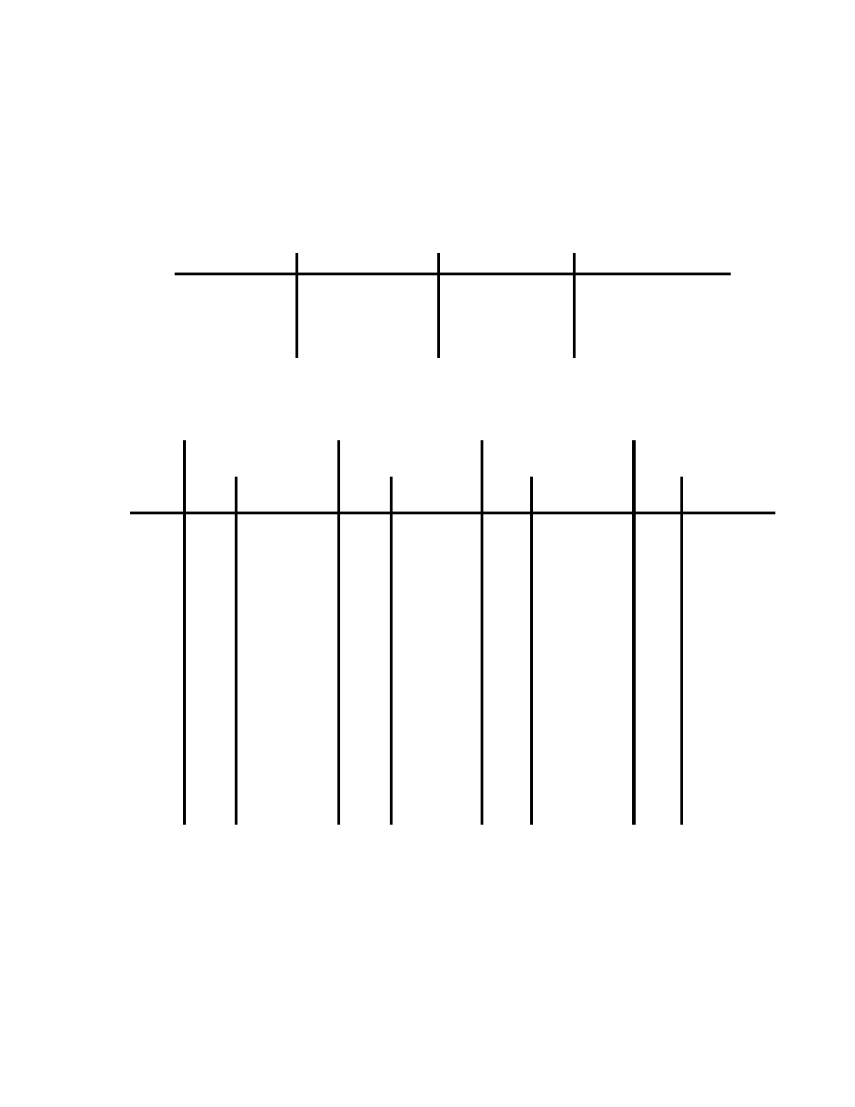
18 December 2000 I-3
APPENDIX I
TABLE I-2
PTRAC Input Format
m = Number of PTRAC keywords = 13
ni = Number of entries for ith keyword or 0 for no entries.
= 1st entry, 2nd entry, ... for the ith keyword (see below).
Index Keyword Index Keyword Index Keyword Index Keyword
1 BUFFER 5 FILTER 9 SURFACE 13 WRITE
2 CELL 6 MAX 10 TALLY
3 EVENT 7 MENP 11 TYPE
4 FILE 8 NPS 12 VALUE
TABLE I-3
Event Line Variable IDs (See TABLE I-4 )*
Type 1 Type 2 Type 3 Type 4
(N12 ≠ 0 WRITE = pos N12 = 0 WRITE=pos (N12 ≠ 0 WRITE = all N12 = 0 WRITE=all
Index N2=5 N4,6,8,10=6 N2=6 N4,6,8,10=7 N2=6 N4,6,8,10=7 N2=7 N4,6,8,10=8
N3=3 N5,7,9,11=3 N3=3 N5,7,9,11=3 N3=9 N5,7,9,11=9 N3=9 N5,7,9,11=9
J177 77 77 77
J288 88 88 88
J39 10,12,10,14 9 10,12,10,14 9 10,12,10,14 9 10,12,10,14
J417 11,13,11,15 16 11,13,11,15 17 11,13,11,15 16 11,13,11,15
J518 17 17 16 18 17 17 16
J6 18 18 17 19 18 18 17
J718 19 19 18
J819
P120 20 20 20 20 20 20 20
P221 21 21 21 21 21 21 21
P322 22 22 22 22 22 22 22
P423 23 23 23
P524 24 24 24
P625 25 25 25
P726 26 26 26
P827 27 27 27
P928 28 28 28
* For a “bnk” event (N4, N5), interpret J1 ... J4 = 7,8,10,11
For a “sur” event (N6, N7), interpret J1 ... J4 = 7,8,12,13
For a “col” event (N8, N9), interpret J1 ... J4 = 7,8,10,11
For a “ter” event (N10, N11), interpret J1 ... J4 = 7,8,14,15
m n1V1
1V2
1…Vn1
1n2V1
2V2
2…Vn2
2…n13V1
13 V2
13 …Vn13
13
V1V2…Vni

I-4 18 December 2000
APPENDIX I
TABLE I-4
Description of Variable IDs
Variable
ID MCNP
Name Description
NPS LINE
1 NPS See Appendix E
2 — Event type of 1st event (see TABLE I-5 )
3 NCL(ICL) See Appendix E
4 NSF(JSU) See Appendix E
5 JPTAL(1,ITAL) See Appendix E
6 TAL(JPTAL(7,ITAL)) See Appendix E
EVENT LINE
7 — Event type of next event (see TABLE I-5 )
8 NODE See Appendix E
9 NSR See Appendix E
10 NXS(2,IEX) See Appendix E
11 NTYN Reaction type (see TABLE I-7 )
12 NSF(JSU) Reaction type (see TABLE I-7 )
13 — Angle with surface normal (degrees)
14 NTER Termination type (see TABLE I-7 )
15 — Branch number for this history
16 IPT See Appendix E
17 NCL(ICL) See Appendix E
18 MAT(ICL) See Appendix E
19 NCP See Appendix E
20 XXX See Appendix E
21 YYY See Appendix E
22 ZZZ See Appendix E
23 UUU See Appendix E
24 VVV See Appendix E
25 WWW See Appendix E
26 ERG See Appendix E
27 WGT See Appendix E
28 TME See Appendix E

18 December 2000 I-5
APPENDIX I
TABLE I-5
Event Type Description
Location Variable
ID Event Type
src bnk** sur col ter Flag*
J11000 ±(2000+l) 3000 4000 5000 9000
*When J1 = 9000, this event is the last event for this history.
**When J1 < 0, the next event has been rejected and is included for
creation information only. The value L is given in TABLE I-6 .
TABLE I-6
Bank Event Descriptions
L Value Description MCNP
Subroutine NXS & NTYN
Provided
1 DXTRAN Track DXTRAN Y
2 Energy Split ERGIMP N
3 Weight Window Surface Split WTWNDO N
4 Weight Window Collision Split WTWNDO Y
5 Forced Collision-Uncollided Part FORCOL N
6 Importance Split SURFAC N
7 Neutron from Neutron (n,xn) (n,f) COLIDN Y
8 Photon from Neutron ACEGAM Y
9 Photon from Double Fluorescence COLIDP Y
10 Photon from Annihilation COLIDP N
ELECTR
11 Electron from Photoelectric EMAKER Y
12 Electron from Compton EMAKER Y
13 Electron from Pair Production EMAKER Y
14 Auger Electron from Photon/X-ray EMAKER Y
15 Positron from Pair Production EMAKER N
16 Bremsstrahlung from Electron TTBR N
BREMS
17 Knock-on Electron KNOCK N
18 X-rays from Electron KXRAY N
19 Photon from Neutron - Multigroup MGCOLN Y
20 Neutron (n,f) - Multigroup MGCOLN Y
21 Neutron (n,xn) k- Multigroup MGCOLN Y
22 Photo from Photon - Multigroup MGCOLN Y
23 Adjoint Weight Split - Multigroup MGACOL N

I-6 18 December 2000
CHAPTER 2
INP File
TABLE I-7
NTER and NTYN Variable Descriptions
NTER Description NTYN Description
1 Escape NEUTRON
2 Energy cutoff 1Inelastic S(α,β)
3 Time cutoff 2 Elastic S(α,β)
4 Weight window -99 Elastic scatter
5 Cell importance >5 Inelastic scatter (see
6 Weight cutoff UKAEA Nuclear
7 Energy importance Data File)
8 DXTRAN
9 Forced collision PHOTON
10 Exponential transform
1 Incoherent scatter
NEUTRON 2 Coherent scatter
3 Fluorescence
11 Downscattering 4 Double fluorescence
12 Capture 5 Pair production
13 Loss to (n,xs)
14 Loss to fission
PHOTON
11 Compton scatter
12 Capture
13 Pair production
ELECTRON
11 Scattering
12 Bremsstrahlung
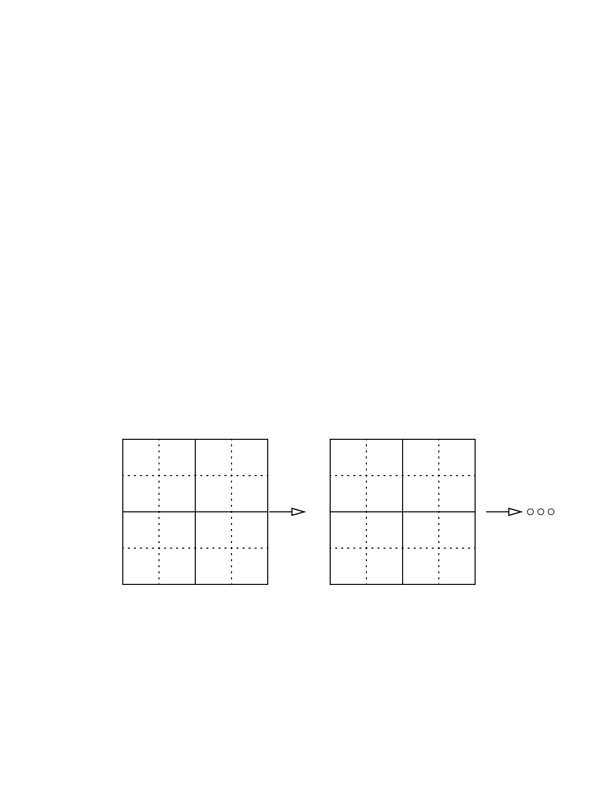
April 10, 2000 J-1
Appendix J
Appendix J
Mesh-Based WWINP, WWOUT, and WWONE File Format
The mesh-based weight window input file WWINP and the mesh-based weight window output files
WWOUT and WWONE are ASCII files with a common format. The files consist of three blocks.
Block 1 contains the header information, energy (or time) group numbers, and basic mesh
information. Block 2 contains the mesh geometry. Block 3 contains the energy (or time) group
boundaries and lower weight window bounds. Table J.1 presents the file format using generic
variables. Table J.2 describes the variables and gives the equivalent variables from the WWINP,
WWOUT, and WWONE files.
The 3 x 3 array of fine mesh cells is stored by assigning an index number to each cell. The
assignment of mesh cells is illustrated in Fig. J-1. For each value of z (or θ), all cells are indexed
in the x-y plane (or the r-z plane). The cell index number is related to the fine mesh number in each
coordinate direction through the following formula:
cell index number = 1 + (i - 1) + nfx (j - 1) + nfx · nfy (k - 1),
where i, j, and kare the fine mesh cell numbers along the x(r),y(z), and z(θ) directions, respectively,
and nfx, nfy, and nfz (by implication) are the total number of fine meshes in the x(r), y(z), and z(θ)
directions, respectively
13 14 15 16
9 101112
567 8
123 4
29 30 31 32
25 26 27 28
21 22 23 24
17 18 19 20
x0 y0
y(1)
y(2)
z=z(1) z=z(2)
x(1) x(2)
y(1)
y(2)
x(1) x(2)
x0 y0
Figure J-1. Superimposed mesh cell indexing

J-2 April 10, 2000
Appendix J
TABLE J.1:
Format of the Mesh-Based WWINP, WWOUT and WWONE File
FORMAT VARIABLE LIST
BLOCK 1
4i10 if iv ni nr
7i10 ne(1) ne(ni)
nr = 10:
6g13.5 nfx nfy nfz x0 y0 z0
6g13.5 ncx ncy ncz nwg
nr = 16:
6g13.5 nfx nfy nfz x0 y0 z0
6g13.5 ncx ncy ncz xmax ymax zmax
6g13.5 xr yr zr nwg
BLOCK 2
nwg = 1:
6g13.5 x0 nfmx(1) x(1) rx(1) nfmx(2) x(2)
6g13.5 rx(2) nfmx(ncx) x(ncx) rx(ncx)
6g13.5 y0 nfmy(1) y(1) ry(1) nfmy(2) y(2)
6g13.5 ry(2) nfmy(ncy) y(ncy) ry(ncy)
6g13.5 z0 nfmz(1) z(1) rz(1) nfmz(2) z(2)
6g13.5 rz(2) nfmz(ncz) z(ncz) rz(ncz)
nwg = 2
6g13.5 r0 nfmr(1) r(1) rr(1) nfmr(2) r(2)
6g13.5 rr(2) nfmr(ncx) r(ncx) rr(ncx)
6g13.5 z0 nfmz(1) z(1) rz(1) nfmz(2) z(2)
6g13.5 rz(2) nfmz(ncy) z(ncy) rz(ncy)
6g13.5 θ0 nfmθ(1) θ(1) rθ(1) nfmθ(2) θ(2)
6g13.5 rθ(2) nfmθ(ncz) θ(ncz) rθ(ncz)
BLOCK 3
Particle i, i=1,ni
6g13.5 e(i,1) e(i,ne(i))
Energy (or time) group j, j=1,ne(i)
6g13.5 w(i,j,1) w(i,j,nwm)
…
…
…
…
…
…
…
…
…

April 10, 2000 J-3
Appendix J
TABLE J.2:
Explanations of Variables from Table J.1
VARIABLE WWINP WWOUT WWONE
if File type. Only 1 is supported.
iv Unused
ni Number of integers on card 2
nr Number of parameters from nfx through nwg at the end of Block 1.
nr = 10 / 16 for rectangular/ cylindrical mesh
ne(i) NWW(i) NGWW(i) 1 for each i for which
NGWW(i) 0
nf[x,y,z] WWM(1-3) WWMA(1-3)
x0, y0, z0WWM(4-6) WWMA(4-6)
nc[x,y,z] WWM(7-9) WWMA(7-9)
[x,y,z]max WWM(10-12) WWMA(10-12)
xr, yr, zr WWM(13-15) WWMA(13-15)
nwg NWGEOM NWGEOA
nfm[x,y,z / r,z,θ](i) WGM(*) WGMA(*)
Number of fine mesh cells in coarse mesh cell i in x,y,z / r,z,θ directions
[x,y,z / r,z,θ](i) WGM(*) WGMA(*)
Upper coordinate of coarse mesh cell i in x,y,z/ r,z,θ directions
r[x,y,z / r,z,θ](i) WGM(*) WGMA(*)
Fine mesh ratio in coarse mesh cell i in x,y,z /r,z,θ directions.
Currently only 1. is supported.
r0, z0,θ0Origin of the radial, axial, and azimuthal directions; must be 0., 0., 0.
e(i,j) WWE(*) EWWG(*) Default maximum
jth upper energy (or time) bound for particle type i
w(i,j,k) WWF(*) Weight window generator output
Lower weight window bound for particle i, energy (or time) group j, and
fine mesh cell k
nwm NWWM NWWMA
≠

J-4 April 10, 2000
Appendix J
