_ MIDAS VT User's Guide
MIDAS-VT-User'sGuide
MIDAS-VT-User'sGuide
MIDAS-VT-User'sGuide
User Manual:
Open the PDF directly: View PDF ![]() .
.
Page Count: 30

MIDAS-VT User’s Guide
Microstructure Inelastic Damage Analysis Software-Virtual Tester
Prepared by:
Dr. Yong-Rak Kim (UNL)
Dr. David Allen (TTI)
Dr. Dallas Little (TAMU)
Dr. Francisco Aragao (UFRJ-COPPE)
Keyvan Zare-Rami (UNL)
October 2018
Contents
1. Overview ........................................................................................................................................ 4
2. Starting MIDAS ............................................................................................................................ 6
3. Preprocessor.................................................................................................................................. 7
3.1 Preprocessor-Case 1 .............................................................................................................. 9
Specimen Geometry ................................................................................................................... 10
Microstructure ............................................................................................................................. 11
Mesh Generation ........................................................................................................................ 12
Export Output ............................................................................................................................. 13
3.2 Preprocessor-Case 2 ............................................................................................................ 15
Specimen Geometry ................................................................................................................... 15
Input Mesh Data ......................................................................................................................... 15
Mesh Generation ........................................................................................................................ 16
Export Output ............................................................................................................................. 16
4. Processor ..................................................................................................................................... 18
Model Data ................................................................................................................................. 19
Analysis Information ................................................................................................................... 19
Test Information ......................................................................................................................... 19
Material Information .................................................................................................................. 20
5. Post processor ............................................................................................................................. 24
Constitutive behavior ........................................................................................................................... 26
A. 1 Boundary value problem ..................................................................................................... 26
A. 2 Linear elasticity ..................................................................................................................... 26
A. 3 Linear viscoelasticity ............................................................................................................ 27
Fracture modeling ............................................................................................................................... 28
Power function damage model ................................................................................................... 29
Gaussian function damage model .............................................................................................. 29
6. Reference .................................................................................................................................... 30

1. Overview
MIDAS-VT software is a 2D finite element (FE) solver capable of analyzing homogenous and
heterogenous media with handling the crack propagation. The software is developed as a standalone
package with an intuitive graphical interface. This package is designed in three modules:
Preprocessor
,
Processor
,
Postprocessor
which work internally with the FE solver through input and
output files (see dashed box in Figure 1.1).
Preprocessor
part generates FE model which contains
mesh and boundary condition data.
Preprocessor
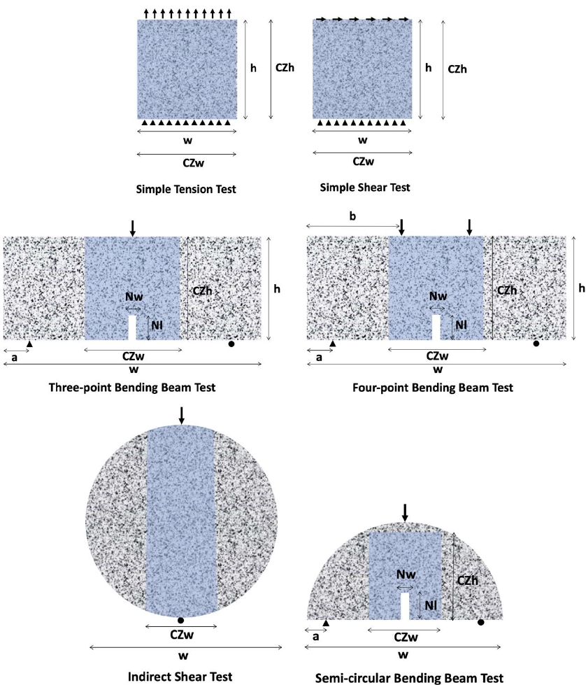
module is tailored for generating FE model from
six common test configurations in infrastructure materials’ field: Simple tension test, Simple shear
test, Three-point bending beam test, Four-point bending beam test, Semi-circular bending beam test
and Indirect shear test. These FE models can be used later in
Processor
where material properties
and other test conditions are defined. Also,
Postprocessor
feature is provided within this package to
display and visualize the result and export required graphs. The descriptions and implementation
details of each modules are presented in the following chapters.
Comments and Questions:
If there is any question about the package or this guide, or run into problems, please contact to
yong-rak.kim@unl.edu
keyvan.zare@gmail.com
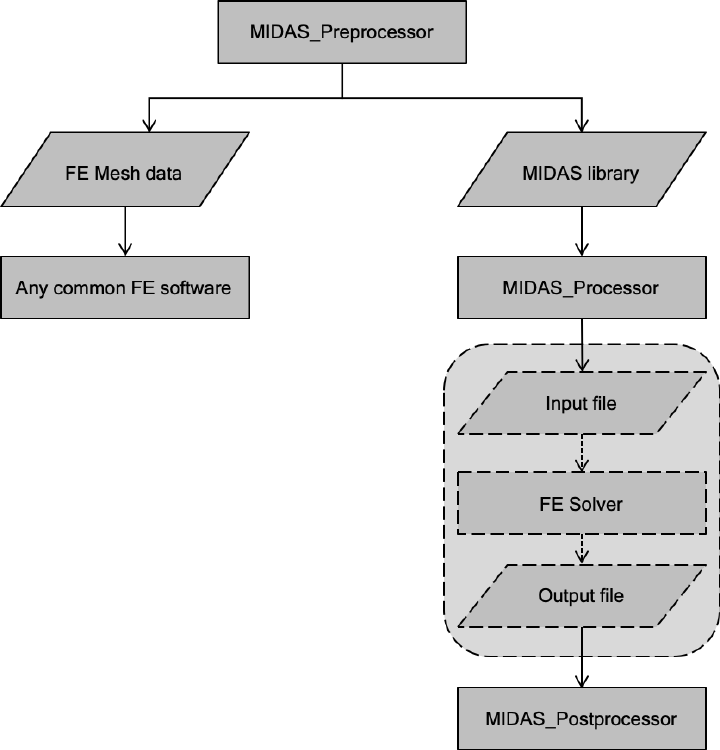
Figure 1.1. Flowchart of MIDAS-VT software

2. Starting MIDAS
1. File in the package:
Gallery folder, FESolver.exe, MIDAS_VT_Pre.exe, MIDAS_VT_Pro.exe, splash.PNG
2. Prerequisites:
Verify the Windows 64-bit version of MATLAB Runtime version 9.5 (R2018b) is installed
on your computer. Or download it from following link:
http://www.mathworks.com/products/compiler/mcr/index.html
3. Run target software:
MIDAS_VT_Pre.exe, MIDAS_VT_Pro.exe
Note: all the output messages will be stored in STATUS.txt for future reference.
Note: The execution may take several minutes.
3. Preprocessor
The
preprocessor
module is designed to generate the FE model which includes mesh information
and boundary condition data. this module is customized according to the following test
configurations (see Figure 3.4):
• Simple tension test
• Simple shear test
• Three-point bending beam test
• Four-point bending beam test
• Semi-circular bending test
• Indirect tension test
Overall flow of
preprocessor
is illustrated in Figure 3.1. To generate a model, the user needs to run
Preprocessor
.
Preprocessor
starts with a pop-up window, Figure 3.2, offering two options. The first
option should be used when the user is generating the FE model directly from the sample image or
sample geometry. This option corresponds to Case I in Figure 3.1 and Figure 3.2. The second option
is only able to add cohessive elemnets into regular FE mesh which is generated in advance. This
option corresponds to Case II in Figure 3.1 and Figure 3.2.
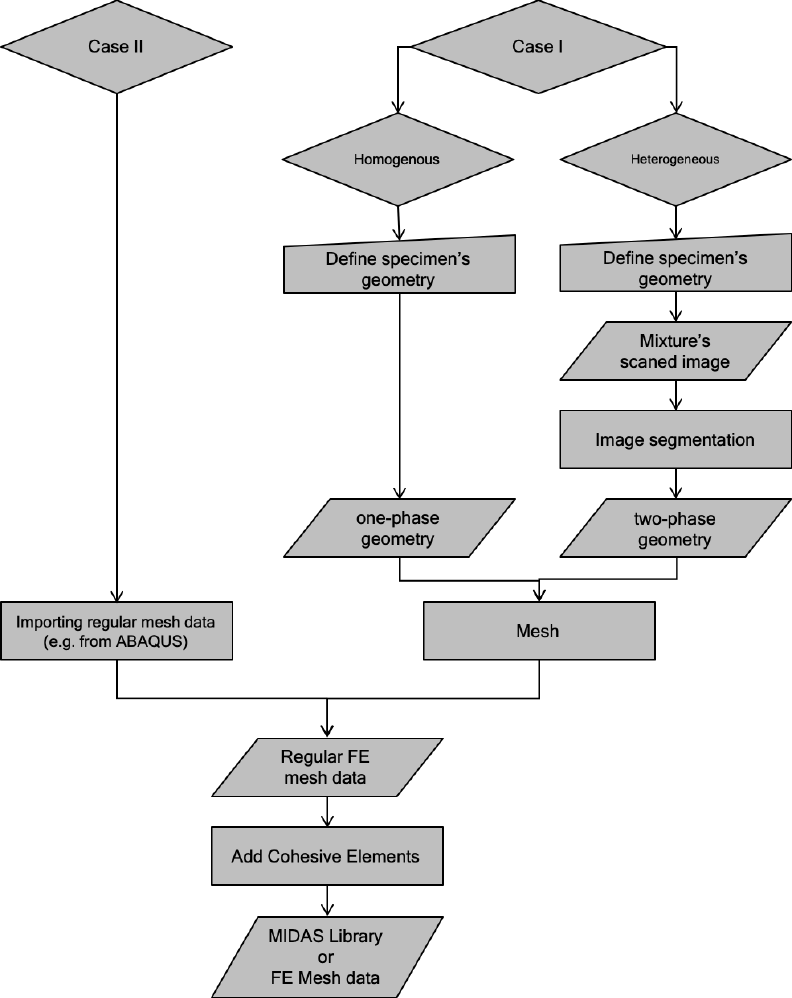
Figure 3.1. Flowchart of MIDAS preprocessor
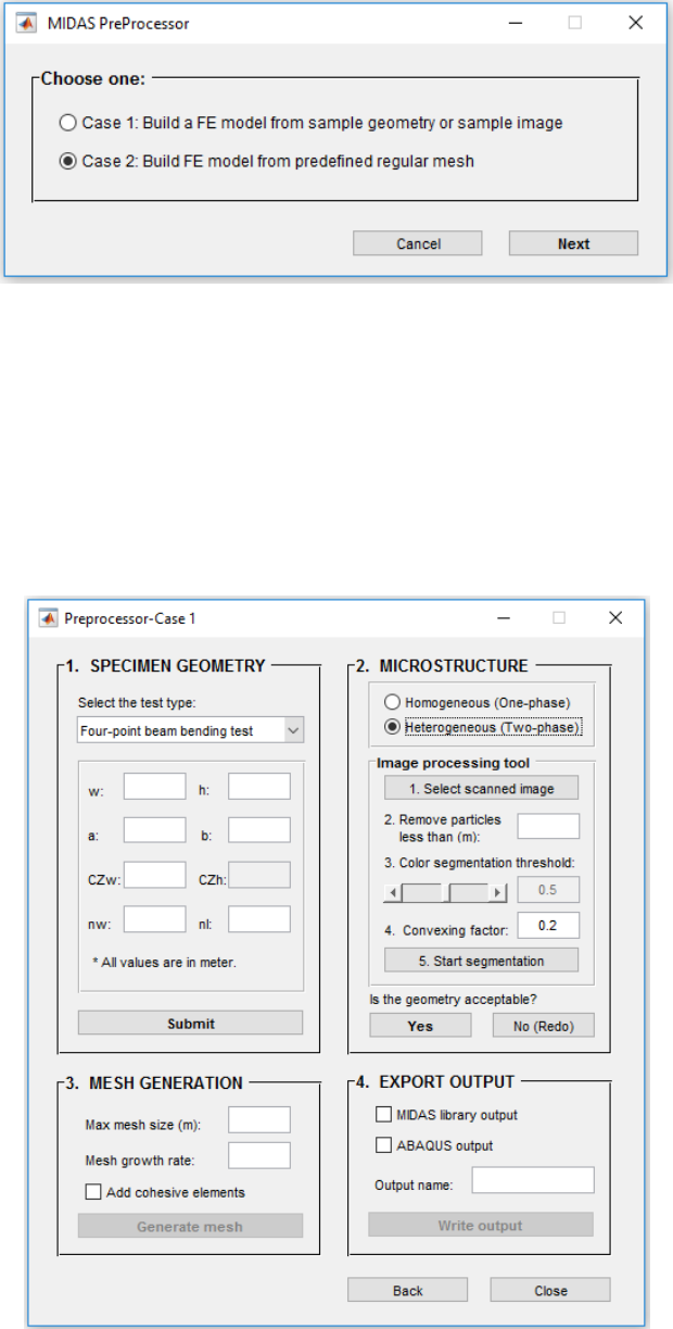
Figure 3.2. Starting preprocessor interface
3.1 Preprocessor-Case I
Case I directs the user to the window shown in Figure 3.3. There are four steps to generated the
model: 1. Specimen Geometry; 2. Microstructure; 3. Mesh; 4. Export Output. For each section
there are number of inputs and actions required which are described bellow.
Figure 3.3. Preprocessor- Case I interface
Microstructure
MIDAS
Preprocessor
is capable of creating either homogenous (one-phase) or heterogenous (two-
phase) models. In homogenous case, the software generates model geometry using specimen
dimensions provided in the first section. Heterogenous media, in current version of MIDAS, is
defined as a two-phase media which is defined as non-contact random particles being scattered within
a matrix phase. An image processing tool is provided in MIDAS
Preprocessor
to obtain mixture’s
microstructure from the actual image of a media. Thus, the user needs to provide the software with
the cross-section image of the sample and follow the steps one to five shown in Figure 3.5.
In the cross-section image, particles must be lighter in color than the matrix background. MIDAS
Preprocessor
uses color segmentation method to distinguish particles from matrix phase.
Color
segmentation threshold
is a value between 0 to 1, which defines the limit between particles (light
color areas) and matrix phase (dark color areas). This value will be calculated automatically, however
the user can adjust the value, if necessary. Also, the user is allowed to adjust how to bound the
particles’ peripheral using
shrink factor
. Setting
shrink factor
to 0 gives a convex hull around the
particles while setting it to higher values gives a compact boundary around the particles (the default
value is 0.2). The proper values of
color segmentation threshold
and
shrink factor
depends on the
image and can be obtained by trial and error. When the image segmentation process is done, the
user can compare the result to the actual microstructure (Figure 3.6). If the microstructure is similar
enough to the original image, the user can approve the image segmentation result and go to the
meshing step by clicking “Yes” button. If there are still mismatches that cannot be improved by
changing color segmentation threshold
and
shrink factor
, the user needs to modify the image
manually. The manual image treatment is basically repainting the indistinct areas or separating the
connected particles in the image. Figure 3.6 shows an image example after treatment. To modify
particles or matrix areas, the selected color’s lightness/darkness should approximately match the
average intensity value of the corresponding area (particles or matrix). To facilitate the manual
treatment procedure, Microsoft Paint software is integrated with MIDAS
Preprocessor
. By clicking
“No (redo)” button (see Figure 3.5) the microstructure’s image will be opened in Microsoft Paint for
additional adjustment. Then, after the image treatment is finished, the user needs to do the image
processing, step one to five (see Figure 3.5), once more. This procedure can be continued until the
desired accuracy is obtained.
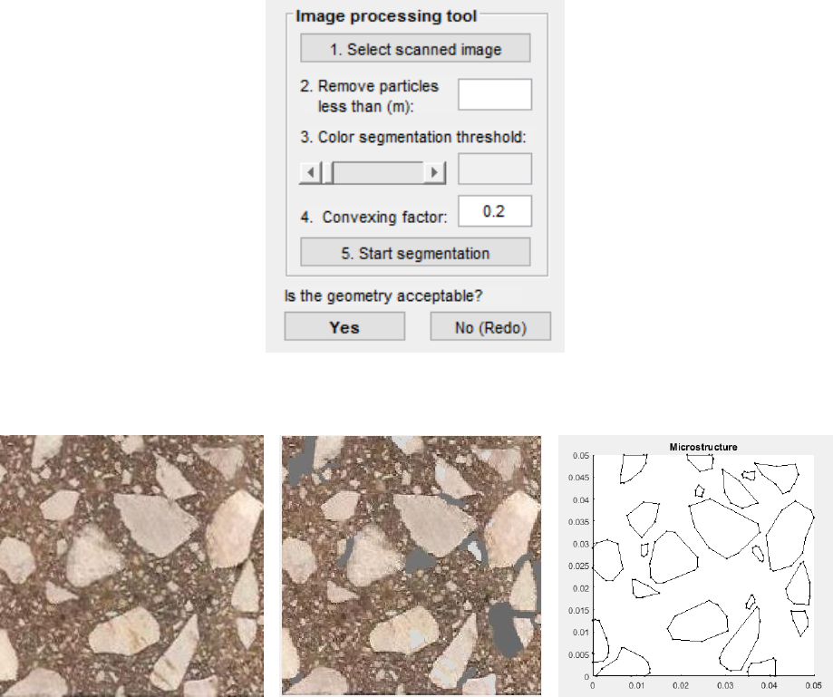
Figure 3.5. Image processing tool interface
(a)
(b)
(c)
Figure 3.6. (a) Original image, (b) treated image and (c) detected microstructure
Mesh Generation
The meshing module is designed to mesh the geometry using three-nodes elements. The user can
adjust the
maximum mesh size
and
mesh growth rate
. The later one is specified as a scalar strictly
between 1 and 2 and defines how the mesh size increases away from small parts of the geometry.
The meshing module comes with an automated Cohesive Element insertion feature. Cohesive
Element allows to simulate crack initiation and propagation within FE framework. Generally,
cohesive elements are zero thickness elements that links adjacent nodes of regular neighbor elements
to each other (Zare Rami Keyvan et al 2017). The
Add Cohesive Element
checkbox permits the
user to add cohesive element between regular FE elements within the cracking region which is
defined in
Specimen geometry
. The Cohesive Elements will be added within matrix phase, which is

called cohesive element, and particle-matrix interface, which is called adhesive element. Cohesive
Elements will be labeled according to their types, i.e. adhesive and cohesive, which allow the user to
assign corresponding properties to them later in
Processor
.
Export Output
The output produced by Preprocessor includes mesh data and boundary condition data associated
with the test type. The mesh data contains node coordinates and element connectivity matrix. The
output data can be exported in two formats, one format is compatible with MIDAS
Processor
, which
is saved as a
.mat
file, another one is compatible with common FE software such as ABAQUS, which
is saved as a
.inp
file. The format of the later one is as follows:
• Nodes coordinate matrix
*Node
Entry 1 Entry 2 Entry 3
… (continued)
Entry 1: node ID
Entry 2: x-coordinate of node
Entry 3: y-coordinate of node
• Bulk elements connectivity matrix
*Element, type= Entry 0
Entry 1 Entry 2 Entry 3 Entry 4
… (continued)
Entry 0: bulk element type, which is 3-node
Entry 1: element ID
Entry 2: 1st node number in global numbering system
Entry 3: 2nd node number in global numbering system
Entry 4: 3nd node number in global numbering system
• Cohesive element connectivity matrix
*Element, type= Entry 0
Entry 1 Entry 2 Entry 3 Entry 4 Entry 5
… (continued)
Entry 0: cohesive element type, which is 4-node cohesive
Entry 1: element ID

Entry 2: 1st node number in global numbering system
Entry 3: 2nd node number in global numbering system
Entry 4: 3rd node number in global numbering system
Entry 5: 4th node number in global numbering system
• Element sets which list the elements ID within each set
*Elset, elset= Entry 0
Entry 1 [Entry 2] …
… (continued)
Entry 0: Set ID, which are: Phase1, which represents elements in matrix phase,
Phase2, which represents elements in particles, Cohesive Elements, and
Adhesive Elements
Entry <i>: element ID
• Node sets which list the nodes related to each boundary condition
*Nset, nset= Entry 0
Entry 1 [Entry 2] …
… (continued)
Entry 0: boundary condition nodes which is different for each test:
o Simple tension test
─ TT_T which corresponds to the top boundary nodes
─ TT_B which corresponds to the bottom boundary nodes
─ TT_L which corresponds to the left boundary nodes
o Simple shear test
─ ST_T which corresponds to the top boundary nodes
─ ST_B which corresponds to the bottom boundary nodes
o Three-point bending beam test
─ TPBT_LS which corresponds to the left support nodes
─ TPBT_RS which corresponds to the right support nodes
─ TPBT_LP which corresponds to the loading point nodes
o Four-point bending beam test
─ FPBT_LS which corresponds to the left support nodes
─ FPBT_RS which corresponds to the right support nodes

─ FPBT_LLP which corresponds to the left loading point nodes
─ FPBT_RLP which corresponds to the right loading point nodes
o Semi-circular bending beam test
─ SCBT_LS which corresponds to the left support nodes
─ SCBT_RS which corresponds to the right support nodes
─ SCBT_LP which corresponds to the loading point nodes
o Indirect tension test
─ ITT_BS which corresponds to the bottom support nodes
─ ITT_TLP which corresponds to the top loading point nodes
Entry <i>: node ID
3.2 Preprocessor-Case II
This feature is provided for a case in which the model is meshed in advance by regular 3-nodes FE
elements. Choosing case II in Figure 3.2, directs the user to
Preprocessor-Case II
window, as shown
in Figure 3.7. To generate the model the user need to finish steps one to four.
Specimen Geometry
Similar to the
preprocessor-case I
the user must select test type which is followed by inputing
specimen dimensions as shown in Figure 3.4. There is no need to enter cracking region dimensions
in this section. The cracking region is specified by introducing elements within the cracking region
(see next section, input mesh data).
Input Mesh Data
The mesh data must include the following information and be written in a single
.txt
file in the
following format:
• Nodes coordinate matrix
*Node
Entry 1 Entry 2 Entry 3
… (continued)
Entry 1: node ID
Entry 2: x-coordinate of node
Entry 3: y-coordinate of node

• Bulk elements connectivity matrix
*Element, type= Entry 0
Entry 1 Entry 2 Entry 3 Entry 4
… (continued)
Entry 0: bulk element type, which is 3-node
Entry 1: element ID
Entry 2: 1st node number in global numbering system
Entry 3: 2nd node number in global numbering system
Entry 4: 3nd node number in global numbering system
• Elements’ sets which list the elements ID within each set
*Elset, elset= Entry 0
Entry 1 [Entry 2] …
… (continued)
Entry 0: Set ID, which are: Phase1, which represents elements of matrix phase,
Phase2, which represents elements of particles, CZ, which represents elements in
cracking region
Entry <i>: element ID
Comment: in common FE softwares such as ABAQUS, to group elements in different sets and
assign associated tag to each group,
partitioning
and
element set
tools is used.
Comment: the user doesn’t need to provide boundary conition nodes, they will be obtaied
automatically using specimen geometry.
Mesh Generation
This module adds zero thickness cohesive elements between bulk elements which are whithin
cracking region (Zare Rami Keyvan et al 2017).
Export Output
This step is identical to
Export output
in
Preprocessor-case I
(see section 3.1).
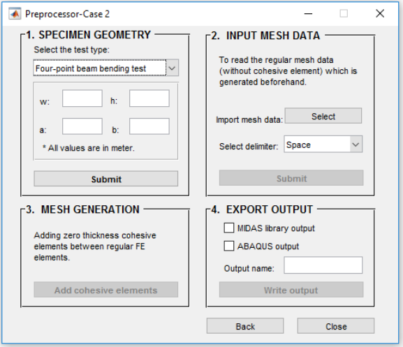
Figure 3.7. Preprocessor- Case II interface
4. Processor
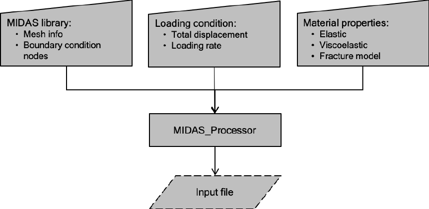
The FE model generated by MIDAS
Preprocessor
which is already stored as MIDAS
Library
file is
imported in MIDAS processor to define the FE model. The MIDAS
Library
file only includes mesh
data and boundary condition data.
Processor
module allows the user to specify test loading
condition, assign material properties and run the simulation (Figure 4.2). This process is categorized
in 4 steps which are described as follows.
Figure 4.1. Flowchart of MIDAS-Processor
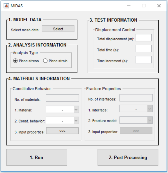
Figure 4.2. Processor interface
Model Data
In the first step, the user needs to load the general information of the model including test type,
mesh information and boundary condition data. This can be done directly by importing
MIDAS
Library
file, which is in
.mat
format, generated using
Preprocessor
(see section 3)
.
Analysis Information
Either plane stress or plane strain can be chosen.
Test Information
At this stage, MIDAS is only able to simulate displacement controlled tests. To define loading
condition,
Total displacement
, which acts on loading boundary points (see Figure 3.4) and
Total
loading time
is needed. As it is clear the loading rate will be calculated internally using the following
formula:
MIDAS uses a fixed time incremental formulation to solve the nonlinear problem. This value must
be specified here.
Material Information
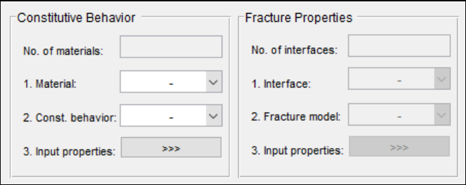
There are two separate panels designed for inputting material models, one is for bulk elements’
constitutive models, and the other is for cohesive element traction separation models. Number of
material types and number of interfaces type will be automatically filled from the MIDAS
library
that is loaded in
Model Data
section. Number of material types can be either 1 or 2 which
corresponds to homogenous model or heterogenous model (at this version of MIDAS-VT, only
two-phase heterogeneity is included) respectively. Number of interphases can be either 0 or 2. Zero
corresponds to a model without cohesive element, and the number 2 corresponds to a model with
cohesive element. The number 2 implies the presence of cohesive and adhesive elements.
(a)
(b)
Figure 4.3. Material information panel.
For each material, steps one to three must be completed (Figure 4.3-a). Firstly, selecting material
type, secondly selecting constitutive behavior type, and finally input associated properties. In
MIDAS, two constitutive behavior is provided for bulk elements: isotropic linear elastic and isotropic
linear viscoelastic.
• Isotropic linear elastic
When the constitutive behavior is isotropic linear elastic, the window shown in Figure 4.4
pops up to enter the elastic modulus and Poisson’s ratio (see Appendix A).

Figure 4.4. Inputting linear elastic properties.
• Isotropic linear viscoelastic
When the constitutive behavior is isotropic linear viscoelastic, the window shown in Figure
4.5 pops up to input the number of Prony series, Prony series coefficients and Poisson’s ratio
(see Appendix A).
Figure 4.5. Inputting linear viscoelastic properties.
Similarly, for each interface steps 1 to 3 must be completed (Figure 4.3-b). Firstly, selecting interface
type, secondly selecting the fracture model, and finally input associated properties. At this stage,
MIDAS provides only one type of fracture model for both cohesive and adhesive elements which is
called viscoelastic fracture model (see Appendix B).
• Viscoelastic fracture model
Viscoelastic fracture model parameters can be entered through the window shown in Figure
4.6. Alongside with the Prony series parameters, critical displacement and initial stress, the
user needs to define damage evolution function parameters. Regarding to the material
response two damage evolution function,
Power function
and
Gaussian function
are
provided (see Appendix B).
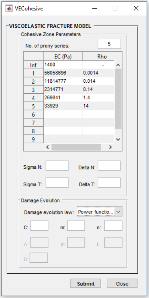
Figure 4.6. Inputting viscoelastic fracture model properties
Start simulation
When the parameters are inputted correctly, the user can start the simulation by pushing
Run
button
in Figure 4.2. The
Processor
will generate an input file and run the
FESolver
. The simulation status
will be updated in
status.txt
within the working directory after each solution step. This file also can
be checked to see whether running is over or not.
5. Post processor
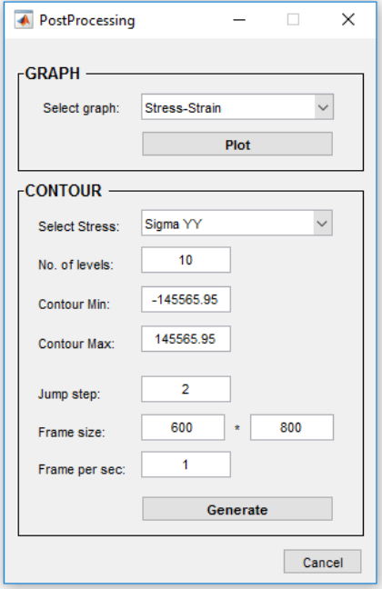
When the simulation is done, the user can visualize the result through
Post Processing
button in
Figure 4.2. The user can select the target graph from the popup menu and plot it (Figure 5.1). Also,
the user can generate the stress contour video using
Contour
panel. After selecting desire stress,
there is need to specify contour levels, then wait until
Postprocessor
calculates color-bar’s Min. and
Max. values. These values can be edited by user’s choice. The video will be created by plotting each
frame on the screen (Figure 5.2). Avoid closing the frames until the “operation completed” appears).
Figure 5.1. Post Processor
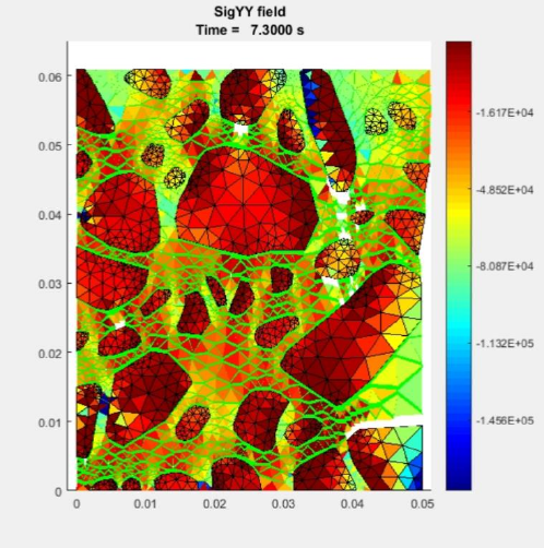
Figure 5.2. Stress contour

Appendix A. Constitutive behavior
A. 1 Boundary value problem
In the absence of body forces, inertial effects, and large deformations, an initial boundary value
problem of the domain can be well-posed by an appropriate initial-boundary conditions and a set
of governing equations: conservation of linear momentum (Eq. [1]), conservation of angular
momentum (Eq. [2]), infinitesimal strain-displacement relationships (Eq. [3]), constitutive
equations (Eq. [4]), and fracture criteria (Eq. [5]) (see references Zocher, Groves et al. 1997;
Arago, Kim et al. 2010; Kim, Arago 2013 ).
in
Equation 1
in
Equation 2
in
Equation 3
in
Equation 4
in
Equation 5
where , stress tensor; , strain tensor; , displacement vector; is a functional mapping that
describes the constitutive behavior at each position in the mixture; , fracture energy release rate at
a particular position in the mixture; , critical energy release rate; , volume of the domain, ,
internal boundary (such as cracks) in the mixture; , spatial coordinates; and time of interest.
A. 2 Linear elasticity
The isothermal-isotropic linear elastic constitutive behavior that is provided in MODAS-VT can be
expressed as:
( )( )
1 1 2 1
ij kk ij ij
EE
=+
+ − +
Equation 6
where
ij
is the stress tensor,
ij
is the strain tensor,
E
is the elastic Young’s modulus,
is
Poisson’s ratio, and
ij
is Kronecker delta.

A. 3 Linear viscoelasticity
Isothermal-isotropic linear viscoelasticity with a time-independent Poisson’s is implemented in
MIDAS, which is given by
( )( ) ( ) ( )
00
1
1 1 2 1
tt
ij
kk
ij ij ij
E t d E t d
= − + −
+ − +
Equation 7
where
( )
Et
is the viscoelastic stress relaxation modulus which is expressed as:
( )
1
exp
N
n
nn
t
E t E E
=
= + −
Equation 8
where
E
and
n
E
are spring constants in the generalized Maxwell model, is the relaxation
time, and is the number of Maxwell units in the generalized Maxwell model.
Appendix B. Fracture modeling
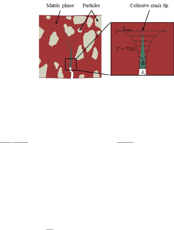
Crack propagation in the matrix phase is modeled by a cohesive zone model (Figure 3). The
cohesive zone can consider gradual damage in the material by employing a traction-separation
response.
Figure 3. Cohesive zone model
The constitutive relation governing mechanical behavior of the cohesive zone is as follows (Allen,
Searcy 2000; Allen, Searcy 2001; Kim, Allen et al. 2007; Kim, Allen et al. 2005; Kim, Allen et al.
2006):
Equation 9
where (normal direction)(tangential direction); , is the cohesive zone area-averaged
traction; , the Euclidean norm of the cohesive zone displacements; , the cohesive zone
displacement; , the cohesive zone material length parameter; , the internal state variable
representing damage evolution characteristics; , the requisite stress level to initiate cohesive zone.
, the linear viscoelastic relaxation modulus of the cohesive zone.
( )
1
exp
N
n
nn
t
E t E E
=
= + −
Equation 10
where
E
and
n
E
are spring constants in the generalized Maxwell model,
n
is the relaxation
time, and
N
is the number of Maxwell units in the generalized Maxwell model.
For the 2D case, can be separated into normal (opening) and tangential (shear sliding) components,
as the following:

Equation 11
Power function damage model
There are two phenomenological model is implemented in MIDAS to model damage evolution I
material. First one is called
Power function model
which is in a form of power relationship as a
function of the strainlike term and internal state variable (Yoon, Allen 1999; Allen,
Searcy 2001):
Equation 12
Equation 13
where and are microscale phenomenological material constants governing damage evolution
behavior. When reaches the value of unity, the crack face traction decays to zero, thus resulting
in crack extension.
Gaussian function damage model
The second model is in form of a Gaussian function that relates with and :
Equation 14
where , , and are microscale phenomenological material constants governing damage
evolution behavior.
6. Reference
ALLEN, D.H. and SEARCY, C.R., 2000. Numerical aspects of a micromechanical model of a
cohesive zone.
Journal of Reinforced Plastics and Composites,
19(3), pp. 240-248.
ALLEN, D.H. and SEARCY, C.R., 2001. A micromechanical model for a viscoelastic cohesive
zone.
International Journal of Fracture,
107(2), pp. 159-176.
ARAGO, F.T.S., KIM, Y., LEE, J. and ALLEN, D.H., 2010. Micromechanical model for
heterogeneous asphalt concrete mixtures subjected to fracture failure.
Journal of Materials in Civil
Engineering,
23(1), pp. 30-38.
KIM, Y., ALLEN, D.H. and LITTLE, D.N., 2007. Computational constitutive model for
predicting nonlinear viscoelastic damage and fracture failure of asphalt concrete mixtures.
International Journal of Geomechanics,
7(2), pp. 102-110.
KIM, Y., ALLEN, D.H. and LITTLE, D.N., 2005. Damage-induced modeling of asphalt
mixtures through computational micromechanics and cohesive zone fracture.
Journal of Materials
in Civil Engineering,
17(5), pp. 477-484.
KIM, Y., ALLEN, D.H. and SEIDEL, G.D., 2006. Damage-induced modeling of elastic-
viscoelastic randomly oriented particulate composites.
Journal of Engineering Materials and
Technology,
128(1), pp. 18-27.
KIM, Y. and ARAGO, F.T.S., 2013. Microstructure modeling of rate-dependent fracture behavior
in bituminous paving mixtures.
Finite Elements in Analysis and Design,
63, pp. 23-32.
YOON, C. and ALLEN, D.H., 1999. Damage dependent constitutive behavior and energy release
rate for a cohesive zone in a thermoviscoelastic solid.
International Journal of Fracture,
96(1), pp.
55-74.
ZOCHER, M.A., GROVES, S.E. and ALLEN, D.H., 1997. A three-dimensional finite element
formulation for thermoviscoelastic orthotropic media.
International Journal for Numerical
Methods in Engineering,
40(12), pp. 2267-2288.
ZARE RAMI KEYVAN, AMELIAN SOROOSH,KIM YONG-RAK, YOU TAESUN, LITTLE
DALLAS, Modeling the 3D Fracture-Associated Behavior of Viscoelastic Asphalt Mixtures.
Engineering Fracture Mechanics (Submitted)
.
