MIN3P THCm User Manual Jan 27 2017
User Manual:
Open the PDF directly: View PDF ![]() .
.
Page Count: 159 [warning: Documents this large are best viewed by clicking the View PDF Link!]
MIN3P-THCm
A Three-dimensional Numerical Model for
Multicomponent Reactive Transport in Variably
Saturated Porous Media
User Manual
(Draft)
K. Ulrich Mayer, Mingliang Xie and Danyang Su
University of British Columbia
Department of Earth, Ocean and Atmospheric Sciences
Vancouver, BC, Canada V5T 2M1
Kerry MacQuarrie
University of New Brunswick
Department of Civil Engineering
Fredericton, N.B., Canada E3B 5A3
January 27, 2017
DRAFT – FOR INTERANL USE ONLY
MIN3P-THCm
A Three-dimensional Numerical Model for Multicomponent Reactive Transport in Variably
Saturated Porous Media
User Guide
K. Ulrich Mayer, Mingliang Xie and Danyang Su
University of British Columbia
Department of Earth, Ocean and Atmospheric Sciences
Vancouver, BC, Canada V5T 2M1
Kerry MacQuarrie
University of New Brunswick
Department of Civil Engineering
Fredericton, N.B., Canada E3B 5A3
COPYRIGHT NOTICE AND USAGE LIMITATIONS
All rights are reserved. The MIN3P-THCm model and User's Guide are copyright. The
documentation, executable, source code, or any part thereof, may not be reproduced, duplicated,
translated, or distributed in any way without the express written permission of the copyright holder.
The MIN3P-THCm program must be specifically licensed for inclusion in software distributed in
any manner, sold commercially, or used in for-profit research/consulting. Distribution of source
code is expressly forbidden.
DISCLAIMER
Although great care has been taken in preparing MIN3P-THCm and its documentation, the authors
cannot be held responsible for any errors or omissions. As such, this code is offered `as is'. The
authors make no warranty of any kind, express or implied. The authors shall not be liable for any
damages arising from a failure of this program to operate in the manner desired by the user. The
authors shall not be liable for any damage to data or property which may be caused directly or
indirectly by use of this program. In no event will the authors be liable for any damages, including,
but not limited to, lost profits, lost savings or other incidental or consequential damages arising out
of the use, or inability to use, this program. Use, attempted use, and/or installation of this program
shall constitute implied acceptance of the above conditions. Authorized users encountering
problems with the code, or requiring specific implementations not supported by this version, are
encouraged to contact the authors for possible assistance.
ACKNOWLEDGEMENTS
The author would like to thank Shawn G. Benner (University of Waterloo, now at Idaho State
University, Boise, ID), Frederic Gerard (Eco&Sols, UMR1222, INRA/IRD/SupAgro, Montpellier,
France), Sergio Andres Bea (UBC, now at CONICET, IHLLA-Large Plains Hydrology Institute,
Buenos Aires, Argentina), Tom Henderson (UBC, now at Montana Department of Environmental
Quality, Helena, MT), Richard Amos (Carleton University) and Anna Harrison (UBC) for their
contributions to earlier versions of this User’s Manual.
User Manual-page# 1-5
ABSTRACT
The MIN3P-THCm code is developed as a multicomponent reactive transport model for variably-
saturated porous media in one, two or three spatial dimensions with the extension of heat transport,
density-dependent flow, one dimensional hydromechanical coupling, multicomponent diffusion
and reactive transport in highly saline solution. Advective-dispersive transport in the aqueous phase,
as well as diffusive gas transport can be considered. Darcy velocities are calculated internally using
a variably-saturated flow module. The governing equations are discretized using a locally mass
conservative finite volume method. The model formulation for reactive transport is based on the
global implicit solution approach, which considers reaction and transport processes simultaneously.
This formulation enforces a global mass balance between solid, surface, dissolved and gaseous
species and thus facilitates the investigation of the interactions of reaction and transport processes.
The model can also be used as a batch model for equilibrium speciation problems, kinetic batch
problems or for the generation of pC-pH-diagrams.
MIN3P-THCm is characterized by a high degree of flexibility with respect to the definition of the
geochemical reaction network to facilitate the application of the model to a wide range of
hydrogeological and geochemical problems. Chemical processes included are homogeneous
reactions in the aqueous phase, such as complexation and oxidation-reduction reactions, as well as
heterogeneous reactions, such as ion exchange, surface complexation, mineral dissolution-
precipitation and gas exchange reactions. Reactions within the aqueous phase and dissolution-
precipitation reactions can be considered as equilibrium or kinetically-controlled processes.
A new, general framework for kinetically-controlled intra-aqueous and mineral dissolution-
precipitation reactions was developed. All kinetically-controlled reactions can be described as
reversible or irreversible reaction processes. Different reaction mechanisms for dissolution-
precipitation reactions are considered, which can be subdivided into surface- and transport-
controlled reactions. This approach allows the consideration of a large number of rate expressions
reported in the literature. Related reaction and rate parameters can be incorporated into the model
through an accompanying database. The model is primarily designed for problems involving
inorganic chemistry, but reactions involving organic chemicals can also be accommodated.
Microbially-mediated reactions can be described using a multiplicative Monod approach. The mass
dependent fractionation model can be used to determine the isotope fractionation during
microbially mediated mass reduction, and precipitation dissolution reactions.
User Manual-page# 1-6
Contents
1 Installing and running min3p-THCm ............................................................................ 1-18
2 File structure .................................................................................................................... 2-20
2.1 INPUT FILES .................................................................................................................................. 2-20
2.2 OUTPUT FILES .............................................................................................................................. 2-20
3 Problem-specific input ..................................................................................................... 3-28
3.1 OVERVIEW ................................................................................................................................... 3-28
3.1.1 prefix.dat file ...................................................................................................................... 3-28
3.1.2 Types of Simulations .......................................................................................................... 3-28
3.1.3 Comment Lines and Notations ........................................................................................... 3-29
3.1.4 Units .................................................................................................................................. 3-30
3.2 GLOBAL CONTROL PARAMETERS (DATA BLOCK 1) ...................................................................... 3-30
3.2.1 Description of Data Block ................................................................................................. 3-30
3.2.2 Description of Input Parameters ....................................................................................... 3-30
3.2.2.1 'global control parameters' ............................................................................................................ 3-30
3.2.2.2 varsat_flow ................................................................................................................................... 3-30
3.2.2.3 steady_flow .................................................................................................................................. 3-30
3.2.2.4 fully_saturated .............................................................................................................................. 3-30
3.2.2.5 reactive_transport ......................................................................................................................... 3-30
3.2.2.6 Additional keywords .................................................................................................................... 3-31
3.2.3 Example Data File Input ................................................................................................... 3-32
3.2.4 Description of Example Input ............................................................................................ 3-32
3.2.5 Additional Notes ................................................................................................................ 3-33
3.3 GEOCHEMICAL SYSTEM (DATA BLOCK 2) .................................................................................... 3-33
3.3.1 Description of Data Block ................................................................................................. 3-33
3.3.2 Description of Input Parameters ....................................................................................... 3-33
3.3.2.1 'geochemical system' .................................................................................................................... 3-33
3.3.2.2 'components' ................................................................................................................................. 3-34
3.3.2.3 'non-aqueous components' ............................................................................................................ 3-35
3.3.2.4 'biomass components ' .................................................................................................................. 3-35
3.3.2.5 'secondary aqueous species' .......................................................................................................... 3-36
3.3.2.6 'minerals' ...................................................................................................................................... 3-36
3.3.2.7 'linear sorption' ............................................................................................................................. 3-37
3.3.2.8 'sorbed species' ............................................................................................................................. 3-37
3.3.2.9 'sorbed species of surface-complex' .............................................................................................. 3-38
3.3.2.10 'sorbed species of ion-exchange' ............................................................................................. 3-38
3.3.2.11 'surface sites of ion-exchange' ................................................................................................. 3-39
User Manual-page# 1-7
3.3.2.12 ‘database directory’ ................................................................................................................. 3-39
3.3.2.13 ‘compute alkalinity’ ................................................................................................................ 3-40
3.3.2.14 ‘define input units’ .................................................................................................................. 3-40
3.3.2.15 ‘define temperature’ ................................................................................................................ 3-40
3.3.2.16 ‘define temperature field’ ........................................................................................................ 3-40
3.3.2.17 'define sorption type' ............................................................................................................... 3-40
3.3.2.18 ‘combine mineralogical parameters’ ....................................................................................... 3-42
3.3.2.19 'use pitzer model' ..................................................................................................................... 3-43
3.3.2.20 This sub-keyword defines the activity correction of the aqueous species according to the HMW
Pitzer model (Harvie et al., 1984; Bea et al., 2010). In such case, the corresponding database pitzer.xml
should be provided.'use macinnes convention' ............................................................................................. 3-43
3.3.3 Example Data File Input ................................................................................................... 3-44
3.3.4 Description of Example Input ............................................................................................ 3-45
3.3.5 Additional Comments ........................................................................................................ 3-46
3.3.5.1 Choosing aqueous species ............................................................................................................ 3-46
3.3.5.2 Redox notes .................................................................................................................................. 3-46
3.3.5.3 Adding additional species ............................................................................................................ 3-46
3.4 SPATIAL DISCRETIZATION (DATA BLOCK 3) ................................................................................ 3-46
3.4.1 Description of Data Block ................................................................................................. 3-46
3.4.2 Description of Input Parameters ....................................................................................... 3-46
3.4.2.1 'spatial discretization' ................................................................................................................... 3-46
3.4.2.2 'radial coordinates' ........................................................................................................................ 3-47
3.4.3 Example Data File Input ................................................................................................... 3-47
3.4.4 Description of Example Input ............................................................................................ 3-48
3.4.5 Additional Notes ................................................................................................................ 3-48
3.5 TIME STEP CONTROL (DATA BLOCK 4) ........................................................................................ 3-48
3.5.1 Description of Data Block ................................................................................................. 3-48
3.5.2 Description of Input Parameters ....................................................................................... 3-49
3.5.2.1 'time step control - global system' ................................................................................................ 3-49
3.5.3 Example Data File Input ................................................................................................... 3-49
3.5.3.1 Description of Example Input ...................................................................................................... 3-49
3.5.3.2 Additional Comments .................................................................................................................. 3-49
3.6 CONTROL PARAMETERS–LOCAL CHEMISTRY (DATA BLOCK 5) ................................................... 3-50
3.6.1 Description of Data Block ................................................................................................. 3-50
3.6.2 Description of Input Parameters ....................................................................................... 3-50
3.6.2.1 'control parameters - local geochemistry' ..................................................................................... 3-50
3.6.2.2 ‘newton iteration settings’ ............................................................................................................ 3-50
3.6.2.3 ‘output time unit’ .......................................................................................................................... 3-50
3.6.2.4 ‘maximum ionic strength’ ............................................................................................................ 3-51
User Manual-page# 1-8
3.6.2.5 ‘minimum activity for h2o’ .......................................................................................................... 3-51
3.6.2.6 ‘redox reactions’ ........................................................................................................................... 3-51
3.6.2.7 'finite minerals' ............................................................................................................................. 3-51
3.6.2.8 'activity update settings' ................................................................................................................ 3-51
3.6.2.9 'define minimum reaction rate' ..................................................................................................... 3-51
3.6.2.10 'sparse block matrices' and 'dense block matrices' ................................................................... 3-51
3.6.3 Example Data File Input ................................................................................................... 3-52
3.6.3.1 Additional Comments .................................................................................................................. 3-52
3.7 CONTROL PARAMETERS – VARIABLY-SATURATED FLOW (DATA BLOCK 6) .................................. 3-52
3.7.1 Description of Data Block ................................................................................................. 3-52
3.7.2 Description of Input Parameters ....................................................................................... 3-53
3.7.2.1 'control parameters - variably-saturated flow' ............................................................................... 3-53
3.7.2.2 ‘mass balance’ .............................................................................................................................. 3-53
3.7.2.3 ‘variable density parameters’ ....................................................................................................... 3-53
3.7.2.4 ‘input units for boundary and initial conditions’ .......................................................................... 3-53
3.7.2.5 ‘input units for media permeability’ ............................................................................................. 3-54
3.7.2.6 ‘centered weighting’ ..................................................................................................................... 3-54
3.7.2.7 ‘compute underrelaxation factor’ ................................................................................................. 3-55
3.7.2.8 ‘newton iteration settings’ ............................................................................................................ 3-55
3.7.2.9 ‘solver settings’ ............................................................................................................................ 3-55
3.7.3 Example Data File Input ................................................................................................... 3-57
3.7.4 Description of Example Input ............................................................................................ 3-57
3.8 CONTROL PARAMETER – ENERGY BALANCE ................................................................................. 3-58
3.8.1 Description of Data Block ................................................................................................. 3-58
3.8.2 Description of Input Parameters ....................................................................................... 3-58
3.8.2.1 'energy balance' ............................................................................................................................ 3-58
3.8.2.2 'update viscosity'........................................................................................................................... 3-58
3.8.2.3 ‘spatial weighting’ ........................................................................................................................ 3-58
3.8.2.4 ‘compute evaporation’ .................................................................................................................. 3-59
3.8.2.5 ‘reference tds’ ............................................................................................................................... 3-59
3.8.2.6 ‘reference temperature for density ................................................................................................ 3-59
3.8.2.7 'energy balance parameters' .......................................................................................................... 3-59
3.8.2.8 ‘non-linear density’ ...................................................................................................................... 3-59
3.8.2.9 'thermal conductivity model' ........................................................................................................ 3-59
3.8.2.10 'newton iteration settings’ ....................................................................................................... 3-60
3.8.2.11 ‘solver settings’ ....................................................................................................................... 3-60
3.8.3 Data File Input .................................................................................................................. 3-60
3.8.4 Description of Example Input ............................................................................................ 3-62
3.9 CONTROL PARAMETERS – EVAPORATION ..................................................................................... 3-64
User Manual-page# 1-9
3.9.1 Description of Data Block ................................................................................................. 3-64
3.9.2 Description of Input Parameters ....................................................................................... 3-65
3.9.2.1 'write transient evaporation info' .................................................................................................. 3-65
3.9.2.2 'vapour density model' .................................................................................................................. 3-65
3.9.2.3 'update vapor density derivatives' ................................................................................................. 3-65
3.9.2.4 'temperature gain factor for soil' ................................................................................................... 3-65
3.9.2.5 'reference vapor diffusivity' .......................................................................................................... 3-65
3.9.2.6 'enhanced factor in isothermal vapor fluxes' ................................................................................. 3-65
3.9.2.7 'compute enhanced factor in thermal vapor fluxes' ....................................................................... 3-66
3.9.2.8 'soil surface resistance to vapor flow' ........................................................................................... 3-66
3.9.2.9 ‘split divergence of vapor density’ ............................................................................................... 3-66
3.9.2.10 'tortuosity model to vapor flow'............................................................................................... 3-67
3.9.2.11 'relative humidity parameters' ................................................................................................. 3-67
3.9.2.12 'temperature parameters' .......................................................................................................... 3-67
3.9.2.13 'solar radiation parameters' ...................................................................................................... 3-68
3.9.2.14 'rain parameters' ...................................................................................................................... 3-68
3.9.2.15 'evaporation parameters' .......................................................................................................... 3-69
3.9.3 Data File Input .................................................................................................................. 3-69
3.9.4 Description of Example Input ............................................................................................ 3-70
3.9.5 Atmospheric (.atm) file input ............................................................................................. 3-71
3.9.5.1 Time ............................................................................................................................................. 3-71
3.9.5.2 Temperature ................................................................................................................................. 3-72
3.9.5.3 Relative humidity ......................................................................................................................... 3-72
3.9.5.4 Wind ............................................................................................................................................. 3-72
3.9.5.5 Radiation ...................................................................................................................................... 3-72
3.9.5.6 Rainfall ......................................................................................................................................... 3-72
3.9.5.7 Cloud index .................................................................................................................................. 3-73
3.9.5.8 Evaporation .................................................................................................................................. 3-73
3.10 CONTROL PARAMETERS – REACTIVE TRANSPORT (DATA BLOCK 7) ........................................ 3-73
3.10.1 Description of Data Block ............................................................................................ 3-73
3.10.2 Description of Input Parameters................................................................................... 3-73
3.10.2.1 ‘mass balance’ ......................................................................................................................... 3-74
3.10.2.2 ‘spatial weighting’................................................................................................................... 3-74
3.10.2.3 ‘activity update settings’ ......................................................................................................... 3-75
3.10.2.4 ‘tortuosity correction’ ............................................................................................................. 3-75
3.10.2.5 ‘spatial averaging - diffusion’ ................................................................................................. 3-76
3.10.2.6 'gas advection' ......................................................................................................................... 3-77
3.10.2.7 ‘cumulative mole fractions’ .................................................................................................... 3-77
3.10.2.8 'enable gravity for gas phase'................................................................................................... 3-77
User Manual-page# 1-10
3.10.2.9 ‘degassing’ .............................................................................................................................. 3-77
3.10.2.10 ‘update porosity’ ..................................................................................................................... 3-77
3.10.2.11 ‘update permeability’ .............................................................................................................. 3-78
3.10.2.12 'newton iteration settings’ ....................................................................................................... 3-78
3.10.2.13 ‘solver settings’ ....................................................................................................................... 3-78
3.10.3 Data File Input .............................................................................................................. 3-79
3.10.4 Description of Example Input ....................................................................................... 3-79
3.11 OUTPUT CONTROL (DATA BLOCK 8) ....................................................................................... 3-81
3.11.1 Description of Data Block ............................................................................................ 3-81
3.11.2 Description of Input Parameters................................................................................... 3-81
3.11.2.1 'output control'......................................................................................................................... 3-81
3.11.2.2 'output of spatial data' .............................................................................................................. 3-81
3.11.2.3 'output of transient data' .......................................................................................................... 3-81
3.11.2.4 ‘output in terms of depth’ ........................................................................................................ 3-82
3.11.2.5 'isotope output' ........................................................................................................................ 3-82
3.11.3 Example Data File Input ............................................................................................... 3-83
3.11.4 Description of Example Input ....................................................................................... 3-83
3.12 PHYSICAL PARAMETERS: POROUS MEDIUM (DATA BLOCK 9) ................................................. 3-83
3.12.1 Description of Data Block ............................................................................................ 3-83
3.12.2 Description of Input Parameters................................................................................... 3-84
3.12.2.1 'physical parameters - porous medium' ................................................................................... 3-84
3.12.2.2 ‘number and name of zone’ ..................................................................................................... 3-84
3.12.3 Example Data File Input ............................................................................................... 3-85
3.12.4 Description of Example Input ....................................................................................... 3-86
3.12.5 Distributed parameters input ........................................................................................ 3-86
3.13 PHYSICAL PARAMETERS-VARIABLY-SATURATED FLOW (DATA BLOCK 10) ............................. 3-87
3.13.1 Description of Data Block ............................................................................................ 3-87
3.13.2 Description of Input Parameters................................................................................... 3-87
3.13.2.1 ‘physical parameters – variably saturated flow’ ...................................................................... 3-87
3.13.2.2 ‘hydraulic conductivity in ?-direction’ .................................................................................... 3-88
3.13.2.3 ‘specific storage coefficient’ ................................................................................................... 3-88
3.13.2.4 ‘soil hydraulic function parameters’........................................................................................ 3-88
3.13.2.5 'residual gas saturation' ........................................................................................................... 3-88
3.13.3 Example Data File Input ............................................................................................... 3-89
3.13.4 Description of Example Input ....................................................................................... 3-90
3.13.5 Distributed parameters input ........................................................................................ 3-90
3.14 PHYSICAL PARAMETERS - ENERGY BALANCE (DATA BLOCK 10B) ........................................... 3-91
3.14.1 Description of Data Block ............................................................................................ 3-91
User Manual-page# 1-11
3.14.2 Description of Input Parameters................................................................................... 3-92
3.14.2.1 'physical parameters - energy balance' .................................................................................... 3-92
3.14.2.2 'specific heat of water' ............................................................................................................. 3-92
3.14.2.3 'specific heat of air'.................................................................................................................. 3-92
3.14.2.4 'gas thermal conductivity' ........................................................................................................ 3-92
3.14.2.5 'specific heat of solid' .............................................................................................................. 3-92
3.14.2.6 'water thermal conductivity in ?-direction' .............................................................................. 3-92
3.14.2.7 'solid thermal conductivity in ?-direction' ............................................................................... 3-92
3.14.2.8 Thermal dispersivities ............................................................................................................. 3-92
3.14.2.9 'read energy balance parameters from file' .............................................................................. 3-93
3.14.3 Example Data File Input ............................................................................................... 3-95
3.14.4 Description of Example Input ....................................................................................... 3-96
3.15 PHYISICAL PARAMETERS – REACTIVE TRANSPORT (DATA BLOCK 11) ..................................... 3-96
3.15.1 Description of Data Block ............................................................................................ 3-96
3.15.2 Description of Input Parameters................................................................................... 3-96
3.15.2.1 ‘physical parameters – reactive transport’ ............................................................................... 3-96
3.15.2.2 ‘diffusion coefficients’ ............................................................................................................ 3-97
3.15.2.3 ‘dispersivity’ ........................................................................................................................... 3-97
3.15.2.4 'update gas density' .................................................................................................................. 3-97
3.15.2.5 'constant gas density' ............................................................................................................... 3-97
3.15.2.6 Gas viscosity models ............................................................................................................... 3-97
3.15.3 Example Data File Input ............................................................................................... 3-99
3.15.4 Description of Example Input ....................................................................................... 3-99
3.16 INITIAL CONDITION - VARIABLY-SATURATED FLOW (DATA BLOCK 12) .................................. 3-99
3.16.1 Description of Data Block .......................................................................................... 3-100
3.16.2 Description of Input Parameters................................................................................. 3-100
3.16.2.1 ‘initial condition – variably-saturated flow’ .......................................................................... 3-100
3.16.2.2 ‘initial condition’ .................................................................................................................. 3-100
3.16.2.3 extent of zone’....................................................................................................................... 3-100
3.16.2.4 ‘read initial condition from file’ ............................................................................................ 3-100
3.16.3 Example Data File Input ............................................................................................. 3-103
3.16.4 Description of Example Input ..................................................................................... 3-104
3.16.5 Additional Comments .................................................................................................. 3-104
3.17 BOUNDARY CONDITIONS - VARIABLY-SATURATED FLOW (DATA BLOCK 13) ........................ 3-104
3.17.1 Description of Data Block .......................................................................................... 3-104
3.17.2 Description of Input Parameters................................................................................. 3-104
3.17.2.1 ‘boundary conditions - variably saturated flow’.................................................................... 3-105
3.17.2.2 'boundary type' ...................................................................................................................... 3-105
User Manual-page# 1-12
3.17.2.3 'extent of zone' ...................................................................................................................... 3-105
3.17.2.4 Transient boundary condition................................................................................................ 3-106
3.17.3 Example Data File Input ............................................................................................. 3-108
3.17.4 Description of Example Input ..................................................................................... 3-110
3.18 INITIAL CONDITION – ENERGY BALANCE (DATA BLOCK 12B) ............................................... 3-110
3.18.1 Description of Data Block .......................................................................................... 3-110
3.18.2 Description of Input Parameters................................................................................. 3-110
3.18.2.1 'initial condition - energy balance' ......................................................................................... 3-110
3.18.2.2 ‘extent of zone’ ..................................................................................................................... 3-111
3.18.2.3 ‘read initial condition from file’ ............................................................................................ 3-111
3.18.3 Example Data File Input ............................................................................................. 3-111
3.18.4 Description of Example Input ..................................................................................... 3-111
3.19 BOUNDARY CONDITIONS – ENERGY BALANCE (DATA BLOCK 13B) ...................................... 3-111
3.19.1 Description of Data Block .......................................................................................... 3-112
3.19.2 Description of Input Parameters................................................................................. 3-112
3.19.3 Example Data File Input ............................................................................................. 3-112
3.19.4 Description of Example Input ..................................................................................... 3-113
3.20 INITIAL CONDITION – BATCH REACTIONS (DATA BLOCK 14) ................................................ 3-113
3.20.1 Description of Data Block .......................................................................................... 3-113
3.20.2 Description of Input Parameters................................................................................. 3-114
3.20.2.1 ‘initial condition – local geochemistry’ ................................................................................. 3-114
3.20.2.2 ‘kinetic batch simulation’ ...................................................................................................... 3-114
3.20.2.3 Concentration Input............................................................................................................... 3-115
3.20.2.4 ‘sorption parameter input’ ..................................................................................................... 3-116
3.20.2.5 'CEC fraction of multisite ion exchange' ............................................................................... 3-118
3.20.2.6 ‘mineral input’ ...................................................................................................................... 3-118
3.20.3 Example Data File Input ............................................................................................. 3-125
3.20.4 Description of Example Input ..................................................................................... 3-128
3.20.5 Additional Comments .................................................................................................. 3-128
3.21 INITIAL CONDITION – REACTIVE TRANSPORT (DATA BLOCK 15) ........................................... 3-129
3.21.1 Description of Data Block .......................................................................................... 3-129
3.21.2 Description of Input Parameters................................................................................. 3-129
3.21.2.1 ‘initial condition – reactive transport’ ................................................................................... 3-129
3.21.2.2 ‘extent of zone’ ..................................................................................................................... 3-132
3.21.3 'Read initial aqueous component concentrations from file' ........................................ 3-129
3.21.4 'Read initial mineral volume fractions from file' ........................................................ 3-129
3.21.5 'Read cec from file' ...................................................................................................... 3-130
3.21.6 'Read initial mineral areas from file' .......................................................................... 3-130
User Manual-page# 1-13
3.21.7 'Read mineral volume fractions nucleation thresholds from file' ................................ 3-130
3.21.8 'Read nucleation threshold reference surface area from file' ..................................... 3-130
3.21.9 initial condition for isotope components ..................................................................... 3-131
3.21.10 'linear sorption input' .................................................................................................. 3-131
3.21.11 Example Data File Input ............................................................................................. 3-132
3.21.12 Description of Example Input ..................................................................................... 3-134
3.22 BOUNDARY CONDITIONS - REACTIVE TRANSPORT (DATA BLOCK 16) ................................... 3-135
3.22.1 Description of Data Block .......................................................................................... 3-135
3.22.2 Description of Input Parameters................................................................................. 3-135
3.22.3 Example Data File Input ............................................................................................. 3-137
3.22.4 Additional Comments .................................................................................................. 3-140
3.23 ICE SHEET LOADING/UNLOADING (DATA BLOCK 17) ............................................................. 3-141
3.23.1 Description of Data Block .......................................................................................... 3-141
3.23.2 Description of Input Parameters................................................................................. 3-141
3.23.3 Example Data File Input ............................................................................................. 3-141
3.23.4 Description of Example Input ..................................................................................... 3-142
3.23.5 Additional parameters ................................................................................................ 3-142
4 Database ......................................................................................................................... 4-144
4.1 COMPONENTS ............................................................................................................................ 4-144
4.1.1 comp.dbs .......................................................................................................................... 4-144
4.1.1.1 aqueous components .................................................................................................................. 4-144
4.1.1.2 non-aqueous components ........................................................................................................... 4-145
4.1.2 Adding new components .................................................................................................. 4-145
4.2 COMPLEXATION REACTIONS ...................................................................................................... 4-145
4.2.1 Line 1. .............................................................................................................................. 4-145
4.2.2 Line 2. .............................................................................................................................. 4-146
4.2.3 Adding complexes ............................................................................................................ 4-146
4.2.4 Isotope complexes ............................................................................................................ 4-146
4.3 GAS EXCHANGE REACTIONS ....................................................................................................... 4-147
4.4 ION EXCHANGE AND SORPTION REACTIONS ................................................................................ 4-147
4.5 EQUILIBRIUM REDOX REACTIONS AND KINETICALLY-CONTROLLED INTRA-AQUEOUS REACTIONS ....
................................................................................................................................................... 4-148
4.6 MINERAL DISSOLUTION-PRECIPITATION REACTIONS .................................................................. 4-150
4.6.1 Surface-controlled rate expressions ................................................................................ 4-150
4.6.2 Diffusion-controlled rate expression ............................................................................... 4-154
4.6.3 Isotope including minerals ...................................................... Error! Bookmark not defined.
4.7 PITZER VIRIAL COEFFICIENTS DATABASE ................................................................................... 4-157
User Manual-page# 1-14
5 References: ..................................................................................................................... 5-159
User Manual-page# 1-15
LIST OF TABLES
Page
Table 2.1: Input file and database files ...................................................................................... 2-20
Table 2.2: Output files – general model output .......................................................................... 2-21
Table 2.3: Output files – Output files - flow solution ................................................................. 2-22
Table 2.4: Output files – reactive transport – contour data. ...................................................... 2-22
Table 2.5: Output files – reactive transport – transient data ..................................................... 2-23
Table 2.6: Output files – local geochemistry .............................................................................. 2-26
Table 3.1: Data blocks for problem specific input file ............................................................... 3-28
Table 3.2: Types of simulations .................................................................................................. 3-29
Table 3.3: Input requirements for simulation types ................................................................... 3-29
Table 3.4: Parameter settings for simulation types .................................................................... 3-31
Table 3.5: Summary of input parameters for data block ‘geochemical system’ ........................ 3-33
Table 3.6: Summary of input parameters for data block 'time step control – global system’ .... 3-49
Table 3.7: Summary of input parameters for data block ‘control parameters – local chemistry’ ....
....................................................................................................................................... 3-51
Table 3.8: Summary of input parameters for section ‘control parameters – variably-saturated flow’
....................................................................................................................................... 3-56
Table 3.9: Summary of input parameters for section 'control parameters - energy balance' .... 3-62
Table 3.10: Example rainfall input in atmosphere file ............................................................... 3-72
Table 3.11: Summary of input parameters for section ‘control parameters – reactive transport’ ...
....................................................................................................................................... 3-80
Table 3.12: Summary of input parameters for section ‘physical parameters – variably-saturated
flow’ ............................................................................................................................... 3-88
Table 3.13: Summary of input parameters for section ‘physical parameters – energy balance’ ... 3-
94
Table 3.14: Summary of input parameters for section ‘physical parameters – reactive transport’
....................................................................................................................................... 3-98
Table 3.15: Summary of input parameters for section ‘initial condition – variably-saturated flow’
..................................................................................................................................... 3-102
Table 3.16: Boundary conditions for flow solution .................................................................. 3-104
Table 3.17: Summary of input parameters for section ‘boundary conditions – variably-saturated
flow’ ............................................................................................................................. 3-107
Table 3.18: Boundary conditions for energy balance .............................................................. 3-112
Table 3.19: Summary of input parameters for section ‘initial condition – local chemistry’, Part 1.
User Manual-page# 1-16
..................................................................................................................................... 3-122
Table 3.20: Summary of input parameters for section ‘initial condition – local chemistry’, Part 2.
..................................................................................................................................... 3-122
Table 3.21: Summary of input parameters for section ‘initial condition – local chemistry’, Part 3.
..................................................................................................................................... 3-124
Table 3.22: Units for effective rate constants dependent on rate expression ........................... 3-125
Table 3.23: Boundary conditions for reactive transport .......................................................... 3-136
User Manual-page# 1-17
LIST OF FIGURES
Page
Figure 3.1: MIN3P-THCm output example when a sinusoidal function for climate variables is
employed. ....................................................................................................................... 3-64
Figure 3.2: Spatial discretization and numbering principle ...................................................... 3-82
Figure 3.3: Allocation of material properties to discretized solution domain. .......................... 3-85
User Manual-page# 1-18
1 INSTALLING AND RUNNING MIN3P-THCM
The following description is based on the assumption that the program will be installed on a PC
with WINDOWS OS. The package can be installed on any drive. This guide assumes that the
program will be installed on the d-drive, if this is not the case the drive letter d must be replaced by
the actual drive letter:
Extract the program and example files at any location on your computer. The program will extract
into a main directory “min3p” that contains a number of subdirectories.
The “bin” directory includes the MIN3P-THCm executable. The “database” directory includes the
database files, the “benchmarks_standard” directory includes a set of worked examples, the
“simulations” directory is empty and is dedicated for new MIN3P-THCm simulations.
There are several ways to run the program. The simplest way is to copy the executable file under
the folder “bin” into the folder containing the input file(s) to be executed. Double click the program
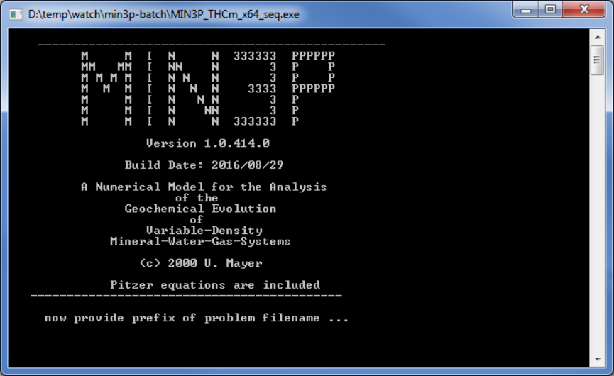
will launch a new DOS-window (Figure 1.1). Now provide the name of the input file and return.
Figure 1.1: DOS window while launching the MIN3P-THCm program
Alternatively, the program can be started using a batch file (e.g. 1min3p.bat) that is included in
each example directory. In this file, the location of the MIN3P-THCm can be specified. To execute
the program, double click on file “1min3p.bat”. A DOS window with a welcome screen will appear
(Figure 1.1). When prompted, enter the problem specific file name, in the example above: amd_ex,
then press enter and the simulation will start. Or you can also put the problem specific file name
without extension in a seperate file root.dat. In such case, double click on file “1min3p”, MIN3P-
THCm will launch the execution automatically.
Due to the potential large number of output files generated by the program, it is highly

User Manual-page# 1-19
recommended to create a directory for each new simulation. You can simply copy an existing
example to a new location in the “simulations” directory, and modify the input file using notepad,
notepad++, wordpad or a similar ascii text editor (in this case the amd_ex.dat file). Start the
simulation as described above:
All of output files generated are ascii text files by default. Most output files have a Tecplot header
that can be read by a variety of postprocessing programs (section 2.2). Alternatively, binary output
is available when MPI parallel version is used.
IMPORTANT: If you want to run the simulations elsewhere than in the “simulations” directory,
you will have to update the path to the database files in the input file (i.e. the prefix.dat file) and
the path to the executable in the 1min3p.bat file. This can be avoided by sticking to the simulations
directory.

User Manual-page# 2-20
2 FILE STRUCTURE
Required input files can be subdivided into problem specific input files and database files.
Additional species or reactions may be specified in the database files. When changing the database
files for a specific problem, an original copy of the database should always be maintained (see
Section 4 on how to maintain the database and on how to add additional components, species, or
reactions to the database).
2.1 INPUT FILES
The input prefix.dat, where prefix is a problem name with up to 72 characters contains the problem-
dependent input. This file together with all database files is required to operate the model. Some
optional file(s) can be required for specifying material properties, initial condition distributions
and/or time dependent boundary conditions. For example, it is optional to specify a depth-
dependent temperature field or an initial condition for transient groundwater flow problems. These
data may be provided in the files prefix.tem (temperature) and prefix.ivs (initial condition variably-
saturated flow). All optional input files are listed in Table 2.1. Details about the construction and
modification in the prefix.dat will be discussed in the following sections.
Table 2.1: Input file and database files
Type
File name
Description
Requirement
problem
specific
input files
prefix.dat
General problem specific input
Required
prefix.tem
Depth dependent temperature field
Optional
prefix.ivs
Distributed initial condition for flow simulation
Optional
prefix.hyc
Initial hydraulic conductivity distribution
Optional
Prefix.bcvs
Transient boundary conditions for flow
Optional
Prefix.cec
Nodal cation exchange capacity (CEC) and bulk
density input (ρb)
Optional
Prefix.spstor
Nodal specific storage (Ss)
Optional
restart.dat
Restart file
Optional
database
files
comp.dbs
Components
Required
complex.dbs
Aqueous complexation
Required
redox.dbs
Oxidation-reduction
Required
gases.dbs
Gas dissolution-exsolution
Required
sorption.dbs
Ion exchange and surface complexation
Required
mineral.dbs
Mineral dissolution-precipitation
Required
Pitzer.xml
Pitzer parameters
Optional
2.2 OUTPUT FILES
A brief summary of all output files can be found in the file prefix_o.fls, which is very helpful for
the new users to have an overview of the output files. This file contains the file names, provides a
brief description of the content of the files and lists the parameters contained in the files. It is
generated on program-execution. The most important output files are summarized in the following

User Manual-page# 2-21
tables (Table 2.2, Table 2.3, Table 2.4, Table 2.5 and Table 2.6). For the remaining output files the
user is referred to the file prefix_o.fls, in which the parameters and units of almost all output files
are described.
The files prefix_o.gen and prefix.log documents the processes of the execution. If the simulation
fails, error messages are normally provided in both files. If the simulation succeeds, “***** normal
exit *****” can be found at the end of both file.
Table 2.2: Output files – general model output
File name
Description
TECPLOT
Header
prefix_o.gen
General problem specific output, contains feed-back from
input file and results of batch simulations including the
equilibration of background and source water chemistry
Output format: assorted
Suffix meaning: gen = general
N
prefix.log
run-specific information on convergence and trouble shooting
Output format: assorted
Suffix meaning:log = logbook
N
prefix_o.fls
Additional information (parameters and units) about the
content of all output files
Output format: assorted
Suffix meaning: fls = output files
N
Prefix_o.dbg
Debug information (for code developer while debugging)
Suffix meaning:dbg = debug
N
prefix_o.psp
Record of all the possible species for a given set of components
Output format: assorted
Suffix meaning: psp = ‘possible species’
N
Prefix_o.dt
Record of time steps and courant number – Transient data
Output format: time, delta t, parameter values
Suffix meaning: dt = delta time
Y/N
Prefix_o.cnv
Record of concentration input and mineral input for reactive
trans
N

User Manual-page# 2-22
Table 2.3: Output files – Output files - flow solution
File name
Description
TECPLOT
Header
prefix_x.gsp
hydraulic head, pressure head, water and gas saturations,
moisture and gas contents at output time x (0 = initial
condition) – contour data
Output format: x,(y),(z), parameter values
Suffix meaning: gsp = global/spatial/pressure
Y
prefix_x.vel
interfacial velocities at output time x (0 = initial condition) –
contour data
Output format: x,(y),(z), vx, (vy), (vz)
Suffix meaning: vel = velocities
Y
prefix_o.mvs
Mass balance files of liquid – transient data
Output format: time, water mass, "water filled volume", "gas
filled volume"
Suffix meaning: mvs = mass and liquid filled volumes
Y
prefix_o.mvc
Mass balance in total flux – transient data
Output format: time, "inflow", "outflow", "change in storage",
"root water uptake"
Suffix meaning: mvc = mass volume change
Y
prefix_o.mve
Mass balance errors – transient data
Output format: time, "absolute mass balance error", "relative
mass balance error", "absolute cumulative mass balance
error", "relative cumulative mass balance error"
Suffix meaning: mve = mass balance (volume) errors
Y
Table 2.4: Output files – reactive transport – contour data.
File name
Description
TECPLO
T Header
prefix_x.gst
total aqueous component concentrations at output time x (0 =
initial condition) – contour data
Output format: x,(y),(z), parameter values
Suffix meaning: gst = global/spatial/total aqueous component
concentrations
Y
prefix_x.gsc
aqueous species concentrations at output time x (0 = initial
condition) – contour data
Output format: x,(y),(z), parameter values
Suffix meaning: gsc = global/spatial/species concentrations
Y
prefix_x.gsi
reaction rates of intra-aqueous kinetic reactions at output time x
– contour data
Output format: x,(y),(z), parameter values
Suffix meaning: gsi = global/spatial/intra-aqueous kinetic
reactions
Y
prefix_x.gsm
master variables (pH, pe, Eh, ionic strength, alkalinity,
temperature) at output time x (0 = initial condition) – contour data
Output format: x,(y),(z), parameter values
Suffix meaning: gsm = global/spatial/master variables
Y

User Manual-page# 2-23
prefix_x.gsg
partial gas pressures at output time level x (0 = initial condition)
– contour data
Output format: x,(y),(z), parameter values
Suffix meaning: gsg = global/spatial/partial gas pressures
Y
prefix_x.gsgr
degassing rates at output time x (0 = initial condition) – contour
data
Output format: x,(y),(z), parameter values
Suffix meaning: gsgr – global/spatial/degassing/rates
Y
prefix_x.gsv
mineral volume fractions at output time x (0 = initial condition)
– contour data
Output format: x,(y),(z), parameter values
Suffix meaning: gsv – global/spatial/volume fractions
Y
prefix_x.gsb
surface species at output time x (0 = initial condition) – contour
data
Output format: x,(y),(z), parameter values
Suffix meaning: gsb – global/spatial/sorbed species
Y
prefix_x.gss
mineral saturation indices at output time x (0 = initial condition)
– contour data
Output format: x,(y),(z), parameter values
Suffix meaning: gss – global/spatial/saturation indices
Y
Prefix_x.cbt
Charge balance output for multicomponent diffusion (MCD) –
contour data
Output format: x,(y),(z), parameter values, charge balance values
Suffix meaning: cbt – charge/balance/time
Y
Prefix_x.gmf
Total flux of each aqueous components for multicomponent
diffusion (MCD) - contour data
Output format: x,(y),(z), parameter values
Suffix meaning: cbt – globe/mass/flux
Y
prefix_x.mac
Mass balance (in moles/d) for the xth aqueous component –
transient data
Output format: time, parameter values
Suffix meaning: mac = total mass of aqueous components
Y
Table 2.5: Output files – reactive transport – transient data
File name
Description
TECPLOT
Header
prefix_x.gsd
mineral dissolution-precipitation rates at output time x –
contour data
Output format: x,(y),(z), parameter values
Suffix meaning: gsd = global/spatial/dissolution-precipitation
rates
Y
prefix_x.gsx
saturation indices of excluded minerals at output time x –
contour data
Output format: x,(y),(z), parameter values
Suffix meaning: gsd = global/spatial/excluded minerals
Y
prefix_x.gsis
Isotope data at output time x – contour data
Output format: x,(y),(z), parameter values
Suffix meaning: gsis = global/spatial/isotopes
Y

User Manual-page# 2-24
prefix_x.gbt
total aqueous component concentrations at output location x –
transient data
Output format: time, parameter values
Suffix meaning: gbt = global/breakthrough/total aqueous
component concentrations
Y
prefix_x.gbc
aqueous species concentrations at output location x – transient
data
Output format: time, parameter values
Suffix meaning: gbc = global/breakthrough/species
concentrations
Y
prefix_x.gbi
reaction rates of intra-aqueous kinetic reactions at output
location x – transient data
Output format: time, parameter values
Suffix meaning: gbi = global/breakthrough/intra-aqueous
kinetic reactions
Y
prefix_x.gbm
master variables (pH, pe, Eh, ionic strength, alkalinity,
temperature) at output location x – transient data
Output format: time, parameter values
Suffix meaning: gbm = global/breakthrough/master variables
Y
prefix_x.gbg
partial gas pressures at output location x – transient data
Output format: time, parameter values
Suffix meaning: gbg = global/breakthrough/partial gas
pressures
Y
prefix_x.gbgr
degassing rates at output location x – transient data
Output format: time, parameter values
Suffix meaning: gbgr – global/breakthrough/degassing/rates
Y
prefix_x.gbv
mineral volume fractions at output location x – transient data
Output format: time, parameter values
Suffix meaning: gbv – global/breakthrough/volume fractions
Y
prefix_x.gbb
surface species at output location x – transient data
Output format: time, parameter values
Suffix meaning: gbb – global/breakthrough/sorbed species
Y
prefix_x.gbs
mineral saturation indices at output location x – transient data
Output format: time, parameter values
Suffix meaning: gbs – global/breakthrough/saturation indices
Y
prefix_x.gbd
mineral dissolution-precipitation rates at output location x –
transient data
Output format: time, parameter values
Suffix meaning: gbd = global/breakthrough/dissolution -
precipitation rates
Y
prefix_x.gbx
saturation indices of excluded minerals at output location x –
transient data
Output format: time, parameter values
Suffix meaning: gbx = global/breakthrough/excluded minerals
Y
prefix_x.gbis
Isotope data at output location x – transient data
Output format: time, parameter values
Suffix meaning: gbis = global/breakthrough/isotope
fractionation
Y

User Manual-page# 2-25
prefix_o.mas
Total mass (in moles) of all aqueous components – transient
data
Output format: time, parameter values
Suffix meaning: mas = total mass of aqueous components
N
prefix_o.mms
Total mass (in moles) of all mineral components – transient data
Output format: time, parameter values
Suffix meaning: mms = total mass of mineral components
N
prefix_o.mgs
Total mass (in moles) of all gases– transient data
Output format: time, parameter values
Suffix meaning: mgs = total mass of gas components
N
prefix_o.mss
Total mass (in moles) of all sorbed species – transient data
Output format: time, parameter values
Suffix meaning: mss = total mass of sorbed species
N
prefix_o.ebal
System energy balance
Output format: time, energy, water filled volume and air filled
volume
Suffix meaning: ebal = energy balance
Y
prefix_o.ebalc
Energy balance contributions
Output format: time, total energy inflow, out flow, and the
change in storage
Suffix meaning: ebal = energy balance contributions
Y
prefix_o.ebale
Energy balance error
Output format: time, total energy inflow, out flow, and the
change in storage
Suffix meaning: ebal = energy balance contributions
Y
prefix.evap
Climate output
Output format: time, parameter values
Suffix meaning: evap = evaporation boundary
Y
If the sub-block ‘mass balance’ is specified, the model will perform mass balance calculations
including contributions of storage, fluxes across the domain boundary and internal sources and
sinks due to the specified geochemical reactions. The total system mass for aqueous phase
components, minerals, gases and surface species are reported in the files prefix_o.mas,
prefix_o.mms, prefix_o.mgs and prefix_o.mss. Mass balance contributions and cumulative changes
are reported for each component, for each mineral phase and for all gaseous species in separate
files. The file prefix_o.fls contains additional information on these mass balance files, the
corresponding mass balance error files and their content. This file will be created for the specific
problem at run-time.
If the sub-block ‘energy balance’ is specified, the model will perform energy balance calculations
including contributions of energy fluxes across the domain boundary and internal sources and sinks
due to the specified heat transport conditions. The total system energy evolution is reported in the
files prefix_o.ebal, prefix_o.ebalc, and prefix_o.ebale. The file prefix_o.ebal includes the solution
time [days], total energy [kJ], water filled volume [m3], and air filled volume [m3]. The file
prefix_o.ebalc includes the solution time [days], total energy inflow [kJ/day], outflow [kJ/day], and
the change in storage [kJ/day].
If the sub-block ‘compute evaporation’ and ‘write transient evaporation info’ are specified, the
model will perform evaporation calculations. The evaporation evolution is reported in the files
prefix.evap. This file includes the solution time [days], evaporation rate [kg s-1 m-2], temperature

User Manual-page# 2-26
[°C], relative humidity [-], wind [m s-1], rainfall rate [kg s-1 m-2], runoff rate [kg s-1 m-2], rain –
runoff [kg s-1 m-2], vapour density (
r
v
) [kg m-3], vapour pressure (Pv) [Pa], solar radiation (Rn) [J
s-1 m-2], latent heat of evaporation (Lw) [J s-1 m-2], sensible heat (Hs) [J s-1 m-2], and total energy
balance at the atmospheric boundary surface [J s-1 m-2].
Table 2.6: Output files – local geochemistry
File name
Description
TECPLOT
Header
prefix_x.lbt
total aqueous component, local geochemistry – transient data,
or pC-pH-data
Output format: time or pH, parameter values
Suffix meaning: lbt = local/breakthrough/total aqueous
component concentrations
Y
prefix_x.lbc
aqueous species concentrations, local geochemistry – transient
data, or pC-pH-data
Output format: time or pH, parameter values
Suffix meaning: lbc = local/breakthrough/species
concentrations
Y
prefix_x.lbi
reaction rates of intra-aqueous kinetic reactions, local
geochemistry – transient data, or pC-pH-data
Output format: time or pH, parameter values
Suffix meaning: lbi = local/breakthrough/intra-aqueous kinetic
reactions
Y
prefix_x.lbm
master variables (pH, pe, Eh, ionic strength, alkalinity,
temperature) , local geochemistry – transient data, or pC-pH-
data
Output format: time or pH, parameter values
Suffix meaning: lbm = local/breakthrough/master variables
Y
prefix_x.lbg
partial gas pressures, local geochemistry – transient data, or pC-
pH-data
Output format: time or pH, parameter values
Suffix meaning: lbg = local/breakthrough/partial gas pressures
Y
prefix_x.lbgr
degassing rates, local geochemistry – transient data, or pC-pH-
data
Output format: time or pH, parameter values
Suffix meaning: lbgr – local/breakthrough/degassing /rates
Y
prefix_x.lbv
mineral volume fractions, local geochemistry – transient data,
or pC-pH-data
Output format: time or pH, parameter values
Suffix meaning: lbv – local/breakthrough/volume fractions
Y
prefix_x.lbb
surface species, local geochemistry – transient data, or pC-pH-
data
Output format: time or pH, parameter values
Suffix meaning: lbb – local/breakthrough/sorbed species
Y

User Manual-page# 2-27
prefix_x.lbs
mineral saturation indices, local geochemistry – transient data,
or pC-pH-data
Output format: time or pH, parameter values
Suffix meaning: lbs – local/breakthrough/saturation indices
Y
prefix_x.lbd
mineral dissolution-precipitation rates, local geochemistry –
transient data, or pC-pH-data
Output format: time or pH, parameter values
Suffix meaning: lbd = local/breakthrough/dissolution-
precipitation rates
Y
prefix_x.lbx
saturation indices of excluded minerals, local geochemistry –
transient data, or pC-pH-data
Output format: time or pH, parameter values
Suffix meaning: lbx = local/breakthrough/excluded minerals
Y

User Manual-page# 3-28
3 PROBLEM-SPECIFIC INPUT
3.1 OVERVIEW
3.1.1 PREFIX.DAT FILE
The problem-specific input file (prefix.dat) is composed of a series of sections or data blocks (Table
3.1). Each data block contains specific input information and may contain a series of sub-sections
or sub-blocks. Each data block is bounded by a keyword at the top and a 'done' statement at the
bottom. There are a total of 17 data blocks.
Table 3.1: Data blocks for problem specific input file
Data Block
Keyword
1
‘global control parameters’
2
‘geochemical system’
3
‘spatial discretization’
4
‘time step control’
5
‘control parameters – local chemistry’
6
‘control parameters – variably-saturated flow’
6B
'control parameters – energy balance'
7
‘control parameters – reactive transport’
8
‘output control’
9
‘physical parameters – porous medium’
10
‘physical parameters – variably-saturated flow’
10B
'physical parameters – energy balance'
11
‘physical parameters – reactive transport’
12
‘initial condition – variably-saturated flow’
12B
'initial condition – energy balance'
13
‘boundary condition – variably-saturated flow’
13B
'boundary conditions - energy balance'
14
‘initial condition – local chemistry’
15
‘boundary conditions – reactive transport’
16
‘initial condition – reactive transport’
17
'ice sheet loading/unloading'
The sections can appear in any order in the input file, and the order of the subsections within each
section can also vary.
3.1.2 TYPES OF SIMULATIONS
MIN3P-THCm can perform six general types of simulations. They are: batch, steady-state flow,
transient flow, flow and reactive transport simulations, heat transport and 1D loading/unloading.

User Manual-page# 3-29
Table 3.2: Types of simulations
Simulation Type
Description
Examples
Batch
No-flow modeling of geochemical
processes
Speciation calculations, and
Kinetic batch experiments
Steady-State Flow
1, 2, or 3-Dimensional flow
modelling at steady-state
Flow in column, x-section, or 3-D
domain
Transient Flow
As above but with conditions
changing with time
As above but with conditions
changing with time
Flow and Reactive
Transport
As above but with geochemical
reactions
Column tests and
Groundwater plume evolution
Heat transport
1, 2, or 3-Dimensional heat
transport, 'energy balance'
Thermohydraulic coupled
processes, e.g. temperature
dependent fluid property
variation, density dependent flow
Loading/Unloading
1D hydromechanics
Loading/unloading of the
subsurface owing to the glaciation
formation and retreat
Depending on the type of simulation to be conducted, certain subsections and even entire sections
are optional, while others, defining the essential problem-specific parameters, are required. Table
3.3 summarizes the input section requirements for each simulation type (R = Required, O = optional,
N = not used):
Table 3.3: Input requirements for simulation types
type
1
2
3
4
5
6/B
7
8
9
10/B
11
12/B
13/B
14
15
16
17
batch
R
R
N
N
O
N
N
N
N
N
N
N
N
R
N
N
N
steady flow
R
N
R
N
N
O
N
O
R
R
N
R
R
N
N
N
N
transient
flow
R
N
R
R
N
O
N
O
R
R
N
R
R
N
N
N
N
flow and
reactive
transport
R
R
R
R
O
O
O
O
R
R
R
R
R
N
R
R
N
heat
transport
R
N
N
N
N
R
N
O
N
R
N
R
R
N
N
N
N
loading
R
N
N
N
N
N
N
N
N
N
N
N
N
N
N
N
R
3.1.3 COMMENT LINES AND NOTATIONS
Each line starting with an exclamation mark (!) is a comment line and will not be read by the
program. The user is encouraged to add comments to the input file whenever deemed necessary.
When the program reads the input file, it searches for the required parameter(s), If found, the
program will read the required the parameters and then moves to the next line. Therefore, any text
found to the right of the required parameter(s) will be ignored and notes can be added without
affecting the input file. In the examples, such comments are starting with “;”. The user can use any
symbols to distinguish it from the required keywords or parameters.
User Manual-page# 3-30
3.1.4 UNITS
All input is in SI-units, unless otherwise noted.
3.2 GLOBAL CONTROL PARAMETERS (DATA BLOCK 1)
3.2.1 DESCRIPTION OF DATA BLOCK
In this data block the problem title is read and the type of simulation to be conducted is specified.
The options are:
Geochemical batch simulation
Flow simulation (transient or steady-state and fully- or variably-saturated)
Flow and reactive transport simulation (transient or steady-state and fully or variably saturated)
Density dependent flow
Energy balance
Loading/unloading because of ice sheet formation/retreat
3.2.2 DESCRIPTION OF INPUT PARAMETERS
3.2.2.1 'global control parameters'
The input is initiated with the header defining the section name ('global control parameters'). In the
next line the problem title must be specified (up to 72 characters in quotes). To specify what type
of simulation is to be performed, four true/false statements must be specified in the following four
input lines:
3.2.2.2 varsat_flow
This statement determines if a flow simulation is to be performed.
3.2.2.3 steady_flow
This statement determines if the flow simulation is to be steady-state or transient.
3.2.2.4 fully_saturated
This statement specifies if the simulation is to be variably-saturated or fully saturated.
3.2.2.5 reactive_transport
This statement specifies if the simulation is to involve reactive transport. The model can also be
used to perform geochemical batch simulations. This requires that all true/false statements are set
to false.
The table below shows the nine types of simulations possible and indicates the required true/false
statements for each scenario.

User Manual-page# 3-31
Table 3.4: Parameter settings for simulation types
Scenarios
True/False Parameters
varsat_
flow
steady_
flow
fully_
saturated
reactive_
transport
Batch
.false.
.false.
.false.
.false.
Steady-state, Fully-saturated Flow
.true.
.true.
.true.
.false.
Transient, Fully-saturated Flow
.true.
.false.
.true.
.false.
Steady-state, Variably-saturated Flow
.true.
.true.
.false.
.false.
Transient, Variably-saturated Flow
.true.
.false.
.false.
.false.
Steady-state, Fully-saturated Flow,
Reactive Transport
.true.
.true.
.true.
.true.
Transient, Fully-saturated Flow, w/
Reactive Transport
.true.
.false.
.true.
.true.
Steady-state, Variably-saturated Flow w/
Reactive Transport
.true.
.true.
.false.
.true.
Transient, Variably-saturated Flow w/
Reactive Transport
.true.
.false.
.false.
.true.
3.2.2.6 Additional keywords
Additional keywords can be added to invoke additional capabilities:
‘multicomponent diffusion’: The keyword to activate for multicomponent diffusion.
‘hybrid multicomponent diffusion’: The keyword to activate for the hybrid
multicomponent diffusion. In such cases, the database files (comp.dbs, complex.dbs) needs to be
checked to ensure the inclusion of the free aqueous diffusion coefficient (D0) for each species are
provided.
‘density dependent flow’: This keyword activates the density dependent flow module. The
related input parameters must be provided in Data Block 6: ‘control parameters –
variably-saturated flow’ with the keyword ‘variable density parameters’.
'compute ice sheet loading/unloading': This keyword activest the function for ice sheet
loading/unloading. The parameters for this function must be provided in an additional data block
(Data Block 17) with the keywords 'ice sheet loading/unloading' (see section
3.23).
'energy balance': keyword to activate energy balance calculations. Additional parameters
must be provided through the following data blocks: Data Block 6B: 'control parameters
- energy balance', Data Block 10B: 'physical parameters - energy balance', Data
block 12B: 'initial condition - energy balance', Data Block 13B: ‘boundary
conditions - energy balance'.
'backup frequency' followed by the number of time steps (Nt) used to control the frequency
of backing up intermediate calculation results. These data can be used for restarting a simulation.
Default value is 10. Generally, there are two files to save the previous results – restart.tmp1 and
restart.tmp2. The file restart.tmp1 saves at the given number of time steps (Nt), while the later file
documents the results at doubled number of specified time steps (2*Nt). The documented results
include all the spatial data needed for the restart of the simulation. In the first line, the parameters
are: current solution time (I/O units), estimated time step for reactive transport, estimated time step
User Manual-page# 3-32
for variably saturated flow, next read time for flow boundary condition(s), pointer to next output
time for contour data. From the second line on the documented parameters denpend on the
processes in the simulation. For example, for the reactive transport simulation, the ionic strength,
total free species of the new and old time levels, mineral concentration at the new and old time
levels etc. (see example 2 below).
‘restart’: keyword to activate the restart function using the last saved results. This function is
especially useful for time consuming calculations if the simulation is accidentally terminated and
needs to be continued. When this function is activated, an additional file restart.dat file (usually
rename of the restart.tmp1 or restart.tmp2, whichever is the latest generated) is needed.
3.2.3 EXAMPLE DATA FILE INPUT
Example 1: General global control parameter
! ---------------------------------------------------------------------------
'global control parameters'
'Flow Simulation - Nickel Rim - Reactive Wall - Base Case'
.true. ;varsat_flow
.true. ;steady_flow
.true. ;fully_saturated
.false. ;reactive_transport
'done'
Example 2: Density dependent flow and backup frequency
! ---------------------------------------------------------------------------
'global control parameters'
'Sedimentary basin'
.true. ;varsat_flow
.false. ;steady_flow
.true. ;fully_saturated
.true. ;reactive_transport
'density dependent flow'
'backup frequency'
20
'done'
Example 3: Restart function
! Data Block 1: global control parameters
! ---------------------------------------------------------------------------
!
'global control parameters'
'Title: EBS-TF:B3.1.2b_MCD WyNa(Ca)02 ion exchange Na-mont'
.true. ;varsat_flow
.true. ;steady_flow
.true. ;fully_saturated
.true. ;reactive_transport
'restart'
'multicomponent diffusion'
'done'
3.2.4 DESCRIPTION OF EXAMPLE INPUT
Example 1: The example input defines a steady state flow simulation under fully-saturated
conditions; reactive transport is excluded. The title is used to identify run-specific information.

User Manual-page# 3-33
Example 2: The example input defines a transient saturated density dependent flow with reactive
transport. The ‘backup frequency’ is set to 20, which indicates that the restart.tmp1 will be
generated in every 20 time steps, and the restart.tmp2 in every 40 time steps.
Example 3: The example input defines a simulation with restart function for a saturated steady state
flow with reactive transport including multicomponent diffusion.
3.2.5 ADDITIONAL NOTES
It is highly recommended that a modeling problem is approached in a step by step manner. For
example, the user can start by simulating flow only until satisfied with the results, then perform
initial geochemical simulations using the batch module. In the final step the reactive transport
simulation can be added. This stepwise approach limits the number of new parameters for each
simulation and will make troubleshooting much easier.
3.3 GEOCHEMICAL SYSTEM (DATA BLOCK 2)
3.3.1 DESCRIPTION OF DATA BLOCK
All problem-specific geochemical species, the redox master variable, minerals, sorbed species and
reactions are defined in this data block. In addition, the input unit of the aqueous components’
concentration, the temperature and the database to be used for the simulation, can be specified.
3.3.2 DESCRIPTION OF INPUT PARAMETERS
3.3.2.1 'geochemical system'
The data block 'geochemical system' is composed of a series of sub-blocks. The sub-block
'components' is required for all simulations. The all possible sub-blocks are tabulated in Table 3.5.
Table 3.5: Summary of input parameters for data block ‘geochemical system’
Name*
Description
Database File
Required?
'components'
Components to be considered
'comp.dbs'
Y
‘secondary
aqueous species’
Equilibrium complexation
reactions
‘complex.dbs’
N
‘redox couples’
Equilibrium oxidation-reduction
reactions
‘redox.dbs’
N
‘gases’
Gas dissolution- exsolution
reactions
‘gases.dbs’
N
‘sorbed species’
Ion exchange or surface
compelexation reactions
‘sorption.dbs’
N
'sorbed species of
surface-complex'
Surface compelexation reactions
‘sorption.dbs’
N
'sorbed species of
ion-exchange'
Ion exchange reactions
‘sorption.dbs’
N
'linear sorption'
Linear sorption model (Kd
-
N

User Manual-page# 3-34
concept)
‘minerals’
Kinetically-controlled mineral
dissolution precipitation reactions
‘mineral.dbs’
N
‘excluded
minerals’
Excluded mineral phases, do not
participate in reactions, but
saturation index is calculated
‘mineral.dbs’
N
'biomass
components'
Biomass component for simulating
biomass growth and
biogeochemical reactions
N
‘intra-aqueous
kinetic reactions’
Kinetically-controlled
complexation and oxidation
reduction reactions
‘redox.dbs’
N
'compute
alkalinity'
Used to calculate and output
alkalinity
none
N
'define input
units'
Define input units
none
N
'define
temperature'
Define temperature
none
N
'define
temperature field'
Define temperature field
prefix.tem
N
'combine
mineralogical
parameters'
Combine same mineral having
different reactions
none
N
'use pitzer model'
Use the Pitzer model
pitzer.xml
N
'use macinnes
convention'
Use the Macinnes convention for
the Pitzer model
none
N
*All keyword headings must appear on a single line in the input file.
Each of these entries is considered a sub-block and is followed by the number of the
species/reactions and by the names of these species (see example input). The names of the reactions
or species can be found in the database files. All specified reactions and species must be composed
of components specified for that simulation.
3.3.2.2 'components'
This sub-block requires the specification of the number and names of components. Possible choices
for components are defined in the database comp.dbs. The components are the basis species for the
geochemical system considered. All other species or reactions consist of or involve one or more
components.
Simulations including isotopes require that related components or species and minerals etc. for each
isotopes to be considered are included in this data block as well as in the database (see section 4).
For example, The geochemical components including light (32S) and heavy (34S) sulfur isotopes
can be defined as the following:
'components'
8 ;number of components
'ca+2'
'fe+2'
'so4-2'
'34so4-2'
'h+1'
User Manual-page# 3-35
'co3-2'
'hs-1'
'34hs-1'
The geochemical system considers 8 components including 4 isotope components of sulfur: 'so4-
2', '34so4-2', and 'hs-1', '34hs-1'. The 'so4-2' and 'hs-1' represent the components containing light
(32S) isotopes and '34so4-2' and '34hs-1' including the heavy (34S) isotopes.
3.3.2.3 'non-aqueous components'
This sub-block requires the specification of the number, names and type of the non-aqueous
components. An example of the usage is:
'non-aqueous components'
1 ;number of non-aqueous components
'=feoh(s)' 'surface' ;names of non-aqueous components
The example defines one non-aqueous component `=feoh(s)` as the surface for surface
complexation reactions.
3.3.2.4 'biomass components '
This sub-block requires the specification of the number and names of biomass components.
Possible choices for biomass components are defined in the database comp.dbs. Normally, the
active biomass is defined as 'c5h7o2n', and the inactive or dead biomass is defined as 'c5h7o2n(d)'.
Biomass exists in the pore network, but it is treated as immobile. The related biogeochemical
reactions should be specified using the keyword 'intra-aqueous kinetic reactions' followed by the
number of reactions and ‘name’ representing the reactions that are defined in the database redox.dbs.
Their rate constants in [s-1] of each reaction should be specified following the keywords 'scaling
for intra-aqueous kinetic reactions' for all reactions. One example of the biogeochemical reactions
is given as the following (Molins et al. 2014, benchmark level column 2):
'intra-aqueous kinetic reactions'
7
'no3-no2-tot'
'no2-n2-tot'
'no3-cr6'
'no2-cr6'
'no3-no2-assim'
'no2-n2-assim'
'c5h7o2n-dec'
'scaling for intra-aqueous kinetic reactions'
4.0d-5 ;'no3-no2-tot'
2.0d-5 ;'no2-n2-tot'
4.7565d-8 ;'no3-cr6'
1.5855d-8 ;'no2-cr6'
4.0d-6 ;'no3-n2-assim'
2.0d-6 ;'no2-n2-assim'
1.250d-7 ;'c5h7o2n-dec'
There are seven biogeochemical reactions considered in the calculation. The first six reactions are
the microbially mediated reactions (for detailed description the user is referred to Table 1.62 in
Section 1.5.21 in the Verification Report). The last reaction represents the biomass decay. The rate
constants of the reactions mentioned above are specified in the data block under the keyword
'scaling for intra-aqueous kinetic reactions' (see the description of the benchmark ‘Microbially
mediated chromium reduction’ in Subsection 1.5.21.3 of the Verification Report).
User Manual-page# 3-36
3.3.2.5 'secondary aqueous species'
This sub-block requires the specification of the number and names of secondary aqueous
components. Possible choices for secondary aqueous components are defined in the database
complex.dbs. The easiest way to find the possible secondary aqueous components is to run a batch
simulation with the specified primary components, all possible secondary aqueous components will
be listed in file *_o.psp file.
Simulation of isotopes as secondary aqueous species requires that each isotope of a particular
secondary species is included in the database and as a secondary aqueous component in the input
file. For example, an input file for the simulation of sulfur isotope fractionation may look like this:
'secondary aqueous species'
28 ;number of secondary aqueous species
'caoh+'
'cahco3+'
'caco3aq'
'caso4aq'
'ca34so4aq'
'cahso4+'
'cah34so4+'
'feoh+'
'feoh3-1'
'feso4aq'
'fe34so4aq'
'fehso4+'
'feh34so4+'
'fehco3+'
'feco3aq'
'feoh2aq'
'fe(hs)2aq'
'fe(h34s)2aq'
'fe(hs)3-'
'fe(h34s)3-'
'hco3-'
'h2co3aq'
'hso4-'
'h34so4-'
'h2saq'
'h234saq'
's-2'
'34s-2'
The example input block defines a geochemical system with 28 secondary aqueous species
including pairs of isotope species of sulfur such as 'caso4aq', 'ca34so4aq', and 'h2saq', 'h234saq'.
The species 'caso4aq' and 'h2saq' represent the light 32S isotopes and 'ca34so4aq' and 'h234saq'
represent the heavier 34S isotopes.
3.3.2.6 'minerals'
This sub-block requires the specification of the number and names of minerals. Possible choices
for minerals are defined in the database mineral.dbs.
Simulations including isotope bearing minerals require the specification of minerals for each
isotope of concern is included in the input file as well as in the database mineral.dbs. For example,
The following data block specifies 9 minerals, in which 6 minerals contain sulfur isotopes:
'minerals'
9 ;number of minerals (nm)
'ch2o-h2s-m'
'ch2o-34h2s-m'
'calcite'
'siderite(d)'

User Manual-page# 3-37
'gypsum_iso'
'34gypsum_iso'
'mackinaw_iso'
'34mackin_iso'
'dolomite'
3.3.2.7 'linear sorption'
This sub-block requires the specification of the number and names of the sorbed species according
to the linear sorption model (constant Kd):
Equation 3-1
Equation 3-2
where q is the amount sorbed per weight of solid, c is amount in solution per unit volume of solution;
R is the retardation factor, is porosity [-], is bulk density in [kg L-1]. Kd is usually expressed
in [L kg-1] and measured in batch tests or column experiments. Ks is a dimensionless linear sorption
coefficient, which is specified in Data Block 14: 'initial condition - reactive transport'.
An example input for two sorbed species (85Sr2+ and 60Co2+) obeying linear sorption model:
'linear sorption'
2 ; number of sorbed species
'sr_85+2' ; Names of sorbed species, one in each line
'co_60+2'
3.3.2.8 'sorbed species'
This sub-block requires the specification of the number and names of the sorbed species of ion
exchange or surface complexation reactions. The related parameters should be provided in Data
Block 14: initial condition - reactive transport using the keyword 'sorption parameter input' (see
Section 3.20.2.4). If the ion exchange reactions are specified, the CEC (Cation Exchange Capacity)
and the dry bulk density of the porous media should be provided. If the surface complexation
reactions are specified, the related parameters are: the surface site, its mass, surface area and the
site density. An example:
'sorbed species'
6
'mg-x(na)'
'na-x(na)'
'k-x(na)'
'zn-x(na)'
'pb-x(na)'
'ca-x(na)'
In the example, six ion exchange species are defined, which implies six ion exchange reactions
defined in the database file sorption.dbs.
In the following example, five surface complexation species are defined, which implies five surface
complexation reactions defined in the database file sorption.dbs. The name and type of the surface
are specified under the keyword 'non-aqueous components'.
User Manual-page# 3-38
'sorbed species'
5 ;number of sorbed species
'=feoh2+(s)' ;names of sorbed species
'=feo-(s)'
'=feozn+(s)'
'=feopb+(s)'
'=feohca+2(s)'
It is important to point out that the keywords ‘sorbed species’ can be used for surface complexation
or ion exchange reactions if only one of them needs to be considered. However, this keywords
'sorbed species' cannot be used for the case when both surface complexation and ion exchange
reactions have to be considered simultaneously. To overcome this problem, both keywords 'sorbed
species of surface-complex' and 'sorbed species of ion-exchange' have to be defined as described
in the following sections.
3.3.2.9 'sorbed species of surface-complex'
This sub-block requires the specification of the number and names of the sorbed species of surface-
complexation reactions. It can be separately applied and has the same functionality as the sub-block
`sorbed species` for surface complexation reactions. An example:
'sorbed species of surface-complex'
5 ;number of sorbed species
'=feoh2+(s)' ;names of sorbed species
'=feo-(s)'
'=feozn+(s)'
'=feopb+(s)'
'=feohca+2(s)'
In the example, five surface complexation species are defined, which implies corresponding five
surface complexation reactions are defined in the database file sorption.dbs. The name and type of
the surface are specified under the keyword 'non-aqueous components'. The advantage of this sub-
block lies in that it can be combined with the sub-block 'sorbed species of ion-exchange' to include
both ion exchange and surface complexation reactions simultaneously.
3.3.2.10 'sorbed species of ion-exchange'
This sub-block requires the specification of the number and names of the sorbed species of ion
exchange reactions. It can be separately applied and has the same functionality as the sub-block
‘sorbed species’ for the specification of ion exchange reactions. An example:
'sorbed species of ion-exchange'
6
'mg-x(na)'
'na-x(na)'
'k-x(na)'
'zn-x(na)'
'pb-x(na)'
'ca-x(na)'
In the example, six ion exchange species are included, which implies the corresponding six ion
exchange reactions are defined in the database file sorption.dbs. The advantage of this sub-block
over the keywords ‘sorbed species’ lies in that it can be combined with the sub-block 'sorbed
species of surface complex' to include both ion exchange and surface complexation reactions in the
simulation.
User Manual-page# 3-39
3.3.2.11 'surface sites of ion-exchange'
This sub-block specifies the number and names of the surface sites of ion exchange reactions when
the multisite ion exchange model is applied (Xie et al. 2014b). An example for the usage of the
keyword 'surface sites of ion-exchange' is:
'surface sites of ion-exchange'
3 ; total number of ion exchange sites
'-FES' ; names of sites
'-II'
'-PS'
In the example, three ion exchange sites are defined: -FES, -II and–PS (Bradbury and Baeyens,
2000). The fraction of each sites should be specified through the keyword 'CEC fraction of multisite
ion exchange' (in Data Block 14: initial condition - reactive transport).
3.3.2.12 ‘database directory’
The geochemical database to be used for the simulation must be specified following the text string
‘database directory’. The full or relative path of the database must be entered, e.g.:
‘database directory’
‘d:\min3p\database\default’
Important is to make sure that the required database files (such as comp.dbs, complex.dbs,
mineral.dbs, sorption.dbs, redox.dbs and gases.dbs) are placed under the provided directory (see
Section 4). The ‘default’ database is based on the databases from MINTEQA2 (Allison et al., 1991)
and WATEQ4F (Ball and Nordstrom, 1991).
If the multicomponent diffusion model (MCD) or the hybrid multicomponent diffusion model
(hMCD) is used, the diffusion coefficients in free water (D0) for each primary and secondary
species must be provided through the databases (i.e. in the file comp.dbs for primary species, in the
file complex.dbs for secondary species).
Below is an example for the modified database entries (D0 value highlighted in bold) in comp.dbs.
Free phase diffusion coefficients must be included at the end of each entry in units of [m2 s-1]:
ca+2 2.0 6.00 .17 40.08000 .00 0.792d-9
cd+2 2.0 .00 .00 112.39940 .00 0.719d-9
cl-1 -1.0 3.00 .01 35.45300 .00 2.032d-9
This means that the D0 of the primary species Ca2+ is 0.792x10⁻⁹ m2 s-1, D0 of Cd2+ is 0.719x10⁻⁹ m2
s-1 and D0 of Cl- is 2.032x10⁻⁹ m2 s-1.
In addition, an example for entering the D0 value (highlighted in bold) for secondary species in the
database is shown below. The diffusion coefficients are included in complex.dbs at the end of the
first line of each Data Block:
oh- 13.3620 -13.9980 -1.00 3.50 .00 17.0074 1.00 5.273d-9
2 h2o 1.000 h+1 -1.000
This means that the D0 of the secondary species OH- is 5.273x10⁻⁹ m2 s-1.
If Pitzer model is required due to the high salinity in the solution, the file Pitzer.xml file is needed.
User Manual-page# 3-40
3.3.2.13 ‘compute alkalinity’
If desired, the program calculates alkalinity, carbonate and non-carbonate alkalinity and writes the
results to the files prefix_x.gsm and prefix_x.gbm. Alkalinity calculations are activated with the
command:
‘compute alkalinity’
3.3.2.14 ‘define input units’
By default, the program assumes that all aqueous component concentrations will be provided in
mol L-1 H2O. Other possible input units are mg L-1, mmol L-1 and g L-1. For example:
‘define input units’
‘mg/l’
This information specifies the unit of aqueous concentrations in mg L-1.
3.3.2.15 ‘define temperature’
By default, the standard temperature (25oC) is assumed for all geochemical calculations. This
implies that if temperature is not explicitly provided. If the environmental temperature is different,
it can be specified using ‘define temperature’ followed by the temperature in oC. For example, the
following information specifies 10oC as the environmental temperature:
‘define temperature’
10.0
3.3.2.16 ‘define temperature field’
It is also possible to define a depth and time dependent temperature field. This option is activated
using the command:
‘define temperature field’
If activated, the program expects that a file with the name prefix.tem exists. This file must follow
the format:
N z1 z2 … zN
T1,1 T1,2 … T1,N
T2,1 T2,2 … T2,N
… … … …
TM,1 TM,2 … TM,N
where N is the time increments for reading the next temperature, z1 to zN, are the depth coordinates
of the temperature points, and T1,1 to TM,N are the observed temperatures. The program interpolates
these temperature values over the spatial solution domain and updates the temperature while
advancing in time. Once the last specified input time is reached, the program reverts to the first
input time. This allows the simulation of temperature effects on geochemical reactions due to
seasonal changes by specifying only one yearly temperature cycle.
3.3.2.17 'define sorption type'
This sub-block defines the sorption type, which is followed by a sub-keyword. Currently, surface
User Manual-page# 3-41
complexation or ion exchange can be considered. By default, ion exchange type 'gaines-
thomas' is specified. This indicates if the sorption type is not specified, sorption type will be
treated as the type of ion exchange based on the 'gaines-thomas' model. If the sorption type is
‘surface-complexation’, it can be specified using 'define sorption type' followed by 'surface-
complex':
'define sorption type'
'surface-complex'
Related keywords are: 'non-aqueous components' for specifying the surface name and the
'sorbed species' for the specification of absorbed species.
!surface complexation
'non-aqueous components'
1 ;number of non-aqueous components
'=soh' 'surface' ;names of non-aqueous components
'sorbed species'
3 ;number of sorbed species
'=soh2+' ;names of sorbed species
'=so-'
'=sa'
Example for the specification of the geochemical system considering sorption by ion exchange is:
! Data Block 2: geochemical system (example ionx)
! ---------------------------------------------------------------------------
!
'geochemical system'
'use new database format'
'database directory'
'.\benchmarks\database\default'
'define input units'
'mg/l'
'components'
6 ;number of components (nc-1)
'na+1' ;component names
'k+1'
'mg+2'
'ca+2'
'cl-1'
'h+1'
'redox couples'
0
'secondary aqueous species'
1 ;number of secondary aqueous species
'oh-' ;names of secondary aqueous species
'sorbed species'
3 ;number of sorbed species
'na-x(na)' ;names of sorbed species
'ca-x(na)v'
'mg-x(na)v'
'minerals'
0 ;number of minerals (nm)
'excluded minerals'
User Manual-page# 3-42
0
'done'
Example for the specification of the geochemical system considering sorption by surface
complexation is:
! Data Block 2: geochemical system
! ---------------------------------------------------------------------------
!
'geochemical system'
'use new database format'
'database directory'
'.\benchmarks\database\surftest'
'define sorption type'
'surface-complex'
'components'
3 ;number of components (nc-1)
'h+1' ;component names
'ha'
'na+1'
'non-aqueous components'
1 ;number of non-aqueous components
'=soh' 'surface' ;names of non-aqueous components
'secondary aqueous species'
2 ;number of secondary aqueous species
'oh-' ;names of secondary aqueous species
'a-'
'sorbed species'
3 ;number of sorbed species
'=soh2+' ;names of sorbed species
'=so-'
'=sa'
'done'
This example defines a geochemical system including three components (i.e. ‘h+1’, ‘ha’, ‘na+1’),
two secondary species (i.e. ‘oh-’ and ‘a-’), in which ‘a-’ stands for anions. In addition, it defines
also surface complexation with the surface name ‘=soh’ under the keywords ‘non-aqueous
components’. Three potential surface species (i.e. ‘=soh2+’, ‘=so-’, ‘=sa’) are also included.
3.3.2.18 ‘combine mineralogical parameters’
If a solid mineral can react with different reactants (e.g. Fe0(s) by several oxidants) in the system,
this function can combine all related reactions to calculate the total volume fractions of the mineral
after joining various reactions. To activate this function, the keyword 'combine mineralogical
parameters' should put after the ‘minerals’ block and be followed by mineral names in the same
number and order as those in block ‘minerals’. The names of the minerals to be combined should
be different in the block ‘minerals’ for representing different reactions, but should be replaced
with the same name in the block ‘combine mineralogical parameters’ to stand for the common
reacting mineral (e.g. Fe0(s)). The volume fractions (VFs) of all minerals are provided in the initial
condition section in the same order as provided in block ‘minerals’. The VFs of those minerals
to be combined should be assigned with the total VF of the common reacting mineral, i.e. the same
amount (see section 3.21.14 example 2). The reaction stoichiometry and reaction constants of all
User Manual-page# 3-43
minerals have to be provided in the database file mineral.dbs.
A sample for minerals input involving ‘combine mineralogical parameters’ is provided
below:
'minerals'
12 ;number of minerals (nm)
'fe_0_h2o_3'
'fe_0_cr'
'fe_0_tce'
'fe_0_cdce'
'fe_0_vc'
'fe_0_so4_2'
'calcite'
'siderite(d)'
'fe(oh)2(s)'
'cr(oh)3(a)'
'mackinawite'
'ferrihydrite'
'combine mineralogical parameters'
'fe_0_h2o_3'
'fe_0_h2o_3'
'fe_0_h2o_3'
'fe_0_h2o_3'
'fe_0_h2o_3'
'fe_0_h2o_3'
'calcite'
'siderite(d)'
'fe(oh)2(s)'
'cr(oh)3(a)'
'mackinawite'
'ferrihydrite'
In this example, the first 6 ‘minerals’ defined in the first parts representing six different chemical
reactions that the zero valent iron (Fe0) participates. The first mineral (i.e. ‘fe-0_h2o_3’) defines
the reaction of Fe0 with water. The other five minerals representing other reactions defined in the
mineral.dbs. The first six minerals in the second part are replaced with the same mineral ‘fe-
0_h2o_3’. Consequently, the total VFs of Fe0 will be calculated based on the amount at the initial
or previous time step plus the total change owing to the first six reactions during the current time
step.
3.3.2.19 'use pitzer model'
This sub-keyword defines the activity correction of the aqueous species according to the HMW
Pitzer model (Harvie et al., 1984; Bea et al., 2010). In such case, the corresponding database
pitzer.xml should be provided.
3.3.2.20 'use macinnes convention'
This sub-keyword should be only used if the Pitzer model is activated. Through this sub-keyword,
all individual-ion activity coefficients are scaled according to the MacInnes (1919) convention.
A sample for minerals input involving 'use pitzer model' and 'use macinnes
convention' is provided below:
! Data Block 2: geochemical system
! --------------------------------------------------------------------------
!
'geochemical system'
'use pitzer model'
User Manual-page# 3-44
'use macinnes convention'
'use new database format'
'database directory'
'database\default'
… …
3.3.3 EXAMPLE DATA FILE INPUT
The specification of the geochemical system is provided in the data block 2. Typical input format
is shown in the following examples:
Example 1: Geochemical system including 9 aqueous components, redox reactions and intra-
aqueous kinetic reaction and mineral dissolution and precipitations:
! ---------------------------------------------------------------------------
'geochemical system'
'components'
9 ;number of components (nc-1)
‘ca+2’ ;component names
‘co3-2’
‘h+1’
‘fe+2’
‘fe+3’
‘so4-2’
‘hs-1’
‘o2(aq)’
‘ch2o’
'redox couples'
1 ;number of redox couples
'fe+2' 'fe+3' ;names of redox couples
'secondary aqueous species'
26 ;number of secondary aqueous species
'oh-' ;names of secondary aqueous species
'caoh+'
'cahco3+'
'caco3aq'
'caso4aq'
'cahso4+'
'feoh+'
'feoh3-1'
'feso4aq'
'fehso4+'
'fehco3+'
'feco3aq'
'feoh2aq'
'fe(hs)2aq'
'fe(hs)3-'
'feoh+2'
'feso4+'
'fehso42+'
'feoh2+'
'feoh3aq'
'feoh4-'
'fe(so4)2-'
'hco3-'
'h2co3aq'
'hso4-'
'h2saq'
'gases'
2 ;number of gases
User Manual-page# 3-45
'o2(g)' ;names of gases
'co2(g)'
'minerals'
5 ;number of minerals
'pyrite' ;mineral names
'calcite'
'ferrihydrite'
'siderite'
'gypsum'
'excluded minerals'
2
'goethite'
'aragonite'
‘intra-aqueous kinetic reactions’
1 ;number of intra-aqueous reactions
‘so4-reduction‘ ;names of intra-aqueous reactions
‘database directory’
‘d:\min3p\database\wall2’
‘define temperature’
10.0
'done'
Example 2: To include reactions with microbial growth and decay, 'biomass components'
must be added to data block 2.
'components'
12 ;number of components
'h+1' ;component names
'na+1'
'ca+2'
'cl-1'
'co3-2'
'ch3coo-'
'no3-1'
'no2-1'
'n2(aq)'
'nh4+1'
'cro4-2'
'cr(oh)2+'
'biomass components'
2 ;number of biomass components
'c5h7o2n' ;biomass component names
'c5h7o2n(d)'
3.3.4 DESCRIPTION OF EXAMPLE INPUT
The first example input includes 9 components. The Fe(II)/Fe(III) redox couple is assumed to be at
equilibrium. The problem also includes 26 secondary aqueous species, 2 gases, and 5 minerals. The
saturation indices of 2 additional minerals will be calculated. Sulfate reduction is specified to be a
kinetically controlled reaction. The location of the database to be used, wall2, has been specified.
The temperature has been specified as 10 degrees Celsius.
The second example input includes 12 components. In addition, two biomass components are
defined: the active biomass 'c5h7o2n' and the inactive (dead) biomass 'c5h7o2n(d)'.
User Manual-page# 3-46
3.3.5 ADDITIONAL COMMENTS
3.3.5.1 Choosing aqueous species
It is possible to determine all the possible species for a given set of components by conducting a
preliminary simulation with only the components specified. The program will generate a file
(prefix_o.psp, where ‘psp’ stands for ‘possible species’) containing the names of species and
reactions, which can be specified. The desired species and reactions can be copied from this file
into the problem-specific input file.
3.3.5.2 Redox notes
If redox couples are specified, it is necessary to include ‘o2(aq)’ as a component, since this species
is used as the redox master variable.
3.3.5.3 Adding additional species
If necessary, additional geochemical reactions can be specified in the database files (see Section 4).
This is particularly useful for kinetically-controlled reactions. HOWEVER, THE DEFAULT
DATABASE SHOULD NEVER BE MODIFIED. Additions or changes should be done in a copy
of the default database. See Section 4 (Modifying Database, Specifying Kinetically Controlled
Reactions)
3.4 SPATIAL DISCRETIZATION (DATA BLOCK 3)
3.4.1 DESCRIPTION OF DATA BLOCK
In this data block the dimensions of the simulation are specified (1D, 2D or 3D) and the geometry
of the domain in Cartesian and cylindrical coordinates is defined. The spatial discretization of the
model is based on a control volume (block centered finite difference) method, and the domain must
be regular (column, rectangle, or 3D block). However, the grid spacing can be varied in all three
directions. The model uses half-cells on the boundaries, which means that the grid coordinates will
correspond to the actual size of the solution domain.
3.4.2 DESCRIPTION OF INPUT PARAMETERS
3.4.2.1 'spatial discretization'
The data block for spatial discretization can be divided into sub-blocks; the first section specifies
the parameters for the x-direction, while the second and third sub-blocks specify the parameters for
the y- and z-directions, respectively. Within each sub-block, the first line is used to specify the
number of discretization intervals or zones in that direction. If the spacing is to be uniform this
value will be "1". For example, setting this value to “3” will yield three discretization zones. Within
each of these zones, the grid spacing will be uniform; however the spacing may differ between
zones. The discretization within each zone is specified by a series of data file entries indicating the
number of cells (control volumes) within the interval followed by the spatial coordinates indicating
the start and end locations for that interval (in meters).
It is necessary to specify values for all three dimensions, even for 1D- and 2D-simulations. The
default values to specify are a "1" for number of zones and number of cells (control volumes) and
0.0 and 1.0 for min and max values, respectively. Orientation of your particular problem within the

User Manual-page# 3-47
x-y-z coordinate system is flexible. However, when modeling variably-saturated flow, the vertical
direction must be oriented in the z direction.
3.4.2.2 'radial coordinates'
MIN3P-THCm is valid for Cartesian (default) as well as radial/cylindrical coordinate. It is very
easy to specify the spatial discretization in radial coordinates – simply adding the keyword 'radial
coordinates' (highlighted in bold in the second example below) in Data Block 3: spatial
discretization, which is described in the previous subsection. Using this keyword, the first
coordinate (i.e. the x-coordinate of the Cartesian system) is considered to be the radial coordinate
r. The second coordinate is not discretized if the radial coordinate option is activated. If the z-
coordinate is discretized, a cylindrical coordinate system is specified.
3.4.3 EXAMPLE DATA FILE INPUT
An example for a two-dimensional Cartesian coordinate discretization (x-z-plane) is:
! ---------------------------------------------------------------------------
'spatial discretization'
3 ;number of discretization intervals in x
20 ;number of control volumes in x
0. 4.0 ;xmin,xmax
40 ;number of control volumes in x
4.0 10.0 ;xmin,xmax
40 ;number of control volumes in x
10.0 20.0 ;xmin,xmax
! ---------------------------------------------------------------------------
1 ;number of discretization intervals in y
1 ;number of control volumes in y
0. 1.0 ;ymin,ymax
! ---------------------------------------------------------------------------
1 ;number of discretization intervals in z
20 ;number of control volumes in z
0. 4. ;zmin,zmax
'done'
An example for a one-dimensional radial coordinate discretization is:
! Data Block 3: spatial discretization
! ---------------------------------------------------------------------------
!
'spatial discretization'
1 ;number of discretization intervals in r
1000 ;number of control volumes in interval r
0.0000E+00 0.1000E+04 ;rmin, rmax
1 ;number of discretization intervals in y
1 ;number of control volumes in interval
0. 1.0 ;ymin,ymax
1 ;number of discretization intervals in z
1 ;number of control volumes in interval
0. 1.0 ;zmin,zmax
'radial coordinates'

User Manual-page# 3-48
'done'
3.4.4 DESCRIPTION OF EXAMPLE INPUT
The first example input file is for a 2D-simulation in the x-z plane in Cartesian coordinate and
default values have been specified for the y-axis. The total distance in the x-direction is 20 m and
the total distance in the z direction is 4 m. The domain in x direction is divided into three intervals.
The first interval extends from 0 to 4 m and contains 20 cells (each 0.2 m in length). The second
interval extends from 4 to 10 m and contains 40 cells (each 0.15 m in length) and the third interval
extends from 10 to 20 m and contains 40 cells (each 0.25 m in length). The discretization in z-
direction is uniform from 0 to 4 m and contains 20 cells (each 0.2 m in length).
The second example input file is for a 1D-simulation in radial direction. In comparison to the first
example, the specification of the spatial data is the same except the additional inclusion of the
keyword 'radial coordinates', which enable the code to treat the first coordinate as radial coordinate.
3.4.5 ADDITIONAL NOTES
The decision of how many zones and what degree of discretization is required will be governed by
the following factors:
Required Resolution: The spatial resolution should be capable of resolving the spatial scale of the
governing physical and chemical processes.
Site specific considerations: The coordinates specified in this section are consistent with the
location of the boundaries defining the zones. If, for example, a rock with a different composition
is to be specified, it as of advantage to specify this zone already when defining the spatial
discretization. This allows defining exactly the areal extent of the various mineral assemblages.
Computation Limitations: The degree of discretization will be limited by the amount of memory
the computer has available.
Half cells at the boundaries: By default, the control volumes (cells) at the boundaries are in half
size in comparison to the internal cells. In such case, the centroid points of the cells at the
boundaries locate exact on the boundaries, which make it easy for the boundary condition
assignment and plotting of the simulated results especially on the boundaries. Alternatively, use
the keyword 'full cells' in this Data Block, no half cells will be used.
3.5 TIME STEP CONTROL (DATA BLOCK 4)
3.5.1 DESCRIPTION OF DATA BLOCK
This data block controls the time steps and the final solution time. This data block is required for
transient flow simulations and all reactive transport simulations. The units for the output can be
specified in years, days, hours, or seconds.
The code includes an adaptive time stepping scheme, which only requires the specification of a
minimum time step and a maximum time step. The minimum time step is used initially and the
time step will increase to maximize efficiency. If difficulties are encountered during a simulation,
the time step may decrease and, therefore, a very small minimum time step should be chosen to
avoid failure of program execution. The maximum time step may affect the accuracy of the model
User Manual-page# 3-49
results. Very large time steps may lead to extensive numerical dispersion. However, many reactive
transport problems, where mineral dissolution precipitation reactions control the geochemical
evolution of the system allow very large time steps. Since the model is based on a fully-implicit
method, there is practically no limit for the maximum time step size.
3.5.2 DESCRIPTION OF INPUT PARAMETERS
3.5.2.1 'time step control - global system'
Five parameters must be specified in this data block. They are tabulated below.
Table 3.6: Summary of input parameters for data block 'time step control – global system’
Parameter
Description
time unit
Possible units: 'years', 'days', 'hours', or 'seconds'
start time
generally set to '0.0'
final solution time
generally the length of time of the simulation
maximum time step
Specifies the maximum # of time steps
minimum time step
Specifies the minimum # of time steps
The maximum and minimum time step parameters constrain the range of time steps that will be
used by the code to solve the transient flow or reactive transport solution. The values selected for
the minimum time step must be sufficiently small to insure that sufficient convergence occurs. This
is particularly important at the beginning of the simulation. The value selected for the maximum
time step may control the length of time required for a solution to be reached; increasing this value
may result in a shorter run time.
3.5.3 EXAMPLE DATA FILE INPUT
Example: time step specification
! ---------------------------------------------------------------------------
'time step control - global system'
'days' ;time unit
0.0 ;time at start of solution
1095.0 ;final solution time
10.0 ;maximum time step
1.0d-8 ;minimum time step
'done'
3.5.3.1 Description of Example Input
The example input defines a simulation time of 1095 days with a maximum time increment of 10
days and a starting time step of 10-8 days.
3.5.3.2 Additional Comments
Note that all physical and chemical input parameters such as hydraulic conductivities, diffusion
coefficients, boundary fluxes, etc. are to be specified in time units of seconds independent of the

User Manual-page# 3-50
time unit specified for the time step control. The chosen time unit will only affect the output times
to be specified in section 4.8. This was done to allow the user to specify the simulation time and
the output times on a meaningful time scale.
3.6 CONTROL PARAMETERS–LOCAL CHEMISTRY (DATA
BLOCK 5)
3.6.1 DESCRIPTION OF DATA BLOCK
In this section, numerical and chemical parameters affecting the batch chemistry calculations are
defined. The entire section is optional, default values are specified for all parameters in the code.
Modify this section only if you are interested in enhancing the model performance, or if
convergence problems occur.
3.6.2 DESCRIPTION OF INPUT PARAMETERS
3.6.2.1 'control parameters - local geochemistry'
This data block is composed of 4 sub-blocks described below.
3.6.2.2 ‘newton iteration settings’
In this sub-block an increment for numerical differentiation and the convergence tolerance can be
specified. The increment for numerical differentiation is used to calculate numerical derivatives
according to the formula
Equation 3-3
where is the increment for numerical differentiation for component Ajc, which is defined relative
to the species concentration:
Equation 3-4
The value specified in the input file corresponds to . The convergence tolerance defines the
accuracy of the concentrations calculated during local geochemical calculations (batch, boundary
or initial conditions). A solution is considered converged if the logarithm of all concentration
updates in the solution domain is smaller than the convergence tolerance :
Equation 3-5
3.6.2.3 ‘output time unit’
This sub-block can be used to specify the time unit for the output of transient evolution of the
system if local geochemical calculations involve kinetic reactions.

User Manual-page# 3-51
3.6.2.4 ‘maximum ionic strength’
This sub-block specifies the maximum ionic strength of the solution. During convergence, it is
possible that unrealistic values for ionic strength will be calculated. To avoid potential convergence
problems an upper limit for the maximum ionic strength can be defined.
3.6.2.5 ‘minimum activity for h2o’
This sub-block is used to specify a minimum activity for water. This approach has been adopted
from the geochemical equilibrium model MINTEQA2 (Allison et al., 1991).
3.6.2.6 ‘redox reactions’
This sub-block is used to specify redox reaction type. It is currently specified for equilibrium redox
reactions only.
3.6.2.7 'finite minerals'
This sub-block is used to specify finite mineral. If it is true, the amount of minerals is limited.
Otherwise, the amount of minerals is unlimited.
3.6.2.8 'activity update settings'
This sub-block is used to define update technique for activity coefficients for local chemistry.
Currently, two options are available: 'no_update' – unity activity coefficient; 'double_update' –
update activity coefficients during Newton iterations for the local chemical reaction calculations.
3.6.2.9 'define minimum reaction rate'
This sub-block is used to define minimum reaction rate of minerals for local chemical reaction
calculations. The parameter cannot be zero. Default value in the code is 1e-300.
3.6.2.10 'sparse block matrices' and 'dense block matrices'
This keywords are used to define the type of matrices as sparse block matrices, which is also the
default value for most geochemical processes except for multicomponent diffusion. Otherwise, the
keyword 'dense block matrices' should be specified.
Default values, possible settings and recommended ranges for these parameters are defined in Table
3.7:
Table 3.7: Summary of input parameters for data block ‘control parameters – local chemistry’
Sub-block
Parameter
Default
value
Possible parameter
settings
Recommended
range
‘newton
iteration
settings’
increment for
numerical
differentiation
10-4
-
10-8-10-4
convergence
tolerance
10-6
-
10-8-10-4
‘output time
unit’
time unit
‘days’
‘seconds’
‘hours’
‘days’
‘years’
-

User Manual-page# 3-52
‘maximum ionic
strength’
value for ionic
strength
2.0
-
>1
‘minimum
activity for h2o’
value for activity of
H2O
0.5
-
<0.75
'redox reactions'
logic
.true.
‘.true.’
-
'finite minerals'
logic
.true.
‘.true.’ or ‘.false.’
-
'activity update
settings'
Type of activity
updating
-
'no_update',
'double_update'
-
'define minimum
reaction rate'
Minimum reaction
rate
1.0e-300
-
<1e-10, >0.0
'sparse block
matrices'
-
'dense block
matrices'
-
3.6.3 EXAMPLE DATA FILE INPUT
An example of the control parameters for local geochemistry:
! ---------------------------------------------------------------------------
'control parameters - local geochemistry'
'newton iteration settings'
1.d-4 ;factor for numerical differentiation
1.d-6 ;convergence tolerance
'output time unit'
'days' ;time unit (local chemistry)
'maximum ionic strength'
1.0d0 ;max. ionic strength
'minimum activity for h2o'
0.5d0 ;min. activity for h2o
'done'
3.6.3.1 Additional Comments
Setting the numerical parameters in the sub-block 'newton iteration settings' to values
outside the recommended ranges may lead to erroneous results or convergence failure. For
calculations involving solutions with high ionic strength, the user should make sure that the settings
for maximum ionic strength and minimum activity for H2O do not affect the activity calculations.
3.7 CONTROL PARAMETERS – VARIABLY-SATURATED FLOW
(DATA BLOCK 6)
3.7.1 DESCRIPTION OF DATA BLOCK
In this data block, numerical and control parameters affecting the flow calculations are defined.

User Manual-page# 3-53
This entire section is optional, default values are specified for all parameters in the code. This
section can be invoked to enhance the model performance, or if convergence problems occur.
3.7.2 DESCRIPTION OF INPUT PARAMETERS
3.7.2.1 'control parameters - variably-saturated flow'
The sub-blocks for this data block are described below, and are also summarized in Table 3.8
together with the corresponding default settings, possible parameter settings and the recommended
range for the parameters.
3.7.2.2 ‘mass balance’
If the text string 'mass balance' is included, the model will perform mass balance calculations
including contributions of storage and fluxes across the domain boundary. Total system mass, mass
balance contributions as change per time unit and as cumulative changes are reported in the files
prefix_o.mvs and prefix_o.mvc. Mass balance errors are documented in the file and prefix_o.mve.
Additional information about the content of these files can be found in the file prefix_o.fls, which
is created at run-time.
3.7.2.3 ‘variable density parameters’
If the text string 'density dependent flow' is included in the input file under ‘global control
parameters’, the model will perform density-driven flow. The related parameters are provided
under the keywords 'variable density parameters'. An example is provided below:
'variable density parameters'
1.0d3 ;ref_dens, reference density, [kg m-3]
0.0 ;dro/dc, Coefficient of density variation, [-]
4 ;maxit_sia, maximum number of Picard iterations, [-]
2 ;iter_target, target number of Picard iterations, [-]
0.1 ;tol_sia, Picard iteration convergence tolerance, [-]
0.1 ;courant, target courant number, [-]
The example input file specifies the density dependent flow and Picard iteration parameters. These
parameters include the reference solution density in kg m-3, the coefficient of the solution density
dependence on the total dissolved solids in [-], the maximum and target number of Picard iterations,
Picard iteration convergence tolerance, and the target courant number.
3.7.2.4 ‘input units for boundary and initial conditions’
This sub-block controls the input units for the flow problem. The default unit is 'hydraulic
head' in [m], as an alternative 'pressure head' (input unit also in [m] but will be internally
converted into [Pa] for the calculation) can be specified using the keyword 'input units for
boundary and initial conditions'. The program expects that initial and first type
boundary conditions in Section 12 (‘initial condition – variably-saturated flow’) and Section 13
(‘boundary conditions – variably-saturated flow’) are specified in consistent units. For example, if
'pressure head' is specified, the media hydraulic conductivity uses the unit for permeability
[m2] as described in the following subsection. An example:
! Data Block 6: control parameters - variably saturated flow
! ---------------------------------------------------------------------------
!
'control parameters - variably saturated flow'
User Manual-page# 3-54
'mass balance'
'density model'
'pitzer'
'update porosity'
1.0d-6 ! Factor for minimum porosity
'iterative solver'
'variable density parameters'
1000.0d0 ;freshwater density g/L
0.688d0 ;linear density coefficient d(rho)/d(TDS)
8 ;max # Picard flow-RT iterations
5 ;Picard iteration target (# iterations)
0.1d0 ;maximum density update: Picard convergence g/L
1.0d50 ;Courant criteria target
'newton iteration settings'
1.0d-4 ;increment for numerical differentiation
100 ;max. number of newton iterations
1.0d-6 ;convergence tolerance
1.0d0 ;sw_star
'input units for boundary and initial conditions'
'hydraulic head' ;input unit
'input units for media permeability'
'hydraulic conductivity'
'solver settings'
3 ;level_vs, incomplete factorization level
100 ;msolvit_vs, max. number of solver iterations
0 ;idetail_vs, solver information level
1.0d-10 ;restol_vs, solver residual tolerance
1.0d-10 ;deltol_vs, solver update tolerance
'done'
The example input specifies the units to be [m] for pressure head and [m2] for hydraulic
conductivity.
3.7.2.5 ‘input units for media permeability’
This sub-block controls the input units for the media permeability. The default unit is [m s-1] for
‘hydraulic conductivity’, as an alternative the unit [m2] for 'permeability' can be
specified (see the example in the previous subsection).
3.7.2.6 ‘centered weighting’
For variably-saturated flow problems, upstream weighting of the relative permeability term leads
to a more efficient solution with little loss of accuracy [Forsyth et al., 1995]. Therefore, upstream
weighting is used for the relative permeability term of the unsaturated flow equation by default. If
the text string ‘centered weighting’ is specified, centered spatial weighting will be used instead.
This setting will have an effect only if partially-saturated conditions exist in the solution domain.
In the case of upstream weighting, the relative permeability () between the centroids of the
control volumes and .are assigned according to:
Equation 3-6

User Manual-page# 3-55
Equation 3-7
In which, and refer to the relative permeabilities of the kth and lth control volumes,
respectively. The and are the hydraulic heads in the kth and lth control volumes, respectively.
For centered weighting, the relative permeability are calculated according to:
Equation 3-8
3.7.2.7 ‘compute underrelaxation factor’
This sub-block invokes an automatic computation of under-relaxation factors for the solution of
the variably-saturated flow problem [modified from Cooley, 1983 and Therrien and Sudicky, 1996].
The value below this subsection heading defines the maximum tolerable update for hydraulic head
in [m]. If the computed update after application of the under-relaxation factor is larger than the
maximum specified update, the update is locally set to the specified maximum update. This
approach ensures that intermediate computed hydraulic head values remain in a physically
reasonable range, which enhances convergence.
3.7.2.8 ‘newton iteration settings’
This sub-block allows the specification of a number of parameters affecting the Newton-Raphson
iteration loop. The first parameter identifies the increment used for the construction of the
numerical derivatives:
Equation 3-9
where h is hydraulic head and
is the increment for numerical differentiation. The following
parameter identifies the maximum number of Newton iterations to be performed, before a solution
is considered non-convergent. For transient flow simulations, the time step is repeated with a
reduced time increment, if the number of iterations exceeds the maximum number of iterations. In
the steady state case, the simulation is terminated and reported non-convergent. The next parameter
specifies the convergence tolerance. A solution is considered converged if all updates for hydraulic
head in the solution domain are smaller than the convergence tolerance :
Equation 3-10
The model also includes an adaptive time stepping scheme modified after Forsyth and Sammon
[1986] and Therrien and Sudicky [1996], which uses the changes in aqueous phase saturation to
determine the anticipated time increment. The anticipated saturation change per time step is the last
parameter specified in this subsection.
3.7.2.9 ‘solver settings’
This sub-block allows the user to specify parameters affecting the efficiency of the sparse iterative
matrix solver WATSOLV (VanderKwaak et al., 1997). The incomplete factorization level defines
the quality of the preconditioner matrix. The level of preconditioning is set to 0 by default. For

User Manual-page# 3-56
difficult problems a higher level of preconditioning may be required to ensure convergence, this
will also require more computer memory and increase the computational effort per solver iteration.
The next parameter defines the maximum number of solver iterations. If the maximum number of
solver iterations is exceeded, the solver (inner) iteration is considered non-convergent. If a transient
simulation is conducted, the time step will be repeated with a decreased time increment. For a
steady-state solution, the simulation will be terminated and reported non-convergent. In this case,
it will be necessary to either increase the maximum number of iterations or the factorization level
(improve quality of solution procedure), or to decrease the maximum allowed update (decrease
difficulty of problem). The solver information level specifies how much information will be written
to the file prefix.log and to the screen. Three different levels are available:
0 no information
1 information on outer iteration (Newton iteration)
2 information on outer and inner iteration (Newton and solver iteration)
By default, the information level is set to 1. The next two parameters define the solver residual
tolerance and the solver update tolerance. These parameters must be set to values smaller than the
convergence tolerance of the Newton iteration (commonly one order of magnitude smaller).
The solver package WATSOLV (VanderKwaak et al., 1997) includes different types of ordering
schemes for the matrix equations in compressed format (RCM=Reverse Cuthill McKee-ordering
and natural ordering). By default, RCM-ordering is used. If the text string ’natural ordering’ is
included, natural ordering is used instead.
Table 3.8: Summary of input parameters for section ‘control parameters – variably-saturated
flow’
Sub-block
Parameter
Default
value
Possible
parameter
settings
Recommended
range
‘mass balance’
-
-
-
-
‘input units for
initial and boundary
conditions’
input unit
‘hydraulic
head’
‘hydraulic
head’
‘pressure
head’
-
‘centered
weighting’1)
-
-
-
-
‘compute
underrelaxation
factor’1)
maximum update [m]
10.0
-
0.1-100.0
‘newton iteration
settings’
increment for numerical
differentiation [m]
10-4
-
10-6-10-4
maximum number of
newton iterations
15
-
10-30
convergence tolerance
10-6
-
10-7-10-4
anticipated saturation
change per time step#
0.1
-
0.1-0.3
‘solver settings’
incomplete factorization
level
0
-
0-2
maximum number of
solver iterations
100
-
100-1000
User Manual-page# 3-57
solver information level
1
0,1,2
-
solver residual tolerance
[m]
10-7
-
10-8-10-5
solver update tolerance
[m]
10-7
-
10-8-10-5
‘natural ordering’
-
-
-
-
# - only applicable under variably-saturated conditions
3.7.3 EXAMPLE DATA FILE INPUT
An example is:
! ---------------------------------------------------------------------------
'control parameters - variably-saturated flow'
'mass balance' ;compute mass balance
'input units for boundary and initial conditions'
'hydraulic head' ;input unit
'centered weighting' ;use centered weighting
'compute underrelaxation factor'
100.0 ;max. allowed update
'newton iteration settings'
1.0d-6 ;increment for numerical differentiation
80 ;max. number of newton iterations
1.0d-4 ;convergence tolerance
0.3 ;sw_star
'solver settings'
0 ;incomplete factorization level
100 ;max. number of solver iterations
0 ;solver information level
1.0d-7 ;solver residual tolerance
1.0d-7 ;solver update tolerance
‘natural ordering’ ;use natural ordering in solver
'done'
3.7.4 DESCRIPTION OF EXAMPLE INPUT
In the example input section, mass balance calculations are performed, hydraulic head is used as
input unit for initial and boundary conditions; centered weighting is used for the relative
permeability. Automatic underrelaxation factor computation for variably-saturated flow is enabled
with a maximum tolerable update of 100 m. The increment for numerical differentiation is set to
10-6 m, the maximum number of Newton iterations is set to 80, the convergence tolerance is set to
10-4 m, and the anticipated change of saturation per time step is 0.3. The incomplete factorization
level is set to the default value 0; the number of solver iterations is restricted to 100. The solver
information level is set to 0. Values for solver residual tolerance and solver update tolerance are set
to 10-7. The solver uses a natural ordering scheme for the preconditioner matrix.

User Manual-page# 3-58
3.8 CONTROL PARAMETER – ENERGY BALANCE
3.8.1 DESCRIPTION OF DATA BLOCK
In this section, numerical and control parameters affecting the energy balance (heat transport
calculations) are defined using the header 'control parameters - energy balance'.
3.8.2 DESCRIPTION OF INPUT PARAMETERS
3.8.2.1 'energy balance'
The sub-keyword 'energy balance' should be given if energy balance must be calculated.
3.8.2.2 'update viscosity'
If the sub-block 'update viscosity' is specified, the viscosity of the aqueous phase (
a
)
depending on the temperature will be considered. Two empirical viscosity models are available:
Diersch model and sutra model. The Diersch model is computed as (e.g. see Lever and Jackson,
1985; Diersch and Kolditz, 2002):
CTfa ff
Equation 3-11
3
3
04832.07063.01
04832.07063.01
ff
T
f
Equation 3-12
Where
f
represents the reference viscosity, and
100/)150( T
, with temperature T
provided in units of oC. Alternatively, the viscosity-temperature dependence (
T
f
) can be
computed based on the expression presented by Voss and Provost (2008):
15.133
37.248
15.133
37.248
10
10
f
T
T
T
f
Equation 3-13
where
f
T
is the reference temperature. This model is used in the code SUTRA and thus called here
the sutra model.
To specify the model, the sub-keyword 'viscosity model' should be provided followed by
the name of the model: 'sutra' or 'diersch'.
3.8.2.3 ‘spatial weighting’
Three different spatial weighting schemes can be used to describe heat transport, which is the same
as those used for reactive transport (see Section3.10.2.2).

User Manual-page# 3-59
3.8.2.4 ‘compute evaporation’
The sub-keyword 'compute evaporation' activates the evaporation calculation. This function is only
applicable in unsaturated condition and energy balance calculation (see Bea et al. 2012). It is to
note that additional parameters should be provided in a separate data block under the header 'control
parameters - evaporation' (see section 3.9).
3.8.2.5 ‘reference tds’
The sub-keyword 'reference tds' specifies the reference total dry substance in the solution.
This parameter is used to calculate the reference solute mass fraction during the viscosity updating
(Equation 3-11) owing to the solute concentration according to (e.g. see Lever and Jackson, 1985;
Diersch and Kolditz, 2002):
32
32
5.441.485.11
5.441.485.11
fff
C
f
Equation 3-14
where
and
f
are the solute mass fractions in the fluid for the actual and reference viscosities,
respectively.
f
is calculated as the ratio of the reference total dry substance and the reference
density of the solution. The unit of the reference TDS is [kg m-3 solution].
3.8.2.6 ‘reference temperature for density
The sub-keyword 'reference temperature for density' specifies the reference
temperature for the density and viscosity calculations.
3.8.2.7 'energy balance parameters'
The sub-keyword 'energy balance parameters' specifies the linear density – temperature
dependence coefficient (d/dT). The dependence of density on temperature,
T
can be
computed using linear relationship as:
T
T
T
Equation 3-15
3.8.2.8 ‘non-linear density’
The sub-keyword 'non-linear density' specifies the non-linear density – temperature
dependence coefficient (d/dT) calculated according to Equation 3-5 and the empirical relationship
provided by Yusa and Oishi (1989):
Equation 3-16
In which, T is temperature in Kelvin. The relation is valid for 373.15K<T<593.15K.
3.8.2.9 'thermal conductivity model'
The sub-keyword 'thermal conductivity model' specifies the thermal conductivity models.
Currently, there are five models implemented in MIN3P-THCm. ‘model 1’ is for saturated porous
media and calculated:
2-52- T 10×2.9540 - T 10×2.1814 + -4.8434
T

User Manual-page# 3-60
Equation 3-17
In which is the porosity, a is the thermal conductivity of the aqueous phase, and s is the thermal
conductivity of the solid phase.
‘model 2’ is based on an empirical equation as a function of water saturation (Sa) (Bea et al., 2012;
Chung and Horton, 1987; Sakai et al., 2009):
Equation 3-18
In which, values of 0.228, -2.406, and 4.909 W m-1 °C-1 are currently implemented for the variables
b1, b2, and b3, respectively (Bea et al., 2012).
'model 3' is for unsaturated porous media and calculated as:
Equation 3-19
where is the thermal conductivity of the gas.
'model 4' is calculated as:
Equation 3-20
'model 5' is calculated as:
Equation 3-21
where n is a coefficient that should be provided in the MIN3P-THCm input file follwing 'model 5'.
3.8.2.10 'newton iteration settings’
This sub-block defines the parameters affecting the Newton iteration. Similar to the definitions for
the reactive transport, the parameters are used to specify the settings of the Newton iteration for
heat transport (see section 3.9.2.9).
3.8.2.11 ‘solver settings’
The solver package WATSOLV (VanderKwaak et al., 1997) is also used for the solution of the
heat transport problem. The settings defined in the sub-block ‘solver settings’ are therefore
equivalent to the one for the variably-saturated flow problem as described in the section 3.7.2.9.
All other parameters are listed in Table 3.9 with the corresponding default settings, possible
parameter settings and the recommended range for the parameters.
3.8.3 DATA FILE INPUT
Two examples were provided to demonstrate the functions. The first example is:
User Manual-page# 3-61
! ---------------------------------------------------------------------------
'control parameters - energy balance'
'update viscosity'
'viscosity model'
'sutra'
'reference tds'
0.0d0
'spatial weighting'
'centered'
'gravity constant'
9.81d0
'non-storage term in flow equation'
'reference temperature for density'
20.0d0
'energy balance parameters'
-0.375d0 ;linear density coefficient d(rho)/d(T)
'newton iteration settings'
1.0d-4 ;increment for numerical differentiation
30 ;max. number of newton iterations
1.0d-7 ;convergence tolerance
5.0d0 ;maximum log cycles update
'solver settings'
1 ;level_vs, incomplete factorization level
100 ;msolvit_vs, max. number of solver iterations
0 ;idetail_vs, solver information level
1.0d-10 ;restol_vs, solver residual tolerance
1.0d-10 ;deltol_vs, solver update tolerance
'done'
The second example provides the input option of evaporation:
! Data Block 6B: control parameters - energy balance
! ---------------------------------------------------------------------------
!
'control parameters - energy balance'
'energy balance'
'upstream factor for heat equation'
1.0d0
'thermal conductivity model'
'model 2'
1.0d0
'compute evaporation'
'reference temperature for density'
25.0d0
'energy balance parameters'
0.0 ;linear density coefficient d(rho)/d(T)
'newton iteration settings'
1.0d-3 ;increment for numerical differentiation
100 ;max. number of newton iterations
1.0d-6 ;convergence tolerance

User Manual-page# 3-62
15.0d0 ;maximum log cycles update
'solver settings'
0 ;level_vs, incomplete factorization level
100 ;msolvit_vs, max. number of solver iterations
0 ;idetail_vs, solver information level
1.0d-10 ;restol_vs, solver residual tolerance
1.0d-10 ;deltol_vs, solver update tolerance
'done'
! ---------------------------------------------------------------------------
3.8.4 DESCRIPTION OF EXAMPLE INPUT
In the first example, energy balance calculation is performed. The code uses centered weighting for
heat transport in the aqueous phase. The Sutra viscosity – temperature dependence model is applied
to update the dynamic viscosity of the aqueous phase. The reference total dry substance was set to
0.0, means that the viscosity change due to solute in the solution is neglected. No storage term is
considered in the flow calculation. The reference temperature for density is 20.0°C. The aqueous
phase density is linearly dependent on the temperature in the coefficient -0.375 kg m-3 °C-1. An
increment of 10-4 (relative to the actual temperature) is specified. The maximum number of
iterations in the Newton loop is 30. The maximum update is locally restricted to 5 log cycles. The
solution is deemed sufficiently accurate, if the magnitude of the logarithm of the temperature update
is less than 10-7. The sparse iterative matrix solver will operate with a level 1-preconditioning, use
natural ordering of the Jacobian matrix and will perform 100 solver iterations before the solution
is considered non-convergent. The information level is set to 0, providing no information on the
Newton-loop. The solver residual tolerance and solver update tolerance have been specified three
orders of magnitude more stringent than the convergence tolerance.
In the second example, ‘model 2’ is selected for calculation of the thermal conductivity (λ) as a
function of aqueous saturation.
The key words ‘energy balance’ and ‘compute evaporation’ activate the energy balance equations
and computation of evaporation rates. The linear density coefficient to determine the dependence
of density on temperature (
) is also specified in this input and in this case is equal to zero.
Table 3.9: Summary of input parameters for section 'control parameters - energy balance'
Subsection
Parameter
Default
value
Possible
parameter
settings
Recommended
range/paramete
r
'energy balance'
-
-
-
-
'compute
evaporation'
-
-
-
-
'update viscosity'
'viscosity model'
-
'sutra'
'diersch'
'diersch'
‘spatial weighting’
type of weighting
scheme
‘upstream’
‘upstream’
‘centered’
‘van leer’
‘upstream’
'reference tds'
Reference total dry
10-20
-
-

User Manual-page# 3-63
substance
'reference
temperature for
density'
Reference temperature
for density in [°C]
20.0
-
-
'gravity constant'
gravitational
acceleration [m s-2]
9.80665
-
-
'energy balance
parameters'
Linear density –
temperature
dependence coefficient
(d/dT) in [M L-3 °C-1]
-0.34
-
-
'non-linear density'
Non-lineal dependence
of density with
temperature
-
-
-
'logarithm in
unknowns'
Derivatives with
respect to log Pa and
log T are considered, if
true
.false.
.false.
.true.
-
'non-advection'
Non-advection in
energy balance
-
-
-
'non-dispersion'
Non-dispersion in
energy balance
-
-
-
'non-conduction'
on-conduction in
energy balance
-
-
-
'non-storage term in
flow equation'
Non-storage term is
computed in flow
equation
-
-
-
'non-storage term in
heat equation'
Non-storage term is
computed in heat
equation
-
-
-
‘newton iteration
settings’
increment for numerical
differentiation [m]
10-4
-
10-6-10-4
maximum number of
Newton iterations
30
-
20-60
convergence tolerance
in log cycles
10-6
-
10-7-10-4
maximum temperature
update in log cycles
1.0
-
1.0-5.0
‘solver settings’
incomplete
factorization level
0
-
0-2
maximum number of
solver iterations
100
-
100-1000
solver information level
1
0,1,2
-
solver residual
tolerance [m]
10-7
-
10-8-10-5
solver update tolerance
[m]
10-7
-
10-8-10-5
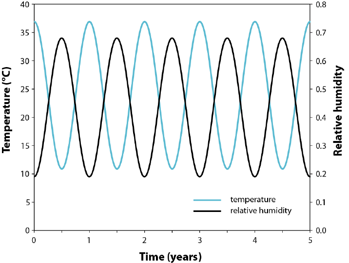
User Manual-page# 3-64
3.9 CONTROL PARAMETERS – EVAPORATION
This Data Block specifies the parameters to calculate the evaporation rate. It includes the
specification of a tortuosity model for vapour flow (τv), a reference vapour diffusivity, and a model
to determine the porous medium surface resistance to flow (rs). The model for calculation of the
saturated vapour density (
r
sv
) is also defined in this Data Block. The enhanced factor in thermal
vapour fluxes is also specified in this Data Block.
Importantly, this Data Block also allows you to specify the desired weather conditions for your
simulation. Correspondence parameters such as relative humidity, temperature, solar radiation,
rainfall, and evaporation rate are specified. Parameters for each of these aspects can be specified
directly in the prefix.dat file, or else may be specified in the separate ‘atmospheric’ file (.atm) (see
subsection 3.9.5). A sinusoidal function with both daily and annual cycles may be specified in Data
Block 6B for both temperature and relative humidity. If the sinusoidal function is used, a maximum,
minimum, and amplitude must be specified for each parameter in the input file. An example of the
output if temperature and relative humidity values are applied in as sinusoidal functions is depicted
in Figure 3.1.
Figure 3.1: MIN3P-THCm output example when a sinusoidal function for climate variables is
employed.
3.9.1 DESCRIPTION OF DATA BLOCK
In this section, control parameters affecting the evaporation model are defined using the header
'control parameters - evaporation'. It is to note that the keywords ‘compute evaporation’ is required
under the header ‘control parameters – energy balance’ to activate the evaporation model (see
section 3.8.2.4).

User Manual-page# 3-65
3.9.2 DESCRIPTION OF INPUT PARAMETERS
3.9.2.1 'write transient evaporation info'
The sub-keyword 'write transient evaporation info' controls the output of transient
evaporation information (e.g. time, evaporation rate, temperature, wind speed, rainfall, run off etc.)
in the file prefix.evap.
3.9.2.2 'vapour density model'
If the sub-block 'vapour density model' is specified, the vapor density () is considered to
be dependent on the relative humidity (), salinity represented by the activity of water and the
temperature-dependent saturated vapor density () (Bea et al. 2012; Saaltink et al., 2005):.
Equation 3-22
Two empirical saturated vapor density models are available: the default model and the Saito et al.
(2006) model.
The default model is the vapor density is calculated:
Equation 3-23
The Saito et al. (2006) model is computed (e.g. Saito et al., 2006):
Equation 3-24
3.9.2.3 'update vapor density derivatives'
If the keyword 'update vapor density derivatives' is specified, the vapor density
derivatives will be updated in each time increment.
3.9.2.4 'temperature gain factor for soil'
The parameter 'temperature gain factor for soil' specifies the gain factor (), which
corrects the temperature dependence of the surface tension (equals to 7 in the study by Nimmo and
Miller (1986).
3.9.2.5 'reference vapor diffusivity'
The parameter 'reference vapor diffusivity' specifies the reference vapor diffusion
coefficient in [m2 s-1].
3.9.2.6 'enhanced factor in isothermal vapor fluxes'
The parameter 'enhanced factor in isothermal vapor fluxes' specifies the enhanced
factor () in isothermal vapor fluxes [-].

User Manual-page# 3-66
3.9.2.7 'compute enhanced factor in thermal vapor fluxes'
If the keyword 'compute enhanced factor in thermal vapor fluxes' is specified, the
enhanced factor () in isothermal vapor fluxes will be calculated according to (Sakai et al. 2009):
Equation 3-25
The parameters (clay fraction in [%]) and a (empirical coefficient [-]) should be provided.
If the keyword is not provided, the enhanced factor is equal to 1.0.
3.9.2.8 'soil surface resistance to vapor flow'
The keyword 'soil surface resistance to vapor flow' followed by model name
specifies the model to account the effect of soil surface resistance () on vapor diffusion. Four
models are implemented in MIN3P-THCm. Model 1 is defined (Bittelli et al., 2008):
Equation 3-26
The formulation of the model 2 is defined:
Equation 3-27
The formulation of the model 3 is defined:
Equation 3-28
The formulation of the model 4 is defined (Simunek et al., 2009):
Equation 3-29
In which is the surface resistance [s m-1], which should theoretically be equal to the resistance
to molecular diffusion across to the water surface (=10) (van de Griend and Owe, 1994). If no
model is specified, the default value of is 0.0.
3.9.2.9 ‘split divergence of vapor density’
The keyword 'split divergence of vapor density' enables the calculation of the vapour
flux according to:
Equation 3-30
In which, the effect of temperature and liquid pressure on the vapour density is separately accounted.
Otherwise,

User Manual-page# 3-67
Equation 3-31
3.9.2.10 'tortuosity model to vapor flow'
The keyword 'tortuosity model to vapor flow' followed by the model name specifies
the tortuosity model for the calculation of diffusive vapour flow transport. The default model is:
Equation 3-32
Alternatively, Millington model ('millington') and no tortuosity model ('not consider')
can be specified. The Millington model is defined:
Equation 3-33
If the tortuosity effect can be neglected (), the model 'not consider' can be specified.
3.9.2.11 'relative humidity parameters'
The keyword 'relative humidity parameters' leads to the input of parameters for the
relative humidity calculation. The following logical parameter specifies the way of parameters’
input. If it is .false., a sinusoidal function with both daily and annual cycles may be specified in
Data Block 6B for relative humidity.
Equation 3-34
If the sinusoidal function is used, a maximum, minimum, and amplitude must be specified for each
parameter in the input file. In such case, the required parameters are provided in the following order:
Averaged relative humidity of the atmosphere [-]
Annualy amplitude in the relative humidity [-]
Diurnal amplitude in the relative humidity [-]
Time during the year when relative humidity is maximum [time units depends on
units of the problem]
Time during the day when relative humidity is maximum [time units depends on
units of the problem]
Alternatively, the parameters may be read from a separate file (prefix.atm) in the same folder of
the input file prefix.dat if the logic parameter is set to ‘.true.’ (see section 3.9.5).
3.9.2.12 'temperature parameters'
The keyword 'temperature parameters' leads to the input of parameters for the temperature
of the atmosphere. The data structure is the same as the previous section relative humidity
parameters'. A sinusoidal function with both daily and annual cycles may be specified in Data Block
6B for atmosphere temperature, if the following parameters are provided in the Data Block:

User Manual-page# 3-68
Averaged temperature of the atmosphere [°C]
Annual temperature increment [°C]
Daily temperature increment [-]
Time during the year when atmospheric temperature is maximum [time units
depends on units of the problem]
Time during the day when atmospheric temperature is maximum [time units
depends on units of the problem]
The related equation is:
Equation 3-35
Alternatively, the parameters for the temperature of the atmosphere can be read from the separate
file prefix.atm as described before.
3.9.2.13 'solar radiation parameters'
The keyword 'solar radiation parameters' leads to the specification of parameters for
the solar radiation. The next two logical parameters (for radiation and the cloud index parameters)
specify whether the parameters should be read from the file prefix.atm (see section 3.9.5). If both
logical parameters are .true., or the second one is .true., the corresponding parameters should be
read from the prefix.atm file. If only the first logical parameter is .true., the radiation parameters
should be given in the prefix.atm file. In such case, the cloud index in the prefix.atm will be
neglected. Otherwise, the following parameters are specified:
Factors to multiply radiation term [-]
Latitude of the place [rad]. Positive value when it locates in the northern part of the earth,
otherwise, negative value.
Time when January is starting. For example, if the experiment starts on July 1, the value is
182.5 days.
Time corresponding to noon during the daylight period
Time when autumn is starting (e.g., September 21 in the northern hemisphere, March 21
in the southern hemisphere)
Cloud index (0=completely clouded sky, 1=clear sky)
Albedo of dry soil
Albedo of wet soil
3.9.2.14 'rain parameters'
The keyword 'rain parameters' leads to the specification of the leakage coefficient () for
runoff term (). The surface runoff is considered in the water balance equations as a part of the
‘source/sink’ term ‘
fw
’.
Equation 3-36
To read rainfall events from the prefix.atm file, the logical parameter followed by the keyword
'rain parameters' is set to ‘.true.’ If it is set to .false., the leakage coefficient for rain runoff
term should be provided in the next line.

User Manual-page# 3-69
3.9.2.15 'evaporation parameters'
The keyword 'evaporation parameters' leads to the specification of the parameters needed
for the evaporation flux calculation. In the next two lines, two logical parameters specify the options
for the parameter input. If the first one is set to ‘.false.’, the evaporation rate [kg m-2 s-1] is to be
read from the file prefix.atm (see section 3.9.5). If the first one is set to ‘.true.’, the evaporation rate
is to be calculated and the related six parameters and/or the wind parameters should be provided in
this block. The six parameters are:
Imposed evaporation rate [kg m-2 s-1];
Factor to multiply evaporation term [-];
Roughness length [m]
Screen height where parameters were measured [m]
Stability factor [-]
Density of air in the atmosphere [kg m-3];
The next terms deal with the input of wind related parameters starting with a logical parameter,
which defines option for the wind parameter input. If it is set to ‘.true.’, the wind speed(s) in [m s-
1] will be read from the file prefix.atm (see section 3.9.5). Otherwise, a sinusoidal function may be
applied for wind speed, although this may not be very representative of natural wind speed
variations.
Equation 3-37
In such case, five parameters have to be provided in the following five lines including:
Averaged wind speed in [m s-1];
Wind speed amplitude during year in [m s-1];
Wind speed amplitude during day [m s-1];
The time at maximum wind speed during year [units of the problem];
The time at maximum wind speed during day [units of the problem].
3.9.3 DATA FILE INPUT
The following example demonstrates the usage of the evaporation model.
! Data Block 6B: control parameters - evaporation
! ---------------------------------------------------------------------------
!
'control parameters - evaporation'
'write transient evaporation info'
'temperature gain factor for soil'
7.0d0
'update vapor density derivatives'
'reference vapor diffusivity'
2.12d-5
!'enhanced factor in isothermal vapor fluxes'
8.0d0
'soil surface resistance to vapor flow'
User Manual-page# 3-70
'model 3'
!'split divergence of vapor density'
'tortuosity model to vapor flow'
'millington'
'compute enhanced factor in thermal vapor fluxes'
2.0 ! clay fraction content
8.0 ! nabla cte
'relative humidity parameters'
.false. ! Read Hr from file
0.85d0 ! Relative humidity of the atmosphere (average)
0.245d0 ! relative humidity (amplitude during the year)
0.00d0 ! relative humidity (amplitude during the day)
182.5d0 ! Time for maximum relative humidity during year [units of the problem]
0.5d0 ! Maximum during day [units of the problem]
'temperature parameters'
.false. ! Read temp from file
23.9d0 ! Temperature of the atmosphere
13.0d0 ! Temperature (amplitude during the year)
0.0 ! Temperature (amplitude during the day)
0.5 ! maximum time during year [units of the problem]
0.5d0 ! maximum time during day [units of the problem]
'solar radiation parameters'
.false. ! Read radiation from file
.false. ! Read cloud index from file
0.0d0 ! Factor to multiply radiation term
-29.0d0 ! Latitude of the place
182.5d0 ! Time when January is starting
0.5d0 ! Time corresponding to moon
273.5d0 ! Time when autumn is starting
0.5d0 ! Cloud index (0=completely clouded sky, 1=clear sky)
0.2d0 ! Albedo dry soil
0.1d0 ! Albedo wet soil
'rain parameters'
.false. ! Read rain events from file
-100.0d0 ! Leakage coefficient for runoff term
'evaporation parameters'
.false. ! Compute evaporation rate based on aerodynamic relationship
.true. ! Read evaporation rate from file (only if compute evaporation rate is false)
1.9675E-06 ! Imposed evaporation rate [kg/m2/s]
1.0 ! Factor to multiply evaporation term
0.001d0 ! Roughness length [m]
0.001d0 ! Screen height where parameters were measured [m]
1.0 ! Stability factor
1.112d0 ! Density of air in the atmosphere
.false. ! Read wind
1. ! Wind speed [m s-1]
0.0 ! Wind speed amplitude during year [m s-1]
0.0 ! Wind speed amplitude during day [m s-1]
0.0 ! Maximum wind speed during year [units of the problem]
0.0 ! Maximum wind speed during day [units of the problem]
'done'
3.9.4 DESCRIPTION OF EXAMPLE INPUT
In the above input, model 3 is used to calculate the porous medium resistance to flow (rs), and the
default model (Millington, 1959) for tortuosity (τv) is used.
The enhanced thermal vapour flux is calculated using a clay content (fc) of 2.0%, and an empirical
User Manual-page# 3-71
constant (a) of 15.
Because nothing is specified for calculation of the saturated vapour density (
r
sv
), it is calculated
internally according to the default model. The alternative model after Saito et al. (2006) could
instead be activated through the following input inserted after the keyword ‘write transient
evaporation info’:
'vapour density model'
'saito et al. (2006)'
.true.
The relative humidity (Hr) parameters are specified as a sinusoidal function with an average of 0.85
and annual amplitude of 0.245. No daily amplitude is specified, thus no diurnal fluctuations are
specified and the relative humidity is constant for the entire day (24 hours). The maximum value
for relative humidity occurs at day 182 of every year.
Similarly, the temperature (T) is defined by a sinusoidal function, with an average temperature of
23.9 °C and amplitude of 13.0 °C (i.e., temperature varies between 10.9-36.9 °C throughout the
year). No diurnal fluctuations in temperature are specified therefore the temperature is constant for
the entire day (24 hours). The annual temperature maximum occurs at 0.5 days (i.e., at noon on the
first day of the simulation). Thus, the temperature and relative humidity functions are antiphase.
The solar radiation is calculated internally (see in the theory manual section 2.1.6.2 Atmospheric
boundary condition) rather than specified in the prefix.atm file. Similarly, the cloud index is
specified in the prefix.dat file at a value of 0.5 (partly cloudy). The latitude is -29° or 29°S, therefore
the location is in the Southern hemisphere. January is specified to start at day 182.5 of every year,
which implies that the summer occurs midway through each year in the simulation as it is in the
Southern hemisphere. This value should therefore correspond to the time of the temperature
maximum and relative humidity minimum that are specified in the previous input. Noon is set to
equal 0.5 days, such that 0.0 days is midnight. If daily amplitude is specified for the temperature
and relative humidity, care should be taken that the maximum values for these parameters properly
correspond to the ‘noon’ value (i.e., peak temperature should occur at noon). The time when autumn
is starting is day 273.5 of each year, or April 1).
The rain events are read in from the prefix.atm file, with a leakage coefficient for the runoff
equation () of -100.
The evaporation rate is calculated using the aerodynamic relationship (Equations 2-100 to 2-103 in
the theory manual section Atmospheric boundary condition). A roughness length (z0) of 0.001 m is
specified. The screen height (za) is 0.001 m. The stability factor (θ; Equation 2-115) is 1.0. The
density of air in the atmosphere (
r
g
atm
; Equation 2-114) is 1.112 kg m-3. The wind speed is specified
in the prefix.dat file and is a constant (i.e. 1.0 m s-1) throughout each day and year.
3.9.5 ATMOSPHERIC (.ATM) FILE INPUT
Some parameters for the atmospheric boundary condition can be specified through a separate file
prefix.atm if at least one of the logic parameters in the example in section 3.9.3 is ‘true’. In this file,
the following parameters should be included.
3.9.5.1 Time
The simulation time is the first column in the prefix.atm file. Its unit should be the same as given
in the data block 'time step control - global system'. Recommended unit is days.
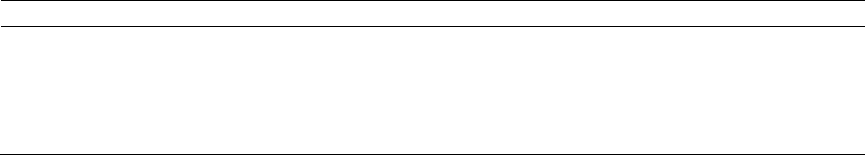
User Manual-page# 3-72
3.9.5.2 Temperature
The temperature (temp) in the prefix.atm file is the second column and is specified in °C. If the
temperature is specified in the prefix.dat file rather than the prefix.atm file, values of zero are
specified in the temperature column in the prefix.atm file.
3.9.5.3 Relative humidity
The relative humidity (Hr) in the prefix.atm file is the third column and is specified as a fraction
ranging from 0 to 1. If the relative humidity is specified in the prefix.dat file rather than the
prefix.atm file, values of zero are specified in the hr column in the prefix.atm file.
3.9.5.4 Wind
The wind (wind) in the prefix.atm file is the fourth column and is specified in m s-1. If the wind is
specified in the prefix.dat file rather than the prefix.atm file, values of zero are specified in the wind
column in the prefix.atm file.
3.9.5.5 Radiation
The radiation (Rn) in the prefix.atm file is the fifth column and is specified in J m-2 s-1. If the
radiation is calculated internally using values defined in the prefix.dat file, values of zero are
specified in the radiation column in the prefix.atm file. To read radiation values from the prefix.atm
file, ‘read radiation from file’ in Data Block 6B(2) is set to ‘true.’
3.9.5.6 Rainfall
The rainfall rate is calculated from values provided by the user in the prefix.atm file. The rainfall
(rain) column is the sixth column in the prefix.atm file. Example input for the prefix.atm file is
shown in Table 3.10.
Table 3.10: Example rainfall input in atmosphere file
Time [days]
Rain [m]
0
0.00
10
2.3×10⁻³
10.21
0.00
15
5.0×10⁻³
15.42
0.00
The rainfall rate is calculated from this input as Rain divided by Time. In the example input file,
no rainfall occurs for the first ten days. This is followed by a 5 hour interval over which a total of
2.3×10⁻³ m of rain is applied. Thus, the rainfall rate over this period is 1.28×10⁻⁴ mm/s. Following
this event, there is no rain until day 15, at which point a rainfall event of 1.28×10⁻⁴ mm/s occurs for
10 hours. From a functional standpoint, care must be taken to ensure sufficient significant digits
are specified in the prefix.atm file to properly apply the desired rainfall interval. For example, if a
rainfall event is to occur on day 9240 for two hours, the entries in the time column must contain at
least 6 significant digits (i.e., 9240.08 days). Certain editing programs will truncate significant
digits, therefore it is important as the user to check over prefix.atm files to ensure the proper values
are maintained. The double precision format is highly recommended.

User Manual-page# 3-73
3.9.5.7 Cloud index
The cloud index (In) in the prefix.atm file is the seventh column and is specified as a fraction
between 0 and 1, with 0 being complete cloud cover, and 1 being clear skies. If the cloud index is
defined in the prefix.dat file, values of zero are specified in the cloud index column in the prefix.atm
file.
3.9.5.8 Evaporation
The evaporation rate can be specified in the prefix.dat file [kg m-2 s-1]. If the evaporation rate is
specified in the prefix.dat file or is calculated internally using values defined in the prefix.dat file,
values of zero are specified in the evap rate column in the prefix.atm file.
An example of the prefix.atm file is:
-----------------------------------------------------------------------------------------
Time Tatm[°C] Hr [-] WindSpeed [m/s] Radiation [KJ day-1 m-2] Rain [m] Cloud index [-]
Evap rate [kg/m2/s]
----------------------------------------------------------------------------------------
0.00E+00 0.0000000E+00 0.0000000E+00 0.0000000E+00 000.0d0 0.0 0.00000E+00 1.5d-6
5.00E+00 0.0000000E+00 0.0000000E+00 0.0000000E+00 000.0d0 0.0 0.00000E+00 2.2d-6
10.00E+00 0.000000E+00 0.0000000E+00 0.0000000E+00 000.0d0 0.0 0.00000E+00 2.3d-6
16.0 0.0000000E+00 0.0000000E+00 0.0000000E+00 0.00000d0 0.0 0.000000E+00 2.8d-6
-1.0
----------------------------------------------------------------------------------------
The first three lines are used for the header, which are only for the description of the parameters to
be provided and are skipped by the program. From the fourth line on, the required parameters must
be provided in the order: Time, temperature of the atmosphere, relative humidity, net solar radiation,
rainfall, cloud index, and the evaporation rate. The number format is flexible as long as there is
space(s) between two parameters. The last negative value -1.0 terminates the read function.
3.10 CONTROL PARAMETERS – REACTIVE TRANSPORT (DATA
BLOCK 7)
3.10.1 DESCRIPTION OF DATA BLOCK
In this section, numerical and control parameters affecting the reactive transport calculations are
defined. The entire section is optional, default values are specified for all parameters in the code.
This section may be modified to enhance the model performance, or potentially correct
convergence problems.
3.10.2 DESCRIPTION OF INPUT PARAMETERS
The content of this section is similar to Section 3.6. The input parameters are described below, and
are also summarized in Table 3.11 together with the corresponding default settings, possible
parameter settings and the recommended range for the parameters.

User Manual-page# 3-74
3.10.2.1 ‘mass balance’
If the sub-block ‘mass balance’ is specified, the model will perform mass balance calculations
including contributions of storage, fluxes across the domain boundary and internal sources and
sinks due to the specified geochemical reactions. The total system mass for aqueous phase
components, minerals, gases and surface species are reported in the files prefix_o.mas,
prefix_o.mms, prefix_o.mgs and prefix_o.mss. Mass balance contributions and cumulative changes
are reported for each component, for each mineral phase and for all gaseous species in separate
files. The file prefix_o.fls contains additional information on these mass balance files, the
corresponding mass balance error files and their content. This file will be created for the specific
problem at run-time.
3.10.2.2 ‘spatial weighting’
Three different spatial weighting schemes can be used to describe advective transport. These
options are controlled under the sub-block ‘spatial weighting’ and are identified by their names.
The three options are ‘upstream’, ‘van leer’ and ‘centered’. By default, upstream weighting will be
used. In this case the concentrations for the advective mass transport term are assigned based on:
0
0
,,,
,,,
kla
a
kj
a
klj
kla
a
kj
a
klj
vifTT
vifTT
Equation 3-38
where Taj,kl is the concentration at the interface of two adjacent control volumes, Taj,k and Taj,l are
the concentration in the control volumes k and l, while va,kl defines the Darcy flux from control
volume k to l. For centered weighting, the interfacial concentrations are defined based on:
2
,,
,
a
lj
a
kj
a
klj
TT
T
Equation 3-39
If centered weighting is used, it is necessary to obey the Peclet criterion to ensure convergence.
The following requirements have to be obeyed:
2
,
,
kla
kla
D
xv
Pe
Equation 3-40
where x defines the distance between the center of the two adjacent control volumes and Da,kl is
the effective dispersion coefficient. If the Van Leer–flux limiter is specified, the interfacial
concentrations are calculated based on:
2
)( ,,
,,
a
lj
a
kj
kl
a
kj
a
klj
TT
rTT
Equation 3-41
where
(rkl) is the Van Leer flux limiter and rkl is a smoothness sensor.
(rkl) ranges from 0 to 2
and is calculated internally (van Leer, 1994, Unger et al., 1996). The present implementation of the
Van Leer flux limiter requires the Courant criteria to be obeyed:
1
,
x
tv
Cr kla
Equation 3-42
where t defines the time increment. Neither the Courant, not the Peclet restrictions apply for

User Manual-page# 3-75
upstream weighting, however, upstream weighting may lead to excessive numerical dispersion.
3.10.2.3 ‘activity update settings’
The model allows several options to update activity coefficients for aqueous species. It is possible
to exclude activity updates altogether by specifying ‘no update’ or ‘no_update’ under the sub-block
‘activity update settings’. By default the activity coefficients are updated after completion of each
time step (‘time lagged’ or ‘time_lagged’) (Lichtner, personal communication, 1997). Alternatively,
the option ‘double update’ or ‘double_update’ can be used. In this case, the activity coefficients for
all aqueous species are updated twice per Newton-iteration to maximize accuracy on the cost of
performance. Comparisons have shown that differences between the option ’time lagged’ and
‘double update’ are minimal. ‘time lagged’ is therefore the recommended option for calculations
including activity corrections.
The input format is:
'activity update settings'
'time_lagged' ;type of activity update
3.10.2.4 ‘tortuosity correction’
The sub-block 'tortuosity correction' defines the options for tortuosity corrections. There are four
options: 'millington', 'archie', 'assigned tau' and 'no correction'. If the text string below the sub-block
‘tortuosity correction’ is set to 'millington', the tortuosity in the aqueous and gas phase is calculated
based on the relationship defined by Millington (1959):
3/13/7
p
S
Equation 3-43
where Sp is the phase saturation and
is porosity. In such case, the tortuosity will be calculated
according to the porosity. An example of the input format:
! Data Block 7: control parameters - reactive transport
! ---------------------------------------------------------------------------
!
'control parameters - reactive transport'
'spatial weighting'
'upstream' ;spatial weighting
'tortuosity correction'
'millington'
The example input specifies the tortuosity is updated according to Millington equation. No
tortuosity parameter is needed in Data block 9 (see Section 3.12). Note: The keyword 'millington'
is also used to specify the tortuosity correction model for vapor (see section 3.9.2.10).
Similiarly, if the text string below the sub-block ‘tortuosity correction’ is set to 'archie', the
tortuosity in the aqueous and gas phase is calculated based on the relationship defined as:
Equation 3-44
In which α is the coefficient of the Achie’s law. To use this function, add 'update tortuosity' to
User Manual-page# 3-76
block 7 and alpha value to block 9. The initial tortuosity and α can be specified in Data block 9 to
each material zone. An example input:
in block 7: control parameters - reactive transport
'tortuosity correction'
'archie'
'update tortuosity'
in block 9: physical parameters - porous medium
'number and name of zone'
1
'concrete'
0.1 ;porosity
0.0383 ;tortuosity
2.0 ;alpha, tortuosity update factor
The example input defines that the tortuosity is updated according to the Archie’s law with a
tortuosity update factor α =2.0. The initial tortuosity is 0.0383. Note: In this model, the
tortuosity is calculated according to Equation 3-44. is not used but it is needed in the input file
so that the coefficient α can be correctly read.
Another option for the update of tortuosity is the assigned tortuosity using 'assigned tau'. In such
case, the assigned tortuosity will be used for the effective diffusion coefficient calculation. This
can be specified in the input file (i.e. for each material zone) or through external file with extension
prefix.tor (i.e. for each control volume, see section 3.12.5).
in block 7: control parameters - reactive transport
'tortuosity correction'
'assigned tau'
'update tortuosity'
in block 9: physical parameters - porous medium
'number and name of zone'
1
'concrete'
0.1 ;porosity
0.0383 ;tortuosity
If ‘no correction’ is specified, tortuosity corrections are neglected and tortuosity is set to unity.
3.10.2.5 ‘spatial averaging - diffusion’
The effective diffusion coefficient (De) is a physical parameter of each control volume. In order to
calculate the diffusive flux between two connected control volumes, a representative De has to be
calculated using the parameters of both control volumes. For example, if the control volumes have
different size, spatially weighted averaged De might be more reasonable. Considering the De is
calculated based on the D0, porosity and tortuosity, there are different ways to calculate the
representative depending on the averaging method (e.g. arithmetic or harmonic) and the order of
averaging (e.g. averaging the effective porosity and tortuosity first and then calculate the
representative De, or calculate the De in each control volume and then spatially weighted averaging
User Manual-page# 3-77
to obtain the representative De). In MIN3P-THCm, three different spatial averaging methods for
the effective diffusion coefficient (De) were implemented: the arithmetic averaging method, the
arithmetic De averaging method and the harmonic averaging method.
The arithmetic averaging method (using key word ‘arithmetic’): first calculate the representative
effective porosity and tortuosity through arithmetic method (i.e. sum of the parameters of connected
pair of control volumes divided by two), then calculated the representative De. An example input:
'spatial averaging - diffusion' ; Keyword
'arithmetic'
The arithmetic De averaging method (using key word 'arithmetic De'): first calculate the De of each
control volume using the corresponding effective porosity and tortuosity; then calculated the
representative De using the arithmetic method and the De of the connected pair of control volumes.
An example input:
' spatial averaging - diffusion' ; Keyword
'arithmetic De'
The harmonic averaging method (using key word 'harmonic'): first calculate the De of each control
volume using the corresponding effective porosity and tortuosity; then calculated the representative
De using the arithmetic method and the De of the connected pair of control volumes. An example
input:
' spatial averaging - diffusion' ; Keyword
‘harmonic’
3.10.2.6 'gas advection'
The sub-block 'gas advection' enables gas advection simulation.
3.10.2.7 ‘cumulative mole fractions’
The sub-block ‘cumulative mole fractions’ enables to provide cumulative gas pressure value in the
output file prefix_x.gsg.
3.10.2.8 'enable gravity for gas phase'
The sub-block 'enable gravity for gas phase' enables the code to take the gravity into consideration
for gas advection simulation.
3.10.2.9 ‘degassing’
The sub-block ‘degassing’ enables degassing of dissolved gases from the saturated zone, if the sum
of the partial gas pressures exceeds the confining pressure. The value specified below the
subkeywords defines the degassing rate in mol L-1 H2O s-1. An example of the input format is:
'degassing' ;allow degassing
1.0d-8 ;rate constant [mol L-1 h2o s-1]
3.10.2.10 ‘update porosity’
The sub-block ‘update porosity’ enables to keep track of porosity changes due to dissolution-
precipitation reactions. If this statement is enabled, porosity is calculated based on:
User Manual-page# 3-78
m
N
i
t
i
tt
i
ttt
1
Equation 3-45
The porosity update will also affect the calculation of the effective diffusion coefficients. If this
option is enabled, the time step should be kept sufficiently small to provide an accurate solution.
This is necessary, because the update of the porosities is done explicitly after completion of a time
step. Usually porosity changes are relatively slow and this simplification does not lead to significant
inaccuracies.
3.10.2.11 ‘update permeability’
When the sub-block ‘update permeability’ is specified, the initial hydraulic conductivities are
modified based on a normalized version of the Carman-Kozeny relationship. The update is of the
form as described in Equation 3-24 in the MIN3P-THCm Theory Manual section 3.5.
If this option is enabled, the option ‘update porosity’ will be enabled automatically. As for the
porosity-update, the time step needs to be kept sufficiently small, because flow and transport are
treated as decoupled processes.
3.10.2.12 'newton iteration settings’
This sub-block defines the parameters affecting the Newton iteration. Similar to the definitions for
the geochemical batch module, the increment for numerical differentiation is used to calculate
numerical derivatives according to the formula (Equation 3-3).
The following parameter specifies the anticipated number of Newton iterations, which is used
internally to calculate an estimate for the time increment for the next time step. The next parameter
identifies the maximum number of Newton iterations to be performed, before a solution is
considered non-convergent. The time step is repeated with a reduced time increment, if the actual
number of Newton iterations exceeds the maximum number of Newton iterations. The maximum
number of Newton iterations must be larger than the anticipated number of Newton iterations
(commonly 3 times).
In the following the anticipated update for the primary unknowns (concentrations of components
as free species) in log concentration [mol L-1] cycles is specified. Below this parameter, the
maximum tolerable update (in log concentration [mol L-1] cycles) is specified. The computed
update is set to the maximum tolerable update, if the computed value is larger than the maximum
allowed value. This is done to ensure that the computed concentrations remain sufficiently close to
the actual solution. Similar to the requirements for the maximum number of Newton iterations, the
maximum tolerable update must be larger than the desired update (usually 2-3 times larger).
The convergence tolerance defines the accuracy of the concentrations calculated during the reactive
transport simulation. A solution is considered converged if the logarithm of all concentration
updates at each spatial discretization point in the solution domain is smaller than the convergence
tolerance (Equation 3-5).
3.10.2.13 ‘solver settings’
The solver package WATSOLV (VanderKwaak et al., 1997) is also used for the solution of the
reactive transport problem. The settings defined in the sub-block ‘solver settings’ are therefore
equivalent to the one for the variably-saturated flow problem and are described in the section on
‘control parameters – variably-saturated flow’.
User Manual-page# 3-79
3.10.3 DATA FILE INPUT
An example is:
! ---------------------------------------------------------------------------
'control parameters - reactive transport'
'mass balance'
'spatial weighting'
'upstream' ;spatial weighting
'activity update settings'
'time lagged' ;type of activity update
‘update porosity’ ;porosity changes
‘update permeability’ ;permeability = f(porosity)
'tortuosity correction'
‘millington’ ;Millington-Quirk tortuosity correction
'newton iteration settings'
1.d-4 ;increment for numerical differentiation
20 ;anticipated number of Newton iterations
60 ;max. number of Newton iterations
1.0d0 ;anticipated update in log cycles
2.0d0 ;maximum update in log cycles
1.d-6 ;convergence tolerance (global system)
'solver settings'
0 ;incomplete factorization level
100 ;max. number of solver iterations
1 ;information level
1.d-7 ;solver residual tolerance
1.d-7 ;solver update tolerance
‘natural ordering’ ;natural ordering
‘degassing’
1.0×10⁻⁸ ;degassing rate [mol L-1 s-1]
'done'
3.10.4 DESCRIPTION OF EXAMPLE INPUT
In the example input file, mass balance calculations are performed. The code uses upstream
weighting for advective transport in the aqueous phase. Activity coefficients are updated after
completion of each time step. The tortuosity is corrected based on the relationship by Millington
[1959]. An increment of 10-4 (relative to the actual concentration of each primary unknown) is
specified. The anticipated and maximum number of iterations in the Newton loop are 20 and 60,
respectively. The anticipated update is 1 log concentration cycle, while the maximum update is
locally restricted to 2 log cycles. The solution is deemed sufficiently accurate, if the magnitude of
the logarithm of the concentration update is less than 10-6. The sparse iterative matrix solver will
operate with a level 0-preconditioning, use natural ordering of the Jacobian matrix and will perform
100 solver iterations before the solution is considered non-convergent. The information level is set
to 1, providing information on the Newton-loop, but not on the inner iteration. The solver residual
tolerance and solver update tolerance have been specified one order of magnitude more stringent
than the convergence tolerance. Degassing has been specified at a rate of 1.0×10⁻⁸ mol L-1 s-1.

User Manual-page# 3-80
Table 3.11: Summary of input parameters for section ‘control parameters – reactive transport’
Subsection
Parameter
Default
value
Possible
parameter
settings
Recommended
range/parameter
‘mass balance’
-
-
-
-
‘spatial
weighting’
type of weighting
scheme
‘upstream’
‘upstream’
‘centered’
‘van leer’
‘upstream’
‘activity update
settings’
type of activity
update
‘time
lagged’
‘no update’
‘time lagged’
‘double update’
‘time lagged’
‘tortuosity
correction’
type of tortuosity
correction
‘millington’
‘millington’
‘no correction’
‘millington’
‘degassing’
degassing rate
0.0
-
system-dependent
‘update
porosity’
-
-
-
-
‘update
permeability’
-
-
-
-
‘user-specified
underrelaxation
factor’
underrelaxation
factor
1.0
-
1.0
‘newton
iteration
settings’
increment for
numerical
differentiation [m]
10-4
-
10-6-10-4
anticipated
number of Newton
iterations
12
10-20
maximum number
of Newton
iterations
15
-
20-60
anticipated
concentration
update in log
cycles
0.5
-
0.5-1.5
maximum
concentration
update in log
cycles
1.0
-
1.0-3.0
convergence
tolerance in log
cycles
10-6
-
10-7-10-4
‘solver settings’
incomplete
factorization level
0
-
0-2
maximum number
of solver iterations
100
-
100-1000
solver information
level
1
0,1,2
-
solver residual
tolerance [m]
10-7
-
10-8-10-5

User Manual-page# 3-81
solver update
tolerance [m]
10-7
-
10-8-10-5
‘natural
ordering’
-
-
-
-
3.11 OUTPUT CONTROL (DATA BLOCK 8)
3.11.1 DESCRIPTION OF DATA BLOCK
In this data block, the output from the simulation is specified. Data can be output as a 'snapshot' at
a specified time (spatial data) or as data through time at a specified location (transient data). Spatial
data in 1D typically would consist of a linear plot of concentration with distance for a specified
time; for a 2D simulation, the concentration data can be visualized as a 2D contour plot. Transient
data typically consists of a plot of concentration with time (breakthrough curve). This section is
entirely optional for all flow and reactive transport simulations and will not be considered for any
batch chemistry simulations. If this section is not specified, the output will only be written at the
end of the simulation.
3.11.2 DESCRIPTION OF INPUT PARAMETERS
3.11.2.1 'output control'
This data block contains up to three sub-blocks, which are described below. If isotope geochemistry
is considered, an additional keyword 'isotope output' is required (see below).
3.11.2.2 'output of spatial data'
The first parameter for specifying spatial data output is the number of desired output times. This
value follows the sub-block header 'output of spatial data'. The second line contains the times at
which the output is desired. Only 4 output times can be specified per line, if the number of output
times exceeds 4, the values for the output times have to be specified in the next line. The time units
used are the same as those specified in the Section 4 (‘time step control’). Spatial data is written to
the files prefix_*.gs*, as described in Section and can be post-processed with TECPLOT (Amtec,
2003). For example, the file prefix_1.gst will contain spatial data at the first (1) specified output
time for total aqueous component concentrations (t). Other output files are described in section 2.2.
3.11.2.3 'output of transient data'
The first parameter for specifying transient data output is the number of desired output locations.
This line follows the sub-block header 'output of transient data.' The following parameter defines
how often transient data is written to the output file (i.e.: setting this parameter to 3 means that
output data will be written to the output files every third time step). This is used to reduce the size
of transient output files (e.g. *.gbt) when the time step is too small. The third line specifies the
control volume numbers of the output locations.
Only 4 output locations can be specified per line, if the number of output locations exceeds 4, the
values for the output locations have to be specified in the next line. Transient data is written to the
files prefix_*.gb*, as described in Section 2. For example, the file prefix_1.gbt will contain
transient data for the first (1) specified output location for total aqueous component concentrations
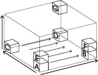
User Manual-page# 3-82
(t).
The control volume numbers can be calculated from the spatial discretization parameters defined
in Section ‘spatial discretization’ (section 3.4). Numbering of the grid is performed in x-direction
first, then in y-direction and finally in z-direction (Figure 3.2).
Figure 3.2: Spatial discretization and numbering principle
Example:
'output of transient data'
5 ;number of output locations (transient data)
1 ;time steps between output (transient data)
1 15 85 95 ;control volume number for transient data
101
This example specified the output of the transient data for five selected control volumes (i.e. 1, 15,
85, 95 and 101). The number of time steps for the output is 1, which means the output at every time
step.
3.11.2.4 ‘output in terms of depth’
The spatial discretization is based on a Cartesian coordinate system, and by default the output in
vertical direction is reported in terms of elevation. Optionally, the output can also be reported in
terms of depth by adding the line ‘output in terms of depth’ to the input file. In this case the z-
coordinates will be transformed prior to output based on:
ii zzz max
where zmax is the maximum elevation in the solution domain (calculated internally) and zi
correspond to the elevations prior coordinate transformation and to depth values after
transformation is completed.
3.11.2.5 'isotope output'
The first parameter for specifying isotope related parameters output is the number of isotope
component sets. This line follows the sub-block header 'isotope output'. The second line specifies
the number of components in each set followed by the master isotope and other isotopes. The ratios
of standard for delta value calculations (Rstd) should be provided in the third line. If the number of
isotope component sets is greater than one, the parameters for each isotope component set should
be provided following the second and third lines mentioned before. The format is as follows:
x-axis
y-axis
z-axis

User Manual-page# 3-83
'isotope output'
2 ;number of isotope component sets for output
2 'so4-2' '34so4-2' ;number of components in set, master isotope, other isotopes,
4.5005d-2 ;and ratios of standard for delta value calculations
2 'hs-1' '34hs-1'
4.5005d-2
The example input block specifies two sets of isotope components for output. One set is sulfate (i.e.
'so4-2' as the master isotope component, followed by the isotope component '34so4-2'), and the
other one is sulfide (i.e. 'hs-1' and '34hs-1'). The master isotope is the isotope that is used in the
numerator of the delta value calculations, 32S in the case of sulfur. The Rstd values for both sets are
4.5005E-2 as the accepted sulfur isotope ratio of the standard Canyon Diablo troilite (CDT)
reference material (Gibson et al. 2011).
3.11.3 EXAMPLE DATA FILE INPUT
An example is as the following:
! ---------------------------------------------------------------------------
'output control'
'output of spatial data'
6 ;number of output times (spatial data)
1.0 2.0 5.0 10.0 ;specified output times (spatial data)
20.0 50.0
'output of transient data'
4 ;number of output locations (transient data)
2 ;time steps between output (transient data)
50 650 1250 1850 ;control volume number for transient data
'output in terms of depth'
'done'
3.11.4 DESCRIPTION OF EXAMPLE INPUT
In the sample input file spatial output will be written at the specified 6 output time: 1.0, 2.0, 5.0,
10.0, 20.0 and 50.0 time units. In total, six spatial output files will be generated. Breakthrough
curves will be generated for the specified 4 locations (i.e. control volumes 50, 650, 1250, and 1850).
The output of the transient data will be written every second time step and will be reported in terms
of depth.
3.12 PHYSICAL PARAMETERS: POROUS MEDIUM (DATA
BLOCK 9)
3.12.1 DESCRIPTION OF DATA BLOCK
This data block is used to specify the zones that are used to discretize a variety of physical properties
across the model domain. In this section, the porosity is also specified for each zone. The zone
names specified in this section are reused in other input sections to allocate physical parameters
specific to variably-saturated flow or reactive transport.

User Manual-page# 3-84
3.12.2 DESCRIPTION OF INPUT PARAMETERS
3.12.2.1 'physical parameters - porous medium'
The first parameter that must be specified in this data block is the number of material property
zones. This value is specified in the second line of this input section immediately below the heading
'physical parameters - porous medium'.
3.12.2.2 ‘number and name of zone’
Each zone is defined by its own sub-block, which is bounded at the top by the statement ‘number
and name of zone’ and at the bottom by the statement 'end of zone'. Each of these input blocks
requires the same input sequence.
The first parameter within each block is the zone number. This value is placed immediately after
the subkeywords 'number and name of zone'. Property zones are numbered sequentially starting
with 1 and the number of the final zone should be the same as the total number of property zones
specified in the beginning of this section. The zones can be specified in any order.
The second input parameter is the name of the zone. This parameter consists of a word or a short
sentence (up to 72 characters) describing the specific material property zone. The zone name must
be placed in single quotes below the zone number. This name identifies each zone and will be used
in additional input sections to allocate other material properties, specific to flow or transport
simulations. It is therefore important that the name is unique to that zone and that it be reproduced
exactly in future input sections.
The third parameter is the porosity for the zone; this value is specified directly below the property
zone name.
The fourth parameter is the tortuosity for the zone. This parameter is specified following the
porosity in a separate line.
The last parameter defines the ‘extent of zone’. Under this parameter the dimensions of the zone
are defined. MIN3P-THCm allows the simulation of flow and reactive transport in three spatial
dimensions. The following input defines the location of minimum and maximum coordinates in the
x, y and z-directions (in meters) for the material properties to be allocated. If a 1D or 2D-simulation
is conducted, the minimum and maximum coordinates for the excluded dimensions should be
specified as 0.0 and 1.0, respectively.
Material properties must be specified for every control volume in the domain. If this is not done,
the program will stop when executed and report an error to the file prefix.log. On the other hand, it
is possible to overwrite existing material properties with new material properties. If this is done, a
warning will be issued to the file prefix.log in case material properties have been overwritten
accidentally. In some applications, it may be most efficient to assign background values to the
entire domain first (see zone 'aquifer' in example input). Any subsequent property zone will simply
overlay and replace previous data within the dimensions of that zone. Material properties are
assigned to the center of the control volumes. If the center of a control volume falls into a property
zone, the entire control volume is assigned the property of that zone. It is unnecessary for the
dimensions of each zone to correspond exactly to the edges of the control volumes as defined in
the section ‘spatial discretization’ (Figure 3.3)
User Manual-page# 3-85
Figure 3.3: Allocation of material properties to discretized solution domain.
3.12.3 EXAMPLE DATA FILE INPUT
An example input file:
! ---------------------------------------------------------------------------
'physical parameters - porous medium'
3 ;number of property zones
! ---------------------------------------------------------------------------
'number and name of zone'
1
'aquifer'
0.35 ;porosity
0.05 ;tortuosity
'extent of zone'
0.0 20.0 0.0 1.0 0.0 4.0
'end of zone'
! ---------------------------------------------------------------------------
'number and name of zone'
2
'reactive barrier'
0.50 ;porosity
0.15 ;tortuosity
'extent of zone'
8.0 12.0 0.0 1.0 0.0 3.5
'end of zone'
! ---------------------------------------------------------------------------
'number and name of zone'
3
'sand, up-gradient'
0.30 ;porosity
0.04 ;tortuosity
'extent of zone'
7.0 8.0 0.0 1.0 0.0 3.5
'end of zone'
'done'
X [m]
Z[m]
0 5 10 15 20
0
5
10
15
0.48
0.46
0.44
0.42
0.4
0.38
0.36
0.34
0.32
Porosity distribution
User Manual-page# 3-86
3.12.4 DESCRIPTION OF EXAMPLE INPUT
In the example file, the number of material property zones is 3. The names for the three zones in
the example file are 'aquifer', 'reactive barrier' and 'sand, up-gradient'. The
porosity of the different zones varies from 0.3 to 0.5. The tortuosity of the different zones is in the
range of 0.04 to 0.15. Aquifer properties are initially assigned to the entire domain and subsequently
overlain by locally defined property zones. For example, the dimensions of the 2nd property zone
entitled 'reactive barrier' extend from 8 to 12 m in the x-direction, 0.0-1.0m in the y-
direction (default values since scenario is 2D) and 0.0 to 3.5 m in the z-direction. This zone overlay
the original property zone ‘aquifer’. The zone 'sand, up-gradient' allocates property
zones to a sand layer located up-gradient of the reactive barrier (see Figure 3.3).
3.12.5 DISTRIBUTED PARAMETERS INPUT
Many distributed porous medium properties, initial concentrations of components and minerals,
and transient flow boundary conditions can be specified through external files in MIN3P-THCm.
Generally, the specification of spatial distribution parameters or conditions requires corresponding
geometry data. MIN3P-THCm uses the x, y, and z-coordinates even for 1D problems. It is
important to note that MIN3P-THCm doesn’t read and use the x,y,z-coordinate in the external files
to specify the parameters. Instead, the code assumes that the external files have the same order of
control volumes as the code discretized the domain. Therefore, it is important to keep the same
order of the control volumes created by the code when providing distributed files by external files.
Additionally, the first three lines (headers) are skipped while reading the file(s). The easiest way to
do that is to run the example without external files and use the spatial output files such as
prefix_0.gst, prefix_0.gsp etc. as a template, and modify the porosity values at all control volumes
only.
MIN3P-THCm specifies initially distributed porosity and tortuosity by reading from an external
data file. To activate the function for distributed porosity, the keywords 'read porosity field
from file' has to be in the Data Block 9: 'physical parameters - porous medium'. An example
for the activation using the keywords is:
! Data Block 9: physical parameters - porous medium
! ------------------------------------------------------------------------!
'physical parameters - porous medium'
1 ;number of property zones
! ---------------------------------------------------------------------------
'read porosity field from file'
! ---------------------------------------------------------------------------
'number and name of zone'
1
'basin'
0.01 ;porosity
'extent of zone'
0.0 440000.0 0.0 1.0 0.0 4000.0
'end of zone'
'done'
In such case, a file in the same name as the input file but with extension prefix.por should be
provided in the same directory as the input file. The first three lines are the header, which are
ignored by the code (This is valid for all external files with spatial data as mentioned below). After
that the x,y,z-coordinates plus the corresponding porosity for each control volume should be
provided, one line for each control volume. An example of the prefix.por file format is:

User Manual-page# 3-87
title = "dataset basin"
variables = "x", "y", "z","porosity"
zone t = "field initial",i = 1000, j = 150, k = 1, f=point
0.0000000E+00 0.0000000E+00 0.0000000E+00 0.1733083E-02
0.4404404E+03 0.0000000E+00 0.0000000E+00 0.2735083E-02
0.8808806E+03 0.0000000E+00 0.0000000E+00 0.8310352E-02
0.1321321E+04 0.0000000E+00 0.0000000E+00 0.7133083E-02
0.1761762E+04 0.0000000E+00 0.0000000E+00 0.1733083E-02
0.2202202E+04 0.0000000E+00 0.0000000E+00 0.1733083E-02
… …
In the same way, the distributed tortuosity values can be read from a file prefix.tor, if the keywords
'read tortuosity field from file' can be found in the Data Block 9: 'physical parameters
- porous medium'. An example of the prefix.tor file is:
title = "dataset basin"
variables = "x", "y", "z","tortuosity"
zone t = "field initial",i = 1000, j = 150, k = 1, f=point
0.0000000E+00 0.0000000E+00 0.0000000E+00 0.1733083E-02
0.4404404E+03 0.0000000E+00 0.0000000E+00 0.2733083E-02
0.8808806E+03 0.0000000E+00 0.0000000E+00 0.7731073E-02
0.1321321E+04 0.0000000E+00 0.0000000E+00 0.6512083E-02
0.1761762E+04 0.0000000E+00 0.0000000E+00 0.1733083E-02
0.2202202E+04 0.0000000E+00 0.0000000E+00 0.1733083E-02
… …
3.13 PHYSICAL PARAMETERS-VARIABLY-SATURATED FLOW
(DATA BLOCK 10)
3.13.1 DESCRIPTION OF DATA BLOCK
This data block specifies physical parameters affecting the flow solution only. Parameters must be
specified for each of the zones defined in Data block 9 (‘physical parameters – porous medium’)
and are identified by the names of the zones. In the case of fully-saturated conditions, the hydraulic
conductivity for each spatial dimension in use needs to be specified. In the case of variably-
saturated conditions, soil hydraulic function parameters (van Genuchten parameters, Woesten and
van Genuchten, 1988) must be additionally specified. These empirical soil function parameters
describe the vertical distribution of water in the unsaturated zone and provide a relationship
between that water distribution and the effective hydraulic conductivity. Transient simulations
require the definition of a specific storage coefficient.
3.13.2 DESCRIPTION OF INPUT PARAMETERS
3.13.2.1 ‘physical parameters – variably saturated flow’
A sub-block is required for each material property zone defined in the previous section (‘physical
parameters – variably saturated flow’). Each material property zone is identified by the name of the
zone as specified in the previous section 'physical parameters - porous medium'. The input for each
material property zone is ended with the statement ‘end of zone’. Within each sub-block the
following parameters are defined.

User Manual-page# 3-88
3.13.2.2 ‘hydraulic conductivity in ?-direction’
The hydraulic conductivity must be provided for any flow problem. Only the hydraulic
conductivities for the active dimensions need to be specified. For example, a 1D-simulation in x-
direction only requires the specification of ‘hydraulic conductivity in x-direction’ and the
corresponding hydraulic conductivity value. The unit of hydraulic conductivity is in [m day-1].
3.13.2.3 ‘specific storage coefficient’
For transient simulations it is necessary to define a specific storage coefficient, introduced by the
identifier ‘specific storage coefficient’.
3.13.2.4 ‘soil hydraulic function parameters’
If the simulation involves unsaturated flow, it is also necessary to define a number of soil hydraulic
function parameters, including the residual saturation of the medium, the van Genuchten
parameters
, n, and l, and the air entry pressure (p×10). These parameters need to be specified
below the subkeywords ‘soil hydraulic function parameters’.
3.13.2.5 'residual gas saturation'
If the simulation involves unsaturated flow and density dependent flow, it is also possible to define
the residual gas saturation
. In such case, the gas saturation is calculated as:
Equation 3-46
Table 3.12: Summary of input parameters for section ‘physical parameters – variably-saturated
flow’
Keywords
Required/
Optional
‘physical parameters – variably-saturated flow’
required
Subsection*
Parameter
Description
Required/
Optional
Nmz-zones
‘hydraulic
conductivity in x-
direction’
Kxx [m d-1]
hydraulic
conductivity in
x-direction
only required if number of
control volumes in x-
direction > 1
‘hydraulic
conductivity in y-
direction’
Kyy [m d-1]
hydraulic
conductivity in
y-direction
only required if number of
control volumes in y-
direction > 1
‘hydraulic
conductivity in z-
direction’
Kzz [m d-1]
hydraulic
conductivity in
z-direction
only required if number of
control volumes in z-
direction > 1
'specific storage
coefficient'
Ss [m-1]
specific storage
coefficient
only required for transient
flow conditions
'soil hydraulic
function
parameters'
Swr [-]
residual
saturation
only required if not fully
saturated
[m-1]
van Genuchten
n [-]
van Genuchten n

User Manual-page# 3-89
l [-]
van Genuchten l
p×10 [m]
air entry
pressure
Gas residual
saturation
Sgr [-]
Gas residual
saturation
only required if not fully
saturated and density
dependent flow
Section Closing
Required/
Optional
‘done’
required
3.13.3 EXAMPLE DATA FILE INPUT
a. Fully Saturated Example
! Section 10: physical parameters - variably-saturated flow
! ---------------------------------------------------------------------------
!
'physical parameters - variably-saturated flow'
! ---------------------------------------------------------------------------
'aquifer' ;name of zone
'hydraulic conductivity in x-direction'
1.80d-5 ;K_xx
'hydraulic conductivity in z-direction'
1.80d-6 ;K_zz
'end of zone'
! ---------------------------------------------------------------------------
'tailings' ;name of zone
'hydraulic conductivity in x-direction'
5.00d-6 ;K_xx
'hydraulic conductivity in z-direction'
1.00d-6 ;K_zz
'end of zone'
'done'
b. Variably-saturated Example
! Section 10: physical parameters - variably-saturated flow
! ---------------------------------------------------------------------------
!
'physical parameters - variably-saturated flow'
! ---------------------------------------------------------------------------
'silty sand'
'hydraulic conductivity in z-direction'
6.0d-6 ;K_zz
'specific storage coefficient'
1.0d-5
'soil hydraulic function parameters'
User Manual-page# 3-90
0.25 ;residual saturation
1.50 ;van genuchten - alpha
2.80 ;van genuchten - n
0.5 ;expn
0.0 ;air entry pressure
'end of zone'
'done'
3.13.4 DESCRIPTION OF EXAMPLE INPUT
Two examples are provided for this data block. The first example is applicable for a steady state
flow problem under fully-saturated conditions, while the second example includes all necessary
input parameters for a transient simulation under variably-saturated conditions. The first example
contains two material property zones identified by the names ‘aquifer’ and ‘tailings’. The example
is for a 2D-vertical cross-section located in the x-z-plane. Therefore the hydraulic conductivities in
these two directions are specified. The hydraulic conductivity in the vertical direction for both
material property zones is lower than in the horizontal direction.
The second example contains only one material property zone (‘silty sand’) and provides the
parameters needed for a 1D-unsaturated flow problem in z-direction. In addition to the first example
input section, the specific storage coefficient and the soil hydraulic function parameters are
specified.
3.13.5 DISTRIBUTED PARAMETERS INPUT
The specific storage coefficient can be specified through a separate file with the extension
prefix.spstor through the keywords 'read specific storage coefficient from file' in the Data Block
10: 'physical parameters - variably-saturated flow'. An example for the activation using keywords
is:
! Data Block 10: physical parameters - variably saturated flow
! ---------------------------------------------------------------------------
'physical parameters - variably saturated flow'
! ---------------------------------------------------------------------------
'read specific storage coefficient from file'
'read hydraulic conductivity field from file'
'read skempton coefficient from file'
! ---------------------------------------------------------------------------
'basin' ;name of zone
'hydraulic conductivity in x-direction'
0.1
'hydraulic conductivity in y-direction'
0.1
'hydraulic conductivity in z-direction'
0.1
'specific storage coefficient'
1.0d-5
'end of zone'
'done'…
The data needed in file prefix.spstor is three header lines followed by the x,y,z-coordinates and the
specific storage coefficient of each control volume as the following:
title = "dataset basin"
variables = "x", "y", "z","specific storage"

User Manual-page# 3-91
zone t = "field",i = 450, j = 100, k = 1, f=point
0.0000000E+00 0.0000000E+00 0.0000000E+00 0.1589782E-06
0.9931983E+03 0.0000000E+00 0.0000000E+00 0.1589782E-06
0.1986396E+04 0.0000000E+00 0.0000000E+00 0.1589782E-06
0.2979594E+04 0.0000000E+00 0.0000000E+00 0.1589782E-06
… …
Similarly, the hydraulic conductivities in three coordinates (kxx, kyy, kzz) can be specified in the
same way using the keywords: 'read hydraulic conductivity field from file'. For 1D problems, the
corresponding k?? must be provided, the other two k?? values can be any number (e.g. the same
value as before). The file should be named with the extension prefix.hyc in the following format:
title = "dataset basin"
variables = "x", "y", "z","kxx","kyy","kzz"
zone t = "field",i = 450, j = 100, k = 1, f=point
0.0000000E+00 0.0000000E+00 0.0000000E+00 0.4095668E-13 0.4095668E-13 0.4095668E-14
0.9931983E+03 0.0000000E+00 0.0000000E+00 0.4095668E-13 0.4095668E-13 0.4095668E-14
0.1986396E+04 0.0000000E+00 0.0000000E+00 0.4095668E-13 0.4095668E-13 0.4095668E-14
0.2979594E+04 0.0000000E+00 0.0000000E+00 0.4095668E-13 0.4095668E-13 0.4095668E-14
0.3972792E+04 0.0000000E+00 0.0000000E+00 0.4095668E-13 0.4095668E-13 0.4095668E-14
… …
If permeability is used instead of hydraulic conductivity, the distributed permeabilities can be
specified in the same way as distributed hydraulic conductivities using the keywords: 'read
permeability field from file'. The file should be with the same extension prefix.hyc and provides
permeability at each control volume.
When ice sheet loading/unloading is considered, the nodal Skempton coefficeints can be specified
in the same way. Skempton coeffiecients (see section 3.23.5) at all control volumes are specified
through a separate file prefix.skempton in the following format.
title = "dataset basin"
variables = "x", "y", "z","skempton"
zone t = "field",i = 450, j = 100, k = 1, f=point
0.0000000E+00 0.0000000E+00 0.0000000E+00 0.9518758E+00
0.9799555E+03 0.0000000E+00 0.0000000E+00 0.9518758E+00
0.1959911E+04 0.0000000E+00 0.0000000E+00 0.9518758E+00
0.2939866E+04 0.0000000E+00 0.0000000E+00 0.9518758E+00
… …
To facilitate this input, the keywords 'read skempton coefficient from file' should be included in
the data block 10: 'physical parameters - variably saturated flow'. This parameter is applied to
calculate the pore water pressure induced by the ice sheet covered on the top.
3.14 PHYSICAL PARAMETERS - ENERGY BALANCE (DATA
BLOCK 10B)
3.14.1 DESCRIPTION OF DATA BLOCK
This data block specifies physical parameters affecting the heat transport solution only. Parameters
must be specified for each of the zones defined in Data block 9 (‘physical parameters – porous
medium’) and are identified by the names of the zones. Parameters to be specified include specific
heat of water, thermal conductivities of water and solid, dispersivities and solid bulk densities.

User Manual-page# 3-92
3.14.2 DESCRIPTION OF INPUT PARAMETERS
3.14.2.1 'physical parameters - energy balance'
A sub-block is required for each material property zone defined in the previous section ('physical
parameters - energy balance'). Each material property zone is suggested to be identified by the name
of the zone as specified in the section 3.12 (Data Block 9) to avoid confusion. However, the zone
names can also be different if the thermal property zones are different to other physical property
zones. In such case, the thermal property zone names should be kept for the data block for initial
conditions – energy balance. The input for each material property zone is ended with the statement
‘end of zone’. An exception to this format is the 'specific heat of water' and 'gas thermal
conductivity', which are specified only once. All related parameters including the keywords,
description, units and requirements are listed in Table 3.13.
3.14.2.2 'specific heat of water'
The specification of specific heat of water is only necessary once in this section, because the
specific heat of water is specified for water/solution, which is independent of porous medium
properties.
3.14.2.3 'specific heat of air'
Similar to the specific heat of water, the specification of specific heat of air is only necessary once
in this section.
3.14.2.4 'gas thermal conductivity'
The specification of 'gas thermal conductivity' is only necessary if not fully saturated. It is also
independent of porous medium properties.
3.14.2.5 'specific heat of solid'
The sub-keyword 'specific heat of solid' specifies the specific heat capacity of solids (the porous
medium). It is dependent of the porous medium properties, and should be defined for each thermal
property zones.
3.14.2.6 'water thermal conductivity in ?-direction'
Water thermal conductivity specifies the thermal conductivity of the aqueous phases and must be
provided for any heat transport problem. Only the water thermal conductivities for the active
dimensions need to be specified. For example, a 1D-simulation in x-direction only requires the
specification of ‘water thermal conductivity in x-direction’ and the corresponding thermal
conductivity value.
3.14.2.7 'solid thermal conductivity in ?-direction'
Similarly, solid thermal conductivity specifies the thermal conductivity of the solid phases must
be provided for any heat transport problem.
3.14.2.8 Thermal dispersivities
Thermal dispersivities are porous medium parameters, and need to be defined for each thermal
property zones. Thermal dispersivities may be specified in longitudinal direction, and in transverse
horizontal and transverse vertical directions. Thermal dispersivities are initiated by the headers
‘longitudinal dispersivity’, ‘transverse horizontal dispersivity’ and ‘transverse vertical dispersivity’,
followed by the appropriate dispersivity values. Only the relevant dispersivities need to be specified.
User Manual-page# 3-93
Which dispersivities are required is a function of the active dimensions (in x, y and z-direction) in
the solution domain (see Table 3.13 for the required dispersivities). The input for each zone is
ended with the statement ‘end of zone’.
3.14.2.9 'read energy balance parameters from file'
The physical parameters for energy balance can be specified through a separate file with the
extension prefix.energybal if the keywords 'read energy balance parameters from file' can be found
in the Data Block 10B: 'physical parameters - energy balance'. An example of the activation using
keywords is:
! Data Block 10B: physical parameters - energy balance
! ---------------------------------------------------------------------------
'physical parameters - energy balance'
1
'read energy balance parameters from file'
'specific heat of water'
4182.0d0
'number and name of zone'
1
'pepe rompe'
'specific heat of solid'
840.0d0
'water thermal conductivity in x-direction'
0.6d0
'water thermal conductivity in y-direction'
0.6d0
'water thermal conductivity in z-direction'
0.6d0
'solid thermal conductivity in x-direction'
3.5d0
'solid thermal conductivity in y-direction'
3.5d0
'solid thermal conductivity in z-direction'
3.5d0
'longitudinal dispersivity'
4.0
'transverse vertical dispersivity'
1.0
'transverse horizontal dispersivity'
1.0
'solid bulk density'
2650.0d0
'extent of zone'
0.0 440000.0d0 0.0 1.0 0.0 4000.0
'end of zone'
'done'
The data required in the file prefix.energybal should include the x,y,z-coordinates, the thermal
capacity in [J kg-1 K-1], thermal conductivity for water in x,y,z-coordinates in [J s-1 m-1 K-1], thermal
conductivity for solid in x,y,z-coordinates in [J s-1 m-1 K-1], longitudinal dispersion coefficient for

User Manual-page# 3-94
heat equation, transverse horizontal dispersion coefficient for heat equation, transverse vertical
dispersion coefficient for heat equation (unit [m]), and solid bulk dry density in [kg m-3] of each
control volume. An example of the prefix.energybal is:
title = "dataset basin"
variables = "x", "y", "z", "heatcapsol", "heatcondwx", "heatcondwy", "heatcondwz",
"heatcondsx", "heatcondsy", "heatcondsz", "disheatx", "disheaty", "disheatz", "denssol"
zone t = "field",i = 300, j = 85, k = 1, f=point
0.0000000E+00 0.0000000E+00 0.0000000E+00 0.6820000E+03 0.6000000E+00 0.6000000E+00
0.6000000E+00 0.2600000E+01 0.2600000E+01 0.2600000E+01 0.3000000E+02 0.3000000E+02
0.3000000E+02 0.2750000E+04
0.1491458E+04 0.0000000E+00 0.0000000E+00 0.6820000E+03 0.6000000E+00 0.6000000E+00
0.6000000E+00 0.2600000E+01 0.2600000E+01 0.2600000E+01 0.3000000E+02 0.3000000E+02
0.3000000E+02 0.2750000E+04
0.2982916E+04 0.0000000E+00 0.0000000E+00 0.6820000E+03 0.6000000E+00 0.6000000E+00
0.6000000E+00 0.2600000E+01 0.2600000E+01 0.2600000E+01 0.3000000E+02 0.3000000E+02
0.3000000E+02 0.2750000E+04
0.4474374E+04 0.0000000E+00 0.0000000E+00 0.6820000E+03 0.6000000E+00 0.6000000E+00
0.6000000E+00 0.2600000E+01 0.2600000E+01 0.2600000E+01 0.3000000E+02 0.3000000E+02
0.3000000E+02 0.2750000E+04
0.5965829E+04 0.0000000E+00 0.0000000E+00 0.6820000E+03 0.6000000E+00 0.6000000E+00
0.6000000E+00 0.2600000E+01 0.2600000E+01 0.2600000E+01 0.3000000E+02 0.3000000E+02
0.3000000E+02 0.2750000E+04
0.7457292E+04 0.0000000E+00 0.0000000E+00 0.6820000E+03 0.6000000E+00 0.6000000E+00
0.6000000E+00 0.2600000E+01 0.2600000E+01 0.2600000E+01 0.3000000E+02 0.3000000E+02
0.3000000E+02 0.2750000E+04
0.8948750E+04 0.0000000E+00 0.0000000E+00 0.6820000E+03 0.6000000E+00 0.6000000E+00
0.6000000E+00 0.2600000E+01 0.2600000E+01 0.2600000E+01 0.3000000E+02 0.3000000E+02
0.3000000E+02 0.2750000E+04
0.1044021E+05 0.0000000E+00 0.0000000E+00 0.6820000E+03 0.6000000E+00 0.6000000E+00
0.6000000E+00 0.2600000E+01 0.2600000E+01 0.2600000E+01 0.3000000E+02 0.3000000E+02
0.3000000E+02 0.2750000E+04
… …
Table 3.13: Summary of input parameters for section ‘physical parameters – energy balance’
Nmz-zones
'specific heat of
solid'
cs0
[J kg-1 °C-1]
Specific heat of
the solid phase
Required for any heat transport
simulation
'water thermal
conductivity in
x-direction'
w
xx
λ
[W m-1 oC-1]
water thermal
conductivity in
x-direction
only required if number of
control volumes in x-
direction > 1
'water thermal
conductivity in
y-direction'
w
yy
λ
[W m-1 oC-1]
water thermal
conductivity in
y-direction
only required if number of
control volumes in y-
direction > 1
Keywords
Required/Optional
'physical parameters - energy balance'
required for any energy balance
simulation
Subsection*
Parameter
Description
Required/Optional
'specific heat of
water'
cw0
[J kg-1 °C-1]
Specific heat of
the aqueous
phase
Required for any heat transport
simulation
'specific heat of
air'
Cg0
[J kg-1 °C-1]
Specific heat of
the gas phase
Required for unsaturated heat
transport simulation
'gas thermal
conductivity'
g
λ
[W m-1 oC-1]
Thermal
conductivity for
gas
Only required if not fully
saturated

User Manual-page# 3-95
'water thermal
conductivity in
z-direction'
w
zz
λ
[W m-1 oC-1]
water thermal
conductivity in
z-direction
only required if number of
control volumes in z-
direction > 1
'solid thermal
conductivity in
x-direction'
s
xx
λ
[W m-1 oC-1]
solid thermal
conductivity in
x-direction
only required if number of
control volumes in x-
direction > 1
'solid thermal
conductivity in
y-direction'
s
yy
λ
[W m-1 oC-1]
solid thermal
conductivity in
y-direction
only required if number of
control volumes in y-
direction > 1
'solid thermal
conductivity in
z-direction'
s
zz
λ
[W m-1 oC-1]
solid thermal
conductivity in
z-direction
only required if number of
control volumes in z-
direction > 1
'longitudinal
dispersivity'
l
[m]
longitudinal
thermal
dispersivity
Only required if number of
control volumes
in x-direction > 1
'transverse
horizontal
dispersivity'
th
[m]
transverse
horizontal
thermal
dispersivity
only required if number of
control volumes in x- and y-
direction > 1
'transverse
vertical
dispersivity'
tv
[m]
transverse
vertical thermal
dispersivity
only required if number of
control volumes in x- and z- or
y- and z-direction > 1
'solid bulk
density'
s
[kg m-3]
Solid bulk dry
density
Required
Section Closing
Required/Optional
‘done’
required
*All keyword headings must appear on a single line in the input file.
3.14.3 EXAMPLE DATA FILE INPUT
! Section 10B: physical parameters - energy balance
! ---------------------------------------------------------------------------
!
'physical parameters - energy balance'
1
'specific heat of water'
4182.0d0
'specific heat of air'
1004.661d0
'number and name of zone'
1
'pepe rompe'
'specific heat of solid'
840.0d0
'water thermal conductivity in x-direction'
0.6d0
'water thermal conductivity in y-direction'
0.6d0

User Manual-page# 3-96
'water thermal conductivity in z-direction'
0.6d0
'solid thermal conductivity in x-direction'
3.5d0
'solid thermal conductivity in y-direction'
3.5d0
'solid thermal conductivity in z-direction'
3.5d0
'longitudinal dispersivity'
10.0d0
'transverse vertical dispersivity'
1.0d0
'transverse horizontal dispersivity'
1.0d0
'solid bulk density'
2650.0d0
'extent of zone'
0.0 1000.0d0 0.0 10.0 0.0 10.0
'end of zone'
3.14.4 DESCRIPTION OF EXAMPLE INPUT
The example provided for this data block contains only one material property zone ('pepe rompe')
and provides the thermal parameters needed for a 3D-saturated heat transport problem. The thermal
conductivities of the aqueous and solid phases are homogeneous and are identical in all directions.
The longitudinal thermal dispersivity is 10 times higher than the transverse horizontal/vertical
thermal dispersivities.
3.15 PHYISICAL PARAMETERS – REACTIVE TRANSPORT
(DATA BLOCK 11)
3.15.1 DESCRIPTION OF DATA BLOCK
This data block specifies physical parameters affecting the reactive transport solution only.
Parameters must be specified for each of the zones defined in Data block 9 (‘physical parameters
– porous medium’, see Section 3.12) and are identified by the names of the zones. Parameters to
be specified include diffusion coefficients and dispersivities.
3.15.2 DESCRIPTION OF INPUT PARAMETERS
3.15.2.1 ‘physical parameters – reactive transport’
A sub-block is required for each material property zone defined in the previous section (‘physical
parameters – porous medium’). Each material property zone is identified by the name of the zone
as specified in the previous section. The input for each material property zone is ended with the

User Manual-page# 3-97
statement ‘end of zone’. An exception to this format is diffusion coefficients, which are specified
only once. All potential parameters are listed in Table 3.14.
3.15.2.2 ‘diffusion coefficients’
The specification of diffusion coefficients is only necessary once in this section, because diffusion
coefficients are specified as free phase diffusion coefficients, which are independent of porous
medium properties. If the solution domain is fully saturated, only a free phase diffusion coefficient
in water needs to be specified. This diffusion coefficient is applied to all dissolved species. Species-
specific diffusion coefficients are at the present time not considered in MIN3P-THCm. The free
phase diffusion coefficient should therefore represent average diffusive transport behavior for the
included species. If the solution domain is partially saturated, it is necessary to also specify an
average free phase diffusion coefficient in air. The input of the diffusion coefficient is initiated with
the subkeywords ‘diffusion coefficients’, followed by the values for the aqueous phase diffusion
coefficient and, for the variably-saturated case, the gaseous phase diffusion coefficient.
3.15.2.3 ‘dispersivity’
Dispersivities are porous medium parameters, and need to be defined for each material property
zone specified in Data block 9 of the input file (’physical parameters – porous medium’). The input
for each zone is initiated by the name of the zone, as specified in Data block 9 of the input file.
Dispersivities may be specified in longitudinal direction, and in transverse horizontal and transverse
vertical directions. Dispersivities are initiated by the headers ‘longitudinal dispersivity’, ‘transverse
horizontal dispersivity’ and ‘transverse vertical dispersivity’, followed by the appropriate
dispersivity values. Only the relevant dispersivities need to be specified. Which dispersivities are
required is a function of the active dimensions (in x, y and z-direction) in the solution domain (see
Table 3.14 for the required dispersivities). The input for each zone is ended with the statement ‘end
of zone’.
3.15.2.4 'update gas density'
The sub-keyword 'update gas density' enables the option to update the gas density during the
simulation. If this sub-keyword is not provided and no gas density is provided, the default value of
gas density in 1.29 kg m-3 is used.
3.15.2.5 'constant gas density'
The sub-keyword 'constant gas density' enables the option to fix the gas density during the
simulation. If this sub-keyword is provided, the gas density should be given in the next line and no
gas density is provided in kg m-3.
3.15.2.6 Gas viscosity models
There are three gas dynamic viscosity models available in MIN3P-THCm: Wilke, linear and
constant viscosity models in [Pa s] by using the keywords 'wilke viscosity', 'linear viscosity' and
'constant viscosity', respectively. The Wilke viscosity model (Wilke 1950) calculates the viscosity
of a gas mixture according to the viscosity, molar weight and molar fraction of each gas
component. The input parameters are the viscosity of each gas component. For example:
'wilke viscosity'
2.04d-5 ;O2
1.46d-5 ;CO2
1.75d-5 ;N2
In the first line, the model name is provided. The following lines specify the gas viscosity values

User Manual-page# 3-98
of all gases in the same order as the gas names specified in data block 2: ‘geochemical system’.
The molar weight of each gas is provided in the database.
Similarly, the linear gas viscosity model, which calculates the viscosity of a gas mixture by the
multiplication of the molar fraction of each gas and viscosity of each gas component, can be
specified using the keyword 'linear viscosity' followed by the gas viscosity values of all gases in
the same order as the gas names specified in data block 2: ‘geochemical system’.
'linear viscosity'
2.04d-5 ;O2
1.46d-5 ;CO2
1.75d-5 ;N2
The constant viscosity model, which treats the gas mixture with a constant value, can be specified
using the keyword 'constant viscosity' followed by one viscosity value of the gas mixture.
'constant viscosity'
1.84d-5 ;viscosity of the gas mixture
Table 3.14: Summary of input parameters for section ‘physical parameters – reactive transport’
Keywords
Required/Optional
Typical
Range of
Values
‘physical parameters – reactive transport’
required for any
reactive transport
simulation
Subsection*
Parameter
Description
Required/Optional
'diffusion
coefficients'
Da0 [m2 s-1]
representative
free phase
diffusion
coefficient in
water
required for any
reactive transport
simulation
10-10-10-8
Dg0 [m2 s-1]
representative
free phase
diffusion
coefficient in air
only required if not
fully-saturated
Nmz-zones
'longitudinal
dispersivity'
l [m]
longitudinal
dispersivity
only required if
number of control
volumes
in x-direction > 1
'transverse
horizontal
dispersivity'
th [m]
transverse
horizontal
dispersivity
only required if
number of control
volumes in x- and y-
direction > 1
'transverse
vertical
dispersivity'
tv [m]
transverse
vertical
dispersivity
only required if
number of control
volumes in x- and z- or
y- and z-direction > 1
Section Closing
Required/Optional
‘done’
required

User Manual-page# 3-99
*All keyword headings must appear on a single line in the input file.
3.15.3 EXAMPLE DATA FILE INPUT
An input example:
! Section 11: physical parameters - reactive transport
! ---------------------------------------------------------------------------
!
'physical parameters - reactive transport'
'diffusion coefficients'
2.0d-10 ;aqueous phase
2.0d-5 ;gaseous phase
! ---------------------------------------------------------------------------
'aquifer' ;name of zone
'longitudinal dispersivity'
0.5
'transverse vertical dispersivity'
0.005
'end of zone'
! ---------------------------------------------------------------------------
'tailings' ;name of zone
'longitudinal dispersivity'
0.1
'transverse vertical dispersivity'
0.001
'end of zone'
‘done’
3.15.4 DESCRIPTION OF EXAMPLE INPUT
The example input file contains the parameters for two zones of materials – the ‘aquifer’ and the
‘tailings’. Diffusion coefficients for the aqueous and gaseous phases are specified independently of
these zones in the beginning of the section. The aqueous phase diffusion coefficient in the example
section is Da0 = 2 ×10⁻¹⁰ m2 s-1, and the gaseous phase diffusion coefficient is Dg0 = 2×10⁻⁵ m2 s-1.
The two material property zones are initiated by the names of the zones ‘aquifer’ and ‘tailings’.
(These names must be consistent with the names defined in the corresponding Data block 9 of the
input file ‘physical parameters – porous medium’). For each of these zones dispersivities in
longitudinal and transverse vertical direction are specified indicating that the section belongs to a
simulation for a 2D-vertical cross section. The dispersivities for the material property zone ‘aquifer’
are 0.5m and 0.005m, respectively, while the dispersivities for the zone ‘tailings’ are 0.1 and
0.001m, respectively.
3.16 INITIAL CONDITION - VARIABLY-SATURATED FLOW

User Manual-page# 3-100
(DATA BLOCK 12)
3.16.1 DESCRIPTION OF DATA BLOCK
This data block specifies the initial condition in the solution domain for the physical flow problem.
The initial condition is defined for fully saturated flow by the hydraulic head and for variably-
saturated flow by the pressure head distribution. The distribution of this parameter can be
discretized across the model domain. These zones do not have to coincide with the material property
zones defined in Data block 9-11 of the input file. It is also possible to base the initial condition on
an existing solution, i.e., by providing a file with a hydraulic head or pressure head value for each
spatial discretization point.
3.16.2 DESCRIPTION OF INPUT PARAMETERS
3.16.2.1 ‘initial condition – variably-saturated flow’
A sub-block is required for each material property zone defined in the previous section (‘physical
parameters – porous medium’). Each initial condition zone is identified by the name of the zone as
specified in the previous section. The input for each material property zone is ended with the
statement ‘end of zone’.
The zone number and a zone name are specified below the subkeywords ‘number and name of zone’
for each zone. The zone names may or may not be identical with the names specified for the
material property zones. Table 3.15 provides a list of the related parameters.
3.16.2.2 ‘initial condition’
The next header ‘initial condition’ initiates the input of the initial condition in terms of hydraulic
head or in terms of pressure head, as specified in Data Block 6 of the input file (’control parameters
– variably-saturated flow’ - if this section is not included, the input for the initial condition will be
expected in terms of hydraulic head).
3.16.2.3 extent of zone’
The specified initial condition needs to be allocated to a specific area of the solution domain below
the header ‘extent of zone’. MIN3P-THCm allows the simulation of flow and reactive transport in
three spatial dimensions. The input in the following line defines the location of minimum and
maximum coordinates in the x, y and z-directions for the initial condition to be allocated. If a 1D
or 2D-simulation is conducted, the minimum and maximum coordinates for the excluded
dimensions should be specified as 0.0 and 1.0, respectively. The input for each section is concluded
with the statement ‘end of zone’. It is possible to overlay initial conditions. The input in the zone
with the higher number replaces earlier input.
3.16.2.4 ‘read initial condition from file’
The initial conditions can be specified by reading from an external file with the extension prefix.ivs,
which fits a pre-specified format (the same format as defined in the prefix_0.gsp files, which
contains the flow solution). In this case, the statement ‘read initial condition from file’ needs to be
included in the input data block ‘initial condition – variably-saturated flow’ instead of the number
of zones and the zone-specific input. In addition a file with the name prefix.ivs must be provided
containing the initial conditions. The required parameters in the file prefix.ivs depend on the flow
processes as described below.
User Manual-page# 3-101
For isothermal saturated flow, the prefix.ivs should provide the x,y,z-coordinates of each control
volume and the hydraulic head (hw) [m] in the following format:
title = "dataset amd"
variables = "x", "y", "z", "h_w"
zone t = "initial condition " i = 40, j = 1, k = 1, f=point
0.0000000E+00 0.0000000E+00 0.0000000E+00 0.5000000E-01
0.0000000E+00 0.0000000E+00 0.5128205E-01 0.4811675E-01
0.0000000E+00 0.0000000E+00 0.1025641E+00 0.4605224E-01
0.0000000E+00 0.0000000E+00 0.1538462E+00 0.4377074E-01
0.0000000E+00 0.0000000E+00 0.2051282E+00 0.4123221E-01
……
For isothermal saturated density dependent flow, the prefix.ivs should provide the x,y,z-coordinates
of each control volume, the hydraulic head (hw) [m], and fluid pressure (Pw) [Pa] in the following
format:
title = "dataset verif_sutra"
variables = "x", "y", "z", "h_w", "p_w"
zone t = "initial condition " i = 35, j = 10, k = 1, f=point
0.0000000E+00 0.0000000E+00 0.0000000E+00 0.3324825E+02 0.3261653E+06
0.1550000E+01 0.0000000E+00 0.0000000E+00 0.3247669E+02 0.3185963E+06
0.2705000E+01 0.0000000E+00 0.0000000E+00 0.3220291E+02 0.3159105E+06
0.3975500E+01 0.0000000E+00 0.0000000E+00 0.3201184E+02 0.3140361E+06
……
For isothermal unsaturated flow, the prefix.ivs should provide the x,y,z-coordinates of each control
volume, the hydraulic head (hw) [m], fluid pressure (Pw) [Pa], aqueous phase saturation (Sa) [-],
aqueous phase content (θa=porosity*Sa) [-], gaseous phase saturation Sg [-] and gaseous phase
content (θg=porosity*Sg) [-] in the following format:
title = "dataset amd"
variables = "x", "y", "z", "h_w", "p_w", "s_a", "theta_a", "s_g", "theta_g"
zone t = "initial condition " i = 40, j = 1, k = 1, f=point
0.0000000E+00 0.0000000E+00 0.0000000E+00 -0.5000000E-01 -0.5000000E-01 0.9991905E+00
0.4995952E+00 0.8095380E-03 0.4047690E-03
0.0000000E+00 0.0000000E+00 0.5128205E-01 -0.4811675E-01 -0.9939880E-01 0.9964679E+00
0.4982340E+00 0.3532082E-02 0.1766041E-02
0.0000000E+00 0.0000000E+00 0.1025641E+00 -0.4605224E-01 -0.1486163E+00 0.9916740E+00
0.4958370E+00 0.8326019E-02 0.4163009E-02
……
For isothermal unsaturated density dependent flow, the prefix.ivs should provide the x,y,z-
coordinates of each control volume, the hydraulic head (hw) [m], fluid pressure (Pw) [Pa], fluid
pressure head (Phw) [m], aqueous phase saturation (Sa) [-], aqueous phase content (θa=porosity*Sa)
[-], gaseous phase saturation (Sg) [-], and gaseous phase content (θg=porosity*Sg) [-]in the following
format:
title = "dataset verif_sutra"
variables = "x", "y", "z", "h_w", "p_w", "ph_w", "s_a", "theta_a", "s_g", "theta_g"
zone t = "initial condition " i = 35, j = 10, k = 1, f=point
0.0000000E+00 0.0000000E+00 0.0000000E+00 0.3324825E+02 0.3261653E+06 0.3375457E+02
0.1000000E+01 0.3500000E+00 0.0000000E+00 0.0000000E+00
0.1550000E+01 0.0000000E+00 0.0000000E+00 0.3247669E+02 0.3185963E+06 0.3297125E+02
0.1000000E+01 0.3500000E+00 0.0000000E+00 0.0000000E+00
0.2705000E+01 0.0000000E+00 0.0000000E+00 0.3220291E+02 0.3159105E+06 0.3269330E+02
0.1000000E+01 0.3500000E+00 0.0000000E+00 0.0000000E+00
0.3975500E+01 0.0000000E+00 0.0000000E+00 0.3201184E+02 0.3140361E+06 0.3249933E+02
0.1000000E+01 0.3500000E+00 0.0000000E+00 0.0000000E+00
……

User Manual-page# 3-102
For non-isothermal saturated density dependent flow, the prefix.ivs should provide the x,y,z-
coordinates of each control volume, the hydraulic head (hw) [m], fluid pressure (Pw) [Pa], fluid
pressure head (Phw) [m], aqueous phase density (a) [kg m-3], aqueous phase saturation (Sa) [-],
aqueous phase content (θa=porosity*Sa) [-], gaseous phase saturation (Sg) [-], gaseous phase content
(θg=porosity*Sg) [-] and temperature [degC] in the following format:
title = "dataset verif_sutra"
variables = "x", "y", "z", "h_w", "p_w", "ph_w", "rho_a", "s_a", "theta_a", "s_g", "theta_g"
"temp_n"
zone t = "initial condition " i = 35, j = 10, k = 1, f=point
0.0000000E+00 0.0000000E+00 0.0000000E+00 0.3324825E+02 0.3261653E+06 0.3375457E+02
0.9850000E+03 0.1000000E+01 0.3500000E+00 0.0000000E+00 0.0000000E+00 0.6000000E+02
0.1550000E+01 0.0000000E+00 0.0000000E+00 0.3247669E+02 0.3185963E+06 0.3297125E+02
0.9850000E+03 0.1000000E+01 0.3500000E+00 0.0000000E+00 0.0000000E+00 0.6000000E+02
0.2705000E+01 0.0000000E+00 0.0000000E+00 0.3220291E+02 0.3159105E+06 0.3269330E+02
0.9850000E+03 0.1000000E+01 0.3500000E+00 0.0000000E+00 0.0000000E+00 0.6000000E+02
0.3975500E+01 0.0000000E+00 0.0000000E+00 0.3201184E+02 0.3140361E+06 0.3249933E+02
0.9850000E+03 0.1000000E+01 0.3500000E+00 0.0000000E+00 0.0000000E+00 0.6000000E+02
……
Table 3.15: Summary of input parameters for section ‘initial condition – variably-saturated flow’
Keywords
Required/Optional
‘initial condition – variably-saturated flow’
required for any flow
simulation
‘read initial condition from file’
optional, requires file
prefix.ivs
Ni
number of zones
required, if initial
condition not read from
file
Subsection
Parameter
Description
Required/Optional
Ni zones
‘number and
name of
zone’
ii
number of zone
required, if initial
condition not read from
file
‘initial
condition’
name
name of zone
hi [m]
pi [m]
initial hydraulic head or initial
pressure head
‘extent of
zone’
xmin [m] xmax
[m] ymin [m]
ymax [m] zmin
[m] zmax [m]
minimum and maximum
coordinates defining zone in x-, y-
and z-directions
‘end of zone’
-
-
Section Closing
Required/Optional
‘done’
required
User Manual-page# 3-103
3.16.3 EXAMPLE DATA FILE INPUT
a. Specified in Input File
'initial condition - variably-saturated flow'
2 ;number of zones
! ---------------------------------------------------------------------------
'number and name of zone'
1
'upper aquifer'
'initial condition'
2.0
'extent of zone'
0.0 20.0 0.0 0.0 0.0 4.0
'end of zone'
! ---------------------------------------------------------------------------
'number and name of zone'
2
'lower aquifer'
'initial condition'
1.0
'extent of zone'
0.0 20.0 0.0 0.0 0.0 2.0
'end of zone'
'done'
b. Specified From an External File
'initial condition - variably-saturated flow'
'read initial condition from file' ;read from file
Note: in such case, the file prefix.ivs containing the initial condition at each control volumes in the
format of prefix.gsp should be provided. The first three lines as the tecplot header will be ignored
by the code. For saturated flow, the initial hydraulic head or pressure is relevant. An example of
the external file for saturated flow problem is:
title = "dataset comptran"
variables = "x", "y", "z", "h_w", "p_w", "s_w", "theta_a"
zone t = "Flow variables, initial condition" i = 41, j = 1, k = 1, f=point
0.0000000E+00 0.0000000E+00 0.0000000E+00 0.1000000E+01 0.1000000E+01 0.1000000E+01
0.3000000E+00
0.2500000E-01 0.0000000E+00 0.0000000E+00 0.1000000E+01 0.1000000E+01 0.1000000E+01
0.3000000E+00
0.5000000E-01 0.0000000E+00 0.0000000E+00 0.1000000E+01 0.1000000E+01 0.1000000E+01
0.3000000E+00
……
For unsaturated flow, all parameters are relevant. An example of the external file for unsaturated
flow problem is:
title = "dataset stedvs"
variables = "x", "y", "z", "h_w", "p_w", "s_w", "theta_a", "s_a", "theta_g"
zone t = "Flow variables, steady state" i = 21, j = 21, k = 1, f=point
0.0000000E+00 0.0 0.0 0.4565453E-01 0.4565453E-01 0.1000000E+01 0.1000000E+01

User Manual-page# 3-104
0.0000000E+00 0.0000000E+00
0.5000000E-01 0.0 0.0 0.4530134E-01 0.4530134E-01 0.1000000E+01 0.1000000E+01
0.0000000E+00 0.0000000E+00
0.1000000E+00 0.0 0.0 0.4423150E-01 0.4423150E-01 0.1000000E+01 0.1000000E+01
0.0000000E+00 0.0000000E+00
0.1500000E+00 0.0 0.0 0.4241359E-01 0.4241359E-01 0.1000000E+01 0.1000000E+01
0.0000000E+00 0.0000000E+00
……
3.16.4 DESCRIPTION OF EXAMPLE INPUT
In the example a, the initial conditions for two zones are defined. The initial hydraulic head/pressure
for the zone ‘upper aquifer’ is 2.0 m, and for the zone 'lower aquifer’ is 1.0 m. The units for the
initial condition need to be consistent with the ones specified in Data Block 6 of the input file
(‘control parameters – variably-saturated flow’). We assume hydraulic head in this case. Initially,
a hydraulic head in 2.0 m for the zone ‘upper aquifer’ is specified for the entire solution domain
(i.e. x=0 to 20.0 m, z=0 to 4.0 m), but is later partially overwritten with the initial condition
specified in the zone ‘lower aquifer’ (i.e. x=0 to 20.0 m, z=0 to 2.0 m) with a hydraulic head in
1.0 m.
3.16.5 ADDITIONAL COMMENTS
For steady state flow simulations, the initial condition is arbitrary, however, it may affect the
efficiency of the solution, in particular for variably-saturated conditions. On the other hand, the
initial condition for the flow problem has a direct impact for transient flow simulations and needs
to be specified carefully. It may be of advantage to base a transient flow solution on an existing
steady state flow solution. In this case the output of the steady state flow solution (prefix_1.gsp)
can be copied to the file prefix.ivs, which is being read as the initial condition.
3.17 BOUNDARY CONDITIONS - VARIABLY-SATURATED FLOW
(DATA BLOCK 13)
3.17.1 DESCRIPTION OF DATA BLOCK
In this data block, the flow boundary conditions for the solution domain are specified. By default,
the boundaries of the solution domain are assigned as second type-Neumann boundaries with a
specified flux of zero (no-flow boundary). Specific boundary conditions, which allow flow into and
out of the domain, can be specified.
3.17.2 DESCRIPTION OF INPUT PARAMETERS
If no boundary conditions are specified, the domain boundary is assumed to be impermeable. To
allow flux into and out of the solution domain, it is necessary to specify boundaries that are not of
this type. The options for boundary types are:
Table 3.16: Boundary conditions for flow solution
Input Name
Boundary Type
Description
Mathematical
User Manual-page# 3-105
Expression
‘first’
Dirichlet
Specified head boundary
b
hh
‘second’
Neumann
Specified flux boundary
b
qq
‘seepage’
Seepage face boundary
‘point’
Dirichlet
Specified head boundary
b
hh
'atmospheric'
Neumann
Specified flux boundary
The input data for flow boundary conditions follows the format previously described for other
spatially distributed properties. However, unlike for the initial condition zones or for material
property zones, boundary conditions can not be overlain on each other.
3.17.2.1 ‘boundary conditions - variably saturated flow’
The first required parameter is the number of boundary zones, which follows the keywords
‘boundary conditions - variably saturated flow’. Each zone is defined by a zone number and zone
name following the statement 'number and name of zone'. These zones are independent of those for
physical material properties or the initial condition zones, but may have the same name.
3.17.2.2 'boundary type'
The statement 'boundary type' initiates the sub-block which defines what type of boundary
condition is to be assigned. The actual boundary type and the numerical value of the boundary
condition have to be specified immediately below this statement. The units of the numerical value
for first type boundaries must coincide with those specified in Section 6 of the input file (‘control
parameters – variably-saturated flow’: ‘hydraulic head’ or ‘pressure head’, both in meters). If a
second type boundary condition is assigned a boundary flux needs to be specified in unit m s-1. A
seepage face boundary is a review boundary condition and requires the specification of an estimate
for the elevation of the seepage face (steady state simulation), or an initial seepage face location
which should coincide with the initial condition within the domain (transient simulation). An
atmospheric boundary condition can be applied for flow to account for the interaction of the ground
water flow with the atmospheric conditions (e.g. evaporation, rain runoff, rainfall). It is a special
boundary condition as described in the MIN3P-THCm theory manual section 2.1.6 atmospheric
boundary condition. Therefore, it is important to ensure that the evaporation function is activated
(see section 3.8 ‘control parameters – energy balance’).
3.17.2.3 'extent of zone'
The dimensions of the boundary zone are specified below the statement 'extent of zone'. As with
other spatially distributed parameters, the precise dimensions of the boundary will be dependent on
the grid spacing (See Data Block 3 of an input file). Since the model is capable of simulating flow
and reactive transport in three dimensions, the specification of the boundaries must be provided in
the x, y, and z-dimensions. The coordinates are also used to specify to which boundary face the
boundary condition will be applied. This is of particular importance for second type (flux) boundary
conditions. For example, the specification:
‘extent of zone’
0.0 0.0 0.0 1.0 0.0 10.0
means that the boundary condition will be applied to the y-z plane of the solution domain at x = 0.0
covering an area from ymin = 0.0 m to ymax = 1.0 m and zmin = 0 m to zmax = 10.0 m. The model
User Manual-page# 3-106
formulation requires that this input structure is also obeyed for 1D- and 2D-simulations. For
example, the specification of the left boundary of a 1D-simulation in x-direction would require the
input:
‘extent of zone’
0.0 0.0 0.0 1.0 0.0 1.0
The model can only handle boundary conditions on the surface (edges) of the solution domain. The
input for each boundary zone is terminated with the statement ‘end of zone’.
3.17.2.4 Transient boundary condition
It is also possible to specify transient boundary conditions for the flow through an additional file
with extension: prefix.bcvs. To activate this function, additional keywords 'transient boundary
conditions' must be added in the data block 13: ‘boundary conditions - variably saturated flow’.
This means that a regular data block 13 should be defined. The keywords 'transient boundary
conditions' can be added before ‘done’ to activate the transient flow boundary conditions. In the
file prefix.bcvs, the time and boundary conditions should be provided. The number and order of
the boundary conditions should be the same as specified in the file prefix.dat in the Data Block
13. The boundary types of each boundary condition are assumed the same as given in the
data block 13 of the file prefix.dat and thus not given in the file prefix.bcvs. In the MIN3P-
THCm execution, the code starts to use the boundary conditions defined in the file prefix.dat for
the first time step. After that, it will compare the time for the calculation (texe) and the time for the
transient boundary conditions (ttrans,i). If texe ≤ ttrans,i, the boundary condition values defined in the
prefix.bcvs will be used.
An example for the activation of specifying transient flow boundary condition using the keywords:
! Data Block 13: boundary conditions - variably saturated flow
! ---------------------------------------------------------------------------
!
'boundary conditions - variably saturated flow'
2 ;number of zones
! ---------------------------------------------------------------------------
'number and name of zone'
1
'inflow boundary'
'boundary type'
'second' 4.11d-5 ;flux
'extent of zone'
0.0 0.5 0.0 1.0 2.0 2.0
'end of zone'
! ---------------------------------------------------------------------------
'number and name of zone'
2
'outflow boundary'
'boundary type'
'first' 0.65d0 ;hydraulic head
'extent of zone'
3.0 3.0 0.0 1.0 0.0 0.65
'end of zone'
'transient boundary conditions'
'done'

User Manual-page# 3-107
And the file prefix.bcvs should be as the following (without header!):
10.0 0.0 0.65d0
20.0 4.11d-5 0.65d0
The example defined two boundary zones for a 2D-vertical cross-section located in the x-z plane
with dimensions 3 m (x-direction) by 2 m (z-direction). The first boundary condition ‘inflow
boundary’ is defined at the top of the domain (x: from 0.0 to 0.5 meter, z = 2.0 m) with a flux of
4.11×10⁻⁵ m s-1 (second type boundary condition). The other boundary condition ‘outflow boundary’
is defined at the right boundary (x=3.0 m, and z: from 0.0 to 0.65 m) as constant hydraulic head in
0.65 m. The transient boundary condition is defined in the prefix.bcvs. At 10 hours (note: the time
unit is defined in the Data block 4: time step control – global system), the flow into the domain is
switched off (no flux for the ‘inflow boundary’), but the ‘outflow boundary’ keeps constant with a
hydraulic head in 0.65 m. At 20 hours, the flow into the domain is switched on again with a flux in
4.11×10⁻⁵ m s-1, while the ‘outflow boundary’ keeps constant with a hydraulic head in 0.65 m.
Table 3.17: Summary of input parameters for section ‘boundary conditions – variably-saturated
flow’
Keywords
Required/Optional
‘boundary conditions – variably-saturated flow’
required for any flow
simulation
Nb
number of zones
required for any flow
simulation
Subsection
Parameter
Description
Required/Optional
Nb zones
‘number and
name of
zone’
ib
number of zone
required for any flow
simulation
‘boundary
type’
name
name of zone
type
type of boundary condition:
‘first’
‘second’
‘seepage’
‘extent of
zone’
hb [m]
pb [m]
qb [m s-1]
hydraulic head or pressure head,
if type = ‘first’ or ‘seepage’
flux, if type = ‘second’
xmin [m] xmax
[m] ymin [m]
ymax [m] zmin
[m] zmax [m]
minimum and maximum
coordinates defining zone in x-,
y- and z-directions
‘end of zone’
-
-
Section
Closing
Required
/Optional
‘done’
required for any flow
simulation
User Manual-page# 3-108
3.17.3 EXAMPLE DATA FILE INPUT
An input example:
'boundary conditions - variably-saturated flow'
3 ;number of zones
! ---------------------------------------------------------------------------
'number and name of zone'
1
'left boundary'
'boundary type'
'first' 10.0 ;hydraulic head
'extent of zone'
0.0 0.0 0.0 1.0 0.0 3.5
'end of zone'
! ---------------------------------------------------------------------------
'number and name of zone'
2
'right boundary'
'boundary type'
'first' 9.53 ;hydraulic head (m)
'extent of zone'
30.0 30.0 0.0 1.0 0.0 3.5
'end of zone'
! ---------------------------------------------------------------------------
'number and name of zone'
3
'top boundary'
'boundary type'
'second' 1.2d-8 ;specified flux (m s-1)
'extent of zone'
13.5 30.0 0.0 1.0 3.5 3.5
'end of zone'
'done'
Example for SEEPAGE FACE BOUNDARY (benchmark shlomo):
! Data Block 13: boundary conditions - variably saturated flow
! ---------------------------------------------------------------------------
!
'boundary conditions - variably saturated flow'
3 ;number of zones
! ---------------------------------------------------------------------------
'number and name of zone'
1
'inflow boundary'
'boundary type'
'second' 1.20d-6 ;flux
'extent of zone'
0.0 6.0 0.0 1.0 1.20 1.20
'end of zone'
! ---------------------------------------------------------------------------
User Manual-page# 3-109
'number and name of zone'
2
'outflow boundary'
'boundary type'
'first' 0.0d0 ;hydraulic head
'extent of zone'
0.0 0.0 0.0 0.0 0.0 0.0
'end of zone'
! ---------------------------------------------------------------------------
'number and name of zone'
3
'seepage face boundary'
'boundary type'
'seepage' 0.0d0 ;elevation of seepage face
'extent of zone'
0.0 0.0 0.0 1.0 0.01 1.20
'end of zone'
Example for transient flow boundary condition:
! Data Block 13: boundary conditions - variably saturated flow
! ---------------------------------------------------------------------------
!
'boundary conditions - variably saturated flow'
2 ;number of zones
! ---------------------------------------------------------------------------
'number and name of zone'
1
'inflow boundary'
'boundary type'
'second' 4.11d-5 ;flux
'extent of zone'
0.0 0.5 0.0 1.0 2.0 2.0
'end of zone'
! ---------------------------------------------------------------------------
'number and name of zone'
2
'outflow boundary'
'boundary type'
'first' 0.65d0 ;hydraulic head
'extent of zone'
3.0 3.0 0.0 0.0 0.0 0.65
'end of zone'
'transient boundary conditions'
'done'
And the transient boundary conditions file prefix.bcvs:
10.0 0.0 0.65d0
20.0 4.11d-5 0.65d0
User Manual-page# 3-110
3.17.4 DESCRIPTION OF EXAMPLE INPUT
The example data file contains three boundary zones for a 2D-vertical cross-section located in the
x-z plane with dimensions 30 m (x-direction) by 3.5 m (z-direction). The left boundary and right
boundary conditions are first type boundary conditions with a value of 10.0 and 9.53 m (hydraulic
head or pressure head, as specified in the Section 5 of the corresponding input file). The third
boundary condition at the top of the domain is a second type boundary condition specifying an
influx (recharge) of 1.2×10⁻⁸ m s-1 (corresponding to 380 mm y-1). This boundary condition does
not extend over the entire top boundary, but only over a zone reaching from 13.5 to 30 m.
The second example defines a seepage face boundary condition (the last boundary condition
'seepage face boundary'. The elevation of the seepage face is assigned to be 0.0 m.
The third example defined two boundary zones for a 2D-vertical cross-section located in the x-z
plane with dimensions 3 m (x-direction) by 2 m (z-direction). The first boundary condition ‘inflow
boundary’ is defined at the top of the domain (x: 0.0 to 0.5 meter, z = 2.0 m) with a flux in 4.11×10-
5 m s-1 (second type boundary condition). The other boundary condition ‘outflow boundary’ is
defined at the right boundary (x=3.0 m, and z: 0.0 to 0.65 m) as constant hydraulic head in 0.65 m.
The transient boundary condition is defined in the prefix.bcvs. At 10 hours (note: the time unit is
defined in the Data block 4: time step control – global system), the flow into the domain is switched
off (no flux for the ‘inflow boundary’), but the ‘outflow boundary’ keeps constant with a hydraulic
head in 0.65 m. At 20 hours, the flow into the domain is switched on again with a flux in 4.11×10-
5 m s-1, while the ‘outflow boundary’ keeps constant with a hydraulic head in 0.65 m.
3.18 INITIAL CONDITION – ENERGY BALANCE (DATA BLOCK
12B)
3.18.1 DESCRIPTION OF DATA BLOCK
This data block defines the initial condition for the heat transport problem. As for the heat transport
problem, the specification of several zones specified in the section 3.14 (‘physical parameters –
energy balance’) is necessary.
3.18.2 DESCRIPTION OF INPUT PARAMETERS
3.18.2.1 'initial condition - energy balance'
The number of zones needs to be specified after the keywords 'initial condition - energy balance'.
In the following, a zone number and a zone name have to be provided below the subkeywords
‘number and name of zone’ for each zone. The zone names may or may not be identical with the
names specified for the material property zones or the initial conditions for the flow problem.
The initial condition can be specified through the sub-keyword 'initial condition' followed by the
temperature value of the zone. For vertically linearly distributed initial condition, the initial
condition can be specified through the sub-keyword 'geothermic gradient' followed by two
parameter values: the temperature gradient in [°C m-1] and the temperature on the top of the domain
in [°C].
User Manual-page# 3-111
3.18.2.2 ‘extent of zone’
As for the heat transport problem, the specified initial condition needs to be allocated to a specific
area of the solution domain below the subkeywords ‘extent of zone’. MIN3P-THCm allows the
simulation of flow, heat transport and reactive transport in three spatial dimensions. Detailed
descriptions of the initial condition specification can be found in 3.21.12.
3.18.2.3 ‘read initial condition from file’
If the keywords ‘read initial condition from file’ are provided in the Data Block 'initial condition -
energy balance', MIN3P-THCm will read the initial aqueous phase density distribution and initial
temperature distribution from the external file prefix.ivs. However, this function is only valid for
non-isothermal density dependent flow. The format of the file prefix.ivs is described in section
3.16.2.4.
3.18.3 EXAMPLE DATA FILE INPUT
An example input:
! Data Block 12B: initial condition - energy balance
! ---------------------------------------------------------------------------
'initial condition - energy balance'
1 ;number of zones
!'geothermic gradient'
!0.03d0 ! geothermic gradient [oC m-1]
!17.0d0 ! temperature in the top
'number and name of zone'
1
'pepe rompe'
'initial condition'
20.0d0
'extent of zone'
0.0 1000.0d0 0.0 1.0 0.0 10.0
'end of zone'
'done'
3.18.4 DESCRIPTION OF EXAMPLE INPUT
The example data file contains one zone for a 2D-vertical cross-section located in the x-z plane
with dimensions 1000 m (x-direction) by 10 m (z-direction). The initial temperature is 20°C for the
entire domain.
The alternative method for the initial condition specification through 'geothermic gradient'
commented out by adding “!” in front of the keyword and the following two parameters - the
thermal gradient in 0.03°C m-1, and the temperature on the top of the domain in 17°C.
3.19 BOUNDARY CONDITIONS – ENERGY BALANCE (DATA

User Manual-page# 3-112
BLOCK 13B)
3.19.1 DESCRIPTION OF DATA BLOCK
The boundary conditions for the heat transport problem are specified through the keywords
'boundary conditions - energy balance'.
3.19.2 DESCRIPTION OF INPUT PARAMETERS
The input data for heat transport boundary conditions follows the format previously described for
other spatially distributed properties. Similar to the input for flow boundary conditions, boundary
types cannot be overlain on each other.
The first required parameter is the number of boundary zones, which follows the keywords
'boundary conditions - energy balance'.
Each zone is defined by a zone number and zone name following the statement 'number and name
of zone'. These zones are independent of those for physical material properties or the initial
condition zones, but may have the same name.
Four types of boundary conditions can be specified below the subsection identifier ‘boundary type’:
Table 3.18: Boundary conditions for energy balance
Type
Name
Description
‘first’
Dirichlet
specified temperature
‘second’
Neumann
specified heat flux
‘point’
Neumann
specified heat flux
‘free’
Neumann
free exit boundary
‘gradient’
Dirichlet
Linear distributed boundary with specified
temperature
If the boundary type ‘gradient’ is specified, three parameters are needed: axis indicator (x-, y- or z-
axis), the temperature at coordinate 0.0 on the specified axis (T0), temperature gradient (dT). The
temperature at the ith boundary control volume (Tb(i)) can be interpolated:
Equation 3-47
Where X(i) is the coordinate of the specified axis at the ith control volume, X(0) is the reference
coordinate (e.g. 0.0).
3.19.3 EXAMPLE DATA FILE INPUT
!
! Data Block 13B: boundary conditions - energy balance
! ---------------------------------------------------------------------------
!
User Manual-page# 3-113
'boundary conditions - energy balance'
2
'number and name of zone'
1
'inflow'
'boundary type'
'free' 60.0d0
'extent of zone'
0.0d0 0.0d0 0.0 1.0 0.0d0 30.0d0
'end of zone'
'number and name of zone'
2
'hydroestatic'
'boundary type'
'free' 20.0d0
'extent of zone'
246.0d0 246.0d0 0.0 1.0 0.0d0 30.0d0
'end of zone'
'done'
3.19.4 DESCRIPTION OF EXAMPLE INPUT
The example data file contains one zone for a 2D-vertical cross-section located in the x-z plane
with dimensions 246 m (x-direction) by 30 m (z-direction).The first zone specifies the line (x=0.0,
z=0.0 – 30.0 m) with ‘free’ boundary condition and temperature in 60.0°C. The second zone
specifies the other line (x=246.0, z=0.0 – 30.0 m) with ‘free’ boundary condition and temperature
in 20.0°C.
3.20 INITIAL CONDITION – BATCH REACTIONS (DATA BLOCK
14)
3.20.1 DESCRIPTION OF DATA BLOCK
This data block is used to define the problem-specific chemical parameters for geochemical batch
simulations. This section specifies the masses, volumes and rates of reaction for the components
and reactions previously specified in Data Block 2 of the input file (’geochemical system’).
Parameters specified in this section include the concentrations of each component present in the
aqueous phase, surface site characteristics for pH dependent sorption and complexation, volume
fraction of mineral phases present and information to control the rates of mineral phase dissolution
and precipitation.
Types of batch simulations that can be conducted using this data block include: speciation
calculations, kinetic batch simulations, speciation and determination of exchanger or surface site
composition with specified water composition, and speciation for fixed total concentrations
involving aqueous and surface complexation reactions.
For example, if you wish to calculate saturation indices for a water sample, the components and
reactions of interest would be specified in data block ’geochemical system’ and the amounts of the
User Manual-page# 3-114
dissolved species would be specified in this data block. Alternatively, if you wish to simulate
kinetically controlled dissolution of calcite, the components (Ca2+, CO32-, H+, etc.) and the mineral
phase calcite would be specified in the data block ’geochemical system’, but the initial aqueous
and solid phase concentrations would be specified in this data block. The parameters related to the
rate of calcite dissolution would also be specified here.
Transient data can be generated for kinetic batch simulations. The output file (prefix_*.lb*) will
contain data describing the transient evolution of the geochemical composition versus time. In
addition to monitoring changes with time, it is also possible to monitor changes with pH (under
equilibrium conditions). These pH-sweep calculations will produce output to this file (prefix_*.lb*)
that can be used for the construction of pC-pH diagrams.
It is possible to carry out an unlimited number of batch problems with different geochemical
assemblages in a single simulation. For example, if you had a series of water samples you wish to
specify, the specific concentrations for each sample can be specified in a separate sub-block and all
the calculations would be made in a single simulation. Alternatively, one can conduct a variety of
separate batch problems involving different processes (e.g. kinetically controlled
precipitation/dissolution, complexation, or simple speciation) in a single simulation. The tables
(from Table 3.19 to Table 3.22) summarize the related parameters described in the following
subsection.
3.20.2 DESCRIPTION OF INPUT PARAMETERS
3.20.2.1 ‘initial condition – local geochemistry’
The chemical conditions for the batch reaction simulation are initiated with the data block header
(‘initial condition – local geochemistry’) followed by the number of simulations that are to be
conducted. The simulation-specific input is initiated using the statement ‘number and name of zone’
followed by the number and the name (up to 72 characters) identifying the simulation.
3.20.2.2 ‘kinetic batch simulation’
If kinetically-controlled dissolution-precipitation reactions are to be considered in the simulation,
the statement ‘kinetic batch simulation’ needs to be included in this input section. If a kinetic batch
simulation is conducted, the transient evolution of all species involved will be reported to the output
files prefix_x.lb*, where x corresponds to the number of the simulation (for content of files see file
prefix_o.fls, generated at run-time). The geochemical composition at the end of the simulation is
reported to the generic output file prefix_o.gen. The following parameters define the initial time
step and the final solution time for the kinetic batch simulation. The initial time step should be set
to a small value and will be automatically adjusted during the course of the simulation. The
magnitude of the initial time increment will be determined by the time scale of the fastest kinetic
process. Time unit is the same as specified in the Data Block 5 – ‘control parameters – local
geochemistry’.
'kinetic batch simulation'
1.0d-2 ;initial time step (local chemistry)
8.00d2 ;final solution time
3.20.2.2.1 'kinetically controlled dissolution-precipitation reactions'
Another method for the kinetically-controlled dissolution-precipitation reactions can be considered
in the simulation by using the statement 'kinetically controlled dissolution-precipitation reactions'
in this input section. Two parameters have to be provided: logical parameter for the output of
User Manual-page# 3-115
transient data, and the initial time step for the kinetic reaction. The difference of this method to the
previous one lies in that no final simulation time is needed. The program will stop the simulation
when the SI is over 0.99.
'kinetically controlled dissolution-precipitation reactions'
.true. ;output of transient data
1.0d-2 ;initial time step (local chemistry)
3.20.2.3 Concentration Input
The next input block describes the unspeciated water composition. An input value must be provided
for each component specified in Data block 2 of the input file (‘geochemical system’) maintaining
the same order as defined in Data block 2.
3.20.2.3.1 Input Types
Input can be provided in various ways and is controlled by the type-specification following the
concentration input. Potential input units are:
total aqueous component or total component concentrations: 'free'
fixed activities: 'fixed'
Use for charge balance: 'charge'
pH (only for component H+): 'ph'
pH-sweep calculations (only for component H+): 'ph_sweep'
pe, Eh (only for redox master variable and for fixed pH). 'pe', 'eh'
fixed partial pressure (pCO2 and pO2 only, if pH is fixed): 'pco2', 'po2', 'pn2'
Total aqueous component concentrations correspond to total analytical concentrations for most
components. These concentrations have to be provided in the input units specified in Data block 2
(‘geochemical system’) of the input file. Alternatively, a fixed activity can be specified for a
specific component. The units of chemical compositions are provided in the input units specified
in the Data Block 2: ‘geochemical system’). For the component H+, a fixed pH can be specified
alternatively, or a pH-sweep calculation can be conducted. Additional input is required for the pH-
sweep simulations. The first value in the input line is the starting-pH of the pH-sweep, while the
value following the type specification ‘ph_sweep’ is the final pH of the pH-sweep calculations. The
last parameter in the input line defines the number of steps for the pH-sweep calculations. If a pH-
sweep calculation is conducted, output for the construction of pC-pH-diagrams will be written to
the output files prefix_x.lb*, where x corresponds to the number of the simulation (for content of
files see file prefix_o.fls, generated at run-time). The number of steps should be set to 50 or greater
to facilitate the generation of well resolved pC-pH-diagrams. A pH-sweep calculation can only be
conducted for a pure equilibrium system.
Alternatively, fixed partial pressures can be specified to constrain selected components (O2(aq),
N2(aq) and CO32-). At the present time these calculations are only accurate for a temperature of
25oC, but may also be used as approximations for higher or lower temperatures. Partial pressures
are to be provided in terms of atm, independent of the input units specified in Data block 2
(‘geochemical system’).
It is also possible to use pe or Eh to constrain the value of the standard redox master variable O2(aq).
As for pCO2, this specification can only be used in conjunction with a fixed pH. The calculations
are only exact for 25 oC.
Alternatively, any charged component can be used to satisfy the charge balance in the equilibrated
solution, provided this is physically possible. In this case it is necessary to provide an estimate for
User Manual-page# 3-116
the total aqueous component concentrations.
If a component is not in the database (for example a specific organic compound), it can be added
to the database comp.dbs. Section 4.1.1 describes the content of comp.dbs and provides information
on how to add additional components.
3.20.2.4 ‘sorption parameter input’
If ion exchange or surface complexation reactions are included in the simulation (as specified in
section ‘geochemical system’), the appropriate input parameters have to be provided for each
simulation under the keywords ‘sorption parameter input’. The required input differs between ion-
exchange and surface complexation reactions. For ion-exchange reactions, it is necessary to provide
the cation exchange capacity (CEC) and the bulk density of the porous medium (rhobulk). For
surface complexation reactions, it is necessary to specify the name of the surface site (as previously
defined in Data block 2: ‘geochemical system’), along with the mass, the surface area and the site
density. Alternatively, the current MIN3P-THCm (starting from version V1.0.106) provides the
option to specify the ion exchange parameters in the current data block using the keywords 'sorption
parameter input of ion-exchange', and the surface complexation parameters using 'sorption
parameter input of surface-complex'. The corresponding components are defined in Data Block 2:
'geochemical system' under keywords 'sorbed species of ion-exchange' or 'sorbed species of
surface-complex'. However, if both ion exchange and surface complexation reactions are included
in the same simulation (as specified in section ‘geochemical system’), the appropriate input
parameters have to be provided for each simulation (zone) under the keywords 'sorption parameter
input of ion-exchange' and 'sorption parameter input of surface-complex' followed by the required
parameters. The required input units for all ion exchange and surface complexation parameters are
specified in Table 3.20. The model assumes by default that the initial total concentrations of the
components provided in the input file are the sum of the aqueous and the sorbed parts. During the
initialization calculations, the code will determine the fractions in the aqueous and the sorbed
components (i.e. as the exchanger or the surface complexes) based on the initial total component
concentrations and the specified cation exchange capacity or surface complexation parameters.
In the practice, chemical analysis often obtains the total concentrations of the pore water, which
can be assumed to be in equilibrium with the solid phase. However, the concentration of the sorbed
components are normally not analyzed. In such cases, MIN3P-THCm has the function to calculate
the sorbed component concentration by fixing the concentrations of the aqueous components under
the assumption of equilibrium between sorbed and aqueous phases. In the case of ion exchange or
surface complexation reactions this can be realized by using the statement 'equilibrate with fixed
solution composition' to implicitly consider the surface sites in the mass balance calculations. If
both ion exchange and surface complexation reactions have to be considered in the same calculation,
both statements 'equilibrate with fixed solution composition of ion-exchange' and 'equilibrate with
fixed solution composition of surface-complex' have to be included (valid only for MIN3P-THCm
version 1.0.106 and newer). The following three examples demonstrate the usage of this function.
An example of the input parameters for a case considering the surface complexation reaction:
-----------------------------------------------------------------------
'number and name of zone'
1
'background chemistry - aquifer'
'concentration input'
8.000 'ph' ;'h+1'
5.147d-4 'charge' ;'so4-2'
1.0d-7 'free' ;'zn+2'
1.0d-7 'free' ;'pb+2'
1.0d-10 'free' ;'ca+2'
User Manual-page# 3-117
1.0d-5 'free' ;'mg+2'
1.0d-5 'free' ;'k+1'
1.0d-3 'free' ;'na+1'
'sorption parameter input'
'=feoh(s)' 100.0d0 10.0d0 6.02228d0 ;surface site, mass, area, site density
'equilibrate with fixed solution composition'
'extent of zone'
0.0 1.0 0.0 1.0 0.00 6.0
'end of zone'
'done'
This example considers surface complexation reactions. The surface site is '=feoh(s)'. Its mass is
100.0 g solid (L H2O)-1, surface area is 10.0 m2 (g solid)-1 and the site density is 6.02228 sites nm-
2.
An example of the input parameters for a case considering the ion exchange reaction:
! Data Block 14: initial condition - reactive transport
! ---------------------------------------------------------------------------
!
'initial condition - reactive transport'
1 ;number of zones
! ---------------------------------------------------------------------------
'number and name of zone'
1
'background chemistry - aquifer'
'concentration input'
1.0d-3 'free' ;'na+1'
2.0d-4 'free' ;'k+1'
1.0d-8 'free' ;'ca+2'
1.0d-8 'free' ;'cl-1'
7.0d0 'ph' ;'h+1'
12.5 'pe' ;'o2(aq)'
1.2d-3 'free' ;'no3-1'
'sorption parameter input'
2.93d-2 ;cation exchange capacity [meq/100 g solid]
1.875d0 ;dry bulk density [g/cm^3]
'equilibrate with fixed solution composition'
'extent of zone'
0.0 0.0 0.0 0.0 0.00 0.8
'end of zone'
'done'
This example includes the parameters of the ion exchange reactions: the CEC is 2.93x10⁻² meq
(100g solid)-1, the dry bulk density is 1.875 g cm-3.
An example of the input parameters for the case including both ion exchange and surface
complexation reactions:
! Data Block 14: initial condition - reactive transport
! ---------------------------------------------------------------------------
!
'initial condition - reactive transport'
1 ;number of zones
! ---------------------------------------------------------------------------
User Manual-page# 3-118
'number and name of zone'
1
'background chemistry - aquifer'
'concentration input'
8.015 'ph' ;'h+1'
5.147d-4 'charge' ;'so4-2'
1.0d-7 'free' ;'zn+2'
1.0d-7 'free' ;'pb+2'
1.0d-10 'free' ;'ca+2'
1.0d-5 'free' ;'mg+2'
1.0d-5 'free' ;'k+1'
1.0d-3 'free' ;'na+1'
'sorption parameter input of surface-complex'
'=feoh(s)' 100.0d0 10.0d0 6.02228d0 ;surface site, mass, area, site density
'sorption parameter input of ion-exchange'
0.7333 ;cation exchange capacity
1.875d0 ;dry bulk density
'equilibrate with fixed solution composition of ion-exchange'
'equilibrate with fixed solution composition of surface-complex'
'extent of zone'
0.0 0.0 0.0 0.0 0.00 16.0
'end of zone'
'done'
This example includes the parameters of surface complexation reactions: the surface site is
'=feoh(s)'. Its mass is 100.0 g solid (L H2O)-1, surface area is 10.0 m2 (g solid)-1 and the site
density is 6.02228 sites nm-2; and the parameters of the ion exchange reactions: the CEC is
0.7333 meq (100g solid)-1, the dry bulk density is 1.875 g cm-3.
3.20.2.5 'CEC fraction of multisite ion exchange'
If multisite ion exchange model is activated through the keyword 'surface sites of ion-exchange' in
the Data Block 2, the initial CEC (Cation Exchange Capacity) fractions of each site type can be
specified in the current data block using the keyword 'CEC fraction of multisite ion exchange'. An
example for that is:
'CEC fraction of multisite ion exchange'
0.0025 ;'-FES'
0.20 ;'-II'
0.7975 ;'-PS'
In the example, three ion exchange sites are defined: site -FES with a fraction of 0.25 %, site -II
with a fraction of 20 %, and site -PS with a fraction of 79.75 % (Xie et al. 2014b). The fractions
should sum up to 100%.
3.20.2.6 ‘mineral input’
If mineral phases have been specified in Data block 2 (‘geochemical system’) and the string
‘kinetically-controlled dissolution-precipitation reactions’ has been included in the current data
block, it is necessary to specify a set of mineralogical parameters under the keyword ‘mineral input’.
Two lines (6 parameters in total) are required if the update type is ‘constant’, ‘twothird’, ‘linear’ or
‘exponent’, three lines (9 parameters in total) are required for the update type ‘geometric’. A
‘constant’ update type means that the mineral reactivity remains constant during the course of a

User Manual-page# 3-119
simulation. This specification is most commonly used and must be applied for secondary mineral
phases, i.e. mineral phases, which are not present initially. The update type-specification ‘exponent’
implies that the reactivity is updated according to the following equation:
Equation 3-48
In which, i is an indicator for the ith minerals, m denotes mineral related parameters, is user
defined coefficient (dimensionless). In this relationship, and define the initial effective
rate constant and mineral volume fraction, respectively. and define the effective rate
constant and mineral volume fraction at the present solution time t. It is important to note that the
initial mineral volume fraction cannot be set as 0.0 according to Equation 3-48. To avoid this
problem, a very small value (e.g. 10-10) can be specified.
The update type-specification ‘twothird’ implies that a twothird-power:
Equation 3-49
is used to update the mineral reactivity (Lichtner, 1996). In some cases, such as secondary minerals
that initially do not exist , or a mineral that can completely dissolve, numerical
instability might emerge. To avoid that, the update type ‘twothird-mix’ can be used instead, which
basically using the same Equation 3-49 as the type ‘twothird’. The difference between them is: an
additional parameter – the volume fractions of mineral for nucleation threshold, is required
for the update type ‘twothird-mix’. If , ; otherwise, is calculated
according to Equation 3-49.
The update type ‘linear’ implies that the reactivity is updated according to (Perko et al. 2015):
Equation 3-50
Similar to the update type ‘twothird-mix’, the volume fractions of mineral for nucleation threshold
is required to calculate the reference effective rate constant according to Equation 3-
51.
Equation 3-51
In which is the initial mineral surface area, is the mineral surface area relative to the
nucleation threshold. If , ; otherwise, is calculated according to
Equation 3-51.
The effective rate constant may be either specified directly in the input file (default option with the
standard database), or it is alternatively possible to specify the reactive surface area instead. This
is only meaningful, if an intrinsic rate constant for the mineral phase is specified in the database
file mineral.dbs. Additional information on the content of the database file mineral.dbs and on how
to add rate expressions to the database is provided in Section 4.7 of this document. The use of the
update type ‘geometric’ is not recommended, however, it is required for transport-controlled

User Manual-page# 3-120
dissolution reactions described by the shrinking core model (for detailed information on this topic,
the reader is referred to see the Theory Manual).
The first input parameter is the mineral volume fraction, i.e. the volume of bulk aquifer occupied
by the specific mineral phase divided by the bulk volume of the aquifer. This quantity has been
chosen, since it is convenient for reactive transport simulations. For batch simulations, the volume
of water is always one liter. The volume fraction has therefore to be determined based on:
m
N
k
k
i
i
V
V
1
1
Equation 3-52
where
i is the volume fraction of the ith mineral to be provided for the input file, and Vi (Vk) are
the volumes of minerals in contact with 1L H2O. It is planned to include additional options for input
units in future model versions, which are more convenient for batch simulations [mol L-1 H2O or g
L-1 H2O]. The mineral volume [L] can be determined from the mineral weight using:
i
i
i
G
V
3
10
Equation 3-53
where Gi is the mineral mass [g] and
i is the density [g cm-3] of the ith mineral phase and 103 is a
conversion factor [cm3 L-1]. The densities for common minerals are included in the database
mineral.dbs and are summarized in section 4.7. If the mineral content is provided in moles, the
conversion can be performed using:
i
ii
i
GFWM
V
3
10
Equation 3-54
where Mi is the mineral mass in moles and GFWi is the gram formula weight of the mineral phase
[g mol-1]. The following input parameter (minequil) is a logical statement defining if the specific
mineral phase is allowed to react in the batch simulation. If this statement is set to .true., the specific
mineral phase may dissolve or precipitate, otherwise the mineral phase will not participate actively
in the simulation (the saturation indexes SIs are calculated nevertheless). The last parameter in the
first input line defines the update_type, which was introduced previously. In the second line, a
minimum mineral volume fraction has to be specified. This parameter can be set to 0.0 if the update
type is ‘constant’. If the update type is ‘twothird’, a value of 0.0 will prohibit the re-formation of a
mineral phase, after it has been dissolved completely. It is therefore recommended to specify a
small value for the minimum mineral volume fraction. This value should be chosen small enough
( 10-10) that the geochemical evolution is not affected notably by the mineral mass which has not
been reacted. The minimum mineral volume fraction must also be set to a small value, if the update
type is ‘geometric’.
For the default database mineral.dbs, the next parameter defines the effective rate constant in units
[mol L-1 bulk s-1] for a zero order reaction. The units for higher order reactions, which depend on
aqueous concentrations, are given by [mol(1-n) Ln H2O L-1 bulk s-1], where n defines the overall
reaction order (see also Table 3.22). Alternatively, laboratory derived rate constants (per unit
surface area) may be inserted into the database. The units for these rate constants are specified in
Table 3.22. In this case, the reactive surface area [m2 mineral L-1 bulk] needs to be specified in the
problem specific data file in place of the effective rate constant. For transport-controlled reactions,
this parameter is simply a scaling factor, which includes the tortuosity of the leached
layer/protective surface layer on the dissolving mineral phase. The last parameter in this row is not
User Manual-page# 3-121
used at the moment and must be set to 0.0.
If a geometric update of the mineralogical parameters is specified (required for transport controlled
reactions), it is necessary to specify 3 additional parameters in a new line, which depend on the
average grain size. The first parameter in the additional line is the radius of a mineral particle with
average grain size specified in meters. The next parameter defines the radius of the unreacted
portion of the mineral [m], which must be smaller than the radius of the mineral grains specified
previously in case of transport controlled reactions. (The formulation of the shrinking core model
requires that the mineral particles are partially reacted initially). The last parameter defines the
minimum radius for the mineral grains, which must be set to a small value.
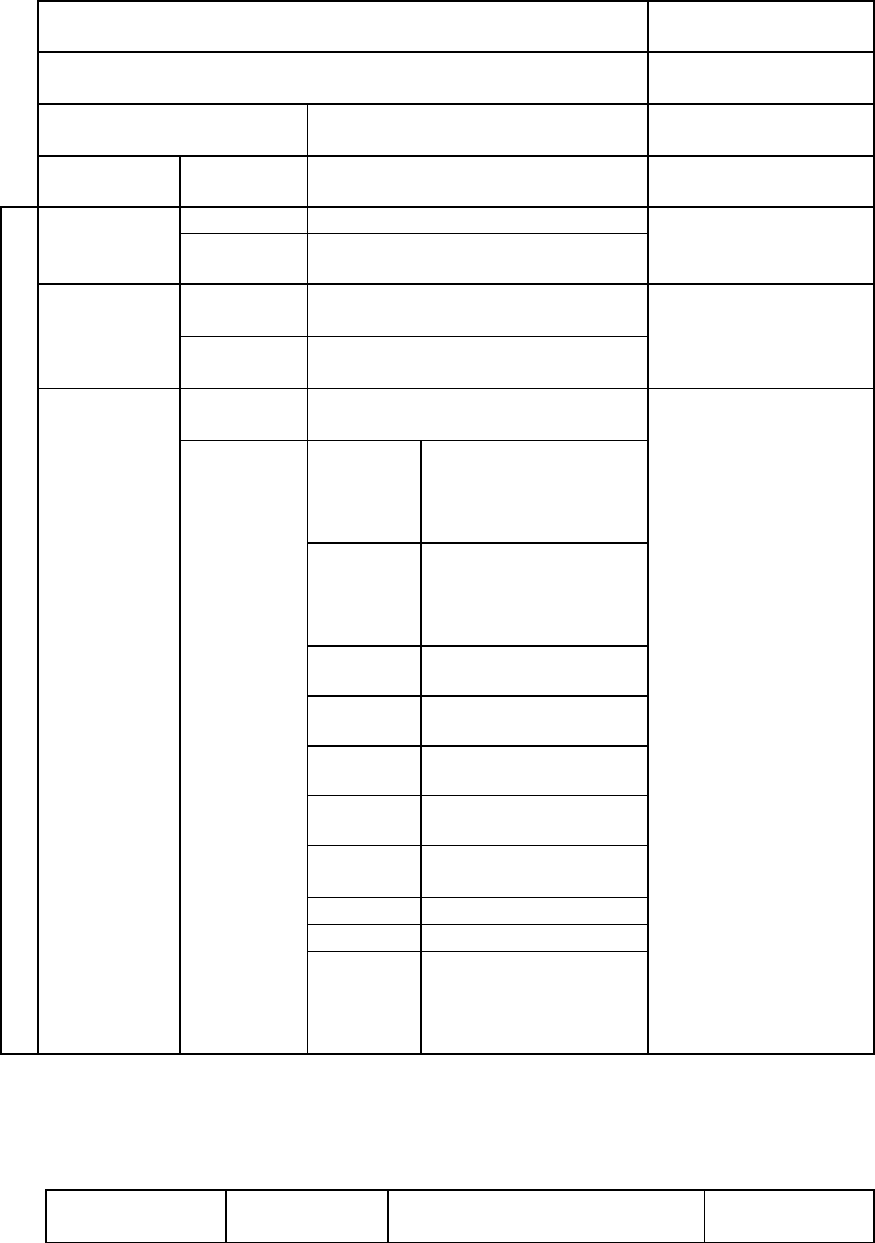
User Manual-page# 3-122
Table 3.19: Summary of input parameters for section ‘initial condition – local chemistry’, Part 1.
Keywords
Required/Optional
‘initial condition – local geochemistry’
required for any batch
simulation
nzone
number of simulations
required for any batch
simulation
Subsection
Parameter
Description
Required/Optional
Ni zones
‘number and
name of
zone’
izone
number of simulation
required for any batch
simulation
name
name of simulation
‘kinetic batch
simulation’
delt
initial time step for local chemistry
calculations
required for any kinetic
batch simulation
tfinal
final solution time for local
chemistry calculations
‘concentratio
n input’
conc
concentration input, as specified by
type
required for all
components specified
in input section
‘geochemical system’
type
‘free’
specified total
concentration units as
specified in section
‘geochemical system’
‘fixed’
fixed species activity,
units as specified in
section ‘geochemical
system’
‘po2’
fixed pO2 [atm]
‘pn2’
fixed pN2 [atm]
‘pco2’
fixed pCO2 [atm]
‘ph’
fixed pH
‘ph_swee
p’
sweep over specified
pH-range
‘pe’
fixed pe
‘eh’
fixed Eh [mV]
‘charge’
use component to
satisfy charge balance
estimate in units [mol
L-1 H2O]
Table 3.20: Summary of input parameters for section ‘initial condition – local chemistry’, Part 2.
Subsection
Parameter
Description
Required/
Optional

User Manual-page# 3-123
Ni zones
‘sorption
parameter input’
cec
cation exchange capacity
[meq (100g soil)-1]
required for ion
exchange
reactions
rhobulk
dry bulk density [g cm-3]
surface site
name of surface site
required for
surface
complexation
reactions
mass
mass of surface site
[g solid L-1 H2O]
area
surface area of surface site
[m2 g-1 solid]
site density
site density [sites nm-2]
'sorption
parameter input
of ion-exchange'
cec
cation exchange capacity
[meq (100g soil)-1]
required for ion
exchange
reactions
rhobulk
dry bulk density [g cm-3]
'sorption
parameter input
of surface-
complex'
surface site
name of surface site
required for
surface
complexation
reactions
mass
mass of surface site
[g solid L-1 H2O]
area
surface area of surface site
[m2 g-1 solid]
site density
site density [sites nm-2]

User Manual-page# 3-124
Table 3.21: Summary of input parameters for section ‘initial condition – local chemistry’, Part 3.
Subsection
Parameter
Description
Required
/Optional
Ni zones
‘mineral
input’
phi
initial mineral volume fraction
[m3 mineral m-3 bulk]
required for all
mineral
specified in
section
‘geochemical
system’ (only if
string
‘kinetically-
controlled
dissolution-
precipitation
reactions’
is specified
minequil
equilibrate with mineral phases
type
‘constant’
no update of rate
constant (surface area)
‘twothird’
update of rate constant
(surface area) based on
two-thirds power law
‘twothird-
mix’
update of rate constant
(surface area) based on
two-thirds power law
with threshold value
‘linear’
update of rate constant
(surface area) based on
linear function
‘exponent’
update of rate constant
(surface area) based on
the exponent defined by
user
‘geometric’
update of rate constant
(surface area) based on
geometric update
phi_min
minimum mineral volume fraction
[m3 mineral m-3 bulk]
k_eff
or
area
or
factor
effective rate constant in [mol l-1 bulk s-
1], (if rate constant in database is set to
unity)
or
reactive surface area in [m2 mineral L-1
bulk], (if rate constant specified in
database)
or
scaling factor (for type ‘geometric’)
sat
level of supersaturation, set to 0.0
Coefficient for type ‘linear’
phinuc
Mineral volume fraction for nucleation
threshold
rad_init
initial radius of mineral grain [m], only
for type ‘geometric’
rad_surf
initial radius of unreacted portion of
mineral grain [m], only for type
‘geometric’
rad_min
minimum radius of mineral grain [m],
only for type ‘geometric’
‘end of
zone’
-
-

User Manual-page# 3-125
Section Closing
Required
/Optional
‘done’
required
Table 3.22: Units for effective rate constants dependent on rate expression
Reaction type
rate expression
units for kim,t
zero order
default option
using standard
database
m
i
m
i
tm
i
m
i
tm
i
m
i
K
IAP
kR
kR
1
,
,
mol l-1 bulk s-1
nth order
m
i
m
i
na
j
tm
i
m
i
na
j
tm
i
m
i
K
IAP
TkR
TkR
1)(
)(
,
,
mol1-n l1-n H2O L-1 bulk s-1
Monod
a
j
moa
j
a
j
tm
i
m
iTK
T
kR ,
,
mol l-1 bulk s-1
In Table 3.22,
m
i
R
is the reaction rate, kim,t is the effective rate constant,
a
j
T
is the total aqueous
component concentration,
m
i
K
is the equilibrium constant,
m
i
IAP
is the ion activity product,
moa
j
K,
is the half saturation constants.
m
i
K
and
moa
j
K,
are provided in the database mineral.dbs,
while kim,t is calculated according to Equation 3-48 or Equation 3-49.
3.20.3 EXAMPLE DATA FILE INPUT
Example 1: Speciation and kinetic batch simulation
! Data Block 14: initial condition - local geochemistry
! ---------------------------------------------------------------------------
!
'initial condition - local geochemistry'
2 ;number of simulations
! ---------------------------------------------------------------------------
'number and name of zone'
1
'Sierras speciation calculation'
'concentration input'
1.0d-3 'free' ;conc, type - ca2+
1.0d-7 'free' ;conc, type - na+
1.0d-3 'free' ;conc, type - co32-
1.0d-7 'free' ;conc, type - h4sio4
User Manual-page# 3-126
1.0d-7 'free' ;conc, type - al3+
5.0 'ph' ;conc, type - h+
'end of zone'
! ---------------------------------------------------------------------------
'number and name of zone'
2
'kinetically-controlled dissolution of calcite and albite'
'kinetic batch simulation'
1.0d-2 ;delt
1.0d0 ;tfinal
'concentration input'
1.7d-5 'free' ;conc, type - ca2+
1.0d-6 'free' ;conc, type - na+
2.0d-5 'free' ;conc, type - co32-
1.0d-6 'free' ;conc, type - h4sio4
1.0d-6 'free' ;conc, type - al3+
5.0 'pH' ;conc, type - h+
'mineral input'
5.0d-4 .true. 'constant' ;phi, minequil, type - calcite
1.0d-10 1.0d-8 0.0 ;phi_min, k_eff, sat
5.0d-1 .true. 'constant' ;phi, minequil, type - albite
1.0d-10 1.0d-13 0.0 ;phi_min, k_eff, sat
0.0d0 .false. 'constant' ;phi, minequil, type - al(oh)3(am)
1.0d-10 1.0d-8 0.0 ;phi_min, k_eff, sat
0.0d0 .false. 'constant' ;phi, minequil, type - sio2(am)
1.0d-10 1.0d-8 0.0 ;phi_min, k_eff, sat
'end of zone'
Example 2: Surface complexation
! Data Block 14: initial condition - local geochemistry
! ---------------------------------------------------------------------------
!
'initial condition - local geochemistry'
2 ;number of zones
! ---------------------------------------------------------------------------
'number and name of zone'
1
'pH-sweep from 0-14, fixed total metal concentration'
'concentration input'
0.0 'ph_sweep' 14.0 50 ;conc type ph_final steps - 'h+1'
1.0d-7 'free' ;conc type - 'me+2'
'sorption parameter input'
'=soh' 1.0d0 10.0d0 6.02228d0 ;surface site, mass, area, site density
'end of zone'
! ---------------------------------------------------------------------------
'number and name of zone'
2
'ph-sweep from 0-14, fixed solution composition'
'concentration input'
0.0 'ph_sweep' 14.0 50 ;conc type ph_final steps - 'h+1’
1.00d-7 'free' ;conc type - 'me+2'
'sorption parameter input'
'=soh' 1.0d0 10.0d0 6.02228d0 ;surface site, mass, area, site density
'equilibrate with fixed solution composition'
User Manual-page# 3-127
'end of zone'
'done'
Example 3: Ion exchange
! Section 14: initial condition – local geochemistry
! ---------------------------------------------------------------------------
!
'initial condition – local geochemistry'
1 ;number of zones
! ---------------------------------------------------------------------------
'number and name of zone'
1
'background chemistry - aquifer'
'concentration input'
1990.0d0 'free' ;conc type - 'na+1'
100.0d0 'free' ;conc type - 'k+1'
436.0d0 'free' ;conc type - 'mg+2'
444.0d0 'free' ;conc type - 'ca+2'
5700.0d0 'free' ;conc type - 'cl-1'
7.0d0 'ph' ;conc type - 'h+1'
'sorption parameter input'
10.0d0 ;cec
1.875d0 ;rhob
'end of zone'
'done'
Example 4: pH-sweep calculations
! Data Block 14: initial condition - local geochemistry
! ---------------------------------------------------------------------------
!
'initial condition - local geochemistry'
1 ;number of zones
! ---------------------------------------------------------------------------
'number and name of zone'
1
'pH-sweep from 0-14 '
'concentration input'
0.0 'ph_sweep' 14.0 50 ;h+1
1.00d-4 'free' ;seo4-2
'end of zone'
'done'
Example 5: specification of mineral update types
'mineral input'
0.20 .true. 'linear' ;phim, minequil, update_type - calcite
1.d-10 5.0d-5 0.00d0 1.0d-7 ;phimin, areanuc, supsatm, phinuc
0.15 .false. 'twothird-mix' ;phim, minequil, update_type - gypsum
1.d-10 200.0 0.00d0 1.0d-7 ;phimin, areanuc, supsatm, phinuc
5.00d-1 .true. 'geometric' ;phim, minequil, update_type - albite-ph-d
1.00d-7 0.1d0 0.00d0 ;phimin, scalfac, supsatm
1.50d-4 1.50d-4 3.00d-7 ;radi, rads, radmin
1.0d-10 .false. 'exponent' ;phim, minequil, update_type - dolomite
User Manual-page# 3-128
1.d-10 200.0 0.80d0 ;phimin, areanuc, alpha
3.20.4 DESCRIPTION OF EXAMPLE INPUT
Example 1 provides the initial conditions for two batch reactions. For the first batch reaction
'Sierras speciation calculation', no minerals are considered. Only the initial total concentrations of
five components plus pH are provided. For the second batch reaction 'kinetically-controlled
dissolution of calcite and albite', in addition to the initial concentrations of the primary components,
the parameters for the kinetic reactions of minerals calcite, albite.
Example 2 specifies the initial conditions for two batch reactions (pH-sweep from 0.0 to 14.0)
considering surface complexation. The difference of the two reactions lies in the methods of the
initial chemical speciation concerning the sorbed species. For the first batch reaction, the total
solution composition is provided and assumed as fixed total concentration. MIN3P-THCm will
calculate the concentrations of the aqueous and sorbed species. The other batch reaction used the
keywords 'equilibrate with fixed solution composition’. The initialization calculation will
determine the sorbed species concentration while the aqueous component concentration provided
in the input file remains unchanged.
Example 3 specifies the initial conditions for a batch reaction considering ion exchange reactions.
The related sorption parameters of the soil are: CEC in 10.0 meq (100g solid)-1, the dry bulk density
in 1.875 g cm-3.
Example 4 demonstrates the initial condition setup for pH-sweep calculation for the specification
of selenium components depending on pH value spanning from 0.0 to 14.0.
Example 5 demonstrates the specification of the mineral update types and related parameters. The
update type ‘linear’ of the mineral calcite is specified in the first two lines. The initial volume
fraction of calcite () is 0.20. The volume fraction of calcite for nucleation threshold is 10-
7. The initial mineral surface area is 100.0 m2 L-1bulk. The reference can be calculated
according to Equation 3-51: 100.0×1.0-7/0.2=5.0×1.0-5 m2 L-1bulk, which is the 2nd input parameter
in the second line. The minimum volume fraction is 10-10 (1st parameter in the 2nd line). The
supersaturation parameter is 0.0 (the 3rd parameter in the 2nd line).
The update type ‘twothird-mix’ is specified to gypsum in the 3rd and 4th lines. The of gypsum
is 0.15. The initial mineral surface area is 200. 0 m2 L-1 bulk. The volume fraction of calcite for
nucleation threshold is 10-7. The minimum volume fraction is 10-10 (1st parameter in the 2nd
line). The supersaturation parameter is 0.0 (the 3rd parameter in the 2nd line).
The following three lines is to specify the update type ‘'geometric' to albite. The of gypsum is
0.50. The minimum volume fraction is 10-10. The scale factor is 0.10. The supersaturation parameter
is 0.0. The initial radius of mineral grain is 1.50×10⁻⁴ [m]. The initial radius of unreacted portion
of mineral grain is also 1.50×10⁻⁴ [m]. The minimum radius of mineral grain is 3.00×10⁻⁷ [m]
The last two lines specifies the update type ‘exponent’ to dolomite. The of gypsum is 0.15. The
minimum volume fraction is 10-10. The initial mineral surface area is 200. 0 m2 L-1 bulk. The
coefficient is 0.8.
3.20.5 ADDITIONAL COMMENTS
MIN3P-THCm provides various forms to simulate kinetic reactions of minerals (see section 4.7).
User Manual-page# 3-129
Some of the required parameters are provided in the database mineral.dbs. Additional parameters
are provided in the input file.
3.21 INITIAL CONDITION – REACTIVE TRANSPORT (DATA
BLOCK 15)
3.21.1 DESCRIPTION OF DATA BLOCK
This data block defines the initial condition for the reactive transport problem. As for the flow
problem, the specification of several zones is necessary. The input structure is consistent with the
one for section ‘initial condition - local chemistry’ with some restrictions:
Kinetic batch simulations cannot be conducted (use batch option of model).
pH-sweep calculations cannot be conducted (use batch option of model).
An additional input section is required defining the extent of the zone in the solution domain
covered by the specified initial condition.
3.21.2 DESCRIPTION OF INPUT PARAMETERS
3.21.2.1 ‘initial condition – reactive transport’
The number of zones needs to be specified after the keywords ‘initial condition – reactive transport’.
In the following, a zone number and a zone name have to be provided below the sub-keywords
‘number and name of zone’ for each zone. The zone names may or may not be identical with the
names specified for the material property zones or the initial conditions for the flow problem.
The initial condition can be specified through the sections ‘concentration input’, ‘mineral input’
and ‘sorption parameter input’ in the same way as described in section ‘initial condition - local
chemistry’.
3.21.3 'READ INITIAL AQUEOUS COMPONENT CONCENTRATIONS FROM FILE'
The initial distributed total component concentrations for reactive transport can be specified
through an external file prefix.aqt. To activate this function, the keywords 'read initial aqueous
component concentrations from file' should be provided in the Data Block 'initial condition -
reactive transport'. In such case, the number of zones should be 1 no matter how many zones
the domain includes. The order of the aqueous components must be the same as defined in
the Data Block 2: 'geochemical system'. The file provides the x,y,z-coordinates and the total
concentrations of each primary component in [mol L-1] in each control volume. This file has exact
the same format of the output file prefix_0.gst.
3.21.4 'READ INITIAL MINERAL VOLUME FRACTIONS FROM FILE'
The distributed initial mineral volume fractions and porosity can be specified through an external
file prefix.min. To activate this function, the keywords 'read initial mineral volume fractions from
file' should be provided in the Data Block 'initial condition - reactive transport'. The file provides
the x,y,z-coordinates, the initial mineral volume fractions in [m3 m-3] and the porosity for each
control volume. The order of the minerals must be the same as defined in the Data Block 2:

User Manual-page# 3-130
'geochemical system'. This file has exact the same format of the output file prefix_0.gsv.
3.21.5 'READ CEC FROM FILE'
The distributed parameters CEC (cation exchange capacity) and dry bulk density can be specified
through an external file prefix.cec. To activate this function, the keywords 'read cec from file'
should be provided in the Data Block 'initial condition - reactive transport'. The file provides the
x,y,z-coordinates, CEC in [meq (100 g solid)-1] and the dry bulk density in [g cm-3] for each control
volume. An example of the prefix.cec file:
title = "dataset basin"
variables = "x", "y", "z","cec","rho"
zone t = "field",i = 1000, j = 150, k = 1, f=point
0.0000000E+00 0.0000000E+00 0.0000000E+00 0.1000000E+01 0.2750000E+01
0.4404404E+03 0.0000000E+00 0.0000000E+00 0.1000000E+01 0.2750000E+01
0.8808806E+03 0.0000000E+00 0.0000000E+00 0.1000000E+01 0.2750000E+01
0.1321321E+04 0.0000000E+00 0.0000000E+00 0.1000000E+01 0.2750000E+01
0.1761762E+04 0.0000000E+00 0.0000000E+00 0.1000000E+01 0.2750000E+01
……
3.21.6 'READ INITIAL MINERAL AREAS FROM FILE'
The distributed initial mineral surface area of each mineral in each control volume can be specified
through an external file prefix.surf. To activate this function, the keywords 'read initial mineral
areas from file' should be provided in the Data Block 15: 'initial condition - reactive transport'. The
file provides the x,y,z-coordinates, the initial surface area of each mineral in [m2 mineral (L bulk)-
1] for surface controlled reaction and in [m mineral (m3 bulk)-1] for transport controlled reaction.
The order of the minerals must be the same as defined in the Data Block 2: 'geochemical
system'. This file has exact the same format of the output file prefix_0.gsv.
3.21.7 'READ MINERAL VOLUME FRACTIONS NUCLEATION THRESHOLDS
FROM FILE'
The mineral volume fractions nucleation threshold () in [m3 m-3] is a parameter defined for
the calculation of mineral reaction rate R till mineral approaching disappearance according to:
Equation 3-55
In which and refer to the initial and current mineral volume fraction [m3 m-3], is the
reference mineral surface area. To use the parameter, the mineral update type should be ‘linear’.
The distributed mineral volume fractions nucleation thresholds as nodal values at each control
volume can be specified through an external file prefix.vnuc. To activate this function, the
keywords 'read mineral volume fractions nucleation thresholds from file' should be provided in the
Data Block 'initial condition - reactive transport'. The file provides the x,y,z-coordinates, the
mineral volume fractions nucleation thresholds in [m3 m-3]. The order of the minerals must be
the same as defined in the Data Block 2: 'geochemical system'. The prefix.vnuc file has the same
format of the output file prefix_0.gsv but without porosity.
3.21.8 'READ NUCLEATION THRESHOLD REFERENCE SURFACE AREA FROM
User Manual-page# 3-131
FILE'
The distributed nucleation threshold reference surface area as nodal values at each control volume
can be specified through an external file prefix.anuc. To activate this function, the keywords 'read
nucleation threshold reference surface area from file' should be provided in the Data Block 'initial
condition - reactive transport'. The file provides the x,y,z-coordinates, the nucleation threshold
reference surface area. The order of the minerals must be the same as defined in the Data Block
2: 'geochemical system'.
3.21.9 INITIAL CONDITION FOR ISOTOPE COMPONENTS
Input parameters for the initial condition for isotope components (data block 15) are essentially the
same as for non-isotope simulations although ensure that inputs for component concentration and
mineral inputs include all isotopes that were includes in the component and mineral sections in data
block 2. In addition, the ratio of isotope component concentrations needs to be such that the initial
isotopic ratio of the solution is represented.
3.21.10 'LINEAR SORPTION INPUT'
The dimensionless linear sorption coefficient Ks (defined in section 3.3.2.7) can be specified using
the keyword 'linear sorption input' as the following:
'linear sorption input'
'sr_85+2' 14.535
'co_60+2' 1377.0
3.21.11'SALINITY DEPENDENT REACTION RATE OF MINERALS'
Additionally, the section 'salinity dependent reaction rate of minerals' can be added to this block to
activate the function accounting the salinity dependent sulfur reducing bacterial (SRB) reaction. To
use the model, please follow the steps:
1. Add the keywords 'salinity dependent reaction rate of minerals' to the data block 'initial
condition - reactive transport' followed by the number of the mineral(s) to be considered for the
model;
2. Add the name of the first mineral plus the keyword ‘equation’, and the number and the values
of the coefficients () of a function to calculate the salinity inhibition factor (in [-])
depending on the salinity S (in [g/L]) based on the experimental data:
Equation 3-56
3. Add the minimum salinity & related , and the maximum salinity & related for the first
mineral to ensure no negative will be calculated according to the above equation;
4. If more than one minerals are considered, follow the steps 2 and 3 for the rest of the minerals;
5. The other properties of the minerals (e.g. kinetics) remain unchanged.).
The input format is demonstrated in the example 3 (section 3.21.13).
User Manual-page# 3-132
3.21.12 ‘EXTENT OF ZONE’
As for the flow problem, the specified initial condition needs to be allocated to a specific area of
the solution domain below the subkeywords ‘extent of zone’. MIN3P-THCm allows the simulation
of flow and reactive transport in three spatial dimensions. The following input defines the location
of minimum and maximum coordinates in the x, y and z-directions for the initial condition to be
allocated. If a 1D or 2D-simulation is conducted, the minimum and maximum coordinates for the
excluded dimensions should be specified as 0.0 and 1.0, respectively. The input for each section is
concluded with the statement ‘end of zone’. It is possible to overlay initial conditions. The input in
the zone with the higher number replaces earlier input. The input zones do not have to coincide
with the material property zones or initial condition zones specified in Data Blocks 9-12 of the
input file.
3.21.13EXAMPLE DATA FILE INPUT
Example 1: input is as the following:
! Section 15: initial condition – reactive transport
! ---------------------------------------------------------------------------
!
'initial condition – reactive transport'
1 ;number of zones
! ---------------------------------------------------------------------------
'number and name of zone'
1
'aquifer'
'concentration input'
1.7d-5 'free' ;conc, type - ca2+
1.0d-6 'free' ;conc, type - na+
2.0d-5 'free' ;conc, type - co32-
1.0d-6 'free' ;conc, type - h4sio4
1.0d-6 'free' ;conc, type - al3+
5.0 'pH' ;conc, type - h+
'mineral input'
5.0d-4 .true. 'constant' ;phi, minequil, type - calcite
1.0d-10 1.0d-8 0.0 ;phi_min, k_eff, sat
5.0d-1 .true. 'constant' ;phi, minequil, type - albite
1.0d-10 1.0d-13 0.0 ;phi_min, k_eff, sat
0.0d0 .false. 'constant' ;phi, minequil, type - al(oh)3(am)
1.0d-10 1.0d-8 0.0 ;phi_min, k_eff, sat
0.0d0 .false. 'constant' ;phi, minequil, type - sio2(am)
1.0d-10 1.0d-8 0.0 ;phi_min, k_eff, sat
'extent of zone'
0.0 1.0 0.0 1.0 0.0 4.0
'end of zone'
'done'
Example 2: combine mineralogical parameters (see section 3.3.2.18)
! Section 15: initial condition – reactive transport
! ---------------------------------------------------------------------------
'initial condition – reactive transport'
3 ;number of zones
… …
'number and name of zone'
3
'background chemistry - reactive barrier'
User Manual-page# 3-133
'concentration input'
6.29 'ph' 'h+1'
4.04d-3 'free' 'cl-1'
1.95d-3 'free' 'co3-2'
1.44d-3 'free' 'so4-2'
5.29d-20 'free' 'hs-1'
5.32d-4 'free' 'ca+2'
2.53d-13 'free' 'fe+2'
4.72d-12 'free' 'fe+3'
9.84d-5 'free' 'cro4-2'
1.52d-7 'free' 'cr(oh)2+'
1.98d-6 'free' 'tce'
1.37d-6 'free' 'cis-1,2-dce'
1.73d-7 'free' 'vc'
2.99d-6 'free' 'ethane'
1.98d-31 'free' 'h2(aq)'
'mineral input'
0.50d0 .false. 'twothird' ;phim, minequil, update_type - fe_0_h2o_1
1.00d-10 1.94d2 0.00d0 ;phimin, area, supsatm
0.50d0 .false. 'twothird' ;phim, minequil, update_type - fe_0_cr
1.00d-10 1.94d2 0.00d0 ;phimin, area, supsatm
0.50d0 .false. 'twothird' ;phim, minequil, update_type - fe_0_tce
1.00d-10 1.94d2 0.00d0 ;phimin, area, supsatm
0.50d0 .false. 'twothird' ;phim, minequil, update_type - fe_0_cdce
1.00d-10 1.94d2 0.00d0 ;phimin, area, supsatm
0.50d0 .false. 'twothird' ;phim, minequil, update_type - fe_0_vc
1.00d-10 1.94d2 0.00d0 ;phimin, area, supsatm
0.50d0 .false. 'twothird' ;phim, minequil, update_type - fe_0_so4_2
1.00d-10 1.94d2 0.00d0 ;phimin, area, supsatm
0.00d0 .false. 'constant' ;phim, minequil, update_type - calcite
1.00d-10 7.3030d-10 0.00d0 ;phimin, k_eff, supsatm
0.00d0 .false. 'constant' ;phim, minequil, update_type - siderite(d)
1.00d-10 1.1574d-10 0.00d0 ;phimin, k_eff, supsatm
0.00d0 .false. 'constant' ;phim, minequil, update_type - fe(oh)2(s)
1.00d-10 1.1574d-9 0.00d0 ;phimin, k_eff, supsatm
0.00d0 .false. 'constant' ;phim, minequil, update_type - cr(oh)3(a)
1.00d-10 1.1574d-10 0.00d0 ;phimin, k_eff, supsatm
0.00d0 .false. 'constant' ;phim, minequil, update_type - mackinawite
1.00d-10 1.1574d-10 0.00d0 ;phimin, k_eff, supsatm
0.00d0 .false. 'constant' ;phim, minequil, update_type - ferrihydrite
1.00d-10 1.1574d-9 0.00d0 ;phimin, k_eff, supsatm
'extent of zone'
1.8 2.4 0.0 0.0 0.00 3.20
'end of zone'
'done'
!
Example 3: salinity dependent reaction rate of minerals
! Data Block 15: initial condition - reactive transport
! ---------------------------------------------------------------------------
!
'initial condition - reactive transport'
1 ;number of zones
! ---------------------------------------------------------------------------
'number and name of zone'
1
'inflow'
'concentration input'
6000.00 'free' 'ca+2'
10900.00 'charge' 'na+1'
2800.00 'free' 'mg+2'
450.00 'free' 'k+1'
31000.00 'free' 'cl-1'
1240.00 'free' 'so4-2'
5.95 'ph' 'h+1'
User Manual-page# 3-134
303.00 'free' 'co3-2'
1.0d-10 'free' 'hs-1'
-200.00 'eh' 'o2(aq)'
'mineral input' ;bottom
1.00d-10 .false. 'constant' ;ch2o-h2s
1.00d-10 6.9d-9 0.00d0 ;
1.00d-10 .false. 'constant' ;calcite
1.00d-10 4.0d-8 0.00d0 ;
0.50d-10 .false. 'constant' ;anhydrite
0.50d-10 4.0d-9 0.00d0 ;
0.50d-10 .false. 'constant' ;halite
0.50d-10 1.16d-8 0.00d0 ;
'salinity dependent reaction rate of minerals'
1 ;number of minerals
ch2o-h2s ;name of minerals
'equation' 4 ;type of relation (=equation), no of parameters
-2.716E-01 2.11E-02 -9.455E-05 -3.20E-08 ;coefficients
15.0 3.0E-02 ; minimum salinity [g/L], k_sal [-]
225.0 0.046e-4 ; maximum salinity [g/L], k_sal [-]
'extent of zone'
0.0 20.0 0.0 1.0 0.0 1.0
'end of zone'
3.21.14DESCRIPTION OF EXAMPLE INPUT
Example 1 provides the initial conditions for a 1D vertical reactive transport problem (z=0.0 to
4.0 m). There is only one zone named 'background chemistry - reactive barrier'. Following the zone
name is the section 'concentration input', which specifies the total aqueous concentrations and types
of six components in the following six lines provided in the same order as defined in the Data Block
2 (‘geochemical system’). The section ‘mineral input’ provides the parameters for the kinetic
reactions of minerals calcite, albite, Al(OH)3(am) and SiO2(am). The mineral update type of all
four minerals is ‘constant’. Initially, the solid phases is composed dominantly of albite with a
volume fraction in 0.50 [m3 m-3], and of tracer amount of calcite in 5.0×10⁻⁴ [m3 m-3]. The other
two minerals are secondary minerals. The minimum volume fractions of all four minerals are 10-
10 [m3 m-3], while the effective rate constants are 10-13 [mol L-1 bulk s-1] for albite and 10-8 [mol L-
1 bulk s-1] for the rest.
Example 2 provides one of the three initial conditions for a 2D vertical reactive transport problem
(x=1.8 to 2.4 m, z= 0.0 to 3.20 m) using the function 'combine mineralogical parameters' (see
section 3.3.2.18). The zone name to be specified is 'background chemistry - reactive barrier'.
Similar to the example 1, the section ‘concentration input’ specifies the total aqueous
concentrations and types of 15 components, while the section ‘mineral input’ provides the
parameters for the kinetic reactions of all minerals. It is important to note that the first six minerals
are treated as combined, which indicates the representation of the same material Fe0 participates in
six dissolution/precipitation reactions. Therefore, the initial total volume fraction of the Fe0 in
0.5 [mol L-1 bulk s-1] is specified to the first six minerals. The update types are ‘twothird’ for the
first six minerals and ‘constant’ for the rest. The reactive surface area of the Fe0 is 194.0 [m2 mineral
L-1 bulk]. The minimum volume fractions of all minerals are 10-10 [m3 m-3]. The effective rate
constants for calcite, siderite, Fe(OH)2, Cr(OH3), mackinawite and ferrihydrite are 7.303×10⁻¹⁰,
1.1574×10⁻¹⁰, 1.1574×10⁻⁹, 1.1574×10⁻¹⁰, 1.1574×10⁻¹⁰, 1.1574×10⁻⁹ [mol L-1 bulk s-1], respectively.
Example 3 demonstrates the input formats for the specification of initial conditions considering
salinity dependent sulfate reduction. The parameters under sections ‘concentration input’ and
‘mineral input’ are defined in the exact same way as described ibn example 1. An additional section
User Manual-page# 3-135
'salinity dependent reaction rate of minerals' defines the parameters required for the salinity
dependent sulfate reduction model based on experimental data. This example applied the model for
one mineral ch2o-h2s using the function (Brandt et al. 2001):
Equation 3-57
The minimum salinity is 15.0 g L-1 and the is 0.03, which means if the salinity lower than 15.0
g L-1, 0.03 will be used for the calculation. The maximum salinity is 225.0 g L-1, and the is
4.6×10⁻⁶. When the salinity is higher than 225.0 g L-1, the is 4.6×10⁻⁶.
3.22 BOUNDARY CONDITIONS - REACTIVE TRANSPORT (DATA
BLOCK 16)
3.22.1 DESCRIPTION OF DATA BLOCK
In the last section of the problem-specific input file, the boundary conditions for the reactive
transport problem need to be specified. The input is as defined in the section of ‘initial condition –
local chemistry’ with the following exceptions:
Kinetic batch simulations cannot be conducted (use batch option of model).
pH-sweep calculations cannot be conducted (use batch option of model).
the subsections ‘mineral input’ and ‘sorption parameter input’ are not needed.
an additional input section is required defining the type of boundary condition.
an additional input section is required defining the extent of the zone in the solution domain
covered by the specified initial condition.
It is also possible to specify transient boundary conditions for the simulation of boundary conditions
changing with time. To realize it, an additional block 'update boundary conditions' has to be
specified followed by one or several boundary conditions.
3.22.2 DESCRIPTION OF INPUT PARAMETERS
The input data for reactive transport boundary conditions follows the format previously described
for other spatially distributed properties. Similar to the input for flow boundary conditions,
boundary types cannot be overlain on each other.
The first required parameter is the number of boundary zones, which follows the keywords
‘boundary conditions – variably-saturated flow’.
Each zone is defined by a zone number and zone name following the statement 'number and name
of zone'. These zones are independent of those for physical material properties or the initial
condition zones, but may have the same name.
Four types of boundary conditions can be specified below the subsection identifier ‘boundary type’:
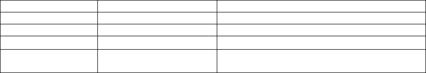
User Manual-page# 3-136
Table 3.23: Boundary conditions for reactive transport
Type
Name
Description
‘first’
Dirichlet
specified concentration (fixed)
‘second’
Neumann
free advective mass outflux for aqueous phase
‘third’
Cauchy
advective mass influx for aqueous phase
‘mixed
Dirichlet/Cauchy
advective mass influx and free diffusive mass
influx for aqueous and gaseous phases
The subsection ‘concentration input’ is only required for first, third and mixed-type boundary
conditions. For additional information on input requirements and options in this section see section
‘initial condition – local chemistry’.
The dimensions of the boundary zone are specified below the statement 'extent of zone'. As with
other spatially distributed parameters, the precise dimensions of the boundary will be dependent on
the grid spacing (See Section 3 of input file). Since the model is capable of simulating reactive
transport in three dimensions, the specification of the boundaries must be provided in the x, y, and
z-dimensions. The coordinates are also used to specify to which boundary face the boundary
condition will be applied. This is of particular importance for third, second and mixed type
boundary conditions. For example the specification
‘extent of zone’
0.0 0.0 0.0 1.0 0.0 10.0
means that the boundary condition will be applied to the y-z plane of the solution domain at x = 0
covering an area from ymin = 0 m t ymax = 1 m and zmin = 0 m to zmax = 10.0 m.. The model formulation
requires that this input structure is obeyed also for 1D- and 2D-simulations. For example, the
specification of the left boundary of a 1D-simulation in x-direction would require the input:
‘extent of zone’
0.0 0.0 0.0 1.0 0.0 1.0
At the present time, the model can only handle boundary conditions on the surface (edges) of the
solution domain. The input for each boundary zone is terminated with the statement ‘end of zone’.
3.22.3 TRANSIENT BOUNDARY CONDITION
For the specification of transient boundary conditions, the keyword 'update boundary conditions',
followed by the number and starting time of boundary conditions to be updated, has to be added to
the initial boundary conditions. The detailed boundary conditions are given in the following blocks
between a pair of keywords - 'start of target read time input' and 'end of target read time input'. The
chemical compositions can be updated with time, but the boundary types cannot be changed. If
BCs to be updated are more than one, they must be placed in the same order as defined in the initial
boundary conditions. Example 2 demonstrates the format for the specification of transient boundary
conditions.
3.22.4 USE BACKGROUND CHEMISTRY FOR BOUNDARY ZONE
It is also possible to specify a boundary condition with a chemical composition specified in the
initial condition. This is only applicable when the first type boundary condition is assigned. The
keyword for that is 'use background chemistry for boundary zone'. This is useful to specify 2D
User Manual-page# 3-137
boundary conditions with local injections. Example 3 in the next subsection demonstrates its usage.
3.22.5 EXAMPLE DATA FILE INPUT
Example 1: Input data for second and third type boundary conditions for a 1D reactive transport
problem:
! Data Block 16: boundary conditions - reactive transport
! ---------------------------------------------------------------------------
!
'boundary conditions - reactive transport'
2 ;number of zones
! ---------------------------------------------------------------------------
'number and name of zone'
1
'infiltrating fluid'
'boundary type'
'third'
'concentration input'
3.0 'ph' ;'h+1'
1.0d-10 'free' ;'fe+3'
2.5d-3 'free' ;'so4-2'
1.0d-3 'free' ;'zn+2'
1.0d-5 'free' ;'fe+2'
1.0d-3 'free' ;'cu+2'
'extent of zone'
0.0 1.0 0.0 1.0 0.0 0.0
'end of zone'
! ---------------------------------------------------------------------------
'number and name of zone'
2
'outflow boundary'
'boundary type'
'second'
'extent of zone'
0.0 1.0 0.0 1.0 16.0 16.0
'end of zone'
'done'
Example 2: Input data for transient boundary conditions for a 1D reactive transport problem:
! Data Block 16: boundary conditions - reactive transport
! ---------------------------------------------------------------------------
!
'boundary conditions - reactive transport'
2 ;number of zones
!
! zone 1
! ---------------------------------------------------------------------------
!
'number and name of zone'
1
'inflow boundary'
User Manual-page# 3-138
'boundary type'
'first'
'concentration input'
2.00d-2 'free' ;h+1
1.00d-2 'free' ;co3-2
'guess for ph'
5.0
'extent of zone'
0.0 0.0 0.0 0.0 0.0 0.0
'end of zone'
! ---------------------------------------------------------------------------
'number and name of zone'
2
'outflow boundary'
'boundary type'
'second'
'extent of zone'
0.0 0.0 0.0 0.0 0.20 0.20
'end of zone'
! ---------------------------------------------------------------------------
'update boundary conditions'
2 ;number of target read times
0.25 ;target read times
0.50
!
! target read time 1
! ---------------------------------------------------------------------------
!
'start of target read time input'
1
!
! zone 1
! ---------------------------------------------------------------------------
!
'number and name of zone'
1
'inflow boundary'
'concentration input'
2.00d-2 'free' ;h+1
1.00d-2 'free' ;co3-2
'guess for ph'
5.0
'end of zone'
'end of target read time input'
!
! target read time 2
! ---------------------------------------------------------------------------
!
'start of target read time input'
2
!
! zone 1
! ---------------------------------------------------------------------------
!
'number and name of zone'
1
'inflow boundary'
User Manual-page# 3-139
'concentration input'
2.00d-7 'free' ;h+1
1.00d-7 'free' ;co3-2
'guess for ph'
5.0
'end of zone'
'end of target read time input'
'done'
Example 3: Use background chemistry for boundary zone
! Data Block 16: boundary conditions - reactive transport
! ---------------------------------------------------------------------------
!
'boundary conditions - reactive transport'
3 ;number of zones
! ---------------------------------------------------------------------------
'number and name of zone'
1
'source'
'boundary type'
'third'
'concentration input'
2.00d-4 'free' ;h+1
1.00d-4 'free' ;co3-2
1.00d-8 'free' ;ca+2
'guess for ph'
5.0
'extent of zone'
0.0 0.02 0.0 0.0 0.0 0.0
'end of zone'
! ---------------------------------------------------------------------------
'number and name of zone'
2
'inflow boundary'
'boundary type'
'first'
'use background chemistry for boundary zone'
'extent of zone'
0.021 0.1 0.0 0.0 0.0 0.0
'end of zone'
! ---------------------------------------------------------------------------
'number and name of zone'
3
'outflow boundary'
'boundary type'
'second'
'extent of zone'
0.0 0.1 0.0 0.0 0.20 0.20
'end of zone'
User Manual-page# 3-140
'done'
3.22.6 DESCRIPTION OF EXAMPLE INPUT
Example 1 specifies the boundary conditions (BCs) for 1D vertical reactive transport problem
(domain length 16.0 m). At z=0.0 m, a third type boundary condition is defined together with the
solution compositions of six components under section ‘concentration input’. The boundary
solution is low in pH (3.0) containing SO42-, Fe2+, Fe3+, Zn2+ and Cu2+. A second type BC is
specified at the outflow boundary (z=16.0 m), indicating free advective mass outflux for the
aqueous phase.
Example 2 specifies transient boundary conditions for reactive transport including two switches of
BCs at 0.25 days and 0.5 days, respectively. These boundary conditions can be divided into two
parts: the initial BCs and the BCs to be switched to. The initial BCs are assigned in the same way
as those in example 1. They consist of two boundary conditions: first type BC for the inflow, and
second type BC for the outflow. Both initial boundary conditions will be applied from the beginning
of the simulation. The second part starts from the statement 'update boundary conditions' followed
by two numbers (i.e. 0.25 and 0.50) in two separate lines, indicating the boundary conditions will
be updated at 0.25 and 0.50 time units (e.g. days, which is defined in Data Block 4). The
corresponding BCs to be updated at both time intervals are specified in the rest part of the input
file between each pairs of statements 'start of target read time input' and 'end of target read
time input'. The boundary condition to be updated at 0.25 days is provided between the first pair
of the statement, which is the same as initial BC. This implies the BC is updated at 0.25 days, but
actually remains unchanged. Similarly, the other BC to be updated at 0.5 days is specified between
the next pairs of the statements. The solution at the boundary is changed to a solution with much
lower concentrations of the components than those in the BC at 0.25 days. The last BC will be
applied until the end of the simulation. Important is to keep the boundary types and required
parameters consistent with the initial BCs. Best practice is to copy the initial boundary conditions
into the pairs of statements, and modify the concentration at the corresponding switch time.
Example 3 specifies the BCs for a 2D vertical reactive transport problem. Three BCs are specified.
The 1st one is a first type BC - the ‘source’ boundary, which is specified using the keywords
‘boundary type’, ‘first’ and ‘concentration input’ followed by the concentrations and types of all
aqueous components. This BC leads to the connection of the ‘source’ boundary solution to the
domain within the region from x= 0.0 to 0.02 m at the bottom boundary (z=0.0). The rest of the
bottom boundary is assigned with a first type BC named ‘inflow boundary’. This boundary solution
has the same chemical compositions as the initial condition through the application of the statement
'use background chemistry for boundary zone'. The top boundary of the domain (x=0.0 to 0.1 m,
z=0.2 m) is assigned with a second type boundary named the ‘outflow boundary’.
3.22.7 ADDITIONAL COMMENTS
Boundary condition types and parameters for isotope components (data block 16) are essentially
the same as for simulations without isotopes.

User Manual-page# 3-141
3.23 ICE SHEET LOADING/UNLOADING (DATA BLOCK 17)
3.23.1 DESCRIPTION OF DATA BLOCK
For the simulation of the glaciation induced hyrogeomechanic coupling simulation, a simplified ice
sheet 1D loading/unloading model can be used to specify the boundary conditions. The parameters
are specified in a separate Data Block with the header 'ice sheet loading/unloading' (see the input
example in section 3.23.3).
3.23.2 DESCRIPTION OF INPUT PARAMETERS
The parameters can be grouped into two parts: general properties and the ice sheet evolution stage
parameters (see the example in the following section).
The general properties: The first logical parameter is to specify the status of the ice sheet. If it is
true, the thickness of the ice sheet remains constant during the simulation. If it is false, the thickness
will change with the glaciation/deglaciation processes. Similar to Bense and Person (2008), the
thickness of the ice sheet (, [L]) and the imposed hydraulic head beneath the ice sheet
(, [L]) are computed as a function of distance and time according to Van der Veen (1999):
Equation 3-58
Equation 3-59
where Hice(t) [L] is the specified maximum ice sheet thickness, L(t) [L] is the corresponding
horizontal length of the ice sheet, x [L] is the distance from the ice sheet origin (i.e. starting point),
a
and
b
are constants [-], and
defines the ratio between the hydraulic head at the base of the ice
sheet and the ice sheet thickness (Bea et al. 2011). Additional parameters are: the hydraulic
conductivities of the ice sheet, ice density, and fresh water density.
The ice sheet evolution stage parameters are: The number of the glaciation/deglaciation stages, bool
parameter for specifying the flow boundary condition (i.e. .true. – considered as flow boundary
condition, .false. – non flow boundary condition, for example during glaciation period), factor for
water pressure, factor for ice pressure, start and end time of the stage, horizontal position of the ice
front, ice sheet thickness at the start and end time of the stage.
3.23.3 EXAMPLE DATA FILE INPUT
An example is provided below (Bea et al., 2011):
! Data Block 17: Ice Sheet loading/unloading
! ---------------------------------------------------------------------------
!
'ice sheet loading/unloading'
.false. ! isconstant
440000.0d0 ! Ice Sheet point source (x)
4000.0d0 ! Ice Sheet point source (z)
2.5d0 ! a
1.0d0 ! b
User Manual-page# 3-142
-50.0d0 ! logkxx – hydraulic conductivity of ice
-50.0d0 ! logkyy
-50.0d0 ! logkzz
1.0d3 ! ice density
1.0d3 ! fresh water density
3 ! number of stages
1 ! istage
.false.
0.0d0 ! Factor for pw
1.0d0 ! Factor for pice
0.0d0 12500.0d0 ! time(1,i),time(2,i)
0.0d0 439950.0d0 ! l(1,i),l(2,i)
0.0d0 2000.0d0 ! h(1,i),h(2,i)
0.0d0 0.0d0 ! l1perm(1,i),l1perm(2,i)
0.0d0 0.0d0 ! l2perm(1,i),l2perm(2,i)
0.0d0 0.0d0 ! thickperm(1,i),thickperm(2,i)
2 ! istage
.false.
0.0d0 ! Factor for pw
1.0d0 ! Factor for pice
12500.0d0 17500.0d0 ! time(1,i),time(2,i)
439950.0d0 439950.0d0 ! l(1,i),l(2,i)
2000.0d0 2000.0d0 ! h(1,i),h(2,i)
0.0d0 0.0d0 ! l1perm(1,i),l1perm(2,i)
0.0d0 0.0d0 ! l2perm(1,i),l2perm(2,i)
0.0d0 0.0d0 ! thickperm(1,i),thickperm(2,i)
3 ! istage
.true.
0.95d0 ! Factor for pw
1.0d0 ! Factor for pice
17500.0d0 22500.0d0 ! time(1,i),time(2,i)
439950.0d0 0.0d0 ! l(1,i),l(2,i)
2000.0d0 0.0d0 ! h(1,i),h(2,i)
0.0d0 0.0d0 ! l1perm(1,i),l1perm(2,i)
0.0d0 0.0d0 ! l2perm(1,i),l2perm(2,i)
0.0d0 0.0d0 ! thickperm(1,i),thickperm(2,i)
!'compute permafrost'
'done'
3.23.4 DESCRIPTION OF EXAMPLE INPUT
The example data file contains 2D xz-plane (x= 0 to 440 km, z=0 to 4 km) ice sheet
loading/unloading parameters in three stages. The general parameters indicate: the thickness of the
ice sheet changes with time. The ice sheet extends up to 440 km horizontally, and up to z=4000 m.
The coefficients of a and b are 2.5 and 1.0, respectively, which are used for the ice thickness
calculations. The hydraulic conductivity of the ice sheet are 10-50 m/s, the densities of ice and water
are assumed to 1000 kg m-3.
The glaciation/deglaciation processes include three stages: During the stage 1 (from 0 to 12500
years), the ice sheet develops and the ice front reaches 439950 m. The ice sheet thickness increased
up to 2000 m. During the stage 2 (from 12500 to 17500 years), the ice sheet remains unchanged.
During the stage 3, the deglaciation process results in the complete retreat of the ice sheet. The
melted ice provides water source on the top of the soil. In this case, a factor of water pressure with
0.95 is applied. More detailed description is referred to the base case simulation in Bea et al. (2011).
3.23.5 ADDITIONAL PARAMETERS
Skempton coeffiecients at all control volumes are specified through a separate file ‘prefix.skempton’
in the following format.
User Manual-page# 3-143
title = "dataset basin"
variables = "x", "y", "z","skempton"
zone t = "field",i = 450, j = 100, k = 1, f=point
0.0000000E+00 0.0000000E+00 0.0000000E+00 0.9518758E+00
0.9799555E+03 0.0000000E+00 0.0000000E+00 0.9518758E+00
0.1959911E+04 0.0000000E+00 0.0000000E+00 0.9518758E+00
0.2939866E+04 0.0000000E+00 0.0000000E+00 0.9518758E+00
To facilitate this input, the keyword 'read skempton coefficient from file' should be included in the
data block 10: 'physical parameters - variably saturated flow'. This parameter is applied to calculate
the pore water pressure owing to the loading of the ice sheet.
User Manual-page# 4-144
4 DATABASE
The geochemical database is derived from the database of MINTEQA2 (Allison et al., 1991).
Because MIN3P-THCm allows the simulation of open or partially open systems (in contact with
the atmosphere) and the inclusion of kinetically-controlled reactions, the half-reaction approach
(i.e. the use of the electron as a component and redox master variable) could not be used in MIN3P-
THCm. The electron is eliminated by combining all half reactions in the MINTEQA2-database
with the O2(aq)/H2O half reaction.
The MIN3P-THCm geochemical database also allows the specification of kinetically-controlled
intra-aqueous and dissolution-precipitation reactions. Default values for ion-exchange and surface
complexation reactions are also provided and were taken from the database of PHREEQC2
(Parkhurst and Appelo, 1999).
4.1 COMPONENTS
4.1.1 COMP.DBS
The database file for the primary components is named comp.dbs. Two types of components can
be specified in the database file: aqueous components and non-aqueous components (currently
limited to surface sites for surface complexation reactions).
4.1.1.1 aqueous components
The entry for the aqueous component Ba2+ is given by:
ba+2 2.0 5.00 .00 137.34000 0.0
where ba+2 is the name of the component, 2.0 is the charge, 5.00 and .00 are the Debye-Huckel
constants a and b. 137.34000 defines the gram formula weight and 0.0 is the alkalinity factor.
4.1.1.1.1 Alkalinity factor
The alkalinity factor is used to determine the alkalinity value of the water. It is defined as the proton
uptake capacity of the species when titrated to the carbonate alkalinity end point. By definition, the
alkalinity factor of CO32- equals two (2).
4.1.1.1.2 Isotope components
The isotope components should be included in the database in the same format as other components.
The following data block defines the sulfur isotope components as sulfate and hydrosulfide:
so4-2 -2.0 4.00 -.04 95.95173 .00
34so4-2 -2.0 4.00 -.04 97.94753 .00
hs-1 -1.0 3.50 .00 33.07200 .00
34hs-1 -1.0 3.50 .00 34.97586 .00
In the example, the components including the master isotope (32S) are represented by so4-2 and hs-
1; while the components including the heavy isotope (34S) are 34so4-2 and 34hs-1. The properties
of the same components including master or heavier/lighter isotopes are the same except the molar
weight.
User Manual-page# 4-145
4.1.1.2 non-aqueous components
The entry for the non-aqueous component FeOH is given by:
=feoh 0.0 .00 .00 .00000 0.0
where =feoh is the name of the component on the surface site. The next value defines the charge of
the surface species. All remaining values are arbitrary for surface complexation reactions and are
set to 0.0.
4.1.2 ADDING NEW COMPONENTS
If components are added to the database, the name of the new component must be different than
the name of any existing component. If the alkalinity factor or the Debye-Huckel parameters are
not known, 0.00 should be specified. When no Debye-Huckel parameters are specified, the Davies
Equation is used. All other parameters are required to allow the consideration of the new component.
When adding additional components the following format must be obeyed:
Line 1: format(a12,f4.1,4x,f5.2,f5.2,8x,f11.5,f7.2)
This data format is based on that used in MINTEQA2 (e.g. a12 indicates a string of 12 characters,
f4.1 indicates a real number that contains up to four (4) digits, of which one digit places to the right
of the decimal point (i.e. 673.8), 4x indicates four (4) blank spaces).
4.1.3 COMPONENTS FOR MULTICOMPONENT DIFFUSION
If multicomponent diffusion model is applied (see section 3.2.2.6), the molecular diffusion
coefficient (in [m2 s-1]) is species dependent. This parameter is required to be attached at the end of
each entry as the following:
ca+2 2.0 6.00 .17 40.08000 .00 0.792d-9
This parameter for the relevant components should be verified before the simulation.
4.2 COMPLEXATION REACTIONS
The database file for aqueous complexation reactions is named complex.dbs. As an example the
database entry for the association reaction
83.9)(log 25104344 KSiOHHSiOH
is given by:
h3sio4- 6.1200 -9.8300 -1.00 4.00 .00 95.1070 .00
2 h4sio4 1.000 h+1 -1.000
4.2.1 LINE 1
The first line begins with the name of the aqueous complex (h3sio4-), 6.1200 is the enthalpy change,
User Manual-page# 4-146
-9.8300 is the equilibrium constant for 25oC. The following value (–1.00) defines the charge of the
species, while 4.00 and .00 define the Debye-Huckel constants a and b. 95.1070 is the gram formula
weight of the aqueous complex, and the last value in the first input line (.00) defines the alkalinity
factor for h3sio4-.
The MIN3P-THCm database uses association reaction for complexation reaction. The sign of the
equilibrium constants logK25 should be turned around if the reactions are expressed as dissociation
reactions.
1
444325 ][][][ SiOHHSiOHK
4.2.2 LINE 2
The second line defines the chemical reaction mentioned above. The number of components, as
well as the pairs of name and stoichiometric coefficient of the associated components, are specified.
In the example, the aqueous complex consists of 2 components (h4sio4 and h+1) with
stoichiometric coefficients of 1.000 and –1.000, respectively.
4.2.3 ADDING COMPLEXES
Additional complexes can be specified. The only requirement is that the complex can be formed
from the components included in the database file comp.dbs. If the numerical values for the
enthalpy change, the Debye-Huckel parameters or the alkalinity factor are not known, 0.00 should
be specified. All other parameters must be known to allow the consideration of the aqueous
complex. At the present time, the following format must be obeyed, if additional complexes are
specified in the database:
Line 1: format(a12,2x,2f10.4,16x,3f5.2,f9.4,f7.2)
Line 2: format(6x,i1,3x,5(a12,1x,f7.3,1x))
The formats are the same as used in MINTEQA2 (e.g. a12 indicates a character string 12 characters
long, f5.1 indicates a real number that contains up to five (5) digits of which one (1) places to the
right of the decimal point, 4x indicates four (4) blank spaces, and i1 is a one (1) digit integer).
4.2.4 ISOTOPE COMPLEXES
Analogous to the complex database, entries are required for each secondary aqueous species that
contains one of the isotope components.
For example the entry including the master sulfur isotope (32S):
khso4(aq) .0000 0.8136 .00 .00 .00 136.1716 .00
3 h+1 1.000 k+1 1.000 so4-2 1.000
requires a corresponding entry for the 34S component:
kh34so4(aq) .0000 0.8136 .00 .00 .00 138.1716 .00
3 h+1 1.000 k+1 1.000 34so4-2 1.000
4.2.5 COMPLEXES FOR MULTICOMPONENT DIFFUSION
If multicomponent diffusion model is applied (see section 3.2.2.6), the molecular diffusion
User Manual-page# 4-147
coefficient (in [m2 s-1]) is species dependent. This parameter for all chemical complexes is required
to be placed at the end of each entry to the first line as the following:
oh- 13.3620 -13.9980 -1.00 3.50 .00 17.0074 1.00 5.273d-9
2 h2o 1.000 h+1 -1.000
This parameter for the relevant complexes should be verified before the simulation.
4.3 GAS EXCHANGE REACTIONS
The database file for gas exchange reactions is named gases.dbs. As an example the database entry
for the formation of CO2(g)
1600.18)(2 2522
2
3 KgCOOHHCO
is given by:
co2(g) -.5300 18.1600 41.0100
3 co3-2 1.000 h+1 2.000 h2o -1.000
where co2(g) defines the name of the gas, -.5300 is the enthalpy change of the reaction, 18.1600 is
the equilibrium constant and 41.0100 is the gram formula weight of the gas. The second line defines
the chemical reaction mentioned above for the formation of CO2(g). The first parameter defines the
number of components comprising the gas (in this case 3). In the following the pairs of name and
stoichiometric coefficient of the components are specified. The three components in the example
are co3-2, h+1 and h2o with stoichiometric coefficients of 1.000, 2.000 and –1.000, respectively.
Line 1: format(a12,2x,2f10.4,31x,f9.4/6x,i1,3x,5(a12,1x,f7.3,1x))
The MIN3P-THCm database uses association reaction for gas exchange reaction. The sign of the
equilibrium constants logK25 should be turned around if the reactions are expressed as dissociation
reactions.
12
3
2
225 ][][)]([ COHgCOK
4.4 ION EXCHANGE AND SORPTION REACTIONS
Component species involved in ion exchange and surface complexation reactions are defined in the
comp.dbs file (see above section on component species). This section refers to the database file
sorption.dbs, which contains secondary exchanged/adsorbed species and parameters of their
formation reactions.
In the default database, ion exchange and adsorption reactions were taken from the database of
PHREEQC2 (Parkhurst and Appelo, 1999).
An example for database entries for the exchange of calcium with sodium is given by:
Ca2+ - 2Na+ Ca-X(Na) logK25 = 0.7959
'ca-x(na)' 0.0000 0.7959 2.00 40.0800
2 'ca+2' 1.000 'na+1' -2.000

User Manual-page# 4-148
where ca-x(na) defines the name of surface species, 0.0000 is the enthalpy change of the reaction,
0.7959 is the equilibrium constant (Gaines-Thomas), 2.00 is the electrical charge of the exchanged
component (here Ca2+), and 40.0800 is the gram formula weight of the exchanged aqueous
component (Ca).
The second line defines the ion exchange reaction mentioned above. The first parameter defines
the number of associated components (in this case 2) followed by the pairs of name and
stoichiometric coefficient of the components. The two components in this example are ca+2 and
na+1 with stoichiometric coefficients of 1.000 and -2.000, respectively. All the components should
be included in the database file comp.dbs.
The MIN3P-THCm database uses association reaction for ion exchange and sorption reactions. The
sign of the equilibrium constants logK25 should be turned around if the reactions are expressed as
dissociation reactions.
122
25 ][][)]([ CaNaNaXCaK
4.5 EQUILIBRIUM REDOX REACTIONS AND KINETICALLY-
CONTROLLED INTRA-AQUEOUS REACTIONS
Equilibrium redox reactions and kinetically-controlled intra-aqueous reactions can be specified in
the database file redox.dbs. The default database contains only equilibrium redox reactions as
defined in the MINTEQA2-database (Allison et al., 1991). The database entry for the reaction:
4725.8log5.0)(
4
1
25
3
22
2 KFeOHHaqOFe
is given by:
'fe+3'
4 'fe+2' 1.000 'o2(aq)' 0.250 'h+1' 1.000 'h2o' -.500
'equilibrium' -8.4725 23.4570
where fe+3 is the secondary component of the redox couple, (i.e. this component will be treated in
a similar way as an aqueous complex). The second line defines the redox reaction as mentioned
above. The number of components comprising the secondary redox species is defined, followed by
the pairs of name and stoichiometric coefficient of these components. This example has 4
components, with the names fe+2, o2(aq), h+1, and h2o and the stoichiometric coefficients
1.000, .250, 1.000 and –.500, respectively. In the third line, the keyword ‘equilibrium’ identifies
the reaction as an equilibrium redox reaction. The equilibrium constant for the reaction (-8.4725)
and the enthalpy change (23.4570) of the reaction are also specified.
Unlike for the database files comp.dbs, complex.dbs, gases.dbs and sorption.dbs, the input in
redox.dbs is format-free. Each line starting with ! is considered a comment line. Additional redox
reaction can be entered.
4.6 KINETICALLY-CONTROLLED INTRA-AQUEOUS
REACTIONS
The MIN3P-THCm database redox.dbs uses association reaction for equilibrium redox reactions

User Manual-page# 4-149
and kinetically-controlled intra-aqueous reactions. The sign of the equilibrium constants logK25
should be turned around if the reactions are expressed as dissociation reactions because the
equilibrium constant for the chemical reaction described in the previous section 4.5 as formation
reaction is defined as the following:
14/1
2
123
25 ][)]([]][[ HaqOFeFeK
It is also possible to specify irreversible, kinetically-controlled reactions in this database file. In
general, the database-structure allows calculating rate expressions including fractional order terms,
Monod-type terms and inhibition terms:
Equation 4-1
where is the reaction rate of the ith intra-aqueous component, is the rate constant are the
total concentrations of the aqueous or biomass components.
ta
ij
o,
,
moa
ij
o,
and
inma
ij
o,,
define the
reaction orders with respect to the total aqueous component concentrations, the Monod-type term
and the inhibition term, respectively. Kija, mo are the half saturation constants, Kija,in are inhibition
constants for aqueous components and Kija,m,in are inhibition constants due to the presence of
minerals. i are the volume fractions of the inhibiting minerals.
Most commonly used are Monod-type rate expressions. For example, a reaction describing the
reduction of methane by sulfate:
OHHHSCOSOCH 2
2
3
2
44
which is inhibited in the presence of O2(aq), NO3- and goethite is defined by the database entry:
!
! ch4-oxidation - sulfate reduction - Monod-kinetics
! inhibition by O2, nitrate, and goethite
!
'ch4-so4'
6 'ch4(aq)' -1.000 'so4-2' -1.000 'h2o' 1.000 'co3-2' 1.000 'hs-1' 1.000 'h+1' 1.000
'irreversible'
'hyperbolic T^a' 4
'so4-2' 1.6d-3 1.0d0
'ch4(aq)' 1.0d-5 1.0d0
'so4-2' 1.0d-10 2.0d0
'ch4(aq)' 1.0d-10 2.0d0
'inhibition T^a' 2
'o2(aq)' 3.125d-5 1.0d0
'no3-1' 1.600d-5 1.0d0
'inhibition phi^m' 1

User Manual-page# 4-150
'goethite' 1.00d-06 1.0
Here ‘ch4-so4’ is the name of the reaction (defined by the user, up to 12 characters). The second
line defines the reaction stoichiometry of the reaction, starting with the number of components
involved and followed by the components and the stoichiometric coefficients. The key word
‘irreversible’ identifies the reaction as a kinetic reaction. The number of Monod and threshold terms
is specified after the key word ‘hyperbolic T^a’. Threshold terms have the same form as Monod
terms and may be included for numerical reasons (i.e. to turn the reaction off, if the concentrations
of reacting species become very small). In each line, first the name of the component is specified,
followed by the half saturation constant [mol L-1] and the exponent oija,mo. This exponent should be
set to 1.0 for all Monod-type expressions, but may be set to a higher value for the threshold terms
(resulting in a more rapid deactivation of the reaction when concentrations fall below the threshold
limit).
The number of inhibition and toxicity terms due to the presence of aqueous components is specified
after the key word ‘inhibition T^a’. It is followed by the entries for these terms in the next lines.
These entries consist of the names of the inhibiting components and the inhibition constants [mol
L-1].
The number of inhibition and toxicity terms due to the presence of mineral phases is specified after
the key word ‘inhibition phi^m’ It is followed by the entries for these terms in the next lines. These
entries consist of the names of the inhibiting minerals and the inhibition constants [mol L-1].
The specification of the fraction order term in the general rate expressions mentioned above, the
keywords 'fractional T^a' can be specified.
4.7 MINERAL DISSOLUTION-PRECIPITATION REACTIONS
Mineral dissolution-precipitation reactions are described as kinetically-controlled reactions in
MIN3P-THCm in the database file mineral.dbs.
4.7.1 SURFACE-CONTROLLED RATE EXPRESSIONS
The default database entry for each reaction is based on the simple rate expression:
1
m
mm i
i i i m
i
IAP
R k S K
where Rim is the reaction rate of the 5th mineral, kim is the rate constant, IAPim is the ion activity
product and Kim is the equilibrium constant for the reaction. The default database entry for the
reaction
4750.8log
3
2
3
2 m
i
KCaCOCOCa
is defined by:
'calcite'
'surface'
100.0894 2.7100
2 'ca+2' 1.000 'co3-2' 1.000
'reversible' 8.4750 2.5850

User Manual-page# 4-151
where ‘calcite’ is the name of the mineral phase, ‘surface’ identifies the reaction as a surface-
controlled reaction (other options are discussed below). The entries in the 3rd input line define the
gram formula weight (100.0894) [g mol-1] and the density (2.7100) [g cm-3] of calcite. The next
line defines the reaction as mentioned above. The first entry in the line defines the number of
components, the names of the components and the corresponding stoichiometric coefficients. The
key word ‘reversible’ identifies the reaction as a reversible reaction. It is followed by the
equilibrium constant log10K25 of the reaction and the enthalpy change (2.5850), in [kcal mol-1]. Other
options of reaction types are: ‘dissolution_to_equilibrium’, ‘precipitation_to_equilibrium’ and
‘raoult’. The same parameters (i.e. logK25 and enthalpy change) should be provided.
The MIN3P-THCm database uses association reaction for mineral dissolution-precipitation
reactions. The sign of the equilibrium constants logK should be turned around if the reactions are
expressed as dissociation reactions.
12
3
1212
3
12
3][][][][][ COCaCOCaCaCOK m
i
It is also possible to use the database to include more complex dissolution-precipitation reactions.
An alternative description for the dissolution of calcite follows the reaction pathways proposed by
Chou et al. [1989]:
3
2
3
3
2
323
3
2
23
2
HCOCaHCaCO
HCOCaCOHCaCO
OHHCOCaOHCaCO
which is described by the rate expression:
The appropriate database entry is (rate data from Chou et al., 1989):
'calcite-ch'
'surface'
100.0894 2.710
2 'ca+2' 1.000 'co3-2' 1.000
'reversible' 8.4600 2.585
'parallel reaction pathways' 3
'pathway' 1
'log rate constant' -0.051
'activation energy' 2.000
'fractional C^c' 1
'h+1' 1.000
'end pathway'
'pathway' 2
'log rate constant' -6.187
'activation energy' 2.000
'fractional C^c' 1
'h2o' 1.000
'end pathway'
'pathway' 3
'log rate constant' -3.301
'activation energy' 2.000
'fractional C^x' 1
'h2co3aq' 1.000
'end pathway'

User Manual-page# 4-152
In addition to the standard database entry, the activation energy is defined (2.000, Plummer et al.,
1978). The three parallel reaction pathways are included. The first and second pathways are
dependent on the activity of protons and water (dependent on one component as species in solution;
'fractional C^c'), while the entry for the third reaction pathway is set to 'fractional C^x', because the
reaction shows a dependence on the aqueous complex ‘h2co3aq’ (a secondary species in the
MIN3P-THCm notation). The rate constants for the reactions are also provided (mass units: mol,
time units: seconds) per unit surface area of the mineral (m2) with the key word 'log rate constant'.
The activation energy is also specified, by means of the key word 'activation energy'.
The irreversible, pH-dependent dissolution of albite can be defined by the rate expression:
The appropriate database entry is:
'albite-ph-d'
'surface'
262.2250 2.620
5 'na+1' 1.000 'al+3' 1.000 'h4sio4' 3.000 'h+1' -4.000 'h2o' -4.000
'irreversible dissolution - log K control ' -2.5920 17.400
'parallel reaction pathways' 3
'pathway' 1
'log rate constant' -9.690
'activation energy' 13.900
'fractional C^c' 1
'h+1' 0.490
'end pathway'
'pathway' 2
'log rate constant' -14.150
'activation energy' 13.900
'fractional C^x' 1
'oh-1' -0.300
'end pathway'
'pathway' 3
'log rate constant' -12.100
'activation energy' 13.900
'end pathway'
where the statement 'irreversible dissolution - logK control' is used to avoid albite precipitation
under low temperature conditions. The other database entries follow the same format as was
described for calcite dissolution-precipitation.
The dissolution of albite may also be described as a far from equilibrium reaction by using the
string 'irreversible dissolution'.
Mineral dissolution reactions can also be described using a Monod-type formulation, similar to
intra-aqueous kinetics. This is particularly useful for reductive dissolution reactions of Mn and Fe-
oxides and hydroxides. The reductive dissolution of ferrihydrite in the presence of benzene for
example can be described by the reaction stoichiometry:
22
16 6 3 2
30
31.6 0.2 2.4Fe OH C H H Fe CO H O
The corresponding rate expression is:

User Manual-page# 4-153
6 6 3
3
6 6 6 6
33
6 6 6 6 6 6 3
33
6 6 2
3
6 6 2
3
,
66
6 6 3
,,
,
2( )
,
[]
[ ] [ ]
[]
i
Fe OH C H NO
Fe OH C H Fe OH C H si
Fe OH C H C H Fe OH C H NO
i
Fe OH C H O
i
aq
Fe OH C H O
K
CH
Rk
K C H K NO
K
KO
The form of the rate expression is based on the assumption that the reaction is first order with
respect to ferrihydrite and takes into account substrate limitation as well as inhibition of the reaction
in the presence of dissolved oxygen and nitrate. This reaction can be described with the database
entry:
'feoh3-c6h6'
'surface'
104.8692 4.3713
5 'c6h6' -0.0333 'h+1' -1.600 'co3-2' 0.200 'fe+2' 1.000 'h2o' 2.400
'irreversible dissolution'
'hyperbolic T^a' 2
'c6h6' 1.0d-3 1.000
'c6h6' 1.d-10 2.000
'inhibition T^a' 2
'o2(aq)' 3.125d-6 1.000
'no3-1' 8.000d-6 1.000
'log rate constant' 1.477d0
Entries for the gram formula weight of the mineral phase, the density, the number of components,
the names of the components and the corresponding stoichiometric coefficients are defined as
before. The reaction type is defined by the string 'irreversible dissolution'.
It is to note that there are two sets of parameters defined under 'hyperbolic T^a'. The second one is
set to avoid the numerical issue when the concentration of C6H6 approaching zero.
It is also possible to use a general rate expression in the same way as Equation 4-1 to define the
mineral kinetic reaction. The equation for the pyrite oxidation by
is:
It is defined as an irreversible dissolution reaction and the reaction rate is dependent on the
concentration as defined in the database mineral.dbs as the following:
!
! pyrite-mno4
! pyrite oxidation by mno4-1
! gram formula weight from MINTEQA2
! density from Manual of Mineralogy (1993)
!
'pyrite-mno4'
'surface'
119.9750 5.0200
6 'mno4-1' -5.000 'h+1' -4.000 'fe+3' 1.000 'so4-2' 2.000 'mno2(aq)' 5.000 'h2o' 2.000
'irreversible dissolution'
'fractional T^a' 1
'mno4-1' 1.000
'hyperbolic T^a' 1
'mno4-1' 1.0d-10 1.000
In this example, the lines begins with ‘!’ are comments, documenting the origin of the data. The

User Manual-page# 4-154
name ‘pyrite-mno2’ is the mineral reaction name, representing the chemical formula FeS2 in the
chemical reaction equation. This reaction is surface controlled as defined in the next line. The rest
of the data provided in the data block is the same as the other examples mentioned above except
the keywords 'fractional T^a', which is for the specification of the fraction order term of the total
concentration of
in the general rate expressions in Equation 4-1. The reaction order is 1.000.
4.7.2 DIFFUSION-CONTROLLED RATE EXPRESSION
All reactions discussed up to now were surface-controlled reactions. MIN3P-THCm also allows
the use of the shrinking core model to describe mineral dissolution reactions. These reactions are
identified in the database file for minerals by the string ‘transport’ in replacement of the string
‘surface’.
Due to the accumulation of alteration products on the mineral surface, the oxidation of pyrite by
dissolved oxygen may be described using the shrinking core model. The reaction stoichiometry for
this reaction is:
HSOFeOHaqOFeS 22)( 2
4
2
22
2
7
2
A rate expression based on the shrinking core model can be expressed as:
)]([
)(
10 2
1
1
3aqO
D
rrr
r
SR m
i
m
i
r
i
r
i
p
i
p
i
i
m
i
In this rate expression 103 is a conversion factor [L m-3], Si is a scaling factor including the tortuosity
of the surface coating or altered rim on the mineral surface, rip is the radius of the particle, rir is the
radius of the unreacted portion of the particle, Di1m is the free phase diffusion coefficient of the
primary reactant in water (in this case O2(aq)), and
i1m is the stoichiometric coefficient of oxygen
in the reaction equation. The parameters Si, rip, and rir are specified in the problem specific input
file (see Data blocks 14 or 15). The remaining parameters are not problem specific and therefore
defined in the database. The database entry for the oxidative dissolution of pyrite described by the
shrinking core model is:
'pyrite-sc'
'transport'
119.9750 5.020
5 'fe+2' 1.000 'so4-2' 2.000 'h+1' 2.000 'h2o' -1.000 'o2(aq)' -3.500
'irreversible dissolution'
'fractional C^c' 1
'o2(aq)' 1.000
'shrinking core parameters' 2.41d-9 3.500
Transport controlled reactions can only be described as irreversible reactions. The other database
entries follow the same format as was described is the previous examples.
Additional parameters are required after the key word 'shrinking core parameters'. These are the
free phase diffusion coefficient of the primary reactant in water (Di1m in m2 s-1), which is 2.41×10⁻⁹
m2 s-1 for the example; and the stoichiometric coefficient of oxygen in the reaction equation (
i1m),
which is 3.5.
User Manual-page# 4-155
4.8 KINETICAL REACTIONS CONTAINING ISOTOPES
The definition of the geochemical database for kinetic reactions containing isotopes are basically
in the same way as mentioned in the previous sections. Generally, additional keywords are required
to define the master and dependent isotopes. The following example showed the definition of
sulfate reduction reaction by organic matter containing the master isotope (i.e. 32S in SO4-2):
'ch2o-h2s-m'
'surface'
30.000 0.8786
4 'co3-2' 1.000 'hs-1' 0.500 'so4-2' -0.500 'h+1' 1.500
'irreversible dissolution'
'hyperbolic sum T^a' 2
2 'so4-2' '34so4-2' 1.62d-3 1.0d0
2 'so4-2' '34so4-2' 2.4d-6 2.0d0
'isotopic fractionation_master' 1
2 'so4-2' '34so4-2'
0.9616
The first five lines define the reaction as surface controlled irreversible intra-aqueous reaction. The
keyword, 'hyperbolic sum T^a' in line 6 specifies that the reaction rate is dependent on the total
sulfate concentration (i.e the sum of two sulfate isotope components 'so4-2' and '34so4-2'). The
number “2” in line 6 indicates two lines are following providing parameters for the dependence –
each line one term as the hyperbolic term in Equation 4-1.The following two lines denote the
number of isotopic components to be summed, the name of the components, the half saturation
constant, and the exponent (see section 4.5).
The next line provides the entry with the relevant parameters to determine isotopic fractionation as
described by Equations 2-128 to 2-132 in the theory manual. The keyword 'isotopic
fractionation_master' is followed by the number of isotope sets in the reaction. For example if both
carbon and sulfur isotopes were to be simulated the number would be 2. The following lines
describe the number of isotopes in the set, the name of the isotope components starting with the
‘master component’ as described for data block 8, followed on the next lines by the fractionation
factor for each isotope component starting with the second in the list of name. To clarify, the master
component is the isotope that the other isotopes are compared to, to get a ratio and delta value, and
therefore does not have a fractionation factor.
In the example, the keyword 'isotopic fractionation_master' in line 9 is followed by the number “1”.
This indicates that the current reaction contains one set of isotope(s) (i.e. the sulfur isotopes: 32S
and 34S in the components 'so4-2' and '34so4-2', respectively). The fractionation factor of '34so4-2'
is 0.9616.
The corresponding entry for the same intra-aqueous kinetic reaction (i.e. the sulfate reduction by
organics components) containing isotope 34S is:
'ch2o-34h2s-m'
'surface'
30.000 0.8786
4 'co3-2' 1.000 '34hs-1' 0.500 '34so4-2' -0.500 'h+1' 1.500
'irreversible dissolution'
'hyperbolic sum T^a' 2
2 'so4-2' '34so4-2' 1.62d-3 1.0d0
2 'so4-2' '34so4-2' 2.4d-6 2.0d0
'isotopic fractionation' 'ch2o-h2s-m'
where the keyword 'isotopic fractionation' and the name of the reaction/mineral 'ch2o-h2s-m' in the
last line of the data block define that the isotope fractionation parameters that determine the reaction
User Manual-page# 4-156
rate are included with the mineral 'ch2o-h2s-m' as the corresponding reaction/mineral containing
the master isotope. In this way, the isotope fractionation parameters are described with only one
mineral, and then the other corresponding minerals just refer to the master mineral.
If the mineral is reversible then a third line is needed under the 'isotopic fractionation_master'
keyword to identify the other minerals with isotopes in the set to properly determine mineral
solubilities. For example gypsum dissolution/precipitation would be represented by the following
entries;
'gypsum_iso'
'surface'
172.1722 2.3200
3 'ca+2' 1.000 'so4-2' 1.000 'h2o' 2.000
'reversible' 4.5800 0.1090
'isotopic fractionation_master' 1
2 'so4-2' '34so4-2'
1
1 '34gypsum_iso'
_________________________________________________
'34gypsum_iso'
'surface'
172.1722 2.3200
3 'ca+2' 1.000 '34so4-2' 1.000 'h2o' 2.000
'reversible' 4.5800 0.1090
'isotopic fractionation' 'gypsum_iso'
As a further example, the entries for the mineral k2cro4 in the four isotope Cr system would include;
'50k2cro4'
'surface'
194.1902 1.0000
2 '50cro4-2' 1.000 'k+1' 2.000
'reversible' -0.0073 -4.2500
'isotopic fractionation' '52k2cro4'
__________________________________________________
'52k2cro4'
'surface'
194.1902 1.0000
2 'cro4-2' 1.000 'k+1' 2.000
'reversible' -0.0073 -4.2500
'isotopic fractionation_master' 1
4 'cro4-2' '50cro4-2' '53cro4-2' '54cro4-2'
1 1 1
3 '50k2cro4' '53k2cro4' '54k2cro4'
__________________________________________________
'53k2cro4'
'surface'
194.1902 1.0000
2 '53cro4-2' 1.000 'k+1' 2.000
'reversible' -0.0073 -4.2500
'isotopic fractionation' '52k2cro4'
__________________________________________________
'54k2cro4'
'surface'
194.1902 1.0000
2 '54cro4-2' 1.000 'k+1' 2.000
'reversible' -0.0073 -4.2500
'isotopic fractionation' '52k2cro4'
In these entries of minerals, the keywords 'isotopic fractionation_master' defines the master isotope
mineral '52k2cro4', which is a surface controlled reversible reaction. The equilibrium constant
log10K25 (-0.0073) of the reaction and the enthalpy change (-4.2500), in [kcal mol-1]. The other three
related isotopic minerals are '50k2cro4', '53k2cro4' and '54k2cro4', which are defined in separate
blocks as surface controlled reversible reactions in the same way as described in section 4.7.1
User Manual-page# 4-157
except the last line. The last line closes the definition of each isotopic minerals by using the
keywords 'isotopic fractionation' followed by the associated isotopic fractionation master, i.e. the
mineral '52k2cro4'.
4.9 PITZER VIRIAL COEFFICIENTS DATABASE
The activity coefficients of aqueous species in highly saline solutions are calculated based on Pitzer
equations (Pitzer, 1973). The HMW (Harvie-Møller-Weare) activity model (Harvie et al. 1984)
that is equivalent to the original Pitzer equation was implemented in MIN3P-THCm (Bea et al.,
2010, 2011). The HMW model consists of a set of polynomial equations for water activity (aw), the
osmotic coefficient (
), the activity coefficients of cations (
C
), anions (
A
), and neutral species
(
N
), which have to be determined using the Pitzer parameters: β(0), β(1), β(2), C, , λ and ψ. A
special xml data file pitzer.xml is required to provide the Pitzer parameters.
In the file, the interaction parameters used in the model are provided, including:
A
- the one third Debye-Hückel slope (
A
=0.392 at 25oC, Pitzer and Mayorga, 1973) (see
equation B-2 in Appendix B.1 of the theory manual) in the form:
<aphi>
<coeff value="0.3915d0"/>
</aphi>
β(0) – ion-interaction parameter,
1
and
2
(see equation B-18 to B-22 in Appendix B.1 of the
theory manual). When either ion in a pair of ion couple is monovalent,
2
1
. For 2−2 or higher
valence pairs,
4.1
1
. For all electrolytes
12
2
.
<b0>
<coeff sps1="na+1" sps2="cl-1" value="7.45618073E-02" alpha1="2.0d0" alpha2="12.0d0" />
<coeff sps1="k+1" sps2="cl-1" value="0.0477811552" alpha1="2.0d0" alpha2="12.0d0" />
<coeff sps1="ca+2" sps2="so4-2" value="0.15" alpha1="1.4d0" alpha2="12.0d0" />
…..
</b0>
β(1) - ion-interaction parameter, (see equation B-18 to B-20 in Appendix B.1 of the theory manual).
<b1>
<coeff sps1="al+3" sps2="so4-2" value="18.53"/>
<coeff sps1="na+1" sps2="cl-1" value="2.75240690E-01"/>
<coeff sps1="k+1" sps2="cl-1" value="2.15510997E-01"/>
……
</b1>
β(2) - ion-interaction parameter, (see equation B-18 to B-20 in Appendix B.1 of the theory manual).
<b2>
<coeff sps1="al+3" sps2="so4-2" value="-500.0"/>
<coeff sps1="mg+2" sps2="so4-2" value="-35.25877546"/>
<coeff sps1="sr+2" sps2="so4-2" value="-41.8"/>
<coeff sps1="fe+2" sps2="so4-2" value="-42.0"/>
<coeff sps1="mn+2" sps2="so4-2" value="-40.0"/>
<coeff sps1="ca+2" sps2="oh-" value="-5.72"/>
</b2>
C - ion-interaction parameter, (see equation B-30 in Appendix B.1 of the theory manual).
<cfi>
<coeff sps1="al+3" sps2="so4-2" value="-0.0911"/>
User Manual-page# 4-158
<coeff sps1="na+1" sps2="cl-1" value="1.53693372E-03"/>
<coeff sps1="k+1" sps2="cl-1" value="-7.48604891d-4"/>
… …
</cfi>
ij
- ionic interaction parameter between cation-cation or anion-anion, (see equation B-23 to B-25
in Appendix B.1 of the theory manual).
<theta>
<coeff sps1="k+1" sps2="na+1" value="-3.20349317E-03"/>
<coeff sps1="k+1" sps2="fe+2" value="-0.07"/>
<coeff sps1="mg+2" sps2="na+1" value="0.07"/>
<coeff sps1="ca+2" sps2="na+1" value="5.00000000E-02"/>
<coeff sps1="h+1" sps2="na+1" value="0.036"/>
<coeff sps1="ca+2" sps2="k+1" value="1.15600000E-01"/>
<coeff sps1="h+1" sps2="k+1" value="0.005"/>
<coeff sps1="ca+2" sps2="mg+2" value="0.007"/>
<coeff sps1="h+1" sps2="mg+2" value="0.1"/>
<coeff sps1="h+1" sps2="ca+2" value="0.092"/>
<coeff sps1="so4-2" sps2="cl-1" value="7.03278797E-02"/>
<coeff sps1="hso4-" sps2="cl-1" value="-0.006"/>
<coeff sps1="hso4-" sps2="so4-2" value="-1.16842489E-01"/>
<coeff sps1="oh-" sps2="cl-1" value="-0.05"/>
… …
</theta>
Ψ – ion-interaction parameter of ternary terms (see equation B-31 in Appendix B.1 of the theory
manual).
<psi>
<coeff sps1="na+1" sps2="k+1" sps3="cl-1" value="-3.69149429E-03"/>
<coeff sps1="na+1" sps2="k+1" sps3="br-1" value="-0.0022"/>
<coeff sps1="na+1" sps2="k+1" sps3="so4-2" value="7.32101065E-03"/>
<coeff sps1="na+1" sps2="k+1" sps3="hco3-" value="-0.003"/>
<coeff sps1="na+1" sps2="k+1" sps3="co3-2" value="0.003"/>
<coeff sps1="na+1" sps2="ca+2" sps3="cl-1" value="-3.00000000E-03"/>
… …
<coeff sps1="hco3-" sps2="co3-2" sps3="na+1" value="0.002"/>
<coeff sps1="hco3-" sps2="co3-2" sps3="k+1" value="0.012"/>
</psi>
– ion – neutral species interaction parameters (see equation B-11 and B16 in Appendix B.1 of the
theory manual).
<lambda>
<coeff sps1="cl-1" sps2="co2(aq)" value="-0.005"/>
<coeff sps1="na+1" sps2="h2co3" value="0.1"/>
<coeff sps1="k+1" sps2="h2co3" value="0.051"/>
<coeff sps1="mg+2" sps2="h2co3" value="0.183"/>
<coeff sps1="ca+2" sps2="h2co3" value="0.183"/>
… …
</lambda>
User Manual-page# 5-159
5 REFERENCES:
(See the references in the theory manual)
Bea, S.A., J. Carrera, C. Ayora and F. Batlle. 2010. Pitzer Algortithm: Efficient implementation of
Pitzer equations in geochemical and reactive transport models. Computers & Geosciences, 36, 526-
538.
Harvie, C.E., N. Moller and J.H. Weare. 1984. The prediction of mineral solubilities in natural
waters: The Na-K-Mg-Ca-H-Cl-SO4-OH-HCO3-CO3-CO2-H2O system to high ionic strengths at
25oC. Geochimica et Cosmochimica Acta, 48, 723-751.
MacInnes, D.A. 1919. The activities of the ions of strong electrolytes: Journal American Chemical
Society, v. 41, p. 1086-1092.
Molins, S., J. Greskowiak, C. Wanner and K. U. Mayer. 2015. A benchmark for microbially
mediated chromium reduction under denitrifying conditions in a biostimulation column experiment,
Computational Geosciences, DOI: 10.1007/s10596-014-9432-0.
