Manual.dvi MINITAB Manual

User Manual:

Open the PDF directly: View PDF .
Page Count: 124 [warning: Documents this large are best viewed by clicking the View PDF Link!]

MINITAB Manual For

David Moore and George McCabe’s

Introduction To The Practice of

Statistics

Michael Evans

University of Toronto

Contents

Preface vii

I Minitab for Data Management 1

1 ManualOverviewandConventions ................. 3

2 Accessing and Exiting Minitab . . . . . . . . . . . . . . . . . . . . 4

3 FilesUsedbyMinitab......................... 7

4 GettingHelp.............................. 7

5 TheWorksheet............................. 8

6 MinitabCommands.......................... 10

7 EnteringDataintoaWorksheet ................... 13

7.1 ImportingData ........................ 14

7.2 PatternedData ........................ 18

7.3 PrintingDataintheSessionWindow ............ 19

7.4 AssigningConstants...................... 20

7.5 NamingVariablesandConstants............... 21

7.6 InformationaboutaWorksheet ............... 22

7.7 EditingaWorksheet...................... 23

8 Saving,Retrieving,andPrinting................... 26

9 RecordingandPrintingSessions ................... 29

10 MathematicalOperations....................... 29

10.1 ArithmeticalOperations ................... 29

10.2 MathematicalFunctions ................... 31

10.3 ColumnandRowStatistics.................. 32

10.4 ComparisonsandLogicalOperations ............ 33

11 SomeMoreMinitabCommands ................... 35

11.1 Coding............................. 35

11.2 ConcatenatingColumns ................... 36

11.3 ConvertingDataTypes.................... 37

11.4 History............................. 38

11.5 ComputingRanks....................... 39

11.6 SortingData.......................... 40

11.7 StackingandUnstackingColumns.............. 41

12 Exercises................................ 43

iii

iv CONTENTS

II Minitab for Data Analysis 45

1 Looking at Data–Distributions 47

1.1 TabulatingandSummarizingData ................. 48

1.1.1 TallyingData......................... 49

1.1.2 DescribingData ....................... 51

1.2 PlottingDatainaGraphWindow ................. 53

1.2.1 Dotplots............................ 53

1.2.2 Stem-and-LeafPlots ..................... 54

1.2.3 Histograms .......................... 55

1.2.4 Boxplots............................ 57

1.2.5 TimeSeriesPlots....................... 59

1.2.6 BarCharts .......................... 60

1.2.7 PieCharts .......................... 60

1.3 TheNormalDistribution....................... 60

1.3.1 CalculatingtheDensity ................... 61

1.3.2 CalculatingtheDistributionFunction ........... 62

1.3.3 Calculating the Inverse Distribution Function . . . . . . . 62

1.3.4 Normal Probability Plots . . . . . . . . . . . . . . . . . . 63

1.4 Exercises ............................... 64

2 Looking at Data–Relationships 67

2.1 Scatterplots.............................. 67

2.2 Correlations.............................. 70

2.3 Regression............................... 70

2.4 Transformations ........................... 74

2.5 Exercises ............................... 75

3 Producing Data 77

3.1 GeneratingaRandomSample.................... 78

3.2 SamplingfromDistributions..................... 80

3.3 Exercises ............................... 82

4 Probability: The Study of Randomness 85

4.1 Basic Probability Calculations . . . . . . . . . . . . . . . . . . . . 85

4.2 MoreonSamplingfromDistributions ............... 86

4.3 Simulation for Approximating Probabilities . . . . . . . . . . . . 89

4.4 SimulationforApproximatingMeans................ 90

4.5 Exercises ............................... 91

5 Sampling Distributions 95

5.1 TheBinomialDistribution...................... 95

5.2 SimulatingSamplingDistributions ................. 98

5.3 Exercises ...............................102

CONTENTS v

6 Introduction to Inference 105

6.1 z-ConÞdenceIntervals ........................105

6.2 z-Tests.................................107

6.3 Simulations for ConÞdenceIntervals ................109

6.4 SimulationsforPowerCalculations.................110

6.5 TheChi-SquareDistribution ....................113

6.6 Exercises ...............................114

7 Inference for Distributions 117

7.1 TheStudentDistribution ......................117

7.2 t-ConÞdenceIntervals ........................118

7.3 t-Tests.................................119

7.4 TheSignTest.............................120

7.5 ComparingTwoSamples ......................122

7.6 The F-Distribution..........................125

7.7 Exercises ...............................126

8 Inference for Proportions 129

8.1 InferenceforaSingleProportion ..................129

8.2 InferenceforTwoProportions....................131

8.3 Exercises ...............................133

9 Inference for Two-Way Tables 135

9.1 TabulatingandPlotting .......................135

9.2 TheChi-squareTest .........................138

9.3 AnalyzingTablesofCounts .....................141

9.4 Exercises ...............................143

10 Inference for Regression 145

10.1SimpleRegressionAnalysis .....................145

10.2Exercises ...............................152

11 Multiple Regression 155

11.1Example................................155

11.2Exercises ...............................160

12 One-Way Analysis of Variance 163

12.1 A Categorical Variable and a Quantitative Variable . . . . . . . . 163

12.2One-WayAnalysisofVariance ...................166

12.3Exercises ...............................171

13 Two-Way Analysis of Variance 173

13.1TheTwo-WayANOVACommand .................173

13.2Exercises ...............................177

vi CONTENTS

14 Nonparametric Tests 179

14.1TheWilcoxonRankSumProcedures................179

14.2TheWilcoxonSignedRankProcedures...............181

14.3 The Kruskal-Wallis Test . . . . . . . . . . . . . . . . . . . . . . . 182

14.4Exercises ...............................183

15 Logistic Regression 185

15.1TheLogisticRegressionModel ...................185

15.2Example................................186

15.3Exercises ...............................188

Appendices 191

AProjects 191

B Mathematical and Statistical Functions in Minitab 193

B.1 MathematicalFunctions .......................193

B.2 ColumnStatistics...........................194

B.3 RowStatistics.............................195

CMacrosandExecs 197

C.1 GlobalMacros ............................197

C.1.1 ControlStatements......................198

C.1.2 StartupMacro ........................202

C.1.3 InteractiveMacros ......................202

C.2 LocalMacros .............................203

C.3 Execs .................................203

C.3.1 CreatingandUsinganExec.................203

C.3.2 The CK Capability for Looping . . . . . . . . . . . . . . . 204

C.3.3 InteractiveExecs.......................205

C.3.4 StartupExecs.........................206

D Matrix Algebra in Minitab 207

D.1 CreatingMatrices ..........................208

D.2 CommandsforMatrixOperations .................210

E Advanced Statistical Methods in Minitab 213

F References 215

Index 216

Preface

This Minitab manual is to be used as an accompaniment to Introduction to

thePracticeofStatistics,Fourth Edition, by David S. Moore and George P.

McCabe, and to the CD-ROM that accompanies this text. We abbreviate the

textbook title as IPS.

Minitab is a statistical software package that was designed especially for the

teaching of introductory statistics courses. It is our view that an easy-to-use

statistical software package is a vital and signiÞcant component of such a course.

This permits the student to focus on statistical concepts and thinking rather

than computations or the learning of a statistical package. The main aim of any

introductory statistics course should always be the “why” of statistics rather

than technical details that do little to stimulate the majority of students or, in

our opinion, do little to reinforce the key concepts. IPS succeeds admirably in

communicating the important basic foundations of statistical thinking, and it is

hoped that this manual serves as a useful adjunct to the text.

It is natural to ask why Minitab is advocated for the course. In the author’s

experience, ease of learning and use are the salient features of the package, with

obvious beneÞts to the student and to the instructor, who can relegate many

details to the software. While more sophisticated packages are necessary for

higher-level professional work, it is our experience that attempting to teach one

of these in a course forces too much attention on technical aspects. The time

students need to spend to learn Minitab is relatively small and that it is a great

virtue. Further Minitab will serve as a perfectly adequate tool for many of the

statistical problems students will encounter in their undergraduate education.

This manual is divided into two parts. Part I is an introduction that pro-

vides the necessary details to start using Minitab and in particular how to use

worksheets. Not all the material in Part I needs to be absorbed on Þrst reading.

We recommend reading I.1—I.10 before starting to use Minitab. The material

in I.11 is more for reference and for later reading. References are made to these

sections later in the manual and can provide the stimulus to read them. Overall,

the introductory Part I also serves as a reference for most of the nonstatistical

commands in Minitab.

vii

viii

Part II follows the structure of the textbook. Each chapter is titled and

numbered as in IPS. The last two chapters are not in IPS but correspond to

optional material included on the CD-ROM. The Minitab commands relevant to

doing the problems in each IPS chapter are introduced and their use illustrated.

Each chapter concludes with a set of exercises, some of which are modiÞcations

of or related to problems in IPS and many of which are new and speciÞcally

designed to ensure that the relevant Minitab material has been understood.

There are also appendices dealing with some more advanced features of Minitab,

such as programming in Minitab and matrix algebra.

Minitab is available in a variety of versions and for diﬀerent types of comput-

ing systems. In writing the manual, we have used Version 13 for Windows, as

discussed in the references in Appendix F, but have tried to make the contents

of the manual compatible with earlier versions and for versions running under

other operating systems. The core of the manual is a discussion of the menu

commands while not neglecting to refer to the session commands. Overall, we

feel that the manual can be successfully used with most versions of Minitab.

This manual does not attempt a complete coverage of Minitab. Rather, we

introduce and discuss those concepts in Minitab that we feel are most relevant

for a student studying introductory statistics with IPS. We do introduce some

concepts that are, strictly speaking, not necessary for solving the problems in

IPS where we feel that they were likely to prove useful in a large number of

data analysis problems encountered outside the classroom. While the manual’s

primary goal is to teach Minitab, generally we want to help develop strong data

analytic skills in conjunction with the text and the CD-ROM.

Thanks to Patrick Farace and Chris Spavins of W. H. Freeman and Company

for their help and consideration. Also thanks to Rosemary and Heather.

For further information on Minitab software, contact:

Minitab Inc.

3081 Enterprise Drive

State College, PA 16801 USA

ph: 814.328.3280

fax: 814.238.4383

email: Info@minitab.com

URL: http://www.minitab.com

Part I

Minitab for Data

Management

New Minitab commands discussed in this part

¯alc ICal

¯culator C

¯alc IC

¯olumn Statistics

¯alc IMake P

¯atterned Data C

¯alc IRo

¯w Statistics

¯dit IC

¯opy Cells E

¯dit IC

¯ut

¯Cells

¯dit IP

¯aste Cells E

¯dit ISelect A

¯ll Cells

¯dit IU

¯ndo Cut E

¯dit IU

¯ndo Paste

¯ditor IEna

¯ble Command Language Ed

¯itor II

¯nsert Cells

¯itor IInsert

¯Columns Ed

¯itor IInsert Rows

¯itor IMake O

¯utput Editable

¯ile IEx

¯it File INew

¯ile IOther F

¯iles IE

¯xport Special Text F

¯ile IOpen W

¯orksheet

¯ile IOther F

¯iles II

¯mport Special Text F

¯ile IP

¯rint Session Window

¯ile IP

¯rint Worksheet F

¯ile IS

¯ave Current Worksheet

¯ile IS

¯ave Current Worksheet As F

¯ile ISav

¯e Session Window As

¯elp

¯anip ICo

¯de M

¯anip ICon

¯catenate

¯anip IC

¯opy Columns M

¯anip IDi

¯splay Data

¯anip IE

¯rase Variables M

¯anip IR

¯ank

¯anip IS

¯ort M

¯anip ISt

¯ack

¯anip IUnstack

¯indow IProject Manager

1ManualOverviewandConventions

The manual is divided into two parts. Part I is concerned with getting data

into and out of Minitab and giving you the tools necessary to perform various

elementary operations on the data so that it is in a form in which you can carry

out a statistical analysis. You do not need to understand everything in Part I to

begin doing the problems in your course. Part II is concerned with the statistical

analysis of the data set and the Minitab commands to do this. The chapters in

Part II follow the chapters in Introduction to the Practice of Statistics, Fourth

Edition, by David S. Moore and George P. McCabe, and to the CD-ROM that

accompanies this text (IPS hereafter) and are numbered accordingly. Before

4Minitab for Data Management

youstartonChapterII.1,however,youshouldreadI.1—I.10andleaveI.11for

later reading.

Minitab is a software package that runs on a variety of diﬀerent types of

computers and comes in a number of versions. This manual does not try to

describe all the possible implementations or the full extent of the package. We

limit our discussion to those features common to the most recent versions of

Minitab and, in particular, Versions 12 and 13. Also, we present only those

aspects of Minitab relevant to carrying out the statistical analyses discussed in

IPS. Of course, this is a fairly wide range of analyses, but the full power of

Minitab is not necessary. Depending on the version of Minitab you are using,

there may be many more useful features, and we encourage you to learn and

use them. Throughout the manual, we point out what some of the additional

useful features of Minitab are and how you can go about learning how to use

them. Version 13 refers to the most current version of Minitab at the time of

writing this manual.

In this manual, special statistical or Minitab concepts will be highlighted in

italic font. You should be sure that you understand these concepts. We will

provide a brief explanation for any terms not deÞnedinIPS.Whenareferenceis

made to a Minitab session command or subcommand , its name will be in bold

font. Primarily, we will be discussing the menu commands that are available in

Minitab. Menu commands are accessed by clicking the left button of the mouse

on items in lists. We use a special notation for menu commands. For example,

AIBIC

is to be interpreted as left click the command A on the menu bar, then in the list

that drops down, left click the command B, and, Þnally, left click C. The menu

commands will be denoted in ordinary font (the actual appearance may vary

slightly depending on the version of Windows you use). Any commands that

we type and the output obtained will be denoted in typewriter font, as will

the names of any Þles used by Minitab, variables, constants, and worksheets.

At the end of each chapter, we provide a few exercises that can be used to

make sure you have understood the material. We recommend, however, that

whenever possible you use Minitab to do the problems in IPS. While many

problems can be done by hand, you will save a considerable amount of time and

avoid errors by learning to use Minitab eﬀectively. We also recommend that

you try out the Minitab commands as you read about them, as this will ensure

full understanding.

2 Accessing and Exiting Minitab

The Þrst thing you should do is Þnd out how to access the Minitab package for

your course. This information will come from your instructor, system personnel,

or from your software documentation if you have purchased Minitab to run on

your own computer.

Minitab for Data Management 5

In some cases, this may mean you type a command such as minitab at

a computer system prompt and then hit the Enter or Return key on the key-

board after you have logged on, i.e., provided a login name and password to the

computer system being used in your course. Typically, you will see the prompt

MTB >

on your screen, and this indicates that you have started a Minitab session.

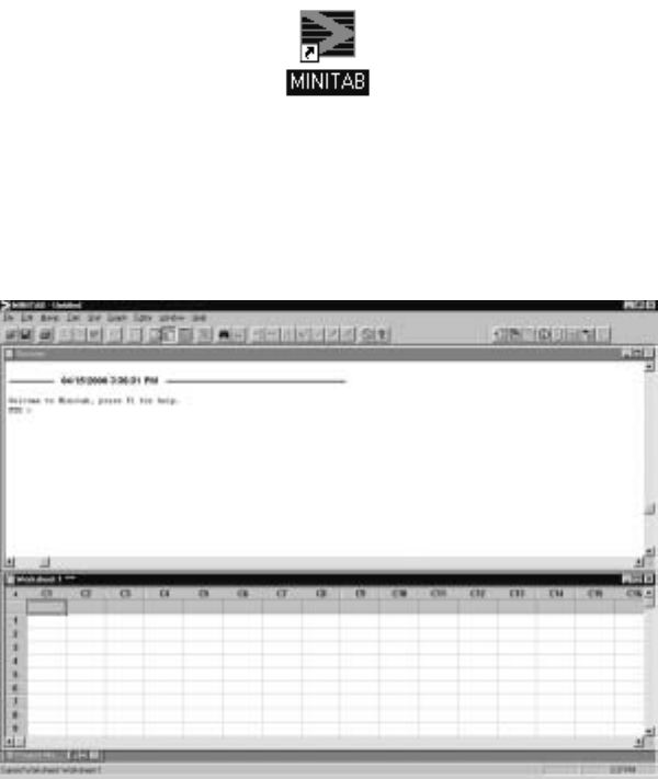
In most cases, you will double click an icon, such as that shown in Display

I.1, that corresponds to the Minitab program.

Display I.1: Minitab icon.

Alternatively, you can use the Start button and click on Minitab in the Programs

list. In this case, the program opens with a Minitab window, such as the one

shown in Display I.2. The Minitab window is divided into two sub-windows

with the upper window called the Session window and the lower one called the

Data window .

Display I.2: Minitab window.

Left clicking the mouse anywhere on a particular window brings that window

to the foreground, i.e., makes it the active window, and the border at the top of

the window turns dark blue. For example, clicking in the Session window will

make the window containing the MTB >prompt active. Alternatively, you can

use the command W

¯indow ISessioninthemenu bar at the top of the Minitab

6Minitab for Data Management

window to make this window active. You may not see the MTB >prompt in

your Session window, and for this manual it is important that you do so. You

can ensure that this prompt always appears in your Session window by using

¯dit IPreferences

¯, doubleclick on Session Window in the Preferences list that

comes up, clicking on the E

¯nable radio button under Command Language in

the Session Window Preferences, clicking on O

¯K, and clicking on Sa

¯ve. Without

the MTB >prompt, you cannot type commands to be executed in the Session

window.

In the session window, Minitab commands are typed after the MTB >prompt

and executed when you hit the Enter or Return key. For example, the Þrst

command you should learn is exit, as this takes you out of your Minitab session

and returns you to the system prompt or operating system. Otherwise, you can

access commands using the menu bar (Display I.3) that resides at the top of the

Minitab window. For example, you can access the exit command using F

¯ile I

¯it. In many circumstances, using the menu commands to do your analyses is

easy and convenient, although there are certain circumstances where typing the

session commands is necessary. You can also exit by clicking on the ×symbol

in the upper right-hand corner of the Minitab window. When you exit, you are

prompted by Minitab in a dialog window with the question, “Save changes to

this Project before closing?” You can safely answer no to this question unless

you are in fact using the Projects feature in Minitab as described in Appendix

A. In I.8, we will discuss how to save the contents of a Data window before

exiting. This is something you will commonly want to do.

Display I.3: Menu bar.

Immediately below the menu bar in the Minitab window is the taskbar. The

taskbar consists of various icons that provide a shortcut method for carrying

out various operations by clicking on them. These operations can be identiÞed

by holding the cursor over each in turn, and it is a good idea to familiarize

yourself with these. Of particular importance are the Cut Cells, Copy Cells,

and Paste Cells icons, which are available when a Data window is active. When

the operation associated with an icon is not available the icon is faded.

Minitab is an interactive program. By this we mean that you supply Minitab

with input data, or tell it where your input data is, and then Minitab responds

instantaneously to any commands you give telling it to do something with that

data. You are then ready to give another command. It is also possible to run

a collection of Minitab commands in a batch program; i.e., several Minitab

commands are executed sequentially before the output is returned to the user.

The batch version is useful when there is an extensive number of computations

to be carried out. You are referred to Appendix C for more discussion of the

batch version.

Minitab for Data Management 7

3 Files Used by Minitab

Minitab can accept input from a variety of Þles and write output to a variety of

Þles. Each Þle is distinguished by a Þle name and an extension that indicates

the type of Þle it is. For example, marks.mtw isthenameofaÞle that would

be referred to as ‘marks’ (note the single quotes around the Þle name) within

Minitab. The extension .mtw indicates that this is a Minitab worksheet. We

describe what a worksheet is in I.5. This Þle is stored somewhere on the hard

drive of a computer as a Þle called marks.mtw.

There are other Þles that you will want to access from outside Minitab,

perhaps to print them out on a printer. Depending on the version of Minitab

you are using, to do this, you may have to exit Minitab and give the relevant

system print command together with the full path name of the Þle you wish to

print. As various implementations of Minitab diﬀer as to where these Þles are

stored on the hard drive, you will have to determine this information from your

instructor or documentation or systems person. For example, in the windows

environment the full path name of the Þle could be

c:\Program Files\MTBWIN\Data\marks.mtw

or something similar. This path name indicates that the Þle marks.mtw is stored

on the C hard drive in the directory called Program Files\Mtbwin\Data. We

will discuss several diﬀerent types of Þlesinthischapter.

In many versions of Minitab, there are restrictions on Þle names. For ex-

ample, in earlier versions a Þle name can be at most eight characters in length

using any symbols except # and ’ and the Þrst character cannot be a blank.

There is no length restriction on Þle names in Versions 12 or 13. It is generally

best to name your Þles so that the Þle name reßects its contents. For example,

the Þle name marks may refer to a data set composed of student marks in a

number of courses.

4 Getting Help

At times, you may want more information about a command or some other

aspect of Minitab than this manual provides, or you may wish to remind yourself

of some detail that you have partially forgotten. Minitab contains an online

manual that is very convenient. You can access this information directly by

clicking on H

¯elp in the Menu bar and using the table of ¯Contents or doing a

¯earch of the manual for a particular concept.

From the MTB >prompt, you can use the help command for this purpose.

Typing help followed by the name of the command of interest and hitting Enter

will cause Minitab to produce relevant output. For example, asking for help on

the command help itself via the command

MTB >help help

8Minitab for Data Management

willgiveyouanoverviewofwhathelpinformationcanbeaccessedonyour

system. The help command should be used to Þnd out about session commands.

5TheWorksheet

The basic structural component of Minitab is the worksheet. Basically, the

worksheet can be thought of as a big rectangular array, or matrix, of cells

organized into rows and columns as in the Data window of Display I.2. Each cell

holds one piece of data. This piece of data could be a number, i.e. numeric data,

or it could be a sequence of characters, such as a word or an arbitrary sequence

of letters and numbers, i.e., text data. Data often comes as numbers, such as

1.7,2.3,... but sometimes it comes in the form of a sequence of characters,

such as black, brown, red, etc. Typically, sequences of characters are used as

identiÞers in classiÞcations for some variable of interest, e.g., color, gender. A

piece of text data can be up to 80 characters in length in Minitab. Version 13

also allows for date data, which is data especially formatted to indicate a date,

for example, 3/4/97. We will not discuss date data.

If possible, try to avoid using text data with Minitab, i.e., make sure all

the values of a variable are numbers, as dealing with text data in Minitab is

more diﬃcult. For example, denote colors by numbers rather than by names.

Still there will be applications where data comes to you as text data, e.g., in

a computer Þle, and it is too extensive to convert to numeric data. So we will

discuss how to input text data into a Minitab worksheet, but we recommend

that in such cases you convert this to numeric data, using the methods of I.11.3,

once it has been input. In Version 13 of Minitab it is somewhat easier to deal

with text data than earlier versions, and this proviso is not as necessary.

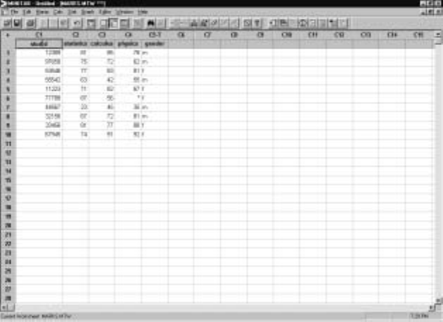
Display I.4 provides an example of a worksheet. Notice that the columns are

labeled C1, C2, etc. and the rows are labeled 1, 2, 3, etc. We will refer to the

worksheet depicted in Display I.4 as the marks worksheet hereafter and will use

it throughout Part I to illustrate various Minitab commands and operations.

Data arises from the process of taking measurements of variables in some

real-world context. For example, in a population of students, suppose that we

are conducting a study of academic performance in a Statistics course. Specif-

ically, suppose that we want to examine the relationship between grades in

Statistics, grades in a Calculus course, grades in a Physics course and gender.

So we collect the following information for each student in the study: student

number, grade in Statistics, grade in Calculus, grade in Physics, and gender.

Therefore, we have 5 variables — student number and the grades in the three

subjects are numeric variables, and gender is a text variable. Let us further

suppose that there are 10 students in the study.

Display I.4 gives a possible outcome from collecting the data in such a study.

Column C1 contains the student number (note that this is a categorical vari-

able even though it is a number). The student number primarily serves as an

identiÞer so that we can check that the data has been entered correctly. This is

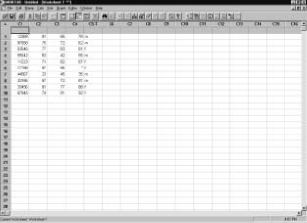
Minitab for Data Management 9

something you should always do as a Þrst step in your analysis. Columns C2—

C4 contain the student grades in their Statistics, Calculus, and Physics courses

and column C5 contains the gender data. Notice that a column contains the

values collected for a single variable, and a row contains the values of all the

variables for a single student. Sometimes, a row is referred to as an observation

or case . Observe that the data for this study occupies a 10×5subtable of the

full worksheet. All of the other blank entries of the worksheet can be ignored,

as they are undeÞned.

Display I.4: The marks worksheet.

There will be limitations on the number of columns and rows you can have in

your worksheet, and this depends on the particular implementation of Minitab

you are using. So if you plan to use Minitab for a large problem, you should

check with the system person or further documentation to see what these are.

For example, in some versions of Minitab there is a limitation of 5000 cells. So

there can be one variable with 5000 values in it, or 50 variables with 100 values

each, etc.

Associated with a worksheet is a table of constants . Typically, these are

numbers that you want to use in some arithmetical operation applied to every

value in a column. For example, you may have recorded heights of people in

inches and want to convert these to heights in centimeters. You must multiply

every height by the value 2.54. The Minitab constants are labeled K1, K2, etc.

Again, there are limitations on the number of constants you can associate with a

worksheet. For example, in many versions there can be at most 1000 constants.

So to continue with the above problem, we might assign the value 2.54 to K1.

InI.7.4,weshowhowtomakesuchanassignment,andinI.10.1weshowhow

to multiply every entry in a column by this value.

10 Minitab for Data Management

In Version 13 of Minitab, there is an additional structure beyond the work-

sheet called the project. A project can have multiple worksheets associated with

it. Also, a project can have associated with it various graphs and records of the

commands you have typed and the output obtained while working on the work-

sheets. Projects, which are discussed in Appendix A, can be saved and retrieved

for later work. Projects .

6 Minitab Commands

We will now begin to introduce various Minitab commands to get data into a

worksheet, edit a worksheet, perform various operations on the elements of a

worksheet, and save and access a saved worksheet. Before we do, however, it is

useful to know something about the basic structure of all Minitab commands.

Associated with every command is of course its name, as in F

¯ile IEx

¯it and

¯elp. Most commands also take arguments, and these arguments are column

names, constants, and sometimes Þle names.

Commands can be accessed by making use of the F

¯ile, E

¯dit, M

¯anip, C

¯alc,

¯tat, G

¯raph and E

¯ditor entries in the menu bar. Clicking any of these brings

up a list of commands that you can use to operate on your worksheet. The lists

that appear may depend on which window is active, e.g., either a Data window

or the Session window. Unless otherwise speciÞed, we will always assume that

the Session window is active when discussing menu commands. If a command

name in a list is faded, then it is not available.

Typically, using a command from the menu bar requires the use of a dialog

box or dialog window thatopenswhenyouclickonacommandinthelist.

These are used to provide the arguments and subcommands to the command

and specify where the output is to go. Dialog boxes have various boxes that

must be Þlled in to correctly execute a command. Clicking in a box that needs

to be Þlled in typically causes a variable list to appear in the left-most box, of

all items in the active worksheet that can be placed in that box. Double clicking

on items in the variable list places them in the box, or, alternatively, you can

type them in directly. When you have Þlled in the dialog box and clicked O

¯K,

the command is printed in the Session window and executed. Any output is

also printed in the Session window. Dialog boxes have a Help button that can

be used to learn how to make the entries.

For example, suppose that we want to calculate the mean of column C2

in the worksheet marks.ThenthecommandC

¯alc IC

¯olumn Statistics brings

up the dialog box shown in Display I.5. Notice that the radio button Su

¯mis

Þlled in. Clicking the radio button labelled M

¯ean results in this button being

ÞlledinandtheSu

¯m button becoming empty. Whichever button is Þlled in will

result in that statistic being calculated for the relevant columns when we Þnally

implement the command by clicking O

¯K.

Currently, there are no columns selected, but clicking in the Input variable

box brings up a list of possible columns in the display window on the left. The

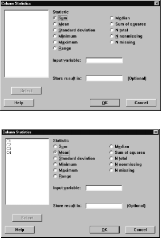
Minitab for Data Management 11

results of these operations are shown in Display I.6. We double click on C2 in

the variable list, which places this entry in the Input v

¯ariable box as shown in

Display I.7. Alternatively, we could have simply typed this entry into the box.

After clicking the O

¯K button, we obtain the output

Mean of C2 = 69.900

in the Session window.

Display I.5: Initial view of the dialog box for Column Statistics.

Display I.6: View of the dialog box for Column Statistics after selecting Mean and

bringing up the variable list.

12 Minitab for Data Management

Display I.7: Final view of the dialog box for Column Statistics.

Quite often, it is faster and more convenient to simply type your commands

directly into the Session window. Sometimes, it is necessary to use the Session

window approach, but for many commands the menu bar is available. So we

now describe the use of commands in the Session window.

Thebasicstructureofsuchacommandwithnarguments is

command name E1,E2,...,En

where Eiis the ith argument. Alternatively, we can write

command name E1E2... En

if we don’t want to type commas. Conveniently, if the arguments E1,E2,...,En

are consecutive columns in the worksheet, we have the following short-form

command name E1-En

which saves even more typing and accordingly decreases our chance of making a

typing mistake. If you are going to type a long list of arguments and you don’t

want them all on the same line, then you can type the continuation symbol &

where you want to break the line and then hit Enter. Minitab responds with

the prompt

CONT>

and you continue to type argument names. The command is executed when you

hit Enter after an argument name without a continuation character following

it.

Many commands can, in addition, be supplied with various subcommands

that alter the behavior of the command. The structure for commands with

subcommands is

Minitab for Data Management 13

command name E1... En1;

subcommand name En1+1 ... En2;

subcommand name Enk−1+1 ... Enk.

Notice that when there are subcommands each line ends with a semicolon until

the last subcommand, which ends with a period. Also, subcommands may have

arguments. When Minitab encounters a line ending in a semicolon it expects a

subcommand on the next line and changes the prompt to

SUBC >

until it encounters a period, whereupon it executes the command. If while

typing in one of your subcommands you suddenly decide that you would rather

not execute the subcommand – perhaps you realize something was wrong on a

previous line – then type abort after the SUBC >prompt and hit Enter. As

a further convenience, it is worth noting that you need to only type in the Þrst

four letters of any Minitab command or subcommand.

For example, to calculate the mean of column C2 in the worksheet marks

we can use the mean command in the Session window, as in

MTB >mean c2

and we obtain the same output in the Session window as before.

There are two additional ways in which you can input commands to Minitab.

Instead of typing the commands directly into the Session window, you can also

type these directly into the Command Line Editor, which is available via E

¯dit

ICom

¯mand Line Editor. Multiple commands can then be typed directly into a

box that pops up and executed when the S

¯ubmit Commands button is clicked.

Output appears in the Session window. Also, many commands are available on

atoolbar that lies just below the menu bar at the top of the Minitab window.

There is a diﬀerent toolbar depending upon which window is active. We give a

brief discussion of some of the features available in the toolbar in later sections.

7EnteringDataintoaWorksheet

There are various methods for entering data into a worksheet. The simplest

approach is to use the Data window to enter data directly into the worksheet by

clicking your mouse in a cell and then typing the corresponding data entry and

hitting Enter. Remember that you can make a Data window active by clicking

anywhere in the window or by using W

¯indows in the menu bar. If you type any

character that is not a number, Minitab automatically identiÞes the column

containing that cell as a text variable and indicates that by appending T to

the column name, e.g., C5-T in Display I.4. You do not need to append the T

when referring to the column. Also, there is a data direction arrow in the upper

left corner of the data window that indicates the direction the cursor moves

14 Minitab for Data Management

after you hit Enter. Clicking on it alternates between row-wise and column-

wise data entry. Certainly, this is an easy way to enter data when it is suitable.

Remember, columns are variables and rows are observations! Also, you can have

multiple data windows open and move data between them. Use the command

¯ile IN

¯ew to open a new worksheet.

7.1 Importing Data

If your data is in an external Þle (not an .mtw Þle), you will need to use F

¯ile

IOther F

¯iles II

¯mport Special Text to get the data into your worksheet. For

example, suppose in the Þle marks.txt we have the following data recorded,

justasitappears.

12389 81 85 78

97658 75 72 62

53546 77 83 81

55542 63 42 55

11223 71 82 67

77788 87 56 *

44567 23 45 35

32156 67 72 81

33456 81 77 88

67945 74 91 92

Each row corresponds to an observation, with the student number being the Þrst

entry, followed by the marks in the student’s Statistics, Calculus, and Physics

courses. These entries are separated by blanks.

Notice the * in the sixth row of this data Þle. In Minitab, a * signiÞes a

missing numeric value, i.e., a data value that for some reason is not available.

Alternatively, we could have just left this entry blank. A missing text value is

simply denoted by a blank. Special attention should be paid to missing values.

In general, Minitab statistical analyses ignore any cases that contain missing

data except that the output of the command will tell you how many cases

were ignored because of missing data. It is important to pay attention to this

information. If your data is riddled with a large number of missing values, your

analysis may be based on very few observations – even if you have a large data

set!

When data in such a Þle is blank-delimited likethisitisveryeasytoreadin.

After the command F

¯ile IOther F

¯iles II

¯mport Special Text, we see the dialog

box shown in Display I.8 minus C1—C4 in the S

¯tore data in column(s): box. We

typed C1-C4 into this window to indicate that we want the data read in to be

stored in these columns. Note that it doesn’t matter if we use lower or upper

case for the column names, as Minitab is not case sensitive. After clicking O

¯K,

we see the dialog box depicted in Display I.9, which we use to indicate from

which Þle we want to read the data. Note that if your data is in .txt Þles

rather than .dat Þles, you will have to indicate that you want to see these in

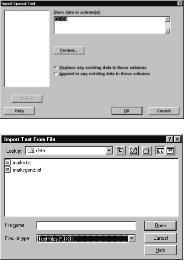
Minitab for Data Management 15

the F

¯iles of type box by selecting Text Files or perhaps All Files. Clicking on

marks.txt results in the data being read into the worksheet.

Display I.8: Dialog box for importing data from external Þle.

Display I.9: Dialog box for selecting Þle from which data is to be read in.

Of course, this data set does not contain the text variable denoting the

student’s gender. Suppose that the Þle marksgend.txt contains the following

data exactly as typed.

16 Minitab for Data Management

12389 81 85 78 m

97658 75 72 62 m

53546 77 83 81 f

55542 63 42 55 m

11223 71 82 67 f

77788 87 56 * f

44567 23 45 35 m

32156 67 72 81 m

33456 81 77 88 f

67945 74 91 92 f

As this Þle contains text data in the Þfth column, we must tell Minitab how

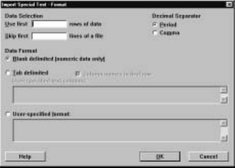
the data is formatted in the Þle. To access this feature we click on the F

¯ormat

button in the dialog box shown in Display I.8. This brings up the dialog box

showninDisplayI.10.

Display I.10: Initial dialog box for formatted input.

To indicate that we will specify the format, we click the radio button User-

speciÞed f

¯ormat and Þll the particular format into the box as shown in Display

I.11. The format statement says that we are going to read in the data accord-

ing to the following rule: a numeric variable occupying 5 spaces and with no

decimals, followed by a space, a numeric variable occupying 2 spaces with no

decimals, a space, a numeric variable occupying 2 spaces with no decimals, a

space, a numeric variable occupying 2 spaces with no decimals, a space, and

a text variable occupying 1 space. This rule must be rigorously adhered to or

errors will occur. So the rules you need to remember if you use formatted input

are that ak indicates a text variable occupying kspaces, kx indicates kspaces,

and fk.l indicates a numeric variable occupying kspaces, of which l are to the

right of the decimal point. Note if a data value does not Þll up the full num-

ber of spaces allotted to it in the format statement, it must be right justiÞed

in its Þeld. Also, if a decimal point is included in the number, this occupies

one of the spaces allocated to the variable and similarly for a negative or plus

Minitab for Data Management 17

sign. There are many other features to formatted input that we will not discuss

here. Use the Help button in the dialog box for information on these features.

Finally, clicking on the O

¯K button reads this data into a worksheet as depicted

in Display I.4. Typically, we try to avoid the use of formatted input because it

is somewhat cumbersome, but sometimes we must use it.

Display I.11: Dialog box for formatted input with the format Þlled in.

In the session environment, the read command is available for inputting

data into a worksheet with capabilities similar to what we have described. For

example, the commands

MTB >read c1-c4

DATA>12389818578

DATA>97658757262

DATA>53546778381

DATA>55542634255

DATA>11223718267

DATA>777888756*

DATA>44567234535

DATA>32156677281

DATA>33456817788

DATA>67945749192

DATA>end

10 rows read.

place the Þrst four columns into the marks worksheet. After typing read c1-c4

after the MTB >prompt and hitting Enter, Minitab responds with the DATA>

prompt, and we type each row of the worksheet in as shown. To indicate that

thereisnomoredata,wetypeend and hit Enter. Similarly, we can enter text

data in this way but can’t combine the two unless we use a format subcommand.

We refer the reader to help for more description of how this command works.

18 Minitab for Data Management

7.2 Patterned Data

Often, we want to input patterned data into a worksheet. By this we mean that

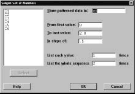
the values of a variable follow some determined rule. We use the command C

¯alc

IMake P

¯atterned Data for this. For example, implementing this command

with the entries in the dialog box depicted in Display I.12 adds a column C6

to the marks worksheet where the sequence 0,0.5,1.0,1.5,2.0is repeated twice.

For this we entered 0 in the F

¯rom Þrstvaluebox,a2intheT

¯olastvaluebox,

a.5intheI

¯nstepsofbox,a1intheListeachv

¯alue box, and a 2 in the List

the w

¯hole sequence box. Basically, we can start a sequence at any number m

and successively increment this with any number d>0until the next addition

would exceed the last value nprescribed, repeat each element ltimes, and Þnally

repeat the whole sequence ktimes.

Display I.12: Dialog box for making patterned data with some entries Þlled in.

There is some shorthand associated with patterned data that can be very

convenient. For example, typing m:nin a Minitab command is equivalent to

typing the values m, m +1,...,n when m<nand m, m −1, ..., n when m>n

and mwhen m=n. The expression m:n/d, where d>0, expands to a list as

above but with the increment of dor −d, whichever is relevant, replacing 1or

−1.Ifm<nthen dis added to muntil the next addition would exceed nand

if m>nthen dis subtracted from muntil the next subtraction would be lower

than n. The expression k(m:n/d)repeats m:n/d for ktimes while (m:n/d)l

repeats each element in m:n/d for ltimes. The expression k(m:n/d)lrepeats

(m:n/d)lfor ktimes.

The set command is available in the session window to input patterned data.

For example, suppose we want C6 to contain the 10 entries 1, 2, 3, 4, 5, 5, 4, 3,

2, 1. The command

Minitab for Data Management 19

MTB >set c6

DATA>1:5

DATA>5:1

DATA>end

does this. Also, we can add elements in parentheses. For example, the command

MTB >set c6

DATA>(1:2/.5 4:3/.2)

DATA>end

creates the column with entries 1.0, 1.5, 2.0, 4.0, 3.8, 3.6, 3.4, 3.2, 3.0. The

multiplicative factors kand lcanalsobeusedinsuchacontext. Obviously,

there is a great deal of scope for entering patterned data with set. The general

syntax of the set command is

set E1

where E1is a column.

7.3PrintingDataintheSessionWindow

Once we have entered the data into the worksheet, we should always check

that we have made the entries correctly. Typically, this means printing out

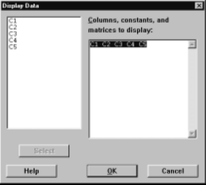
the worksheet and checking the entries. The command M

¯anip IDi

¯splay Data

will print the data you ask for in the Session window. For example, with the

worksheet marks the dialog box pictured in Display I.13 causes the contents of

this worksheet to be printed when we click on O

¯K. We selected which variables

to print by Þrst clicking in the C

¯olumns, constants, and matrices to display box

and then double clicking on the variables in the variable list on the left.

Display I.13: Dialog box for printing worksheet in the Session window.

20 Minitab for Data Management

The print command is available in the Session window and is often conve-

nient to use. The general syntax for the print command is

print E1... Em

where E1,..., Emare columns and constants.

7.4 Assigning Constants

To enter constants, we use the C

¯alc ICal

¯culator command and Þll in the dialog

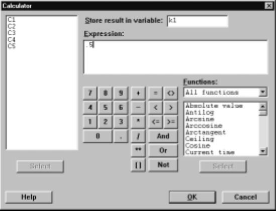
box appropriately. For example, suppose we want to assign the values k1=.5,

k2=.25 and k3=.25 to the constants k1, k2, and k3. These could serve as weights

to calculate a weighted average of the marks in the marks worksheet. Then the

¯alc ICal

¯culator command leads to the dialog box displayed in Display I.14,

where we have typed k1 into the S

¯tore result in variable box and the value .5

into the E

¯xpression box. Clicking on O

¯K then makes the assignment. Note that

we can assign text values to constants by enclosing the text in double quotes.

We will talk about further features of Calculator later in this manual. Similarly,

we assign values to k2 and k3.

Display I.14: Filled in dialog box for assigning the constant k1 the value .5.

The let command is available in the Session window and is quite convenient.

The following commands make this assignment and then we check, using the

print command, that we have entered the constants correctly.

Minitab for Data Management 21

MTB >let k1=.5

MTB >let k2=.25

MTB >let k3=.25

MTB >print k1-k3

K1 0.500000

K2 0.250000

K3 0.250000

Also, we can assign constants text values. For example,

MTB >let k4=’’result’’

assigns K4 the value result. Note the use of double quotes.

7.5 Naming Variables and Constants

It often makes sense to give the columns and constants names rather than just

referring to them as C1, C2, ..., K1, K2, etc. This is especially true when there

are many variables and constants, as it would be easy to slip and use the wrong

column in an analysis and then wind up making a mistake. To assign a name to

a variable simply go to the blank cell at the top of the column in the worksheet

corresponding to the variable and type in an appropriate name. For example,

we have used studid, statistics, calculus, physics, and gender for the

names of C1, C2, C3, C4, and C5, respectively, and these names appear in

Display I.15.

Display I.15: Worksheet marks with named variables.

22 Minitab for Data Management

In the Session window, the name command is available for naming variables

and constants. For example, the commands

MTB >name c1 ’studid’ c2 ’stats’ c3 ’calculus’ &

CONT>c4 ’physics’ c5 ’gender’ &

CONT>k1 ’weight1’ k2 ’weight2’ k3 ’weight3’

give the names studid to C1, stats to C2, calculus to C3, physics to C4,

gender to C5, weight1 to K1, weight2 to K2, and weight3 to K3. Notice that

we have made use of the continuation character & for convenience in typing in

the full input to name. When using the variables as arguments just enclose the

names in single quotes. For example,

MTB >print ’studid’ ’calculus’

prints out the contents of these variables in the Session window.

Variable and constant names can be at most 31 characters in length, cannot

include the characters # and ’ and cannot start with a leading blank or *. Recall

that Minitab is not case sensitive, so it does not matter if we use lower or upper

case letters when specifying the names.

7.6 Information about a Worksheet

We can get information on the data we have entered into the worksheet by using

the info command in the Session window. For example, we get the following

results based on what we have entered into the marks worksheet so far.

MTB >info

Column Name Count Missing

A C1 studid 10 0

C2 stats 10 0

C3 calculus 10 0

C4 physics 10 1

A C5 gender 10 0

Constant Name Value

K1 weight1 0.500000

K2 weight2 0.250000

K3 weight3 0.250000

Notice that the info command tells us how many missing values there are and

in what columns they occur and also the values of the constants.

This information can also be accessed directly from the Project Manager

window via W

¯indow IProject Manager.

Minitab for Data Management 23

7.7 Editing a Worksheet

It often happens that after data entry we notice that we have made some mis-

takes or we obtain some additional information, such as more observations. So

far, the only way we could change any entries in the worksheet or add some

rows is to reenter the whole worksheet!

Editing the worksheet is straightforward because we simply change any cells

by retyping their entries and hitting the Enter key. We can add rows and

columns at the end of the worksheet by simply typing new data entries in the

relevant cells. To insert a row before a particular row, simply click on any entry

in that row and then the menu command Ed

¯itor IInsert Rows

¯. Fill in the

blank entries in the new row. To insert a column before a particular column,

simplyclickonanyentryinthatcolumnandthenthemenucommandEd

¯itor

IInsert

¯Columns. Fill in the blank entries in the new column. To insert a

cell before a particular cell, simply click on any entry in that cell and the menu

command Ed

¯itor II

¯nsert Cells. Fill in the blank entry in the new cell that

appears in place of the original with all other cells in that column – and only

that column – pushed down.

If you wish to clear a number of cells in a block, click in the cell at the

start of the block, and holding the mouse key down, drag the cursor through

the block so that it is highlighted in black. Click on the Cut Cells icon on the

Minitab taskbar, and all the entries will be deleted. Cells immediately below the

block move up to Þll in the vacated places. A convenient method for clearing

all the data entries in a worksheet, with the relevant Data window active, is

to use the command E

¯dit ISelect A

¯ll Cells, which causes all the cells to be

highlighted, and click on the Cut Cells icon. Always save the contents of the

current worksheet before doing this unless you are absolutely sure you don’t

need the data again. We discuss how to save the contents of a worksheet in

I.8.1.

To copy a block of cells, click in the cell at the start of the block and, holding

the mouse key down, drag the cursor through the block so that it is highlighted

in black, but, instead of hitting the backspace key, use the command E

¯dit I

¯opy Cells or click on the Copy Cells icon on the Minitab taskbar. The block

of cells is now copied to your clipboard. If you not only want to copy a block of

cells to your clipboard but remove them from the worksheet, use the command

¯dit IC

¯ut

¯Cells or the Cut Cells icon on the Minitab taskbar instead. Note

that any cells below the removed block will move up to replace these entries.

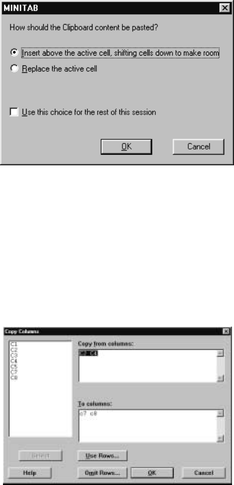
To paste the block of cells into the worksheet, click on the cell before which you

want the block to appear or that is at the start of the block of cells you wish to

replace and issue the command E

¯dit IP

¯aste Cells, or use the Paste Cells icon

on the Minitab taskbar. A dialog box appears as in Display I.16, where you are

prompted as to what you want to do with the copied block of cells. If you feel

that a cutting or pasting was in error, you can undo this operation by using

¯dit IU

¯ndo Cut or E

¯dit IU

¯ndo Paste, respectively, or use the Undo icon on

the Minitab taskbar.

24 Minitab for Data Management

Display I.16: Dialog box that determines how a block of copied cells is used, whether

being inserted into a worksheet or replacing a block of cell of the same size.

An alternative approach is available for copying operations using M

¯anip I

¯opy Columns and Þlling in the dialog box appropriately. For example, suppose

we want to copy all the entries in the marks worksheet in rows 5 and 8 of columns

C2 and C4 and place these in columns C7 and C8. The dialog box shown in

Display I.17 would result in all the entries in columns C2 and C4 being copied

to C7 and C8. To prevent this, we click on the U

¯se Rows button, which brings

up the dialog box shown in Display I.18. Clicking on the Use r

¯ows radio button

and Þlling in the associated box with the entries 5 and 8 speciÞes that only

entries in the Þfth and eighth rows will be copied. Clicking on the O

¯K buttons

in these dialog boxes then completes the operation.

Display I.17: Dialog box for copying entries in columns and pasting them.

Minitab for Data Management 25

Display I.18: Dialog box to select rows from columns to be copied.

One can also delete selected rows from speciÞed columns using M

¯anip ID

¯elete

Rows and Þlling in the dialog box appropriately. Notice, however, that whenever

we delete a cell, the contents of the cells beneath the deleted one in that column

simply move up to Þll the cell. The cell entry does not become missing; rather,

cells at the bottom of the column become undeÞned! If you delete an entire row,

this is not a problem because the rows below just shift up. For example, if we

delete the third row then in the new worksheet, after the deletion, the third row

is now occupied by what was formerly the fourth row. Therefore, you should be

very careful, when you are not deleting whole rows, to ensure that you get the

result you intended.

Note that if you should delete all the entries from a column, this variable

is still in the worksheet, but it is empty now. If you wish to delete a variable

and all its entries, this can be accomplished from M

¯anip IE

¯rase Variables and

Þlling in the dialog box appropriately. This is a good idea if you have a lot of

variables and no longer need some of them.

There are various commands in the Session window available for carrying

out these editing operations. For example, the restart command in the Session

window can be used to remove all entries from a worksheet. The let command

allows you to replace individual entries. For example,

MTB >let c2(2)=3

assigns the value 3 to the second entry in the column C2. The copy command

can be used to copy a block of cell from one place to another. The insert

command allows you to insert rows or observations anywhere in the worksheet.

The delete command allows you to delete rows. The erase command is avail-

able for the deletion of columns or variables from the worksheet. As it is more

convenient to edit a worksheet by directly working on the worksheet and using

the menu commands, we do not discuss these commands further here.

26 Minitab for Data Management

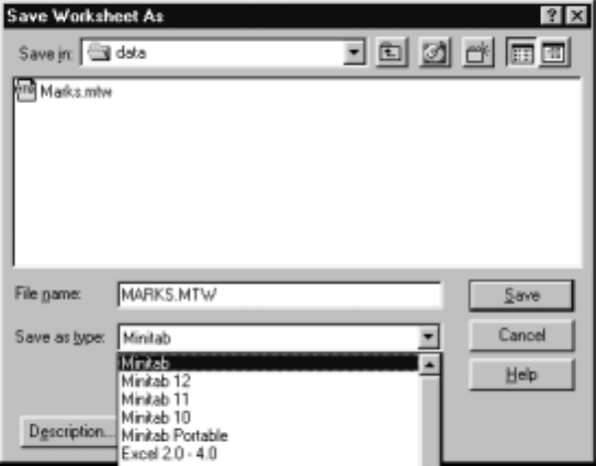
8 Saving, Retrieving, and Printing

Quite often, you will want to save the results of all your work in creating a work-

sheet. If you exit Minitab before you save your work, you will have to reenter

everything. So we recommend that you always save. To use the commands of

this section make sure that the Worksheet window of the worksheet in question

is active.

Use F

¯ile IS

¯ave Current Worksheet to save the worksheet with its current

name, or the default name if it doesn’t have one. If you want to provide a name

or store the worksheet in a new location, then use F

¯ile IS

¯ave Current Worksheet

As and Þll in the dialog box depicted in Display I.19 appropriately. The Save

¯n box at the top contains the name of the folder in which the worksheet will

besavedonceyouclickontheS

¯ave button. Here the folder is called data,and

you can navigate to a new folder using the Up One Level button immediately

to the right of this box. The next button takes you to the Desktop and the

third button allows you to create a subfolder within the current folder. The box

immediately below contains a list of all Þles of type .mtw in the current folder.

YoucanselectthetypeofÞle to display by clicking on the arrow in the Save

as t

¯ype box, which we have done here, and click on the type of Þle you want

to display that appears in the drop-down list. There are several possibilities

including saving the worksheet in other formats, such as Excel. Currently, there

is only one .mtw Þle in the folder data and it is called marks.mtw.Ifyouwant

to save the worksheet with a diﬀerent name, type this name in the File n

¯ame

boxandclickontheS

¯ave button.

Display I.19: Dialog box for saving a worksheet.

To retrieve a worksheet, use F

¯ile IOpen W

¯orksheet and Þll in the dialog

box as depicted in Display I.20 appropriately. The various windows and buttons

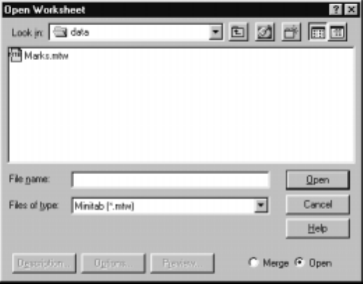
Minitab for Data Management 27

in this dialog box work as described for the F

¯ile IS

¯ave Current Worksheet As

command, with the exception that we now type the name of the Þle we want to

open in the File n

¯ameboxandclickontheO

¯pen button.

Display I.20: Dialog box for retrieving a worksheet.

To print a worksheet, use the command F

¯ile IP

¯rint Worksheet. The dialog

box that subsequently pops up allows you to control the output in a number of

ways.

It may be that you would prefer to write out the contents of a worksheet to

an external Þle that can be edited by an editor or perhaps used by some other

program. This will not be the case if we save the worksheet as an .mtw Þle as

only Minitab can read these. To do this, use the command F

¯ile IOther F

¯iles

¯xport Special Text, Þlling in the dialog box and specifying the destination

Þle when prompted. For example, if we want to save the contents of the marks

worksheet, this command results in the dialog box of Display I.21 appearing.

We have entered all Þve columns into the C

¯olumns to export box and have not

speciÞed a format so the columns will be stored in the Þle with single blanks

separating the columns. Clicking the O

¯K button results in the dialog box of

Display I.22 appearing. Here, we have typed in the name marks.dat to hold the

contents. Note that while we have chosen a .dat type Þle, we also could have

chosen a .txt type Þle. Clicking on the Save button results in a Þle marks.dat

being created in the folder data with contents as displayed in Display I.23.

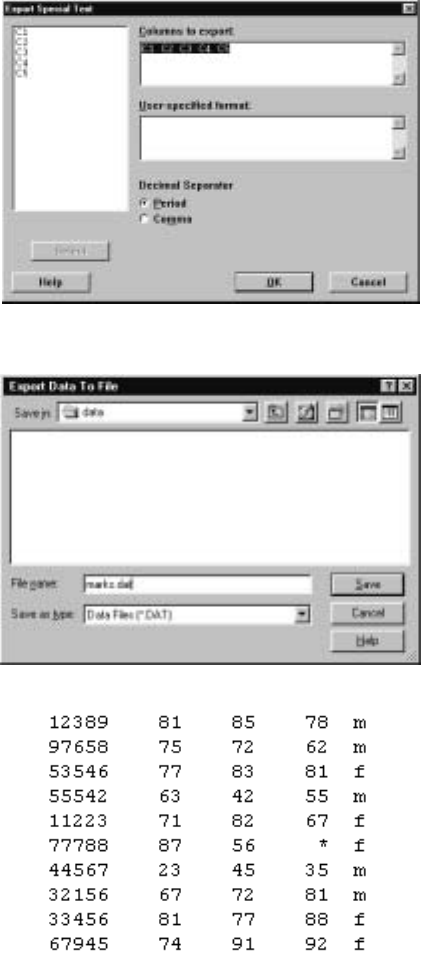
28 Minitab for Data Management

Display I.21: Dialog box for saving the contents of a worksheet to an external

(non-Minitab) Þle.

Display I.22: Dialog box for selecting external Þle to hold contents of a worksheet.

Display I.23: Contents of the Þle marks.dat.

In the Session window, the commands save and retrieve areavailablefor

saving and retrieving a worksheet in the .mtw format and the command write

is available for saving a worksheet in an external Þle. We refer the reader to

help for a description of how these commands work.

Minitab for Data Management 29

9RecordingandPrintingSessions

Sometimes, it is useful – e.g., when you have to hand in an assignment –

to maintain a record of all the commands you used, the output you obtained,

and any comments you want to make on what you are doing in a Minitab

session. Note that after executing a menu command the relevant Session window

commands are automatically typed in the Session window.

To use the commands for saving or printing the Session window Þrst make

sure that the Session window is active. If you issue the menu command Ed

¯itor

¯utput Editable Þrst, you can edit the Session window contents before saving

or printing its contents simply by typing or erasing text in the Session window.

You can turn this feature oﬀusing the same command. To save the contents of

a Session window use F

¯ile ISav

¯e Session Window As and Þll in the dialog box

appropriately. Note that the saved Þle is in the .txt format unless you make

adiﬀerent choice in the Save as t

¯ypebox. ToprintthecontentsoftheSession

window use F

¯ile IP

¯rint Session Window.

In the Session window, the outﬁle command is available for recording the

full or partial contents of a Minitab session. We refer the reader to help for a

description of how this command works.

10 Mathematical Operations

When carrying out a data analysis a statistician is often called upon to transform

the data in some way. This may involve applying some simple transformation to

a variable to create a new variable – e.g., take the natural logarithm of every

grade in the marks worksheet – to combining several variables together to form

a new variable – e.g., calculate the average grade for each student in the marks

worksheet. In this section, we present some of the ways of doing this.

10.1 Arithmetical Operations

Simple arithmetic can be carried out on the columns of a worksheet using the

arithmetical operations of addition +, subtraction −, multiplication *, division

/, and exponentiation ** via the C

¯alc ICal

¯culator command. When columns

are added together, subtracted one from the other, multiplied together, divided

one by the other (make sure there are no zeros in the denominator column),

or one column exponentiates another, these operations are always performed

component-wise. For example, C1*C2 means that the ith entry of C1 is multi-

plied by the ith entry of C2; etc. Also, make sure that the columns on which you

are going to perform these operations correspond to numeric variables! While

these operations have the order of precedence **, */, +−, parentheses ( ) can

and should be used to ensure an unambiguous result. For example, suppose in

the marks worksheet we want to create a new variable by taking the average of

the Statistics and Calculus grades and then subtracting this from the Physics

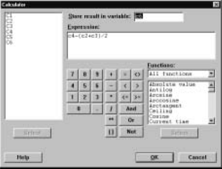
30 Minitab for Data Management

grade and placing the result in C6. Filling in the dialog box, corresponding to

¯alc ICal

¯culator, as shown in Display I.24 accomplishes this when we click on

the O

¯K button.

Display I.24: Dialog box for carrying out mathematical calculations.

Note that we can either type the relevant expression into the E

¯xpression box or

use the buttons and double clicking on the relevant columns. Further, we type

the column where we wish to store the results of our calculation in the S

¯tore

result in variable box. These operations are done on the corresponding entries in

each column; corresponding entries in the columns are operated on according to

the formula we have speciÞed, and a new column of the same length containing

all the outcomes is created. Note that the sixth entry in C6 will be * – missing

– because this entry was missing for C4.

These kinds of operations can also be carried out directly in the Session

window using the let command, and in some ways this is a simpler approach.

For example, the session command

MTB >let c6=c4-(c2+c3)/2

accomplishes this.

We can also use these arithmetical operations on the constants K1, K2,

etc., and numbers to create new constants or use the constants as scalars in

operations with columns. For example, suppose that we want to compute the

weighted average of the Statistics, Calculus, and Physics grades where Statistics

gets twice the weight of the other grades. Recall that we created, as part of the

marks worksheet, the constants weight1 =.5,weight2 =.25,andweight3 =

.25 in K1, K2, and K3, respectively. So this weighted average is computed via

the command

MTB >let c7=’weight1’*’stats’+’weight2’*’calculus’&

CONT>+’weight3’*’physics’

Minitab for Data Management 31

and the result is placed in C7. We have used the continuation character & for

convenience in this computation. Alternatively, we could have used the C

¯alc I

Cal

¯culator command as above for this.

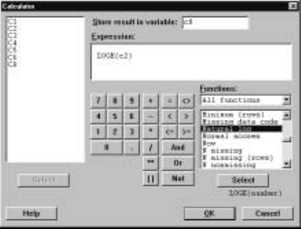
10.2 Mathematical Functions

Various mathematical functions are available in Minitab. For example, suppose

we want to compute the natural logarithm of the Statistics mark for each stu-

dent. Using the C

¯alc ICal

¯culator command with the dialog box as in Display

I.25 accomplishes this.

Display I.25: Dialog box for mathematical calculations illustrating the use of the

natural logarithm function.

A complete list of such functions is given in the Functions window when All

functions is in the window directly above the list.

The same result can be obtained using the session command let and the

natural logarithm function loge. For example,

MTB >let c8=loge(c2)

calculates the natural log of every entry in c2 and places the results in C8. There

are a number of such functions and a complete list is provided in Appendix B.1.

These functions can be applied to numbers as well as constants. If you want to

know the sine of the number 3.4, then

MTB >let k4=sin(3.4)

MTB >print k4

K4 -0.255541

gives the value.

32 Minitab for Data Management

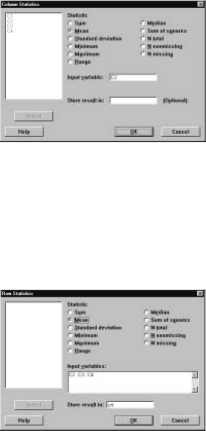
10.3 Column and Row Statistics

There are various column statistics that compute a single number from a column

by operating on all of the elements in a column. For example, suppose that we

want the mean of all the Statistics marks, i.e., the mean of all the entries in C2.

The command C

¯alc IC

¯olumn Statistics produces the dialog box of Display I.26

where we have selected Mean as the particular statistic to compute and C2 as

the column to use. Clicking O

¯K causes the mean of column C2 to be printed in

the Session window.

Display I.26: Dialog box for computing column statistics.

If we want to, we can store this result in a constant or column by making an

appropriate entry in the Store resu

¯lt in box. We see from the dialog box that

there are a number of possible statistics that can be computed.

We can also compute statistics row-wise. One diﬀerence with column statis-

tics is that these must be stored. For example, suppose we want to compute

the average of the Statistics, Calculus, and Physics marks. The command C

¯alc

IRo

¯w Statistics produces the dialog box shown in Display I.27 where we have

placed C2, C3, and C4 into the Input v

¯ariables box and c6 into the Store resul

¯t

in box.

Display I.27: Dialog box for computing row statistics.

Minitab for Data Management 33

It is also possible to compute column statistics using session commands. For

example,

MTB >mean(c2)

MEAN = 69.900

computes the mean of c2. If we want to save the value for subsequent use, then

the command

MTB >let k1=mean(c2)

does this. The general syntax for column statistic commands is

column statistic name(E1)

where the operation is carried out on the entries in column E1, and output is

written to the screen unless it is assigned to a constant using the let command.

See Appendix B.2 for a list of all the column statistics available.

Also, for most column statistics there are versions that compute row statis-

tics, and these are obtained by placing rin front of the column statistic name.

For example,

MTB >rmean(c2 c3 c4 c6)

computes the mean of the corresponding entries in C2, C3, and C4 and places

the result in C6. The general syntax for row statistic commands is

row statistic name(E1... EmEm+1)

where the operations are carried out on the rows in columns E1,..., Em,and

the output is placed in column Em+1.See Appendix B.3 for a list of all the row

statistics available.

10.4 Comparisons and Logical Operations

Minitab also contains the following comparison and logical operators.

Comparison Operators Logical Operators

equal to =, eq &, and

not equal to <>,ne \,or

less than <,lt ~, not

greater than >,gt

less than or equal to <=, le

greater than or equal to >=, ge

Notice that there are two choices for these operators; for example, use either

the symbol >=orthemnemonicge.

The comparison and logical operators are useful when we have simple ques-

tions about the worksheet that would be tedious to answer by inspection. This

34 Minitab for Data Management

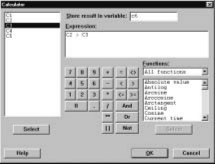
feature is particularly useful when we are dealing with large data sets. For ex-

ample, suppose that we want to count the number of times the Statistics grade

was greater than the corresponding Calculus grade in the marks worksheet. The

command C

¯alc ICal

¯culator gives the dialog box shown in Display I.28 where we

have put c6 in the S

¯tore result in variable box and c2 >c3 in the E

¯xpression

box. Clicking on the O

¯K button results in the ith entry in C6 containing a 1

if the ith entry in C2 is greater than the ith entry in C3, i.e., the comparison

is true, and a 0 otherwise. In this case, C6 contains the entries: 0, 1, 0, 1, 0,

1, 0, 0, 1, 0, which the worksheet in Display I.4 veriÞes as appropriate. If we

use C

¯alc ICal

¯culator to calculate the sum of the entries in C6, we will have

computed the number of times the Statistics grade is greater than the Calculus

grade.

These operations can also be simply carried out using session commands.

For example,

MTB >let c6=c2>c3

MTB >let k4=sum(c6)

MTB >print k4

K4 4.00000

accomplishes this.

Display I.28: Dialog box for comparisons.

The logical operators combine with the comparison operators to allow more

complicated questions to be asked. For example, suppose we wanted to calculate

the number of students whose Statistics mark was greater than their Calculus

mark and less than or equal to their Physics mark. The commands

MTB >let c6=c2>c3 and c2<=c4

MTB >let k4=sum(c6)

MTB >print k4

K4 1.00000

Minitab for Data Management 35

accomplish this. In this case, both conditions c2>c3 and c2<=c4 have to be

true for a 1 to be recorded in C6. Note that the observation with the missing

Physics mark is excluded. Of course, we can also implement this using C

¯alc I

Cal

¯culator and Þlling in the dialog box appropriately.

Text variables can be used in comparisons where the ordering is alphabetical.

For example,

MTB >let c6=c5<’’m’’

puts a 1 in C6 whenever the corresponding entry in C5 is alphabetically smaller

than m.

11 Some More Minitab Commands

In this section we discuss some commands that can be very helpful in certain

applications. We will make reference to these commands at appropriate places

throughout the manual. It is probably best to wait to read these descriptions

until such a context arises.

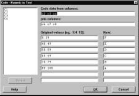
11.1 Coding

The M

¯anip ICo

¯de command is used to recode columns. By this we mean that

data entries in columns are replaced by new values according to a coding scheme

that we must specify. You can recode numeric into numeric, numeric into text,

text into numeric, or text into text by choosing an appropriate subcommand.

For example, suppose in the marks worksheet we want to recode the grades in

C2, C3, and C4 so that any mark in the range 0—39 becomes an F, every mark

in the range 40—49 becomes an E, every mark in the range 50—59 becomes a

D, every mark in the range 60—69 becomes a C, every mark in the range 70—79

becomes a B, every mark in the range 80—100 becomes an A, and the results are

placed in columns C6, C7, and C8, respectively. Then the command M

¯anip I

¯de INu

¯meric to Text brings up the dialog box shown in Display I.29. The

ranges for the numeric values to be recoded to a common text value are typed

in the Or

¯iginal values box, and the new values are typed in the N

¯ew box. Note

that we have used a shorthand for describing a range of data values as discussed

in section 7.2. Because the sixth entry of C4 is *, i.e., it is missing, this value

is simply recoded as a blank. You can also recode missing values by including

*inoneoftheOr

¯iginal values boxes. If a value in a column is not covered by

one of the values in the Or

¯iginal values boxes, then it is simply left the same in

the new column.

36 Minitab for Data Management

Display I.29: Dialog box for recoding numeric values to text values.

Note that this menu command restricts the number of new code values to 8.

The session command code allows up to 50 new codes. For example, suppose

in the marks worksheet we want to recode the grades in C2, C3, and C4 so that

any mark in the range 0—9 becomes a 0, every mark in the range 10—19 becomes

10, etc., and the results are placed in columns C6, C7, and C8. The following

command

MTB >code(0:9) to 0 (10:19) to 10 (20:29) to 20 (30:39) to 30 &

CONT>(40:49) to 40 (50:59) to 50 (60:69) to 60 (70:79) to 70 &

CONT>(80:89) to 80 (90:99) to 90 for C2-C4 put in C6-C8

accomplishes this. Note the use of the continuation symbol &, as this is a long

command. The general syntax for the code command is

code (V1)tocode

1... (Vn)tocode

nfor E1... Emput in Em+1 ... E2m

where Videnotes a set of possible values and ranges for the values in columns

E1... Emthat are all coded as the number codei,andtheresultsofthiscoding

are placed in the columns Em+1 ... E2m, i.e., the recoded E1is placed in Em+1,

etc.

11.2 Concatenating Columns

The M

¯anip ICon

¯catenate combines two or more text columns into a single text

column. For example, if C6 contains m,m,m,f,f, reading Þrst to last entry, and

C7 contains to,ta,ti,to,ta, then the entries in the M

¯anip ICon

¯catenate

dialog box shown in Display I.30 result in a new text column C8 containing the

entries mto,mta,mti,fto,fta.

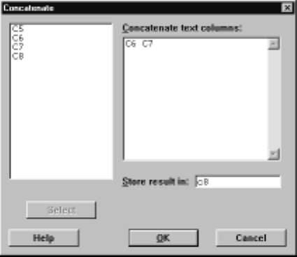
Minitab for Data Management 37

Display I.30: Dialog box for concatenating text columns.

In the session environment, the concatenate command is available for this

operation. The general syntax of the concatenate command is

concatenate E1... Emin Em+1

where E1, ..., Em,are text columns, and Em+1 is the target text column.

11.3 Converting Data Types

The M

¯anip ICo

¯de IUs

¯e Conversion Table command is used to change text

data into numeric data and vice versa. As dealing with text data is a bit more

diﬃcult in Minitab, we recommend either converting text data to numeric before

input or using this command after input to do this.

For example, in the worksheet marks suppose we want to change the gender

variable from text, with male and female denoted by mand f, respectively, to a

numerical variable with male denoted by 0 and female by 1. To do this, we must

Þrst set up a conversion table. The conversion table comprises two columns in

the worksheet, where one column is text and contains the text values used in

the text column, and the second column is numeric and contains the numerical

values that you want these changed into. For example, suppose we have entered

columns C6 and C7 in the marks worksheet, as shown in Display I.31. The

¯anip ICo

¯de IU

¯se Conversion Table command produces the dialog box

shown in Display I.32, where we have indicated that we want to convert the

text column C5 into a numeric column and that each mshouldbecomea0and

each fshould become a 1.

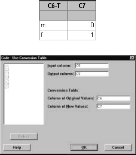
38 Minitab for Data Management

Display I.31: Columns c6 and c7 in the marks worksheet as a conversion table.

Display I.32: Dialog box for converting text column c5 of the marks worksheet into a

numeric column with the conversion table given in columns c6 and c7.

The general syntax for the corresponding session command convert is

convert E1E2E3E4

where E1,E2are the columns containing the conversion table, E3is the column

to be converted and E4is the column containing the converted column.

11.4 History

Minitab keeps a record of the commands you have used and the data you have

input in a session. This information can be obtained in the History folder of the

Project Manager window. The commands can be copied from wherever they are

listed and pasted into the Session window to be reexecuted, so that a number

of commands can be executed at once without retyping. These commands can

be edited before being executed again. This is very helpful when you have

implemented a long sequence of commands and realize that you made an error

early on. Note that even if you use the menu commands, a record is kept only

of the corresponding session commands.

The journal command is available in the Session window if you want to

keep a record of the commands in an external Þle. For example,

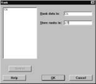
Minitab for Data Management 39

MTB >journal ’comm1’

Collecting keyboard input(commands and data)in file: comm1.MTJ

MTB >read c1 c2 c3

DATA>123

DATA>end

1 rows read.

MTB >nojournal

puts

read c1 c2 c3

123

end

nojournal

into the Þle comm1.mtj. The history is turned oﬀas soon as the nojournal

command is typed.

11.5 Computing Ranks

Sometimes, we want to compute the ranks of the numeric values in a column.

The rank riof the ith value in a column is a value that reßects its relative size

in the column. For example, if the ith value is the smallest value then ri=1,

if it is the third smallest then ri=3,etc. If values are the same, i.e., tied, then

each value receives the average rank. To calculate the ranks of the entries in

acolumnweusetheM

¯anip IR

¯ank command. For example, suppose that C6

containsthevalues6,4,3,2,3,1. ThentheM

¯anip IR

¯ank command brings

up the dialog box in Display I.33, which is Þlled in so that the ranks of the

entries in C6 are placed in C7. In this case, the ranks are 6.0, 5.0, 3.5, 2.0, 3.5,

and 1.0, respectively.

Display I.33: Dialog box for computing ranks.

The syntax of the corresponding session command rank is

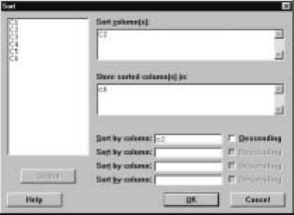
40 Minitab for Data Management

rank E1E2

where E1is the column whose ranks we want to compute, and E2is the column

that will hold the computed ranks.

11.6 Sorting Data

It often occurs as part of a data analysis that we want to sort a column so that

its values ascend from smallest to largest or descend from largest to smallest.

Note that ordering here could refer to numerical order or alphabetical order,

so we also consider ordering text columns. Also, we may want to sort all the

rows contained in some subset of the columns in the worksheet by aparticular

column. The M

¯anip IS

¯ort command allows us to carry out these tasks.

For example, suppose that we want to sort the entries in C2 in the marks

worksheet – the Statistics grades – from smallest to largest and place the

sorted values in C6. Then the M

¯anip IS

¯ort command brings up the dialog

box shown in Display I.34, where the Sort co

¯lumn(s) box contains the column

C2 to be sorted, the Store sorted column(s) In box contains C6, where we will

store the sorted column, and C2 is also placed in the S

¯ort by column box. This

command results in C6 containing 23, 63, 67, 71, 74, 75, 77, 81, 81, 87. If we

had clicked the D

¯escending box, the order of appearance of these values in C6

would have been reversed.

IfwehadplacedanothercolumnintheS

¯ort by column box, say C5, then C5

would have been sorted with the values in C2 carried along and placed in C6,

i.e., the values in C2 would be sorted by the values in C5. So all the Statistics

marks of females, in the order they appear in C2 will appear in C6 Þrst and

then the Statistics marks of males. For example, replacing C2 by C5 in this box

would result in the values in C6 becoming 77, 71, 87, 81, 74, 81, 75, 63, 23, 67.

If we Þll in the next S

¯ort by column box with another column, say C3, then the

values in C2 are sorted Þrst by gender and then within gender by the values in

C3.

Display I.34: Dialog box for sorting.

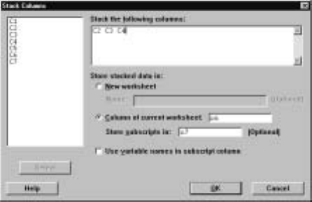
Minitab for Data Management 41

The general syntax of the corresponding session command sort is

sort E1E2...EmEm+1 ...E2m

where E1is the column to be sorted, and E2, ..., Emare carried along with

the results placed in columns Em+1, ..., E2m.Note that this sort can also be

accomplished using the by subcommand, where the general syntax is

sort E1E2...EmEm+1 ...E2m;

by E2m+1 ...En.

where now we sort by columns E2m+1, ..., En,sortingÞrst by E2m+1,then

E2m+2,etc., carrying along E1,...,E

mand placing the result in Em+1, ...,

E2m.The descending subcommand can also be used to indicate which sorting

variables we want to use in descending order rather than ascending order.

11.7StackingandUnstackingColumns

The M

¯anip ISt

¯ack command is used to literally stack columns one on top of

the other or unstack a column into separate columns. For example, in the marks

worksheet the M

¯anip ISt

¯ack IS

¯tack Columns command brings up the dialog

box shown in Display I.35, which has been Þlled in to stack columns C2, C3,

andC4intoC6withthevaluesinC2Þrst, followed by the values in C3 and then

the values in C4. In C7 we have stored an index which indicates that column

eachvalueinC6camefromwitha1everytimeavaluecamefromC2,a2every

time a value came from C3, and a 3 every time a value came from C4. It is not

necessary to create such an index.

Display I.35: Dialog box for stacking columns.

In the Session window, this same result can be obtained using the stack

command. The general syntax for the stack command is given by

stack E1E2...Eminto Em+1

where E1,E

2, ..., Emdenote the columns or constants to be stacked one on top

of the other, starting with E1, and with the result placed in column Em+1.If we

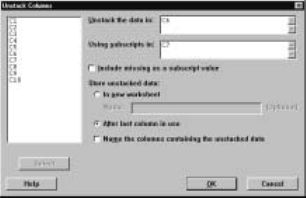
42 Minitab for Data Management

want to keep an index of where the values came from, then use the subcommand

subscripts Em+2

which results in index values being stored in column Em+2.

To unstack values in a column by the values in an index column we use the

¯anip IUnstack command. For example, given the columns C6 and C7 of

the marks worksheet as described above, the dialog box shown in Display I.36

unstacks C6 into three columns by the values in C7. The three columns are

C8, C9, and C10. Note that they are identical to columns C2, C3, and C4,

respectively. We must always specify a column containing the subscripts when

unstacking a column.

Display I.36: Dialog box for unstacking columns.

The general syntax for the corresponding session command unstack is

unstack E1into E2...Em;

subscripts Em+1.

where E1is the column to be unstacked, E2, ..., Emare the columns and con-

stants to contain the unstacked column, and Em+1 gives the subscripts 1, 2, ...

that indicate how E1is to be unstacked.

Note that it is also possible to simultaneously unstack blocks of columns.

We refer the reader to help or H

¯elpforinformationonthis.

Minitab for Data Management 43

12 Exercises

1. The following data give the Hi and Low trading prices in Canadian dollars

for various stocks on a given day on the Toronto Stock Exchange. Create

a worksheet, giving the columns the same variable names, using any of

the methods discussed in I.7. Be careful to ensure that the value of the

variable stock starts with a letter. Print the worksheet to check that

you have successfully entered it. Save the worksheet giving it the name

stocks.

Stock Hi Low

ACR 7.95 7.80

MGI 4.75 4.00

BLD 112.25 109.75

CFP 9.65 9.25

MAL 8.25 8.10

CM 45.90 45.30

AZC 1.99 1.93

CMW 20.00 19.00

AMZ 2.70 2.30

GAC 52.00 50.25

2 Retrieve the worksheet stocks created in Exercise 1. Change the Low

value in the stock MGI to 3.95. Calculate the average of the Hi and

Low prices for all the stocks, and save this in a column called average.

Calculate the average of all the Hi prices, and save this in a constant

called avhi. Similarly, do this for all the Low prices, and save this in a

constant called avlo. Save the worksheet using the same name. Write all

the columns out to a Þle called stocks.dat.PrinttheÞle stocks.dat on

your system printer.

3 Retrieve the worksheet created in Exercise 2. Using the Minitab com-

mands discussed in I.10, calculate the number of stocks in the worksheet

whose average is greater than $5.00 and less than or equal to $45.00.

4 Using the worksheet created in Exercise 2, insert the following stocks at

the beginning of the worksheet.

Stock Hi Low

CLV 1.85 1.78

SIL 34.00 34.00

AC 14.45 14.05

Delete the variable average. Save the worksheet.

44 Minitab for Data Management

5 Using the worksheet created in Exercise 4, sort the stocks into alphabetical

order. Calculate the ranks of the individual stocks based on their Hi price,

and save the ranking in a new column. Save the worksheet.

6 Using the worksheet created in Exercise 5, calculate the average Hi price

of all the stocks beginning in A.

7 Using the worksheet created in Exercise 5, recode all the Low prices in the

range $0—9.99 as 1, in the range $10—39.99 as 2, and greater than or equal

to $40 as 3, and save the recoded variable in a new column.

8 Using patterned data input, place the values from −10 to 10 in increments

of .1 in C1. For each of the values in C1, calculate the value of the

quadratic polynomial 2x2+4x−3(i.e., substitute the value in each entry

in C1 into this expression) and place these values in C2. Using Minitab

commands and the values in C1 and C2, estimate the point in the range

from −10 to 10 where this polynomial takes its smallest value and what

this smallest value is. Using Minitab commands and the values in C1 and

C2 estimate the points in the range from −10 to 10,where this polynomial

is closest to 0.

9 Using patterned data input, place values in the range from 0 to 5 using an

increment of .01 in C1. Calculate the value of 1−e−xfor each value in

C1, and place the result in C2. Using Minitab commands, Þnd the largest

value in C1 where the corresponding entry in C2 is less than or equal to .5.

Note that e−xcorresponds to the exponentiate command (see Appendix

B.1) evaluated at −x.

10 Using patterned data input, place values in the range from −4to4using

an increment of .01 in C1. Calculate the value of

√2πe−x2/2

for each value in C1, and place the result in C2, where π=3.1415927.

Using parsums (see Appendix B.1), calculate the partial sums for C2,

and place the result in C3. Multiply C3 times .01. Find the largest value

in C1 such that the corresponding entry in C3 is less than or equal to .25.

Part II

Minitab for Data Analysis

Chapter 1

Looking at

Data–Distributions

New Minitab commands discussed in this chapter

¯alc IProbability D

¯istributions IN

¯ormal

¯ile IOpen G

¯raph

¯ile ISav

¯eGraphAs

¯raph IB

¯oxplot

¯raph IC

¯hart

¯raph IDo

¯tplot

¯raph IH

¯istogram

¯raph IPi

¯eChart

¯raph IProbability

¯Plot

¯raph IStem-and-Leaf

¯raph IT

¯ime Series Plot

¯anip ICo

¯de

¯tat IB

¯asic Statistics ID

¯isplay Descriptive Statistics

¯tat IB

¯asic Statistics IS

¯tore Descriptive Statistics

¯tat IT

¯ables ITa

¯lly

ThischapterofIPSisconcernedwiththevariouswaysofpresentingandsum-

marizing a data set. By presenting data, we mean convenient and informative

methods of conveying the information contained in a data set. There are two

basic methods for presenting data, namely graphically and through tabulations.

Still, it can be hard to summarize exactly what these presentations are saying

about the data. So the chapter also introduces various summary statistics that

are commonly used to convey meaningful information in a concise way.

All of these topics can involve much tedious, error prone calculation, if we

were to insist on doing them by hand. An important point is that you should

48 Chapter 1

almost never rely on hand calculation in carrying out a data analysis. Not only

are there many far more important things for you to be thinking about, as the

text discusses, but you are also likely to make an error. On the other hand,

never blindly trust the computer! Check your results and make sure that they

make sense in light of the application. For this, a few simple hand calculations

can prove valuable. In working through the problems in IPS, you should try to

use Minitab as much as possible, as this will increase your skill with the package

and inevitably make your data analyses easier and more eﬀective.

1.1 Tabulating and Summarizing Data

If a variable is categorical, we construct a table using the values of the variable

and record the frequency (count) of each value in the data and perhaps the

relative frequency (proportion) of each value in the data as well. These relative

frequencies then serve as a convenient summarization of the data.

If the variable is quantitative, we typically group the data in some way,

i.e., divide the range of the data into nonoverlapping intervals and record the

frequency and proportion of values in each interval. Grouping is accomplished

using the M

¯anip ICo

¯de command discussed in I.11.1.

If the values of a variable are ordered, we can record the cumulative dis-

tribution, namely the proportion of values less than or equal to each value.

Quantitative variables are always ordered but sometimes categorical variables

are as well, e.g., when a categorical variable arises from grouping a quantitative

variable.

Often, it is convenient with quantitative variables to record the empirical

distribution function, which for data values x1,...,x

nand at a value xis given

by ˆ

F(x)=#of xi≤x

i.e., ˆ

F(x)is the proportion of data values less than or equal to x. We can

summarize such a presentation via the calculation of a few quantities such as

the Þrst quartile, the median, and the third quartile or present the mean and

the standard deviation.

We introduce some new commands to carry out the necessary computations

using the data shown in Table 1.1. This is data collected by A.A. Michelson

and Simon Newcomb in 1882 concerning the speed of light. We will refer to this

hereafter as Newcomb’s data and place these in the column C1 with the name

time in the worksheet called newcomb.

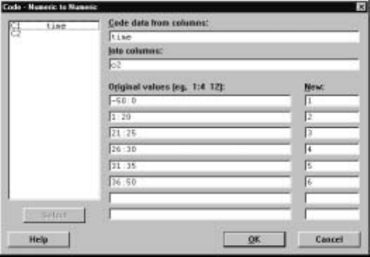
Looking At Data–Distributions 49

28 22 36 26 28 28

26 24 32 30 27 24

33 21 36 32 31 25

24 25 28 36 27 32

34 30 25 26 26 25

-442321303329

27 29 28 22 26 27

16 31 29 36 32 28

40 19 37 23 32 29

-2 24 25 27 24 16

29 20 28 27 39 23

Table 1.1: Newcomb’s data..

1.1.1 Tallying Data

The S

¯tat IT

¯ables ITa

¯lly command tabulates categorical data. Consider New-

comb’s measurements in Table 1.1. These data range from −44 to 40 (use min-

imum and maximum in C

¯alc ICal

¯culator to calculate these values). Suppose

we decide to group these into the intervals (−50,0],(0,20],(20,25],(25,30],

(30,35],0(35,40]. Next we want to record the frequencies, relative frequencies,

cumulative frequencies, and cumulative distribution of this grouped variable.

First, we used the M

¯anip ICo

¯de IN

¯umeric to Numeric command, as de-

scribedinI.11.1,torecodethedatasothateveryvaluein(−50,0] is given the

value 1, every value in (0,20] is given the value 2, etc., and these values are

placed in C2. The dialog box for doing this is shown in Display 1.1.

Display 1.1: Dialog box for recoding Newcomb’s data.

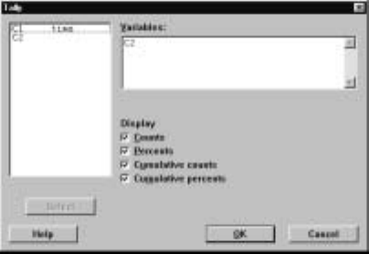
50 Chapter 1

Next we used the S

¯tat IT

¯ables ITa

¯lly command, with the dialog box shown

in Display 1.2,

Display 1.2: Dialog box for tallying the variable C2 in the newcomb worksheet.

to produce the output

C2 Count Percent CumCnt CumPct

1 2 3.03 2 3.03

2 4 6.06 6 9.09

3 17 25.76 23 34.85

4 26 39.39 49 74.24

5 10 15.15 59 89.39

6 7 10.61 66 100.00

N= 66

in the Session window.

We can also use the S

¯tat IT

¯ables ITa

¯lly command to compute the empir-

ical distribution function of C1 in the newcomb worksheet. First, we must sort

the values in C1, from smallest to largest, using the M

¯anip IS

¯ort command

described in I.11.6, and then we apply the S

¯tat IT

¯ables ITa

¯lly command to

this sorted variable.

The general syntax of the corresponding session command tally is

tally E1...Em

where E1, ..., Emare columns of categorical variables, and the command is

applied to each column. If no subcommands are given, then only frequencies

are computed, while the subcommands percents computes relative frequencies,

cumcnts computes the cumulative frequency function, and cumpcts computes

the cumulative distribution of C2. Any of the subcommands can be dropped.

For example, the commands

MTB >sort c1 c3

MTB >tally c3;

SUBC>cumpcnts;

SUBC>store c4 c5.

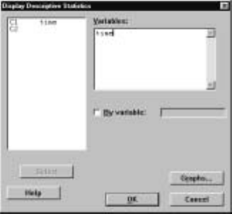
Looking At Data–Distributions 51

Þrst use the sort command to sort the data in C1 from smallest to largest and

place the results in C3. The cumulative distribution is computed for the values

in C3 with the unique values in C3 stored in C4 and the cumulative distribution

at each of the unique values stored in C5 via the store subcommand to tally.

1.1.2 Describing Data

The S

¯tat IB

¯asic Statistics ID

¯isplay Descriptive Statistics command is used

with quantitative variables to present a numerical summary of the variable val-

ues. These values are in a sense a summarization of the empirical distribution

of the variable. For example, in the newcomb worksheet the dialog box shown

in Display 1.3 leads to the output

Variable N Mean Median TrMean StDev SE Mean

time 66 26.21 27.00 27.40 10.75 1.32

Variable Minimum Maximum Q1 Q3

time -44.00 40.00 24.00 31.00

in the Session window. This provides the count N, the mean, median, trimmed

mean TrMean (removes lower 5% and upper 5% of the data and averages the

rest), standard deviation, standard error of the mean, minimum, maximum, Þrst

quartile Q1, and third quartile Q3 ofthevariableC1. Ifwewantsuchasummary

of a variable by the values of another variable, we check the B

¯yvariablebox

and indicate the by variable in the box to the right of this. For example, we

mightwantsuchasummaryforeachofthegroupswecreatedinII.1.1,andso

we would place C2 in this box. Note that a number of summary statistics can

also be computed using the Column Statistics discussed in I.10.3.

Display 1.3: Dialog box for computing basic descriptive statistics of a quantitative

variable.

If we wish to compute some basic statistics and store these values for later

use, then the S

¯tat IB

¯asic Statistics IS

¯tore Descriptive Statistics command is

available for this. For example, with the newcomb worksheet this command leads

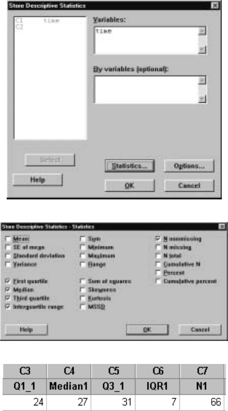
52 Chapter 1

to the dialog box shown in Display 1.4. Clicking on the S

¯tatistics button results

in the dialog box of Display 1.5 where we have checked F

¯irst quartile, Me

¯dian,

¯ird quartile, Interq

¯uartile range, and N

¯nonmissing as the statistics we want

to compute. The result of these choices is that the next available variables in

the worksheet contain these values. So in this case, the values of C3—C7 are as

depicted in Display 1.6. Note that these variables are now named as well. Note

that many more statistics are available using this command.

Display 1.4: Dialog box for computing and storing various descriptive statistics.

Display 1.5: Dialog box for choosing the descriptive statistics to compute and store.

Display 1.6: Values obtained for descriptive statistics using dialog boxes in Figures

1.4 and 1.5.

The general syntax of the Session command describe, corresponding to S

¯tat

¯asic Statistics ID

¯isplay Descriptive Statistics, is

Looking At Data–Distributions 53

describe E1...Em

where E1, ..., Emare columns of quantitative variables and the command is

applied to each column. A by subcommand can also be used. The stats

command is available in the Session window if we want to store the values of

statistics. We refer the reader to help for a description of this command.

1.2 Plotting Data in a Graph Window

One of the most informative ways of presenting data is via a plot. There are

many diﬀerent types of plots within Minitab, and which one to use depends on

the type of variable you have and what you are trying to learn. In this section

we describe how to use the plotting features in Minitab. There are, however,

many features of plotting that we will not describe. For example, there are

many graphical editing capabilities that allow you to add features, such as titles

or legends. Some of these features are accessed via G

¯raph IL

¯ayout. We refer

the reader to H

¯elp for more details on these features.

EachplotinMinitabismadeinaGraph window. You can make multiple

plots and retain each Graph window until you want to delete it simply by clicking

the ×symbol in the upper right-hand corner. You make any particular Graph

window active by clicking in it or by using the W

¯indow command. A plot can

besavedinanexternalÞle in a variety of formats, such as Minitab graph .mgf,

bitmap .bmp,JPEG.jpg, etc., using the F

¯ile ISav

¯e Graph As command. If

a graph has been saved in the .mgf format, it can be reopened using the F

¯ile I

Open G

¯raph command.

1.2.1 Dotplots

The G

¯raph IDo

¯tplot command is used with quantitative variables and produces

a plot of each data value as a dot along the x-axis so that you get a general

idea of the location of the data and how much scatter there is. Actually, the

data is grouped before plotting and multiple observations in a group are stacked

over the x-axis. The interval between successive tick (+) marks on the x-axis

is divided into 10 equal-length subintervals for the grouping. Typically, one

also looks for points that are far from the main scatter of points as these may

be identiÞed as outliers and, as such, deleted from the data set for subsequent

analysis. For example, for the newcomb worksheet dialog box in Display 1.7

results in the plot of Display 1.8.

The general syntax of the corresponding Session command dotplot is

dotplot E1...Em

where E1, ..., Emare columns, and a dotplot is produced for each. There are a

number of subcommands available. The same subcommand ensures the scales

of the dotplots are the same for each column. The by subcommand allows

plotting of a variable by the values of another variable with all plots having

thesamescale. Theincrement subcommand allows for control of the distance

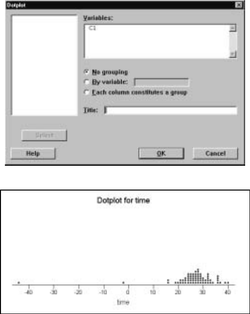
54 Chapter 1

between the tick marks and start and end allow you to specify where the

dotplot should begin and end. For example,

MTB >dotplot c1;

SUBC>increment=5;

SUBC>start=20 end=35.

puts the tick marks 5 units apart, starts the plot at 20, and ends it at 35, so

some points are not plotted in this case.

Display 1.7: Dialog box for producing a dotplot.

Display 1.8: Dotplot of the Newcomb data.

1.2.2 Stem-and-Leaf Plots

Stem-and-leaf plots are similar to histograms and are produced by the G

¯raph

IStem-and-Leaf

¯command. These plots are also referred to as stemplots as in

IPS. For example, using this command with the newcomb worksheet produces

the output in the Session window

Looking At Data–Distributions 55

Stem-and-leafoftimeN=66

Leaf Unit = 1.0

1-44

1-3

1-2

1-1

2-02

51669

(41) 2 01122333444445555566666777777888888899999

20 3 0001122222334666679

140

which is a stem-and-leaf plot of the values in time.TheÞrst column gives the

depths for a given stem, i.e., the number of observations on that line and below

it or above it, depending on whether or not the observation is below or above

the median. The row containing the median is enclosed in parentheses ( ), and

the depth is only the observations on that line. If the number of observations is

even and the median is the average of values on diﬀerent rows, then parentheses

do not appear. The second column gives the stems, as determined by Minitab,

and the remaining columns give the ordered leaves, where each digit represents

one observation. The Leaf Unit determines where the decimal place goes after

each leaf. So in this example, the Þrst observation is −44.0,while it would be

−4.4if the Leaf Unit were .1. Multiple stem-and-leaf plots can be carried out

for a number of columns simultaneously and also for a single variable by the

values of another variable.

1.2.3 Histograms

A histogram is a plot where the data are grouped into intervals, and over each

such interval a bar is drawn of height equal to the frequency of data values in

that interval or of height equal to the relative frequency (proportion) of data

values in that interval or of height equal to the density of points in that interval,

i.e., the proportion of points in the interval divided by the length of the interval.

The G

¯raph IH

¯istogram command is used to obtain these plots.

For example, using this command with the newcomb worksheet, produces

the dialog box shown in Display 1.9. We have placed the variable time in the

Þrst xbox to indicate we want a histogram of this variable. We can produce

multiple histograms by placing more variables in the xboxes. To select the type

of histogram to plot, we next click on the O¯ptions button, which produces the

dialog box of Display 1.10. Here, we have selected a density histogram and have

speciÞed the intervals to use for grouping the data by specifying the cutpoints

−45,−30,−15,0,15,30,45,which prescribe the intervals [−45,−30),[−30,−15),

etc., for the grouping. Alternatively, we could have speciÞed the midpoints of

the grouping intervals. The advantage with cutpoints is that subintervals of

unequal lengths can be speciÞed. Clicking on the O

¯K buttons in these boxes

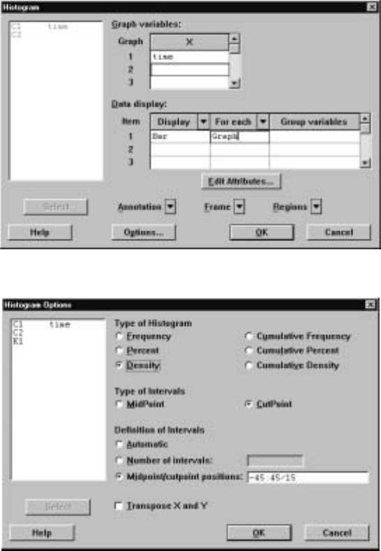
56 Chapter 1

produces the histogram shown in Display 1.11. As can be seen from the dialog

box of Display 1.9, there are a variety of methods for controlling the appearance

of the histogram produced, and we refer the reader to the Help button for a

description of these.

Display 1.9: Dialog box for creating a histogram of the time variable in the newcomb

worksheet.

Display 1.10: Dialog box for selecting the type of histogram to plot.

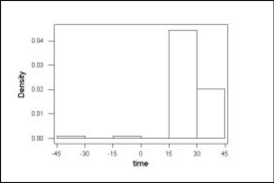
Looking At Data–Distributions 57

Display 1.11: Density histogram of the time variable in the newcomb worksheet.

An important consideration when plotting multiple histograms is to ensure

that all the histograms have the same xand yscales so that the plots are visually

comparable. This can be accomplished from the dialog box shown in Display

1.9 by F

¯rame IMu

¯ltiple Graphs and then selecting S

¯ame X and same Y.

The session command histogram is also available. This has the general

syntax

histogram E1...Em

where E1, ..., Emcorrespond to columns. For example, the commands

MTB >histogram c1;

SUBC>cutpoints -45 -30 -15 0 15 30 45;

SUBC>density.

produce the histogram in Display 1.11 using the cutpoints and density sub-

commands. There are also subcommands midpoints, nintervals, which spec-

ify the number of subintervals, and frequency or percent, which respectively

ensure that the heights of the bar lines equal the frequency and relative fre-

quency of the data values in the interval. Also, the cumulative subcommand

is available so that the bars represent all the values less than or equal to the end-

point of an interval. The subcommand same ensures that multiple histograms

all have the same scale.

1.2.4 Boxplots

Boxplots are useful summaries of a quantitative variable and are obtained using

the G

¯raph IB

¯oxplot command. Boxplots are used to provide a graphical

notion of the location of the data and its scatter in a concise and evocative way.

For example, in the newcomb worksheet this command produces the dialog box

shown in Display 1.12 and the plot in Display 1.13. The line in the center of the

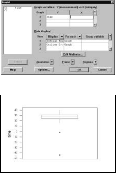
58 Chapter 1

box is the median. The line below the median is the Þrst quartile, also called the

lower hinge, and the line above is third quartile, also called the upper hinge.

The diﬀerence between the third and Þrst quartile, is called the interquartile

range or IQR. The vertical lines from the hinges are called whiskers, and these

run from the hinges to the adjacent values. The adjacent values are given by the

greatest value less than or equal to the upper limit (the third quartile plus 1.5

times the IQR) and by the least value greater than or equal to the lower limit

(the Þrst quartile minus 1.5 times the IQR). The upper and lower limits are

also referred to as the inner fences. The outer fences are deÞned by replacing

the multiple 1.5 in the deÞnition of the inner fences by 3.0. Values beyond the

outer fences are plotted with a *and are called outliers. As with the plotting

of histograms, multiple boxplots can be plotted for comparison purposes, and

again, it is important to make sure that they all have the same scale.

Display 1.12: Dialog box for producing a boxplot of the time variable in the newcomb

worksheet.

Display 1.13: Boxplot of the time variable in the newcomb worksheet.

There is a corresponding session command called boxplot. We refer the

reader to help for more discussion of this command.

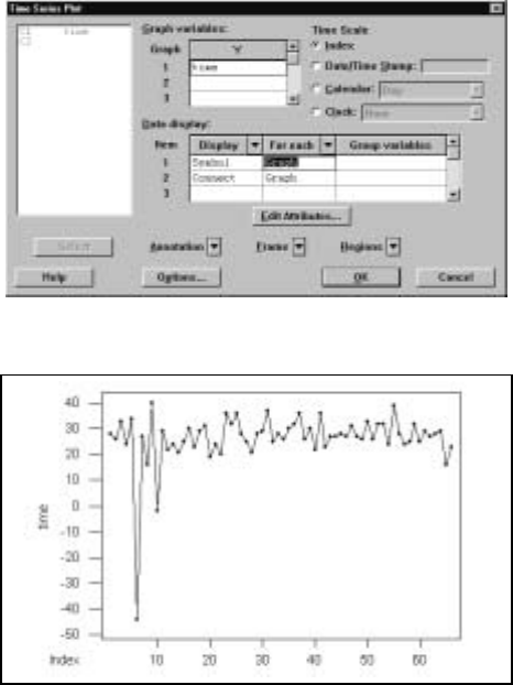
Looking At Data–Distributions 59

1.2.5 Time Series Plots

Often, data are collected sequentially in time. In such a context, it is instructive

to plot the values of quantitative variables against time in a time series plot.

ForthisweusetheG

¯raph IT

¯ime Series Plot command. If we suppose that

the data values in time of the newcomb worksheet were obtained in the order

they are listed, then applying this command to that data with the dialog box

as in Display 1.14 produces the time plot shown in Display 1.15. Notice that in

the D

¯ata display box we have speciÞed that the graph should plot a symbol for

each point and that the symbols plotted should connect via lines. For example,

if we had left out connect, only the points would have been plotted. The lines

help to visualize the form of the graph. The symbol plotted is a solid circle but

other choices could have been made using the E

¯dit Attributes button. Also,

for the Time Scale we have chosen Index, which is just the order in which

the observations are listed. If these observations were made at periodic time

intervals, there are other possible choices that could be more meaningful.

Display 1.14: Dialog box for a time series plot of the variable time from the newcomb

worksheet.

Display 1.15: Time series plot of the variable time from the newcomb worksheet.

There is also a corresponding session command tsplot. We refer the reader

to help for more discussion of this.

60 Chapter 1

1.2.6 Bar Charts

It is also possible to produce various charts using the G

¯raph IC

¯hart command.

For example, the dialog box shown in Display 1.16 plots a bar chart of the

variable C2 in the newcomb worksheet. Each distinct value of C1 is plotted

along the x-axis simply as a categorical value, not as a quantitative value, and

a bar of height equal to the number of times that value occurs in the variable is

drawn. A bar chart is a good way to plot categorical variables. There are many

possibilities for the types of bar charts drawn, and we refer the reader to the

Help button for a discussion of these.

Display 1.16: Dialog box for plotting bar charts.

The corresponding session command is

chart E1

which produces a bar chart for the values in column E1.

1.2.7 Pie Charts

Apie chart is a disk divided up into wedges where each wedge corresponds to

a unique value of a variable, and the area of the wedge is proportional to the

relative frequency of the value with which it corresponds. Pie charts can be

obtained via G

¯raph IPi

¯e Chart, and there are various features available in the

dialog box that can be used to enhance these plots. Pie charts are a common

method for plotting categorical variables.

1.3 The Normal Distribution

It is important in statistics to be able to do computations with the normal

distribution. The equation of the density curve for the normal distribution with

mean µand standard deviation σis given by

√2πe−1

2(z−µ

σ)2

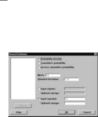
Looking At Data–Distributions 61

where zis a number. We refer to this as the N(µ, σ)density curve. Also of

interest is the area under the density curve from −∞ to a number x,i.e., the

area between the graph of the N(µ, σ)density curve and the interval (−∞,x].

As noted in IPS, this is a value between 0 and 1. Sometimes, we specify a value

pbetween 0 and 1 and then want to Þnd the point xp,such that pof the area

under the N(µ, σ)density curve lies over (−∞,x

p].The point xpis called the

pth percentile of the N(µ, σ)density curve.

Often, we are given a mean µand a standard deviation σand asked to

standardize a variable xwhose values are in some column, i.e., produce the new

variable z=x−µ

σ.These arithmetical operations can be carried out using the

let command as described in I.10.1.

1.3.1 Calculating the Density

Suppose that we want to evaluate the N(µ, σ)density curve at a value x. For

this,weusetheC

¯alc IProbability ¯Distributions IN

¯ormal command. For

example, the dialog box in Display 1.17 indicates that we want to evaluate the

N(10,1) density curve at the value x=11.0.

Display 1.17: Dialog box for normal probability calculations.

After clicking on the O

¯K button the output

Normal with mean = 10.0000 and standard deviation = 1.00000

x f(x)

11.0000 0.2420

is printed in the Session window, which gives the value as .2420. Sometimes, we

will want to evaluate the density curve at every value in a column of values, e.g.,

when we are plotting this curve. For this we simply click on the radio button

Input col

¯umn and type the relevant column in the associated box.

The general syntax of the corresponding session command pdf with the

normal subcommand is

pdf E1...Eminto Em+1 ...E2m;

normal mu =V

1sigma = V2.

62 Chapter 1

where E1,..., Emare columns or constants containing numbers and Em+1, ...,

E2mare the columns or constants that store the values of the N(µ, σ)density

curve at these numbers and V1=µand V2=σ. If no storage is speciÞed, then

the values are printed. For example, if we want to compute the N(−.5,1.2) den-

sity curve at every value between −3and 3in increments of .01,the commands

MTB >set c1

DATA>-3:3/.01

DATA>end

MTB >pdf c1 c2;

SUBC>normal mu=-.5 sigma=1.2.

put the values between −3and 3in increments of .01 in C1 using the set

command. The pdf command with the normal subcommand calculates the

N(−.5,1.2) density curve at each of these values and puts the outcomes in the

corresponding entries of C2. If we plot C2 against C1, we will have a plot of

the density curve of this distribution. For this, we use the scatterplot facilities

in Minitab as discussed in II.3. Note that with the normal subcommand we

must also specify the mean and the standard deviation via mu and sigma.

1.3.2 Calculating the Distribution Function

Suppose that we want to evaluate the area under N(µ, σ)density curve over the

interval (−∞,x].This is the value of the cumulative distribution function of

the N(µ, σ)distribution at the value x. For this, we use the C

¯alc IProbability

¯istributions IN

¯ormal as well, but in this case in the dialog box of Display

1.17 we select C

¯umulative probability instead. Making this change in the dialog

box of Display 1.17, we get the output

xP(X<=x)

11.0000 0.8413

in the Session window. Again, we can evaluate this function at a single point

or at every value in a variable.

The general syntax of the corresponding Session command cdf command

with the normal subcommand is

cdf E1...Eminto Em+1 ...E2m;

normal mu =V

1sigma = V2.

where E1,..., Emare columns or constants containing numbers and Em+1, ...,

E2mare the columns or constants that store the values of the area under N(µ, σ)

density curve over the interval from −∞ to these numbers and V1=µand V2

=σ. If no storage is speciÞed, the values are printed.

1.3.3 Calculating the Inverse Distribution Function

Suppose that we want to evaluate percentiles for the N(µ, σ)density curve.

Again, we use the C

¯alc IProbability D

¯istributions IN

¯ormal command, but

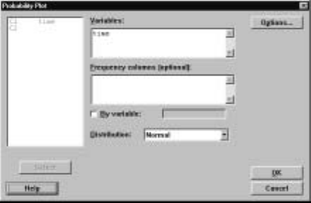
Looking At Data–Distributions 63

in this case, in the dialog box of Display 1.17 we select I

¯nverse cumulative

probability instead. Making this change in the dialog box of Display 1.17 and

replacing 11 by .75 – recall that the argument to this function must be between

0 and 1 – we get the output

P( X <=x) x

0.7500 10.6745

in the Session window. This indicates that the area to the left of 10.6745 un-

derneath the N(−.5,1.2) density curve is .75.

The general syntax of the corresponding session command invcdf with the

normal subcommand is

invcdf E1...Eminto Em+1 ...E2m;

normal mu =V

1sigma = V2.

where E1,..., Emare columns or constants containing numbers between 0 and

1andE

m+1, ..., E2mare the columns or constants that store the values of the

percentiles of the N(µ, σ)density curve at these numbers and where V1=µ

and V2=σ. If no storage is speciÞed, then the values are printed.

1.3.4 Normal Probability Plots

Some statistical procedures require that we assume that values for some variables

are a sample from a normal distribution. A normal probability plot is a diagnostic

that checks for the reasonableness of this assumption. To create such a plot, we

use the G

¯raph IProbability

¯Plot command. For example, using this command

on the newcomb worksheet we get the dialog box in Display 1.18 where we have

placed time in the V

¯ariables box. Clicking on the O

¯K button produces the plot

in Display 1.19. The normal probability plot is given by the dark dotted curve.

The plot also contains other information and further output is printed in the

Session window. Of course, the plot should be like a straight line and it is not

in this case.

Display 1.18: Dialog box for producing normal probability plots.

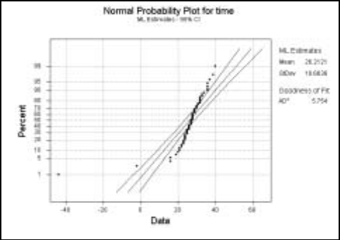
64 Chapter 1

Display 1.19: Normal probability plot of the time variable in the newcomb worksheet.

The session commands

MTB >nscores c1 c3

MTB >plot c3*c1

produce a normal probability plot like that shown in Display 2.3. The plot

command will be discussed much more extensively in II.3. The nscores (normal

scores) command relies on some concepts that are beyond the level of this course

so we do not discuss this further.

1.4 Exercises

When the data for an exercise come from an exercise in IPS, the IPS exercise

number is given in parentheses ( ). All computations in these exercises are

to be carried out using Minitab, and the exercises are designed to ensure that

you have a reasonable understanding of the Minitab material in this chapter.

Generally, you should be using Minitab to do all the computations and plotting

required for the problems in IPS.

1. Using Newcomb’s measurements in Table 1.1, create a new variable by

grouping these values into three subintervals [−50,0),[0,20),[20,50).

Calculate the frequency distribution, the relative frequency distribution,

and the cumulative distribution of this ordered categorical variable.

2. (1.21) Use Minitab to print the empirical distribution function. From this,

determine the Þrst quartile, median, and third quartile. Also, use the

empirical distribution function to compute the 10th and 90th percentiles.

3. Use Minitab to produce the stemplot of Example 1.4 of IPS.

4. Use Minitab to produce the time plot of Example 1.5 of IPS.

Looking At Data–Distributions 65

5. (1.29) Use Minitab commands for the stemplot and the time plot. Use

Minitab commands to compute a numerical summary of this data, and

justify your choices.

6. (1.30) Transform the data in this problem by subtracting 5 from each value

and multiplying by 10. Calculate the means and standard deviations,

using any Minitab commands, of both the original and transformed data.

Compute the ratio of the standard deviation of the transformed data to

the standard deviation of the original data. Comment on this value.

7. (1.30) Transform this data by multiplying each value by 3. Compute

the ratio of the standard deviation to the mean (called the coeﬃcient of

variation) for the original data and for the transformed data. Justify the

outcome.

8. For the N(6,1.1) density curve, compute the area between the interval

(3,5) and the density curve. What number has 53% of the area to the left

of it for this density curve?

9. Use Minitab commands to verify the 68-95-99.7 rule for the N(2,3) density

curve.

10. Calculate and store the values of the N(0,1) density curve at each value

in [−3,3] using an increment of .01. Put the values in the interval [−3,3]

in C1 and the values of the density curve in C2. Using the command plot

C2*C1, plot the density curve. Comment on the shape of this curve.

11. Use Minitab commands to make the normal quantile plots presented in

Figures 1.31 and 1.32 of IPS.

66 Chapter 1

Chapter 2

Looking at

Data–Relationships

New Minitab commands discussed in this chapter

¯raph IP

¯lot

¯tat IB

¯asic Statistics IC

¯orrelation

¯tat IR

¯egression IF

¯itted Line Plot

¯tat IR

¯egression IR

¯egression

In this chapter, Minitab commands are described that permit the analysis of

relationships among two variables. The methods are diﬀerent depending on

whether or not both variables are quantitative, both variables are categorical,

or one is quantitative and the other is categorical. This chapter considers rela-

tionships between two quantitative variables with the remaining cases discussed

in later chapters. Graphical methods are very useful in looking for relationships

among variables, and we examine various plots for this.

2.1 Scatterplots

Ascatterplot of two quantitative variables is a useful technique when looking

for a relationship between two variables. By a scatterplot we mean a plot of

one variable on the y-axis against the other variable on the x-axis. For exam-

ple, consider Example 2.4 in IPS, where we are concerned with the relationship

between the length of the femur and the length of the humerus in an extinct

species. Suppose that we have input the data so that length of the femur

measurements are in C1, which has been named femur,andthelengthofthe

humerus measurements are in C2, which has been named humerus,ofthework-

sheet archaeopteryx. The command G

¯raph IP

¯lot produces the dialog box of

Display 2.1, where we have placed femur into the Þrst box for the yvariable

68 Chapter 2

and humerus in the Þrst box for the xvariable. This produces the plot shown in

Display 2.2. Note that we could alter the plotting symbol using the dialog box

that appears when we click on the E

¯dit Attributes box. Using the dialog box

that appears when you click on the A

¯nnotation button, it is possible to give the

plot a title, label plotted points, etc. Using the dialog box that appears when

youclickontheF

¯rame button, you can change the labels on the axes. Rather

than just plotting the points inascatterplot,youcanaddconnection lines (join

the points with lines), add projection lines (drop a line from each point to the

x-axis), and add areas (Þll in the area under a polygon joining the points).

Also, you can employ the scatterplot smoother lowess to plot a piecewise linear

continuous curve through the scatter of points. These features are available via

¯raph IP

¯lot IDisplay. There are a number of other features that allow you

to control the appearance of the plot.

Display 2.1: Dialog box for producing a scatterplot.

85807570656055504540

humerus

femur

Display 2.2: Scatter plot of femur length (C1) versus humerus length (C2) of

Example 2.4 in IPS.

Looking At Data–Relationships 69

It is also possible to have multiple scatterplots on the same plot. For exam-

ple, suppose that C3 in the archaeopteryx worksheet contains the natural log

of the femur variable. We obtained the plot of Display 2.3 by adding another

pair of variables to the second G

¯raph variables box as in Display 2.1 with C3

as the yvariable and humerus as the xvariable. To put these scatterplots on

thesameplotuseF

¯rame IMu

¯ltiple Graphs and click on the Ov

¯erlay graphs

on the same page radio button.

85807570656055504540

humerus

femur

Display 2.3: Multiple scatterplots in the same plot.

The technique of brushing is available after obtaining the plot to see which

observations (rows) the points correspond to. This is helpful in identifying the

points that correspond to outliers. Brushing is accessed from the toolbar just

below the menu bar by clicking on the brush when the Graph window is active.

The corresponding session command is plot. For example,

MTB >plot femur*humerus

produces the plot of Display 2.2. Note that the Þrst variable is plotted along the

y-axis, and the second variable is plotted along the x-axis. There are various

subcommands that can be used with plot, and we refer the reader to H

¯elp for

a description of these.

There are a number of additional plots available in Minitab that are related

to the scatterplot. For example, a marginal plot of two variables is a scatterplot

of one variable against the other where in addition histograms, dotplots or

boxplots are plotted along the sides of the scatterplot for each variable. These

are available via the menu command G

¯raph IMa

¯rginal Plot. Draftsman plots

allow you to produce a number of scatterplots in a rectangular array so that

they can be compared. For example, you may want to plot C1 against C3, C2

against C3, C1 against C4, and C2 against C4 and see all of these in a common

plot. This capability is available via the menu command G

¯raph IDraftsman

Plot and Þlling in the dialog box. Matrix plots provide a mechanism for placing

a number of scatterplots in a rectangular array or matrix so that they can be

directly compared or examined for relationships. Matrix plots are available via

70 Chapter 2

the command G

¯raph IM

¯atrix Plot. Also three-dimensional scatterplots are

available via G

¯raph I3

¯D Plot and contour plots via G

¯raph ICon

¯tour Plot.

2.2 Correlations

While a scatterplot is a convenient graphical method for assessing whether or

not there is any relationship between two variables, we would also like to assess

this numerically. The correlation coeﬃcient provides a numerical summariza-

tion of the degree to which a linear relationship exists between two quantita-

tive variables, and this can be calculated using the S

¯tat IB

¯asic Statistics I

¯orrelation command. For example, applying this command to the femur and

humerus variables of the worksheet archaeopteryx, i.e., the data of Example

2.4 in IPS and depicted in Display 2.2, we obtain the output

Pearson correlation of femur and humerus = 0.994

P-Value = 0.001

in the Session window. For now, we ignore the number recorded as P-Value.

The general syntax of the corresponding session command correlate is given

correlate E1... Em

where E1, ..., Emare columns corresponding to numerical variables, and a cor-

relation coeﬃcient is computed between each pair. This gives m(m−1)/2

correlation coeﬃcients. The subcommand nopvalues is available if you want

to suppress the printing of P-values.

2.3 Regression

Regression is another technique for assessing the strength of a linear relationship

existing between two variables and it is closely related to correlation. For this,

we use the S

¯tat IR

¯egression command.

As noted in IPS, the regression analysis of two quantitative variables involves

computing the least-squares line y=a+bx,where one variable is taken to be

theresponsevariableyand the other is taken to be the explanatory variable

x. Note that the least squares line is diﬀerent depending upon which choice is

made. For example, for the data of Example 2.4 in IPS and plotted in Display

2.2 letting femur be the response and humerus be the predictor or explanatory

variable, the S

¯tat IR

¯egression IR

¯egression command leads to the dialog box

of Display 2.4, where we have made the appropriate entries in the Re

¯sponse and

Predi

¯ctors boxes. Clicking on the O

¯K button leads to the output of Display

2.5 being printed in the Session window. This gives the least-squares line as

y=3.70 + .826x, i.e., a=3.70 and b=.826, which we also see under the Coef

column in the Þrst table. In addition, we obtain the value of the square of the

correlation coeﬃcient, also known as the coeﬃcient of determination, as R-Sq

= 98.8%. We will discuss the remaining output from this command in II.10.

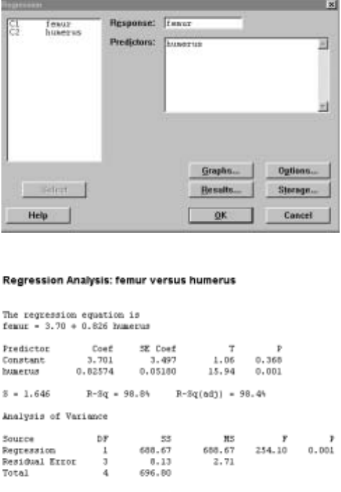
Looking At Data–Relationships 71

Display 2.4: Dialog box for a regression analysis.

Display 2.5: Output from the dialog box of Display 2.4.

It is very convenient to have a scatterplot of the points together with the

least-squares line. This can be accomplished using the S

¯tat IR

¯egression I

¯itted Line Plot command.Filling in the dialog box for this command as in

Display 2.4 produces the output in the Session window of Display 2.5 together

with the plot of Display 2.6.

There are some additional quantities that are often of interest in a regression

analysis. For example, you may wish to have the Þtted values ˆy=a+bx at each

xvalue printed as well as the residuals y−ˆy.Clicking on the R

¯esults button in

the dialog box of Display 2.4 and Þlling in the ensuing dialog box as in Display

2.7 results in these quantities being printed in the Session window as well as the

output of Display 2.5.

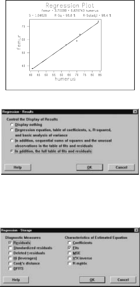
72 Chapter 2

Display 2.6: Scatterplot of femur versus humerus in the archaeopteryx worksheet

together with the least-squares line.

Display 2.7: Dialog box for controlling output for a regression analysis.

You will probably want to keep these values for later work. In this case, clicking

on the Storage button of Display 2.4 and Þlling in the ensuing dialog box as

in Display 2.8 results in these quantities being saved in the next two available

columns – in this case, C3 and C4 – with the names resl1 and fits1 for the

residuals and Þts, respectively.

Display 2.8: Dialog box for storing various quantities computed as part of a

regression analysis.

Even more likely is that you will want to plot the residuals as part of assessing

whether or not the assumptions that underlie a regression analysis make sense

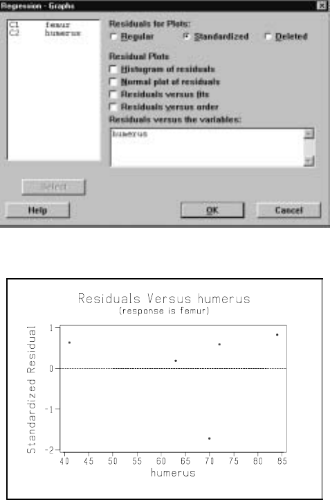
Looking At Data–Relationships 73

in the particular application. For this, click on the Graphs button in the dialog

box of Display 2.4. The dialog box of Display 2.9 becomes available. Notice that

we have requested that the standardized residuals – each residual divided by

its standard error – be plotted, and this plot appears in Display 2.10. All the

standardized residuals should be in the interval (−3,3),and no pattern should

be discernible. In this case, this residual plot looks Þne. From the dialog box of

Display 2.9, we see that there are many other possibilities for residual plots.

Display 2.9: Dialog box for selecting various residual plots as part of a regression

analysis.

Display 2.10: Plot of the standardized residuals versus humerus after regressing

femur against humerus in the archaeopteryx worksheet.

The corresponding session command is given by regress, and by using the

subcommands pﬁts, residual, and sresidual we can calculate and store Þtted

values, residuals, and standardized residuals, respectively. For example,

74 Chapter 2

MTB >regress c1 1 c2;

SUBC>fits c3;

SUBC>residuals c4;

SUBC>sresiduals c5.

gives the output of Display 2.5 and also stores the Þtted values in C3, stores the

residuals y−ˆyin C4, and stores the standardized residuals in C5. Note that the

1inregress c1 1 c2 refers to the number of predictors we are using to predict

the response variable. To plot the standardized residuals against humerus, we

use

MTB >plot c5*c2

which results in a plot like Display 2.10 but with diﬀerent labels on the xaxis.

2.4 Transformations

Sometimes, transformations of the variables are appropriate before we carry

out a regression analysis. This is accomplished in Minitab using the C

¯alc I

Cal

¯culator command and the arithmetical and mathematical operations dis-

cussed in I.10.1 and I.10.2. In particular, when a residual plot looks bad, some-

timesthiscanbeÞxed by transforming one or more of the variables using a

simple transformation, such as replacing the response variable by its logarithm

or something else. For example, if we want to calculate the cube root – i.e., x1/3

– of every value in C1 and place these in C2, we use the C

¯alc ICal

¯culator

command and the dialog box as depicted in Display 2.11. Alternatively, we

could use the session command let as in

MTB >let c2=c1**(1/3)

which produces the same result.

Display 2.11: Dialog box for calculating transformations of variables.

Looking At Data–Relationships 75

2.5 Exercises

When the data for an exercise come from an exercise in IPS, the IPS exercise

number is given in parentheses ( ). All computations in these exercises are

to be carried out using Minitab, and the exercises are designed to ensure that

you have a reasonable understanding of the Minitab material in this chapter.

Generally, you should be using Minitab to do all the computations and plotting

required for the problems in IPS.

1. (2.10) Calculate the least-squares line and make a scatterplot of Fuel used

against Speed together with the least-squares line. Plot the standard-

ized residuals against Speed. What is the squared correlation coeﬃcient

between these variables?

2. (2.11) Make a scatterplot of Rate against Mass where the points for dif-

ferent Sexes are labeled diﬀerently (use Minitab for the labeling, too) and

with the least-squares line on it. Hint: Make use of the stack command

discussed in I.11.7.

3. Place the values 1 through 100 with an increment of .1 in C1 and the

square of these values in C2. Calculate the correlation coeﬃcient between

C1 and C2. Multiply each value in C1 by 10, add 5, and place the results

in C3. Calculate the correlation coeﬃcient between C2 and C3. Why are

these correlation coeﬃcients the same?

4. Place the values 1 through 100 with an increment of .1 in C1 and the

square of these values in C2. Calculate the least-squares line with C2 as

response and C1 as explanatory variable. Plot the standardized residuals.

If you see such a pattern of residuals what transformation, might you use

to remedy the problem?

5. (2.54) For the data in this problem, numerically verify the algebraic re-

lationship that exists between the correlation coeﬃcient and the slope of

the least-squares line.

6. For Example 2.17 in IPS, calculate the least-squares line and reproduce

Display 2.21. Calculate the sum of the residuals and the sum of the

squared residuals and divide this by the number of data points minus 2.

Is there anything you can say about what these quantities are equal to in

general?

7. (2.62) Use Minitab to do all the calculations in this problem.

8. Place the values 1 through 10 with an increment of .1 in C1, and place

exp(−1+2x)of these values in C2. Calculate the least-squares line using

C2 as the response variable, and plot the standardized residuals against

C1. What transformation would you use to remedy this residual plot?

What is the least-squares line when you carry out this transformation?

76 Chapter 2

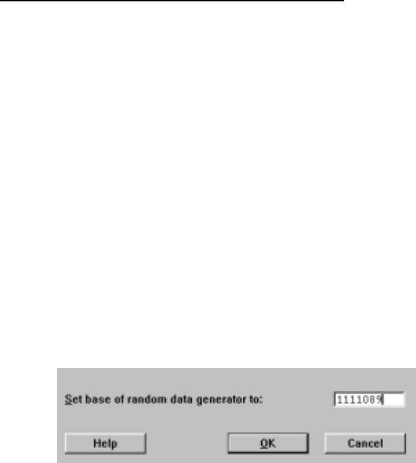
Chapter 3

Producing Data

New Minitab commands discussed in this chapter

¯alc ISet B

¯ase

¯alc IR

¯andom Data

This chapter is concerned with the collection of data, perhaps the most impor-

tant step in a statistical problem, as this determines the quality of whatever

conclusions are subsequently drawn. A poor analysis can be Þxedifthedata

collected are good by simply redoing the analysis. But if the data have not been

appropriately collected, then no amount of analysis can rescue the study. We

discuss Minitab commands that enable you to generate samples from popula-

tions and also to randomly allocate treatments to experimental units.

Minitab uses computer algorithms to mimic randomness. Still, the results

are not truly random. In fact, any simulation in Minitab can be repeated, with

exactly the same results being obtained, using the C

¯alc ISet B

¯ase command.

For example, in the dialog box of Display 3.1 we have speciÞed the base, or seed,

random number as 1111089. The base can be any integer. When you want to

repeat the simulation, you give this command, with the same integer. Provided

you use the same simulation commands, you will get the same results. This can

also be accomplished using the session command base V,whereVis an integer.

Display 3.1: Dialog box for setting base or seed random number.

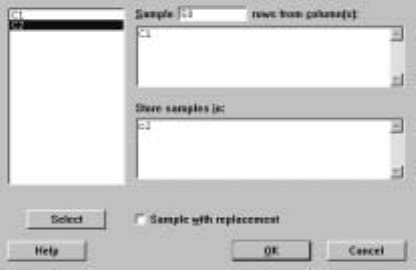
78 Chapter 3

3.1 Generating a Random Sample

Suppose that we have a large population of size Nand we want to select a

sample of n<N from the population. Further, we suppose that the elements

of the population are ordered, i.e., we have been able to assign a unique number

1,...,N to each element of the population. To avoid selection biases, we want

this to be a random sample, i.e., every subset of size nfrom the population has

the same “chance” of being selected. As discussed in IPS, this implies that we

generate our sample so that every subset of size nin the population has the same

chance of being chosen. We can do this physically by using some simple random

system, such as chips in a bowl or coin tossing. We could also use a table of

random numbers, or, more conveniently, we can use computer algorithms that

mimic the behavior of random systems.

For example, suppose there are 1000 elements in a population, and we want

to generate a sample of 50 from this population without replacement. We can

use the C

¯alc IR

¯andom Data ISam

¯ple from Columns command to do this.

For example, suppose we have labeled each element of the population with a

unique number in 1,2,...,1000,and, further, we have put these numbers in C1

of a worksheet. The dialog box of Display 3.2 results in a random sample of 50

being generated without replacement from C1 and stored in C2.

Display 3.2: Dialog box for generating a random sample without replacement.

Printing this sample gives the output

MTB >print c2

441 956 87 736 185 515 883 957 690

438 205 760 246 16 321 371 493 393

538 348 70 54 362 492 182 841 287

277 112 610 890 503 332 413 886 798

764 584 566 495 547 488 206 557 263

414 613 618 685 864

in the Session window. So now we go to the population and select the elements

labeled 441, 956, 87, etc. The algorithm that underlies this command is such

that we can be conÞdent that this sample of 50 is like a random sample.

Producing Data 79

The general syntax of the corresponding session command sample is

sample VE

1... Emput into Em+1 ... E2m

whereVisthesamplesizenand V rows are sampled from the columns E1,

..., EmandstoredincolumnsE

m+1, ..., E2m.If we wanted to sample with

replacement – i.e., after a unit is sampled, it is placed back in the population

so that it can possibly be sampled again – we use the replace subcommand. Of

course, for simple random sampling, we do not use the replace subcommand.

Note that the columns can be numeric or text.

Sometimes we want to generate random permutations , i.e., n=N,and we

are simply reordering the elements of the population. For example, in exper-

imental design, suppose we have N=n1+··· +nkexperimental units and

ktreatments, and we want to allocate niapplications of treatment i. Suppose

further that we want all possible such applications to be equally likely. Then we

generate a random permutation (l1,...,l

N)of (1,...,N)and allocate treatment

1 to those experimental units labeled l1,...,l

n1,allocate treatment 2 to those

experimental units labeled ln1+1,...,l

n1+n2,etc. For example, if we have 30

experimental units and 3 treatments and we want to allocate 10 experimental

units to each treatment, placing the numbers 1,2,...,30 in C1 and using the

¯alc IR

¯andom Data ISam

¯ple from Columns command as in the dialog box

of Display 3.2, but with 30 in the S

¯ample box, generates a random permutation

of 1,2,...,30 in C2. Implementing this gives us the random permutation

MTB >print c2

13 7 26 8 22 23 28 17 3 25

9 2 14 29 15 18 6 11 16 5

12 27 4 30 20 24 1 19 21 10

and for the treatment allocation you can read the numbers row-wise or column-

wise, as long as you are consistent. Row-wise is probably best, as this is how the

numbers are stored in C2, and so you can always refer back to C2 (presuming

you save your worksheet) if you get mixed up.

The above examples show how to directly generate a sample from a popu-

lation of modest size. But what happens if the population is huge or it is not

convenient to label each unit with a number? For example, suppose we have

a population of size 100,000 for which we have an ordered list and we want a

sample of size 100. In this case more sophisticated techniques need to be used,

but simple random sampling can still typically be accomplished (see Exercise

3.3 for a simple method that works in some contexts).

Simple random sampling corresponds to sampling without replacement, i.e.,

after we randomly select an element from the population, we do not return

it to the population before selecting the next sample element. Sampling with

replacement corresponds to replacing each sample element in the population

after selecting it and recording only the element that was obtained. So at each

selection, every element has the same chance of being selected, and an element

may appear more than once in the sample. Notice that we can also sample with

80 Chapter 3

replacement if we check the Sample w

¯ith replacement box in the dialog box of

Display 3.2.

3.2 Sampling from Distributions

Once we have generated a sample from a population, we measure various at-

tributes of the sampled elements. For example, if we were sampling from a pop-

ulation of humans, we might measure each sampled unit’s height. The height for

the sample unit is now a random variable that follows the height distribution in

the population from which we are sampling. For example, if 80% of the people

in the population are between 4.5 feet and 6 feet, then under repeated sampling

of an element from the population (with replacement) in the long run, 80% of

the sampled units will have their heights in this range.

Sometimes, we want to sample directly from this population distribution,

i.e., generate a number in such a way that under repeated sampling in the long

run the proportion of values falling in any range agrees with that prescribed by

the population distribution. Of course, we typically don’t know the population

distribution, as this is what we want to Þnd out about in a statistical investiga-

tion. Still, there are many instances where we want to pretend that we do know

it and simulate from this distribution, e.g., perhaps we want to consider the

eﬀect of various choices of population distribution on the sampling distribution

of some statistic of interest.

There are computer algorithms that allow us to do this for a variety of

distributions. In Minitab, this is accomplished using the C

¯alc IR

¯andom Data

command. For example, suppose that we want to simulate the tossing of a fair

coin (a coin where head and tail are equally likely as outcomes). The C

¯alc I

¯andom Data IBe

¯rnoulli command together with the dialog box of Display

3.3 generates a sample of 100 from the Bernoulli(.5) distribution and places

these values in C1. A random variable has a Bernoulli(p)distribution if the

probability the variable equals 1 – success – is pand the probability the

variable equals 0 – failure – is 1−p. So to generate a sample of nfrom the

Bernoulli(p)distribution, we put nin the G

¯enerate box and pin the P

¯robability

of success box. In such a case, we are simulating the tossing of a coin that

produces a head on a single toss with probability p,i.e., the long-run proportion

of heads that we observe in repeated tossing is p. Note that we can generate m

samples of size nby putting mdistinct columns in the S

¯tore in column(s) box.

Often, a normal distribution with some particular mean and standard devia-

tion is considered a reasonable assumption for the distribution of a measurement

in a population. For example, the C

¯alc IR

¯andom Data IN

¯ormal command

together with the dialog box of Display 3.4 generates a sample of 200 from the

N(5.2,1.3) distribution and places this sample in C1. To generate a sample of

nfrom the N(µ, σ)distribution, we put nin the G

¯enerate box, µin the M

¯ean

box, and σin the St

¯andard deviation box.

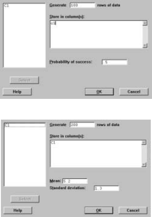
Producing Data 81

Display 3.3: Dialog box for generating a sample of 100 from the Bernoulli(.5)

distribution.

Display 3.4: Dialog box for generating a sample of 200 from a N(5.2,1.3)

distribution.

The general syntax of the corresponding session command random is

random VintoE

1... Em

and this puts a sample of size V into each of the columns E1, ..., Em,according

to the distribution speciÞed by the subcommand. For example,

MTB >random 100 c1;

SUBC>bernoulli .5.

simulates the tossing of a fair coin 100 times and places the results in C1 using

the bernoulli subcommand. If no subcommand is provided, this distribution

is taken to be the N(0,1) distribution. The command

82 Chapter 3

MTB >random 200 c1;

SUBC>normal mu=2.1 sigma=3.3.

generates a sample of 200 from the N(2.1,3.3) distribution using the normal

subcommand. There are a number of other subcommands specifying distribu-

tions, and we refer the reader to help for a description of these.

3.3 Exercises

When the data for an exercise come from an exercise in IPS, the IPS exercise

number is given in parentheses ( ). All computations in these exercises are

to be carried out using Minitab, and the exercises are designed to ensure that

you have a reasonable understanding of the Minitab material in this chapter.

Generally, you should be using Minitab to do all the computations and plotting

required for the problems in IPS.

If your version of Minitab places restrictions such that the value of the sim-

ulation sample size Nrequested in these problems is not feasible, then substitute

a more appropriate value. Be aware, however, that the accuracy of your results

is dependent on how large Nis.

1. (3.13) Generate a random permutation of the names using Minitab.

2. (3.32) Use the M

¯anip IS

¯ort command described in I.11.6 to order the

subjects by weight. Use the values 1—5 to indicate Þve blocks of equal

length in a separate column, and then use the M

¯anip IUnstack command

described in I.11.7 to put the blocks in separate columns. Generate a

random permutation of each block.

3. Use the following methodology to generate a sample of 20 from a pop-

ulation of 100,000. First, put the values 0—9 in each of C1—C5. Next,

use sampling with replacement to generate 50 values from C1, and put

the results in C6. Do the same for each of C2—C5 and put the results

in C7—C10 (don’t generate from these columns simultaneously). Create a

single column of numbers using the digits in C6—C10 as the digits in the

numbers. Pick out the Þrst unique 20 entries as labels for the sample. If

you do not obtain 20 unique values, repeat the process until you do. Why

does this work?

4. Suppose you wanted to carry out stratiÞed sampling where there are 3

strata, with the Þrst stratum containing 500 elements, the second stratum

containing 400 elements, and the third stratum containing 100 elements.

Generate a stratiÞed sample with 50 elements from the Þrst stratum, 40

elements from the second stratum, and 10 elements from the third stratum.

When the strata sample sizes are the same proportion of the total sample

size as the strata population sizes are of the total population size this is

called proportional sampling.

Producing Data 83

5. Suppose we have an urn containing 100 balls with 20 labeled 1, 50 labeled

2, and 30 labeled 3. Using sampling with replacement, generate a sample

of size 1000 from this distribution employing the C

¯alc IR

¯andom Data

command to generate the sample directly from the relevant population

distribution. Use the S

¯tat IT

¯ables IC

¯ross Tabulation command to

record the proportion of each label in the sample.

6. Carry out a simulation study with N=1000of the sampling distribution

of ˆpfor n=5,10,20 and for p=.5,.75,.95.In particular, calculate the

empirical distribution functions and plot the histograms. Comment on

your Þndings.

7. Carry out a simulation study with N=2000of the sampling distribution

of the sample standard deviation when sampling from the N(0,1) distri-

bution based on a sample of size n=5.In particular, plot the histogram

using cutpoints 0, 1.5, 2.0 2.5, 3.0 5.0. Repeat this for the sample coeﬃ-

cient of variation (sample standard deviation divided by the sample mean)

using the cutpoints −10,−9, ..., 0, ..., 9, 10. Comment on the shapes of

the histograms relative to an N(0,1) density curve.

84 Chapter 3

Chapter 4

Probability:The Study of

Randomness

In this chapter the concept of probability is introduced more formally than pre-

viously in the book. Probability theory underlies the powerful computational

methodology known as simulation, which we introduced in Chapter 3. Simula-

tion has many applications in probability and statistics and also in many other

Þelds, such as engineering, chemistry, physics, and economics.

4.1 Basic Probability Calculations

The calculation of probabilities for random variables can often be simpliÞed

by tabulating the cumulative distribution function. Also, means and variances

are easily calculated using component-wise column operations in Minitab. For

example, suppose we have the probability distribution

x1 2 3 4

probability .1 .2 .3 .4

in columns C1 and C2, with the values in C1 and the probabilities in C2. The

¯alc ICal

¯culator command with the dialog box as in Display 4.1 computes the

cumulative distribution function in C3 using Partial Sums.

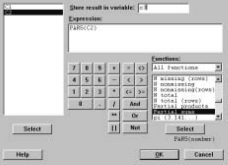
86 Chapter 4

Display 4.1: Dialog box for computing partial sums of entries in C2 and placing these

sums in C3.

Printing C1 and C3 gives

Row C1 C3

110.1

220.3

330.6

441.0

in the Session window. We can also easily compute the mean and variance of

this distribution. For example, the session commands

MTB >let c4=c1*c2

MTB >let c5=c1*c1*c2

MTB >let k1=sum(c4)

MTB >let k2=sum(c5)-k1*k1

MTB >printk1k2

K1 3.00000

K2 1.00000

calculate the mean and variance and store these in K1 and K2, respectively. The

mean is 3 and the variance is 1. Of course, we can also use C

¯alc ICal

¯culator

to do these calculations. In presenting more extensive computations, it is some-

what easier to list the appropriate session commands, as we will do subsequently.

However, this is not to be interpreted as the required way to do these compu-

tations, as it is obvious that the menu commands can be used as well. Use

whatever you Þnd most convenient.

4.2 More on Sampling from Distributions

As we saw in II.3.2, Minitab includes algorithms for generating from many

probability distributions using C

¯alc IR

¯andom Data. This menu command

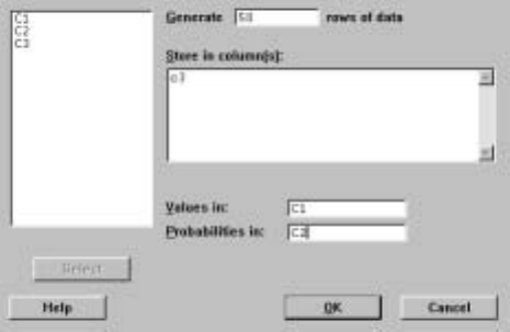
Probability: The Study of Randomness 87

produces a drop-down list that includes the normal, binomial, Chi-square, F,

t,uniform, and many other distributions that the text, and this manual, will

discuss. Clicking on one of these names results in a dialog box with entries to

be Þlled in further specifying the distribution and the size of the sample.

For example, we can generate from one particularly important class of prob-

ability distributions using C

¯alc IR

¯andom Data ID

¯iscrete. These probability

distributions are concentrated on a Þnite number of values. To illustrate this,

suppose we have the following values in C1 and C2.

Row C1 C2

1-10.3

220.2

330.4

4100.1

Here, C1 contains the possible values of an outcome, and C2 contains the prob-

abilities that each of these values is obtained, so, for example, P({−1})=

.3,P ({2})=.2,etc. The dialog box of Display 4.2 generates a sample of 50

from this discrete distribution and stores the sample in C3.

Display 4.2: Dialog box for generating a sample from a discrete distribution with

values in C1 and probabilities in C2 and storing the sample in C3.

It is an interesting exercise to check that the algorithms Minitab is using are

in fact producing samples appropriately. There are a variety of things one could

check, but perhaps the simplest is to check that the long-run relative frequencies

are correct. So in the example of this section, we want to make sure that, as

we increase the size of the sample, the relative frequencies of −1,2,3,10 in the

sample are getting closer to .3, .2, .4, and .1, respectively. Note that it is not

guaranteed that as we increase the sample size that the relative frequencies get

closer monotonically to the corresponding probabilities, but inevitably this must

be the case.

First, we generated a sample of size 100 from this distribution and stored

the values in C3 as in Display 4.2. Next, we recorded a 1 in C4 whenever the

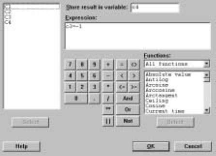
88 Chapter 4

corresponding entry in C3 was −1and recorded a 0 in C4 otherwise. To do this,

we used the C

¯alc ICal

¯culator command with dialog box as shown in Display

4.3.

Display 4.3: Dialog box to record the incidence of a −1in C3.

It is clear that the mean of C4 is the relative frequency of −1in the sample.

We calculated this mean using C

¯alc IC

¯olumn Statistics, as discussed in I.10.3,

which gave the output

Mean of C4 = 0.33000

in the Session window. Repeating this with a sample of size 1000, we obtained

Mean of C4 = 0.28100

which we can see is a bit closer to the true value of .3. Repeating this with a

sample of size 10,000 from this distribution, we obtained

Mean of C4 = 0.29300

which is closer still. It would appear that the relative frequency of −1is indeed

converging to .3.

We can generate a randomly chosen point from the line interval (a, b),where

a<b,using C

¯alc IR

¯andom Data IU

¯niform. For example, the dialog box

of Display 4.4 generates a sample of 1500 from the uniform distribution on the

interval (3.0,6.3).With this distribution, the probability of any subinterval (c, d)

of (a, b)is given by (d−c)/(b−a),i.e., the length of (c, d)over the length of

(a, b).Of course, we can estimate this probability by just counting the number

of times the generated response falls in the interval (c, d)and dividing this by

the total sample size. For example, using the outcomes from the dialog box

of Display 4.3 and estimating the probability of the interval (4,5),wegetthe

relative frequency 0.30867, which is close to the true value of (5 −4)/(6.3−3) =

0.30303.

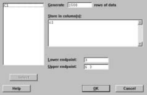
Probability: The Study of Randomness 89

Display 4.4: Dialog box for generating a sample of 1500 from the uniform

distribution on the interval (3.0,6.3).

We can generalize this to generate from a point randomly chosen from a

rectangle (a, b)×(c, d),i.e., the set of all points (x, y)such that a<x<b,c<

y<d.If we want a sample of nfrom this distribution, we generate a sample

x1,...,x

nfrom the uniform on (a, b)and also generate a sample y1,...,y

nfrom

the uniform distribution on (c, d).Then (x1,y

1),...,(xn,y

n)is a sample of

nfrom the uniform distribution on (a, b)×(c, d).We can approximate the

probability of a random pair (x, y)falling in any subset A⊂(a, b)×(c, d)by

computing the relative frequency of Ain the sample.

The random command is the session command for carrying out simulations

in Minitab. For example, the subcommand

uniform V1V2

speciÞes the continuous uniform distribution on the interval (V1,V2); i.e., subin-

tervals of the same length have the same probability of occurring. If we have

placed a discrete probability distribution in column E2, on the values in column

E1, the subcommand

discrete E1E2

generates a sample from this distribution.

4.3 Simulation for Approximating Probabilities

As previously noted, simulation can be used to approximate probabilities. For

a variety of reasons, these simulations are most easily presented using session

commands but it is clear that we can replace each step by the appropriate menu

command.

For example, suppose we are asked to calculate

P(.1≤X1+X2≤.3)

90 Chapter 4

when X1,X

2are both independent and follow the uniform distribution on the

interval (0,1).The session commands

MTB >random 1000 c1 c2;

SUBC>uniform 0 1.

MTB >let c3=c1+c2

MTB >letc4=.1<=c3 and c3<=.3

MTB >let k1=sum(c4)/n(c4)

MTB >print k1

K1 0.0400000

MTB >let k2=sqrt(k1*(1-k1)/n(c4))

MTB >print k2

K2 0.00619677

MTB >let k3=k1-3*k2

MTB >let k4=k1+3*k2

MTB >printk3k4

K3 0.0214097

K4 0.0585903

generate N=1000independent values of X1,X

2and place these values in C1

and C2, respectively, then calculate the sum X1+X2and put these values in

C3. Using the comparison operators discussed in I.10.4, a 1 is recorded in C4

every time .1≤X1+X2≤.3is true and a 0 is recorded there otherwise. We

then calculate the proportion of 1’s in the sample as K1, and this is our estimate

ˆpof the probability. We will see later that a good measure of the accuracy of

this estimate is the standard error of the estimate, which in this case is given

by pˆp(1 −ˆp)/N

and this is computed in K2. Actually, we can feel fairly conÞdent that the true

value of the probability is in the interval

ˆp±3pˆp(1 −ˆp)/N

which in this case, equals the interval (0.0214097,0.0585903). So we know the

true value of the probability with reasonable accuracy. As the simulation size

Nincreases, the Law of Large Numbers says that ˆpconverges to the true value

of the probability.

4.4 Simulation for Approximating Means

The means of distributions can also be approximated using simulations in Minitab.

For example, suppose X1,X

2are both independent and follow the uniform

distribution on the interval (0,1) andthatwewanttocalculatethemeanof

Y=1/(1 + X1+X2).We can approximate this in a simulation. The session

commands

Probability: The Study of Randomness 91

MTB >random 1000 c1 c2;

SUBC>uniform 0 1.

MTB >let c3=1/(1+c1+c2)

MTB >let k1=mean(c3)

MTB >let k2=stdev(c3)/sqrt(n(c3))

MTB >print k1 k2

K1 0.521532

K2 0.00375769

MTB >let k3=k1-3*k2

MTB >let k4=k1+3*k2

MTB >print k3 k4

K3 0.510259

K4 0.532805

generate N= 1000 independent values of X1,X

2and place these values in C1,

C2, then calculate Y=1/(1+X1+X2)and put these values in C3. The mean

of C3 is stored in K1, and this is our estimate of the mean value of Y.As a

measure of how accurate this estimate is, we compute the standard error of the

estimate, which is given by the standard deviation divided by the square root

of the simulation sample size N.Again, we can feel fairly conÞdent that the

interval given by the estimate plus or minus 3 times the standard error of the

estimate contains the true value of the mean. In this case, this interval is given

by (0.510259,0.532805), and so we know this mean with reasonable accuracy.

As the simulation size Nincreases, the Law of Large Numbers says that the

approximation converges to the true value of the mean.

4.5 Exercises

When the data for an exercise come from an exercise in IPS, the IPS exercise

number is given in parentheses ( ). All computations in these exercises are

to be carried out using Minitab, and the exercises are designed to ensure that

you have a reasonable understanding of the Minitab material in this chapter.

Generally, you should be using Minitab to do all the computations and plotting

required for the problems in IPS.

If your version of Minitab places restrictions such that the value of the sim-

ulation sample size Nrequested in these problems is not feasible, then substitute

a more appropriate value. Be aware, however, that the accuracy of your results

is dependent on how large Nis.

1. Suppose we have the probability distribution

x1 2 3 4 5

probability .15 .05 .33 .37 .10

on the values 1, 2, 3, 4, and 5. Calculate the mean and variance of this

distribution. Suppose that three independent outcomes (X1,X

2,X

3)are

92 Chapter 4

generated from this distribution. Compute the probability that 1<X

1≤

4,2≤X2and 3<X

3≤5.

2. Suppose we have the probability distribution

x12345

probability .15 .05 .33 .37 .10

onthevalues1,2,3,4,and5. UsingMinitab,verifythatthisisa

probability distribution. Make a bar chart (probability histogram) of this

distribution. Generate a sample of size 1000 from this distribution and

plot a relative frequency histogram for the sample.

3. (4.23) Indicate how you would simulate the game of roulette using Minitab.

Basedonasimulationof N= 1000,estimate the probability of getting

red and a multiple of 3.

4. A probability distribution is placed on the integers 1, 2, ..., 100, where the

probability of integer iis c/i2. Determine cso that this is a probability

distribution. What is the 90th percentile? Generate a sample of 20 from

the distribution.

5. Suppose an outcome is random on the square (0,1)×(0,1).Usingsimula-

tion, approximate the probability that the Þrst coordinate plus the second

coordinate is less than .75 but greater than .25.

6. Generate a sample of 1000 from the uniform distribution on the unit disk

7. The expression e−xfor x>0is the density curve for what is called the

Exponential (1) distribution. Plot this density curve in the interval from

0to10usinganincrementof.1.TheC

¯alc IR

¯andom Data IEx

¯ponential

command can be used to generate from this distribution by specifying the

Mean as 1 in the ensuing dialog box. Generate a sample of 1000 from this

distribution and estimate its mean. Approximate the probability that a

value generated from this distribution is in the interval (1,2). The general

Exponential (λ)has a density curve given by λ−1e−x/λ for x>0and

where λ>0is the mean. Repeat the simulation with mean λ=3.

Comment on the values of the estimated means.

8. Suppose you carry out a simulation to approximate the mean of a random

variable Xand you report the value 1.23 with a standard error of .025.

If you are asked to approximate the mean of Y=3+5X, do you have

to carry out another simulation? If not, what is your approximation, and

what is the standard error of this approximation?

9. Suppose that a random variable Xfollows an N(3,2.3) distribution. Sub-

sequently, conditions change and no values smaller than −1or bigger than

9.5 can occur, i.e., the distribution is conditioned to the interval (−1,9.5).

Probability: The Study of Randomness 93

Generate a sample of 1000 from the truncated distribution, and use the

sample to approximate its mean.

10. Suppose that Xis a random variable and follows an N(0,1) distribution.

Simulate N= 1000 values from the distribution of Y=X2,and plot these

values in a histogram with cutpoints 0, .5, 1, 1.5, ..., 15. Approximate the

mean of this distribution. Generate Ydirectly from its distribution, which

is known to be a Chisquare(1) distribution. In general, the Chisquare(k)

distribution can be generated from via the command C

¯alc IR

¯andom Data

¯hi-Square, where kis speciÞed as the D

¯egrees of freedom in the dialog

box. Plot the Yvalues in a histogram using the same cutpoints. Comment

on the two histograms. Note that you can plot the density curve of these

distributions using C

¯alc IProbability D

¯istributions IC

¯hi-Square and

evaluating the probability density at a range of points as we discussed in

II.2 for the normal distribution.

11. If X1and X2are independent random variables with X1following a

Chisquare(k1)distribution and X2following a Chisquare(k2)distribu-

tion, then it is known that Y=X1+X2follows a Chisquare(k1+k2)

distribution. For k1=1,k

2=1,verify this empirically by plotting his-

tograms with cutpoints 0, .5, 1, 1.5, ..., 15, based on simulations of size

N= 1000.

12. If X1and X2are independent random variables with X1following an

N(0,1) distribution and X2following a Chisquare(k)distribution, then

it is known that

Y=X1

pX2/k

follows a Student(k)distribution. The Student(k)distribution can be

generated from using the command C

¯alc IR

¯andom Data It

¯,wherek

is the D

¯egrees of freedom and must be speciÞed in the dialog box.For

k=3,verify this result empirically by plotting histograms with cutpoints

−10,−9, ..., 9, 10, based on simulations of size N=1000.

13. If X1and X2are independent random variables with X1following a

Chisquare(k1)distribution and X2following a Chisquare(k2)distribu-

tion, then it is known that

Y=X1/k1

X2/k2

follows an F(k1,k

2)distribution. The F(k1,k

2)distribution can be gen-

erated from using the subcommand C

¯alc IR

¯andom Data IF

¯,wherek1

is the N

¯umerator degrees of freedom and k2is the D

¯enominator degrees

of freedom, both of which must be speciÞed in the dialog box.For k1=1,

k2=1,verify this empirically by plotting histograms with cutpoints 0, .5,

1, 1.5, ..., 15, based on simulations of size N= 1000.

94 Chapter 4

Chapter 5

Sampling Distributions

New Minitab command discussed in this chapter

¯alc IProbability D

¯istributions IB

¯inomial

Once data have been collected, they are analyzed using a variety of statistical

techniques. Virtually, all of these involve computing statistics that measure

some aspect of the data concerning questions we wish to answer. The answers

determined by these statistics are subject to the uncertainty caused by the fact

that we typically do not have the full population but only a sample from the

population. As such, we have to be concerned with the variability in the answers

when diﬀerent samples are obtained. This leads to a concern with the sampling

distribution of a statistic.

Sometimes, the sampling distribution of a statistic can be worked out exactly

through various mathematical techniques, e.g., in Chapter 5 of IPS it is seen

that the number of 1’s in a sample of nfrom a Bernoulli(p)distribution is

Binomial(n, p). Often, however, this is not possible, and we must resort to

approximations. One approximation technique is to use simulation. Sometimes,

however, the statistics we are concerned with are averages, and, in such cases,

we can typically approximate their sampling distribution via an appropriate

normal distribution.

5.1 The Binomial Distribution

Suppose that X1,...,X

nis a sample from the Bernoulli(p)distribution, i.e.,

X1,...,X

nare independent realizations, where each Xitakes the value 1 or 0

with probabilities pand 1−p,respectively. The random variable Y=X1+

··· +Xnequals the number of 1’s in the sample and follows, as discussed in

IPS, a Binomial(n, p)distribution. Therefore, Ycan take on any of the values

0,1,...,n with positive probability. In fact, an exact formula can be derived

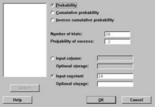
96 Chapter 5

for these probabilities; namely

P(Y=k)=µn

pk(1−p)n−k

is the probability that Ytakes the value kfor 0≤k≤n. When nand kare small,

this formula could be used to evaluate this probability but it is almost always

better to use software like Minitab to do it, and when these values are not small,

it is necessary. Also, we can use Minitab to compute the Binomial(n, p)cumu-

lative probability distribution – the probability contents of intervals (−∞,x]

and the inverse cumulative distribution – percentiles of the distribution.

For individual probabilities, we use the C

¯alc IProbability D

¯istributions I

¯inomial command. For example, suppose we have a Binomial(30,.2) distri-

bution and want to compute the probability P(Y=10).This command, with

the dialog box as in Display 5.1, produces the output

Binomialwithn=30andp=0.200000

x P(X=x)

10.00 0.0355

in the Session window, i.e., P(Y= 10) = .0355.

Display 5.1: Dialog box for Binomial(n, p)probability calculations.

If we want to compute the probability of getting 10 or fewer successes, this is

the probability of the interval (−∞,10],and we can use the C

¯alc IProbability

¯istributions IB

¯inomial command with the dialog box as in Display 5.2. This

produces the output

Binomialwithn=30andp=0.200000

xP(X<=x)

10.00 0.9744

in the Session window, i.e., P(Y≤10) = .9744.

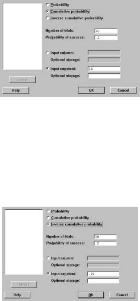
Sampling Distributions 97

Display 5.2: Dialog box for computing cumulative probabilities for the

Binomial(n, p)distribution.

Suppose we want to compute the Þrst quartile of this distribution. The C

¯alc

IProbability D

¯istributions IB

¯inomial command, with the dialog box as in

Display 5.3, produces the output

Binomialwithn=30andp=0.200000

xP(X<=x) x P(X<=x)

3 0.1227 4 0.2552

in the Session window. This gives the values xthat have cumulative probabilities

just smaller and just larger than the value requested. Recall that with a discrete

distribution, such as the Binomial(n, p),we will not in general be able to obtain

an exact percentile.

Display 5.3: Dialog box for computing percentiles of the Binomial(n, p)

distribution.

98 Chapter 5

These commands can operate on all the values in a column simultaneously.

This is very convenient if you should want to tabulate or graph the probability

function, cumulative distribution function, or inverse distribution function.

The general syntax of the pdf, cdf, and invcdf session commands is given

in II.1.3, and here we use them with the binomial subcommand as in

MTB >pdf 10;

SUBC>binomial 30 .2.

which outputs P(Y=10)when Yhas the Binomial(30,.2) distribution.

Actually, when nis very large even software will not be useful to compute

these probabilities, and you will have to use normal approximations to binomial

probabilities via the central limit theorem. The pdf and cdf commands with

the normal subcommandcanbeusedforthis.

WemightalsowanttosimulatefromtheBinomial(n, p)distribution. For

this we use the C

¯alc IR

¯andom Data IB

¯inomial command or the session

command random with the binomial subcommand. For example,

MTB >random 10 c1;

SUBC>binomial 30 .2.

MTB >print c1

22421157852

generates a sample of 10 from the Binomial(30,.2) distribution.

5.2 Simulating Sampling Distributions

First, we consider an example where we know the exact sampling distribution.

Suppose we ßip a possibly biased coin ntimes and want to estimate the unknown

probability pof getting a head. The natural estimate is ˆpthe proportion of heads

in the sample. We would like to assess the sampling behavior of this statistic

in a simulation. To do this, we choose a value for p,then generate Nsamples

from the Bernoulli distribution of size n,for each of these compute ˆp,look at

the empirical distribution of these Nvalues, perhaps plotting a histogram as

well. The larger Nis the closer the empirical distribution and histogram will

be to the true sampling distribution of ˆp.

Note that there are two sample sizes here: the sample size nof the original

sample the statistic is based on, which is Þxed, and the simulation sample size N,

which we can control. This is characteristic of all simulations. Sometimes, using

more advanced analytical techniques we can determine Nso that the sampling

distribution of the statistic is estimated with some prescribed accuracy. Some

techniques for doing this are discussed in later chapters of IPS. Another method

is to repeat the simulation a number of times, slowly increasing Nuntil we

see the results stabilize. This is sometimes the only way available, but caution

should be shown as it is easy for simulation results to be very misleading if the

Þnal Nis too small.

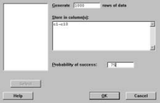
Sampling Distributions 99

We illustrate a simulation to determine the sampling distribution of ˆpwhen

sampling from a Bernoulli(.75) distribution. For this, we use the commands

¯alc IR

¯andom Data IBe

¯rnoulli, C

¯alc IRo

¯w Statistics, and S

¯tat IT

¯ables

ITa

¯lly, with the dialog boxes given by Displays 5.4, 5.5, and 5.6, respectively,

to produce the output

Summary Statistics for Discrete Variables

C11 CumPct

0.3 0.40

0.4 2.20

0.5 7.60

0.6 23.10

0.7 47.70

0.8 78.00

0.9 94.70

1.0 100.00

in the Session window. Here we have generated N= 1000 samples of size n=10

from the Bernoulli(.75) distribution, i.e., we simulated the tossing of this coin

10,000 times, and we placed the results in the rows of columns C1—C10 using

¯alc IR

¯andom Data IBe

¯rnoulli. The proportion of heads ˆpin each sample

is computed and placed in C11 using C

¯alc IRo

¯w Statistics. Note that a mean

of values equal to 0 or 1 is just the proportion of 1’s in the sample. Finally, we

used S

¯tat IT

¯ables ITa

¯lly to compute the empirical distribution function of

these 1000 values of ˆp. For example, this says 78% of these values were .8 or

smaller and there were no instances smaller than .3.

Display 5.4: Dialog box for generating 10 columns of 1000 Bernoulli(.75) values.

100 Chapter 5

Display 5.5: Dialog box for computing the proportion of 1’s in each of the 1000

samples of size 10.

Display 5.6: Dialog box for computing the empirical distribution function of ˆp.

In Display 5.7, we have plotted a histogram of the 1000 values of ˆp. Based

on N=800,the following empirical distribution was obtained:

C11 CumPct

0.4 1.20

0.5 7.20

0.6 22.20

0.7 47.80

0.8 78.20

0.9 95.00

1.0 100.00

Because these values are reasonably close to those obtained with N= 1000,we

stopped at N= 1000.

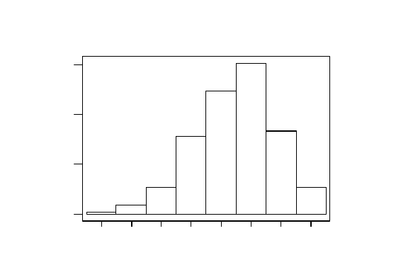
Sampling Distributions 101

1.00.90.80.70.60.50.40.3

300

200

100

C11

Frequency

Display 5.7: Histogram of simulation of N=1000values of ˆpbasedonasampleof

size n=10from the Bernoulli(.75) distribution.

The corresponding session commands for this simulation are

MTB >random 1000 c1-c10;

SUBC>bernoulli .75.

MTB >rmean c1-c10 c11

MTB >tally c11;

SUBC>cumpcts.

and these might seem like an easier way to implement the simulation.

In Chapter 5 of IPS we saw that the sampling distribution of ˆpcan be de-

termined exactly, i.e., there are formulas to determine this, and we can simulate

directly from the sampling distribution, so this simulation can be made much

more eﬃcient. In eﬀect, this entails using the C

¯alc IR

¯andom Data IBinomial

command with dialog box as in Display 5.8 and dividing each entry in C1 by 10.

This generates N= 1000 values of ˆpbut uses a much smaller number of cells.

Still, there are many statistics for which this kind of eﬃciency reduction is not

available, and, to get some idea of what their sampling distribution is like, we

must resort to the more brute force form of simulation of generating directly

from the population distribution.

Sometimes, more sophisticated simulation techniques are needed to get an

accurate assessment of a sampling distribution. Within Minitab, there are pro-

gramming techniques, which we do not discuss in this manual, that can be

applied in such cases. For example, it is clear that if our simulation required

the generation of 106cells (and this is not at all uncommon for some harder

problems), the simulation approach we have described would not work within

Minitab, as the worksheet would be too large.

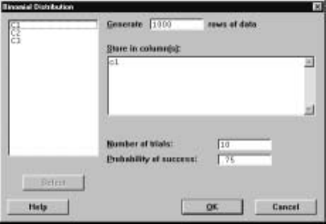
102 Chapter 5

Display 5.8: Dialog box for generating 1000 values from the sampling distribution of

10ˆpusing the Binomial(10,.75) distribution.

5.3 Exercises

When the data for an exercise come from an exercise in IPS, the IPS exercise

number is given in parentheses ( ). All computations in these exercises are

to be carried out using Minitab, and the exercises are designed to ensure that

you have a reasonable understanding of the Minitab material in this chapter.

Generally, you should be using Minitab to do all the computations and plotting

required for the problems in IPS.

If your version of Minitab places restrictions such that the value of the sim-

ulation sample size Nrequested in these problems is not feasible, then substitute

a more appropriate value. Be aware, however, that the accuracy of your results

is dependent on how large Nis.

1. Calculate all the probabilities for the Binomial(5,.4) distribution and the

Binomial(5,.6) distribution. What relationship do you observe? Can you

explain this and state a general rule?

2. Compute all the probabilities for a Binomial(5,.8) distribution and use

these to directly calculate the mean and variance. Verify your answers

using the formulas provided in IPS.

3. Compute and plot the probability and cumulative distribution functions of

the Binomial (10,.2) and the Binomial (10,.5) distributions. Comment

on the shapes of these distributions.

4. Generate 1000 samples of size 10 from the Bernoulli(.3) distribution.

Compute the proportion of 1’s in each sample and compute the propor-

tion of samples having no 1’s, one 1, two 1’s, etc. Compute what these

proportions would be in the longrun and compare.

Sampling Distributions 103

5. Carry out a simulation study with N=1000of the sampling distribution

of ˆpfor n=5,10,20 and for p=.5,.75,.95.In particular, calculate the

empirical distribution functions and plot the histograms. Comment on

your Þndings.

6. Suppose that X1,X

2,X

3,... are independent realizations from the

Bernoulli(p)distribution, i.e., each Xitakes the value 1 or 0 with prob-

abilities pand 1−p,respectively. If the random variable Ycounts the

number of tosses until we obtain the Þrst head in a sequence of inde-

pendent tosses X1,X

2,X

3,..., then Yhas a Geometric(p)distribution.

Minitab does not have built-in algorithms for computing the probabil-

ity function, distribution function, inverse distribution function, and for

generating from this distribution. The probability function for this distri-

bution is given by

P(Y=y)=(1−p)y−1p

for y=1,2,.... Plot the probability function for the Geometric (.5) dis-

tribution for the values y=1,...,10.DothesamefortheGeometric (.1)

distribution. What do you notice?

7. Using methods for summing geometric sums, the cumulative distribution

function of the Geometric (p)distribution (see Exercise II.5.6) is given

by P(Y≤y)=1−(1 −p)y.Plot the cumulative distribution function

for the Geometric (.5) and Geometric (.1) distribution for the values y=

1,...,10.What do you notice?

8. To randomly generate from the Geometric(p)distribution (see Exercise

II.5.6), we can repeatedly generate from a Bernoulli(p)and count how

many times we did this until the Þrst 1 appeared. A simple way to do this

in Minitab is to generate Nvalues from the Bernoulli(p)into a column.

Count the number of entries until the Þrst 1, count the number of subse-

quent entries until the next 1, etc. These counts are identically and inde-

pendently distributed according to the Geometric(p)distribution. This

is a very ineﬃcient method when pis small and much better algorithms

exist. Generate a sample of 10 from the Geometric (.5) distribution.

9. Carry out a simulation study, with N=2000,of the sampling distribution

of the sample standard deviation when sampling from the N(0,1) distri-

bution, based on a sample of size n=5.In particular, plot the histogram

using cutpoints 0, 1.5, 2.0 2.5, 3.0 5.0. Repeat this for the sample coeﬃ-

cient of variation (sample standard deviation divided by the sample mean)

using the cutpoints −10,−9, ..., 0, ..., 9, 10. Comment on the shapes of

the histograms relative to a N(0,1) density curve.

10. Generate N=1000samples of size n=5from the N(0,1) distribution.

Record a histogram for ¯xusing the cutpoints −3,−2.5,−2, ..., 2.5,3.0.

Generate a sample of size N= 1000 from the N(0,1/√5) distribution.

Plot the histogram using the same cutpoints and compare the histograms.

What will happen to these histograms as we increase N?

104 Chapter 5

11. Generate N= 1000 values of X1,X

2,where X1follows a N(3,2) distri-

bution and X2follows a N(−1,3) distribution. Compute Y=X1−2X2

for each of these pairs and plot a histogram for Yusing the cutpoints

−20,−15,...,25,30. Generate a sample of N=1000from the appropriate

distribution of Yand plot a histogram using the same cutpoints.

12. Plot the density curve for the Exponential(3) distribution (see Exercise

II.4.7) between 0 and 15 with an increment of .1. Generate N=1000

samples of size n=2from the Exponential(3) distribution and record

the sample means. Standardize the sample of ¯xusing µ=3and σ=3.

Plot a histogram of the standardized values using the cutpoints −5,−4,

..., 4, 5. Repeat this for n=5,10.Comment on the shapes of these

histograms.

13. Plot the density of the uniform distribution on (0,1). Generate N=1000

samples of size n=2from this distribution. Standardize the sample of ¯x

using µ=.5and σ=p1/12.Plot a histogram of the standardized values

using the cutpoints −5,−4, ..., 4,5. Repeat this for n=5,10.Comment

on the shapes of these histograms.

14. The Weibull (β)has density curve given by βxβ−1e−xβfor x>0,where

β>0is a Þxed constant. Plot the Weibull (2) density in the range 0 to

10 with an increment of .1 using the C

¯alc IProbability D

¯istributions I

¯eibull, command. Generate a sample of N= 1000 from this distribu-

tion using the subcommand C

¯alc IR

¯andom Data IW

¯eibull where β

is the Sh

¯ape parameter and the Sc

¯ale parameter is 1. Plot a probability

histogram and compare with the density curve.

Chapter 6

Introduction to Inference

New Minitab commands discussed in this chapter

¯tat IB

¯asic Statistics I1-Sample Z

¯ower and Sample Size I1-Sample Z

In this chapter, the basic tools of statistical inference are discussed. There

are a number of Minitab commands that aid in the computation of conÞdence

intervals and for carrying out tests of signiÞcance.

6.1 z-Conﬁdence Intervals

The command S

¯tat IB

¯asic Statistics I1-Sample Z

¯computes conÞdence inter-

vals for the mean µusing a sample x1,...,x

nfrom a distribution where we know

the standard deviation σ.There are three situations when this is appropriate:

(1) We know that we are sampling from a normal distribution with unknown

mean µand known standard deviation σ,and thus

z=¯x−µ

σ/√n

is distributed N(0,1).

(2) We have a large sample from a distribution with unknown mean µand

known standard deviation σ,and the central limit theorem approximation to

the distribution of ¯xis appropriate, i.e., the distribution of

z=¯x−µ

σ/√n

is approximately distributed N(0,1).

105

106 Chapter 6

(3) We have a large sample from a distribution with unknown mean µand

unknown standard deviation σ,and the sample size is large enough so that

z=¯x−µ

s/√n

is approximately N(0,1),wheresis the sample standard deviation.

The conÞdence interval takes the form ¯x±z∗σ/√n, where sis substituted

for σin case (3), and z∗is determined from the N(0,1) distribution by the

conÞdence level desired, as described in IPS. Of course, situation (3) is probably

the most realistic, but note that the conÞdence intervals constructed for (1) are

exact, while those constructed under (2) and (3) are only approximate, and a

larger sample size is required in (3) for the approximation to be reasonable than

for (2).

Consider the sample given by 0.8403, 0.8363, 0.8447, which are stored in

C1, and suppose that it makes sense to take σ=.0068. The command S

¯tat I

¯asic Statistics I1-Sample Z

¯with the dialog boxes as in Displays 6.1 and 6.2

produces the output

Variable N Mean StDev SE Mean

C1 3 0.84043 0.00420 0.00393

99.0% CI

(0.83032, 0.85055)

in the Session window. This speciÞes the 99% conÞdence interval (0.83032,

0.85055) for µ. Note that in the dialog box of Display 6.1, we specify where the

data resides in the V

¯ariables box, the value of σin the S

¯igma box, and click on

the O

¯ptions button to bring up the dialog box in Display 6.2. In this dialog box

we have speciÞed the 99% conÞdence level in the C

¯onÞdence level box.

Display 6.1: First dialog box for producing the z-conÞdence interval for µ.

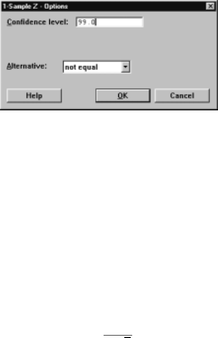
Introduction to Inference 107

Display 6.2: Second dialog box for producing the z-conÞdence interval. Here we

specify the conÞdence level.

The general syntax of the corresponding session command zinterval is

zinterval V1sigma = V2E1...Em

where V1is the conÞdence level and is any value between 1 and 99.99, V2is

the assumed value of σ, and E1, ..., Emare columns of data. A V1%conÞdence

interval is produced for each column speciÞed. If no value is speciÞed for V1,

the default value is 95%.

6.2 z-Tests

The S

¯tat IB

¯asic Statistics I1-Sample Z

¯command is used when we want to

test the hypothesis that the unknown mean µequals a value µ0and one of the

situations (1), (2), or (3) as discussed in II.10.1 is appropriate. The test is based

on computing a P-value using the observed value of

z=¯x−µ0

σ/√n

and the N(0,1) distribution as described in IPS.

Suppose the sample 2.0,0.4,0.7,2.0,−0.4,2.2,−1.3,1.2,1.1,2.3is stored in

C1, and we are asked to test the null hypothesis H0:µ=0against the alterna-

tive Ha:µ>0and it makes sense to take σ=1.The S

¯tat IB

¯asic Statistics

I1-Sample Z

¯command together with the dialog boxes of Displays 6.3 and 6.4

produces the output

Variable 99.0% Lower Bound Z P

C1 0.284 3.23 0.001

in the Session window. This speciÞes the P-value for this test as .001, and so we

reject the null hypothesis in favor of the alternative. In the Þrst dialog box, we

speciÞed where the data is located, the value of σas before and that we want

to test H0:µ=0by 0 in the T

¯est mean box. We brought up the second dialog

box by clicking on the O

¯ptions button. In the second dialog box, we speciÞed

that we want to test this null hypothesis against the alternative Ha:µ>0by

selecting “greater than” in A

¯lternative box. The other choices are “not equal,”

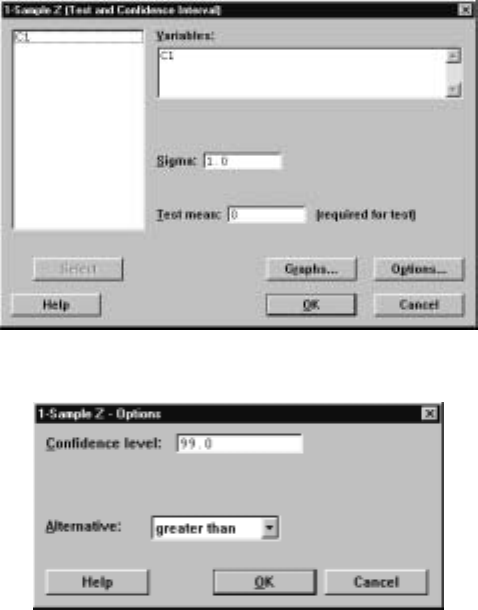
108 Chapter 6

which selects the alternative Ha:µ6=0,and “less than,” which selects the

alternative Ha:µ<0.

Display 6.3: First dialog box for testing a hypothesis concerning the mean using a

z-test.

Display 6.4: Second dialog box for testing a hypothesis using the z-test.

The general syntax of the corresponding session command ztest is

ztest V1sigma = V2E1...Em

where V1is the hypothesized value to be tested, V2is the assumed value of σ,

and E1, ..., Emare columns of data. If no value is speciÞed for V1, the default

is 0. A test of the hypothesis is carried out for each column. If no alternative

subcommand is speciÞed, a two-sided test is conducted, i.e., H0:µ=V1against

the alternative Ha:µ6=V1.If the subcommand

SUBC>alternative 1.

is used, a test of H0:µ=V1against the alternative Ha:µ>V1is conducted.

If the subcommand

SUBC>alternative -1.

is used, a test of H0:µ=V1against the alternative Ha:µ<V1is conducted.

Introduction to Inference 109

6.3 Simulations for Conﬁdence Intervals

When we are sampling from a N(µ, σ)distribution and know the value of σ,the

conÞdence intervals constructed in II.6.1 are exact, i.e., in the long run a pro-

portion 95% of the 95% conÞdence intervals constructed for an unknown mean

µwill contain the true value of this quantity. Of course, any given conÞdence

interval may or may not contain the true value of µ,and, in any Þnite number of

such intervals so constructed, some proportion other than 95% will contain the

true value of µ. As the number of intervals increases, however, the proportion

covering will go to 95%.

We illustrate this via a simulation study based on computing 90% conÞdence

intervals. The session commands

MTB >random 100 c1-c5;

SUBC>normal 1 2.

MTB >rmean c1-c5 c6

MTB >invcdf .95;

SUBC>normal 0 1.

Normalwithmean=0andstandarddeviation=1.00000

P( X <=x)x

0.9500 1.6449

MTB >let k1=1.6449*2/sqrt(5)

MTB >let c7=c6-k1

MTB >let c8=c6+k1

MTB >let c9=c7<1 and c8>1

MTB >mean c9

Mean of C9 = 0.94000

MTB >set c10

DATA>1:25

DATA>end

MTB >delete 26:100 c7 c8

MTB >mplot c7 versus c10 c8 versus c10;

SUBC>xstart=1 end=25;

SUBC>xincrement=1.

generate 100 random samples of size 5 from the N(1,2) distribution, place the

means in C6, the lower end-point of a 90% conÞdence interval in C7, and the

upper end-point in C8, and record whether or not a conÞdence interval covers

thetruevalueµ=1by placing a 1 or 0 in C9, respectively. The mean of C9

is the proportion of intervals that cover, and this is 94%, which is 4% too high.

Finally, we plotted the Þrst25oftheseintervalsinaplotshowninFigure6.1.

Drawing a solid horizontal line at 1 on the y-axis indicates that most of these

intervals do indeed cover the true value µ=1.

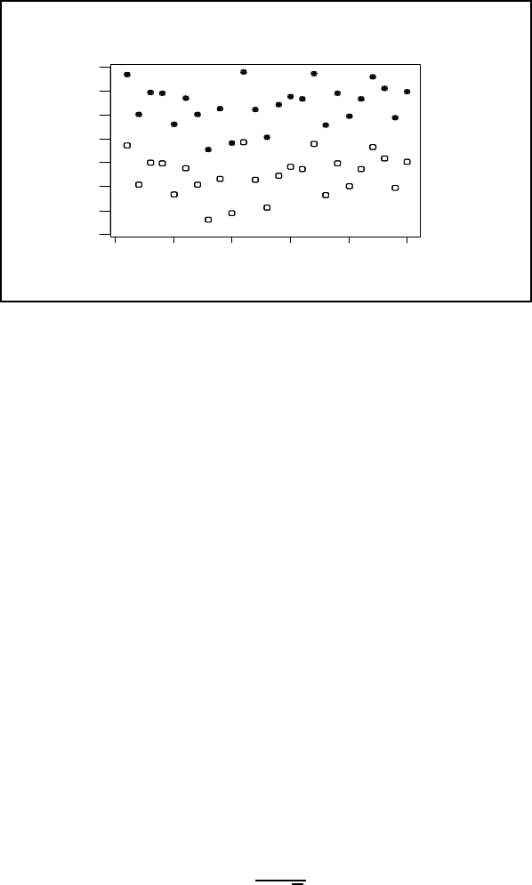
110 Chapter 6

2520151050

-1

-2

-3

C10

Figure 6.1: Plot of 90% conÞdence intervals for the mean when sampling from the

N(1,2) distribution with n=5. The lower end-point is open and the upper

end-point is closed.

The simulation just carried out simply veriÞes a theoretical fact. On the

other hand, when we are computing approximate conÞdence intervals – i.e., we

are not sampling necessarily from a normal distribution – it is good to do some

simulations from various distributions to see how much reliance we can place

in the approximation at a given sample size. The true coverage probability of

the interval, i.e., the long-run proportion of times that the interval covers the

true mean, will not in general be equal to the nominal conÞdence level. Small

deviations are not serious, but large ones are.

6.4 Simulations for Power Calculations

It is also useful to know in a given context how sensitive a particular test of

signiÞcance is. By this we mean how likely it is that the test will lead us to

reject the null hypothesis when the null hypothesis is false. This is measured by

the concept of the power of a test. Typically, a level αis chosen for the P-value

at which we would deÞnitely reject the null hypothesis if the P-value is smaller

than α. For example, α=.05 is a common choice for this level. Suppose that

we have chosen the level of .05 for the two-sided z-test and we want to evaluate

the power of the test when the true value of the mean is µ=µ1,i.e., evaluate

the probability of getting a P-value smaller than .05 when the mean is µ1.The

two-sided z-test with level αrejects H0:µ=µ0whenever

|Z|>

¯¯x−µ0

σ/√n

≤α

where Zis a N(0,1) random variable. This is equivalent to saying that the null

hypothesis is rejected whenever

Introduction to Inference 111

¯¯x−µ0

σ/√n

is greater than or equal to the 1−α/2percentile for the N(0,1) distribution.

For example, if α=.05,then 1−α/2=.975 and this percentile can be obtained

using the command C

¯alc IProbability D

¯istributions IN

¯ormal and the inverse

distribution function, which gives the output

Normalwithmean=0andstandarddeviation=1.00000

P( X <=x) x

0.9750 1.9600

in the Session window, i.e., the .975 percentile of the N(0,1) distribution is 1.96.

Denote this percentile by z∗.If µ=µ1,then

¯x−µ0

σ/√n

is a realized value from the distribution of Y=¯

X−µ0

σ/√nwhen ¯

Xis distributed

N(µ1,σ/

√n).Therefore, Yfollows a N(µ1−µ0

σ/√n,1) distribution. The power of

the two-sided test at µ=µ1is

P(|Y|>z

∗)

and this can be evaluated exactly using the command C

¯alc IProbability

¯istributions IN

¯ormal and the distribution function, after writing

P(|Y|>z

∗)=P(Y>z

∗)+P(Y<−z∗)

Z>−(µ1−µ0)

σ/√n+z∗

¶+P

Z<−(µ1−µ0)

σ/√n−z∗

with Zfollowing an N(0,1) distribution.

Alternatively, exact power calculations can be carried out under the assump-

tion of sampling from a normal distribution using the P

¯ower and Sample Size

I1-Sample Z

¯command and Þlling in the dialog box appropriately. Also, the

minimum sample size required to guarantee a given power at a prescribed dif-

ference |µ1−µ0|can be obtained using this command. For example, Þlling in

the dialog box for this command as in Display 6.5 creates the output

Testing mean = null (versus not = null)

Calculating power for mean = null + difference

Alpha = 0.05 Sigma = 1.3

Sample

Difference Size Power

0.1 10 0.0568

0.2 10 0.0775

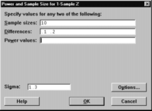
112 Chapter 6

in the Session window. This gives the power for testing H0:µ=µ0versus

H0:µ6=µ0at |µ1−µ0|=.1and |µ1−µ0|=.2when n=10,σ=1.3,and

α=.05.These powers are given by .0568 and .0775, respectively. Clicking on

the Op

¯tions button allows you to choose other alternatives and specify other

values of αin the S

¯igniÞcance level box.

Display 6.5: Dialog box for calculating powers and minimum sample sizes.

If we had instead ÞlledinPow

¯er values at .1 and .2 in the dialog box of

Display 6.5, say as .8 and .9, and had left the S

¯ample sizes box empty, we would

have obtained the output

Testing mean = null (versus not = null)

Calculating power for mean = null + difference

Alpha = 0.05 Sigma = 1.3

Sample Target Actual

Difference Size Power Power

0.1 1327 0.8000 0.8002

0.1 1776 0.9000 0.9000

0.2 332 0.8000 0.8005

0.2 444 0.9000 0.9000

in the Session window. This prescribes the minimum sample sizes n=1327

and n= 1776 to obtain the powers .8 and .9, respectively, at the diﬀerence

.1 and the sample sizes n=332and n=444to obtain the powers .8 and .9,

respectively, at the diﬀerence .2.

This derivation of the power of the two-sided test depended on the sample

coming from a normal distribution, as this leads to ¯

Xhaving an exact normal

distribution. In general, however, ¯

Xwill be only approximately normal, and so

the normal calculation is not exact. To assess the eﬀect of the nonnormality,

however, we can often simulate sampling from a variety of distributions and

estimate the probability P(|Y|>z

∗).For example, suppose that we want to

Introduction to Inference 113

test H0:µ=0in a two-sided z-test based on a sample of 10, where we estimate

σby the sample standard deviation and we want to evaluate the power at 1. Let

us further suppose that we are actually sampling from a uniform distribution

on the interval (−10,12),which indeed has its mean at 1. The simulation given

by the session commands

MTB >random 1000 c1-c10;

SUBC>uniform -10 12.

MTB >rmean c1-c10 c11

MTB >rstdev c1-c10 c12

MTB >let c13=absolute(c11/(c12/sqrt(10)))

MTB >let c14=c13>1.96

MTB >let k1=mean(c14)

MTB >let k2=sqrt(k1*(1-k1)/n(c14))

MTB >print k1 k2

K1 0.112000

K2 0.00997276

estimates the power to be .112, and the standard error of this estimate, as

given in K2, is approximately .01. The application determines whether or not

the assumption of a uniform distribution makes sense and whether or not this

power is indicative of a sensitive test or not.

6.5 The Chi-Square Distribution

If Zis distributed according to the N(0,1) distribution, then Y=Z2is

distributed according to the Chisquare(1) distribution. If X1is distributed

Chisquare(k1)independent of X2distributed Chisquare(k2),then Y=X1+X2

is distributed according to the Chisquare(k1+k2)distribution. There are

Minitab commands that assist in carrying out computations for the Chisquare(k)

distribution. Note that kis any positive value and is referred to as the degrees

of freedom.

The values of the density curve for the Chisquare(k)distribution can be

obtained using the C

¯alc IProbability D

¯istributions IC

¯hi-Square command,

with kas the D

¯egrees of freedom in the dialog box, or the session command pdf

with the subcommand chisquare. For example, the command

MTB >pdf c1 c2;

SUBC>chisquare 4.

calculates the value of the Chisquare(4) density curve at each value in C1 and

stores these values in C2. This is useful for plotting the density curve. The C

¯alc

IProbability D

¯istributions IC

¯hi-Square command, or the session commands

cdf and invcdf, can also be used to obtain values of the Chisquare(k)cumu-

lative distribution function and inverse distribution function, respectively. We

use the C

¯alc IR

¯andom Data IC

¯hi-Square command, or the session command

random, to obtain random samples from these distributions.

114 Chapter 6

We will see applications of the chi-square distribution later in the book but

we mention one here. In particular, if x1,...,x

nis a sample from a N(µ, σ)

distribution, then (n−1)s2/σ2=Pn

i=1 (xi−¯x)2/σ2is known to follow a

Chisquare(n−1) distribution, and this fact is used as a basis for inference

about σ(conÞdence intervals and tests of signiÞcance). Because of the nonro-

bustness of these inferences to small deviations from normality, these inferences

are not recommended.

6.6 Exercises

When the data for an exercise come from an exercise in IPS, the IPS exercise

number is given in parentheses ( ). All computations in these exercises are

to be carried out using Minitab, and the exercises are designed to ensure that

you have a reasonable understanding of the Minitab material in this chapter.

Generally, you should be using Minitab to do all the computations and plotting

required for the problems in IPS.

If your version of Minitab places restrictions such that the value of the sim-

ulation sample size Nrequested in these problems is not feasible, then substitute

a more appropriate value. Be aware, however, that the accuracy of your results

is dependent on how large Nis.

1. (6.6) Use the S

¯tat IB

¯asic Statistics I1- Sample Z

¯command to compute

90%, 95%, and 99% conÞdence intervals for µ.

2. (6.49) Use the S

¯tat IB

¯asic Statistics I1- Sample Z

¯command to test the

null hypothesis against the appropriate alternative. Evaluate the power

of the test with level α=.05 at µ=225.

3. Simulate N=1000samples of size 5 from the N(1,2) distribution, and

calculate the proportion of .90 z-conÞdence intervals for the mean that

cover the true value µ=1.

4. Simulate N=1000samples of size 10 from the uniform distribution on

(0,1), and calculate the proportion of .90 z-conÞdence intervals for the

mean that cover the true value µ=.5.Use σ=1/√12.

5. Simulate N= 1000 samples of size 10 from the Exponential(1) distribu-

tion (see Exercise II.4.7), and calculate the proportion of .95 z-conÞdence

intervals for the mean that cover the true value µ=1.Use σ=1.

6. The density curve for the Student(1) distribution takes the form

1+x2

for −∞ <x<∞. This special case is called the Cauchy distribution. Plot

this density curve in the range (−20,20) using an increment of .1. Simulate

N= 1000 samples of size 5from the Student(1) distribution (see Exercise

Introduction to Inference 115

II.4.12), and calculate the proportion of .90 conÞdence intervals for the

mean, using the sample standard deviation for σ,that cover the value

µ=0.It is possible to obtain very bad approximations in this example

because the central limit theorem does not apply to this distribution. In

fact, it does not have a mean.

7. Suppose we are testing H0:µ=3versus H0:µ6=3when we are sampling

from a N(µ, σ)distribution with σ=2.1and the sample size is n=20.

If we use the critical value α=.01,determine the power of this test at

µ=4.

8. Suppose we are testing H0:µ=3versus H0:µ>3when we are

sampling from a N(µ, σ)distribution with σ=2.1.If we use the critical

value α=.01,determine the minimum sample size so that the power of

this test at µ=4is .99.

9. The uniform distribution on the interval (a, b)has mean µ=(a+b)/2

and standard deviation σ=q(b−a)2/12.Calculate the power at µ=1

of the two-sided z-test at level α=.95 for testing H0:µ=0when the

sample size is n=10,σis the standard deviation of a uniform distribution

on (−10,12), and we are sampling from a normal distribution.

10. Suppose that we are testing H0:µ=0in a two-sided test based on

a sample of 3. Approximate the power of the z-test at level α=.1at

µ=5when we are sampling from the distribution of Y=5+W, where

Wfollows a Student(6) distribution (see Exercise II.4.12) and we use

the sample standard deviation to estimate σ.Note that the mean of the

distribution of Yis 5.

116 Chapter 6

Manual.dvi MINITAB Manual

Navigation menu

Versions of this User Manual:

Views

Navigation