91530.dvi MIP Guide
User Manual:
Open the PDF directly: View PDF ![]() .
.
Page Count: 55

SIAM REVIEW c
2015 Society for Industrial and Applied Mathematics
Vol. 57, No. 1, pp. 3–57
Mixed Integer Linear
Programming Formulation
Techniques∗
Juan Pablo Vielma†
Abstract. A wide range of problems can be modeled as Mixed Integer Linear Programming (MIP)
problems using standard formulation techniques. However, in some cases the resulting MIP
can be either too weak or too large to be effectively solved by state of the art solvers. In
this survey we review advanced MIP formulation techniques that result in stronger and/or
smaller formulations for a wide class of problems.
Key words. mixed integer linear programming, disjunctive programming
AMS subject classifications. 90C11, 90C10
DOI. 10.1137/130915303
1. Introduction. Throughout more than 50 years of existence, mixed integer
linear programming (MIP) theory and practice have been significantly developed, and
it is now an indispensable tool in business and engineering [68, 94, 104]. Two reasons
for the success of MIP are linear programming (LP) based solvers and the modeling
flexibility of MIP. We now have several extremely effective state-of-the-art solvers
[82, 69, 52, 171] that incorporate many advanced techniques [1, 2, 25, 23, 92, 112, 24]
and, since its early stages, MIP has been used to model a wide range of applications
[44, 45].
While in many cases constructing valid MIP formulations is relatively straightfor-
ward, some care should be taken in this construction as certain formulation attributes
can significantly reduce the effectiveness of LP-based solvers. Fortunately, construct-
ing formulations that behave well with state-of-the-art solvers can usually be achieved
by following simple guidelines described in standard textbooks. However, more ad-
vanced techniques can often perform significantly better than textbook formulations
and are sometimes a necessity. The main objective of this survey is to summarize
the state of the art of such formulation techniques for a wide range of problems.
To keep the length of this survey under control, we concentrate on formulations for
sets of a mixed integer nature that require both integer constrained and continuous
variables. We hence purposefully place less emphasis on some related areas such as
combinatorial optimization, quadratic and polynomial 0/1 optimization, and polyhe-
dral approximations of convex sets. These topics are certainly areas of important and
active research, so we cover them succinctly in section 12.
∗Received by the editors April 2, 2013; accepted for publication (in revised form) July 21, 2014;
published electronically February 5, 2015.
http://www.siam.org/journals/sirev/57-1/91530.html
†Sloan School of Management, Massachusetts Institute of Technology, Cambridge, MA (jvielma@
mit.edu).
3
4JUAN PABLO VIELMA
Throughout this survey we emphasize the potential advantages of each technique.
However, we should note that given the complexities of state-of-the-art solvers, it is
hard to predict with high accuracy which formulation performs better. Some guide-
lines can be found in computational studies (e.g., [163, 91, 155]), but the formulation
that performs best can be strongly dependent on the specific problem structure or
data. Fortunately, there is a high correlation between certain favorable formulation
properties and good computational performance. In addition, it is often easy to con-
struct several alternative formulations for a preliminary computational test. Finally,
we refer the reader to [78, 88, 138, 164] for complementary information on the topics
covered in this survey and their relation to other areas.
The rest of this survey is organized as follows. We begin in section 2 with a
motivating example that allows us to precisely define the idea of an MIP formulation
or model. This same example serves to illustrate one of the most important favorable
properties of an MIP formulation: the strength of its LP relaxation. Through this
section we also introduce basic MIP concepts and notation that we use in the rest of
the paper. The construction and evaluation of effective MIP formulations also requires
some basic concepts and results from polyhedral theory, which we review in section 3.
Armed with such results, in section 4, we introduce the use of auxiliary variables as
a way to construct strong formulations without incurring an excessive size. Then in
section 5 we show how these auxiliary variables can be used to construct strong for-
mulations for a finite set of alternatives described as the union of certain polyhedra or
mixed integer sets. In section 6 we discuss how to reduce formulation size by forgoing
the use of auxiliary variables. We show how this can result in a significant loss of
strength, but also discuss cases in which this loss can be prevented. Then in section 7
we consider the use of large formulations and an LP-based technique that can be used
to reduce their size in certain cases. Sections 8 and 9 review some advanced techniques
that can be used to reduce the size of formulations and to improve the performance of
branch-and-bound-based MIP solvers. After that, in section 10 we discuss alternative
ways of combining formulations and in section 11 we consider precise geometric and
algebraic characterizations of sets that can be modeled with different classes of MIP
formulations. Finally, section 12 considers other topics related to MIP formulations.
2. Preliminaries and Motivation.
2.1. Modeling with MIP. Modeling non-convex functions has been a central topic
of MIP formulations since its early developments [119, 120, 122, 121, 85, 84, 81, 91, 89],
so our first example falls in this category. Consider the mathematical programming
problem given by
zMP := min
n
i=1
fi(xi)(2.1a)
s.t.Ex ≤h,(2.1b)
0≤xi≤u∀i∈{1,...,n},(2.1c)
where fi:[0,u]→Qare univariate piecewise linear functions of the form
(2.2) f(x)=⎧
⎪
⎪
⎪
⎪
⎨
⎪
⎪
⎪
⎪
⎩
m1x+c1,x∈[d0,d
1],
m2x+c2,x∈[d1,d
2],
.
.
.
mkx+ck,x∈[dk−1,d
k],
MIXED INTEGER LINEAR PROGRAMMING FORMULATION TECHNIQUES 5
for given breakpoints 0 = d0<d
1<···<d
k−1<d
k=u, slopes {mi}k
i=1 ⊆Q,and
constants {ci}k
i=1 ⊆Q. We assume that the slopes and constants are such that the
functions are continuous, but not convex. For instance, one of these functions could
be
(2.3) f(x)=⎧
⎨
⎩
x+2,x∈[0,1],
−2x+5,x∈[1,2],
1,x∈[2,3],
which will be our running example for this section.
Because the functions we consider are non-convex, we cannot transform (2.1) into
an equivalent LP problem. However, we can transform it into an MIP problem as
follows.
The first step in the transformation is to identify a set or a constraint that we want
to model as an MIP problem. In the case of a piecewise linear function f, an appro-
priate set to model is the graph of fgiven by gr(f):={(x, z)∈Q×Q:f(x)=z}.
Indeed, we can reformulate (2.1) by explicitly including gr(fi) to obtain the equivalent
problem given by
zMP := min
n
i=1
zi
(2.4a)
s.t.
Ex ≤h,(2.4b)
0≤xi≤u∀i∈{1,...,n},(2.4c)
(xi,z
i)∈gr(fi)∀i∈{1,...,n}.(2.4d)
Now, as illustrated in Figure 2.1 for our running example, the graph of a univariate
continuous piecewise linear function (with bounded domain) is the finite union of line
segments, which we can easily model with MIP. For instance, for the function defined
in (2.3) we can construct the textbook MIP formulation of gr(f)givenby
0λ0+1λ1+2λ2+3λ3=x,(2.5a)
2λ0+3λ1+1λ2+1λ3=z,(2.5b)
λ0+λ1+λ2+λ3=1,(2.5c)
λ0≤y1,(2.5d)
λ1≤y1+y2,(2.5e)
λ2≤y2+y3,(2.5f)
λ3≤y3,(2.5g)
y1+y2+y3=1,(2.5h)
λj≥0∀j∈{0,...,3},(2.5i)
0≤yj≤1∀j∈{1,2,3},(2.5j)
yj∈Z∀j∈{1,2,3}.(2.5k)
Formulation (2.5) illustrates how MIP formulations can use both continuous and inte-
ger variables to enforce requirements on the original variables. Formulations that use
auxiliary variables different from the original variables are usually denoted extended,
lifted,orhigher-dimensional. In the case of formulation (2.5) these auxiliary variables
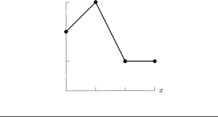
6JUAN PABLO VIELMA
1
1230
0
2
3
z=f(x)
Fig. 2.1 Graph of the continuous piecewise linear function defined in (2.3).
are necessary to construct the formulation. However, as we will see in section 4, aux-
iliary variables can provide an advantage even when they are not strictly necessary.
For this reason we use the following definition of an MIP formulation that always
considers the possible use of auxiliary variables.
Definition 2.1. For A∈Qm×n,B∈Qm×s,D∈Qm×t,andb∈Qmconsider
the set of linear inequalities and continuous and integer variables of the form
Ax +Bλ +Dy ≤b,(2.6a)
x∈Qn,(2.6b)
λ∈Qs,(2.6c)
y∈Zt.(2.6d)
We say (2.6) is an MIP formulation for a set S⊆Qnif the projection of (2.6) onto
the xvariables is exactly S. That is, if we have x∈Sif and only if there exist λ∈Qs
and y∈Ztsuch that (x, λ, y)satisfies (2.6).
Note that generic formulation (2.6) does not explicitly consider the inclusion of
integrality requirements on the original variables x. While example (2.5) does not
require such integrality requirements, it is common for at least some of the original
variables to be integers. Formulation (2.6) implicitly considers that possibility by
allowing the inclusion of constraints of the form xi=yj. Hence, we can replace (2.6b)
with x∈Qn1×Zn2without really changing the definition of an MIP formulation.
Using Definition 2.1 we can now write a generic MIP reformulation of (2.1) by
replacing every occurrence of (xi,z)∈gr(fi) with an MIP formulation of gr(fi)to
obtain
zMIP := min
n
i=1
zi
(2.7a)
s.t.Ex ≤h,(2.7b)
MIXED INTEGER LINEAR PROGRAMMING FORMULATION TECHNIQUES 7
0≤xi≤u∀i∈{1,...,n},(2.7c)
Aixi
zi+Biλi+Diyi≤bi∀i∈{1,...,n},(2.7d)
yi∈Zk∀i∈{1,...,n},(2.7e)
where Ai,Bi,Di,andbiare appropriately constructed matrices and vectors, and k
is an appropriate number of integer variables. There are many choices for (2.7d), but
as long as they are valid formulations of gr(fi), we have zMP =zMIP and we can
extract a solution of (2.1) by looking at the xvariables of an optimal solution of (2.7).
However, some versions of (2.7d) can perform significantly better when solved with
an MIP solver. We study this potential difference in the next subsection.
2.2. Strength, Size, and MIP Solvers. While all state-of-the-art MIP solvers are
based on the branch-and-bound algorithm [102], they also include a large number of
advanced techniques that make it hard to predict the specific impact of an alternative
formulation. However, there are two aspects of an MIP formulation that usually have
a strong impact on both simple branch-and-bound algorithms and state-of-the-art
solvers: the size and strength of the LP relaxation, and the effect of branching on the
formulation. Instead of giving a lengthy description of the branch-and-bound algo-
rithm and state-of-the-art solvers, we introduce the necessary concepts by considering
the first step of the solution of MIP reformulation (2.7) with a simple branch-and-
bound algorithm. For more details on basic branch-and-bound and state-of-the-art
solvers, we refer the reader to [22, 36, 131, 166] and [1, 2, 25, 23, 92, 112, 24], respec-
tively.
The first step in solving MIP formulation (2.7) with a branch-and-bound al-
gorithm is to solve the LP relaxation of (2.7) obtained by dropping all integrality
requirements. The resulting LP problem given by (2.7a)–(2.7d) is known as the root
LP relaxation and can be solved efficiently both in theory and in practice. Its optimal
value zLP := min {n
i=1 zi: (2.7b)–(2.7d)}provides a lower bound on zMIP known
as the LP relaxation bound. If the optimal solution to the LP relaxation satisfies the
dropped integrality constraints, then zMIP =zLP and this solution is also optimal
for (2.7). In contrast, if optimal solution ¯x, ¯z, ¯
λ, ¯yis such that for some iand jwe
have ¯yi
j/∈Z, we can eliminate this infeasibility by branching on yi
j. To achieve this we
create two new LP problems by adding yi
j≤¯yi
jand yi
j≥¯yi
jto the LP relaxation,
respectively. These two new problems are usually denoted branches and are processed
in a similar way, which generates a binary tree known as the branch-and-bound tree.
The behavior of this first step is usually a good predictor of the performance of the
whole algorithm, so we now concentrate on the effect of an MIP formulation on this
step. We consider the effect of different formulations on subsequent steps in section 8.
To understand the effect of a formulation on the root LP relaxation we need
to understand what the LP relaxation of the formulation is modeling. Going back
to our running example, consider the LP relaxation of (2.5) given by (2.5a)–(2.5j).
Constraints (2.5a)–(2.5c) and (2.5i) show that any (x, z)thatispartofafeasible
solution for this LP relaxation must be a convex combination of points (0,2), (1,3),
(2,1), and (3,1). Conversely, any (x, z) that is a convex combination of these points
is part of a feasible solution for the LP relaxation (let λbe the appropriate convex
combination multipliers, y1=λ0,y2=1−λ0−λ3,andy3=λ3). Hence, the projection
onto the (x, z) variables of the LP Relaxation of (2.5) is equal to conv (gr (f)), the
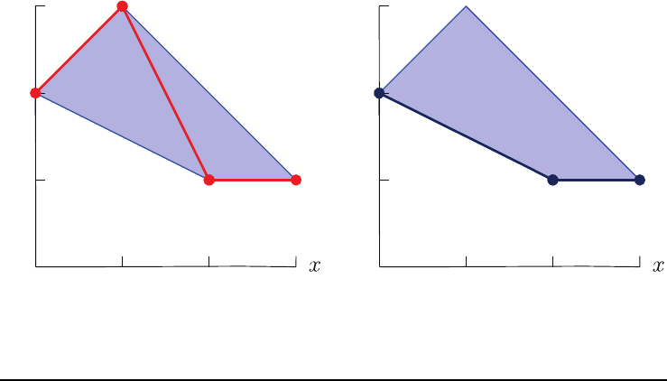
convex hull of gr (f). As illustrated in Figure 2.2(a), this convex hull corresponds to
the smallest convex set containing gr (f). Now, if we used this formulation for fiin
8JUAN PABLO VIELMA
(2.1) (for simplicity imagine that all these functions are equal to f), the LP relaxation
of (2.7) would be equivalent to
zLP := min
n
i=1
φi(xi)(2.8a)
s.t.
Ex ≤h,(2.8b)
0≤xi≤u∀i∈{1,...,n},(2.8c)
where φi:[0,u]→Qis the convex envelope or lower convex envelope [80] of fi.This
lower convex envelope is the tightest convex underestimator of fand is illustrated for
our running example in Figure 2.2(b).
1
1230
0
2
3
z=f(x)
(a) gr (f) in red and conv (gr (f)) in light blue.
1
1230
0
2
3
z=f(x)
(b) conv (gr (f)) in light blue and lower convex
envelope of fin dark blue.
Fig. 2.2 Effect of the LP relaxation of formulation (2.5) of fdefined in (2.3).
This reasoning suggests that, at least with respect to the LP relaxation bound,
formulation (2.5) of our example function is as strong as it can be. Indeed, the
projection onto the (x, z)-space of any formulation of fis a convex (and polyhedral)
setthatmustcontaingr(f) and the LP relaxation of (2.5) projects to the smallest
of such sets. By the same argument, the projection onto the xvariables of the LP
relaxation of an MIP formulation of any set S⊆Qnmust also contain conv(S)
and formulations whose LP relaxations project precisely to conv(S) yield the best
LP relaxation bounds. Jeroslow and Lowe [90, 113] denoted those formulations that
achieve this best possible LP relaxation bound as sharp. Other authors also denote
them convex hull formulations.
Definition 2.2. An MIP formulation of set S⊆Qnis sharp if and only if the
projection onto the xvariables of its LP relaxation is exactly conv(S).
It is important to note that sharp formulations yield the best LP relaxation
bound among all MIP formulations for the sets we selected to model. However, the
LP relaxation bound can vary if we elect to model other sets. For instance, in our
MIXED INTEGER LINEAR PROGRAMMING FORMULATION TECHNIQUES 9
example, we elected to independently model gr(fi) for all i∈{1,...,n}. However, we
could instead have elected to model
(2.9) S=⎧
⎪
⎪
⎪
⎪
⎨
⎪
⎪
⎪
⎪
⎩
(x, z)∈Qn×Q:
z=
n
i=1
fi(xi),
Ex ≤h,
0≤xi≤u∀i∈{1,...,n}
⎫
⎪
⎪
⎪
⎪
⎬
⎪
⎪
⎪
⎪
⎭
to obtain a formulation that considers all possible nonconvexities at the same time.
A sharp formulation for this case would be significantly stronger as we can show that
for Sdefined in (2.9) we have min {z:(x, z)∈conv (S)}=zMP =zMIP . Because
the LP relaxation of a sharp formulation of Sis equal to conv(S), we have that calcu-
lating the optimal value of (2.4) could be done by simply solving an LP problem. Of
course, unlike our original piecewise sharp formulation, constructing a sharp formula-
tion for this joint Swould normally be harder than solving (2.4). Furthermore, this
approach can result in a significantly larger formulation. Selecting which portions of
a mathematical programming problem to model independently to balance size and
final strength is a crucial and nontrivial endeavor. However, the appropriate selection
is usually ad hoc to the specific structure of the problem considered. For instance,
Croxton, Gendron, and Magnanti [42] study the case where (2.1) corresponds to a
multicommodity network flow problem with piecewise linear costs. In this setting,
they show that a convenient middle ground between constructing independent formu-
lations of each gr (fi) and a single formulation for the complete problem (2.9) is to
construct independent formulations for each gr i∈Iafi(xi),whereIacorresponds
to the flow variables of all commodities in a given arc aof the network. From now
on we assume that a similar analysis has already been carried out and we focus on
constructing small and strong formulations for the individual portions selected. How-
ever, in section 10 we will succinctly consider the selection of such portions and the
combination of the associated formulations.
As we have mentioned, sharp formulations are strongest in one sense. However,
if we consider the integer variables of our MIP formulation we can construct even
stronger formulations. To illustrate this, let us go back to our example and consider
an optimal solution ¯x, ¯z, ¯
λ, ¯yof the LP relaxation of (2.7) given by (2.7a)–(2.7d).
Because the root LP relaxation is usually solved by a simplex algorithm, we can ex-
pect this to be an optimal basic feasible solution. However, analyzing basic feasible
solutions of (2.7b)–(2.7d) can be quite hard, so let us analyze basic feasible solutions
of the LP relaxations of the individual formulations of gr(fi) (i.e., (2.5a)–(2.5j)) as a
reasonable proxy. We can check that one optimal basic feasible solution of minimizing
zover (2.5a)–(2.5j) is given by ¯
λ2=¯
λ3=1/2, ¯
λ0=¯
λ1=0, ¯y1=¯y3=1/2, ¯y2=0,
¯x=2.5, and ¯z= 1. Because (2.5) is a sharp MIP formulation, it is not surprising
that this gives the same optimal value as minimizing zover (2.5). Indeed we have
that 1 = f(2.5) = φ(2.5) and x=2.5 is a minimizer of f. However, the basic feasible
solution obtained has some of its integer variables set at fractional values. Because
a general purpose branch-and-bound solver is not aware of the specific structure of
the problem, it would have no choice but to unnecessarily branch on one of these
variables (let’s say ¯y1) or to run a rounding heuristic to obtain an integer feasible
solution. Hence, while sharp formulations are the strongest possible with regard to
LP relaxation bounds, they can be somewhat weak with respect to finding optimal
or good quality integer feasible solutions. Fortunately, it is possible to construct MIP
formulations that are strong from both the LP relaxation bound and integer feasibility
10 JUAN PABLO VIELMA
perspectives. These formulations are those whose LP relaxations have basic feasible
solutions that automatically satisfy the integrality requirements on the yvariables.
Such LP relaxations are usually denoted integral and formulations with this property
were denoted locally ideal by Padberg and Rijal [136, 137]. Ideal comes from the fact
that this is the strongest property we can expect from an MIP formulation from any
perspective. Locally serves to clarify that this property refers to a formulation for a
specifically selected portion and not to the whole mathematical programming problem
(following this convention, we should then refer to sharp formulations as locally sharp,
but we avoid it for simplicity and historical reasons). For simplicity, here we restrict
our attention to MIP formulations with LP relaxations that have at least one basic fea-
sible solution, which is the case for all practical formulations considered in this survey.
Definition 2.3. An MIP formulation (2.6) is locally ideal if and only if its LP
relaxation has at least one basic feasible solution and all such basic feasible solutions
have integral yvariables.
As expected, the following simple proposition states that a locally ideal formu-
lation is at least as strong as a sharp formulation. We postpone the proof of this
proposition until section 3 where we introduce some useful results concerning the
feasible regions of LP problems.
Propositions 2.4. A locally ideal MIP formulation is sharp.
Finally, formulation (2.5) shows that being locally ideal can be strictly stronger
than being sharp. However, one case in which the converse of Proposition 2.4 holds is
that of traditional MIP formulations without auxiliary variables (i.e., (2.6) with s=0
and such that for all i∈{1,...,t}constraints (2.6a) include an equality of the form
xj=yifor some j∈{1,...,n}). We again postpone the proof of this proposition
until section 3.
Propositions 2.5. For A∈Qm×n,b∈Qm,andn1,n
2∈Z+such that n=
n1+n2,let
Ax ≤b,(2.10a)
x∈Qn1×Zn2,(2.10b)
be an MIP formulation of S⊆Qn(i.e., Sis precisely the feasible region of (2.10)).
If the LP relaxation of (2.10) has at least one basic feasible solution, then (2.10) is
locally ideal if and only if it is sharp.
3. Polyhedra. Most sets modeled with MIP are of the form S=k
i=1 Pi,where
Piare rational polyhedra (e.g., the graph of a univariate piecewise linear function is
the union of line segments). Sets of this form usually appear as the feasible regions of
certain disjunctive programming problems [10, 11, 13]. For this reason we refer to such
sets as disjunctive constraints or disjunctive sets. While in the theory of disjunctive
programming these terms are also used to describe a slightly broader class of sets, in
this survey we concentrate on disjunctive sets that are the union of certain unbounded
rational polyhedra. To construct and evaluate MIP formulations for these and other
sets it will be convenient to use definitions and results from polyhedral theory that
we now review. We begin by considering some basic definitions and a fundamental
result that relates two natural definitions of polyhedra. We then consider the relation
between polyhedra and the feasible regions of MIP problems. After that we study
the linear transformations of polyhedra, which will be useful when analyzing the
strength of MIP formulations. Finally, we consider the smallest possible descriptions
of polyhedra to consider the real sizes of MIP formulations. We refer the reader to
[22, 131, 145, 166, 170] for omitted proofs and a more detailed treatment of polyhedra.
MIXED INTEGER LINEAR PROGRAMMING FORMULATION TECHNIQUES 11
3.1. Definitions and the Minkowski–Weyl Theorem. Polyhedra are usually
described as the region bounded by a finite number of linear inequalities, such as
the feasible region of an LP problem. However, formulation (2.5) of the graph of
the piecewise linear function defined in (2.3) can be more easily described using the
endpoints of the line segments of this graph. These two aspects of the description of
polyhedra can be formalized through the following definition.
Definition 3.1. We say P⊆Qnis a rational H-polyhedron if there exist
A∈Qm×nand b∈Qmsuch that
(3.1) P={x∈Qn:Ax ≤b}.
In this case, we say that the right-hand side of (3.1) is an H-representation of P.
We say P⊆Qnis a rational V-polyhedron if there exist finite sets V⊆Qnand
R⊆Qnsuch that
(3.2) P=conv(V)+cone(R),
where cone (R)is the set of all nonnegative linear combinations of elements in Rand
+denotes the Minkowski sum of sets (i.e., conv (V)+cone(R):={x+r:x∈
conv (V),r∈cone (R)}). In this case, we say that the right-hand side of (3.2) is a
V-representation of P.
Both H-andV-polyhedra can also be defined in Rn. However, some results in
section 11 require the polyhedra to be rational. For this reason, from now on we
assume that, unless specified, all polyhedra considered are rational and we often refer
to them simply as polyhedra.
One of the most important results in polyhedral theory shows that the definitions
of H-andV-polyhedra are indeed equivalent (i.e., every rational polyhedron has both
an H-andaV-representation). To formalize this statement we need a few definitions
and results. We begin by considering the boundedness properties of polyhedra.
Definition 3.2. For an H-orV-polyhedron Pwe have the following definitions.
•Polyhedron Pis a cone (or more precisely a polyhedral cone) if and only if
λx ∈Pfor all λ≥0and x∈P.
•Polyhedron Pis a polytope if and only if it is bounded.
•The recession cone of Pis given by
P∞:= {d∈Qn:x+λd ∈P∀x∈P, λ ≥0}.
The following simple proposition characterizes the recession cone of H-andV-
polyhedra.
Proposition 3.3. The recession cone of a polyhedron is always a cone. Further-
more, a nonempty polyhedron Pis bounded if and only P∞={0}.
If Pis a nonempty H-polyhedron of the form (3.1),thenP∞={x∈Qn:Ax ≤0}.
If Pis a nonempty V-polyhedron of the form (3.2),thenP∞=cone(R).
The last concept needed for the equivalence is a geometric characterization of basic
feasible solutions and certain directions of unboundedness that are not dependent on
the H-representation of a polyhedron (remember that x∈Pis a basic feasible solution
of H-polyhedron P⊆Qnif and only if it satisfies nof its linear inequalities at equality
and the left-hand sides of these inequalities are linearly independent).
Definition 3.4. Let Pbe an H-oraV-polyhedron. Then the following hold:
•Apointx∈Pis an extreme point of Pif and only if there are no x1,x
2∈P
and λ∈(0,1) such that x=λx1+(1−λ)x2and x1=x2.Weletext(P)
denote the set of all extreme points of P.
12 JUAN PABLO VIELMA
•Adirectionr∈P∞\{0}is an extreme ray of Pif and only if there are no
r1,r
2∈P∞\{0}such that r=r1+r2and r1=λr2for any λ>0.Wesay
two extreme rays rand rare equivalent if and only if there exists λ>0such
that r=λr.Weletray(P)denote the set of all extreme rays of Pwhere,
for each set of equivalent extreme rays, we select exactly one representative
to be in ray(P).
•If Phas at least one extreme point, we say that Pis pointed.
The definitions of extreme point and basic feasible solutions immediately coincide
for H-polyhedra and we also get an alternative characterization for extreme rays that
is analogous to basic feasible solutions.
Lemma 3.5. Let P⊆Qnbe an H-polyhedron. Then the following hold:
•Apointx∈Pis an extreme point of Pif and only it is a basic feasible
solution of P.
•Adirectionr∈P∞\{0}is an extreme ray of Pif and only if it satisfies
n−1of the linear inequalities of P∞at equality and the left-hand sides of
these inequalities are linearly independent.
Of course, as the following theorem finally shows, focusing on H-polyhedra is not
really a restriction.
Theorem 3.6 (Minkowski–Weyl). Let P⊆Qnsuch that P=∅.ThenPis a
pointed H-polyhedron if and only if Pis a pointed V-polyhedron.
Furthermore, for any nonempty pointed polyhedron Pwe have that ext(P)and
ray(P)are finite and a valid V-representation of Pis given by P=conv(ext(P)) +
cone (ray(P)).
The Minkowski–Weyl theorem can also be stated for nonpointed polyhedra (e.g.,
see [145, section 8.9]). However, for simplicity, from now on we assume that all poly-
hedra considered are pointed and nonempty. Such an assumption is naturally present
or can be easily enforced in most applications. For instance, the assumption holds
if all variables considered are nonnegative, which can be assured through standard
LP modeling tricks (e.g., through the reformulation x=u−vwith u, v ≥0 for any
variable xwith unrestricted sign).
While equivalent, both definitions of polyhedra have their advantages and, in
particular, provide alternative ways of describing sets to be modeled through MIP
formulations. We illustrate this using piecewise linear functions since modeling them
will be a running example for almost all formulations considered in this survey. The
following definition naturally extends piecewise linear functions such as the one defined
in (2.3) to the multivariate setting. In section 11.1, we will see that this definition
almost precisely describes the functions that have binary MIP formulations.
Definition 3.7. Let f:D⊆Qn→Qbe a multivariate function. We define the
graph of fto be
gr(f):={(x, z)∈Qn×Q:x∈D, f(x)=z}
and the epigraph of fto be
epi(f):={(x, z)∈Qn×Q:x∈D, f(x)≤z}.
We say fis a bounded domain continuous piecewise linear function if fis con-
tinuous, Dis bounded, and there exist mik
i=1 ⊆Qn,{ci}k
i=1 ⊆Q, and rational
MIXED INTEGER LINEAR PROGRAMMING FORMULATION TECHNIQUES 13
polytopes Qik
i=1 such that
D=
k
i=1
Qi,(3.3a)
f(x)=⎧
⎪
⎪
⎨
⎪
⎪
⎩
m1x+c1,x∈Q1,
.
.
.
mkx+ck,x∈Qk.
(3.3b)
The following proposition describes the Hand V-representations of the graphs
and epigraphs of bounded domain continuous piecewise linear functions.
Proposition 3.8. Let f:D⊆Qn→Qbe a bounded domain continuous
piecewise linear function for which Qi=x∈Qn:Aix≤bifor all i∈{1,...,k}.
Then the graph of fcan be described, respectively, as the union of H-andV-polyhedra
as follows:
gr(f)=
k
i=1 (x, z)∈Qn×Q:Aix≤bi,m
ix+ci=z,(3.4a)
gr(f)=
k
i=1
conv v
f(v)v∈ext(Qi).(3.4b)
Furthermore, the epigraph of fcan be described, respectively, as the union of H-and
V-polyhedra with a common recession cone as follows:
epi(f)=
k
i=1 (x, z)∈Qn×Q:Aix≤bi,m
ix+ci≤z,(3.5a)
epi(f)=
k
i=1
conv v
f(v)v∈ext(Qi)+cone 0n
1,(3.5b)
where in both cases the recession cone of all polyhedra considered is equal to
cone 0n
1={(x, z)∈Qn×Q:x=0,z≥0}.
3.2. Fundamental Theorem of Integer Programming and Formulation
Strength. The finite V-representation of any polyhedron guaranteed by Theorem 3.6
yields a convenient way to prove Proposition 2.4 as follows.
Propositions 2.4. A locally ideal MIP formulation is sharp.
Proof. Let (2.6) be a locally ideal MIP formulation of a set Sand let Q⊆
Qn×Qs×Qtbe the polyhedron described by (2.6a). We need to show that the
projection of Qonto the xvariables is contained in conv(S).
By Lemma 3.5 and locally idealness of (2.6) we have that ext (Q)⊆Qn×Qs×Zt.
Then, by Theorem 3.6 and through an appropriate scaling of the extreme rays of Q,
we have that there exist ˆxj,ˆuj,ˆyjp
j=1 ⊆Qn×Qs×Ztand ˜xl,˜ul,˜yld
l=1 ⊆
Zn×Zs×Ztsuch that ext (Q)=ˆxj,ˆuj,ˆyjp
j=1,ray(Q)=˜xl,˜ul,˜yld
l=1,and
Q=convˆxj,ˆuj,ˆyjp
j=1+cone˜xl,˜ul,˜yld
l=1.

14 JUAN PABLO VIELMA
Then for any (x, u, y)∈Qthere exist λ∈Δp:= λ∈Qp
+:p
i=1 λi=1
and μ∈Qd
+
such that
(x, u, y)=
p
j=1
λjˆxj,ˆuj,ˆyj+
d
l=1
μl˜xl,˜ul,˜yl.
Let (x1,u
1,y
1):=p
j=1 λjˆxj,ˆuj,ˆyj. Because points ˆxj,ˆuj,ˆyjp
j=1 satisfy (2.6),
we have ˆxj∈Sfor all jand hence x1∈conv(S). Now, without loss of generality,
assume λ1>0 and let
(x2,u
2,y
2):=
p
j=1
λjˆxj,ˆuj,ˆyj+α
d
l=1
μl˜xl,˜ul,˜yl
=λ1(¯x, ¯u, ¯y)+
p
j=2
λjˆxj,ˆuj,ˆyj,
where α≥1 is such that (α/λ1)d
l=1 μl˜yl∈Ztand
(¯x, ¯u, ¯y):=ˆx1,ˆu1,ˆy1+(α/λ1)
d
l=1
μl˜xl,˜ul,˜yl.
Then ¯y=ˆy1+(α/λ1)d
l=1 μl˜yl∈Ztand (¯x, ¯u, ¯y) satisfies (2.6) by Theorem 3.6.
Hence, ¯x∈Sand x2∈conv(S). The result then follows by noting that x=(1−
1/α)x1+(1/α)x2.
To show Proposition 2.5 we need the following consequence of Theorem 3.6 known
as the Fundamental Theorem of Integer Programming. The theorem states that
the convex hull of (mixed) integer points in a rational polyhedron is also a rational
polyhedron and gives further structural guarantees on its V-representation.
Theorem 3.9. Let P⊆Qnbe a nonempty pointed rational polyhedron and let
n1,n
2∈Z+be such that n=n1+n2. Then there exists a finite set V⊆P∩
(Qn1×Zn2)such that
(3.6) conv (P∩(Qn1×Zn2)) = conv (V)+cone(ray(P)) .
Theorem 3.9 shows that conv (P∩(Qn1×Zn2)) is the LP relaxation of a sharp
(by definition) formulation of P∩(Qn1×Zn2). Furthermore, through Proposition 2.5
it shows that this formulation is additionally locally ideal.
Propositions 2.5. For A∈Qm×n,b∈Qm,andn1,n
2∈Z+such that n=
n1+n2,let
Ax ≤b,(2.10a)
x∈Qn1×Zn2,(2.10b)
be an MIP formulation of S⊆Qn(i.e., Sis precisely the feasible region of (2.10)).
If the LP relaxation of (2.10) has at least one basic feasible solution, then (2.10) is
locally ideal if and only if it is sharp.
Proof. Locally idealness implying sharpness is direct from Propositions 2.4. For
the converse assume sharpness of (2.10) so that
Q:= {x∈Rn:Ax ≤b}=conv(S)=conv({x∈Qn1×Zn2:Ax ≤b}).

MIXED INTEGER LINEAR PROGRAMMING FORMULATION TECHNIQUES 15
Then by Theorem 3.9 there exist ˆxjp
j=1 ⊆P∩(Qn1×Zn2)and˜xld
l=1 ⊆Znsuch
that for any x∈ext (Q)⊆Qthere exist λ∈Δp:= λ∈Qp
+:p
i=1 λi=1
and μ∈
Qd
+such that x=p
j=1 λjˆxj+d
l=1 μl˜xl.Ifd>0andμl>0forsomel∈{1,...,d},
then, assuming without loss of generality that such l=1,wehavex=x1/2+x2/2,
where x1=p
j=1 λjˆxj+(1/2)μ1˜x1+d
l=2 μl˜xland x2=p
j=1 λjˆxj+(3/2)μ1˜x1+
d
l=2 μl˜xlare such that x1,x
2∈Qand x1=x2. This contradicts the extremality of
x,sowehavex=p
j=1 λjˆxj.Iftherearei, j ∈{1,...,p}such that i=j,λi>0,
and λj>0, then, assuming without loss of generality that i=1andj=2,wehave
x=λ1x1/(λ1+λ2)+λ2x2/(λ1+λ2), where x1=(λ1+λ2)ˆx1+p
j=3 λjˆxjand
x2=(λ1+λ2)ˆx2+p
j=3 λjˆxjare such that x1,x
2∈Qand x1=x2. This again
contradicts the extremality of x, so we may assume without loss of generality that
λ1=1,λi=0foralli≥2andμ= 0. Hence, x=ˆx1∈Sand (2.10) is locally
ideal.
3.3. Linear Transformations and Projections. A convenient way to analyze the
strength of an MIP formulation is to show that its LP relaxation is the linear image
of the LP relaxation of another strong formulation. The following simple proposition
shows that the extreme points of the image LP relaxation are contained in the image
of the extreme points of the original LP relaxation. Hence, if the original formulation
is locally ideal and the linear transformation preserves integrality, then the image
formulation is also locally ideal.
Proposition 3.10. Let P⊆Qnbe a rational polyhedron and L:Rn→Rp
be a linear transformation (i.e., L(αx +βy)=αL(x)+βL(y)for all α, β ∈Rand
x, y ∈Rn). Then ext (L(P)) ⊆L(ext (P)),whereL(S):={L(x):x∈S}for any
set S⊆Qn.
Proof.Lety∈ext (L(P)) and let x∈Pbe such that y=L(x). By Theorem 3.6
there exist ˆxjp
j=1 ⊆ext(P), ˜xld
l=1 ⊆ray(P), λ∈Δp,andμ∈Qd
+such that
x=p
j=1 λjˆxj+d
l=1 μl˜xland hence y=p
j=1 λjLˆxj+d
l=1 μlL˜xl.Ifd>0
and μl>0forsomelsuch that L˜xl= 0, then we contradict the extremality of yas
in the proof of Proposition 2.5. Then, y=p
j=1 λjLˆxj.Iftherearei, j ∈{1,...,p}
such that i=j,λi>0, λj>0, and Lˆxi=Lˆxj, we again reach a contradiction
with the extremality of y. Hence, y=Lˆxjfor some j∈{1,...,p}, which concludes
the proof.
Since the projection onto a set of variables is a linear transformation, Proposi-
tion 3.10 shows that the extreme points of the projection of a polyhedron are contained
in the projection of the extreme points of the same polyhedron. Hence, because pro-
jection preserves integrality, the projection of locally ideal formulations is also locally
ideal. However, in section 5 we will show that projecting a polyhedron (or formula-
tion) can result in a significant increment in the number of inequalities. To achieve
this we will need the following proposition that gives a more detailed description of
an H-representation of the projection of a polyhedron.
Proposition 3.11. Let A∈Qm×n,D∈Qm×p,b∈Qm,
P={x∈Qn:∃w∈Qps.t. Ax +Dw ≤b},
and C=μ∈Qm:DTμ=0,μ≥0.Then
P=x∈Qn:μTAx ≤μTb∀μ∈ray(C).
In particular we have that P∞={x∈Qn:∃w∈Qps.t. Ax +Dw ≤0}.
16 JUAN PABLO VIELMA
3.4. Implied Equalities, Redundant Inequalities, and Facets. The number of
constraints of an MIP formulation is equal to the number of inequalities used in
the specific H-representation of the polyhedron associated to the LP relaxation of
that formulation. However, the size of an H-representation of a polyhedron can be
artificially inflated by adding redundant linear inequalities. Hence, to evaluate the
real size of an MIP formulation (without redundant inequalities) we need to calculate
the size of the smallest H-representation of a polyhedron. The following definition
formalizes some concepts that will allow us to describe such a smallest representation.
Definition 3.12. Let A∈Qm×n,b∈Qm,P:= {x∈Qn:Ax ≤b},andaibe
the ith row of A.WesayF⊆Pis
•aface of Pif and only if F=x∈P:alx=bl∀l∈Lfor some L⊆
{1,...,m};
•aproper face of Pif and only if Fis a face of P,F=∅,andF=P;and
•afacet of Pif and only if Fis a proper face of Pthat is maximal with respect
to inclusion.
We also say that an inequality aix≤biof Pis
•an implied equality of Pif and only if aix=bifor all x∈P;
•afacet-defining inequality of Pif and only if F:= x∈P:aix=biis a
facet (in such case we say the inequality defines F); and
•aredundant inequality of Pfor subsystem L⊆{1,...,m}with i∈Lif and
only if
P=x∈Qn:alx≤bl∀l∈L\{i}.
Finally we say that subsystem L⊆{1,...,m}is a minimal representation of Pif
P=x∈Qn:alx≤bl∀l∈L
and there is no l∈Lsuch that alx≤blis a redundant inequality of Pfor L.
Note that redundancy is strongly dependent on the selected subsystem, which
can lead to the existence of multiple minimal representations when implied equalities
are present. This is illustrated in the following example.
Example 1. Let
A=
⎡
⎢
⎢
⎢
⎢
⎢
⎢
⎣
01
0−1
10
−1−1
−11
−10
⎤
⎥
⎥
⎥
⎥
⎥
⎥
⎦
,b=
⎛
⎜
⎜
⎜
⎜
⎜
⎜
⎝
0
0
1
0
0
0
⎞
⎟
⎟
⎟
⎟
⎟
⎟
⎠
and P=x∈Q2:Ax ≤b=x∈Q2:x2=0,0≤x1≤1.ThefacesofPare
F0:= ∅,F2:= {(0,0)},F3:= {(1,0)},andF4:= P. The facets of Pare F2and
F3. We also have that aix≤biis an implied equality for i∈{1,2}, is facet defining
for i∈{3,4,5,6}, and is redundant for system L={1,...,5}for i∈{4,5,6}.
However, facet F2is defined by aix≤bifor any i∈{4,5,6}and at least one of these
inequalities is necessary to describe P.Infact,Phas three minimal representations
given by L1={1,2,3,4},L2={1,2,3,5},andL3={1,2,3,6}.
Constructing a minimal representation can be complicated even in the absence of
implied equalities. Fortunately, as shown by the following proposition, the concept of
facet-defining inequality and some linear algebra allows us to give a precise charac-
terization of the number of inequalities in a minimal representation of a polyhedron.
MIXED INTEGER LINEAR PROGRAMMING FORMULATION TECHNIQUES 17
Proposition 3.13. Let A∈Qm×n,b∈Qm,andP:= {x∈Qn:Ax ≤b}.
Then for any facet of Fof Pthere exists i∈{1,...,m}such that aix≤bidefines F.
Hence the number of facets of a polyhedron is always finite.
Let F⊆{1,...,m}be the set of facet-defining inequalities, fbe the number
of facets of P,E⊆{1,...,m}be the set of implied equalities of P,andr=
rank [Al]l∈E(i.e., the maximum number of linearly independent vectors in {Al}l∈E).
Then there exist F⊆Fwith |F|=fand E⊆Ewith |E|=rsuch that
P=)x∈Qn:alx≤bl∀l∈F
alx=bl∀l∈E*
is a minimal representation of P. In particular, every minimal representation of P
has 2r+finequalities (or requalities and finequalities)
Determining what inequalities of a polyhedron are facet defining can be done using
linear algebra techniques, but this can still be a highly nontrivial endeavor. We will
present several examples of facet-defining inequalities throughout this survey, but a
detailed description of the techniques used to show that they are indeed facet defining
is beyond the scope of this survey. For more details, we refer the interested reader
to the references on polyhedral theory [22, 131, 145, 166, 170] and to [146] for a wide
range of examples, techniques, and applications from combinatorial optimization.
4. Size and Extended MIP Formulations. Strength and small size can some-
times be incompatible in MIP formulations. Fortunately, this can often be conciliated
by utilizing the power of auxiliary variables in extended formulations. We first il-
lustrate this by showing an example where the incompatibility between strength and
small size can be resolved by using the same binary variables that are required to
construct even the simplest formulation.
Example 2. Consider the set S:= n
i=1 Piwhere, for each i∈{1,...,n},
we have Pi:= {x∈Qn:|xi|≤1,x
j=0∀j=i}. It is easy to check that an MIP
formulation of Sis given by
yi−1≤xj≤1−yi∀i∈{1,...,n},j=i,(4.1a)
n
i=1
yi=1,(4.1b)
0≤yi≤1∀i∈{1,...,n},(4.1c)
y∈Zn.(4.1d)
Formulation (4.1) in Example 2 can be easily constructed with simple logic or
with a basic application of a well-known formulation technique (see Example 8). Un-
fortunately, in this case the resulting formulation is not sharp. Indeed, for n=3
we have that xi=2/3fori∈{1,...,3}and y1=y2=y3=1/3isfeasiblefor
the LP relaxation of (4.1) given by (4.1a)–(4.1c). However, for n=3,conv(S)=
x∈Q3:3
i=1 |xj|≤1, which does not contain (2/3,2/3,2/3). This is illustrated
in Figure 4.1(a), which shows in blue the projection onto the xvariables of the LP
relaxation of the formulation (4.1), and in Figure 4.1(b), which does the same for the
convex hull conv(S). Both figures show Sin red.
From Figure 4.1 we can see that formulation (4.1) can be made sharp by adding
the 8 inequalities defining the diamond depicted in Figure 4.1(b). In fact, we can
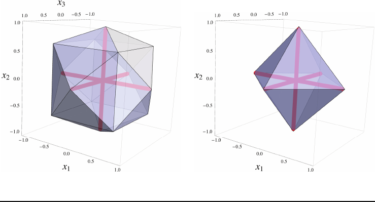
18 JUAN PABLO VIELMA
(a) LP relaxation of formulation (4.1) for n=3. (b) Convex Hull.
Fig. 4.1 Geometric view of formulation strength.
show that the n-dimensional form of these inequalities is
(4.2)
n
i=1
rixi≤1∀r∈ {−1,1}n,
and that for any n,
conv(S)=)x∈Qn:
n
i=1 |xj|≤1*={x∈Qn: (4.2)}.
Then, the formulation obtained by adding (4.2) to (4.1) is automatically sharp. How-
ever, formulation (4.1)–(4.2) has two problems. First, it is not locally ideal because,
for n=3,wehavethatx1=x2=y2=y3=1/2, x3=y1= 0 is an extreme point of
the LP relaxation of (4.1)–(4.2). Second, the formulation is extremely large, because
the number of linear inequalities described by (4.2) is 2n. Unfortunately, each one of
these inequalities defines a different facet of conv(S) and together they form a min-
imal representation of conv(S). Thus removing any of them destroys the sharpness
property. Fortunately, careful use of auxiliary variables yallows constructing a much
smaller and locally ideal formulation for S.
Example 3. A polynomial-sized sharp formulation for set Sin Example 2is
given by
−yi≤xi≤yi∀i∈{1,...,n},(4.3a)
n
i=1
yi=1,(4.3b)
yi≥0∀i∈{1,...,n},(4.3c)
y∈Zn.(4.3d)
Formulation (4.3) is locally ideal and can be constructed using a well-known LP
modeling trick or by using standard MIP formulation techniques (see Examples 6
MIXED INTEGER LINEAR PROGRAMMING FORMULATION TECHNIQUES 19
and 8). Formulation (4.3)’s only auxiliary variables are the binary variables that are
used to indicate which Picontains x. The following example shows that these binary
variables might not be enough to construct a polynomial-sized sharp formulation.
Example 4. For i∈{1,...,n},letvi,w
i∈Qnbe defined by
vi
j=)n, j =i,
−1,j=i, wi
j=)−1,j=i,
0,j=i,
for all j∈{1,...,n}. In addition, let v0,w
0∈Qnbe defined by v0
j=−w0
j=−1for
all j∈{1,...,n}.
Let S=(V×{0})∪(W×{1})⊆Qn+1,whereV=conv
vin
i=0and W=
conv win
i=0.Sand conv(S)are depicted for n=2in Figure 4.2,whereSis
shown in red and conv(S)is shown in blue. By noting that
V×{0}=⎧
⎨
⎩
x∈Qn+1 :xn+1 =0,
n
j=1
xj≤1,−xj≤1∀j∈{1,...,n}⎫
⎬
⎭
(4.4a)
and
W×{1}=⎧
⎪
⎪
⎪
⎪
⎪
⎨
⎪
⎪
⎪
⎪
⎪
⎩
x∈Qn+1 :
xn+1 =1,−
n
j=1
xj≤1,
(n+1)xi−
n
j=1
xj≤1∀i∈{1,...,n}
⎫
⎪
⎪
⎪
⎪
⎪
⎬
⎪
⎪
⎪
⎪
⎪
⎭
(4.4b)
we can check that a valid formulation of Sis given by
−xj≤1∀j∈{1,...,n},(4.5a)
n
j=1
xj≤1+(n−1)(1 −y1),(4.5b)
xn+1 =1−y1,(4.5c)
(n+1)xi−
n
j=1
xj≤1+(n2+n−2)(1 −y2)∀i∈{1,...,n},(4.5d)
−
n
j=1
xj≤1+(n−1)(1 −y2),(4.5e)
xn+1 =y2,(4.5f)
y1+y2=1,(4.5g)
y∈{0,1}2.(4.5h)
Now for n=3,x1=x2=−1,x3=0,andx4=y1=y2=1/2is feasible for the LP
relaxation of (6.8), but violates x1+x2−x4≥−2, which is a facet-defining inequality
of conv(S).
Although Figure 4.2 shows that conv(S) has few facets for small n, the following
lemma shows that the number of facets of conv(S) grows exponentially in n.Further-
more, the lemma shows that the two binary variables used by (4.5) are not enough
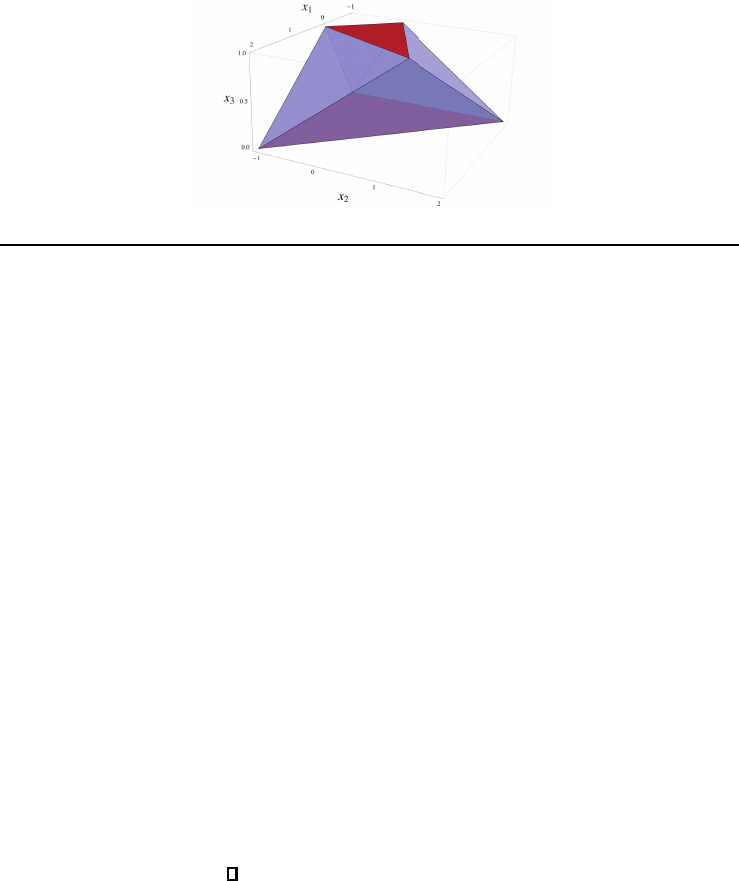
20 JUAN PABLO VIELMA
Fig. 4.2 Set for Example 4for n=2.
to yield a polynomial-sized sharp formulation even if a constant (independent of n)
number of additional auxiliary variables is used.
Lemma 4.1. Let Sbe the set defined in Example 4. Then the number of facets
of conv(S)grows exponentially in n. Furthermore, there is no sharp formulation of
Sof the form
Ax +Bλ +Dy ≤b, x ∈Qn+1,λ∈Qk,y∈Z2,
where A∈Qp(n)×(n+1),B∈Qp(n)×k,D∈Qp(n)×2,andb∈Qp(n)for some polyno-
mial pand a constant k∈Z+independent of n.
Proof. To prove the first statement we note that Vand Ware two n-dimensional
simplicies that are dual to each other. Then, conv(S)istheantiprism of V[28] and V
satisfies the conditions for Theorem 2.1 in [28]. Hence, by this theorem, the number
of facets of conv(S) is exactly two more than the number of proper faces of V.The
number of proper faces of an n-dimensional simplex is n−1
i=0 n+1
i+1 =2
n+1 −2[63],
so we conclude that the number of facets of conv(S) is precisely 2n+1.
For the second statement we note that by Propositions 3.11 and 3.13 the number
of facets of the projection of the LP relaxation of the proposed formulation onto the
xvariables is at most the number of extreme rays of cone
+μ∈Qp(n)
+:DTμ=0,B
Tμ=0
,.
By Lemma 3.5, the number of extreme rays of this cone is at most p(n)
p(n)−3−k,which
is also a polynomial. Hence, no formulation of this form can have an LP relaxation
that projects to conv(S).
Fortunately, by allowing a growing number of auxiliary variables, the following
proposition by Balas, Jeroslow, and Lowe [13, 90, 113] yields polynomial-sized formu-
lations for a wide range of disjunctive constraints that include the set in Example 4.
We postpone the proof of this proposition to section 5.1, where we consider a slightly
more general version of this formulation.
Proposition 4.2. Let Pik
i=1 be a finite family of polyhedra with a common
recession cone (i.e., Pi
∞=Pj
∞for all i, j), such that Pi=x∈Qn:Aix≤bifor
all i. Then, a locally ideal MIP formulation of S=k
i=1 Piis given by
Aixi≤biyi∀i∈{1,...,k},(4.6a)
k
i=1
xi=x,(4.6b)
MIXED INTEGER LINEAR PROGRAMMING FORMULATION TECHNIQUES 21
k
i=1
yi=1,(4.6c)
yi≥0∀i∈{1,...,k},(4.6d)
xi∈Qn∀i∈{1,...,k},(4.6e)
y∈Zk.(4.6f)
Example 5. Using formulation (4.6) for characterization (4.4) of set Sin Ex-
ample 4results in the following polynomial-sized sharp (and locally ideal) formulation
that uses a linear number of additional continuous auxiliary variables:
x1
n+1 =0,(4.7a)
n
j=1
x1
j≤y1,(4.7b)
−x1
i≤y1∀i∈{1,...,n},(4.7c)
x2
n+1 =y2,(4.7d)
−
n
j=1
x2
j≤y2,(4.7e)
(n+1)x2
i−
n
j=1
x2
j≤y2∀i∈{1,...,n},(4.7f)
xi=x1
i+x2
i∀i∈{1,...,n+1},(4.7g)
y1+y2=1,(4.7h)
y∈{0,1}2,(4.7i)
x1,x
2∈Qn+1,(4.7j)
x∈Qn+1.(4.7k)
The use of a growing number of auxiliary variables in Proposition 4.2 and similar
techniques allows the construction of polynomial-sized sharp extended formulations
for a wide range of sets. However, there are cases in which these formulations cannot
be constructed. Most examples of sets that do not have polynomial-sized extended
formulations arise from intractable combinatorial optimization problems (e.g., the
traveling salesman problem considered in [53]). However, the following recent result by
Rothvoß [140] shows that this can also happen for polynomially solvable combinatorial
optimization problems.
Theorem 4.3. Let G=(V, E)be the complete graph on |V|=nnodes where
V={1,...,n}and E={{i, j}:i, j ∈{1,...,n},i=j}.LetSbe the set of
incident vectors of perfect matchings of Ggiven by
(4.8) S:= ⎧
⎨
⎩
x∈{0,1}E:
j∈{1,...,n}\{i}
x{i,j}=1 ∀i∈{1,...,n}⎫
⎬
⎭
.
If nis even, then there is no polynomial-sized sharp extended formulation for S.
The proof techniques used to show results such as Theorem 4.3 are significantly
more elaborate than those used in Lemma 4.1 and are beyond the scope of this survey.
We refer the reader interested in these techniques to [53, 140] and their references and
to [35, 95].
22 JUAN PABLO VIELMA
5. Basic Extended Formulations. Disjunctive constraints can model a wide
range of logical constraints. However, there are other aspects of MIP formulations
that are generally encountered in practice, such as feasible regions of knapsacks or
other problems with general integer variables. One class of sets that combines these
two aspects is that of the unions of mixed integer sets of the form
(5.1) S=
k
i=1
Pi∩(Qn1×Zn2),
where Pik
i=1 is a finite family of polyhedra with a common recession cone. Hooker
[76] showed that such sets can be modeled through a simple extension of formulation
(4.6). Hooker also showed that this extension is sharp if the formulations of these
mixed integer sets are sharp (i.e., if Pi=convPi∩(Qn1×Zn2)). However, achiev-
ing this could require a large number of inequalities in the descriptions of the Pis.
Fortunately, as noted in [37], we may significantly reduce the number of inequalities
by using auxiliary variables in the description of Pi. This results in the following
generalization of formulation (4.6) that also yields a locally ideal or sharp formulation
when locally ideal or sharp extended formulations of Pi∩(Qn1×Zn2)areused.
Proposition 5.1. Let Pik
i=1 be a finite family of polyhedra with a common
recession cone (i.e., Pi
∞=Pj
∞for all i, j ∈{1,...,k})andp∈Zk
+be such that
Pi=x∈Qn:∃w∈Qpis.t. (x, w)∈Qi,where
Qi=(x, w)∈Qn×Qpi:Aix+Diw≤bi
for Ai∈Qmi×n,Di∈Qmi×pi,andbi∈Qmifor each i∈{1,...,k}. Then, for any
n1,n
2∈Z+such that n=n1+n2, an MIP formulation of S=k
i=1 Pi∩(Qn1×Zn2)
is given by
Aixi+Diwi≤biyi∀i∈{1,...,k},(5.2a)
k
i=1
xi=x,(5.2b)
k
i=1
yi=1,(5.2c)
yi≥0∀i∈{1,...,k},(5.2d)
xi∈Qn∀i∈{1,...,k},(5.2e)
wi∈Qpi∀i∈{1,...,k},(5.2f)
y∈Zk,(5.2g)
x∈Qn1×Zn2.(5.2h)
Furthermore, if Pi=conv
Pi∩(Qn1×Zn2)for all i∈{1,...,k},then(5.2) is
sharp, and if ext Qi⊆Qn1×Zn2×Qpifor all i∈{1,...,k},then(5.2) is locally
ideal.
Proof. For validity of (5.2), without loss of generality, assume y1=1andyi=0
for all i≥2. Then x1∈P1and by Proposition 3.11 we have that xi∈Pi
∞for all
i≥2. Then by the common recession cone assumption we have xi∈P1
∞for all i≥2
and hence x∈P1.

MIXED INTEGER LINEAR PROGRAMMING FORMULATION TECHNIQUES 23
To prove sharpness let (x, w, y) be feasible for the LP relaxation of (5.2) and
I={i∈{1,...,k}:yi>0}.Thenx=i∈Iyixi/yi,i∈Iyi=1,y≥0, and
xi/yi,w
i/yi∈Qifor all i∈I. By the assumption on Piwe then have that
xi/yi∈conv Pi∩(Qn1×Zn2)and hence
x∈conv k
i=1
conv Pi∩(Qn1×Zn2)=convk
i=1
Pi∩(Qn1×Zn2)=conv(S).
To prove locally idealness first note that if (x, w, y)isanextremepointoftheLP
relaxation of (5.2) and y∈{0,1}k, we may again assume without loss of generality
that y1=1andyi=0foralli≥2. Then by extremality of (x, w, y)wehave
that xi=0andwi=0foralli≥2, x=x1,andx1,w
1∈ext Q1. Then, by
the assumption on Q1we have x=x1∈Qn1×Zn2and hence (x, w, y) satisfies the
integrality constraints. To finish the proof, assume for a contradiction that (x, w, y)
is an extreme point of the LP relaxation of (5.2) such that y/∈{0,1}k. Without loss
of generality we may assume that y1,y
2∈(0,1). Let ε=min{y1,y
2,1−y1,1−y2}∈
(0,1),
yi=⎧
⎪
⎨
⎪
⎩
yi+ε, i =1,
yi−ε, i =2,
yi,otherwise,
yi=⎧
⎪
⎨
⎪
⎩
yi−ε, i =1,
yi+ε, i =2,
yiotherwise.
xi=(yi/yi)xi,wi=(yi/yi)wi,xi=(yi/yi)xi,andwi=(yi/yi)wifor i∈{1,2},
xi=xi=xiand wi=wi=wifor all i/∈{1,2},x=k
i=1 xi,andx=k
i=1 xi.Then
(x,w,y)=(x, w, y), (x, w, y)=(1/2)(x,w,y)+(1/2)(x, w, y), and (x,w,y),(x, w, y)
are feasible for the LP relaxation of (5.2), which contradicts (x, w, y) being an extreme
point.
Formulation 5.2 can be used to construct several known formulations for piecewise
linear functions and more general disjunctive constraints. The following proposition
illustrates this by constructing a variant of (5.2) that is convenient when Piare
described through their extreme points and rays. The resulting formulation is a
straightforward extension of a formulation for disjunctive constraints introduced by
Jeroslow and Lowe [90, 113].
Corollary 5.2. Let Pik
i=1 ⊆Qnbe a finite family of polyhedra with a com-
mon recession cone C. Then, for any n1,n
2∈Z+such that n=n1+n2,anMIP
formulation of S=k
i=1 Pi∩(Qn1×Zn2)is given by
k
i=1
v∈ext(Pi)
vλi
v+
r∈ray(C)
rμr=x,(5.3a)
v∈ext(Pi)
λi
v=yi∀i∈{1,...,k},(5.3b)
k
i=1
yi=1,(5.3c)
λi
v≥0∀i∈{1,...,k},v∈ext Pi,(5.3d)
μr≥0∀r∈ray(C),(5.3e)
y∈{0,1}k,(5.3f)
x∈Qn1×Zn2.(5.3g)
24 JUAN PABLO VIELMA
Furthermore, if Pi=conv
Pi∩(Qn1×Zn2)for all i∈{1,...,k},then(5.3) is a
locally ideal formulation of S.
Proof. By Theorem 3.6 we have that Piis the projection onto the xvariables
of
Qi=
⎧
⎪
⎪
⎪
⎪
⎪
⎪
⎪
⎪
⎨
⎪
⎪
⎪
⎪
⎪
⎪
⎪
⎪
⎩
(x, μ, λ)∈Qn×Qray(C)×Qext(Pi):
v∈ext(Pi)
vλv+
r∈ray(C)
rμr=x
v∈ext(Pi)
λv=1
λv≥0∀v∈ext Pi
μr≥0∀r∈ray (C)
⎫
⎪
⎪
⎪
⎪
⎪
⎪
⎪
⎪
⎬
⎪
⎪
⎪
⎪
⎪
⎪
⎪
⎪
⎭
for all i∈{1,...,k}. Using these extended formulations of the Qiswehavethat
formulation (5.2) for Sis given by
v∈ext(Pi)
vλi
v+
r∈ray(C)
rμi
r=xi∀i∈{1,...,k},(5.4a)
v∈ext(Pi)
λi
v=yi∀i∈{1,...,k},(5.4b)
k
i=1
xi=x,(5.4c)
k
i=1
yi=1,(5.4d)
λi
v≥0∀i∈{1,...,k},v∈ext Pi,(5.4e)
μi
r≥0∀i∈{1,...,k},r∈ray (C),(5.4f)
yi≥0∀i∈{1,...,k},(5.4g)
xi∈Qn∀i∈{1,...,k},(5.4h)
λi∈Qext(Pi)∀i∈{1,...,k},(5.4i)
μi∈Qray(C)∀i∈{1,...,k},(5.4j)
y∈Zk,(5.4k)
x∈Qn1×Zn2.(5.4l)
We claim that the LP relaxation of (5.3) is equal to the image of the LP relaxation
of (5.4) through the linear transformation that projects out the xiand μivariables
and lets μ=k
i=1 μi. We first show that the LP relaxation of (5.3) is contained
in the image of the LP relaxation of (5.4). For this, simply note that any point in
the LP relaxation of (5.3) is the image of the point in the LP relaxation of (5.4)
obtained by letting xi=v∈ext(Pi)vλi
v+(1/k)r∈ray(C)rμrand μi
r=(1/k)μr
for all i∈{1,...,k}and r∈ray (C). The reverse containment is straightforward.
Validity then follows directly from Proposition 5.1.
For locally idealness note that by Proposition 2.5 and the assumption on Piwe
have that ext Pi⊆Qn1×Zn2.Bynotingthat(x, μ, λ)∈ext Qiif and only
if x∈ext Pi,μ=0,λx=1,andλv=0forv∈ext Pi\{x},wehavethat
ext Qi⊆Qn1×Zn2×Qray(C)×Qext(Pi). Then by Proposition 5.1 we have that (5.4)

MIXED INTEGER LINEAR PROGRAMMING FORMULATION TECHNIQUES 25
is locally ideal and hence so is (5.3) by Proposition 3.10 and the linear transformation
described in the previous paragraph.
To distinguish extreme point/ray formulation (5.3) from inequality formulation
(5.2), we refer to the first one as the V-formulation and to the second as the H-
formulation. While V-formulation (5.3) can be derived from H-formulation (5.2),
their application to specific disjunctive constraints can yield formulations with very
different structures. The following two examples illustrate this for the case n2=0in
both formulations and pi=0foralli∈{1,...,k}in Proposition 5.1.
Example 6. Consider the set S=n
i=1 {x∈Qn:−1≤xi≤1,x
j=0∀j=i}
from Example 2.H-formulation (5.2) for Sis given by
−yi≤xi
i≤yi∀i∈{1,...,n},(5.5a)
xj
i=0 ∀i, j ∈{1,...,n},i =j,(5.5b)
n
i=1
yi=1,(5.5c)
xi=
n
j=1
xj
i∀i∈{1,...,n},(5.5d)
y∈{0,1}n.(5.5e)
Similarly to the proof of Proposition 5.1, we can show that the projection of (5.5) onto
the xand yvariables is precisely formulation (4.3) from Example 3, which is given
by
−yi≤xi≤yi∀i∈{1,...,n},(5.6a)
n
i=1
yi=1,(5.6b)
yi≥0∀i∈{1,...,n},(5.6c)
y∈Zn.(5.6d)
If we instead use V-formulation (5.3), we obtain the alternative formulation of Sgiven
by
λi
1−λi
2=xi∀i∈{1,...,n},(5.7a)
λi
1+λi
2=yi∀i∈{1,...,n},(5.7b)
n
i=1
yi=1,(5.7c)
λi
1,λ
i
2≥0∀i∈{1,...,n},(5.7d)
y∈{0,1}n.(5.7e)
It is interesting to contrast formulations (5.6) and (5.7). We know that conv(S)=
{x∈Qn:n
i=1|xi|≤1}and that both formulations are sharp. Hence the LP
relaxations of both formulations should contain lifted representations of n
i=1|xi|≤
1.H-formulation (5.6) does this using the standard trick of modeling |xi|≤yias
−yi≤xi≤yi,whileV-formulation (5.7) does it by the alternative trick of modeling
|xi|≤yias xi=λi
1−λi
2,λi
1+λi
2=yi,andλi
1,λ
i
2≥0. The latter trick uses the fact
that x=x+−x−and |x|=x++x−,wherex+:= max{x, 0}and x−:= {−x, 0}.
26 JUAN PABLO VIELMA
Example 7. Let f:D⊆Qd→Qbe a piecewise linear function defined by (3.3)
for a given finite family of polytopes {Qi}k
i=1. Formulation (5.2) for characterization
(3.4a) of gr(f)results in the MIP formulation of gr(f)given by
z=
k
i=1
zi,(5.8a)
zi=mixi+ci,(5.8b)
x=
k
i=1
xi,(5.8c)
Aixi≤yibi∀i∈{1,...,k},(5.8d)
k
i=1
yi=1,(5.8e)
y∈{0,1}k.(5.8f)
If we replace (5.8a) and (5.8b) in (5.8) by
(5.9) z=
k
i=1
mixi+ci,
we obtain a standard MIP formulation for piecewise linear functions that is denoted
the multiple choice model in [155]. Similarly to the proof of Proposition 5.1,wecan
show that the multiple choice model is the projection onto the x,xi,y,andzvariables
of (5.8). If we instead use formulation (5.3) for characterization (3.4b) of gr(f),we
obtain the formulation of gr(f)given by
k
i=1
v∈ext(Qi)
vλi
v=x,(5.10a)
k
i=1
v∈ext(Qi)
f(v)λi
v=z,(5.10b)
v∈ext(Qi)
λi
v=yi∀i∈{1,...,k},(5.10c)
k
i=1
yi=1,(5.10d)
λi
v≥0∀i∈{1,...,k},v∈ext Qi,(5.10e)
y∈{0,1}k,(5.10f)
which is a standard MIP formulation for piecewise linear functions that is denoted the
disaggregated convex combination model in [155].
For examples of formulation (5.2) with pi>0andn2>0 we refer the reader to
[37] and [76], respectively.
6. Projected Formulations. One disadvantage of basic formulations (5.2) and
(5.4) is that they require multiple copies of the original xvariables (i.e., the xivari-
ables) or of some auxiliary variables (i.e., the λivariables). In this section we study
formulations that do not use these copies of variables and are hence much smaller.
The cost of this reduction in variables is usually a loss of strength, but it some cases

MIXED INTEGER LINEAR PROGRAMMING FORMULATION TECHNIQUES 27
this loss can be avoided. We begin by considering the well-known Big-M approach
and an alternative formulation that combines the Big-M approach with a formulation
tailored to polyhedra with a common structure. We then consider the strength of
both classes of formulations in detail.
6.1. Traditional Big-M Formulations. One way to write MIP formulations with-
out using copies of the original variables is to use the Big-M technique. The following
proposition proven in [164] for the bounded case and in [76] for the unbounded de-
scribes the technique.
Proposition 6.1. Let Pik
i=1 be a finite family of polyhedra with a common
recession cone (i.e., Pi
∞=Pj
∞for all i, j), such that Pi=x∈Qn:Aix≤bi,
where Ai∈Qmi×nand bi∈Qmifor all i∈{1,...,k}. Furthermore, for each
i, j ∈{1,...,k},i=j,andl∈{1,...,m
i},letMi,j
l∈Qbe such that
(6.1) Mi,j
l≥max
xai,lx:Ajx≤bj,
where ai,l ∈Qnis the lth row of Ai. Then, for any n1,n
2∈Z+such that n=n1+n2,
an MIP formulation for S=k
i=1 Pi∩(Qn1×Zn2)is given by
Aix≤bi+Mi−bi(1 −yi)∀i∈{1,...,k},(6.2a)
k
i=1
yi=1,(6.2b)
yi≥0∀i∈{1,...,k},(6.2c)
y∈Zk,(6.2d)
x∈Qn1×Zn2,(6.2e)
where Mi∈Qmiare such that Mi
l=max
j=iMi,j
lfor each l∈{1,...,m
i}.
Proof.IfallMi,j
lare finite, validity of the formulation is straightforward. To
show their finiteness, assume for a contradiction that for a given i,j,andlthe left-
hand side of (6.1) is infinite. The unboundedness of this LP problem is equivalent to
the existence of an r∈Pj
∞=x∈Qn:Ajx≤0such that ai,lr>0 [21, Theorem
4.13]. However, by the assumption on the recession cones, such an ris also in Pi
∞
and hence the LP problem given by maxxai,lx:Aix≤biis unbounded, which
contradicts bi
lbeing finite.
The strongest possible version of formulation (6.2) is obtained when equality holds
in (6.1), which, as illustrated in the following example, can sometimes yield sharp or
locally ideal formulations.
Example 8. Consider the set Sfrom Example 2, which corresponds to the case
Ai=[ I
−I]∈Q2n×nand
bi
l=)1,l∈{i, k +i},
0otherwise
for all i, l ∈{1,...,k},andn2=0. A valid Big-M selection is to take Mi
l=1for all
i, l ∈{1,...,k}. For this choice, (6.2) is equal to the nonsharp formulation (4.1).In
contrast, the strongest choice of Migiven by
Mi
l=)0,l∈{i, k +i},
1otherwise
yields locally ideal formulation (4.3).
28 JUAN PABLO VIELMA
Unfortunately, as the following example shows, even the strongest version of (6.2)
can fail to be sharp.
Example 9. The strongest version of formulation (6.2) for Sfrom Example 4is
precisely the nonsharp formulation (4.5).
For more discussion about Big-M formulations for general and specially structured
sets, we refer the reader to [18, 76, 79, 164].
6.2. Hybrid Big-M Formulations. A different class of projected formulations was
introduced by Balas, Blair, and Jeroslow [12, 26, 87] for families of polyhedra with
a common left-hand side matrix (i.e., where Ai=Ajfor all i, j). Balas, Blair, and
Jeroslow showed that such formulations can have very favorable strength properties.
However, while the common left-hand side structure appears in many problems (see
Example 10), these formulations still have more limited applicability than the tra-
ditional Big-M formulation from Proposition 6.1. For this reason we here combine
the projected formulation of Balas, Blair, and Jeroslow with the traditional Big-M
formulation to introduce the following hybrid Big-M formulation that generalizes the
former and improves upon the latter. While this formulation does not require the
common left-hand side structure, it is equipped to exploit it when present.
Proposition 6.2. For k∈Zp
+,letp
s=1 Ps,iks
i=1 be a finite family of polyhedra
with a common recession cone (i.e., Ps,i
∞=Pt,j
∞for all s, t, i, j) such that
Ps,i =x∈Qn:Asx≤bs,i,
where As∈Qms×nand bs,i ∈Qmsfor each s∈{1,...,p}and i∈{1,...,k
s}.
Furthermore, for each s, t ∈{1,...,p},i∈{1,...,k
s},andl∈{1,...,m
s},let
Ms,t,i
l∈Qbe such that
(6.3) Ms,t,i
l≥max
xas,lx:Atx≤bt,i,
where as,l ∈Qnis the lth row of As. Then, for any n1,n
2∈Z+such that n=n1+n2,
an MIP formulation for S=p
s=1 ks
i=1 Ps,i ∩(Qn1×Zn2)is given by
Asx≤
p
t=1
kt
i=1
Ms,t,iyt,i ∀s∈{1,...,p},(6.4a)
p
s=1
ks
i=1
ys,i =1,(6.4b)
ys,i ≥0∀s∈{1,...,p},i∈{1,...,k
s},(6.4c)
ys,i ∈Z∀s∈{1,...,p},i∈{1,...,k
s},(6.4d)
x∈Qn1×Zn2.(6.4e)
In particular, we may take Ms,s,i =bs,i for all s∈{1,...,p},i∈{1,...,k
s}.
Validity of this formulation is again straightforward from finiteness of the Ms,t,i
l,
which can be proven analogously to Proposition 6.1. Furthermore, the strongest
possible version of formulation (6.4) is again obtained when equality holds in (6.3).
In particular, Ms,s,i =bs,i is the strongest possible coefficient unless some Ps,i has
a redundant constraint. Of course, even in the case of a redundant constraint, it is
always valid and convenient to use Big-M constants such that Ms,s,i ≤bs,i.Forthis
reason, we assume this to be the case from now on.
MIXED INTEGER LINEAR PROGRAMMING FORMULATION TECHNIQUES 29
Hybrid Big-M formulation (6.4) reduces to the formulation introduced by Balas,
Blair, and Jeroslow when all left-hand side matrices are identical (i.e., for p=1),and
we take Ms,s,i =bs,i for all i. An advantage of this formulation is that it can be
constructed without solving or bounding any LP problem in (6.3). In what follows
we refer to this formulation as the simple version of (6.4). An example of what can
be modeled with this simple version of the hybrid Big-M formulation is the following
class of problem that includes the SOS1 and SOS2 constraints introduced by Beale
and Tomlin [17].
Example 10. For given lik
i=1 ,uik
i=1 ⊆{0,1}n, consider the family of poly-
topes Pi:= x∈Qn:li
j≤xj≤ui
j∀j∈{1,...,n}for i∈{1,...,k}and its union
S=k
i=1 Pi. For instance, if we let li
j=0for all i, j and k=nand
ui
j=)1,j=i,
0otherwise
or k=n−1and
ui
j=)1,j∈{i, i +1},
0otherwise,
we have that Scorresponds, respectively, to the SOS1and SOS2constraints introduced
by Beale and Tomlin [17]. For the cases of SOS1and SOS2constraints, formula-
tion (6.4) with p=1reduces, respectively, to
0≤xi≤yi∀i∈{1,...,k},
k
i=1
yi=1,
y∈{0,1}k,
and
0≤x1≤y1,
0≤xi≤yi−1+yi∀i∈{2,...,k},
0≤xk+1 ≤yk,
k
i=1
yi=1,
y∈{0,1}k,
which are the standard MIP formulations for such constraints.
We end this section by showing how the simple version of hybrid big-M formu-
lation (6.4) can be used to obtain a smaller version of V-formulation (5.3). This
results in the extension of a known formulation for piecewise linear functions (e.g.,
[45, 91, 113, 106, 165]).
Corollary 6.3. Let Pik
i=1 ⊆Qnbe a finite family of polyhedra with a common
recession cone Cand V:= k
i=1 ext Pi. Then, for any n1,n
2∈Z+such that
n=n1+n2, two MIP formulations of S=k
i=1 Pi∩(Qn1×Zn2)are given by
v∈V
vλv+
r∈ray(C)
rμr=x,(6.5a)
30 JUAN PABLO VIELMA
v∈V
λv=1,(6.5b)
λv≤
i:v∈ext(Pi)
yi∀v∈V,(6.5c)
k
i=1
yi=1,(6.5d)
λv≥0∀v∈V,(6.5e)
μr≥0∀r∈ray(C),(6.5f)
y∈{0,1}k,(6.5g)
x∈Qn1×Zn2,(6.5h)
and
v∈V
vλv+
r∈ray(C)
rμr=x,(6.6a)
v∈V
λv=1,(6.6b)
v∈ext(Pi)
λv≥yi∀i∈{1,...,k},(6.6c)
k
i=1
yi=1,(6.6d)
λv≥0∀v∈V,(6.6e)
μr≥0∀r∈ray(C),(6.6f)
y∈{0,1}k,(6.6g)
x∈Qn1×Zn2.(6.6h)
Furthermore, if Pi=convPi∩(Qn1×Zn2)for all i∈{1,...,k}, then both formu-
lations are sharp.
Proof. Let
Qi=
⎧
⎪
⎪
⎪
⎪
⎪
⎪
⎪
⎪
⎪
⎪
⎪
⎪
⎪
⎨
⎪
⎪
⎪
⎪
⎪
⎪
⎪
⎪
⎪
⎪
⎪
⎪
⎪
⎩
(x, λ, μ)∈Qn×QV×Qray(C):
v∈V
vλv+
r∈ray(C)
rμr=x
v∈V
λv=1
λv≤1∀v∈ext Pi
λv≤0∀v∈V\ext Pi
λv≥0∀v∈V
μr≥0∀r∈ray(C)
⎫
⎪
⎪
⎪
⎪
⎪
⎪
⎪
⎪
⎪
⎪
⎪
⎪
⎪
⎬
⎪
⎪
⎪
⎪
⎪
⎪
⎪
⎪
⎪
⎪
⎪
⎪
⎪
⎭
.
Validity of (6.5) follows by noting that k
i=1 Piis the projection onto the xvariables
of k
i=1 Qiand that (6.5) is the simple version of (6.4) for k
i=1 Qi. Validity of (6.6)

MIXED INTEGER LINEAR PROGRAMMING FORMULATION TECHNIQUES 31
follows by noting that Qican be described alternatively as
Qi=
⎧
⎪
⎪
⎪
⎪
⎪
⎪
⎪
⎪
⎪
⎪
⎪
⎪
⎪
⎪
⎪
⎪
⎪
⎪
⎨
⎪
⎪
⎪
⎪
⎪
⎪
⎪
⎪
⎪
⎪
⎪
⎪
⎪
⎪
⎪
⎪
⎪
⎪
⎩
(x, λ, μ)∈Qn×QV×Qray(C):
v∈V
vλv+
r∈ray(C)
rμr=x
v∈V
λv=1
v∈ext(Pi)
λv≥1
v∈ext(Pj)
λv≥0∀j=i
λv≥0∀v∈V
μr≥0∀r∈ray(C)
⎫
⎪
⎪
⎪
⎪
⎪
⎪
⎪
⎪
⎪
⎪
⎪
⎪
⎪
⎪
⎪
⎪
⎪
⎪
⎬
⎪
⎪
⎪
⎪
⎪
⎪
⎪
⎪
⎪
⎪
⎪
⎪
⎪
⎪
⎪
⎪
⎪
⎪
⎭
.
For sharpness, note that the projection onto the xvariables of the LP relaxation
of both formulations is contained in conv (V)+C. The result then follows because,
under the assumption on Piand by Theorem 3.6, we have
conv(S)=convk
i=1
Pi∩(Qn1×Zn2)
=convk
i=1
conv Pi∩(Qn1×Zn2)
=convk
i=1
Pi
=convk
i=1
conv ext Pi+C
=convk
i=1
conv ext Pi+C
=convk
i=1
ext Pi+C=conv(V)+C.
While (6.5) and (6.6) are equivalent, their LP relaxations are not contained in one
another. Of course this can only happen because neither formulation is locally ideal.
In fact, Lee and Wilson [106, 165] show that constraints (6.6c) are valid inequalities for
the convex hull of integer feasible points of (6.5) and hence can be used to strengthen
it. These inequalities are sometimes facet defining and are part of a larger class
of inequalities that are enough to describe the convex hull of integer feasible points
of (6.5). Unfortunately, the number of such inequalities can be exponential in k.
However, in section 7 we show how an LP-based separation of these inequalities allows
us to construct a different formulation that ends up being equivalent to (5.3). If
we specialize formulation (6.5) to piecewise linear functions, we obtain the following
formulation from [106, 165].
Example 11. Let f:D⊆Qd→Qbe a piecewise linear function defined by (3.3)
for a given finite family of polytopes {Qi}k
i=1. Formulation (6.5) for characterization
32 JUAN PABLO VIELMA
(3.4b) of gr(f)results in the MIP formulation of gr(f)given by
v∈k
i=1 ext(Qi)
vλv=x,(6.7a)
v∈k
i=1 ext(Qi)
f(v)λv=z,(6.7b)
λv≤
i:v∈ext(Qi)
yi∀v∈
k
i=1
ext Qi,(6.7c)
k
i=1
yi=1,(6.7d)
λv≥0∀v∈ext Qi,(6.7e)
y∈{0,1}k,(6.7f)
which is a standard MIP formulation for piecewise linear functions that is denoted the
convex combination model in [155].
6.3. Formulation Strength. The traditional Big-M formulation has been signif-
icantly more popular than the simple version of the hybrid Big-M formulation. One
reason for this is the somewhat limited applicability of the latter formulation. The
general version of the hybrid Big-M formulation resolves this issue as it can be used in
the same class of problems as the traditional Big-M formulation. In addition, the hy-
brid Big-M formulation provides an advantage over the traditional one with respect to
size, even if only partial common left-hand side structure is present in the polyhedra.
Indeed, both formulations have the same number of variables, but the hybrid formu-
lation has 1 + p
s=1 msconstraints while the traditional one has 1 + p
s=1 ms×ks
constraints. Of course, such an advantage in size is meaningless if it is accompanied
by a significant reduction in strength. For this reason we now study the relative and
absolute strengths of these formulations. In particular, concerning the hybrid Big-
M formulation we show that it is always at least as strong as the traditional Big-M
formulation, that its simple version can be sharp and strictly stronger than the tra-
ditional formulation, but that even its strongest version can fail to be locally ideal
or sharp. We begin with the following proposition that shows that one case where
the hybrid and traditional formulations coincide is when Sis the union of only two
polyhedra.
Proposition 6.4. If Sis the union of two polyhedra whose description does not
include any redundant constraints, and equality is taken in (6.1) and (6.3), then the
LP relaxations of formulations (6.2) and (6.4) are equivalent.
Proof. For (6.2) the case of two polyhedra corresponds to k= 2, and in this case
(6.2a) is equal to
A1x≤b1+M1,2−b1(1 −y1),
A2x≤b2+M2,1−b2(1 −y2).
For (6.3) the case of two polyhedra corresponds to p=1andk1=2orp=2,k1=1,
and k2= 1. In the former case (6.4) is equal to
A1x≤M1,1,1y1+M1,1,2y2

MIXED INTEGER LINEAR PROGRAMMING FORMULATION TECHNIQUES 33
and the equivalence follows from y1+y2= 1 by noting that for this case A1=
A2,M1,2=M1,1,2=b2,andM2,1=M1,1,1=b1, because of the nonredundancy
assumption. In the latter, (6.4) is equal to
A1x≤M1,1,1y1+M1,2,1y2,
A2x≤M2,1,1y1+M2,2,1y2,
and the equivalence follows from y1+y2= 1 by noting that for this case M1,1,1=b1,
M2,2,1=b2,M1,2,1=M1,2,andM2,1,1=M2,1, because of the nonredundancy
assumption.
Unfortunately, as the following example shows, this equal strength can fail to
yield sharp formulations even for the case of equal left-hand side matrices and no
redundant constraints.
Example 12. For
A=⎡
⎢
⎢
⎢
⎢
⎣
101
−101
011
0−11
00−1
⎤
⎥
⎥
⎥
⎥
⎦
,b
1=⎛
⎜
⎜
⎜
⎜
⎝
1
1
2
2
0
⎞
⎟
⎟
⎟
⎟
⎠
,b
1=⎛
⎜
⎜
⎜
⎜
⎝
2
2
1
1
0
⎞
⎟
⎟
⎟
⎟
⎠
,
let P1={x∈Q3:Ax ≤b1}and P2={x∈Q3:Ax ≤b2}. The strongest versions
of formulations (6.2) and (6.4) for S=P1∪P2are equal to
Ax ≤b1+(1−y1)⎛
⎜
⎜
⎜
⎜
⎝
1
1
−1
−1
0
⎞
⎟
⎟
⎟
⎟
⎠
,(6.8a)
Ax ≤b2+(1−y2)⎛
⎜
⎜
⎜
⎜
⎝
−1
−1
1
1
0
⎞
⎟
⎟
⎟
⎟
⎠
,(6.8b)
y1+y2=1,(6.8c)
y∈{0,1}2.(6.8d)
Formulation (6.8) is not sharp because x1=x2=0,x3=3/2,y1=y2=1/2is
feasible for its LP relaxation and x3≤1for any x∈conv(S).
The lack of sharpness of formulation (6.8) in Example 12 can be corrected by
simply adding x3≤1, as conv(S) is exactly the projection of the LP relaxation of
(6.8) onto the xvariables plus this inequality. However, this correction cannot always
be done with a polynomial number of inequalities (e.g., see Lemma 4.1). Furthermore,
as the following theorem by Blair [26] shows, recognizing sharpness of even the simple
version of hybrid Big-M formulation (6.4) is hard.
Theorem 6.5. Let p=1and M1,1,i =b1,i for all i∈{1,...,k}in formulation
(6.4). Deciding whether the resulting formulation is sharp is NP-hard.
Fortunately, Balas, Blair, and Jeroslow gave some practical (but not exhaustive)
necessary and sufficient conditions for sharpness of the simple version of (6.4) [12,
26, 87]. An extremely useful example of such conditions is given by the following
proposition.
34 JUAN PABLO VIELMA
Definition 6.6. For b∈Qm,A∈Qm×n,andI⊆{1,...,m}such that |I|=n
and det(AI)=0,weletAI(bI) be the submatrix (subvector) of A(b)obtainedby
selecting only the rows (components) indexed by I.Wealsoletx(I,b)∈Qnbe the
unique solution to AIx=bI. That is, x(I,b)is the basic solution associated to basis
Ifor polyhedron {x∈Qn:Ax ≤b}.
Let Pik
i=1 be a finite family of H-polyhedra such that for each iwe have Pi:=
x∈Qn:Ax ≤bi. We say that Pik
i=1 have the same shape if for all I⊆
{1,...,m}such that |I|=nand det(AI)=0we have either xI,bi∈Pifor all i
or xI,bi/∈Pifor all i. In other words, polyhedra with a common structure have
the same shape if and only if for every basis the associated basic solution is feasible
for all polyhedra or is infeasible for all polyhedra.
Proposition 6.7. If p=1,polyhedraP1,ik
i=1 have the same shape, and
M1,1,i =b1,i for all i∈{1,...,k},then(6.4) is sharp.
One case in which these shape conditions hold are the sets in Example 10, as
the polyhedra considered are all rectangles (possibly degenerate ones). In particular,
this partially explains the success of the standard formulations for SOS1 and SOS2
constraints and gives an alternative proof of the sharpness of formulation (4.3) in
Example 3.
Unfortunately, as the following example shows, the shape condition does not
necessarily imply that formulation (6.4) is locally ideal.
Example 13. Let
A=
⎡
⎢
⎢
⎢
⎢
⎢
⎢
⎢
⎢
⎢
⎢
⎢
⎢
⎢
⎢
⎣
1111
−1−1−1−1
1000
0100
0010
0001
−10 0 0
0−10 0
00−10
000−1
⎤
⎥
⎥
⎥
⎥
⎥
⎥
⎥
⎥
⎥
⎥
⎥
⎥
⎥
⎥
⎦
,b
1=
⎛
⎜
⎜
⎜
⎜
⎜
⎜
⎜
⎜
⎜
⎜
⎜
⎜
⎜
⎜
⎝
1
−1
1
1
0
0
0
0
0
0
⎞
⎟
⎟
⎟
⎟
⎟
⎟
⎟
⎟
⎟
⎟
⎟
⎟
⎟
⎟
⎠
,b
2=
⎛
⎜
⎜
⎜
⎜
⎜
⎜
⎜
⎜
⎜
⎜
⎜
⎜
⎜
⎜
⎝
1
−1
0
1
1
0
0
0
0
0
⎞
⎟
⎟
⎟
⎟
⎟
⎟
⎟
⎟
⎟
⎟
⎟
⎟
⎟
⎟
⎠
,b
3=
⎛
⎜
⎜
⎜
⎜
⎜
⎜
⎜
⎜
⎜
⎜
⎜
⎜
⎜
⎜
⎝
1
−1
0
0
1
1
0
0
0
0
⎞
⎟
⎟
⎟
⎟
⎟
⎟
⎟
⎟
⎟
⎟
⎟
⎟
⎟
⎟
⎠
,
and Pi={x∈Q4:Ax ≤bi}for i∈{1,...,3}. These polyhedra satisfy the shape
condition of Proposition 6.7 and hence the associated version of formulation (6.4) is
sharp. However, we can check that x3=x4=1/2,x1=x2=0,y1=y3=1/2,
and y2=0is a fractional extreme point of the LP relaxation of (6.4) and hence the
formulation is not locally ideal. Finally, note that this formulation is precisely parts
(2.5c)–(2.5k) of the standard formulation (2.5) for piecewise linear functions, we saw
in section 2.1.
Nevertheless, Proposition 6.7 can still be used to construct the following example
that shows how simple hybrid Big-M formulation (6.4) can be strictly stronger than
big-M formulation (6.2).
Example 14. Let k=n−1and uik
i=1 ⊆{0,1}nbe such that
ui
j=)1,j∈{i, i +1},
0otherwise,
and let Pi:= x∈Qn:0≤xj≤ui
j∀j∈{1,...,n}for i∈{1,...,k}.Formula-
MIXED INTEGER LINEAR PROGRAMMING FORMULATION TECHNIQUES 35
tion (6.4) for S:= n
i=1 Pireduces to
x1≤y1,(6.9a)
xi≤yi−1+yi∀i∈{2,...,k},(6.9b)
xk+1 ≤yk,(6.9c)
k
i=1
yi=1,(6.9d)
y∈{0,1}k,(6.9e)
and the strongest version of Big-M formulation (6.2) for Sreduces to
x1≤y1,(6.10a)
xj≤1−yi∀j∈{1,...,k+1},i∈{1,...,k}\{j−1,j},(6.10b)
xk+1 ≤yk,(6.10c)
k
i=1
yi=1,(6.10d)
y∈{0,1}k.(6.10e)
Lemma 6.8. Hybrid Big-M formulation (6.9) is always sharp, while traditional
Big-M formulation (6.10) is not sharp for k≥4.
Proof. The first formulation is sharp by Proposition 6.7.
For the lack of sharpness of the second formulation, note that x1=xk+1 =1/k,
xj=(k−1)/k for j∈{2,...,k},andyi=1/k for i∈{1,...,k}is feasible for its LP
relaxation.
For k≥4 this solution is not in conv(S) and hence this Big-M formulation is not
sharp (e.g., note that this xdoes not belong to the projection of the LP relaxation of
(6.9) onto the xvariables).
Finally, the following proposition shows that the hybrid formulation is always at
least as strong as the traditional formulation if equivalent Big-M constants are used.
Proposition 6.9. If the Big-M constants in (6.1) and (6.3) are identical and
such that Ms,s,i ≤bs,i, then hybrid Big-M formulation (6.4) is at least as strong as
traditional Big-M formulation (6.2).
Proof. Using the notation of formulation (6.4) (i.e., accounting for the possible
common left-hand side matrices), (6.2a) from the traditional Big-M formulation is
equal to
Asx≤bs,i +Ms,i −bs,i(1 −ys,i)∀s∈{1,...,p},i∈{1,...,k
s},
where Ms,i
l=max
t∈{1,...,p},j∈{1,...,kt},(t,j)=(s,i)Ms,t,j
l. Using the fact that in this case
(6.2b) is equal to p
s=1 ks
i=1 ys,i = 1, we can rewrite this equation as
Asx≤bs,iys,i +
t∈{1,...,p},
j∈{1,...,kt}
(t,j)=(s,i)
Ms,iyt,i ∀s∈{1,...,p},i∈{1,...,k
s}.
The result then follows from assumption Ms,s,i ≤bs,i and because, by definition,
Ms,i ≥Ms,t,i.

36 JUAN PABLO VIELMA
Proposition 6.9 and the formulation sizes suggest that, at least from a theoretical
perspective, hybrid Big-M formulation (6.4) is always preferable to traditional Big-
M formulation (6.2). This theoretical advantage often results in a computational
advantage [156]. However, the complexities of state-of-the-art solvers could still allow
the traditional formulation to outperform the hybrid one, particularly when the size
and strength differences are small.
7. Large Formulations. The aim of the techniques reviewed in this survey is
to construct strong, but small MIP formulations. However, there are many cases in
which all known MIP formulations (strong or weak) are large. If these formulations
are such that the number of variables is small and the number of constraints is large,
but can be separated fast, it is sometimes possible to use them in a branch-and-
cut procedure [131, 39, 128]. Similarly, when only the number of variables is large,
the formulations can be used in column generation or branch-and-price procedures
[15]. These procedures can be very effective and so can extensions such as branch-
and-cut-and-price [48] and branch-and-price for extended formulations [142]. For this
reason, when both large and small (usually extended) formulations are available it is
not always clear which is more convenient. Sometimes it is advantageous to solve the
large formulation with one of these specialized procedures [40, 50, 32], and other times
it is more convenient to solve the small extended formulation directly [31]. Exploring
these alternatives is beyond the scope of this survey, so in this section we restrict
our attention to one class of large formulations from which alternative small extended
formulations can be easily constructed. Such a construction was introduced by Martin
[115] (see also [30]) and can be summarized in the following proposition.
Proposition 7.1. Let Q:= {x∈Qn:Ax ≤b, Dx ≤d}and suppose there is a
separation LP problem for R:= {x∈Qn:Dx ≤d}. That is, there exist F∈Qr×n,
H∈Qr×m,c∈Qm,andg∈Qrfor which the LP problem given by
z(x) :=max
n
i=1
xiπi+
m
j=1
cjρj,(7.1a)
Fπ+Hρ ≤g,(7.1b)
ρj≥0∀j∈{1,...,m},(7.1c)
is such that x∈Rif and only if z(x)≤0. Then an extended LP formulation of Qis
given by
Ax ≤b,(7.2a)
FTw=x,(7.2b)
HTw≥c,(7.2c)
gTw≤0,(7.2d)
wj≥0∀j∈{1,...,r}.(7.2e)
If Qis the LP relaxation of an MIP formulation such that Rhas a large number
of constraints but a small separation LP problem, we can replace Dx ≤dwith (7.2b)–
(7.2e) to obtain a smaller extended formulation. Proposition 7.1 was used by Lee and
Wilson in [106, 165] to obtain an extended formulation that strengthens (6.5) and
(6.6). To describe this approach we need the following proposition from [106, 165].
For simplicity, we concentrate on formulation (6.5) for n2=0,whichwerestatein
the proposition for convenience.

MIXED INTEGER LINEAR PROGRAMMING FORMULATION TECHNIQUES 37
Proposition 7.2. Let Pik
i=1 ⊆Qnbe a finite family of polyhedra with a com-
mon recession cone C,ext Pibe the finite sets of extreme points of polyhedron Pi,
ray(C)be the finite set of extreme rays of polyhedral cone C,andV:= k
i=1 ext Pi.
Then S=k
i=1 Pican be modeled with formulation (6.5) given by
v∈V
vλv+
r∈ray(C)
rμr=x,
v∈V
λv=1,
λv≤
i:v∈ext(Pi)
yi∀v∈V,
k
i=1
yi=1,
λv≥0∀v∈V,
μr≥0∀r∈ray(C),
y∈{0,1}k.
While (6.5) is sharp, it is not always locally ideal. However, all facet-defining in-
equalities of the convex hull of solutions to (6.5) are of the form λv≥0,μr≥0,
or
(7.3)
i∈I
yi≤
v∈U
λv
for some I⊆{1,...,k}and U⊆V. Furthermore, for a given (y, λ)a separation LP
problem for (7.3) is given by
max
k
i=1
yiαi+
v∈V
λvβv,(7.4a)
αi−βv≤0∀i∈{1,...,k},v∈Pi,(7.4b)
αi≥0∀i∈{1,...,k},(7.4c)
βv≥0∀v∈V.(7.4d)
The following example shows how Propositions 7.1 and 7.2 can be used to strengthen
(6.5) to a locally ideal formulation.
Example 15. Lee and Wilson [106, 165] gave a precise characterization of sets
Iand Ufor which (7.3) are facet defining. By adding these inequalities to (6.5) or
(6.6) we would immediately obtain a locally ideal formulation. Unfortunately, Lee
and Wilson also gave examples in which the number of facets defined by inequalities
(7.3) can grow exponentially in |V|. However, using Proposition 7.1 and the fact that
constraints (7.3) can be separated with LP problem (7.4), Lee and Wilson adapted
(6.5) to the locally ideal formulation given by
v∈V
vλv+
r∈ray(C)
rμr=x,(7.5a)
v∈V
λv=1,(7.5b)

38 JUAN PABLO VIELMA
v∈Pi
wi
v≥yi∀i∈{1,...,k},(7.5c)
i:v∈Pi
wi
v≤λv∀v∈V,(7.5d)
k
i=1
yi=1,(7.5e)
λv≥0∀v∈V,(7.5f)
μr≥0∀r∈ray(C),(7.5g)
wi
v≥0∀i∈{1,...,k},∀v∈V,(7.5h)
y∈{0,1}k.(7.5i)
It is interesting to note that by eliminating variables λvand renaming wi
vto λi
vwe
obtain formulation (5.3). In other words, as expected, if we try to strengthen (6.5) or
(6.6) to recover what we lost by eliminating the copies of λvariables of (5.3) through
Corollary 6.3, we recover (5.3).
Similar formulations for the case in which the separation problem can be solved
using dynamic programming and other extensions can be found in [96, 116]. How-
ever, note that having a generic polynomial time algorithm for the separation is not
sufficient to obtain a polynomial-sized extended formulation. For instance, if Scor-
responds to the incidence vectors of perfect matchings of a complete graph as defined
in (4.8), then all inequalities of conv(S) can be separated in polynomial time [146].
However, Theorem 4.3 shows that Sdoes not have a polynomial-sized sharp extended
formulation. Finally, we note that another way to obtain small formulations from
large ones in a systematic way is to define approximate versions that are slightly
weaker, but significantly smaller [161].
8. Incremental Formulations. All formulations for disjunctive constraints we
have considered so far include binary variables ysuch that k
i=1 yi= 1. The problem
with such a configuration is that it can be quite detrimental to branch-and-bound
algorithms. To see this, imagine that the optimal solution to the LP relaxation at a
node of the branch-and-bound tree (e.g., the root LP relaxation) is such that yi0/∈Z
for some i0∈{1,...,k}. As described in section 2.2, a branch-and-bound-based MIP
solver will branch on yi0by creating two new LP problems by adding yi0≤yi0to the
LP relaxation in the first branch and yi0≥yi0in the second branch. Because the LP
relaxation includes constraints 0 ≤yi0≤1, we have that this branching is equivalent
to fixing yi0= 0 in the first branch and yi0= 1 in the second one. These branches
are usually denoted down-branching and up-branching, respectively, and have very
different effects on the branch-and-bound tree. The difference is that up-branching
(i.e., fixing yi0= 1) automatically forces all other yivariables to zero, while down-
branching (i.e., fixing yi0= 0) does not imply any restriction on other yivariables.
This asymmetry results in what are usually denoted unbalanced branch-and-bound
trees, which can result in a significant slow-down of the algorithm [141].
One way to resolve this issue is to use specialized constraint branching schemes
[141]. In our particular case, an appropriate scheme is the SOS1branching of Beale
and Tomlin [17] that can be described as follows. Because k
i=1 yi=1andy≥0,
we have that for a fractional ythere must be i0<i
1∈{1,...,k}such that yi0, yi1∈
(0,1). We can then exclude this fractional solution by creating two new LP problems
by adding y1=y2=···=yi0= 0 in the first branch and yi0+1 =yi0+2 =···=yk=0

MIXED INTEGER LINEAR PROGRAMMING FORMULATION TECHNIQUES 39
in the second one. In contrast to the traditional up-down variable branching, this
approach usually fixes to zero around half the integer variables in each branch and
hence yields much more balanced branch-and-bound trees.
An alternative to constraint branching is to use a well-known MIP formulation
trick that uses a redefinition of variables y(e.g., [27, 111, 132, 149, 33, 129, 110]).
This transformation can be formalized in the following straightforward proposition.
Proposition 8.1. Let Δk:= y∈Qk
+:k
i=1 yi=1
and L:Qk→Qkbe the
linear function defined as
L(y)i:=
k
j=i
yi.
Then L(Δk)=Γ
k:= {w∈Qk:1=w1≥w2≥···≥wk≥0}and the inverse of L
is
L−1(w)i:= )wi−wi+1,i<k,
wk,otherwise.
Hence Lis a one-to-one correspondence between Δkand Γk,and,inparticular,Lis
a one-to-one correspondence between Δk∩{0,1}kand Γk∩{0,1}k.
Then, in any formulation that includes the constraint y∈Δk∩{0,1}kwe can
replace such a constraint by w∈Γk∩{0,1}kand every occurrence of yiby L−1(w)i.
This is illustrated in the following example from [168], which shows that variable
branching on the wvariables can be much more effective than variable branching on
the yvariables.
Example 16. Let kbe even, a∈Qk\{0}be such that
a1<···<ak
2=−1<0<ak
2+1 =1<···<a
k,
and for S:= {a1,a
2,...,a
k}consider the problem minx{|x|:x∈S}, which has an
optimal value of 1. This problem can be solved through the standard MIP formulation
given by
min z,(8.1a)
x≤z,(8.1b)
−x≤z,(8.1c)
x=
k
i=1
aiyi,(8.1d)
1=
k
i=1
yi,(8.1e)
y∈{0,1}k.(8.1f)
However, using Proposition 8.1 we can construct the alternative MIP formulation of
Sgiven by
min z,(8.2a)
x≤z,(8.2b)

40 JUAN PABLO VIELMA
−x≤z,(8.2c)
x=a1w1+
k
i=2
(ai−ai−1)wi,(8.2d)
wi≥wi+1 ∀i∈{1,...,k−1},(8.2e)
w1=1,(8.2f)
w∈{0,1}k.(8.2g)
We can show that a pure branch-and-bound algorithm requires branching in at least
k/2of the variables of (8.1) to solve it (see [168] for more details). However, a
pure branch-and-bound algorithm can solve (8.2) branching in a single variable as
follows. The optimal solution to the LP relaxation of (8.2) has z=x=0,wi=1
for all i∈1,..., k
2,wk
2+1 =1/2,andwi=0for all i∈k
2+2,...,k
. Adding
wk
2+1 =0to this LP relaxation results in an optimal solution with z=1and x=−1,
while adding wk
2+1 =1results in an optimal solution with z=1and x=1.Hence
branching on wk
2+1 is enough to solve the problem. Finally, it is interesting to note
that variable branching on whas essentially the same effect as SOS1branching on y.
For instance, branching on wk
2+1 =1and wk
2+1 =0has the same effect as branching
on y1=y2=···=yk
2=0and yk
2+1 =yk
2+2 =···=yk=0.
The reason for the effectiveness of branching on wcomes from the fact that both
down- and up-branching on wifix the value of many other wvariables (around half
the variables depending on i). This behavior is usually denoted double contracting
[66, 67, 150] to contrast it with the behavior of branching on y(only up-branching fixes
other variables), which is denoted single contracting. The fact that double contracting
incremental formulations result in solves with fewer branch-and-bound nodes was
confirmed computationally in [155, 157].
The transformation from Proposition 8.1 can be used on any formulation that
includes y∈{0,1}k. However, in some cases, an additional transformation of the
continuous variables can result in an ad-hoc incremental formulation. An example of
this is the following formulation introduced in [168] that generalizes a formulation for
piecewise linear functions introduced in [165].
Proposition 8.2. Let Pik
i=1 ⊆Qnbe a finite family of polyhedra with a
common recession cone Cand let vi
jri
j=1 := ext Piand ray(C)be the finite sets of
extreme points and rays of polyhedron Piand polyhedral cone C, respectively. Then
a locally ideal MIP formulation of S=k
i=1 Piis given by
v1
1+
k
i=2 vi
1−vi−1
riwi
+
k
i=1
ri
j=2
δi
jvi
j−vi
1
+
r∈ray(C)
rμr=x,(8.3a)
r1
j=2
δ1
j≤1,(8.3b)
MIXED INTEGER LINEAR PROGRAMMING FORMULATION TECHNIQUES 41
ri
j=2
δi
j≤wi∀i∈{2,...,k},(8.3c)
δi
ri≥wi+1 ∀i∈{1,...,k−1},(8.3d)
δi
j≥0∀i∈{1,...,k},j∈{2,...,r
i},(8.3e)
μr≥0∀r∈ray(C),(8.3f)
wi∈{0,1}∀i∈{2,...,k}.(8.3g)
When S=gr(f) for a piecewise linear function fdefined by (3.3) for polytopes
Qik
i=1 that satisfy a special ordering condition, formulation (8.3) reduces to a stan-
dard MIP formulation for piecewise linear functions that is denoted the incremental
model in [155]. For more details, examples of incremental formulations, and their
advantages, we refer the reader to [168, 20].
9. Logarithmic Formulations. Standard MIP formulations for the union of k
polyhedra use kbinary variables, while incremental formulations essentially reduce
this to k−1 variables (one of the kvariables is fixed to 1). In this section we review
techniques that allow us to reduce the number of binary variables to log2(k).
The simplest technique for using a logarithmic number of binary variables con-
siders S=k
i=1 Pi⊆Qwhere Pi={i−1}. In this case, basic V-formulation (5.3)
reduces to
x=
k
i=1
(i−1)yi,(9.1a)
1=
k
i=1
yi,(9.1b)
y∈{0,1}k.(9.1c)
We can think of formulation (9.1) as a unary encoding of x∈{0,1,...,k−1}.Ifwe
instead use a binary encoding, we can obtain the formulation given by
x=
log2(k)
i=1
2i−1wi,(9.2a)
x≤k−1,(9.2b)
w∈{0,1}log2(k).(9.2c)
This technique appeared in the mathematical programming literature as early as [162]
and, while it is not an effective way to deal with general integer variables in MIP
[134], it has been used as the basis for effective MIP formulations of mixed integer
nonlinear programming problems (e.g., [162, 58, 72]). A similar technique is used in
[105, 103, 41] to model the constraint programming all-different requirement [75] in
problems such as graph coloring. For more general problems, MIP formulations with
a logarithmic number of binary variables were originally considered in [81, 148] and
have received significant attention recently [155, 127, 156, 107, 74, 6, 125, 159, 160].
One way to construct MIP formulations with a logarithmic number of variables
is to use the following proposition.
Proposition 9.1. Let hik
i=1 ⊆{0,1}log2(k)be such that hi=hjfor any
i=j. Then a locally ideal formulation of S:= y∈{0,1}k:k
i=1 yi=1
is given
42 JUAN PABLO VIELMA
by
k
i=1
yi=1,(9.3a)
k
i=1
hiyi=w,(9.3b)
w∈{0,1}log2(k),(9.3c)
yi≥0∀i∈{1,...,k}.(9.3d)
Recently, formulations that are essentially identical to this one were independently
proposed in [6, 74, 107, 159, 160]. However, the basic idea behind formulation (9.3)
has in fact been part of the mathematical programming folklore for a long time. For
instance, Glover [58] attributes (9.3) for a specific choice of hik
i=1 to Sommer [148].
The following proposition from [74, 6] shows how to use (9.3) to construct formu-
lations for simple disjunctive constraints.
Proposition 9.2. Let hik
i=1 ⊆{0,1}log2(k)be such that hi=hjfor any
i=j. Then a locally ideal formulation for S={a1,a
2,...,a
k}is given by
k
i=1
yi=1,(9.4a)
k
i=1
hiyi=w,(9.4b)
k
i=1
aiyi=x,(9.4c)
w∈{0,1}log2(k),(9.4d)
yi≥0∀i∈{1,...,k}.(9.4e)
If log2(k)∈Zand there exists (c0,c)∈Q×Qlog2(k)such that
(9.5) ai=c0+
log2(k)
j=1
hi
jcj∀i∈{1,...,k},
then formulation (9.4) can be reduced to the locally ideal formulation given by
c0+
log2(k)
j=1
cjwj=x,(9.6a)
w∈{0,1}log2(k).(9.6b)
An advantage of (9.6) over (9.4) is the elimination of yvariables. However, unlike
(9.4), (9.6) requires log2(k)∈Z. For the case log2(k)/∈Z, formulation (9.6) remains
valid only if we add the constraint w∈hik
i=1.Ifhicorresponds to the binary
expansion of i−1, this constraint can be enforced through log2(k)
i=1 2i−1wi≤k−1.
The resulting formulation is a generalization of (9.2) and, unfortunately, it can fail
MIXED INTEGER LINEAR PROGRAMMING FORMULATION TECHNIQUES 43
to be locally ideal. Stronger methods to implement w∈hik
i=1 can be found in
[9, 41, 130].
One way to use Proposition 9.1 to construct MIP formulations for more general
disjunctive constraints is to combine it with formulation (5.3). The resulting formula-
tion was introduced in [155] for piecewise linear functions and its extension to general
polyhedra was introduced in [168].
Proposition 9.3. Let Pik
i=1 ⊆Qnbe a finite family of polyhedra with a
common recession cone Cand let ext Piand ray(C)be the finite sets of extreme
points and rays of polyhedron Piand polyhedral cone C, respectively. Furthermore,
let hik
i=1 ⊆{0,1}log2(k)be such that hi=hjfor any i=j. Then a locally ideal
MIP formulation of S=k
i=1 Piis given by
k
i=1
v∈ext(Pi)
vλi
v+
r∈ray(C)
rμr=x,
(9.7a)
k
i=1
v∈ext(Pi)
λi
v=1,(9.7b)
k
i=1
v∈ext(Pi)
hiλi
v=w,(9.7c)
λi
v≥0∀i∈{1,...,k},v∈ext Pi,(9.7d)
μr≥0∀r∈ray(C),(9.7e)
w∈{0,1}log2(k).(9.7f)
The following proposition shows an entirely different technique that was intro-
duced in [81].
Proposition 9.4. Let Pik
i=1 be a finite family of polyhedra with a common
recession cone (i.e., Pi
∞=Pj
∞for all i, j), such that Pi=x∈Qn:Aix≤biwith
Ai∈Qmi×nand bi∈Qmifor all i∈{1,...,k}. Also, let hik
i=1 ⊆{0,1}log2(k)be
such that hi=hjfor any i=j. An MIP formulation for S=k
i=1 Piis given by
Aix≤bi+Mi⎛
⎝
log2(k)
j=1
hi
j−
j:hi
j=1
wj+
j:hi
j=0
wj⎞
⎠∀i∈{1,...,k},(9.8a)
w∈{0,1}log2(k),(9.8b)
for sufficiently large Mi∈Qmi.
Formulation (9.8) does not require any auxiliary variables besides w. However,
because it is an adaptation of Big-M formulation (6.2), it is not necessarily locally
ideal or sharp.
Other logarithmic formulations for specific constraints were introduced in [127,
125, 159, 160]. Further comparisons between logarithmic and incremental formula-
tions can be found in [168].
10. Combining Formulations and Propositional Logic. Another way to keep
the sizes of MIP formulations controlled is to construct them for different parts of
44 JUAN PABLO VIELMA
a mathematical programming problem independently and then combine them. This
combination of formulations, which was denoted model linkage by Jeroslow and Lowe
[91], can reduce the strength of the final formulation, but can also result in a significant
reduction in size.
The simplest way to combine formulations is to intersect them. For instance, if
S=-r
i=1 Si, we can obtain an MIP formulation of Sby intersecting MIP formulations
for Si. However, alternative formulations can be obtained by considering the specific
structure of parts Si. One example of this is
(10.1) S=
r
.
j=1
kj
i=1
Pi,j ,
where Pi,j are given polytopes. In this case, (10.1) can also be written using the
single disjunctive constraint,
(10.2) S=
s∈r
j=1 {1,...,kj}
r
.
j=1
Psj,j .
Formulating this single combined constraint directly results in stronger, but larger
MIP formulations than when combining formulations for each constraint. However,
using the rules of propositional calculus we can construct other variations between
extreme cases (10.1) and (10.2) [11, 86]. Systematically constructing such variations
can lead to formulations that effectively balance size and strength (e.g., [139, 143,
144]). Furthermore, in some cases formulations based on (10.1) do not incur any loss
of strength [159, 160].
The reverse transformation from (10.2) to (10.1) is not always evident and some-
times requires the addition of auxiliary variables. Examples of this include the formu-
lations for joint probabilistic constraints introduced in [101, 114, 157]. In this case,
auxiliary binary variables that keep track of violated constraints are used to combine
formulations for single row or k-row probabilistic constraints into a formulation for
the full row joint probabilistic constraint.
For more information on propositional calculus, logic, and other techniques from
constraint programming with MIP formulations, we refer the reader to [78, 88, 164,
76, 79, 77].
11. MIP Representability. A systematic study of which sets can be modeled as
MIP problems began with the work of Meyer [118, 119, 120, 122, 121] and Ibaraki
[81], and the first precise characterization of these sets was given by Jeroslow and
Lowe [90, 113]. For general MIP formulations with unbounded integer variables this
characterization is quite technical, so Jeroslow and Lowe [90, 113] also introduced a
much simpler characterization for MIP formulations with binary or bounded integer
variables. This characterization was later extended by Hooker [76] to consider a
restricted use of unbounded integer variables that nevertheless allows for the modeling
of most sets that are used in practice, while preserving most of the simplicity of
Jeroslow and Lowe’s characterization. The first simple characterization to correspond
precisely to the sets modeled by basic formulations (4.6) was denoted bounded MIP
representability by Jeroslow and Lowe.
Definition 11.1. S⊆Qnis bounded MIP representable if and only if it has an
MIP formulation of the form (2.6),whereyis additionally constrained to be a binary
vector.

MIXED INTEGER LINEAR PROGRAMMING FORMULATION TECHNIQUES 45
Jeroslow and Lowe showed that bounded MIP representable sets are precisely the
union of a finite number of polyhedra with a common recession cone.
Proposition 11.2. AsetS⊆Qnis bounded MIP representable if and only if
there exists a finite family of polyhedra Pik
i=1 such that Pi
∞=Pj
∞for all i, j and
(11.1) S=
k
i=1
Pi,
or, equivalently, if and only if
(11.2) S=C+
k
i=1
Pi,
where Pik
i=1 is a finite family of polytopes (i.e., Pi
∞={0}for all i)andCis a
polyhedral cone.
Proof. The fact that a set of the form (11.1) is bounded MIP representable follows
from Proposition 4.2.
For the converse, let (2.6) be an MIP formulation of set Ssuch that yis bounded.
Then the feasible region of this MIP formulation is a finite union of polyhedra (one
for each possible value of y) with the same recession cone. The result then follows by
projecting this union onto the xvariables.
Of course, through unary or binary expansion, bounded MIP representability is
equivalent to asking for yto be bounded in (2.6). However, we can extend the class
of MIP representable sets by allowing unbounded integer variables. If we restrict
these unbounded integer variables to be part of the original variables x,weobtain
the second simple characterization introduced by Hooker. Because this representation
does not allow unbounded integer auxiliary variables, we denote it “projected MIP
representability.”
Definition 11.3. S⊆Qnis projected MIP representable if and only if it has
an MIP formulation of the form
Ax +Bλ +Dy ≤b,(11.3a)
x∈Qn1×Zn2,(11.3b)
λ∈Qs,(11.3c)
y∈{0,1}t.(11.3d)
Note that (11.3) is a special version of (2.6) in which the linear inequalities are
such that every integer auxiliary variable is either bounded or identical to one of the
original variables. Projected MIP representability certainly subsumes bounded MIP
representability, but as shown by Hooker [76] it can model a much wider class of sets.
Proposition 11.4. AsetS⊆Rnis projected MIP representable if and only if
there exists a finite family of polyhedra Pik
i=1 such that Pi
∞=Pj
∞for all i, j and
(11.4) S=
k
i=1
Pi∩(Qn1×Zn2).
Proof. The fact that a set of the form (11.4) is projected MIP representable
follows from Proposition 5.1.

46 JUAN PABLO VIELMA
The converse is analogous to Proposition 11.2.
Projected MIP representable sets are then precisely those sets that can be formu-
lated by (5.2) and (5.3). While projected MIP representability covers most sets that
are used in practice, it does not characterize all sets that can be modeled with MIP
formulations. We now consider the most general version of the MIP representation
theorem introduced by Jeroslow and Lowe [90, 113], for which we need the following
definition.
Definition 11.5. Afinitely generated integral monoid is a set M⊆Znsuch
that there exists rid
i=1 ⊆Znfor which M=d
i=1 μiri:μ∈Zd
+. We say that
Mis generated by rid
i=1.
General MIP representability is obtained by simply replacing cone Cby a finitely
generated integral monoid Min bounded MIP characterization (11.2).
Theorem 11.6. AsetS⊆Qnis MIP representable if and only if
(11.5) S=M+
k
i=1
Pi
for a finite family of polytopes Pik
i=1 and a finitely generated monoid M.
Proof. For necessity assume Shas a MIP formulation of the form (2.6) and let
Q⊆Qn×Qs×Qtbe the polyhedron described by (2.6a). By Theorem 3.6 and because
Qis a rational polyhedron, there exist points ˆxj,ˆuj,ˆyjp
j=1 ⊆Qn×Qs×Qtand
scaled rays ˜xl,˜ul,˜yld
l=1 ⊆Zn×Zs×Ztsuch that for any (x, u, y) feasible for (2.6)
there exist λ∈Δpand μ∈Qd
+such that
(x, u, y)=
p
j=1
λjˆxj,ˆuj,ˆyj+
d
l=1
μl˜xl,˜ul,˜yl.
Now, for such λand μdefine
(x∗,u
∗,y
∗):=
p
j=1
λjˆxj,ˆuj,ˆyj+
d
l=1
(μl−μl)˜xl,˜ul,˜yl
and
(11.6) (x∞,u
∞,y
∞):=
d
l=1 μl˜xl,˜ul,˜yl.
Then, (x∞,u
∞,y
∞)∈Zn×Zs×Ztand (x∗,u
∗,y
∗) belongs to bounded set
S0:= ⎧
⎨
⎩
p
j=1
λjˆxj,ˆuj,ˆyj+
d
l=1
μl˜xl,˜ul,˜yl:λ∈Δp,μ∈[0,1]d⎫
⎬
⎭
.
Also, because y=y∗+y∞and y∈Ztwe have y∗∈Zt. Hence (x∗,u
∗,y
∗)∈
S0∩Qn×Qs×Zt, which is a finite union of polytopes (one for each possible value
of y∗in S0). Let Pik
i=1 be the projection of such polytopes onto the xvariables,
so that x∗∈k
i=1 Pi. The result then follows from x=x∗+x∞and the fact that
(11.6) implies x∞belongs to the integral monoid generated by ˜xld
l=1.

MIXED INTEGER LINEAR PROGRAMMING FORMULATION TECHNIQUES 47
For sufficiency, let Sbe of the form (11.5), let (4.6) be an MIP formulation for
k
i=1 Pi, and let Mbe generated by rid
i=1 ⊆Zn. ThenanMIPformulationforS
is given by
Aixi≤biyi∀i∈{1,...,k},(11.7a)
k
i=1
xi+
d
l=1
zlrl=x,(11.7b)
k
i=1
yi=1,(11.7c)
xi∈Qn∀i∈{1,...,k},(11.7d)
y∈{0,1}k,(11.7e)
z∈Zd
+.(11.7f)
By comparing (11.2) and (11.5), we see that general MIP representability replaces
the continuous recession directions of polyhedral cone Cwith the discrete recession
directions of monoid M. The fact that this replacement gives further modeling power
stems from the following lemma, which shows that continuous recession directions
can be obtained from discrete recession directions and a polytope through Minkowski
addition of sets.
Lemma 11.7. Let C=d
i=1 μiri:μ∈Qd
+be a polyhedral cone generated by
rid
i=1 ⊆Zn.ThenC=M+P,whereP:= d
i=1 λiri:λ∈[0,1]dis a polytope
and M:= d
i=1 μiri:μ∈Zd
+is a finitely generated integral monoid.
Proof. The result follows from noting that
d
i=1
μiri=
d
i=1 μiri+
d
i=1
(μi−μi)ri.
Using this lemma we have that bounded MIP characterization (11.2) is equivalent
to
(11.8) S=M+Q0+
k
i=1
Qi
for a finite family of polytopes Qik
i=0 and a finitely generated integral monoid M.
We then obtain general MIP characterization (11.5) by noting that Q0+k
i=1 Qi=
k
i=1 Q0+Qiand that Pi=Q0+Qiis a polytope for every i. We could carry
out the reverse transformation if we could factor out a common polyhedron Q0from
polytopes Pifrom bounded MIP characterization (11.2). However, as the following
example from [90, 113] shows, this factorization cannot always be done and general
characterization (11.5) includes more cases than bounded characterization (11.1)–
(11.2) and than projected MIP characterization (11.4).
Example 17. Let S=({0}∪[2,∞)) ∩Z.Sis a finitely generated integral
monoid and a general MIP formulation for Sis given by
x−2y1−3y2=0,
y∈Z2
+.

48 JUAN PABLO VIELMA
However, Sdoes not satisfy bounded characterization (11.1)–(11.2) or projected MIP
characterization (11.4).
Bounded, projected, and general MIP representability can sometimes be hard to
recognize (e.g., see Example 20). One way to check the potential for MIP repre-
sentability is through the following necessary conditions proven in [90, 113].
Proposition 11.8. If S⊆Qnis MIP representable, then Sis closed and conv(S)
is a polyhedron.
Unfortunately, the following example from [153] shows that these conditions are
not sufficient for MIP representability.
Example 18. Let
S=x∈Qn:xn=max
i∈{1,...,n−1}xi,x
j≥0∀j∈{1,...,n}
=
n−1
i=1 {x∈Qn:xn=xi,x
n≥xj≥0∀j∈{1,...,n}}.
We have that conv(S)=x∈Qn:xn≤n−1
i=1 xi,x
n≥xj≥0∀j∈{1,...,n}
is a polyhedron, but Sis not MIP representable.
We now illustrate some of these representability concepts by considering MIP
formulations of piecewise linear functions. However, we first introduce the following
example, which shows that rationality is crucial to the presented representability
results. For more information concerning MIP representability for nonpolyhedral or
nonrational polyhedral sets, we refer the reader to [49, 73].
Example 19. Consider the MIP formulation with irrational data given by S=
x∈R2:x2−√2x1≤0,x
2≥0,x∈Z2. We have that Sis closed and the closure
of the convex hull of Sis the nonrational polyhedron given by the LP relaxation of
this formulation. However, conv(S)is not closed. Furthermore, we have that Sis an
integral monoid (it is composed by integer points and is closed under addition), but
by Lemma 3in [83] we have that Sis not finitely generated.
11.1. MIP Representability of Functions. Functions that have MIP formula-
tions include most piecewise linear functions. The study and use of MIP formulations
for piecewise linear functions has been and still is a very prolific area of research with
a wide range of applications. While it is beyond the scope of this paper to include
a detailed survey of the literature on such formulations, we have included several
MIP formulations of piecewise linear functions and we now cover some issues con-
cerning representability of piecewise linear functions. For more details we refer the
reader to [155] and the references therein. Some recent work concerning piecewise
linear functions that are not referenced in [155] include [151, 51, 57, 124, 62, 123,
126, 127, 43, 156, 153]. Finally, we note that there is also a vast literature on in-
corporating piecewise linear functions into optimization models without using MIP
[17, 54, 55, 56, 38, 99, 158, 47, 169, 46]
Functions with bounded MIP representable graphs and epigraphs include most
piecewise linear functions. In particular, for continuous multivariate functions with
bounded domain we can give the following precise characterization.
Proposition 11.9. Let f:D⊆Qd→Qbe a continuous function.
1. If gr(f)is bounded MIP representable, then epi(f)is bounded MIP repre-
sentable
2. gr(f)is bounded MIP representable if and only if there exist {mi}k
i=1 ⊆Qn,
MIXED INTEGER LINEAR PROGRAMMING FORMULATION TECHNIQUES 49
{ci}k
i=1 ⊆Q, and a finite family of polytopes {Qi}k
i=1 such that
D=
k
i=1
Qi,(11.9a)
f(x)=⎧
⎪
⎪
⎨
⎪
⎪
⎩
m1x+c1,x∈Q1,
.
.
.
mkx+ck,x∈Qk.
(11.9b)
Proof. For item 1 we first note that epi(f)=C++gr(f), where C+:= {(0,z)∈
Qn×Q:z≥0},andthatforfwith bounded domain gr(f) is bounded. Now, if gr(f)
is bounded MIP representable, we have by Proposition 11.2 that gr(f)=k
i=1 Pifor
a finite family of polytopes {Pi}k
i=1. Then, epi(f)=C++k
i=1 Pi=k
i=1 C++Pi
and C++Pik
i=1 is a finite family of polyhedra with common recession cone C+.
Hence, by Proposition 11.2 epi(f) is bounded MIP representable.
For the “if” part of item 2 let Pi:= {(x, z)∈Qn×Q:x∈Qi,z=mix+ci}for
each i∈{1,...,k}.Then{Pi}k
i=1 is a finite family of polytopes and gr(f)=k
i=1 Pi;
hence by Proposition 11.2 gr(f) is bounded MIP representable. For the only if part,
if gr(f) is bounded MIP representable, then, by Proposition 11.2, gr(f)=k
i=1 Pi
for a finite family of polytopes {Pi}k
i=1.LetQibe the projection onto the xvariables
of polytope Piand let {vj}p
j=1 be the extreme points of polytope Qi. We claim that
there exists a solution mi,c
i∈Qn×Qto the system mivj+ci=f(vj) for all
j∈{1,...,p}. If such a solution exists we have that Pi={(x, z)∈Qn×Q:x∈
Qi,m
ix+ci=z}, which gives the desired result. To show the claim first assume
without loss of generality that vd+1 = 0. After that, assume again without loss of
generality that {vj}d
j=1 are linearly independent where 1 <d=rank/vj0p
j=1(if d=
0, then Qi=vd+1={0}and the claim is straightforward). Let mi∈Qnand ci∈Q
be such that ci=fvd+1=f(0) and mivj=f(vj)−cifor all j∈{1,...,d},which
exist by the linear independence assumption. To arrive at a contradiction assume
without loss of generality that mivd+2 +ci>f
vd+1. Because of the assumption on
{vj}d
j=1, there exist λ∈Qdsuch that vd+2 =d
i=1 λivi. Furthermore, without loss
of generality we may assume that λ1≤λifor all i∈{1,...,d}.Let
˜v(δ):=δd+1
i=1
1
d+1vi+(1−δ)vd+2 =
d
i=1
˜
λi(δ)vi,
where ˜
λi(δ):=δ1
d+1 +(1−δ)λifor all i∈{1,...,d}.Ifλ1≥0, let δ1:= 0, and if
λ1<0, let
δ1:= λ1
λ1−1
d+1 ∈(0,1).
If d
i=1 λi≤1, let δ2:= 0, and if d
i=1 λi>1, let
δ2:= d
i=1 λi−1
d
i=1 λi−d
d+1 ∈(0,1).

50 JUAN PABLO VIELMA
Then, for δ∗=max{δ1,δ
2}we have d
i=1 ˜
λi(δ∗)≤1and˜
λi(δ∗)≥0 for all i∈
{1,...,d}. Hence, ˜v(δ∗)∈conv {vj}d+1
j=1 . Now, because gr(f)=k
i=1 Pi,we
have vi,f(vi)∈Pifor all i∈{1,...,d+2}. Then, by the definition of ˜v(δ∗)and
convexity of Pi,wehave˜v(δ∗),d+1
j=1 δ1
d+1 f(vi)+(1−δ)f(vd+2)∈Pi.Furthermore,
by the definition of mi,c
i, the assumption on f(vd+2), and the fact that 1 −δ∗>0,
we have mi˜v(δ∗)+ci>f(˜v(δ∗)). However, because ˜v(δ∗)∈conv {vj}d+1
j=1 and
due to the definition of mi,c
iwe also have mi˜v(δ∗)+ci=f(˜v(δ∗)), which is a
contradiction.
Conditions (11.9) imply that a function with a bounded MIP representable graph
is automatically continuous. However, if we only require the epigraph of a function to
be bounded MIP representable, we can also model some discontinuous functions and
some functions with unbounded domains. This is illustrated in the following example,
which also shows that to recognize bounded MIP representability it is sometimes
necessary to have some redundancy in characterization (11.1) (i.e., the interiors of
some polyhedra must intersect to comply with the common recession cone condition).
Example 20. Let f:[0,∞)→Qbe defined as
f(x)=)−x+2,x∈[0,1),
x−1,x∈[1,∞).
This function is depicted in black Figure 11.1(a), where its epigraph is depicted in
red. The function is discontinuous at 1so its graph is not closed and hence cannot
be MIP representable by Proposition 11.8. However, epi(f)=P1∪P2where P1:=
{(x, z):x+z≥2,z−x≥0,x≥0}and P2:= {(x, z):z−x≥−1,x≥1}are
polyhedra with a common recession cone. This is illustrated in Figure 11.1(b),where
P1is depicted in green and P2is depicted in blue. Proposition 11.2 then implies that
epi(f)is bounded MIP representable.
Some continuous functions with unbounded domains also have bounded MIP
representable graphs, but the necessary conditions for this to hold are more restrictive.
For more details concerning functions with unbounded domains, we refer the reader
to [84, 113, 120], and for discontinuous functions to [155] and the references therein.
12. Other Topics.
12.1. Combinatorial Optimization and Approximation of Convex Sets. An
important part of LP or polyhedral methods for combinatorial optimization can be
interpreted as the construction of sharp or locally ideal formulations for such prob-
lems [146]. The use of extended formulations for such constructions is a mature and
yet extremely active area of research. For instance, in 1991 Yannakakis [167] raised
the question of the nonexistence of a polynomial-sized sharp extended formulation
for the traveling salesman problem (TSP) and for perfect matchings. This nonexis-
tence was only proven recently for the TSP by Fiorini et al. [53] and for matching by
Rothvoß [140]. In addition, the construction of extended formulations for combinato-
rial optimization is strongly related to approximation questions in convex geometry
(e.g., [98]). For example, the recent paper by Kaibel and Pashkovich [97] develops
a technique for constructing extended formulations that generalizes and unifies ap-
proaches for the polyhedral approximation of convex sets [19] and for formulations of
combinatorial optimization problems [61].
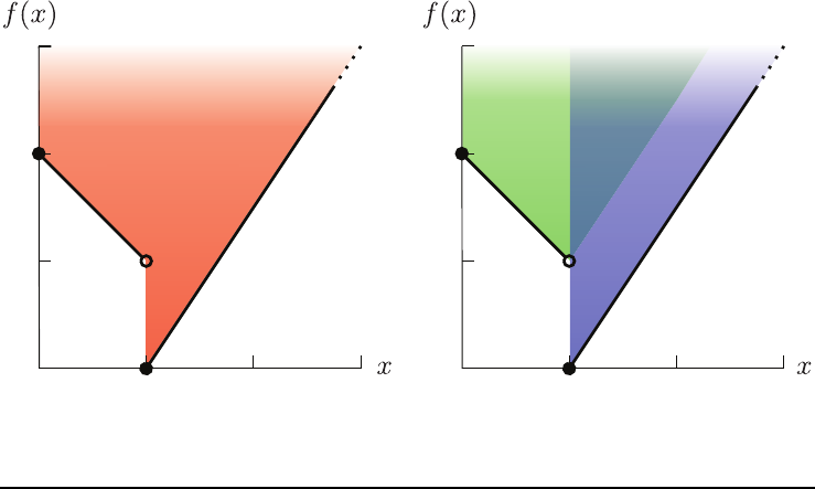
MIXED INTEGER LINEAR PROGRAMMING FORMULATION TECHNIQUES 51
1
1230
0
2
3
(a) Epigraph of function from Example 20
1
1230
0
2
3
(b) Epigraph as union of polyhedra.
Fig. 11.1 Discontinuous Function with Unbounded Domain.
For more information on extended formulations in combinatorial optimization we
refer the reader to [35, 154, 95] and for more on polyhedral approximations of convex
sets we refer the reader to [14, 16, 152] and [93, Chapters 8 and 17].
12.2. Linearization of Products. Another important MIP formulation technique
that we omitted because of space is the linearization of products of binary or bounded
integer variables and the products of these variables with bounded continuous vari-
ables. These linearizations are some of the oldest MIP formulation techniques [58,
7, 100, 133, 59, 162, 60, 70, 8, 117, 72, 135] and continue to be a very active area
of research [5, 3, 71, 64, 65, 4]. They are an important tool for nonconvex mixed
integer nonlinear programming [29] and have been extensively studied in the con-
text of mathematical programming reformulations [109, 108]. In particular, many of
these linearized formulations can be obtained through the reformulation-linearization
technique of Sherali and Adams [147].
Acknowledgment. The author would like to thank two anonymous referees and
one associate editor for their helpful feedback.
REFERENCES
[1] T. Achterberg,Constraint Integer Programming, Ph.D. thesis, TU Berlin,2007.
[2] T. Achterberg,SCIP: Solving constraint integer programs, Math. Program. Comput., 1
(2009), pp. 1–41.
[3] W. Adams and R. Forrester,A simple recipe for concise mixed 0-1linearizations,Oper.
Res. Lett., 33 (2005), pp. 55–61.
[4] W. Adams and R. Forrester,Linear forms of nonlinear expressions: New insights on old
ideas, Oper. Res. Lett., 35 (2007), pp. 510–518.
[5] W. Adams, R. Forrester, and F. Glover,Comparisons and enhancement strategies for
linearizing mixed 0-1 quadratic programs, Discrete Optim., 1 (2004), pp. 99–120.
52 JUAN PABLO VIELMA
[6] W. Adams and S. Henry,Base-2expansions for linearizing products of functions of discrete
variables, Oper. Res., 60 (2012), pp. 1477–1490.
[7] W. Adams and H. Sherali,A tight linearization and an algorithm for zero-one quadratic
programming problems, Management Sci., 32 (1986), pp. 1274–1290.
[8] F. Al-Khayyal and J. Falk,Jointly constrained biconvex programming, Math. Oper. Res.,
8 (1983), pp. 273–286.
[9] G. Angulo, S. Ahmed, S. S. Dey, and V. Kaibel,Forbidden vertices, Math. Oper. Res., to
appear; doi:10.1287/moor.2014.0673.
[10] E. Balas,Disjunctive programming, Ann. Discrete Math., 5 (1979), pp. 3–51.
[11] E. Balas,Disjunctive programming and a hierarchy of relaxations for discrete optimization
problems, SIAM J. Algebraic Discrete Methods, 6 (1985), pp. 466–486.
[12] E. Balas,On the convex-hull of the union of certain polyhedra, Oper. Res. Lett., 7 (1988),
pp. 279–283.
[13] E. Balas,Disjunctive programming: Properties of the convex hull of feasible points, Discrete
Appl. Math., 89 (1998), pp. 3–44.
[14] K. M. Ball,An elementary introduction to modern convex geometry, in Flavors of Geometry,
S. Levy, ed., Math. Sci. Res. Inst. Publ. 31, Cambridge University Press, Cambridge, 1997,
pp. 1–58.
[15] C. Barnhart, E. Johnson, G. Nemhauser, M. Savelsbergh, and P. Vance,Branch-
and-price: Column generation for solving huge integer programs, Oper. Res., 46 (1996),
pp. 316–329.
[16] A. Barvinok and E. Veomett,The computational complexity of convex bodies, in Surveys
on Discrete and Computational Geometry: Twenty Years Later, J. Goodman, J. Pach,
and R. Pollack, eds., Contemp. Math. 453, AMS, Providence, RI, 2008, pp. 117–138.
[17] E. M. L. Beale and J. A. Tomlin,Special facilities in a general mathematical programming
system for non-convex problems using ordered sets of variables, in OR 69: Proceedings of
the Fifth International Conference on Operational Research, J. Lawrence, ed., Tavistock
Publications, 1970, pp. 447–454.
[18] N. Beaumont,An algorithm for disjunctive programs, European J. Oper. Res., 48 (1990),
pp. 362–371.
[19] A. Ben-Tal and A. Nemirovski,On polyhedral approximations of the second-order cone,
Math. Oper. Res., 26 (2001), pp. 193–205.
[20] D. Bertsimas, S. Gupta, and G. Lulli,Dynamic resource allocation: A flexible and tractable
modeling framework, European J. Oper. Res., 236 (2014), pp. 14–26.
[21] D. Bertsimas and J. Tsitsiklis,Introduction to Linear Optimization, Athena Scientific,
1997.
[22] D. Bertsimas and R. Weismantel,Optimization over Integers, Dynamic Ideas, 2005.
[23] R. Bixby, M. Fenelon, Z. Gu, E. Rothberg, and R. Wunderling,MIP: Theory and
practice—closing the gap, in System Modelling and Optimization, 1999, pp. 19–50.
[24] R. Bixby, M. Fenelon, Z. Gu, E. Rothberg, and R. Wunderling,Mixed-integer program-
ming: A progress report, in The Sharpest Cut: The Impact of Manfred Padberg and His
Work, SIAM, Philadelphia, PA, 2004, Chap. 18, pp. 309–325.
[25] R. Bixby and E. Rothberg,Progress in computational mixed integer programming: A look
back from the other side of the tipping point, Ann. Oper. Res., 149 (2007), pp. 37–41.
[26] C. Blair,Representation for multiple right-hand sides, Math. Programming, 49 (1990), pp. 1–
5.
[27] D. Bricker,Reformulation of special ordered sets for implicit enumeration algorithms, with
applications in nonconvex separable programming, AIIE Trans., 9 (1977), pp. 195–203.
[28] M. N. Broadie,A theorem about antiprisms, Linear Algebra Appl., 66 (1985), pp. 99–111.
[29] S. Burer and A. Letchford,Non-convex mixed-integer nonlinear programming: A survey,
Surv. Oper. Res. Manag. Sci., 17 (2012), pp. 97–106.
[30] R. D. Carr and G. Lancia,Compact vs. exponential-size LP relaxations, Oper. Res. Lett.,
30 (2002), pp. 57–65.
[31] R. D. Carr and G. Lancia,Compact optimization can outperform separation: A case study
in structural proteomics, 4OR, 2 (2004), pp. 221–233.
[32] R. Carvajal, M. Constantino, M. Goycoolea, J. P. Vielma, and A. Weintraub,Impos-
ing connectivity constraints in forest planning models, Oper. Res., 61 (2013), pp. 824–836.
[33] C. Cavalcante, C. C. de Souza, M. Savelsbergh, Y. Wang, and L. Wolsey,Scheduling
projects with labor constraints, Discrete Appl. Math., 112 (2001), pp. 27–52.
[34] J. Cochran, L. A. Cox, Jr., P. Keskinocak, J. Kharoufeh, and J. Smith,Wiley Ency-
clopedia of Operations Research and Management Science, John Wiley & Sons, 2011.
[35] M. Conforti, G. Cornu´
ejols, and G. Zambelli,Extended formulations in combinatorial
optimization, 4OR, 8 (2010), pp. 1–48.
MIXED INTEGER LINEAR PROGRAMMING FORMULATION TECHNIQUES 53
[36] M. Conforti, G. Cornu´
ejols, and G. Zambelli,Integer Programming,Grad.Textsin
Math. 271, Springer, 2014.
[37] M. Conforti and L. Wolsey,Compact formulations as a union of polyhedra, Math. Pro-
gramming, 114 (2008), pp. 277–289.
[38] A. Conn and M. Mongeau,Discontinuous piecewise linear optimization, Math. Program-
ming, 80 (1998), pp. 315–380.
[39] W. Cook,Fifty-plus years of combinatorial integer programming, in 50 Years of Integer
Programming 1958–2008: From the Early Years to the State-of-the-Art, Springer-Verlag,
New York, 2010, Chap. 12, pp. 387–430.
[40] W. Cook,In Pursuit of the Traveling Salesman: Mathematics at the Limits of Computation,
Princeton University Press, Princeton, NJ, 2011.
[41] D. Coppersmith and J. Lee,Parsimonious binary-encoding in integer programming, Discrete
Optim., 2 (2005), pp. 190–200.
[42] K. L. Croxton, B. Gendron, and T. L. Magnanti,Variable disaggregation in network flow
problems with piecewise linear costs, Oper. Res., 55 (2007), pp. 146–157.
[43] C. D’Ambrosio, A. Lodi, and S. Martello,Piecewise linear approximation of functions of
two variables in MILP models, Oper. Res. Lett., 38 (2010), pp. 39–46.
[44] G. B. Dantzig,Discrete-variable extremum problems, Oper. Res., 5 (1957), pp. 266–277.
[45] G. B. Dantzig,On the significance of solving linear-programming problems with some integer
variables, Econometrica, 28 (1960), pp. 30–44.
[46] I. R. de Farias, E. Kozyreff, R. Gupta, and M. Zhao,Branch-and-cut for separable
piecewise linear optimization and intersection with semi-continuous constraints,Math.
Program. Comput., 5 (2013), pp. 75–112.
[47] I. R. de Farias Jr., M. Zhao, and H. Zhao,A special ordered set approach for optimizing
a discontinuous separable piecewise linear function, Oper. Res. Lett., 36 (2008), pp. 234–
238.
[48] J. Desrosiers and M. E. L¨
ubbecke,Branch-Price-and-Cut Algorithms, in Wiley Encyclo-
pedia of Operations Research and Management Science, John Wiley & Sons, 2011.
[49] S. Dey and D. Mor´
an R.,Some properties of convex hulls of integer points contained in
general convex sets, Math. Programming, 141 (2013), pp. 507–526.
[50] B. Dilkina and C. Gomes,Solving connected subgraph problems in wildlife conservation,
in Integration of AI and OR Techniques in Constraint Programming for Combinatorial
Optimization Problems, Lecture Notes in Comput. Sci. 6140, A. Lodi, M. Milano, and
P. Toth, eds., Springer, Berlin, Heidelberg, 2010, pp. 102–116.
[51] P. Domschke, B. Geißler, O. Kolb, J. Lang, A. Martin, and A. Morsi,Combination of
nonlinear and linear optimization of transient gas networks, INFORMS J. Comput., 23
(2011), pp. 605–617.
[52] Fair Isaac Corporation,FICO Xpress Optimization Suite, http://www.fico.com/en/
Products/DMTools/Pages/FICO-Xpress-Optimization-Suite.aspx.
[53] S. Fiorini, S. Massar, S. Pokutta, H. R. Tiwary, and R. de Wolf,Linear vs. semidefinite
extended formulations: Exponential separation and strong lower bounds, in Proceedings
of the 44th Symposium on Theory of Computing Conference, STOC 2012, New York,
2012, H. J. Karloff and T. Pitassi, eds., ACM, New York, 2012, pp. 95–106.
[54] R. Fourer,A simplex algorithm for piecewise-linear programming I: Derivation and proof,
Math. Programming, 33 (1985), pp. 204–233.
[55] R. Fourer,A simplex algorithm for piecewise-linear programming II: Finiteness, feasibility
and degeneracy, Math. Programming, 41 (1988), pp. 281–315.
[56] R. Fourer,A simplex algorithm for piecewise-linear programming III: Computational anal-
ysis and applications, Math. Programming, 53 (1992), pp. 213–235.
[57] B. Geißler, A. Martin, A. Morsi, and L. Schewe,Using piecewise linear functions for
solving MINLPs, in Mixed Integer Nonlinear Programming, J. Lee and S. Leyffer, eds.,
Math. Appl. 154, Springer, New York, 2012, pp. 287–314.
[58] F. Glover,Improved linear integer programming formulations of nonlinear integer problems,
Management Sci., 22 (1975), pp. 455–460.
[59] F. Glover,Improved MIP formulation for products of discrete and continuous variables,J.
Inf. Optim. Sci., 5 (1984), pp. 69–71.
[60] F. Glover and E. Woolsey,Converting the 0-1polynomial programming problem to a 0-1
linear program, Oper. Res., 22 (1974), pp. 180–182.
[61] M. X. Goemans,Smallest compact formulation for the permutahedron, Math. Program., to
appear; doi:10.1007/s10107-014-0757-1.
[62] C. Gounaris, R. Misener, and C. A. Floudas,Computational comparison of piecewise-
linear relaxations for pooling problems, Indust. Engrg. Chem. Res., 48 (2009), pp. 5742–
5766.
54 JUAN PABLO VIELMA
[63] B. Gr¨
unbaum,Convex Polytopes, Grad. Texts in Math., Springer, 2003.
[64] S. Gueye and P. Michelon,Miniaturized linearizations for quadratic 0/1problems, Ann.
Oper. Res., 140 (2005), pp. 235–261.
[65] S. Gueye and P. Michelon,A linearization framework for unconstrained quadratic (0-1)
problems, Discrete Appl. Math., 157 (2009), pp. 1255–1266.
[66] M. Guignard, C. Ryu, and K. Spielberg,Model tightening for integrated timber harvest
and transportation planning, European J. Oper. Res., 111 (1998), pp. 448–460.
[67] M. Guignard and K. Spielberg,Logical reduction methods in zero-one programming: Min-
imal preferred variables, Oper. Res., 29 (1981), pp. 49–74.
[68] M. Guignard-Spielberg and K. Spielberg,Integer Programming: State of the Art and
Recent Advances, Ann. Oper. Res. 139, Springer, New York, 2005.
[69] Gurobi Optimization,The Gurobi Optimizer, available online from http://www.gurobi.com.
[70] P. Hansen,Methods of nonlinear 0-1programming, Ann. Discrete Math., 5 (1979), pp. 53–70.
[71] P. Hansen and C. Meyer,Improved compact linearizations for the unconstrained quadratic
0-1 minimization problem, Discrete Appl. Math., 157 (2009), pp. 1267–1290.
[72] I. Harjunkoski, R. P¨
orn, T. Westerlund, and H. Skrifvars,Different strategies for
solving bilinear integer non-linear programming problems with convex transformations,
Comput. Chem. Engrg., 21 (1997), pp. S487–S492.
[73] R. Hemmecke and R. Weismantel,Representation of sets of lattice points, SIAM J. Optim.,
18 (2007), pp. 133–137.
[74] S. M. Henry,Tight Polyhedral Representations of Discrete Sets using Projections, Simplices,
and Base-2Expansions, Ph.D. thesis, Clemson University, 2011.
[75] J. N. Hooker,Logic-Based Methods for Optimization: Combining Optimization and Con-
straint Satisfaction, Wiley Series in Discrete Mathematics and Optimization, John Wiley
& Sons, 2000.
[76] J. N. Hooker,A principled approach to mixed integer/linear problem formulation,inOper-
ations Research and Cyber-Infrastructure, J. W. Chinneck, B. Kristjansson, and M. J.
Saltzman, eds., Oper. Res./Comput. Sci. Interfaces Ser. 47, Springer, New York, 2009,
pp. 79–100.
[77] J. N. Hooker,Hybrid modeling, in Hybrid Optimization: The Ten Years of CPAIOR,
P. Van Hentenryck and M. Milano, eds., Springer Optim. Appl. 45, Springer, 2011, pp. 11–
62.
[78] J. N. Hooker,Integrated Methods for Optimization, 2nd ed., Internat. Ser. Oper. Res. Man-
agement Sci. 170, Springer, 2012.
[79] J. N. Hooker and M. A. Osorio,Mixed logical-linear programming, Discrete Appl. Math.,
96 (1999), pp. 395–442.
[80] R. Horst and H. Tuy,Global Optimization: Deterministic Approaches, Springer, 2003.
[81] T. Ibaraki,Integer programming formulation of combinatorial optimization problems,Dis-
crete Math., 16 (1976), pp. 39–52.
[82] IBM ILOG,CPLEX High-Performance Mathematical Programming Engine, http://www.
ibm.com/software/integration/optimization/cplex/.
[83] R. G. Jeroslow,Some basis theorems for integral monoids, Math. Oper. Res., 3 (1978),
pp. 145–154.
[84] R. G. Jeroslow,Representations of unbounded optimization problems as integer programs,
J. Optim. Theory Appl., 30 (1980), pp. 339–351.
[85] R. G. Jeroslow,Representability in mixed integer programming I: Characterization results,
Discrete Appl. Math., 17 (1987), pp. 223–243.
[86] R. G. Jeroslow,Alternative formulations of mixed integer programs, Ann. Oper. Res., 12
(1988), pp. 241–276.
[87] R. G. Jeroslow,A simplification for some disjunctive formulations,EuropeanJ.Oper.Res.,
36 (1988), pp. 116–121.
[88] R. G. Jeroslow,Logic-Based Decision Support: Mixed Integer Model Formulation, Ann.
Discrete Math. 40, North-Holland, Amsterdam, 1989.
[89] R. G. Jeroslow,Representability of functions, Discrete Appl. Math., 23 (1989), pp. 125–137.
[90] R. G. Jeroslow and J. K. Lowe,Modeling with integer variables, Math. Programming
Stud., 22 (1984), pp. 167–184.
[91] R. G. Jeroslow and J. K. Lowe,Experimental results on the new techniques for integer
programming formulations, J. Oper. Res. Soc., 36 (1985), pp. 393–403.
[92] E. L. Johnson, G. L. Nemhauser, and M. W. P. Savelsbergh,Progress in linear
programming-based algorithms for integer programming: An exposition,INFORMSJ.
Comput., 12 (2000), pp. 2–23.
[93] W. B. Johnson and J. Lindenstrauss, eds.,Handbook of the Geometry of Banach Spaces.
Vol. I, North-Holland, Amsterdam, 2001.
MIXED INTEGER LINEAR PROGRAMMING FORMULATION TECHNIQUES 55
[94] M. J¨
unger, T. Liebling, D. Naddef, G. Nemhauser, W. Pulleyblank, G. Reinelt, G. Ri-
naldi, and L. Wolsey,50Years of Integer Programming 1958–2008: From the Early
Years to the State-of-the-Art, Springer-Verlag, New York, 2010.
[95] V. Kaibel,Extended formulations in combinatorial optimization, Optima, 85 (2011), pp. 2–7.
[96] V. Kaibel and A. Loos,Branched polyhedral systems, in Integer Programming and Combina-
torial Optimization, 14th International Conference, IPCO 2010, Lausanne, Switzerland,
June 9-11, 2010. Proceedings, F. Eisenbrand and F. B. Shepherd, eds., Lecture Notes in
Comput. Sci. 6080, Springer, 2010, pp. 177–190.
[97] V. Kaibel and K. Pashkovich,Constructing extended formulations from reflection relations,
in Proceedings of IPCO 2011, O. G¨unl¨uk and G. J. Woeginger, eds., Lecture Notes in
Comput. Sci. 6655, Springer, 2011, pp. 287–300.
[98] B. S. Kashin,The widths of certain finite-dimensional sets and classes of smooth functions,
Izv. Akad. Nauk SSSR Ser. Mat., 41 (1977), pp. 334–351 (in Russian).
[99] A. Keha, I. de Farias, and G. Nemhauser,A branch-and-cut algorithm without binary
variables for nonconvex piecewise linear optimization, Oper. Res., 54 (2006), pp. 847–
858.
[100] O. Kettani and M. Oral,Equivalent formulations of nonlinear integer problems for efficient
optimization, Management Sci., 36 (1990), pp. 115–119.
[101] S. K¨
uc¸¨
ukyavuz,On mixing sets arising in chance-constrained programming, Math. Program-
ming, 132 (2012), pp. 31–56.
[102] A. H. Land and A. G. Doig,An automatic method for solving discrete programming prob-
lems, Econometrica, 28 (1960), pp. 497–520.
[103] J. Lee,All-different polytopes, J. Comb. Optim., 6 (2002), pp. 335–352.
[104] J. Lee,A celebration of 50 years of integer programming, Optima, 76 (2008), pp. 10–14.
[105] J. Lee and F. Margot,On a binary-encoded ILP coloring formulation,INFORMSJ.Com-
put., 19 (2007), pp. 406–415.
[106] J. Lee and D. Wilson,Polyhedral methods for piecewise-linear functions I: The lambda
method, Discrete Appl. Math., 108 (2001), pp. 269–285.
[107] H. Li and H. Lu,Global optimization for generalized geometric programs with mixed free-sign
variables, Oper. Res., 57 (2009), pp. 701–713.
[108] L. Liberti,Reformulations in mathematical programming: Definitions and systematics,
RAIRO Oper. Res., 43 (2009), pp. 55–85.
[109] L. Liberti and N. Maculan,Reformulation techniques in mathematical programming,Dis-
crete Appl. Math., 157 (2009), pp. 1165–1166.
[110] E. Lin and D. Bricker,Connecting special ordered inequalities and transformation and
reformulation technique in multiple choice programming, Comput. Oper. Res., 29 (2002),
pp. 1441–1446.
[111] E. Y. Lin and D. L. Bricker,On the calculation of true and pseudo penalties in multiple
choice integer programming, European J. Oper. Res., 55 (1991), pp. 228–236.
[112] A. Lodi,Mixed integer programming computation, in 50 Years of Integer Programming 1958–
2008: From the Early Years to the State-of-the-Art, Springer-Verlag, New York, 2010,
Chap. 16, pp. 619–645.
[113] J. K. Lowe,Modelling with Integer Variables, Ph.D. thesis, Georgia Institute of Technology,
1984.
[114] J. Luedtke, S. Ahmed, and G. Nemhauser,An integer programming approach for linear
programs with probabilistic constraints, Math. Programming, 122 (2010), pp. 247–272.
[115] R. K. Martin,Using separation algorithms to generate mixed integer model reformulations,
Oper. Res. Lett., 10 (1991), pp. 119–128.
[116] R. K. Martin, R. L. Rardin, and B. A. Campbell,Polyhedral characterization of discrete
dynamic programming, Oper. Res., 38 (1990), pp. 127–138.
[117] G. McCormick,Nonlinear Programming: Theory, Algorithms and Applications, John Wiley
& Sons, 1983.
[118] R. R. Meyer,On the existence of optimal solutions to integer and mixed-integer programming
problems, Math. Programming, 7 (1974), pp. 223–235.
[119] R. R. Meyer,Integer and mixed-integer programming models: General properties,J.Optim.
Theory Appl., 16 (1975), pp. 191–206.
[120] R. R. Meyer,Mixed integer minimization models for piecewise-linear functions of a single
variable, Discrete Math., 16 (1976), pp. 163–171.
[121] R. R. Meyer,A theoretical and computational comparison of equivalent mixed-integer for-
mulations, Naval Res. Logistics, 28 (1981), pp. 115–131.
[122] R. R. Meyer, M. V. Thakkar, and W. P. Hallman,Rational mixed-integer and polyhedral
union minimization models, Math. Oper. Res., 5 (1980), pp. 135–146.
56 JUAN PABLO VIELMA
[123] R. Misener and C. A. Floudas,Global optimization of large-scale generalized pooling prob-
lems: Quadratically constrained MINLP models, Indust. Engrg. Chem. Res., 49 (2010),
pp. 5424–5438.
[124] R. Misener and C. A. Floudas,Piecewise-linear approximations of multidimensional func-
tions, J. Optim. Theory Appl., 145 (2010), pp. 120–147.
[125] R. Misener and C. A. Floudas,Global optimization of mixed-integer quadratically-
constrained quadratic programs (MIQCQP) through piecewise-linear and edge-concave
relaxations, Math. Programming, 136 (2012), pp. 155–182.
[126] R. Misener, C. Gounaris, and C. A. Floudas,Mathematical modeling and global optimiza-
tion of large-scale extended pooling problems with the (EPA) complex emissions con-
straints, Comput. Chem. Engrg., 34 (2010), pp. 1432–1456.
[127] R. Misener, J. Thompson, and C. A. Floudas,APOGEE: Global optimization of stan-
dard, generalized, and extended pooling problems via linear and logarithmic partitioning
schemes, Comput. Chem. Engrg., 35 (2011), pp. 876–892.
[128] J. E. Mitchell,Branch and cut, in Wiley Encyclopedia of Operations Research and Man-
agement Science, John Wiley & Sons, 2011.
[129] R. H. M¨
ohring, A. S. Schulz, F. Stork, and M. Uetz,On project scheduling with irregular
starting time costs, Oper. Res. Lett., 28 (2001), pp. 149–154.
[130] F.M.Muldoon,W.P.Adams,andH.D.Sherali,Ideal representations of lexicographic
orderings and base-2expansions of integer variables, Oper. Res. Lett., 41 (2013), pp. 32–
39.
[131] G. L. Nemhauser and L. A. Wolsey,Integer and Combinatorial Optimization, Wiley-
Interscience, 1988.
[132] W. Ogryczak,A note on modeling multiple choice requirements for simple mixed integer
programming solvers, Comput. Oper. Res., 23 (1996), pp. 199–205.
[133] M. Oral and O. Kettani,A linearization procedure for quadratic and cubic mixed-integer
problems, Oper. Res., 40 (1992), pp. 109–116.
[134] J. Owen and S. Mehrotra,On the value of binary expansions for general mixed-integer
linear programs, Oper. Res., 50 (2002), pp. 810–819.
[135] M. W. Padberg,The boolean quadric polytope: Some characteristics, facets and relatives,
Math. Programming, 45 (1989), pp. 139–172.
[136] M. W. Padberg,Approximating separable nonlinear functions via mixed zero-one programs,
Oper. Res. Lett., 27 (2000), pp. 1–5.
[137] M. W. Padberg and M. P. Rijal,Location, Scheduling, Design, and Integer Programming,
Springer, 1996.
[138] Y. Pochet and L. Wolsey,Production Planning by Mixed Integer Programming, Springer
Ser. Oper. Res. Financ. Eng., Springer, 2006.
[139] R. Raman and I. Grossmann,Modelling and computational techniques for logic based integer
programming, Comput. Chem. Engrg., 18 (1994), pp. 563–578.
[140] T. Rothvoß, The matching polytope has exponential extension complexity,inSymposiumon
Theory of Computing (STOC 2014), D. B. Shmoys, ed., ACM, New York, 2014, pp. 263–
272.
[141] D. M. Ryan and B. A. Foster,An integer programming approach to scheduling, in Computer
Scheduling of Public Transport Urban Passenger Vehicle and Crew Scheduling, A. Wren,
ed., North-Holland, 1981, pp. 269–280.
[142] R. Sadykov and F. Vanderbeck,Column generation for extended formulations, Electron.
Notes Discrete Math., 37 (2011), pp. 357–362.
[143] N. Sawaya and I. Grossmann,A cutting plane method for solving linear generalized disjunc-
tive programming problems, Comput. Chem. Engrg., 29 (2005), pp. 1891–1913.
[144] N. Sawaya and I. Grossmann,A hierarchy of relaxations for linear generalized disjunctive
programming, European J. Oper. Res., 216 (2012), pp. 70–82.
[145] A. Schrijver,Theory of Linear and Integer Programming, Wiley Series in Discrete Mathe-
matics & Optimization, John Wiley & Sons, 1998.
[146] A. Schrijver,Combinatorial Optimization: Polyhedra and Efficiency, Algorithms and Com-
binatorics, Springer, 2003.
[147] H. Sherali and W. P. Adams,A Reformulation-Linearization Technique for Solving Discrete
and Continuous Nonconvex Problems, Kluwer Academic Publishers, 1999.
[148] D. Sommer,Computational Experience with the Ophelie Mixed Integer Code,talkpresented
at the International TIMS Conference, Houston, 1972.
[149] C. C. Souza and L. A. Wolsey,Scheduling Projects with Labour Constraints,relat´orio
t´ecnico ic-97-22, IC - UNICAMP, 1997.
[150] K. Spielberg,Minimal Preferred Variable Methods in 0-1 Programming, Tech. Report 320-
3013, IBM Philadelphia Scientific Center, 1972.
MIXED INTEGER LINEAR PROGRAMMING FORMULATION TECHNIQUES 57
[151] D. Stralberg, D. L. Applegate, S. J. Phillips, M. P. Herzog, N. Nur, and N. Warnock,
Optimizing wetland restoration and management for avian communities using a mixed
integer programming approach, Biological Conservation, 142 (2009), pp. 94–109.
[152] S. Szarek,Convexity, complexity, and high dimensions, in International Congress of Math-
ematicians. Vol. II, Eur. Math. Soc., Z¨urich, 2006, pp. 1599–1621.
[153] A. Toriello and J. P. Vielma,Fitting piecewise linear continuous functions,EuropeanJ.
Oper. Res., 219 (2012), pp. 86–95.
[154] F. Vanderbeck and L. Wolsey,Reformulation and decomposition of integer programs,in50
Years of Integer Programming 1958–2008: From the Early Years to the State-of-the-Art,
Springer-Verlag, New York, 2010, Chap. 16, pp. 431–502.
[155] J. P. Vielma, S. Ahmed, and G. L. Nemhauser,Mixed-integer models for nonseparable
piecewise-linear optimization: Unifying framework and extensions, Oper. Res., 58 (2010),
pp. 303–315.
[156] J. P. Vielma, S. Ahmed, and G. L. Nemhauser,A note on “a superior representation
method for piecewise linear functions,” INFORMS J. Comput., 22 (2010), pp. 493–497.
[157] J. P. Vielma, S. Ahmed, and G. L. Nemhauser,Mixed integer linear programming formu-
lations for probabilistic constraints, Oper. Res. Lett., 40 (2012), pp. 153–158.
[158] J. P. Vielma, A. B. Keha, and G. L. Nemhauser,Nonconvex, lower semicontinuous piece-
wise linear optimization, Discrete Optim., 5 (2008), pp. 467–488.
[159] J. P. Vielma and G. L. Nemhauser,Modeling disjunctive constraints with a logarithmic
number of binary variables and constraints, in Proceedings of IPCO 2008, A. Lodi,
A. Panconesi, and G. Rinaldi, eds., Lecture Notes in Comput. Sci. 5035, Springer, 2008,
pp. 199–213.
[160] J. P. Vielma and G. L. Nemhauser,Modeling disjunctive constraints with a logarithmic
number of binary variables and constraints, Math. Programming, 128 (2011), pp. 49–72.
[161] M. V. Vyve and L. A. Wolsey,Approximate extended formulations, Math. Programming,
105 (2006), pp. 501–522.
[162] L. Watters,Reduction of integer polynomial programming problems to zero-one linear pro-
gramming problems, Oper. Res., 15 (1967), pp. 1171–1174.
[163] H. P. Williams,Experiments in the formulation of integer programming problems,Math.
Programming Stud., 2 (1974), pp. 180–197.
[164] H. P. Williams,Logic and Integer Programming, International Series in Operations Research
& Management Science, Springer, 2009.
[165] D. L. Wilson,Polyhedral Methods for Piecewise-Linear Functions,Ph.D.thesis,University
of Kentucky, Lexington, KY, 1998.
[166] L. Wolsey,Integer Programming, Wiley Series in Discrete Mathematics and Optimization,
Wiley, 1998.
[167] M. Yannakakis,Expressing combinatorial optimization problems by linear programs,J.Com-
put. System Sci., 43 (1991), pp. 441–466.
[168] S. Yıldız and J. P. Vielma,Incremental and encoding formulations for mixed integer pro-
gramming, Oper. Res. Lett., 41 (2013), pp. 654–658.
[169] M. Zhao and I. R. de Farias, Jr.,The piecewise linear optimization polytope: New inequal-
ities and intersection with semi-continuous constraints, Math. Program., 141 (2013),
pp. 217–255.
[170] G. M. Ziegler,Lectures on Polytopes, Springer-Verlag, 1995.
[171] Zuse Institute Berlin,SCIP: Solving Constraint Integer Programs, http://scip.zib.de/.
