MOM1 Manual

MOM1_manual

User Manual:

Open the PDF directly: View PDF .
Page Count: 46

The G.F.D.L.

Modular Ocean Model

Users Guide

Version 1.0 - September 1991

G.F.D.L. Ocean Group Technical Report Number 2

Ronald C. Pacanowski

Keith W. Dixon

Anthony Rosati

Geophysical Fluid Dynamics Laboratory

Princeton, New Jersey

UNITED STATES DEPARTMENT OF COMMERCE

National Oceanic and Atmospheric Administration

<Pacanowski, Dixon & Rosati - GFDL Ocean Group Tech. Report No. 2>

TABLE OF CONTENTS

TABLE OF CONTENTS .................................................................................... i

DISCLAIMER NOTICE ...............................................................................................iii

AVAILABILITY OF THIS DOCUMENT ....................................................................... iii

REFERENCING THE GFDL MODULAR OCEAN MODEL AND THIS DOCUMENT iv

FONTS USED IN THIS DOCUMENT .........................................................................iv

AVAILABILITY OF THE G.F.D.L. MODULAR OCEAN MODEL CODE..................... iv

PREFACE ..........................................................................................................vi

ACKNOWLEDGEMENTS...............................................................................vii

CHAPTER 1: Beginning to Work with the GFDL Modular Ocean Model

(1.1) BRIEF FILE DESCRIPTIONS ..........................................................................1-2

(1.2) REQUIREMENTS FOR RUNNING THE M.O.M. CODE ..................................1-3

(1.3) EXTRACTING THE INDIVIDUAL FORTRAN SOURCE FILES ......................1-4

(1.4) GETTING ACQUAINTED WITH THE M.O.M. CODE ......................................1-5

(1.5) RECOMMENDATIONS FOR M.O.M. CODE MAINTENANCE ........................1-5

CHAPTER 2: Coding Design of the GFDL Modular Ocean Model

(2.1) GENERAL CODING DESIGN ..........................................................................2-2

(2.2) SOME NEW FEATURES & NOTES FOR USERS OF THE COX CODE ........2-3

(2.3) SIMPLIFIED CALLING TREE DIAGRAMS FOR THE GFDL M.O.M. CODE..2-6

CHAPTER 3: Code Options in the GFDL Modular Ocean Model

(3.1) OVERVIEW OF CODE OPTIONS....................................................................3-2

(3.2) GRID OPTIONS................................................................................................3-2

(3.3) EXTERNAL MODE OPTIONS .........................................................................3-3

(3.4) LATERAL MIXING SCHEMES.........................................................................3-4

(3.5) VERTICAL MIXING SCHEMES .......................................................................3-5

(3.6) HYBRID MIXING SCHEME OPTIONS.............................................................3-7

(3.7) OPTIMIZATION OPTIONS ...............................................................................3-8

(3.8) FILTERING OPTIONS......................................................................................3-9

(3.9) I/O OPTIONS..................................................................................................3-10

<Pacanowski, Dixon & Rosati - GFDL Ocean Group Tech. Report No. 2>

(3.10) MISCELLANEOUS CODE OPTIONS ..........................................................3-10

INDEX...........................................................................................................IN-1

<Pacanowski, Dixon & Rosati - GFDL Ocean Group Tech. Report No. 2>

iii

DISCLAIMER NOTICE

Mention of a commercial company or

product does not constitute an

endorsement by NOAA Environmental

Research Laboratories.

Use for publicity or advertising purposes of

information from this report concerning

proprietary products or the tests of such

products is not authorized.

The authors and NOAA Environmental

Research Laboratories assume no

responsibility for errors in, or incorrect use

of the GFDL Modular Ocean Model. It is

ﬁrst and foremost an ocean modeling

research tool used by researchers at

NOAA’s Geophysical Fluid Dynamics

Laboratory. The model and this Users

Guide have been made available as a

service to the oceanographic community.

No guarantees concerning the code, the

documentation, nor their continued

support are intended. It is left to the

individual user to satisfy (him/her)self that

a particular conﬁguration is working

correctly.

AVAILABILITY OF THIS

DOCUMENT

Copies of GFDL Ocean Group Technical

Reports can be obtained by writing the

authors at...

Geophysical Fluid Dynamics Lab / NOAA

Princeton University, Box 308

Princeton, New Jersey 08542

Postscript ﬁles of this report may also be

obtained via anonymous ftp across the

internet from a GFDL server named

gfdl.gov which has the IP address

140.208.1.9

After making the anonymous ftp

connection, the ﬁles containing this

document can be found in the directory

named.../pub/GFDL_MOM/UsersGuide

Updates to this Users Guide are planned,

but no timetable has been set for those

updates. Users of the GFDL Modular

Ocean Model who have provided the

authors with an e-mail address that can be

reached via internet connections, will be

notiﬁed as updates become available.

REFERENCING THE GFDL

MODULAR OCEAN MODEL AND

THIS DOCUMENT

Those who use the GFDL Modular Ocean

Model in part of their research should

reference the model in papers and other

publications as as follows:

REFERENCE:

Pacanowski, R., K. Dixon and A. Rosati,

“The GFDL Modular Ocean Model Users

Guide version 1.0”, GFDL Ocean Group

Technical Report #2, (1991).

FONTS USED IN THIS

DOCUMENT

This document was prepared using Frame

Technology Corporation’s copywrited

FrameMaker workstation publishing

software.

In the examples in this document, we have

adopted the convention of representing

user keyboard input in FrameMaker’s

bold Courier font, and computer

responses in a regular Courier

font.

Fortran variable names, UNIX commands

and ﬁle names also appear in a regular

Courier font

The names of GFDL Modular Ocean

Model code options enabled through the

use of ifdef directives are shown in a font

FrameMaker calls demibold Avant

G arde.

AVAILABILITY OF THE G.F.D.L.

MODULAR OCEAN MODEL CODE

The Fortran code and related support ﬁles

for the GFDL Modular Ocean Model can

be obtained free of cost via anonymous

ftp on the internet. Those wishing to

obtain the model in this manner can ﬁnd

the ﬁles under the /pub/GFDL_MOM

directory of the GFDL server named

gfdl.gov (IP address 140.208.1.9).

Example:

First, on your own machine, make a

directory and a subdirectory and change

to it:

mkdir my_mom (for the MOM ﬁles)

cd my_mom

mkdir prep_data (for the DATA ﬁles)

cd prep_data

Then, do the ftp and transfer the ﬁles:

ftp -i 140.208.1.9

Name (140.208.1.9:xxx): ftp

Password: anything (your last name

would do nicely)

cd pub/GFDL_MOM/PREP_DATA (this

directory contains programs for preparing

data for use with the MOM code. It does

not contain any datasets, and is not

needed to run the model test case.)

mget * (transfer the DATA ﬁles)

lcd ../ (change local directory)

cd ../ (change remote directory)

mget * (transfer the MOM ﬁles)

quit (close the ftp connection)

<Pacanowski, Dixon & Rosati - GFDL Ocean Group Tech. Report No. 2>

On your local machine, change directories

and list the contents of the directories to

check that you have received the ﬁles:

NOTE: the MOM_NEWS ﬁle will change size

as bug reports and other updates are

added to it over time.

cd ../

ls -goF

total 1672

-r--r--r-- 1 19413 Apr 24 09:46 MOM_NEWS

dr-xr-xr-x 2 512 Dec 5 1990 prep_data/

-r--r--r-- 1 48290 Dec 14 1990 READ_ME

-r-xr--r-- 1 2109 Dec 14 1990 cray.run*

-r-xr--r-- 1 1524 Dec 14 1990 mergelib*

-r--r--r-- 1 555072 Dec 14 1990 mom_1.0

-r--r--r-- 1 361 Feb 2 1991 ocean.in

-r--r--r-- 1 221239 Dec 14 1990 printout

-r--r--r-- 1 3735 Dec 14 1990 splitlib.c

-r-xr--r-- 1 1188 Dec 14 1990 upgrade*

cd prep_data

ls -goF

total 157

-r--r--r-- 1 8670 Dec 14 1990 READ_ME

-r-xr--r-- 1 39 Dec 14 1990 export.batch*

-r-xr--r-- 1 1282 Dec 14 1990 export.data*

-r--r--r-- 1 14906 Dec 14 1990 ic.F

-r-xr--r-- 1 32 Dec 14 1990 ic.batch*

-r--r--r-- 1 211 Dec 14 1990 ic.i.salt

-r--r--r-- 1 211 Dec 14 1990 ic.i.temp

-r-xr--r-- 1 3418 Dec 14 1990 ic.run*

-r--r--r-- 1 6634 Dec 14 1990 prep_utl.F

-r--r--r-- 1 15068 Dec 14 1990 sbc.F

-r-xr--r-- 1 33 Dec 14 1990 sbc.batch*

-r--r--r-- 1 110 Dec 14 1990 sbc.i

-r-xr--r-- 1 2302 Dec 14 1990 sbc.run*

-r--r--r-- 1 18431 Dec 14 1990 topo.F

-r-xr--r-- 1 34 Dec 14 1990 opo.batch*

-r--r--r-- 1 194 Dec 14 1990 topo.i

-r-xr--r-- 1 2011 Dec 14 1990 topo.run*

-r-xr--r-- 1 39 Dec 14 1990 verify.batch*

-r-xr--r-- 1 1400 Dec 14 1990 verify.data*

PREFACE

The GFDL Modular Ocean Model is

intended to be a ﬂexible tool for exploring

ocean and coupled air-sea applications

over a wide range of space and time

scales. This model code has been written

as a collaborative effort by Ron

Pacanowski, Keith Dixon and Anthony

Rosati at the National Oceanographic and

Atmospheric Administration’s Geophys-

ical Fluid Dynamics Laboratory in

Princeton, New Jersey. It is the successor

to the code written by Michael Cox, which

he documented in the GFDL Ocean Group

Technical Report #1, (1984).

As was the case for the Cox model, the

GFDL Modular Ocean Model is distributed

freely to members of the oceanographic

community. However, we can not certify

that the code nor its documentation are

free of errors. Also, we can not provide in-

depth support for users of the model.

We recognize that many users will ﬁnd this

ﬁrst version of the GFDL Modular Ocean

Model Users Guide to be quite incomplete.

We consider this Users Guide to be a

dynamic document, and one that we will

revise and expand. We also expect the

model itself to continue to be improved

and expanded. Our hope is that the model

and documentation will grow together. Our

goal is to have this Users Guide evolve to

where it thoroughly describes the model

and its options, as well as provides users

with guidelines for its use.

For now, version 1 of the Users Guide is

intended to serve as an introduction to the

GFDL Modular Ocean Model version 1.0.

Users unfamiliar with the earlier Cox

model are referred to Cox’s GFDL Ocean

Tech Report #1 and Kirk Bryan’s 1969

Journal of Computational Physics article

for a discussion of the numerics. As was

the case for the Cox model and the model

of Bert Semtner (1974) that preceded it,

the GFDL Modular Ocean Model is a

Fortran implementation of equations

described by Bryan (1969).

Comments and suggestions concerning

the GFDL Modular Ocean Model are

welcome. Anyone wishing to develop

reﬁnements and/or additions will be

acknowledged for their efforts in

subsequent releases of the code. Please

contact one of us if you have something

you feel might be worthwhile to add to the

model or if you uncover an error in the

existing code. We suggest that when

developing code, the style and modularity

evident in the model be followed. Its

modular design is speciﬁcally intended to

aid in ease of use, ﬂexibility, and continued

development without sacriﬁcing clarity.

Ronald C. Pacanowski rcp@gfdl.gov

Keith W. Dixon kd@gfdl.gov

Anthony Rosati ar@gfdl.gov

September 1991

REFERENCES:

Bryan, K., J. Computat. Phys., 4, 347-376,

(1969).

Cox, M. D., “A Primitive Equation, 3-Dimen-

sional Model of the Ocean”, GFDL Ocean

Group Technical Report #1, (1984).

Semtner, A., UCLA Dept. of Meteorology

Tech. Report No. 9, (1974)

<Pacanowski, Dixon & Rosati - GFDL Ocean Group Tech. Report No. 2>

vii

ACKNOWLEDGEMENTS

Various aspects of the GFDL Modular

Ocean Model can be associated with the

efforts of many people over a number of

years. Its lineage can be traced directly

back in time to the codes of Michael Cox,

Bert Semtner, and ultimately to the

equations described by Kirk Bryan in1969.

Numerous others have added useful

reﬁnements to the GFDL Modular Ocean

Model’s predecessors, strengthening its

heritage. We have endeavored to note

contributions by citing names and

references in this document and in the

model code itself. No doubt some have

been omitted through our own oversight or

simply because the collective memory of

GFDL ocean modeling can grow fuzzy

over time. We apologize to those whose

names have been omitted.

Of more recent importance has been the

support we have received that afforded us

the opportunity and freedom needed to

devote time to writing the GFDL Modular

Ocean Model. This continued support has

come from Jerry Mahlman (Director of

GFDL), Kirk Bryan, (GFDL Ocean

Circulation Project Leader), Kikuro

Miyakoda (GFDL Experimental Prediction

Project Leader), and other GFDL

colleagues.

We also wish to thank Christopher Kerr of

Cray Research for his help in getting the

model to autotask and multitask correctly.

This page was intentionally left blank

viii

<Pacanowski, Dixon & Rosati - GFDL Ocean Group Tech. Report No. 2>

1-1

Once the GFDL Modular Ocean Model

(MOM) ﬁles have been obtained, one

naturally asks a question along the lines

of... “I’ve got all these ﬁles, so now what

do I do with them?”.

This chapter is intended to begin to

answer the above question by giving the

new user an overview of the contents of

the ﬁles and suggestions regarding how to

work with them.

NOTE: The following descriptions assume

that the ﬁles have been arranged in UNIX

directories as described earlier in this

document, in the section entitled

“AVAILABILITY OF THE G.F.D.L.

MODULAR OCEAN MODEL CODE”.

CHAPTER 1: Beginning to Work with the

GFDL Modular Ocean Model

1-2

(1.1) BRIEF FILE DESCRIPTIONS

(a) mom_x ... the MOM source code in

“mergelibed” form (see the entry for

mergelib (g) below). The “x” sufﬁx

represents the version number. i.e.:

mom_1.0)

(b) MOM_NEWS ... this ﬁle contains an up

to date list of bugs and problems

associated with the MOM code, along with

recommended ﬁxes, and other relevant

information. This ﬁle should be consulted

before a user constructs an ocean model

for his/her own purposes. The bug ﬁxes

will not appear in the current mom_x code

ﬁle. Bug ﬁxes will of course be included in

later released versions of the GFDL MOM

code.

idealized world ocean test case executed

on a Cray YMP. Users should compare

this ﬁle to results of the test case run on

their own machines. For a description of

the sample test case provided with the

GFDL M.O.M. code, see section (1.7) at

the end of this chapter

(d) ocean.in ... the input ﬁle containing

“namelist” input needed to run the test

case.

(e) cray.run ... a sample run deck for

running the test case on a Cray YMP.

While set up for the Cray YMP, this ﬁle

should be consulted for running the test

case on other computers as well

(f) READ_ME ... an ASCII text ﬁle

containing much of the same information

covered in this document.

(g) mergelib & splitlib.c (two utilities)

mergelib is a UNIX script that can be used

to concatenate all code ﬁles with sufﬁxes

F, f, or h (abbreviated as *.[Ffh] ﬁles) into

one big ﬁle.

USAGE:

mergelib [-h] [-d indir]

[-o ofile] [file...]

-h ; print this summary

-d ; indir ; input directory,

default = current directory

-o ; ofile ; output file,

default is standard output

file... ; files to merge,

default = *.[hfFc]

splitlib does the inverse of

mergelib... breaking the

mergelibed ﬁle back into its

component ﬁles (*.[Ffh] ﬁles).

splitlib is written in the C

programming language and needs

to be compiled.

USAGE:

splitlib [-h] [-d outdir]

[file]

-h ; print this summary

-d outdir ; outdir is the

directory that will contain

the source files that

splitlib will extract. The

default is the current

working directory.

file ;if no file name is

given standard input is

assumed

(NOTE: The UNIX tar command can

perform essentially the same functions as

<Pacanowski, Dixon & Rosati - GFDL Ocean Group Tech. Report No. 2>

1-3

splitlib and mergelib, but we provide

these utilities, since there may be tar

machine dependencies.)

(h) upgrade ... a sample script for source

management on SUN workstations (for

upgrading your changes to future versions

of the MOM code)

(i) PREP_DATA ... is a directory which

contains a collection of ﬁles (routines and

rundecks) for interfacing Scripps 1 degree

topography (Smith, Menard and Sharman,

[1966]), Hellerman and Rosenstein (1983)

wind stress, Oort (198?) air temperature,

and Levitus (1982) temperature and

salinity climatologies directly to the MOM

code. Check the READ_ME ﬁle included in

the PREP_DATA directory for details.

Refer to Chapter 5 for more detailed

descriptions.

REFERENCES:

Hellerman, S., and M. Rosenstein, J. Phys.

Oceanogr.,13, 1093-1104, (1983).

Levitus, S.,Climatological Atlas of the World

Ocean: NOAA Prof. Paper 13, US Govt.

Printing Ofﬁce, Washington DC, (1982)

Oort, A., Global Atmospheric Circulation

Statistics 1958-1973: NOAA Prof. Paper

14, US Govt. Printing Ofﬁce, Washington

DC, (198?)

Smith, S., W. Menard, and G. Sharman,

World-wide ocean depths and continental

elevations averaged for areas

approximating one-degree squares of

latitude and longitude,Ref. 65-80, 14 pp.,

Scripps Instit. of Oceanogr., (1966).

(1.2) REQUIREMENTS FOR

RUNNING THE M.O.M. CODE

In addition to requiring a Fortran compiler,

the C-language preprocessor (cpp) is

required. Any computer that runs the C-

language should have cpp, and many

Fortran compilers have cpp functionality

built into them.

The cpp is used stand alone or by

compilers to allow sections of the GFDL

Modular Ocean Model Fortran code to be

selectively turned on or off for compilation

via ifdef directives. Many compilers

incorporate cpp into their processing, even

if not explicitly stated. We use this feature

of cpp to control which options and/or

modules are used in any speciﬁc

conﬁguration of the MOM. code. UNIX

manual pages for the cpp command can

help users become familiar with ifdefs.

1-4

(1.3) EXTRACTING THE

INDIVIDUAL FORTRAN SOURCE

FILES

When beginning to work with the GFDL

Modular Ocean Model, ﬁrst create a new

work directory and copy the original ﬁles

into the work directory.

This is a good place to be reminded to

always save your originals. They are

needed when upgrading your changes to

newer versions of the MOM code. We

strongly recommend that users change

the ﬁle permissions in the directory

containing the original MOM ﬁles to “read

only” (chmod 444 *).

Now, in the work directory, break mom_x

into its component ﬁles by using the

splitlib utility.

cc splitlib.c -o splitlib

(compile the C-language

program)

splitlib mom_x (to run it)

Now there should be lots of ﬁles. They are

classiﬁed by their ﬁlename sufﬁx:

(a) *.F and *.f ﬁles: ....these are the Fortran

source ﬁles (subroutines, main programs,

and functions)

(b) *.h ﬁles:

....these are the “include” ﬁles (groups of

parameter statements, common blocks,

etc., that are inserted into a *.F ﬁle (or

other ﬁles) via #include directives)

To merge the individual code ﬁles back

into “mergelibed” form, do the following:

mergelib > onebigfile

Note that all the *.[Ffh] ﬁles are still

left in the directory and there is a new one

named onebigfile.

NOTE: be careful that there are no other

non-MOM .F, .f or .h ﬁles in the

directory, or they will be incorporated into

the ﬁle onebigfile.

<Pacanowski, Dixon & Rosati - GFDL Ocean Group Tech. Report No. 2>

1-5

(1.4) GETTING ACQUAINTED

WITH THE M.O.M. CODE

We recommend that after reading this

documentation, you begin your exploration

of the GFDL Modular Ocean Model by

scanning the “.h” ﬁles. A convenient way

to do this (under UNIX) is to use:

cat *.h > allh

This concatenates all the “.h” ﬁles together

into the ﬁle named allh.

One can then print the allh ﬁle and

browse through its contents. All variables

contained in common blocks should be

described in the comments (if we missed

some, please let us know). By reading

through the “.h” “Include” ﬁles, one can

become acquainted with the variable

names used in the model, and with some

of the model organization.

Next, take a look at the model results from

the test case stored in ﬁle printout.

Locate the section in the printout ﬁle

which lists the model options available to

the user. This list is produced by the

subroutine found in ﬁle docmnt.F. One of

the ways in which the GFDL MOM code

may be customized for a particular

application is by selecting various

combinations of these options. The

options are described in more detail in

chapter 3 of this Users Guide.

(1.5) RECOMMENDATIONS FOR

M.O.M. CODE MAINTENANCE

It is strongly recommended that source

management be done on a UNIX based

computer (workstation or mainframe).

While we do source code management

and version control using the UNIX Source

Code Control System (SCCS), the method

of source management is left to the

individual. We’ve included our own

upgrade utility based on SCCS, as an

example of one way to do source

management on a SUN workstation:

AN EXAMPLE USING THE “upgrade”

UTILITY:

Suppose you have been working with a

version of the GFDL Modular Ocean

Model (let’s call it MOM.old) and have

added local changes to make

MOM.yours. When the next version of

MOM (MOM.new) is released, you would

like to take advantage of its new features.

How do you get MOM.yours upgraded

from MOM.old to MOM.new?

If your modiﬁcations are mostly sections of

code grouped together (as opposed to

being strewn everywhere) you might

simply “cut & paste” them into MOM.new.

More extensive changes can be handled

more or less in an automated way. An

example using the upgrade script follows:

First, create a new working directory and

copy four ﬁles into it: the mergelibed forms

of MOM.old, MOM.yours and MOM.new

along with the upgrade script itself.

Next, to run the script type upgrade and

at the prompts input MOM.old,

1-6

MOM.yours and MOM.new. The script will

produce a ﬁle named new_source which

is MOM.yours upgraded to MOM.new.

The upgrade script will also likely point

out places where possible problems and

conﬂicts occurred by showing the line

numbers in new_source.

After investigating and ﬁxing all problems

and conﬂicts (start from the highest line

numbers (bottom) and work backwards in

your favorite editor), you should then

compare the new_source with MOM.new,

as in:

diff MOM.new new_source > my.chgs

Inspect the ﬁle my.chgs to make sure that

your modiﬁcations went into new_source

properly.

NOTE: If code is altered in MOM.yours

and the same code is altered in MOM.new

but NOT in MOM.old, both the altered

code from MOM.yours and MOM.new will

appear in new_source.

Once one is satisﬁed that the upgrade has

been completed and checked, the

component *.[Ffh] ﬁles may be

generated by using:

splitlib new_source

(1.6) NOTES ON THE M.O.M.

TEST CASE:

The GFDL Modular Ocean Model code

obtained from GFDL’s anonymous ftp

server is fully functional and ready to run a

sample test case. We recommend that

users attempt to run the test case on their

machine of choice after they become

familiar with the code.

To run the sample test case, one needs to

select the set of ifdef code options listed

in the sample cray.run ﬁle, and then

compile the code. When successfully

compiled, one should use the sample

ocean.in ﬁle provided, and make a short

test run that will produce output that

should be compared with the sample

printout ﬁle.

The test case uses an idealized

conﬁguration that permits the model

resolution to be changed to ﬁt on various

computers without having to worry about

land/sea geometry, model bathymetry,

boundary conditions or initial conditions.

All of the above automatically adapt

themselves to changes in resolution.

However, it should be noted that the

intended purpose of the test case is to test

the model code. The test case is not

meant to be a scientiﬁcally meaningful

conﬁguration of the GFDL M.O.M. code.

The test case’s land/sea geometry

resembles the gross features of present

day continental outlines. The model

bathymetry, however, is unrealistic (there

is a ridge in the Paciﬁc, but most

everywhere else there is a ﬂat bottom).

For the default sample provided, a 3x4

<Pacanowski, Dixon & Rosati - GFDL Ocean Group Tech. Report No. 2>

1-7

degree horizontal resolution was

speciﬁed.

Initial conditions for the test case call for

potential temperatures to vary with depth

and latitude in a manner roughly

consistent with observations. Salinity is

initially constant everywhere.

Surface boundary conditions are held

constant in time, in the test case. They

vary with latitude, but not longitude. The

surface momentum ﬂux is given by the x

and y components of the zonally averaged

annual mean wind stresses (Hellerman

and Rosenstein, (1983). Surface salinities

and temperatures are damped back

towards zonally averaged, annual mean

values calculated from Levitus (1982).

When comparing results with the sample

printout ﬁle, we suggest that users ﬁrst

check that the land/sea geometries match.

A quick look at the global surface area and

volume statistics will reveal if there is good

agreement. If this comparison reveals

differences larger than those one might

expect from roundoff errors, a check of the

model bathymetry is called for in order to

determine the location(s) where the

sample Cray version differs from the

user’s run. The scheme use to determine

land/sea boundaries can be sensitive to

the precision or the way in which number

are represented, causing variations in the

model’s continental outlines to arise on

different machines.

REFERENCES:

Hellerman, S., and M. Rosenstein, J. Phys.

Oceanogr.,13, 1093-1104, (1983).

Levitus, S.,Climatological Atlas of the World

Ocean: NOAA Prof. Paper 13, US Govt.

Printing Ofﬁce, Washington DC, (1982)

This page was intentionally left blank

1-8

2-1

As mentioned in the Preface, one of the

primary goals in constructing the GFDL

Modular Ocean Model (MOM) was to

produce a model that was easily to

conﬁgure and work with, while at the same

time being ﬂexible enough to be a

research tool for various scientiﬁc

problems. Increased ﬂexibility and clarity

have been achieved through modularity.

This chapter describes the ways in which

the modular design and structure of the

GFDL MOM code works toward this goal.

Since the GFDL MOM code is not

intended to be a static product, we

welcome user input as to how it may

evolve to better achieve our goal of having

a truly ﬂexible and easy to use research

tool.

CHAPTER 2: Coding Design of the GFDL

Modular Ocean Model

<Pacanowski, Dixon & Rosati - GFDL Ocean Group Tech. Report No. 2>

2-2

(2.1) GENERAL CODING DESIGN

Users of previous versions of GFDL’s

ocean model codes will notice that there

are many more subroutines in the MOM

code. The modular design is intended to

aid in the logical organization of the code

with “hooks” readily available for adding

new options to the model.

Deciding which modules to use is done at

the pre-processing level. Modules do not

interact with each other, but interact with

the main code in only a few places through

a short argument list and/or the include

ﬁles. This approach to interfacing tends to

localize code modiﬁcations, thereby

keeping the code structure simple, under-

standable, and easily supplemented.

Again, we strongly suggest that this

approach, some of which is outlined

below, be followed when users make their

own code modiﬁcations.

The GFDL Modular Ocean Model code is

written in standard Fortran-77, except for

the use of the common extension of

namelist.

Variable organization: variables have been

organized and grouped in terms of

physical (or where appropriate logical)

signiﬁcance. This allows for better

modularity. Look at the *.h ﬁles. Note that

all variables are commented. To ﬁnd out

where variable yyy is used, use the UNIX

command:

grep -i -n yyy *.[Ffh]

which searches all ﬁles with .F, .f, or

.h sufﬁxes for the string yyy. The use of

grep is invaluable in tracing variables and

options and its use is strongly

encouraged. Note also that the include

ﬁles may be nested (see the bottom of ﬁle

param.h for example).

When modifying the code, one should

consider whether it is appropriate to add

new variables to existing common blocks

and “.h” ﬁles, or if a new “.h” ﬁle and

common block are called for to enhance

modularity. When in doubt, try to minimize

the interactions between various parts of

the code.

No out-of-bounds references are found in

the MOM code. This can simplify

debugging new code by turning on a

compiler’s bounds checking option. If, on

execution, an array subscript goes out of

bounds, the compiler’s bounds checker

will let you know where and when this

important design feature has been

violated.

Statement functions are used to deﬁne

physical operators. This allows one to

write code that more closely resembles

the equations. Another advantage is that

complicated code can be made more

understandable. At the same time, more

operations per loop often allows a

compiler to generate more efﬁcient code.

On computers like the Cray YMP, this can

lead to signiﬁcantly more parallelism. Look

in ﬁle tracer.F and clinic.F to see

how we have used them. We have also

included an ifdef option named

keepterms, that allows the use of arrays

2-3

(instead of statement functions) to retain

terms in momentum and tracer equations.

This can be useful when using the terms

often in more than one place. The price for

this is increased memory (but less

computation).

Naming conventions have also been

adopted, and appear as comments in the

model. Conventions exist for naming

numerical constants, grid variables,

reciprocals, etc. (see ﬁle pconst.h). By

adhering to these rules, one can more

easily analyze unfamiliar sections of the

code.

The slab variables have been deﬁned as

four dimensional variables, utilizing the

concept of a memory slab window. Look at

ﬁle slabs.h for details. This increases

the generality and ﬂexibility of the code

and simpliﬁes management of the data

ﬂow from disk through memory. In addition

to longitude and depth indicators, the

dimensions on the slabs include time level

and j-row location “pointers”. So instead of

shufﬂing data into the “correct slab

positions”, the MOM code simply updates

pointers to existing data

The MOM code has been written with the

underlying assumption that memory size

has been increasing for the types of

computers that the code is typically run on.

So, there are places where we trade-off

extra memory usage in order to achieve

clarity, modularity, and to minimize the

probability of introducing errors when

modifying the code in the future.

(2.2) SOME NEW FEATURES &

NOTES FOR USERS OF THE COX

CODE

As noted before, the GFDL Modular

Ocean Model code is intended to be much

more modular in design than the Cox

(1984) model and other earlier codes.

Increased modularity and an increased

number of code options result in there

being many more subroutines and include

ﬁles in the MOM code. The simpliﬁed ﬂow

chart provided in this document (see

section 2.3) should help users familiar with

the Cox code to follow the ﬂow of the

MOM code. In this section, we point out

some of the more substantial differences

users will encounter when migrating from

the Cox code to the GFDL MOM code.

Customizing via ifdef directives: Refer to the

sample printout ﬁle and chapter 3 of

this Users Guide for the complete list of

currently allowable ifdef options

available for customization of the model.

Note that there is a skipland option for

doing calculations only over ocean points

(as opposed to everywhere), options for

choosing various lateral and vertical

mixing parameterizations (explicit or

implicitly solved), plus a selection of

Poisson solvers including a very accurate

9 point conjugate gradient scheme which

allows for direct reconstruction of the rigid

lid surface pressure.

Various MOM code options are controlled

by ifdef options, rather than Cox’s

UPDOC program. It is recommended that

users put ifdef directives around

<Pacanowski, Dixon & Rosati - GFDL Ocean Group Tech. Report No. 2>

2-4

personal code modules and that users try

to keep modules from interacting, as in the

base MOM code. Some UNIX tools for

source management include: diff,

sdiff, diff3, and SCCS. UNIX

manual pages for the cpp command can

help users become familiar with ifdefs.

No boundary conditions in the slabs: Note

also that the slabs are deﬁned in a way

such that no boundary conditions have

been added onto the slabs as in Cox’s

code. The vertical boundary conditions

can be found in their own common block in

ﬁle cvbc.h (common of vertical boundary

conditions). By increasing the number of

dimensions on the slabs to include time

level and j-row location “pointers”, the

number of slab variable names and do

loops that switch time and j-row positions

have been reduced.

New and redeﬁned variables: New variables

have been added and some old ones

redeﬁned (see ﬁle coord.h for

examples). There are also “source terms”

for the momentum and tracer equations

(variables sourcu,sourcv and sourct)

which allow easy inclusion of sources and

sinks (i.e.: biology, imposing baroclinic

ﬂows, etc.).

Consistency checks are carried out for

ifdef options along with various other

conditions by code found in ﬁle checks.F.

Notice the “warning” and “error”

messages. that are generated by

checks.F. Warnings allow the model to

procede, but error messages terminate

execution.

Island calculations are done by line (rather

than area) integrals and the island

deﬁnition has been simpliﬁed by the

automatic calculation of island perimeters

(see ﬁle iperim.F) requiring only that

one point within the island be speciﬁed.

This allows for easy use of islands within

complex geometries.

A time manager (see ﬁle tmngr.F and

ctmngr.h) controls all time dependent

decisions within the model. Time

dependent information such as length of

integration, time between energy

diagnostics, etc., are entered through

namelist in units of days (only variable

nmix, the number of timesteps between

mixing timesteps, is not in units of days).

This information is used by the time

manager to decide how logical variables in

ﬁle switch.h are to be set each time

step. These logical variables control time

dependent data ﬂow.

Included in tmngr.F are utilities for aiding

in interpolating time dependent boundary

conditions (i.e.: monthly wind stress, etc.)

to the time step. However, these are not

used in the test case.

Finding the nearest model grid point:

Another utility is function indp, found in

ﬁle setgrid.F. This function is used in

many places and provides users with an

easy way to map real world coordinates

(latitudes, longitudes and depths) to the

nearest model grid point. This allows all

spatial information to be independent of

changes in model resolution.

2-5

Minimize equivalence statements: In addition

to outlawing out-of bounds references in

order to improve the code’s clarity, an

attempt has been made to minimize

equivalence statements. Equivalence

statements should be added with caution.

Regional averages and term balances: The

ability to compute volume weighted tracer

averages, surface ﬂuxes, and term

balances for the momentum and tracer

equations has been added to facilitate

analysis and debugging. These

computations can be done over arbitrary

volumes in arbitrary locations. The volume

sizes and locations can be speciﬁed using

horizontal and vertical masks (see ﬁles

ocean.F and cregin.h and option

readrmsk).

Writing data for off-line analysis: The GFDL

Modular Ocean Model code provides the

user with a ”snapshot” feature to write

instantaneous data for ofﬂ-ine analysis.

(see variable snaps in ﬁle switch.h and ﬁle

iounit.h for details). Many users will

want to modify or supplement this feature

for their own local purposes.

Bottom drag in the MOM code is controlled

by the linear drag coefﬁcient variable

cdbot. There is no bottom drag when

cdbot = 0.0 (see ﬁles scalar.h and

blkdta.F). As in the Cox model, lateral

boundaries are no slip for momentum and

no ﬂux across boundaries for tracers.

Run-time documentation: The MOM code

uses ﬁle docmnt.F to arrange data to be

written out as a form of documentation

summarizing the model characteristics

that uniquely deﬁne a given model run. It

also lists the requested ifdef options.

The user will need to review this routine

when conﬁguring a model run or adding

new options to the code. This feature can

be beneﬁcial to those setting up new

model runs, comparing different model

runs, and for analysis purposes.

REFERENCE:

Cox, M. D., “A Primitive Equation, 3-Dimen-

sional Model of the Ocean”, GFDL Ocean

Group Technical Report #1, (1984).

<Pacanowski, Dixon & Rosati - GFDL Ocean Group Tech. Report No. 2>

2-6

The ﬁrstcalling tree represents the EQSTAT program found in ﬁle denscoef.F, which

generates a dncoef.h ﬁle.

EQST

T (main program for deriving coefﬁcients of polynomial approximations for the equation of state)

{

KNUEKM

}

{

UNESCO

}

(routines returning density as a function of T, S and P)

POTEM (returns potential temperature for in situ temperature, salinity and pressure)

{

KNUEKM

}

{

UNESCO

}

(routines returning density as a function of T, S and P)

LSQSL

(iteratively computes a least squares ﬁt)

The stand alone depths program generates a thick.h ﬁle of model layer thicknesses.

DEPTHS

The stand alone size program determines memory and disk requirements for various

conﬁgurations of the GFDL MOM code.

SIZE

The following ﬂowchart is for the GFDL MOM code’s main ocean program.

(2.3) SIMPLIFIED CALLING TREE

DIAGRAMS FOR THE GFDL

M.O.M. CODE

These calling tree diagrams are intended

to help illustrate how the coding design

discussed previously has been

implemented in the GFDL Modular Ocean

Model code.

However, for clarity, not all calls are

represented in the calling tree for the main

ocean model program shown on the next

page. The calls that have been omitted

tend to appear often in the code (a sign of

their modularity).

Speciﬁcally, calls which printout informa-

tion using the code in ﬁle matrix.F

have been omitted. Those involving the i/

o routines odam.F and getvar.F have

been omitted also. So too have

references to function indp, a utility

found in ﬁle setgrd.F that is used to

ﬁnd the nearest grid point to a speciﬁed

location.

Calls which are conditional upon the

ifdef options a user has deﬁned

appear within curly brackets {}.

2-7

OCE

N (main program)

BLKDT

(initialize variables)

GRIDS(set up the grids: in ﬁle setgrd.F)

MESH (utility for setting up grids: in ﬁle setgrd.F)

CMESH (utility for setting up grids: in ﬁle setgrd.F)

DOCMNT (documents the run)

OCN1ST (set up initial conditions on the ﬁrst timestep)

TOPOG (set up idealized world topography)

SETKMP (set the number of levels for the t,s grid)

RDREST (read the restart ﬁle if it is not the ﬁrst timestep: in ﬁle restio.F)

{

REG1ST

}

(set up for regional averages of tracers)

{

IPERIM

}

(calculate island perimeters)

{

FINDEX

}

(calculate indices for ﬁltering)

CHECKS(test for consistency of conﬁguration)

TMNGR(time manager called once per timestep)

TMNSET (function to set time dependent logical switches: in ﬁle tmngr.F)

STEP (cycle latitude rows between disk & memory slab window)

{

DELSQ

}

(calculate quantities for biharmonic mixing)

SET

BC (set vertical boundary conditions)

BCEST (get surface boundary conditions for test case)

{

PPMIX

}

(Pacanowski/Philander richardson mixing)

TEC (density calculation for vertical stability)

{

MIX

}

(set coefﬁcients for constant vertical mixing)

{

TEC

}

(densities for vertical stability if implicitvmix: in ﬁle state.F)

{

TCMIX

}

(Mellor-Yamada turbulence closure mixing)

TEC (density calculation for vertical stability: in ﬁle state.F)

{

IMPLQ

}

(for implicit vetical mixing)

{

ISOP0

}

(Isopycnal mixing set up: in ﬁle isopyc.F)

TEC(called 3 times for densities for isopycnal slopes: in ﬁle state.F)

{

CFL

}

(for cﬂ monitoring)

CLINIC (calculate internal mode velocities)

TE (density calculations for pressure gradients)

{

NLMIX

}

(nonlinear Smagorinsky mixing)

{

TRI

}

(for implicit vertical diffusion)

{

FILU

}

(ﬁltering u & v at high latitudes)

{

FILTR

}

(if fourﬁl option was selected)

{

FILFIR

}

(if ﬁrﬁl option was selected)

CER (calculate tracers)

{

ISOP1

}

(ﬁnish isopycnal mixing: in ﬁle isopyc.F)

{

TRI

}

(for implicit vertical diffusion)

TEC (density calculation for vertical stability: in ﬁle state.F)

{

FILT

}

(ﬁltering tracers at high latitudes)

{

FILTR

}

(if fourﬁl option was selected)

{

FILFIR

}

(if ﬁrﬁl option was selected)

REGION (periodically does basin averages of tracers)

G (periodic energy diagnostic and term balance calculations)

ORT (calculates vorticity)

{

FILZ

}

(ﬁltering vorticity at high latitudes)

{

FILTR

}

(if fourﬁl option was selected

{

FILFIR

}

(if ﬁrﬁl option was selected)

{

REL

}

{

PER

}

{

CONGR

}

{

CONGR9

}

(Poisson solvers for external mode)

(periodic energy diagnostic & term balance printouts)

DOCMNT (document the run)

RDREST (write the restart ﬁle )

This page was intentionally left blank

2-8

3-1

As discussed earlier, a very powerful

feature of the GFDL Modular Ocean

Model (MOM) is the ability to deﬁne

ifdef options so as to conﬁgure the

model in a manner suitable for the

problem a user wishes to investigate. We

also feel that the use of cpp (the C-

language preprocesor) and ifdef

directives helped us write a model in

which numerous code options could co-

exist and still leave the code readable and

receptive for future development.

This chapter contains brief descriptions of

the various MOM code customization

options that a user may turn on or off

through the use of cpp and ifdef

directives. It is suggested that the user

examine at the code itself and read the

references given, in order to develop a

fuller understanding of the options.

These descriptions introduce users of the

GFDL MOM code to what it has to offer

now. We will also brieﬂy mention some

tentative plans for future work. We invite

users to sharie with us their ideas and

code modules so that together the ocean

modeling community can enhance this

widely distributed research tool.

CHAPTER 3: Code Options in the GFDL

Modular Ocean Model

<Pacanowski, Dixon & Rosati - GFDL Ocean Group Tech. Report No. 2>

3-2

(3.1) OVERVIEW OF CODE

OPTIONS

The options available in the MOM code

are quite extensive and range from

various subgrid mixing parameterizations

to computing performance enhancements.

The current implementation is such that if

there are more than two options within a

category of code options, there is no

default value, so care should be taken to

deﬁne the desired option.

Within the MOM code, subroutine checks

(see the checks.F ﬁle) searches the

selected options to determine if the user

has asked for conﬂicting options.

For example, if a user in selecting an I/O

scheme turned on both diskless (fully

contained within memory) and ﬁo (Fortran

direct access), an obvious inconsistency

exists and a message to this effect will be

printed and execution of the model will

halt.

Many Fortran compilers allow ifdef

options to be enabled (deﬁned) by using

the “-D” option on the compile statement

(as shown in the next chapter). This form

of using a “-D” option may also be used

with the cpp command (see ﬁle

cray.run) to preprocess the code before

sending separately it to the compiler.

(3.2) GRID OPTIONS

cyclic is an option for setting cyclic

boundary conditons in a zonal direction. If

enabled, anything exiting the eastern side

of the MOM model grid comes back in

through the western side. If not enabled,

then solid walls are assumed on the

eastern and western boundaries of the

model.

symmetry is an option for setting a

symmetric condition across the northern

boundary of the model. The condition is :

Tracers at row jmt on the “t” grid = tracers

at row jmt-1 on the “t” grid. zonal velocity

at row jmt-1 on the “u” grid = zonal velocity

at row jmt-2 on the “u” grid. meridional

velocity at row jmt-1 on the “u” grid is zero.

meridional velocity at row jmt on the “u”

grid is the negative of the meridional

velocity at row jmt-2 on the “u” grid. If not

enabled, solid walls exist at the northern

and southern boundaries.

3-3

(3.3) EXTERNAL MODE OPTIONS

Basically, there are four Poisson solvers

provided in the GFDL MOM code. All of

them require the rigidlid option to also be

enabled.

oldrelax duplicates the meothod used in

Mike Cox’s (1984) ocean model base

code. If you use it, you should twiddle with

variable sor (the overrelaxation constant)

to minimize the number of scans for your

geometry. Variable crit (which along with

sor can be speciﬁed through the

namelist) controls the accuracy. See ﬁle

relax.F for more details.

congrad5pt is an option which speciﬁes

the use of a conjugate gradient technique.

Variable sor is not needed here, but the

convergence criterion crit, which when

satisﬁed halts the iterative scheme, is

used. This scheme is generally faster (in

terms of cpu time) than oldrelax, but may

be a bit less stable in the presence of

steep topographic gradients. With

congrad5pt deﬁned, the surface

pressure is calculated only as a basis for

comparison with the congrad9pt option.

See ﬁle congr5.F for more details.

congrad9pt is another conjugate

gradient solver that uses a 9 point

laplacian instead of the 5 point laplacians

used by the other schemes. Its advantage

is that it is the most accurate and thus

allows the surface pressure to be

calculated directly. Reducing crit when

using congrad9pt will give better results

(as shown by the closed line surface

pressure integrals in the test case) than

congrad5pt (this is because there is

signiﬁcant truncation due to the 5 point

numerics). In fact, the accuracy of the

congrad9pt scheme’s streamfunction

solution is limited only by the variable

crit and computer precision.The 9 point

scheme’s down sides are that it may have

stability problems for topographies with

sharp gradients and it will take more cpu

time. How much you ask? It depends

greatly on your conﬁguration. Try it and

see. See ﬁle congr9.F for more details.

hypergrid is a variation of oldrelax

solved using a checkerboard technique:

ﬁrst on the black squares, then on the red

ones: Numerically it is very similar to

oldrelax (sor and crit comments

apply), however it does run somewhat

faster than oldrelax on some types of

computer architectures.

REFERENCES:

Cox, M. D., “A Primitive Equation, 3-Dimen-

sional Model of the Ocean”, GFDL Ocean

Group Technical Report #1, (1984).

<Pacanowski, Dixon & Rosati - GFDL Ocean Group Tech. Report No. 2>

3-4

(3.4) LATERAL MIXING SCHEMES

Lateral mixing applies to both momentum

and tracers. One (and only one) scheme

must be enabled.

consthmix enables a linear second order

mixing scheme with constant eddy

coefﬁcients: variable am is the eddy

coefﬁcient for momentum while variable

ah is for heat and the other tracers. One

usually attempts to choose these values to

be just large enough to suppress small

scale numerical noise. A typical value for

variable am in a one degree resolution

conﬁguration of the MOM code might be

1.0 x 107 cm2 sec-1. Usually variable ah is

chosen to be smaller so as not to diffuse

away frontal features.

biharmonic selects a linear fourth order

mixing with constant coefﬁcients as in

consthmix:am for momentum and ah for

heat, salinity, and other tracers if present.

The biharmonic scheme is more scale

selective than the consthmix option (ie:

more severly damps the small scale

features). For a 1/3 degree resolution

version of the MOM code, variable am

should be roughly 1019 to 1020 cm4 sec-1

(the minus sign is in the equations and

thus does not appear in the eddy

coefﬁcients).

nlhmix is the non-linear horizontal

subgrid-scale mixingoption, based upon

Smagorinsky’s non-linear viscocity

scheme as implemented and described in

Rosati and Miyakoda (1988). In this

formulation, the horizontal eddy diffusion

coefﬁcient is proportional to the horizontal

grid length and to the local deformation

ﬁeld. The eddy coefﬁcients computed by

the scheme are sensitive to the spatial

scales of motion. Accordingly, mixing

coefﬁcients are relatively small in the open

ocean, where the scales of motion are

comparatively large, and are relatively

large in regions where the scales of

motion are comparatively small.

REFERENCES:

Rosati, A., and K. Miyakoda, J. Phys.

Oceanogr., 18, ??-??, (1988)..

3-5

(3.5) VERTICAL MIXING

SCHEMES

Vertical mixing applies to both momentum

and tracers. One (and only one) scheme

must be enabled. The default is for explicit

solution. Choosing the implicitvmix

option will cause the vertical mixing

equations to be solved implicitly. NOTE: in

the GFDL MOM code, explicitfor the

solution unstable density proﬁles lead to

tracers being mixed via convective

adjustment but NOT momenum. But both

momentum and the tracers are vertically

mixed when the implicitvmix option has

been deﬁned by the user.

implicitvmix solves the vertical diffusion

term implicitly for all vertical mixing

schemes. This allows for large mixing

coefﬁcients without the need to reduce the

timestep. With this option enabled,

convective adjustment is not done in ﬁle

tracer.F and the unstable density

proﬁle is mixed using large mixing

coefﬁcient limits (see variables vvclim

and vdclim). For the constvmix and

ppvmix options, these limits are set in the

blkdta.F ﬁle and for option tcvmix the

coefﬁcients are computed. Selecting the

implicitvmix option also requires that

varaible aidif (the implicit factor) be set

(see ﬁles cvmix.h, and blkdta.F and

the namelist inputs).

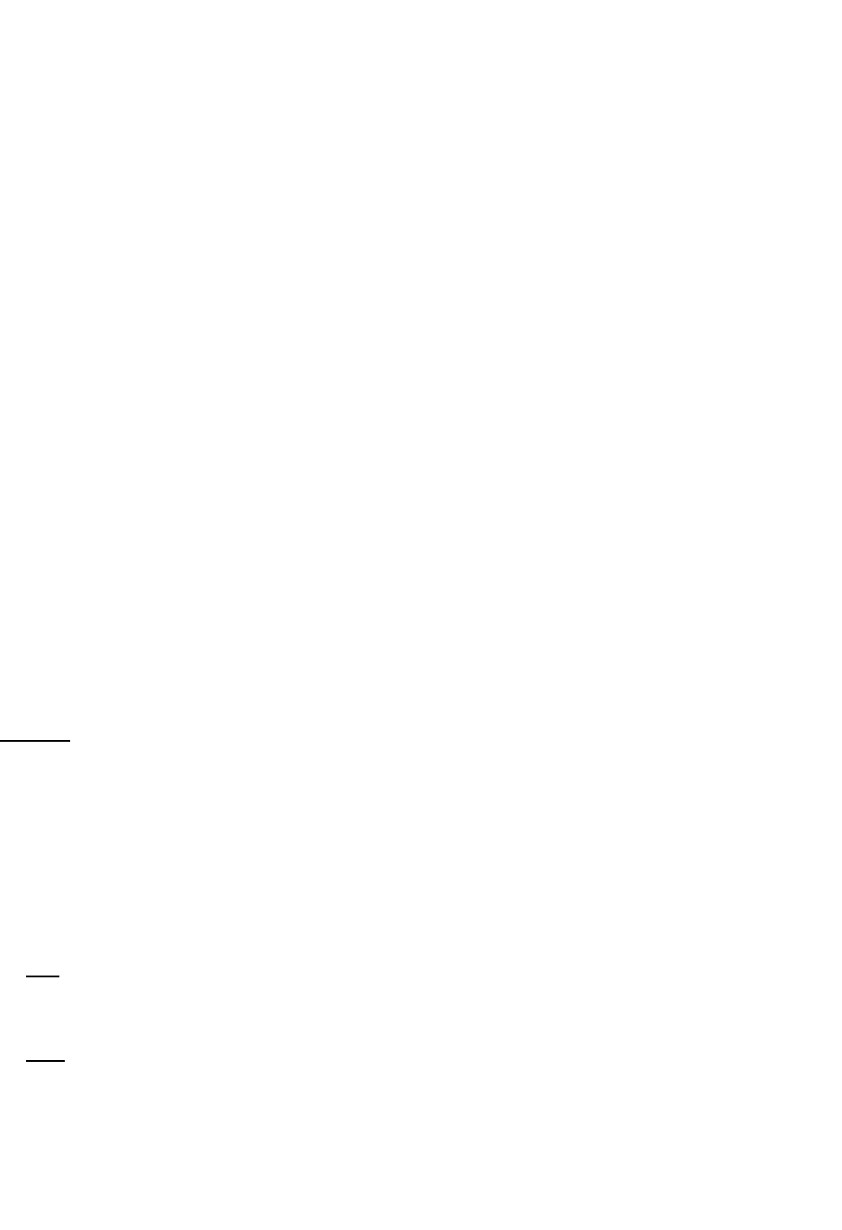
0.5 < aidif < 1 ; always stable

0 < aidif < 0.5 ; stable if ...

dt

dz()

×1

24aidif×()

where  is the maximum vertical mixing

coefﬁcient.

constvmix utilizes constant eddy

coefﬁcients (variables fkpm and fkph for

momentum and heat, respectively) for

linear second order mixing of momentum

and tracers in the vertical. In the explicit

case (when implicitvmix has not been

deﬁned), convective adjustment handles

regions of gravitational instability for the

tracers. If implicitvmixis deﬁned, then

the convective section is bypassed and

the large mixing coefﬁcient values (limits

set in variables vdclim and vvclim)

are used to set the vertical mixing

coefﬁcients to handle the instability for

both the tracers and momentum.

ppvmix is a vertical mixing option based

on the Pacanowski and Philander (1981)

Richardson mixing scheme. This

parameterization was designed primarily

for equatorial models with vertical

resolution of about 10 meters between

levels in the upper ocean (we were most

interested in the structure of the

undercurrent). Previous versions of this

code assumed the “t,s” grid was

coincident with the “u,v” grid and gave

good results. In the present case, we have

relaxed this assumption. We tried this

newer, more consistent version a few

ways and got lots of numerical noise, at

ﬁrst (particularly on the equator off Brazil).

The present conﬁguration minimizes

noise. If noise develops off steep shelf

breaks it can sometimes be suppressed

by turning on a bottom drag (see variable

cdbot). The background mixing variable

bvdc should be kept much less than 1.0 to

<Pacanowski, Dixon & Rosati - GFDL Ocean Group Tech. Report No. 2>

3-6

avoid diffusing the thermocline away on

long time scales.

In regions of gravitational instability,

ppvmix uses the vertical mixing limit

variables vdclim and vvclim to set the

vertical eddy coefﬁcients. In the explicit

case they must satisfy the “CFL” criterion

and may be too small to remove the

instability. However, the convective

adjustment is operative and tries to

remove the instability. Whether it does or

not depends on the ncon variable (setable

through namelist), which controlls the

number of passes through the convective

adjustment section of code in ﬁle

tracer.F. If implicitvmix is used,

vdclim and vvclim are set large and

the convective adjustment section is

bypassed. The ppvmix scheme also

assumes the use of equal timesteps on

the density and momentum equations. If a

longer time step is desired, try using the

implicitvmix option.

tcvmix invokes the Mellor-Yamada level

2.5 turbulence closure scheme. Here the

mixing coefﬁcients are a function of the

turbulence length scale (l), the turbulent

kinetic energy (q2), the analytically derived

stability factors (Sm & Sh), and the

boundary conditions. There are two

options within tcvmix to compute the

length scale:

leq solves an additional equation for q2

from which the length scale may be

derived at each level.

lalg, obtains the length scale from an

algebraic relationship. The lalg option

may be sufﬁcient for the boundary layer

but not in cases where there would be

multiple turbulent regimes. The horizontal

diffusion coefﬁcient of turbulent kinetic

energy is set using the variable aq (see

ﬁles ctcmix.h, blkdta.F and the namelist

input). For this scheme to be effective the

implicitvmix option should be enabled

and also the vertical resolution should be

sufﬁcient.

REFERENCES:

Pacanowski, R. and S.G. Philander, J. Phys.

Oceaonogr., 11, ??-??, (1981)

Mellor, G. and Yamata ?????

3-7

(3.6) HYBRID MIXING SCHEME

OPTIONS

We are using the term “hybrid” here to

describe schemes which apply to either

momentum or tracers but not both. For all

cases in which implicitvmix is not

enabled, convective adjustment is the

default. Recall that when solved explicitly

convective adjustment mixes tracers

vertically in regions of gravitational

instability, but not momentum. The

effectiveness of convective adjustment is

controlled by variable ncon which is the

number of passes through the convective

section (use grep -i -n ncon *.[Ffh] to see

its usage). If impllicitvmix is enabled, the

convective adjustment section is

bypassed. in ﬁle tracer.F. The

assumption is that the vertical mixing

schemes will handle it.

isopycmix is a scheme in which a mixing

tensor is computed from the local

isopycnal slope and the diffusion of tracers

is then conducted along that direction. It

therefore inﬂuences both the lateral and

vertical mixing of tracers in the model. Its

use is intended to partially mitigate a

perceived shortcoming of z-coordinate

primitive equation ocean models in

parameterizing oceanic mixing due to

mesoscale motions. Since such mixing is

believed to take place along isopycnal

surfaces, the isopycmix option seeks to

orient the mixing of tracers along

isopycnal surfaces rather than purely

horizontal surfaces, as described by Redi

(1982).

As described by Cox (1987), in addition to

specifying the mixing coefﬁcient for along

isopycnal diffusion (variable ahisop), a

non-zero background horizontal mixing

coefﬁcient (here we use variable ah) is

often needed to supress gridpoint noise.

Additionally, a constraint is placed on the

steepest isopycnal slope (see varable

slmxr) that the scheme will consider

when computing the components of the

mixing tensor. A typical value of slmxr is

100.0, which translates into a slope of

1:100. Steeper slopes would then be

considered to be 1:100 for the purpose of

computing the mixing tensor.

A vertical mixing scheme must be

speciﬁed for use with isopycmix. The zz

component of the isopycnal mixing is

added to the vertical diffusion coefﬁcient

produced by the vertical mixing scheme.

Since isopycmix only affects tracers, one

must also specify a lateral mixing scheme

from the above list to be used for

momentum. This additional lateral mixing

scheme has no effect on tracer diffusion.

REFERENCES:

Cox, M., Ocean Modelling, issue 74, 1-5,

(1987)

Redi, M., J. Phys. Oceanogr., 12, 1154-1158,

(1982).

<Pacanowski, Dixon & Rosati - GFDL Ocean Group Tech. Report No. 2>

3-8

(3.7) OPTIMIZATION OPTIONS

skipland is an option that allows

calculations in the GFDL Modular Ocean

Model to be done over blocks of ocean

while skipping land points. The trade off

here is the time saved by not doing the

calculation over land versus the time used

in starting and stopping a lot of vectors.

Whether or not cp time will be saved by

using this option is largely a function of

land mass geometry and grid resolution. A

global ocean would be a good candidate

for this option, but a idealized basin would

not.

timing is an option that cp and wall clock

times for running on a Cray YMP.

Additionally, the time per grid point per

time step is calculated.

multitasking is an option that was

developed with the Cray YMP in mind. It

allows the slabs to be divided into a series

of tasks. Each task contains approximately

the same number of slabs and there

should ideally be one task per processor.

This is all handled by simply specifying

variable ntasks to be the number of

processors (we’ve defaulted it to 8 in ﬁle

blkdta.F).

The idea behind multitasking is that since

all tasks are independent, all tasks can be

worked on simultaneously. This reduces

the total wall clock time for the job but

NOT the total cpu time. Note: the

ntasks variable may be set > 1 even

when unitasking (running on one

processor), but this is not recommended,

since there is extra work being done at the

interfaces between tasks. Also, on

diagnostic, tracer averaging, and data

saving time steps, the MOM code will

revert to one task of jmt-2 slabs, so

effectively multitasking is shut down for

these time steps.

The multitasking option currently does

not work with the diskless option (see

below) because only two time levels are

used for slabs on simulated disk

(ntlev=2) to save memory and this is

incompatible with ntasks > 1. This

condition may, in principle, be removed by

setting parameter ntlev = 3 when

enabling the diskless option. We haven’t

explored it yet.

To date, we have conﬁrmed that all

combinations of unitasked, multitasked,

and autotasked runs give the same

answers down to the last hex digit on the

Cray YMP. To really utilize this feature on

the Cray YMP, the SSD (solid state disk)

must be used for the slabs (unless large

memory and the diskless option is used).

We have not yet added the best i/o

scheme for the SSD, so the wall clock

times are higher than they could be.

3-9

(3.8) FILTERING OPTIONS

Filtering is used to combat the effect of the

convergence of meridians (shrinking

longitudinal grid spacing) near the poles.

The problem is that the grid spacing

severly limits the time step (especially

when using large density time steps) due

to the “CFL” criterion. Filtering relaxes this

constraint by truncating high wave

numbers. Users should be aware that the

ﬁltering options can be time consuming,

and alter the model solution, and therefore

should be used only as a last resort

Conﬁgurations of the GFDL Modular

Ocean Model code that are prime

candidates for ﬁltering are coarse

resolution global models used to examine

long term climate. The timestep

constraints imposed by including the Arctic

Ocean, and the timescales of the problem

being studied, often lead to the need for

ﬁltering at high latitudes.

fourﬁl is a fourier ﬁlter which acts on

longitudinal strips of ocean points. The

number of wave numbers to be allowed at

each latitude is decided upon and

wavenumbers above are truncated

(without using any reasonable window).

This option is provided as a backward

compatability feature for the Cox (1984)

code. Note: Both in the MOM code and in

the Cox code, the amount of ﬁltering

depends on the number of ocean points

within the longitudinal strip (determined by

lmodel bathymetry). This actually leads to

possibly different truncations at the same

latitude!

ﬁrﬁl is a simple ﬁnite impluse response

ﬁlter based on the familiar 1/4, 1/2, 1/4

weights (the response function is a

cosine). It comes in two ﬂavors: One to

with symmetric boundary conditions (ie:

for tracers) and one for asymmetric

boundary conditons (ie: momentum).

The ﬁrﬁl option also works on longitudinal

strips of ocean points, and may be applied

an arbitrary number of times for an

arbitrary number of latitudes. While the

ﬁrﬁl option is far less cp time intensive

alternative to fourﬁl, we really have not

done any long running comparisons to

comapre the two schemes

<Pacanowski, Dixon & Rosati - GFDL Ocean Group Tech. Report No. 2>

3-10

(3.9) I/O OPTIONS

diskless simulates disk usage using an

array in memory. Since when using this

option no “wall clock” time lost during disk

transfers (because they are memory to

memory transfers), this method gives the

best efﬁciency (cp time / total time). The

cost for achieving this cpu time efﬁciency

is that the model may not be able to ﬁt into

available memory.

As a memory saving feature, diskless

keeps only two time levels of prognostic

variables (ntlev=2) instead of the usual

three. See the size.F ﬁle to examine

resource requirements. Users may wish to

read the discussion of the multitasking

option for related information.

crayio is an option tested on GFDL’s Cray

YMP. Currently, it uses the “getwa/

putwa” routines. If the disk units are set

up on “non SSD” type disk, then the

efﬁciency (cp time / total time) will be bad.

This shows the mismatch in speed

between computationand disk use. SSD

(solid state disk), however, is really the

preferred way to go. It can be looked at as

an extended memory and the efﬁciency is

much better.

ﬁo is the option for using standard Fortran

direct access i/o. The comments from

crayioapply here also.

(3.10) MISCELLANEOUS CODE

OPTIONS

:keepterms is an option allows the use of

arrays instead of statement functions for

component terms in the MOM code’s

tracer and momentum equations. This

may be desirable when using component

terms over and over for some purpose.

The trade off is the extra memory needed

for the arrays versus the extra time

needed to recalculate the statement

functions. See the size.F ﬁle to look at

resource requirements.

nohilatsstands for no high latitudes. If the

latitudinal domain of the model is limited to

equatorial redions, for instance, then the

metric nonlinear terms in the momentum

equations may be dropped. Deﬁning the

nohilats option will save some cp time and

allows for backward compatibility with the

Cox (1984) code.

restorst stands for restore surface tracers

to some prescribed values by a newtonian

damping term. In the sample test case of

the GFDL Modular Ocean Model code,

temperatures and salinities are restored

back toward zonally averaged annual

mean conditions on a time scale of 50

days (ee ﬁle setvbc.F). Without much

work, this option could easily be extended

to damp certain regions while leaving

others alone by simple making the

damping time scale a function of latitude,

for instance.

3-11

testcﬂtests whether any velocity exceeds

the local “CFL” criterion by a factor of

cflcrt(see ﬁle blkdta.F for where

variable cflcrt is set). This option will

print out the places where the CFL

criterion is most nearly met on diagnostic

time steps. If the cflcrt factor is

exceeded on any time step, the MOM

code will stop its execution and print out

the surrounding variables.

NOTE: the testcﬂ option is not meant to

be left on all the time, since is uses much

cp time. It is best used as an analysis aid.

For example, it can be used infrequently

on a model that is being run for a long

time, or should a version of the model

“blow up”, it can be useful in pointing to

where the problem arises.

This page was intentionally left blank

3-12

<Pacanowski, Dixon & Rosati - GFDL Ocean Group Tech. Report No. 2>

4-1

Any general circulation model contains an

intimidating number of “things” to keep

track of. For a new user, deciding which

things to study in detail ﬁrst so that other

portions of the model can be understood

can be important question. This chapter

seeks to describe for the user several of

the basic building blocks that one needs to

know in order to develop working

knowldege of the GFDL MOM code. We

expect that more seasoned users will refer

to these pages when seeking to refresh

their memories.

The discussion of building blocks begins

with the model grid itself. However, while

describing the grid, we will also introduce

some speciﬁcs concerning conventions

used in the naming of variables.

CHAPTER 4: Some Basics of the GFDL

Modular Ocean Model

4-2

(4.1)THE THREE DIMENSIONAL

GRID

The structure of the model grid itself is a

reasonable topic to tackle ﬁrst when

building up knowledge of the GFDL

Modular Ocean Model code.

Understanding the layout of the grid and

some of the MOM code’s naming

conventions that relate to grid locations is

crucial if one it to be able to mentally

translate many parts of the code into

visual images.

Figure 4.1.1 displays the horizontal grid

structure used in the MOM code and

Figure 4.1.2 displays the vertical grid..

Variables are arranged in the manner of

the “B-grid” convention described by

Arakawa and Lamb (1977). Users may

refer to the coord.h and grdvar.h ﬁles

for lists and descriptions of many of the

variables relating to the grid.

Parameters used to set the number of

model grid points in the west-to-east,

south-to-north, and top-to-bottom

directions are imt,jmt, and km,

respectively (see the param.h ﬁle). Thus,

variables aligned along a speciﬁc latitude

can be referred to as being in the same “j-

row”, with values of i increasing as one

moves eastward. The ﬁrst j-row (j=1) lies

at the southern limit of the model domain,

and values of j increase as one moves

northward. In the vertical, values of k

increase as one moves downward to

greater depths.

Since the GFDL MOM code employs the

B-grid, tracer quantities (potential

temperature, salinity, and other tracers)

are deﬁned in the horizontal at different

locations than the velocity component

variables u and v. As shown in Figure

4.1.1, a “u,v” grid point with a given i,j

designation is located to the northeast of

the tracer grid location having the same

i,j values. The two-dimensional volume

transport streamfunction  (variable p in

the emode.h ﬁle) is also aligned on the

horizontal tracer grid.

In the GFDL Modular Ocean Model,

horizontal grid locations are carried in

terms of degrees of latitude and longitude.

Variable xt(i) represents the longitude

of the “i-th” point on the tracer grid, and

variable xu(i) represents the longitude of

the “i-th” point on the u,v grid. Similarly,

variable yt(j) represents the latitude of

the “j-th” model row on the tracer grid,

while the latitude of the “j-th”u,v j-row is

stored in variable yu(j).

In the horizontal, tracer grid points lie in

the exact center of tracer grid box cells.

The four points of a tracer grid cell lie at

u,v grid point locations. The distance (in

centimeters) across a tracer grid box cell

in the north-south (meridional) direction at

location i,j is stored in variable dyt(j),

while the distance in the east-west (zonal)

direction at the Equator is stored in

variable dxt(i)(see the grdvar.h ﬁle).

As depicted in Figure 4.1.1, the GFDL

Modular Ocean Model allows for variable

grid spacing in the horizontal. Therefore,

u,v grid points do not necessarily lie in

the center of the four surrounding tracer

gridpoints. Distances across u,v grid cells

are given by variables dyu and dxu, and

correspond to the distances (in

centimeters) between tracer grid points in

the north-south and east-west directions,

respectively.

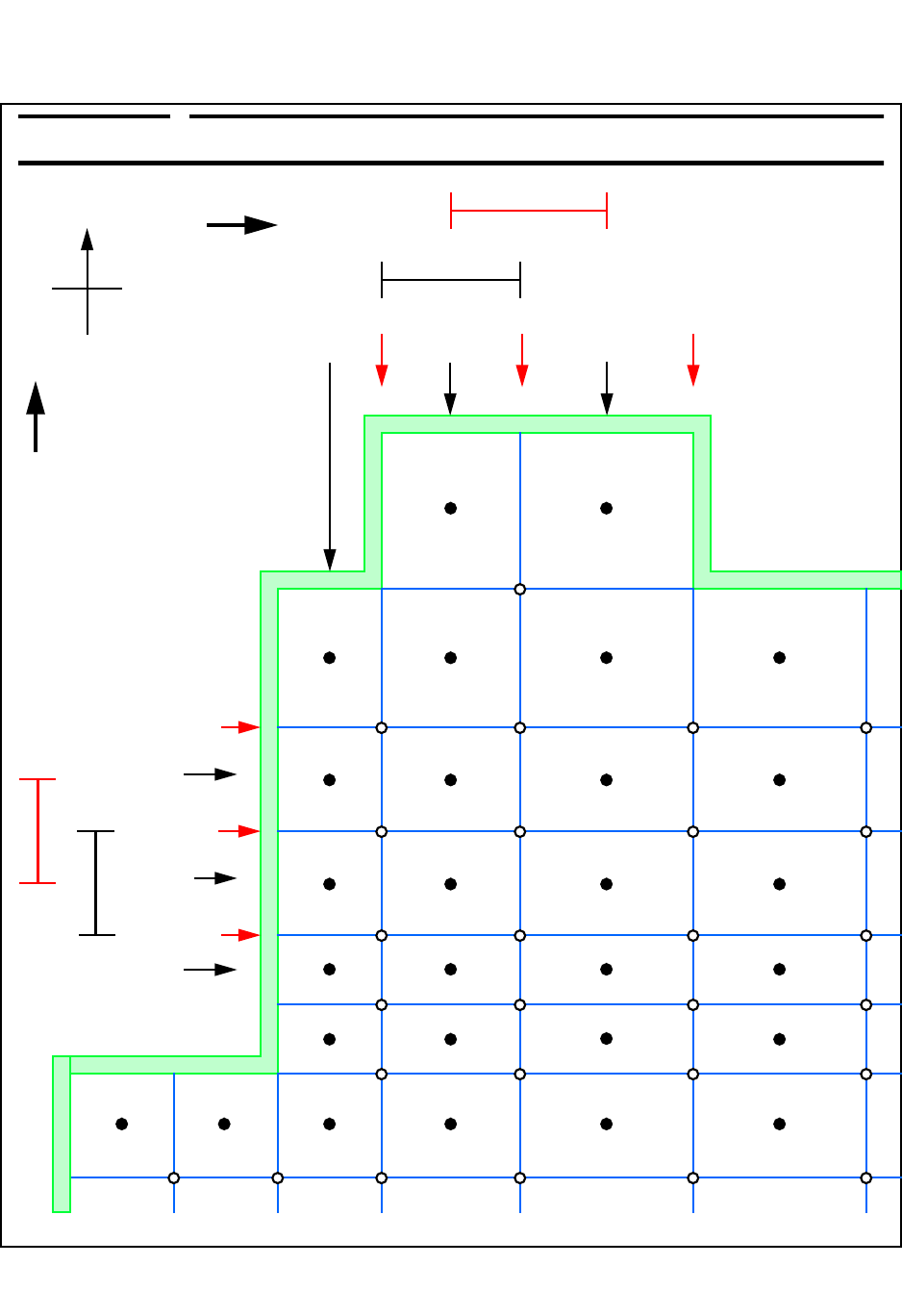
<Pacanowski, Dixon & Rosati - GFDL Ocean Group Tech. Report No. 2>

4-3

u v

u v(i,j)

u v

u vu v

yu(j)

yu(j+1)

yu(j-1)

yt( j )

yt( j+1)

xt(i)xt(i+1)

xt(i-1)

xu(i) xu(i+1)

xu(i-1)

dxt( i )

dxu(i)

dyu(j)

dyt( j )

FIGURE 4.1.1 Skematic view of the GFDL Modular Ocean Model’s horizontal grid arrangement.





yt( j-1)

(i,j)

4-4

Since the dxu and dxu variables are

calculated as the distance (in centimeters)

across a grid cell in the zonal direction at

the Equator, one must multiply these

variables by the cosine of the latitude of

the j-row of interest in order to determine

the true east-west distance between grid

points at a given latitude. The cosines of

the latitudes of tracer grid points (yt(j))

are stored in variable cst(j), and the

cosines of the u,v grid point latitudes

(yv(j)) of tracer grid points are stored in

variable csu(j) (see ﬁle grdvar.h).

The following sentence attempts to tie

together some of the elements presented

thus far concerning the horizontal grid

used in the GFDL MOM code:

The east-west distance, in centimeters,

across the southern face of the tracer grid

box cell centered at latitude yt(j) and

longitude xt(i) is equal to the distance

from longitude xu(i-1) to xu(i) at

latitude yu(j), which can be computed

as... csu(j-1) * dxu(i)

With the above preliminaries out of the

way we can now turn to the question of

how a user speciﬁes the horizontal grid

desired for a particular application in the

MOM code. The process begins when

program ocean calls subroutine

grids.Subroutine grids, and

supporting subroutines mesh and

cmesh and function indp are found in

ﬁle setgrid.F.

Upon entering subroutine grids, a call to

subroutine mesh is made in order to

determine tracer grid cell widths dxt and

dyt. All other grid variables are calculated

within the subroutine grids from

these two variables.

As alluded to earlier, the GFDL MOM code

provides a means by which variable grid

spacing can be incorporated into the

model. This is achieved in subroutine

mesh. The nxres and nyres parameters

are the number of subdomains of either

constant or smoothly varying grid cell

dimensions. For the simplest case of a

grid that is uniform in terms of latitude and

longitude grid spacing, parameters nxres

and nyres are set to be equal to one in

ﬁle param.h. This was done for the sample

conﬁguration of the MOM code.

Variables used to determine the grid

spacing (be the spacing either uniform or

variable) are set by the user in the

blkdta.F ﬁle. These variables (namely,

variables stlon, xmax, xmin, xwid

and idir for longitudinal subdomains,

and stlat, ymax, ymin, ywid and

jdir for the latitudinal subdomains) are

described in the comments found in the

coord.h ﬁle.

For each of the longitudinal and latitudinal

subdomains asked for (nxres and

nyres) the user must specify the sum of

the distances (in degrees) to be covered

by tracer grid box cells within that

subdomain. Subdomain widths are given

by xwid(nx) and ywid(ny), where ny

goes from 1 to nxres and ny from 1 to

nyres. Variables xmax and xmin and

ymax and ymin are used to specify the

minimum and maximum tracer grid box

cell widths within the given domain.

Uniform spacing within a subdomain can

be achieved by setting the minimum and

maximum widths to be equal. Otherwise,

smoothly varying grid cell widths will be

computeda, and the idir and jdir

variables are set to either +1 or -1 to

signify whether the grid box cells are to

<Pacanowski, Dixon & Rosati - GFDL Ocean Group Tech. Report No. 2>

4-5

increase or decrease as one moves

across the subdomain to higher i or j

values. The calculations for the variable

tracer grid cell widths are performed in

subroutine cmesh.

The model grid point located in the far

southwest of the entire model domain is a

tracer grid point with an i,j location of

(1,1). All model grid locations are

computed using this position as a starting

point.. This starting location for the model

grid is given (in degrees) by variables

stlat and stlon.

Variables xt,yt,xt and xu are each

monotonically increasing in the MOM

code. In cases of an ocean model with

pseudo-realistic geometry, the cyclic

option needs to be speciﬁed, and thus the

sum of all the longitudinal subdomains

must be greater than 360 degrees (as in

the sample case).

Should a user have a special application in

which it is desired to have latiitudal and/or

longitudinal grid spacing that varies in a

way not readily produced by the above

described method, we suggest the

following get-around. Add a new ifdef

option to the code, such that when it is

deﬁned subroutine grids calls a new, user

supplied routine, rather than subroutine

mesh.. This new routine should return

variables dxt and dyt. Once that is

accomplished, all other grid variables will

be computed, starting at the stlat and

stlon tracer gridpoint location.

REFERENCES

Arakawa, A., and V. Lamb, “Computational

Design of the basic dynamical processes

of the UCLA general circulation model”,

Methods in Computational Physics, vol 17,

Academic Press, (1977)

4-6

<Pacanowski, Dixon & Rosati - GFDL Ocean Group Tech. Report No. 2>

IN-1

INDEX

ah variable ............................................... 3-4,3-7

see also eddy coefﬁcients

ahisop variable ........................................... 3-7

see also eddy coefﬁcients ........................... 3-7

aidif variable .............................................. 3-5

am variable ....................................................... 3-4

see also eddy coefﬁcients

anonymous ftp, see ftp command .......... iii

aq variable ....................................................... 3-6

see also eddy coefﬁcients .......................... 3-6

biharmonic option ........................................... 3-4

blkdta.F file ............... 2-5,3-5,3-6,3-8,3-11

bottom drag ..................................................... 2-5,3-5

boundary conditions

lateral ...................................................................... 2-5

vertical .................................................................... 2-4

Bryan, Kirk ...........................................................vi,vii

bvdc variable ................................................. 3-5

calling tree diagrams .......................................... 2-6

cdbot variable .............................................. 3-5

see also eddy coefﬁcients

fkpm variable ................................................. 3-5

see also eddy coefﬁcients

fonts ...............................................................................iv

Fortran-77 ................................................................ 2-2

fourﬁl option .......................................................... 3-9

fourier filter, see fourﬁl option ..................... 3-9

fourth order mixing .............................................. 3-4

ftp command ....................................................iii,iv

getvar.F file ................................................. 2-6

IN-2

GFDL Ocean Group Technical Report #1 .vi

GFDL Ocean Group Technical Report #2 .iv

grid options .............................................................. 3-8

Hellerman and Rosenstein winds ................ 1-3

horizontal mixing schemes, see lateral mixing

schemes

hybrid mixing schemes ..................................... 3-7

hypergrid option ................................................ 3-3

I/O options ............................................................. 3-10

ifdef directives ................................ 1-3,2-3

conﬂict checks ................................................... 3-2

implicitvmix option .......................... 3-5,3-6,3-7

include files ................................. 1-4,1-5,2-2

indp function ......................................... 2-4,2-6

input/output, see I/O options

internet ....................................................................iii,iv

iounit.h file ................................................. 2-5

iperim.F file ................................................. 2-4

island calculations ............................................... 2-4

isopycmix option .............................................. 3-7

isopycnal mixing, see isopycmix............... 3-7

isopycnal mixing, see isopycmix option

keepterms option ................................... 2-2,3-10

Kerr, Christopher ................................................... vii

lalg option,see tcvmix option

lateral mixing schemes ............................. 3-4,3-7

leq option,see tcvmix option

Levitus climatology .............................................. 1-3

Mahlman, J. ............................................................. vii

matrix.F file ................................................. 2-6

Mellor, George ....................................................... 3-6

Mellor-Yamada turbulence closure, see also

tcvmix option ............................................... 3-6

memory size ........................................................... 2-3

mergelib utility ................................ 1-2,1-4

metric nonlinear terms ..................................... 3-10

Miyakoda, Kikuro ........................................... vii,3-4

modular design ...................................................... 2-2

MOM_NEWS file .............................................v,1-2

multitasking option ................................ 3-8,3-10

my_mom directory ...........................................iv

namelist ..................................... 2-2,2-4,3-3,3-5,3-6

naming conventions ........................................... 2-3

ncon variable ......................................... 3-6,3-7

nearest model gridpoint .................................... 2-4

newtonian damping .......................................... 3-10

nlhmix option ....................................................... 3-4

nmix variable ................................................. 2-4

nohilats option .................................................. 3-10

non-linear horizontal subgrid-scale mixing

see also nlhmix option .............................. 3-4

ntasks variable ........................................... 3-8

ntlev parameter ................................. 3-8,3-10

ocean program ................................................. 2-6

ocean.F file .................................................... 2-5

ocean.in file ................................................. 1-2

odam.F file ....................................................... 2-6

off-line analysis ..................................................... 2-5

oldrelax option ................................................... 3-3

Oort climatology .................................................... 1-3

optimization options ............................................ 3-8

organization of variables .................................. 2-2

out-of-bounds references ................................ 2-2

Pacanowski, Ronald ..............................vi,3-5,3-6

param.h file .................................................... 2-2

parameter statements ....................................... 1-4

pconst.h file ................................................. 2-3

Philander, S.G. .............................................. 3-5,3-6

Poisson solvers, see external mode options

ppvmix option ............................................. 3-5,3-6

PREP_DATA directory ..........................iv,1-3

printout file ......................................... 1-2,1-5

READ_ME file ............................................ 1-2,1-3

readrmsk option ................................................ 2-5

readrmsk option ........................................... 2-5

Redi, M. ..................................................................... 3-7

REFERENCES ..........iv,vi,1-3,3-3,3-4,3-6,3-7

region masks

horizontal .............................................................. 2-5

vertical ................................................................... 2-5

regional averages ................................................ 2-5

relax.F file .................................................... 3-3

<Pacanowski, Dixon & Rosati - GFDL Ocean Group Tech. Report No. 2>

IN-3

resource requirements ...................................... 2-6

restorst option .................................................... 3-10

rigidlid option ....................................................... 3-3

Rosati, Anthony .........................................iv,vi,3-4

runtime documentation ..................................... 2-5

saving original files .............................................. 1-4

scalar.h file ................................................. 2-5

scale selective mixing ........................................ 3-4

SCCS ................................................................. 1-5,2-4

Scripps topography ............................................. 1-3

second order mixing ................................... 3-4,3-5

Semtner, A. .........................................................vi,vii

setgrd.F file ................................................. 2-6

setgrid.F file .............................................. 2-4

setvbc.F file ............................................... 3-10

size program .................................................... 2-6

size.F file ..................................................... 3-10

skipland option ........................................... 2-3,3-8

slabs ............................................................ 2-3,2-4,3-8

slabs.h file .................................................... 2-3

slmxr variable .............................................. 3-7

Smagorinsky, J. .................................................... 3-4

snaps variable .............................................. 2-5

snapshot option ................................................. 2-5

solid state disk, see Cray YMP ..................... 3-8

sor variable .................................................... 3-3

Source Code Control System, see SCCS

sources and sinks ................................................ 2-4

splitlib utility ........................ 1-2,1-4,1-6

SSD, see Cray YMP ($nopage) ................... 3-8

statement functions ............................................. 2-3

streamfunction

volume transport ............................................... 3-3

switch.h file ......................................... 2-4,2-5

symmetry option ............................................... 3-2

tcvmix option ............................................... 3-5,3-6

leq option ........................................................... 3-6

term balances ........................................................ 2-5

testcﬂ option ....................................................... 3-11

thick.h file .................................................... 2-6

time manager ......................................................... 2-4

timing option ........................................................ 3-8

tmngr.F file .................................................... 2-4

tracer averaging timestep ................................ 3-8

tracer averaging timestep, see also regional

averages ($nopage) ................................... 3-8

tracer.F file ......................... 2-2,3-5,3-6,3-7

tracing variables and options ......................... 2-2

turbulent kinetic energy .................................... 3-6

UNIX commands

cat ............................................................................ 1-5

chmod .................................................................... 1-4

cpp, see cpp command ............................... 1-3

diff .................................................................... 1-6,2-4

ftp, see ftp command ................................... iii

grep ................................................................. 2-2,3-7

ls ...................................................................................v

tar ............................................................................. 1-2

UPDOC ..................................................................... 2-3

upgrade utility ........................... 1-3,1-5,1-6

vdclim variable ........................................... 3-5

vdclim variable, see also eddy

coefﬁcients ...................................................... 3-5

version number ..................................................... 1-2

vertical mixing schemes ........................... 3-5,3-7

vertical resolution ................................................. 3-6

vvclim variable ........................................... 3-5

vvclim variable, see also eddy

coefﬁcients ...................................................... 3-5

wind stress .............................................................. 1-3

MOM1 Manual

MOM1_manual

Navigation menu

Versions of this User Manual:

Views

Navigation