MOM3 Manual
MOM3_manual
User Manual:
Open the PDF directly: View PDF ![]() .
.
Page Count: 708 [warning: Documents this large are best viewed by clicking the View PDF Link!]
—Draft— Feb 2000 —
ii

Contents
I Introduction to MOM and its use 1
1 Introduction 3
1.1 What is MOM? . . . . . . . . . . . . . . . . . . . . . . . . . . . . . . . . . . . . . 3
1.2 Accessing the manual, code, and database . . . . . . . . . . . . . . . . . . . . . . 3
1.3 Minimum computational requirements . . . . . . . . . . . . . . . . . . . . . . . 4
1.4 How this manual is organized . . . . . . . . . . . . . . . . . . . . . . . . . . . . . 4
1.5 Special acknowledgments and disclaimers . . . . . . . . . . . . . . . . . . . . . 5
1.5.1 Acknowledgments . . . . . . . . . . . . . . . . . . . . . . . . . . . . . . . 5
1.5.2 Disclaimer . . . . . . . . . . . . . . . . . . . . . . . . . . . . . . . . . . . . 5
1.5.3 Software license . . . . . . . . . . . . . . . . . . . . . . . . . . . . . . . . . 5
2 A brief history of ocean model development at GFDL 7
2.1 Bryan-Cox-Semtner: 1965-1989 . . . . . . . . . . . . . . . . . . . . . . . . . . . . 7
2.2 The GFDL Modular Ocean Models: MOM 1 and MOM 2: 1990-1995 . . . . . . . 7
2.3 MOM 3: 1996-1999 . . . . . . . . . . . . . . . . . . . . . . . . . . . . . . . . . . . 8
2.4 Documentation . . . . . . . . . . . . . . . . . . . . . . . . . . . . . . . . . . . . . 8
2.4.1 Main differences between MOM 2 and MOM 3 . . . . . . . . . . . . . . . 9
2.4.2 Parallelization and Fortran 90 . . . . . . . . . . . . . . . . . . . . . . . . . 9
2.4.3 Model physics and numerics . . . . . . . . . . . . . . . . . . . . . . . . . 9
2.5 Main differences between MOM 1 and MOM 2 . . . . . . . . . . . . . . . . . . . 11
2.5.1 Architecture . . . . . . . . . . . . . . . . . . . . . . . . . . . . . . . . . . . 11
2.5.2 Physics and analysis tools . . . . . . . . . . . . . . . . . . . . . . . . . . . 12
3 Getting Started 15
3.1 How to find things in MOM . . . . . . . . . . . . . . . . . . . . . . . . . . . . . . 15
3.2 Directory Structure . . . . . . . . . . . . . . . . . . . . . . . . . . . . . . . . . . . 15
3.3 The MOM Test Cases . . . . . . . . . . . . . . . . . . . . . . . . . . . . . . . . . . 19
3.3.1 The run mom script . . . . . . . . . . . . . . . . . . . . . . . . . . . . . . 20
3.4 Sample printout files . . . . . . . . . . . . . . . . . . . . . . . . . . . . . . . . . . 21
3.5 How to set up a model . . . . . . . . . . . . . . . . . . . . . . . . . . . . . . . . . 22
3.6 Executing the model . . . . . . . . . . . . . . . . . . . . . . . . . . . . . . . . . . 24
3.7 Analyzing solutions . . . . . . . . . . . . . . . . . . . . . . . . . . . . . . . . . . . 24
3.8 Executing on 32 bit workstations . . . . . . . . . . . . . . . . . . . . . . . . . . . 24
3.9 NetCDF and time averaged data . . . . . . . . . . . . . . . . . . . . . . . . . . . 25
3.10 Using Ferret . . . . . . . . . . . . . . . . . . . . . . . . . . . . . . . . . . . . . . . 25
3.11 Upgrading from MOM 1 . . . . . . . . . . . . . . . . . . . . . . . . . . . . . . . . 27
3.12 Upgrading to the latest version of MOM . . . . . . . . . . . . . . . . . . . . . . . 27
iii

iv
CONTENTS
3.12.1 The recommended method to incorporate personal changes . . . . . . . 28
3.12.2 An alternative recommended method . . . . . . . . . . . . . . . . . . . . 28
3.13 Finding all differences between two versions of MOM . . . . . . . . . . . . . . . 29
3.14 Applying bug fixes . . . . . . . . . . . . . . . . . . . . . . . . . . . . . . . . . . . 29
II Basic formulation 33
4 Fundamental equations 35
4.1 Assumptions . . . . . . . . . . . . . . . . . . . . . . . . . . . . . . . . . . . . . . . 35
4.2 The primitive equations . . . . . . . . . . . . . . . . . . . . . . . . . . . . . . . . 36
4.2.1 Basic constants and parameters . . . . . . . . . . . . . . . . . . . . . . . . 37
4.2.2 Hydrostatic pressure and the equation of state . . . . . . . . . . . . . . . 38
4.2.3 Horizontal momentum equations . . . . . . . . . . . . . . . . . . . . . . 38
4.2.3.1 Coriolis force . . . . . . . . . . . . . . . . . . . . . . . . . . . . . 38
4.2.3.2 Horizontal pressure gradient . . . . . . . . . . . . . . . . . . . . 38
4.2.3.3 Advection . . . . . . . . . . . . . . . . . . . . . . . . . . . . . . . 38
4.2.3.4 Nonlinear advective “metric” term . . . . . . . . . . . . . . . . 39
4.2.3.5 Vertical friction . . . . . . . . . . . . . . . . . . . . . . . . . . . . 39
4.2.3.6 Horizontal friction . . . . . . . . . . . . . . . . . . . . . . . . . . 39
4.2.4 Tracer equations . . . . . . . . . . . . . . . . . . . . . . . . . . . . . . . . 39
4.3 Boundary and initial conditions . . . . . . . . . . . . . . . . . . . . . . . . . . . . 40
4.3.1 Bottom kinematic boundary condition . . . . . . . . . . . . . . . . . . . . 41
4.3.2 Surface kinematic boundary condition . . . . . . . . . . . . . . . . . . . . 41
4.3.3 Dynamic boundary conditions . . . . . . . . . . . . . . . . . . . . . . . . 42
4.3.4 Tracer fluxes through the model boundaries . . . . . . . . . . . . . . . . 43
4.3.5 Open boundaries and sponges . . . . . . . . . . . . . . . . . . . . . . . . 44
4.3.6 Initial conditions . . . . . . . . . . . . . . . . . . . . . . . . . . . . . . . . 44
4.4 Comments on volume versus mass conservation . . . . . . . . . . . . . . . . . . 44
4.4.1 Volume conservation . . . . . . . . . . . . . . . . . . . . . . . . . . . . . . 44
4.4.2 Mass conservation . . . . . . . . . . . . . . . . . . . . . . . . . . . . . . . 45
4.4.3 Surface kinematic boundary conditions revisited . . . . . . . . . . . . . . 46
4.5 Flux form and finite volumes . . . . . . . . . . . . . . . . . . . . . . . . . . . . . 47
4.6 Some basic formulae and notation . . . . . . . . . . . . . . . . . . . . . . . . . . 47
4.6.1 Differential operators . . . . . . . . . . . . . . . . . . . . . . . . . . . . . . 48
4.6.2 Leibnitz’s Rule . . . . . . . . . . . . . . . . . . . . . . . . . . . . . . . . . 49
4.6.3 Cross-products and the Levi-Civita symbol . . . . . . . . . . . . . . . . . 49
4.6.4 Area element and volume element on a sphere . . . . . . . . . . . . . . . 49
4.6.5 Vertical grid levels . . . . . . . . . . . . . . . . . . . . . . . . . . . . . . . 49
5 Momentum equation methods 51
5.1 Separation into vertical modes . . . . . . . . . . . . . . . . . . . . . . . . . . . . 51
5.1.1 Vertical modes in MOM and their relation to eigenmodes . . . . . . . . . 52
5.1.2 Motivation for separating the modes . . . . . . . . . . . . . . . . . . . . . 53
5.2 Methods for solving the separated equations . . . . . . . . . . . . . . . . . . . . 53
5.2.1 The fixed surface /rigid lid method in brief . . . . . . . . . . . . . . . . . 54
5.2.1.1 Fixed surface height . . . . . . . . . . . . . . . . . . . . . . . . . 54
5.2.1.2 Vanishing velocity at the ocean surface . . . . . . . . . . . . . . 55
CONTENTS
v
5.2.1.3 Fresh water forcing in the rigid lid . . . . . . . . . . . . . . . . 55
5.2.1.4 Two rigid lid methods in MOM . . . . . . . . . . . . . . . . . . 55
5.2.2 The free surface /non-rigid lid method in brief . . . . . . . . . . . . . . . 56
5.2.2.1 The barotropic equation and its two solution methods . . . . . 56
5.2.2.2 The non-rigid lid approximation . . . . . . . . . . . . . . . . . . 56
6 Rigid lid streamfunction method 59
6.1 The barotropic streamfunction . . . . . . . . . . . . . . . . . . . . . . . . . . . . . 59
6.2 Streamfunction and volume transport . . . . . . . . . . . . . . . . . . . . . . . . 60
6.3 Hydrostatic pressure with the rigid lid . . . . . . . . . . . . . . . . . . . . . . . . 60
6.4 The barotropic vorticity equation . . . . . . . . . . . . . . . . . . . . . . . . . . . 61
6.4.1 Tendencies for the vertically averaged velocities . . . . . . . . . . . . . . 61
6.4.2 The barotropic vorticity equation . . . . . . . . . . . . . . . . . . . . . . . 63
6.4.3 Caveat: inversions with steep topography . . . . . . . . . . . . . . . . . 64
6.5 Boundary conditions and island integrals . . . . . . . . . . . . . . . . . . . . . . 64
6.5.1 Dirichlet boundary condition on the streamfunction . . . . . . . . . . . . 64
6.5.2 Separating the streamfunction’s boundary value problem . . . . . . . . 65
6.5.3 Island integrals for the volume transport . . . . . . . . . . . . . . . . . . 66
6.6 The baroclinic mode . . . . . . . . . . . . . . . . . . . . . . . . . . . . . . . . . . 67
6.7 Summary of the rigid lid streamfunction method . . . . . . . . . . . . . . . . . . 67
6.8 Rigid lid surface pressure method . . . . . . . . . . . . . . . . . . . . . . . . . . 68
7 Free surface method 69
7.1 Hydrostatic pressure with the free surface . . . . . . . . . . . . . . . . . . . . . . 69
7.2 The barotropic system . . . . . . . . . . . . . . . . . . . . . . . . . . . . . . . . . 71
7.2.1 Vertically integrated transport . . . . . . . . . . . . . . . . . . . . . . . . 71
7.2.2 Bottom and surface kinematic boundary conditions . . . . . . . . . . . . 72
7.2.3 Free surface height equation . . . . . . . . . . . . . . . . . . . . . . . . . 72
7.2.4 Vertically integrated momentum equations . . . . . . . . . . . . . . . . . 73
7.2.5 Global water budget . . . . . . . . . . . . . . . . . . . . . . . . . . . . . . 73
7.3 A linearized barotropic system . . . . . . . . . . . . . . . . . . . . . . . . . . . . 74
7.3.1 The barotropic system . . . . . . . . . . . . . . . . . . . . . . . . . . . . . 74
7.3.2 The shallow water limit . . . . . . . . . . . . . . . . . . . . . . . . . . . . 75
7.3.3 The linearized free surface height equation . . . . . . . . . . . . . . . . . 75
7.3.4 Summary of the linear barotropic system . . . . . . . . . . . . . . . . . . 76
7.4 Stresses at the ocean surface and bottom . . . . . . . . . . . . . . . . . . . . . . . 77
7.4.1 Bottom stress . . . . . . . . . . . . . . . . . . . . . . . . . . . . . . . . . . 78
7.4.2 Surface stress . . . . . . . . . . . . . . . . . . . . . . . . . . . . . . . . . . 79
7.4.3 Revisiting the surface stress . . . . . . . . . . . . . . . . . . . . . . . . . . 80
7.5 A comment about atmospheric pressure . . . . . . . . . . . . . . . . . . . . . . . 81
7.6 Vertically integrated transport . . . . . . . . . . . . . . . . . . . . . . . . . . . . . 81
7.6.1 General considerations . . . . . . . . . . . . . . . . . . . . . . . . . . . . . 81
7.6.2 An approximate streamfunction . . . . . . . . . . . . . . . . . . . . . . . 81
8 The tracer budget 85
8.1 The continuum tracer concentration budget . . . . . . . . . . . . . . . . . . . . . 85
8.2 Finite volume budget for the total tracer . . . . . . . . . . . . . . . . . . . . . . . 85
8.3 Surface tracer flux . . . . . . . . . . . . . . . . . . . . . . . . . . . . . . . . . . . . 86
vi
CONTENTS
8.4 Comments on the surface tracer fluxes . . . . . . . . . . . . . . . . . . . . . . . . 87
8.4.1 Fresh water flux into the free surface model . . . . . . . . . . . . . . . . . 88
8.4.2 Heat flux into the free surface model . . . . . . . . . . . . . . . . . . . . . 89
9 Momentum friction 91
9.1 History of friction in MOM . . . . . . . . . . . . . . . . . . . . . . . . . . . . . . 91
9.2 Basic properties of the stress tensor . . . . . . . . . . . . . . . . . . . . . . . . . . 92
9.2.1 The deformation or rate of strain tensor . . . . . . . . . . . . . . . . . . . 92
9.2.2 Relating strain to stress . . . . . . . . . . . . . . . . . . . . . . . . . . . . 94
9.2.3 Angular momentum and symmetry of the stress tensor . . . . . . . . . . 94
9.3 The stress tensor in Cartesian coordinates . . . . . . . . . . . . . . . . . . . . . . 95
9.3.1 Generalized Hooke’s law form . . . . . . . . . . . . . . . . . . . . . . . . 96
9.3.2 Angular momentum . . . . . . . . . . . . . . . . . . . . . . . . . . . . . . 96
9.3.3 Dissipation of total kinetic energy . . . . . . . . . . . . . . . . . . . . . . 96
9.3.4 Transverse isotropy . . . . . . . . . . . . . . . . . . . . . . . . . . . . . . . 97
9.3.5 Trace-free frictional stress . . . . . . . . . . . . . . . . . . . . . . . . . . . 98
9.3.6 Summary of the frictional stress tensor . . . . . . . . . . . . . . . . . . . 98
9.3.7 Quasi-hydrostatic assumption . . . . . . . . . . . . . . . . . . . . . . . . 99
9.3.8 Cartesian form of the friction vector . . . . . . . . . . . . . . . . . . . . . 99
9.3.9 The case of nonconstant viscosity . . . . . . . . . . . . . . . . . . . . . . . 100
9.4 Orthogonal curvilinear coordinates . . . . . . . . . . . . . . . . . . . . . . . . . . 100
9.4.1 Some rules of tensor analysis on manifolds . . . . . . . . . . . . . . . . . 101
9.4.2 Orthogonal coordinates . . . . . . . . . . . . . . . . . . . . . . . . . . . . 104
9.4.3 Physical components of tensors . . . . . . . . . . . . . . . . . . . . . . . . 104
9.4.4 General form of the frictional stress tensor . . . . . . . . . . . . . . . . . 105
9.4.5 Horizontal tension and shearing rate of strain . . . . . . . . . . . . . . . 106
9.4.6 The friction vector . . . . . . . . . . . . . . . . . . . . . . . . . . . . . . . 107
9.4.7 Effects on kinetic energy . . . . . . . . . . . . . . . . . . . . . . . . . . . . 108
9.4.8 Summary of second order friction . . . . . . . . . . . . . . . . . . . . . . 109
9.5 Biharmonic friction . . . . . . . . . . . . . . . . . . . . . . . . . . . . . . . . . . . 110
9.5.1 General formulation . . . . . . . . . . . . . . . . . . . . . . . . . . . . . . 111
9.5.2 Effects on kinetic energy . . . . . . . . . . . . . . . . . . . . . . . . . . . . 112
9.6 Comments on frictional and advective metric terms . . . . . . . . . . . . . . . . 112
9.6.1 Motion on an infinite plane . . . . . . . . . . . . . . . . . . . . . . . . . . 113
9.6.2 Conservation of angular momentum about the north pole . . . . . . . . 114
9.6.3 The advective and frictional metric terms . . . . . . . . . . . . . . . . . . 115
9.7 Functional formalism . . . . . . . . . . . . . . . . . . . . . . . . . . . . . . . . . . 116
9.7.1 Continuum formulation . . . . . . . . . . . . . . . . . . . . . . . . . . . . 116
9.7.2 Discrete formulation . . . . . . . . . . . . . . . . . . . . . . . . . . . . . . 118
9.8 Old friction implementation . . . . . . . . . . . . . . . . . . . . . . . . . . . . . . 118
9.8.1 Spherical form of second order friction . . . . . . . . . . . . . . . . . . . 118
9.8.2 Zonal friction . . . . . . . . . . . . . . . . . . . . . . . . . . . . . . . . . . 119
9.8.3 Meridional friction . . . . . . . . . . . . . . . . . . . . . . . . . . . . . . . 120
9.8.4 Old biharmonic algorithm . . . . . . . . . . . . . . . . . . . . . . . . . . . 121

CONTENTS
vii
III Code design 125
10 Design Philosophy 127
10.1 Objective . . . . . . . . . . . . . . . . . . . . . . . . . . . . . . . . . . . . . . . . . 127
10.1.1 Speed . . . . . . . . . . . . . . . . . . . . . . . . . . . . . . . . . . . . . . . 127
10.1.2 Flexibility . . . . . . . . . . . . . . . . . . . . . . . . . . . . . . . . . . . . 128
10.1.3 Modularity . . . . . . . . . . . . . . . . . . . . . . . . . . . . . . . . . . . 128
10.1.4 Documentation . . . . . . . . . . . . . . . . . . . . . . . . . . . . . . . . . 128
10.1.5 Coding efficiency. . . . . . . . . . . . . . . . . . . . . . . . . . . . . . . . . 129
10.1.6 Ability to upgrade. . . . . . . . . . . . . . . . . . . . . . . . . . . . . . . . 129
11 Uni-tasking 131
11.1 Why memory management is important . . . . . . . . . . . . . . . . . . . . . . . 131
11.2 Minimizing the memory requirement . . . . . . . . . . . . . . . . . . . . . . . . 132
11.2.1 Slicing through the 3-D prognostic data . . . . . . . . . . . . . . . . . . . 133
11.3 The Memory Window . . . . . . . . . . . . . . . . . . . . . . . . . . . . . . . . . 133
11.3.1 Detailed anatomy . . . . . . . . . . . . . . . . . . . . . . . . . . . . . . . . 134
11.3.2 Solving prognostic equations within the MW. . . . . . . . . . . . . . . . 135
11.3.3 Moving the memory window . . . . . . . . . . . . . . . . . . . . . . . . . 137
11.3.4 Questions and Answers . . . . . . . . . . . . . . . . . . . . . . . . . . . . 138
12 Multi-tasking 149
12.1 Scalability . . . . . . . . . . . . . . . . . . . . . . . . . . . . . . . . . . . . . . . . 149
12.2 When to multi-task . . . . . . . . . . . . . . . . . . . . . . . . . . . . . . . . . . . 149
12.3 Approaches to multi-tasking . . . . . . . . . . . . . . . . . . . . . . . . . . . . . . 150
12.4 The distributed memory paradigm . . . . . . . . . . . . . . . . . . . . . . . . . . 150
12.5 Domain Decomposition . . . . . . . . . . . . . . . . . . . . . . . . . . . . . . . . 151
12.5.1 Calculating row boundaries on processors . . . . . . . . . . . . . . . . . 152
12.5.2 Communications . . . . . . . . . . . . . . . . . . . . . . . . . . . . . . . . 153
12.5.3 The barotropic solution . . . . . . . . . . . . . . . . . . . . . . . . . . . . 154
13 Database 159
13.1 Data files . . . . . . . . . . . . . . . . . . . . . . . . . . . . . . . . . . . . . . . . . 159
14 Variables 161
14.1 Naming convention for variables . . . . . . . . . . . . . . . . . . . . . . . . . . . 161
14.2 The main variables . . . . . . . . . . . . . . . . . . . . . . . . . . . . . . . . . . . 162
14.2.1 Relating indices j and jrow . . . . . . . . . . . . . . . . . . . . . . . . . . . 162
14.2.2 Cell faces . . . . . . . . . . . . . . . . . . . . . . . . . . . . . . . . . . . . . 163
14.2.3 Model size parameters . . . . . . . . . . . . . . . . . . . . . . . . . . . . . 163
14.2.4 T cells . . . . . . . . . . . . . . . . . . . . . . . . . . . . . . . . . . . . . . 163
14.2.5 U cells . . . . . . . . . . . . . . . . . . . . . . . . . . . . . . . . . . . . . . 164
14.2.6 Vertical spacing . . . . . . . . . . . . . . . . . . . . . . . . . . . . . . . . . 164
14.2.7 Time level indices . . . . . . . . . . . . . . . . . . . . . . . . . . . . . . . . 165
14.2.8 3-D Prognostic variables . . . . . . . . . . . . . . . . . . . . . . . . . . . . 165
14.2.9 2-D Prognostic variables . . . . . . . . . . . . . . . . . . . . . . . . . . . . 166
14.2.10 3-D Workspace variables . . . . . . . . . . . . . . . . . . . . . . . . . . . . 166
14.2.11 3-D Masks . . . . . . . . . . . . . . . . . . . . . . . . . . . . . . . . . . . . 167

viii
CONTENTS
14.2.12 Surface Boundary Condition variables . . . . . . . . . . . . . . . . . . . . 167
14.2.13 2-D Workspace variables . . . . . . . . . . . . . . . . . . . . . . . . . . . . 168
14.3 Operators . . . . . . . . . . . . . . . . . . . . . . . . . . . . . . . . . . . . . . . . 169
14.3.1 Tracer Operators . . . . . . . . . . . . . . . . . . . . . . . . . . . . . . . . 169
14.3.2 Momentum Operators . . . . . . . . . . . . . . . . . . . . . . . . . . . . . 170
14.4 Input Namelist variables . . . . . . . . . . . . . . . . . . . . . . . . . . . . . . . . 170
14.4.1 Time and date . . . . . . . . . . . . . . . . . . . . . . . . . . . . . . . . . . 170
14.4.2 Integration control . . . . . . . . . . . . . . . . . . . . . . . . . . . . . . . 172
14.4.3 Surface boundary conditions . . . . . . . . . . . . . . . . . . . . . . . . . 172
14.4.4 Time steps . . . . . . . . . . . . . . . . . . . . . . . . . . . . . . . . . . . . 173
14.4.5 External mode . . . . . . . . . . . . . . . . . . . . . . . . . . . . . . . . . . 174
14.4.6 Mixing . . . . . . . . . . . . . . . . . . . . . . . . . . . . . . . . . . . . . . 174
14.4.7 Diagnostic intervals . . . . . . . . . . . . . . . . . . . . . . . . . . . . . . 176
14.4.8 Directing output . . . . . . . . . . . . . . . . . . . . . . . . . . . . . . . . 178
14.4.9 Isoneutral diffusion . . . . . . . . . . . . . . . . . . . . . . . . . . . . . . . 179
14.4.10 Nonconstant isoneutral diffusivities . . . . . . . . . . . . . . . . . . . . . 179
14.4.11 Pacanowski/Philander mixing . . . . . . . . . . . . . . . . . . . . . . . . 179
14.4.12 Smagorinsky mixing . . . . . . . . . . . . . . . . . . . . . . . . . . . . . . 180
14.4.13 Bryan/Lewis mixing . . . . . . . . . . . . . . . . . . . . . . . . . . . . . . 180
15 Modules and Modularity 181
15.1 List of Modules . . . . . . . . . . . . . . . . . . . . . . . . . . . . . . . . . . . . . 181
15.1.1 convect.F . . . . . . . . . . . . . . . . . . . . . . . . . . . . . . . . . . . . . 181
15.1.2 denscoef.F and MOM’s density . . . . . . . . . . . . . . . . . . . . . . . . 182
15.1.2.1 Bryan and Cox 1972 . . . . . . . . . . . . . . . . . . . . . . . . . 182
15.1.2.2 Computing density within MOM . . . . . . . . . . . . . . . . . 182
15.1.2.3 in situ density and potential density . . . . . . . . . . . . . . . . 183
15.1.2.4 Linearized density and option linearized density . . . . . . . . 184
15.1.3 grids.F . . . . . . . . . . . . . . . . . . . . . . . . . . . . . . . . . . . . . . 185
15.1.4 iomngr.F . . . . . . . . . . . . . . . . . . . . . . . . . . . . . . . . . . . . . 185
15.1.5 poisson.F . . . . . . . . . . . . . . . . . . . . . . . . . . . . . . . . . . . . . 186
15.1.6 vmix1d.F . . . . . . . . . . . . . . . . . . . . . . . . . . . . . . . . . . . . . 186
15.1.7 timeinterp.F . . . . . . . . . . . . . . . . . . . . . . . . . . . . . . . . . . . 187
15.1.8 timer.F . . . . . . . . . . . . . . . . . . . . . . . . . . . . . . . . . . . . . . 187
15.1.9 Time manager . . . . . . . . . . . . . . . . . . . . . . . . . . . . . . . . . . 187
15.1.9.1 Introduction . . . . . . . . . . . . . . . . . . . . . . . . . . . . . 188
15.1.9.2 Overview of interfaces . . . . . . . . . . . . . . . . . . . . . . . 188
15.1.9.3 Time interfaces . . . . . . . . . . . . . . . . . . . . . . . . . . . . 188
15.1.9.4 Calendar Interfaces . . . . . . . . . . . . . . . . . . . . . . . . . 190
15.1.9.5 Sample test program . . . . . . . . . . . . . . . . . . . . . . . . 192
15.1.9.6 Logical Switches . . . . . . . . . . . . . . . . . . . . . . . . . . . 194
15.1.10 topog.F . . . . . . . . . . . . . . . . . . . . . . . . . . . . . . . . . . . . . . 195
15.1.11 util.F . . . . . . . . . . . . . . . . . . . . . . . . . . . . . . . . . . . . . . . 195
15.1.11.1 indp . . . . . . . . . . . . . . . . . . . . . . . . . . . . . . . . . . 196
15.1.11.2 ftc . . . . . . . . . . . . . . . . . . . . . . . . . . . . . . . . . . . 196
15.1.11.3 ctf . . . . . . . . . . . . . . . . . . . . . . . . . . . . . . . . . . . 196
15.1.11.4 extrap . . . . . . . . . . . . . . . . . . . . . . . . . . . . . . . . . 196
15.1.11.5 setbcx . . . . . . . . . . . . . . . . . . . . . . . . . . . . . . . . . 196
CONTENTS
ix
15.1.11.6 iplot . . . . . . . . . . . . . . . . . . . . . . . . . . . . . . . . . . 196
15.1.11.7 imatrix . . . . . . . . . . . . . . . . . . . . . . . . . . . . . . . . 196
15.1.11.8 matrix . . . . . . . . . . . . . . . . . . . . . . . . . . . . . . . . . 196
15.1.11.9 scope . . . . . . . . . . . . . . . . . . . . . . . . . . . . . . . . . 196
15.1.11.10sum1st . . . . . . . . . . . . . . . . . . . . . . . . . . . . . . . . 196
15.1.11.11plot . . . . . . . . . . . . . . . . . . . . . . . . . . . . . . . . . . 197
15.1.11.12checksum . . . . . . . . . . . . . . . . . . . . . . . . . . . . . . . 197
15.1.11.13print checksum . . . . . . . . . . . . . . . . . . . . . . . . . . . 197
15.1.11.14wrufio . . . . . . . . . . . . . . . . . . . . . . . . . . . . . . . . . 197
15.1.11.15rrufio . . . . . . . . . . . . . . . . . . . . . . . . . . . . . . . . . 197
15.1.11.16tranlon . . . . . . . . . . . . . . . . . . . . . . . . . . . . . . . . 197
IV Grids, Geometry, and Topography 199
16 Grids 201
16.1 Domain and Resolution . . . . . . . . . . . . . . . . . . . . . . . . . . . . . . . . 201
16.1.1 Regions . . . . . . . . . . . . . . . . . . . . . . . . . . . . . . . . . . . . . 202
16.1.2 Resolution . . . . . . . . . . . . . . . . . . . . . . . . . . . . . . . . . . . . 202
16.1.3 Describing a domain and resolution . . . . . . . . . . . . . . . . . . . . . 202
16.1.3.1 Example 1: One resolution domain . . . . . . . . . . . . . . . . 203
16.1.3.2 Example 2: Two resolution domains . . . . . . . . . . . . . . . 204
16.1.3.3 Example 3: Horizontally isotropic grid . . . . . . . . . . . . . . 204
16.2 Grid cell arrangement . . . . . . . . . . . . . . . . . . . . . . . . . . . . . . . . . 205
16.2.1 Relation between T and U cells . . . . . . . . . . . . . . . . . . . . . . . . 205
16.2.2 Regional and domain boundaries . . . . . . . . . . . . . . . . . . . . . . 205
16.2.3 Non-uniform resolution . . . . . . . . . . . . . . . . . . . . . . . . . . . . 206
16.2.3.1 Accuracy of numerics . . . . . . . . . . . . . . . . . . . . . . . . 207
16.3 Constructing a grid . . . . . . . . . . . . . . . . . . . . . . . . . . . . . . . . . . . 207
16.3.1 Grids in two dimensions . . . . . . . . . . . . . . . . . . . . . . . . . . . . 208
16.4 Summary of options . . . . . . . . . . . . . . . . . . . . . . . . . . . . . . . . . . 209
17 Grid Rotation 215
17.1 Defining the rotation . . . . . . . . . . . . . . . . . . . . . . . . . . . . . . . . . . 215
17.2 Rotating Scalars and Vectors . . . . . . . . . . . . . . . . . . . . . . . . . . . . . . 217
17.3 Considerations . . . . . . . . . . . . . . . . . . . . . . . . . . . . . . . . . . . . . 217
18 Topography and geometry 219
18.1 Designing topography and geometry . . . . . . . . . . . . . . . . . . . . . . . . . 219
18.2 Options for constructing the KMT field . . . . . . . . . . . . . . . . . . . . . . . 220
18.3 Meta land masses . . . . . . . . . . . . . . . . . . . . . . . . . . . . . . . . . . . . 222
18.4 Modifications to KMT . . . . . . . . . . . . . . . . . . . . . . . . . . . . . . . . . 222
18.4.1 Altering the code . . . . . . . . . . . . . . . . . . . . . . . . . . . . . . . . 222
18.4.2 Directly editing the KMT field . . . . . . . . . . . . . . . . . . . . . . . . 223
18.5 Topographic instability . . . . . . . . . . . . . . . . . . . . . . . . . . . . . . . . . 223
18.6 Viewing results . . . . . . . . . . . . . . . . . . . . . . . . . . . . . . . . . . . . . 224
18.7 Summary of options for topography . . . . . . . . . . . . . . . . . . . . . . . . . 224

x
CONTENTS
V Boundary Conditions 229
19 Generalized Surface Boundary Condition Interface 231
19.1 Coupling to atmospheric models . . . . . . . . . . . . . . . . . . . . . . . . . . . 231
19.1.1 GASBC . . . . . . . . . . . . . . . . . . . . . . . . . . . . . . . . . . . . . . 232
19.1.1.1 SST outside Ocean domain . . . . . . . . . . . . . . . . . . . . . 233
19.1.1.2 Interpolations to atmos grid . . . . . . . . . . . . . . . . . . . . 233
19.1.2 GOSBC . . . . . . . . . . . . . . . . . . . . . . . . . . . . . . . . . . . . . . 234
19.1.2.1 Interpolations to ocean grid . . . . . . . . . . . . . . . . . . . . 234
19.2 Coupling to datasets . . . . . . . . . . . . . . . . . . . . . . . . . . . . . . . . . . 235
19.2.1 Bulk parameterizations . . . . . . . . . . . . . . . . . . . . . . . . . . . . 237
19.3 Surface boundary conditions . . . . . . . . . . . . . . . . . . . . . . . . . . . . . 237
19.3.1 Default Surface boundary conditions . . . . . . . . . . . . . . . . . . . . 238
19.3.2 Adding or removing surface boundary conditions . . . . . . . . . . . . . 239
20 Stevens Open Boundary Conditions 245
20.1 Boundary specifications . . . . . . . . . . . . . . . . . . . . . . . . . . . . . . . . 246
20.2 Options . . . . . . . . . . . . . . . . . . . . . . . . . . . . . . . . . . . . . . . . . . 247
20.3 New Files . . . . . . . . . . . . . . . . . . . . . . . . . . . . . . . . . . . . . . . . . 247
20.4 Important changes to existing subroutines . . . . . . . . . . . . . . . . . . . . . . 248
20.5 Data Preparation Routines . . . . . . . . . . . . . . . . . . . . . . . . . . . . . . . 249
20.6 TO-DO List (How to set up open boundaries) . . . . . . . . . . . . . . . . . . . . 249
VI Finite Difference Equations 253
21 The Discrete Equations 255
21.1 Time and Space discretizations . . . . . . . . . . . . . . . . . . . . . . . . . . . . 255
21.1.1 Averaging operators . . . . . . . . . . . . . . . . . . . . . . . . . . . . . . 255
21.1.2 Derivative operators . . . . . . . . . . . . . . . . . . . . . . . . . . . . . . 255
21.2 Key to understanding finite difference equations . . . . . . . . . . . . . . . . . . 256
21.2.1 Rules for manipulating operators . . . . . . . . . . . . . . . . . . . . . . . 257
21.2.2 Rules involving summations . . . . . . . . . . . . . . . . . . . . . . . . . 258
21.2.3 Other rules . . . . . . . . . . . . . . . . . . . . . . . . . . . . . . . . . . . 258
21.3 Primitive finite difference equations . . . . . . . . . . . . . . . . . . . . . . . . . 258
21.3.1 Momentum equations . . . . . . . . . . . . . . . . . . . . . . . . . . . . . 259
21.3.2 Tracer equations . . . . . . . . . . . . . . . . . . . . . . . . . . . . . . . . 261
21.4 Time Stepping Schemes . . . . . . . . . . . . . . . . . . . . . . . . . . . . . . . . 262
21.4.1 Leapfrog . . . . . . . . . . . . . . . . . . . . . . . . . . . . . . . . . . . . . 262
21.4.2 Forward . . . . . . . . . . . . . . . . . . . . . . . . . . . . . . . . . . . . . 263
21.4.3 Euler Backward . . . . . . . . . . . . . . . . . . . . . . . . . . . . . . . . . 263
21.4.4 Robert time filter . . . . . . . . . . . . . . . . . . . . . . . . . . . . . . . . 264
22 Solving the Discrete equations 267
22.1 Start of computation within Memory Window . . . . . . . . . . . . . . . . . . . 267
22.2 loadmw (load the memory window) . . . . . . . . . . . . . . . . . . . . . . . . . 268
22.2.1 Land/Sea masks . . . . . . . . . . . . . . . . . . . . . . . . . . . . . . . . . 268
22.2.2 Reading latitude rows into the Memory window . . . . . . . . . . . . . . 268

CONTENTS
xi
22.2.3 Constructing the total velocity . . . . . . . . . . . . . . . . . . . . . . . . 268
22.2.4 Computing quantities within the memory window . . . . . . . . . . . . 269
22.2.4.1 Example 1: density . . . . . . . . . . . . . . . . . . . . . . . . . 270
22.2.4.2 Example 2: Advective velocity on the eastern face of T-cells . . 271
22.2.4.3 Example 3: Advective velocity on the bottom face of U-cells . . 271
22.3 adv vel (computes advective velocities) . . . . . . . . . . . . . . . . . . . . . . . 271
22.3.1 Advective velocities for T cells . . . . . . . . . . . . . . . . . . . . . . . . 271
22.3.2 Advective velocities for U cells . . . . . . . . . . . . . . . . . . . . . . . . 273
22.3.3 Vertical velocity on the ocean bottom . . . . . . . . . . . . . . . . . . . . 274
22.3.3.1 Summary of the continuum results . . . . . . . . . . . . . . . . 274
22.3.3.2 Discrete vertical velocity at the ocean bottom . . . . . . . . . . 275
22.4 isopyc (computes isoneutral mixing tensor components) . . . . . . . . . . . . . 277
22.5 vmixc (computes vertical mixing coefficients) . . . . . . . . . . . . . . . . . . . . 277
22.6 hmixc (computes horizontal mixing coefficients) . . . . . . . . . . . . . . . . . . 278
22.7 setvbc (set vertical boundary conditions) . . . . . . . . . . . . . . . . . . . . . . 278
22.8 tracer (computes tracers) . . . . . . . . . . . . . . . . . . . . . . . . . . . . . . . . 279
22.8.1 Tracer components . . . . . . . . . . . . . . . . . . . . . . . . . . . . . . . 279
22.8.2 Advective and Diffusive fluxes . . . . . . . . . . . . . . . . . . . . . . . . 279
22.8.3 Isoneutral fluxes . . . . . . . . . . . . . . . . . . . . . . . . . . . . . . . . 280
22.8.4 Source terms . . . . . . . . . . . . . . . . . . . . . . . . . . . . . . . . . . . 281
22.8.5 Sponge boundaries . . . . . . . . . . . . . . . . . . . . . . . . . . . . . . . 281
22.8.6 Shortwave solar penetration . . . . . . . . . . . . . . . . . . . . . . . . . 281
22.8.7 Tracer operators . . . . . . . . . . . . . . . . . . . . . . . . . . . . . . . . . 281
22.8.7.1 Implicit vertical diffusion . . . . . . . . . . . . . . . . . . . . . . 282
22.8.7.2 Isoneutral mixing . . . . . . . . . . . . . . . . . . . . . . . . . . 282
22.8.7.3 Gent-McWilliams advection velocities . . . . . . . . . . . . . . 282
22.8.8 Solving for the tracer . . . . . . . . . . . . . . . . . . . . . . . . . . . . . . 283
22.8.8.1 Explicit vertical diffusion . . . . . . . . . . . . . . . . . . . . . . 283
22.8.8.2 Implicit vertical diffusion . . . . . . . . . . . . . . . . . . . . . . 284
22.8.9 Diagnostics . . . . . . . . . . . . . . . . . . . . . . . . . . . . . . . . . . . 284
22.8.10 End of tracer components . . . . . . . . . . . . . . . . . . . . . . . . . . . 284
22.8.11 Explicit Convection . . . . . . . . . . . . . . . . . . . . . . . . . . . . . . . 284
22.8.12 Filtering . . . . . . . . . . . . . . . . . . . . . . . . . . . . . . . . . . . . . 285
22.8.13 Accumulating sbcocni,jrow,m. . . . . . . . . . . . . . . . . . . . . . . . . . 285
22.9 baroclinic (computes internal mode velocities) . . . . . . . . . . . . . . . . . . . 285
22.9.1 Hydrostatic pressure gradient terms . . . . . . . . . . . . . . . . . . . . . 285
22.9.2 Momentum components . . . . . . . . . . . . . . . . . . . . . . . . . . . . 286
22.9.3 Advective and Diffusive fluxes . . . . . . . . . . . . . . . . . . . . . . . . 287
22.9.4 Source terms . . . . . . . . . . . . . . . . . . . . . . . . . . . . . . . . . . . 287
22.9.5 Momentum operators . . . . . . . . . . . . . . . . . . . . . . . . . . . . . 288
22.9.5.1 Coriolis treatment . . . . . . . . . . . . . . . . . . . . . . . . . . 289
22.9.6 Solving for the time derivative of velocity . . . . . . . . . . . . . . . . . . 289
22.9.6.1 Explicit vertical diffusion . . . . . . . . . . . . . . . . . . . . . . 289
22.9.6.2 Implicit vertical diffusion . . . . . . . . . . . . . . . . . . . . . . 290
22.9.7 Diagnostics . . . . . . . . . . . . . . . . . . . . . . . . . . . . . . . . . . . 291
22.9.8 Vertically averaged time derivatives of velocity . . . . . . . . . . . . . . 291
22.9.9 End of momentum components . . . . . . . . . . . . . . . . . . . . . . . 291
22.9.10 Computing the internal modes of velocity . . . . . . . . . . . . . . . . . 291
xii
CONTENTS
22.9.10.1 Explicit Coriolis treatment . . . . . . . . . . . . . . . . . . . . . 291
22.9.10.2 Semi-implicit Coriolis treatment . . . . . . . . . . . . . . . . . . 291
22.9.11 Filtering . . . . . . . . . . . . . . . . . . . . . . . . . . . . . . . . . . . . . 292
22.9.12 Accumulating sbcocni,jrow,m. . . . . . . . . . . . . . . . . . . . . . . . . . 292
22.10End of computation within Memory Window . . . . . . . . . . . . . . . . . . . . 293
22.11barotropic (computes external mode velocities) . . . . . . . . . . . . . . . . . . . 293
22.12diago . . . . . . . . . . . . . . . . . . . . . . . . . . . . . . . . . . . . . . . . . . . 293
VII General model options 299
23 Options for testing modules 303
23.1 test convect ....................................... 303
23.2 drive denscoef . . . . . . . . . . . . . . . . . . . . . . . . . . . . . . . . . . . . . . 303
23.3 drive grids . . . . . . . . . . . . . . . . . . . . . . . . . . . . . . . . . . . . . . . . 303
23.4 test iomngr........................................ 303
23.5 test poisson ....................................... 304
23.6 test vmix......................................... 304
23.7 test rotation . . . . . . . . . . . . . . . . . . . . . . . . . . . . . . . . . . . . . . . 304
23.8 test timeinterp . . . . . . . . . . . . . . . . . . . . . . . . . . . . . . . . . . . . . . 304
23.9 test timer......................................... 304
23.10test tmngr ........................................ 304
23.11drive topog ....................................... 304
23.12test util . . . . . . . . . . . . . . . . . . . . . . . . . . . . . . . . . . . . . . . . . . 304
24 Options for the computational environment 305
24.1 Computer platform . . . . . . . . . . . . . . . . . . . . . . . . . . . . . . . . . . . 305
24.1.1 cray ymp .................................... 305
24.1.2 cray c90 ..................................... 305
24.1.3 cray t90 . . . . . . . . . . . . . . . . . . . . . . . . . . . . . . . . . . . . . 305
24.1.4 cray t3e ..................................... 305
24.1.5 sgi . . . . . . . . . . . . . . . . . . . . . . . . . . . . . . . . . . . . . . . . 305
24.2 Compilers . . . . . . . . . . . . . . . . . . . . . . . . . . . . . . . . . . . . . . . . 305
24.3 Dataflow I/O Options . . . . . . . . . . . . . . . . . . . . . . . . . . . . . . . . . . 306
24.3.1 ramdrive . . . . . . . . . . . . . . . . . . . . . . . . . . . . . . . . . . . . . 306
24.3.2 crayio . . . . . . . . . . . . . . . . . . . . . . . . . . . . . . . . . . . . . . . 307
24.3.3 ssread sswrite . . . . . . . . . . . . . . . . . . . . . . . . . . . . . . . . . . 307
24.3.4 fio......................................... 307
24.4 Parallelization . . . . . . . . . . . . . . . . . . . . . . . . . . . . . . . . . . . . . . 307
24.4.1 parallel 1d.................................... 307
25 Options for grid, geometry and topography 309
25.1 Grid generation . . . . . . . . . . . . . . . . . . . . . . . . . . . . . . . . . . . . . 309
25.1.1 drive grids.................................... 309
25.1.2 generate a grid . . . . . . . . . . . . . . . . . . . . . . . . . . . . . . . . . 309
25.1.3 read my grid . . . . . . . . . . . . . . . . . . . . . . . . . . . . . . . . . . 309
25.1.4 write my grid . . . . . . . . . . . . . . . . . . . . . . . . . . . . . . . . . . 309
25.1.5 centered t . . . . . . . . . . . . . . . . . . . . . . . . . . . . . . . . . . . . 309
CONTENTS
xiii
25.2 Grid Transformations . . . . . . . . . . . . . . . . . . . . . . . . . . . . . . . . . . 310
25.2.1 rot grid . . . . . . . . . . . . . . . . . . . . . . . . . . . . . . . . . . . . . . 310
25.3 Topography and geometry generation . . . . . . . . . . . . . . . . . . . . . . . . 310
25.3.1 rectangular box . . . . . . . . . . . . . . . . . . . . . . . . . . . . . . . . . 310
25.3.2 idealized kmt . . . . . . . . . . . . . . . . . . . . . . . . . . . . . . . . . . 310
25.3.3 gaussian kmt . . . . . . . . . . . . . . . . . . . . . . . . . . . . . . . . . . 310
25.3.4 scripps kmt . . . . . . . . . . . . . . . . . . . . . . . . . . . . . . . . . . . 310
25.3.5 etopo kmt . . . . . . . . . . . . . . . . . . . . . . . . . . . . . . . . . . . . 311
25.3.6 read my kmt . . . . . . . . . . . . . . . . . . . . . . . . . . . . . . . . . . 311
25.3.7 write my kmt . . . . . . . . . . . . . . . . . . . . . . . . . . . . . . . . . . 311
25.3.8 flat bottom . . . . . . . . . . . . . . . . . . . . . . . . . . . . . . . . . . . . 311
25.3.9 fill isolated cells . . . . . . . . . . . . . . . . . . . . . . . . . . . . . . . . 311
25.3.10 fill shallow . . . . . . . . . . . . . . . . . . . . . . . . . . . . . . . . . . . 311
25.3.11 deepen shallow . . . . . . . . . . . . . . . . . . . . . . . . . . . . . . . . . 311
25.3.12 round shallow . . . . . . . . . . . . . . . . . . . . . . . . . . . . . . . . . 311
25.3.13 fill perimeter violations . . . . . . . . . . . . . . . . . . . . . . . . . . . . 311
25.3.14 widen perimeter violations . . . . . . . . . . . . . . . . . . . . . . . . . . 312
26 Partial Bottom Cells 313
26.1 Motivation . . . . . . . . . . . . . . . . . . . . . . . . . . . . . . . . . . . . . . . . 313
26.2 Discrete Equations . . . . . . . . . . . . . . . . . . . . . . . . . . . . . . . . . . . 314
26.2.1 Momentum equations . . . . . . . . . . . . . . . . . . . . . . . . . . . . . 314
26.2.2 Pressure gradient . . . . . . . . . . . . . . . . . . . . . . . . . . . . . . . . 316
26.2.2.1 Example where density varies linearly with depth . . . . . . . 317
26.2.2.2 Computing density in partial bottom cells . . . . . . . . . . . . 318
26.2.3 Tracer equations . . . . . . . . . . . . . . . . . . . . . . . . . . . . . . . . 318
26.3 Conservation of energy . . . . . . . . . . . . . . . . . . . . . . . . . . . . . . . . . 319
26.3.1 Changes in Kinetic energy due to partial bottom cells . . . . . . . . . . . 319
26.3.2 Additional kinetic energy change due to boundary effects . . . . . . . . 320
26.3.3 Changes in Potential energy due to partial bottom cells . . . . . . . . . . 321
27 Filtering 327
27.1 Convergence of meridians . . . . . . . . . . . . . . . . . . . . . . . . . . . . . . . 327
27.1.1 fourfil . . . . . . . . . . . . . . . . . . . . . . . . . . . . . . . . . . . . . . 327
27.1.2 firfil . . . . . . . . . . . . . . . . . . . . . . . . . . . . . . . . . . . . . . . . 329
27.1.3 An analysis of polar filtering . . . . . . . . . . . . . . . . . . . . . . . . . 331
27.1.4 Recommendation for tuning the polar filter . . . . . . . . . . . . . . . . . 332
27.2 Inertial period . . . . . . . . . . . . . . . . . . . . . . . . . . . . . . . . . . . . . . 333
27.2.1 damp inertial oscillation . . . . . . . . . . . . . . . . . . . . . . . . . . . 333
28 Initial and boundary conditions 335
28.1 Initial Conditions . . . . . . . . . . . . . . . . . . . . . . . . . . . . . . . . . . . . 335
28.1.1 ideal thermocline . . . . . . . . . . . . . . . . . . . . . . . . . . . . . . . . 335
28.1.2 ideal pycnocline . . . . . . . . . . . . . . . . . . . . . . . . . . . . . . . . 335
28.1.3 idealized ic . . . . . . . . . . . . . . . . . . . . . . . . . . . . . . . . . . . 336
28.1.4 levitus ic . . . . . . . . . . . . . . . . . . . . . . . . . . . . . . . . . . . . . 336
28.2 Surface Boundary Conditions . . . . . . . . . . . . . . . . . . . . . . . . . . . . . 337
28.2.1 simple sbc . . . . . . . . . . . . . . . . . . . . . . . . . . . . . . . . . . . . 337
xiv
CONTENTS
28.2.2 constant taux . . . . . . . . . . . . . . . . . . . . . . . . . . . . . . . . . . 337
28.2.3 constant tauy .................................. 337
28.2.4 analytic zonal winds . . . . . . . . . . . . . . . . . . . . . . . . . . . . . . 337
28.2.5 linear tstar.................................... 338
28.2.6 time mean sbc data . . . . . . . . . . . . . . . . . . . . . . . . . . . . . . 339
28.2.7 time varying sbc data . . . . . . . . . . . . . . . . . . . . . . . . . . . . . 339
28.2.8 coupled . . . . . . . . . . . . . . . . . . . . . . . . . . . . . . . . . . . . . 339
28.2.9 restorst . . . . . . . . . . . . . . . . . . . . . . . . . . . . . . . . . . . . . . 339
28.2.10 shortwave . . . . . . . . . . . . . . . . . . . . . . . . . . . . . . . . . . . . 340
28.2.11 minimize sbc memory . . . . . . . . . . . . . . . . . . . . . . . . . . . . . 341
28.3 Lateral Boundary Conditions . . . . . . . . . . . . . . . . . . . . . . . . . . . . . 341
28.3.1 cyclic . . . . . . . . . . . . . . . . . . . . . . . . . . . . . . . . . . . . . . . 341
28.3.2 solid walls.................................... 341
28.3.3 symmetry . . . . . . . . . . . . . . . . . . . . . . . . . . . . . . . . . . . . 342
28.3.4 sponges . . . . . . . . . . . . . . . . . . . . . . . . . . . . . . . . . . . . . 342
28.3.5 obc . . . . . . . . . . . . . . . . . . . . . . . . . . . . . . . . . . . . . . . . 342
29 Old options for the external mode 347
29.1 Concerning which external mode option to use . . . . . . . . . . . . . . . . . . . 347
29.1.1 Wave processes . . . . . . . . . . . . . . . . . . . . . . . . . . . . . . . . . 347
29.1.2 Surface tracer fluxes . . . . . . . . . . . . . . . . . . . . . . . . . . . . . . 348
29.1.3 Killworth topographic instability . . . . . . . . . . . . . . . . . . . . . . . 348
29.1.4 Wave speed considerations . . . . . . . . . . . . . . . . . . . . . . . . . . 349
29.1.5 Polar filtering . . . . . . . . . . . . . . . . . . . . . . . . . . . . . . . . . . 349
29.1.6 Parallelization . . . . . . . . . . . . . . . . . . . . . . . . . . . . . . . . . . 350
29.2 stream function . . . . . . . . . . . . . . . . . . . . . . . . . . . . . . . . . . . . . 350
29.2.1 The equation . . . . . . . . . . . . . . . . . . . . . . . . . . . . . . . . . . 351
29.2.2 The coefficient matrices . . . . . . . . . . . . . . . . . . . . . . . . . . . . 353
29.2.3 Solving the equation . . . . . . . . . . . . . . . . . . . . . . . . . . . . . . 354
29.2.4 Island equations . . . . . . . . . . . . . . . . . . . . . . . . . . . . . . . . 354
29.2.4.1 Another approach . . . . . . . . . . . . . . . . . . . . . . . . . . 355
29.2.5 Symmetry in the stream function equation . . . . . . . . . . . . . . . . . 356
29.2.5.1 Symmetry of the explicit equations . . . . . . . . . . . . . . . . 357
29.2.5.2 Anti-symmetry of the implicit Coriolis terms . . . . . . . . . . 357
29.2.5.3 Island equations and symmetry . . . . . . . . . . . . . . . . . . 357
29.2.5.4 Asymmetry of the barotropic equations in MOM 1 . . . . . . . 358
29.2.6 zero island flow . . . . . . . . . . . . . . . . . . . . . . . . . . . . . . . . 358
29.3 rigid lid surface pressure . . . . . . . . . . . . . . . . . . . . . . . . . . . . . . . 359
29.3.1 The equations . . . . . . . . . . . . . . . . . . . . . . . . . . . . . . . . . . 359
29.3.2 Remarks . . . . . . . . . . . . . . . . . . . . . . . . . . . . . . . . . . . . . 360
29.3.2.1 Boundary conditions . . . . . . . . . . . . . . . . . . . . . . . . 360
29.3.2.2 Conditioning of the elliptic operator . . . . . . . . . . . . . . . 360
29.3.2.3 Non-divergent barotropic velocities . . . . . . . . . . . . . . . . 360
29.3.2.4 Polar filtering . . . . . . . . . . . . . . . . . . . . . . . . . . . . . 361
29.3.2.5 Checkerboarding in surface pressure . . . . . . . . . . . . . . . 361
29.4 implicit free surface . . . . . . . . . . . . . . . . . . . . . . . . . . . . . . . . . . 361
29.4.1 The equations . . . . . . . . . . . . . . . . . . . . . . . . . . . . . . . . . . 361
29.4.1.1 Modifications for various kinds of time steps . . . . . . . . . . 363

CONTENTS
xv
29.4.2 Remarks . . . . . . . . . . . . . . . . . . . . . . . . . . . . . . . . . . . . . 364
29.4.2.1 Boundary conditions . . . . . . . . . . . . . . . . . . . . . . . . 364
29.4.2.2 Conditioning with topography . . . . . . . . . . . . . . . . . . 364
29.4.2.3 Barotropic velocities . . . . . . . . . . . . . . . . . . . . . . . . . 364
29.4.2.4 Polar filtering . . . . . . . . . . . . . . . . . . . . . . . . . . . . . 364
29.4.2.5 Checkerboarding in surface pressure . . . . . . . . . . . . . . . 364
29.5 The Killworth et al explicit free surface . . . . . . . . . . . . . . . . . . . . . . . 365
29.5.1 The numerical implementation . . . . . . . . . . . . . . . . . . . . . . . . 365
29.5.1.1 Time stepping . . . . . . . . . . . . . . . . . . . . . . . . . . . . 365
29.5.1.2 The delplus - delcross filter . . . . . . . . . . . . . . . . . . . . . 366
29.5.1.3 Interaction with subroutine baroclinic ............... 368
29.5.2 Energy analysis . . . . . . . . . . . . . . . . . . . . . . . . . . . . . . . . . 368
29.5.3 Options . . . . . . . . . . . . . . . . . . . . . . . . . . . . . . . . . . . . . 368
29.5.4 Compatibility with other model options . . . . . . . . . . . . . . . . . . . 369
29.5.5 Test cases . . . . . . . . . . . . . . . . . . . . . . . . . . . . . . . . . . . . 369
29.5.6 Open boundary conditions and river inflow . . . . . . . . . . . . . . . . 369
30 Explicit free surface and fresh water 371
30.1 Free surface options . . . . . . . . . . . . . . . . . . . . . . . . . . . . . . . . . . . 371
30.2 Momentum equations . . . . . . . . . . . . . . . . . . . . . . . . . . . . . . . . . 372
30.3 Time stepping algorithm . . . . . . . . . . . . . . . . . . . . . . . . . . . . . . . . 375
30.4 Vertical velocities . . . . . . . . . . . . . . . . . . . . . . . . . . . . . . . . . . . . 380
30.5 Comments on the algorithm . . . . . . . . . . . . . . . . . . . . . . . . . . . . . . 381
30.6 Discrete tracer budgets . . . . . . . . . . . . . . . . . . . . . . . . . . . . . . . . . 381
30.7 Time discretization of the tracer budgets . . . . . . . . . . . . . . . . . . . . . . . 382
30.8 Further comments on surface fluxes and the case of salt . . . . . . . . . . . . . . 382
30.9 Discrete conservation properties . . . . . . . . . . . . . . . . . . . . . . . . . . . 384
30.9.1 Volume conservation . . . . . . . . . . . . . . . . . . . . . . . . . . . . . . 384
30.9.2 Energetic consistency . . . . . . . . . . . . . . . . . . . . . . . . . . . . . . 385
30.9.3 Tracer quasi-conservation . . . . . . . . . . . . . . . . . . . . . . . . . . . 385
30.10Detailed treatment of surface tracer budgets . . . . . . . . . . . . . . . . . . . . . 386
30.10.1 Summary of the surface tracer fluxes . . . . . . . . . . . . . . . . . . . . . 387
30.10.1.1 Flux between the ocean model and other model components . 387
30.10.1.2 Surface flux in the ocean model . . . . . . . . . . . . . . . . . . 387
30.10.2 Advection and diffusion on different time slices . . . . . . . . . . . . . . 388
30.10.3 Multiple sources and sinks of fresh water . . . . . . . . . . . . . . . . . . 389
30.10.4 The special case of salt . . . . . . . . . . . . . . . . . . . . . . . . . . . . . 390
30.10.5 Neutral tracer fluxes . . . . . . . . . . . . . . . . . . . . . . . . . . . . . . 390
30.11Implementation of fresh water fluxes and rivers in MOM . . . . . . . . . . . . . 391
30.11.1 How river fluxes are input to MOM . . . . . . . . . . . . . . . . . . . . . 391
30.11.2 Approximations for the surface boundary conditions . . . . . . . . . . . 391
30.11.3 New files and changed subroutines . . . . . . . . . . . . . . . . . . . . . 392
30.11.4 Changed and new variables for the surface boundary conditions . . . . 393
30.11.5 Data flow between the model components . . . . . . . . . . . . . . . . . 393
30.11.6 New model options . . . . . . . . . . . . . . . . . . . . . . . . . . . . . . 394
30.11.7 The river code . . . . . . . . . . . . . . . . . . . . . . . . . . . . . . . . . . 395
30.11.7.1 Files . . . . . . . . . . . . . . . . . . . . . . . . . . . . . . . . . . 395
30.11.7.2 Setup of the river geometry . . . . . . . . . . . . . . . . . . . . . 395
xvi
CONTENTS
30.11.7.3 The river - ocean interface . . . . . . . . . . . . . . . . . . . . . 396
30.11.7.4 Time dependent fresh water and tracer data management . . . 397
30.11.7.5 Initializing the river procedures . . . . . . . . . . . . . . . . . . 398
30.11.8 The time interpolation . . . . . . . . . . . . . . . . . . . . . . . . . . . . . 399
30.11.9 Limitations of the river code . . . . . . . . . . . . . . . . . . . . . . . . . 399
30.12Checkerboard null mode . . . . . . . . . . . . . . . . . . . . . . . . . . . . . . . . 402
30.12.1 Experiences with the checkerboard null mode . . . . . . . . . . . . . . . 402
30.12.2 A caveat concerning filtering the surface height . . . . . . . . . . . . . . 403
30.12.3 Suggestions . . . . . . . . . . . . . . . . . . . . . . . . . . . . . . . . . . . 404
30.13Polar filtering . . . . . . . . . . . . . . . . . . . . . . . . . . . . . . . . . . . . . . 404
31 Options for solving elliptic equations 405
31.1 conjugate gradient . . . . . . . . . . . . . . . . . . . . . . . . . . . . . . . . . . . 405
31.2 sf 9point......................................... 407
31.3 sf 5 point . . . . . . . . . . . . . . . . . . . . . . . . . . . . . . . . . . . . . . . . . 409
32 Options for advecting tracers 411
32.1 Considerations of accuracy in one-dimension . . . . . . . . . . . . . . . . . . . . 411
32.1.1 Lattice and continuum operators . . . . . . . . . . . . . . . . . . . . . . . 412
32.1.2 Leap frog in time and centered in space . . . . . . . . . . . . . . . . . . . 413
32.1.3 A critique of upwind advection . . . . . . . . . . . . . . . . . . . . . . . . 414
32.2 second order tracer advection . . . . . . . . . . . . . . . . . . . . . . . . . . . . 416
32.3 linearized advection . . . . . . . . . . . . . . . . . . . . . . . . . . . . . . . . . . 417
32.4 fourth order tracer advection . . . . . . . . . . . . . . . . . . . . . . . . . . . . . 417
32.5 quicker . . . . . . . . . . . . . . . . . . . . . . . . . . . . . . . . . . . . . . . . . . 418
32.6fct ............................................. 420
32.6.1 Sub-options fct dlm1 and fct dlm2 . . . . . . . . . . . . . . . . . . . . . . 423
32.6.2 Sub-option fct 3d................................ 425
32.7 bottom upwind . . . . . . . . . . . . . . . . . . . . . . . . . . . . . . . . . . . . . 426
33 Vertical SGS options 427
33.1 Vertical convection . . . . . . . . . . . . . . . . . . . . . . . . . . . . . . . . . . . 427
33.1.1 Summary of the vertical convection options . . . . . . . . . . . . . . . . 428
33.1.2 Explicit convection . . . . . . . . . . . . . . . . . . . . . . . . . . . . . . . 429
33.1.2.1 The standard Cox 1984 scheme: oldconvect . . . . . . . . . . . . 430
33.1.2.2 Marotzke’s scheme . . . . . . . . . . . . . . . . . . . . . . . . . 430
33.1.2.3 The fast way: MOM default explicit convection . . . . . . . . . 430
33.1.2.4 Discussion . . . . . . . . . . . . . . . . . . . . . . . . . . . . . . 431
33.2 Vertical SGS mixing schemes . . . . . . . . . . . . . . . . . . . . . . . . . . . . . 433
33.2.1 constvmix . . . . . . . . . . . . . . . . . . . . . . . . . . . . . . . . . . . . 433
33.2.2 bryan lewis vertical . . . . . . . . . . . . . . . . . . . . . . . . . . . . . . 433
33.2.3 kppvmix . . . . . . . . . . . . . . . . . . . . . . . . . . . . . . . . . . . . . 434
33.2.3.1 Vertical discretization . . . . . . . . . . . . . . . . . . . . . . . . 434
33.2.3.2 Semi-implicit time integration . . . . . . . . . . . . . . . . . . . 436
33.2.3.3 Diagnostic output . . . . . . . . . . . . . . . . . . . . . . . . . . 438
33.2.4 ppvmix . . . . . . . . . . . . . . . . . . . . . . . . . . . . . . . . . . . . . . 439
33.2.4.1 Richardson number . . . . . . . . . . . . . . . . . . . . . . . . . 439
33.2.4.2 Vertical mixing coefficients . . . . . . . . . . . . . . . . . . . . . 440
CONTENTS
xvii
33.2.4.3 Adjustable parameters . . . . . . . . . . . . . . . . . . . . . . . 440
33.2.5 tcvmix . . . . . . . . . . . . . . . . . . . . . . . . . . . . . . . . . . . . . . 441
34 Horizontal SGS options 443
34.1 Summary of the options . . . . . . . . . . . . . . . . . . . . . . . . . . . . . . . . 443
34.1.1 Horizontal tracer mixing options . . . . . . . . . . . . . . . . . . . . . . . 443
34.1.2 Horizontal velocity mixing options . . . . . . . . . . . . . . . . . . . . . . 445
34.2 Some numerical constraints . . . . . . . . . . . . . . . . . . . . . . . . . . . . . . 446
34.2.1 Balance between advection and diffusion . . . . . . . . . . . . . . . . . . 446
34.2.2 Linear stability of the diffusion equation . . . . . . . . . . . . . . . . . . 448
34.2.2.1 Laplacian mixing . . . . . . . . . . . . . . . . . . . . . . . . . . 448
34.2.2.2 Biharmonic mixing . . . . . . . . . . . . . . . . . . . . . . . . . 449
34.2.3 Western boundary currents . . . . . . . . . . . . . . . . . . . . . . . . . . 450
34.2.4 Summary: viscosity on the sphere . . . . . . . . . . . . . . . . . . . . . . 450
34.3 A comment on mixing and finite impulse filtering . . . . . . . . . . . . . . . . . 451
34.4 Comparing Laplacian and biharmonic mixing . . . . . . . . . . . . . . . . . . . 453
34.5 bryan lewis horizontal . . . . . . . . . . . . . . . . . . . . . . . . . . . . . . . . . 454
34.6 Variable horizontal mixing coefficients . . . . . . . . . . . . . . . . . . . . . . . . 454
34.6.1 Discretization of the new metric terms . . . . . . . . . . . . . . . . . . . . 455
34.6.2 am cosine . . . . . . . . . . . . . . . . . . . . . . . . . . . . . . . . . . . . 455
34.6.3 am taper highlats . . . . . . . . . . . . . . . . . . . . . . . . . . . . . . . . 455
34.7 The Smagorinsky scheme . . . . . . . . . . . . . . . . . . . . . . . . . . . . . . . 455
34.7.1 General ideas . . . . . . . . . . . . . . . . . . . . . . . . . . . . . . . . . . 456
34.7.2 Choosing the scaling coefficient . . . . . . . . . . . . . . . . . . . . . . . . 458
34.7.3 Scaling coefficient conventions . . . . . . . . . . . . . . . . . . . . . . . . 459
34.7.4 Smagorinsky and isoneutral mixing together . . . . . . . . . . . . . . . . 459
34.7.5 Biharmonic Smagorinsky . . . . . . . . . . . . . . . . . . . . . . . . . . . 459
34.7.6 Discretization of the Smagorinsky viscosity coefficient . . . . . . . . . . 460
34.7.7 Diffusive terms for the tracer equation . . . . . . . . . . . . . . . . . . . . 462
34.8 tracer horz laplacian . . . . . . . . . . . . . . . . . . . . . . . . . . . . . . . . . . 462
34.9 tracer horz biharmonic . . . . . . . . . . . . . . . . . . . . . . . . . . . . . . . . . 463
34.10velocity horz laplacian . . . . . . . . . . . . . . . . . . . . . . . . . . . . . . . . . 464
34.11velocity horz biharmonic . . . . . . . . . . . . . . . . . . . . . . . . . . . . . . . 465
34.12velocity horz friction operator . . . . . . . . . . . . . . . . . . . . . . . . . . . . 466
35 Isoneutral SGS options 467
35.1 Basic isoneutral schemes . . . . . . . . . . . . . . . . . . . . . . . . . . . . . . . . 467
35.1.1 A note about MOM3 updates . . . . . . . . . . . . . . . . . . . . . . . . . 467
35.1.2 Summary of the isoneutral mixing schemes . . . . . . . . . . . . . . . . . 467
35.1.3 Summary of the options and namelist parameters . . . . . . . . . . . . . 469
35.1.4 Some caveats and comments . . . . . . . . . . . . . . . . . . . . . . . . . 471
35.1.5 redi diffusion . . . . . . . . . . . . . . . . . . . . . . . . . . . . . . . . . . 472
35.1.5.1 Zonal isoneutral diffusion flux . . . . . . . . . . . . . . . . . . . 472
35.1.5.2 Meridional isoneutral diffusion flux . . . . . . . . . . . . . . . . 473
35.1.5.3 Vertical isoneutral diffusion flux . . . . . . . . . . . . . . . . . . 474
35.1.6 gent mcwilliams . . . . . . . . . . . . . . . . . . . . . . . . . . . . . . . . 474
35.1.6.1 gm skew . . . . . . . . . . . . . . . . . . . . . . . . . . . . . . . 475
35.1.6.2 gm advect . . . . . . . . . . . . . . . . . . . . . . . . . . . . . . 475
xviii
CONTENTS
35.1.7 Linear numerical stability for Redi and GM . . . . . . . . . . . . . . . . . 477
35.1.8 biharmonic rm ................................. 477
35.1.8.1 The RM98 operator . . . . . . . . . . . . . . . . . . . . . . . . . 478
35.1.8.2 RM98 for a special vertical profile . . . . . . . . . . . . . . . . . 479
35.1.8.3 Effects on potential energy of the RM98 operator . . . . . . . . 480
35.1.8.4 Effects on potential energy of an operator suggested by Gent . 481
35.1.8.5 A note about spherical coordinates and extra metric terms . . . 481
35.1.8.6 Linear numerical stability for the RM98 operator . . . . . . . . 484
35.1.8.7 Choosing the biharmonic coefficient . . . . . . . . . . . . . . . 485
35.1.8.8 Discretization details for the RM98 operator . . . . . . . . . . . 485
35.1.9 Isoneutral mixing and steep sloped regions . . . . . . . . . . . . . . . . . 487
35.1.9.1 dm taper . . . . . . . . . . . . . . . . . . . . . . . . . . . . . . . 488
35.1.9.2 gkw taper . . . . . . . . . . . . . . . . . . . . . . . . . . . . . . . 488
35.1.9.3 isotropic mixed . . . . . . . . . . . . . . . . . . . . . . . . . . . 488
35.2 Schemes with nonconstant diffusivities . . . . . . . . . . . . . . . . . . . . . . . 489
35.2.1 hl diffusivity . . . . . . . . . . . . . . . . . . . . . . . . . . . . . . . . . . 490
35.2.1.1 The thermal wind Richardson number and the depth range . . 491
35.2.1.2 The effective βparameter . . . . . . . . . . . . . . . . . . . . . . 492
35.2.1.3 Smoothing and temporal frequency of computation . . . . . . 492
35.2.1.4 Summary of namelist parameters . . . . . . . . . . . . . . . . . 493
35.2.2 vmhs diffusivity . . . . . . . . . . . . . . . . . . . . . . . . . . . . . . . . 494
35.2.2.1 Time scale same as Held and Larichev . . . . . . . . . . . . . . 494
35.2.2.2 Length scale based on baroclinic zone width . . . . . . . . . . . 494
35.2.2.3 Diffusivity and the basic tunable parameter . . . . . . . . . . . 495
35.2.2.4 Smoothing and temporal frequency of computation . . . . . . 496
35.2.2.5 Summary of namelist parameters . . . . . . . . . . . . . . . . . 496
35.2.3 Held and Larichev combined with Visbeck et al. . . . . . . . . . . . . . . 496
35.2.4 Netcdf information for nonconstant diffusivities . . . . . . . . . . . . . . 497
36 Miscellaneous SGS options 499
36.1 Eddy-topography interactions and neptune . . . . . . . . . . . . . . . . . . . . . 499
36.2 xlandmix . . . . . . . . . . . . . . . . . . . . . . . . . . . . . . . . . . . . . . . . . 500
36.2.1 Formulation . . . . . . . . . . . . . . . . . . . . . . . . . . . . . . . . . . . 500
36.2.2 Considerations . . . . . . . . . . . . . . . . . . . . . . . . . . . . . . . . . 500
36.2.3 xlandmix eta .................................. 501
37 Bottom Boundary Layer 503
38 Miscellaneous options 505
38.1 max window ...................................... 505
38.2 knudsen . . . . . . . . . . . . . . . . . . . . . . . . . . . . . . . . . . . . . . . . . 505
38.3 pressure gradient average . . . . . . . . . . . . . . . . . . . . . . . . . . . . . . . 505
38.4 fourth order memory window . . . . . . . . . . . . . . . . . . . . . . . . . . . . 506
38.5 implicitvmix . . . . . . . . . . . . . . . . . . . . . . . . . . . . . . . . . . . . . . . 507
38.6 beta plane ........................................ 509
38.7fplane .......................................... 509
38.8 source term . . . . . . . . . . . . . . . . . . . . . . . . . . . . . . . . . . . . . . . 509
38.9 readrmsk . . . . . . . . . . . . . . . . . . . . . . . . . . . . . . . . . . . . . . . . . 509
CONTENTS
xix
38.10show details . . . . . . . . . . . . . . . . . . . . . . . . . . . . . . . . . . . . . . . 509
38.11timing . . . . . . . . . . . . . . . . . . . . . . . . . . . . . . . . . . . . . . . . . . . 509
38.12equivalence mw . . . . . . . . . . . . . . . . . . . . . . . . . . . . . . . . . . . . . 509
VIII Diagnostic options 511
39 Design of diagnostic options 513
39.1 Ferret . . . . . . . . . . . . . . . . . . . . . . . . . . . . . . . . . . . . . . . . . . . 513
39.2 Naming Diagnostic files . . . . . . . . . . . . . . . . . . . . . . . . . . . . . . . . 514
39.3 Format of diagnostic data files . . . . . . . . . . . . . . . . . . . . . . . . . . . . . 514
39.4 Sampling data . . . . . . . . . . . . . . . . . . . . . . . . . . . . . . . . . . . . . . 514
39.5 Regional masks . . . . . . . . . . . . . . . . . . . . . . . . . . . . . . . . . . . . . 515
39.6 A note about areas on the sphere . . . . . . . . . . . . . . . . . . . . . . . . . . . 516
40 Diagnostics for physical analysis 517
40.1 cross flow netcdf . . . . . . . . . . . . . . . . . . . . . . . . . . . . . . . . . . . . 517
40.1.1 Continuous formulation . . . . . . . . . . . . . . . . . . . . . . . . . . . . 517
40.1.2 Discretization . . . . . . . . . . . . . . . . . . . . . . . . . . . . . . . . . . 518
40.2 density netcdf . . . . . . . . . . . . . . . . . . . . . . . . . . . . . . . . . . . . . . 519
40.3 diagnostic surf height . . . . . . . . . . . . . . . . . . . . . . . . . . . . . . . . . 520
40.4 energy analysis . . . . . . . . . . . . . . . . . . . . . . . . . . . . . . . . . . . . . 521
40.5 fct netcdf . . . . . . . . . . . . . . . . . . . . . . . . . . . . . . . . . . . . . . . . . 523
40.6 gyre components . . . . . . . . . . . . . . . . . . . . . . . . . . . . . . . . . . . . 523
40.7 local potential density terms . . . . . . . . . . . . . . . . . . . . . . . . . . . . . 525
40.7.1 Locally referenced potential density equation . . . . . . . . . . . . . . . . 526
40.7.1.1 Cabbeling, thermobaricity, and halobaricity . . . . . . . . . . . 527
40.7.1.2 Summary of the terms forcing locally referenced potential density529
40.7.2 Discretization . . . . . . . . . . . . . . . . . . . . . . . . . . . . . . . . . . 530
40.7.2.1 Equation of state considerations . . . . . . . . . . . . . . . . . . 530
40.7.2.2 Advection . . . . . . . . . . . . . . . . . . . . . . . . . . . . . . . 531
40.7.2.3 Vertical diffusion . . . . . . . . . . . . . . . . . . . . . . . . . . . 532
40.7.2.4 Laplacian horizontal diffusion . . . . . . . . . . . . . . . . . . . 532
40.7.2.5 Laplacian skew-diffusion . . . . . . . . . . . . . . . . . . . . . . 533
40.7.2.6 Biharmonic skew-diffusion . . . . . . . . . . . . . . . . . . . . . 533
40.7.2.7 Cabbeling, thermobaricity, halobaricity, and partial cells . . . . 533
40.7.2.8 Cabbeling . . . . . . . . . . . . . . . . . . . . . . . . . . . . . . . 534
40.7.2.9 Thermobaricity and halobaricity . . . . . . . . . . . . . . . . . . 534
40.7.3 Output . . . . . . . . . . . . . . . . . . . . . . . . . . . . . . . . . . . . . . 535
40.8 matrix sections . . . . . . . . . . . . . . . . . . . . . . . . . . . . . . . . . . . . . 535
40.9 meridional overturning . . . . . . . . . . . . . . . . . . . . . . . . . . . . . . . . 535
40.9.1 Thickness equation . . . . . . . . . . . . . . . . . . . . . . . . . . . . . . . 536
40.9.2 Zonally integrated circulation and its streamfunction . . . . . . . . . . . 537
40.9.3 Overturning streamfunction . . . . . . . . . . . . . . . . . . . . . . . . . 538
40.9.4 Comments on the free surface overturning streamfunction . . . . . . . . 540
40.9.5 Overturning streamfunction in the (φ, z) plane . . . . . . . . . . . . . . . 541
40.9.6 Overturning streamfunction in the (φ, θ) plane . . . . . . . . . . . . . . . 542
40.9.7 Overturning streamfunction in the (φ, ρ(0)) plane . . . . . . . . . . . . . . 542
xx
CONTENTS
40.9.8 Overturning streamfunction in the (φ, ρ(p)) plane . . . . . . . . . . . . . . 542
40.9.9 Overturning streamfunction in the (φ, ρneutral) plane . . . . . . . . . . . . 542
40.9.10 Discrete vertical-meridional streamfunction . . . . . . . . . . . . . . . . 543
40.9.11 Discrete density-meridional streamfunction . . . . . . . . . . . . . . . . 543
40.9.12 Option merid by basin ............................. 544
40.9.13 Output . . . . . . . . . . . . . . . . . . . . . . . . . . . . . . . . . . . . . . 544
40.10meridional tracer budget . . . . . . . . . . . . . . . . . . . . . . . . . . . . . . . 544
40.11monthly averages . . . . . . . . . . . . . . . . . . . . . . . . . . . . . . . . . . . . 546
40.12save convection . . . . . . . . . . . . . . . . . . . . . . . . . . . . . . . . . . . . . 546
40.13save mixing coeff.................................... 547
40.14show external mode . . . . . . . . . . . . . . . . . . . . . . . . . . . . . . . . . . 548
40.15show zonal mean of sbc . . . . . . . . . . . . . . . . . . . . . . . . . . . . . . . . 548
40.16snapshots . . . . . . . . . . . . . . . . . . . . . . . . . . . . . . . . . . . . . . . . . 549
40.17term balances . . . . . . . . . . . . . . . . . . . . . . . . . . . . . . . . . . . . . . 550
40.17.1 Momentum Equations . . . . . . . . . . . . . . . . . . . . . . . . . . . . . 551
40.17.2 Tracer Equations . . . . . . . . . . . . . . . . . . . . . . . . . . . . . . . . 553
40.18time averages . . . . . . . . . . . . . . . . . . . . . . . . . . . . . . . . . . . . . . 554
40.19time step monitor . . . . . . . . . . . . . . . . . . . . . . . . . . . . . . . . . . . . 556
40.20topog diagnostic . . . . . . . . . . . . . . . . . . . . . . . . . . . . . . . . . . . . 557
40.21tracer averages . . . . . . . . . . . . . . . . . . . . . . . . . . . . . . . . . . . . . 557
40.22tracer yz ......................................... 558
40.23trajectories . . . . . . . . . . . . . . . . . . . . . . . . . . . . . . . . . . . . . . . . 559
40.24save xbts......................................... 560
40.24.1 Momentum Equations . . . . . . . . . . . . . . . . . . . . . . . . . . . . . 561
40.24.2 Tracer Equations . . . . . . . . . . . . . . . . . . . . . . . . . . . . . . . . 563
41 Diagnostics for numerical analysis 565
41.1 General debug options . . . . . . . . . . . . . . . . . . . . . . . . . . . . . . . . . 565
41.2 stability tests....................................... 565
41.3 trace coupled fluxes . . . . . . . . . . . . . . . . . . . . . . . . . . . . . . . . . . 567
41.4 trace indices....................................... 567
IX Appendices and references 569
A Kinetic energy budget 571
A.1 Continuum version of the kinetic energy budget . . . . . . . . . . . . . . . . . . 571
A.1.1 The kinetic energy density . . . . . . . . . . . . . . . . . . . . . . . . . . . 571
A.1.2 External and internal mode kinetic energies . . . . . . . . . . . . . . . . . 572
A.1.3 Budget for the local kinetic energy . . . . . . . . . . . . . . . . . . . . . . 573
A.1.4 Budget for the volume averaged kinetic energy and kinetic energy density574
A.1.4.1 Budget for the kinetic energy within a vertical column . . . . . 574
A.1.4.2 Interpreting the terms in the kinetic energy budget . . . . . . . 575
A.1.4.3 Budget for the averaged kinetic energy density within a column 576
A.1.4.4 Budget for the globally averaged kinetic energy density . . . . 577
A.1.5 External mode kinetic energy budget . . . . . . . . . . . . . . . . . . . . 577
A.1.5.1 Partitioning the budget into physical processes . . . . . . . . . 577
A.1.5.2 Basic interpretation of the terms in the budget . . . . . . . . . . 579

CONTENTS
xxi
A.1.5.3 Budget for the global volume averaged external mode energy density579
A.1.6 Internal mode global kinetic energy density budget . . . . . . . . . . . . 580
A.1.6.1 Comparing the external mode and full energy density budgets 580
A.1.6.2 Budget for the internal mode’s global averaged kinetic energy density581
A.1.7 Concerning the diagnostic option energy analysis .............. 581
A.1.7.1 Splitting of the energy density . . . . . . . . . . . . . . . . . . . 582
A.1.7.2 A useful result . . . . . . . . . . . . . . . . . . . . . . . . . . . . 582
A.1.7.3 Algorithm for the internal mode . . . . . . . . . . . . . . . . . . 583
A.1.7.4 Algorithm for the external mode . . . . . . . . . . . . . . . . . . 583
A.1.7.5 Special case of a flat bottom and rigid lid . . . . . . . . . . . . . 584
A.2 Energetics on the discrete grid . . . . . . . . . . . . . . . . . . . . . . . . . . . . . 584
A.2.1 Conservative advection: part I . . . . . . . . . . . . . . . . . . . . . . . . 584
A.2.2 Conservative advection: part II . . . . . . . . . . . . . . . . . . . . . . . . 585
A.2.3 Zero work by the Coriolis force . . . . . . . . . . . . . . . . . . . . . . . . 587
A.2.4 Work done by pressure terms . . . . . . . . . . . . . . . . . . . . . . . . . 587
A.2.5 Work done by Buoyancy . . . . . . . . . . . . . . . . . . . . . . . . . . . . 589
B Tracer mixing kinematics 591
B.1 Basic properties . . . . . . . . . . . . . . . . . . . . . . . . . . . . . . . . . . . . . 591
B.1.1 Kinematics of an anti-symmetric tensor . . . . . . . . . . . . . . . . . . . 592
B.1.1.1 Effective advection velocity . . . . . . . . . . . . . . . . . . . . . 592
B.1.1.2 Skew or anti-symmetric flux . . . . . . . . . . . . . . . . . . . . 593
B.1.2 Tracer moments . . . . . . . . . . . . . . . . . . . . . . . . . . . . . . . . . 593
B.2 Horizontal-vertical diffusion . . . . . . . . . . . . . . . . . . . . . . . . . . . . . . 594
B.3 Isopycnal diffusion . . . . . . . . . . . . . . . . . . . . . . . . . . . . . . . . . . . 595
B.3.0.1 Basis vectors . . . . . . . . . . . . . . . . . . . . . . . . . . . . . 595
B.3.0.2 Orthonormal isopycnal frame . . . . . . . . . . . . . . . . . . . 596
B.3.0.3 z-level frame . . . . . . . . . . . . . . . . . . . . . . . . . . . . . 596
B.3.0.4 Small angle approximation . . . . . . . . . . . . . . . . . . . . . 597
B.3.0.5 Errors with z-level mixing . . . . . . . . . . . . . . . . . . . . . 598
B.4 Symmetric and anti-symmetric tensors . . . . . . . . . . . . . . . . . . . . . . . . 600
B.5 Summary . . . . . . . . . . . . . . . . . . . . . . . . . . . . . . . . . . . . . . . . . 600
C Isoneutral diffusion discretization 601
C.0.1 Summary and Caveats . . . . . . . . . . . . . . . . . . . . . . . . . . . . . 601
C.0.2 Functional formalism . . . . . . . . . . . . . . . . . . . . . . . . . . . . . 602
C.0.3 Neutral directions . . . . . . . . . . . . . . . . . . . . . . . . . . . . . . . 603
C.0.4 Full isoneutral diffusion tensor . . . . . . . . . . . . . . . . . . . . . . . . 603
C.0.5 Active tracers versus passive tracers . . . . . . . . . . . . . . . . . . . . . 603
C.1 Functional for isoneutral diffusion . . . . . . . . . . . . . . . . . . . . . . . . . . 604
C.2 Discretization of the diffusion operator . . . . . . . . . . . . . . . . . . . . . . . . 605
C.2.1 A one-dimensional warm-up . . . . . . . . . . . . . . . . . . . . . . . . . 606
C.2.2 Grid partitioning . . . . . . . . . . . . . . . . . . . . . . . . . . . . . . . . 607
C.2.3 Partial cells . . . . . . . . . . . . . . . . . . . . . . . . . . . . . . . . . . . 608
C.2.4 Quarter cell volumes . . . . . . . . . . . . . . . . . . . . . . . . . . . . . . 611
C.2.4.1 x-y plane . . . . . . . . . . . . . . . . . . . . . . . . . . . . . . . 611
C.2.4.2 x-z plane . . . . . . . . . . . . . . . . . . . . . . . . . . . . . . . 612
C.2.4.3 y-z plane . . . . . . . . . . . . . . . . . . . . . . . . . . . . . . . 613
xxii
CONTENTS
C.2.5 Tracer gradients within the 36 quarter cells . . . . . . . . . . . . . . . . . 614
C.2.5.1 x-y plane . . . . . . . . . . . . . . . . . . . . . . . . . . . . . . . 614
C.2.5.2 x-z plane . . . . . . . . . . . . . . . . . . . . . . . . . . . . . . . 615
C.2.5.3 y-z plane . . . . . . . . . . . . . . . . . . . . . . . . . . . . . . . 616
C.2.6 Schematic form of the discretized functional . . . . . . . . . . . . . . . . 617
C.2.7 Reference points for computing the density gradients . . . . . . . . . . . 618
C.2.8 Piecing together the discretized functional . . . . . . . . . . . . . . . . . 619
C.2.8.1 Functional in the x-y plane . . . . . . . . . . . . . . . . . . . . . 619
C.2.8.2 Functional in the x-z plane . . . . . . . . . . . . . . . . . . . . . 620
C.2.8.3 Functional in the y-z plane . . . . . . . . . . . . . . . . . . . . . 621
C.2.9 Slope constraint . . . . . . . . . . . . . . . . . . . . . . . . . . . . . . . . . 621
C.2.10 Derivative of the functional . . . . . . . . . . . . . . . . . . . . . . . . . . 622
C.2.10.1 x-y plane . . . . . . . . . . . . . . . . . . . . . . . . . . . . . . . 622
C.2.10.2 x-z plane . . . . . . . . . . . . . . . . . . . . . . . . . . . . . . . 625
C.2.10.3 y-z plane . . . . . . . . . . . . . . . . . . . . . . . . . . . . . . . 628
C.2.10.4 Recombination of terms in the x-y plane . . . . . . . . . . . . . 631
C.2.10.5 Recombination of terms in the x-z plane . . . . . . . . . . . . . 636
C.2.10.6 Recombination of terms in the y-z plane . . . . . . . . . . . . . 641
C.3 Isoneutral diffusive flux . . . . . . . . . . . . . . . . . . . . . . . . . . . . . . . . 641
C.3.1 Zonal component to the isoneutral diffusive flux . . . . . . . . . . . . . . 641
C.3.2 Meridional component to the isoneutral diffusive flux . . . . . . . . . . . 644
C.3.3 Vertical component to the isoneutral diffusive flux . . . . . . . . . . . . . 646
C.3.4 Stencils for small angle flux components . . . . . . . . . . . . . . . . . . 648
C.4 General comments . . . . . . . . . . . . . . . . . . . . . . . . . . . . . . . . . . . 648
C.4.1 Isoneutral diffusion operator . . . . . . . . . . . . . . . . . . . . . . . . . 648
C.4.2 Vertical diffusion equation . . . . . . . . . . . . . . . . . . . . . . . . . . . 649
C.4.3 Dianeutral piece . . . . . . . . . . . . . . . . . . . . . . . . . . . . . . . . 649
C.4.3.1 Full tensor . . . . . . . . . . . . . . . . . . . . . . . . . . . . . . 649
C.4.3.2 Small tensor . . . . . . . . . . . . . . . . . . . . . . . . . . . . . 649
C.4.4 Highlighting the different average operations . . . . . . . . . . . . . . . 650
D Horizontal friction discretization 657
D.1 Motivation and summary . . . . . . . . . . . . . . . . . . . . . . . . . . . . . . . 657
D.2 Review of the continuum results . . . . . . . . . . . . . . . . . . . . . . . . . . . 659
D.3 Discretization of the functional . . . . . . . . . . . . . . . . . . . . . . . . . . . . 660
D.3.1 General form of the discrete functional . . . . . . . . . . . . . . . . . . . 660
D.3.2 Subcell volumes . . . . . . . . . . . . . . . . . . . . . . . . . . . . . . . . . 662
D.3.3 Derivative operators . . . . . . . . . . . . . . . . . . . . . . . . . . . . . . 662
D.3.4 Tension for the subcells . . . . . . . . . . . . . . . . . . . . . . . . . . . . 662
D.3.5 Strain for the subcells . . . . . . . . . . . . . . . . . . . . . . . . . . . . . 662
D.4 Discrete friction . . . . . . . . . . . . . . . . . . . . . . . . . . . . . . . . . . . . . 663
D.4.1 Functional derivative of the physical velocity components . . . . . . . . 663
D.4.2 Functional derivative of DT. . . . . . . . . . . . . . . . . . . . . . . . . . 664
D.4.3 Functional derivative of DS. . . . . . . . . . . . . . . . . . . . . . . . . . 664
D.4.4 Rearrangement of terms for the zonal friction . . . . . . . . . . . . . . . . 665
D.4.5 Rearrangement of terms for the meridional friction . . . . . . . . . . . . 668
D.5 Discretization of tension and strain for the quadrants . . . . . . . . . . . . . . . 669
D.6 Comments . . . . . . . . . . . . . . . . . . . . . . . . . . . . . . . . . . . . . . . . 670
CONTENTS
xxiii
E A note about computational modes 671
F References 673
xxiv
CONTENTS
List of Figures
3.1 Directory structure for MOM . . . . . . . . . . . . . . . . . . . . . . . . . . . . . 31
4.1 Ocean free surface . . . . . . . . . . . . . . . . . . . . . . . . . . . . . . . . . . . . 42
11.1 Various ways to slice a 3-D volume of data on disk and the array shapes needed in memory.141
11.2 Anatomy of a Memory Window for 2nd order numerics. . . . . . . . . . . . . . 142
11.3 Anatomy of a Memory Window for 3rd or 4th order numerics . . . . . . . . . . 143
11.4 Using a 2nd order memory window to integrate 3-D prognostic equations for one timestep144
11.5 Using a 4th order memory window to integrate 3-D prognostic equations for one timestep145
11.6 Copying data within a memory window . . . . . . . . . . . . . . . . . . . . . . . 146
11.7 Copying data within a memory window for pressure gradient averaging . . . . 147
11.8 Various ways of configuring MOM . . . . . . . . . . . . . . . . . . . . . . . . . . 148
12.1 1d vs 2d Domain Decomposition . . . . . . . . . . . . . . . . . . . . . . . . . . . 155
12.2 Basic Dataflow for Multi-tasking with 2nd order numerics . . . . . . . . . . . . 156
12.3 Basic Dataflow for Multi-tasking with 4th order numerics . . . . . . . . . . . . . 157
16.1 Specifying a region of T cells. . . . . . . . . . . . . . . . . . . . . . . . . . . . . . 210
16.2 Grid cells in λand φ. . . . . . . . . . . . . . . . . . . . . . . . . . . . . . . . . . 211
16.3 Grid cells in λand z . . . . . . . . . . . . . . . . . . . . . . . . . . . . . . . . . . . 212
16.4 Grid cells in φand z . . . . . . . . . . . . . . . . . . . . . . . . . . . . . . . . . . 213
16.5 Comparing grid construction methods . . . . . . . . . . . . . . . . . . . . . . . . 214
17.1 Euler rotation angles for grid rotations . . . . . . . . . . . . . . . . . . . . . . . . 218
18.1 A sample kmti,jrow field . . . . . . . . . . . . . . . . . . . . . . . . . . . . . . . . . 227
19.1 Coupling ATMOS and OCEAN models . . . . . . . . . . . . . . . . . . . . . . . 232
19.2 Flowchart for program driver . . . . . . . . . . . . . . . . . . . . . . . . . . . . . 241
19.3 Flowchart for subroutine gasbc . . . . . . . . . . . . . . . . . . . . . . . . . . . . 242
19.4 Flowchart for subroutine gosbc . . . . . . . . . . . . . . . . . . . . . . . . . . . . 243
20.1 Topography at the open boundary . . . . . . . . . . . . . . . . . . . . . . . . . . 251
20.2 Example of specified throughflow . . . . . . . . . . . . . . . . . . . . . . . . . . 252
21.1 Dataflow for various types of timesteps . . . . . . . . . . . . . . . . . . . . . . . 265
22.1 Flowchart for subroutine mom . . . . . . . . . . . . . . . . . . . . . . . . . . . . . 294
22.2 Grid cells within the memory window indicating where quantities are defined 295
xxv
xxvi
LIST OF FIGURES
22.3 Advective velocities . . . . . . . . . . . . . . . . . . . . . . . . . . . . . . . . . . . 296
22.4 Vertical velocity at ocean bottom . . . . . . . . . . . . . . . . . . . . . . . . . . . 297
26.1 Comparing realistic and discretized bottom topography . . . . . . . . . . . . . . 323
26.2 Comparing realistic and discretized bottom topography . . . . . . . . . . . . . . 324
26.3 Two vertical columns of T-cells with one partial bottom cell . . . . . . . . . . . . 325
26.4 Partial Relation between partial bottom T-cells and U-cells . . . . . . . . . . . . 326
28.1 Analytic zonal wind stress and its curl. . . . . . . . . . . . . . . . . . . . . . . . . 344
28.2 Linear surface temperature profile. . . . . . . . . . . . . . . . . . . . . . . . . . . 345
29.1 Relationship between baroclinic and barotropic timesteps. . . . . . . . . . . . . 370
30.1 Schematic of surface model cells . . . . . . . . . . . . . . . . . . . . . . . . . . . 378
30.2 Schematic of the split-explicit time stepping scheme . . . . . . . . . . . . . . . . 379
30.3 Sketch of the cell arrangement for a northern river . . . . . . . . . . . . . . . . . 400
30.4 Sketch of the cell arrangement for a river flowing eastward . . . . . . . . . . . . 401
35.1 Baroclinic zone used for the Visbeck et al. scheme . . . . . . . . . . . . . . . . . 498
40.1 Fresh water input and net northward transport . . . . . . . . . . . . . . . . . . . 541
C.1 One dimensional warm-up . . . . . . . . . . . . . . . . . . . . . . . . . . . . . . 607
C.2 Full cell partitioning of tracer cells in x-y plane . . . . . . . . . . . . . . . . . . . 651
C.3 Full cell partitioning of tracer cells in x-z plane . . . . . . . . . . . . . . . . . . . 652
C.4 Partial cell partitioning of tracer cells in x-z plane . . . . . . . . . . . . . . . . . 653
C.5 Partial cell partitioning of tracer cells in y-z plane . . . . . . . . . . . . . . . . . 654
C.6 Grid stencil for zonal diffusion flux . . . . . . . . . . . . . . . . . . . . . . . . . . 655
C.7 Grid stencil for vertical diffusion flux . . . . . . . . . . . . . . . . . . . . . . . . . 656
D.1 Stencil for the discrete frictional functional . . . . . . . . . . . . . . . . . . . . . 661
D.2 Notation for the quadrants surrounding a velocity point . . . . . . . . . . . . . 669

Part I
Introduction to MOM and its use
1

Chapter 1
Introduction
1.1 What is MOM?
MOM is an acronym for Modular Ocean Model. The model was designed and developed
by researchers at the Geophysical Fluid Dynamics Laboratory (GFDL/NOAA Department of
Commerce) as a numerical ocean modelling tool for use in studying ocean circulation over
a wide range of space and time scales. Institutionally, MOM is supported by GFDL. The
focus of development work is to maximize scientific productivity within the computational
environment at GFDL. However, the model is sufficiently general to be of use elsewhere.
Therefore, MOM is being made freely available to the general oceanographic and climate
research community as public domain software. Unless otherwise noted, MOM refers to
MOM 3 version 0 (MOM 3.0) which represents the state of the art in ocean modelling at GFDL
near the end of 1999.
This manual is included as part of MOM. Its purpose is to provide documentation as well as
guidance to aid in the educated use of MOM by exposing details of the salient theoretical and
numerical ideas upon which MOM is based. Without it, details inappropriate for published
papers would certainly be lost or at best remain obscure to all but a very few. Although the
bulk of this document has been written by two main authors, many researchers from around
the world have contributed as well and their work is acknowleged in their respective sections.
If questions arise, authors may be contacted for help. However, do not expect them to solve
your coding problems.
1.2 Accessing the manual, code, and database
The manual and FORTRAN code in their entirety may be obtained by anonymous ftp from
GFDL using:
ftp ftp.gfdl.gov use ftp as your login name and your e-mail address as password
cd pub/GFDL MOM3 Change to the pub/GFDL MOM2 directory
get manual3.0.ps.Z Copy the manual to your directory
get mom3.0.tar.Z Copy the model to your directory
quit disconnect from the ftp
uncompress manual3.0.ps.ZExpand to manual3.0.ps
uncompress mom3.0.tar.Z Expand to mom3.0.tar
tar xvf mom3.0.tar Extract MOM 3 from the tar file
3

4
CHAPTER 1. INTRODUCTION
A database is also included as part of MOM and is the same as the database that was
included with MOM 2. While in the pub/GFDL MOM3 directory, do a cd DATABASE to get
into the DATABASE directory. This DATABASE directory contains approximately 160MB of
IEEE 32bit data files which are described in Chapter 13. Files can be retrieved with the get
command as in the anonymous ftp example given above. It is best to copy the files one at
a time since file sizes range from about 4MB to about 8MB and there are 30 of them. So be
prepared to go to lunch. The dataset is not available via exabyte tape or any other way.
1.3 Minimum computational requirements
MOM requires a Fortran 90 compiler, UNIX, and a C-preprocessor.
MOM was designed to execute most efficiently on vector processors, although it will run
reasonably well on scalar processors. It was also designed with a single processor in mind.
However, it was extended for use on multiple processors. On the CRAY T90 or CRAY T3E at
GFDL, compiler version 3.1.0.0 (or later) and message passing toolkit version 1.2.1.0 (or later)
are required. Both SHMEM and MPI message passing protocols are supported through the
GFDL message passing interface (http://www.gfdl.gov/vb). Parallel I/O is supported through
the GFDL parallel I/O interface (http://www.gfdl.gov/vb).
1.4 How this manual is organized
The table of contents serves as a detailed outline of what is available within MOM. This manual
consists the following parts.
•A brief history of ocean modelling at GFDL.
•The nuts and bolts of using MOM
•The basic formulation
•The code design
•Grids, Geometry, and Topography
•Boundary conditions
•Finite difference equations.
•Physics and numerics options
•Diagnostic options
•Appendices and references
The best way to digest this manual is in piecemeal fashion by bouncing back and fourth
between the table of contents and reading sections of interest.

1.5. SPECIAL ACKNOWLEDGMENTS AND DISCLAIMERS
5
1.5 Special acknowledgments and disclaimers
1.5.1 Acknowledgments
To a large part, MOM owes its existence to Kirk Bryan and to Jerry Mahlman (the director of
GFDL) for creating an environment in which this work could take place. Continued strong
support comes from Robbie Toggweiler who is the current head of the ocean group at GFDL.
Their generosity is gratefully appreciated. Also appreciated is the time and efforts of countless
researchers who have tested beta versions, pointed out problems, and continue to suggest
improvements along with offering parameterizations. Clipart is from Corel Gallery.
1.5.2 Disclaimer
As with any research tool of this magnitude and complexity, bugs are inevitable and some
have undoubtedly survived the testing phase. Researchers are encouraged to bring them to
our attention.
Although the model will catch many oversights of the kind typically made by novices, it is
ultimately the responsibility of the researcher to insure that the combination of options being
used is relevant to the problem being studied. It is also stressed that the researcher accepts full
responsibility for verifying that their particular configuration is working correctly.
Anyone may use MOM freely on a ”use as is” basis. The authors of MOM assume no
responsibility (zero) for any problems, incorrect usage, or bugs.
1.5.3 Software license
U.S. Department of Commerce (DOC) Software License for MOM 3
1. Scope of License. Subject to all the terms and conditions of this license, DOC grants USER
the royalty-free, nonexclusive, non transferable, and worldwide rights to reproduce,
modify, and distribute MOM, herein referred to as the Product.
2. Conditions and Limitations of Use Warranties. Neither the U.S. Government, nor any
agency or employee thereof, makes any warranties, expressed or implied, with respect
to the Product provided under this License, including but not limited to the implied war-
ranties or merchantability and fitness for any particular purpose. Liability. In no event
shall the U.S. Government, nor any agency or employee thereof, be liable for any direct,
indirect, or consequential damages flowing from the use of the Product provided under
this License. Non-Assignment. Neither this License nor any rights granted hereunder
are transferable or assignable without the explicit prior written consent of DOC. Names
and Logos. USER shall not substitute its name or logo for the name or logo of DOC, or
any of its agencies, in identification of the Product. Export of technology. USER shall
comply with all U.S. laws and regulations restricting the export of the Product to other
countries. Governing Law. This License shall be governed by the laws of United States
as interpreted and applied by the Federal courts in the District of Columbia.
3. Term of License. This License shall remain in effect as long as USER uses the Product in
accordance with Paragraphs 1 and 2.
6
CHAPTER 1. INTRODUCTION

Chapter 2
A brief history of ocean model
development at GFDL
2.1 Bryan-Cox-Semtner: 1965-1989
The GFDL Ocean Model started as a three dimensional primitive equation model based on
the pioneering work of Kirk Bryan (1969). Early Fortran implementations of Bryan’s ideas
were carried out chiefly by Mike Cox in Washington, D.C. during the late 1960’s on an IBM
70301/stretch and then a CDC 6600 computer. After GFDL moved to Forrestal Campus of
Princeton University, Cox continued developments by constructing a global model in 1968 on
a UNIVAC 1108. Bert Semtner1converted that model to execute on Princeton University’s IBM
360/91 in 1970 and both codes were in use through 1973 with Semtner’s version surviving for
use on an interim IBM 360/195 in 1974. While at GFDL and UCLA, Semtner (1974) rewrote
the model to take advantage of the instruction stack on the IBM 360/195 and also with future
vector architectures in mind. The first vector machine arrived at GFDL in 1975. It was a
four pipeline Texas Instrument ASC (acronym for Advanced Scientific Computer) and the
model of Semtner (1974) was used as the starting point for further conversion efforts by Cox
and Pacanowski. After the ASC, Cox abandoned the ASC version of the model in favor of
Semtner’s latest version and optimized it for the CDC Cyber 205 which required very long
vector lengths for efficiency. Actually, the Cyber 205 experience involved two Cyber 205’s and
a Cyber 170 front end delivered to GFDL in stages between 1982 and 1983. It was the resulting
“Cyberized” version of the model that was distributed as the Cox (1984) ocean model code.
Over the lifetime of the Cyber system, Cox installed other features such as variable horizontal
resolution, multiple tracers, and isopycnal mixing until his untimely death in 1989. The Cox
code entailed about 5000 lines of fortran code.
2.2 The GFDL Modular Ocean Models: MOM 1 and MOM 2: 1990-
1995
In anticipation of a Cray YMP with 8 processors, 32 Mwords of central memory (eventually
upgraded to 64 Mwords), and 256 Mwords of Solid State Disk arriving at GFDL in 1990, the Cox
code was abandoned. The reason was that many of the coding features specific to the CYBER
1He was stationed at GFDL in the early 1970’s as a commissioned officer in the NOAA CORPS. He later did his
Ph.D work with Kirk Bryan at Princeton.
7

8
CHAPTER 2. A BRIEF HISTORY OF OCEAN MODEL DEVELOPMENT AT GFDL
205 design were not needed to take advantage of the Cray class of supercomputers. The model
was rewritten again, this time by Pacanowski, Dixon, and Rosati (1991) using ideas of modular
programming to allow for more options and increased model flexibility. This development
work, which became known as MOM 1 (the first Modular Ocean Model) entailed about 17000
lines of fortran code. It could not have happened without reliance on new ideas for model
design, workstations, and the acceptance of UNIX2. With the realization of the importance of
workstations for productivity within GFDL, SUN workstations were replaced by a suite of SGI
4D/25, INDIGO, and INDIGO2’s totaling 115 within the early 1990’s. With the aid of these
faster workstations, further design work was carried out primarily by Pacanowski and Rosati
but with numerous contributions from others both inside and outside of GFDL. This led to the
incarnation known as MOM 2 Version 1 (1995). MOM 2 entailed about 60,000 lines of fortran
77 code.
2.3 MOM 3: 1996-1999
Early in 1996, a Cray C90 was installed at GFDL with 16 processors, 256 Mwords of central
memory, 1 Gword of solid state disk, and 370 Gbytes of rotating disk. Later that year, the
system was replaced by a Cray T90 having 20 processors, 512 Mword central memory and a 2
Gword solid state disk. The Cray T90 was later upgraded to 26 processors in 1997 and a Cray
T3E with 40 processors and 640 Mwords of memory also arrived. In 1998, a Cray T90 with 4
processors was added. In 1996, a beta version of MOM 2 (version 2) was made available as a
stepping stone to MOM 3. In anticipation that parallelization will be needed to keep overall
system efficiency high in the future, attention has been and continues to be placed in this
direction. Throughout these developments, the intent has been to construct a flexible research
tool useful for ocean and coupled air-sea modeling applications over a wide range of space
and time scales. As outlined below, progress with parallelization, and the implementation of
fundamentally new physics and numerics options, motivated the release of MOM 3 which is
described within this manual.
2.4 Documentation
Early use of the GFDL ocean model in the 1960’s and early 1970’s was limited to researchers
within GFDL. In the early 1980’s, as the number of researchers increased, Kirk Bryan convinced
Mike Cox of the need for documentation and Cox proceeded to document the numerical
discretizations used at that time. As a result, the Cox manual was made available in 1984 along
with his code. By entraining outside researchers, the GFDL model opened itself up to a larger
variety of uses. In turn, the code and manual were exposed to intense scrutiny, much of which
has led to the development of numerous improvements.
With the release of MOM 1 in 1990, there were many requests for updated documentation.
To satisfy this need, the core of this present document was written for the release of MOM 2 in
1995 (Pacanowski 1995). Subsequent additions and revisions by Pacanowski and Griffies have
resulted in the present document associated with the release of MOM 3.
References to MOM in the literature can be given as
2In the latter half of the 1980’s, SUN 3/50 workstations were introduced which ushered in a new era of model
development. Before this, code development was done without the aid of editors or utilities like UNIX grep.
2.4. DOCUMENTATION
9
•Pacanowski, R. C., and S. M. Griffies, 2000: MOM 3.0 Manual, NOAA/Geophysical Fluid
Dynamics Laboratory, Princeton, USA 08542. 680 pages.
2.4.1 Main differences between MOM 2 and MOM 3
This section highlights the main differences between MOM 2 and MOM 3. Section 2.5 provides
a discussion of the differences between MOM 1 and MOM 2. In general, model variables and
indices are the same as in MOM 2 except that two dimensional arrays have been removed
from common blocks and placed into modules. The three dimensional arrays associated with
the baroclinic and tracer portions of the model remain as common blocks. The intent is to
eventually have all arrays placed within modules but this has not yet been implemented
because doing so currently results in a significant speed penalty (about 30%) on the CRAY T90.
At present common blocks can be replaced by modules under control of an ifdef for testing
purposes. When the Fortran 90 environment matures, the intent is to remove common blocks
and install modules. For upgrading local modifications from MOM 2 to MOM 3, refer to
Section 3.12.
2.4.2 Parallelization and Fortran 90
In MOM 2 and previous versions, Fortran 77 was required. The minimum requirement for
MOM 3 is Fortran 90. Much has been learned from experimenting with parallelization in
MOM 2. From this experience, a distributed memory paradigm has been adopted with com-
munication calls to exchange data between processors. The domain decomposition is limited
to one dimensional (latitude only) which means that there must be more latitude rows than
processors. Both SHMEM and MPI message passing protocols are supported through the
GFDL message passing interface (http://www.gfdl.gov/vb). Parallel I/O is supported through
the GFDL parallel I/O interface (http://www.gfdl.gov/vb).
2.4.3 Model physics and numerics
The main advances in MOM 3 relative to MOM 2 are in the model’s physics, numerics, and
parallelization. The following is a brief outline of the additions to physics and numerics.
1. Implementation of KPP vertical mixing scheme of Large, McWilliams, and Doney (1994)
(Section 33.2.3).
2. Implementation of partial bottom cell topography of Pacanowski and Gnanadesikan
(1998) (Chapter 26).
3. Implementation of bottom boundary layer of Gnanadesikan, Winton, and Hallberg (1998)
(Chapter 37. Work on this option is ongoing.).
4. Implementation of the Gent-McWilliams skew-flux of Griffies (1998) (Section 35.1.6).
5. Generalization of the isoneutral diffusion scheme of Griffies et al. (1998) to allow for
partial bottom cells (derivation in Appendix C).
6. Streamlining of the isoneutral mixing schemes which results in a reduction in model run
time relative to the MOM 2 implementation.
10
CHAPTER 2. A BRIEF HISTORY OF OCEAN MODEL DEVELOPMENT AT GFDL
7. Implementation of the Held and Larichev (1996) and Visbeck, Marshall, Haine, and Spall
(1997) closures for the Redi and GM tracer diffusivities (Section 35.2).
8. Implementation of the Roberts and Marshall (1998) biharmonic mixing scheme (Section
35.1.8).
9. Implementation of an explicit free surface (Chapter 7 and Section 29.5).
10. Implementation of fresh water fluxes into the explicit free surface, rather than virtual salt
fluxes. Formulation is given in Chapter 7.
11. Implementation of a specified spatially variable horizontal viscosity which includes the
proper kinematic terms proportional to the spatial derivatives of the viscosity (Chapter
9 and Section 34.6).
12. The meridional streamfunction diagnostic has been expanded so that the streamfunction
can be computed using potential density as a vertical coordinate (Section 40.9).
13. A diagnostic has been implemented which will map all the terms affecting the evolution
of locally referenced potential density (Section 40.7).
14. The old time manager has been replaced by a Fortran 90 time manager which defines
time structures and overloads the standard numerical operations of plus, minus, times,
and divide to work with structures. All manipulations involving time are now much
simpler than before.
15. An exchange module will be added to conserve quantities being passed between different
latitude-longitude grids. The intent is for coupled air-sea applications. (planned but
currently not implemented)
16. Common blocks are being replaced by Fortran 90 modules. (For the barotropic portion
only. There is a 30% slow down in speed when common blocks are removed from the
baroclinic and tracer portions of the model. As Fortran 90 matures, the remaining ones
will be replaced.)
17. In addition to the Euler Backward and the forward mixing time steps every nmix time
steps (usually nmix =17), an option has been added for a Robert filter applied every time
step (Section 21.4.4).
18. The model topography can now be changed by editing the file kmt.dtawith a text editor.
19. There is an option for an isotropic grid (one where ∆ycompensates for the convergence
of meridians to keep the grid cells square).
20. The test case resolution has been changed from a 4◦x3◦grid to a 3◦x2.765◦grid to
facilitate parallel processing tests with up to 64 processors.
21. The mean radius of the earth has been changed from 6370 km to 6371 km.
22. A parameterization for mixing tracers between unconnected regions of ocean has been
added as a way to handle the tracer exchange between the Mediterranean and Atlantic as
well as other regions where resolution is insufficient to allow realistic exchanges (Section
36.2).
2.5. MAIN DIFFERENCES BETWEEN MOM 1 AND MOM 2
11
23. The older relaxation methods for solving elliptic equations have been removed in favor
of the method of conjugate gradients.
24. As an ongoing research topic, ways to speed up communication between processors are
being explored. When improvements are implemented, changes are confined to a small
communication package.
2.5 Main differences between MOM 1 and MOM 2
This section highlights the main differences between MOM 1 and MOM 2. As mentioned
above, there are more fundamental architectural similarities between MOM 2 and MOM 3
than between MOM 1 and MOM 2.
2.5.1 Architecture
There are major architectural differences between MOM 1 and MOM 2. As a result, there is no
simple utility which will provide a meaningful upgrade path from MOM 1 to MOM 2. One
of the first differences to notice is a change in naming variables. To remove lack of uniformity
and to provide guidance in choosing variable names for future parameterizations, a naming
convention has been adopted as described in Section 14.1. Not only variable names but details
of subscripts and numerics within this documentation consistently match what is found in the
model code. Therefore, understanding this documentation will allow the researcher to take a
big step towards gaining a working knowledge of MOM 2.
Apart from renaming of variables, the next thing to notice is that a latitude “j” index has
been added to expose all indices of arrays in MOM 2. Although the organization of the code
bears similarity to MOM 1, this added “j” index results in fewer variable names being required
and triply nested “do loops” replacing the doubly nested loop structure in MOM 1. It also
allows the slab architecture of MOM 1 to be extended to a more general memory window
structure which permits solving equations on one or more latitude rows at a time. This has
implications for parallelization and simplifies incorporating parameterizations (such as fourth
order accurate schemes, flux corrected transport schemes, etc.) which require referencing data
from more than one grid point away. For such parameterizations, the memory window is
simply opened up to contain four latitude rows as opposed to the usual three. In the limit
when enough central memory is available, the memory window can be opened all the way
to contain all latitude rows, in which case all data is entirely within central memory, and
therefore no movement of data between central memory and disk is needed. Also, in contrast
to a partially opened memory window, there are no redundant computations necessary. The
main point is that all arrays and equations look the same regardless of the size of the memory
window and whether one, a few, or all latitude rows are being solved at once. The details are
given in Chapter 10.
The memory window also allows flexibility in parallelization as described in Chapter 12.
When executing on multiple processors, MOM 2 can make use of fine grained parallelism
(“autotasking”) or the coarse grained parallelism (“microtasking”). Each method has its ad-
vantages and disadvantages. Fine grained parallelism makes efficient use of available memory
and offers a robust coding environment which is easy to use thereby keeping the researchers
efforts focused on science as opposed to debugging. It suffers from relatively low parallel
12
CHAPTER 2. A BRIEF HISTORY OF OCEAN MODEL DEVELOPMENT AT GFDL
efficiency3which limits its use to multi-tasking with a small number of processors. However,
the highest parallel efficiency may not be important when multi-tasking on systems with tens
of processors and when the number of jobs in the system exceeds the number of processors.
Higher parallel efficiency, which is necessary when executing in a dedicated system, can be
achieved through coarse grained parallelism. The down side is that this approach uses signifi-
cantly more memory than fine grained parallelism and is more prone to introducing errors. The
researcher who is intent on developing new parameterizations with coarse grained parallelism
in mind may find the focus shifts from science to debugging.
2.5.2 Physics and analysis tools
Other features which are new to MOM 2 relative to MOM 1 include the following.
1. Various modules can be exercised alone or as part of a fully configured model, as dis-
cussed in Chapter 15.
2. An integrated DATABASE is described in Chapter 13 along with run scripts in Section
3.2 which will automatically prepare this data for any of the configurations and arbitrary
resolutions of MOM 2.
3. Chapter 19 details a generalized surface boundary condition interface which handles
all surface boundary conditions as if they come from a hierarchy of atmospheric mod-
els. This includes simple datasets which are fixed in time through complicated atmo-
spheric GCM’s. Mismatches in geometry and resolution between atmospheric GCM’s
and MOM 2 are automatically taken care of. However, since linear interpolation is used
to apply atmospheric fluxes to MOM 2, the fluxes are not stricly conserved.
4. Elliptic equation solvers for the external mode have been re-worked to be more accurate
and give speedier convergence as discussed in Section 22.11.
5. The vertical velocity fields have been reformulated to prevent numerical separation in
the presence of sharp topographic gradients as described in Section 22.3. The grid is
constructed by a module which allows for a MOM 1 type construction with grid points
always in the center of tracer cells on non-uniform grids or a new way with grid points
always in the center of velocity cells on a non-uniform grids. Both are second order
accurate if the stretching function is analytic and are described in Chapter 16.
6. All diagnostics have been re-written to be more modular, old ones have been improved,
many new ones added (such as reconstructing the surface pressure from the stream
function, calculating particle trajectories, time averaged fields, xbt’s etc.), and all are
described in Chapter 39.
7. The prognostic surface pressure and implicit free surface methods of Dukowicz and
Smith (1993,1994) have been implemented.
8. The isoneutral diffusion scheme of Griffies et al. (1998) has been implemented.
9. The eddy advection of Gent and McWilliams (1990) has been implemented, with numerics
made consistent with the new isoneutral diffusion formulation.
3The efficiency is limited by how smart the parallelizing compiler is.
2.5. MAIN DIFFERENCES BETWEEN MOM 1 AND MOM 2
13
10. Options for tracer advection include the traditional centered differences, a fourth order
advection scheme taken from Mahlman’s stratospheric code (SKYHI), the FCT scheme
of Gerdes, K¨oberle and Willebrand (1991), a third order advection scheme (by Holland)
very similar to the Quick scheme of Leonard (1979).
11. The pressure gradient averaging technique of Brown and Campana (1978).
12. Neptune effect of Holloway (1992).
13. Rigid grid rotation; i.e., rotate poles, while keeping the identical lat/lon structure.
14. Open boundaries of Stevens (1990).
15. The discretization of vertical mixing of Pacanowski/Philander (1981) has been changed
to yield more accurate and stable solutions as indicated in Section 33.2.4.
16. Some restructuring of the memory window logic to allow for a more robust implemen-
tation of parallelism and fourth order schemes.
17. There are also more options for configuring MOM as described in Part VII and many other
little features and code improvements too numerous to summarize here but covered in
this manual.
Some of the differences between MOM 2 version 1 and version 2 are as follows.
1. All diagnostics have been given an interface to generate NetCDF formatted output as
described in Chapter 39. The NetCDF format allows easy access to results without writing
intermediate analysis code. The recommended way to visualize results is to use Ferret
which is a graphical analysis tool developed by Steve Hankin (1994) at NOAA/PMEL
email: ferret@pmel.noaa.gov
web: http://www.pmel.noaa.gov/ferret/home.html
2. Uni-tasking is discussed in Chapter 11 and multi-tasking is discussed in Chapter 12.
3. Since the arrival of a CRAY T90 and Unicos 9 operating system in August 1996, there is
no longer a CRAY Fortran 77 compiler. It has been replaced by a Fortran 90 compiler
which for the most part is compatible with “cf77”. The minimum requirement for MOM
is now Fortran 90.
14
CHAPTER 2. A BRIEF HISTORY OF OCEAN MODEL DEVELOPMENT AT GFDL
Chapter 3
Getting Started
This chapter describes what is needed to start using the code by executing the supplied test
cases. These test cases are only intended as examples of how to start using MOM. Once the
concepts are clear, researchers are expected to devise their own run scripts and configurations
for archiving data. Since most researchers wish to start running MOM as soon as possible with-
out knowing what they are doing, this “nuts and bolts” chapter is presented at the beginning
of the manual rather than at the end. Accessing MOM are given in 1.2
3.1 How to find things in MOM
Assuming nothing about MOM is know, finding things presents a problem. The solution is
to use UNIX utilities such as grep. For example, suppose all areas within the model having
anything to do with isoneutral mixing are to be located. Searching for option isoneutralmix
with the following command
grep -i isoneutralmix *.[Fh]
will find all such sections. The “-i” option is useful because it ignores upper/lower case
distinctions. Searching for names of variables can likewise show every place where they are
used. Definitions for variables can be seen by searching all “.h” files. Another very useful
UNIX utility is “diff” as described in Section 3.13.
3.2 Directory Structure
First, refer to Figure 3.1 for a schematic view of how the directory structure of MOM 3 is
organized at GFDL. The structure is divided between two file systems: the CRAY file system
contains the data part and the workstation file system contains all code and run scripts. This
structure is arbitrary but not without reason; especially the flat file structure used for the code
which is described below. The recommendation is that this structure be retained as much as
possible. Doing so will make things easy.
On the CRAY file system, there is an ARCHIVE/MOM 3/DATABASE directory. The
DATABASE contains Hellerman and Rosenstein (1983) monthly climatological wind stress
on a 2◦grid, Oort (1983) Monthly Surface air temperature on a 5◦grid, Levitus (1982) monthly
15
16
CHAPTER 3. GETTING STARTED
temperature and salinity on a 1◦grid, and Scripps topography on a 1◦grid1. There is also
an ARCHIVE/MOM 3/EXP directory where interpolated data from the DATABASE and re-
sults2from various experiments are stored, each under their own sub-directory3. The only
sub-directory included is ..EXP/TEST CASE which (after executing run scripts described be-
low) will contain an interpolated version4of the DATABASE appropriate for the domain and
resolution of the test case which is described below.
On the workstation file system,there is also a MOM 3 directory containing code, run scripts,
and four sub-directories: MOM 3/PREP DATA for preparing surface boundary conditions and
initial conditions, MOM 3/SBC for handling various types of surface boundary conditions,
MOM 3/NETCDF5containing routines to interface to the netcdf library, and MOM 3/EXP
which in general contains a sub-directory for each experiment.
Note that as far as the actual fortran code, the file structure is basically flat with all code
relating to the model proper being lumped into one place (in the MOM 3 directory). An
alternative is to impose some structure by dividing the code up and placing related routines
into sub-directories under MOM 3. For instance, vertical diffusion routines could be placed
under sub-directory MOM 3/VERT DIFFUSION, etc. With such a segmented file structure,
finding and editing source code becomes a chore. However, with the aid of UNIX, any file
structure can be easily sifted out of the flat file structure. For instance, suppose, it is necessary
to look at all routines having anything to do with biharmonic mixing. The following UNIX call
grep -l biharmonic *
will list the subset of filenames. The files are all in one place and immediately available
for editing. For the future, this method can be made even more effective by embedding
keywords in the comments of routines. For instance, placing a comment with the phrase ”SGS
parameterization” in each routine that is a sub-grid scale parameterization will allow all such
routines to be easily listed.
Details of the sub-directories under MOM 3 are given below:
•PREP DATA contains subroutines and CRAY T90 run scripts for extracting data6from
the DATABASE and interpolating it to arbitrary resolution for use as surface boundary
conditions and initial conditions within MOM. Before this can be done, the domain and
resolution must first be specified in module grids as discussed in Chapter 16. The run
scripts are:
1. run sbc reads unformatted climatological monthly (also annual means) Hellerman
stress (1983) and Oort (1983) surface air temperature and interpolates to the grid
1In principle, this DATABASE could be expanded to include other datasets but this has not been done as of this
writing
2Model output may be composed of a printout file, diagnostic files and restart data.
3For example, EXP/ATLANTIC, EXP/PACIFIC, EXP/GLOBE.
4Note that these interpolated datasets are only needed for test cases #1 and #2. Test cases #0 and #3 rely on
internally generated data.
5This directory has been superseded by the parallel I/O interface described in http://www.gfdl.gov/vb.
6All DATABASE data consists of a header record preceding each data record. Included in each header is a
time stamp. It contains the time corresponding to the instantaneous time at the end of the averaging period. It
also contains a period which refers to the length of the time average. As an example, a time stamp of: m/d/y=2/
1/1900,h:m:s=0: 0: 0. points to the beginning of the 1st day of Feb on year 1900. A period of 31 days for this record
means that the data is average over the preceding 31 days; i.e, it is an average for January.
3.2. DIRECTORY STRUCTURE
17
defined by module grids. Look for the USER INPUT section to choose the type of
interpolation appropriate for the grid resolution. The run script uses file sbc.F which
is included in the directory. If option netcdf is enabled in run sbc then a NetCDF
version of the interpolated dataset sbc.dta.nc will also be produced. Land values are
not flagged. Refer to Section 3.10 for how to mask out land values in plots.
2. run ic reads unformatted monthly Levitus (1982) temperature7and salinity data
and generates monthly (and annual mean) climatological initial conditions along
with surface temperature and salinity for the grid defined by module grids. Look for
the USER INPUT section to choose the type of interpolation appropriate for the grid
resolution. This script uses file ic.F which is included in the directory. If option netcdf
is enabled in run ic then a NetCDF version of the interpolated dataset ic.dta.nc will
also be produced. Land values are not flagged. Refer to Section 3.10 for how to
mask out land values in plots.
3. run sponge reads output files produced by run ic to construct sponge rows for
damping model predicted temperature and salinity back to these data near northern
and southern artificial walls. This is only appropriate for use in limited domain
models and is the poor mans open boundary condition. This script uses file sponge.F
which is included. The width of the sponge layers and the variation of Newtonian
damping time scale within the sponge layer may be set within file sponge.F.
4. run read levitus is a simple workstation script showing how to read the Levitus
(1982) data (with Levitus land/sea masks) on a workstation. It assumes the Levitus
(1982) data has been copied to the workstation’s local disk. If option netcdf is
enabled in run read levitus then a NetCDF dataset levitus.dta.nc will be produced.
Land values are flagged.
5. run obc is a run script which uses file obc.F for constructing data needed for open
boundary conditions. This was done by Arne Biastoch (abiastoch@ifm.uni-kiel.de)
but has not been converted to the CRAY T90 at GFDL at this point.
6. run obcpsi is a run script which uses file obcpsi.F for constructing data needed for
open boundary conditions. This was done by Arne Biastoch (abiastoch@ifm.uni-
kiel.de) but has not been converted to the CRAY T90 at GFDL at this point.
•SBC contains three sub-directories for supplying various types of surface boundary
conditions to MOM. Each is located in a separate sub-directory:
1. TIME MEAN contains subroutines which supply the time mean Hellerman and
Rosenstein climatological winds (1983) along with the time mean Levitus (1982)
SST and sea surface salinity climatologies which are used by the test case to com-
pute effective heat and salt fluxes given a damping time scale and thickness which
can be input from a MOM namelist. Refer to Section 14.4 for information on namelist
variables. Note that the time scale can be different for restoring temperature and
salinity. These time means are assumed to have been created using scripts from
PREP DATA so they are appropriately defined as functions of latitude and longi-
tude on the domain and resolution specified by module grids. The option used to
configure this type of surface boundary condition for MOM is time mean sbc data
which is described further in Chapter 19.
7These are potential temperatures.
18
CHAPTER 3. GETTING STARTED
2. MONTHLY contains subroutines which supply monthly mean Hellerman and
Rosenstein climatological winds along with monthly mean Levitus (1982) clima-
tological SST and sea surface salinity which are used by the test case to compute
effective monthly mean heat and salt fluxes given a damping time scale which can
be input from a MOM namelist. Refer to Section 14.4 for information on namelist
variables. Note that the time scale can be different for restoring temperature and
salinity. All are assumed to have been created by scripts from PREP DATA so they
are monthly averages appropriately defined as functions of latitude and longitude
on the domain and resolution specified by module grids. Each dataset is defined by
an averaging period and time stamp which marks the end of the averaging period.
As the model integrates, the datasets are used to interpolate to the time correspond-
ing to each model time step. It should be noted that there is enough generality
to accommodate datasets with other periods (daily, hourly, etc) and treat them as
climatologies (periodic) or real data (non periodic). Also datasets with differing
periods may be mixed (example: climatological monthly SST may be used with
hourly winds from other datasets). The option used to configure this type of surface
boundary condition for MOM is time varying sbc data which is described further in
Chapter 19. There are four methods for interpolating these datasets to the time step
level required by MOM as described in Section 19.2 .
3. ATMOS contains subroutines that prototype what must be done to couple MOM to
an atmosphere model for the general case of two way coupling when resolution and
land/sea areas do not match. The atmosphere model is unrealistic. It is intended
only to show that essentially two things must be done: a boundary condition grid
must be defined to match the atmospheric grid (which is assumed to be different
from the MOM grid resolution) and boundary conditions such as winds and heat
flux must be accumulated in arrays as indicated. The option used to configure this
type of surface boundary condition for MOM is coupled which is explained further
in Section 19.1.
•NETCDF contains8fortran routines written by John Sheldon at GFDL for interfacing to
lower level netcdf routines. These lower level routines are resolved by linking to the
appropriate NetCDF libraries which will be site specific. The proper linking to these
libraries at GFDL is given in script run mom. For other sites, the appropriate links will
have to be made by the researcher. The NetCDF section of any diagnostic can be used as
a template to add NetCDF capability to new diagnostics.
•EXP contains one sub-directory for each experimental design but only EXP/TEST CASE
is indicated. If there were others, they would have the same structure. EXP may also
contains printout files from the four test cases described later. They were produced on the
CRAY T90 at GFDL and are named printout.0.gfld,printout.1.gfld,printout.2.gfld, and print-
out.3.gfld. These files can be used for comparison with results generated elsewhere and
are described further in Section 3.4. Under the EXP/TEST CASE are two sub-directories:
1. MOM UPDATES contains only code and run scripts from the MOM 3 directory
which need to be altered to define an experiment (e.g. the test case on another
platform). Actually, no fortran code is included here because the basic MOM 3 files
are already configured for the test case at GFDL. Typically though, the following
8This directory has been superseded by the parallel I/O interface described in http://www.gfdl.gov/vb.
3.3. THE MOM TEST CASES
19
would be a minimum set of useful ones: module grids and run grids which are used
to design the grid, size.h which is used to implement the grid size, and module topog
and run topog which are used to design the topography and geometry. Also, any
other subroutine requiring changes must be placed in this directory because Cray
script run mom looks to this MOM UPDATES directory for all updated code.
2. PREP UPDATES contains only code and CRAY T90 run scripts from the PREP DATA
directory which would have be altered to define the test case. Actually, none are
here since the ones in PREP DATA are already setup to do the test case. Typically
though, only run scripts need be copied into this directory to alter pathnames (near
the beginning of the scripts) which point to where interpolated initial conditions and
surface boundary conditions are to be written. The scripts are then executed from
this directory on the CRAY T90 to build the interpolated DATABASE appropriate
for the resolution specified by module grids.
3.3 The MOM Test Cases
MOM is executed by a CRAY T90 script run mom which is in directory MOM 3 on the work-
station side of the file structure. The script executes a test case global domain with a horizontal
resolution of 3◦in longitude by about 2.8◦in latitude with 15 vertical levels. This yields 122
points in longitude (120 +2 for cyclic conditions) and 66 latitude rows (64 +2 for boundary
rows which is a useful size for parallel processing tests with up to 64 processors). For simplicity
and portability, idealized internally generated geometry (not very accurate) and topography
(absolutetly bogus) are used. More realistic data can be easily included by enabling the option
for Scripps topography in the run script. Many diagnostics are enabled (to demonstrate that
they work) and output is in 32 bit IEEE format. As an alternative, an option for NetCDF
formatted output can be enabled within the run script.
Only a very few options are enabled to keep physics simple for the test cases. Basically, an
option is enabled for constant vertical mixing. In the horizontal, a variable horizontal mixing
parameterization is enabled which weights the constant horizontal viscosity coefficient by the
cosine of latitude to compensate for the convergence of meridians. This aids in resolving
the Munk boundary layer at each latitude yet keeps the Killworth time step restriction from
limiting the time step at high latitudes. When realistic topography is used, a light smoothing of
topography is also needed and enabled northward of 85N to reduce topographic slopes so the
Killworth condition remains satisfied. Latitudes northward of 75N are filtered with a fourier
filter to compensate for time step restrictions due to convergence of meridians.
The barotropic equation is solved by the method of rigid lid stream function although
options exist for an implicit and explicit free surface as well. The time steps are asynchronous
with 1 day for density and 1 hour for internal and external modes.
Test cases #0, #1, #2, and #3 use various types of surface boundary conditions with the
above configuration. They are selected by setting the CASE variable within script run mom as
follows:
•CASE=0 uses idealized surface boundary conditions which are a function of latitude
only and independent of time: zonally averaged annual mean Hellerman and Rosen-
stein (1983) wind stress with surface temperature and salinity damped back to initial
conditions on a time scale of 50 days using a thickness of about 25 meters. Initial condi-
tions are no motion and an idealized temperature (function of latitude and depth) and
20
CHAPTER 3. GETTING STARTED
salinity (constant) structure9. All required data is generated internally and therefore the
DATABASE is not needed. This is similar to the test case for MOM 1. The results are in
file EXP/TEST CASE/printout.0.gfdl.
•CASE=1 is similar to CASE=0 except uses time mean surface boundary conditions
from SBC/TIME MEAN which are assumed to have been prepared using scripts run sbc
and run ic in PREP DATA. These surface boundary conditions are a function of longitude
and latitude but independent of time. The results are in file EXP/TEST CASE/printout.1.gfdl.
•CASE=2 is similar to CASE=0 except uses time varying surface boundary conditions from
SBC/MONTHLY as described in Section 3.2 which are assumed to have been prepared
using scripts run sbc and run ic in PREP DATA. The surface boundary conditions are
linearly interpolated to each time step as the integration proceeds. The results are in
file EXP/TEST CASE/printout.2.gfdl.
•CASE=3 is similar to CASE=0 except uses surface boundary conditions supplied by an
idealized atmospheric model as described in Section 3.2. This illustrates coupling MOM
to an atmospheric GCM. The results are in file EXP/TEST CASE/printout.3.gfdl.
3.3.1 The run mom script
As mentioned previously, script run mom is a UNIX C shell script which executes the MOM four
test cases (#0, #1, #2, and #3) on the CRAY T90 at GFDL. Questions regarding the extension of
this script or developing scripts for other platform architectures cannot be answered by GFDL.
All extensions or alterations are left to the researcher. The following is a description of how
script run mom works: Near the beginning of script run mom, pathnames point to where all
required directories are located at GFDL. They will have to be changed at each installation.
Control for which test case executes is given by C shell variable CASE. CASE=0 is for test case
0 and so forth.
When run mom executes, it copies all Fortran code from directory MOM 3 into a work-
ing directory followed by all code from either MOM 3/SBC/TIME MEAN (if CASE =1),
MOM 3/SBC/MONTHLY (if CASE =2), or MOM 3/SBC/ATMOS (if CASE =3). If any NetCDF
option is on, all files from MOM 3/NETCDF10 are also copied. Lastly, it copies all Fortran code
from the EXP/TEST CASE/MOM UPDATES directory thereby installing all changes necessary
(if any) to build the particular model.
Various ways of configuring MOM are controlled by options in Part VII. Diagnostics
options are enabled as described in Chapter 39 . Options are set within the script using cpp
preprocessor commands of the form -Doption1,-Doption2 and so forth. These options eliminate
or include various portions of code to construct a model having the desired components. They
are also used to enable diagnostics and whether output is in NetCDF format or not. Note
also, that the computer platform is specified within run mom. Currently, the list includes -
Dcray ymp, -Dcray c90, -Dcray t90, and -Dsgi. Based on which setting is chosen, appropriate
platform options are added for routines in MOM 3/NETCDF11.
There is no makefile supplied for compiling MOM. If compile time is an issue, then one can
be constructed by the researcher. In the compiling section of the script, there is provision for
9If Levitus (1982) SST and sea surface salinity are to be used as initial conditions, option levitus ic must be
enabled as discussed in Section 28.1.
10This directory has been superseded by the parallel I/O interface described in http://www.gfdl.gov/vb.
11This directory has been superseded by the parallel I/O interface described in http://www.gfdl.gov/vb.
3.4. SAMPLE PRINTOUT FILES
21
enabling a bounds checker. This is strongly recommended as standard operating practice for
verifying that subscripts do not exceed array bounds in newly developed code. Afterwards,
the bounds checker should not be used since it significantly slows execution.
The compiling and linking to an executable is done in one step under Fortran 90. After
compiling, separate namelist files are constructed which contain specifications to reset various
defaulted quantities. Refer to Section 14.4 for a list. These namelist files are read by subrou-
tine setocn and other initialization subroutines specific to individual parameterizations which
have been enabled.
At this point, the executable is executed and output is redirected to file results which is later
copied to the appropriate printout file. Except for the printout file which is ASCII, all diagnostic
data is written to separate files as either IEEE 32 bit data (having a “.yyyyyy.mm.dd.dta”
suffix) or NetCDF formatted data (having a “.nc” suffix) as described in Chapter 39. The
“yyyyyy.mm.dd” is a place holder for year, month, and day and this naming convention is
explained further in Section 39.2.
There are some additional files. The files document.dta and restart.yyyyyy.mm.dd.dta also
have a “.dta” suffix but are not diagnostic files. The “yyyyyy.mm.dd” is a place holder
for year, month, and day and this naming convention is explained further in Section 39.2.
File document.dta is a formatted file containing all namelist settings plus some additional
information. File restart.yyyyyy.mm.dd.dta contains data needed to restart the integration from
the point where it last ended. To write a restart, variable restrt must be set to true in the namelist.
Within an actual integration, pathnames would be changed so that these files would be copied
to the experiment directory (e.g. cp ∗.nc EXP/ATLANTIC) on the supercomputer archive. Refer
to Section 39.3 for post processing the results.
The script run mom is set to execute CASE=0. All test cases have a heavy load of diagnostics
enabled for demonstration purposes. Look at the timing estimates at the end of the printout
to see what they cost. Turn offthe ones not needed by removing them from the option list in
script run mom.
3.4 Sample printout files
As mentioned previously, there are four printout files corresponding to four test cases which
were executed at GFDL on a CRAY T90. Results from CASE=0 are in file EXP/TEST CASE/printout.0.gfdl,
from CASE=1 are in file EXP/TEST CASE/printout.1.gfdl, and so forth. These cases are not in-
tended to be scientifically meaningful. Rather they are included as examples of how to use
various types of surface boundary conditions and provide a means of checking that MOM is
behaving as intended. The following is a brief tour of file printout.0.gfdl.
File EXP/TEST CASE/printout.0.gfdl begins by listing various surface boundary condition
names and units followed by the version number of MOM and the values of namelist variables.
If any variable was not included in the run mom script namelist section, then it retains its
initialized value. Otherwise, the new value is given. Immediately below, there is the file
sizes in megawords needed for two dimensional fields (kflds) and the three dimensional fields
(latdisk1 and latdisk2) where the latitude rows reside. If option ramdisk is enabled, these files
are actually stored in memory but behave as if stored on disk.
Next, there is output from the grids module detailing everything relevant to grid cells. All
this is summarized by a checksum which is essentially a sum over all grid cell information.
Following this is a summary of temperature and salinity ranges used to compute density
22
CHAPTER 3. GETTING STARTED
coefficients and a checksum of the coefficients12. Afterwards, output from the topography
module topog supplies information about the kmti,jrow field. Changes to the kmti,jrow field
are best done in a stand alone mode using script run topog. Checking for violations is done
iteratively so this section rambles on for awhile. If everything is as it should be then some
basic statistics relating to geometry and topography are given with a map of land masses and
island perimeters followed by a map of kmti,jrow . Along with these maps is information on
how to suppress their printing since they can take up lots of space. The section finishes with a
checksum for the topography and geometry.
After constructing a checksum over initial conditions, various initializations are indicated.
The time manager module tmngr gives details on the calendar and time at initial conditions
as well as information on the reference time for diagnostic switches. This is followed by
information on damping surface tracers back to data which is given when option restorst is
enabled.
Since the test case is of global extent, filtering of latitude rows is enabled (by option fourfil
or firfil) and information is given as to which latitudes are filtered and by how much. Refer to
Chapter 27 for a discussion of filtering.
Next comes some statistics on regions which have been arbitrarily set for diagnostic pur-
poses along with a map detailing where the regions are. A detailed listing of filtering indices
is suppressed but may be switched on as indicated in the printout. The time step multipliers
are all set to unity indicating that there is no timestep acceleration with depth.
If option time averages has been enabled, information on the grid over which data will be
time averaged is given and if option save xbts is enabled, the XBT station locations are given.
Depending on enabled options, other initializations may give output here after which a general
consistency check is done involving all enabled options. Two levels of messages are given:
error and warning checks. After all messages are listed, if one or more error messages is present
the model will stop. Warning messages will not stop the model, but the researcher should be
aware of them and convinced they are harmless before continuing.
The preliminary setup finishes with a summary of enabled options after which a breakdown
of the number of time steps per ocean segment and number of segments per integration is given.
This is of interest only when option coupled is enabled.
A heavy battery of diagnostics are enabled but only for illustrative purposes. They are
fully described in Chapter 39 and the I/O control variables are set to save data to unformatted
files with suffix .dta as well as formatted to the printout file. At the end of the integration,
all files are listed and a timing analysis is given detailing times taken by various sections of
MOM. This is useful but once the information is digested, the timing should be turned offby
not enabling option timing.
The other printout files are very similar except for case #3 which has more output because
option trace coupled fluxes has been enabled to show details of surface boundary conditions as
they are being interpolated from ocean to atmosphere and visa versa.
3.5 How to set up a model
As an example, assume an Atlantic model is to be set up. Once familiar with the directory
structure as outlined in Section 3.2 and illustrated in Fig 3.1, the following steps13 may be used:
12Density coefficients are computed by a call to module denscoef.F from within the model.
13Note that it is no longer necessary to construct density coefficients prior to executing the model.
3.5. HOW TO SET UP A MODEL
23
1. Add a sub-directory under EXP with two additional sub-directories for containing up-
dates or changes which when applied to the base code in MOM 3 will defined the new
model. For example, the new experiment might be named EXP/ATLANTIC and the two
additional sub-directories: EXP/ATLANTIC/MOM UPDATES and EXP/ATLANTIC/PREP UPDATES.
2. Copy file grids.F and script run grids from MOM into EXP/ATLANTIC/MOM UPDATES.
If not executing on a CRAY T90, add option sgi to script run grids. Specify a domain and
grid resolution by entering changes in the USER INPUT of module grids as described in
Chapter 16. Execute script run grids. Examine the output and when satisfied, copy size.h
from MOM into the EXP/ATLANTIC/MOM UPDATES directory and make the indicated
parameter changes. This domain and grid resolution will now be available to other
modules and MOM.
3. Copy file topog.F and script run topog from MOM 3 into EXP/ATLANTIC/MOM UPDATES.
The model geometry and topography will be generated by executing script run topog
with options outlined in Chapter 18. If not executing on a CRAY T90, add option sgi to
script run topog. The domain and resolution will be defined from module grids. Note
that the kmti,jrow field is printed out. Decide which if any changes are needed and enter
them in the USER INPUT section of module topog. The kmti,jrow field can also be viewed
with option topog netcdf which may be more convenient.
Recommendation: When setting up a model for the first time, use options idealized kmt
with flat bottom to generate a flat bottomed idealized geometry for the region of interest.
After becoming comfortable with the way the process works, enable a more appropriate
option (e.g., option scripps kmt).
4. Select options from a list of available ones described in Part VII. Enable selected options
by including them on the compile statement in script run mom to configure the model.
Diagnostics are the analysis tools used to help understand the model solution. Select
appropriate diagnostics from the ones described in Chapter 39 and enable them by
including them on the compile statement in script run mom.
Recommendation: When setting up a new model, use options idealized ic,simple sbc,
and restorst which will simplify initial conditions and boundary conditions. Also, choose
the simplest mixing schemes using options consthmix and constvmix. Only after verifying
that results are as expected should consideration be given to moving on to more appro-
priate options. In general, progress by enabling and verifying one option at a time until
the desired configuration is reached. If problems occur, simlify the configuration to help
pinpoint the cause.
5. Some options require input variables to be set. All are set to default values but these
values may not be appropriate for the researcher’s particular configuration. Their values
may be changed to more appropriate ones through namelist. For setting input variables,
read through Section 14.4 for a description of the namelist variables. Also, guidance is
often given within the description of the option and this information should be read.
The following steps are optional. They apply if the DATABASE is to be used or op-
tion time averages is enabled.
1. If it is desirable to use data from the DATABASE, copy the scripts from PREP DATA
into the EXP/ATLANTIC/PREP UPDATES directory, change pathnames to point appro-
priately, and execute run sbc followed by scripts run ic and run sponge. These will build
24
CHAPTER 3. GETTING STARTED
a copy of the DATABASE appropriate to the domain and resolution specified in mod-
ule grids.
2. If it is desirable to produce time averages during the integration, copy script run timeavgs
and file timeavgs.F to EXP/ATLANTIC/MOM UPDATES. The grid used for producing
time averages must be defined by modifying the USER INPUT section of file timeavgs.F.
The entire model grid or a subset of grid points may be chosen. If after executing this
script, a change is made to module grids, then this script must be executed again to
re-establish the averaging grid. If examining the results file indicates that everything is
as intended, copy file timeavgs.h from MOM 3 to EXP/ATLANTIC/MOM UPDATES and
make the indicated parameter changes.
3.6 Executing the model
Once the steps in Section 3.5 have been taken, make a copy of script run mom, change pathnames
to point appropriately and add the desired options from Part VII. Any options used in
scripts run grids and run topog must also be included in the run mom script. If not executing
on a CRAY T90, try using option sgi, option cray ymp, or option cray c90 in script run mom. To
keep things simple, make a short test run with options time step monitor,snapshots and netcdf
to produce a snapshot of the data. Have a look at the data using Ferret (Section 39). After a
successful test run, enable the desired diagnostic options and disable option timing.
3.7 Analyzing solutions
MOM is instrumented with a large number of diagnostic options for analyzing model solu-
tions. Some diagnostics simply output prognostic quantities while others perform involved
computations to generate derived quantities. Diagnostic datasets can be saved in NetCDF
format and the recommended way of visualizing and manipulating this data is with Ferret.
Ferret is a graphical analysis tool developed by Steve Hankin (1994) at NOAA/PMEL ( email:
ferret@pmel.noaa.gov, web: http://www.pmel.noaa.gov/ferret/home.html).
Production scripts
Production scripts are left to the researcher although they can be modeled after run mom.
At the minimum, commands must be added to allow for automatic reloading, archiving of
results, and handling problems associated with long running experiments which may be site
specific.
3.8 Executing on 32 bit workstations
The platform option to use with workstations is “-Dsgi” which works for the SGI workstations
at GFDL. Other workstation platforms may require some changes. For instance, It has been
reported that 32 bit IEEE formatted data can be read on a DEC Alpha workstation by altering
the open statement and using the option “convert” as in
open ( ... ,convert=’big_endian’)
3.9. NETCDF AND TIME AVERAGED DATA
25
although since GFDL has no DEC Alpha’s, this has not been verified.
If executing on any workstation with a typical 32 bit word length, it is recommended that
double precision (usually a compiler option) be used otherwise numerical truncation may
significantly limit accuracy. On an SGI Indigo 4000 workstation, the options to do this are “-O2
-mips2 -r8 -align64 -Olimit 2160”.
For test cases #1 and #2, recall that data in the DATABASE is in 32 bit IEEE format. Routines
for reading this data (e.g. ic.F and sbc.F in PREP DATA) and preparing it for the model can
be compiled with 32 bit word length “-O2” and the write statements changed to output real*8
data.
Also note that when a direct access record length is being specified while executing in double
precision (as is done in MOM 3/SBC/MONTHLY/setatm.F), the number of words needs to be
doubled to account for writing double precision data.
3.9 NetCDF and time averaged data
All datasets with NetCDF format end with a “.nc” suffix. If these datasets contain time averaged
data, the time at which the data is defined is at the middle of the averaging period (not at the
end). For example, a monthly mean windstress for September would be defined at Sept 15th.
This is done to prevent confusion on plots. Otherwise, if the convention of placing the time
stamp at the end of the averaging period were followed, the same plot would show a date of
October 1st at zero hours.
3.10 Using Ferret
Here are some useful things to keep in mind when using Ferret to analyze diagnostic output
in Netcdf format.
•Ferret recognized files as being Netcdf format by the “use” command. For example, to
analyze the diagnostic file “snapshots.dat.nc”, try
use snapshots.dat.nc
If a message about negative values at the start of the time axis appears, it just means that
the time stamp in the file is before year 1900.
If a message appears complaining that “evenly spaced axis has edges definition: xt i
- ignored”, it just means that the grid has constant resolution and edges specifications
which have been added to the NetCDF file to account for non-uniform grid resolution is
being ignored. Nothing to worry about.
•All data on land points are currently set to a flag value of −1.E34 in MOM 3. In early
versions, the flag value was set to zero. Ferret can use either of these values to mask
out land points for plots. For example, if a flag value of zero was used, the temperature
(variable “temp”) at level k=1 from a snapshot file “snapshots.yyyyyy.mm.dd.dta.nc”
can be plotted using
26
CHAPTER 3. GETTING STARTED
shade if temp ne 0 then temp
If the flag value is −1.E34, the following command will produce the same plot
shade temp
because Ferret interprets −1.E34 as missing data.
•When analyzing data from global models where option cyclic has been enabled, it is
sometimes useful to move the Greenwich Meridian to the middle of a plot. Otherwise, the
Atlantic ocean will be split at the Greenwich Meridian between the eastern and western
sides of the plot. As an example, consider the file “snapshots.yyyyyy.mm.dd.dta.nc”
from the test case. Moving the Greenwich Meridian can be done in Ferret by defining a
new longitude axis “xnew” by cloning a portion of the original x-axis without the extra
longitudes (i=1 and i=92), and using option “modulo”. The Ferret command is
define axis/from_data/name=xnew/x/units=degrees x=[g=temp,i=2:91]
set axis/modulo xnew
The following Ferret commands will contour the stream function from file “snapshots.yyyyyy.mm.dd.dta.nc”
with the Greenwich with a longitudinal region specified from 20◦Wto 20◦E.
set reg/x=20w:20e
fill psi[gx=xnew]
•Some NetCDF datasets such as Hellerman windstress which has been interpolated to
model resolution by script run sbc or Levitus data which has been interpolated to model
resolution by script run ic do not have land values flagged. The interpolated data from
which NetCDF formatted data is constructed contains linearly extrapolated values over
land (there is no information on which cells are land and which are ocean). The rea-
son for this is so that if changes are made to topography the datasets don’t need to
be re-generated. However, the un-interpolated Levitus NetCDF dataset produced by
script run levitus netcdf) has land values flagged. When comparing interpolated datasets
(without flagged land values) with model generated data, the land flags can easily be
generated for plotting purposes. For instance, suppose model generated temperature
(variable “temp” from “snapshots.yyyyyy.mm.dd.dta.nc” which is assumed to be the
first dataset [d=1]) is to be compared with interpolated Levitus temperature (variable
“t lev” from “levitus.dta.nc”) for March at level k=2 (the second dataset [d=2]). The
following commands will show the interpolated Levitus data with land masked out
shade if temp[d=1] ne -1.E34 then t_lev[k=2,l=3,d=2,j=2:60]
If the flag value of “-1.E34” does not work then use a “0” instead. The l=3 signifies the
month of March and the range on “j” is to make the latitude range match the range from
the file snapshots.yyyyyy.mm.dd.dta.nc for the test case resolution.
3.11. UPGRADING FROM MOM 1
27
3.11 Upgrading from MOM 1
MOM 1 included an upgrade script for incorporating changes. Since there is a major architec-
tural difference between MOM 1 and MOM 2, there are too many changes to offer a meaningful
upgrade approach from MOM 1. The only recourse is to bite the bullet and switch to the latest
release. It should be obvious that the appropriate time for switching is at the beginning of an
experiment but not in the middle of one.
3.12 Upgrading to the latest version of MOM
MOM 2 version 1.0 included a script “run upgrade sgi” for incorporating local changes into
newer versions of MOM 2. This approach has since been discarded in favor of a much better
one: reliance on the directory structure in MOM and a new utility ... the graphical difference
analyzer “gdiff” which exists on Silicon Graphics workstations and makes easy, painless work
out of what was once a difficult, time consuming, and complicated task. Even better is “xdiff”
which is an X windows based graphical difference analyzer. If similar tools are not available,
an alternative method outlined below will still work reasonable well, only not as easily as
using “gdiff” of “xdiff”. These utilities have become indispensable for development work at
GFDL.
Standard operating practice
First and foremost, as a matter of operating practice, NEVER change a routine within the parent
MOM 3 directory. Copy the routine first into an UPDATES sub-directory and make changes
there. A different UPDATES sub-directory should be maintained for each experiment. Variants
of routines within each UPDATES sub-directory can be kept in further sub-directories; with
each sub-directory inheriting routines to be changed from its parent directory and adding local
modifications; for example,
•PACIFIC/MOM UPDATES/HLFX
•PACIFIC/MOM UPDATES/HLFX/TEST1
In this way, a hierarchy of changes can be built. If this hierarchy is carefully designed, se-
lecting sub-directories to copy in decending order down the branches of the hierarchy will
allow any combination of updates to be applied. This can convieniently be done within
the run script. Look at script run mom to see how all routines are first copied from the
parent directory MOM 3 into a temporary working directory followed by all routines from
MOM 3/EXP/TEST CASE/MOM UPDATES. If there were a sub-directory hanging offof MOM UPDATES,
all routines from this last sub-directory would be copied next and so forth. After routines from
all sub-directories have been copied, the desired model will have been built in the working
directory.
Before starting to upgrade to a newer version of MOM, move the whole existing MOM 3
directory structure to MOM 3 OLD using
mv MOM_3 MOM_3_OLD
Then install the newer MOM 3 directory by uncompressing and extracting the tar file after
retrieving it from the GFDL anonymous ftp. Now, for illustrative purposes, assume all local
updates are kept in
28
CHAPTER 3. GETTING STARTED
MOM_3_OLD/EXP/BOX/MOM_UPDATES
This sub-directory will be referred to as OLD UPDATES. It is important to realize that although
many of the routines in the newer version of MOM may have changed, only routines in
OLD UPDATES will have to be examined. Make a similar sub-directory within the new
MOM 3 directory using
mkdir MOM_3/EXP/BOX/MOM_UPDATES
Let this new sub-directory be referred to as NEW UPDATES. Note the list of files in OLD UPDATES.
Copy the corresponding files from the new MOM 3 directory into NEW UPDATES. If ad-
ditional personal files have been added to OLD UPDATES, then copy them as well into
NEW UPDATES.
3.12.1 The recommended method to incorporate personal changes
Go to the NEW UPDATES sub-directory and use “gdiff” or “xdiff” to compare each file (one
at a time) in OLD UPDATES with the corresponding one in NEW UPDATES. As an example,
consider the file “grids.F” and use the command
gdiff OLD_UPDATES/grids.F grids.F
Within “gdiff”, click the right mouse button to bring up the option menu. Select PICK
RIGHT to mark all changes from “grids.F” in NEW UPDATES. Then scroll through the
code and use the left mouse button to mark each local change to be taken from “grids.F”
in OLD UPDATES. In the event that part of a local change from OLD UPDATES overlaps a
change from NEW UPDATES, an editor can be used afterwards to make the resulting code as
intended. With “xdiff”, individual lines from overlapping changes can be selected from each
file which makes the use of an editor unnecessary. When done, use the right mouse button to
select WRITE FILE. The correct filename and path “NEW UPDATES/grids.F” should appear
as the default. After clicking on the OK button, this new file containing all marked changes
merged together will replace the existing file in NEW UPDATES.
When finished, all local changes will have been transferred to the files in NEW UPDATES. As
a check, use “gdiff” to compare routines in NEW UPDATES to the ones in the new MOM 3
directory. Only local changes should show up. As newer releases of MOM become available,
the above strategy for upgrading is strongly recommended. This method has been in use at
GFDL over the past year to incorporate new changes into the development version of MOM
as well as to upgrade researchers from older versions to the development version.
3.12.2 An alternative recommended method
If there is no access to a “gdiff” or “xdiff” utility, the alternative method will work well. Com-
pare each routine (one at a time) in OLD UPDATES to the corresponding one in MOM 3 OLD
to find local changes. Do this using “diff” with the “-e” option. As an example, take the file
“grids.F” and use the command
diff -e MOM_3_OLD/grids.F OLD_UPDATES/grids.F > mods

3.13. FINDING ALL DIFFERENCES BETWEEN TWO VERSIONS OF MOM
29
Inspect the file “mods” to view local modifications which have been made. While view-
ing file ‘mods” in an editor, open another editor and look for each modification in file
OLD UPDATES/grids.F. Find the corresponding location in file NEW UPDATES/grids.F and
use the “cut and paste” method to transfer the local modifications.
3.13 Finding all differences between two versions of MOM
As changes, bug fixes, and new parameterizations are incorporated into MOM, newer versions
of the code and manual will be placed along older versions on the GFDL anonymous ftp server.
To upgrade existing code to the latest version, refer to Section 3.12. To inspect what changes
have been made since a previous version, create a NEW directory, then from within this NEW
directory, uncompress and extract the tar file (e.g. MOM3.xtar.Z)to build the latest MOM 3
directory structure. Differences between old and new versions can be generated using
diff -r MOM_3_OLD MOM_3_NEW > x
where option “r” generates differences between sub-directories recursively and places the
differences in file “x” which may be a huge file. To find which routines have changes, use
grep \ˆdiff x
Files that appear in one directory and not in the other can be found with
grep \ˆOnly x
3.14 Applying bug fixes
In between releases of MOM, it is necessary to be able to correct bugs. If the number of lines
of code needed to correct a bug is significantly smaller than the number of code lines in the
file being corrected, then it is more efficient to supply the changes rather than the new file. For
example, If file “changes” was constructed as
diff -e oldfile newfile > changes
then file “newfile” can be constructed from file “oldfile” using the following C shell script:
#! /bin/csh -f
# update script to build newfile from oldfile using changes which
# were generated by diff -e oldfile newfile > changes
if ($3 == "") then
echo " "
echo ’script "update" builds "newfile" from "oldfile" using "changes"’
echo "which were generated by diff -e oldfile newfile > changes"
30
CHAPTER 3. GETTING STARTED
echo "->usage: update oldfile changes newfile"
exit
endif
set oldfile = $1
set chgs = $2
set newfile = $3
set work = .temp
cat $chgs > $work
echo "w $newfile" >> $work
echo "q $newfile" >> $work
ed $oldfile < $work
/bin/rm $work
echo "->Done building $newfile from $oldfile + $changes"
If the above script is saved as file “update”, then the following one-liner will built the “newfile”
from the “oldfile”:
update oldfile changes newfile
3.14. APPLYING BUG FIXES
31
MOM Directory Structure
R.C.P.
OTHER EXP
Cray
ARCHIVE
•Hellerman Stress
•Oort Air Temp
• Levitus T and S
MOM_2
EXP
TEST_CASE
•Hellerman Stress
•Oort Air Temp
• Levitus T and S
• Scripps Topography
OTHERS
DATABASE
MOM_2
Workstation
•Subroutines
ATMOS
•Subroutines
MONTHLY •Subroutines
NETCDF
•Subroutines
EXP
PREP_UPDATES •Subroutines
•Run scripts
SBC
•Subroutines
•Modules
•Run scripts
TIME_MEAN
MOM_UPDATES
TEST_CASE
•Subroutines
•Modules
•Run scripts
PREP_DATA
•Subroutines
•Run scripts
OTHER EXP
Figure 3.1: Directory structure for MOM at GFDL
32
CHAPTER 3. GETTING STARTED

Part II
Basic formulation
33

Chapter 4
Fundamental equations
The continuum equations discretized by MOM are introduced in this chapter. Subsequent
chapters in this part of the manual will elaborate on the equations and the numerical methods
used to realize solutions. Much of this discussion was written with the help of Martin Schmidt
(martin.schmidt@io-warnemuende.de).
4.1 Assumptions
MOM is a finite difference version of the ocean primitive equations, which govern much of the
large scale ocean circulation. As described by Bryan (1969), the equations consist of the Navier-
Stokes equations subject to the Boussinesq and hydrostatic approximations. The equation of
state relating density to temperature, salinity, and pressure can generally be nonlinear, thus
representing important aspects of the ocean’s thermodynamics. Prognostic variables are the
two active tracers potential temperature and salinity, the two horizontal velocity components,
any number of passive tracer fields, and optionally the height of the free ocean surface. The
discretization consists of spatial coordinates fixed in time (fully Eulerian), with surfaces of
constant depth determining the vertical discretization and a spherical (latitude/longitude) grid
for the horizontal.
As discussed by many authors, including the original paper by Boussinesq (1903), as well as
Spiegel and Veronis (1960), Chandrasekhar (1961), Gill (1982), and M ¨uller (1995), the Boussinesq
approximation is justified for large-scale ocean modeling on the basis of the relatively small
variations in density within the ocean. The mean ocean density profile ρ◦(z) typically varies
no more than 2% from its depth averaged value ρ◦=1.035 g cm−3(page 47 of Gill 1982).
The Boussinesq approximation consists of replacing ρ◦(z) by its vertically averaged value ρ◦.1
In order to account for density variations affecting buoyancy, the Boussinesq approximation
retains the full prognostic density ρ=ρ(λ, φ, z,t) when multiplying the constant gravitational
acceleration. Equivalently, the vertical scale for variations in the vertical velocity is much
less than the vertical scale for variations in ρ◦(z), and fluctuating density changes due to
local pressure variations are negligible. The latter implies that the fluid can be treated as
incompressible, which excludes sound and shock waves.
In addition to the Boussinesq approximation, Bryan imposed the hydrostatic approxima-
tion, which implies that vertical pressure gradients are due only to density. When horizontal
1In MOM 1 and the Cox versions of the model, ρ◦was set to 1.0 g cm−3(a difference of 3.5% relative to the accepted
value of 1.035 g cm−3) to eliminate a few multiplies in the momentum equations for reasons of computational speed.
MOM 2 and subsequent versions use ρ◦=1.035 g cm−3.
35
36
CHAPTER 4. FUNDAMENTAL EQUATIONS
scales are much greater than vertical scales, the hydrostatic approximation is justified and, in
fact, is identical to the long-wave approximation for continuously stratified fluids. According
to Gill (1982), the ocean can be thought of as being composed of thin sheets of fluid in the
sense that the horizontal extent is very much larger than the vertical extent2. Therefore, kinetic
energy is largely dominated by horizontal motions.
Consistent with the above approximations, Bryan also made the thin shell approximation
because the depth of the ocean is much less than the earth’s radius, which itself is assumed
to be a constant (i.e., a sphere rather than an oblate spheroid). The thin shell approximation
amounts to replacing the radial coordinate of a fluid parcel by the mean radius of the earth,
unless this cordinate is differentiated. Correspondingly, the Coriolis component and viscous
terms involving vertical velocity in the horizontal momentum equations are ignored on the
basis of scale analysis. These assumptions form the basis of the Traditional Approximation.
For a review and critique of the Traditional Approximation, as well as for a review of the
typical approximations made in ocean modeling, see Marshall et al. (1997). Additionally, the
thesis by Adcroft (1995) provides added details regarding the different dynamical processes
omitted upon making the various approximations.
For the handling of subgrid scale (SGS) processes, Bryan made an eddy viscosity/diffusivity
hypothesis. This hypothesis says that the affect of sub-grid scale motion on larger scale motions
can be accounted for in terms of eddy mixing coefficients, whose size is many orders of
magnitude larger than the molecular values. This hypothesis is controversial, and likely will
remain so as long as turbulence remains a fundamentally unsolved problem. Pragmatically,
however, some form of this approximation appears necessary in order to maintain numerical
stability. Much of the research since Bryan revolves around SGS parameterizations. The hope
is that such work will yield more physically based and consistent SGS assumptions.
Bryan made the rigid lid approximation to filter out external gravity waves. The speed
of these waves places a severe limitation on economically solving the equations numerically.
As noted above, displacements of the ocean surface are relatively small. Their affect on the
solution is represented as a pressure against the rigid lid at the ocean surface. Two options in
MOM relax the rigid lid approximation by allowing a free surface.
4.2 The primitive equations
The continuous equations solved by MOM are given by
ut=−∇ · (uu)+v f+utan φ
a!− 1
aρ◦·cos φ!pλ+(κmuz)z+Fu(4.1)
vt=−∇ · (vu)−u f+utan φ
a!− 1
aρ◦!pφ+(κmvz)z+Fv(4.2)
wz=−∇h·uh(4.3)
pz=−ρg(4.4)
2Note that this is not valid if the purpose is to accurately model convection where horizontal and vertical scales
may be comparable. See Marshall et al. (1997) for more details.

4.2. THE PRIMITIVE EQUATIONS
37
θt=−∇ · [uθ+F(θ)] (4.5)
st=−∇ · [us+F(s)] (4.6)
ρ=ρ(θ, s,z).(4.7)
The coordinate φis latitude, which increases northward and is zero at the equator. λis longi-
tude, which increases eastward with zero defined at an arbitrary longitude (e.g., Greenwich,
England). zis the vertical coordinate, which is positive upwards and zero at the surface of a
resting ocean. Boldface characters represent vector quantities.
4.2.1 Basic constants and parameters
All units in MOM are cgs.
•The Boussinesq density is given by (page 47, Gill 1982)
ρo=1.035 g cm−3.(4.8)
•The mean acceleration from gravity is given by
g=980.6 cm s−2.(4.9)
•The mean radius of the earth is given by
a=6371 ×105cm.(4.10)
This is the radius of a sphere having the same volume as the earth (page 597, Gill 1982).
For earth, the equatorial radius is about 6378 km and the polar radius is about 6357 km.
Neglect of such non-spheroidal effects is ubiquitous in ocean modeling. For a discussion
of the differences between spheroidal and the more exact oblate-spheroidal, refer to the
discussion in Veronis (1973).
•The Coriolis parameter is given by
f=2Ωsin φ. (4.11)
The earth’s angular velocity Ωis comprised of two main contributions: the spin of the
earth about its axis, and the orbit of the earth about the sun. Other heavenly motions
can be neglected. Therefore, in the course of a single period of 24 * 3600 =86400 s, the
earth experiences an angular rotation of (2π+2π/365.24) radians. As such, the angular
velocity of the earth is given by
Ω = 2π+2π/365.24
86400s
=π
43082 s−1
=7.292 ×10⁻⁵s−1.(4.12)
38
CHAPTER 4. FUNDAMENTAL EQUATIONS
4.2.2 Hydrostatic pressure and the equation of state
The pressure pis diagnosed through the hydrostatic equation (4.4). In this equation, the in situ
density ρis employed, where ρ=ρ(θ, s,p) is a diagnostic expression for the equation of state.
Note that traditionally, ρ=ρ(θ, s,z) is used to evaluate the equation of state, rather than ρ=
ρ(θ, s,p). Due to the strong hydrostatic nature of the ocean, the horizontal pressure variations
are neglected for the purpose of evaluating the equation of state. Dewar et al. (1997) discuss the
potential inaccuracies associated with this approach. Recent MOM implementations include
the ability to diagnose density using the actual pressure from the previous model time step.
4.2.3 Horizontal momentum equations
Equations (4.1) and (4.2) are the horizontal momentum equations. The velocity field
u=(u,v,w)=(uh,w) (4.13)
is written in terms of the zonal, meridional and vertical components, respectively. The vertical
velocity is diagnosed through the continuity equation (4.3). Horizontal velocities are driven
by the following terms:
4.2.3.1 Coriolis force
The Coriolis force
FC=u∧fˆ
z=f(v,−u,0) (4.14)
arises from writing the equations in the rotating reference frame of the earth. This force does
zero work on the fluid, since u·FC=0. In the northern hemisphere, this force acts to the right
of the fluid velocity vector, and in the south, it acts to the left.
4.2.3.2 Horizontal pressure gradient
The horizontal pressure gradient −∇hpacts to drive the fluid towards regions of low pressure.
This gradient arises from spatial gradients in the pressure at the ocean surface (the barotropic
pressure gradient) and pressure interior to the ocean (the baroclinic pressure gradient). Baroclinic
pressure gradients arise from density gradients as determined through the hydrostatic relation.
The steady state balance of the Coriolis force and the total pressure gradient force forms the
geostrophic balance. This balance is relevant for large scale ocean circulation. All of the other
terms in the velocity equation act to make the flow deviate from geostrophy.
4.2.3.3 Advection
The convergence of the advective fluxes −∇h·(uuh) and −∇h·(vuh) provide fundamental
sources of nonlinearity to the equations of motion. They arise from the use of an Eulerian,
rather than a Lagrangian, reference frame for describing the fluid motion. Their presence adds
substantially to both the richness and complexity of fluid dynamics.

4.2. THE PRIMITIVE EQUATIONS
39
4.2.3.4 Nonlinear advective “metric” term
The term
a−1u(u∧ˆ
z) tan φ(4.15)
arises from the curvature of the earth. Since the longitudinal and latitudinal unit vectors ( ˆ
λ, ˆ
φ)
are not material constants, they contribute to the material time derivative of the velocity vector
Duh
Dt =D(ˆ
λu+ˆ
φv)
Dt
=ˆ
λDu
Dt +ˆ
φDv
Dt +uDˆ
λ
Dt +vDˆ
φ
Dt .(4.16)
For a derivation of the material derivatives of the unit vectors, see Section 2.3 of Holton (1992).
These these extra “metric” terms vanish when working on a plane, such as the f-plane or
β-plane, since for this case the unit vectors ˆ
xand ˆ
yare constant. Additionally, this term, just as
the Coriolis force, does zero work on the fluid.
4.2.3.5 Vertical friction
The vertical friction (κmuh)zparameterizes the vertical exchange of horizontal momentum
due to subgrid scale processes. An eddy-viscosity hypothesis is the basis for the form of the
friction. No “metric terms” are needed, regardless of whether the vertical viscosity is constant
or spatially dependent.
4.2.3.6 Horizontal friction
Horizontal momentum friction parameterizes the exchange of horizontal momentum from the
SGS processes to the grid scale. An eddy-viscosity hypothesis is the basis for the form of the
friction. In general, this friction acts to dissipate kinetic energy without introducing spurious
sources of angular momentum. MOM provides options in which the friction can be second
order (Laplacian) or a fourth order (biharmonic). Details concerning the derivation of these
operators are provided in Chapter 9.
4.2.4 Tracer equations
Equations (4.5) and (4.6) are the equations for the active tracers potential temperature θand
salinity s. Potential temperature is used rather than in situ temperature because it more
closely approximates a conservative variable. However, the paper by McDougall and Jackett
(1998) provide motivation to employ a modified version of potential temperature which even
more closely approximates a conservative variable than the traditional definition of potential
temperature. Note that in an adiabatic ocean for which nonlinear equation of state effects are
ignored, both salinity and potential temperature are materially conserved active tracers.
The flux vector Ftakes on one of a variety of forms depending on the choice of subgrid scale
parameterizations. For example, an older choice is to use horizontal and vertical diffusion
Fh(T)=−Ah∇hT(4.17)
Fz(T)=−κhTz,(4.18)

40
CHAPTER 4. FUNDAMENTAL EQUATIONS
where Ahis the horizontal diffusivity (cm2s−1) and κh(cm2s−1) is the vertical diffusivity. The
“h” subscript on the diffusivities is historical, and it stands for “heat.” As discussed in Section
B.3.0.5 of Appendix B, there is no problem with the use of vertically aligned tracer diffusion as
a framework for parameterizing dianeutral processes. Yet there is a fundamental problem with
horizontally aligned diffusive fluxes. The problem is that the ocean has a strong tendency to
diffuse along, rather than across, directions of constant locally referenced potential density (the
neutral directions as described by McDougall 1987), rather than constant depth. The differences
can be nontrivial for certain regions of the ocean, especially in western boundary currents
(Veronis 1975). For this reason, preference is given to use of the isoneutral diffusion tensor (see
Section 35.1) rather than horizontal diffusion. Another increasingly common choice is to add
the Gent-McWilliams eddy induced transport, which can be formulated as a skew-diffusion
(see Section 35.1.6). Given these two choices, along with vertical diffusion, the flux for an
arbitrary tracer Tis then given by
Fh(T)=−AI∇hT−(AI−κ)STz(4.19)
Fz(T)=−(AI+κ)S· ∇hT−(κh+AIS2)Tz,(4.20)
where
S=− ∇hρ
ρz!(4.21)
is the isoneutral slope vector with magnitude S,AIis the isoneutral diffusivity, and κis the
“thickness diffusivity.” Note that κparameterizes the mixing of thickness only in the case when
κis constant. The distinction is discussed by McDougall (1998). Taking AI=κis common,
and it simplifies the horizontal tracer flux tremendously.
The hydrostatic approximation necessitates the use of a parameterization of vertical over-
turning associated with gravitationally unstable water columns. This parameterization is often
represented in the model by a convective adjustment algorithm, as described in Section 33.1.
Other means to gravitationally stabilize the column are through the use of a very large value
of the vertical diffusivity, thus enhancing the vertical flux. More on vertical convection is
discussed in Section 33.1.
Finally, the model allows for the input of various tracer source terms, which may represent,
for example, a radioactive source for a passive tracer. These terms are not explicitly represented
in the equations written above for purposes of brevity.
4.3 Boundary and initial conditions
The system of model equations (4.1)-(4.7) is completed by a set of boundary conditions. The
kinematic boundary conditions define the ocean domain and describe its volume budget. The
sea floor is defined by specifying a surface with no normal flow. The sea surface is defined by
means of an equation of motion of the sea surface height.
The dynamic boundary conditions prescribe the flux of various quantities such as momen-
tum, heat, and passive tracers through the ocean boundaries. The sea floor employs insulation
conditions for heat, salt, and passive tracers; i.e., no-normal tracer flux through the sea floor.
Geothermal heating can be set through the model’s tracer source field. At the ocean surface,
boundary conditions are supplied for heat, passive tracers, and momentum. If fresh water flux
is not considered in the volume budget, an additional virtual salinity flux is needed.
4.3. BOUNDARY AND INITIAL CONDITIONS
41
4.3.1 Bottom kinematic boundary condition
The bottom kinematic boundary condition is the no-normal flow condition
ˆ
nbottom ·u=0.(4.22)
Namely, with the ocean bottom defined by the algebraic expression f(λ, φ, z)=z+H(λ, φ)=0,
the unit vector normal to the ocean bottom is given by
ˆ
nbottom =∇f
|∇f|
=(∇hH,1)
p1+|∇hH|2.(4.23)
As such, the no-normal flow condition implies
w=−uh· ∇hH z =−H(λ, φ).(4.24)
For the degenerate case of a steep sidewall, ˆ
nbottom orients horizontally and the usual lateral
boundary condition
ˆ
nwall ·uh=0 (4.25)
is retained, where ˆ
nwall is a horizontal unit vector normal to the sidewall.
A second derivation uses the fact that the bottom is a material surface at z=−H(λ, φ). This
fact means that a particle initially on the bottom will remain so, and hence
D(z+H)
Dt =0.(4.26)
This result implies again equation (4.24).
For the rigid lid, a third derivation allows for a more ready implementation in MOM of the
bottom condition. The bottom kinematic condition can be generated by integrating Equation
(4.3) from the surface to the ocean bottom using Equations (4.1), (4.2), (6.4), and (6.5). The
finite difference equivalent of this method is used to generate vertical velocities in the interior
as well as at the bottom. A more complete discussion of the discrete vertical velocity at the
ocean bottom is given in Section 22.3.3.
4.3.2 Surface kinematic boundary condition
In order to construct the boundary condition to be placed at the free surface z=η(see Figure
4.1), consider the algebraic equation which defines the position of the free surface
η−z=0.(4.27)
In the special case when there is zero water penetrating the free surface, D(η−z)/Dt =0 since
the free surface in this case is a material boundary for which a particle initially on the boundary
will remain on the boundary. The same reasoning was used previously to derive the bottom
kinematic boundary condition. The advent of a fresh water flux means that the free surface
is generally not an impermeable material boundary. Rather, the material time derivative of
(η−z) has a source term determined by the fresh water flux
D(η−z)
Dt =qwz=η, (4.28)
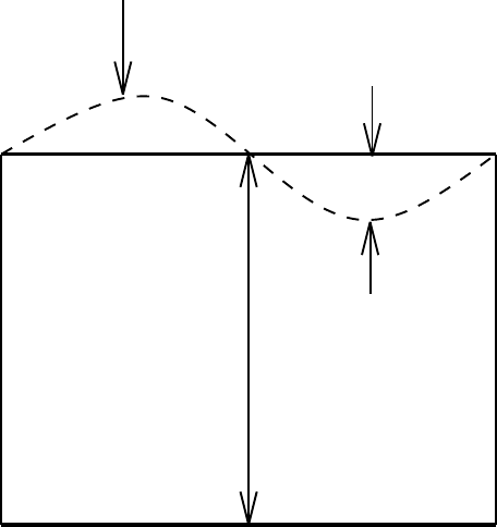
42
CHAPTER 4. FUNDAMENTAL EQUATIONS
where qwis the volume per unit time per unit area (dimensions of a velocity) of fresh water
entering the ocean through the free surface (qw>0 for water entering the ocean across the free
surface). This result leads to the surface kinematic boundary condition
(∂t+uh· ∇h)η=w+qwz=η. (4.29)
As such, the surface height z=ηhas a time tendency ∂tηdetermined by an advective flux of
height −uh· ∇hη, the Eulerian vertical velocity w(η), and the fresh water velocity qw.
1
η
qw
-z
Figure 4.1: Sketch of a shallow layer of fluid with a free surface and whose lower interface
is flat. Both the top and bottom boundaries are generally open to fluid. The height ηis the
deviation from a resting ocean state, and z=z1<0 is the vertical position of the layer bottom.
4.3.3 Dynamic boundary conditions
The purpose of this section is to discuss the dynamic boundary conditions,which are conditions
that prescribe the momentum flux through the model’s side, bottom, and top boundaries.
As discussed in Section 7.4.1, bottom stress arises from both resolved topography, as well as
unresolved or sub-grid scale (SGS) topography and bottom boundary layer effects. In MOM,
it is possible to parameterize the SGS bottom stress either as a free-slip bottom drag,
τbottom−sgs =0,(4.30)
or in terms of the flow near the bottom
τbottom−sgs =ρoCD|uh|uh.(4.31)
Issues related to the stress arising from resolved topography with the full and partial cells are
discussed in Chapter 26, and the bottom boundary layer issues are discussed in Chapter 37.
4.3. BOUNDARY AND INITIAL CONDITIONS
43
The momentum flux through the sea surface τsur f (dyn cm−2) comes from two sources:
τsur f =τwinds +τf resh,(4.32)
which are the wind stress τwinds and momentum transfer in connection with a fresh water flux,
τf resh. The dominating mechanism is the wind stress which comes from the interaction of the
wind field with the ocean surface waves. Since the atmosphere-ocean boundary layer is not
resolved by the model, it is parametrized, e.g., as function of the wind speed in some reference
height in the boundary layer. A simple example is
τwinds =ρaCwind
D|uwind|uwind,(4.33)
where ρais the density of the air, uwind is the wind speed and Cwind
Da drag coefficient which
depends on the wind speed, but also on the stability of the atmospheric boundary layer and the
wave height. Generally, the physically correct calculation of the wind stress is not well known.
Such uncertainty has prompted some climate modelers to consider coupling their ocean model
to a surface wave model. The wave model then directly feels the winds from the atmosphere
and is able to more accurately compute the surface stress field for use in the ocean model.
The other mechanism for the vertical momentum transfer is fresh water flux. The fresh
water volume flux through the air-sea interface carries a momentum which is approximately
τf resh =qwρfuwind.(4.34)
As discussed in Section 7.4.2, MOM identifies this flux with qwρou(z=η), where u(z=η) is
the horizontal current at the ocean surface. With a resolved boundary layer model, such as a
wave model, this identification would not necessarily be exact.
Momentum flux through lateral boundaries is given by no-normal flow as well as no-slip
boundary conditions. Therefore, all velocity components next the side walls are set to zero.
The means for doing so are through the model’s land-sea mask. Although the model employs
no-slip next to the side boundaries, all that is necessary for formulating the solution methods
for the tracer and momentum equations is the no-normal flow condition. This is an important
point since the distinction made in MOM between “side” and “bottom” is possible only through
its use of artificial stepped topography. In the real ocean, there clearly is no distinction. In
principle, therefore, the methods employed in MOM can be used for a free-slip model with a
smooth representation of the bottom.
The details on how the prescribed momentum flux through the model boundaries is linked
with the model variables are described in Sections 6.4.1.
4.3.4 Tracer fluxes through the model boundaries
The tracer equations as given in Section 4.2.4 require the specification of tracer fluxes through
the model boundaries. Tracer fluxes through the lateral boundaries and the sea-floor are
generally set to zero. The fluxes through the sea surface as heat flux, fresh water flux or
radiation are maintained by turbulent processes in the atmosphere-ocean boundary layer
which is not resolved by MOM. Parameterizations require input from both, such as the sea
surface temperature, surface salinity, surface air temperature, humidity, and/or wind speed.
MOM provides a coupling module which collects the required variables and permits the
calculation of the tracer surface fluxes. This includes information which is not calculated by
MOM but must be provided from a database or an atmosphere model. The relation of the
surface tracer fluxes to the scheme for the calculation of the ocean model variables is given in
Section 8. Simple parameterizations for the heat flux and the fresh water flux are discussed in
Section 8.4.
44
CHAPTER 4. FUNDAMENTAL EQUATIONS
4.3.5 Open boundaries and sponges
Limited domain models must consider the manner for which open boundaries are handled. In
general, the mathematical consistency of open boundaries is not clear, so much care should be
exercised. In MOM, the methodology of Stevens (1990) has been implemented (Section 28.3.5).
An alternative to open boundaries is to restore fields along the boundary to some prescribed
values. This method goes by the name of “sponge” boundary conditions. Details of the MOM
implementation of sponges is described in Section 28.3.4.
4.3.6 Initial conditions
Initial conditions for model experiments on a global scale typically consist of specifying a
density structure through potential temperature and salinity, with the ocean at rest. Limited
area models often start with prescribed nonzero velocity fields.
4.4 Comments on volume versus mass conservation
MOM assumes the volume of a fluid parcel is conserved, unless the parcel is affected by external
sources such as surface fresh water fluxes. This assumption is part of the standard Boussinesq
approximation. Mass conservation is more fundamental than volume conservation. One
place where the limitations of volume conservation are most apparent is when formulating the
equations for the free surface. This section briefly discusses this point.
4.4.1 Volume conservation
Consider a shallow layer of fluid with a free surface as shown in Figure 4.1. For definiteness,
such a fluid layer can be considered the fluid which occupies the surface layer of the ocean
model. The position z=η(λ, φ, t), which could be negative, is the vertical deviation from a
resting ocean state z=0. The position z=z1<0 is the fixed position of the bottom of the layer.
The volume of an infinitesimally thin column of fluid extending over the finite vertical extent
of this layer is given by
δV=hδA,(4.35)
where
h=−z1+η(4.36)
is the height of the fluid column, and δAis its infinitesimal horizontal cross-sectional area.
Volume conservation implies that the change of the box volume with time equals the sum of
all volume fluxes through the box surface,
∂t(δV)= qw+w1− ∇h·Zη
z1
dz uh!δA.(4.37)
The convergence of the horizontal flux stems from the infinitesimal horizontal extension of
the box. w1δAis the volume per unit time crossing through the bottom of the layer, where
w1=w(z=z1) is positive for water moving upward into the surface layer. qwδAis the volume
per unit time of ocean water appearing in the surface box. In the spirit of a volume conserving
model, it is equivalent to the volume of fresh water per unit time crossing the free surface, with

4.4. COMMENTS ON VOLUME VERSUS MASS CONSERVATION
45
qw>0 indicating water entering the ocean. The accuracy of this equivalence is determined by
the deviation of the ratio of the fresh water density ρfand the ocean density from unity
ρf
ρ(z=η)−1.(4.38)
For the most applications this deviation should be smaller than the accuracy of the fresh water
flux data.
The identity
∂t(δV)=δA∂th(4.39)
leads to the balance for the layer thickness
∂th+∇h·Zη
z1
uh=qw+w1.(4.40)
With a uniform velocity in the surface layer, this result takes the more familiar form
∂th+∇h·(huh)=qw+w1.(4.41)
4.4.2 Mass conservation
Now consider the mass of the infinitesimal column of water
δm=Zη
z1
dz ρ δA.(4.42)
In this expression, ρis the mass density. The column mass changes when either the volume or
the density is changed,
∂t(δm)=ρ(η)δA∂tη+Zη
z1
dz ∂tρ δA.(4.43)
Mass conservation implies that this change is due to mass flux through the box surface, i.e.,
from the convergence of the horizontal mass flux and from the water coming through the
bottom and through the free surface
∂t(δm)= Qw+w1ρ1− ∇h·Zη
z1
dz ρuh!δA,(4.44)
where ρ1is the density of water entering from the bottom of the layer, and Qwis the mass
flux density of water entering through the free surface. This result leads to the mass balance
equation for the surface layer
∂tZη
z1
dz ρ+∇h·Zη
z1
ρuh=Qw+w1ρ1.(4.45)
A more transparent form emerges from the assumption of a vertically uniform density in the
surface layer, and δm≈ρshδA, which leads to
∂t(ρsh)+∇h·(hρsuh)=Qw+w1ρ1,(4.46)
46
CHAPTER 4. FUNDAMENTAL EQUATIONS
or in the alternate form
∂th+∇h·(huh)=w1ρ1+Qw−h Dhρs/Dt
ρs
.(4.47)
Comparison with the volume conservation equation (4.41) reveals three differences. The first
is the presence of the density ratio weighting the vertical velocitiy w1. To leading order, this
ratio is close to unity. The second is the occurence of the fresh water mass flux instead of the
volume flux. The third difference is the fundamentally new term
−h
ρs
Dhρs
Dt =−h
ρs∂tρs+uh· ∇hρs(4.48)
This term acts to increase the surface height whenever the density of the surface layer is
reduced, such as occurs when the layer is heated. It is this effect which is absent in the current
formulation of MOM. A general way to incorporate this effect is to reformulate the model’s
equations in their non-Boussinesq form.
Differences between a volume conserving and mass conserving ocean model are discussed
more thoroughly in the papers by Greatbatch (1994) and Mellor and Ezer (1995). Both papers
argue that the difference in sea level height is a spatially independent, time dependent height.
4.4.3 Surface kinematic boundary conditions revisited
The discussion in Section 4.3.2 provided one method to derive the surface kinematic boundary
condition. This section provides another, which is based on the volume or mass conserving
balance equations for the layer thickness.
For a volume conserving fluid, the thickness equation (4.40) can be written
(∂t+uh· ∇h)η=qw+w1−Zη
z1
dz ∇h·uh.(4.49)
To recover the surface boundary condition (4.29), vertically integrate the incompressibility
condition (4.3), ∇ · u=0, to yield an expression for the vertical velocity at the bottom of the
surface layer
w1=w(η)+Zz1
η
dz wz
=w(η)+Zη
z1
dz ∇h·uh.(4.50)
This expression in equation (4.49) then yields the surface kinematic boundary condition
(∂t+uh· ∇h)η=qw+w(η).(4.51)
For a mass conserving fluid, the thickness equation (4.45) can be written
ρ(η)(∂t+uh· ∇h)η=w1ρ1+Qw−Zη
z1
dz (Dhρ/Dt +ρ∇h·uh) (4.52)
With the identity
w1ρ1=w(η)ρ(η)−Zη
z1
dz ∂(wρ)
∂z(4.53)
4.5. FLUX FORM AND FINITE VOLUMES
47
the horizontal Langrangian derivative Dhρ/Dt can be completed to the full Lagrangian deriva-
tive
ρ(η)(∂t+uh· ∇h)η=w(η)ρ(η)+Qw−Zη
z1
dz (Dρ/Dt +ρ∇ · u).(4.54)
The term on the right hand side under the integral vanishes due to mass conservation
Dρ
Dt +ρ∇ · u=0.(4.55)
As such, one recovers the surface kinematic boundary condition appropriate for a mass con-
serving fluid
(∂t+uh· ∇h)η=w+Qw
ρz=η. (4.56)
The quantity
qw=Qw
ρ(η)(4.57)
is the volume flux in a mass conserving model. Thus, the only apparent difference from the
volume conserving kinematic condition (4.29) is the approximation used for the calculation of
the volume flux through the sea surface. However, other differences as thermal expansion are
hidden in the vertical velocity w(η).
4.5 Flux form and finite volumes
In general, MOM implments tracer and momentum advection as the divergence of a flux, rather
than the advective form u· ∇Ψ. In the continuum with an incompressible fluid, the advective
form u·∇Ψand flux form ∇·(Ψu) are equivalent. In a numerical model, the flux formulation
provides a straightforward way to ensure conservation properties of scalar quantities, and it
allows a clear finite volume interpretation of the discrete equations.
As discussed by Adcroft et al (1996), a finite volume approach aims to formulate the discrete
equations as self-consistent approximations of the volume integrated continuum equations,
where the volume integration is taken over the a grid cell control volume. Such an approach is
natural on a C-grid. With the B-grid in MOM, there are difficulties. Most notably, the bottom
for a tracer cell does admit a finite volume interpretation. However, the bottom velocity cells
do not rest on the ocean bottom (see Section 22.3.3). This is a notable instance where MOM
does not respect the traditional finite volume approach.
4.6 Some basic formulae and notation
Before closing this chapter, it is useful to summarize some of the formulae, definitions, and
notation which will at times be useful in this manual.
48
CHAPTER 4. FUNDAMENTAL EQUATIONS
4.6.1 Differential operators
In MOM, the radial coordinate is taken as
r=a+z(4.58)
where ais the earth’s radius. z=0 is assumed to be the position of the resting ocean, which is
defined parallel to the geoid. z=−H(λ, φ) is the position of the ocean bottom. As mentioned
earlier, although the geoid is not a perfect sphere, the relatively mild deviations from a sphere
are ignored in MOM, which allows for spherical coordinates. Finally, since z=r−a, the unit
vector ˆ
zpoints in the radial direction ˆ
r
ˆ
z=ˆ
r.(4.59)
Consistent with the Traditional Approximation (see Marshall et al. 1997 for a review),
the differential operators used in the model take on the following form (see Appendix A of
Washington and Parkinson (1986) for derivations). The gradient operator is given by
∇Ψ = ˆ
λ Ψλ
acos φ!+ˆ
φ Ψφ
a!+ˆ
zΨz
=∇hΨ + ˆ
zΨz.(4.60)
The three-dimensional divergence operator acting on a vector u=(uh,w) is given by
∇ · u= 1
acos φ![uλ+(vcos φ)φ]+wz
=∇h·uh+wz.(4.61)
If uis the velocity field, then its three dimensional divergence vanishes since the fluid is always
assumed incompressible in MOM. The three-dimensional curl operator acting on the velocity
is given by
ω=ˆ
λ 1
a
∂w
∂φ −∂v
∂z!+ˆ
φ ∂u
∂z−1
acos φ
∂w
∂λ !+ˆ
z 1
acos φ
∂v
∂λ −1
acos φ
∂(ucos φ)
∂φ !,
(4.62)
where ω=∇∧uis the three dimensional vorticity vector. Often, the vertical component of the
vorticity will be written
ζ=ˆ
z·ω= 1
acos φ!hvλ−(ucos φ)φi.(4.63)
The three-dimensional Laplacian is given by
∇ · (∇Ψ)= 1
a2cos φ! 1
cos φΨλλ +(cos φ·Ψφ)φ!+ Ψzz
=∇h·(∇hΨ)+ Ψzz.(4.64)

4.6. SOME BASIC FORMULAE AND NOTATION
49
4.6.2 Leibnitz’s Rule
Leibnitz’s Rule for differentiation of integrals
∂
∂xZg(x)
f(x)
dx′F(x,x′)=F(x,g(x))∂g(x)
∂x−F(x,f(x))∂f(x)
∂x
+Zg(x)
f(x)
dx′∂
∂xF(x,x′) (4.65)
is employed especially when dealing with vertical integrals where the bottom topography
z=−Hand free surface height z=ηare integration limits.
4.6.3 Cross-products and the Levi-Civita symbol
In this manual, cross products are sometimes written with the notation
A×B=A∧B.(4.66)
This notation is consistent with many math and physics texts. Its use is helpful for those
situations when the usual ×symbol can be mistaken for the spatial variable x.
When writing the components of a vector cross-product, it is often useful to employ the
Levi-Civita symbol ǫijk
(A∧B)k=ǫijk AiBj,(4.67)
where repeated indices are summed over the spatial directions. The Levi-Civita symbol ǫijk is
defined by
ǫijk =
0,if any two labels are the same
1,if i,j,kis an even permutation of 1,2,3
−1,if i,j,kis an odd permutation of 1,2,3.
(4.68)
This symbol is anti-symmetric on each pair of indices.
4.6.4 Area element and volume element on a sphere
When considering budgets over finite domains, integration over an element of the sphere is
common. A useful bit of notation is the area of an infinitesimal element of the sphere
dΩ = a2cos φdφdλ=a2d(sin φ)dλ. (4.69)
With this notation, the volume element on the sphere takes the form
dx=dΩdz.(4.70)
4.6.5 Vertical grid levels
For the interior part of the model ocean, discrete cells have time independent depths zk<0.
In this case, the interior “layers” are most often called “levels” to make the distinction with
models for which the vertical coordinate evolves in time (e.g., isopycnal-layer models such as
that of Bleck et al., 1992, or Hallberg 1995), or models where the vertical coordinate is contoured
50
CHAPTER 4. FUNDAMENTAL EQUATIONS
according to the bottom topography (i.e., sigma-layer models such as that of Blumberg and
Mellor 1987 or Haidvogel et al. 1991). The top ocean cell, however, generally has a time
dependent upper surface height
z0=η, (4.71)
where η, which can be positive or negative, represents the vertical distance from the sea surface
to the height z=0 of a resting sea. In the rigid lid approximation, η=0, and so all model cells
have fixed volumes, whereas for the free surface, η,0.
Chapter 5
Momentum equation methods
This chapter describes the methods available in MOM for solving the momentum equations.
There are two basic approaches: the rigid lid and the free surface. Each approach itself has two
different methods: the rigid lid streamfunction, the rigid lid surface pressure, the explicit free
surface, and the implicit free surface. Currently, development work is focused on the explicit
formulation of the free surface. The other methods essentially remain in their MOM 2 form.
Plans are to only support development of the explicit free surface in the future (post Summer
1999). The reasons for this focus can be summarized by the following:
•The rigid lid is less physically complete than the free surface. Most notably, it does not
allow for a direct treatment of fresh water fluxes.
•The rigid lid in MOM has not been parallelized, nor are there plans to do so.
•Both the explicit and implicit free surfaces have been parallelized in MOM. The explicit
free surface shows enhanced scaling properties over the implicit scheme.
•The explicit free surface has been formulated so that it can be of use for either global
climate integrations or limited area models.
•The implicit free surface algorithm is more complex than the explicit free surface.
•As of Summer 1999, the explicit free surface has incorporated the effects of the undulating
top cell thickness into the depth dependent equations. Hence, the model is conservative
of tracers, including total salt in the presence of fresh water fluxes, as well as momentum.
Each of these points will become more clear in this chapter as well as Chapters 8 and 29.
5.1 Separation into vertical modes
Numerical solutions are computed within MOM by dividing the ocean volume into a three di-
mensional lattice, discretizing the equations within each lattice cell, and solving these equations
by finite difference techniques. The solution method could be formulated in a straightforward
manner, but the result would be a numerically inefficient algorithm. Instead, Bryan (1969)
introduced a fundamental technique to ocean modeling in which the ocean velocity field is
separated into its depth averaged part and the deviation from the depth average. The following
discussion introduces the motivations and ideas behind this approach.
51
52
CHAPTER 5. MOMENTUM EQUATION METHODS
5.1.1 Vertical modes in MOM and their relation to eigenmodes
As discussed in Section 6.11 of Gill (1982), the linearized primitive equations for a stratified
fluid can be partitioned into a countably infinite (i.e., discrete) number of orthogonal eigen-
modes, each with a different vertical structure. Gill denotes the zeroth vertical eigenmode
the barotropic mode, and the infinity of higher modes are called baroclinic modes. Because
of the weak compressibility of the ocean, wave motions associated with the barotropic mode
are weakly depth dependent, and so correspond to elevations of the sea surface (see Hidgon
and Bennett 1996 for a proof of the weak depth dependence in a flat bottomed ocean). Conse-
quently, the barotropic field goes also by the name external mode. Barotropic or external waves
constitute the fast dynamics of the ocean primitive equations. Baroclinic waves are associated
with undulations of internal density surfaces, which motivates the name internal mode. Baro-
clinic waves, along with advection and planetary waves, constitute the slow dynamics of the
ocean primitive equations.
For a flat bottom ocean, the vertical eigenmode problem is straightforward to solve, and
many important ideas can be garnered from its analysis. For a free surface with a flat bottom,
Gill shows that the barotropic mode has a vertical velocity which is approximately a linear
function of depth, with the maximum vertical velocity at the free ocean surface and zero velocity
at the flat bottom. In contrast, for a rigid lid and flat bottom ocean, the barotropic mode is
depth independent and the vertical velocity identically vanishes. The baroclinic modes, as
they are associated with movements of the internal interfaces, are little affected by the surface
boundary condition. Therefore, the baroclinic modes in the free surface are quite similar to
those in the rigid lid. Note that nonlinearities and nontrivial bottom topography generally
couple the barotropic and baroclinic modes.
By construction, the depth averaged momentum equations only have solutions which
depend on the horizontal directions. Consequently, the depth averaged mode of a rigid lid
ocean model corresponds directly to the barotropic mode of the linearized rigid lid primitive
equations. Additionally, the rigid lid model’s depth dependent modes correspond to the
baroclinic modes of the linearized rigid lid primitive equations. Therefore, depth averaging in
the rigid lid model provides a clean separation between the linear vertical modes.
Just as for the rigid lid, the baroclinic modes are well approximated by the depth dependent
modes of the free surface ocean model, since the baroclinic modes do not care so much about the
upper surface boundary condition. In contrast, the ocean model’s depth averaged mode cannot
fully describe the free surface primitive equation’s barotropic mode, which is weakly depth
dependent. Therefore, some of the true barotropic mode spills over into the model’s depth
dependent modes. In other words, a linearized free surface ocean model’s depth averaged
mode is only approximately orthogonal to the model’s depth dependent modes. It turns out
that the ensuing weak coupling between the ocean model’s fast and slow linear modes can
be quite important for free surface ocean models, as described by Killworth et al. (1991) and
Higdon and Bennett (1996). The coupling, in addition to the usual nonlinear interactionas
associated with advection, topography, etc., can introduce pernicious linear instabilities whose
form is dependent on details of the time stepping schemes.
Regardless of the above distinction between vertically averaged and barotropic mode for
free surface models, it is common parlance in ocean modeling to refer to the vertically integrated
mode as the barotropic or external mode. This terminology is largely based on the common
use of the rigid lid approximation, for which there is no distinction. With the above discussion
kept in mind, there should be no confusion, and so the terminology will be used in this manual
for both the rigid lid and free surface formulations. Since there is little difference between the
5.2. METHODS FOR SOLVING THE SEPARATED EQUATIONS
53
rigid lid and free surface baroclinic modes, it is quite sensible to use this term to refer to the
ocean model’s depth dependent modes.
5.1.2 Motivation for separating the modes
Although there are several technical problems associated with the separation into the vertically
averaged and vertically dependent modes, it is essential to build large scale ocean models using
some version of this separation for the following reasons:
1. Without a separation, the full momentum field will be subject to the CFL constraints
of the external mode gravity wave speed, which is roughly pg H =200 −250m s−1for
ocean depths H=4000m−6000m. When splitting, the internal modes, which are roughly
100 times slower than the external mode, can be integrated with approximatly 100 times
longer time steps, thus enhancing the utility of the model for climate simulations.
2. As vertical resolution is improved, the computation requirements for the barotropic mode
will remain the same. However, for a non-separated model, adding vertical resolution
adds more equations which are subject to the barotropic mode time step. Modern ocean
simulations are tending towards increasing the vertical resolution in order to improve
the representation of vertical physical processes such as boundary layers. Therefore,
the low efficiency of the non-separated model is a greater burden for these high vertical
resolution models.
There are two fundamental methods in MOM for solving the momentum equations. The
traditional rigid lid method completely filters out the very fast waves associated with the
external mode by fixing the ocean surface to be flat. This filtering transforms the generally
hyperbolic external mode problem to an elliptic problem. The free surface, in contrast, admits
the fast external waves and so care must be exercised in order to maintain numerical stability,
and additional care must be exercised due to the possible linear interaction between the depth
independent and depth dependent modes. It turns out that each method, and certain variants
thereof, imply far reaching consequences for the numerical methods and physical content
of the whole model. Much of the discussion in the remainder of this chapter elaborates on
these consequences. The remainder of this section provides a general overview of these two
methods, and later sections and chapters provide the full details.
5.2 Methods for solving the separated equations
In symbols, the horizontal velocity uhis separated into two parts. The vertically averaged
velocity representing the approximate barotropic or external part is given by
uh=1
H+ηZη
−H
dz uh,(5.1)
where H(λ, φ) is the distance from the resting ocean surface z=0 to the bottom, and η(λ, φ, t)
is the departure of the ocean surface height from z=0. Typically, |η| ≤ 200cm, but may be
much larger, if tides are taken into consideration. In general, fields which are averaged over
the vertical coordinate will be denoted with the overbar. The residual
b
uh=uh−uh(5.2)

54
CHAPTER 5. MOMENTUM EQUATION METHODS
is a depth dependent velocity, which embodies the approximate baroclinic or internal mode
flow. Often, it will be convenient to introduce the vertically integrated horizontal velocity field
U=(H+η)uh=Zη
−H
dz uh.(5.3)
Additionally, the following vertically integrated velocity
U0=Z0
−H
dz uh(5.4)
will prove useful. In the fixed surface /rigid lid method (see below), there is no distinction
between Uand U0in the baroclinic model part, since η=0 is assumed. Additionally, with
η=0 and w(z=0) =0, then ∇h·U=0. This result is exploited in the rigid lid formulation, as
seen in Section 5.2.1.
The dynamical equations for the vertically averaged velocity are generally more compli-
cated than the unaveraged equations. Two means for handling these equations are imple-
mented in MOM:
•The fixed surface /rigid lid method. This method fixes the upper surface to η=0, and
closes the upper boundary with w(z=0) =0. There are two flavors of this method: the
streamfunction and the surface pressure methods.
•The free surface /non-rigid lid method. This method allows for a freely evolving surface
η,0, and it uses open boundary conditions at z=0 with w(0) ,0 for the baroclinic
and tracer equations. There are two flavors of this method: the explicit and implicit free
surface methods.
In short, these two methods differ fundamentally in how they handle the upper ocean boundary
conditions.
5.2.1 The fixed surface /rigid lid method in brief
The basics of the rigid lid method are summarized in this section. More complete details for the
rigid lid streamfunction method are given in Chapter 6.
5.2.1.1 Fixed surface height
The key assumption with the rigid lid is that the ocean surface height is fixed
η≡0.(5.5)
This assumption eliminates the wave modes associated with vertical displacements of the full
water column. These are the modes associated with the fast external mode gravity waves.
Therefore, fixing the surface height eliminates the fast waves and consequently allows for
relatively large momentum time steps. On its own, the removal of the fast modes is thought
to be of minimal consequence for global ocean simulations. It does preclude the study of
phenomena associated with barotropic waves, such as the barotropic tides.

5.2. METHODS FOR SOLVING THE SEPARATED EQUATIONS
55
5.2.1.2 Vanishing velocity at the ocean surface
A related assumption made by Bryan (1969) is to set the vertical velocity at the surface to zero
w(z=0) =0.(5.6)
Setting wto zero at the ocean surface is not necessary for eliminating the external mode gravity
waves. Again, η=0 is sufficient. As discussed in Section 6.1, Bryan’s choice to set w(z=0) =0
is based on the consequent ability of a single streamfunction to specify the two components of
the barotropic velocity. If wis allowed to fluctuate at the surface, and η=0 is still imposed,
then a velocity potential must be used in addition to the streamfunction (see Section 7.6). Both
the streamfunction and velocity potential have separate elliptical problems which must be
solved. In large scale ocean models, especially those with realistic geography and topography,
the elliptic problems are quite expensive computationally. Therefore, Bryan’s choice to set
w(z=0) =0 removed a large amount of computational burden from the model.
5.2.1.3 Fresh water forcing in the rigid lid
A constant surface height, η=0, does not imply a vanishing vertical velocity component at
the ocean surface. The basic reason is that the surface height is a Lagrangian coordinate and
the vertical velocity at the surface is Eulerian. Relatedly, as seen by the equation (4.29) for the
surface kinematic boundary condition, η=0 does not imply w(z=0) =0if there is a surface
fresh water flux. This is the fundamental point raised in the work of Huang (1993). As can be
seen through the kinematic boundary condition, allowing wto fluctuate at the surface, while
still keeping η=0, will enable a more physical means to force a rigid lid model with fresh water
qw,0 while at the same time filtering out the external mode gravity waves. Setting both η=0
and w(z=0) =0 precludes a direct use of fresh water forcing. As such, the upper boundary
is effectively closed to fresh water in the traditional rigid lid method. Instead, the effects of
fresh water must be introduced through a virtual salt flux added to the salinity equation. The
implementation of other surface boundary conditions likewise may involve certain unphysical
assumptions.
In summary, the tradeoffthat Bryan (1969) made was to eliminate the need for computing
a velocity potential while sacrificing a physically based fresh water forcing. Huang (1993)
argues that this choice is not satisfactory for large scale modeling since it eliminates some
fundamental modes of the ocean circulation. Additionally, it possibly affects the sensitivity
of the oceanic variability which might be realized in a coupled ocean-atmosphere model.
Currently, the choice made in the development of MOM is to not implement the method from
Huang. Rather, it is to focus on the free surface method for the reasons explained below.
5.2.1.4 Two rigid lid methods in MOM
Since the method of Huang (1993) has not been implemented, in this manual the rigid lid
will imply the two assumptions η=0 and w(z=0) =0. In MOM, there are two methods
which employ the rigid lid approximation. The first is the original Bryan (1969) streamfunction
method (option stream function). The second method is that from Smith, Dukowicz, and Malone
(1992) and Dukowicz, Smith, and Malone (1993). Instead of solving for a streamfunction, they
solved for the surface pressure. Hence, the option is called rigid lid surface pressure (Section
6.8). Both of these rigid lid methods have been unchanged since MOM 2.

56
CHAPTER 5. MOMENTUM EQUATION METHODS
5.2.2 The free surface /non-rigid lid method in brief
In the last few years, modelers have been motivated for various reasons to jettison the fixed
surface /rigid lid approximation. Instead, they have decided to formulate the free surface
problem in various manners. Briefly, these reasons are the following:
1. A free surface method treats the sea level elevation as a prognostic variable and allows
for a representation of the spreading of surface gravity waves and/or Kelvin waves.
2. A free surface allows for a more accurate representation of surface tracer fluxes, such as
providing for a real fresh water flux (see Section 5.2.1.3).
3. A free surface eliminates the Killworth (1987) topographic instability.
4. A free surface allows for more ready code parallelization, whereas the island integrals in
the rigid lid streamfunction approach are more cumbersome on shared memory archi-
tectures.
Section 29.1 provides a more a detailed discussion of these points.
5.2.2.1 The barotropic equation and its two solution methods
Integrating the continuity equation vertically yields a prognostic equation for the sea surface
elevation η, together with the vertically integrated momentum equations. These equations
describe the fast barotropic gravity waves. In general, the numerical solution scheme for
these equations requires a very small time step if these waves are resolved. There are two
methods used in MOM: the option implicit free surface of Dukowicz and Smith (1994), and the
option explicit free surface. The explicit free surface can be time stepped either by the methods
of Killworth, Stainforth, Webb and Paterson (1991), or by the methods discussed in Section
29.5 and in Griffies, Pacanowski, Schmidt, and Balaji (2000). The implicit method as coded
in MOM has not been found to be unconditionally stable, although in principle it should be
so. In general, if the time step is too large, the barotropic gravity waves are damped out with
the implicit scheme. If this damping is not desired, then the explicit method can be used. In
this approach, the barotropic mode is integrated with a small time step. While integrating
the barotropic equations, the baroclinic flow as well as tracer fields are kept constant. This
approximation is justified since the time scale of baroclinic and tracer processes is much larger
than the barotropic process. Note that if the time step is smaller than required by the CFL-
criterion for barotropic gravity waves, both the implicit and explicit methods have been found
to yield similar results.
5.2.2.2 The non-rigid lid approximation
An ocean model with a free surface strictly has a time dependent domain with a top model
grid box possessing a variable upper surface. This added degree of freedom increases the
complexity of the numerical scheme for the tracers and the baroclinic mode due to the need
to take into account the variable top model grid box. Instead of introducing this complexity,
those using a free surface in z-level models have instead considered a model with fixed vertical
levels. The upper kinematic, dynamic, and tracer boundary conditions are formulated as open
boundary conditions applied at z=0 rather than at z=η. The application of the upper
boundary at z=0 is similar to the rigid lid approach. However, for the non-rigid lid free
5.2. METHODS FOR SOLVING THE SEPARATED EQUATIONS
57
surface, the upper boundary is open or permeable, whereas the upper boundary in the rigid lid
method is closed or impermeable. Most notably, the vertical velocity w(z=0) does not vanish
with the free surface. This comparison motivates the name non-rigid lid method for the handling
of surface boundary conditions in the free surface method.
An approach such as this was employed by Killworth et al. (1989) and is also used by
Dukowicz and Smith (1994). In general, the non-rigid lid approximation is well justified so long
as the top model grid box between z1≤z≤0 is much thicker than the maximum free surface
height η. In shallow seas or in models with very fine vertical grid spacings, this assumption is
not valid. More crucially, such models do not conserve total tracer or momentum. It is for this
reason that MOM has recently (Summer 1999) implemented a full free surface method in which
the effects of the undulating surface height has been incorporated into the depth dependent
fields. This method is fully documented in Griffies, Pacanowski, Schmidt, and Balaji (2000).
58
CHAPTER 5. MOMENTUM EQUATION METHODS
Chapter 6
Rigid lid streamfunction method
The rigid lid streamfunction method was developed by Bryan (1969). This chapter presents
the formulation of the rigid lid in a fashion to closely parallel the derivation given for the free
surface in Chapter 7.
6.1 The barotropic streamfunction
With a rigid lid at the ocean surface, the surface height η=0. Setting ηto zero eliminates the
very fast (order 200 m s−1in water with depth 4000−5000m) external mode gravity waves. As a
result of making the rigid lid assumption, the vertically integrated horizontal velocity satisfies
∇h·U=uh(−H)· ∇hH+Z0
−H
dz ∇h·uh
=uh(−H)· ∇hH−Z0
−H
dz wz
=uh(−H)· ∇hH+w(−H)−w(0)
=−w(0).(6.1)
To reach this result, Leibnitz’s Rule (4.65), the continuity equation (4.3), and the bottom kine-
matic boundary condition (4.24) were used. Taking the additional assumption
w(z=0) =0 (6.2)
renders
∇h·U=∇h·H(u,v)=0.(6.3)
As a result, the external mode velocity can be expressed in terms of the external mode
streamfunction
u=−1
Haψφ(6.4)
v= 1
Ha ·cos φ!ψλ.(6.5)
As a vector equation, this relation takes the form
U=H(u,v)=ˆ
z∧∇hψ. (6.6)
59
60
CHAPTER 6. RIGID LID STREAMFUNCTION METHOD
6.2 Streamfunction and volume transport
The barotropic streamfunction is specified only to within a constant. As such, only differences
are physically relevant. In particular, consider the vertically integrated advective transport
between two points
Tab =Zb
a
dl ˆ
n·Z0
−H
dz uh,(6.7)
where dl is the line element along any path connecting the points aand b, and ˆ
nis a unit
vector pointing perpendicular to the path in a rightward direction when facing the direction of
integration. As written, Tab has units of volume/time, and so it represents a volume transport.
The definition of the barotropic streamfunction and Stokes’ Theorem renders
Tab =Zb
a
dl ˆ
n·U
=Zb
a
dl ˆ
n·ˆ
z∧ ∇hψ
=−Zb
a
dl ∇hψ·(ˆ
z∧ˆ
n)
=−Zb
a
dl ∇hψ·ˆ
t
=ψa−ψb,(6.8)
where
ˆ
t=ˆ
z∧ˆ
n(6.9)
is a unit vector tangent to the integration path, pointing in the direction of integration from
point ato point b. Therefore, the difference between the barotropic streamfunction at two
points represents the vertically integrated volume transport between the two points. It is for
this reason that the barotropic streamfunction is sometimes called the volume transport stream-
function. Note that Bryan (1969) defined the barotropic streamfunction with an extra factor of
the Boussinesq density ρo, such than ψbryan =ρoψmom. Hence, the barotropic streamfunction
of Bryan has the dimensions of mass/time rather than volume per time, and so it represents a
mass transport streamfunction. Since MOM assumes a Boussinesq fluid, the difference is trivial.
6.3 Hydrostatic pressure with the rigid lid
The hydrostatic equation pz=−ρgcan be integrated from the surface z=0 to some position
z<0 to yield
p(λ, φ, z,t)=pa(λ, φ, t)+pl(λ, φ, t)+gZ0
z
dz ρ
=pa(λ, φ, t)+pl(λ, φ, t)+pb(λ, φ, z,t),(6.10)
where pais the atmospheric pressure, plis the surface lid pressure, and pbis the hydrostatic
pressure arising from the ocean’s density field. The surface lid pressure is the pressure which
6.4. THE BAROTROPIC VORTICITY EQUATION
61
would be exerted by an imaginary rigid lid placed on top of the ocean. An alternative interpre-
tation is that it is the pressure exerted by undulations of a free surface. The latter interpretation
is further disscussed in Section 7.1. In summary, the horizontal pressure gradient is given by
∇hp=∇h(pa+pl)+gZ0
z
dz ∇hρ. (6.11)
The horizontal pressure gradient at some depth zhas a contribution from gradients in the
atmospheric and lid pressure, gradients which act the same for all depths, and the vertical
integral of horizontal gradients in the interior density. These latter gradients are due to
baroclinicity in the density field, which prompts the often used name baroclinic pressure gradient,
and which motivates the “b” subscript. The vertically integrated horizontal pressure gradient
is needed for the development of the barotropic vorticity equation. This gradient is given by
Z0
−H
dz ∇hp=Z0
−H
dz ∇h(pa+pl)+Z0
−H
dz gZ0
z
dz′∇hρ!.(6.12)
Since the horizontal gradient of the atmospheric and lid pressures are independent of depth,
Z0
−H
dz ∇h(pa+pl)=H∇h(pa+pl),(6.13)
which renders
Z0
−H
dz ∇hp=H∇h(pa+pl)+∇hpb.(6.14)
6.4 The barotropic vorticity equation
For cases where the ocean model is driven by a realistic atmospheric model, the atmospheric
pressure pamay be determined. But since the lid pressure plis actually an artifact of making
the rigid lid approximation, it is generally not available. To address this fact, Bryan formed the
barotropic vorticity equation in which case the lid and atmospheric pressures are eliminated.
Through inverting the vorticity equation, the streamfunction is obtained. As a result, the
barotropic velocities can then be determined through the relation (6.6). As will be seen in
Section 6.6, the lid and atmospheric pressures will likewise not be needed for determining the
baroclinic velocity. This algorithm has been used for solving the rigid lid in MOM up until
the formulation of the surface pressure approach of Smith, Dukowicz, and Malone (1992) and
Dukowicz, Smith, and Malone (1993) (Section 6.8). In the present section, a derivation of the
barotropic vorticity equation is provided.
6.4.1 Tendencies for the vertically averaged velocities
The first step is to integrate the horizontal velocity equations (4.1) and (4.2) vertically over the
full depth of the rigid lid ocean
∂tU−f V =− H
aρocos φ!(pa+pl)λ+X0(6.15)
∂tV+f U =− H
aρo!(pa+pl)φ+Y0.(6.16)
62
CHAPTER 6. RIGID LID STREAMFUNCTION METHOD
The vertical integral of depth dependent quantities (mod the Coriolis force) has been lumped
into the terms
X0=Z0
−H
dz −∇ · (uu)+uv tan φ
a+(κmuz)z+Fu−(pb)λ
aρ◦cos φ!(6.17)
Y0=Z0
−H
dz −∇ · (vu)−u2tan φ
a+(κmvz)z+Fv−(pb)φ
aρ◦!.(6.18)
These equations are implemented in MOM through a straightforward vertical integration of
the forcing terms.
To facilitate physical interpretation of the surface terms forcing the vertically integrated
momentum, it is useful to perform some manipulations on X0and Y0. First, use the bottom
kinematic boundary condition (4.24) and the surface kinematic condition w(0) =0 in order to
bring the vertical integral of the convergence of the advective flux to the form
−Z0
−H
dz ∇h·(αuh)+(αw)z=−∇h·Z0
−H
dz αuh
+α(−H)∇hH·uh(−H)+w(−H)−w(0) α(0)
=−∇h·Z0
−H
dz αuh,(6.19)
where α=u,v. Second, recall from equations (9.187) and (9.193) that the horizontal momentum
friction can be written as a Laplacian acting on the horizontal velocity, plus an extra “metric”
term
F=∇h·(Am∇hu)+Fmetric.(6.20)
As such, the depth integral of momentum friction can be written
Z0
−H
dz(κmuz)z+F
= τsur f −τbottom
ρo!+Zη
−H
dz Fmetric +∇h·Z0
−H
dz Am∇hu,(6.21)
where
τsur f =ρoκmuz|z=0(6.22)
τbottom =ρoκmuz+Am(∇hH)·(∇hu)z=−H(6.23)
are the surface and bottom stresses (dyn cm−2) due to the winds at the ocean surface and
friction and topography at the bottom. The above results render
X0=∆(τλ)
ρo−Z0
−H
dz (pb)λ
aρ◦cos φ
+Z0
−H
dz uv tan φ
a+Fu
metric!− ∇h· Z0
−H
dz (uuh−Am∇hu)!(6.24)
X0=∆(τφ)
ρo−Z0
−H
dz (pb)φ
aρ◦
+Z0
−H
dz −u2tan φ
a+Fv
metric!− ∇h· Z0
−H
dz (vuh−Am∇hv)!.(6.25)
6.4. THE BAROTROPIC VORTICITY EQUATION
63
Using an overline to denote a vertical column average, and using the expression (6.14) for the
horizontal pressure gradient, yields the vertically averaged velocity equations
∂tu=f v − 1
aρocos φ!(pa+pl)λ+(pb)λ+(∆τλ/ρoH)+ Γu,(6.26)
∂tv=−f u − 1
aρo!(pa+pl)φ+(pb)φ+(∆τφ/ρoH)+ Γv,(6.27)
where
Γu=Fu
metric +u v (tan φ/a)+H−1∇h·H(Am∇h−uh)u(6.28)
Γv=Fv
metric −u u (tan φ/a)+H−1∇h·H(Am∇h−uh)v.(6.29)
represent the vertical average of the horizontal friction metric terms, advection metric terms,
divergence of the horizontal viscous fluxes, and convergence of the horizontal advective fluxes.
6.4.2 The barotropic vorticity equation
In order to eliminate the lid and atmospheric pressures, it is sufficient to form the time tendency
of the barotropic vorticity
ζ=ˆ
z· ∇ ∧ ω
= 1
acos φ![vλ−(ucos φ)φ]
=1
acos φ1
cos φ ψλ
H!λ
+ ψφcos φ
H!φ
=∇h·1
H∇hψ.(6.30)
A few lines of manipulations renders
ζt+βv=
−f∇h·uh− 1
a2ρocos φ!h∂λ(∂φpb)−∂φ(∂λpb)i+ˆ
z· ∇ ∧ ∆τ
ρoH+ Γu!,
(6.31)
where
β=1
a
∂f
∂φ
=(2 Ω/a) cos φ(6.32)
is the planetary vorticity gradient. The forcing for tendencies in ζconsists of the following
terms:
1. Meridional advection of planetary vorticity: −βv.
64
CHAPTER 6. RIGID LID STREAMFUNCTION METHOD
2. Curl of the Coriolis force, which takes the form of the convergence of the barotropic
velocity weighted by the Coriolis parameter: −f∇h·uh. For a flat bottom, this term
vanishes with the rigid lid. Combined with the βvterm, these provide the forcing
−∇h·(fuh) to the barotropic vorticity.
3. The antisymmetric term proportional to ∂λ(∂φpb)−∂φ(∂λpb). This term vanishes in a
barotropic model, or in a baroclinic model with a flat bottom.
4. Curl of the depth weighted surface minus bottom stresses: ˆ
z· ∇ ∧ (∆τ/ρoH).
5. Curl of the nonlinear lateral friction terms and advection terms embodied by Γ.
To touch bases with familiar textbook dynamics, note that a steady state ocean with Γ = 0 and
a flat bottom will result in the familiar barotropic Sverdrup balance
βv=ˆ
z· ∇ ∧ ∆τ
ρoH!.(6.33)
6.4.3 Caveat: inversions with steep topography
In order to solve for the barotropic velocity u, it is necessary to invert the elliptical operator
appearing in the relation (6.30) relating the barotropic vorticity to the barotropic streamfunction.
The presence of the inverse depth in this operator implies that near regions where Hchanges
rapidly, the elliptic operator also changes rapidly. As emphasized by Smith, Dukowicz, and
Malone (1992) and Dukowicz, Smith, and Malone (1993), numerical elliptic inversions will
potentially have problems converging in the presence of such regions. This form for the
elliptic operator is also the central reason for the Killworth topographic instability (Killworth
1987). This instability can result in significant time step constraints in rigid lid models with non-
smoothed topography, and these time step constraints can be more stringent than the typical
CFL constraints. More problematic from the perspective of very long-term climate modeling,
the Killworth instability can sometimes be slowly growing, and may become problematical
only after some few hundreds of years. A slow growing instability is arguably more pernicious
than rapidly growing instabilities, since a significant amount of computation time can be used
before encountering the problem. Experience at GFDL indicates that the Killworth instability
is a nontrivial problem with realistic models, and so it provides motivation to avoid the rigid
lid streamfunction method in such models.
6.5 Boundary conditions and island integrals
6.5.1 Dirichlet boundary condition on the streamfunction
The no-normal flow boundary condition implies that next to lateral boundaries,
ˆ
n·H(u,v)=ˆ
n·ˆ
z∧ ∇hψ
=−ˆ
t· ∇hψ
=0,(6.34)
where ˆ
nis a unit vector pointing outwards from the boundary, with the interior of the closed
domain to the left, and ˆ
t=ˆ
z∧ˆ
nis a unit vector parallel to the path traversing the boundary.
6.5. BOUNDARY CONDITIONS AND ISLAND INTEGRALS
65
This constraint says that the streamfunction is a constant along the boundaries. In the parlance
of applied mathematics, such boundary conditions are known as Dirichlet conditions. In
general, the streamfunction can be a different time dependent constant along the different
closed boundaries
ψ=µr(t),(6.35)
where µr(t) is a time dependent number, and r=1,2, ...Rlabels the particular boundary
(an island label), with Rthe total number of islands. The interpretation afforded by Stokes’
Theorem, discussed in Section 6.1, indicates that µr(t) represents the time dependent volume
transport circulating around the island with label r.
The presence of Dirichlet boundary conditions on the streamfunction indicates that the
streamfunction at one point along the boundary is identical to the streamfunction at another
point, which can generally be thousands of kilometres away. Such non-local forms of infor-
mation can be quite problematical in the solution of the streamfunction on parallel machines.
The discussions in Smith, Dukowicz, and Malone (1992), Dukowicz, Smith, and Malone (1993),
and Dukowicz and Smith (1994) highlight this point.
6.5.2 Separating the streamfunction’s boundary value problem
The purpose of this section is to develop an algorithm for solving the streamfunction’s bound-
ary value problem (BVP). To do so, reconsider the horizontal momentum equations written in
the form
ut=−∇h(p/ρo)+G,(6.36)
where the vector Grepresents all the remaining terms given in equations (4.1) and (4.2).
Taking the vertical average of this equation, substituting the definition (6.6) for the barotropic
streamfunction, and using the expression (6.14) for the hydrostatic pressure gradient, yields
1
Hˆ
z∧∇hψt=−1
ρo∇h(pa+pl)+∇hpb+G.(6.37)
Taking the curl of this equation eliminates the atmospheric and lid pressures
∇h∧1
Hˆ
z∧ ∇hψt=−1
ρo∇h∧∇hpb−G.(6.38)
The elliptic boundary value problem
∇h∧1
Hˆ
z∧ ∇hψt=−1
ρo∇h∧∇hpb−Ginterior points (6.39)
ψ=µr(t) on island r,(6.40)
can be separated into two simpler BVPs. The first one is a forced elliptical problem with
homogeneous boundary conditions
∇h∧1
Hˆ
z∧∇h(ψo)t=−1
ρo∇h∧∇hpb−Ginterior points (6.41)
ψo=0 on islands.(6.42)
66
CHAPTER 6. RIGID LID STREAMFUNCTION METHOD
This system can be solved for ψousing some time-stepping scheme, such as leap-frog. The sec-
ond BVP is a time-independent unforced elliptical problem with constant boundary conditions
on the islands
∇h∧1
Hˆ
z∧∇hψr=0 everywhere, except island boundaries (6.43)
ψr=1 on islands.(6.44)
This BVP can be solved for ψrusing some type of an elliptical solver, such as congugate
gradient. The full streamfunction is built from the sum
ψ(λ, φ, t)=ψo(λ, φ, t)+
R
X
r=1
µr(t)ψr(λ, φ),(6.45)
which can be shown to satisfy the original boundary value problem.
6.5.3 Island integrals for the volume transport
As a final step in the streamfunction solution, it is necessary to formulate a prognostic equation
for the volume transports µr(t). To do so, reconsider the elliptical problem for the streamfunc-
tion
∇h∧1
Hˆ
z∧ ∇hψt=−1
ρo∇h∧∇hpb−G.(6.46)
Now integrate both sides over the area bounding a particular island with label r, and employ
Stokes’ Theorem. The direction normal to the island’s surface is ˆ
z, and the area element on the
island is dΩr. The left hand side becomes
Z Z ˆ
z dΩr∇h∧1
Hˆ
z∧ ∇hψt=Z Z ˆ
z dΩr∇h∧1
Hˆ
z∧ ∇hψr˙µr
=˙µrIdl ˆ
t·1
Hˆ
z∧ ∇hψr
=−˙µrIdl ˆ
n·1
H∇hψr,(6.47)
where ˆ
t∧ˆ
z=−ˆ
nwas used, and ˆ
nrepresents the outward normal to the island boundary. The
right hand side becomes
−Z Z ˆ
z dΩr∇h∧1
ρo∇h∧∇hpb−G=−1
ρoIdl ˆ
t·(∇hpb−G).(6.48)
Equating yields the prognostic equations for the volume transports around an island
˙µr=1
ρoHdl ˆ
t·(∇hpb−G)
Hdl ˆ
n·1
H∇hψr
.(6.49)
6.6. THE BAROCLINIC MODE
67
6.6 The baroclinic mode
The time tendency for the zonal baroclinic velocity is given by
∂tb
u=∂t(u−u)
= 1−1
HZ0
−H
dz! Gu− 1
aρ◦cos φ!(pb+pl+pa)λ!(6.50)
where the vector Gwas introduced in equation (6.36). Since the atmospheric and lid pressures
are depth independent, these pressures have zero deviation from their depth average. Hence,
the tendency for the baroclinic velocity is independent of the atmospheric and lid pressures.
In determining the baroclinic velocity, it is therefore sufficient to consider
∂tb
u=∂t(u′−u′) (6.51)
where u′and u′satisfy the full zonal velocity equation and vertically averaged zonal velocity
equation, respectively, but without any atmospheric or lid pressure contributing to the forcing.
Without the atmospheric and lid pressure contributions, all forcing terms in the two “primed”
equations are known. Consequently, the primed velocities can be time stepped in a straight-
forward manner without using any tricks such as those needed to eliminate the atmospheric
and lid pressures from the streamfunction equation. Time stepping the primed velocities then
yields the updated baroclinic velocity through equation (6.51). After obtaining the updated
baroclinic velocity, the full horizontal velocity field
(u,v)=(u,v)+(b
u,b
v) (6.52)
is known at the new time step. Formulation of the rigid lid streamfunction method is now
complete.
6.7 Summary of the rigid lid streamfunction method
In summary, the rigid lid streamfunction method allows for the computation of the total
velocity field using the following algorithm:
•Baroclinic mode
1. Compute the forcing terms for the “primed” momentum equation, which include
all terms except the lid pressure and atmospheric pressure (Section 6.6).
2. Solve the primed momentum equation at each model level to get the primed velocity
at the next time step.
3. Subtract the vertically averaged primed momentum from the primed momentum
in order to get the baroclinic velocity field at the next time step.
•Barotropic mode
1. Compute the forcing terms in the barotropic vorticity equation (Section 6.4).
2. Solve the elliptical boundary value problem for the time tendency of the barotropic
streamfunction.
3. Time step the streamfunction forward and compute the barotropic velocity field at
the new time step.
•Add the baroclinic velocity to the barotropic velocity to then have the full velocity field.
68
CHAPTER 6. RIGID LID STREAMFUNCTION METHOD
6.8 Rigid lid surface pressure method
The rigid lid surface pressure method in MOM was developed by Smith, Dukowicz, and
Malone (1992) and Dukowicz, Smith, and Malone (1993). A useful discussion of the analyt-
ical issues related to the surface pressure formulation can be found in the paper by Pinardi,
Rosati, and Pacanowski (1995). The basic advantages over the streamfunction approach are
the following:
1. The elliptical operator has an Hfactor, rather than the H−1found in the streamfunction
approach. This property makes the elliptical operator more readily inverted than with
the streamfunction approach (see Section 6.4.3). In particular, steep topography is much
less of an issue with the surface pressure approach.
2. The boundary conditions for the elliptical problem are Neumann rather than Dirichlet.
As discussed by Smith, Dukowicz, and Malone (1992) and Dukowicz, Smith, and Malone
(1993), Neumann boundary conditions are much easier to handle on parallel machines
than Dirichlet conditions.
As the formulation of the rigid lid surface pressure method follows quite closely the logic
of the streamfunction approach, the details are not reproduced here. Rather, reference should
be made to the Smith, Dukowicz, and Malone (1992), Dukowicz, Smith, and Malone (1993)
and Pinardi, Rosati, and Pacanowski (1995) papers.
Chapter 7
Free surface method
This chapter presents the continuum formulation of the free surface momentum equations.
Issues related to the tracer equations are described in Chapter 8. The discrete formulation is
presented in Chapter 29.
Much of the foundations for the free surface approach in MOM were established by Blum-
berg and Mellor (1987), Killworth et al. (1991) and Dukowicz and Smith (1994). From the
perspective of global climate modeling, it is arguable that the most significant change from
MOM’s rigid lid is the natural ability to directly incorporate fresh water into the free surface
ocean model.
Recent MOM development has focused on the explicit free surface. In particular, a new
time stepping scheme for the explicit free surface has been introduced. This new scheme is
more suitable for large scale modeling than that of Killworth et al. (1991) due to its enhanced
stability. Additionally, the fresh water flux terms have been incorporated into the equation
for the surface height only for the explicit free surface. As of Summer 1999, to provide a
conservative model, the effects of an undulating surface height have been incorporated into
the baroclinic and tracer equations. MOM’s free surface is completely documented in the paper
Griffies, Pacanowski, Schmidt, and Balaji (2000).
7.1 Hydrostatic pressure with the free surface
To separate the fast barotropic gravity waves from the much slower baroclinic fluctuations, it
is necessary to split the hydrostatic pressure into three terms. To start, integrate the hydrostatic
equation (4.4) from the atmosphere-ocean interface at z=η(λ, φ, t) to some ocean depth z
p(λ, φ, z,t)=pa(λ, φ, t)+gZη(λ,φ,t)
z
ρ(λ, φ, z′,t)dz′(7.1)
In this expression, ηis the free surface displacement with respect to a resting ocean (ηcan be
positive or negative), pais the atmospheric pressure at the surface of the ocean, and ρis the in
situ ocean density. Note that paand ηare functions only of the horizontal position (λ, φ) and
time. The use of Leibnitz’s Rule (equation (4.65)) leads to the expression for the horizontal
pressure gradient
∇hp=∇hpa+gρ(z=η)∇hη+gZη
z∇hρdz′.(7.2)
69
70
CHAPTER 7. FREE SURFACE METHOD
This gradient is needed in the horizontal momentum equations. In this expression, the first
term arises from horizontal gradients of the atmospheric pressure, the second term from
horizontal gradients of the free surface height, and the third term from the vertically integrated
baroclinicity in the ocean column above the depth z. It is the gradient of the free surface height
which is responsible for fast gravity waves, and so it must be separated from the baroclinic
model part.
Now consider the integral
Zη
z∇hρdz′=Zη
0∇hρdz′+Z0
z∇hρdz′.(7.3)
The first integral is over the very small vertical distance from the resting ocean height z=0
to the free surface height z=η, with the free surface height |η| ≈ 100 −200 cm at the most. In
this region, the ocean has very small vertical density gradients due to the strong mixing effects
from interactions with the atmosphere. Therefore, it is quite accurate to assume that
ρ(z=η)≈ρ(z=0).(7.4)
This approximation leads to the expression
gZη
z∇hρdz′≈gη∇hρ(z=0) +gZ0
z∇hρdz′
=gη∇hρ(0) +∇hpb,(7.5)
where
pb(λ, φ, z,t)=gZ0
z
ρ(λ, φ, z′,t)dz′(7.6)
defines the hydrostatic pressure field associated with density in the vertical column between
zand a resting ocean surface z=0. In turn, the horizontal gradient of this field, ∇hpb=
gR0
z∇hρdz′, arises from baroclinic effects in that part of the ocean between the resting ocean
surface and the depth z. It is for this reason that pbis often termed the baroclinic pressure field.
Note that the full depth integral of pbdoes not vanish, as may mistakenly be construed by the
adjective “baroclinic.”
As a result of the well mixed assumption, the horizontal pressure gradient can be written
∇hp=∇h(pa+pb)+g∇h[η ρ(z=0)]
=∇h(pa+pb+ps).(7.7)
In this expression, the surface pressure
ps(λ, φ, t)=gρ(z=0) η, (7.8)
was introduced. This is the hydrostatic pressure head associated with the surface height, where
again is it assumed that the density field is well mixed between z=0 and z=η. The total
hydrostatic pressure field has been written
p=pa+pb+ps.(7.9)
For z<0 the depth dependent baroclinic pressure is separated from the depth independent
atmospheric and surface pressures. Such a separation is important for the methods described
7.2. THE BAROTROPIC SYSTEM
71
below for integrating the momentum equations. Note that for z>0 the baroclinic pressure pb
cancels partly the surface pressure ps. Thus, for z=ηthe boundary condition p(z=η)=pais
correctly recovered.
It is interesting to make a connection between the prognostic surface pressure used in the
free surface method to the diagnostic lid pressure associated with the rigid lid method. To do
so, recall that the pressure at an arbitrary depth in the rigid lid method (Section 6.3) can be
written
prl =pa+pl+pb,(7.10)
where the atmospheric and baroclinic pressures are identical to those used in the free surface.
Hence, the lid pressure plcan be identified with the surface pressure. Indeed, if the rigid lid is
allowed to freely deform, the ocean surface would then take the shape given by η.
In practice, the gradient of the surface pressure ∇h[η ρ(z=0)] is often approximated (e.g.,
Killworth et al., Dukowicz and Smith ) by
∇h[η ρ(z=0)] ≈ρo∇hη, (7.11)
where the space-time dependent surface density is approximated as a constant
ρ(λ, φ, z=0,t)≈ρo=1.035 g cm−3.(7.12)
For convenience, this constant is also the constant value for the Boussinesq density used
in MOM. The approximation (7.12) is valid so long as η∆ρ/(ρ∆η)<< 1, where ∆ρand ∆η
represent typical horizontal variations. This assumption is true in the ocean over the horizontal
scales of a model grid box (order 100km). Note that the global averaged annual mean surface
density from Levitus (1982) is 1.024 g cm−3, which is close to the chosen ρo. However, setting
ρ(z=0) =1.035 g cm−3may yield an unacceptably large systematic error for regions where the
average density differs drastically from 1.035 g cm−3. In such cases, it may be more appropriate
to use a different value than ρo, or it might be best to avoid the approximation (7.12). Since
Summer 1999, the standard explicit free surface in MOM does not use this approximation.
Now that the pressure field has been suitably split into the surface and atmospheric pres-
sure ps+pa, whose fluctuations are associated with fast barotropic processes, and the baroclinic
pressure pb, whose fluctuations are associated with the slower baroclinic processes, it is appro-
priate to consider the formulation of the barotropic and baroclinic systems. This formulation
provides the focus for the next few sections.
7.2 The barotropic system
The purpose of this section is to derive the equations describing the barotropic motion. These
equations result from vertically integrating the momentum and continuity equations.
7.2.1 Vertically integrated transport
The vertically integrated horizontal velocity field, also called the vertically integrated transport,
is defined by
U=Zη
−H
dz uh.(7.13)

72
CHAPTER 7. FREE SURFACE METHOD
In the following, prognostic equations for Uwill be derived. From the updated value of U, the
updated value for the vertically averaged velocity field
uh=1
H+ηZη
−H
dz uh(7.14)
can be diagnosed for use in constructing the full velocity field in combination with the baroclinic
field.
7.2.2 Bottom and surface kinematic boundary conditions
The bottom of the ocean is a material surface. The corresponding kinematic boundary condi-
tion, as derived in Section 4.3.1, is given by
w=−uh· ∇hH z =−H(λ, φ).(7.15)
The details of how MOM realizes this boundary condition on the discrete grid are given in
Section 22.3.3.
The ocean surface is generally permeable to fresh water fluxes. The surface kinematic
boundary condition, as derived in Section 4.3.2, is given by
(∂t+uh· ∇h)η=w+qwz=η(λ, φ, t).(7.16)
where qwis the flux of fresh water, in units of velocity (volume per unit time per unit area),
crossing the ocean surface. The presence of horizontal advection of the free surface height
makes this equation nonlinear.
7.2.3 Free surface height equation
Knowledge of the surface currents and fresh water flux qwallow one to time step the free
surface height through use of the surface kinematic boundary condition (7.16). However,
because the motion of the free surface height is associated with fast barotropic motions, it is
more useful algorithmically to determine ηwithin the barotropic system. Additionally, a direct
discretization of the surface kinematic boundary condition (7.16) would require a discretization
of the advective term, which is inconvenient at best.
Instead of directly discretizing the kinematic boundary condition, perform a vertical inte-
gral of the continuity equation over the full depth of the ocean to find
w(η)−w(−H)=−Zη
−H
dz ∇h·uh
=−∇h·U+u(η)· ∇hη+u(−H)· ∇hH.(7.17)
Use of the bottom and surface kinematic boundary conditions (7.15) and (7.16) yields
ηt=−∇h·U+qw.(7.18)
This is a fundamental balance with the free surface. In words, the time tendency for the free
surface height is determined by the convergence of the vertically integrated transport plus the
fresh water flux through the sea surface. Note that no extra boundary conditions for ηare
needed to solve this equation. Namely, the surface and bottom kinematic boundary conditions
are implicitly fulfilled, and the lateral boundary conditions come from the boundary condition
for the vertically integrated transport, which vanishes at the side walls. Note that in the rigid
lid approximation, each of the three terms in this balance is individually set to zero.
7.2. THE BAROTROPIC SYSTEM
73
7.2.4 Vertically integrated momentum equations
From the definition of Uand Leibnitz’s Rule (4.65), the time tendency Uttakes the form
Ut=ηtuh(η)+Zη
−H
dz ∂tuh.(7.19)
In this expression, uh(η) is the horizontal current on the ocean side of the free surface z=η,
and the term ηtuh(η) arises from changes in the free surface height. The following discussion
amounts to an insertion of the terms from the momentum equations into Rη
−Hdz ∂tuh.
Recall the considerations of Section 7.1, which rendered the decomposition (7.9) of hy-
drostatic pressure into a depth dependent “baroclinic pressure” pband a depth independent
“barotropic pressure” pa+ps. As a result, the horizontal momentum equations take the form
ut=f v −(pa+ps+pb)λ
aρ◦cos φ− ∇ · (uu)+uv tan φ
a+(κmuz)z+Fu(7.20)
vt=−f u −(pa+ps+pb)φ
aρ◦− ∇ · (vu)−u2tan φ
a+(κmvz)z+Fv.(7.21)
A vertical integral of these equations between −H≤z≤ηleads to the equations for the
vertically integrated velocity
Ut−f V =ηtu(η)− H+η
aρ◦cos φ!(pa+ps)λ+X(7.22)
Vt+f U =ηtv(η)− H+η
aρ◦!(pa+ps)φ+Y.(7.23)
The forcing terms
X=Zη
−H
dz −∇ · (uu)+uv tan φ
a+(κmuz)z−(pb)λ
aρ◦cos φ+Fu!(7.24)
Y=Zη
−H
dz −∇ · (vu)−u2tan φ
a+(κmvz)z−(pb)φ
aρ◦
+Fv!(7.25)
contain vertically integrated baroclinic-baroclinic, barotropic-barotropic, and baroclinic-barotropic
interactions as well as the vertically integrated baroclinic pressure gradient and friction. Note
that the nonlinear term ηtuh(η) follows from equation (7.19); it arises from the time depen-
dence of the free surface η. Since the surface and atmospheric pressures are independent of
depth, their horizontal gradients can be trivially integrated vertically, hence the H+ηfactors
multiplying these terms in equations (7.22) and (7.23).
The equation (7.18) for the free surface height η, and the equations (7.22) and (7.23) for U,
form the dynamical equations for the barotropic system. Again, this is the barotropic system
defined by vertically integrating the continuity and momentum equations between −H≤z≤η.
7.2.5 Global water budget
For the computation of global budgets, it is useful to consider the global integral of the free
surface height tendency given in equation (7.18). Due to the no-normal flow condition, the
global integral of the convergence −∇h·Uvanishes. Additionally, for a closed fresh water
74
CHAPTER 7. FREE SURFACE METHOD
budget, the global integral of qwvanishes. Hence, the global integral of ηtvanishes. This result
means that the volume of water in the global ocean is constant, assuming no net water flux
into or out of the ocean. Constant total ocean volume results for such a closed system when
assuming an incompressible fluid. Assuming the total surface area of the ocean is constant, the
global integral of ηtvanishing implies that the global integral of ηis a constant. This constant
can conveniently be set to zero. Conservation of volume is an important constraint to satisfy
with a discretization of the free surface method.
For regional models, the total model volume may vary due to fresh water flux or due to
fluxes through open model boundaries. For these cases, the global integral of the free surface
height need not be constant in time. Also, for coupled models, there can be source and sink
terms on land and in the atmosphere which may render the ocean volume non-constant.
7.3 A linearized barotropic system
The previous discussion made no approximation other than to employ a hydrostatic and
Bousinnesq fluid, as well as assumptions in Section 7.1 leading to the expression for the
surface pressure. The purpose of this section is to discuss a version of the barotropic system
which has been is implemented by Killworth et al (1991) and Dukowicz and Smith (1994). This
method is also available in MOM, but is not recommended due to its inability to conserve (see
Griffies, Pacanowski, Schmidt, and Balaji (2000) for details).
7.3.1 The barotropic system
For the barotropic system, split the vertically integrated transport into two terms
U=U0+Zη
0
dz uh,(7.26)
where
U0=Z0
−H
dz uh(7.27)
is the vertically integrated transport contained within −H≤z≤0, and Rη
0dz uhis that transport
maintained within the free surface layer. Consequently,
∂tU=∂tU0+ηtuh(η)+Zη
0
dz ∂tuh.(7.28)
In a similar manner, split the vertically integrated forcing into two terms
X=X0+Zη
0
dz −∇ · (uu)+uv tan φ
a+(κmuz)z−(pb)λ
aρ◦cos φ+Fu!
Y=Y0+Zη
0
dz −∇ · (vu)−u2tan φ
a+(κmvz)z−(pb)φ
aρ◦
+Fv!,(7.29)
where X0and Y0are the contributions from −H≤z≤0
X0=Z0
−H
dz −∇ · (uu)+uv tan φ
a+(κmuz)z−(pb)λ
aρ◦cos φ+Fu!
Y0=Z0
−H
dz −∇ · (vu)−u2tan φ
a+(κmvz)z−(pb)φ
aρ◦
+Fv!.(7.30)
7.3. A LINEARIZED BAROTROPIC SYSTEM
75
Using these expressions in equation (7.22) for the zonal transport yields
∂tU0−f V0+H(pa+ps)λ
aρocos φ−X0=−η(pa+ps)λ
aρocos φ
+Zη
0
dz −ut+f v − ∇ · (uu)+uv tan φ
a+(κmuz)z−(pb)λ
aρ◦cos φ+Fu!.(7.31)
Note the cancelation of the ηtu(η) term. Use of the zonal momentum equation (7.20) pro-
vides for a convenient cancellation of the remaining terms, hence revealing that the vertically
integrated transport U0satisfies the equation
∂tU0−f V0=−H(pa+ps)λ
aρocos φ+X0.(7.32)
Similarly, the meridional transport V0satisfies
∂tV0+f U0=−H(pa+ps)φ
aρo
+Y0.(7.33)
7.3.2 The shallow water limit
The equations satisfied by the two fields Uand U0are rewritten here for purposes of comparison
∂tU+fˆ
z∧U=−(H+η)∇h(pa+ps)/ρo+ηtuh(η)+X(7.34)
∂tU0+fˆ
z∧U0=−H∇h(pa+ps)/ρo+X0.(7.35)
Notice that the equation satisfied by U0contains nonlinearities only within the vertically
integrated forcing term X0. Hence, the “shallow water version” of the U0equation, defined
by dropping X0, is linear. In contrast, the shallow water version of the Uequation contains
additional nonlinearities arising from the terms
ηtuh(η)−η∇hps/ρo=ηtuh(η)−(g/2) ∇hη2.(7.36)
Each of these terms is very small in comparison to the other terms, except in those regions of the
ocean where the depth His on the order of the free surface height undulations η. It is in these
regions that nonlinear wave steepening and breaking become important processes which the
nonlinear shallow water equations admit.
7.3.3 The linearized free surface height equation
Recall the two equivalent equations for the free surface height, repeated here for convenience
ηt=−∇h·U+qw
=w(η)−uh(η)· ∇hη+qw.(7.37)
Given knowledge of U0rather than U, it is possible to determine a linearized free surface height
η0
t=−∇h·U0+qw.(7.38)
As a brief aside, it is useful to note that if one vertically integrates the continuity equation
between −Hand 0, then uses the bottom kinematic boundary condition (7.15), one finds that
w(z=0) =−∇h·U0.(7.39)

76
CHAPTER 7. FREE SURFACE METHOD
Hence, equation (7.38) can be equivalently written
η0
t=w(0) +qw.(7.40)
Considering this result as a diagnostic for w(0), one sees that nonzero w(0) arises from the
difference between the free surface height tendency η0
tand the fresh water flux qw. For
example, when there is zero fresh water flux, w(0) ≈η0
t, whereas in a steady state, w(0) arises
just from the input of fresh water. Note that a positive input of fresh water into the ocean
model, with qw>0, drives a negative vertical velocity w(0) <0.
Of note is the linear nature of equation (7.40) for η0. This property should be contrasted
with the nonlinear kinematic boundary condition satisfied by η. To pursue this point a bit
further, start from the surface kinematic boundary condition and write
(∂t+uh(η)· ∇h)η=w(η)+qw
= w(0) +Zη
0
dz wz!+qw
=η0
t+Zη
0
dz wz.(7.41)
Hence, neglect of the advection of free surface height, as well as the vertical shear of the vertical
velocity within the layer between ηand 0, brings η→η0. Otherwise, the two heights differ.
That is, a linearized version of the equation satisfied by ηyields the equation satisfied by η0.
7.3.4 Summary of the linear barotropic system
The linearized barotropic system consists of the vertically integrated momentum and continuity
equations, where the vertical integral extends between −H≤z≤0. The results are the
dynamical equations
∂tU0=−fˆ
z∧U0−H∇h(pa+ps)/ρo+X0(7.42)
∂tη0=−∇h·U0+qw,(7.43)
where the vertically integrated forcing is given by
X0=Z0
−H
dz−∇ · (uhu)+(uh∧ˆ
z)utan φ/a− ∇h(pb/ρo)+(κmuz)z+Fu.(7.44)
The shallow water limit consists of setting X0=0. The result is the linear shallow water
equations. In general, the barotropic system for U0and η0is identical to the linearized version
of the barotropic equations for Uand η, where the U, η system results from vertically integrating
the momentum and continuity equations between −H≤z≤η.
Note that the barotropic system has been formulated for the vertically integrated transport.
After solving for this transport, the vertically averaged velocity can simply be diagnosed
and then the full barotropic plus baroclinic velocity field can be constructed. An alternative
approach is to directly time step the prognostic equations for the vertically averaged velocity
and hence save some computational time by avoiding the extra diagnostic step. However,
undocumented experience with shallow water models (Pacanowski) has shown that time
stepping the equations for uhprovides for less numerical stability and introduces more noise.
The formulation of MOM’s free surface is motivated by this experience.

7.4. STRESSES AT THE OCEAN SURFACE AND BOTTOM
77
In the shallow water system, linear waves with speeds pg H are admitted. In the deep
ocean, these waves can reach over 200m/sec, and they are generally much faster than the first
baroclinic wave motions. An explicit time stepping algorithm is therefore constrained by the
need to resolve these fast shallow water waves. When X0is not neglected, there are additional
nonlinear couplings between the shallow water system and the depth dependent baroclinic
system. Due to the complexity of this nonlinear coupling, and due to the large contribution
from the slower baroclinic modes to the temporal changes of X0, it is reasonable to hold X0
constant when integrating over the small barotropic time steps, and to only update them at
the long baroclinic time steps. This is the approach used by Blumberg and Mellor (1987),
Killworth et al. (1991), Hallberg (1995), and in the MOM implementation of the explicit free
surface (Section 29.5).
It is useful to compare the linearized barotropic system with the rigid lid method. Indeed,
the comparison is trivial: the only difference is that the rigid lid equations set ηto zero
and introduce a streamfunction to describe the divergence-free transport U0. The vertically
integrated forcing X0is formally the same in both the rigid lid and free surface. The essential
difference is that X0in the free surface contains contributions from a generally nonzero vertical
velocity w(0). But note that in the steady state with fresh water input set to zero, the free
surface w(0) vanishes. Hence, the steady state solutions realized with the linearized free
surface reduce to the rigid lid solutions. Such connection between the two solution methods
provides an essential point of departure for developing the free surface.
7.4 Stresses at the ocean surface and bottom
In Section 4.3.3, a discussion was given of the dynamic boundary conditions. These conditions
determine how the momentum field is forced at the ocean surface and bottom. That discussion
is now extended by performing a few manipulations on the expressions for the vertically
integrated forcing discussed in Section 7.2.4. The ideas in this section are also relevant for
considering how the baroclinic system is forced at the ocean surface and bottom, and so
they will be revisited in that context later in this chapter. The formulation here employs the
barotropic equations as defined by vertically integrating between −Hand η. The limit of these
results for η→0 recovers the expressions relevant for a linearized free surface method.
First, use the kinematic boundary conditions (7.15) and (7.16) to establish the identity
α(η)ηt−Zη
−H
dz ∇ · (αu)=α(η) [ηt−w(η)] +w(−H)α(−H)−Zη
−H
dz ∇h·(αuh)
=α(η)qw−uh(η)· ∇η−α(−H)uh(H)· ∇H
−Zη
−H
dz ∇h·(αuh)
=α(η)qw− ∇h·Zη
−H
dz αuh.(7.45)
Note that Killworth et al. (1991) performed similar manipulations, yet their equations (19) and
(20) are missing a cos φfactor in the ∂/∂φ terms, which precludes them from exposing the
convergence as done in equation (7.45). Additionally, they omit the freshwater forcing term.
Second, recall from the discussion of momentum friction in Chapter 9 (i.e., equations (9.187)
and (9.193)) that the second order friction operator can be written as a Laplacian acting on the
78
CHAPTER 7. FREE SURFACE METHOD
horizontal velocity, plus an extra metric term
F=∇h·(A∇huh)+Fmetric.(7.46)
The biharmonic friction operator described in Section 9.5 has a similar form, and so no loss
of generality arises from assuming such. Consequently, the vertical integral of momentum
friction can be rewritten as
Zη
−H
dzF=−A(∇hη)·(∇huh)|z=η−A(∇hH)·(∇huh)|z=−H
+Zη
−H
dzFmetric +∇h·Zη
−H
dzA ∇huh.(7.47)
Combining these two results brings the vertically integrated forcing to the form
X=
τλ
sur f
ρo−τλ
bottom
ρo− ∇h·Zη
−H
dz (uuh−A∇hu)
+Zη
−H
dz uv tan φ
a−(pb)λ
aρ◦cos φ+Fu
metric!,(7.48)
Y=
τφ
sur f
ρo−τφ
bottom
ρo− ∇h·Zη
−H
dz (vuh−A∇hv)
+Zη
−H
dz −u2tan φ
a−(pb)φ
aρ◦
+Fv
metric!.(7.49)
In these expressions, the surface and bottom stresses have been introduced
τsur f
ρo
=κmuz−A(∇hη)·(∇hu)+qwuhz=η(λ, φ, t) (7.50)
τbottom
ρo
=κmuz+A(∇hH)·(∇hu)z=−H(λ, φ).(7.51)
Each term is now interpreted physically and their appearance in the numerical model indicated.
7.4.1 Bottom stress
At the ocean bottom, there is a stress arising from two terms. The first is a stress associated
with variations in the model’s resolved bottom topography
τbottom−resolved =ρoA(∇hH)·(∇hu).(7.52)
For a model with full bottom cells, this term appears as a direct result of discretizing horizontal
momentum friction and bottom topography on the velocity cells. For the partial bottom cells
discussed in Chapter 26, there are added terms which occur due to variations in the bottom
cell thickness.
In addition to bottom stress from resolved topography, there is the possibility of adding
a parameterized stress which can be used to account for subgrid scale (SGS) effects. MOM
assumes this stress to take the aerodynamic form (see equation (4.31))
τbottom−sgs =ρoCD|uh|uh.(7.53)
7.4. STRESSES AT THE OCEAN SURFACE AND BOTTOM
79
This stress is formally associated with the vertical friction term evaluated at the ocean bottom
ρoCD|uh|uh=κmuzz=−H(λ, φ).(7.54)
The stress τbottom−sgs is what the model calls the “bottom momentum flux.” The default in MOM
is to set CDto zero, which means that all bottom stress arises from the resolved topography.
The introduction of a bottom boundary layer (Chapter 37) in MOM also affects the presence or
absence of SGS bottom stress.
Note that the treatment of the ocean bottom is identical in both the rigid lid and free surface
methods.
7.4.2 Surface stress
The stress τsur f at the ocean surface arises from two terms
τsur f =τf resh +τwinds.(7.55)
The first term is the usual wind stress contribution τwind. Unless MOM is coupled to a wave
model which resolves the interactions between the sea surface and atmospheric winds, the
surface wind stress is unresolved and so must be parameterized. As discussed in Section
4.3.3, MOM assumes that this parameterization takes the same aerodynamic form used for the
bottom
τwind =ρaCwind
D|uwind|uwind (7.56)
where CDis a dimensionless drag coefficient and ρais the atmospheric density. This stress is
formally identified with the friction terms evaluated at the ocean surface
ρaCwind
D|uwind|uwind =κmuz−A(∇hη)·(∇hu).(7.57)
In the linearized free surface as well as the rigid lid, the contribution from A(∇hη)·(∇hu), which
arises from the curvature of the free surface, is absent. However, since the identification (7.57)
is formal in the sense that no rigorous microscopic treatment of these friction terms is enabled
in MOM, the differences are not important in practice. The stress τwinds is what MOM calls the
“surface momentum flux.”
In addition to the turbulent stress from the winds, fresh water entrained in atmospheric
winds introduces momentum into the free surface ocean in the form given by equation (4.34)
τf resh =qwρfuwind,(7.58)
where ρfis the density of the fresh water. Equivalently, this stress can be thought of as the
vertical advection of horizontal momentum across the ocean surface. In this case it should be
proportional to the momentum of the fresh water outside the ocean. In general, it might be
appropriate to consider the presence of an atmospheric model, a river model, or both, coupled
to MOM. One may then wish to evaluate this stress from the zonal wind velocity and the zonal
river current. Such detail, however, is not currently incorporated into MOM (although see
Section 30.11 for a preliminary river runoffmodel). As a default, the simplest case
τf resh =ρou(η)qw(7.59)

80
CHAPTER 7. FREE SURFACE METHOD
is assumed. In actuality, there is always some difference in the wind speed and ocean current,
and so some effective velocity may be more appropriate. Some consideration to this fact is
given in the paper by Pacanowski (1987).
It is useful to further mention the importance of the stress from the fresh water term,
especially in seas with a high fresh water flux. The implication of this term is that fresh
water entrains also momentum if it enters the ocean with a horizontal velocity, which should
be approximately the wind velocity. Thus, the above more complete boundary condition is
necessary for an overall momentum conservation. An ocean with neither horizontal shear nor
horizontal pressure gradients can be used as a simple test case to see the effect of the modified
momentum flux boundary condition. It can be checked easily that the total momentum is
constant if water is added at zero wind speed. If the wind speed is equal to the ocean
surface velocity, there acts the usual wind stress but additionally the total momentum grows
proportionally to the increasing surface height due to the input of volume through the fresh
water.
In summary, the complete free surface dynamic boundary condition takes the form
qwuh+κmuz−A(∇hη)·(∇hu)=ρa
ρCwind
D|uwind|uwind +qwuwind z=η(λ, φ, t).
(7.60)
The left hand side is the vertical momentum flux in the ocean, and the right hand side describes
the vertical turbulent momentum flux in the atmosphere-ocean boundary layer. Note that for
the fresh water volume flux the mass conserving form (see Section 4.4.3) has been used,
although MOM strictly conserves only volume.
7.4.3 Revisiting the surface stress
The surface stress applied at z=0 for the linearized free surface
τsur f /ρo≈qwu(z=0) +κmuz|z=0(7.61)
was found through taking the η→0 limit of the η,0 results. The following discussion
attempts to further illustrate this limit.
For this purpose, subdivide the surface box in the η,0 case into two boxes. The first box,
with z1<z<0, is explicitly resolved by the ocean model. It represents the surface model grid
cell, and it has a fixed volume. The second layer, between z=0 and z=η, is considered a
virtual model cell. It is not explicitly part of the ocean model, and it has a variable volume.
When η < 0, the virtual box overlaps with the z1<z<0 box, whereas for η > 0 it is distinct
from the z1<z<0 box. Without an extra prognostic equations integrated by the ocean model
for the virtual box, the velocity and the tracer concentration in both boxes must be taken to
be same. This assumption should be valid since the small virtual box is typically well mixed
with the model box due to interactions with the atmosphere. The momentum flux entering the
model domain from the virtual box through the level z=0 is given by
Fzo=(κmuz)z=0−(w(z)u(z))z=0.(7.62)
Again, the first term is the turbulent momentum flux, and the second term is an advective flux
representing the vertical advection of horizontal momentum. The goal is to incorporate the
effects of the virtual box on the resolved box through an appropriate form of the flux (κmuz)z=0.

7.5. A COMMENT ABOUT ATMOSPHERIC PRESSURE
81
The momentum balance of the virtual upper box can be found from the volume averaged
velocity equations by replacing z1by z0=0. Resolving the momentum equations for the top
model box for Fzo, taking the limit as η→0, and neglecting gradients of η, an approximation
for the open vertical boundary condition at z=0 is found to be
Fzo≈τsur f /ρo−u(z=0) w(z=0) +qw.(7.63)
Combined with equation (7.62), this result can be rearranged to the form
(κmuz)z=0≈τsur f /ρo−u(z=0) qw.(7.64)
This result is identical to the expression (7.61) obtained through the formal η→0 limit.
7.5 A comment about atmospheric pressure
Short of providing a realistic atmospheric model for the upper ocean surface conditions, the
atmospheric pressure pa(λ, φ, t) is typically set to zero. Nevertheless, in some cases the atmo-
spheric pressure gradients should be included, especially if open boundary conditions apply
with sea level values taken from gauges. So the atmospheric pressure is included in the model.
It turns out to be more convenient to do so within the baroclinic equations rather than the
barotropic equations. One is allowed such freedom since pa(λ, φ, t) is depth independent.
7.6 Vertically integrated transport
7.6.1 General considerations
As shown in Section 6.1, without making the assumption that w(z=0) =0, the barotropic
streamfunction provides an incomplete description of the external mode velocity since the
vertically integrated velocity is no longer divergence-free. Instead, both a streamfunction and
a velocity potential are necessary
U=ˆ
z∧∇hψ+∇hχ, (7.65)
where χis the velocity potential and U=(H+η) (u,v) is the vertically integrated horizontal
velocity. Taking the horizontal divergence of both sides of this equation, and using the free
surface height equation (7.18) renders
∇h· ∇hχ=−ηt+qw.(7.66)
Only in the case of a steady state ocean with zero surface water fluxes can the velocity potential
be ignored.
7.6.2 An approximate streamfunction
In general, to evaluate the vertically integrated transport passing between two points, a direct
evaluation of the integral (see Section 6.2)
Tab =Zb
a
dl ˆ
n·U,(7.67)
82
CHAPTER 7. FREE SURFACE METHOD
can be given. Although accurate and complete, this integral does not readily provide a map of
transport, and so it looses much of the appeal associated with the barotropic streamfunction
used with a rigid lid. Instead, for many practical situations, maps of the function
Ψ(λ, φ)=−aZφ
φo
dφ′U(λ, φ′) (7.68)
may prove useful, where the lower limit φois taken at the southern boundary of the domain
(either a wall or −π/2). The meridional derivative of Ψyields the exact zonal transport
−1
aΨ,φ =U.(7.69)
The longitudinal derivative, however, is given by
1
acos φΨ,λ =V−a
cos φZφ
φo
dφ′cos φ′∇h·U,(7.70)
where cos φoV(λ, φo)=0 was used. The free surface height equation (Section 7.2.3)
∇h·U=−ηt+qw(7.71)
indicates that ∇h·Uvanishes only when there is zero time tendency of the free surface height
and zero fresh water flux through the surface. Hence, the longitudinal derivative leads to the
meridional transport plus an error term, where the error term vanishes in the case of a steady
state (ηt=0) and a zero fresh water flux. It is useful to see how large the error term might be.
For this purpose, zonally integrate Ψ,λ to find
Ψ(λ, φ)−Ψ(λo, φ)=acos φZλ
λo
dλ′V(λ′, φ)
−a2Zλ
λo
dλ′Zφ
φo
dφ′cos φ′(−ηt+qw).(7.72)
For example, with −ηt+qw=1m/year applied over a 1000km ×1000km area, the error term
contributes much less than a Sv to the streamfunction. Cases where the differences are larger
certainly can be constructed. But for many diagnostic purposes, the differences are negligible.
By construction, Ψreduces to the barotropic streamfunction in the case of a rigid lid model
where ∇h·U=0. However, this is not a unique choice and alternatives do exist. For example,
Ψ∗(λ, φ)= Ψ(λo, φ)+acos φZλ
λo
dλ′V(λ′, φ),(7.73)
gives
U(λ, φ)=−1
aΨ∗
,φ +acos φZλ
λo
dλ′∇h·U(7.74)
V=1
acos φΨ∗
,λ.(7.75)
Ψ∗has the advantage that zonal derivatives give the exact meridional transport. In the end,
it might be useful to plot Ψand Ψ∗and compare. These two streamfunctions are indeed
7.6. VERTICALLY INTEGRATED TRANSPORT
83
plotted in MOM’s snapshots when the free surface is enabled. In snapshots, Ψis called psiU,
and Ψ∗is called psiV. The reference points are φois the southern-most latitude and λois the
western-most longitude.
Additionally, as each streamfunction is defined only up to an arbitrary constant, it is
useful to specify this constant in a manner to correspond to that resulting from the rigid lid
approximation. The option explicit psi normalize normalizes each streamfunction by the value
at λ=300◦and φ=−20◦, which corresponds to a point over South America. This convention
corresponds to taking the Americas as the zeroth island in the rigid lid method.
A final example distributes the (−ηt+qw) piece evenly:
Ψ∗∗ =−a
2Zφ
φo
dφ′[U(λ, φ′)−U(λo, φ′)] +acos φ
2Zλ
λo
dλ′V(λ′, φ) (7.76)
yields
U=−1
aΨ∗∗
,φ +acos φ
2Zλ
λo
dλ′(−ηt+qw) (7.77)
V=1
acos φΨ∗∗
,λ +a
2 cos φZφ
φo
dφ′cos φ′(−ηt+qw).(7.78)
This streamfunction is not computed in MOM.
84
CHAPTER 7. FREE SURFACE METHOD
Chapter 8
The tracer budget
The purpose of this chapter is to discuss the tracer budget in the continuum as well as finite
volumes. Discrete budgets are described in Section 30.6.
8.1 The continuum tracer concentration budget
Before starting, it is useful to summarize the terms appearing in a local budget for the tracer
concentration, as determined by the tracer equation
Tt=−∇ · (uT+F).(8.1)
In this equation, Trepresents the amount of a substance (generically called a tracer) per unit
volume; i.e., it is a concentration. Equation (8.1) is the conservation equation for this tracer
concentration (e.g., Gill 1982, chapter 4 or Apel 1987, chapters 3,4). Within the Boussinesq
approximation employed by MOM, T=ρos, representing the mass of salt per volume of
seawater, satisfies this equation. Note that salinity s, which is a prognostic variable carried
in MOM, is dimensionless since it represents the grams of salt per kilogram of seawater (ppt).
Additionally, with the same Boussinesq approximation, the amount of potential heat per vol-
ume T=ρocpθ, satisfies this equation (in this context, heat is considered a “substance”). Note
that cp, the specific heat at constant pressure, is held fixed within the Boussinesq approxima-
tion (e.g., Chandrasekhar 1961). Passive tracers, where Trepresents the amount of tracer per
volume, also satisfy this equation.
The terms on the right hand side were discussed in Section 4.2.4. In particular, F=Fh,Fz
are the horizontal and vertical tracer flux components distinct from the advective flux uTdue
to the resolved velocity field. Typically in the mixed layer, which includes the region between
the free surface z=ηand the bottom of the upper ocean model box z=z1, the fluxes take
the form Fh(T)=−Ah∇T, and Fz(T)=−κhTz. More general closures can be considered. In
the following, these fluxes are not specified explicitly and they are generally dependent on the
space-time resolution used in the model. For purposes of terminology, they will be referred to
as diffusive fluxes.
8.2 Finite volume budget for the total tracer
The time tendency for the total amount of tracer in a cell is given by
∂t[[T]k]=[[Tt]k]+[T(η)ηt]δk1,(8.2)
85
86
CHAPTER 8. THE TRACER BUDGET
where the square brackets denote volume integration. For example, within the Boussinesq
approximation, the volume integral of T=ρosrepresents the total mass of salt within this
volume. Likewise, the volume integral of T=ρocpθrepresents the total heat (in units of
energy) within this volume. For Trepresenting the mass/volume of a passive tracer, the
volume integral of Tis the total mass of this tracer in the volume.
The first term on the right hand side of equation (8.2) arises from the time tendency of the
tracer concentration inside the box. The second term occurs only for a surface cell and comes
from the time tendency of the surface height multiplied by the surface tracer concentration.
This term alters the tracer budget through changing the volume of the box, and it is absent in
the rigid lid approximation for which η=0. Note that the value of the tracer in this expression
is that at the ocean side of the free surface T(η).
Use of the surface kinematic boundary condition (7.16) brings the tracer budget equation
(8.2) to the form
∂t[[T]k]=[[−∇ · (uT+F)]k]+Tw+qw−uh· ∇hηδk1,(8.3)
where all the terms multiplying δk1are evaluated at z=η. Integration by parts leads to
[[∇h·(uhT+Fh)]k]=[∇h·[uhT+Fh]k]−[∇hη·(uhT+Fh)] δk1,(8.4)
where again the terms multiplying δk1are evaluated at z=η. Using this result in equation (8.3)
brings about a cancellation of the ∇hη·uhTterm appearing in the δk1part of the budget. The
vertical divergence integrates to
[[∂z(w T +Fz)]k]=[(w T +Fz)z=zk−1−(w T +Fz)z=zk],(8.5)
which is the divergence of the area integrated flux across the horizontal cell faces. These results
render
∂t[[T]k]=−[∇h·[uhT+Fh]k]−[(w T +Fz)z=zk−1−(w T +Fz)z=zk]
+[T(w+qw)+∇hη·Fh]δk1(8.6)
For a surface cell with k=1, there is a cancellation of the T(η)w(η) term to yield the budget
∂t[[T]k=1]=−[∇h·[uhT+Fh]k]+[(w T +Fz)z=z1+(qwT−Fz+∇hη·Fh)z=η] (8.7)
8.3 Surface tracer flux
From the budget equation (8.7), it is possible to identify the total concentration flux (dimensions
tracer/volume ×velocity) across the air-sea interface as
QwT =−Fz(T)+Fh(T)· ∇hη+T qwz=η. (8.8)
The area integral [QwT] represents the area integrated tracer concentration flux entering or
leaving the ocean across the free surface interface. Equivalently, it is the total amount of tracer
substance crossing the ocean surface per unit time (dimensions tracer/time). The subscript
wsignifies that the flux is measured at the ocean or “water” side of the interface. The sign
convention is that QwT is counted as positive if it is directed into the ocean.

8.4. COMMENTS ON THE SURFACE TRACER FLUXES
87
It is useful to note that the total surface tracer flux (8.8) has a direct analogue in the equation
(7.50) for the surface momentum stress, which is rewritten here for convenience
τsur f
ρo
=κmuz−A(∇hη)·(∇hu)+qwuhz=η. (8.9)
For momentum, the friction terms κmuz−A(∇hη)·(∇hu) are formally associated with param-
eterized turbulent momentum fluxes across the air-sea interface. Likewise, diffusive terms
−Fz+Fh· ∇hηare formally associated with parameterized turbulent tracer fluxes across the
air-sea interface. These fluxes can be derived from a boundary layer model and are discussed
in Section 8.4.
8.4 Comments on the surface tracer fluxes
The diffusive or turbulent part of the surface tracer flux
Qdi f f
wT =Fh(T)· ∇hη−Fz(T) (8.10)
must be specified by a boundary condition. This flux enters the ocean after passing a sequence
of boundary layers between atmosphere and ocean. The tracer transport through these layers
is governed by a complex superposition of several processes, as molecular and turbulent
diffusion, wave breaking, Langmuir circulation, radiation processes, chemical reactions and
biological processes. Strong local gradients as in a thermal skin layer may be built up. Thus,
the calculation of Qdi f f
wT is a problem in nonequilibrium thermodynamics, turbulence theory,
physical chemistry, and/or biophysics and is a rather complex problem by itself. For an
introduction see the book by de Groot and Mazur (1962), or the articles by Forland et al. (1988)
or Doney (1995).
The set of basic equations of MOM does not provide information on the turbulent tracer
transport, and the complicated vertical structure of the air-sea boundary layer is not resolved.
However, especially for long time integrations, the surface boundary conditions are cruical for
the accuracy of MOM integrations. Therefore it is useful to make a few general statements
here in hopes of exposing the basic issues.
First, recall that the dimensions of the flux QwT are tracer concentration times velocity (see
the definition of QwT in equation (8.8)). As such, Qdi f f
wT represents the total mass (or energy for
the case of heat) of a tracer passing through the sea surface per unit area and per unit time. The
amount of the tracer substance crossing the air-sea interface fulfills certain conservation laws.
For example, if the tracer is a substance i, the mass of the tracer passing the air-sea interface
must be conserved, i.e., the flux at the ocean and the air side of the interface is the same,
Qdi f f
wi =Qdi f f
ai (8.11)
If chemical reactions at the sea surface are possible, more general expressions can be found
from the conservation of mass for the involved chemical elements. If the tracer is an energy,
the reaction heats QRfrom phase transitions or chemical reactions must be included into the
total energy balance at the air-sea interface,
Qdi f f
wi =Qdi f f
ai +QR.(8.12)

88
CHAPTER 8. THE TRACER BUDGET
At the ocean side of the boundary layer, the flux (equation (8.8))
QwT =T qw+Fh(T)· ∇hη−Fz(T)z=η(8.13)
appears at the top of the uppermost ocean box. As mentioned earlier, the first contribution,
T(η)qw, brings about a change in tracer concentration due to changes in ocean volume upon
introducing fresh water. The air-sea interface acts on a tracer like a filter with a transparency
depending on the difference of the chemical potentials of the tracers in the air and in water. For
example, ionic tracers such as dissolved salt have a total air-sea flux QwT which is zero due to the
large hydration energy. On the other hand, many weakly dissolved trace gases leave the ocean
together with evaporating water. For this reason, the remaining terms Qdi f f
wT =Fh(T)·∇hη−Fz(T)
in equation (8.13) are not independent of the fresh water flux term T(η)qw. Rather, they describe
the turbulent diffusive tracer flux at the top of the surface box, and this flux is established by
both the tracer concentration gradients across the air-sea interface, and tracer gradients within
the ocean boundary layer coming from the chemical tracer kinetics in connection with the fresh
water flux.
The next issue concerns how approximations for the tracer fluxes can be found. The
complexity of the boundary layer prevents a direct coupling of an ocean circulation model
with a boundary layer model which resolves the genuine dynamics of the boundary layer.
Alternately, the tracer fluxes are often calculated from empirical approximations. The difference
of the bulk tracers in the atmosphere and the ocean, Ta−Ts, is taken as the thermodynamic
force for the diffusive tracer flux. Then the tracer flux has the general form
Qdi f f
wT ∼CTuwind (Ta−Ts)(8.14)
The empirical tubulent kinetic coefficient CTsummarizes the complex dynamics within the
boundary layer. It depends mainly on the tracer properties, on the wind velocity and on the
stability of the boundary layer.
In the following, the boundary conditions for the fresh water flux, heat flux, and salt flux
are specified in more detail.
8.4.1 Fresh water flux into the free surface model
The calculation of the fresh water flux requires a boundary layer model to be coupled with
MOM. Here, a very simple version is described which permits a first order guess for the fresh
water flux. Fresh water flux may have two different components, rain QR
wand vapour from
condensation or evaporation at the sea surface, QV
w,
Qw=QR
w+QV
w,(8.15)
The fresh water velocity, qw, which is needed in the boundary condition is
qw=Qw
ρ(8.16)
The amount of rain can be provided by an atmosphere model or field data might be used.
If the boundary layer is in a turbulent steady state the water vapour flux through the
boundary layer can be parameterized as
QV
w=ρaCwuwind (ha−hs).(8.17)

8.4. COMMENTS ON THE SURFACE TRACER FLUXES
89
Here the thermodynamic forcing is the difference of the specific humidity hain some reference
height (usually 10 m) and at the sea surface, hs. The specific humidity is defined as the mass
ratio
h=mw
m=ρw
ρa
(8.18)
where mis the total mass of the air in a volume element and mwthe mass of water vapour in the
same volume. Alternatively the difference of the water vapour pressure or the partial density
of water vapour can be used. The kinetic coefficient Cwuwind describes the vertical turbulent
diffusion in the boundary layer and is a function of the wind speed uwind in the reference
height and of the stability of the atmospheric boundary layer. There is a considerable literature
on empirical parameterizations of Cwfrom experimental data sets. Details can be found for
example in Large and Pond (1982), Smith and Dobson (1984), Rosati and Miyakoda (1988) and
in the literature cited there.
As a result for the calculation of the fresh water flux the specific humidity haand the wind
velocity uwind must be known in some reference height. This information may come from
an atmosphere model. For the calculation of the drag coefficient Cwadditional information
on the stability of the boundary layer, i.e, on the atmosphere temperature is necessary. The
specific humidity at the sea surface, hs, can be calculated from the assumption of saturated
water vapour immediately over the sea surface.
8.4.2 Heat flux into the free surface model
For temperature, the heat balance in the upper box has to be considered. The heat flux enters
the ocean through a boundary layer which has an atmospheric and an oceanic component.
There are four major contributions to the heat flux,
•the insolation,
•the infrared radiation balance between ocean and atmosphere,
•the sensible heat flux, which is basically a turbulent diffusion of heat,
•the heat transfer in connection with a fresh water flux. This effect involves a direct energy
flux in connection with the flux of matter and a latent heat due to the liquid-vapour phase
transition at the sea surface.
The insolation and the infrared radiation are not discussed here. For simple parameterization
see e.g. Smith and Dobson (1984) or Rosati and Miyakoda (1988).
The enthalpy flux Qae through the top of the atmosphere-ocean boundary layer is,
Qae =Qf resh
ae +Qrad
ae +Qsens
ae .(8.19)
The radiative component Qrad
ae includes insolation and the infrared radiation from the ocean
and the atmosphere. The thermal radiation is emitted or absorbed in a thin skin layer at the sea
surface and the approximation of a surface flux is justified. For the structure of the thermocline
it may be important to resolve the vertial absorption profile of short wave radiation. To do this,
the short wave radiation must be removed from the surface flux and the vertical divergence
of the short wave radiation must be included in the source term. Qsens
ae describes the turbulent
diffusion of heat, Qf resh
ae is the heat flux in connection with the heat capacity of the fresh water
90
CHAPTER 8. THE TRACER BUDGET
advected relative to the sea surface. Under the assumption that the heat flux in the boundary
layer has no vertical divergence, the enthalpy flux from the bottom of the boundary layer into
the ocean, Qwe, is
Qwe =Qae +Qlat
e,(8.20)
where Qlat
eis the latent heat from that amount of fresh water which undergoes a phase transition
at the air-sea interface and can be calculated from the water vapour flux qV
w,
Qlat
e=LQV
w.(8.21)
Lis the evaporation heat of fresh water. Qlat
eis positive if the ocean gains heat by condensation
and negative if heat is used for evaporation. It is a common approximation that the latent heat
flux goes directly into the ocean and leaves the atmosphere temperature unaffected.
For a simple parameterization of the sensible heat flux the difference of the bulk virtual po-
tential temperature of the atmosphere, θva and the ocean, θvs, is assumed as the thermodynamic
forcing function,
Qsens
ae =ρacapCTuwind (θva −θvs).(8.22)
As for the fresh water flux the kinetic coefficient CTuwind describes the turbulent vertical
diffusion of heat and can be parameterized in terms on the wind speed and the stability of the
atmosphere. cap is the specific heat of air at constant pressure, ρathe density of air. The sign
convention is to count a heat flux directed into the ocean as positive.
The heat flux between atmosphere and air-sea boundary layer due to the heat capacity of
the fresh water is
Qf resh
ae =ρwcpTRQR
w+ρacapθaQV
w.(8.23)
TRis the temperature of the liquid fresh water flux, i.e. of rain, ρwthe fresh water density, Ta
the temperature of vapour, which should be the atmosphere temperature. Usually, TRis not
known and simpler approximations are necessary.
Finally, the boundary condition for the potential temperature θis
Qdi f f
wθ=θ(η)Qw+∇hη·Fh(θ)−Fz(θ),
=(cpρ)−1Qwe
=(cpρ)−1Qrad
ae +Qsens
ae +LQV
w+cpTrQR
w+capθaQV
w.(8.24)

Chapter 9
Momentum friction
The purpose of this chapter1is to discuss the formulation of momentum friction used in MOM.
Maintaining certain symmetry properties of the frictional stress tensor guarantees that the
resulting friction vector, which is constructed as the covariant divergence of the stress tensor,
dissipates total kinetic energy without introducing internal sources of angular momentum.
Providing a representation of these properties using curvilinear coordinates is facilitated with
some of the tools of tensor analysis.
The central reference for this chapter is the review article by Smagorinsky (1993) as well as
some unpublished notes of his from 1963. The related papers by Williams (1972) and Wajsowicz
(1993) are also of use. These papers are generally complete, yet the derivations lack some of the
tools of modern tensor analysis. Consequently, it has been found useful to rederive the results
in this chapter using such tools in hopes of adding some clarity and generality to arbitrary
orthogonal coordinates. Smagorinsky based much of his ideas on works from elasticity theory
(e.g., Love 1944, Landau and Lifshitz 1986, Synge and Schild 1949, and Segel 1987). The fluid
mechanics books by Aris (1962) and Landau and Lifshitz (1987) also consider many of the
matters dealt with in the following. The mathematical formalism of Aris, which is consistent
with the tensor analysis used by many mathematical physicists today, is closely followed in
this chapter. Those more familiar with general relativity will also find such books as Weinberg
(1972) useful.
9.1 History of friction in MOM
A brief history of discretizing friction in MOM is the following:
•Bryan (1969): Scalar Laplacian plus metric term for constant viscosity.
•Cox (1984): Omitted metric terms for constant viscosity.
•Rosati and Miyakoda (1988): Smagorinsky scheme in which friction, with a non-constant
viscosity, was determined from derivatives of the stress tensor components.
•MOM1: Reintroduced metric terms for constant viscosity.
•MOM2/MOM3: Scalar Laplacian plus constant viscosity metric terms of Bryan (1969)
and non-constant viscosity terms of Wajsowicz (1993).
1This chapter benefited greatly by comments from Bob Hallberg.
91

92
CHAPTER 9. MOMENTUM FRICTION
•MOM3/MOM4 (after Summer 1999): Functional formalism in which discretization of
the derivatives of the stress tensor are provided. Approach valid for constant and non-
constant viscosity and generalizes easily to arbitrary orthogonal horizontal curvilinear
coordinates.
In the remainder of this chapter as well as Appendix D, the details of these approaches will be
described.
9.2 Basic properties of the stress tensor
The forces acting on an element of a continuous media are of two kinds. External or body forces,
such as gravitation, Coriolis, or electromagnetic forces, act throughout the media. Internal
or contact forces, such as pressure forces, act on an element of volume through its bounding
surface. The balance between these forces and acceleration leads, through Newton’s second
law, to the equations of motion. Furthermore, if all torques acting on the fluid arise from
macroscopic forces, which is the case in typical Newtonian fluids, then fluid elements respect
an angular momentum conservation law. As MOM assumes the fluid it simulates to be
Newtonian, ideally its solutions conserve angular momentum for closed systems.
The stresses acting within a continuous media can be organized into a second order stress
tensor with generally 3 ×3 independent elements. The divergence of these stresses gives rise
to the internal forces acting in the media. As seen in the following discussion, a proper account
of the angular momentum budget implies that the stress tensor is symmetric, which brings the
number of independent stress elements down to six. It is useful to note that symmetry of the
stress tensor is equivalent to Cauchy’s reciprocal theorem (section 5.13 of Aris), which says that
each of two stresses at a point has an equal projection on the normal to the surface on which
the other acts.
For simplicity, the analysis in this section assumes Cartesian coordinates. Generalizations
are straightforward (e.g., Chapters 7 and 8 of Aris).
9.2.1 The deformation or rate of strain tensor
Consider two infinitesimally close fluid parcels with material coordinates ζsand ζs+dζs,
where s=1,2,3. The components (u1,u2,u3) of the velocity for these two parcels differ by the
increment
dum=∂um
∂ζsdζs
=∂um
∂ζs
∂ζs
∂xndxn
=∂um
∂xndxn.(9.1)
The velocity derivatives ∂um/∂xnform the components to a second order tensor. In order to
attach physical significance to this tensor, it is useful to separately consider its symmetric and
anti-symmetric components, which are written
um,n= Ωmn +emn,(9.2)
9.2. BASIC PROPERTIES OF THE STRESS TENSOR
93
where
2Ωmn =um,n−un,m(9.3)
2emn =um,n+un,m,(9.4)
and um=gmn unare the covariant components to the velocity vector. Note that in curvi-
linear coordinates, the partial derivatives appearing in Ωmn and emn generalize to covariant
derivatives.
The anti-symmetric piece of the velocity derivative tensor is related to the vorticity through
2ωi=−ǫijk Ωjk
=ǫijk uk,j,(9.5)
where ǫijk is the Levi-Civita symbol defined in Section 4.6.3. In conventional Cartesian vector
notation, this result takes the form
ω=1
2∇ ∧ u.(9.6)
Standard results from fluid mechanics establish the connection between vorticity and rigid
body rotation of a fluid parcel. If the motion is completely rigid, which means that it consists
of a translation plus a rotation, then the symmetric part of the velocity derivative tensor
vanishes. Consequently, the symmetric tensor emn is called the deformation or rate of strain
tensor since it represents deviations from rigid body motion.
To provide a further interpretation of the strain tensor, consider the squared distance
between two infinitesimally close material parcels of fluid
ds2=gmn dxmdxn
=gmn
∂xm
∂ζp
∂xn
∂ζqdζpdζq,(9.7)
where gmn =δmn since we are working with Cartesian coordinates. The material time derivative
of this distance is given by
D(ds2)
Dt =gmn ∂um
∂ζp
∂xn
∂ζq+∂xm
∂ζp
∂un
∂ζq!dζpdζq(9.8)
where Dζp/Dt =0 since ζpare material coordinates. Use of the chain rule in the forms
∂um
∂ζpdζp=um
,ndxn(9.9)
∂xm
∂ζpdζp=dxm(9.10)
renders
D(ds2)
Dt =2emn dxmdxn,(9.11)
or equivalently
1
ds
D(ds)
Dt =emn
dxm
ds
dxn
ds .(9.12)
94
CHAPTER 9. MOMENTUM FRICTION
Now dxm/ds is a component of the unit vector which points from one fluid parcel to the other.
Hence, equation (9.12) says that the rate of change of the infinitesimal distance separating
the two parcels, as a fraction of the distance, is related to the relative position of the parcels
through the strain tensor. Section 4.42 of Aris (1962), amongst other places, provides further
elaboration.
9.2.2 Relating strain to stress
Newton’s second law of motion provides a relation between forces on a fluid parcel and the
parcel’s acceleration. The forces are given by the sum of the external and internal forces.
Relating the stress, whose divergence yields the internal forces, to the strain, which arises from
the kinematics of parcel deformations, forms a fundamental problem in continuum mechanics.
In elasticity theory, the relation between stress and strain is typically assumed to follow
some form of Hooke’s law. In its simplest form, this “law” linearly relates the stress to the
strain. In fluid dynamics, it is common to also assume a stress-strain relation in the form of
Hooke’s law. The details of this relation often depend quite strongly on the properties of the
fluid as well as the flow state. Such dependencies can generally make the fluid’s stress-strain
relation nonlinear.
Under hydrostatic balance, the only form of stress on a fluid parcel is due to the pressure.
Hence, the stress tensor for such a state takes the form
Tij =−pδij (9.13)
where pis the pressure and δij is the Kronecker delta. Chapter 1 of Salmon (1998) provides
some comments on the implicit identification of this pressure with thermodynamic pressure.
When the fluid undergoes deformations, there will be further stresses which bring the stress
tensor to the more general form
Tij =−pδij +τij.(9.14)
The divergence of τij is typically associated with dissipative stresses in the fluid, which moti-
vates the name frictional stress tensor. For a Newtonian fluid, the frictional stress tensor can be
written
τij =ρCijmn emn.(9.15)
In general, this relation between stress and strain is of the form of Hooke’s law, where the
components Cijmn of the fourth-order kinematic viscosity tensor can depend on the state of the
fluid. Assuming this form for the internal stresses, the essential problem with subgrid scale
parameterization of momentum fluxes reduces to determining appropriate forms for Cijmn.
9.2.3 Angular momentum and symmetry of the stress tensor
As mentioned previously, the symmetric deformation or strain tensor vanishes for motion
consisting of rigid rotation plus uniform translation. In such cases, the generalized Hooke’s
law (9.15) says that the stress tensor Tij reduces to −pδij since τij vanishes. The purpose of
this section is to provide some further details regarding these ideas and their connection to
conservation of angular momentum.

9.3. THE STRESS TENSOR IN CARTESIAN COORDINATES
95
The continuum form of Newton’s law is given by
ρDui
Dt =ρfi+Tij
,j(9.16)
where ρis the mass density, and fiare components to external or body forces such as those
arising from gravity and the Coriolis force. Tij
,jis the divergence of the stress tensor, where
Tij is written in the form (9.14) which incorporates the pressure. A component of the angular
momentum for a fluid parcel is given by
Li=ǫijk xjukρdV,(9.17)
where ρdV is the mass of the infinitesimal parcel. The material time derivative of this angular
momentum is given by
DLi
Dt =ǫijk xjDuk
Dt ρdV,(9.18)
where D(ρdV)/Dt =0 through conservation of mass. For a Boussinesq fluid, ρappears as the
constant ρo, and D(dV)/Dt =0 then follows from volume conservation. Substituting Newton’s
law into this expression leads to
DLi
Dt =ǫijk (xjρfk+xjTkm
,m)dV.(9.19)
The first term accounts for torques placed on the parcel from external forces. The second term
arises from torques on the fluid from internal stresses. To further interpret the second term,
consider the budget for total angular momentum of the fluid, which is obtained by integrating
over the fluid volume
DLT
i
Dt =Zǫijk (xjρfk+xjTkm
,m)dV.(9.20)
Now integrate by parts on the stress tensor term to find
Zǫijk xjTkm
,mdV =Zǫijk [∂m(xjTkm)−Tk j]dV.(9.21)
The first term integrates to a boundary contribution, which is non-vanishing for cases in which
there are torques arising from boundary stresses. The second term is a volume contribution
and it picks out the term ǫijk τkj, since ǫijk δkj =0. For most fluids, such as ocean water, the
internal torques are balanced and so there will be no net contribution to angular momentum
from internal stresses. This case can be ensured if the frictional stress tensor is symmetric
τmn =τnm,(9.22)
which renders ǫijk τkj =0.
9.3 The stress tensor in Cartesian coordinates
In general, the viscosity tensor Cijmn contains 81 degrees of freedom (81 =3×3×3×3). However,
the properties just described, and others to follow, greatly reduce this number. The purpose of
this section is to provide such a reduction. Thereafter, the form of the stress tensor and friction
vector will be written. For simplicity, the coordinates will again be assumed Cartesian in this
section.

96
CHAPTER 9. MOMENTUM FRICTION
9.3.1 Generalized Hooke’s law form
By assuming the form τmn =ρCmnij eij, one immediately assumes that the only relevant forms
of the viscosity tensor are those satisfying
Cmnij =Cmnji (9.23)
since the strain or deformation tensor eij is symmetric. This constraint reduces the degrees of
freedom to 3 ×3×6=54. The 6 arises from the 3 +2+1=6 degrees of freedom in a symmetric
3×3 matrix.
9.3.2 Angular momentum
Assuming a symmetric stress tensor brings about the following symmetry on the viscosity
tensor
Cmnij =Cnmij.(9.24)
As such, the total degrees of freedom become 6×6=36, which are the same degrees of freedom
in a 6 ×6 matrix.
9.3.3 Dissipation of total kinetic energy
The budget for kinetic energy of a fluid parcel is given by
ρ
2
D(δij uiuj)
Dt =ρ δij uifj+δij uiTjk
,k
=ρuifi+∂k(ujTjk)−uj,kTjk
=ρuifi+∂k(ujTjk)−ejk Tjk
=ρuifi+∂k(ujTjk)+p uj
,j−ejk τjk.(9.25)
The first term on the right hand side arises from work done by external forces. The second
term, when integrated over the fluid domain, accounts for work done at boundaries by the
stresses. The third term arises from pressure work against changes in the parcel’s volume.
This term vanishes for a volume conserving fluid. The fourth term is present throughout the
fluid domain, and it can be written
eij τij =ρeij Cijmn emn.(9.26)
In general, this term is sign-indefinite. However, for a frictional stress tensor which manifests
dissipative friction at each point in the fluid, one requires
eij Cijmn emn ≥0.(9.27)
Since the strain tensor eij is symmetric, this constraint can be satisfied if
Cijmn =Cmnij.(9.28)
This constraint brings the number of degrees of freedom in the viscosity tensor down to
21 =6+5+4+3+2+1, which is the number of degrees of freedom in a symmetric 6×6 matrix.
9.3. THE STRESS TENSOR IN CARTESIAN COORDINATES
97
9.3.4 Transverse isotropy
The presence of gravity provides a symmetry breaking from three-dimensional isotropy down
to transverse isotropy about the local vertical direction ˆ
z. It is important that the stress tensor
also respect this symmetry, which in turn provides constraints on the form of the viscosity
tensor.
In order to understand what transverse, or axial, isotropy imposes on the viscosity tensor,
it is necessary to recall that a fourth order tensor transforms under a change of coordinates in
the following manner
Ca b c d = Λa
aΛb
bΛc
cΛd
dCabcd.(9.29)
Transverse isotropy means two things. First, the physical system remains invariant under
arbitrary rotations about the ˆ
e3direction, where ˆ
e3=ˆ
zis the vertical direction. Second, the
physical system remains invariant under the transformation z→ −z, and x→y,y→x, which
is a transformation between two right handed coordinate systems, with the vertical pointing
up and down, respectively. The transformation matrix for the rotational symmetry takes the
form of a rotation about the vertical
Λa
a=
cos αsin α0
−sin αcos α0
0 0 1
,(9.30)
and the transformation matrix between right handed systems takes the form
Λa
a=
0 1 0
1 0 0
0 0 −1
.(9.31)
Imposing the constraint that
Ca b c d ≡Cabcd
= Λa
aΛb
bΛc
cΛd
dCabcd,(9.32)
where Λa
ais one of the given transformation matrices, provides for relations between the 21
remaining elements of Cabcd.
To determine the relations between the elements of Cabcd requires no more than careful
enumeration of the possibilities. For example, with a rotation angle of π/2 about ˆ
z, rotational
symmetry implies
C1222 ≡C1222 =−C2111.(9.33)
However, the transformation between the two right handed coordinate systems implies
C1222 =C2111.(9.34)
These two results are satisfied only if
C1222 =C2111 =0.(9.35)
For a rotation of π/4, isotropy implies
C1111 =(C1111 +C1122 +2C1212)/2,(9.36)
98
CHAPTER 9. MOMENTUM FRICTION
or
C1212 =(C1111 −C1122)/2.(9.37)
Continuing in this manner implies that the only nonzero elements of Cijmn are Cijij, where
i,j, and Ciijj. The relation between these nonzero elements can be written
Ciijj ≡cij =
c11 c12 c13
c12 c11 c13
c13 c13 c33
,(9.38)
and
C1212 =(c11 −c12)/2 (9.39)
C2323 =C1313 =c44/2,(9.40)
which brings to five the total number of independent degrees of freedom.
9.3.5 Trace-free frictional stress
The frictional stress tensor under consideration here is a deviatoric stress tensor (e.g., Smagorin-
sky 1993, Salmon 1998), which is defined to have a zero trace
δik τik =τii =0.(9.41)
Consequently,
Ciimn emn =(C1111 +C1122 +C3311) (e11 +e22)+C3333 e33.(9.42)
Since MOM assumes an incompressible fluid, the trace of the strain or deformation tensor also
vanishes
emm =um,m=0.(9.43)
As such, a trace-free frictional stress tensor implies the following relation between the viscosity
tensor elements
C3333 =C1111 +C1122 −C3311,(9.44)
or
c33 =c11 +c12 −c13.(9.45)
9.3.6 Summary of the frictional stress tensor
In summary, the viscous stress tensor is given by
τmn =ρ
e11 (c11 −c13)+e22 (c12 −c13)e12 (c11 −c12)e13 c44/2
e12 (c11 −c12)e11 (c12 −c23)+e22 (c11 −c13)e23 c44
e13 c44 e23 c44 e33 (c33 −c13)
.(9.46)
Motivated by Wajsowicz (1993) and Smagorinsky (1993), define the kinematic viscosity coeffi-
cients
ν=3α=(c11 +c12)/2−c13,(9.47)
A=β=(c11 −c12)/2 (9.48)
κ=γ=c44/2,(9.49)
9.3. THE STRESS TENSOR IN CARTESIAN COORDINATES
99
where ν, A, κ is the notation used in Wajsowicz (1993), and α, β, γ is the notation used in
Smagorinsky (1993). The stress tensor components now take the form
τmn =ρ
(A+ν)e11 +(ν−A)e22 2A e12 2κe13
2A e12 (ν−A)e11 +(ν+A)e22 2κe23
2κe13 2κe23 2νe33
(9.50)
which exposes a total of three viscous degrees of freedom.
9.3.7 Quasi-hydrostatic assumption
As MOM is designed for large-scale ocean modeling, it is a good approximation to assume mo-
tions maintain the hydrostatic balance. So far as the stress tensor is concerned, this assumption
boils down to setting the viscosity coefficient νto zero (Smagorinsky 1993),
ν=0.(9.51)
It also amounts to approximating the following off-diagonal strains as
2e13 ≈u1,3(9.52)
2e23 ≈u2,3.(9.53)
The resulting stress tensor is given by
τmn =ρ
A(e11 −e22) 2 A e12 2κe13
2A e12 A(e22 −e11) 2 κe23
2κe13 2κe23 0
,(9.54)
=ρ
A(u1,1−u2,2)A(u1,2+u2,1)κu1,3
A(u1,2+u2,1)A(u2,2−u1,1)κu2,3
κu1,3κu2,30
,(9.55)
which exposes the familiar two viscous degrees of freedom. The scales
A>> κ ≥0 (9.56)
are relevant for large-scale stratified GFD flows. Generalizations for non-hydrostatic applica-
tions are given in Williams (1972).
9.3.8 Cartesian form of the friction vector
The friction vector in Cartesian coordinates is given by the divergence of the frictional stress
tensor
ρFm=τmn
,n.(9.57)
Performing the divergence leads to the components
ρF1=∇h·(ρA∇hu1)+ˆ
z· ∇hu2∧∇hρA+[ρ κ (u1,3)],z(9.58)
ρF2=∇h·(ρA∇hu2)−ˆ
z· ∇hu1∧∇hρA+[ρ κ (u2,3)],z(9.59)
ρF3=0.(9.60)
100
CHAPTER 9. MOMENTUM FRICTION
In these expressions, the horizontal divergence operator ∇h=(∂1, ∂2,0) was introduced, and
z=ξ3is the vertical coordinate. The factors of density cancel out trivially upon making the
Boussinesq approximation. Note that when making the quasi-hydrostatic approximation, the
vertical friction F3is set to zero so that the vertical momentum equation reduces to the inviscid
hydrostatic equation. The extra cross-product terms appearing in the transverse friction vanish
when using a constant viscosity. Their importance when using a spatially nonconstant viscosity
is briefly highlighted in the next section.
9.3.9 The case of nonconstant viscosity
It is not uncommon for ocean modelers to employ a nonconstant viscosity for various numeri-
cal reasons. As emphasized by Wajsowicz (1993), some implementations of the corresponding
friction vector often ignore the importance of formulating friction as the divergence of a sym-
metric stress tensor. Namely, what is sometimes done is to simply take the friction appropriate
for a constant viscosity for a Boussinesq fluid
F1
const =∇h·(A∇hu1)+[κ(u1,3)],z(9.61)
F2
const =∇h·(A∇hu2),+[κ(u2,3)],z(9.62)
and then letting Abe nonconstant. That is, the cross-product terms derived above are dropped.
Focusing on the two-dimensional transverse sub-space, doing so amounts to employing the
non-symmetric stress tensor
τmn
NS =ρoA u1,1u1,2
u2,1u2,2!.(9.63)
It is easy to show that the chosen friction dissipates kinetic energy since it is written as a
Laplacian. However, for a fluid in uniform rotation
u=Ω∧x,(9.64)
where u=(u1,u2,0), x=(x1,x2,0), and Ωis spatially constant, the horizontal friction vector
takes the form
Fh=−∇ ∧ (AΩ),(9.65)
and it vanishes only when Ais a constant. As such, by using friction derived from a non-
symmetric stress tensor and with a non-constant viscosity, a uniformly rotating fluid will feel
a nonzero stress. Conversely, such a stress tensor can introduce uniform rotation; i.e., it can
act as an internal source or sink of angular momentum. Unless one has a physical reason for
doing so, such viscosity dependent sources of angular momentum should be avoided.
9.4 Orthogonal curvilinear coordinates
The purpose of this section is to derive the stress tensor and the corresponding friction vector in
orthogonal curvilinear coordinates. The derivation requires a fair amount of calculations using
curvilinear tensors. Since there are ocean models running with general curvilinear coordinates,
the following derivation for general coordinates may be of use for understanding the form of
friction used in those models.
9.4. ORTHOGONAL CURVILINEAR COORDINATES
101
9.4.1 Some rules of tensor analysis on manifolds
For many pragmatic situations, the rules of tensor analysis can be thought of as a systematic
way to apply the chain rule on curved manifolds. More fundamentally, tensor analysis provides
a general formalism which efficiently exploits the linkage between analysis and geometry. In
turn, it can render a deeper and more concise description of physical laws without being
diverted by often cumbersome coordinate dependent statements.
One of the key reasons that tensor analysis is so useful in physics is that an equation written
in a form which respects a basic set of tensor rules remains form invariant under changes in
coordinates. Consequently, one can work within a simple set of coordinates, such as Cartesian,
in order to establish results which are then easily generalizable to other coordinates. This result
allows for much of the discussion in this chapter to employ Cartesian tensors, as in the work
of Smagorinsky (1993) and Wajsowicz (1993). However, to facilitate the eventual transition to
curvilinear coordinates, the approach taken here is to employ the notation of curvilinear tensor
analysis (e.g., Aris 1962).
The purpose of this section is to summarize salient aspects of tensor analysis. Use of the
following rules and ideas will prove sufficient.
•Conservation of indices: Lower and upper tensor indices are balanced across equal
signs.
•Einstein summation convention: Repeated indices are summed, unless otherwise noted.
•Metric tensor: The metric tensor provides a means to measure the distance between two
points on a manifold:
(ds)2=gmn dξmdξn.(9.66)
In this expression, (ds)2, often written ds2, is the squared infinitesimal arc-length between
the points, ξmis the coordinate for a point, and m=1,2,3 labels the coordinate (mis not
a power).
The metric for spherical coordinates on a sphere is diagonal. With coordinates (ξ1, ξ2, ξ3)=
(λ, φ, r), where λis longitude and φlatitude, the metric is
gmn =diag(gλλ,gφφ,grr)=diag(r2cos2φ, r2,1).(9.67)
The inverse metric components gmn will also be needed, and they are given by
gmn =diag((rcos φ)−2,r−2,1).(9.68)
In Cartesian coordinates, the metric tensor is given by
gmn =δmn =δmn =δm
n,(9.69)
where δis the unit or Kronecker delta tensor. There is no distinction between raised and
lowered indices in Cartesian coordinates, hence the ability to jettison the conservation of
indices rule. For curvilinear coordinates, however, this rule is essential.
•Covariant and contravariant: A lower label is often termed “covariant” and an upper
label “contravariant.” The mnemonic “co-low” assists in remembering the terminol-
ogy. Modern tensor language jettisons this terminology, yet it will be sufficient for the
following.
102
CHAPTER 9. MOMENTUM FRICTION
Covariant and contravariant tensors can be considered dual, where the connection is
through the metric tensor. For example, the covariant components to the velocity vector
umare related to the contravariant components through
um=gmnun.(9.70)
Some examples are useful. In Cartesian coordinates, the velocity vector takes the familiar
form
(u1,u2,u3)=(u1,u2,u3)= Dx
Dt ,Dy
Dt ,Dz
Dt !,(9.71)
where again there is no distinction between covariant and contravariant for Cartesian
tensors. In spherical coordinates, however,
(u1,u2,u3)= Dλ
Dt ,Dφ
Dt ,Dr
Dt !,(9.72)
whereas the covariant components are
(u1,u2,u3)= (rcos φ)2Dλ
Dt ,r2Dφ
Dt ,Dr
Dt !.(9.73)
•Notation: As the above indicates, for curvilinear tensor analysis the difference between a
raised and lowered label is important. Additionally, in order to avoid confusion, partial
derivatives will be denoted with a comma:
um,n=∂um
∂ξn.(9.74)
•Covariant derivative: In order to account for nonconstant unit vectors on a curved man-
ifold, it is necessary to generalize partial derivatives to so-called covariant derivatives.
In particular, the strain tensor (described later) has components
emn =1
2(um;n+un;m),(9.75)
where the comma has been generalized to a semi-colon.
For a “torsionless” manifold, such as a sphere, each component of the metric tensor has
a vanishing covariant derivative
gmn;p=0.(9.76)
This is a trivial property for Cartesian coordinates on a plane, in which case the metric is
the constant unit tensor and the covariant derivative a partial derivative
δmn;p=δmn,p=0.(9.77)
However, for curvilinear coordinates gmn;p=0 is quite useful. For example, it provides
for the convenient relation
um;n=(gmp up);n
=gmp up
;n.(9.78)
9.4. ORTHOGONAL CURVILINEAR COORDINATES
103
This result brings the strain tensor to the form
2emn =gmp up
;n+gnp up
;m.(9.79)
In general, the covariant derivative of a vector on a torsionless manifold is given by
up
;n=up
,n+ Γp
mn un,(9.80)
where Γp
mn are components to the Christoffel symbol, which is given by
Γp
mn =1
2gpq (gqm,n+gqn,m−gmn,q).(9.81)
A more geometric means of understanding the Christoffel symbol is to note that they
form the expansion coefficients of the partial derivative of the basis vectors for a manifold
~
ea,b= Γm
ab ~
em.(9.82)
That is, the Christoffel symbol accounts for the nonzero changes in the basis vectors on a
curved manifold. Note that it is symmetric on the lower two labels:
Γp
mn = Γp
nm,(9.83)
which is the defining property of torsionless manifolds.
•Transformation rules: Under a coordinate transformation
ξm=ξm(ξm),(9.84)
tensors transform as, for example,
emn = Λm
mΛn
nemn,(9.85)
where the transformation matrix is given by the partial derivatives
Λm
m=∂ξm
∂ξm.(9.86)
Sometimes it is useful to write the transformation matrix in traditional matrix form. The
convention is that the index which is placed a bit closer to the Λdenotes the row (min
Λm
m), and the one pushed away a bit is the column (min Λm
m). The inverse transformation
of a tensor takes the form
emn = Λm
mΛn
nemn,(9.87)
where the inverse transformation matrix is given by
Λm
m=∂ξm
∂ξm.(9.88)
Generalizations to tensors of different order follow analogously.

104
CHAPTER 9. MOMENTUM FRICTION
9.4.2 Orthogonal coordinates
The metric tensor for orthogonal coordinates is diagonal
gij =diag(g11,g22,g33),(9.89)
where the components gij =gij(t, ξ1, ξ2, ξ3) are generally functions of space-time. The infinitesi-
mal arc-length measuring the distance between any two closely spaced points is therefore given
by the diagonal quadratic-form
ds2=g11(dξ1)2+g22(dξ2)2+g33(dξ3)2
=(h1dξ1)2+(h2dξ2)2+(h3dξ3)2,(9.90)
where the metric functions gmm =(hm)2, with no sum, are often useful to introduce. Addition-
ally, the relation between covariant and contravariant components of a tensor is given through
a single multiplication. For example,
um=gmn un
=gmm um,(9.91)
relates the covariant velocity components umto the contravariant components um. Importantly,
there is no sum on the mlabel in the last expression.
For the purposes of large-scale ocean modeling, it is usually sufficient to assume the simpler
form of the metric
gij =diag(g11,g22,1),(9.92)
where the nontrivial metric components are independent of time. This assumption follows
from the quasi-hydrostatic approximation and will be made in the following.
In the following, the determinant of the metric tensor
G=g11 g22 g33 (9.93)
will appear quite frequently. With the quasi-hydrostatic approximation for which g33 =1, the
determinant is given by
G=g11 g22 =(h1h2)2.(9.94)
9.4.3 Physical components of tensors
In many applications, it is useful to introduce the physical components of a tensor (see Section
7.4 of Aris or 4.8 of Weinberg). For example, the velocity field using spherical coordinates is
often written
(u,v,w)=√gλλ uλ,pgφφ uφ,√grr ur
= rcos φDλ
Dt ,rDφ
Dt ,Dr
Dt !.(9.95)
Additionally, the infinitesimal displacements along the coordinate directions on the sphere are
given by
(δx, δy, δz)=(rcos φ)δλ, rδφ, δr.(9.96)

9.4. ORTHOGONAL CURVILINEAR COORDINATES
105
More generally, for any orthogonal coordinate system, the physical components of the dis-
placement will be written
(δx, δy, δz)=(h1δξ1,h2δξ2,h3δξ3) (9.97)
Likewise, the physical components of the velocity are written
(u,v,w)=(h1u1,h2u2,h3u3).(9.98)
As such, for example,
u1
,1=√g11 (u/√g11),x=h1(u/h1),x(9.99)
Note that the traditional Cartesian notation x,y,zis used for convenience; the coordinates are
generally curvilinear.
The key property of the physical components of a tensor is that each has the same di-
mensions; e.g., length for the physical displacement components, length/time for the physical
velocity components, etc. Importantly, the physical components are not components to a true
tensor since the tensorial transformation rules are corrupted by the square root of the metric.
Correspondingly, the physical components of the partial derivative operator do not necessarily
commute; i.e., ∂x∂y=h−1
1∂1h−1
2∂2equals ∂y∂xonly for a constant metric. Hence, it is best to
perform mathematical manipulations with the tensor quantities, and only after establishing
the final result should the physical components be introduced before discretizing. This is the
approach taken in the following.
9.4.4 General form of the frictional stress tensor
In Cartesian coordinates, the stress tensor given in equation (9.54) can be written as the sum of
two tensors, each defined on orthogonal subspaces
τij =τij
tran +τij
vert,(9.100)
where
τij
tran =ρA(gik gjl +gil gjk −gij gkl)ekl
=ρA(2 eij −gij ek
k) (9.101)
is the transverse stress tensor, defined over the transverse coordinates i,j,k,l=1,2 and set to
zero if one of the indices is 3.
τij
vert =2ρ κ ei3gj3(9.102)
is the vertical stress tensor, where i=1,2 and τji
vert =τij
vert. In these expressions, gij are the
components to the inverse metric tensor, which is the Kronecker delta in Cartesian coordinates.
The transformation to curvilinear coordinates of interest here maintains orthogonality of the
coordinates and transverse isotropy about the third direction. Such a coordinate transformation
maintains the form of the stress tensor given here, where the metric tensor is now generally
nontrivial, and the strain tensor is computed using covariant derivatives as described in the
next section.
It is notable that such a form for the stress tensor could have been “guessed” given the three
constraints: (A) symmetry τmn =τnm, (B) separately trace-free in the two lateral directions and
in the vertical direction; τ1
1+τ2
2=0=τ3
3, and (C) laterally isotropic. The previous analysis
of the viscosity tensor, although more tedious than starting from these three assumptions,
exposed more of the underlying properties of the stress tensor.
106
CHAPTER 9. MOMENTUM FRICTION
9.4.5 Horizontal tension and shearing rate of strain
Given the form for the stress tensor in equation (9.100), it is useful to follow Smagorinsky
(1993) by introducing the horizontal tension DT
DT=e1
1−e2
2
=u1
;1 −u2
;2
=u1
,1−u2
,2+um(Γ1
1m−Γ2
2m)
=u1
,1−u2
,2+1
2um∂mln(g11/g22)
=rg22
g11 u1rg11
g22 !,1−rg11
g22 u2rg22
g11 !,2
+u3∂3ln rg11
g22
=√g22 (u/√g22 ),x−√g11 (v/√g11 ),y,(9.103)
where the last step wrote DTin terms of the physical velocity and differential components, and
the ∂zterm was dropped based on assuming the metric components are independent of depth
as implied by the quasi-hydrostatic approximation (Section 9.3.7). In Cartesian coordinates,
DT=u,x−v,y. It is also useful to introduce the horizontal shearing strain DSwhich is given by
DS=2pGe12
=2pGg11 e2
1.(9.104)
A bit of work yields
2e2
1=u2
;1 +g22 g11 u1
;2
=u2
,1+ Γ2
1mum+g22 g11 (u1
,2+ Γ1
2mum)
=u2
,1+1
2g2d(g1d,m+gmd,1−g1m,d)um+g22 g11 u1
,2
+1
2g22 g11 g1d(g2d,m+gmd,2−g2m,d)um
=g22 (g11 u1
,2+g22 u2
,1),(9.105)
which brings the horizontal shearing strain to
DS=G−1/2(g11 u1
,2+g22 u2
,1)
=√g11 (u/√g11 ),y+√g22 (v/√g22 ),x,(9.106)
where the last step introduced the physical components. In Cartesian coordinates, DS=u,y+v,x.
A similar calculation yields the strain component e3
1
2e3
1=u3
;1 +g33 g11 u1
;3
=g33 (g11 u1
,3+g33 u3
,1)
=g11 u1
,3+u3
,1
≈g11 u1
,3
=√g11 u,z,(9.107)
9.4. ORTHOGONAL CURVILINEAR COORDINATES
107
where the last two steps follow from the quasi-hydrostatic approximation. In summary, these
results bring the quasi-hydrostatic stress tensor to the form
τij =ρ
A g11 DTA DS/√Gκ(u/√g11),z
A DS/√G −A g22 DTκ(v/√g22),z
κ(u/√g11),zκ(v/√g22),z0
,(9.108)
where again g11,z=g22,z=0 was used.
9.4.6 The friction vector
The friction vector is given by the covariant divergence of the frictional stress tensor
ρFm=τmn
;n
=τmn
,n+ Γm
nc τnc + Γn
nc τmc,(9.109)
where the covariant derivative of the second order stress tensor is a straightforward general-
ization of the result for a vector. Recall that in the quasi-hydrostatic limit, only the friction in
the transverse directions is of interest, since the vertical momentum equation reduces to the
inviscid hydrostatic equation.
The expression (9.109) is quite general. For the purpose of representing such friction in an
ocean model, it is necessary to make this result a bit more explicit. For this purpose, it is useful
to start from the equivalent expression
ρFm=(pG)−1pGτmn,n+ Γm
ab τab.(9.110)
This expression is valid for any metric. Its derivation is omitted here.
To proceed, employ the expression (9.81) for the Christoffel symbol written in terms of the
metric, the expression (9.100) for the stress tensor, and the diagonal form of the metric tensor.
First, the contraction Γn
ab τab is given by
Γm
ab τab =1
2gmd (gad,b+gbd,a−gab,d)τab
=gmm (gam,b−1
2gab,m)τab
=gmm gmm,bτmb −1
2gmm gab,mτab (9.111)
where there is no sum on the mlabel. Plugging this result into the expression (9.110) for the
friction vector yields
ρFm=(gmm pG)−1gmm pGτmn,n−1
2gmm gab,mτab.(9.112)
Now recall that g33 =1 and τ1
1=−τ2
2. Consequently, for m=1 the friction is
ρF1=(g11 pG)−1g11 pGτ1n,n−1
2g11 gab,1τab
=τ1n
,n+τ1n∂nln(g11 pG)−τ11 ∂1ln √g11 −1
2τ22 g11 g22,1
=τ11
,1+τ11 ∂1ln(g11 pG)+(g11 pG)−1(g11 pGτ12 ),2+(g11 pG)−1(g11 pGτ13 ),3
108
CHAPTER 9. MOMENTUM FRICTION
−τ11 ∂1ln √g11 +τ11 ∂1ln √g22
=τ11
,1+τ11 ∂1ln G+(g11 pG)−1(g11 pGτ12 ),2+(g11 pG)−1(g11 pGτ13 ),3
=G−1(Gτ11),1+(g11 pG)−1(g11 pGτ12 ),2+(g11 pG)−1(g11 pGτ13 ),3
=√g11
G(g22 ρA DT),x+1
g11 √g11
(g11 ρA DS),y+g−1/2
11 (ρ κ u,z),z(9.113)
where the last step introduced the physical components, and the depth independence of the
metric components has been used. Multiplying by √g11 determines the physical component
to the generalized zonal friction
ρFx=g−1
22 (g22 ρA DT),x+g−1
11 (g11 ρA DS),y+(κu,z),z.(9.114)
Similar considerations lead to the second friction component
ρF2=G−1(Gτ22),2+(g22 pG)−1(g22 pGτ21 ),1+(g22 pG)−1(g22 pGτ31 ),3.(9.115)
Multiplying by √g22 leads to the generalized meridional friction component
ρFy=−g−1
11 (g11 ρA DT),y+g−1
22 (g22 ρA DS),x+(ρ κ v,z),z.(9.116)
Again, for Boussinesq fluids, the factors of density can be canceled on both sides, since each are
formally replaced by ρo. For non-Boussinesq fluids, the cancelation is also often performed,
since the values of the kinematic viscosities are not precisely known.
9.4.7 Effects on kinetic energy
Although it has been built into the formalism, it is useful to explicitly show that the friction
dissipates horizontal kinetic energy. For this purpose, recall that the kinetic energy for a parcel
of fluid is the scalar quantity
2K=ρdV umum
=ρdV gmn unum,(9.117)
where m=1,2 represents the label for the horizontal coordinates. The evolution of this energy
is given by
˙
K=dV gmn un(ρfm+Tmp
;p),(9.118)
where mass conservation and Newton’s Law were employed. Consequently, friction con-
tributes to the evolution of kinetic energy through the term
dV gmn unτmp
;p=ρdV gmn unFm.(9.119)
The question then arises as to whether ρdV gmn unFmintegrated over the horizontal extent of
the domain is negative semi-definite, which would be the case for dissipative friction. First
note that the term um(κum
,z),zis not at issue here; it appears in the same form as for Cartesian
coordinates and has well known dissipative properties. Some manipulations using previous
results from this section yield
ZdV umτmp
;p=ZdV [(umτmp);p−τmp um;p].(9.120)
9.4. ORTHOGONAL CURVILINEAR COORDINATES
109
The first term integrates to a boundary contribution, which vanishes with a no-slip and/or no
normal stress boundary condition. Hence,
ZdV umτmp
;p=−1/2ZdV τmp (um;p+up;m)
=−ZdV τmp emp,(9.121)
where the strain tensor emp was introduced. Use of the expression (9.101) for the transverse
stress tensor leads to
2ρAτmp emp =τmp (τmp +Aρgmp eq
q)
=τmp τmp,(9.122)
where gmp τmp =0 was used. Hence, the contribution to kinetic energy from horizontal friction
takes the form
ZdV umτmp
;p=−ZdV(2 ρA)−1τmp τmp
=−ZρdV A (D2
T+D2
S),(9.123)
which shows that the kinetic energy is indeed dissipated by the chosen form of the friction, so
long as the viscosity is non-negative. Since the dissipation is the scalar
τmn τmn =2(ρA)2(D2
T+D2
S),(9.124)
it is coordinate invariant. Again, note that the indices m,nextend only over the horizontal
directions m,n=1,2.
It is convenient here to point out a connection between the rate of kinetic energy dissipation
and the Smagorinsky formulation for viscosity. In the Smagorinsky (1963) scheme (Section
34.7), viscosity Ais determined as a function of the total amount of horizontal strain in the
flow, as well as the grid spacing. By “total amount of strain”, Smagorinsky means the scalar
quantity
D2=2 (2 ρA)−2τmn τmn
=D2
T+D2
S.(9.125)
That is, |D|represents the total rate of horizontal strain for the resolved motions. As Dis
constructed as a scalar quantity, its value is the same in any set of horizontal curvilinear
coordinates. Hence, from a mathematical and numerical perspective, Dis a sensible quantity
to use for constructing viscosity.
9.4.8 Summary of second order friction
The fundamental assumptions that determine the form of the momentum friction are the
following:
•Horizontal kinetic energy is dissipated by the friction.
•The friction does not introduce interior sources or sinks of angular momentum.
110
CHAPTER 9. MOMENTUM FRICTION
•The fluid motion is quasi-hydrostatic.
•The friction exhibits lateral or transverse isotropy in which gravity picks out the only
special direction.
Each of these properties is satisfied by the following two components to the friction
ρFx=g−1
22 (g22 ρA DT),x+g−1
11 (g11 ρA DS),y+(ρ κ v,z),z(9.126)
ρFy=−g−1
11 (g11 ρA DT),y+g−1
22 (g22 ρA DS),x+(ρ κ v,z),z(9.127)
With the Boussinesq approximation, the factors of density are formally replaced by the constant
ρo, and so cancel out from these expressions. The metric tensor is assumed to be diagonal and
to define the infinitesimal distance between two points as
ds2=(h1dξ1)2+(h2dξ2)2+dz2=dx2+dy2+dz2(9.128)
In this expression, the metric components g11 =h2
1and g22 =h2
2are functions only of the
transverse coordinates, and the physical displacements
dx =h1dξ1(9.129)
dy =h2dξ2(9.130)
have dimensions of length. The corresponding physical components of the partial derivative
operators
∂x=h−1
1∂1(9.131)
∂y=h−1
y∂2(9.132)
bring the horizontal tension to the form
DT=h2(u/h2),x−h1(v/h1),y(9.133)
and the horizontal shearing strain
DS=h1(u/h1),y+h2(v/h2),x(9.134)
DTand DSare generically called the deformation rates, and the each have dimensions of
t−1. In spherical coordinates, (ξa, ξ2)=(λ, φ), h1=acos φ,h2=a, and ∂x=(acos φ)−1∂λ,
∂y=a−1∂φ. The viscosity Ais generally a function of the fluid flow, and it has dimension
L2/t. The generalized curvilinear coordinates x,y,zare physical components, and so each has
dimension of length. Likewise, the corresponding physical velocity components (u,v,w) have
dimension L/t.
9.5 Biharmonic friction
The previous derivations were all concerned with second order, or Laplacian, friction. It is
often useful to consider another method of dissipating momentum through use of a fourth
order, or biharmonic, friction. Such friction acts more strongly on the small scales than the

9.5. BIHARMONIC FRICTION
111
Laplacian friction, and less strongly on the large scales (see Section 34.4 for more discussion).
Each property is desirable, especially when aiming to realize some form of a quasi-geostrophic
turbulent cascade in which enstrophy cascades to the small scales and energy to the large
scales. Biharmonic friction is therefore commonly used in ocean modeling. It should be noted,
however, that biharmonic friction is motivated mostly from numerical reasons and has no first
principle derivation.
The goal of this section is to derive the appropriate form of the biharmonic operator which
both dissipates kinetic energy yet does not introduce spurious sources of angular momentum.
As with the previous derivations, some work is necessary in order to realize these properties
on a sphere with a generally non-constant viscosity.
Recall that the quasi-hydrostatic approximation allowed for the separation of the transverse
or horizontal subspace from the vertical subspace. Consequently, the vertical term (κu,z),zwas
isolated from the other terms in the friction vector. As a result, the following will focus solely
on deriving the biharmonic operator for use in the two-dimensional transverse subspace.
9.5.1 General formulation
The general formulation of biharmonic friction is a straightforward extension of the Laplacian
friction given in the previous sections. What is done is to basically iterate twice on the Laplacian
approach. More precisely, the components Fi
Bof the biharmonic friction vector are derived
from the covariant divergence
ρFm
B= Θmn
;n,(9.135)
where
Θmn =−ρB(2 Emn −gmn Ep
p),(9.136)
B>0 has units of L2/t1/2, and ρis set to ρowhen making the Boussinesq approximation. As
shown in the next subsection, use of the “square-root” biharmonic viscosity in prompted by
the desire to dissipate kinetic energy. This detail only matters for cases with a non-constant
viscosity. Note that all labels in this section run over m,n,p=1,2. Θmn has the same form as
the stress tensor used for second order friction discussed in Section 9.4.4, except with a minus
sign. The components of the symmetric “strain” tensor are given by
Emn =1
2(Fm;n+Fn;m).(9.137)
The vector Fmis the friction vector determined through the second order frictional stress tensor
ρFm=τmn
;n
=[Bρ(2 emn −gmn ep
p)];n(9.138)
as derived in the previous sections, where the only difference is that the viscosity used for
computing the stress tensor τmn is now set to B, and the dimensions on Fmare L t−3/2.
This approach ensures that the biharmonic friction is derived from the divergence of a
symmetric tensor Θmn, hence ensuring a proper angular momentum budget. Additionally, the
computational work necessary to compute the Laplacian friction is directly employed for the
biharmonic friction. Finally, as shown in the next subsection, this form for biharmonic friction
also dissipates kinetic energy.
112
CHAPTER 9. MOMENTUM FRICTION
9.5.2 Effects on kinetic energy
The manipulations necessary to show that the biharmonic friction dissipates kinetic energy are
analogous to those used for second order friction in Section 9.4.8. As with that discussion, the
relevant contribution from horizontal biharmonic friction is given by dV umΘmn
;n. Assuming
either no-slip or no-normal Θstress at the boundaries brings this expression to the form
ZdV umΘmn
;n=−ZdV Θmn emn
=ZdV ρB[2 Emn emn −en
nEm
m].(9.139)
For the product of traces, one has
ZdV ρB en
nEm
m=ZdV ρB en
nFm
;m
=ZdV [(ρB en
nFm);m−(ρB en
n);mFm].(9.140)
The first term reduces to a boundary contribution, which will be assumed to vanish. For the
contraction of the two strain tensors, one has
2ZdV ρB emn Emn =2ZdV ρB emn Fm;n
=−2ZdV Fm(ρB emn);n,(9.141)
where the boundary term (ρB emn Fm);nwas assumed to vanish. Combining the two contribu-
tions leads to
ZdV umΘmn
;n=−ZdV Fm[2 Bρemn −gmn Bρek
k];n
=−ZdV ρFmFm,(9.142)
which is non-positive.
If the viscosity Bis distributed non-symmetrically, then the effects on kinetics energy are
guaranteed to be dissipative only for the special case of constant viscosity. That is, in cartesian
coordinates, the operator ∇h·B∇h(∇h·B∇hψ) is dissipative for all B>0, whereas ∇h·B∇h(∇2
hψ)
or ∇2
h(∇h·B∇hψ) can be proven to be dissipative only for constant B. Until May 1999, this point
was not recognized when implementing the biharmonic friction with non-constant viscosities
in MOM.
9.6 Comments on frictional and advective metric terms
This section benefited from discussions with Bob Hallberg and Gavin Schmidt.
When discretizing physical processes in MOM, it is desirable to formulate these processes
in terms of the finite difference of a flux across the faces of a grid cell. Hence, the forcing
terms in the continuous equations should be in the form of a divergence of a flux. However,
it is not possible to do so for the friction acting on the zonal and meridional momentum on a
9.6. COMMENTS ON FRICTIONAL AND ADVECTIVE METRIC TERMS
113
sphere. Likewise, it is not possible to do so for advection of zonal and meridional momentum,
as mentioned in Section 4.2. The purpose of this section is to provide some discussion of these
ideas.
As seen in Section 9.3.7, the hydrostatic approximation brings the vertical friction to the
flux-form (κmu,z),z, regardless of the details of the horizontal coordinates. For brevity, the
following discussion will therefore omit the vertical portion of the friction and just focus on
the lateral components.
9.6.1 Motion on an infinite plane
To get started, it is useful to consider fluid motion on an infinite flat plane. In the absence of
external forces which act to make a particular horizontal direction special, the environment
maintains translational symmetry in either of the horizontal directions. Hence, the total
horizontal momentum in either direction is conserved. Mathematically, this result means that
the momentum of a fluid parcel takes the form of a conservation equation. That is, the forces
affecting the time tendency of this momentum are represented as a total divergence. These
statements take their mathematical form as the time tendency for the momentum density
(ρum),t=(Tmn −ρumun),n+ρfm(9.143)
where the tensor labels extend over the horizontal Cartesian coordinates x,y, and the conser-
vation of mass was used in the form
ρ,t+(ρun),n=0.(9.144)
Additionally, the stress tensor has been written in the form
Tmn =τmn −δmn p,(9.145)
which is the sum of the symmetric frictional stress tensor and diagonal pressure stress tensor.
In the absence of external forces fm, or in the case when these forces can be derived as the
divergence of a scalar, the total horizontal momentum per unit volume RρumdV is a constant
in time.
In addition to momentum in a particular direction, the discussion in Section 9.2.3 showed
that so long as the stress tensor is symmetric and there is an absence of external forces, there
is an angular momentum conservation law. For motion on the plane, this conservation law
arises from symmetry of the unforced motion under rotations about the vertical axis. That is,
angular momentum about the vertical direction is conserved in the absence of external forces or
boundary effects. Mathematically, the conservation of angular momentum can be derived from
the momentum equation in a similar manner to that used in Section 9.2.3. For completeness,
the derivation is summarized. Recall that the angular momentum per unit volume is given by
ρMm=ρ ǫmnp xnup.(9.146)
Using the conservation of mass, the momentum equations, and symmetry of the stress tensor,
it is straightforward to determine the conservation law
(ρMm)t+(ρMmup),p=ǫmnp [(xnTpq),q+xnρfp].(9.147)
The first term on the right hand side takes the form of a total divergence, and the second
term represents external torques. In the absence of external torques and boundary effects,
RρMmdV is a constant in time.
114
CHAPTER 9. MOMENTUM FRICTION
9.6.2 Conservation of angular momentum about the north pole
In general, for unforced motion on a manifold which contains a translational symmetry, mo-
mentum in the direction of this symmetry is conserved. Likewise, if the manifold contains an
axis of symmetry, the angular momentum about this axis is conserved. In either case, the form
of the equation describing the evolution of the density of the conserved quantity will take the
form of a conservation law. To be more specific, for unforced motion on a rotating sphere,
it is angular momentum about the axis of rotation which is conserved. In contrast, zonal
and meridional momentum are not conserved on the sphere, even in the absence of external
forces, since the manifold is not flat. As such, the time tendency of the zonal and meridional
momentum will not appear in a conservative form. This is the physical/geometric explanation
for why the momentum equations on the sphere contain both “advective metric terms” and
“frictional metric terms.” The following discussion provides an elaboration of this point.
Consider the case of spherical coordinates for describing motion on a rotating sphere.
In this subsection, it is sufficient to employ the more familiar vector notation introduced in
Section 4.6. In this special case, the friction components (9.182) and (9.183) can be written in
the compact form
Fu=(cos φ)−1∇h·P(9.148)
Fv=(cos φ)−1∇h·Q,(9.149)
where Pand Qare horizontal vectors given by
P=Acos φ(ˆ
λDT+ˆ
φDS) (9.150)
Q=Acos φ(ˆ
λDS−ˆ
φDT).(9.151)
As a result, the zonal momentum equation takes the form
ρdV [u,t+u· ∇u−(u v/a) tan φ−f v]=dV(−p,x+(cos φ)−1∇h·P),(9.152)
where again ρdV is the conserved mass of a parcel. Notably, this equation cannot be written
in the form of a conservation equation, as expected since the zonal momentum ρdV u is
not conserved on a sphere. However, the angular momentum about the north pole can be
written such, as now shown. For the purpose, multiply equation (9.152) by cos φand use the
conservation of mass to find
(∂t+u· ∇) [ρdV a cos φ(u+ Ω acos φ)] =a dV (−p,λ +∇h·P) (9.153)
where Ωis the Earth’s rotation rate. This equation states that the angular momentum per unit
volume
ρM=ρacos φ(u+ Ω acos φ) (9.154)
satisfies the conservation equation
∂t(ρM)+∇ · (ρMu)=−p,λ +∇h·P.(9.155)
That is, for motion on a smooth sphere, RdV ρMis a constant in time.
9.6. COMMENTS ON FRICTIONAL AND ADVECTIVE METRIC TERMS
115
9.6.3 The advective and frictional metric terms
It is useful to provide a more mathematical statement concerning the origin of the metric terms.
For this purpose, consider the momemtum equations for fluid motion on an arbitrary manifold
ρDum
Dt =Tmn
;n+ρfm.(9.156)
The acceleration of a fluid parcel takes the form
ρDum
Dt =ρ(um
,t+unum
;n)
=(ρum),t+(ρumun);n.(9.157)
To reach this result, the conservation of mass on a curved manifold has been used
ρ,t+(ρun);n=0.(9.158)
As such, the time tendency for the momentum density is given by
(ρum),t=(Tmn −ρumun);n+ρfm.(9.159)
This equation is written in the same form as the Cartesian equivalent (9.143), except that now
the derivatives are covariant and so contain information about the generally curved manifold.
Expanding the covariant divergence using equation (9.110) yields
(ρum),t=(pG)−1[pG(Tmn −ρumun)],n+(Tab −ρuaub)Γm
ab +ρfm.(9.160)
The Christoffel symbol Γm
np accounts for the spatial dependence of the basis vectors. The Γm
ab τab
term is the “frictional metric term” and the ρuaubΓm
ab term is the “advective metric term.”
Integration of a quantity over the volume of a finite grid cell in arbitrary coordinates means
performing an integral of the form
ZdVψ=ZpGdξ1dξ2dξ3ψ, (9.161)
where
dV =pGdξ1dξ2dξ3(9.162)
is the invariant volume element. For example, in spherical coordinates
dV =a2cos φdλdφdz.(9.163)
Hence, the metric terms cannot be written as the difference of fluxes across grid cells faces,
whereas the remaining terms can. For flat space using Cartesian coordinates, the metric terms
drop out, thus recovering the results discussed in Section 9.6.1.

116
CHAPTER 9. MOMENTUM FRICTION
9.7 Functional formalism
When implementing friction operators in a numerical model, it is important to maintain
as much of the continuum properties as feasible. For constant viscosity models, a direct
discretization based on the formulas of Bryan (1969) (see Section 9.8) seem to be sufficient.
These formulas consist of a Laplacian plus extra “metric terms” which arise from the spherical
geometry. When using non-constant viscosities, Wajsowicz (1993) pointed out that there are
extra metric terms proportional to the derivatives of the viscosity (Section 9.8). The metric
terms are cumbersome to discretize, and they generally introduce computational modes to the
discreted friction operator on a B-grid. Hence, they are often ignored as in Cox (1984), but at
the cost of no longer maintaining angular momentum conservation, as discussed previously.
For general orthogonal curvilinear coordinates, the metric terms are tedious to compute. In
this case, it becomes even more clear that it is preferable to directly discretize the expressions
(9.126) and (9.127). However, some attempts to do so on the B-grid have led to the presence
of computational modes. Indeed, when using the Smagorinsky viscosity, these approaches
can lead to unacceptably noisy solutions, more-so than found using the Laplacian plus metric
approach.
In conclusion, either approach is unsatisfying, and so another approach is required. The
purpose of this section is to introduce a different approach based on the same functional
formalism applied to the isoneutral diffusion operator (Appendix C and Griffies, Gnanade-
sikan, Pacanowski, Larichev, Dukowicz, and Smith, 1998). This method provides a general
framework that leads to a suitable discretization of the friction operator.
9.7.1 Continuum formulation
As shown in Section 9.4.7, the effects on kinetic energy dissipation from horizontal deformations
in the fluid takes the form −ρoRdV A (D2
T+D2
S), where a Boussinesq fluid has been assumed.
One is therefore led to consider the functional
S=−ρoZpGdξ1dξ2dz A (D2
T+D2
S).(9.164)
As shown in this section, the functional derivative δS/δuais proportional to the friction gab Fb.
The connection between a functional and the friction is afforded through the self-adjointness
of the friction operator. This result will then lead to a numerical discretization of the friction
which is ensured to dissipate kinetic energy on the discrete lattice.
To make this method work, two assumptions are needed: (1) The viscosity is functionally
independent of the velocity field. (2) The flow satisfies “natural boundary conditions”, of which
no-slip is one. The Smagorinsky viscosity does not satisfy the first assumption. Nonetheless,
the functional approach will lead to a discretization inside of which one can employ the
Smagorinsky viscosity. A similar assumption was used to discretize the isoneutral diffusion
operator when diffusing active tracers.
Writing the functional as S=R√Gdξ1dξ2dz Lleads to the variation
δS=ZpGdξ1dξ2dz δL.(9.165)
Note that the metric components are held fixed, since the only variation considered here is
that of the velocity field ua→ua+δua, not the underlying space-time geometry. Since Lis a
9.7. FUNCTIONAL FORMALISM
117
function of the velocity and its derivative, L[ua,ua
,b], its variation leads to
δS=ZpGdξ1dξ2dz δL
δuaδua+δL
δua
,b
δua
,b
=Zdξ1dξ2dz pGδL
δuaδua+∂b
pGδL
δua
,b
δua
−∂b
pGδL
δua
,b
δua,(9.166)
where an integration by parts has been performed. The total derivative reduces to a surface
term, which vanishes when either δua=0 on all boundaries, or ˆ
nb(δL/δua
,b)δua=0, where
ˆ
nbare components to the outward normal at the boundaries. These two conditions define
the “natural boundary conditions” mentioned above. If the velocity, and hence its variation,
satisfy the no-slip condition, then δua=0 on all boundaries and the total derivative can be
dropped. More general boundary conditions can be derived from the second type of natural
boundary condition, yet they are not considered here since MOM employs no-slip on the side
boundaries. With natural boundary conditions, the variation of the functional takes the form
δS=ZpGdξ1dξ2dz δL
δua− G−1/2∂b
pGδL
δua
,b
δua,(9.167)
which then leads to the functional derivative
δS
δua=δL
δua− G−1/2∂b
pGδL
δua
,b
.(9.168)
To reach this result, it was necessary to use the identity
δua(~
x)
δub(~
y)=δa
bδ(~
x−~
y),(9.169)
where δ(~
x−~
y) is the Dirac delta-function. The delta-function has physical dimensions of
inverse volume L−3. Hence, ZpGdξ1dξ2dz δ(~
x−~
y)=1,(9.170)
so long as the integration is over a domain containing the singular point ~
x=~
y; otherwise, the
integral vanishes.
Now that the general functional derivative of Shas been computed, it remains to prove
the connection to the friction vector. For this purpose, recall equation (9.103), for which is was
shown that the horizontal tension can be written
DT=u1
,1−u2
,2+um∂mln(h1/h2),(9.171)
and the horizontal shearing strain can be written
DS=h1
h2
u1
,2+h2
h1
u2
,1.(9.172)
Hence, the horizontal tension is functionally dependent on both the velocity and its partial
derivatives, whereas the shearing strain is dependent only on the velocity partial derivatives.
These results lead to the functional derivatives
−δL
δua=2ρoA DT[δ1
a∂1ln(h1/h2)+δ2
a∂2ln(h1/h2) ],(9.173)
118
CHAPTER 9. MOMENTUM FRICTION
and
−δL
δua
,b
=2ρoA
DT
δDT
δua
,b
+DS
δDS
δua
,b
=2ρoA DT(δ1
aδb
1−δ2
aδb
2)+DS(h1
h2
δ1
aδb
2+h2
h1
δ2
aδb
1)!.(9.174)
For a=1, these results lead to
1
2ρo
δS
δu1=−A DT∂1ln(h1/h2)+A DT∂1ln(h1h2)+(A DT),1+1
h1h2
(h2
1A DS),2
=h−2
2(h2
2A DT),1+1
h1h2
(h2
1A DS),2
=h2
1F1.(9.175)
Similar manipulations with a=2 lead to
1
2ρo
δS
δua=gab Fb,(9.176)
which is the desired general result.
9.7.2 Discrete formulation
The discrete formulation requires a number of details that are provided in Appendix D.
9.8 Old friction implementation
The purpose of this section is to summarize the old method for discretizing friction in MOM,
which was to directly discretize the equations of Bryan (1969) and Wajsowicz (1993).
9.8.1 Spherical form of second order friction
In spherical coordinates, the metric takes the form
gij =diag (gλλ,gφφ,grr)
=diag (a2cos2φ, a2,1) (9.177)
and
(δx, δy, δz)=(acos φ δλ, aδφ, δr).(9.178)
Consequently, it is only g11 =gλλ which has nonzero spatial dependence. The friction then
can be written
Fx=∂(A DT)
∂x+1
cos2φ
∂(Acos2φDS)
∂y+(κu,z),z(9.179)
Fy=∂(A DS)
∂x−1
cos2φ
∂(Acos2φDT)
∂y+(κv,z),z,(9.180)

9.8. OLD FRICTION IMPLEMENTATION
119
where
DT=u,x−v,y−(v/a) tan φ
=(acos φ)−1(u,λ −v,φ cos φ−vsin φ)
DS=v,x+cos φ(u/cos φ),y
=(acos φ)−1(v,λ +u,φ cos φ+usin φ).(9.181)
The terms
Fu=1
acos φ
∂(A DT)
∂λ +1
acos2φ
∂(Acos2φDS)
∂φ (9.182)
Fv=1
acos φ
∂(A DS)
∂λ −1
acos2φ
∂(Acos2φDT)
∂φ (9.183)
can be massaged into the form presented by Bryan (1969) and Wajsowicz (1993); that is the
purpose of the remainder of this section.
9.8.2 Zonal friction
The lateral friction acting on the zonal velocity takes the expanded form
a Fu=1
cos φ(DT∂λA+A∂λDT)
+1
cos2φ(DS∂φAcos2φ+A∂φDScos2φ−2A DScos φsin φ)
=1
cos φ(DT∂λA+DS∂φAcos φ)
−2A
acos φ(v,λ tan φ+u,φ sin φ+usin φtan φ)
+A
acos φ(u,λλ sec φ+u,φφ cos φ+u,φ sin φ+usec φ)
=1
cos φ(DT∂λA+DS∂φAcos φ)
+A
au,λλ sec2φ+u,φφ −u,φ tan φ+u(sec2φ−2 tan2φ)−2v,λ sec2φsin φ
=1
cos φ(DT∂λA+DS∂φAcos φ)
+A
au,λλ sec2φ+sec φ(u,φ cos φ),φ +u(1 −tan2φ)−2v,λ sec2φsin φ,(9.184)
which renders
Fu=A ∇2
hu+u(1 −tan2φ)
a2−2v,λ sin φ
a2cos2φ!
+1
acos φ(DT∂λA+DS∂φAcos φ).(9.185)
120
CHAPTER 9. MOMENTUM FRICTION
The second bracketed term in this expression arises from the spatial dependence of the viscosity
coefficient, and should be present for any non-constant viscosity coefficient model. These non-
constant viscosity coefficient terms amount to those identified by Wajsowicz (1993).
It is useful to perform one final step in the formulation in order to bring the non-constant
viscosity coefficient inside the Laplacian. For this purpose, the Laplacian and non-constant
viscosity coefficient terms are expanded to yield
Fu=A
a2cos2φu,λλ +A
a2cos φ(u,φ cos φ),φ +A u (1 −tan2φ)
a2−2A v,λ sin φ
a2cos2φ
+Aλ
a2cos2φ(u,λ −v,φ cos φ−vsin φ)+A,φ
a2cos φ(v,λ +u,φ cos φ+usin φ)
=1
a2cos2φ(A u,λλ +A,λ u,λ)+ 1
a2cos φ(A u,φ cos φ),φ −A,φ u,φa−2!
+A u (1 −tan2φ)
a2−2A v,λ sin φ
a2cos2φ
−A,λ
a2cos2φ(v,φ cos φ+vsin φ)+a−2Aφ(v,λ sec φ+u,φ +utan φ)
=∇h·(A∇hu)+A u (1 −tan2φ)
a2−2A v,λ sin φ
a2cos2φ
−A,λ
a2cos φ(v,φ +vtan φ)+A,φ
a2cos φ(v,λ +usin φ).(9.186)
This expression can be written as
Fu=∇h·(A∇hu)+old metricu+new metricu,(9.187)
where
∇h·(A∇hu)=1
a2cos2φ(Au,λ),λ +1
a2cos φ(A u,φ cos φ),φ (9.188)
is the horizontal Laplacian with the generally non-constant viscosity coefficient inserted. Note
that this Laplacian is acting on the zonal velocity as if it was a scalar field. The term
old metricu=A u (1 −tan2φ)
a2−2A v,λ sin φ
a2cos2φ(9.189)
is the metric term employed for constant horizontal viscosity coefficient (Bryan 1969), and
new metricu=−∂λA
a2cos φ(v,φ +vtan φ)+∂φA
a2cos φ(v,λ +usin φ) (9.190)
is the metric term arising from spatial dependence in the viscosity coefficient (Wajsowicz 1993).
9.8.3 Meridional friction
Repeating the exercise just performed for the zonal friction yields the following lines of algebra
for the meridional friction
aFv=1
cos φ(DS∂λA+A∂λDS)
9.8. OLD FRICTION IMPLEMENTATION
121
−1
cos2φ(DT∂φAcos2φ+A∂φDTcos2φ−2A DTcos φsin φ)
=1
cos φ(DS∂λA−DT∂φAcos φ)
+2A
acos φ(u,λ tan φ−v,φ tan φcos φ−vtan φsin φ)
+A
acos φv,λλ sec φ+v,φφ cos φ+v,φ sin φ+vsec φ
=1
cos φ(DS∂λA−DT∂φAcos φ)
+A
av,λλ sec2φ+v,φφ −v,φ tan φ+v(sec2φ−2 tan2φ)+2u,λ sec2φsin φ
=1
cos φ(DS∂λA−DT∂φAcos φ)
+A
av,λλ sec2φ+sec φ(v,φ cos φ),φ +v(1 −tan2φ)+2u,λ sec2φsin φ,(9.191)
which renders
Fv=A ∇2
hv+v(1 −tan2φ)
a2+2u,λ sin φ
a2cos2φ!
+1
acos φ(DS∂λA−DT∂φAcos φ).(9.192)
Again, it is useful to expand this friction one more step in order to bring the viscosity coefficient
inside the Laplacian. This manipulation yields
Fv=∇h·(A∇hv)+old metricv+new metricv,(9.193)
where
old metricv=A v (1 −tan2φ)
a2+2A u,λ sin φ
a2cos2φ(9.194)
is the metric employed for constant horizontal viscosity coefficient, and
new metricv=∂λA
a2cos φ(u,φ +utan φ)+∂φA
a2cos φ(−u,λ +vsin φ).(9.195)
9.8.4 Old biharmonic algorithm
The following algorithm summarizes the steps used to compute the biharmonic friction vector
in MOM prior to Summer 1999. This method for non-constant viscosities was incorrect as
it distributed the viscosity only on the second part of the calculation, rather than evenly
as necessitated by the constraints of kinetic energy dissipation (Section 9.5.2). Hence, this
approach may lead to problems with non-constant viscosities, although none have been found,
and it is thought that the differences will be small.
122
CHAPTER 9. MOMENTUM FRICTION
•Second order calculation: The physical components (Fx,Fy) of the second order friction
vector are summarized in Section 9.4.8. The same calculation is made for the biharmonic
scheme, only using here a unit viscosity. Define the physical components (Fu,Fv), which
equal (Fx,Fy) sans the vertical derivative term (κu,z),z
Fu=g−1
22 (g22 DT),x+g−1
11 (g11 DS),y(9.196)
Fv=g−1
11 (g11 DT),y−g−1
22 (g22 DS),x(9.197)
where the horizontal tension and strain are given by the usual forms
DT=√g22 (u/√g22 ),x−√g11 (v/√g11 ),y(9.198)
DS=√g11 (u/√g11 ),y+√g22 (v/√g22 ),x.(9.199)
•Fourth order calculation: Use again the results from the second order calculation, only
now with the second order friction vector taking the place of the velocity vector and the
viscosity Aset to the biharmonic viscosity. That is, compute
Fu
B=g−1
22 (g22 A DB
T),x+g−1
11 (g11 A DB
S),y(9.200)
Fv
B=g−1
11 (g11 A DB
T),y−g−1
22 (g22 A DB
S),x(9.201)
where the new horizontal tension and strain are given by
DB
T=√g22 (Fu/√g22 ),x−√g11 (Fv/√g11 ),y(9.202)
DB
S=√g11 (Fu/√g11 ),y+√g22 (Fv/√g22 ),x(9.203)
For spherical coordinates in MOM, the following steps are taken:
•Second order calculation: The Laplacian friction vector is computed as in Section 9.8.2,
only with a unit viscosity:
Fu=∇h· ∇hu+old metricu(9.204)
Fv=∇h· ∇hv+old metricv,(9.205)
where
old metricu=u(1 −tan2φ)
a2−2v,λ sin φ
a2cos2φ,(9.206)
old metricv=v(1 −tan2φ)
a2+2u,λ sin φ
a2cos2φ.(9.207)
•Fourth order calculation: Now use the full biharmonic viscosity to compute the bihar-
monic friction
Fu
B=∇h·(A∇hFu)+old metricu+new metricu(9.208)
Fv
B=∇h·(A∇hFv)+old metricv+new metricv.(9.209)
9.8. OLD FRICTION IMPLEMENTATION
123
The metric terms are given by
old metricu=A Fu(1 −tan2φ)
a2−2A Fv
,λ sin φ
a2cos2φ(9.210)
old metricv=A Fv(1 −tan2φ)
a2+2A Fu
,λ sin φ
a2cos2φ(9.211)
new metricu=−A,λ
a2cos φ(Fv
,φ +Fvtan φ)+A,φ
a2cos φ(Fv
,λ +Fusin φ) (9.212)
new metricv=A,λ
a2cos φ(Fu
,φ +Futan φ)+A,φ
a2cos φ(−Fu
,λ +Fvsin φ).(9.213)
124
CHAPTER 9. MOMENTUM FRICTION

Part III
Code design
125

Chapter 10
Design Philosophy
10.1 Objective
The GFDL Modular Ocean Model was designed with one purpose in mind: to maximize
scientific productivity within the research environment at GFDL. As indicated in the introduc-
tion, the computational environment at GFDL has undergone change with each new computer
procurement. To keep pace, efforts have focused on developing one model capable of taking
advantage of scalar, vector and multiple processors within this increasingly varied computa-
tional environment. At the same time, consideration has been given to organizing the model
to allow a large number of options, diagnostics, and physics parameterizations to co-exist in
a way that is understandable, extendable, and easily accessible to scientists. In one sense,
the design was strongly influenced by having CRAY vector platforms as the computational
workhorses at GFDL since 1990. Although changes have been introduced to take advantage
of scalability on multiple processors, the focus has remained on factors that influence overall
scientific productivity and the design continues to be motivated by a search for a better way
to do science from the trenches of scientific programming. As such, the scientific generality
and flexibility within MOM make it well suited for use by the general oceanographic commu-
nity1. The following factors are considered to be important in maximizing overall scientific
productivity.
10.1.1 Speed
In the past, speed was often thought of as being the equivalent of scientific productivity. In
an operational setting where a model is rarely changed, it is justifiable to expend enormous
effort to minimize wall clock time. In a research environment, it has become increasingly
apparent that other considerations are important. This is particularly noticeable when changes
introduced to take advantage of speed on a particular platform make implementation of science
thereafter more difficult2. What is needed are changes which increase speed3but don’t reduce
clarity. This is best met by using more appropriate numerical algorithms, more optimizing
1Optimizing for the idiosyncrasies in computer environments outside GFDL is left to the researcher.
2As in the Cyber 205 experience.
3It is reassuring that the ideas influencing the design of MOM have not significantly altered speed when
compared to MOM 1. Early comparisons were carried out using the standard test case resolution of 4◦by 3◦and
15 levels. Changes in the external mode of MOM 1 were necessary to assure the same accuracy as in MOM and
there were no diagnostics enabled. MOM ranged from 3% slower to 6% faster (depending on size of the memory
window) than MOM 1. Minimum memory configuration in MOM was 1% greater than in MOM 1.
127
128
CHAPTER 10. DESIGN PHILOSOPHY
compilers, and faster processors. In the long run, straightforward coding is best. Tricky coding
introduced to increase speed is often rendered useless by newer compilers. Worse yet, these
tricks may be detrimental on other platforms. Ultimately, speed should be the business of
compilers and better algorithms, not physical scientists playing games to beat compilers.
Two philosophies of model building can be summarized by first stating the intent and then
asking a question.
1. The aim is to do as much science as possible with this model. Now, how can it be made
to execute as fast as possible?
2. The aim is to make this model execute as fast as possible. Now, what science can be done
with it?
MOM is the result of focusing on the first.
10.1.2 Flexibility
To be a useful research tool, MOM needs to be easily configurable in many different ways. Also
of importance is access to a large number of parameterizations for intercomparisons within
the framework of one model. Using preprocessor “ifdefs” gives this flexibility. However, they
must be used wisely. Indiscriminant use of preprocessor “ifdefs” can lead to a tangled mess
of limited usefullness. With time, more and more constructs within MOM will be replaced by
their Fortran 90 counterparts which should allow for even greater flexibility.
10.1.3 Modularity
MOM is continually being infused with new ideas and the resulting growth can present prob-
lems. For example, anyone who repeatedly changes or adds to a large model will appreciate
that after time, the model can become unmanageable. At some point, inter-connectivity be-
tween sections of code increases to a point where making changes in one place inadvertently
breaks something seemingly unrelated. Further limitations become apparent when previously
added code acts as a road block to new development. To a large extent, modularity has been
used as the key organizational approach to solve this problem and its use is explained in
Chapter 15. The other part of the solution involves resisting temptation to make changes in
a quick and dirty way for short term gains which inevitably turn into long term hindrances.
Again, Fortran 90 with its well defined modules and interfaces should increase modularity.
10.1.4 Documentation
A good documentation aids in understanding the big picture as well as the little details which
are necessary if a model is to be used and extended by many researchers. To this end, details
of numerics right down to the subscripts within this documentation consistantly match what
is found in the model code. This level of detail plus a straightforward coding style bolsters
the scientific accessibility of MOM. It also provides another way of verifying that complicated
numerics are correct. The manual should be considered a living document which actively
reflects the current status of MOM as well as serving as a repository for details inappropriate
for published papers and guidelines for usage of parameterizations. Therefore, understanding
this manual will allow researchers to take a big step towards gaining a working knowledge of
MOM.

10.1. OBJECTIVE
129
10.1.5 Coding efficiency.
Inevitably, the size of a research model increases with time. However, economy of code
is always desirable. Voluminous coding to support issues which are not central to science
accumulates and, if not restrained, starts to account for the bulk of model code. This practice
is to be discouraged, although there is fine line to be drawn and the answers are not always
unambiguous. When adding a new feature, the question to be asked is: How much code is this
idea worth and can it be justified with respect to the prevailing level of scientific approximations
being made? Some areas within MOM have become overly large and complex but with
questionable4gain. As time permits, “dead wood” will be eliminated and simplifications will
follow.
10.1.6 Ability to upgrade.
It is vitaly important for researchers to be able to incorporate code changes (which may be
of interest personally but not appropriate for general dissemination) into newer versions of a
model. It is in this way that researchers are able to take advantage of new parameterizations
while retaining local personal changes. Also of importance is the ability to incorporate “bug”
fixes. In the past, both of these operations have presented significant difficulties. These
difficulties have been largely eliminated by the tools and method described in Section 3.12.
4Cases in point were the old I/O manager and time manager modules.
130
CHAPTER 10. DESIGN PHILOSOPHY

Chapter 11
Uni-tasking
Uni-tasking refers to executing on one processor as opposed to multi-tasking which is executing
on multiple processors. This chapter describes the dataflow used to integrate equations given
in Chapter 4 on a single processor. The method allows problems to be solved which would
otherwise be intractable due to their large size1. The method is extended to multiple processors
in Chapter 12.
11.1 Why memory management is important
Productivity is related to total throughput of a computer system over time. The throughput
is limited by how well a mix of jobs fits into available storage (memory and disk) and how
fast the mix executes. At GFDL, the job mix is a combination of production models, analysis,
development and interactive work. It is time dependent and is determined by guidelines
intended to optimize total throughput. All jobs tie up a certain amount of memory2. The
amount of memory consumed by high resolution models has a cruicial impact on overall
productivity because it can easily exceed the computational storage capacity of the system.
How much storage is enough? To admit most eddy structures would require a resolution of
about 1/12◦which would take about 930MW for one time level of one variable in a global
model assuming 100 vertical levels3. Even low resolution models that use memory wastefully
limit the number of jobs in the system and therefore also impact overall throughput. The
dataflow scheme described below utilizes a memory window to minimize model memory
requirements. Without this memory window, memory requirements could easily increase by
one or two orders of magnitude on a single processor! This is the scenerio for large jobs where
the bulk of data must stored on a rotating or preferably solid state disk. For smaller jobs, the
bulk of data may be stored on a ramdrive4and for this scenerio, memory requirements on a
single processor would increase by at least 50% if a memory window were not employed.
1The size of the problem is related to the product of the number of grid cells in latitude, longitude, and depth.
It is also related to which options are enabled and how many additional passive tracers are used.
2The assumption is that memory is a precious resource which is to be conserved. Historically, this has been true
and the expectation is that it will continue to be in the future.
3At GFDL, the eight processor CRAY YMP had 32MW of central memory which had been upgraded to 64MW
within the last year of its lifetime. Solid state disk space was 256MW.
4A ramdrive is a portion of memory used as a disk to speed up reading and writing of data. If solid state disk
is not available, a ramdrive is a good alternative.
131

132
CHAPTER 11. UNI-TASKING
11.2 Minimizing the memory requirement
To integrate the equations detailed in Chapter 4, a volume of ocean is divided into a large
number of rectangularly shaped cells within which equations are solved by finite difference
techniques. Storage for each variable in addition to other quantities such as fluxes through
cell faces must be allocated for each cell. As noted above, if storage were allocated entirely
within memory, the maximum attainable resolution on a single processor would be severely
limited. This restriction can be greatly relaxed by allocating the bulk of storage on a secondary
device such as disk (preferably solid state) and allocating only enough memory to integrate
equations for one slice through the ocean’s volume at a time. Successively reading slices from
disk into memory, integrating, and writing updated slices back to disk5allows equations to
be solved for the entire volume of ocean with significantly less memory in comparison to total
storage requirements. This is the essence of a memory window which is described in more
detail below. For models with domain sizes which are small compared to available memory,
or on architectures where disk access may be prohibitively slow, an option is available (Section
24.3) to turn the disk area into a ramdrive.
There are various ways to slice through a volume of data. As an example, refer to Figure
11.1a which illustrates a three dimensional block of data on disk arranged such that there are
i=1···imt longitudes, jrow =1···jmt latitudes, and k=1···km depth levels. As indicated,
slicing the volume of data along surfaces of constant longitude, latitude, and depth requires
that when brought into central memory, the arrays needed to hold the slices be of size imt xkm,
jmt xkm, or imt xjmt. Perhaps the most intuitive way of dimensioning arrays is Array(imt,jmt).
However, in general, the number of model latitudes jmt is usually comparable (within a factor
of 1/2) to the number of longitudes imt but the number of depth levels km is typically 1/5 to 1/10
the number of longitudes. Therfore, dimensioning slices as Array(imt,jmt) can be eliminated
as being too wasteful of memory. Even though dimensioning slices as Array(jmt,km) requires
the least space, it is less favorable based on other considerations: chiefly, the added cost of
more vector startups (discussed below) and the desire to easily reference longitudinal sections
along circles of constant latitude (i.e. for diagnostic purposes and polar filtering). Based on
the above, slices are dimensioned as Array(imt,km).
The reason that slices are dimensioned as Array(imt,km) instead of as Array(km,imt) is
largely historical and again based on speed issues: the inner dimension is the vector dimension
in Fortran and longer vectors execute faster than shorter ones. In addition, vector startup time
can be significant for short vectors. Therefore the idea is to have long vectors and as few of
them as possible6on vector computers. Essentially, these ideas led to dimensioning slices as
Array(imt,km) to represents a longitudinal section of data along a circle of constant latitude.
In general, more than one latitude row is needed in memory to solve equations and so arrays
are dimensioned by a local latitude index as in Array(imt,km,jmw) where the number of local
latitudes is typically jmw =3.
On cache (fast on-chip memory) processors of the type seen in distributed platforms, the
size of cache has a significant impact on speed. Smaller sized arrays are more likely to fit
5The viability of this depends on disk access speed. Solid State Disk on the CRAY YMP, C90, and T90 is fast
enough to allow this to work well. Slower disk access can also work if the reads from disk are buffered by the work
involved in updating the slice. In practice this is not difficult to implement as long as the slices are to be accessed
in a predetermined way.
6In general, two dimensional variables will not collapse into one long vector because operations along the first
dimension typically do not include boundary cells i=1 and i=imt. In the kdimension, limits are sometimes a
function of iand j. Running indices over boundary cells leads to out of bounds references which is to be discouraged
because it leads to programming errors and prevents use of the bounds checking feature on compilers.
11.3. THE MEMORY WINDOW
133
within available cache than larger sized arrays and this results in speed improvements. In
fact, when multi-tasking, fitting arrays into available cache is the reason for observed super
linear speed ups as the number of processors are increased. In this case, vectors are not as
important as fitting arrays into cache. However, performance is not as simple as just cache
size. On-chip bottlenecks can occur for a variety of reasons which are beyond the scope of this
documentation. Regardless of chip design details, the focus should be to write code which is
scientifically clear and general enough to stand through time. Incorporating code to correct a
compiler’s shortcommings is to be discouraged since the coding quirk is likely to survive long
after the compiler is gone. If carried to excess, accumulation of antiquated “speed ups” serve
only to obscure the science behind the code. In the long run, faster integrations are the result
of more appropriate numerical techniques, better optimizing compilers, and faster computers.
11.2.1 Slicing through the 3-D prognostic data
Since there is a large separation in speed between internal and external gravity wave modes,
the equations of motion are divided into a set of internal mode (3-D or baroclinic) and external
mode (2-D or barotropic) equations for computational efficiency. The external mode equations
represent the vertical integral of the full equations while the internal mode equations represent
deviations from the vertical mean. In support of this division, prognostic data is divided into
3-D and 2-D data.
Two time levels of 3-D prognostic data at τ−1 and τare illustrated in Figure 11.1b. Two time
levels are needed because it takes two time levels to integrate the equations forward in time.
The dashed line marks a longitudinal slice at latitude index “jrow” through both time levels.
Within each slice, data is arranged as follows: The zonal component of velocity (internal mode
only) is first, followed by the meridional component of velocity (internal mode only) and then
temperature (T) and salinity (S). In general, there may be n=1,nt tracers but typically nt =2
with n=1 referring to T and n=2 referring to S. Therefore, each latitude row indexed by “jrow”
contains imt ·km ·(2 +nt) data points for two time levels.
Figure 11.1c is a schematic of all 3-D prognostic data arranged by two time levels of
latitude slices on disk from south to north by increasing global index “jrow”. The disk area
may also be thought of as a ramdrive which is just an array in memory dimensioned as
3D(imt,km,variable,jmt,2). The “2” accounts for the two time levels. A third time level for
τ+1 is not needed on disk because updated data at τ+1 can be written back over the τ−1
area. However, in the memory window discussed below, space for the third time level τ+1 is
needed. This is the reason why it is best to arrange prognostic data on a ramdrive rather than
opening the memory window up to contain all of the latitude rows.
11.3 The Memory Window
The memory window (MW) provides the framework for solving all tracer and baroclinic
equations in a uni-tasking as well as a multi-tasking environment. It is not used for the
barotropic equation since the total storage for 2D arrays is small compared to 3D arrays. In
precursors to MOM, an array of data along longitude and depth was indexed as A(i,k). Within
the MW, the same array would be indexed as A(i,k,j) where the “j” index is a latitude index
local to the MW. This generalized approach is capable of simulating the older method but
allows for much greater flexibility. Some of the advantages of the MW are:

134
CHAPTER 11. UNI-TASKING
•Higher order finite difference schemes and parameterizations which require access to
more than three latitude rows can be implemented in a straight forward manner.
•There is a reduction in the number of names required for variables. For example, in
MOM 1 and previous incarnations, tracers required three names: one for the row being
computed, one for the row to the north and another for the row to the south. However,
there is only need for one name: the row being computed is accessed by local index j
and rows to the north and south are accessed by local row indices j-1 and j+1.
•Essentially all prognostic variables are subscripted by three spatial indices (i,k,j) as if
infinite central memory were available. However, the actual memory needed is controlled
by the size of the memory window jmw. Equations and coding looks the same, regardless
of how large or small the memory window is. In fact, the memory window can be opened
all the way so that all dataflow between disk and memory vanishes. However, this is
wasteful of memory when the number of latitude rows per processor is large since the
memory window requires three time levels and only two time levels are needed on disk
(or ramdrive).
•Increases in speed can be realized when opening up the memory window on a single
processor. This is the case when lots of diagnostic options are enabled. The reason is that
less redundant computations are required when the memory window is opened up.
•All 3D parameterizations are easily parallelizable with a minimum of communication
calls.
The only disadvantage of opening the MW up beyond the minimim size is that memory
will be aggressively consumed.
11.3.1 Detailed anatomy
The inner workings of the memory window will now be exposed so it will become clear how the
window is used for multi-tasking. The memory window is a chunk of memory dimensioned to
hold a few latitude rows of 3-D prognostic data plus some workspace. A detailed schematic of
the minimum sized MW appropriate for second order numerics (i.e.. numerics which requires
access to nearest neighboring cells) is given in Figure 11.2a. Arrays are dimensioned within
the MW to hold two prognostic variables (velocity and tracer) plus a workspace area. Each
prognostic variable is an array subscripted by 5 indices7. The first three i,k,j are used to denote
longitude, depth, and latitude. The fourth denotes prognostic component (e.g. for velocity, a
1 pertains to the zonal component of velocity and a 2 pertains to the meridional component.
For tracers, a 1 pertains to temperature and a 2 pertains to salinity) and the fifth index which
denotes time level (e.g. typically, this index takes on values of {−1,0,1}to represent discrete
time levels {τ−1, τ, or τ+1}.). The latitude rows for which 3-D prognostic equations are solved
(updated to time level τ+1) are indicated in red. The remaining latitude rows indicated in
blue are used as buffer rows for boundary conditions on the computed row.
A work area is also indicated as part of the memory window. The storage required for this
area varies depending on which options are enabled and may be comparable to the storage
required for prognostic arrays. In general, space is needed to hold diffusive and advective
fluxes of prognostic quantities defined on the faces of each cell. Arrays for these fluxes are
7Reasons for this ordering are given in Section 11.2.
11.3. THE MEMORY WINDOW
135
also subscripted by indices i,k,j but without a fourth or fifth index since they are recalculated
for each prognostic variable to conserve memory. Additionally, some options require diffusive
coefficients with spatial dependence. In this case, three dimensional arrays are used for
diffusive coefficients which are also defined on cell faces.
A simplified schematic of the MW is given on the right side of Figure 11.2a by collapsing
all indices except for the local latitude index “j”. Two important characteristics are indicated:
the MW contains jmw =3 latitude rows and prognostic equations are integrated to update
prognostic variables to time level τ+1 starting on local row j=2 and ending on local row
j=2. Rows on which prognostic equations are solved are indicated by an “‘x” and buffer
rows which hold data one row away are indicated by a “circle” in the simplified schematic. An
example of a larger MW is given in Figure 11.2b. In this example, the window holds jmw =6
rows and prognostic equations are solved for local rows j=2 through j=5. In both windows,
local rows given by j=1 and j=jmw are needed as boundaries for the second order numerics.
Note that the MW is always symmetrical in that there are as many boundary rows to the north
of the computed rows as to the south. Why aren’t prognostic equations solved on rows j=1
and j=jmw? Because indexing into arrays required by the 2nd order numerics would reach
outside the MW (i.e. j<1 or j>jmw).
In general, the number of rows for which prognostic equations are solved within a MW is
given by the size of the MW minus the number of northern and southern boundary or buffer
rows “jbuf”. Equations for intermediate quantities such as density or fluxes on cell faces are
solved on these extra rows. However, details about which quantities are solved and where
they are defined on the grid system within the MW are not needed here and are covered more
thoroughly in Section 22.2.4. The important point for now is that the number of computed
rows “ncrows” where prognostic equations are solved within the MW is given by
ncrows =jmw −2∗jbu f (11.1)
and prognostic equations are solved on every row within the MW from j=js calc through j=je calc
where
js calc =1+jbu f (11.2)
je calc =jmw −jbu f (11.3)
In the case of second order numerics, jbuf=1, the minimum sized window is jmw=3, and there
is only one row on which prognostic equations are solved:js calc =je calc =2. For a larger
window where jmw >3, prognostic equations are solved from MW rows js calc =2 through
je calc =jmw −1.
For third and fourth order numerics, nearest neighbors of nearest neighbor cells are required
which means a larger minimum sized MW is needed. An example is given in Figure 11.3a
which is the minimum size required when executing with third or fourth order numerics. In
this case, jbu f =2, the window holds jmw =5 rows, and prognostic equations are solved from
rows js calc =3 through je calc =3. As with the 2nd order MW, equations for intermediate
quantities are solved on the buffer rows as long as the indexing does not reach outside of the
MW.
11.3.2 Solving prognostic equations within the MW.
Refer to the example in Figure 11.4a. On disk (or ramdrive), there are jmt =8 latitude rows
arranged monotonically from south to north with jrow =1 representing the southernmost row
136
CHAPTER 11. UNI-TASKING
and jrow =jmt the northernmost one. Notice also that the first and last rows are marked with
starting and ending indices “jstask” and “jetask”. These define the limits of the processor’s
task and the processor does not reference data outside of these limits. The other set of indices
“jscomp” and “jecomp” mark the starting and ending rows on which prognostic equations are
solved (computed).
A minimum sized MW for 2nd order numerics is shown accessing data from latitude rows
on disk (or ramdrive). Note that the global index jrow =4 corresponds to local index j=2
within the MW. The arrows pointing from the disk (or ramdrive) to the MW indicate that τand
τ−1 data in local MW rows j={1,2,3}are from disk latitude rows jrow ={3,4,5}. Prognostic
equations are solved on latitude row j=2 within the MW. The arrow pointing from the MW
to the disk (or ramdrive) indicates that updated data at time level τ+1 is written back to disk
over the tau −1 slot. Note that the relation between local index jand global index jrow is given
by the offset jo f f in the figure. In general, for any local index j, the mapping to global index
jrow is
jrow =j+jo f f (11.4)
where offset jo f f is simply how far the memory window has been moved northward from the
latitude given by “jstask”.
In general, prognostic equations are solved on all jrows from “jscomp” to “jecomp” by a
northward moving MW which solves a small group of rows (usually one) at a time. All steps
are illustrated in Figure 11.4b. The first MW loads data from jrow ={1,2,3}and the offset is
jo f f =0. Prognostic equations are solved for local index j=2 within the MW and written
back to the jrow =2 slot on the τ−1 disk (or ramdrive). Then the MW is moved northward by
the following operation. All data within the MW on row j=2 is copied to row j=1 followed
by all data on row j=3 being copied into row j=2. This is explained more fully below. Then
two time levels of disk data from global latitude row with index jrow =4 are read from disk (or
ramdrive) into MW row j=3 and the offset is bumped up by the number of computed rows
which in this case is one. Therefore, jo f f =1 for the second MW. After prognostic equations
are solved for row j=2, the updated data is written back to the jrow =3 slot on the τ−1 disk
(or ramdrive). The process continues until all rows from jscomp =2 to jecomp =jmt −1 have
been updated to τ+1 values on the τ−1 disk (or ramdrive).
Figure 11.5 is the counterpart to Figure 11.4 for a fourth order window. Since, third
and fourth order numerical schemes require two additional rows in the MW, the minimum
size of the MW is jmw=5. Using five rows, the essential point is to calculate second order
quantities on the three central rows j={2,3,4}. Meridional differences of these second order
quantities yield a fourth order result defined at the central row8j=3. All schemes which use
nearest neighbors of nearest neighbor cells require option fourth order memory window which is
automatically enabled in file size.h when any of the existing fourth order schemes are enabled.
Any new parameterization which requires the above 4th order differencing must also enable
option fourth order memory window. In contrast to the 2nd order MW, jo f f =−1 for the first
MW and prognostic equations are solved for the central row which is j=3. Note also, that
8When uni-tasking, since calculations proceed from south to north and the southern most latitude is land,
the second order quantity can be set to zero at jrow=1. This may be utilized to reduce the minimum size of the
MW to jmw=4which makes the MW assymetrical. This is no longer allowed because assymetrical MW’s lead
to complications when multi-tasking. To make the assymetrical MW work when multi-tasking requires extra
communication calls and the management of the MW becomes more complicated. For simplicity, the MW is
required to be symmetric with the same number of buffer rows to the north and south of the computed rows. The
price is 25% more memory for the symmetric MW which buys simplicity and generality.
11.3. THE MEMORY WINDOW
137
the j=1 row in the first MW hangs below the physical domain which starts at jrow =1. Data
from row j=2 is replicated in row j=1 to fill this first MW. As can be seen in Figure 11.5b,
prognostic equations are still solved from rows jscomp =2 to jecomp =jmt −1 as in the 2nd
order MW case.
11.3.3 Moving the memory window
After prognostic equations have been integrated on rows within the MW and these rows have
been written to disk (or ramdrive), the MW must be moved northward before computation
can begin on the next group of rows. The movement takes place by copying quantities from
the northernmost rows into the southernmost rows of the MW and then filling the remaining
rows with data from disk (or ramdrive). The number of rows to be copied depends on the
order of the MW. The ordering of the copies is important else data copied in one operation will
be wiped out by the next copy. Which rows are to be copied is intimately tied into how arrays
are dimensioned.
All arrays dimensioned within the MW must have their latitude dimension fall into one of
the following four catagories:
dimension A(,,jmw) ! all cells within the MW
dimension B(,,1:jmw-1) ! all cells except j=jmw
dimension C(,,2:jmw) ! all cells except j=1
dimension D(,,2:jmw-1) ! all cells except j=1 and j=jmw
For further explanation and some examples of how array dimensions are determined, refer to
Section 22.2.4. Assuming the above array structures, the copy part of the northward movement
of the MW is demonstrated by the following segment of code which should be viewed in
conjuction with Fig 11.6 to illustrate how the copy occurs for various array shapes and MW
configurations. After prognostic equations have been solved on rows marked by “x”, τ+1
data from those rows is written to disk. Figure 11.7 illustrates the copy and move operations
when option pressure gradient average is enabled. Note that tracers are computed on one
row to the north of where baroclinic velocities are computed. The extra row is to allow
for a four point average of pressure gradients when computing baroclinic velocities. When
option pressure gradient average is enabled, only rows for which baroclinic equations are solved
are written to disk (or ramdrive). Updated tracers on the extra row are copied into the next
MW and get written to disk (or ramdrive) with baroclinic velocities from that MW.
for j=1,num rows to copy
jfrom = jmw - num rows to copy + j ! MW row to copy data from
jto = j ! MW row to copy data to
do k=1,km ! for arrays dimensioned (1:jmw)
do i=1,imt
A(i,k,jto) = A(i,k,jfrom)
enddo
enddo
if (jfrom .le. jmw-1) then ! for arrays dimensioned (1:jmw-1)
do k=1,km
do i=1,imt
B(i,k,jto) = B(i,k,jfrom)
enddo
138
CHAPTER 11. UNI-TASKING
enddo
endif
if (jto .ge. 2) then ! for arrays dimensioned (2:jmw)
do k=1,km
do i=1,imt
C(i,k,jto) = C(i,k,jfrom)
enddo
enddo
endif
#if defined fourth order window ! for arrays dimensioned (2:jmw-1)
if (jto .ge. 2 .and. jfrom .le. jmw-1) then
do k=1,km
do i=1,imt
D(i,k,jto) = D(i,k,jfrom)
enddo
enddo
endif
#endif
enddo
Note that the number of copied rows is typically9
num rows to copy =2∗jbu f (11.5)
which is the total number of buffer rows in the MW. The number of buffer rows required on the
northern side and the southern side of the MW depends on the order of the MW (i.e. jbu f =n/2
for an n-th order MW). Note also that data in array “D” needs to be copied only when the
MW is fourth order. After these copies have been made, the remaining rows in the MW from
j=num rows to copy +1 through j=jmw must be read from disk (or ramdrive) to fill up the
MW before prognostic equations can be solved.
11.3.4 Questions and Answers
Here are some questions and answers about memory window and related issues:
•How much space does the memory window require?
There are 12 arrays required to hold three time levels of prognostic data for two hor-
izontal velocity components and two tracers within the memory window. The arrays
are dimensioned as A(imt,km,jmw). For the simplest options, the workspace part of the
memory window must allow space for 3 advective velocities on the faces of T-cells, 3
advective velocities on the faces of U-cells, 3 temporary arrays for use as fluxes on cell
faces, 1 array for density, and 2 arrays for land/sea masks. If it is assumed that all of these
12 arrays in the workspace part are dimensioned as above, then 50% of the space within
the memory window is workspace and 50assumption when the memory window is fully
opened (jmw=jmt for second order numerics). The percent of space taken by workspace
arrays is significantly less when the window is minimum (jmw=3). But the minimum
window is not the constraining configuration.
9When option pressure gradient average is enabled, the value of num rows to copy must be increased by one.
11.3. THE MEMORY WINDOW
139
•What are the basic ways to use the memory window and how do the space requirements
compare?
Refer to Fig 11.8a which is a typical situation when MOM 3 is configured to solve a
problem which is too big to fit into memory on a conventional vector platform such as
the CRAY T90 at GFDL. All latitude rows are placed on disk. This is viable only if the
disk is a solid state device such as SSD on the CRAY10. The option for keeping data on
solid state disk on the CRAY T90 is ssread sswrite.
Figure 11.8b indicates what happens when option ramdrive is used instead of option ss-
read sswrite. This option is appropriate for platforms that do not have solid state disk.
Note that in comparison to figure 11.8a, the memory has increased dramatically and no
disk space is required. The ramdrive is just an array dimensioned large enough to hold
all latitude rows. Reads and writes to the ramdrive are replaced by memory to memory
copies.
Figure 11.8c is the situation when the memory window is fully opened up. The options
for this configuration is radmrive and max window. In this case, all latitude rows are stored
directly in the memory window. For large models with many latitude rows, the fully
opened memory window takes three times as much memory space as the case in figure
11.8b. For more detail, refer to Section 38.1.
•When the memory window is opened all the way, is the global index “jrow” the same as
the local window index “j”?
Yes and no. When fully opened, the number of latitude rows in the memory window
is given by jmw =(jmt −2) +2∗jbu f . Consider the case of one processor: global
arrays are dimensioned as A(imt,1:jmt) and memory window arrays are dimensioned
as B(imt,km,1:jmw). For a second order window (when equations require second order
numerics), jbu f =1 so jmw =jmt and jrow =1 references the same latitude row as j=1
in the memory window array.
However, the same is not true for a fourth order window. The reason is that jbu f =2
which makes the memory window arrays dimensioned as B(imt,km,1:jmt+2) while global
arrays are still dimensioned as A(imt,1:jmt). The relationship between indices is such
that jrow =1 in the global arrays references the same latitude row as j=2 in the memory
window arrays.
To make the local and global latitude indices the same for all cases, the memory win-
dow arrays would have to be made allocatable and dimensioned as B(imt,km,jscomp-
2*jbuf:jecomp+2*jbuf) where “jscomp” and “jecomp” are a function of processor. Allo-
cating these arrays as such currently slows the model down by 30%.
•Can space be saved by dimensioning workspace arrays as B(imt,km) instead of B(imt,km,jmw)?
Yes. All “j-loops” could be replaced by one large “j-loop” wrapped around all routines
needed to compute internal modes and tracers. However, there are problems with this
technique when message passing on multiple processors. Essentially, the computation
becomes “serialized” when processor “n” must wait for adjacent processor “n-1” to finish
before inter-processor communication can be used to extract correct quantities at domain
boundaries. This happens, for instance, when quantities are computed incorrectly at
domain boundaries because the proper inputs are unavailable. The standard solution is
10Usually the wait time for rotating disk significantly affects efficiency. The option for using rotating disk is fio.

140
CHAPTER 11. UNI-TASKING
to replace incorrectly computed quantities with correct ones from adjacent domains via
inter-processor communication. Alternatively, the memory window can be bumped up to
the next higher order to include more buffer rows. Another problem with using the single
“j-loop” technique is the arrangement is not flexible enough to cover all possibilities. For
instance, option pressure gradient average which requires tracers to be solved to the north
of velocity cells before baroclinic velocities are solved is problematic.
•Can moving of data within the memory window be eliminated by using indices and
rotating the indices as the window is moved northward?
Yes. If a new set of indices “jm1,jc,jp1” are introduced to refer to rows “j-1,j,j+1” in
the memory window, then instead of moving data, the new indices can be rotated.
This technique would also save memory. There are two disadvantages: for higher
order schemes, new indices need to be introduced (i.e. “jm2” and “jp2” for forth order
schemes); and the scheme is prone to errors. For instance, if an array is referenced with
“j+1” instead of “jp1”, then errors result.
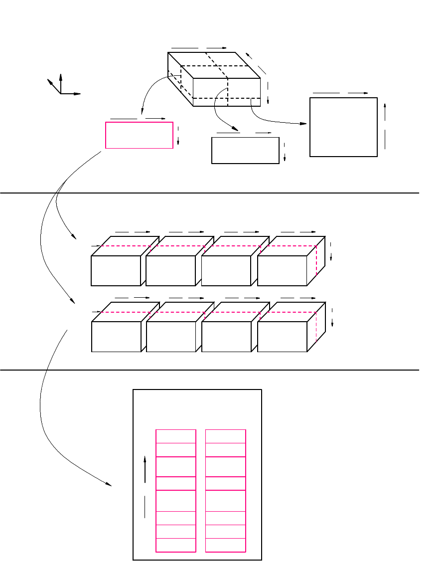
11.3. THE MEMORY WINDOW
141
imt jmt
x
jmt km
x
U
i,k,jrow
internal mode
V
i,k,jrow
internal mode
T
i,k,jrow
S
i,k,jrow
U
i,k,jrow
internal mode
V
i,k,jrow
internal mode
T
i,k,jrow
S
i,k,jrow
λ
z
ϕ
Longitude
Latitude
Depth
λ
ϕ
-z
τ
-1
imt km
x
.
.
.
.
.
.
.
.
.
.
.
.
a)
jrow
1
jrow
jmt
i
imt
1
i
imt
1
jmt
1
i
imt
1
jmt
Longitude slice
Latitude slice
Horizontal slice
k
km
1
k
km
k
km
1
1
imt
i
1
imt
i
1
imt
i
1
imt
i
1
imt
i
1
imt
i
1
imt
i
1
imt
i
τ
}
-1
Data
τ
Data
}
k
km
1
k
km
1
jrow
jmt
1
1
jrow
jmt
1
jrow
Longitude indices: i=1...imt
Latitude indices: jrow=1..jmt
Depth indices: k=1...km
3
2
1
jmt-1
jmt
3
2
1
jmt-1
jmt
Disk or Ramdrive
τ
b)
c)
ϕ
jrow
jrow
Figure 11.1: a) Slicing a volume along surfaces of constant latitude, longitude, and depth
showing relative sizes of slices. b) A longitudinal slice through two time levels of prognostic
data on disk or ramdrive with latitude index “jrow”. c) Schematic arrangement of all slices
arranged by latitude index “jrow” on disk or ramdrive area.
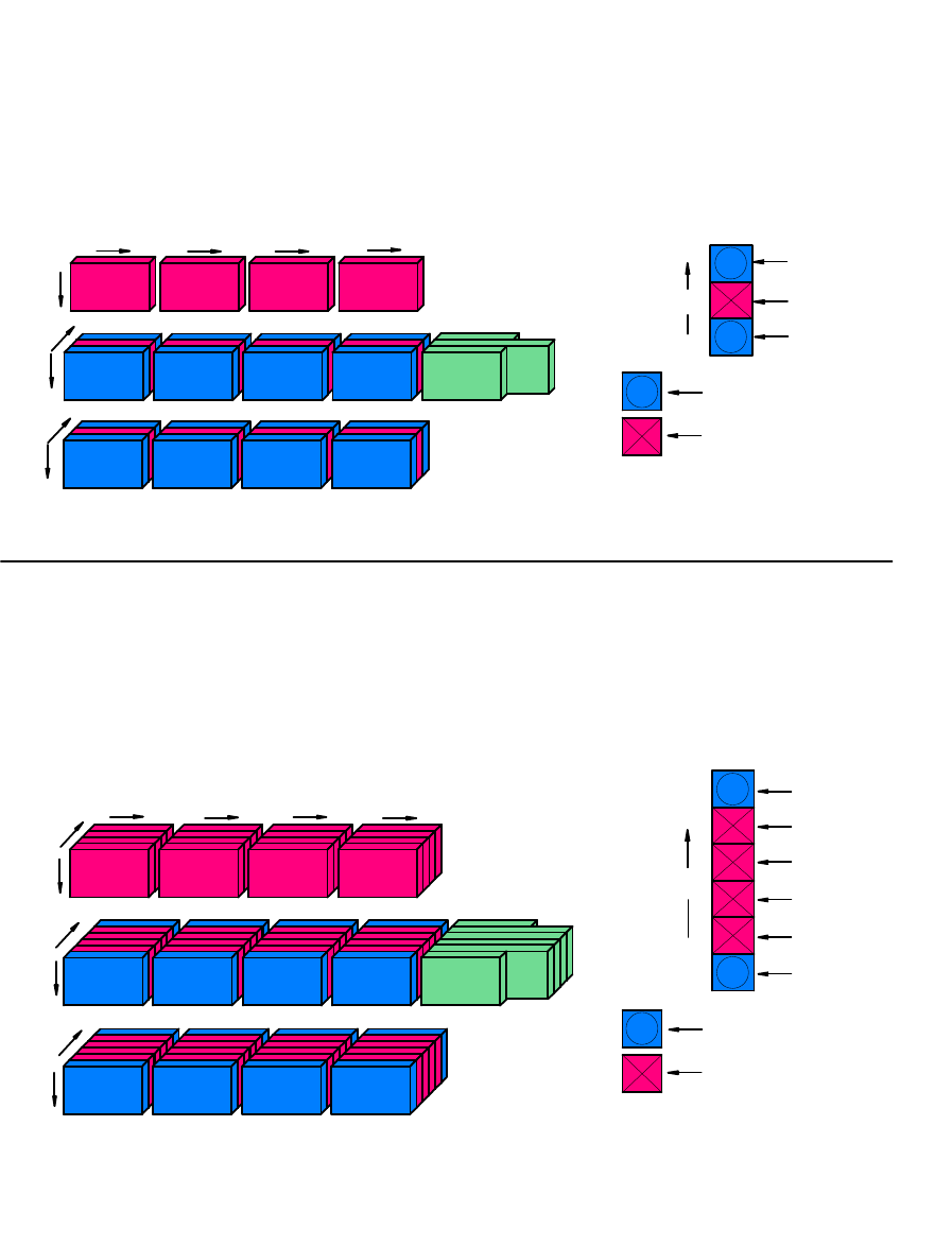
142
CHAPTER 11. UNI-TASKING
u
i,k,j,1,
i,k,j,2,
t
i,k,j,1,
t
u
i,k,j,2,
τ
τ
τ
τ
Work
i,k,j
j
u
i,k,j,1,
τ
+1
i,k,j,2,
τ
+1
t
i,k,j,1,
τ
+1
t
u
i,k,j,2,
τ
+1
k
i
i
i
i
u
i,k,j,1,
i,k,j,2,
t
i,k,j,1,
t
u
i,k,j,2,
τ
-1
τ
-1
τ
-1
τ
-1
j
k
k
j
u
i,k,j,1,
τ
+1
i,k,j,2,
τ
+1
t
i,k,j,1,
τ
+1
t
u
i,k,j,2,
τ
+1
u
i,k,j,1,
i,k,j,2,
t
i,k,j,1,
t
u
i,k,j,2,
τ
τ
τ
τ
u
i,k,j,1,
i,k,j,2,
t
i,k,j,1,
t
u
i,k,j,2,
τ
-1
τ
-1
τ
-1
τ
-1
Work
i,k,j
k
i
i
i
i
k
k
j
j
j
a)
}
Detailed schematic
"j" is a latitude index
local to the memory window
Minimun sized memory window (jmw=3) for 2nd order numerics
Buffer row
Prognostic Equations
solved on this row
b)
Larger memory window (jmw=6) for 2nd order numerics
j=5
j=jmw
j=4
j=3
j=2
j=1
Longitude indices: i=1...imt
Latitude indices: j=1...jmw
Depth indices: k=1...km
Simplified schematic
Buffer row
Prognostic Equations
solved on this row
"j" is a latitude index
local to the memory window
j
j=2
j=1
j=jmw
Longitude indices: i=1...imt
Latitude indices: j=1...jmw
Depth indices: k=1...km
Simplified schematic
Detailed schematic
}
Figure 11.2: a) Detailed and simplified schematic of the minimum sized memory window
with jmw =3 latitude rows for 2nd order numerics. b) Memory window opened up to hold
jmw =6 latitude rows.
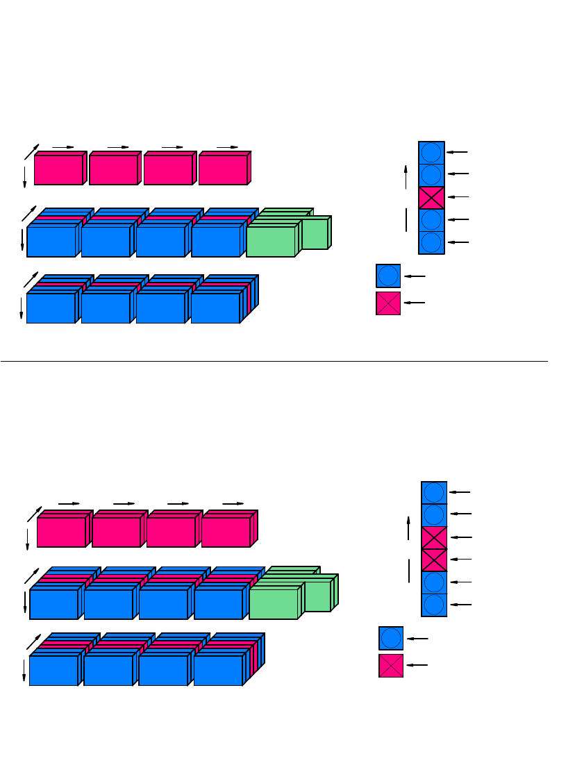
11.3. THE MEMORY WINDOW
143
j
u
i,k,j,1,
i,k,j,2,
t
i,k,j,1,
t
u
i,k,j,2,
τ
τ
τ
τ
u
i,k,j,1,
i,k,j,2,
t
i,k,j,1,
t
u
i,k,j,2,
τ
-1
τ
-1
τ
-1
τ
-1
Work
i,k,j
k
k
k
j
j
u
i,k,j,1,
τ
+1
i,k,j,2,
τ
+1
t
i,k,j,1,
τ
+1
t
u
i,k,j,2,
τ
+1
Work
i,k,j
i
i
i
i
j=4
j=3
j=2
j=1
j
u
i,k,j,1,
i,k,j,2,
t
i,k,j,1,
t
u
i,k,j,2,
τ
τ
τ
τ
u
i,k,j,1,
i,k,j,2,
t
i,k,j,1,
t
u
i,k,j,2,
τ
-1
τ
-1
τ
-1
τ
-1
k
k
k
j
j
u
i,k,j,1,
τ
+1
i,k,j,2,
τ
+1
t
i,k,j,1,
τ
+1
t
u
i,k,j,2,
τ
+1
Work
i,k,j
Work
i,k,j
i
i
i
i
a)
Minimum sized Memory window (jmw=5) for 4th order numerics
Detailed schematic
Longitude indices: i=1...imt
Latitude indices: j=1...jmw
Depth indices: k=1...km
}
"j" is a latitude index
local to the memory window
Buffer row
Prognostic Equations
solved on this row
j=jmw
j
Simplified schematic
b)
Minimum sized Memory window (jmw=6) for pressure gradient average
}
"j" is a latitude index
local to the memory window
Buffer row
Prognostic Equations
solved on this row
j=3
j=2
j=1
Simplified schematic
j=5
j=jmw
j=4
j
Detailed schematic
Longitude indices: i=1...imt
Latitude indices: j=1...jmw
Depth indices: k=1...km
Figure 11.3: a) Minimum sized memory window for 4th order numerics.
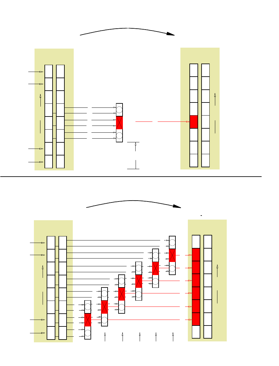
144
CHAPTER 11. UNI-TASKING
τ
-1
τ
-1
jrow
τ
τ
τ
-1
τ
τ
τ
-1
τ
τ
τ
-1
τ
+1
0.89
3-D Prognostic data
3-D Prognostic data
τ
-1
τ
-1
jrow
τ
-1
τ
τ
τ
τ
τ
τ
τ
-1
τ
-1
τ
+1
τ
+1
τ
+1
τ
+1
τ
+1
τ
+1
τ
τ
τ
-1
τ
τ
τ
-1
τ
τ
τ
-1
τ
τ
τ
-1
τ
τ
τ
-1
τ
τ
τ
-1
τ
τ
τ
-1
τ
τ
τ
-1
τ
τ
τ
-1
τ
τ
τ
-1
τ
τ
τ
-1
τ
τ
τ
-1
τ
τ
τ
-1
τ
τ
τ
-1
τ
τ
τ
-1
4
7
6
5
1
3
2
jmt
4
7
6
5
1
3
2
jmt
τ
jrow
4
7
6
5
1
3
2
jmt
4
7
6
5
1
3
2
jmt
τ
joff
Disk or Ramdrive
Disk or Ramdrive
One time step
a)
4
7
6
5
1
3
2
jmt
4
7
6
5
1
3
2
jmt
τ
jrow
4
7
6
5
1
3
2
jmt
4
7
6
5
1
3
2
jmt
1st
3rd
4th
5th
6th
2nd
Disk or Ramdrive
Disk or Ramdrive
3-D Prognostic data
3-D Prognostic data
One time step
b)
Memory Window
(2nd order)
τ
jscomp
jstask
jscomp
jstask
jetask
jecomp
j=1
j=jmw
j=2
jecomp
jetask
Figure 11.4: a) Loading the memory window, solving prognostic equations on the central row
and writing τ+1 data back to τ−1 disk for latitude row jrow =4. b) Solving prognostic
equations for all latitude rows from “jscomp” to “jecomp” by moving the memory window
northward.
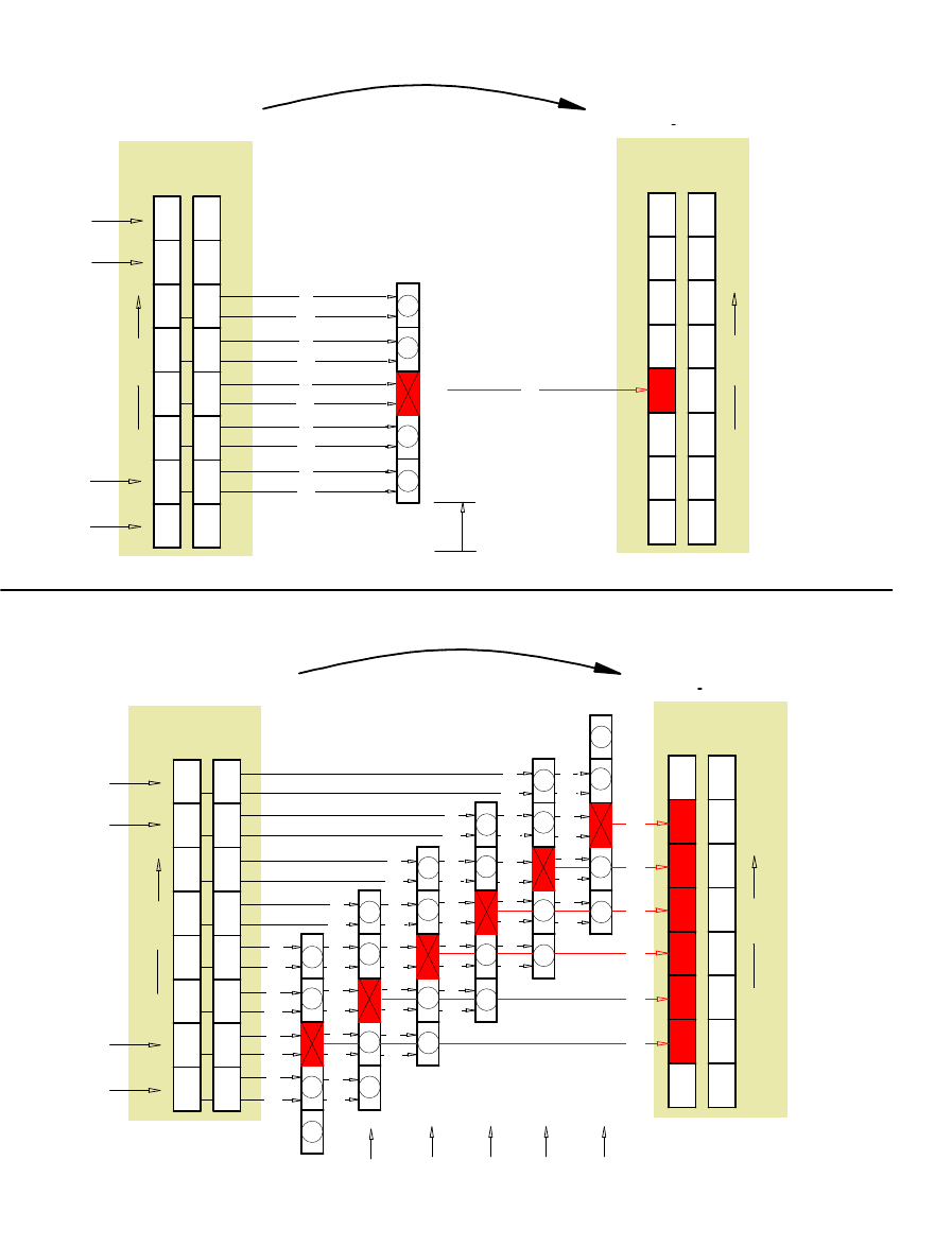
11.3. THE MEMORY WINDOW
145
τ
-1
τ
-1
jrow
τ
τ
τ
-1
τ
τ
τ
-1
τ
+1
τ
τ
τ
-1
τ
τ
τ
-1
τ
-1
τ
-1
τ
-1
jrow
τ
-1
τ
τ
τ
τ
τ
τ
τ
-1
τ
-1
τ
+1
τ
+1
τ
τ
τ
-1
τ
τ
τ
-1
τ
τ
τ
-1
τ
τ
τ
-1
τ
τ
τ
-1
τ
τ
τ
-1
τ
τ
τ
-1
τ
τ
τ
-1
τ
τ
τ
-1
τ
τ
τ
-1
τ
τ
τ
-1
τ
τ
τ
-1
τ
τ
τ
τ
τ
-1
τ
τ
τ
-1
τ
τ
τ
-1
τ
τ
τ
-1
τ
τ
τ
-1
τ
τ
τ
-1
τ
τ
τ
-1
τ
τ
τ
-1
τ
τ
τ
-1
τ
τ
τ
-1
τ
τ
τ
-1
τ
τ
τ
-1
τ
+1
τ
+1
τ
+1
τ
+1
4
7
6
5
1
3
2
jmt
4
7
6
5
1
3
2
jmt
τ
jrow
4
7
6
5
1
3
2
jmt
4
7
6
5
1
3
2
jmt
τ
τ
τ
-1
Disk or Ramdrive
Disk or Ramdrive
One time step
3-D Prognostic data
3-D Prognostic data
b)
a)
Memory Window
(4th order)
joff
jscomp
jstask
4
7
6
5
1
3
2
jmt
4
7
6
5
1
3
2
jmt
τ
jrow
4
7
6
5
1
3
2
jmt
4
7
6
5
1
3
2
jmt
Disk or Ramdrive
Disk or Ramdrive
3-D Prognostic data
3-D Prognostic data
One time step
τ
jscomp
jstask
3rd
4th
5th
6th
2nd
1st
jecomp
jetask
jecomp
jetask
j=jmw
j=4
j=3
j=2
j=1
Figure 11.5: a) Loading the memory window, updating the central row and writing to disk
for latitude row jrow =4. b) Updating all latitude rows by moving the memory window
northward.
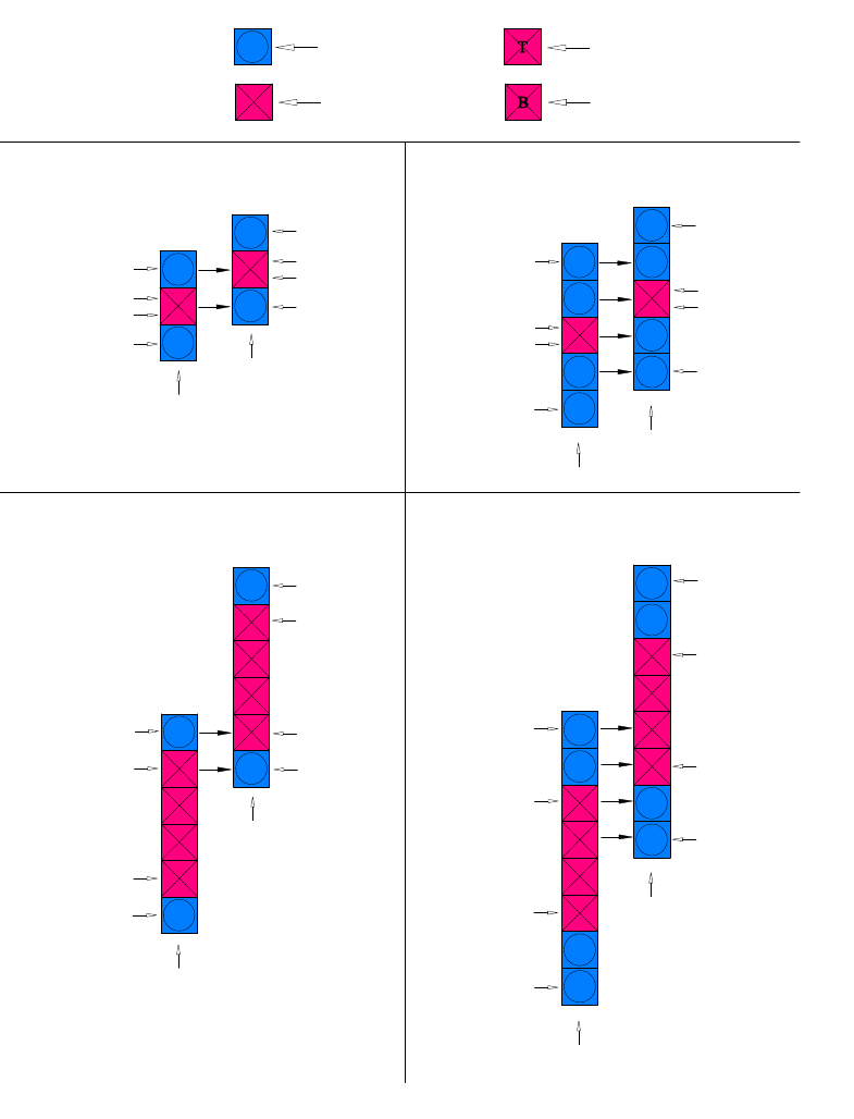
146
CHAPTER 11. UNI-TASKING
j=jmw-jbuf
j=1+jbuf
j=jmw-jbuf
j=1+jbuf
j=jmw
j=1
j=1
j=jmw
MW #(n+1)
MW #n
Minimum sized 4th order MW
jmw=5 and jbuf=2
j=jmw
j=jmw-jbuf
j=1+jbuf
j=1
j=jmw
j=jmw-jbuf
j=1+jbuf
j=1
MW #n
MW #(n+1)
Minimum sized 2nd order MW
jmw=3 and jbuf=1
j=1
MW #n
j=jmw
j=jmw-jbuf
j=1+jbuf
j=jmw
j=jmw-jbuf
j=1+jbuf
j=1
MW #(n+1)
Larger sized 4th order MW
jmw=8 and jbuf=2
j=jmw
j=1
MW #(n+1)
j=1
j=1+jbuf
j=jmw-jbuf
MW #n
j=jmw
j=jmw-jbuf
j=1+jbuf
Larger sized 2nd order MW
jmw=6 and jbuf=1
a) Key to rows in the
memory window
Copy
Copy
Copy
Copy
Copy
Copy
Copy
Copy
Copy
Copy
Copy
Copy
b)
c)
d)
e)
Only Tracer equations are
solved on this row
Only Baroclinic equations are
solved on this row
Buffer row
Tracer and Baroclinic equations are
solved on this row
Figure 11.6: The memory window is moved northward by copying data from the northernmost
rows into the southernmost rows followed by reading of new data. a) Various types of rows
within the memory window. b) Copy operation for a 2nd order memory window with jmw=3.
c) Copy operation for a 4th order memory window with jmw=5. d) Copy operation for a larger
2nd order memory window. e) Copy operation for a larger 4th order memory window.
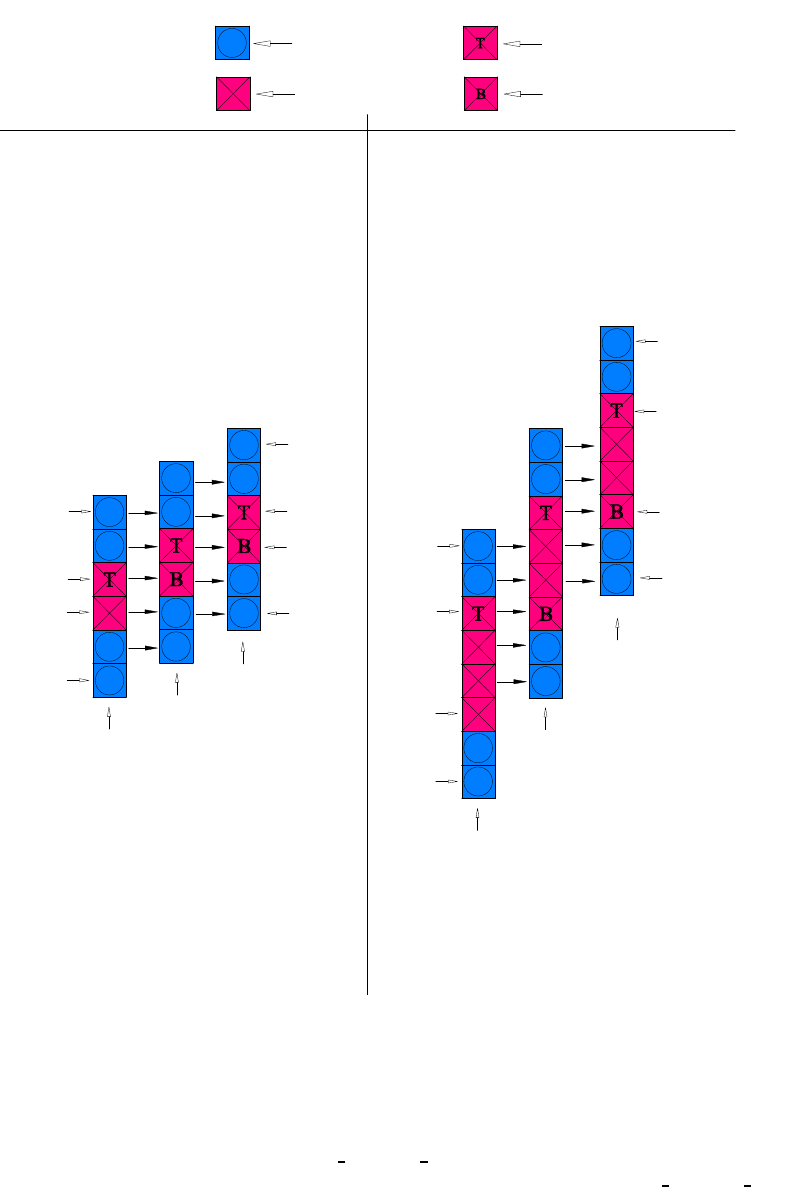
11.3. THE MEMORY WINDOW
147
a) Key to rows in the
memory window
Only Tracer equations are
solved on this row
Only Baroclinic equations are
solved on this row
Buffer row
Tracer and Baroclinic equations are
solved on this row
j=jmw
j=1
MW #1
j=jmw-jbuf
j=1+jbuf
Copy
Copy
Copy
Copy
Copy
Copy
Copy
Copy
MW #2
MW #3
j=1
j=jmw
j=jmw-jbuf
j=1+jbuf
Copy
Copy
j=1
MW #1
j=1+jbuf
j=jmw
j=jmw-jbuf
Copy
Copy
Copy
Copy
Copy
Copy
Copy
Copy
Copy
Copy
MW #2
MW #3
j=1
j=1+jbuf
j=jmw
j=jmw-jbuf
b)
c)
Larger sized 4th order MW for
Pressure Gradient Averaging
jmw=8 and jbuf=2
Minimun sized 4th order MW for
Pressure Gradient Averaging
jmw=6 and jbuf=2
Figure 11.7: The memory window is moved northward by copying data from the northernmost
rows into the southernmost rows followed by reading of new data. Note that only rows where
baroclinic velocities are computed are written back to disk (or ramdrive). a) Various types of
rows within the memory window. b) Copy operation for the first three memory windows of
minimum size jmw=6 when option pressure gradient average is enabled. c) Copy operation for
the first three memory windows of a larger size jmw=8 when option pressure gradient average
is enabled.
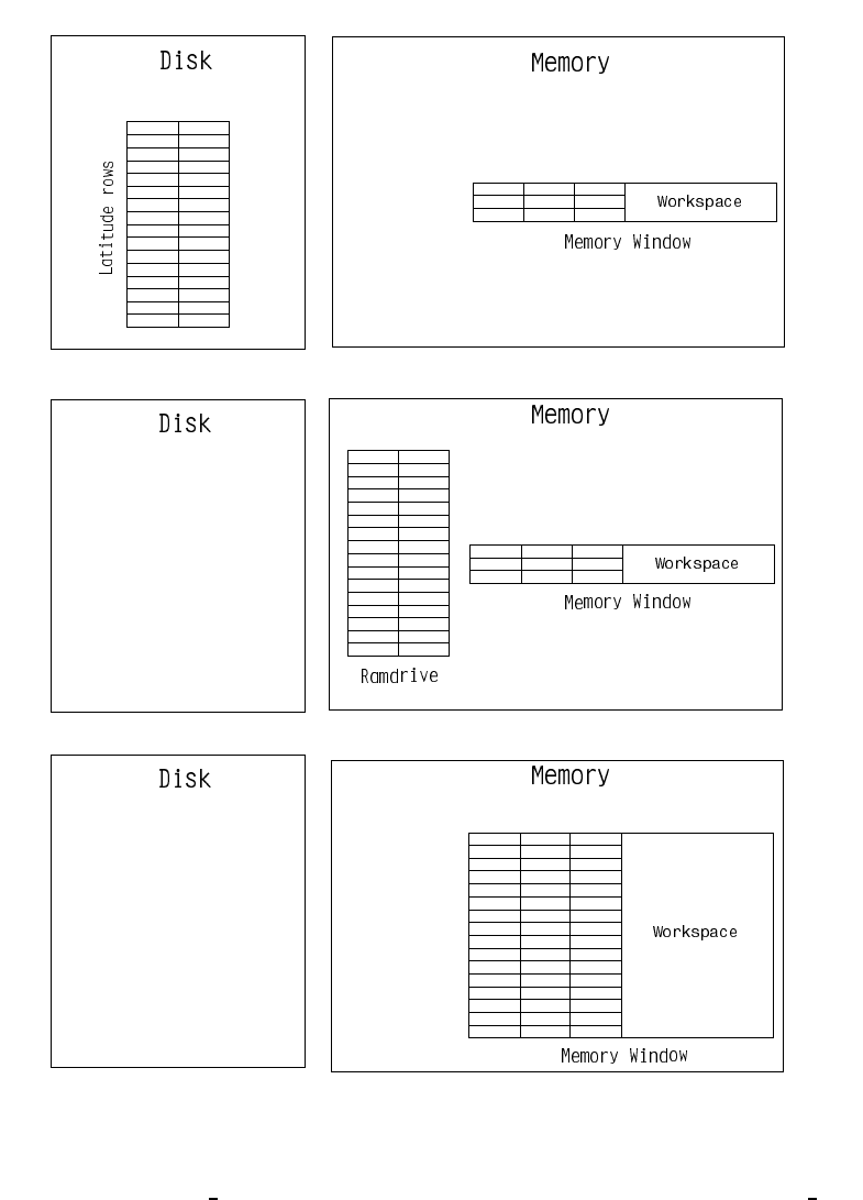
148
CHAPTER 11. UNI-TASKING
τ+1
-1
ττ
τ+1
-1
ττ
-1
ττ
-1
τττ+1
-1
ττ
a)
b)
c)
Figure 11.8: Various ways of configuring MOM illustrating the space used on disk and in mem-
ory. a) Options fio and ssread sswrite. b) Option ramdrive. c) Options ramdrive and max window.

Chapter 12
Multi-tasking
Since multi-tasking is a straightforward extension of uni-tasking, familarity with uni-tasking
as described in Chapter 11 is assumed.
12.1 Scalability
When multi-tasking, multiple processors are deployed against a job to reduce the job’s overall
wall clock time. The cpu time (summed over all processors) is not reduced1compared to
uni-tasking. The degree to which multiple processors are able to reduce a job’s wall clock time
is a measure of the job’s parallel efficiency or scalability. For instance, if a job, which takes
10 hours of wall clock time on one processors, can be divided into pieces so that it will take
one hour using 10 processors, then the job is 100% parallel. The job is then said to scale well
which means it scales linearly with the number of processors. It should be kept in mind that
a prefectly linear scaling with the number of processors assumes a dedicated environment. In
a non-dedicated environment, other executables will steal processors and the job’s captured
processors must wait for stolen processors to be re-claimed before continuing. The wait time
degrades scaling.
How parallel must a job be? Almost linear scaling may be good enough for a small number
of processors, but it is not for large numbers of processors. For instance, if a job is 99.5%
parallel, it will saturate about 14.8 out of 16 processors. That means the speedup from 16
processors is about 15 times as fast as the uni-tasked job. However, the same job will only give
a speedup of 49 on 64 processors and on 1024 processors, the speedup is only 168! This is a
consequence of Amdahl’s law.
12.2 When to multi-task
If the number of processors exceed the number of jobs in the system, some processors stand
idle and overall system efficiency degrades unless jobs are multi-tasked. In an operational
environment, if a forecast is required every 4 hours but takes 8 hours on a single processor,
then multi-tasking will be useful. Other examples include long running experiments that take
too long to complete or when it’s impossible to exhaust a monthly computer time allocation
using one processor. In environments where multiple processors are dedicated to a single job, it
1In fact, it may increase. However, the focus is changed from cpu time to wall clock time. Wall clock time is the
time it takes to get results back.
149
150
CHAPTER 12. MULTI-TASKING
is essential to attain high parallel efficiency otherwise system efficiency and overall throughput
suffers. In the past, multi-tasking has not been used in any significant way at GFDL. The reason
is that there have always been enough jobs in the system to keep all processors busy. Typically,
in the middle of 1997, there were about 30 batch jobs in GFDL’s Cray T90 at all times and the
system efficiency averaged over 24 hours was about 93%. At the point where a system becomes
under saturated, overall system efficiency will drop significantly unless multi-tasking is used.
12.3 Approaches to multi-tasking
Two approaches to multi-tasking MOM have been experimented with at GFDL. They were:
•The fine grained approach to multi-tasking where parallelism is applied at the level of
each nested do loop. This is also known as “autotasking”. All processors work simultane-
ously on each nested do loop and there are many parallel regions.
•The coarse grained approach to multi-tasking where parallelism is applied at the level of
latitude rows. For example, all work associated with solving equations for one latitude
row is assigned to one processor. All work associated with solving the equations for
another latitude row is assigned to a second processor . . . and so forth. Then, all proces-
sors work simultaneously and independently. This implies that there is only one parallel
region.
In a nutshell, the fine grained approach to multi-tasking gives about 85% parallelism. That
translates into a speedup of a little less than 4 on 8 processors. Why is the parallel efficiency
so low? The reason is basically due to not enough work within the many parallel regions and
the fact that the range on the parallel loop “j” index is not the same for all loops. Increasing
the model resolution can somewhat address the first problem but not the second. The result
is that processors stand idle and the parallel performance degrades. This is clearly not a long
term solution. The coarse grained approach is the best and yields a near linear speedup with
the number of processors.
12.4 The distributed memory paradigm
A distributed memory paradigm is one where each processor has its own chunk of memory
but the memory is not shared among processors. This means that an array on one processor
cannot be dimensioned larger than the processor’s local memory and the processor cannot
easily access arrays dimensioned in other processors memory. Accessing arrays in other
processor’s memory is possible by making “communication” calls to transfer data between
processors.
MOM uses a distributed memory paradigm. The method builds on the coarse grained
approach and assumes that both baroclinic and barotropic parts are divided among processors
with distributed memories and therefore “communication” calls must be added to exchange
boundary cells between processors at critical points within the code. The “communication”
calls are made via a message passing module which supports SHMEM as well as MPI protocols.
For details, refer to http:/www.gfdl.gov/vb. The advantages of the distributed paradigm are:
1. Higher parallel efficiency is attainable.

12.5. DOMAIN DECOMPOSITION
151
2. No complicated “ifdef” structure is needed to partition code differently for uni-tasking
or multi-tasking on shared or distributed memory platforms.
3. Only two time levels are required for 3-D prognostic data on disk (or ramdrive) as
opposed to three time levels with the coarse grained shared memory method.
Most options have been tested in parallel. It bears stating that when an option is par-
allelized, it means that answers are the same to the last bit of machine precision regardless
of the number of processors used2. Some options will probably never be parallelized. One
example is the stream function method. This method requires land mass perimeter integrals
which cut across processors in compilicated ways and this is a recipe for poor scaling. The
implicit free surface method is better since it does not require perimeter integrals. However,
global sums are still required which do degrade scaling but not as much as the island integrals.
Improvement can be made to the existing global sum reductions because they are only a crude
first attempt. However, even if global sum reductions were no problem, the accuracy of the
method depends on the number of iterations which is tied to the grid size3. The best scaling is
achieved by the explicit free surface option which does not require any global sum reductions
and the number of iterations (sub-cycles) depends on the ratio of internal to external gravity
wave speed independent of the number of grid cells.
12.5 Domain Decomposition
If all arrays were globally dimensioned4on all processors, available memory could easily be
exceeded with even modest sized problems. Each processor should only dimension arrays large
enough to cover the portion of the domain being worked on by the specific processor. Refer to
Fig 12.1a which is an example of a domain with i=1,imt longitides and jrow =1,jmt latitudes
divided among 9 processors arranged in a 2d (two dimensional) domain decomposition. Fig
12.1b gives the arrangement for a 1d (one dimensional) domain decomposition in latitude
using the same 9 processors. In both cases, two dimensional arrays need only be dimensioned
large enough to cover the area worked on by each processor. As discussed below, this area will
actually be one or two cells larger at the processor boundaries to include boundary cells required
by the numerics. Boundary cells on each processor must be updated with predicted values
from the domain of the adjoining processor. The arrows indicate places where communication
takes place across boundaries between processors.
Figure 12.1c indicates three cases: one for 9 processors, 100 processors, and 900 processors.
Within each case, three domain shapes are considered: imt =jmt,imt =2∗jmt, and imt =
jmt/2. The tables indicate how many communication calls are required. Since both processors
which share a boundary require data from the other processor, two communication calls
are required at each boundary and the same amount of words are transferred across the
boundary for each processor. Two things are worth noting. First, as the number of processors
increases, the number of words transferred in the 2d domain decomposition is much less
than in the 1d domain decomposition. Second, for large numbers of processors, 1d domain
decomposition requires half as many communication calls as 2d domain decomposition. An
additional problem for 2d domain decomposition which is not indicated in Figure 12.1c is
that the equations are not symmetric with respect to latitude and longitude. Specifically, a
2This is necessary otherwise science may become processor dependent.
3As the number of grid cells increase, the number of iterations must increase to keep the same level of accuracy.
4Dimensioned by the full number of grid cells in latitude, longitude, and depth.
152
CHAPTER 12. MULTI-TASKING
wrap around or cyclic condition is placed on longitudes for global simulations. No such
condition is needed along latitudes. The implication is that many additional communication
calls will be needed to impose a cyclic condition on intermediate computations for 2d domain
decomposition. These communication calls are not needed in a 1d decomposition in latitude
because each latitude strip including the cyclic boundary is on processor. To lessen the need
for extra communication calls in 2d decomposition, additional points can be added near the
cyclic boundary thereby extending the domain slightly.
Whether 1d or 2d decomposition is better depends on the the latency involved in issuing a
communication call versus the time taken to transfer the data. Another factor is whether polar
filtering is used because it would also require extra communications in a 2d decomposition.
At this point, the 1d domain decomposition of Fig 12.1a is what is done in MOM.
Executing the 3 degree global test case #0 for MOM on multiple processors of a T3E using
1-D decomposition in latitude indicates that scaling falls offquickly when there are fewer
than 8 latitude rows per processors. This result has dire implications for climate models. For
instance, a 2 degree global ocean model will have about 90 latitiude rows. Efficient scaling
implies only 11 processors can be used. On the GFDL T3E, it takes about 10 processors to equal
the speed of one T90 processor. If it is assumed that processors on the next system are 2.5 times
as fast as the T3E processors and the ratio of network speed to processor speed stays the same,
a two degree climate model will only gain a factor of about 3 in speed over a T90 processor.
If the processor speed increases faster than the network speed, then the situation gets worse.
The implication is that 2-D domain decomposition will be needed for climate modeling if an
order of magitude speed up is to be attained..
On the other hand, a 1/5 degree global ocean model with 50 levels has 900 latitude rows
and requires 2 gigawords of storage with a fully opened memory window. Using 9 rows per
processor implies that 100 processors can be used with 1-D decomposition. Each processor
must have at least 20 megawords. Realistically, by the next procurement, each processor will
have at least 32 megawords of memory. If the GFDL T3E had enough processors,then a speedup
of 25 times that of one T90 processor would be realized. It seems that 2-D decomposition is
more important for coarse resolution models.
Since the majority of simulations with MOM have been carried out on vector machines at
GFDL, the idea has been to compute values over land rather than to incur the cost of starting
extra vectors to skip around land cells. In an earlier implementation, extra logic was in place
to skip computations on land cells. It turned out that the speed increase on vector machines
was not worth the extra coding complexity so the logic was removed. On scalar machines, it
may be beneficial to skip computation over land areas. A 2d domain decomposition would in
principle more easily allow computation over land to be skipped by not assigning processors
to areas containing all land cells. In a 1d decomposition, extra logic would need to be added
to eliminate computation over land cells.
12.5.1 Calculating row boundaries on processors
The number of processors is read in through namelist as variable num processors. The model
domain is divided into num processors pieces with each piece containing the same number5of
latitude rows. Each processor is assigned the task of working on its own piece of the domain
starting with latitude index jrow =jstask and ending with latitude index jrow =jetask. Each
5The important point is to have the same amount of work on each processor. If more work is required on some
rows than others, then the number of rows on each processsor should be different. It is assumed here that the same
amount of work is on every row and that each processor should get the same number of rows.
12.5. DOMAIN DECOMPOSITION
153
processor has its own memory window to process only those latitude rows within its own task.
The starting and ending rows of each processor’s task are given by
jstask =nint((pn −1) ∗calculated rows)+(2 −jbu f ) (12.1)
jetask =nint(pn ∗calculated rows)+(1 +jbu f ) (12.2)
where pn is the processor number (pn =1··· num processors), the number of buffer rows “jbuf”
is explained in Section 11.3.1, and
calculated rows =f loat(jmt −2)/num processors.(12.3)
The latitude rows for which the tracer and baroclinic equations are solved within the processor’s
task are controlled by the starting and stopping rows
jscomp =jstask +jbu f (12.4)
jecomp =jetask −jbu f (12.5)
12.5.2 Communications
Figure 12.2a gives an example of multi-tasking with num processors =3 processors and jmt =14
latitude rows for a second order memory window. Note that latitude rows on disk (or ramdrive)
for each processor in Figure 12.2b look like a miniture version of Figure 11.4 where jstask =1
and jetask =jmt. For example, on the disk (or ramdrive) of processor #1, the global latitude
index runs from jrow =1 to jrow =6. On this processor, the task limits are jstask =1 and
jetask =6 and the limits for integrating prognostic equations are from jscomp =2 through
jecomp =5. On processor #2, the task limits are jstask =5 and jetask =10 and the limits for
integrating prognostic equations are from jscomp =6 through jecomp =9.
Apart from dividing up the domain into pieces, the new aspect in Figure 12.2 is commu-
nication between processors indicated by short arrows pointing to the boundary rows. In the
second order memory window, there is one boundary row at the borders of each task. Look
at latitude row jrow =6 on the updated disk of processor #1. This row cannot be updated
to τ+1 by processor #1’s MW because data from jrow =7 is needed. Instead, data at τ+1
from jrow =6 on processor #2 is copied into the jrow =6 slot of processor #1 by a call to the
communication routine after all processors have finished working on their tasks. Similarly,
jrow =5 on processor #2 is updated with τ+1data from jrow =5 on processor #1 and so forth.
The situation with fourth order numerics is similar except that more communication is
required at the end of the timestep. This is illustrated in Figure 12.3a. Note that since jbu f =2
for forth order windows, the task for processor #1 ranges from jstask =1 to jetask =7. For
processor #2, the task ranges from jstask =4 to jetask =11, and so forth. However, the rows on
which prognostic equations are solved within each task are the same as in the case with a 2nd
order memory window. Additional communication is indicated by the extra arrows which are
needed because there are now two buffer rows on the borders of each task (i.e. jbu f =2).
For all processor numbers from pn =2,num processors the following prescribes the required
communication for second order numerics:
•copy all data from latitude row “jstask+1” on processor “pn” to latitude row “jetask” on
processor “pn-1”.
154
CHAPTER 12. MULTI-TASKING
•copy all data from latitude row “jetask-1” on processor “pn-1” to latitude row “jstask”
on processor “pn”.
When a fourth order memory window is involved, the following communication is required:
•copy all data from latitude row “jstask+3” on processor “pn” to latitude row “jetask” on
processor “pn-1”.
•copy all data from latitude row “jstask+2” on processor “pn” to latitude row “jetask-1”
on processor “pn-1”.
•copy all data from latitude row “jetask-3” on processor “pn-1” to latitude row “jstask”
on processor “pn”.
•copy all data from latitude row “jetask-2” on processor “pn-1” to latitude row “jstask+1”
on processor “pn”.
12.5.3 The barotropic solution
The 2-D barotropic equation is divided into tasks in the same way as was done for the prognostic
equation. Since the processor boundaries are the same, communication involves the same
rows. Each processor dimensions arrays for only that part of the domain being worked on
by the specific processor and the actual memory requirement is small. Therefore, within each
processor’s task no memory window is needed. All indexing into 2-D arrays is in terms of the
absolute global index “jrow”.
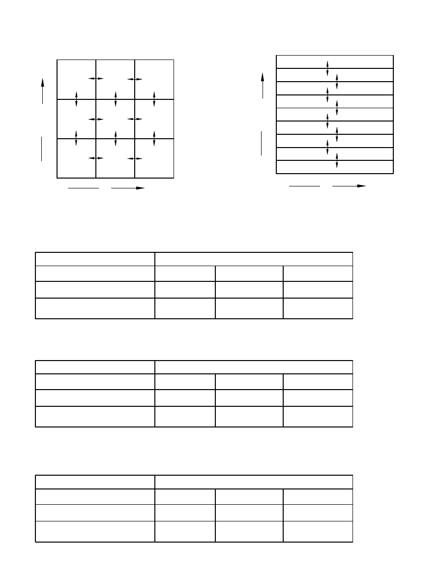
12.5. DOMAIN DECOMPOSITION
155
p
3,3
p
3,1
p
1,3
2,2
p
p
3,2
p
2,3
p
2,1
p
1,2
p
1,1
1
i
imt
p
3,2
2,2
p
p
3,1
p
3,3
p
2,1
p
2,3
p
1,2
p
1,3
p
1,1
1
i
imt
jmt
1
jrow
jmt
1
jrow
3 processors
2
10 processors
2
a)
2-d domain decomposition
c)
b)
1-d domain decomposition
16*imt
8*imt
16*imt
6*imt
16*imt
12*imt
Total number of words transferred
when imt=jmt
when jmt = imt/2
when jmt = 2*imt
number of communication calls
16
24
2-d
1-d
198*imt
36*imt
198*imt
27*imt
198*imt
54*imt
Total number of words transferred
when imt=jmt
when jmt = imt/2
when jmt = 2*imt
number of communication calls
198
360
2-d
1-d
1798*imt
116*imt
1798*imt
87*imt
1798*imt
174*imt
Total number of words transferred
when imt=jmt
when jmt = imt/2
when jmt = 2*imt
number of communication calls
1798
3480
2-d
1-d
30 processors
2
Figure 12.1: a) A 2d domain decomposition using 9 processors. b) Rearranging the 9 processors
for a 1d domain decomposition in latitude. c) Comparison of 1d and 2d domain decomposition
giving number of communication calls and words transferred for 9, 100, and 900 processors.

156
CHAPTER 12. MULTI-TASKING
Disk or Ramdrive
jrow
jrow
jrow
jrow
jrow
jrow
jrow
a) Multi-tasking with 3 processors and 2nd order numerics
1
2
3
1
2
3
1
2
3
1
2
3
4
5
6
5
6
7
8
9
10
9
10
11
12
13
jmt
Processors
#1
#3
#2
Processors
One Time Step
Disk or Ramdrive
1
2
3
4
5
6
7
8
9
10
11
12
13
jmt
5
6
7
8
9
10
1
2
3
4
5
6
9
10
11
12
13
jmt
}
}
}
3-D data
#1
#3
#2
Processor #3
Memory Window
Processor #2
Memory Window
Processor #1
Memory Window
1
2
3
4
5
6
jstask
jscomp
jetask
jecomp
Processor #1
b) Starting and ending row limits for each processor
5
6
7
8
9
10
Processor #2
9
10
11
12
13
jmt
Processor #3
jstask
jscomp
jetask
jecomp
jstask
jscomp
jetask
jecomp
Figure 12.2: a) Integrating prognostic equations using 3 processors and 2nd order numerics.
b) Task limits “jstask” and “jetask” as well as row limits “jscomp” and “jecomp” for each
processor.
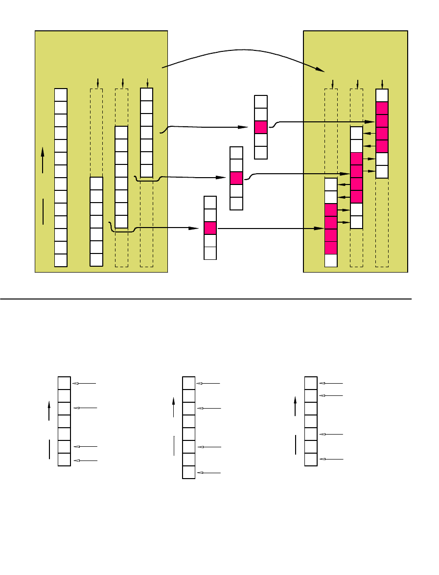
12.5. DOMAIN DECOMPOSITION
157
Disk or Ramdrive
Disk or Ramdrive
jrow
jrow
jrow
1
2
3
4
5
6
7
8
9
10
11
12
13
jmt
jrow
5
6
7
8
9
10
1
2
3
4
5
6
9
10
11
12
13
jmt
7
4
}
11
8
}
}
1
2
3
4
5
6
5
6
7
8
9
10
9
10
11
12
13
jmt
7
4
11
8
2
3
4
5
1
2
3
4
5
1
2
3
4
5
1
3-D data
#1
#3
#2
Processors
#1
#3
#2
Processors
One Time Step
a) Multi-tasking with 3 processors and 4th order numerics
Processor #1
Memory Window
Processor #2
Memory Window
Processor #3
Memory Window
b) Starting and ending row limits for each processor
Processor #1
Processor #2
Processor #3
1
2
3
4
5
6
jstask
jscomp
jecomp
7
jetask
5
6
7
8
9
10
jscomp
jecomp
11
4
jstask
jetask
9
10
11
12
13
jmt
jscomp
jetask
jecomp
8
jstask
Figure 12.3: a) Integrating prognostic equations using 3 processors and 4th order numerics.
b) Task limits “jstask” and “jetask” as well as row limits “jscomp” and “jecomp” for each
processor.
158
CHAPTER 12. MULTI-TASKING

Chapter 13
Database
A database is included with MOM. The database is not needed to start using MOM, although
use of MOM is certainly limited without it. Refer to Chapter 3 for details on how to get this data
and Section 3.2 for a description of programs which access it. This database is far from being
complete. It should be considered as a starting point and act as a prototype for extensions
using other datasets. GFDL is not a data center and there is no intention to extend this with
other datasets.
13.1 Data files
The DATABASE contains approximately 160MB of IEEE 32bit data and the files are named as
follows:
•scripps.top is the Scripps topography (265816 bytes).
•hellerman.tau is the Hellerman/Rosenstein (1983) windstress climatology (1757496 bytes).
•oorts.air is the Oort (1983) 1000mb air temperature climatology (294268 bytes).
•levitus.mask is the Levitus (1982) land/sea mask (8680716 bytes).
•ann.temp is the Levitus (1982) annual mean potential temperatures (8682036 bytes).
•ann.salt is the Levitus (1982) annual mean salinities (8682036 bytes).
Then there are the Levitus (1982) monthly climatological potential temperatures. There
are twelve monthly files where the three letter suffix gives the month.
•jan.temp is the Levitus (1982) monthly mean potential temperatures (4998748 bytes).
The remaining eleven monthly temperature files are of the same size but use a different
month as the suffix.
Then there are the Levitus (1982) monthly climatological salinities. There are twelve
monthly files where the three letter suffix gives the month.
•jan.salt is the Levitus (1982) monthly mean salinities (6314208 bytes).
The remaining eleven monthly salinity files are of the same size but use a different month
as the suffix.
159
160
CHAPTER 13. DATABASE
Note that the file size for the monthly Levitus (1982) data is less than the file size for the
annual means. This is because seasonal effects only penetrate down to 1000m or so and
the monthly data only extends to this depth. Also, salinity has been interpolated from four
seasonal values to twelve monthly values within this dataset. All Levitus (1982) data as well
as Hellerman/Rosenstein (1983) and Oort (1983) data has been forced into land areas on their
native grid resolutions by solving
∇2ξi,jrow =0 (13.1)
over land areas using values of ξi,jrow over ocean areas as boundaries values where ξi,jrow
represents the various types of data. This method is similar to what was done with surface
boundary conditions in Section 19.1.2.

Chapter 14
Variables
14.1 Naming convention for variables
The 6 character restriction on naming variables has been relaxed since MOM 2 although
economy of characters in choosing names is always desirable. In an attempt to unify naming
of variables, a convention is introduced which uses abbreviated forms of the fundamental
conceptual pieces of the numerical oceanography. This convention also gives guidance for
building the names for variables in future parameterizations and keeps an overall consistency
throughout the model. Constructing names for variables is then a matter of assembling these
abbreviations in various ways. Note that when names of variables are spelled out, the naming
convention should not be applied. However, when names seem cryptic, the convention is
intended to help decipher their meaning. A list of abbreviations is given below:
u=Velocity point d =Delta adv =Advective
t=Tracer point f =Flux diff = Diffusive
n=North face p =Pressure visc =Viscous
e=East face c =Coefficient psi =Stream function
b=Bottom face v =Velocity ps =Surface pressure
Variables described subsequently within this chapter are build in terms of these abbrevia-
tions. All variables are positioned relative to the arrangement of grid cells discussed in Chapter
16. When an unknown variable is encountered in MOM, it may be possible to determine its
meaning from context or the naming convention. For example, the variable adv vnt is an ad-
vective velocity on the north face of T cells. If this fails, it may be useful to search all include
files for comments using the UNIX command: grep as described in Section 3.1.
Operators are used in MOM to construct various terms in finite difference equations which
are the counterpart to equations detailed in Chapter 4. Unlike arrays, operators are build using
expressions which relate variables but require no explicit memory. The details of a particu-
lar operation are forced into the operator and buried from view which allows complicated
equations to be written in terms of simple, easy to understand, pieces. At the same time,
compilers can expand these pieces in-line into an un-intelligible mess (by human standards)
and subsequently optimize it. In fact, there is no difference in speed on the CRAY (or any
mature compiler) between writing an equation with operators and writing an equation with
all terms expanded out. The big difference is that the former is easier to understand and work
with for humans.
161

162
CHAPTER 14. VARIABLES
Instead of using operators, all terms in the equations could be computed once and stored
in arrays. This would allow less redundant calculation but be prohibitive in memory usage. It
is an interesting counter intuitive point that it is sometimes faster to do redundant calculation
rather than save intermediate results in arrays. Depending on the speed of the load/store
operations compared with the multiply/add operations, if redundant computation contains
little work it may be faster to compute redundantly. In practice, this depends on the computer
and compiler optimizations. This can be verified by executing script run timer which exercises
the timing utilities in module timer by solving a tracer equation in various ways. It is one
measure of a mature compiler when the speed differences implied by solving the equations in
various ways is relatively small. On the CRAY YMP the differences are about 10% whereas on
the SGI workstation, they can exceed 50%.
Within operators, capital letters are reserved for the intended operation and small letters
act as qualifiers. A list of abbreviations is given below:
ADV T=Advection of tracer x =longitude direction
DIFF T=Diffusion of tracer y =latitude direction
ADV U=Advection of velocity z =vertical direction
DIFF U=Diffusion of velocity
As an example, tracer diffusion in the longitude direction at a given point is given by operator
DIFF Tx(i,k,j). These operators are defined in include files and may be located using the UNIX
command grep as indicated in Section 3.1.
14.2 The main variables
14.2.1 Relating indices j and jrow
In MOM, index “jrow” is the index of a latitude row and it takes on values from “1” to “jmt”.
Index “j” refers to a latitude row within the memory window which takes on values from “1”
to “jmw” which is the size of the memory window. The indices are related by a simple offset
“joff” which measures how far the memory window has been moved northward as equations
are being solved
j=jrow −jo f f (14.1)
Why are some variables referenced by “j” where others are referenced by “jrow”? To
save memory. Typically, one or two dimensional variables which are functions of latitude
are dimensioned by “jmt” and referenced by index “jrow”. Three dimensional variables are
dimensioned by “jmw” and referenced with index “j”. If memory size were no issue (but it is)
then all variables could be dimensioned by “jmt” and referenced by one latitude index. When
the memory window is opened up all the way then jmw =jmt,jo f f =0, and j=jrow.
For a description of how the memory window moves northward, refer to Section 11.3.2.
In MOM, whether an array is indexed by jor by jrow is dictated entirely by whether it is
dimensioned by jmw or jmt.

14.2. THE MAIN VARIABLES
163
14.2.2 Cell faces
As described below, in addition to defining prognostic variables at grid points within T cells
and U cells, it is useful to define other variables on the faces of these cells. This is because
the equations are written in finite difference flux form to allow quantities to be conserved
numerically. Each cell has six faces and certain variables must be defined on all faces. For
instance, advective velocities (zonal, meridional, and vertical) are located on cell faces defined
normal to those faces and positive in a direction of increasing longitude, latitude and decreasing
depth1. Additional variables defined on cell faces are diffusive coefficients, viscous coefficients,
diffusive fluxes, and advective fluxes. Note that names for variables on cell faces are only
needed on the east, north, and bottom faces of cells. This is because the west, south, and top
faces of cell Ti,k,jare the east face of cell Ti−1,k,j, the north face of cell Ti,k,j−1, and bottom face of
cell Ti,k−1,j. A similar arrangement holds for U cells.
14.2.3 Model size parameters
The main dimensional parameters are:
•imt =number of longitudinal grid cells in the model domain. This is output by mod-
ule grids when specifying a domain and resolution.
•jmt =number of latitudinal grid cells in the model domain. This is output by module grids
when specifying a domain and resolution.
•km =number of grid cells between the ocean surface and the bottom in the model
domain. This is output by module grids when specifying a domain and resolution.
•jmw =number of latitude rows within the memory window. The minimum is three and
the maximum is jmt.
•nt =number of tracers in the model. Usually set to two. The first is for potential
temperature and the second is for salinity as described in Section 14.2.8. Additional
tracers (when nt >2) are passive and initialized to 1.0 at level k=1 amd 0.0 for levels
k>1.
Some secondary ones are:
•mnisle =maximum number of unconnected land masses (islands).
•maxipp =maximum number of island perimeter (coastal) points. This includes coastlines
from all land masses.
14.2.4 T cells
A complete description of grid cells is given in Chapter 16. For cells on the T grid given by
Ti,k,j, the primary grid distances in longitude and latitude are given by:
•xti=longitudinal coordinate of grid point within cell Ti,k,jin degrees. Index iincreases
eastward with increasing longitude.
1Positive vertical velocity at the bottom of a cell points upward in the positive zdirection
164
CHAPTER 14. VARIABLES
•ytjrow =latitudinal coordinate of grid point within cell Ti,k,jin degrees. This is written
in the equations of this manual as φT
jrow. Index jrow increases northward with increasing
latitude.
•dxti=longitudinal width of equatorial cell Ti,k,jin cm.
•dytjrow =latitudinal width of cell Ti,k,jin cm.
•cstjrow =cosine of latitude at the grid point within cell Ti,k,j. This is written in the
equations of this manual as cos φT
jrow.
14.2.5 U cells
A complete description of grid cells is given in Chapter 16. For cells on the U grid given by
Ui,k,j, the primary grid distances in longitude and latitude are given by:
•xui=longitudinal coordinate of grid point within cell Ui,k,jin degrees. Index iincreases
eastward with increasing longitude.
•yujrow =latitudinal coordinate of grid point within cell Ui,k,jin degrees. This is written
in the equations of this manual as φU
jrow. Index jrow increases northward with increasing
latitude.
•dxui=longitudinal width of equatorial cell Ui,k,jin cm.
•dyujrow =latitudinal width of cell Ui,k,jin cm.
•csujrow =cosine of latitude at the grid point within cell Ui,k,j. This is written in the
equations of this manual as cos φU
jrow.
14.2.6 Vertical spacing
A complete description of grid cells is given in Chapter 16. For T cells and U cells, the primary
grid distances in the vertical are given by:
•ztk=distance from the surface to the grid point in cell Ti,k,jor Ui,k,jin units of cm.
The T cells and U cells are not staggered vertically. Note that although ztkis positive
downwards, the coordinate zis positive upwards. Index kincreases downward.
•zwk=distance from the surface to the bottom face of cell Ti,k,jor Ui,k,jin cm. The T cells
and U cells are not staggered vertically.
•dztk=vertical thickness of cell Ti,k,jor Ui,k,jin cm.
•dzwk=vertical distance between the grid point within cell Ti,k,jand the grid point within
cell Ti,k+1,jin cm. It’s the same for the U cells.

14.2. THE MAIN VARIABLES
165
14.2.7 Time level indices
As explained in Section 21.4, indices are used to point to various time levels on disk and in the
memory window. Note that all of these indices are integers.
The indices which point to time levels within the memory window are:
•taum1 which points to data at time level τ−1.
•tau which points to data at time level τ.
•taup1 which points to data at time level τ+1.
The indices which point to time levels on disk are:
•taum1disk which points to data at time level τ−1.
•taudisk which points to data at time level τ.
•taup1disk which points to data at time level τ+1.
Note that typically there are only two disks needed (unless multi-tasking with the coarse
grained parallel approach). In this typical case, the “taup1disk” takes on the value of
“taum1disk”.
14.2.8 3-D Prognostic variables
The three dimensional2prognostic variables are:
•ui,k,j,n,τ =horizontal velocity components located at grid points within cell Ui,k,j
•ti,k,j,n,τ =tracer components located at grid points within cell Ti,k,j
Here, subscript iis the longitude index of the cell from i=1 (westernmost cell) to i=imt
(easternmost cell); subscript kis the depth index of the cells from k=1 (surface cell) to k=km
(bottom cell); and subscript jis the latitude index of the cells from j=1 (southernmost cell) to
j=jmw (northernmost cell)3. With regard to U cells, subscript nis the velocity component4in
units of cm/sec. With regard to T cells, subscript nrefers to a particular tracer 5. Subscript τin
both cases refers to the discrete time level.
2Referring to three spatial dimensions.
3The jindex need only be dimensioned for the size of the memory window. Refer to Chapter 10 for a description
of the memory window and Section 14.2 for a description of jrow.
4n=1 is the zonal and n=2 is the meridional velocity component. Vertical velocity is not a prognostic variable.
It is a diagnostic variable defined as an advective velocity at the bottom face of cells. Note that since there are T
cells and U cells, there are vertical velocities associated with each. For diagnostic purposes, the vertical velocity on
the bottom of T cells is output.
5n=1 is for potential temperature in units of degrees C, n=2 is for salinity. The “model salinity unit” is (ppt-
35)/1000 where “ppt” is “parts per thousand” or “grams of salt per kilogram of water”. The “ppt” unit of salinity
has been largely replaced by “practical salinity units” or “psu” in the literature which is based on conductivity
measurements instead of measuring “grams of salt per kilogram of water”. MOM uses ρ◦=1.035 gm/cm3for the
Boussinesq approximation. The model salinity units can be converted back to “ppt” by adding 0.035 grams/cm3
and multiplying by 1000. n >2 is for additional passive tracers.
166
CHAPTER 14. VARIABLES
14.2.9 2-D Prognostic variables
The two dimensional prognostic quantities are:
•psii,jrow,τ =stream function defined at ijlocations on the T grid in units of cm3/sec, where
1012cm3/sec is one sverdrup. psii,jrow,τ is written as ψi,jrow,τ in this manual.
•psi,jrow,τ =prognostic surface pressure defined at ijlocations on the T grid in units of
gram/cm/sec2. This variable is also used as the implicit free surface (in terms of pressure)
and the units are the same.
14.2.10 3-D Workspace variables
These variables are determined diagnostically in the sense that they are computed from other
prognostic quantities and are therefore not indexed by time level. The three dimensional
diagnostic and workspace variables are listed below:
•Six variables are needed for advective velocities on T cells and U cells. Units are cm/sec
1. adv veti,k,j=advective velocity on the east face of cell Ti,k,j
2. adv vnti,k,j=advective velocity on the north face of cell Ti,k,j
3. adv vbti,k,j=advective velocity on the bottom face of cell Ti,k,j
4. adv veui,k,j=advective velocity on the east face of cell Ui,k,j
5. adv vnui,k,j=advective velocity on the north face of cell Ui,k,j
6. adv vbui,k,j=advective velocity on the bottom face of cell Ui,k,j
•Two variables are needed for density and hydrostatic pressure gradients
1. rhoi,k,j=density defined at T cell grid points. Units are in sigma units gm/cm3
and represent departures from reference densities specific to each model level as
described in Section 15.1.2. In this manual, rhoi,k,jis written as ρi,k,j.
2. grad pi,k,j,n=hydrostatic pressure gradient. n=1 is for the zonal component and n=2
is for the meridional component. Units are in cm/sec2assuming ρ◦=1.035 gm/cm3.
•Six variables are needed for fluxes through the faces of T cells and U cells. Note that
there is no explicit T or U cell suffix on these names because they are re-calculated for
each prognostic variable in T cells and U cells. Note also that since these are re-calculated
for each prognostic variable, they are not candidates for being moved as the memory
window moves northward. Units are in cgs and specific to the quantity being advected
or diffused.
1. adv fei,k,j=advective flux on the east face of a cell
2. adv fni,k,j=advective flux on the north face of a cell
3. adv fbi,k,j=advective flux on the bottom face of a cell
4. difffei,k,j=diffusive flux on the east face of a cell
5. difffni,k,j=diffusive flux on the north face of a cell
6. difffbi,k,j=diffusive flux on the bottom face of a cell

14.2. THE MAIN VARIABLES
167
•There are three coefficients for diffusion of tracers across T cells and another three for
diffusion (viscous transfer of momentum) across U cells. They may or may not be triply
subscripted. It depends on the physics parameterization. For instance, options consth-
mix andconstvmix use coefficients which are constant throughout the grid and therefore
require no subscripts. Units are cm2/sec.
1. diffceti,k,j=diffusive coefficient on the east face of cell Ti,k,j
2. diffcnti,k,j=diffusive coefficient on the north face of cell Ti,k,j
3. diffcbti,k,j=diffusive coefficient on the bottom face of cell Ti,k,j
4. visc ceui,k,j=viscous coefficient on the east face of cell Ui,k,j
5. visc cnui,k,j=viscous coefficient on the north face of cell Ui,k,j
6. visc cbui,k,j=viscous coefficient on the bottom face of cell Ui,k,j
Additionally, other variables may be needed but these are dependent on enabled options and
will not be listed here.
14.2.11 3-D Masks
•To promote vectorization, two fields are used to differentiate ocean and land cells.
1. tmaski,k,j=mask for Ti,k,j. 1.0 for ocean, 0.0 for land
2. umaski,k,j=mask for Ui,k,j. 1.0 for ocean, 0.0 for land
14.2.12 Surface Boundary Condition variables
The surface boundary condition quantities are contained in three arrays. Note that one is
dimensioned by the total number of latitude rows (jmt) while two are dimensioned by the size
of the memory window (jmw).
•sbcocni,jrow,m=surface boundary conditions which are dimensioned as (imt,jmt,numsbc)
where numsbc is the number of surface boundary conditions. Refer to Section 19.3 for
usage details.
•smfi,j,n=components of the surface momentum flux defined on the U grid for the latitude
rows within the memory window. n=1 is for zonal momentum flux (windstress in the
zonal direction) and n=2 is for meridional momentum flux (windstress in the meridional
direction). This field is dimensioned by the memory window size as smf(imt,jmw,2). Units
are in dynes/cm2.
•stfi,j,n=components of the surface tracer flux defined on the T grid for the latitude rows
within the memory window. n=1 is for heat flux in units of langley/sec where 1 langley
=1cal/cm2,n=2 is for salt flux in units of grams/cm2/sec, and n>2 is for additional
tracers. This field is dimensioned by the memory window size as stf(imt,jmw,nt).
168
CHAPTER 14. VARIABLES
14.2.13 2-D Workspace variables
These two dimensional quantities are functions of geometry and topography. Being indepen-
dent of time, they are computed only once and are dimensioned by (imt,jmt):
•kmti,jrow=number of T cells between the surface and bottom of the ocean defined at
ijlocations on the T grid. It is constructed by module topog.
•kmui,jrow=number of T cells between the surface and bottom of the ocean defined at
ijlocations on the U grid. It is given by Equation (18.3).
•mskhri,jrow=horizontal regional mask number used for certain diagnostics as described
in Section 39.5.
•mskvrk=vertical regional mask number used for certain diagnostics as described in
Section 39.5. This is only a function of kbut is included here because of its close association
with mskhri,jrow.
•hi,jrow =depth from the surface to the bottom of the ocean defined at ijlocations on the
U grid in units of cm. In this manual, hi,jrow is written as Hi,jrow and is computed by
Equation (18.4).
•hri,jrow =reciprocal of hi,jrow defined at ijlocations on the U grid in units of 1/cm. For
masking purposes, hri,jrow =0 whenever hi,jrow =0
The following two dimensional quantities are diagnosed from other prognostic quantities
and are therefore recomputed every time step. They are dimensioned by (imt,jmt):
•zui,jrow,n=vertical average of time derivatives of the momentum equation used as forcing
for the external mode equations at ijlocations on the U grid. Units are cm/sec2.
•ztdi,jrow =curl of zui,jrow,ndefined at ijlocations on the T grid. Units are 1/sec2.
•resi,jrow =residual from the elliptic solver defined at ijlocations on the T grid. Units
depend on whether streamfunction or rigid lid surface pressure or implicit free surface
method is used. Refer to these variables for units.
•ptdi,jrow =time rate of change of stream function, rigid lid surface pressure, or implicit
free surface defined at ijlocations on the T grid. Refer to these variables for units.
•cfi,jrow,−1:1,−1:1 =coefficient arrays for solving the external mode elliptic equation with
5 point or 9 point numerics. Units are 1/sec/cm3. Normally, this is independent of
time except when solving the Coriolis part of the external mode implicitly. Since this
computation is done very fast, it is computed every time step even when the Coriolis
term is solved explicitly. The third and fourth indices are deviations about iand jrow
respectively. They give access to cell (i,jrow) and all eight surrounding grid cells.
14.3. OPERATORS
169
14.3 Operators
As outlined in Section 14.1, operators are used to construct various terms in the tracer and
momentum equations. They are implemented as statement functions requiring no storage
and their details are expanded out in Sections 22.9.5 and 22.8.7. It is important to note that
for operators to work correctly, all items buried within the details of the operator must be
defined correctly at the time when the operator is used. As with variables, operators also have
a placement on the grid as explained below:
14.3.1 Tracer Operators
The details of the following operators used in solving the tracer equations are defined in
file fdift.h.
•ADV Txi,k,j=the flux form of the zonal (x) advection of tracer defined on the Ti,k,jgrid
point. Units are in tracer units per second.
•ADV Tyi,k,j=the flux form of the meridional (y) advection of tracer defined on the Ti,k,j
grid point. Units are in tracer units per second.
•ADV Tzi,k,j=the flux form of the vertical (z) advection of tracer defined on the Ti,k,jgrid
point. Units are in tracer units per second.
•ADV Txisoi,k,j=the counterpart to ADV Txi,k,jusing the Gent-McWilliams advective
velocity which comes from parameterizing the effect of mesoscale eddies on isopycnals.
Only used when option gm advect is enabled. Units are in tracer units per second.
•ADV Tyisoi,k,j=the counterpart to ADV Tyi,k,jusing the Gent-McWilliams advective
velocity which comes from parameterizing the effect of mesoscale eddies on isopycnals.
Only used when option gm advect is enabled. Units are in tracer units per second.
•ADV Tzisoi,k,j=the counterpart to ADV Tzi,k,jusing the Gent-McWilliams advective
velocity which comes from parameterizing the effect of mesoscale eddies on isopycnals.
Only used when option gm advect is enabled. Units are in tracer units per second.
•DIFF Txi,k,j=the flux form of zonal (x) diffusion of tracer defined on the Ti,k,jgrid point.
Units are in tracer units per second.
•DIFF Tyi,k,j=the flux form of the meridional (y) diffusion of tracer defined on the Ti,k,j
grid point. Units are in tracer units per second.
•DIFF Tzi,k,j=the flux form of the vertical (z) diffusion6of tracer defined on the Ti,k,jgrid
point. Units are in tracer units per second.
•DIFF Tzisoi,k,j=the flux form7of the vertical component of isoneutral tracer diffusion
defined on the Ti,k,jgrid point. Only used when option isoneutralmix is enabled. Units
are in tracer units per second.
6This is the explicit portion of K33 indicated in 35.1 when option isoneutralmix is enabled. If option implicitvmix
is enabled, then it is the explicit part of the vertical diffusion.
7These are the K31 and K32 tensor components indicated in Section 35.1.
170
CHAPTER 14. VARIABLES
14.3.2 Momentum Operators
The details of the following operators used in solving the momentum equations are defined in
file fdifm.h.
•ADV Uxi,k,j=the flux form of the zonal (x) advection of momentum defined on the Ui,k,j
grid point. Units are in cm/sec2.
•ADV Uyi,k,j=the flux form of the meridional (y) advection of momentum defined on
the Ui,k,jgrid point. Units are in cm/sec2.
•ADV Uzi,k,j=the flux form of the vertical (z) advection of momentum defined on the
Ui,k,jgrid point. Units are in cm/sec2.
•ADV metrici,k,j,n=the metric term for momentum advection defined on the Ui,k,jgrid
point. Units are in cm/sec2.
•DIFF Uxi,k,j=the flux form of the zonal (x) diffusion of momentum defined on the Ui,k,j
grid point. Units are in cm/sec2.
•DIFF Uyi,k,j=the flux form of the meridional (y) diffusion of momentum defined on the
Ui,k,jgrid point. Units are in cm/sec2.
•DIFF Uzi,k,j=the flux form of the vertical (z) diffusion8of momentum defined on the
Ui,k,jgrid point. Units are in cm/sec2.
•DIFF metrici,k,j,n=the metric term for momentum diffusion defined on the Ui,k,jgrid
point. Units are in cm/sec2.
•CORIOLISi,k,j,n=Coriolis term defined on the Ui,k,jgrid point. Units are in cm/sec2.
14.4 Input Namelist variables
Although MOM is configured in various ways using UNIX cpp options, the value of many
of the variables and constants within MOM and its parameterizations are defaulted and their
values can be over-ridden using namelist9input. Included below are the variables input through
namelists categorized by namelist name.
14.4.1 Time and date
Namelist /ictime/
These variables are for use setting the time and date for initial conditions, referencing
diagnostic calculations, and related items.
•year0 =year of initial conditions (integer).
8If option implicitvmix is enabled, then it is the explicit part of the vertical diffusion.
9This is a non-standard Fortran 77 feature that is very useful. Most compilers support it. Refer to any Fortran
manual for usage.
14.4. INPUT NAMELIST VARIABLES
171
•month0 =month of initial conditions (integer).
•day0 =day of initial conditions (integer).
•hour0 =hour of initial conditions (integer).
•min0 =minute of initial conditions (integer).
•sec0 =second of initial conditions (integer).
•ryear =user specified reference year (integer).
•rmonth =user specified reference month (integer).
•rday =user specified reference day (integer).
•rhour =user specified reference hour (integer).
•rmin =user specified reference min (integer).
•rsec =user specified reference sec (integer).
•refrun =Boolean used to specify that the time and date to be used for calculating diag-
nostic switches is the starting time and date of each submitted job. For example, suppose
each job submission integrates for one month starting at the beginning of a month but
the number of days per month changes. Setting “refrun” =true and setting “timavgint”
=(days in month)/3 will give 3 averaged outputs per month at intervals of approxi-
mately 10 days each. The averaging period timavgper may be set less than timavgint for
shorter averages but the output is still every timavgint days. The only restriction is that
“timavgint” divided into the integration time for each job should work out to be an inte-
gral number (because this diagnostic is an average over time). If not, then “timavgint” is
reset internally to insure this condition.
•refinit =Boolean used to specify that the time and date to be used for calculating
diagnostic switches is the time and date of the initial conditions. For example, if term
balances are desired every 20 days “trmbint” =20.0, then they will be calculated and
written out every 20 days starting from initial condition time.
•refuser =Boolean used to specify that the time and date to be used for calculating
diagnostic switches is a user specified time and date given by (ryear, rmonth, rday, rhour,
rmin, rsec) described above.for comparing diagnostics from various experiments with
different initial condition times, refuser =true is appropriate. Note that setting refuser
=true and choosing the reference time to be the initial condition time is the same as
specifying refinit =true.
Note that one of these reference time Booleans must be set true and the other two set false.
•eqyear =Boolean which forces all years to have the same number of days (no leap years).
If false, then a Julian calendar is used.
•eqmon =Boolean which forces all months to have the same number of days. If false, then
the actual number of days per month will be used. This is only used when eqyear is true.
•monlen =the length of each month in days when eqmon =true.
172
CHAPTER 14. VARIABLES
14.4.2 Integration control
Namelist /contrl/
These variables are used for setting the integration time, when to initialize, and when to
write restart files.
•init =Boolean for denoting whether the first time step of a run is to perform initializations
such as reading in initial conditions, etc. When init =false, then the execution is started
from a restart data file. Refer to restrt listed below.
•runlen =length of run in units given by rununits
•rununits =units for runlen. Either ’days’, ’months’ or ’years’.
•segtim =time in days for one segment of ocean or atmosphere. Only used with op-
tion coupled.
•restrt =Boolean for controlling whether a restart is to be written at the end of the run.
•initpt =Boolean for controlling whether particle trajectories are to be initialized on the
first time step of a run. This is only used if option trajectories is enabled.
14.4.3 Surface boundary conditions
Namelist /mbcin/
These variables are for surface boundary conditions.
•ocean sbc =names for surface boundary conditions chosen from the list within mod-
ule setup sbc. Note that if specifying surface boundary conditions from namelist, the
entire list of ocean and atmos surface boundary conditions must be given.
•atmos sbc =names for surface boundary conditions chosen from the list within mod-
ule setup sbc. Note that if specifying surface boundary conditions from namelist, the
entire list of ocean and atmos surface boundary conditions must be given.
•numpas =maximum number of iterations used to extrapolate data into land regions
on the model grids where it was constructed. This only applies when option coupled is
enabled.
•bwidth =blending zone width in degrees when using limited domain ocean models with
global atmosphere models. This only applies when option coupled is enabled.
•taux0 =zonal windstress in dynes/cm2for idealized equatorial studies. Refer to Section
28.2.2.
•tauxy =meridional windstress in dynes/cm2for idealized equatorial studies. Refer to
Section 28.2.3.
14.4. INPUT NAMELIST VARIABLES
173
14.4.4 Time steps
Namelist /tsteps/
Historically, ocean time is measured in terms of tracer time steps. It should be noted that
the equations in MOM can be solved asynchronously (Bryan 1984) using one timestep for the
internal mode dtuv, another for the external mode dtsf, and a third for the tracers dtts. Each are
input through namelist.
Basically asynchronous timestepping can be done because the three processes have different
time scales. Since the timescale for adjustment of density is much greater than that of velocity,
it is reasoned that integrations to equilibrium can be speeded up by taking a large time step on
the tracer equations (within CFL restrictions) and letting the velocities come into geostrophic
adjustment with the density. If the problem is linear and only the equilibrium solution is
sought, the equilibrium solution is unique and it doesn’t matter how the integration gets there.
However, if the solution is non-linear enough to have multiple equilibria or the transient
response is of interest, all three time steps should be synchronous with the rigid lid, and
dtts =dtuv for the explicit free surface.
A similar argument can be made for the adjustment time scale of the deep layers being much
greater than that of the surface layers. An acceleration with depth factor dtxcelk, initialized
to 1.0 for all levels, is used to increase the length of the tracer time step with depth to reach
equilibrium sooner (Bryan 1984).
Given the resolution defined by module grids, a time step can be estimated from the linear
CFL condition (see Haltiner and Williams 1980)
∆t≤∆min
2·c·sin(2π∆min/L)(14.2)
where ∆min is the minimum grid cell width, cis the wavespeed, and Lis the scale of the wave.
The most restrictive scale is L=4∆min. The external gravity wave is the fastest wave with
c=pgrav ·Hbut this is filtered out of the equations by the rigid lid approximation. If the
explicit free surface option is enabled, then this wave speed must be resolved and this accounts
for the relatively short time step on the external mode. Next fastest are the low frequency
external mode barotropic Rossby basin-scale waves with c=−β
k2+l2where k=2π
Lxand l=2π
Lyare
zonal and meridional wavenumbers. These waves limit the barotropic time step when using
the rigid lid stream function method. Eastward traveling Rossby waves have small scales and
their speed is too slow to be a limiting factor on the time step. Small scale internal mode
gravity waves and the non-dispersive Kelvin waves travel with maximum speed c≈3m/sec.
In general, these are the waves that restrict the baroclinic time step. The trace time step is
limited by advective velocity which can easily reach 1 or 2m/sec in boundary currents.
In some models, wavespeed is not the limiting factor for determining timestep length.
For instance, when vertical resolution is approximately 10 meters thick, the time step may
be limited by vertical velocity near the surface in regions such as the equator. Regardless of
what limits the time step, it is recommended that diagnostic option stability tests be enabled
to show how close the model is to the local CFL condition and where that position is located.
Large vertical diffusion coefficients can also limit the timestep length and when this is the case,
option implicitvmix should be enabled to solve the vertical diffusion components implicitly.
Here are some rough examples from models run at GFDL.

174
CHAPTER 14. VARIABLES
•For a 2.4◦by 2.4◦mid latitude thermocline model, the following settings were used:
dts f =dtuv =3000.0 sec; dtts =30000.0 with acceleration of dtts with depth using
dtxcel1=1.0 to dtxcelkm =5.0.
•For a ∆λ=1◦by ∆φ=1/3◦equatorial basin the following settings were used: dts f =
dtuv =dtts =3000.0 sec.
The following variables set the time steps in seconds.
•dtts =time step length for tracers
•dtuv =time step length for internal mode velocities
•dtsf =time step length for external mode velocities
14.4.5 External mode
Namelist /riglid/
These variables are for setting limits for the elliptic solvers.
•mxscan =maximum number of iterations.
•tolrsf =admissible error for the stream function in cm3/sec. A reasonable starting point
is 108. Refer to Section 29.2.
•tolrsp =admissible error for the surface pressure in gram/cm/sec2. A reasonable starting
point is 10−4. Refer to Section 29.3.2.
•tolrfs =admissible error for the implicit free surface in gram/cm/sec2. A reasonable
starting point is 10−4. Refer to Section 29.5.
•land mass a =the land mass number of the first land mass for specifying zero net transport
between two land masses. The number is taken from the island map which is printed
out when the model executes. Refer to Section 29.2.6.
•land mass b =the land mass number of the second land mass for specifying zero net
transport between two land masses. The number is taken from the island map which is
printed out when the model executes. Refer to Section 29.2.6.
14.4.6 Mixing
Namelist /mixing/
These variables are for setting mixing and related values.
•am =lateral viscosity coefficient in cm2/sec for option consthmix. Refer to Bryan, Manabe,
Pacanowski (1975) for estimating a value.
•ah =lateral diffusion coefficient in cm2/sec for option consthmix.
14.4. INPUT NAMELIST VARIABLES
175
•ambi =absolute value of lateral viscosity coefficient in cm4/sec for option velocity horz biharmonic.
Refer to Section 34.4 for estimating a value.
•ahbi =absolute value of lateral diffusion coefficient in cm4/sec for option tracer horz biharmonic.
Refer to Section 34.4 for estimating a value.
•kappa m =vertical viscosity coefficient in cm2/sec for option constvmix.
•kappa h=vertical diffusion coefficient in cm2/sec for option constvmix.
•cdbot =bottom drag coefficient which is unitless. A typical value would be around
2.5x10⁻³.
•aidif =implicit vertical diffusion factor. In cases where the vertical mixing coefficients
severely limit the time step (because of fine vertical resolution or large vertical eddy co-
efficients), this constraint on the time step can be relaxed by solving the vertical diffusion
term implicitly. The vertical diffusion term is solved implicitly when option implic-
itvmix or isoneutralmix is enabled. Otherwise, aidi f is not used. When solving implicitly,
0≤aidi f ≤1 with aidi f =1 giving fully implicit and aidi f =0 giving fully explicit treat-
ment. Why should semi-implicit vertical diffusion be used? The recommendation from
Haltiner and Williams (1980) is for aidi f =0.5 when solving semi-implicitly. This gives
the Crank-Nicholson implicit scheme which is always stable. This setting is supposed to
be the most accurate one. However, this is not the case when solving a time dependent
problem as discussed in Section 38.5.
•ncon =number of passes on the convective adjustment routine. Only meaningful when
option fullconvect is not enabled and implicitvmix is not enabled.
•nmix =number of time steps between mixing time steps. A mixing time step is either a
Forward or Euler Backward time step as opposed to the normal leapfrog time step.
•eb =Boolean for using Euler backward mixing scheme used on mixing time steps.
•acor =implicit Coriolis factor for treating the Coriolis term semi-implicitly. For semi-
implicit treatment, 0.5<acor <1 and option damp inertial oscillation must be enabled.
Refer to Section 27.2.1 for a discussion of when this is appropriate.
•dampts =Newtonian damping time scale in days used with option restorst. Note that
damping time scale may by set differently for each tracer.
•annlev =Boolean for replacing seasonal sponge data by annual means when enabling
option sponges.
•filter reflat s =southern latitude (degrees) below which polar filtering operates if op-
tion fourfil is enabled. The filter will remove zonal scales from the solution which are less
than the zonal grid spacing at latitude filter reflat s.
•filter reflat n =northern latitude (degrees) above which polar filtering operates if op-
tion fourfil is enabled. The filter will remove zonal scales from the solution which are less
than the zonal grid spacing at latitude filter reflat n.
•rjfrst =southern latitude (degrees) below which polar filtering is turned offwhen op-
tion fourfil is enabled. The purpose of this is to save computations over the land mass of
Antarctica.
176
CHAPTER 14. VARIABLES
14.4.7 Diagnostic intervals
Namelist /diagn/
These variables are used for setting diagnostic intervals and related items. The interval
is a real number and has a Boolean variable (switch) associated with it which is set by the
time manager every time step. The Boolean variable is set to true when the model integration
time mod the interval is less than or equal to half a timestep. Otherwise, it is set false.
To add a switch, three variables must be added to the common block in switch.h: an interval
(real numbner), a Boolean variable which acts as the logical switch, and an integer variable
used as an index within module tmngr. Refer to include file switch.h to see the structure. Refer
to the section where alarms are set within module tmngr for examples of how to implement
new switches.
•tsiint =interval in days between writing time step integrals. This is used with op-
tion time step monitor.
•tavgint =interval in days between writing data for use with option tracer averages.
•itavg =Boolean for writing regional mask when used with option tracer averages. It
should be set true on the first time step of the first run and false thereafter. This allows
datasets from multiple runs to be concatenated without regional mask information being
duplicated.
•tmbint =interval in days between writing data for option meridional tracer budget.
•tmbper =period in days for producing time averaged data for use with option merid-
ional tracer budget. This averaging period may be set shorter than the interval tmbint.
•itmb =Boolean for writing “msktmb” when used with option meridional tracer budget.It
should be set true on the first time step of the first run and false thereafter. This allows
datasets from multiple runs to be concatenated without regional mask information being
duplicated.
•stabint =interval in days between doing stability analysis for use with option stabil-
ity tests.
•cflons =starting longitude (deg) for computing data for use with option stability tests.
•cflone =ending longitude (deg) for computing data for use with option stability tests.
•cflats =starting latitude (deg) for computing data for use with option stability tests.
•cflate =ending latitude (deg) for computing data for use with option stability tests.
•cfldps =starting depth (cm) for computing data for use with option stability tests.
•cfldpe =ending depth (cm) for computing data for use with option stability tests.
•maxcfl =maximum number of CFL violations before quitting for use with option stabil-
ity tests.
•zmbcint =interval in days between writing data for option show zonal mean of sbc.
14.4. INPUT NAMELIST VARIABLES
177
•glenint =interval in days between writing data for option energy analysis.
•trmbint =interval in days between writing data for option term balances.
•itrmb =Boolean for writing regional masks when used with option term balances.
•vmsfint =interval in days between writing data for option meridional overturning.
•igyre =Boolean for writing regional masks when used with option gyre components.
•gyreint =interval in days between writing data for option gyre components.
•exconvint =interval in days between writing data for option save convection.
•cmixint =interval in days between writing data for option save mixing coeff.
•extint =interval in days between writing data for option show external mode.
•prxzint =interval in days between writing data for use with option matrix sections.
•prlat =latitudes for writing data for use with option matrix sections.
•prslon =starting longitude (deg) for writing (xz) data for use with option matrix sections.
•prelon =ending longitude (deg) for writing (xz) data for use with option matrix sections.
•prsdpt =starting depth (cm) for writing (xz) data for use with option matrix sections.
•predpt =ending depth (cm) for writing (xz) data for use with option matrix sections.
•slatxy =starting latitude (deg) for writing (xy) data for use with option matrix sections.
•elatxy =ending latitude (deg) for writing (xy) data for use with option matrix sections.
•slonxy =starting longitude (deg) for writing (xy) data for use with option matrix sections.
•elonxy =ending longitude (deg) for writing (xy) data for use with option matrix sections.
•trajint =interval in days between writing data for use with option trajectories.
•dspint =interval in days between writing data for use with option diagnostic surf height.
•dspper =period in days for producing time averaged data for use with option diagnos-
tic surf height. This averaging period may be set shorter than the interval dspint.
•snapint =interval in days between writing data for use with option snapshots.
•snapls =starting latitude (deg) for writing data for use with option snapshots.
•snaple =ending latitude (deg) for writing data for use with option snapshots.
•snapds =starting depth (cm) for writing data for use with option snapshots.
•snapde =ending depth (cm) for writing data for use with option snapshots.
•timavgint =interval in days between writing data for use with option time averages.
178
CHAPTER 14. VARIABLES
•timavgper =period in days for producing time averaged data for use with option time averages.
This averaging period may be set shorter than the interval timavgint.
•xbtint =interval in days between writing data for use with option save xbts.
•xbtper =period in days for producing time averaged data for use with option save xbts.
This averaging period may be set shorter than the interval xbtint.
14.4.8 Directing output
Namelist /io/
These variables are used for directing diagnostic output to either the model printout file
which is in ascii or to 32 bit IEEE data files with suffixes .dta. These control variables will
not direct output to NetCDF formatted files. NetCDF format files have suffixes .dta.nc and
this format is controlled by options described under each diagnostic in Chapter 39. Control
variables are integers and exert control as follows:
•If control variable <0 then output is written to unformatted IEEE file and stdout.
•If control variable >0and ,6 then output is written to unformatted IEEE file.
•If control variable =6 then output is written to stdout which is file fort.6. The script run mom
redirects stdout to file results and copies it to a printout file.
The namelist variables are:
•expnam =character*60 experiment name.
•iotavg =control variable for writing output from option tracer averages.
•iotmb =control variable for writing output from option meridional tracer budget.
•iotrmb =control variable for writing output from option term balances.
•ioglen =control variable for writing output from option energy analysis.
•iovmsf =control variable for writing output from option meridional overturning.
•iogyre =control variable for writing output from option gyre components.
•ioprxz =control variable for writing output from option matrix sections.
•ioext =control variable for writing output from option show external mode.
•iodsp =control variable for writing output from option diagnostic surf height.
•iotsi =control variable for writing output from option time step monitor.
•iozmbc =control variable for writing output from option show zonal mean of sbc.
•iotraj =control variable for writing output from option trajectories.
•ioxbt =control variable for writing output from option save xbts.
14.4. INPUT NAMELIST VARIABLES
179
14.4.9 Isoneutral diffusion
Namelist /isopyc/
These variables are for use with option isoneutralmix.
•ahisop =isoneutral diffusion coefficient in cm2/sec.
•athkdf =GM90 diffusion coefficient in cm2/sec. This is only used with option gent mcwilliams.
•abihrm =Roberts and Marshall (1998) biharmonic diffusion coefficient in cm4/sec. This
is only used with option biharmonic rm.
•ahsteep =Minimum diffusivity in cm2/sec used for determining the strength of the lateral
diagonal terms in the tracer mixing tensor.
•slmx =maximum slope of isopycnals.
14.4.10 Nonconstant isoneutral diffusivities
Namelist /ncdi f f /
These variables are for use with either option hl diffusivity or option vmhs diffusivity. A full
description of the namelist variables for these schemes is given in Sections 35.2.1 and 35.2.2.
14.4.11 Pacanowski/Philander mixing
Namelist /ppmix/
These variables are for use with option ppvmix.
•wndmix =min value for mixing at surface to simulate high frequency wind mixing in
cm2/sec. (if absent in forcing).
•frcmx =maximum mixing in cm2/sec.
•diffcbt back =background diffusion coefficient in cm2/sec.
•visc cbu back =background viscosity coefficient in cm2/sec.
•diffcbt limit =limiting diffusion coefficient in cm2/sec. This is to be used in regions of
negative Richardson number.
•visc cbu limit =limiting viscosity coefficient in cm2/sec. This is to be used in regions of
negative Richardson number.
180
CHAPTER 14. VARIABLES
14.4.12 Smagorinsky mixing
Namelist /smagnl/
These variables are for use with option smagnlmix.
•diffc back =background diffusion coefficient which is added to predicted diffusion
coefficient in cm2/sec.
•visc c back =background viscosity coefficient which is added to predicted diffusion
coefficient in cm2/sec.
•ksmag =von Karman coefficient for calculating minimum resolvable wavelength.
14.4.13 Bryan/Lewis mixing
Namelist /blmix/
These variables are for use with option bryan lewis vertical and bryan lewis horizontal.
•Ahvk=vertical diffusion coefficient for tracers as a function of depth in cm2/sec.
•Ahhk=horizontal diffusion coefficient for tracers as a function of depth in cm2/sec.
•afkph =coefficient for setting up vertical dependence of Ahvk. Refer to Section 33.2.2.
•dfkph =coefficient for setting up vertical dependence of Ahvk. Refer to Section 33.2.2.
•sfkph =coefficient for setting up vertical dependence of Ahvk. Refer to Section 33.2.2.
•zfkph =coefficient for setting up vertical dependence of Ahvk. Refer to Section 33.2.2.
Chapter 15
Modules and Modularity
MOM was originally designed within Fortran 77 which did not support the concept of a
module. Nevertheless, there was an attempt to emulate the module concept as implemented
in languages other than Fortran (i.e. Turbo Pascal). For purposes of MOM, modules and
modularity were used as key organizational tools to minimize inter-connectivity between
various model components so that the model’s structure remained relatively clear even when
subjected to a large number of additions.
Since the adoption of Fortran 90 as a minimum requirement for MOM, the intent was to
take advantage of the Fortran 90 modules where possible. Although most of the coding is still
in the fortran 77 style, some of the latter additions are in the style of Fortran 90. Time does not
permit re-writing MOM 3 to make better use of Fortran 90. A good example of a Fortran 90
module is the time manager which is described below.
15.1 List of Modules
The following sections contain a listing of modules by filename and a description of what they
do. The run scripts which activate these modules in a stand alone mode are all UNIX C shell
scripts and should work on any workstation running UNIX. They are amenable to change and
are intended as prototypes.
Recommendation
When experiencing problems in MOM relating to modules, the recommendation is to run
the module in isolation (stand alone mode) as described below in an attempt to reproduce
the problem in a simpler environment. For example, if a problem is suspected with I/O, try
to replicate it within the driver for the I/O manager iomngr. Or if a diagnostic is not being
saved at the intended time, try to replicate the problem in the driver for the time manager
module tmngr. For additional information, refer to related options in Chapter 23 as indicated
below.
15.1.1 convect.F
File convect.F contains the convection module. It may be exercised in a stand alone mode
by executing script run convect which enables option test convect. The driver is intended to
show what happens to two bubbles in a one dimensional column of fluid when acted on
by the old style explicit convection used in previous versions of MOM and a newer explicit
181

182
CHAPTER 15. MODULES AND MODULARITY
convection scheme enabled by option fullconvect. Refer to Section 33.1 for details on both types
of convection.
15.1.2 denscoef.F and MOM’s density
This section provides a general discussion of density used in MOM. It also mentions the
diagnosis of the in situ density and potential density available through the model diagnostic
option density netcdf (Section 40.2).
15.1.2.1 Bryan and Cox 1972
In Bryan and Cox (1972), a density is constructed as a third order polynomial approximation
at each model level kby defining a set of coefficients xℓ,k, ℓ =1,9. The polynomial is written
as
[ρ(T,S,Zk)−ρ0,k−1] ·103=x1,kδT+x2,kδS+x3,k(δT)2+x4,k(δS)2+x5,kδTδS
+x6,k(δT)3+x7,k(δS)2δT+x8,k(δT)2δS+x9,k(δS)3(15.1)
where Tis in-situ temperature, Sis salinity, Zkis the depth to the grid point within level k,
ρ0,kis a reference density for level k, and ρ(T,S,Zk) is the density. Anomolies δTand δSare
referenced to mean values T0,kand S0,kat the appropriate levels
δT=T−T0,k(15.2)
δS=S−S0,k(15.3)
ρ0,k=ρ(T0,k,S0,k,Zk) (15.4)
MOM uses potential temperature instead of in-situ temperature. Because of this, there are some
differences between what is described in the Cox and Bryan paper and what is actually done
within module denscoef. The method used in module denscoef for calculating the references and
coefficients is described below.
15.1.2.2 Computing density within MOM
For dynamical purposes, density in MOM is calculated as an anomoly ρ˜
t,˜
s,krelative to a
reference density ρre f
kat each model level. The reason for calculating an anomaly instead of an
actual density is accuracy since the anomaly ρ˜
t,˜
s,k<< ρre f
k. If an actual density were used, three
significant digits in accuracy would be lost when taking gradients. Dynamically, there is no
difference between using an anomoly and an actual density because only gradients of density
are important and the horizontal gradient operator eliminates ρre f
kfrom the anomoly. When
vertical gradients of density are needed, both densities in the derivative are referenced to the
same local depth which again eliminates ρre f
k.
MOM uses a polynomial very similar to Equation (15.1) to calculate the density anomoly.
The pressure effect with depth is incorporated into the polynomial coefficients ck,ℓ, ℓ =1,9 for
each model level k. The relevant equations are
˜
t=ti,k,j,1,τ −Tre f
k(15.5)
15.1. LIST OF MODULES
183
˜
s=ti,k,j,2,τ −Sre f
k(15.6)
ρ˜
t,˜
s,k=(ck,1+(ck,4+ck,7∗˜
s)∗˜
s+(ck,3+ck,8∗˜
s+ck,6∗˜
t)∗˜
t)∗˜
t+
(ck,2+(ck,5+ck,9∗˜
s)∗˜
s)∗˜
s(15.7)
The density ρ˜
t,˜
s,kis the result of calling the model’s statement function dens(˜
t,˜
s,k). The ref-
erences Tre f
k,Sre f
k,ρre f
k, and the coefficients ck,ℓ, ℓ =1,9, are computed by module den-
scoef for each model level kas follows. First, (T⋆min
i,T⋆max
i) and (S⋆min
i,S⋆max
i) are defined
as in-situ temperature and salinity ranges at 33 equi-spaced levels ( at depths given by
(i−1) ∗250meters f or i =1to 33) based on analysis of a world ocean hydrographic
database as described in Bryan and Cox (1972). These ranges are interpolated to the depth of
model levels ztkf or k =1,km by simply picking ranges from the equi-spaced depths that are
nearest to model depths ztk. The result is a new set of in-situ temperature ranges (Tmin
k,Tmax
k)
and salinity ranges (Smin
k,Smax
k).
At each model level k, the range of specified in-situ temperatures is divided into 10 equi-
spaced in-situ temperatures and the range of specified salinities into 5 equi-spaced salinities.
From the 50 combinations, 50 in-situ densities are computed based on either the Knudsen-
Ekman formula (if option knudsen is enabled) or the UNESCO equation of state (this is the
default. For the appropriate equations, refer to Gill (1982), Appendix Three). Additionally,
50 potential temperatures corresponding to the 50 in-situ densities are computed. Then the
average in-situ temperature, potential temperature, and salinity are constructed. The average
potential temperature is used as the reference temperature Tre f
kand the average salinity is used
as the reference salinity Sre f
k. A reference density ρre f
kis constructed from Tre f
kand Sre f
kat the
depth of each model level ztkusing either the Knudsen-Ekman or the UNESCO (the default)
equation of state.
Potential temperature anomolies ˜
t, salinity anomolies ˜
s, and in-situ density anomolies
ρ˜
t,˜
s,kare then created by subtracting the reference values from the 50 potential temperatures,
salinities, and in-situ densities within level k. Plugging these values into Equation 15.7 yields
50 equations and 9 unknown polynomial coefficients at each model level k. The system of
equations is over determined at each level, and a best fit for the coefficients in the least squares
sense is given by Hanson and Lawson (1969). In MOM, the solution is produced by a Jet
Propulsion Laboratory subroutine “LSQL2”.
From the above description, it should be clear that the values of the coefficients ck,lused
in MOM are appropriate for potential temperatures and not in-situ temperatures. To check
whether potential temperatures or salinities predicted by the model are outside the range of
specified in-situ temperature and salinity ranges used to construct ck,ℓ, the in-situ temperature
ranges are converted to potential temperature ranges for use within model diagnostics. When
diagnostic option stability tests is enabled, any predicted temperature or salinity outside of the
ranges used to calculate ck,ℓ will be flagged (although only on diagnostic time steps).
Normally, module denscoef is called from within a model execution to compute density
coefficients and references. However, script run denscoef enables option drive dencoef and exe-
cutes denscoef.F in a “stand alone mode” to produce a listing of the coefficients ck,ℓ along with
Tre f
k,Sre f
kand ρre f
k. In a model run, option drive dencoef is not enabled.
15.1.2.3 in situ density and potential density
Even though the absolute density is not directly needed for the model’s dynamics, it is common
to diagnose in situ density or potential density. Option density netcdf (Section 40.2) allows for

184
CHAPTER 15. MODULES AND MODULARITY
such a diagnosis. The following discussion is relevant for that option. The in situ density at
the model potential temperature ti,k,j,1, salinity ti,k,j,2, and depth k, is given by the sum of the
model’s dynamical density, the depth dependent reference value, and unity
ρin situ(ti,k,j,1,ti,k,j,2,k)=ρ˜
t,˜
s,k+ρre f
k+1,(15.8)
where again ˜
t=ti,k,j,1−Tre f
k, and ˜
s=ti,k,j,s−Sre f
k. The dimensions of ρin situ are g/cm3. To get
the density in sigma units, simply drop the one and multiply by 1000
σin situ(ti,k,j,1,ti,k,j,2,k)=1000 (ρ˜
t,˜
s,k+ρre f
k).(15.9)
The potential density referenced to a particular model depth level Mis given by
ρ(M)(ti,k,j,1,ti,k,j,2,k)=ρ(M)
˜
t,˜
s,k+ρre f
k=M+1,(15.10)
where
ρ(M)
˜
t,˜
s,k=(cM,1+(cM,4+cM,7∗˜
s)∗˜
s+(cM,3+cM,8∗˜
s+cM,6∗˜
t)∗˜
t)∗˜
t+
(cM,2+(cM,5+cM,9∗˜
s)∗˜
s)∗˜
s(15.11)
˜
t=ti,k,j,1−Tre f
k=M(15.12)
˜
s=ti,k,j,2−Sre f
k=M.(15.13)
In words, the potential density referenced to level Mis computed by setting all the reference
temperatures, salinities, densities, and expansion coefficients to those of the level k=M.
15.1.2.4 Linearized density and option linearized density
For a number of idealized studies, it is useful to employ a linear equation of state which
depends only on temperature
ρ=ρo[1 −α(T−To)],(15.14)
where Tois some reference temperature. Option linearized density invokes the following linear
equation of state. Taking the reference temperature as 19◦C, the reference salinity as 35psu, and
the reference pressure as 0, Appendix Three of Gill (1982) gives
ρo=1.025022 g/cm3(15.15)
α=2489 ×10−7◦K−1.(15.16)
(15.17)
Hence, for all depths k, the expansion coefficients and equation of state are
ck,1=−α ρo=−2.55 ×10⁻⁴(15.18)
ck,ℓ =0ℓ,1 (15.19)
ρ˜
t,˜
s,k=ck,1˜
t(15.20)
The remaining reference values are given by
Tre f
k=19 (15.21)
Sre f
k=0 (15.22)
ρre f
k=ρo−1=0.025022.(15.23)
15.1. LIST OF MODULES
185
These values are used for all vertical levels, which means that pressure effects are removed.
Recall that salinity is carried in MOM as a deviation from 35psu
Smodel =(S(psu)−35)/1000,(15.24)
which means that the reference salinity Sre f =0 corresponds to 35psu.
15.1.3 grids.F
File grids.F contains the grids module. Script run grids uses option drive grids to execute the
module in a stand alone mode which is the recommended way to design a domain and grid
resolution for MOM. The grid is specified in the USER INPUT section of file grids.F. When
option drive grids is not enabled, module grids is used by the model to install the specified grid
information. Refer to Chapter 16 for a description of how to construct a grid.
15.1.4 iomngr.F
Th I/O manager can be tested by setting the appropriate computer PLATFORM variable in
script run iomngr and executing. The purpose of the I/O manager is to find unit numbers
which are not already attached to other files and open then with the specified attributes.
The interface to subroutines is much the same as in the older version except that no
abbreviations are allowed. As an example, consider writing data to a file named “test.dta”
which is to be a sequential unformatted file. The following call
call getunit (nu,‘test.dta’, ‘sequential unformatted rewind’)
finds a unit number “nu” which is not attached to any other opened file, assigns it to file
“test.dta”, and performs an “open” statement with the requested file attributes. After writing
data to unit “nu”, the unit can be closed and the unit number released with the following call
call relunit (nu)
The file may subsequently be opened with an “append” attribute using
call getunit (nu,‘test.dta’, ‘sequential unformatted append’)
to append data after which the file can again be closed and the unit number released with
another call to “relunit(nu)”. Possible file keyword attributes include:
•“sequential” for sequential files, or “direct” for direct access files, or “word ” (note the
blank at the end) for CRAY word I/O files.
•“formatted” or “unformatted”.
•“rewind” or “append”.
•“words=” for specifying record length in words for direct access files.
•“sds” for solid state disk on CRAY computers outfitted with solid state disk.
186
CHAPTER 15. MODULES AND MODULARITY
•“ieee” for 32bit IEEE format on CRAY computers
•“cray float” for reading restart data written by a CRAY YMP or C90 but read on a CRAY
T90 which has a 64bit IEEE native format.
Note that the argument lists are the same as in the older version but that abbreviations for file
attributes are not allowed.
15.1.5 poisson.F
poisson.F contains the elliptic equation solver module. It is exercised in a stand alone mode by
using script run poisson which enables option test poisson. Module poisson uses the grid defined
by module grids and the topography and geometry defined by module topog.
Only one method of solution is provided within module poisson: conjugate gradients. The
conjugate gradient solver forms the basis of solving the external mode stream function and the
rigid lid surface pressure and implicit free surface method developed by Dukowicz and Smith
(1994). It is not used for the explicit free surface.
The stopping criterion for convergence within the elliptic solvers is input through a namelist
(tolrsf for stream function, tolrsp for surface pressure, and tolrfs for the implicit free surface).
This criterion behaves differently than the corresponding variable crit which was used in MOM
1. In MOM, the sum of the truncated series of future corrections to the prognostic variable is
estimated assuming geometric convergence and the iteration is terminated when this sum is
within the requested tolerance. This means that the solution differs from the true solution to
within an error given by the tolerance. The tolerance is given in the same units as the external
mode prognostic variable. In MOM 1, when the residual was smaller than crit the iteration was
stopped. This, however, did not mean that the solution was within crit of the true solution.
Before using one of these solvers, it must be decided whether 5 point or 9 point numerics are
to be used. For the rigid lid surface pressure and implicit free surface method, only the 9
point numerics are appropriate. For the stream function, either the 5 point (option sf 5 point)
or the 9 point (option sf 9 point) numerics is appropriate. The recommendation is to use
option sf 9 point. The generation of the coefficient matrix for the elliptic equation is described
in Section 31.2. The resulting matrix is slightly different that the one calculated in previous
versions of the model but presumed to be more accurate.
There are other differences besides the coefficient matrix when comparing the way the
elliptic equation for the stream function was solved in MOM 1 and MOM. The result of the
differences (as measured in the conjugate gradient) is that the solvers in MOM converge faster
and in less time than in MOM 1. How much is problem dependent but for the test cases
measured, the difference is about 10 to 20% of the time taken by the external mode when
solving to equivalent accuracy. Refer to Section 29.2.4 for details of the island equations.
15.1.6 vmix1d.F
File vmix1d.F executes vertical mixing schemes in a simple one dimensional model (depth ver-
sus time). Currently, it will exercise option ppvmix which is the scheme based on Pacanowski/Philander
(1981) or option kppvmix which is the scheme based on Large, McWilliams, and Doney (1994)
depending on which one is set in the run script run vmix1d. Script run vmix1d exercises this
module in stand alone mode by enabling option test vmix and ppvmix or kppvmix. The driver
uses a simplified 1-D equation configuration with Coriolis and vertical diffusion terms at a
specific latitude to indicate how mixing penetrates vertically. The 1-D equations are
15.1. LIST OF MODULES
187
∂tu−f v =∂z(κm·∂z(u)) (15.25)
∂tv+f u =∂z(κm·∂z(v)) (15.26)
∂tT=∂z(κh·∂z(T)) (15.27)
with values of κmand κhbeing predicted by the enabled scheme. Refer to Section 33.2.4 for
details of the scheme.
15.1.7 timeinterp.F
File timeinterp.F contains the time interpolator module. It is exercised in a stand alone mode us-
ing script run timeinterp which enables option test timeinterp. The output indicates how surface
boundary condition data (which may be monthly averages, daily averages, etc) is interpolated
to the current time step in a simulated model integration. Keep in mind that interpolating sur-
face boundary conditions in time only applies in the model when option time varying sbc data
is enabled.
Based on model time, the time interpolator decides when to read data from disk into
memory buffers. When to read and which data to read is determined by the relation between
the model time and the time at the centers of the data records. There are two memory buffers:
one to hold data from the disk record whose centered time1precedes the model time (the
previous data) and one to hold data from the disk record whose centered time has not yet
been reached by the model time (the next data). Four alternative interpolation methods are
supported as described in Section 19.2.
15.1.8 timer.F
File timer.F contains the timer module. It can be exercised in a stand alone mode by executing
script run timer which enables option test timer. The module contains general purpose timing
routines which are useful for optimizing any code. The timing routines consist of calls to“tic”
and “toc” routines which are placed around code to be timed. Many levels of nesting are
allowed as well as dividing times into categories and sub-categories. The driver (which
is overly complex) simulates solving a tracer equation using various forms for calculating
advection and diffusion. Timing results are given for each case. Experience shows there is no
one form that is optimum on all computers, so if one wants to optimize speed for a particular
environment, these routines will be useful. In MOM, most code sections are outfitted with
calls to these timing routines. Enabling option timing in MOM will give an indication of how
much time is taken by various options and sections. These routines take time themselves to
execute2and so should be disabled once results are obtained.
15.1.9 Time manager
File tmngr mod.F90 contains the time manager module. MOM uses this module for working
with times and dates but the module can also be exercised in stand alone mode by using
script run tmngr which activates the module’s driver (main program). A specific clock and
1Date and time defined at the center of the data record. For instance, if the record was January (31 days long),
the centered time would be at day 15.5 which is the center.
2This time is accounted for in the timer routines.
188
CHAPTER 15. MODULES AND MODULARITY
calendar, which may be changed, are defined within the module’s driver along with a timestep
length and specific intervals for certain events. The driver then integrates time forward (one
timestep at a time) and indicates on which time steps the requested events take place. This
time manager is well suited for use in any modelling project. Note that it depends heavily on
Fortran 90 constructs. The following writeup was contributed by JeffAnderson (jla@gfdl.com).
15.1.9.1 Introduction
This document describes a software package that provides a set of simple interfaces for model-
ers to perform computations related to time and dates. The package defines a “type” that can
be used to represent discrete times (accurate to within one second) and to map these times into
dates using a variety of calendars. A time is mapped to a date by representing the time since
some base date. The base date is implicitly defined so researchers don’t have to think about it.
15.1.9.2 Overview of interfaces
The time manager provides a single defined type, time type, which is used to store time and
date quantities. A time type is a positive definite quantity that represents an interval of time.
It can be most easily thought of as representing the number of seconds in some time interval.
A time interval can be mapped to a date under a given calendar definition by using it to
represent the time that has passed since some base date. A number of interfaces are provided
to operate on time type variables and their associated calendars. Time intervals can be as
large as n days where n is the largest number represented by the default integer type on a
compiler. This is typically considerably greater than 10 million years (assuming 32 bit integer
representation) which is likely to be adequate for most applications. The description of the
interfaces is separated into two sections. The first deals with operations on time intervals while
the second deals with operations that convert time intervals to dates for a given calendar.
15.1.9.3 Time interfaces
If t1,t2, and t3 are of type time type, then following operators are allowed:
1. t3 =t1 +t2 :: Sum of two time intervals
2. t3 =t1 - t2 :: Difference of two time intervals. WARNING: The difference is a positive
definite time interval; so t1-t2 is the same as t2-t1.
3. t2 =n * t1 :: Product of time interval with integer.
4. t2 =t1 /n:: Integer scalar divide.
5. n=t2 /t1 :: Gives largest integer nfor which n * t1 <t2
6. d=t2 // t1 :: Gives double precision result of dividing t2 by t1
7. Relational operators :: t1 >t2,t1 >=t2,t1 == t2,t1 <=t2,t1 <t2,t1 /= t2
The following are subroutine and function interfaces for working with times:
15.1. LIST OF MODULES
189
1. time =set time(seconds, days)
type(time type) :: set time
integer, intent(in) :: seconds, days
Given some number of seconds and days, set time returns the corresponding time type.
The number of seconds can be greater than 86400.
2. get time(time, seconds, days)
type(time type), intent(in) :: time
integer, intent(out) :: seconds, days
Given a time interval, returns the corresponding seconds (¡ 86400) and days.
3. time =increment time(time, seconds, days)
type (time type) :: increment time
type(time type), intent(in) :: time
integer, intent(in) :: days, seconds
Given a time and an increment of days and seconds (both positive definite, seconds
not necessarily ¡ 86400) returns a time that adds this increment to an input time.
4. time =decrement time(time, seconds, days)
type (time type) :: decrement time
type(time type), intent(in) :: time
integer, intent(in) :: days, seconds
Given a time and a decrement of days and seconds (both positive definite, seconds
not necessarily ¡ 86400) returns a time that subtracts this decrement from an input time.
If the result is negative, it is considered a fatal error.
5. b=interval alarm(time, time interval, alarm, alarm interval)
logical :: incremental alarm
type(time type), intent(in) :: time, time interval, alarm interval
type(time type), intent(inout) :: alarm interval
This is a specialized operation that is frequently performed in models. Given a time,
and a time interval, the interval alarm function is true if this is the closest time step to the
alarm time. The actual computation is:
if ((alarm time - time) <=(time interval /2))
If the function is true, the alarm time is incremented by the alarm interval; WARNING,
this is a featured side effect. Otherwise, the function is false and there are no other effects.
CAUTION: if the alarm interval is smaller than the time interval, the alarm may fail to
return true ever again.
190
CHAPTER 15. MODULES AND MODULARITY
6. b=set switch(switch interval, time since, dt time)
logical :: set switch
type(time type), intent(in) :: switch interval, time since, dt time
This is a specialized operation that is frequently performed within MOM. Given a switch
interval, a time since some reference date, and a time step, the set switch function is
either true or false based on the following operation:
set switch =mod (time since,switch interval) <=dt time/2
15.1.9.4 Calendar Interfaces
The following are subroutine and function interfaces for working with dates:
1. call set calendar type(type)
integer, intent(in) :: type
Sets the default calendar type for mapping time intervals to dates. At present, four
integer constants are defined for setting the calendar type: THIRTY DAY MONTHS,
JULIAN, NO LEAP, and GREGORIAN. Note: the GREGORIAN calendar has not been
fully implemented as of this writing.
2. n=get calendar type()
integer :: get calendar type
Returns the value of the default calendar type as an integer. Users should test this re-
turned value using the predefined calendar type parameters: THIRTY DAY MONTHS,
JULIAN, NO LEAP, GREGORIAN, and NO CALENDAR. NO CALENDAR is the de-
fault value of the calendar type.
3. time =set date(year, month, day, hours, minutes, seconds)
type(time type) :: set date
integer, intent(in) :: day, month, year
integer, intent(in), optional :: seconds, minutes, hours
Given an input date in seconds, minutes, etc., creates a time type that represents this
time interval from the internally defined base date. Optional arguments that are not
present are set to 0. For the julian and thirty day months calendars, the base date is
0 seconds, 0 minutes, 0 hours, day 1, month 1, year 1. For the Gregorian calendar, the
base date is 1 January, 1900, 0 seconds, 0 minutes, 0 hours. Negative time intervals are
not supported, so one cannot represent dates before the base dates. Illegal dates result
in an error. The default calendar type as set in set calendar type is used. The func-
tions set date julian,set date gregorian,set date thirty, and set date no leap are also
available with the same interface allowing users to circumvent the default calendar type.
4. call get date(time, year, month, day, hours, minutes, seconds)
type(time type), intent(in) :: get date
15.1. LIST OF MODULES
191
integer, intent(out) :: seconds, minutes, hours, day, month, year
Given a time interval, returns the corresponding date under the default calendar (see
set date). Subroutines get date julian,get date gregorian,get date thirty, and set date no leap
are also available with the same interface allowing users to circumvent the default calen-
dar type.
5. time =increment date(time, years, months, days, hours, minutes, seconds)
type(time type) :: increment date
type(time type), intent(in) :: time
integer, intent(in), optional :: seconds, minutes, hours, days, months, years
Increments the date represented by a time interval and the default calendar type by a
number of seconds, etc. For all but the thirty day months calendar, increments to months
and years must be made separately from other units because of the non-associative nature
of the addition. All the input increments must be positive. Subroutines increment julian,
increment gregorian,increment thirty, and increment no leap are also available with
the same interface allowing users to circumvent the default calendar type.
6. time =decrement date(time, years, months, days, hours, minutes, seconds)
type(time type) :: decrement date
type(time type), intent(in) :: time
integer, intent(in), optional :: seconds, minutes, hours, days, months, years
Decrements the date represented by a time interval and the default calendar type by a
number of seconds, etc. For all but the thirty day months calendar, decrements to months
and years must be made separately from other units because of the non-associative nature
of addition. All the input decrements must be positive. Subroutines decrement julian,
decrement gregorian,decrement thirty, and decrement no leap are also available with
the same interface allowing users to circumvent the default calendar type. If the result is
a negative time (i.e. date before the base date) it is considered a fatal error.
7. n=days in month(time)
integer :: days in month
type(time type), intent(in) :: time
Given a time interval, gives the number of days in the month corresponding to the default
calendar. Subroutines days in month julian,days in month gregorian,days in month thirty,
and days in month no leap are also available with the same interface allowing users to
circumvent the default calendar type.
8. b=leap year(time)
logical :: leap year
type(time type), intent(in) :: time

192
CHAPTER 15. MODULES AND MODULARITY
Returns true if the year corresponding to the date for the default calendar is a leap year.
Returns false for THIRTY DAY MONTHS and NO LEAP. Subroutines leap year julian,
leap year gregorian,leap year thirty, and leap year no leap are also available with the
same interface allowing users to circumvent the default calendar type.
9. time =length of year()
type(time type) :: time
Returns the mean length of the year in the default calendar setting. Subroutines length of year julian,
length of year gregorian,length of year thirty, and length of year no leap are also
available with the same interface allowing users to circumvent the default calendar type.
10. n=days in year(time)
integer :: days in year
type(time type), intent(in) :: time
Returns the number of days in the calendar year corresponding to the date represented by
time for the default calendar. Subroutines days in year julian,days in year gregorian,
days in year thirty, and days in year no leap are also available with the same interface
allowing users to circumvent the default calendar type.
11. s=month name(n)
character*9 :: month name
integer, intent(in) :: n
Returns a character string containing the name of the month corresponding to month
number n. Definition is the same for all calendar types.
15.1.9.5 Sample test program
The following is a sample program that shows some of the capabilities of the time manager.
The driver within the module is different as illustrates how time computations are handled
within MOM. The driver can be executed with script run tmngr.
program main
use time_manager_mod
implicit none
type(time_type) :: dt, init_date, astro_base_date, time, final_date
type(time_type) :: next_rad_time, mid_date type(time_type) ::
repeat_alarm_freq, repeat_alarm_length integer :: num_steps, i, days,
months, years, seconds, minutes, hours integer :: months2, length real
:: astro_days
15.1. LIST OF MODULES
193
!Set calendar type
!call set_calendar_type(THIRTY_DAY_MONTHS)
!call set_calendar_type(NO_LEAP)
call set_calendar_type(JULIAN)
! Set timestep
dt = set_time(1100, 0)
! Set initial date
init_date = set_date(1992, 1, 1)
! Set date for astronomy delta calculation
astro_base_date = set_date(1970, 1, 1, 12, 0, 0)
! Copy initial time to model current time
time = init_date
! Determine how many steps to do to run one year
final_date = increment_date(init_date, years = 1)
num_steps = (final_date - init_date) / dt
write(*, *) ‘Number of steps is ‘, num_steps
! Want to compute radiation at initial step, then every two hours
next_rad_time = time + set_time(7200, 0)
! Test repeat alarm repeat_alarm_freq = set_time(0, 1)
repeat_alarm_length = set_time(7200, 0)
! Loop through a year do i = 1, num_steps
! Increment time
time = time + dt
! Test repeat alarm
if (repeat_alarm(time, repeat_alarm_freq, repeat_alarm_length)) then
write(*, *) ‘REPEAT ALARM IS TRUE’
endif
! Should radiation be computed? Three possible tests.
! First test assumes exact interval; just ask if times are equal
! if(time == next_rad_time) then
! Second test computes rad on last time step that is <= radiation time
! if((next_rad_time - time) < dt .and. time < next_rad) then
! Third test computes rad on time step closest to radiation time
if (interval_alarm(time, dt, next_rad_time, set_time(7200, 0))) then
call get_date(time, years, months, days, hours, minutes, seconds)
write(*, *) days, month_name(months), years, hours, minutes,seconds

194
CHAPTER 15. MODULES AND MODULARITY
! Need to compute real number of days between current time and astro_base
call get_time(time - astro_base_date, seconds, days)
astro_days = days + seconds / 86400.
! write(*, *) ‘astro offset ‘, astro_days
end if
! Can compute daily, monthly, yearly, hourly, etc. diagnostics as for rad
! Example: do diagnostics on last time step of this month
call get_date(time + dt, years, months2, days, hours, minutes, seconds)
call get_date(time, years, months, days, hours, minutes, seconds)
if (months /= months2) then
write(*, *) ‘last timestep of month’ write(*, *) days, months,
years, hours, minutes, seconds
endif
! Example: mid-month diagnostics; inefficient to make things clear
length = days_in_month(time)
call get_date(time, years, months, days, hours, minutes, seconds)
mid_date = set_date(years, months, 1) + set_time(0, length) / 2
if (time < mid_date .and. (mid_date - time) < dt) then
write(*, *) ‘mid-month time’ write(*, *) days, months, years, hours, minutes, seconds
endif
end do
end program main
15.1.9.6 Logical Switches
Once model time corresponding to the current time step has been calculated by module tmngr,
a long list of logical variables are set based on input variables specified by the researcher and
the current model time. The logical variables act as switches which indicate whether specific
events (diagnostics, mixing time steps, end of month, end of week, Tuesday, etc.) will happen
or not during the current time step. They are computed in subroutine set time switches located
in file switch.F.
Include file switch.h contains all logical switches along with a long list of input variables
used by the researcher to specify the interval in days between various requested events3or the
period in days for averaging diagnostic quantities4. The list of input variables can be accessed
through namelist and each input variable must have an associated logical switch. The logical
switch is set to true when within half a time step of the requested interval or averaging period,
otherwise it is set to false. Also associated with each switch is an internal variable containing
the time when the logical switch will next be true.
In principle, any question regarding time can have a logical switch associated with it. It is
easy to add new switches following the examples in files switch.h and switch.F. As a naming
convention, all logical switches end in ts. One example is snapts which is the logical switch for
3The interval must be referenced to a starting time which may be specified as the beginning of the experiment,
the beginning of a particular job, or a specific date in time.
4Each event may have its own interval and averaging period.
15.1. LIST OF MODULES
195
determining whether a snapshot of the model solution is to be taken during the current time
step. Use the UNIX grep snapts ∗.[Fh] to see where the switch snapts is defined and calculated,
then replicate the form. Before adding a new switch, check through file switch.h because the
switch may already be there. The following examples further indicate how to add a logical
switch for various purposes in MOM:
How to set a Switch based on an interval.
Suppose the intent was to compute global energetics every 15.0 days. The following two
variables would be added (they are already there) to the common block in file switch.h. Let glen
be the desired mnemonic for global energetics, then the naming convention used in switch.h
implies the following
•glenint =an interval (real) for diagnostic output.
•glents =a switch (logical) corresponding to the interval.
The researcher specifies the interval [e.g., glenint] for diagnostic output in units of days
through namelist. Subroutine set time switches sets the corresponding logical switch [e.g.,
glents] every time step. It is set to true when within half a time step of the requested interval,
otherwise it is false. All decisions relating to the interval [e.g., glenint] are based on the logical
switch [e.g., glents]. The following statement placed inside the time manager in the section for
switches based on an interval will calculate the logical switch.
glents =set switch (glenint, time since base, dt time)
In the above, variables time since base and dt time are time structures related to a specified
starting date and the model time step. Switch glents is updated every time step and is available
anywhere in MOM by including file switch.h in the routine where the switch is needed. Other
examples of ways to set switches can be seen in the driver for the time manager.
15.1.10 topog.F
File topog.F contains the topography module which is used to design a topography and geom-
etry for the particular resolution specified by module grids. The module is exercised in stand
alone mode by script run topog which enables option drive topog. This is the recommended way
of generating topography and geometry. When option drive topog is not enabled, the geometry
and topography are constructed from with the model. Before executing module topog, the grid
must be defined using module grids. Refer to Chapter 18 for a description of how to construct
geometry and topography.
15.1.11 util.F
File util.F contains the utility module. It is exercised in stand alone mode by script run util
which enables option test util. The module is a collection of various subroutines or utilities
used throughout MOM. All output from these utilities is passed through argument lists. Input
to the utilities is also passed through argument lists, except for dimensional information which
is passed by including file size.h within each utility. The include file is used for purposes of
parallelization. If it were not for this include file, this module would be truly “plug compatible”
and highly portable. The following is a summary of subroutines within the utility module:
196
CHAPTER 15. MODULES AND MODULARITY
15.1.11.1 indp
Function indp (index of nearest data point) searches an array to find which element is closest
to a specified value and returns the index of that array element.
15.1.11.2 ftc
Subroutine ftc (fine to coarse) interpolates data defined on a fine resolution grid to a coarser
resolution grid. It does this by averaging together all cells on the fine grid which lie within
each coarse cell. Partial overlapping areas are taken into account.
15.1.11.3 ctf
Subroutine ctf (coarse to fine) linearly interpolates data defined on a coarse resolution grid to
a fine resolution grid.
15.1.11.4 extrap
Subroutine extrap extrapolates data defined at ocean cells to land cells on the same grid.
The intent is to force oceanographic quantities into land areas to allow reasonable values
for interpolations involving coastlines. This is important in air/sea coupled models where
coastlines and resolution may not match between models.
15.1.11.5 setbcx
Subroutine setbcx sets boundary conditions on arrays.
15.1.11.6 iplot
Subroutine iplot plots an integer array with characters thereby giving a quick “contour” map
of the data.
15.1.11.7 imatrix
Subroutine imatrix prints values of an integer array in matrix format.
15.1.11.8 matrix
Subroutine matrix prints values of an real array in matrix format.
15.1.11.9 scope
Subroutine scope interrogates an array for the minimum, maximum and simple unweighted
average. It also list their positions within the array.
15.1.11.10 sum1st
Subroutine sum1st performs a simple sum on the first index of and array for each value of the
second index.

15.1. LIST OF MODULES
197
15.1.11.11 plot
Subroutine plot contours an array by dividing the array values into bins and assigning a
character to each bin. It then prints the characters to produce a quick “contour” map. The
array must be real.
15.1.11.12 checksum
Function checksum calculates a checksum for a two dimensional array and returns the value.
The value is not printed.
15.1.11.13 print checksum
Subroutine print checksum prints a checksum for a two dimensional array.
15.1.11.14 wrufio
Subroutine wrufio writes an array as an unformatted fortran write. The purpose is to speed up
writing by eliminating the indexed list when writing sub-sections of arrays.
15.1.11.15 rrufio
Subroutine rrufio reads an array as an unformatted fortran read. The purpose is to speed up
reading by eliminating the indexed list when reading into sub-sections of arrays.
15.1.11.16 tranlon
Subroutine tranlon is only used in limited domain models to move the Greenwich meridian
outside of the limited grid domain. It translates data in longitude and redefines longitudes
to accommodate interpolating data which starts and ends at the Greenwich meridian. Recall
that for interpolating data, grid coordinates must be monotonically increasing with increasing
index.
198
CHAPTER 15. MODULES AND MODULARITY

Part IV
Grids, Geometry, and Topography
199
Chapter 16
Grids
Before constructing surface boundary conditions, initial conditions, or executing a model,
the model domain and resolution must be specified. The specification takes place within
module grids which is contained in file grids.F.
16.1 Domain and Resolution
The model domain, which may be global, is defined as a thin shelled volume bounded by six
coordinates: two latitudes, two longitudes, and two depths on the surface of a spherical earth.
Embedded within this domain is a “rectangular” grid system aligned such that the principle
201

202
CHAPTER 16. GRIDS
directions are along longitude λ(measured in degrees east of Greenwich), latitude φ(measured
in degrees north of the equator), and depth zt (measured in centimeters from the surface of the
spherical shell to the ocean bottom). Note that the vertical coordinate zincreases upwards.
16.1.1 Regions
The domain may be further sub-divided into regions; each of which is similarly bounded by
six coordinates: two latitudes, two longitudes, and two depths. Within each region, resolution
can be specified as constant or non-uniform along each of the coordinate directions. Although
non-uniform resolution is permitted, it is not allowed in the sense of generalized curvilinear
coordinates. Resolution along any coordinate is constrained to be a function of position along
that coordinate. For instance, vertical thickness of grid cells may vary with depth but not with
longitude or latitude.
16.1.2 Resolution
The resolution within a region is determined by the width of the region and resolution at
the bounding coordinates. Refer to Fig 16.1 as an illustration of specifying resolution within
regions of longitude, latitude, and depth. Along any coordinate, if resolution at the bounding
coordinates is the same, then resolution is constant across the region, otherwise it varies
continuously from one boundary to the other according to an analytic function. The function
describing the variation is prescribed to be a cosine. Although arbitrary, this function has
two important properties: it allows the average resolution within any region to be calculated
as an average of the two bounding resolutions; and it insures that the first derivative of the
resolution vanishes at the region’s boundaries. A vanishing first derivative allows regions to
be smoothly joined. The only restriction is that there is an integral number of grid cells within
a region.
To formalize these ideas, let a region be bounded along any coordinate direction (latitude,
longitude, or depth) by two points αand βat which resolutions are ∆αand ∆β. The number of
discrete cells Ncontained between αand βis given by
N=|β−α|
(∆α+ ∆β)/2(16.1)
where Nmust be an integer and the resolution for any cell ∆mis given by
∆m=∆α+ ∆β
2−∆β−∆α
2cos(πm−0.5
N) (16.2)
where m=1···N.As an example, if αand βwere longitudes, the western edge of the first
cell would be a αand the eastern edge of cell Nwould be at β.
16.1.3 Describing a domain and resolution
The model domain is composed of one or more regions in latitude, longitude, and depth.
Latitude and longitude are specified in degrees east of Greenwich and depth is in centimeters
from the surface downwards. Each region is defined by its bounds and resolution at those
bounds. Within each region, resolution may be constant or smoothly varying but there must
be an integral number of grid cells contained within the region‘s bounds.

16.1. DOMAIN AND RESOLUTION
203
If the resolution at both bounds of a region is the same, then resolution within the region
is constant. If the bounding resolutions differ, resolution varies smoothly across the region to
make the transition. The functional for the variation is arbitrarily taken to be a cosine. Regions
sharing a common boundary have the same resolution at that boundary and the first derivative
is zero at the boundary to minimize effects of discrete jumps in the numerics. In the vertical,
the last region allows a stretching factor applied to the analytic function to provide a more
drastic fall offof resolution to the bottom if desired.
In each of the following examples, a grid domain and resolution is built by specifying
bounding coordinates and resolution for each region.
16.1.3.1 Example 1: One resolution domain
Imagine a grid with a longitudinal resolution ∆λ=1◦encircling the earth and a meridional
resolution ∆φ=1/3◦equatorward of 10◦N and 10◦S, and a vertical grid spacing ∆z=10 meters
between the surface and a depth of 100 meters. This domain and resolution is specified in the
following manner. Two bounding longitudes: one at 0◦E and the other as 360◦E with ∆λ=1◦
at both longitudes; two bounding latitudes: one at −10◦and the other at +10◦with ∆φ=1/3◦
at both latitudes; and two bounding depths: one at 0cm and the other at 100x102cm with
∆z=10x102cm at both depths. These specifications imply 360 grid cells in longitude, 60 grid
cells in latitude, and 10 grid cells in depth1
The above is specified within the USER INPUT section of module grids by the following
code:
c
c "nxlons" = number of bounding longitudes to define 1 region
c "x_lon" = bounding longitudes {0.0E, 360.0E}
c "dx_lon" = resolution centered at "x_lon" {1.0, 1.0}
c
parameter (nxlons=2)
data (x_lon(i), i=1,nxlons) /0.0, 360.0/
data (dx_lon(i),i=1,nxlons) /1.0, 1.0/
c
c "nylats" = number of bounding latitudes to define 1 region
c "y_lat" = bounding latitudes {-10.0, 10.0}
c "dy_lat" = resolution centered at "y_lat" {1/3, 1/3}
c
parameter (nylats=2)
data (y_lat(j), j=1,nylats) /-10.0, 10.0/
data (dy_lat(j),j=1,nylats) / 0.3333333, 0.3333333/
c
c "nzdepths" = number of bounding depths to define 1 region
c "z_depth" = bounding latitudes {0.0, 100.0m}
c "dz_depth" = resolution centered at "z_depth" {10m, 10m}
c
parameter (nzdepths=2)
1Actually, two extra boundary cells are added to the grid domain in the latitude and longitude dimensions, but
not in the vertical (historical reasons). Calculations range from i=2 to imt −1 in longitude, jrow =2 to jmt −1 in
latitude, and k=1 to km in depth where domain size is (imt xjmt xkm) cells.
204
CHAPTER 16. GRIDS
data (z_depth(k), k=1,nzdepths) / 0.0, 100.0e2/
data (dz_depth(k),k=1,nzdepths) /10.e2, 10.e2/
Note that “x lon” marks the edges of T-cells in longitude. Similarly, “y lat” marks the
edges of T-cells in latitude, and “z depth” marks the edges of T-cells in depth. Also, “dx lon”
is the desired grid resolution at “x lon” which is the longitude of a U-cell (not the T-cell). Since
MOM uses an Arakawa B grid, the U-cell grid points are at the vertices of the T-cells and visa
versa when looking down at the grid toward increasing depth. A U-cell with coordinates (i,j)
is on the northeast vertex of a T-cell with coordinates (i,j). In the vertical, U cells and T cells are
at the same level. More on this later.
16.1.3.2 Example 2: Two resolution domains
In the preceeding example, if it were desired to extend the latitudinal domain poleward of
10◦N and 10◦S to 30◦N and 30◦S where the meridional resolution was to be ∆φ=1◦, then
the two previous bounding latitudes would need to be replaced by four: one at −30◦where
∆φ=1◦, one at −10◦where ∆φ=1/3◦, one at +10◦where ∆φ=1/3◦and one at +30◦where
∆φ=1◦. Poleward of 10 degrees, meridional resolution would telescope from ∆φ=1/3◦to
∆φ=1◦over a span of 20◦. The average meridional resolution in this region is calculated as
the average of the bounding resolutions which is 1◦+1/3◦
2=2/3◦. Therefore, there would be
20◦
2/3◦=30 additional grid cells in each hemisphere between latitudes 10◦and 30◦. This would
be specified in the code as follows:
c
c "nylats" = number of bounding latitudes to define 3 region
c "y_lat" = bounding latitudes {-30, -10.0, 10.0, 30}
c "dy_lat" = resolution centered at "y_lat" {1, 1/3, 1/3, 1}
c
parameter (nylats=4)
data (y_lat(j), j=1,nylats) /-30.0, -10.0, 10.0, 30.0/
data (dy_lat(j),j=1,nylats) /1.0, 0.3333333, 0.3333333, 1.0/
16.1.3.3 Example 3: Horizontally isotropic grid
Suppose it was desired to construct a square grid between latitude 65◦S and 65◦N with 3◦
resolution at the equator. The condition is that ∆x= ∆y=3◦at the equator and in general ∆y
must shrink with latitude to match the decreasing ∆xdue to the convergence of the meridians.
Consequently,
∆y= ∆x·cos φ. (16.3)
Enabeling option isotropic grid enforces the above condition and yields a square grid be-
tween the bounding longitudes which are set as follows:
c
c "nxlons" = number of bounding longitudes to define 1 region

16.2. GRID CELL ARRANGEMENT
205
c "x_lon" = bounding longitudes {0.0E, 360.0E}
c "dx_lon" = resolution centered at "x_lon" {3.0, 3.0}
c
parameter (nxlons=2)
data (x_lon(i), i=1,nxlons) /0.0, 360.0/
data (dx_lon(i),i=1,nxlons) /3.0, 3.0/
c
c "nylats" = number of bounding latitudes to define 1 region
c "y_lat" = bounding latitudes {-65, 65}
c "dy_lat" = resolution centered at equator {3.0, 3.0}
c
parameter (nylats=2)
data (y_lat(j), j=1,nylats) /-65.0, 65.0/
data (dy_lat(j),j=1,nylats) / 3.0, 3.0/
The above specification yields a regional domain with 58 grid cells in latitude between 65.284◦N
and 65.284◦S. Resolution is 3.0 degrees on the equator and about 1.26 degrees at the latitudinal
boundaries. Note that the regional bounds have been adjusted to fit an integral number of
cells.
The isotropic regional domain can be extended to a global domain by enabeling option ex-
tend isotropic grid. Note that to fit an integral number of cells between 65.284◦and the poles
requires a slight increase in ∆ypoleward of 65. At the poles, ∆y=1.34. In general, Deltay
increases slighlty outside the isotropic region to insure the integral constraint.
16.2 Grid cell arrangement
The grid system is a rectangular Arakawa staggered B grid (Bryan 1969) containing T-cells and
U-cells. In order to visualize this arrangement, it will be helpful to refer to Figs 16.2, 16.3, and
16.4 which depict grid cells within horizontal and vertical surfaces. Within each T cell is a T
grid point which defines the location of tracer quantities. Similarly, each U cell contains a U
grid point which defines the location of the zonal and meridional velocity components.
16.2.1 Relation between T and U cells
Within a horizontal surface at depth level k, grid points and cells are arranged such that a grid
point Ui,k,j(where subscript iis the longitude index, jis the latitude index, and kis the depth
index) is located at the northeast vertex of cell Ti,k,j. Conversely, the grid point Ti,k,jis located at
the southwest vertex of cell Ui,k,j. The southwestern most column of T-cells has indices “i=1”
and “jrow=1”. Similarly, the northeasternmost column of T-cell within the grid has indices
“i=imt” and “jrow=jmt”. This horizontally staggered grid system is replicated and distributed
vertically between the ocean surface and bottom of the domain. Ti,k=1,jis the first cell below
the surface and Ti,k=km,jis the deepest cell. Unlike in the horizontal, T cells and U cells are not
staggered vertically so all T cells and U cells with index kare at the same depth.
16.2.2 Regional and domain boundaries
As mentioned in Section 16.1, when specifying bounding coordinates and resolution, there
must be an integral number of cells contained between these coordinates in each of the coor-
206
CHAPTER 16. GRIDS
dinate directions. The integral number of cells refers specifically to T cells. In the horizontal
plane, bounding surfaces of constant longitude and latitude define the location of U grid points
and resolution at those surfaces is given to the corresponding U cells. Resolution varies con-
tinuously between bounding surfaces and is discretized, using Equations (16.1) and (16.2), to
cell widths and heights. In the vertical plane, bounding surfaces are at the top or bottom of
cells and resolution is discretized to cell thicknesses as in the horizontal plane. It should be
noted that in the vertical, allowance is made for a stretching factor in the last region to provide
for a more drastic fall offof resolution to the bottom if desired.
16.2.3 Non-uniform resolution
Within a region of constant resolution, all T and U grid points are located at the centers of their
respective cells. When resolution is non-uniform, this is not the case. Within MOM 2, there are
two methods to discretize non-uniform resolution onto T cells and U cells. Based on Equations
(16.1) and (16.2) in section 16.1, and the averaging operator given by
(ξ)m=(ξ)m+(ξ)m+1
2,(16.4)
the two methods are
1. ∆T
m=∆U
α+∆U
β
2−∆U
α−∆U
β
2cos(πm−0.5
N); ∆U
m=∆T
m
m
2. ∆U
m=∆U
α+∆U
β
2−∆U
α−∆U
β
2cos(πm
N); ∆T
m=∆U
m
m
where ∆U
αand ∆U
βare resolution of U cells at the bounding surfaces αand β,Nis the number
of cells given by Equation (16.1) in section 16.1, and the subscript mrefers to longitude index
ior latitude index j. These methods can also be applied to cells in the vertical, even though T
and U cells are not staggered vertically. Refer to Figure 16.5 and assume phantom Wcells (of
thickness dzwk) staggered vertically such that the Wgrid point within cell Wklies at the bottom
of cell Tkand the T grid point within cell Tklies at the top of cell Wk. Now replace U by W in
the expressions for both methods given above.
The motivation for method 2 is first to notice that on a non-uniform grid,advective velocities
are a weighted average of velocities but the denominator is not the sum of the weights as
indicated in Section 22.3. This form of the advective velocities is implied by energy conservation
arguments as given in Section A.2.4. Secondly, the average of the quantity being advected is not
defined coincident with the advecting velocity. Redefining the average operator in Equation
(16.4) differently results in second moments not being conserved as indicated in Chapter A.
Method 2 remedies both problems by simply redefining the location of grid points within grid
cells. All equations remain the same. Both method 1 and 2 conserve second moments.
In method 1, U cell size is the average of adjacent T cell sizes. This means that T points are
always centered within T cells, but U points are offcenter when the grid is non-uniform. This
was the method used in model versions prior to MOM 2. In method 2, the construction is the
other way around: T cell size is the average of adjacent U cell sizes. Accordingly, U points are
always centered within U cells but T points are offcenter when the resolution is non-uniform.
It should be noted that MOM 2 allows both methods. Although the default grid construction
is by method 2, enabling option centered t2when compiling will result in grid construction by
method 1.
2Centered refers to the centering of the t grid point within the T grid cell.
16.3. CONSTRUCTING A GRID
207
16.2.3.1 Accuracy of numerics
When resolution is constant, the finite difference numerics are second order accurate. In
this case, grid cells and grid points are at the same locations regardless of whether they are
constructed using method 1 or method 2. However, contrary to widespread belief, when
resolution is non-uniform, numerics are still second order accurate if the stretching is based on
a smooth analytic function. See Treguier, Dukowicz, and Bryan (1995).
Even though methods 1 and 2 are second order accurate, is one slightly better than the
other? In particular, does the horizontal staggering of grid cells implied by method 2 give
slightly better horizontal advection3of tracers while the staggering implied by method 1 give
more accurate horizontal advection of momentum? Also, since T cells and U cells are not
staggered in the vertical, does method 2 gives more accurate vertical advection of tracers and
momentum than method 1?
The reasoning behind these questions can be seen by referring to Figure 16.5 and noting
the placement of T grid points within T cells4. Advective fluxes are constructed as the product
of advective velocities and averages of quantities to be advected.
advective f lux =Wk·Tk+Tk+1
2(16.5)
When resolution is constant, both advective velocity and averaged quantities lie on cell faces,
but when resolution is non-uniform, averaged quantities may lie offthe cell faces. Whether or
not this happens depends on the placement of grid points within grid cells. Method 2 defines
tracer points offcenter in such a way that the averaged tracer given by Equation (16.4) is placed
squarely on the cell faces. Recall from Chapter A that defining the average operator differently
than in Equation (16.4) will not conserve second moments.
Simple one dimensional tests using a constant advection velocity of 5 cm/sec to advect a
gaussian shaped waveform through a non-uniform resolution varying from 2 to 4 degrees and
back to 2 degrees suggests that method 2 is better than method 1. Also, a one dimensional
thermocline model employing a stretched vertical coordinate indicates again that method 2 is
better than method 1. In both cases, better means that the variance of the solution was closer
to the variance of the analytic solution by a few percent. In short integrations using MOM, the
effect showed up as less spurious creation of tracer extrema in grids constructed with method 2
as compared to method 1. Whether this difference is robust in all integrations has not been
demonstrated. Nevertheless, in light of these results, the default grid construction in MOM is
method 2. Method 1 can be implemented by using option centered t.
It should be stressed, that regardless of which method of grid construction is used, the
equations don’t change and first and second moments are conserved. Of primary importance
when constructing a grid is whether the physical scales are adequately resolved by the number
of grid points. Beyond this, grid construction by method 1 or method 2 is of secondary
importance.
16.3 Constructing a grid
The domain and resolution is constructed in MOM by calling module grids to construct a grid
system. Executing MOM to design a grid is similar to using a sledge hammer to work with
3Of course, this is not to be compared to the significant gains due to higher order advective schemes.
4Although the argument is given for the vertical direction, it applies in the horizontal as well.
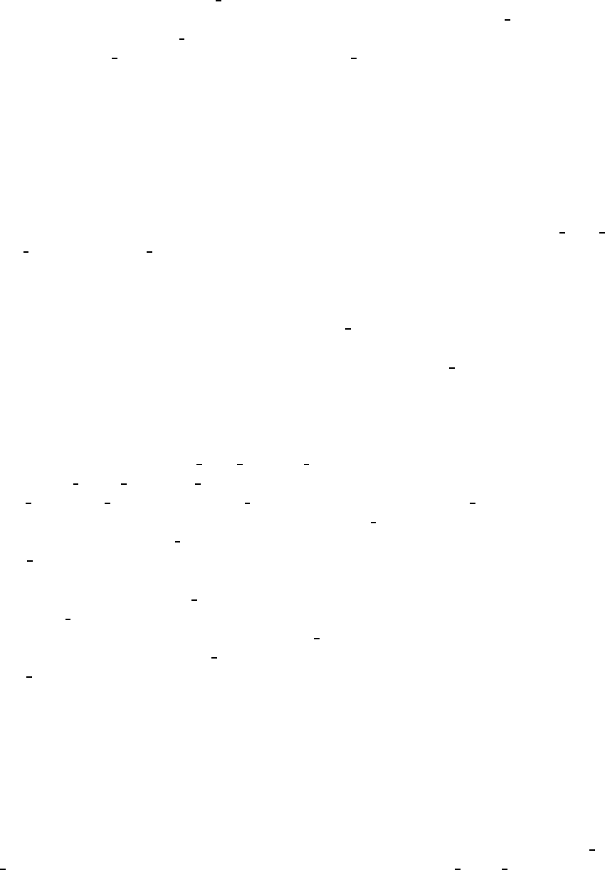
208
CHAPTER 16. GRIDS
tacks. Instead, module grids can be executed in a much simpler environment (without the
rest of MOM) by using script run grids. This is a simple UNIX C shell script which assumes
a Fortran 90 compiler. Although the script can be executed from the MOM 2 directory, it’s a
safer practice to use a MOM UPDATES directory for each experiment as described in Section
3.2. Copy both run grids and file grids.F into the MOM UPDATES directory, and make changes
to defined the grid there.
To define a grid, go to the USER INPUT section of module grids. After reading the infor-
mation in this chapter and looking at the examples given in module grids, implementing a grid
design should be straightforward. About the only potential problem might be that a particular
specification leads to a non-integral number of T cells within a region. Recall that the number
of T cells can be found by dividing the span of the region by the average resolution. Either the
position of the bounding coordinates or the resolution at these coordinates may be changed to
resolve the problem.
In the USER INPUT section, the bounding coordinates are specified by variables xlon,y lat,
and zdepth. Variable x lon is dimensioned by parameter nxlons which gives the number of
bounding longitudes to define one or more regions in longitude. Units are in degrees of longi-
tude measured at the equator and these points define the longitude of U grid points. Refer to
Figs 16.2, 16.3, and 16.4 which indicate U grid points on bounding coordinates with an integral
number of T cells inbetween. Similarly, variable y lat is dimensioned by parameter nylats
which gives the number of bounding latitudes to define one or more regions in latitude. These
coordinates mark the position on U points in latitude. Variable zdepth is dimensioned by
parameter nzdepths which gives the number of bounding depth coordinates to define one or
more regions in depth. Units are in cm and mark where the position of the bases of T and U
cells will be. Note that the bottoms of T and U cells define where the vertical velocity points
are located.
Associated with variables x lon,y lat, and z depth are variables which define the respective
resolution dx lon,dy lat, and dz depth of cells at the bounding coordinates. Units are in degrees
for dx lon and dy lat but in cm for dz depth. Note the variable stretch z provides additional
stretching for the last region in the vertical. When stretch z=1.0, there is no additional stretch-
ing. However, when stretch z>1.0 additional stretching is applied. To see how it works, set
stretch z=1.1 and gradually increase it. It can be used to approximate an exponential fall off
in the vertical.
When executed, script run grids creates a sub directory and compiles module grids using
option drive grids to activate a driver as the main program. After executing, results are copied
to a file in the directory from which script run grids was executed and the sub-directory is
eliminated. View the file results grids with an editor. When satisfied, copy size.h from the
MOM 2 directory and change the parameters according to the indicated directions. Any
component of MOM which accesses the updated module grids and size.h will get the new grid.
All components of MOM which use module grids and size.h perform a consistency check. If
there is an inconsistency, MOM will give an error message and stop.
16.3.1 Grids in two dimensions
When the grid system is contracted to a minimum along one dimension, MOM is essentially
reduced to a two dimensional model. For instance, if it is desirable to have a two dimensional
model that is a function of latitude φand depth z, then setting nxlons =2 and specifying dx lon1,
dx lon2such that there are two grid cells between bounding surfaces x lon1,x lon2will generate
imt =4 grid cells in the longitudinal direction. Two T cells i=2 and i=3 will be calculated
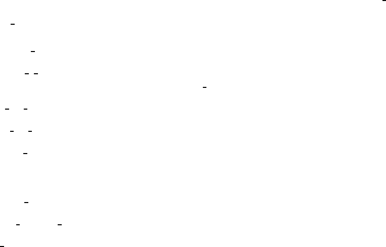
16.4. SUMMARY OF OPTIONS
209
and the two extra T cells i=1 and i=4 are for boundaries. Only one U cell, i=2, is not in the
boundary. If option cyclic is enabled, then the domain is zonally re-entrant. If the forcing and
initial conditions are independent of longitude λ, then the solution is independent of λand the
model is two dimensional in φand z. Obviously the relevance of this model depends on the
scientific question being posed. This is just to demonstrate how the longitudinal dimension
can be contracted to a minimum of imt =4 cells. The memory window should be opened to
jmw =jmt to make it as efficient as possible but this will not be as fast as the two dimensional
model in λand zdiscussed below because of the short vector lengths in longitude.
A similar contraction can be performed in the latitudinal direction to end up with a two
dimensional model in longitude λand depth z. Here again, the minimum number of latitudes
is jmt =4 with jrow =2 and jrow =3 being ocean T cells and jrow =1 and jrow =4 being land
cells. Note that there is only one latitude of ocean U cells. If these U cells are placed at the
equator (with the two ocean T cell latitudes placed symmetrically about the equator) and there
is no meridional variation in initial conditions or forcing, then the model is two dimensional
in λand z. Again, the scientific question being posed needs to be suited to this design. Note
that this type of model really flies computationally because of the long vectors in the longitude
dimension. The memory window should be opened to jmw =jmt to make it as efficient as
possible.
In the vertical, the minimum number of ocean levels is 2. Therefore the bounding surfaces
and resolutions can be set to yield km =2. Note that kmti,jrow <2 is not allowed.
16.4 Summary of options
The following options are used by module grids when executing in a stand alone mode. They
are enabled by compiling with options of the form -Doption1 -Doption1 . . . as in script run grids.
•drive grids turns on a small driver which allows the module grids to be executed in
a simple environment (stand alone). This is only used for designing grids with the
script run grids. It is not appropriate when executing MOM.
•generate a grid generates a grid based on specifications in the USER INPUT section of
module grids. It is used both in the script run grids and when executing MOM.
•read my grid allows grids developed elsewhere to be imported into MOM.
•write my grid writes a copy of the grid information to file grid.dta.out.
•centered tconstructs a grid using method 1 from Section 16.2.3. If not enabled, the grid
is constructed using method 2 from Section 16.2.3 which is different than the way it has
been constructed in previous versions of the model.
•isotropic grid constructs a square grid between two bounding latitudes.
•extend isotropic grid extends the isotropic grid to the poles using a nearly constant ∆y.
•bbl ag modifies the vertical grid to account for a bottom boundary layer.
•symmetry used when specifying a symmetry condition at the northern boundary of the
domain. Note that symmetry can only be specified when the northern part of the domain
is at the equator.
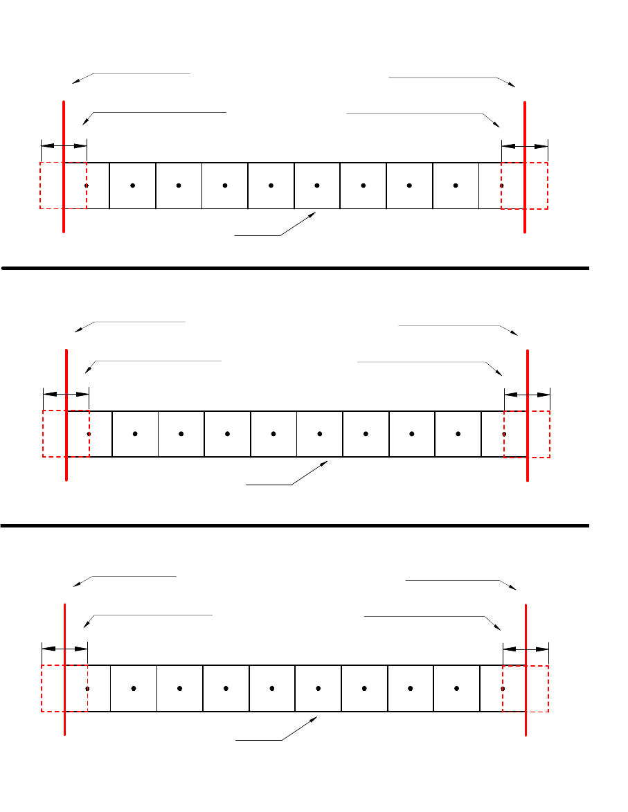
210
CHAPTER 16. GRIDS
Specifying a region of T cells bounded by two longitudes and resolutions.
a)
∆λ
1
0
0
0
∆λ
2
0
0
0
0
0
0
0
0
0
0
0
1
λ
λ
2
First bounding longitude
Resolution at bounding longitude
Specifying a region of T cells bounded by two latitudes and resolutions.
b)
1
ϕ
∆ϕ
1
ϕ
2
First bounding latitude
Resolution at bounding latitude
∆ϕ
2
Specifying a region of T cells bounded by two depths and resolutions.
c)
1
z
∆
1
z
2
First bounding depth
Resolution at bounding depth
Second bounding depth
Resolution at bounding longitude
Second bounding longitude
Second bounding latitude
Resolution at bounding latitude
z
Resolution at bounding depth
∆
z
2
T cells
T cells
T cells
RCP
Figure 16.1: a) A region bounded by two longitudes. b) A region bounded by two latitudes.
c) A region bounded by two depths.
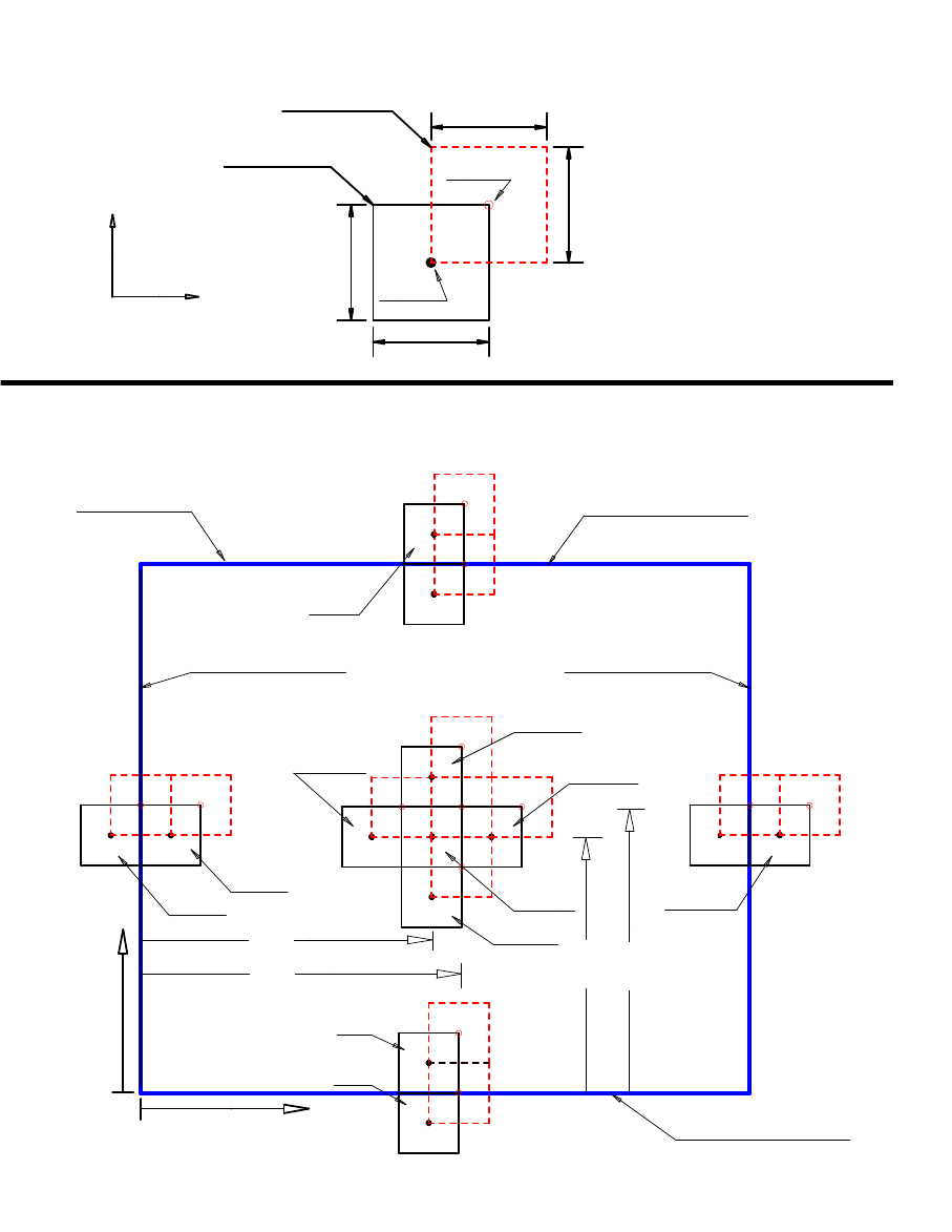
16.4. SUMMARY OF OPTIONS
211
yt
jrow
yu
jrow
xu
i
T
i,k,1
T
i,k,2
0
Latitude
ϕ
Latitude
ϕ
0
i,k,jrow
cell U
Horizontal Resolution of T and U cells
i
dyu jrow
jrow
dyt
dxt
i
i,k,jrow
dxu
cell T
xt
i
Longitude
λ
Northern boundary
Southern boundary
T
T
i,k,jrow-1
T
i,k,jrow
T
T
T
T
T
imt,k,jrow
T
Western boundary
Eastern boundary
a)
b)
Model domain with cells on a surface of constant depth
(index "i")
(index "jrow")
i,k,jrow+1
i+1,k,jrow
i-1,k,jrow
i,k,jmt
2,k,jrow
1,k,jrow
Longitude
λ
(index "i")
(index "jrow")
Domain
grid point
grid point
RCP
Figure 16.2: a) Horizontal resolution of grid cells. b) Grid cell arrangement on a longitude-
latitude surface of constant depth.
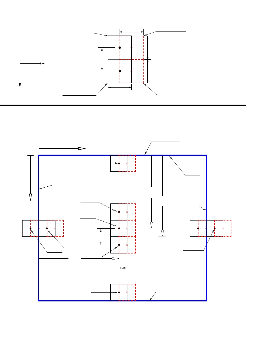
212
CHAPTER 16. GRIDS
xu
i
0
0
0
0
0
0.54
0
0
0
0
0
0
0
0
0
0.76
0
0
0
0
0
0
0
0
xt
i
T
T
b)
Model domain with cells on a surface of constant latitude
i,1,jrow
a)
Resolution of T and U cells in the longitude-depth plane
T
imt,k,jrow
T
1,k,jrow
2,k,jrow
Longitude
(index "i")
λ
(index "k")
Depth
T
i,km,jrow
zt
k
zw
k
dzw
k
Bottom
boundary
Eastern
boundary
Ocean
surface
Domain
Western
boundary
T
i,k,jrow
T
i,k-1,jrow
T
i,k+1,jrow
Depth
(index "k")
Longitude
(index "i")
λ
i
dzt
dxu
k
dxt
i
dzt
k+1
dzw
k
i,k,jrow
cell U
i,k,jrow
cell T
i,k+1,jrow
cell T
i,k+1,jrow
cell U
RCP
Figure 16.3: a) Vertical resolution of grid cells. b) Grid cell arrangement on a longitude-depth
surface of constant latitude.
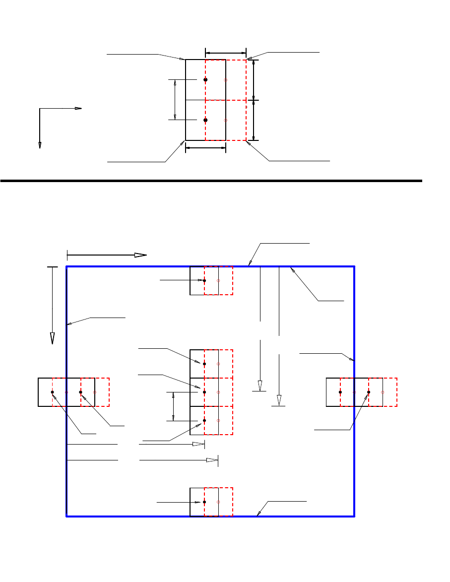
16.4. SUMMARY OF OPTIONS
213
xu
i
0
0
0
0
0.54
0
0
0
0
0
0
0
0.76
0
0
0
0
0
0
0
0
xt
i
T
T
b)
Model domain with cells on a surface of constant longitude
i,1,jrow
a)
Resolution of T and U cells in the latitude-depth plane
T
i,k,jmt
T
i,k,1
i,k,2
Latitude
(index "k")
Depth
T
i,km,jrow
zt
k
zw
k
dzw
k
Bottom
boundary
Northern
boundary
Ocean
surface
Domain
Southern
boundary
T
i,k,jrow
(index "jrow")
ϕ
T
i,k-1,jrow
T
i,k+1,jrow
Depth
(index "k")
Latitude
(index "jrow")
ϕ
dzt
k
dzt
k+1
dzw
k
i,k,jrow
cell U
i,k,jrow
cell T
i,k+1,jrow
cell T
i,k+1,jrow
cell U
jrow
dyu
jrow
dyt
RCP
Figure 16.4: a) Vertical resolution of grid cells. b) Grid cell arrangement on a latitude-depth
surface of constant longitude.
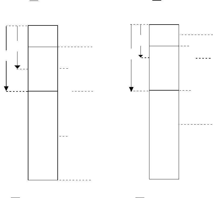
214
CHAPTER 16. GRIDS
Method 1
}
dztk
Tk+1
Tk
Tk-1
zwk
o
{
wk+1
wk-1
wk
ztk
{
dzwk
dzwk-1
Method 2
R.C.P.
Grid points within non-uniform grid cells
dztk = dzwk
z= (dzwk-1+dzwk)/2
}
}
dztk+1
dztk
Tk+1
Tk
Tk-1
o
dzwk
{
wk+1
wk-1
wk
ztk
zwk
T is not located on W T is located on W
z z
dzwk = dztk
z= (dztk+1+dztk)/2
Figure 16.5: Comparison of two grid cell construction methods applied in the vertical dimen-
sion. Method 2 is the default in MOM.

Chapter 17
Grid Rotation
This chapter was contributed by Michael Eby (eby@uvic.ca). A grid rotation is one of the
simplest types of grid transformations that can be applied to a spherically gridded model. This
transform is particularly useful for studies of high latitude oceans where the convergence of
lines of longitude may limit time steps or where the ocean contains a pole (as in the Arctic).
The idea is to define a new grid in which the area of interest is far from the grid poles. In
limited domain models, the pole can be rotated outside of the domain. For global models, one
possibility is rotate the North Pole to (40◦W,78◦N) which puts the North pole in Greenland
and keeps the South pole in Antarctica. Other uses include rotating the grid to match the angle
of a coastline or to provide more flexibility in specifying lateral boundary conditions.
Option rot grid modifies the Coriolis term to handle a rotated model grid which is specified
using three Euler angles for solid body rotation. The Euler angles are computed by defining the
geographic latitude and longitude of the rotated north pole and a point on the prime meridian
as described below.
To make this option easier to use, several rotation routines are provided within module ro-
tation.F. The driver may be used to help define the rotation, write a file of geographic latitudes
and test the rotation with idealized data. Other routines demonstrate how to interpolate scalar
and vector data from a geographically gridded data set, to a rotated model grid. To run the
driver, use the script run rotation.
17.1 Defining the rotation
Any spherical grid rotation can be specified by defining three solid body rotations. The angles
which define the rotations are usually referred to as Euler angles (see “Classical Mechanics” by
Goldstein, 1950 or a similar text). First, define the Z axis to be through the poles such that the
X-Y plane defines the equator and the X axis runs through the prime meridian. In the routines
(in rotation.F), the rotation angles are called phir,thetar and psir. The angle phir is defined as
a rotation about the original Z axis. Angle thetar is defined as a rotation about the new X axis
(after the first rotation) and angle phir is defined as a rotation about the final Z axis (see Figure
17.1).
It is helpful to have a globe to look at when thinking about this. Imagine that the globe has
a clear sphere surrounding it, with only grid lines of latitude and longitude. By moving the
outer sphere, the grid poles can be moved to line up with different points on the globe. Once
the new poles are located, two of the rotation angles can be defined as follows. The definition
for phir is 90 degrees minus the geographic longitude of the new north pole. This rotates the
215
216
CHAPTER 17. GRID ROTATION
Y axis under the new pole. To move the Z axis down, thetar is defined to be 90 degrees minus
the geographic latitude of the new north pole. This places the original Z axis though the new
north pole position.
To completely define the grid, a third rotation about the new Z axis, must be specified. The
rotated grid longitude of any point on the geographic grid is still undefined. To specify this last
rotation, choose a point on the geographic grid (the globe) to locate the rotated grid’s prime
meridian. Set angle psir to zero and calculate the longitude of this point on the rotated grid.
This longitude is the final angle psir, the angle needed to rotate the point back to the prime
meridian. The definition of psir is usually not very important since the new grid longitude is
arbitrary, but it does make a difference in defining exactly where the new grid starts. This may
be important if it is desirable to line up grids for nesting. Looking at Figure 17.1, it may appear
that all of the angle definitions are of the opposite sign to what they should be, but this comes
from thinking about rotating the axes rather than rotating the rigid body.
Generally, the idea is to move the poles so that they are 90 degrees away from the area of
interest. For example, to set up a model with an equatorial grid over the Arctic and North
Atlantic, the rotated grid north pole could be positioned at 0 N, 110 W and a prime meridian
point at 0 N, O E. This defines a grid rotation in which the new grid equator is along the 20
W and 160 E meridians. The rotated grid longitude is east, north of the geographic equator
and west to the south. On the rotated grid, North America is in the north and Europe in the
south, and the geographic north pole is at 0 N, 90 E. It is more difficult if you want to specify an
arbitrary grid rotation, but usually a few trials is enough to locate the necessary pole position.
Having defined the angles of rotation, an orthogonal transformation matrix can be written.
The first rotation through an angle Φabout the z axis (counterclockwise looking down the -z
direction) is given by
D=
cos Φsin Φ0
−sin Φcos Φ0
0 0 1
The second rotation through an angle Θabout the new x axis (counterclockwise looking down
the -x direction) is given by
C=
1 0 0
0 cos Θsin Θ
0−sin Θcos Θ
and the final rotation through an angle Ψabout the z axis (counterclockwise looking down the
-z direction) is given by
B=
cos Ψsin Ψ0
−sin Ψcos Ψ0
0 0 1
Note that the total rotation Acan be written as the product of the three rotations A=BCD
(ordering is important here).
A=
cos Ψcos Φ−cos Θsin Φsin Ψcos Ψsin Φ + cos Θcos Φsin Ψsin Ψsin Θ
−sin Ψcos Φ−cos Θsin Φcos Ψ−sin Ψsin Φ + cos Θcos Φcos Ψcos Ψsin Θ
sin Θsin Φ−sin Θcos Φcos Θ

17.2. ROTATING SCALARS AND VECTORS
217
Transforming points from the unrotated system to the rotated system (marked by primes)
is given as
x′
y′
z′
=A
x
y
z
(17.1)
and transforming points from the rotated system (marked by primes) to the unrotated system
is given as
x
y
z
=A−1
x′
y′
z′
(17.2)
where the inverse transform A−1is
A−1=
cos Ψcos Φ−cos Θsin Φsin Ψ−sin Ψcos Φ−cos Θsin Φcos Ψsin Θsin Φ
cos Ψsin Φ + cos Θcos Φsin Ψ−sin Ψsin Φ + cos Θcos Φcos Ψ−sin Θcos Φ
sin Θsin Ψsin Θcos Ψcos Θ
Note that the inverse transform A−1is really just Awith Ψand Φswitched and all rota-
tion angles made negative. In MOM, Equation (17.1) is used in routine “rotate” to produce
coordinates with respect to the rotated frame.
17.2 Rotating Scalars and Vectors
Code changes to mom are limited to modifying the calculation and dimension of the Coriolis
variable cori. Running the rotation driver will create the latitude data file needed to calculate
the correct Coriolis terms, but the creation of all other data files is left to the researcher. The
subroutine rot intrp sclr may be used to interpolate scalars (such as depths, surface tracers, etc.)
while subroutine rot intrp vctr can be used to interpolate and correct the angles for vectors (such
as wind stress).
17.3 Considerations
Although additional execution time used by this option is negligible,the option may complicate
subsequent analysis by the researcher. Rotated model results can be interpolated back to the
geographic grid for comparison, but this may involve recalculating many diagnostics (such
as zonal integrals) since all diagnostics within MOM are only computed on the rotated model
grid.
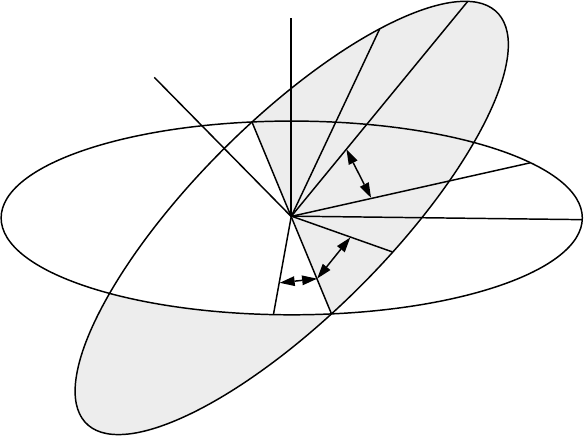
218
CHAPTER 17. GRID ROTATION
X0 X1
X2
X3
Y0
Y1
Y2
Y3
Z0
Z1
Z2
Z3
Φ
Ψ
θ
Figure 17.1: Euler solid body rotation angles and their associated axes for rotating the MOM
latitude and longitude grid.

Chapter 18
Topography and geometry
As described in Chapter 16, the model domain (as defined in module grids) is populated with
a horizontally rectangular arrangement of T-cells and U-cells arranged in an Arakawa B-grid
fashion and stacked vertically on top of each other. The vertical stacking is such that T-cells
overlay T-cells and U-cells overlay U-cells. In general, some of these grid cells will be treated as
land cells and others as ocean cells. Geometry and topography determine whether individual
cells are treated as land or ocean. This three dimensional land/ocean cell arrangement is
encapsulated in a two dimensional array of integers kmti,jrow (an example is given in Figure
18.1) which indicate the number of ocean cells stacked vertically between the surface and ocean
bottom for each longitude and latitude coordinate xtiand ytjrow on the T-grid. For instance,
the following settings
kmti,jrow =0 (18.1)
kmti+1,jrow =6 (18.2)
specify that there are no ocean cells1at coordinate location with index (i,jrow) but the location
immediately to the east has 6 ocean T-cells2. On the U grid, there is a corresponding field of
integers kmui,jrow derived as the minimum of the four surrounding kmti,jrow values.
kmui,jrow =min(kmti,jrow,kmti+1,jrow,kmti,jrow+1,kmti+1,jrow+1) (18.3)
Vertical levels are indexed from the uppermost at k=1 to the bottom of the domain at k=km.
Beneath the ocean surface, land cells exist where k>kmti,jrow on the T grid and where k>
kmui,jrowon the U grid. The depth from the ocean surface to the bottom of the ocean is defined
at the longitude and latitude of U-cells by
Hi,jrow =zwkbu where kbu =kmui,jrow (18.4)
where zwkis the depth from the ocean surface to the bottom face of the kth vertical level.
18.1 Designing topography and geometry
Although module topog is executed as part of MOM, designing kmti,jrow by executing MOM
is similar to using a sledge hammer to work with tacks. The preferred method is to do the
1All T-cells in the vertical at this location are treated as land cells.
2The cells below level 6 are treated as land cells.
219
220
CHAPTER 18. TOPOGRAPHY AND GEOMETRY
construction by executing script run topog from a MOM UPDATES directory as described for
module grids in Section 16.3. Put script run topog in the MOM UPDATES directory and it will
execute module topog in a stand alone mode by enabling option drive topog. The execution will
produce a file results topog which should be inspected. Once topography and geometry are
judged as satisfactory, module topog along with the resulting topography and geometry are
available to MOM during model executions. This is done by not including the option drive topog
in the list of options within the run mom script.
18.2 Options for constructing the KMT field
Various ocean depth construction methods may be selected for use within MOM by enabeling
options described below. Before being used, realistically derived depth fields must first be
interpolated to the latitude and longitude coordinates for the domain defined by module grids.
After the interpolation, ocean depth within the model is approximated as the nearest number
of discrete vertical levels that comes closest to matching the interpolated ocean depth field. If
option partial cell is enabled, the deepest ocean cells have variable depth so the model ocean
depth matches the interpolated ocean depth exactly. Refer to Chapter 26 for a discussion of
partial cells. The resulting field of model levels is the base kmti,jrow field defined at all latitude
and longitude coordinates given by (xti,ytjrow). One (and only one) of the following options
for selecting the various forms of ocean depth fields must be enabled:
•rectangular box constructs a flat bottomed rectangular box with kmti,jrow =km (deepest
level) for all interior points on the grid (i=2,imt −1 and jrow =2,jmt −1) while setting
kmti,jrow =0 on all boundary cells. Enabling option cyclic turns the box into a zonally
re-entrant channel by re-setting
kmt1,jrow =kmtimt−1,jrow (18.5)
kmtimt,jrow =kmt2,jrow (18.6)
for jrow =1,jmt.
•idealized kmt constructs an idealized version of the earth’s geometry. Continental features
are very coarse3but map onto whatever grid resolution is specified by module grids.
They are built with the aid of subroutine setkmt which approximates continental shapes
by filling in trapezoidal areas of kmti,jrow with zero. Subroutine setkmt readily allows
idealized geometries to be constructed. All that is required for input are the grid point
coordinates, the coordinates of four vertices of a trapezoid, and a value for setting kmti,jrow
within the trapezoid. The bottom topography has a sinusoidal variation which is totally
unrealistic. It is intended only to provide a test for the numerics in MOM. Since this
option generates geometry and topography internally, no external data is required and
therefore the DATABASE (explained in Chapter 3) is not needed. Typically, this option
is useful when researching idealized geometries and topographies since arbitrary ones
can be easily constructed. Also, this is useful when porting MOM to other computer
platforms since no data files need be considered.
3Their scale is about 10 degrees in latitude and longitude.
18.2. OPTIONS FOR CONSTRUCTING THE KMT FIELD
221
•gaussian kmt constructs a kmti,jrow field derived from an analytical gaussian bump super-
imposed on a sloping ocean floor in a rectangular basin without geometry. The intent of
this option is to provide a basis for regional idealized studies. The slope of the floor and
scale of the bump can be set by modifying the USER INPUT section under the gaussian
bump section in module topog.F. Further code modifications can easily turn the bump
into a bowl or depression in the ocean floor if desired. This option requires no data and
is therefore also highly portable. Results are interpolated to the resolution specified by
module grids. The ocean bottom depth hti,jrow is specified as
hti,jrow =zwkm −b0·exp−((xti−xuimt/2)2+(ytjrow −yujmt/2)2)/b2
1)
−slope x·(xti−xu1)−slope y ·(ytjrow −yu1) (18.7)
where
b0=zwkm/2 (18.8)
b1=0.25 ·min(xtimt−1−xt2,ytjmt−1−yt2) (18.9)
slope x =10 meter/deg (18.10)
slope y=10 meter/deg (18.11)
and hti,jrow is discretized to the nearest model level to construct the kmti,jrow field.
•scripps kmt reads the scripps.top 1◦x 1◦topography file (from the MOM DATABASE
explained in Chapter 3) and interpolates to kmti,jrow for the grid defined by module grids.
Subroutine scripp within module topog makes an educated guess as to whether resolution
specified by module grids is coarser or finer than the native Scripps resolution. If finer, it
does a linear interpolation from Scripps data, otherwise it uses area averaging of Scripps
data to estimate the value of kmti,jrow for the resolution required by module grids.
•etopo kmt reads the file ETOPO5.NGDCunformat ieee which is a 1/12◦x 1/12◦topogra-
phy dataset. The dataset may be purchased from the Marine Geology and Geophysics
Division of the National Geophysical Data Center and is not included in the MOM
DATABASE. Depths are interpolated to a kmti,jrow field for the grid defined by mod-
ule grids. Subroutine etopo within module topog does the interpolation. If model reso-
lution is finer than 1/12◦, a linear interpolation from the dataset is used, otherwise area
averaging over the dataset is used to estimate the value of kmti,jrow for the resolution
required by module grids.
•read my kmt allows importing kmti,jrow fields into MOM which have been exported from
module topog using option write my kmt. One purpose of importing is to provide a hook
for reading kmti,jrow fields which have been constructed outside the MOM environment.
Another is to allow direct editing of the kmti,jrow field using a text editor as explained in
Section 18.4.2. Still another use is when working with gigantic datasets like the 1/12◦
ETOPO5. Bringing these gigantic datasets into a model run simply to compute a kmti,jrow
field can adversely affect model turn around time. Expecially when trying a new model
setup which requires multiple attempts to get problems resolved. It is better to export the
resulting kmti,jrow field from a stand alone execution of module topog. Then just import
kmti,jrow into a model execution instead of the huge dataset.

222
CHAPTER 18. TOPOGRAPHY AND GEOMETRY
Note that the kmti,jrow field only needs to be constructed or imported into the model once
at initial condition time. After that, it is incorporated as part of the restart file restart.dta.
Regardless of how kmti,jrow is generated, module topog produces a checksum which can be
used to verify that the kmti,jrow field produced by script run topog is the one being used by
MOM.
18.3 Meta land masses
Figure 18.1 is an example of a base kmti,jrow field. Note the cell pointed to by the “perimeter
violation” arrow. When using option stream function, it is incorrect4to have two distinct land
masses seperated by a minimum of only one ocean T-cell. The reason is that if these two land
masses are to remain unconnected, then the value of the stream function at the cell in question
can be multivalued: one stream function value is implied by the integral of the pressure
gradients around one land mass and the other is implied by the integral around the other land
mass. But, since all four surrounding U-cells of the offending “perimeter violation” cell are
land cells, no flow can exist between the land masses. So the integrals are not independent
after all. The way to think of this is that the two seperate land masses are components of a
“meta ” land mass where all components are treated as a single mass. This is achieved by
modifying the path of the island perimeters of the land masses so that the “meta” land mass
has only one perimeter. Therefore “perimeter violation” cells are no longer a problem. They
are automatically accounted for by constructing “meta” land masses. If desired, the “perimeter
violation” cells can always be changed to land cells.
The difference between filling the “perimeter violation” cell in with land and leaving it
as part of a “meta” land mass is that if the cell is made into land, then tracers cannot be
diffused across it. However, as part of a “meta” land mass, two lateral faces of the “perimeter
violation” cell connect with other ocean cells and diffusion of tracer quantities can occur.
Therefore, if “perimeter violation” cells are left as an ocean cells, two ocean basins which
cannot communicate advectively may still be able to communicate diffusively.
18.4 Modifications to KMT
The base kmti,jrow field constructed above may have problem cells as illustrated in Figure 18.1.
These include minimum depth violations and potentially troublesome areas such as isolated
cells. Or possibly, the researcher may wish to modify the kmti,jrow field by changing ocean cells
to land cells or visa versa for various reasons.
18.4.1 Altering the code
Changes can be made by hard wiring kmti,jrow to specific values in the USER INPUT section of
module topog. For example
kmt37,82 =0 (18.12)
sets all T-cells at location given by indices (i,jrow)=(37,82) from k=1to km to land cells.
Setting large areas of kmti,jrow to land or ocean cells may be handled using routine setkmt as
4This is not a restriction for the rigid lid surface pressure option, the implicit free surface option, or the explicit
free surface option because they do not perform island integrals.
18.5. TOPOGRAPHIC INSTABILITY
223
is done when generating the idealized dataset. Note that idealized geometries are readily
constructed by blocking out areas of kmti,jrow with the aid of subroutine setkmt. Refer to
option idealized kmt in Section 18.2 for usage. The two problems mentioned above are remedied
automatically using guidance given in the form of options. Those options are:
•If option fill isolated cells is enabled, isolated T-cells are made into land cells. Isolated
T-cells are deeper than nearest neighbor T-cells. Think of them as potholes or one cell
wide trenches in the topography. They cannot communicate with horizontal neighbors
through advection because all surrounding velocities are zero.
A sub-option of fill isolated cells is fill isolated dont change landmask which restores any
kmti,jrow which was set to zero in the process of filling cells. Using this sub-option allows
the land/sea areas to be preserved when filling isolated cells.
•Limit the minimum number of vertical levels in the ocean to parameter kmt min =2. This
parameter may be increased but not decreased. There is some choice for altering kmti,jrow
to meet this condition. The choice is made by enabling one of the following options:
–fill shallow makes land cells where there are fewer than kmt min vertical levels
–deepen shallow sets kmti,jrow =kmt min where there are fewer than kmt min vertical
levels
–round shallow sets kmti,jrow to either 0 or kmt min depending on which is closest
18.4.2 Directly editing the KMT field
Another way to change kmti,jrow is to export the field using option write my kmt which saves
kmti,jrow to file kmt.dta under formatted control. Formatting is determined by the model’s
deepest level. File kmt.dta can then be edited with any text editor. Care must be exercised
when editing so as not to change the format. If a character is deleted, a space or another
character must be inserted in its place. When finished, the kmti,jrow field can then be imported
with option read my kmt.
18.5 Topographic instability
When using option stream function, it sometimes happens that steep topographic gradients as
described in Killworth (1987) are a source of problems. Essentially, a restriction on the external
mode time step dts f is given by the condition
dts f <∆τ(18.13)
where
∆τ=
(dxticos φT
jrow)2
Am·(8 h1h2)/(h1+h2)2+(dxticos φT
jrow)2/(dytjrow)2
4+(dxticos φT
jrow)2/(dytjrow)2(18.14)
h1=zwk1(18.15)
h2=zwk2(18.16)
k1=kmui+1,jrow−1(18.17)
k2=kmui+1,jrow (18.18)
224
CHAPTER 18. TOPOGRAPHY AND GEOMETRY
The above condition on time step ∆τmust be met at each point with index (i,jrow) within the
domain. Since analysis requires knowledge of time step length and mixing coefficients, the
above time step restriction is not detected in module topog. Rather, detection is left to MOM
where all the information is known. Notably, the above condition is most restrictive in polar
regions where convergence of meridians makes the effective zonal grid length dxticos φT
jrow go
toward zero. The time step restriction can be ameliorated by making the mixing coefficient a
function of latitude to compensate for the convergence of meridians. For using variable mixing
coefficients, refer to Sections 34.6 and 34.6.2.
Locally smoothing the topography can also help by lessening topographic gradients in
the meridional direction and thereby increasing the factor (8 h1h2)/(h1+h2)2. This can be
accomplished with option smooth topo. When enabled, the smoothing is applied northward
of a specified latitude by successively applying a 2D5finite impulse response symmetric filter
where 1D weights are given by (1/4, 1/2, 1/4). Additional conditions are applied to insure
that the original coastline is not changed6and topographic depths can only by decreased7
by applying this filter. When option smooth topo is enabled, latitudes northward of 85N are
filtered by 10 passes of this filter. To change the smoothing latitude or the number of passes
(both are arbitrary), look at the USER INPUT section of topog.F under the options scripps kmt
and etopo kmt.
In the test case resolution with Scripps topography, options varhmix and am cosine along
with the above mentioned topographic filter will eliminate the Killworth time step restriction.
Another alternative is to change the external mode solution technique from option stream function
to option implicit free surface.
18.6 Viewing results
The recommended way of viewing the resulting topography, kmti,jrow field, and f/Hfield is to
save these results using option topog diagnostic. This is described in Section 40.20. A good way
to visualize results is with Ferret which is a graphical analysis tool developed by Steve Hankin
(1994) at NOAA/PMEL (email: ferret@pmel.noaa.gov URL: http://www.pmel.noaa.gov/ferret/home.html).
As an alternative, a map of the resulting kmti,jrow field is printed out as as part of the re-
sults topog file from executing module topog. It is also possible to export the kmti,jrow field and
use an editor to view file kmt.dta.
18.7 Summary of options for topography
The following is a list of options used within the topography module. They are in no particular
order.
•topog diagnostic. Saves out topography and related fields in NetCDF or IEEE format for
analysis.
•drive topog. To execute module topog in a stand alone mode rather from within a model
execution.
5Although the application of a 1D filter in the meridional direction will remove the topographic slopes, the 1D
smoothing can introduce bizzare effects due to shallow water near coastlines. The 2D filter works best.
6The coastline is made invisible to the filter.
7Allowing the filter to incrase the depths requires realistic initial density profiles to be known below the realistic
bottom. Therefore, the filter is restriced so that it can only shallow the bottom.
18.7. SUMMARY OF OPTIONS FOR TOPOGRAPHY
225
•scripps kmt. Builds a kmti,jrow field from Scripps 1 degree topography data.
•etopo kmt. Builds a kmti,jrow field from Etopo 1/12 degree topography data.
•smooth topo. Smooths the interpolated topography from Etopo 1/12 degree or Scripps 1
degree datasets to help eliminate the Killworth Instability (Section 18.5). Such smoothing
is also useful for removing grid scale power in the topography field. Note, however, that
option smooth topo will not allow for grid points to be deepened. To allow deepening,
one must also turn on option smooth topo allow deepening.
•smooth topo allow deepening. When enabled with smooth topo, this option will smooth the
topography and will allow for this smoothing to deepen grid cells. The topography from
both smooth topo and smooth topo allow deepening is somewhat smoother than the topog-
raphy using only smooth topo. It should be noted that if using Levitus initial conditions,
the values used in the deepened grid points will need to be computed through an extrap-
olation procedure described in Section 28.1.4. Errors can arise from this extrapolation
and so one should be aware of this issue when using the deepening option.
•smooth topog after user changes. This option is useful for those cases in which the re-
searcher changes the land mask by adding or removing land points, but still wants to
maintain a smooth topography to avoid numerical problems.
•rectangular box. Builds a kmti,jrow field for a flat bottomed rectangular box.
•idealized kmt. Builds a kmti,jrow field based on a highly idealized (not very accurate) ge-
ometry. Topography is un-realistic. It is useful for porting MOM to various architectures
without having to worry about datasets. It can be easily modified for other idealized
studies.
•gaussian kmt. Builds the kmti,jrow based on a gaussian bump on a sloping ocean floor in a
rectangular domain. It is highly portable and can be easily modified for other idealized
studies.
•flat bottom. Resets the bottom within the ocean to the deepest level regardless of which
method was used to construct the kmti,jrow field.
•partial cell. Allows bottom cells to be of variable thickness within the same vertical level.
•bbl ag. Allows for a bottom boundary layer.
•rough mixing. Calculates the bottom roughness by examining the curvature of the Etopo
1/12 degree dataset. If option etopo kmt is not used, then the roughness is set to zero.
•read unformatted kmt. Imports kmti,jrow from older kmt.dta files saved without format
control.
•read my kmt. Imports kmti,jrow from file kmt.dta under format control.
•write my kmt. Exports kmti,jrow fo file kmt.dta under format control.
•read my roughness. Imports a roughness field from file rough.dta (unformatted).
•write my roughness. Exports a roughness field from file rough.dta (unformatted).
226
CHAPTER 18. TOPOGRAPHY AND GEOMETRY
•solid walls. Land boundaries along the northern, southern, eastern, and western limits
of the domain.
•cyclic. Land boundaries along the northern and southern limits of the domain. However,
what flows out of the eastern boundary enters through the western boundary and visa
versa.
•fill shallow. Fills ocean cells with land where the bottom is less than the specified
minimum number of vertical levels.
•round shallow. Where the bottom is less than the specified minimum number of vertical
levels, the bottom is rounded to either zero depth or the minimum number of vertical
levels.
•deepen shallow. Where the bottom is less than the specified minimum number of vertical
levels, the bottom is deepened to the minimum number of vertical levels.
•fill isolated cells. Fills one cell wide potholes and trenches with land.
•fill isolated dont change landmask does not allow the land/sea mask to change when filling
isolated cells.
•skip island map. To eliminate land mass map indicating island perimeters.
•skip perimeter details. To eliminate listing the land mass perimeter points.
•skip kmt map. To eliminate printing the map of kmt.
•skip translation details. Interpolating data near the prime meridian is a problem for the
interpolation routines because the longitude is not monotonic. Basically, it is difficult
for the interpolation routines to decide in general if an error was made in specifying
longitudes or not. So the topography data is translated in longitude to move the prime
meridian so that longitudes defining real data are monotonic within the model domain.
Normally, the original and translated longitudes are printed out. Use this option to
eliminate the printing.
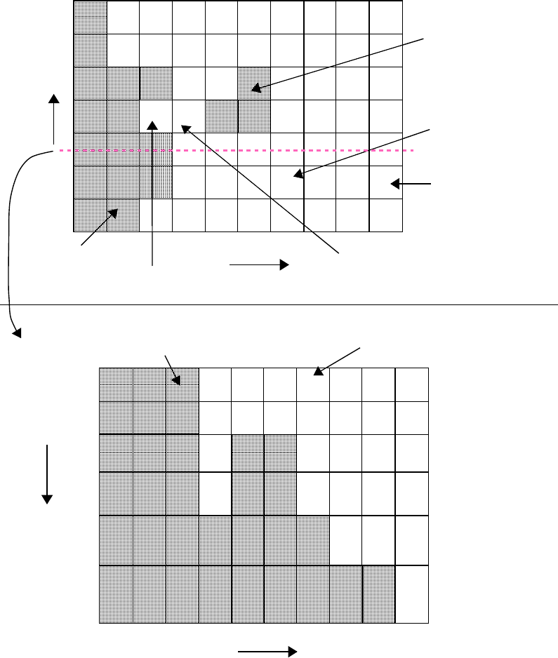
18.7. SUMMARY OF OPTIONS FOR TOPOGRAPHY
227
0 2 2 3 4 4 4 5 6 9
0 3 2 3 4 3 3 6 7 8
0 0 0 2 2 0 4 4 5 4
0 0 4 5 0 0 3 3 4 5
0 0 0 4 2 2 4 5 5 6
0 0 0 2 3 5 8 5 9 1
0 0 2 2 2 4 6 6 9 9
Perimeter violation
Land cell
Pothole
Island
jrow
kmti,jrow
minimum depth
violation
a)
b)
i
i
1
2
3
4
5
6
k
Ocean cells
Land cells
non-advective cell
Figure 18.1: a) A portion of the kmt field indicating ocean and land areas with potential
problems. b) Topography along the slice indicated in a)
228
CHAPTER 18. TOPOGRAPHY AND GEOMETRY

Part V
Boundary Conditions
229

Chapter 19
Generalized Surface Boundary
Condition Interface
The ocean is driven by surface boundary conditions1which come from the atmosphere and the
atmosphere is in turn driven by surface boundary conditions2which come from the ocean. The
difficulty in understanding the coupled system is that each component influences the other.
For purposes of MOM, the atmosphere may be thought of as a hierarchy of models ranging
from a simple idealized wind dataset fixed in time through a complicated atmospheric GCM3.
Regardless of which is used, MOM is structured to accommodate both extremes as well as
atmospheres of intermediate complexity as discussed in the following sections.
19.1 Coupling to atmospheric models
In this section, the general case will be considered where the atmosphere is assumed to be a
GCM with domain and resolution differing from that of MOM and two-way coupling between
MOM and the atmosphere model will be allowed. Option coupled configures MOM for this
general case and the test case prototype is described in Sections 3.2 and 3.3 as CASE=3.
A flowchart of driver4is given in Figure 19.2. It begins by calling subroutine setocn5to
perform initializations for mom6. Included in the list are such things as initializing variables,
reading namelists to over-ride defaults, setting up the grid, topography, initial conditions,
region masks, etc. In short, everything that needs to be done only once per model execution.
Following this, a call is made to subroutine setatm7which completes whatever setup is required
by atmos8.
At this point, the integration is ready to begin. Integration time is divided into a number
of equal length time segments9which determine the coupling period. In practice, this interval
1Wind, rain, heatflux, etc.
2Primarily SST.
3General circulation model.
4Contained within file driver.F. This is the main program for MOM.
5Contained within file setocn.F.
6Contained within file mom.F. This is the subroutine that does the time integration for the ocean model.
7Contained within file setatm.F in the MOM 2/SBC directories.
8Contained within file atmos.F in the SBC directories. This is the subroutine that does the time integration for
the atmosphere model.
9The length of one time segment should be divisible by the length on one ocean time step to allow an integral
number of calls to subroutine mom. The same holds true for the atmosphere time step.
231
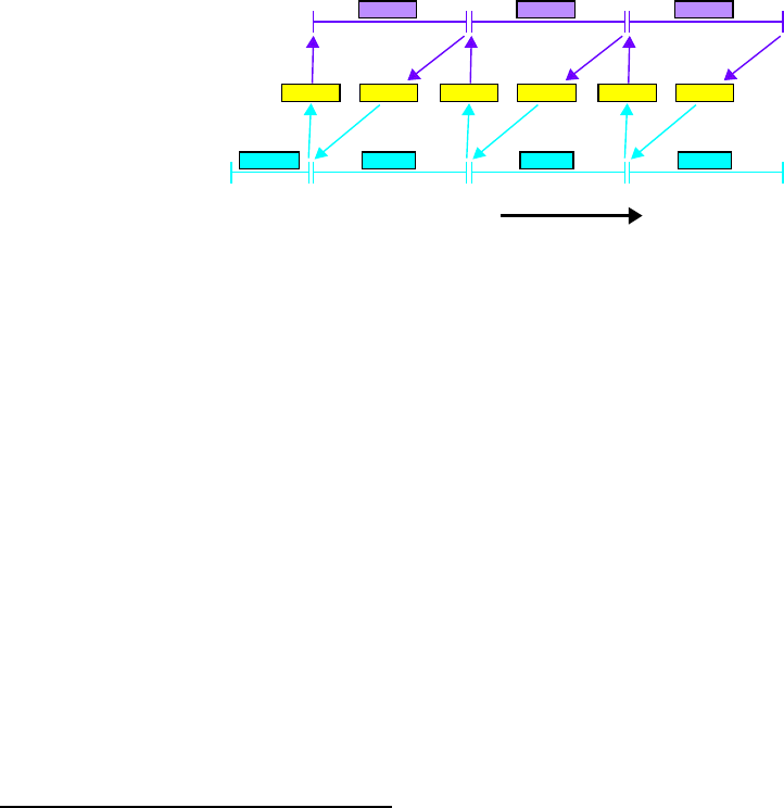
232
CHAPTER 19. GENERALIZED SURFACE BOUNDARY CONDITION INTERFACE
should always be chosen short enough to adequately resolve time scales of coupled interac-
tion. Typically this value would be one day10. Within the segment loop, atmos and mom are
alternately integrated for each time segment while holding surface boundary conditions fixed.
Note that this may require multiple calls to each model. In Figure 19.2, the loop variable ntspas
stands for the number of time steps per atmosphere segment and the loop variable ntspos stands
for the number of time steps per ocean segment. Products of each atmosphere segment include
surface boundary conditions11 for the ocean averaged over that segment. These are held fixed
and applied to mom while it integrates over the same segment. Products of integrating mom
include surface boundary conditions for the atmosphere which are also averaged over this
segment. Subsequently, they are held fixed and applied to atmos on the following segment.
This process is represented schematically as a function of time in Figure 19.1 and continues
until all time segments are completed. Using asynchronous time segments12 is possible with a
small code modification but this is left to the researcher.
SETOCN
ATMOS
MOM
GASBC GOSBC
ATMOS
MOM
GASBC GOSBC
ATMOS
MOM
GASBC GOSBC
time segment 1 time segment 2 time segment 3
Time
Figure 19.1: Schematic of two way coupling between an atmosphere model (ATMOS) and an
ocean model (MOM) showing time segments.
In MOM and in the descriptions that follow, index jrefers to any variable dimensioned by
the number of rows in the memory window and index jrow refers to any variable dimensioned
by the total number of latitude rows. They are related by an offset jrow =j+joffwhich indicates
how far the memory window has moved northward. Refer to Section 14.2 and also 11.3.2 for
a more complete description.
19.1.1 GASBC
Getting surface boundary conditions for the atmosphere model defined on the atmosphere grid
is the purpose of subroutine gasbc13 which is an acronym for get atmosphere surface boundary
conditions. All of the surface boundary conditions are two dimensional fields defined in
longitude and latitude at model grid points. In the ocean, all quantities which are to be
used as surface boundary conditions for the atmosphere are defined on the Ti,jgrid14 in array
10If the diurnal cycle is included, the coupling period needs to be reduced to allow adequately resolution in time.
11The first set of surface boundary conditions for the atmosphere are products of setocn.
12Where, for example, an ocean segment is much longer than an atmosphere segment. This assumes the coupled
system is linear with one equilibrium. Exercise caution if contemplating this!
13Contained in file gasbc.F.
14At grid locations given by xtiand ytjrow.

19.1. COUPLING TO ATMOSPHERIC MODELS
233
sbcocni,jrow,mwhere subscript mrefers to the ordering described in Section 19.3. Typically,
only SST is needed but it may be desirable to let the atmosphere sense that the ocean surface
is moving in which case the horizontal velocity components might also be used (Pacanowski
1987). In any event, these quantities are accumulated in sbcocni,jrow,mwithin MOM and averaged
at the end of each time segment. Basically what needs to be done in gasbc is to interpolate the
time averaged sbcocni,jrow,mfields to sbcatmi′,j′,mwhich is an array of the same surface boundary
conditions except defined on the atmosphere boundary condition grid15 Ai′,j′. One of the
duties of setatm is to define Ai′,j′as the atmospheric boundary condition grid which includes
extra boundary points along the borders to facilitate these interpolations.
19.1.1.1 SST outside Ocean domain
There is a complication if the ocean is of limited extent: SST must be prescribed outside
the ocean domain as a surface boundary condition for the atmosphere on the Ai′,j′grid. To
accommodate this, the ocean domain Ti,jmust be known in terms of Ai′,j′and a buffer or
blending zone must be established. Within this zone, SST from mom is blended with the
prescribed SST outside the ocean domain as indicated in Figure 19.3. As a simplification,
SST is prescribed outside the domain of mom as a constant which is obviously unrealistic and
should be prescribed by the researcher as a function of space and time appropriately along
with the width of the blending zone. SST within the blending zone is a linear interpolation
between the two regions.
19.1.1.2 Interpolations to atmos grid
Each surface boundary condition is interpolated one at a time using essentially the following
steps:
•For limited ocean domains, prescribe SST in sbcatmi′,j′outside the mom domain as de-
scribed above. When ocean and atmosphere domains match, this is not necessary.
•Extrapolate sbcocni,jrow,minto land areas on the mom grid. This is done by solving
∇2(SSTi,jrow)=0 over land cells using ocean SSTi,jrowas boundary conditions16. The
idea is to get reasonable SSTi,jrowin land adjacent to coastlines but not necessarily to pro-
duce accurate SSTi,jrowin the middle of continents. Where land and ocean areas on the
ocean and atmosphere grids are mismatched, this extrapolation will ameliorate the sens-
ing of erroneous SSTi,jrowby the atmosphere. Such situations are common when coupling
spectral atmospheres to MOM which has an Arakawa B-grid.
•Interpolate sbcocni,jrow,mto sbcatmi′,j′,m. The ocean resolution is typically higher than that
of the atmosphere because the Rossby radius is larger in the atmosphere. To prevent
aliasing, the interpolation is an area average of sbcocni,jrow,mfor those ijcells which fall
within each Ai′,j′grid cell17. The interpolation is carried out using subroutine ftc18 which
15Grid locations given by abcgxi′and abcgyj′.
16This method is arbitrary. However, when solving this equation iteratively, it is important not to zero out SST
from previous solutions over land areas. Their purpose is to act as a good initial guess to limit the iterations needed
for subsequent solutions.
17Partial ocean cells are accounted for to conserve the interpolated value.
18Acronym for fine to coarse resolution. It is an interpolation utility in module util.

234
CHAPTER 19. GENERALIZED SURFACE BOUNDARY CONDITION INTERFACE
can easily be replaced by subroutine ctf 19 (or something else) if ocean resolution is less
than atmosphere resolution.
•Set cyclic conditions on sbcatmi′,j′,mand convert to units expected by the atmosphere.
•Compute global mean of sbcatmi′,j′,m
The structure of gasbc is arranged such that components can be removed or replaced with more
appropriate ones if desired.
Caveat
In the process of constructing sbcatmi′,j′,mno attempt has been made at removing small scale
spatial features from the grid which could potentially be a source of noise for the atmosphere
model.
19.1.2 GOSBC
Getting surface boundary conditions for the ocean model defined on the grid of mom is the
purpose of subroutine gosbc20 which is an acronym for get ocean surface boundary conditions .
This is the counterpart of gasbc. All of the surface boundary conditions are two dimensional
fields as described in Section 19.1.1. In the atmosphere, all quantities which are to be used
as surface boundary conditions for MOM are defined on the Ai′,j′grid in array sbcatmi′,j′,m
where subscript magain refers to the ordering described in Section 19.3. Typically, they are
quantities like windstress components, heatflux and precipitation minus evaporation. These
must be accumulated in sbcatmi′,j′,mwithin the atmosphere model and averaged at the end of
each time segment. Basically what needs to be done in gosbc is to interpolate the time averaged
sbcatmi′,j′,mto sbcocni,jrow,mwhich is defined on the ocean grid.
19.1.2.1 Interpolations to ocean grid
Unlike in Section 19.1.1, there are no complications since the ocean domain is assumed to be
contained within the atmosphere domain as shown in Figure 19.4. Each surface boundary
condition is interpolated one at a time with the essential steps being:
•Set cyclic conditions of sbcatmi′,j′,m. This assumes a global atmosphere domain.
•Extrapolate sbcatmi′,j′,minto land areas on the atmosphere grid. This is done as in Section
19.1.1 by solving ∇2ξi′,j′=0 over land areas using values of ξi′,j′over non-land areas as
boundaries where ξi′,j′represents windstress components, heatflux, etc21. The idea, as on
the ocean grid, is to get reasonable ξi′,j′adjacent to coastlines while not trying to produce
accurate ξi′,j′in the middle of continents. Where land and ocean areas on the ocean and
atmosphere grids are mismatched, this will ameliorate the sensing of erroneous ξi′,j′by
the ocean.
19Acronym for coarse to fine resolution. It is an interpolation utility in module util.
20Contained within file gosbc.F.
21This method is arbitrary. However, when solving this equation iteratively, it is important not to zero out ξfrom
previous solutions over land areas. Their purpose is to act as a good initial guess to limit the iterations needed for
subsequent solutions.

19.2. COUPLING TO DATASETS
235
•Interpolate sbcatmi′,j′,mto sbcocni,jrow,m. Since ocean resolution is typically higher than
that of the atmosphere due to the difference in Rossby radius scales, the interpolation
is linear. The interpolation is carried out using subroutine ctf from file util.F. Note that
linear interpolation does not exactly conserve the quantity being interpolated. However,
linear interpolation has been used without causing noticable drift in coupled integrations
(without flux correction) of up to 20 years at GFDL.
For integrations simulating thousands of years, linear interpolation may not be good
enough. To conserve fluxes exactly, one possibility (although drastic) is to design the
grids such that an integral number of ocean cells overlay each atmospheric grid cell.
Then the quantity to be interpolated can simply be broadcast from each atmospheric cell
to all underlying ocean cells. However, this is really not necessary. Assume that the
value of the quantity being interpolated is constant over the entire atmospheric grid cell.
For exact conservation, the value in each ocean cell is just an integral of the atmospheric
quantity over the area of the ocean cell. It would be a matter of writing a subroutine to
do it and substituting this subroutine for the call to ctf.
•Set cyclic conditions on sbcocni,jrow,mand convert to units expected by the ocean. MOM
expects units of cgs.
•Compute global mean of sbcocni,jrow,m
Caveat
In the process of constructing sbcocni,jrow,mno attempt has been made at removing small scale
spatial features from the grid which could potentially be a source of noise for the ocean model.
19.2 Coupling to datasets
In Section 19.1, the general case of two way coupling to an atmospheric GCM was considered.
It is also useful to drive mom with atmospheric datasets representing simpler idealized atmo-
spheres. One problem with doing this is that datasets act as infinite reservoirs of heat capable
of masking shortcomings in parameterizations which only become apparent when two way
coupling is allowed. Nevertheless, driving ocean models with surface boundary conditions
derived from datasets is useful.
These datasets can be thought of as simple atmospheres prepared a priori such that data
is defined at grid locations expected by mom for surface boundary conditions. All spatial
interpolations are done beforehand, as described in Section 3.2. In this case, subroutines gasbc
and goabc are bypassed because spatial interpolation to the mom grid is not needed. Also, the
length of a time segment reduces to the length of one ocean time step. In general, the datasets
contain either time mean conditions or time varying conditions and there are three options
which configure these types of surface boundary conditions for mom:
•simple sbc allows for the simplest of atmospheric datasets. All surface boundary condi-
tions are a function only of latitude. No time dependence here although it could easily
be incorporated. The test case prototype is described in Sections 3.2 and 3.3 as CASE=0.
In this case, there is no dataset on disk and sbcocni,jrow,mis not needed since all surface
boundary conditions are generated internally. This is an appropriate option for building
forcing functions for idealized surface boundary conditions .
236
CHAPTER 19. GENERALIZED SURFACE BOUNDARY CONDITION INTERFACE
•time mean sbc data uses an atmosphere dataset defined in SBC/TIME MEAN. The test
case prototype is described in Sections 3.2 and 3.3 as CASE=1. The dataset resides on
disk and each surface boundary condition is a function of latitude and longitude. The
dataset should be prepared for the grid in MOM using scripts in PREP DATA as described
in Section 3.2. The surface boundary condition data is read into the surface boundary
condition array sbcocni,jrow,monce in atmos for all latitude rows where mgives the ordering
of the boundary conditions as described in Section 19.3. On every time step, data from
sbcocni,jrow,mis loaded into the surface tracer flux array stfi,j,nand the surface momentum
flux array smfi,j,n. This is done in subroutine setvbc for rows j=2,jmw −1 in the memory
window22.
•time varying sbc data uses an atmosphere dataset defined in SBC/MONTHLY. The test
case prototype is described in Sections 3.2 and 3.3 as CASE=2. The dataset resides
on disk as a series of records. Each record is a climatological monthly mean surface
boundary condition as a function of latitude and longitude. This dataset should be
prepared for the grid in mom using scripts in PREP DATA as described in Section 3.2.
The complication is one of interpolating the monthly values to the model time in mom
for each time step. Basically, the model time must be mapped into the dataset to find
which two months (data records) straddle the current model time23. For the purpose of
interpolation, months are defined at the center of their averaging periods. Both months
are read into additional boundary condition arrays in atmos and used to interpolate to
array sbcocni,jrow,mfor the current model time. When the model time crosses the midpoint
of a month, the next month is read into a boundary condition array24 and the process
continues indefinitely assuming the dataset is specified as periodic. If it is not, mom will
stop when the ocean integration time reaches the end of the dataset. Although data is
read into the additional boundary condition arrays only when ocean model time crosses
the mid month boundary, data is interpolated into sbcocni,jrow,mon every timestep. There
are four allowable methods for interpolating these datasets in time:
Method=0 is for no interpolation; the average value is used for all times within the
averaging period. This is the simplest interpolation. It preserves the integral over
averaging periods, but is discontinuous at period boundaries.
Method=1 is for linear interpolation between the middles of two adjacent averaging
periods. It is continuous but does not preserve integrals for unequal averaging
periods.
Method=2 is for equal linear interpolation. It assumes that the value on the boundary
between two adjacent averaging periods is the unweighted average of the two
average values. Linearly interpolates between the midperiod and period boundary.
It is continuous but does not preserve integral for unequal periods.
Method=3 is for equal area (midperiod to midperiod) interpolation. It chooses a value
for the boundary between two adjacent periods such that linear interpolation be-
22Refer to Chapters 10 and 14. In CASE=0, the surface boundary conditions are zonally averaged time means.
Since they are only functions of latitude, array sbcocni,jrow,mdoes not exist and surface boundary conditions are set
directly into arrays stfi,j,nand smfi,j,n.
23It should be noted that there is enough generality to accommodate datasets with other periods such as daily,
hourly, etc and treat them as climatologies (periodic) or real data (non periodic). Also datasets with differing
periods may be mixed. For example: climatological monthly SST may be used with hourly winds.
24The one which is no longer needed.
19.3. SURFACE BOUNDARY CONDITIONS
237
tween the two midperiods and this value will preserve the integral midperiod to
midperiod.
To explore how time interpolation works in a very simple environment, one can execute
script run timeinterp which exercises timeinterp25 as a stand alone program.
As mentioned above, two additional boundary condition arrays are needed for each
surface boundary condition. The memory increase may get excessive with large resolu-
tion models. In that case, option minimize sbc memory reduces these arrays from being
dimensioned as (imt,jmt) to being dimensioned as (imt,jmw). The trade offis increased
disk access which may be prohibitive if using rotating disk. If efficiency is an issue,
asynchronous reads with look ahead capability would be worth trying. This look ahead
feature has not been implemented.
19.2.1 Bulk parameterizations
Section 19.2 describes three simple atmospheres requiring very little computation. In all cases,
the atmosphere is sensitive to SST but not sea surface salinity. Since fresh water flux into
the ocean is not known very accurately, it is reasonable to damp sea surface salinity back
to climatological values on some Newtonian time scale for a surface boundary condition.
As mentioned in Section 19.3, restoring SST and sea surface salinity to data can be done by
enabling option restorst. Note that damping time scale may by set differently for each tracer.
However, instead of restoring SST, the next simplest atmosphere in the hierarchy may be
thought of as being parameterized with bulk formulae as given by the idealized version in
Philander/Pacanowski (1986) or the more complete version in Rosati/Miyakoda (1988).
Although these bulk parameterizations are not included in MOM as of this writing, they
are easy to implement. The largest uncertainties are due to clouds. Caution must be used with
this type of atmosphere since the global integral of heatflux into the ocean averaged over one
seasonal cycle may be non-zero which may lead to a drift in the ocean heat content with time.
19.3 Surface boundary conditions
As mentioned in the previous sections, surface boundary conditions are contained within
array sbcocni,jrow,mand defined on the MOM grid. If option coupled is enabled, the same set is
also contained within array sbcatmi′,j′,mdefined on the atmosphere grid. The array sbcatmi′,j′,m
only exists if option coupled is enabled. The total number of surface boundary conditions numsbc
is partitioned into numosbc for the ocean and numasbc for the atmosphere. Surface boundary
conditions are chosen from a list of possibilities maintained within module sbc info. The module
contains two routines: setup sbc selects a particular surface boundary condition from the list
of possible ones and a sequence of ordered calls to setup sbc builds the desired ordered list of
surface boundary conditions. The other routine index of sbc returns the index of any surface
boundary condition within the ordered list. The ordering of surface boundary conditions is
the same in array sbcocni,jrow,mand array sbcatmi′,j′,m; the only difference is that one set is on the
MOM grid and the other is on the atmosphere grid.
25Contained in file timeinterp.F. This is the subroutine that does interpolations in time.

238
CHAPTER 19. GENERALIZED SURFACE BOUNDARY CONDITION INTERFACE
19.3.1 Default Surface boundary conditions
The default set of surface boundary conditions and ordering for the MOM test case is con-
structed by the following code in driver.F:
m = 0
call setup_sbc (’taux’, m)
call setup_sbc (’tauy’, m)
call setup_sbc (’heatflux’, m)
call setup_sbc (’saltflux’, m)
numosbc = m
call setup_sbc (’sst’, m)
call setup_sbc (’sss’, m)
numasbc = m - numosbc
numsbc = numasbc + numosbc
where “numosbc” is the number of surface boundary conditions for the ocean, “numasbc”
is the number of surface boundary conditions for the atmosphere, and “numsbc” is the total
number. Given the above ordering of calls, the index for heatflux “i” can be determined from
i = index_of_sbc (’heatflux’)
and the value of iwill be i=3. The above six boundary conditions within sbcocni,jrow,mand
sbcatmi′,j′,mwill be indexed as follows:
•m=1 for “taux” which references ~
τ·ˆ
λwhich is the eastward windstress exerted on the
ocean in units of dynes/cm2. If the wind in the atmosphere model is positive (blowing
towards the east) then the ocean and land exert a westward stress which decelerates the
atmosphere. From the atmosphere point of view, this stress is negative. However, the
ocean and land are being accelerated by the transfer of momentum through the boundary
layer. Therefore the correct sign for the stress acting on the ocean is positive (towards the
east).
•m=2 for “tauy” which references ~
τ·ˆ
φwhich is the northward windstress exerted on the
ocean in units of dynes/cm2. A northward windstress is positive.
•m=3 for “heatflux” which references heat flux in units of langley/sec where 1 langley =1
cal/cm2. A positive heatflux means heat is being pumped into the ocean.
•m=4 for “saltflux” which references a salinity flux into the ocean in units of grams/cm2/sec.
In MOM, the rigid lid approximation implies that ocean volume is constant26. Therefore,
when it rains, salt must change since ocean volume cannot. If the atmosphere model
supplies a fresh water flux, this should be converted to a salt flux =-(P-E+R) Sre f where
P-E+R represents a precipitation minus evaporation plus runoffrate in cm/sec, and Sre f
26When using option implicit free surface the ocean volume is allowed to change. This allows for a fresh water
flux to be used directly. This has not been implemented as of this writing. The recommendation is to set the salinity
flux to zero and add fresh water flux directly to the free surface elevation.
19.3. SURFACE BOUNDARY CONDITIONS
239
is a reference salinity in units of grams of salt per gram of water (units of parts per part
such as 0.035). Depending upon the application of interest, Sre f may be a constant over
the entire model domain or the locally predicted salinity of the uppermost model level.
If the intent is for a global average P-E+R flux of zero to imply a zero trend in the ocean
salt content, then Sre f must be chosen as a constant. A positive precipitation minus
evaporation into the ocean means that fresh water is being added to the ocean which
decreases the salinity. This implies that the salt flux is negative.
•m=5 references “sst” which is sea surface temperature in units of deg C.
•m=6 references “sss” which is sea surface salinity in units of (S-35.0)/1000.
Other surface boundary conditions are possible as defined within the module list. For
instance . . .
call setup_sbc (’short wave’, m)
sets up a solar short wave flux in units of langley/sec where 1 langley =1cal/cm2. Normally
this effect is included in the surface heat flux. However, solar short wave penetration into the
ocean is a function of wavelength. The default clear water case (Jerlov turbidity type I) assumes
energy partitions between two exponentials as follows: 58% of the energy decays with a 35 cm
e-folding scale; 42% of the energy decays with a 23 m e-folding scale. If the thickness of the
first ocean level dztk=1=50 meters, then shortwave penetration wouldn’t matter. However,
for dztk=1=10 meters, the effect can be significant and may be particularly noticeable in the
summer hemisphere. See Paulson and Simpson (1977), Jerlov (1968) and Rosati (1988).
Surface boundary conditions such as solar shortwave “short wave” or fresh water flux
“fresh wtr” require datasets that are not part of MOM. It is the responsibility of the researcher
to supply these datasets.
When option restorst is enabled, surface tracers are restored to prescribed data t⋆
i,j,n,time
27
using a Newtonian damping time scale dampts in units of days input through a namelist. Refer
to Section 14.4 for information on namelist variables. Note that the damping time scale may
by set differently for each surface tracer. The Newtonian damping term is actually converted
into a surface tracer flux as described under option restorst in Section 28.2.9.
19.3.2 Adding or removing surface boundary conditions
Look in module setup sbc to see the list of possbile surface boundary conditions. The list can
be extended indefinately. Then select the desired surface boundary conditions using a set of
ordered calls in driver.F as indicated in Section 19.3. Alternatively, the set may be entered
through namelist. If entering surface boundary condition names through namelist, make sure
to enter the complete set of all names. The ordering of names determines how the surface
boundary conditions will be stored. The only restrictions on ordering are:
•Keep all surface boundary conditions for the ocean bundled together and put them first.
Then bundle all surface boundary conditions for the atmosphere together and keep them
last.
27A product of PREP DATA scripts operating on the DATABASE in CASE=1 and CASE=2. CASE=0 uses an
idealized data generated internally as a function of latitude only. Interpolations to model time are explained under
option time varying sbc data in Section 19.2.
240
CHAPTER 19. GENERALIZED SURFACE BOUNDARY CONDITION INTERFACE
•Within each bundle. Keep the ordering the same as the variables for which the surface
boundary conditions are used. For instance, if there are six tracers, then keep the six
tracer surface boundary conditions ordered the same way as the tracers.
19.3. SURFACE BOUNDARY CONDITIONS
241
Do n=1,segments
End do
Get Atmos SBC and
interpolate to Atmos grid
•••••••••
Integrate Ocean for one time
segment holding SBC fixed
•••••••
•••Divide integration time into segments
Get Ocean SBC and
interpolate to Ocean grid
•••••••••
GASBC
SST SSS U V •••
SST SSS U V •••
GOSBC
•••HFX PME
τxτy
•••HFX PME
τxτy
Do n=1,ntspos
End do
MOM
Do n=1,ntspas
End do
ATMOS
R.C.P.
Integrate Atmos for one time
segment holding SBC fixed
•••••••
••••••••••••Atmos Initialization
Setatm
••••••••••••Ocean Initialization
Setocn
Driver
Figure 19.2: Flowchart for main program driver.F which controls surface boundary conditions
in MOM
242
CHAPTER 19. GENERALIZED SURFACE BOUNDARY CONDITION INTERFACE
GASBC
R.C.P.
•Find ocean domain in terms of Atmos indices
•If ocean domain is limited... set blending zone
if (first) then
End if
Do n=1,num_asbc
•Extrapolate sbcocnm into land areas
•Interpolate sbcocnm to sbcatmm
•Set cyclic conditions on sbcatmm
•Convert sbcatmm to atmos units
•Compute global mean of scbatmm
End do
•If ocean domain is limited then
Apply prescribed sbcatmm outside ocean domain
else
Set cyclic conditions on sbcocnm
Atmos domain
•Set index "m" to reference Atmos S.B.C. "n" (eg: SST...)
sbcatm = array of Atmospheric S.B.C.(eg: SST...) on the atmos grid
sbcocn = array of Atmospheric S.B.C.(eg: SST...) on the ocean grid
•If ocean domain is limited then
Extrapolate sbcatmm into blending zone
Ocean domain
Figure 19.3: Flowchart for subroutine gasbc.F
19.3. SURFACE BOUNDARY CONDITIONS
243
GOSBC
R.C.P.
Atmos domain
Do n=1,num_osbc
•Set cyclic conditions on sbcatmm
•Compute global mean of sbcatmm
•Extrapolate sbcatmm into land areas
•Interpolate sbcatmm to sbcocnm
•Set cyclic conditions on sbcocnm
•Convert sbcocnm to ocean units
•Compute global mean of scbocnm
End do
•Set index "m" to reference ocean S.B.C. "n" (eg: τx,τy...)
sbcatm = array of Ocean S.B.C.(eg: τx,τy...) on the atmos grid
sbcocn = array of Ocean S.B.C.(eg: τx,τy...) on the ocean grid
Ocean domain
Figure 19.4: Flowchart for subroutine gosbc.F
244
CHAPTER 19. GENERALIZED SURFACE BOUNDARY CONDITION INTERFACE

Chapter 20
Stevens Open Boundary Conditions
This chapter was contributed by Arne Biastoch (abiastoch@ifm.uni-kiel.de). Open boundary
conditions have been tested successfully in the FRAM model (Stevens 1991) and in the com-
munity modeling effort (CME), (e.g. D ¨oscher and Redler 1995). They have also been used in a
GFDL-model of the North Atlantic in the framework of MAST2-DYNAMO (Dynamo 1994) as
well as in a regional model of the subpolar North Atlantic (Redler and B¨oning 1996). The above
mentioned experiments performed at Kiel were based on Ren´e Redler’s1implementation in
MOM 1. This chapter was written by Arne Biastoch2and describes an implementation of these
open boundary conditions at the northern, southern, eastern and/or western boundary for a
basin in MOM. The approach is based on the methodology of Stevens (1990).
There are two types of open boundary conditions: ‘active’ in which the interior is forced at
inflow points by data prescribed at the boundary and ‘passive’ in which there is no forcing at
the boundary and phenomena generated within the domain can propagate outward without
disturbing the interior solution.
At open boundaries, baroclinic velocities are calculated using linearized horizontal mo-
mentum equations and the streamfunction is prescribed from other model results or calculated
transports (e.g. directly or indirectly from the Sverdrup relation). Thus, the vertical shear of
the current is free to adjust to local density gradients and internal waves are allowed to prop-
agate out through the boundaries. Heat and salt are advected out of the domain if the normal
component of the velocity at the boundary is directed outward. When the normal component
of the velocity at the boundary is directed inward, heat and salt are restored to prescribed data
(‘active’ open boundary conditions). During the course of a model integration, grid points can
change from inflow to outflow (and vice-versa).
In contrast to ‘active’ open boundary conditions, ‘passive’ ones are characterized by not
restoring tracers at inflow points. Additionally, a simple Orlanski radiation condition (Orlanski
1976) is used for the streamfunction.
In what follows, details are given for the northern and southern open boundaries. Open
boundaries at the eastern and western end of the domain are handled in a similar manner
except where noted.
WARNING: Tests for ‘active’ and ‘passive’ open boundary conditions are included as
options. However, open boundary conditions is not an option which can be simply enabled to
see what happens. Not only is data along the open boundaries needed (in the case of ‘active’
1Check the mailing list for e-mail address.
2Dept. Theoretical Oceanography, Institut f ¨ur Meereskunde, D ¨usternbrooker Weg 20, 24105 Kiel, Germany.
Check the mailing list for e-mail address.
245
246
CHAPTER 20. STEVENS OPEN BOUNDARY CONDITIONS
open boundaries) but topography along open boundary points must be chosen carefully.
Additionally, prescribing a net tranport along the open boundary (via ψb), requires that changes
be made in the stream function calculation. Although open boundary conditions have been
tested in simple cases, attention must be given to details to insure that specific configurations
are working properly. For more details the reader is referred to Stevens (1990) and a ‘TO-DO’
list given at the end of this chapter.
20.1 Boundary specifications
Geographically, open boundaries within MOM are defined at latitude rows jrow =2 and
jrow =jmt −1 (or at longitudes given by i=2 and i=imt −1). This is in contrast to Stevens
(1990) where the open boundaries reside directly at the sides of the domain. The advantage of
this definition within MOM is that memory management, diagnostics, and the Poisson solver
for the external mode remain unchanged. On the other side the model domain has to be
enlarged by one row/column per open boundary.
During outflow conditions, new tracer values are calculated on the boundaries using
∂T
∂t+vad +cT
a
∂T
∂φ =FT(20.1)
where cT=−a∂T
∂t/∂T
∂φ,−a∆φ/∆t≤cT≤0
where cTis the phase speed of the tracer T(where the sign is appropriate for the southern open
boundary), vad meridional velocity, aradius of the Earth and φlatitude. The limitation of cTis
due to the CFL criteria.
During inflow conditions, nothing is done unless the open boundary is ‘active’. If ‘active’,
tracer values at the boundary are set using a Newtonian restoring condition on a time scale
defined by the researcher.
The baroclinic velocity components at jrow =2 and jrow =jmt −2 are calculated by a
linearized momentum equation with only the advective terms being omitted.
Solving for the external mode stream function is similar to solving in a closed domain
with walls at jrow =1 and jmt. After each solution, two boundary rows are set (‘active’ open
boundary conditions) or calculated (‘passive’ open boundary conditions) using a radiation
condition after Orlanski (1976)
∂ψ
∂t=−cψ
a
∂ψ
∂φ (20.2)
Because the Poisson solver calculates the updated stream function from jrow =3 to jrow =
jmt −2 (In Stevens (1990) ψis calculated from from jrow =2 to jrow =jmt −1) the first and the
last two boundary rows are equal in ψ. This is desirable because there should be no barotropic
velocity tangent to the boundary and a zero derivative across the first two rows assures this.
20.2. OPTIONS
247
20.2 Options
When using open boundary conditions, it is advisable to configure a case using the simplest
most straightforward options before moving to more complex ones. In this way, problems can
more easily be isolated. The following options are available as ifdefs.
obc south open boundary at the southern wall (jrow =2).
obc north open boundary at the northern wall (jrow =jmt −1).
obc west open boundary at the western wall (i=2).
obc east open boundary at the eastern wall (i=imt −1).
obc is automatically defined if any of the above ifdefs are enabled.
orlanski Orlanski radiation condition for ‘passive’ open boundary conditions . If not set:
‘active’ open boundary conditions are assumed.
obcparameter writes open boundary conditions related parameters into snapshot file (only if
obc south and/or obc north are enabled)
obctest configuration for ‘passive’ open boundary conditions test from Chap.5 of Stevens
(1990). Requires obc north,obc south and orlanski. The option no sbc (no surface
boundary conditions) must also be enabled.
obctest2 configuration for ‘active’ open boundary conditions test from Chap.6 of Stevens
(1990). Requires obc south . Data for the southern boundary is taken from a run with a
larger domain without obc south enabled.
The following options have been tested with open boundary conditions
cray ymp, cray t90, generate a grid, read my grid, generate a kmt, read my kmt, etopo kmt,
flat bottom, rectangular box, timing, restorst, source term, sponges, levitus ic, time varying sbc data,
simple sbc, constvmix, consthmix, biharmonic, fullconvect, stream function, sf 9 point,
conjugate gradient and several diagnostic options
The following options do not work:
symmetry with obc north,obc south;cyclic with obc west,obc east
20.3 New Files
cobc.F This subroutine is used instead of tracer.F at northern and southern open boundaries.
At boundary cells, new tracer values are calculated using (20.1) for outflow conditions
and restored for inflow conditions (only for ‘active’ open boundary conditions). The
subroutine is called by mom.F.
cobc2.F This subroutine is used instead of tracer.F at western and eastern open boundaries
and is similar in most respects to cobc.F, but called from tracer.F.
248
CHAPTER 20. STEVENS OPEN BOUNDARY CONDITIONS
addobcpsi.F This subroutine is used for prescribing values of ψat open boundaries in the case
of ‘active’ open boundary conditions. It is called by topog.F.
cobc.h Coefficient definitions are given for advective and phase velocities at open boundaries.
obc data.h Definitions are given for open boundary data, pointers and damping coefficients
(based on sponge.h).
20.4 Important changes to existing subroutines
To keep the structure of the model clear substantial changes to the code are contained in include
files (*.inc) which are included when obc options are enabled.
baroclinic.F (baroclinic obc.inc) Linearize velocity components at open boundaries (which
simply means to omit the advective terms).
loadmw.F (loadmw obc.inc) Set velocity values at jrow =1 and jrow =jmt −1 to prevent
diffusion over the boundaries: ui,k,1,n=ui,k,2,n,ui,k,jmt,n=ui,k,jmt−1,n=ui,k,jmt−2,n(for τand
τ−1). Set rho values at jrow =jmt to prevent errors in the calculation of the hydrostatic
pressure gradients at the northern boundary: ρi,k,jmt,n=ρi,k,jmt−1,n.
mom.F (mom obc.inc) •first memory window (example for options obc south and obc north,
for options obc west and obc east changes are in the routines itself):
–cobc for jrow =2
–tracer for the rest of the memory window
–call baroclinic as without obc (changes are in the subroutine itself)
•last memory window:
–tracer for the first part of the window
–cobc for jrow =jmt −1
–call baroclinic as without obc
setocn.F (setocn obc.inc) Initialization of several quantities and reading of the open boundary
data (only active open boundaries)
topog.F Potentially, open boundaries can reside at latitudinal rows jrow =2 and jrow =jmt−1
and at longitudinal columns i=2 and i=imt −1. In support of the open boundaries,
virtual points are needed at latiudinal rows jrow =1 and jrow =jmt and at longitudinal
columns i=1 and i=imt. The topography on the virtual rows/columns must be identical
to the topography on the corresponding open boundary row/column and module topog
insures this. However, on the two rows/columns interior to the open boundary, the
topography must not slope upwards toward the interior of the domain. Otherwise the
calculation of phase velocities at the open boundary row would deliver wrong values
at the bottom cells (example for a southern open boundary: cT∝(ti,4,k−ti,3,k)−1. E.g.,
if kmt(i,3) =4,kmt(i,4) =3, then the calculation at k=4 would be point into bottom
by cT∝1/(0 −ti,3,4)−1). Refer to Figure 20.1. Actually a minimum depth is chosen for
option obc south as in Figure 20.1d (e.g. kmti,2=kmti,3=kmti,4=min(kmti,2,kmti,3,kmti,4),
but the rearcher is free to change this.
20.5. DATA PREPARATION ROUTINES
249
tracer.F Before (in the case of an western open boundary) and after (eastern obc) the calculation
of new tracer values subroutine cobc2.F is called.
barotropic.F (barotropic1 obc.inc, barotropic2 obc.inc) For the Orlanski (1976) radiation con-
dition, new stream function values at the open boundary are calculated using (20.2). For
active open boundaries, values for ψare prescribed by calling subroutine addobcpsi.F.
20.5 Data Preparation Routines
obc.F This routine is based on the routine PREP DATA/sponge.F and prepares the open bound-
ary values for Tand S. For input it uses the standard Levitus data (prepared by ic.F) or
ASCII data written by FERRET (Hankin and Denham 1994). The damping factors have
to be specified (search for USER INPUT). Two files, obc1.mom for zonal and obc2.mom for
meridional open boundaries, are written. Following ifdefs can be chosen:
makeobc driver
readferret use FERRET-data as input (formatted listing); otherwise Levitus-data are used
obc north, obc south, obc west, obc east
write netcdf additional netCDF output
obcpsi.F This routine prepares open boundary values for ψ, required for ‘active’ open bound-
aries. It uses output (formatted listing) of FERRET. Alternatively values for psi must
be given directly in the code. Two files, obcpsi1.mom for zonal and obcpsi2.mom for
meridional open boundaries, are written. The same ifdefs as in obc.F can be chosen.
20.6 TO-DO List (How to set up open boundaries)
This list is only a sketch of what is necessary to use the open boundary options in MOM 2. The
interference with new options (e.g. new diffusion schemes) must be tested carefully. It must
be kept in mind that the geographical position of the open boundaries and the prescribed data
can substantially affect the solution.
1. Choose regions of open boundaries carefully at locations where the barotropic velocity
is mostly perpendicular to the boundary.
2. Open the grid one cell further for open boundaries, so the open boundary conditions
reside at the second row (column) in the domain. The first row(column) is only a virtual
dummy point. Topography is set automatically by subroutine topog.F similar to the
open boundary row(column). If the researcher does not want the drastic choice of setting
the next three rows(columns) identically, the corresponding lines in topog.F must be
commented out and it is up to the researcher to insure that the bottom topography is not
sloping upward within the next two rows away from the boundary.
3. Choose a restoring time scale (USER INPUT in obc.F) and create tracer values at the open
boundaries either from Levitus or FERRET written data.
4. Choose ψvalues at the open boundaries in obcpsi.F or read FERRET written data to
create ψvalues.

250
CHAPTER 20. STEVENS OPEN BOUNDARY CONDITIONS
5. If ψvalues at the open boundaries indicate a net transport through the domain, land
masses have to be set to a non-zero value. This has to be done at the end of the subroutine
adobcpsi.F. In the following example (Fig. 20.2) open western and eastern boundaries
are chosen, transporting 130 Sv through the domain. psiwall west and psiwall east rise
from zero at the northern end to 130 Sv at the southern end, whereby the shapes of
the curves can be different. To guide the current through the domain all southern land
masses must set to 130 Sv.
do jrow=1,jpsimax+1
do i=1,imt
if (map(i,jrow) .ne. 0) then
psi(i,jrow,1) = 130.e12
psi(i,jrow,2) = 130.e12
endif
enddo
enddo
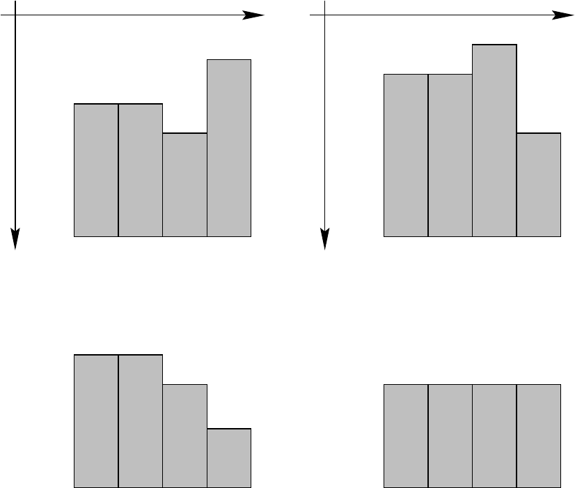
20.6. TO-DO LIST (HOW TO SET UP OPEN BOUNDARIES)
251
(c)
(a)
j = 1 2 3 4
k k
(d)
(b)
1 2 3 4j =
obc
obc
obc
obc
Figure 20.1: Topography at the open boundary (y-z-view). For southern obc, (c) and (d) are
allowed configurations, but (a) and (b) are not. Configuration (d) is the default construced by
topog.F.
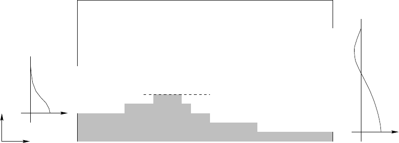
252
CHAPTER 20. STEVENS OPEN BOUNDARY CONDITIONS
j=jpsimax
j
i
130
130 Sv
Figure 20.2: Example for throughflow of 130 Sv from western to eastern open boundary
(x-y-view). jpsimax is the northernmost extension of the southern land mass

Part VI
Finite Difference Equations
253
Chapter 21
The Discrete Equations
This chapter details the time and space discretizations used for writing the finite difference
counterpart of the continuous prognostic equations in Chapter 4. After these preliminaries, the
finite difference equations are given for the simplest case of options consthmix and constvmix.
Note that throughout all equations were appropriate, numerical indices are exposed within
expressions so as to match exactly with those used in the fortran code. This extra bit of detail
is insisted upon as another way of insuring that complex formulations are correct. MOM uses
a wide variety of options to configure variants of the prognostic equations in Chapter 4. The
available options are explained in Part VII and the steps for solving these equations are covered
in Chapter 22.
21.1 Time and Space discretizations
The following operators are used to discretize equations on the grid system used in MOM.
Before going further, the grid system should be firmly in mind. Refer to Section 16.2 if in doubt.
21.1.1 Averaging operators
Simple averaging operators are defined as follows:
αi,k,jλ=αi+1,k,j+αi,k,j
2(21.1)
αi,k,jφ=αi,k,j+1+αi,k,j
2(21.2)
αi,k,jz=αi,k+1,j+αi,k,j
2(21.3)
where αis any variable defined on grid points within T-cells or U-cells. It should be noted that
the average is defined midway between the variables being averaged.
21.1.2 Derivative operators
Simple derivative operators in space and time are defined as follows:
255
256
CHAPTER 21. THE DISCRETE EQUATIONS
δλ(αi,k,j)=αi+1,k,j−αi,k,j
a∆λi
(21.4)
δφ(αi,k,j)=αi,k,j+1−αi,k,j
a∆φjrow
(21.5)
δz(αi,k,j)=−αi,k+1,j−αi,k,j
∆zk
(21.6)
δτ(βτ)=βτ+1−βτ−1
2∆τ(21.7)
where grid distances (measured in cm) are determined by the distance between variables as
indicated in Figures 16.2, 16.3, and 16.4 and discussed in Chapter 14. These operators are
second order accurate with non-uniform resolution as long as the grid is constructed so that
the stretching is based on a smooth analytic function. See Treguier, Dukowicz, and Bryan
(1995). When αi,k,jis defined at Ti,k,jgrid points, then a∆λi=dxui(a=6370 x 105cm) and when
αi,k,jis defined at Ui,k,jgrid points, then a∆λi=dxti+1. Similarly, a∆φjrow =dyujrow when αi,k,j
is defined at Ti,k,jgrid points and a∆φjrow =dytjrow+1when αi,k,jis defined at Ui,k,jgrid points.
Note the negative sign in the vertical derivative. This is because zincreases upwards while k
increases downwards. The negative sign in Equation (21.6) is usually absorbed by reversing
the indexing to give
δz(αi,k,j)=αi,k,j−αi,k+1,j
∆zk
(21.8)
In the finite difference approximation to the continuous time derivative, Equation (21.7) is
appropriate for the normal leapfrog time steps where 2∆τis in seconds. As indicated in Section
21.4, on mixing time steps, the denominator is replaced by ∆τ.
21.2 Key to understanding finite difference equations
The grid distances (measured in cm) are determined by the distance between variables as
indicated in Figures 16.2, 16.3, and 16.4. Before looking at any finite difference equations, the
reader should be convinced of the following relations:
•If αi,k,jis defined at the T cell grid point given by Ti,k,j, then the operation δλ(αi,k,jφ) results
in a quantity defined at the U cell grid point with index Ui,k,j.
•If βi,k,jis defined at the U cell grid point given by Ui,k,j, then the operation δλ(βi−1,k,j−1
φ)
results in a quantity defined at the T cell grid point given by Ti,k,j.
These operations reflect the nature of the staggered B grid. Once convinced of the above,
the second thing to be aware of is that it’s not sufficient to only know what a quantity is; where
the quantity is defined is just as important. The where information is usually built into the
name of the variable by the naming convention described in Chapter 14. There are a small
number of interesting places on the grid. The grid point within a grid cell is one; the east,
north, and bottom face of a cell are others. A quantity indexed by (i,k,j) may be defined at the
grid point in celli,k,jor on the east, north, or bottom face of celli,k,j. Note that if a variable αi,k,j
21.2. KEY TO UNDERSTANDING FINITE DIFFERENCE EQUATIONS
257
is defined on the east face of celli,k,j, its value on the west face of the cell is αi−1,k,j. Similarly, if
defined on the north face of celli,k,j, then its value on the south face of the cell is αi,k,j−1. Likewise,
if defined on the bottom face of celli,k,j, then its value on the top face of the cell is αi,k−1,j.
Note that this convention is a departure from the indexing used in Bryan (1969) where the
faces of cells were referenced by half indexes (i.e., i+1
2). Half indexes do not map well into
Fortran and are not used in this manual. The idea is that by looking at this manual it should
be possible to determine if the code is wrong (or vice versa).
21.2.1 Rules for manipulating operators
In general, finite difference derivative and average operators don’t commute unless the grid
resolution is constant. Assuming that αiis defined at grid points within T-cells, then the above
condition is illustrated by the following
δλ(αiλ),δλ(αi)λ(21.9)
How is a term like δλ(αiλ) evaluated? It can be expanded from the inside out as
δλ(αiλ)=δλ(αi+αi+1
2)
=(αi+1+αi+2)/2−(αi+αi+1)/2
dxti+1
=αi+2−αi
2·dxti+1
(21.10)
or from the outside in as
δλ(αiλ)=αi+1λ−αiλ
dxti+1
=(αi+1+αi+2)/2−(αi+αi+1)/2
dxti+1
=αi+2−αi
2·dxti+1
(21.11)
Both results are equal. Now expand the following:
δλ(αi)λ=(αi+1−αi)/dxui+(αi+2−αi+1)/dxui+1
2(21.12)
Equation (21.12) is only equal to Equation (21.11) when
dxti+1=dxui=dxui+1(21.13)
Also, it is worth remembering that the results of operators are displaced by the distance of
a half cell width. For example, the single operator δλ(αi,k,j) results in a quantity defined on the
eastern face1of cell Ti,k,jand the double operator δλ(δλ(αi,k,j)) results in a quantity defined at
the grid point within Ti+1,k,j. These results easily extend to two and three dimensions. Mixed
double operators such as δλ(αi,k,jφ) results in a quantity defined on the grid point within cell
Ui,k,j.
1This is the the longitude of the grid point within Ui,k,j.
258
CHAPTER 21. THE DISCRETE EQUATIONS
21.2.2 Rules involving summations
A zero normal component of velocity on walls (material surfaces) implies the following iden-
tities
imt−1
X
i=2
uiαiλdxui=
imt−1
X
i=2
ui−1dxui−1
λαi(21.14)
imt−1
X
i=2
uiδλ(αi)dxui=−
imt−1
X
i=2
δλ(ui−1)αidxti(21.15)
Similar identities hold in the vertical (rigid lid only) and meridional directions.
21.2.3 Other rules
There is no ambiguity in manipulating finite difference objects. As noted in Bryan (1969), there
are formal rules and some are given below. They can be verified by substituting the basic
finite difference derivative and averaging operators and expanding the terms. For illustrative
purposes, consider one dimensional quantities αiand γi(defined on longitudes of T cell grid
points) and βi(defined on longitudes of U cell grid points).
αiγiλ=αiλγiλ+1
4dxu2
iδλ(αi)δλ(γi) (21.16)
δλ(αiγi)=αiλδλ(γi)+γiλδλ(αi) (21.17)
dxti+1·δλ(αiλβi)=βi·dxui·δλ(αi)λ+αi+1·dxti+1·δλ(βi) (21.18)
αiλβi
λ
=αi+1·βi
λ+1
4dxti+1δλ(βi·dxui·δλ(αi)) (21.19)
These expressions also hold along other dimensions. In particular if φis substituted2for λor
if zis substituted for λ. Consider further the two dimensional case where αiis defined at T
cell grid points, and βiis defined at U cell grid points. The following rule may be derived by
combining Equations (21.18) and (21.19)
αi,k,j·dxti·δλ(βi−1,k,j−1
φ)+βi−1,k,j−1dxui−1·δλ(αi−1,k,j−1)φφλ
=dxti·δλ(αi−1,k,jλβi−1,k,j−1φ)
+1
4dytjrowδφ(βi−1,k,j−1·dyujrow−1δφ(dxui−1δλ(αi−1,k,j−1)))λ) (21.20)
21.3 Primitive finite difference equations
The finite difference equations are given below for the simplest case of options consthmix
and constvmix assuming explicit vertical diffusion and explicit coriolis terms. Note that the
numerical indices are exposed within expressions so as to match exactly with those used in
2The grid distances must also be replaced accordingly.
21.3. PRIMITIVE FINITE DIFFERENCE EQUATIONS
259
the fortran code. This extra bit of detail is insisted upon as another way of insuring that
complex formulations are correct. The steps for solving these equations (plus other variants)
are detailed in Chapter 22.
21.3.1 Momentum equations
Prognostic equations are written for the zonal (n=1) and meridional (n=2) component of
velocity by breaking each component into internal and external modes. The internal modes for
both components are solved for first. For each component, of the uncorrected internal mode
velocity u⋆
i,k,j,n, the equation is
δτ(u⋆
i,k,j,n)=−grad pi,k,j,n+CORIOLISi,k,j,n− LU(ui,k,j,n,τ)+DU(ui,k,j,n,τ−1) (21.21)
where the advection operator LUand diffusion operator DUfor velocity components are given
by
LU(ui,k,j,n,τ)=ADV Uxi,k,j+ADV Uyi,k,j+ADV Uzi,k,j−ADV metrici,k,j,n
(21.22)
DU(ui,k,j,n,τ−1)=DIFF Uxi,k,j+DIFF Uyi,k,j+DIFF Uzi,k,j−DIFF metrici,k,j,n
(21.23)
and
ADV Uxi,k,j=1
2 cos φU
jrow
δλ(adv f ei−1,k,j) (21.24)
ADV Uyi,k,j=1
2 cos φU
jrow
δφ(adv f ni,k,j−1) (21.25)
ADV Uzi,k,j=1
2δz(adv f bi,k−1,j) (21.26)
ADV metrici,k,j,n=∓
tan φU
jrow
radius ui,k,j,1,τ ·ui,k,j,3−n,τ (21.27)
DIFF Uxi,k,j=1
cos φU
jrow
δλ(diff f ei−1,k,j) (21.28)
DIFF Uyi,k,j=1
cos φU
jrow
δφ(diff f ni,k,j−1) (21.29)
DIFF Uzi,k,j=δz(diff f bi,k−1,j) (21.30)
DIFF metrici,k,j,n=Am
1−tan2φU
jrow
radius2ui,k,j,n,τ−1(21.31)
∓Am
2 sin φU
jrow
radius2·cos2φU
jrow
δλ(ui−1,k,j,3−n,τ−1λ) (21.32)
In the metric terms, the “-” sign is used when n=1 and the “+” sign is used when n=2. The
fluxes on U-cell faces are
260
CHAPTER 21. THE DISCRETE EQUATIONS
diff f ei,k,j=visc ceui,k,j
cos φU
jrow
δλ(ui,k,j,n,τ−1) (21.33)
diff f ni,k,j=visc cnui,k,j·cos φT
jrow+1δφ(ui,k,j,n,τ−1) (21.34)
diff f bi,k,j=visc cbui,k,j·δz(ui,k,j,n,τ−1) (21.35)
adv f ei,k,j=2adv veui,k,j·ui,k,j,n,τλ(21.36)
adv f ni,k,j=2adv vnui,k,j·ui,k,j,n,τφ(21.37)
adv f bi,k,j=2adv vbui,k,j·ui,k,j,n,τz(21.38)
Horizontal advective velocities on east and north U-cell faces “adv veu” and “adv vnu” are
defined in Section 22.3.2 and vertical advective velocity on the bottom face of U-cells “adv vbu”
is computed by vertically integrating LU(1) =0. Note that for purposes of speed in the Fortran
code, an extra factor of 2 appears in all advective fluxes (i.e. in adv f e) to cancel a factor of
2 in the averaging operator. The cancelled factor of 2 is reclaimed in the divergence operator
(i.e. ADV Ux) by combining it with a grid spacing from the derivative so as to allow one
less multiply operation when computing the divergence of flux. Refer to Section 22.3.3 for a
discussion of bottom vertical velocity.
The Coriolis and pressure gradient terms are
CORIOLISi,k,j,n=±2Ωsin φU
jrow ·ui,k,j,3−n,τ (21.39)
grad pi,k,j,1=1
ρ◦·cos φU
jrow
δλ(pi,k,jφ) (21.40)
grad pi,k,j,2=1
ρ◦δφ(pi,k,jλ) (21.41)
and the “+” sign is used when n=1 and the “-” sign is used when n=2. The pressure pis
related to density by
δz(pi,k,j)=−grav ·ρi,k,jz(21.42)
with gravity grav =980.6 cm/sec2. Therefore, the pressure at level “k” is given by
pi,k,j=−grav ·ρi,1,j·dzw0−grav ·
k
X
m=2
ρi,m−1,jzdzwm−1(21.43)
The uncorrected internal mode velocity is solved as
u′
i,k,j,n,τ+1=ui,k,j,n,τ−1+2∆τ·δτ(u⋆
i,k,j,n) (21.44)
and the corrected internal mode velocity (with bogus vertical mean removed) is constructed
by
ˆ
ui,k,j,n,τ+1=u′
i,k,j,n,τ+1−1
Hi,jrow ·
kb
X
k=1
dztk·u′
i,k,j,n,τ+1(21.45)
21.3. PRIMITIVE FINITE DIFFERENCE EQUATIONS
261
where the bottom U-cell is at level kb =kmui,jrow. As detailed in Section 29.2.1, the external
mode velocity components ¯
ui,j,n,τ+1are solved for by a variety of methods. Once the external
mode is obtained, the full velocity ui,k,j,n,τ+1is constructed by adding internal mode to external
mode
ui,k,j,n,τ+1=ˆ
ui,k,j,n,τ+1+¯
ui,j,n,τ+1(21.46)
21.3.2 Tracer equations
For each component3“n” of the tracer field ti,k,j,n
δt(ti,k,j,n,τ)=−LT(ti,k,j,n,τ)+DT(ti,k,j,n,τ−1) (21.47)
where the advection operator LTand diffusion operator DTfor tracers are
LT(ti,k,j,n,τ)=ADV Txi,k,j+ADV Tyi,k,j+ADV Tzi,k,j(21.48)
DT(ti,k,j,n,τ−1)=DIFF Txi,k,j+DIFF Tyi,k,j+DIFF Tzi,k,j(21.49)
and
ADV Txi,k,j=1
2 cos φT
jrow
δλ(adv f ei−1,k,j) (21.50)
ADV Tyi,k,j=1
2 cos φT
jrow
δφ(adv f ni,k,j−1) (21.51)
ADV Tzi,k,j=1
2δz(adv f bi,k−1,j) (21.52)
DIFF Txi,k,j=1
cos φT
jrow
δλ(diff f ei−1,k,j) (21.53)
DIFF Tyi,k,j=1
cos φT
jrow
δφ(diff f ni,k,j−1) (21.54)
DIFF Tzi,k,j=δz(diff f bi,k−1,j) (21.55)
The fluxes on T-cell faces are
adv f ei,k,j=2adv veti,k,j·ti,k,j,n,τ
λ=adv veti,k,j·(ti,k,j,n,τ +ti+1,k,j,n,τ) (21.56)
adv f ni,k,j=2adv vnti,k,j·ti,k,j,n,τ
φ=adv vnti,k,j·(ti,k,j,n,τ +ti,k,j+1,n,τ) (21.57)
adv f bi,k,j=2adv vbti,k,j·ti,k,j,n,τ
z=adv vbti,k,j·(ti,k,j,n,τ +ti,k+1,j,n,τ) (21.58)
diff f ei,k,j=diff ceti,k,j
cos φT
jrow
δλ(ti,k,j,n,τ−1) (21.59)
diff f ni,k,j=diff cnti,k,j·cos φU
jrowδφ(ti,k,j,n,τ−1) (21.60)
diff f bi,k,j=diff cbti,k,j·δz(ti,k,j,n,τ−1) (21.61)
3Subscript n=1 denotes the temperature and n=2 denotes the salinity. n>2 is for passive tracers
262
CHAPTER 21. THE DISCRETE EQUATIONS
Horizontal advective velocities on east and north T-cell faces “adv vet” and “adv vnt” are
defined in Section 22.3.1 and vertical advective velocity on the bottom face of T-cells “adv vbt”
is computed by vertically integrating LT(1) =0. Note that for purposes of speed in the Fortran
code, an extra factor of 2 appears in all advective fluxes (i.e. in adv f e) to cancel a factor of
2 in the averaging operator. The cancelled factor of 2 is reclaimed in the divergence operator
(i.e. ADV Tx) by combining it with a grid spacing from the derivative so as to allow one
less multiply operation when computing the divergence of flux. Refer to Section 22.3.3 for a
discussion of bottom vertical velocity. Each tracer is solved by
ti,k,j,n,τ+1=ti,k,j,n,τ−1+2∆τ·δt(ti,k,j,n,τ) (21.62)
21.4 Time Stepping Schemes
Basically, MOM uses a ceneterd leapfrog time stepping scheme to integrate prognostic equa-
tions forward in time. To handle the computational mode characteristic of the leapfrog scheme,
there are three choices: periodic application of a forward timestep, periodic application of an
Euler backward timestep, or a Robert time filter applied every time step.
If option robert time filter is enabled, a Robert time filter is applied every time step. If op-
tion robert time filter is not enabled, then the type of mixing is determined by logical variable eb
which if true indicates an Euler backward mixing scheme, otherwise a forward mixing scheme
is used. Intervals between mixing timesteps are set by logical switch mixts. In the past, mixing
time steps were applied every 17 time steps. This interval seems to work satisfactorily and has
been retained. Of the two mixing schemes (forward and Euler backward), the Euler backward
is more dissipative. It also damps spatial scales whereas the forward scheme does not (Haltiner
and Williams 1980).
The focus now will be to explain how these schemes are implemented within MOM. The
following description assumes that the idea of a memory window as outlined in Section 11.3.1
is understood. Refer to Figure 21.1 and note the four columns: Time Step,Type of Time Step, a
partially opened memory window with two disk areas indicated bu column jmw <jmt, and a
fully opened memory window with no disk area indicated by column jmw=jmt.
Two sets of indices are required to act as pointers to specific areas on disk and in the memory
window: one set points to τ−1, τ, and τ+1 locations on disk and these indices are named
taum1disk, taudisk, and taup1disk; the other set points to τ−1, τ, and τ+1 locations within
the memory window and these indices are named taum1, tau, and taup1.
At the beginning of each time step, memory window indices are updated as shown schemat-
ically in the Type of Time Step column. The whole idea is to get data positioned properly inside
the memory window so that the equations can be solved for various types of time steps with
only minimal changes4.
To actually see how disk indices are cycled for various types of time steps, enable op-
tion trace indices as described in Chapter 39.
21.4.1 Leapfrog
Consider the partially opened memory window shown in the third column. On leapfrog time
steps, the updating arrows indicate that τ−1 variables in the memory window are being filled
with what was τdisk data on the previous time step. Likewise, τvariables in the memory
4The only change is whether a time step length is ∆τor 2∆τ

21.4. TIME STEPPING SCHEMES
263
window are being filled with what was τ+1 disk data on the previous time step. The equation
for a typical prognostic variable hindicates a central difference or leapfrog scheme in time.
Note that the forcing term Fis a function of τfor advective processes and τ−1 for diffusive
processes. Before the leapfrog step, disk indices are set as follows:
•taum1disk =mod(itt +1,2) +1
•tau =mod(itt,2) +1
•taup1disk =taum1disk
This formulation cyclically exchanges disk pointer indices every time step to assure that the
correct disk data is read into and written from the proper memory window locations as
described above. Memory window indices are always as follows when the memory window
is partially opened:
•taum1 =1
•tau =2
•taup1 =3
When the time step is complete, τ+1 data is written back over the τ−1 disk area. Looking to
the fourth column, the fully opened memory window has no arrows therefore no movement
of data. The disk pointers are not used and instead of being fixed in time, the memory pointers
are cyclicly updated according to
•taum1 =mod(itt +0,3) +1
•tau =mod(itt +1,3) +1
•taup1 =mod(itt +2,3) +1
which accomplishes renaming of areas within the memory window without moving data.
Comparing time step nwith n+1 will clarify this.
21.4.2 Forward
On forward time steps when the memory window is partially opened as indicated by time
step n+2, both τ−1 and τvariables are loaded with what was τ+1 disk data on the previous
time step. In the third column, memory pointers are set to reflect this. The equation is the
same as for the leapfrog time steps except that 2∆τis replaced by ∆τ.
21.4.3 Euler Backward
Euler backward steps are comprised of two half steps. The first is identical to a forward step
and the second fills τvariables within the memory window with τ+1 data from the first step.
When the memory window is opened all the way, an euler shuffleis required to get data properly
aligned in preparation for the next time step. This is the only data movement required when
the memory window is fully opened5.
5This can be eliminated by recalculating the pointers differently on the time step after the Euler backward step.
However, the calculation gets tricky and has complications.
264
CHAPTER 21. THE DISCRETE EQUATIONS
21.4.4 Robert time filter
The Robert time filter (enabled by option robert time filter) is applied every time step in con-
junction with using a leapfrog scheme. Schematically, this amounts to:
hτ=hτ+smooth ·((hτ+1+hτ−1)/2−hτ) (21.63)
where hτis the filtered value of the prognostic variable hat time level τand smooth is an
adjustable parameter which may be set via namelist. The default value is smooth =0.01 which
is a reasonably small value. The largest value possible is smooth =0.2 which is a very heavy
smoothing. The Robert time filter will give smoother solutions than periodic application of
either forward or Euler backward mixing steps. The disadvantage of the Robert time filter is
that it requires an extra read through of data on disk. However, if option ramdrive is enabled
and disk data is actually held in memory, the extra overhead for reading is small. However,
for other I/O options where disk data is stored on rotating disk, the overhead may result in a
substantial increase in wall clock time.
Caveat: As implemented, the Robert time filter will not work correctly when applied to
surface currents for the purpose of Doppler shilting windspeeds when restart files are involved
for anything other than option simple sbc. The reason is that on non-restart time steps,unfiltered
values of uτare used. However, filtered values of uτare written to the restart file. Therefore,
when re-starting from a restart file, filtered values of uτare loaded from disk and used on
the first time step of a restart. This is difficult to remedy since the barotropic portion of uτ+1
is unknown at the time the filter is applied. Filtering the tracer fields will preserve answers
across restart points. The difference in answers due to this error in velocity is very tiny judging
from the observation that if the error is not accounted for in the tracer fields, the differences in
surface tracer boundary conditions is the the 6th decimal place.
21.4. TIME STEPPING SCHEMES
265
τ−1 τ τ+1
τ−1 ττ+1
τ−1
τ τ+1
τ−1 τ τ+1
τ−1
τ
τ+1
τ−1 τ τ+1
τ−1
τ τ+1
R.C.P.
Leapfrog
h = h + 2∆τ*F
τ−1τ+1 τ−1τ,
τ+1 τ
τ−1
τ
h = h + ∆τ*F
τ−1τ+1 τ−1τ,
τ+1 τ
τ−1
τ+1
Forward
Leapfrog
h = h + 2∆τ*F
τ−1τ+1 τ−1τ,
τ+1 τ
τ−1
τ
Leapfrog
h = h + 2∆τ*F
τ−1τ+1 τ−1τ,
τ+1 τ
τ−1
τ
Euler backward
h = h + ∆τ*F
τ−1τ+1 τ−1τ,
τ+1 τ
τ−1
τ+1
τ+1 τ
h = h + ∆τ*F
τ−1τ+1 τ−1τ,
Type of Time Step
Memory
(MW)
τ−1
τ+1
τ
τ−1
τ+1
τ
τ−1
τ−1 τ τ+1
τ−1 τ τ+1
τ−1 τ τ+1
τ−1 τ τ+1
τ−1 τ τ+1
τ−1 τ τ+1
Disk(1) Disk(2)
Time
Step jmw < jmt jmw = jmt
n
n+1
n+2
n+3
n+4
Memory
(MW)
τ+1
τ+1
τ+1
τ
τ
τ−1
τ−1
τ+1
τ+1
τ
τ
τ
τ
τ
τ
τ
τ
Figure 21.1: Time discretization used in MOM when memory window is partially opened and
fully opened. components
266
CHAPTER 21. THE DISCRETE EQUATIONS

Chapter 22
Solving the Discrete equations
The reader will note that all numerical indices are exposed within expressions so as to match
exactly with those used in the Fortran code. This extra bit of detail is insisted upon as another
way of insuring that complex formulations are correct.
Once surface boundary conditions are available for the ocean as described in Chapter 19,
the ocean equations are integrated for one time step with each call to subroutine mom1. As
indicated schematically in Figure 19.2 and described further in Section 19.1, mom may need
to be called repeatedly until integration has been carried out for one time segment. For a
flowchart indicating the calling sequence within mom for one time step, refer to Figure 22.1.
The process starts by incrementing the ocean time step counter itt by one
itt =itt +1 (22.1)
and calling module tmngr2which increments ocean time by the number of seconds in one
time step. Refer to Section 14.4.4 for choosing a time step length. Module tmngr additionally
calculates a time and date as described in Section 15.1.9 and determines which events are to
be activated on the current time step and which are not. Each event has an associated logical
switch which is kept in file switch.h. An event might be something like writing a particular
diagnostic for analysis, or doing a mixing time step, etc. After determining all logical switches,
a call is made to the diagnostic initialization subroutine diagi which performs initializations for
various diagnostics when required3.
22.1 Start of computation within Memory Window
Equations are solved for a group of latitude rows within the memory window. The group may
be as few as one4or as many as (jmt −2) latitudes5. The number of groups depends on the
size of the memory window and each group is solved one at a time until all groups have been
solved. The northward movement of the memory window is described in Section 11.3.1. The
reader is referred to Chapter 14 for a description of the variables, Chapter 16 for a description
of the grid system, and Chapter 11 for a description of the memory window.
1Contained in file mom.F.
2Contained in file tmngr.F.
3Assuming these diagnostics have been enabled by their options at compile time.
4Requiring three rows in the memory window.
5Requiring jmt rows in the memory window.
267

268
CHAPTER 22. SOLVING THE DISCRETE EQUATIONS
The number of memory window moves needed to solve all latitude rows is controlled by
a “do loop” which essentially extends from Section 22.2 to Section 22.10. The subroutines
called for each group of latitudes within the memory window are outlined in Figure 22.1 and
explained in the following sections.
22.2 loadmw (load the memory window)
Subroutine loadmw6begins by moving the memory window northward if necessary7. This
movement begins by copying data from the top two rows into the bottom two rows of the
memory window as described in Section 11.3.2.
22.2.1 Land/Sea masks
At this point, land/sea masks tmaski,k,jfor the T-cells and umaski,k,jfor the U-cells are constructed
from kmti,jrow and kmui,jrow. They are set as
tmaski,k,j=(1.0 if cell Ti,k,jis an ocean cell
0.0 if cell Ti,k,jis a land cell (22.2)
and
umaski,k,j=(1.0 if cell Ui,k,jis an ocean cell
0.0 if cell Ui,k,jis a land cell (22.3)
The purpose of these masks is to promote vectorization by allowing computation every-
where but zeroing out the results within land cells. Note that when the memory window is
fully opened (jmw =jmt), this calculation is only done once per run instead of redundantly
every time step.
22.2.2 Reading latitude rows into the Memory window
After building the land/sea vectorization masks, the next latitude rows are read from disk to
fill the remaining latitude slots within the memory window. Latitude rows are read from the
τand τ−1 disks. Time level indices depend on whether it is a normal leapfrog time step or a
mixing time step as described in Section 21.4.
22.2.3 Constructing the total velocity
Once all data is in place within the memory window, preliminary calculations are ready to
begin. The process starts by adding the external mode velocity to the internal mode velocity
to construct the total velocity as in Equations (4.1) and (4.2). The finite difference counterpart
to the external mode given in Equations (6.4) and (6.5) is
6Contained in file loadmw.F.
7It is necessary for all but the first group of latitudes. If the memory window is opened all the way (when
jmw =jmt), then no movement is necessary.
22.2. LOADMW (LOAD THE MEMORY WINDOW)
269
ui,jrow,1=−1
Hi,jrow ·δφ(ψi,jrow,τ
λ) (22.4)
ui,jrow,2=1
Hi,jrow ·cos φU
jrow ·δλ(ψi,jrow,τ
φ) (22.5)
The total velocity needs to be constructed for both time levels at this point because only the
internal mode velocities8are kept in the latitude rows on disk.
ui,k,j,1,τ−1=ˆ
ui,k,j,1,τ−1−1
Hi,jrow ·δφ(ψi,jrow,τ−1
λ) (22.6)
ui,k,j,2,τ−1=ˆ
ui,k,j,2,τ−1+1
Hi,jrow ·cos φU
jrow ·δλ(ψi,jrow,τ−1
φ) (22.7)
ui,k,j,1,τ =ˆ
ui,k,j,1,τ −1
Hi,jrow ·δφ(ψi,jrow,τ
λ) (22.8)
ui,k,j,2,τ =ˆ
ui,k,j,2,τ +1
Hi,jrow ·cos φU
jrow ·δλ(ψi,jrow,τ
φ) (22.9)
where ˆ
uis the internal mode velocity, ψis the stream function, and His the ocean depth defined
over U cells by Equation (18.4).
Finally, the density rhoi,k,jis computed by Equation (15.7) as a function of ti,k,j,1,τ,ti,k,j,2,τ,
and depth of level kbased on a third order polynomial fit to the equation of state for sea water.
The density is actually a deviation from a reference density ρre f
kas described in Section 15.1.2.
22.2.4 Computing quantities within the memory window
The memory window (MW) is fundamental to solving 3-D baroclinic and tracer equations
within MOM. It is not used for solving the 2-D barotropic equation. For a description of the
MW, refer to Section 11.3. Figure 22.2 illustrates the horizontal grid within a minimum sized
MW and shows sites where prognostic quantities are defined as well as sites populated by
derived quantities. Recall that equations for prognostic quantities are solved only on row j=2
within this minimum sized MW. Prognostic quantities on rows j=1 and j=3 are used only to
supply access to neighboring cells required by the numerics for solving prognostic equations
on row j=2.
Prognostic quantities within grid cells such as temperature, salinity, and horizontal velocity
components are defined at grid points within T-cells and U-cells on rows j={1,2,3}and
therefore dimensioned by the size of the MW as in the following array:
dimension A(imt,km,jmw) ! all cells within the memory window
Advective velocity on the north face of T-cells “adv vnt(i,k,j)” is a derived quantity. It is
defined for T-cells on rows j={1,2,3}and computed as a zonal average of meridional velocity
8After each group of internal mode velocities are solved within a time step, they are written back to disk. The
external mode is unknown until all rows have been solved and subroutine barotropic solves for the external mode.
The only way to get the total velocity on disk is to read all rows back into memory after the external mode has been
solved. This is why the external mode is added at the beginning of each time step for time levels τand τ−1.
270
CHAPTER 22. SOLVING THE DISCRETE EQUATIONS
components which are defined on U-cell grid points for rows j={1,2,3}. Since all components
for the computation exist within the MW, “adv vnt(i,k,j)”, must also be dimensioned as above.
Note that some derived quantities cannot occupy certain sites and these are indicated by
a circle with at line across it. For instance, neither the advective velocity on the east face of
T-cells for j=1 nor the advective velocity on the south face of U-cells for j=1 can be defined
because their computation references quantities outside the MW. As a more detailed example,
consider derived quantities such as the advective flux through the northern face of a T-cell
“adv f n(i,k,j)” which involve the product of an advective velocity on the northern T-cell face
“adv vnt(i,k,j)” and the average temperature on that cell face. Since the average temperature
on the northern face of cell “j” is
Ti,k,j
φ=(Ti,k,j+Ti,k,j+1)/2 (22.10)
the advective flux can only be dimensioned as adv f n(imt,km,jmw −1) otherwise the flux at
index j=jmw would require knowledge of temperature at j=jmw +1 which is unknown
because it is outside of the MW. Apart from quantities like density and advective velocity, other
quantities such as Richardson number, mixing coefficients, etc. may be required by enabled
options. In general, placement of derived quantities within the grid system is determined
soley by numerics within finite difference equations.
The rule is simple. Any latitude row for which a quantitiy can be calculated should be pop-
ulated by the calculation. Furthermore, the number of rows that can be populated within the
memory window determines the dimension of the quantity. As the memory window is moved
northward, all prognostic as well as derived quantities are copied from the northernmost rows
into the southernmost rows (as described further in Section 11.3.3) so that no redundant com-
putations are required. All arrays dimensioned within the memory window must have their
latitude dimension fall into one of the following four catagories:
dimension A(,,jmw) ! all cells within the memory window
dimension B(,,1:jmw-1) ! all cells except j=jmw
dimension C(,,2:jmw) ! all cells except j=1
dimension D(,,2:jmw-1) ! all cells except j=1 and j=jmw
A few more examples follow:
22.2.4.1 Example 1: density
Density ρi,k,jis defined at each grid point within T-cells by Equation (15.7). It is a function of
temperature, salinity, and pressure (or equivalently depth) without regard to spatial gradients
of temperature or salinity and so should be dimensioned as
dimension rho(imt,km,jmw)
The computation of density can therefore populate T-cells within rows “j=1” through “j=jmw”
in the memory window. There is no need for redundant computations of “rho” since as the
memory window is moved northward, rows within array “rho” are cycled by the prescription
given in Section 11.3.3.
22.3. ADV VEL (COMPUTES ADVECTIVE VELOCITIES)
271
22.2.4.2 Example 2: Advective velocity on the eastern face of T-cells
The advective velocity on the eastern face of T-cells “adv veti,k,j” is defined by Equation (22.11).
Note that it cannot be computed for the first latitude row “j=1” in the memory window. Why?
Because Equation (22.11) references zonal velocity at “j-1” which is outside of the dimensional
bounds on zonal velocity and therefore outside the bounds of the memory window. How-
ever, “adv veti,k,j” can be computed for rows “j=2” through “j=jmw” in the memory window.
Therefore, it is dimensioned as
dimension adv_vet(imt,km,2:jmw)
and its computation must populate rows “2” through “jmw” in the memory window. Once
computed, rows within array “adv vet” are cycled according to the prescription given in Section
11.3.3 so that no redundant computations of advective velocity are involved as the window
moves northward.
22.2.4.3 Example 3: Advective velocity on the bottom face of U-cells
Advective velocity on the bottom face of U-cells “adv vbui,k,j” is defined as the vertically
integrated divergence of horizontal advective velocities (which are on the faces of U-cells) by
Equation (22.23). Inspection of the indices in the numerics indicates that “adv vbui,k,j” cannot
be computed within the first or last row of the memory window because this would require
knowledge of quantities outside of the memory window. Therefore, “adv vbui,k,j” can only be
dimensioned as
dimension adv_vbu(imt,km,2:jmw)
22.3 adv vel (computes advective velocities)
Subroutine adv vel9constructs advective velocities on the north, east and bottom faces of tracer
cells Ti,k,jwithin the memory window. These advective velocities are then suitably averaged
to construct advective velocities on the north, east and bottom faces of velocity cells Ui,k,j. Both
sets of advective velocities will now be described.
22.3.1 Advective velocities for T cells
Advective velocities are defined in a direction normal to T-cell faces. Refer to Figure 22.3a
which illustrates a T-cell with all six advective velocities and their indices. Note that a T grid
point is within the T-cell and there are four surrounding U points; one on each corner of the
T-cell. A horizontal slice through the plane containing the grid points is depicted in Figure
22.3c showing the relation between indices in the central T-cell and four surrounding U-cells.
Advective velocity on the eastern face of a T cell is a meridional weighted average of the zonal
velocities at the vertices of the face. A similar relation holds for the advective velocity on the
northern face of a T cell but it involves a zonal average of the meridional velocities. In both
cases the averaging takes place within the plane of the face.
9Contained within file adv vel.F.
272
CHAPTER 22. SOLVING THE DISCRETE EQUATIONS
adv veti,k,j=ui,k,j,1,τ ·dyujrow +ui,k,j−1,1,τ ·dyujrow−1
2·dytjrow
(22.11)
adv vnti,k,j=cos φU
jrow
ui,k,j,2,τ ·dxui+ui−1,k,j,2,τ ·dxui−1
2·dxti
(22.12)
This form of the advective velocities is not arbitrary and comes from the condition that the
work done by horizontal pressure forces must equal the work done by buoyancy. The details
are given in Section A.2.4. Note that with non-uniform resolution, the denominator is not
equal to the sum of the weights if the grid is constructed as:
dxui=dxti+dxti+1
2(22.13)
dyujrow =dytjrow +dytjrow+1
2(22.14)
which was done in MOM 1 and earlier implementations10. However, MOM allows grid
construction11 by
dxti=dxui+dxui−1
2(22.15)
dytjrow =dyujrow +dyujrow−1
2(22.16)
which guarantees that the denominator always equals the sum of the weighting factors. This
is presumed to allow more accurate advective velocities when the grid is stretched in the
horizontal although differences should be of second order. Refer to Chapter 16 for a further
discussion on non-uniform grids and advection.
From the incompressibility condition expressed by Equation (4.3), the advective velocity
on the bottom face of each cell is defined as the vertical integral of the convergence of the
horizontal advective velocities on each cell face from the surface down to the bottom face of
any cell. The rigid lid assumption sets the advective velocity at the top face of the first cell
to zero. If option implicit free surface is enabled, the advective velocity at the top face of the
first cell is diagnosed from 1
rho◦·grav ·δτ(psi,jrow). If the option explicit free surface is enabled, then
the vertical velocity is diagnosed as the convergence of the vertically integrated transport. As
discussed in Section 7.2.3, this convergence includes both the time tendency of the free surface
height as well as the input of fresh water.
For points within the ocean, the vertical advection velocity is calculated diagnostically as
the advective velocity at the bottom face of each cell through the expression
adv vbti,k,j=1
cos φT
jrow ·
k
X
m=1δλ(adv veti−1,m,j)+δφ(adv vnti,m,j−1)·dztm
10This was the motivation for exploring grid construction by method 2 as detailed in Section 16.2.3
11The old construction method 1 is enabled by option centered t. Refer to Chapter 16 for a description of grid
design.
22.3. ADV VEL (COMPUTES ADVECTIVE VELOCITIES)
273
=1
cos φT
jrow ·
k
X
m=1adv veti,m,j−adv veti−1,m,j
dxti
+
adv vnti,m,j−adv vnti,m,j−1
dytjrow ·dztm(22.17)
where φT
jrow refers to the latitude at point Ti,k,j.
22.3.2 Advective velocities for U cells
Another set of advective velocities are defined in a direction normal to U-cell faces. Refer to
Figure 22.3b which illustrates a U-cell with all six advective velocities and their indices. Note
that a U grid point is within the U-cell and there are four surrounding T points; one at each
corner of the U-cell. A horizontal slice through the plane containing the grid points is depicted
in Figure 22.3d showing the relation between indices in the central U-cell and four surrounding
T-cells. To calculate advective velocities on faces of U cells, the averaging approach indicated
by Dukowicz and Smith (1994) and subsequently described by Webb (1995) is used. Their
formulae are:
adv veui,k,j=adv veti,k,j
λφ (22.18)
adv vnui,k,j=adv vnti,k,j
λφ (22.19)
adv vbui,k,j=adv vbti,k,j
λφ (22.20)
The above averaging works when the grid resolution is uniform. For MOM, a more general
form is used to conserve volume within each U cell when resolution is non-uniform. Volume
conservation is insured by taking a weighted average of T cell advective velocities within the
plane of the cell face and a linear interpolation in a direction normal to the cell face. Refer to
Figure 22.3c. Using the indicated grid distances, the resulting four point averaging operators
are given by:
adv vnui,k,j=1
dytjrow+1·dxui×
(adv vnti,k,j·duwi+adv vnti+1,k,j·duei)·dusjrow+1
+(adv vnti,k,j+1·duwi+adv vnti+1,k,j+1·duei)·dunjrow(22.21)
adv veui,k,j=1
dyujrow ·dxti+1· ×
(adv veti,k,j·dusjrow +adv veti,k,j+1·dunjrow)·duwi+1
+(adv veti+1,k,j·dusjrow +adv veti+1,k,j+1·dunjrow)·duei.(22.22)
The vertical velocity at the bottom face of U cells can be calculated by directly integrating the
continuity equation
274
CHAPTER 22. SOLVING THE DISCRETE EQUATIONS
adv vbui,k,j=1
cos φU
jrow ·
k
X
m=1δλ(adv veui−1,m,j)+δφ(adv vnui,m,j−1)·dztm(22.23)
Equivalently, the vertical velocity at the bottom face of U cells can by calculated as an area
preserving weighted average of the vertical velocities at the bottom face of four surrounding
T cells.
adv vbui,k,j=1
dyujrow ·dxui·cos φU
jrow ×
adv vbti,k,j·dusjrow ·duwi·cos φT
jrow
+adv vbti+1,k,j·dusjrow ·duei·cos φT
jrow
+adv vbti,k,j+1·dunjrow ·duwi·cos φT
jrow+1
+adv vbti+1,k,j+1·dunjrow ·duei·cos φT
jrow+1(22.24)
This volume conserving averaging operation eliminates the problem of numerical de-coupling
between advective velocities on the bottom of T cells and U cells in the presence of flow
over topographic gradients. As discussed by Webb (1995), this de-coupling can introduce a
large mis-match between the vertical velocity on T-cells and U-cells, with the U-cell velocity
generally very noisy near topography. Implementations of vertical velocity in MOM 1 and
previous versions of the GFDL ocean model suffered from such de-coupling and noise. It
should be noted that the weighting factors dus,dun,due, and duw are always equal if resolution
is uniform. In this case, the averaging used here reduces to that of Webb (1995).
Refer to Sections 22.9.5 and 22.8.7 for details on how advective velocities are used to
compute the advective fluxes of momentum and tracers.
22.3.3 Vertical velocity on the ocean bottom
Before tracer or momentum equations can be solved, it is necessary to evaluate the vertical
velocity at the ocean surface and bottom. More specifically, as discussed in Sections 22.3.1
and 22.3.2, vertical velocity at the ocean surface and bottom enters the continuity equation
as an upper and lower boundary condition. Since the continuity equation is a first order
differential constraint, only one boundary condition is needed to diagnose the vertical velocity
w(z). Either w(0) or w(−H) may be used. For historical reasons based on the early use of
the rigid lid approximation, MOM uses vertical velocity at the ocean surface and integrates
downward to construct w(z) at all depths. The vertical velocity at the ocean bottom will now
be given for the discrete equations. The result for integrating from the bottom up will also be
given.
22.3.3.1 Summary of the continuum results
Before discussing the discrete results, it is useful to first recall the discussion of the vertical
velocity within the context of the continuum equations as given in Chapter 7. The main result
is that the vertical velocity at the ocean surface is given by (equation 7.39)
w(0) =−∇h·U0,(22.25)
22.3. ADV VEL (COMPUTES ADVECTIVE VELOCITIES)
275
which in words means that w(z=0) is due to the convergence of the vertically integrated
velocity
U0=Z0
−H
dz uh.(22.26)
This result is general; i.e., it holds even when there is fresh water input to the free surface.
For the rigid lid, there is identically zero convergence and so w(0) =0. For the implicit free
surface, only the case without fresh water is implemented in which w(0) ≈ηtis assumed. For
the explicit free surface, w(0) =−∇h·U0is implemented. For the ocean bottom, recall the
discussion from Section 4.3.1, in which it was shown that the vertical velocity at the ocean
bottom is given through the kinematic boundary condition
w=−uh· ∇hH z =−H(λ, φ).(22.27)
Each of these results will now be discussed within the context of the discrete ocean model in
which nontrivial bottom topography is allowed.
22.3.3.2 Discrete vertical velocity at the ocean bottom
As described in Chapter 18, the discretized ocean bottom is defined by land T-cells beneath the
deepest ocean T-cells. The deepest ocean T-cells are given by Ti,kb,jwhere kb =kmti,jrow and
2≤kb ≤km .(22.28)
Refer to Fig 22.4a which illustrates the ocean bottom using land T-cells (the land cells are drawn
with solid lines). The bottom face of the deepest ocean T-cells12 is marked with an “x”. In total,
all exposed faces of these land T-cells define the material surface across which no flow can pass
(i.e. normal velocity component at the material surface is zero). To keep the figure simple,
only one vertical column of T-cells extending from the ocean surface to the ocean bottom is
illustrated (the ocean T-cells are drawn with dashed lines). Let the location of this vertical
column be given by coordinate indices “i,j” where cell Ti,kb,jis the deepest ocean T-cell in the
column and the bottom face of cell Ti,kb,jis marked with an “x”.
Vertical velocity at the bottom face of any ocean T-cell can be found by vertically integrating
as in Equaton (22.17) from the resting ocean surface z=0 to the bottom face of the cell in
question. Vertical velocity on the bottom face of cell Ti,kb,j(marked by “x”) is zero because
bottom faces are horizontally flat and the normal velocity component on a material surface
which is fixed in time is zero. That is, the model’s bottom topography is piece-wise flat on the
T-cell grid and so the vertical velocity must vanish there. Hence, the vertical component to the
advective velocity on the T-cell vanishes at the bottom of the T-cell grid
adv vbti,kb,j=adv vbti,0,j+1
cos φT
jrow
kb
X
k=1
(δλ(adv veti−1,k,j)+δφ(adv vnti,k,j−1)) ·dztk
=0.(22.29)
The vertical advection velocity at the ocean surface adv vbti,0,jvanishes when using a rigid lid
option, but is generally nonzero if using a free surface option. Similarly, vertical velocity is
zero on all other bottom T-cell faces marked by “x”.
12This cell face is also the top face of the first land T-cell below the ocean bottom.
276
CHAPTER 22. SOLVING THE DISCRETE EQUATIONS
Now consider the “black dot” in Figure 22.4a. This dot marks the bottom face of the deepest
ocean U-cell having coordinate indices “i,j”. The vertical column of U-cells extending from the
ocean surface to the deepest ocean cell Ui,kbu,jis indicated in Fig 22.4b (the ocean U-cells are
drawn with dashed lines). The depth index “kbu” is calculated as the minimum of the four
surrounding T-cell depth indices:
kbu =kmui,jrow =min(kmti,jrow,kmti,jrow+1,kmti+1,jrow,kmti+1,jrow+1) (22.30)
Importantly, note that the bottom face of the U-cell Ui,kbu,jis not a material surface. This fact is
evident in Figure 22.4c which illustrates partial ocean U-cells existing below the bottom face
of cell Ui,kbu,j(the U-cells are drawn with dashed lines). These ocean U-cells are only partially
full grid cells since they are truncated by the material surfaces of the surrounding land T-cells.
Since the bottom face of cell Ui,kbu,jis not a material surface, it follows that the vertical
velocity at the “black dot” in Figure 22.4a is not generally zero
adv vbui,kbu,j,0.(22.31)
Instead, using Equation (22.17) to vertically integrate from the surface downwards to the “black
dot” in Figure 22.4b yields
adv vbui,kbu,j=adv vbti,0,j
λφ +1
cos φU
jrow
kbu
X
m=1δλ(adv veui−1,m,j)+δφ(adv vnui,m,j−1)·dztm
(22.32)
The above considerations always started from the ocean surface. Volume conservation
ensures that one can equivalently start from the bottom of the U-cells and integrate upwards.
For this purpose, it is necessary to define the deepest partially full cell Ui,kmax,jas shown in
Figure 22.4c. The depth index “kmax” for this cell is calculated as the maximum of the four
surrounding T-cell depth indices
kmax =max(kmti,jrow,kmti,jrow+1,kmti+1,jrow,kmti+1,jrow+1) (22.33)
The vertical advective velocity adv vbui,kmax,jvanishes since it represents the vertical velocity at
the flat material surface which is the bottom of a U-cell column. Integrating Equation (22.17)
upwards from the bottom of the U-cell column at kmax to the “black dot “ at kbu yields
adv vbui,kbu,j=−1
cos φU
jrow
kmax
X
m=kbu+1δλ(adv veui−1,m,j)+δφ(adv vnui,m,j−1)·dztm.
(22.34)
Volume conservation ensures that this result is identical to equation (22.32).
The question now arises as to why Equation (22.34) does not have the appearance of
a discretized version of Equation (22.27)? The answer is that Equation (22.27) should be
discretized at the location of the “open circle” in Figure 22.4 rather than at the “black dot”
itself. The reason is that location of the “open circle” is determined as the maximum distance
above the bottom face of cell Ui,kmax,jfor which both the northern and western cell faces are
material surfaces.
For purposes of completeness, the discrete form of Equation (22.27) can be written for the
location of the “open circle” through the following considerations. Let “ko” be the vertical
22.4. ISOPYC (COMPUTES ISONEUTRAL MIXING TENSOR COMPONENTS)
277
index of the U-cell whose top face contains the “open circle”. Also, let the height of the “open
circle” from the base of cell Ui,kmax,jbe given by
Hb=zw(kmax)−zw(ko).(22.35)
Integrating upwards from the bottom face of level “kmax” to “ko” yields
adv vbui,ko,j=−1
cos φU
jrow
kmax
X
m=koδλ(adv veui−1,m,j)+δφ(adv vnui,m,j−1)·dztm
(22.36)
Defining the average advective velocity normal to cell faces as
Ub
i,j=1
Hb
kmax
X
m=ko
adv veui,m,jdztm(22.37)
Vb
i,j=1
Hb
kmax
X
m=ko
adv vnui,m,jdztm(22.38)
and substituting into Equation (22.36) yields
adv vbui,ko,j=−1
cos φU
jrow Hbδλ(Ub
i−1,j)+Hbδφ(Vb
i,j−1)(22.39)
Since the north and west face of the cells summed over in Equation (22.36) are material surfaces
Ub
i−1,j=0 (22.40)
Vb
i,j=0 (22.41)
which leads to the finite difference counterpart of Equation (22.27).
adv vbui,ko,j=1
cos φU
jrow −Ub
i,j
Hb
dxui
+Vb
i,j−1
Hb
dyujrow
=1
cos φU
jrow Ub
i,j·δλ(Hb)+Vb
i,j−1·δφ(Hb).(22.42)
22.4 isopyc (computes isoneutral mixing tensor components)
Subroutine isopyc13 computes the isoneutral mixing tensor components. Refer to Sections
35.1.5, 35.1.6, and 35.1.8 for the details.
22.5 vmixc (computes vertical mixing coefficients)
Subroutine vmixc14 computes vertical mixing coefficients for momentum (diff cbui,k,j) and trac-
ers (diff cbti,k,j) according to the scheme selected by options at compile time. Subscripts for the
13Contained in file isopyc.F.
14Contained in file vmixc.F.
278
CHAPTER 22. SOLVING THE DISCRETE EQUATIONS
mixing coefficients depend on which option was enabled. Options are constvmix for constant
vertical mixing coefficients, ppvmix for Richardson dependent vertical mixing coefficients as
in Pacanowski/Philander (1981), and tcvmix for the second order turbulence closure of Mel-
lor/Yamada as given in Rosati and Miyakoda (1988). However, tcvmix is not available as of this
writing but is being implemented by Rosati at GFDL. One of these must be enabled and all
adjustable values are input through namelist. Refer to Section 14.4 for information on namelist
variables.
Additionally, there are two hybrid options allowed which supply mixing coefficients in the
vertical for tracers but not momentum. Option isoneutral is for mixing of tracers according to the
structure of the isoneutral directions, as described in Section 35.1, and option bryan lewis vertical
(Bryan/Lewis 1979) sets constant values as a function of depth for the vertical mixing coefficient.
When option isoneutralmix is enabled, mixing coefficients for tracers from other options such
as constvmix,ppvmix, or bryan lewis vertical are used as background values and added to the
vertical diffusion coefficient15 from option isoneutralmix.
22.6 hmixc (computes horizontal mixing coefficients)
Subroutine hmixc16 computes horizontal mixing coefficients for momentum (diff ceui,k,jand
diff cnui,k,j) and tracers (diff ceti,k,jand diff cnti,k,j) according to the scheme selected by options
at compile time. Currently, options include consthmix which use constant horizontal mix-
ing coefficients appropriate for ∇2mixing, biharmonic which use constant mixing coefficients
appropriate for higher order ∇4mixing, and smagnlmix for Smagorinsky nonlinear mixing
coefficients after Smagorinsky (1963).
As in Section 22.5, coefficients from hybrid schemes for mixing of tracers but not mixing
of momentum are also allowed. They are bryan lewis horizontal,isoneutralmix and held larichev
as referred to in Section 22.5. When option isoneutralmix is enabled, mixing coefficients for
tracers from consthmix,smagnlmix, or bryan lewis vertical are used as background values and
added to the horizontal diffusion coefficients17 from option isoneutralmix. For details on specific
schemes, consult their options.
22.7 setvbc (set vertical boundary conditions)
Subroutine setvbc18 sets vertical boundary conditions for momentum sm fi,j,nand tracers st fi,j,n
at the ocean surface and their counterparts defined at the ocean bottom bm fi,j,nand bt fi,j,n.
Also, bm fi,j,ncan be set to zero (free slip) or a linear bottom drag condition with the drag
coefficient being input through namelist. Refer to Section 14.4 for information on namelist
variables. Refer to Chapter 19 for further discussion on surface boundary conditions.
15This is effectively done by adding diffusive fluxes from the basic scheme to the isoneutral flux across the bottom
face of the T cell.
16Contained in file hmixc.F.
17This is effectively done by adding diffusive fluxes from the basic scheme to the isoneutral flux across the
northern and eastern face of the T cell.
18Contained in file setvbc.F.
22.8. TRACER (COMPUTES TRACERS)
279
22.8 tracer (computes tracers)
Subroutine tracer is contained in file tracer.F and computes tracers given by ti,k,j,n,τ+1for n=1
to nt, where nt is the number of tracers. Index n=1 corresponds to potential temperature
in Equation (4.5) and index n=2 is for salinity in Equation (4.6). These first two tracers are
dynamically active in the sense that they determine density by Equation (15.7). Other tracers
may be added by setting parameter nt >2 but the additional tracers are passive. In previous
versions of the model, tracers were solved after the baroclinic velocities. However, in order
to accommodate option pressure gradient average tracers are now computed before baroclinic
velocities.
22.8.1 Tracer components
Each tracer is considered as a component of one tracer equation and solved separately by a “do
n=1,nt” loop extending to Section 22.8.10. As with the finite difference momentum equations
given in Section 22.9.5, the finite difference tracer equation is written in flux form to conserve
first and second moments as discussed in Chapter A.
22.8.2 Advective and Diffusive fluxes
Advective and diffusive fluxes across the north, east, and bottom faces of T cells within the
memory window are calculated for use by the advection and diffusion operators described in
Sections 21.3.2 and 22.8.7. The canonical forms of the fluxes are given in Section 21.3.2 and
expanded below. The actual form of the diffusive flux may differ depending on which option is
enabled. Note that for purposes of speed in the Fortran code, an extra factor of 2 appears in all
advective fluxes (i.e. in adv f e) to cancel a factor of 2 in the averaging operator. The cancelled
factor of 2 is reclaimed in the divergence operator (i.e. ADV Ux) by combining it with a grid
spacing from the derivative so as to allow one less multiply operation when computing the
divergence of flux. Also, a cosine factor has been absorbed into the definition of adv vnti,k,j
for reasons of speed. Fluxes are typically computed from j=2 through j=jmw −1, except
for the last memory window, which may only be partially full. Meridional operators require
meridional flux to be computed for j=1, which is why the lower limit of the jindex is not
identical for the flux across the north, east, and bottom cell faces. Refer to Figure 11.2 for a
schematic of the memory window to help clarifiy the latitude indexing limits.
adv f ei,k,j=adv veti,k,j·(ti,k,j,n,τ +ti+1,k,j,n,τ),j=2,jmw −1 (22.43)
adv f ni,k,j=adv vnti,k,j·(ti,k,j,n,τ +ti,k,j+1,n,τ),j=1,jmw −1 (22.44)
adv f bi,k,j=adv vbti,k,j·(ti,k,j,n,τ +ti,k+1,j,n,τ),j=2,jmw −1 (22.45)
diff f ei,k,j=diff ceti,k,j·ti+1,k,j,n,τ−1−ti,k,j,n,τ−1
cos φT
jrowdxui
,j=2,jmw −1 (22.46)
diff f ni,k,j=diff cnti,k,j·cos φU
jrow
ti,k,j+1,n,τ−1−ti,k,j,n,τ−1
dyujrow
,j=1,jmw −1 (22.47)
280
CHAPTER 22. SOLVING THE DISCRETE EQUATIONS
diff f bi,k,j=diff cbti,k,j·ti,k,j,n,τ−1−ti,k+1,j,n,τ−1
dzwk
,j=2,jmw −1 (22.48)
At the top and bottom, boundary conditions are applied to the vertical fluxes where the
bottom cell is at level kb =kmti,jrow. Also, the advective flux through the bottom of the last
level kb =kmti,jrow is zero19. Note that the advective flux through the bottom of the last vertical
cell k=km is set to zero. Also, when option stream function is enabled, adv vbti,0,j=0 because
of the rigid lid but adv vbti,0,j,0 when option implicit free surface is enabled.
kb =kmti,jrow (22.49)
diff f bi,0,j=st fi,j,n(22.50)
diff f bi,kb,j=bt fi,j,n(22.51)
adv f bi,0,j=adv vbti,0,j·(ti,1,j,n,τ +ti,1,j,n,τ) (22.52)
adv f bi,km,j=0.0 (22.53)
22.8.3 Isoneutral fluxes
When option isoneutralmix is enabled, the horizontal components of the isoneutral diffusive
flux in Section 35.1 are added to the horizontal diffusive flux in Equations (22.46) and (22.47).
The complete diffusive flux across the northern and eastern face of a T cell then is given by
diff f ei,k,j=diff f eold
i,k,j+diff f etiso
i,k,j(22.54)
diff f ni,k,j=diff f nold
i,k,j+diff f ntiso
i,k,j(22.55)
where the isoneutral diffusion fluxes diff f etiso
i,k,jand diff f ntiso
i,k,jare given in Section 35.1. The
background fluxes are given by
diff f eold
i,k,j=diff ceti,k,j·ti+1,k,j,n,τ−1−ti,k,j,n,τ−1
cos φT
jrowdxui
(22.56)
diff f nold
i,k,j=diff cnti,k,j·cos φU
jrow
ti,k,j+1,n,τ−1−ti,k,j,n,τ−1
dyujrow
(22.57)
where diff ceti,k,jand diff cnti,k,jare the coefficients from whatever subgrid scale mixing param-
eterization option has been enabled. The [K31] and [K32] parts of the diffusive flux across the
bottom face of the T cell is given as diff f bisoi,k,jwhich is the vertical flux term −Fz
i,k,jfrom
Section 35.1 minus the [K33] piece.
diff f bisoi,k,j=−Fz
i,k,j−K33
i,k,jδzTi,k,j(22.58)
Note that the isoneutral diffusion coefficient AIhas been absorbed into the tensor components
[K31], [K32], [K33]. The [K33] component is handled implicitly as indicated in Section 22.8.7.
19Zero to within roundoff. Note that unlike adv vbti,kb,j, adv vbui,kb,jcan be non-zero if there is a bottom slope.
22.8. TRACER (COMPUTES TRACERS)
281
22.8.4 Source terms
It is possible to introduce sources into the tracer equation by enabling option source term. If
this option is enabled, the source term is initialized to zero for each component of the tracer
equation.
sourcei,k,j=0.0 (22.59)
Adding new sources or sinks to the tracer equations is a matter of calculating them and
adding to sourcei,k,jas indicated in Sections 22.8.5 and 22.8.6.
22.8.5 Sponge boundaries
If option sponges is enabled, a Newtonian damping term is added to the tracer equation through
the source term near northern and southern boundaries where γ−1is a Newtonian damping
time scale input through a namelist and t⋆
i,k,j,nis interpolated in time from data prepared by the
scripts in PREP DATA. If option equatorial sponge is enabled, then the profile from Equation
(28.1) is used for t⋆
i,k,j,ninstead of data prepared in PREP DATA. Refer to Section 14.4 for
information on namelist variables. The time interpolation method is the same as described in
Section 19.2.
sourcei,k,j=sourcei,k,j−γ·(ti,k,j,n,τ−1−t⋆
i,k,j,n) (22.60)
22.8.6 Shortwave solar penetration
If option shortwave is enabled, the divergence of shortwave penetration is also added to the
source term using
sourcei,k,j=sourcei,k,j+sbcocni,jrow,mi,jrow,isw ·divpenk(22.61)
where subscript isw points to the shortwave surface boundary condition. This only applies for
n=1. Refer to Section 28.2.10 for more details about the divergence of shortwave penetration.
22.8.7 Tracer operators
Finite difference tracer operators (see Section 14.1 for naming convention) are used for the
various terms when solving for ti,k,j,n,τ+1and parallel those used in the solution of the internal
mode velocities. Operators are implemented as statement functions and so require negligible
memory allocation. These operators are also used in diagnostics throughout MOM. The
definitions of the operators are given in Section 21.3.2 and their canonical forms are expanded
as:
ADV Txi,k,j=adv f ei,k,j−adv f ei−1,k,j
2 cos φT
jrowdxti
(22.62)
ADV Tyi,k,j=adv f ni,k,j−adv f ni,k,j−1
2 cos φT
jrowdytjrow
(22.63)
ADV Tzi,k,j=adv f bi,k−1,j−adv f bi,k,j
2dztk
(22.64)
282
CHAPTER 22. SOLVING THE DISCRETE EQUATIONS
DIFF Txi,k,j=diff f ei,k,j·tmaski+1,k,j−diff f ei−1,k,j·tmaski−1,k,j
cos φT
jrow ·dxti
(22.65)
DIFF Tyi,k,j=diff f ni,k,j·tmaski,k,j+1−diff f ni,k,j−1·tmaski,k,j−1
cos φT
jrow ·dytjrow
(22.66)
DIFF Tzi,k,j=diff f bi,k−1,j−diff f bi,k,j
dztk
(22.67)
where the vertical diffusion operator needs no masking because the masking effect has been
built into boundary conditions st fi,j,nand bt fi,j,nat the top and bottom of the column. Note that
for purposes of speed in the Fortran code, an extra factor of 2 appears in all advective fluxes
(i.e. in adv f e) to cancel a factor of 2 in the averaging operator. The cancelled factor of 2 is
reclaimed in the divergence operator (i.e. ADV Tx) by combining it with a grid spacing from
the derivative so as to allow one less multiply operation when computing the divergence of
flux.
22.8.7.1 Implicit vertical diffusion
When option implicitvmix is enabled, the vertical diffusion operator in Equation (22.67) becomes
DIFF Tzi,k,j=(1 −aidi f )·diff f bi,k−1,j−diff f bi,k,j
dztk
(22.68)
where the implicit factor aidi f is used to separate the term into explicit and implicit parts.
22.8.7.2 Isoneutral mixing
When option isoneutralmix is enabled, the vertical diffusion operator in Equation (22.67) be-
comes
DIFF Tzi,k,j=(1 −aidi f )·diff f bi,k−1,j−diff f bi,k,j
dztk
+
diff f bisoi,k−1,j−diff f bisoi,k,j
dztk
(22.69)
where the implicit factor is aidi f and the K33 term is within diff f bi,k−1,jwhich is solved implicitly.
The K31 and K32 terms are handled explicitly (no implicit treatment) within diff f bisoi,k,jwhich
is defined by Equation (22.58). The horizontal isoneutral fluxes are given by Equations (22.54)
and (22.55). Refer to Section 35.1 for further details on isoneutral mixing.
22.8.7.3 Gent-McWilliams advection velocities
If option isoneutralmix and option gent mcwilliams and option gm advect are enabled, the advec-
tive operators for Equation (22.75) are given by
ADV Txisoi,k,j=adv vetisoi,k,j·ti,k,j,n,τ−1
λ−adv vetisoi−1,k,j·ti−1,k,j,n,τ−1
λ
cos φT
jrowdxti
(22.70)
22.8. TRACER (COMPUTES TRACERS)
283
ADV Tyisoi,k,j=adv vntisoi,k,j·ti,k,j,n,τ−1
φ−adv vntisoi,k,j−1·ti,k,j−1,n,τ−1
φ
cos φT
jrowdytjrow
(22.71)
ADV Tzisoi,k,j=adv f bisoi,k−1,j−adv f bisoi,k,j
2dztk
(22.72)
where twice the advective flux at the bottom of the T cell is
adv f bisoi,k,j=2(adv vbisoi,k,j·ti,k,j,n,τ−1
z) (22.73)
As with the normal advective flux, the factor of two is for reasons of computational speed.
Note also, that a cosine factor has been absorbed within adv vntisoi,k,jto mimic the regular
meridional advective velocity. The horizontal components are treated differently than the
vertical component to save memory at the expense of speed. If memory is not a problem,
the advective flux across the north and east face of the T cell can be computed separately
to eliminate the redundancy. The total advection becomes the regular advection plus the
Gent-McWilliams advection given as
Ltotal(ti,k,j,n,τ)=LT(ti,k,j,n,τ)+Lgm(ti,k,j,n,τ−1) (22.74)
where the Gent-McWilliams advective operator is
Lgm(ti,k,j,n,τ−1)=ADV Txisoi,k,j+ADV Tyisoi,k,j+ADV Tzisoi,k,j(22.75)
It should be noted that when option fct is enabled, Equation 22.75 is not used in tracer.F.
Instead, the Gent-McWilliams advection velocities are added to the regular advective velocities
within the flux corrected transport calculations.
22.8.8 Solving for the tracer
The tracer equation is solved using a variety of time differencing schemes (leapfrog, forward,
Euler backward) as outlined in Section 21.4. A complication arises due to the vertical diffusion
term which may be solved explicitly or implicitly. The implicit treatment is appropriate when
large vertical diffusion coefficients (or small vertical grid spacing) limit the time step. The
following discussion pertains to the leapfrog scheme. The other schemes amount to changing
2∆tto ∆tin what follows.
22.8.8.1 Explicit vertical diffusion
Using the above operators, the tracer is computed directly as:
ti,k,j,n,τ+1=ti,k,j,n,τ−1+2∆τ·(DIFF Txi,k,j+DIFF Tyi,k,j+DIFF Tzi,k,j
−ADV Txi,k,j−ADV Tyi,k,j−ADV Tzi,k,j
+sourcei,k,j)·tmaski,k,j(22.76)
When options isoneutralmix and gent mcwilliams are enabled, the right hand side of Equation
(22.76) also includes the flux form of the advection terms20 given by Equations (22.70), (22.71),
20These could have been added directly to the advective fluxes computed previously. For now they are kept
separately for diagnostic reasons.
284
CHAPTER 22. SOLVING THE DISCRETE EQUATIONS
and (22.72). In effect, combining Equations (21.48) and (22.75) gives the total advection as in
Equation (22.74).
22.8.8.2 Implicit vertical diffusion
In general, vertical diffusion is handled implicitly when using option implicitvmix or op-
tion isoneutralmix. In either case, Equation (22.76) is solved in two steps. The first calculates an
explicit piece t⋆
i,k,j,nusing all terms except the portion of vertical diffusion which is to be solved
implicitly. The equation is
t⋆
i,k,j,n=ti,k,j,n,τ−1+2∆τ·(DIFF Txi,k,j+DIFF Tyi,k,j+(1 −aidi f )·DIFF Tzi,k,j
−ADV Txi,k,j−ADV Tyi,k,j−ADV Tzi,k,j
+sourcei,k,j)·tmaski,k,j(22.77)
where aidi f is the implicit vertical diffusion factor. Setting aidif =1.0 gives full implicit treatment
and setting aidif =0gives full explicit treatment for the vertical diffusion term. Intermediate
values give semi-implicit treatment. The second step involves solving the implicit equation
ti,k,j,n,τ+1=t⋆
i,k,j,n+2∆τ·δz(aidi f ·diff cbti,k,j·δz(ti,k,j,n,τ+1)) (22.78)
Notice that ti,k,j,n,τ+1appears on both sides of the equation. Solving this involves inverting
a tri-diagonal matrix and the technique is taken from pages 42 and 43 of Numerical Recipes in
Fortran (1992). For details, refer to Section 38.5.
22.8.9 Diagnostics
At this point, diagnostics are computed for tracer component n. For a description of the
diagnostics, refer to Chapter 39.
22.8.10 End of tracer components
At this point, the “do n=1,nt” loop issued in Section 22.8.1 is ended and all tracers have been
computed.
22.8.11 Explicit Convection
The condition for gravitational instability is given by
δz(ρi,k,j)<0 (22.79)
If option implicitvmix is enabled, the instability is handled by implicit vertical diffusion using
huge vertical diffusion coefficients di f f cbt limit input through namelist. Refer to Section 14.4
for information on namelist variables. Otherwise, when option implicitvmix is not enabled, the
temperature and salinity within each vertical column of T cells is stabilized where needed by
one of two explicit convection methods. These methods involve mixing predicted temperature
and salinity between two adjacent levels (ti,k,j,n,τ+1and ti,k+1,j,n,τ+1for n=1,2). If option full-
convect is enabled, the convection scheme of Rahmstorf (1993) is used. Otherwise, the original

22.9. BAROCLINIC (COMPUTES INTERNAL MODE VELOCITIES)
285
scheme involving alternate mixing of odd and even pairs of levels is used. Refer to Section 33.1.
The mixing in the latter case may be incomplete and multiple passes through the scheme is
allowed by variable ncon which is also input through namelist. If explicit convection is active,
additional diagnostics are computed. Refer to Section 15.1.1 for the details.
22.8.12 Filtering
If the time step constraint imposed by convergence of meridians is to be relaxed, ti,k,j,n,τ+1is
filtered in longitude by one of two techniques: Fourier filtering (Bryan, Manabe, Pacanowski
1975) enabled by option fourfil or finite impulse response filtering enabled by option firfil. Both
should be used with caution and only when necessary at high latitudes. firfil is much faster
than fourfil. Refer to Section 27.1.
22.8.13 Accumulating sbcocni,jrow,m
Finally, if required as a surface boundary condition for the atmosphere, ti,1,j,n,τ is accumulated
and averaged over one time segment. The result is stored in sbcocni,jrow,mwhere mrelates the
ordering of nin the array of surface boundary conditions as discussed in Section 19.3.
Note that in a coupled mode where the average over a segment contains many time steps,
it does not matter much whether τor τ+1 values are accumulated because the average over
a segment will be about the same in both cases. However, when the segment contains only
one time step, the τtime level of SST should be used. The τvalue is appropriate for Test Case
1 and 2 when vertical mixing is explicit (i.e. option implicitvmix is not enabled). When the τ
time level is accumulated, the boundary condition for vertical diffusion (on the next time step)
uses values from τ−1 which is correct because explicit vertical diffusion should be lagged
by one time step. If option implicitvmix is used however, then the τ+1 SST values should be
used in the implicit vertical diffusion . . . but τ+1 values are unknown so τvalues are used
instead as the best available approximation. To achieve this, τ+1 instead of τvalues must be
accumulated during the previous time step.
22.9 baroclinic (computes internal mode velocities)
Subroutine baroclinic21 computes the baroclinic or internal mode velocities ˆ
ui,k,j,n,τ+1for velocity
components n=1 (the zonal velocity) and 2 (the meridional velocity). They are the finite
difference counterparts of the velocities in Equations (4.1) and (4.2) after the vertical means
have been removed. The finite difference equations given below are written in flux form to
allow conservation of first and second moments as discussed in Chapter A. The solution starts
by computing the hydrostatic pressure gradient terms.
22.9.1 Hydrostatic pressure gradient terms
Both horizontal pressure gradient terms in Equations (4.1) and (4.2) are computed first. The
unknown barotropic surface pressure gradients exerted by the rigid lid at the ocean surface
are not needed since only the internal mode velocities are being solved for22. The discretized
forms are given by
21Contained in file baroclinic.F.
22Indeed, lack of knowledge about these barotropic surface pressure gradients is the very reason the internal
mode velocities are being solved for.
286
CHAPTER 22. SOLVING THE DISCRETE EQUATIONS
−1
ρ◦a·cos φpλ≈ −grad pi,k,j,1=−1
ρ◦·cos φU
jrow
δλ(pi,k,jφ) (22.80)
−1
ρ◦apφ≈ −grad pi,k,j,2=−1
ρ◦
δφ(pi,k,jλ) (22.81)
The discrete form of the hydrostatic Equation (4.4) is given is given by Equation (21.42) with
grav =980.6 cm/sec2and is used to eliminate pfrom Equations (22.80) and (22.81). Note that the
hydrostatic pressure is an anomaly because ρi,k,jis an anomaly as described in Section 15.1.2.
The hydrostatic pressure gradient terms at the depth of the grid point in the first level are
grad pi,1,j,1=grav ·dzw0
ρ◦·cos φU
jrow
δλ(ρi,1,jφ) (22.82)
grad pi,1,j,2=grav ·dzw0
ρ◦δφ(ρi,1,jλ) (22.83)
which assumes that density at the ocean surface is the same as at depth ztk=123. Pressure
gradient terms at successive levels 2 through kmui,jrow are built by partial sums
grad pi,k,j,1=
k
X
m=2
grav ·dzwm−1
ρ◦·cos φU
jrow
δλ(ρi,m,j+ρi,m−1,j
2
φ
) (22.84)
grad pi,k,j,2=
k
X
m=2
grav ·dzwm−1
ρ◦
δφ(ρi,m,j+ρi,m−1,j
2
λ
) (22.85)
When option pressure gradient average is enabled, ρin Equations (21.42) through (22.85)
is replaced by the time averaged value ˜ρgiven by Equation (38.1) and discussed further in
Section 38.3. Note that since the integration is to levels of constant depth, hydrostatic pressure
gradients at depth are zero when ρis a function of zonly. Note also, that the pressure gradients
are different for grid construction methods 1 and 2 as discussed in Chapter 16.2.3.
22.9.2 Momentum components
After constructing both components of the hydrostatic pressure gradients, the remaining terms
on the right hand side of the momentum equations are computed first for the zonal component
of momentum given by Equation (4.1) and then for the meridional component of momentum
given by Equation (4.2). This is accomplished by a “do n=1,2” loop extending to Section
22.9.9. All workspace arrays used in the momentum operators are re-computed for each
component of momentum. Therefore all momentum operators can only be used from within
this nloop which implies all diagnostics using these operators are issued from within this n
loop.
23This is the depth of the grid point within the first T cell and U cell.
22.9. BAROCLINIC (COMPUTES INTERNAL MODE VELOCITIES)
287
22.9.3 Advective and Diffusive fluxes
Advective and diffusive fluxes across the north, east, and bottom faces of U-cells within the
memory window are calculated for use by the advection and diffusion operators described in
Sections 21.3.1 and 22.9.5. The canonical forms of the fluxes are given in Section 21.3.1 and
expanded below. The actual form for the diffusive flux may differ depending upon which
option is enabled. Note that advective flux is missing a factor of 1
2which is incorporated in
the advection operator for speed reasons. Also for reasons of speed, a cosine factor has been
absorbed into the definition of adv vnui,k,j. Fluxes are typically computed from j=2 through
j=jmw −1, except for the last memory window, which may be only partially full. Meridional
operators require meridional flux to be computed for j=1, which is why the lower limit of
the jindex is not identical for all fluxes. Refer to the simplified schematic in Figure 11.2 to see
what rows are available within the memory window.
adv f ei,k,j=adv veui,k,j·(ui,k,j,n,τ +ui+1,k,j,n,τ),j=2,jmw −1 (22.86)
adv f ni,k,j=adv vnui,k,j·(ui,k,j,n,τ +ui,k,j+1,n,τ),j=1,jmw −1 (22.87)
adv f bi,k,j=adv vbui,k,j·(ui,k,j,n,τ +ui,k+1,j,n,τ),j=2,jmw −1 (22.88)
diff f ei,k,j=diff ceui,k,j·ui+1,k,j,n,τ−1−ui,k,j,n,τ−1
cos φU
jrowdxti+1
,j=2,jmw −1 (22.89)
diff f ni,k,j=diff cnui,k,j·cos φT
jrow+1
ui,k,j+1,n,τ−1−ui,k,j,n,τ−1
dytjrow+1
,j=1,jmw −1 (22.90)
diff f bi,k,j=diff cbui,k,j·ui,k,j,n,τ−1−ui,k+1,j,n,τ−1
dzwk
,j=2,jmw −1 (22.91)
Note that for purposes of speed in the Fortran code, an extra factor of 2 appears in all advective
fluxes (i.e. in adv f e) to cancel a factor of 2 in the averaging operator. The cancelled factor of
2 is reclaimed in the divergence operator (i.e. ADV Ux) by combining it with a grid spacing
from the derivative so as to allow one less multiply operation when computing the divergence
of flux. The top and bottom boundary conditions are applied to the vertical fluxes where the
bottom cell is at level kb =kmui,jrow. Also, the advective flux through the bottom of the last
level k=km is set to zero since there can be no bottom slope at the bottom of the deepest level.
kb =kmui,jrow (22.92)
diff f bi,0,j=sm fi,j,n(22.93)
diff f bi,kb,j=bm fi,j,n(22.94)
adv f bi,0,j=adv vbui,0,j·(ui,1,j,n,τ +ui,1,j,n,τ) (22.95)
adv f bi,km,j=0.0 (22.96)
22.9.4 Source terms
There is the possibility of introducing sources into the momentum equation by enabling op-
tion source term. If this option is enabled, the source term is initialized to zero for each
288
CHAPTER 22. SOLVING THE DISCRETE EQUATIONS
component of the momentum equations.
sourcei,k,j=0.0 (22.97)
Adding new sources or sinks to the momentum equations is a matter of calculating new
terms and adding them to sourcei,k,j. For instance, suppose it was desirable to add a Rayleigh
damping in some region of the domain. The damping could be calculated as
rayleighi,k,j,n=−γ·ui,k,j,n,τ−1·ray maski,jrow (22.98)
Where ray maski,jrow is a mask of ones and zeros to limit the region of damping and γis the
reciprocal of the damping time scale in seconds. This term could be added to the momentum
equations using
sourcei,k,j=sourcei,k,j+rayleighi,k,j,n(22.99)
and additional sources and sinks could be stacked in a likewise manner.
22.9.5 Momentum operators
Finite difference momentum operators (see Section 14.1 for naming convention) are used for
various terms when solving for the time derivatives in Equations (4.1) and (4.2). Operators
are implemented as statement functions and so require negligible memory allocation. These
operators are also used in diagnostics throughout MOM. Note that the arrays embedded within
the operators must be defined when the operators are invoked. The definitions of the operators
are given in Section 21.3.1 and their canonical forms are expanded as:
DIFF Uxi,k,j=diff f ei,k,j−diff f ei−1,k,j
cos φU
jrow ·dxui
(22.100)
DIFF Uyi,k,j=diff f ni,k,j−diff f ni,k,j−1
cos φU
jrow ·dyujrow
(22.101)
DIFF Uzi,k,j=diff f bi,k−1,j−diff f bi,k,j
dztk
(22.102)
DIFF metrici,k,j,n=Am
1−tan2φU
jrow
radius2ui,k,j,n,τ−1(22.103)
∓Am
2 sin φU
jrow
radius ·cos2φU
jrow
ui+1,k,j,3−n,τ−1−ui−1,k,j,3−n,τ−1
dxti+dxti+1
ADV Uxi,k,j=adv f ei,k,j−adv f ei−1,k,j
2cos φU
jrowdxui
(22.104)
ADV Uyi,k,j=adv f ni,k,j−adv f ni,k,j−1
2cos φU
jrowdyujrow
(22.105)
ADV Uzi,k,j=adv f bi,k−1,j−adv f bi,k,j
2dztk
(22.106)
ADV metrici,k,j,n=∓
tan φU
jrow
radius ui,k,j,1,τ ·ui,k,j,3−n,τ (22.107)
22.9. BAROCLINIC (COMPUTES INTERNAL MODE VELOCITIES)
289
(22.108)
where the earth’s rotation rate24 Ω = π
43082.0sec−1, and the mean radius of the earth (from Gill,
page 597) is given by radius =6371.0x105cm. The ∓indicates a minus sign for n=1 and a
plus sign for n=2. Note that for purposes of speed in the Fortran code, an extra factor of 2
appears in all advective fluxes (i.e. in adv f e) to cancel a factor of 2 in the averaging operator.
The cancelled factor of 2 is reclaimed in the divergence operator (i.e. ADV Ux) by combining
it with a grid spacing from the derivative so as to allow one less multiply operation when
computing the divergence of flux.
In terms of the above operators, the finite difference advection plus advection metric term
in Equations (4.1) and (4.2) is given as
LU(ui,k,j,n,τ)=ADV Uxi,k,j+ADV Uyi,k,j+ADV Uzi,k,j+ADV metrici,k,j,n(22.109)
22.9.5.1 Coriolis treatment
The Coriolis term may be handled explicitly or semi-implicitly. Refer to Section 27.2.1 for a
discussion of the semi-implicit treatment of the Coriolis term and when it is warranted. When
solving explicitly, the Coriolis term is given by
CORIOLISi,k,j,n=±2Ωsin φU
jrow ·ui,k,j,3−n,τ (22.110)
When solving implicitly, option damp inertial oscillation is enabled and the semi-implicit Cori-
olis factor acor is used. In the semi-implicit treatment of the Coriolis term, the explicit part is
given by
CORIOLISi,k,j,n=±2Ωsin φU
jrow ·ui,k,j,3−n,τ−1(22.111)
and the handling of the implicit part is detailed below in Section 22.9.10. For both explicit and
semi-implicit treatment, the ±indicates a plus sign for n=1 and a minus sign for n=2.
22.9.6 Solving for the time derivative of velocity
The vertical diffusion term in the momentum equations may be solved explicitly or implicitly.
The implicit treatment is appropriate when large diffusion coefficients (or small vertical grid
spacing) limit the time step.
22.9.6.1 Explicit vertical diffusion
Using the above operators (and flux terms calculated previously), the time derivative of velocity
is computed by including all terms except the unknown surface pressure gradients exerted by
the rigid lid at the ocean surface. If the vertical diffusion term is handled explicitly, then the
time derivative of velocity is given by:
24The 43082.0 sec is arrived at assuming approximately 86400 ∗(1 −1
366 )=86164 seconds in one sidereal day. The
366 is used to account for a 1 day co-rotation.
290
CHAPTER 22. SOLVING THE DISCRETE EQUATIONS
δτ(u⋆
i,k,j,n)=(DIFF Uxi,k,j+DIFF Uyi,k,j+DIFF Uzi,k,j
+DIFF metrici,k,j,n−ADV Uxi,k,j−ADV Uyi,k,j
−ADV Uzi,k,j+ADV metrici,k,j,n−grad pi,k,j,n
+CORIOLISi,k,j,n+sourcei,k,j)·umaski,k,j(22.112)
22.9.6.2 Implicit vertical diffusion
When solving the vertical diffusion implicitly, option implicitvmix must be enabled and the
implicit diffusion factor aidif is used. The vertical diffusion operator in Equation (22.102) is
replaced by
DIFF Uzi,k,j=(1 −aidi f )·diff f bi,k−1,j−diff f bi,k,j
dztk
(22.113)
and the time derivative of velocity is computed in two steps. The first computes the derivative
as
δτ(u⋆⋆
i,k,j,n)=(DIFF Uxi,k,j+DIFF Uyi,k,j+DIFF Uzi,k,j
+DIFF metrici,k,j,n−ADV Uxi,k,j−ADV Uyi,k,j
−ADV Uzi,k,j+ADV metrici,k,j,n−grad pi,k,j,n
+CORIOLISi,k,j,n+sourcei,k,j)·umaski,k,j(22.114)
and an intermediate velocity u⋆⋆
i,k,j,nis constructed as
u⋆⋆
i,k,j,n=ui,k,j,n,τ−1+2∆τ·δt(u⋆⋆
i,k,j,n) (22.115)
The next step solves the following equation by inverting a tri-diagonal matrix as given in pages
42 and 43 of Numerical Recipes in Fortran (1992)25.
u⋆
i,k,j,n,τ+1=u⋆⋆
i,k,j,n+2∆τ·δz(aidi f ·diff cbui,k,j·δz(u⋆
i,k,j,n,τ+1)) (22.116)
The time derivative of velocity is then given by
δτ(u⋆
i,k,j,n)=
u⋆
i,k,j,n,τ+1−ui,k,j,n,τ−1
2∆τ(22.117)
The recommendation from Haltiner and Williams (1980) is for aidi f =0.5 which gives the
Crank-Nicholson implicit scheme which is always stable. This setting is supposed to be the
most accurate one. However, this is not the case when solving a time dependent problem
as discussed in Section38.5. Note that in the model code, δτ(u⋆
i,k,j,n) is temporarily stored in
ui,k,j,n,τ+1as a space saving measure until the internal modes are computed as indicated below.
25The surface boundary condition smfi,j,nshould be at τ+1 but that value isn’t known. Instead, the τvalue is
used. In MOM 1, The Richardson number in ppmix.F was calculated at tau −1 in the implicit case. It should be at
τ+1 but that is unknown. In MOM, the Richardson number can easily be changed to τ. The effect of this on the
solution should be small but has not been explored.

22.9. BAROCLINIC (COMPUTES INTERNAL MODE VELOCITIES)
291
22.9.7 Diagnostics
At this point, diagnostics are computed for velocity component nusing previously defined
operators. For a description of the diagnostics, refer to Chapter 39.
22.9.8 Vertically averaged time derivatives of velocity
The vertical average of the time derivative of the velocity components is computed as the last
item within the loop over velocity components. The vertical averages are constructed as
zui,jrow,n=1
Hi,jrow ·
km
X
k=1
dztk·δτ(u⋆
i,k,j,n) (22.118)
and later used to construct the forcing for the external mode.
22.9.9 End of momentum components
At this point, the “do n=1,2” loop issued in Section 22.9.2 is ended. After completion of this
loop, all right hand terms in Equations (4.1) and (4.2) have been computed.
22.9.10 Computing the internal modes of velocity
The internal modes of velocity are solved using a variety of time differencing schemes (leapfrog,
forward, Euler backward) as outlined in Section 21.4. When the time derivatives of both veloc-
ity components have been computed using Equations (22.112) through (22.117), the uncorrected
velocities26 u′
i,k,j,1,τ+1and u′
i,k,j,2,τ+1are computed. A complication arises due to the vertical dif-
fusion term which may be solved explicitly or implicitly. The implicit treatment is appropriate
when large vertical viscosity coefficients (or small vertical grid spacing) limit the time step. The
following discussion pertains to the leapfrog scheme. The other schemes amount to changing
2∆tto ∆tin what follows.
22.9.10.1 Explicit Coriolis treatment
If the Coriolis term is treated explicitly, the solution is given by
u′
i,k,j,1,τ+1=ui,k,j,1,τ−1+2∆τ·δτ(u⋆
i,k,j,1) (22.119)
u′
i,k,j,2,τ+1=ui,k,j,2,τ−1+2∆τ·δτ(u⋆
i,k,j,2) (22.120)
22.9.10.2 Semi-implicit Coriolis treatment
If the Coriolis term is treated semi-implicitly (refer to Section 27.2.1 for a discussion of the
semi-implicit treatment and when it is warranted), the equations are
u′
i,k,j,1,τ+1−2∆τ·acor ·fjrow ·u′
i,k,j,2,τ+1=ui,k,j,1,τ−1+2∆τ·δτ(u⋆
i,k,j,1) (22.121)
u′
i,k,j,2,τ+1+2∆τ·acor ·fjrow ·u′
i,k,j,1,τ+1=ui,k,j,2,τ−1+2∆τ·δτ(u⋆
i,k,j,2) (22.122)
26Velocities with incorrect vertical means due to the missing unknown surface pressure.

292
CHAPTER 22. SOLVING THE DISCRETE EQUATIONS
and the solution, after a little algebra, is given by
u′
i,k,j,1,τ+1=ui,k,j,1,τ−1+2∆τ·
δτ(u⋆
i,k,j,1)+(2∆τ·f·acor)·δτ(u⋆
i,k,j,2)
1+(2∆τ·f·acor)2(22.123)
u′
i,k,j,2,τ+1=ui,k,j,2,τ−1+2∆τ·
δτ(u⋆
i,k,j,2)−(2∆τ·f·acor)·δτ(u⋆
i,k,j,1)
1+(2∆τ·f·acor)2(22.124)
The pure internal modes ˆ
ui,k,j,n,τ+1are then calculated by removing the incorrect vertical means
ˆ
ui,k,j,n,τ+1=u′
i,k,j,n,τ+1−1
Hi,jrow ·
kb
X
k=1
dztk·u′
i,k,j,n,τ+1(22.125)
where kb =kmui,jrow. In the MOM code, ˆ
ui,k,j,n,τ+1is actually stored in array ui,k,j,n,τ+1and it
is these internal mode velocities that are saved to disk from the memory window. The full
velocity is actually not available until the next timestep when the external mode velocity is
added to the internal mode velocity in subroutine loadmw.
22.9.11 Filtering
If the time step constraint imposed by convergence of meridians is to be relaxed, the internal
modes are filtered by one of two techniques: Fourier filtering (Bryan, Manabe, Pacanowski
1975) enabled by option fourfil, or finite impulse response filtering enabled by option firfil. Both
should be used with caution and only when necessary at high latitudes. firfil is much faster
than fourfil.
22.9.12 Accumulating sbcocni,jrow,m
Finally, if required as a surface boundary condition for the atmosphere (Pacanowski 1987)27,
surface velocity components ui,1,j,n,τ are accumulated and averaged over one time segment.
The result is stored in sbcocni,jrow,mwhere mrelates the ordering of nin the array of surface
boundary conditions as discussed in Section 19.3.
Note that in a coupled mode where the average over a segment contains many time steps,
it does not matter much whether τor τ+1 values are accumulated because the average over a
segment will be about the same in both cases. However, when the segment contains only one
time step, the τtime level of velocity should be used. The τvalue is appropriate for Test Case
1 and 2 when vertical mixing is explicit (i.e. option implicitvmix is not enabled). When the τ
time level is accumulated, the boundary condition for vertical diffusion (on the next time step)
uses values from τ−1 which is correct because explicit vertical diffusion should be lagged by
one time step. If option implicitvmix is used however, then the τ+1 velocity values should be
used in the implicit vertical diffusion . . . but τ+1 values are unknown so τvalues are used
instead as the best available approximation. To achieve this, τ+1 instead of τvalues must be
accumulated during the previous time step.
27Although the paper explored the affect on SST primarily through Ekman divergence, there may also be an
impact on evaporative flux in certain regions where the ocean surface velocities are large.
22.10. END OF COMPUTATION WITHIN MEMORY WINDOW
293
22.10 End of computation within Memory Window
As each group of latitudes is solved within the memory window, the updated baroclinic
velocities and tracers are written to disk as explained in Section 11.3.1 and the next group
issued in Section 22.1 is started. After all memory windows have been solved, the forcing for
the barotropic velocity has been constructed in Section 22.9.8 and the external mode equations
can now be solved.
22.11 barotropic (computes external mode velocities)
After the baroclinic velocities have been computed for all latitude rows in the domain, the
barotropic or external mode velocity can be computed. Subroutine barotropic28 computes the
barotropic velocity ¯
ui,k,j,n,τ+1for n=1 and 2 by one of three options: stream function described
in Section 29.2, prognostic surface pressure described in Section 29.3, or implicit free surface de-
scribed in Section 29.4. Refer to the above sections for details.
22.12 diago
After the external mode has been solved, the remaining diagnostics can be calculated and
written out. This is done in subroutine diago29 and described in Chapter 39.
28Contained in file tropic.F.
29Contained in file diago.F.
294
CHAPTER 22. SOLVING THE DISCRETE EQUATIONS
MOM
Solves equations for one time step
diago
0
Initialize diagnostics
diagi
tmngr
Increment time by one timestep
putmw
Output diagnostics
Solve barotropic equations
Use a moving memory window to solve
prognostic equations on each processor
between row limits ``jstask'' and ``jetask''
Do mw=1,num_loads
loadmw
adv_vel
isopyc
vmixc
hmixc
setvbc
tracer
Write updated MW latitudes back to disk
Solve baroclinic equations
Solve tracer equations
Set vertical boundary conditions
Compute horizontal mixing coefficients
Compute vertical mixing coefficients
Compute isopycnal mixing tensor
Compute advective velocities
Load the MW with latitude rows from disk (or ramdrive)
baroclinic
enddo
Communication
define
= starting memory window row for loading rows
= ending memory window row for loading rows
= offset between rows in the memory window and disk (or ramdrive)
js
je
joff
{
Update rows on the boundaries
of each processor's task
barotropic
Figure 22.1: Flowchart for subroutine mom.F showing order of components
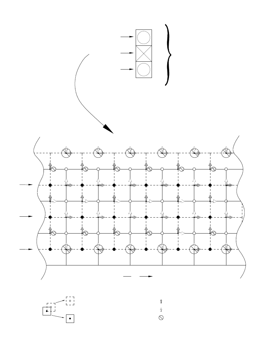
22.12. DIAGO
295
U-cell with grid point at coordinate (i,j)
T-cell with grid point at coordinate (i,j)
Advective velocity on face of T-cell
Advective velocity on face of U-cell
Quantity is not allowed at this location
j=3
j=2
j=1
i
j=3
j=2
j=1
{
Memory Window
Figure 22.2: The horizontal grid layout within a memory window of size jmw =3 indicating
cells, grid points, and sites where derived quantities can be defined. Allowable sited determine
how arrays must be dimensioned within the memory window.
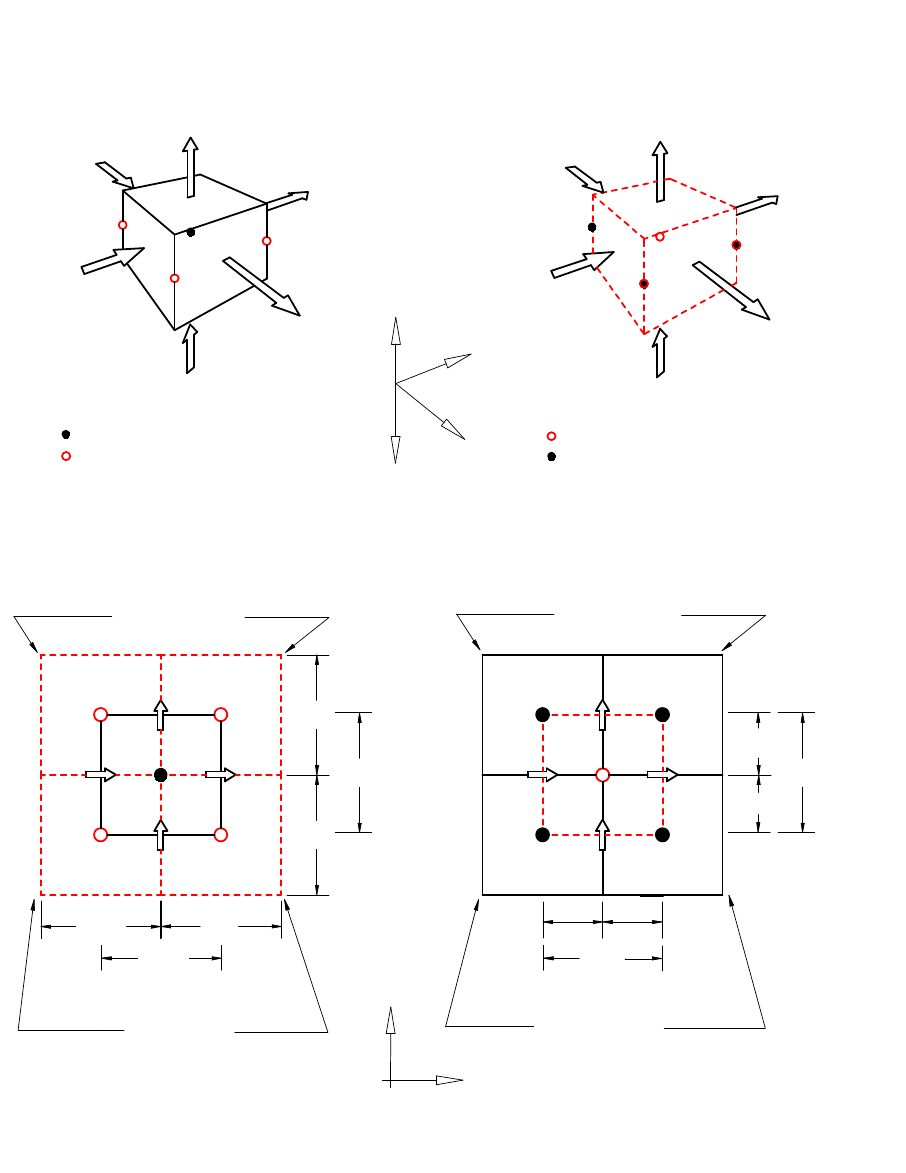
296
CHAPTER 22. SOLVING THE DISCRETE EQUATIONS
- T grid point inside cell
- U grid points on cell corners
adv_vet
i-1,k,j
adv_vbt
i,k,j
adv_vnt
i,k,j-1
adv_vet
i,k,j
adv_vnt
i,k,j
Cell T
i,k,j
Cell U
i,k,j
dyu
dyu
jrow-1
jrow
dxu
i-1
dxu
i
dxt
i
adv_vnt
i,k,j-1
adv_vet
adv_vet
i,k,j
i-1,k,j
adv_vnt
i,k,j
dyt
jrow
cell U
i-1,k,j
cell U
i,k,j
cell U
i,k,j-1
cell U
i-1,k,j-1
Cell T
i,k,j
Cell U
i,k,j
z
k
i
j
j
i
RCP
- U grid point inside cell
- T grid points on cell corners
a)
adv_vbt
i,k-1,j
adv_vbu
adv_veu
i-1,k,j
adv_vbt
i,k,j
adv_vnu
i,k,j-1
adv_veu
adv_vnu
i,k-1,j
i,k,j
i,k,j
b)
c)
dxu
adv_vnu
adv_veu
adv_veu
i-1,k,j
adv_vnu
due
i
i
dyu
jrow
i,k,j-1
i,k,j
i,k,j
duw
dus
jrow
dun
jrow
cell T
i,k,j+1
d)
cell T
i+1,k,j+1
cell T
i+1,k,j
cell T
i,k,j
i
Figure 22.3: a) Advective velocities on a T-cell. b) Advective velocities on a U-cell. c)
Horizontal slice through a T-cell showing grid points and surrounding U-cells d) Horizontal
slice through a U-cell showing grid points and surrounding T-cells
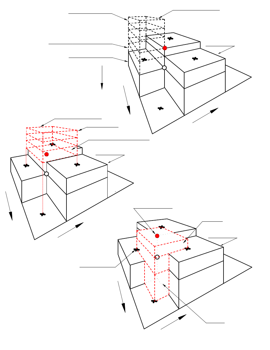
22.12. DIAGO
297
0.54
0
i
0
0
i
0.54
0
i
0
0
ocean surface z=0
Ocean U-cells
U
i,kbu+1,j
U
i,kmax,j
RCP
Land T-cells
Ocean cell T
Land cell T
k
ocean surface z=0
a)
Land T-cells
b)
Land T-cells
Bottom Ocean cell U
Depth
- z
Bottom Ocean cell T
i,kb,j
i,k=1,j
i,kb+1,j
adv_vbu
i,kbu,j
adv_vbt
i,kb,j
c)
j
j
j
i,kbu,j
Figure 22.4: a) Column of ocean T-cells in relation to bottom topography. “x” denotes vertical
velocity at the base of ocean bottom T-cells. “black dot” denotes vertical velocity at the base
of an ocean bottom U-cell. “open circle” denotes position of bottom vertical velocity from
continuous equation. b) Corresponding column of ocean U-cells. c) Truncated ocean U-cells
below bottom of the U-cell column.
298
CHAPTER 22. SOLVING THE DISCRETE EQUATIONS

Part VII
General model options
299

301
MOM is configured in various ways through the use of options which are enabled by setting
preprocessor type directives. The directives are usually placed on a preprocessor or compile
statement in a run script and take the form -Doption1 -Doption2 etc. Note that the -D must be
used as a prefix to the option name. For an example, refer to script run mom. Care should
be exercised when enabling options because there is no check for mispelled options. When
enabled, options eliminate or include portions of code thereby implementing desired features.
As MOM executes, a summary of all enabled options is given.
Some options are incompatible with others. Subroutine checks30 looks for all conflicting
options and if any are found, writes all error messages to the printout file before stopping.
Various additional checking is done and warning messages may also be issued. These are less
serious than error messages and allow MOM to continue. This does not mean they should be
ignored. They often give information about possibly inappropriate values being used. In fact,
it is a good idea to search the printout file to locate any “warning” messages and verify they
are harmless before continuing. Refer to Section 3.1 for details on how to perform searches.
In the rest of this part of the manual, MOM options will be grouped into catagories and
given brief explanations along with guidelines for useage. Diagnostic options are discussed
separately in Part VIII. Note that all numerical indices are exposed within expressions given
in this documentation so as to closely match with those used in the Fortran code. This extra
bit of detail is insisted upon as another way of insuring that complex formulations are correct.
30contained in file checks.F
302
Chapter 23
Options for testing modules
Modules and the usage of modules are described in Chapter 15. Within each module is a driver
intended to exercise the module in a simple environment. This means executing in a “stand
alond mode” as opposed to from within a model execution. Associated with each module is
arun script which activates the included driver with an option. These options are listed below
and are not to be enabled from within a model execution (because the model becomes the
driver).
23.1 test convect
This option activates a driver for the convection module in file convect.F. Refer to Section 15.1.1
for details.
23.2 drive denscoef
When executing the model, required density coefficients are automatically computed1from
within by calling module denscoef. However, script run denscoef activates a driver in “stand
alone mode” which gives details about density coefficients. Executing run denscoef uses infor-
mation from module grids and file size.h to construct density coefficients which depend on the
vertical discretization of the grid cells. Refer to Section 15.1.2 for details on density.
23.3 drive grids
This option activates a driver for the grids module in file grids.F. Refer to Section 15.1.3 for
details.
23.4 test iomngr
This option activates a driver for the I/O manager module in file iomngr.F. Refer to Section
15.1.4 for details.
1It is no longer required to construct density coefficients before executing the model.
303

304
CHAPTER 23. OPTIONS FOR TESTING MODULES
23.5 test poisson
This option activates a driver for the poisson module in file poisson.F. For more details refer to
Sectionsubsection:poisson.F.
23.6 test vmix
This option activates a driver for testing the vertical mixing scheme enabled by option ppvmix
or kppvmix. Refer to Section 15.1.6 for details.
23.7 test rotation
The model grid may be rotated using a set of Euler angles for solid body rotation. The Euler
angles are computed by defining the geographic latitude and longitude of the rotated north
pole and a point on the prime meridian. This option activates the driver which gives results
from a sample rotation of the model grid. It indicates how scalars and vectors are interpolated
and rotated before being used on the rotated model grid. Refer to Section 25.2.1 for details.
23.8 test timeinterp
This option activates a driver for the the time interpolation module in file timeinterp.F. Refer
to Section 15.1.7 for details.
23.9 test timer
This option activates a driver for the timing module in file timer.F. For more details refer to
Sectionsubsection:timer.F.
23.10 test tmngr
This option activates a driver for the time manager module in file tmngr.F. Refer to Section
15.1.9 for details.
23.11 drive topog
This option activates a driver for the topography and geometry module in file topog.F. Refer
to Section 15.1.10 for details.
23.12 test util
This option activates a driver for the utility module in file util.F. Refer to Section 15.1.11 for
details.

Chapter 24
Options for the computational
environment
24.1 Computer platform
Options are used to invoke minor changes in MOM which are computer platform specific
thereby enabling MOM to execute on various platforms. These changes tend to be concentrated
in the I/O manager, timing, and NetCDF routines. Only one platform must be specified.
24.1.1 cray ymp
This option configures MOM for the CRAY YMP which no longer exists at GFDL.
24.1.2 cray c90
This option configures MOM for the CRAY C90 which no longer exists at GFDL.
24.1.3 cray t90
This option configures MOM for the CRAY T90 which is the current computational workhorse
at GFDL. The operating system is Unicos 9.1.0.1 or later which does not have a “cf77” compiler.
Therefore all scripts assume an Fortran 90 compiler.
24.1.4 cray t3e
This option configures MOM for the CRAY T3e at GFDL and is necessary to insure the variables
on the heaps are aligned for communication purposes.
24.1.5 sgi
This option configures MOM for Silicon graphics workstations at GFDL. Fortran 90 is assumed.
24.2 Compilers
The intent is for an Fortran 90 compiler to be used in all scripts.
305
306
CHAPTER 24. OPTIONS FOR THE COMPUTATIONAL ENVIRONMENT
24.3 Dataflow I/O Options
Various options for handling I/O between disk and the memory window are available. Each
has its advantages and disadvantages as described in the following sections. One and only
one of these options must be enabled. It should be noted that regardless of which option is
used, details are implemented at the lowest level routines. This allows the higher level code
structure (where reading and writing takes place) to remain the same for all options.
Characteristics for each file are controlled by specifying file attributes (i.e. whether the
file is sequential, direct access, cray wordio, unformatted, etc.) in a character string which is
passed into the I/O manager iomngr.F. The I/O manager then assigns a unit number for each
file and opens the file with the specified attributes. Refer to Section 15.1.4 for details on the I/O
manager.
Otions relating to I/O are set at compile time with UNIX “cpp” directives of the form -
Doption. The available I/O options are “crayio”, “fio”, “ramdrive” or “ssread swrite” and are
described below. The platform options are “cray ymp”, cray c90”, “cray t90”, or “sgi” and are
described in Section 24.1.
The I/O within MOM occurs during initialization, integration, diagnostic analysis, and
shutdown. Initialization consists of reading namelist files, and possibly a restart file, boundary
condition data, and data for sponge zones along artificial boundaries. The namelist files have
the attributes “formatted sequential” and these files allow an easy way to override default
settings of coefficients and miscellaneous variables (i.e. mixing coefficients, time step lengths,
etc). They only amount to O(100) words and are therefore unimportant as far as efficiency
is concerned. The biggest part of initialization is the reading of a restart file which may be
huge (it contains two time levels of prognostic data plus the topography mask). The restart
file has the attributes “unformatted sequential” and on CRAY systems is buffered through the
“cachea layer” by an assign issued from within the I/O manager. The size of the buffer is
calculated within MOM and passed within the attribute character string. The attributes given
to boundary condition and sponge data are similar but contain the additional attribute “ ieee”.
The “ieee” attribute specifies that the data was created as 32 bit IEEE. The large initialization
files are buffered through the “cachea layer” on CRAY systems.
Prognostic data from the restart file is placed on “tau files” which take various forms
depending on whether option “ramdrive”, “crayio”, “fio”, or “ssread sswrite” was enabled.
The “tau files” are used during the integtration phase. By default, all of these options (except
for ramdrive) use attribute “sds” to instruct the I/O manager to put the files on CRAY Solid
state disk. The assign statements in the I/O manager can be changed to put the files on rotating
disk if desired (although this is very inefficient compared with solid state disk).
During the integration phase, diagnostic data is also written out. It may be of two forms:
Either 32bit IEEE or NetCDF. The recommended way is NetCDF which is specified by option
“netcdf”. The 32bit IEEE form is older and has not been extended to use buffering. The
shutdown phase basically writes the last image of the “tau files” onto a restart file with the
previously specified characteristics.
24.3.1 ramdrive
This one is similar in concept to the usage of the word ramdrive in the IBM PC world. It concerns
configuring a portion of memory to behave like disk which speeds up programs that are I/O
intensive particularly when disks are relatively slow. The catch is that there must be enough
memory available to contain the disk data. In MOM, this option defines a huge memory array
24.4. PARALLELIZATION
307
and replaces all reads and writes to disk with copying variables into or out of locations in this
huge array. This is done at the lowest subroutine levels so that the higher level routines look
the same regardless of whether this I/O option is used or not. This option is not specific to any
computer platform and therefore makes MOM highly portable.
24.3.2 crayio
This option uses the CRAY specific wordio package to read and write data to and from disk. As
currently configured, option crayio directs the iomngr to assign scatch files to CRAY solid state
disk. So solid state disk is assumed. If the “sds” attribute is removed from the file specification,
then the files will reside on rotating disk. Script run iomngr executes the driver in iomngr.F to
exercise this form of I/O in a simple environment.
24.3.3 ssread sswrite
This option uses the CRAY specific ssread/sswrite package to read and write data to and from
solid state disk. Solid state disk is assumed and this is the fastest way to more data between
solid state disk and memory. The performance is comparable to option ramdrive. All I/O is
done in blocks of 512 words and all blocking and buffering is done in iomngr.F and odam.F.
On the CRAY YMP, option crayio was sufficient for good performance. On the CRAY T90 it is
not. Script run iomngr executes the driver in iomngr.F to exercise this form of I/O in a simple
environment.
24.3.4 fio
This option uses Fortran direct access I/O to read and write data to and from disk. It works
on CRAY, SGI workstations and presumably any other platform which supports Fortran direct
access I/O. Record size is specified in words which is converted to bytes within the iomngr.
If solid state disk is not availbale, this option is very inefficient. However, it does allow the
model to run on non-CRAY systems which do not have enough memory to use option ramdrive
on a particular problem size. Script run iomngr executes the driver in iomngr.F to exercise this
form of I/O in a simple environment.
24.4 Parallelization
Currently, there is only one way to do multi-tasking in MOM as discussed in Chapter 12.
24.4.1 parallel 1d
Option parallel 1d is automatically added to the option list in the run mom script if the number
of processors is set greater than one. This option enforces a high level parallelism as described
in Section 12. When option parallel 1d is enabled, the message passing toolkit “mpt” must be
available on CRAY T90 platforms. All communication is in terms of Cray specific “shmem”
calls because it is faster than MPI or PVM on Cray platforms. When executing on the CRAY
T3E, option cray t3e must be enabled.
308
CHAPTER 24. OPTIONS FOR THE COMPUTATIONAL ENVIRONMENT
Chapter 25
Options for grid, geometry and
topography
25.1 Grid generation
How to design grids is detailed in Chapter 16. The options for implementing these ideas are
summarized below.
25.1.1 drive grids
Script run grids uses option drive grids to execute the grids module in “stand alone mode”.
This is the recommended method for designing grids. Option drive grids is not appropriate
when executing a model because the model itself becomes the driver.
25.1.2 generate a grid
This option is used for generating a grid domain and resolution as opposed to importing one.
Either this one or option read my grid must be enabled.
25.1.3 read my grid
This is the option to use when importing a domain and resolution generated from outside of
the MOM environment. Either this one or option generate a grid must be enabled.
25.1.4 write my grid
For exporting a domain and resolution generated by module grids.
25.1.5 centered t
This is for constructing a grid by method 1 as described in Chapter 16. If this option is not
enabled, grid construction is by method 2 which is the default method for MOM.
309
310
CHAPTER 25. OPTIONS FOR GRID, GEOMETRY AND TOPOGRAPHY
25.2 Grid Transformations
25.2.1 rot grid
Option rot grid allows the grid system defined by module grids to be rotated so that the pole is
outside the area of interest. Refer to Chapter 17 for details.
25.3 Topography and geometry generation
The options available for constructing topography and geometry are covered in detail in
Chapter 18 and summarized below. One and only one of the following options must be
enabled: rectangular box,idealized kmt,gaussian kmt,scripps kmt,etopo kmt, or read my kmt.
All others are optional.
25.3.1 rectangular box
This option constructs a flat bottomed rectangular domain on the grid resolution specified
by module grids. All interior ocean kmti,jrow are set to level km. If used with option cyclic
it configures a zonally re-entrant channel. If used with option solid walls then all boundary
kmti,jrow cells are land cells.
25.3.2 idealized kmt
This option constructs an idealized map of the world’s geometry with a bottom depth that is
not realistic. It requires no data and is highly portable. The geometry and topography are
interpolated to the resolution specified by module grids.
This option is also a good starting point for investigations where idealized geometries
need to be constructed. Other idealized geometries can be readily constructed with the aid
of subroutine setkmt which approximates continental shapes by filling in trapezoidal areas of
kmti,jrow with zero. All that is required for input are the grid point coordinates, the coordinates
of four vertices of a trapezoid, and a value for setting /kmt/within the trapezoid.
25.3.3 gaussian kmt
This option constructs a kmti,jrow field with a gaussian bump superimposed on a sloping
ocean floor in a rectangular basin without geometry. The slope of the floor and scale of the
bump can be set by modifying the USER INPUT section under the gaussian bump section
in module topog.F. This option requires no data and is therefore highly portable. Results are
interpolated to the resolution specified by module grids. Refer to Section 18.2 for more details.
25.3.4 scripps kmt
This generates geometry and topography interpolated from SCRIPPS data (in the DATABASE
described in Section 3.2) to the resolution specified by module grids.
25.3. TOPOGRAPHY AND GEOMETRY GENERATION
311
25.3.5 etopo kmt
This generates geometry and topography interpolated from a 1/12◦x 1/12◦dataset1to the
resolution specified by module grids.
25.3.6 read my kmt
This option imports a topography and geometry kmti,jrow field from outside of the MOM
environment or one produced from option write my kmt.
25.3.7 write my kmt
This option exports a topography and geometry kmti,jrow field by writing it to disk.
25.3.8 flat bottom
To deepen all ocean kmti,jrow cells to the maximum number of levels given by level km, enable
this option. It works with option idealized kmt or scripps kmt.
25.3.9 fill isolated cells
This option converts all isolated ocean T cells into land cells. An ocean T cell Ti,k,jis isolated if
the four surrounding U cells Ui,k,j,Ui−1,k,j,Ui−1,k,j−1, and Ui,k,j−1at the same vertical level kare
land cells. Potholes as well as trenches which are one T cell wide fall into this category.
25.3.10 fill shallow
This option converts ocean cells to land cells in regions where the ocean depth is shallower
than what is allowed.
25.3.11 deepen shallow
This option increases the number of ocean cells in regions where the ocean depth is shallower
than what is allowed.
25.3.12 round shallow
This option rounds the number of ocean cells to zero or the minimum number of allowable
ocean levels in regions where the ocean depth is shallower than what is allowed.
25.3.13 fill perimeter violations
This option builds a land bridge between two distinct land masses which are seperated only
by a distance of one ocean T cell. There must be at least two ocean T cells separating distinct
land masses.
1This dataset may be purchased from the Marine Geology and Geophysics Division of the National Geophysical
Data Center and is not included in the MOM DATABASE.

312
CHAPTER 25. OPTIONS FOR GRID, GEOMETRY AND TOPOGRAPHY
25.3.14 widen perimeter violations
This option removes land cells between two distinct land masses which are seperated only by
a distance of one ocean T cell. There must be at least two ocean T cells separating distinct land
masses.

Chapter 26
Partial Bottom Cells
Traditionally, all cells within a vertical level in MOM have the same vertical thickness. Op-
tion partial cell allows bottom ocean cells within any given level to be of different vertical
thickness so as to more accurately resolve the physical bottom (Pacanowski and Gnanade-
sikan, 1998). This option must be used right from the beginning of an experiment. It is not
intended as an option which can be enabled in the middle of an experiment. Nor is it intended
to be disabled in the middle of an experiment. Either a model is constructed using full-cells
(the default) or partial-cells (option partial cell).
26.1 Motivation
Bottom topography is discretized to model levels as described in Chapter 18. Fig 26.1a is an
example of a typical section of bottom topography compared with the resulting discretized
bottom. The solid line represents the “true” bottom which the discretization is trying to capture.
Ocean T-cells are indicated with grid points and land T-cells are shaded. The same bottom
discretized with partial bottom cells is indicated in Fig 26.1b where the bottom T-cell in each
column is allowed to be partially filled with land. Note that the topography is significantly
more accurately approximated when partial cells are used. Most of the change in regions of
steep slopes is captured by changes in the number of levels. Even so, partial cells give a better
estimation of the true slope in these regions. In general, T-cell (and U-cell) thickness becomes
a function of latitude, longitude and depth when partial cells are used. Note how the grid
points follow the topography in Fig 26.1b. In effect, a one level “sigma coordinate” has been
added by the partial cells.
Refer to Fig 26.2 which indicates what happens when horizontal resolution in Fig 26.1 is
doubled but vertical resolution remains unchanged. Comparing Fig 26.1a with Fig 26.2a indi-
cates that discretized bottom topography using full cells does not significantly improve when
horizontal resolution is increased. In fact, it remains about the same. However, comparing Fig
26.1b with Fig 26.2b, the improvement using partial cells is significant.
In addition to ocean volume and f/Hbeing more accurately represented by partial-cells,
topographic wave speeds are also more accurate and therefore so is the dispersion relation for
topographic waves as discusssed in Pacanowski and Gnanadesikan (1997). The disadvantage
of partial-cells is that the integration time is 10 to 15% longer than for full-cells for the same
number of vertical levels. However, to achieve the same accuracy, partial-cells are significantly
more computationally efficient than using full-cells and increasing the number of vertical
313
314
CHAPTER 26. PARTIAL BOTTOM CELLS
levels1. There is also a pressure gradient error with partial-cells but this is tiny as discussed
in Pacanowski and Gnanadesikan (1997). In the interior of the ocean, equations are second
order accurate (Treguier et al., 1996) but reduce to first order at bottom boundaries because the
thickness of partial-cells breaks the analytical stretching of grid cell thickness in the vertical.
Although equations drop from second order in the interior to first order for non full-cells at the
bottom, a leading order error in the position of the topography has been corrected. Globally,
the solution remains second order accurate.
26.2 Discrete Equations
The essential point is to note that part of the northern, southern, eastern, or western face of a
grid cell may be partially land and this must be taken into account when fluxing information
across cell faces. The discrete equations in Section 21.3 must be altered to account for vertical
cell thickness which is a function of λ,φ, and depth. In general, vertical cell thickness dztk
is replaced by dhti,k,jwhich is the vertical thickness of T-cells and dhui,k,jwhich is the vertical
thickness of U-cells. The thickness of T-cells dhti,k,jis determined when bottom topography
is discretized. Although ocean cells may be partial, all land cells are considered as full-cells.
Since material surfaces are defined by faces of T-cells, it follows that
dhui,k,j=min (dhti,k,j,dhti+1,k,j,dhti,k,j+1,dhti+1,k,j+1) (26.1)
Refer Fig 26.4 depicts the relationship between partial bottom T-cells and U-cells.
26.2.1 Momentum equations
To account for a generalized variation in cell thickness, a factor of dhui,k,jmust be included in
horizontal diffusive and advective operators. The following equations should be compared
with the corresponding set in Section 21.3.1:
ADV Uxi,k,j=1
2 cos φU
jrow dhui,k,j
δλ(adv f ei−1,k,j) (26.2)
ADV Uyi,k,j=1
2 cos φU
jrow dhui,k,j
δφ(adv f ni,k,j−1) (26.3)
DIFF Uxi,k,j=1
cos φU
jrow dhui,k,j
δλ(diff f ei−1,k,j) (26.4)
DIFF Uyi,k,j=1
cos φU
jrow dhui,k,j
δφ(diff f ni,k,j−1) (26.5)
where the horizontal viscous fluxes on U-cell faces become
diff f ei,k,j=visc ceui,k,j
cos φU
jrow
min(dhui,k,j,dhui+1,k,j)δλ(ui,k,j,n,τ−1) (26.6)
diff f ni,k,j=visc cnui,k,jcos φT
jrow+1min(dhui,k,j,dhui,k,j+1)δφ(ui,k,j,n,τ−1) (26.7)
1Increasing the number of vertical levels does allow interior flows to be better resolved.
26.2. DISCRETE EQUATIONS
315
Because the lateral boundary condition is no-flux for tracers but no-slip for velocity, the hori-
zontal viscosity 1
h∇ · (h∇(~
u)) has zonal and meridional components given by
VISCλ=Am
dhui,k,jcos2φUδλ(ζUλδλu)+Am
dhui,k,jcos φUδφ(cos φTζUφδφu)
+Am
1−tan2φU
a2u−Am
2 sin φU
a2cos2φUδλ(vλ)
+S(u) (26.8)
VISCφ=Am
dhui,k,jcos2φUδλ(ζUλδλv)+Am
dhui,k,jcos φUδφ(cos φTζUφδφv)
+Am
1−tan2φU
a2v+Am
2 sin φU
a2cos2φUδλ(uλ)
+S(v).(26.9)
where Amis the lateral viscosity coefficient2. The above form differs from Bryan (1969) due to
the inclusion of effective cell face heights ζUλand ζUφand a sink term due to a no-slip lateral
boundary condition given by
ζUλ
i,k,j=min(dhui,k,j,dhui+1,k,j) (26.10)
ζUφ
i,k,j=min(dhui,k,j,dhui,k,j+1) (26.11)
S(β)=−Am
dhui,k,jcos2φUdxuidhui,k,j−ζUλ
dxti+1
+dhui,k,j−ζUλ
i−1
dxtiβ
−Am
dhui,k,jcos φUdyujrow cos φT
j+1(dhui,k,j−ζUφ)
dytjrow+1
+
cos φT(dhui,k,j−ζUφ
j−1)
dytjrow β(26.12)
which is zero where U-cell thickness is constant (i.e. dhui,k,j=ζUλ) within a vertical level but
acts effectively as a bottom drag
S(β)∝(Am/∆2xU)β··· assuming dxui=dyujrow (26.13)
where U-cell thickness varies within a vertical level. The constant of proportionality ((dhui,k,j−
ζUλ)/dhui,k,j) represents the fraction of cell face height over which a no-slip condition is applied.
There is no change in the form of the horizontal advective flux given by Equations (22.86) and
(22.87) because advective velocities adv vnti,k,jand adv veti,k,jabsorb a factor dhui,k,jand become
advective transports given by Equations (26.40) and (26.41). Horizontal advective velocities
for the U-cells are then given by Equations (22.22) and (22.21).
The only change in the vertical advective and vertical diffusive operators is to replace dztk
in the vertical derivative with dhui,k,j. When defining vertical fluxes at the bottom cell faces,
dhwkin the vertical derivatives is replaced by min (dhuti,k,j,dhuti+1,k,j,dhuti,k,j+1,dhuti+1,k,j+1).
2The formulation is for constant Am. Variable Amrequires additional terms.
316
CHAPTER 26. PARTIAL BOTTOM CELLS
26.2.2 Pressure gradient
When vertical thickness of cells is a function of λ,φ, and depth, extra terms are needed to
construct the pressure gradient. Refer to Pacanowski and Gnanadesikan for a discussion of
the pressure gradient. Another way to look at it is the following: With the aid of Leibnitz’s
Rule (Equation (4.65), the zonal and meridional pressure gradients are written as
−grav
ρ◦a·cos φZ0
z
∂ρ
∂λdz′=−grav
ρ◦a·cos φ∂
∂λ(Z0
z
ρdz′)−ρ∂z
∂λ(26.14)
−grav
ρ◦aZ0
z
∂ρ
∂φdz′=−grav
ρ◦a∂
∂φ(Z0
z
ρdz′)−ρ∂z
∂φ(26.15)
where ρis density and the acceleration due to gravity is grav =980.6 cm/sec2. Let Px(k)
symbolize the the discrete form for the right hand side of the zonal pressure gradient in
Equation (26.14) and Py(k) symbolize the discrete form for the right hand side of the meridional
pressure gradient in Equation (26.15). The discrete forms are
Px(k)=−1
ρ◦cos φU
jrow δλ(pi,k,j)−grav ·ρi,k,jλ·δλ(zti,k,j)
φ
(26.16)
Py(k)=−1
ρ◦δφ(pi,k,j)−grav ·ρi,k,jφ·δφ(zti,k,j)
λ(26.17)
where the ()φin Px(k) and the ()λin Py(k) are used to move the results onto a U-cells. The
pressure pi,k,jis defined on T-cells and is calculated by vertically integrating the density from
the surface to the depth of the T-grid point at level “k”.
pi,k,j=grav ·ρi,1,j·dhwi,0,j+grav ·
k
X
m=2
ρi,m−1,jzdhwi,m−1,j(26.18)
where dhwi,k,jis the vertical distance between a T-grid point at level “k” and its neightbor at
“k+1” for any coordinate index “i,j”. In the first term, dhwi,0,jis the distance between the ocean
surface and the grid point within level k=1. Partial cells are only allowed for levels k>1
and so dhwi,0,jis constant for all “i,j”. Using Equation (26.18), the term δλ(pi,k,j) in Px(k) can be
written as
δλ(pi,k,j)=grav ·dhwi,0,j·δλ(ρi,1,j)+grav ·δλ(
k
X
m=2
ρi,m−1,jzdhwi,m−1,j)(26.19)
Refer to Fig 26.3 which illustrates two vertical columns of T-cells with one partial bottom
cell at level “k”. Consider the vertically stratified case where density is a function of depth
only. This condition implies
δλ(ρi,k′,j)=δφ(ρi,k′,j)=0f or k′<k(26.20)
ρi,k′,jλ=ρi,k′,jφ=ρi,k′,jf or k′<k(26.21)
26.2. DISCRETE EQUATIONS
317
which reduces Equation (26.19) to
δλ(pi,k,j)=grav ·δλ(ρi,k−1,jzdhwi,k−1,j)(26.22)
Distributing the derivative and reducing further yields
δλ(pi,k,j)=grav ·ρi,k−1,jzλ·δλ(dhwi,k−1,j)+dhwi,k−1,j
λ·δλ(ρi,k−1,jz)
=grav
2·(ρi,k−1,jλ+ρi,k,jλ)·δλ(zti,k,j)+dhwi,k−1,j
λ·δλ(ρi,k,j)(26.23)
Substituting the above form for δλ(pi,k,j) into Equation (26.16) yields
Px(k)=−grav
2ρ◦cos φU
jrow ρi,k−1,jλ·δλ(zti,k,j)+dhwi,k−1,j
λ·δλ(ρi,k,j)−ρi,k,jλ·δλ(zti,k,j)
φ
(26.24)
In general, density can be divided into two pieces: one that varies linearly with depth and
another that varies non-linearly with depth. The non-linear part will lead to non-zero pressure
gradients in the vicinity of partial cells. The linear portion of the density variation with depth
goes to zero.
26.2.2.1 Example where density varies linearly with depth
If density varies linearly with depth, then
δz(ρi,k,j)=constant (26.25)
and density ρi,k,jcan be expanded in terms of density in the upper level ρi,k−1,jas
ρi,k,j=ρi,k−1,j+δzρi,k−1,j·dhwi,k−1,j.(26.26)
Using the above expansion to eliminate ρi,k,jin Equation (26.24) results in the following expan-
sions:
δλ(ρi,k,j)=δz(ρi,k−1,j)·δλ(zti,k,j) (26.27)
ρi,k,jλ=ρi,k−1,j+δz(ρi,k−1,j)·dhwi,k−1,j
λ.(26.28)
Substituting the above expansions into Equation (26.24) results in
Px(k)=0 (26.29)
318
CHAPTER 26. PARTIAL BOTTOM CELLS
26.2.2.2 Computing density in partial bottom cells
The dependence of density on pressure is linear below a few hundred meters. As was shown
above, there are no pressure gradients induced by partial bottom cells due to linear variations
in density with depth. With a linear equation of state, bottom flows induced by partial bottom
cells are within machine roundoff. Density anomoly using a non-linear equation of state as
given by Equation (15.7) is not correct at grid points within partial cells because the polynomial
coefficients, reference temperatures and reference salinities are defined only at the depth of grid
points within discrete model levels. Effectively, partial bottom cells imply an infinite number
of vertical levels. Density anomoly at the grid point within a partial cell can be approximated
by linearly interpolating the polynomial coefficients, reference temperatures and reference
salinities used in the equation of state (Equation 15.7) to the depth of the partial bottom cell
grid point.
Without correcting the density anomoly for the depth of the partial bottom cells, a linear
stratification of temperature in a non-linear equation of state generates error flows of about 1
cm/sec along topography (gaussian bump) in a 1◦resolution model simulation. However, by
accounting for the depth of the grid point within the polynomial approximation to the equation
of state, the error flows are reduced by an order of magnitude.
26.2.3 Tracer equations
To account for a generalized variation in cell thickness, a factor of dhti,k,jmust also be included
in horizontal diffusive and advective operators for tracers. The following equations should be
compared with the corresponding set in Section 21.3.2:
ADV Txi,k,j=1
2 cos φT
jrow dhti,k,j
δλ(adv f ei−1,k,j) (26.30)
ADV Tyi,k,j=1
2 cos φT
jrow dhti,k,j
δφ(adv f ni,k,j−1) (26.31)
DIFF Txi,k,j=1
cos φT
jrow dhti,k,j
δλ(diff f ei−1,k,j) (26.32)
DIFF Tyi,k,j=1
cos φT
jrow dhti,k,j
δφ(diff f ni,k,j−1) (26.33)
(26.34)
The diffusive fluxes on T-cell faces are
diff f ei,k,j=diff ceti,k,j
cos φT
jrow
min(dhti,k,j,dhti+1,k,j)δλ(tint
i,k,j,n,τ−1) (26.35)
diff f ni,k,j=diff cnti,k,j·cos φU
jrow min(dhti,k,j,dhti,k,j+1)δφ(tint
i,k,j,n,τ−1) (26.36)
The superscript “int” in the tracer quantity denotes a linear interpolation in the vertical to the
minimum depth of the two points being considered in the horizontal derivative. The form of
the linear interpolation is

26.3. CONSERVATION OF ENERGY
319
δλ(tint
i,k,j,n,τ−1)=(ti+1,k,j,n,τ−1−min(dhwti+1,k,j,dhwti,k,j)·ti+1,k−1,j,n,τ−1−ti+1,k,j,n,τ−1
dhwti+1,k−1,j
−(ti,k,j,n,τ−1−min(dhwti+1,k,j,dhwti,k,j)·ti,k−1,j,n,τ−1−ti,k,j,n,τ−1
dhwti,k−1,j
)
)/dxui(26.37)
where dhwti,k,jis the vertical distance between the grid point in cell Ti,k,jand cell Ti,k+1,j.
If the above linear interpolation is not done, horizontal diffusion leads to an enhanced vertical
diffusion in the vicinity of partial cells. This can easily be demonstrated by defining a temper-
ature and salinity stratification which is only a linear function of depth. Horizontal diffusion
should be zero. However, in the vicinity of partial cells, it will not be zero unless the above
linear interpolation is used.
The form of the advective fluxes given by Equations (22.43) and (22.44) does not change.
However, horizontal advective velocities adv veti,k,jand adv veti,k,jabsorb a factor of dhui,k,jto
become horizontal advective transports given by Equations (26.40) and (26.41).
26.3 Conservation of energy
26.3.1 Changes in Kinetic energy due to partial bottom cells
When vertical thickness of cells is a function of λ,φ, and depth, extra terms are needed to
construct the change in kinetic energy due to pressure forces. Multiplying the zonal pressure
gradient given in Equation (26.14) by uand the meridional pressure gradient given in Equation
(26.15) by vand integrating over the entire ocean volume yields the change in kinetic energy.
The finite difference equivalent of this expression is
−1
ρ◦
jmt−1
X
jrow=2
km
X
k=1
imt−1
X
i=2
dvoli,k,jui,k,j,1,τ
δλ(pi,k,jφ)
cos φU
jrow
+ui,k,j,2,τ ·δφ(pi,k,jλ)
−ui,k,j,1,τ
grav ρi.k.jλδλ(zti,k,j)
φ
cos φU
jrow −ui,k,j,2,τ grav ρi.k.jφδφ(zti,k,j)
λ(26.38)
where the velocity cell volume element is
dvoli,k,j=dxuicos φU
jrow dyujrow dhui,k,j.(26.39)
Note that there are four terms in Equation (26.38). The first two are similar to Equation (A.89)
except that dztkin the U-cell volume element has been replaced by dhui,k,jwhich is the vertical
thickness of a U-cell as given by Equation (26.1).
The reduction of Equation (26.38) is similar to the one given for Equation (A.89) except for
differences needed to account for spatial dependence of dhui,k,j. In Equation (A.91), dztkmust
be removed and dhui,k,jis placed inside both derivatives with subscripts matching those on
the velocity. In Equation (A.92), dztkis eliminated and dhui,k,jis placed inside both averages
with subscripts matching those on the velocity. The horizontal advective velocites become
advective transports defined as
320
CHAPTER 26. PARTIAL BOTTOM CELLS
adv vnti,k,j=ui−1,k,j,2,τ ·dxui−1·dhui−1,k,j
λ
dxti
cos φU
jrow (26.40)
adv veti,k,j=ui,k,j−1,1,τ ·dyujrow−1·dhui,k,j−1
φ
dytjrow
(26.41)
but the vertical advective velocities remain as velocities and the continuity equation becomes
adv veti,k,j−adv veti−1,k,j
dxti·cos φT
jrow
+adv vnti,k,j−adv vnti,k,j−1
dytjrow ·cos φT
jrow
+adv vbti,k−1,j−adv vbti,k,j=0 (26.42)
which leads to a change in kinetic energy given by
−grav
ρ◦
jmt−1
X
jrow=2
km
X
k=1
imt−1
X
i=2
adv vbti,k−1,j·ρi,k−1,jzdxticos φT
jrow dytjrow dhwi,k−1,j(26.43)
Note that thickness factor dzwk−1in Equation (A.99) has been replaced by its spatially dependent
counterpart dhwi,k−1,jwhich is the vertical distance between grid points within cells Ti,k,jand
Ti,k−1,j. The change in kinetic energy due to the third and fourth terms is given next.
26.3.2 Additional kinetic energy change due to boundary effects
After cancelling the cosine, the third term in Equation (26.38) is written as
−grav
ρ◦
jmt−1
X
jrow=2
km
X
k=1
imt−1
X
i=2
ui,k,j,1,τ ρi.k.jλδλ(zti,k,j)
φ
dxuidyujrow dhui,k,j(26.44)
where zti,k,jis the depth from the ocean surface to the point within cell Ti,k,j. Using the
latitudinal version of Equation (21.14) to re-arrange terms in the summation on “jrow” gives
−grav
ρ◦
jmt−1
X
jrow=2
km
X
k=1
imt−1
X
i=2
ui,k,j−1,1,τ ·dhui,k,j−1·dyujrow−1
φ·ρi.k.jλδλ(zti,k,j)dxui(26.45)
and substitution from Equation (26.41) yields
−grav
ρ◦
jmt−1
X
jrow=2
km
X
k=1
imt−1
X
i=2
adv veti,k,j·ρi,k,jλ·δλ(zti,k,j)dxuidytjrow (26.46)
Again, using Equation (21.15) to re-arrange terms in the longitudinal summation on“i” yields
26.3. CONSERVATION OF ENERGY
321
grav
ρ◦
jmt−1
X
jrow=2
km
X
k=1
imt−1
X
i=2
δλ(adv veti−1,k,j·ρi−1.k.jλ)zti,k,jdxtidytjrow (26.47)
The fourth term in Equation (26.38) is
−grav
ρ◦
jmt−1
X
jrow=2
km
X
k=1
imt−1
X
i=2
ui,k,j,2,τ ·ρi.k.jφδφ(zti,k,j)
λ
dxuicos φU
jrow dyujrow dhui,k,j(26.48)
A similar manipulation as given for the third term above reduces this fourth term to
grav
ρ◦
jmt−1
X
jrow=2
km
X
k=1
imt−1
X
i=2
δφ(adv vnti,k,j−1ρi.k.j−1φ)zti,k,jdxtidytjrow (26.49)
Combining Equations (26.43), (26.47) and (26.49) gives the total change in kinetic energy due
to pressure terms as
grav
ρ◦
jmt−1
X
jrow=2
km
X
k=1
imt−1
X
i=2δλ(adv veti−1,k,jρi−1,k,jλ)+δφ(adv vnti,k,j−1ρi.k.j−1φ)zti,k,jdxtidytjrow
−adv vbti,k−1,jρi,k−1,jzdxticos φT
jrow dytjrow dhwi,k−1,j(26.50)
26.3.3 Changes in Potential energy due to partial bottom cells
When vertical thickness of bottom cells at a given depth is a function of λand φthen extra terms
are needed to construct the change in potential energy due to advection. As a consequence of
absorbing a vertical grid cell thickness factor into the advective transports of Equations (26.41)
and (26.40) , the advection operator for T-cells takes the form
LT(αi,k,j)=δλ(adv veti−1,k,j·αi−1,k,jλ)+δφ(adv vnti,k,j−1·αi,k,j−1φ)
dhti,k,jcos φT
jrow
+δz(adv vbti,k−1,j·αi−1,k,jλ) (26.51)
and Equation (A.100) is re-written as
−grav
ρ◦
jmt−1
X
jrow=2
km
X
k=1
imt−1
X
i=2
zti,k,j(dxticos φT
jrow dytjrow dhti,k,j)×
δλ(adv veti−1,k,j·ρi−1,k,jλ)+δφ(adv vnti,k,j−1·ρi,k,j−1φ)
dhti,k,jcos φT
jrow
+δz(adv vbti,k−1,j·ρi,k−1,jz)(26.52)
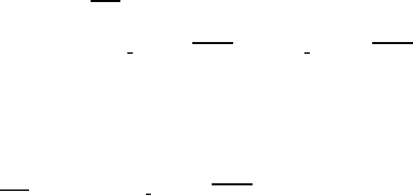
322
CHAPTER 26. PARTIAL BOTTOM CELLS
where ztkhas been replaced by zti,k,jand dztkhas been replaced by dhti,k,j. Note the extra
factor of dhti,k,jin the denominator. Because of these changes, the summation of the first two
terms over a horizontal surface will not vanish. After some cancellations, the work done by
horizontal advection of density is
−grav
ρ◦
jmt−1
X
jrow=2
km
X
k=1
imt−1
X
i=2
zti,k,jdxtidytjrow ×
δλ(adv veti−1,k,j·ρi−1,k,jλ)+δφ(adv vnti,k,j−1·ρi,k,j−1φ).(26.53)
which exactly compensates for the loss of kinetic energy due to the first two terms in Equation
(26.50). The third term in Equation (26.52) may be re-arranged in the vertical summation to
yield
grav
ρ◦
jmt−1
X
jrow=2
km
X
k=1
imt−1
X
i=2
adv vbti,k−1,j·ρi,k−1,jz·dhwi,k−1,jdxticos φT
jrow dytjrow (26.54)
which is the work due to buoyancy and exactly compensates for the remaining change in
kinetic energy in Equation (26.50).
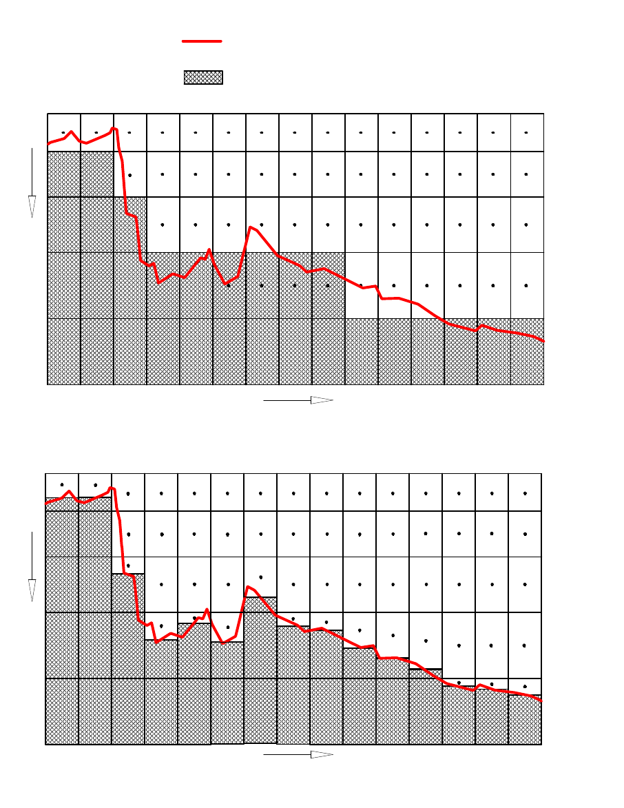
26.3. CONSERVATION OF ENERGY
323
a)
Full cells
Actual bottom topography
Discretized bottom topography
Depth
Depth
Latitude
Latitude
RCP
b)
Partial cells
Figure 26.1: Comparing bottom topography for a 1x horizontal resolution a) Using full cells.
b) Using partial bottom cells
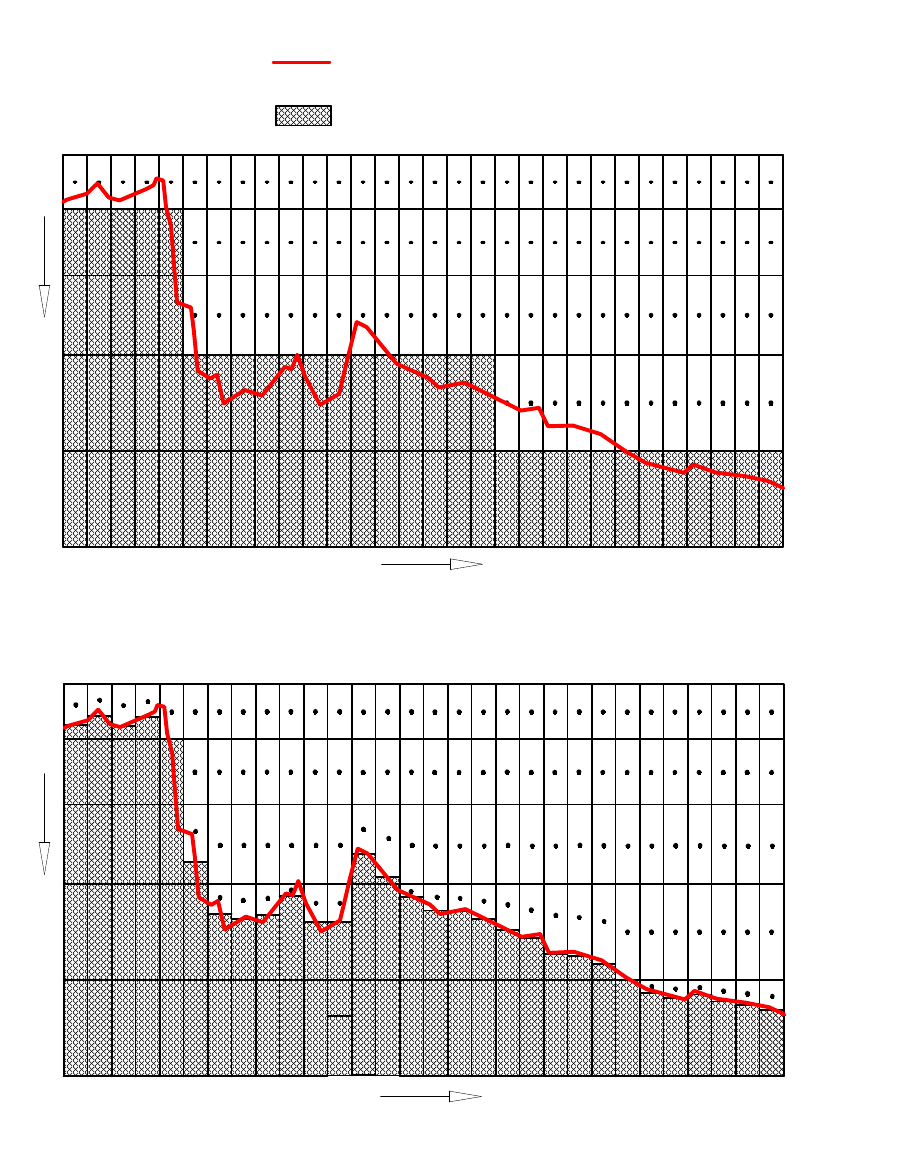
324
CHAPTER 26. PARTIAL BOTTOM CELLS
a)
Full cells
Actual bottom topography
Discretized bottom topography
Depth
Depth
Latitude
Latitude
b)
Partial cells
RCP
Figure 26.2: Comparing bottom topography for a 2x horizontal resolution a) Using full cells.
b) Using partial bottom cells
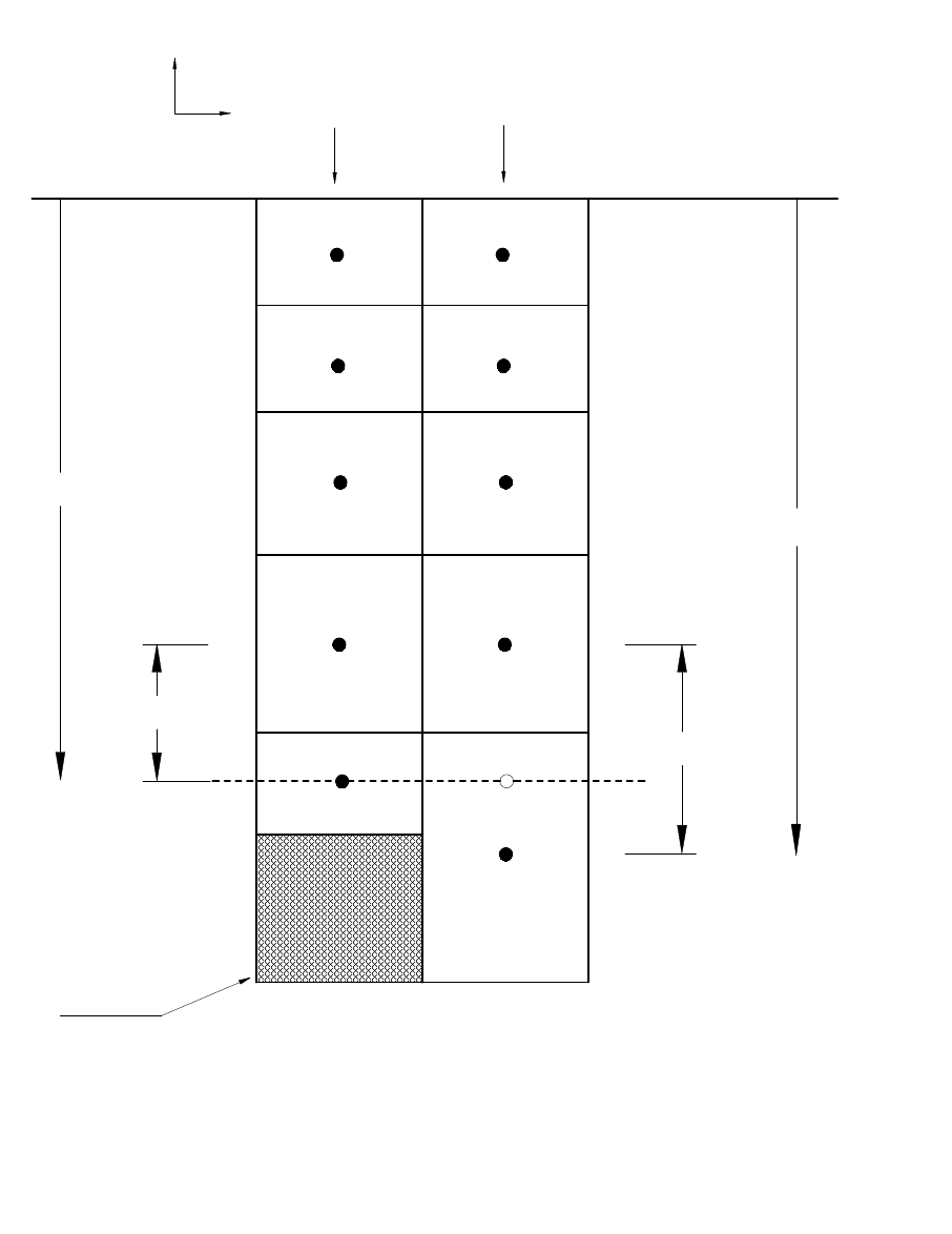
26.3. CONSERVATION OF ENERGY
325
+1
i
dhw
i+1,k-1,j
dhw
i,k-1,j
zt
i,k,j
zt
i+1,k,j
ρ
i,k,j
ρ
i,k-1,j
ρ
i+1,k-1,j
ρ
i+1,k,j
i
z=0
Partial cell
λ
Z
Figure 26.3: Two vertical columns of T-cells with one partial bottom cell
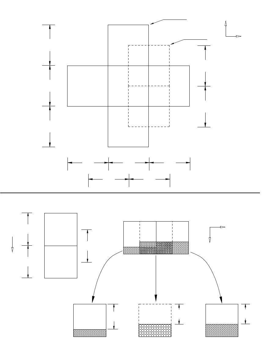
326
CHAPTER 26. PARTIAL BOTTOM CELLS
α
i,k,j
α
i,k-1,j
1
1
1
h
∆
h
∆
W
i,k-1,j
W
i,k,j
0.61
1
0.61
1
U
i,k,j
U
i-1,k,j
α
i,k,j+1
α
i,k,j-1
1
1
1
1
1
u
i,k,j
u
i,k,j-1
α
i,k,j
V
i,k,j
V
i,k,j-1
1
1
1
1
1
1
h
∆
T
i,k,j
u
i,k,j
a)
b)
h
W
∆
i,k-1,j
T
i,k,j
i,k-1,j
T
Depth
k
u
i,k,j
h
U
∆
i,k,j
α
i+1,k,j
α
i,k,j
α
i+1,k,j
h
T
∆
i+1,k,j
α
i-1,k,j
α
i+1,k,j
x
T
x
U
x
T
x
T
x
U
∆
∆
∆
∆
∆
i
i
i-1
i-1
i+1
y
∆
T
j+1
y
∆
T
j
y
∆
T
j-1
y
∆
U
j+1
y
∆
U
j
T-cells
U-cells
j
i
c)
Depth
k
i
α
i,k,j
Figure 26.4: a) Horizontal arrangement of T-cells and U-cells. b) Two partial bottom T-cells
with a partial bottom U-cell. In general, the partial bottom U-cell thickness is determined by
the minimum thickness of four surrounding partial bottom T-cells.
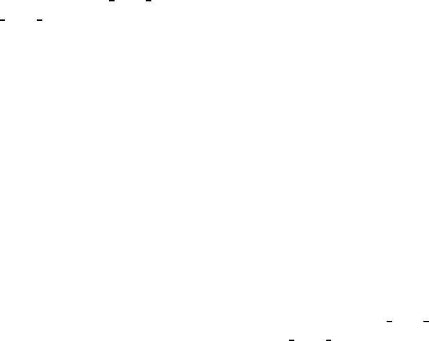
Chapter 27
Filtering
In general, the equations of motion are filtered in various ways to remove components from
the solution which are physically unimportant but nevertheless limit the length of the time
step.
27.1 Convergence of meridians
Because the model is formulated in spherical coordinates, convergence of meridians near
the earth’s poles reduces the effective grid size in longitude. At high latitude, the solution
may start to become unstable because of too large a time step. Instead of decreasing the
time step, an alternative is to filter the solution at high (polar) latitudes to remove unstable
wavenumber components. There are two filtering methods described below for suppressing
these components. Option fourfil uses Fourier filtering and option firfil uses a finite impulse
response filter to accomplish the same thing. Either one of these is typically applied polward
of a reference latitude determined by the researcher. In the southern hemisphere, the reference
latitude is given by filter reflat s and in the northern hemisphere, the reference latitude is given
by filter reflat n. To save computation over the land mass of Antarctica, filtering is turned off
southward of latitude rjfrst. These variables can be set through namelist. Refer to Section
14.4.6.
An alternative to filtering is to rotate the grid so that the convergence of meridians takes
place outside to the model domain. Refer to Section 25.2.1 for details.
27.1.1 fourfil
Due to the convergence of meridians on a sphere, longitudinal grid resolution decreases toward
zero as the poles are approached. For global domains this may severely limit the length of the
time step due to the CFL constraint given in Section 14.4.4. The instability can be removed
by filtering (Bryan, Manabe, and Pacanowski, 1975 and Takacs, Balgovind, 1983) the smallest
scales out of the solution since they impose the most severe restriction on the time step.
Filtering is not to be encouraged and is not recommended unless absolutely necessary.
When necessary, it should be restricted to the northernmost and southernmost polar latitudes
in the domain. Typically, the filtering works on strips of latitude defined by the researcher. In
the southern hemisphere, the reference latitude is given by filter reflat s and in the northern
hemisphere, the reference latitude is given by filter reflat n. By default, these values are set to
70◦N and 70◦S latitude for the test case resolution. With higher resolution, these reference
327
328
CHAPTER 27. FILTERING
latitudes can and should be pushed further poleward. To save computation over the land mass
of Antarctica, filtering is turned offsouthward of variable rjfrst which is defaulted to 81◦S. If
needed, these variables can be set through namelist. Refer to Section 14.4.6.
Option fourfil does a Fourier smoothing of prognostic variables in the longitudinal direction
by truncating wavenumbers larger than a critical one given by
N=im cos φT
jrow
cos f ilter re f lat s (27.1)
where Nis the number of waves to retain, im is the length of a strip of ocean data along
the latitude given by cos φT
jrow, and f ilter re f lat s is a reference latitude row in the southern
hemisphere ( f ilter re f lat n would be used for the northern hemisphere.). If data were being
filtered on the latitude of U-cells, then cos φT
jrow would be replaced by cos φU
jrow. Because of
geometry and topography break up each latitude circle, each filtering latitude is composed of
strips defined by starting and stopping longitudes for ocean data and each strip is therefore
a function of latitude and depth. There are a lot of different sized strips which rules out the
use of an FFT. Also, FFT’s are inherently square whereas for filtering purposes, fewer than
im wavenumbers are generally needed. Instead, a fourier transform is used which has been
optimized in prehistoric times. As such, it is difficult to understand1exactly how this fourier
decomposition and systhesis works by looking at the code since no reference was left by the
original designer (Mike Cox who is now deceased). In principle the filter is doing the following.
Any variable αiwhere i=1,im can be decomposed and re-constructed in terms of a discrete
Fourier transform given by
˜αi=A◦+
N/2
X
ℓ=1
wℓAℓcos 2πiℓ
im +
N/2−1
X
ℓ=1
wℓBℓsin 2πiℓ
im (27.2)
where ˜αiis the filtered value of αcomposed of Nwavenumbers (N≤im) given by Equation
(27.1) and the even and odd Fourier coefficients Aℓand Bℓare
A◦=1
im
im
X
i=1
αi(27.3)
Aℓ=2
im
im
X
i=1
αicos 2πiℓ
im f or ℓ=1,2,··· ≤ N
2−1 (27.4)
Aim/2=1
im
im
X
i=1
αicos(iπ) (27.5)
Bℓ=2
im
im
X
i=1
αisin 2πiℓ
im f or ℓ=1,2,··· ≤ N
2−1 (27.6)
The window wℓis given by the boxcar function
wℓ=1 (27.7)
1If any researcher understands what is being done then please contact me. (rcp@gfdl.gov)
27.1. CONVERGENCE OF MERIDIANS
329
which can lead to oscillations when wavenumbers greater than N are truncated. These os-
cillations are known as the Gibbs effect which is particularly pronounced if energy exists at
the truncation wavenumber N. The Gibbs effect can increase variance and this is a drawback.
The Gibbs effect can be minimized by multiplying the wavenumbers by a window. A typical
cosine window is
wℓ=cos((π/2)ℓ/N).(27.8)
Tracers are filtered using even Fourier coefficients (cosines) because the boundary condition
at edges of the tracer strips is no-flux. Odd Fourier coefficients (sines) are used for velocity
components because of the no-slip boundary condition at the edges of the velocity strips.
Vorticity (ztdi,jrow) is filtered with even Fourier coefficients2. Strips which completely encircle
the earth are filtered using the full series of sines and cosines using a cyclic boundary condition.
Any vector which is filtered must first remove the wavenumber which is due to the changing
direction of a latitude circle. This is wavenumber one for all latitudes. For instance, the x-
component of constant cross polar flow will exhibit a wavenumber one influence. After the
filtering operation, this wavenumber one due to the changing direction of the latitude circle
must be put back.
Apart from the Gibbs problem, another drawback of fourier filtering is that two strips of
different length on the same latitude circle will contain different wavenumbers after filtering.
The reason is that truncation wavenumber is a function of strip length and not total distance
around the latitude circle. If the two strips were on adjacent latitudes, then taking the diver-
gence of horizontal velocity might introduce ficticious vertical velocities (because of differing
scales on the strips. Note that option firfil does not have this problem.). Also, fourier filtering
can be a real time burner and FFT’s are of little help because of the arbitrary strip widths
and the need to enforce proper boundary conditions at the side walls (i.e. zero filling of land
will not work). It should be noted that filtering a function with a fourier transform and the
cosine window given above yields results very similar to the much faster finite impulse filter
described below. Also, the finite impulse filter does not induce a ficticious vertical velocity
because the filtering is not a function of strip size.
27.1.2 firfil
For the reasons given above, it may be desirable to filter the solution in polar latitudes. Op-
tion firfil uses multiple passes with a simple symmetric finite impulse response filter (Hamming
1977) to accomplish the filtering. Its advantage over fourier filtering with option fourfil is speed
and there is also no ficticiously induced vertical velocity (described above) because the amount
of filtering is not a function of strip size. The finite impluse filter is also designed to handle
land points without the need for code to pull out the various strips as is needed for fourier
filtering. Additionally, option firfil will not increase variance (and there is no introduction of
negative values into a field that is all positive).
As with fourier filtering, the amount of filtering is a function of latitude and is controlled
by the number of passes of the filter. The number of passes is arbitrairly given by
num f lt =cos f ilter re f lat s
cos φT
jrow
(27.9)
2Strips for the vorticity do not include coastal ocean cells because of the island integrals.
330
CHAPTER 27. FILTERING
where f ilter re f lat s is the southern reference latitude and numflt is the number of filter appli-
cations per prognostic variable per latitude and the cos φT
jrow is the cosine of that latitude. If
filtering in the northern hemisphere, then f ilter re f lat n would be used instead of f ilter re f lat s.
Variable numflt is for T cell latitudes and there is a corresponding numflu for the number of
passes used for variables on U cell latitudes. Equation (27.9) is arbitrary and should be adjusted
by the researcher to get the desired effect.
A finite impulse filter can be written as
˜αi=
M
X
ℓ=−M
cℓαi+ℓ(27.10)
and its transfer function is
H(ω)=c◦+2
M
X
ℓ=1
Cℓcos(ω)f or ω=0to π(27.11)
A very simple one is used with M=1 and weights given by
˜αi=1
4αi−1+1
2αi+1
4αi+1(27.12)
The transfer function is
H(ω)=1
2(1 +cos(ω)) (27.13)
The effect of multiple applications of this filter can be easily calculated. If the filter is
applied num f lt times then the transfer function is Hnum f lt(ω).
It is useful to demonstrate that the M=1 filter (a “1-2-1” filter) does not change the zonal
mean of a field, so long as the zonal grid spacing is uniform and the field has cyclic symmetry,
or the field satisfies the no-flux condition on the zonal land/ocean boundaries. For this purpose,
consider the zonal sum of the filtered field
h˜αix=
imt−1
X
i=2
˜αi
=
imt−1
X
i=2
(1
4αi−1+1
2αi+1
4αi+1)
=1
2
imt−1
X
i=2
αi+1
4
imt−1
X
i=2
(αi−1+αi+1).(27.14)
The first term represents the zonal sum of the unfiltered field
hαix=
imt−1
X
i=2
αi.(27.15)
The other two terms are almost this zonal sum, except for some boundary points
imt−1
X
i=2
αi−1=
imt−2
X
i=1
αi
27.1. CONVERGENCE OF MERIDIANS
331
=α1−αimt−1+
imt−1
X
i=2
αi
=α1−αimt−1+hαix,(27.16)
and likewise
imt−1
X
i=2
αi+1=
imt
X
i=3
αi
=−α2+αimt +
imt−1
X
i=2
αi
=−α2+αimt +hαix.(27.17)
Therefore, the zonal sum of the filtered field is given by
h˜αix=hαix+(α1−α2+αimt −αimt−1),(27.18)
and the zonal sum is unchanged if the unfiltered field satisfies the zonally cyclic conditions:
α1=αimt−1(27.19)
αimt =α2,(27.20)
or if the field satisfies the no-flux condition on the zonal walls
α1=α2(27.21)
αimt =αimt−1.(27.22)
27.1.3 An analysis of polar filtering
In the past, test case integrations for 5 years using a global domain with roughly 3◦resolution
and realistic geometry, topography, initial conditions, and forcing yielded results which were
different depending on whether fourier filtering or finite impulse filtering was used. In general,
results using the finite impulse filter were inferior to those using the fourier filter based on a
comparison with an integration using very small time steps and no filtering. For many years,
the reason for this result was unknown and thought to be due to a code bug. However, the
reason was not due to a code bug. The result can be explained with the following argument.
Assume time is discretized as t=n∆τwhere n is the time step. At time t=0, assume that
quantity Tn=0is known. To predict (Tn=1), a change in T over the time step is computed as δT0,1
(details are unimportant) and
Tn=1=Tn=0+δT0,1(27.23)
Then Tn=1is filtered yielding
˜
Tn=1=˜
Tn=0+˜
δT0,1(27.24)
To predict Tn=2, the next change in T is computed as δT1,2and
Tn=2=˜
Tn=1+δT1,2(27.25)
332
CHAPTER 27. FILTERING
After filtering, the result is
˜
Tn=2=˜
˜
Tn=1+˜
δT1,2(27.26)
which can be expanded to yield
˜
Tn=2=˜
˜
Tn=0+˜
˜
δT0,1+˜
δT1,2(27.27)
Consider the term ˜
˜
Tn=0. If a fourier filter is used with wavenumbers truncated above some
critical cutoff, then two or more applications of this filter is the same as one application. The
reason is that “m” applications of the filter is the same as multiplying “m” response functions
together. However, since the response fuction of the simple finite impulse filter with weights
(1/4, 1/2, 1/4) is a cosine, multiple applications yield successively more smoothing at lower
wavenumbers.
An alternative to filtering prognostic variables is to filter the time tendencies. Using the
above example, after δT0,1is computed, it can be filtered to yield ˜
δT0,1. Then ˜
Tn=1can be
constructed as
˜
Tn=1=Tn=0+˜
δT0,1(27.28)
After computing and filtering to yield the next time tendency ˜
δT1,2, the updated and filtered
variable ˜
Tn=2can be constructed as
˜
Tn=2=˜
Tn=1+˜
δT1,2(27.29)
which can be expanded to yield
˜
Tn=2=Tn=0+˜
δT0,1+˜
δT1,2(27.30)
Comparing Equations 27.27 and 27.30, it can be seen that there are effectively fewer filter
applications when time tendencies are filtered compared to when prognostic variables are
filtered. Fourier filtering with a sharp cutoffgives essentially the same results using either
method for the reason given above. However, the finite impulse filter will produce much
less smoothing of long waves when time tendencies are filtered. Results using the explicit
free surface and realistic forcing bear this out. For stability reasons within the explicit free
surface scheme, it turns out that tracer tendencies and barotropic velocity tendencies can be
filtered but baroclinic velocity must be filtered instead of the baroclinic tendency. Using the
explicit free surface method and the above described filtering combination yields solutions
which compare well with the unfiltered case. However, the filtering must be tunned to each
geometric configuration.
27.1.4 Recommendation for tuning the polar filter
Tests have been carried out using the tuning method given below and the explicit free surface
option. Similar tests have not been carried out with the stream function option. Use of
the explicit free surface method is recommended. The following steps are recommended for
tuning the polar filter. For reasons given above, the finite impulse response filter (-Dfirfil) is
the recommended filter of choice.
•Make a short integration of a few months using the intended model configuration except
shorten the density, baroclinic, and barotropic time steps so that no filtering is needed.
27.2. INERTIAL PERIOD
333
Use the same time step for density and baroclinic velocity. Do not use any polar filtering
and save a snapshot at the end of the integration.
•Set the filtering latitudes as far poleward as possible. In the test case, the polar filtering
latitudes start at 70◦. This is for the purpose of studying the interaction of filtering on shelf
processes and is for testing purposes only. Based on testing, it may be desirable to move
the filtering poleward of 80◦. This will eliminate filtering in the southern hemisphere
and keep the filter away from coastal shelf areas in the Arctic.
•Turn on filtering with the finite impulse filter (-Dfirfil) and repeat the run using the
same small timesteps. Examine the differences in snapshot files. Change the filtering
latitudes and number of filter applications (numflt and numflu in setocn.F) until results
are acceptable. Testing in this way shows what damage is done by the filtering. If there is
alot of small scale information in the initial density stratification, then the initial T and S
will have to be filtered more to remove it. It is counter intuitive but if small scales are left
in the initial conditions, then increasing the amount of polar filtering in the integration
will cause the model to blow up faster. The reason is that when filtering tendencies,
increasing the number of filtering passes kills offthe small scales in the tendencies which
prevents them from wiping out small scales in the initial conditions. These small scales
persist and eventually contaminate the solution.
•Increase the time steps to the expected values consistant with filtering latitudes. (The
model output will give an analysis of what time steps should be ok). Repeat the run. If
it blows up, increase the filtering on tracers first (numflt). If it still blows up, increase the
filtering on velocity (numflu).
27.2 Inertial period
Another limiting factor on the time step is the earth’s inertial period. The time step for coarse
global models (i.e. grid size greater than 5 deg) is severly restricted by having to resolve
the inertial period near the poles. Option damp inertial oscillation, described below, filters the
Coriolis term and removes this restriction.
27.2.1 damp inertial oscillation
Option damp inertial oscillation damps inertial oscillations by treating the Coriolis term semi-
implicitly. Why treat the Coriolis terms semi-implicitly? It only makes sense in coarse res-
olution (∆x≥5◦) global models where the time step allowed by the CFL condition does not
resolve the inertial period which is 1/2 day at the poles. Treating the Coriolis term semi-
implicitly damps the inertial oscillation and allows a longer time step. For global models with
∆x≤2◦, the time step allowed by the CFL condition is typically small enough (less than 2
hours) to resolve the inertial period at the poles and so semi-implicit treatment is not needed.
Consider the simple system for inertial oscillations
ut−f v =0 (27.31)
vt+f u =0 (27.32)

334
CHAPTER 27. FILTERING
where f=2Ωsin φ,uis zonal velocity, and vis meridional velocity. When discretizing and
solving the Coriolis term explicitly, the solution is given by
uτ+1=uτ−1+2∆τ·f vτ(27.33)
vτ+1=vτ−1−2∆τ·f uτ(27.34)
When treating the Coriolis term semi-implicitly, an implicit Coriolis factor 0.5≤acor <1 is
used and the system becomes
uτ+1−2∆τ·acor ·f vτ+1=uτ−1+2∆τ·(1 −acor)·f vτ−1(27.35)
vτ+1+2∆τ·acor ·f uτ+1=vτ−1−2∆τ·(1 −acor)·f uτ−1(27.36)
The solution, after a little algebra, is given by
uτ+1=uτ−1+2∆τ·f vτ−1−(2∆τ·acor ·f)·f uτ−1
1+(2∆τ·acor ·f)2(27.37)
vτ+1=vτ−1−2∆τ·f uτ−1+(2∆τ·acor ·f)·f vτ−1
1+(2∆τ·acor ·f)2(27.38)
Note that option damp inertial oscillation will also damp external Rossby waves.
Chapter 28
Initial and boundary conditions
This chapter documents the initial and boundary conditions offered by MOM.
28.1 Initial Conditions
Typically, at initial condition time, the model is at rest with a specified density distribution.
This is accomplished by zeroing all velocities (internal and external mode) and setting potential
temperature and salinity at each grid cell using one of the options described below. All passive
tracers are initialized to unity in the first level (k=1) and zero for all other levels. In principle,
initial conditions could also come from a particular MOM restart file although this is not the
intent of the following options. One and only one of these options must be enabled.
28.1.1 ideal thermocline
An idealized equatorial thermocline from Philander and Pacanowski (1980) is approximated
by a function dependent on depth but not latitude or longitude. Salinity is held constant at 35
ppt and the temperature profile is given by
tk=T◦1−tanh ztk−H◦
Z◦+T1 1−ztk
ztkm !(28.1)
where H◦=80x102cm, Z◦=30x102cm,T◦=7.5◦Cand T1=10.0◦C. The intent is to initialize
idealized equatorial models. It is also useful to use option sponges which damps the solution
back to Equation (28.1) along the northern and southern boundaries to kill offKelvin waves.
Simple idealized windstress can also be set using options constant taux and constant tauy. Refer
to these options for more details.
28.1.2 ideal pycnocline
This option prescribes a linear profile for salinity which increases with depth
sk=(35 −sok)/1000 (28.2)
where
sok =s1(1 −100 h z/zbot),(28.3)
h=1/200, s1=35.2, and zbot is the depth of the ocean. More sophisticated profiles can easily
be prescribed through modifying this option.
335
336
CHAPTER 28. INITIAL AND BOUNDARY CONDITIONS
28.1.3 idealized ic
This constructs an idealized temperature and salinity distribution based on zonal averages of
annual means from the Levitus (1982) data. The distribution is only a function of latitude and
depth and is contained totally within MOM so no external datasets are needed. This option
makes MOM easily portable to various computer platforms.
Recommendation: As a matter of strategy, it is recommended that any new model be first set
up using option idealized ic to eliminate problems which could potentially come from more
realistic initial conditions. Only after the model sucessfully executes and the solution is judged
reasonable should more realistic initial conditions be considered.
28.1.4 levitus ic
This option accesses three dimensional temperature and salinity data which have previously
been prepared by scripts in PREP DATA for the resolution specified by module grids as dis-
cussed in Section 3.2. The particular month from the Levitus (1982) climatology which is to
be used as initial conditions must be accessed by pathname from within script run mom. The
researcher should supply the pathname.
The flag values in the Levitus analyzed dataset have been replaced by values extrapolated
from valid Levitus ocean points. The extrapolation was accomplished by solving the following
two-dimensional elliptic boundary value problem on land points for each horizontal level
within the Levitus dataset.
∇2
hT(λ, φ)=0 (λ, φ)∈land,(28.4)
The reason for the above was to provide data values everywhere within the dataset to
ease the procedure of interpolating Levitus data to ocean points within arbitrary model grid
resolutions. As long as the boundary between ocean and land cells in the model domain is
not too different than the boundary in the Levitus dataset, the extrapolation yields reasonably
good values. However, if model topography is modified by any means to produce ocean cells
far from Levitus ocean points, the extrapolation may not be good enough. It is up to the
researcher to verify that data is reasonable for particular configurations of model geometry
and topography.
Ideally, the above procedure will not result in any extrema. The two-dimensional approach
used in this algorithm can be limiting. For example, say one needs to prescribe data inside of a
deep canyon for a high resolution model, or perhaps inside of a wide seamount whose top has
been chopped offin order to smooth topography. In both cases, the two-dimensional approach
will effectively extrapolate from values horizontally outside the canyon or seamount, through
the rock, to the point of interest. No information from adjacent vertical points are used. A
more complete algorithm would involve solving a three-dimensional Laplacian in order to
incorporate vertical information as well. The three-dimensional approach has not been taken
due to the added computational complexity.
The importance of these issues depends on how important the initial conditions are to the
model experiment. For many climate models, initial conditions are almost irrelevant since
the models are integrated for many thousands of years to equilibrium. For higher resolution
models which are not integrated for so long, initial conditions can be important and something
more general than the above procedure might be relevant.
28.2. SURFACE BOUNDARY CONDITIONS
337
28.2 Surface Boundary Conditions
As detailed in Chapter 19, surface boundary conditions are viewed as comming from a hier-
archy of atmospheric models: the simplest of which are datasets of varying complexity and
the most complicated ones are the GCM’s. The following is a summary of the various options
relating to surface boundary conditions with further details being left to Chapter 19. One and
only one option of the following options must be enabled: simple sbc,time mean sbc data,
time varying sbc data, or coupled.
28.2.1 simple sbc
These boundary conditions are based on zonal averages of Hellerman and Rosenstein annual
mean windstress (1983). If option restorst is enabled, the surface temperature and salinity are
damped back to initial conditions on a time scale given by dampts in days as given by Equation
(28.23) in Section 28.2.9. This option together with options idealized ic and restorst allow MOM
to be easily portable to various computer platforms.
Recommendation: When setting up a new model for the first time, it is recommended that
option simple sbc be used. Only after verifying that results are reasonable should more suitable
options be considered.
28.2.2 constant taux
This option is meant to specify a constant windstress of taux0 dynes/cm2in the zonal direction
for idealized studies
τλ=taux0.(28.5)
It will replace the zonal windstress given by option simple sbc. and its default value of
taux0=−0.5 can be changed via namelist.mbcin. Refer to Section 14.4 for discussion of namelist
parameters.
28.2.3 constant tauy
This option is meant to specify a constant windstress of tauy0 dynes/cm2in the meridional
direction for idealized studies
τφ=tauy0.(28.6)
It will replace the meridional windstress given by option simple sbc. Its default value of
tauy0=0.0 can be changed via namelist.mbcin. Refer to Section 14.4 for discussion of namelist
parameters.
28.2.4 analytic zonal winds
F. Bryan (1987) introduced an idealized wind stress which has been used in many subsequent
studies (e.g., Weaver and Sarachik 1991)
τλ=0.2−0.8 sin(6 |φ|)−0.5 [1 −tanh(10 |φ|)] −0.51−tanh[10(π/2− |φ|)]
=−0.8 [sin(6 |φ|)+1] +tanh(5π−10|φ|)+tanh(10|φ|)
2(28.7)
τφ=0.(28.8)
338
CHAPTER 28. INITIAL AND BOUNDARY CONDITIONS
The units are dyne/cm2for the wind stress, and the latitude φis in radians. The curl of this
wind stress is given by
∇ ∧~
τ=−ˆ
z a−1∂φτλ
=−ˆ
z
a24
5cos(6φ)+5 sech2(5π−10|φ|)−5 sech2(10φ).(28.9)
Figure 28.1 shows a plot of the wind stress and its curl.
28.2.5 linear tstar
For restoring the surface buoyancy in idealized ocean models using temperature alone, it is
often useful to employ a linear profile. The papers by Cox and Bryan (1984) and Cox (1985)
used the density profile
σ∗=23 +6|φ|
65 (28.10)
where φis latitude in degrees and σ=1000 (ρ−1). The profile is symmetric across the equator.
For MOM, it is necessary to translate this density profile into a temperature. For this purpose,
assume a linear equation of state as discussed in Sections 15.1.2.4 and 15.1.2.4
ρ=ρo[1 −α(T−To)],(28.11)
which implies
T∗=To+σo−σ∗
1000 αρo
.(28.12)
The following reference values are chosen (see Appendix 3 of Gill 1982)
To=19◦C(28.13)
So=35psu (28.14)
po=0dbar (28.15)
ρo=1.025022 g/cm3(28.16)
σo=1000 (ρo−1) =25.022 (28.17)
α=2489 ×10−7◦K−1.(28.18)
As a result,
T∗=26.93 −.3618 |φ|,(28.19)
where again, φis in degrees latitude, and T∗is in Celcius. With σ∗given by (28.10), the restoring
temperature takes the values
T∗(φ=0) =26.9◦C(28.20)
T∗(φ=65) =3.4◦C.(28.21)
Figure 28.2 shows the temperature profile across the northern hemisphere obtained with this
option. This profile can easily be changed in the model code (routine setvbc.F).
28.2. SURFACE BOUNDARY CONDITIONS
339
28.2.6 time mean sbc data
This option is used to supply annual mean Hellerman and Rosenstein windstress and annual
mean Levitus (1982) sea surface temperature and salinity for use with option restorst. Data is
prepared for the resolution in mom as described in Section 3.2. Refer to Section 19.2 for further
discussion. If option restorst is enabled, surface temperature and salinity are damped back to
this annual mean data as given by Equation (28.23) in Section 28.2.9.
28.2.7 time varying sbc data
This option is used to supply monthly mean Hellerman and Rosenstein windstress and monthly
mean Levitus (1982) sea surface temperature and salinity for use with option restorst. Data
is prepared for the resolution specified in module grids as described in Section 3.2. It is
interpolated to the time step level in mom as described in Section 19.2. If option restorst is
enabled, surface temperature and salinity are damped back to this monthly mean data as
given by Equation (28.23) in Section 28.2.9.
28.2.8 coupled
This option is used to couple mom to an atmospheric model assumed to have resolution differing
from that of mom. It allows for two way coupling as described in Section 19.1.
28.2.9 restorst
Ocean tracers are driven directly by surface tracer fluxes. In some cases, specification of surface
tracer flux may lead to surface tracers drifting far away from observed data. This may be due to
errors in the data or in paramaterizations not capturing the proper physics. When this happens,
it is desirable to restrict how closely sea surface tracers remain to prescribed data by use of a
restoring term. The prescribed data typically comes from options simple sbc,time mean sbc data,
or time varying sbc data as described above. Enabeling option restorst provides the restoring
by means of Newtonian damping.
The damping is actually converted to a sea surface tracer flux and enters the tracer equation
as a top boundary condition for vertical diffusion. The amount of damping is defined by a
time scale dampts in days which is input through namelist ( Refer to Section 14.4). Note that
the damping time scale may by set differently for each tracer.
A Newtonian damping term applied to the first vertical level may be converted into a
surface tracer flux by vertically summing as in
km
X
k=1
(κtz)z∆z=−
km
X
k=1
δ1,k·1
damptsn·86400.0(t−t⋆)∆z(28.22)
where tis temperature and δ1,kis the Kronecker delta (δ1,1=1 and δ1,k>1=0). The left hand
side of Equation (28.22) equates to st f −bm f where st f is the surface tracer flux and bm f is the
bottom tracer flux (which is taken as zero). Applying the indexing terminology of MOM, the
equation becomes
st fi,j,n=−dztk=1
damptsn·86400.0(ti,1,j,n,τ−1−t⋆
i,j,n,time) (28.23)

340
CHAPTER 28. INITIAL AND BOUNDARY CONDITIONS
where t⋆
i,j,n,time represents prescribed surface data for tracer nand damptsnis the damping time
scale (Note that “stf” entered the tracer equation as a newtonian damping term in MOM 1 so the
factor dztk=1was not there.). The effective damping coefficient is ρ◦cp·dztk=1/(damptsn·86400.0)
and is printed out when the model executes. The damping coefficient is printed in units of
“Watts/m2/deg C” for n=1 and “Kg/m2/sec/model salinity unit” for n=2. Recall that a
“model salinity unit” is (ppt-35)/1000 where “ppt” is “parts per thousand” or “grams of salt
per kilogram of water”. The “ppt” unit of salinity has been largely replaced by “practical
salinity units” or “psu” in the literature which is based on conductivity measurements instead
of measuring “grams of salt per kilogram of water”. For n>2, the “model salinity unit” is
replaced by “tracer unit”. It should be apparent that two models with differing dztk=1require
differing values of damptsnto insure both models are getting the same tracer flux across the top
layer.
28.2.10 shortwave
Heatflux at the ocean surface is composed of latent, sensible, longwave, and shortwave com-
ponents. When applied as an upper boundary condition at the ocean surface, all of the flux
is absorbed within the first vertical model level. If vertical resolution is less than 25m, this
may lead to too much heating within the first level resulting in SST that is too warm. Op-
tion shortwave allows some of the solar shortwave energy to penetrate below the first level.
This penetration below the surface is a function of wavelength. For the case of clear water, it
is assumed that energy partitions between two exponentials with a vertical dependency given
by
penk=A·e−zwk/ℓ1+(1 −A)·e−zwk/ℓ2f or k =1to km (28.24)
Coefficients are set for the case of clear water using A=0.58, ℓ1=35 cm, and ℓ2=2300 cm.
This means that 58% of the energy decays with a 35 cm e-folding scale and 42% of the energy
decays with a 23 m e-folding scale. If the thickness of the first ocean level dztk=1=50 meters,
then penetration of solar shortwave wouldn’t matter. However, for the case where dztk=1=10
meters, the effect can be significant and may be particularly noticeable as warm SST in the
summer hemisphere.
The divergence of the vertical penetration penkis calculated as
divpenk=(penk−1−penk)/dztk,f or k =1to km (28.25)
and the sub-surface heating due to the divergence is added to the temperature component of
the tracer equation through a source term (refer to Section 22.8.5) given by
sourcei,k,j=sourcei,k,j+sbcocni,jrow,mi,jrow,isw ·divpenk(28.26)
where subscript isw points to the shortwave surface boundary condition1. In general, since
surface heatflux st fi,j,1already contains a solar shortwave component, the penetration func-
tion at the ocean surface is set to zero (pen0=0) to prevent the shortwave component from
being added in twice: once through the surface boundary condition (st fi,j,1) for vertical diffu-
sion (given by Equation (22.50)) and once through the source term given above. For further
information refer to Paulson and Simpson (1977), Jerlov (1968) and Rosati (1988).
1Note that solar shortwave data is not supplied with MOM and so must be supplied by the researcher.

28.3. LATERAL BOUNDARY CONDITIONS
341
28.2.11 minimize sbc memory
This option re-dimensions buffer arrays used with option time varying sbc data for time inter-
polations. Instead of being dimensioned as (imt,jmt) these arrays are dimensioned as (imt,jmw)
and there are two buffer fields for each surface boundary condition. The resulting savings in
memory is approximately 2 ·numobc ·imt ·jmt where numobc is the number of ocean surface
boundary conditions . However, the price to be paid is increased disk access which will signif-
icantly slow execution if conventional rotating disk is used. The intent of this option is for very
high resolution models which cannot fit into available memory and require a very conservative
approach to memory usage. For additional space saving measures, refer to Section 38.12.
28.3 Lateral Boundary Conditions
Neumann conditions are assumed for heat and salt on lateral boundaries (no-flux across
boundaries). For momentum, a Dirichlet condition is assumed (no-slip). There are some
minor variations on these at the domain boundaries as described in the following sections.
Note that land cells are where kmti,jrow=0. In the following set of options, a choice must be
made between enabeling option cyclic or solid walls. The others are optional.
28.3.1 cyclic
This makes a semi-infinite domain. It implements cyclic conditions in longitude. Whatever
flows out of the (eastern,western) end of the basin enters the (western,eastern) end. Normally,
the computations in longitude proceed from i=2 to imt −1 after which cyclic conditions are
imposed. In latitude, the computations proceed from jrow =2 to jmt −1. The cyclic boundary
condition is
kmt1,jrow =kmtimt−1,jrow
kmtimt,jrow =kmt2,jrow (28.27)
Note, there is no option for the doubly cyclic case (cyclic in latitude also) and on the northern
and southernmost cells
kmti,1=0
kmti,jmt =0 (28.28)
28.3.2 solid walls
This implements solid walls at domain boundaries in longitude and latitude. The condition is
kmt1,jrow =0
kmtimt,jrow =0
kmti,1=0
kmti,jmt =0 (28.29)
The domain is finite and closed.
342
CHAPTER 28. INITIAL AND BOUNDARY CONDITIONS
28.3.3 symmetry
This implements a symmetric boundary condition across the equator. Specifically, the second
last row of velocity points must be defined on the equator (φU
jmt−1=0.0). Note that the equator
is at the northern end of the domain. The condition applies when jin the memory window
corresponds to jrow =jmt −1 and is given by
ti,k,j+1,n=ti,k,j,n
ui,k,j+1,1=ui,k,j,1
ui,k,j+1,2=−ui,k,j,2
psii,jrow+1=−psii,jrow
kmti,jrow+1=kmti,jrow (28.30)
28.3.4 sponges
This implements a poor man’s open boundary condition along the northernmost and south-
ernmost artificial walls in a limited domain basin. A Newtonian damping term is added to
the tracer equations which damps the solution back to data within a specified width from the
walls. The form is given by Equation 22.60 and the data is generated by script run sponge2in
PREP DATA.
If option equatorial thermocline is enabled, then the profile from Equation (28.1) is used
instead of data prepared in PREP DATA. The meridional width of the sponge layer spng width
is hard wired to 3 degrees and the reciprocal of the damping time scale spng damp is hard
wired to 1/5 days. Their purpose is to damp Kelvin waves in idealzed equatorial models. As
indicated in Section 3.1, use UNIX grep to find their location if changes are to be made.
The current implementation uses data defined at the latitude of the northern and southern
walls as the data to which the solution is damped. This data varies monthly, but the annual
mean values can be used instead by setting variable annlev in the namelist. Refer to Section
14.4 for information on namelist variables. The width of the sponge layers is determined by a
Newtonain damping time scale that is a function of latitude and set in subroutine sponge which
is executed by script run sponge.
If a more realistic sponge layer is desired, data from latitude rows within the sponge layers
needs to be saved instead of just the data at the latitude of the walls. This is a bit more I/O
intensive and is not an option as of this writing. Refer to Sections 3.2 and 22.8.5 for further
details.
28.3.5 obc
Open boundary conditions are based on the methodology of Stevens (1990). There are two
types of open boundary conditions: ‘active’ in which the interior is forced by data prescribed
at the boundary and ‘passive’ in which there is no forcing at the boundary and phenomena
generated within the domain can propagate outward without disturbing the interior solution.
Open boundaries may be placed along the northern, southern, eastern and/or western
edges of the domain. At open boundaries, baroclinic velocities are calculated using linearized
2Note that this script can only be run after script run ic which prepares temperature and salinity data for all
latitude rows.
28.3. LATERAL BOUNDARY CONDITIONS
343
horizontal momentum equations and the streamfunction is prescribed from other model results
or calculated transports (e.g. directly or indirectly from the Sverdrup relation). Thus, the
vertical shear of the current is free to adjust to local density gradients. Heat and salt are
advected out of the domain if the normal component of the velocity at the boundary is directed
outward. When the normal component of the velocity at the boundary is directed inward,
heat and salt are either restored to prescribed data (‘active’ open boundary conditions) or not
(‘passive’ open boundary conditions).
In contrast to the above described ‘active’ open boundary conditions, ‘passive’ ones are
characterized by not restoring tracers at inflow points. Additionally, a simple Orlanski radia-
tion condition (Orlanski 1976) is used for the streamfunction.
Refer to Chapter 20 for all the options and details.
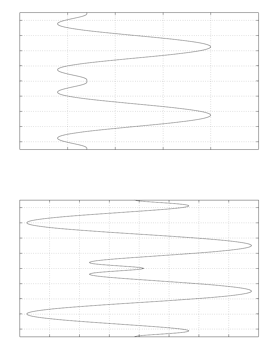
344
CHAPTER 28. INITIAL AND BOUNDARY CONDITIONS
−1 −0.5 0 0.5 1 1.5
−80
−60
−40
−20
0
20
40
60
80
Analytical zonal wind stress
dyne/cm2
latitude
−8 −6 −4 −2 0 2 4 6 8
x 10−9
−80
−60
−40
−20
0
20
40
60
80
Curl of analytical zonal wind stress
dyne/cm3
latitude
Figure 28.1: Upper panel: Analytic zonal wind stress from F. Bryan (1987). Lower panel: Curl
of the wind stress.
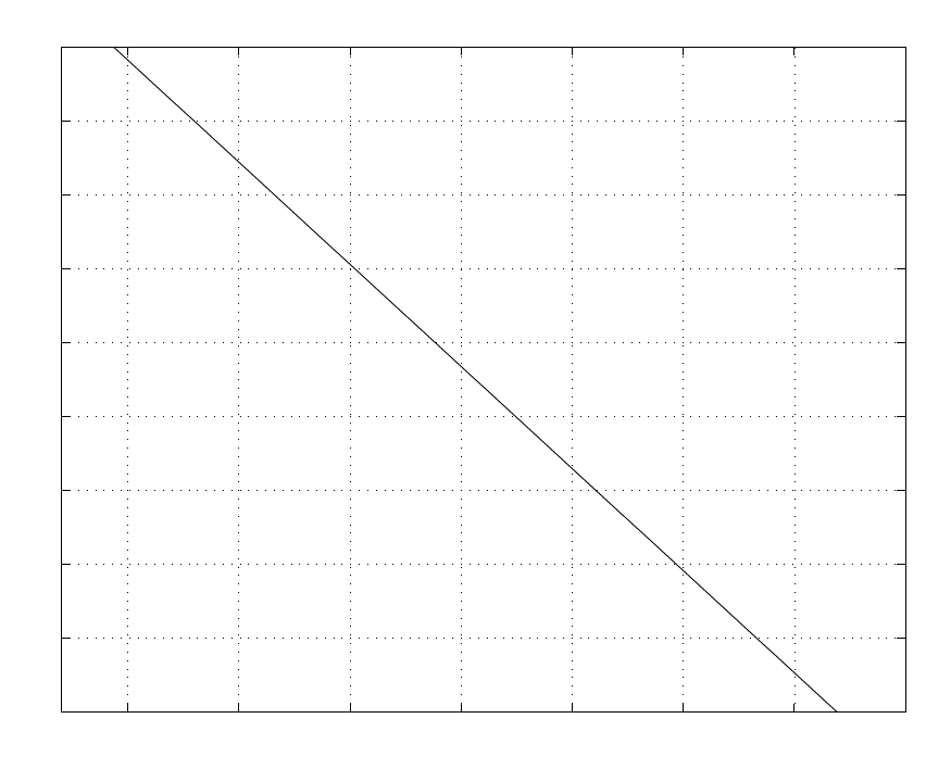
28.3. LATERAL BOUNDARY CONDITIONS
345
−5 0 5 10 15 20 25 30
0
10
20
30
40
50
60
70
80
90 Tstar
Celsius
Latitude
Figure 28.2: Linear profile of temperature from Cox and Bryan (1984).
346
CHAPTER 28. INITIAL AND BOUNDARY CONDITIONS
Chapter 29
Old options for the external mode
There are various ways to solve for the external mode (depth integrated) velocities in MOM.
The purpose of this chapter, as well as Chapter 30, is to describe the numerical issues involved.
Many of the theoretical issues were discussed in Chapter 4. Starting this chapter are some
comments concerning the main points to be considered when choosing a particular method.
Additionally, within the discussion of each method, certain caveats, which are mostly sug-
gestive and not rigorous, are mentioned. In general, stability of the external mode in ocean
modeling tends to be the very sensitive, especially in global models with realistic geography
and topography. A great deal of energy has gone into deriving various methods for solving
the external mode. The present methods are not perfect, and development continues.
29.1 Concerning which external mode option to use
The methods available for updating the velocity field are the following:
•Option stream function uses the Bryan (1969) rigid lid streamfunction approach.
•Option rigid lid surface pressure uses the rigid lid surface pressure approach of Dukowicz,
Smith, and Malone (1993).
•Option implicit free surface employs the implicit free surface method of Dukowicz and
Smith (1994).
•Option explicit free surface and explicit eb or explicit fb employ the free surface method of
Killworth, Stainforth, Webb and Paterson (1991).
•Option explicit free surface employs an explicit free surface method which fully incorpo-
rates the undulating surface height within the baroclinic momentum and tracer equations.
It also allows for longer tracer time steps than the Killworth et al method.
Researchers at GFDL are using the last option (explicit free surface) most frequently (Summer
1999). This method is the only one which will be available in post MOM 3 releases of MOM.
29.1.1 Wave processes
The explicit free surface was written with the spreading of surface gravity waves and/or Kelvin
waves as one of the main physical phenomenon of interest (Killworth et al. 1991). The rigid lid
347

348
CHAPTER 29. OLD OPTIONS FOR THE EXTERNAL MODE
stream function and rigid lid surface pressure approaches completely filter out these waves.
The implicit free surface is very diffusive and so may not provide a satisfactory simulation of
these waves for certain purposes, such as tidal studies.
In addition, note that even for climate studies, the assumptions of a rigid lid might not
be valid for equatorial dynamics. Namely, the rigid lid approximation makes the speed of all
external gravity waves infinite and therefore instantly equilibrates them. This is reasonable
in mid and high latitudes where there is a large time scale separation between gravity waves
and Rossby waves. However, this separation of time scales is not the case in the equatorial
domain. Both explicit and implicit free surface methods resolve Rossby and gravity waves
within the equatorial region, while equilibrating higher frequency gravity waves at mid and
high latitudes. It remains to be shown if this difference between rigid lid and free surfaces is
significant.
29.1.2 Surface tracer fluxes
An incresingly large number of modelers are paying close attention to how tracers are forced.
For example, ocean biogeochemical modeling requires some dozens of tracers with varying
surface and interior sources. The central problem with the rigid lid approximation is the
manner in which fresh water enters the ocean model, and consequently how tracers contained
in precipitation and river runoffenter as well. Namely, fresh water enters not as a fresh water
flux, but as a “virtual salt flux.” The reason it must do so in a rigid lid approximation can be
seen by looking at the kinematic boundary condition at the ocean surface. For a free surface,
the kinematic boundary condition in the presence of fresh water fluxes Qwis given by
ηt=w+qw−~
uh· ∇hηz=η, (29.1)
where ηis the deviation of the surface height from z=0. This equation is derived in Section
7.2.2. For a rigid lid, the surface velocity is set to zero, and the surface elevation is a constant
η=0. Therefore, Qw=0 everywhere on the ocean surface, which precludes the introduction
of a fresh water flux through a rigid lid. Instead, for the purpose of garnering some sort
of dynamical input of fresh water, it is necessary to introduce an unphysical salt flux in the
salinity equation. Huang (1993) provides a thorough critique of this approach and proposes an
alternative within the context of a generalized rigid lid model for which the vertical velocity
is not set to zero, yet there is no explicit equation for the free surface height. Since w(z=0)
is not set to zero, an extra elliptical problem needs to be solved for the stream potential,
which is necessary since the vertically integrated velocity is no longer divergence-free when
w(z=0) ,0. The presence of two elliptic equations in a climate model can potentially be quite
costly, and so this approach has not been implemented in MOM.
The use of a free surface with proper accounting of fresh water flux is arguably the most
physically and numerically satisfying approach. The option explicit free surface allows for a
conservative model with fresh water input.
29.1.3 Killworth topographic instability
Killworth (1987) identified a fundamental problem with the rigid lid streamfunction when
used with steeply sloping bottom topography. The condition places a limit on the time step
based on lateral viscosity, resolution, and topographic slope. This condition and methods for
relaxing it are given in Section 18.5.

29.1. CONCERNING WHICH EXTERNAL MODE OPTION TO USE
349
Basically, due to a factor of topographic factor of 1/Hin the elliptic equation for the rigid
lid streamfunction (Section 29.2.1), there is a sensitivity to rapid changes in topography1. As
pointed out by Dukowicz and Smith (1994), the rigid lid surface pressure and implicit free
surface approaches are better conditioned than the streamfunction because the factor 1/Hin
the stream function is replaced by a factor of H(see Section 29.4).
The explicit free surface does not have an elliptic equation to solve,and so is not restricted by
the Killworth topographic condition. Qualitatively, since the explicit free surface’s barotropic
mode can change height, it is not “squashed” like the barotropic mode in the rigid lid cases in
the presence of rapidly changing bottom topography. Hence, both free surface options are not
subject to the Killworth topographic condition.
29.1.4 Wave speed considerations
Use of rigid lid and implicit free surface methods allow relatively long time steps to be used by
eliminating fast external gravity waves. The next fastest waves are large scale external Rossby
waves which limit the time step for the external mode. The fastest remaining waves are internal
gravity waves due to vertical differences in density and they travel at speeds less than 3 m/sec.
Since the inertial period at the pole is 1/2 day, time steps greater than about 2 hours are unstable
unless the inertial oscillation is filtered out. Typically, either internal gravity waves or inertial
oscillations limit the time step for the internal mode in coarse resolution models. Density is
limited by advective velocity which is usually less than 2 m/sec. As an example, in a 4-degree
model, time steps as long a few days are typical for the density (i.e., temperature and salinity).
For large-scale ocean modeling in which the momentum field is close to geostrophic balance,
the density time sets the “time” for the ocean model. Therefore, maintaining a long density
time step is central to quickly spinning up global ocean models (see Bryan 1984 and Killworth,
Smith, and Gill 1984 for more details on acceleration techniques). However, as mentioned by
Killworth et al. (1991), it is necessary to greatly reduce the density time step in the explicit
free surface due to a bleeding of the barotropic mode into the baroclinic mode. This bleeding
effectively makes the density time step constrained by the first baroclinic Rossby wave speed
which results in roughly a factor of 10 reduction in the density time step from that available
in the rigid lid and implicit free surface. Empirical tests with MOM are consistent with this
constraint.
29.1.5 Polar filtering
The rigid lid stream function and explicit free surface are much more tolerant of polar filtering
than the implicit free surface. Nonetheless, whenever polar filtering, there is a tendency for
the vertical velocity field to become noisy, especially when running with fourier filtering. Note
that when applying a polar filter with option firfil or fourfil, the forcing for the rigid lid stream
function is also filtered. Details of polar filtering are discussed further in Chapter 27.
In the explicit free surface, polar filtering must be applied within every barotropic time
step. For the rigid lid and the implicit free surface, polar filtering is applied only once before
the elliptic equation is solved. Therefore, when using the explicit free surface, it is important
1This instability has been associated with problems in various versions of the GFDL coupled model in the
Drake Passage region. For example, a traditional time step analysis indicates that the ocean component of the
4-degree/R15 GFDL coupled model should work fine with a 6 hour barotropic time step. However, it is unable to
run with time steps much larger than 2 hours. The consensus is that the Killworth instability is the dominant factor
determining the time step in this rigid lid model (Keith Dixon and Ron Stouffer, personal communication).
350
CHAPTER 29. OLD OPTIONS FOR THE EXTERNAL MODE
to move the latitude where filterting starts as far poleward as possible since polar filtering is
expensive.
Tests with the implicit free surface indicate that polar filtering of the external mode velocities
leads to a problem in the filtered latitudes. Removing the filtering has been shown to eliminate
the problem. However, the standard TEST CASE 0 will not run without filtering and so the
filtering has been left in the code.
Finally, it should be noted that polar filtering may not always be necessary, even for global
models. Due to its rather unphysical properties, initial tests should be run for each model
configuration to see just how much polar filtering is required and whether its affects are
detrimental to the physics of interest. In particular, experience at GFDL indicates that for some
model configurations, it is economical to run the explicit free surface without polar filtering the
barotropic mode. Although the absence of polar filtering requires taking smaller barotropic
time steps, there are nontrivial savings due to the absence of polar filtering on every barotropic
time step.
29.1.6 Parallelization
There is currently a lot of attention paid to parallelizing MOM (Chapter 12 and Section 24.4).
The presence of island integrals in the rigid lid streamfunction approach (Section 29.2) renders
the rigid lid unsuitable for parallelism due to nonlocal processes (i.e. island integrals). Both
the explicit (Section 29.5 Killworth et al. 1991) and implicit (Section 29.4, Dukowicz and Smith
1994) free surfaces do not require island integrals, hence their use offers strong advantages over
the rigid lid stream function. Preliminary experience indicates that the explicit free surface is
better scalable to larger numbers of processors. This is especially true if gravity can be reduced
by a factor of 10 in the explicit free surface. This is under investigation.
Both the implicit and explicit free surfaces, have been parallelized. Work to increase the
efficiency of these schemes is ongoing.
29.2 stream function
Option stream function enables the time honored standard approach which eliminates surface
pressure from the momentum equations by vertically integrating, taking the curl, and assuming
that vertical velocity vanishes at the ocean surface which is taken at z=0. This rigid lid approach
was developed by Bryan (1969) and has remained the choice of numerous ocean modelers
for almost 30 years. However, for the reasons mentioned in Section 29.1, the rigid lid is
being displaced by the more physically complete and computationally efficient (with regard to
parallelism) free surface approaches. This section discusses the computational implementation
of the rigid lid. The theoretical formulation is given in Bryan (1969).
Boundary conditions for the rigid lid barotropic streamfunction are Dirichlet, which neces-
sitate solving island equations as given in Section 29.2.4. Artificially setting the flow between
land masses to zero may be implemented, as described in Section 29.2.6. Changes2to the
coefficient matrices and in the handling of islands in the elliptic solvers have resulted in faster
convergence rates than in MOM 1. The external mode velocities given by the stream function
approach are guaranteed to be divergence free even if the solution for change in stream func-
tion ∆ψis not accurate. The accuracy of the solution for ∆ψis governed by “tolrsf” which is
input through namelist. Typically, the value is 108cm3/sec.
2Worked out by Charles Goldberg.
29.2. STREAM FUNCTION
351
29.2.1 The equation
The stream function equation is generated by taking the curl of the vertically averaged momen-
tum equations to knock out the unknown surface pressure terms. This is done by vertically
averaging the Equations (4.1) and (4.2), expressing the averaged velocities in terms of a stream
function ψ, and taking the ˆ
k· ∇× of these equations yielding:
∇ · (1
H· ∇ψt)−J(acor ·f
H, ψ)=ˆ
k· ∇×F(29.2)
where Jis the Jacobian3,acor is the implicit Coriolis factor4, the Coriolis term f=2Ωsin φ, and
Fis the vertically averaged forcing computed in subroutine baroclinic. The boundary condition
is that the normal component of the gradient of the stream function ˆ
n· ∇ψ=0 on lateral
boundaries. Actually, since the viscous terms in the vertically averaged forcing are of the form
∇2uand ∇2v, another boundary condition is necessary. The additional boundary condition is
that the tangential component of the stream function ˆ
t· ∇ψ=0 on lateral boundaries.
Bryan(1969) gives the discretization of Equation (29.2) in terms of five point numerics. This
means that the discretized equation at grid point with subscripts (i,jrow) involves the four
nearest neighboring points with subscripts (i+1,jrow),(i−1,jrow), (i,jrow +1), and (i,jrow −1).
Semtner (1974) derives the nine point equivalent of Bryan’s external mode equation which
additionally involves the four nearest neighboring corner points (i+1,jrow +1),(i−1,jrow +1),
(i+1,jrow −1), and (i−1,jrow −1). A similar approach5is given below.
The finite difference counterpart of Equation (29.2) is arrived at by starting with the verti-
cally averaged finite differenced momentum equations
¯
ui,j,1,τ+1−¯
ui,j,1,τ−1
2∆τ−˜
fjrow ·(¯
ui,j,2,τ+1−¯
ui,j,2,τ−1)=−1
ρ◦·cos φU
jrow ·δλ(ps
i,jrow
φ)
+zui,jrow,1(29.3)
¯
ui,j,2,τ+1−¯
ui,j,2,τ−1
2∆τ+˜
fjrow ·(¯
ui,j,1,τ+1−¯
ui,j,1,τ−1)=−1
ρ◦·δφ(ps
i,jrow
λ)
+zui,jrow,2(29.4)
where psis the unknown surface pressure and zui,jrow,ncontains the vertically averaged ad-
vection, diffusion, hydrostatic pressure gradients, and explicit part of the Coriolis term. The
implicit part of the Coriolis term is given by
˜
fjrow =acor ·2Ωsin φU
jrow (29.5)
When the finite difference curl is taken, particular attention must be taken to assure that the
unknown surface pressure terms are eliminated even when the grid is non-uniform. Here is
3The Jacobian is given as J(A,B)=1
a2cos φ(∂A
∂λ
∂B
∂φ −∂B
∂λ
∂A
∂φ ).
4acor =zero implies that the Coriolis term is handled explicitly. Otherwise, 0.5≤acor <1.0 implies implicit
handling of the Coriolis term. This is useful for coarse models with global domains where the time step is limited
by the inertial period 1/f.
5This approach was first worked out by Charles Goldberg (personal communication) using algebraic manipu-
lations. The derivation given here is in terms of finite difference operators.
352
CHAPTER 29. OLD OPTIONS FOR THE EXTERNAL MODE
an outline of the steps needed to do this. Starting with Equations (29.3) and (29.4), make the
following substitutions:
¯
ui,j,1,τ−1=−1
Hi,jrow ·δφ(ψi,jrow,τ−1
λ) (29.6)
¯
ui,j,2,τ−1=1
Hi,jrow ·cos φU
jrow ·δλ(ψi,jrow,τ−1
φ) (29.7)
¯
ui,j,1,τ+1=−1
Hi,jrow ·δφ(ψi,jrow,τ+1
λ) (29.8)
¯
ui,j,2,τ+1=1
Hi,jrow ·cos φU
jrow ·δλ(ψi,jrow,τ+1
φ) (29.9)
∆ψi,jrow =ψi,jrow,τ+1−ψi,jrow,τ−1(29.10)
where the horizontal stream function ψi,jrow is defined on T cells. Next, take
dxui·cos φU
jrow ×equation(29.3) (29.11)
dyujrow· × equation(29.4) (29.12)
Then take the finite difference equivalent of the curl operation using:
−dytjrow ·δφ(equation(29.11)λ)+dxti·δλ(equation(29.12)φ) (29.13)
The result is the finite difference counterpart of Equation (29.2) which is valid for non-uniform
grids
1
2∆τ·dytjrow ·δφ
(dxui−1·cos φU
jrow−1
Hi−1,jrow−1·dyujrow−1
)·dyujrow−1·δφ(∆ψi−1,jrow−1
λ)
λ
+dxti·δλ
(dyujrow−1
Hi−1,jrow−1·cos φU
jrow−1·dxui−1
)·dxui−1·δλ(∆ψi−1,jrow−1
φ)
φ
+dytjrow ·δφ
˜
fjrow−1
Hi−1,jrow−1·dxui−1·δλ(∆ψi−1,jrow−1
φ)
λ
−dxti·δλ
˜
fjrow−1
Hi−1,jrow−1·dyujrow−1·δφ(∆ψi−1,jrow−1
λ)
φ
=−dytjrow ·δφ(dxui−1·cos φU
jrow−1·zui−1,jrow−1,1
λ)
+dxti·δλ(dyujrow−1·zui−1,jrow−1,2
φ)(29.14)
For each ψi,jrow, Equation (29.14) involves nine points of ψand ˜
fjrow is given by Equation (29.5).
Comparing this to Equation (29.2), ∇ · (1
H· ∇ψt) corresponds to the first bracket, −J(acor ·f
H, ψ)
29.2. STREAM FUNCTION
353
corresponds to the second bracket and ˆ
k· ∇×Fcorresponds to the third bracket. In the model,
this third bracket is stored as array ztdi,jrow.
ztdi,jrow =−dytjrow ·δφ(dxui−1·cos φU
jrow−1·zui−1,jrow−1,1
λ)
+dxti·δλ(dyujrow−1·zui−1,jrow−1,2
φ) (29.15)
If the time step constraint imposed by convergence of meridians needs to be relaxed, ztdi,jrow can
be filtered in longitude by one of two techniques: Fourier filtering (Bryan, Manabe, Pacanowski
1975) enabled by option fourfil or finite impulse response filtering enabled by option firfil. Both
should be used with caution6and only when necessary at high latitudes. firfil is much faster
than fourfil.
The boundary condition is no slip on lateral boundaries. This is expressed as
δλ(ψi,jrow
φ)=0 (29.16)
δφ(ψi,jrow
λ)=0 (29.17)
which implies that ψi,jrow =constant on all land masses and their associated coastal ocean T
cells. In domains containing disconnected land masses (islands), the value of ψi,jrow on each
land mass mis a different constant ψm. The solution of Equation (29.14) contains an arbitrary
constant which means that the value of ψcan be specified arbitrarily on any one land mass. The
remaining values of ψon other land masses are determined and cannot be specified (actually
the way to do this is given below). Refer to Section 29.2.4 for how to solving for ψmon islands.
29.2.2 The coefficient matrices
Equation (29.14) involves nine values of ∆ψcentered at ∆ψi,jrow which may be written as
1
X
i′=−1
1
X
j′=−1
coeffi,jrow,i′,j′∆ψi+i′,jrow+j′=ztdi,jrow (29.18)
where the 3rd and 4th subscripts on the coefficient matrix refer to coefficients on neighboring
cells. For example, i′=−1 and j′=0 refers to the coefficient of ∆ψi−1,jrow (the value on the
western neighboring cell). The coefficient of ∆ψi+1,jrow+1on the northeast neighboring cell is
given by i′=1 and j′=1. When option sf 9 point is enabled, MOM calculates the coefficient
matrix coeffi,jrow,i′,j′for Equation (29.18) using summation formulas given in Section 31.2. This
nine point coefficient matrix differs slightly from the one in MOM 1 and is more accurate. The
elliptic solvers also converge in fewer iterations using this coefficient matrix. The ¯
ui,j,1,τ+1and
¯
ui,j,2,τ+1derived from the solution of Equation (29.14) are exact solutions7of the finite difference
vertically averaged momentum Equations (29.3) and (29.4).
When option sf 5 point is enabled, the nine point coefficient matrix is approximated by a
five point coefficient matrix involving five non-zero coefficients coeffi,jrow,i′,j′for i′=0 or j′=0
as in Bryan (1969). It is arrived at by averaging terms used to construct the nine point coefficient
6This filtering induces spurious vertical velocities because each latitude if filtered independently and the strips
are of varying length due to topography.
7To within roundoff.
354
CHAPTER 29. OLD OPTIONS FOR THE EXTERNAL MODE
matrix in a different way resulting in a coefficient matrix that differs from the one used by Bryan
(1969). The five point coefficient matrix is not as accurate as the nine point matrix although the
nine point matrix has a checkerboard null mode. Refer to Appendix E for a discussion on null
modes. However, in the stream function, this null mode is largely suppressed because ψi,jrow is
constant along boundaries. Also, spatial derivatives of ψi,jrow remove the this null mode and so
it is of no dynamical consequence. The five point matrix does not have this checkerboard null
mode. However, both five and nine point operators have an arbitrary unspecified constant
null mode. Therefore, the value of ψon one land mass can be arbitrarily specified (usually set
to zero) and all stream function values referenced to this land mass value. Either the five point
or nine point operator must be chosen by enabling options sf 5 point or sf 9 point.
29.2.3 Solving the equation
After choosing whether five point numerics enabled by option sf 5 point or nine point numerics
enabled by option sf 9 point is to be used with Equation (29.14), the elliptic equation is inverted
by the method of conjugate gradients. Note that the conjugate gradient solver may fail to
converge for large values of the implicit Coriolis parameter acor, which de-symmetrize the
equations.
29.2.4 Island equations
When solving Equations (29.3) and (29.3) by the method of stream function, Dirichlet boundary
conditions on velocity are used. Specifically, both components of vertically integrated velocity
are set to zero on all land U cells. This implies
δλ(ψi,jrow
φ)=0 (29.19)
δφ(ψi,jrow
λ)=0 (29.20)
which further implies that ψi,jrow =ψmwhere ψmis a constant on all T cells within land mass
mand surrounding ocean coastal perimeter cells. Now pick any land mass mand change to a
directional notation letting cell (i,jrow) be referred to as cell ℓ. The central coefficient coeffi,jrow,0,0
for cell ℓfrom Equation (29.18) is referred to as C◦
ℓ, the coefficient coeffi,jrow,1,0at the eastern
face of cell ℓis referred to as Ce
ℓ, the coefficient coeffi,jrow,1,1at the northeastern corner of cell ℓ
is referred to as Cne
ℓ, and so forth. Using this notation, Equation (29.18) may be written for the
ℓ’th T cell as
Cn
ℓ·ψn
ℓ+Ce
ℓ·ψe
ℓ+Cs
ℓ·ψs
ℓ+Cw
ℓ·ψw
ℓ+C◦
ℓ·ψ◦
ℓ+
Cne
ℓ·ψne
ℓ+Cnw
ℓ·ψnw
ℓ+Cse
ℓ·ψse
ℓ+Csw
ℓ·ψsw
ℓ=ztd◦
ℓ(29.21)
where superscript nindicates the cell to the north of cell ℓwith index (i,jrow +1), superscript
ne indicates the cell to the northeast of cell ℓwith index (i+1,jrow+1) and so forth. Superscript
◦refers to the the ℓ’th cell with index (i,jrow).
The central coefficient C◦
ℓis related to the surrounding coefficients by
c◦
ℓ=−(Cn
ℓ+Cs
ℓ+Ce
ℓ+Cw
ℓ+Cne
ℓ+Cnw
ℓ+Cse
ℓ+Csw
ℓ) (29.22)

29.2. STREAM FUNCTION
355
An equation for land mass mis generated by summing Equation (29.21) over all cells within
the land mass including coastal ocean perimeter cells. At each cell ℓwithin the island proper,
the left hand side of Equation (29.21) is zero because of Equation (29.22) and the condition that
ψ◦
ℓ=ψn
ℓ=ψs
ℓ=ψe
ℓ=ψw
ℓ=ψne
ℓ=ψnw
ℓ=ψse
ℓ=ψsw
ℓ=constant (29.23)
After summing over all cells within land mass mand it’s ocean perimeter, the only locations
with non-zero contributions to the left hand side of Equation (29.21) are ocean perimeter cells.
The result in general can be expressed as the sum of nine products summed from ℓ=1 to L
which is the number of perimeter cells for land mass m.
L
X
ℓ=1
(Cn
ℓ·ψn
ℓ+Ce
ℓ·ψe
ℓ+Cs
ℓ·ψs
ℓ+Cw
ℓ·ψw
ℓ+C◦
ℓ·ψ◦+
Cne
ℓ·ψne
ℓ+Cnw
ℓ·ψnw
ℓ+Cse
ℓ·ψse
ℓ+Csw
ℓ·ψsw
ℓ)=
L
X
ℓ=1
ztd◦
ℓ(29.24)
Without loss of generality, all coefficients adjacent to land cells on the left hand side may be set
to zero which leaves only ψ◦and values of ψexterior to the island perimeter. Indeed, this is
the very reason why reciprocals of Hare set to zero on land (to zero out the coefficients there)
in the code.
Recall from Equation (29.15) that ztdi,jrow is in fact the finite difference version of the curl of
zui,jrow,n. By Stokes theorem, summing the curl over any area leaves only values of zui,jrow,nat
the outer boundary of the perimeter cells. And at these locations, values of zui,jrow,nare well
defined by Equation (22.118).
Solving Equation (29.24) for ψ◦yields
ψ◦=(
L
X
ℓ=1
ztd◦
ℓ−
L
X
ℓ=1
(Cn
ℓ·ψn
ℓ+Ce
ℓ·ψe
ℓ+···))/
L
X
ℓ=1
C◦
ℓ(29.25)
where ψm=ψ◦is the value of the stream function on island m. In the code, zui,jrow,nis set to
zero on land cells so that PL
ℓ=1ztd◦
ℓpicks up contributions only from values of zui,jrow,nin the
ocean.
The solution of Equation (29.2) is determined only to within an arbitrary constant. If the
domain is multiply connected by two or more distinct land masses (islands), the value of the
stream function can be chosen arbitrarily on one of the land masses. In MOM 1, the value
on the main continent is held fixed at zero and each iteration involved calculating an integral
around each other island. In MOM, this option is retained, but it has been determined that the
solution converges more quickly if the stream function values on all land masses are allowed
to “float”. Afterwards, the entire solution is adjusted to make the stream function zero on the
main continent. Choosing a stream function value of zero on the main continent and on an
island amounts to an over specification of the problem and is not correct.
29.2.4.1 Another approach
Another approach suggested by Charles Goldberg leads to the same result. Equation (31.12)
indicates that the right hand side of Equation (29.14) centered at a land or ocean perimeter cell
356
CHAPTER 29. OLD OPTIONS FOR THE EXTERNAL MODE
Ti,jcontains values of zui,jrow,non land that are not available. In fact, f orci,jrow is the line integral
of zui,jrow,naround the boundary of cell Ti,j. The island equation for land mass mis formed by
summing Equation (29.14) over all land and ocean perimeter T cells of land mass m.
Since each right hand side is a line integral around the boundary of one T cell, in the sum
of such line integrals over all of land mass mand its surrounding ocean perimeter cells, all
contributions from interior edges cancel, leaving only known values of zui,jrow,nat ocean U cells.
On the left side of an island equation, Equations (31.9) and (31.10) and the fact that ψi,jrow =
ψmon all land and ocean perimeter T cells of land mass mimply that all contributions from
land T cells are zero as follows. At a land T cell, all nine values of ψare the constant value
ψm, so by pulling all terms that don’t involve i′or j′out of the i′and j′summations, Equation
(31.9) reduces to
0
X
i′′=−1
0
X
j′′=−1cddyti′′,j′′ ·
dxui+i′′ ·cos φU
jrow+j′′
Hi+i′′,jrow+j′′ ·dyujrow+j′′ ·2∆τ∆ψm
1
X
i′=0
1
X
j′=0
cddyui′,j′
+
0
X
i′′=−1
0
X
j′′=−1cddxti′′,j′′ ·dyujrow+j′′
Hi+i′′,jrow+j′′ ·dxui+j′′ ·cos φU
jrow+j′′ ·2∆τ∆ψm
1
X
i′=0
1
X
j′=0
cddxui′,j′
= = 0 (29.26)
since the sum of the partial derivative coefficients cddxu and cddyu are zero. Similarly, at land
points, the contributions to the island equation from the implicit Coriolis terms is also zero
because Equation (31.10) reduces to
0
X
i′′=−1
0
X
j′′=−1−cddyti′′,j′′ ·−˜
fjrow+j′′
Hi+i′′,jrow+j′′ ∆ψm
1
X
i′=0
1
X
j′=0
cddxui′,j′
+
0
X
i′′=−1
0
X
j′′=−1−cddxti′′,j′′ ·
˜
fjrow+j′′
Hi+i′′,jrow+j′′ ∆ψm
1
X
i′=0
1
X
j′=0
cddyui′,j′
=0 (29.27)
Because of these simplifications, the island equation for land mass mmay be calculated by
summing Equations (29.14) only over the ocean perimeter T cells of land mass m.
In fact, in the Fortran code of MOM , the full island equation never appears. Instead,
each set of contributions to the island equation from an island perimeter cell Ti,jis stored in
coeffi,jrow,i′′,j′′. The sum over the island perimeter is done in the elliptic solver.
29.2.5 Symmetry in the stream function equation
This section on symmetry in the stream function equation was contributed by Charles Gold-
berg. Conjugate gradient solvers work by transforming the system of equations
Ax =b(29.28)
into minimizing the quadratic form
Q(x)=1
2xTAx −bTx(29.29)
This transformation is justified as long as Ais symmetric, that is, Aα,β =Aβ,α for all αand β.

29.2. STREAM FUNCTION
357
29.2.5.1 Symmetry of the explicit equations
In Equation (29.14), the three major brackets are expanded into summation notation as given
by Equations (31.9), (31.10), and (31.12). Interpreting these equations in the formalism given
above, the “vector” xis ∆Ψi,jrow at all mid-ocean points and island values ∆Ψm, the linear
operator Ais the array coeffi,jrow,i′+i′′,j′+j′′, and the subscripts are α=(i,jrow) and β=(i⋆,j⋆),
where i⋆=i+i′+i′′ and j⋆=jrow +j′+j′′ for some values of i′,j′∈ {0,1}and i′′,j′′ ∈ {−1,0}.
More simply, β=(i⋆,j⋆) is one of the eight nearest neighbors of α=(i,jrow) and α=(i,jrow) is
one of the eight nearest neighbors of β=(i⋆,j⋆). This section shows that the contributions to
the coefficients arising from the first brackets, Equation (31.9), are symmetric.
If i⋆,i, then i′and i′′ must both be at their upper limits or both must be at their lower
limits. In either case, i′=i′′ +1. Similarly, if j⋆,j, then j′=j′′ +1. If both are unequal, that is,
if (i,jrow) and (i⋆,j⋆) are diagonal neighbors, then i+i′′ =i+i′+i′′ −i′=i⋆−i′=i⋆+(−1−i′′),
and similarly jrow +j′′ =j⋆+(−1−j′′). Note that the expressions (i⋆)′=1−i′, (j⋆)′=1−j′,
(i⋆)′′ =−1−i′′, and (j⋆)′′ =−1−j′′ describe the transition in the opposite direction, so the
relations i+i′′ =i⋆+(−1−i′′) and jrow +j′′ =j⋆+(−1−j′′) show that the evaluation point
of most of the factors in Equation (31.9) is the same going both ways. The remaining factors,
cddyui′,j′,cddyti′′,j′′,cddxui′,j′, and cddxti′′,j′′ all change sign when i′is replaced by 1 −i′,j′is
replaced by 1 −j′,i′′ is replaced by −1−i′′, and j′′ is replaced by −1−j′′. Thus the product
of any two of these is unchanged, and each diagonal coeffiecient at (i,jrow) is equal to the
opposite diagonal coefficient at (i⋆,j⋆).
If i=i⋆, there are two possibilities: either i′=i′′ =0 or i′=−i′′ =1. Assume that j,j⋆.
Otherwise, (i,jrow) and (i⋆,j⋆) are not neighbors, but identical. The transitions back to (i,jrow)
are in this case: i=i⋆=i⋆+i′+i′′ and jrow =j⋆+(1 −j′)+(−1−j′′), so i+i′′ =i⋆+i′′
and, as above, jrow +j′′ =j⋆+(−1−j′′). This time, only j′changes to 1 −j′and j′′ changes
to −1−j′′. As a result, the factors cddyui′,j′and cddyti′′,j′′ change sign, but the factors cddxui′,j′,
and cddxti′′,j′′ remain unchanged. All other factors remain evaluated at the same points, so
again symmetry holds in that the northern or southern coefficient in Equation (31.9) centered
at (i,jrow) is the same as the opposite coefficient in Equation (31.9) centered at (i⋆,j⋆). The case
where j=j⋆is proved similarly.
29.2.5.2 Anti-symmetry of the implicit Coriolis terms
If one applies the same arguments to the implicit Coriolis terms in Equation (31.10), the result
is a proof of antisymmetry rather than symmetry. First, the diagonal coefficients in the implicit
Coriolis terms are zero, so this case need not be considered. In the northern and southern terms
(i.e., when i=i⋆), the evaluation points given by (i+i′′,jrow +j′′)=(i⋆+i′′),j⋆+(−1−j′′))
still remain the same, but each term has one cddx coefficient and one cddy coefficient, so the
product of these two factors changes sign. The antisymmetry of the eastern and western
implicit Coriolis coefficients is proved similarly.
Since conjugate gradient solvers are derived under the assumption of symmetry of coef-
ficients, the larger the implicit Coriolis terms, the less suitable a conjugate gradient solver is
for the elliptic Equations (29.14). For large values of the implicit Coriolis parameter acor, the
conjugate gradient solver will not converge.
29.2.5.3 Island equations and symmetry
If one of the T cells, α=(i,jrow) or β=(i⋆,j⋆) is an island perimeter cell, the arguments in the
above section on symmetry of the explicit equations must be made more carefully, since each
358
CHAPTER 29. OLD OPTIONS FOR THE EXTERNAL MODE
island equation is a sum of Equations (29.14). Note that it cannot happen that both αand βare
island perimeter T cells because islands must be separated by at least two ocean T cells.
Without loss of generality, we may assume that βis an island perimeter cell and the αis
not. In this case, βmay not be the only island perimeter cell of land mass mthat is a nearest
neighbor of α. The coefficient of the island perimeter value ∆Ψmin the elliptic Equation (29.14)
centered at αis the sum of the contributions from all nearest neighbors of αthat are in the
island perimeter of land mass m. Each contribution will be shown equal to a corresponding
contribution of ∆Φαto the island equation for land mass m. Individually, each coefficient8of the
equation centered at cell α, say, the coefficient in the direction of cell β, is equal to the opposite
coefficient in the contribution to the island equation arising from β. Since multiple island
perimeter cells as nearest neighbors of αlead to a sum of their individual contributions, and
since the island equation is the sum of the individual equations centered at island perimeter
points β, both summations lead to the same result9. Thus even the coefficient values involving
islands satisfy the symmetry relation Aα,β =Aβ,α if the implicit Coriolis parameter is zero.
29.2.5.4 Asymmetry of the barotropic equations in MOM 1
The barotropic equations presented to the solvers in MOM 1 were not symmetric, even when
the implicit Coriolis parameter acor was set to zero. In an attempt to optimize the code to
save a few floating point operations in the calculation of Ax, each equation was divided by
its diagonal coefficient, coeffi,jrow,0,0. Since these diagonal coefficients depend on topography
and grid factors, they are not equal at neighboring cells, and the resulting equations are not
symmetric. The asymmetry between a mid-ocean cell and a neighboring island perimeter is
likely to be especially severe. It is possible that some of the problems arising with the use of
conjugate gradient solvers in MOM 1 may be attributed to MOM 1’s “normalization” of the
elliptic equations and the resulting de-symmetrization of the coefficient array.
29.2.6 zero island flow
Specifying the value of the stream function ψon two or more distinct land masses amounts
to an over-specification of conditions for solving the stream function equation. This over-
specification is strictly not correct. Nevertheless, it is sometimes useful to be able to specify a
zero net transport between two land masses. Option zero island flow effectively combines the
coastal perimeter cells from two arbitrary land masses into one perimeter which implies that
the stream function will have the same value on both land masses; even though the land masses
are not physically connected. Therfore, there is no net transport between the land masses.
Option zero island flow requires “land mass a” and “land mass b” to be specified through
namelist. Values for “land mass a” and “land mass b” can be taken from the island map which
is printed out when MOM 2 executes. Refer to Section 14.4 for information on namelist vari-
ables. It must always be kept in mind that option zero island flow is an over-specification which
may have side effects. To judge whether these side effects are significant or not, a companion
experiment should be run without specifying the flow between land masses. Although this
option is only written to specify zero net transport between two land masses, it can be easily
extended to handle more land masses.
8Only the first brackets are being done here. The implicit Coriolis terms stand no chance of being symmetric.
9Note that remote island perimeter cells neither appear in the equation centered at α, nor do they contain
references to cell αin their (up to) nine terms.
29.3. RIGID LID SURFACE PRESSURE
359
Note: Specifying a non-zero net transport between arbitrary land masses has been tried by
re-setting ψafter it has been predicted by the conjugate gradient solver. This method seems
to work for land masses with relatively short perimeters but fails for land masses with long
perimeters. The right way to specify flow is to modify the conjugate gradient solver by
specifying the net flow between land masses within the “scan” loop. In principle, a modification
of this kind should work but, so far, attempts have failed.
29.3 rigid lid surface pressure
Option rigid lid surface pressure enables the method developed by Smith, Dukowicz, and Mal-
one (1992) which is hereafter referred to as SDM. Instead of taking the curl of the vertically
integrated momentum equations to drop the surface pressure, the divergence is taken which
yields an elliptic equation for the surface pressure instead of a stream function. Its main
advantage is that Neumann boundary conditions apply instead of Dirichlet boundary condi-
tions, and there is no need to solve island integrals which perform poorly on SIMD10 parallel
computers. However, elliptic equation solvers converge very slowly using this method.
29.3.1 The equations
Basically, the SDM approach is to define the external mode velocities Uτ+1and Vτ+1in terms
of auxiliary velocities ˆ
Uand ˆ
Vand a time difference of surface pressure ∆ps as follows
Uτ+1
i,jrow =ˆ
Ui,jrow −2∆τ
cos φU
jrow
δλ(∆psi−1,jrow−1
φ) (29.30)
Vτ+1
i,jrow =ˆ
Vi,jrow −2∆τ·δφ(∆psi−1,jrow−1
λ) (29.31)
∆psi,jrow =psτ
i,jrow −psτ−1
i,jrow (29.32)
The momentum equations can then be re-written in terms of ˆ
Uand ˆ
Vas
ˆ
Ui,jrow =1
1+ω2(˜
Ui,jrow +ω˜
Vi,jrow)+Uτ−1
i,jrow −2∆τωδφ(∆psi−1,jrow−1
λ) (29.33)
ˆ
Vi,jrow =1
1+ω2(˜
Vi,jrow −ω˜
Ui,jrow)+Vτ−1
i,jrow +2∆τωδλ(∆psi−1,jrow−1
φ) (29.34)
˜
Ui,jrow =2∆τ(zui,jrow,1−1
cos φU
jrow
δλ(psτ−1
i−1,jrow−1
φ)) (29.35)
˜
Vi,jrow =2∆τ(zui,jrow,2−δφ(psτ−1
i−1,jrow−1
λ)) (29.36)
zui,jrow,1=f(gcor ·Vτ
i,k,j+(1 −gcor)·Vτ−1
i,k,j)+Gi,jrow,1(29.37)
zui,jrow,2=−f(gcor ·Uτ
i,k,j+(1 −gcor)·Uτ−1
i,k,j)+Gi,jrow,2(29.38)
where ω=2∆τ·acor ·fand the forcing terms Gi,jrow,1and Gi,jrow,2contain all remaining terms
which are known. If solving the Coriolis term explicitly (acor =0), then gcor =1 otherwise
gcor =0 for implicit treatment (acor >1/2).
10Single Instruction stream–Multiple Data streams
360
CHAPTER 29. OLD OPTIONS FOR THE EXTERNAL MODE
Equations (29.33) and (29.34) can be solved if terms involving ∆ps are dropped. The
justification given by SDM is that these terms are the same order of magnitude as the time
truncation error which is O(τ3). This is the operator splitting technique of SDM which leads
to a self-adjoint elliptic equation and therefore a symmetric coefficient matrix which can be
solved with efficient conjugate gradient techniques. Multiplying Equations (29.30) and (29.31)
by the total depth Hand taking the divergence gives the second order elliptic equation for ∆ps
in terms of known quantities ˆ
Uand ˆ
V.
δλ(Hi−1,jrow−1
cos φU
jrow−1
δλ(∆psi−2,jrow−2)φ
φ
)+δφ(Hi−1,jrow−1cos φU
jrow−1δφ(∆psi−2,jrow−2
λ)
λ
)
=1
2∆τ(δλ(Hi−1,jrow−1ˆ
Ui−1,jrow−1
φ)+δφ(cos φU
jrow−1Hi−1,jrow−1ˆ
Vi−1,jrow−1
λ)) (29.39)
Equation (29.39) is solved using a conjugate gradient technique with option sf 9 point. Note
that the number of islands is set to zero (nislsp =0) because no island equations are to be
solved. After solving for ∆ps, a checkerboard null space and mean are removed after which
the predicted surface pressure is
psτ+1
i,jrow =psτ−1
i,jrow + ∆psi,jrow (29.40)
The above equations are written with a leapfrog time step in mind. During mixing time
steps (forward or first pass of an Euler backward), quantities at time level τ−1 are replaced
by their values at τand 2∆τis replaced by ∆τ. The second pass of an Euler backward mixing
time step is as described in Section 21.4 and indicated in Figure 21.1.
29.3.2 Remarks
29.3.2.1 Boundary conditions
It should be noted that Equation (29.39) only requires a Neumann boundary condition at the
boundaries instead of the Direchlet boundary condition required for the elliptic equation of
the stream function method. The implication is that there are no island equations to be solved
and hence this method should be faster than the stream function method on massively parallel
computers.
29.3.2.2 Conditioning of the elliptic operator
The second point to be made is that Equation (29.39) contains a factor Hi,jrow whereas the elliptic
equation for the stream function contains the factor 1/Hi,jrow which should make this method
less prone to stability problems than the stream function equation when topography contains
steep slopes.
29.3.2.3 Non-divergent barotropic velocities
The third point to be noted is that the barotropic velocities Uτ+1
i,jrow and Vτ+1
i,jrow given by this method
are not non-divergent. The degree of non-divergence is related to how accurately Equation
(29.39) is solved for the change in surface pressure ∆ps and the accuracy depends on the
tolerance variable tolrsp which is input through namelist and typically set to 10−4gram/cm/sec2.
Refer to Section 14.4 for information on namelist variables.

29.4. IMPLICIT FREE SURFACE
361
29.3.2.4 Polar filtering
Use of polar filtering on ˆ
Uand ˆ
Vleads to a problem. Removing the filtering eliminates the
problem. So the filtering has been removed for this method.
29.3.2.5 Checkerboarding in surface pressure
The surface pressure field in the rigid lid - surface pressure method will sometimes exhibit a
checkerboard pattern due to the use of the 9-point Laplacian operator. Namely, this operator
contains a zero frequency eigenmode (“null mode”) which has a checkerboard pattern. This
null mode can be excited in general, and so must be subtracted out. Further discussion is given
in Smith, Dukowicz, and Malone (1992).
29.4 implicit free surface
Option implicit free surface enables the method developed by Dukowicz and Smith (1994) which
is hereafter referred to as DS. This work is an extension of their earlier work described in Section
29.3. The rigid lid assumption is replaced by a free surface which exerts a surface pressure at
z=0. As in the rigid lid surface pressure approach, an elliptic equation can be derived for the
change in surface pressure ∆ps but the resulting equation is more diagonally dominant than
the rigid lid surface pressure equation. The implication is that the DS method converges faster
than the rigid lid surface pressure method. As with the rigid lid surface pressure approach, DS
is well suited for SIMD parallel computers because it requires Neumann boundary conditions
and thus needs no island integrals.
Chapter 7 discusses the general mathematical issues concerning the formulation of the free
surface. This section discusses the numerical details of how to implement the implicit solution
for the surface pressure, and thus the surface elevation. Note that the implicit free surface
implemented in MOM has been frozen in its MOM 2 version. The updates to include fresh
water forcing have only been done for the explicit free surface discussed in Section 29.5.
29.4.1 The equations
The equations are given as (E1), (E2) and (E3) in DS and will be repeated here for convienence.
They are
(I+α′τB)( ˆu−un−1)=τ(F−g·G( ˜γηn+(1 −˜γ)ηn−1)
−B( ˜γ′un+(1 −˜γ′)un−1) (29.41)
(DHG −2
αθgτ2I)∆η=1
αθgτDH(θˆu+(1 −θ)un−1+un) (29.42)
un+1=ˆu−ατgG∆η(29.43)
where Bis the Coriolis operator, Dis the divergence operator, and Gis the gradient operator.
The centering coefficients (α, α′, γ, γ′, θ) and the quantities I,u,∆η, gand τare as defined in
DS. The above set of equations is very similar to the set in SDM (1992) except there is an extra
divergence term and three centering coefficients needed to damp two computational modes.
Because of the similarities, the surface pressure and implicit free surface methods share much
of the same code in MOM.
362
CHAPTER 29. OLD OPTIONS FOR THE EXTERNAL MODE
In the terminology of MOM, the centering coefficients (alph,gam,theta) are set to (1,0,1) for
the rigid lid surface pressure method and (1/3,1/3,1/2) for the implicit free surface method.
The relevant equations corresponding to Equations (29.41), (29.42), and (29.43) are as follows
Uτ+1
i,jrow =ˆ
Ui,jrow −2∆τ·apgr
cos φU
jrow
δλ(∆psi,jrow
φ)−Uτ
i,jrow (29.44)
Vτ+1
i,jrow =ˆ
Vi,jrow −2∆τ·apgr ·δφ(∆psi,jrow
λ)−Vτ
i,jrow (29.45)
∆psi,jrow =psτ
i,jrow −psτ−1
i,jrow (29.46)
ˆ
Ui,jrow =1
1+ω2(˜
Ui,jrow +ω˜
Vi,jrow)+Uτ−1
i,jrow +Uτ
i,jrow (29.47)
ˆ
Vi,jrow =1
1+ω2(˜
Vi,jrow −ω˜
Ui,jrow)+Vτ−1
i,jrow +Vτ
i,jrow (29.48)
˜
Ui,jrow =2∆τ(zui,jrow,1
−1
cos φU
jrow
δλ((1 −gam)·psτ−1
i−1,jrow−1
φ+gam ·psτ
i−1,jrow−1
φ)) (29.49)
˜
Vi,jrow =2∆τ(zui,jrow,2
−δφ((1 −gam)·psτ−1
i−1,jrow−1
λ+gam ·psτ
i−1,jrow−1
λ)) (29.50)
zui,jrow,1=f(gcor ·Vτ
i,k,j+(1 −gcor)·Vτ−1
i,k,j)+Gi,jrow,1(29.51)
zui,jrow,2=−f(gcor ·Uτ
i,k,j+(1 −gcor)·Uτ−1
i,k,j)+Gi,jrow,2(29.52)
where Uand Vare vertically averaged velocity components and terms involving ∆psi−1,jrow−1
have been dropped from Equations (29.47) and (29.48) to obtain the operator splitting as
discussed in DS. Also, ω=2∆τ·acor ·fand the forcing terms Gi,jrow,1and Gi,jrow,2contain all
remaining terms which are known. The right hand side of Equation 29.42 is constructed by
taking the divergence of Htimes Equations 29.47 and 29.48. The resulting elliptic equation
takes the form
δλ(Hi−1,jrow−1
cos φU
jrow−1
δλ(∆psi−2,jrow−2)φ
φ
)+δφ(Hi−1,jrow−1cos φU
jrow−1δφ(∆psi−2,jrow−2
λ)
λ
)
−cos φT
jrowdytjrow
apgr ·2∆τ2·grav ∆psi,jrow
=1
apgr ·2∆τ(δλ(Hi−1,jrow−1ˆ
Ui−1,jrow−1
φ)+δφ(cos φU
jrow−1Hi−1,jrow−1ˆ
Vi−1,jrow−1
λ))
(29.53)
Note that the piece −cos φT
jrowdytjrow
apgr·2∆τ2·grav ∆psi,jrow is included only when the implicit free surface
method is used. Also, the coefficient apgr is set to alph for leapfrog time steps and theta for mix-
ing time steps. Equation (29.53) is solved a conjugate gradient technique with option sf 9 point
with the number of islands nislsp set to zero because no island equations are being solved.
After solving for ∆ps, the predicted surface pressure is given by
29.4. IMPLICIT FREE SURFACE
363
psτ+1
i,jrow =psτ−1
i,jrow + ∆psi,jrow (29.54)
and the free surface elevation at time level τ+1 is
ηi,jrow =ρ◦·grav ·psτ+1
i,jrow (29.55)
but ηis not explicitly needed in the code and so is not calculated. The vertical velocity at the
top of the free surface is
adv vbti,k=0,j=(pstau+1
i,jrow −pstau−1
i,jrow)/(g∆τ) (29.56)
29.4.1.1 Modifications for various kinds of time steps
The following setting are needed on various types of time steps:
Leapfrog time steps
The equations are as given above and the centering coefficients are given as
•implicit free surface method: Centering coefficient apgr =alph. If solving the Coriolis
term explicitly (acor =0), then centering coefficient gcor =1. If solving the Coriolis term
implicitly (acor ,0), then acor is reset to acor =alph and centering coefficient gcor =gam.
•rigid lid surface pressure method: Centering coefficient apgr =alph. If solving the
Coriolis term explicitly (acor =0), then centering coefficient gcor =1 otherwise gcor =0.
Mixing time steps (Forward and Euler backward)
The equations for forward mixing time steps and the first step of an Euler backward are
modified to:
ˆ
Ui,jrow =1
1+ω2(˜
Ui,jrow +ω˜
Vi,jrow)+Uτ−1
i,jrow (29.57)
ˆ
Vi,jrow =1
1+ω2(˜
Vi,jrow −ω˜
Ui,jrow)+Vτ−1
i,jrow (29.58)
˜
Ui,jrow =2∆τ(zui,jrow,1−1
cos φU
jrow
δλ(psτ
i−1,jrow−1
φ)) (29.59)
˜
Vi,jrow =2∆τ(zui,jrow,2−δφ(psτ
i−1,jrow−1
λ)) (29.60)
The equations for the second step of an Euler backward are modified to:
ˆ
Ui,jrow =1
1+ω2(˜
Ui,jrow +ω˜
Vi,jrow)+Uτ−1
i,jrow (29.61)
ˆ
Vi,jrow =1
1+ω2(˜
Vi,jrow −ω˜
Ui,jrow)+Vτ−1
i,jrow (29.62)
˜
Ui,jrow =2∆τ(zui,jrow,1
−1
cos φU
jrow
δλ((1 −theta)·psτ
i−1,jrow−1
φ+theta ·psτ+1
i−1,jrow−1
φ)) (29.63)

364
CHAPTER 29. OLD OPTIONS FOR THE EXTERNAL MODE
˜
Vi,jrow =2∆τ(zui,jrow,2
−δφ((1 −theta)·psτ
i−1,jrow−1
λ+theta ·psτ+1
i−1,jrow−1
λ)) (29.64)
In both cases of mixing time steps, the time step factor 2∆τis replaced by ∆τ(also in ω) and
the centering coefficients are given as
•implicit free surface method: Centering coefficient apgr =theta. Centering coefficient
gcor =0. For implicit treatment of the Coriolis term, acor is reset to acor =theta. Also on the
second pass of an Euler backward time step the term dytjrowcos φT
jrowdxti
apgr·g·2∆τ2(psτ+1
i,jrow −psτ
i,jrow)
must be added to the right hand side of Equation (29.53).
•rigid lid surface pressure method: Centering coefficient apgr =theta. Centering coeffi-
cient gcor =1 when the Coriolis term is handled explicitly but gcor =0 when the Coriolis
term is handled implicitly.
29.4.2 Remarks
29.4.2.1 Boundary conditions
It should be noted that Equation (29.39) only requires a Neumann boundary condition at the
boundaries instead of the Dirichlet boundary condition required for the elliptic equation of
the stream function method. The implication is that there are no island equations to be solved
and hence this method should be faster than the stream function method on massively parallel
computers.
29.4.2.2 Conditioning with topography
Another point to be made is that Equation (29.39) contains a factor Hi,jrow whereas the elliptic
equation for the stream function contains the factor 1/Hi,jrow. Therefore, the implicit free
surface method should be less prone to stability problems than the stream function method
when topography contains steep gradients. This has yet to be verified.
29.4.2.3 Barotropic velocities
It should also be noted that the barotropic velocities Uτ+1
i,jrow and Vτ+1
i,jrow given by this method are
not non-divergent due to the rising and falling of the sea level (e.g., see discussion in Section
7.2.1).
29.4.2.4 Polar filtering
Use of polar filtering on ˆ
Uand ˆ
Vin some cases leads to a problem in the external mode in the
filtered latitudes. Removing the filtering has been shown to eliminate the problem.
29.4.2.5 Checkerboarding in surface pressure
The surface pressure will sometimes exhibit a checkerboard pattern when using the implicit
free surface method. As mentioned in Section 29.3.2.5, the rigid lid - surface pressure method
has a zero frequency eigenmode associated with the 9-point Laplacian, and this null mode has

29.5. THE KILLWORTH
ET AL
EXPLICIT FREE SURFACE
365
the spatial structure of a checkerboard pattern. This mode, which is global in extent, is strictly
eliminated with the free surface method (Dukowicz and Smith 1994). However, according to
Rick Smith, there might be other low frequency modes of similar structure which are present
in the free surface operator. Experience indicates that these modes are more local than the rigid
lid’s null mode. In general, the Los Alamos group has found that the checkerboard patterns
with the free surface have not presented a problem so far as long-term stability of the run is
concerned.
29.5 The Killworth et al explicit free surface
This section was contributed by Martin Schmidt (mschmidt@paula.io −warnemuende.de). Note:
as of January, 2000, this method has been removed from MOM 3. The standard MOM 3 explicit
free surface is the replacement, and is described in Chapter 30. This section remains for those
with the older code wishing to still use the Killworth et al. approach.
Option explicit free surface, along with one of the two options explicit eb or explicit efb
enables the method introduced by Killworth, Stainforth, Webb and Paterson (1991). The free
sea surface elevation is treated as an additional prognostic variable calculated together with the
vertically integrated barotropic velocity. One major difference between the implicit free surface
and explicit free surface code is a small timestep used to resolve the linear components of the
barotropic equations. The reason for the smaller time steps in the explicit free surface is due to
the allowance of external gravity waves (with wave speeds on the order of 100−200 m/sec). Note
that the method has been found suitable also for open boundary conditions where measured
sea levels are prescribed.
29.5.1 The numerical implementation
29.5.1.1 Time stepping
There are two time step implementations discussed by Killworth et al. (1989,1991), and Figure
29.1a indicates how the explicit free surface fits into the leapfrog scheme of the baroclinic mode.
The barotropic mode starts from level τ, after the baroclinic flow is updated for τ+1. The
barotropic flow is thence updated to baroclinic time level τ+1. The forcing comes from the τ
level, except for the friction terms, which are taken from τ−1 as required by linear stability.
The barotropic mode does not use the leapfrog scheme of the baroclinic mode, and so there
is no barotropic mixing time step. Additionally, the Coriolis contribution is updated on each
barotropic time step, hence it does not appear in the vertically integrated forcing.
It does not matter much whether the barotropic turbulent momentum exchange is updated
for each barotropic substep (Killworth et al. (1989)). A considerable amount of CPU time
can be saved if the turbulent momentum flux is kept constant over the whole series of the
barotropic sub-steps. The differences can be assessed with the option explhmix, in which
case the barotropic turbulent momentum flux for every sub-step is calculated from the actual
barotropic velocity. Note that option explhmix requires the use of constant viscosity Laplacian
friction.
Two barotropic time step schemes are implemented: a full Euler backward scheme and an
Euler forward-backward. The full Euler backward scheme is performed in two steps. In the
first step intermediate values η′,U′and V′are calculated:
η′−η
∆t+1
acos φδλUφ+δφcos φVλ =0,(29.65)
366
CHAPTER 29. OLD OPTIONS FOR THE EXTERNAL MODE
U′−U
∆t−fV′+V
2+gH
acos φδληφ=X0,(29.66)
V′−V
∆t+fU′+U
2+gH
aδφηλ=Y0.(29.67)
Note the semi-implicit treatment of the Coriolis term. In the second part of a barotropic time
step these intermediate values are used to calculate the new barotropic fields η′′,U′′ and V′′,
η′′ −η
∆t+1
acos φδλU′φ+δφcos φV′λ =0,(29.68)
U′′ −U
∆t−fV′′ +V
2+gH
acos φδλη′φ=X0,(29.69)
V′′ −V
∆t+fU′′ +U
2+gH
aδφη′λ=Y0.(29.70)
Then the next barotropic sub-step starts.
In the forward-backward version the sea surface elevation ηis updated in a forward step
and the new value is used to update the barotropic velocities in a backward step. Explicitly,
this scheme takes the form
ητ+1=ητ−∆t 1
acos φδλUτ
φ+δφcos φVτ
λ!(29.71)
Uτ+1=Uτ+f∆t
2(Vτ+1+Vτ)−g H ∆t
acos φδλητ+1φ+ ∆t X0(29.72)
Vτ+1=Vτ−f∆t
2(Uτ+1+Uτ)−g H ∆t
aδφητ+1λ+ ∆t Y0.(29.73)
The properties of both schemes are discussed in Killworth et al. (1989, 1991). The full
backward scheme numerically damps barotropic waves, except the geostrophic modes. This
damping reduces the feedback of barotropic surface waves to the baroclinic mode sampled with
a baroclinic time step, which would act as a noise generator. For possible limitations of the tracer
time step due to the phase speed of planetary Rossby waves contained in the divergence of the
geostropic barotropic velocity field, refer to the Killworth et al.. Nevertheless, the Killworth
et al. explicit free surface method is used mostly for marginal seas of small horizontal extend
where the β-effect is small.
If the barotropic waves are a direct point of interest, i.e. for tidal waves, the forward-
backward scheme can be used, which does not damp the barotropic waves. Due to the
feedback from the barotropic to the baroclinic mode, considerably smaller baroclinic timesteps
are necessary. Otherwise the model generates much energy in checkerboard waves and may
become unstable.
29.5.1.2 The delplus - delcross filter
The discretization of gradients in the surface pressure introduces computational modes to
the surface pressure field. This is a common problem with B-grid implementations, and the
result can be grid noise in the free surface height and the vertical velocity w(z=0). For many
situations, this noise is mild. However, when adding fresh water to the model, the noise tends
to increase. Additionally, with added realism and length of integration times, the noise appears
to be more prominent.
29.5. THE KILLWORTH
ET AL
EXPLICIT FREE SURFACE
367
In order to remove the grid splitting which allows for the noisy checkerboard patterns,
Killworth et al. (1991) found that the implementation of a spatial filter, motivated by similar
filters used for atmospheric models, was sufficient. When this filter is applied every barotropic
time step, the computational cost is large. When added only every baroclinic time step, the
cost is negligible. The frequency necessary for using this filter depends on the choice for time
stepping the free surface. If explicit eb nor explicit efb are enabled, the filter is applied every
time step as specified by Killworth et al..
For the surface pressure, the basic idea is to introduce a damping of the form
∂tpnew
s=∂tpold
s+wght g H ∆tbt (dxtidytjcos φT
jrow)−1(∆+−∆×)pold
s,(29.74)
where gis the gravitational acceleration, His the total model depth, ∆tbt is the barotropic time
step, dxtidytjcos φT
jrow the horizontal area of the (i,jrow) tracer grid cell,
∆+ψ=ψi,jrow+1+ψi+1,jrow +ψi−1,jrow +ψi,jrow−1−4ψi,jrow,(29.75)
is a difference operator for the usual 5-point Laplacian on a uniform grid, and
2∆×ψ=ψi+1,jrow+1+ψi−1,jrow+1+ψi+1,jrow−1+ψi−1,jrow−1−4ψi,jrow (29.76)
is the difference operator for a Laplacian using the diagonal neighbours. Note that in the
model, appropriate masking is used for these operators to ensure volume conservation. For
long waves, the difference (∆+−∆×)pold
sis very small and the filter will only mildly influence
these waves. For short waves, and especially for checkerboard patterns, the difference can be
large. The result is a dissipation of the short waves through a volume transfer between the +
and the ×grid. The dimensionless weight factor wght rules the strength of the filter and is of
order unity. The factor (dxtidytjcos φT
jrow)−1ensures that the filter conserves volume.
The implementation of the filter follows the code described in Killworth —em et al., which
is volume conserving. In order to keep perturbations arising from the filter near coasts small,
special artificial values for the surface elevation are prescribed at perimeter land points before
the filter is applied. Another implementation of a delplus - delcross filter can be found in the
MOMA code of the OCCAM group.
Note that the perimeter points used by this filter are land points, but the perimeter points
used for the Poisson solvers in MOM are ocean points. Since these ocean perimeter points are
never needed if the option explicit free surface is enabled, the same variables are used to store
the land perimeter points for the delplus-delcross filter.
At one point, applying the filter only for each baroclinic time step was tried, but not found
suitable with the Killworth et al. method. The changes necessary to do so are nonetheless
summarized. In this case, at the end of all barotropic time steps, the surface pressure should
be updated according to
pnew
s=pold
s+wght g H(∆tbt)2(dxtidytjcos φT
jrow)−1(∆+−∆×)pold
s.(29.77)
The extra factor of ∆tbt is needed since the filter is applied here to the pressure and not the
tendency of the pressure as in the case above. For some reasonably fine global models (e.g.,
better than 1◦) in which there is polar filtering, it may be necessary to put wght =min(cos φT)
in order to stabilize an instability which appears in the high latitudes. The mechanism for the
instability is not well understood, but it might be related to the large differences between cosine
of the latitude when approaching the model’s highest latitude, hence the reduction of wght

368
CHAPTER 29. OLD OPTIONS FOR THE EXTERNAL MODE
according to the smallest value of cosine. The min(cos φT) factor does not appear necessary
when running without polar filtering, and is unnecessary in some coarse global models. The
default is to place wght =1 in the model. Tuning of this parameter may be necessary for
individual needs.
29.5.1.3 Interaction with subroutine baroclinic
The coupling to subroutine baroclinic differs from the implicit free surface procedure only in the
removal of the Coriolis force from the vertically integrated forcing field. Instead, the Coriolis
force is introduced explicitly to the barotropic system (see Section 7.2.4).
The horizontal convergence of the vertically integrated velocity is used to calculate the
vertical velocity at the surface for the next baroclinic time step. In particular, the vertical velocity
at the ocean surface on tracer cells is constructed through discretizing w(z=0) =−∇h·U, which
takes the form in the model
w0i,jrow =(2 dxtidytjrow cos φT
jrow)−1×
dyujrow (Ui,jrow −Ui−1,jrow)+dyujrow−1(Ui,jrow−1−Ui−1,jrow−1)
+dxui(cos φU
jrow Vi,jrow −cos φU
jrow−1Vi,jrow−1)
+dxui−1(cos φU
jrow Vi−1,jrow −cos φU
jrow−1Vi−1,jrow−1)(29.78)
The extra factors of dxu and dyu account for the area of the sides of the grid cells. The vertical
velocity on velocity cells is determined through the averaging procedure discussed in Section
22.3.2.
29.5.2 Energy analysis
Since there is no barotropic mixing time step, minor changes in the energy analysis are neces-
sary.
The vertical velocity does not vanish at the free surface, and so there is a contribution from
the surface level to the work by buoyancy. So the work by surface pressure forces has to be
included to guarantee the consistency of the energy analysis. This is also necessary for the
implicit solution method.
29.5.3 Options
The options available in connection with the Killworth et al. explicit free surface code are the
following:
-explicit free surface enables an explicit free surface scheme. All other barotropic solution
schemes have to be disabled.
-explicit eb enables the full Euler backward scheme according to Killworth et al.
-explicit efb a forward step is used to calculate the free surface elevation, and the velocity
fields are calculated with a full Euler backward step. This again is according to the
method of Killworth et al.
29.5. THE KILLWORTH
ET AL
EXPLICIT FREE SURFACE
369
-explicit dpdc enables the delplus - delcross filter. This method is only available with the
Killworth et al. explicit free surface. It is not available with the MOM default free surface.
-explicit polar filter enables the polar filtering on the external mode. Filtering is applied
every barotropic time step to the free surface height and the vertically integrated velocity
field. Either firfil or fourfil are possible, though firfil is recommended. Polar filtering can
be expensive, and so it is suggested that one reduce the barotropic time step to compare
costs of simply resolving the dynamics.
-explhmix calculates the turbulent mixing for every barotropic substep. This option is only
available with the Killworth et al. explicit free surface.
-explicit fresh water flux inserts fresh water into the free surface height equation. Conser-
vation of total salt is not realized with the Killworth et al. free surface.
29.5.4 Compatibility with other model options
The majority of model options are not influenced by how the barotropic mode is treated. Some
obviously incompatible or useless combinations are excluded in checks.rot grid is implemented
as for the implicit free surface but has not been tested yet. If explhmix is enabled, then neither
biharmonic nor Smagorinsky mixing is available.
All variables from the island algorithm in the rigid lid version (nisle, nippts , ...) are used
to identify land perimeter points for the delplus-delcross filter. In future versions of MOM, in
which the rigid lid is removed, then so will the delplus-delcross filter.
29.5.5 Test cases
A possible test case is a Rossby adjustment problem, which consists of the following situation.
Consider a long zonally oriented rectangular basin with an initial step-like surface elevation in
the left part of the basin. Then, a front of barotropic surface gravity waves propagates from the
initial step in the surface elevation to the left and the right leaving behind a barotropic flow.
The wave front is reflected at the left boundary and later at the right boundary. The initial
potential energy is transformed into kinetic energy and back into potential energy if the wave
group is reflected at the right boundary. The gross flow patterns have been found to be similar
for all free surface options.
29.5.6 Open boundary conditions and river inflow
Another version of open boundary conditions is inspired by the implementation of the Orlanski
scheme by Stevens. An arbitrary number of boundaries is possible which need not to be at the
outer model rows. Basically, these boundary conditions are similar to those provided by Redler
at al., however, the code cannot be merged and the new option obc iow had to be introduced.
A. Mutzke has developed a more refined method to calculate the phase speed of waves which
may be a source of instability of the Stevens scheme. Moreover, the Sommerfeld radiation
condition does not contain the complete information necessary to fix an asymptotic value of
the sea level in a basin with an open boundary. Another method is used to decide whether
a Sommerfeld radiation condition applies or relaxation to prescribed values takes place. So
ill-posed situations as self discharging basins are avoided.
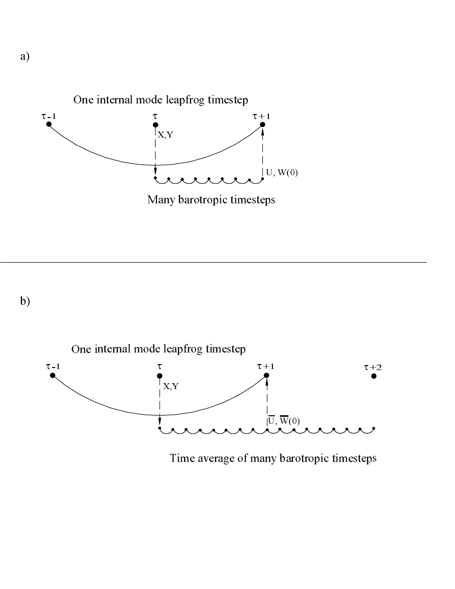
370
CHAPTER 29. OLD OPTIONS FOR THE EXTERNAL MODE
Figure 29.1: (a) Method according to Killworth et al. (1991). (b) The standard MOM method
which allows stretching the tracer timestep for global climate simulations. This method is
described in Chapter 30.

Chapter 30
Explicit free surface and fresh water
Neither of the two time stepping schemes of the Killworth et al. (1991) method (see Section
29.5) allows the tracer timestep to be stretched significantly longer than the baroclinic timestep.
Taking a tracer timestep which is 10 to 20 times longer than the baroclinic timestep is important
for spinning up global ocean simulations on climate time scales. It is for this reason that another
time stepping scheme has been implemented, and it has been found to be substantially more
stable.
The relation between baroclinic and barotropic timesteps is shown in Figure 29.1b. The
barotropic equations are integrated by the previously mentioned forward-backward scheme,
but the integration is over two baroclinic timesteps from τto τ+2. The solution is time averaged
over this period, which centers the barotropic fields at baroclinic time step τ+1. The time
averaged barotropic fields at τ+1 are used in the rest of the code as the effective barotropic
solution, and for purposes of initializing the subsequent barotropic integration.
As of Summer 1999, the MOM free surface has incorporated the effects of the undulating
surface height into the baroclinic and tracer equations. This element allows the model to be
conservative, even in the presence of fresh water forcing. Full details of the algorithm are
documented in Griffies, Pacanowski, Schmidt, and Balaji (2000). Much of this chapter is taken
from this paper, except for Sections 30.10 and 30.11, which were written by Martin Schmidt
(martin.schmidt@io-warnemuende.de) and Stephen Griffies.
The presence of a free surface which undulates as the surface height varies introduces the
possibility for much more physically realistic surface boundary conditions on the ocean model.
In particular, tracers can be input to the model with values which are distinct from the tracer
value in the surface ocean cell. This situation may arise, for example, when coupling the ocean
model to a river. Section 30.11 discusses, in detail, the issues of fresh water forcing in MOM,
and introduces a means for interfacing MOM to river models.
30.1 Free surface options
The options available in connection with the Griffies, Pacanowski, Schmidt, and Balaji (2000)
MOM explicit free surface code are the following:
-explicit free surface enables the explicit free surface scheme. All other barotropic solution
schemes have to be disabled. So long as neither explicit eb nor explicit efb are enabled, the
algorithm is that discussed in this section, and is not that of Killworth et al. This option
371
372
CHAPTER 30. EXPLICIT FREE SURFACE AND FRESH WATER
must also have either explicit free surface nonlinear or explicit free surface linear enabled.
There is no default.
-explicit free surface nonlinear provides the full effects of the surface height are incorpo-
rated. In order to do so, it is necessary to also enable option partial cell. This method will
conserve total tracer amount.
-explicit free surface linear enables a free surface in which the baroclinic and tracer equa-
tions employ constant volume upper model cells. This option yields a linearized free
surface which is similar in principle to that of Killworth et al (1991) and Dukowicz and
Smith (1994). This method will not conserve total tracer amount, which is a limitation
shared by the Killworth et al (1991) and Dukowicz and Smith (1994) methods.
-explicit eta laplacian enables a Laplacian filter to reduce the checkerboard null mode in
the sea surface height. Filtering is done after a sequence of barotropic time steps. More
details can be found in Section 30.12.
-explicit eta dpdc enables a “del-plus /del-cross” filter to reduce checkerboard null mode
in the sea surface height. As default filtering is done after a sequence of barotropic time
steps. Option explicit eta dpdc all enables filtering for each barotropic time step. More
details can be found in Section 30.12.
-explicit polar filter enables the polar filtering on the external mode. Filtering is applied
every barotropic time step to the free surface height and the vertically integrated velocity
field. Either firfil or fourfil are possible, though firfil is recommended. Polar filtering can be
expensive, and so it is suggested that one reduce the barotropic time step to compare costs
of simply resolving the dynamics. Polar filtering the barotropic fields also introduces a
lot of noise to the solution, as discussed in Sections 30.12 and 30.13.
-explicit fresh water flux inserts fresh water into the free surface height equation. Conser-
vation of total salt is realized so long as the tracer and baroclinic time steps are equal.
See Section 30.11 for further options related to water forcing.
-salinity psu computes model salinity in units of psu, rather than the traditional model
units (s−35)/1000. Option salinity psu is necessary with explicit fresh water flux in order
to get the correct sign in the salinity equation in regions where salinity is less than 35.
Options which are not available with the MOM free surface are explhmix,explicit eb,ex-
plicit efb.
The remainder of this chapter presents the details of the MOM explicit free surface method.
More complete treatment, with examples, is provided in Griffies, Pacanowski, Schmidt, and
Balaji (2000).
30.2 Momentum equations
Figure 30.1 details a zonal-depth cross-section of the rectangular control volumes over which
the model’s surface equations are discretized. Notably, the position of a grid point within a
cell is assumed to be fixed in time, hence maintaining the Eulerian nature of MOM. However,
the corresponding grid cell volume generally changes according to temporal undulations of
the surface height. We do not make the common approximation that the surface height is small

30.2. MOMENTUM EQUATIONS
373
relative to any other length scale in the model, including the ocean depth. Consequently, the
resulting barotropic equations represent nonlinear shallow water equations. In the following,
we focus on the zonal momentum budget as it is sufficient to expose the essence of the numerical
algorithm.
Ignoring meridional gradients for brevity, the continuous time budget for the zonal mo-
mentum of a Boussinesq fluid occupying a rectangular velocity cell is given by
∂t(ρoA huu)i=(ρoA huf v)i−hudy (pi+1−pi)
−ρody (Fx
i+1−Fx
i)−ρoA(Fz
k−1−Fz
k).(30.1)
In this equation, A=dx dy is the horizontal cross-sectional area of the velocity cell, huis
its thickness, idenotes the zonal grid point and kthe vertical, and these labels are exposed
only when needed. Metric terms arising from momentum advection and friction on a sphere
(e.g., Wajsowicz 1993, Griffies and Hallberg 1999) have been omitted for brevity, but they are
present in the numerical code. The constant Boussinesq density, ρo, is not set to 1g cm−3, as
previously done in the Bryan-Cox-Semtner model (Bryan 1969, Cox 1984, Semtner 1974) or
previous versions of MOM (Pacanowski, Dixon, and Rosati 1991). Instead, ρo=1.035 g cm−3,
from which density in the World Ocean generally deviates by less than 2% (Gill 1982, page 47),
whereas using ρo=1.0 g cm−3is less accurate.
Fxrepresents the thickness weighted zonal advective and turbulent momentum fluxes passing
across the vertical faces of the cell. To compute these fluxes with space-time varying cell
thicknesses, we exploit the numerical methods developed by Pacanowski and Gnanadesikan
(1998) for use with a partial bottom cell representation of topography. Notably, those methods
provide a means to discretize the model equations when the cell thicknesses are functions of
horizontal position. It is a straightforward extension of their work to allow the cell thicknesses
to be functions of time. For further numerical details, refer to Pacanowski and Gnanadesikan
(1998).
Fzrepresents the vertical advective and turbulent momentum flux passing across the hori-
zontal cell faces. In particular, Fz
k=0represents the momentum flux passing through the ocean
surface at z=η. It consists of the usual vertical turbulent momentum flux and a contribution
from the vertical advection of momentum relative to the moving sea surface,
Fz
k=0=Fz,turb
k=0−qwuk=0.(30.2)
The surface flux Fz
k=0must be prescribed by the boundary condition that the total vertical
momentum flux through the air sea interface is continuous at z=η. That is, Fz
k=0=M, where
the prescribed momentum flux Mtakes the form
M=−(ρ−1
oτx
winds +qwuw),(30.3)
which has contributions from wind stress and momentum flux with fresh water. Although the
total momentum flux is continuous at z=η, the two components need not be. For example,
the fresh water velocity uwmay be different from uk=0, although most climate models assume
they are equal and take them equal to the horizontal velocity uk=1in the top model grid cell.
This point is further discussed below.
On the B-grid used in MOM, the offset in the horizontal between velocity and tracer/density
points means that the hydrostatic pressure at the western face of a velocity cell is given by
pi=gρi(|z1|/2+ηi)y+patm
i,(30.4)
374
CHAPTER 30. EXPLICIT FREE SURFACE AND FRESH WATER
where αyis a meridional grid average. pb=(g|z1|/2) ρiyis a discretization of the baroclinic
pressure, whose horizontal gradients arise from baroclinicity in the density field. Note that z1
has been assumed independent of horizontal position, hence its removal from the meridional
average operator. ps=gρiηiyis a discretization of the surface pressure, whose gradients arise
from those in the density weighted free surface height. patm
irepresents an atmospheric pressure
contribution. It is dropped in the following for brevity, yet is maintained in the numerical code
when coupling to atmospheric models.
For Boussinesq models, it is common to approximate the surface pressure as ps≈gρoηiy,
rather than the hydrostatic form gρiηiy. With this approximation, surface pressure gradients
arise solely from gradients in the free surface height. To maintain self-consistency with the
hydrostatic baroclinic pressure field, while incurring only trivial computational expense, we
maintain the hydrostatic form ps=gρiηiyin the model.
As discussed in the next subsection, time stepping of the baroclinic velocity in MOM is
performed using the average cell velocity. Dividing the budget (30.1) by the generally time
dependent volume of the velocity cell hudx dy, and performing the product rule on the time
derivative ∂t(huu), leads to the zonal velocity equation
∂tuk=f vk−∂xps/ρo+˜
Gk(30.5)
where ˜
Gkrepresents the forcing
hu
k˜
Gk=hu
kGk−δk1uk∂tη
=−hu
k∂xpb/ρo−∂xFx−(Fz
k−1−Fz
k+δk1uk∂tη).(30.6)
The u1∂tηterm and the time dependent surface cell thicknesses represent fundamentally new
elements relative to the traditional rigid lid analogs of these equations. Notably, the cell
thicknesses huused for computing the terms in Gkare taken at baroclinic time τ, as are the
other inviscid contributions such as pressure and advection.
The fresh water velocity uwin the surface momentum flux (30.3) requires additional efforts
to specify the complete boundary conditions. However, the momentum flux with fresh water
is in many cases smaller than the uncertainty in the parameterized wind stress. So, simple
approximations for uwmay exploited to reduce the model complexity. Considering
u1∂tη+Fz
k=0=−ρ−1
oτx
winds −u1∇h·U+qw(u1−uw),(30.7)
it is seen that the approximation uw≈u1removes the explicit dependence of baroclinic mo-
mentum on the fresh water flux. Fresh water does influence baroclinic momentum indirectly,
however, through its affects on the convergence −∇h·Uof the vertically integrated velocity.
The approximation uw≈u1should be well justified for many cases, and generalizations for
special cases such as heavy rainfall are straightforward.
Instead of time stepping the barotropic velocity, MOM time steps the vertically integrated
transport U=Pkhkuk, as is common in shallow water models. Its evolution takes the form
∂tU=u1∂tη+X
k
hk∂tuk
=f V −D∂xps/ρo+G,(30.8)
where equation (30.5) was used for ∂tuk, the vertically integrated forcing is given by G=
PkhkGkwith Gkdefined in equation (30.6), and D=Pkhkis the time dependent ocean depth.
Once the transport and ocean depth are updated, the updated barotropic velocity can be
diagnosed through u=U/D.
30.3. TIME STEPPING ALGORITHM
375
30.3 Time stepping algorithm
The focus in this subsection is on time and depth discretization, with Figure 30.2 summarizing
the following algorithm. For purposes of brevity, the horizontal spatial discretization discussed
in the previous subsection will not be exposed. Also, discrete baroclinic times and time steps
will be denoted by the Greek τand ∆τ, respectively, whereas the barotropic analogs will use
the Latin tand ∆t.
The basic idea is to split the velocity at an arbitrary depth level kand baroclinic time
τ′=τ+ ∆τinto two components
uk(τ′)=Bkm(τ)um(τ′)+(δkm −Bkm(τ)) um(τ′)
≡ˆ
uk(τ, τ′)+u(τ, τ′).(30.9)
The following “baroclinicity operator” is used to affect this split
Bkm(τ)=δkm −D(τ)−1hu
m(τ),(30.10)
where δkm is the Kronecker delta, summation over the repeated vertical level index mis implied,
and
D(τ)=X
k
hu
k(τ)=Do+ηu(τ) (30.11)
is the ocean depth at baroclinic time τover a column of velocity points, with Dothe resting
ocean depth.
The introduction of two baroclinic time labels to equation (30.9) is necessitated by the
freedom afforded the ocean depth to change in time. This property is in contrast to the case
with a rigid lid, or the fixed volume free surface models of Killworth et al. (1991) and Dukowicz
and Smith (1994).
Equation (30.9) is an identity which is valid for any baroclinic times τ′and τ. Its utility
depends on the ability to render a relatively clean and stable split between the fast and slow
dynamics. The form of the baroclinicity operator Bkm(τ) is motivated by an attempt to perform
such a split. That is, it projects out the approximate baroclinic portion of a field, where the
projection is based on the distribution of cell thicknesses at time τ.
If the split introduced in equation (30.9) is successful, the baroclinic velocity ˆ
uk(τ, τ′) will
evolve on a slow time scale ∆τ. In turn, the barotropic velocity u(τ, τ′) will evolve on the fast
time scale ∆t=2N−1∆τ, with Ndetermined by the ratio of external to internal gravity wave
speeds (N≈100 for climate models). The method therefore proceeds by separately updating
ˆ
uk(τ, τ′) and u(τ, τ′) by exploiting the time scale split. Upon doing so, the right hand side of the
identity (30.9) will be specified, hence allowing for an update of the full velocity field uk(τ+∆τ).
The following discussion details these ideas.
By construction, evolution of the baroclinic mode is unaffected by vertically independent
forces, such as those from surface pressure gradients. Therefore, it is sufficient to update the
“primed” velocity
u′
k(τ+ ∆τ)=uR
k(τ−∆τ)+2∆τ[f vk(τ)+˜
Gk(τ)],(30.12)
which represents a temporal discretization of the full momentum equation (30.5), yet without
the surface pressure gradient. The lagged velocity uR
k(τ−∆τ) is a Robert time filtered version
of the full velocity field. A weak form of such filtering has been found sufficient to suppress a
splitting between the two branches of the leap-frog (e.g., Haltiner and Williams 1980). It is also
useful to dampen any fast dynamics which may partially leak through the baroclinicity operator
376
CHAPTER 30. EXPLICIT FREE SURFACE AND FRESH WATER
due to the imperfect baroclinic/barotropic split discussed in Section 5.1.1. The baroclinic piece
of the primed velocity u′
k(τ+ ∆τ) is equivalent to the updated baroclinic velocity
ˆ
uk(τ, τ + ∆τ)=B(τ)km u′
m(τ+ ∆τ),(30.13)
thus specifying one half of the identity (30.9).
To update the barotropic velocity u(τ, τ+∆τ), we employ a forward-backward time stepping
scheme (e.g., Haltiner and Williams 1980). For this scheme, the surface height is time stepped
using the small barotropic time step ∆t
η∗(tn+1)=η∗(tn)−∆t[∇h·U∗(tn)−qw(τ)],(30.14)
with tn=n∆tthe barotropic time, and n∈[0,N]. The asterisk is used to denote intermediate
values of the barotropic fields, each of which are updated on the barotropic time steps. For
stability purposes, it is important to take the initial condition η∗(0) as the time average η∗from
the previous barotropic integration (time averaging is defined by equation (30.17) discussed
below). Note that it is assumed that the fresh water flux qwis constant over the small barotropic
time steps, since the hydrological fluxes are typically updated at a period no shorter than the
baroclinic time step.
Having the surface height η∗updated to the new barotropic time step allows for an update
of the transport
U∗(tn+1)=U∗(tn)+f∆t V∗(tn)+V∗(tn+1)
2!
+ ∆t[G(τ)−D(τ)∂x˜
p∗
s(tn+1)],(30.15)
where ˜
p∗
s(tn+1)=gη∗(tn+1)ρ(τ)/ρois the surface pressure normalized by the Boussinesq density.
Both the ocean depth D(τ) and depth integrated forcing G(τ) are assumed to evolve on the
baroclinic time scale, and so are held constant over the extent of the barotropic time steps
from τto τ+2∆τ. The Coriolis force is computed using a Crank-Nicholson semi-implicit time
stepping scheme (e.g., Haltiner and Williams 1980).
After Nbarotropic time steps, the vertical transport and surface height are time averaged
to produce
U∗(τ+ ∆τ)=1
N+1
N
X
n=0
U∗(tn) (30.16)
η∗(τ+ ∆τ)=1
N+1
N
X
n=0
η∗(tn).(30.17)
The time averaged fields are centered on the baroclinic time step τ+ ∆τ, so long as Nis an
even integer. Equating the barotropic velocity u(τ, τ + ∆τ) to U∗(τ+ ∆τ)/D(τ) allows for the full
velocity field u(τ+ ∆τ) to be updated according to equation (30.9). The time averaged field
η∗(τ+ ∆τ) is used to initialize the next suite of barotropic integrations from τ+ ∆τto τ+3∆τ.
To begin the next baroclinic time step, it is necessary to determine the updated surface
height η(τ+ ∆τ) and vertically integrated velocity U(τ+ ∆τ). A natural choice is to equate
these fields to the time averages of the intermediate fields η∗and U∗given by equations (30.16)
and (30.17). Unfortunately, this choice does not lead to a self-consistent and conservative
algorithm. The reason is that it is essential to maintain consistency between the updated ocean
30.3. TIME STEPPING ALGORITHM
377
depth, full velocity, barotropic velocity, all while maintaining basic conservation properties.
The following approach has been found to be sufficient for these purposes.
As discussed in Section 30.9, since the tracer concentration is time stepped with a leap-frog
scheme, quasi-conservation of tracer results if the surface height is similarly time stepped
η(τ+ ∆τ)=η∗(τ−∆τ)−2∆τ[∇h·U(τ)−qw(τ)].(30.18)
To maintain stability and smoothness of the solutions, it has been found necessary to use the
lagged surface height η∗(τ−∆τ) rather than a more traditional Robert filtered height. As
so defined, η(τ+ ∆τ) is used to update thicknesses of the surface grid cells ht
k(τ+ ∆τ) and
hu
k(τ+ ∆τ). Given these new thicknesses, the updated transport U(τ+ ∆τ) can be diagnosed
from the known full velocity uk(τ+ ∆τ) through
U(τ+ ∆τ)=X
k
hu
k(τ+ ∆τ)uk(τ+ ∆τ),(30.19)
thus ensuring self-consistency between the updated full velocity and the updated vertically
integrated velocity. That is, with time dependent thicknesses, U(τ+ ∆τ) differs from the time
averaged field U∗(τ+ ∆τ) because of the changing level thicknesses. To complete the time
stepping, the updated barotropic velocity is diagnosed through
u(τ+ ∆τ)=U(τ+ ∆τ)/D(τ+ ∆τ),(30.20)
where D(τ+ ∆τ)=Phu
k(τ+ ∆τ) is the new depth of a velocity cell column.
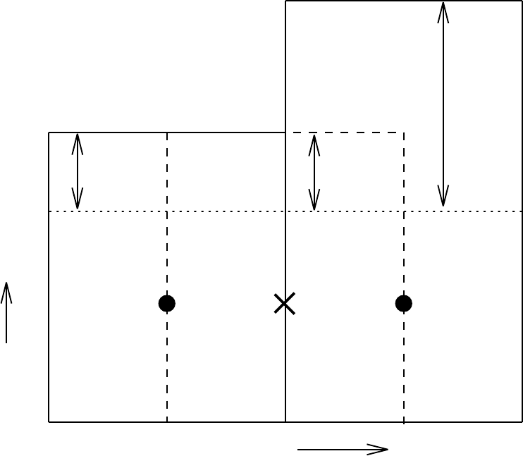
378
CHAPTER 30. EXPLICIT FREE SURFACE AND FRESH WATER
east
T(i) U(i) T(i+1)
z=0
z=z1
ηt
i+1
ηi
u
ηt
i
up
Figure 30.1: Schematic of rectangular surface tracer and velocity cells with the free surface.
The tracer points are denoted by a solid dot and the tracer cells are enclosed by solid lines; a
velocity point is denoted by an “x” and is enclosed by dashed lines. These points have fixed
vertical position z=z1/2<0, regardless of the value for the free surface height. The thickness
of a tracer cell is ht=−z1+ηt, where ηtis the prognostic surface height determined through
volume conservation (i.e., the vertically integrated continuity equation (7.18)). The thickness
of a velocity cell is hu=−z1+ηu, where ηuis determined by taking the minimum height of
the four surrounding tracer cells, as prescribed by the partial cell approach of Pacanowski and
Gnanadesikan (1998). Thicknesses of the cells are assumed to be positive, so that −z1+ηt>0.
In models without an explicit representation of tides, this constraint in practice means that |z1|
must be greater than roughly 2m. For models with tides, |z1|may need to be somewhat larger,
depending on the tidal range considered.
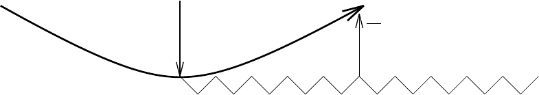
30.3. TIME STEPPING ALGORITHM
379
τ
~U
τ−∆τ τ+∆τ τ+2∆τ
G
Figure 30.2: Schematic of the split-explicit time stepping scheme. Time increases to the right.
The baroclinic time steps are denoted by τ−∆τ, τ, τ+∆τ, and τ+2∆τ. The curved line represents
a baroclinic leap-frog time step, and the smaller barotropic time steps N∆t=2∆τare denoted
by the zig-zag line. First, a baroclinic leap-frog time step updates the baroclinic mode to τ+ ∆τ.
Then, using the vertically integrated forcing G(τ) (equation 30.8) computed at baroclinic time
step τ, a forward-backward time stepping scheme integrates the surface height and vertically
integrated velocity from τto τ+2∆τusing Nbarotropic time steps of length ∆t, while keeping
G(τ) and the ocean depth D(τ) fixed. Time averaging the barotropic fields over the N+1 time
steps (endpoints included) centers the vertically integrated velocity and free surface height at
baroclinic time step τ+ ∆τ. Note that for accurate centering, Nis set to an even integer.

380
CHAPTER 30. EXPLICIT FREE SURFACE AND FRESH WATER
30.4 Vertical velocities
Vertical velocities are diagnosed at baroclinic time steps using volume conservation within
a grid cell. In particular, volume conservation over a surface cell indicates that the vertical
velocity at the bottom face of this cell arises from the horizontal convergence of volume in this
cell, time tendencies in the thickness of this cell, and volume passing across the top face from
fresh water fluxes.
It is useful to see precisely how these velocities are determined. For this purpose, consider
a vertical integral of the continuity equation ∇ · u=0 over a rectangular top model grid cell
wk=1=w(η)+Zη
z1
dz ∇h·uh.(30.21)
Use of the surface kinematic boundary condition
(∂t+u(η)· ∇h)η=w(η)+qw,(30.22)
and Leibnitz’s Rule with ∇hz1=0 leads to
wk=1=∂tη−qw+∇h·Zη
z1
dz uh
=−∇h·U+∇h·Zη
z1
dz uh,(30.23)
where the last step used the vertically integrated continuity equation (7.18). This exact expres-
sion for wk=1is approximated in the model with a discretized version of
wk=1≈ −∇h·U+∇h·(huh),(30.24)
where h=η+|z1|is the surface cell thickness, and the horizontal velocity uhis that in the
surface cell k=1. Notably, many implementations of the free surface linearize the surface
kinematic boundary condition by dropping the surface height advection u(η)· ∇hη. No such
approximation has been made here.
Given an expression for the convergence −∇h·U, diagnosing wk=1in this manner allows for
the remaining interior vertical velocities to be successively found through further integration of
the continuity equation downward through a vertical column. On a B-grid, −∇h·Uis centered
on a tracer point. Hence, equation (30.24) yields the vertical velocity on the bottom face of the
surface tracer cell. The vertical velocity on the surrounding velocity cells is constructed as a
volume conserving average of the surrounding tracer cell vertical velocities.
In MOM, the bottom of the ocean on tracer cells is a flat surface, representing the “lopped
off” surfaces of topography1. Hence, the vertical velocity must vanish at this location. A
self-consistency check on how accurate the model’s numerics conserve volume amounts to
testing how well this property is satisfied when integrating downwards from the ocean sur-
face, starting from the vertical velocity given by equation (30.24). Adding fresh water to the
model provides a nontrivial test of these properties. The present scheme produces zero ver-
tical velocities at the bottom of tracer cells, to within computer roundoff, regardless of the
topography or surface forcing.
1The bottom velocity cell generally does not sit on the ocean bottom, and so can support a vertical velocity due
to sloping topography. Details of how MOM handles this velocity are given in Webb (1995) and Section 22.3.3.

30.5. COMMENTS ON THE ALGORITHM
381
30.5 Comments on the algorithm
The time averaged portion of the algorithm provides a fairly heavy filter of the fast barotropic
gravity waves active on the barotropic time scales. Since these waves are not of interest here,
such filtering is justified. As might be expected, time averaging greatly stabilizes the scheme
so that stretching of tracer time steps to values larger than the baroclinic time step is available.
Note that the Killworth et al. (1991) scheme has no time averaging, and correspondingly we
have found it to be quite unstable with stretched tracer time steps.2The stretching of tracer
time steps is ubiquitous in coarse resolution ocean models (e.g., Bryan 1984, Killworth et al.
1984, Danagasoglu et al. 1996), and so we consider the added stability of the present scheme
to be of great practical value.
Allowing the grid cell thicknesses to evolve introduces a fundamentally new element to
the traditional algorithms relevant for constant cells in z-coordinate models. However, since
the model does not integrate the thickness equation at each vertical depth, as required in an
isopycnal layered model, and since we impose positive cell thicknesses for all cells, including
the surface, modifications to the constant cell approach are relatively modest.
Although the immediate application of the algorithm is for the free surface method, the
algorithm is general so that any thickness within a vertical column can vary in time, within
the constraints of positive cell thicknesses mentioned above. In particular, it is thought that
this approach will find additional use for models with a time varying bottom boundary layer
thickness, such as that proposed by Killworth and Edwards (1999).
30.6 Discrete tracer budgets
The purpose of this section is to derive the discrete tracer budgets within the free surface ocean
model with a time dependent top cell volume.
As for the formulation of the discrete momentum equations in Section 30.2, the continuous
time budget for the total amount of tracer within a given tracer cell (Figure 30.1) is given by
∂t(A htT)=−dy (Fx
i+1−Fx
i)−A(Fz
k−1−Fz
k),(30.25)
where Tis the tracer per unit volume, i.e., a tracer concentration, Ais now the horizontal area
of the tracer cell, htis the thickness of the tracer cell, meridional gradients are omitted for
brevity, and the thickness weighted horizontal advective and diffusive fluxes Fxare computed
as in Pacanowski and Gnanadesikan (1998) to account for the generally different adjacent cell
thicknesses.
Fz
kis the vertical turbulent and advective tracer flux through the cell interface k. The special
term Fz
k=0for the vertical tracer flux at the sea surface z=ηinvolves vertical tracer advection,
relative to the undulating sea surface, by fresh water, as well as the usual parameterized
turbulent flux
Fz
k=0=Fz,turb
k=0−qwTk=0.(30.26)
The tracer flux Fz
k=0must be calculated from a boundary condition which equates this flux with
the total tracer flux QTthrough the surface. The flux QTgenerally has a contribution from
2Tests conducted at the Southampton Oceanography Center indicate a need to perform a time average over
barotropic time steps, even when using equal tracer and baroclinic time steps, to suppress an instability associated
with aliased barotropic Rossby waves near the equator (David Webb, personal communication).
382
CHAPTER 30. EXPLICIT FREE SURFACE AND FRESH WATER
parameterized turbulence as well as a tracer flux with fresh water,
QT=Qturb
T−qwTw,(30.27)
where Twis the tracer concentration in the fresh water. Although Twand Tk=0may be of the
same order of magnitude, the terms qwTwand qwTk=0stand for different physical processes.
The term qwTwrepresents the amount of tracer passing through the air sea interface with fresh
water, whereas qwTk=0represents the advection of tracer in the ocean relative to the sea surface.
Note that for the special case of salt, the total surface salt flux Qsis well approximated to be
zero for climate modeling. More will be said about salt below.
In general, specification of the surface tracer flux involves details of how the air-sea interface
is modeled. A simple example of a “closure” for the turbulence term is a restoring condition
Qturb
T=γht(T1−T∗), where γis an inverse damping time and T1is the time lagged surface
tracer concentration. For the advection term, a simple choice is to set the tracer concentration
Twin the fresh water equal to the surface cell concentration T1, now without time lag as it
represents an advective contribution. Other forms are generally appropriate when employing
ocean models with more realistic surface boundary conditions, such as for coupled climate
simulations.
30.7 Time discretization of the tracer budgets
The question arises whether it is more suitable to time step the thickness weighted tracer
concentration htT, or the tracer concentration T. Indeed, this question is also relevant for
the baroclinic velocity equations. As discussed in Section 30.2, we found time stepping the
baroclinic velocity, rather than the thickness weighted baroclinic velocity, to be suitable and
to involve only a small number of changes to the equations relevant for the rigid lid version
of MOM. Energetic consistency, in which buoyancy effects in the density equation balance the
work done by pressure from the momentum equation, and convenience motivate a similar
temporal discretization of the tracer budget.
Our starting point is the tracer concentration budget, which is obtained by dividing the
tracer budget (30.25) by the tracer cell cross-sectional area, and performing the product rule on
∂t(htT)
ht∂tT=−∂xFx−(δk1Tk∂tη+Fz
k−1−Fz
k).(30.28)
The δk1Tk∂tηterm, as well as the time dependent thickness ht, distinguish this budget from
that considered with the partial bottom cells of Pacanowski and Gnanadesikan (1998). Note
that as for the momentum equations, the thickness is computed at the present time step ht(τ)
as are other non-diffusive terms.
The tracer concentration budget (30.28) is time stepped with a leap-frog scheme along with
the same Robert time filter used with the baroclinic integration. Upon setting the tracer to unity
and omitting boundary fluxes, the tracer budget reduces to volume conservation. This self-
consistency between tracer and volume conservation must be maintained with the discretized
equations in order to allow for tracer conservation (Section 30.9).
30.8 Further comments on surface fluxes and the case of salt
It is useful to further elucidate the different terms describing the surface tracer fluxes. Addi-
tionally, the special case of salt deserves some comments.
30.8. FURTHER COMMENTS ON SURFACE FLUXES AND THE CASE OF SALT
383
Use of the free surface equation (7.18) and the surface tracer flux expression (30.27) leads
to the relation
T1∂tη+Fz
k=0=T1∂tη+QT
=Qturb
T−T1∇h·U+qw(T1−Tw).
(30.29)
Hence, only the balance of the advective and turbulent tracer fluxes enters the model equations.
Notably, neither the tracer Tk=0nor the turbulent flux Fz,turb
k=0are explicitly needed. Relatedly,
the distinction should be made between qwT1, which naturally appears here in the relation
(30.29), and qwTk=0, which appears in the expression for Fz
k=0in equation (30.26).
The relation (30.29) is analogous to the surface momentum flux relation given by equation
(30.7). Assuming that the tracer concentration in the fresh water is the same as in the surface
cell, Tw≈T1, makes the tracer time tendency independent of any explicit fresh water forcing.
Instead, the dependence is restricted to the affects that fresh water has on the convergence
∇h·U. This approximation simplifies the setup of boundary conditions for the tracer flux.
However, in general Twand T1are distinct and so Twmay need to be specified explicitly from
data or another component model.
For salt, due to a large hydration energy, the air-sea interface effectively acts as an impene-
trable barrier. Therefore, neglecting the formation of sea spray and the interchange of salt with
sea ice, and in the absence of salt entering through the solid earth boundaries, total ocean salt
is constant. In turn, the salt concentration ρoswithin a grid cell, where sis salinity, changes
only through advective and turbulent fluxes from the interior ocean, as well as time tendencies
in the volume of the grid cell. From the flux expression (30.27), a zero salt flux through the
air-sea interface formally represents a balance
Fz
k=0=Fz,turb
k=0−qwsk=0=Qs=0 (30.30)
between the turbulent flux and advective flux. Discussion of this balance has been given by
Huang (1993), where the turbulent flux was called an anti-advective flux. Specifying Qs=0
in the relation (30.29) indicates that surface salinity is affected only through the s1∂tηterm.
Alternatively, but perhaps less fundamentally, one sees that s1∂tηis the only relevant term
when one sets the salinity of the fresh water to zero, sw=0, and drops the turbulent flux term
Qturb
s=0.
For purposes of numerical accuracy, MOM has traditionally time stepped salinity deviation
smom =(s−35)/1000 rather than the non-negative salt concentration s.smom is useful for models
where the salinity does not deviate much from 35 psu. Turbulent fluxes of smom, as they depend
on spatial gradients, are scaled by 1000 from fluxes of salinity s. For a Boussinesq fluid in the
absence of fresh water fluxes, advective fluxes scale likewise. Hence, smom can be used for a
rigid lid or free surface model, so long as there are no fresh water fluxes.
In the presence of fresh water fluxes, however, salinity can deviate significantly from 35
psu, especially when using high resolution ocean models with a realistic hydrological cycle.
Additionally, in order to represent the proper effect on salinity from the input of fresh water, it
is more straightforward to employ salinity sin the model instead of the deviation smom. To see
why, consider the case of zero interior fluxes for which the continuous time salinity equation in
a surface cell takes the form ∂ts=−(q s)/h. If sis less than 35 psu, then q smom has the opposite
sign of q s. Time stepping ∂tsmom =−(q smom)/hwould hence lead to the unphysical result of
increasing smom when adding fresh water.
384
CHAPTER 30. EXPLICIT FREE SURFACE AND FRESH WATER
Allowing salinity to deviate significantly from 35psu motivates a more general approach
than that discussed by Bryan and Cox (1972) for computing ocean density. Bryan and Cox
approximate the full UNESCO equation of state by different cubic polynomials for each model
depth level. This approach is warranted for models in which salinity is close to 35psu and
for which the model’s vertical cell thickness is independent of horizontal position. The latter
assumption is broken by the Pacanowski and Gnanadesikan (1998) partial bottom cells, and
the former is broken by realistic fresh water fluxes. Hence, for the purpose of computing the
model’s hydrostatic pressure, we employ the full UNESCO equation of state as formulated by
Jackett and McDougall (1995). In this approach, in situ density is computed as
ρ(τ)=ρ[θ(τ),s(τ),p(τ−∆τ)],(30.31)
where θis the model’s potential temperature, sis salinity, and pressure is lagged one time step
instead of performing the iterative approach described by Dewar et al. (1998). The added cost
of this approach is modest (5 −10% depending on the model configuration).
This is an opportune point to recall the salt budget employed in rigid lid streamfunction
models. In that case, one assumes that ∂tη=∇h·U=0, which means that the only way to
affect salinity when there is a surface water flux is to do so indirectly through the addition of a
non-zero salt flux
Qs=soqw,(30.32)
where sois a global constant representing the mean ocean salinity, which is typically taken as
35 psu. The use of a globally constant normalization sois required in order to conserve both
salt and fresh water. Referring to the more realistic zero salt flux given by equation (30.30)
for the free surface, the rigid lid salt flux, often termed a virtual salt flux, can be considered a
linearization of the turbulent salt flux Qturb about the mean salinity state of the ocean. Barnier
(1998) provides a detailed and pedagogical discussion of virtual salt fluxes.
Within the context of a constant volume model, Huang (1993) provides a discussion of
how steadily forced ocean models can behave when forced with fresh water fluxes. We
are also intrigued by the possible differences in response under transient forcing, such as
occurs in realistic coupled climate models where potentially large local departures of salinity
from the global mean soare associated with river runoff, evaporation, precipitation, and ice
melting/freezing.
30.9 Discrete conservation properties
As mentioned previously, it is essential that the free surface method provide for a physically
relevant set of discrete conservation laws. This section discusses these issues.
30.9.1 Volume conservation
To conserve model volume, it is sufficient to ensure that the surface height ηevolves in a
conservative manner. Both explicit time stepping discretizations (30.14) and (30.18) trivially
satisfy such conservation. All model tests indicate that volume is conserved to within computer
roundoff.

30.9. DISCRETE CONSERVATION PROPERTIES
385
30.9.2 Energetic consistency
Energetic consistency of the methods used here have been shown elsewhere. First, the argu-
ments given by Bryan (1969) account for the momentum advection terms, which are discretized
using second order centered differences. The result is a redistribution of local kinetic energy,
yet a preservation of its global integral. Second, the arguments in the appendix of Pacanowski
and Gnanadesikan (1998) show that the partial cell methods ensure that the change in energy
due to horizontal pressure forces balances potential energy change when density is linearly
dependent on temperature and salinity. Importantly, this consistency is realized only when
incorporating the undulating surface grid cell thickness into both the tracer and baroclinic ve-
locity equations, as done here. Third, Appendix B of Dukowicz and Smith (1994) provide a
complementary analysis of the energetic consistency within their implicit free surface method,
much of which is relevant for the present considerations.
30.9.3 Tracer quasi-conservation
An analysis of tracer conservation for the present method has not been given elsewhere, and so
warrants discussion. For this purpose, multiply the tracer budget (30.28) by the area of a tracer
cell Aij and sum over all cells. All flux terms reduce to boundary fluxes, which are assumed
for the following purposes to vanish. The result is the balance
X
ijk
Aij ht
k(τ)∂tTk(τ)+δk1Tk(τ)∂tη(τ)=0.(30.33)
A simplified form of this budget was discussed in the Introduction. Using a leap-frog time
stepping scheme for both the tracer concentration and surface height leads to the discrete time
budget
X
ijk
Aij ht
k(τ)(Tk(τ+ ∆τ)−TR
k(τ−∆τ)=−X
ij
Aij T1(τ)η(τ+ ∆τ)−η∗(τ−∆τ).(30.34)
Note that it was necessary to assume that the tracer and baroclinic time steps are equal in
order to reach this result. In this expression, TR
krepresents the Robert time filtered tracer
concentration, and η∗is the time averaged surface height. The presence of the Robert time
filtering and the time averaging makes this discrete balance only a quasi-conservation law.
That is, in the absence of boundary fluxes, the total tracer
X
ijk
Aij hk(τ)Tk(τ+ ∆τ)+δk1Tk(τ)hk(τ+ ∆τ)(30.35)
is not exactly constant in time. Instead, time truncation errors allow for only partial conserva-
tion. Note that even if one were to employ a time stepping scheme for the surface height which
did not use time averaging, or if one time stepped thickness weighted tracer instead of tracer
concentration, the use of a Robert filter to suppress the leap-frog splitting for the tracer concen-
tration precludes exact tracer conservation. Alternative approaches, such as Hallberg (1997),
can be constructed which use only two-time levels and which do not admit time splitting. In
this case, an exact discrete form of tracer conservation can be given. Given these caveats, it
has nonetheless been found that for all tests conducted, including realistic simulations with
mesoscale eddies, the total tracer given by equation (30.35) remains steady with the present
free surface scheme. That is, the tests show near exact conservation with no noticeable trend.
386
CHAPTER 30. EXPLICIT FREE SURFACE AND FRESH WATER
Even though we have found the model to be numerically stable when stretching tracer time
steps longer than baroclinic steps, as commonly done in rigid lid models, doing so precludes
tracer conservation within top model grid cells since their volumes temporally vary. This is
not a constraint shared by rigid lid models, and so it warrants some explanation.
Technically, the constraint of equal baroclinic and tracer time steps is seen by noting that
without equating them, it is not possible to identify a physically relevant quasi-conserved
property such as the total tracer given by equation (30.35). Fundamentally, the constraint arises
from the coupling between tracer and volume conservation. For example, with a rigid lid, the
volume of each cell is temporally constant, and so there is no constraint on tracer time steps
so far as tracer or volume conservation are concerned. In contrast, when the volume of a cell
is allowed to dynamically change, this change must occur in concert with the change in tracer
concentration in order to conserve total tracer. It is interesting to note that attempts at time
stepping the thickness weighted tracer equation (30.25), which yields the more conventional
quasi-conserved discrete quantity h(τ)Tk(τ), results in numerical instabilities when stretching
the tracer time step longer than the baroclinic time step. This approach is therefore severely
limited in its utility for coarse resolution climate studies.
Although it is important to conduct realistic tests of this conservation property, and such
tests have been done, it is useful to mention here some idealized cases, each of which start with
uniform temperature and salinity fields. Blowing winds causes the free surface to undulate and
hence to redistribute volume and generate barotropic currents. However, pure wind forcing
will not cause the temperature or salinity within a grid cell to change, and it will not cause
the total model heat, total salt, or total volume to change. In effect, this experiment checks the
consistency of the discretized tracer and volume budgets. If instead of blowing winds, there is
fresh water added with temperature equal to that in the ocean, but with zero salinity, then the
temperature in each cell will stay constant, the heat increase, the volume increase, the salinity
decrease, and the total model salt remain constant.
Tracer conservation issues are relevant for spinning up coarse resolution z-coordinate cli-
mate models to a thermodynamic equilibrium. The rigid lid procedure, as discussed by Bryan
(1984), Killworth et al. (1984), and Danagasoglu et al. (1996), typically employs a stretched
tracer time step. Doing so with the current free surface will not allow for tracer conservation in
the surface grid cells. However, preliminary idealized restoring boundary condition tests in-
dicate that this subtlety does not alter the equilibrium solution as compared to that found with
the rigid lid method. Further tests will be necessary to determine whether this insensitivity is
robust when employing more realistic boundary conditions, including fresh water.
30.10 Detailed treatment of surface tracer budgets
The purpose of this section is to revisit, in detail, the issues of surface tracer budgets, and in
particular to describe the various decisions that have been made in the model implementation.
One of the main goals is to provide a conservative numerical scheme which circumvents the
peculiarity of advection and diffusion operators acting on different time levels. There is some
overlap with the discussion in Section 30.6, although, again, the present section is closely tied
to specific choices made in the numerical code.
30.10. DETAILED TREATMENT OF SURFACE TRACER BUDGETS
387
30.10.1 Summary of the surface tracer fluxes
Recall the continuous time tracer budget
ht∂tT=−∂xFx−(δk1Tk∂tη+Fz
k−1−Fz
k).(30.36)
For all levels except the sea surface where k=1, the tracer fluxes can be calculated from the
model variables. At the surface, the vertical flux Fz(z=η), or the discrete counterpart Fz
k=0,
must be specified in order to solve the vertical advection-diffusion equation. Conservation
of tracer indicates that the surface tracer flux entering the ocean must equal that flux leaving
other component models, such as the atmosphere, river, ice, etc. For substances such as salt,
gases, or trace metals, the total tracer mass is conserved. For heat flux, the latent heat from
condensation and evaporation provides a heat source at the sea surface which can be included
in the heat, or enthalpy, budget.
30.10.1.1 Flux between the ocean model and other model components
Letting QTsymbolize the flux leaving the other component models and entering the ocean,
tracer conservation leads to the surface boundary condition
Fz
k=0=QT.(30.37)
This equation acts to close the surface tracer budget associated with vertical transfer, where
the flux QTis prescribed from data, determined via a restoring procedure, or calculated from a
model which resolves details of the planetary boundary layer. In general, QThas a contribution
from parameterized turbulent flux as well as an advective tracer flux coming in with fresh water,
QT=−(Qturb
T+qwTw).(30.38)
In this expression, Twis the tracer concentration in the fresh water, and qwis the fresh water
volume per time per area (units of velocity) entering or leaving the ocean. Both qwand the
turbulent tracer flux Qturb
Tare counted as positive if tracer enters the surface cell, and the sign
convention corresponds to that employed in the numerical model.
For the case of salt, if one neglects sea spray and brine formation in sea ice, the surface salt
flux, due to the large hydration energy, is zero,
Qs=0.(30.39)
Notably, knowledge of the detailed dynamics of wave breaking and wind stirring, which
generally are not resolved in an ocean climate model, is not needed for a correct salt budget.
For heat and fresh water fluxes, the specification of the surface flux QTappears to be more
complex than salt. Firstly, the surface fluxes are sensitive to the sea surface temperature (SST).
Secondly, due to the skin effect and the complex surface radiation balance, the SST may differ
substantially from the average temperature of the surface model cell. The following discussion
assumes that this very difficult problem in boundary layer physics is solved, or approximately
solved, so that QTis considered a known quantity.
30.10.1.2 Surface flux in the ocean model
The vertical flux Fz
k=0involves vertical tracer advection by fresh water, as well as the usual
parameterized turbulent flux
Fz
k=0=Fz,turb
k=0+Fz,adv
k=0.(30.40)
388
CHAPTER 30. EXPLICIT FREE SURFACE AND FRESH WATER
Both components, Fz,turb
k=0and Fz,adv
k=0, are governed by special processes in the ocean-atmosphere
boundary layer which are generally not resolved by the ocean model. In particular, the
advective flux
Fz,adv
k=0=−qwTk=0(30.41)
represents that flux of tracer advected by fresh water relative to the undulating sea surface.
To compute this flux, the surface tracer concentration Tk=0is required. This concentration
depends on small scale processes in the ocean-atmosphere boundary layer, and it is generally
different from the surface cell tracer concentration Tk=1. For example, with a large fresh water
flux, surface salinity may be substantially reduced in a very thin surface layer. Additionally,
due to the complex surface radiation balance, such as implied by the skin effect, the “true” SST
may differ substantially from the temperature of the surface model cell. In general, however
these flux components are discretized, they must maintain conservation of tracer.
The identification (30.37) indicates that
Fz,turb
k=0+Fz,adv
k=0=−(Qturb
T+qwTw).(30.42)
Notably, it is not generally correct to separately identify the two turbulent terms and two
advective terms. For example, a zero surface salt flux, Qs=0, yields the balance at the ocean
surface between advection and turbulence
Fz,turb
k=0=−Fz,adv
k=0,(30.43)
where each term is generally non-zero (see discussion surrounding equation (30.30)). However,
the concentration of salt is well approximated by zero for rivers, rain, and evaporation, and so
Qs=0 and sw=0 implies
qwsw=Qturb =0.(30.44)
Hence, attempts to generally identify Fz,turb
k=0with −Qturb
Tand Fz,adv
k=0with −qwTwcan yield incor-
rect results.
30.10.2 Advection and diffusion on different time slices
MOM updates tracer and baroclinic velocities with a leapfrog time step. Likewise, as discussed
in Section 30.3, the sea surface elevation is also updated with a leapfrog time step,and it requires
the fresh water flux qw(τ) for calculation of sea level η(τ+1). Consequently, both the advective
and turbulent pieces of QT(equation (30.38)) must come from time level τ.
A complication arises when considering the diffusive piece of the surface tracer flux. For
numerical stability reasons, explicitly computed diffusive fluxes are taken at time level τ−1
instead of τ. Additionally, for the vertical diffusive fluxes, it is more common to employ
an implicit time stepping scheme in order to allow realistically large vertical fluxes active in
boundary layers. In this case, the tracer flux is determined at time step τ+1. For the surface
fluxes, this situation generally leads to a separate temporal specification of the advective and
the diffusive tracer flux components in equation (30.40), Fz,turb
k=0and Fz,adv
k=0. Thus, fresh water
and tracer flux may become temporally inconsistent, which compromises tracer conservation
in the ocean model. The following considerations aim to eliminate this problem.
For this purpose, return to equation(30.36). The total surface contribution to the tracer time
tendency is given by
Fz∗
k=0=Fz,turb
k=0+Fz,adv
k=0+T1∂tη
=Fz,turb
k=0+Fz,adv∗
k=0,(30.45)
30.10. DETAILED TREATMENT OF SURFACE TRACER BUDGETS
389
where
Fz,adv∗
k=0=Fz,adv
k=0+T1∂tη(30.46)
represents a generalized non-turbulent, or “advective”, contribution to the evolution of the
surface tracer concentration. As previously discussed, the turbulent and generalized advective
terms are handled quite differently in the model, with the turbulent term handled via vertical
diffusion, and the advective term via a surface advective flux. Use of the identification Fz
k=0=
QT(equation (30.37)) allows for these two terms to be written in the alternative form, each
taken at time step τ,
Fz,turb
k=0(τ)=Fz
k=0−Fz,adv
k=0
=QT(τ)+qw(τ)Tk=0(τ)
=−Qturb
T(τ)+qw(τ)(Tk=0(τ)−Tw(τ)),(30.47)
Fz,adv∗
k=0(τ)=−qw(τ)Tk=0(τ)+T1(τ)∂tη(τ)
=−T1(τ)∇h·U(τ)+qw(τ)(T1(τ)−Tk=0(τ)),(30.48)
where the free surface height equation ∂tη(τ)=−∇ · U(τ)+qw(τ) was used to reach the last
equality.
As mentioned earlier, the surface tracer concentration Tk=0is not a model variable, and so an
approximation is needed to specify the fluxes (30.47) and (30.48). So long as this approximation
is made consistently in both Fz,turb
k=0and Fz,adv∗
k=0, the total tracer flux Fz
k=0is unchanged, and
the details of the approximation itself should be unimportant. In many cases it should be
reasonable to set
Tk=0(τ)≈T1(τ).(30.49)
This approximation results in the elimination of the fresh water term in the generalized surface
advective flux (30.48), which is very convenient for many purposes. Other, more detailed,
approximations may be considered, such as those which somehow account for the structure
of a surface layer. However, the approximations outlined here should be sufficient for most
regional or global climate modeling purposes. Approximations for the tracer concentration in
the fresh water, Tw, are considered in Sections 30.10.5 and 30.11.
30.10.3 Multiple sources and sinks of fresh water
The boundary conditions (30.47) and (30.48) are valid under the special assumption that there
is only one fresh water source. However, there may be a fresh water flux between ocean
and atmosphere, river discharge, and sea ice formation all within the same model grid cell.
Consequently, it is important to consider generalizations of the surface fluxes (30.47) and (30.48)
to the case of multiple sources
Fz,turb
k=0(τ)=QT(τ)+qw(τ)Tk=0(τ)
=−Qturb
T(τ)+qw(τ)Tk=0(τ)−X
l=a,r,i
ql(τ)Tl(τ),(30.50)
Fz,adv∗
k=0(τ)=−qw(τ)Tk=0(τ)+T1(τ)∂tη(τ)
=−T1(τ)∇h·U(τ)+qw(τ)(T1(τ)−Tk=0(τ)),(30.51)
390
CHAPTER 30. EXPLICIT FREE SURFACE AND FRESH WATER
where qlis the fresh water flux contribution from the atmosphere (a), rivers (r) and sea ice (i),
Tlis the corresponding tracer concentration, and qwis the total fresh water flux,
qw=X
l=a,r,i
ql.(30.52)
Likewise, the turbulent flux Qturb
Tmay consist of several contributions.
30.10.4 The special case of salt
As mentioned earlier, salt is a special tracer in so far that the large hydration energy precludes
a nontrivial salt flux through the sea surface,
Qs=0.(30.53)
Additionally, the salinity of rivers, rain, and evaporation is also approximately zero,
sr=sa=0.(30.54)
The turbulent and advective surface salt fluxes are thence given by
Fz,turb
k=0(τ)=qw(τ)sk=0(τ) (30.55)
Fz,adv∗
k=0(τ)=−s1(τ)∇h·U(τ)+qw(τ)(s1(τ)−sk=0(τ)).(30.56)
The approximation sk=0(τ)≈sk=1(τ) further simplifies these fluxes. Note that in the case of
sea ice, salt fluxes through the sea surface are often important to consider. Thus, the surface
boundary condition of no salt flux should not be “hard wired” in the model.
Verifying the conservation of salt has proven to be an important test case for the accuracy of
the numerical scheme. Any new implementation of component models, or changes in the form
of the surface fluxes, should be tested to see that they do not adversely affect salt conservation.
30.10.5 Neutral tracer fluxes
In many cases, the tracer concentration in the incoming freshwater is unknown. For example,
the river temperature is typically not included in river discharge datasets, and atmospheric
component models typically do not carry the temperature of precipitation as a variable separate
from the air temperature. Hence, approximations are needed to specify the surface boundary
conditions (30.47) and (30.48).
If the tracer concentration in the fresh water is the same as in the surface box, the fresh
water flux does not change the surface tracer concentration,
Tl=T1(τ).(30.57)
This type of tracer flux is termed “neutral” in the following. It is clear that salt should never
be approximated as a “neutral” tracer since the salinity of fresh water is effectively zero.
For the special case that all fresh water borne tracer flux components, i.e. atmosphere, rivers
and sea ice, are “neutral”, then the surface boundary conditions (30.47) and (30.48) become
Fz,turb
k=0(τ)=−Qturb
T(τ)−qw(τ)(T1(τ)−Tk=0(τ)),(30.58)
Fz,adv∗
k=0(τ)=−T1(τ)∇h·U(τ)+qw(τ)(T1(τ)−Tk=0(τ)).(30.59)
30.11. IMPLEMENTATION OF FRESH WATER FLUXES AND RIVERS IN MOM
391
With the further approximation Tk=0(τ)≈T1(τ), the fresh water flux does not appear in the
surface flux
Fz,turb
k=0(τ)≈ −Qturb
T(τ),(30.60)
Fz,adv∗
k=0(τ)≈ −T1(τ)∇h·U(τ).(30.61)
Although absent from the surface tracer flux, fresh water does influence tracers through its
effects on the volume of the surface tracer cell. In general, such neutral tracers have proven
to be important for tests of the numerical schemes, and they provide a suitable approximation
for many modeling purposes.
The more general case when only one or two components are “neutral” is straightforward.
For example, consider a neutral atmosphere, non-neutral rivers, and no sea ice. In this case,
the turbulent surface flux component is given by
Fz,turb
k=0(τ)=−Qturb
T(τ)−qa(τ)T1(τ)−qr(τ)Tr(τ)+qw(τ)Tk=0(τ).(30.62)
Approximating Tk=0(τ)≈T1(τ) indicates that the atmosphere fresh water flux does not con-
tribute to the surface tracer flux
Fz,turb
k=0(τ)=−Qturb
T(τ)−qr(τ)(Tr(τ)−T1(τ)).(30.63)
(Note that the latent heat for temperature needs special consideration, and should be included
in Qturb
T(τ).) For neutral river but non-neutral atmosphere tracers, one has
Fz,turb
k=0(τ)=−Qturb
T(τ)−qa(τ)(Ta(τ)−T1(τ)).(30.64)
30.11 Implementation of fresh water fluxes and rivers in MOM
This section documents the means for interfacing MOM to various models which input fresh
water into the ocean. In particular, a river interface is described. The discussion here builds
much on that given in Section 30.10.
30.11.1 How river fluxes are input to MOM
For the case of rivers, one may conclude that the most realistic implementation would be an
open boundary condition in the ocean model with prescribed values for the mass transport,
the heat flux, and other tracer fluxes entering or leaving through river mouths. However, such
a coupling of rivers with the ocean model is very complex and not necessary for most large-
scale modeling purposes. One particular simplification that is made in MOM when coupling
to rivers is to assume that it is unimportant whether a momentum or tracer flux enters the
surface cell vertically through the sea surface or horizontally as a lateral flux. Consequently, in
practice, all fluxes from other component models enter vertically through the surface boundary
condition.
30.11.2 Approximations for the surface boundary conditions
To summarize much of the discussion in Section 30.10, note that the following approximations
and defaults are used for the implementation of fresh water fluxes in MOM:
392
CHAPTER 30. EXPLICIT FREE SURFACE AND FRESH WATER
- For the update of tracer concentration and sea surface height, fresh water and surface
tracer fluxes come from time level τ.
- The surface tracer concentration is approximated by
Tk=0(τ)≈T1(τ).(30.65)
- MOM provides interfaces for the interaction of the ocean model with other component
models, such as an atmospheric model, a sea-ice model, and a model of river discharge.
The interface calculates the surface boundary condition for the tracer equations. The
most general expression for the advective and diffusive flux through the sea surface for
all tracers is
adv f bi,k=0,j=Fz,adv∗
k=0
=−T1(τ)∇h·U(τ),(30.66)
di f f f bi,k=0,j=−Fz,turb
k=0
=Qturb
T(τ)−qw(τ)T1(τ)+X
l=a,r,i
ql(τ)Tl(τ).(30.67)
The sum includes the atmosphere (a), river (r) and sea-ice (i) contribution.
- For salt Qturb
T=0. For ocean-atmosphere and river flux sa=sr=0. Sea-ice flux can allow
si,0.
- As the default, the surface fluxes of heat and other tracers are approximated as a “neu-
tral” flux; i.e., it does not change the surface tracer concentration. With the options
river tracer explicit,atmos tracer explicit and ice tracer explicit an explicit specifiction of the
tracer concentration in the fresh water can be enabled.
- For the surface tracer flux, the following diagnostic is printed to snapshots and time
mean files
st f =Qturb
T(τ)+X
l=a,r,i
ql(τ)Tl(τ).(30.68)
- Option simple sbc permits river inflow but no sea ice. The ocean - atmosphere tracer
fluxes are specified directly in setvbc. The river inflow is specified in subroutine river.
Only “neutral” fresh water flux is allowed for simple sbc.
- With option time mean sbc data and coupled, arbitrary surface fluxes may be specified from
an atmosphere, river and ice model. The different fluxes are specified prior the call of
the ocean model in the subroutine get ocean sbc. If no other option is specified, “neutral”
fluxes are the default.
30.11.3 New files and changed subroutines
Rivers, and extensive accounting of fresh water fluxes, were not part of the MOM 3.0.0 distri-
bution. Updates to certain files were necessary to incorporate these effects. In particular, files
checks.F,datamod.F90,derived options.h,driver.F,loadmw.F,mw.h,setocn.F,setvbc.F and tracer.F
have code which considers fresh water flux. Additionally, get ocean sbc.F is new (it was not
30.11. IMPLEMENTATION OF FRESH WATER FLUXES AND RIVERS IN MOM
393
part of MOM 3.0.0), and the files setffs.F and getriver.F, which were part of MOM 3.0.0, are now
obsolete and must be removed or replaced by dummy subroutines. The module tinterp.F90
replaces a part of timeinterp.F.
To model river inflow, a set of subroutines is provided which read river flux data from a
database, interpolate to model time, and assign the data to the corresponding surface grid cells
of the ocean model. These subroutines could be replaced by a separate hydrological model of
river runoffwithout any changes to the MOM interface.
The following files are provided for modeling river inflow: check river.F,river.F,river.h,
rivermod.F90,setriver.F. These are described in Section 30.11.7.
30.11.4 Changed and new variables for the surface boundary conditions
sfftThe total fresh water flux qwin cm s−1at tracer points. It is defined on the processor
domain.
sfftexpl The fresh water flux contributions from those sources, where the default “neutral”
tracer flux is not desired and the corresponding tracer fluxes are calculated explicitly.
If, e.g., river tracers are calculated explicitly, sfft expl =qr. If all tracer fluxes are
assumed to be “neutral,” then this variable is not defined and not allocated. It is
defined on the processor domain.
sffuThe total fresh water flux qwin cm s−1at velocity points. It is defined on the processor
domain.
strf The turbulent surface tracer flux, and contributions of tracer flux with fresh water
which are not assumed to be “neutral.” Instead, they are calculated explicitly. This
field is defined on the processor domain.
stf The total surface tracer flux. The field is needed for diagnostic purposes only. It is
defined in the memory window.
stf turb The turbulent part of the surface tracer flux tracer flux as in eq. (30.67). It is defined
in the memory window.
30.11.5 Data flow between the model components
Here is an outline of the data flow between the model components.
1. The fresh water fluxes from atmosphere, rivers and sea ice are updated on different time
scales. First the atmosphere model (or in some cases a boundary layer model) runs over
one time segment and provides averaged surface fluxes between ocean and atmosphere
or ocean and sea ice respectively. gosbc manages the data flow from the atmosphere
model to the variable sbcocn which contains the corresponding surface fluxes for the
ocean model.
2. The subroutine river is called after each atmosphere segment and provides the river fresh
water flux as well as river tracer fluxes averaged over one time segment.
3. Then the ocean model is called several times during one time segment. If there is a sea ice
model it is called in turns with the ocean model. Hence, the procedure gosbc as provided
in MOM is not sufficient to manage explicit fresh water flux coupled with other model
394
CHAPTER 30. EXPLICIT FREE SURFACE AND FRESH WATER
components. This is done now by subroutine get ocean sbc which collects all surface
boundary conditions for the ocean model prior to when an ocean time step is executed.
The subroutine setffs, previously called from driver, is now part of get ocean sbc.
4. The fields sfft,sfftexpl and strf collect the fresh water flux and all tracer fluxes from the
atmosphere (provided in sbcocn), the rivers and from sea ice. These fields are needed in
subroutine setvbc to calculate stf and stf turb.
This complex structure is needed especially for the river inflow. In principle, the output of
the river model could be used directly in setvbc. However, since setvbc works in the memory
window, a check for river inflow would be necessary for each grid cell at each time step. The
present implementation avoids this at the price of more memory consumption.
30.11.6 New model options
The explicit consideration of fresh water flux in the ocean model requires one to enable the
option explicit fresh water flux. Also, recall that the option sailinty psu is required in order to
handle salinity in the presence of fresh water fluxes (see Section 30.8 for discussion). The
following options can be used to specify details of the treatment of fresh water flux in MOM:
river inflow
Enables the inclusion of river runoffin the surface fresh water flux.
river tracer explicit
As default the tracer concentration in the river is assumed to be the same as in the ocean
surface grid cell (“neutral” tracers). In this case the river discharge leaves the tracer
concentration in the ocean unchanged, except for salinity, in which case, for example, the
salinity is reduced upon increasing the volume of the surface cell. For simple sbc this is
“hard wired”. If river tracer explicit is enabled, the tracer values in the river are read from
a database. This option does not influence salt.
atmos tracer explicit
As default the tracer concentration in the atmospheric fresh water flux is assumed to be
the same as in the ocean surface grid cell (“neutral” tracers). In this case the fresh water
flux leaves the tracer concentration in the ocean unchanged. For simple sbc this is “hard
wired”. If atmos tracer explicit is enabled, the tracer values must be provided from atmos.
This option does not influence salt.
need sfft expl
This option is defined in derived option.h if atmos tracer explicit or river tracer explicit is
enabled. It is used in setocn to detect whether or not sfftexpl must be allocated. It must
not be specified from a run script.
skip river map
The printout of an ASCII map showing the position of the rivers is suppressed.
show river details
Enables detailed output to follow the data flow.
diag river
Enables diagnostics for river inflow. For each river the fresh water flux, the tracer flux
and the time integrals of both are written to a separate file.
30.11. IMPLEMENTATION OF FRESH WATER FLUXES AND RIVERS IN MOM
395
debug river
Enables debugging of the river code.
30.11.7 The river code
This section details the river code and provides examples of how to set up river discharge into
MOM.
30.11.7.1 Files
All files needed for river inflow can be found in the directory RIVER, and they include river.F,
river.h,setriver.F,rivermod.F90, and check river.F. The file example data.dat provides an example
of the data format expected for tracer data from a river. Two kinds of information on a river
are needed. The geographic location of rivers is defined in terms of the ocean model grid.
The user must edit file river.h to provide this information for MOM. The time dependent fresh
water flux and the tracer concentration in the river is provided in separate files.
30.11.7.2 Setup of the river geometry
In river.h the following parameters must be specified:
nriv The number of rivers in the model domain,
ntriv The number of tracers in the fresh water. This parameter is valid only if
option simple sbc is disabled. For simple sbc neutral rivers are assumed and
no tracer values are needed.
nboxmax The maximum numbers of surface grid cells used for one river.
rivertrname A name for each tracer. This parameter is required only if river tracers are
not “neutral”. The names are used only to trace the data flow to the S.B.C
in get ocean bc.
monthly data The river database may contain data with arbitrary time scales. For
monthly river data the database may not be suitable for leap years. If
monthly data is .true., the length of the February is adjusted automatically
to the calendar defined for the model run. Setting monthly data to .false.
disables this adjustment. Monthly data must be set to .false. in any case
when the river data are not monthly data.
The following example configures two rivers, the Amazon and Zaire rivers:
parameter (nriv = 2)
# ifndef simple sbc
parameter (ntriv = 2)
# endif
parameter (nboxmax = 4)
!
integer nboxriv(nriv)
integer iriv(nriv,nboxmax), jriv(nriv,nboxmax), riverindex(nriv)
!
character rivername(nriv) *16
data (riverindex(nr),nboxriv(nr),
& (iriv(nr,nb),jriv(nr,nb),nb=1,nboxmax),
396
CHAPTER 30. EXPLICIT FREE SURFACE AND FRESH WATER
& rivername(nr), nr=1,nriv)
& / 1, 3, 10,98, 10,99, 11,98, 0,0, ’Amazon’
&, 2, 2, 89,80, 89,81, 0,0, 0,0, ’Zaire’
&/
# ifndef simple sbc
character rivertrname(ntriv) *12
data (rivertrname(n),n=1,ntriv) /’temperature’,’salinity’/
# endif
logical monthly data
data monthly data /.true./
The first item in the data statement is a running number used to identify the river. The
second item indicates the number of surface grid cells used for the river, three for the Amazon
River, two for the Zaire River. The next numbers specify the zonal and meridional grid cell
index of these river boxes. The grid cell index can be found from the output of grids and topog.
Here an arbitrary example is used! Also note that upon changing model resolution, this part
of the river information generally needs to be altered. Since nboxmax is 4, two additional cells
with index (0,0) must be specified. The river name is used for transparent logging of river
inflow. monthly data /.true./ specifies that monthly data are in the database and an adjustment
of the February length to the model calendar is desired.
If option river inflow is enabled, topog calls subroutine check river which analyzes the setup
in river.h. For rivers on land points error messages are generated, rivers located in the open
ocean are tolerated but a warning is printed.
30.11.7.3 The river - ocean interface
The data flow for rivers is organized in terms of grid cells instead of rivers. This makes parallel
processing simple and avoids checks for river inflow at all grid cells for every ocean time step.
The setup is done in subroutine setriver. In a first step each grid cell is checked for river inflow.
If a grid cell belongs to a river, i.e., the grid cell index is found in river.h, the counter of river
grid cells is incremented and the cell index is stored. If all grid cell are checked each PE knows
it’s number of grid cells with river inflow, rivbox in pe, and the index of these grid cells in the
ocean grid.
Now a field of the dimension rivbox in pe is allocated. Each field element belongs to one
river grid cell on the PE and is a specific data structure which contains all information needed
to update the surface fresh water flux and the tracer flux in this grid cell. The complex data
type river type is defined in the module rivermod.F90 and has the form
type, public :: river type
integer :: index ! identifies river
character*16 :: name ! name of the river
integer :: ir,jr ! zonal and meridional grid index
real :: area ! area of all boxes of the river
character*32 :: dstamp ! time stamps marking the end of each record
real, pointer :: rff ! river fresh water flux
real, pointer :: rtf(:) ! river tracer flux(tracer index)
character*20, pointer :: trname(:) ! Name of the tracers ( tracer index)
end type river type
30.11. IMPLEMENTATION OF FRESH WATER FLUXES AND RIVERS IN MOM
397
The field river rec of type river type and of dimension rivbox in pe is the interface between the
river model and the ocean model. It provides all information on the river fresh water and
tracer flux for later use by subroutine get ocean bc at time level τ.
30.11.7.4 Time dependent fresh water and tracer data management
The purpose of the subroutine river is to provide the data in river rec used in subroutine
get ocean bc. Although many coupled models calculate river discharge from hydrological
model components, the river data used here must come from a database and river has to do
only some time interpolation. Before this can be done subroutine setriver reads the database
and prepares the time interpolation algorithm.
The database must provide a volume flux R(t) as function of time given, e.g., in units
cm3s−1. It is useful to prescribe R(t) instead of qrsince the volume flux as well as the tracer
concentration is independent of the model geometry and the data files may be used for models
with various configurations. All data of each river are collected in one file and the file name
convention ”rivername“.dat is used. Thus, the example configuration would require the files
Amazon.dat and Zaire.dat. The files are organized in data records averaged over a certain period,
say one month. Each line contains one record, starting with a time stamp with the end time of
the averaging period followed by the averaging period in days, the fresh water flux in cm3s−1,
the river temperature, salinity and concentration of other tracers. The number of data records
and tracers is defined in the file header. The subsequent example file is for a Swedish river and
contains 6 records with four tracers.
monthly discharge of river Angermansalv (zero salinity)
6
4
yy,mm,dd,hh,mm,ss,per(days),tr(cm**3/s),temp,sal,a,n
1970 2 1 0 0 0 31.0000 .1149E+10 1.1 0.0 0.6 2.4
1970 3 1 0 0 0 28.2425 .1065E+10 0.0 0.0 0.5 2.4
1970 4 1 0 0 0 31.0000 .9798E+09 0.0 0.0 0.6 3.5
1970 5 1 0 0 0 30.0000 .1663E+10 3.0 0.0 1.7 9.5
1970 6 1 0 0 0 31.0000 .3330E+10 3.1 0.0 0.8 4.2
1970 7 1 0 0 0 30.0000 .1785E+10 6.2 0.0 0.4 1.3
The volume flux is distributed uniformly over the total area ARof the river which may
involve one or more grid cells. In these surface cells the fresh water flux due to the river is,
qR=R(t)
AR
.(30.69)
qRhas the dimension of a velocity and has to be added to the surface fresh water flux velocity,
qw→qw+qR.(30.70)
The fluxes of heat and additional tracers entrained with the fresh water are,
QRT =R(t)
AR
TR
=qRTR,(30.71)
398
CHAPTER 30. EXPLICIT FREE SURFACE AND FRESH WATER
where TRis the tracer concentration in the river water. They must be added to the fresh water
driven surface fluxes,
QwT →QwT +QRT.(30.72)
The additional momentum entrained with rivers can be estimated from the river volume
flux rate, R(t), and the vertical river cross section, CR. When the cross river circulation in the
boundary cells is zero, the average velocity is through the vertical cross section is
uR=R(t)
ρCR
ˆ
CR.(30.73)
ˆ
CRis the normal unit vector of the river cross section, CR. The momentum advected through
the river cross section with the river flux is
MR=ρCR|uR|uR
=ρR(t)uR.(30.74)
The components of the equivalent surface stress, which gives the same momentum input in
form of a vertical momentum flux, are
τλ
R=ρR(t)
AR
uR,
=ρqRuR,(30.75)
τφ
R=ρqRvR.(30.76)
These terms are not implemented yet (as of Feb, 2000) but will be added later.
30.11.7.5 Initializing the river procedures
For each river grid cell a data structure is allocated which is used to organize the time interpo-
lation of river data. The data type is defined in the module rivermod.F90
type, public :: river data type
integer :: index ! identifies river
character*16 :: name ! name of the river
integer :: ir,jr ! zonal and meridional grid index
real :: area ! area of all boxes of the river
integer :: mrecriv ! number of data records
logical :: perriv ! true for periodic data
integer :: ninterp ! data index for timeinterp
real, pointer :: aprec(:) ! period lengths
real, pointer :: tdrec(:) ! times of data records
type(time type) :: start time, end time
character*32, pointer :: dstamp(:) ! time stamp of record end time
real, pointer :: rff(:) ! river fresh water flux (time)
real, pointer :: rtf(:,:) ! river tracer flux (tracer index, time)
character*20, pointer :: trname(:) ! Name of the tracers ( tracer index)
end type river data type
30.11. IMPLEMENTATION OF FRESH WATER FLUXES AND RIVERS IN MOM
399
After determining, grid index, river name and area of all river grid cells, setriver prepares
the river data for time interpolation. For each river grid cell the corresponding river data file
is read. The fresh water flux velocity qRas well as the tracer fluxes QRT are calculated for each
time record and are stored in the grid cell specific data set.
This procedure looks overly complex but it is of fundamental importance for parallel
architectures. On a massive parallel machine all PEs do this initialization procedure separately.
Each PE generates a private list of it’s river grid cells and knows where to get the required data.
Thus, a PE selects and stores the information only for those river grid cells which are located
on the PE’s domain. If a river is on a domain boundary nothing special has to be done. Both
neighboring PEs get the information for their river grid cells independently and no message
passing is needed. For later use in the ocean model it is important, that each PE has a list of the
river grid cells where fresh water flux has to be added. Hence, it is not necessary to check at
each time step and for all grid cells, whether or not they belong to one of the rivers. However,
this is of advantage only, if the
30.11.8 The time interpolation
The fresh water data are available in most cases as monthly data sets. Thus, time interpolation
is necessary which is done with subroutine timeinterp. This procedure is provided with MOM
to interpolate monthly atmosphere data sets and can be used in the same manner for the river
data. The fluxes for each river grid cell form one dataset. The fields required for the time
interpolation, aprec and tdrec, are part of the fields of type river data type.
get ocean bc expects fresh water flux at a time which corresponds to time level τof the
circulation model. If river is called within the ocean loop, it interpolates the river data to time
level tau. However, such frequent calls of river are not needed in many cases and as the default
river is called prior an ocean segment. In this case river returns data from time
model time +0.5 (segtim −dtts).(30.77)
The interpolation of river data may not be the only use of timeinterp, other boundary
data as surface boundary conditions or data for open lateral boundaries may be interpolated
with the same subroutine. To avoid conflicts between calls from different model components
timeinterp has been slightly changed. timeinterp uses a parameter nto identify the dataset to be
interpolated. Specifying n=−1timeinterp assumes that this dataset is used the first time and
provides an unique index to identify this dataset for the next interpolation steps. For rivers
this identifier, ninterp, is part of the data field river data. See the initialization of timeinterp in
setriver.F and the comments in tinterp.F90 for more details.
The amount of river data is small and they can be kept in the memory during the model
run. Thus, river data works like a ram disk and the interpolation procedure can be simplified.
The index iprevdriv points to the ”left“ dataset used for interpolation, inextdriv to the ”right“
dataset respectively.
30.11.9 Limitations of the river code
The treatment of river inflow with the aforementioned method has limitations which warrant
some remarks.
- Data on river runoffare provided mostly as climatological data, i.e. only monthly or
seasonal time scales are resolved. However, big rivers may have estuaries with a large
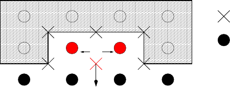
400
CHAPTER 30. EXPLICIT FREE SURFACE AND FRESH WATER
storage capacity. Due to wind surge or tides, the river outflow may be temporarily
blocked and fresh water enters the ocean intermittently in form of drifting river plumes.
To implement such features, the processes producing intermittency in the river outflow
must be resolved by the model. Thus, the estuary must be part of the model and the river
runoffmust enter the model area more upstream.
- The river is assumed to be unstratified and horizontally uniform. Improvements require
a higher resolution of the river component. Nonuniform distribution of the fresh water
flux over the river grid cells can be added in setriver.F
- River inflow is confined to the surface cells. For rivers much deeper than the surface
layer, this may introduce too much stratification and an intensified estuarine circulation.
If this is not desired, two or more surface layers should be mixed explicitly at the cells
with river inflow. This requires code changes and is not part of the basic MOM code.
- The momentum flux may be incorrect. The method distributes the mass flux over several
tracer points and establishes surface pressure gradients which reflect the model setup
but not the dynamics in a river mouth. If the dynamical features of the outflow are
important, a sufficiently large part of the river must be included in the model.
In order to prevent unrealistic currents due to different position of velocity and tracer
cells in the Arakawa B-grid, the fresh water flux and the tracer flux should be distributed
at least over two adjacent tracer cells, the momentum flux should be added in the
corresponding velocity cell between the tracer cells. Figures 30.3 and 30.4 give some
hints for how the rivers could be configurated. However, the method does not require
an adjustment of the coastline to configure rivers so long as land-points or non-advective
cells are avoided.
qRuR
t - points
RR
q
0.5 T
u - points
Figure 30.3: Sketch of the cell arrangement for a river flowing southward. The fresh water and
tracer flux is distributed over the two red tracer points, the momentum flux is added in the red
velocity point.
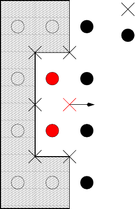
30.11. IMPLEMENTATION OF FRESH WATER FLUXES AND RIVERS IN MOM
401
u - points
t - points
RR
q
0.5 T
RR
q
0.5 T
qRuR
Figure 30.4: Sketch of the cell arrangement for a river flowing eastward. The fresh water and
tracer flux is distributed over the two red tracer points, the momentum flux is added in the red
velocity point.

402
CHAPTER 30. EXPLICIT FREE SURFACE AND FRESH WATER
30.12 Checkerboard null mode
As discussed by Killworth et al. (1991), discretization of gravity waves on a B-grid can admit
a stationary grid scale checkerboard pattern (see also Messinger 1973 and Jancic 1974 for
atmospheric discussions). This pattern is associated with an unsuppressed grid splitting that
can be initiated through grid scale forcing, such as topography. That is, the discrete equations
admit a checkerboard null mode. Beckers (1999) also discusses subtleties associated with
traditional linear stability. In our experience, when the model goes unstable due to CFL
violations, this grid mode is the spatial pattern associated with the instability.
Strictly, the grid mode is present only when the surface pressure gradient takes the form
∇hps=ρg∇hη, where ρis an averaged surface density. For example, in the implementation of
Killworth et al. (1991), ∇hps=ρog∇hη, and so the null mode is always present. Tests with the
alternative expression ps=ρk=1gηused in MOM, in which surface pressure gradients arise
from gradients in both the surface density ρk=1and surface height, suggest that the null mode
is slightly suppressed. A more significant means to suppress the mode, however, is provided
through the use of time averaging over the barotropic time steps, as well as with nonlinearity
in the shallow water system present when the undulating surface height is fully incorporated
to the dynamics.
Hence, for many of our simulations, the grid mode is absent or quite mild. Nonetheless,
some experiments did realize the grid mode in the surface height, and so we considered various
means of suppressing it. The following relates our experience with this mode and provides
suggestions and caveats.
30.12.1 Experiences with the checkerboard null mode
Under certain circumstances, Killworth et al. (1991) noted that the checkerboard pattern can
appear in the barotropic velocity. In order to dissipate this mode, they suggested that horizontal
friction acting on the barotropic velocity be updated each barotropic time step, instead of only
during the baroclinic time steps. This approach was found to be especially appropriate in
simulations with strong eddy activity.
Updating friction on each time step can be quite costly. Therefore, in practice, one is
restricted to the use of a constant viscosity Laplacian friction for both the barotropic and
baroclinic modes. Notably, use of a biharmonic viscosity, updated each barotropic time step,
could be prohibitively costly. As discussed by Semtner and Minz (1977) and recently by Griffies
and Hallberg (1999), Laplacian friction for eddy-permitting simulations significantly under-
utilizes the model grid as it strongly suppresses mesoscale eddy formation. We therefore
believe that restricting the model to constant viscosity Laplacian friction is not an acceptable
solution to the grid splitting problem. Relatedly, barotropically updating a depth dependent
viscosity, such as that arising from the Smagorinsky scheme (Smagorinsky 1963, 1993, and
Griffies and Hallberg 1999), is very cumbersome due to the need to maintain self-consistency
between friction applied in the barotropic and baroclinic equations.
For the time stepping procedure described in this paper, regions where the barotropic
fields are evolving experience an effective spatial averaging associated with the barotropic
time averaging. Eddy-rich regions are therefore preferentially smoothed, in contrast to the
algorithm of Killworth et al. in which there is no time averaging. Consequently, we conjecture
that time averaging provides for an effective suppression of the grid splitting in both the
surface height and vertically integrated velocity. Indeed, we have rarely observed noise in the
vertically integrated velocity with the time filtering scheme, and so have not been motivated
30.12. CHECKERBOARD NULL MODE
403
to update the friction on each barotropic time step.
Since the equations for the surface height are inviscid, the checkerboard pattern tends to
appear most prominently in this field. To suppress the noise, Killworth et al proposed the
addition of the so-called “del-plus /del-cross” operator to the prognostic equation for the
free surface height. Their approach is an extension of that suggested by Jancic (1974). The
operator is basically the difference between Laplacians computed in two different manners,
and it preferentially removes the checkerboard pattern by coupling the grids. This coupling
occurs in a scale-selective manner so that the larger scales are only modestly affected. The
construction of this operator requires the definition of time dependent image points over land
to allow for it to conserve volume.
30.12.2 A caveat concerning filtering the surface height
In quiescent regions, such as embayments, enclosed seas, and idealized steady state models
with nontrivial topography and geography, we have found the checkerboard pattern some-
times is visible in the free surface height. As such, various filters were tested, such as the
del-plus /del-cross operator, as well as a two-dimensional Shapiro filter designed to conserve
volume with arbitrary geography. Either spatial filter successfully removed noisy patterns
from the surface height. However, we found their effects on other model fields, such as vertical
velocity, to be quite dependent on the strength of the filter. In particular, for many cases where
the filter was sufficient to suppress noise in the surface height, it had detrimental effects on the
vertical velocity.
The reason for this sensitivity can be seen by considering the equations for gravity waves
on a B-grid using a forward-backward time stepping scheme (note that the following consid-
erations do not depend on the choice of time stepping schemes). To better expose our point,
assume ps=ρogη,D=H+η≈H, and omit fresh water forcing. The discretized equations
take the form
η(tn+1)=η(tn)−∆t[∇h·U(tn)−F(η) ] (30.78)
U(tn+1)=U(tn)−H g ∆tδxη(tn+1)y(30.79)
V(tn+1)=V(tn)−H g ∆tδyη(tn+1)x,(30.80)
where F(η) represents a spatial filter applied to the surface height, and the temporal notation
has been streamlined from the more complete notation used in Section 30.2.
Consider first a case in which the free surface contains power in the checkerboard pattern,
as well as longer waves, yet there is no spatial filter and so F=0. The discretized surface
pressure gradients do not feel the checkerboard pattern since this pattern is a null mode
of the discrete gradient operators δx()yand δy()x. Therefore, discrete pressure gradients are
determined only by the longer waves, and so the gradients are smooth. Since the checkerboard
pattern is stationary in time, it does not contribute to the vertical velocity. Neglecting the time
varying top cell volume in the baroclinic and tracer equations, as in the free surface methods
of Killworth et al. (1991) and Dukowicz and Smith (1994), renders the checkerboard pattern
dynamically irrelevant. Instead, it is simply an esthetic nuisance. Yet when solving the more
general equations with undulating top cell thicknesses, it cannot be ignored as it potentially
will influence the other model fields.
Now add the spatial filter which is designed to preferentially remove the checkerboard
grid noise. Unlike the unfiltered η, the filter Fwill generally not be invisible to the discretized
pressure gradients, and so these gradients are affected by an unphysical source. In practice,
404
CHAPTER 30. EXPLICIT FREE SURFACE AND FRESH WATER
we have found that these sources can be nontrivial, especially when using the Shapiro filter,
which is the strongest available grid scale filtering. For the del plus /del minus filter, using the
weighting factor suggested by Killworth et al. (1991), we found a large amount of noise was
transferred to the vertical velocity field. Again, the reason is that this filter is not invisible to
the discretized gradients, and so while it acts to smooth the surface height, it correspondingly
adds noise to the surface pressure gradients.
One attempt to suppress the transfer of noise was to also filter ∇h·Uin order to counteract
the noisy pressure gradients. Unfortunately, this approach is problematic, since doing so
breaks the precise connection between the barotropic and baroclinic mode systems. As a
result, spatially filtering ∇h·Uproduces a nontrivial spurious vertical velocity throughout the
ocean, and in particular it creates unacceptable advective fluxes through the ocean bottom.
30.12.3 Suggestions
As mentioned at the beginning of this section, we find the need for filtering to be greatly
reduced due to the use of a nonlinear free surface in which the barotropic time steps are time
averaged. Nevertheless, for those cases in which filtering is needed, we have found it sufficient
to add a straightforward Laplacian to the free surface height equation with a reasonably small
viscosity. The more sophisticated Shapiro filter or del-plus minus del-minus operator were
no better, and often much worse in their affects on vertical velocity. Note that a Laplacian,
using no-flux boundary conditions, conserves volume. Therefore, adding a Laplacian to the
free surface equation is trivial to implement relative to the del plus /del minus operator,
which requires the specification of time dependent image points in order to preserve volume
in arbitrary geometry.
30.13 Polar filtering
The CFL time step requirements for the barotropic mode can be quite stringent when reaching
the pole on a spherical grid. Instead of reducing the time steps, it is common to prescribe a
spatial filtering in order to remove the small scale features. This filtering traditionally takes the
form of Fourier filtering (e.g., Bryan et al. 1975). We have instead found one-dimensional
Shapiro filtering preferable due to its increased speed. Nevertheless, as such filtering is
necessary for each of the small barotropic mode time steps, the computational cost can be
high and it can render strong load imbalances between adjacent parallel computer processors.
Indeed, the cost can be higher than the cost of simply reducing the barotropic time step in order
to satisfy the CFL constraint. Additionally, for reasons related to the mechanism discussed
above, tests have shown that polar filtering of the surface height can result in a nontrivial
amount of grid noise in the vertical velocity field within the polar filtering regions. As a result,
we do not recommend polar filtering the barotropic fields. The more general solution of pole
displacement using non-spherical coordinates (e.g., Smith et al, 1995, Murray 1996, Madec et
al. 1998) is currently under investigation.

Chapter 31
Options for solving elliptic equations
The external mode elliptic equation is solved by conjugate gradients with two possible forms
for the numerics of the coefficient matrix. One form of the coefficient matrix must be chosen.
In previous versions of MOM, a solution by sucessive over relaxation was available but this
has been eliminated in favor of the conjugate gradient technique.
The accuracy of the external mode solution for the stream function ∆ψ=ψτ+1−ψτ−1is
determined by setting a tolerence (see Section 14.4.5). The preferred method of solution is by
conjugate gradients which is an iterative technique. The iteration is ended and the equation
is considered solved when the estimated sum of future corrections to ∆ψ(the truncated ones)
is less than the specified tolerence. The estimated sum is approximated assuming a geometric
decrease in the maximum correction to ∆ψwith time.
Typically, as a rule of thumb, the number of scans taken to solve the external mode equation
should not be << max (imt,jmt) when the forcing (i.e. windstress) is time dependent. If the
number of scans is much less than this, it may indicate that the specified tolerence is set too
large. As an example, if the specified tolerence is 108, then in 10,000 time steps the computed
solution is guaranteed to be within 1 Sverdrup (1x10¹²) of the true solution at every point.
This is a worst case assuming systematic errors always of the same sign. If time steps are very
small, then ∆ψwill be small and the tolerence should be decreased particularly if long running
experiments are involved. The amount of error that is tolerable is dependent on the goal of the
experiment.
In cases where the windstress is set constant or zero, the number of scans may eventually
get very small as equilibrium is approached. The reason is that a guess at the solution is made
from the previous solutions. If the solution is not evolving, then eventually, the guess is within
the specified tolerence and zero scans result. It is left up to the researcher to determine the
appropriate value of the tolerence. The number of times that the scans are <max (imt,jmt) are
counted and a message is printed at the end of the execution.
31.1 conjugate gradient
This section was contributed by Charles Goldberg. The conjugate gradient technique is used to
invert the elliptic equation for external mode options other than explicit free surface using either
five point or nine point operators, selected by options sf 9 point or sf 5 point. The algorithm
below is a Fortran 90 version of the algorithm in Smith, Dukowicz, and Malone (1992).
subroutine congrad (A, guess, forc, dpsi, iterations, epsilon)
405
406
CHAPTER 31. OPTIONS FOR SOLVING ELLIPTIC EQUATIONS
use matrix module
intent (in) :: A, guess, forc, epsilon
intent (out) :: dpsi, iterations
type(dpsi type) :: guess, dpsi, Zres, s
type(res type) :: res, As, forc
type(operator) :: A
type(inv op) :: Z
dimension (0:max iterations) :: dpsi, res, s, As, beta, alpha
dpsi(0) = guess
res(0) = forc - A ⋆dpsi(0)
beta(0) = 1
s(0) = zerovector()
do k = 1 to max iterations
Zres(k-1) = Z ⋆res(k-1)
beta(k) = res(k-1) ⋆Zres(k-1)
s(k) = Zres(k-1) + (beta(k)/beta(k-1)) ⋆s(k-1)
As(k) = A ⋆s(k)
alpha(k) = beta(k) / (s(k) ⋆As(k))
dpsi(k) = dpsi(k-1) + alpha(k) ⋆s(k)
res(k) = res(k-1) - alpha(k) ⋆As(k)
estimated error = err estimate(k, alpha(k), s(k))
if (estimated error) < epsilon) exit
end do
if (k > max iterations) then
print ⋆, ’did not converge in ’,k,’ iterations’
stop ’congrad’
end if
iterations = k
dpsi = dpsi(k)
end
In MOM, all land masses are usually treated as islands when using this option with op-
tion stream function because it has been found that this treatment speeds convergence. Island
sums are turned offwhen solving for surface pressure by setting nisle=0. The test for con-
vergence has also been changed from that used in MOM 1 and previous versions. In MOM,
the sum of all estimated future corrections to the prognostic variable is calculated assuming
geometric decrease of the maximum correction, and the iteration is terminated when this sum
is within the requested tolerance. Tests indicate that this solver converges significantly faster
than the one in MOM 11.
1Because of the difference in meaning between the MOM 1 tolerance crit and the MOM tolerance tolrsf, care
must be taken to assure that both are converging to the same tolerance when doing these tests.
31.2. SF 9 POINT
407
31.2 sf 9 point
This option uses the full nine point numerics for the coefficient matrix in Equation (29.18) when
inverting the external mode elliptic Equation (29.14). This matrix is slightly different than the
one used in MOM 1 and earlier versions. Particular attention has been given to assuring that
the operator remains symmetric with respect to islands. This form exactly eliminates2the
surface pressure term from the momentum equations when used with option stream function.
It has a checkerboard null space which in most cases is not a problem because of the Dirichlet
boundary conditions.
Options rigid lid surface pressure and implicit free surface require the use of a nine point co-
efficient matrix3, and in these cases, option sf 9 point must also be enabled. The null space is
a problem when option rigid lid surface pressure is chosen, and it must be removed. Adding
the missing divergence from the rigid lid surface pressure to the central term constructs the im-
plicit free surface which suppresses the null space. Details of these methods appear later.
Constructing the coefficient matrix for Equation (29.14) can be difficult. The mathematician
among us (Goldberg) points out that the finite difference operators can be written in terms of
matrices as follows:
dxti·δλ(αi,jrowφ)=
0
X
j′=−1
0
X
i′=−1
cddxti′,j′αi+i′,jrow+j′(31.1)
dytjrow ·δφ(αi,jrowλ)=
0
X
j′=−1
0
X
i′=−1
cddyti′,j′αi+i′,jrow+j′(31.2)
dxui·δλ(αi,jrowφ)=
1
X
j′=0
1
X
i′=0
cddxui′,j′αi+i′,jrow+j′(31.3)
dyujrow ·δφ(αi,jrowλ)=
1
X
j′=0
1
X
i′=0
cddyui′,j′αi+i′,jrow+j′(31.4)
where cddxti′,j′,cddyti′,j′,cddxui′,j′, and cddyui′,j′are defined as 2x2 matrices:
cddxti′,j′=ai′,j′=
a−1,0a0,0
a−1,−1a0,−1
=
−1
21
2
−1
21
2
(31.5)
cddyti′,j′=ai′,j′=
a−1,0a0,0
a−1,−1a0,−1
=
1
21
2
−1
2−1
2
(31.6)
cddxui′,j′=ai′,j′=
a0,1a1,1
a0,0a1,0
=
−1
21
2
−1
21
2
(31.7)
2To within roundoff.
3However, in these cases, the elliptic equations for the prognostic surface pressure psare, of course, different
than those given above for the prognostic stream function Ψ.
408
CHAPTER 31. OPTIONS FOR SOLVING ELLIPTIC EQUATIONS
cddyui′,j′=ai′,j′=
a0,1a1,1
a0,0a1,0
=
1
21
2
−1
2−1
2
(31.8)
Using Equations (31.1) – (31.4), the first brackets in Equation (29.14) can be rewritten as
1
X
i′=0
1
X
j′=0
0
X
i′′=−1
0
X
j′′=−1
cddyui′,j′·cddyti′′,j′′ ·
dxui+i′′ ·cos φU
jrow+j′′
Hi+i′′,jrow+j′′ ·dyujrow+j′′ ·2∆τ
+cddxui′,j′·cddxti′′,j′′ ·dyujrow+j′′
Hi+i′′,jrow+j′′ ·dxui+j′′ ·cos φU
jrow+j′′ ·2∆τ∆ψi+i′+i′′,jrow+j′+j′′
(31.9)
and in a similar fashion, the implicit Coriolis contributions from the second brackets in Equation
(29.14) can be rewritten as:
1
X
i′=0
1
X
j′=0
0
X
i′′=−1
0
X
j′′=−1
−cddxui′,j′·cddyti′′,j′′ ·−˜
fjrow+j′′
Hi+i′′,jrow+j′′
−cddyui′,j′·cddxti′′,j′′ ·
˜
fjrow+j′′
Hi+i′′,jrow+j′′ ∆ψi+i′+i′′,jrow+j′+j′′ (31.10)
which provides a very compact and efficient way of calculating the coefficient matrix coeffi,jrow,i⋆,j⋆.
coeffi,jrow,i⋆,j⋆=
1
X
i′=0
0
X
i′′=−1
1
X
j′=0
0
X
j′′=−1
δi′+i′′,i⋆δj′+j′′,j⋆
cddyui′,j′·cddyti′′,j′′ ·
dxui+i′′ ·cos φU
jrow+j′′
Hi+i′′,jrow+j′′ ·dyujrow+j′′ ·2∆τ
+cddxui′,j′·cddxti′′,j′′ ·dyujrow+j′′
Hi+i′′,jrow+j′′ ·dxui+j′′ ·cos φU
jrow+j′′ ·2∆τ
−cddxui′,j′·cddyti′′,j′′ ·−˜
fjrow+j′′
Hi+i′′,jrow+j′′
−cddyui′,j′·cddxti′′,j′′ ·
˜
fjrow+j′′
Hi+i′′,jrow+j′′ (31.11)
where δi′+i′′,i⋆is the Kronecker Delta function which is 1 when i′+i′′ =i⋆and 0 when i′+i′′ ,i⋆.
The entire coefficient array is calculated by six nested loops on i,jrow,i′,j′,i′′, and j′′, with
each iteration adding the terms above to the proper coefficient bucket4.
The matrix for right hand side of Equation (29.14) can be written as:
f orci,jrow =
1
X
i′=0
1
X
j′=0
h−cddyti′,j′·zui+i′,jrow+j′,1·dxui+i′·cos φU
jrow+j′
4We have come to call these loops “Amtrack Normal Form,” because the indentation of the DO loops and
the long executable statement in the middle resemble the “Amtrack” logo. Properly ordered, these nested loops
vectorize very well on a Cray YMP.
31.3. SF 5 POINT
409
+cddxti′,j′·zui+i′,jrow+j′,2·dyujrow+j′i(31.12)
The coefficient matrix is symmetric5except for the implicit Coriolis term (the second bracket
in Equation (29.14)). The preferred method of solving Equation (29.14) is by conjugate gradients
as described in Dukowicz, Smith and Malone (1993). Refer to Section 31.1 for more detail on
the elliptic solvers and to Appendix 29.2.4 for more details on the island equations.
31.3 sf 5 point
This section was contributed by Charles Goldberg. The five point form approximates aver-
ages of contributions to the corner points of the nine point operator to produce a five point
operator that has coefficients only in the center, north, east, south, and west places in the
coefficient matrix for inverting the external mode elliptic equation. This option can be used
with option stream function but is not appropriate for options rigid lid surface pressure or im-
plicit free surface because of energy leakage.
In Equation (31.9), corresponding to the first bracket of Equation (29.2), all 32 contribu-
tions to the elliptic operator are calculated as in the 9 point operator, except that in the first
group, i.e., in the terms originating in a second difference in the δφdirection, the coefficient
of the northeast variable ∆φi,jrow,1,1is averaged with the coefficient of the northwest variable
∆φi,jrow,−1,1, and both are applied to the northern variable ∆φi,jrow,0,1. This averaging centers
the coefficient on the northern edge of the central T cell, so that continuous derivatives in the
φdirection are well approximated. Similarly, the southeast and southwest contributions from
the first group are applied to the southern variable ∆φi,jrow,0,−1. The second group of terms
originate in a second difference in the δλdirection, and here the northeastern and southeastern
contributions are averaged and applied to the eastern variable ∆φi,jrow,1,0, and the northwestern
and southwestern contributions are averaged and applied to the western variable ∆φi,jrow,−1,0,
giving good approximations to the continuous derivatives in the λdirection. The resulting
summations are
1
X
i′=0
1
X
j′=0
0
X
i′′=−1
0
X
j′′=−1
cddyui′,j′·cddyti′′,j′′ ·
dxui+i′′ ·cos φU
jrow+j′′
Hi+i′′,jrow+j′′ ·dyujrow+j′′ ·2∆τ∆ψi,jrow+j′+j′′
+
1
X
i′=0
1
X
j′=0
0
X
i′′=−1
0
X
j′′=−1
cddxui′,j′·cddxti′′,j′′ ·dyujrow+j′′
Hi+i′′,jrow+j′′ ·dxui+j′′ ·cos φU
jrow+j′′ ·2∆τ∆ψi+i′+i′′,jrow
(31.13)
Bryan (1969) uses a five point approximation to ( 1
H· ∇ψt) which as implemented in MOM 1
takes the form
1
cos φT
jrowdxtidytjrowdxti·dytjrow ·δφ
cos φU
jrow−1
Hi−1,jrow−1
λ·dyujrow−1
dyujrow−1·δφ∆ψi,jrow−1
+dytjrow ·dxti·δλ
1
Hi−1,jrow−1
φ·cos φT
jrow dxui−1
dxui−1·δλ∆ψi−1,jrow
5Refer to Section 29.2.5.
410
CHAPTER 31. OPTIONS FOR SOLVING ELLIPTIC EQUATIONS
(31.14)
In this notation, the five point approximation used in MOM takes the form
1
2∆τ·dytjrow ·δφ
dxui−1·cos φU
jrow−1
Hi−1,jrow−1·dyujrow−1
λ
·dyujrow−1·δφ∆ψi,jrow−1
+dxti·δλ
dyujrow−1
Hi−1,jrow−1·cos φU
jrow−1·dxui−1
φ
·dxui−1·δλ∆ψi−1,jrow
(31.15)
For comparison with MOM, Bryan’s form must be multiplied by (cos φT
jrowdxtidytjrow)/(2∆τ).
The principal differences between these two forms arise from Bryan’s use of averages of
reciprocals of the form 2
Hi,jrow +Hi−1,jrow
where MOM uses 1
2(1
Hi,jrow
+1
Hi−1,jrow
). These differ
by a factor of two in the second order term in Hi,jrow −Hi−1,jrow. Other differences arise on a
nonuniform grid.
The second bracket, the implicit Coriolis terms, may be seen to already be in five point form
because each corner coefficient consists of two terms of equal magnitude, but opposite sign.
1
X
i′=0
1
X
j′=0
0
X
i′′=−1
0
X
j′′=−1
−cddxui′,j′·cddyti′′,j′′ ·−˜
fjrow+j′′
Hi+i′′,jrow+j′′
−cddyui′,j′·cddxti′′,j′′ ·
˜
fjrow+j′′
Hi+i′′,jrow+j′′ ∆ψi+i′+i′′,jrow+j′+j′′ (31.16)
The right hand side of Equation (29.14) also remains the same in the five point equations
as in the nine point equations.
f orci,jrow,=
1
X
i′=0
1
X
j′=0
h−cddyti′,j′·zui+i′,jrow+j′,1·dxui+i′·cos φU
jrow+j′
+cddxti′,j′·zui+i′,jrow+j′,2·dyujrow+j′i(31.17)
Although the five point operator approximates the continuous differential equation (29.2)
well, its solutions are not exact solutions of the finite difference momentum equations (29.3)
and (29.4). Moreover, the time saved by calculating a five point operator instead of a nine point
operator in two places per iteration in a conjugate gradient solver is not large, and the nine
point equations usually take fewer iterations to converge.
Chapter 32
Options for advecting tracers
The advection of tracers and momentum discussed in this chapter refer to advection by that
portion of the velocity field which is explicitly computed by the ocean model. Depending on
the model resolution, there may be need to parameterize the effects from unresolved parts of
the spectrum through one or more of the schemes discussed in Chapters 35
In MOM, the advection of momentum always uses second order accurate centered dif-
ferencing in space and time. This approach ensures that the first and second moments of
momentum, namely the total momentum and kinetic energy, are preserved in conservative
flow situations. In addition to this second order accurate scheme, other schemes are available
for the advection of tracers. If no scheme is explicitly enabled, then the default second order
accurate scheme is also used for tracers.
Basically, each tracer advective scheme has its advantages and disadvantages. As men-
tioned above, the standard second order scheme conserves first (mean) and second (variance)
moments. However, it produces over(under)-shoots and phase errors when scales in the tracer
or velocity field are not well resolved by the grid resolution. The fourth order advection does
a better job by reducing the amplitude of the over(under)-shoots and the phase errors but
does not preserve second moments in general. The flux corrected transport scheme is positive
definite (no over(under)-shoots), does not conserve second moments, and tends to sharpen
fronts. It is also expensive to use. The third order scheme (quicker) balances the diffusion of the
scheme by its dispersion. It does not conserve second moments and is not positive definite but
the over(under)-shoots are drastically reduced compared to second or fourth order schemes. It
is interesting to note that “quicker” can result in less dissapation than the second order scheme
because of the non-linear action of convection on the over(under)-shoots of the second order
scheme.
32.1 Considerations of accuracy in one-dimension
The purpose of this section is to introduce some basic ideas regarding how well advection
on the discrete lattice approximates advection in the continuum. Much of the intuition for
advection comes from the many studies that have been done using a single space dimension,
and this section is restricted to such systems. In this case, the continuum equation for the
advection of a quantity ψis given by
ψt+Uψx=0.(32.1)
411
412
CHAPTER 32. OPTIONS FOR ADVECTING TRACERS
In the following, the solution ψ(x,t) to this equation will be termed the continuum field; it is
defined at each continuous point (x,t). This field will be compared to the various solutions
Ψn
iwhich live on the discrete space time lattice, with xi=i∆xand tn=n∆tthe spatial and
temporal grid points, respectively. The goal is to make the differences between the continuum
and lattice fields small using discrete approximations to the continuum advection equation
(32.1). Note that for the following, all considerations will be for uniform space-time lattices.
For a single space dimension, an incompressible fluid corresponds to a constant advecting
velocity U. Hence, the simplest case to consider is tracer advection by a constant velocity U
discretized on a uniform spatial and temporal grid (∆x,∆t).
32.1.1 Lattice and continuum operators
A good reference for the methods used in this subsection is chapter 2 from the book by Mitchell
and Griffiths (1980).
Consider the continuum field ψevaluated at an arbitrary lattice point
ψn
i=ψ(xi,tn).(32.2)
Using a Taylor series expansion, the relation between ψn
iand ψn
i+p, where xp=p∆x, is given by
ψn
i+p=1+p∆x∂x+1
2! (p∆x)2∂(2)
x+1
3! (p∆x)3∂(3)
x+...ψn
i
=exp(p∆x∂x)ψn
i.(32.3)
The linear operator exp(p∆x∂x) can be thought of as a spatial translation operator; a terminol-
ogy familiar to those having studied quantum mechanics. Similarly, the temporal translation
operator exp(q∆t∂t) connects ψn
ito another point in time tq=q∆tthrough the relation
ψn+q
i=exp(q∆t∂t)ψn
i.(32.4)
In the following, it will prove useful to derive relations between the continuum differential
operators ∂xand ∂tand various finite difference or lattice operators. To start, consider the
familiar centered difference spatial operator as defined by
δC
xψn
i=ψn
i+1−ψn
i−1
2∆x.(32.5)
Using the spatial translation operators, this relation takes the form
δC
xψn
i= sinh(∆x∂x)
∆x!ψn
i.(32.6)
Since ψn
iis arbitrary, this equation yields the relation between the centered difference lattice
operator and the continuous partial derivative
∆xδC
x=sinh(∆x∂x).(32.7)
Inverting this relation yields
∆x∂x=sinh−1(∆xδC
x).(32.8)
32.1. CONSIDERATIONS OF ACCURACY IN ONE-DIMENSION
413
Similar relations hold for the temporal centered difference, or leap frog, operator
∆tδC
t=sinh(∆t∂t) (32.9)
∆t∂t=sinh−1(∆tδC
t).(32.10)
The forward difference lattice operator is also quite common
δF
xψn
i=ψn
i+1−ψn
i
∆x
=[exp(∆x∂x)−1] ψn
i.(32.11)
This relation leads to the operator equalities
∆xδF
x=exp(∆x∂x)−1 (32.12)
∆x∂x=ln(1 + ∆xδF
x),(32.13)
with analogous results for the temporal forward difference operator. The relation between
other finite difference operators and the continuum operator can be derived similarly.
32.1.2 Leap frog in time and centered in space
The previous relations between continuum and lattice operators render the differential advec-
tion equation ψt+Uψx=0 equivalent to the finite difference advection equation
sinh−1(∆tδC
t)+U∆t
∆xsinh−1(∆xδC
x)ψn
i=0,(32.14)
where the lattice operators are each centered difference operators. Various finite difference
methods can be obtained by expanding the sinh−1functions and truncating at some desired
order. For example, keeping only the first terms yields
(δC
t+UδC
x)Ψn
i=0.(32.15)
This equation defines the lattice field Ψn
i, which is an approximation to the continuum field
ψn
i. In order to determine the accuracy of the approximation, consider the error field
Dn
i=ψn
i−Ψn
i.(32.16)
This field satisfies the equation
(δC
t+UδC
x)Dn
i=(δC
t+UδC
x)ψn
i
=1
∆tsinh(∆t∂t)+U
∆xsinh(∆x∂x)ψn
i
=
(∆t)2∂(3)
t+U(∆x)2∂(3)
x
3! +...
ψn
i.(32.17)
where (δC
t+UδC
x)Ψn
i=0 and (∂t+U∂x)ψn
i=0 were used. This result defines the truncation
error
E[ψn
i]≡
(∆t)2∂(3)
t+U(∆x)2∂(3)
x
3!
ψn
i+. . . , (32.18)
414
CHAPTER 32. OPTIONS FOR ADVECTING TRACERS
which is seen to be second order in both ∆xand ∆t. This expression can be written solely in
terms of spatial derivatives using the relation satisfied by the continuum field
∂(p)
tψ=(−U)p∂(p)
xψ, (32.19)
which follows from successive differentiation of ∂tψ=−U∂xψ. As such, the truncation error
takes the form
E[ψn
i]=U(∆x)2
3! "1−U∆t
∆x2#∂(3)
xψn
i+... (32.20)
As seen from the above analysis, the lattice field Ψn
ionly approximates the continuous field
ψdue to the nonzero truncation error. A complementary issue concerns the properties of the
continous field ˜
ψthat exactly corresponds to Ψn
i. Namely, consider a continuum field ˜
ψwhich
satisfies the discrete equation
(δC
t+UδC
x)˜
ψn
i=0.(32.21)
Substituting the relations between the lattice and continuous operators into this equation yields
the differential equation satisfied by ˜
ψ
1
∆tsinh(∆t∂t)+U
∆xsinh(∆x∂x)˜
ψn
i=0.(32.22)
Expanding, rearranging, and dropping lattice labels reveals
(∂t+U∂x)˜
ψ=−
(∆t)2∂(3)
t
3! +U(∆x)2∂(3)
x
3! +...
˜
ψ
=−E[˜
ψ].(32.23)
Consequently, the lattice field Ψn
icorresponds exactly to the continuous field ˜
ψ, where ˜
ψ
satisfies the advection equation with a linear source term determined by minus the truncation
error E[˜
ψ]. Note that in E[˜
ψ], it is not possible to exactly eliminate the ∂(n)
toperator as was
done for E[ψ], since ˜
ψt,−U˜
ψx.
32.1.3 A critique of upwind advection
Another method to discretize the advection equation is the so-called upwind method. Upwind
advection was used in early numerical weather models due to its good stability properties,
and it still finds use in idealized ocean box models (e.g., Stommel 1961) as well as some general
circulation models. It is available in MOM for use in advecting tracers along the ocean bottom
(Section 32.7) and within the parameterized bottom boundary layer (Chapter 37). When using
upwind, however, one should realize that it is highly diffusive, for reasons first discussed by
Molenkamp (1968) and outlined in the following.
The upwind scheme uses backward space differences if the velocity is in the positive x
direction, and forward space differences for negative velocities
UδF
xΨn
iif U<0
UδB
xΨn
iif U>0,(32.24)

32.1. CONSIDERATIONS OF ACCURACY IN ONE-DIMENSION
415
where δB
xΨn
i=(Ψn
i−Ψn
i−1)/∆xis the backward difference operator. The name upwind denotes
the use of upwind, or upstream, information in determining the form for the finite difference;
downstream information is ignored.
In order to analyze the accuracy of the upwind scheme, consider the case with U>0 for
definiteness. In this case, leap frog in time and backward difference in space yields the finite
difference equation
(δC
t+UδB
x)Ψn
i=0.(32.25)
The error field Dn
i=ψn
i−Ψn
isatisfies the equation
(δC
t+UδB
x)Dn
i=(δC
t+UδB
x)ψn
i
=1
∆tsinh(∆t∂t)+U
∆x[1 −exp(−∆x∂x)]ψn
i
=
(∆t)2∂(3)
t
3! −U∆x∂(2)
x
2+...
ψn
i
=−U∆x
2 1+(U∆t)2∂x
3∆x+...!∂(2)
xψn
i
≡E[ψn
i].(32.26)
The truncation error is seen to be second order in ∆tand first order in ∆x.
To determine the differential equation to which the finite difference equation corresponds,
introduce the continuum field ˜
ψwhich satisfies
(δC
t+UδB
x)˜
ψn
i=1
∆tsinh(∆t∂t)+U
∆x[1 −exp(−∆x∂x)]˜
ψi
n
=0.(32.27)
Expanding the transcendental functions and rearranging yields the differential equation
(∂t+U∂x)˜
ψ=
−(∆t)2∂(3)
t
3! +U∆x∂(2)
x
2+...
˜
ψ
=−E[˜
ψ].(32.28)
Since ˜
ψdoes not solve the continuum advection equation, it is not possible to exactly eliminate
the ∂(3)
toperator in terms of the ∂(3)
xoperator as done for E[ψ]. Regardless, the main point here
is that the lowest order derivative in the truncation error represents a dissipative, or diffusive,
term where the numerical or effective diffusivity is given by
κ=(U∆x)/2.(32.29)
For a one-degree model at the equator with horizontal velocity U=20cm/sec, the numer-
ical diffusivity is roughly 108cm2/sec. If upwind advection is used in the vertical, with
U=10−3cm/sec −10−2cm/sec and ∆z=1000cm, the vertical numerical diffusivity is roughly
0.5cm2/sec −5cm2/sec. Both diffusivities are huge. Granted, it is possible that the higher order
terms in the truncation error will alter these numbers. However, there is no reason to believe
that they will systematically reduce the diffusivities to the extent necessary to bring them more
416
CHAPTER 32. OPTIONS FOR ADVECTING TRACERS
in line with observations. The paper by Griffies, Pacanowski, and Hallberg (1999) further
discusses these points for upwind and other advection schemes.
The analysis of Molenkamp (1968) considered the case of upwind advection with forward
time differences. In this case, the finite difference equation for U>0 is
(δF
t+UδB
x)Ψn
i=0.(32.30)
This equation corresponds to the differential equation
1
∆t[exp(∆t∂t)−1] +U
∆x[1 −exp(−∆x∂x)]˜
ψn
i=0.(32.31)
Expanding and rearranging yields
(∂t+U∂x)˜
ψ=U∆x
2
∂(2)
x−∆t∂(2)
t
U∆x+...
˜
ψ. (32.32)
If one drops derivatives higher than second, or does some back substitution, it is possible to
approximately eliminate the ∂(2)
tterm in favor of the ∂(2)
x. In this way, the equation satisfied by
˜
ψis given by
(∂t+U∂x)˜
ψ=U∆x
21−U∆t
∆x∂xx ˜
ψ+. . . . (32.33)
This result corresponds to equation (15) of Molenkamp (1968) and equation (32.88) discussed
in the FCT section of this chapter. Note that stability of the upwind scheme with forward
time difference requires |U|∆t/∆x<1, thus leading to a positive effective diffusivity. It is seen
that the effective diffusivity is systematically reduced from that resulting from the leap frog
scheme. Interestingly, as the CFL number |U|∆t/∆xapproaches unity, the leading term in the
truncation error vanishes, and so the upwind scheme, with forward time differences, becomes
more accurate. This fortuitous situation, however, is not general and so is not justification for
using upwind.
In general, as argued here and in many other places, the upwind advection scheme is too
diffusive to be of direct use for realistic ocean general circulation modeling. However, the
upwind scheme in combination with a less dissipative scheme, such centered differences, can
be quite useful for many purposes. The discussion of FCT in Section 32.6 clarifies this point.
Additionally, for use in advecting tracers along the ocean bottom (Section 32.7) and within the
parameterized bottom boundary layer (Chapter 37).
32.2 second order tracer advection
This option is automatically enabled in file size.h if no other advective schemes are enabled.
Do not directly enable it with a preprocessor directive. Twice the advective flux on the eastern,
northern, and bottom sides of cell Ti,k,jis given by
adv f ei,k,j=adv veti,k,j·(ti,k,j,n,τ +ti+1,k,j,n,τ) (32.34)
adv f ni,k,j=adv vnti,k,j·(ti,k,j,n,τ +ti,k,j+1,n,τ) (32.35)
adv f bi,k,j=adv vbti,k,j·(ti,k,j,n,τ +ti,k+1,j,n,τ) (32.36)
32.3. LINEARIZED ADVECTION
417
Note that twice the advective flux is computed in the model. For purposes of speed in the
Fortran code, an extra factor of 2 appears in all advective fluxes (i.e. in adv f e) to cancel a factor
of 2 in the averaging operator. The cancelled factor of 2 is reclaimed in the divergence operator
(i.e. ADV Ux) by combining it with a grid spacing from the derivative so as to allow one less
multiply operation when computing the divergence of flux.
32.3 linearized advection
It is sometimes useful to linearize about a state of no motion as in Philander and Pacanowski
(1980). The state of no motion is given by
t=t(z) (32.37)
ρ=ρ(t) (32.38)
where tis temperature and the density ρis linearized as in option linearized density. If the ad-
vective velocities are thought of as being composed of a mean and deviation, then linearizing
about this state eliminates the advective terms in the momentum equations. In the temperature
equation, only the advective term w·tzremains where tis an initial equatorial stratification given
by Equation 28.1. Note that this stratification is the initial condition. Options levitus ic and ide-
alized ic are therefore incompatible and must not be enabled with option linearized advection. It
is not necessary to enable option equatorial thermocline for linearized advection.
32.4 fourth order tracer advection
Option fourth order tracer advection replaces the second order advective scheme with a fourth
order scheme and requires option fourth order memory window to be enabled. This is automat-
ically done when option fourth order tracer advection is enabled. Consider any quantity qifor
i=1to N points. Expanding qi+1,qi−1,qi+2, and qi−2in a Taylor series about qiyields
qi+1=qi+∂qi
∂i+1
2
∂2qi
∂2i+1
6
∂3qi
∂3i+1
24
∂4qi
∂4i+··· (32.39)
qi−1=qi−∂qi
∂i+1
2
∂2qi
∂2i−1
6
∂3qi
∂3i+1
24
∂4qi
∂4i+··· (32.40)
qi+2=qi+2∂qi
∂i+2∂2qi
∂2i+8
6
∂3qi
∂3i+16
24
∂4qi
∂4i+··· (32.41)
qi−2=qi−2∂qi
∂i+2∂2qi
∂2i−8
6
∂3qi
∂3i+16
24
∂4qi
∂4i+··· (32.42)
The above expansions can be combined to yield
(qi+1+qi)−(qi+qi−1)≈2∂qi
∂i+1
3
∂3qi
∂3i(32.43)
(qi+2+qi−1)−(qi+1+qi−2)≈2∂qi
∂i+7
3
∂3qi
∂3i(32.44)
418
CHAPTER 32. OPTIONS FOR ADVECTING TRACERS
Multiplying Equation (32.43) by 7, subtracting Equation (32.44) and changing to grid spacing
∆xyields
∂qi/∂x≈Fi−Fi−1
∆x(32.45)
Fi=A(qi+1+qi)−B(qi+2+qi−1) (32.46)
where A=7/12 and B=1/12 for fourth order accuracy and A=1/2 and B=0 for second
order accuracy. Since the argument is the same for zonal, meridional, and vertical directions,
consider the zonal direction. A fully fourth order advective scheme would set
qi,k,j=adv veti−1,k,j
λ·ti,k,j,n,τ (32.47)
However, as implemented in MOM, the scheme is only psuedo fourth order1because the
advecting velocity is left second order while the average tracer on the cell faces is expanded to
fourth order using
Fi=adv veti,k,j·(A(ti+1,k,j,n,τ +ti,k,j,n,τ)−B(ti+2,k,j,n,τ +ti−1,k,j,n,τ)) (32.48)
Note that for ocean T cells adjacent to land cells, the scheme is reduced to second order.
This is easily accomplished by using a land/sea mask to select the appropriate coefficients A
and Bfor each T cell. In principle, a fully fourth order scheme could be implemented by
expanding fluxes according to Equation (32.47) but this has not been done. Also, this scheme
has only been implemented for the case of constant resolution.
32.5 quicker
This is a third order advection scheme for tracers which significantly reduces the over-shooting
inherent in the second order center differenced advection scheme. The cost is less than a 10%
increase in overall time. It is enabled by option quicker and is based on the “quick” scheme
of Leonard (1979), but has been modified to lag the upstream correction by putting it on time
level τ−1. This approach was recommended by Jeurgen Willebrand (personal communication,
1995) who demonstrated it in a one dimensional advection diffusion model. It has also been
incorporated into the NCAR ocean model as described by Holland et al. (1998). The advantage
of this lagging in time is that it allows the same time step to be used as for second order
advection. If not done, the scheme is unstable unless the time step is reduced by about
one half. The discretization of Farrow and Stevens (1995) has been followed but not their
predictor corrector method since the lagged correction mentioned above solves the stability
problem. The formulation given in NCAR (1996) is recovered by changing the τ−1 to τ
in all upstream corrective terms. This is done by additionally enabling option ncar upwind3.
Each direction is discretized independently of others and so the scheme is un-compensated for
multi-dimensions. In the zonal direction, twice the advective flux out of the eastern face of the
T cell is given by
u+=(adv veti,k,j+|adv veti,k,j|)/2 (32.49)
u−=(adv veti,k,j− |adv veti,k,j|)/2 (32.50)
1The idea of a psuedo fourth order technique was taken from the GFDL SKYHI stratospheric GCM.
32.5. QUICKER
419
adv f ei,k,j=adv veti,k,j·(quickx
i,1·ti,k,j,n,τ +quickx
i,2·ti+1,k,j,n,τ)
−u+·(curvx+
i,1·ti+1,k,j,n,τ−1+curvx+
i,2·ti,k,j,n,τ−1+curvx+
i,3·ti−1,k,j,n,τ−1
−u−·(curvx−
i,1·ti+2,k,j,n,τ−1+curvx−
i,2·ti+1,k,j,n,τ−1+curvx−
i,3·ti,k,j,n,τ−1)
(32.51)
where the coefficients are given by
quickx
i,1=2·dxti+1/(dxti+1+dxti) (32.52)
quickx
i,2=2·dxti/(dxti+1+dxti) (32.53)
curvx+
i,1=2·dxti∗dxti+1/((dxti−1+2·dxti+dxti+1)·(dxti+dxti+1)) (32.54)
curvx+
i,2=−2·dxti∗dxti+1/((dxti+dxti+1)·(dxti−1+dxti)) (32.55)
curvx+
i,3=2·dxti∗dxti+1/((dxti−1+2·dxti+dxti+1)·(dxti−1+dxti)) (32.56)
curvx−
i,1=2·dxti∗dxti+1/((dxti+2·dxti+1+dxti+2)·(dxti+1+dxti+2)) (32.57)
curvx−
i,2=−2·dxti∗dxti+1/((dxti+1+dxti+2)·(dxti+dxti+1)) (32.58)
curvx−
i,3=2·dxti∗dxti+1/((dxti+2·dxti+1+dxti+2)·(dxti+dxti+1)) (32.59)
In the meridional direction, twice the advective flux out of the northern face of the T cell is
given by
v+=(adv vnti,k,j+|adv vnti,k,j|)/2 (32.60)
v−=(adv vnti,k,j− |adv vnti,k,j|)/2 (32.61)
adv f ni,k,j=adv vnti,k,j·(quicky
jrow,1·ti,k,j,n,τ +quicky
jrow,2·ti,k,j+1,n,τ)
−v+·(curvy+
jrow,1·ti,k,j+1,n,τ−1+curvy+
jrow,2·ti,k,j,n,τ−1+curvy+
jrow,3·ti,k,j−1,n,τ−1
−v−·(curvy−
jrow,1·ti,k,j+2,n,τ−1+curvy−
jrow,2·ti,k,j+1,n,τ−1+curvy−
jrow,3·ti,k,j,n,τ−1)
(32.62)
where the coefficients are given by
quicky
jrow,1=2·dytjrow+1/(dytjrow+1+dytjrow) (32.63)
quicky
jrow,2=2·dytjrow/(dytjrow+1+dytjrow) (32.64)
curvy+
jrow,1=2·dytjrow ∗dytjrow+1/((dytjrow−1+2·dytjrow +dytjrow+1)
·(dytjrow +dytjrow+1)) (32.65)
curvy+
jrow,2=−2·dytjrow ∗dytjrow+1/((dytjrow +dytjrow+1)
·(dytjrow−1+dytjrow)) (32.66)
curvy+
jrow,3=2·dytjrow ∗dytjrow+1/((dytjrow−1+2·dytjrow +dytjrow+1)
·(dytjrow−1+dytjrow)) (32.67)
curvy−
jrow,1=2·dytjrow ∗dytjrow+1/((dytjrow +2·dytjrow+1+dytjrow+2)
·(dytjrow+1+dytjrow+2)) (32.68)
420
CHAPTER 32. OPTIONS FOR ADVECTING TRACERS
curvy−
jrow,2=−2·dytjrow ∗dytjrow+1/((dytjrow+1+dytjrow+2)
·(dytjrow +dytjrow+1)) (32.69)
curvy−
jrow,3=2·dytjrow ∗dytjrow+1/((dytjrow +2·dytjrow+1+dytjrow+2)
·(dytjrow +dytjrow+1)) (32.70)
Note that the indices in the above expressions require that option fourth order memory window
be enabled. This is automatically done when option quicker is enabled. Also, for ocean cells
next to land cells (and the surface), the correction term on the face parallel to the land boundary
is dropped thereby reducing the flux to second order. Normal flux on faces shared by land
cells is set to zero. Masking (not shown) is used to enfore this.
In the vertical direction, twice the advective flux through the bottom face of the T cell is
given by
w+=(adv vbti,k,j+|adv vbti,k,j|)/2 (32.71)
w−=(adv vbti,k,j− |adv vbti,k,j|)/2 (32.72)
adv f bi,k,j=adv vbti,k,j·(quickz
k,1·ti,k,j,n,τ +quickz
k,2·ti,k+1,j,n,τ)
−w−·(curvz+
k,1·ti,k+1,j,n,τ−1+curvz+
k,2·ti,k,j,n,τ−1+curvz+
k,3·ti,k−1,j,n,τ−1
−w+·(curvz−
k,1·ti,k+2,j,n,τ−1+curvz−
k,2·ti,k+1,j,n,τ−1+curvz−
k,3·ti,k,j,n,τ−1)
(32.73)
Note the way w−and w+are used to account for a z axis which is positive upwards. The
coefficients are given by
quickz
k,1=2·dztk+1/(dztk+1+dztk) (32.74)
quickz
k,2=2·dztk/(dztk+1+dztk) (32.75)
curvz+
k,1=2·dztk∗dztk+1/((dztk−1+2·dztk+dztk+1)·(dztk+dztk+1)) (32.76)
curvz+
k,2=−2·dztk∗dztk+1/((dztk+dztk+1)·(dztk−1+dztk)) (32.77)
curvz+
k,3=2·dztk∗dztk+1/((dztk−1+2·dztk+dztk+1)·(dztk−1+dztk)) (32.78)
curvz−
k,1=2·dztk∗dztk+1/((dztk+2·dztk+1+dztk+2)·(dztk+1+dztk+2)) (32.79)
curvz−
k,2=−2·dztk∗dztk+1/((dztk+1+dztk+2)·(dztk+dztk+1)) (32.80)
curvz−
k,3=2·dztk∗dztk+1/((dztk+2·dztk+1+dztk+2)·(dztk+dztk+1)) (32.81)
32.6 fct
This section was contributed by Ruediger Gerdes (rgerdes@AWI −Bremerhaven.de). The main
disadvantage of the widely used central differences advection scheme (or other higher order
schemes) is the numerical dispersion that is most noticeable near large gradients in the ad-
vected quantity. Non-physical oscillations or “ripples” (under and overshoots) and negative
concentrations of positive definite quantities may occur. Addition of explicit diffusion in the
coordinate directions is required to reduce or eliminate this problem. The one-dimensional
advection diffusion equation
32.6. FCT
421
U∂T
∂x=A∂
∂x(∂T
∂x) (32.82)
discretized with central differences
U
2∆x(Ti+1−Ti−1)=A
∆x2(Ti+1−2Ti+Ti−1) (32.83)
has solutions of the form Ti=ξiwhich when put into Equation (32.83) results in a quadratic
equation with roots
ξ=1and ξ=(2 +Pe)/(2 −Pe) (32.84)
where Pe =U∆x/Ais the P´ecl`et number for the grid scale ∆x. The second solution changes sign
from grid point to grid point (two grid point noise) unless the grid P´ecl`et number is less than
two. Simple estimates demonstrate that the required diffusion in a typical ocean model is rather
large. For a current of 10 cm/sand a grid distance of 100 km, a diffusion coefficient of 5x10⁷
cm2/sis implied. A moderate vertical velocity of 10−5cm/sand a grid distance of 100m would
require a vertical diffusion coefficient of 0.25 cm2/s. Note that in the deep ocean grid distances
are usually much larger and vertical velocities can easily be one or two orders of magnitude
larger. In the standard case of constant diffusion coefficients the numerical requirements in
regions of strong currents determine the magnitude of the coefficients. In quiet regions this
implies a diffusively dominated tracer balance that is not physically justified.
The above analysis only consideres a one dimensional advective diffusive balance and the
requirements on diffusion to suppress two grid point noise can be relaxed somewhat in three
dimensions. However, the problem is indeed of great practical importance as shown, among
others, by Weaver and Sarachik 1990, Gerdes et al. 1991, Farrow and Stevens 1995.
The upstream scheme is an equally simple advection scheme that is free from the dis-
persive effects mentioned above. However, it has very different numerical errors. The main
disadvantage of the only first order accurate scheme is its large amount of implicit diffusion.
Here one-sided upstream differences are used to calculate the advective fluxes. The upstream
discretized advective diffusive balance in one dimension is
U+|U|
2∆tx (Ti−Ti−1)+U− |U|
2∆x(Ti+1−Ti)=A
∆x2(Ti+1−2Ti+Ti−1) (32.85)
and the solution is as given above for the central differences scheme except that the grid P´ecl`et
number is replaced by
Pe′=(2U∆x)/(2A+|U|∆x) (32.86)
that is always less than two. The truncation error of the advection scheme in multi-dimensions
is
X
i
∂
∂i
0.5(|ui|∆xi−∆tu2
i)+X
i,j
0.5∆tuiuj
∂T
∂xj
(32.87)
which can be interpreted as implicit diffusion with diffusion coefficients given by
Ai
impl =0.5(|ui|∆xi−∆tu2
i) (32.88)
422
CHAPTER 32. OPTIONS FOR ADVECTING TRACERS
For small time steps (small compared to the maximum time step allowed by the CFL
criterion) the effective diffusion is such that the grid P´ecl`et number is two. It should be noted
that the tracer balance is thus always advectively dominated. Therefore the upstream scheme
might actually be less diffusive than the central differences scheme with explicit diffusion in
the larger part of the model domain.
Central differences and upstream algorithms represent, in a sense, opposite extremes,
each minimizing one kind of error at the expense of another. A linear compromise between
both schemes may be useful in certain cases (e.g. Fiadeiro and Veronis 1977) but will in
general exhibit dispersive effects. A nonlinear compromise is the flux-corrected transport
(FCT) algorithm (Boris and Book 1973; Zalesak 1979. A comparison of the central differences,
upstream and FCT schemes for (oceanographic) two- and three-dimensional examples is given
in Gerdes et al. 1991). Here the flux difference (anti-diffusive flux) between a central difference
scheme (or any other higher order scheme) and an upstream scheme is computed. Adding the
anti-diffusive flux in full to the upstream flux would maximally reduce diffusion but introduce
dispersive ripples. The central idea is to limit the anti-diffusive flux locally such that no under
and overshoots are introduced.
One possible criterion is to insist that from one time step to the next no new maxima or
minima around one grid cell are created by advection. As remarked by Rood (1987), the FCT is
more a philosophy rather than an explicit algorithm, as the crucial limiting step is essentially
left to the user’s discretion. Depending on the choice of the limiting step the results will be
closer to those of either the upstream or the central differences scheme. The amount of implicit
mixing does, therefore, depend on a subjective choice. With this limitation in mind, the FCT
algorithm may be regarded as a way to find the minimum mixing that is consistent with the
thermodynamical constraint. With the FCT scheme, the model can be run without any explicit
diffusion and the author suggests running a case with all tracer diffusion coefficients set to zero
to appreciate the effects of the advection scheme. This offers an opportunity to study cases
where the tracer balance is advectively dominated everywhere. Furthermore, the scheme
allows use of physically motivated mixing that will not be swamped by numerically necessary
explicit diffusion or large implicit diffusion of the advection scheme.
The recommended options (all of which should be specified) for the FCT scheme are fct,
fct dlm1, and fct 3d. An alternative option to fct dlm1 is fct dlm2 which specifies the limiter
as originally proposed by Zalesak (1979). Changes in tracer due to FCT, (i.e. FCT minus
central differences), are written in NetCDF format to file fct.yyyyyy.mm.dd.dta.nc when the di-
agnostic option fct netcdf is enabled. The “yyyyyy.mm.dd” is a place holder for year, month,
and day and this naming convention is explained further in Section 39.2. Two additional op-
tions tst fct his and tst fct los were introduced mainly for debugging purposes. Option tst fct his
suppresses the limitation of the anti-diffusive fluxes and thus results in the high-order scheme.
With this option, the model should reproduce the results of the central differences scheme.
Option tst fct los forces a complete limitation of the anti-diffusive fluxes thus realizing the
upstream scheme. However, all intermediate steps of the algorithm are performed. So for per-
formance reasons, it is not recommended to use tst fct los to implement an upstream scheme.
With option fct enabled, the advective fluxes are calculated in subroutine adv flx fct. The
implementation closely follows the FCT algorithm as given by Zalesak (1979). The low-order
(upstream) fluxes are calculated first and a preliminary upstream solution is given by
tlow
i,k,j,n=ti,k,j,n,τ−1−2∆t(ADV Txi,k,j+ADV Tyi,k,j+ADV Tzi,k,j) (32.89)
where the advective operator is defined by Equations (22.62), (22.63), (22.64) except that the
32.6. FCT
423
fluxes are given by
adv f eups
i,k,j=adv veti,k,j(ti,k,j,n,τ−1+ti+1,k,j,n,τ−1)
+|adv veti,k,j|(ti,k,j,n,τ−1−ti+1,k,j,n,τ−1) (32.90)
adv f nups
i,k,j=adv vnti,k,j(ti,k,j,n,τ−1+ti,k,j+1,n,τ−1)
+|adv vnti,k,j|(ti,k,j,n,τ−1−ti,k,j+1,n,τ−1) (32.91)
adv f bups
i,k,j=adv vbti,k,j(ti,k,j,n,τ−1+ti,k+1,j,n,τ−1)
+|adv vbti,k,j|(ti,k+1,j,n,τ−1−ti,k,j,n,τ−1) (32.92)
Note that for purposes of speed in the Fortran code, an extra factor of 2 appears in all
advective fluxes (i.e. in adv f e) to cancel a factor of 2 in the averaging operator. The cancelled
factor of 2 is reclaimed in the divergence operator (i.e. ADV Ux) by combining it with a grid
spacing from the derivative so as to allow one less multiply operation when computing the
divergence of flux. A forward time step over 2∆tis used because the usual forward time
step turned out to be unstable in the ocean model. For stability reasons, discretization by
Equation (32.89) is not allowed with option damp inertial oscillation which treats the Coriolis
term implicitly.
32.6.1 Sub-options fct dlm1 and fct dlm2
The next step involves limitation of anti-diffusive fluxes using options fct dlm1 or fct dlm2.
The anti-diffusive fluxes are limited for each coordinate direction separately. Flux limitation
in three dimensions is (optionally) done afterwards. This procedure was recommended by
Zalesak (1979) in the case that a tracer is transported in a direction perpendicular to a large
gradient in the tracer. In ocean models, the possible range of the solution is frequently given
by a large variation in the vertical direction while the largest anti-diffusive fluxes occur in the
horizontal direction. Experience shows that using only three-dimensional limiting results in
very noisy fields although the solution is free from overshoots and undershoots2.
As an example, the following presents details of the algorithm for the one-dimensional
limiter in the x-direction. The procedure is the same for the other coordinate directions.
Assume that the solution is required to stay within bounds given by Trmax
iand Trmin
i. There
are currently two different ways to calculate these bounds and are selected by options fct dlm1
and fct dlm2. For option fct dlm1 these bounds are specified as
Trmax
i=max(ti−1,k,j,n,τ +ti,k,j,n,τ
2,ti,k,j,n,τ +ti+1,k,j,n,τ
2,tlow
i,k,j,n)
Trmin
i=min(ti−1,k,j,n,τ +ti,k,j,n,τ
2,ti,k,j,n,τ +ti+1,k,j,n,τ
2,tlow
i,k,j,n) (32.93)
while option fct dlm2 employs
Trmax
i=max(tlow
i−1,k,j,n,tlow
i,k,j,n,tlow
i+1,k,j,n)
Trmin
i=min(tlow
i−1,k,j,n,tlow
i,k,j,n,tlow
i+1,k,j,n) (32.94)
2Experimentation with the limitation process can be useful: The combination of two-dimensional limiting in
the horizontal and one-dimensional limiting in the vertical is likely to generate less implicit diffusion than the
implemented scheme.
424
CHAPTER 32. OPTIONS FOR ADVECTING TRACERS
which is the original formula of Zalesak (1979). The upstream solution at all neighbouring
points enters the version given by Equation (32.94) which requires additional storage for the
meridional direction. With the version given by Equation (32.93), the current values of the
tracers at neighbouring points are used instead of the upstream solution that enters only at
the central point. Experimentally, the author has found that differences in solutions using
Equations (32.93) and (32.94) are very small and thus option fct dml1 is recommended in
general. Obviously, Equations (32.93) and (32.94) are not the only possible choices for upper
and lower bounds on the solution. Narrower bounds will make the solution more diffusive.
Specification of Trmax
iand Trmin
ican be used to keep the solution within a certain range (always
positive for example).
To calculate the limiters, the possible change of the solution in either direction is determined
by considering the sum of anti-diffusive fluxes into and out of the grid cell. For the x-direction:
P+
i,k,j=max(0,Aei−1,k,j)−min(0,A ei,k,j) (32.95)
P−
i,k,j=max(0,Aei,k,j)−min(0,A ei−1,k,j) (32.96)
where
Aei,k,j=2∆tanti f ei,k,j
2cos φT
jrowdxti
(32.97)
and
anti f ei,k,j=adv f ei,k,j−adv f eups
i,k,j(32.98)
is the anti-diffusive flux at the eastern edge of the tracer cell. It is worth noting that in the
vertical direction, the kindex in the expressions for P+
i,k,jand P−
i,k,jwould take the form
P+
i,k,j=max(0,Abi,k,j)−min(0,A bi,k−1,j) (32.99)
P−
i,k,j=max(0,Abi,k−1,j)−min(0,A bi,k,j) (32.100)
where Abi,k,jis the couterpart to Equation (32.97) at the bottom of the cell face. The change
in kindices is due to the fact that the zaxis is positive upwards but the index kis positive
downwards. The maximum permitted positive or negative changes in the solution due to the
divergence of the delimited anti-diffusive fluxes are
Q+
i,k,j=Trmax
i−tlow
i,k,j
Q−
i,k,j=tlow
i,k,j−Trmin
i(32.101)
so that with the ratios3
R+
i,k,j=min(1,
Q+
i,k,j
P+
i,k,j+ǫ)
R−
i,k,j=min(1,
Q−
i,k,j
P−
i,k,j+ǫ) (32.102)
3Where ǫis a small value O(10−25) to avoid division by zero.
32.6. FCT
425
the limiters can be defined as
Cei,k,j=min(R+
i+1,k,j,R−
i,k,j)f or A ei,k,j≥0
Cei,k,j=min(R+
i,k,j,R−
i+1,k,j)f or A ei,k,j<0 (32.103)
32.6.2 Sub-option fct 3d
Limitation of the anti-diffusive fluxes in the coordinate directions separately does not guarantee
that the solution stays in the permitted range. To assure that no undershoots and overshoots
appear a three-dimensional limitation of the anti-diffusive fluxes must be performed. This is
accomplished with option fct 3d. This option is, however, not automatically enabled because
the one-dimensional limitation is sufficient in many cases and has slightly less implicit diffusion
than the full scheme.
The one-dimensional scheme shown above easily generalizes to multiple dimensions. For
instance, the possible increase in the solution by anti-diffusive fluxes into the grid cell becomes
P+
i,k,j=max(0,Aei−1,k,j)−min(0,A ei,k,j)
+max(0,Abi,k,j)−min(0,A bi,k−1,j)
+max(0,Ani,k,j−1)−min(0,A ni,k,j) (32.104)
where the “A”s are defined analogously to Equation (32.97). For option fct dlm2, the upper
bound for the solution is
Trmax
i,k,j=max(tlow
i−1,k,j,n,tlow
i+1,k,j,n,tlow
i,k−1,j,n,tlow
i,k+1,j,n,tlow
i,k,j−1,n,tlow
i,k,j+1,n,tlow
i,k,j,n) (32.105)
The additional computational load due to the three-dimensional limiter is moderate because
most of the needed maxima and minima have already been computed during the calculation
of the one-dimensional limiters. Total advective fluxes are given by
adv f ei,k,j=adv f eups
i,k,j+Cei,k,j·anti f ei,k,j
adv f ni,k,j=adv f nups
i,k,j+Cni,k,j·anti f ni,k,j
adv f bi,k,j=adv f bups
i,k,j+Cbi,k,j·anti f bi,k,j(32.106)
Note that for purposes of speed in the Fortran code, an extra factor of 2 appears in all
advective fluxes (i.e. in adv f e) to cancel a factor of 2 in the averaging operator. The cancelled
factor of 2 is reclaimed in the divergence operator (i.e. ADV Ux) by combining it with a grid
spacing from the derivative so as to allow one less multiply operation when computing the
divergence of flux. In comparing the program code with this description, it will noticed that
most quantities are computed for row j+1instead of row j. The anti-diffusive flux anti f nj+1
is needed to compute Rj+1which enters Equation (32.103) for the meridional direction. If
option fct dlm2 is used, the low-order solution is needed in Equation (32.94). For economic
reasons, zonal and vertical fluxes for row j+1are already calculated and delimited at row j. The
meridional flux anti f nj+1is calculated but not yet limited at row j while anti f njhas already
been calculated the row before and is now delimited at row j.

426
CHAPTER 32. OPTIONS FOR ADVECTING TRACERS
The scheme is expensive in terms of computer time. The time spent in subroutine tracer
increases by a factor 2.5. In a typical coarse resolution model with potential temperature and
salinity subroutine tracer may require 40% of the total time, in which case the CPU time of the
ocean model with FCT will be 1.6 times larger than without.
32.7 bottom upwind
One of the most pernicious problems with models that use realistically small mixing in the ocean
interior is that this mixing is not sufficient to eliminate problems with numerical “digging” next
to realistic bottom topography. Digging is the accumulation of unphysical tracer extrema which
are localized near topography. Partial cells (Chapter 26), unfortunately, have not eliminated
digging. Smoothing the bottom topography does reduce digging, and smoothing is a method
of choice for many modelers.
Another approach to reducing digging is to allow the amount of mixing next to the bottom
to be enhanced. Such is perhaps occurring in the real ocean, and so might be a step towards
a more realistic simulation. Indeed, in the bottom boundary layer (Chapter 37), an enhanced
amount of mixing is enabled through the use of upwind tracer advection. As shown in Section
32.1.3, the mixing from upwind is larger when the currents are stronger, which is arguably a
realistic feature. Use of the bottom boundary layer has resulted in a reduced amount of digging
as a result of such mixing from the upwind scheme. Additionally, the FCT scheme (Section
32.6) is useful for reducing digging since it effectively reduces to the positive definite upwind
scheme near the bottom in order to eliminate the dispersion errors from centered advection.
Unfortunately, FCT is quite expensive.
In light of these ideas, it might be sensible to employ upwind tracer advection over the level
just above the bottom topography. This approach can be used in combination with another
advection scheme in the interior rather than the expensive FCT scheme. Option bottom upwind
enables this scheme. The implementation of option bottom upwind is quite simple. All that is
done is to over-write the advective flux predicted from any of the other advection schemes
with the flux computed from upwind. The default implementation is to employ upwind to the
lowest level next to the bottom topography. Each of the three advective fluxes entering this
box are computed via upwind. Modifications to this approach are straightforward.
Chapter 33
Vertical SGS options
The parameterization of processes which are not explicitly resolved by an ocean model con-
stitute subgridscale parameterizations. In many ways, the area of subgridscale (SGS) parameter-
izations is the most challenging, and frustrating, endeavor in oceanography. Many oceanog-
raphers would wish nothing more than to ignore the issue, while others are obsessed with it.
Its importance from a pragmatic modeling perspective rests largely on the crucial part such
parameterizations play in determining the physical integrity of the numerical solutions. Fun-
damentally, “good” parameterizations often (but not always) come only after understanding
the process which is to be parameterized. For a very educational and entertaining summary
of certain SGS parameterization issues as of 1989, the reader is encouraged to read Holloway’s
lectures from the Les Houches School (Holloway, 1989). These lectures place some perspective
on the SGS affair.
MOM provides a large number of SGS parameterizations. Fundamentally, the large number
reflects the broad spectrum of processes present in the ocean requiring parameterization in a
finite sized ocean model. Additionally, it manifests the diverse requirements within the ocean
modeling community whose goals are far from uniform. Unfortunately, this state of affairs can
be intimidating and confusing to many researchers wishing to use MOM. The purpose of this
and the following chapters is to provide an overview of the options. The hope is to reduce the
intimidation and thence to allow for a more informed choice of the options suitable for each
researcher’s particular needs.
The present chapter focuses on the options in MOM associated with vertical processes.
Most notably, options for representing convection and parameterizing mixed layer processes
are described.
33.1 Vertical convection
The hydrostatic approximation necessitates the use of a parameterization of vertical over-
turning processes. The original parameterization used by Bryan in the 1960’s was motivated
largely from ideas then used for modeling convection in stars. Recent work by Marshall and
collaborators (Klinger et al. 1996, Marshall et al. 1997) have largely indicated that the basic
ideas of vertical adjustment are useful for purposes of large-scale ocean circulation. As diss-
cussed below, the Cox (1984) implementation of convective adjustment had the possibility of
leaving columns unstable after completing the code’s adjustment loop. Various full convective
schemes have come on-line, with that from Rahmstorf implemented in MOM. An alternative
to the traditional form of convective adjustment is to increase the vertical diffusion coefficient
427

428
CHAPTER 33. VERTICAL SGS OPTIONS
to some large value (say ≥50cm2/sec) in order to quickly diffuse vertically unstable water
columns. Indeed, it is this form which is recommended from the study of Klinger et al. (1996).
The recently implemented KPP vertical mixing scheme effectively uses the large vertical diffu-
sion coefficient approach in the context of a local and non-local vertical mixing scheme. This
scheme computes the vertical diffusivity based on a series of physical and heuristic arguments
(option discussed in Section 33.2.3).
33.1.1 Summary of the vertical convection options
In short, the handling of vertically unstable water columns in MOM can happen in one of three
basic ways:
1. Implicit A: By enabling option implicitvmix, a large vertical diffusion coefficient (di f f cbt limit
set in namelist) is employed between ocean cells that are gravitationally unstable. This
large coefficient severely limits the model time step, and so vertical diffusion is solved
implicitly to relax the restriction (see Section 38.5 for a discussion of the implicit solution
to the vertical diffusion equation).
2. Implicit B: Enabling the option kppvmix (discussed in Section 33.2.3) automatically em-
ploys implicit vertical diffusion, with vertical diffusivities prescribed from the KPP
boundary layer scheme.
3. Explicit: Explicit convection (Section 33.1.2) is MOM’s default if not enabling option im-
plicitvmix or option kppvmix. There are two choices for explicit convection, and both
explicit convective schemes can be tested in a one dimensional model (refer to Section
15.1.1 for details). The two choices are the following:
•The recommended scheme is that from Rahmstorf (see Section 33.1.2.3). In MOM 2,
this scheme was implemented with option fullconvect. In MOM 3, nothing needs to
be enabled since this scheme is the default. All instabilities in the water column are
removed on every time step.
•Option oldconvect is the old style convective adjustment (Cox 1984) which takes
multiple passes through the water column, alternately looking for instability on
odd and even model levels (Section 33.1.2.1). When an instability is found, tracers
are mixed, with their means (weighted by cell thickness) preserved. This process
may induce further instability and therefore more than one pass through the water
column may be needed to remove all instability. The number of passes through
the water column is controlled by variable “ncon” which is input through namelist.
Refer to Section 14.4 for information on namelist variables. This scheme is not
recommended, and is maintained for historical reasons.
The original Cox (1984) “NCON convection scheme” has come under a lot of scrutiny. The
discussion in Section 33.1.2 from Rahmstorf, and the articles by Killworth (1989) and Marotzke
(1991), provide some elaboration and motivation to not employ the NCON scheme. It is for
these reasons that all releases of MOM, starting from MOM 3, use the Rahmstorf scheme for
its default explicit convection sheme. The old convection remains in MOM due to historical
reasons and for purposes of comparison.
It should be noted that upon encountering a vertically unstable water column, explicit
convection and the 1998 MOM 3 implementation of KPP rapidly mix only the tracers, whereas

33.1. VERTICAL CONVECTION
429
option implicitvmix mixes both tracers and momentum. When momentum is not mixed, it is
thought that it is simply carried along through the effects on the density field. Killworth (1989)
supports this idea, so long as the purpose is large-scale ocean modeling. Basically, through the
geostrophic relation, affecting density appears sufficient. Also, the vertical thermal wind shears
in simulated convection regions were found by Killworth to not be too strong. Hence, mixing
momentum along with density did little to affect the overall solution. These ideas, however,
appear less sound for equatorial oceanography, and so the mixing of both momentum and
tracers, as afforded by option implicitvmix, might be more important in this region.
33.1.2 Explicit convection
Explicit convection happens in one of two ways. The default is the scheme of Rahmstorf
(the fullconvect scheme from MOM 2, now the default). Option oldconvect employs the older
style explicit convection. In either case, when option save convection is enabled, the results
of explicit convection can be subsequently analyzed. Both explicit convection schemes are
explained below. The following discussion is taken from Stefan Rahmstorf (rahmstorf@pik-
potsdam.de), which is largely taken from “A fast and complete convection scheme for ocean
models” Ocean Modeling, volume 101.
Imagine having three half-filled glasses of wine lined up in front of you. On the left a
German Riesling, in the middle a French Burgundy and on the right a Chardonnay from New
Zealand. Imagine further that you’re not much of a connoisseur, so you want to mix the three
together to a refreshing drink, with exactly the same mixture in each glass. The trouble is,
you can only mix the contents of two adjacent glasses at a time. So you start offby mixing
the Riesling with the Burgundy, then you mix this mixture with the Chardonnay, then... How
often do you need to repeat this process until you get an identical mix in all glasses?
Incidentally, putting this question to a friend is a good test to see whether she (or he) is a
mathematician or a physicist. A mathematician would answer “an infinite number of times”,
while a physicist would be well aware that there is only a finite number of molecules involved,
so you can get your perfect drink with a finite mixing effort (only you would have no way to
tell whether you’ve got it or not).
In any case, the number of times you need to mix is very large, and this is the problem of the
standard convection scheme of the GFDL ocean model (Cox 1984), which mixes two adjacent
levels of the water column if they are statically unstable. The model includes the option to
repeat this mixing process a number of times at each time step, as an iteration process towards
complete removal of static instabilities. The minimum number of iterations needed to mix
some of the information from layer 1 down to layer n is n-1.
To avoid this problem, one needs to relax the condition that only two levels may be mixed
at a time. To achieve complete mixing, a convection scheme is required that can mix the whole
unstable part of the water column in one go. I have been using such a scheme back in 1983
in a one-dimensional mixing model for the Irish Sea, and I’m sure many other people have
been using similar ones. Marotzke (1991) introduced such a scheme into the GFDL ocean
model. It appears that it hasn’t been taken up as enthusiastically as it might have been, and
an implicit convection scheme (which increases the vertical diffusivity at unstable parts of the
water column) has been preferred because of lower computational cost (e.g. Weaver et al,
1993). However, it is not difficult to set up a complete convection scheme which uses less
computer time than the implicit scheme.
430
CHAPTER 33. VERTICAL SGS OPTIONS
33.1.2.1 The standard Cox 1984 scheme: oldconvect
Since the GFDL model works the grid row by row, we’ll only discuss how one grid-row is
treated. Here’s how:
1. Compute the densities for all grid cells in the row. Two adjacent levels are always
referenced to the same pressure in order to get the static stability of this pair of levels.
2. Mix all unstable pairs.
3. Since we have now only compared and mixed “even” pairs (i.e. levels 1 & 2; levels 3 &
4; etc), repeat steps (1) and (2) for “odd” pairs (i.e. levels 2 & 3; levels 4 & 5; etc).
4. Repeat steps (1)-(3) a predetermined number of times.
There are a couple of problems here. We’ve already said that strictly speaking this never leads
to complete mixing of an unstable water column. So the process is repeated several times at
each time step to approximate complete mixing. But each time all grid cells are checked for
instabilities again, even those we already found to be stable. Each density calculation requires
evaluation of a third order polynomial (Cox 1972) in T and S. This is where the cpu time is
eaten up.
33.1.2.2 Marotzke’s scheme
1. Same as step (1) above, except that the stability of all pairs of grid cells is checked, odd
and even pairs (so that the density of interior levels is computed twice, for two different
reference pressures).
2. Don’t mix yet: just mark all unstable pairs and find continuous regions of the water
column which are unstable (neutral stability is treated as unstable).
3. Mix the unstable regions.
4. If there was instability in any column, repeat steps (1) to (3). Those columns which were
completely stable in the previous round are not dealt with again in (2) and (3), but the
densities are still recomputed for the entire grid row. Repeat until no more instabilities
are found.
So Marotzke relaxed the condition that only two levels are mixed at a time, and complete
mixing will be achieved with at most k-1 passes through the water column, if k is the number
of model levels. However, if only one grid point of a row requires n iterations, the densities
for the entire grid row will be recomputed n times, so it still doesn’t look too good in terms of
cpu efficiency.
33.1.2.3 The fast way: MOM default explicit convection
1. Compute all densities like in (1) of Marotzke.
2. Compare all density pairs to find instabilities.
From here on, deal column by column with those grid points where an instability was
found, performing the following steps:
33.1. VERTICAL CONVECTION
431
3. Mix the uppermost unstable pair.
4. Check the next level below. If it is less dense than the mixture, mix all three. Continue
incorporating more levels in this way, until a statically stable level is reached.
5. Then check the level above the newly mixed part of the water column, to see whether
this has become unstable now. If so, include it in the mixed part and go back to (3). If
not, search for more unstable regions below the one we just mixed, by working your way
down the water column comparing pairs of levels; if you find another unstable pair, go
to (3).
Note that levels which have been mixed are from then on treated as a unit. This scheme has
a slightly more complicated logical structure; it needs a few more integer variables and if
statements to keep track of which part of the water column we have already dealt with. The
advantage is that we only recompute the densities of those levels we need; levels which are
not affected by the convection process are only checked once. The scheme includes diagnostics
which allow to plot the convection depth at each grid point.
33.1.2.4 Discussion
Perhaps these schemes are best discussed with an example. Imagine a model with five levels.
At one grid point levels 2 & 3 and levels 3 & 4 are statically unstable. The standard scheme will,
at the first pass, mix 3 & 4 and then 2 & 3. It will repeat this ncon times. Marotzke’s scheme
will mark the unstable pairs and then mix 2-4 in one go. It will then return to this column for
a second pass and check all levels once more. My scheme will mix 2 & 3; then compare the
densities of 3 & 4 and (if unstable) mix 2-4 like Marotzke’s scheme. It will then recompute the
density of level 4, compare levels 4 & 5 and mix 2-5 if unstable. Finally it will compare 1 & 2
again, since the density of 2 has changed in the mixing process, so level 1 might have become
statically unstable. Only the density of 2 is recalculated for this.
Note that Marotzke’s scheme handles the initial mixing of levels 2-4 more efficiently. Prob-
ably my scheme could be made slightly faster still by including the “marking” feature from
Marotzke’s scheme (the schemes were developed independently). However, in the typical
convection situation only levels 1 & 2 are initially unstable, due to surface cooling. In this
situation marking doesn’t help. My scheme saves time by “remembering” which parts of the
water column we already know to be stable, and rechecking only those levels necessary.
There is a subtlety that should be mentioned: due to the non-linear equation of state the
task of removing all static instability from the water column may not have a unique solution.
In the example above, mixing 2 & 3 could yield a mixture with a lower density than level 4, in
spite of 3 being denser than 4, and 2 being denser than 3 originally. In this case, my scheme
would only mix 2 & 3, while Marotzke’s scheme would still mix 2-4. So both schemes are not
strictly equivalent, though for all practical purposes they almost certainly are.
I performed some test runs with the GFDL modular ocean model (MOM) in a two-basin
configuration (the same as used by Marotzke and Willebrand 1991). The model has ca. 1000
horizontal grid points and 15 levels, and was integrated for 1 year (time step 1.5 h) on a Cray
YMP. Three different model states were used: (A) a state with almost no static instability,
achieved by strong uniform surface heating; (B) a state with convection occurring at about 15%
of all grid points; (C) a state with convection at 30% of all grid points. The latter two were near
equilibrium, with permanent convection. I compared the overall cpu time consumed by these
runs with different convection schemes. The standard scheme was tried for three different

432
CHAPTER 33. VERTICAL SGS OPTIONS
numbers of iterations ncon. The results are summarized in the table; the overall cpu time is
given relative to a run with no convection scheme.
Convection scheme relative cpu time
A B C
No convection scheme 1 1 1
standard, ncon=1 1.13 1.13 1.13
standard, ncon=7 1.88 1.89 1.92
standard, ncon=10 2.25 2.27 2.32
implicit 1.52 1.52 1.52
complete 1.12 1.20 1.36
It was surprising to find that the few innocent-looking lines of model code that handle the
convection consume a large percentage of the overall processing time. The numbers are
probably an upper limit; a model with realistic topography and time-dependent forcing will
use a bigger chunk of the cpu time for iterations in the relaxation routine for the stream
function, so that the relative amount spent on convection will be lower. In my test runs, the
standard scheme adds 13% cpu time per pass. My complete convection scheme used as much
time as 1-3 iterations of the standard scheme, depending on the amount of convection. For
zero convection it is as fast as one pass of the standard scheme, because it does the same job
in this case. Additional cpu time is only used at those grid points where convection actually
occurs. My scheme is considerably faster than the implicit scheme, especially for models
where convection happens only at a few grid points, or only part of the time. I did not have
Marotzke’s scheme available for the test, but in his 1991 paper he mentions a comparison where
the computation time with the implicit scheme was 60% of that with his scheme. This would
give Marotzke’s scheme a relative cpu time of about 2.5 in the table, with strong dependence
on the amount of convective activity.
Surface heat fluxes looked identical in the runs with the implicit and complete schemes.
The standard scheme showed significant deviations, however, in the surface flux as well as
the convective heat flux at different depths. This is not surprising, since the rate at which heat
is brought up by convection will be reduced if mixing is incomplete. The runs with ncon=7
and ncon=10 still differed noticeably from each other, and from the complete mixing case. It is
possible that this could affect the deep circulation, which is driven by convective heat loss, but
I didn’t do long integrations to test this. The problem gets worse for longer time steps; with the
standard scheme the rate of vertical mixing depends on the time step length. If acceleration
techniques are used (“split time stepping”, Bryan 1984), the final equilibrium could differ from
one without acceleration due to this unwanted time-step dependence. Marotzke (1991) reports
a case where the choice of convective scheme had a decisive influence on the deep circulation.
The intention of this note is not to examine these problems any further; it is to provide an
efficient alternative.
Conclusion
A convection scheme which completely removes static instability from the water column in
one pass has been described, and which is much faster than the implicit scheme of the GFDL
model. This scheme avoids possible problems resulting from the incomplete mixing in the
standard scheme, while only using as much computer time as 1-3 iterations of the standard
scheme.
33.2. VERTICAL SGS MIXING SCHEMES
433
33.2 Vertical SGS mixing schemes
The following options parameterize the way in which momentum and tracers are mixed
vertically through parameterized subgridscale processes. One and only one of these options
must be enabled.
33.2.1 constvmix
This is a basic mixing scheme that uses constant values for vertical mixing coefficients κmand
κhin Equations (4.1), (4.2), (4.5), and (4.6) which amounts to using the following form for
mixing coefficients at the bottom of U and T cells
diff cbui,k,j=κm(33.1)
diff cbti,k,j=κh(33.2)
If implicit vertical mixing is used by enabling option implicitvmix then mixing coefficients in
regions of gravitational instability are set to their maximum values using
di f f cbti,k,j=di f f cbt limit (33.3)
Typically, the value of di f f cbt limit is set to 106cm2/sec. Note that visc cbu limit is not used to
limit di f f cbui,k,jbut could be. What value to use for visc cbu limit in convective regions needs
further study. Diffusive fluxes at the bottom of cells take the form
diff f bi,k,j=di f f cbui,k,j(ui,k,j,n,τ−1−ui,k+1,j,n,τ−1)/dzwk(33.4)
for momentum and
diff f bi,k,j=di f f cbti,k,j(ti,k,j,n,τ−1−ti,k+1,j,n,τ−1)/dzwk(33.5)
for tracers. The mixing coefficients κmand κhare independent of time and are input through
namelist. Refer to Section 14.4 for information on namelist variables.
33.2.2 bryan lewis vertical
This is a hybrid mixing scheme in the sense that it affects only tracers. It was introduced
by (Bryan and Lewis 1979) and is used in many climate models as a background diffusivity.
It specifies the vertical tracer diffusivity κhas a time-independent depth dependent function
given by
diff cbti,k,j=a f kph +d f kph
πarctan(s f kph ·(zwk−z f kph)).(33.6)
Taking a f kph =0.8cm2/sec,d f kph =1.05 cm2/sec,s f kph =4.5x10⁻⁵cm−1, and z f kph =
2500.0x102cm implies a diffusivity coefficient ranging from 0.3cm2/sec near the surface
of the ocean to 1.3cm2/sec near the bottom. Alternatively, taking a f kph =0.69 cm2/sec,
d f kph =1.25 cm2/sec,s f kph =4.5x10⁻⁵cm−1, and z f kph =2500.0x102cm implies a diffusivity
coefficient ranging from 0.1cm2/sec near the surface of the ocean to 1.3cm2/sec near the bot-
tom. Values required for this option can be changed through namelist. Refer to Section 14.4
for information on namelist variables.

434
CHAPTER 33. VERTICAL SGS OPTIONS
33.2.3 kppvmix
This section was contributed from the NCAR documentation by William Large (wily@ncar.ucar.edu)
and transcribed to L
A
T
E
X(with apologies from me to Wily). Equation numbers are retained to
match the original but some option names have been changed to match those in MOM. When
time permits, the names of some variables and indices will also be changed to be consistent
with their use throughout the rest of this manual. Here are some considerations to keep in
mind. The Richardson number is computed as described in Section 33.2.4.1. All vertical mix-
ing schemes use this discretization for the Richardson number. If the Prandtl number is not
one and more than two tracers are used (i.e. nt >2) then the vertical diffusion coefficient for
salinity is used for all subsequent passive tracers. This scheme may not work well without
option gent mcwilliams due to excessive deepening of isopycnals when penetrative convection
is active. This scheme may also be exercised in a 1-D framework. Refer to Section 15.1.6. What
follows is the transcribed NCAR documentation.
Option kppvmix enables the KPP Boundary Layer Mixing Scheme of Large, McWilliams,
and Doney (1994) which is based on an adaptation of the nonlocal K-profile parameterization of
Troen and Mahrt (1986) for use as an oceanic boundary layer model. Important characteristics
of both applications are that they are consistent with similarity theory in the surface layer,
the boundary layer is capable of penetrating the interior stratification, and turbulent transport
vanishes at the surface. The OBL (ocean boundary layer) model also has additional desirable
features. For example, turbulent shear contributes to the diagnosed boundary layer depth, so
as to make the entrainment of buoyancy at the base of the OBL independent of the interior
stratification. Interior mixing at the base of the boundary layer (d=h) influences the turbulence
throughout the boundary layer. Also, in the convective limit the turbulent velocity scales for
both momentum and scalars become directly proportional to w∗. The problem of determining
the vertical turbulent fluxes of momentum and both active and passive scalars throughout the
OBL is closed by adding a nonlocal transport term γx:
wx(d)=−Kx(∂zX−γx).(G1)
In practice the external forcing is first prescribed, then the boundary layer depth, h, is
determined, and finally profiles of the diffusivity and nonlocal transport are computed. A
complete description of this model can be found in Large et al. (1994), and what follows is based
on Appendix D of that paper. The KPP scheme is activated in the model by specifying the ifdef
option kppvmix. The ifdef option implicitvmix must also be specified, because the vertical mixing
is done implicitly. Specifying this ifdef option also eliminates the explicit convective adjustment
scheme. Other vertical mixing paramaterizations such as option constvmix or ppvmix must not
be specified when using kppvmix. There are an additional three sub-options that can be specified
with kppvmix: option kmixcheckekmo does an additional check against the Ekman and Monin-
Obukhov length scales; option kmixnori sets the vertical viscosity and diffusivity below the
boundary layer to the constant background values, fkpm and fkph which are not dependent on
the local Richardson number; and option kmixdd adds a double diffusion contribution is added
to the vertical diffusivity, see Large et al. (1994).
33.2.3.1 Vertical discretization
Layer grid points are denoted by whole number indices, whereas layer interfaces are denoted
by half number indices. The layer thicknesses are ∆n=dn+0.5−dn−0.5, and the distances between
grid levels are ∆n+0.5=dn+1−dn. To define the latter for n=0 and n=M, where Mis the total
33.2. VERTICAL SGS MIXING SCHEMES
435
number of layers, d0is taken to be zero and a fictitious layer, M+1, of zero thickness is added
at the bottom. An index kcan always be found such that dk−1≤h<dk. A useful variable that
varies from 0 to 1 over this grid interval is
δ=(h−dk−1)/∆k−.5(G2)
Property values are defined at the grid levels, dn, for 1 ≤n≤M+1, where the M+1 values
are prescribed bottom boundary conditions. In computing near surface reference values, Xr,
as the average value between the surface and ǫh, the following continuous profile is assumed:
X(d)=X1,d<d1
=Xn−1+Xn−Xn−1
dn−dn−1
(d−dn−1),d1≤dn−1≤d<dn≤D
(G3)
Property gradients are required both at interfaces and grid levels, and in the model where
partial derivatives with respect to dequal −∂zthese are computed, respectively, as
[∂zX]n+.5=Xn−Xn+1
∆n+.5
,1≤n≤M
[∂zX]n=Xn−1−Xn+1
∆n−.5+ ∆n+.5
,1<n≤M
=X1−X2
2∆1.5
,n=1(G4)
Interior—boundary layer matching
The convective and wind deepening cases are handled well, but not ideally by a low vertical
resolution KPP model. Several techniques were explored in an attempt to dampen oscillations
and reduce the bias in h. One approach is to use nonlinear interpolation. Several schemes were
tested and they could be made to work very well with idealized profiles. However, in general
the property profiles, and especially the bulk Richardson number profile, are highly variable
and no one scheme could be found to work well over a wide variety of naturally occurring
conditions.
The following practical scheme is used to remove the bias and dampen oscillations. It
involves enhancing the diffusivity at the k−.5 interface. Figure G1 shows the diffusivities
produced by the model’s parameterizations in the vicinity of layer kfor two situations: (a)
dk−1<h<dk−.5(left panel) and (b) dk−.5<h<dk(right panel). The first step in the matching
process is to determine the interior diffusivities (triangles). These are interpolated (dotted line)
to give νx(h) and the gradient, ∂zνx(h), at h. The only important requirement here is that there
not be discontinuities in either quantity as hprogresses through the grid. This is true of the
simple scheme used in the model:
νx(h)=νx(dn+.5)+∂zνx(h)(dn+.5−h),dn−.5<h≤dn+.5
∂zνx(h)=(1 −R)hνx(dn−.5)−νx(dn+.5)∆ni
+Rhνx(dn+.5)−νx(dn+1.5)∆n+1i,(G5)
436
CHAPTER 33. VERTICAL SGS OPTIONS
with n=k−1 in situation (a) and n=kin situation (b). The interpolated gradient is just a
weighted average of two discrete gradients, with the weight R=(h−dn−.5)∆−1
n. The continuous
boundary layer diffusivity profile is the solid line in Fig. G1. The dotted line in Fig. G1 follows
the νx(h) that would be computed from (G5) for different values of hbetween dk−1.5and dk+.5.
The next step is to compute a modified diffusivity, Λx(cross in Fig. G1), which is to be
applied at the k−.5 interface. It is a weighted average of νx(dk−.5) (triangle in Fig. G1) and an
enhanced boundary layer diffusivity, K∗
x, such that for case (b) situations
Λx=(1 −δ)νx(dk−.5)+δK∗
x,
K∗
x=(1 −δ)2K(dk−1)+δ2K(dk−.5),(G6)
where δ, as defined in (G2), varies from 0 to 1. For case (a), νx(dk−.5) replaces K(dk−.5) in (G6),
because the latter is not defined for d>h. The important feature is that the dependency on
K(dk−1) (square in Fig. G1) leads to an enhanced diffusivity at the k−.5 interface as soon as h
becomes greater than dk−1. The increased deepening that results greatly reduces the boundary
layer depth bias of low, relative to high, resolution simulations.
Figure G2 compares the diffusivity, Λx, used by the model to the boundary layer diffusivity
at dk−.5=15m, as δvaries from 0 to 1. The latter are kept small by using a small u∗=0.006ms−1
and by using the grid of Fig. G1 with k=4, so that hdoes not get very large. Two extreme
cases are shown: no interior mixing (dashed versus dot-dashed lines) and substantial interior
mixing (solid versus dotted lines). In the latter case, the interior diffusivities are 1,2,4, and
8×10⁻⁴m2/sat 25,20,15, and 10mdepth, respectively. The boundary layer diffusivities at the
k−.5 interface in the range 0 ≤δ≤0.5 are constant at the interior value. The importance
of using Λxis to enhance these diffusivities in this range of δ, when the interior diffusivity is
small. When there is substantial interior mixing as in the cases shown in Figs. G1 and G2, the
enhancement is not necessary and is much reduced. As δapproaches 1, the form of (G6) makes
Λxless than Kx(dk−.5) in an attempt to reduce biases.
33.2.3.2 Semi-implicit time integration
The prognostic equations of the model are solved by a semi–implicit integration scheme whose
general matrix form is:
Ai
xXi+1
t+1=Xt+Hi
x,(G7)
where Ais an Mby Mtridiagonal matrix, and Xand Hare vectors of length M. Integration
over a time step, ∆t, is accomplished by inversion of A, which allows the properties at the new
time t+1 to be computed from past values at t. The integration can only be semi-implicit,
because Aand Hdepend on quantities like the diffusivity that depend on h, which in turn
depend on the profiles Xt+1that are themselves computed from Aand H. The superscripts in
(G7) denote various choices of when and how Aand Hare calculated. The simplest method,
denoted by i=0, would be to compute all the required quantities, including the forcing, at
time t using Xtvalues. In some numerical schemes the prognostic variables are updated by
advection prior to vertical diffusion, so that these updated X0
t+1values could also be used.
33.2. VERTICAL SGS MIXING SCHEMES
437
Equation (G7) has been iterated until the new boundary layer depth from the ith iteration,
hi+1, differs from the previous hiby less than a specified tolerance, ηh:
|hi−hi+1|
∆k
< ηh,(G8)
where again dk−1≤hi+1≤dk, defines the vertical index, k, and ∆kis the local vertical resolution.
Iteration allows the Xi
t+1values used to determine Ai
xand Hi
xto be close to the final Xi+1
t+1
values. Either Xtor X0
t+1from above could be used for the first iteration, i=1. Alternatively,
linear extrapolations of Xt−1and Xtcan be used to give the first iteration X1
t+1values. Since it
is undesirable to use the extrapolated values in the final iteration, at least two iterations are
always performed. Over an annual cycle at OWS Papa less than 1% of all time integrations
required more than two iterations. At most 12 iterations were needed, but 0.3 percent of all
iterations (when the stratification was weak) failed to converge and the results of the twentieth
iteration were used.
The elements of Ahave the same form for all properties, so the subscript xcan be dropped
for convenience. The elements of Athen become An,m, where nis the row index and mthe
column. The non–zero elements are:
A1,1=(1 + Ω+
1)
An,n−1=−Ω−
n2≤n≤M
An,n=(1 + Ω−
n+ Ω+
n) 2 ≤n≤M
An,n+1=−Ω+
n1≤n≤M−1,(G9)
where
Ω−
n=∆t
∆n
Kx(dn−.5)
∆n−.5
and Ω+
n=∆t
∆n
Kx(dn+.5)
∆n+.5
.(G10)
The vector His very different for scalars than for velocity. In general, the scalar Hincludes
the boundary conditions, countergradient terms, and non-turbulent forcing. Let Jbe the non-
turbulent forcing at the interfaces, Qn(d) for temperature and −Fn(d) for salinity, with Jothe
surface value. For a surface turbulent flux of wso, the elements of Hsare :
H1=∆t
∆1(Ksγs)1.5−wso+J1.5−Jo
Hn=∆t
∆n(Ksγs)n+.5−(Ksγs)n−.5+Jn+.5−Jn−.52≤n≤M−1
HM=∆t
∆M(Ksγs)M+.5−(Ksγs)M−.5+JM+.5
−JM−.5+SM+1
Ks(dM+.5)
∆M+.5,(G11)
438
CHAPTER 33. VERTICAL SGS OPTIONS
where SM+1is the prescribed bottom boundary value of the scalar and subscripts n+.5 and
n−.5 denote evaluation at dn−.5and dn+.5, respectively. For velocity components, Hincludes
only boundary conditions and Coriolis terms. For the zonal velocity component the elements
of Huare:
H1= ∆t f Vt+.5
1−∆t
∆1
wuo
Hn= ∆t f Vt+.5
n2≤n≤M−1
HM= ∆t f Vt+.5
M+∆t
∆M
UM+1Km(dM+.5)
∆M+.5
.(G12)
For the meridional velocity component the elements of Hvare:
H1=−∆t f Ut+.5
1−∆t
∆1
wvo
Hn=−∆t f Ut+.5
n2≤n≤M−1
HM=−∆t f Ut+.5
M+∆t
∆M
VM+1Km(dM+.5)
∆M+.5
.(G13)
In (G12) and (G13) the fixed bottom boundary conditions are UM+1and VM+1. The Coriolis
terms are estimates of their average value over the time step:
Ut+.5
n=0.5 (Ut
n+Ui
n)
Vt+.5
n=0.5 (Vt
n+Vi
n),(G14)
where the layer nvelocity components at time tare Ut
nand Vt
n.
Note: the following figures have not been received yet from NCAR.
Figure G1. Schematic of the diffusivities required to match the interior and boundary layer
mixing for two cases: (a) hbetween dk−1and dk−1/2, and (b) hbetween dk−1/2and dk. Shown are
the discrete interior diffusivities (triangles) and their interpolation (dashed curve) from (G6);
the continuous boundary layer diffusivity profile Kx(d) (solid trace), including its value at dk−1
(square); and finally the modified diffusivity Λxat dk−1/2, which is used by the model (cross).
Figure G2. Comparison of Λxused by the model and Kx(dk−0.5) as δvaries from 0 to 1.
Shown are a case of no interior mixing (Λx, dashed trace; Kx, dot-dashed trace) and a case with
substantial interior mixing (Λx, solid trace; Kx, dotted trace).
33.2.3.3 Diagnostic output
The boundary layer depth “hbl” is added to the snapshots file when option -Dnetcdf is used.
33.2. VERTICAL SGS MIXING SCHEMES
439
33.2.4 ppvmix
This is a basic vertical mixing scheme which calculates Richardson dependent values of mixing
coefficients κmand κhbased on the formulation given in Pacanowski and Philander (1981).
This option may be exercised in a 1-D framework. Refer to Section 15.1.6.
33.2.4.1 Richardson number
In previous discretizations of this scheme, the Richardson number was first computed at
the base of U-cells, then averaged onto T-cells after which the three dimensional viscosity
coefficient visc cbui,k,jwas computed using Richardson numbers at the base of U-cells and the
three dimensional diffusivity coefficient di f f cbti,k,jwas computed using Richardson numbers
at the base of T-cells.
Actually, the above is only one of many possible ways to discretize the scheme. Instead
of averaging Richardson numbers, another way is to compute Richardson numbers, viscosity,
and diffusivity coefficients at the base of U-cells and then average the diffusivity coefficients
onto T-cells. A third way is to compute separate Richardson numbers at the base of T-cells and
U-cells separately after which the mixing coefficients are then computed.
Two other approaches are as follows: The first involves computing Richardson numbers at
the base of T-cells, averaging to the base of U-cells, then computing mixing coefficients at the
base of T-cells and U-cells. The second involves computing Richardson numbers at the base
of T-cells, computing both mixing coefficients at the base of T-cells, and then averaging the
viscosity coefficients onto U-cells.
Based on a combination of analytic and numerical explorations at GFDL by Anand Gnanade-
sikan, the last way turns out to be the most accurate of the above five schemes. This last scheme
was used in an intermediate version1of MOM 2 for about 8 months. However, a variety of
three dimensional simulations indicated that a weak instability exists which under certain
conditions manifests as a two grid point structure (numerical noise) in the tracer fields. Based
on these results, a change was made back to the original scheme which is currently being
used and is described below. All vertical mixing schemes compute the Richardson number the
following way.
The Richardson number is first computed at the base of U-cells using
riui,k,j=−grav ·δz(ρi,k,j,τ−1)λφ
(δz(ui,k,j,1,τ−1))2+(δz(ui,k,j,2,τ−1))2(k<kmui,jrow) (33.7)
=0 (k≥kmui,jrow) (33.8)
where grav =980.6cm/sec2and the local index jis related to the global index jrow by the
memory window offset given in Equation 11.4. Note that, because of the averaging in latitude
and longitude, riui,k,jis defined at the base of U-cells and can only be computed for rows 1
through jmw −1 in the memory window (Refer to Section 22.2.4 for a discussion). Note also
that riui,k,jis zero on the top and bottom faces of land cells. The Richardson number at the base
of U-cells is then averaged onto the base of T-cells by
riti,k,j=riui−1,k,j−1
λφ (33.9)
1It was in MOM 2.0 version 2.0 (beta).
440
CHAPTER 33. VERTICAL SGS OPTIONS
However, with the aid of masking (not shown) only non-zero values of riu are considered in the
average. This prevents generating low values of rit next to topography for the wrong reason2.
Again, because of the averaging in latitude and longitude, riti,k,jcan only be computed for
rows 2 through jmw −1 in the memory window.
33.2.4.2 Vertical mixing coefficients
After computing the Richardson number, both vertical mixing coefficients are computed at the
bases of their respective cells for rows 2 through jmw −1 in the memory window
di f f cbti,k,j=f ricmax
(1 +5·riti,k,j)3+di f f cbt back (33.10)
visc cbti,k,j=f ricmax
(1 +5·riui,k,j)2+visc cbu back (33.11)
In regions of vertical instability, the mixing coefficients are set to their limiting values.
visc cbti,k,j=visc cbu limit (f or riti,k,j<0) (33.12)
di f f cbti,k,j=di f f cbt limit (f or riui,k,j<0) (33.13)
Typically, di f f cbt limit is set to 106cm2/sec when option implicitvmix is enabled. Otherwise it
is set to f ricmax. The value of visc cbu limit is set to f ricmax regardless of whether option im-
plicitvmix is enabled or not.
To account for the effect of high frequency wind mixing near the surface (which is absent in
climatological monthly mean wind stress), the mixing coefficients at the base of level one are
taken as the maximum of the predicted mixing coefficients and parameter windmix.
di f f cbti,k=1,j=max(windmix,di f f cbti,k=1,j) (33.14)
visc cbui,k=1,j=max(windmix,visc cbui,k=1,j) (33.15)
33.2.4.3 Adjustable parameters
A reasonable range for the background diffusion coefficient diffcbt back is from molecular
values of 0.00134 cm2/sec to bulk values of about 0.1 cm2/sec. For background viscosity coeffi-
cient visc cbu back, a reasonable range is from molecular values of 0.0134 cm2/sec to bulk values
of about 1.0 cm2/sec. Based on Pacanowski and Philander (1981), reasonable values for the
maximum mixing coefficient fricmax range from about 50 cm2/sec to 100 cm2/sec. The Prandtl
number is about 10 for stable regions and 1 for regions of strong mixing.
Choosing diffcbt back too large tends to erode the thermocline away. Values of visc cbu back
occur in regions of high Richardson number and have an affect on limiting the speed of the
Equatorial Undercurrent: lower (higher) values resulting in faster (slower) speeds. To work
2If a simple four point average is used, cases arise where values of rit are generated near the bottom which
are much lower than any surrounding riu in the area. This is an artificial result which can lead to a situation with
high vertical diffusion amidst low vertical viscosity. Martin Schmidt (personal communication) has observed the
vertical density profile being unrealically eroded away in shallow regions when zero values of riu are used in the
average.
33.2. VERTICAL SGS MIXING SCHEMES
441
reasonably well, this scheme needs about 10 meter or finer resolution in the vertical. It may not
do well offthe equator if shortwave penetration isn’t taken into account because vertical shear
may not be enough to overcome buoyancy when all the heat flux is absorbed within the first
vertical cell. In simulations, maximum values for mixing coefficients occur in regions of low
Richardson number such as surface mixed layers. Philander speculates that fricmax should
be a function of windspeed and this is being explored. The windmix parameter is arbitrary
and is meant to simulate the high frequency wind bursts that are absent (due to the averaging
process) from climatological forcing. Typically, windmix has been set at 15 cm2/sec.
Various parameters for this option may be changed through namelist. Refer to Section 14.4
for information on namelist variables.
33.2.5 tcvmix
This section was contributed by Tony Rosati (ar@g f dl.gov). This is a basic scheme which
supplies values for vertical mixing coefficients κmand κhbased on the second order turbulence
closure scheme of Mellor and Yamada level 2.5 as given in Rosati and Miyakoda (1988). The
scheme is being implemented by Tony Rosati but is not yet ready. Questions should be directed
to Tony (ar@gfdl.gov).
442
CHAPTER 33. VERTICAL SGS OPTIONS
Chapter 34
Horizontal SGS options
The purpose of this chapter is to document the options in MOM which parameterize horizontal
mixing of momentum and tracers. The mixing tensor in this chapter is aligned parallel to the
geopotential. Chapter 35 discusses options which orient the tracer mixing tensor according to
locally defined neutral directions.
34.1 Summary of the options
The options for horizontal mixing can be broken into two main categories: Laplacian and
biharmonic. Laplacian mixing is the traditional approach which involves adding a second
order operator to the momentum and/or tracer equations. The biharmonic options replace the
second order operator with a fourth order operator. The central motivation of this replacement
is to enhance the scale selectivity of the mixing.
Each of the Laplacian and biharmonic options can be applied either together or separately to
the velocity and tracers, and each can employ a constant or nonconstant viscosity/diffusivity.
Because there are a number of options and sub-options, the names have been designed to
provide a clear description of what each affects. The options are summarized in the following.
34.1.1 Horizontal tracer mixing options
There are two main options for specifying the horizontal diffusion of the tracer fields: options
tracer horz laplacian and tracer horz biharmonic. One and only one must be specified. Each has
various sub-options as well.
1. Option tracer horz laplacian enables the horizontal Laplacian mixing of tracers using the
following mixing operator
RL(T)=∇h·(Ah∇hT),(34.1)
where Ahis the horizontal Laplacian diffusivity. There are three ways in which Ahcan be
specified. Only one can be specified at a time, and one must be specified.
(a) Option tracer horz mix const sets Ahto a spatial and temporal constant value deter-
mined from namelist.
(b) Option bryan lewis horizontal (Section 34.5) specifies Ahaccording to Bryan and
Lewis (1979). In this case, the horizontal diffusivity is a function of depth.
443
444
CHAPTER 34. HORIZONTAL SGS OPTIONS
(c) Option tracer horz mix var allows for Ahto be an arbitrary three-dimensional func-
tion. There are one and a “half” sub-options which are available with options
tracer horz laplacian and tracer horz mix var, only one of which need be specified:
i. Option tracer horz mix smag (Section 34.7) specifies Bhas a space-time dependent
function according to the Smagorinsky (1963) scheme. If option tracer horz mix smag
is enabled, then option tracer horz mix var is also automatically enabled. Since
most ocean model applications of the Smagorinsky scheme are for determin-
ing the horizontal viscosity, not the horizontal diffusivity, then option veloc-
ity horz mix smag (see below) must also be enabled if one wishes to use op-
tion tracer horz mix smag. Additionally, if option isoneutralmix is enabled (Chap-
ter 35), then the Smagorinsky diffusivity is not used for the tracers, and so
option tracer horz mix smag is ignored. The reason is that with option isoneu-
tralmix, it is assumed that one does not wish to use horizontal diffusion, or at
most one wishes to use some constant background horizontal diffusivity which
is entered through namelist.
ii. The “half” sub-option is to simply provide a profile in the USER INPUT section
of the code where Smagorinsky is computed.
Again, one and only one of the three options tracer horz mix const,tracer horz mix var,
or bryan lewis horizontal for Ahneeds to be specified in order for the model to run.
Even if the experiment involves one of the isoneutral mixing schemes (Chapter 35),
with Ah=0, then option tracer horz mix const needs to be enabled.
2. Option tracer horz biharmonic enables the horizontal biharmonic mixing of tracers using
the following iterated mixing operator
RB(T)=−∇h·(∇hRL(T)) (34.2)
RL(T)=∇h·(Bh∇hT) (34.3)
where Bh>0 is the horizontal biharmonic diffusivity. There are two ways in which Bh
can be specified:
(a) Option tracer horz mix const sets Bhto a spatial and temporal constant determined
from namelist.
(b) Option tracer horz mix var (Section 34.6) allows for Bhto be an arbitrary three-
dimensional function. There are one and a “half” suboptions which are available
with tracer horz biharmonic and tracer horz mix var:
i. Option tracer horz mix smag (Section 34.7) specifies Bhas a space-time dependent
function according to the Smagorinsky (1963) scheme. If option tracer horz mix smag
is enabled, then option tracer horz mix var is also automatically enabled. Since
most ocean model applications of the Smagorinsky scheme are for determin-
ing the horizontal viscosity, not the horizontal diffusivity, then option veloc-
ity horz mix smag (see below) must also be enabled if one wishes to use op-
tion tracer horz mix smag. Additionally, if option isoneutralmix is enabled (Chap-
ter 35), then the Smagorinsky diffusivity is not used for the tracers, and so
option tracer horz mix smag is ignored. The reason is that with option isoneu-
tralmix, it is assumed that one does not wish to use horizontal diffusion, or at
most one wishes to use some constant background horizontal diffusivity which
is entered through namelist.
34.1. SUMMARY OF THE OPTIONS
445
ii. The “half” sub-option is to simply provide a favorite profile in the USER INPUT
section of the code where Smagorinsky is computed.
34.1.2 Horizontal velocity mixing options
There are two main options for specifying the horizontal viscous dissipation of the zonal and
meridional velocity fields: options velocity horz laplacian and velocity horz biharmonic. One
and only one must be specified. Each has various sub-options as well.
1. Option velocity horz laplacian enables the horizontal Laplacian mixing of velocity using
the following friction vector
Fa=τab
;b(34.4)
where a,b=1,2, the semi-colon symbolizes a covariant derivative, and τab is a symmetric
and trace-free stress-tensor. This method is the MOM default, and it is automatically
enabled unless velocity horz biharmonic is enabled. Chapter 9 provides complete details
regarding the form of the friction vector relevant for arbitrary coordinates and how it is
discretized with MOM’s spherical coordinates. For the present purposes, it is sufficient
to quote the Cartesian form, in which the stress tensor is
τab =Am ux−vyuy+vx
uy+vxvy−ux!,(34.5)
where Amis a Laplacian momentum viscosity. The Cartesian form of the covariant
derivative is just the familiar partial derivative, and so the zonal and meridional friction
components are
Fu=∇h·(Am∇hu)+ˆ
z· ∇hv∧∇hAm(34.6)
Fv=∇h·(Am∇hv)−ˆ
z· ∇hu∧∇hAm.(34.7)
The cross-product terms are necessary to provide a proper angular momentum budget
when using nonconstant viscosities (Section 9.3.9).
There are two ways in which the viscosity Amcan be specified:
(a) Option velocity horz mix const sets Amto a spatial and temporal constant value de-
termined from namelist.
(b) Option velocity horz mix var (Section 34.6) allows for Amto be an arbitrary spa-
tially nonconstant function. There are four and a “half” sub-options for veloc-
ity horz mix var:
i. Option velocity horz mix smag (Section 34.7) specifies Amas a space-time de-
pendent function according to the Smagorinsky (1963) scheme. If option veloc-
ity horz mix smag is enabled, then option velocity horz mix var is automatically
enabled.
ii. Option am cosine sets Am=Aocos φ, where Aois the value taken from namelist.
iii. Option am cosinep1 sets Am=Ao(cos φ+1), where Aois the value taken from
namelist. This option has been used in the Hadley Centre’s Unified Model.
iv. Option am taper highlats tapers the viscosity to a small values in the high lati-
tudes.
446
CHAPTER 34. HORIZONTAL SGS OPTIONS
v. The “half” sub-option is to provide one’s favorite profiled in the USER INPUT
section of the code where the Smagorinsky coefficients are computed.
One of the two options velocity horz mix const and velocity horz mix var needs to be
specified in order for the model to run with option velocity horz laplacian.
2. Option velocity horz biharmonic enables the horizontal biharmonic dissipation of the zonal
and meridional velocity components using an iterative approach. This approach is
discussed in Section 9.5. As with the velocity horz laplacian option, the biharmonic
viscosity Bmcan be determined through either one of the following ways:
(a) Option velocity horz mix const sets Bmto a spatial and temporal constant value de-
termined from namelist.
(b) Option velocity horz mix var (Section 34.6) allows for Bmto be an arbitrary function.
There are three and a “half” sub-options for velocity horz mix var:
i. Option velocity horz mix smag (Section 34.7) specifies Bmas a space-time depen-
dent function according to the Smagorinsky (1963) scheme. If option veloc-
ity horz mix smag, then option velocity horz mix var is automatically enabled.
ii. Option am cosine sets Bm=Bocos3φ, where Bois the value taken from namelist.
iii. Option am cosinep1 sets Bm=Bo(cos φ+1)3, where Bois the value taken from
namelist.
iv. Option am taper highlats tapers the viscosity to a small values in the high lati-
tudes.
v. The “half” sub-option is to provide one’s favorite profiled in the USER INPUT
section of the code where the Smagorinsky coefficients are computed.
One of the two options velocity horz mix const and velocity horz mix var needs to be
specified in order for the model to run with option velocity horz biharmonic.
The remaining sections of this chapter provide some guidance for choosing a particular
diffusivity and/or viscosity scheme. Details of the discretizations are provided thereafter.
34.2 Some numerical constraints
When deciding on values to be used for the various mixing coefficients, it is useful to know the
numerical constraints which bound their sizes. The purpose of this section is to review some
of the basic considerations.
34.2.1 Balance between advection and diffusion
The representation of advection in a numerical model is nontrivial. In MOM, most concern has
gone into providing some options for advecting tracers (Chapter 32). Advection of momentum
is still done with centered difference scheme used by Bryan (1969). As discussed there, centered
advection of momentum provides for an energetically conservative scheme, which in turn
eliminates Phillip’s (1959) nonlinear instability. The introduction of viscous friction eliminates
the energetically conservative nature of the model. However, having the underlying dynamical
core energetically conservative has been a very important element in diagnosing problems with
various new physical parameterizations.

34.2. SOME NUMERICAL CONSTRAINTS
447
The purpose of this section is to summarize the issues concerning the use of centered
differences. Most notably, it will be shown that some amount of mixing is needed in order
to eliminate a computational mode. The arguments are taken from Appendix B of Bryan,
Manabe, and Pacanowski (1975).
Consider the steady state balance between advection and diffusion
Uψx=Aψxx,(34.8)
where Uis a constant advection velocity, ψis any field which is advected, including velocity
and tracers, and Ais a Laplacian viscosity or diffusivity. Using centered differences in space
on a constant grid of size ∆, the finite difference counterpart to this equation takes the form
(R−2) ψi+1+4ψi−(R+2) ψi−1=0,(34.9)
where
R=U∆
A.(34.10)
When ψis one of the velocity components, Ris the grid Reynolds number, where the qualifier
“grid” is used since the length scale is the grid scale. When ψis a tracer, Ris the grid Peclet
number. In either case, Rmeasures the ratio of advection to diffusion.
A constant solves the finite difference equation (34.9). In addition, a power solves it
ψi=Cξi,(34.11)
where Cis a constant and the isuperscript on the right-hand side represents a power. Substi-
tuting this function into the finite difference equation yields the quadratic equation
(R−2) ξ2+4ξ−(R+2) =0.(34.12)
The two real roots to this equation are
ξ=1 (34.13)
ξ=2+R
2−R.(34.14)
The first root is the constant which has already been mentioned. The second root is the most
relevant. With ψi=Cξi, if ξiis negative, then ψiwill oscillate in space with a wave length
given by the grid size. Such behaviour is not physical and so should be avoided. Ensuring
that R<2, or
U∆
A<2 (34.15)
keeps the second root positive and so eliminates the unphysical behaviour. Therefore, with
centered difference discretization of advection, it is necessary to also include a nonzero amount
of viscosity or diffusivity.
For the case of tracers, various discretizations other than centered differences can either
reduce the need to include diffusivity, or will introduce diffusivity in regions where the Peclet
number does not satisfy the above constraint. For momentum, this constraint is always relevant
since MOM only uses centered differences for momentum advection.
Experience has shown that if the Reynolds/Peclet number constraint is not satisfied, then
the model will not necessarily blow-up. Instead, the solution may have a tendency to slowly
degrade over the length of the integration.

448
CHAPTER 34. HORIZONTAL SGS OPTIONS
34.2.2 Linear stability of the diffusion equation
Convergence of the meridions makes it possible that a horizontal mixing coefficient appropriate
for the mid-latitudes will be too large in the high latitudes. In order to derive conservative
constraints, it is sufficient to consider the situation in Cartesian coordinates.
34.2.2.1 Laplacian mixing
Consider two dimensional Laplacian mixing in Cartesian coordinates
ψt=Al(ψxx +ψyy),(34.16)
where Alis the Laplacian viscosity. With a uniform grid, the discrete form of this equation is
given by
ψn+1
i,j=(1 −2σx−2σy)ψn−1
i,j+σx(ψn−1
i+1,j+ψn−1
i−1,j)+σy(ψn−1
i,j+1+ψn−1
i,j−1) (34.17)
where
σx=Al 2∆t
(∆x)2!(34.18)
σy=Al 2∆t
(∆y)2!.(34.19)
In time, this equation has the form of a forward discretization with a time step 2∆t. As shown
in Section (5-9) of Haltiner and Williams (1980), such forward time stepping is necessary for
stability of the diffusion equation. Note that in MOM, the splitting encured by the leapfrog
scheme is removed by either a Robert time filter or a periodic Euler forward or Euler backward
step (see Section 21.4 for a discussion of time stepping schemes).
A von Neumann stability analysis is sufficient for the present purposes. This method
determines the constraints necessary for numerical stability of an arbitrary grid wave which
takes the form
ψn
i,j=Bneiµxieiνyj,(34.20)
where xi=i∆x,yj=j∆y, and µand νare arbitrary wavenumbers. With this wave ansatz, the
finite difference form of the diffusion equation becomes
Bn+1= Ω Bn−1(34.21)
where the amplification factor is
Ω = 1−4σxsin2(µxi/2) −4σysin2(νyj/2).(34.22)
To ensure stability, −1<Ω<1 is required. So long as σxand σyare positive, Ω<1 is trivial to
satisfy. The opposite inequality requires
σxsin2(µxi/2) +σysin2(νyj/2) <1/2.(34.23)
The most conservative form of this constraint occurs when the sine terms are unity, in which
case one finds
Al<1
4∆t(∆x)−2+(∆y)−2−1.(34.24)
34.2. SOME NUMERICAL CONSTRAINTS
449
For one spatial dimension, this constraint implies
Aone−dim
l<(∆s)2
4∆t,(34.25)
where again 2∆tis the leap frog time step.
For two dimensions, again being conservative and so choosing ∆x= ∆y= ∆s, yields the
constraint
Atwo−dim
l<(∆s)2
8∆t.(34.26)
A final conservative approximation is to take ∆sas the minimum of ∆xand ∆ywithin this
equation.
The constraint discussed here can be likened to the CFL constraint placed on the time
step due to wave propagation. That is, a diffusive or viscous flux represents a transfer of
information across the grid. If this transfer occurs too fast relative to the model’s time step, then
the numerical scheme will go unstable. Correspondingly, in one dimension, the constraint is
less strong by a factor of 1/2. The increased restriction placed on the two-dimensional problem
is similar to the two dimensional CFL constraint, as discussed in Section (5-6-7) of Haltiner
and Williams (1980). Namely, the effective size of the smallest grid wave is reduced through
the addition of an extra dimension, and so the constraint is stronger.
As with the CFL condition, experience has shown that if the linear diffusion equation
constraint is not satisfied, even mildly, then the model will soon become wildly unstable. The
instability can be removed by either reducing the time steps or reducing the mixing coefficient.
34.2.2.2 Biharmonic mixing
The same type of analysis for the two-dimensional Cartesian biharmonic equation
ψt=−Ab(ψxxxx +2ψxxyy +ψyyyy),(34.27)
where Ab>0 is the biharmonic viscosity, leads to the biharmonic amplification factor
Ω = 1−16 [ √σxsin2(µ∆x/2) +√σysin2(ν∆y/2)]2,(34.28)
where now
σx=Ab 2∆t
(∆x)4!(34.29)
σy=Ab 2∆t
(∆y)4!.(34.30)
Restricting −1<Ω<1 implies
[√σxsin2(µ∆x/2) +√σysin2(ν∆y/2)]2<1/8.(34.31)
This constraint is satisfied if the following more conservative constraint is satisfied
(√σx+√σy)2<1/8,(34.32)
450
CHAPTER 34. HORIZONTAL SGS OPTIONS
or
Ab<1
16 ∆t(∆x)−2+(∆y)−2−2.(34.33)
The most conservative constraint is to set
Ab<(∆s)4
64 ∆t(34.34)
where ∆sis the minimum grid spacing.
34.2.3 Western boundary currents
In models with meridional boundaries, there will be boundary currents. The Munk layer
(Munk 1950, Gill 1982) is relevant for determining the width of the boundary layer in MOM.
As discussed by Bryan, Manabe, and Pacanowski 1975), the model must resolve this layer with
at least one grid point (optimally more than one grid point) in order to maintain numerical
stability. Under-resolution of the Munk layer shows up most visibly in the vertically integrated
velocity field (i.e., the barotropic streamfunction when using the rigid lid, or the free surface
height with the free surface). In addition, the work of Griffies, Pacanowski, and Hallberg (1998)
emphasized the importance of having at least two grid points in the Munk layer in order to
minimize the level of spurious diapycnal mixing associated with tracer advection.
With n grid points per Munk layer, the viscosity must satisfy
A> β(n∆s√3/π)3,(34.35)
where β=2.28 ×10⁻¹³(cm sec)−1cos φ, which implies
A(cm2/sec)>3.82 ×10−14(n∆s)3cos φ. (34.36)
For example, with ∆s=100km at the equator, having one grid cell within the Munk boundary
layer requires a viscosity of 2.7×107cm2/sec, whereas with a 10km resolution, the viscosity
must be larger than only 2.7×104cm2/sec.
Experience has shown that if the Munk layer constraint is mildly not satisfied, the model
will not tend to blow-up. Instead, the barotropic mode will steadily become more noisy, and
the solution less numerically and physically satisfying as the model is integrated further in
time.
34.2.4 Summary: viscosity on the sphere
On a sphere using spherical coordinates, the grid spacing in the zonal direction changes
according to cos φ. From many numerical and physical perspectives, it is useful to employ
isotropic grids in which the latitudinal resolution is kept abreast with the converging meridions
∆φ=cos φ∆λ. (34.37)
In this way, a grid cell is roughly square, or isotropic, with squares becoming smaller as one
moves poleward. As discussed in Section 16.1.3, MOM provides an option which constructs
grids satisfying this equation.
Consistent with the desire to employ isotropic grids, it might be useful to prescribe a
momentum friction which damps a particular grid scale anomaly with the same time scale

34.3. A COMMENT ON MIXING AND FINITE IMPULSE FILTERING
451
regardless of the position on the sphere. As shown in Section 34.4, the damping times for a
constant viscosity used for Laplacian and biharmonic friction in one Cartesian dimension is
given by
τLap =(∆/2)2/A(34.38)
τBih =(∆/2)4/B,(34.39)
where ∆is the grid spacing and Bis the biharmonic viscosity. Preserving the damping time
as ∆changes on the sphere suggests letting Ahave a cos2φdependence and Bhave a cos4φ
dependence.
Besides providing for a constant damping time, a latitudinally dependent friction can be
prescribed that relieves the time step constraint given in Section 34.2.2 which ensues when
employing a constant viscosity over the extent of the sphere. That constraint becomes more
restrictive on the size of A∆twhen moving towards the poles. Again, letting Ahave a cos2φ
dependence relieves this constraint. Similar stability considerations with biharmonic friction
leads to a biharmonic coefficient with cos4φdependence.
The above considerations neglect the lower bound considerations given in Sections 34.2.1
and 34.2.3. Notably, if the viscosity gets too small, the flow will become numerically unstable.
Therefore, as a compromise, instead of a cos2φdependence, the Laplacian viscosity is typically
given a cos φdependence
A=Aocos φ, (34.40)
where Aohas no latitudinal dependence. This form for the viscosity is furthermore not carried
all the way to the pole. In practice, the cos φdependence appears sufficient to alleviate the
time step restrictions arising from friction. This form for the viscosity is enabled through
option varhmix and the suboption am cosine as discussed in Section 34.6.2. For biharmonic
friction, the analogous viscosity is given by
B=Bocos3φ, (34.41)
where Bohas no latitudinal dependence.
In summary, there are three main constraints which are placed on the viscosity. The
Reynolds number and Munk boundary layer constraint provide a lower bound on viscosity,
whereas the linear diffusion equation constraint provides an upper bound. In general, modelers
hope to reduce the viscosity to its lowest value consistent with these constraints. The reason
is that it will allow the flow to become more advectively dominant, which is more realistic.
Unfortunately, that effort is often difficult to achieve, largely due to the Reynolds number and
Munk constraints.
As proposed in Section 34.7, the Smagorinsky scheme provides the most general means of
satisfying each of the above three constraints with only one adjustable constant. This scheme,
originally used in the GFDL model by Rosati and Miyakoda (1988), is currently being employed
more frequently in experiments at GFDL.
34.3 A comment on mixing and finite impulse filtering
The simplest one-dimensional spatial finite impulse filter (Section 27.1.2) is a 1-2-1 filter given
by
ψn∗
i=(ψn
i−1+2ψn
i+ψn
i+1)/4,(34.42)
452
CHAPTER 34. HORIZONTAL SGS OPTIONS
where ψn∗
iis the filtered version of ψn
i. This filter will identically eliminate a 2∆xgrid wave
defined by the condition
ψn
i−1=ψn
i+1(34.43)
ψn
i=−ψn
i+1.(34.44)
The above filtering can be written in the form of a Laplacian mixing by subtracting ψn
ifrom
both sides
(ψn∗
i−ψn
i)=(ψn
i−1−2ψn
i+ψn
i+1)/4.(34.45)
Now consider the discrete one-dimensional Laplacian mixing equation centered in space using
a leapfrog timestep of 2∆t
ψn+1
i=ψn−1
i+2∆t Al
(∆x)2(ψn−1
i+1−2ψn−1
i+ψn−1
i−1).(34.46)
The maximum mixing coefficient compatible with linear stability constraints (Section 34.2.2) is
Amax
l=(∆x)2
4∆t(34.47)
Setting the mixing coefficient to
Al=1
2Amax
l(34.48)
results in the discrete diffusion equation
ψn+1
i=(ψn−1
i−1+2ψn−1
i+ψn−1
i+1)/4.(34.49)
Equation (34.49) should be compared with the 1-2-1 filter given in equation (34.42). If one
identifies ψn+1with ψn∗, then the equations agree exactly. Multiple applications of equation
(34.49) with resetting of ψ=ψn∗after each application is identical with integration of equation
(34.42) in time.
The comparison between finite impulse filtering and mixing prompts the following com-
ments. First, generalize the diffusion equation to include other processes which are discretized
at the central time n,
ψn+1
i=ψn−1
i+(2 ∆t)A[ψn]+2∆t Al
(∆x)2(ψn−1
i+1−2ψn−1
i+ψn−1
i−1),(34.50)
where A[ψn] is a functional of ψn. In particular, A[ψn] could represent the advection operator.
Now consider the case in which A[ψn] introduces grid noise into ψn+1
isuch as may occur with
dispersion errors arising from numerical advection. Because the diffusion operation is always
lagged in time, it will never be able to completely remove grid noise added through A[ψn]. It
is for this reason that solutions of the advection-diffusion equation may contain grid noise. In
contrast, if the advection-diffusion equation is solved first using
ψn∗+1
i=ψn−1
i+(2 ∆t)A[ψn] (34.51)
and the diffusion component is added afterwards using
ψn+1
i=ψn∗+1
i+2∆t Al
(∆x)2(ψn−1
i+1−2ψn−1
i+ψn−1
i−1),(34.52)
then 2∆xgrid noise will be eliminated identically. The downside is that breaking the equation
into two parts reduces the order of accuracy in time from second to first order. The consequence
of this reduction of order of accuracy has yet to be investigated.
34.4. COMPARING LAPLACIAN AND BIHARMONIC MIXING
453
34.4 Comparing Laplacian and biharmonic mixing
To understand the differences and similarities between Laplacian and biharmonic dissipation,
it is sufficient to consider the following linear evolution equations in one Cartesian space
dimension (Semtner and Mintz 1977)
ψt=Alψxx (34.53)
ψt=−Abψxxxx,(34.54)
where Alis the Laplacian eddy coefficient and Abis the biharmonic eddy coefficient. Discretiz-
ing the Laplacian operator on a Cartesian grid of constant size ∆yields
ψt=(Al/∆2)ψi+1−2ψi+ψi−1
=(Al/∆2)D1/2−D−1/22ψi(34.55)
where
Dmψi=ψi+m(34.56)
is a linear shift operator. A similar discretization of the biharmonic operator leads to
ψt=−(Ab/∆4)ψi+2−4ψi+1+6ψi−4ψi−1+ψi−2
=−(Ab/∆4)D1/2−D−1/24ψi(34.57)
To garner a sense of how the two forms of dissipation compare, consider a monochromatic
grid wave
ψ=c(t)ej k xi,(34.58)
where kis a wavenumber, j=√−1, and xi=i∆. For such a wave,
(D1/2−D−1/2)ej k xi=2jsin(k∆/2) ej k xi(34.59)
(D1/2−D−1/2)2ej k xi=−4 sin2(k∆/2) ej k xi.(34.60)
(D1/2−D−1/2)4ej k xi=16 sin4(k∆/2) ej k xi.(34.61)
As such, the evolution equations for this wave under the two forms of dissipation are given by
dln c(t)
dt =−Al sin(k∆/2)
(∆/2) !2
(34.62)
dln c(t)
dt =−Ab sin(k∆/2)
(∆/2) !4
.(34.63)
The solution to these equations is an exponential damping c(t)=c(0) e−t/τ, where the inverse
damping times are given by
τ−1
Lap(k)=Al sin(k∆/2)
∆/2!2
(34.64)
τ−1
Bih(k)=Ab sin(k∆/2)
∆/2!4
.(34.65)
454
CHAPTER 34. HORIZONTAL SGS OPTIONS
The damping times are equal whenever
Al=Ab sin(k∆/2)
∆/2!2
.(34.66)
For example, the smallest grid wave that can live on a discrete grid has size 2∆, which means
the wavenumber for this wave is k=π/∆. In this case, sin(k∆/2) =1, and so the damping
times for this wave are given by
τLap =(∆/2)2/Al(34.67)
τBih =(∆/2)4/Ab.(34.68)
This is the strongest damping available from either form of dissipation; waves of smaller
wavenumber, or longer wavelength, are less damped and so have larger τ. For the k=π/∆
grid wave, if the dissipation coefficients satisfy
Ab=(∆/2)2Al,(34.69)
then the damping times are the same. For a typical mid-latitude eddy permitting model, let
∆ = .25 ×cos(π/6) ×111 ×1000 ×100 =2.4×106cm. A biharmonic coefficient Ab=1019cm4/sec
leads to a damping time of 2.4days for the smallest grid scale waves. Relation (34.69) says that
if Al=7×106cm2/sec, the Laplacian dissipation will lead to the same damping time.
34.5 bryan lewis horizontal
This is a hybrid mixing scheme in the sense that it affects only tracers and not velocity. It
specifies the horizontal tracer diffusivity Ahto be a function of depth given by the Bryan and
Lewis (1979) form
diff cetk=diff cntk=(ahb +(ahs −ahb) exp(−ztk
50000.0)) ·1.0x10⁴,(34.70)
with ahs =5.0x10³m2/sec and ahb =1.0x10³m2/sec. The diffusivities di f f cetkand di f f cntk
are functions of k. It should be noted that the functional relationship can easily be changed
to whatever vertical dependence is desired. Values required for this option can be changed
through namelist. Refer to Section 14.4 for information on namelist variables.
34.6 Variable horizontal mixing coefficients
As discussed in Sections 34.2.4, care must be taken when formulating the form of momentum
friction when employing spatially variable viscosities. This section discusses the numerical
discretization of the formulation provided in Section 9.8. For the option velocity horz mix var,
viscosity may be specified a priori to be any function of latitude, longitude, and depth. Addi-
tionally, as discussed in Section 34.7, it may be specified through the Smagorinsky scheme. The
option tracer horz mix var allows for a similar specification of the horizontal tracer diffusivity.
34.7. THE SMAGORINSKY SCHEME
455
34.6.1 Discretization of the new metric terms
Once the viscosity coefficients have been computed, either from some a priori profile or using
a scheme such as that of Smagorinsky (Section 34.7), the new metric terms (Section 9.8) arising
from the non-constant viscosity coefficient must be computed. The discretization of the new
metric terms, which are located at the center of the U-cell, is given schematically by
new metric(1) =−δλAφ
cos φ(δφvφ+a−1vtan φ)+δφAλ
cos φ(δλvλ+a−1usin φ) (34.71)
new metric(2) =δλAφ
cos φ(δφuφ+a−1utan φ)+δφAλ
cos φ(−δλuλ+a−1vsin φ).(34.72)
Recall that the finite difference operators δλand δφabsorb one factor of the earth’s radius
a. The averaging performed on the viscosity coefficients assumes they are defined on the
corners of the U-cell. This is the natural positioning of these coefficients when employing
the Smagorinsky scheme (see Section 34.7), and so the same positioning is employed in the
general case described here. Note the presence of computational modes in the discretization
of the velocity gradients. Again, they are of no consequence since the discretization of the
corresponding Laplacian acts on all waves, thus eliminating the potential for this splitting in
the metric terms to be harmful.
34.6.2 am cosine
One sub-option for varhmix is option am cosine which applies a cosine function to the con-
stant value of am to counteract the convergence of meridians. When implemented with the
option laplacian velocity, the Laplacian viscosity is given by
Al=am ·csuj.(34.73)
When implemented with option biharmonic velocity, the biharmonic viscosity is given by
Ab=ambi ·(csuj)3.(34.74)
34.6.3 am taper highlats
Another sub-option for varhmix is option am taper highlats. This option keeps the viscosity
constant until reaching a specified latitude, defaulted to 60◦, and then will taper the viscosity
quadratically poleward until it reaches a fraction of the namelist viscosity. Details of the
function used to taper are easily altered, and they are specified in the Smagorinsky fortran
routine, along with option am cosine
34.7 The Smagorinsky scheme
The Smagorinsky scheme in MOM provides expressions for horizontal momentum viscosity
coefficients and horizontal tracer diffusivity coefficients. It does not provide expressions for
vertical dissipation. The framework established by Smagorinsky dissipation allows for the
general introduction of a non-constant viscosity coefficient in a physically consistent fashion,
456
CHAPTER 34. HORIZONTAL SGS OPTIONS
and the details for general non-constant viscosity are provided in Section 34.6. The values
of the dissipation coefficients are based on a closure scheme which dissipates energy and
tracer variance where the maximum dissipation acts on grid scale features. The fundamental
ideas and history behind the method are nicely summarized in Smagorinsky (1993). For an
alternative perspective, Leith (1996) has provided a critique of the Smagorinsky closure and
argues for a form of dissipation based on ideas from two-dimensional turbulence.
34.7.1 General ideas
The Smagorinsky scheme is based on some physical assumptions. The first is the relevance of
momentum dissipation as motivated by elasticity theory. Within that framework, Smagorinsky
produced expressions for the friction relevant to a horizontally isotropic and hydrostatic fluid
on a sphere (see Chapter 9 for complete details). This form for the friction is employed
by MOM for the general case of a non-constant horizontal viscosity (option varhmix), and
is described in Section 34.6. In addition to elasticity theory, Smagorinsky applied certain
ideas from Kolmogorov and Heisenberg, which are only justified strictly to 3-dimensional
homogeneous and isotropic turbulence. These ideas were used to determine energy dissipation
rates and the dissipation or viscosity coefficient. This section provides a discussion of the
Smagorinsky scheme and its implementation in MOM.
In the closure scheme, Smagorinsky introduced an adjustable parameter which is basically
tuned for each model situation. This parameter sets the overall magnitude of the viscosity
coefficient computed from the scheme. In an attempt to bring the definition of this parameter
into line with that used by others, it is useful to present the following discussion, based largely
on that given in Smagorinsky (1993), Section 1.9.
First, consider the dissipation of kinetic energy, which is written
ǫ=A D2,(34.75)
where |D|=qD2
T+D2
Sis the total deformation rate,
DT=1
acos φ
∂u
∂λ −cos φ∂(vsec φ)
∂(aφ)(34.76)
DS=1
acos φ
∂v
∂λ +cos φ∂(usec φ)
∂(aφ),(34.77)
are the horizontal tension and shearing rate of strain (see Chapter 9 for more discussion), and
the viscosity coefficient Ais written as
A=(ko/km)2|D|.(34.78)
The viscosity depends in a nonlinear manner on the flow, and so is often termed a nonlinear
viscosity. Note that the dimension of the deformation rates are time−1.kois an adjustable
dimensionless parameter, and has been predicted by theories and determined by experiments.
In MOM, ko≡ksmag is used as an adjustable parameter. Originally, Smagorinsky (1963) was
motivated to set ksmag =0.4, which is the value expected from wall boundary layer turbulence,
where 0.4 is the “von Karman constant.” This is the default value in the model. However, ko
depends on the particular geometry and symmetry of the turbulent flow. Consequently, there
is little theoretical justification for choosing one particular value of 0.4 in an ocean model, and

34.7. THE SMAGORINSKY SCHEME
457
so the researcher should consider tuning this parameter accordingly, much as one tunes values
for the constant viscosity coefficient.
For the purpose of directly comparing the MOM implementation of Smagorinsky dissipa-
tion with other model implementations, it is important to be explicit about how the horizontal
wavenumber kmis defined. In MOM, kmis defined to be the largest resolvable wavenumber
local to the grid cell of interest. That is, for a given horizontal grid scale ∆s, 2∆srepresents the
smallest explicitly resolvable wave length. The corresponding largest resolvable wavenumber
is km=(2π)/(2∆s)=π/∆s. Hence, the viscosity is determined by
A=(ko∆s/π)2|D|.(34.79)
This result differs by a factor of πfrom that employed by Smagorinsky (1963), as well as that
used in MOM 1. More will be said about differences between the MOM 1 and MOM coefficients
in Section 34.7.3. On an anisotropic grid,
∆s≡min(∆x,∆y).(34.80)
Note that it is important to define a single viscosity, not a separate one for each of the two
horizontal directions as suggested by Rosati and Miyakoda (1988). The reason is that if
two viscosities are introduced, then that would generally break the trace-free and symmetric
properties of the stress tensor. As discussed in Chapter 9, these properties are fundamental to
ensuring the friction is truly dissipative and will not introduce unphysical torques.
For the dissipation of tracer variance through horizontal diffusion, Smagorinsky assumed
that the turbulent tracer transport is purely forced, unlike the geostrophic mixing of tracers
occurring with baroclinic eddies. This assumption implies a unit value for the horizontal
turbulent Prandtl number1, thus equating the horizontal viscosity to diffusivity. In MOM,
this unit Prandtl number assumption is the default. Yet the researcher can change this value
through the namelist parameter prandtl. For coarse models (resolution greater than 2 degrees),
a horizontal Prandtl number close to 100 is typical.
A necessary condition for 3D turbulence theories to be relevant for a GFD model is that the
resolved scales of motion should cover at least a portion of the geostrophic turbulence spectrum.
The reason is that 3D turbulence ideas, which incorporate a cascade of energy to small scales,
are not dominant at length scales within the mostly two-dimensional planetary geostrophic
range, where energy cascades to large scales. Therefore, the Smagorinsky dissipation is not
meant to parameterize the effects from synoptic-scale eddies. This restriction is not so strong for
atmospheric models in which the synoptic scale geostrophic eddies are typically well resolved
(although Leith 1996 argues differently). For the ocean, the synoptic eddies are much smaller
in scale and thus more difficult to numerically resolve. Therefore, the use of the Smagorinsky
scheme may not strictly appear to be relevant for models which do not at least partially
resolve the geostrophic eddies. However, the amount of the geostrophic turbulent scale that
should be resolved remains unclear. On a less theoretical note, the state of the art in most
large-scale GFD parameterizations of subgrid energy dissipation is approached in a mostly
empirical manner. For example, in ocean models containing a good bit of the geostrophic eddy
spectrum, biharmonic dissipation (see Section 34.4) is the choice most commonly employed.
Such dissipation acts less on the large scales of motion than Laplacian dissipation, and so allows
for more energetic geostrophic eddies (Semtner and Mintz 1977). The Smagorinsky scheme
is an alternative to biharmonic dissipation, and it provides a means, within a second order
1Recall that the Prandtl number is the ratio of the viscosity to diffusivity.

458
CHAPTER 34. HORIZONTAL SGS OPTIONS
scheme, for selectively dissipating only those scales with the largest energy. Furthermore, as
shown by Rosati and Miyakoda (1988), the Smagorinsky scheme provides the ocean modeler
with the means to employ relatively small dissipation, even in a modestly resolved global
model, while maintaining numerical integrity. When using the Smagorinsky scheme in MOM,
one is treading on mostly new ground with little z-coordinate experience, other than that of
Rosati and collaborators.
34.7.2 Choosing the scaling coefficient
As discussed in Section 34.2, there are at least three things which must be considered when
deciding what value to use for the scaling coefficient ko. Firstly, the viscosity used in a centered
differenced advection scheme must be large enough so that the cell Reynolds number satisfies
(Bryan et al 1975)
Recell =U∆s/A<2⇒A>U∆s/2,(34.81)
where Uis a velocity scale and ∆sthe corresponding grid spacing. In order to get a rough value
for kobased on this constraint, let |D| ≈ U/∆s,which means that the Smagorinsky viscosity is
roughly A≈(ko/π)2U∆s. Forcing Recell <1/2 implies that
ko> π/ √2≈2.2.(34.82)
Actually, this estimate provides an upper bound on the viscosity realized with the scheme,
since ∆U≈Uonly in regions of strong horizontal shear. In other regions, the nonlinear
viscosity will be significantly smaller.
The second consideration involves the western boundary layer (Section 34.2.3). With n grid
points within the Munk layer, the viscosity must satisfy
A> β(n∆s√3/π)3,(34.83)
where β=2.28 ×10⁻¹³(cm sec)−1cos φ, which implies
A(cm2/sec)>3.82 ×10−14(n∆s)3cos φ. (34.84)
For example, with a 100km model resolution ∆s, having one grid cell within the Munk boundary
layer requires a viscosity of 2.7×107cm2/sec, whereas with a 10km resolution, the viscosity must
be larger than only 2.7×104cm2/sec. In a 100km resolution model, the typical velocities are
10cm/sec, and so the maximum Smagorinsky nonlinear viscosities will be on the order of
k2
o×107cm2/sec. With ko=2.2, the model might be safely resolving the Munk layer since the
regions where the layer is formed is also where there are strong shears. A larger value of ko,
however, might be necessary.
The considerations concerning the Munk boundary layer can be computed prior to any
model computations since they do not involve flow properties. If the result of this calculation
is that the needed Munk viscosity far excedes a reasonable estimate based on a chosen ko,
such as the 2.2 based on the cell Reynolds number, then there are two choices that can be
made. The first is to run with a constant background viscosity set large enough to satisfy
the Munk boundary layer condition. If this choice is made, there is little reason to employ
the Smagorinsky scheme since the viscosities that it will compute will be swamped by the
background. The second choice is to increase koso that the nonlinear viscosity will satisfy the
Munk boundary layer condition, at least for the cells within the boundary layer.
34.7. THE SMAGORINSKY SCHEME
459
A final consideration concerns the linear stability constraint discussed in Section 34.2.2. For
constant viscosity, the main region in which this constraint becomes important is in the high
latitudes due to the convergence of the meridions. Because the Smagorinsky scheme “knows
about the sphere”, which means it has the proper cos φfactors, it naturally produces small
viscosities in the high latitudes. Hence, the convergence of the meridions is of no issue. That
is, koneed not have any latitudinal dependence. This property is quite convenient for global
models.
34.7.3 Scaling coefficient conventions
There are a few factors in the viscosity coefficients that differ in these expressions from those
defined in Rosati and Miyakoda (1988). First, the factor of πis missing since their work was
based on the earlier work of Smagorinsky (1963) which omitted this factor. Secondly, there
are some factors of 2 which differ. The implementation of the scheme in MOM 1 effectively
multiplied the definition of Rosati and Miyakoda’s cλand cφby √2. Additionally, the iden-
tification of a different viscosity in the respective horizontal directions is not followed in the
MOM implementation, since to do so would generally sacrifice the trace-free and symmetric
properties of the stress tensor. This latter change in approach precludes a clean comparison
between the MOM 1 and MOM implementations of the scheme. However, the lack of di-
rect compatibility was deemed acceptable since preserving the continuum properties of the
stress tensor are fundamental to the method. Nonethless, it is useful to provide the relevant
expressions for the viscosity coefficients employed in the two implementations.
Aλ
mom1=|D|(c a∆λcos φ)2/√2 (34.85)
Aφ
mom1=|D|(c a∆φ)2/√2,(34.86)
whereas MOM uses
A=|D|(ksmag ∆s/π)2,(34.87)
where ∆s=min(acos φ∆λ, a∆φ). If ∆λcos φ= ∆φ, then a ksmag =0.4 in MOM corresponds to
a constant c=0.15 in MOM 1. The default value in MOM 1 was 0.14.
34.7.4 Smagorinsky and isoneutral mixing together
If one of the isoneutral mixing schemes (Section 35.1) is enabled, it is likely that the researcher
does not wish the Smagorinsky scheme to specify horizontal or lateral tracer diffusivities.
Rather, either a constant isoneutral diffusivity or one of the nonconstant schemes discussed in
Section 35.2 are typical. Consequently, when both options smagnlmix and one of the isoneutral
mixing schemes are enabled, the tracer diffusivity computed from the Smagorinsky scheme
is set to zero inside of the routine smagnl.F. In this case, the Smagorinsky scheme will only
specify the horizontal viscosities.
34.7.5 Biharmonic Smagorinsky
Section 9.5 provided the theoretical framework for implementing nonconstant viscosities with
the biharmonic scheme, and Section 34.11 described how MOM implements such a scheme. If
460
CHAPTER 34. HORIZONTAL SGS OPTIONS
the Smagorinsky scheme is employed along with the laplacian mixing, then the discussion in
Section 34.2.2 indicates that the Smagorinsky viscosity should satisfy
Al<(∆s)2
8∆t,(34.88)
where ∆s=min(∆x,∆y). A biharmonic viscosity should likewise satisfy
Ab<(∆s)4
64 ∆t.(34.89)
These results suggest setting the biharmonic viscosity from the Smagorinsky scheme according
to
Ab=Al min[(∆x)2,(∆y)2]
8!,(34.90)
where Alis the Laplacian Smagorinsky viscosity. This scheme has the advantages of the
Laplacian Smagorinsky scheme while providing the enhanced scale selectivity of a biharmonic
operator.
34.7.6 Discretization of the Smagorinsky viscosity coefficient
The nonlinear viscosity coefficient is determined in terms of the deformation rate and grid
spacing. Since DTand DSinvolve terms with derivatives in both horizontal directions, there
needs to be some sort of averaging to place them at a common grid position. What was done
in MOM 1 was to define both at the north face of the U-cell (see Figure 16.2). This is the natural
position for the meridional derivative terms ∂u/∂φ and ∂v/∂φ. To get the zonal derivative
terms ∂u/∂λ and ∂v/∂λ defined at the north face, it was necessary to average over the four
zonal derivatives surrounding the north face. The problem with such “four point” averages
on the B-grid, as discussed in Appendices C and E, is that they can introduce computational
modes, and such modes were present in MOM 1. Computational modes are not always
problematical if there are other processes which can render the possible growth of the modes
harmless. The problem with these particular modes in the Smagorinsky scheme is that they
are field configurations which will yield a zero deformation rate, and so they will not be
dissipated. Furthermore, these modes are waves at the grid scale, which is the scale for which
the Smagorinsky scheme should provide the largest amount of dissipation. Therefore, the
modes are not acceptable for the implementation of the scheme, and so another approach is
neccesary.
The following discretization eliminates the computational modes present in MOM 1 by
performing a symmetric discretization of the shearing strains to define them at the northeast
corner of a U-cell (point Ti+1,j+1). The strains are later averaged to define the viscosity coef-
ficient where needed. In this average, since |D|=qD2
T+D2
Sis nonlinear, there will be no
computational mode in the velocity field arising from such averaging operations.
The discretized DTand DS, located at the northeast corner of the U-cell (i.e., at the T-point
Ti+1,k,j+1), are given by
DT=1
cos φδλuφ−cos φ δφ(v/cos φ)λ(34.91)
34.7. THE SMAGORINSKY SCHEME
461
DS=1
cos φδλvφ+cos φ δφ(u/cos φ)λ(34.92)
Refer to Fig 16.2 for the layout of grid cells in the horizontal. Exposing grid indices to
define quantities on the northeast corner of a U-cell yields
[DT]i,k,j=1
2dxti+1cos φT
jrow+1
[(ui+1,k,j,1,τ−1−ui,k,j,1,τ−1)+(ui+1,k,j+1,1,τ−1−ui,k,j+1,1,τ−1)]
−cos φT
jrow+1
2dytjrow+1
[(ui,k,j+1,2,τ−1+ui+1,k,j+1,2,τ−1)/cos φU
jrow+1
−(ui,k,j,2,τ−1+ui+1,k,j,2,τ−1)/cos φU
jrow] (34.93)
[DS]i,k,j=1
2dxti+1cos φT
jrow+1
[(ui+1,k,j,2,τ−1−ui,k,j,2,τ−1)+(ui+1,k,j+1,2,τ−1−ui,k,j+1,2,τ−1)]
+cos φT
jrow+1
2dytjrow+1
[(ui,k,j+1,1,τ−1+ui+1,k,j+1,1,τ−1)/cos φU
jrow+1
−(ui,k,j,1,τ−1+ui+1,k,j,1,τ−1)/cos φU
jrow] (34.94)
The square brackets on DTand DSare intended only to highlight the indices. Since DT
and DSare needed only for computing the nonlinear viscosity coefficient A, there is actually
no need to save them in storage. The viscosity coefficient Ais defined at the same point as the
strains, thus yielding
Ai,k,j=(ksmag ∆s/π)2|D|i,k,j(34.95)
where
∆s=min(dxti+1cos φT
jrow+1,dytjrow+1),(34.96)
with
|D|i,k,j=q[DT]2
i,k,j+[DS]2
i,k,j.(34.97)
Again, since |D|is only needed for computing the viscosity, it is not stored in memory. Note
that the grid spacing used for determining ∆scorresponds to the T-cell since the viscosity
coefficient is centered on a T-point.
For constructing the viscosity on the east and north side of the U-cell, which is where they
are required for constructing momentum fluxes, a spatial average must be performed
visc ceui,k,j=visc c back +Ai,k,j
φ(34.98)
visc cnui,k,j=visc c back +Ai,k,j
λ.(34.99)
For those viscosity coefficients needed at that center of the U-cell, which is required for con-
structing the old metric terms, a four point average yields
Ai,k,j
λφ.(34.100)
462
CHAPTER 34. HORIZONTAL SGS OPTIONS
Spatial averages of the viscosity coefficients can be performed with impunity since this will not
introduce computational modes into the velocity field. Again, the reason is that viscosity is a
nonlinear function of the velocity gradients through the deformation rate |D|, and so there will
be no splitting of the grid upon averaging. Even if there was such a splitting, it would be of no
consequence since the formulation of the non-constant viscosity friction exposes a Laplacian
operator, which has no computational mode and so renders harmless any such modes which
may occur in other portions of the friction (see Section 34.6 for further discussion).
In the MOM Smagorinsky code, there are three parameters which are input to the scheme:
ksmag,visc c back, and di f f c back. Each can be changed through the namelist. Refer to
Section 14.4 for information on namelist variables. The MOM default for ksmag is ksmag =
0.4. With ksmag set large enough, the Smagorinsky scheme should in principle produce
enough dissipation to ensure satisfaction of the relevant grid stability criteria. Nevertheless, the
researcher may wish to add additional constant background viscosity coefficient and diffusivity
through the parameters visc c back and di f f c back, both of which are defaulted to zero but can
be changed through namelist.
34.7.7 Diffusive terms for the tracer equation
Since metric terms do not appear for diffusion of scalars (tracers), it is only necessary to
formulate diffusion coefficients rather than horizontal flux and metric terms as in the case of
velocity. The diffusive flux is computed inside routine tracer. The diffusion coefficients at the
east and north face of a T-cell are given by
di f f ceti,k,j=di f f c back +prandtl−1Ai−1,k,j−1
λ(34.101)
di f f cnti,k,j=di f f c back +prandtl−1Ai−1,k,j−1
φ(34.102)
where the Prandtl number prandtl has been exposed. It is set to unity in the Smagorinsky
implementation.
For diagnostic purposes, the viscosity coefficient and diffusivity coefficients are written out
when option matrix sections or option save mixing coeffare enabled.
34.8 tracer horz laplacian
With option tracer horz laplacian, the general form of the horizontal piece of the tracer tracer
mixing operator is given by (see also Section 21.3.2)
R(ti,k,j,n)=DIFF Txi,k,j+DIFF Tyi,k,j(34.103)
DIFF Txi,k,j=1
cos φT
jrow
δλ(diff f ei−1,k,j) (34.104)
DIFF Tyi,k,j=1
cos φT
jrow
δφ(diff f ni,k,j−1).(34.105)
The diffusive fluxes diff f e and diff f n are situated on the east and north sides of the tracer cells,
respectively, and are given by
diff f ei,k,j=diff ceti,k,j
cos φT
jrow
δλ(ti,k,j,n,τ−1) (34.106)
diff f ni,k,j=diff cnti,k,j·cos φU
jrowδφ(ti,k,j,n,τ−1).(34.107)
34.9. TRACER HORZ BIHARMONIC
463
This piece of the mixing operator is combined with the vertical piece discussed in Chapter
33 to form the full tracer mixing operator. Note the time lag placed on the diffusive fluxes,
consistent with the linear stability discussion in Section 34.2.2.
When using option velocity horz mix const, the tracer diffusivities at the eastern and northern
faces of tracer grid cells take the constant values
diff cet =Ah(34.108)
diff cnt =Ah.(34.109)
When using option velocity horz mix var,diff cet and diff cnt become arrays. Note that this use
of two conventions slightly complicates the model code, but it is important since constant
coefficient experiments remain quite common and it is useful to keep memory requirements
to a minimum.
For reasons of computational speed, the mixing coefficients are combined with grid factors
when computing diffusive fluxes. For example, with constant diffusivities, the diffusive flux
at the east side of a tracer cell takes the form
diff f ei,k,j=ah cstdxuri,j(ti+1,k,j,n,τ−1−ti,k,j,n,τ−1),(34.110)
where
ah cstdxuri,j=diff cet
cos φT
jrow ·dxui
(34.111)
There is a similar absorption of the mixing coefficient diff cnt for computing the northward
diffusive tracer flux. The coefficient Ahis input through namelist. Refer to Section 14.4 for
information on namelist variables.
34.9 tracer horz biharmonic
With option tracer horz biharmonic, the general form of the horizontal piece of the tracer mixing
operator is determined by iterating the Laplacian mixing. That is, first one computes minus
the Laplacian mixing operator
del2traceri,k,j,n=−DIFF Txi,k,j−DIFF Tyi,k,j,(34.112)
where the fluxes used to construct DIFF Txi,k,jand DIFF Tyi,k,jare the usual diffusive fluxes
described in Section 34.8. Note that the full biharmonic diffusivity is used to compute these
diffusive fluxes. The nlabel is for the tracers, with n=1,nt. The biharmonic diffusivity will be
a constant if option tracer horz mix const is enabled, and an array if option tracer horz mix var
is enabled.
Next, fluxes of the scalar quantity del2traceri,k,j,non the eastern and northern sides of T cells
are computed using
diff f ei,k,j=δλ(del2traceri,k,j,n)
cos φT
jrow
=del2traceri+1,k,j,n−del2traceri,k,j,n
cos φT
jrowdxui
,j=2,jmw −1 (34.113)
464
CHAPTER 34. HORIZONTAL SGS OPTIONS
diff f ni,k,j=cos φU
jrowδφ(del2traceri,k,j,n)
=cos φU
jrow
del2traceri,k,j+1,n−del2traceri,k,j,n
dyujrow
,j=1,jmw −1.
(34.114)
These fluxes are of the same form as fluxes of the tracers, with the important difference that
fluxes of del2tracer require no diffusivity. The reason is that the full biharmonic diffusivity has
already been used to compute the scalar del2tracer. The fluxes of del2tracer are then used in
the operators DIFF Txi,k,jand DIFF Tyi,k,j. The result is the tracer biharmonic mixing operator.
Two extra boundary conditions are required beyond the usual Laplacian operator, and they
are prescribed to be a vanishing of fluxes of del2 at land boundaries.
Since option tracer horz biharmonic is a fourth order scheme, the minimum size of the mem-
ory window is jmw =4 instead of jmw =3 required for second order differences. As with
all fourth order schemes, option fourth order memory window must be enabled to handle this
option. This is automatically done when either option tracer horz biharmonic or option veloc-
ity horz biharmonic is enabled.
34.10 velocity horz laplacian
As derived in Section 9.8, the general form of the zonal (n=1) and meridional (n=2) friction
as implemented with MOM’s spherical coordinates is given by (see also Section 21.3.1)
FU(ui,k,j,n,τ−1)=DIFF Uxi,k,j+DIFF Uyi,k,j+DIFF metrici,k,j,n(34.115)
DIFF Uxi,k,j=1
cos φU
jrow
δλ(diff f ei−1,k,j) (34.116)
DIFF Uyi,k,j=1
cos φU
jrow
δφ(diff f ni,k,j−1) (34.117)
DIFF metrici,k,j,n=Am
1−tan2φU
jrow
radius2ui,k,j,n,τ−1
∓Am
2 sin φU
jrow
radius2·cos2φU
jrow
δλ(ui−1,k,j,3−n,τ−1λ)
+new metrici,k,j,n,τ−1(34.118)
Again note the time lag placed on each of the friction terms, which is required for linear
stability. The form of term new metric is given in Section 34.6.1. This term vanishes when using
a constant viscosity, but generally is nonzero. The horizontal velocity fluxes are given by
diff f ei,k,j=visc ceui,k,j
cos φU
jrow
δλ(ui,k,j,n,τ−1) (34.119)
diff f ni,k,j=visc cnui,k,j·cos φT
jrow+1δφ(ui,k,j,n,τ−1),(34.120)
where visc ceu and visc cnu are arrays if option velocity horz mix var is enabled, and a constant
scalar if using option velocity horz mix const.
34.11. VELOCITY HORZ BIHARMONIC
465
34.11 velocity horz biharmonic
As derived in Section 9.5, the biharmonic operator acting on the horizontal velocity field can be
implemented as an iterative algorithm in a similar manner to when biharmonic acts on tracers.
The central difference is the addition of the metric terms.
First, the del2vel operator is constructed from minus the Laplacian friction
del2i,k,j,n=−DIFF Uxi,k,j−DIFF Uyi,k,j−DIFF metrici,k,j,n.(34.121)
The northern and eastern fluxes of velocity have been computed as in Section 34.10. The
metric term is computed with the spatial dependence of the viscosity taken into account, just
as for Laplacian friction. Note that because it is necessary to take the spatial derivative of the
viscosities to construct the new metric term (e.g., Section 34.6), it is important to use the full
biharmonic viscosity when constructing del2vel, and not to use the square-root of the viscosity
as was done in earlier versions of MOM.
Next, fluxes of del2veli,k,j,non the eastern and northern sides of U cells along with the metric
term are computed using
diff f ei,k,j=δλ(del2veli,k,j,n)
cos φU
jrow
=del2veli+1,k,j,n−del2veli,k,j,n
cos φU
jrowdxti+1
,j=2,jmw −1 (34.122)
diff f ni,k,j=cos φT
jrow+1δφ(del2veli,k,j,n)
=cos φT
jrow+1
del2veli,k,j+1,n−del2veli,k,j,n
dytjrow+1
,j=1,jmw −1
DIFF metrici,k,j,n=
1−tan2φU
jrow
radius2del2veli,k,j,n
∓
2 sin φU
jrow
radius ·cos2φU
jrow
del2veli+1,k,j,3−n−del2veli−1,k,j,3−n
dxti+dxti+1
.
(34.123)
Note the absence of a viscosity in these fluxes. The reason is that the biharmonic viscosity
has already been used in the del2vel operator. Hence, the metric term here does not include
the new piece arising from a nonconstant viscosity. Again, this result holds whether the
biharmonic viscosity is a constant or not. Two extra boundary conditions are required, and
they are prescribed to be a vanishing of fluxes of del2vel at land boundaries.
Finally, the fluxes of del2veli,k,j,nare used to define the biharmonic mixing operator
bihi,k,j,n=DIFF Uxi,k,j+DIFF Uyi,k,j+DIFF metrici,k,j,n,(34.124)
where the operators DIFF Ux and DIFF Uy are defined using the del2vel fluxes.
Since option biharmonic velocity is a fourth order scheme, the minimum size of the memory
window is jmw =4 instead of jmw =3 required for second order differences. As with all fourth
order schemes, option fourth order memory window must be enabled to handle this option. This
is automatically done when either option biharmonic velocity is enabled.

466
CHAPTER 34. HORIZONTAL SGS OPTIONS
34.12 velocity horz friction operator
This option enables the discretization of friction according to the development given in Sections
9.7 and Appendix D. Either Laplacian or biharmonic friction are available, with constant or
variable viscosity. Refer to those sections for details. Note that this code is available only with
option max window also enabled. This form of the friction discretization will be the default in
future versions of MOM.

Chapter 35
Isoneutral SGS options
This chapter is devoted to options whose main focus is on the isoneutral mixing and stirring
of tracers and thickness. For horizonal and vertical tracer mixing options, refer to Chapters 33
and 34.
35.1 Basic isoneutral schemes
The goal of this section is to help guide the researcher through the various model options for
mixing tracers with isoneutral diffusion and/or one of the various skew-diffusion processes.
These schemes explicitly mix only tracers. These schemes should be enabled concurrently with
one basic mixing option discussed in Chapters 34 and 33. This section describes only those
schemes which are implemented with constant diffusivities. Generalizations to nonconstant
diffusivities are described in Section 35.2.
35.1.1 A note about MOM3 updates
The code for the isoneutral mixing schemes have undergone some restructuring in MOM3 to
account for the additional options of biharmonic rm (Section 35.1.8), and the possibility of using
nonconstant diffusivities (Section 35.2). Additional streamlining of the code to help speed up
the schemes have been implemented as well. In summary, although there are major changes
in the MOM2 versus MOM3 code for isoneutral mixing, these changes do not reflect any bugs
in the MOM2 code.
35.1.2 Summary of the isoneutral mixing schemes
There are two common aspects of each mixing scheme. Firstly, each involves the computation
of neutral directions, or more precisely, the slopes at each grid point of the tangent to the locally
defined potential density surface. These isoneutral slopes provide the fundamental orientation
for the tracer mixing schemes described here. As such, all schemes which compute the slopes
are referred to in the following as isoneutral mixing schemes, and the central model option
associated with these schemes is isoneutralmix. In MOM, the isoneutral slopes are computed
using the best available (within the chosen grid stencil) discrete approximation to the locally
referenced potential density. A great deal of effort has gone into refining the discretization
of these slopes. The reason for such effort is that inconsistently discretized slopes can lead to
instabilities in the isoneutral diffusion scheme (Griffies et al. 1998). The isoneutral slopes used
467
468
CHAPTER 35. ISONEUTRAL SGS OPTIONS
in all of the following mixing schemes are computed as discussed in Griffies et al. (see also
Appendix C).
Secondly, Griffies et al. motivate a discretization of the diffusive flux components consisting
of groups of four “triads” of slopes. These triads build up each of the isoneutral diffusion flux
components on the side of the tracer cells. The use of this discretization ensures that isoneutral
diffusion will reduce the tracer variance. Section 35.1.5 provides details of the isoneutral
diffusion scheme in MOM.
In addition to using the slope computation and triad structure for isoneutral diffusion,
Griffies (1998) showed how this technology can be exploited for the discretization of the Gent
and McWilliams (1990; GM90) eddy stirring process. The results provide strong motivation
for using a skew-diffusion, or skew-flux, approach for discretizing parameterized adiabatic
eddy stirring. As a result, this approach is the default option in MOM for the adiabatic stirring
schemes. The alternative approach, which is more cumbersome and inefficient computation-
ally, involves the use of an extra term in the tracer advection velocity. This “eddy-induced
advection velocity” approach is retained for comparative and diagnostic purposes.
Roberts and D. Marshall (1998; RM98) provide motivation for employing an adiabatic
biharmonic operator. RM98 show how such an operator can provide an adiabatic means
to damp grid-scale structures. Their scheme is implemented in MOM using the skew-flux
approach. Section 35.1.8 provides details of the RM98 scheme in MOM.
Note that the continous versions of the GM90 and RM98 schemes are adiabatic in the sense
that they preserve all moments of a tracer. On the discrete lattice, however, this property can
at best be emulated by conserving the first (mean) and second (variance) moments. The skew
flux approach, when implemented in terms of the triads of Griffies et al. (1998), conserves the
first and second tracer moments for the GM90 and RM98 schemes.
In a level model, the isoneutral slopes can become steep, if not vertical. For example,
isoneutral slopes are effectively vertical in regions of free convection. The relative steepness of
a slope is determined by the model’s grid aspect ratio, the time step, and the diffusivity. For
slopes that are greater in magnitude than some maximum slope, it is necessary to implement a
numerical stabilization for each of the isoneutral mixing schemes. Otherwise, the schemes will
become linearly unstable (Cox 1987, Griffies et al. 1998). The form for stabilization in the past
was “slope clipping.” As discussed by Griffies et al., slope clipping can introduce a substantial
amount of unphysical dianeutral fluxes. Consequently, slope clipping is not available in MOM.
Rather, either one of two means of diffusivity tapering is now employed. This approach ensures
numerical stability without introducing spurious dianeutral fluxes (see Gerdes et al. 1991,
Danabasoglu and McWilliams 1996, or Griffies et al. 1998). Note that when tapering, all of the
isoneutral mixing processes are turned down to zero as the slope increases. The only nonzero
mixing, besides that from advection or convection, arises from any nonzero vertical diffusivity.
For various reasons, such as those discussed by Treguier et al. (1997), it might be desirable
to maintain an additional nonzero horizontal diffusivity in these steep sloped regions. Such
diffusion will be the only dissipative source of density mixing in regions with vertical density
isolines. This option is available in MOM. Section 35.1.9 provides details of steep slope options.
Within the framework of any of the above mixing schemes, particular values for the eddy
diffusivities must be chosen. Currently, most large-scale modelers use constant diffusivities.
However, recent papers (e.g., Held and Larichev 1996, Treguier et al. 1997, Visbeck et al. 1997,
Killworth 1997, and others) have criticized this approach from various perspectives. In MOM,
the schemes of Held and Larichev (1996) and Visbeck et al. (1997) have been implemented.
Section 35.2 provides details of these nonconstant diffusivity schemes. The remainder of this
section is devoted to the constant diffusivity schemes.
35.1. BASIC ISONEUTRAL SCHEMES
469
35.1.3 Summary of the options and namelist parameters
Option isoneutralmix is referred to as a hybrid mixing scheme since it only mixes tracers, not
momentum. One basic horizontal mixing scheme (e.g. option consthmix) and one basic vertical
mixing scheme (e.g. option constvmix) must also be enabled for use with option isoneutralmix.
Optionsredi diffusion,gent mcwilliams, and biharmonic rm are the three main sub-options to
option isoneutralmix. Enabling either of these three sub-options will automatically enable
isoneutralmix. There is one other sub-option, diffnonconstant, which is described in Section
35.2.
For conceptual orientation, the combined mixing tensor which defines the default tracer
fluxes arising from redi diffusion,gent mcwilliams, and biharmonic rm takes the form
Jmn =
AI0 (AI−κ+B∇2
h)Sx
0AI(AI−κ+B∇2
h)Sy
(AI+κ−B∇2
h)Sx(AI+κ−B∇2
h)Sy(AIS2+AD)
,(35.1)
where AIis the along isoneutral diffusivity, κis the GM90 diffusivity, Bis the RM98 biharmonic
diffusivity, Sxand Syare the isoneutral slopes in the xand ydirections, respectively, S2=S2
x+S2
y,
ADis the dianeutral diffusivity, approximated here as vertical diffusion, and ∇2
his the horizontal
Laplacian operator. This tensor represents the sum of the symmetric small angle isoneutral
diffusion tensor, the anti-symmetric GM90 tensor, and the anti-symmetric RM98 tensor. The
central goals of the numerical algorithms are to discretize the tracer fluxes arsing from this
tensor in a numerically stable and physically consistent fashion. It is believed that the current
algorithms in MOM provide a workable approximation to these two goals.
1. Option redi diffusion enables the Redi isoneutral diffusion process. There are two sub-
options for redi diffusion.
•Option small tensor (Section 35.1.5) is the default version of redi diffusion. It employs
the small angle approximated tensor first written down by Gent and McWilliams
(1990). This approximation is discussed further in Griffies et al. (1998).
•Option full tensor employs the full, unapproximated isoneutral diffusion tensor of
Redi (1982). This scheme requires roughly 5-10 times more computational time than
small tensor; it is not compatible with the default option gm skew; it is not compatible
with option diffnonconstant, and it has questionable physical relevance in mixed
layer regions (see Section 35.1.9). Therefore, option full tensor is not recommended.
The code for the full tensor remains frozen and so will not be made compatible with
future options, unless trivially done. It remains in MOM, nevertheless, since the full
tensor code is cleanly isolated, and it is of potential interest to those comparing the
results from different ways to handle the steep sloped regions.
For the small tensor, and for most parameter ranges of the full tensor, some form of
tapering is required in order to scale to zero the along isoneutral diffusivity as the slope
increases. There are two options for implementing this tapering.
•Option dm taper (section 35.1.9.1) uses the scheme of Danabasoglu and McWilliams
(1996).
•Option gkw taper (Section 35.1.9.2) uses the scheme of Gerdes et al. (1991). This is
the default option.
470
CHAPTER 35. ISONEUTRAL SGS OPTIONS
If one uses a mixed layer scheme such as option kppvmix (Section 33.2.3), it might be
useful to compute horizontal tracer fluxes within the boundary layer using the same
horizontal diffusivity as used to compute vertical tracer fluxes. Option isotropic mixed
(Section 35.1.9.3) enables this choice to be made in MOM.
The namelist parameters (refer to Section 14.4 for information on namelist variables) for
redi diffusion are the following:
•ahisop is the along isoneutral diffusion coefficient. The default value is 107cm2/sec.
ahisop is identical to AIin the mixing tensor shown in equation (35.1).
•slmx is the maximum isoneutral slope. The default value is 0.01. For slopes with
magnitudes larger than slmx, one of the tapering schemes dm taper or gkw taper is
used.
•ahsteep is the horizontal diffusion coefficient which kicks in whenever the isoneutral
slopes are larger than slmx. The default value is ahsteep =ahthk. When one of the
nonconstant diffusivity schemes described in Section 35.2 is used, ahsteep defaults
to the value of the non-constant skew-diffusivity. This default for the horizontal
diffusion in steep regions is based on the ideas in Treguier et al. (1997).
•del dm is the transition for scaling isoneutral diffusivities with option dm taper. The
default value is 0.004.
•sdm is the half width scaling for diffusivity with option dm taper. The default is
0.001.
In order to obtain the standard small slope tensor using the Gerdes et al. (1991) form for
tapering, the option redi diffusion is all that is needed. Default options small tensor and
gkw taper are automatically enabled. Setting the alternatives will override these defaults.
2. Option gent mcwilliams enables the GM90 adiabatic stirring process. There are two sub-
options for gent mcwilliams.
•Option gm skew (Section 35.1.6.1) implements GM90 in terms of the skew-flux ap-
proach described in Griffies (1998). This is the default option.
•Option gm advect (Section 35.1.6.2) implements GM90 in terms of the advective-flux
approach discussed in Danabasoglu and McWilliams (1996).
The namelist parameter for gent mcwilliams is the following:
•athkdf is the GM90 diffusion coefficient. The default value is 107cm2/sec.athkdf is
identical to κin the mixing tensor shown in equation (35.1).
Just as for the isoneutral diffusion scheme, it is necessary to scale the GM90 diffusivity to
zero as the isoneutral slope increases. The same options, with the same maximum slope
slmx, are used here as for isoneutral diffusion.
In order to obtain the standard gent mcwilliams scheme, employing skew-fluxes and the
Gerdes et al. (1991) form for tapering, the option gent mcwilliams is all that is needed.
Default options gm skew and gkw taper are automatically enabled. Setting the alternatives
will override these defaults.
3. Option biharmonic rm (Section 35.1.8) enables the RM98 adiabatic biharmonic operator
in terms of skew-fluxes. There are no sub-options for biharmonic rm. The namelist
parameter is

35.1. BASIC ISONEUTRAL SCHEMES
471
•abihrm is the RM98 diffusion coefficient. The default value is 1019cm4/sec.abihrm is
identical to Bin the mixing tensor shown in equation (35.1).
Just as for the isoneutral diffusion scheme, it is necessary to scale the RM98 diffusivity to
zero as the isoneutral slope increases. The same options, with the same maximum slope
slmx, are used here as for isoneutral diffusion.
4. Option diffnonconstant enables one of the mesoscale eddy closures for use in producing
an eddy diffusivity which is a function of space and time. This option is described in
Section 35.2.
35.1.4 Some caveats and comments
Each of the above mentioned schemes has been implemented in MOM so that zero horizontal
background diffusion is required; i.e., the schemes are stable. This situation is in contrast to
the Cox (1987) isoneutral diffusion scheme which required roughly 106−107cm2/sec horizontal
background diffusion; otherwise, the solution blew-up (Griffies et al. 1998). In summary, the
new diffusion scheme does the following:
1. It produces a zero flux of locally referenced potential density. The Cox (1987) scheme did
not respect this property, and this led to the instability of that scheme.
2. It reduces tracer variance, and produces downgradient oriented tracer fluxes when con-
sidering a particular finite volume.
3. It computes the best approximation to the neutral directions within the limitations of the
discrete lattice.
4. It requires zero background diffusion to remain stable; the Cox (1987) scheme blew-up
without this diffusion.
Unfortunately, there is no constraint with the new diffusion or skew-diffusion schemes equiv-
alent to the positive definiteness possessed by certain advection schemes, such as FCT (Section
32.6). As such, it is possible to realize unphysical tracer values even though the schemes are
numerically stable. Experience has shown that most problems occur with passive tracers when
employing isoneutral diffusion without skew-diffusion. Additionally, the problems occur most
readily in regions of steep isoneutral slopes. The reason that steep sloped regions (say slopes
greater than 1/100 or so) are most problematical relates to the inability to resolve these regions
with grid aspect ratios typically on the order of 1/1000. Namely, the three components to the
tracer flux may not properly balance to provide a strictly downgradient diffusion and cross-
gradient skew-diffusion. The active tracers, as they are constrained to preserve the locally
defined potential density, appear less problematic than the passive tracers. Also, depending
on the value of the thickness diffusivity, GM90 can reduce the problems since it acts to reduce
slopes. At this time, there are no feasible alternatives to the current methods of implementing
these schemes in MOM which may overcome this difficulty with positive definiteness. The
note by Beckers et al. (1998) provides some useful speculation.
The numerical problems with isoneutral mixing in steep sloped regions prompts one to
assess how far the physics indicates that steep sloped regions need to preserve the along
isoneutral nature of the diffusion. Measurements clearly indicate that the use of 106−107cm2/sec
globally applied horizontal background diffusion is not justified due to its huge dianeutral
472
CHAPTER 35. ISONEUTRAL SGS OPTIONS
nature in regions of even modest slopes. However, in regions of steep slopes, it is arguable
(e.g., Treguier et al. 1997) that the mesoscale eddy processes are transporting tracers across
the steeply sloped mean density surfaces. Additionally, such slopes are typically associated
with boundary layer processes, which are far from adiabatic. These two points indicate that a
fair amount of horizontally aligned background diffusion might be warranted in steep sloped
regions. As mentioned above, MOM allows for the use of such mixing in steep sloped regions
(Section 35.1.9 provides further details). As might be expected, adding some form of horizontal
diffusion in steep sloped regions ameliorates many of the numerical problems.
Another caveat concerns the ubiquitous problems with dispersive advection schemes.
Upon stabilizing the isoneutral diffusion scheme, it is now possible to remove the horizontal
background diffusion previously required with the Cox (1987) scheme. In so doing, however,
one is exposed to problems with dispersive advection schemes. These problems are most
apparent next to topography in regions where the tracers are aligned with isoneutrals, and
so diffusive fluxes are weak. This “Peclet grid noise” problem is fundamental to dispersive
advection. It is not a problem with the rotated diffusion.
35.1.5 redi diffusion
Now that the various isoneutral mixing schemes and model options have been summarized,
the following sections provide more details and discussions. First, this section quotes the
discretized isoneutral diffusion flux in the special case of the small angle approximation (the
default option small tensor). Complete details for the derivation and explanation of the labels
are presented in Griffies et al. (1998) and Appendix C. The results for the full tensor are
provided there as well.
Note that the discretizations given below for all the isoneutral mixing schemes assume
the use of MOM’s default grid construction. The desired numerical properties are rigorously
not maintained for the grid option centered twhich always centers grid points within T-cells
as in MOM 1. However, preliminary idealized tests (flat bottom) indicate no problem using
option centered t. Additionally, the isoneutral mixing schemes have been coded for either the
full or partial vertical cells (see Chapter 26 for details of the partial vertical cells).
35.1.5.1 Zonal isoneutral diffusion flux
The component of the isoneutral diffusive flux through the eastern face of a T cell di f f f etiso
i,k,j
for the small angle Redi tensor is given by
−Fx
i,k,j=diff f etiso
i,k,j=K11 small
i,k,jδxTi,k
+1
4
1
X
kr=0
∆(i,k−1+kr,j)
(i,k,j)
1
X
ip=0
Ax(i+ip,k)
(i,k|i+ip,k−1+kr)Sx(i+ip,k)
(i,k|i+ip,k−1+kr)δzTi+ip,k−1+kr,(35.2)
where the non-negative diagonal component to the small angle isoneutral diffusion tensor is
given by
K11 small
i,k,j=1
4
1
X
kr=0
∆(i,k−1+kr,j)
(i,k,j)
1
X
ip=0
Ax(i+ip,k)
(i,k|i+ip,k−1+kr).(35.3)
35.1. BASIC ISONEUTRAL SCHEMES
473
The contribution of this flux to the diffusion operator is given by
Rx(T)i,k,j= 1
dhti,k,j!
δx(diff f etiso
i−1,k,j)
cos φT
jrow
.(35.4)
Note that certain irrelevant latitudinal jlabels were omitted for brevity.
As written, it appears necessary to dimension two arrays: Ax(i+ip,k)
(i,k|i+ip,k−1+kr)and Sx(i+ip,k)
(i,k|i+ip,k−1+kr).
However, it turns out that it is possible code this flux so that only one array, (Ax∗Sx)(i+ip,k)
(i,k|i+ip,k−1+kr)
is dimensioned. This trick is also employed for discretizing the other flux components, as well
as for the gent mcwilliams and biharmonic rm schemes. However, it cannot be employed for
full tensor. In the following, this approach will be implicit in the expressions written for the
fluxes. This approach was not used in the original MOM 2 implementation of isoneutral
diffusion. Instead, the slopes were computed both in the subroutine which determined the
diffusivities and in the subroutine which determined the flux components. This double com-
putation of the slopes was chosen instead of saving the slopes inside of an array dimensioned
as the diffusivity and hence incurring an increase in memory cost. The new approach uses the
same memory, but eliminates the second calculation of the slope. A test with the flat bottom
sector model used in Griffies et al. (1998), using two active tracers and the small angle isoneu-
tral diffusion process, realized a 15% reduction in total model runtime with the new code over
the MOM 2 code. The relative savings will clearly increase upon using more tracers.
35.1.5.2 Meridional isoneutral diffusion flux
The component of the isoneutral diffusive flux through the northern face of a T cell di f f f ntiso
i,k,j
for the full Redi tensor is given by
−Fy
i,k,j=diff f ntiso
i,k,j=cos φU
jK22 small δyTk,j
+
cos φU
j
4 cos φT
j
1
X
kr=0
∆(i,k−1+kr,j)
(i,k,j)
1
X
jq=0
Ay(k,j+jq)
(k,j|k−1+kr,j+jq)×
Sy(k,j+jq)
(k,j|k−1+kr,j+jq)δzTk−1+kr,j+jq.(35.5)
where the diagonal component to the small angle isoneutral diffusion tensor is given by
K22 small
i,k,j=1
4 cos φT
j
1
X
kr=0
1
X
jq=0∆(i,k−1+kr,j)
(i,k,j)Ay(k,j+jq)
(k,j|k−1+kr,j+jq).(35.6)
The contribution of this flux to the diffusion operator is given by
Ry(T)i,k,j= 1
dhti,k,j!
δy(diff f ntiso
i,k,j−1)
cos φT
jrow
(35.7)
Note that certain irrelevant longitudinal ilabels were omitted for brevity.
474
CHAPTER 35. ISONEUTRAL SGS OPTIONS
35.1.5.3 Vertical isoneutral diffusion flux
The component of the isoneutral diffusive flux through the bottom face of a T cell di f f f btiso
i,k,j
is broken into two parts: the K33
i,k,jcomponent and the offdiagonal component di f f f bisoi,k,j
which contains K31
i,k,jand K32
i,k,jpieces. The vertical diffusion operator term for tracers is also
broken into two parts for isoneutral diffusion. First, the part containing di f f f bisoi,k,jis solved
explicitly with all other explicit components. Second, the part containing the K33
i,k,jcomponent
is solved implicitly along with any other vertical diffusivity piece arising from dianeutral
diffusion. The use of an implicit solver for the K33
i,k,jterm allows for steeper neutral direction
slopes to be handled within the constraints of the linear diffusion equation stability (see Cox
1987 and Griffies et al. 1997 for details). In the model, the vertical component is written
−Fz
i,k,j=K33
i,k,jδzTi,k,j+diff f bisoi,k,j=K33
i,k,jδzTi,k,j
+1
4dxtidhti,k,j
1
X
ip=0
dxui−1+ip
1
X
kr=0
∆(i−1+ip,k,j)
(i−1+ip,k+kr,j)Ax(i,k+kr)
(i−1+ip,k+kr|i,k)
×Sx(i,k+kr)
(i−1+ip,k+kr|i,k)δxTi−1+ip,k+kr
+1
4 cos φT
jdytjdhti,k,j
1
X
jq=0
cos φU
j−1+jqdyuj−1+jq
1
X
kr=0
∆(i,k,j−1+jq)
(i,k+kr,j−1+jq)Ay(k+kr,j)
(k+kr,j−1+jq|k,j)
×Sy(k+kr,j)
(k+kr,j−1+jq|k,j)δyTk+kr,j−1+jq.(35.8)
where the non-negative diagonal component to the small angle isoneutral diffusion tensor is
given by
K33 small
i,k,j=1
4dxtidhti,k,j
1
X
ip=0
dxui−1+ip ×
1
X
kr=0
∆(i−1+ip,k,j)
(i−1+ip,k+kr,j)Ax(i,k+kr)
(i−1+ip,k+kr|i,k)(Sx(i,k+kr)
(i−1+ip,k+kr|i,k))2
+1
4 cos φT
jdytjdhti,k,j
1
X
jq=0
cos φU
j−1+jqdyuj−1+jq ×
1
X
kr=0
∆(i,k,j−1+jq)
(i,k+kr,j−1+jq)Ay(k+kr,j)
(k+kr,j−1+jq|k,j)(Sy(k+kr,j)
(k+kr,j−1+jq|k,j))2,(35.9)
The contribution of this flux to the diffusion operator is given by
Rz(T)i,k,j=δz(diff f btiso
i,k−1,j).(35.10)
Note that certain irrelevant longitudinal iand latitudinal jlabels were omitted for brevity.
35.1.6 gent mcwilliams
There are two methods for implementing the GM90 scheme: a skew-flux approach, which is
the default, and an advective flux approach. This section provides a summary of the basic
issues.
35.1. BASIC ISONEUTRAL SCHEMES
475
35.1.6.1 gm skew
The addition of a divergence-free eddy-induced velocity to the tracer equation is equivalent
to adding an anti-symmetric component to the tracer mixing tensor. This equivalence is well
known. Griffies (1998) argued that for the purpose of numerically implementing GM90, the use
of its anti-symmetric tensor is preferred to the use of eddy-induced velocities. The advantages
over the use of the advective formulation are basically the following:
1. One less spatial differentiation of the slope and diffusivity is required with the skew-
flux approach. Spatial differentiation of these objects can be numerically problematical,
especially in regions of steep isoneutral slopes where both the slope, and the possibly
spatially dependent diffusivity, are rapidly changing.
2. It exploits the work of Griffies et al (1998) for implementing isoneutral diffusion. That
framework makes for a trivial implementation of GM90 in which the tracer variance is
conserved.
3. The skew-flux is faster computationally than the advective flux.
4. When setting the diffusivities AIand κequal, the off-diagonal terms in the horizontal
flux drop out identically, unless option biharmonic rm is also enabled. This relative
setting of the diffusivities is commonly employed in the literature (e.g., Danabasoglu
and McWilliams 1996, Hirst and McDougall 1996). It should be noted that researchers
are currently suggesting that the GM90 diffusivity be set to roughly 1/2 to 1/4 that of
the along isoneutral diffusivity. Regardless of the relative setting of the diffusivities, the
skew-flux approach is preferable.
The implementation of option gm skew is trivial once the implementation of the small slope
isoneutral diffusion process has been done. All that is necessary is to modify the diffusivities
appearing in the off-diagonal terms already used in the isoneutral diffusion scheme. Note
that all skew-flux components are integrated explicitly in time, since there is no diagonal
contribution to the vertical tracer flux component.
Regardless of the numerical preference for the skew-flux approach,it is useful diagnostically
to map the GM90 eddy induced velocities. For this purpose, anytime option snapshots is
enabled, these GM90 velocities are computed using the algorithm from option gm advect and
placed in the snapshots file.
35.1.6.2 gm advect
In this approach, the GM90 parameterization is implemented in terms of an eddy-induced
transport velocity. The implementation of the eddy-induced velocity in MOM is different than
what is described in Danabasoglu and McWilliams (1996). Most notably, a computational mode
(see Appendix E for a disucssion of computational modes), which was related to the original
Cox (1987) implementation of the isoneutral diffusion, has been removed. Additionally, MOM
employs a reference level for every depth level, rather than the reduced number of reference
levels originally employed in the Danabasoglu and McWilliams code. As described in Section
35.1.6.1, the advection velocity approach is not as computationally efficient as the skew-flux
approach. Therefore, gm advect is retained solely for the comparative and diagnostic purposes.
Consequently, the code for gm advect is basically frozen, and future implementations of eddy
stirring processes (e.g., biharmonic rm) will be made using the skew-flux approach.
476
CHAPTER 35. ISONEUTRAL SGS OPTIONS
The eddy-induced velocities, as with the regular advection velocities in MOM, are com-
puted at the centers of the eastern, northern, and bottom faces of the cells. The velocities are
given by adv vetisoi,k,j,adv vntisoi,k,j, and adv vbtisoi,k,jrespectively. In MOM 2 version 1, the
eddy induced transport velocities were discretized based on the notes of Gokhan Danabasoglu
as
adv vetisoi,k,j=−δz(κ
AI
[K13]i,k−1,j
z
) (35.11)
adv vntisoi,k,j=−δz(κ
AI
[K23]i,k−1,j
z
) (35.12)
However, the above form contains a null mode and has been replaced by the following
adv vetisoi,k,j=−δz(κ·Sxb
i,k−1,j) (35.13)
adv vntisoi,k,j=−δz(κ·Syb
i,k−1,j) (35.14)
where the isoneutral slope in the zonal direction at the bottom of the eastern face of a T grid
cell is given by
Sxb
i,k,j=−αi,k,jλ,zδλ(ti,k,j,1,τ−1)z+βi,k,j
λ,zδλ(ti,k,j,2,τ−1)z
αi,k,jλ,zδz(ti,k,j,1,τ−1)λ+βi,k,j
λ,zδz(ti,k,j,2,τ−1)λ(35.15)
and the neutral slope in the meridional direction at the bottom of the northern face of a T grid
cell is given by
Syb
i,k,j=−αi,k,jφ,zδφ(ti,k,j,1,τ−1)z+βi,k,j
φ,zδφ(ti,k,j,2,τ−1)z
αi,k,jφ,zδz(ti,k,j,1,τ−1)φ+βi,k,j
φ,zδz(ti,k,j,2,τ−1)φ(35.16)
where the αi,k,jand βi,k,jare defined as in Section C.2.7.
The vertical component of the eddy-advection velocity is obtained by vertically integrating
the divergence of the horizontal eddy-advection velocities as is done in the notes of Gokhan
Danabasoglu.
adv vbtisoi,k,j=1
cos φT
jrow
k
X
m=1hδλ(adv vetisoi−1,m,j)+δφ(adv vntisoi,m,j−1)i·dztm(35.17)
Note that traditionally there is a zero vertical eddy-advection velocity at the top face of
celli,k=1,jand bottom face of celli,k=bottom,j. This boundary condition on the velocity effectively
places a boundary condition on the diffusivity κ(e.g., see discussion in Treguier et al 1997).
noindent The eddy-induced advection terms are discretized as:
Lgm(γi,k,j)=1
cos φT
jrow hδλ(adv vetisoi−1,k,jγi−1,k,jλ)+δφ(adv vntisoi,k,j−1γi,k,j−1φ)i
−δz(adv vbtisoi,k−1,jγi,k−1,jz) (35.18)
where adv vntisoi,k,j−1contains an embedded cosine factor as does adv vnti,k,j. Refer to Section
22.8.7 for a definition of the advective operator.
35.1. BASIC ISONEUTRAL SCHEMES
477
35.1.7 Linear numerical stability for Redi and GM
Numerically realizing isoneutral diffusion along steep isoneutral slopes is difficult partly be-
cause of the small vertical to horizontal aspect ratio in the ocean and hence the ocean model
grid. As isoneutral slopes steepen, the projection of diffusive fluxes onto the vertical become
stronger, pushing up against the limits of the linear stability criteria for the diffusion equation.
This issue is relevant for discretizing both the small and full diffusion tensors. In particular,
the linear numerical constraint from the diffusion equation, as discussed in Cox (1987) and
Griffies et al. (1998), indicates that an explicit numerical scheme with a leap-frog time step will
be stable if the grid CFL number satisfies
|Kmn|∆t
∆xm∆xn≤1
4,(35.19)
where Kmn are the components of the diffusion tensor K, and there is no sum implied in this
expression. This stability constraint is also relevant for the Gent-McWilliams scheme when
implemented according to the skew-flux approach. Similar stability constraints hold for the
advective-flux approach.
Assuming a geophysically relevant vertical to horizontal aspect ratio for the grid (∆x/∆z≤
1/1000), the two dimensional horizontal sub-matrix is stable when the diffusion equation in
the horizontal is stable. In general, satisfying this stability constraint in the horizontal is trivial
and so will not be considered further. Solving the vertical Kzz diagonal piece implicitly, as done
by Cox (1987), points to the Kxz and Kyz cross terms as setting the most restrictive constraint.
From these terms, the diffusion equation using the fluxes from the full tensor will be linearly
stable when, for each grid cell,
|Sa|
1+S2
x+S2
y≤∆a∆z
4AI∆t≡δ, (35.20)
where ais either xor y. The small tensor’s stability is determined with the 1 +S2
x+S2
y
denominator set to unity. For the present discussion, the small slope approximation is made.
Linear stability for the full tensor is further discussed in Griffies et al. (1998). For the small
angle tensor, δrepresents the maximum allowable slope which can be used before some
prescription must be employed to ensure numerical stability. For many large-scale ocean
model configurations, this slope check parameter is roughly 1/100, thus providing for the self-
consistency of the discretization of the small slope tensor. The prescriptions for maintaining
stability are discussed in Section 35.1.9.
This analysis is based on the conservative assumption that if all components to the dif-
fusion tensor produce linearly stable diffusion, then the scheme is linearly stable. Although
conservative, experience has shown that violation of these constraints can result in unaccept-
ably large numerical inaccuracies. These inaccuracies are of special concern since they make it
more difficult to realize the balance αFz
I(θ)=βFz
I(s), thus exposing the solution to the nonlinear
instability discussed in Griffies et al. (1998).
35.1.8 biharmonic rm
Roberts and D. Marshall (1998) (RM98) proposed a new biharmonic operator for use in z-level
models. Ideally, this operator adiabatically dissipates structures at the grid scale. This property
is useful for both eddy permitting models, where enstrophy cascades to the small scales and so

478
CHAPTER 35. ISONEUTRAL SGS OPTIONS
must be dissipated, and coarse models, where problems with advection schemes can pollute
the solution with spurious noise. This operator is motivated for numerical reasons, not from
any fundamental arguments. Stated quite simply, the goal is to enhance the advective nature of
the simulation without sacrificing adiabaticity. Without some way to suppress the grid noise,
an advectively dominant solution can become a sea of noise. If the manner to suppress the grid
noise does not take into account the needs of adiabaticity, such as the traditional horizontal
biharmonic operator or dissipative advection schemes, then the solution may also be of low
value due to the loss of water mass integrity. These competing needs are potentially addressed
by this new operator.
RM98 termed their operator a “biharmonic GM” operator since it represents a straight-
forward generalization of the usual “Laplacian GM” operator. Yet, as shown by RM98 and
in the following, their biharmonic operator does not generally dissipate APE, whereas the
usual GM operator does. Therefore, the RM98 operator is perhaps better considered one of
the many possible adiabatic biharmonic operators. Indeed, an alternative adiabatic operator,
which always dissipates APE, is mentioned in the following. It turns out, however, that the
RM98 operator is more readily discretized using the triad approach already used for the Redi
diffusion (Section 35.1) and GM skew-diffusion (Section 35.1.6) processes.
35.1.8.1 The RM98 operator
The additional “eddy-induced” velocity proposed by RM98 has the components
u∗
h=∂zB∇2
hS(35.21)
w∗=−∇h·B∇2
hS,(35.22)
where
S=− ∇hρ
ρz!(35.23)
is the isoneutral slope vector, ρis the locally referenced potential density, and B≥0 is the bihar-
monic dissipation coefficient with units of length4/time. The realization of this dissipation can
readily be made through the skew-flux approach of Griffies (1998), as discussed in Appendix B
and Section 35.1.6.1. The anti-symmetric tensor corresponding to the RM98 advection velocity
takes the form
A=[Amn]=
0 0 B∇2
hSx
0 0 B∇2
hSy
−B∇2
hSx−B∇2
hSy0
,(35.24)
and the components to the corresponding skew-flux components for an arbitrary tracer are
Fh=−B∇2
hSTz(35.25)
Fz=B∇2
hS· ∇hT.(35.26)
In general, the skew-flux for a particular tracer is directed normal to the gradient of that tracer
∇T·F(T)=0.(35.27)
Notably, this result holds when Tis the locally referenced potential density ρ, which reflects
the adiabatic nature of the scheme. The manner in which this continuum result is implemented
numerically is discussed in Griffies (1998). That approach ensures that the numerical scheme
does not alter the tracer mean and variance. It is therefore conservative in this sense.

35.1. BASIC ISONEUTRAL SCHEMES
479
35.1.8.2 RM98 for a special vertical profile
Consider the GM90 skew-flux discussed in Griffies (1998)
Fh=κSTz(35.28)
Fz=−κS· ∇hT.(35.29)
Recall that in the special case of a linear equation of state, the GM90 density skew-flux takes
the especially simple form
Fh(ρ)=−κ∇hρ(35.30)
Fz(ρ)=κS2ρz.(35.31)
With a stable density profile, ρz<0, which means that the vertical skew-flux component is
always negative. In general, the horizontal GM90 skew-flux components are directed down
the density gradient, and the vertical component is upgradient.
With an always upgradient flux of density, the GM90 scheme always decreases the potential
energy in the stably stratified fluid. This property is not generally respected by RM98, as
discussed in Section 35.1.8.3. However, it is useful to consider a case in which these properties
are shared for the purpose of illustrating the biharmonic nature of the RM98 scheme. One such
profile is given by
ρ=ρo(z)+ρ1cos(p·x),(35.32)
where ρo(z) is some stable mean vertical profile, ρ1is a (possibly time dependent) amplitude
function, and p=(px,py,0) is a horizontal wave-vector. The slope vector for this profile is
given by
S=ρ1psin(p·x)
ρ′
o(z),(35.33)
and the horizontal Laplacian is
∇2
hS=−p2S,(35.34)
where p2=p·p. The RM98 skew-flux therefore takes the form
Fh=(B p2)STz(35.35)
Fz=−(B p2)S· ∇hT.(35.36)
The RM98 skew-flux of density, linearly dependent on temperature, is given by
Fh(ρ)=−(B p2)∇hρ(35.37)
Fz(ρ)=(B p2)S2ρz.(35.38)
As such, just as for the GM90 case which holds in general, the horizontal RM98 skew-flux
components for density are down the horizontal density gradient, and the vertical skew-flux
component is up the vertical density gradient. The effective diffusivity, however, is scale-
dependent in the RM98 case, with small scales, or large p2, acted on with the largest effective
diffusivity. It is this sort of behaviour which is characteristic of a biharmonic mixing scheme.
480
CHAPTER 35. ISONEUTRAL SGS OPTIONS
35.1.8.3 Effects on potential energy of the RM98 operator
Now consider how the RM98 operator affects the potential energy for the case when density is
a linear function of potential temperature. A similar discussion was given in the RM98 paper,
where they employ the advective flux formulation rather than the skew-flux formulation. A
few speculative remarks are added here as well. Focusing just on the biharmonic operator, the
time tendency for potential energy is given by
Pt=gZdxzρt
=−gZdxz∇ · F
=gZdxFz,(35.39)
where the no-normal flux condition at the sides was assumed. Note that for simplicity, a rigid
lid was also assumed, although this assumption has no bearing on the effects the gRdxFzterm
has on the evolution of the total potential energy. Using the RM98 skew-diffusion leads to
ZdxFz=−ZdxBρzS· ∇2
hS
=−Zdx∇h·(BρzSi∇hSi)+Zdx∇h(BρzSi)· ∇hSi,(35.40)
where i=1,2 is summed. Assuming the isopycnal slopes vanish next to the lateral ocean
boundaries allows for the total derivative term to be dropped. The result is
ZdxFz=(1/2) Zdx∇h(Bρz)· ∇hS2+ZdxBρz(∂jS·∂jS),(35.41)
where S2=S·S, and j=1,2 is summed in the second term over the horizontal spatial
dimensions. The second term is non-positive in stably stratified fluids, for which ρz≤0. It
therefore represents a potential energy sink. The first term, however, is sign indefinite even
when Bis a constant. For the special case of Bρzindependent of horizontal position, the first
term vanishes and so potential energy is reduced. For example, the special density profile
considered previously ρ=ρo(z)+ρ1cos(p·x) has Bρzhorizontally constant if Bis constant,
and so the potential energy is reduced. In the slightly more general case of constant Band
with ρz=ρ0
z(z)+ρ1
z(x), where |ρ0
z|>> |ρ1
z|, the first term in the expression for potential energy
is nonzero, but subdominant to the second term. So potential energy is again reduced in this
case. It is unclear what happens in the more general case.
It might be speculated that the inability to prove that the potential energy is generally re-
duced may indicate that the RM98 operator is unstable. However, if numerically implemented
according to the triad approach of Griffies et al. (1998), the discretized RM98 skew-fluxes will
preserve the density variance. As variance growth is typically associated with linearly unstable
numerical schemes, any potential instability of the RM98 scheme will likely be nonlinear. So
far, no such instabilities have been encountered. Rather, the operator appears to be quite stable
in a wide suite of both coarse and fine models.
35.1. BASIC ISONEUTRAL SCHEMES
481
35.1.8.4 Effects on potential energy of an operator suggested by Gent
An alternative operator suggested by Peter Gent (personal communication; reported in RM98)
is derived from the velocities
U∗
h=−∂z∇h
B∇2
hρ
ρz
(35.42)
W∗=∇2
h
B∇2
hρ
ρz
.(35.43)
Since the operator does not maintain the integrity of the slope vector S=−∇hρ/ρz, its imple-
mentation in MOM is not as simple as the RM98 operator.
The anti-symmtric tensor corresponding to the Gent biharmonic operator is given by
A=[Amn]=
0 0 −∂xB∇2
hρ
ρz
0 0 −∂yB∇2
hρ
ρz
∂xB∇2
hρ
ρz∂yB∇2
hρ
ρz0
,(35.44)
and the components to the skew-flux for an arbitrary tracer takes the form
Fh=∇h
B∇2
hρ
ρz
Tz(35.45)
Fz=−∇h
B∇2
hρ
ρz
· ∇hT.(35.46)
The effects on the time tendency of potential energy arising from this skew-flux take the form
ZdxFz=−Zdx∇h
B∇2
hρ
ρz
·∇hρ
=Zdx∇h·(BS∇2
hρ)+Zdx(B/ρz)∇2
hρ2.(35.47)
The first term can be dropped upon assuming the isoneutral slopes vanish at the horizontal
boundaries. The second term is non-positive in stably stratified water, and so represents a sink
for potential energy for any density profile.
The Gent operator cannot naively be discretized using the triad technology employed by
Griffies et al. (1998) or Griffies (1998). The reason is that the slope vector is not a fundamental
piece of the Gent operator, whereas it fundamental for isoneutral diffusion, and GM90 and
RM98 skew-diffusion. Indeed, results from a straightforward discretization of the Gent op-
erator indicate the presence of numerical instabilities (RM98 and personal communication).
Further research is necessary to determine the relative merits of the RM98 and Gent operators
amongst other possible adiabatic biharmonic operators.
35.1.8.5 A note about spherical coordinates and extra metric terms
In the formulation of Redi diffusion and GM90 skew-diffusion, there is no need to worry about
spherical versus Cartesian coordinates. The Cartesian form for the expressions transform
482
CHAPTER 35. ISONEUTRAL SGS OPTIONS
trivially to spherical. RM98, however, prescribe a Laplacian acting on the slope vector. On
the sphere, the unit vectors ˆ
λ, ˆ
φare spatially dependent and so the Laplacian will pick up
extra terms1. These metric terms are related, though not identical, to the metric terms arising
in the dissipation of momentum (a vector) as described in Section 9.8. For the purpose of
completeness, it is worth presenting these metric terms, and then discussing why it may make
sense to ignore them.
The two-dimensional slope vector can be written in the form
S=Sλˆ
λ+Sφˆ
φ, (35.48)
where the components to the slope are given by
Sλ=−1
acos φ ρλ
ρz!(35.49)
Sφ=−1
a ρφ
ρz!.(35.50)
The following expression for the horizontal Laplacian acting on a spherical vector can be
obtained from Appendix 2 in Batchelor (1967)
∇2
hS=ˆ
λ" ∇2
h−1
a2cos2φ!Sλ− 2 sin φ
a2cos2φ!∂Sφ
∂λ #
+ˆ
φ" ∇2
h−1
a2cos2φ!Sφ+ 2 sin φ
a2cos2φ!∂Sλ
∂λ #,(35.51)
where
∇2
hα= 1
a2cos φ! 1
cos φαλλ +(cos φ αφ)φ!(35.52)
is the horizontal Laplacian acting on a scalar which lives on the sphere. The terms appearing
in equation (35.51) in addition to ∇2
hSλand ∇2
hSφconstitute the “metric terms.” To see what
the metric terms do, it is useful to write the tracer flux with the GM90 scheme included as well
Fh=Tz κ+B
a2cos2φ−B∇2
h+ 2Bsin φ
a2cos2φ!ˆ
z∂λ∧!S(35.53)
Fz=−∇hT· κ+B
a2cos2φ−B∇2
h+ 2Bsin φ
a2cos2φ!ˆ
z∂λ∧!S.(35.54)
In general, the metric terms are smaller than the Laplacian in those cases when the power is
concentrated at the grid scale. This is the situation for which the RM98 biharmonic operator is
designed. One therefore finds little motivation to include the metric terms. Even so, it is useful
to look a bit more closely at how the metric terms contribute to the properties of the operator.
The first metric term, which is proportional to the slope, acts in a manner just like the κ
term from GM90. As such, this metric term provides a sign definite sink of potential energy.
To gauge the strength of this sink, consider a very high latitude point φ=89◦and a relatively
large diffusivity B=1020cm4/sec. In this case,
B
a2cos2φ=8×105cm2/sec.(35.55)
1This point was emphasized by Bob Hallberg, 1997.
35.1. BASIC ISONEUTRAL SCHEMES
483
For the more reasonable φ=45◦and B=1019cm4/sec,
B
a2cos2φ=50cm2/sec.(35.56)
Both of these values should be compared to the usual κ≈107cm2/sec GM90 diffusivity. As
such, the sink is quite small.
The second metric term, proportional to the zonal derivative of the slope, adds a term to
the vertical density flux of the form
− 2Bsin φ
a2cos2φ!∇hρ·(ˆ
z∧∂λS)= 2Bsin φ
a2cos2φ!ρzS·(ˆ
z∧∂λS)
= 2Bsin φ
a2cos2φ!ρzˆ
z·(∂λS∧S).(35.57)
This term has no definite sign, and so its effects on potential energy cannot be established in
general. As with the constant slope metric term, this term is largest at the high latitudes. To
consider its strength, let the slopes have a scale Sλ≈Sφ≈S, where |S| ≤ 1/100. Also, let the
contributions to the Laplacian due to zonal variations be about the same as the meridional
variations: ∂λλS≈cos φ ∂φ(cos φ ∂φS). As such, the second metric term is large whenever
∂2S
∂λ2!× 2 sin φ∂S
∂λ!−1
(35.58)
is small. Let ∂λS≈S/∆λ, and ∂2
λS≈S/(∆λ)2, where ∆λis the zonal grid spacing in radians.
The question then becomes whether 2 sin φ∆λis larger than one. If it is, then the second metric
term is non-negligible. For a 3◦=0.0524 radian zonal resolution and φ≈90◦, 2 sin φ∆λ≈1/10.
For mid-latitudes and ∆λ=1/4◦, 2 sin φ∆λ≈1/162.Both of these results suggests that the
second metric term is no more than 10% as large as the Laplacian term, for the cases when the
scaling is relavent. Of course, when there is zero curvature in the slope field, then Laplacian
vanishes when the metric term may not. But again, such a slope field is perhaps not the kind
for which the RM98 scheme is designed to attack.
In summary, the added metric terms do the following:
•The first metric term is proportional to the slope, and it acts in a manner just like
GM90. The latitudinally dependent diffusivity setting the scale of this term increases
with increasing latitude, with largest values no larger than 104−105cm2/sec next to the
pole. This term is trivial to incorporate into the existing numerical framework from
Griffies et al. (1998).
•The second term is proportional to the zonal derivative of the slope. This term adds a sign
indefinite contribution to the potential energy. It is at most 1/10 the size of the Laplacian
term for fields in which the slope curvature is nonzero, with 1/100 being the a more
realistic size. This term cannot be discretized using the Griffies et al. (1998) numerical
framework.
In conclusion, MOM currently ignores the metric terms, and this was also the approach
taken by Roberts and Marshall (1998) (M. Roberts, personal communication, 1998). As seen
from the above arguments, ignoring these terms is consistent with a desire to act on noise at the
grid scale, and to leave the larger scales untouched. Recall that neglecting the analogous (not
484
CHAPTER 35. ISONEUTRAL SGS OPTIONS
identical) metric terms in the second order momentum friction operator leads to unphysical
consequences, as discussed in Section 9.3.9 and Wajsowicz (1993). Nevertheless, the angular
momentum arguments which guide the form of second order momentum friction are absent
for the tracer mixing operators. In the absence of other arguments, there appears little to
motivate retaining the metric terms for RM98.
35.1.8.6 Linear numerical stability for the RM98 operator
For linear stability, it is sufficient, and conservative, to consider the numerical stability issues
raised by Cox (1987) and Griffies et al. (1998) isoneutral diffusion papers. In particular, one
requires
(B|∇2
hSx|)∆t
∆x∆z≤1
4(35.59)
(B|∇2
hSy|)∆t
∆y∆z≤1
4.(35.60)
For a conservative estimate of the stability, introduce the dimensionless grid factor
δ=∆z(∆a)3
4B∆t,(35.61)
where ∆ais the minimum horizontal grid spacing over the extent of the model domain, and
∆zis the minimum vertical spacing. Note that ∆ashould take into account the convergence of
the meridions. With this notation, the stability constraint takes the form
|Sx| ≤ δ(35.62)
|Sy| ≤ δ. (35.63)
As with the isoneutral diffusion scheme, these constraints place limits on the maximum isoneu-
tral slope that can be realized without introducing some form of tapering to the biharmonic
coefficient B. When either component of the slope vector has a magnitude larger than δ, then
the tapering of dm taper (section 35.1.9.1) or gkw taper (Section 35.1.9.2; the default) is employed.
An example is useful. Consider a typical mid-latitude channel model with
∆a=cos(π/4) (.25◦) (35.64)
∆z=10m(35.65)
∆t=1000secs (35.66)
B=1019cm4/sec.(35.67)
Linear stability says that tapering of the biharmonic coefficient must occur when the slope is
larger than
δ=75/100.(35.68)
In the ocean, this is a rather steep slope, and so should not place a serious constraint on the
regions for which the biharmonic dissipation acts with the full diffusivity. Note that the use of
B=1019cm4/sec implies a dissipation time scale of grid sized tracer anomalies (see Section 34.4
for details of how this damping time is derived)
τ=(∆a/2)4/B(35.69)
35.1. BASIC ISONEUTRAL SCHEMES
485
equal to 1day. Such a time scale corresponds to the time needed to damp out a wave with
wavenumber k=π/∆a, which is the highest wavenumber available to the grid.
Note that for most model grids, the huge maximum slope of 75/100 is indistinguishable
from the more modest 1/100 value commonly used with redi diffusion or gent mcwilliams. The
reason is that the grid aspect ratio is typically on the order of 1/1000 in the models. Therefore,
the model grid essentially equates a slope ≥1/100 to an infinite slope. Hence, it makes
little difference whether one uses the same maximum slope for the biharmonic rm option as
for the redi diffusion or gent mcwilliams options, or if one allows the maximum slope for the
biharmonic rm option to be larger. For coding simplicity and consistency between the different
schemes, MOM uses the same maximum slope slmx for all of the isoneutral mixing schemes.
35.1.8.7 Choosing the biharmonic coefficient
The choice of the biharmonic diffusivity is based on the need to maintain linear stability in
steep sloped regions, and the interest to damp grid scale features within a reasonable time. The
previous section mentioned the slope constraints. The smallest “resolvable” wave on a grid
has size 2∆and wavenumber k=π/∆. For such a wave, as mentioned above, the biharmonic
scheme will act to damp it within a time scale τ=(∆/2)4/B. Again, this relation is derived in
Section 34.4 for the analysis of the traditional biharmonic scheme. Its application to the present
scheme is approximate.
35.1.8.8 Discretization details for the RM98 operator
Discretization of the RM98 skew-fluxes directly parallels that of the GM skew-fluxes discussed
in Section 35.1.6.1. Just as for the Laplacian GM scheme, the skew-flux approach using the
Griffies et al. (1998) algorithm guarantees that the biharmonic scheme will not alter the tracer
variance. Additionally, the biharmonic tracer fluxes are much less noisy than the fluxes
resulting from computing the eddy-velocity (see discussion in Section 35.1.6.1). However,
when applied to the biharmonic scheme, the Griffies et al. (1998) algorithm brings a relatively
heavy computational load. The algorithm described by RM98 is likely cheaper, but it computes
eddy-velocities and so has not been implemented at this time.
The main difference between the Laplacian GM scheme and the biharmonic scheme is
the extension of the stencil due to the Laplacian operator acting on the slopes. In order to
maintain numerical stability in steep sloped regions, each slope comprising the elements of
the Laplacian is weighted by its corresponding diffusivity. In the case of constant diffusivity
and small slopes, this discretization reduces to that prescribed in the continuum. All flux
components are integrated explicitly in time, since there is no diagonal contribution to the
vertical tracer flux component.
To get started, recall that the off-diagonal term in the discretized small angle x-component
of the Redi diffusive flux is given by
−Fo f f −diag
i,k,j=1
4
1
X
kr=0
∆(i,k−1+kr,j)
(i,k,j)
1
X
ip=0
Ax(i+ip,k)
(i,k|i+ip,k−1+kr)Sx(i+ip,k)
(i,k|i+ip,k−1+kr)δzTi+ip,k−1+kr,(35.70)
where the terms in this equation are defined in Section 35.1.5.1. This form for the flux is taken
for the discretization of the RM98 operator, with the diffusivity times the slope becoming the
486
CHAPTER 35. ISONEUTRAL SGS OPTIONS
horizontal Laplacian of the biharmonic diffusivity times the slope
−Fx−biharm
i,k,j=1
4
1
X
kr=0
∆(i,k−1+kr,j)
(i,k,j)
1
X
ip=0∇2
hBx(i+ip,k)
(i,k|i+ip,k−1+kr)Sx(i+ip,k)
(i,k|i+ip,k−1+kr)δzTi+ip,k−1+kr.(35.71)
Again, the inclusion of Bx(i+ip,k)
(i,k|i+ip,k−1+kr)inside the Laplacian is necessary for maintaining nu-
merical stability in regions of steep slopes. Otherwise, for example, ∇2
hSx(i+ip,k)
(i,k|i+ip,k−1+kr)could be
large due to the presence of a steep slope, say Sx(i+1+ip,k)
(i+1,k|i+1+ip,k−1+kr). With Bx(i+ip,k)
(i,k|i+ip,k−1+kr)outside
the Laplacian, the product Bx(i+ip,k)
(i,k|i+ip,k−1+kr)∇2
hSx(i+ip,k)
(i,k|i+ip,k−1+kr)will then be larger than allowed by
numerical stability.
The meridional flux is given likewise by
−Fy−biharm
i,k,j=1
4 cos φT
j
1
X
kr=0
∆(i,k−1+kr,j)
(i,k,j)
1
X
jq=0∇2
hBy(k,j+jq)
(k,j|k−1+kr,j+jq)Sy(k,j+jq)
(k,j|k−1+kr,j+jq)δzTk−1+kr,j+jq.(35.72)
The vertical flux is given by
−Fz−biharm
i,k,j=−1
4dxtidhti,k,j
1
X
ip=0
dxui−1+ip
1
X
kr=0
∆(i−1+ip,k,j)
(i−1+ip,k+kr,j)
× ∇2
hBx(i,k+kr)
(i−1+ip,k+kr|i,k)Sx(i,k+kr)
(i−1+ip,k+kr|i,k)δxTi−1+ip,k+kr
−1
4 cos φT
jdytjdhti,k,j
1
X
jq=0
cos φU
j−1+jqdyuj−1+jq
1
X
kr=0
∆(i,k,j−1+jq)
(i,k+kr,j−1+jq)
× ∇2
hBy(k+kr,j)
(k+kr,j−1+jq|k,j)Sy(k+kr,j)
(k+kr,j−1+jq|k,j)δyTk+kr,j−1+jq.(35.73)
In each of the above expressions, the horizontal Laplacian operator is given by
∇2
hα=1
dxti(cos φT
j)2αi+1−αi
dxui−αi−αi−1
dxui−1
+1
dytjcos φT
j
cos φU
j(αj+1−αj)
dyuj−
cos φU
j−1(αj−αj−1)
dyuj−1
.(35.74)
35.1. BASIC ISONEUTRAL SCHEMES
487
35.1.9 Isoneutral mixing and steep sloped regions
Regions of extremely steep isoneutral slopes are typically associated with a strong amount
of dianeutral mixing. These are the ocean’s mixed layers. To fully resolve them requires
non-hydrostatic models with nearly isotropic grid aspect ratios (e.g., Marshall et al. 1997).
MOM is hydrostatic and so must parameterize the physics of these boundary layer regions
through one of its mixed layer schemes. In these regions, the adiabatic stirring and isoneutral
diffusion schemes can be eliminated in favor of a mixed layer scheme. This argument prompts
an approach which says that when isoneutral slopes steepen, the fluxes from redi diffusion,
gent mcwilliams, and biharmonic rm schemes are systematically reduced in favor of the fluxes
arising from the mixed layer scheme. This is the central argument motivating one to not bother
using the full Redi diffusion tensor. This argument is also coincident with the numerical need
to turn down the fluxes from the isoneutral schemes as the slopes steepen in order to maintain
linear stability (Cox 1987, Griffies et al. 1998). The way to turn offthese schemes is simple:
scale or taper the diffusivities AI,κ, and Bto zero as the magnitude of the slope increases.
There are two ways in MOM to taper these coefficients to zero: in a quadratic manner as
implemented in option gkw taper (Gerdes, K ¨oberle, and Willebrand 1991) or exponentially as
with option dm taper. The option gkw taper is the default approach used in MOM.
When tapering the fluxes from redi diffusion,gent mcwilliams, and biharmonic rm in steep
sloped regions, it has traditionally been assumed that the only remaining nonzero fluxes arise
from a nonzero vertical diffusivity. Namely, all horizontal fluxes are zeroed out in the steep
sloped regions. However, one might suspect that horizontal mixing occurs by the unresolved
eddies in the mixed layers, as argued by Treguier, Held, and Larichev (1997). Otherwise, there
is no way to dissipate density structures using only vertical diffusion, since the isoneutral
slopes are nearly vertical. Consequently, Treguier et al. suggest the retention of a nonzero
horizontal diffusivity in the mixed layers, where the strength of this diffusivity is the same as
the skew-diffusivity used in the interior. The diffusivity ahsteep serves this purpose. As the
slopes steepen, the diagonal component to the two horizontal tracer fluxes employ a diffusivity
which is no smaller than ahsteep. For the case of constant diffusivities, setting ahsteep to zero
recovers the traditional approach with zero horizontal fluxes. When the diffusivities are
nonconstant, as described in Section 35.2, the default is to have ahsteep equal the nonconstant
skew-diffusivity used in the interior.
The use of a nontrivial ahsteep in steep sloped regions is restricted to models which employ
the default redi diffusion option small tensor. For example, models without option small tensor,
but with biharmonic rm, are meant to be eddy-permitting models, and so the eddies should
explicitly provide the horizontal stirring parameterized by ahsteep. The most simple choice
for coarse models is to set ahisop =athkd f =ahsteep. In this case, the algorithm becomes
particularly simple in that the 13 and 23 components to the mixing tensor are identically
eliminated, unless option biharmonic rm is also enabled.
Another approach is to employ a horizontal diffusivity equal to the value of the vertical
diffusivity arising from some prognostic mixed layer scheme. In this way, the steep sloped
regions maintain a 3D isotropic symmetry, as appropriate for a 3D isotropic turbulent mixed
later. Option isotropic mixed implements this parameterization so long as option redi diffusion
is enabled.
488
CHAPTER 35. ISONEUTRAL SGS OPTIONS
35.1.9.1 dm taper
Option dm taper enables the hyperbolic tangent re-scaling for steep slopes by Danabasoglu and
McWilliams (1996). The tapering is given by
taper =0.5"1−tanh |S| − deldm
Sdm !#,(35.75)
where Sis the neutral direction slope, and deldm and Sdm are namelist input parameters. These
three tunable parameters determine the details of this tapering scheme. One should exercise
some care in choosing these coefficients in order to maintain model stability.
Since the tanh function is so quickly changing, there is no need to provide a slope check
if-test with dm taper. Instead, the diffusivities are always defined according to
(AI, κ, B)e f f ective =taper ∗(AI, κ, B)un−scaled.(35.76)
With the GFDL Cray T90, a strange code bug is associated with the tanh function. Whenever
tanh is called with an argument larger than roughly 19, an overflow results and the model is
brought down. The tanh of numbers larger than 19 are quite close to unity, and so a fix for this
bug has been implemented so that the argument never gets too large. Those wishing to use
option dm taper who do not share such silly problems are certainly encouraged to remove this
fix in order to save in computation time. With the current code, the option dm taper is slower
than gkw taper.
Note that neither gkw taper nor dm taper apply to option full tensor, which is re-scaled as
given in Section C.2.9.
35.1.9.2 gkw taper
If option gkw taper is enabled, the algebraic tapering of Gerdes et al. (1991) is used
taper = slmx
|S|!2
.(35.77)
This is the MOM3 default tapering option. In this case, when the slope is larger in absolute
value than slmx, then the effective diffusivities take the values
(AI, κ, B)e f f ective =taper ∗(AI, κ, B)un−scaled.(35.78)
To determine when to taper, an if-test is required. This taper is much weaker than that used
with option dm taper. However, preliminary tests indicate the absence of much difference in
the large scale features in coarse models between the different tapers.
Note that neither gkw taper nor dm taper apply to option full tensor, which is re-scaled as
given in Section C.2.9.
35.1.9.3 isotropic mixed
In planetary boundary layers, it might be of interest to compute diagonal horizontal tracer
diffusion fluxes with the same diffusivity as the vertical tracer diffusion flux. In this case,
the parameterized turbulence is represented by isotropic horizontal/vertical diffusion. The
physical picture is of large eddies moving parcels both horizontally and vertically in the mixed
35.2. SCHEMES WITH NONCONSTANT DIFFUSIVITIES
489
layer. If one is using some mixed layer scheme such as option kppvmix (Section 33.2.3), then
the vertical diffusivities can sometimes reach up 103−105cm2/sec, especially in mixed layers
associated with deep convection. In these regions, the use of equal horizontal and vertical
diffusivities can provide a nontrivial amount of horizontal fluxes in addition to the vertical
fluxes. Option isotropic mixed implements this idea in MOM.
For use in models with isoneutral mixing, the above ideas are implemenated inside the small
angle redi diffusion scheme (the default option for redi diffusion). In this case, the continuum
horizontal diffusion fluxes take the form
−Fx=(AI+AD)Tx+AISxTz(35.79)
−Fy=(AI+AD)Ty+AISyTz.(35.80)
Only in regions where ADis on the same order as AIwill its presence be significant. For regions
outside the boundary layer, ADis generally 7-8 orders of magnitude smaller than AI, and so
it is completely negligible. Inside the boundary layer in regions with steep isoneutral slopes,
the effective AIis tapered to a small value using either gkw taper or dm taper. The effective AD,
computed from the boundary layer scheme, is also much larger than in the interior, and so it
can contribute a relatively larger amount to the horizontal fluxes.
In the code, the vertical diffusivity di f f cbt is the sum AD+K33, as this coefficient is
that which is used for the implicit solution of the vertical diffusion equation. Using a mixed
continuous/numerical notation, option isotropic mixed uses the algorithm
−Fx=[AI+di f f cbt −K33z,x]Tx+AISxTz(35.81)
−Fy=[AI+di f f cbt −K33z,y]Ty+AISyTz,(35.82)
where the ()z,xand ()z,yrepresent four point averages used to bring the vertical diffusivities,
defined on the bottom of a T-cell, to the relevant zonal or meridional sides.
There are no namelist parameters to set with option isotropic mixed. Turning it on, however,
requires the use of option fourth order memory window. The reason is that the vertical diffusivity
AD=di f f cbt is computed on the bottom face of the tracer cell. To add it to the diagonal piece
of the horizontal tracer fluxes, however, it must be averaged using a four point horizontal and
vertical average. Such an average in the y−zplane requires option fourth order memory window.
Option fourth order memory window is automatically enabled when option isotropic mixed is
used. Note that option isotropic mixed can be run in parallel to setting ahsteep to some nonzero
value (see discussion at beginning of Section 35.1.9).
35.2 Schemes with nonconstant diffusivities
The isoneutral diffusion and skew-diffusion eddy coefficients have traditionally been assumed
constant, with the exception of tapering discussed in Section 35.1.9 and the zero eddy flux con-
dition at the ocean surface (Gent et al 1995). Recent studies, however, indicate the importance
of moving away from a constant diffusivity towards the use of flow dependent diffusivities
(e.g., Held and Larichev 1996, Visbeck et al. 1997, Treguier et al. 1997, Killworth 1997, Stammer
1998, Bryan et al. 1999).
At present, there are two schemes implemented in MOM for prescribing the isoneutral
diffusion and skew-diffusion eddy coefficients according to the large-scale geostrophic flow
field: the theories of Held and Larichev (1996) and Visbeck et al. (1997). The resulting
490
CHAPTER 35. ISONEUTRAL SGS OPTIONS
diffusivities have no more depth dependence than that already implied by the discussion in
Section 35.1. As such, either the eddy-induced velocity of Gent et al. (1995), or the skew-flux
formulation of Griffies (1998), are used with a diffusivity that is a function of (λ, φ, t). The
more general ideas from Treguier et al. (1997) and Killworth (1997), which include depth
dependence in the diffusivity and extra terms in the closure associated with the β-effect, have
not been implemented. Both the skew-flux (Section 35.1.6.1) and advective flux (Section
35.1.6.2) formulation of GM have been extended to the nonconstant diffusivities. Again, the
recommended approach is the skew-flux approach.
Held and Larichev and Visbeck et al. develop expressions for a time scale Tand length
scale Laccording to properties of the model’s resolved flow field. Thereafter, a diffusivity is
given by
κ=L2/T.(35.83)
The two schemes prescribe the same time scale, but different length scales.
In general, the quasi-geostrophic approximation is fundamental to all the theories used to
prescribe the mixing coefficients. Since this approximation breaks down near the equator, care
should be exercised when interpreting global model results using the given parameterizations.
For MOM, there are three main cases available for setting the relative values of the isoneutral
diffusivity and skew-diffusivity:
1. For the constant diffusivity case discussed in Section 35.1, the namelist parameters ahisop
and athkd f set the isoneutral and skew diffusivities. When ahisop =athkd f , the code
exploits the simplifications in the tracer flux discussed in Section 35.1.6.1 so long as the
default option gm skew is employed.
2. For the nonconstant diffusivity case, setting ahisop =athkd f will also provide for equal
nonconstant diffusivities, and the code will exploit the simplifications in the tracer flux
discussed in Section 35.1.6.1 so long as the default option gm skew is employed.
3. If either of the nonconstant diffusivity options is enabled, and if the namelist parameters
ahisop ,athkd f , then the isoneutral diffusive flux will be computed with the constant
diffusivity ahisop, whereas the skew-flux or eddy-induced velocity will be computed
with a nonconstant diffusivity.
35.2.1 hl diffusivity
Held and Larichev (1996) specified a time and length scale given by
T−2=f2
DZ−Dt
−Db
Ri−1dz (35.84)
L−1
hl =βe f f T,(35.85)
where D=Db−Dt. The resulting diffusivity is given by
κ=L2
hl T−1
=(β2
e f f T3)−1.(35.86)
The time scale is related to the growth rate of a baroclinic wave (an Eady growth rate; on the
order of days), and the length scale is related to the Rhines’ scale.
35.2. SCHEMES WITH NONCONSTANT DIFFUSIVITIES
491
35.2.1.1 The thermal wind Richardson number and the depth range
Fundamental to the mesoscale eddy closure theories (e.g., Held and Larichev, Treguier et al.,
Visbeck et al., Killworth) is the assumption that the mesoscale eddy field is quasi-geostrophic.
As such, the Richardson number, Ri, is a large-scale Richardson number based on vertical
shears under thermal-wind balance with the buoyancy field. This assumption renders
Ri =N2
U2
z+V2
z
=−gρz/ρo
(g/fρo)2(ρ2
x+ρ2
y)
=− f2ρo
gρz!S−2
=(f/NS)2(35.87)
where S2=(ρ2
x+ρ2
y)/ρ2
zis the squared isoneutral slope vector and N2=−gρz/ρois the squared
buoyancy frequency based on the vertical gradient of locally referenced potential density.
The integration depth range, D=Db−Dt, corresponds to the depth over which the
baroclinic eddies predominanty occur. Treguier et. al. (1996) use the values Dt=100mand
Db=2000m. This depth range is also taken in the Hadley Centre ocean model in which they
implement the Visbeck et al. scheme (Section 35.2.2), and it is also the default for MOM. This
depth range is not fundamental, and sensitivity of the results to the details of this range has
not been documented. In order to avoid problems with unstratified lowest model levels, as
might occur with bottom boundary layers, the bottom level of the depth range is set to at least
two depth levels above the ocean bottom. In this way, the computed Eady growth rate is taken
over interior model levels. Pragmatically, this restriction also avoids the distinction between
partial and full bottom cells (Chapter 26). In regions where the ocean is shallower than Dt, the
diffusivities default to the background values AI=ahisop and κ=ahthk used in the constant
diffusivity case, which are set in the namelist.
Using the thermal wind Richardson number (35.87) brings the squared inverse time scale
to the form
T−2=1
DZ−Dt
−Db
N2S2dz
=g
ρoDZ−Dt
−Db|ρz|S2dz.(35.88)
Note how the explicit dependence on the Coriolis parameter fhas cancelled. Again, the source
of this cancellation is the use of thermal wind balance for computing the Richardson number.
Consequently, the time scale is an explicit function only of the vertically averaged horizontal
and vertical stratification. Notably, the inverse time scale, or the growth rate, vanishes when
the vertically integrated horizontal stratification vanishes; i.e., when there is zero baroclinicity.
As such, the diffusivity vanishes when the neutral directions are flat, as one would expect from
theories of baroclinic instability. Relatedly, the explicit cancelation of the Coriolis parameter
allows for the time scale calculation to be naively applied globally, including at the equator,
where geostrophy is irrelevant.

492
CHAPTER 35. ISONEUTRAL SGS OPTIONS
35.2.1.2 The effective βparameter
The parameter βe f f incorporates both planetary vorticity gradients and gradients in the large-
scale topography
βe f f =H|∇h(f/H)|
=(β−f Hy/H)2+(f Hx/H)21/2
(35.89)
where β=∂yfis the planetary vorticity gradient, H=H(λ, φ)≥0 is the total depth of the
ocean, and
Hx=Hλ
acos φ(35.90)
Hy=Hφ
a.(35.91)
35.2.1.3 Smoothing and temporal frequency of computation
As the Held and Larichev mixing coefficients are derived under the assumptions of quasi-
geostrophy, it is sensible to impose on the diagnosed diffusivity some smoothness whose scales
reflect the large-scale geostrophic flow. To ensure this smoothness, the following filtering is
performed. The researcher can impose more or less filtering as desired.
For evaluating βe f f , the model’s stepped bottom topography is first smoothed with a 2-
dimensional finite impulse response filter
˜
Hi,j=
1
X
ip=−1
1
X
jq=−1
Hi+ip,j+jq Mip,jq (35.92)
where the smoothing matrix has components
Mip,jq =
1/16 1/8 1/16
1/8 1/4 1/8
1/16 1/8 1/16
.(35.93)
Multiple passes through this filter will further smooth the topography. The researcher can
choose the number of passes through changing the parameter num f ltrtopog inside of the
fortran routine topog.F. The default is one pass. The spatial derivatives of the topography are
then computed using the filtered topography field.
Implicit in the formalism is some smoothing in both time and space due to the use of
the thermal wind relation when computing the time scale in equation (35.88). A further
smoothing can be performed on this time scale through the use of the two dimensional finite
impulse response filter. The parameter num f ltrgrth, set inside of nonconstdi f f.F, determines
the number of passes through the FIR for the growth rate. The default is num f ltrgrth =0
for zero filtering. To avoid problems with overly huge growth rates computed in regions of
very low vertical stratification, a minimum time scale for the growth is taken to be 1/4day,
which leads to a maximum squared growth rate of 2.14 ×10⁻⁹sec−1. This limit can be changed
through altering the parameter growth2max inside of nonconstdi f f.F. Temporal smoothing of
the growth rate in the form of a Robert filter has been suggested by Visbeck et al. (1997). This
smoothing has not been implemented in MOM.
35.2. SCHEMES WITH NONCONSTANT DIFFUSIVITIES
493
The time scale Tis computed in MOM based on density fields one time step previous
to the present time step. Tis accumulated as a vertical average within the isopyc.Froutine
using the same code that computes the isoneutral slopes (inside subroutines ai east,ai north,
and ai bottom), where the slopes are computed as described in Griffies et al. (1998), Section
35.1.5, and Appendix C. Conveniently, no extra slope computations are needed beyond that
already required by the constant diffusivity isoneutral schemes. A minimum time scale of
T=1day is imposed on the computation; this value is set by the parameter growthmax inside
of nonconstdi f f.F.
When finished computing the vertically averaged Richardson number, a two-dimensional
time scale field T(λ, φ) is retained and then used to define the Rhines’ length and diffusivity.
The time scale field is saved inside of a restart file as well as the nonconstant diffusivity, thus
allowing for a smooth evolution of the nonconstant diffusivity across model restarts.
To facilitate those cases in which one wishes to turn on a nonconstant diffusivity after
running for some time with constant diffusivities, the option nonconst di f f usivity initial will
initialize T(λ, φ) to zero and it will override the attempt to read in T(λ, φ) from the restart file.
Conversely, for those wishing to change from nonconstant to constant diffusivity in the middle
of an ongoing experiment, turning on nonconst di f f usivity f inal will mean that T(λ, φ) will not
be written to the restart file.
The namelist parameter di f f int sets the temporal frequency used to update the diffusivities.
The idea is that the diffusivities should change only over time scales determined by the eddy
time scale T, which is a few days. Indeed, for the extreme example of a static model exhibiting
no internal or forced varibility, the diffusivities are unchanging. For more dynamic models, for
example with a seasonal cycle and/or realistic atmospheric forcing, more frequent diffusivity
calculations are prudent. The parameter di f f int determines the number of time steps skipped
before computing a new value for the diffusivity. Hence, the frequency of computing the
diffusivity is dependent on the model time step. The current implementation was found
useful in order to ensure results agree across restart files. The MOM default is di f f int =5, but
this should be adjusted according to the time steps used for the particular experiment.
35.2.1.4 Summary of namelist parameters
In summary, the namelist parameters for the Held and Larichev scheme, which are set in the
namelist /ncdi f f /, are the following:
1. Db=depthbot is the maximum depth over which the vertically averaged Richardson
number is computed. The default is depthbot =1000m. In regions shallower than depthbot,
the lower limit on the vertical average defaults to the local model depth.
2. Dt=depthtop is the minimum depth over which the vertically averaged Richardson
number is computed. The default is depthtop =100m. In regions where the depth is
shallower than depthtop, the scheme returns a diffusivity equal to the value athkd f input
to the namelist.
3. di f f min is the minimum diffusivity returned from the scheme. The default is di f f min =
106cm2/sec.
4. di f f max is the maximum diffusivity returned from the scheme. The default is di f f max =
2×107cm2/sec. Note that the effective value of the maximum diffusivity employed is
constrained by the steep slope conditions discussed in Section 35.1.9.
494
CHAPTER 35. ISONEUTRAL SGS OPTIONS
5. di f f int sets the frequency, in model time steps, on which the nonconstant diffusivity will
be updated. The default is di f f int =5.
35.2.2 vmhs diffusivity
The MOM implementation of the Visbeck, Marshall, Haine, and Spall (1997) (denoted VMHS
for the duration of this section) scheme follows closely to the Hadley Centre’s implementation
(Wright 1997, Malcolm Roberts personal communication, 1998). Many thanks go to Malcolm
Roberts for communicating the details of their implementation, especially for sharing the
length scale algorithm described below.
35.2.2.1 Time scale same as Held and Larichev
For the VMHS scheme, the time scale Tis written
T−1
vmhs =1
DZ−Dt
−Db
(f2/Ri)1/2dz.(35.94)
The square of this expression is not identical to equation (35.84) from the Held and Larichev
scheme
T−2
hl =1
DZ−Dt
−Db
(f2/Ri)dz.(35.95)
However, in both approaches the time scale is determined by scaling arguments rather than
from a fundamental theory. Therefore, consistency and simplicity motivate using an identical
expression in MOM. Note that the expression from Held and Larichev was also used by Wright
(1997) in the VMHS scheme implemented in the Hadley Centre ocean model. Hence, due partly
to historical reasons (the Held and Larichev scheme was implemented first), and the desire to
be consistent with the Hadley Centre implementation, the Held and Larichev expression for
the time scale is implemented in MOM for both the hl diffusivity and vmhs diffusivity schemes.
As mentioned in Section 35.2.1.1, the thermal wind relation is used to compute the above
Richardson number (equation (35.87)). The reason is that the theories used to define the
diffusivities are based on quasi-geostrophic scaling. For computational reasons, the Hadley
Centre uses the vertical shears of the full velocity field, rather than the thermal wind shears,
in their Richardson number computation. This difference in Richardson number calculation
represents the central difference between the MOM implementation of VMHS and that of the
Hadley Centre. It is unclear how much difference this approach will make for the resulting
time scale.
35.2.2.2 Length scale based on baroclinic zone width
The length scale Lin the scheme of VMHS is determined by the regional structure of the
baroclinicity. Figure 35.1 illustrates the basics of the algorithm used to determine L(algorithm
based on that used at the Hadley Centre).
•VMHS used a minimum Las the maximum of either the grid spacing ∆sor the first
baroclinic Rossby radius (NH/f), where ∆s=max(∆x,∆y). For most global models
employing this scheme, ∆swill be larger than the first baroclinic Rossby radius. Only
for those cases in which the mesoscale eddies are partially resolved will there be overlap.
35.2. SCHEMES WITH NONCONSTANT DIFFUSIVITIES
495
The implementation in MOM simply sets the minimum length scale to Lmin = ∆s=
max(∆x,∆y).
•Generally, Lwill be larger than its minimum value. To determine its value, the spatial
variability of the time scale Tis used to determine L.Lis proportional to the distance
it takes to have the growth rate T−1become smaller than some rate vmhs rate limit.
The MOM default value is vmhs rate limit =1.4×10⁻⁶sec−1. This value yields reasonable
diffusivities using the Levitus (1982) dataset (Malcolm Roberts, personal communication).
In words, the algorithm proceeds as follows (see Figure 35.1):
1. If the growth rate at a grid point (xi,yj) is less than vmhs rate limit, then the length
scale at this point is set to Li,j=max(∆xi,∆yj). Point P1 in Figure 35.1 is an example
of such a point.
2. If the growth rate at a grid point (i,j) is greater than vmhs rate limit, then the “width
of the baroclinic zone” is determined. Using point P2 in Figure 35.1 as an example,
the distances
distns =distn +dists (35.96)
distew =diste +distw (35.97)
zone =min(distns,distew) (35.98)
are found using a search algorithm. The distance zone defines the “width of the
baroclinic zone” so far as point point P2 is concerned. Additionally, the four “dist”
distances (distn,dists,diste,distw) have a maximum grid spacing of ijvmhs maxlength.
ijvmhs maxlength =10 is the default used in MOM (based on the same value used
at the Hadley Centre).
3. For point P2 in Figure 35.1, zone =distns. In this case, define the fraction
f rac =min(distn,dists)
max(distn,dists).(35.99)
For point P2, f rac =distn/dists. The length scale for point P2 is then defined by
LP2=f rac ∗zone
=distn 1+distn
dists !.(35.100)
Note that the length scale LP2is always larger than the grid scale ∆y. If f rac
were instead defined by f rac =min(distn,dists)/distns, then LP2would simply equal
min(distn,dists), which has a minimum value equal to the grid scale. Instead, the
chosen algorithm gives a bit more weight to any of the points within a baroclinic
zone, even if they are just a single point within the zone.
35.2.2.3 Diffusivity and the basic tunable parameter
Once the length and time scales are computed, the diffusivity is given by
κ=αL2
vmhs T−1(35.101)
where αis a tuning parameter. α=0.015 was found by VMHS to be optimal for fitting their
model experiments. This value is also used in the Hadley Centre ocean model. It is the default
value in MOM, and can be changed by setting the namelist parameter vmhs alpha.
496
CHAPTER 35. ISONEUTRAL SGS OPTIONS
35.2.2.4 Smoothing and temporal frequency of computation
The issues of smoothness and frequency of computation for the diffusivities were discussed in
Section 35.2.1.3 for the Held and Larichev scheme. That discussion is relevant for the VMHS
scheme as well.
35.2.2.5 Summary of namelist parameters
In summary, the namelist parameters for the VMHS scheme, which are set in the namelist
/ncdi f f /, are the following:
1. Db=depthbot is the maximum depth over which the vertically averaged Richardson
number is computed. The default is depthbot =1000m. In regions shallower than depthbot,
the lower limit on the vertical average defaults to the local model depth.
2. Dt=depthtop is the minimum depth over which the vertically averaged Richardson
number is computed. The default is depthtop =100m. In regions where the depth is
shallower than depthtop, the scheme returns a diffusivity equal to the value athkd f input
to the namelist.
3. di f f min is the minimum diffusivity returned from the scheme. The default is di f f min =
106cm2/sec.
4. di f f max is the maximum diffisivity returned from the scheme. The default is di f f max =
2×107cm2/sec. Note that the effective value of the maximum diffusivity employed is
constrained by the steep slope conditions discussed in Section 35.1.9.
5. di f f int sets the frequency, in model time steps, on which the nonconstant diffusivity will
be updated. The default is di f f int =5.
6. vmhs alpha is a tuning parameter which scales the diffusivity. The default is vmhs alpha =
0.015.
7. vmhs rate limit defines what is meant by a large growth rate when defining the length
scale. The default is vmhs rate limit =1.4×10⁻⁶sec−1
8. ijvmhs maxlength is the maximum value of the search which is conducted in the north,
south, east, and west directions for determining the width of the baroclinic zone. The
default is 10 latitude and longitude grid boxes.
The last three namelist parameters are the only ones not also used by the Held and Larichev
scheme (Section 35.2.1).
35.2.3 Held and Larichev combined with Visbeck et al.
Both the Held and Larichev and Visbeck et al. schemes employ the same time scale. They
differ only in their choice of length scale. Held and Larichev (1996) use the Rhines’ length,
whereas Visbeck et al. use a length determined by the width of the baroclinic zone. Treguier
et al. suggest that the Larichev and Held (1995) and Held and Larichev (1996) studies indicate
that an appropriate choice is the smaller of the two length scales. In MOM, if both options
hl diffusivity and vmhs diffusivity are employed, then the smaller of the two length scales will
be used.

35.2. SCHEMES WITH NONCONSTANT DIFFUSIVITIES
497
35.2.4 Netcdf information for nonconstant diffusivities
The nonconstant diffusivity schemes provide an added amount of structure to the tracer
diffusivities. This structre is of interest when studying the details of the schemes. For this
purpose, a number of two dimensional fields are mapped to the netcdf file ncdi f f.dta.nc
whenever the diagnostic option ncdiffnetcdf is enabled. The interval of output is determined
by the namelist parameter di f f snapint, which is set along with the other nonconstant diffusivity
namelist parameters. The following fields are plotted: T−2,βe f f ,Lhl,κhl,Lvmhs,κvmhs, and Agm.
Agm =min(κhl, κvmhs) is the nonconstant GM diffusivity. Note that Aredi =Agm if the namelist
parameters ahisop =athkd f , whereas Aredi =ahisop if ahisop ,athkd f . Again, the above fields
depend only on latitude and longitude.
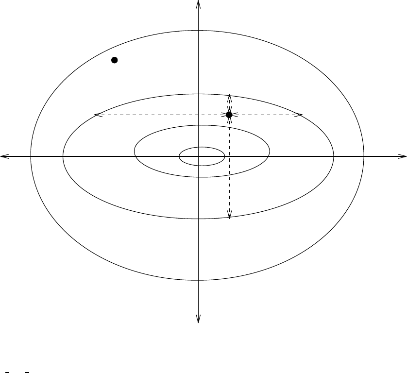
498
CHAPTER 35. ISONEUTRAL SGS OPTIONS
W
P1
S
E
N
123
distw diste
dists
distn
P2
Figure 35.1:
An illustration of the ideas used to generate the algorithm for determining
the width of the baroclinic zone. Shown are contours of the growth rate
T−1
in units of
vmhs rate limit
. Points outside the unit contour are outside the “baroclinic zone,” and those
inside the contour are inside the zone. For example, point P1 is outside the zone, and so the
length scale at P1 takes the value
LP1=max(∆x,∆y)
. Point P2 is inside the baroclinic zone. In
order to determine its length scale
LP2
, the distances
distn
,
dists
,
diste
, and
distw
are determined
as the distance from P2 to the unit contour in the north, south, east, and west directions,
respectively. These distances are then employed using the algorithm described in the text to
find
LP2
.

Chapter 36
Miscellaneous SGS options
This chapter is summarizes some miscellaneous SGS options.
36.1 Eddy-topography interactions and neptune
Option neptune implements the following. Based on statistical mechanics arguments, Holloway
(1992) proposed that interaction between mesoscale eddies and topography results in a stress
on the ocean with two important consequences: first, the ocean is not driven towards a state
of rest and secondly, the resulting motion may have scales much larger than the scale of the
eddies. Somewhat suprisingly, this interaction1can generate coherent mean flows on the scale
of the topography. The magnitude of this topographic stress is dependent on the correlation
between pressure pand topographic gradients ∇Hwhich is largely unknown but even if the
correlation is 0.1, the resulting topographic stress would be comparable in magnitude to that
of the surface wind.
If the view is taken that equations of motion are solved for moments of probable flow
(because of imperfect resolution) then those moments are forced in part by derivatives of the
distribution entropy with respect to the realized moments. The entropy gradient is estimated
as begin proportional to a departure of the realized moments from a state in which the entropy
gradient is weak. This latter state is approximated by a transport streamfunction ψ⋆and
maximum entropy velocity u⋆given by
ψ⋆=−f L′H(36.1)
u⋆=ˆ
z× ∇ψ⋆(36.2)
where fis the Coriolis term, His depth, and L′is O (10 km). If model resolution is coarse relative
to the first deformation radius, u⋆is independent of depth. Instead of eddy viscosity driving
flow towards rest, flow is driven towards u⋆using an eddy viscosity of the form A∇2(u⋆−u).
Note that topographic influence on flow2is not strongest near bottom topography. Instead,
the flow implied by ψ⋆only approximates a maximum entropy system given eddies and
topography. Since this approximation is admittedly crude, further refinements are open to
researchers.
1Which is missing or at best poorly represented in numerical models at any resolution.
2This is referred to as the Neptuneeffect because when Greg Holloway described coastal currents that persistantly
flow againgst both wind forcing and pressure gradient, the response was that it must be due to King Neptune.
Who else?
499

500
CHAPTER 36. MISCELLANEOUS SGS OPTIONS
There is legitimate concern about the stepwise resolution of bottom topography in level
models such as MOM and its predecessors. Option neptune is an attempt to instruct the model
about physical consequences due to topography and eddies which are nearly unachievable
even at the most ambitious resolutions. The hope is that if the model can be suitably informed
about the effect of topography, it matters little if that topography is only “approximately”
represented.
36.2 xlandmix
This section was contributed by Keith Dixon (kd@g f dl.gov), with modifications made for the
free surface height by Eli Tziperman (ett@g f dl.gov) and Stephen Griffies (smg@g f dl.gov).
It is sometimes useful to allow water masses which are separated by land to exchange
tracer properties. A case in point is when model grid resolution is too coarse to resolve narrow
passageways which in reality connect water masses. For example, insufficient resolution may
close offthe Mediterranean from the Atlantic at Gibraltar, or the Arctic from the Pacific in the
Bering Strait region.
Option xlandmix allows researchers to establish communication between bodies of water
separated by land. The communication consists of mixing tracers between non-adjacent water
columns. Momentum is not mixed. If the explicit free surface is enabled, option xlandmix eta
allows for the mixing of free surface height.
The scheme conserves tracers and volume. Its influence on tracers is tracked in the MOM
diagnostics as part of the tracer source terms.
36.2.1 Formulation
Let nxland be the number of water column pairs to be mixed. For each pair “nxl”, the “i,jrow”
coordinates are given by “ixland(nxl,1), jxland(nxl,1)” and “ixland(nxl,2), jxland(nxl,2)”. Be-
tween each pair, mixing takes place from level “kxland(nxl,1)” to level “kxland(nxl,2)”. When
one of these “i,jrow” coordinates is encountered in the memory window, the source term for
each tracer is modified as follows:
For all k-levels k=kxland(nxl,1) through kxland(nxl,2)
sourcei,k,j=sourcei,k,j+bxlandnxl ·(tithere,k,jthere,n,τ−1−ti,k,j,n,τ−1) (36.3)
bxlandnxl =vxland(nxl)
Pkxland(nxl,2)
k=kxland(nxl,1) cos φT
jrow dxtidytjrow dztk
(36.4)
where ithere,jthere represents the “i,j” coordinates of the other point in the nxlth mixed pair within
the memory window.
36.2.2 Considerations
•After identifying the “i,jrow” locations of the water column pairs to be mixed, an appro-
priate volume rate of mixing and the depth range for mixing must be specified. Refer to
physical oceanography resources for guidance.
•Specify the following information by editing the USER INPUT section of subroutine
xland1st: the number of crossland mixing point pairs (parameter nxland), their “i,jrow”

36.2. XLANDMIX
501
locations (ixland and jxland), the range of model k-levels to be mixed (kxland), and the
time invariant volume rate of mixing (vxland) in units of cm3/sec.
•An upper limit is placed on the value of vxland(nxl). Within a leap frog timestep (including
any tracer timestep acceleration effects), no more than one half of a water column may
be transported into its paired column. During initialization, a consistancy check is made
to insure that the mixing rate specified byvxland(nxl) is not too large. If the researcher
implementsvxland(nxl) as a function of time, then this check must be made each time
step.
•The size of the model’s memory window (parameter jmw) may need to be adjusted,
depending upon the j-row separation of pairs of crossland mixing points. The following
condition must be met:
|(jxland(nxl,2) −jxland(nxl,1)| ≤ (jmw −1)/2f or nxl =1,nxland (36.5)
36.2.3 xlandmix eta
Consider a model in which the Mediterranean Sea is artificially land-locked due to the use
of coarse resolution. When using MOM’s explicit free surface with explicit fresh water
fluxes, the net evaporation over the Mediterranean Sea will cause the free surface height
to decrease without bound. In a model resolving the Straits of Gilbraltor, there will be a
transfer of volume across the Strait from the Atlantic. This volume transfer will create a
change in the height of the free surface, and the transfer time will be determined by the
speed of external gravity waves. The purpose of this section is to describe a means of
parameterizing this effect in MOM when employing the explicit free surface and explicit
fresh water fluxes.
As discussed in Section 7.3.3, MOM’s free surface tendency is given by
η0
t=w(z=0) +qw,(36.6)
where η0is the linearized free surface height, w(z=0) =−∇h·U0is the vertical velocity
at the ocean surface, as determined by the convergence of the vertically integrated flow,
and qwis the fresh water input through evaporation, precipitation, and river runoff.
This equation results from neglecting the advection of free surface height by the surface
currents.
In the model, if ηlives at a grid point identified as one of a cross-land mixing pair, and
option xlandmix eta is enabled, the time tendency for these points takes the modified form
ηhere
t=w(0) +qw+Shere/Ahere,(36.7)
where Shere is the volume mixing term
Shere = ηthere −ηhere
τ! Ahere +Athere
2!.(36.8)
The mixing term Shere nudges the free surface height ηhere towards ηthere. Note that the
straightforward volume difference form Shere =(Athere ηthere −Ahere ηhere)/τ will lead to a
502
CHAPTER 36. MISCELLANEOUS SGS OPTIONS
nonzero source when ηthere =ηhere but if Athere ,Ahere. Such mixing is not desirable, hence
motivating the chosen form.
Originally, the time scale τfor the mixing was determined by an estimate of the time it
takes an external gravity wave to cross between the two points:
τ=L(g H)−1/2,(36.9)
where His set to the averaged depth of the two cross-land points, and Lis the horizontal
distance between them. However, this time scale gave very noisy results. Consequently,
the model currently has the value τ=3days hardwired. Changes to this time scale may
be necessary depending on grid resolution.
It is useful to discuss what cross-land ηmixing implies about tracers. For this purpose,
consider the case in which one starts with two basins connected by a strait, where the
basins have differing surface heights, yet let the temperature and salinity be the same
uniform values. Also, remove all surface heat and water fluxes. In a model with strait
resolved by at least one velocity point (which, for a B-grid, means at least two tracer
points), there will be an adjustment process in which the free surface height equilibrates
to the same value across the two basins. In contrast, the tracer concentrations, as there
are no surface fluxes, remain unchanged throughout the adjustment. In a model with an
unresolved strait, one should achieve the same equilibrated solution. Cross-land mixing
of ηclearly yields a uniform free surface height at equilibrium. In order to preclude
affecting the tracer concentrations through the ηmixing, it is necessary to not include the
cross-land mixing term Shere in the tracer budget. Similar considerations apply to the
baroclinic velocity tendency. Note that this result does not depend on having made the
linearized free surface approximation. Rather, it is simply a result of tracer conservation.
The result is convenient, since it means that no model changes are required for the tracer
or baroclinic equations when adding cross-land ηmixing.
Chapter 37
Bottom Boundary Layer
Dense water flowing down a slope is at best only poorly represented in z-level coordinate
models. However, this situation is remedied within MOM by enabling option bbl which
parameterizes the bottom boundary layer (hereafter referred to as BBL) by assuming frictional
dynamics within a thin layer that effectively “hangs” underneath bottom-most ocean cells.
Although the surface under which the BBL cells are “hung” is disconnected due to changes in
the number of vertical levels given by kmti,jrow, the BBL cells are mapped onto a continuous two
dimensional surface so that each BBL cell is in communication with its four nearest neighbors.
For practical reasons, this two dimensional surface is defined to be at constant depth within
level k=km. For the interior model, level k=km is treated as if it were always land. Within
the BBL model (level k=km), there are no land cells . . . only a two dimensional continuously
connected lattice of BBL cells. The BBL cells communicate vertically through advection and
diffusion with the bottom-most interior ocean cells above them. Note that land cells may exist
between the bottom-most ocean cell and the BBL cell beneath it.
This configuration works well for steeply sloping topography but is inadequate in regions
where the topographic slope is less than the grid aspect ratio. Refer to Chapter 26. Enabling
option partial cell resolves these mildly sloping regions and the BBL cells are then “hung”
underneath partial-cells which allows the BBL to feel shallow as well as steep topographic
slopes. As without option partial cell, the BBL cells populate level k=km.
Just as with option partial cell, the bbl option must be used right from the beginning of
an experiment. It is not intended as an option which can be enabled in the middle of an
experiment because it will wipe out all information in level k=km. For further information,
refer to http://www.gfdl.gov/a1g/bbl.html.
503
504
CHAPTER 37. BOTTOM BOUNDARY LAYER
Chapter 38
Miscellaneous options
This chapter contains various options which have not been placed into other catagories.
38.1 max window
The memory window supports second order, fourth order, and sixth order numerics. For each
order numerics, the memory window is configured to contain the minimum number of latitude
rows to solve the equations. For second order numerics, three rows are needed, five rows for
fourth order, and seven rows for sixth order. The extra rows are used as buffers to hold data
needed to solve equations on the central row within the window. If option max window is
enabled, the memory window is opened up all the way to hold all rows. For more detail, refer
to Section 11.3.4.
38.2 knudsen
Option knudsen computes density coefficients according to the Knudsen formulation. If this
option is not enabled, then density coefficients are computed according to the UNESCO for-
mulation. Refer to Section 15.1.2 for details.
38.3 pressure gradient average
Option pressure gradient average implements the pressure gradient averaging technique of
Brown and Campana (1978) which can allow the time step to be increased by up to a fac-
tor of two in certain circumstances! This applies when the time step is limited by internal
gravity waves. The actual time step, which should always be determined empirically, will
typically be somewhat less than the theoretical factor of two limit. It should be noted that this
is not a damping scheme. The amplification factor |λ|in the stability analysis given by Brown
and Campana (1978) is unity within the region of stable solutions.
Basically, the way it works is that instead of using ρτin the hydrostatic pressure gradient,
a semi-implicit density given by
˜ρ=alpha′(ρtau+1+ρtau−1)+(1 −2α′)ρτ(38.1)
is used with alpha′=1/4. Brown and Campana (1978) also discuss three computational modes
which are introduced by this technique. They are handled by either reducing alpha′slightly
505
506
CHAPTER 38. MISCELLANEOUS OPTIONS
or applying additional time averaging to other prognostic variables. Both methods sharply
reduce the maximum allowable time step. In MOM 2, the Euler backward mixing time step
damps the computational modes. For a discussion on when a semi-implicit pressure gradient
is applicable, refer to Killworth, Smith, and Gill (1984). Their analysis indicates that a semi-
implicit pressure gradient is applicable for coarse and medium resolution (≥1 deg) studies but
may not be applicable for high resolution (≤30 km) ones.
In order to apply this scheme for one or more rows within the memory window, there
must be one additional row of tracers calculated before the internal modes of velocity can
be calculated. This is because the pressure gradient, which is defined on U cell latitude
rows, requires an average of four surrounding densities which are defined on adjacent T cell
latitude rows. Although, strictly not a fourth order option, this extra computed tracer row
requires that option fourth order window also be enabled. This is automatically done when
option pressure gradient average is enabled.
For the minimum fourth order window configuration with jmw=5, tracers are computed
for rows 3 and 4 while velocities are only computed on row 3. To accommodate this, starting
and ending rows for tracer calculations are given by
jstrac =jbu f +2−1/mw (38.2)
jetrac =min(jmw −jbu f +1,jmt −1−jo f f ) (38.3)
where the number of buffer rows is typically jbu f =2, the memory window counter is mw, and
the function “min” limits jetrac to memory window rows corresponding to latitude rows less
than jmt. Refer to the formal treatment of dataflow in the memory window given in Section
11.3.2 where the starting and ending rows are given. The situation is further complicated when
this option is used in conjunction with a fourth order option such as option biharmonic. The
minimum configuration for the memory window is then jmw=5. This time, tracers are again
computed for rows 2 and 3, while velocities are computed for row 2 but an extra fifth row is
needed for the biharmonic computation for tracers on row 3. Yes, it works!
38.4 fourth order memory window
The memory window typically has a minimum size of three latitude rows (jmw=3) which is
appropriate for second order accurate numerics. Some options use fourth order numerics or,
in some cases, averaging operators which require information from two cells away. All fourth
order schemes require option fourth order memory window which is automatically enabled in
file size.h when any of the existing fourth order schemes are enabled. These schemes require the
minimum size of the memory window to be four latitude rows (jwm=4). Some combination
of schemes require the minimum memory window to be of size jmw =5. However, more is
required than simply opening up the window to jmw=4 rows. In the minimum size fourth
order window, prognostic equations are solved only on row 2. In a second order window with
jmw =4, they are solved for rows 2 and 3. For a further description of how the window works
with higher order schemes, refer to Section 11.3.2.
Calculations always proceed up to latitude row jrow =jmt −1 even with higher order
schemes!. There are no out of bounds references because meridional indexing is limited to a
maximum at latitude jrow =jmt and a maximum corresponding memory window row given
by j=min(j+jo f f,jmt)−jo f f . To accommodate higher order schemes when a fully open
38.5. IMPLICITVMIX
507
memory window jmw =jmt is used, meridional fluxes are set to zero at latitude jrow =jmt
which allows calculations to proceed through latitude row jrow =jmt −1.
38.5 implicitvmix
Option implicitvmix allows the vertical diffusion of momentum and tracers to be solved implic-
itly under control of an implicit vertical diffusion factor aidif which is input through namelist.
Refer to Section 14.4 for information on namelist variables. Setting aidif =1.0 gives full implicit
treatment and setting aidif =0gives full explicit treatment.
Pages 42 and 43 of Numerical Recipes (1992) recommend a setting of aidif =0.5 which is the
Crank-Nicholson scheme followed by a few fully implicit steps using aidif =1.0. The reason,
according to Anand Gnanadesikan, is because when R=Kvδt/∆z2>1, the explicit treatment
of diffusion produces wiggles in the solution, which are then smoothed out by the implicit
treatment. Essentially, using the fully implicit treatment gives more smoothing than may be
realistic for R>1. However, using a few fully implicit steps at the end of the integration
allows for proper averaging in cases where R>> 1. In MOM however, the interval of interest
is each timestep and without a fully implicit treatement, the wiggles produced by the explicit
treatment are left. In order for the most accurate solution of the diffusion term it is necessary
to set aidi f =1.0 for all cases where R>1.
Option implicitvmix solves both the vertical diffusion of tracers and vertical diffusion of
horizontal velocity components implicitly. When option implicitvmix is not enabled, the vertical
diffusion of horizontal velocity components is always solved explicitly. However, in the case
where option implicitvmix is not enabled, vertical diffusion of tracers is still solved implicitly if
option isoneutralmix is enabled.
When option isoneutralmix is enabled, the vertical diffusion of tracers is solved implicitly to
handle stability problems brought about by large vertical mixing coefficients. Recall that mixing
is along isoneutrals, and the maximum slope is constrained by the small slope approximation.
However, explicit convection operates when isoneutralmix is enabled to handle convective
regions which cannot be dealt with by isoneutralmix. Note that when option full tensor is used
with isoneutralmix, the isoneutral may wrap over on itself vertically but mixing is still along
the isoneutral. Explicit convection of tracers will break through the isoneutral and cause it to
align with the vertical.
Therefore, explicit convection of tracers as described in Section 33.1 operates only when
option implicitvmix is not enabled or option isoneutralmix is enabled.
Assume that the one dimensional vertical diffusion equation to be solved implicitly is given
by
ξk=ξ⋆
k+aidi f ·2∆τδz(dcbk·δz(ξk)) (38.4)
for levels k=1 to k=km where ξkis the vertical profile of a tracer or a horizontal velocity
component at time level τ+1. The given quantities are dcbkwhich is the diffusion coefficient
at the bottom of T or U cells, ∆τwhich is the time step, aidi f which is the implicit factor, and
ξ⋆
k. If ξis a tracer , ξ⋆
kis known from the solution of Equation (22.77). If ξis a horizontal
component of velocity, ξ⋆
kis the solution from Equation (22.116).
Equtation (38.4) is solved subject to flux boundary conditions at the top of the first cell at
k=1 (given as s f lux) and base of the bottom cell at k=kz (given as b f lux). The solution
follows from pages 42 and 43 of Numerical Recipes (1992). Note that when ξis a horizontal
508
CHAPTER 38. MISCELLANEOUS OPTIONS
component of velocity, s f lux =sm f and b f lux =bm f . When ξis a tracer, s f lux =st f and
b f lux =bt f . Equation (38.4) can be written as
ξk=ξ⋆
k+aidi f ·2∆τ(dcbk−1
ξk−1−ξk
dztk·dzwk−1−dcbk
ξk−ξk+1
dztk·dzwk
) (38.5)
which can be re-arranged to
Ak·ξk−1+Bk·ξk+Ck·ξk+1=ξ⋆
k(38.6)
where
Ak=−aidi f ·2∆τ·dcbk−1
dztk·dzwk−1
(38.7)
Ck=−aidi f ·2∆τ·dcbk
dztk·dzwk
(38.8)
Bk=1−Ak−Ck(38.9)
At k=1, Ak=0 and at k=kz,Ck=0. Note that the last ocean level kz may be less than bottom
level km to accommodate bottom topography. The boundary conditions at the top k=1 and
bottom k=kz are imposed by setting
Fk=1=ξ⋆
k=1+s f lux ·aidi f ·2∆τ
dztk=1·dzwk=0
(38.10)
Fk=ξ⋆
k(38.11)
Fk=kz =ξ⋆
k=kz −b f lux ·aidi f ·2∆τ
dztk=kz ·dzwk=kz
(38.12)
The solution is arrived at by performing a decomposition and forward substitution using
bet =Bk=1
ξk=1=Fk=1/bet
do k =2,kz
Ek=Ck−1/bet
bet =Bk−Ak·Ek
ξk=(Fk−Ak·ξk−1)/bet
enddo
then a back substitution using
do k =kz-1,1,-1
ξk=ξk−Ek+1·ξk+1
enddo
38.6. BETA PLANE
509
38.6 beta plane
Normally, the equations in MOM are formulated in spherical coordinates. This option turns
the model into a beta plane: f=f◦+β·ywhere β=∂f/∂yand f◦is taken at the latitude given
by φU
jrow=1.
38.7 f plane
Normally, the equations in MOM are formulated in spherical coordinates. This option turns
the model into a f plane as in option beta plane with β=0. Choosing f◦as the equator sets a
flat space cartesian grid.
38.8 source term
This option allows adding source terms to the momentum and tracer equations as indicated in
Sections 22.9.4 and 22.8.4.
38.9 readrmsk
This option allows importing region masks mskhri,jrowand mskvrkinto MOM for use with certain
diagnostics.
38.10 show details
When enabled, this option allows details from various parts of the setup calculations to be
printed to file stdout. When MOM executed, the printout indicates where this option will give
more information if enabled. When enabled, it leads to lots of printout and is left disabled
unless the missing details are needed.
38.11 timing
This option allows any Fortran source code or portions of the code to be timed using a simple
set of timing routines. Executing script run timer will exercise these routines by solving a
tracer equation in various ways. This is useful when trying to optimize speed for a particular
computer platform. Refer to Section 15.1.8 for details.
38.12 equivalence mw
This option hides the nine two dimension fields of the coefficient matrix for inverting the
external mode elliptic equation over the memory window space. This can be done since the
external mode and internal mode are essentially orthogonal calculations and the space required
by one can be used by the other.
510
CHAPTER 38. MISCELLANEOUS OPTIONS

Part VIII
Diagnostic options
511

Chapter 39
Design of diagnostic options
MOM is instrumented with a variety of diagnostic options. Some are useful for diagnosing
model problems while others are aimed towards providing information to help resolve ques-
tions of a more scientific nature. All are independent of each other and each is activated with its
own option at compile time. For added flexibility, each diagnostic has an associated interval,
control, and possibly an averaging period variable which are input through namelist. To see
all namelist variables, refer to Section 14.4.
When not enabled, a diagnostic requires neither memory nor computational time. When
enabled, some require large amounts of memory, disk, or cpu time so it is important to use them
cautiously with specific goals in mind. The amount of time generally depends on the particular
configuration of MOM, which diagnostics are enabled, the interval between diagnostic output,
and the averaging period (if applicable). An assessment of the computational time1can easily
be made by enabling the required diagnostics along with option timing2in a short model
execution.
The purpose of this chapter is to introduce some general ideas about the design of diag-
nostics in MOM. Subsequent chapters describe the different physical and numerical analysis
options.
39.1 Ferret
MOM can produce many types of diagnostics and all are described within this chapter. How
to organize and view results from these diagnostics has been a major problem in the past. With
the adoption of a NetCDF standard, results can now be viewed almost without effort. A good
way to visualize and further analyze results is to use Ferret which is a graphical analysis tool
developed by Steve Hankin (1994) at NOAA/PMEL (URL: http://ferret.wrc.noaa.gov/Ferret/
This package is highly recommended because it works well with large datasets, supports
non-uniform staggered grids, allows dynamic regridding of data, abstract variables, modulo
axes, and contains many useful transformations and built in functions.
1Note that when enabling lots of diagnostics, substantial reduction in computational time can be realized by
opening up the memory window even on a single processor. As an example, execute the test case script run mom
and open the memory window wider than the minimum (jmw exceeds 3 in file size.h). Of course, the price to be
paid is an increase in the required memory.
2After timing a particular configuration, option timing should always be disabled because the act of timing takes
non-negligible time!
513
514
CHAPTER 39. DESIGN OF DIAGNOSTIC OPTIONS
39.2 Naming Diagnostic files
Many diagnostic options may be enabled during a single run of MOM. Each one writes data
to a filename which is unique to the particular diagnostic. For instance, data from diagnostic
option snapshots will be written to a filename containing the keyword “snapshots” while data
from option tracer averages will be written to a filename containing the keyword “tracer avg”.
Within a given diagnostic, if data is written as unformatted 32 bit IEEE, then the output
filename is given the suffixyyyyyy.mm.dd.dta. If data is written in NetCDF format, then the
output filename is given the suffixyyyyyy.mm.dd.dta.nc. The “yyyyyy.mm.dd” is a place holder
for the year, month, and day information. The purpose of this infomation is to allow for easy
file management using UNIX.
If option separate diag files is enabled, the year, month, and day correspond to the timestep
during which the diagnostic data was written. If the interval for saving data results in multiple
datasets being written during one run, then each dataset will have a distinct filename (i.e. same
keyword name but different date information). If option separate diag files is not enabled, the
year, month, and day information in the filename will correspond to the last timestep of the
run. So multiple datasets written out for a particular diagnostic during a single run will all be
appended to one filename.
Since data from options time step monitor and trajectories are typically written out very often
within a model run, both options write to a filenames which corresponds to the last timestep
of the run.
39.3 Format of diagnostic data files
In general, diagnostic output can be written in either 32bit unformatted IEEE or NetCDF
format. In both cases, the actual writing of data is done through the I/O interface described
in http://www.gfdl.gov/vb. The option for NetCDF format is use netCDF. If not enabled, then
data will be written in 32bit unformatted IEEE.
Saving diagnostic data in NetCDF format is the preferred approach since diagnostic output
is immediately accessible to visualization packages which support NetCDF. This means that
there is no need to write and maintain code for manipulating diagnostic data in order to
visualize it. NetCDF format also allows data to be passed between various computer platforms
easily and is therefore the preferred method for sharing data.
Two options affect the efficiency of writing data. Option diagnostics himem uses large buffers
to speed up writing of data at the expense of using extra memory. Option diagnostics lomem
uses small buffers and increases computer time but uses much less memory than the former
option. Option diagnostics himem is the default.
39.4 Sampling data
Depending on the particular diagnostic, output may consist of instantaneous or time averaged
data. Instantaneous data is written out periodically on those time steps that fall nearest to
the end of a specified interval. For instance, specifying a 30 day interval means that results
are written out every 30 days from some specified reference time. The reference time is also
specified through namelist and is the same for all diagnostics.
Averaged data starts out being accumulated over all time steps within a specified interval.
It is then averaged and written out periodically at the end of the interval. If the interval were

39.5. REGIONAL MASKS
515
30 days, results would be output every 30 days from the reference time and would represent
30 day averages. It is possible to produce sub sampled averages by specifying an averaging
period as less than an interval. The averaging period is also input through namelist. For
example, if the interval was set to 30 days and the averaging period was set to 2.0 days, then
2 day averages would be written out every 30 days and the averaging would be over days 29
and 30 of each interval. How about producing monthly averages when months vary in length?
Enabling option monthly averages will over-ride values specified by “interval” and “period”
and make it so. However, this option is global and applies to all time averaged diagnostics
that are enabled. Refer to Section 40.11 for more details.
How often is it necessary to sample model generated data? It should be sampled often
enough to resolve the shortest time scale which is of interest. Of course, it follows that longer
time scales will also be resolved. For example, if data is sampled at an interval of once per
month, the implicit assumption is that time scales with periods of four months and longer are
being resolved.
What happens when the data has energy at periods of one week? If data is sample
instantaneously once per month, then sampled data will be aliased by the shorter period. One
way to remove this alias is to produce a monthly climatology. This is done by saving data
for many years and averaging all Januaries together, all Februaries together and so forth to
produce twelve climatological or “mean” months. The alias error reduces as more and more
years are included in the climatology.
A better way is to filter out energy at periods of one week by constructing monthly averages
which are then saved once per month. A dataset of monthly averages represents estimates
that are statistically more stable than a dataset of instantaneous values. If there is little energy
at periods shorter than the period of interest, then saving instantaneous samples is essentially
the same as saving monthly averages.
The averaging period need not always equal the interval at which results are saved. This
applies when frequencies are widely separated. For instance, suppose that the amplitude of a
diurnal period (one cycle per day) is not negligible compared to the amplitude of an annual
period (one cycle per year). The diurnal period can be effectively removed and the annual
period resolved by saving a three or four day average at the end of every month.
39.5 Regional masks
For use with certain diagnostics calculations, the model domain may be sub-divided into
a number of regions over which calculations are averaged. An arbitrary number of non-
overlapping regions of areal extent are defined by setting a horizontal region mask number
mskhri,jrow=mwhere (i,jrow) is in region mfor m=1···nhreg and nhreg is the number of
regions. One way to do this is to use the subroutine sethr which assigns mskhri,jrowto a region
number within a rectangular region. Regions may be built up from calls to sethr but in general
need not be simply rectangular.
In a similar fashion, the vertical region mask number mskvrk=ℓwhere kis in vertical region
ℓfor ℓ=1···nvreg and nvreg is the number of vertical regions. Unlike mskhri,jrowwhich may
contain a region which is multiply connected, the kindices within a vertical region ℓmust be
contiguous.
Regional volumes are constructed in subroutine setocn by the union of mskhri,jrowand
mskvrksuch that the regional volume numbers are given by
516
CHAPTER 39. DESIGN OF DIAGNOSTIC OPTIONS
nreg =nhreg ·(mskvrk−1) +mskhri,jrow (39.1)
39.6 A note about areas on the sphere
The area of a grid box on the sphere is given by
A=a2Zλ2
λ1
dλZφ1
φ2
cos φdφ. (39.2)
In a grid-point model with uniform resolution, this area is often approximated with
Aapprox =a2∆λ∆φcos φ, (39.3)
where
φ=φ1+φ2
2(39.4)
represents the midpoint latitude. The exact area of the finite sized grid box is given by
Aexact =a2∆λZφ1
φ2
d(sin φ)
=a2∆λ∆(sin φ).(39.5)
It is useful to determine the error made in the approximate expression through the use of some
trigonometry:
∆(sin φ)=sin φ2−sin φ1
=2 cos φsin(∆φ/2)
≈∆φcos φ(1 −(∆φ)2/24) (39.6)
Hence,
Aexact =a2∆λ∆(sin φ)
≈Aapprox (1 −(∆φ)2/24).(39.7)
As a result, the area of the grid box is overestimated by the amount (∆φ)2/24 when using the
approximate expression. For a model with ∆φ=4◦=0.0698rad, the leading error is
(∆φ)2/24 =0.0002 =0.02% (39.8)
It is important to note that the above error estimate is a lower bound for the case of a grid
where the cosine factor does not represent the cosine of the latitude at the center of the grid box
(as in a Gaussian grid). Atmospheric models at GFDL use the exact areas, not the approximate
values. Hence, care must be taken to use the same area weights between an atmospheric model
and MOM. Unless the weights are identical, flux conservation is not possible. Currently, the
approximate area method is used for computing diagnostics in MOM. It is clear that for the
purpose of ocean-only diagnostics, the differences are quite minor and can be safely ignored.
When time permits, these approximate area calculations will be replaced by the correct ones.
Chapter 40
Diagnostics for physical analysis
Physical science is involved with MOM at two central stages. First, there is the formulation of
the basic equations of the model, and the physical assumptions inherent in that formulation.
The next stage is in the analysis of solutions obtained from the model. It is for the second stage
that the analysis tools described in this chapter are designed. The options are presented here
in alphabetical order.
40.1 cross flow netcdf
How much of the velocity field is along the neutral directions, and how much is in the
dianeutral direction? Option cross flow netcdf computes the projection of the velocity field
into a component parallel to the neutral direction and a component in the dianeutral direction.
When combined with the diagnostic option local potential density terms, such a partitioning of
the velocity vector is useful for diagnosing the mechanisms of water mass transformation.
Note that in order to compute the neutral directions, it is necessary to compute the deriva-
tives ρθand ρs(see below). These fields are computed in the model only when option isoneu-
tralmix is enabled. If one wishes to employ the diagnostic option cross flow netcdf yet does not
wish to diffuse the tracers with option isoneutralmix, it is necessary to run with option isoneu-
tralmix on, yet with the isoneutral diffusivity ahiso set to zero.
40.1.1 Continuous formulation
The partitioning of the velocity vector into a neutral and dianeutral component is straightfor-
ward. Consider now the relevant kinematics in the continuum. Let the unit vector ˆγdefine
the dianeutral direction. This vector is given by
ˆγ=ρθ∇θ+ρs∇s
|ρθ∇θ+ρs∇s|,(40.1)
where
ρθ=∂ρ
∂θ (40.2)
ρs=∂ρ
∂s(40.3)
517
518
CHAPTER 40. DIAGNOSTICS FOR PHYSICAL ANALYSIS
are the partial derivatives of in situ density with respect to the active tracers potential temper-
ature and salinity. For more discussion, see Appendix C or Griffies et al. (1998) in which the
discretization of isoneutral diffusion is discussed. Note that in the case of a single active tracer,
the dianeutral direction is simply in the direction of the active tracer gradient. Also note that in
many regions of the ocean, the denominator is dominated by the vertical tracer gradients. This
result may motivate approximating the denominator by ρθ∂zθ+ρs∂zs. However, such an
approximation introduces a spurious singularity in vertically unstratified regions. Therefore,
it is useful to compute the full denominator for the purposes of this diagnostic.
Given the expression (40.1) for the dianeutral direction, it is possible to split the velocity
field into the dianeutral and neutral components
~
u=(~
u−~
D)+~
D
≡~
N+~
D,(40.4)
where
~
N=~
u−~
D(40.5)
defines the component of the velocity field parallel to the neutral direction, and
~
D=(~
u·ˆγ) ˆγ(40.6)
defines the dianeutral velocity vector. These are the two vectors which are provided by this
diagnostic. Mapping these vectors on top of potential density isolines gives an approximate
view of how much of the currents are along and how much are across the neutral directions.
The approximation occurs when noting that neutral directions are not quite parallel to potential
density isolines. But for regions not extending too much in the vertical direction (e.g., a few
hundred to a 1000 meters), the approximation is rather good (e.g., McDougall 1987).
40.1.2 Discretization
When discretizing, there will be some averaging that must be made in order to provide a
consistent computation of the neutral and dianeutral velocity vectors. First, it is necessary to
assume a position on the lattice at which the different components will be computed. For the
present diagnostic purposes, it is not crucially important how the averaging is done, only that
it is done in a consistent manner. One simple choice is to average all quantities so that they
lie at the tracer point. This choice is motivated by having the density derivatives ρθand ρs
already available at the tracer points in the computation of isoneutral diffusion (Appendix C).
This choice leads to the discretization of the numerator of the dianeutral direction
ρθ∇θ+ρs∇s≈
(ρθ)i,k,j
1
cos φT
jrow
δλ(ti−1,k,j,1,tau)λ·ˆ
x+δφ(ti,k,j−1,1,tau)φ·ˆ
y+δz(ti,k−1,j,1,tau)z·ˆ
z
+(ρs)i,k,j
1
cos φT
jrow
δλ(ti−1,k,j,2,tau)λ·ˆ
x+δφ(ti,k,j−1,2,tau)φ·ˆ
y+δz(ti,k−1,j,2,tau)z·ˆ
z
=1
cos φT
jrow (ρθ)i,k,jδλ(ti−1,k,j,1,tau)λ+(ρs)i,k,jδλ(ti−1,k,j,2,tau)λˆ
x
40.2. DENSITY NETCDF
519
+(ρθ)i,k,jδφ(ti,k,j−1,1,tau)φ+(ρs)i,k,jδφ(ti,k,j−1,2,tau)φˆ
y
+(ρθ)i,k,jδz(ti,k−1,j,1,tau)z+(ρs)i,k,jδz(ti,k−1,j,2,tau)zˆ
z,(40.7)
where ˆ
x,ˆ
y, and ˆ
zare local unit vectors in longitude (eastward), latitude (northward), and
vertical (upward). The velocity field must be averaged in order to provide an approximation
for its value at the cell Ti,k,j. The following averaging is employed
˜
Vi,k,j=ui−1,k,j−1,1,τλφ ·ˆ
x+ui−1,k,j−1,2,τλφ ·ˆ
y+adv vbti,k−1,j
z·ˆ
z.(40.8)
Therefore, the instantaneous discretized dianeutral ~
Dand neutral ~
Nvelocity fields are given
by
~
Di,k,j=˜
Vi,k,j·ˆγi,k,jˆγi,k,j(40.9)
~
Ni,k,j=˜
Vi,k,j−~
Di,k,j(40.10)
Output in 32 bit IEEE unformatted data is not an option for this diagnostic. The three
velocity components (zonal, meridional, and vertical) of ~
Dand ~
Nare output only in NetCDF
format to file cross.yyyyyy.mm.dd.dta.nc and the interval between output is specified by namelist
variable crossint in units of days. The “yyyyyy.mm.dd” is a place holder for year, month, and
day and this naming convention is explained further in Section 39.2. Refer to Section 14.4 for
information on namelist variables.
40.2 density netcdf
It is useful to construct both a locally referenced potential density ρf ull
i,k,jand potential density
σi,k,jreferenced to a specific depth. The superscript in is used to differentiate between potential
density anomaly (used throughout MOM) and the full potential density. To construct the full
density ρf ull
i,k,jin units of gm/cm3at each T cell, the mean reference density must be added to the
deviation
ρf ull
i,k,j=ρi,k,j+ρre f
k(40.11)
where ρre f
kis described in Section 15.1.2. When option potential density is enabled, σ0(referenced
to the surface), σ1(referenced to 1000m), σ2(referenced to 2000m), and σ3(referenced to 3000m)
are also constructed and saved.
Using, ρi,k,j, the hydrostatic pressure is given by integrating Equation 21.42 to yield
pi,k,j=grav ·dzw0·ρi,1,j+
k
X
m=2
grav ·dzwm−1ρi,m−1,jz(40.12)
The internal mode pressures in units of gm/cm/sec2are given by removing the vertical mean
pint
i,k,j=pi,k,j−1
zwk=kmt(i,jrow)
kmt(i,jrow)
X
k=1
pi,k,j·dztk(40.13)
520
CHAPTER 40. DIAGNOSTICS FOR PHYSICAL ANALYSIS
The external mode pressure is available from diagnostic diagnostic surf height. Note that output
from this diagnostic is only available in NetCDF format in file density.yyyyyy.mm.dd.dta.nc and
the interval between output is specified by namelist variable densityint in units of days. The
“yyyyyy.mm.dd” is a place holder for year, month, and day and this naming convention is
explained further in Section 39.2. Refer to Section 14.4 for information on namelist variables.
40.3 diagnostic surf height
Option diagnostic surf height constructs an average sea surface elevation from the prognostic
stream function. It does this by accumulating a forcing term in time, then averaging over a
specified interval (because this is a linear problem) to produce an average forcing Xand solving
an elliptic equation of the form
∇ · H∇ps=X(40.14)
for average surface pressure psi,jrow which is then converted into height using
dspi,jrow =psi,jrow
ρ◦·grav (40.15)
where the height dspi,jrow is in units of cm.
The process begins after solving for the external mode stream function. The surface pressure
gradient terms can be reconstructed from Equations (29.3) and (29.4) by replacing the vertically
integrated velocities by ψwith the aid of Equations (29.6) through (29.10) to yield
1
ρ◦cos φU
jrow
δλ(ps
i,jrow
φ)=1
2∆τ1
Hi,jrow
δφ(∆ψi,jrow
λ)+
˜
fjrow
Hi,jrow ·cos φU
jrow
δλ(∆ψi,jrow
φ)
+zui,jrow,1(40.16)
1
ρ◦δφ(ps
i,jrow
λ)=1
2∆τ−1
Hi,jrow ·cos φU
jrow
δλ(∆ψi,jrow
φ)+
˜
fjrow
Hi,jrow
δφ(∆ψi,jrow
λ)
+zui,jrow,2(40.17)
where ˜
fjrow is given by Equation (29.5). Since the coefficient matrix required for solving
Equation (40.14) is generated within MOM for purposes of solving the prognostic surface
pressure and implicit free surface methods, this coefficient matrix can be easily generated. It is
done by essentially replacing 1/Hwith Hin the method given within Section 31.2. The average
forcing Xis computed as
X=1
L
L
X
ℓ=1
δλ
Hi−1,jrow−1
cos φU
jrow−1·δλ(ps
i−1,jrow−1
φ)
φ
+δφ
Hi−1,jrow−1·cos φU
jrow−1·δφ(ps
i−1,jrow−1
λ)
λ
(40.18)
with the aid of Equations (40.16) and (40.17) where Lis the number of timesteps in the averaging
period. Equation (40.14) is then inverted for psi,jrow by the method of conjugate gradients.
40.4. ENERGY ANALYSIS
521
Equations (40.16) and (40.17) may be solved directly by line integrals to construct psi,jrow.
However, the integration paths must be chosen carefully so as not to propagate errors intro-
duced by solving the stream function equation exactly (hy using a non-zero tolerance “tolrsf”).
Choosing nine point numerics by enabling option sf 9 point minimizes these errors compared
to using option sf 5 point.
The solution psi,jrow is thus an average and may be written as ascii to the model printout or
as 32 bit IEEE unformatted data to file diag surf.yyyyyy.mm.dd.dta. If option netcdf or diagnos-
tic surf height netcdf is enabled, data is written in NetCDF format to file diag surf.yyyyyy.mm.dd.dta.nc
rather than in unformatted IEEE. The “yyyyyy.mm.dd” is a place holder for year, month, and
day and this naming convention is explained further in Section 39.2. The interval between out-
put is specified by variable dspint and the control is specified by variable iodsp. The averaging
period dspper is typically set the same as the interval but may be specified shorter. How about
producing monthly averages when months vary in length? Enabling option monthly averages
will over-ride values in dspper and dspint and make it so. However, this option is global and
applies to all time averaged diagnostics that are enabled. Refer to Section 40.11 for more details.
Variables dspper and dspint are input through namelist. Refer to Section 14.4 for information
on namelist variables.
40.4 energy analysis
Option energy analysis computes the instantaneous scalar product of ~
uand the momentum
Equations (4.1) and (4.2) integrated over the entire domain to verify energy conservation as
demonstrated for the continuous equations in Section A.1. The finite discrete equivalent is
demonstrated in Chapter A. From Equations (4.1) and (4.2) the total velocity ~
uis divided into
internal mode ˆ
uand external mode ucomponents. The work done by each term in Equations
(4.1) and (4.2) is broken into internal and external mode contributions. Note that this approach
is different than that given in Cox (1984). Units are in gm/cm/sec3.
Define two operators for integrating the scalar product of ~
uand any terms in Equations
(4.1) and (4.2). In finite difference form, they are
<αi,k,j,next >=1
VolU
jmt−1
X
jrow=2
km
X
k=1
imt−1
X
i=2
2
X
n=1
ui,j,n,τ ·(αi,k,j,n)∆U
i,k,j(40.19)
<αi,k,j,nint >=1
VolU
jmt−1
X
jrow=2
km
X
k=1
imt−1
X
i=2
2
X
n=1
ˆ
ui,k,j,n,τ ·(αi,k,j,n)∆U
i,k,j(40.20)
(40.21)
<αi,k,j,next >represents the external mode component of the work done by αi,k,j,n,< αi,k,j,nint >
represents the internal mode component of the work done by αi,k,j,n, and the relation between j
and jrow is as described in Section 14.2. The volume element and total volume are given by
∆U
i,k,j=umaski,k,j·dxui·cos φU
jrow ·dyujrow ·dztk(40.22)
VolU=
jmt−1
X
jrow=2
km
X
k=1
imt−1
X
i=2
∆U
i,k,j(40.23)
522
CHAPTER 40. DIAGNOSTICS FOR PHYSICAL ANALYSIS
Work done by each term in the momentum equations is computed using operators described
in Sections 22.9.5.
Total change in kinetic energy
E=<ui,k,j,n,τ+1−ui,k,j,n,τ−1
2∆τ
ext
>+<ui,k,j,n,τ+1−ui,k,j,n,τ−1
2∆τ
int
>(40.24)
Non-linear terms
The work done by non-linear terms on the velocity is broken into two parts: G1 is the
horizontal part including the metric term and G2 is the vertical part. G1 +G2 should be zero.
The “nonlinear error” =G1 +G2 which should be roundoffto within machine precision. On
a Cray YMP with 64 bit words, this amounts to the error being about 1x10⁻¹² smaller than the
leading term in the computation of G1 and G2.
G1=<ADV Uxi,k,j+ADV Uyi,k,j+ADV metrici,k,j,n
ext >
+<ADV Uxi,k,j+ADV Uyi,k,j+ADV metrici,k,j,n
int >(40.25)
G2=<ADV Uzi,k,j
ext >
+<ADV Uzi,k,j
int >(40.26)
Buoyancy
B=<grav ·adv vbti,k,j·ρi,k,jzext >+<grav ·adv vbti,k,j·ρi,k,jzint >(40.27)
Horizontal pressure gradients
G=<grad pi,k,j,n
ext >+<grad pi,k,j,n
int >(40.28)
The work done by the horizontal pressure gradients should equal the work done by buoy-
ancy. G −B should be zero. The imbalance G −B is the “energy conversion error” which
should be roundoffwithin machine precision. On a Cray YMP with 64 bit words, this amounts
to the error being about 1x10⁻¹² smaller than either term.
Mixing
The work done by viscous mixing terms on the velocity is broken into two parts
D1=<DIFF Uxi,k,j+DIFF Uyi,k,j+DIFF metrici,k,j,n
ext >
+<DIFF Uxi,k,j+DIFF Uyi,k,j+DIFF metrici,k,j,n
int >(40.29)
D2=<DIFF Uzi,k,j
ext >+<DIFF Uzi,k,j
int >(40.30)
40.5. FCT NETCDF
523
Wind and Bottom drag
W1=<sm fi,j,n
ext >+<sm fi,j,n
int >(40.31)
W2=<bm fi,j,n
ext >+<bm fi,j,n
int >(40.32)
The output from this diagnostic may be written as ascii to the model printout or as 32 bit IEEE
unformatted data to file energy int.yyyyyy.mm.dd.dta. If option netcdf or energy analysis netcdf
is enabled, data is written in NetCDF format to file energy int.yyyyyy.mm.dd.dta.nc rather than
in unformatted IEEE. The “yyyyyy.mm.dd” is a place holder for year, month, and day and
this naming convention is explained further in Section 39.2. The interval between output is
specified by variable glenint and the control is specified by variable ioglen.
40.5 fct netcdf
When using the FCT advection scheme, it is common to wonder how much the upwind part of
FCT is active for any particular flow regime. A simple way to judge this property is to subtract
from the FCT advective flux the centered differenced advective flux:
∆~
F=~
F(f ct)−~
F(ctr).(40.33)
The option fct netcdf maps the three components of ∆~
Ffor each tracer. In addition, this option
maps the convergence
− ∇ · (∆~
F),(40.34)
which tells one how FCT and centered differ as they act in the tracer equation.
When the Gent-McWilliams scheme is implemented through the eddy-velocity formulation
(see Section 35.1.6.2) and FCT is employed, the FCT advective flux incorporates both the
resolved velocity and the GM velocity. The diagnostic option fct netcdf takes this fact into
account.
Output from diagnostic option fct netcdf is only available in NetCDF format. If op-
tion fct netcdf is enabled, data is written in NetCDF format to file fct.yyyyyy.mm.dd.dta.nc.
The “yyyyyy.mm.dd” is a place holder for year, month, and day and this naming convention
is explained further in Section 39.2. The interval between output is specified by variable fctint
and the data is instantaneous.
40.6 gyre components
Option gyre components computes instantaneous values of various components of northward
tracer transport. The longitudinally averaged temperature and meridional velocity are con-
structed for the latitude of φU
jrowas a function of depth. Also, the vertically averaged temperature
and meridional velocity are constructed for the latitude of φU
jrowas a function of longitude
<Tφ
k,j>λ=1
VolxT
k,j
imt−1
X
i=2
ti,k,j,n,τ
φ∆T
i(40.35)
524
CHAPTER 40. DIAGNOSTICS FOR PHYSICAL ANALYSIS
<Vk,j>λ=1
VolxU
k,j
imt−1
X
i=2
ui,k,j,2,τ∆U
i(40.36)
<Tφ
i,j>z=1
VolzT
i,j
km
X
k=1
ti,k,j,n,τ
φ∆T
k(40.37)
<Vi,j>z=1
VolzU
i,j
km
X
k=1
adv vnti,k,j∆U
k(40.38)
Note that a factor of cos φU
jrowis built into adv vnti,k,j. The volume elements and volume of the
latitude strip as a function of depth are
∆T
i=tmaski,k,j·tmaski,k,j+1·dxti(40.39)
∆U
i=dxui ·cos φU
jrow (40.40)
∆T
k=tmaski,k,j·tmaski,k,j+1·dztk(40.41)
∆U
k=dztk(40.42)
VolxT
k,j=
imt−1
X
i=2
∆T
i(40.43)
VolxU
k,j=
imt−1
X
i=2
∆U
i(40.44)
VolzT
i,j=
km
X
k=1
∆T
k(40.45)
VolzU
i,j=
km
X
k=1
∆U
k(40.46)
(40.47)
The canonical form of the northward components of tracer transport by various means and
deviations is given as
ttn1,jrow,n=
km
X
k=1
<Tφ
k,j>λ·<Vk,j>λ·dztk(40.48)
ttn2,jrow,n=ttn6,jrow,n−ttn1,jrow,n(40.49)
ttn3,jrow,n=
imt−1
X
i=2
<Tφ
i,j>z·<Vi,j>z·dxti(40.50)
ttn4,jrow,n=ttn6,jrow,n−ttn3,jrow,n−ttn5,jrow,n(40.51)
ttn5,jrow,n=
imt−1
X
i=2−(sm fi−1,j,1·dxui−1
λ)·(ti,1,j,n,τ
φ−<Tφ
i,j>z)·cos φU
jrow
fjrow
(40.52)
ttn6,jrow,n=
km
X
k=1
imt−1
X
i=2
0.5·adv f ni,k,j·∆T
i·dztk(40.53)
40.7. LOCAL POTENTIAL DENSITY TERMS
525
ttn7,jrow,n=
km
X
k=1
imt−1
X
i=2
di f f f ni,k,j·∆T
i·dztk(40.54)
ttn8,jrow,n=ttn6,jrow,n+ttn7,jrow,n(40.55)
Note the factor of 0.5 which is needed to correct the advective flux of tracer as described in
Section 22.8.2. These terms may also be broken down as a function of latitude within mskhri,jrow.
The output from this diagnostic may be written as ascii to the model printout or as 32 bit IEEE
unformatted data to file gyre comp.yyyyyy.mm.dd.dta. If option netcdf or gyre components netcdf
is enabled, data is written in NetCDF format to file gyre comp.yyyyyy.mm.dd.dta.nc rather than
in unformatted IEEE. The “yyyyyy.mm.dd” is a place holder for year, month, and day and
this naming convention is explained further in Section 39.2. The interval between output is
specified by variable gyreint and the control is specified by variable iogyre.
40.7 local potential density terms
Option local potential density terms diagnoses processes affecting the time evolution of locally
referenced potential density. These processes include
1. Advection
2. Vertical diffusion
3. Laplacian horizontal diffusion
4. Laplacian skew-diffusion
5. Biharmonic skew-diffusion
6. Cabbeling
7. Thermobaricity
8. Halobaricity.
Such a diagnosis can be useful for understanding processes affecting water mass formation
and transformation. Note that the added important effects from convective mixing can be
deduced from the option save convection (section 40.12) and so are not built into option lo-
cal potential density terms. In order to diagnose cabbeling, thermobaricity, and halobaricity,
the code assumes that the isoneutral diffusion scheme is employed using the small angle ap-
proximation (option isoneutralmix described in Section 35.1). If Gent-McWilliams is used, then
its effects on locally referenced potential density is computed in terms of skew-diffusion (see
Section 35.1.6).
The first part of this section describes the breakdown of terms in the locally referenced
potential density equation, the second part describes the discretization of these terms, and the
third part describes the model output.
In coding this diagnostic, it was decided that a straightforward approach should be taken,
rather than one which involves tricks to save computation time and memory. Consequently,
the code should be rather easy to read. Yet, due to the rather large number of terms to compute,
this diagnostic is currently expensive.

526
CHAPTER 40. DIAGNOSTICS FOR PHYSICAL ANALYSIS
40.7.1 Locally referenced potential density equation
Some of the discussion in this section can be found in McDougall (1991) and Appendix B in
Griffies et al., (1998). What is of interest is the time tendency of locally referenced potential
density
∂tρ=ρθ∂tθ+ρs∂ts,(40.56)
where
ρθ=∂ρ
∂θ =−αρ
ρs=∂ρ
∂s=βρ (40.57)
are the partial derivatives of density with respect to the active tracers potential temperature θ
and salinity s. These derivatives are evaluated at the local temperature, salinity, and pressure.
The reason there is no pressure time tendency term in equation (40.56) is due to the local
referencing used for locally referenced potential density. In other words, locally referenced
potential density is a local water mass variable in the sense that it changes only when water
mass properties (temperature and salinity) change. Jackett and McDougall (1997) discuss an
approximate global water mass variable called neutral density.
Now split the right hand side of equation (40.56) into various processes using the prognostic
equations for temperature and salinity
∂tρ=ρθ∂tθ+ρs∂ts
=−~
u·(ρθ∇θ+ρs∇s)−(ρθ∇ · ~
F(θ)+ρs∇ · ~
F(s))
=−[ρθ∇(~
uθ)+ρs∇(~
u s)] −[ρθ∇ · ~
F(θ)+ρs∇ · ~
F(s)] (40.58)
where ~
uis the divergence-free current vector. The non-advective tracer flux takes the form
~
F=~
FI+~
Fskew−lap +~
Fskew−bih +~
FV+~
FH,(40.59)
where
•~
FIis the diffusive flux of tracer along the neutral directions.
•~
Fskew−lap is the skew-diffusive flux arising from Laplacian skew-diffusion (e.g.,option gent mcwilliams
discussed in Section35.1.6).
•~
Fskew−bih is the skew-diffusive flux arising from biharmonic skew-diffusion (e.g., option bi-
harmonic rm discussed in Section 35.1.8).
•~
FVis the vertical diffusive flux.
•~
FHis the Laplacian horizontal diffusive flux.
Note again that convection is absent in this analysis, as its effects on density are readily diag-
nosed using the option save convection. Additionally, the effects from a biharmonic horizontal
diffusive flux currently has not been implemented in this diagnostic.

40.7. LOCAL POTENTIAL DENSITY TERMS
527
40.7.1.1 Cabbeling, thermobaricity, and halobaricity
To isolate the mathematical expressions for cabbeling, thermobaricity, and halobaricity, write
the convergence of the isoneutral diffusive fluxes in the form
−ρθ∇ · ~
FI(θ)−ρs∇ · ~
FI(s)=∇ρθ·~
FI(θ)+∇ρs·~
FI(s) (40.60)
where the identity
ρθ~
FI(θ)+ρs~
FI(s)=0 (40.61)
was used. This identity represents an important balance between the isoneutral diffusive flux
of the two active tracers. It is a manifestation of the absence of a neutral direction diffusive
flux of locally referenced potential density. More simply, isoneutral diffusion does not act on
buoyancy, and equation (40.61) is a mathematical statement of this physical property. Griffies
et al 1998 provide further discussion of this balance, and its importance when discretizing
isoneutral diffusion. To procede, use the identities
∇s·~
FI(θ)=∇θ·~
FI(s) (40.62)
∇ρθ=ρθθ∇θ+ρθs∇s+ρθp∇p(40.63)
∇ρs=ρsθ∇θ+ρss∇s+ρs p∇p.(40.64)
The first identity is most easy to verify when writing the diffusive flux in terms of a symmetric
diffusion tensor
∇s·~
FI(θ)=−∂is Kij ∂jθ
=−∂jθKji ∂is
=∇θ·~
FI(s).(40.65)
Identities (40.63) and (40.64) follow from the chain rule. The pressure gradient terms represent
the effects of probing different pressure surfaces, and hence different potential density surfaces.
Such is necessary for computing the spatial gradients of the thermal and saline expansion
coefficients, and they lead to the thermobaric and halobaric effects. When evaluating the
horizontal pressure gradient for this diagnostic, the gradient in the lid or surface pressure is
ignored. These three identities, along with the balance of temperature and salinity fluxes given
by equation (40.61), render
−ρθ∇ · ~
FI(θ)−ρs∇ · ~
FI(s)=
ρθθ∇θ·~
FI(θ)+ρss∇s·~
FI(s)+2ρθs∇s·~
FI(θ)+∇p·[ρθp~
FI(θ)+ρs p~
FI(s)]
=∇θ·~
FI(θ)[ρθθ −2ρθs(ρθ/ρs)+ρss(ρθ/ρs)2]+∇p·[ρθp~
FI(θ)+ρs p~
FI(s)].(40.66)
The terms in equation (40.66) proportional to the second derivatives of density with respect
to temperature and salinity are identified as cabbeling. There is a useful way to make the form
for cabbeling appear in a slightly more tidy and intuitive manner. To do so, introduce the
vector
~
V=(1, α/β)
=(1,−ρθ/ρs) (40.67)

528
CHAPTER 40. DIAGNOSTICS FOR PHYSICAL ANALYSIS
and the symmetric tensor
ρab = ρθθ ρθs
ρsθρss !,(40.68)
which yields
ρθθ∇θ·~
FI(θ)+ρss∇s·~
FI(s)+2ρθs∇s·~
FI(θ)=∇θ·~
FI(θ)ρabVaVb.(40.69)
The quadratic form
ρabVaVb=ρθθ −2ρsθ(ρθ/ρs)+ρss (ρθ/ρs)2
=−αθ−2(α/β)αs+(α/β)2βs(40.70)
can be thought of as the squared length of the vector ~
Von the curved potential density surface
characterized locally by the metric tensor ρab. It can be easily computed in MOM through
tabulating the first and second partial derivatives of the density (see Section 40.7.2.1). A
fundamental property of seawater is that the total or Gaussian curvature (Aris, 1962) of a
potential density surface
κgauss =det(ρab)(1 +ρ2
θ+ρ2
s)−1
=(ρθθ ρss −ρ2
θs)(1 +ρ2
θ+ρ2
s)−1(40.71)
is negative. Consequently,
ρabVaVb≤0.(40.72)
In summary, cabbeling
cabbeling =∇θ·~
FI(θ)ρabVaVb(40.73)
is written as the product of two separate quadratic forms whose physical content can be
individually identified. The first
∇θ·~
FI(θ)=−∂iθKij ∂jθ(40.74)
is the projection of the temperature gradient onto the isoneutral diffusive flux of temperature.
This term is negative semi-definite for a downgradient isoneutral diffusive temperature flux.
In this case, the tensor Kij is the symmetric and positive semi-definite Redi isoneutral diffusion
tensor. The second term, ρabVaVb, as just discussed, summarizes certain intrinsic properties of
the potential density surface. The combined effects of a negatively curved potential density
surface and a downgradient isoneutral diffusive flux of temperature render
cabbeling ≥0.(40.75)
As a result, cabbeling increases the value of the locally referenced potential density ρ, thus
moving a water parcel downward.
The terms proportional to the pressure gradient
thermobaricity +halobaricity =ρθp~
FI(θ)· ∇p+ρs p~
FI(s)· ∇p
=ρθp~
FI(θ)· ∇p−ρs p ρθ
ρs!~
FI(θ)· ∇p(40.76)

40.7. LOCAL POTENTIAL DENSITY TERMS
529
represent the effects from thermobaricity and halobaricity. The balance (40.61) was used to
obtain the second equality. These processes arise from the pressure dependence of the equation
of state for seawater. The ratio
thermobaricity
halobaricity =− ρθpρs
ρsp ρθ!(40.77)
is quite large in absolute value, indicating the dominance of thermobaricity over halobaricity
(McDougall 1987). In contrast to the cabbeling term, both the thermobaric and halobaric terms
are sign-indefinite.
40.7.1.2 Summary of the terms forcing locally referenced potential density
In summary, the time tendency of locally referenced potential density can be written
∂tρ=advection +vertical diffusion +Laplacian horizontal diffusion
+Laplacian skew-diffusion +biharmonic skew-diffusion
+cabbeling +thermobaricity +halobaricity,(40.78)
where
advection =−[ρθ∇ · (~
uθ)+ρs∇ · (~
u s)] (40.79)
vertical diffusion =−[ρθ∇ · ~
FV(θ)+ρs∇· ~
FV(s)] (40.80)
Laplacian horizontal diffusion =−[ρθ∇ · ~
FH(θ)+ρs∇· ~
FH(s)] (40.81)
Laplacian skew-diffusion =−[ρθ∇ · ~
Fskew−lap(θ)+ρs∇ · ~
Fskew−lap(s)] (40.82)
Biharmonic skew-diffusion =−[ρθ∇ · ~
Fskew−bih(θ)+ρs∇ · ~
Fskew−bih(s)] (40.83)
cabbeling =∇θ·~
FI(θ)ρabVaVb(40.84)
thermobaricity =ρθp~
FI(θ)· ∇p(40.85)
halobaricity =ρs p~
FI(s)· ∇p.(40.86)
Notice that each term has the dimensions of density per time.
A steady state ocean represents a balance between the terms on the right hand side of
equation (40.78). For the simplest case, there is only advection by the resolved current ~
u. In this
case, the steady state current is aligned parallel to the neutral directions: ~
u·(ρθ∇θ+ρs∇s)=
~
u·∇ρ=0. Such a flow field is typically associated with steady state adiabatic fluid flow. When
there is time dependence, and/or when cabbeling, thermobaricity, halobaricity, diffusion, or
skew-diffusion are present, there will be a nonzero dianeutral component to the velocity field:
~
u· ∇ρ,0. Note that since the cabbeling term is sign-definite, the balance between advection
and cabbeling,
~
ucab · ∇ρ=∇θ·~
FI(θ)ρabVaVb,(40.87)
results in a dianeutral component to the velocity which is always directed towards values of
increasing locally referenced potential density
~
ucab · ∇ρ≥0.(40.88)
530
CHAPTER 40. DIAGNOSTICS FOR PHYSICAL ANALYSIS
Namely, for a stably stratified fluid, the velocity field which balances cabbeling acts in a
downward dianeutral direction (McDougall 1991). The other processes, as they are not sign-
definite, do not necessarily lead to a particular flow direction for their associated dianeutral
velocity.
The diagnostic option cross flow netcdf (Section 40.1) allows one to diagnose the component
of velocity along and across the neutral directions. In many regions of the ocean, dianeutral
advection is presumed to be small. The option local potential density terms allows one to diag-
nose terms in the locally referenced potential density equation and thus to associate a cause
for any dianeutral flow in the model.
40.7.2 Discretization
The diagnostic option local potential density terms provides a discretization of the terms on the
right hand side of equations (40.79)–(40.86). Since they represent source/sink terms for the time
tendency of locally referenced potential density, it is useful to diagnose them at a model tracer
point. All terms, except advection, are computed inside the fortran program ptlrhoterms.F.
The need to separate all of the various processes implies that none of the fluxes computed in
isopyc.F can be used, since that code, for optimization reasons, combines the various processes
to form a single flux vector. As such, it is very important to maintain consistency between the
algorithms used in isopyc.F and ptlrhoterms.F.
Whenever discretizing continuous equations which possess certain local properties, it is not
always possible to maintain those local properties on the lattice. Griffies et al. (1998) discuss
how their discretization of the isoneutral diffusive flux maintains a downgradient property
only over an extended “finite volume” rather than on each grid cell. In particular, ~
FI(θ)·∇θon
the lattice is not constrained to be negative. This result means that the lattice form of cabbeling,
∇θ·~
FI(θ)ρabVaVb, will not generally maintain non-negative values as it does in the continuum.
The negative values for cabbeling on the lattice, however, should be minimal and localized.
Note that in the model, the computation of tracer flux components employs the opposite
sign to that employed in the continuum formulation given above. Hence, the discrete equations
will have a minus sign inserted to account for this convention.
40.7.2.1 Equation of state considerations
As described in Section 15.1.2, the density is evaluated as a cubic approximation (Bryan and
Cox, 1972) to the UNESCO equation of state
ρ(˜
t,˜
s,k)=(ck,1+(ck,4+ck,7∗˜
s)∗˜
s+
(ck,3+ck,8∗˜
s+ck,6∗˜
t)∗˜
t)∗˜
t+
(ck,2+(ck,5+ck,9∗˜
s)∗˜
s)∗˜
s
=ck,1˜
t+ck,2˜
s+ck,3˜
t2+ck,4˜
s˜
t+ck,5˜
s2
+ck,6˜
t3+ck,7˜
s2˜
t+ck,8˜
s˜
t2+ck,9˜
s3(40.89)
where
˜
ti,k,j=ti,k,j,1,τ −Tre f
k(40.90)
˜
si,k,j=ti,k,j,2,τ −Sre f
k(40.91)
40.7. LOCAL POTENTIAL DENSITY TERMS
531
are tracer anomalies with respect to some pre-specified reference values. The choice of comput-
ing density anomalies is based on the increased numerical accuracy inherent in this approach
(see Section 15.1.2 for further discussion). The nine polynomial coefficients ck,1−9in this equa-
tion depend on the depth level k. They are defined at the tracer points, which means that the
density is defined there as well. The first partial derivative of the density with respect to the
active tracers are given in MOM by the quadratic expressions
(ρθ)i,k,j=∂˜
tρ(˜
t,˜
s,k)=ck,1+2ck,3˜
t+ck,4˜
s+3ck,6˜
t2+ck,7˜
s2+2ck,8˜
s˜
t(40.92)
(ρs)i,k,j=∂˜
sρ(˜
t,˜
s,k)=ck,2+ck,4˜
t+2ck,5˜
s+2ck,7˜
t˜
s+ck,8˜
t2+3ck,9˜
s2(40.93)
The second partial derivatives of density with respect to the active tracers are given by the
linear expressions
(ρθθ)i,k,j=∂˜
t˜
tρ(˜
t,˜
s,k)=2ck,3+6ck,6˜
t+2ck,8˜
s(40.94)
(ρθs)i,k,j=∂˜
t˜
sρ(˜
t,˜
s,k)=ck,4+2ck,7˜
s+2ck,8˜
t(40.95)
(ρss)i,k,j=∂˜
s˜
sρ(˜
t,˜
s,k)=2ck,5+2ck,7˜
t+6ck,9˜
s(40.96)
These expressions are tabulated in the routine dens.h. The second partial derivatives of the
density with respect to an active tracer and pressure are given by
ρθp=zp
∂ρθ
∂z
=− 1
ρg!∂zρθ(40.97)
ρs p =zp
∂ρs
∂z
=− 1
ρg!∂zρs,(40.98)
where the hydrostatic approximation has been used. Consistent with the Boussinesq approx-
imation used in MOM, the ρgterm will be evaluated as ρog, where ρo=1.035g/cm3and
g=980.6cm/sec2. The vertical derivatives are discretized in a centered fashion:
(ρθp)i,k,j=(∂˜
tpρ)i,k,j=−1
ρog (ρθ)i,k−1,j−(ρθ)i,k+1,j
dhwti.k−1,j+dhwti,k,j!(40.99)
(ρsp)i,k,j=(∂˜
s p ρ)i,k,j=−1
ρog (ρs)i,k−1,j−(ρs)i,k+1,j
dhwti.k−1,j+dhwti,k,j!.(40.100)
Next to surface and bottom boundaries, the values of (ρθp)i,k,jand (ρsp)i,k,jare equated to the
value one level away. Note that these vertical derivatives compute differences in in situ density;
i.e., the two densities are not referenced to the same temperature, salinity, and pressure. The
reason is that one is interested in gradients between different potential density surfaces when
computing thermobaricity and halobaricity.
40.7.2.2 Advection
Advection is diagnosed using the same advection operators used in the model for the chosen
advection scheme. The contribution to locally referenced potential density takes the form
advrhoi,k,j=−(ρθ)i,k,jADVi,k,j,1−(ρs)i,k,jADVi,k,j,2.(40.101)
532
CHAPTER 40. DIAGNOSTICS FOR PHYSICAL ANALYSIS
This term is computed inside of tracer.F. Note that the contribution from advection may include
some dianeutral effects if using a dissipative advection scheme such as QUICKER or FCT.
40.7.2.3 Vertical diffusion
The contribution from vertical diffusion is given by
di f f verti,k,j=(ρθ)i,k,j(di f f vertθ)i,k,j+(ρs)i,k,j(di f f verts)i,k,j,(40.102)
where the contribution from each tracer takes the form
(di f f vertθ)i,k,j=dz tri,k,jdi f f f bi,k−1,j−di f f f bi,k,j,(40.103)
with
di f f f bi,k,j=di f f cbti,k,jti,k,j,1−ti,k+1,j,1dz wtri,k,j.(40.104)
Note that if the double-diffusive aspect of KPP vertical mixing (Section 33.2.3) is enabled, then
the vertical diffusion coefficient di f f cbti,k,jis generally different for temperature and salinity.
As inside of tracer.F, the surface and bottom tracer fluxes are incorporated into the vertical
tracer flux at the top and bottom model levels, respectively. In the integration of the tracer
equation in tracer.F, vertical diffusion is usually computed implicitly in time. For the purposes
of this diagnostic, however, it will be evaluated explicitly.
40.7.2.4 Laplacian horizontal diffusion
The contribution from horizontal diffusion consists of three model processes:
•Nonzero horizontal diffusivity Ah
•Use of option isotropic mixed (Section 35.1.9.3)
•Use of ahsteep in regions where the scaled isoneutral diffusivity is less than ahsteep (Section
35.1.9).
It is generally written
di f f horzi,k,j=(ρθ)i,k,j(di f f horzθ)i,k,j+(ρs)i,k,j(di f f horzs)i,k,j.(40.105)
The contribution from horizontal diffusion for each tracer takes the form
(di f f horz)i,k,j=dx tri,k,jdi f f f ei,k,j−di f f f ei−1,k,j
+dy tri,k,jdi f f f ni,k,j−di f f f ni,k,j−1(40.106)
where
di f f f ei,k,j=di f f cet(i,k,j) (ti+1,k,j,n−ti,k,j,n)cstdxuri,j(40.107)
di f f f ni,k,j=di f f cnt(i,k,j) (ti,k,j+1,n−ti,k,j,n)csu dyurj.(40.108)
The isotropic mixed and ahsteep contributions are added where appropriate.
40.7. LOCAL POTENTIAL DENSITY TERMS
533
40.7.2.5 Laplacian skew-diffusion
If the Gent-McWilliams transport is enabled (Section 35.1.6), then the convergence of the GM
skew-flux of temperature and salinity are diagnosed. Note that the contribution from GM
is computed in terms of the GM skew-flux regardless of whether the GM scheme is actually
implemented with the default option gm skew, or with option gm advect. The reason is that the
computation of the skew flux is much easier than the alternative advective flux.
The contribution from the skew-flux is given by
di f f gmskewi,k,j=(ρθ)i,k,j(di f f gmskewθ)i,k,j+(ρs)i,k,j(di f f gmskews)i,k,j.(40.109)
The contribution from temperature and salinity each take the form
(di f f gmskewθ)i,k,j=dx tri,k,jskew f ei,k,j−skew f ei−1,k,j
+dy tri,k,jskew f ni,k,j−skew f ni−1,k,j
+dz tri,k,jskew f bi,k−1,j−skew f bi,k,j.(40.110)
The skew-flux components are computed just as in the solution of the tracer equation (Section
35.1.6 and Appendix C).
40.7.2.6 Biharmonic skew-diffusion
If the option biharmonic rm is enabled (Section 35.1.8), then the convergence of the Roberts and
Marshall biharmonic skew-flux of temperature and salinity is diagnosed. The contribution
from the biharmonic skew-flux is given by
di f f bihskewi,k,j=(ρθ)i,k,j(di f f bihskewθ)i,k,j+(ρs)i,k,j(di f f bihskews)i,k,j.(40.111)
The contribution from temperature and salinity each take the form
(di f f bihskewθ)i,k,j=dx tri,k,jbihskew f ei,k,j−bihskew f ei−1,k,j
+dy tri,k,jbihskew f ni,k,j−bihskew f ni−1,k,j
+dz tri,k,jbihskew f bi,k−1,j−bihskew f bi,k,j.(40.112)
The biharmonic skew-flux components are computed just as in the solution of the tracer
equation (Section 35.1.8.8).
40.7.2.7 Cabbeling, thermobaricity, halobaricity, and partial cells
For cabbeling, thermobaricity, and halobaricity, it is necessary to compute the isoneutral dif-
fusive flux of temperature and salinity. There is a subtle point in the calculation of this flux in
the case of partial vertical cells. As discussed in Appendix C, the physical dimension of the
diffusive flux is different depending on whether full or partial cells are employed. The different
dimensions of the flux are irrelevant for the tracer equation, since it is the convergence which
affects the time tendency, and the convergence does have the same dimension. For diagnosing
cabbeling, thermobaricity, and halobaricity, however, the different dimensions introduces a
problem. It turns out that the full cell discretization has the same dimension as the continuum
534
CHAPTER 40. DIAGNOSTICS FOR PHYSICAL ANALYSIS
formulation given above. Hence, for this diagnostic, the partial cell option will be ignored
when computing cabbeling, thermobaricity, and halobaricity. This shortcoming only affects
the values at the bottom model level. Note that the diagnosis of all other terms affecting locally
referenced potential density properly take into account the partial cell option.
40.7.2.8 Cabbeling
The isoneutral diffusion piece ∇θ·~
FI(θ) of cabbeling is given by
ISOi,k,j=ison f e1,i,k,jδxti,k,j,1,τ−1+ison f e1,i−1,k,jδxti−1,k,j,1,τ−1
2
+ison f n1,i,k,jδyti,k,j,1,τ−1+ison f n1,i,k,j−1δyti,k,j−1,1,τ−1
2
+ison f b1,i,k,jδzti,k,j,1,τ−1+ison f b1,i,k−1,jδzti,k−1,j,1,τ−1
2,(40.113)
where the isoneutral diffusion flux components are those for temperature, and they are defined
by
ison f en,i,k,j=di f f f eiso
i,k,j(40.114)
ison f nn,i,k,j=di f f f niso
i,k,j(40.115)
ison f bn,i,k,j=di f f f biso
i,k,j+K33i,k,jδzti,k,j,n,τ−1.(40.116)
The diffusive fluxes di f f f eiso,di f f f niso,di f f f biso and diagonal diffusion tensor component
K33 are defined in Section 35.1. The nonlinear equation of state piece ρabVaVbis given by
NONLINi,k,j=(ρθθ)i,k,j−2(ρθs)i,k,j
(ρθ)i,k,j
(ρs)i,k,j
+(ρss)i,k,j (ρθ)i,k,j
(ρs)i,k,j!2
.(40.117)
The cabbeling term is given by the product of these two terms
cabbeli,k,j=−ISOi,k,j∗NONLINi,k,j,(40.118)
where the minus sign accounts for the minus sign used for computing the discretized flux
components.
40.7.2.9 Thermobaricity and halobaricity
In the model, the horizontal hydrostatic pressure gradients are stored in an array grad pi,k,j
(Section 22.9.1). These gradients are defined at the U-cell point, which is the northeast corner
of a T-cell in the x-y plane. Since the diffusive flux components are defined at the T-cell faces, it
is necessary to average the pressure gradients before multiplying by the tracer flux. Thereafter,
an average over the faces of the T-cell is prescribed in order to get the thermobaric and
halobaric contributions at the tracer point. For the vertical pressure gradient, the hydrostatic
approximation yields ∂zpi,k,j=−gρi,k,j. Within the Bousinessq limit, this pressure gradient
is evaluated as −gρo, where ρo=1.035g/cm3. In symbols, this prescription yields for the
40.8. MATRIX SECTIONS
535
contribution to thermobaricity and halobaricity
thermoi,k,j=−(ρpθ)i,k,j (grad pi,k,j,1+grad pi,k,j−1,1)ison f e1,i,k,j
4
+(grad pi−1,k,j,1+grad pi−1,k,j−1,1)ison f e1,i−1,k,j
4
+(grad pi,k,j,2+grad pi−1,k,j,2)ison f n1,i,k,j
4
+(grad pi,k,j−1,2+grad pi−1,k,j−1,2)ison f n1,i,k,j−1
4
−gρo(ison f b1,i,k,j+ison f b1,i,k−1,j)
2!,(40.119)
where the overall minus sign accounts for the minus sign used for computing the discretized
flux components, relative to the fluxes in the continuum. The pressure derivatives of ρθand
ρsare evaluated as
∂pρθ=−(ρog)−1∂zρθ(40.120)
∂pρs=−(ρog)−1∂zρs.(40.121)
Halobaricity is diagnosed from thermobaricity as
halobi,k,j=− (ρθ)i,k,j(ρsp)i,k,j
(ρs)i,k,j(ρθp)i,k,j!thermoi,k,j.(40.122)
40.7.3 Output
Output in 32 bit IEEE unformatted data is not an option for this diagnostic. The three di-
mensional fields advrho,di f f dvert,di f f horz,di f f gmskew,di f f bihskew,cabbel,thermob,halob are
output only in NetCDF format to file ptlrho terms.nc. The interval between output is specified
by namelist variable ptlrhoint in units of days. Refer to Section 14.4 for information on namelist
variables.
40.8 matrix sections
The purpose of option matrix sections is mainly for debugging. It is useful when trying to look
at numbers as the model integrates. Various quantities are printed in matrix form as a function
of longitude xand depth zfor specific latitudes. The latitudes and ranges of longitudes
and depths for limiting the printout are input through namelist. Refer to Section 14.4 for
information on namelist variables. The output from this diagnostic is written as ascii to the
model printout file and there is no NetCDF capability. The interval between output is specified
by variable prxzint.
40.9 meridional overturning
This section resulted from the combined efforts of Stephen Griffies and Young-Gyu Park
(ygp@g f dl.gov).

536
CHAPTER 40. DIAGNOSTICS FOR PHYSICAL ANALYSIS
The large-scale circulation in numerical models is often abbreviated in terms of its meridional-
vertical plane circulation. Under certain assumptions, this circulation can be rendered by an
overturning streamfunction. The streamfunction is constructed by integrating over the zonal
direction between either two fixed meridional boundaries, on which the zonal velocity is
assumed to vanish, or over a zonally periodic domain such as the World Ocean. Although
useful, this abbreviated picture is potentially misleading due to the integration over sometimes
important details of longitudinal variation. To alleviate some of the misleading characters, it
is often useful to employ various vertical coordinates to construct different versions of the
streamfunction. The purpose of this section is to provide a general formulation of the over-
turning streamfunction, and then to discuss the manners of computing this streamfunction in
MOM.
40.9.1 Thickness equation
For a stably stratified fluid, it is possible to introduce a general monotonic vertical coordinate
s=s(λ, φ, z,t).(40.123)
Conservation of volume (incompressible fluid) for a fluid parcel implies
D
Dt (a2cos φdλdφdz)=D
Dt (a2cos φdλdφzsds)=0,(40.124)
where D/Dt is the material time derivative. This relation leads to the thickness equation
∂tzs+∇s·(~
uhzs)+∂s(zs˙
s)=0,(40.125)
where ∇sis the lateral gradient operator taken with the generalized vertical coordinate sheld
fixed, and the dot represents a Lagrangian time derivative. ~
uhis the horizontal velocity vector
~
uh=(u,v)=(˙
x,˙
y),(40.126)
whereas ˙
sis the component of the velocity in the generalized vertical direction. In the direction
perpendicular to the geopotential, the vertical velocity is given by
w=˙
z=(∂t+~
uh· ∇s+˙
s∂s)z.(40.127)
In this expression, ztis the time tendency for the depth of a constant ssurface.
∇sz=−∇hs
sz(40.128)
is the horizontal slope vector of constant ssurfaces, where ∇hsis the horizontal gradient of s
taken with depth zheld fixed, and szis the vertical gradient of the ssurfaces. In general, if
there is zero flow across the ssurfaces, then ˙
s=0. Mathematically, zs=(sz)−1is the Jacobian of
transformation between the (x,y,z,t) and the (x,y,s,t) coordinate systems. Often zsis called
the specific thickness. For a smooth and monotonic vertical coordinate, zsis single signed and
does not vanish. A trivial example for a vertical coordinate is s=z, which leads to zs=1,
˙
s=˙
z=w, and the thickness equation reduces to ∇ · ~
u=0, which is the continuity equation
used in MOM. In the following, it will prove useful to write the thickness equation in one of
the two following equivalent forms:
∂s(zt+zs˙
s)+∇s·(~
uhzs)=0,(40.129)
or, upon insertion of the vertical velocity wfrom equation (40.127),
∂s(w−~
uh· ∇sz)+∇s·(~
uhzs)=0.(40.130)

40.9. MERIDIONAL OVERTURNING
537
40.9.2 Zonally integrated circulation and its streamfunction
Now consider the zonally integrated water transport
V(φ, s,t)=acos φZdλzsv(40.131)
W(φ, s,t)=acos φZdλ(zt+zs˙
s)=acos φZdλ(w−~
uh· ∇sz).(40.132)
In these expressions, the zonal integration is taken with both the latitude φand generalized
vertical coordinate sheld fixed. The component Vrepresents the zonally integrated water
transport moving in the meridional direction. The weighting with the specific thickness can
best be understood in a finite difference context, for which a weighting zsδsimplies that V
is the meridional transport (in units of length2/time) between the surfaces sand s+δs. In the
continuum, the units of Vare length2/time×length/s. The component Wrepresents the zonally
integrated time tendency for the changes in height of a constant ssurface, plus the specific
thickness weighted velocity of water moving across a constant ssurface. The units for Ware
length2/time.
In the following, the zonal integration will be taken either within a particular basin enclosed
by meridional boundaries on which the zonal velocity is assumed to vanish, or for a zonally
symmetric domain such as the World Ocean for which the zonal velocity is periodic. As such,
the two components of the zonally integrated transport are related by
∂sW=acos φZdλ ∂s(zt+zs˙
s)
=−acos φZdλ∇s·(~
uhzs)
=−acos φZdλ1
acos φ(zsvcos φ)φ
=−a−1∂φV,(40.133)
where the thickness equation (40.129) has been used. The assumptions regarding the zonal
velocity allow for the elimination of the Rdλ(zsu)λterm. Hence, the two dimensional zonally
integrated circulation is divergent-free.
The assumption of zero zonal velocity on the meridional boundaries prompts some further
comments. In closed basins, a no-normal flow boundary condition does not imply a zero zonal
velocity next to the meridional water-land boundaries. In MOM, there is an unambiguous
distinction made between bottom and side boundaries, which is allowed by the use of step-
topography. Bottom boundaries generally employ the no-normal flow condition relevant for
an inviscid fluid, with an option available to add a bottom boundary layer. Side boundaries,
however, always use the no-slip condition which means that all components of the velocity
vanish next to side boundaries. Therefore, the elimination of the Rdλ(zsu)λterm is always
valid in MOM.
Since the two components of the zonally integrated water transport satisfy the zero diver-
gence condition
∂sW+a−1∂φV=0,(40.134)
the zonally integrated transport can be determined by an overturning streamfunction
−∂sψ=V(40.135)
a−1∂φψ=W.(40.136)
538
CHAPTER 40. DIAGNOSTICS FOR PHYSICAL ANALYSIS
It is important to remember that the latitudinal derivative ∂φis taken at fixed generalized
vertical coordinate s, and for the generalized vertical derivative ∂s, the latitude is held fixed.
In words, the vertical convergence of the streamfunction at constant latitude gives the zonally
integrated transport across that latitude. Likewise, the latitudinal divergence on constant s
surfaces yields the zonally integrated transport across the ssurface plus the zonally integrated
time tendency for the height of the surface. It is useful to state these results another way, in
terms of finite differences. The difference between the streamfunction at two points at the same
latitude, yet on different ssurfaces, represents the total meridional transport of fluid (in units
of volume/time) crossing this latitude in between the two ssurfaces. Likewise, the difference
between the value of the streamfunction at two points at the same ssurface, but at different
latitudes, equals the total transport of fluid (in units of volume/time) crossing this particular
ssurface, plus a contribution due to the time tendency for the height of the ssurface. An
alternative interpretation of the latitudinal divergence on constant ssurfaces follows from the
equivalence zt+zs˙
s=w−~
uh· ∇sz.
Integration of the equation (40.135) at a fixed latitude yields
ψ(φ, s,t)=ψ(φ, so,t)−Zs
so
ds′V(φ, s′,t),(40.137)
where sois a reference value for the generalized vertical coordinate. Likewise, a latitudinal
integral of equation (40.136) along a fixed surface syields
ψ(φ, s,t)=ψ(φo,s,t)+aZφ
φo
dφ′W(φ′,s,t),(40.138)
where φois a reference latitude. It is now possible to develop two equivalent expressions for
the overturning streamfunction. The first is found through substituting the expression (40.137)
into (40.138)
ψ(φ, s,t)=ψ(φo,so,t)−Zs
so
ds′V(φo,s′,t)+aZφ
φo
dφ′W(φ′,s,t).(40.139)
The second expression is determined through substituting equation (40.138) into (40.137)
ψ(φ, s,t)=ψ(φo,so,t)−Zs
so
ds′V(φ, s′,t)+aZφ
φo
dφ′W(φ′,so,t).(40.140)
Note that the streamfunction has dimensions volume/time, and so it represents the volume
transport of water in the (φ, s) plane.
40.9.3 Overturning streamfunction
The question now is how to choose the reference values φoand soto simplify the computation
of the overturning streamfunction. In general, evaluation of the vertical transport term is more
difficult than the meridional transport term. One is therefore motivated to focus on equation
(40.140) when computing the streamfunction, rather than equation (40.139). For choosing
the reference value soof the generalized vertical coordinate, it is useful to consider the water
budget and how it closes. In the rigid lid, the water budget is closed within the ocean domain.
As such, so long as the value of socorresponds to a value anywhere completely outside the

40.9. MERIDIONAL OVERTURNING
539
ocean domain, the vertical transport term Rφ
φodφ′W(φ′,so,t) will vanish. For the free surface,
however, the possibility of surface water fluxes allows for an open water budget above the
ocean surface. Since there is no attempt here to account for water cycling through the rock
beneath the ocean, one can assume all water transport in rock vanishes. Hence, by taking so
to be some value completely beneath the ocean bottom, the vertical transport term can again
be dropped with the free surface. As a consequence, a general expression for the overturning
streamfunction, valid for both the free surface and rigid lid, is given just by the meridional
transport term
ψ(φ, s,t)=−Zs
so
ds′V(φ, s′,t)=−acos φZs
so
ds′Zdλzsv.(40.141)
In practice, of course, it is not necessary to evaluate the integral anyplace beneath the ocean
bottom, since the water velocity vanishes there. On the bottom, the generalized vertical
coordinate takes on the non-constant value s(λ, φ, z=−H,t). As such, when integrating just
to the ocean bottom, it is necessary to perform the vertical integral first, and then the zonal
integral
ψ(φ, s,t)=−acos φZdλZs
s(λ,φ,z=−H,t)
ds′zsv=−acos φZdλZz(λ,φ,s,t)
−H(λ,φ)
dz′v,(40.142)
where zsds =dz was used to reach the final expression. Note that z(λ, φ, s,t) is the depth of the
smooth surface whose generalized vertical coordinate has the value s.
For the rigid lid, the expression (40.142) for the streamfunction can be brought to a more
familiar form by noting that the volume of water passing northward across any latitude must
balance the volume flowing southward. Therefore,
ZdλZ0
−H(λ,φ)
dz′v(λ, φ, z′,t)=0.(40.143)
The result leads to the familiar expression for the rigid lid overturning streamfunction
ψrl(φ, s,t)=acos φZdλZs(λ,φ,z=0,t)
s
ds′(zs′v)=acos φZdλZ0
z(λ,φ,s,t)
dz′v.(40.144)
Again, this expression is valid only for the rigid lid, since the balance given by equation (40.143)
is only valid in this case. For the free surface, the more general expression (40.142) must be
used. The differences between these two expressions will be further discussed in the next
section.
In the ocean interior, the no-normal flow condition implies that the overturning stream-
function is a constant along the side and bottom boundaries (for the relevant arguments, see
Section 6.5 in which the boundary conditions for the barotropic streamfunction are derived).
For the rigid lid, the absence of fresh water input to the ocean surface also implies that its
overturning streamfunction is a constant at the ocean surface. The choice ψ(φo,so,t)=0 means
that the rid lid overturning streamfunction is zero along all the boundaries. For the free surface,
however, the overturning streamfunction need not be a constant on the ocean surface, due to
the presence of surface water fluxes, whereas it remains zero on the sides/bottom just as for
the rigid lid.
540
CHAPTER 40. DIAGNOSTICS FOR PHYSICAL ANALYSIS
40.9.4 Comments on the free surface overturning streamfunction
Consider now an alternative method for computing the free surface streamfunction. It is less
concise than equation (40.142), and requires some approximations whereas equation (40.142) is
exact. However, it has the virtue of exposing the fresh water contribution to the streamfunction.
It is discussed here for pedagogical reasons.
The central difference from the previous result is that the reference value of sois taken
someplace above the ocean surface rather than beneath the bottom. Now care must be taken
for how to handle the upper surface boundary condition where the fresh water enters the
ocean. To do so, some approximations will be made. First, assume that the region for which
the water flux enters the ocean is a completely mixed region, and use a z-coordinate as the
generalized vertical coordinate for which zt=0 and zs˙
s=w. Next, recall from Section 4.3.2
the surface boundary condition for the free surface
ηt=w+qw−~
uh· ∇hηz=η, (40.145)
where qw(λ, φ, t)>0 means that water enters the ocean through the free surface. In order
to account for the large-scale effects of fresh water in the overturning streamfunction, it is
sufficient to assume that η=0, and in turn to employ
w≈ −qwz=η. (40.146)
This approximate expression is the “Natural Boundary Condition” of Huang (1993). Taking
so=zo=0, this assumption brings the zonally integrated vertical transport at the ocean surface
to the form
W(φ, z=0,t)=−acos φZdλqw.(40.147)
Note that a net zonally integrated fresh water input leads to transport into the ocean, and so
W<0. The corresponding overturning streamfunction then takes the form
ψ(φ, s,t)=acos φZdλ Zz=0
z(λ,φ,s,t)
dz′v−Zφ
φo
a dφ′qw!.(40.148)
Setting the fresh water term to zero in equation (40.148) recovers the rigid lid result (40.144).
Note that the small transport in the region between z=ηand z=0 has been neglected. Using
Z0
z(λ,φ,s,t)
dz′v=Z0
−H
dz′v−Zz(λ,φ,s,t)
−H
dz′v(40.149)
in equation (40.148), and recalling the general expression (40.142) for the overturning stream-
function, results in the identity
ZdλZ0
−H(λ,φ)
dz′v=Zφ
φo
a dφ′Zdλqw.(40.150)
Taking the reference latitude φo=φsouth leads to a simple interpretation for this result. For
example, if there is a net water input through the surface in the region to the south of a
particular latitude, then in the steady state, there is a net northward meridional transport in
the ocean (see Figure 40.1).
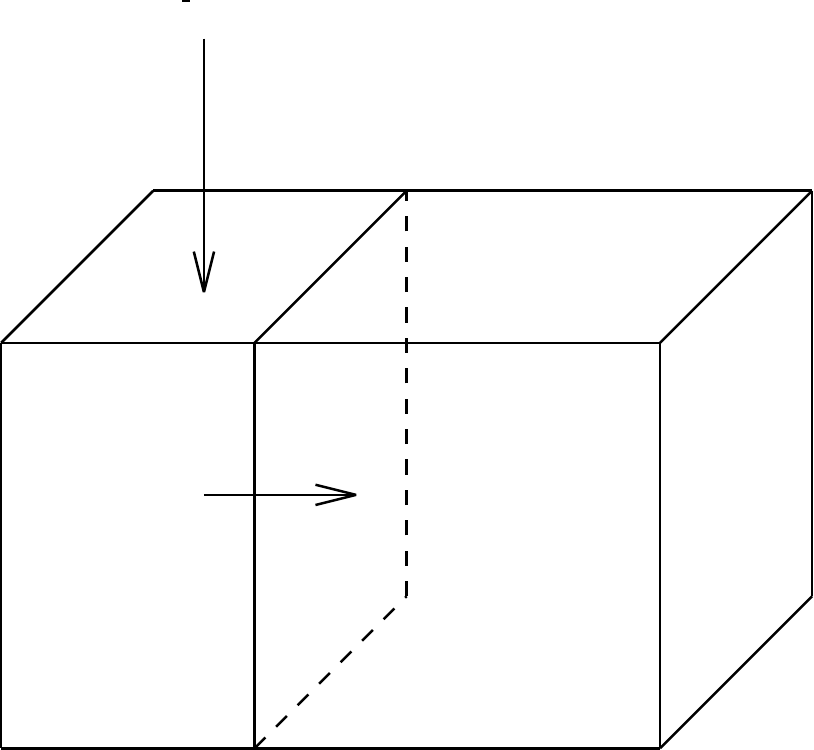
40.9. MERIDIONAL OVERTURNING
541
north
Q
z=-H
z=0
φ
v
Figure 40.1: Sketch of an ocean domain in which there is a net input of surface fresh water
through the free surface in the region to the south of a particular latitude. In the steady state,
the result is a net northward meridional transport of water in the interior of the ocean at this
latitude.
40.9.5 Overturning streamfunction in the (φ, z)plane
For those running z-level models such as MOM, the simplest choice for vertical coordinate is
s=z, where zis the time independent height of the constant depth surfaces. Derivatives of the
streamfunction yield the zonally integrated Eulerian meridional and vertical transport
−∂zψ(φ, z,t)=acos φZdλv(λ, φ, z,t) (40.151)
a−1∂φψ(φ, z,t)=acos φZdλw(λ, φ, z,t),(40.152)
and the streamfunction from equation (40.142) is given by
ψ(φ, z,t)=−acos φZdλZz
−H(φ,λ)
dz′v.(40.153)

542
CHAPTER 40. DIAGNOSTICS FOR PHYSICAL ANALYSIS
40.9.6 Overturning streamfunction in the (φ, θ)plane
Another choice for the vertical coordinate is s=θ, with θthe potential temperature. This
choice was discussed by Bryan and Sarmiento (1985). Taking s=θmakes sense only when
θsurfaces are monotonic. Assuming such, the overturning streamfunction from equation
(40.142) is given by
ψ(φ, θ, t)=−acos φZdλZz(λ,φ,θ,t)
−H(λ,φ)
dz′v(λ, φ, z′,t).(40.154)
Derivatives of the streamfunction yield
−∂θψ=acos φZdλzθv(40.155)
a−1∂φψ=acos φZdλ(zt+zθ˙
θ),(40.156)
where ztis the time tendency for the height of a θsurface. Note that zθ>0 for a stably stratified
fluid dominated by temperature. For a fluid with θthe only active tracer, ˙
θ=0 results when
the flow is adiabatic. In this case, and assuming a steady state, the meridional streamfunction
ψis dependent only on the potential temperature: ∂φψ=0.
40.9.7 Overturning streamfunction in the (φ, ρ(0))plane
Another choice is to set s=ρ(0), where ρ(0) is the potential density using the ocean surface as
the reference pressure. This choice, as with the choice s=θ, is adequate only when the ocean
stratification is monotonic in ρ(0). The discussion with s=θfollows through here, with the
material derivative now given by
Dρ(0)
Dt =∂ρ(0)
∂θ ˙
θ+∂ρ(0)
∂S˙
S,(40.157)
with Sthe salinity.
40.9.8 Overturning streamfunction in the (φ, ρ(p))plane
Another choice is to set s=ρ(p), where ρ(p)is the density referenced to a particular pressure level.
The only difference with the s=ρ(0) discussion is that the reference pressure for evaluating the
thermal and saline expansion coefficients is altered.
40.9.9 Overturning streamfunction in the (φ, ρneutral)plane
Another vertical coordinate which is quite useful is the neutral density coordinate of Jackett
and McDougall (1997). The paper by Hirst, McDougall, and Jackett (1996) illustrates the utility
of this coordinate for globally diagnosing mechanisms of water mass transformation. The
(φ, ρneutral) plane streamfunction requires the software of Jackett and McDougall (1997), which
is not provided with MOM.

40.9. MERIDIONAL OVERTURNING
543
40.9.10 Discrete vertical-meridional streamfunction
For the (φ, z) plane, a straightforward discretization of equation (40.142)
ψ(φ, z,t)=−acos φZdλZz
−H(λ,φ)
dz′v,(40.158)
leads to the discretized overturning streamfunction valid for either the rigid lid or free surface
vms fjrow,k=−cos φU
jrow
imt−1
X
i=2
kmt(i,jrow)
X
m=k
dxuidztmui,m,j,2,τ.(40.159)
Note that the switch in the limits on the sum, relative to the integral, accounts for kincreasing
downward, whereas zincreases upwards.
The vertical integration procedes from the ocean bottom, which is the bottom of the bottom-
most velocity cell, upwards to the top of the particular grid cell of interest. As such, the vertical
placement of the meridional streamfunction is at the interface of the cells in which the velocity
is located. These points are labeled by zwkin the model, where k=1,km. To aid in visualization,
the top of the ocean at z=0 is plotted as well. For the rigid lid, the streamfunction value is
zero at z=0; for the free surface, it represents the zonally averaged fresh water flux crossing
the ocean-atmosphere interface.
40.9.11 Discrete density-meridional streamfunction
The streamfunction computed with potential density as the vertical coordinate requires a bit
more work. The most important part of the process is how to partition the potential density
layers. In general, how the layers are placed will largely determine the quality of the diagnosed
overturning streamfunction. Currently, the density range is divided into km layers, since this is
the maximum number of horizontally uniform density layers which can be resolved in a level
model. Using fewer density layers will generally produce a smoother streamfunction, but the
value of the streamfunction is typically reduced in magnitude. More layers typically produces
a noisy solution, and will make the streamfunction have larger values for its extrema. More
sophisticated schemes are possible, in which various forms of interpolation are applied. These
have not been tried. If someone has a better scheme, please feel free to suggest its use. Currently,
the simplest algorithm was chosen, in which zero interpolation is used. Furthermore, since
each model solution likely will require its own particular partitioning, it is currently left to the
researcher to determine the density layers. The placement of the density layers occurs inside the
routine diag.F. Look for the USER INPUT section within the ifdef option meridional overturning.
Given a partitioning of the density coordinate σm, for m=1,km, the algorithm for computing
the streamfunction is the following:
sigms fjrow,m=−cos φU
jrow
imt−1
X
i=2
kmt(i,jrow)
X
k=1
dxuidztmH(σi,k,j−σm)ui,m,j,2,τ,(40.160)
where H(x) is a Heaviside step function (equal to zero for x<0 and unity for x>0.
As coded in MOM, there are two potential densities which are used for defining the
streamfunction: potential density referenced to the surface, and potential density referenced
to 2000m. The framework for using these potential densities can easily be extended.
544
CHAPTER 40. DIAGNOSTICS FOR PHYSICAL ANALYSIS
40.9.12 Option merid by basin
For global models, it is often useful to plot the overturning streamfunction within particular
basins in addition to the global ocean. With option merid by basin, the streamfunction can
be computed for different ocean domains using masks set up by the researcher. See the code
for details of how to set up the masks. Also note that MOM generically computes an ASCII
file kmt.dta which is a useful place to start when constructing the masks. An objective way
to construct masks is to use a “fill algorithm” such as that used in MOM for constructing the
land-sea boundaries.
40.9.13 Output
The output for the vertical-meridional streamfunction may be written as ascii to the model print-
out or as 32 bit IEEE unformatted data to file overturn.yyyyyy.mm.dd.dta. If option netcdf
or meridional overturning netcdf is enabled, the vertical-meridional streamfunction is written
in NetCDF format to file overturn.yyyyyy.mm.dd.dta.nc rather than in unformatted IEEE. The
“yyyyyy.mm.dd” is a place holder for year, month, and day and this naming convention is ex-
plained further in Section 39.2. If the sub-option meridional overturning potential is also enabled,
the sigma-meridional streamfunctions are written to files overturn.sigAmsf.yyyyyy.mm.dd.dta.nc
for σ0and overturn.sigBmsf.yyyyyy.mm.dd.dta.nc for σ2000. The interval between output for each
of these streamfunctions is specified by the single variable vmsfint, and the control is specified
by variable iovmsf.
40.10 meridional tracer budget
What are the dominant meridional balances (if any) in the model and how do they depend
on time? Option meridional tracer budget contracts the tracer equation into a one dimensional
equation in latitude by averaging over longitude and depth cells. Using operators described
in Section 22.8.7, this yields
1
VolT
j
imt−1
X
i=2
km
X
k=1
∆T
i,k,j·hδt(Ti,k,j,n,τ)+ADV Txi,k,j+ADV Tyi,k,j+ADV Tzi,k,j=
DIFF Txi,k,j+DIFF Tyi,k,j+DIFF Tzi,k,j+sourcei,k,ji(40.161)
where nis the tracer and the relation between jand jrow is as described in Section 14.2. The
volume element and total volume as a function of latitude are given by
∆T
i,k,j=tmaski,k,j·dxti·cos φT
jrow ·dytjrow ·dztk(40.162)
VolT
j=
km
X
k=1
imt−1
X
i=2
∆T
i,k,j(40.163)
The quantity tmaski,k,jis 1 for ocean cells and 0 for land cells. Integrating and applying boundary
conditions in depth and longitude to Equation (40.161) yields
40.10. MERIDIONAL TRACER BUDGET
545
X
i,k
δt(Ti,k,j,n,τ)∆T
i,k,j+X
i,k
(ADV Tyi,k,j)∆T
i,k,j=X
i,k
(st fi,j,n)∆T
i,k,j+X
i,k
(DIFF Tyi,k,j)∆T
i,k,j
+X
i,k
(sourcei,k,j)∆T
i,k,j(40.164)
where Pi,kis shorthand for summing over all cells in longitude and depth. Each term in
Equation (40.164) is then averaged in time to produce stable estimates which can indicate the
dominant meridional balances as a function of time. The meridional tracer equation becomes
1
L
L
X
i,k,ℓ=1hδt(Ti,k,j,n,τ)+ADV Tyi,k,j=st f i,j,n+DIFF Tyi,k,j
+sourcei,k,ji(40.165)
where ℓis the time step counter and Lis the number of time steps in the averaging period
described below. The i,kin the sum indicates a sum over all longitude and depth cells. The
individual terms in Equation (40.165) are given as
tstorjrow,n=1
L
L
X
ℓ=1h1
VolT
j
km
X
k=1
imt−1
X
i=2
ti,k,j,n,τ+1−ti,k,j,n,τ−1
2∆τ∆T
i,k,ji(40.166)
tdivjrow,n=−1
L
L
X
ℓ=1h1
VolT
j
km
X
k=1
imt−1
X
i=2
ADV Tyi,k,j·∆T
i,k,ji(40.167)
t f luxjrow,n=−1
L
L
X
ℓ=1h1
AreaT
j
imt−1
X
i=2
st fi,j,n·AT
i,ji(40.168)
tsorcjrow,n=1
L
L
X
ℓ=1h1
VolT
j
km
X
k=1
imt−1
X
i=2
sourcei,k,j·∆T
i,k,ji(40.169)
tdi fjrow,n=−1
L
L
X
ℓ=1h1
VolT
j
km
X
k=1
imt−1
X
i=2
DIFF Tyi,k,j·∆T
i,k,ji(40.170)
where the area element and total area of a latitude are given by
AT
i,j=tmaski,1,j·dxti·cos φT
jrow ·dytjrow (40.171)
AreaT
j=
imt−1
X
i=2
AT
i,j(40.172)
(40.173)
The output from this diagnostic may be written as ascii to the model printout or as
32 bit IEEE unformatted data to file tracer bud.yyyyyy.mm.dd.dta. If option netcdf or merid-
ional tracer budget netcdf is enabled, data is written in NetCDF format to file tracer bud.yyyyyy.mm.dd.dta.nc
546
CHAPTER 40. DIAGNOSTICS FOR PHYSICAL ANALYSIS
rather than in unformatted IEEE. The “yyyyyy.mm.dd” is a place holder for year, month, and
day and this naming convention is explained further in Section 39.2. The interval between out-
put is specified by variable tmbint and the control is specified by variable iotmb. The averaging
period tmbper is typically set equal to the interval but may be specified shorter. How about
producing monthly averages when months vary in length? Enabling option monthly averages
will over-ride values in tmbper and tmbint and make it so. However, this option is global
and applies to all time averaged diagnostics that are enabled. Refer to Section 40.11 for more
details. Variables tmbper and tmbint are input through namelist. Refer to Section 14.4 for
information on namelist variables. Note further that this dataset may be contracted in latitude
and region space to yield a zero dimensional model which describes the total heat content of
one tremendously gigantic cell as a function of time.
<tstorjrow,n>φ=1
AreaT
jmt−1
X
jrow=2ht f luxjrow,ni∆T
j(40.174)
where the area element is
AreaT=
jmt−1
X
jrow=2
∆T
j(40.175)
However, this can only be done if the averaging period equals the interval for writing the
output. But, when the averaging period equals the sampling interval this diagnostic is a
significant time burner. For most cases, it may be adequate to specify a short averaging period
at the end of the sampling interval (e.g. in the limit, a one time step average at the end of every
sampling interval.). The terms in the above analysis may be further decomposed into regions
based on mask msktmbi,jrow along the lines of Section 39.5. However, msktmbi,jrow =1 and it is
left to the researcher to define other regions if desired. Note that the regional mask msktmbi,jrow
is also written to file tracer bud.yyyyyy.mm.dd.dta when the initialization boolean itmb is true.
It should be set true on the first run but false thereafter.
40.11 monthly averages
It is useful to produce monthly averaged datasets for diagnostics which compute time av-
eraged quantities. Specifying a periodic “interval” for output and an averaging “period” as
discussed in Section 39.4 is not helpful when months vary in length. However, enabling op-
tion monthly averages will over-ride values specified by “interval” and “period” and produce
monthly averaged datasets. However, this option is global and applies to all time averaged
diagnostics that are enabled. The only caveat is that if the model is started or stopped at any
time other than a month boundary, the first or last average will not be over the full month.
40.12 save convection
When convection is being computed explicitly (option implicitvmix is not enabled), the in-
stantaneous value of the component of the time rate of change of temperature due to explicit
convection can be saved three dimensionally. If cell Ti,k,jis a land cell, its value is set to a flag
40.13. SAVE MIXING COEFF
547
value =10−20 to denote land. If no convection has taken place in cell Ti,k,j, the convection for
that cell is zero. Otherwise
convecti,k,j=
ta f ter convection
i,k,j,1,τ+1−tbe f ore convection
i,k,j,1,τ+1
2∆τ(40.176)
The output from this diagnostic is written only as 32 bit IEEE unformatted data to file cvct.yyyyyy.mm.dd.dta
If option netcdf or save convection netcdf is enabled, data is written in NetCDF format to
file cvct.yyyyyy.mm.dd.dta.nc rather than in unformatted IEEE. The “yyyyyy.mm.dd” is a place
holder for year, month, and day and this naming convention is explained further in Section
39.2. The interval between output is specified by variable exconvint and there is no control
variable since only the unformatted data is written.
40.13 save mixing coeff
Much of the physics in MOM is distilled into mixing coefficients. Mixing coefficients can
be computed in a variety of ways depending on the combinations of horizontal and vertical
subgrid scale mixing parameterization options which have been enabled. In some cases, the
mixing coefficients are not explicitly computed. However, the flux across faces of cells is always
computed. Option save mixing coeffestimates mixing coefficients from flux across cell faces.
For momentum, the coefficients on east, north, and bottom faces of U cells is estimated by
cei,k,j,1=di f f f ei,k,j
1
cos φU
jrow
δλ(ui,k,j,1,τ−1)+ǫ(40.177)
cni,k,j,1=di f f f ni,k,j
δφ(ui,k,j,1,τ−1)+ǫ(40.178)
cbi,k,j,1=di f f f bi,k,j
δz(ui,k,j,1,τ−1)+ǫ(40.179)
where ǫ=10−20 to keep from dividing by zero where no gradient in velocity exists. For tracers,
the coefficients on east, north, and bottom faces of T cells is estimated by
cei,k,j,2=di f f f ei,k,j
1
cos φU
jrow
δλ(ti,k,j,1,τ−1)+ǫ(40.180)
cni,k,j,2=di f f f ni,k,j
δφ(ti,k,j,1,τ−1)+ǫ(40.181)
cbi,k,j,2=di f f f bi,k,j
δz(ti,k,j,1,τ−1)+ǫ(40.182)
where ǫplays the same role as for velocities. If option isoneutralmix is enabled, the K11i,k,j,
K22i,k,j,K33i,k,jelements of the isoneutral mixing tensor along with the suitably averaged
mixing coefficients Aez
i,k,j,Anz
i,k,j,Abx
i,k,j, and Aby
i,k,jare additionally output.
548
CHAPTER 40. DIAGNOSTICS FOR PHYSICAL ANALYSIS
The output from this diagnostic is written as 32 bit IEEE unformatted data to file cmix.yyyyyy.mm.dd.dta.
If option netcdf or save mixing coeffnetcdf is enabled, data is written in NetCDF format to
file cmix.yyyyyy.mm.dd.dta.nc rather than in unformatted IEEE. The “yyyyyy.mm.dd” is a place
holder for year, month, and day and this naming convention is explained further in Section
39.2. The interval between output is specified by variable cmixint and there is no control
variable since only the unformatted data is written.
40.14 show external mode
Option show external mode saves instantaneous values (at time level τ+1) of either the stream
function, prognostic surface pressure, or implicit free surface depending on which option is en-
abled. Stream function is in units of cm3/sec, surface pressure and implicit free surface is in units
of gram/cm/sec2. The output from this diagnostic may be written as ascii to the model print-
out or as 32 bit IEEE unformatted data to file psi.yyyyyy.mm.dd.dta,surf press.yyyyyy.mm.dd.dta,
or ifree surf.yyyyyy.mm.dd.dta. If option netcdf or show external mode netcdf is enabled, data
is written in NetCDF format to file psi.yyyyyy.mm.dd.dta.nc,surf press.yyyyyy.mm.dd.dta.nc,
or ifree surf.yyyyyy.mm.dd.dta.nc rather than in unformatted IEEE. The “yyyyyy.mm.dd” is
a place holder for year, month, and day and this naming convention is explained further in
Section 39.2. The interval between output is specified by variable extint and the control is
specified by variable ioext.
40.15 show zonal mean of sbc
Option show zonal mean of sbc saves instantaneous zonal means of all surface boundary con-
ditions as a function of latitude. This is useful to verify that the surface boundary conditions
are reasonable, at least in the zonal mean sense.
zmsmjrow,n=1
VolU
j
imt−1
X
i=2
ui,1,j,n,τ ·∆U
i,j(40.183)
zmsm fjrow,n=1
VolU
j
imt−1
X
i=2
sm fi,j,n·∆U
i,j(40.184)
zmstjrow,n=1
VolT
j
imt−1
X
i=2
ti,1,j,n,τ ·∆T
i,j(40.185)
zmst fjrow,n=1
VolT
j
imt−1
X
i=2
st fi,j,n·∆T
i,j(40.186)
where the volume elements and total volumes on U cells and T cells are
∆U
i,j=umaski,1,j·dxui·cos φU
jrow ·dyujrow ·dztk(40.187)
∆T
i,j=tmaski,1,j·dxti·cos φT
jrow ·dytjrow ·dztk(40.188)
VolU
j=
imt−1
X
i=2
∆U
i,j(40.189)
40.16. SNAPSHOTS
549
VolT
j=
imt−1
X
i=2
∆T
i,j(40.190)
and the relation between jand jrow is as described in Section 14.2. Surface heat flux is
converted to watts/m2, windstress is in dyne/cm2precip minus evaporation is in mm/day,
velocity is in cm/sec, temperature is in degC and salinity is in ppt −35.0. The output from
this diagnostic may be written as ascii to the model printout or as 32 bit IEEE unformatted
data to file zmean sbc.yyyyyy.mm.dd.dta. If option netcdf or show zonal mean of sbc netcdf is
enabled, data is written in NetCDF format to file zmean sbc.yyyyyy.mm.dd.dta.nc rather than
in unformatted IEEE. The “yyyyyy.mm.dd” is a place holder for year, month, and day and
this naming convention is explained further in Section 39.2. The interval between output is
specified by variable zmbcint and the control is specified by variable iozmbc.
40.16 snapshots
Option snapshots saves instantaneous values of prognostic and associated variables. The vari-
ables are tracers ti,k,j,n,τ for n=1,nt, horizontal velocities ui,k,j,n,τ for n=1,2, vertical velocity
at the base of T cells adv vbti,k,j, surface tracer flux st fi,j,nfor n=1,nt, surface momentum flux
sm fi,j,nfor n=1,2, and the external mode which is given by either1psii,jrow,τ or psi,jrow,τ.
This output data may be restricted to certain contiguous latitude and depth ranges using
variables input through namelist. Refer to Section 14.4 for information on namelist variables.
Note that on time step =itt (which corresponds to τ+1), data is written from time level τrather
than τ+1 because the τ+1 external mode is unknown at the time when data is written. There-
fore, ui,k,j,n,τ is a total velocity containing both internal and external modes. The output from
this diagnostic is written as 32 bit IEEE unformatted data to file snapshots.yyyyyy.mm.dd.dta.
If option netcdf or snapshots netcdf is enabled, data is written in NetCDF format to file snap-
shots.yyyyyy.mm.dd.dta.nc rather than in unformatted IEEE. The “yyyyyy.mm.dd” is a place
holder for year, month, and day and this naming convention is explained further in Section
39.2.
It should be noted that for use with Ferret, file snapshots.yyyyyy.mm.dd.dta.nc has the x, y,
and z axes defined such that “edges” of cells along any axis on the T grid coincide with grid
point coordinates on the U grid and visa versa. This is important when performing operations
like integrals from within Ferret. For instance, if the dimensions of cell Ti,k,jare dxti,dytjrow, and
dztk, then the cell edges are defined as follows: eastern edge of cell Ti,k,jis at xt i edgesi=xuiand
the western edge is at xt i edgesi−1=xui−1. The northern edge is at yt j edgesjrow =yujrow and
the southern edge is at yt j edgesjrow−1=yujrow−1and the bottom edge is at zt k edgesk=zwk
and the top edge is at zt k edgesk−1=zwk−1. Therefore, the cell dimensions can be computed
from
dxti=xt i edgesi−xt i edgesi−1(40.191)
dytjrow =yt j edgesjrow −yt j edgesjrow−1(40.192)
dztk=zt k edgesk−zt k edgesk−1(40.193)
and the volume is then given by
1Depending on whether option stream function,rigid lid surface pressure or implicit free surface is enabled.
550
CHAPTER 40. DIAGNOSTICS FOR PHYSICAL ANALYSIS
T voli,k,jrow =dxti·cos φT
jrow ·dytjrow ·dztk(40.194)
For cell Ui,k,j, the corresponding cell dimensions are
dxui=xu i edgesi−xu i edgesi−1(40.195)
dyujrow =yu j edgesjrow −yu j edgesjrow−1(40.196)
dztk=zt k edgesk−zt k edgesk−1(40.197)
and the volume is
U voli,k,jrow =dxui·cos φU
jrow ·dyujrow ·dztk(40.198)
The structure of this NetCDF file is very similar to the one from option time averages. The
interval between output is specified by variable snapint.
40.17 term balances
Option term balances constructs instantaneous spatial averages of all terms2in the prognostic
equations over arbitrary regional volumes defined by horizontal and vertical region masks
as described in Section 39.5. Regional volumes may be set up as indicated by the test case
example in file setocn.F. They may not overlap one another. This diagnostic is useful when
trying to understand the dominant balances within regional volumes of the model domain.
Be aware that aliasing may occur because results are not averaged in time. This diagnostic
is relatively slow and can appreciably degrade the speed of MOM. The output from this
diagnostic may be written as ascii to the model printout or as 32 bit IEEE unformatted data to
file term bal.yyyyyy.mm.dd.dta. If option netcdf or term balances netcdf is enabled, data is written
in NetCDF format to file term bal.yyyyyy.mm.dd.dta.nc rather than in unformatted IEEE. The
“yyyyyy.mm.dd” is a place holder for year, month, and day and this naming convention is
explained further in Section 39.2. The interval between output is specified by variable trmbint
and the control is specified by variable iotrmb. Note that the regional masks mskhri,jrowand
mskvrkare also written to file term bal.yyyyyy.mm.dd.dta when the initialization boolean itrmb is
true. It should be set true on the first run but false thereafter.
Partial sums are taken over all (i,k,j) within the domain to contract quantities into regional
volumes given as
nreg =(mskvrk−1) ·nhreg +mskhri,jrow (40.199)
where masks mskvrkand mskhri,jroware defined as in Section 39.5 and the range of nreg is from
0 to nhreg ·nvreg. Two operators are defined to perform these contractions separately for
quantities defined on T cells and U cells. They are given by
αi,k,jU(nreg)=1
VolU(nreg)
jmt−1
X
jrow=2
km
X
k=1
imt−1
X
i=2
2
X
n=1
αi,k,j·∆U
i,k,j(40.200)
2Plus a few extra ones.
40.17. TERM BALANCES
551
βi,k,jT(nreg)=1
VolT(nreg)
jmt−1
X
jrow=2
km
X
k=1
imt−1
X
i=2
2
X
n=1
βi,k,j·∆T
i,k,j(40.201)
(40.202)
where αi,k,jis defined on U cells, βi,k,jis defined on T cells, and the respective volume elements
and total volumes for each region are
∆U
i,k,j=umaski,k,j·dxui·cos φU
jrow ·dyujrow ·dztk(40.203)
VolU(nreg)=
jmt−1
X
jrow=2
km
X
k=1
imt−1
X
i=2
∆U
i,k,j(40.204)
VolU(0) =
nhreg
X
nreg=1
VolU(nreg)(40.205)
∆T
i,k,j=tmaski,k,j·dxti·cos φT
jrow ·dytjrow ·dztk(40.206)
VolT(nreg)=
jmt−1
X
jrow=2
km
X
k=1
imt−1
X
i=2
∆T
i,k,j(40.207)
VolT(0) =
nhreg
X
nreg=1
VolT(nreg)(40.208)
with the relation between jand jrow as described in Section 14.2.
40.17.1 Momentum Equations
Using arrays and operators described in Section 22.9.5, all components of the momentum
Equation are contracted into regional volumes with the canonical forms given below. One way
to think of this is that all cells within a regional volume U(nreg)are replaced by one gigantic U
cell and the value of all terms in the momentum equation are given for this one cell. Subscript
n=1 refers to the zonal velocity component and n=2 refers to the meridional component.
termbm1,n,nreg =ui,k,j,n,τ+1−ui,k,j,n,τ−1
2∆τ
U(nreg)
(40.209)
termbm2,n,nreg =−grad pi,k,j,nU(nreg)(40.210)
termbm3,n,nreg =−ADV Uxi,k,jU(nreg)(40.211)
termbm4,n,nreg =−ADV Uyi,k,jU(nreg)(40.212)
termbm5,n,nreg =−ADV Uzi,k,jU(nreg)(40.213)
termbm6,n,nreg =DIFF Uxi,k,jU(nreg)(40.214)
termbm7,n,nreg =DIFF Uyi,k,jU(nreg)(40.215)
552
CHAPTER 40. DIAGNOSTICS FOR PHYSICAL ANALYSIS
termbm8,n,nreg =DIFF Uzi,k,jU(nreg)(40.216)
termbm9,n,nreg =DIFF metrici,k,j,nU(nreg)(40.217)
termbm10,n,nreg =CORIOLISi,k,j,nU(nreg)(40.218)
termbm11,n,nreg =sourcei,k,jU(nreg)(40.219)
termbm12,n,nreg =−grad ps
i,k,j,nU(nreg)(40.220)
termbm13,n,nreg =ADV metrici,k,j,nU(nreg)(40.221)
(40.222)
where the surface pressure gradient terms grad ps
i,k,j,1and grad ps
i,k,j,2are reconstructed from
Equations (29.3) and (29.4) by replacing the vertically integrated velocities by ψwith the aid of
Equations (29.6) through (29.10) to yield
grad ps
i,k,j,1≡1
ρ◦cos φU
jrow
δλ(ps
i,jrow
φ)=1
2∆τ1
Hi,jrow
δφ(∆ψi,jrow
λ)
+
˜
fjrow
Hi,jrow ·cos φU
jrow
δλ(∆ψi,jrow
φ)+zui,jrow,1
(40.223)
grad ps
i,k,j,2≡1
ρ◦
δφ(ps
i,jrow
λ)=1
2∆τ−1
Hi,jrow ·cos φU
jrow
δλ(∆ψi,jrow
φ)
+
˜
fjrow
Hi,jrow
δφ(∆ψi,jrow
λ)+zui,jrow,2(40.224)
where ˜
fjrow is given by Equation (29.5). The equation for the gigantic grid cell in each regional
volume U(nreg)is given by
termbm1,n,nreg =
13
X
ℓ=2
termbmℓ,n,nreg (40.225)
Note that terms 3,4, and 5 are the flux form of advection. When summed up, they represent
the physical advection in the cell. However, when taken separately, they do not represent the
true advection in λ, φ, zbecause they contain divergent components. The true advection in
λ, φ, zis given below by terms 14,15, and 16.
termbm14,n,nreg =ui,k,j,n,τ ·adv veui,k,j−adv veui−1,k,j
dxui·cos φU
jrow −ADV Uxi,k,j
U(nreg)
(40.226)
termbm15,n,nreg =ui,k,j,n,τ ·adv vnui,k,j−adv vnui,k,j−1
dyujrow ·cos φU
jrow −ADV Uyi,k,j
U(nreg)
(40.227)
40.17. TERM BALANCES
553
termbm16,n,nreg =ui,k,j,n,τ ·adv vbui,k−1,j−adv vnui,k,j
dztk−ADV Uzi,k,j
U(nreg)
(40.228)
termbm17,n,nreg =ui,k,j,n,τU(nreg)(40.229)
avgwnreg =adv vbui,k−1,j+adv vbui,k,j
2
U(nreg)
(40.230)
sm f lxn,nreg =sm fi,j,nU(nreg)(40.231)
Term 17 represents the average horizontal velocity components within the cell and avgw is
the average vertical component. smflx represents the windstress acting on the top of the near
surface cells and Equation (40.231) is only averaged over the regional volumes at the ocean
surface.
40.17.2 Tracer Equations
Using operators and arrays described in Section 22.8.7, all components of the tracer equation
are contracted into regional volumes with the canonical forms given below. As with the
momentum contraction above, one way to think of this is that all cells within a regional
volume T(nreg)are replaced by one gigantic T cell and the value of all terms in the tracer
equation are given for this one cell. Subscript n=1 refers to the temperature component and
n=2 refers to the salinity.
termbt1,n,nreg =ti,k,j,n,τ+1−ti,k,j,n,τ−1
2∆τ
T(nreg)
(40.232)
termbt2,n,nreg =−ADV Txi,k,jT(nreg)(40.233)
termbt3,n,nreg =−ADV Tyi,k,jT(nreg)(40.234)
termbt4,n,nreg =−ADV Tzi,k,jT(nreg)(40.235)
termbt5,n,nreg =DIFF Txi,k,jT(nreg)(40.236)
termbt6,n,nreg =DIFF Tyi,k,jT(nreg)(40.237)
termbt7,n,nreg =DIFF Tzi,k,jT(nreg)(40.238)
termbt8,n,nreg =sourcei,k,jT(nreg)(40.239)
termbt9,n,nreg =explicit convectionT(nreg)(40.240)
(40.241)
When options gent mcwilliams and gm advect are enabled, then Equations (40.233), (40.234),
and (40.235) also include the flux form of the advection terms from option gm advect given by
−ADV Txisoi,k,j,−ADV Tyisoi,k,j, and −ADV Tzisoi,k,j, respectively. Alternatively, when options
and gent mcwilliams and the default gm skew are enabled, or if option biharmonic rm is enabled,
then Equations (40.236), (40.237), and (40.238) include the flux form of the skew-diffusive terms.
554
CHAPTER 40. DIAGNOSTICS FOR PHYSICAL ANALYSIS
In Equation (40.240), the quantity explicit convection comes from solving Equation (40.232)
before and after explicit convection. The equation for the gigantic grid cell in each regional
volume T(nreg)is given by
termbt1,n,nreg =
9
X
ℓ=2
termbtℓ,n,nreg (40.242)
Note that terms 2,3, and 4 are the flux form of advection. When summed up, they represent
the physical advection in the cell. However, when taken separately, they do not represent the
true advection in λ, φ, zbecause they contain divergent components. The canonical form for
the true advection in λ, φ, zis given below by terms 11,12, and 13.
termbt11,n,nreg =ti,k,j,n,τ ·adv veti,k,j−adv veti−1,k,j
dxti·cos φT
jrow −ADV Txi,k,j
T(nreg)
(40.243)
termbt12,n,nreg =ti,k,j,n,τ ·adv vnti,k,j−adv vnti,k,j−1
dytjrow ·cos φT
jrow −ADV Tyi,k,j
T(nreg)
(40.244)
termbt13,n,nreg =ti,k,j,n,τ ·adv vbti,k−1,j−adv vnti,k,j
dztk−ADV Tzi,k,j
T(nreg)
(40.245)
termbt15,n,nreg =ti,k,j,n,τT(nreg)(40.246)
st f lxn,nreg =st fi,j,nT(nreg)(40.247)
When options and gent mcwilliams and gm advect are enabled, Equations (40.243), (40.244),
and (40.245) also include the advective or transport velocities from option gm advect given by
adv vetisoi,k,j,adv vntisoi,k,j, and adv vbtisoi,k,jrespectively. Term 15 represents the average tracer
within the cell and term stflx represents the surface tracer flux acting on the top of the surface
cells. Equation (40.247) is only averaged over the regional volumes at the ocean surface.
40.18 time averages
Option time averages saves the same variables as does option snapshots. However, the variables
are time averaged for stability and are defined on an averaging grid which can be the model
grid or a sparse subset of the model grid. Often, for analysis purposes, it is not necessary to
have data at every grid point or for the entire domain. When this is the case, the size of the
archive disk space may be significantly reduced. The variables are tracers ti,k,j,n,τ for n=1,nt,
horizontal velocities ui,k,j,n,τ for n=1,2, vertical velocity at the base of T cells adv vbti,k,j, surface
tracer flux st fi,j,nfor n=1,nt, surface momentum flux sm fi,j,nfor n=1,2, and the external
mode which is given by either3psii,jrow,τ or psi,jrow,τ.
Before using this diagnostic, the averaging grid must be constructed by first executing
script run timeavgs with option drive timeavgs enabled. This runs the averaging grid generator
in a stand alone mode. To define the averaging grid, follow the example in the USER INPUT
3Depending on whether option stream function,rigid lid surface pressure or implicit free surface is enabled.
40.18. TIME AVERAGES
555
section of timeavgs.F. It is possible to arbitrarily pick which model grid points will be on the
averaging grid. However, the code is set to specify a constant spacing between points on the
averaging grid in longitude, latitude, and depth. Model grid points nearest to this spacing
will be chosen as the averaging grid. To incorporate this averaging grid into MOM, follow the
directions given when script run timeavgs executes.
The output from this diagnostic is written as 32 bit IEEE unformatted data to file time mean.yyyyyy.mm.dd.dta
If option netcdf or time averages netcdf is enabled, data is written in NetCDF format to file time mean.yyyyyy.mm.dd.dta.nc
rather than in unformatted IEEE. The “yyyyyy.mm.dd” is a place holder for year, month, and
day and this naming convention is explained further in Section 39.2.
It should be noted that for use with Ferret, file time mean.yyyyyy.mm.dd.dta.nc has the x,
y, and z axes defined such that “edges” of cells along any axis on the T grid coincide with
grid point coordinates on the U grid and visa versa. This is important when performing
operations like integrals from within Ferret. For instance, if the dimensions of cell Ti,k,jare
dxti,dytjrow, and dztk, then the cell edges are defined as follows: eastern edge of cell Ti,k,jis at
xtav i edgesi=xuaviand the western edge is at xtav i edgesi−1=xuavi−1. The northern edge
is at ytav j edgesjrow =yuavjrow and the southern edge is at ytav j edgesjrow−1=yuavjrow−1and
the bottom edge is at ztav k edgesk=zwavkand the top edge is at ztav k edgesk−1=zwavk−1.
Therefore, the cell dimensions can be computed from
dxti=xtav i edgesi−xtav i edgesi−1(40.248)
dytjrow =ytav j edgesjrow −ytav j edgesjrow−1(40.249)
dztk=ztav k edgesk−1−ztav k edgesk(40.250)
and the volume is then given by
Tvoli,k,jrow =dxti·cos φT
jrow ·dytjrow ·dztk(40.251)
For cell Ui,k,j, the corresponding cell dimensions are
dxui=xuav i edgesi−xuav i edgesi−1(40.252)
dyujrow =yuav j edgesjrow −yuav j edgesjrow−1(40.253)
dztk=ztav k edgesk−1−ztav k edgesk(40.254)
and the volume is
U voli,k,jrow =dxui·cos φU
jrow ·dyujrow ·dztk(40.255)
Note that the above definitions are only true if the averaging grid is the same as the model
grid. They should not be used when the averaging grid is a subset of the model grid.
The interval between output is specified by variable timavgint. The averaging period is
controlled by variable timavgper. Typically the averaging period is set equal to the interval
for output but it may be specified as less than the interval. How about producing monthly
averages when months vary in length? Enabling option monthly averages will over-ride values
in timavgper and timavgint and make it so. However, this option is global and applies to all time
averaged diagnostics that are enabled. Refer to Section 40.11 for more details. Variables timavg-
per and timavgint are input through namelist. Refer to Section 14.4 for information on namelist
variables.Refer to Section 39.4 for a discussion of when this is appropriate.
556
CHAPTER 40. DIAGNOSTICS FOR PHYSICAL ANALYSIS
If option time averages can produce the same output as option snapshots then isn’t op-
tion snapshots redundant? It would be except for the fact that option time averages needs storage
space to accumulate data to produce averages. This space is equal to the size of the data being
averaged. Typically 5(imt ·jmt ·km +imt ·jmt) words are needed. If option time averages disk is
enabled, disk space is used for the storage area, otherwise the storage space is in memory! If
memory is insufficient or solid state disk space is insufficient, option snapshots is the only way
to save the data.
40.19 time step monitor
Option time step monitor computes instantaneous values of total kinetic energy4per unit vol-
ume averaged over the entire domain volume in units of gm/cm/sec2. It also computes first and
second moments of tracer quantities. The mean tracer is the first moment and tracer variance5
is the second moment about the mean in units of tracer squared. Additionally, the quantity
|∂T/∂t|in units of degC/sec (for n=1) and (grams of salt per grams of water)/sec (for n=2) averaged
over the domain volume is computed. The explicit forms are given by
<ke >=ρ◦
2
1
VolU
jmt−1
X
jrow=2
km
X
k=1
imt−1
X
i=2
2
X
n=1
u2
i,k,j,n,τ ·∆U
i,k,j(40.256)
<ti,k,j,n,τ >=1
VolT
jmt−1
X
jrow=2
km
X
k=1
imt−1
X
i=2
ti,k,j,n,τ ·∆T
i,k,j(40.257)
tracer variance =<t2
i,k,j,n,τ >−<ti,k,j,n,τ >2(40.258)
<|δτ(ti,k,j,n,τ)|>=1
VolT
jmt−1
X
jrow=2
km
X
k=1
imt−1
X
i=2
|ti,k,j,n,τ+1−ti,k,j,n,τ−1|
2∆τ·∆T
i,k,j(40.259)
where
<t2
i,k,j,n,τ >=1
VolT
jmt−1
X
jrow=2
km
X
k=1
imt−1
X
i=2
t2
i,k,j,n,τ ·∆T
i,k,j(40.260)
and the volume elements for U cells and T cells are
∆U
i,k,j=umaski,k,j·dxui·cos φU
jrow ·dyujrow ·dztk(40.261)
∆T
i,k,j=tmaski,k,j·dxti·cos φT
jrow ·dytjrow ·dztk(40.262)
The masks umaski,k,jand tmaski,k,jare 1.0 on ocean U cells and T cells but 0.0 on land U cells and
T cells. Also, the relation between jand jrow is as described in Section 14.2. The total volumes
are constructed as
4Neglecting the vertical velocity component on the basis of scale analysis.
5Tracer variance is not conserved if explicit convection is active or there is a non zero surface tracer flux. It is
also not conserved when diffusion is present. Refer to Appendix B for further discussion.
40.20. TOPOG DIAGNOSTIC
557
VolU=
jmt−1
X
jrow=2
km
X
k=1
imt−1
X
i=2
∆U
i,k,j(40.263)
VolT=
jmt−1
X
jrow=2
km
X
k=1
imt−1
X
i=2
∆T
i,k,j(40.264)
In addition to the above quantities, the iteration count from the elliptic solver is saved.
When option netcdf is enabled, the output from this diagnostic has a NetCDF format and
is written to file ts integrals.yyyyyy.mm.dd.dta.nc. Otherwise, the output from this diagnos-
tic may be written as ascii to the model printout or as 32 bit IEEE unformatted data to
file ts integrals.yyyyyy.mm.dd.dta. If option netcdf or time step monitor netcdf is enabled, data
is written in NetCDF format rather than in unformatted IEEE. The “yyyyyy.mm.dd” is a place
holder for year, month, and day and this naming convention is explained further in Section
39.2. The interval between output is specified by variable tsiint and the control is specified by
variable iotsi.
40.20 topog diagnostic
The output from option topog diagnostic is ocean depth at T cells given by
HTi,jrow =zwkmti,jrow (40.265)
in units of cm and f/HTi,jrow in units of cm−1sec−1where the Coriolis term fis defined at the
latitude of T cells. When this option is enabled, output is written in a NetCDF format to
file topog.dta.nc. There is no 32 bit IEEE unformatted data option. Therefore, the only way
to get it is to enable option topog diagnostic (using option netcdf will not do it). Although this
option is intended to be used when executing the topography module in stand alone mode
from script run topog, it can also be enabled in a model run using script run mom. There is no
associated interval or control variable.
40.21 tracer averages
Option tracer averages constructs instantaneous spatial averages of tracers over regional areas
described by mskhri,jrowin Section 39.5. This diagnostic is useful when trying to examine how
the model equilibrates with area and depth. The average of tracer nas a function of depth
level kand region number mis constructed as
Tk,m,n=1
AreaT
k,m
imt−1
X
i=2
jmt−1
X
jrow=2
ti,k,j,n,τ ·AT
i,k,j(40.266)
m=mskhri,jrow (40.267)
where the area element and area of each region at level kare given by
558
CHAPTER 40. DIAGNOSTICS FOR PHYSICAL ANALYSIS
AT
i,k,j=tmaski,k,j·dxti·cos φT
jrow ·dytjrow (40.268)
AreaT
k,m=
imt−1
X
i=2
jmt−1
X
jrow=2
AT
i,k,j(40.269)
(40.270)
and the relation between jand jrow are as described in Section 14.2. The average of tracer n
over all regions as a function of depth is given by
Tm
k,n=1
AreaT
k,0
nhreg
X
m=1
Tk,m,n·AreaT
k,m(40.271)
AreaT
k,0=
nhreg
X
m=1
AreaT
k,m(40.272)
where AreaT
k,0is the total area of all regions at level k. In a likewise manner, the tracer flux
through the ocean surface for tracer nas a function of region number mis given by
st f m,n=1
AreaT
1,m
imt−1
X
i=2
jmt−1
X
jrow=2
st fi,j,n·AT
i,1,j(40.273)
st f m
n=1
AreaT
1,0
nhreg
X
m=1
st f m,n·AreaT
1,m(40.274)
The output from this diagnostic is written as ascii to the model printout or as 32 bit IEEE
unformatted data to file tracer avg.yyyyyy.mm.dd.dta. If option netcdf or tracer averages netcdf is
enabled, data is written in NetCDF format to file tracer avg.yyyyyy.mm.dd.dta.nc rather than in
unformatted IEEE. The “yyyyyy.mm.dd” is a place holder for year, month, and day and this
naming convention is explained further in Section 39.2. The interval between output is specified
by variable tavgint and the control is specified by variable iotavg. Note that the regional mask
mskhri,jrowis also written to file tracer avg.yyyyyy.mm.dd.dta when the initialization boolean itavg
is true. It should be set true on the first run but false thereafter.
40.22 tracer yz
Option tracer yz computes instantaneous values of the zonal integral of the tracer and tracer
equation, term by term for each component. Contraction of the tracer equation along longitude
yields a two dimensional equation as a function of latitude and depth. Using operators
described in Section 22.8.7 yields
1
LT
k,j
imt−1
X
i=2
∆T
i,k,j·δt(Ti,k,j,n,τ)=−1
LT
k,j
imt−1
X
i=2
∆T
i,k,j(ADV Tzi,k,j+ADV Tyi,k,j)
40.23. TRAJECTORIES
559
+1
LT
k,j
imt−1
X
i=2
∆T
i,k,j(DIFF Tzi,k,j+DIFF Tyi,k,j)
+1
LT
k,j
imt−1
X
i=2
∆T
i,k,j·sourcei,k,j(40.275)
where nis the tracer and the relation between jand jrow is as described in Section 14.2. The
zonal advection and diffusion are not shown because they are eliminated by the summing
operation. The length element and total length are given by
∆T
i,k,j=tmaski,k,j·dxti(40.276)
LT
k,j=
imt−1
X
i=2
∆T
i,k,j(40.277)
Each sum in Equation (40.275) is output as one data field along with the zonally averaged
tracer. The output from this diagnostic is only written in NetCDF format (no option for IEEE)
to file tracer yz.yyyyyy.mm.dd.dta.nc. The “yyyyyy.mm.dd” is a place holder for year, month,
and day and this naming convention is explained further in Section 39.2. The interval between
output is specified by variable tyzint.
40.23 trajectories
Option trajectories integrates particles along trajectories6using a forward time step and a
particle velocity determined by instantaneous linear interpolation every time step.
Let nparticles be placed at positions P1(x,y,z),P2(x,y,z),P3(x,y,z)···Pn(x,y,z) at time t0. The
position of the nth particle at time t1 is given as
Pn(x,y,z)=Zt1
t0
Vn(x,y,z)·dt (40.278)
which is discretized as
Pτ+1
n(x,y,z)=Pτ
n(x,y,z)+ ∆τ·Vτ
n(x,y,z) (40.279)
where Vτ
nis the particle velocity at Pτ
n(x,y,z) arrived at by linear interpolation from ui,k,j,1,τ,
ui,k,j,2,τ, and adv vbti,k,j.
Particles are neutrally buoyant and are initially spread uniformly within an arbitrary vol-
ume as indicated by the example in ptraj.F. If option lyapunov is enabled, the deformation rate
matrix em is also calculated7as the particles are integrated (Pierrehumpert, Yang 1993). The
Lyapunov exponent λis useful in quantifying the dispersion of the particle cloud and can be
computed from the eigenvalues of this matrix as follows. Let
6On the fly while MOM integrates
7Only in two dimensions: longitude and latitude.
560
CHAPTER 40. DIAGNOSTICS FOR PHYSICAL ANALYSIS
c=(em2,2−em1,1)2+4(em1,2·em2,1) (40.280)
Then the Lyapunov coefficient is given by
λ=log(|θ|)/T(40.281)
If c>=0 then
|θ|=|(em1,1+em2,2)2±p(c)|
2(40.282)
Otherwise
|θ|=p(em1,1+em2,2)2+|c|
2(40.283)
This diagnostic is useful for investigating the evolution of water masses, three dimensional
flow structure, and mixing properties of currents and waves (Stokes drift, chaotic mixing, etc).
The storage requirement is six times8the number of particles and the computation is
relatively fast. How many particles are reasonable? Start with about 10,000 and depending
on how the results look, make adjustments. Particle positions are saved to the restart file to
provide the necessary starting point for integrating the particles for arbitrary lengths of time.
The output from Equation (40.279) which consists of an (x,y,z) position and a set of 3 integers
per particle may be written as ascii to the model printout or as 32 bit IEEE unformatted data
to file particles.yyyyyy.mm.dd.dta. If option netcdf or trajectories netcdf is enabled, data is written
in NetCDF format to file particles.yyyyyy.mm.dd.dta.nc rather than in unformatted IEEE. The
“yyyyyy.mm.dd” is a place holder for year, month, and day and this naming convention is
explained further in Section 39.2. The interval between output is specified by variable trajint
and the control is specified by variable iotraj.
40.24 save xbts
Originally, option save xbts sampled temperatures and salinities at various latitude and longi-
tude locations on the model grid down to some prescribed level and produced time averages
of these quantities. In time, it grew to construct time averages of all terms in the prognos-
tic equations9at each model level down to a specified depth for a set of stations. Station
locations and depth at each station can be specified by looking at the USER INPUT section
of xbt.F and following the examples. This diagnostic is useful when trying to understand the
time evolution of dominant balances at specific locations in MOM. For instance, deploying
a group of XBTs can elucidate how waves propagate or currents meander. It is also useful
for planning where to deploy instrumented arrays or moorings in ship based experiments.
save xbts is similar to term balances but instead of averaging over space in various regions of
8Nine times if option lyapunov is enabled.
9This option has outgrown its name. Think of it as an enhanced XBT.
40.24. SAVE XBTS
561
the domain, it averages over time at specific stations to prevents aliasing. Unlike term balances
this diagnostic is fast although it can get expensive in memory10. The output from this di-
agnostic may be written as ascii to the model printout or as 32 bit IEEE unformatted data to
file xbt.yyyyyy.mm.dd.dta. If option netcdf or xbts netcdf is enabled, data is written in NetCDF
format to file xbt.yyyyyy.mm.dd.dta.nc rather than in unformatted IEEE. The “yyyyyy.mm.dd”
is a place holder for year, month, and day and this naming convention is explained further
in Section 39.2. The interval between output is specified by variable xbtint and the control is
specified by variable ioxbt. The averaging period xbtper is typically set equal to the interval
but may be specified shorter. How about producing monthly averages when months vary in
length? Enabling option monthly averages will over-ride values in xbtper and xbtint and make it
so. However, this option is global and applies to all time averaged diagnostics that are enabled.
Refer to Section 40.11 for more details. Variables xbtper and xbtint are input through namelist.
Refer to Section 14.4 for information on namelist variables.
Define mstations with coordinates (λm, φm) which are sampled to a depth of zcm. Discretize
these locations to the nearest model grid points (xbtlonm,xbtlatm,xbtdptm).
40.24.1 Momentum Equations
Using operators and arrays described in Section 22.9.5, all components of the Momentum
Equation are averaged in time for each station mand at each level k. The averaging period L
corresponds to the number of time steps in the average. Subscript n=1 refers to the zonal
velocity component and n=2 refers to the meridional component.
The canonical form of the terms for the mth station at level kare given as
uxbt1,k,n,mth =1
L
L
X
ℓ=1
ui,k,j,n,τ+1−ui,k,j,n,τ−1
2∆τ(40.284)
uxbt2,k,n,mth =1
L
L
X
ℓ=1−grad pi,k,j,n(40.285)
uxbt3,k,n,mth =1
L
L
X
ℓ=1−ADV Uxi,k,j(40.286)
uxbt4,k,n,mth =1
L
L
X
ℓ=1−ADV Uyi,k,j(40.287)
uxbt5,k,n,mth =1
L
L
X
ℓ=1−ADV Uzi,k,j(40.288)
uxbt6,k,n,mth =1
L
L
X
ℓ=1
DIFF Uxi,k,j(40.289)
uxbt7,k,n,mth =1
L
L
X
ℓ=1
DIFF Uyi,k,j(40.290)
uxbt8,k,n,mth =1
L
L
X
ℓ=1
DIFF Uzi,k,j(40.291)
1067 items are computed for each T and U grid cell combination
562
CHAPTER 40. DIAGNOSTICS FOR PHYSICAL ANALYSIS
uxbt9,k,n,mth =1
L
L
X
ℓ=1
DIFF metrici,k,j,n(40.292)
uxbt10,k,n,mth =1
L
L
X
ℓ=1
CORIOLISi,k,j,n(40.293)
uxbt11,k,n,mth =1
L
L
X
ℓ=1
sourcei,k,j(40.294)
uxbt12,k,n,mth =1
L
L
X
ℓ=1−grad ps
i,k,j,n(40.295)
uxbt13,k,n,mth =1
L
L
X
ℓ=1
ADV metrici,k,j,n(40.296)
(40.297)
where the surface pressure gradient terms grad ps
i,k,j,1and grad ps
i,k,j,2are reconstructed from
Equations (29.3) and (29.4) by replacing the vertically integrated velocities by ψwith the aid of
Equations (29.6) through (29.10) to yield
grad ps
i,k,j,1≡1
ρ◦cos φU
jrow
δλ(ps
i,jrow
φ)=1
2∆τ1
Hi,jrow
δφ(∆ψi,jrow
λ)
+
˜
fjrow
Hi,jrow ·cos φU
jrow
δλ(∆ψi,jrow
φ)+zui,jrow,1
(40.298)
grad ps
i,k,j,2≡1
ρ◦δφ(ps
i,jrow
λ)=1
2∆τ−1
Hi,jrow ·cos φU
jrow
δλ(∆ψi,jrow
φ)
+
˜
fjrow
Hi,jrow
δφ(∆ψi,jrow
λ)+zui,jrow,2(40.299)
where ˜
fjrow is given by Equation (29.5). The equation for the kth grid cell at the mth station is
given by
uxbt1,k,n,mth =
13
X
ℓ=2
uxbtℓ,k,n,mth (40.300)
Note that terms 3,4, and 5 are the flux form of advection. When summed up, they represent
the physical advection in the cell. However, when taken separately, they do not represent the
physical advection in λ, φ, zbecause they contain divergent components. The canonical form
of the physical advection in λ, φ, zis given below by terms 14,15, and 16.
uxbt14,k,n,mth =1
L
L
X
ℓ=1
ui,k,j,n,τ ·adv veui,k,j−adv veui−1,k,j
dxui·cos φU
jrow −ADV Uxi,k,j(40.301)
40.24. SAVE XBTS
563
uxbt15,k,n,mth =1
L
L
X
ℓ=1
ui,k,j,n,τ ·adv vnui,k,j−adv vnui,k,j−1
dyujrow ·cos φU
jrow −ADV Uyi,k,j(40.302)
uxbt16,k,n,mth =1
L
L
X
ℓ=1
ui,k,j,n,τ ·adv vbui,k−1,j−adv vnui,k,j
dztk−ADV Uzi,k,j(40.303)
uxbt17,k,n,mth =1
L
L
X
ℓ=1
ui,k,j,n,τ (40.304)
xbtwmth =1
L
L
X
ℓ=1
adv vbui,k−1,j+adv vbui,k,j
2(40.305)
uxbts fn,mth =1
L
L
X
ℓ=1
sm fi,j,n(40.306)
Term 17 represents the average horizontal velocity components within the cell and xbtw is
the average vertical component. uxbtsf represents the windstress acting on the top of the near
surface cell.
40.24.2 Tracer Equations
Using operators and arrays described in Section 22.8.7, all components of the Tracer Equation
are averaged in time for each station mand at each level k. The averaging period Lcorresponds
to the number of time steps in the average. Subscript n=1 refers to the temperature component
and n=2 refers to the salinity.
txbt1,k,n,mth =1
L
L
X
ℓ=1
ti,k,j,n,τ+1−ti,k,j,n,τ−1
2∆τ(40.307)
txbt2,k,n,mth =1
L
L
X
ℓ=1−ADV Txi,k,j(40.308)
txbt3,k,n,mth =1
L
L
X
ℓ=1−ADV Tyi,k,j(40.309)
txbt4,k,n,mth =1
L
L
X
ℓ=1−ADV Tzi,k,j(40.310)
txbt5,k,n,mth =1
L
L
X
ℓ=1
DIFF Txi,k,j(40.311)
txbt6,k,n,mth =1
L
L
X
ℓ=1
DIFF Tyi,k,j(40.312)
txbt7,k,n,mth =1
L
L
X
ℓ=1
DIFF Tzi,k,j(40.313)
txbt8,k,n,mth =1
L
L
X
ℓ=1
sourcei,k,j(40.314)
564
CHAPTER 40. DIAGNOSTICS FOR PHYSICAL ANALYSIS
txbt9,k,n,mth =1
L
L
X
ℓ=1
explicit convection (40.315)
(40.316)
When options gent mcwilliams and gm advect are enabled, then Equations (40.308), (40.309),
and (40.310) also include the flux form of the advection terms from option gm advect given by
−ADV Txisoi,k,j,−ADV Tyisoi,k,j, and −ADV Tzisoi,k,jrespectively. Alternatively, when options
and gent mcwilliams and the default gm skew are enabled, of if option biharmonic rm is enabled,
then the operators DIFF Txi,k,j,DIFF Tyi,k,j, and DIFF Tzi,k,jinclude the flux form of the skew-
diffusive terms from option gm skew. In Equation (40.315), the quantity explicit convection comes
from solving Equation (40.232) before and after explicit convection. The equation for the kth
grid cell in station mis given by
txbt1,k,n,mth =
9
X
ℓ=2
txbtℓ,k,n,mth (40.317)
Note that terms 2,3, and 4 are the flux form of advection. When summed up, they represent
the physical advection in the cell. However, when taken separately, they do not represent
the physical advection in λ, φ, zbecause they contain divergent components. The physical
advection in λ, φ, zis given below by terms 11,12, and 13.
txbt11,k,n,mth =1
L
L
X
ℓ=1
ti,k,j,n,τ ·adv veti,k,j−adv veti−1,k,j
dxti·cos φT
jrow −ADV Txi,k,j(40.318)
txbt12,k,n,mth =1
L
L
X
ℓ=1
ti,k,j,n,τ ·adv vnti,k,j−adv vnti,k,j−1
dytjrow ·cos φT
jrow −ADV Tyi,k,j(40.319)
txbt13,k,n,mth =1
L
L
X
ℓ=1
ti,k,j,n,τ ·adv vbti,k−1,j−adv vnti,k,j
dztk−ADV Tzi,k,j(40.320)
txbt15,k,n,mth =1
L
L
X
ℓ=1
ti,k,j,n,τ (40.321)
txbts fn,mth =1
L
L
X
ℓ=1
st fi,j,n(40.322)
When options gent mcwilliams and gm advect are enabled, Equations (40.318), (40.319), and
(40.320) also include the transport velocities from option gm advect given by adv vetisoi,k,j,
adv vntisoi,k,j, and adv vbtisoi,k,jrespectively. Term 15 represents the average tracer within the
cell and term txbtsf represents the surface tracer flux acting on the top of the surface cells.
Chapter 41
Diagnostics for numerical analysis
Inevitably, problems appear with the model code or configuration. The diagnostic options
discussed in Chapter 40 will likely be the first place one detects problems, since these options
are designed to show the physical properties of the solution. After problems are seen with
those diagnostics, it might be useful to turn on some of the options discussed in this chapter,
which are mostly designed for numerical purposes.
41.1 General debug options
In addition to the diagnostics listed in the following sections, there are numerous “debug”
options in critical areas of the source code. These options can be enabled to give more infor-
mation for debugging purposes. An example of one of these options is be debug adv vel near
the bottom of file adv vel.F which computes advective velocities. When enabled, debug adv vel
gives the components of the divergence of advective velocities for all T-cells and U-cells in
the vertical at any location identified by indices “i,jrow” . These “debug” options can also be
found using UNIX grep as described in Section 3.1.
41.2 stability tests
Option stability tests computes various stability criteria and related items within a portion or
all of the model domain. The limits of volume of domain to be considered when testing are set
through namelist. Refer to Section 14.4 for information on namelist variables. If MOM blows
up, this diagnostic is useful in finding where it went unstable. The following are computed:
1. Based on local velocities within each cell, a maximum local time step is computed for the
three principal directions as
∆τx
i,k,j=cos φU
jrow ·dxui
2·ui,k,j,1,τ
(41.1)
∆τy
i,k,j=dyujrow
2·ui,k,j,2,τ
(41.2)
∆τz
i,k,j=dzwk
2·adv vbti,k,j
(41.3)
565
566
CHAPTER 41. DIAGNOSTICS FOR NUMERICAL ANALYSIS
These local time steps are compared with the model specified time step and the location
of the largest is chosen as the position of the most unstable cell. If the local time step
exceeds the model time step by an amount which can be set through namelist, then a CFL
violation is detected. Refer to Section 14.4.4 for a discussion of the CFL condition and
choosing time step lengths. The number of times a CFL violation is allowed may also
be set through namelist. Refer to section 14.4.7 for setting a region over which stability
calculations are performed. The default region is the entire domain. Variables within the
local neighborhood of the offending cells are shown and when the number of offenses
exceeds the allowable number, the model is brought down.
2. The local Reynolds number is estimated along each of the principle directions as
reyx
i,k,j=ui,k,j,1,τ ·cos φU
jrowdxui
visc ceui,k,j
(41.4)
reyy
i,k,j=ui,k,j,2,τ ·dyujrow
visc cnui,k,j
(41.5)
reyz
i,k,j=adv vbui,k,j·dzwk
visc cbui,k,j
(41.6)
and the location of the maximum is found and printed.
3. The local Peclet number is estimated along each of the principle directions as
peclx
i,k,j=ui,k,j,1,τ ·cos φU
jrowdxui
di f f ceti,k,j
(41.7)
pecly
i,k,j=ui,k,j,2,τ ·dyujrow
di f f cnti,k,j
(41.8)
peclz
i,k,j=adv vbti,k,j·dzwk
di f f cnti,k,j
(41.9)
and the location of the maximum is found and printed.
4. The locations where numerics are breaking down and producing spurious tracer extrema
are determined. This is done by searching the immediate neighborhood of cell (i,k,j) for
extrema in temperature at τand τ−1. If ti,k,j,1,τ+1exceeds this extrema by an amount
which may be specified through namelist, then there is numerical truncation at (i,k,j).
Note that this statement can only be made because of the incompressibility condition.
If there are more than 100 locations exhibiting numerical truncation, only the first 100
locations are shown.
5. The locations are shown where predicted temperatures or salinities are outside the
bounds of temperatures and salinities which were used for the construction of den-
sity coefficients. If there are more than 100 locations where this occurs, only the first 100
locations are shown.
41.3. TRACE COUPLED FLUXES
567
6. The location of maximum error in continuity is calculated considering all U cells and T
cells separately.
7. The maximum error in vertical velocity at the ocean bottom on T cells is computed. This
is the residual error from integrating Equation (22.17) vertically from the surface to the
ocean bottom.
8. The maximum vertical velocity at the ocean bottom on U cells from Equation (22.24) is
computed. This is non-zero if the bottom has a slope since the bottom flow is required to
parallel the bottom slope.
As described above, if more than a specified number of CFL violations are found when this
diagnostic is active (only at times specified by the interval), the integration will stop indicating
where the most unstable locations are with matrix printouts of variables in the neighborhoods.
If a violation is not found, statistics will be printed indicating how close the integration is to
violating the CFL condition along with other information described above. The output from
this diagnostic may only be written as ascii to the model printout. The interval between output
is specified by variable stabint.
41.3 trace coupled fluxes
This diagnostic is useful as an aid to diagnosing problems with coupling to atmosphere models
using option coupled. It gives some gross statistics for the surface boundary conditions at
various key places as they are being constructed for both atmosphere and ocean models. Output
from this diagnostic is only written to file printout and is not intended for post processing.
41.4 trace indices
This diagnostic is useful when trying to understand how the memory window operates for
various settings of jmw. Refer to Section 11.3.2 for a description of how the memory window
works. It gives a trace of the latitude loop indices indicating the dataflow from disk to memory
window as MOM executes. Also indicated are the latitude rows being worked on by various
subroutines in preparation for solving the equations on rows in the memory window. As the
memory window is moved northward, a listing of “which rows are copied where” is given.
As new code is added to MOM, it is strongly recommended that this option be included as an
aid in verifying that the code is correct. When using this option, disable all diagnostics and
execute the model for only a limited number of time steps since the output can get voluminous.
568
CHAPTER 41. DIAGNOSTICS FOR NUMERICAL ANALYSIS

Part IX
Appendices and references
569

Appendix A
Kinetic energy budget
The budget of kinetic energy is of fundamental interest in ocean modeling. The manners in
which various processes contribute to this budget are considered in this chapter. In particular,
a breakdown of the budget for the total kinetic energy, the external mode kinetic energy,
and the internal mode kinetic energy are derived for the continuum equations in the case of
a free surface. The rigid lid results are also indicated. After doing so, two aspects of the
discrete model energetics are considered. First, a proof that the work done by the discrete
pressure terms is equal to the work done by buoyancy is given. In addition, the arguments
from Bryan (1969) and Semtner(1974) are summarized concerning the conservation of first and
second moments for velocity. This result holds for the case of zero forcing, zero dissipation,
and when employing centered-differenced advection of momentum. The conservation of
these two moments for momentum prevent systematic errors that accumulate in time (i.e.,
spurious growth or decay of kinetic energy). Additionally, the preservation of the second
moment eliminates the problems with Phillip’s (1959) non-linear instability (Arakawa 1966,
Bryan 1969). These two points have provided the strong motivation for employing centered
advection of momentum in the GFDL ocean model. Note that there are alternative advection
schemes for tracers, as discussed in Chapter 32. The use of these schemes for tracers does not
compromise the numerical stability maintained by centered differenced momentum advection.
In general, it is important for an ocean model to provide a diagnostic of the kinetic energy
density. Pragmatically, the implementation of numerous algorithms in MOM have been de-
bugged through an analysis of the kinetic energy budget. The diagnostic option energy analysis
(Section 40.4) provides the domain averaged budget for the kinetic energy density for MOM.
A.1 Continuum version of the kinetic energy budget
This section discusses a kinetic energy budget for the ocean primitive equations in their con-
tinuous form. For the rigid lid approximation, the work of Holland (1975) is classic. Bryan and
Lewis (1979), F. Bryan (1986), Treguier (1992), and Goddard (1995) provide further discussions
and examples. The present derivations are given for the free surface, with the rigid lid results
obtained in the limit of a fixed surface height.
A.1.1 The kinetic energy density
For the scalings relevant for a hydrostatic and Boussinesq fluid (i.e., the ocean primitive
equations using the “Traditional Approximation”), the kinetic energy per unit volume (kinetic
571
572
APPENDIX A. KINETIC ENERGY BUDGET
energy density) is determined just by the energy in the horizontal currents
e≡ρo
2(u2+v2)=ρo
2~
uh·~
uh.(A.1)
Hence, to develop an equation for the kinetic energy, it is necessary to consider the horizontal
momentum equations
ut=−∇ · (~
u u)+v f+utan φ
a!−pλ
aρocos φ+(κmuz)z+Fu(A.2)
vt=−∇ · (~
u v)−u f+utan φ
a!−pφ
aρo
+(κmvz)z+Fv,(A.3)
where the horizontal frictional terms
F~
u=(Fu,Fv,0) (A.4)
were defined in Equations (9.187) and (9.193), and
~
u=(u,v,w)=(~
uh,w) (A.5)
is the velocity field.
A.1.2 External and internal mode kinetic energies
In MOM, the splitting of the flow into a vertically averaged velocity and a deviation from that
average prompts an analysis of the kinetic energy which takes such a split into account. For
this purpose, it is useful to introduce a depth averaging operator
α≡1
H+ηZη
−H
dz α. (A.6)
The symbol for deviations from the depth average is given by a hat
b
α=α−α. (A.7)
Using this notation, the horizontal velocity components can be split into the external (depth
averaged) and internal modes
(u,v)=(u,v)+(b
u,b
v).(A.8)
Substituting these velocities into the kinetic energy density yields
e=ρo
2(u u +v v)+ρo
2(b
ub
u+b
vb
v)+ρo(ub
u+vb
v).(A.9)
The depth averaged kinetic energy density is given by
e=ρo
2(u u +v v)+ρo
2(b
ub
u+b
vb
v).(A.10)
Note the uncoupling of the external and internal modes in the depth averaged kinetic energy
density. Hence, the depth averaged kinetic energy density can be thought of as a contribution
from the external mode kinetic energy density
eext =ρo
2(u u +v v),(A.11)
A.1. CONTINUUM VERSION OF THE KINETIC ENERGY BUDGET
573
and the depth averaged internal mode kinetic energy density
eint =ρo
2(b
ub
u+b
vb
v).(A.12)
Of central interest is how the budget for the volume averaged kinetic energy density,
derived in equation (A.37), breaks up into external and internal mode components. Namely,
with
hei=V−1ZdΩZη
−H
dz e
=V−1ZdΩ(H+η)eext +V−1ZdΩZη
−H
dz eint
=heexti+heinti,(A.13)
what are the terms determining the individual time evolution of heextiand heinti? That question
is answered for the external mode in Section A.1.5, and the internal mode in the Section A.1.6.
A.1.3 Budget for the local kinetic energy
Taking the scalar product of ρo(u,v)=ρo~
uhwith the horizontal momentum equations (A.2)
and (A.3) yields for the time tendency of the kinetic energy density
et=−∇ · (~
u e)−~
uh· ∇hp+ρo~
uh·(F~
u+[κm(~
uh)z]z).(A.14)
Therefore, the time tendency is determined by the three-dimensional convergence of the ad-
vective flux of kinetic energy density
− ∇ · (~
u e),(A.15)
the advection of horizontal pressure gradients (i.e., work against the horizontal pressure gra-
dients)
−~
uh· ∇hp,(A.16)
and the effects of frictional dissipation
F ≡ ρo~
uh·(F~
u+[κm(~
uh)z]z).(A.17)
Using the continuity equation (4.61) and hydrostatic relation pz=−ρg, the kinetic energy
density budget becomes
et=−∇ · (e~
u)−~
uh· ∇hp+F
=−∇ · (e~
u)− ∇h·(p~
uh)+p∇h·~
uh+F
=−∇ · (e~
u)− ∇h·(p~
uh)−p wz+F
=−∇ · (e~
u)− ∇ · (p~
u)+w pz+F
=−∇ · [(e+p)~
u]−wρg+F.(A.18)
In this form, the terms contributing to the time tendency of kinetic energy density are given by
the three-dimensional convergence of an advective flux of kinetic energy density plus pressure
− ∇ · [(e+p)~
u],(A.19)
574
APPENDIX A. KINETIC ENERGY BUDGET
the effects from buoyancy
−wρg,(A.20)
and the effects from friction F. Importantly, notice how for a closed domain, the contribution
to the time tendency from buoyancy is equivalent to that arising from the horizontal pressure
gradients. This equivalence is important to maintain in a numerical model, and is discussed
more fully in Section A.2.4.
A.1.4 Budget for the volume averaged kinetic energy and kinetic energy density
The kinetic energy budget over a finite volume of ocean is derived in this section. The particular
case of a vertical column extending from the ocean surface to the bottom is considered. The
column is assumed to have fixed side and bottom boundaries, yet to have a generally non-
constant free surface top. The derivation proceeds with the free surface, and specializes in
relevant places to the rigid lid.
A.1.4.1 Budget for the kinetic energy within a vertical column
Start with the time tendency for the kinetic energy density given in the form
et=−∇ · [(e+p)~
u]−wρg+F.(A.21)
Integrating the left hand side over a vertical column extending from the ocean bottom to the
free surface yields
Zη
−H
dz et=−e(η)ηt+∂tZη
−H
dz e.(A.22)
The term e(η)ηtvanishes in the rigid lid case. Rearrangement, integration, use of the kinematic
boundary conditions (4.29) and (4.24), and use of the free surface equation (7.18), yields
∂tZη
−H
dz e =e(η)ηt−[w(p+e)]z=η+[w(p+e)]z=−H
+Zη
−H
dz (−∇h·[~
uh(p+e)] −wρg+F)
=[e(η)+p(η)] [ηt−w(η)] −p(η)ηt−[~
uh· ∇hH(p+e)]z=−H
−Zη
−H
dz ∇h·[~
uh(p+e)] +Zη
−H
dz (−wρg+F)
=[e(η)+p(η)] [Qw−~
uh· ∇hη]−p(η)ηt−[~
uh· ∇hH(p+e)]z=−H
−Zη
−H
dz ∇h·[~
uh(p+e)] +Zη
−H
dz (−wρg+F)
=e(η)Qw+p(η)Qw−ηt
− ∇h· Zη
−H
dz ~
uh(p+e)!+Zη
−H
dz (−wρg+F)
=e(η)Qw+p(η)∇h·~
U
− ∇h· Zη
−H
dz ~
uh(p+e)!+Zη
−H
dz (−wρg+F).(A.23)
A.1. CONTINUUM VERSION OF THE KINETIC ENERGY BUDGET
575
A volume integration over fixed side walls, fixed bottom, and generally non-constant free
surface height, leads to the following budget for the total kinetic energy within a vertical
column
∂t ZdΩZη
−H
dz e!=ZdΩe Qw+p∇h·~
Uz=η−ZdΩ∇h· Zη
−H
dz ~
uh(p+e)!
+ZdΩZη
−H
dz (−wρg+F).(A.24)
A.1.4.2 Interpreting the terms in the kinetic energy budget
An interpretation of these terms is the following. The term
ZdΩe(η)Qw(A.25)
represents the power (energy/time) contributed by the fresh water flux at the free surface. This
term is zero for the rigid lid case, since for the rigid lid there is no fresh water flux. Rather,
there is a virtual salt flux. The term ZdΩp∇h·~
Uz=η(A.26)
represents the work/time done by the surface pressure as it acts on the vertically integrated
flow. This term is zero in the rigid lid since the vertically integrated flow is divergence-free (see
Section 6.1 which discusses the barotropic streamfunction). It arguably should be in the rigid
lid’s budget, however, since the surface pressure in the rigid lid case is not zero. However, as
seen in the derivation above, this term does not appear naturally in a rigid lid budget since it
is ultimately related to the time tendency of the free surface height. The term
−ZdΩ∇h· Zη
−H
dz ~
uh(p+e)!=−aZφ2
φ1
dφ Zη
−H
dz u(e+p)!
λ2
λ1
−aZλ2
λ1
dλ Zη
−H
dz v cos φ(e+p)!
φ2
φ1
,(A.27)
represents the convergence of the advective flux of p+eacross the lateral boundaries of the
vertical column. If the lateral domain encompasses the whole ocean domain, this term vanishes
due to the no-normal flow condition on the velocity field at the solid boundaries. In a periodic
channel, this term also vanishes. For the rigid lid, the upper limit on the vertical integral is set
to z=0 rather than z=η. The term
−ZdΩZη
−H
dz w ρg(A.28)
represents the work/time done by the buoyancy forces. Again, it appears in the rigid lid case
with the upper limit set to z=0. Finally, the term
ZdΩZη
−H
dz F=ρoZdΩZη
−H
dz ~
uh·(F~
u+[κm(~
uh)z]z)
=ρoZdΩZη
−H
dz [~
uh·F~
u−κm(~
uh)z·(~
uh)z]
+ZdΩ~
τwinds ·(~
uh)z=η−ZdΩ~
τbottom ·(~
uh)z=−H(A.29)
576
APPENDIX A. KINETIC ENERGY BUDGET
represents the effects from internal dissipation, wind power, and bottom dissipation. This term
appears in the rigid lid budget as well, with the upper limit set to z=0. Note that this result
employed the following upper and lower boundary conditions on the horizontal currents
ρoκm(uz,vz)z=zup ≡(τλ, τφ)wind (A.30)
ρoκm(uz,vz)z=−H≡(τλ, τφ)bottom,(A.31)
with ~
τwind the wind stress (dyne/cm2), ~
τbottom the bottom stress (dyne/cm2), and the horizontal
currents dotted into each of these stresses taken as the surface and bottom currents,respectively.
It is interesting to note that the bottom topography explicitly appears in the kinetic energy
budget only through the bottom stress term.
A.1.4.3 Budget for the averaged kinetic energy density within a column
The previous discussion considered the budget for the total kinetic energy within a vertical
column of the ocean. It is useful to also consider the budget for the averaged kinetic energy
density over this column. For this purpose, define the average over the vertical column of any
quantity
hαi ≡ V−1ZdΩZη
−H
dz α, (A.32)
where the volume of the vertical column is given by
V=ZdΩZη
−H
dz.(A.33)
For the free surface, this volume is time dependent
Vt=ZdΩηt,(A.34)
unless the volume is for the global domain, in which case it is constant. For the rigid lid, all
cell volumes are constant.
The time tendency of the averaged kinetic energy density is given by
∂thei=−hei∂tln V+V−1∂t ZdΩZη
−H
dz e!.(A.35)
Substituting the result for the total kinetic energy budget from equation (A.24), yields the
following budget for the averaged kinetic energy density over a full vertical column
∂thei=−(hei/V)ZdΩηt+V−1ZdΩe Qw+p∇h·~
Uz=η
−V−1ZdΩ∇h· Zη
−H
dz ~
uh(p+e)!
− hwρgi+ρoh~
uh·F~
u−κm(~
uh)z·(~
uh)zi
+V−1ZdΩ[~
τwinds ·(~
uh)z=η−~
τbottom ·(~
uh)z=−H].(A.36)
For columns which have a positive area integrated free surface height tendency, the first term
acts to reduce the kinetic energy density in the volume due to the increasing volume. The
converse holds for negative area integrated free surface height tendencies. The remaining
terms have the same interpretation as in the budget for the total kinetic energy. Again, all the
terms in the first line vanish for the rigid lid case regardless of the budget’s domain.
A.1. CONTINUUM VERSION OF THE KINETIC ENERGY BUDGET
577
A.1.4.4 Budget for the globally averaged kinetic energy density
If the budget is taken over the full model domain, then RdΩηtvanishes whenever the fresh
water budget is closed. The reason is that the total volume of ocean water is constant when
assuming an incompressible fluid (see Section 4.6). Additionally, the horizontal convergence
term in the second line vanishes for a budget over the full model domain. In summary, the
global budget for the kinetic energy density takes the form
∂theigbl =V−1ZdΩe Qw+p∇h·~
Uz=η
+V−1ZdΩ[~
τwinds ·(~
uh)z=η−~
τbottom ·(~
uh)z=−H].
− hwρgi+ρoh~
uh·F~
u−κm(~
uh)z·(~
uh)zi(A.37)
A.1.5 External mode kinetic energy budget
The time tendency for the external mode’s kinetic energy density is given by
∂teext =ρo(u∂tu+v∂tv).(A.38)
The time derivative of the vertically integrated zonal velocity is given by
∂tu=∂t 1
H+ηZη
−H
dz u!
=ηt[u(η)−u]
H+η+1
H+ηZη
−H
dz ut
=ηt[u(η)−u]
H+η+ut.(A.39)
A similar relation holds for the meridional velocity. Therefore, the time tendency for the
external mode’s kinetic energy density takes the form
∂teext =~
u·~
uh(η)−~
u·~
uρoηt
H+η+ρou ut+v vt.(A.40)
The first terms vanish for the rigid lid approximation.
A.1.5.1 Partitioning the budget into physical processes
It is useful to decompose the terms u ut+v vtin order to identify various physical processes
contributing to the time tendency. For this purpose, vertically integrate the zonal momentum
equation
Zη
−H
dz ut=(−w u +κmuz)|η
−H−Zη
−H
dz ∇h·(u~
uh)
+Zη
−H
dz "v f+utan φ
a!−pλ
aρocos φ+Fu#.(A.41)
578
APPENDIX A. KINETIC ENERGY BUDGET
The surface and bottom kinematic boundary conditions (4.29) and (4.24), along with the free
surface height equation (7.18), bring the first part of the surface term to the form
−w(η)u(η)+w(−H)u(−H)=−u(η)ηt+~
uh(η)· ∇hη−Qw−u(−H)~
uh(−H)· ∇hH
=u(η)∇h·~
U−u(η)~
uh(η)· ∇hη−u(−H)~
uh(−H)· ∇hH.(A.42)
These results bring the vertically integrated zonal velocity equation to the form
Zη
−H
dz ut=(H+η)ut
=u(η)∇h·~
U+(κmuz)|η
−H− ∇h· Zη
−H
dz u ~
uh!
+Zη
−H
dz "v f+utan φ
a!−pλ
aρocos φ+Fu#.(A.43)
The term u(η)∇h·~
Uis not present in the rigid lid approximation. Otherwise, this result is valid
for the rigid lid, with the upper boundary at z=0 rather than z=η. Similar manipulations
yields the vertically integrated meridional velocity equation
Zη
−H
dz vt=(H+η)vt
=v(η)∇h·~
U+(κmvz)|η
−H− ∇h· Zη
−H
dz v ~
uh!
+Zη
−H
dz "−u f+utan φ
a!−pφ
aρo
+Fv#.(A.44)
Adding these results, multiplied by the external mode velocity and ρo, yields
(H+η)∂teext =ρoηt~
u·~
uh(η)−~
u·~
u+ρo(H+η) [u ut+v vt]
=−2ηteext +~
u·ρo~
uh(η)Qw+~
τwinds −~
τbottom
−ρo u∇h·Zη
−H
dz u ~
uh+v∇h·Zη
−H
dz v ~
uh!
+~
u· Zη
−H
dz (u~
uh∧ˆ
z) (ρo/a) tan φ− ∇hp+ρoF~
u!.(A.45)
Notice how the Coriolis term dropped out. Also, equation (7.18) for the free surface height
was used to introduce the fresh water flux term. For subsequent development, it is useful to
massage this result in order to extract a convergence from the middle term
− u∇h·Zη
−H
dz u ~
uh+v∇h·Zη
−H
dz v ~
uh!=Zη
−H
dz ~
uh·(u∇hu+v∇hv)
− ∇h· Zη
−H
dz ~
uh(~
u·~
uh)!.(A.46)
These results lead to the following expression for the time tendency of the external mode’s
kinetic energy density, weighted by the total depth,
(H+η)∂teext =−2eext ηt+~
u·ρo~
uh(η)Qw+~
τwinds −~
τbottom
A.1. CONTINUUM VERSION OF THE KINETIC ENERGY BUDGET
579
+ρoZη
−H
dz ~
uh·(u∇hu+v∇hv)−ρo∇h· Zη
−H
dz ~
uh(~
u·~
uh)!
+~
u· Zη
−H
dz (u~
uh∧ˆ
z) (ρo/a) tan φ− ∇hp+ρoF~
u!.(A.47)
A.1.5.2 Basic interpretation of the terms in the budget
The first term
−2eext ηt(A.48)
accounts for a reduction in energy density when the free surface height increases, which
corresponds to an increase in volume of the vertical column. The second term
ρo~
u·~
uh(η)Qw+~
u·(~
τwinds −~
τbottom) (A.49)
represents the combined effects from the fresh water flux, wind stress, and bottom stress. Note
that the fresh water flux term is absent in the rigid lid approximation. The third term, written
in the original form
−ρo u∇h·Zη
−H
dz u ~
uh+v∇h·Zη
−H
dz v ~
uh!,(A.50)
represents a nonlinear coupling between the external mode and the vertically integrated con-
vergence of the horizontal momentum advective flux. The last term
~
u· Zη
−H
dz (ρo/a) (u~
uh∧ˆ
z) tan φ− ∇hp+ρoF~
u!(A.51)
represents the combined effects from the curvature of the sphere,the work done by the vertically
integrated horizontal pressure gradients, and the effects of vertically integrated horizontal
friction.
A.1.5.3 Budget for the global volume averaged external mode energy density
Now that the time tendency for the external mode’s kinetic energy density has been established,
it is necessary to consider the tendency for the external mode’s energy density averaged over
some finite volume extending from the ocean surface to the bottom
∂theexti=∂t V−1ZdΩZη
−H
dz eext!
=−heexti∂tln V+V−1ZdΩeext ηt+V−1ZdΩ∂teext (H+η)
=V−1ZdΩηt(eext − heexti)+V−1ZdΩ(H+η)∂teext.(A.52)
The results from equation (A.47) yields the budget for the globally averaged external mode
kinetic energy density
∂theextigbl =V−1ZdΩh−ηteext +~
u·ρo~
uh(η)Qw+~
τwinds −~
τbottomi
580
APPENDIX A. KINETIC ENERGY BUDGET
+ρoV−1ZdΩZη
−H
dz ~
uh·(u∇hu+v∇hv)
+V−1ZdΩ~
u· Zη
−H
dz (u~
uh∧ˆ
z) (ρo/a) tan φ− ∇hp+ρoF~
u!
=V−1ZdΩh−ηteext +~
u·ρo~
uh(η)Qw+~
τwinds −~
τbottomi
+ρo~
uh·(u∇hu+v∇hv)+D~
u·h(u~
uh∧ˆ
z) (ρo/a) tan φ− ∇hp+ρoF~
uiE.(A.53)
Note that RdΩηt=0 was used to reach this result, and the total convergence terms were
dropped due to the no-normal flow boundary condition. The basic interpretation of these
terms has been discussed already. Again, the only surface terms which remain for the rigid lid
are the wind and bottom stresses.
A.1.6 Internal mode global kinetic energy density budget
In this section, only the globally averaged budget of the internal mode kinetic energy is
presented. For this purpose, the previous two budgets can be combined to form the domain
averaged internal mode kinetic energy density tendency
∂theinti=∂thei − ∂theexti.(A.54)
A.1.6.1 Comparing the external mode and full energy density budgets
For ease in discussing the manipulations, recall the results for the global averaged kinetic
energy density
∂theigbl =V−1ZdΩe Qw+p∇h·~
Uz=η
+V−1ZdΩ[~
τwinds ·(~
uh)z=η−~
τbottom ·(~
uh)z=−H]
− hwρgi+ρoh~
uh·F~
u−κm(~
uh)z·(~
uh)zi.(A.55)
and the global averaged external mode kinetic energy density
∂theextigbl =V−1ZdΩh−ηteext +~
u·ρo~
uh(η)Qw+~
τwinds −~
τbottomi
+ρo~
uh·(u∇hu+v∇hv)+D~
u·h(u~
uh∧ˆ
z) (ρo/a) tan φ− ∇hp+ρoF~
uiE.(A.56)
At this point, it is interesting to directly compare these budgets before looking at the internal
mode’s budget. First, notice how all the nonlinear advection terms and spherical terms drop
out from the budget for the domain averaged kinetic energy density, whereas such terms are
present in the external mode’s budget. Next, for the domain averaged kinetic energy, notice
how the effects from pressure reduce to just the surface pressure acting on the divergence of
the vertically integrated flow. For the external mode, pressure appears in a domain integrated
sense. A slightly more direct comparison of the pressure effects can be rendered through
massaging the external mode’s pressure contribution
−~
u·Zη
−H
dz ∇hp=−Zη
−H
dz ~
u· ∇hp
A.1. CONTINUUM VERSION OF THE KINETIC ENERGY BUDGET
581
=−Zη
−H
dz [∇h·(~
u p)−p∇h·~
u]
=~
u·[p(η)∇hη+p(−H)∇hH]+∇h·~
uZη
−H
dz p
− ∇h· Zη
−H
dz ~
u p!.(A.57)
The convergence term drops out for the domain averaged budget through either the no-normal
flow boundary condition for closed domains, or periodicity for channels. Hence, the external
mode’s global kinetic energy density budget can be written in the form
∂theextigbl =−V−1ZdΩηteext
+V−1ZdΩ~
u·ρo~
uh(η)Qw+~
τwinds −~
τbottom +p(η)∇hη+p(−H)∇hH
+Dρo~
uh·(u∇hu+v∇hv)+~
u·h(u~
uh∧ˆ
z) (ρo/a) tan φ+ρoF~
uiE
+hp∇h·~
ui.(A.58)
A.1.6.2 Budget for the internal mode’s global averaged kinetic energy density
The previous results combine to yield the budget for the internal mode’s global averaged
kinetic energy density
∂theintigbl =V−1ZdΩhηteext +ρo~
uh(η)·~
uh(η)/2−~
uQwi
+V−1ZdΩ~
τwinds ·(~
uh(η)−~
u)−~
τbottom ·(~
uh(−H)−~
u)
+V−1ZdΩp(η)∇ · ~
U−~
u·[p(η)∇hη+p(−H)∇hH]
−Dρo~
uh·(u∇hu+v∇hv)+~
u·h(u~
uh∧ˆ
z) (ρo/a) tan φ+ρoF~
uiE
+hp∇h·~
ui − hwρgi+ρoh~
uh·F~
u−κm(~
uh)z·(~
uh)zi.(A.59)
Each of the surface terms in the first line vanishes for the rigid lid. Only the work done by the
bottom pressure acting on sloped topography survives from the third line with a rigid lid. The
remaining terms are the same for the free surface and the rigid lid.
A.1.7 Concerning the diagnostic option energy analysis
The discussion of the kinetic energy balance given in the previous sections allows for a parti-
tioning of the terms determining the kinetic energy evolution into various physical processes.
In MOM, it is also useful to determine such budgets for certain physical and numerical reasons.
For example, by computing separately both sides to the various kinetic energy budgets, it is
possible to determine the consistency of the various discretizations of physical processes. This
calculation is provided by the diagnostic option energy analysis (Section 40.4). This diagnostic
has proven an indispensible tool in formulating various new algorithms in MOM. The follow-
ing discussion provides the basic approach used to determine the internal and external mode
582
APPENDIX A. KINETIC ENERGY BUDGET
energy budgets as implemented in option energy analysis. Note that some of the manipula-
tions presented in earlier sections can be generalized quite simply to those required for this
section. However, for the sake of completeness, the manipulations are presented here in their
fundamental form.
A.1.7.1 Splitting of the energy density
In the following, brackets will always denote a global volume average
hαi=V−1
globe Zglobe
dΩZη
−H
dz α, (A.60)
where Vglobe is the constant global volume of the ocean water. The “globe” subscript is dropped
in further equations in this section. Recall that Vglobe is constant, even with the free surface,
since the ocean is incompressible and it is assumed that the budget for the surface fresh water
forcing is closed.
Because
hb
uui=hb
v vi=0,(A.61)
the volume averaged kinetic energy density splits into two terms
hei=heexti+heinti,(A.62)
where
heexti=(ρo/2)hu u +v vi(A.63)
and
heinti=(ρo/2)hb
ub
u+b
vb
vi.(A.64)
Now the time tendency of the global averaged external mode kinetic energy density is given
by
∂theexti=ρohu∂tu+v∂tvi
=ρohu∂t(u−b
u)+v∂t(v−b
v)i.(A.65)
Similarily, the time tendency of the global averaged internal mode kinetic energy density is
given by
∂theinti=ρohb
u∂tb
u+b
v∂tb
vi
=ρohb
u∂t(u−u)+b
v∂t(v−v)i.(A.66)
A.1.7.2 A useful result
These expressions can be reduced by using the following result
Zη
−H
dz b
u∂tu=Zη
−H
dz [∂t(b
uu)−u∂tb
u]
=∂t Zη
−H
dz b
uu!−b
u(η)uηt−u∂t Zη
−Hb
u!+ub
u(η)ηt
=∂t uZη
−H
dz b
u!−u∂t Zη
−Hb
u!
=0,(A.67)
A.1. CONTINUUM VERSION OF THE KINETIC ENERGY BUDGET
583
where
Zη
−H
dz b
u=0 (A.68)
has been used. This result says that there is zero depth integrated correlation between a
component of the internal mode velocity, and time tendency for the corresponding component
of the external mode velocity tendency. This result of course also holds for the rigid lid. It
follows that
hb
u∂tui=hb
v∂tvi=0.(A.69)
A.1.7.3 Algorithm for the internal mode
The result (A.69) indicates that the internal mode’s globally averaged kinetic energy density
has a time tendency given by
∂theinti=ρohb
u∂tu+b
v∂tvi.(A.70)
The terms contributing to this tendency are given in the budget equation (A.59). In the model,
∂theintiis directly computed by taking the time tendency for the global averaged internal mode
kinetic energy density. The right hand side is then computed through taking the scalar product
of the internal mode velocity and the various terms in the horizontal velocity equations (A.2)
and (A.3), and then averaging this scalar product over the ocean domain (the result is the right
hand side of equation (A.59)). The calculation of ∂theintishould agree with the scalar product
calculation, to within computer roundoff. Differences indicate a problem with some portion
of the numerical discretization in the model. This diagnostic has been quite useful in tracking
down problems with discretizations, especially with those concerning the discretization of
pressure gradients.
A.1.7.4 Algorithm for the external mode
The result (A.69) allows for the following reduction in the external mode’s budget
hu∂tb
ui=h∂t(ub
u)i
=∂thub
ui − V−1ZdΩηtub
u(η)
=−V−1ZdΩηtub
u(η),(A.71)
where hub
ui=0 was used. Hence, the time tendency for the globally averaged external mode
kinetic energy density can be written in the form
∂theexti=ρohu∂tu+v∂tvi+V−1ZdΩηt(b
u(η)u+b
v(η)v).(A.72)
This result is basically the same as that derived in Section A.1.2. It says that the time tendency
for the domain averaged external mode kinetic energy density is given by two general terms.
The first term
ρohu∂tu+v∂tvi(A.73)
584
APPENDIX A. KINETIC ENERGY BUDGET
arises from correlations between the external mode velocity and the time tendency for the full
velocity field. This term is present for the rigid lid and free surface. As for the internal mode,
for purposes of budget analysis, this term is computed in the diagnostic option energy analysis
by taking the scalar product of the external mode’s velocity and the right hand side of the
horizontal velocity equations (A.2) and (A.3). This scalar product is then averaged over the
full model domain. The second term
V−1ZdΩηt[b
u(η)u+b
v(η)v] (A.74)
arises from the time tendency of the surface height and the projection of the internal mode’s
surface velocity onto the external mode’s velocity. This term is absent in the rigid lid. It is
computed directly in the option energy analysis when the free surface option is enabled.
A.1.7.5 Special case of a flat bottom and rigid lid
For a flat bottom, rigid lid ocean, which is a common idealized model configuration, the domain
averaged pressure forces can do no work on the external mode. To prove this property, it is
useful to start with the identity
∇hp=∇h H−1Z0
−H
dz p!
=∇p+(pbottom −p)∇ln H,(A.75)
where pbottom is the pressure at z=−H. The second term vanishes for a flat bottom domain
(∇H=0) and so the domain averaged pressure work on the external mode becomes
−<~
u·∇hp>=−<~
u· ∇hp> . (A.76)
The continuity equation implies ∇h·~
u+wz=0. Hence, ∇h·~
u=w(z=−H)−w(z=zup), where
w(z=zup)=0 for a rigid lid and w(z=−H)=0 for a flat bottom. Therefore, ~
u·∇hp=∇h·(~
up),
which vanishes when averaged over a closed domain due to the no-normal flow boundary
condition place on velocity.
A.2 Energetics on the discrete grid
The purpose of this section is to present a discussion of the energetics for the discrete equations.
A.2.1 Conservative advection: part I
MOM always implements the advection of momentum using centered differences. Tracers
can likewise be advected, but there are alternatives as discussed in Chapter 32. To illustrate
the generic conservative properties of centered differences, let qbe any three dimensional
prognostic quantity at the centers of grid cells q1,q2,q3,···qNwith volumes α1, α2, α3,···αN
respectively. What will be shown is that the finite difference analogue of the advection equation
∂t(q)+∇ · (~
vq)=0 (A.77)
A.2. ENERGETICS ON THE DISCRETE GRID
585
keeps the two quantities
N
X
n=1
αnqn
N
X
n=1
αnq2
n(A.78)
constant in time. Using Stokes’ theorem to change volume integrals into surface integrals, the
finite difference form of the volume integral of Equation (A.77) is
N
X
n=1
(αn
dqn
dt +
6
X
i=1
Ai
nVi
nqi
n)=0 (A.79)
with
qi
n=(qn+qi
n)
2(A.80)
where qnis the value in the nth cell, Ai
nis the area of the ith face of that cell, Vi
nis the velocity
normal to the ith face, and qi
nis the average value of qon the ith face with qi
nbeing the value in
the other cell that shares that face. Using Equations (A.79) and (A.80), the time change of the
volume integral of qnwhen integrated over all cells can be written as
d
dt
N
X
n=1
αnqn=
N
X
n=1
αn
dqn
dt =−
N
X
n=1
6
X
i=1
Ai
nVi
n
(qn+qi
n)
2=0.(A.81)
To obtain this result, the normal velocity Vi
nmust be zero at land boundaries. Note that Vi
n
is anti-symmetric on the common face between adjacent cells due to the change in sign of
the normal vector, whereas the average qi
nis symmetric with respect to adjacent cells. This
result indicates that integrals of first moments are conserved by Equation (A.80). It should be
further noted that constructing qi
nby any linear interpolation of qnand qi
nwill also conserve
first moments.
Using similar techniques, the time change of the volume integral of q2is given by:
d
dt
N
X
n=1
αnq2
n=2
N
X
n=1
αnqn
dqn
dt =−
N
X
n=1
q2
n(
6
X
i=1
Ai
nVi
n)−
N
X
n=1
6
X
i=1
Ai
nVi
nqnqi
n=0.(A.82)
The third term in Equation (A.82) vanishes because the fluid is incompressible and volume
conservation applies over each cell. The fourth term vanishes because qnqi
nis symmetric
and Vi
nis anti-symmetric for pairs of adjacent cells (again due to the change in sign of the
normal vector) and Vi
n=0 on all land boundaries. It should be noted here that, in particular,
constructing qi
nas β·qn+γ·qi
nwhere β,γ,1/2 will not conserve second moments because
neither the third nor fourth term will vanish. MOM uses Equation (A.80) to construct averaged
quantities for the second order centered advective scheme. For this case, it conserves first and
second moments. In general, advective schemes other than the second order centered scheme
do not conserve second moments.
A.2.2 Conservative advection: part II
It is useful to provide a more explicit derivation using spherical coordinates and non-uniform
grids as employed by MOM. Similar steps are required to show that both the kinetic energy
586
APPENDIX A. KINETIC ENERGY BUDGET
and tracer variance is conserved using centered advection. For the kinetic energy derivation,
let qn=ui,k,j,n,τ and construct the volume integral of the work done by the advection terms
using operators defined in Section 22.9.5
A=
imt−1
X
i=2
jmt−1
X
jrow=2
km
X
k=1
2
X
n=1
ui,k,j,n,τ cos φU
jrowdxuidyujrow dztk×
hADV Uxi,k,j+ADV Uyi,k,j+ADV Uzi,k,j+ADV metrici,k,j,ni.(A.83)
Expansion of the advection operators yields the work done in terms of advective fluxes on all
faces of the U cells
A=
imt−1
X
i=2
jmt−1
X
jrow=2
km
X
k=1
2
X
n=1
ui,k,j,n,τ cos φU
jrowdxuidyujrow dztk×
adv f ei,k,j−adv f ei−1,k,j
2cos φU
jrowdxui
+adv f ni,k,j−adv f ni,k,j−1
2cos φU
jrowdyujrow
+adv f bi,k−1,j−adv f bi,k,j
2dztk∓
tan φU
jrow
radius ui,k,j,1,τ ·ui,k,j,3−n,τ,(A.84)
where the minus sign on the metric term is used when n=1 and the plus sign is used when
n=2. The metric term trivially vanishes since
∓
2
X
n=1
ui,k,j,n,τ ui,k,j,1,τ ui,k,j,3−n,τ
=−u2
i,k,j,1,τ ui,k,j,2,τ +ui,k,j,2,τ ui,k,j,1,τ ui,k,j,1,τ
=0.(A.85)
For the remaining terms, expand the advective fluxes further to yield
A=
imt−1
X
i=2
jmt−1
X
jrow=2
km
X
k=1
2
X
n=1
ui,k,j,n,τ
adv veui,k,j
ui,k,j,n,τ +ui+1,k,j,n,τ
2−adv veui−1,k,j
ui,k,j,n,τ +ui−1,k,j,n,τ
2dyujrow dztk
+adv vnui,k,j
ui,k,j,n,τ +ui,k,j+1,n,τ
2−adv vnui,k,j−1
ui,k,j,n,τ +ui,k,j−1,n,τ
2dxuidztk
+adv vbui,k−1,j
ui,k−1,j,n,τ +ui,k,j,n,τ
2−adv vbui,k,j
ui,k,j,n,τ +ui,k+1,j,n,τ
2cos φU
jrowdxuidyujrow
=1
2
imt−1
X
i=2
jmt−1
X
jrow=2
km
X
k=1
2
X
n=1
u2
i,k,j,n,τ
(adv veui,k,j−adv veui−1,k,j)dyujrow dztk
+(adv vnui,k,j−adv vnui,k,j−1)dxuidztk
A.2. ENERGETICS ON THE DISCRETE GRID
587
+(adv vbui,k−1,j−adv vbui,k,j)cos φU
jrowdxuidyujrow
+1
2
imt−1
X
i=2
jmt−1
X
jrow=2
km
X
k=1
2
X
n=1
ui,k,j,n,τ
(adv veui,k,jui+1,k,j,n,τ −adv veui−1,k,jui−1,k,j,n,τ)dyujrow dztk
+(adv vnui,k,jui,k,j+1,n,τ −adv vnui,k,j−1ui,k,j−1,n,τ)dxuidztk
+(adv vbui,k−1,jui,k−1,j,n,τ −adv vbui,k,jui,k+1,j,n,τ)cos φU
jrowdxuidyujrow.(A.86)
The first group of terms vanishes identically due to the conservation of volume over each
grid cell. The second group also vanishes, so long as there is a zero normal flux at the side
boundaries or periodicity. For example, consider the zonal term n=1 and keep only the zonal
label
imt−1
X
i=2
ui(adv veuiui+1−adv veui−1ui−1)=
imt
X
i=3
ui−1uiadv veui−1−
imt−1
X
i=2
uiui−1adv veui−1
=−u1u2adv veu1+uimt−1uimt adv veuimt−1.
(A.87)
For solid walls, u1=uimt =0. For zonally periodic conditions, adv veu1u1=adv veuimt−1uimt−1
and u2=uimt. The other flux components cancel likewise. Hence, in both the case of solid
walls and zonal periodicity, A=0, and so the advection terms do not contribute to the kinetic
energy. It should be noted that if ui,k,j,n,τ in equation (A.83) is replaced by the internal or
external mode velocity, ˆ
ui,k,j,n,τ or ui,j,n,τ, then Awill not vanish; the full velocity must be used
to get the cancelation.
A.2.3 Zero work by the Coriolis force
There is no contribution from integrating the work done by the Coriolis force. The summation
is
C=
imt−1
X
i=2
jmt−1
X
jrow=2
km
X
k=1
2
X
n=1
ui,k,j,n,τ ·2Ωsin φU
jrow ·ui,k,j,3−n,τ =0 (A.88)
Again, only use of the full velocity guarantees that the sum will vanish.
A.2.4 Work done by pressure terms
In Section A.1.3, it was shown in the continuous equations that the net change in kinetic
energy due to pressure forces equals the net change in energy due to buoyancy. The discrete
counterpart of this result is given below using the definition of variables, indices and the
relation between jrow and jas described in Section 14.2.1. In this terminology of MOM, the
change in kinetic energy due to pressure forces summed over all ocean U cells is given by
588
APPENDIX A. KINETIC ENERGY BUDGET
−1
ρ◦
jmt−1
X
jrow=2
km
X
k=1
imt−1
X
i=2
ui,k,j,1,τ ·1
cos φU
jrow
δλ(pi,k,jφ)+ui,k,j,2,τ ·δφ(pi,k,jλ)
dvoli,k,j
(A.89)
where the U-cell volume element dvoli,k,jis
dvoli,k,j=dxuicos φU
jrow dyujrow dztk(A.90)
and pressure pis defined on T cells. Applying Equation (21.15) to the “i” summation for the
first term in Equation (A.89) and similarly to the “jrow” summation for the second term yields
1
ρ◦
jmt−1
X
jrow=2
km
X
k=1
imt−1
X
i=2
δλ(ui−1,k,j,1,τ)pi,k,jφdxtidyujrow dztk
+δφ(ui,k,j−1,2,τ cos φU
jrow−1)pi,k,jλdxuidytjrow dztk(A.91)
Applying Equation (21.14) to the “jrow” summation for the first term in Equation (A.91) and
to the “i” summation for the second term yields
1
ρ◦
jmt−1
X
jrow=2
km
X
k=1
imt−1
X
i=2δλ(ui−1,k,j−1,1,τ)dyujrow−1
φdxtidztk
+δφ(ui−1,k,j−1,2,τ cos φU
jrow−1)dxui−1
λdytjrow dztkpi,k,j(A.92)
Defining the advective velocities on the eastern and northern face of a T-cell as
adv veti,k,j=ui,k,j−1,1,τ ·dyujrow−1
φ
dytjrow
(A.93)
adv vnti,k,j=ui−1,k,j,2,τ ·dxui−1
λ
dxti
cos φU
jrow (A.94)
and substituting into Equation (A.92) yields
1
ρ◦
jmt−1
X
jrow=2
km
X
k=1
imt−1
X
i=2δλ(adv veti−1,k,j,1,τ)dytjrow dxtidztk
+δφ(adv vnti,k,j−1,2,τ)dxtidytjrow dztk)pi,k,j(A.95)
Note that the finite difference counterpart of incompressibility, Equation (4.3), for T-cells uses
advective velocities defined on the faces of T cells
A.2. ENERGETICS ON THE DISCRETE GRID
589
1
cos φT
jrow
(δλ(adv veti−1,k,j)+δφ(adv vnti,k,j−1)) +δz(adv vbti,k−1,j)=0 (A.96)
Substituting Equation (A.96) into Equation (A.95) yields
−1
ρ◦
jmt−1
X
jrow=2
km
X
k=1
imt−1
X
i=2
pi,k,j·δz(adv vbti,k−1,j)dxticos φT
jrow dytjrowdztk(A.97)
Once again, using Equation (21.15) to re-arrnage the summation on “k” in Equation (A.97)
yields
1
ρ◦
jmt−1
X
jrow=2
km
X
k=1
imt−1
X
i=2
adv vbti,k−1,j·δz(pi,k−1,j)dxticos φT
jrow dytjrow dzwk−1(A.98)
Substituting the discrete hydrostatic equation given by Equation (21.42) reduces Equation
(A.98) to
−grav
ρ◦
jmt−1
X
jrow=2
km
X
k=1
imt−1
X
i=2
adv vbti,k−1,j·ρi,k−1,jzdxticos φT
jrow dytjrow dzwk−1(A.99)
Equation (A.99) is the discrete counterpart of a result derived for the continuum in equation
(A.18). It represents the change in kinetic energy due to horizontal pressure terms. Comparing
with Equation (A.102) indicates that the change in kinetic energy due to horizontal pressure
forces is compensated by an equal change in energy due to buoyancy effects.
A.2.5 Work done by Buoyancy
In Section A.1.3, it was shown in the continuous equations that the net change in kinetic energy
due to pressure forces equals buoyancy effects in the absence of sources and sinks. In what
follows, the discrete form of the net change in potential energy is arrived at by summing the
horizontal and vertical advection of tracers multiplied by grav ·ztk/ρ◦over the entire ocean
volume. If it is assumed that density ρis a linear function of tracers (temperature and salinity)
then the net change in potential energy is given by
−grav
ρ◦
jmt−1
X
jrow=2
km
X
k=1
imt−1
X
i=2
ztk1
cos φT
jrow hδλ(adv veti−1,k,j·ρi−1,k,jλ)+δφ(adv vnti,k,j−1·ρi,k,j−1φ)i
+δz(adv vbti,k−1,j·ρi,k−1,jz)dxticos φT
jrow dytjrow dztk(A.100)
Noting that adv veti,k,jand adv vnti,k,jare zero on land boundaries and summing in the horizon-
tal over all cells for any level keliminates the horizontal advection terms reducing the kernal
to
590
APPENDIX A. KINETIC ENERGY BUDGET
−grav
ρ◦
jmt−1
X
jrow=2
km
X
k=1
imt−1
X
i=2
ztk·δz(adv vbti,k−1,j·ρi,k−1,jz)dxticos φT
jrow dytjrow dztk(A.101)
Using the vertical equivalent of Equation (21.15) to re-arrange the summation on “k” in the
vertical (for a rigid lid only) yields
grav
ρ◦
jmt−1
X
jrow=2
km
X
k=1
imt−1
X
i=2
adv vbti,k−1,j·ρi,k−1,jz·dzwk−1dxticos φT
jrow dytjrow (A.102)
which should be compared to Equation (A.99) to show that the change in potential energy is
exactly compensated for by the change in kinetic energy from horizontal pressure terms.

Appendix B
Tracer mixing kinematics
In the process of arriving at a new formulation for the isopycnal diffusion scheme in MOM, it
was useful to understand the basic kinematical properties of tracer mixing when parameterized
by a second order mixing tensor. This appendix serves to document certain of these properties
which, although perhaps well known by some, were not found to be readily accessible in the
literature. In this appendix, only continuum equations will be discussed, and coordinates
are referenced to a frame tangent to the geopotential [i.e., (x,y,z)]. The MOM code uses
spherical coordinates and the coordinate transformations are straightforward (e.g., Haltiner
and Williams, Chapter 1).
The basic equation to be considered here is the tracer mixing equation
(∂t+~
u· ∇)T=R(T),(B.1)
where the mixing operator R(T) is given in an orthogonal coordinate frame by
R(T)=∂m(Jmn∂nT).(B.2)
In these expressions, the Einstein summation convention is assumed in which repeated indices
(m,n) are summed over the three spatial directions. Jis a second order tensor whose con-
travariant components are written as Jmn. The three-dimensional velocity field ~
uis assumed to
be divergence-free (∇ · ~
u=0). Trepresents any tracer such as potential temperature, salinity,
or a passive tracer.
In general, this equation represents a parameterization of mixing due to many different
processes occurring over a wide range of scales. Therefore, the explicit form for the tensor J
depends on the particular phenomenon being parametrized. Two basic forms of mixing are
considered here as distinguished by the symmetry of the tensor. Either the process is purely
dissipative, as represented by a symmetric positive semi-definite diffusion tensor, or purely
advective, as represented by an anti-symmetric tensor.
B.1 Basic properties
Consider a mixing process governed by a tensor J. This tensor in general contains both
symmetric and anti-symmetric components1given by
Jmn =1
2(Jmn +Jnm)+1
2(Jmn −Jnm)≡Kmn +Amn,(B.3)
1The anti-symmetric component is sometimes called the skew-symmetric component in the literature.
591

592
APPENDIX B. TRACER MIXING KINEMATICS
where the symmetric part of the tensor is written Kmn and the anti-symmetric part as Amn =
−Anm. For diffusive or dissipative mixing, Kmn is symmetric and positive semi-definite. Note
that anti-symmetry implies the diagonal terms in Amn vanish. Additionally, anti-symmetry is
a frame invariant property of a tensor.
B.1.1 Kinematics of an anti-symmetric tensor
Anti-symmetry introduces constraints on the form of mixing described by anti-symmetric
tensors. All these constraints originate from the property that the tensor contraction of a
symmetric tensor with an anti-symmetric tensor vanishes. Explicitly, consider a symmetric
tensor (Smn =Snm) and its contraction (under a flat Euclidean metric) with an anti-symmetric
tensor (Amn =−Anm).
SmnAmn =S12A12 +S21A21 +S13A13 +S31A31 +S23A23 +S32A32 (B.4)
=S12A12 −S12A12 +S13A13 −S13A13 +S23A23 −S23A23 (B.5)
=0,(B.6)
where the symmetry of Smn and the anti-symmetry of Amn were used. This property implies,
for example, that
Amn∂mT∂nT=0 (B.7)
Amn∂m∂nT=0 (B.8)
∂m∂nAmn =0.(B.9)
B.1.1.1 Effective advection velocity
Consider the tracer mixing operator constructed from an anti-symmetric tensor
R(T)A=∂m(Amn∂nT).(B.10)
Property (B.8) implies
R(T)A=(∂mAmn)∂nT,(B.11)
which allows for the identification of a velocity
un
A≡ −∂mAmn,(B.12)
and which brings the anti-symmetric mixing process into the form of an advection
R(T)A=−~
uA· ∇T.(B.13)
It is important to note that the advection velocity ~
uAis divergence-free
∇ · ~
uA=∂nun
A(B.14)
=−∂n∂mAmn (B.15)
=0,(B.16)
where the last identity used relation (B.9) above. Therefore, tracer mixing as parameterized
with an anti-symmetric tensor
DT
Dt ≡(∂t+~
u· ∇)T=R(T)A(B.17)

B.1. BASIC PROPERTIES
593
can be written
[∂t+(~
u+~
uA)· ∇]T=0,(B.18)
which allows for the identification of an effective advective transport velocity (Plumb and Mahlman
1987) ~
U≡~
u+~
uA.(B.19)
B.1.1.2 Skew or anti-symmetric flux
Rhines (1986) and Middleton and Loder (1989) discuss the skew flux instead of the effective
advection velocity. This flux is defined as
Fm
A≡Amn∂nT,(B.20)
which allows the skew-symmetric mixing process to be written as
(∂t+~
u· ∇)T=∇· ~
FA.(B.21)
The skew flux is directed orthogonal to the local tracer gradient since
~
FA· ∇T=Fm
A∂mT=Amn∂nT∂mT=0.(B.22)
B.1.2 Tracer moments
Multiplying the tracer equation
(∂t+~
u· ∇)T=∂m(Jmn∂nT) (B.23)
by TN−1, where Nis some positive integer, yields
1
N∂tTN+1
N∇ · (~
uTN)=TN−1∂m(Jmn∂nT) (B.24)
=∂m(TN−1Jmn∂nT)−∂mTN−1∂nTJmn (B.25)
=1
N∂m(Jmn∂nTN)−(N−1)TN−2∂m∂nJmn.(B.26)
The time tendency is therefore given by
∂tTN=−∇ · (~
uTN)+∂m(Jmn∂nTN)−N(N−1)TN−2∂mT∂nTJmn (B.27)
=∇ · (~
FTN−1−~
uTN)−N(N−1)TN−2∂mT∂nTKmn,(B.28)
where the flux
Fm=Jmn∂nT(B.29)
=Kmn∂nT+Amn∂nT(B.30)
≡Fm
K+Fm
A(B.31)
was introduced. Note that the above steps assumed a divergence-free velocity field (∇ · ~
u=0)
and the identity (B.7) (Amn∂mT∂nT=0) was employed.
Integrating the previous equation over some domain yields
∂tZd~
x TN=Zd~
xh∇ · (~
FTN−1−~
uTN)−N(N−1)TN−2Kmn∂mT∂nTi.(B.32)

594
APPENDIX B. TRACER MIXING KINEMATICS
Stokes’ Theorem brings this expression to
∂tZd~
x TN=ZdA ˆ
n·(~
FTN−1−~
uTN)−N(N−1) Zd~
x TN−2Kmn∂mT∂nT,(B.33)
where ˆ
nis the outward normal to the boundary. Assuming the normal velocity vanishes at the
domain boundary (~
u·ˆ
n=0) yields for the time tendency of the globally integrated N′th tracer
moment
∂tZd~
x TN=ZdA ˆ
n·(~
FK+~
FA)TN−1−N(N−1) Zd~
x TN−2Kmn∂mT∂nT.(B.34)
It is of interest to consider some special cases. First, consider the case with no diffusive
mixing, which means there is a zero symmetric component to the tracer mixing tensor (Kmn =
Fm
K=0). Therefore, all moments of the tracer are conserved when there is no normal skew flux
at the boundaries (~
FA·ˆ
n=0), or equivalently there is zero normal induced velocity (~
uA·ˆ
n=0)
at the boundaries. For example, the skew flux associated with the Gent-McWilliams effective
transport velocity satisfies these conditions and so preserves all tracer moments (Gent and
McWilliams 1990).
For the case with zero anti-symmetric but nonzero symmetric tracer mixing tensor, the first
moment, or the total tracer, is conserved in source free regions where there is no tracer flux
normal to the boundary; i.e., if ˆ
n·~
FK≡ˆ
nmKmn∂nT=0 at the domain boundaries. In the absence
of sources, the tracer’s second moment satisfies the evolution equation
∂tZd~
x T2=−2Zd~
x∂mTKmn∂nT.(B.35)
Therefore, this mixing tensor dissipates the tracer variance 2over the source-free domain if the
tensor Kmn is a positive semi-definite tensor (i.e., the right hand side is negative semi-definite
if Kmn is positive semi-definite). This property of diffusion is fundamental, and is taken as the
foundation for the numerical discretization of isopycnal diffusion in MOM. All higher moments
of the tracer are also dissipated by diffusion assuming the usual case of a non-negative tracer
concentration.
B.2 Horizontal-vertical diffusion
The previous discussion is now specialized to particular forms of mixing used in MOM. The
first form is Cartesian or horizontal-vertical diffusion in which the principle axes are assumed to
be defined by the local tangent to the geopotential surface; i.e., the constant Eulerian (x,y,z)
frame (the term z-level is used in the subsequent). The tracer mixing tensor is diagonal in
the (x,y,z) coordinate system and there is no anti-symmetric component. Additionally, the
components of the diffusion tensor in the horizontal directions are generally taken to be roughly
107times larger than the vertical components. This large anisotropy arises from the strong
vertical stratification in most regions of the ocean which suppresses vertical mixing.
2The variance of the tracer is given by var(T)=V−1[Rd~
x T 2−V−1(Rd~
x T)2]≥0, with V=Rd~
xthe domain
volume. Reducing Rd~
x T 2is therefore equivalent to reducing var(T).
B.3. ISOPYCNAL DIFFUSION
595
B.3 Isopycnal diffusion
From the standpoint of tracer mixing, the natural set of coordinates are those defined with
respect to the isopycnal or neutral directions. These coordinates define what is termed here
the orthonormal isopycnal frame. Diffusion in this frame is assumed to be diagonal in the
formulation of Redi (1982). The along isopycnal diffusion is on the order of 107times greater
than the diapycnal diffusion. Refer to Redi (1982), McDougall (1987), Gent and McWilliams
(1990) for discussions motivating such diffusive mixing.
This section presents some technical details related to representing the isopycnal diffusion
tensor, which is diagonal and thus simple in the orthogonal isopycnal frame, in the Eulerian (x,y,z)
frame which is relevant for MOM. Some of these results are derived by Redi (1982) but using
a different formalism.
B.3.0.1 Basis vectors
Consider a first order tensor, or a vector ~
V. This object has any number of representations
determined by the particular frame of reference. For example, a basis for two frames of interest
yield the representations
~
V=Vm~
em,(B.36)
=Vm~
em,(B.37)
where the space-time dependent functions Vmand Vmare the coordinates for the vector as
represented in the respective frame. There are two sets of basis vectors which define the
frames considered here:
~
e1=ˆ
x(B.38)
~
e2=ˆ
y(B.39)
~
e3=ˆ
z,(B.40)
which is the familiar Cartesian unit basis for the z-level frame, and
~
e1=ˆ
z× ∇ρ
|ˆ
z× ∇ρ|(B.41)
~
e2=~
e3×~
e1,(B.42)
~
e3=∇ρ
|∇ρ|,(B.43)
which defines the orthonormal isopycnal frame determined by the fluctuating geometry of a
locally referenced isopycnal surface.
Transforming from the z-level frame to the orthonormal isopycnal frame requires a linear
transformation. As a tensor equation, the transformation is written ~
em= Λm
m~
em. For the
purposes of organizing the components of the transformation, this equation can be written as
(~
e1~
e2~
e3)=(~
e1~
e2~
e3)
Sy
S
Sx
S√1+S2−Sx
√1+S2
−Sx
S
Sy
S√1+S2−Sy
√1+S2
0S
√1+S2
1
√1+S2
(B.44)
596
APPENDIX B. TRACER MIXING KINEMATICS
where ~
S=∇ρz=−zρ∇zρ=(Sx,Sy,0) =(−ρx/ρz,−ρy/ρz,0) is the isopycnal slope vector with
magnitude S. Since the transformation is between two orthonormal frames, this transformation
matrix is a rotation (unit determinant and inverse given by the transpose) and so can be
interpreted in terms of Euler angles (e.g., Redi 1982).
B.3.0.2 Orthonormal isopycnal frame
The relevance of the orthonormal isopycnal frame arises from the diagonal nature of diffusion
within this frame, as assumed by Redi (1982). In general, diffusion is thought to occur predom-
inantly along the two orthogonal directions ~
e1and ~
e2, which define the neutral directions that
are tangent to the locally referenced isopycnal surface. Diffusion in the diapycnal direction
~
e3typically occurs with a diffusion coefficient which is on the order of 10−7times smaller.
Therefore, in this frame the symmetric diffusion tensor takes on the diagonal form
Kmn =
AI0 0
0AI0
0 0 AD
,(B.45)
where AIare the along isopycnal diffusion coefficients and AD≈10−7AIis the diapycnal
diffusion coefficient 3. The diffusion tensor written in terms of projection operators takes the
form
Kmn =AI(δmn −em
3en
3)+ADem
3en
3(B.46)
with ~
e3having the components (0,0,1)Tin the orthonormal isopycnal frame. Explicitly, the
diffusion operator in these coordinates is
R(T)=∂~
e1(AI∂~
e1T)+∂~
e2(AI∂~
e2T)+∂~
e3(AD∂~
e3T) (B.47)
where the diffusion coefficients are generally nonconstant.
B.3.0.3 z-level frame
The orthogonal isopycnal frame allowed for a simple prescription of the isopycnal diffusion
process. In order to describe such a diffusion process in other frames of reference, the compo-
nents of Kmust be transformed. Such rules of transformation are standard (e.g., Aris 1962).
The diagonal components Kmn from the orthogonal isopycnal frame are transformed to the
z-level frame through
Kmn = Λm
mKmnΛn
n,(B.48)
where the transformation matrix is given by equation (B.44). Written as matrices with Λhaving
components Λn
n, this transformation takes the form K= ΛKΛT, where Khas the diagonal form
given in equation (B.45). Performing the matrix multiplication
Kmn =
Sy
S
Sx
S√1+S2−Sx
√1+S2
−Sx
S
Sy
S√1+S2−Sy
√1+S2
0S
√1+S2
1
√1+S2
AI0 0
0AI0
0 0 AD
Sy
S−Sx
S0
Sx
S√1+S2
Sy
S√1+S2
S
√1+S2
−Sx
√1+S2−Sy
√1+S2
1
√1+S2
,(B.49)
3Since this frame is flat (metric is the unit tensor), there is no distinction between lower and upper labels on the
components of a tensor. In general, the convention for tensors such as Kmn, when written as a matrix, is that the
first index indicates the row and the second index is for the column.
B.3. ISOPYCNAL DIFFUSION
597
yields the components of the diffusion tensor in the z-level system given by Redi (1982)
Kmn =AI
(1 +S2)
1+ρ2
y+ǫρ2
x
ρ2
z(ǫ−1)ρxρy
ρ2
z(ǫ−1)ρx
ρz
(ǫ−1)ρxρy
ρ2
z1+ρ2
x+ǫρ2
y
ρ2
z(ǫ−1)ρy
ρz
(ǫ−1)ρx
ρz(ǫ−1)ρy
ρzǫ+S2
,(B.50)
which can also be written
Kmn =AI
(1 +S2)
1+S2
y+ǫS2
x(ǫ−1)SxSy(1 −ǫ)Sx
(ǫ−1)SxSy1+S2
x+ǫS2
y(1 −ǫ)Sy
(1 −ǫ)Sx(1 −ǫ)Syǫ+S2
.(B.51)
Note that Redi uses the symbol δinstead of Sin her expression. The ratio of the diapycnal to
isopycnal diffusivities defines the typically small number ǫ=AD/AI≈10−7. An equivalent
form is suggested by writing the tensor in the orthonormal isopycnal frame as
Kmn =AI
1 0 0
0 1 0
0 0 1
+AI(ǫ−1)
0 0 0
0 0 0
0 0 1
,(B.52)
which separates the effects of the anisotropy between the along and across isopycnal directions.
This expression can be written in the compact form
Kmn =Kmn =AI[δmn −(~
e3)m(~
e3)n]+AD(~
e3)m(~
e3)n,(B.53)
as noted in equation (B.46). Transforming to the z-level frame yields
Kmn =AI
1 0 0
0 1 0
0 0 1
+AI(ǫ−1)
ρ2
x+ρ2
y+ρ2
z
ρ2
xρxρyρxρz
ρxρyρ2
yρyρz
ρxρzρyρzρ2
z
,(B.54)
which can also be written
Kmn =Kmn =AIδmn +AI(ǫ−1)∂mρ ∂nρ
|∇ρ|2=AI(δmn −ˆρmˆρn)+ADˆρmˆρn,(B.55)
where ˆρm=∂mρ/|∇ρ|are the components of the diapycnal unit vector ~
e3written in the z-
level frame [see equation (B.43)]. Note that equation (B.55) could have been written down
immediately once equation (B.53) was hypothesized, and the unit vectors (B.41), (B.42), and
(B.43) were determined.
B.3.0.4 Small angle approximation
There have been no small angle approximations (i.e., S<< 1) made in computing the represen-
tation Kmn. Therefore, for modeling the physical process of diffusion employing the isopycnal
diffusive mixing hypothesis in the z-level frame, Kmn given here is the form of the diffusion
tensor to be used. In so doing, the physics of diapycnal diffusion is isolated in the parameter ǫ.
The small angle approximation of Cox (1987) is an additional statement regarding the behavior
598
APPENDIX B. TRACER MIXING KINEMATICS
of the bulk of the ocean (that isopycnals have only a rather small slope except in convection
regions). This approximation recovers the form quoted in Gent and McWilliams (1990)
Kmn
small =AI
1 0 (ǫ−1)ρx
ρz
0 1 (ǫ−1)ρy
ρz
(ǫ−1)ρx
ρz(ǫ−1)ρy
ρzǫ+S2
=AI
1 0 (1 −ǫ)Sx
0 1 (1 −ǫ)Sy
(1 −ǫ)Sx(1 −ǫ)Syǫ+S2
(B.56)
Note that Cox (1987) originally retained the (1,2) =(2,1) elements equal to −SxSy. In the small
angle approximation, however, this term is negligible. Additionally, and most crucially, if this
term is retained, the small angle tensor will diffuse locally referenced potential density whereas
the full tensor will not. Hence, it is important to use the physically consistent form of the small
angle approximation which drops the (1,2)and(2,1) elements.
As the small angle approximation is commonly used, it is perhaps interesting to ask the
following question: Given the small angle approximation representation of the diffusion tensor
in the z-level frame, what is the representation of this tensor in the orthonormal isopycnal
frame? This tensor cannot be the diagonal form given in equation (B.45) since that form
transformed into the full non-small angle representation of equation (B.50). Using the full
transformation back to the orthonormal isopycnal frame, Kmn
small = Λm
mKmn
smallΛnn, or in matrix
form
Kmn
small =AI
Sy
S−Sx
S0
Sx
S√1+S2
Sy
S√1+S2
S
√1+S2
−Sx
√1+S2−Sy
√1+S2
1
√1+S2
×(B.57)
1 0 (1 −ǫ)Sx
0 1 (1 −ǫ)Sy
(1 −ǫ)Sx(1 −ǫ)Syǫ+S2
Sy
S
Sx
S√1+S2−Sx
√1+S2
−Sx
S
Sy
S√1+S2−Sy
√1+S2
0S
√1+S2
1
√1+S2
,(B.58)
yields the orthonormal isopycnal frame representation of the small angle approximated tensor4
Kmn
small =
AI0 0
0AI(1 +S2) 0
0 0 AD
+ADS2
1+S2
0 0 0
0−1S
0S1
.(B.59)
The small angle approximation is seen to add a small amount of along isopycnal mixing (the
(2,2) term AI(1 +S2)) as well as a term proportional to the generally small number ADS2.
Dropping these terms is consistent with the small angle approximation, which then recovers
the purely diagonal mixing tensor Kmn =AI(δmn −em
3en
3)+ADem
3en
3.
B.3.0.5 Errors with z-level mixing
Consider the traditional diffusive mixing (Section B.2) with some tensor Ithat is diagonal in
the z-level frame. Diffusive mixing with Iis quite different than diffusive mixing with K, as
4Note the rotation need not transform the ˆ
x↔ˆ
ysymmetry present in the (x,y,z) form of the small angle mixing
tensor into a ~
e1↔~
e2symmetry in the (~
e1,~
e2,~
e3) form. The (x,y) coordinate symmetry, however, is preserved.
B.3. ISOPYCNAL DIFFUSION
599
can be seen clearly by transforming Ito the orthonormal isopycnal frame
Imn =
Sy
S−Sx
S0
Sx
S√1+S2
Sy
S√1+S2
S
√1+S2
−Sx
√1+S2−Sy
√1+S2
1
√1+S2
AH0 0
0AH0
0 0 AV
Sy
S
Sx
S√1+S2−Sx
√1+S2
−Sx
S
Sy
S√1+S2−Sy
√1+S2
0S
√1+S2
1
√1+S2
,(B.60)
which yields
Imn =AH
1+S2
1+S20 0
0 1 +˜
ǫS2−S(1 −˜
ǫ)
0−S(1 −˜
ǫ)˜
ǫ+S2
,(B.61)
where ˜
ǫ=AV/AHis the ratio of the vertical to horizontal diffusion coefficient.
Therefore, diffusive mixing with Iin the z-level frame introduces first order in slope errors
in the offdiagonal terms, whereas the diagonal terms contain second order in slope errors. The
error in the (3,3) component, however, is the most relevant as it represents an added source of
diapycnal mixing (i.e., a false diapycnal mixing). For example, with the usual diffusivity ratio
˜
ǫ≈10−7, modest slopes S≈3×10⁻⁴are sufficient to add diapycnal mixing through the S2term
which is on the same order as ˜
ǫ. It is for this reason that horizontal mixing, especially in regions
of the ocean with larger than modest slopes but still within the small slope approximation, is
incompatible with the hypothesis that mixing is predominantly along the isopycnal directions.
As seen above, the distinction between horizontal and along isopycnal mixing is quite
important. However, the distinction between vertical mixing and diapycnal mixing is not
generally important except for extremely large slopes. The reason for this ambiguity can be
easily understood by looking at the small angle approximation to the isopycnal tensor [equation
(B.56], and setting AIto zero in order to focus on the diapycnal piece
Kmn(AI=0)small =AD
0 0 −Sx
0 0 −Sy
−Sx−Sy1
.(B.62)
The offdiagonal terms represent the difference between vertical mixing and diapycnal mixing.
These terms are down by a single factor of the slope. To completely determine the error
introduced by neglecting these terms, it is useful to write the diffusion operator R(T) arising
from this tensor and performing a scaling within the small slope approximation. For this
purpose, consider the horizontal direction of steepest slope to be the x-direction. The y-
direction will therefore be ignored. Also assume a constant diapycnal mixing coefficient AD.
With these approximations, the diffusion operator takes the form
R(T)=AD[∂z(Sx∂xT)+∂z∂zT]
≈AD ∆T
(∆x)2+∆T
(∆z)2!
≈AD
∆T
(∆z)2,(B.63)
where the last approximation assumed ∆z<< ∆x. Hence, the off-diagonal pieces in the
diffusion tensor are quite negligible in the small slope approximation. Therefore, with this
scaling, the distinction between vertical and diapycnal mixing is negligible as well.
600
APPENDIX B. TRACER MIXING KINEMATICS
B.4 Symmetric and anti-symmetric tensors
The horizontal-vertical and isopycnal mixing of the previous two sections employed symmetric
positive semi-definite tensors representing dissipative mixing processes. The presence of an
anti-symmetric component to the mixing tensor, as seen in Section B.1, can be thought of as an
added advective transport of tracers [see in particular the equations leading up to (B.19)]. The
transport velocity defined by such a tensor is divergence-free [equation (B.16)] and preserves
all tracer moments if it has zero normal value on the boundaries [discussion following equation
(B.34)]. The parameterization of Gent and McWilliams (1990) has been reformulated in terms
of such an effective transport velocity by Gent et. al., (1995). Other types of mixing can be
parameterized by anti-symmetric mixing tensors. For example, Middleton and Loder (1989)
summarize the effects of mixing by non-zero angular momentum waves which gives rise to
skew-fluxes.
B.5 Summary
The traditional manner of parameterizing tracer mixing in ocean models is through the use of
a second order mixing tensor. The basic mathematical properties of such mixing have been
reviewed in this appendix. In general, the mixing tensor contains both a symmetric positive-
semi-definite component and an anti-symmetric component. The symmetric component rep-
resents dissipative processes associated with diffusive mixing. The numerical discretization
of this process is discussed further in Appendix C. The anti-symmetric component can be
formulated in terms of an advective velocity which, in addition to the usual Eulerian velocity,
contributes to conservative tracer mixing.
Because there will always be mixing processes too small to resolve in ocean models, there
will always be a need to rationally parameterize these processes. Determining the nature of
mixing tensors relevant for these parameterizations, if such objects exist, is proving to be one
of the most challenging problems in physical oceanography today.
Appendix C
Isoneutral diffusion discretization
The purpose of this appendix is to present a full derivation of MOM’s isoneutral diffusion
discretization. Most readers will find this appendix quite uninteresting. It is presented as part
of the MOM manual, nevertheless, since it illustrates in the utility of functional approaches
to deriving discretizations. A more streamlined, and hopefully interesting, discussion can
be found in Griffies, Gnanadesikan, Pacanowski, Larichev, Dukowicz, and Smith (hereafter,
Griffies et al. 1998).
Brief history of this appendix:
•Early 1996: Derivation presented for full bottom cells.
•June 1997: Generalization to partial bottom cells.
•March 1998: Typos corrected in the discussion of the meridional flux. These mistakes
were not made in the original MOM 2 code.
•May 1999: Bug found in computation of vertical flux component for partial cells. Division
by dht should have been division by dhwt. Code and manual updated.
Note that in this Appendix, diagonal diffusive fluxes are considered positive if they are
down the tracer gradient. The code in MOM, however, employs the opposite convention. The
diffusion operator in MOM picks up a minus sign which renders it the same as discussed in
this Appendix. Clarification of this comment is provided in Section C.4.1.
C.0.1 Summary and Caveats
The new scheme does the following:
1. It produces a zero flux of locally referenced potential density. The Cox (1987) scheme did
not respect this property, and this led to the instability of that scheme.
2. It reduces tracer variance, and produces downgradient oriented tracer fluxes when con-
sidering a particular finite volume.
3. It computes the best approximation to the neutral directions within the limitations of the
discrete lattice.
4. It requires zero background diffusion to remain stable; the Cox (1987) scheme blew-up
without this diffusion.
601

602
APPENDIX C. ISONEUTRAL DIFFUSION DISCRETIZATION
Some limitations of the new scheme:
1. Because it only guarantees downgradient oriented tracer fluxes over finite volumes,
rather than individual tracer cells, tracers can move outside their physically constrained
range. As such, the new scheme does not guarantee positive-definiteness of tracers.
This problem appears most pernicious for passive tracers in steep sloped regions. The
temperature and salinity, being constrained by the need to produce a zero flux of locally
referenced potential density, appear less problematic, though they too can move outside
physical bounds. In order to do the pure isoneutral diffusion problem for all slopes,
it appears necessary to employ a positive-definite isoneutral diffusion scheme. Specu-
lations about the requirements of such a scheme were given by Beckers et al. (1998).
Currently, no scheme exists. Note that since the problems appear mostly in steep sloped
regions, it might be physically justifiable to apply horizontal fluxes in these regions (e.g.,
see Treguier, Held, and Larichev 1997). If this is the case, then the issue becomes much
less problematic, and one perhaps is not constrained by this technical limitation of the
current diffusion scheme.
2. Upon stabilizing the diffusion scheme, it is possible to remove the horizontal background
diffusion previously required with the Cox (1987) scheme. In so doing, one is now
exposed to problems with dispersive advection schemes. These problems are most
apparent next to topography in regions where the tracers are aligned with isoneutrals,
and so diffusive fluxes are weak. This “Peclet grid noise” problem is fundamental to
dispersive advection schemes. It is not a problem with the rotated diffusion scheme.
C.0.2 Functional formalism
A fundamental property of diffusion is that it dissipates tracer variance. Unfortunately, it
is not guaranteed that every discretization of a diffusion operator will satisfy this desired
dissipative property. Fortunatly, there is a means to ensure variance reduction by employing
a straightforward formalism. The mathematical property that is exploited with this formalism
is to note that the diffusion operator, when acting on a passive tracer, is a linear self-adjoint
operator. As such, it has an associated negative semi-definite functional (e.g., Courant and
Hilbert, 1953). For example, Laplacian diffusion in an isotropic media, R(T)=∇2T, is identified
with the functional derivative R(T)=δF/δT, where F ≡ −(1/2) R|∇T|2d~
x≤0 is the associated
functional. For a general diffusion tensor, the functional is given by F ≡ (1/2) Rd~
x~
F· ∇T
=(1/2) Rd~
x TmKmn Tn, where Tm=∂mTand repeated indices are summed. The negative semi-
definiteness of the functional Fis related to the dissipative property of the diffusion operator;
i.e., one implies the other. It is also directly related to the symmetric positive semi-definiteness
of the diffusion tensor Kmn =Knm and the associated downgradient orientation of the diffusive
flux ~
F· ∇T≤0.
On the lattice, not every consistent1discrete diffusion operator corresponds to a negative
semi-definite discrete functional. Therefore, a consistent numerical diffusion operator does not
necessarily possess the dissipative properties of the continuum operator. For the Laplacian in
an isotropic media, it is trivial to produce a dissipative numerical operator. In the anisotropic
case, such as isoneutral diffusion, it is nontrivial. Indeed, the original discretization of the
isoneutral diffusion operator in the GFDL model (Cox, 1987) is numerically consistent but not
dissipative. The approach taken in the derivation of the new discretization of this operator is to
1Consistent in that the discretization reduces to the correct continuum operator as the grid size goes to zero.
603
focus on discretizing the functional first and then to take the discrete version of the functional
derivative in order to derive the discrete diffusion operator. This approach ensures that the
discretized operator is dissipative, no matter how the functional is discretized.
C.0.3 Neutral directions
Within the functional framework, provision is made for a discretization of the diffusion fluxes
which are aligned according to a self-consistent approximation to the neutral directions. Self-
consistency means that there is a zero along isoneutral flux of locally referenced potential
density. A zero isoneutral flux of locally referenced potential density implies a balance between
the neutral direction flux of the two active tracers: α~
F(θ)=β~
F(s), where α=−ρθ/ρ and β=ρs/ρ
are the thermal expansion and saline contracion coefficients. In order to ensure this balance
in a z-coordinate ocean model, it is sufficient to compute the density gradients in terms of the
active tracer gradients and the thermal and saline coefficients (see Griffies et al. 1998 for more
details). Special care must be taken when choosing the reference points for evaluating these
gradients, and the details are given in Section C.2.7. Without a self-consistent discretization
which guarantees a zero flux of locally referenced potential density, the isoneutral diffusion
operator will produce grid noise, even if it ensures variance does not increase.
C.0.4 Full isoneutral diffusion tensor
Traditionally, the implementation of isoneutral diffusion has been with the small slope approx-
imation made to the full tensor (Cox 1987, Gent and McWilliams 1990). In MOM, both the
small and full Redi tensors are discretized in this appendix. At this time (June, 1997) there is no
compelling reason to employ the full tensor. As a result, little effort has been made to optimize
the computational efficiency of the full tensor diffusion operator. Currently, it runs roughly six
times slower than the small angle tensor. It remains as a frozen part of the code. It remains in
this appendix since it turned out that the derivation was a easier to check when using the full
tensor due to the greater amount of three-dimensional symmetry than present with the small
tensor.
C.0.5 Active tracers versus passive tracers
When acting on the active tracers, the isoneutral diffusion operator is nonlinear since the
diffusion tensor is a function of the active tracers. This point is important since the functional
formalism assumes the diffusion operator to be a linear self-adjoint operator. However, since
it is assumed that the diffusion operator is the same for both the active and passive tracers,
the restriction of the functional formalism to the passive tracers is no problem. What is done
is to use the functional machinery assuming the tracer is passive. When it comes time to
discretize the neutral directions, the understanding of how to properly align the slopes so that
the diffusion operator is self-consistent (i.e., so that it will not flux locally referenced potential
density along the neutral directions) will be incorporated. Without ensuring self-consistency,
the variance reducing diffusion operator can produce an accumulation of active tracer variance
at the grid scale, which can create a useless numerical solution full of grid noise.
604
APPENDIX C. ISONEUTRAL DIFFUSION DISCRETIZATION
C.1 Functional for isoneutral diffusion
The diffusion tensor representing along and across isoneutral mixing is given in the projection
operator form as
Kmn =AI(δmn −ˆγmˆγn)+ADˆγmˆγn
=(AI−AD)(δmn −ˆγmˆγn)+ADδmn (C.1)
with δmn the Kronecker delta, ˆγ=∇ρ/|∇ρ|the unit vector normal to the neutral direction (i.e.,
the dianeutral unit vector), ∇ρ=ρθ∇θ+ρs∇sthe gradient of locally referenced potential density,
ρθ=−ρ α,ρs=ρ β, where αand βare the usual thermal and saline expansion coefficients (Gill,
1982). Note the absence of pressure gradients in this expression for the gradient of locally
referenced potential density (see Griffies et al. 1998 for more discussion of neutral directions
within the present context). The isoneutral and dianeutral diffusion coefficients AIand AD
are non-negative and can in general be functions of space-time. When acting on a vector, the
isoneutral piece of the diffusion tensor projects the vector onto the local neutral direction, and
the dianeutral piece projects the vector into the dianeutral direction.
Given this diffusion tensor, the functional for isoneutral diffusion is written
F=−1
2Zd~
x(AI−AD)|∇ρ∧∇T|2
|∇ρ|2−1
2Zd~
x AD|∇T|2,(C.2)
or more explicitly,
F=−1
2Zd~
x(AI−AD)(Txρy−Tyρx)2+(Tyρz−Tzρy)2+(Tzρx−Txρz)2
ρ2
x+ρ2
y+ρ2
z
−1
2Zd~
x AD(T2
x+T2
y+T2
z).(C.3)
The small slope approximation amounts to taking the limit of |ρx|,|ρy|<< |ρz|, and dropping
terms of order slope ∗(AD/AI),with slope the small isoneutral slope. The resulting functional is
Fsmall =−1
2Zd~
x AI
(Tyρz−Tzρy)2+(Tzρx−Txρz)2
ρ2
z−1
2Zd~
x AD(Tz)2.(C.4)
For comparison with the results in the discrete case, it is useful to obtain the continuum
diffusion operator using the relation
R(T)=−∇ · ~
F=δL
δT−∂m(δL
δTm
),(C.5)
where F=Rd~
xLdefines the integrand Lto the functional. With the quadratic form defined
in Equation (C.3), and δL/δT=0, the diffusive fluxes are given by
~
F=δL
∇T.(C.6)
For the full tensor, this leads to the isoneutral flux
~
F(T)=−(AI−AD)( ˆγ∧ ∇T)∧ˆγ−AD∇T,(C.7)
C.2. DISCRETIZATION OF THE DIFFUSION OPERATOR
605
and the small angle result is given by
~
F=− AI
ρz!(∇ρ∧ ∇T)∧ˆ
z−ˆ
z ADTz(C.8)
In order to directly compare with the discrete form of the flux, it is useful to expand these
vector expressions into components:
−Fx=−δL
δTx
=(AI−AD)ρy(Txρy−Tyρx)+ρz(Txρz−Tzρx)
|∇ρ|2+ADTx,(C.9)
−Fy=−δL
δTy
=(AI−AD)ρz(Tyρz−Tzρy)+ρx(Tyρx−Txρy)
|∇ρ|2+ADTy,(C.10)
−Fz=−δL
δTz
=(AI−AD)ρx(Tzρx−Txρz)+ρy(Tzρy−Tyρz)
|∇ρ|2+ADTz.(C.11)
−Fx=AI(Tx−Tz
ρx
ρz
) (C.12)
−Fy=AI(Ty−Tz
ρy
ρz
) (C.13)
−Fz=AI
−Tx
ρx
ρz−Ty
ρy
ρz
+Tz
ρ2
x+ρ2
y
ρ2
z
+ADTz,(C.14)
The first term in these expressions vanishes when the tracer is parallel to the neutral directions.
For most oceanographic cases, the difference AI−AD≈AIto many orders of accuracy. This
assumption is made in the model implementation of the full isoneutral diffusion tensor. Note
the presence of the dianeutral pieces ADTxand ADTyin the full tensor. In the case of very steep
neutral directions, these terms become relevant.
C.2 Discretization of the diffusion operator
In various iterations with this derivation, it was found that the form of the functional given by
Equation (C.3) is most convenient to discretize as it allows for projection onto two-dimensional
planar regions rather than having to consider a full three-dimensional discretization as might
be necessary for discretizing the full tensor. The derivation of the full tensor is presented in
these notes with the small slope results obtained from the small slope limit of the full tensor.
An independent derivation starting from a discretization of the small slope version of the
functional (equation (C.4)) verifies the validity of the small slope limit from the full tensor.
Additionally, the derivation is presented for the MOM default grid in which for nonuniform
grids, the T-point is not in the center of the T-cell. The form of the discretized operator is
dependent on this choice of T-cell placement. As of this writing, only the MOM default grid
discretization of the diffusion operator has been implemented. Therefore, it is recommended
that one not use the option tcenter. Idealized tests (flat bottom model) of the new diffusion
scheme with option tcenter, however, show no problems.
As seen in the discussion from Section C.1, the discretization of the diffusion operator at
a particular grid point is derived from the functional derivative of the discretized functional.
On a discrete lattice, this derivative is simply the partial derivative
R(T)i,k,j=1
VTi,k,j
∂F[Ti,k,j]
∂Ti,k,j
.(C.15)
606
APPENDIX C. ISONEUTRAL DIFFUSION DISCRETIZATION
It is necessary to divide out the volume of the T-cell in the discrete case since with finite cell
volumes, the appropriate delta function which occurs in the derivative is the dimensionless
Kronecker delta rather than the dimensionful (dimensions 1/volume) Dirac delta which appears
in the continuum case. The procedure, therefore, is to identify those pieces of the discretized
functional which contain contributions from the discretized tracer value Ti,k,j, as these are the
pieces which contribute to the diffusion operator for this T-cell. An enumeration of these
pieces depends on the particular discretization of the functional. One overriding principle
used to guide this discretization is to recover the familiar discretization of the Laplacian (5-
point in the two-dimensional case) in the case of flat neutral directions. Furthermore, all details
about the discretization will be made at the level of the functional. These details include the
particular grid choice and the choice for reference points to be used in approximating the
neutral directions.
In the following, no explicit reference will be made to the time step. As it is necessary to
lag the time step by one step for numerical stability of the diffusion equation, a time step of
τ−1 will be implicit throughout.
C.2.1 A one-dimensional warm-up
In order to illustrate the general framework provided by the functional approach, it is useful to
consider the trivial case of one-dimensional diffusion. It should be noted that in one-dimension,
there is no issue of isoneutral diffusion and so this example cannot illustrate any of the subtle
issues related to the discretization of the neutral directions. The issues of partial vertical cells
are avoided in this one-dimensional case as well. Both of these issues will be discussed at the
appropriate point in the derivation of the three-dimensional case.
Figure C.1 shows the grid, which corresponds to the x-axis in Figure C.2. Let V(n) and A(n)
be the volume and diffusion coefficient corresponding to the subcell n. Consider the following
discretization of the functional
F=−1
2X
iX
n
A(n)V(n)(δxT(n))2,(C.16)
where the nsum is over the subcells relevant for each T-cell. In particular, the four terms
containing a contribution from Tiare given by
2F[Ti]=−A(7)V(7)(δxTi−1)2−A(1)V(1)(δxTi−1)2
−A(2)V(2)(δxTi)2−A(5)V(5)(δxTi)2,(C.17)
where the tracer derivative is assumed the same for the two subcells cells 7 and 1 and the two
subcells 2 and 5. The volumes of the subcells are
V(1) =V(7) =dxui−1
2(C.18)
V(2) =V(5) =dxui
2,(C.19)
and the derivatives are
δxTi−1=Ti−Ti−1
dxui−1
(C.20)
δxTi=Ti+1−Ti
dxui
.(C.21)
C.2. DISCRETIZATION OF THE DIFFUSION OPERATOR
607
The derivative of the functional with respect to Tiis
∂F
∂Ti
=−A(7)V(7)
dxui−1
δxTi−1−A(1)V(1)
dxui−1
δxTi−1+A(2)V(2)
dxui
δxTi+A(5)V(5)
dxui
δxTi,(C.22)
which can be rearranged to
∂F
∂Ti
=A(2)xδxTi−A(7)xδxTi−1(C.23)
=dxtiδxA(7)xδxTi−1,(C.24)
yielding the discretized diffusion operator acting on Ti
1
dxti
∂F
∂Ti
=R(T)i=δxA(7)xδxTi−1.(C.25)
The averaging operation for the diffusion coefficient is given by
A(2)x=A(2) +A(5)
2(C.26)
A(7)x=A(7) +A(1)
2.(C.27)
It is this averaging which is the only difference from the discretization derived using more
traditional approaches. In the isoneutral case, the freedom to define the diffusion coefficient
differently for each of the subcells will be an important degree of freedom exploited for ensuring
stability of the diffusion scheme in the case of large neutral direction slopes.
The main points to be taken from this example are (A) The assumption that the tracer
gradient is the same across the two adjacent subcells 1 & 7 and 2 & 5, respectively, (B) The
presence of an average operator which arises from the recombination of terms, and (C) The
freedom to prescribe a different diffusion coefficient to each of the sub-cells. The assumption (A)
was necessary in order to derive the traditional 3-point Laplacian starting from the functional.
Ti-1 Ti+1
dxti
dxui-1 dxui
5
x x x x x
ui-1 ui Ti
7 1 2
Figure C.1: One dimensional grid with subcells 7,1,2,5 corresponding to the x-axis cells in the
x-y plane shown in Figure C.2.
C.2.2 Grid partitioning
Using the functional in the form given in Equation (C.3) for the full tensor, or Equation (C.4)
for the small tensor, motivates a discretization which projects separately onto the three planar
608
APPENDIX C. ISONEUTRAL DIFFUSION DISCRETIZATION
slices x-y, y-z, and x-z. The only derivative in the orthogonal direction is within the |∇ρ|−2
piece in the full tensor. The discretization of the AD|∇T|2term can be done using the traditional
5-point Laplacian and will not be discussed further.
Figures C.2 and C.3 show the projections for the x-y and x-z planes as defined on the
MOM default grid. Partial vertical cells are discussed in the Section C.2.3. The y-z plane is
similar. Within a plane, the central T-cell is partitioned into 4 generally non-equal squares,
with one corner being the T-point and the other corners being the corners of the T-cell. The
sides of these squares have dimensions 1/2 the relevant cell distance. Note that the T-cell in
the MOM default can generally be offcentered; hence, the different sizes for the four quarter
cells. There are an additional 8 quarter cells which surround the 4 central cells, each of size
determined by the 1/2 cell distances and each of which has one corner lying at a T-point. In the
discretization considered here, these are the 12 cells for a particular x-y or x-z projection which
contain contributions from the central T-point. They correspond to the 4 subcells discussed
in the previous one-dimensional example. For the three planes, there are a total of 36 quarter
cells to which Ti,k,jcontributes. The direction perpendicular to the plane has distance given by
the T-distance, either dhti,k,jfor the x-y plane, dxtifor the y-z plane, or dytjfor the x-z plane.
Inside of these quarter cells, it is possible to prescribe a different diffusion coefficient. This
added freedom in choosing the diffusion coefficients is essential to the method employed for
maintaining the numerical stability when the slopes get large. These details for slope checking
will be given in Section C.2.9
C.2.3 Partial cells
The use of partial vertical cells (Chapter 26) introduces some added complication to the dis-
cretization of the isoneutral diffusion operator. Figures C.4 and C.5 illustrate the basic issues.
When describing partial cells, it is necessary to introduce the following grid fields
dhti,k,j=zwi,k,j−zwi,k−1,j(C.28)
dhwti,k−1,j=zti,k,j−zti,k−1,j.(C.29)
The field zwi,k,jdefines the vertical distance from the ocean surface to the bottom of T-cell Ti,k,j.
The field zti,k,jdefines the vertical distance from the ocean surface to the center of the T-cell
Ti,k,j. The grid dimension dhti,k,jmeasures the vertical dimension of the T-cell Ti,k,j. When the
partial cells are not used, dhti,k,jis known as dztk. The grid dimension dhwti,k−1,jmeasures the
vertical distance between the grid points within the T-cells Ti,k,jand Ti,k−1,j. When the partial
cells are not used, dhwti,k−1,jis known as dzwk−1.
Inspection of Figures C.4 and C.5 indicates that in order to construct the volume of the
quarter cells, it is necessary to take differences such as zwi,k,j−zti,k,j(vertical dimension of
quarter-cells 15 & 16 and 27 & 28), and zti,k,j−zwi,k−1,j(vertical dimension of quarter-cells 13 &
14 and 25 & 26). It will therefore prove useful to define the following field
δ(i,k1,j)
(i,k2,j)=2(−1)k1−k2(zwi,k1,j−zti,k2,j).(C.30)
Explicitly, for example, one has
δi,k−1+kr,j
i,k,j=(2(zti,k,j−zwi,k−1,j) if kr =0
2(zwi,k,j−zti,k,j) if kr =1(C.31)
and
δi,k,j
i,k+kr,j=(2(zwi,k,j−zti,k,j) if kr =0
2(zti,k+1,j−zwi,k,j) if kr =1. (C.32)
C.2. DISCRETIZATION OF THE DIFFUSION OPERATOR
609
Note that the added factor of 2 is used in order to allow for the equations with the partial
vertical cells to reduce more easily to those of the full vertical cells.
Although δas defined above represents the vertical distance of a quarter cell, this distance
is not always that which is relevant for constructing the volume of the quarter cell for the
purposes of the discretizing the functional. The reason is that when taking horizontal tracer
derivatives across partial cells, a linear interpolation is performed to approximate the tracer
which lives at the deeper point to the depth of the shallower point. For example, when taking
a horizontal derivative between points Ti,k,jand Ti+1,k,jshown in Figure C.4, the value of Ti+1,k,j
is approximated by a linear interpolation to the same depth level as Ti,k,j. The method used for
performing this interpolation is described in Section 26.2.3.
This interpolation, which in general is an interpolation to the minimum depth between two
laterally adjacent tracer cells, effectively reduces the vertical spacing of quarter cell 17 to that
of quarter cell 14. A similar consideration applies between quarter cells 19 and 13, for which
the vertical spacing for quarter cell 19 is effectively the same as the smaller vertical spacing
in quarter cell 13. Note that with this prescription for determining the horizontal gradients
through interpolation, the isoneutral diffusion scheme that is derived in this appendix will
correctly reduce to the horizontal diffusion scheme described in Section 26.2.3 for the case of
zero neutral slopes.
In general, the above minimum vertical spacing rule implies that it is sufficient to only
explicitly denote the vertical height of the quarter cells living in the eastern half, say, of a
particular T-cell. Such is the case for full vertical cells as well, in which the vertical height
is a function only of the vertical grid position (see Figures C.2 and C.3). Therefore, the only
difference between the volume specification for the partial cells and the full cells is that for the
partial cells, it is necessary to introduce the minimum operation. With this minimum vertical
spacing rule, the vertical spacing relevant for defining the x-z plane quarter cell volumes will
be written
∆(i,k1,j)
(i,k2,j)=min δ(i,k1,j)
(i,k2,j), δ(i+1,k1,j)
(i+1,k2,j).(C.33)
Likewise, the vertical spacing relevant for defining the y-z plane quarter cell volumes will be
written
∆(i,k1,j)
(i,k2,j)=min δ(i,k1,j)
(i,k2,j), δ(i,k1,j+1)
(i,k2,j+1).(C.34)
Explicitly, the vertical spacings for the 12 x-z plane quarter cells in Figure C.4 are given by
δ(13) =2(zti,k−zwi,k−1)=δi,k−1
i,k(C.35)
δ(14) =2(zti,k−zwi,k−1)=δi,k−1
i,k(C.36)
δ(15) =2(zwi,k−zti,k)=δi,k
i,k(C.37)
δ(16) =2(zwi,k−zti,k)=δi,k
i,k(C.38)
δ(17) =2(zti+1,k−zwi+1,k−1)=δi+1,k−1
i+1,k(C.39)
δ(18) =2(zwi+1,k−zti+1,k)=δi+1,k
i+1,k(C.40)
δ(19) =2(zti−1,k−zwi−1,k−1)=δi−1,k−1
i−1,k(C.41)
δ(20) =2(zwi−1,k−zti−1,k)=δi−1,k
i−1,k(C.42)
610
APPENDIX C. ISONEUTRAL DIFFUSION DISCRETIZATION
δ(21) =2(zwi,k−1−zti,k−1)=δi,k−1
i,k−1(C.43)
δ(22) =2(zwi,k−1−zti,k−1)=δi,k−1
i,k−1(C.44)
δ(23) =2(zti,k+1−zwi,k)=δi,k
i,k+1(C.45)
δ(24) =2(zti,k+1−zwi,k)=δi,k
i,k+1,(C.46)
whereas the vertical spacing used to compute the volumes of these quarter cells is given by
∆(13) =min δi−1,k−1
i−1,k, δi,k−1
i,k= ∆(i−1,k−1)
(i−1,k)(C.47)
∆(14) =min δi,k−1
i,k, δi+1,k−1
i+1,k= ∆(i,k−1)
(i,k)(C.48)
∆(15) =min δi−1,k
i−1,k, δi,k
i,k= ∆(i−1,k)
(i−1,k)(C.49)
∆(16) =min δi,k
i,k, δi+1,k
i+1,k= ∆(i,k)
(i,k)(C.50)
∆(17) =min δi,k−1
i,k, δi+1,k−1
i+1,k= ∆(i,k−1)
(i,k)(C.51)
∆(18) =min δi,k
i,k, δi+1,k
i+1,k= ∆(i,k)
(i,k)(C.52)
∆(19) =min δi−1,k−1
i−1,k, δi,k−1
i,k= ∆(i−1,k−1)
(i−1,k)(C.53)
∆(20) =min δi−1,k
i−1,k, δi,k
i,k= ∆(i−1,k)
(i−1,k)(C.54)
∆(21) =min δi−1,k−1
i−1,k−1, δi,k−1
i,k−1= ∆(i−1,k−1)
(i−1,k−1) (C.55)
∆(22) =min δi,k−1
i,k−1, δi+1,k−1
i+1,k−1= ∆(i,k−1)
(i,k−1) (C.56)
∆(23) =min δi−1,k
i−1,k+1, δi,k
i,k+1= ∆(i−1,k)
(i−1,k+1) (C.57)
∆(24) =min δi,k
i,k+1, δi+1,k
i+1,k+1= ∆(i,k)
(i,k+1).(C.58)
The jlabel has been omitted in these x-z expressions for purposes of brevity. Likewise, the
vertical spacing for the 12 y-z plane quarter cells in Figure C.5 is given by
δ(25) =2(ztk,j−zwk−1,j)=δk−1,j
k,j(C.59)
δ(26) =2(ztk,j−zwk−1,j)=δk−1,j
k,j(C.60)
δ(27) =2(zwk,j−ztk,j)=δk,j
k,j(C.61)
δ(28) =2(zwk,j−ztk,j)=δk,j
k,j(C.62)
δ(29) =2(ztk,j+1−zwk−1,j+1)=δk−1,j+1
k,j+1(C.63)
δ(30) =2(zwk,j+1−ztk,j+1)=δk,j+1
k,j+1(C.64)
δ(31) =2(ztk,j−1−zwk−1,j−1)=δk−1,j−1
k,j−1(C.65)
δ(32) =2(zwk,j−1−ztk,j−1)=δk,j−1
k,j−1(C.66)
δ(33) =2(zwk−1,j−ztk−1,j)=δk−1,j
k−1,j(C.67)
δ(34) =2(zwk−1,j−ztk−1,j)=δk−1,j
k−1,j(C.68)
δ(35) =2(ztk+1,j−zwk,j)=δk,j
k+1,j(C.69)
C.2. DISCRETIZATION OF THE DIFFUSION OPERATOR
611
δ(36) =2(ztk+1,j−zwk,j)=δk,j
k+1,j,(C.70)
(C.71)
whereas the vertical spacing used to compute the volumes of these quarter cells is given by
∆(25) =min δk−1,j−1
k,j−1, δk−1,j
k,j= ∆(k−1,j−1)
(k,j−1) (C.72)
∆(26) =min δk−1,j
k,j, δk−1,j+1
k,j+1= ∆(k−1,j)
(k,j)(C.73)
∆(27) =min δk,j−1
k,j−1, δk,j
k,j= ∆(k,j−1)
(k,j−1) (C.74)
∆(28) =min δk,j
k,j, δk,j+1
k,j+1= ∆(k,j)
(k,j)(C.75)
∆(29) =min δk−1,j
k,j, δk−1,j+1
k,j+1= ∆(k−1,j)
(k,j)(C.76)
∆(30) =min δk,j
k,j, δk,j+1
k,j+1= ∆(k,j)
(k,j)(C.77)
∆(31) =min δk−1,j−1
k,j−1, δk−1,j
k,j= ∆(k−1,j−1)
(k,j−1) (C.78)
∆(32) =min δk,j−1
k,j−1, δk,j
k,j= ∆(k,j−1)
(k,j−1) (C.79)
∆(33) =min δk−1,j−1
k−1,j−1, δk−1,j
k−1,j= ∆(k−1,j−1)
(k−1,j−1) (C.80)
∆(34) =min δk−1,j
k−1,j, δk−1,j+1
k−1,j+1= ∆(k−1,j)
(k−1,j)(C.81)
∆(35) =min δk,j−1
k+1,j−1, δk,j
k+1,j= ∆(k,j−1)
(k+1,j−1) (C.82)
∆(36) =min δk,j
k+1,j, δk,j+1
k+1,j+1= ∆(k,j)
(k+1,j).(C.83)
The ilabel has been omitted in these y-z expressions for purposes of brevity.
C.2.4 Quarter cell volumes
In order to discretize the functional, it is necessary to construct the volumes of the various
subcells which partition the grid into the quarter-cells shown in Figures C.2, C.3, C.4 and C.5.
In order to include the possibility of partial bottom cells, it is necessary to expose the three grid
labels on the vertical grid factors. The considerations of the previous section are relevant for
constructing the volumes of the quarter cells defined in the x-z and y-z planes.
C.2.4.1 x-y plane
On a spherical earth, the areas in the x-y plane for a domain of longitudinal width ∆λand
latitudinal width φ2−φ1is given by (a∆λ)(asin φ2−asin φ1), where ais the radius of the earth.
For box 1 in Figure C.2, for example, a∆λ=(1/2)dxui−1and so the volume of box 1 is
V(1) =(1/2)dxui−1(asin φU
j−asin φT
j)dhti,k,j.(C.84)
Taking φT
j=φU
j−dyuj/(2a) gives sin φT
j=sin φU
j−cos φU
jdyuj/(2a)+O(dyuj/(2a))2. Hence,
within this local β-plane approximation, the volume of box 1 is given by
V(1) =(1/4)dxui−1dyujcos φU
jdhti,k,j.(C.85)

612
APPENDIX C. ISONEUTRAL DIFFUSION DISCRETIZATION
The variance reduction property of the discretized diffusion operator is not sacrificed by making
this approximation, and so the approximation will be taken in the following. Note that dhti,k,j
was used for the vertical spacing of this quarter cell, consistent with quarter cell 1 being part
of the T-cell Ti,k,j.
The above leads to the volumes for the 12 quarter cells in the x-y plane
V(1) =1
4dxui−1cos φU
jdyujdhti,k,j(C.86)
V(2) =1
4dxuicos φU
jdyujdhti,k,j(C.87)
V(3) =1
4dxui−1cos φU
j−1dyuj−1dhti,k,j(C.88)
V(4) =1
4dxuicos φU
j−1dyuj−1dhti,k,j(C.89)
V(5) =1
4dxuicos φU
jdyujdhti+1,k,j(C.90)
V(6) =1
4dxuicos φU
j−1dyuj−1dhti+1,k,j(C.91)
V(7) =1
4dxui−1cos φU
jdyujdhti−1,k,j(C.92)
V(8) =1
4dxui−1cos φU
j−1dyuj−1dhti−1,k,j(C.93)
V(9) =1
4dxui−1cos φU
jdyujdhti,k,j+1(C.94)
V(10) =1
4dxuicos φU
jdyujdhti,k,j+1(C.95)
V(11) =1
4dxui−1cos φU
j−1dyuj−1dhti,k,j−1(C.96)
V(12) =1
4dxuicos φU
j−1dyuj−1dhti,k,j−1.(C.97)
Notice that when full vertical cells are used, the vertical spacing for each of these 12 quarter
cells is the same: dhti,k,j→dztk. In this special case, the volumes for the 12 cells split into
four groups of three: V(1) =V(7) =V(9), V(2) =V(5) =V(10), V(3) =V(8) =V(11), and
V(4) =V(6) =V(12). Otherwise, the quarter cells all have different volumes.
C.2.4.2 x-z plane
For the x-z plane, there are no subtleties related to the spherical earth. Referring to Figure C.4
yields, without approximation, the volumes for the 12 quarter cells
V(13) =1
4dxui−1cos φT
jdytj∆(i−1,k−1)
(i−1,k)(C.98)
V(14) =1
4dxuicos φT
jdytj∆(i,k−1)
(i,k)(C.99)
V(15) =1
4dxui−1cos φT
jdytj∆(i−1,k)
(i−1,k)(C.100)
V(16) =1
4dxuicos φT
jdytj∆(i,k)
(i,k)(C.101)
V(17) =1
4dxuicos φT
jdytj∆(i,k−1)
(i,k)(C.102)

C.2. DISCRETIZATION OF THE DIFFUSION OPERATOR
613
V(18) =1
4dxuicos φT
jdytj∆(i,k)
(i,k)(C.103)
V(19) =1
4dxui−1cos φT
jdytj∆(i−1,k−1)
(i−1,k)(C.104)
V(20) =1
4dxui−1cos φT
jdytj∆(i−1,k)
(i−1,k)(C.105)
V(21) =1
4dxui−1cos φT
jdytj∆(i−1,k−1)
(i−1,k−1) (C.106)
V(22) =1
4dxuicos φT
jdytj∆(i,k−1)
(i,k−1) (C.107)
V(23) =1
4dxui−1cos φT
jdytj∆(i−1,k)
(i−1,k+1) (C.108)
V(24) =1
4dxuicos φT
jdytj∆(i,k)
(i,k+1).(C.109)
The jlabel has been omitted in the ∆expressions for purposes of brevity.
C.2.4.3 y-z plane
For the y-z plane, there are no subtleties related to the spherical earth. Referring to Figure C.5
yields, without approximation, the volumes for the 12 quarter cells
V(25) =1
4dxticos φU
j−1dyuj−1∆(k−1,j−1)
(k,j−1) (C.110)
V(26) =1
4dxticos φU
jdyuj∆(k−1,j)
(k,j)(C.111)
V(27) =1
4dxticos φU
j−1dyuj−1∆(k,j−1)
(k,j−1) (C.112)
V(28) =1
4dxticos φU
jdyuj∆(k,j)
(k,j)(C.113)
V(29) =1
4dxticos φU
jdyuj∆(k−1,j)
(k,j)(C.114)
V(30) =1
4dxticos φU
jdyuj∆(k,j)
(k,j)(C.115)
V(31) =1
4dxticos φU
j−1dyuj−1∆(k−1,j−1)
(k,j−1) (C.116)
V(32) =1
4dxticos φU
j−1dyuj−1∆(k,j−1)
(k,j−1) (C.117)
V(33) =1
4dxticos φU
j−1dyuj−1∆(k−1,j−1)
(k−1,j−1) (C.118)
V(34) =1
4dxticos φU
jdyuj∆(k−1,j)
(k−1,j)(C.119)
V(35) =1
4dxticos φU
j−1dyuj−1∆(k,j−1)
(k+1,j−1) (C.120)
V(36) =1
4dxticos φU
jdyuj∆(k,j)
(k+1,j).(C.121)
The ilabel has been omitted in the ∆expressions for purposes of brevity.

614
APPENDIX C. ISONEUTRAL DIFFUSION DISCRETIZATION
C.2.5 Tracer gradients within the 36 quarter cells
Within the 36 quarter cells, the gradient of the tracer and density are required. The form for
the grid difference operators are given here. There are further details regarding the reference
points to be used in determining the density gradient, and these reference point issues are
discussed in Section C.2.7. The difference operator approximating a derivative will be written
δxTi,k,j=Ti+1,k,j−Ti,k,j
dxuicos φT
j
(C.122)
δyTi,k,j=Ti,k,j+1−Ti,k,j
dyuj
(C.123)
δzTi,k,j=Ti,k,j−Ti,k+1,j
dhwti,k,j
.(C.124)
On the staggered B-grid used in the model, these difference operators are located at the
T-cell faces and provide second order accurate approximations to the continuous derivative
operators. Notice how the cos φT
jis absorbed into the δxoperator. Also notice that for the partial
cells, the horizontal gradients are computed according to the interpolation scheme described
in Section C.2.3 and detailed in Section 26.2.3. For the sake of brevity, such interpolation will
be implicit in the notation; i.e., each horizontal derivative next to the bottom will be assumed
to be computed using this interpolation scheme.
C.2.5.1 x-y plane
For the x-y plane, suppressing the k-index, the tracer gradient in the 12 boxes is given by
∇T(1) =ˆ
ıδxTi−1,j+ˆ
δyTi,j+ˆ
kδzTi,j(C.125)
∇T(2) =ˆ
ıδxTi,j+ˆ
δyTi,j+ˆ
kδzTi,j(C.126)
∇T(3) =ˆ
ıδxTi−1,j+ˆ
δyTi,j−1+ˆ
kδzTi,j(C.127)
∇T(4) =ˆ
ıδxTi,j+ˆ
δyTi,j−1+ˆ
kδzTi,j(C.128)
∇T(5) =ˆ
ıδxTi,j+ˆ
δyTi+1,j+ˆ
kδzTi+1,j(C.129)
∇T(6) =ˆ
ıδxTi,j+ˆ
δyTi+1,j−1+ˆ
kδzTi+1,j(C.130)
∇T(7) =ˆ
ıδxTi−1,j+ˆ
δyTi−1,j+ˆ
kδzTi−1,j(C.131)
∇T(8) =ˆ
ıδxTi−1,j+ˆ
δyTi−1,j−1+ˆ
kδzTi−1,j(C.132)
∇T(9) =ˆ
ıδxTi−1,j+1+ˆ
δyTi,j+ˆ
kδzTi,j+1(C.133)
∇T(10) =ˆ
ıδxTi,j+1+ˆ
δyTi,j+ˆ
kδzTi,j+1(C.134)
∇T(11) =ˆ
ıδxTi−1,j−1+ˆ
δyTi,j−1+ˆ
kδzTi,j−1(C.135)
∇T(12) =ˆ
ıδxTi,j−1+ˆ
δyTi,j−1+ˆ
kδzTi,j−1.(C.136)
There is one thing to note regarding the z-derivative in these expressions. It is no longer
centered on the i,j plane and so presents a problem. The only place this issue raises its head is
in the |∇ρ|−2term for the full tensor, in which all three derivatives are required. A centering of
the squared z-derivative will be prescribed, in which no computational modes are introduced
and proper placement is given. This point will be addressed in the discussion of Equation
(C.286); for now, it will be ignored.
C.2. DISCRETIZATION OF THE DIFFUSION OPERATOR
615
The functional derivative of these x-y plane gradients is given by
∂∇T(1)
∂Ti,j
=ˆ
ı
cos φT
jdxui−1−ˆ
dyuj
+ˆ
k
dhwti,k,j
(C.137)
∂∇T(2)
∂Ti,j
=−ˆ
ı
cos φT
jdxui−ˆ
dyuj
+ˆ
k
dhwti,k,j
(C.138)
∂∇T(3)
∂Ti,j
=ˆ
ı
cos φT
jdxui−1
+ˆ
dyuj−1
+ˆ
k
dhwti,k,j
(C.139)
∂∇T(4)
∂Ti,j
=−ˆ
ı
cos φT
jdxui
+ˆ
dyuj−1
+ˆ
k
dhwti,k,j
(C.140)
∂∇T(5)
∂Ti,j
=−ˆ
ı
cos φT
jdxui
(C.141)
∂∇T(6)
∂Ti,j
=−ˆ
ı
cos φT
jdxui
(C.142)
∂∇T(7)
∂Ti,j
=ˆ
ı
cos φT
jdxui−1
(C.143)
∂∇T(8)
∂Ti,j
=ˆ
ı
cos φT
jdxui−1
(C.144)
∂∇T(9)
∂Ti,j
=−ˆ
dyuj
(C.145)
∂∇T(10)
∂Ti,j
=−ˆ
dyuj
(C.146)
∂∇T(11)
∂Ti,j
=ˆ
dyuj−1
(C.147)
∂∇T(12)
∂Ti,j
=ˆ
dyuj−1
(C.148)
C.2.5.2 x-z plane
For the x-z plane, suppressing the j-index, the tracer gradient in the 12 boxes is given by
∇T(13) =ˆ
ıδxTi−1,k+ˆ
δyTi,k+ˆ
kδzTi,k−1(C.149)
∇T(14) =ˆ
ıδxTi,k+ˆ
δyTi,k+ˆ
kδzTi,k−1(C.150)
∇T(15) =ˆ
ıδxTi−1,k+ˆ
δyTi,k+ˆ
kδzTi,k(C.151)
∇T(16) =ˆ
ıδxTi,k+ˆ
δyTi,k+ˆ
kδzTi,k(C.152)
∇T(17) =ˆ
ıδxTi,k+ˆ
δyTi+1,k+ˆ
kδzTi+1,k−1(C.153)
∇T(18) =ˆ
ıδxTi,k+ˆ
δyTi+1,k+ˆ
kδzTi+1,k(C.154)
∇T(19) =ˆ
ıδxTi−1,k+ˆ
δyTi−1,k+ˆ
kδzTi−1,k−1(C.155)
∇T(20) =ˆ
ıδxTi−1,k+ˆ
δyTi−1,k+ˆ
kδzTi−1,k(C.156)
∇T(21) =ˆ
ıδxTi−1,k−1+ˆ
δyTi,k−1+ˆ
kδzTi,k−1(C.157)
616
APPENDIX C. ISONEUTRAL DIFFUSION DISCRETIZATION
∇T(22) =ˆ
ıδxTi,k−1+ˆ
δyTi,k−1+ˆ
kδzTi,k−1(C.158)
∇T(23) =ˆ
ıδxTi−1,k+1+ˆ
δyTi,k+1+ˆ
kδzTi,k(C.159)
∇T(24) =ˆ
ıδxTi,k+1+ˆ
δyTi,k+1+ˆ
kδzTi,k.(C.160)
The functional derivative of these x-z plane gradients is given by
∂∇T(13)
∂Ti,j
=ˆ
ı
cos φT
jdxui−1−ˆ
dyuj−ˆ
k
dhwti,k−1,j
(C.161)
∂∇T(14)
∂Ti,k
=−ˆ
ı
cos φT
jdxui−ˆ
dyuj−ˆ
k
dhwti,k−1,j
(C.162)
∂∇T(15)
∂Ti,k
=ˆ
ı
cos φT
jdxui−1−ˆ
dyuj
+ˆ
k
dhwti,k,j
(C.163)
∂∇T(16)
∂Ti,k
=−ˆ
ı
cos φT
jdxui−ˆ
dyuj
+ˆ
k
dhwti,k,j
(C.164)
∂∇T(17)
∂Ti,k
=−ˆ
ı
cos φT
jdxui
(C.165)
∂∇T(18)
∂Ti,k
=−ˆ
ı
cos φT
jdxui
(C.166)
∂∇T(19)
∂Ti,k
=ˆ
ı
cos φT
jdxui−1
(C.167)
∂∇T(20)
∂Ti,k
=ˆ
ı
cos φT
jdxui−1
(C.168)
∂∇T(21)
∂Ti,k
=−ˆ
k
dhwti,k−1,j
(C.169)
∂∇T(22)
∂Ti,k
=−ˆ
k
dhwti,k−1,j
(C.170)
∂∇T(23)
∂Ti,k
=ˆ
k
dhwti,k,j
(C.171)
∂∇T(24)
∂Ti,k
=ˆ
k
dhwti,k,j
(C.172)
C.2.5.3 y-z plane
For the y-z plane, suppressing the i-index, the tracer gradient in the 12 boxes is given by
∇T(25) =ˆ
ıδxTj,k+ˆ
δyTj−1,k+ˆ
kδzTj,k−1(C.173)
∇T(26) =ˆ
ıδxTj,k+ˆ
δyTj,k+ˆ
kδzTj,k−1(C.174)
∇T(27) =ˆ
ıδxTj,k+ˆ
δyTj−1,k+ˆ
kδzTj,k(C.175)
∇T(28) =ˆ
ıδxTj,k+ˆ
δyTj,k+ˆ
kδzTj,k(C.176)
∇T(29) =ˆ
ıδxTj+1,k+ˆ
δyTj,k+ˆ
kδzTj+1,k−1(C.177)

C.2. DISCRETIZATION OF THE DIFFUSION OPERATOR
617
∇T(30) =ˆ
ıδxTj+1,k+ˆ
δyTj,k+ˆ
kδzTj+1,k(C.178)
∇T(31) =ˆ
ıδxTj−1,k+ˆ
δyTj−1,k+ˆ
kδzTj−1,k−1(C.179)
∇T(32) =ˆ
ıδxTj−1,k+ˆ
δyTj−1,k+ˆ
kδzTj−1,k(C.180)
∇T(33) =ˆ
ıδxTj,k−1+ˆ
δyTj−1,k−1+ˆ
kδzTj,k−1(C.181)
∇T(34) =ˆ
ıδxTj,k−1+ˆ
δyTj,k−1+ˆ
kδzTj,k−1(C.182)
∇T(35) =ˆ
ıδxTj,k+1+ˆ
δyTj−1,k+1+ˆ
kδzTj,k(C.183)
∇T(36) =ˆ
ıδxTj,k+1+ˆ
δyTj,k+1+ˆ
kδzTj,k.(C.184)
The functional derivative of these y-z plane gradients is given by
∂∇T(25)
∂Tj,k
=−ˆ
ı
cos φT
jdxui
+ˆ
dyuj−1−ˆ
k
dhwti,k−1,j
(C.185)
∂∇T(26)
∂Tj,k
=−ˆ
ı
cos φT
jdxui−ˆ
dyuj−ˆ
k
dhwti,k−1,j
(C.186)
∂∇T(27)
∂Tj,k
=−ˆ
ı
cos φT
jdxui
+ˆ
dyuj−1
+ˆ
k
dhwti,k,j
(C.187)
∂∇T(28)
∂Tj,k
=−ˆ
ı
cos φT
jdxui−ˆ
dyuj
+ˆ
k
dhwti,k,j
(C.188)
∂∇T(29)
∂Tj,k
=−ˆ
dyuj
(C.189)
∂∇T(30)
∂Tj,k
=−ˆ
dyuj
(C.190)
∂∇T(31)
∂Tj,k
=ˆ
dyuj−1
(C.191)
∂∇T(32)
∂Tj,k
=ˆ
dyuj−1
(C.192)
∂∇T(33)
∂Tj,k
=−ˆ
k
dhwti,k−1,j
(C.193)
∂∇T(34)
∂Tj,k
=−ˆ
k
dhwti,k−1,j
(C.194)
∂∇T(35)
∂Tj,k
=ˆ
k
dhwti,k,j
(C.195)
∂∇T(36)
∂Tj,k
=ˆ
k
dhwti,k,j
(C.196)
C.2.6 Schematic form of the discretized functional
For each of the three planes, there are 12 components to the functional which contain contribu-
tions from the grid tracer value Ti,k,j. These 12 components correspond to the 12 quarter cells
shown in Figures Figures C.2, C.3, C.4 and C.5. For example, the x-y plane functional can be
618
APPENDIX C. ISONEUTRAL DIFFUSION DISCRETIZATION
written
F(x−y)=−1
2X
i,k
12
X
n=1
A(n)V(n)|∇T(n)∧ ∇ρ(n)|2
|∇ρ(n)|2
≡X
i,k
Li,k,(C.197)
where the discretized quadratic form
Li,k=−1
2
12
X
n=1
A(n)V(n)|∇T(n)∧ ∇ρ(n)|2
|∇ρ(n)|2
≡
12
X
n=1
L(n)
i,k(C.198)
consists of 12 non-negative contributions, and A(n) is the non-negative diffusion coefficient for
each of the different quarter cells.
C.2.7 Reference points for computing the density gradients
Consider the component of the x-y plane functional arising from the first subcell (see Figure
C.2), which has the form
L(1)
i,k,j=−A(1)V(1)
2|∇ρ(1)|2δxTi−1,k,jδyρi,k,j−δyTi,k,jδxρi−1,k,j2.(C.199)
The numerator has contributions from density at the three grid points: ρi,k,j+1, ρi,k,j, and ρi−1,k,j.
These three points form a triangle, or triad, in the x-y plane (see Figure C.2). A self-consistent
and simple choice of reference point is the corner of this triad, which for this case is the T-cell
point i,k,j. Such a choice is valid whether the triad is wholly in a full vertical cell region, or
has a part in a partial cell. With this choice, each of the three densities appearing in a triad
will employ the same thermal and saline partial derivatives which are referenced to this single
point. Therefore, the density gradients for this particular contribution to the functional will be
discretized as
δxρi−1,k,j=αi,k,jδxθi−1,k,j+βi,k,jδxSi−1,k,j≡δxρ(i,k,j)
i−1,k,j(C.200)
δyρi,k,j=αi,k,jδyθi,k,j+βi,k,jδySi,k,j≡δyρ(i,k,j)
i,k,j.(C.201)
In this expression, the thermal and saline coefficients are written
αi,k,j=ρθθi,k,j,Si,k,j,k(C.202)
βi,k,j=ρSθi,k,j,Si,k,j,k,(C.203)
where the arguments of the density partial derivatives indicate the value of the potential tem-
perature, salinity, and pressure reference level kfor use in their computation. MOM generally
employs a cubic approximation to the UNESCO equation of state. Once this approximation
is determined, the quadratic expressions for the partial derivatives ρθand ρSare found and
tabulated along with the cubic equation of state. The superscripts introduced on the density

C.2. DISCRETIZATION OF THE DIFFUSION OPERATOR
619
gradients allow for a compact notation which exposes the information about the referece point.
Parentheses are included in this notation to help distinguish it from the subscripts referring to
explicit grid points. Finally, the discretization of the denominator is prescribed to be consistent
with that determined by the numerator. Note that only the x and y gradients are explicitly
prescribed since the z gradient does not appear in the numerator. This ambiguity will be settled
at a later stage of the derivation. For the present purposes, let
(∇ρ(1))2=(δxρ(i,k,j)
i−1,k,j)2+(δyρ(i,k,j)
i,k,j)2+(δzρ(i,k,j)
i,k,j)2.(C.204)
Note that the new implementation of the isoneutral diffusion operator employs the same
number of reference levels as there are depth levels. This allows for the most accurate ap-
proximation to the neutral directions as possible with the particular vertical resolution. Such a
procedure was also employed in the original Cox (1987) implementation of isoneutral diffusion.
In an early derivation of the new discretized diffusion operator,the issues of reference points
were ignored until the very end of the derivation. At that point, reasonable choices were made
for choosing the reference points, which consisted of referencing on the various sides of the
T-cells consistent with the location of the diffusive fluxes. However, it was soon realized that
the numerical constraint of defining a dissipative diffusion operator was not satisfied by this
choice. Rather, in order to ensure a dissipative operator, all choices of discretization should
be made in the framework of the discretized functional. As noted earlier, the power of this
perspective is that whatever the discretization used for the functional, the resulting diffusion
operator derived from taking the functional derivative will be dissipative.
C.2.8 Piecing together the discretized functional
The different components of the functional have now been considered, and so it is time to piece
things together.
C.2.8.1 Functional in the x-y plane
The x-y plane functional is relevant only for the full tensor as it vanishes in the small angle
limit. The quadratic form which contains contributions from the T-point Ti,k,jin the x-y plane
is given by the sum of the following 12 terms (k index suppressed)
L(1)
i,j=−A(1)V(1)
2|∇ρ(1)|2δxTi−1,jδyρ(i,j)
i,j−δyTi,jδxρ(i,j)
i−1,j2
(C.205)
L(2)
i,j=−A(2)V(2)
2|∇ρ(2)|2δxTi,jδyρ(i,j)
i,j−δyTi,jδxρ(i,j)
i,j2
(C.206)
L(3)
i,j=−A(3)V(3)
2|∇ρ(3)|2δxTi−1,jδyρ(i,j)
i,j−1−δyTi,j−1δxρ(i,j)
i−1,j2
(C.207)
L(4)
i,j=−A(4)V(4)
2|∇ρ(4)|2δxTi,jδyρ(i,j)
i,j−1−δyTi,j−1δxρ(i,j)
i,j2
(C.208)
L(5)
i,j=−A(5)V(5)
2|∇ρ(5)|2δxTi,jδyρ(i+1,j)
i+1,j−δyTi+1,jδxρ(i+1,j)
i,j2
(C.209)
L(6)
i,j=−A(6)V(6)
2|∇ρ(6)|2δxTi,jδyρ(i+1,j)
i+1,j−1−δyTi+1,j−1δxρ(i+1,j)
i,j2
(C.210)

620
APPENDIX C. ISONEUTRAL DIFFUSION DISCRETIZATION
L(7)
i,j=−A(7)V(7)
2|∇ρ(7)|2δxTi−1,jδyρ(i−1,j)
i−1,j−δyTi−1,jδxρ(i−1,j)
i−1,j2
(C.211)
L(8)
i,j=−A(8)V(8)
2|∇ρ(8)|2δxTi−1,jδyρ(i−1,j)
i−1,j−1−δyTi−1,j−1δxρ(i−1,j)
i−1,j2
(C.212)
L(9)
i,j=−A(9)V(9)
2|∇ρ(9)|2δxTi−1,j+1δyρ(i,j+1)
i,j−δyTi,jδxρ(i,j+1)
i−1,j+12
(C.213)
L(10)
i,j=−A(10)V(10)
2|∇ρ(10)|2δxTi,j+1δyρ(i,j+1)
i,j−δyTi,jδxρ(i,j+1)
i,j+12
(C.214)
L(11)
i,j=−A(11)V(11)
2|∇ρ(11)|2δxTi−1,j−1δyρ(i,j−1)
i,j−1−δyTi,j−1δxρ(i,j−1)
i−1,j−12
(C.215)
L(12)
i,j=−A(12)V(12)
2|∇ρ(12)|2δxTi,j−1δyρ(i,j−1)
i,j−1−δyTi,j−1δxρ(i,j−1)
i,j−12
(C.216)
C.2.8.2 Functional in the x-z plane
The x-z plane quadratic form contains contributions from the T-point Ti,k,jin the following 12
terms (j index suppressed)
L(13)
i,k=−A(13)V(13)
2|∇ρ(13)|2δzTi,k−1δxρ(i,k)
i−1,k−δxTi−1,kδzρ(i,k)
i,k−12(C.217)
L(14)
i,k=−A(14)V(14)
2|∇ρ(14)|2δzTi,k−1δxρ(i,k)
i,k−δxTi,kδzρ(i,k)
i,k−12(C.218)
L(15)
i,k=−A(15)V(15)
2|∇ρ(15)|2δzTi,kδxρ(i,k)
i−1,k−δxTi−1,kδzρ(i,k)
i,k2(C.219)
L(16)
i,k=−A(16)V(16)
2|∇ρ(16)|2δzTi,kδxρ(i,k)
i,k−δxTi,kδzρ(i,k)
i,k2(C.220)
L(17)
i,k=−A(17)V(17)
2|∇ρ(17)|2δzTi+1,k−1δxρ(i+1,k)
i,k−δxTi,kδzρ(i+1,k)
i+1,k−12(C.221)
L(18)
i,k=−A(18)V(18)
2|∇ρ(18)|2δzTi+1,kδxρ(i+1,k)
i,k−δxTi,kδzρ(i+1,k)
i+1,k2(C.222)
L(19)
i,k=−A(19)V(19)
2|∇ρ(19)|2δzTi−1,k−1δxρ(i−1,k)
i−1,k−δxTi−1,kδzρ(i−1,k)
i−1,k−12(C.223)
L(20)
i,k=−A(20)V(20)
2|∇ρ(20)|2δzTi−1,kδxρ(i−1,k)
i−1,k−δxTi−1,kδzρ(i−1,k)
i−1,k2(C.224)
L(21)
i,k=−A(21)V(21)
2|∇ρ(21)|2δzTi,k−1δxρ(i,k−1)
i−1,k−1−δxTi−1,k−1δzρ(i,k−1)
i,k−12(C.225)
L(22)
i,k=−A(22)V(22)
2|∇ρ(22)|2δzTi,k−1δxρ(i,k−1)
i,k−1−δxTi,k−1δzρ(i,k−1)
i,k−12(C.226)
L(23)
i,k=−A(23)V(23)
2|∇ρ(23)|2δzTi,kδxρ(i,k+1)
i−1,k+1−δxTi−1,k+1δzρ(i,k+1)
i,k2(C.227)
L(24)
i,k=−A(24)V(24)
2|∇ρ(24)|2δzTi,kδxρ(i,k+1)
i,k+1−δxTi,k+1δzρ(i,k+1)
i,k2(C.228)
C.2. DISCRETIZATION OF THE DIFFUSION OPERATOR
621
C.2.8.3 Functional in the y-z plane
The y-z plane quadratic form contains contributions from the T-point Ti,k,jin the following 12
terms (i index suppressed)
L(25)
j,k=−A(25)V(25)
2|∇ρ(25)|2δzTj,k−1δyρ(j,k)
j−1,k−δyTj−1,kδzρ(j,k)
j,k−12
(C.229)
L(26)
j,k=−A(26)V(26)
2|∇ρ(26)|2δzTj,k−1δyρ(j,k)
j,k−δyTj,kδzρ(j,k)
j,k−12
(C.230)
L(27)
j,k=−A(27)V(27)
2|∇ρ(27)|2δzTj,kδyρ(j,k)
j−1,k−δyTj−1,kδzρ(j,k)
j,k2
(C.231)
L(28)
j,k=−A(28)V(28)
2|∇ρ(28)|2δzTj,kδyρ(j,k)
j,k−δyTj,kδzρ(j,k)
j,k2
(C.232)
L(29)
j,k=−A(29)V(29)
2|∇ρ(29)|2δzTj+1,k−1δyρ(j+1,k)
j,k−δyTj,kδzρ(j+1,k)
j+1,k−12
(C.233)
L(30)
j,k=−A(30)V(30)
2|∇ρ(30)|2δzTj+1,kδyρ(j+1,k)
j,k−δyTj,kδzρ(j+1,k)
j+1,k2
(C.234)
L(31)
j,k=−A(31)V(31)
2|∇ρ(31)|2δzTj−1,k−1δyρ(j−1,k)
j−1,k−δyTj−1,kδzρ(j−1,k)
j−1,k−12
(C.235)
L(32)
j,k=−A(32)V(32)
2|∇ρ(32)|2δzTj−1,kδyρ(j−1,k)
j−1,k−δyTj−1,kδzρ(j−1,k)
j−1,k2
(C.236)
L(33)
j,k=−A(33)V(33)
2|∇ρ(33)|2δzTj,k−1δyρ(j,k−1)
j−1,k−1−δyTj−1,k−1δzρ(j,k−1)
j,k−12
(C.237)
L(34)
j,k=−A(34)V(34)
2|∇ρ(34)|2δzTj,k−1δyρ(j,k−1)
j,k−1−δyTj,k−1δzρ(j,k−1)
j,k−12
(C.238)
L(35)
j,k=−A(35)V(35)
2|∇ρ(35)|2δzTj,kδyρ(j,k+1)
j−1,k+1−δyTj−1,k+1δzρ(j,k+1)
j,k2
(C.239)
L(36)
j,k=−A(36)V(36)
2|∇ρ(36)|2δzTj,kδyρ(j,k+1)
j,k+1−δyTj,k+1δzρ(j,k+1)
j,k2
(C.240)
C.2.9 Slope constraint
The diffusion coefficient A(n) for a particular quarter cell will be chosen to satisfy the numerical
stability constraint on the linear diffusion equation (Cox, 1987, Griffies et al. 1998). For the
small angle tensor, the prescription of Gerdes et al (1991) is the MOM default, in which
for large slopes, the diffusion coefficient is quadratically rescaled to a smaller value. Their
prescription applied to the present formulation says that for each quarter cell, if the slope
|S(n)|=|δxiρ/δzρ|> δ, where δis the maximum slope prescribed by the researcher through
namelist, then the corresponding diffusion coefficient A(n) is rescaled as A(n)→A(n)(δ/S(n))2.
This prescription provides a unique definition of the diffusion coefficient and thus provides for
a unique definition of the diffusive fluxes. An alternative used by Danabasoglu and McWilliams
(1995) suggests a hyperobolic tangent rescaling. This second rescaling is implemented in MOM
as the option dm taper (Section 35.1). For the full tensor, the rescaling is A(n)→δA(n)(|S(n)|+
|S(n)|−1) for S(−1) <|S(n)|<S−1
(−1) (Griffies et al. 1998). For the special case of a grid in which
δ > 1/2, the full tensor requires no rescaling of the diffusion coefficients in order to maintain
622
APPENDIX C. ISONEUTRAL DIFFUSION DISCRETIZATION
numerical stability. Slope constraints are discussed more completely in Griffies et al. (1998).
Note that the original slope clipping scheme of Cox (1987) is not supported anymore due to
its potential to introduce unphysically large diapycnal fluxes and to interact with convection
(Griffies et al. 1998).
C.2.10 Derivative of the functional
In order to construct the diffusion operator, it is necessary to take the functional derivative
of the functional F(Griffies et al. 1998). On the lattice, the functional derivative is simply a
partial derivative of Fwith respect to the tracer Ti,k,j. When taking this derivative, all terms in
the functional which are independent of Ti,k,jdrop out. Hence, it is only necessary to consider
that part of Fwhich includes some contribution from Ti,k,j. It is this fact which motivated the
focus on just the 36 quarter cells shown in Figures C.2, C.3, C.4 and C.5. The calculation in this
section is straightforward, but somewhat tedious.
C.2.10.1 x-y plane
Taking the derivative of the 12 contributions to the functional in the x-y plane yields
∂L(1)
i,j
∂Ti,k,j
=−A(1)V(1)
|∇ρ(1)|2δxTi−1,jδyρ(i,j)
i,j−δyTi,jδxρ(i,j)
i−1,j
×
δyρ(i,j)
i,j
cos φT
jdxui−1
+
δxρ(i,j)
i−1,j
dyuj
=−
A(1) cos φU
jdhti,k,j
4|∇ρ(1)|2δxTi−1,jδyρ(i,j)
i,j−δyTi,jδxρ(i,j)
i−1,j
×
dyuj
cos φT
j
δyρ(i,j)
i,j+dxui−1δxρ(i,j)
i−1,j
(C.241)
∂L(2)
i,j
∂Ti,k,j
=−A(2)V(2)
|∇ρ(2)|2δxTi,jδyρ(i,j)
i,j−δyTi,jδxρ(i,j)
i,j
×
−
δyρ(i,j)
i,j
cos φT
jdxui
+
δxρ(i,j)
i,j
dyuj
=−
A(2) cos φU
jdhti,k,j
4|∇ρ(2)|2δxTi,jδyρ(i,j)
i,j−δyTi,jδxρ(i,j)
i,j
×
−dyuj
cos φT
j
δyρ(i,j)
i,j+dxuiδxρ(i,j)
i,j
(C.242)
∂L(3)
i,j
∂Ti,k,j
=−A(3)V(3)
|∇ρ(3)|2δxTi−1,jδyρ(i,j)
i,j−1−δyTi,j−1δxρ(i,j)
i−1,j
×
δyρ(i,j)
i,j−1
cos φT
jdxui−1−
δxρ(i,j)
i−1,j
dyuj−1
C.2. DISCRETIZATION OF THE DIFFUSION OPERATOR
623
=−
A(3) cos φU
j−1dhti,k,j
4|∇ρ(3)|2δxTi−1,jδyρ(i,j)
i,j−1−δyTi,j−1δxρ(i,j)
i−1,j
×
dyuj−1
cos φT
j
δyρ(i,j)
i,j−1−dxui−1δxρ(i,j)
i−1,j
(C.243)
∂L(4)
i,j
∂Ti,k,j
=−A(4)V(4)
|∇ρ(4)|2δxTi,jδyρ(i,j)
i,j−1−δyTi,j−1δxρ(i,j)
i,j
×
−
δyρ(i,j)
i,j−1
cos φT
jdxui−
δxρ(i,j)
i,j
dyuj−1
=
A(4) cos φU
j−1dhti,k,j
4|∇ρ(4)|2δxTi,jδyρ(i,j)
i,j−1−δyTi,j−1δxρ(i,j)
i,j
×
dyuj−1
cos φT
j
δyρ(i,j)
i,j−1+dxuiδxρ(i,j)
i,j
(C.244)
∂L(5)
i,j
∂Ti,k,j
=−A(5)V(5)
|∇ρ(5)|2δxTi,jδyρ(i+1,j)
i+1,j−δyTi+1,jδxρ(i+1,j)
i,j
×
−
δyρ(i+1,j)
i+1,j
cos φT
jdxui
=
A(5) cos φU
jdhti+1,k,j
4|∇ρ(5)|2δxTi,jδyρ(i+1,j)
i+1,j−δyTi+1,jδxρ(i+1,j)
i,j
×
dyuj
cos φT
j
δyρ(i+1,j)
i+1,j
(C.245)
∂L(6)
i,j
∂Ti,k,j
=−A(6)V(6)
|∇ρ(6)|2δxTi,jδyρ(i+1,j)
i+1,j−1−δyTi+1,j−1δxρ(i+1,j)
i,j
×
−
δyρ(i+1,j)
i+1,j−1
cos φT
jdxui
=
A(6) cos φU
j−1dhti+1,k,j
4|∇ρ(6)|2δxTi,jδyρ(i+1,j)
i+1,j−1−δyTi+1,j−1δxρ(i+1,j)
i,j
×
dyuj−1
cos φT
j
δyρ(i+1,j)
i+1,j−1
(C.246)
∂L(7)
i,j
∂Ti,k,j
=−A(7)V(7)
|∇ρ(7)|2δxTi−1,jδyρ(i−1,j)
i−1,j−δyTi−1,jδxρ(i−1,j)
i−1,j
×
δyρ(i−1,j)
i−1,j
cos φT
jdxui−1
624
APPENDIX C. ISONEUTRAL DIFFUSION DISCRETIZATION
=−
A(7) cos φU
jdhti−1,k,j
4|∇ρ(7)|2δxTi−1,jδyρ(i−1,j)
i−1,j−δyTi−1,jδxρ(i−1,j)
i−1,j
×
dyuj
cos φT
j
δyρ(i−1,j)
i−1,j
(C.247)
∂L(8)
i,j
∂Ti,k,j
=−A(8)V(8)
|∇ρ(8)|2δxTi−1,jδyρ(i−1,j)
i−1,j−1−δyTi−1,j−1δxρ(i−1,j)
i−1,j
×
δyρ(i−1,j)
i−1,j−1
cos φT
jdxui−1
=−
A(8) cos φU
j−1dhti−1,k,j
4|∇ρ(8)|2δxTi−1,jδyρ(i−1,j)
i−1,j−1−δyTi−1,j−1δxρ(i−1,j)
i−1,j
×
dyuj−1
cos φT
j
δyρ(i−1,j)
i−1,j−1
(C.248)
∂L(9)
i,j
∂Ti,k,j
=−A(9)V(9)
|∇ρ(9)|2δxTi−1,j+1δyρ(i,j+1)
i,j−δyTi,jδxρ(i,j+1)
i−1,j+1
×
δxρ(i,j+1)
i−1,j+1
dyuj
=−
A(9) cos φU
jdhti,k,j+1
4|∇ρ(9)|2δxTi−1,j+1δyρ(i,j+1)
i,j−δyTi,jδxρ(i,j+1)
i−1,j+1
×dxui−1δxρ(i,j+1)
i−1,j+1(C.249)
∂L(10)
i,j
∂Ti,k,j
=−A(10)V(10)
|∇ρ(10)|2δxTi,j+1δyρ(i,j+1)
i,j−δyTi,jδxρ(i,j+1)
i,j+1
×
δxρ(i,j+1)
i,j+1
dyuj
=−
A(10) cos φU
jdhti,k,j+1
4|∇ρ(10)|2δxTi,j+1δyρ(i,j+1)
i,j−δyTi,jδxρ(i,j+1)
i,j+1
×dxuiδxρ(i,j+1)
i,j+1(C.250)
∂L(11)
i,j
∂Ti,k,j
=−A(11)V(11)
|∇ρ(11)|2δxTi−1,j−1δyρ(i,j−1)
i,j−1−δyTi,j−1δxρ(i,j−1)
i−1,j−1
×
−
δxρ(i,j−1)
i−1,j−1
dyuj−1
=
A(11) cos φU
j−1dhti,k,j−1
4|∇ρ(11)|2δxTi−1,j−1δyρ(i,j−1)
i,j−1−δyTi,j−1δxρ(i,j−1)
i−1,j−1
C.2. DISCRETIZATION OF THE DIFFUSION OPERATOR
625
×dxui−1δxρ(i,j−1)
i−1,j−1(C.251)
∂L(12)
i,j
∂Ti,k,j
=−A(12)V(12)
|∇ρ(12)|2δxTi,j−1δyρ(i,j−1)
i,j−1−δyTi,j−1δxρ(i,j−1)
i,j−1
×
−
δxρ(i,j−1)
i,j−1
dyuj−1
=
A(12) cos φU
j−1dhti,k,j−1
4|∇ρ(12)|2δxTi,j−1δyρ(i,j−1)
i,j−1−δyTi,j−1δxρ(i,j−1)
i,j−1
×dxuiδxρ(i,j−1)
i,j−1.(C.252)
C.2.10.2 x-z plane
Taking the derivative of the 12 contributions to the functional in the x-z plane yields
∂L(13)
i,k
∂Ti,k,j
=−A(13)V(13)
|∇ρ(13)|2δzTi,k−1δxρ(i,k)
i−1,k−δxTi−1,kδzρ(i,k)
i,k−1
×
−δxρ(i,k)
i−1,k
dhwti,k−1,j−δzρ(i,k)
i,k−1
cos φT
jdxui−1
=
A(13) dytj∆(i−1,k−1)
(i−1,k)
4|∇ρ(13)|2δzTi,k−1δxρ(i,k)
i−1,k−δxTi−1,kδzρ(i,k)
i,k−1
×
dxui−1cos φT
j
dhwti,k−1,j
δxρ(i,k)
i−1,k+δzρ(i,k)
i,k−1
(C.253)
∂L(14)
i,k
∂Ti,k,j
=−A(14)V(14)
|∇ρ(14)|2δzTi,k−1δxρ(i,k)
i,k−δxTi,kδzρ(i,k)
i,k−1
×
−δxρ(i,k)
i,k
dhwti,k−1,j
+δzρ(i,k)
i,k−1
cos φT
jdxui
=−
A(14) dytj∆(i,k−1)
(i,k)
4|∇ρ(14)|2δzTi,k−1δxρ(i,k)
i,k−δxTi,kδzρ(i,k)
i,k−1
×
−
dxuicos φT
j
dhwti,k−1,j
δxρ(i,k)
i,k+δzρ(i,k)
i,k−1
(C.254)
∂L(15)
i,k
∂Ti,k,j
=−A(15)V(15)
|∇ρ(15)|2δzTi,kδxρ(i,k)
i−1,k−δxTi−1,kδzρ(i,k)
i,k
×
δxρ(i,k)
i−1,k
dhwti,k,j−δzρ(i,k)
i,k
cos φT
jdxui−1
=−
A(15) dytj∆(i−1,k)
(i−1,k)
4|∇ρ(15)|2δzTi,kδxρ(i,k)
i−1,k−δxTi−1,kδzρ(i,k)
i,k
626
APPENDIX C. ISONEUTRAL DIFFUSION DISCRETIZATION
×
dxui−1cos φT
j
dhwti,k,j
δxρ(i,k)
i−1,k−δzρ(i,k)
i,k
(C.255)
∂L(16)
i,k
∂Ti,k,j
=−A(16)V(16)
|∇ρ(16)|2δzTi,kδxρ(i,k)
i,k−δxTi,kδzρ(i,k)
i,k
×
δxρ(i,k)
i,k
dhwti,k,j
+δzρ(i,k)
i,k
cos φT
jdxui
=−
A(16) dytj∆(i,k)
(i,k)
4|∇ρ(16)|2δzTi,kδxρ(i,k)
i,k−δxTi,kδzρ(i,k)
i,k
×
dxuicos φT
j
dhwti,k,j
δxρ(i,k)
i,k+δzρ(i,k)
i,k
(C.256)
∂L(17)
i,k
∂Ti,k,j
=−A(17)V(17)
|∇ρ(17)|2δzTi+1,k−1δxρ(i+1,k)
i,k−δxTi,kδzρ(i+1,k)
i+1,k−1
×
δzρ(i+1,k)
i+1,k−1
cos φT
jdxui
=−
A(17) dytj∆(i,k−1)
(i,k)
4|∇ρ(17)|2δzTi+1,k−1δxρ(i+1,k)
i,k−δxTi,kδzρ(i+1,k)
i+1,k−1
×dytjδzρ(i+1,k)
i+1,k−1(C.257)
∂L(18)
i,k
∂Ti,k,j
=−A(18)V(18)
|∇ρ(18)|2δzTi+1,kδxρ(i+1,k)
i,k−δxTi,kδzρ(i+1,k)
i+1,k
×
δzρ(i+1,k)
i+1,k
cos φT
jdxui
=−
A(18) ∆(i,k)
(i,k)
4|∇ρ(18)|2δzTi+1,kδxρ(i+1,k)
i,k−δxTi,kδzρ(i+1,k)
i+1,k
×dytjδzρ(i+1,k)
i+1,k(C.258)
∂L(19)
i,k
∂Ti,k,j
=−A(19)V(19)
|∇ρ(19)|2δzTi−1,k−1δxρ(i−1,k)
i−1,k−δxTi−1,kδzρ(i−1,k)
i−1,k−1
×
−δzρ(i−1,k)
i−1,k−1
cos φT
jdxui−1
=
A(19) ∆(i−1,k−1)
(i−1,k)
4|∇ρ(19)|2δzTi−1,k−1δxρ(i−1,k)
i−1,k−δxTi−1,kδzρ(i−1,k)
i−1,k−1
×dytjδzρ(i−1,k)
i−1,k−1(C.259)
∂L(20)
i,k
∂Ti,k,j
=−A(20)V(20)
|∇ρ(20)|2δzTi−1,kδxρ(i−1,k)
i−1,k−δxTi−1,kδzρ(i−1,k)
i−1,k
C.2. DISCRETIZATION OF THE DIFFUSION OPERATOR
627
×
−δzρ(i−1,k)
i−1,k
cos φT
jdxui−1
=
A(20) ∆(i−1,k)
(i−1,k)
4|∇ρ(20)|2δzTi−1,kδxρ(i−1,k)
i−1,k−δxTi−1,kδzρ(i−1,k)
i−1,k
×dytjδzρ(i−1,k)
i−1,k(C.260)
∂L(21)
i,k
∂Ti,k,j
=−A(21)V(21)
|∇ρ(21)|2δzTi,k−1δxρ(i,k−1)
i−1,k−1−δxTi−1,k−1δzρ(i,k−1)
i,k−1
×
−δxρ(i,k−1)
i−1,k−1
dhwti,k−1,j
=
A(21)∆(i−1,k−1)
(i−1,k−1)
4|∇ρ(21)|2δzTi,k−1δxρ(i,k−1)
i−1,k−1−δxTi−1,k−1δzρ(i,k−1)
i,k−1
×
dxui−1cos φT
jdytj
dhwti,k−1,j
δxρ(i,k−1)
i−1,k−1
(C.261)
∂L(22)
i,k
∂Ti,k,j
=−A(22)V(22)
|∇ρ(22)|2δzTi,k−1δxρ(i,k−1)
i,k−1−δxTi,k−1δzρ(i,k−1)
i,k−1
×
−δxρ(i,k−1)
i,k−1
dhwti,k−1,j
=
A(22) ∆(i,k−1)
(i,k−1)
4|∇ρ(22)|2δzTi,k−1δxρ(i,k−1)
i,k−1−δxTi,k−1δzρ(i,k−1)
i,k−1
×
dxuicos φT
jdytj
dhwti,k−1,j
δxρ(i,k−1)
i,k−1
(C.262)
∂L(23)
i,k
∂Ti,k,j
=−A(23)V(23)
|∇ρ(23)|2δzTi,kδxρ(i,k+1)
i−1,k+1−δxTi−1,k+1δzρ(i,k+1)
i,k
×
δxρ(i,k+1)
i−1,k+1
dhwti,k,j
=−
A(23) ∆(i−1,k)
(i−1,k+1)
4|∇ρ(23)|2δzTi,kδxρ(i,k+1)
i−1,k+1−δxTi−1,k+1δzρ(i,k+1)
i,k
×
dxui−1cos φT
jdytj
dhwti,k,j
δxρ(i,k+1)
i−1,k+1
(C.263)
∂L(24)
i,k
∂Ti,k,j
=−A(24)V(24)
|∇ρ(24)|2δzTi,kδxρ(i,k+1)
i,k+1−δxTi,k+1δzρ(i,k+1)
i,k
×
δxρ(i,k+1)
i,k+1
dhwti,k,j
628
APPENDIX C. ISONEUTRAL DIFFUSION DISCRETIZATION
=−
A(24) ∆(i,k)
(i,k+1)
4|∇ρ(24)|2δzTi,kδxρ(i,k+1)
i,k+1−δxTi,k+1δzρ(i,k+1)
i,k
×
dxuicos φT
jdytj
dhwti,k,j
δxρ(i,k+1)
i,k+1
(C.264)
C.2.10.3 y-z plane
Taking the derivative of the 12 contributions to the functional in the y-z plane yields
∂L(25)
j,k
∂Ti,k,j
=−A(25)V(25)
|∇ρ(25)|2δzTj,k−1δyρ(j,k)
j−1,k−δyTj−1,kδzρ(j,k)
j,k−1
×
−
δyρ(j,k)
j−1,k
dhwti,k−1,j−
δzρ(j,k)
j,k−1
dyuj−1
=
A(25) ∆(k−1,j−1)
(k,j−1)
4|∇ρ(25)|2δzTj,k−1δyρ(j,k)
j−1,k−δyTj−1,kδzρ(j,k)
j,k−1
×dxticos φU
j−1 dyuj−1
dhwti,k−1,j
δyρ(j,k)
j−1,k+δzρ(j,k)
j,k−1!(C.265)
∂L(26)
j,k
∂Ti,k,j
=−A(26)V(26)
|∇ρ(26)|2δzTj,k−1δyρ(j,k)
j,k−δyTj,kδzρ(j,k)
j,k−1
×
−
δyρ(j,k)
j,k
dhwti,k−1,j
+
δzρ(j,k)
j,k−1
dyuj
=−
A(26) ∆(k−1,j)
(k,j)
4|∇ρ(26)|2δzTj,k−1δyρ(j,k)
j,k−δyTj,kδzρ(j,k)
j,k−1
×dxticos φU
j −dyuj
dhwti,k−1,j
δyρ(j,k)
j,k+δzρ(j,k)
j,k−1!(C.266)
∂L(27)
j,k
∂Ti,k,j
=−A(27)V(27)
|∇ρ(27)|2δzTj,kδyρ(j,k)
j−1,k−δyTj−1,kδzρ(j,k)
j,k
×
δyρ(j,k)
j−1,k
dhwti,k,j−
δzρ(j,k)
j,k
dyuj−1
=−
A(27) ∆(k,j−1)
(k,j−1)
4|∇ρ(27)|2δzTj,kδyρ(j,k)
j−1,k−δyTj−1,kδzρ(j,k)
j,k
×dxticos φU
j−1 dyuj−1
dhwti,k,j
δyρ(j,k)
j−1,k−δzρ(j,k)
j,k!(C.267)
∂L(28)
j,k
∂Ti,k,j
=−A(28)V(28)
|∇ρ(28)|2δzTj,kδyρ(j,k)
j,k−δyTj,kδzρ(j,k)
j,k
C.2. DISCRETIZATION OF THE DIFFUSION OPERATOR
629
×
δyρ(j,k)
j,k
dhwti,k,j
+
δzρ(j,k)
j,k
dyuj
=−
A(28)∆(k,j)
(k,j)
4|∇ρ(28)|2δzTj,kδyρ(j,k)
j,k−δyTj,kδzρ(j,k)
j,k
×dxticos φU
j dyuj
dhwti,k,j
δyρ(j,k)
j,k+δzρ(j,k)
j,k!(C.268)
∂L(29)
j,k
∂Ti,k,j
=−A(29)V(29)
|∇ρ(29)|2δzTj+1,k−1δyρ(j+1,k)
j,k−δyTj,kδzρ(j+1,k)
j+1,k−1
×
δzρ(j+1,k)
j+1,k−1
dyuj
=−
A(29) ∆(k−1,j)
(k,j)
4|∇ρ(29)|2δzTj+1,k−1δyρ(j+1,k)
j,k−δyTj,kδzρ(j+1,k)
j+1,k−1
×dxticos φU
jδzρ(j+1,k)
j+1,k−1(C.269)
∂L(30)
j,k
∂Ti,k,j
=−A(30)V(30)
|∇ρ(30)|2δzTj+1,kδyρ(j+1,k)
j,k−δyTj,kδzρ(j+1,k)
j+1,k
×
δzρ(j+1,k)
j+1,k
dyuj
=−
A(30) ∆(k,j)
(k,j)
4|∇ρ(30)|2δzTj+1,kδyρ(j+1,k)
j,k−δyTj,kδzρ(j+1,k)
j+1,k
×dxticos φU
jδzρ(j+1,k)
j+1,k(C.270)
∂L(31)
j,k
∂Ti,k,j
=−A(31)V(31)
|∇ρ(31)|2δzTj−1,k−1δyρ(j−1,k)
j−1,k−δyTj−1,kδzρ(j−1,k)
j−1,k−1
×
−
δzρ(j−1,k)
j−1,k−1
dyuj−1
=
A(31) ∆(k−1,j−1)
(k,j−1)
4|∇ρ(31)|2δzTj−1,k−1δyρ(j−1,k)
j−1,k−δyTj−1,kδzρ(j−1,k)
j−1,k−1
×dxticos φU
j−1δzρ(j−1,k)
j−1,k−1(C.271)
∂L(32)
j,k
∂Ti,k,j
=−A(32)V(32)
|∇ρ(32)|2δzTj−1,kδyρ(j−1,k)
j−1,k−δyTj−1,kδzρ(j−1,k)
j−1,k
×
−
δzρ(j−1,k)
j−1,k
dyuj−1
630
APPENDIX C. ISONEUTRAL DIFFUSION DISCRETIZATION
=
A(32) ∆(k,j−1)
(k,j−1)
4|∇ρ(32)|2δzTj−1,kδyρ(j−1,k)
j−1,k−δyTj−1,kδzρ(j−1,k)
j−1,k
×dxticos φU
j−1δzρ(j−1,k)
j−1,k(C.272)
∂L(33)
j,k
∂Ti,k,j
=A(33)V(33)
|∇ρ(33)|2δzTj,k−1δyρ(j,k−1)
j−1,k−1−δyTj−1,k−1δzρ(j,k−1)
j,k−1
×
δyρ(j,k−1)
j−1,k−1
dhwti,k−1,j
=
A(33) ∆(k−1,j−1)
(k−1,j−1)
4|∇ρ(33)|2δzTj,k−1δyρ(j,k−1)
j−1,k−1−δyTj−1,k−1δzρ(j,k−1)
j,k−1
×
dxticos φU
j−1dyuj−1
dhwti,k−1,j
δyρ(j,k−1)
j−1,k−1
(C.273)
∂L(34)
j,k
∂Ti,k,j
=−A(34)V(34)
|∇ρ(34)|2δzTj,k−1δyρ(j,k−1)
j,k−1−δyTj,k−1δzρ(j,k−1)
j,k−1
×
−
δyρ(j,k−1)
j,k−1
dhwti,k−1,j
=
A(34) ∆(k−1,j)
(k−1,j)
4|∇ρ(34)|2δzTj,k−1δyρ(j,k−1)
j,k−1−δyTj,k−1δzρ(j,k−1)
j,k−1
×
dxticos φU
jdyuj
dhwti,k−1,j
δyρ(j,k−1)
j,k−1
(C.274)
∂L(35)
j,k
∂Ti,k,j
=−A(35)V(35)
|∇ρ(35)|2δzTj,kδyρ(j,k+1)
j−1,k+1−δyTj−1,k+1δzρ(j,k+1)
j,k
×
δyρ(j,k+1)
j−1,k+1
dzwk
=−
A(35) ∆(k,j−1)
(k+1,j−1)
4|∇ρ(35)|2δzTj,kδyρ(j,k+1)
j−1,k+1−δyTj−1,k+1δzρ(j,k+1)
j,k
×
dxticos φU
j−1dyuj−1
dhwti,k,j
δyρ(j,k+1)
j−1,k+1
(C.275)
∂L(36)
j,k
∂Ti,k,j
=−A(36)V(36)
|∇ρ(36)|2δzTj,kδyρ(j,k+1)
j,k+1−δyTj,k+1δzρ(j,k+1)
j,k
×
δyρ(j,k+1)
j,k+1
dhwti,k,j
C.2. DISCRETIZATION OF THE DIFFUSION OPERATOR
631
=−
A(36) ∆(k,j)
(k+1,j)
4|∇ρ(36)|2δzTj,kδyρ(j,k+1)
j,k+1−δyTj,k+1δzρ(j,k+1)
j,k
×
dxticos φU
jdyuj
dhwti,k,j
δyρ(j,k+1)
j,k+1
.(C.276)
C.2.10.4 Recombination of terms in the x-y plane
At this stage, the functional derivatives have been computed and so the diffusion operator is
available. In order to organize the results in a more compact form, it is useful to rearrange terms
in order to identify Cartesian components to the isoneutral diffusive flux. The contributions to
the diffusion operator from the x-y plane portion of the functional yield the x-y cross terms and
one of two pieces each for the x-x and y-y diagonal terms. All these terms are of no concern
for the numerical stability issues (see Griffies et al. 1998). Therefore, the diffusion coefficients
in each sub-cell in the x-y plane will be set to their a priori value Ao
I. Finally, in this section all
reference to depth levels will be omitted except for the vertical grid spacing.
The terms from quarter cells 1 +7+9 are
Ao
I
4dyuj
cos φU
j
cos φT
j
×
(dhti,k,jδyρ(i,j)
i,j)(δxρ(i,j)
i−1,jδyTi,j−δxTi−1,jδyρ(i,j)
i,j)
(δxρ(i,j)
i−1,j)2+(δyρ(i,j)
i,j)2+(δzρ(i,j)
i,j)2
+
Ao
I
4dyuj
cos φU
j
cos φT
j
×
(dyti−1,k,jδyρ(i−1,j)
i−1,j)(δxρ(i−1,j)
i−1,jδyTi−1,j−δxTi−1,jδyρ(i−1,j)
i−1,j)
(δxρ(i−1,j)
i−1,j)2+(δyρ(i−1,j)
i−1,j)2+(δzρ(i−1,j)
i−1,j)2
+ Ao
I
4dxui−1cos φU
j!×
(dhti,k,jδxρ(i,j)
i−1,j)(δxρ(i,j)
i−1,jδyTi,j−δxTi−1,jδyρ(i,j)
i,j)
(δxρ(i,j)
i−1,j)2+(δyρ(i,j)
i,j)2+(δzρ(i,j)
i,j)2
+ Ao
I
4dxui−1cos φU
j!×
(dhti,k,j+1δxρ(i,j+1)
i−1,j+1)(δxρ(i,j+1)
i−1,j+1δyTi,j−δxTi−1,j+1δyρ(i,j+1)
i,j)
(δxρ(i,j+1)
i−1,j+1)2+(δyρ(i,j+1)
i,j)2+(δzρ(i,j+1)
i,j+1)2
.(C.277)
Introducing a summation allows these four terms to be combined into two terms
Ao
I
4dyuj
cos φU
j
cos φT
j
×

632
APPENDIX C. ISONEUTRAL DIFFUSION DISCRETIZATION
0
X
ip=−1dhti+ip,k,jδyρ(i+ip,j)
i+ip,j
δxρ(i+ip,j)
i−1,jδyTi+ip,j−δxTi−1,jδyρ(i+ip,j)
i+ip,j
(δxρ(i+ip,j)
i−1,j)2+(δyρ(i+ip,j)
i+ip,j)2+(δzρ(i+ip,j)
i+ip,j)2
+ Ao
I
4dxui−1cos φU
j!×
1
X
jq=0dhti,k,j+jq δxρ(i,j+jq)
i−1,j+jq
δxρ(i,j+jq)
i−1,j+jqδyTi,j−δxTi−1,j+jqδyρ(i,j+jq)
i,j
(δxρ(i,j+jq)
i−1,j+jq)2+(δyρ(i,j+jq)
i,j)2+(δzρ(i,j+jq)
i,j+jq )2
.(C.278)
The terms from quarter cells 2 +5+10 are
Ao
I
4dyuj
cos φU
j
cos φT
j
×
(dhti,k,jδyρ(i,j)
i,j)(δyρ(i,j)
i,jδxTi,j−δyTi,jδxρ(i,j)
i,j)
(δxρ(i,j)
i,j)2+(δyρ(i,j)
i,j)2+(δzρ(i,j)
i,j)2
+
Ao
I
4dyuj
cos φU
j
cos φT
j
×
(dhti+1,k,jδyρ(i+1,j)
i+1,j)(δyρ(i+1,j)
i+1,jδxTi,j−δyTi+1,jδxρ(i+1,j)
i,j)
(δxρ(i+1,j)
i,j)2+(δyρ(i+1,j)
i+1,j)2+(δzρ(i+1,j)
i+1,j)2
+ Ao
I
4dxuicos φU
j!×
(dhti,k,jδxρ(i,j)
i,j)(δxρ(i,j)
i,jδyTi,j−δxTi,jδyρ(i,j)
i,j)
(δxρ(i,j)
i,j)2+(δyρ(i,j)
i,j)2+(δzρ(i,j)
i,j)2
+ Ao
I
4dxuicos φU
j!×
(dhti,k,j+1δxρ(i,j+1)
i,j+1)(δxρ(i,j+1)
i,j+1δyTi,j−δxTi,j+1δyρ(i,j+1)
i,j)
(δxρ(i,j+1)
i,j+1)2+(δyρ(i,j+1)
i,j)2+(δzρ(i,j+1)
i,j+1)2
.(C.279)
Introducing a summation allows these four terms to be combined into two terms
Ao
I
4dyuj
cos φU
j
cos φT
j
×
1
X
ip=0dhti+ip,k,jδyρ(i+ip,j)
i+ip,j
δyρ(i+ip,j)
i+ip,jδxTi,j−δyTi+ip,jδxρ(i+ip,j)
i,j
(δxρ(i+ip,j)
i,j)2+(δyρ(i+ip,j)
i+ip,j)2+(δzρ(i+ip,j)
i+ip,j)2
+ Ao
I
4dxuicos φU
j!×
1
X
jq=0dhti,k,j+jq δxρ(i,j+jq)
i,j+jq
δxρ(i,j+jq)
i,j+jq δyTi,j−δxTi,j+jqδyρ(i,j+jq)
i,j
(δxρ(i,j+jq)
i,j+jq )2+(δyρ(i,j+jq)
i,j)2+(δzρ(i,j+jq)
i,j+jq )2
.(C.280)

C.2. DISCRETIZATION OF THE DIFFUSION OPERATOR
633
The terms from quarter cells 3 +8+11 are
Ao
I
4dyuj−1
cos φU
j−1
cos φT
j
×
(dhti,k,jδyρ(i,j)
i,j−1)(δxρ(i,j)
i−1,jδyTi,j−1−δxTi−1,jδyρ(i,j)
i,j−1)
(δxρ(i,j)
i−1,j)2+(δyρ(i,j)
i,j−1)2+(δzρ(i,j)
i,j)2
+
Ao
I
4dyuj−1
cos φU
j−1
cos φT
j
×
(dhti−1,k,jδyρ(i−1,j)
i−1,j−1)(δxρ(i−1,j)
i−1,jδyTi−1,j−1−δxTi−1,jδyρ(i−1,j)
i−1,j−1)
(δxρ(i−1,j)
i−1,j)2+(δyρ(i−1,j)
i−1,j−1)2+(δzρ(i−1,j)
i−1,j)2
+ Ao
I
4dxui−1cos φU
j−1!×
(dhti,k,jδxρ(i,j)
i−1,j)(δyρ(i,j)
i,j−1δxTi−1,j−δyTi,j−1δxρ(i,j)
i−1,j)
(δxρ(i,j)
i−1,j)2+(δyρ(i,j)
i,j−1)2+(δzρ(i,j)
i,j)2
+ Ao
I
4dxui−1cos φU
j−1!×
(dhti,k,j−1δxρ(i,j−1)
i−1,j−1)(δyρ(i,j−1)
i,j−1δxTi−1,j−1−δyTi,j−1δxρ(i,j−1)
i−1,j−1)
(δxρ(i,j−1)
i−1,j−1)2+(δyρ(i,j−1)
i,j−1)2+(δzρ(i,j−1)
i,j−1)2
.(C.281)
Introducing a summation allows these four terms to be combined into two terms
Ao
I
4dyuj−1
cos φU
j−1
cos φT
j
×
0
X
ip=−1dhti+ip,k,jδyρ(i+ip,j)
i+ip,j−1
δxρ(i+ip,j)
i−1,jδyTi+ip,j−1−δxTi−1,jδyρ(i+ip,j)
i+ip,j−1
(δxρ(i+ip,j)
i−1,j)2+(δyρ(i+ip,j)
i+ip,j−1)2+(δzρ(i+ip,j)
i+ip,j)2
+ Ao
I
4dxui−1cos φU
j−1!×
0
X
jq=−1dhti,k,j+jq δxρ(i,j+jq)
i−1,j+jq
δyρ(i,j+jq)
i,j−1δxTi−1,j+jq −δyTi,j−1δxρ(i,j+jq)
i−1,j+jq
(δxρ(i,j+jq)
i−1,j+jq)2+(δyρ(i,j+jq)
i,j−1)2+(δzρ(i,j+jq)
i,j+jq )2
.(C.282)
The terms from quarter cells 4 +6+12 are
Ao
I
4dyuj−1
cos φU
j−1
cos φT
j
×
(dhti,k,jδyρ(i,j)
i,j−1)(δyρ(i,j)
i,j−1δxTi,j−δyTi,j−1δxρ(i,j)
i,j)
(δxρ(i,j)
i,j)2+(δyρ(i,j)
i,j−1)2+(δzρ(i,j)
i,j)2

634
APPENDIX C. ISONEUTRAL DIFFUSION DISCRETIZATION
+
Ao
I
4dyuj−1
cos φU
j−1
cos φT
j
×
(dhti+1,k,jδyρ(i+1,j)
i+1,j−1)(δyρ(i+1,j)
i+1,j−1δxTi,j−δyTi+1,j−1δxρ(i+1,j)
i,j)
(δxρ(i+1,j)
i,j)2+(δyρ(i+1,j)
i+1,j−1)2+(δzρ(i+1,j)
i+1,j)2
+ Ao
I
4dxuicos φU
j−1!×
(dhti,k,jδxρ(i,j)
i,j)(δyρ(i,j)
i,j−1δxTi,j−δyTi,j−1δxρ(i,j)
i,j)
(δxρ(i,j)
i,j)2+(δyρ(i,j)
i,j)2+(δzρ(i,j)
i,j)2
+ Ao
I
4dxuicos φU
j−1!×
(dhti,k,j−1δxρ(i,j−1)
i,j−1)(δyρ(i,j−1)
i,j−1δxTi,j−1−δyTi,j−1δxρ(i,j−1)
i,j−1)
(δxρ(i,j−1)
i,j−1)2+(δyρ(i,j−1)
i,j−1)2+(δzρ(i,j−1)
i,j−1)2
.(C.283)
Introducing a summation allows these four terms to be combined into two terms
Ao
I
4dyuj−1
cos φU
j−1
cos φT
j
×
1
X
ip=0dhti+ip,k,jδyρ(i+ip,j)
i+ip,j−1
δyρ(i+ip,j)
i+ip,j−1δxTi,j−δyTi+ip,j−1δxρ(i+ip,j)
i,j
(δxρ(i+ip,j)
i,j)2+(δyρ(i+ip,j)
i+ip,j−1)2+(δzρ(i+ip,j)
i+ip,j)2
+ Ao
I
4dxuicos φU
j−1!×
0
X
jq=−1dhti,k,j+jq δxρ(i,j+jq)
i,j+jq
δyρ(i,j+jq)
i,j−1δxTi,j+jq −δyTi,j−1δxρ(i,j+jq)
i,j+jq
(δxρ(i,j+jq)
i,j+jq )2+(δyρ(i,j+jq)
i,j−1)2+(δzρ(i,j+jq)
i,j+jq )2
.(C.284)
There are now a total of eight terms. It is possible to combine the pairs appearing with the
same summation into a total of four terms, each with a double summation. These four terms
are
Ao
I
4 cos φT
j
0
X
jq=−1
dyuj+jq cos φU
j+jq
0
X
ip=−1dhti+ip,k,jδyρ(i+ip,j)
i+ip,j+jq×
δxρ(i+ip,j)
i−1,jδyTi+ip,j+jq −δxTi−1,jδyρ(i+ip,j)
i+ip,j+jq
(δxρ(i+ip,j)
i−1,j)2+(δyρ(i+ip,j)
i+ip,j+jq)2+(δzρ(i+ip,j)
i+ip,j)2
+
Ao
I
4 cos φT
j
0
X
jq=−1
dyuj+jq cos φU
j+jq
1
X
ip=0dhti+ip,k,jδyρ(i+ip,j)
i+ip,j+jq×
δyρ(i+ip,j)
i+ip,j+jqδxTi,j−δyTi+ip,j+jqδxρ(i+ip,j)
i,j
(δxρ(i+ip,j)
i,j)2+(δyρ(i+ip,j)
i+ip,j+jq)2+(δzρ(i+ip,j)
i+ip,j)2

C.2. DISCRETIZATION OF THE DIFFUSION OPERATOR
635
+
Ao
Icos φU
j−1
4
0
X
ip=−1
dxui+ip
0
X
jq=−1dhti,k,j+jq δxρ(i,j+jq)
i+ip,j+jq×
δyρ(i,j+jq)
i,j−1δxTi+ip,j+jq −δyTi,j−1δxρ(i,j+jq)
i+ip,j+jq
(δxρ(i,j+jq)
i+ip,j+jq)2+(δyρ(i,j+jq)
i,j−1)2+(δzρ(i,j+jq)
i,j+jq )2
+
Ao
Icos φU
j
4
0
X
ip=−1
dxui+ip
1
X
jq=0dhti,k,j+jq δxρ(i,j+jq)
i+ip,j+jq×
δxρ(i,j+jq)
i+ip,j+jqδyTi,j−δxTi+ip,j+jqδyρ(i,j+jq)
i,j
(δxρ(i,j+jq)
i+ip,j+jq)2+(δyρ(i,j+jq)
i,j)2+(δzρ(i,j+jq)
i,j+jq )2.(C.285)
In order to identify a difference operator, in the first term of equation (C.285), let the label ip
run from 0 to 1 and adjust the ilabel accordingly. With this shift, the first and second terms in
equation (C.285) take the form
−
Ao
I
4 cos φT
j
0
X
jq=−1
dyuj+jq cos φU
j+jq
1
X
ip=0dhti−1+ip,k,jδyρ(i−1+ip,j)
i−1+ip,j+jq×
δxTi−1,jδyρ(i−1+ip,j)
i−1+ip,j+jq −δxρ(i−1+ip,j)
i−1,jδyTi−1+ip,j+jq
(δxρ(i−1+ip,j)
i−1,j)2+(δyρ(i−1+ip,j)
i−1+ip,j+jq)2+(δzρ(i−1+ip,j)
i−1+ip,j)2
+
Ao
I
4 cos φT
j
0
X
jq=−1
dyuj+jq cos φU
j+jq
1
X
ip=0dhti+ip,k,jδyρ(i+ip,j)
i+ip,j+jq×
δxTi,jδyρ(i+ip,j)
i+ip,j+jq −δxρ(i+ip,j)
i,jδyTi+ip,j+jq
(δxρ(i+ip,j)
i,j)2+(δyρ(i+ip,j)
i+ip,j+jq)2+(δzρ(i+ip,j)
i+ip,j)2.(C.286)
In order to center the elements of the first term in equation (C.286) to the west side of the T-cell
i,k,j, take an average over z of the z-derivative squared in the denominator. This prescription
will also bring the second term to the east side, which allows for a zonal difference operator
across the T-cell to be identified. This averaging in the denominator does not disturb any of the
numerical or physical properties of the scheme and it allows for an unambiguous placement
of these terms without introducing computational modes. With this prescription, these two
terms become
Ao
Idxti
4!δx
0
X
jq=−1
dyuj+jq cos φU
j+jq
1
X
ip=0dhti−1+ip,k,jδyρ(i−1+ip,j)
i−1+ip,j+jq×
δxTi−1,jδyρ(i−1+ip,j)
i−1+ip,j+jq −δxρ(i−1+ip,j)
i−1,jδyTi−1+ip,j+jq
(δxρ(i−1+ip,j)
i−1,j)2+(δyρ(i−1+ip,j)
i−1+ip,j+jq)2+.5Pkr=0,1(δzρ(i−1+ip,k,j)
i−1+ip,k−1+kr,j)2
.
It is convenient to shift the jq sum and to introduce the volume of the T-cell VTi,k,j=dxticos φT
jdytjdhti,k,j,
which yields
Ao
IVTi,k,j
4dhti,k.jdytjcos φT
j
δx
1
X
jq=0
dyuj−1+jq cos φU
j−1+jq
1
X
ip=0dhti−1+ip,k,jδyρ(i−1+ip,j)
i−1+ip,j−1+jq×

636
APPENDIX C. ISONEUTRAL DIFFUSION DISCRETIZATION
δxTi−1,jδyρ(i−1+ip,j)
i−1+ip,j−1+jq −δxρ(i−1+ip,j)
i−1,jδyTi−1+ip,j−1+jq
(δxρ(i−1+ip,j)
i−1,j)2+(δyρ(i−1+ip,j)
i−1+ip,j−1+jq)2+.5Pkr=0,1(δzρ(i−1+ip,k,j)
i−1+ip,k−1+kr,j)2
.(C.287)
Now let jq run from 0 to 1 in the third term of Equation (C.285) and shift jaccordingly, to bring
the third and fourth terms of Equation (C.285) to
−
Ao
Icos φU
j−1
4
0
X
ip=−1
dxui+ip
1
X
jq=0dhti,k,j−1+jq δxρ(i,j−1+jq)
i+ip,j−1+jq×
δyTi,j−1δxρ(i,j−1+jq)
i+ip,j−1+jq −δyρ(i,j−1+jq)
i,j−1δxTi+ip,j−1+jq
(δxρ(i,j−1+jq)
i+ip,j−1+jq)2+(δyρ(i,j−1+jq)
i,j−1)2+(δzρ(i,j−1+jq)
i,j−1+jq )2
+
Ao
Icos φU
j
4
0
X
ip=−1
dxui+ip
1
X
jq=0dhti,k,j+jq δxρ(i,j+jq)
i+ip,j+jq×
δxρ(i,j+jq)
i+ip,j+jqδyTi,j−δxTi+ip,j+jqδyρ(i,j+jq)
i,j
(δxρ(i,j+jq)
i+ip,j+jq)2+(δyρ(i,j+jq)
i,j)2+(δzρ(i,j+jq)
i,j+jq )2,
which can be combined into the meridional difference
Ao
Idytj
4!δy
cos φU
j−1
0
X
ip=−1
dxui+ip
1
X
jq=0dhti,k,j−1+jq δxρ(i,j−1+jq)
i+ip,j−1+jq×
δyTi,j−1δxρ(i,j−1+jq)
i+ip,j−1+jq −δyρ(i,j−1+jq)
i,j−1δxTi+ip,j−1+jq
(δxρ(i,j−1+jq)
i+ip,j−1+jq)2+(δyρ(i,j−1+jq)
i,j−1)2+.5Pkr=0,1(δzρ(i,k,j−1+jq)
i,k−1+kr,j−1+jq)2
,
where the z-derivative in the denominator was averaged in order to bring it to the appropriate
meridional face of the T-cell. Shifting the ip sum and introducing the volume factor VTi,k,jyields
Ao
IVTi,k,j
4dxticos φT
jdhti,k,j
δy
cos φU
j−1
1
X
ip=0
dxui−1+ip
1
X
jq=0dhti,k,j−1+jq δxρ(i,j−1+jq)
i−1+ip,j−1+jq×
δyTi,j−1δxρ(i,j−1+jq)
i−1+ip,j−1+jq −δyρ(i,j−1+jq)
i,j−1δxTi−1+ip,j−1+jq
(δxρ(i,j−1+jq)
i−1+ip,j−1+jq)2+(δyρ(i,j−1+jq)
i,j−1)2+.5Pkr=0,1(δzρ(i,k,j−1+jq)
i,k−1+kr,j−1+jq)2
.(C.288)
C.2.10.5 Recombination of terms in the x-z plane
For the x-z plane, it is important to be explicit about the particular value of the diffusion
coefficient to be used in order to ensure that the numerical stability criteria discussed in
Griffies et al. (1998) is satisfied. Explicit reference to the latitude will be omitted except for dytj.
The manipulations follow quite analogously to those just performed for the x-y terms.
The three terms 13 +19 +21 combine to form
∆(i−1,k−1)
(i−1,k)
dhwti,k−1
dxui−1cos φT
jdytj
4
A(13) δxρ(i,k)
i−1,k×

C.2. DISCRETIZATION OF THE DIFFUSION OPERATOR
637
δzTi,k−1δxρ(i,k)
i−1,k−δxTi−1,kδzρ(i,k)
i,k−1
(δxρ(i,k)
i−1,k)2+(δyρ(i,k)
i,k)2+(δzρ(i,k)
i,k−1)2
+
∆(i−1,k−1)
(i−1,k−1)
dhwti,k−1
dxui−1cos φT
jdytj
4
A(21) δxρ(i,k−1)
i−1,k−1×
δzTi,k−1δxρ(i,k−1)
i−1,k−1−δxTi−1,k−1δzρ(i,k−1)
i,k−1
(δxρ(i,k−1)
i−1,k−1)2+(δyρ(i,k−1)
i,k−1)2+(δzρ(i,k−1)
i,k−1)2
+
∆(i−1,k−1)
(i−1,k)dytj
4
A(13) δzρ(i,k)
i,k−1×
δzTi,k−1δxρ(i,k)
i−1,k−δxTi−1,kδzρ(i,k)
i,k−1
(δxρ(i,k)
i−1,k)2+(δyρ(i,k)
i,k)2+(δzρ(i,k)
i,k−1)2
+
∆(i−1,k−1)
(i−1,k)dytj
4
A(19) δzρ(i−1,k)
i−1,k−1×
δzTi−1,k−1δxρ(i−1,k)
i−1,k−δxTi−1,kδzρ(i−1,k)
i−1,k−1
(δxρ(i−1,k)
i−1,k)2+(δyρ(i−1,k)
i−1,k)2+(δzρ(i−1,k)
i−1,k−1)2
.(C.289)
The diffusion coefficient A(13) is chosen to make the x-projection of the neutral direction slope
Sx(i,k)
(i−1,k|i,k−1) ≡ −δxρ(i,k)
i−1,k
δzρ(i,k)
i,k−1
(C.290)
satisfy
S(−)≤ |Sx(i,k)
(i−1,k|i,k−1)| ≤ S−1
(−)(C.291)
if the grid parameter
δ=min(∆xi∆zk
4AI∆t) (C.292)
is <1/2, where one and only one of the grid spacing is in the vertical. Otherwise, no rescaling
of the diffusion coefficient is necessary to maintain numerical stability. To make explicit this
association, introduce the notation
A(13) ≡Ax(i,k)
(i−1,k|i,k−1).(C.293)
Likewise, let
A(19) ≡Ax(i−1,k)
(i−1,k|i−1,k−1),(C.294)
A(21) ≡Ax(i,k−1)
(i−1,k−1|i,k−1) (C.295)
denote the other diffusion coefficients whose values are set according the value of their re-
spective slopes. Introducing summation notation, the three terms 13 +19 +21 can now be

638
APPENDIX C. ISONEUTRAL DIFFUSION DISCRETIZATION
written
dxui−1cos φT
jdytj
4dhwti,k−1
0
X
kr=−1
∆(i−1,k−1)
(i−1,k+kr)Ax(i,k+kr)
(i−1,k+kr|i,k−1) δxρ(i,k+kr)
i−1,k+kr ×
δzTi,k−1δxρ(i,k+kr)
i−1,k+kr −δxTi−1,k+krδzρ(i,k+kr)
i,k−1
(δxρ(i,k+kr)
i−1,k+kr)2+(δyρ(i,k+kr)
i,k+kr )2+(δzρ(i,k+kr)
i,k−1)2
+
dytj∆(i−1,k−1)
(i−1,k)
4
0
X
ip=−1
Ax(i+ip,k)
(i−1,k|i+ip,k−1) δzρ(i+ip,k)
i+ip,k−1×
δzTi+ip,k−1δxρ(i+ip,k)
i−1,k−δxTi−1,kδzρ(i+ip,k)
i+ip,k−1
(δxρ(i+ip,k)
i−1,k)2+(δyρ(i+ip,k)
i+ip,k)2+(δzρ(i+ip,k)
i+ip,k−1)2
.(C.296)
Similar considerations lead to the quarter cells 14 +17 +22 becoming
dxuicos φT
jdytj
4dhwti,k−1
0
X
kr=−1
∆(i,k−1)
(i,k+kr)Ax(i,k+kr)
(i,k+kr|i,k−1) δxρ(i,k+kr)
i,k+kr ×
δzTi,k−1δxρ(i,k+kr)
i,k+kr −δxTi,k+krδzρ(i,k+kr)
i,k−1
(δxρ(i,k+kr)
i,k+kr )2+(δyρ(i,k+kr)
i,k+kr )2+(δzρ(i,k+kr)
i,k−1)2
+
dytj∆(i,k−1)
(i,k)
4
1
X
ip=0
Ax(i+ip,k)
(i,k|i+ip,k−1)δzρ(i+ip,k)
i+ip,k−1×
δxTi,kδzρ(i+ip,k)
i+ip,k−1−δzTi+ip,k−1δxρ(i+ip,k)
i,k
(δxρ(i+ip,k)
i,k)2+(δyρ(i+ip,k)
i+ip,k)2+(δzρ(i+ip,k)
i+ip,k−1)2
,(C.297)
the quarter cells 15 +20 +23 becoming
dxui−1cos φT
jdytj
4dhwti,k
1
X
kr=0
∆(i−1,k)
(i−1,k+kr)Ax(i,k+kr)
(i−1,k+kr|i,k)δxρ(i,k+kr)
i−1,k+kr ×
δxTi−1,k+krδzρ(i,k+kr)
i,k−δzTi,kδxρ(i,k+kr)
i−1,k+kr
(δxρ(i,k+kr)
i−1,k+kr )2+(δyρ(i,k+kr)
i,k+kr )2+(δzρ(i,k+kr)
i,k)2
+
dytj∆(i−1,k)
(i−1,k)
4
0
X
ip=−1
Ax(i+ip,k)
(i−1,k|i+ip,k)δzρ(i+ip,k)
i+ip,k×
δzTi+ip,kδxρ(i+ip,k)
i−1,k−δxTi−1,kδzρ(i+ip,k)
i+ip,k
(δxρ(i+ip,k)
i−1,k)2+(δyρ(i+ip,k)
i+ip,k)2+(δzρ(i+ip,k)
i+ip,k)2
,(C.298)
and the quarter cells 16 +18 +24 becoming
dxuicos φT
jdytj
4dhwti,k
1
X
kr=0
∆(i,k)
(i,k+kr)Ax(i,k+kr)
(i,k+kr|i,k)δxρ(i,k+kr)
i,k+kr ×

C.2. DISCRETIZATION OF THE DIFFUSION OPERATOR
639
δxTi,k+krδzρ(i,k+kr)
i,k−δzTi,kδxρ(i,k+kr)
i,k+kr
(δxρ(i,k+kr)
i,k+kr )2+(δyρ(i,k+kr)
i,k+kr )2+(δzρ(i,k+kr)
i,k)2
+
dytj∆(i,k)
(i,k)
4
1
X
ip=0
Ax(i+ip,k)
(i,k|i+ip,k)δzρ(i+ip,k)
i+ip,k×
δxTi,kδzρ(i+ip,k)
i+ip,k−δzTi+ip,kδxρ(i+ip,k)
i,k
(δxρ(i+ip,k)
i,k)2+(δyρ(i+ip,k)
i+ip,k)2+(δzρ(i+ip,k)
i+ip,k)2
.(C.299)
There are now a total of eight terms, which can be combined into four terms, each with two
summations. This combination renders
cos φT
jdytj
4dhwti,k−1
0
X
ip=−1
dxui+ip
0
X
kr=−1
∆(i+ip,k−1)
(i+ip,k+kr)Ax(i,k+kr)
(i+ip,k+kr|i,k−1) δxρ(i,k+kr)
i+ip,k+kr ×
δzTi,k−1δxρ(i,k+kr)
i+ip,k+kr −δxTi+ip,k+krδzρ(i,k+kr)
i,k−1
(δxρ(i,k+kr)
i+ip,k+kr )2+(δyρ(i,k+kr)
i,k+kr )2+(δzρ(i,k+kr)
i,k−1)2
+
cos φT
jdytj
4dhwti,k
0
X
ip=−1
dxui+ip
1
X
kr=0
∆(i+ip,k)
(i+ip,k+kr)Ax(i,k+kr)
(i+ip,k+kr|i,k)δxρ(i,k+kr)
i+ip,k+kr ×
δxTi+ip,k+krδzρ(i,k+kr)
i,k−δzTi,kδxρ(i,k+kr)
i+ip,k+kr
(δxρ(i,k+kr)
i+ip,k+kr )2+(δyρ(i,k+kr)
i,k+kr )2+(δzρ(i,k+kr)
i,k)2
+dytj
4
0
X
kr=−1
∆(i,k+kr)
(i,k)
1
X
ip=0
Ax(i+ip,k)
(i,k|i+ip,k+kr)δzρ(i+ip,k)
i+ip,k+kr ×
δxTi,kδzρ(i+ip,k)
i+ip,k+kr −δzTi+ip,k+krδxρ(i+ip,k)
i,k
(δxρ(i+ip,k)
i,k)2+(δyρ(i+ip,k)
i+ip,k)2+(δzρ(i+ip,k)
i+ip,k+kr )2
+dytj
4
0
X
kr=−1
∆(i−1,k+kr)
(i−1,k)
0
X
ip=−1
Ax(i+ip,k)
(i−1,k|i+ip,k+kr)δzρ(i+ip,k)
i+ip,k+kr ×
δzTi+ip,k+krδxρ(i+ip,k)
i−1,k−δxTi−1,kδzρ(i+ip,k)
i+ip,k+kr
(δxρ(i+ip,k)
i−1,k)2+(δyρ(i+ip,k)
i+ip,k)2+(δzρ(i+ip,k)
i+ip,k+kr )2
.(C.300)
In the first term of Equation (C.300), let the kr sum run from 0 to 1 and adjust the klabels
appropriately to get the first and second terms into the form
cos φT
jdytj
4dhwti,k−1
0
X
ip=−1
dxui+ip
1
X
kr=0
∆(i+ip,k−1)
(i+ip,k−1+kr)Ax(i,k−1+kr)
(i+ip,k−1+kr|i,k−1) δxρ(i,k−1+kr)
i+ip,k−1+kr ×
δzTi,k−1δxρ(i,k−1+kr)
i+ip,k−1+kr −δxTi+ip,k−1+kr δzρ(i,k−1+kr)
i,k−1
(δxρ(i,k−1+kr)
i+ip,k−1+kr )2+(δyρ(i,k−1+kr)
i,k−1+kr )2+(δzρ(i,k−1+kr)
i,k−1)2

640
APPENDIX C. ISONEUTRAL DIFFUSION DISCRETIZATION
−
cos φT
jdytj
4dhwti,k
0
X
ip=−1
dxui+ip
1
X
kr=0
∆(i+ip,k)
(i+ip,k+kr)Ax(i,k+kr)
(i+ip,k+kr|i,k)δxρ(i,k+kr)
i+ip,k+kr ×
δzTi,kδxρ(i,k+kr)
i+ip,k+kr −δxTi+ip,k+krδzρ(i,k+kr)
i,k
(δxρ(i,k+kr)
i+ip,k+kr )2+(δyρ(i,k+kr)
i,k+kr )2+(δzρ(i,k+kr)
i,k)2
.(C.301)
With an average on the y-derivative in the denominator in order to center all terms onto the
bottom face of T-cells, these two terms can be identified as the vertical difference across the
faces of T-cell (i,k,j):
cos φT
jdytjdhti,k
4δz
0
X
ip=−1
dxui+ip
1
X
kr=0
∆(i+ip,k−1)
(i+ip,k−1+kr)
dhwti,k−1
Ax(i,k−1+kr)
(i+ip,k−1+kr|i,k−1) δxρ(i,k−1+kr)
i+ip,k−1+kr
δzTi,k−1δxρ(i,k−1+kr)
i+ip,k−1+kr −δxTi+ip,k−1+kr δzρ(i,k−1+kr)
i,k−1
(δxρ(i,k−1+kr)
i+ip,k−1+kr)2+.5Pjq=0,1(δyρ(i,k−1+kr,j)
i,k−1+kr,j−1+jq)2+(δzρ(i,k−1+kr)
i,k−1)2
.
Introducing the volume factor VTi,k,j=dxticos φT
jdytjdhti,k,jand shifting the ip sum, this
difference becomes
VTi,k,j
4dxti
δz
1
X
ip=0
dxui−1+ip
1
X
kr=0
∆(i−1+ip,k−1)
(i−1+ip,k−1+kr)
dhwti,k−1
Ax(i,k−1+kr)
(i−1+ip,k−1+kr|i,k−1) δxρ(i,k−1+kr)
i−1+ip,k−1+kr
δzTi,k−1δxρ(i,k−1+kr)
i−1+ip,k−1+kr −δxTi−1+ip,k−1+kr δzρ(i,k−1+kr)
i,k−1
(δxρ(i,k−1+kr)
i−1+ip,k−1+kr)2+.5Pjq=0,1(δyρ(i,k−1+kr,j)
i,k−1+kr,j−1+jq)2+(δzρ(i,k−1+kr)
i,k−1)2
.(C.302)
In the fourth term of Equation (C.300), shift the ip sum to 0,1 and adjust the ilabel accordingly
to have the third and fourth terms take the form
dytj
4
0
X
kr=−1
∆(i,k+kr)
(i,k)
1
X
ip=0
Ax(i+ip,k)
(i,k|i+ip,k+kr)δzρ(i+ip,k)
i+ip,k+kr ×
δxTi,kδzρ(i+ip,k)
i+ip,k+kr −δzTi+ip,k+krδxρ(i+ip,k)
i,k
(δxρ(i+ip,k)
i,k)2+(δyρ(i+ip,k)
i+ip,k)2+(δzρ(i+ip,k)
i+ip,k+kr )2
−dytj
4
0
X
kr=−1
∆(i−1,k+kr)
(i−1,k)
1
X
ip=0
Ax(i−1+ip,k)
(i−1,k|i−1+ip,k+kr)δzρ(i−1+ip,k)
i−1+ip,k+kr ×
δxTi−1,kδzρ(i−1+ip,k)
i−1+ip,k+kr −δzTi−1+ip,k+krδxρ(i−1+ip,k)
i−1,k
(δxρ(i−1+ip,k)
i−1,k)2+(δyρ(i−1+ip,k)
i−1+ip,k)2+(δzρ(i−1+ip,k)
i−1+ip,k+kr)2
,
which becomes the zonal difference across the T-cell Ti,k,jupon averaging the y-difference in
the denominator
dxticos φT
jdytj
4δx
0
X
kr=−1
∆(i−1,k+kr)
(i−1,k)
1
X
ip=0
Ax(i−1+ip,k)
(i−1,k|i−1+ip,k+kr)δzρ(i−1+ip,k)
i−1+ip,k+kr

C.3. ISONEUTRAL DIFFUSIVE FLUX
641
δxTi−1,kδzρ(i−1+ip,k)
i−1+ip,k+kr −δzTi−1+ip,k+krδxρ(i−1+ip,k)
i−1,k
(δxρ(i−1+ip,k)
i−1,k)2+.5Pjq=0,1(δyρ(i−1+ip,k,j)
i−1+ip,k,j−1+jq)2+(δzρ(i−1+ip,k)
i−1+ip,k+kr)2
.(C.303)
Introducing the volume factor VTi,k,j=dxticos φT
jdytjdhti,k,jand shifting the kr sum, this
difference becomes
VTi,k,j
4dhti,k
δx
1
X
kr=0
∆(i−1,k−1+kr)
(i−1,k)
1
X
ip=0
Ax(i−1+ip,k)
(i−1,k|i−1+ip,k−1+kr)δzρ(i−1+ip,k)
i−1+ip,k−1+kr
δxTi−1,kδzρ(i−1+ip,k)
i−1+ip,k−1+kr −δzTi−1+ip,k−1+kr δxρ(i−1+ip,k)
i−1,k
(δxρ(i−1+ip,k)
i−1,k)2+.5Pjq=0,1(δyρ(i−1+ip,k,j)
i−1+ip,k,j−1+jq)2+(δzρ(i−1+ip,k)
i−1+ip,k−1+kr )2
.(C.304)
C.2.10.6 Recombination of terms in the y-z plane
The y-z plane is done similarly to the x-z plane. Its solution can be read from the x-z solution
with the appropriate index and cos φchanges
VTi,k,j
4 cos φT
jdytj
δz
1
X
jq=0
cos φU
j−1+jqdyuj−1+jq
1
X
kr=0
∆(k−1,j−1+jq)
(k−1+kr,j−1+jq)
dhwtk−1,j
Ay(k−1+kr,j)
(k−1+kr,j−1+jq|k−1,j)
δyρ(k−1+kr,j)
k−1+kr,j−1+jq
δzTk−1,jδyρ(k−1+kr,j)
k−1+kr,j−1+jq −δyTk−1+kr,j−1+jqδzρ(k−1+kr,j)
k−1,j
.5Pip=0,1(δxρ(i,k−1+kr,j)
i−1+ip,k−1+kr,j)2+(δyρ(k−1+kr,j)
k−1+kr,j−1+jq)2+(δzρ(k−1+kr,j)
k−1,j)2
+VTi,k,j
4dhtk,jcos φT
j
δy
cos φU
j−1
1
X
kr=0
∆(k−1+kr,j−1)
(k,j−1)
1
X
jq=0
Ay(k,j−1+jq)
(k,j−1|k−1+kr,j−1+jq)
δzρ(k,j−1+jq)
k−1+kr,j−1+jq
δyTk,j−1δzρ(k,j−1+jq)
k−1+kr,j−1+jq −δzTk−1+kr,j−1+jqδyρ(k,j−1+jq)
k,j−1
.5Pip=0,1(δxρ(k,j−1+jq)
i−1+ip,k,j−1+jq)2+(δyρ(k,j−1+jq)
k,j−1)2+(δzρ(k,j−1+jq)
k−1+kr,j−1+jq)2
.(C.305)
C.3 Isoneutral diffusive flux
The above details provide the explicit form for the discretization of the diffusion operator
R(T)=−∇ · ~
F(T). All that is needed is to divide out the volume factor VTi,k,jaccording to
Equation (C.15). As an additional step, it is useful to identify the three components to the
diffusive flux since MOM is coded in terms of flux components across cell faces. Identifying
the diffusive flux components also allows for an easier implementation of the no-flux boundary
conditions than working directly with the diffusion operator. This section provides the explicit
form for the discretized components to the isoneutral diffusive flux.
C.3.1 Zonal component to the isoneutral diffusive flux
The zonal component Fx
i,k,j, defined at the east face of T-cell (i,k,j), is given by
−Fx
i,k,j=
1
4dytjcos φT
j
1
X
jq=0
dyuj−1+jq cos φU
j−1+jq
1
X
ip=0dhti+ip,k,jAo
Iδyρ(i+ip,j)
i+ip,j−1+jq×
642
APPENDIX C. ISONEUTRAL DIFFUSION DISCRETIZATION
δxTi,jδyρ(i+ip,j)
i+ip,j−1+jq −δxρ(i+ip,j)
i,jδyTi+ip,j−1+jq
(δxρ(i+ip,j)
i,j)2+(δyρ(i+ip,j)
i+ip,j−1+jq)2+.5Pkr=0,1(δzρ(i+ip,k,j)
i+ip,k−1+kr,j)2
+1
4
1
X
kr=0
∆(i,k−1+kr,j)
(i,k,j)
1
X
ip=0Ax(i+ip,k)
(i,k|i+ip,k−1+kr)δzρ(i+ip,k)
i+ip,k−1+kr×
δxTi,kδzρ(i+ip,k)
i+ip,k−1+kr −δzTi+ip,k−1+kr δxρ(i+ip,k)
i,k
(δxρ(i+ip,k)
i,k)2+.5Pjq=0,1(δyρ(i+ip,k,j)
i+ip,k,j−1+jq)2+(δzρ(i+ip,k)
i+ip,k−1+kr)2.(C.306)
The isoneutral flux simplifies greatly when taking the small slope approximation. In this case,
the first term of the zonal flux component is neglected, and only the vertical density gradient
in the denominator of the second term is kept. This approximation leads to the zonal flux
component
−Fx small
i,k,j=1
4
1
X
kr=0
∆(i,k−1+kr,j)
(i,k,j)
1
X
ip=0
Ax(i+ip,k)
(i,k|i+ip,k−1+kr)×
δxTi,k+Sx(i+ip,k)
(i,k|i+ip,k−1+kr)δzTi+ip,k−1+kr.(C.307)
Note that the diffusion coefficient for the small angle approximation flux is subject to a different
slope constraint than the full slope (see Griffies et al. 1998). Also note that for full cells,
∆(i,k−1+kr,j)
(i,k,j)=dzwk−1+kr, which allows for a recovery of the full cell discretization from the
partial cell algorithm.
It is important to note that this zonal diffusive flux component is defined with dimensions
(tracer ×L2/t), rather than (tracer ×L/t). The reason is that when taking the divergence of this
flux in order to determine the contribution to the diffusion operator, the flux is normalized by
the vertical size of the T-cell:
Rx(T)i,k,j=− 1
dhti,k,j!δxFx
i−1,k,j.(C.308)
This normalization appeared naturally in the derivation of the diffusion operator. For the case
of full vertical cells, this factor can be incorporated into the definition of the zonal flux since
the factor will then be a function only of the vertical grid point. In this case, for example, the
zonal component to the flux takes the form
−Fx small,f ull cell
i,k(T)=1
4dztk
1
X
kr=0
dzwk−1+kr
1
X
ip=0
A(i+ip,k)
(i,k|i+ip,k−1+kr)×
δxTi,k+Sx(i+ip,k)
(i,k|i+ip,k−1+kr)δzTi+ip,k−1+kr,(C.309)
and the contribution to the diffusion operator is given by Rx(T)i,k,j=−δxFx f ull cell
i−1,k,j.
The off-diagonal terms for the diffusion tensor are not separable from the tracers. The
diagonal terms, however, are separable. For purposes of computational speed, it is useful to
explicitly identify the non-negative diagonal elements since they can be used for all tracers and

C.3. ISONEUTRAL DIFFUSIVE FLUX
643
so need be computed only once. For the full Redi diffusion tensor, one has the zonal diagonal
component
K11
i,k,j=
1
4dytjcos φT
j
1
X
jq=0
dyuj−1+jq cos φU
j−1+jq
1
X
ip=0
dhti+ip,k,jAo
I×
(δyρ(i+ip,j)
i+ip,j−1+jq)2
(δxρ(i+ip,j)
i,j)2+(δyρ(i+ip,j)
i+ip,j−1+jq)2+.5Pkr=0,1(δzρ(i+ip,k,j)
i+ip,k−1+kr,j)2
+1
4
1
X
kr=0
∆(i,k−1+kr,j)
(i,k,j)
1
X
ip=0
Ax(i+ip,k)
(i,k|i+ip,k−1+kr)×
(δzρ(i+ip,k)
i+ip,k−1+kr)2
(δxρ(i+ip,k)
i,k)2+.5Pjq=0,1(δyρ(i+ip,k,j)
i+ip,k,j−1+jq)2+(δzρ(i+ip,k)
i+ip,k−1+kr)2.(C.310)
Using this definition brings the zonal component to the full tensor flux to the form
−Fx
i,k,j=K11
i,k,jδxTi,j
−
1
4dytjcos φT
j
1
X
jq=0
dyuj−1+jq cos φU
j−1+jq
1
X
ip=0dhti+ip,k,jAo
Iδyρ(i+ip,j)
i+ip,j−1+jq×
δxρ(i+ip,j)
i,jδyTi+ip,j−1+jq
(δxρ(i+ip,j)
i,j)2+(δyρ(i+ip,j)
i+ip,j−1+jq)2+.5Pkr=0,1(δzρ(i+ip,k,j)
i+ip,k−1+kr,j)2
−1
4
1
X
kr=0
∆(i,k−1+kr,j)
(i,k,j)
1
X
ip=0Ax(i+ip,k)
(i,k|i+ip,k−1+kr)δzρ(i+ip,k)
i+ip,k−1+kr×
δzTi+ip,k−1+krδxρ(i+ip,k)
i,k
(δxρ(i+ip,k)
i,k)2+.5Pjq=0,1(δyρ(i+ip,k,j)
i+ip,k,j−1+jq)2+(δzρ(i+ip,k)
i+ip,k−1+kr)2.(C.311)
For the small angle approximation, one has the diagonal Redi tensor component
K11 small
i,k,j=1
4
1
X
kr=0
∆(i,k−1+kr,j)
(i,k,j)
1
X
ip=0
Ax(i+ip,k)
(i,k|i+ip,k−1+kr),(C.312)
which brings the zonal flux to the form
−Fx small
i,k,j=K11 small
i,k,jδxTi,k
+1
4
1
X
kr=0
∆(i,k−1+kr,j)
(i,k,j)
1
X
ip=0
Ax(i+ip,k)
(i,k|i+ip,k−1+kr)Sx(i+ip,k)
(i,k|i+ip,k−1+kr)δzTi+ip,k−1+kr.(C.313)
These formulae can be interpreted as a weighted average of four sub-fluxes, each weighted
by certain grid spacing factors. The grid weighting factors take the form
dyuj−1+jq cos φU
j−1+jq
4dytjcos φT
j
dhti+ip,k,j(C.314)

644
APPENDIX C. ISONEUTRAL DIFFUSION DISCRETIZATION
for the x-y term, and
1
4∆(i,k−1+kr,j)
(i,k,j)(C.315)
for the x-z term. These weighting factors embody information about the grid size and the
minimum vertical spacing rule discussed in Section C.2.3. An additional global factor (dhti,k,j)−1
is applied to the flux diveregence.
C.3.2 Meridional component to the isoneutral diffusive flux
The meridional component Fy
i,k,j, defined at the north face of T-cell (i,k,j), is given by
−Fy
i,k,j=
cos φU
j
4dxticos φT
j
1
X
ip=0
dxui−1+ip
1
X
jq=0dhti,k,j+jq Ao
Iδxρ(i,j+jq)
i−1+ip,j+jq×
δyTi,jδxρ(i,j+jq)
i−1+ip,j+jq −δyρ(i,j+jq)
i,jδxTi−1+ip,j+jq
(δxρ(i,j+jq)
i−1+ip,j+jq)2+(δyρ(i,j+jq)
i,j)2+.5Pkr=0,1(δzρ(i,k,j+jq)
i,k−1+kr,j+jq)2
+
cos φU
j
4 cos φT
j
1
X
kr=0
∆(i,k−1+kr,j)
(i,k,j)
1
X
jq=0Ay(k,j+jq)
(k,j|k−1+kr,j+jq)δzρ(k,j+jq)
k−1+kr,j+jq×
δyTk,jδzρ(k,j+jq)
k−1+kr,j+jq −δzTk−1+kr,j+jqδyρ(k,j+jq)
k,j
.5Pip=0,1(δxρ(k,j+jq)
i−1+ip,k,j+jq)2+(δyρ(k,j+jq)
k,j)2+(δzρ(k,j+jq)
k−1+kr,j+jq)2.(C.316)
The small slope approximation leads to the meridional flux component
−Fy small
i,k,j=
cos φU
j
4 cos φT
j
1
X
kr=0
∆(i,k−1+kr,j)
(i,k,j)
1
X
jq=0
Ay(k,j+jq)
(k,j|k−1+kr,j+jq)×
δyTk,j+Sy(k,j+jq)
(k,j|k−1+kr,j+jq)δzTk−1+kr,j+jq.(C.317)
As for the zonal flux, the contribution of this flux component to the diffusion operator is given
by the normalized divergence
Ry(T)i,k,j=− 1
dhti,k,j!δyFy
i,k,j−1.(C.318)
The diagonal meridional component to the full Redi tensor is given by
K22
i,k,j=1
4dxticos φT
j
1
X
ip=0
dxui−1+ip
1
X
jq=0dhti,k,j+jq Ao
I×
(δxρ(i,j+jq)
i−1+ip,j+jq)2
(δxρ(i,j+jq)
i−1+ip,j+jq)2+(δyρ(i,j+jq)
i,j)2+.5Pkr=0,1(δzρ(i,k,j+jq)
i,k−1+kr,j+jq)2
+1
4 cos φT
j
1
X
kr=0
∆(i,k−1+kr,j)
(i,k,j)
1
X
jq=0Ay(k,j+jq)
(k,j|k−1+kr,j+jq)×
C.3. ISONEUTRAL DIFFUSIVE FLUX
645
(δzρ(k,j+jq)
k−1+kr,j+jq)2
.5Pip=0,1(δxρ(k,j+jq)
i−1+ip,k,j+jq)2+(δyρ(k,j+jq)
k,j)2+(δzρ(k,j+jq)
k−1+kr,j+jq)2,(C.319)
which brings the full slope meridional flux component to the form
−Fy
i,k,j=cos φU
jK22
i,k,jδyTi,j
−
cos φU
j
4dxticos φT
j
1
X
ip=0
dxui−1+ip
1
X
jq=0dhti,k,j+jq Ao
Iδxρ(i,j+jq)
i−1+ip,j+jq×
δyρ(i,j+jq)
i,jδxTi−1+ip,j+jq
(δxρ(i,j+jq)
i−1+ip,j+jq)2+(δyρ(i,j+jq)
i,j)2+.5Pkr=0,1(δzρ(i,k,j+jq)
i,k−1+kr,j+jq)2
−
cos φU
j
4 cos φT
j
1
X
kr=0
∆(i,k−1+kr,j)
(i,k,j)
1
X
jq=0Ay(k,j+jq)
(k,j|k−1+kr,j+jq)δzρ(k,j+jq)
k−1+kr,j+jq×
δzTk−1+kr,j+jqδyρ(k,j+jq)
k,j
.5Pip=0,1(δxρ(k,j+jq)
i−1+ip,k,j+jq)2+(δyρ(k,j+jq)
k,j)2+(δzρ(k,j+jq)
k−1+kr,j+jq)2.(C.320)
The small slope approximation leads to
K22 small
i,k,j=1
4 cos φT
j
1
X
kr=0
1
X
jq=0∆(i,k−1+kr,j)
(i,k,j)Ay(k,j+jq)
(k,j|k−1+kr,j+jq),(C.321)
and the meridional component to the flux
−Fy small
i,k,j=cos φU
jK22 small
i,k,jδyTk,j
+
cos φU
j
4 cos φT
j
1
X
kr=0
∆(i,k−1+kr,j)
(i,k,j)
1
X
jq=0
Ay(k,j+jq)
(k,j|k−1+kr,j+jq)×
Sy(k,j+jq)
(k,j|k−1+kr,j+jq)δzTk−1+kr,j+jq.(C.322)
These formulae can be interpreted as a weighted average of four sub-fluxes, each weighted
by certain grid spacing factors. The grid weighting factors take the form
dxui−1+ip cos φU
j
4dxticos φT
j
dhti,k,j+jq(C.323)
for the y-x term, and
cos φU
j
4 cos φT
j
∆(i,k−1+kr,j)
(i,k,j)(C.324)
for the y-z term. These weighting factors embody information about the grid size and the
minimum vertical spacing rule discussed in Section C.2.3. An additional global factor (dhti,k,j)−1
is applied to the flux diveregence.

646
APPENDIX C. ISONEUTRAL DIFFUSION DISCRETIZATION
C.3.3 Vertical component to the isoneutral diffusive flux
The vertical component Fz
i,k,j, defined at the bottom face of T-cell (i,k,j), is given by
−Fz
i,k,j=1
4dxtidhwti,k,j
1
X
ip=0
dxui−1+ip
1
X
kr=0
∆(i−1+ip,k,j)
(i−1+ip,k+kr,j)Ax(i,k+kr)
(i−1+ip,k+kr|i,k)(δxρ(i,k+kr)
i−1+ip,k+kr)
δzTi,kδxρ(i,k+kr)
i−1+ip,k+kr −δxTi−1+ip,k+krδzρ(i,k+kr)
i,k
(δxρ(i,k+kr)
i−1+ip,k+kr)2+.5Pjq=0,1(δyρ(i,k+kr,j)
i,k+kr,j−1+jq)2+(δzρ(i,k+kr)
i,k)2
+1
4 cos φT
jdytjdhwti,k,j
1
X
jq=0
cos φU
j−1+jqdyuj−1+jq
1
X
kr=0
∆(i,k,j−1+jq)
(i,k+kr,j−1+jq)Ay(k+kr,j)
(k+kr,j−1+jq|k,j)
δyρ(k+kr,j)
k+kr,j−1+jq
δzTk,jδyρ(k+kr,j)
k+kr,j−1+jq −δyTk+kr,j−1+jqδzρ(k+kr,j)
k,j
.5Pip=0,1(δxρ(i,k+kr,j)
i−1+ip,k+kr,j)2+(δyρ(k+kr,j)
k+kr,j−1+jq)2+(δzρ(k+kr,j)
k,j)2.(C.325)
The small slope approximation leads to the vertical flux
−Fz
i,k,j=1
4dxtidhwti,k,j
1
X
ip=0
dxui−1+ip
1
X
kr=0
∆(i−1+ip,k,j)
(i−1+ip,k+kr,j)Ax(i,k+kr)
(i−1+ip,k+kr|i,k)
Sx(i,k+kr)
(i−1+ip,k+kr|i,k)δxTi−1+ip,k+kr +Sx(i,k+kr)
(i−1+ip,k+kr|i,k)δzTi,k
+1
4 cos φT
jdytjdhwti,k,j
1
X
jq=0
cos φU
j−1+jqdyuj−1+jq
1
X
kr=0
∆(i,k,j−1+jq)
(i,k+kr,j−1+jq)Ay(k+kr,j)
(k+kr,j−1+jq|k,j)
Sy(k+kr,j)
(k+kr,j−1+jq|k,j)δyTk+kr,j−1+jq +Sy(k+kr,j)
(k+kr,j−1+jq|k,j)δzTk,j.(C.326)
The diagonal vertical component to the full Redi tensor is given by
K33
i,k,j=1
4dxtidhwti,k,j
1
X
ip=0
dxui−1+ip
1
X
kr=0
∆(i−1+ip,k,j)
(i−1+ip,k+kr,j)Ax(i,k+kr)
(i−1+ip,k+kr|i,k)
(δxρ(i,k+kr)
i−1+ip,k+kr)2
(δxρ(i,k+kr)
i−1+ip,k+kr)2+.5Pjq=0,1(δyρ(i,k+kr,j)
i,k+kr,j−1+jq)2+(δzρ(i,k+kr)
i,k)2
+1
4 cos φT
jdytjdhwti,k,j
1
X
jq=0
cos φU
j−1+jqdyuj−1+jq
1
X
kr=0
∆(i,k,j−1+jq)
(i,k+kr,j−1+jq)Ay(k+kr,j)
(k+kr,j−1+jq|k,j)
(δyρ(k+kr,j)
k+kr,j−1+jq)2
.5Pip=0,1(δxρ(i,k+kr,j)
i−1+ip,k+kr,j)2+(δyρ(k+kr,j)
k+kr,j−1+jq)2+(δzρ(k+kr,j)
k,j)2,(C.327)
which leads to the full slope vertical flux component
−Fz
i,k,j=K33
i,k,jδzTi,k
C.3. ISONEUTRAL DIFFUSIVE FLUX
647
−1
4dxtidhwti,k,j
1
X
ip=0
dxui−1+ip
1
X
kr=0
∆(i−1+ip,k,j)
(i−1+ip,k+kr,j)Ax(i,k+kr)
(i−1+ip,k+kr|i,k)(δxρ(i,k+kr)
i−1+ip,k+kr)
δxTi−1+ip,k+krδzρ(i,k+kr)
i,k
(δxρ(i,k+kr)
i−1+ip,k+kr)2+.5Pjq=0,1(δyρ(i,k+kr,j)
i,k+kr,j−1+jq)2+(δzρ(i,k+kr)
i,k)2
−1
4 cos φT
jdytjdhwti,k,j
1
X
jq=0
cos φU
j−1+jqdyuj−1+jq
1
X
kr=0
∆(i,k,j−1+jq)
(i,k+kr,j−1+jq)Ay(k+kr,j)
(k+kr,j−1+jq|k,j)
δyρ(k+kr,j)
k+kr,j−1+jq
δyTk+kr,j−1+jqδzρ(k+kr,j)
k,j
.5Pip=0,1(δxρ(i,k+kr,j)
i−1+ip,k+kr,j)2+(δyρ(k+kr,j)
k+kr,j−1+jq)2+(δzρ(k+kr,j)
k,j)2.(C.328)
The small angle approximation leads to
K33 small
i,k,j=1
4dxtidhwti,k,j
1
X
ip=0
dxui−1+ip ×
1
X
kr=0
∆(i−1+ip,k,j)
(i−1+ip,k+kr,j)Ax(i,k+kr)
(i−1+ip,k+kr|i,k)(Sx(i,k+kr)
(i−1+ip,k+kr|i,k))2
+1
4 cos φT
jdytjdhwti,k,j
1
X
jq=0
cos φU
j−1+jqdyuj−1+jq ×
1
X
kr=0
∆(i,k,j−1+jq)
(i,k+kr,j−1+jq)Ay(k+kr,j)
(k+kr,j−1+jq|k,j)(Sy(k+kr,j)
(k+kr,j−1+jq|k,j))2,(C.329)
and the small angle vertical flux component
−Fz small
i,k,j=K33
i,k,jδzTi,k
+1
4dxtidhwti,k,j
1
X
ip=0
dxui−1+ip
1
X
kr=0
∆(i−1+ip,k,j)
(i−1+ip,k+kr,j)Ax(i,k+kr)
(i−1+ip,k+kr|i,k)
×Sx(i,k+kr)
(i−1+ip,k+kr|i,k)δxTi−1+ip,k+kr
+1
4 cos φT
jdytjdhwti,k,j
1
X
jq=0
cos φU
j−1+jqdyuj−1+jq
1
X
kr=0
∆(i,k,j−1+jq)
(i,k+kr,j−1+jq)Ay(k+kr,j)
(k+kr,j−1+jq|k,j)
×Sy(k+kr,j)
(k+kr,j−1+jq|k,j)δyTk+kr,j−1+jq.(C.330)
These formulae can be interpreted as a weighted average of four sub-fluxes, each weighted
by certain grid spacing factors. The grid weighting factors take the form
dxui−1+ip
4dxti!
∆(i−1+ip,k,j)
(i−1+ip,k+kr,j)
dhwti,k,j
(C.331)
648
APPENDIX C. ISONEUTRAL DIFFUSION DISCRETIZATION
for the x-z term, and
cos φU
j−1+jq dyuj−1+jq
4 cos φT
jdytj
∆(i,k,j−1+jq)
(i,k+kr,j−1+jq)
dhwti,k,j
(C.332)
for the y-z term. These weighting factors embody information about the grid size and the
minimum vertical spacing rule discussed in Section C.2.3. Note the presence of four ∆factors,
as opposed to the two factors appearing in the zonal and meridional flux components. The
reason there are four here is related to the rotated sense of the triads building up the vertical
component to the flux, which implies each of the four triads is connected to an independent
pair of quarter cells (see Section C.3.4). For the case of full vertical cells, the ∆factors cancel
the dhwt factors, leaving only horizontal grid weights.
C.3.4 Stencils for small angle flux components
A figure is useful to garner insight into the stencil prescribed by the discretization. Figure C.7
provides such a stencil for the zonal component to the small angle isoneutral flux Fx small
i,k. Each
triad is weighted by the smallest vertical distance consistent with the minimum vertical spacing
rule discussed in Section C.2.3. A similar stencil holds for the meridional component to the
isoneutral diffusive flux.
For the vertical component (Figure C.7) to the diffusive flux, a set of four triads are used,
each of which is rotated by 90 degrees relative to the triads shown for the zonal component to
the flux. The weighting for each triad is a combination of the zonal grid spacing and a ratio of
the minimum vertical spacing rule spacing, normalized by the relevant vertical T-cell distance.
As a result of the rotation, the ∆weighting for each of the four triads is generally different.
C.4 General comments
This section presents some general comments and details regarding the implementation of the
new isoneutral diffusion scheme.
C.4.1 Isoneutral diffusion operator
The isoneutral diffusion operator is given by the divergence of the diffusive fluxes
R[T]i,k,j=−
1
dhti,k,j
δxFx
i−1,k,j+1
dhti,k,jcos φT
j
δyFy
i,k,j−1+δzFz
i,k−1,j
(C.333)
The fluxes admit no computational modes in the density since only nearest neighbor differences
are employed. This operator is defined at the center of the T-grid cell Ti,k,j. Exposing the
spherical coordinates, gives
R[T]i,k,j= = DIFF Txi,k,j+DIFF Tyi,k,j+DIFF Tzi,k,j
=δλ(diff f ei−1,k,j)
dhti,k,jcos φT
jrow
+δφ(diff f ni,k,j−1)
dhti,k,jcos φT
jrow
+δz(diff f bi,k−1,j),(C.334)
C.4. GENERAL COMMENTS
649
where the diffusive flux vector in the appendix is related to that defined in the model through
~
Fi,k,j=−(diff f ei,k,jdiff f ni,k,jdiff f bi,k,j).(C.335)
The flux vector has components defined at the center of the east, north, and bottom of cell
Ti,k,jrespectively. The diffusive flux vector satisfies the appropriate flux conditions at the
domain boundaries. At the walls, there is no normal flux; at the bottom, there is the option of
specifying a bottom flux (for studying, say, geothermal processes; typically assumed zero), and
at the top, surface tracer flux information is fed into the vertical flux component. In general,
these flux conditions are enforced in the model using the mask array tmaski,k,j.
The shifting of the labels on the respective diffusive flux components is necessary in order
to bring the difference of the fluxes onto the center of the cell Ti,k,j. For example, the difference
δλ(diff f ei−1,k,j)=diff f ei,k,j−diff f ei−1,k,j
dxti
(C.336)
is defined at the center of Ti,k,j, whereas δλ(diff f ei,k,j) is defined at the center of Ti+1,k,jrow. The
denominator dxtirepresents the grid distance between the east and west faces of Ti,k,j. The
fluxes in the meridional and vertical directions follow similarly, which yields
R[T]i,k,j=diff f ei,k,j−diff f ei−1,k,j
cos φT
jrow ·dxti·dhti,k,j
+diff f ni,k,j−diff f ni,k,j−1
cos φT
jrow ·dytjrow ·dhti,k,j
+diff f bi,k−1,j−diff f bi,k,j
dhzk
.(C.337)
C.4.2 Vertical diffusion equation
The ability to identify the 3,3 component of the Redi tensor is very useful since it enables the
vertical diffusion equation to be solved implicitly in the same manner as with the old scheme.
C.4.3 Dianeutral piece
C.4.3.1 Full tensor
The diffusion coefficients A(n) in the previous discussion of the full tensor corresponded to
isoneutral diffusivities, minus any explicit dianeutral diffusivity (e.g., see Equations (C.9)-
(C.11)). For modest slopes, these two coefficients are very different, with the isoneutral dif-
fusivity roughly 107−108larger than the dianuetral diffusivity. When the full tensor needs
rescaling for the intermediate slopes in which it is not stable, the rescaled isoneutral diffusivity
is still roughly 103−104larger than the dianeutral diffusivity. Therefore, the diffusion coeffi-
cient is essentially the isoneutral diffusivity. The discretization of dianeutral diffusion therefore
reduces to the discretization of ∂m(AD∂mT), with the vertical piece done implicitly along with
the K3,3piece of the diffusion tensor.
C.4.3.2 Small tensor
For the small tensor, the dianeutral piece is simply ∂z(AD∂zT), which should be done implicitly
along with the K3,3piece of the isoneutral diffusion tensor.
650
APPENDIX C. ISONEUTRAL DIFFUSION DISCRETIZATION
C.4.4 Highlighting the different average operations
There are numerous differences between the new scheme and that implemented by Cox (1987).
One difference is in the form of the averaging operations. In particular, for the small slope
fluxes, taking a uniform grid in the respective directions and neglecting the specification of the
reference points allows for the double sums in the new scheme to collapse to familiar averaging
operators. For example, consider the x-z fluxes in the small angle limit. The old scheme used
the discretization
−Fx
i,k=AI
δxTi,k−δzTx,z
i,k−1
δzρx,z
i,k−1
δxρi,k
(C.338)
−Fz
i,k=−AI
δzρi,kδxTx,z
i−1,kδxρx,z
i−1,k+AI
δzTi,k
(δzρi,k)2(δxρx,z
i−1,k)2,(C.339)
whereas the new fluxes (with uniform grid, neglecting the reference points, and assuming
constant diffusion coefficients) are given by
−Fx
i,k,j=AI
δxTi,k,j− δzTi,k−1,j
δzρi,k−1,j!x,z
δxρi,k,j
(C.340)
−Fz
i,k,j=−AI
δzρi,k,jδxTi−1,k,jδxρi−1,k,j
x,z+AI
δzTi,k,j
(δzρi,k,j)2(δxρi−1,k,j)2x,z.(C.341)
The difference between the fluxes is related to how the averages are applied to the z-derivative
terms for the x-flux, and how the averages are applied to the x-derivative terms in the z-
flux. Namely, the new scheme applies averages over a product or ratio of fields rather than
individually as done in the original scheme. The new procedure provides for a scheme that
has no computational modes in the density. Indeed, this discretization might be an inspired
guess by one motivated by the desire to eliminate computational modes. It is unclear how
one could be inspired to guess the details of the grid weights and the reference points. It is
therefore very satisfying that the functional approach provides an objective means to traverse
the sea of details inherent in the discretization.
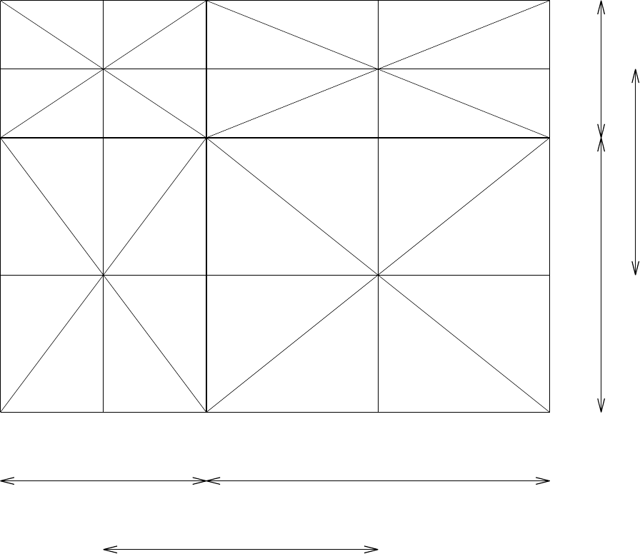
C.4. GENERAL COMMENTS
651
7
Ti,j+1
Ti,j
Ti,j-1
8
10
11
dxt(i)
dyt(j)
dyu(j)
dyu(j-1)
Ti-1,j
dxu(i-1) dxu(i)
Ti+1,j
Ti-1,j-1
Ti-1,j+1
Ti+1,j-1
Ti+1,j+1
2 5
9
12
4 6
3
1
Figure C.2: MOM x-y plane and its partitioning into 12 quarter cells. The generally nonconstant
grid spacing is indicated, which implies a non-centered T-point.
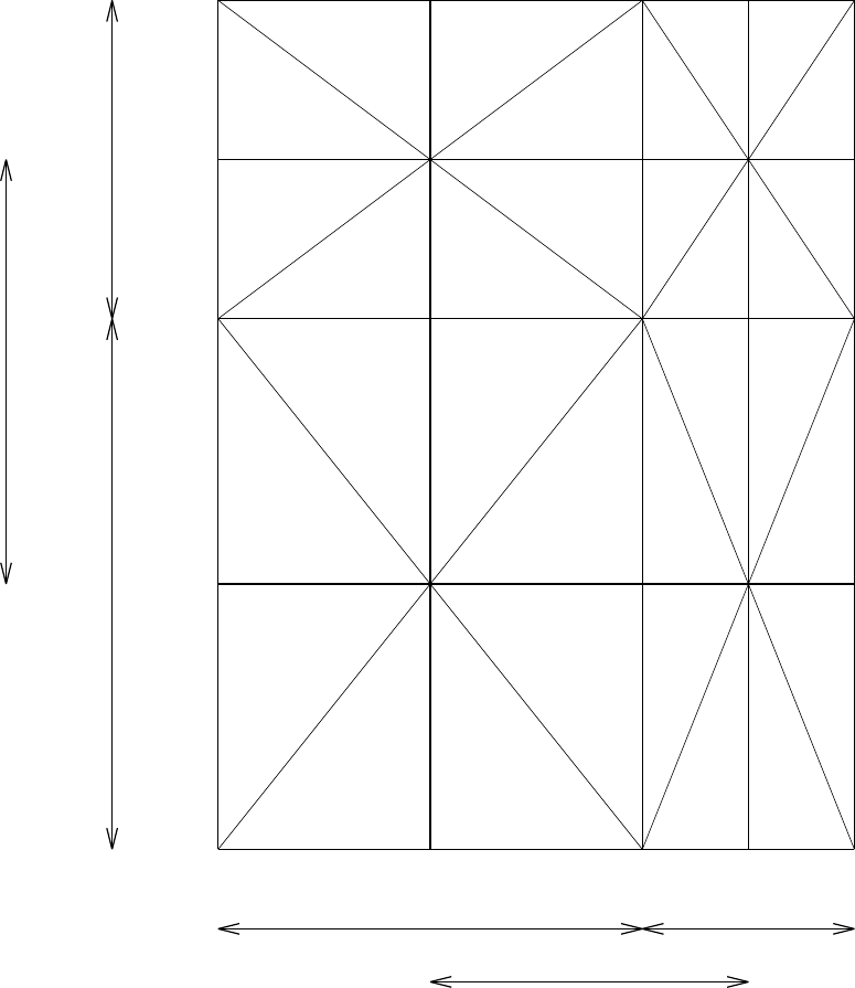
652
APPENDIX C. ISONEUTRAL DIFFUSION DISCRETIZATION
Ti+1,k-1
dxu(i-1) dxu(i)
dxt(i)
dzt(k)
dzw(k-1)
dzw(k)
Ti,k
Ti,k-1
Ti,k+1
Ti+1,kTi-1,k
Ti-1,k-1
Ti-1,k+1 Ti+1,k+1
13 14
15 16
17
18
19
20
21 22
23 24
Figure C.3: MOM x-z plane and its partitioning into 12 quarter cells. The generally nonconstant
grid spacing is indicated, which implies a non-centered T-point. This figure assumes that the
vertical grid spacing is dependent only on the vertical grid position. For the more general
case with partial vertical cells, the vertical grid spacing is a function of both the vertical and
horizontal grid positions (see Figure C.4).
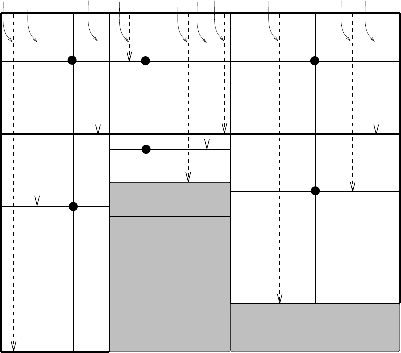
C.4. GENERAL COMMENTS
653
zt(i,k-1)
Ti-1,k
Ti-1,k-1 Ti,k-1
Ti,k
Ti+1,k
Ti+1,k-1
19
20
13
15
21
16
14
zw(i,k-1) zw(i+1,k)
zw(i-1,k-1)
17
18
22
zw(i-1,k) zt(i-1,k) zw(i,k) zt(i,k) zt(i+1,k) zw(i+1,k-1)
23 24
Figure C.4: MOM x-z plane for the case with partial bottom cells. T-cells are surrounded by
dark solid lines. Rock is shaded. The thin solid lines define the quarter cells. The vertical
position of the T-point in a T-cell maintains the same ratio for all the cells, whether full or
partial. The 12 quarter cells corresponding to those in Figure C.3 are shown, where Figure C.3
used full vertical cells. Note that quarter-cells 23 and 24 are in rock for this particular example.
Whether they are in rock or are ocean cells, quarter-cells 23 and 24 have the same volume as
quarter cells 15 and 16 (as for the full cell case shown in Figure C.3). The vertical distances
from the ocean surface to the bottom of the T-cells (zw) and to the T-cell center (zt) are shown
by dashed lines.
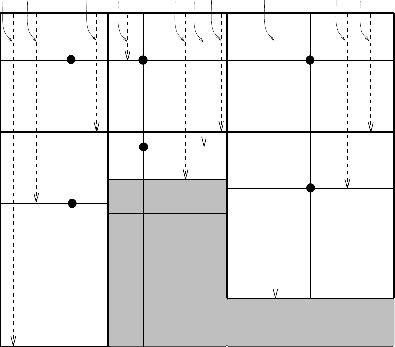
654
APPENDIX C. ISONEUTRAL DIFFUSION DISCRETIZATION
zw(k-1,j+1)
32 30
29
31
25 26
2827
33 34
3635
zw(k,j-1) zt(k,j-1) zw(k-1,j-1) zt(k-1,j) zw(k,j) zt(k,j) zw(k-1,j) zw(k,j+1) zt(k,j+1)
Tk-1,j-1
Tk,j-1
Tk,j
Tk-1,j Tk-1,j+1
Tk,j+1
Figure C.5: MOM y-z plane for the case with partial bottom cells. Otherwise, as in Figure C.4.
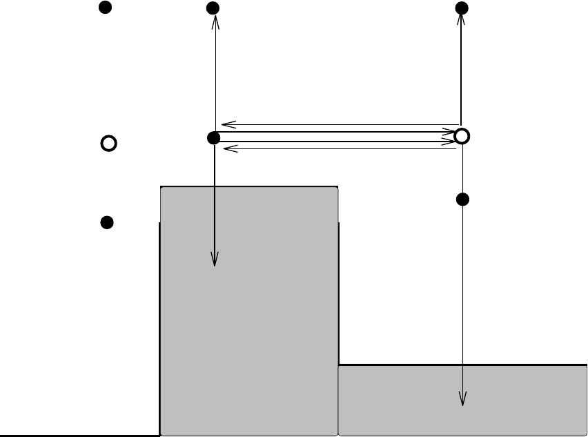
C.4. GENERAL COMMENTS
655
Ti,k+1
Ti-1,k
Ti-1,k-1
Ti+1,k
Ti+1,k-1
Ti+1,k
Ti-1,k
~~
Ti,k
Ti,k-1
∆
∆
∆
∆
i,k-1
i,k i,k-1
i,k
i,k
i,k i,k
i,k
Ti+1,k+1
Figure C.6: Stencil for computing the zonal component to the small angle isoneutral flux Fx small
i,k,
which is located at the east face of T-cell Ti,k. Shown are four density triads, each weighted by
the relevant vertical spacing factor ∆. For the two triads extending upwards, the weighting is
∆(i,k−1)
(i,k), whereas the two triads extending downwards are weighted by ∆(i,k)
(i,k). The tracer points
with the open circles denote tracer values which are determined through linear interpolation.
For the two triads extending into rock (shaded regions), they are zeroed out in the code since
they should not contribute to the diffusion operator.
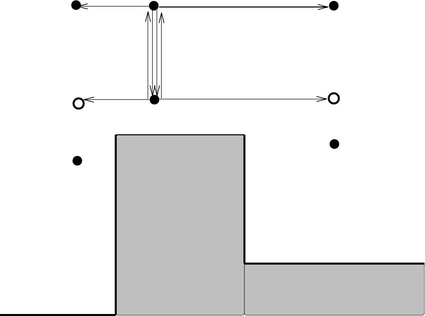
656
APPENDIX C. ISONEUTRAL DIFFUSION DISCRETIZATION
i,k-1
Ti-1,k
Ti-1,k-1
Ti+1,k
Ti+1,k-1
Ti+1,k
Ti-1,k
~~
Ti,k-1
Ti,k
i-1,k
i-1,k-1
∆
∆i-1,k-1
i-1,k-1
∆i,k-1
i,k
∆i,k-1
Figure C.7: Stencil for computing the vertical component to the small angle isoneutral flux
Fz small
i,k−1, which is located at the bottom face of T-cell Ti,k−1. Shown are four density triads, each
weighted by the relevant vertical spacing factor ∆. Note the rotation of the triads relative to
those used to construct the zonal flux in Figure C.6. Each of the four triads in this figure employ
a generally different vertical weighting factor ∆.
Appendix D
Horizontal friction discretization
The purpose of this appendix is to present a derivation of MOM’s discretized horizontal
friction operator. Much here follows the functional approach used for the isoneutral diffusion
discretization in Appendix C. However, the present discussion is considerably simpler because
of the need to only discretize a two dimensional (x-y plane) operator, and because there are no
subtleties associated with neutral directions. The approach here is therefore a straightforward
application of the functional formalism outlined in Section 9.7 for the continuum friction, and
Appendix C for the diffusion operator.
Brief history of this method in MOM:
•Summer 1999: Discretization derived and tested on one-processor and only for fully
opened memory window. This scheme will not be made available for use in MOM 3 as it
is motivated largely by the desire to introduce generalized horizontal coordinates, which
is being considered for MOM 4 but not MOM 3.
D.1 Motivation and summary
In a horizontal plane with second order numerics, the discrete Laplacian forms a 5-point stencil.
This stencil precludes computational modes, and hence always acts to smooth. It is for this
reason that many ocean models employ a Laplacian operator for dissipating momentum in
order to satisfy various numerical stability requirements.
On a sphere and in the presence of non-homogeneous grids, boundaries, and various
flow regimes, a Laplacian operator which uses a constant viscosity is often insufficient and
generally sub-optimal in the sense that it will over-dissipate the simulation. The paper by Griff
ies and Hallberg (1999) provide discussion which motivates consideration of the Smagorinsky
viscosity in either a second order (Laplacian) or fourth order (biharmonic) friction operator.
Additional considerations necessary to preserve angular momentum on a sphere warrant
added sophistication to the operator beyond that of the familiar Cartesian form of the Laplacian
operator.
Until Summer 1999, MOM has handled the added complications due to sphericity and
non-constant viscosities in two basic ways. First, there are the formulae of Bryan (1969)
and Wajsowicz (1993), in which friction is written as a “Laplacian plus metric” form. The
“Laplacian” is the spherical coordinate form of a Laplacian operator acting on a component
of the velocity, as if the component was a scalar field. The “metric term” is an added piece
which accounts for the sphericity of the earth and provides for a proper angular momentum
657
658
APPENDIX D. HORIZONTAL FRICTION DISCRETIZATION
budget. Bryan (1969) used metric terms appropriate for constant viscosities, and Wajsowicz
(1993) showed how to add the metric terms appropriate for non-constant viscosities. Standard
discretizations of these metric terms on a B-grid lead to computational modes. The presence
of the scalar Laplacian, however, can in many situations, especially with constant viscosities,
render these modes harmless.
The second manner of discretizing friction is to apply the tensor formalism of Smagorinsky
(1963, 1993) in the process of discretizing the Smagorinsky nonlinear viscosity method. This
was the approach of Rosati and Miyakoda (1988). In the continuum, this approach is equivalent
to Wajsowicz (1993) (see Section 9.8 for details). Yet on the discrete lattice, there are differences.
Furthermore, the tensor formalism is considerably more concise, and the ability to generalize
to arbitrary orthogonal curvilinear coordinates is cleaner. Chapter 9 provides a full account of
these issues.
Experience with the Smagorinsky scheme at GFDL has recently matured to the point of
realizing that both of the above approaches to discretization can lead to unsatisfying solutions.
Most notably, some model results with the Laplacian Smagorinsky scheme have shown grid
noise in the velocity field. The reason for this noise is not well known, but it is likely due to
the presence of computational modes which arise in either of the discretizations. Additionally,
there is an effort underway to re-write MOM so that it employs general horizontal curvilinear
coordinates. Hence, it is desirable to discretize friction in the manner described in Chapter 9,
in particular through the tidy expressions (9.126) and (9.127). Otherwise, it will be necessary
to introduce cumbersome metric terms which are not simple to derive in general.
In order to derive a discretization for an operator, one can proceed in numerous manners.
The first approach might be to take the continuum form and provide reasonable second order
discretizations, performing averaging whenever needed to place quantities in their proper
position on the grid. This has been the approach taken for the friction in the past with
MOM, where the continuum formulas of Bryan (1969) and Wajsowicz (1993), or Smagorinsky
(1963, 1993), were the starting point. As discussed in Appendix C, this direct approach led to
considerable difficulty with the isoneutral diffusion operator. Although it has not led to such
serious problems for friction, it has not been satisfying for the reasons mentioned above.
After having some success with the reformulation of isoneutral diffusion, in which the
diffusion operator was shown to be equivalent to the functional derivative of the tracer variance,
it was decided to attempt similar approaches for the friction. As shown in Section 9.7, the
friction operator is equivalent to the functional derivative of the kinetic energy dissipation.
Both of these results follow from the self-adjointness of the diffusion and friction operators.
Through this connection, the general approach is to first discretize the functional. Thereafter,
the functional derivative of the discrete functional is used to derive the discretized friction.
It is notable that functional discretization of the friction operator leads to the use of velocity
triads. These triads result because of the B-grid in which both velocity components are at a
single point. Such triads will not emerge,for example, if working on a C-grid. For discretization
of the isoneutral diffusion operator, density triads, as seen in Appendix C, are fundamental.
Triads emerge for diffusion since all quantities of interest live on the tracer grid. Hence, discrete
isoneutral diffusion, derived from a functional, will contain triads on any grid.
D.2. REVIEW OF THE CONTINUUM RESULTS
659
D.2 Review of the continuum results
As discussed in Section 9.7, the continuum functional for horizontal friction is given by
S=−ρoZdξ1dξ2dz pGA(D2
T+D2
S).(D.1)
In this equation, the horizontal tension is
DT=h2
h1 h1
h2
u1!,1−h1
h2 h2
h1
u2!,2
(D.2)
and the horizontal shearing strain is
DS=h1
h2
u1
,2+h2
h1
u2
,1.(D.3)
The infinitesimal horizontal distance between two points is written
ds2=g11 (dξ1)2+g22 (dξ2)2+dz2
=(h1dξ1)2+(h2dξ2)2+dz2
=dx2+dy2+dz2.(D.4)
The non-negative metric components h1and h2are generally functions of both horizontal
directions (ξ1, ξ2). In spherical coordinates, with (ξ1, ξ2)=(λ, φ) longitude and latitude,
ds2=(acos φdλ)2+(a dφ)2+dz2(D.5)
The square-root of the metric determinant takes the form
pG=h1h2h3(D.6)
with h3=1. The invariant horizontal volume element is therefore given by √Gdξ1dξ2dz,
which in spherical coordinates takes the form a2cos2φdλdφdz. The velocity vector compo-
nents uaare related to the physical tensor components through
(u,v,w)=(h1u1,h2u2,w).(D.7)
It is u,vwhich are time stepped in the ocean model. However, for purposes of deriving the
discretization, it is important to recognize their distinction from ua. In terms of the physical
velocity and partial derivatives, the tension and strain take the form
DT=h2(u/h2),x−h1(v/h1),y
=(acos φ)−1u,λ −a−1cos φ(v/cos φ),φ (D.8)
DS=h1(u/h1),y+h2(v/h2),x
=cos φ(u/acos φ),φ +(acos φ)−1v,λ (D.9)
where the second expression introduced the spherical coordinate form. Given the functional,
its functional derivative yields the friction vector through the relation
1
2ρo
δS
δua=gab Fb,(D.10)
where a,b=1,2. The physical components of the friction are
Fx=h−2
2(h2
2A DT),x+h−2
1(h2
1A DS),y(D.11)
Fy=−h−2
1(h2
1A DT),y+h−2
2(h2
2A DS),x,(D.12)
where Fx=h1F1and Fy=h2F2.
660
APPENDIX D. HORIZONTAL FRICTION DISCRETIZATION
D.3 Discretization of the functional
The goal of this section is to provide a consistent discretization of the functional for horizontal
friction. Spherical coordinates will be used, with some sprinkling of ideas relevant for gen-
eral orthogonal curvilinear coordinates. Since all considerations in this appendix are for the
horizontal deformations, the friction arising from vertical deformations is dropped, as is the
vertical grid label.
D.3.1 General form of the discrete functional
The discrete friction functional takes the form
S=−ρoX
i,j
12
X
n=1
V(n)A(n) (D2
T(n)+D2
S(n))
≡X
i,jSi,j.(D.13)
Figure D.1 illustrates the nearest neighbor stencil used for discretizing the functional. The
summation n=1,12 arises from the 12 subcells to which the velocity point Ui,jcontributes
when discretizing the functional. V(n) are the volumes of each of the subcells, A(n) are the
viscosities, and D2
T(n) and D2
S(n) are the corresponding tensions and strains. The stencil is
directly analogous to that used for discretizing the isoneutral diffusion functional shown in
Figure C.2.
For a finite velocity grid cell Ui,j, the friction acting on the velocity is given by the discrete
functional derivative
1
2ρoVU
i,j
∂S
∂(ua)i,j
=gab Fb.(D.14)
Equivalently, the physical components of the friction vector are
Fx=1
2ρo(h1)i,jVU
i,j
∂S
∂(u1)i,j
(D.15)
Fy=1
2ρo(h2)i,jVU
i,j
∂S
∂(u2)i,j
.(D.16)
In spherical coordinates, (h1)i,j=acos φU
jand (h2)i,j=a. The velocity cell volume VU
i,jaccounts
for the differing dimensions of the Kronecker and Dirac delta functions. That is,
V−1δab →δ(xa−xb),(D.17)
where the zero volume limit is taken.
D.3. DISCRETIZATION OF THE FUNCTIONAL
661
5
7
Ui-1,j Ui+1,j
Ui-1,j-1
Ui+1,j+1
Ti,j
Ui+1,j-1
Ti,j+1 Ti+1,j+1
x
Ui-1,j+1 x
xx
xx
Ti+1,j
Ui,j
11 12
x
x
Ui,j-1
x
Ui,j+1
12
10
9
46
83
Figure D.1: Stencil for the discrete frictional functional. The 12 quarter cells each contain
contributions to the functional from the central velocity point Ui,j. In general, the grid di-
mensions are defined as follows: dxui,jrepresents the zonal distance between tracer points Ti,j
and Ti+1,j,dyui,jis the meridional distance between tracer points Ti,jand Ti,j+1,dxti+1,jis the
zonal distance between velocity points Ui,jand Ui+1,j, and dyti,j+1is the meridional distance
between velocity points Ui,jand Ui,j+1,. With spherical coordinates, dxui,j→cos φU
jdxui, which
now represents the zonal dimension of the Ui,jcell, dyui,j→dyujrepresents the meridional
dimension of the Ui,jcell, dxti+1,j→cos φT
jdxti+1, represents the zonal dimension of the Ti+1,j
cell, dyti,j+1→dytj+1represents the meridional dimension of the Ti,j+1cell. For spherical co-
ordinates, the velocity points, denoted by “x”, are always defined at the center of the velocity
cells, denoted by the dashed lines. The tracer points, denoted by “o”, are generally not at the
center of the tracer cells.
662
APPENDIX D. HORIZONTAL FRICTION DISCRETIZATION
D.3.2 Subcell volumes
In spherical coordinates, the volumes of the 12 subcells are
V(1) =V(2) =V(3) =V(4) =1
4dxuicos φU
jdyujdhui,k,j(D.18)
V(5) =V(6) =1
4dxui+1cos φU
jdyujdhui+1,k,j(D.19)
V(7) =V(8) =1
4dxui−1cos φU
jdyujdhui−1,k,j(D.20)
V(9) =V(10) =1
4dxuicos φU
j+1dyuj+1dhui,k,j+1(D.21)
V(11) =V(12) =1
4dxuicos φU
j−1dyuj−1dhui,k,j−1(D.22)
D.3.3 Derivative operators
For spherical coordinates, the horizontal finite difference derivative operators are given by
δxui,j=ui+1,j−ui,j
cos φU
jdxti+1
(D.23)
δyui,j=ui,j+1−ui,j
dytj+1
.(D.24)
D.3.4 Tension for the subcells
In spherical coordinates, the tension in the 12 subcells are
DT(1) =δxui−1,j−cos φT
j+1δy(vi,j/cos φU
j) (D.25)
DT(2) =δxui,j−cos φT
j+1δy(vi,j/cos φU
j) (D.26)
DT(3) =δxui−1,j−cos φT
jδy(vi,j−1/cos φU
j−1) (D.27)
DT(4) =δxui,j−cos φT
jδy(vi,j−1/cos φU
j−1) (D.28)
DT(5) =δxui,j−cos φT
j+1δy(vi+1,j/cos φU
j) (D.29)
DT(6) =δxui,j−cos φT
jδy(vi+1,j−1/cos φU
j−1) (D.30)
DT(7) =δxui−1,j−cos φT
j+1δy(vi−1,j/cos φU
j) (D.31)
DT(8) =δxui−1,j−cos φT
jδy(vi−1,j−1/cos φU
j−1) (D.32)
DT(9) =δxui−1,j+1−cos φT
j+1δy(vi,j/cos φU
j) (D.33)
DT(10) =δxui,j+1−cos φT
j+1δy(vi,j/cos φU
j) (D.34)
DT(11) =δxui−1,j−1−cos φT
jδy(vi,j−1/cos φU
j−1) (D.35)
DT(12) =δxui,j−1−cos φT
jδy(vi,j−1/cos φU
j−1) (D.36)
D.3.5 Strain for the subcells
In spherical coordinates, the strain in the 12 subcells are
DS(1) =cos φT
j+1δy(ui,j/cos φU
j)+δxvi−1,j(D.37)
D.4. DISCRETE FRICTION
663
DS(2) =cos φT
j+1δy(ui,j/cos φU
j)+δxvi,j(D.38)
DS(3) =cos φT
jδy(ui,j−1/cos φU
j−1)+δxvi−1,j(D.39)
DS(4) =cos φT
jδy(ui,j−1/cos φU
j−1)+δxvi,j(D.40)
DS(5) =cos φT
j+1δy(ui+1,j/cos φU
j)+δxvi,j(D.41)
DS(6) =cos φT
jδy(ui+1,j−1/cos φU
j−1)+δxvi,j(D.42)
DS(7) =cos φT
j+1δy(ui−1,j/cos φU
j)+δxvi−1,j(D.43)
DS(8) =cos φT
jδy(ui−1,j−1/cos φU
j−1)+δxvi−1,j(D.44)
DS(9) =cos φT
j+1δy(ui,j/cos φU
j)+δxvi−1,j+1(D.45)
DS(10) =cos φT
j+1δy(ui,j/cos φU
j)+δxvi,j+1(D.46)
DS(11) =cos φT
jδy(ui,j−1/cos φU
j−1)+δxvi−1,j−1(D.47)
DS(12) =cos φT
jδy(ui,j−1/cos φU
j−1)+δxvi,j−1(D.48)
D.4 Discrete friction
Given the form of the functional, it is now a matter of performing the functional derivatives
with respect to (u1)i,jand (u2)i,j, where in spherical coordinates,
ui,j=acos φU
j(u1)i,j(D.49)
vi,j=a(u2)i,j,(D.50)
with
u1=Dλ/Dt (D.51)
u2=Dφ/Dt.(D.52)
In general, the functional derivative of Si,jwith respect to (ub)i,jis given by
∂Si,j
∂(ub)i,j
=−2ρo
12
X
n=1
V(n)A(n) DT(n)∂DT(n)
∂(ub)i,j
+DS(n)∂DS(n)
∂(ub)i,j!,(D.53)
where b=1,2.
D.4.1 Functional derivative of the physical velocity components
The physical velocity components have the following functional derivatives with respect to
the tensorial velocity components
∂ui1,j1
∂(u1)i2,j2
=acos φU
j1δi2
i1δj2
j1(D.54)
∂vi1,j1
∂(u2)i2,j2
=aδi2
i1δj2
j1.(D.55)
All other functional derivatives vanish.
664
APPENDIX D. HORIZONTAL FRICTION DISCRETIZATION
D.4.2 Functional derivative of DT
The functional derivative of the tension within the 12 subcells is given by
∂DT(1)
∂(ub)i,j
=a
dxtiδ1
b+
acos φT
j+1
dytj+1cos φU
j
δ2
b(D.56)
∂DT(2)
∂(ub)i,j
=−a
dxti+1δ1
b+
acos φT
j+1
dytj+1cos φU
j
δ2
b(D.57)
∂DT(3)
∂(ub)i,j
=a
dxtiδ1
b−
acos φT
j
dytjcos φU
j
δ2
b(D.58)
∂DT(4)
∂(ub)i,j
=−a
dxti+1δ1
b−
acos φT
j
dytjcos φU
j
δ2
b(D.59)
∂DT(5)
∂(ub)i,j
=−a
dxti+1δ1
b(D.60)
∂DT(6)
∂(ub)i,j
=−a
dxti+1δ1
b(D.61)
∂DT(7)
∂(ub)i,j
=a
dxtiδ1
b(D.62)
∂DT(8)
∂(ub)i,j
=a
dxtiδ1
b(D.63)
∂DT(9)
∂(ub)i,j
=
acos φT
j+1
dytj+1cos φU
j
δ2
b(D.64)
∂DT(10)
∂(ub)i,j
=
acos φT
j+1
dytj+1cos φU
j
δ2
b(D.65)
∂DT(11)
∂(ub)i,j
=−
acos φT
j
dytjcos φU
j
δ2
b(D.66)
∂DT(12)
∂(ub)i,j
=−
acos φT
j
dytjcos φU
j
δ2
b.(D.67)
D.4.3 Functional derivative of DS
The functional derivative of the strain within the 12 subcells is given by
∂DS(1)
∂(ub)i,j
=−
acos φT
j+1
dytj+1
δ1
b+
a
cos φU
jdxti
δ2
b(D.68)
∂DS(2)
∂(ub)i,j
=−
acos φT
j+1
dytj+1
δ1
b−
a
cos φU
jdxti+1
δ2
b(D.69)
D.4. DISCRETE FRICTION
665
∂DS(3)
∂(ub)i,j
=
acos φT
j
dytj
δ1
b+
a
cos φU
jdxti
δ2
b(D.70)
∂DS(4)
∂(ub)i,j
=
acos φT
j
dytj
δ1
b−
a
cos φU
jdxti+1
δ2
b(D.71)
∂DS(5)
∂(ub)i,j
=−
a
cos φU
jdxti+1
δ2
b(D.72)
∂DS(6)
∂(ub)i,j
=−
a
cos φU
jdxti+1
δ2
b(D.73)
∂DS(7)
∂(ub)i,j
=
a
cos φU
jdxti
δ2
b(D.74)
∂DS(8)
∂(ub)i,j
=
a
cos φU
jdxti
δ2
b(D.75)
∂DS(9)
∂(ub)i,j
=−
acos φT
j+1
dytj+1
δ1
b(D.76)
∂DS(10)
∂(ub)i,j
=−
acos φT
j+1
dytj+1
δ1
b(D.77)
∂DS(11)
∂(ub)i,j
=
acos φT
j
dytj
δ1
b(D.78)
∂DS(12)
∂(ub)i,j
=
acos φT
j
dytj
δ1
b(D.79)
D.4.4 Rearrangement of terms for the zonal friction
Bringing things together for b=1 leads to the functional derivative of S
−1
2aρo
∂S
∂(u1)ij
=V(1) A(1) DT(1) +A(3) DT(3)
dxti−A(2) DT(2) +A(4) DT(4)
dxti+1!
+V(7) A(7) DT(7) +A(8) DT(8)
dxti!−V(5) A(5) DT(5) +A(6) DT(6)
dxti+1!
+V(1)
cos φT
j[A(3) DS(3) +A(4) DS(4)]
dtyj−
cos φT
j+1[A(1) DS(1) +A(2) DS(2)]
dtyj+1
+V(11)
cos φT
j[A(11) DS(11) +A(12) DS(12)]
dytj
−V(9)
cos φT
j+1[A(9) DS(9) +A(10) DS(10)]
dytj+1
(D.80)
666
APPENDIX D. HORIZONTAL FRICTION DISCRETIZATION
Figure D.1 indicates that a velocity point Ui,jis associated with four triads, each of which is
used to construct a tension and strain along with a viscosity. Introducing the notation (1,1),
(0,1), (0,0), (1,0) to denote the four triads, where (1,1) =northeast triad, (0,1) =northwest
triad, (0,0) =southwest triad, and (1,0) =southeast triad (Figure D.2), the functional derivative
can be written
1
2aρo
∂S
∂(u1)ij
=V(1)
dxti+1 h(A DT)(1,1) +(A DT)(1,0)ii,j+V(5)
V(1) h(A DT)(0,1) +(A DT)(0,0)ii+1,j!
−V(1)
dxti h(A DT)(0,1) +(A DT)(0,0)ii,j+V(7)
V(1) h(A DT)(1,1) +(A DT)(1,0)ii−1,j!
+
V(1) cos φT
j+1
dytj+1 h(A DS)(0,1) +(A DS)(1,1)ii,j+V(9)
V(1) h(A DS)(0,0) +(A DS)(1,0)ii,j+1!
−
V(1) cos φT
j
dytj h(A DS)(0,0) +(A DS)(1,0)ii,j+V(11)
V(1) h(A DS)(0,1) +(A DS)(1,1)ii,j−1!.
(D.81)
The subcell volumes from Section D.3.2 brings the two terms proportional to dxt−1
ito the
form
V(1)
dxti+1 h(A DT)(1,1) +(A DT)(1,0)ii,j+V(5)
V(1) h(A DT)(0,1) +(A DT)(0,0)ii+1,j!
=V(1)
dxuidhui,k,jdxti+1
dxuidhui,k,jh(A DT)(1,1) +(A DT)(1,0)ii,j+dxui+1dhui+1,k,jh(A DT)(0,1) +(A DT)(0,0)ii+1,j.
(D.82)
Likewise, the other terms can be brought to the form
V(1)
dxti h(A DT)(0,1) +(A DT)(0,0)ii,j+V(7)
V(1) h(A DT)(1,1) +(A DT)(1,0)ii−1,j!
=V(1)
dxuidhui,k,jdxti
dxuidhui,k,jh(A DT)(0,1) +(A DT)(0,0)ii,j+dxui−1dhui−1,k,jh(A DT)(1,1) +(A DT)(1,0)ii−1,j.
(D.83)
V(1) cos φT
j+1
dytj+1 h(A DS)(0,1) +(A DS)(1,1)ii,j+V(9)
V(1) h(A DS)(0,0) +(A DS)(1,0)ii,j+1!
=
V(1) cos φT
j+1
cos φU
jdyujdhui,k,jdytj+1
cos φU
jdyujdhui,k,jh(A DS)(0,1) +(A DS)(1,1)ii,j
+cos φU
j+1dyuj+1dhui,k,j+1h(A DS)(0,0) +(A DS)(1,0)ii,j+1(D.84)
D.4. DISCRETE FRICTION
667
V(1) cos φT
j
dytj h(A DS)(0,0) +(A DS)(1,0)ii,j+V(11)
V(1) h(A DS)(0,1) +(A DS)(1,1)ii,j−1!
=
V(1) cos φT
j
cos φU
jdyujdhui,k,jdytj
cos φU
jdyujdhui,k,jh(A DS)(0,0) +(A DS)(1,0)ii,j
+cos φU
j−1dyuj−1dhui,k,j−1h(A DS)(0,1) +(A DS)(1,1)ii,j−1.(D.85)
The volume of the velocity cell is VU
i,k,j=4V(1). Use of equation (D.15), with (h1)i,j=acos φU
j
for spherical coordinates, leads to
Fx
i,k,j=
1
4 cos φU
jdxuidhui,k,j
1
dxti+1dxuidhui,k,jh(A DT)(1,1) +(A DT)(1,0)ii,j
+dxui+1dhui+1,k,jh(A DT)(0,1) +(A DT)(0,0)ii+1,j
−1
dxtidxuidhui,k,jh(A DT)(0,1) +(A DT)(0,0)ii,j
+dxui−1dhui−1,k,jh(A DT)(1,1) +(A DT)(1,0)ii−1,j
+
1
4 (cos φU
j)2dyujdhui,k,j
cos φT
j+1
dytj+1cos φU
jdyujdhui,k,jh(A DS)(0,1) +(A DS)(1,1)ii,j
+cos φU
j+1dyuj+1dhui,k,j+1h(A DS)(0,0) +(A DS)(1,0)ii,j+1
−
cos φT
j
dytjcos φU
jdyujdhui,k,jh(A DS)(0,0) +(A DS)(1,0)ii,j
+cos φU
j−1dyuj−1dhui,k,j−1h(A DS)(0,1) +(A DS)(1,1)ii,j−1
=
1
4 cos φU
jdxuidhui,k,j
1
dxti+1
1
X
ip=0
dxui+ip dhui+ip,k,j
1
X
jq=0
(A DT)(1−ip,jq)
i+ip,j
−1
dxti
1
X
ip=0
dxui−ip dhui−ip,k,j
1
X
jq=0
(A DT)(ip,jq)
i−ip,j
+
1
4 (cos φU
j)2dyujdhui,k,j
668
APPENDIX D. HORIZONTAL FRICTION DISCRETIZATION
cos φT
j+1
dytj+1
1
X
jq=0
cos φU
j+jq dyuj+jq dhui,k,j+jq
1
X
ip=0
(A DS)(ip,1−jq)
i,j+jq
−
cos φT
j
dytj
1
X
jq=0
cos φU
j−jq dyuj−jq dhui,k,j−jq
1
X
ip=0
(A DS)(ip,jq)
i,j−jq .(D.86)
Comparison with the continuum zonal friction given by equation (D.11) indicates that the
discretization is consistent; i.e., the discrete friction reduces to the continuum as the grid size
goes to zero.
D.4.5 Rearrangement of terms for the meridional friction
Similar manipulations for the meridional friction leads to
cos φU
j
2ρoa
∂S
∂(u2)i,j
=−
cos φT
j+1V(1)
dytj+1A(1) DT(1) +A(2) DT(2) +V(9)
V(1) (A(9) DT(9) +A(10) DT(10))
+
cos φT
jV(1)
dytjA(3) DT(3) +A(4) DT(4) +V(11)
V(1) (A(11) DT(11) +A(12) DT(12))
+V(1)
dxti+1A(2) DS(2) +A(4) DS(4) +V(5)
V(1) (A(5) DS(5) +A(6) DS(6))
−V(1)
dxtiA(1) DS(1) +A(3) DS(3) +V(7)
V(1) (A(7) DS(7) +A(8) DS(8)),(D.87)
which leads to the meridional friction
Fy
i,k,j=−
1
4 (cos φU
j)2dyujdhui,k,j
cos φT
j+1
dytj+1cos φU
jdyujdhui,k,jh(A DT)(0,1) +(A DT)(1,1)ii,j
+cos φU
j+1dyuj+1dhui,k,j+1h(A DT)(0,0) +(A DT)(1,0)ii,j+1
−
cos φT
j
dytjcos φU
jdyujdhui,k,jh(A DT)(0,0) +(A DT)(1,0)ii,j
+cos φU
j−1dyuj−1dhui,k,j−1h(A DT)(0,1) +(A DT)(1,1)ii,j−1
+
1
4 cos φU
jdxuidhui,k,j
1
dxti+1dxuidhui,k,jh(A DS)(1,0) +(A DS)(1,1)ii,j
+dxui+1dhui+1,k,jh(A DS)(0,0) +(A DS)(0,1)ii+1,j
−1
dxtidxuidhui,k,jh(A DS)(0,1) +(A DS)(0,0)ii,j
+dxui−1dhui−1,k,jh(A DS)(1,1) +(A DS)(1,0)ii−1,j
D.5. DISCRETIZATION OF TENSION AND STRAIN FOR THE QUADRANTS
669
=−
1
4 (cos φU
j)2dyujdhui,k,j
cos φT
j+1
dytj+1
1
X
jq=0
cos φU
j+jq dyuj+jq dhui,k,j+jq
1
X
ip=0
(A DT)(ip,1−jq)
i,j+jq
−
cos φT
j
dytj
1
X
jq=0
cos φU
j−jq dyuj−jq dhui,k,j−jq
1
X
ip=0
(A DT)(ip,jq)
i,j−jq
+
1
4 cos φU
jdxuidhui,k,j
1
dxti+1
1
X
ip=0
dxui+ip dhui+ip,k,j
1
X
jq=0
(A DS)(1−ip,jq)
i+ip,j
−1
dxti
1
X
ip=0
dxui−ip dhui−ip,k,j
1
X
jq=0
(A DS)(ip,jq)
i−ip,j(D.88)
Comparison with the continuum meridional friction given by equation (D.12) indicates that
the discretization is consistent.
(1,1)(0,1)
(0,0) (1,0)
y
x
Figure D.2: Notation for the quadrants surrounding a velocity point.
D.5 Discretization of tension and strain for the quadrants
For each velocity point, there are four tensions and strains. Referring to Figure D.2, assuming
the central point is Ui,j, one has for the tensions
(DT)i,j,1,1=δxui,j−cos φT
j+1δy(vi,j/cos φU
j) (D.89)
(DT)i,j,0,1=δxui−1,j−cos φT
j+1δy(vi,j/cos φU
j) (D.90)
(DT)i,j,0,0=δxui−1,j−cos φT
jδy(vi,j−1/cos φU
j−1) (D.91)
(DT)i,j,1,0=δxui,j−cos φT
jδy(vi,j−1/cos φU
j−1),(D.92)

670
APPENDIX D. HORIZONTAL FRICTION DISCRETIZATION
and for the strains
(DS)i,j,1,1=cos φT
j+1δy(ui,j/cos φU
j)+δxvi,j(D.93)
(DS)i,j,0,1=cos φT
j+1δy(ui,j/cos φU
j)+δxvi−1,j(D.94)
(DS)i,j,0,0=cos φT
jδy(ui,j−1/cos φU
j−1)+δxvi−1,j(D.95)
(DS)i,j,1,0=cos φT
jδy(ui,j−1/cos φU
j−1)+δxvi,j.(D.96)
In general, the four tensions can be written
(DT)i,j,ip,jq =δxui+ip−1,j−cos φT
j+jq δy(vi,j+jq−1/cos φU
j+jq−1) (D.97)
and the four strains can be written
(DS)i,j,ip,jq =cos φT
j+jq δy(ui,j+jq−1/cos φU
j+jq−1)+δxvi+ip−1,j,(D.98)
where ip =0,1 and jq =0,1. These four tensions and strains are computed in the model. They
are then used to compute the friction operator. When the Smagorinsky scheme is enabled
(option velocity horz mix smag), they are used to compute the Smagorinsky viscosity as well.
D.6 Comments
It is important to note that the tension and strain are generally nonzero for interface points
between land and sea, even though the velocity vanishes at such points. The reason is that
when computing the tension and strain at such points, one reaches into the interior, which
leads to a nonzero shear at the wall. It is therefore important not to mask the model’s tension
and strain fields in order to provide a full accounting of the generally strong shears next to
no-slip walls.
In the special case of a Cartesian grid (e.g., model options fplane or beta plane), and with con-
stant viscosity, the triad generated algorithm reduces to the familiar 5-point discrete Laplacian,
which is known to have very stable computational properties.
Currently, this algorithm is not available for use in MOM 3. It is being considered for use
in MOM 4 upon switching to generalized orthogonal coordinates.
Appendix E
A note about computational modes
Fundamental to the discretization of MOM is the discretization of fluxes: advective fluxes,
diffusive fluxes, etc. Working with fluxes provides for a useful way to preserve the internal
consistency of the transport of momentum and tracers, which means, for example, that there
should be no false sources or sinks assuming we have a sound numerical scheme. The con-
vergence of fluxes is what is fundamentally of interest. Therefore, the fluxes must be defined
on the boundaries of the relevant grid cell: diffusive fluxes at the boundary of the T-cell and
advective fluxes at the boundary of the U-cell. To achieve this placement of fluxes often re-
quires some creative discretization in the form of averaging operations (see Section 21.2 for
more details of finite difference operators). When introducing average operators, however, it
is important to be aware of the potential to introduce computational modes. A computational
mode is basically a configuration of the discretized field which is invisible to the object which is
being discretized. With nearest neighbor discretization on the respective T and U grid, which
is done in MOM for second order accurate expressions, computational modes take the form
of “2-delta X” type waves; i.e., the smallest resolvable lattice wave. Higher order schemes are
exposed to computational modes of longer wavelength. The presence of these waves often
signal the ability for “grid noise” to manifest in the solution and so should be avoided.
As an example of the what is described above, consider one part of a recent study of
isoneutral diffusion in the GFDL model. In Griffies et al., (1998) (see also Appendix C), it was
found that one source of grid noise in MOM is the original Cox (1987) discretization of the
isoneutral diffusive flux. For the small angle approximated diffusion tensor, the Cox (1987)
discretization of the flux in a two-dimensional x-z model is
−Fx
i,k=AIδxTi,k−
δxρi,k
δzρx,z
i,k−1
δzTx,z
i,k−1,(E.1)
−Fz
i,k=AI
δxρx,z
i−1,k
δzρi,k
2δzTi,k−
δzρi,k
δxρx,z
i−1,k
δxTx,z
i−1,k.(E.2)
In order to define the diffusive fluxes consistently on the B-grid, the x-flux must be placed at
the east face of the T-cell (i,k) and the z-flux at the bottom of this cell. With this placement, the
divergence of these fluxes across the T-cell results in a diffusion operator R(T)i,k=−(δxFx
i−1,k+
δzFz
i,k−1) properly placed at the center of the cell at the location of the tracer Ti,k. For the off-
diagonal terms (the second terms of the fluxes), a spatial averaging in the form of a double
average ( )x,zbrings the z-derivative terms appearing in the x-flux onto the east face of a T-cell
and the x-derivative terms appearing in the z-flux onto the bottom face of the T-cell. This is a
671

672
APPENDIX E. A NOTE ABOUT COMPUTATIONAL MODES
natural choice for averaging when working on the B-grid and provides an example of what is
meant in the previous paragraph about “creative discretization”.
There is a problem, however, with this discretization due to the presence of both the average
and derivative operations acting in the same spatial direction on a single field. The problem
is that this combination of operations introduces computational modes. For example, in the
x-flux, the z-derivative of the tracer defined on the east face of T-cell (i,k) is
δzTx,z
i,k−1=Ti,k−1−Ti,k+1+Ti+1,k−1−Ti+1,k+1
4dztk
,(E.3)
and likewise for the z-derivative of the density. A quick inspection of this forumla indicates
that by taking both a z-average and a z-derivative allows for the presence of 2∆zcomputational
modes Ti,k−1=Ti,k+1and ρi,k−1=ρi,k+1. For fields containing this structure, the discretized z-
derivative on the east face will vanish. For the z-flux, 2∆xcomputational modes exist due to
the combination of the x-average and x-derivative. In general, when working on the B-grid
and acting on a single field, such combinations of an average in one direction combined with a
derivative in the same direction introduces computational modes in this field. The presence of
the grid waves, and the ability to increase their amplitude, were two of the fundamental reasons
that the Cox (1987) diffusion scheme was unstable and so required background horizontal
diffusion. Consult Griffies et al., (1998) for complete details.
Appendix F
References
Adcroft, A. J., 1995: Numerical algorithms for use in a dynamical model of the ocean. Ph.D
Thesis, University of London.
Adcroft, A. ,C. Hill, and J. Marshall, 1996: Representation of Topography by Shaved Cells in
a Height Coordinate Ocean Model. Submitted to Monthly Weather Review
Apel, J. R., 1987: Principles of ocean physics, International Geophysics series, No. 38. Aca-
demic Press, London. 634 pages.
Arakawa, A., 1966: Computational design for long-term numerical integration of the equa-
tions of fluid flow: Two-dimensional incompressible flow. Part I. Journal of Computational
Physics,1, 119–143.
Arakawa, A. and V. R. Lamb, 1977: Computational design of the basic dynamical processes
of the UCLA general circulation model. Methods in Computational Physics,17, 174–265.
Aris, R. , 1962: Vectors, Tensors and the basic equations of Fluid Mechanics, Dover publish-
ing.
Batchelor, G. K., 1967: An introduction to fluid dynamics, Cambridge University Press. 615
pages.
Beckers, J. M. , H. Burchard, J.M. Campin, E. Deleersnijder, and P.P. Mathieu, 1998: Comments
on the paper: “Isoneutral diffusion in a z-coordinate ocean model by Griffies et al.,Journal
of Physical Oceanography, accepted.
Bleck, R., C. Rooth, D. Hu, and L. T. Smith, 1992: Salinity-driven thermocline transients in a
wind and thermohaline forced isopycnic coordinate model of the North Atlantic. Journal
of Physical Oceanography,22, 1486-1505.
Blumberg, A. F., and G. L. Mellor, 1987: A description of a three-dimensional coastal ocean cir-
culation model. Three-Dimensional Coastal Ocean Models. Vol. 4, N. Heaps, Ed., American
Geophysical Union. 208 pp.
B¨oning, C., 1988: Particle disperson and mixing of conservative properties in an eddy-
resolving model. Journal of Physical Oceanography,18, 320–338.
Boussinesq, J., 1903: Th´eorie analytique de la chaleur. Paris: Gathier-Villars, Vol. 2.
673
674
APPENDIX F. REFERENCES
Boris, J. P. , D. L. Book, 1973: Flux-corrected transport, I. SHASTA: A fluid transport algorithm
that works. Journal of Computational Physics,11, 38-69.
Brown, J. A. ,K. A. Campana, 1978: An economical time-differencing system for numerical
weather prediction. Monthly Weather Review,106, 1125–1136.
Bryan, F. 1986: Maintenance and variability of the thermohaline circulation. Geophysical
Fluid Dynamics Program Thesis, Princeton University.
Bryan, F., 1986: Parameter sensitivity of primitive equation ocean general circulation models.
Journal of Physical Oceanography,17, 970–985.
Bryan, K., 1969: A numerical method for the study of the circulation of the world ocean.
Journal of Computational Physics,4, 347–376.
Bryan, K. and M. D. Cox, 1972: An approximate equation of state for numerical models of the
ocean circulation. Journal of Physical Oceanography,2, 510–514.
Bryan, K., S. Manabe, and R.C. Pacanowski, 1975: A global ocean-atmosphere climate model.
Part II. The oceanic circulation. Journal of Physical Oceanography,5, 30–46.
Bryan, K. and L. J. Lewis, 1979: A water mass model of the world ocean. Journal of Geophysical
Research,84, 2503–2517.
Bryan, K., 1984: Accelerating the convergence to equilibrium of ocean-climate models. Journal
of Physical Oceanography,14, 666–673.
Bryan, K. and J. L. Sarmiento, 1985: Modeling ocean circulation. Advances in Geophysics,28a,
433–459.
Bryan, K., 1989: The Design of Numerical Models of the Ocean Circulation. Oceanic Circulation
Models: Combining Data and Dynamics, D.L.T. Anderson and J. Willebrand (eds.), Kluwer
Academic Publishers, 465–500.
Bryan, K., 1991: Michael Cox (1941–1989): His pioneering contributions to ocean circulation
modeling. Journal of Physical Oceanography,21, 1259–1270.
Bryan, K., R. D. Smith, and J. Dukowicz, 1998: A note on the bolus velocity field in an eddy
resolving global ocean model. In preparation.
Chandrasekhar, S., 1961: Hydrodynamic and hydromagnetic stability, Dover Publications,
New York. 652 pages.
Courant and Hilbert, Methods of Mathematical Physics, 2 volumes. Wiley-Interscience.
Cox, M. D., 1985: An eddy resolving numerical model of the ventilated thermocline. Journal
of Physical Oceanography,15, 1312–1324.
Cox, M. D. and K. Bryan, 1984: A numerical model of the ventilated thermocline. Journal of
Physical Oceanography,14, 674–687.
Cox, M. D., 1984: A primitive equation, 3-dimensional model of the ocean. GFDL Ocean
Group Technical Report No. 1.
675
Cox, M. D., 1987: Isopycnal diffusion in a z-coordinate ocean model. Ocean modeling,74, 1–5.
Danabasoglu, G. and J. C. McWilliams, 1995: Sensitivity of the global ocean circulation to
parameterizations of mesoscale tracer transports. Journal of Climate, 8, 2967–2987.
Deardorff, J. W., 1973: The use of subgrid scale transport equations in a three-dimensional
model of atmospheric turbulence. Journal of Fluid Eng.,Sep., 429-438.
Dewar, W. K., Y. Hsueh, T. J. McDougall, and D. Yuan, 1998: Calculation of Pressure in Ocean
Simulations. Journal of Physical Oceanography,28, 577–588.
Doescher, R. and R. Redler, 1997: The Relative Influence of North Atlantic Overflow and
Subpolar Deep Convection on the Thermohaline Circulation in an OGCM, JPO,27, 1894–
1902
DYNAMO groups at IMG Grenoble, JRC Southampton and IfM Kiel: 1994, 1994 scientific
report, EC MAST DYNAMO contract no. MAS2-CT93-0060, .
Dukowicz, J.K. and R.D. Smith, 1997: Stochastic theory of compressible turbulent fluid trans-
port. Physics of Fluids,9, 3523-3529.
Dukowicz, J. K. and R. D. Smith, 1994: Implicit free-surface method for the Bryan-Cox-Semtner
ocean model. Journal of Geophysical Research,99, 7991–8014.
Dukowicz, J. K., R. D. Smith, and R. C. Malone, 1993: A reformulation and implementation of
the Bryan-Cox-Semtner ocean model on the Connection Machine. Journal of Atmospheric
and Oceanic Technology,10, 195–208.
Farrow, D. E. , D. P. Stevens, 1995: A new tracer advection scheme for Bryan and Cox type
ocean general circulation models. Journal of Physical Oceanography,25, 1731-1741.
Fetter, A. L., and Walecka, J. D., 1980: Theoretical Mechanics of Particles and Continua,
McGraw-Hill Book Company. New York.
Fiadeiro M. E. , G. Veronis, 1977: On weighted-mean schemes for the finite-difference approx-
imation to the advection-diffusion equation. Tellus,29, 512-522.
Gent, P. R., and J. C. McWilliam, 1996: Eliassen-Palm fluxes and the momentum equation
in non-eddy-resolving ocean circulation models. Journal of Physical Oceanography,26,
2539–2546.
Gent, P. R., and J. C. McWilliams, 1990: Isopycnal mixing in ocean circulation models. Journal
of Physical Oceanography,20, 150–155.
Gent, P. R., J. Willebrand, T. McDougall, and J. C. McWilliams, 1995: Parameterizing eddy-
induced tracer transports in ocean circulation models. Journal of Physical Oceanography,
25, 463–474.
Gerdes, R., C. K¨oberle, and J. Willebrand, 1991: The influence of numerical advection schemes
on the results of ocean general circulation models. Climate Dynamics,5, 211–226.
Gerdes, R. 1993: A primitive equation ocean circulation model using a general vertical co-
ordinate transformation 1. Description and testing of the model. Journal of Geophysical
Research,98, 14683–14701.
676
APPENDIX F. REFERENCES
Gill, A. E., 1982: Atmosphere-Ocean Dynamics.Academic Press Inc.
Goddard, L. 1995: The energetics of interannual variability in the tropical Pacific Ocean.
Program in Atmospheric and Oceanic Sciences Thesis, Princeton University.
Goloviznin, V. M., Samarskii, A. A., and A. P. Favorskii, 1977: A variational approach to
constructing finite-difference mathematical models in hydrodynamics. Sov. Phys. Dokl.,
22 432–434.
Greatbatch, R. J., 1994: A note on the representation of steric sea level in models that conserve
volume rather than mass. Journal of Geophysical Research.99, 12767–12771.
Griffies, S. M., 1998: The Gent-McWilliams Skew-Flux. Journal of Physical Oceanography,28,
831-841.
Griffies, S. M., A. Gnanadesikan, R. C. Pacanowski, V. Larichev, J. K. Dukowicz, and R.
D. Smith, 1998: Isoneutral diffusion in a z-coordinate ocean model. Journal of Physical
Oceanography,28, 805–830.
Griffies, S. M., R. C. Pacanowski, and R. W. Hallberg, 1998: Spurious mixing associated with
advection in a z-coordinate ocean model. Monthly Weather Review in press.
Griffies, S.M. and R.W. Hallberg, 1999: Biharmonic friction with a Smagorinsky viscosity for
use in large-scale eddy-permitting ocean models. Accepted by Monthly Weather Review.
Griffies, S.M., R. C. Pacanowski, M. Schmidt, and V. Balaji, 2000: The explicit free surface
method in the GFDL modular ocean model. Submitted to Monthly Weather Review.
Haidvogel, D. B., J. L. Wilkin, and R. E. Young, 1991: A semi-spectral primitive equation ocean
circulation model using vertical sigma and orthogonal curvilinear horizontal coordinates.
Journal of Computational Physics,94, 151–185.
Hallberg, R., 1995: Some aspects of the circulation in ocean basins with isopycnals intersecting
the sloping boundaries, Ph.D thesis, University of Washington, Seattle, 244 pp.
Haltiner, G. J. and R. T. Williams, 1980: Numerical Prediction and Dynamic Meteorology,
Wiley.
Hamming, R. W., 1977: Digital Filters, Prentice-Hall.
Haney, R. L., 1971: Surface thermal boundary condition for ocean circulation models. Journal
of Physical Oceanography,1, 241–248.
Hankin, S. and M. Denham: 1996, FERRET: An Analysis Tool for Gridded Data, Users
Guide, Version 4.4, NOAA/PMEL/TMAP, 243 pages.
Hanson, R. J. , and C. L. Lawson, 1969: Extensions and applications of the Householder
algorithm for solving linear least squares problems. Math. Comput.,23 787-812.
Held, I. M. and V. D. Larichev, 1996: A scaling theory for horizontally homogeneous baroclin-
ically unstable flow on a beta plane, Journal of Atmospheric Sciences,53, 946–952.
Hellerman, S. and M. Rosenstein, 1983: Normal Monthly Stress over the World Ocean with
Error Estimates. Journal of Physical Oceanography,13, 1093–1104.
677
Higdon, R. L. and A. F. Bennett, 1996: Stability analysis of operator splitting for large-scale
ocean modeling. Journal of Computational Physics,123, 311-329.
Hirst, A. C. and T. McDougall, 1996: Deep-water properties and surface buoyancy flux as
simulated by a z-coordinate model including eddy-flux advection. Journal of Physical
Oceanography,26, 1320–1343.
Hirst, A. C., D. R. Jackett, and T. J. McDougall, 1996: The meridional overturning cells of a
world ocean model in neutral density coordinates. Journal of Physical Oceanography,26,
775–791.
Holland, W. R., 1975: Energetics of baroclinic oceans. In Numerical Models of Ocean
Circulation, National Academy of Sciences, Washington, D.C.
Holland, W. R., J. C. Chow, and F. O. Bryan, 1998: Application of a third-order upwind scheme
in the NCAR ocean model. Journal of Climate,11, 1487–1493.
Holloway, Greg, 1992: Representing Topographic Stress for Large-Scale Ocean Models. Jour-
nal of Physical Oceanography,22, 1033–1046.
Holloway, G., 1989: Subgridscale representation. In D. L. T. Anderson and J. Willebrand (eds.),
Oceanic circulation models: combining data and dynamics. pages 513–593. Kluwer
Academic Publishers.
Holton, J. R., 1992: An introduction to dynamic meteorology, 3rd Edition. Academic Press.
507 pages.
Huang, 1993: Real freshwater flux as a natural boundary condition for the salinity balance
and thermohaline circulation forced by evaporation and precipitation. Journal of Physical
Oceanography,23, 2428–2446.
Jackett, D., R., and T. J. McDougall, 1997: A neutral density variable for the world’s oceans.
Journal of Physical Oceanography,27, 237–263.
Jerlov 1968: Optical oceanography.Elsevier.
Killworth, P. D., 1989: On the parameterisation of deep convection in ocean models. In Param-
terizing small scale processes in the ocean, Proceedings of the Hawaiian Winter Workshop,
’Aha Huiliko’a.
Killworth, P. D., J. M. Smith, A. E. Gill, 1984: Speeding up ocean ciruclation models. Ocean
Modeling,56, 1–5.
Killworth, P. D., 1987: Topographic instabilities in level model OGCM’s. Ocean Modeling,75,
9–12.
Killworth, P. D., D. Stainforth, D. J. Webb and S. M. Paterson, 1989:
A free surface Bryan-Cox-Semtner model,
Institute of Oceanographic Sciences, Deacon Laboratory,
Report No. 270.
Killworth, P. D., 1997: On the parameterization of eddy transfer. Part I: theory. Journal of
Marine Research,55, 1171–1197.
678
APPENDIX F. REFERENCES
Killworth, P. D., D. Stainforth, D. J. Webb, and S. M. Paterson, 1991: The development of
a free-surface Bryan-Cox-Semtner ocean model. Journal of Physical Oceanography,21,
1333–1348.
Klinger, B. A., J. Marshall, and U. Send, 1996: Representation of convective plumes by vertical
adjustment. Journal of geophysical research,101, 18175–18182.
Korshiya, T. K., Tishkin, V. F., Favorskii, A. P., and M. Y. Shashkov, 1980: Flow-variational
difference schemes for calculating the diffusion of a magnetic field. Sov. Phys. Dokl.,25
832–834.
Lamport, L., 1986: L
A
T
E
XUser’s Guide and Reference Manual, First edition. Addison-Wesley
Publishing Co., 242 pages.
Lamport, L., 1994: L
A
T
E
XUser’s Guide and Reference Manual, Second edition. Addison-
Wesley Publishing Co., 272 pages.
Landau, L. D., Lifshitz, E. M., 1986: Theory of Elasticity. Course of Theoretical Physics,
Volume 7. Pergamon Press, Oxford.
Landau, L. D., Lifshitz, E. M., 1987: Fluid Mechanics. Course of Theoretical Physics, Volume
6. Pergamon Press, Oxford.
Large, W. G. , J. C. McWilliams, and S. C. Doney, 1994: Oceanic vertical mixing: A review and
a model with a nonlocal boundary layer parameterization. Rev. of Geophys,32, 363-403.
Larichev, V. D. and I. M. Held, 1995: Eddy amplitudes and fluxes in a homogeneous model
of fully developed baroclinic instability. Journal of Physical Oceanography,25, 2285–2297.
Leith, C. E. 1996: Stochastic models of chaotic systems. Physica D 98, 481–491. In Nonlinear
phenomena in ocean dynamics, edited by D.D. Holm, R.C. Malone, and Len G. Margolin.
Leonard, B. P., 1979: A stable and accurate convective modelling procedure based on quadratic
upstream interpolation. Computer Methods in Applied Mechanics and Engineering,19, 59–98
Levitus, S., 1982: Climatological atlas of the world ocean. NOAA Prof. Pap. 13, 173 pp. U. S.
Government Printing Office, Washington, D. C.
Love, A. E. H., 1944: A treatise on the mathematical theory of elasticity. Dover, New York,
1944; reprinted from the 4th edition published by Macmillian courtesy of Cambridge
University Press 1927.
Marotzke, J., 1991: Influence of convective adjustment on the stability of the thermohaline
circulation. Journal of Physical Oceanography,21, 903–907.
Marshall, J., C. Hill, L. Perelman, and A. Adcroft, 1997: Hydrostatic, quasi-hydrostatic, and
nonhydrostatic ocean modeling. Journal of Geophysical Research,102, 5733–5752.
McDougall, T. J., 1987: Neutral surfaces. Journal of Physical Oceanography,17, 1950–1964.
McDougall, T. J., 1998: Residual-mean theory and its implications for parameterizing the
eddy-induced component of the total tracer transport. In Ocean modeling and param-
eterization, edited by Eric P. Chassignet and Jacques Verron. NATO Advanced Study
Institute.
679
McDougall, T. R., and D. R. Jackett, 1998: Potential enthalpy and modified potential temper-
ature: conservative oceanic variables. For submission to Journal of Physical Oceanography.
McDougall, T. J., 1991: Parameterizing mixing in inverse models, in Dynamics of Oceanic
Internal Gravity Waves, edited by P. M¨uller and D. Henderson. Proceeding of the sixth
’Aha Huliko ’a Hawaiian Winter Workshop, University of Hawaii at Manoa, 355–386.
Mellor, G. L., and T. Ezer, 1995: Sea level variations induced by heating and cooling: an
evaluation of the Boussinesq approximation in ocean models. Journal of Geophysical
Research.100, 20565–20577.
Middleton, J.F. and J.W. Loder, 1989: Skew fluxes in polarized wave fields. Journal of Physical
Oceanography,19, 68–76.
Mitchell, A. R., and D. F. Griffiths, 1980: The finite difference method in partial differential
equations, Wiley-Interscience Publications.
Molenkamp, C. R., 1968: Accuracy of finite-difference methods applied to the advection
equation. Journal of Applied Meteorology,7, 160–167.
M ¨uller, P., 1995: Ertel’s potential vorticity theorem in physical oceanography. Reviews if
Geophysics,33, 67–97.
Munk, W. H., 1950: On the wind-driven ocean circulation. Journal of Meteorology,7, 3–29.
NCAR, 1996: The NCAR CSM Ocean Model. NCAR Technical Note NCAR/TN 423+STR Cli-
mate and Clobal Dynamics Division, National Center for Atmospheric Research, Boulder,
Colorado
Oberhuber, J. M., 1988: An atlas based on the “COADS” data set: The budgets of heat,
buoyancy and turbulent kinetic energy at the surface of the global ocean. Technical
Report No. 15, Max-Plack-Institut f ¨ur Meteorologie, Hamburg, Germany.
Oort, A., 1983: Global atmospheric circulation statistics 1958-1973. NOAA Prof. Pap. 14, 180
pp. U. S. Government Printing Office, Washington, D. C.
Orlanski, I.: 1976, A simple boundary condition for unbounded hyperbolic flows, J. Comp.
Phys 21, 251–269.
Pacanowski, R. C., and A. Gnanadesikan: 1998, Transient response in a z-level ocean model
that resolves topography with partial-cells. Monthly Weather Review 126, No. 12, 3248-
3270.
Pacanowski, R. C., and G. Philander, 1981: Parametrization of vertical mixing in numerical
models of the tropical ocean. Journal of Physical Oceanography,11, 1442–1451.
Pacanowski, R. C., 1987: Effect of Equatorial Currents on Surface Stress, Journal of Physical
Oceanography,17, No. 6, 833-838.
Pacanowski, R. C., K. Dixon, and A. Rosati, 1991: The GFDL modular ocean model user
guide, The GFDL Ocean Group Technical Report No. 2., Geophysical Fluid Dynamics
Laboratory, Princeton, USA., 16 pages.
680
APPENDIX F. REFERENCES
Paulson and Simpson, 1977: Irradiance measurements in the upper ocean. Journal of Physical
Oceanography 7, 952-956.
Pierrehumbert, R. T. and H. Yang, 1993: Global chaotic mixing on isentropic surfaces. Journal
of Atmospheric Science,50, No. 15, 2462-2480.
Pinardi, N., A. Rosati, and R. C. Pacanowski, 1995: The sea surface pressure formulation of
rigid lid models. Implications for altimetric data assimilation studies. Journal of Marine
Systems,6, 109–119.
Philander, S. G. H. and R. C. Pacanowski, 1986: A model of the Seasonal Cycle in the Tropical
Atlantic Ocean. Journal of Geophysical Research,91, 14192-14206.
Phillips, N. A., 1959: An example of a non-linear computational instability. The Atmosphere
and the Sea in Motion, Rossby Memorial Volume. Rockefeller Institute Press, pages
501-504.
Plumb, R. A. and J. D. Mahlman, 1987: The zonally averaged transport characteristics of the
GFDL general circulation/transport model. Journal of the Atmospheric Sciences,44, 298–327.
Press, W. H., S. A. Teukolsky, W. T. Vetterling, B. P. Flannery, 1992: Numerical Recipes in
Fortran, Second Edition, Cambridge University Press
Redi, M. H., 1982: Oceanic isopycnal mixing by coordinate rotation. Journal of Physical
Oceanography,12, 1154–1158.
Redler, R. and C. W. B ¨oning, 1997: Effect of the overflows on the circulation in the subpolar
North Atlantic: A regional model study, JGR,102, 18529–18552
Rhines, P. B., 1986: Lectures on ocean circulation dynamics. In Large-scale transport processes
in oceans and atmospheres, edited by J. Willebrand and D. L. T. Anderson. D. Reidel
Publishing.
Roberts, M., and D. Marshall, 1998: Do we require adiabatic dissipation schemes in eddy-
resolving ocean models? Accepted by Journal of Physical Oceanography.
Rood, R. B. , 1987: Numerical advection algorithms and their role in atmospheric transport
and chemistry models. Rev. Geophys,25, 71-100.
Rosati, A. and K. Miyakoda, 1988: A general circulation model for upper ocean simulation.
Journal of Physical Oceanography,18, 1601–1626.
Segel, L. A., 1987: Mathematics applied to continuum mechanics. Dover Publications, Inc.,
New York.
Semtner, Jr., A. J., 1974: An oceanic general circulation model with bottom topography. In
Numerical Simulation of Weather and Climate, Technical Report No. 9, UCLA Department
of Meteorology.
Semtner, A. J. and Y. Mintz, 1977: Numerical simulation of the Gulf Stream and mid-ocean
eddies. Journal of Physical Oceanography.7, 208–230.
681
Semtner, Jr., A. J., 1986a: Finite-difference formulation of a World Ocean model. In Ad-
vanced Physical Oceanographic Numerical Modeling, J. J. O’Brien, Ed., D. Reidel Publishing
Company, 187–202.
Semtner, Jr., A. J., 1986a: History and methodology of modeling the circulation of the World
Ocean. In Advanced Physical Oceanographic Numerical Modeling, J. J. O’Brien, Ed., D. Reidel
Publishing Company, 23–32.
Smagorinsky, J. 1963: General circulation experiments with the primitive equations: I. The
basic experiment. Monthly Weather Review,91, 99–164.
Smagorinsky, J. 1993: Some historical remarks on the use of nonlinear viscosities, in Large
eddy simulation of complex engineering and geophysical flows, edited by B. Galperin
and S. A. Orszag. Cambridge University Press.
Smith, R. D., J. K. Dukowicz, and R. C. Malone, 1992: Parallel ocean general circulation
modeling. Physica D,60, 38–61.
Smith, S. D., 1988: Coefficients for sea surface wind stress, heat flux, and wind profiles
as a function of wind speed and temperature. Journal of Geophysical Research,93(C12),
15,467–15,472.
Smith, S. D., and F. W. Dobson, 1984: The heat budget at ocean weather station bravo.
Atmosphere-Ocean,22, 1–22.
Spiegel, E. A., and G. Veronis, 1960: On the Boussinesq approximation for a compressible
fluid. The Astrophysical Journal,131, 442–447.
Stammer, D., 1998: On eddy characteristics, eddy transport, and mean flow properties. Journal
of Physical Oceanography 28, 727–739.
Stevens, D. P. 1991: The open boundary condition in the United Kingdom Fine– Resolution
Antarctic Model, Journal of Physical Oceanography 21, 1494–1499.
Stevens, D. P. 1990: On open boundary conditions for three dimensional primitive equation
ocean circulation models, Geophysical and Astrophysical Fluid Dynamics 51, 103–133.
Stommel, H., 1961: Thermohaline convection with two stable regimes of flow. Tellus,13,
224–230.
Synge, J. L., and A. Schild, 1949: Tensor Calculus. University of Toronto Press, Toronto.
Takacs, L. L., and R. Balgovind, 1983: High latitude filtering in global grid point models.
Monthly Weather Review,111, 2005–2015.
Tishkin, V. F., Favorskii, A. P., and M. Y. Shashkov, 1979: Variational-difference schemes for
the heat-conduction equation on nonregular grids. Sov. Phys. Dokl.,24 446–448.
Treguier, A. M., 1992: Kinetic energy analysis of an eddy resolving, primitive equation model
of the North Atlantic. Journal of Geophysical Research,97, 687–701.
Treguier, A. M., J. K. Dukowicz, and K. Bryan. 1996: Properties of nonuniform grids used in
ocean general circulation models. Journal of Geophysical Research 101(C9) 20877-20881.
682
APPENDIX F. REFERENCES
Treguier, A. M., I. M. Held, and V. D. Larichev, 1997: On the parameterization of quasi-
geostrophic eddies in primitive equation ocean models. Journal of Physical Oceanography,
27, 567–580.
Troen, I. B., and L. Mahrt, 1986: A simple model of the atmospheric boundary layer; sensitivity
to surface evaporation. Boundary-Layer Meteor.,37, 129–148.
Turner, J. 1963: General circulation experiments with the primitive equations: I. The basic
experiment. Monthly Weather Review,91, 99–164.
Turner, J. S., 1973: Buoyancy effects in fluids.Cambridge University Press.
Veronis, G., 1973: Large scale ocean circulation. Advances in Applied Mechanics,13, 2–92.
Veronis, G., 1975: The role of models in tracer studies. In Numerical Models of Ocean
Circulation, National Academy of Sciences, Washington, D.C.
Visbeck, M., J. Marshall, T. Haine, and M. Spall, 1997: Specification of eddy transfer coefficients
in coarse resolution ocean circulation models. Journal of Physical Oceanography,27, 381–
402.
Weaver, A. J. and E. S. Sarachik 1990: On the importance of vertical resolution in certain ocean
general circulation models. Journal of Physical Oceanography,20, 600-609.
Weaver, A. J. and E. S. Sarachik 1991: Evidence for decadal variability in an ocean general
circulation model: and advective mechanism. Atmos. Ocean,29, 197–231.
Wajsowicz, R. C. , 1993: A consistent formulation of the anisotropic stress tensor for use in
models of the large-scale ocean circulation. Journal of Computational Physics,105, 333-338.
Washington, W. M., and C. L. Parkinson, 1986: An Introduction to Three-dimensional
Climate Modeling, University Science Books, Mill Valley, CA, USA. 422 pages.
Webb, D. J., 1995: The Vertical Advection of Momentum in Bryan-Cox-Semtner OCean Gen-
eral Circulation Models. Journal of Physical Oceanography,25, 3186–3195.
Weinberg, S., 1972: Gravitation and Cosmology, J. Wiley and Sons. 657 pages.
Williams, G. P., 1972: Friction term formulation and convective instability in a shallow atmo-
sphere. Journal of Atmospheric Sciences,29, 870–876.
Wright, D. K., 1997: A new eddy mixing parametrization and ocean general circulation model.
WOCE International Newsletter. Number 26, April, pp. 27-29.
Zalesak S. T. , 1979: Fully multidimensional flux-corrected transport algorithms for fluid.
Journal of Computational Physics,31, 335-362.
