MOM4 Manual
MOM4_manual
User Manual:
Open the PDF directly: View PDF ![]() .
.
Page Count: 291 [warning: Documents this large are best viewed by clicking the View PDF Link!]
- I Basics of MOM4
- An introduction to MOM
- MOM4 QuickStart Guide
- Derived types used in MOM4.0
- Code organization
- How boundary conditions are handled
- Grid and topography generation
- Initial conditions and boundary conditions
- Managing multiple tracers
- Static memory for optimizing on SGI machines
- SHMEM versus MPI
- MOM4 printout
- Test cases
- Reproducibility across processors and restarts
- II Fundamentals of MOM4
- III Vertical physics and transport
- IV Some coupled modeling issues
- V Quasi-physical Parameterizations
- VI Some diagnostics
- VII Miscellaneous Topics
A Technical Guide to MOM4
GFDL OCEAN GROUP TECHNICAL REPORT NO. 5
AUTHORS FOR MOM4.0
STEPHEN M. GRIFFIES, MATTHEW J. HARRISON,
RONALD C. PACANOWSKI,AND ANTHONY ROSATI
ADDITIONAL CONTRIBUTIONS FROM
ZHI LIANG, MARTIN SCHMIDT,
HARPER SIMMONS,AND RICHARD SLATER

This document is being freely distributed by
S.M. Griffies, M.J. Harrison, R.C. Pacanowski, and A. Rosati
Stephen.Griffies@noaa.gov
Matthew.Harrison@noaa.gov
Ronald.Pacanowski@noaa.gov
Tony.Rosati@noaa.gov
It should be referenced as
A TECHNICAL GUIDE TO MOM4
GFDL OCEAN GROUP TECHNICAL REPORT NO. 5
S.M. Griffies, M.J. Harrison, R.C. Pacanowski, and A. Rosati
NOAA/Geophysical Fluid Dynamics Laboratory
Version prepared on February 4, 2008
Available online at www.gfdl.noaa.gov
Information about how to download and run MOM4 can be found at the GFDL
Flexible Modeling System (FMS) web site accessible from www.gfdl.noaa.gov.
This document was prepared using L
A
T
E
X as described by Lamport (1994) and
Goosens et al. (1994).
CONTENTS
I Basics of MOM4 11
1 An introduction to MOM 15
1.1 What is MOM? . . . . . . . . . . . . . . . . . . . . . . . . . . . . . . . 16
1.2 Release of MOM4.0 October 2003 . . . . . . . . . . . . . . . . . . . . . 17
1.3 MOM4 documentation . . . . . . . . . . . . . . . . . . . . . . . . . . . 17
1.4 Modeling frameworks . . . . . . . . . . . . . . . . . . . . . . . . . . . 17
1.5 Some characteristics of MOM4 . . . . . . . . . . . . . . . . . . . . . . 19
1.6 Reproducing older results using MOM4.0 . . . . . . . . . . . . . . . . 24
1.7 Planned ocean model development . . . . . . . . . . . . . . . . . . . . 25
2 MOM4 QuickStart Guide 27
2.1 Derived types used in MOM4.0 . . . . . . . . . . . . . . . . . . . . . . 28
2.2 Code organization . . . . . . . . . . . . . . . . . . . . . . . . . . . . . . 29
2.3 How boundary conditions are handled . . . . . . . . . . . . . . . . . 31
2.4 Grid and topography generation . . . . . . . . . . . . . . . . . . . . . 32
2.5 Initial conditions and boundary conditions . . . . . . . . . . . . . . . 33
2.6 Managing multiple tracers . . . . . . . . . . . . . . . . . . . . . . . . . 34
2.7 Static memory for optimizing on SGI machines . . . . . . . . . . . . . 45
2.8 SHMEM versus MPI . . . . . . . . . . . . . . . . . . . . . . . . . . . . 46
2.9 MOM4 printout . . . . . . . . . . . . . . . . . . . . . . . . . . . . . . . 47
2.10 Test cases . . . . . . . . . . . . . . . . . . . . . . . . . . . . . . . . . . . 47
2.11 Reproducibility across processors and restarts . . . . . . . . . . . . . 48
II Fundamentals of MOM4 51
3 Ocean primitive equations 55
3.1 Orthogonal coordinates and the Traditional Approximation . . . . . 55
3.2 Ocean primitive equations . . . . . . . . . . . . . . . . . . . . . . . . . 58
3.3 Ensemble averaged ocean primitive equations . . . . . . . . . . . . . 60
3.4 Mapping to ocean model variables . . . . . . . . . . . . . . . . . . . . 64
4 Grids and halos 67
4.1 The B-grid used in MOM4 . . . . . . . . . . . . . . . . . . . . . . . . . 67
4.2 The Murray (1996) tripolar grid . . . . . . . . . . . . . . . . . . . . . . 71
4.3 Specifying fields and grid distances within halos . . . . . . . . . . . . 77
3
4
CONTENTS
5 Advection velocity components and remapping operators 87
5.1 General considerations . . . . . . . . . . . . . . . . . . . . . . . . . . . 87
5.2 Remapping operators for horizontal fluxes . . . . . . . . . . . . . . . 89
5.3 Remapping operator for vertical fluxes . . . . . . . . . . . . . . . . . . 90
5.4 Remapping error . . . . . . . . . . . . . . . . . . . . . . . . . . . . . . 95
5.5 Subtleties at the southern-most row . . . . . . . . . . . . . . . . . . . 96
6 Energetics on the B-grid lattice 97
6.1 Introduction . . . . . . . . . . . . . . . . . . . . . . . . . . . . . . . . . 98
6.2 Pressure work conversions . . . . . . . . . . . . . . . . . . . . . . . . . 101
6.3 Kinetic energy advection . . . . . . . . . . . . . . . . . . . . . . . . . . 109
6.4 Kinetic energy in the external and internal modes . . . . . . . . . . . 113
6.5 A caveat regarding the tripolar grid . . . . . . . . . . . . . . . . . . . 114
7 Total ocean mass and tracer content 115
7.1 Introduction . . . . . . . . . . . . . . . . . . . . . . . . . . . . . . . . . 115
7.2 Continuum model budget . . . . . . . . . . . . . . . . . . . . . . . . . 116
7.3 Discrete Boussinesq rigid lid budget . . . . . . . . . . . . . . . . . . . 116
7.4 Discrete non-Boussinesq free surface budget . . . . . . . . . . . . . . 118
7.5 Global adjustments to recover conservation . . . . . . . . . . . . . . . 122
7.6 Comments on three versus two time level schemes . . . . . . . . . . . 127
III Vertical physics and transport 129
8 Shortwave heating 133
8.1 General considerations and model implementation . . . . . . . . . . 133
8.2 The Paulson and Simpson (1977) irradiance function . . . . . . . . . . 134
8.3 Shortwave penetration based on chlorophyll-a . . . . . . . . . . . . . 135
9 Vertical adjustment schemes 137
9.1 Introduction . . . . . . . . . . . . . . . . . . . . . . . . . . . . . . . . . 137
9.2 Summary of the vertical adjustment options . . . . . . . . . . . . . . . 138
9.3 Concerning a double application of vertical adjustment . . . . . . . . 138
9.4 Boussinesq and non-Boussinesq cases . . . . . . . . . . . . . . . . . . 139
9.5 Implicit vertical mixing . . . . . . . . . . . . . . . . . . . . . . . . . . . 139
9.6 Convective adjustment . . . . . . . . . . . . . . . . . . . . . . . . . . . 143
10 Vertical advection 145
10.1 Vertical transport equation . . . . . . . . . . . . . . . . . . . . . . . . . 145
10.2 Vertical CFL violations . . . . . . . . . . . . . . . . . . . . . . . . . . . 146
10.3 Integer and non-integer advection . . . . . . . . . . . . . . . . . . . . 146
10.4 Implicit second order vertical advection . . . . . . . . . . . . . . . . . 148
10.5 Implicit first order upwind advection . . . . . . . . . . . . . . . . . . 151
CONTENTS
5
IV Some coupled modeling issues 153
11 Considerations for ice-ocean modeling 157
11.1 Introduction . . . . . . . . . . . . . . . . . . . . . . . . . . . . . . . . . 157
11.2 Ocean heating due to frazil formation . . . . . . . . . . . . . . . . . . 158
11.3 Ice with a free surface in a z-model . . . . . . . . . . . . . . . . . . . . 159
11.4 Steady state mass budget . . . . . . . . . . . . . . . . . . . . . . . . . . 159
11.5 Dynamical budgets . . . . . . . . . . . . . . . . . . . . . . . . . . . . . 160
11.6 The problem for z-coordinate ocean models . . . . . . . . . . . . . . . 161
11.7 The alternatives . . . . . . . . . . . . . . . . . . . . . . . . . . . . . . . 162
11.8 Heat budget in coupled models . . . . . . . . . . . . . . . . . . . . . . 164
11.9 Some comments on suppressing a leap-frog mode . . . . . . . . . . . 165
12 River discharge into the ocean model 167
12.1 Introduction . . . . . . . . . . . . . . . . . . . . . . . . . . . . . . . . . 167
12.2 General considerations . . . . . . . . . . . . . . . . . . . . . . . . . . . 168
12.3 Steps in the algorithm . . . . . . . . . . . . . . . . . . . . . . . . . . . 169
V Quasi-physical Parameterizations 173
13 Cross-land mixing 177
13.1 Introduction . . . . . . . . . . . . . . . . . . . . . . . . . . . . . . . . . 177
13.2 Tracer and mass/volume compatibility . . . . . . . . . . . . . . . . . 178
13.3 Tracer mixing in a Boussinesq fluid with fixed boxes . . . . . . . . . . 178
13.4 Mixing of mass/volume . . . . . . . . . . . . . . . . . . . . . . . . . . 179
13.5 Tracer and mass mixing . . . . . . . . . . . . . . . . . . . . . . . . . . 182
13.6 Formulation with multiple depths . . . . . . . . . . . . . . . . . . . . 182
13.7 Implementation in MOM4 . . . . . . . . . . . . . . . . . . . . . . . . . 185
13.8 Suppression of B-grid null mode . . . . . . . . . . . . . . . . . . . . . 187
14 Cross-land insertion 189
14.1 Introduction . . . . . . . . . . . . . . . . . . . . . . . . . . . . . . . . . 189
14.2 Algorithm details . . . . . . . . . . . . . . . . . . . . . . . . . . . . . . 190
14.3 An example: insertion to three cells . . . . . . . . . . . . . . . . . . . . 192
14.4 An example: insertion to just the top cell . . . . . . . . . . . . . . . . . 194
15 Sigma tracer diffusion 197
15.1 Motivation for the scheme . . . . . . . . . . . . . . . . . . . . . . . . . 197
15.2 Diffusivities . . . . . . . . . . . . . . . . . . . . . . . . . . . . . . . . . 198
15.3 Implementation . . . . . . . . . . . . . . . . . . . . . . . . . . . . . . . 198
16 Discharging overflow waters into the deep 201
16.1 The ubiquitous cliffs in coarse z-models . . . . . . . . . . . . . . . . . 201
16.2 The Campin and Goosse (1999) algorithm . . . . . . . . . . . . . . . . 202
16.3 Implementation in MOM4 . . . . . . . . . . . . . . . . . . . . . . . . . 205
16.4 Comments on the two overflow schemes in MOM4 . . . . . . . . . . 207
6
CONTENTS
VI Some diagnostics 209
17 Streamfunctions 213
17.1 Meridional-overturning streamfunction . . . . . . . . . . . . . . . . . 213
17.2 Vertically integrated transport . . . . . . . . . . . . . . . . . . . . . . . 218
18 Diagnosing tracer transport 221
18.1 Introduction . . . . . . . . . . . . . . . . . . . . . . . . . . . . . . . . . 221
18.2 Integrated mass budget . . . . . . . . . . . . . . . . . . . . . . . . . . 222
18.3 Integrated tracer budget . . . . . . . . . . . . . . . . . . . . . . . . . . 223
18.4 Northward tracer transport . . . . . . . . . . . . . . . . . . . . . . . . 224
19 Effective dianeutral diffusivity 227
19.1 Potential energy and APE in Boussinesq fluids . . . . . . . . . . . . . 228
19.2 Effective dianeutral mixing . . . . . . . . . . . . . . . . . . . . . . . . 229
19.3 An example with vertical density gradients . . . . . . . . . . . . . . . 233
19.4 An example with vertical and horizontal gradients . . . . . . . . . . . 239
20 Age tracers 249
20.1 Fundamental considerations . . . . . . . . . . . . . . . . . . . . . . . . 249
20.2 Age tracers . . . . . . . . . . . . . . . . . . . . . . . . . . . . . . . . . . 250
VII Miscellaneous Topics 253
21 Equation of state considerations 257
21.1 Introduction . . . . . . . . . . . . . . . . . . . . . . . . . . . . . . . . . 257
21.2 Comments on highly accurate equations of state . . . . . . . . . . . . 258
21.3 Linear equation of state . . . . . . . . . . . . . . . . . . . . . . . . . . . 258
21.4 McDougall, Jackett, Wright, and Feistel’s EOS . . . . . . . . . . . . . . 259
22 Tidal forcing from the moon and sun 263
22.1 Tidal consituents and tidal forcing . . . . . . . . . . . . . . . . . . . . 263
22.2 Implementation in MOM4 . . . . . . . . . . . . . . . . . . . . . . . . . 264
23 Eddy-topography interaction via Neptune 267
23.1 Introduction . . . . . . . . . . . . . . . . . . . . . . . . . . . . . . . . . 267
23.2 Basics of the parameterization . . . . . . . . . . . . . . . . . . . . . . . 267
23.3 As implemented in MOM4 . . . . . . . . . . . . . . . . . . . . . . . . . 268
24 Temporal treatment of the Coriolis force 269
24.1 Inertial oscillations . . . . . . . . . . . . . . . . . . . . . . . . . . . . . 269
24.2 Explicit temporal discretization . . . . . . . . . . . . . . . . . . . . . . 270
24.3 Semi-implicit temporal discretization . . . . . . . . . . . . . . . . . . . 271
24.4 As implemented in MOM4 . . . . . . . . . . . . . . . . . . . . . . . . . 272
CONTENTS
7
25 Checkerboard null mode 275
25.1 Introduction . . . . . . . . . . . . . . . . . . . . . . . . . . . . . . . . . 275
25.2 Experiences with the checkerboard null mode . . . . . . . . . . . . . 276
25.3 Polar filtering . . . . . . . . . . . . . . . . . . . . . . . . . . . . . . . . 279
25.4 The checkerboard damping module in MOM4-beta . . . . . . . . . . 279
BIBLIOGRAPHY 280

LIST OF FIGURES
3.1 Rotating earth . . . . . . . . . . . . . . . . . . . . . . . . . . . . . . . . 56
3.2 Generalized horizontal coordinates . . . . . . . . . . . . . . . . . . . . 58
4.1 Placement of fields onto the MOM4 B-grid . . . . . . . . . . . . . . . 69
4.2 Four basic grid points for B and C grids . . . . . . . . . . . . . . . . . 69
4.3 Grid distances between points and vertices . . . . . . . . . . . . . . . 72
4.4 Cell distances . . . . . . . . . . . . . . . . . . . . . . . . . . . . . . . . 73
4.5 Distances between grid points . . . . . . . . . . . . . . . . . . . . . . . 74
4.6 Bipolar grid lines . . . . . . . . . . . . . . . . . . . . . . . . . . . . . . 75
4.7 Tracer and velocity cells on bipolar grid . . . . . . . . . . . . . . . . . 76
4.8 North and east vectors on tracer cell faces within the bipolar grid . . 76
4.9 Basic elements of halos . . . . . . . . . . . . . . . . . . . . . . . . . . . 77
4.10 Zonally periodic array . . . . . . . . . . . . . . . . . . . . . . . . . . . 79
4.11 Quarter-cell distances at the bipolar fold . . . . . . . . . . . . . . . . . 82
4.12 Tracer cell distances at the bipolar fold . . . . . . . . . . . . . . . . . . 84
4.13 Velocity cell distances at the bipolar fold . . . . . . . . . . . . . . . . . 85
4.14 Grid distances between tracer points at the bipolar fold . . . . . . . . 85
5.1 Schematic of the remapping function REMAP ET TO EU . . . . . . 91
5.2 Tracer and velocity cell quarter distances . . . . . . . . . . . . . . . . 92
5.3 Tracer and velocity cell spacings . . . . . . . . . . . . . . . . . . . . . 93
5.4 Tracer cell distances . . . . . . . . . . . . . . . . . . . . . . . . . . . . . 94
5.5 Velocity cell distances . . . . . . . . . . . . . . . . . . . . . . . . . . . . 94
6.1 Computation of discrete pressure . . . . . . . . . . . . . . . . . . . . . 107
6.2 Tracer cell distances . . . . . . . . . . . . . . . . . . . . . . . . . . . . . 108
6.3 Velocity cell distances . . . . . . . . . . . . . . . . . . . . . . . . . . . . 113
7.1 Schematic of total tracer time stepping . . . . . . . . . . . . . . . . . . 122
10.1 Vertical advective fluxex . . . . . . . . . . . . . . . . . . . . . . . . . . 147
11.1 Conservation of volume for a column of fluid . . . . . . . . . . . . . . 160
11.2 Freezing of liquid ocean to form sea ice . . . . . . . . . . . . . . . . . 161
12.1 Schematic of river discharge algorithm . . . . . . . . . . . . . . . . . . 170
9
10
LIST OF FIGURES
13.1 Schematic of cross-land mixing . . . . . . . . . . . . . . . . . . . . . . 180
14.1 Schematic of cross-land insertion . . . . . . . . . . . . . . . . . . . . . 192
14.2 Example of cross-land insertion . . . . . . . . . . . . . . . . . . . . . . 195
15.1 Schematic of sigma-diffusion pathways . . . . . . . . . . . . . . . . . 199
16.1 Schematic of the Campin and Goosse overflow method . . . . . . . . 203
16.2 Specifying where a step occurs in the topography . . . . . . . . . . . 205
16.3 Comparison of Campin and Goosse overflow method to Beckmann and D ¨oscher208
19.1 Sample vertical density profile . . . . . . . . . . . . . . . . . . . . . . 234
19.2 Vertical diffusive flux . . . . . . . . . . . . . . . . . . . . . . . . . . . . 235
19.3 Example of effective diffusivity . . . . . . . . . . . . . . . . . . . . . . 237
19.4 Example of effective diffusivity . . . . . . . . . . . . . . . . . . . . . . 238
19.5 Sorting a density profile . . . . . . . . . . . . . . . . . . . . . . . . . . 240
19.6 Vertical diffusive flux and sorted density . . . . . . . . . . . . . . . . 241
19.7 Vertical diffusive flux and sorted density . . . . . . . . . . . . . . . . 243
19.8 Sorting the density and the potential energy . . . . . . . . . . . . . . . 245
19.9 Sorting the density field and the effective diffusivity . . . . . . . . . . 247
Part I
Basics of MOM4
11
13
BASICS OF MOM4
The purpose of this part of the MOM4 Guide is to familiarize the reader with
the basics of MOM4. There are two chapters, with the first providing an overview
of MOM4 and its relation to other versions of MOM. The second chapter provides
details of the computational aspects of MOM4. This part of the book should satisfy
those readers most interested in a quick overview and summary of MOM.

CHAPTER
ONE
An introduction to MOM
Contents
1.1 What is MOM? . . . . . . . . . . . . . . . . . . . . . . . . . . . . . 16
1.2 Release of MOM4.0 October 2003 . . . . . . . . . . . . . . . . . . 17
1.3 MOM4 documentation . . . . . . . . . . . . . . . . . . . . . . . . 17
1.4 Modeling frameworks . . . . . . . . . . . . . . . . . . . . . . . . . 17
1.4.1 The GFDL Flexible Modeling System . . . . . . . . . . . . 18
1.4.2 MOM4 within FMS . . . . . . . . . . . . . . . . . . . . . . . 18
1.4.3 MOM4 on the web . . . . . . . . . . . . . . . . . . . . . . . 19
1.5 Some characteristics of MOM4 . . . . . . . . . . . . . . . . . . . . 19
1.5.1 Streamlining the options . . . . . . . . . . . . . . . . . . . . 19
1.5.2 Eliminating ifdefs ........................ 20
1.5.3 Key computational characteristics . . . . . . . . . . . . . . 21
1.5.3.1 Computational aspects: overview . . . . . . . . . 21
1.5.3.2 Computational aspects: derived types . . . . . . 22
1.5.4 Key numerical characteristics . . . . . . . . . . . . . . . . . 22
1.5.5 Physical aspects . . . . . . . . . . . . . . . . . . . . . . . . . 23
1.6 Reproducing older results using MOM4.0 . . . . . . . . . . . . . 24
1.7 Planned ocean model development . . . . . . . . . . . . . . . . . 25
1.7.1 General requirements for code to be incorporated to mom4 25
1.7.2 Algorithm development at GFDL starting from mom4 . . 25
1.7.3 Concerning a committment to model development . . . . 26
The Modular Ocean Model (MOM) is a numerical representation of the ocean’s
hydrostatic primitive equations. It is designed primarily as a tool for studying the
ocean climate system. The purpose of this chapter is to introduce the Modular
Ocean Model (MOM) and to provide an overview of this document. Information
about how to download and run MOM4 can be found at
http://nomads.gfdl.noaa.gov/.
15
16
CHAPTER 1. AN INTRODUCTION TO MOM
1.1 What is MOM?
The Modular Ocean Model (MOM) is a numerical representation of the ocean’s
hydrostatic primitive equations. It is designed primarily as a tool for studying the
ocean climate system. The model is developed and supported by researchers at
NOAA’s Geophysical Fluid Dynamics Laboratory (GFDL), with contributions also
provided by researchers worldwide. The model is freely available via
www.gfdl.noaa.gov/∼fms
MOM evolved from numerical ocean models developed in the 1960’s-1980’s by
Kirk Bryan and Mike Cox at GFDL. Most notably, the first internationally released
and supported primitive equation ocean model was developed by Mike Cox (Cox
(1984)). It cannot be emphasized enough how revolutionary it was in 1984 to freely
release, support, and document code for use in numerical ocean climate modeling.
The Cox-code provided scientists with a powerful tool to investigate basic and ap-
plied questions about the ocean and its interactions with other components of the
climate system. Previously, rational investigations of such questions by most sci-
entists were limited to restrictive idealized models and analytical methods. Quite
simply, the Cox-code started what has today become a right-of-passage for every
high-end numerical model of dynamical earth systems.
Upon the untimely passing of Mike Cox in 1990, Ron Pacanowski, Keith Dixon,
and Tony Rosati rewrote the Cox code with an eye on new ideas of modular pro-
gramming in Fortran 77. The result was the first version of MOM (Pacanowski et al.
(1991)). Version 2 of MOM (Pacanowski (1995)) introduced the memory window
idea, which was a generalization of the vertical-longitudinal slab approach used
in the Cox-code and MOM1. Both of these methods were driven by the desires
of modelers to run large experiments on machines with relatively small memories.
The memory window provided enhanced flexibility to incorporate higher order nu-
merics, whereas slabs used in the Cox-code and MOM1 restricted the numerics to
second order. MOM3 (Pacanowski and Griffies (1999)) even more fully exploited
the memory window with a substantial number of physics and numerics options.
The Cox-code and each version of MOM came with a manual. Besides describ-
ing the elements of the code, these manuals aimed to provide transparency to the
rationale underlying the model’s numerics. Without such, the model could in many
ways present itself as a black box, thus greatly hindering its utility to the researcher.
This philosophy of documentation saw its most significant realization in the MOM3
Manual, which reaches to 680 pages. The present document is written with this
philosophy in mind, yet allows itself to rely somewhat on details provided in the
previous manuals as well as theoretical discussions given by Griffies (2004).
The most recent version of MOM is version 4. The origins of MOM4 date back
to a transition from vector to parallel computers at GFDL, starting near 1999. Other
models successfully made the transition some years earlier (e.g., The Los Alamos
Parallel Ocean Program (POP) and the OCCAM model from Southampton, UK).
New computer architectures generally allow far more memory than previously
available, thus removing many of the reasons for the slabs and memory window
approaches used in earlier versions of MOM. Hence, we concluded that the mem-
ory window should be jettisoned in favor of a straightforward horizontal 2D do-
main decomposition. Thus began the project to redesign MOM for use on parallel
machines.
1.2. RELEASE OF MOM4.0 OCTOBER 2003
17
1.2 Release of MOM4.0 October 2003
As may be anticipated, when physical scientists aim to rewrite code based on soft-
ware engineering motivations, more than software issues are addressed. During
the writing of MOM4, numerous algorithmic issues were also addressed, with many
physical parameterizations, dynamical schemes, diagnostics, etc., being rewritten
and/or added. Hence, the naively simple task of rewriting MOM3 into MOM4 has
only now matured, after some five years of undertaking.
MOM4 was released twice to the public as a beta-code during the middle of
2002. A third beta release was held September-October, 2004, with only a few ex-
perienced users participating. Significant input from users throughout the MOM
community has assisted in the development of the code. Such evolution of the code
will clearly continue. Nonetheless, the present architecture and overall structure of
MOM4 appears robust enough that we are soliciting general usage from the ocean
modeling community, without the reservations attendant with a beta-release. That
is, we sanction the present code as a full release of MOM4.0.
1.3 MOM4 documentation
The main goal of this document is to provide the ocean climate modeler with a
guide to Version 4 of the Modular Ocean Model (MOM4). In particular, we address
the needs of the those picking up MOM4 and wishing to use the code and to under-
stand many of the numerical details of the code. There are three other documents
written in tandem with the present document:
•The MOM4 Users’ Guide. This web-based document is available from the
MOM4-link at
http://nomads.gfdl.noaa.gov/.
The MOM4 Users’ Guide provides details necessary to download the source
code and run the model. Here you will also be able to register as a MOM4-
user.
•FUNDAMENTALS OF OCEAN CLIMATE MODELS by Griffies (2004) presents a
theoretical foundation for ocean climate models, with MOM4 as one exam-
ple. It is here that a rationalization of the model equations and algorithms
are presented. This document will remain available on-line until Sometime
during the early part of 2004, at which time it will be published by Princeton
University Press.
•THE MOM3 MANUAL of Pacanowski and Griffies (1999) provides a thorough
discussion of MOM3, some of which is relevant for MOM4.
1.4 Modeling frameworks
As the field of climate modeling grows, and the realism of numerical models im-
proves, the software engineering issues posed by high-end earth system models
increase in complexity. Additionally, the efficient use of rapidly changing computa-
tional platforms requires expertise beyond the traditional model developer. Hence,

18
CHAPTER 1. AN INTRODUCTION TO MOM
climate modelers have increased their collaboration with each other and with soft-
ware engineers and computational scientists. The aim of such collaborations is an
improved software infrastructure thus reducing the burden on any particular re-
searcher or group.
1.4.1 The GFDL Flexible Modeling System
To assist with the development of MOM4, we have employed much of the code
developed and supported at GFDL for use in all of its numerical models. This Flex-
ible Modeling System (FMS) is the result of many years (starting in force around
1997-1998) of re-thinking, re-structuring, and re-writing the previously disparate
research codes at GFDL. FMS is designed with the goal of producing code that is
simple to use, simple to understand, simple to modify, well documented, and sup-
ported by a sound base of scientists and engineers at GFDL and elsewhere.
In its broadest terms, FMS aims to remove computational barriers (e.g., code
structure and language, standards, scripts, units, I/O, etc.) between codes used
for the study of dynamical geophysical systems. This goal should not be mis-
taken as a call to unify or homogenize algorithms. Instead, it provides a common
software infrastructure inside of which various algorithms (e.g., different vertical
coordinate choices, dynamical cores, and/or physical parameterizations) coexist.
FMS also aims to provide a common superstructure (e.g., coupler, run-scripts, post-
processing) which allow the various models to communicate with one another, and
for the researcher to communicate with the model code and results.
If the broader climate modeling community can realize these rather idealistic,
and nontrivial, goals, then the choice to use a particular model code can be based
on the physical and numerical attributes of the code, instead of restrictions based
on code style or platform issues. The effort spear-headed by NASA’s Earth System
Modeling Framework (ESMF)
http://www.esmf.ucar.edu)
aims for nothing less.
1.4.2 MOM4 within FMS
Participating within GFDL’s FMS allows for MOM4 to use numerous FMS modules.
The following represents a sample.
•time manager: keeps time and sets time dependent flags
•coupler and data override: used to couple MOM4 to other component models
and/or datasets.
•I/O: to read and write data
•initial and boundary data: regrids spherical fields to the generally non-spherical
ocean model grid
•grid and topography specification: sets model grid spacing and interpolates
spherical topography to the model grid
•parallelization tools: for passing messages across parallel processors
1.5. SOME CHARACTERISTICS OF MOM4
19
•diagnostic manager: to register and send fields to be written to a file for later
analysis
•field manager: for organizing multiple tracers for use especially in biogeo-
chemistry studies.
Being part of FMS greatly frees up those interested in developing physical and
numerical algorithms to focus on just that, instead of also needing to become ex-
perts in computational platforms and various software engineering issues. It also
allows for efficient input from computational scientists and engineers since they
can more readily focus on computational issues. Finally, it allows us in the ocean
modeling community to play a role in establishing common software infrastruc-
tures and coding standards, such as the ESMF efforts mentioned previously.
The FMS infrastructure was first released to the public earl 2002, with further
releases following on a regular basis. Notably, MOM4 represents the first major
model code to be released within FMS. Full documentation of FMS can be found at
www.gfdl.noaa.gov.
It is here that the researcher will find information about how to download and run
MOM4.
1.4.3 MOM4 on the web
MOM4.0 is released via the GFDL-FMS web site. Originally it was planned that
it would be released via the open source site SourceForge. However, as we wish
to know more about who actually takes the code, it is necessary that we run a
SourceForge-like software locally at GFDL, where all code, documentation, and
bulletin boards are maintained. Note that as we aim to nurture the MOM and FMS
communities, we strongly encourage users to contact developers via one of the
email lists maintained at the FMS web site.
1.5 Some characteristics of MOM4
As with all previous versions of MOM, MOM4 discretizes the ocean’s hydrostatic
primitive equations on a fixed Eulerian grid, with the Arakawa B-grid defining the
horizontal arrangement of model fields. That is, the grid cells live on a lattice fixed
in space-time. Given that MOM4 remains a z-coordinate ocean model, it shares
much with its predecessors. However, there are some notable characteristics that
we highlight in this section.
1.5.1 Streamlining the options
MOM3 arguably contains everything but the proverbial kitchen sink. For exam-
ple, when building MOM3, we were uncertain what would be the most suitable
external mode solver for the needs of z-coordinate ocean climate modeling. Hence,
we kept all those ever having been implemented in earlier MOMs. These methods
included the traditional rigid lid streamfunction of Bryan (1969), the rigid lid sur-
face pressure of Smith et al. (1992) and Dukowicz et al. (1993), the implicit free sur-
face of Dukowicz and Smith (1994), and the explicit free surface of Killworth et al.
20
CHAPTER 1. AN INTRODUCTION TO MOM
(1991) and Griffies et al. (2001). After investigations leading to the Griffies et al.
(2001) paper, it was concluded that the explicit free surface method is most suitable
since it allows for efficient use of parallel computers while rendering the model’s
algorithms physically and numerically sound and simple. Hence, there is only one
external mode solver in MOM4, and it is a slight variant of the Griffies et al. method
detailed in Griffies (2004).
Other examples abound where numerous options were made available in MOM3
for physical parameterization schemes. Quite simply, MOM3 represented the end
of some ten years of research and experience with various approaches used in
MOM. Building up to that point required testing of numerous options prior to de-
ciding which ones to jettison. The advantage of this approach is that it allows for
ready examination of the many permutations and combinations leading to a well
tuned model. The disadvantage is that is leaves the inexperienced modeler with
little guidance since there are so many options.
In the development of MOM4, we attempted a balance between including mul-
tiple options and hard-line decisions about what would be supported and not sup-
ported. We hope that our choices will be suitable for a broad class of ocean climate
researchers.
1.5.2 Eliminating ifdefs
One of the most noticeable change between MOM3 and MOM4 is that MOM4
has no cpp preprocessor options associated with physical parameterizations, com-
monly known as ifdefs. There remains only a single ifdef associated with code op-
timization (Section 2.7). The proliferation of physics ifdefs in MOM3 presented the
user with a complex menagerie of logical structures (e.g., multiple and nested ifdefs)
to wade through in order to reveal the utilized Fortran code. A rough count of the
ifdefs available in MOM3.1 came to something between 300 and 400 options, with
multiple permutations allowed! Furthermore, cpp pre-processor options cannot be
checked at compile time for typos. Locally, we experienced numerous occasions
where an ifdef was misspelled, yet the model continued to run using an undesired
piece of code. We suspect that other researchers have had similar unfortunate ex-
periences.
We have done a few things to replace ifdefs. Firstly, as mentioned in the previous
subsection, we made decisions to streamline the supported options. Supporting
one instead of five external mode solvers helped tremendously. Additionally, we
aimed to have the code flexible and simple so that researchers wishing to do some-
thing different will find coding their changes to be a trivial task. Hence, we left
out many smaller options that MOM3 chose to include. Secondly, we introduced
Fortran if-tests in many places where ifdefs formerly lived. Doing so allows for the
Fortran compiler to detect typos, thus enhancing the quality control aspects of the
model.
Finally, where large chunks of physical parameterization code could be isolated,
we made Fortran modules out of the options. For example, if one wishes to use the
KPP vertical mixing scheme, then
/mom4/ocean_param/mixing/vert/kpp/ocean_vert_mix_coeff.F90
1.5. SOME CHARACTERISTICS OF MOM4
21
should be compiled. If instead, one wishes the constant vertical diffusivity ap-
proach, then
/mom4/ocean_param/mixing/vert/const/ocean_vert_mix_coeff.F90
should be compiled. This approach effectively replaces the selection of major ifdef
options with a pointer within a shell script to a desired module. The downside to
this approach is that some code in the different modules is similar, and so there is
a modest increase in code maintenance. The upside is that it cleans up the logic in
the separate modules.
1.5.3 Key computational characteristics
We summarize here some of the computational characteristics of MOM4.
1.5.3.1 Computational aspects: overview
•As discussed in Section 1.4, the computational framework (i.e., infrastructure
and superstructure) upon which MOM4 is based is that of the GFDL Flexible
Modeling System (FMS).
•All code is Fortran 90.
•There is only a single cpp-preprocessor option (i.e., i f de f ) associated with the
static memory option (Section 2.7). Files which use this ifdef must have the
extension .F90, whereas files with no cpp-preprocessor options have a . f90
extension.
•3D arrays are dimensioned (i,j,k)instead of the slab-like (i,k,j)structure
used in earlier MOMs. Consequently, there is no memory window or slabs. It
is essentially for these reasons, plus the increased elegance of Fortran 90, that
algorithm development and coding is far simpler with MOM4 than earlier
MOMs.
•2D (latitudinal/longitudinal) horizontal domain decomposition is the model
standard of use on single or multiple parallel processors.
•Multiple tracers are managed using the FMS field manager that organizes tracer
names, fluxes, sources, initializations, restarts, advection schemes, etc. This
manager was written, in particular, to serve the needs of ocean biogeochem-
istry research, as well as for use by atmospheric chemists.
•The FMS diagnostic manager is used to register and send fields to output for
analysis. The diagnostic manager and asociated diagnostic table allows for
the trivial addition of a new field to be added to the suite of model diagnostics
available for an experiment. This manager has been found to be extremely
useful and powerful.
•I/O is generally written in NetCDF. This capability includes files for restarts,
boundary forcing, initialization, topography, grids, sponges, etc. Some native
format capabilities remain, but with less support by GFDL than NetCDF.
22
CHAPTER 1. AN INTRODUCTION TO MOM
1.5.3.2 Computational aspects: derived types
Motivated by the desire to use MOM4 for a broad range of applications, data flow
between the various modules has been streamlined through the use of derived type
structures available in F90. The use of derived types, for instance, eases the devel-
opment of ocean data assimilation systems using mom4, and faciliates generalized
managing of biogeochemical tracers. The
β
1 and beta2 releases of mom4 used very
few derived types. It is therefore useful to highlight some of their advantages.
•User-friendliness - various inputs and outputs to MOM’s routines are more
clearly defined and protected with the f90 intent attribute.
•Maintainability - algorithmic changes requiring additional variables can be
easily imbedded within the type structures.
•Enhanced modularity - fewer dependencies between the modules. This leads to
clarity within the code and easier development.
We provide details of the derived types used in MOM4.0 in Section 2.1.
1.5.4 Key numerical characteristics
Here we summarize some of the numerical aspects of MOM4.
•The model uses generalized orthogonal horizontal coordinates, with spheri-
cal curvilinear coordinates a special case. We are supporting the “tripolar”
grid of Murray (1996), as discussed in Chapter 4. Other locally orthogonal
grids should be readily usable with the MOM4 framework. Because of this
added functionality to simulate the Arctic, MOM4 only minimally supports a
polar filtering scheme for tracers.
•Bottom topography is represented using the Pacanowski and Gnanadesikan
(1998) partial cells. The older “full cell” approach is available via a namelist
in the topography generation pre-processing module.
•For the inviscid dynamics, time stepping is with the leap-frog and Robert-
Asselin time filter. The Euler forward or Euler backward “mixing” time step
used in earlier MOMs has been eliminated. The dissipative dynamics (e.g.,
friction and diffusion) remains forward, as required for numerical stability.
•As a forward model, MOM4 is compatible with the most recent adjoint com-
piler of Ralf Giering. To fully exploit this compiler for research requires a
license agreement from Giering. See
http://www.fastopt.de/ralf/
for more details.
•There are numerous diagnostics for checking code integrity, such as energetic
consistency, tracer conservation, solution stability, etc.
•Through FMS, there are a full suite of pre-processing modules available for
setting up idealized or realistic grid specification files, initial conditions, and
boundary conditions.
1.5. SOME CHARACTERISTICS OF MOM4
23
1.5.5 Physical aspects
Here we summarize some of the physical aspects of mom4.
•Physical units are MKS.
•MOM4 employs the non-Boussinesq approach of Greatbatch et al. (2001). Hence,
the kinematics, dynamics, and physics are based on a mass conserving frame-
work, instead of the traditional volume conserving Boussinesq approach. No-
tably, the non-Boussinesq simulations yield a more accurate prognostic calcu-
lation of the model’s sea level, including the steric effects absent in the Boussi-
nesq models. The volume conserving Boussinesq option remains available
for comparison via a namelist. Griffies (2004) presents details and rationale.
For realistic global simulations where a full physical parameterization suite is
used, the non-Boussinesq simulations have been found to be only some 2% to
3% slower.
•The external mode solver is a variant of the Griffies et al. (2001) explicit free
surface. Top model grid cells have time dependent volume, thus allowing
for conservative fresh water input. Griffies (2004) presents full details and
rationale. There is no rigid-lid option in MOM4.
•Neutral tracer diffusion is implemented according to Griffies et al. (1998). Like-
wise, Gent-McWilliams (Gent and McWilliams (1990); Gent et al. (1995)) stir-
ring is implemented using the skew-diffusion method of Griffies (1998). Flow
dependent diffusivities are dependent on the depth integrated Eady growth
rate and Rossby radius of deformation, as motivated by the ideas of Held and Larichev
(1996) and Visbeck et al. (1997). Griffies (2004) presents full details and ratio-
nale.
•Two equations of state are available. The most accurate is that described
by McDougall et al. (2003b). In particular, the model’s density is a function
of the local potential temperature, salinity, and pressure. Pressure used for
this calculation is the time dependent hydrostatic pressure arising from fluid
above the point of interest, including the atmospheric pressure and pressure
within the ocean free surface (see Dewar et al. (1998)), and surface pressure is
computed using the local surface ocean density, not the constant Boussinesq
density
ρ
o. The second equation of state is a linearized equation for use in
idealized Boussinesq models. Here, density is equated to potential density
and is a linear function of potential temperature. Nonlinear and pressure ef-
fects are ignored in the linear equation of state. Chapter 21 details the MOM4
implementation.
•Vertical mixing schemes include the time-independent depth profile of Bryan and Lewis
(1979), the Richardson number dependent scheme of Pacanowski and Philander
(1981), and the KPP scheme of Large et al. (1994).
•Horizontal friction schemes include constant and grid dependent viscosity
schemes, as well as the Smagorinsky viscosity scheme implemented accord-
ing to Griffies and Hallberg (2000). Laplacian and biharmonic operators are
24
CHAPTER 1. AN INTRODUCTION TO MOM
available. The anisotropic scheme of Large et al. (2001) and Smith and McWilliams
(2003) has been implemented for both the Laplacian and biharmonic friction
operators, as has the associated Laplacian viscosity used in the Large et al.
(2001) paper. Griffies (2004) presents full details and rationale. Finally, the
methods of Holloway (1992) allow for horizontal friction to be computed as a
deviation from an approximate barotropic maximum entropy state (see Chap-
ter 23).
•Tracer advection is available using 2nd, 4th, 6th order centered schemes (Pacanowski and Griffies
(1999)), and the quicker scheme documented by Holland et al. (1998) as well
as Pacanowski and Griffies (1999). The algorithms for the 4th and 6th order
schemes assume constant grid spacing, thus simplifying their code though
compromising their accuracy on grids with large anisotropies. MOM4 also
provides for two multi-dimensional flux limited schemes ported from the
MIT GCM. These schemes are monotonic and quite efficient.
•A sigma diffusion scheme is available, whereby tracers are diffused along
topography, with enhanced diffusion when heavy parcels are above lighter
parcels. This scheme aims to provide an extra diffusive pathway for dense
water to flow off shelves, as well as to add mixing next to the bottom. It
is implemented according to the ideas of Beckmann and D¨oscher (1997) and
D¨oscher and Beckmann (2000). Their sigma advection piece has not been
coded, largely due to the recommendations of D¨oscher and Beckmann (2000)
who concluded that the diffusive piece was sufficient for many purposes.
Chapter 15 describes the MOM4 implementation.
•The overflow scheme of Campin and Goosse (1999) has been implemented
in MOM4. This scheme has similar, yet complementary, characteristics rela-
tive to the Beckmann and D ¨oscher (1997) scheme. Chapter 16 describes the
MOM4 implementation of Campin and Goosse (1999).
•Tidal forcing from eight lunar and solar constituents has been incorporated
into the free surface module of MOM4. Chapter 22 describes the implemen-
tation.
•An open boundary condition (OBC) has been implemented into MOM4 to
allow the model to be of use for regional studies.
1.6 Reproducing older results using MOM4.0
During the development of MOM4.0, there were significant efforts made to verify
that results generated with older versions of MOM were consistent with the new
code. Numerous bugs were found in such re-engineering exercises. Notably, how-
ever, one should not expect to regenerate exactly the same results due to (1) changes
in operation order, (2) resolving bugs present in older codes, (3) algorithm changes
resulting from increased understanding of the physics, dynamics, and numerics.
Nonetheless, for most cases, the overall qualitative behaviour of the solution should
remain identical. Indeed, if such is not the case, then please carefully document the
differences and provide input to the developers.
1.7. PLANNED OCEAN MODEL DEVELOPMENT
25
1.7 Planned ocean model development
During the
β
-testing phase of the MOM4 development (middle 2002 to late 2003),
many parts of the code have undergone testing whereby outstanding known and
unknown bugs/features have been resolved. As always, even after the
β
-testing
phase, we solicit your critical input to help solidify the model’s integrity and func-
tionality. This section outlines plans for future development with mom4 and even
longer term plans for mom5.
1.7.1 General requirements for code to be incorporated to mom4
As stated in Section 1.5.1, we aim to maintain a balance between multiple options
and hard-line decisions about what is and is not supported. If there are notable
omissions or problems that the researcher identifies, then we solicit your input,
both in words and code, to expand the utility and integrity of the code.
Given this invitation for contributions, note that we aim to maintain a sound
sense of modularity whereby added code minimally interacts with other parts of
the code. Notably, any added code must first pass the tests posed by the various
MOM4 test cases described in Section 2.10. Finally, patience with your contribu-
tions is greatly appreciated, as the authors of this guide, who represent the core
MOM developers, are scientists also trying to use MOM4 to address fundamental
ocean climate questions.
1.7.2 Algorithm development at GFDL starting from mom4
Differences within models of the same vertical coordinate can be large, depend-
ing on details of numerics, physics, and forcing. The climate modeling community
needs to clarify these differences and to reduce modeling artefacts based on out-
dated assumptions and methods. Additionally, it is crucial that future model de-
velopment reduce computational barriers between different models, so that model-
ers can easily test different approaches and run different models. That is, it should
be trivial for anyone familiar with one model, regardless the vertical coordinate, to
run any other model.
Although difficult to predict with certainty, it is anticipated that long term MOM
development will focus on a generalized vertical coordinate model with a likely
move to the Arakawa C-grid. The trend towards generalized vertical coordinates,
though motivated theoretically, may be frought with unforeseen practical difficul-
ties tempering the theoretical arguments. Hence, it is necessary to garner the state-
of-the-art within each model framework to gauge progress with the more sophis-
ticated generalized models. This mandate motivates our development with the
z-coordinate MOM4.
Here, we identify some near-term development paths that are being investi-
gated at GFDL, starting from MOM4. They represent steps along the way towards
more generalized time stepping and vertical coordinate capabilities. Much of this
development is inspired by work with the MITgcm.
•The leap-frog time stepping scheme has been the traditional approach for
time stepping the inviscid dynamics in MOM. Much of the code structure
26
CHAPTER 1. AN INTRODUCTION TO MOM
assumes the leap-frog scheme, and such restricts ones ability to investigate
the utility of alternative approaches. The main problem with the leap-frog
scheme, at least for climate uses, is the inability to construct a discretely ex-
act conservation principle for tracers (e.g., Griffies et al. (2001) and Chapter
7). This scheme can also exhibit substantial time-domain noise, even when
using the Robert-Asselin filter. Future development aims to remove the fun-
damental nature of the three-time level leap-frog scheme in MOM, so to allow
testing of alternative methods.
•MOM has always been discretized using a B-grid. With grid resolution in-
creasing, there are arguably some reasons for using the C-grid. In particular,
the C-grid provides far more flexibility in representing the complex topogra-
phy/geometry of an ocean basin since it allows for flow through single tracer
grid point channels. Work is planned to allow future GFDL models to use
either the B or C grids.
•MOM has always been a z-coordinate model. Recent advances based on the
isomorphism between depth and pressure suggest that minimal changes to
the dynamical kernal are needed to use sigma, eta, or pressure as the vertical
coordinate (e.g., Marshall et al. (2004) and Losch et al. (2004)). Such work is
planned for future development.
1.7.3 Concerning a committment to model development
Ocean climate models are not conceived one year, to be then publicly released and
supported the next. Instead, they take years of creative passion, with a near infi-
nite amount of obsession to details, from numbers of people. Even to move from
MOM3 to MOM4, a move that did not involve fundamental numerical or physical
algorithm changes, took roughly four to five years of steady research and develop-
ment.
It is only through patience and persistence that an ocean model is successfully
taken from its initial vision phase, to its prototype phase, and then onto its public
release phase. Furthermore, public release in no way represents the final step. In-
deed, it is perhaps the most difficult step as it exposes the previously insular model
code to the critical eyes of multiple researchers with numerous needs and experi-
ences.
In short, the construction of an ocean model requires a marriage of research with
development, with each phase requiring an unpredictable amount of time to debate
and explore various avenues. Allowing such time requires dedication and support
from funding agencies and managers. In its absence, ocean model development is
handicapped and the integrity of the simulations compromised. NOAA and GFDL
have provided dedication and support for long-term research and development in
the past. Continuance is necessary as we embark upon model development projects
into the 21st century thus taking us far beyond MOM4.

CHAPTER
TWO
MOM4 QuickStart Guide
Contents
2.1 Derived types used in MOM4.0 . . . . . . . . . . . . . . . . . . . 28
2.2 Code organization . . . . . . . . . . . . . . . . . . . . . . . . . . . 29
2.3 How boundary conditions are handled . . . . . . . . . . . . . . . 31
2.4 Grid and topography generation . . . . . . . . . . . . . . . . . . . 32
2.5 Initial conditions and boundary conditions . . . . . . . . . . . . 33
2.6 Managing multiple tracers . . . . . . . . . . . . . . . . . . . . . . 34
2.6.1 Definitions . . . . . . . . . . . . . . . . . . . . . . . . . . . . 34
2.6.1.1 Prognostic tracers . . . . . . . . . . . . . . . . . . 34
2.6.1.2 Diagnostic tracers . . . . . . . . . . . . . . . . . . 34
2.6.1.3 Tracer package . . . . . . . . . . . . . . . . . . . . 34
2.6.1.4 Tracer package instances . . . . . . . . . . . . . . 34
2.6.1.5 The Tracer Tree . . . . . . . . . . . . . . . . . . . . 35
2.6.1.6 Ocean Tracer Package Manager . . . . . . . . . . 35
2.6.1.7 Field Manager . . . . . . . . . . . . . . . . . . . . 35
2.6.1.8 T prog and T diag arrays . . . . . . . . . . . . . . 36
2.6.2 Using tracer packages . . . . . . . . . . . . . . . . . . . . . 36
2.6.2.1 Introduction . . . . . . . . . . . . . . . . . . . . . 36
2.6.2.2 Field Table processed . . . . . . . . . . . . . . . 36
2.6.2.3 Prognostic tracer initialization . . . . . . . . . . . 39
2.6.2.4 Diagnostic tracer set up . . . . . . . . . . . . . . . 43
2.6.2.5 Namelist tree set up . . . . . . . . . . . . . . . . . 43
2.6.2.6 Error checking . . . . . . . . . . . . . . . . . . . . 45
2.6.3 Coding new tracer packages . . . . . . . . . . . . . . . . . 45
2.7 Static memory for optimizing on SGI machines . . . . . . . . . . 45
2.8 SHMEM versus MPI . . . . . . . . . . . . . . . . . . . . . . . . . . 46
2.9 MOM4 printout . . . . . . . . . . . . . . . . . . . . . . . . . . . . . 47
2.10 Test cases . . . . . . . . . . . . . . . . . . . . . . . . . . . . . . . . . 47
2.10.1 Purposes of the test cases . . . . . . . . . . . . . . . . . . . 47
2.10.2 Namelists . . . . . . . . . . . . . . . . . . . . . . . . . . . . 48
27
28
CHAPTER 2. MOM4 QUICKSTART GUIDE
2.11 Reproducibility across processors and restarts . . . . . . . . . . . 48
2.11.1 Testing for reproducibility . . . . . . . . . . . . . . . . . . . 48
2.11.2 Reproducibility between static and dynamic allocation . . 49
The purpose of this chapter is to detail some computational aspects of MOM4.0.
It is meant to be a quick-start guide for those wishing minimal conceptual details
but instead wish to start running the model code as quickly as possible.
2.1 Derived types used in MOM4.0
As discussed in Section 1.5.3.2, MOM4.0 makes use of Fortran90 derived type struc-
tures. In particular, the code is organized around several derived types that com-
bine logically related fields. Top-level ocean interfaces accept the following derived
types:
•grid type - grid locations, distances, metric terms and coriolis factors
•domain type - local and global indices, mpp domains flags and domain2d type.
•time type - timestep counter, initial time, current time and time level indices.
•advective velocity type - horizontal and vertical advective velocities for tracers
and momentum.
•velocity type - horizonal velocity and density weighted velocity for non-boussinesq
calculations.
•tracer prog type - tracer concentration, surface and bottom fluxes and tracer
metadata including name and units. These are tracers that evolve via the
tracer equation.
•tracer diag type - tracer concentration and tracer metadata including name and
units. These are tracers that are diagnosed and so possess only a single time
level.
•external mode type - quantities related to the external mode, including surface
height and height tendency and freesurface forcing.
•density type - density quantities, including in-situ pressure and non-boussinesq
quantities.
•ocean data type - Surface quantities for communication with fms coupler.
•ice ocean boundary type - surface flux quantities returned from the coupler.
Objects that are not contained in derived types include certain fields not associ-
ated with the ocean model as well as certain constants. Time independent objects
not contained in a derived type can be accessed by a module via the “use only”
statement. Time dependent objects are generally passed through subroutine inter-
faces. Maintaining this philosophy has reduced the head-aches associated with F90
predessor cycles (i.e., self-referential loops).

2.2. CODE ORGANIZATION
29
2.2 Code organization
We provide here the general flow of mom4.0 where we assume use of the gener-
alaized coupler to drive the model. When using this coupler, the ocean model is
run as one of any number of component models, even when the component mod-
els are null or dummy models. Using the coupler, even for simplified ocean-only
experiments, can be a useful way to familiarize oneself with how to run a coupled
model, and so it is recommended that one use the coupler when feasible. However,
for those cases with idealized boundary conditions, it may be desirable to focus
just on the ocean relevant issues. For this case, the driver ocean solo.F90 can be
used instead. This module is quite similar to the coupler, but omits some of the
unnecessary calls. Use of ocean solo.F90 may also be warranted when one has an
alternative coupler to use, such as one arising from the European PRISM effort.
Note that the following list of steps may be a bit out of date due to the introduc-
tion of some added physics modules subsequent to the writing of this document.
Regardless, the general ideas are relevant and should give the reader an overall
sense for the code flow.
Coupler_main (driver)
+initialize fms infrastructure
+initialize component models (atmos/ice/land/ocean)
+initialize flux exchange grid
+begin coupled loop
+ calculate flux from ocean to ice
+ udpate ice surface for atmospheric fast physics
+ time-step atmos/ice/land on ‘‘fast’’ physics timestep
and perform boundary layer computations
+ update ‘‘slow’’ ice and land processes (dynamics, transport, mass)
+ calculate flux between ice/ocean
+ timestep ocean (update_ocean_model)
++derive flux quantities for ocean (ocean_sfc_mod:get_ocean_fluxes)
++calculate restoring fluxes or adjustments (ocean_sbc_mod:flux_adjust)
++calculate bottom boundary fluxes
(ocean_bbc_mod:get_ocean_bbc)
++calculate ocean density quantities
(ocean_density_mod:update_ocean_density)
++calculate ocean advection fields
(ocean_advection_velocity_mod:ocean_advection_velocity)
++calculate surface height tendency
(ocean_freesurf_mod:surface_height_tendency)
++calculate vertical mixing coefficients
(ocean_vert_mix_coeff_mod:vertical_mix_coeff)
++calculate thickness weighted tracer source from neutral physics
(ocean_neutral_physics_mod:neutral_physics)
add update vertical diffusion coefficient
++calculate thickness weighted temperature tendency from shortwave
30
CHAPTER 2. MOM4 QUICKSTART GUIDE
(ocean_shortwave_pen_mod:sw_source)
++calculate tracer tendency due to sponges
(ocean_sponge_mod:sponge_tracer_source)
++calculate thickness weighted tracer tendency from cross-land mixing
(ocean_xlandmix_mod:xlandmix)
++calculate thickness weighted tracer tendency due to river discharge
(ocean_rivermix_mod:rivermix)
++calculate thickness weighted tracer tendency due to sigma diffusion
(ocean_sigma_diffuse_mod:sigma_diffusion)
++update tracer(ocean_tracer_mod:update_ocean_tracer)
++calculate polarfiltered version of tracers
(polar_filter_tracers_mod:polar_filter_tracers)
++calculate anomalous density using updated tracer
(ocean_density_mod:calc_rho_tilde)
++calculate density-weighted velocity
(for non-boussinesq - ocean_velocity_mod:calc_u_rho)
++calculate acceleration terms handled explicitly in time
(ocean_velocity_mod:ocean_explicit_accel)
++calculate acceleration of top layer due to freesurface
effects(ocean_freesurf_mod:ocean_freesurf_drag)
++calculate frictional terms handled implicitly in time
(ocean_velocity_mod:ocean_implicit_accel)
++calculate forcing for freesurface based on baroclinic field
(ocean_freesurf_mod:ocean_freesurf_forcing)
++calculate acceleration terms handled explicitly in time
(ocean_velocity_mod:ocean_explicit_accel)
++calculate Coriolis term handled implicitly in time
(ocean_velocity_mod:ocean_implicit_coriolis)
++update freesurface (replace vertical mean -
ocean_freesurf_mod:update_ocean_freesurf)
++update velocity
(ocean_velocity_mod:update_ocean_velocity)
++compute energetic diagnostics
(ocean_velocity_mod:energy_analysis)
++compute remaining ocean diagnostics
(ocean_diagnostics_mod:ocean_diagnostics)
++apply robert time filter
++update top-level thickness
++fill boundaries
++perform data assimilation
++return ocean surface properties to coupler
(ocean_sfc_mod:get_ocean_sfc)
+end coupled loop

2.3. HOW BOUNDARY CONDITIONS ARE HANDLED
31
2.3 How boundary conditions are handled
A major difference in MOM4 compared with previous releases is the availability
of a coupler for exchanging fluxes with other component models. Atmosphere, ice
and land component models developed at GFDL with interfaces to the coupler are
made available publicly. Within the coupling framework, all fluxes to the ocean are
routed through the ice component model. The fluxes are made available to mom4.0
via the derived type ice ocean boundary type. The boundary field components are as
follows:
Ice_ocean_boundary%sw_flux : Net downward shortwave flux (Watts/m^2)
Ice_ocean_boundary%lw_flux : Net downward longwave flux (Watts/m^2)
Ice_ocean_boundary%fprec : frozen precipitation (kg/m^2/sec)
Ice_ocean_boundary%lprec : liquid precipitation (kg/m^2/sec)
Ice_ocean_boundary%calving : frozen runoff to ocean (kg/m^2/sec)
Ice_ocean_boundary%t_flux : upward sensible heat flux (Watts/m^2)
Ice_ocean_boundary%q_flux : upward specific humidity flux (kg/m^2/sec)
Ice_ocean_bounrary%salt_flux : upward salt flux( kg/m^2/sec)
Ice_ocean_boundary%runoff : liquid runoff to ocean (kg/m^2/sec)
Ice_ocean_boundary%u_flux : zonal momentum flux to ocean (N/m^2)
Ice_ocean_boundary%v_flux : meridional momentum flux to ocean (N/m^2)
Ice_ocean_boundary%p : pressure of overlying ice and atmosphere (N/m^2)
In order to use the coupler (coupler/coupler main.f90), boundaries of the ocean-
atmosphere-ice-land grid cells must be supplied. This information is used to define
an “exchange grid” for conservative exchange of fluxes. The exchange grid rep-
resents the union of the component model grids. Exchange grid information is
calculated prior to running the model. This step involves executing the make xgrids
command.
At runtime, the atmosphere, ice, land, and/or ocean component models can
be disabled through namelist flags coupler nml: do atmos, do ice, do land, do ocean.
The component boundary fields keep their initial values, or may be overridden
with data from a specified NetCDF file. This information is provided through the
data override table. For instance, the windstress to the ocean (from the ice model) can
be overridden with data from a climatological file with the following table entry:
"OCN", "u_flux", "taux" , "INPUT/ssmi_tau.nc",-1,-1,-1.e10,.false.,1
"OCN", "v_flux", "tauy" , "INPUT/ssmi_tau.nc",-1,-1,-1.e10,.false.,1
‘‘OCN’’ - identifies the target component model
‘‘u_flux’’ - corresponds to the name of the boundary field
‘‘taux’’ - is the name of the field as it exists in the NetCDF data file
‘‘INPUT/ssmi_tau.nc’’ - is the name of the file containing the winds
‘‘-1’’ - not used
‘‘-1’’ - not used
‘‘-1.e10’’ - constant value (-1.e10 is a flag to use the data from the file)
‘‘.false.’’ - data is on the target grid (true) or off-grid(false)
‘‘1.0’’ - scale factor
32
CHAPTER 2. MOM4 QUICKSTART GUIDE
Alternatively, the ocean model can be run in stand-alone mode using the stand-
alone driver (mom4/drivers/ocean solo.F90). Boundary fields are inserted into
the ice ocean boundary field using data override table entries in an identical fash-
ion to the coupled model. The stand-alone option does not require execution of
make xgrids and is appropriate for limited domain ocean configurations or more
idealized experiments.
2.4 Grid and topography generation
The grid spec.nc file is fundamental to the running of a model within FMS. This file
contains information about the horizontal and vertical grid spacings in the model
as well as the land/sea mask. We require this file to subsequently create initial and
boundary conditions for the ocean model experiment. When running a coupled
model, grid spec.nc also contains information about the exchange grid (as garnered
by running make xgrids subsequent to generating the grid for the ocean-alone).
There are various options available for generating the ocean grid specification
file. For example, a global grid can be spherical or tripolar, and there are options
available for changing the resolution within regions such as the tropics. The to-
pography mask can be generated from an idealized function, or re-mapped from
another topography file such as from a dataset. All of these options, and more, are
spelled out in the preprocessing directory
src/preprocessing/generate_grids/ocean
The development of a topography file to be used in a particular ocean model
experiment generally requires a great deal of effort. The reason is that it is difficult
to provide an objective specification of the topography on an ocean model grid
which includes all the essential details about straights and throughflows. The case
of Panama is a good example, where an objective specification of a global 4-degree
grid often results in a disconnected North and South America, which clearly is
unacceptable for a realistic simulation of modern ocean circulation. Hence, some
manner of tuning is inevitable.
Topography tuning is as much an art as there comes in ocean modeling, and
it typically requires lots of experience and testing. The sensitivity of the solution
to topography details is also quite dependent on model subgrid-scale parameters,
such as viscosity. One tool that was developed at GFDL for use in organizing hand-
edits to the topography file is the edit grid module contained in
src/preprocessing/generate_grids/ocean
An ASCII file containing index, depth pairs is prepared. edit grid makes the
necessary modifications and outputs to a separate grid specification file. Again,
refer to the script and code for this module to garner full details for the usage.
edit grid ASCII file format
i_index[:i_index2], j_index[:j_index2], depth
...
2.5. INITIAL CONDITIONS AND BOUNDARY CONDITIONS
33
2.5 Initial conditions and boundary conditions
Initial condition fields can be created in two manners. First, there are various ide-
alized initial conditions (e.g., global constant, zonal averaged Levitus) which can
be created for a particular grid specification file. Second, there are more realistic
initial conditions which are obtained by regridding an analyzed product, such as
that from Levitus (1982), onto the model grid. The first capability is provided by
files in
src/preprocessing/mom4_prep/idealized_ic
The regridding capability is provided by code in
src/preprocessing/regrid_3d
Notably, the regrid option can take a dataset that is originally gridded on a spherical
grid and regrid it to either a spherical ocean model grid, or to a tripolar ocean model
grid. Either form of the regridding uses a nearest neighbor approach.
As with initial conditions, it is necessary to setup boundary conditions on the
particular model grid (defined by the grid spec.nc file) used to run the experiment.
Boundary conditions can be either idealized, with code available in
src/preprocessing/mom4_prep/idealized_ic
or taken from some dataset and regridded to the model grid, as done using files in
src/preprocessing/regrid_2d
The scripts and code are very similar to those used for the initial conditions, and
detailed documentation is provided in the code and scripts.
Note that when running a model using realistic boundary forcing, it is not nec-
essary to perform the regrid 2dstep. An alternative is to leave the dataset on its
native grid and perform the regrid each time step of the model run. This is the
procedure for running a coupled model when the atmospheric grid differs from
the ocean. When the data has been regridded prior to running the ocean model, as
may be appropriate for an ocean-only run, then the “ongrid” flag can be set .true. in
the data override table, when running with the FMS coupler. Otherwise, the data
can reside on an arbitrary spherical grid which covers the ocean domain, in which
case “ongrid” is set false in the data override table.
Interior tracer restoring (or sponges) are generated exactly the same way as ini-
tial conditions, using regrid 3d.pl. An additional NetCDF file containing the damp-
ing timescale for the tracers should be generated as well. This can be accomplished
with an analysis package such as Ferret.
NOTE: missing values (such as land points) should be removed from the datasets before
using the regrid 2d and regrid 3d codes, or data override. Ferret provides tools for removing
missing values.

34
CHAPTER 2. MOM4 QUICKSTART GUIDE
2.6 Managing multiple tracers
The purpose of this section is to describe the way that MOM4 handles tracers. The
capabilities are quite extensive, and have evolved over many years of experience
with biogeochemical simulations in earlier versions of MOM. In particular, there are
numerous means for quality control, whereby errors checks are aimed at assisting
the user when setting up the model for tracer studies.
This section was contributed by Richad.Slater@noaa.gov.
2.6.1 Definitions
This section introduces some definitions to be referred to in the following discus-
sions.
2.6.1.1 Prognostic tracers
Prognostic tracers are those tracers transported in the model via processes such as
advection and diffusion. Prognostic tracers are read in and written out to restart
files at the beginning and end of runs, respectively. There are several fields associ-
ated with each prognostic tracer. Examples are: long name, units, input file, output
file, advection schemes, minimum and maximum values.
2.6.1.2 Diagnostic tracers
Diagnostic tracers are not transported in the model. Instead, they are calculated, or
diagnosed, from local fields. Examples are frazil, in the core code, or chlorophyll
in the ocean prognostic biology package. Diagnostic tracers may be read in and
written out to restart files, but not all diagnostic tracers would do this. Diagnostic
tracers also have several fields associated with them, like the prognostic tracers.
2.6.1.3 Tracer package
Atracer package is a group of related prognostic tracers, which either have inter-
dependencies (such as the components of an ecosystem model), or are logically
related (such as CFC-11 and CFC-12). A tracer package will likely add extra tracers
in some increment greater than one (for instance, the ocmip2 biotic package adds
the following tracers: PO4, DOP (dissolved organic phosphorus), ALK (alkalinity),
O2, and DIC (dissolved inorganic carbon)). Tracer package names must be unique.
A tracer package may also have diagnostic tracers associated with it. It may also
add extra fields to the restart files, as may be necessary to ensure model answers
remain independent of whether a restart has been written or not (i.e., restart repro-
ducibility). The default package required is set for Temperature and Salinity since
these two tracers are always integrated in MOM4.
2.6.1.4 Tracer package instances
A tracer package may have a number of instances. An instance is an increment of
tracers for a given tracer package. Examples are: multiple age tracers (one global,
one northern hemisphere and one southern hemisphere), or a control run for an
2.6. MANAGING MULTIPLE TRACERS
35
ecosystem model and a nutrient depletion run. Multiple instances save on cod-
ing by reusing code, and save on computation by using a single integration of the
physical model.
Each instance in a tracer package must have a unique name for that package.
The instance name will be appended to each variable name with an underscore
in-between. For example, for an age tracer with a name of global, the resultant
name will be age global.This is the name that should be used in places such as
the diag table, and it is the name used in restart files. If the instance name consists
of a single underscore ( ), then nothing will be appended to the variable names.
If a tracer package contains any variables which are not passive, then that pack-
age may only have one instance.
2.6.1.5 The Tracer Tree
The Tracer Tree is a linked list of fields which contain the state of the definitions of
the tracer packages, prognostic and diagnostic tracers, and some “namelist” infor-
mation for the different tracer packages.
The tracer tree consists of lists and fields. One may think of the tracer tree as a
Unix file system, where lists are like directories and fields are files. A field may con-
tain an array of one of the following types: integer, logical, real or string [character
(len = fm string len)].
The tracer tree is controlled, internally, via the FMS file field manager.F90
module located in the shared/field manager directory. Externally, it is controlled
via the Field Table.
2.6.1.6 Ocean Tracer Package Manager
The Ocean Tracer Package Manager (TPM) consists of a module ocean tpm.F90
located in the MOM4 directory ocean tracers. This file houses the subroutine
calls to perform the various tasks needed to run a tracer package. There are seven
subroutines that do initialization, start of run functions (eg., read extra restart fields
or read namelists), update source terms, do end of iteration calculations, set surface
boundary conditions, set bottom boundary conditions, and end of run functions
(eg., write extra restart information). Whenever tracer packages are added to the
model, ocean tpm.F90 needs to be changed.
There is one other module which provides support for the ocean TPM. This is
the module ocean tpm util.F90 located in the MOM4 directory ocean core. This
module contains pointers to things like the grid and domain variables, as well as
routines to set up tracer packages and prognostic and diagnostic tracers.
2.6.1.7 Field Manager
The field manager resides in field manager.F90 in shared/field manager and
contains routines to manipulate and query the tracer tree. Manipulation may be
done either through subroutine and function calls, or through the reading and pars-
ing of text files.
The field manager also contains routines which handle the Field Table, which
is also used by the atmospheric tracer manager and some other functions, such as
36
CHAPTER 2. MOM4 QUICKSTART GUIDE
the cross-land mixing.
2.6.1.8 T prog and T diag arrays
After the tracer trees are processed, the relevant information is passed into the
T prog and T diag arrays. These are arrays of types prog tracer type and diag tracer type,
respectively. These types are defined in ocean types.F90 in the MOM4 directory
ocean core.
These arrays hold such things as the 3-d values for the tracer field, name, long
name, units, surface tracer flux, bottom tracer flux, etc.
2.6.2 Using tracer packages
This section provides an overview of the steps which the program will take in de-
termining whether a tracer package is to be used, and then what it does to use it.
2.6.2.1 Introduction
To use a particular tracer package, several things need to be done:
1. A module must be created that defines the desired tracers, their sources,
boundary conditions, etc., and this routine placed in the MOM4 directory
ocean tracers,
2. ocean tpm mod must be modified to use the module and to call the appropri-
ate init,start, etc. routines,
3. the model must be (re-)compiled,
4. the run script must turn on the desired tracer package(s) via the Field Table,
provide initial and boundary condition files (if needed), select the desired
diagnostics via the Diag Table, and set and “namelist” and control values
(i.e., advection schemes, long name, units) via the Field Table.
The foloowing sections describe the steps that the model takes to run the basic
tracers potential temperature and salinity, as well as an age tracer.
2.6.2.2 Field Table processed
The first thing that is done in the model pertaining to ocean tracers is that the Field
Table is read and processed. A sample field table file is given below for the case
when we are initializing the tracer.
#
# Potential temp and salinity
#
"tracer_packages" "ocean_mod" "required"
2.6. MANAGING MULTIPLE TRACERS
37
horizontal-advection-scheme = mdfl_sweby
vertical-advection-scheme = mdfl_sweby
file_out=RESTART/ocean_temp_salt.res.nc
/
"prog_tracers","ocean_mod","temp"
file_in = INPUT/INPUT/woa01_temp_annual_om1p5.nc
init=t
/
"prog_tracers","ocean_mod","salt"
file_in = INPUT/INPUT/woa01_salt_annual_om1p5.nc
init=t
/
#
# Age tracers
#
"tracer_packages","ocean_mod","ocean_age_tracer"
names = global, nh
horizontal-advection-scheme = mdfl_sweby
vertical-advection-scheme = mdfl_sweby
file_in = INPUT/ocean_age.res.nc
file_out = RESTART/ocean_age.res.nc
min_tracer_limit=0.0
/
"prog_tracers","ocean_mod","age_global"
init=t
const_init_tracer = t
const_init_value = 0.0
/
"prog_tracers","ocean_mod","age_nh"
init=t
const_init_tracer = t
const_init_value = 0.0
/
"namelists","ocean_mod","ocean_age_tracer/global"
slat = -90.0
nlat = 90.0
wlon = 0.0
elon = 360.0
/
38
CHAPTER 2. MOM4 QUICKSTART GUIDE
"namelists","ocean_mod","ocean_age_tracer/nh"
slat = 0.0
nlat = 90.0
wlon = 0.0
elon = 360.0
/
Note that the field table file is divided into blocks. Each block starts with a line
containing three quoted strings, and ends with a line with a slash. The unquoted
slash will end the block wherever it occurs. For clarity, it is good practice to put the
slash on its own line. Comments start with a # in the first column, and blank lines
are ignored.
The second string at the start of the block is the model name. For the ocean
model, it should always be ocean mod when using the field table. The first string
should be one of the following:
tracer package This string will turn on a tracer package and set default values
that will apply to all tracers in the package.
prog tracers This string will set values for individual, prognostic tracers.
diag tracers This string will set values for diagnostic tracers.
namelists There are some instances where FORTAN namelists are not appropri-
ate (dynamically allocated arrays, multiple namelists with the same name in
the same file). The tracer tree provides a mechanism to overcome these limi-
tations.
The third string is the name of the element which we want to modify. The other
lines are basically just assignments, where, if the field being assigned is an ar-
ray, one may give a comma-separated list of values (see the names variable in the
ocean age tracer tracer packages block.
The table above will create a tracer tree of the following form:
/ocean_mod/
tracer_packages/
required/
file_out=’RESTART/ocean_temp_salt.res.nc’
vertical-advection-scheme=’mdfl_sweby’
horizontal-advection-scheme=’mdfl_sweby’
ocean_age_tracer/
names[1]=global
names[2]=nh
min_tracer=0.0
file_out=’RESTART/ocean_age.res.nc’
vertical-advection-scheme=’mdfl_sweby’
horizontal-advection-scheme=’mdfl_sweby’
prog_tracers/
temp/
init=T
2.6. MANAGING MULTIPLE TRACERS
39
file_in=’INPUT/woa01_temp_annual_om1p5.nc’
salt/
init=T
file_in=’INPUT/woa01_salt_annual_om1p5.nc’
age_global/
init=T
const_init_tracer=T
const_init_value=0.E+0
age_nh/
init=t
const_init_tracer=T
const_init_value=0.E+0
namelists/
ocean_age_tracer/
global/
slat=-90.
nlat=90.
wlon=0.E+0
elon=360.
nh/
slat=0.E+0
nlat=90.
wlon=0.E+0
elon=360.
where the lists end in slashes and fields are assignments.
2.6.2.3 Prognostic tracer initialization
The initialization of a tracer package is done in ocean prog tracer init, which is
containted in ocean tracer.F90. Two subroutines are provided in ocean tpm util mod
to make this easier. They are otpm set tracer package, to set a tracer package, and
otpm set prog tracer, to set a prognostic tracer. The otpm set tracer package
will set a tracer package, and optionally define new values for the fields of all of
the prognostic variables in that tracer package. These values are merged with those
defined by the Field Table. In our exampple above, this will give us a dump of
the tracer packages part of the Tracer Tree as:
tracer_packages/
required/
names=NULL
units=’ ’
conversion=1.
offset=0.E+0
min_tracer=-1.E+20
max_tracer=1.E+20
min_range=1.
max_range=0.E+0

40
CHAPTER 2. MOM4 QUICKSTART GUIDE
use_only_advection=F
file_in=’INPUT/ocean_tracer.res’
init=F
name_in=’ ’
scale_in=1.
additive_in=0.E+0
const_init_tracer=F
const_init_value=0.E+0
file_out=’RESTART/ocean_temp_salt.res.nc’
flux_units=’ ’
min_flux_range=1.
max_flux_range=0.E+0
min_tracer_limit=-1.E+20
max_tracer_limit=1.E+20
vertical-advection-scheme=’mdfl_sweby’
horizontal-advection-scheme=’mdfl_sweby’
ocean_age_tracer/
names[1]=global
names[2]=nh
units=’yr’
conversion=1.
offset=0.E+0
min_tracer=0.0
max_tracer=1.E+20
min_range=1.
max_range=0.E+0
use_only_advection=F
file_in=’INPUT/ocean_age.res’
init=F
name_in=’ ’
scale_in=1.
additive_in=0.E+0
const_init_tracer=F
const_init_value=0.E+0
file_out=’RESTART/ocean_age.res.nc’
flux_units=’m’
min_flux_range=1.
max_flux_range=0.E+0
min_tracer_limit=-1.E+20
max_tracer_limit=1.E+20
vertical-advection-scheme=’mdfl_sweby’
horizontal-advection-scheme=’mdfl\_sweby’
The default tracer package, required, is initialized in ocean prog tracer init,
whereas all other packages are initialized in calls from ocean tpm init.
After the call to otpm set tracer package, the names fields are checked for each
tracer package. If any of them are NULL (have no value assigned) then that tracer
2.6. MANAGING MULTIPLE TRACERS
41
package will not be used in the run and a flag will be set to indicate that. If there
are values set (as in the ocean age tracer above), then the tracer package will be
marked as being used, and an instance of the tracer package will be created for
each value in the names array. Therefore, in out above example we’ll create two
instances of the age tracer, one named age global and one named age nh. Note
that the required package is a special case, Even though its names is NULL, the
package is still used. After all, it is required.
Next, for each instance of the tracer package, each variable will be initialized
via a call to otpm set prog tracer. Again, optional values for the fields of the
prognostic tracer may be set in the call. This routine will merge the values from the
tracer packages tree for this package with any values that were set via the Field
Table, and it own arguments and defaults. The precedence is Field Table, local
arguments, tracer packages tree. A dump of the prog tracers tree is as follows:
prog_tracers/
temp/
longname=’Potential~temperature’
units=’deg_C’
conversion=4128868.526280635
offset=273.14999999999998
min_tracer=-5.
max_tracer=55.
min_range=-10.
max_range=100.
use_only_advection=F
file_in=’INPUT/woa01_temp_annual_om1p5.nc’
init=T
name_in=’temp’
scale_in=1.
additive_in=0.E+0
const_init_tracer=F
const_init_value=0.E+0
file_out=’RESTART/ocean_temp_salt.res.nc’
flux_units=’Watts’
min_flux_range=-10000000000000000.
max_flux_range=10000000000000000.
min_tracer_limit=-2.
max_tracer_limit=32.
vertical-advection-scheme=’mdfl_sweby’
horizontal-advection-scheme=’mdfl_sweby’
salt/
longname=’Salinity’
units=’psu’
conversion=1.0349999999999999
offset=0.E+0
min_tracer=-1.
max_tracer=55.
42
CHAPTER 2. MOM4 QUICKSTART GUIDE
min_range=-10.
max_range=100.
use_only_advection=F
file_in=’INPUT/woa01_salt_annual.nc’
init=T
name_in=’salt’
scale_in=1.
additive_in=0.E+0
const_init_tracer=F
const_init_value=0.E+0
file_out=’RESTART/ocean_temp_salt.res.nc’
flux_units=’kg/sec’
min_flux_range=-100000.
max_flux_range=100000.
min_tracer_limit=5.
max_tracer_limit=42.
vertical-advection-scheme=’mdfl_sweby’
horizontal-advection-scheme=’mdfl_sweby’
age_global/
longname=’Age~global’
units=’yr’
conversion=1.
offset=0.E+0
min_tracer=0.E+0
max_tracer=1.E+20
min_range=1.
max_range=0.E+0
use_only_advection=F
file_in=’INPUT/ocean_age.res.nc’
init=T
name_in=’age_global’
scale_in=1.
additive_in=0.E+0
const_init_tracer=T
const_init_value=0.E+0
file_out=’RESTART/ocean_age.res.nc’
flux_units=’m’
min_flux_range=1.
max_flux_range=0.E+0
min_tracer_limit=0.E+0
max_tracer_limit=1.E+20
vertical-advection-scheme=’mdfl_sweby’
horizontal-advection-scheme=’mdfl_sweby’
age_nh/
longname=’Age~nh’
units=’yr’

2.6. MANAGING MULTIPLE TRACERS
43
conversion=1.
offset=0.E+0
min_tracer=0.E+0
max_tracer=1.E+20
min_range=1.
max_range=0.E+0
use_only_advection=F
file_in=’INPUT/ocean_age.res.nc’
init=T
name_in=’age_nh’
scale_in=1.
additive_in=0.E+0
const_init_tracer=T
const_init_value=0.E+0
file_out=’RESTART/ocean_age.res.nc’
flux_units=’m’
min_flux_range=1.
max_flux_range=0.E+0
min_tracer_limit=0.E+0
max_tracer_limit=1.E+20
vertical-advection-scheme=’mdfl_sweby’
horizontal-advection-scheme=’mdfl_sweby’
After the file is processed, ocean prog tracer init will determine the number of
prognostic tracers and allocate the T prog array and will loop over the variables in
the tracer tree and assign values into the T prog array. Restart, or initial condition,
files are read and some variables are set up for processing by the diag manager.
2.6.2.4 Diagnostic tracer set up
The set up for diagnostic tracers is similar to that used for prognostic tracers. Diag-
nostic tracers are set up in ocean diag tracer init for base MOM4 tracers, and in
the appropriate tracer package set up routine, for those associated with a given
tracer package. The T diag array is allocated and filled in the ocean diag tracer init
routine.
Diagnostic tracers are not turned on or off explicitly like prognostic tracers.
Instead, the appropriate tracer packages are coded to set up diagnostic tracers as
needed, and the user only needs to possibly modify such things as the restart file
names or initial conditions. Diagnostic tracers may also be defined in the base
MOM4 code (such as frazil), and these, too, are defined because of the selected
features/schemes which have been compiled into the model.
2.6.2.5 Namelist tree set up
The tracer packages could use regular Fortran90 namelists to set parameter values.
However, there are some problems with this relating to the number of instances.
If we have multiple instances of a tracer package, say three age tracers, we need
a way to set the parameters for each instance. One possible way to do this is to
make each parameter a dynamically allocated array—of dimension 3, in this case.
44
CHAPTER 2. MOM4 QUICKSTART GUIDE
Unfortunately, Fortran90 does not allow allocatable arrays in namelists. Another
alternative is to use multiple namelists in the input, where the namelist includes
the instance name. This works on some platforms, but the Fortran90 specification
does not say what should be done in the situation of more than one namelist with
the same name in a single file. Therefore, this solution may not be portable. Finally,
one could put the the namelists in separate files, but then the program would need
to be told which files to look in, and this quickly gets complicated.
A solution is to use the field manager in a manner similar to the tracer trees
to handle namelists. A separate tree is set up at /ocean mod/namelists and each
tracer package can set up a list off of that. These are typically set up in the appropri-
ate tracer package start routine and processed in tracer package start. Rou-
tines to aid in the namelist set up are otpm start namelist and otpm end namelist
in the ocean tpm util mod module. As is the case with the other initialization rou-
tines, the values from the Field Table will be merged with those defaults set in the
subroutines. The namelists tree that results from the ocean age tracer mod and the
Field Table above is:
namelists/
ocean_age_tracer/
global/
coastal_only=F
t_mask[1]=T
t_mask[2]=T
t_mask[3]=T
t_mask[4]=T
t_mask[5]=T
t_mask[6]=T
t_mask[7]=T
t_mask[8]=T
t_mask[9]=T
t_mask[10]=T
t_mask[11]=T
t_mask[12]=T
age_tracer_type=’not used’
wlon=0.E+0
elon=360.
slat=-90.
nlat=90.
nh/
coastal_only=F
t_mask[1]=T
t_mask[2]=T
t_mask[3]=T
t_mask[4]=T
t_mask[5]=T
t_mask[6]=T
t_mask[7]=T

2.7. STATIC MEMORY FOR OPTIMIZING ON SGI MACHINES
45
t_mask[8]=T
t_mask[9]=T
t_mask[10]=T
t_mask[11]=T
t_mask[12]=T
age_tracer_type=’not used’
wlon=0.E+0
elon=360.
slat=0.E+0
nlat=90.
2.6.2.6 Error checking
When you look at the code, you will find much effort has gone into checking for
errors in the entries of the Field Table. Hopefully this code will help catch, at start
up, many typos which sometimes find their way into our input files. Things that
can be caught are typing wlonn instead of wlon. If this happens, an error message
is printed, the extra field name is printed and the model will abort. This is similar
to what would happen in a traditional FORTRAN90 namelist. Two classes of er-
rors cannot be caught: when what one mistypes is a valid name in itself (like wlon
instead of the desired elon), and entries in another component model (like typing
atmos mod instead of ocean mod).
2.6.3 Coding new tracer packages
Until more documentation is written, and even thereafter, the best place to see how
to write your own MOM4 tracer packages is to look at the example code in the
ocean tracers directory. There are presently a handful of packages supported for
use in MOM4.0. Future contributions to MOM4 tracer capabilities should emulate
the approaches used in these tracer packages.
2.7 Static memory for optimizing on SGI machines
Fundamental to the FMS design philosophy is the desire to maximize flexibility of
code. This approach has its benefits in allowing for minimal spin-up time for users
to use FMS tools for productive research. Consistent with this philosophy is the
use of dynamic memory allocation as the default in mom4.0 and other FMS com-
ponent models. Dynamic memory allocation means that the model does not know
the size of the arrays until specified at runtime via the input of the grid-spec file
and the tables setting the number of tracers. Hence, with the same executable, the
user can change the processor domain decomposition, model grid, and number of
tracers. This flexibility has been found to be quite useful for development purposes,
adding tracers at an intermediate point in an experiment, and running ensembles
of experiments.
Experience at other research institutions have indicated that dynamic memory
allocation can come with the price of relatively poor performance. Experience at
GFDL with SGI Origin machines are consistent with this experience. However,
46
CHAPTER 2. MOM4 QUICKSTART GUIDE
it is not fully clear where the problem lives. Preliminary suggestions point to a
feature that slows down code employing array syntax, especially array syntax in-
volving derived type fields. However, tests moving from mom4-beta2 to mom4.0
are ambiguous, since mom4-beta2 did not use derived types whereas mom4.0 uses
them extensively, and no significant efficiency difference was noted between the
two codes. Whether it is a compiler bug or not, SGI is presently investigating this
issue which will hopefully be resolved in the near-future. Furthermore, it is not
known whether other machines share this bug.
In the meantime, mom4.0 is provided with a static memory allocation option
implemented via the cpp-preprocessor compiler option STATIC MEMORY. Static
allocations mean that the memory requirements for the model are specified at com-
pile time. Tests with mom4.0 on the GFDL SGI Origin machines result in an ap-
proximately 2x performance enhancement. Use of the STATIC MEMORY cpp-
preprocessor option in mom4.0 requires the model domain decomposition and model
grid size to be specified at compile time. Furthermore, the resulting processor
domain decomposed grid must have an identical number of computational grid
points for each processor domain. This constraint restricts ones ability to arbitrar-
ily decompose the grid across processors. It is important to keep this point in mind
when developing the grid for an experiment. For example, use of a prime number
of grid points severely limits the domain decomposition possibilities available for
the experiment.
Although grid information at compile time is needed, we do not need to specify
the number of prognostic and diagnostic tracers at compile time. This is due to the
treatment of tracers through the FMS f ield manager, where tracer information is
read in via tables.
An example of a compiler option for a model with 180 points in the i-direction,
174 points in the j-direction, 50 vertical levels, and running on 6 ×6 processors is
the following:
set cppDefs = ( "-Duse_netCDF -Duse_libMPI -DSTATIC_MEMORY -DNI_=180
-DNJ_=174 -DNK_=50 -DNI_LOCAL_=30 -DNJ_LOCAL_=29" )
2.8 SHMEM versus MPI
MOM4 can be compiled and run using either MPI or SHMEM. For an MPI compi-
lation, we add
-Duse_libMPI
the cppDefs as shown above. For SHMEM, we have
set cppDefs = ( "-Duse_netCDF -Duse_libSMA -DSTATIC_MEMORY -DNI_=180
-DNJ_=174 -DNK_=50 -DNI_LOCAL_=30 -DNJ_LOCAL_=29" )
On the SGI Origin at GFDL, SHMEM is more efficient than MPI. When running
MOM4, the answers obtained with MPI agree at the bit-level to those obtained with
SHMEM.
2.9. MOM4 PRINTOUT
47
2.9 MOM4 printout
MOM4.0 generates ascii output that is sent to the Fortran units stdout and stdlog.
stdlog contains information about the module version being employed as well as
the namelist settings for the module. This information is crucial for those wishing
to reproduce experimental results at later dates, where code or parameter settings
may have been changed in the interim. All FMS modules write this information to
stdlog.
For the ocean model, namelist information is also written to stdout. In addition,
stdout contains various quality control statements highlighting what the model is
using, as well as warnings to indicate possible conflicts. MOM4.0 has a wide array
of options, and it is important that such verbosity be employed to communicate
to the user what the model is doing. Correspondingly, it is strongly encouraged
that the user frequently read printout files to ensure that the model is running in a
physically relevant manner. If users have suggestions for clearer or more complete
output statements, please provide such to the MOM4.0 developers.
2.10 Test cases
MOM4 is distributed with test cases. The test cases serve many purposes for both
the developers and researchers using the code. Details of the test cases can be found
in the runscripts and README files distributed with the code. The first test case
is a flat bottom sector model with solid walls. Similar models have been used for
idealized studies of thermohaline circulation variability. The second test case is a
global model whose grid is based on spherical coordinates. The third test case is a
global model whose grid is based on the Murray (1996) tripolar grid described in
Chapter 4. No polar filter is used for this test case since the polar singularity has
been removed from the ocean. The fourth test case couples the ocean to the GFDL
Sea Ice Simulator (SIS) model. The fifth test case is a channel model that tests the
open boundary condition.
2.10.1 Purposes of the test cases
Importantly, MOM4 test cases are not sanctioned for physical integrity. Let us be
clear on this statement:
MOM4TESTS ARE NOT SANCTIONED
FOR THEIR PHYSICAL INTEGRITY!
Instead, tests are distributed for the following reasons:
•To illustrate how to set up and run an experiment.
•To verify that the model solution is independent of the number of processors
and whether a restart occurred or not.
48
CHAPTER 2. MOM4 QUICKSTART GUIDE
•To computationally exercise certain parts of the code, such as domain topolo-
gies, physical parameterizations, and numerical methods. That is, to pro-
vide the researcher with a sense for the baseline numerical/computational
behaviour of the code.
•Those wishing to contribute new code to the main branch of mom4 should
document how the test cases are affected. If appropriate, a new test case
should be constructed exercising the new algorithm.
There has been minimal tuning involved in the construction of test cases. Hence,
the researcher should not consider a test case as an “off the shelf model configura-
tion” appropriate for conducting relevant and publishable research. Indeed, there is
no guarantee that the test cases will run for an indefinite period of time. Providing
full support for “off the shelf” configurations is, unfortunately, beyond the abili-
ties of the MOM team. Given these caveats, the test cases nonetheless can provide
a useful starting point for the researcher who wishes to build models addressing
particular research questions.
2.10.2 Namelists
A particular experiment is defined by its grid, forcing, physics, and dynamics.
Much of the experimental details are specified by namelist settings. Namelists al-
low one to modify many of the experiment details while using the same executable,
and so not requiring a new compilation. This approach, introduced in MOM1,
greatly enhances the model flexibility and usability.
A complete listing of the namelist parameters available for a module can be
found via the associated html documentation provided with each module. Reading
the fortran source code is also, clearly, a way to understand what is available.
2.11 Reproducibility across processors and restarts
Simulations conducted on multiple processors should not be a function of the num-
ber of processors. In addition, answers should not depend on whether the model is
run with static or dyanamic memory allocation. To verify that answers are identi-
cal requires one to simply run the model on various numbers of processor elements
(PEs), and the results must be bit-wise exactly the same. Analogously, models run-
ning for a time period Xon NaPEs should agree bitwise to models running a time
X/2 on NbPEs plus X/2 on NcPEs. The second check is more encompassing since
it tests both the integrity of the code used to start and stop the model (i.e., restarts),
as well as the internal functioning of the model’s algorithms in a parallel computa-
tional environment.
2.11.1 Testing for reproducibility
There are two basic ways to test that answers reproduce across PEs. The first is to do
a binary comparison of the restarts produced at the end of runs realized on different
PEs. A second way is to examine the “ending checksums” printed at the bottom of
the MOM4 printout file (the file produced from stdout). This checksum will exhibit
2.11. REPRODUCIBILITY ACROSS PROCESSORS AND RESTARTS
49
differences when there is a bug. The preferred method for checking reproducibility
is the checksum approach. The reason is that for some processor counts, we have
found that the number “0” within a restart file can be translated into the equivalent
“-0”. Doing a binary difference of the restart files can then lead to the misconception
that there is a significant difference. In these cases, the checksums written to the
prinout files will remain identical to the bit. The problem with plus/minus zero in
the restart files remains under investigation. Again, it is of no consequence to the
ability of the stdout checksums to reproduce.
Bit-wise reproducibility is often a computationally expensive means of com-
puting. Hence, forcing the model to exhibit such reproducibility for all numerical
diagnostics may be prohibitively expensive on some platforms. Therefore, some
diagnostics (e.g., energetics) printed to stdout will not agree to the bit, and so can-
not be used to verify reproducibility across PE counts. Other diagnostics, such as
single time step diagnostics for tracers, are bitwise reproducible and can therefore
be used to verify the model is properly reproducing.
2.11.2 Reproducibility between static and dynamic allocation
Reproducibility across PEs, across restarts, and between static/dynamic memory
allocation are important constraints that generally must be maintained in order for
the code’s integrity to remain solid. All test cases run on the GFDL SGI Origin
machine satisfy these constraints.
However, maintaining a bit-wise agreement between static and dynamic arrays
on other machines, such as a Beowulf cluster at GFDL, has been found difficult to
achieve. Based on the bit-wise agreement found on the SGI Origin, we believe there
is no bug in the code. Instead, we speculate that some compilers may not allow for
bit-wise agreement when changing the way memory is allocated. Note that the
motivation for using static allocation is far less when running on the Beowulf, since
timing differences are much smaller than on the SGI Origin.
In general, we hope to resolve the static and dynamic differences in efficiency
found on SGI machines, both by working with compiler writers and modifying
certain FMS code algorithms. If we succeed, we plan to remove the static option in
the near future.
Part II
Fundamentals of MOM4
51
53
FUNDAMENTALS OF MOM4
The purpose of this part of the MOM4 Guide is to provide some grounding in
the fundamental physical, mathematical, and numerical aspects of MOM4. There
are many topics omitted here, with the book by Griffies (2004) suggested for those
wishing to understand fundamentals underlying ocean climate models. Nonethe-
less, there are many details outlined in this part of the MOM4 Guide that are useful
to those wishing to understand certain details of the model’s algorithms.

CHAPTER
THREE
Ocean primitive equations
Contents
3.1 Orthogonal coordinates and the Traditional Approximation . . 55
3.1.1 Spherical and Cartesian coordinates . . . . . . . . . . . . . 56
3.1.2 Elements of horizontal orthogonal coordinates . . . . . . . 56
3.1.3 Geometry of the Traditional Approximation . . . . . . . . 57
3.2 Ocean primitive equations . . . . . . . . . . . . . . . . . . . . . . 58
3.2.1 Kinematics, dynamics, and tracers . . . . . . . . . . . . . . 58
3.2.2 Boussinesq equations . . . . . . . . . . . . . . . . . . . . . 59
3.2.3 Vertically integrated equations . . . . . . . . . . . . . . . . 59
3.3 Ensemble averaged ocean primitive equations . . . . . . . . . . 60
3.3.1 Ensemble averages . . . . . . . . . . . . . . . . . . . . . . . 61
3.3.2 Averaged kinematics independent of dynamical assumptions 61
3.3.3 Linear momentum density . . . . . . . . . . . . . . . . . . 62
3.3.4 Summary of the averaged equations . . . . . . . . . . . . . 62
3.4 Mapping to ocean model variables . . . . . . . . . . . . . . . . . 64
This chapter presents a summary of the ocean primitive equations. We also
describe their ensemble mean form discretized in MOM4. Full details are provided
by Griffies (2004).
3.1 Orthogonal coordinates and the Traditional Approxima-
tion
The ocean primitive equations are based on taking the Traditional Approximation to
the Navier-Stokes equations. This approximation represents a statement about the
spherical geometry on which fluid parcels move. We summarize here some key
mathematical results of use in the following.
55
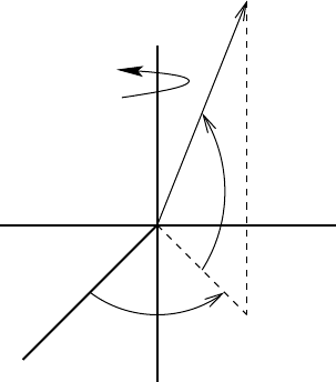
56
CHAPTER 3. OCEAN PRIMITIVE EQUATIONS
Ω
x1
x2
λ
φ
x3 r
Figure 3.1: A schematic of the coordinates used for describing fluid dynamics on
a rotating sphere, where the rotation axis is aligned through the north pole of the
sphere. The coordinate 0 ≤
λ
≤2
π
is the longitude, with positive values measured
eastward from Greenwich, England. The coordinate
φ
is the latitude, with values
φ
=0 at the equator and
φ
=
π
/2(−
π
/2)at the north (south) poles. The radial dis-
tance ris measured here with respect to the center of the sphere. The explicit coor-
dinate transformations are x1=rcos
φ
cos
λ
,x2=rcos
φ
sin
λ
, and x3=rsin
φ
.
Note that for many idealized geophysical fluid studies, cartesian coordinates refer
to those defined locally to a tangent plane at some point on the surface of the rotat-
ing sphere. Such
β
-plane or f-plane coordinates (e.g., Gill (1982); Pedlosky (1987))
are distinct from the cartesian coordinates defined here.
3.1.1 Spherical and Cartesian coordinates
The World Ocean forms a thin layer of fluid moving on the rotating earth. For
purposes of ocean climate modeling, it is sufficient to approximate the earth as a
sphere (see Veronis (1973) for a discussion). Such constitutes a fundamental distinc-
tion from non-geophysical fluid mechanics formulations of the equations of motion
(e.g., Landau and Lifshitz (1987)), where the equations are typically derived in 3D
Euclidean space. A rigorous and lucid treatment of fluid motion on arbitrary sur-
faces is given by Aris (1962).
Figure 3.1 provides a schematic illustrating the relation between spherical and
Cartesian coordinates of use for describing fluid dynamics on a rotating sphere. The
axis of rotation passes from the southern pole to the northern pole of the sphere.
Both sets of coordinates are fixed on the rotating sphere (non-inertial coordinates).
In the next subsection, we note that MOM4 generalizes the angular coordinates
(
λ
,
φ
)to allow arbitrary locally orthogonal coordinates to specify angular positions
on the sphere.
3.1.2 Elements of horizontal orthogonal coordinates
MOM4 is written in generalized horizontal coordinates, where horizontal means
coordinates within a locally defined tangent plane on the surface of a spherical

3.1. ORTHOGONAL COORDINATES AND THE TRADITIONAL APPROXIMATION
57
earth (see Figure 3.1). The use of orthogonal curvilinear coordinates (
ξ
1,
ξ
2)allows
for the squared infinitesimal distance between two points in the ocean to be written
as
(ds)2= (h1d
ξ
1)2+ (h2d
ξ
2)2+dz2, (3.1)
where the metric, or stretching functions, h1and h2are non-negative. In terms of
the dimensionful physical horizontal distances
dx =h1d
ξ
1(3.2)
dy =h2d
ξ
2, (3.3)
the line element takes the compact form
(ds)2= (dx)2+ (dy)2+ (dz)2, (3.4)
the volume of an infinitesimal Eulerian region of the ocean is given by
dV = (h1d
ξ
1) (h2d
ξ
2)dz =dx dy dz, (3.5)
and the physical components of the horizontal partial derivatives are
∂x=h−1
1∂1(3.6)
∂y=h−1
2∂2. (3.7)
Figure 3.2 illustrates these formulae. Notably, although the introduction of phys-
ical displacements brings the metric tensor into a form analogous to that for 3D-
Euclidean space, the non-Euclidean nature of the sphere manifests by the non-
vanishing commutator
∂x,∂y=∂x∂y−∂y∂x= (∂xln dy)∂y−(∂yln dx)∂x, (3.8)
which vanishes only when the horizontal geometry is flat instead of curved. In
particular, the use of spherical coordinates leads to
∂x,∂y=tan
φ
R∂x. (3.9)
3.1.3 Geometry of the Traditional Approximation
The Traditional Approximation assumes that the metric functions h1and h2are
dependent only on the horizontal coordinates (
ξ
1,
ξ
2). Radial dependence of the
metric functions is reduced to a constant radial factor R, where
R=6.371 ×10⁶m (3.10)
is the radius of a sphere with the same volume as the earth. Therefore, the distances
used to compute partial derivatives, covariant derivatives, areas, and volumes are
determined by a metric tensor whose components are functions only of the hori-
zontal position on the sphere.
This geometric approximation is accurate for many purposes because the ocean
forms a thin layer of fluid moving on the outer part of the earth. For example,
vertical motions of fluid parcels in stratified regions of the World Ocean occur over
distances of only a few centimeters to meters per day, which is far smaller than the
earth’s radius. For larger deviations, such as those occuring in convective regions,
the Traditional Approximation may be less useful (see Marshall et al. (1997) for a
discussion).
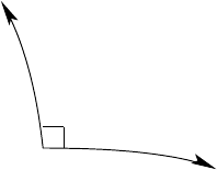
58
CHAPTER 3. OCEAN PRIMITIVE EQUATIONS
ξ2
ξ1
Figure 3.2: Illustrating the generalized horizontal orthogonal coordinates used in
MOM4. The coordinate lines intersect at right angles, but generally do not fol-
low lines parallel to constant longitude or latitude on the sphere. An infinites-
imal horizontal region has area given by dA = (h1d
ξ
1) (h2d
ξ
2) = dx dy. For
spherical coordinates (
ξ
1,
ξ
2) = (
λ
,
φ
), the infinitesimal horizontal distances are
dx = (rcos
φ
)d
λ
and dy =r d
φ
.
3.2 Ocean primitive equations
The laws of classical physics, including Newtonian mechanics and linear irreversible
thermodynamics, form a theoretical basis for a physical description of ocean dy-
namics. MOM4 also exploits the Traditional Approximation described in Section
3.1. Although previously fundamental to z-coordinate ocean models, MOM4 has
eliminated the Boussinesq approximation using the methods of Greatbatch et al.
(2001). A full accounting of how MOM4 discretizes a non-Boussinesq is given by
Griffies (2004). The purpose of this section is to summarize these equations.
3.2.1 Kinematics, dynamics, and tracers
In fluid mechanics, mass conservation is associated with fluid kinematics, whereas
momentum conservation constitutes the fluid dynamics. Mass conservation for a
fluid parcel renders a relation between velocity and in situ density often known as
the continuity equation
ρ
,t+∇ · (
ρ
v) = 0. (3.11)
Conservation of linear momentum for a fluid parcel leads to the prognostic equa-
tion for the velocity field
(
ρ
v),t+∇· (
ρ
v v) = −
ρ
gˆz−(f+M)ˆz∧
ρ
v−∇p+
ρ
F(v). (3.12)
In these equations,
ρ
is the in situ density,
v= (u,w)(3.13)
is the three-dimensional velocity field, pis the pressure field, and
M=v∂xln dy −u∂yln dx (3.14)
is the advection metric frequency arising from the non-Euclidean nature of the sphere.
The friction vector F(v)is associated with momentum transport due to molecular

3.2. OCEAN PRIMITIVE EQUATIONS
59
viscosity.1Following the Traditional Approximation, we assume a hydrostatic bal-
ance for the vertical momentum equation, thus rendering
(
ρ
u),t+∇· (
ρ
v u) = −(f+M)ˆz∧
ρ
u−∇p+
ρ
F(u)(3.15)
p,z=−
ρ
g. (3.16)
Coupled to the mass and momentum equations is the equation for conserva-
tion of tracers. There are three main ocean tracers: passive tracers, such as certain
biological constituents, the active tracers temperature and salinity, and dynamical
tracers such as potential vorticity. The terms passive and active refer to their influ-
ence on density, thus influencing dynamics through pressure. MOM4 time steps
the equations for passive and active tracers, whose form is generally given by
(
ρ
T),t+∇· (
ρ
Tv) = −∇ ·(
ρ
F) +
ρ
S. (3.17)
In this equation, Tis the tracer mass per mass of water (i.e., the tracer concentration),
The tracer flux Fis interpreted as that arising from sub-grid-scale (SGS) molecular
processes, such as molecular diffusion. It will be reinterpreted in terms of ensemble
averages in Section 3.3. Sis an interior tracer source term whose form depends on
details of the particular tracer.
3.2.2 Boussinesq equations
The Boussinesq equations are recovered by setting
ρ
→
ρ
owherever it appears,
except when multiplying gravity
∇· v=0 (3.18)
u,t+∇· (v u) = −(f+M)ˆz∧u−∇(p/
ρ
o) + F(u)(3.19)
p,z=−
ρ
g(3.20)
T,t+∇·(Tv) = −∇·F+S. (3.21)
The constraint ∇· v=0 means the Boussinesq fluid parcels conserve their volume
instead of their mass.
3.2.3 Vertically integrated equations
To time step the dynamical equations, it is most efficient to separate the fast ver-
tically integrated processes from the slower vertically dependent processes. For
this purpose, we integrate the continuity equation over the full ocean column of
thickness
D=H+
η
, (3.22)
where H=H(
ξ
1,
ξ
2)is the time independent ocean depth, and
η
=
η
(
ξ
1,
ξ
2,t)is
the time dependent deviation of the ocean surface from its resting state at z=0.
Assuming mass sources/sinks only at the ocean surface leads to the balance of mass
per unit area within an ocean column
(
ρ
zD),t=−
ρ
o∇· e
U+
ρ
wqw(3.23)
1Ensemble averaging (Section 3.3) introduces more substantial SGS processes associated with
larger-scale turbulence, such as that occuring at the ocean’s microscale to mesoscale ranges.

60
CHAPTER 3. OCEAN PRIMITIVE EQUATIONS
as well as the surface and bottom kinematic boundary conditions
ρ
(∂t+u·∇)
η
=
ρ
wqw+
ρ
wat z=
η
(3.24)
u·∇H+w=0 at z=−H. (3.25)
In these expressions,
ρ
oe
U=Z
η
−Hdz
ρ
u(3.26)
is the depth integrated horizontal momentum density,
ρ
z=D−1Z
η
−Hdz
ρ
(3.27)
is the depth averaged density,
ρ
ois a constant density set to
ρ
o=1035 kg/m3(3.28)
(see page 47 of Gill (1982)), and
ρ
wqwis the mass per unit time per unit horizontal
area of fresh water crossing the ocean surface.
To consider the time tendency for free surface height
η
, we expand the columnar
mass balance (3.23) to reveal
ρ
z
η
,t=−
ρ
o∇· e
U+
ρ
wqw−D∂t
ρ
z. (3.29)
Consequently, the ocean surface height is affected by three processes: convergence
of vertically integrated momentum, mass entering through the ocean surface, and
dilatations of the water column associated with changes in vertically integated den-
sity field (i.e., steric effects).
A similar analysis for a Boussinesq column of fluid, assuming volume sources/sinks
only at the ocean surface, leads to the balance of volume per unit area within an
ocean column
η
,t=−∇ · U+qw(3.30)
as well as the surface and bottom kinematic boundary conditions
(∂t+u·∇)
η
=qw+wat z=
η
(3.31)
u·∇H+w=0 at z=−H, (3.32)
where
U=Z
η
−Hdz u(3.33)
is the depth integrated horizontal velocity field, and qwis the volume per unit time
per unit horizontal area of fresh water crossing the ocean surface. Notably, the sur-
face height is affected only by convergence of vertically integrated momentum and
surface fluxes of volume; steric effects are absent in Boussinesq fluid kinematics.
3.3 Ensemble averaged ocean primitive equations
The ocean is fundamentally turbulent. Given sensitive dependence on initial con-
ditions, and the limitations of ocean measurements, it is not possible to obtain com-
plete knowledge of the ocean state. Therefore, when formulating the ocean’s gov-
erning equations, it is necessary to recognize our limited access to information.
3.3. ENSEMBLE AVERAGED OCEAN PRIMITIVE EQUATIONS
61
3.3.1 Ensemble averages
A common way to account for incomplete information is to consider ensemble av-
erages. As in statistical mechanics, ensemble averages are obtained by formally
considering an infinite number of ocean states, each of which is described by the
kinematic, dynamic, and tracer balances of Section 3.2. Our interpretation of en-
semble averages directly associates the distance in phase space between members
of an ensemble with the space-time scales that are not resolved by the “averaged
observer.” Assuming z-coordinates, we take ensemble averages at a fixed point in
space-time (i.e., a single point Eulerian average), and note that they commute with
all space-time derivatives and integrals.
Even though we specify averaging at a particular space-time point, there remain
ambiguities in details of the averaging method. Different methods reveal different
aspects of the averaged or mean dynamics, and deviations from the mean. Density
weighted averaging plays a central role in our preferred method. Such averaging has
recently become more commonplace in the ocean modeling literature (e.g., Smith
(1999); McDougall et al. (2003a); Lu (2001), yet it has long been part of the com-
pressible fluids literature (e.g., Favre (1965) as noted in the footnote on pages 21-22
of Hinze (1975)).
3.3.2 Averaged kinematics independent of dynamical assumptions
There are two forms of fluid parcel kinematics of importance for ocean modeling:
parcels conserving their volume and parcels conserving their mass. In general,
parcel kinematic relations provide constraints on the fluid that are maintained re-
gardless the dynamics. Therefore, we believe it to be key to the integrity and usabil-
ity of the equations describing the ensemble averaged ocean, and consequently the
ocean model, that kinematics of the averaged fluid remains independent of dynam-
ical assumptions. In particular, we do not wish to require specification of unknown
closure terms, whose form depends on dynamical details, in order to determine
kinematic relations satisfied by the averaged ocean or the ocean model. Care in for-
mulating and interpreting the averaged equations is required to maintain this very
basic principle.
A key motivation for using density weighted averaging is that it assists in our
desire to keep the averaged parcel kinematics independent of dynamical closure as-
sumptions. Providing such a simple mapping between unaveraged and averaged
kinematics generally does not require much thought when averaging the Boussi-
nesq equations, since volume conservation ∇ · v=0 is a linear constraint. Yet
for non-Boussinesq equations, mass conservation
ρ
,t+∇ · (v
ρ
) = 0 is a nonlinear
constraint, thus requiring extra consideration.
Besides the mathematical utility of the density weighed approach for the non-
Boussinesq system, McDougall et al. (2003a) argued for maintaining this average
even when considering the averaged Boussinesq equations. Their reasoning is
based on noting that the resulting Boussinesq system is far more accurate than the
mean-field equations resulting from non-density weighted averages. In this con-
text, accuracy is based on comparing with the small levels of diapycnal mixing in
the ocean interior.

62
CHAPTER 3. OCEAN PRIMITIVE EQUATIONS
3.3.3 Linear momentum density
For the purpose of ensemble averaging, the linear momentum density (momentum
per volume)
ρ
v=
ρ
oe
v(3.34)
plays a fundamental role. Hence, let us introduce it to the unaveraged balances
from Section 3.2 to yield
ρ
,t+
ρ
o∇· e
v=0 (3.35)
e
v,t+∇· [(
ρ
o/
ρ
)e
ve
v] + (
ρ
o/
ρ
)f
Mˆz∧e
v=−(
ρ
/
ρ
o)gˆz−fˆz∧e
v−∇(p/
ρ
o) + (
ρ
/
ρ
o)F(v)
(3.36)
(
ρ
T),t+
ρ
o∇· (Te
v) = −∇ ·(
ρ
F) +
ρ
S, (3.37)
where we wrote the advection metric frequency as
M=v∂xln dy −u∂yln dx = (
ρ
o/
ρ
) (e
v∂xln dy −e
u∂yln dx) = (
ρ
o/
ρ
)f
M. (3.38)
3.3.4 Summary of the averaged equations
Details of the averaging process require more discussion that warranted here. We
refer the reader to McDougall et al. (2003a), Greatbatch et al. (2001), and Griffies
(2004) for systematic development. For the present purposes, it is sufficient to sum-
marize the results from Griffies (2004).
Using an angular bracket to signify ensemble mean, the averaged non-Boussinesq
equations take the following form. First, mass conservation for a fluid parcel and
for a vertical column of fluid is given by
h
ρ
i,t+
ρ
o∇ · he
vi=0 (3.39)
D∗h
ρ
iz,t=−
ρ
o∇· he
Ui+
ρ
o˜
q∗
w. (3.40)
For the Boussinesq fluid, volume conservation for the parcel and column are given
by
∇· he
vi=0 (3.41)
η
∗
,t=−∇ ·he
Ui+˜
q∗
w. (3.42)
In these equations, we introduced density weighted averages via
h
ρ
ihΨi
ρ
=h
ρ
Ψi, (3.43)
and the linear momentum density of fresh water
ρ
o˜
qw=
ρ
wqw. (3.44)
A starred quantity represents a modified mean field given by an infinite series of en-
semble mean correlations (Griffies (2004)). The precise relation between the starred
quantities and the correlations is not important, since the modified mean fields
provide the appropriate field to discretize in an ocean model, instead of the corre-
sponding ensemble mean field.
3.3. ENSEMBLE AVERAGED OCEAN PRIMITIVE EQUATIONS
63
The surface and bottom kinematic boundary conditions for the non-Boussinesq
fluid are
h
ρ
i
η
∗
,t+
ρ
ohe
ui· ∇
η
∗=
ρ
ohe
wi+
ρ
o˜
q∗
wat z=
η
∗(3.45)
he
ui· ∇H+he
wi=0 at z=−H(3.46)
and for the Boussinesq fluid we have
η
∗
,t+he
ui· ∇
η
∗=he
wi+˜
q∗
wat z=
η
∗(3.47)
he
ui· ∇H+he
wi=0 at z=−H. (3.48)
The tracer budget for the non-Boussinesq fluid is
(h
ρ
ihTi
ρ
),t+
ρ
o∇· (he
vihTi
ρ
) = −
ρ
o∇· h˜
Fsgsi+h
ρ
ihSi
ρ
(3.49)
and for the Boussinesq fluid
∂thTi
ρ
+∇· (he
vihTi
ρ
) = −∇ · h˜
Fsgsi+hSi
ρ
. (3.50)
Finally, the non-Boussinesq momentum budget is
he
vi,t+∇· (hvi
ρ
he
vi) + hf
Mi ˆz∧hvi
ρ
=
−(h
ρ
i/
ρ
o)gˆz−fˆz∧he
vi− ∇(hpi/
ρ
o) + h˜
Fv
sgsi(3.51)
whereas the Boussinesq budget is
he
vi,t+∇· (he
vihe
vi) + hf
Mi ˆz∧he
vi=
−(h
ρ
i/
ρ
o)gˆz−fˆz∧he
vi− ∇(hpi/
ρ
o) + h˜
Fv
sgsi. (3.52)
Recall that he
vi=hvi
ρ
for a Boussinesq fluid, whereas
ρ
ohe
vi=h
ρ
ihvi
ρ
for the
non-Boussinesq case. In the tracer equations, the SGS flux term is given by
ρ
Fsgs =
ρ
T0
ρ
v0
ρ
≡
ρ
o˜
Fsgs, (3.53)
which dominates the contribution from molecular diffusion. The SGS friction vec-
tor ˜
Fv
sgs likewise incorporates SGS turbulence terms
ρ
F(v)
sgs =∇ ·(
ρ
v0
ρ
v0
ρ
) + ˆz∧
ρ
M0
ρ
v0
ρ
≡
ρ
o˜
F(v)
sgs . (3.54)
The averaged equations have the same mathematical form as the unaveraged
equations given in Section 3.2. Precisely, the mapping between unaveraged and
averaged fields is given by
ρ
→ h
ρ
i(3.55)
p→ hpi(3.56)
v→ hvi
ρ
(3.57)
e
v→ he
vi(3.58)
T→ hTi
ρ
(3.59)
˜
F→ h˜
Fsgsi(3.60)
S → hSi
ρ
(3.61)
˜
Fv→ h˜
Fv
sgsi(3.62)
η
→
η
∗(3.63)
qw→q∗
w. (3.64)
˜
qw→˜
q∗
w. (3.65)

64
CHAPTER 3. OCEAN PRIMITIVE EQUATIONS
This mapping is very useful for purposes of analyzing properties of the two sys-
tems, such as their energetic balances discussed in Chapter 6. The fewer equations
we need to concern ourselves with, the better!
3.4 Mapping to ocean model variables
Having established a set of self-consistent averaged equations, we are ready to
write down the equations to be discretized in the numerical model. The discretiza-
tion is applied to the appropriate averaged continuous equations, which are written
down in this section in a bit more tidy manner than in the previous section.
First, the density variable to be discretized by the ocean model is the Eulerian
mean density
h
ρ
i →
ρ
model. (3.66)
Again, this is the in situ density used for the mass continuity equation. It is gen-
erally distinct from potential density. At this point the “model” suffix refers to the
continuous ocean model, since no discretization has yet occured. Through the hy-
drostatic approximation, h
ρ
i →
ρ
model leads to
hpi → pmodel. (3.67)
As argued in Section 3.3.2, maintaining a tidy form of the averaged continu-
ity equation motivates our discretizing he
vi, instead of the conventional hvi. The
distinction is nontrivial for both non-Boussinesq and Boussinesq ocean models.
Hence, we make the correspondence
he
vi → vmodel. (3.68)
Analogously, we choose to use hTi
ρ
in our model, instead of the conventional hTi
hTi
ρ
→Tmodel. (3.69)
Again, the distinction between hTi
ρ
and hTiis nontrivial for both non-Boussinesq
and Boussinesq ocean models. Finally, the surface height in the ocean model corre-
sponds to the modified mean surface height
η
∗
η
∗→
η
model, (3.70)
as will the modified mean surface fresh water flux
˜
q∗
w→(qw)model. (3.71)
These mappings lead to the following equations to be discretized in the non-
Boussinesq ocean model (dropping the “model” subscript for brevity)
ρ
,t+
ρ
o∇· v=0 (3.72)
(h
ρ
z),t=−
ρ
o∇· U+
ρ
oqw(3.73)
v,t+∇· [(
ρ
o/
ρ
)v v] + (
ρ
o/
ρ
)Mˆz∧v=
−(
ρ
/
ρ
o)gˆz−fˆz∧v− ∇(p/
ρ
o) + (
ρ
/
ρ
o)F(v)(3.74)
(
ρ
T),t+
ρ
o∇· (vT) = −
ρ
o∇· F+
ρ
S, (3.75)
3.4. MAPPING TO OCEAN MODEL VARIABLES
65
where we also made the correspondence
h˜
Fsgsi → Fmodel (3.76)
hSi
ρ
→ Smodel (3.77)
h˜
Fv
sgsi → Fv
model. (3.78)
These equations are combined with the surface and bottom kinematic boundary
conditions
ρ η
,t+
ρ
ou·∇
η
=
ρ
ow+
ρ
oqwat z=
η
(3.79)
u·∇H+w=0 at z=−H. (3.80)
The mapping from unaveraged to averaged fields, and then from averaged to model
fields, is summarized in Table 3.1. This table is the key result from this chapter.
The continuous model equations presented above are identical in form to the
continuous unaveraged non-Boussinesq equations summarized in Section 3.2. Al-
though in the end somewhat trivial (i.e., what a round-about way to get back to the
same equations!), the intermediate steps reveal a nontrivial interpretation of the
fields discretized in the numerical model. It is hoped that such care in providing a
precise physical and mathematical interpretation for the variables adds rigor and
clarity to the foundations of MOM.
The Boussinesq model equations arise by setting
ρ
model →
ρ
o, except when
multiplying gravity. These equations are
∇· v=0 (3.81)
η
,t=−∇ ·U+qw(3.82)
v,t+∇· (v v) + Mˆz∧v=−(
ρ
/
ρ
o)gˆz−fˆz∧v−∇(p/
ρ
o) + F(v)(3.83)
T,t+∇· (vT) = −∇ ·F+S(3.84)
along with the surface and bottom kinematic boundary conditions
η
,t+u·∇
η
=w+qwat z=
η
(3.85)
u·∇H+w=0 at z=−H. (3.86)
As emphasized by McDougall et al. (2003a) and Greatbatch et al. (2001), upon mak-
ing the hydrostatic approximation, these equations for the Boussinesq ocean model
are identical to those integrated by the Boussinesq version of MOM, with the ex-
ception of details that have been absorbed by the turbulence tracer and momentum
fluxes Fand Fv. Additionally, McDougall et al. argue that the interpretation of
model fields as proposed here allows for the Boussinesq equations to be far more
accurate than the alternative interpretation. Hence, for this reason, and for reasons
of mathematical elegance, we prefer the interpretation summarized by Table 3.1 for
the variables carried by the Boussinesq and non-Boussinesq versions of MOM.

66
CHAPTER 3. OCEAN PRIMITIVE EQUATIONS
Unaveraged Averaged Model Model Discrete
ρ
h
ρ
i
ρ
model
ρ
phpipmodel p
˜vh˜vivmodel v
vhvi
ρρ
model v
ρ
model =
ρ
ovmodel
ρ
v
ρ
=
ρ
ov
η η
∗
η
model
η
˜
qw˜
q∗
w(qw)model qw
ThTi
ρ
Tmodel T
S hSi
ρ
Smodel S
˜
Fh˜
FsgsiFmodel F
˜
F(v)h˜
F(v)
sgs iF(v)
model F(v)
Table 3.1: Correspondence between unaveraged continuous fields, ensemble aver-
aged continuous fields, continuous model fields, and discrete model fields.

CHAPTER
FOUR
Grids and halos
Contents
4.1 The B-grid used in MOM4 . . . . . . . . . . . . . . . . . . . . . . 67
4.1.1 Variables on the B-grid . . . . . . . . . . . . . . . . . . . . . 68
4.1.2 Describing the horizontal grid . . . . . . . . . . . . . . . . 68
4.1.2.1 Four basic grid points and corresponding cells . 68
4.1.2.2 Computing the grid distances . . . . . . . . . . . 69
4.1.2.3 Grid distances carried by the model . . . . . . . . 71
4.2 The Murray (1996) tripolar grid . . . . . . . . . . . . . . . . . . . 71
4.3 Specifying fields and grid distances within halos . . . . . . . . . 77
4.3.1 Interior domains . . . . . . . . . . . . . . . . . . . . . . . . 77
4.3.2 Exterior domains . . . . . . . . . . . . . . . . . . . . . . . . 78
4.3.2.1 Solid wall boundary conditions . . . . . . . . . . 78
4.3.2.2 Periodic boundary conditions . . . . . . . . . . . 78
4.3.3 The bipolar Arctic grid . . . . . . . . . . . . . . . . . . . . . 79
4.3.3.1 Fields defined at points T,U,N, and E . . . . . . . 79
4.3.3.2 Grid distances for horizontal quarter-cells . . . . 80
4.3.3.3 Grid distances for horizontal full cells . . . . . . 82
4.3.3.4 Summary of redundancies and halo mappings . 83
The purpose of this chapter is to detail the horizontal B-grid used in MOM4 as
well as the specification of field and grid values in halo regions.
4.1 The B-grid used in MOM4
The continuum partial differential equations of MOM4 are derived and discussed in
Griffies (2004). Semi-discrete versions of these equations are also discussed, where
the equations are cast on an Arakawa B-grid. As summarized in the review article
by Griffies et al. (2000a), the B-grid allows for a reasonably accurate representation
of geostrophic currents even when running a coarse grid model. It was this prop-
erty that motivated Bryan (1969) to choose the B-grid. Future model development,
67

68
CHAPTER 4. GRIDS AND HALOS
in which the first baroclinic radius of deformation is assumed to be well resolved,
will likely focus on the C-grid. The reasons are that the C-grid typically performs
better at fine resolution than course, and it has some advantages over the B-grid
when discretizing transport operators. Nonetheless, as pointed out by Webb et al.
(1998), there will always be unresolved baroclinic modes, such as in the equato-
rial region. Hence, the B-grid may continue to have some advantage even at fine
resolution.
The purpose of this section is to document the grid used in MOM4. In addi-
tion to the usual B-grid conventions, we describe grid factors used to build discrete
derivative and integral operators. Chapter 16 of The MOM3 Manual Pacanowski and Griffies
(1999) provides a complete discussion of the three slices x−y,x−z, and y−z. Al-
though we briefly discuss the vertical grid, our main focus is on the horizontal x−y
plane since this is where details of domain decomposition on parallel computers is
considered.
4.1.1 Variables on the B-grid
Figure 4.1 illustrates the horizontal arrangement of prognostic model fields used
in MOM4’s B-grid. The B-grid places both horizontal prognostic velocity compo-
nents at the same point. MOM’s convention is that this point lives at the “northeast
corner” of the corresponding tracer cell, where northeast is in a generalized sense
when using general orthogonal coordinates. With half-integer notation, the U-point
lives at (i+1/2, j+1/2)whereas the T-point is at (i,j). As density is a function of
temperature, salinity, and pressure, density is naturally defined at the tracer point,
as is hydrostatic pressure.
The vertical velocity component is defined according to the requirements of con-
tinuity across the tracer and velocity cells. Hence, this component lives at the bot-
tom face of the corresponding cell. Once the horizontal grid placement is defined,
the vertical position is specified for both the grid point and the vertical velocity po-
sition. Chapter 16 of The MOM3 Manual provides further details of the vertical
grid.
4.1.2 Describing the horizontal grid
With a generalized horizontal grid, there are many grid distances required to com-
pute discrete derivatives and integrals. When constructing the grid distances in
MOM4, we aimed to design a structure useful for both B and C-grids.1It is with
this goal in mind that the names for the grid distances in the grid generator mod-
ule are distinct from grid distances used in MOM4’s grids module. We note the
mapping between the two grid conventions in the following.
4.1.2.1 Four basic grid points and corresponding cells
On both the B and C grids, it is useful to consider the tracer cell as the basic cell, and
all other cells in their relation to the tracer cell. Given this convention, there are four
basic grid points and corresponding grid cells that can be identified: Ti,j,Ei,j,Ci,j,
1Other grids can also be accounted for using the conventions described here. Our focus is on the
B and C grids, as these are the two most commonly used grids in ocean modeling.
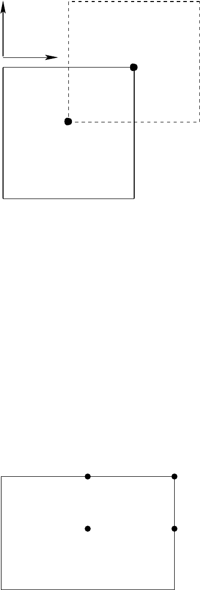
4.1. THE B-GRID USED IN MOM4
69
T(i,j,k)
U(i,j,k)
j
i
Figure 4.1: Illustration of how fields are placed on the horizontal B-grid used in
MOM4. Velocity points Ui,j,kare placed to the northeast of tracer points Ti,j,k. Both
horizontal velocity components ui,j,kand vi,j,kare placed at the velocity point Ui,j,k.
and Ni,j. Figure 4.2 illustrates these points as oriented according to the tracer cell,
with Ti,jthe usual tracer point. Ci,jlives at the northeast corner of the tracer cell,
and so represents B-grid velocity point Ui,j.Ni,jlives at the north face of the tracer
cell and so represents the C-grid meridional velocity point. Ei,klives at the east
face of the tracer cell and so is the C-grid zonal velocity point. The geographical
coordinates of these four points is sufficient to place them on the discrete lattice.
4.1.2.2 Computing the grid distances
To support a discretized calculus, we must specify distances between grid points
and the grid cells. Knowing the geographical position of the four basic grid points
T(i,j) E(i,j)
C(i,j)
N(i,.j)
Figure 4.2: The four basic grid points for the B and C grids: Ti,j,Ci,j,Ei,j, and Ni,j.
Ti,jis the usual tracer point, with the corner Ci,jand side points Ei,j,Ni,jassociated
with the tracer point.

70
CHAPTER 4. GRIDS AND HALOS
as well as the vertices of their corresponding grid cells is not sufficient. In addition,
we need information regarding the metric or stretching functions specific to the
coordinate system used to tile the sphere.
The traditional approach is to use spherical coordinates for tiling the sphere. In
this method, the distance between two points zonally displaced a finite distance
from one another is given by the analytic formula
∆x[a,b] = Rcos
φ
λ
b
Z
λ
a
d
λ
= (Rcos
φ
) (
λ
b−
λ
a), (4.1)
and the distance between two points along a line of constant longitude is given by
∆y[a,b] = R
φ
b
Z
φ
a
d
φ
=R(
φ
b−
φ
a). (4.2)
Writing this expression in a general manner leads to the generalized zonal and gen-
eralized meridional distance given by
∆x[a,b] =
ξ
(a)
1
Z
ξ
(b)
1
h1d
ξ
1(4.3)
∆y[a,b] =
ξ
(a)
2
Z
ξ
(b)
2
h2d
ξ
2, (4.4)
where (
ξ
1,
ξ
2)represent generalized orthogonal coordinates, and (h1,h2)are the
stretching functions specific to the coordinate system. They determine the distance
between two infinitesimally close points via the line element formula
(ds)2= (h1d
ξ
1)2+ (h2d
ξ
2)2. (4.5)
With dx =h1d
ξ
1and dy =h2d
ξ
2, the line element formula takes the form of the
usual Cartesian expression
(ds)2= (dx)2+ (dy)2. (4.6)
It is not possible to perform the distance integrals analytically for an arbitrary
general orthogonal coordinate system. Therefore, approximations must be made.
Indeed, in MOM3 the analytical form for the zonal distance was actually approxi-
mated according to
∆x≈Rcos
φ
(4.7)
where
φ
= (
φ
1+
φ
2)/2 (see discussion in Section 39.6 of Pacanowski and Griffies
(1999)). Assuming information is available only at the grid points and at the cell
vertices, MOM4 chooses to compute the distance between two points along a gen-
eralized zonal direction (i−line) as
∆x[a,b] =
ξ
(a)
1−
ξ
(b)
1h(a)
1+h(b)
1/2. (4.8)
4.2. THE MURRAY (1996) TRIPOLAR GRID
71
Likewise, the distance along a generalized meridional direction (j−line) is com-
puted as
∆y[a,b] =
ξ
(a)
2−
ξ
(b)
2h(a)
2+h(b)
2/2. (4.9)
4.1.2.3 Grid distances carried by the model
Given coordinates for the grid points and grid vertices, as well as the stretching
functions evaluated at these points, we can use the approximate expressions (4.8)
and (4.9) to compute distances between the T,U,N, and E points. Figure 4.3 shows
the notation for the grid distances that define four quarter-cells splitting up each
tracer and velocity cell. Shown is the notation used in the grid descriptor module
as well as that used in MOM4. The full dimensions of the tracer and velocity cells
are shown in Figure 4.4, where again the distances computed in the grid descriptor
module are translated into the grid distances used in MOM4. Finally, Figure 4.5
shows the distances specifying the separation between adjacent tracer and velocity
points.
4.2 The Murray (1996) tripolar grid
The Murray (1996) tripolar grid (see his Figure 7) has been a focus of ocean climate
model development with MOM4 during the year 2001-2002. This grid is comprised
of the usual spherical coordinate grid southward of a chosen latitude circle, typi-
cally taken at 65◦N. This part of the grid has a single pole over Antarctica, which is
of no consequence to the numerical ocean climate model. In the Arctic region, the
Murray grid places a bipolar region with two poles situated over land, and so these
poles are also of no consequence to the numerical ocean model.
Figure 4.6 illustrates the grid lines used to discretize the ocean equations in the
Arctic using Murray’s grid. The placement of discrete model tracer and velocity
points along the bipolar grid lines is schematically represented in Figure 4.7. The
arrangement of northern and eastern vector components centered on the tracer cell
faces is shown in Figure 4.8. Details for how to transfer information across the
bipolar prime meridion located along the j=nj line are provided in Section 4.3.
Motivation for choosing the Murray (1996) grid includes the following:
•It removes the spherical coordinate singularity present at the geographical
north pole.
•It maintains the usual spherical coordinate grid lines for latitudes southward
of the Arctic region, thus simplifying analysis.
•It is locally orthogonal, and so can be used with the MOM4 generalized hori-
zontal coordinates.
•Similar grids have been successfully run by the French OPA modeling group
and the Miami MICOM modeling group.
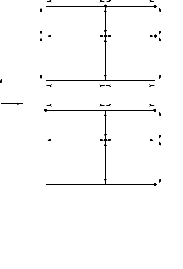
72
CHAPTER 4. GRIDS AND HALOS
dts(i,j)
dus(i,j)
dun(i,j−1)
duw(i,j)due(i−1,j)
T(i,j)
T(i,j)
C(i,j)
E(i,j)
dtw(i,j) dte(i,j)
i
j
(2,2)
(2,1)
ds_20_21_T
ds_21_22_T
ds_10_11_T
ds_11_12_T
ds_00_01_T
ds_01_02_T
ds_02_12_T ds_12_22_T
ds_01_11_T
ds_00_10_T ds_10_20_T
(1,1)
N(i,j)
(1,2)(0,2)
(0,0) (2,0)
(1,0)
(0,1)
ds_11_21_T
U(i−1,j)
dtn(i,j)
U(i,j)
U(i,j−1)
Figure 4.3: Upper panel: Grid distances used to measure the distance between the
four fundamental grid points shown in Figure 4.2. These distances are computed
in the FMS grid descriptor module. The naming convention is based on a Cartesian
grid with the origin at the lower left corner of the tracer cell at (0, 0), the upper
right hand corner is (2, 2), the center at (1, 1), and all other points set accordingly.
The distances are then named as distances between these grid points. Note that
each tracer cell has a local Cartesian coordinate set as here, and so there is redu-
dancy in the various grid distances. Lower panel: When read into MOM4, the grid
distances set the distance between the tracer and velocity points used in the model
(Figure 4.1) and the sides of the corresponding grid cells. A translation of the upper
panel distance names to those used in MOM4 is made within MOM4’s ocean grid
module.
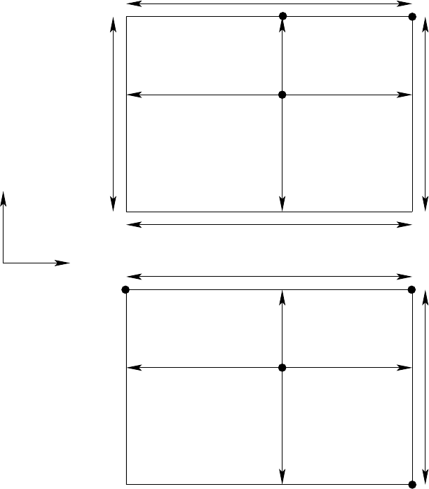
4.2. THE MURRAY (1996) TRIPOLAR GRID
73
C(i,j)
T(i,j)
T(i,j)
U(i,j−1)
dxt(i,j)
dyt(i,j)
dyte(i,j)=dyun(i,j−1)
dxtn(i,j) = dxue(i−1,j)
ds_02_22_T
i
j
(0,1)
ds_10_12_T
ds_01_21_T
(2,2)
(2,0)
(1,0)
ds_00_02_T ds_20_22_T
ds_00_20_T
(0,2)
(0,0)
(2,1)
(1,1)
(1,2)
U(i−1,j) U(i,j)
Figure 4.4: Grid cell distances used for computing the area of a grid cell. These
dimensions are related to the fundamental quarter-cell dimensions shown in Figure
4.3. Upper panel: distances computed in the FMS grid descriptor module. Lower
panel: names of the distances used in MOM4.
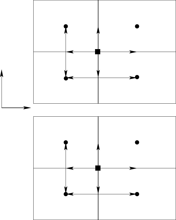
74
CHAPTER 4. GRIDS AND HALOS
T(i,j)
T(i+1,j+1)
T(i,j)
T(i+1,j+1)
dytn(i,j)
dxte(i,j)
dxu(i,j)
dyu(i,j)
C(i,j)
U(i,j)
T(i+1,j)
T(i,j+1)
T(i,j+1)
T(i+1,j)
j
i
ds_00_20_C
ds_00_02_C
Figure 4.5: Distances between fundamental grid points (upper panel) as computed
by the grid descriptor module. These distances are taken into MOM4 and used to set
the distances between tracer and velocity points (lower panel).
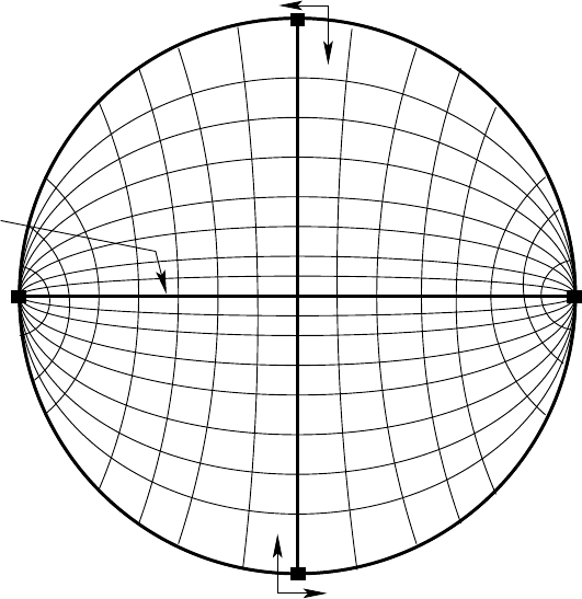
4.2. THE MURRAY (1996) TRIPOLAR GRID
75
j
i
j
i
i=0=ni
i=ni/4
i=3ni/4
j=nj
i=ni/2
Figure 4.6: Illustration of the grid lines forming the bipolar region in the Arctic.
This figure is taken after Figure 7 of Murray (1996). The thick outer boundary is a
line of constant latitude in the spherical coordinate grid. This latitude is typically at
the latitude nearest to 65◦N. As in the spherical coordinate region, lines of constant
imove in a generalized eastward direction. They start from the bipolar south pole
at i=0, which is identified with i=ni. The bipolar north pole is at i=ni/2. As
shown in Figure 4.7, the poles are centered at a velocity point. Lines of constant j
move in a generalized northward direction. The bipolar prime-meridion is situated
along the j-line with j=nj. This line defines the bipolar fold that bisects the tracer
grid. Its fold topology causes the velocity points centered along j=n j to have a
two-fold redundancy (see Figure 4.7 for more details).
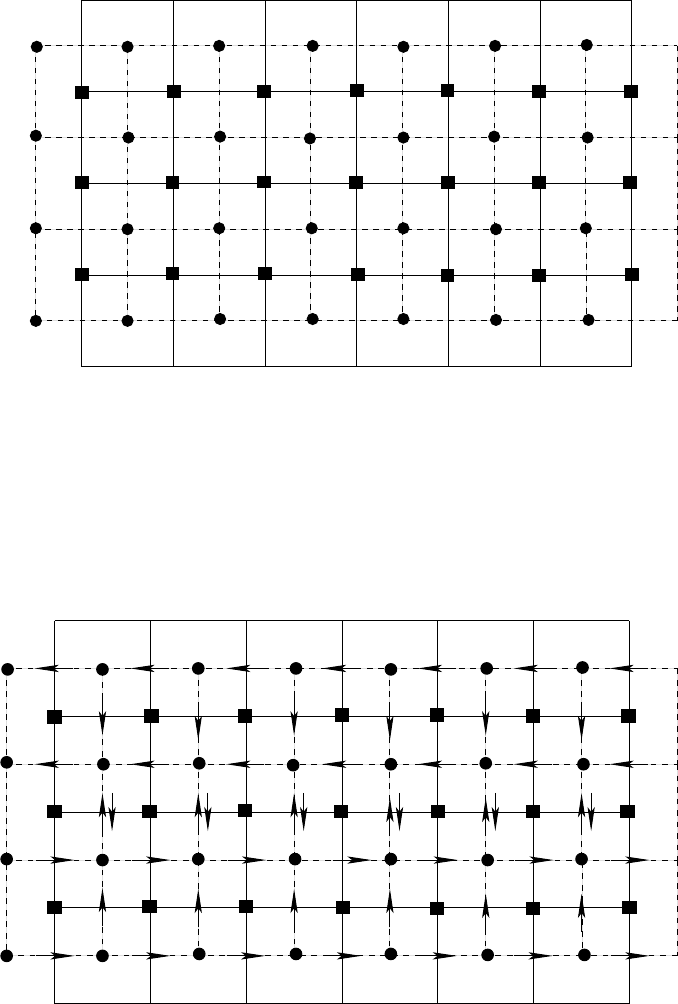
76
CHAPTER 4. GRIDS AND HALOS
T(ni,nj−1)
T(ni−1,nj−1)
T(ni−1,nj) T(ni,nj) T(nj,ni+1)
U(ni−1,nj−1) U(ni,nj−1)
U(ni−1,nj) U(ni,nj)
T(6,nj−1)
T(5,nj−1)T(4,nj−1)
T(3,nj−1)T(2,nj−1)T(1,nj−1)
T(6,nj)T(5,nj)
T(4,nj)
T(3,nj)
T(2,nj)
T(1,nj)
U(6,nj)
U(5,nj)U(4,nj)
U(3,nj)
U(2,nj)
U(1,nj)
U(6,nj−1)U(5,nj−1)
U(4,nj−1)U(3,nj−1)
U(2,nj−1)
U(1,nj−1)
T(10,nj)
T(9,nj)T(8,nj)
T(7,nj)
T(7,nj−1) T(8,nj−1) T(9,nj−1) T(10,nj−1)
U(10,nj−1)U(9,nj−1)U(8,nj−1)U(7,nj−1)
U(10,nj)
U(9,nj)
U(8,nj)
U(7,nj)
U(6,nj)
U(6,nj−1)
T(nj−1,ni+1)
T(0,nj−1)
T(0,nj)
U(0,nj−1)
Figure 4.7: Schematic representation of the tracer and velocity cells on the bipolar
grid shown in Figure 4.6. The global computational domain consists of ni =12
i-points for this example. The j=nj line bisects the tracer grid, which means there
are redundant velocity points along this line. Along an i−line of velocity points,
velocity cells with i=ni/2 live at the bipolar north pole, whereas velocity cells
with i=0=ni live at the bipolar south pole.
E(0,nj−1) E(1,nj−1) E(2,nj−1) E(3,nj−1) E(4,nj−1) E(5,nj−1) E(6,nj−1)
E(0,nj) E(1,nj) E(2,nj) E(3,nj) E(4,nj) E(5,nj) E(6,nj)
E(7,nj−1) E(8,nj−1) E(9,nj−1) E(10,nj−1) E(ni−1,nj−1) E(ni,nj−1)E(6,nj−1)
E(6,nj) E(7,nj) E(8,nj) E(9,nj) E(10,nj) E(ni−1,nj) E(ni,nj)
N(1,nj−1) N(2,nj−1) N(3,nj−1) N(4,nj−1) N(5,nj−1) N(6,nj−1)
N(1,nj) N(2,nj) N(3,nj) N(4,nj) N(5,nj) N(6,nj)
N(7,nj) N(8,nj) N(9,nj) N(10,nj) N(ni−1,nj) N(ni,nj)
N(8,nj−1) N(10,nj−1)N(9,nj−1)N(7,nj−1) N(ni−1,nj−1) N(ni,nj−1)
Figure 4.8: Schematic representation of fields living at the north and east faces of the
tracer cells as configured using the bipolar grid shown in Figure 4.6. Typical fields
of this sort are diffusive and advective tracer flux components, and so they are
components to a vector field, hence the vector notation. The global computational
domain consists of ni =12 i-points for this example. The j=n j line bisects the
tracer grid, which means there are redundant velocity points along this line. Along
an i−line of velocity points, velocity cells with i=ni/2 live at the bipolar north
pole, whereas velocity cells with i=0=ni live at the bipolar south pole.
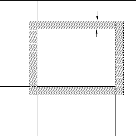
4.3. SPECIFYING FIELDS AND GRID DISTANCES WITHIN HALOS
77
halo for PE(0)
PE(2)
PE(1)
PE(0)
PE(4)
PE(5)
PE(3)
Figure 4.9: Elements of halos needed for computing derivative information on a
local domain. The hatched region is comprised of halo points needed in order for
the processor labelled PE(0) to time step its equations. The halo values must be
transmitted from the surrounding processors since they live outside of PE(0)’s local
domain.
4.3 Specifying fields and grid distances within halos
MOM4 has been designed to run on multiple parallel processors. The computation
of finite derivative operators requires the passage of information across processor
boundaries. In particular, the decomposition of the model’s global domain into mul-
tiple local domains requires that fields and grid information from one local domain
be mapped to halos of adjacent local domains. For second order numerics, the
calculation of derivatives on the boundary of a local domain requires information
within one grid row halo surrounding the local domain. Higher order numerics
require larger halos.
4.3.1 Interior domains
Within the interior of the ocean model, away from global boundaries, the mapping
between domains is performed using an FMS utility that fills the halo points for
one local domain using information available to another local domain. Figure 4.9
illustrates this basic point. Shown is a central processor, arbitrarily labelled PE(0),
and a surrounding hatched region representing halo points. The width of the halo
is a function of the numerics used in the model. For second order numerics, a halo
width of a single point is sufficient. The values of fields and grid factors within the
halo are transmitted from the surrounding processors to PE(0) in order for PE(0) to
time step its portion of the ocean equations discretized on its local domain.
78
CHAPTER 4. GRIDS AND HALOS
4.3.2 Exterior domains
For processors whose boundary touches the global model boundary, it is necessary
to specify whether the global boundary is a solid wall as in a sector model, peri-
odic as in a zonal channel, or folded as in the bipolar grid of Murray (1996). That
is, we must specify the model’s topology. Each of these three topologies requires
some special consideration, with the cases built into the MOM4 update boundary
condition module. Since these conditions are specific to the experimental design,
they are handled by a MOM4 module that sets the boundary conditions. We focus
here on the three common topologies supported by MOM4. A fourth case, open
boundary conditions, is discussed separately in chapter ??.
4.3.2.1 Solid wall boundary conditions
For a solid wall boundary condition, all fluxes passing across the walls are zeroed
out via masks, and fields within the solid wall are either trivial or masked. Hence,
no halo updates are necessary for fields and fluxes at solid walls. However, it is im-
portant to specify self-consistent grid distances separating points within the solid
wall from those within the model’s computational domain. The reason is that vari-
ous remapping operators require grid distances be well defined for all points within
the computational domain, including those distances reaching into the halo. See
Chapter 5 for details of remapping operators. For this reason, we extend the grid
into the solid wall halo so that resolution in this region is given by the resolution
between the two nearest interior points.
4.3.2.2 Periodic boundary conditions
Zonally periodic channels (x-cyclic) are commonly run for idealized studies. Meri-
odionally periodic (y-cyclic) domains may also be of interest for simulations on an
f−plane or
β
-plane. For these reasons, we need to specify grid factors within the
halo assuming periodicity at the global domain boundary.
We focus here on the needs of the more common zonally periodic boundary
conditions, and refer to Figure 4.10. The same considerations hold for y-cyclic con-
ditions. For either case, we envision the grid wrapped onto itself in the appropriate
direction. With second order numerics, computation of the prognostic tracer in grid
cells Ti=1, jrequires information regarding Ti=0, j. Likewise, Ti=ni,jrequires informa-
tion about Ti=ni+1, j. Higher order numerics will need to reach out further.
First consider the eastern boundary of the domain where i=ni. For a single
grid halo, we need to specify values of fields living at the T,E,N, and Cpoints at
i=ni +1 (recall Figures 4.1 and 4.2 where the Cpoint is equivalent to the B-grid U
point). Zonal periodicity renders the equalities
Tni+1, j=T1, j(4.10)
Eni+1, j=E1, j(4.11)
Nni+1, j=N1, j(4.12)
Cni+1, j=C1, j. (4.13)
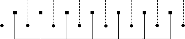
4.3. SPECIFYING FIELDS AND GRID DISTANCES WITHIN HALOS
79
T(1,j) T(2,j) T(3,j) T(ni−1,j) T(ni,j)
T(4,j)
U(1,j) U(2,j) U(3,j) U(4,j) U(ni−1,j) U(ni,j)
T(ni+1,j)
U(0,j)
T(0,j)
Figure 4.10: A zonally periodic array of tracer and velocity points with a single
halo point. In this example there are ni =6 points in the global computational
domain, and halo =1 point in the surrounding halo region. The cyclic mapping
leads us to specify halo points with values Ti=0, j=Ti=ni,j,Ti=ni+1, j=Ti=1, j, and
Ui=0, j=Ui=ni,j.
More generally, halo points with ni <i≤ni +halo acquire the x-cyclic mapping
Ti,j=Ti−ni,j(4.14)
Ei,j=Ei−ni,j(4.15)
Ni,j=Ni−ni,j(4.16)
Ci,j=Ci−ni,j. (4.17)
At the western boundary, similar considerations lead to halo points 1 −halo ≤i<1
mapped to interior points according to
Ti,j=Ti+ni,j(4.18)
Ei,j=Ei+ni,j(4.19)
Ni,j=Ni+ni,j(4.20)
Ci,j=Ci+ni,j. (4.21)
4.3.3 The bipolar Arctic grid
The ideas considered for the cyclic case are now generalized to the more complex
topology of the Murray (1996) bipolar grid shown in Figures 4.6 and 4.7. In partic-
ular, Figures 4.7 and 4.8 allow us to deduce the mappings between related points
on the grid.
4.3.3.1 Fields defined at points T,U,N, and E
The generalized zonal direction (along a constant i-line) is treated with the x-cyclic
conditions shown Figure 4.10. It is the bipolar prime meridion along the j−line
with j=nj that introduces the most subtle issues. This line bisects the tracer grid.
Relating points across the prime meridion requires knowledge of the tensorial na-
ture of the field being considered. In particular, scalar fields map without a change
in sign, whereas components of a vector field have a sign change.
The U−points contain a two-fold redundancy of points along the j=nj line.
For scalars living at these points, such as some grid factors, we have the identity
Ui,n j =Uni−i,n j. (4.22)

80
CHAPTER 4. GRIDS AND HALOS
Likewise, scalars living at the northern face of a tracer cell contain a two-fold re-
dundancy of points along the j=nj line so that
Ni,n j =Nni−i+1,n j. (4.23)
For vector components living at U−points, such as the B-grid horizontal velocity
field, we associate transition across the j=n j meridion with a sign change
ui,n j =−uni−i,n j (4.24)
vi,n j =−vni−i,n j. (4.25)
This sign change takes the right handed orientation into a right handed orientation
across the meridion. Likewise, for components of vector fluxes living at the north
face of a tracer cell, we have
Fn
Ni,n j =−Fn
Nni−i+1,n j. (4.26)
Note that numerical roundoff may compromise these equalities in the model. Such
compromise will generally make the model energetics appear to be larger than
when running with the spherical grid, or with the tripolar grid with the fold closed
(debug tripolar =.true.).
Moving along a j-line, halo points for scalar fields with n j <j≤nj +halo are
evaluated according to the following rules
Ti,j=Tni−i+1,2n j−j+1
Ui,j=Uni−i,2n j−j
Ni,j=Nni−i+1,2n j−j
Ei,j=Eni−i,2n j−j+1
for nj <j≤n j +halo (4.27)
Vector components living at these points have the same index mapping along with
a sign flip for the field values.
4.3.3.2 Grid distances for horizontal quarter-cells
Grid distances must also be specified in halo points. Some distances also maintain
redundancy relations. Since grid distances are taken between T,U,N, or E points,
their redudancy relations and halo mappings are determined by those of their end-
points. We start by considering the grid factors defining the dimensions of quarter-
cells defined in Figure 4.3. These require the most care. Figure 4.11 illustrates the
placement of these factors on the bipolar grid. Immediately we see that the two-
fold redundancy in the velocity cells Ui,n j leads to the two-fold redundancy in grid
cell distances
duei,n j =duwni−i,n j (4.28)
duwi,n j =dueni−i,n j (4.29)
duni,n j =dusni−i,n j (4.30)
dusi,n j =dunni−i,n j. (4.31)
Now consider the mappings needed to evaluate distances within halos. First
consider the distances associated with the tracer cells. By definition, dtei,jmeasures
4.3. SPECIFYING FIELDS AND GRID DISTANCES WITHIN HALOS
81
the distance between the tracer point Ti,jand its “eastern” neighbor Ei,j, and dtwi,j
is the distance between Ti,jwith its “western” neighbor Ei−1, j, where “eastern” and
“western” are in a generalized sense. Mathematically, these distances are
∆x(Ti,j,Ei,j) = dtei,j(4.32)
∆x(Ti,j,Ei−1, j) = dtwi,j(4.33)
where ∆x(A,B)is the distance between points Aand Bcomputed according to
the generalized zonal distance in equation (4.8). The question is how to map these
distances across the bipolar fold. To do so, we note that if we are in a halo region
where nj <j≤nj +halo, then the scalar mappings given by equation (4.27) lead
to
∆x(Ti,j,Ei,j) = ∆x(Tni−i+1,2n j−j+1,Eni−i,2n j−j+1)(4.34)
∆x(Ti,j,Ei−1, j) = ∆x(Tni−i+1,2n j−j+1,Eni−i+1,2n j−j+1). (4.35)
Comparison of these equalities with the definitions of dte and dtw then leads to the
halo cell relations
dtei,j=dtwni−i+1,2n j−j+1
dtwi,j=dteni−i+1,2n j−j+1for n j <j≤nj +halo (4.36)
Distances to the northern and southern faces of the tracer cell, dtn and dts, are
defined by
∆y(Ti,j,Ni,j) = dtni,j(4.37)
∆y(Ti,j,Ni,j−1) = dtsi,j(4.38)
where ∆yis the generalized meridional distance given by equation (4.9). Equation
(4.27) indicate that within the halo region nj <j≤nj +halo,
∆y(Ti,j,Ni,j) = ∆y(Tni−i+1,2n j−j+1,Nni−i+1,2n j−j)(4.39)
∆y(Ti,j,Ni,j−1) = ∆y(Tni−i+1,2n j−j+1,Nni−i+1,2n j−j+1). (4.40)
Comparison of these equalities with the definitions of dtn and dts leads to the halo
cell relations
dtni,j=dtsni−i+1,2n j−j+1
dtsi,j=dtnni−i+1,2n j−j+1for n j <j≤nj +halo (4.41)
Velocity cell distances are defined by
∆x(Ui,j,Ni+1, j) = duei,j(4.42)
∆x(Ui,j,Ni,j) = duwi,j(4.43)
∆y(Ui,j,Ei,j+1) = duni,j(4.44)
∆y(Ui,j,Ei,j) = dusi,j(4.45)
Equation (4.27) indicate that within the halo region nj <j≤n j +halo,
∆x(Ui,j,Ni+1, j) = ∆x(Uni−i,2n j−j,Nni−i,2n j−j)(4.46)
∆x(Ui,j,Ni,j) = ∆x(Uni−i,2n j−j,Nni−i+1,2n j−j)(4.47)
∆y(Ui,j,Ei,j+1) = ∆x(Uni−i,2n j−j,Eni−i,2n j−j)(4.48)
∆y(Ui,j,Ei,j) = ∆x(Uni−i,2n j−j,Eni−i,2n j−j+1), (4.49)
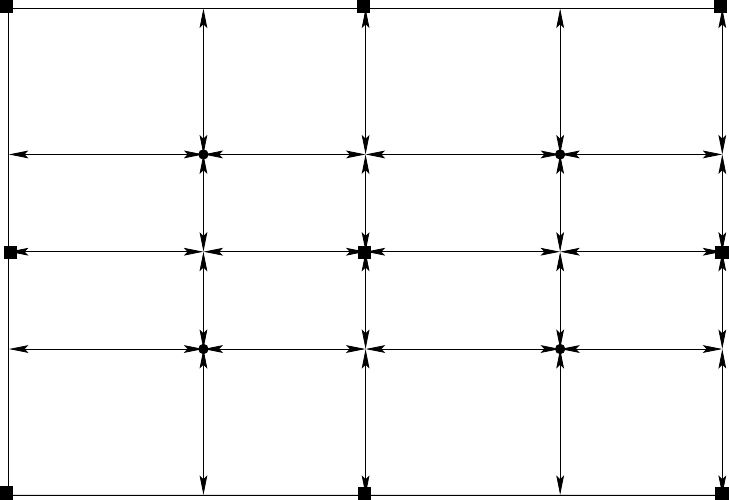
82
CHAPTER 4. GRIDS AND HALOS
T(1,nj)
dtn(1,nj)
U(1,nj−1)
T(ni/2,nj)
U(ni/2,nj−1)
U(1,nj)U(0,nj) due(0,nj) U(ni/2,nj)
U(0,nj−1)
U(ni/2,nj) U(ni,nj)
T(ni,nj)
U(ni/2+1,nj−1) U(ni,nj−1)
U(ni/2,nj−1)
dtn(ni/2,nj)
dtw(1,nj) dte(1,nj)
dus(1,nj)
dun(1,nj−1)
dts(1,nj)
dte(ni/2,nj)dtw(ni/2,nj)
dts(ni/2,nj)
dus(ni/2,nj)
dtn(ni/2+1,nj)
dun(ni/2+1,nj−1)dts(ni/2+1,nj)
dte(ni/2+1,nj)
T(ni/2+1,nj)
dtw(ni/2+1,nj)
dus(ni/2+1,nj)
dts(ni,nj)
dte(ni,nj)
dtw(ni,nj)
dtn(ni,nj)
duw(ni/2+1,nj) U(ni/2+1,nj) due(ni/2+1,nj) duw(ni,nj)
due(ni/2,nj)
dun(ni/2,nj−1)
dus(ni/2,nj)
duw(ni/2,nj)
due(1,nj)
dun(ni/2,nj−1)
dun(1,nj)
dun(ni/2+1,nj)
dun(ni/2,nj)
dun(ni/2,nj)
duw(1,nj)
Figure 4.11: Placement of quarter-cells distances at the bipolar fold. For this exam-
ple, there are ni =4 points in the generalized zonal computational domain. Equiv-
alance of grid factors on the fold leads to the two-fold redundancy for velocity cell
distances duei,n j =duwni−i,n j and dusi,n j =dunni−i,n j.
which then leads to the halo cell relations
duei,j=duwni−i,2n j−j
duwi,j=dueni−i,2n j−j
duni,j=dusni−i,2n j−j
dusi,j=dunni−i,2n j−j
for nj <j≤n j +halo (4.50)
4.3.3.3 Grid distances for horizontal full cells
Inspection of Figures 4.4 and 4.5, with the definitions of grid points shown in Figure
4.2, leads to the definitions of distances for full horizontal cells
∆x(Ei−1, j,Ei,j) = dxti,j(4.51)
∆y(Ni,j−1,Ni,j) = dyti,j(4.52)
∆x(Ui−1, j,Ui,j) = dxtni,j(4.53)
∆y(Ui,j,Ui,j−1) = dytei,j(4.54)
∆x(Ti,j,Ti+1, j) = dxtei,j(4.55)
∆y(Ti,j,Ti,j+1) = dytni,j(4.56)
∆x(Ni,j,Ni+1, j) = dxui,j(4.57)
∆y(Ei,j,Ei,j+1) = dyui,j(4.58)
4.3. SPECIFYING FIELDS AND GRID DISTANCES WITHIN HALOS
83
Figures 4.12, 4.13, and 4.14 show these distances for regions surrounding the bipo-
lar fold. To generate the redudancy conditions and halo mappings, we again use
the scalar mappings given by equation (4.27). Using these relations we see that
redundancy is satisfied by the distances
dxtni,n j =dxtnni−i+1,n j (4.59)
dytni,n j =dytnni−i+1,n j (4.60)
dxui,n j =dxuni−i,n j (4.61)
dyui,n j =dyuni−i,n j (4.62)
Equation (4.27) indicates that within the halo region nj <j≤n j +halo,
∆x(Ei−1, j,Ei,j) = ∆x(Eni−i+1,2n j−j+1,Eni−i,2n j−j+1)(4.63)
∆y(Ni,j−1,Ni,j) = ∆y(Nni−i+1,2n j−j+1,Nni−i+1,2n j−j)(4.64)
∆x(Ui−1, j,Ui,j) = ∆x(Uni−i+1,2n j−j,Uni−i,2n j−j)(4.65)
∆y(Ui,j,Ui,j−1) = ∆y(Uni−i,2n j−j,Uni−i,2n j−j+1)(4.66)
∆x(Ti,j,Ti+1, j) = ∆x(Tni−i+1,2n j−j+1,Tni−i,2n j−j+1)(4.67)
∆y(Ti,j,Ti,j+1) = ∆y(Tni−i+1,2n j−j+1,Tni−i+1,2n j−j)(4.68)
∆x(Ni,j,Ni+1, j) = ∆x(Nni−i+1,2n j−j,Nni−i,2n j−j)(4.69)
∆y(Ei,j,Ei,j+1) = ∆y(Eni−i,2n j−j+1,Eni−i,2n j−j)(4.70)
which then leads to to the halo cell relations
dxti,j=dxtni−i+1,2n j−j+1
dyti,j=dytni−i+1,2n j−j+1
dxtni,j=dxtnni−i+1,2n j−j
dytei,j=dyteni−i,2n j−j+1
dxtei,j=dxteni−i,2n j−j+1
dytni,j=dytnni−i+1,2n j−j
dxui,j=dxuni−i,2n j−j
dyui,j=dyuni−i,2n j−j
for nj <j≤n j +halo (4.71)
4.3.3.4 Summary of redundancies and halo mappings
Table 4.1 summarizes the halo relations and redundancies realized at the bipolar
fold. Notice that those distances exhibiting a redundancy have their halo relations
reduce to their redundancy relations for j=n j. Additionally, the quarter-cell dis-
tances all transform from a right handed system to a right handed system. In gen-
eral, this table should be sufficient to deduce relations for any derived fields, fluxes,
etc., computed in the model.
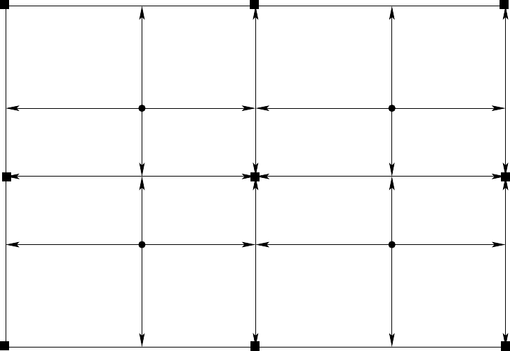
84
CHAPTER 4. GRIDS AND HALOS
T(1,nj)
U(1,nj−1)
T(ni/2,nj)
U(ni/2,nj−1)
U(0,nj) U(ni/2,nj)
U(0,nj−1)
U(ni/2,nj) U(ni,nj)
U(ni/2+1,nj−1) U(ni,nj−1)
U(ni/2,nj−1)
dxt(1,nj)
dyt(1,nj)
dyte(1,nj) dxt(ni/2,nj)
dyt(ni/2,nj)
dyte(ni/2,nj)
dyte(ni/2,nj)
T(ni/2+1,nj)
dxt(ni/2+1,nj)
dyt(ni/2+1,nj)
T(ni,nj)
dyt(ni,nj)
dxt(ni,nj)
dyte(ni/2+1,nj) dyte(ni,nj)
U(ni/2+1,nj)
U(1,nj)
dxtn(ni/2+1,nj)
dxtn(ni/2,nj)dxtn(1,nj)
dxtn(ni,nj)
Figure 4.12: Placement of tracer cell dimensions at the bipolar fold. For this
example, there are ni =4 points in the generalized zonal computational do-
main. Equivalance of grid factors on the fold leads to the two-fold redundancy
dxtni,n j =dxtnni−i+1,n j.
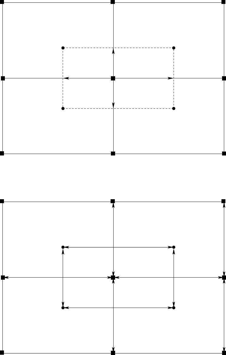
4.3. SPECIFYING FIELDS AND GRID DISTANCES WITHIN HALOS
85
T(1,nj)
U(1,nj−1)
T(ni/2,nj)
U(ni/2,nj−1)
U(0,nj) U(ni/2,nj)
U(0,nj−1)
U(ni/2,nj) U(ni,nj)
U(ni/2+1,nj−1) U(ni,nj−1)
U(ni/2,nj−1)
T(ni,nj)
U(ni/2+1,nj)
U(1,nj)
T(ni/2+1,nj)
dyu(ni/2+1,nj)
dyu(1,nj)
dxu(ni/2+1,nj)
dxu(1,nj)
Figure 4.13: Velocity cell distances at the bipolar fold.
T(1,nj)
U(1,nj−1)
T(ni/2,nj)
U(ni/2,nj−1)
U(0,nj) U(ni/2,nj)
U(0,nj−1)
U(ni/2,nj) U(ni,nj)
U(ni/2+1,nj−1) U(ni,nj−1)
U(ni/2,nj−1)
T(ni/2+1,nj) T(ni,nj)
U(ni/2+1,nj)
U(1,nj)
dytn(ni,nj)
dytn(1,nj)
dxte(1,nj)
dxte(ni/2+1,nj)
dytn(ni/2+1,nj)
dytn(ni/2,nj)
Figure 4.14: Grid distances for tracer points at the bipolar fold.

86
CHAPTER 4. GRIDS AND HALOS
Halo relations (n j <j≤nj +halo) Redundancy relations
Ui,j=
ε
Uni−i,2n j−jUi,n j =
ε
Uni−i,n j
Ti,j=
ε
Tni−i+1,2n j−j+1
Ni,j=
ε
Nni−i+1,2n j−jNi,n j =
ε
Nni−i+1,n j
Ei,j=
ε
Eni−i,2n j−j+1
dtei,j=dtwni−i+1,2n j−j+1
dtwi,j=dteni−i+1,2n j−j+1
dtni,j=dtsni−i+1,2n j−j+1
dtsi,j=dtnni−i+1,2n j−j+1
duei,j=duwni−i,2n j−jduei,n j =duwni−i,n j
duwi,j=dueni−i,2n j−jduwi,n j =dueni−i,n j
duni,j=dusni−i,2n j−jduni,n j =dusni−i,n j
dusi,j=dunni−i,2n j−jdusi,n j =dunni−i,n j
dxti,j=dxtni−i+1,2n j−j+1
dyti,j=dytni−i+1,2n j−j+1
dxtni,j=dxtnni−i+1,2n j−jdxtni,n j =dxtnni−i+1,n j
dytei,j=dyteni−i,2n j−j+1
dxtei,j=dxteni−i,2n j−j+1
dytni,j=dytnni−i+1,2n j−jdytni,n j =dytnni−i+1,n j
dxui,j=dxuni−i,2n j−jdxui,n j =dxuni−i,n j
dyui,j=dyuni−i,2n j−jdyui,n j =dyuni−i,n j
Table 4.1: Summary of the halo mappings and redundancies realized at the bipolar
fold. The symbol
ε
is 1 for scalar fields, and −1 for horizontal components of vector
fields.

CHAPTER
FIVE
Advection velocity components and remapping operators
Contents
5.1 General considerations . . . . . . . . . . . . . . . . . . . . . . . . 87
5.1.1 Two main issues . . . . . . . . . . . . . . . . . . . . . . . . 88
5.1.2 Constraints for discrete vertical velocities . . . . . . . . . . 88
5.2 Remapping operators for horizontal fluxes . . . . . . . . . . . . . 89
5.2.1 Uniformly distributed volume flux across a face . . . . . . 89
5.2.2 Lever-rule and the horizontal remapping operators . . . . 90
5.3 Remapping operator for vertical fluxes . . . . . . . . . . . . . . . 90
5.4 Remapping error . . . . . . . . . . . . . . . . . . . . . . . . . . . . 95
5.4.1 Linear grids . . . . . . . . . . . . . . . . . . . . . . . . . . . 95
5.4.2 Nonlinear grids . . . . . . . . . . . . . . . . . . . . . . . . . 95
5.5 Subtleties at the southern-most row . . . . . . . . . . . . . . . . . 96
The purpose of this chapter is to discuss the computation of advection velocity
components in MOM4. We also discuss the linear operators used to interpolate a
field from one grid to another. These operators are used to map advection velocity
components from the tracer grid to velocity grid, as well as to map selected other
fields.
5.1 General considerations
Advective fluxes are fundamental to the Eulerian evolution of tracer and momen-
tum. How these fluxes are discretized represents a basic problem in computational
fluid dynamics. Notably, because of the interpretation of model velocity discussed
in Griffies (2004), there is no distinction between the advective fluxes for the Boussi-
nesq and non-Boussinesq versions of MOM4: they are computed using the same
numerical considerations detailed in this chapter.
87
88
CHAPTER 5. ADVECTION VELOCITY COMPONENTS AND REMAPPING OPERATORS
5.1.1 Two main issues
There are two considerations required to compute advective fluxes of tracer or mo-
mentum. First, there is the question of how to compute the advective velocity. Such
is the focus of this chapter. For computing fluxes across cell faces, the three com-
ponents to the advective velocity must be known on the corresponding face of the
tracer and velocity cells. However, on the B-grid, both horizontal prognostic veloc-
ity components are placed at the velocity cell point, not at the cell faces. Hence, an
averaging operation must be prescribed to diagnose the horizontal advective ve-
locity components from the prognostic B-grid velocity. MOM4 computes the hor-
izontal components of the advection velocity on the faces of T-cells in a manner
necessitated by equating pressure work to buoyancy (see Chapter 6). The vertical
advective velocity component is then diagnosed at the bottom face of the tracer
cell, based on the needs of volume or mass conservation across the tracer cell (see
Chapter 6 or Griffies (2004)). Computing the advective velocity on the faces of the
velocity cell remains to be determined, and that is the main technical subject of this
chapter.
Once the advective velocity is computed on the cell faces, it remains to approx-
imate the tracer and momentum values on these faces for use in constructing the
advective tracer and momentum fluxes. There are many different approaches avail-
able. As with previous versions of the GFDL ocean model, MOM4 chooses to com-
pute the advective flux of momentum according to the requirements of energetic
consistency described in Chapter 6. These constraints necessitate a second order
centered approach, as in Bryan (1969). The advective flux of tracer, however, is
not so constrained and there are hence many options available, some of which are
detailed in The MOM3 Manual of Pacanowski and Griffies (1999).
5.1.2 Constraints for discrete vertical velocities
One important constraint for self-consistency of the discretization is that the ver-
tical velocity at the T-cell bottom topography must vanish: wbti,j,k=Nk =0, since
the T-cell top and bottom faces are horizontally oriented. A vanising bottom veloc-
ity on T-cells is necessitated by the requirements of volume or mass conservation
(see Griffies (2004)). Many ocean models choose to set w bti,j,k=Nk =0. However,
MOM chooses to start from the ocean surface and integrate the continuity equation
downwards. Verification that the computed w bti,j,k=Nk indeed vanishes has been
found to be a very useful check on code integrity. Relatedly, for a flat bottomed
ocean w bui,j,k=Nk =0. However, with topography, w bu is generally nonzero at
the bottom, since the bottom on velocity cells is not flat. Section 22.3 in The MOM3
Manual of Pacanowski and Griffies (1999) details this point.
Furthermore, since the interior of the ocean domain uses constant cell thick-
nesses, in a Boussinesq model volume should be conserved (the ocean surface con-
serves volume when also incorporating the possibly nonzero fresh water fluxes).
Hence, integrating wbti,j,kacross a particular depth k>1 should leave no net
volume flux upward or downward: ∑i,jdxti,jdyti,jwbti,j,k=0 for all levels k.
Finally, volume conservation warrants the MOM4 approach for diagnosing sur-
face height on the U-cell,
η
u, according to an area weighted average of the sur-
rounding T-cell heights
η
T, instead of using the minimum operation used in MOM3

5.2. REMAPPING OPERATORS FOR HORIZONTAL FLUXES
89
and described in the Griffies et al. (2001) paper. This issue is relevant for the Boussi-
nesq and non-Boussinesq versions of MOM4. We visit this issue in Section 5.3.
5.2 Remapping operators for horizontal fluxes
As stated in Section 5.1, MOM4 computes the horizontal components of the T-cell
advection velocity in a manner necessitated by equating pressure work to buoyancy
(see Chapter 6). The vertical component is diagnosed based the needs of continuity.
Hence, we assume the T-cell advective velocity components are known. We thus
need to determine the corresponding advective velocity on the face of velocity cells.
Advective velocities represent fluxes of volume per unit area. There are three
remapping operators that take discrete volume fluxes defined at tracer points or
sides of tracer cells, to discrete fluxes defined at velocity points or sides of velocity
cells. Although MOM4 is generally non-Boussinesq, we use the ideas of volume
conservation to generate algorithms for coupling advective velocities on the sides
of tracer cells to those on the sides of velocity cells. Here, we describe the linear
remapping operator taking horizontal advective velocities centered on the face of a
tracer cell to the corresponding face of a velocity cell.
5.2.1 Uniformly distributed volume flux across a face
Reference to Figure 5.1 reveals four eastward fluxes of volume per area leaving
a tracer cell that surround the single flux per volume leaving the corresponding
velocity cell. The flux leaving a tracer cell is denoted by Et in the figure, which is
a shorthand for the model’s thickness weighted advective velocity uh et, with the
thickness factor dropped since we are concerned here with fluxes at a fixed depth.
Eu denotes the corresponding eastward flux leaving the velocity cell, and this flux
is to be determined in terms of the surrounding Et and appropriate grid distances.
We assume that along the face of a tracer cell, volume leaves through the face
with a uniform distribution. Hence, the volume per unit length per time passing
across the meridional face through the velocity point Ui,jis given by
Et(i,j)dus(i,j) + Et(i,j+1)dun(i,j), (5.1)
where the distances dus and dun are lengths along sides of the four quarter-cells
comprising a single velocity cell (Figure 5.2). Likewise, the volume per unit length
per time passing across the meridional face through the velocity point Ui+1, jis
given by
Et(i+1, j)dus(i+1, j) + Et(i+1, j+1)dun(i+1, j), (5.2)
and the volume per unit length per time passing across the eastern face of the ve-
locity cell Ui,jis given by
Eu(i,j)dytn(i+1, j), (5.3)
where Eu is to be determined in terms of Et, and the grid distance dytn is the merid-
ional distance between tracer points, as defined in Figure 5.3.

90
CHAPTER 5. ADVECTION VELOCITY COMPONENTS AND REMAPPING OPERATORS
5.2.2 Lever-rule and the horizontal remapping operators
We now employ linear interpolation, or a lever-rule average, to construct the vol-
ume per time passing across the east face of the Ui,jcell, thus leading to
Eu(i,j)dytn(i+1, j)dxtn(i+1, j) = [Et(i,j)dus(i,j) + Et(i,j+1)dun(i,j)] duw(i+1, j)
[Et(i+1, j)dus(i+1, j) + Et(i+1, j+1)dun(i+1, j)] due(i,j),
where dxtn is the zonal distance along the north face of a tracer cell (Figure 5.4).
Solving for Eu leads to the remapping operator
Eu(i,j) = REMAP ET TO EU(Et)(i,j)
≡[Et(i,j)dus(i,j)duw(i+1, j) + Et(i,j+1)dun(i,j)duw(i+1, j)
+Et(i+1, j)dus(i+1, j)due(i,j) + Et(i+1, j+1)dun(i+1, j)due(i,j)]
datnr(i+1, j), (5.4)
where datnr is the reciprocal area at the north face of a T-cell given by
datnr(i,j) = 1
dxtn(i,j)dytn(i,j)(5.5)
Analogous considerations lead to the remapping operator that takes a volume flux
Nt defined at the north face of T-cells to a flux leaving the north face of U-cells
Nu(i,j) = REMAP NT TO NU(Nt)(i,j)
≡[Nt(i,j)duw(i,j)dus(i,j+1) + Nt(i+1, j)due(i,j)dus(i,j+1)
+Nt(i,j+1)duw(i,j+1)dun(i,j) + Nt(i+1, j+1)due(i,j+1)dun(i,j)]
dater(i,j+1). (5.6)
In this expression, dater is the reciprocal area at the east face of a T-cell given by
dater(i,j) = 1
dxte(i,j)dyte(i,j), (5.7)
dxte is the zonal distance between the T-cell points (Figure 5.3) and dyte is the
meridional distance along the east face of the T-cell (Figure 5.4).
5.3 Remapping operator for vertical fluxes
We now consider the remapping taking vertical volume fluxes passing across the
bottom face of tracer cells to the bottom face of velocity cells. This operator also
maps surface height from T-cells to U-cells. This remapping is distinguished from
the horizontal remapping in that there is no analogous lever-rule step. The distinc-
tion boils down to noting that the vertical remapping REMAP BT TO BU moves
vertical fluxes horizontally, whereas the east and north remapping operators move
horizontal fluxes horizontally.
Reference to Figures 5.2 and 5.3, and again assuming fluxes are distributed uni-
formly across a cell face, indicates that the vertical flux of volume per unit length
passing across the southern face of the velocity cell Ui,jis given by
Bt(i,j)dte(i,j) + Bt(i+1, j)dtw(i+1, j), (5.8)
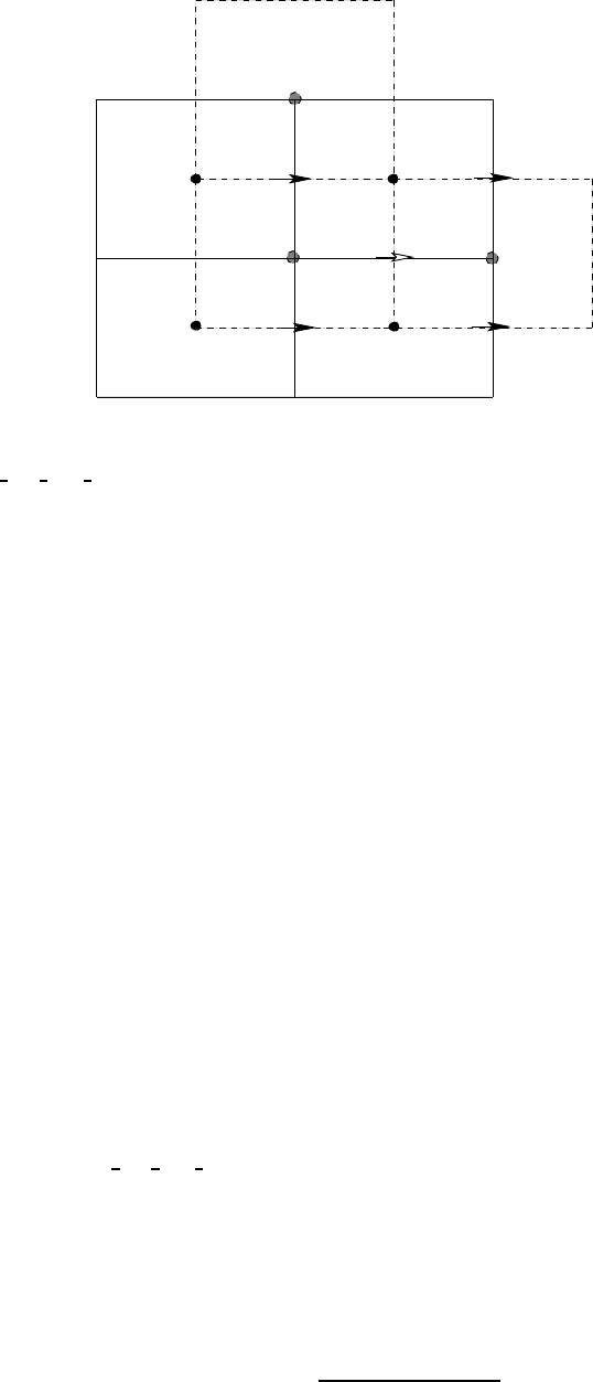
5.3. REMAPPING OPERATOR FOR VERTICAL FLUXES
91
U(i,j)
U(i,j+1)
T(i,j+1)
T(i,j)
U(i+1,j)
T(i+1,j+1)
T(i+1,j)
Et(i,j) Et(i+1,j)
Et(i+1,j+1)
Et(i,j+1)
Eu(i,j)
Figure 5.1: Schematic representation of the remapping function
REMAP ET TO EU defined by equation (5.4). This function is used to remap
a horizontal flux of volume defined at the east face of T-cells (denoted by Et in
this figure) onto a horizontal flux of volume defined at the east face of U-cells
(denoted by Eu in this figure). The four fluxes Et(i,j),Et(i+1, j),Et(i,j+1), and
Et(i+1, j+1)are used to construst the flux Eu(i,j).
the vertical flux of volume per unit length passing across the northern face of the
velocity cell Ui,jis given by
Bt(i,j+1)dte(i,j+1) + Bt(i+1, j+1)dtw(i+1, j+1), (5.9)
and the vertical flux of volume passing through the velocity cell is given by
Bu(i,j)dxu(i,j)dyu(i,j). (5.10)
Assuming that the total flux passing through the velocity cell is equivalent to that
passing across the northern plus southern parts of the cell leads to
Bu(i,j)dxu(i,j)dyu(i,j) = [Bt(i,j)dte(i,j) + Bt(i+1, j)dtw(i+1, j)] dus(i,j)
+ [Bt(i,j+1)dte(i,j+1) + Bt(i+1, j+1)dtw(i+1, j+1)] dun(i,j).
Solving for Bu yields the vertical remapping operator
Bu(i,j) = REMAP BT TO BU(Bt)(i,j)
≡[Bt(i,j)dte(i,j)dus(i,j) + Bt(i+1, j)dtw(i+1, j)dus(i,j)
+Bt(i,j+1)dte(i,j+1)dun(i,j) + Bt(i+1, j+1)dtw(i+1, j+1)dun(i,j)]
daur(i,j)(5.11)
with daur the reciprocal area of the U-cell
daur(i,j) = 1
dxu(i,j)dyu(i,j)(5.12)
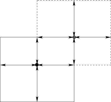
92
CHAPTER 5. ADVECTION VELOCITY COMPONENTS AND REMAPPING OPERATORS
dtw(i,j)
dtn(i,j)
dts(i,j)
T(i,j)
dte(i,j)
dun(i,j)
due(i,j)duw(i,j)
U(i,j)
dus(i,j)
Figure 5.2: Time independent horizontal grid distances (meters) used for the tracer
cell Ti,jand velocity cell Ui,jin MOM4. These “quarter-cell” distances are refined
relative to those shown in Figures 5.4 and 5.5, and they are needed for the remap-
ping between T and U cells when computing advection velocities. All distances are
functions of both iand jdue to the use of generalized orthogonal coordinates. Com-
paring with Figures 5.4 and 5.5 reveals the identities dtw(i,j) + dte(i,j) = dxt(i,j),
dts(i,j) + dtn(i,j) = dyt(i,j),duw(i,j) + due(i,j) = dxu(i,j), and dus(i,j) +
dun(i,j) = dyu(i,j).
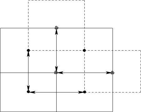
5.3. REMAPPING OPERATOR FOR VERTICAL FLUXES
93
U(i,j)
U(i,j+1)
T(i,j+1)
T(i,j)
U(i+1,j)
T(i+1,j+1)
T(i+1,j)
dyun(i,j)
dxte(i,j)
dytn(i,j) dxue(i,j)
Figure 5.3: Time independent horizontal grid distances (meters) setting the spac-
ing between tracer and velocity points in MOM4. All distances are functions of
both iand jdue to the use of generalized orthogonal coordinates. When these
distances are combined with those in Figures 5.4 and 5.5, and the quarter-cell dis-
tances given in Figure 5.2, we then have full information about the discrete hori-
zontal T and U cells on the model grid. Note there is some redundancy with the
distances defined in Figures 5.4 and 5.5, where we have dytn(i,j) = dyue(i−1, j),
dxte(i,j) = dxun(i,j−1),dxue(i,j) = dxtn(i+1, j), and dyun(i,j) = dyte(i,j+1).
Additionally, comparision with Figure 5.2 leads to the identities dyun(i,j) =
dun(i,j) + dus(i,j+1),dxue(i,j) = due(i,j) + duw(i+1, j),dytn(i,j) = dtn(i,j) +
dts(i,j+1), and dxte(i,j) = dte(i,j) + dtw(i+1, j).
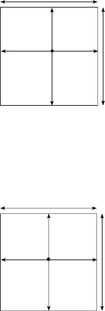
94
CHAPTER 5. ADVECTION VELOCITY COMPONENTS AND REMAPPING OPERATORS
T(i,j)
dxt(i,j) dyte(i,j)
dxtn(i,j)
dyt(i,j)
Figure 5.4: Time independent horizontal grid distances (meters) used for the tracer
cell Ti,jin MOM4. dxti,jand dyti,jare the grid distances of the tracer cell in the
generalized zonal and meridional directions, and dati,j=dxti,jdyti,jis the area of
the cell. The grid distance dxtni,jis the zonal width of the north face of a tracer cell,
and dytei,jis the meridional width of the east face. Note that the tracer point Ti,jis
not generally at the center of the tracer cell. Distances are functions of both iand j
due to the use of generalized orthogonal coordinates.
U(i,j)
dyu(i,j)
dxu(i,j)
dxun(i,j)
dyue(i,j)
Figure 5.5: Time independent horizontal grid distances (meters) used for the ve-
locity cell Ui,jin MOM4. dxui,jand dyui,jare the grid distances of the velocity cell
in the generalized zonal and meridional directions, and daui,j=dxui,jdyui,jis the
area of the cell. The grid distance dxuni,jis the zonal width of the north face of
a velocity cell, and dyuei,jis the meridional width of the east face. Note that the
velocity point Ui,jis not generally at the center of the velocity cell. Distances are
functions of both iand jdue to the use of generalized orthogonal coordinates.
5.4. REMAPPING ERROR
95
5.4 Remapping error
There are two ways to compute the vertical velocity on the velocity cell. The first
method is to compute this velocity according to the requirements of continuity over
the velocity cell, using the convergence of the remapped horizontal advective ve-
locities entering the velocity cell. The second method is to use the vertical remap
operator REMAP BT TO BU to move the vertical velocity on the tracer cells to the
velocity cells. The result of these two approaches is identical when the tracer and
velocity grids are related by a linear average operator, as is the case for a spherical
grid. The need to maintain a linear relation between the tracer and velocity grids is
based on the use of linear methods to derive the remapping operators.
5.4.1 Linear grids
MOM4 computes a diagnostic that examines the differences between the two ap-
proaches for computing vertical advective velocities. It reports the difference as
a “remapping error.” If the numerical discretization is self-consistent, then the
remapping error for a spherical grid will be roundoff, with values on the order
of 10−20m s−1common. Therefore, with a spherical grid, the remapping error pro-
vides a check on the self-consistency of the grid distances and the remapping op-
erators. Effectively, what is done is to check that volume is conserved with the
remapping operators. Even when running a non-Boussinesq model, the remapping
operators are constructed to respect volume conservation.
5.4.2 Nonlinear grids
For a grid defined via a nonlinear transformation of the spherical grid, such as the
bipolar region of the tripolar grid, the grid no longer maintains a linear relation
between tracer and velocity cell distances. The result is a nontrivial remapping
error. This error can be reduced by defining new remapping operators that account
for a generally nonlinear relation between tracer and velocity grid distances. Such
remains to be done for MOM4.
One consequence of the nonzero remapping error is that for a flat bottom model
in regions where the grid distances are nonlinearly related, wbui,j,k=Nk does not
vanish, even though continuity is maintained for all the grid cells. The problem is
that w bui,j,k=0is defined by
w bui,j,k=0=REMAP BT TO BU(w bti,j,k=0). (5.13)
For nonlinear grids, the linear operator REMAP BT TO BU results in a slightly
different value for wbui,j,k=0than would result from an integration of the conti-
nuity equation upwards from the bottom, assuming wbui,j,k=Nk =0. Because the
vertical advective flux at the ocean bottom is masked so that no momentum will
spuriously leak out the bottom of the ocean, having w bui,j,k=Nk slightly nonzero
is of no consequence. Nonetheless, it would be more satisfying to have a general
remapping operator to clean-up this issue.
96
CHAPTER 5. ADVECTION VELOCITY COMPONENTS AND REMAPPING OPERATORS
5.5 Subtleties at the southern-most row
Consider the special case of j=0 in Figure 5.1. This row is strictly south of the
southern-most latitude comprising the computational domain of the model. How-
ever, there is a subtlety related to the treatment of the eastward volume flux leaving
the velocity cell Ui,j=0. That is, since this cell straddles the tracer cells Ti,j=0and
Ti,j=1, it contains some portion that is within the computational domain. Thus, the
eastward volume flux leaving this cell is nonzero, as it is comprised of weighted av-
erage of the four surrounding eastward fluxes leaving the tracer cells. Because the
remapping function (5.4) is normalized with the area datn =dxtn dytn for j=0, it
is necessary to know the grid factors dxtni,j=0and dytni,j=0. In particular, dytni,j=0
is the distance between the computed tracer point Ti,j=1and the tracer point Ti,j=0
that lives outside the computational domain.
The need to know dytni,j=0presents a problem with the MOM4 method for
computing grid specifications. Grids in MOM4 are computed in two steps. First,
there is a preprocessing step whereby grid factors are computed in a generic man-
ner compatible with other models used at GFDL. This step knows nothing about
halo regions, so it only computes grid information over the computational domain.
The result of this step is a NetCDF grid specification file. The second step is to read
the grid specification file into MOM4 and translate the generic grid information into
grid arrays used by MOM4. Since there is no halo information contained in the grid
specification file, we cannot unambiguously specify values for the grid outside the
computational domain. And because we need dytni,j=0to be known consistently
with the values for dytni,jwith j>0, we cannot simply fill dytni,j=0with an arbi-
trary placeholder. If we do so, then the remapping function used to compute the
eastward flux leaving the velocity cell Ui,j=0will be incorrect, thus compromising
the vertical velocity leaving Ui,j=0. The symptom will be most notable in spuri-
ously large values of the vertical velocity on the velocity cell at the computational
row j=1, as well as huge remapping errors at j=1.
There are three solutions to this problem. First, we could extend the definition
of the grid within the grid specification file to include the extra j=0 row. This
solution has been rejected since it adds an extra calculation that is specific to the
northeast B-grid used in MOM4. As the grid specification file is designed for use by
all grid point models, it is not desirable to corrupt it with special cases. The second
solution is to require the southern-most row in MOM4 to be filled with land. This
solution is arguably inelegant, and it has indeed prompted some debate with the
MOM4 developers. Yet this is the solution used in the GFDL ice model, which is
also on a B-grid, and so it has been the most popular solution thus far in MOM4
when aiming to couple MOM4 to other models. The third solution is to extend
the grid southward within MOM4 after reading in the grid specification file. This
solution is appropriate if we can assume a spherical grid in the southern part of the
domain, as true in most cases.

CHAPTER
SIX
Energetics on the B-grid lattice
Contents
6.1 Introduction . . . . . . . . . . . . . . . . . . . . . . . . . . . . . . . 98
6.1.1 The utility of discrete energy conversions . . . . . . . . . . 98
6.1.2 Continuous equations for the ocean model . . . . . . . . . 99
6.1.3 Kinetic energy budget for a continuum ocean model parcel 99
6.1.4 Semi-discrete momentum budget . . . . . . . . . . . . . . 100
6.1.5 Vertical advective velocities . . . . . . . . . . . . . . . . . . 100
6.2 Pressure work conversions . . . . . . . . . . . . . . . . . . . . . . 101
6.2.1 Continuum results: Part I . . . . . . . . . . . . . . . . . . . 101
6.2.2 Continuum results: Part II . . . . . . . . . . . . . . . . . . . 102
6.2.3 B-grid results . . . . . . . . . . . . . . . . . . . . . . . . . . 103
6.2.3.1 Defining the horizontal advection velocities . . . 104
6.2.3.2 Completing the manipulations for P1. . . . . . . 105
6.2.3.3 Correspondence to the continuum results . . . . 106
6.2.3.4 The sigma-correction term P2........... 107
6.2.3.5 Summary . . . . . . . . . . . . . . . . . . . . . . . 108
6.3 Kinetic energy advection . . . . . . . . . . . . . . . . . . . . . . . 109
6.3.1 Continuum results . . . . . . . . . . . . . . . . . . . . . . . 109
6.3.2 B-grid results . . . . . . . . . . . . . . . . . . . . . . . . . . 110
6.4 Kinetic energy in the external and internal modes . . . . . . . . 113
6.5 A caveat regarding the tripolar grid . . . . . . . . . . . . . . . . . 114
The purpose of this chapter is to discuss energetic balances on the discrete B-
grid lattice. Most notably, choosing to maintain the integrity of certain balances
prescribes the form of the discrete advection velocity components located on the
sides of tracer cells. It also necessitates the use of second order finite differenced
advective fluxes of momentum. Tracer fluxes can remain arbitrarily discretized.
Energy balance diagnostics are important methods of use for checking the integrity
of algorithms.
97
98
CHAPTER 6. ENERGETICS ON THE B-GRID LATTICE
6.1 Introduction
This chapter is concerned with details of how the discrete model respects the con-
version between various forms of energy. For example, how does work done by
currents against the horizontal pressure gradient get converted into work against
gravity and/or compression? How does globally integrated discrete advection of
momentum get converted to boundary contributions? How do conversions differ
for Boussinesq and non-Boussinesq fluids?
As discussed in Griffies (2004), energy conversions in the continuum largely
follow from manipulations using the kinematic and dynamic balances. Analogous
manipulations occur on the lattice, yet with more care given to how various terms
are discretized. Maintaining exact discrete energic conversions is neither neces-
sary nor sufficient for ensuring a physically realistic solution. However, without
analytical solutions to compare with, discrete energy conversions afford the ocean
modeler some insurance that the numerical algorithm is performing with a degree
of physical integrity.
6.1.1 The utility of discrete energy conversions
Arbitrary discretizations generally fail to satisfy exact energy conversion proper-
ties. Hence, maintaining discrete energy conversions is a choice going beyond the
usual goal of providing a consistent discretization. Indeed, it can be considered a
guiding-principle, of which there are others affecting the design of MOM’s numerical
algorithms. These principles generally reduce many of the arbitrary choices other-
wise available when discretizing terms in a continuous partial differential equation.
Another analogous principle used in MOM insists that the discrete friction and dif-
fusion operators dissipate the discrete kinetic energy and discrete tracer variance,
respectively. Griffies (2004) details these issues.
MOM is predominantly of use for ocean climate modeling, where integrations
of many thousands of years are common. Therefore, it is essential that systematic
errors in algorithms, however small, be obviated. It is important for the develop-
ment of algorithms to have well defined energetic balances to test code integrity.
Without known analytic solutions, there remain few other methods to track down
bugs, short of hoping they manifest in an egregious and obviously unphysical man-
ner.
Unfortunately, it is often found that some physically relevant properties are sac-
rificed in order to ensure discrete energy conservation. Most notably, the smooth-
ness of the solution is often compromised. Hence, some model developers con-
sider order of accuracy to be the prime consideration for a numerical model. Yet
highly accurate operators do not always afford themselves exact discrete conserva-
tion laws; only approximate laws.
MOM maintains the traditional use of second order numerics for the momen-
tum equation. Doing so affords satisfaction of the discrete energy conversion prop-
erties described in this chapter. Efforts to increase order of accuracy are focused on
tracer advection, where various schemes are available beyond the traditional sec-
ond order scheme of Bryan (1969). Notably, the tracer advection scheme does not
affect considerations in this chapter.

6.1. INTRODUCTION
99
6.1.2 Continuous equations for the ocean model
The equations considered in this chapter represent discrete realizations of the con-
tinuum model equations presented in Griffies (2004). For completeness, we repeat
them here assuming hydrostatic balance. The non-Boussinesq hydrostatic equa-
tions are
ρ
,t+
ρ
o∇· v=0 (6.1)
(D
ρ
z),t=−
ρ
o∇· U+
ρ
wqw(6.2)
u,t+∇· (v u
ρ
) + Mˆz∧v
ρ
=−fˆz∧v− ∇(p/
ρ
o) + (
ρ
/
ρ
o)F(u)(6.3)
p,z=−
ρ
g(6.4)
(
ρ
T),t+
ρ
o∇· (vT) = −∇·(
ρ
F) +
ρ
S, (6.5)
where
ρ
v
ρ
=
ρ
ov(6.6)
is the linear momentum density. For finite domains, these equations are combined
with the surface and bottom kinematic boundary conditions
ρ η
,t+
ρ
ou·∇
η
=
ρ
ow+
ρ
wqwat z=
η
(6.7)
u·∇H+w=0 at z=−H. (6.8)
The Boussinesq hydrostatic equations are recovered by setting
ρ
→
ρ
o, except when
multiplying gravity
∇ · v=0 (6.9)
η
,t=−∇ · U+qw(6.10)
u,t+∇· (v u) + Mˆz∧v=−fˆz∧v− ∇(p/
ρ
o) + F(u)(6.11)
p,z=−
ρ
g(6.12)
T,t+∇·(vT) = −∇· F+S. (6.13)
The surface and bottom kinematic boundary conditions are
η
,t+u·∇
η
=w+qwat z=
η
(6.14)
u·∇H+w=0 at z=−H. (6.15)
6.1.3 Kinetic energy budget for a continuum ocean model parcel
As discussed in Griffies (2004), the kinetic energy of a fluid parcel is modified by
the effects of pressure and friction. It is useful to summarize these results in or-
der to anticipate some of the discrete manipulations made in this chapter. For this
purpose, multiply the momentum equation (6.3) by
ρ
oto find
(
ρ
u
ρ
),t+∇· (
ρ
v
ρ
u
ρ
) +
ρ
M
ρ
ˆz∧v
ρ
=−fˆz∧
ρ
v
ρ
−∇p+
ρ
F(u), (6.16)
where we used the relation
ρ
v
ρ
=
ρ
ovfor the linear momentum density. Now take
the inner product of this budget with the horizontal velocity u
ρ
to find
u
ρ
·(
ρ
u
ρ
),t+ (u
ρ
)i∂j(
ρ
(v
ρ
)j(u
ρ
)i) = −u
ρ
·∇p+
ρ
u
ρ
·F(u), (6.17)

100
CHAPTER 6. ENERGETICS ON THE B-GRID LATTICE
where tensor labels were exposed where needed for clarity. Use of mass conserva-
tion in the form
ρ
,t+∇· (
ρ
v
ρ
) = 0 leads to
(
ρ
K),t+∇· (
ρ
v
ρ
K) = −u
ρ
·∇p+
ρ
u
ρ
·F(u), (6.18)
where
K=1
2u
ρ
·u
ρ
(6.19)
is the kinetic energy per mass of a continuum model fluid parcel. Notably, it is
the model’s velocity u
ρ
, not u, that determines the model’s kinetic energy. This
distinction is relevant only for the non-Boussinesq fluid, since for the Boussinesq
fluid u=u
ρ
.
6.1.4 Semi-discrete momentum budget
A starting point for discretizing the continuum equations is to integrate these equa-
tions vertically over the extent of a model grid cell. Vertical integration allows for
an explicit treatment of surface and bottom boundary conditions, whose details are
crucial for the proper forcing of the ocean model. Griffies (2004) derived such semi-
discrete budgets, where it was shown that the momentum budget for an interior
model grid cell with k>1 is given by
hzk(∂t+fˆz∧)uzk=−(hMˆz∧u
ρ
)zk−∇ ·(hu u
ρ
)zk−(h∇p)zk/
ρ
o+ (h
ρ
Fu
horz)zk
−[(wu
ρ
)zk−1−(wu
ρ
)zk] + [(
ρκ
u
ρ
,z)zk−1−(
ρκ
u
ρ
,z)zk]/
ρ
o, (6.20)
with hkthe vertical thickness of the cell. The surface cell k=1 has the budget
hz1(∂t+fˆz∧)uz1=−(hMˆz∧u
ρ
)z1−∇ ·(hu u
ρ
)z1−(h∇p)z1/
ρ
o+ (h
ρ
Fu
horz)z1
+
ρ
−1
o[
ρ
owu
ρ
−
ρκ
u
ρ
,z]z1+
ρ
−1
o[−u
ρ
z1
ρ η
,t+
ρ
wqwu
ρ
w+
τ
]. (6.21)
The budget for a Boussinesq model is recovered by setting densitites to
ρ
oand u=
u
ρ
. For the surface cell, volume conservation in the form
η
,t=−∇ · U+qwleads
to the Boussinesq balance
hz1(∂t+fˆz∧)uz1=−(hMˆz∧u)z1−∇ · (hu u)z1−(h∇p)z1/
ρ
o+ (hFu
horz)z1
+ (wu−
κ
u,z)z1+ [qw(uw−uz1) + uz1∇ ·U+
τ
/
ρ
o]. (6.22)
6.1.5 Vertical advective velocities
As discussed in Griffies (2004), the vertical component to the advective velocity is
diagnosed by constraining the discrete fluid to satisfy mass continuity over a grid
cell. At the base of a grid cell at depth level k>1, the model’s vertical advective
velocity is given by
wzk=wzk−1+∇· (hu)zk+hzk∂t(
ρ
/
ρ
o)zk, (6.23)
where the time derivative term is dropped for Boussinesq fluids. For surface cells
where k=1,
ρ
owz1= (−
ρ
wqw+
ρ
z1
η
,t) + ∇· (hu)zk+hzk∂t(
ρ
/
ρ
o)zk, (6.24)
6.2. PRESSURE WORK CONVERSIONS
101
thus prompting us to formally set
ρ
owz0=−
ρ
wqw+
ρ
z1∂t
η
(6.25)
which in the Boussinesq case reduces to
wz0=−∇ ·U. (6.26)
Note that it is important not to confuse the advective velocity wz0, diagnosed through
continuity, with the distinct vertical velocity w(z=
η
)used in the surface kinematic
boundary condition.
6.2 Pressure work conversions
We follow here the derivation first given by Semtner (1974) for the rigid lid Boussi-
nesq model. Generalizations are given here for MOM4’s bottom partial cells, ex-
plicit free surface, and non-Boussinesq formulation. A practical result from this
section is the specification of discrete advection velocities used to transport tracers.
6.2.1 Continuum results: Part I
Following the discussion of Section 6.1.3, where we derived the local budget for
kinetic energy of a parcel
(
ρ
K),t+∇· (
ρ
v
ρ
K) = −u
ρ
·∇p+
ρ
u
ρ
·F(u), (6.27)
we start by noting that the projection of the horizontal velocity u
ρ
onto the horizon-
tal pressure gradient is given by
u
ρ
·∇p=v
ρ
·∇p−w
ρ
p,z
=∇· (v
ρ
p)−p∇· v
ρ
+
ρ
g w
ρ
(6.28)
where the hydrostatic balance p,z=
ρ
gwas used. The divergence ∇ · v
ρ
vanishes
for a Boussinesq fluid, yet it represents a nontrivial conversion of kinetic to internal
energy for the non-Boussinesq fluid (see Griffies (2004)). Integration over the full
ocean domain yields
−ZdV u
ρ
·∇p=Z
z=
η
dA p (u
ρ
·∇
η
−w
ρ
) + ZdV (p∇ · v
ρ
−w
ρρ
g)(6.29)
where use was made of periodic and/or no-normal flow side boundary conditions,
as well as the bottom kinematic boundary condition. The surface kinematic bound-
ary
u
ρ
·∇
η
−w
ρ
=
ρ
wqw−
ρ η
,t(6.30)
leads to
−ZdV u
ρ
·∇p=Z
z=
η
dA p [(
ρ
w/
ρ
)qw−
η
,t] + ZdV (p∇ · v
ρ
−w
ρρ
g). (6.31)

102
CHAPTER 6. ENERGETICS ON THE B-GRID LATTICE
Note that mass conservation over a fluid column allows us to alternatively write
ρ
wqw−
ρ η
,t=−
ρ
o∇· U+
η
Z
−H
dz
ρ
,t(6.32)
with the second term, the so-called steric contribution, absent for the volume-conserving
Boussinesq fluid (see Griffies (2004) for more discussion of steric effects). Indeed,
for the Boussinesq fluid we have (1) v=v
ρ
, (2) ∇ · v=0, (3) the density
ρ
(
η
)
appearing in the surface kinematic boundary condition is set to
ρ
o, (4)
η
,t=−∇ ·
U+qwexpressing volume conservation over a fluid column, thus leading to
−ZdV u· ∇p=Z
z=
η
dA p ∇ · U−ZdV w
ρ
g. (6.33)
It is useful to consider three special cases, the simplest of which is the rigid lid
Boussinesq ocean. Most rigid lid models suppress the addition of fresh water1, in
which case ∇ · U=0 thus rendering
ZdV u· ∇p=ZdV w
ρ
g. (6.34)
That is, for the rigid lid hydrostatic Boussinesq ocean without fresh water forc-
ing, the global effects of work done by the horizontal currents against horizontal
pressure gradients are equal to the work by vertical currents against gravity. This
equality affords the following interpretation. In a hydrostatic fluid, vertically in-
tegrated density directly determines pressure. Hence, work against a horizontal
pressure gradient force is associated with a rearrangement of the density field in
the vertical, which then involves work against gravity.
A free surface Boussinesq fluid satisfies the more general balance
−ZdV u· ∇p=Z
z=
η
dA p ∇ · U−ZdV w
ρ
g. (6.35)
The surface term accounts for the possibility of atmospheric pressure to apply work
to a dilatating vertical column of fluid.
For a free surface non-Boussinesq fluid, the full identity (6.37) is applicable.
The new term p∇ · v
ρ
accounts for the ability of pressure forces internal to the
fluid to do work on dilatating fluid parcels, and the term Rz=
η
dA (p/
ρ
) (R
η
−Hdz
ρ
,t)
accounts for work done by atmospheric pressure on a column of ocean fluid ex-
periencing expansion and/or contraction due to changes in the depth integrated
density–the so-called steric effects.
6.2.2 Continuum results: Part II
As noted in Section 6.1.1, one motivation for considering the discrete energy con-
versions is that they provide guidance on how to discretize objects in the model. In
particular, they guide how to discretize advection velocities on the faces of tracer
1Huang (1993) noted the possibility of relaxing this restriction, yet we know of no realistic model
having implemented this approach.
6.2. PRESSURE WORK CONVERSIONS
103
cells. With the B-grid used in MOM4, it is otherwise not obvious how to compute
these velocities. An alternative to the approach in Section 6.2.1 provides insight
for this purpose, with the distinction relevant only for the non-Boussinesq case.
Instead of u
ρ
·∇p, we here consider
u·∇p=v·∇p−w p,z
=∇· (v p)−p∇ · v+
ρ
g w. (6.36)
The divergence term ∇ · v=−
ρ
,t/
ρ
ovanishes for the Boussinesq fluid. Integrat-
ing over the ocean domain and using the surface and bottom kinematic boundary
conditions leads to
−
ρ
oZdV u· ∇p=Z
z=
η
dA p (
ρ
wqw−
ρ η
,t)−
ρ
oZdV [p(
ρ
,t/
ρ
o) + w
ρ
g], (6.37)
where use was made of periodic and/or no-normal flow side boundary conditions.
This result reduces to the same Boussinesq result (6.33) considered in Section 6.2.2.
The non-Boussinesq case is distinct.
6.2.3 B-grid results
We now consider manipulations of the globally integrated discrete B-grid repre-
sentation of u· ∇panalogous to those discussed in Section 6.2.2. Note that in this
section, discrete grid labels will be exposed when appropriate, with many labels
suppressed to reduce clutter.
As stated in Section 6.2.2, we prefer a discrete analysis of u· ∇prather than
u
ρ
·∇pbecause of the guidance u·∇pprovides for discretizing the tracer advection
velocities, as well as the ability to use the resulting discrete balance to check code
integrity. However, for the non-Boussinesq case, the direct interpretation of each
term according to a work per time is not as straightforward as for the considerations
of Section 6.2.1.
The domain integrated scalar product of the horizontal velocity uand the hori-
zontal pressure gradient −∇pis given by
P ≡ − ∑
i,j,k
dau dhu [u FDX NT(FAY(p)) + v FDY ET(FAX(p))]
+g∑
i,j,k
dau dhu [u FAY(FAX(
ρ
)
δ
iH)/dxu +v FAX(FAY(
ρ
)
δ
jH)/dyu].(6.38)
MOM4 employs the following forward derivative operators
FDX NT(a) = ai+1−ai
dxu (6.39)
FDY ET(a) = aj+1−aj
dyu , (6.40)
where the derivatives live on the east and north faces, respectively, of a tracer cell.
The operators
δ
iHand
δ
jHcompute the forward difference
δ
iH=Hi+1−Hi(6.41)
δ
jH=Hy+1−Hy(6.42)
104
CHAPTER 6. ENERGETICS ON THE B-GRID LATTICE
of the bottom topography. The first term in equation (6.38) is the lateral pressure
gradient taken between cells living on the same discrete k-level. The second term
arises from the use of bottom partial cells, where the depth of a k-level is generally
a function of horizontal position. This term is the same that appears in terrain-
following sigma models. In both cases, the horizontal pressure gradient is given by
two terms
∇zp= (∇
σ
+∇
σ
H∂z)p=∇
σ
p−
ρ
g∇
σ
H, (6.43)
where the hydrostatic balance p,z=−
ρ
gwas used to reach the second relation. The
slope of sigma surfaces can reach 1/100 next to continental slopes, at which point
the “sigma-coordinate correction term”
ρ
g∇
σ
Hcan be on the order of ∇
σ
p. In this
case, the horizontal pressure force becomes the result of two sizable terms, each
having separate numerical errors that generally do not cancel. The result can be
spurious pressure forces that drive nontrivial unphysical currents. As described by
Pacanowski and Gnanadesikan (1998), the sigma correction term introduces only
very minor spurious currents in MOM due to (1) MOM’s use of z-levels throughout
the region above the topography, thus isolating the sigma-correction term to just the
bottom-most level, (2) The discrete horizontal pressure gradient is chosen so that
if pressure is a linear function of depth, then the discrete gradient vanishes. This
discretization choice greatly reduces the magnitude of spurious flows.
6.2.3.1 Defining the horizontal advection velocities
Focus on the zonal piece of the first term
P1x≡ − ∑
i,j,k
dau dhu u FDX NT(FAY(p))
=−1
2∑dyu dhu u
δ
i(pj+pj+1)
=−∑BAY(dyu dhu u)
δ
ipj, (6.44)
where the boundary terms drop out for either periodic or solid wall conditions, and
we introduced the backward meridional average operator
BAY(a) = aj+aj−1
2. (6.45)
Let us now define the zonal thickness weighted advective transport velocity on the
eastern face of a tracer cell as
uh eti,j,k=BAY(dyu dhu u)
dytei,j
, (6.46)
where dytei,jis the meridional width of the tracer cell’s east side (see Figure 6.2 for
definitions of grid distances). Doing so leads to
P1x=−∑
δ
ip(dyte uh et)
=∑p
δ
i(dyte uh et)
=∑p dat BDX ET(uh et), (6.47)
6.2. PRESSURE WORK CONVERSIONS
105
where boundary terms vanish, and
BDX ET(a) = ai,jdytei,j−ai−1, jdytei−1, j
dati,j
(6.48)
is a backwards finite difference operator for fields defined on the east face of tracer
cells. Similar manipulations with the meridional term v∂ypleads to
P1=∑p dat (BDX ET(uh et) + BDY NT(vh nt)), (6.49)
with
vh nti,j,k=BAX(dxu dhu v)
dxtni,j
(6.50)
the meridional tracer advective velocity on the north face of the tracer cell, and
BDY NT(a) = ai,jdxtni,j−ai,j−1dxtni,j−1
dati,j
(6.51)
is a backwards finite difference operator for fields defined on the north face of tracer
cells.
The horizontal advective velocities uh et and vh nt are defined at the sides of
the tracer cells and at the depth of the tracer point. Hence, their finite differenced
derivatives are defined at the tracer point. The corresponding vertical velocity w btk
is also defined at the horizontal tracer point, yet at the bottom of the tracer cell, at
the “W-point”. As discussed in Section 6.1.5, the vertical advective velocity compo-
nent is diagnosed through continuity. In a discrete form, this velocity component is
given by
wbtk=w btk−1+BDX ET(uh etk) + BDY NT(vh ntk) + dhtk∂t(
ρ
k/
ρ
o). (6.52)
In this equation, dhti,j,kis the vertical thickness of the tracer cell, the time derivative
term is absent for Boussinesq fluids, and (see Section 6.1.5)
ρ
ow bt0=
ρ
1∂t
η
−
ρ
wqw(6.53)
for the non-Boussinesq fluid, and
w bt0=−∇ · U(6.54)
for the Boussinesq fluid.
6.2.3.2 Completing the manipulations for P1
Substitution of expression (6.52) for the vertical advective velocity component into
equation (6.49) leads to
P1=−∑pkdat (wbtk−1−w btk+dhtk∂t(
ρ
k/
ρ
o)), (6.55)
with rearrangement of the sums rendering
P1=∑
i,j
dati,j(−p1wbt0+pnk+1w btnk)(6.56)
+∑
i,j,k
dat dhwtkwbtk
pk−pk+1
dhwtk−1
ρ
o∑
i,j,k
pkdat dhtk∂t
ρ
k, (6.57)
106
CHAPTER 6. ENERGETICS ON THE B-GRID LATTICE
where dhwti,j,kis the vertical distance between tracer points Tkand Tk+1. The
pnk+1w btnk boundary term vanishes since w btnk =0; however, the surface term
p1w bt0is nonzero for a free surface model where w bt06=0 (e.g., equations (6.53)
and (6.54)).
The discrete hydrostatic pressure is computed as an estimate of pressure at the
depth of the tracer point, rather than as an average pressure over the full tracer cell
(Figure 6.1). That is,
pk+1=pk+g dhwtk
ρ
kz, (6.58)
where
ρ
kz= (
ρ
k+
ρ
k+1)/2 is the vertically averaged density over the tracer cell.
Using this pressure then leads to
P1=−∑
i,j
dati,j p1wbt0+g∑
k
dhwtkwbtk
ρ
kz+1
ρ
o∑
k
pkdhtk∂t
ρ
k!. (6.59)
6.2.3.3 Correspondence to the continuum results
It is useful to make a correspondence with terms from the continuum given in Sec-
tion 6.2.2. First, a rigid lid Boussinesq fluid with zero fresh water flux has
P1=−∑
i,j
dati,j g∑
k
dhwtkwbtk
ρ
kz!, (6.60)
where w bt0=0 and the density time tendency term vanishes. Hence, in this
case, work by horizontal currents on the horizontal pressure gradient equals work
against gravity. Allowing for a free surface Boussinesq fluid yields
P1=−∑
i,j
dati,j −p1∇ · U+g∑
k
dhwtkwbtk
ρ
kz!, (6.61)
where the density time tendency term vanishes and w bt0=−∇ · U. The added
term accounts for work done by pressure p1at the surface tracer point on a dilatat-
ing vertical column of fluid. This pressure is given by
p1=
ρ
1g(dhwtk=0+eta t) + patm (6.62)
where eta t is the surface height on tracer cells, and dhwtk=0is the distance from
z=0 to the k=1 tracer point z1. This pressure has a contribution from the
hydrostatic pressure within the fluid layer between z=eta t and z=z1, and that
from the overlying atmosphere. For a non-Boussinesq fluid, equation (6.53) for
wbt0leads to
P1=−∑
i,j
dati,j (p1/
ρ
o) (
ρ
1∂t
η
−
ρ
wqw) + g∑
k
dhwtkwbtk
ρ
kz+∑
k
dhtkpk∂t
ρ
k!,
(6.63)
which again has a direct correspondence to the continuum results.
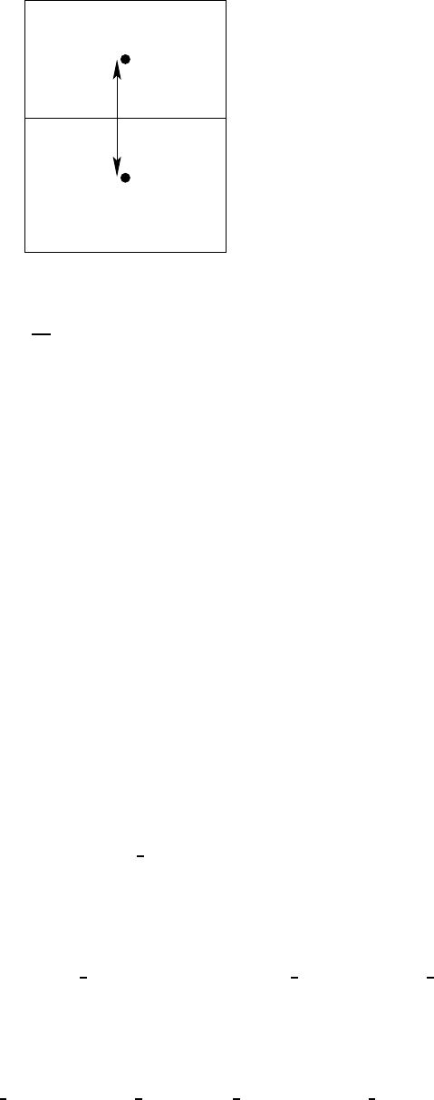
6.2. PRESSURE WORK CONVERSIONS
107
k+1
k
dhwt(k)
Figure 6.1: Schematic of the vertical grid cell arrangment used for computing the
hydrostatic pressure at a depth k+1 in terms of the pressure at depth kusing the
equation pk+1=pk+g dhwtk
ρ
kz. The vertical average of density is meant to ac-
count for the part of density within each of the two adjacent cells. The factor of 1/2
used in the average operator yields an approximate average when vertical cells are
non-uniform. Yet the 1/2 factor is used for all vertical grid spacing since it renders
a simple conversion of discrete pressure work to discrete gravity work.
6.2.3.4 The sigma-correction term P2
Now consider the zonal piece of the sigma-correction term from equation (6.38)
P2x=g∑
i,j,k
dxu dyu dhu u FAY(FAX(
ρ
)
δ
iH)/dxu. (6.64)
Transferring the forward average FAY to a backward average BAY leads to
P2x=g∑BAY(dyu dhu u)FAX(
ρ
)
δ
iH, (6.65)
where boundary terms vanish. Introducing the zonal thickness weighted advective
transport velocity (6.46) yields
P2x=g∑dyte uh et FAX(
ρ
)
δ
iH. (6.66)
Moving the difference operator
δ
iH=Hi+1−Hifrom the depth Hto the remaining
terms gives
P2x=−g∑H
δ
i(dyte FAX(
ρ
)uh et) = −g∑H dat BDX ET(FAX(
ρ
)uh et),
(6.67)
where boundary terms vanish. Similar manipulations with the meridional piece of
P2lead to
P2=−g∑H dat [BDX ET(FAX(
ρ
)uh et) + BDY NT(FAY(
ρ
)vh nt)]. (6.68)
The P2term accounts for alterations in the potential energy due to the use of partial
bottom cells.
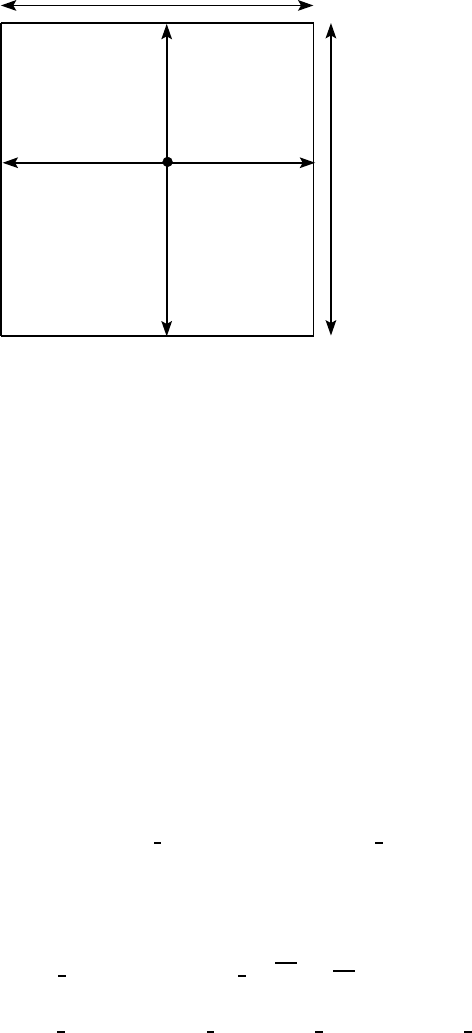
108
CHAPTER 6. ENERGETICS ON THE B-GRID LATTICE
T(i,j)
dxt(i,j) dyte(i,j)
dxtn(i,j)
dyt(i,j)
Figure 6.2: Time independent horizontal grid distances (meters) used for the tracer
cell Ti,jin MOM4. dxti,jand dyti,jare the grid distances of the tracer cell in the
generalized zonal and meridional directions, and dati,j=dxti,jdyti,jis the area of
the cell. The grid distance dxtni,jis the zonal width of the north face of a tracer cell,
and dytei,jis the meridional width of the east face. Note that the tracer point Ti,jis
not generally at the center of the tracer cell. Distances are functions of both iand j
due to the use of generalized orthogonal coordinates.
6.2.3.5 Summary
In summary, the projection of the horizontal velocity onto the downgradient pres-
sure field is given by
P ≡ − ∑
i,j,k
dau dhu [u FDX NT(FAY(p)) + v FDY ET(FAX(p))]
+g∑
i,j,k
dau dhu [u FAY(FAX(
ρ
)
δ
iH)/dxu +v FAX(FAY(
ρ
)
δ
jH)/dyu].
=−∑
i,j
dati,j p1w bt0+g∑
k
dhwtkwbtk
ρ
kz+1
ρ
o∑
k
dhtkp∂t
ρ
k!
−g∑H dat [BDX ET(FAX(
ρ
)uh et) + BDY NT(FAY(
ρ
)vh nt)] (6.69)
The MOM4 diagnostic energy conversion error has proven to be quite useful for de-
tecting improper discretization of various algorithms. That diagnostic computes
the left hand side of equation (6.69) and compares to the right hand side. Differ-
ences are due to errors in the code. The reason this diagnostic is so effective is that
it involves advective velocities on the tracer cells, both tracer and velocity cell dis-
tances, the calculation of pressure, and details of partial cells. Each require precise
discretization in order to ensure an energy conversion error at the roundoff level.
6.3. KINETIC ENERGY ADVECTION
109
6.3 Kinetic energy advection
This section illustrates how second order accurate centered discrete advection con-
serves globally integrated discrete kinetic energy for a rigid lid Boussinesq model.
Notably, such variance or energy conserving advection schemes are not so useful for
tracer transport due to their relatively large dispersion errors (e.g., Griffies et al.
(2000b)). Yet second order methods remain the norm for velocity advection in most
z-coordinate ocean models based on the original Cox (1984) code, such as MOM.
For the more general case with a free surface, the integrated advection term reduces
to generally nonzero boundary contributions.
6.3.1 Continuum results
Recall from Section 6.1.3 that the kinetic energy per mass in a hydrostatic fluid
is written K=u
ρ
·u
ρ
/2, where
ρ
u
ρ
=
ρ
ouis the horizontal component to the
linear momentum density (Section 6.1.2). For the Boussinesq fluid, v
ρ
=v, so the
distinction between velocities is only relevant for the non-Boussinesq case. Let us
now define the volume integral of the scalar product of horizontal velocity u
ρ
and
the velocity advection terms in equation (6.3) as
A ≡ −ZdV u
ρ
·[∇· (v u
ρ
) + M(ˆz∧
ρ
v
ρ
)]. (6.70)
The advection metric term drops out trivially. For clarity, we selectively expose
tensor labels on the horizontal velocity components to rewrite the divergence term
as
u
ρ
m∇· (vu
ρ
m) = ∇ ·(v u
ρ
·u
ρ
)−(vu
ρ
m)·∇u
ρ
m
=2∇ · (vK)−v· ∇K
=∇· (vK) + K ∇· v
=∇· (vK)−K(
ρ
,t/
ρ
o),
where the continuity equation
ρ
,t=−
ρ
o∇ · vwas used in the last step. For a
Boussinesq fluid, similar manipulations lead to
um∇· (vum) = ∇ ·(vK), (6.71)
where use was made of the non-divergence condition ∇ · v=0. Integration over
the ocean domain and use of the surface and bottom kinematic boundary condi-
tions leads to the non-Boussinesq result
ρ
oAnB =ZdV K
ρ
,t−
ρ
oZ
z=
η
dA K(w−u· ∇
η
)
=ZdV K
ρ
,t+Z
z=
η
dA K(
ρ
wqw−
ρ η
,t)(6.72)
and to the Boussinesq result
AB=Z
z=
η
dA K ∇· U. (6.73)

110
CHAPTER 6. ENERGETICS ON THE B-GRID LATTICE
For a rigid lid Boussinesq model with zero fresh water forcing, AB=0. More
general models have nonzero Adue either to boundary contributions and/or di-
latations of fluid parcels/columns.
6.3.2 B-grid results
We first verify that the scalar product of horizontal velocity and the advection met-
ric term trivially vanishes at each grid point. Similar manipulations are appropriate
for the Coriolis term. Written as in the numerical model, keeping only grid labels
of relevance, we have
u
ρ
·M(ˆz∧u
ρ
)→
2
∑
n=1
u
ρ
nu
ρ
3−n(u
ρ
1dh1dy −u
ρ
2dh2dx) = 0. (6.74)
In this equation,
dh1dy =∂yln dx (6.75)
dh2dx =∂xln dy (6.76)
are the model arrays carrying information about the partial derivatives of the grid
spacing in the two orthogonal directions. The sum in equation (6.74) vanishes triv-
ially at each grid point upon writing out the two terms.
We next consider the scalar product of the horizontal convergence term with the
horizontal velocity u
ρ
, and integrate over the full ocean
−Ahorz =
∑
i,j,k
dau dhu u
ρ
·BDX EU(uh eu ∗FAX(u
ρ
)) + BDY NU(vh nu ∗FAY(u
ρ
))/dhu.
(6.77)
MOM4 uses the following forward averaging operators
FAX(a) = (ai+1+ai)/2 (6.78)
FAY(a) = (aj+1+aj)/2. (6.79)
These operators are the unweighted averages used to estimate velocity on the ve-
locity cell faces. They are used to define the centered difference advective fluxes of
velocity. MOM4 also uses the backward derivative operators
BDX EU(a) = dyuei,jai−dyuei−1, jai−1
daui,j
(6.80)
BDY NU(a) = dxuni,jaj−dxuni,j−1aj−1
daui,j
. (6.81)
These backward derivative operators act on fields defined at the east and north face
of velocity cells, respectively (see Figure 6.3 for definitions of grid distances).
As detailed in Chapter 5, thickness weighted horizontal advective velocities
uh eu and vh nu are defined in MOM4 by remapping the horizontal advective ve-
locities uh et and vh nt, defined in Section 6.2.3.1, onto the velocity cell faces. They
6.3. KINETIC ENERGY ADVECTION
111
satisfy continuity for each velocity cell
w buk=w buk−1+BDX EU(uh euk) + BDY NU(vh nuk) + dhuk∂t(
ρ
k/
ρ
o).
(6.82)
In this equation, wbu is vertical advective velocity component defined at the bot-
tom face of the velocity cells. It is defined as a remapped version2of the analogous
advective velocity on the bottom of tracer cells (equations (6.52)-(6.54)). The thick-
ness dhu is the thickness of the velocity cell, and
ρ
kis the density in this cell. Both
quantities are defined as remapped versions of the tracer cell thickness and densi-
ties, respectively, using the MOM4 horizontal remap function REMAP BT TO BU.
We now perform the discrete analog of integration by parts. For this purpose,
expand the backwards derivative and average operators on the zonal flux terms,
dropping the j,klabels for brevity
2∑
i
dau u
ρ
i·BDX EU(uh eu ∗FAX(u
ρ
)) =
∑u
ρ
i·dyueiuh euiu
ρ
i+1+dyueiuh euiu
ρ
i−dyuei−1uh eui−1u
ρ
i−dyuei−1uh eui−1u
ρ
i−1
=∑u
ρ
i·u
ρ
i(dyueiuh eui−dyuei−1uh eui−1)
+∑u
ρ
i·(dyueiuh euiu
ρ
i+1−dyuei−1uh eui−1u
ρ
i−1). (6.83)
Focus now on the second group of terms, where shifting sum labels leads to
nx
∑
i=1
u
ρ
i·u
ρ
i+1dyueiuh eui−
nx
∑
i=1
u
ρ
i·u
ρ
i−1dyuei−1uh eui−1=
nx+1
∑
i=2
u
ρ
i−1·u
ρ
idyuei−1uh eui−1−
nx
∑
i=1
u
ρ
i·u
ρ
i−1dyuei−1uh eui−1
=u
ρ
nx ·u
ρ
nx+1dyuenx uh eunx −u
ρ
1·u
ρ
0dyue0uh eu0. (6.84)
This result vanishes for either solid wall or periodic boundary conditions. Simi-
lar manipulations apply for the meridional term ∑u
ρ
·dau dhu ∗BDY NU(vh nu ∗
FAY(u
ρ
)), thus leading to
Ahorz =−∑K(dyueiuh eui−dyuei−1uh eui−1+dxunjvh nuj−dxunj−1vh nuj−1)
=−∑dau dhu K[BDX EU(uh eu) + BDY NU(vh nu)]/dhu, (6.85)
where
Ki,j,k=1
2u
ρ
i,j,k·u
ρ
i,j,k(6.86)
is the discrete kinetic energy per mass.
Now focus on the vertical advection term. We choose to handle the surface cell
k=1 separately from the interior cells with k>1. For the interior cells,
−2Ainterior
vert =
Nk
∑
k=2
dau u
ρ
k·wbuk−1(u
ρ
k−1+u
ρ
k)−wbuk(u
ρ
k+u
ρ
k+1)
=∑dau w bu1(u
ρ
2·u
ρ
1)−∑dau w buNk (u
ρ
Nk ·u
ρ
Nk+1)
+2
Nk
∑
k=2
dau Kk(wbuk−1−w buk).
2Using the MOM4 mapping function REMAP BT TO BU.
112
CHAPTER 6. ENERGETICS ON THE B-GRID LATTICE
It is appropriate to set
uNk+1=0 (6.87)
since k=Nk +1 is interpreted as part of the solid earth, thus leading to
−2Ainterior
vert =∑dau w bu1(u
ρ
2·u
ρ
1) + 2
Nk
∑
k=2
dau Kk(wbuk−1−w buk).
For the surface cell, reference to the semi-discrete momentum budget (6.21) leads
to
−2Ak=1
vert =−∑dau w bu1u
ρ
1·(u
ρ
1+u
ρ
2)−
ρ
−1
o∑dau u
ρ
1·(−u
ρ
z1
ρ
1
η
,t+
ρ
wqwu
ρ
w)
(6.88)
which when added to Ainterior
vert yields
Avert =
Nk
∑
k=2
dau Kk(wbuk−w buk−1) + ∑dau K1w bu1
+ (2
ρ
o)−1∑dau u
ρ
1·(−u
ρ
1
ρ
1
η
,t+
ρ
wqwu
ρ
w). (6.89)
To bring this expression more in line with the continuum results of Section 6.3.1, let
us write
u
ρ
w= (u
ρ
w−u
ρ
1) + u
ρ
1(6.90)
to yield
Avert =
Nk
∑
k=2
dau Kk(wbuk−w buk−1) + ∑dau K1w bu1
+
ρ
−1
o∑dau K1(−
ρ
1
η
,t+
ρ
wqw) + (2
ρ
o)−1∑dau u
ρ
1·(u
ρ
w−u
ρ
1)
ρ
wqw
=
Nk
∑
k=1
dau Kk(wbuk−w buk−1) + (2
ρ
o)−1∑dau u
ρ
1·(u
ρ
w−u
ρ
1)
ρ
wqw
(6.91)
where we used equation (6.25) to write
ρ
owbuk=0=
ρ
1
η
,t−
ρ
wqw. The second
term in equation (6.91) vanishes for the special case of fresh water velocity equal to
the ocean surface velocity. This is the case typically used in ocean climate models.
Combining the results for Ahorz and Avert renders
Ahorz +Avert =−
Nk
∑
k=1
dau K[BDX EU(uh eu) + BDY NU(vh nu) + (w buk−1−w buk)]
+ (2
ρ
o)−1∑dau u
ρ
1·(u
ρ
w−u
ρ
1)
ρ
wqw
=
Nk
∑
k=1
dau dhu Kk∂t(
ρ
k/
ρ
o) + (2
ρ
o)−1∑dau u
ρ
1·(u
ρ
w−u
ρ
1)
ρ
wqw
(6.92)
where the continuity equation (6.82) was used to reach the second equality. For the
Boussinesq model with zero fresh water forcing, or with u
ρ
w−u
ρ
1=0, then Ahorz +
Avert =0, whereas the more general case is nonzero due to the compressibility of
seawater and/or fresh water forcing.
6.4. KINETIC ENERGY IN THE EXTERNAL AND INTERNAL MODES
113
U(i,j)
dyu(i,j)
dxu(i,j)
dxun(i,j)
dyue(i,j)
Figure 6.3: Time independent horizontal grid distances (meters) used for the ve-
locity cell Ui,jin MOM4. dxui,jand dyui,jare the grid distances of the velocity cell
in the generalized zonal and meridional directions, and daui,j=dxui,jdyui,jis the
area of the cell. The grid distance dxuni,jis the zonal width of the north face of
a velocity cell, and dyuei,jis the meridional width of the east face. Note that the
velocity point Ui,jis not generally at the center of the velocity cell. Distances are
functions of both iand jdue to the use of generalized orthogonal coordinates.
6.4 Kinetic energy in the external and internal modes
We note here a feature of global balances of kinetic energy related to the splitting
of the velocity field into a vertically averaged (external mode) and a deviation from
that average (internal mode). This decomposition prompts an analysis of the global
kinetic energy budget taking the split into account, where we introduce a depth
averaging operator
ψ
z≡1
H+
η
η
Z
−H
dz
ψ
, (6.93)
and deviations from the depth average
b
ψ
=
ψ
−
ψ
z. (6.94)
Using this notation, the horizontal velocity is split into its external and internal
modes
u=uz+b
u. (6.95)
Substituting these velocities into the kinetic energy per unit mass yields
K=1
2(uz·uz+b
u·b
u+2uz·b
u). (6.96)
The depth averaged kinetic energy per mass is given by
Kz=1
2(uz·uz+b
u·b
uz). (6.97)
114
CHAPTER 6. ENERGETICS ON THE B-GRID LATTICE
Note the decoupling of the external and internal modes when vertically integrating.
Hence, the depth averaged kinetic energy per mass can be thought of as the sum of
a contribution from the external mode kinetic energy per mass
Kext =1
2uz·uz, (6.98)
and the depth averaged internal mode kinetic energy per mass
Kz
int =1
2b
u·b
uz. (6.99)
In particular, this means that when computing the terms contributing to the evolu-
tion of global kinetic energy, it is sufficient to take the scalar product of the terms in
the equation of motion with the internal and external mode velocities, respectively,
and then volume average. Notably, surface pressure gradients contribute only to
the external mode energy.
6.5 A caveat regarding the tripolar grid
When running MOM4 with spherical coordinates, the diagnosed energetic balances
discussed in Sections 6.2 and 6.3 are maintained to an accuracy far exceeding the
largest nontrivial term in the equations of motion. Hence, as stated in Section 6.1.1,
energetic balances provide a useful means for diagnosing problems with the dis-
cretization of new algorithms.
The implementation of the tripolar grid leads to a problem with the diagnosed
energetic balances. The problem is solely diagnostic, and so does not represent a
fundamental problem with the prognostic equations. The issue is related to the
need to specify exact agreement between terms computed along the bipolar fold
(see Sections 4.2 and 4.3). Redundancies are handled for the prognostic equations
thus ensuring model stability and self-consistency. However, for the energetic di-
agnostics in MOM4, we have not added the additional calls to the domain updates
necessary to maintain the energetic diagnostics. A debugging tool useful for check-
ing that the energetic balances are maintained in the nonlinear bipolar region is to
simply set land at the j=n j row. Setting debug tripolar topog =.true. inside the
namelist ocean topog nml will perform this step, thus leading to improved energet-
ics. As this step sets land across the Arctic, it is of relevance only for debugging.

CHAPTER
SEVEN
Total ocean mass and tracer content
Contents
7.1 Introduction . . . . . . . . . . . . . . . . . . . . . . . . . . . . . . . 115
7.2 Continuum model budget . . . . . . . . . . . . . . . . . . . . . . . 116
7.3 Discrete Boussinesq rigid lid budget . . . . . . . . . . . . . . . . 116
7.4 Discrete non-Boussinesq free surface budget . . . . . . . . . . . 118
7.4.1 Separate time stepping for tracer, density, and thickness . 119
7.4.2 Concerning the tracer and baroclinic time steps . . . . . . 120
7.4.3 MOM4 diagnostics for tracer mass . . . . . . . . . . . . . . 121
7.5 Global adjustments to recover conservation . . . . . . . . . . . . 122
7.5.1 Boussinesq volume budget . . . . . . . . . . . . . . . . . . 123
7.5.2 non-Boussinesq mass budget . . . . . . . . . . . . . . . . . 123
7.5.3 non-Boussinesq tracer budget . . . . . . . . . . . . . . . . . 124
7.5.4 Comments on global adjustments . . . . . . . . . . . . . . 126
7.6 Comments on three versus two time level schemes . . . . . . . . 127
The purpose of this chapter is to interpret the evolution of total ocean tracer con-
tent. It is noted that a fundamental problem of time filtered leap-frog time stepping
schemes is the inability to exactly conserve total mass/volume and tracer. The com-
putation of global adjustments brings back conservation, but at the cost of nonlocal
effects.
7.1 Introduction
Time evolution of the total ocean tracer is determined by its input through the
ocean boundaries and source/sink terms within the interior. Upon time discretiza-
tion, the definition of total ocean tracer becomes dependent on details of the time
stepping scheme. Furthermore, the introduction of explicit time filters, such as the
Robert-Asselin filter used with the leap-frog scheme or time averaging used in the
MOM4 explicit free surface method, alters the evolution of total tracer in a non-
conservative manner. The goal of this chapter is to precisely define what we mean
by total ocean tracer content in light of time discretization details.
115
116
CHAPTER 7. TOTAL OCEAN MASS AND TRACER CONTENT
7.2 Continuum model budget
Before discussing the discrete issues, let us review the continuum results. The total
ocean tracer mass is given by
MT=Z(
ρ
dV)T. (7.1)
Note that for a Boussinesq fluid, tracer concentration remains a scalar if it is inter-
preted as the tracer mass per volume of a water parcel, since volume is a scalar for
Boussinesq fluids. In this case, the total tracer mass for a Boussinesq fluid is given
by MT=
ρ
oRdV T.
Time evolution of the total tracer mass is determined by sources and sinks of
tracer within the fluid and at the oceanic boundaries. Using the mass and tracer
budgets given in Chapter 3 leads to
∂tMT=∂tZ(
ρ
dV)T
=ZdA
(
ρ
T)z=
ηη
,t+
η
Z
−H
dz (
ρ
T),t
=Z
z=
η
dA T(
ρ η
,t−
ρ
ob
N·v)−b
N·
ρ
F+Z(
ρ
dV)S
=Z
z=
η
dA T
ρ
wqw−b
N·
ρ
F+Z(
ρ
dV)S
=Z
z=
η
dA T
ρ
wqw−b
N·
ρ
F+Z(
ρ
dV)S
=−Z
z=
η
dA
ρ
QT+Z(
ρ
dV)S,
(7.2)
where we used the surface kinematic boundary condition, assumed zero flux through
the solid boundaries and/or periodic lateral boundary conditions, and set the sur-
face tracer flux equal to that coming in from boundary layer model.
7.3 Discrete Boussinesq rigid lid budget
We start our considerations of the discrete budget by focusing on the simplest case,
that being the rigid lid Boussinesq ocean with no surface fresh water fluxes. In this
case, the volume of all model grid cells is constant in time. We also drop interior
source/sink terms and set b
N=ˆz, both for purposes of brevity.
The thickness weighted tendency for tracer concentration at a depth kis given
by (see Griffies (2004) for a derivation)
∂t(h T)zk=−∇· (huT+hFh)zk−[(w T +Fz)zk−1−(w T +Fz)zk], (7.3)
where wz0=0 for the rigid lid. Integrating over the total model volume cancels the
horizontal fluxes so long as there are no tracer sources, such as geothermal heating,

7.3. DISCRETE BOUSSINESQ RIGID LID BUDGET
117
at the solid boundaries. The volume integrated vertical flux convergence reduces to
an area integral of the surface tracer flux. Hence, exposing some model grid fields
and discrete indices leads to the time tendency
∂t ∑
i,j,k
dat dht T!=−∑
i,j
dat QT=−∑
i,j
dat Qturb
T(7.4)
where dhti,j,kis the tracer cell thickness, dati,j=dxti,jdyti,jis the horizontal area
of a tracer cell, and indices are exposed only when needed. Multiplying both sides
by the constant density
ρ
orenders the budget for total tracer mass in the rigid lid
Boussinesq fluid.
The balance (7.4) takes on various forms depending on how time is discretized.
Following the approach in MOM, we introduce a leap-frog time stepping scheme
for the tendency of tracer concentration
∑
i,j,k
dat dht T(
τ
+∆
τ
) = ∑
i,j,k
dat dht TR(
τ
−∆
τ
)−2∆
τ
∑
i,j
dat QT, (7.5)
where
TR(
τ
−∆
τ
) = T(
τ
−∆
τ
) + (
α
/2) [T(
τ
)−2T(
τ
−∆
τ
) + TR(
τ
−2∆
τ
)] (7.6)
is a Robert-Asselin time filtered version of the lagged tracer concentration (e.g.,
Haltiner and Williams (1980)). A weak form of such filtering, with
α
≈0.01 −0.05,
has been found sufficient to suppress much of the splitting between the two leap-
frog branches in MOM4.1However, it is notable that the use of a time filter compro-
mises the conservation properties of the model. Namely, it alters the tracer content
at each grid point, yet is not associated with a physical source/sink of tracer. We
now discuss this point further.
To reduce clutter, introduce the following expression for domain integrated
tracer mass
T(
τ
)≡
ρ
o∑
i,j,k
dat dht T(
τ
), (7.7)
and area integrated surface tracer flux
F(
τ
)≡ −
ρ
o∑
i,j
dat QT, (7.8)
with positive Findicating tracer added to the ocean domain. Trepresents the total
mass of tracer if Trepresents mass per volume, or the total ocean heat divided by
Cpif Tis the potential temperature
θ
. The budget for total tracer mass now takes
the more tidy form
T(
τ
+∆
τ
) = TR(
τ
−∆
τ
) + 2∆
τ
F(
τ
). (7.9)
1Time series of prognostic variables, sampled every time step, will generally still show time noise
even with the presence of the Robert-Asselin filter. The noise is most apparent in regions where
temporal variability is strong, such as the equatorial currents. The researcher should judge the level
of noise acceptable for the solution, balanced by the desire not to overdamp the transients by using a
very large filter coefficient.
118
CHAPTER 7. TOTAL OCEAN MASS AND TRACER CONTENT
Because of the Robert time filter, tracer mass at
τ
+∆
τ
does not equal that at
τ
−∆
τ
plus that input through the ocean surface. That is, time filtering compromises the
discrete balance of total ocean tracer mass. It is as if the flux input via the surface
term F(
τ
)were modified, with the magnitude of the modification depending on
the amount of time filtering applied. This is not a satisfying situation. Yet it is a
necessary consequence of using the time filtered leap-frog scheme. Such will also
be the case with the free surface, where there is a time filter applied to both the
tracer and surface height, thus further compromising the integrity of the conserva-
tion properties. Two-time level schemes, such as predictor-corrector, avoid these
problems via the use of implicit time dissipation, and so are preferable from the
present perspective. Yet we will have more to say on two-time level schemes in
Section 7.6.
To pursue this point a bit further, consider the special case of zero surface tracer
flux for all time, for which case
T(
τ
+∆
τ
) = TR(
τ
−∆
τ
). (7.10)
Hence, there is an apparent time evolution of total tracer content even when there
are no surface fluxes. However, upon assuming Tconstant for all earlier time steps,
one can show inductively that Tremains constant for all future time steps. As
shown in the next section, the nonlinear product of the time dependent surface
thickness and time dependent tracer concentration, in the presence of separately
applied time filters, leads this conservation statement to be compromised with a
free surface.
7.4 Discrete non-Boussinesq free surface budget
To garner a budget for total tracer mass in the discrete non-Boussinesq free surface
model, we first integrate the tracer budget over the ocean domain and drop bound-
ary terms at solid walls, and use the surface cell budget derived in Griffies (2004).
In particular, the budget for a surface cell is given by
(
ρ
o)−1∂t(
ρ
h T)z1=−∇· (huT+hFh)z1+ [(w T)z1+qwTw] + [Fz
z1−Q(turb)
T],
(7.11)
and for interior cells with k>1
(
ρ
o)−1∂t(
ρ
h T)zk=−∇· (huT+hFh)zk+ [(w T)zk−(w T)zk−1] + [Fz
zk−Fz
zk−1],
(7.12)
where we dropped source terms for brevity. When integrating over the global do-
main, the horizontal convergence terms drop out due to no-flux side boundary con-
ditions. The vertical fluxes collapse to surface and bottom boundary terms. Focus-
ing on surface fluxes, we have
∂t ∑
i,j,k
dat dht
ρ
T!=F(
τ
), (7.13)
with dht =hthe thickness of the tracer cells, and the area integrated surface tracer
flux is determined by fresh water and turbulent fluxes of tracer
F(
τ
) =
ρ
o∑
i,j
dat [qwTw−Qturb
T]. (7.14)
7.4. DISCRETE NON-BOUSSINESQ FREE SURFACE BUDGET
119
Performing a leap-frog time step on the thickness weighted tracer concentration
leads to the conservation statement
T(
τ
+∆
τ
) = T(
τ
−∆
τ
) + 2∆
τ
F(
τ
), (7.15)
where
T(
τ
)≡∑
i,j,k
dat dht(
τ
) (
ρ
T)(
τ
)(7.16)
is the domain integrated tracer mass,
(
ρ
T)(
τ
) =
ρ
(
τ
)T(
τ
)(7.17)
is the density weighted tracer concentration, and time filtering is briefly ignored.
This conservation statement has the same form as that for the rigid lid. In both
cases, the use of time filters compromises our familiar interpretation of the dis-
crete time budget for total tracer. Additionally, because thickness must be time
stepped separately from the thickness weighted tracer, time filtering is also ap-
plied separately. Hence, upon introducing time filtering, the nonlinear product
of thickness times tracer concentration further compromises the integrity of the
conservation statement. No such issue arises with density, and hence total ocean
mass, since its time stepping is diagnosed by the extrapolation method described
in Greatbatch et al. (2001) and Griffies (2004).
7.4.1 Separate time stepping for tracer, density, and thickness
We dissect this result a bit further by separately considering the leap-frog time step-
ping of density, tracer concentration, and thickness
∑
i,j,k
dat dht(
τ
) [(
ρ
T)(
τ
+∆
τ
)−(
ρ
T)(
τ
−∆
τ
)]
+ (
ρ
T)(
τ
) [dht(
τ
+∆
τ
)−dht(
τ
−∆
τ
)]=2∆
τ
F(
τ
). (7.18)
This time discretization has the same accuracy as when discretizing the product
h
ρ
Tas a single object. However, the conservation statement is a bit more compli-
cated in the present approach, as seen in the following. Note that dht(
τ
+∆
τ
)−
dht(
τ
−∆
τ
)is nonzero only for the surface grid cell. However, for purposes of
symmetry, it is useful to keep it around for all depths.
To proceed, rearrange the previous result and indicate where the time filtered
fields are used in the model’s time stepping.
∑
i,j,k
dat [dht(
τ
) (
ρ
T)(
τ
+∆
τ
) + dht(
τ
+∆
τ
) (
ρ
T)(
τ
)]
−[dhtF(
τ
−∆
τ
) (
ρ
T)(
τ
) + dht(
τ
)
ρ
(
τ
−∆
τ
)TR(
τ
−∆
τ
)]=2∆
τ
F(
τ
), (7.19)
where there is no time filtering applied to the density field since it is updated via an
extrapolation method. Furthermore, as detailed in Griffies (2004), the time filtered

120
CHAPTER 7. TOTAL OCEAN MASS AND TRACER CONTENT
ocean surface height takes the form of a time average over the barotropic cycle
η
F(
τ
) =
η
(b)(
τ
) = 1
N+1
N
∑
n=0
η
(b)(
τ
−∆
τ
,tn). (7.20)
To isolate the effects of time filtering on the tracer content, we find it convenient
to write
∑
i,j,k
dat [dht(
τ
) (
ρ
T)(
τ
+∆
τ
) + dht(
τ
+∆
τ
) (
ρ
T)(
τ
)]
−∑
i,j,k
dat [dht(
τ
−∆
τ
) (
ρ
T)(
τ
) + dht(
τ
) (
ρ
T)(
τ
−∆
τ
)]
+∑
i,j,k
dat dht(
τ
)
ρ
(
τ
−∆
τ
) [T(
τ
−∆
τ
)−TR(
τ
−∆
τ
)]
+∑
i,j,k
dat
ρ
(
τ
)T(
τ
) [dht(
τ
−∆
τ
)−dhtF(
τ
−∆
τ
)]
=2∆
τ
F(
τ
). (7.21)
To bring this equation into a more tidy form, define the two-time level tracer mass
2T(
τ
,
τ
+∆
τ
) = ∑
i,j,k
dat [dht(
τ
) (
ρ
T)(
τ
+∆
τ
) + dht(
τ
+∆
τ
) (
ρ
T)(
τ
)] (7.22)
and the time filtered form of this mass
2TF(
τ
,
τ
+∆
τ
) =
∑
i,j,k
dat [dhtF(
τ
)
ρ
(
τ
+∆
τ
)T(
τ
+∆
τ
) + dht(
τ
+∆
τ
)
ρ
(
τ
)TR(
τ
)], (7.23)
thus bringing the conservation statement (7.21) to the form
T(
τ
,
τ
+∆
τ
) = T(
τ
−∆
τ
,
τ
) + ∆
τ
F(
τ
) + [TF(
τ
−∆
τ
,
τ
)−T (
τ
−∆
τ
,
τ
)]. (7.24)
This result leads to the following interpretation: consider T(
τ
,
τ
+∆
τ
)as centered
at
τ
+∆
τ
/2 and T(
τ
−∆
τ
,
τ
)centered at
τ
−∆
τ
/2. Equation (7.24) then says
that a leap-frog time step ∆
τ
links the two half-time step total tracer mass; Figure
7.1 provides an illustration. The difference TF(
τ
−∆
τ
,
τ
)−T (
τ
−∆
τ
,
τ
)acts as a
source/sink in addition to the physical source/sink ∆
τ
F(
τ
). The size of this time
filtering source can be nontrivial in some situations.
7.4.2 Concerning the tracer and baroclinic time steps
As discussed in Griffies (2004), the free surface height is time stepped using a “big-
leap-frog” at the end of the small barotropic sub-cycle. Consequently, it is natural to
update the free surface using the baroclinic time step. However, the rearrangement
used to reach equation (7.19) assumed the same time steps were used to update
tracer and volume. Without equating the two time steps, we cannot identify a total
ocean tracer content. This result is to be expected for the following reason. The
undulating surface height (and undulating volume) closely couples the tracer and

7.4. DISCRETE NON-BOUSSINESQ FREE SURFACE BUDGET
121
mass/volume budgets in the surface grid cells, necessitating the use of equal time
steps to maintain a self-consistent time stepping so that tracer mass can be con-
served.
In Pacanowski and Griffies (1999) and Griffies et al. (2001), it was assumed that
the surface height would always be updated using the baroclinic time step. How-
ever, tests in MOM4 indicate that the time stepping scheme for the surface height is
stable enough to allow
η
to be updated using the tracer time step. Hence, even for
those coarse resolution models where tracer time steps are typically much larger
than baroclinic time steps, it is possible to maintain compatibility between the vol-
ume and tracer budgets. The usual tricks for quickly spinning-up coarse resolution
ocean models (Bryan (1984); Killworth et al. (1984); Danabasoglu et al. (1996)) are
therefore still available with the MOM4 free surface, all while maintaining volume
and tracer compatibility. Conservation, however, is still compromised due to the
time filtering.
7.4.3 MOM4 diagnostics for tracer mass
Equation (7.19) represents a simple rearrangement of the discrete equations as they
are implemented in the ocean model. Hence, the two sides should be equal even if
they are evaluated separately. However, in the development of various algorithms,
it has proven extremely useful to separately diagnose the two sides of this equation
and verify that they are indeed equal, to within some value determined by roundoff
errors. Notably, if the tracer and volume budgets are updated using a different time
step, this diagnostic reveals the extent of the associated tracer non-conservation.
Such is part of the tracer-change diagnostic in MOM4.
In addition to checking the left and right hand sides of equation (7.19) over a
single time step, it is important to check how well the ocean inputs the tracer fluxed
through its surface over a period of time. That is, does the tracer content at some
given time equal to that at an earlier time plus the total tracer input through the
surface during the intermediate times? We already answered this question in the
negative for the rigid lid, in which case the mis-match arises from the use of time
filters. The negative answer applies also for the free surface, again because of time
filters as seen by equation (7.24). We now consider details in order to formulate the
MOM4 diagnostic which determines the magnitude of the mis-match.
For this purpose, sum equation (7.24) over a finite time N∆
τ
to obtain
T(
τ
+N∆
τ
,
τ
+ (N+1)∆
τ
) = T(
τ
,
τ
+∆
τ
) + ∆
τ
N
∑
n=1F(
τ
+n∆
τ
)
+
N
∑
n=1
[TF(
τ
+ (n−1)∆
τ
,
τ
+n∆
τ
)−T (
τ
+ (n−1)∆
τ
,
τ
+n∆
τ
)]. (7.25)
A useful means to define an error due to time filtering is to convert to a flux. We do
this in two ways. First, compute an effective flux due to the filter
error(1)=1
N∆
τ
A×
N
∑
n=1
[TF(
τ
+ (n−1)∆
τ
,
τ
+n∆
τ
)−T (
τ
+ (n−1)∆
τ
,
τ
+n∆
τ
)] (7.26)
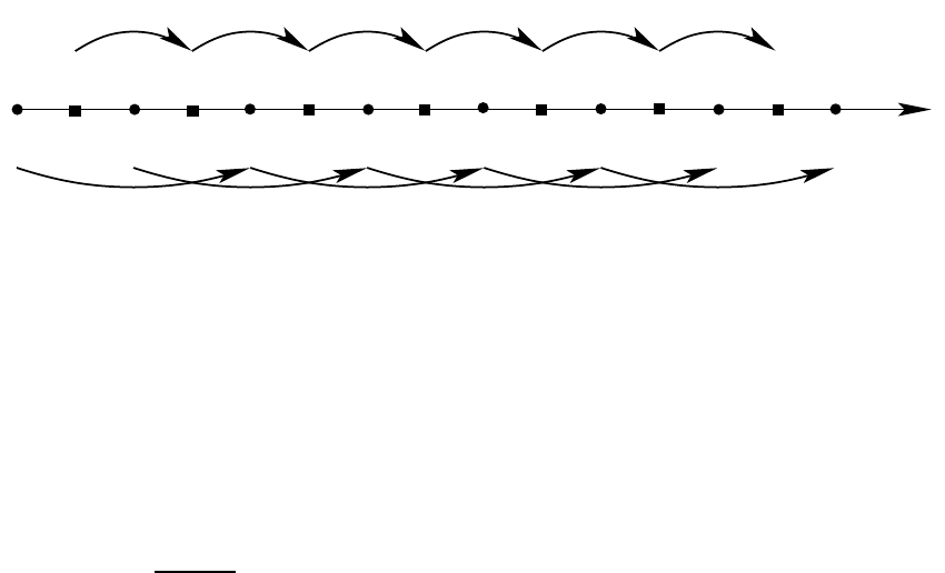
122
CHAPTER 7. TOTAL OCEAN MASS AND TRACER CONTENT
ττ+1 τ+2 τ+3 τ+4 τ+5 τ+6
τ+1/2 τ+3/2 τ+5/2 τ+7/2 τ+9/2 τ+11/2 τ+13/2
∆τ ∆τ ∆τ ∆τ ∆τ ∆τ
2∆τ 2∆τ 2∆τ 2∆τ 2∆τ 2∆τ
τ+7
Figure 7.1: Schematic of time stepping for tracer concentration and total tracer mass
in the case where N=6. The lower branch shows the Nover-lapping 2∆
τ
leap-
frog steps used for updating the tracer field. The upper branch shows the Ntime
steps of length ∆
τ
moving the total tracer mass over the half-integer
τ
levels. Note
that the increments for
τ
are in units of ∆
τ
.
where A=∑dat is the total tracer cell area at the ocean surface. Second, compute
an effective flux
error(2)=1
N∆
τ
A×
[T(
τ
+N∆
τ
,
τ
+ (N+1)∆
τ
)−T (
τ
,
τ
+∆
τ
)−∆
τ
N
∑
n=1F(
τ
+n∆
τ
)] (7.27)
where ideally we have
error(1)=error(2). (7.28)
Differences can be interepreted as due to numerical roundoff. Note that for po-
tential temperature, multiplying by Cpyields an error with units Watts per square
meter. For other tracers, the error is in units of kilograms per second per meter
squared. The magnitude of these errors is dependent on the model configuration,
the frequency at which surface forcing is altered, the level of time filtering, and the
time interval over which the diagnostic is computed.
Figure 7.1 illustrates the time steps involved in integrating tracer concentra-
tion and the implied integration of total tracer mass. Total tracer mass is cen-
tered on the half-time steps and is moved forward ∆
τ
upon each 2∆
τ
leap-frog
update of the tracer concentration. Assuming knowledge of the tracer, density,
and thickness fields at times
τ
and
τ
+∆
τ
, we can diagnose the total tracer mass
T(
τ
,
τ
+∆
τ
) = T(
τ
+∆
τ
/2). The N=6 time steps used to move from T(
τ
,
τ
+
∆
τ
)to T(
τ
+6∆
τ
,
τ
+7∆
τ
)require the surface tracer flux over the six time steps
F(
τ
+n∆
τ
)n=1,6.
7.5 Global adjustments to recover conservation
The absence of global conservation is a very unsatisfying aspect of the time filtered
leap-frog and explicit free surface methods. As discussed in Griffies et al. (2001),
some cases may be fine. Various attempts have been made to recover conservation.
We outline here some approaches that were tried, but with less than successful
results.

7.5. GLOBAL ADJUSTMENTS TO RECOVER CONSERVATION
123
7.5.1 Boussinesq volume budget
To start, let us consider the Boussinesq volume budget, as given by a discretization
of the free surface height equation
∂t
η
=−∇ ·U+qw. (7.29)
The time filtered “big leap-frog” step which updates
η
is given in the model by
[
η
(
τ
+∆
τ
)−
η
F(
τ
−∆
τ
)−A(
η
)] = 2∆
τ
(−∇ ·U+qw)(7.30)
where the time averaged surface height
η
Fis given in equation (7.20). The term A(
η
)
is an term added to recover global conservation of volume. It is hoped that such
can be a global constant which vanishes when there is no time filtering. Indeed,
such is possible with the following serving our needs
A(
η
)=
∑
i,j
dat [
η
(
τ
−∆
τ
)−
η
F(
τ
−∆
τ
)]
∑
i,j
dat . (7.31)
With this definition, we are led to the global integrated volume balance
∑
i,j
dat
η
(
τ
+∆
τ
) = ∑
i,j
dat
η
(
τ
−∆
τ
) + 2∆
τ
∑
i,j
dat qw. (7.32)
Notably, the time filtered surface height
η
F(
τ
−∆
τ
)dropped out of the balance.
Hence, we are left with a proper conservation statement, where the global integral
of the new surface height equals to the integral of the old height plus the integrated
fresh water forcing. Hence, at least for volume budget, a single global constant,
added to each of the surface heights, can bring back the usual balance of global
volume.
7.5.2 non-Boussinesq mass budget
From Griffies (2004), the semi-discrete budget for mass over a column of fluid takes
the form
ρ
z1∂t
η
+∑
k
hk∂t
ρ
k=
ρ
o(−∇ ·U+qw). (7.33)
Discretizing in time leads to
ρ
z1(
τ
) [
η
(
τ
+∆
τ
)−
η
F(
τ
−∆
τ
)−A(
ρ η
)] + 2∆
τ
∑
k
dhtk(
τ
)∂t
ρ
k(
τ
)
=2∆
τ ρ
o[−∇ · U(
τ
) + qw(
τ
)]. (7.34)
To recover total mass conservation, we define the constant adjustment
A(
ρ η
)=
∑
i,j
dat
ρ
z1(
τ
) [
η
(
τ
−∆
τ
)−
η
F(
τ
−∆
τ
)]
∑
i,j
ρ
z1(
τ
)dat . (7.35)
124
CHAPTER 7. TOTAL OCEAN MASS AND TRACER CONTENT
To verify mass conservation, let us integrate over the globe to find
∑
i,j
dat
ρ
z1(
τ
) [dht1(
τ
+∆
τ
)−dht1(
τ
−∆
τ
)] + 2∆
τ
∑
i,j
dat ∑
k
dhtk(
τ
)∂t
ρ
k(
τ
).
=2∆
τ ρ
o∑
i,j
dat qw(
τ
), (7.36)
with dht1=
η
+∆z1the upper cell thickness. With the time tendency ∂t
ρ
k(
τ
)dis-
cretized as discussed in Griffies (2004), this global budget is a proper discretization
of the continuum budget. To add some symmetry to this result, we add zero in the
form dhtk(
τ
+∆
τ
)−dhtk(
τ
−∆
τ
)for k>1. Doing so, and discretizing the density
tendency, leads to
∑
i,j
dat ∑
k
ρ
zk(
τ
) [dhtk(
τ
+∆
τ
)−dhtk(
τ
−∆
τ
)]
+∑
i,j
dat ∑
k
dhtk(
τ
) [
ρ
k(
τ
+∆
τ
)−
ρ
k(
τ
−∆
τ
)] = 2∆
τ ρ
o∑
i,j
dat qw(
τ
). (7.37)
As discussed in Griffies (2004), the density is time stepped via an extrapolation
method introduced by Greatbatch et al. (2001). It therefore has no time filtering.
Rearrangement leads to the discrete conservation law
∑
i,j
dat ∑
k
[
ρ
zk(
τ
)dhtk(
τ
+∆
τ
) +
ρ
zk(
τ
+∆
τ
)dhtk(
τ
)]
=∑
i,j
dat ∑
k
[
ρ
zk(
τ
−∆
τ
)) dhtk(
τ
) +
ρ
zk(
τ
)dhtk(
τ
−∆
τ
)] + 2∆
τ ρ
o∑
i,j
dat qw(
τ
).
(7.38)
Introducing a total mass with two time levels
2M(
τ
,
τ
+∆
τ
) = ∑
i,j
dat ∑
k
[
ρ
zk(
τ
)dhtk(
τ
+∆
τ
) +
ρ
zk(
τ
+∆
τ
)dhtk(
τ
)]. (7.39)
leads to the discrete total mass conservation law
M(
τ
,
τ
+∆
τ
) = M(
τ
−∆
τ
,
τ
) + ∆
τ ρ
o∑
i,j
dat qw(
τ
). (7.40)
As for the volume conservation, we are able to recover discrete mass conservation
by adding a global constant which vanishes upon removing the time filtering.
7.5.3 non-Boussinesq tracer budget
The semi-discrete tracer budget for the surface cells was given in Section 7.4. We
repeat it here for completeness
∂t(h
ρ
T)z1=−
ρ
o∇ · (huT+hFh)z1+
ρ
o[(w T)z1+qwTw] +
ρ
o[Fz
z1−Q(turb)
T].
(7.41)
The budget for interior cells with k>1 is given by
∂t(
ρ
h T)zk=−
ρ
o∇· (huT+hFh)zk+
ρ
o[(w T)zk−(w T)zk−1] +
ρ
o[Fz
zk−Fz
zk−1].
(7.42)
7.5. GLOBAL ADJUSTMENTS TO RECOVER CONSERVATION
125
Time discretizing the left hand side of the surface budget leads to
(2∆
τ
)∂t(h
ρ
T)z1≈dhtz1(
τ
) [(
ρ
T)(
τ
+∆
τ
)−(
ρ
T)R(
τ
−∆
τ
)−A(
ρ
T)]z1
+ (
ρ
T)z1(
τ
) [dht(
τ
+∆
τ
)−dhtF(
τ
−∆
τ
)−Az1
(
ρ η
)]z1. (7.43)
In this equation
(
ρ
T)R(
τ
−∆
τ
) =
ρ
(
τ
−∆
τ
)TR(
τ
−∆
τ
)(7.44)
is the density weighted Robert time-filtered tracer concentration. The surface height
adjustment A(
ρ η
)is defined by equation (7.35). As for volume and mass, we hope
to define the density weighted tracer adjustment Az1
(
ρ
T)to ensure conservation of
global tracer mass. We are motivated to define this adjustment as a function of
depth, since most of the time filtering is applied to the upper ocean, where tempo-
ral variability is largest. To remove time filtering in the area integrated budget for
the surface cells, we set
Az1
(
ρ
T)=∑i,jdat dht(
τ
) [(
ρ
T)(
τ
−∆
τ
)−(
ρ
T)R(
τ
−∆
τ
)]z1
∑i,jdat dhtz1(
τ
)
+∑i,jdat (
ρ
T)(
τ
) [dht(
τ
−∆
τ
)−dhtF(
τ
−∆
τ
)−A(
ρ η
)]z1
∑i,jdat dhtz1(
τ
). (7.45)
As the interior cells with k>1 have time independent volumes, the interior
tracer budget has a discrete time tendency
(2∆
τ
)∂t(h
ρ
T)zk≈dhtzk(
τ
) [(
ρ
T)(
τ
+∆
τ
)−(
ρ
T)R(
τ
−∆
τ
)−A(
ρ
T)]zk. (7.46)
For these cells, we remove time filtering from the area integrated budget by setting
Azk
(
ρ
T)=∑i,jdat dhtzk(
τ
)[(
ρ
T)(
τ
−∆
τ
)−(
ρ
T)R(
τ
−∆
τ
)]zk
∑i,jdat dhtzk(
τ
). (7.47)
Use of the adjustments A(
ρ η
)and Azk
(
ρ
T)leads to the discrete tracer budget over
the surface cell
dhtz1(
τ
) (
ρ
T)(
τ
+∆
τ
) = dhtz1(
τ
) [(
ρ
T)R(
τ
−∆
τ
) + A(
ρ
T)]z1
−(
ρ
T)z1(
τ
) [dht(
τ
+∆
τ
)−dhtF(
τ
−∆
τ
)−A(
η
)]z1
+ (2∆
τ
)−
ρ
o∇· (huT+hFh)z1+
ρ
o[(w T)z1+qwTw] +
ρ
o[Fz
z1−Q(turb)
T]
(7.48)
and the interior cells with k>1
dhtzk(
τ
) (
ρ
T)(
τ
+∆
τ
) = dhtzk(
τ
) [(
ρ
T)R(
τ
−∆
τ
) + A(
ρ
T)]zk
+ (2∆
τ
)−
ρ
o∇· (huT+hFh)zk+
ρ
o[(w T)zk−(w T)zk−1] +
ρ
o[Fz
zk−Fz
zk−1].
(7.49)
126
CHAPTER 7. TOTAL OCEAN MASS AND TRACER CONTENT
Assuming all fluxes through solid-walls vanish, we are led to the global tracer bud-
get
∑
i,j
dat ∑
k
dhtzk(
τ
) [(
ρ
T)(
τ
+∆
τ
)−(
ρ
T)(
τ
−∆
τ
)]
+∑
i,j
dat (
ρ
T)(
τ
)z1[dhtz1(
τ
+∆
τ
)−dhtz1(
τ
−∆
τ
)]
=2∆
τ ρ
o∑
i,j
dat [qw(
τ
)Tw(
τ
)−Q(turb)
T(
τ
)]. (7.50)
Since the cells in the interior are time independent, we can add zero via the differ-
ence dhtzk(
τ
+∆
τ
)−dhtzk(
τ
−∆
τ
)to yield the equivalent result
∑
i,j
dat ∑
k
dhtzk(
τ
) [(
ρ
T)(
τ
+∆
τ
)−(
ρ
T)(
τ
−∆
τ
)]
+∑
i,j
dat ∑
k
(
ρ
T)(
τ
)zk[dhtzk(
τ
+∆
τ
)−dhtzk(
τ
−∆
τ
)]
=2∆
τ ρ
o∑
i,j
dat [qw(
τ
)Tw(
τ
)−Q(turb)
T(
τ
)]. (7.51)
Rearrangement leads to the conservation statement
∑
i,j
dat ∑
k
[dhtzk(
τ
) (
ρ
T)(
τ
+∆
τ
) + dhtz1(
τ
+∆
τ
) (
ρ
T)(
τ
)]
=∑
i,j
dat ∑
k
[dhtzk(
τ
−∆
τ
) (
ρ
T)(
τ
) + dhtz1(
τ
) (
ρ
T)(
τ
−∆
τ
)]
+2∆
τ ρ
o∑
i,j
dat [qw(
τ
)Tw(
τ
)−Q(turb)
T(
τ
)]. (7.52)
Using the two-time level tracer mass notation from equation (7.22), we are led to
the balance
T(
τ
,
τ
+∆
τ
) = T(
τ
−∆
τ
,
τ
) + ∆
τ
F(
τ
), (7.53)
where the surface flux F(
τ
)is given by equation (7.14).
7.5.4 Comments on global adjustments
The adjustments to the surface height and the density weighted tracer concentra-
tion are sufficient to render a discretely exact global conservation for mass and
tracer content. Likewise, note that the adjusted tracer and surface height equations
are self-consistent, in that if the density weighted tracer concentration everywhere
was set to a constant, then the tracer budget would reduce to the volume budget.
This self-consistency means, for example, that a wind blowing across an ocean with
uniform tracer concentration will not set up spurious gradients in the tracer con-
centration. Griffies et al. (2001) further discuss this point.
There are two notable problems with having a global adjustment required to re-
cover conservation. First, it requires the computation of a global sum for each time
step and for each depth. Such is cumbersome on parallel computers, and can ren-
der the method inefficient. Second, the method alters prognostic fields in a nonlocal
7.6. COMMENTS ON THREE VERSUS TWO TIME LEVEL SCHEMES
127
manner. Although we chose to decouple the vertical levels, the horizontal remains
nonlocally coupled. That is, time filtering necessitated by temporal variability in
one horizontal region instantaneously affects the values of fields in other horizon-
tal regions. Such is clearly nonphysical. Just as we suggested for the vertical, we
can limit the extent to which horizontal nonlocality applies, by introducing distinct
adjustments over different prescribed horizontal regions. However, the limit where
the region goes to a point will, of course, remove time filtering altogether, and so
recover problems with leap-frog splitting. So horizontal regional adjustments must
be considered with care.
7.6 Comments on three versus two time level schemes
We pointed out in this chapter some fundamental problems with tracer conserva-
tion using the three time level leap-frog scheme. Again, the problem arises when
applying some form of time filtering, either the Robert-Asselin filter to the tracer
concentration (7.6) or the barotropic time average applied to the free surface (see
Griffies (2004)). Such time filters act to borrow from the past and future to alter
the present. Doing so in the presence of nonlinear products of time filtered prog-
nostic variables leads to problems with conservation that can only be overcome by
prescribing some global adjustments.
The problems identified here prompt some comments regarding the utility of
two time level schemes, many of which are common in ocean models (see Griffies et al.
(2000a) for a summary). These comments should be considered speculative, since
we have not under-taken a systematic investigation of the issues. Nonetheless, they
are presented in hopes that they highlight certain relevant points.
Let us first summarize the issues arising with the leap-frog. Because tracer is
time stepped via a leap-frog, it is necessary to also update surface height with a
leap-frog using the same time step. Otherwise, the discrete volume and tracer bud-
gets would be incompatible and there would be no way to form a discrete analog
of total ocean tracer content which undergoes a physically relevant time evolution,
even in the absence of time filtering. When the volume and tracer budgets are
compatible, non-conservation of total tracer content still arises when applying a
time filter to both the tracer and the surface height, with tests indicating that both
contribute roughly an equal amount to the non-conservation. Additionally, due
to the tendency for the surface height to generate noise when time stepping the
split equations on the B-grid, it has proven essential to compute the filtered surface
height contribution using the time averaged surface height from the previous and
future time steps. Note that this computational mode is absent on the C-grid, thus
motivating its use for discretizing gravity waves. However, C-grid models suffer
from a computational mode associated with the Coriolis force, and such is nontriv-
ial to damp in a conservative manner. See Adcroft et al. (1999) for a review with
suggestions.
Two-time level predictor-corrector schemes contain time damping applied in
a semi-implicit manner. Hence, there is no need to employ a Robert-Asselin time
filter. Careful discretization in the C-grid Hallberg Isopycnal Model Hallberg (1997)
allows for an exact conservation of total tracer if the predictor-corrector is applied
to the tracer fields as well as within the barotropic sub-cycle. The surface height
128
CHAPTER 7. TOTAL OCEAN MASS AND TRACER CONTENT
that is used to maintain conservation is driven by the barotropically time averaged
vertically integrated transport.
In an attempt to see whether a two-time level scheme is warranted for MOM,
we implemented a predictor-corrector approach for the barotropic system (similar
to Hallberg’s), yet maintained the leap-frog for the tracer and baroclinic velocity.
Unfortunately, the model was very unstable, likely due to the B-grid computational
mode, unless a time averaged surface height was incorporated at some stage in the
barotropic algorithm (see Griffies et al. (2001) for comments on such instabilities).
Yet the use of time averaging no longer allows for exact tracer conservation, even if
the tracer equation is changed to a predictor-corrector. Hence, we have found little
motivation in modifying the leap-frog scheme in the B-grid MOM. Conversion to
a C-grid may lead to more positive results, so long as the Coriolis null mode does
not then become pernicious (Adcroft et al. (1999)).
Even with the rigid lid, a leap-frog compromises the total tracer conservation.
Short of a fully two-time level scheme, it has been common to remove the leap-frog
splitting mode by periodically applying a two-time level Euler step instead of us-
ing a time filter. Extensive experience with this approach has prompted modelers to
abandon the use of such special-time step “tricks”, largely due to subtleties related
to vertical adjustment processes (see Griffies et al. (2000a) for a review and refer-
ences). A predictor-corrector for a rigid lid B-grid model thus makes more sense,
because the issues of stabilizing the free surface are no longer relevant and all time
steps are treated the same. Because the rigid lid is not suitable for other reasons
(e.g., Griffies (2004)), there has been no attempt to see how useful a two-time level
B-grid MOM would be.
Part III
Vertical physics and transport
129
131
NUMERICS OF VERTICAL PHYSICS
Vertical physics is relatively simple to implement in a z-coordinate ocean model.
Nonetheless, we find it useful to discuss some issues relevant to the implementa-
tion of vertical processes in MOM4, and so present salient issues in this part of the
MOM4 Guide.

CHAPTER
EIGHT
Shortwave heating
Contents
8.1 General considerations and model implementation . . . . . . . 133
8.2 The Paulson and Simpson (1977) irradiance function . . . . . . . 134
8.3 Shortwave penetration based on chlorophyll-a . . . . . . . . . . 135
8.3.1 Solar penetration in the ocean . . . . . . . . . . . . . . . . . 135
8.3.2 Morel and Antoine (1994) shortwave penetration model . 135
8.3.3 SeaWiFS based chlorophyll-a climatology . . . . . . . . . . 136
The purpose of this chapter is to discuss the numerical implementation of short-
wave heating. Sensitivity of the ocean solution to the penetration of shortwave ra-
diation into the ocean column can be quite large. Penetrative shortwave heating is
implemented in MOM4 via the tracer source array.
This chapter, especially Section 8.3, benefitted from contributions by Colm Sweeney
(cos@gfdl.noaa.gov).
8.1 General considerations and model implementation
Solar penetration brings solar shortwave heating downward in the ocean column,
thus providing a heating at depth. The parameterization of the oceanic absorption
of downward solar radiation is generally written as
I(x,y,z) = I0−(x,y)F(z), (8.1)
where I0−, in units of W m−2, is the total shortwave downwelling radiative heating
per unit area incident at the earth surface, and F(z)is a dimensionless attenuation
function. Note that the total downwelling radiation I0−is to be distinguished from
the total shortwave heating I0, where I0−= (1−
α
)I0, with
α
≈0.06 the sea surface
albedo.
Shortwave heating affects the heat budget locally according to
(
ρ
T),t=−(
ρ
o/cp)∂z(cpFz−I). (8.2)
133
134
CHAPTER 8. SHORTWAVE HEATING
In this equation, Fzaccounts for vertical processes such as advection and diffusion,
cpis the heat capacity of seawater,
ρ
is the in-situ density which for a Boussinesq
fluid is set to the Boussinesq reference density
ρ
o.
Shortwave heating leads to the following net heat flux over a column of ocean
fluid
(
ρ
o/cp)
η
Z
−H
dz ∂zI= (
ρ
o/cp) [I(
η
)−I(−H)]. (8.3)
where I(
η
)is often approximated as I(0). We assume there is no shortwave heating
of the solid rock underneath the ocean fluid, so I(z=−H) = 0 is appropriate,
with this boundary condition set via masks in MOM4. Although the expression
(8.5) suggests the upper boundary condition I(0) = I0−, we must be careful to not
double-count the shortwave source in MOM4 since it is typically also carried as
part of the surface temperature flux array st f . We now present the two approaches
available in MOM4.
The vertical convergence of penetrative shortwave radiation, (
ρ
o/cp)∂zI, is in-
corporated into MOM4’s potential temperature equation via a source term. Addi-
tionally, it is typical to include the total downwelling shortwave heating I0−within
the surface flux array st f , where other forms of heating such as those from latent
and long-wave affects are also incorporated. Hence, for proper accounting of the
shortwave heating, the upper boundary condition for the irradiance function must
be specified as
I(
η
) = 0 if I0−is already included in st f
I0−(x,y)if I0−is NOT already included in st f .(8.4)
The typical practice at GFDL is to set I(
η
) = 0 since I0−is already included in st f .
Care should be exercised by those using the opposite convention.
8.2 The Paulson and Simpson (1977) irradiance function
Jerlov (1968) classified water into five types according to its optical properties,
which determines the extent that solar radiation penetrates into a vertical fluid
column. For example, clear water allows for deeper penetration, whereas mirky
water, as occurs in the presence of active biology, more rapidly attenuates the radi-
ation. Studies by Paulson and Simpson (1977) then suggest a form for the attenua-
tion function F(z)based on the optical properties of water.
The parameterization of solar shortwave absorption of downwelling solar ra-
diation used by Rosati and Miyakoda (1988) is given by the Paulson and Simpson
(1977) form
I(x,y,z) = I0−(x,y) [R ez/
ζ
1+ (1−R)ez/
ζ
2], (8.5)
where I0−is the total shortwave downwelling radiative heating per unit area inci-
dent at the earth surface,
ζ
1and
ζ
2are attentuation lengths and Ris an empirical
constant dependent on the optical properties of the water. In the Rosati and Miyakoda
(1988) study, they chose R=0.58,
ζ
1=0.35m, and
ζ
2=23m, corresponding to
Jerlov Type I water (clear water). This is the form of shortwave penetration orig-
inally implemented in MOM. However, MOM4 now implements the scheme dis-
cussed in Section 8.3.
8.3. SHORTWAVE PENETRATION BASED ON CHLOROPHYLL-A
135
8.3 Shortwave penetration based on chlorophyll-a
This Section was contributed by Colm Sweeney (cos@gfdl.noaa.gov).
Recent investigations with solar penetration have indicated a strong sensitivity
of ocean simulations to how light penetrates into the ocean and warms the upper
few tens of meters. This section describes recent work at GFDL whereby the use
of a spatially and temporally dependent penetration depth is specified according
to climatological chlorophyll data. Although this data is taken from a climatology,
its use is believed to be preferable, even for climate change simulations, to the use
of a space-time independent optical type. Research into bio-optical influences on
ocean climate remains an active area, and the methods presented here remain under
investigation by various groups.
8.3.1 Solar penetration in the ocean
Observations and models describing the distribution of solar radiation with depth
in seawater have demonstrated that nearly all (99.9%) of the downwelling infrared
radiation (wavelengths of 750nm-2500nm) is absorbed in the upper 2 meters of the
ocean. While variability in the penetration depth of long wave radiation has large
implications for skin temperature and surface layer heat fluxes, this IR radiation
has little effect below the surface over the depths (roughly 10 m) used in present
day ocean models (Morel and Antoine (1994), Ohlmann and Siegel (2000)).
In contrast, attenuation of shortwave solar radiation (wavelengths <750nm) is
both spatially and temporally variable at scales important to ocean climate models.
In waters with high particulate and dissolved organic matter concentrations, the
1% light penetration depth can be less than 10 meters while in the clear, biologically
unproductive waters of the subtropical gyres, solar radiation can directly contribute
to the heat content at depths greater than 100 meters.
Previously, ocean climate models have parameterized the penetration of light
into the ocean by identifying six water types distinguished by the ”clarity” of the
water (Paulson and Simpson (1977)). This method is described in Section 8.2. More
recently, the correlation between chlorophyll pigment concentrations and short wave
penetration depths has enabled us to parameterize shortwave penetration of solar
radiation with satellite observations of ocean color (Morel (1988), Morel and Antoine
(1994), Ohlmann and Siegel (2000)). By assimilating satellite observations of ocean
color (e.g., SeaWiFS, OCTS, MODIS), it is possible to more accurately simulate the
spatial and temporal variability of penetrating radiation.
8.3.2 Morel and Antoine (1994) shortwave penetration model
Present modeling work at GFDL (Spring 2003) makes use of a parameterization
developed by Morel and Antoine (1994). This scheme was explicitly developed for
large-scale ocean models with coarse depth resolution (i.e., grids with ∆z>5m).
Morel and Antoine (1994) expand the exponential function used by Denman (1973)
into three exponentials to describe solar penetration into the water column.
The first exponential is for wavelengths >750nm (i.e., IIR) and assumes a single
attenuation of 0.267meter with a solar zenith angle
θ
=0. At present we assume
that the solar zenith angle stays constant throughout the daily integration of the
136
CHAPTER 8. SHORTWAVE HEATING
model. Thus, the resulting equation for the infared portion of the downwelling
radiation is:
IIR (x,y,z) = IIR−(x,y)e−z/(0.267 cos
θ
)(8.6)
where again
θ
=0. This relationship assumes z is the depth in meters and that
IIR−(x,y)is a fraction, of the total downwelling radiation, I0−such that
IIR−(x,y) = FIR I0−(8.7)
and
FIR +FV IS =1 (8.8)
where FIR and FVIS are the fractions of infared (750nm to 2500nm) and visible
(300nm to 750nm) radiation downwelling from the surface ocean. Although Morel and Antoine
(1994) note that water vapor, zenith angle, and aerosol content each can effect the
fraction of incoming radiation that is represented by infared and visible light, in the
present implementation we have chosen to keep these fractions constant such that
FIR =0.46.
The second and third exponentials represent a parameterization of the attenua-
tion function for downwelling radiation in the visible range (300nm -750nm) in the
following form:
IVIS(x,y,z) = IVIS−(x,y) (V1ez/
ζ
1+V2ez/
ζ
2). (8.9)
This form further partitions the visible radiation into long (V1) and short (V2) wave-
lengths assuming
V1+V2≡1. (8.10)
V1,V2,
ζ
1and
ζ
2are calculated from an empirical relationship as a function of
chlorophyll-a concentration using methods from Morel and Antoine (1994). Through-
out most of the ocean V1<0.5 and V2>0.5. The e-folding length scales
ζ
1
and
ζ
2are the e-folding depths of the long (
ζ
1) and short visible and ultra vio-
let (
ζ
2) wavelengths. Based on the chlorophyll-a climatology used in the GFDL
models,
ζ
1should not exceed 3m while
ζ
2will vary between 30m in oligotrophic
waters and 4m in coastal regions. All of these constants are based on satellite es-
timates of chlorophyll-a plus Pheaophytin-a, as well as parameterizations which
have “nonuniform pigment profiles” (Morel and Antoine (1994)). The ”nonuni-
form pigment profiles” have been proposed to account for deep chlorophyll max-
ima that are often observed in highly stratified oligotrophic waters (Morel and Berthon
(1989)).
8.3.3 SeaWiFS based chlorophyll-a climatology
A ”non- El Ni˜no” chlorophyll-a climatology was produced from estimates of the
Sea-viewing Wide Field-of-view Sensor (SeaWiFS). The ”non - El-Ni˜no” climatol-
ogy is based on 8-day composites of SeaWiFS images taken from 1999 to the end
of 2001. The climatology calculates the weighted average chlorophyll-a concentra-
tion on the 15th day of each month considering all data 16 days before, and after
the 15th day of each month. Each 8-day composite is assigned a gaussian (alpha =
2.5) weight based on its proximity to the 15th day of each month. This data set is
available from the GFDL NOMADS server where MOM4 datasets are distributed.

CHAPTER
NINE
Vertical adjustment schemes
Contents
9.1 Introduction . . . . . . . . . . . . . . . . . . . . . . . . . . . . . . . 137
9.2 Summary of the vertical adjustment options . . . . . . . . . . . . 138
9.3 Concerning a double application of vertical adjustment . . . . . 138
9.4 Boussinesq and non-Boussinesq cases . . . . . . . . . . . . . . . 139
9.4.1 Vertical momentum friction . . . . . . . . . . . . . . . . . . 139
9.4.2 Vertical tracer diffusion . . . . . . . . . . . . . . . . . . . . 139
9.5 Implicit vertical mixing . . . . . . . . . . . . . . . . . . . . . . . . 139
9.5.1 General form of discrete vertical diffusion . . . . . . . . . . 140
9.5.2 Discretization of vertical fluxes . . . . . . . . . . . . . . . . 140
9.5.3 Manipulating into a generic form . . . . . . . . . . . . . . . 141
9.5.3.1 Surface cells . . . . . . . . . . . . . . . . . . . . . 141
9.5.3.2 Interior cells . . . . . . . . . . . . . . . . . . . . . 142
9.5.3.3 Bottom cells . . . . . . . . . . . . . . . . . . . . . 142
9.5.3.4 A generic form . . . . . . . . . . . . . . . . . . . . 142
9.5.3.5 Solution method . . . . . . . . . . . . . . . . . . . 143
9.6 Convective adjustment . . . . . . . . . . . . . . . . . . . . . . . . 143
9.6.1 Comments on the convective adjustment schemes . . . . . 143
9.6.2 Coding of full convection by M. Eby . . . . . . . . . . . . . 143
The purpose of this chapter is to present the vertical adjustment schemes avail-
able in MOM4.
9.1 Introduction
The hydrostatic approximation necessitates the use of a parameterization of vertical
overturning processes. The original parameterization used by Bryan in the 1960’s
was motivated largely from ideas then used for modeling convection in stars (Bryan
(1969)). Work by Marshall and collaborators (Klinger et al. (1996), Marshall et al.
137
138
CHAPTER 9. VERTICAL ADJUSTMENT SCHEMES
(1997)) have largely indicated that the basic ideas of vertical adjustment are useful
for purposes of large-scale ocean circulation.
The Cox (1984) implementation of convective adjustment (the “NCON” scheme)
may leave columns unstable after completing the code’s adjustment loop. Various
full convective schemes have come on-line, with that from Rahmstorf (1993) imple-
mented in MOM4. An alternative to the traditional form of convective adjustment
is to increase the vertical mixing coefficient to some large value (say ≥10m2s−1) in
order to quickly diffuse vertically unstable water columns. Indeed, it is this form
recommended from the study of Klinger et al. (1996), and it is the approach com-
monly used in mixed layer schemes such as Pacanowski and Philander (1981) and
Large et al. (1994).
9.2 Summary of the vertical adjustment options
The handling of gravitationally unstable water columns in MOM4 can happen in
one of two basic ways.
•Implicit vertical mixing: By setting the namelist parameter aidi f =1.0, all
vertical diffusion is handled implicitly. There are two approaches depending
on the vertical mixing scheme used.
1. When using the constant vertical mixing module, the vertical diffusiv-
ity is set to a maximum value determined by a namelist di f f cbt limit
upon reaching a gravitationally unstable situation. di f f cbt limit =10.0
(MKS) is a typical value.
2. When using the Pacanowski and Philander or KPP vertical mixing scheme,
both the vertical diffusivity and vertical viscosity are set to the namelist
settings di f f cbt limit and visc cbu limit upon reaching a gravitationally
unstable situation. di f f cbt limit =visc cbu limit =10.0 (MKS) are typ-
ical values.
•Convective adjustment: There are two convective adjustment schemes in MOM4.
Both schemes act only on tracers when mixing. The default is the full convect
scheme of Rahmstorf (1993). The alternative scheme is the older one from
Cox (1984) and is known colloquially as the “NCON scheme”. The NCON
scheme has been implemented in mom4.0 for legacy purposes and is not rec-
ommended for new models.
9.3 Concerning a double application of vertical adjustment
Whether solving the vertical diffusion equation implicitly (aidi f =1.0) or explic-
itly (aidi f =0.0), it is possible to use convective adjustment. To avoid a double
application of vertical adjustment, one should keep in mind the following points.
When using neutral diffusion, it is necessary to have aidi f =1.0 for numerical
stability. Hence, vertical diffusion will be computed implicitly in time. For those
wishing to have vertical adjustment applied just via the convective adjustment
scheme, then it will be necessary to set di f f cbt limit =kappa h and visc cbu limit =

9.4. BOUSSINESQ AND NON-BOUSSINESQ CASES
139
kappa m. If wishing to adjust via large vertical diffusivities, then set di f f cbt limit
to a large value as described above, and set the namelist convective adjust =.f alse.
9.4 Boussinesq and non-Boussinesq cases
The treatment of vertical adjustment schemes differs somewhat between Boussi-
nesq and non-Boussinesq formulations in MOM4. We highlight these differences in
this section.
9.4.1 Vertical momentum friction
As mentioned in Chapters 3 and 6 in this document, and more fully discussed in
Greatbatch et al. (2001) and Griffies (2004), friction is computed in the non-Boussinesq
formulations using the model velocity u
ρ
rather than u, where the linear momen-
tum per volume in the ocean model is given by
ρ
ou=
ρ
u
ρ
. (9.1)
Hence, for the non-Boussinesq model, it is u
ρ
that is mixed implicitly in time when
using the implicit mixing scheme. There is no distinction between u
ρ
and ufor the
Boussinesq model.
9.4.2 Vertical tracer diffusion
As also treated in Greatbatch et al. (2001) and Griffies (2004), the vertical tracer dif-
fusion equation takes the form
(
ρ
T),t=−
ρ
o∂zFz(9.2)
where
Fz=−
κ
T,z(9.3)
is the downgradient vertical tracer flux. In MOM4, we prefer to separate the density
and tracer concentration prior to temporal discretization, thus to isolate the time
tendency of the tracer concentration
T,t=−(T/
ρ
)
ρ
,t−(
ρ
o/
ρ
)∂zFz(9.4)
The density time tendency term vanishes for the Boussinesq case, and the factor
ρ
o/
ρ
is set to unity. For the non-Boussinesq case, the term −(T/
ρ
)
ρ
,tprovides an
added forcing to the tracer concentration, and the
ρ
o/
ρ
factor modifies the vertical
diffusion operator. The modification to the vertical diffusion operator is considered
in the following sections where we discuss the implicit treatment of this equation
via either implicit vertical diffusion or convective adjustment.
9.5 Implicit vertical mixing
When the namelist aidi f is set to unity, vertical mixing of momentum and tracers is
time stepped implicitly. When aidi f =0.0, vertical mixing is time stepped explic-
itly. Intermediate values give a semi-implicit treatment, although at present MOM4

140
CHAPTER 9. VERTICAL ADJUSTMENT SCHEMES
does not support semi-implicit treatments. An implicit treatment of vertical mix-
ing allows unrestrained values of the vertical mixing coefficients. An explicit treat-
ment, especially with fine vertical grid resolution, places an unreasonable limitation
on the size of the time step. The use of fine vertical resolution with sophisticated
mixed layer and/or neutral physics schemes has prompted the near universal im-
plicit treatment of vertical mixing in ocean climate models.
We now detail the implicit treatment of one dimensional vertical mixing in
MOM4. As discussed in Section 9.4, the tracer equation presents the most gen-
erality through the added
ρ
o/
ρ
factor seen in equation (9.4), and so we consider the
tracer equation here. For vertical tracer diffusion in the Boussinesq system, and for
the Bousinesq or non-Boussinesq vertical velocity equation, the
ρ
o/
ρ
factor is set to
unity.
9.5.1 General form of discrete vertical diffusion
We can write the vertical diffusion equation in the discrete form
φ
k(
τ
+1) =
φ
∗
k(
τ
+1)−Γk(
τ
) (Fz
k−1−Fz
k). (9.5)
where we introduced the inverse velocity
Γk(
τ
) = aidi f 2∆
τ
(
ρ
k(
τ
)/
ρ
o)dhtk(
τ
)(9.6)
which appears quite frequently in the following discussion. The profile
φ
∗
k(
τ
+1)
represents the tracer at the updated model time
τ
+1 arising from all processes
treated explicitly in time. The leap-frog time step 2 ∆
τ
is generally larger than that
allowed by CFL stability given the value of the vertical diffusivity, hence the need to
solve the equation implicitly in time. The implicit vertical mixing parameter aidi f
is set to unity for the fully implicit method. The field dhtkis the vertical thickness
of the tracer cells at time
τ
. For vertical mixing of velocity, dht becomes the velocity
cell thickness dhu.
The influence of the non-Boussinesq formulation can be thought of as modi-
fying the vertical thickness dhtkof the tracer cells to (
ρ
k(
τ
)/
ρ
o)dhtk(
τ
)(e.g., see
equation (9.6)). Notably, this modification holds whether we are considering ver-
tical diffusion or vertical convective adjustment, since it is independent of vertical
diffusivity.1
9.5.2 Discretization of vertical fluxes
The vertical flux Fz
kis located at the bottom of the kth tracer or velocity cell. A
positive value for Fz
kleads to an increase in
φ
k(
τ
+1). Away from surface and
bottom boundaries, this flux takes the downgradient form
Fz
k=−
κ
k
φ
k(
τ
+1)−
φ
k+1(
τ
+1)
dhwtk. (9.7)
1For these purposes, vertical convective adjustment can be thought of as vertical diffusion with an
infinite diffusivity.

9.5. IMPLICIT VERTICAL MIXING
141
The factors of
φ
are evaluated at time
τ
+1 because of the implicit treatement. The
vertical mixing coefficient
κ
khas a general space-time dependence set by a vertical
mixing scheme. As for the flux itself, the diffusivity
κ
kis situated at the bottom of
the tracer or velocity cell, depending on whether
φ
is a tracer field or velocity com-
ponent. The array dhwtkrepresents the vertical distance between tracer points at
time
τ
. For vertical mixing of velocity, dhwt becomes the distance between velocity
points dhwu.
At the ocean surface, the vertical flux is given by the surface boundary condition
s f lux placed on the velocity or tracer. For a tracer,
Fz
k=0=−st f , (9.8)
with st f MOM4’s surface tracer flux array with units of velocity times tracer con-
centration. The minus sign arises from the MOM4 convention that associates a
positive st f with an increase in tracer within the k=1 cell. In contrast, the present
discussion assumes a convention for the flux Fzwhereby a positive Fz
k=0is associ-
ated with a decrease in tracer within the k=1 cell. For velocity,
Fz
k=0=−sm f , (9.9)
with sm f the surface momentum flux with units of squared velocity. At the ocean
bottom, a similar condition leads to
Fz
k=kmt =−bt f (9.10)
for bottom tracer fluxes, and
Fz
k=kmt =−bm f (9.11)
for bottom momentum fluxes. The minus signs again represent a difference in con-
vention between MOM4 and the present discussion. In MOM4, a negative bt f rep-
resents the passage of tracer from solid rock into the ocean domain, as in geother-
mal heating. For velocity, a positive bm f represents a drag on the ocean momentum
field.
9.5.3 Manipulating into a generic form
To develop the solution algorithm, it is necessary to put the vertical diffusion equa-
tion into a generic form. For this purpose, let us consider in sequence the equation
for surface cells k=1, interior cells with k>1, and bottom cells with k=kmt.
9.5.3.1 Surface cells
For surface cells with k=1 we have
φ
∗
k(
τ
+1) =
φ
k(
τ
+1) + Γk(
τ
) (Fz
k−1−Fz
k)
=
φ
k(
τ
+1)−Γk(
τ
) (st f +Fz
k)
=
φ
k(
τ
+1)−Γk(
τ
)st f +Γk(
τ
)
κ
k
φ
k(
τ
+1)−
φ
k+1(
τ
+1)
dhwtk, (9.12)
142
CHAPTER 9. VERTICAL ADJUSTMENT SCHEMES
which leads to
φ
∗
k(
τ
+1) + Γk(
τ
)st f =
φ
k(
τ
+1)1+Γk(
τ
)
κ
k
dhwtk−
φ
k+1(
τ
+1)Γk(
τ
)
κ
k
dhwtk.
(9.13)
For velocity mixing, st f becomes sm f , and dhwt becomes dhwu.
9.5.3.2 Interior cells
For interior cells,
φ
∗
k(
τ
+1) =
φ
k(
τ
+1) + Γk(
τ
) (Fz
k−1−Fz
k)
=
φ
k(
τ
+1)−Γk(
τ
)
κ
k−1
φ
k−1(
τ
+1)−
φ
k(
τ
+1)
dhwtk−1
+Γk(
τ
)
κ
k
φ
k(
τ
+1)−
φ
k+1(
τ
+1)
dhwtk(9.14)
which leads to
φ
∗
k(
τ
+1) =
φ
k(
τ
+1)1+Γk(
τ
)
κ
k−1
dhwtk−1
+Γk(
τ
)
κ
k
dhwtk
−
φ
k−1(
τ
+1)Γk(
τ
)
κ
k−1
dhwtk−1−
φ
k+1(
τ
+1)Γk(
τ
)
κ
k
dhwtk. (9.15)
9.5.3.3 Bottom cells
Bottom cells with k=kmt(i,j)have
φ
∗
k(
τ
+1) =
φ
k(
τ
+1) + Γk(
τ
) (Fz
k−1−Fz
k)
=
φ
k(
τ
+1) + Γk(
τ
) (Fz
k−1+bt f )
=
φ
k(
τ
+1) + Γk(
τ
)bt f −Γk(
τ
)
κ
k−1
φ
k−1(
τ
+1)−
φ
k(
τ
+1)
dhwtk−1,
(9.16)
which leads to
φ
∗
k(
τ
+1)−Γk(
τ
)bt f =
φ
k(
τ
+1)1+Γk(
τ
)
κ
k−1
dhwtk−1−
φ
k−1(
τ
+1)Γk(
τ
)
κ
k−1
dhwtk−1.
(9.17)
9.5.3.4 A generic form
Introducing the notation
Ak=−Γk(
τ
)
κ
k−1/dhwtk−1if k>1
0 if k=1(9.18)
Ck=−Γk(
τ
)
κ
k/dhwtkif k<kmt
0 if k=kmt (9.19)
Bk=1−Ak−Ck(9.20)
Φ∗
k=
φ
∗
k(
τ
+1) + Γk(
τ
)st f if k=1
φ
∗
k(
τ
+1)if 1 <k<kmt
φ
∗
k(
τ
+1)−Γk(
τ
)bt f if k=kmt
(9.21)
9.6. CONVECTIVE ADJUSTMENT
143
renders
Φ∗
k=Ak
φ
k−1(
τ
+1) + Bk
φ
k(
τ
+1) + Ck
φ
k+1(
τ
+1). (9.22)
9.5.3.5 Solution method
The solution is arrived at by performing a decomposition and forward substitution.
The details are taken from pages 42 and 43 of Press et al. (1992).
9.6 Convective adjustment
This section provides a description of the NCON and full convective adjustment
schemes.
9.6.1 Comments on the convective adjustment schemes
As detailed in Rahmstorf (1993) and Pacanowski and Griffies (1999), the NCON
convection scheme takes multiple passes through the water column, alternately
looking for instability on odd and even model levels. When an instability is found,
tracers are mixed, with their means (weighted by cell thickness) preserved. This
process may induce further instability and therefore more than one pass through
the water column may be needed to remove all instability. The number of passes
through the water column is controlled by the parameter ncon, hence the name of
the scheme.
The NCON convection scheme has come under a lot of scrutiny. The discussion
in Rahmstorf (1993), Killworth (1989) and Marotzke (1991), provide some elabora-
tion and motivation to not employ the NCON scheme. Its presence in MOM4.0 is
solely for legacy purposes so that modelers can attempt to reproduce older results
using the new code.
The question inevitably arises of whether to mix or not mix momentum during
a vertical adjustment process. When momentum is not mixed, it is thought that it
is simply carried along through the effects on the density field. Killworth (1989)
supports this idea, so long as the purpose is large-scale ocean modeling. Basically,
through geostrophy, adjusting density appears sufficient. Also, the vertical thermal
wind shears in simulated convection regions were found by Killworth to not be too
strong. Hence, mixing momentum along with density did little to affect the overall
solution. These ideas, however, appear less sound for equatorial oceanography, and
so the mixing of both momentum and tracers might be more important in there.
9.6.2 Coding of full convection by M. Eby
In June 2000, Michael Eby (eby@uvic.ca) ported a new coding of the Rahmstorf
scheme to MOM3.1. His code is a bit more efficient and modern. In particular,
there are no more “goto” statements. This code was incorporated into MOM3.1 and
MOM4. Tests reveal that the results from the Eby code and the original Rahmstorf
code are nearly identical. The researcher can uncomment/comment out two lines
highlighted in the code to get the exact same results if one so desires.

CHAPTER
TEN
Vertical advection
Contents
10.1 Vertical transport equation . . . . . . . . . . . . . . . . . . . . . . 145
10.2 Vertical CFL violations . . . . . . . . . . . . . . . . . . . . . . . . . 146
10.3 Integer and non-integer advection . . . . . . . . . . . . . . . . . . 146
10.4 Implicit second order vertical advection . . . . . . . . . . . . . . 148
10.4.1 Discrete implicit advection . . . . . . . . . . . . . . . . . . 148
10.4.2 Comparing to implicit vertical diffusion . . . . . . . . . . . 151
10.5 Implicit first order upwind advection . . . . . . . . . . . . . . . . 151
Vertical advection has been found to constrain the model time step for certain
global model configurations moreso than other of transport processes. The purpose
of this chapter is to present some methods to relax the vertical CFL constraint. The
first method is based on ideas presented by Lin and Rood (1996), in which the in-
teger and non-integer pieces of the advection velocity are split. The next method
time steps second order centered advection implicitly in time, and the final method
time steps the first order upwind implicitly in time. Linear stability analysis for the
implicit schemes have not been performed, and should be done prior to bothering
to code them.
10.1 Vertical transport equation
The vertical tracer transport equation in MOM4 takes the form
(
ρ
T),t=−
ρ
o∂zFz, (10.1)
where we focus on tracer concentration for the moment, with trivial generalization
available for treating vertical velocity transport. For diffusive transport, as treated
in Chapter 9,
Fz=−
κ
T,z(10.2)
is the downgradient vertical tracer flux. For advection, as treated in this chapter,
Fz=w T (10.3)
145

146
CHAPTER 10. VERTICAL ADVECTION
is the vertical advective flux. In MOM4, we prefer to separate the density and tracer
concentration prior to temporal discretization, thus to isolate the time tendency of
the tracer concentration
T,t=−(T/
ρ
)
ρ
,t−(
ρ
o/
ρ
)∂zFz. (10.4)
The density time tendency term vanishes for the Boussinesq case, and the factor
ρ
o/
ρ
is set to unity. For the non-Boussinesq case, the term −(T/
ρ
)
ρ
,tprovides an
added forcing to the tracer concentration, and the
ρ
o/
ρ
factor modifies the vertical
transport operator. The modification to the vertical transport operator is considered
in the following sections where we discuss the implicit treatment of this equation.
10.2 Vertical CFL violations
Consider the leap-frog time stepped vertical transport equation for an arbitrary
tracer field T
Tk(
τ
+∆
τ
) = Tk(
τ
−∆
τ
) + 2
ρ
o∆
τ
ρ
k(
τ
)dhtk(Fz
k−Fz
k−1)(10.5)
where Fz
kis the vertical flux of Tentering the kth tracer cell through its bottom face
(see Figure 10.1). The thickness of the kth tracer cell is written dhtkto correspond to
the numerical model’s notation. Note that all considerations in this chapter focus
on a single vertical column, so the horizontal grid labels i,jare dropped for brevity.
There are many occasions where large vertical diffusive transport engenders
large vertical diffusive CFL numbers, especially in mixed layer regions. In this
case, it is computationally advantageous to move to a time implicit solution of the
vertical diffusion equation. Otherwise, the model’s time step would need to be
quite low in order to maintain numerical stability. Such is the common means for
time stepping vertical mixing in ocean climate models, and the details are presented
in Section 9.5.
We can also have problems with onerous time step constraints in model con-
figurations with large vertical velocities and refined vertical resolution. As for the
diffusive case, “large” is defined via the vertical CFL number, with the CFL num-
ber increasing when we refine the vertical resolution, enhance the current strengths,
and increase the strength and frequency of the surface forcing. Indeed, the time step
used in many ocean climate models (circa 2003) are constrained by vertical advec-
tion. Hence, ways to reduce the tightness of this constraint, if only by a few tens
of percents, greatly enhance model efficiency. As with any methods used for com-
putational expediency, they must be tested against conventional approaches to see
whether the solution’s physical integrity is unacceptably compromised.
10.3 Integer and non-integer advection
Lin and Rood (1996) present a means to relax the CFL constraint on 3-dimensional
advection using explicit in time methods. Because vertical advection constrains
the time step for some global models, we limit our considerations just to the one-
dimensional implementation of their scheme.1
1This section benefited from discussions with Isaac Held, 2003.
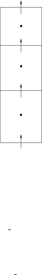
10.3. INTEGER AND NON-INTEGER ADVECTION
147
F(k)
(z)
F(k−1)
(z)
k
k−1
k+1
Figure 10.1: Schematic illustrating the vertical advective transport passing across
the faces of a model grid cell.
The numerically realized vertical advective flux of Tis a discretization of the
advective flux w T. If the vertical velocity component is directed upward, then we
are interested in checking the value of the leap-frog Courant number
C(+)
k=w btk(2∆
τ
)/dhtk+1. (10.6)
The use of the thickness dhtk+1is appropriate since and upward velocity compo-
nent advects tracer from cell Tk+1into cell Tk. When vertical velocity is downward,
we are interested in the Courant number
C(−)
k=−w btk(2∆
τ
)/dhtk, (10.7)
since the downward velocity component advects tracer from cell Tkinto cell Tk+1.
Consider the special case of a unit Courant number C(+)
k=1. If the tracer
concentration for a grid cell represents the value for a uniformly distributed con-
centration within the cell, then the first order upwind advective flux
Fz
k=wI
kTk+1(
τ
−∆
τ
)(10.8)
is an exact discretization of the continuum advective flux passing through the bot-
tom face of the kth tracer cell (e.g., page 93 of Durran (1999)). Here, the velocity
component
wI
k=dhtk+1/(2∆
τ
)(10.9)
is termed the integer velocity component, since it corresponds to an integer Courant
number. If we ignore all other fluxes entering or leaving the Tk+1grid cell, then a

148
CHAPTER 10. VERTICAL ADVECTION
unit Courant number C(+)
k=1 means that over a leap-frog time step 2∆
τ
, all of
the uniformly distributed tracer in cell Tk+1will leave this cell and pass across the
bottom interface of the Tkcell.
If the Courant number is larger than unity but less than two, then we need to
reach into one more box to gather all the tracer that will pass through the bottom of
the kth tracer cell. For this purpose, we split the vertical velocity component into its
integer and remainder pieces
w btk=wI
k+wR
k. (10.10)
A first order upwind flux crossing the bottom of the Tktracer cell is therefore given
by
Fz
k=wI
kTk+1(
τ
−∆
τ
) + wR
kTk+2(
τ
−∆
τ
). (10.11)
This flux has the form of an extended upwind flux, where the non-integer portion
of the velocity extends into the next deeper box, since this stronger vertical velocity
can move tracer from both the Tk+1and Tk+2boxes. Note that masks should be
applied in the model to ensure that there is actually ocean in the k+2 tracer cell
rather than land. If there is no ocean present, then we cannot apply the present
techniques. That is, if the Courant number is greater than one at a point next to a
boundary, and the flow is directed away from the boundary, then we cannot apply
these techniques, since we “run out” of fluid from which to draw.
To see if it is necessary to extend into yet another box, it is necessary to compute
the Courant number based on the remainder velocity wR
kand the box k+2
C(+)
k+1=wR
k(2∆
τ
)/dhtk+2. (10.12)
If this is larger than unity, then we compute the second integer velocity
wI
k+1=dhtk+2/(2∆
τ
)(10.13)
and the doubly extended upwind flux
Fz
k=wI
kTk+1(
τ
−∆
τ
) + wI
k+1Tk+2(
τ
−∆
τ
) + wR
k+1Tk+3(
τ
−∆
τ
). (10.14)
Note that the further that we move into deeper boxes, the less accurate the scheme
becomes.
10.4 Implicit second order vertical advection
Second order centered advection is the means used in mom4 to vertically advect
velocity. It is becoming less common, however, for advecting tracer. Nonetheless,
we detail how to implement time implicit second order vertical advection. Doing
so removes the vertical advection CFL constraint. Much here follows from the dis-
cussion of vertical mixing in Section 9.5.
10.4.1 Discrete implicit advection
As in the discussion of Section 9.5, we start by focusing on vertical tracer transport
given by equation (10.5). Second order centered advection leads to the discrete
10.4. IMPLICIT SECOND ORDER VERTICAL ADVECTION
149
vertical flux
Fz
k=
α
w btk/2[Tk(
τ
+∆
τ
) + Tk+1(
τ
+∆
τ
)]
+ (1−
α
)w btk/2[Tk(
τ
) + Tk+1(
τ
)]. (10.15)
In this equation, 0 ≤
α
≤1 sets the level by which the advective flux is evaluated
implicitly, with
α
=1 fully implicit, and
α
=0 fully explicit. A similar factor,
known in the model as aidi f , is used for vertical diffusion in Section 9.5. We focus
now on the implicit piece of vertical advection.
In equation (10.15), w btkis the vertical component to the tracer advection ve-
locity. It is centered at the bottom face of the kth tracer cell (see Figure 10.1). For
the
α
part of this equation, tracer concentration is evaluated at the new time step
τ
+∆
τ
, representing an implicit discretization of the flux. The vertical velocity
is computed at the present time step
τ
regardless whether we consider implicit
or explicit advection. If we instead tried to use velocity at the new time
τ
+∆
τ
;
i.e., implicitly, then the implicit method would become nonlinear and impractical.
Note that a similar approach is taken when implementing implicit vertical mixing
schemes. In these cases, although we may time step the tracer concentration implic-
itly, the flow dependent diffusivity is computed at time
τ
instead of
τ
+∆
τ
. Again,
to do otherwise would entail an impractical nonlinear implicit algorithm for ver-
tical mixing. Because we always evaluate velocity at
τ
, we do not expose its time
dependence.
In mom4, we time step the explicit terms first to compute a partially updated
tracer T∗
k(
τ
+∆
τ
). Then, we time step the implicit portion, which for tracers in-
cludes vertical diffusion and, if using the present scheme, second order vertical
advection. For velocity, we may also choose to compute the Coriolis force implic-
itly in time, as discussed in Chapter 24. The implicit vertical advection piece leads
to
Tk(
τ
+∆
τ
) = T∗
k(
τ
+∆
τ
) +
α ρ
o∆
τ
ρ
k(
τ
)dhtk
[wbtk(Tk(
τ
+∆
τ
) + Tk+1(
τ
+∆
τ
))
−w btk−1(Tk−1(
τ
+∆
τ
) + Tk(
τ
+∆
τ
))]. (10.16)
Following the discussion of vertical diffusion in Section 9.5.1, we introduce the
shorthand
Γ(adv)
k(
τ
) = 2
α
∆
τ
(
ρ
k(
τ
)/
ρ
o)dhtk(
τ
). (10.17)
Note that Γhas dimensions of an inverse velocity. The density ratio is set to unity
when employing the Boussinesq approximation. Note that the parameter
α
used
for vertical advection need not be equal to the aidi f parameter used for vertical
diffusion. Hence, it is useful to introduce the adv label on Γ, thus bringing equation
(10.16) to the form
Tk(
τ
+∆
τ
) = T∗
k(
τ
+∆
τ
)
+ (Γ(adv)
k/2)[wbtk(Tk(
τ
+∆
τ
) + Tk+1(
τ
+∆
τ
)) −w btk−1(Tk−1(
τ
+∆
τ
) + Tk(
τ
+∆
τ
))].
(10.18)
150
CHAPTER 10. VERTICAL ADVECTION
We can put these results into a standard form via manipulations similar to those
used for vertical diffusion in Section 9.5.3. For this purpose, some rearrangement
brings equation (10.16) into the form
T∗
k(
τ
+∆
τ
) = Tk(
τ
+∆
τ
)1−(Γ(adv)
k/2)w btk+ (Γ(adv)
k/2)w btk−1
+Tk−1(
τ
+∆
τ
) (Γ(adv)
k/2)w btk−1−Tk+1(
τ
+∆
τ
) (Γ(adv)
k/2)w btk. (10.19)
This equation holds for all grid points in the vertical, starting from k=1. However,
it is useful to distinguish the treatment at the top and bottom boundaries. For k=1,
the w btk=0contribution is handled via a separate portion of the update process
associated with surface height time tendencies. So this term does not contribute
here, thus leading to
Tk=1(
τ
+∆
τ
) = T∗
k=1(
τ
+∆
τ
)
+ (Γ(adv)
k=1/2) [w btk=1(Tk=1(
τ
+∆
τ
) + Tk=2(
τ
+∆
τ
)) −0], (10.20)
or in the rearranged form
T∗
k=1(
τ
+∆
τ
) = Tk=1(
τ
+∆
τ
)1−(Γ(adv)
k=1/2)w btk=1+0
+0−Tk=2(
τ
+∆
τ
) (Γ(adv)
k=1/2)w btk=1. (10.21)
A similar equation results for vertical advection of velocity at the k=1 velocity cell.
At the bottom of a tracer column, w btk=kmt generally vanishes due to volume/mass
conservation, thus leading to
Tk=kmt(
τ
+∆
τ
) = T∗
k=kmt(
τ
+∆
τ
)
+ (Γ(adv)
k=kmt/2) [0−w btk=kmt−1(Tk=kmt−1(
τ
+∆
τ
) + Tk=kmt(
τ
+∆
τ
))], (10.22)
or in the rearranged form
T∗
k=kmt(
τ
+∆
τ
) = Tk=kmt(
τ
+∆
τ
)1−0+ (Γ(adv)
k=kmt/2)w btk=kmt−1
+Tk=kmt−1(
τ
+∆
τ
) (Γ(adv)
k=kmt/2)w btk=kmt−1−0. (10.23)
At the bottom of a column of velocity points, w buk=kmu generally does not vanish,
since this velocity does not sit at the ocean bottom when there is nontrivial topo-
graphic slope. Hence, both advective fluxes are present for the velocity equation at
k=kmu. The issue of vertical velocities at the ocean bottom is discussed in Section
22.3.3 of Pacanowski and Griffies (1999).
Following the diffusion discussion in Section 9.5.3, we introduce
2Ak=(Γ(adv)
k(
τ
)w btk−1if k>1
0 if k=1(10.24)
Bk=1+Ak+Ck(10.25)
2Ck=−Γ(adv)
k(
τ
)w btk(10.26)

10.5. IMPLICIT FIRST ORDER UPWIND ADVECTION
151
to render
T∗
k(
τ
+∆
τ
) = AkTk−1(
τ
+∆
τ
) + BkTk(
τ
+∆
τ
) + CkTk+1(
τ
+∆
τ
). (10.27)
Note that higher order advection schemes lead to larger stencils. So, if time stepped
implicitly, these schemes require a more expensive matrix inversion.
10.4.2 Comparing to implicit vertical diffusion
There are two differences in details between implicit vertical mixing and implicit
vertical advection: (1) advection and mixing generally use different aidi f factors,
(2) the sign for Akfor advection, defined above equation (10.27), is opposite that for
mixing (see Section 9.5.3.4), (3) Bkfor diffusion is defined as 1 −Ak−Ckwhereas for
advection it is 1 −Ak−Ck. These differences must be kept in mind when inverting
the system.
10.5 Implicit first order upwind advection
Second order advection suffers from the well known null-mode. One may wish
to employ, instead, a first order upwind scheme which is made more stable via its
large levels of implicit diffusion. If the implicit upwind is applied only at selected
places, then the cost in solution integrity of added diffusion may be worth the ad-
vantage of running with longer time steps.
Following the discussion in Section 10.4.1, we are led to consider the implicit
upwind advection flux
Fz
k=hw(−)
kTk(
τ
+∆
τ
) + w(+)
kTk+1(
τ
+∆
τ
)i, (10.28)
where
2w(±)
k=maskk+1(w btk± |w btk|)(10.29)
and mask is the land-sea mask. Recall that wkis positive if the vertical component
to the advection velocity is directed upwards at the bottom face of the kth tracer cell.
Use of the flux (10.28) in the tracer equation leads to
Tk(
τ
+∆
τ
) = T∗
k(
τ
+∆
τ
)
+Γ(adv)
kh−w(−)
k−1Tk−1(
τ
+∆
τ
) + (w(−)
k−w(+)
k−1)Tk(
τ
+∆
τ
) + w(+)
kTk+1(
τ
+∆
τ
)i.
(10.30)
where Γis defined by equation (10.17), and T∗
k(
τ
+∆
τ
)is the updated tracer arising
from the explicit time-stepped processes. At the top with k=1, this equation
becomes
Tk=1(
τ
+∆
τ
) = T∗
k=1(
τ
+∆
τ
)
+Γ(adv)
k=1h−0.0 + (w(−)
k=1−0.0)Tk=1(
τ
+∆
τ
) + w(+)
k=1Tk=2(
τ
+∆
τ
)i, (10.31)
152
CHAPTER 10. VERTICAL ADVECTION
and at the bottom k=kmt,
Tk=kmt(
τ
+∆
τ
) = T∗
k=kmt(
τ
+∆
τ
)
+Γ(adv)
k=kmt h−w(−)
k=kmt−1Tk=kmt−1(
τ
+∆
τ
) + (w(−)
k=kmt −w(−)
k=kmt−1)Tk=kmt(
τ
+∆
τ
) + 0.0i.
(10.32)
Rearrangement leads to
T∗
k(
τ
+∆
τ
) = AkTk−1(
τ
+∆
τ
) + BkTk(
τ
+∆
τ
) + CkTk+1(
τ
+∆
τ
). (10.33)
where
Ak=(0 if k=1
Γ(adv)
k(
τ
)w(−)
k−1if k>1(10.34)
Bk=
1−Γ(adv)
k(
τ
)w(−)
kif k=1
1+Γ(adv)
k(
τ
)w(+)
k−1−Γ(adv)
k(
τ
)w(−)
kif k>1
1+Γ(adv)
k(
τ
)w(+)
k−1if k=kmt
(10.35)
Ck=(−Γ(adv)
k(
τ
)w(+)
kif k<kmt
0 if k=kmt (10.36)
Part IV
Some coupled modeling issues
153
155
SOME COUPLED MODELING ISSUES
MOM has traditionally been used as a component within a coupled climate
modeling system. Moving to a free surface has introduced some new issues that
must be addressed when coupling MOM4 to sea ice and river models. These issues
are outlined in this part of the MOM4 Guide.

CHAPTER
ELEVEN
Considerations for ice-ocean modeling
Contents
11.1 Introduction . . . . . . . . . . . . . . . . . . . . . . . . . . . . . . . 157
11.2 Ocean heating due to frazil formation . . . . . . . . . . . . . . . . 158
11.3 Ice with a free surface in a z-model . . . . . . . . . . . . . . . . . 159
11.4 Steady state mass budget . . . . . . . . . . . . . . . . . . . . . . . 159
11.5 Dynamical budgets . . . . . . . . . . . . . . . . . . . . . . . . . . . 160
11.6 The problem for z-coordinate ocean models . . . . . . . . . . . . 161
11.7 The alternatives . . . . . . . . . . . . . . . . . . . . . . . . . . . . . 162
11.7.1 Coarse vertical resolution . . . . . . . . . . . . . . . . . . . 162
11.7.2 Limit the ice thickness . . . . . . . . . . . . . . . . . . . . . 162
11.7.3 Zero fresh water fluxes and nonzero virtual salt fluxes . . 162
11.7.4 Pressure coordinate ocean models . . . . . . . . . . . . . . 164
11.8 Heat budget in coupled models . . . . . . . . . . . . . . . . . . . 164
11.9 Some comments on suppressing a leap-frog mode . . . . . . . . 165
This chapter presents some considerations relevant for coupling a z-coordinate
free surface ocean model to a dynamical ice model. We focus on the issues within
the context of a Boussinesq model, although the points are generic to any free sur-
face z-coordinate model.
11.1 Introduction
There are regions where ice-sheets have yet to form, yet ice is present in the liq-
uid water. This slurry of water-ice is commonly known as frazil. The liquid water
portion of frazil has a temperature given by the freezing temperature, which is a
function of the salinity and pressure.
During the formation of frazil, latent heat and salt is released to the liquid sea-
water. To get a rational representation of the salt added to the ocean model requires
that it be coupled to a sea ice model. For the present purposes, we describe a sim-
ple means to represent the heating effect. Note that when implementing a “frazil”
157
158
CHAPTER 11. CONSIDERATIONS FOR ICE-OCEAN MODELING
option in MOM4 without sea ice, we are led to the unphysical circumstance of hav-
ing sea ice formation stabilize the ocean water column. Hence, one should be quite
careful not to over interpret solutions where frazil heating occurs without the cor-
responding salinification.
11.2 Ocean heating due to frazil formation
To represent the heating due to frazil formation, we assume a linear empirical rela-
tion can be used to express the temperature at which sea ice starts to form (ignoring
pressure and nonlinear salinity effects)
T(◦C) = −0.054 s(psu). (11.1)
Water with higher salinity freezes at lower temperatures than water with lower
salinity. If the model’s prognostic temperature equation (i.e., advection, diffusion,
surface cooling) predict that T(◦C)<−0.054 s(psu), two effects occur. First, heat
is input to the liquid ocean water as it is extracted from the freezing ocean water.
The amount of heat given to the liquid is
Qf razil (Joule) = |0.054 s(psu) + T(◦C)|dV
ρ
Cp(11.2)
where
dV =dx dy (∆z+
η
)(11.3)
is the surface grid cell volume,
ρ
is the in situ ocean density, and Cpis the heat
capacity of seawater with
ρ
oCp=1035 kg m−3×3985 Joule ◦C−1kg−1=4.125 ×10⁶Joule m−3C−1. (11.4)
As defined, Qf razil is the heat sufficient to raise the sea surface temperature to
T(◦C) = −0.054 s(psu). Note that as the frazil heat is given to the liquid ocean
over the course of a tracer leap-frog time step, the rate of heating of the liquid due
to frazil formation is given by
dQf razil /dt= (2dtts)−1|0.054 s(psu) + T(◦C)|dV
ρ
oCp. (11.5)
Written as in a prognostic leap-frog time step, we have
T(
τ
+dtts) = T∗(
τ
+dtts) + 2dtts dQf razil /dt, (11.6)
with T∗(
τ
+dtts)the potential temperature updated to the new time step due to
the effects of processes other than frazil formation.
We determine the frazil heat Qf razil (Joule)within the ocean model. This heat
is applied to the ocean over a single leap-frog time step of length 2 dtts. For heat
conservation within the coupled ocean and sea ice system, this same amount of
heat must be extracted from the sea ice model. Importantly, if the sea ice model
uses a different time stepping scheme than MOM4’s leap-frog, then the frazil heat
Qf razil extracted from the sea ice model must be adjusted accordingly. For example,
the GFDL sea ice model (Sea Ice Simulator) uses a single-time step scheme rather
than a leap-frog. So the frazil heat Qf razil extracted from the sea ice model over a
11.3. ICE WITH A FREE SURFACE IN A Z-MODEL
159
single dtts time step within the ice model will be given by one-half that input to the
ocean model over a single ocean leap-frog time step 2 dtts
|QMOM4
f razil (Joule)|=2|QSIS
f razil (Joule)|. (11.7)
An example helps to illustrate the magnitude of this heating. Consider the cool-
ing of a surface grid cell with salinity 35psu, and let the cooling be such that the
model’s prognostic temperature equation predicts an updated surface cell temper-
ature of −2◦C. Since −2<−0.054 ×35 =1.89, frazil will form. The latent heat
given to the liquid ocean associated with the frazil formation is
Qf razil (Joule) = |1.89 −2|dV
ρ
oCp, (11.8)
where we made the Boussinesq approximation and so set the in situ density to the
reference density
ρ
o. For a surface grid cell of volume 105m×105m×10 m, the
formation of frazil leads to a local heat given to the ocean of
Qf razil =4.5 ×10¹⁶ Joule. (11.9)
If this heating occurs over the course of a day (i.e., 2 dtts =1 day), then the rate of
heating is given by
dQf razil /dt=4.25 ×1011 Watt. (11.10)
If the surface area dAof the grid cell is 105m×105m, this heating by frazil con-
tributes
(dQf razil /dt)/dA=42.5 Watt m−2. (11.11)
11.3 Ice with a free surface in a z-model
The remainder of the chapter is concerned with the issues of how sea-ice on the
ocean surface affects the surface height and thus the ocean currents. To introduce
the issues, recall that a column of Boussinesq ocean expands and contracts accord-
ing to
η
,t=−∇ ·U+qw. (11.12)
This equation represents a volume budget over a column of fluid, and it is derived
in Griffies (2004). In this equation,
η
is the deviation of the ocean surface from its
resting position at
η
=0. The first term on the right hand side is the convergence
of the vertically integrated velocity. For non-tidal motions, this term accounts for
some one-two meters of surface height deviation. The second term is the fresh
water forcing. Rain, rivers, evaporation, and non-tidal dynamics typically lead to
|
η
| ≤ 3m. Our concern in this chapter is the additional effect associated with ice
formation. Figure 11.1 illustrates this balance.
11.4 Steady state mass budget
We consider here the steady state mass budget for a single ocean model grid cell
before and after the formation of ice, as shown in Figure 11.2. Without ice, the mass
of fluid in the grid cell is given by
dMocean =
ρ
ocean dV = (∆z+
η
initial )
ρ
ocean dx dy, (11.13)
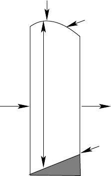
160
CHAPTER 11. CONSIDERATIONS FOR ICE-OCEAN MODELING
η
z=
ηD=H+
UU
qw
z=−H
Figure 11.1: The balance of volume within a column of Boussinesq fluid extending
from the free surface to the ocean bottom is represented by
η
,t=−∇ · U+qw,
where
η
is the time dependent deviation of the surface height from its resting state
at z=0. Time dependent fluctuations (
η
,t) are driven by (1) the convergence of
volume fluxes associated with the vertically integrated horizontal currents, and (2)
the flux of volume across the ocean surface from fresh water.
where
ρ
ocean is the in situ density of ocean fluid, and
∆z+
η
initial =hocean
initial (11.14)
is the initial thickness of ocean liquid in the grid cell. For the purposes of deriving
the ice-ocean mass balance, we are not concerned with the in situ density of ocean
fluid, but the in situ density of fresh water in the surface grid cell. That is, we are
concerned with the mass of fresh water in the cell
dMf resh =
ρ
f resh dV = (∆z+
η
initial )
ρ
f resh dx dy. (11.15)
As determined by the dynamical ice model, some fraction of this fresh water freezes
into sea ice with density
ρ
ice, thus forming ice of mass
dMice =hice
ρ
ice dx dy, (11.16)
where hice is the ice thickness. Assuming all the fresh water mass used to form ice
comes locally from an ocean model grid cell, ice formation reduces the thickness of
liquid ocean in this grid cell. At equilibrium, the thickness of ocean fluid is therefore
given by
(∆z+
η
f inal ) = (∆z+
η
initial )−hice (
ρ
ice/
ρ
f resh). (11.17)
11.5 Dynamical budgets
We now consider an oceanic perspective on the volume and momentum budgets
associated with ice formation and thawing.
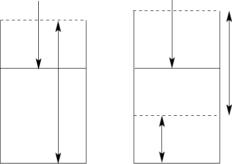
11.6. THE PROBLEM FOR Z-COORDINATE OCEAN MODELS
161
η
z=
η
z=
z=z1
z=0
P=P(atm) + g ρ η P=P(atm) + P(ice) + g ρ η
h(ice)
z=0
h(ocean)
h(ocean)
z=z1
Figure 11.2: Freezing of liquid ocean to form sea ice. Shown here is a single surface
model grid cell with vertical thickness ∆z+
η
, where ∆z=|z1|. The left panel
shows a cell filled with liquid ocean of some thickness hocean. The right panel shows
a cell with ice floating on liquid ocean in an equilibrium state after the transfer of
fresh water from ocean to ice has occured.
For the volume budget, the ice model provides the ocean model with a rate at
which fresh water is transferred between the sea ice and ocean. That is, the ice
model determines the ice contribution to the fresh water flux qwto be applied to
the surface height equation (11.12).
For the momentum budget, we consider the pressure applied at z=0. This
pressure drives the vertically integrated momentum field in the model. Without
ice, Figure 11.2 shows that pz=0is set by the atmospheric pressure as well as the
hydrostatic pressure arising from the layer of fluid between z=0 and z=
η
pz=0=patm +
ρ
ocean g
η
, (11.18)
where again
ρ
ocean is the in situ ocean fluid density. In the presence of ice, pressure at
z=0 has a contribution due to the mass of ice floating on the ocean. This pressure
is given by the weight per area of ice, thus leading to
pz=0=patm +
ρ
ocean g
η
+
ρ
ice g hice. (11.19)
The overall dynamical effect of ice on the ocean is small since the density of ice is
close to that of fresh water. Hence, the pressure pz=0is nearly the same whether
there is ice or liquid ocean in the grid cell.
11.6 The problem for z-coordinate ocean models
Sea ice in parts of the high latitudes can reach thicknesses on the order of ten meters
or more. Hence, the ocean surface height can be depressed by a large amount,
which in many cases is larger than the thickness of the ocean model’s surface grid
cell. This situation is unfortunate for MOM4 since the model does not allow for the
162
CHAPTER 11. CONSIDERATIONS FOR ICE-OCEAN MODELING
vanishing of grid cells. Additionally, for purposes of simulating the surface mixed
layer, modelers refine the vertical resolution near the surface, and so the depression
of the surface by ice could easily cause the surface grid cell to vanish.
This limitation of z-coordinate models is fundamental. It warrants the consider-
ation of other vertical coordinates. One which has been proposed is p−patmosphere.
This coordinate will always vanish at the ocean surface, no matter how low the
surface height is. It is presently a research topic to see whether this coordinate is
indeed useful for global ocean climate modeling.
11.7 The alternatives
We discuss here some choices available to the z-coordinate ocean modeler.
11.7.1 Coarse vertical resolution
One option for ocean-sea ice coupling is to use coarse vertical resolution so that
∆zof the ocean surface grid cell is larger than the anticipated sea ice thickness.
When considering this as an option, be sure to recognize the following points. Low
vertical resolution will compromise the integrity of surface ocean mixed layer sim-
ulations. Empirically, we have found resolutions in the upper ocean on the order of
10m or finer is required within the mixed layer. Intermediate resolutions, such as
20m-40m, traditionally have been avoided since they neither provide the necessary
resolution for a mixed layer scheme, nor enough volume to form a simple bulk
mixed layer. For this reason, climate modelers running without a surface mixed
layer scheme typically set their top box to some 50m thick.
11.7.2 Limit the ice thickness
If we insist on have refined vertical resolution for a mixed layer, then coupling a
sea ice model to a free surface z-coordinate ocean model requires one of two alter-
natives. First, we can run the ocean model with real fresh water forcing, yet limit
the ice thickness. From an ocean perspective, this choice is preferable. However,
artificially limiting the ice thickness may in turn affect ice extent. As one key role
of ice in the climate system is how it affects the earth’s albedo, artificially affecting
the ice extent is not desirable.
11.7.3 Zero fresh water fluxes and nonzero virtual salt fluxes
Another alternative is to let the ice thickness be unlimited, yet to remove the direct
effects of fresh water forcing from the ocean. That is, we solve the free surface
equation as
η
,t=−∇ · U, (11.20)
instead of the budget (11.12). In turn, there is no pressure applied to the ocean from
the overlying ice. It is as if the ice has a zero mass and it exchanges zero mass of
liquid with the ocean. Since the non-tidal dynamical effects yield a surface height
deviation on the order of a few meters, this choice ensures that the ocean model

11.7. THE ALTERNATIVES
163
will not loose surface grid cells, so long at ∆zis something larger than some few
meters (e.g., ∆z=5m should be sufficient).
By removing fresh water from the volume budget, we reduce the Boussinesq
ocean to an ocean with constant total volume. There is no longer a transfer of vol-
ume across the ocean surface. As the volume transfer between sea ice and ocean is
the problem, one may wish to remove just this transfer, but still allow the ocean to
feel the effects of fresh water from rivers, precipitation, and evaporation. However,
doing so will compromise the conservation of fresh water in the fully coupled sys-
tem. The reason is that ice grows via precipitation (snow). If we allow precipitation
to fall into the ocean as rain, but do not allow fresh water melt from sea ice to enter
the ocean, we have an open loop and so cannot conserve.
Removing fresh water transfers between the ocean and the rest of the climate
system is not the full story for the ocean. The reason is that freshening changes the
ocean salinity, which in turn changes the ocean density. This effect is crucial for
driving ocean currents, and so must be parameterized. As in the rigid lid models,
a means for incorporating this effect into the constant volume ocean model is to
introduce a salt flux across the model surface whenever there is a transfer of fresh
water in the real system.
To motivate the form of the salt flux, let us first consider the case of an ocean
model consisting of a single free surface grid cell affected only by surface water
fluxes. Due to the large hydration energy of salts, there is no salt flux across the
ocean surface, thus leading to the salt budget
∂t[dx dy (∆z+
η
)s] = 0. (11.21)
That is, total salt is constant in time. Solving for the salinity tendency leads to
s,t=−s qw
∆z+
η
, (11.22)
where
η
,t=qwwas used since we are considering the whole ocean to be one grid
cell, and so the ∇ · Uterm is absent. This budget says that as water is added to the
ocean (qw>0) it drives salinity to smaller values (s,t<0).
We now consider the case where there is no transfer of volume across the ocean
surface, and so the total ocean volume is constant. For the present example of
a single grid cell ocean, we therefore have
η
constant in time. To allow for the
freshening effect, fresh water transported into the ocean is replaced by a virtual salt
flux out of the ocean. In order to provide the same salinity tendency as in the case
of fresh water transfer, we are motivated to define our virtual salt flux as
Fexact =−s qw. (11.23)
However, this flux, which is the product of the local time dependent value of salin-
ity and the local fresh water flux, will not allow for conservation of total salt, even
if fresh water is globally constant. That is, Rdx dyFpropose is not constant, even if
Rdx dy qwis constant. Instead, to conserve total salt we must take the virtual salt
flux as
Fvirtual =−soqw, (11.24)

164
CHAPTER 11. CONSIDERATIONS FOR ICE-OCEAN MODELING
where sois a constant. In this case, the salinity equation becomes
s,t=−soqw
∆z+
η
. (11.25)
Comparison with the salinity tendency for the case of real fresh water fluxes reveals
that a virtual salt flux yields an accurate salinity tendency only when the constant
salinity sois close to the local salinity s. Errors scale as so/s. With global salinity
running on average near 35psu, it is typical to set so=35psu. With this value, how-
ever, river mouths introduce problems with this approach, especially with higher
resolution ocean models where the local salinity can become quite small. In this
case, as the river introduces fresh water to the ocean, the virtual salt flux is too
large in magnitude, thus causing the salinity tendency to be too large. Such large
jumps in salinity can introduce numerical problems on top of the physical problems
associated with spuriously large haline forcing in the model.
11.7.4 Pressure coordinate ocean models
If we redefine our vertical coordinate to be s=p(z)−patm −pice, then the surface
of the ocean is always at s=0. Discretizing the vertical according to s-levels al-
lows for arbitrary deviations of the ice thickness, since ice always lives at s=0.
Investigation of this vertical coordinate has not been thorough, and there may be
nontrivial issues to deal with, especially at the ocean bottom. Such remains a topic
for future studies.
11.8 Heat budget in coupled models
The change in energy at the solid/liquid phase transition is hundreds of times
larger than changes associated with raising the temperature of liquid water by a
degree celcius. Hence, global atmospheric models traditionally do not carry tem-
perature for water. River and land models similarly do not carry a temperature for
its fresh water. Sea ice models do carry a temperature of sea ice by default, since
the water temperature is always at the freezing point. Ocean models, of course,
do carry temperature, as this determines ocean density which in turn affects its cir-
culation. This different treatment of water in the coupled system leads to a global
non-conservation of heat when fresh water is allowed to be transferred across the
ocean interface.
To garner a sense for the magnitude of the imbalance, consider an ocean of two
grid boxes. Fresh water evaporating from a warm box and then condensing into a
cool box will lead to an ocean heat transport per unit area given by
∆H/A=
ρ
f resh Cpqw(Twarm −Tcold). (11.26)
This result assumes that fresh water transferred across the ocean-atmosphere in-
terface, either as precipitation or evaporation, has the same temperature as the sea
surface temperature carried by the ocean model. With
ρ
f resh Cp≈4×10⁶J/(m3K◦),
qwon the order of a meter per year, and Twarm −Tcold ≈10K◦, we have ∆H/A≈
11.9. SOME COMMENTS ON SUPPRESSING A LEAP-FROG MODE
165
1 W m−2. With atmospheric models not carrying temperature, there is no corre-
sponding atmospheric heat transport. The coupled system thus has an open loop
and so conservation is lost.
Fluxes crossing the ocean surface are on the order of tens to hundreds of W m−2,
and so this imbalance is small from an ocean-only perspective. Yet the imbalance is
systematic since evaporation tends to occur over certain regions, and precipation in
other regions. Furthermore, this heat flux imbalance is on the order of that associ-
ated with global warming forcing. Hence, for climate simulations, it may be unac-
ceptable and “corrections” or “adjustments” may be necessary to maintain proper
balances. Notably, this conclusion is independent of the limitations of z-coordinate
models discussed in the previous sections.
11.9 Some comments on suppressing a leap-frog mode
Martin Scdmidt reports that when coupling an ice model to mom with high fre-
quency coupling, it is possible to initiate the leap-frog computational mode. Pulses
of fresh water may arrive intermittedly from the ice, and this can project in some
cases more onto one of the leap-frog branches. Instability can be the result. For this
purpose, it is useful to average the fresh water from ice (or other sources) over two
time steps before sending fresh water to the ocean. This approach then couples the
leap-frog branches.

CHAPTER
TWELV
River discharge into the ocean model
Contents
12.1 Introduction . . . . . . . . . . . . . . . . . . . . . . . . . . . . . . . 167
12.2 General considerations . . . . . . . . . . . . . . . . . . . . . . . . 168
12.3 Steps in the algorithm . . . . . . . . . . . . . . . . . . . . . . . . . 169
This chapter presents a method to distribute river runoff throughout a vertical
column comprised of more than a single ocean model grid cell. This issue is most
important for ocean models with fine vertical grid resolution. Care is taken to ac-
count for the needs to conserve properties using the constraints of a z-model where
only the top cell is allowed to change its volume. The algorithm presented here is
based on discussions with Mike Winton (mw@gfdl.noaa.gov).
We formulate the river mixing process in terms of sources added to the tracer
concentration equations. Changes in the free surface height are handled just as for
other forms of fresh water, such as precipitation and evaporation.
12.1 Introduction
Coupling rivers to an ocean model is necessary when building fully coupled climate
models. For z-models, river discharge is typically given fully to the top model grid
cell. Depending on the model resolution, dumping all the river properties to the top
grid cell can cause problems. Notably, without enhanced mixing, a strong halocline
can arise, with associated problems appearing due to noise from vertical advection
across the strong front. This problem is enhanced in models with relatively fine
vertical resolution, such as the 10m now common for the top grid cell in ocean
climate models.
In the real world, there are two reasons that the halocline at river mouths is
somewhat weaker than can occur in ocean climate models. First, river water does
not generally fill only a single layer of some 10m depth. Instead, rivers discharge
into the ocean over a vertical column whose depth can be deeper than 10m. Second,
and more generally, river properties are mixed through a vertical column due to
waves and tides near the coasts.
167
168
CHAPTER 12. RIVER DISCHARGE INTO THE OCEAN MODEL
Two methods to relieve numerical problems can be considered. First, we can en-
hance vertical mixing of tracers in the region next to river mouths. This approach
is straightforward and is available in MOM4. In detail, the enhanced mixing is
strongest near the surface and tapers to zero at a specified depth. Such is the only
method available to rigid lid ocean models for handling enhanced mixing at river
mouths. Another method is to distribute the river water, along with its tracer con-
tent, over a pre-defined vertical column. Since the top model grid cell in the z-
coordinate MOM4 is the only one capable of changing its volume through changes
in the surface height, distributing river water into deeper cells must be done care-
fully. In the remainder of this chapter, we detail such a method.
Note that we typically do not alter the transfer of momentum from the river
to the ocean. Instead, we assume that river horizontal momentum is the same as
the corresponding ocean cell, thus leading to no change in the ocean momentum
associated with river discharge. This assumption may require modifications for
careful studies of coastal processes, but it should be sufficient for ocean climate
modeling.
12.2 General considerations
Consider a column of discrete ocean with kr cells in the vertical over which we aim
to discharge river water:
kr =# of vertical ocean cells into which river water is discharged. (12.1)
Allow the river to be discharging at a volume per area per time given by R, which
has units of a velocity:
R=volume per area per time of river water discharge. (12.2)
The river water flux Ris distinguished in MOM4 from fresh water associated with
evaporation and precipitation.
The tracer concentration within the river water is given by Criver:
Criver =tracer concentration within river water. (12.3)
Criver is distinguished in MOM4 from the tracer concentration associated with evap-
oration and precipitation. What tracer concentration should be taken for the river
water? Typically, we think of rivers at their discharge point as having tracers of uni-
form concentration. More information about tracer profiles requires a river model,
and even so we may wish to summarize the river information prior to passing it
into the ocean. Assuming a single uniform value for the river tracer concentrations,
and absent a river model, it is typical to assume the following river tracer concen-
tration
θ
river =
θ
k=1
ocean (12.4)
sriver =0 (12.5)
Triver =Tk=1
ocean (12.6)

12.3. STEPS IN THE ALGORITHM
169
where k=1 is the top cell of the ocean column into which the river water is dis-
charged,
θ
is the potential temperature, which equals the in situ temperature at the
ocean surface, sriver is the zero salinity of the fresh water river, and Triver is the con-
centration of a passive tracer in the river. By assuming
θ
river =
θ
k=1
ocean, vertically
distributing river water acts to warm the ocean column in regions where the ocean
surface is warmer than depth. In contrast, rivers with zero salinity do not alter the
ocean salt content, yet they do reduce the salinity.
Over a leap-frog tracer time step 2 dtts, a thickness Hriver =R∗2dtts of river
water is to be distributed throughout the vertical ocean column:
Hriver =R∗2dtts =river water thickness discharged per tracer leap-frog. (12.7)
Along with this distribution of river water into the ocean column, we distribute the
tracer content of the river into the ocean column:
Criver Hriver =river tracer content discharged per tracer leap-frog. (12.8)
12.3 Steps in the algorithm
We derive the algorithm by considering the conservation equations for tracer in a
vertical column of ocean model grid cells. To isolate effects from river discharge,
we ignore all horizontal processes. Without distributing river runoff with depth,
tracer conservation is given by
∂t(V
ρ
C)k=1=
ρ
oA R Criver
∂t(V
ρ
C)k>1=0(12.9)
where V=A h is the volume of a grid cell, Cis the tracer concentration,
ρ
is the in
situ density, Ris the river discharge rate, and Criver is the concentration of tracer in
the river. As the horizontal area Ais constant, it can be dropped from the discus-
sion. Conservation of total tracer in the four-box system is manifest by
∂t
kr
∑
k=1
(h
ρ
C) =
ρ
oR Criver. (12.10)
Whatever is done to redistribute river runoff with depth, this conservation law
must be preserved.1
To derive the algorithm, we refer to Figure 12.1. Here, we prescribe that a frac-
tion of the river water and its tracer content is inserted into each of the cells within
the column, where the fractions sum to unity
kr
∑
k=1
δ
k=1. (12.11)
We choose the fractions according to the grid cell thickness
δ
k=hk
∑kr
k=1hk
(12.12)
1The appearance of
ρ
oon the right hand side, rather than
ρ
river, is described in Chapter 3 as well
as Griffies (2004).
170
CHAPTER 12. RIVER DISCHARGE INTO THE OCEAN MODEL
R C water
R C water
R C water
R C water
R C
R C
R C2
3
4
δ
δ
δ
δ
δ
δ
δ
1
2
3
4
4
3
2
k=4
k=3
k=2
k=1
Figure 12.1: Schematic of river discharge algorithm for the case with kr =4. We
insert a fraction of the river water into grid cells throughout the column, with a
corresponding amount leaving each cell bubbling upwards in order to conserve
water mass/volume.
where hkis the tracer cell thickness, and is known as dhtkin the MOM4 code.
Because the interior cell volumes remain constant in MOM4, the same amount
of water that entered the cell via the river water must then leave. We assume that
it leaves with the tracer concentration of the cell prior to the insertion of the river
water. That is, by inserting some of the river water into the cell at tracer concen-
tration Criver, we then displace the same amount of water but at concentration Ck.
This displaced water is bubbled upwards towards the surface cell. Conservation
equations for this algorithm take the form
∂t(h
ρ
C)1=R[(
δ ρ
C)2+
δ
1
ρ
oCriver]
∂t(h
ρ
C)k=R[(
δ ρ
C)k+1−(
δ ρ
C)k+
δ
k
ρ
oCriver]
∂t(h
ρ
C)kr =R[−(
δ ρ
C)kr +
δ
kr
ρ
oCriver]
(12.13)
where the first equation is for k=1, the second for 1 <k<kr, and the third
for k=kr. The algorithm has the appearance of upwind advection throughout
the column. Hence, conservation of total tracer for the column is trivially verified.
12.3. STEPS IN THE ALGORITHM
171
Formulation as a thickness-weighted tracer source leads to
ρ
odht ·tracer-source1=R[(
δ ρ
C)2+
δ
1
ρ
oCriver]
ρ
odht ·tracer-sourcek=R[(
δ ρ
C)k+1−(
δ ρ
C)k+
δ
k
ρ
oCriver]
ρ
odht ·tracer-sourcekr =R[−(
δ ρ
C)kr +
δ
kr
ρ
oCriver]
(12.14)
For kr =1, the method reduces to the default discharge of river into the top cell.
Part V
Quasi-physical Parameterizations
173
175
QUASI-PHYSICAL PARAMETERIZATIONS
In the construction of a realistic ocean climate model, there are issues that arise
warranting a quasi-physical, or engineering, approach rather than a first principles
approach. Tracer transport between regions of the ocean disconnected due to lack
of model resolution (e.g., Mediteranean and Atlantic), and tracer transport across
overflows within coarse models, each provide cases where engineering approaches
have been used. We describe approaches taken in MOM4 to address these aspects
of the simulation.

CHAPTER
THIRTEEN
Cross-land mixing
Contents
13.1 Introduction . . . . . . . . . . . . . . . . . . . . . . . . . . . . . . . 177
13.2 Tracer and mass/volume compatibility . . . . . . . . . . . . . . . 178
13.3 Tracer mixing in a Boussinesq fluid with fixed boxes . . . . . . . 178
13.4 Mixing of mass/volume . . . . . . . . . . . . . . . . . . . . . . . . 179
13.4.1 Instantaneous and complete mixing . . . . . . . . . . . . . 179
13.4.2 A finite time incomplete mixing . . . . . . . . . . . . . . . 180
13.4.3 A finite time incomplete mixing only when surface heights differ181
13.5 Tracer and mass mixing . . . . . . . . . . . . . . . . . . . . . . . . 182
13.6 Formulation with multiple depths . . . . . . . . . . . . . . . . . . 182
13.6.1 MOM1 formulation of cross-land tracer mixing . . . . . . 183
13.6.2 Generalizing to free surface and non-Boussinesq . . . . . . 183
13.7 Implementation in MOM4 . . . . . . . . . . . . . . . . . . . . . . 185
13.7.1 Semi-discrete mass and tracer budgets . . . . . . . . . . . . 185
13.7.2 Semi-discrete budgets with cross-land mixing sources . . . 186
13.7.3 Comment on MOM3 implementation . . . . . . . . . . . . 187
13.8 Suppression of B-grid null mode . . . . . . . . . . . . . . . . . . 187
The purpose of this chapter is to present the method used in MOM4 for mixing
tracers and mass/volume across land separated points, such as across an unre-
solved Strait of Gibraltar.
13.1 Introduction
In climate modeling, it is often necessary to allow water masses that are separated
by land to exchange properties. This situation arises in models when the grid mesh
is too coarse to resolve narrow passageways that in reality provide crucial connec-
tions between water masses. For example, coarse grid spacing typically closes off
the Mediterranean from the Atlantic at the Straits of Gibraltar. In this case, it is im-
portant for climate models to include the effects of salty water entering the Atlantic
177

178
CHAPTER 13. CROSS-LAND MIXING
from the Mediterranean. Likewise, it is important for the Mediterranean to replen-
ish its supply of water from the Atlantic to balance the net evaporation occurring
over the Mediterranean region.
We describe here a method used in MOM4 to establish communication between
bodies of water separated by land. The communication consists of mixing trac-
ers and mass/volume between non-adjacent water columns. Momentum is not
mixed. The scheme conserves total tracer content, total mass or volume (depend-
ing on whether using the non-Boussinesq or Boussinesq versions of MOM4), and
maintains compatibility between the tracer and mass/volume budgets. It’s only re-
striction is that no mixing occur between cells if their time independent thicknesses
differ. This constraint is of little practical consequence.
13.2 Tracer and mass/volume compatibility
Consider two boxes with fluid masses M(1)=
ρ
(1)V(1)and M(2)=
ρ
(2)V(2)and
tracer concentrations (tracer mass per mass of fluid) T(1)and T(2)(for a Boussinesq
fluid, the density is set to the constant Boussinesq density
ρ
o). A mixing process
that conserves total tracer mass and total fluid mass must satisfy
∂t(T(1)
ρ
(1)V(1)+T(2)
ρ
(2)V(2)) = 0 (13.1)
∂t(
ρ
(1)V(1)+
ρ
(2)V(2)) = 0. (13.2)
Notably, mass conservation can be considered a special case of total tracer conser-
vation when the tracer concentration is uniform and constant: T≡1. This re-
sult provides an important compatibility constraint between the discrete tracer and
mass/volume budgets. For constant volume boxes with a Boussinesq fluid, such as
considered in rigid lid models, compatibility is trivial. For boxes which change in
time, such as the top cells in MOM4’s free surface, and/or for non-Boussinesq for-
mulation where total mass is conserved, then compatibility provides an important
constraint on the methods used to discretize the budgets for mass/volume and
tracer. The remainder of this chapter incorporates these ideas into the proposed
cross-land mixing scheme.
13.3 Tracer mixing in a Boussinesq fluid with fixed boxes
To start in our formulation of cross-land mixing, let us consider mixing of two vol-
umes of Boussinesq fluid, where the separate volumes remain constant in time
∂tV(1)=∂tV(2)=0. (13.3)
An example is the mixing between two constant volume grid cells. If the mixing
takes place instantaneously and between the full contents of both boxes, as in con-
vective adjustment, then the final tracer concentration in both boxes is given by
Tf inal =T(1)V(1)+T(2)V(2)
V(1)+V(2). (13.4)

13.4. MIXING OF MASS/VOLUME
179
It is assumed in convective mixing that the volumes of the two boxes remains un-
changed. The picture is of an equal volume of water rapidly mixing from one box
to the other, without any net transport between the boxes.
Instead of instantaneous and complete convective mixing, consider mixing of
the two boxes at a volume rate U. That is, Urepresents an equal volume per time
of water mixing between the boxes, with no net transport. As shown in Figure 13.1,
Uis chosen based on the observed amount of water exchanged through the pas-
sageway. Just as for convective adjustment, the volumes of the two boxes remains
fixed. But the tracer concentrations now have a time tendency. One form for this
tendency relevant for constant volume cells is given by
∂t(V(1)T(1)) = U(T(2)−T(1))(13.5)
∂t(V(2)T(2)) = U(T(1)−T(2)). (13.6)
Since the volumes are constant, we can write these budgets in the form
∂tT(1)=U
V(1)(T(2)−T(1))(13.7)
∂tT(2)=U
V(2)(T(1)−T(2)), (13.8)
This is the form of cross-land tracer mixing used in the rigid lid full cell MOM1.
In the real world, transport is often comprised of stacked flows where deep wa-
ter flows one way and shallow water oppositely (e.g., see Figure 13.1). Hence, a
more refined form of cross-land mixing may consist of upwind advective fluxes
acting between non-local points in the model, where the advective velocity is spec-
ified based on observations. Such sophistication, however, is not implemented in
MOM4. Indeed, it is arguable that one may not wish to have more details than
provided by the simpler form above, since more details also further constrain the
solution.
13.4 Mixing of mass/volume
In a model with a coarse mesh, the Mediterranean is typically land-locked. Hence,
the net evaporation experienced over the Mediterranean region will cause an ocean
model’s free surface height to decrease without bound. In a model resolving the
Straits of Gibraltar, there is a transfer of mass across the Strait from the Atlantic.
This mass transfer creates a change in the height of the free surface.
Our goal is to have a parameterized mass transfer associated just with a dif-
ference in the free surface height. That is, if the densities are different yet the free
surface heights are equal, then there is no mixing. By transferring masses of wa-
ter, we must also recognize that the water contains tracer. Hence, mass and tracer
mixing must maintain the compatibility mentioned in Section 13.2. In this section,
however, we only introduce a basic form for mass transfer. Full compatibility with
tracer transfer is achieved in Section 13.5
13.4.1 Instantaneous and complete mixing
To start by considering what form for mixing is appropriate, consider a convective
analog whereby a complete mixing of masses
ρ
(1)A(1)h(1)and
ρ
(2)A(2)h(2)leaves
180
CHAPTER 13. CROSS-LAND MIXING
kbot kbot
ktop ktop
U1
U2
Figure 13.1: Schematic of cross-land mixing. The model’s grid mesh is assumed
too coarse to explicitly represent the lateral exchange of water masses. For this
schematic, we consider an observed sub-grid scale transport U1moving in one di-
rection, and U2in another. To represent the mixing effects on tracers by these trans-
ports, we suggest taking the exchange rate Uin MOM4’s cross-land mixing to be
the average of the transports U= (U1+U2)/2. Cross-land mixing occurs between
the user-specified depth levels k=ktop and k=kbot. If ktop =1, then cross-land
mixing of volume in the top cell must be considered, in addition to tracer transport,
in order to maintain compatibility between volume and tracer budgets.
the final mass per area in both cells given by
(
ρ
h)f inal =
ρ
(1)A(1)h(1)+
ρ
(2)A(2)h(2)
A(1)+A(2), (13.9)
where A(1)and A(2)are the temporally constant horizontal areas of the two grid
cells and h(1)and h(2)are their generally time dependent thicknesses. There are
two problems with this mixing. First, it is too rapid and too complete. Second, it
changes the mass within a grid cell in cases where the initial masses per area are
equal yet the constant horizontal areas of the cells differ.
13.4.2 A finite time incomplete mixing
A finite time and incomplete mixing is analogous to that taken for the tracers in
Section 13.3. Here, we consider the time tendencies for the mass per area within a
cell
∂t(
ρ
(1)h(1)) =
γ
(1)(
ρ
(2)h(2)−
ρ
(1)h(1))(13.10)
∂t(
ρ
(2)h(2)) =
γ
(2)(
ρ
(1)h(1)−
ρ
(2)h(2)), (13.11)
13.4. MIXING OF MASS/VOLUME
181
where
γ
(1)and
γ
(2)are inverse damping times. This proposed mixing results in
a transfer of mass only when the mass per area within the two boxes differs. The
total mass of the two-box system is conserved if the following constraint is satisfied
∂t[(
ρ
h A)(1)+ (
ρ
h A)(2)] = (A(1)
γ
(1)−A(2)
γ
(2)) (
ρ
(2)h(2)−
ρ
(1)h(1)) = 0. (13.12)
This relation places a constraint on the inverse damping times
γ
(1)and
γ
(2)
A(1)
γ
(1)=A(2)
γ
(2)(13.13)
which is easily satisfied.
The problem with the mixing prescribed by equations (13.10) and (13.11) is that
mixing will ensue in the following two undesirable cases. First, if the densities of
the two cells are initially the same
ρ
(1)=
ρ
(2)=
ρ
, yet we have time independent
cells with different thicknesses (e.g., partial bottom cells), then we have a density
change driven solely by the difference in cell thicknesses
h(1)∂t
ρ
(1)=
ρ γ
(1)(h(2)−h(1))(13.14)
h(2)∂t
ρ
(2)=
ρ γ
(2)(h(1)−h(2)). (13.15)
This situation prompts us to restrict our application of cross-land mixing to be-
tween grid cells with either the same time independent thicknesses, of between
two surface grid cells.
Another problem with the mixing prescribed by equations (13.10) and (13.11) is
seen by considering the situation whereby two top model grid cells have initially
equal thicknesses h(1)=h(2)=hyet different densities. The model grid cell thick-
ness will evolve because of the difference in densities
ρ
(1)∂th(1)=h
γ
(1)(
ρ
(2)−
ρ
(1))(13.16)
ρ
(2)∂th(2)=h
γ
(2)(
ρ
(1)−
ρ
(2)). (13.17)
However, as stated at the beginning of this section, we aim to prescribe a mixing
process that occurs only when the tracer concentration and/or free surface heights
differ. Therefore, we must consider an alternative to equations (13.10) and (13.11)
13.4.3 A finite time incomplete mixing only when surface heights differ
The following prescription satisfies our desires to mix only when the surface heights
differ
∂t(
ρ
(1)h(1)) =
γ
(1)
ρ
(h(2)−h(1))(13.18)
∂t(
ρ
(2)h(2)) =
γ
(2)
ρ
(h(1)−h(2)). (13.19)
When considered over interior time independent model grid cells, then we restrict
its application to grid cells of equal thicknesses. Restricted as such, the right hand
side vanishes for the time independent interior cells, thus leading to no density
mixing. The density factor
ρ
can be given by anything convenient, such as
ρ
=
ρ
(1)+
ρ
(2)
2, (13.20)
or the even simpler prescription (used in MOM4)
2
ρ
=
ρ
o. (13.21)
182
CHAPTER 13. CROSS-LAND MIXING
13.5 Tracer and mass mixing
The general case of mixing tracers and mass is now considered. There are four
constraints desired in the formulation.
•Total fluid mass in the two boxes is conserved.
•Total tracer mass in the two boxes is conserved.
•In the rigid lid Boussinesq full cell case, the tracer tendency reduces to equa-
tions (13.7) and (13.8) used in MOM1.
•If the tracer concentration in the two boxes is the same yet the mass differs,
then mixing of mass will leave the tracer concentrations unchanged.
The last constraint is satisfied if the tracer and mass budgets are compatible, as
described in Section 13.2.
Mixing that satisfies these constraints is given by
∂t(
ρ
(1)h(1)T(1)) = 2U
ρ
A(1)(h(1)+h(2))(h(2)T(2)−h(1)T(1))(13.22)
∂t(
ρ
(2)h(2)T(2)) = 2U
ρ
A(2)(h(1)+h(2))(h(1)T(1)−h(2)T(2))(13.23)
∂t(
ρ
(1)h(1)) = 2U
ρ
A(1)(h(1)+h(2))(h(2)−h(1))(13.24)
∂t(
ρ
(2)h(2)) = 2U
ρ
A(2)(h(1)+h(2))(h(1)−h(2))(13.25)
In these equations, his the vertical thickness of a tracer cell. For the top cell, thick-
ness takes the form
h=∆z+
η
(13.26)
where ∆zis the time independent thickness of the fixed volume rigid lid case, and
η
is the surface height. The mass per area equations (13.24) and (13.25) result from
the tracer equations (13.22) and (13.23) upon setting the tracer concentrations to a
constant, as required for compatible budgets. When the cell thicknesses are time
independent, such as the ocean model interior with k>1, then we restrict our
applications to cases where h(1)=h(2), for reasons articulated in Section 13.4.2.
13.6 Formulation with multiple depths
We now consider the case where there are multiple boxes in the vertical, with the
top box generally possessing space-time dependence yet interior cells static. We
restrict attention to situations where mixing occurs between boxes at the same ver-
tical level, as shown in Figure 13.1, and where the time independent boxes have the
same vertical thicknesses.
13.6. FORMULATION WITH MULTIPLE DEPTHS
183
13.6.1 MOM1 formulation of cross-land tracer mixing
In MOM1, the vertical cells all have time independent thicknesses (i.e., no free sur-
face), and the fluid is Boussinesq. It is useful to start with this case prior to consid-
ering MOM4’s more general case.
In the full cell rigid lid case, we follow the approach given by equations (13.7)
and (13.8), where the relevant volume now becomes that for the respective column.
The volumes for the two columns lx =1, 2 are given by
V(lx)=A(lx)ktop
∑
k=kbot
dzk=A(lx)H(lx), (13.27)
where
A(lx)=dxt(lx)
i,jdyt(lx)
i,j(13.28)
are the generally different horizontal cross-sectional areas of the tracer cells in the
two columns, and H(1)=H(2)is the vertical thickness of the two columns. The top
and bottom k-levels for the columns are set by k=ktop and k=kbot. As mentioned
earlier, the formulation here allows for mixing only between boxes that live on the
same k-level, so k=ktop and k=kbot are the same for both columns lx =1, 2.
Use of these volumes in equations (13.7) and (13.8) leads to the tracer time ten-
dencies for a particular k-level
∂tT(1)
k=B(1)(T(2)
k−T(1)
k)(13.29)
∂tT(2)
k=B(2)(T(1)
k−T(2)
k), (13.30)
where
B(lx)=U
V(lx)(13.31)
represents the rate (B(lx)has units of inverse time) at which the two columns par-
ticipate in the mixing. Conservation of total tracer is maintained between two hor-
izontally adjacent boxes within the two columns. We see such conservation via
multiplying the above tendencies by the respective time independent volumes of
the two cells, and adding
∂t(V(1)
kT(1)
k+V(2)
kT(2)
k) = (T(2)
k−T(1)
k) (A(1)B(1)h(1)
k−A(2)B(2)h(2)
k) = 0, (13.32)
where A(1)B(1)h(1)
k=U(h(1)
k/H(1)) = U(h(2)
k/H(2)) = A(2)B(2)h(2)
kwas used.
13.6.2 Generalizing to free surface and non-Boussinesq
We now generalize to the case of time varying top model grid cells with a non-
Boussinesq fluid. Based on the considerations of Section 13.5 and the form used in
MOM1, we write for the general case
∂t(
ρ
(1)
kh(1)
kT(1)
k) = 2U
ρ
k
A(1)(H(1)+H(2))(h(2)
kT(2)
k−h(1)
kT(1)
k)(13.33)
∂t(
ρ
(2)
kh(2)
kT(2)
k) = 2U
ρ
k
A(2)(H(1)+H(2))(h(1)
kT(1)
k−h(2)
kT(2)
k), (13.34)
184
CHAPTER 13. CROSS-LAND MIXING
where H(1)and H(2)are the generally different depths of the two columns. By
inspection, for each k-level this formulation conserves total tracer mass and total
fluid mass (recall Section 13.4). Also, when the mass per area (
ρ
h)is constant in
time, as in a rigid lid Boussinesq fluid, and when H(1)=H(2), as in a full cell
model, then these budgets reduce to equations (13.29) and (13.30) used in MOM1.
Furthermore, setting the tracers to uniform constants leads to the transfer of mass
per area between two cells living at the same k-level
∂t(
ρ
(1)
kh(1)
k) = 2U
ρ
k
A(1)(H(1)+H(2))(h(2)
k−h(1)
k)(13.35)
∂t(
ρ
(2)
kh(2)
k) = 2U
ρ
k
A(2)(H(1)+H(2))(h(1)
k−h(2)
k). (13.36)
Again, for time independent cells with k>1, we restrict our applications to those
cells with h(1)=h(2), which means there is no added density mixing. This restric-
tion is minimal as it only precludes our using cross-land mixing within a partial cell
bottom.
Both of these budgets can be written in a form familiar from other damping
processes
∂t(
ρ
(1)h(1)T(1)) =
γ
(1)
ρ
(h(2)T(2)−h(1)T(1))(13.37)
∂t(
ρ
(2)h(2)T(2)) =
γ
(2)
ρ
(h(1)T(1)−h(2)T(2))(13.38)
∂t(
ρ
(1)h(1)) =
γ
(1)
ρ
(h(2)−h(1))(13.39)
∂t(
ρ
(2)h(2)) =
γ
(2)
ρ
(h(1)−h(2))(13.40)
where the depth label kwas omitted for brevity, and
γ
(1)=2U
A(1)(H(1)+H(2))(13.41)
γ
(2)=2U
A(2)(H(1)+H(2))(13.42)
defines the damping coefficients. Note that the damping coefficients are gener-
ally time dependent for cases with mixing in the top cell and where the free surface
height is included when computing the column thicknesses H(1)and H(2). One may
alternatively be motivated to keep the damping coefficients constant in time by set-
ting H(1)and H(2)to be the time independent depth of the respective columns. This
choice is appropriate when using cross-land mixing between columns in shallow
regions where the free surface height is some nontrivial fraction of the full column
depth. MOM4 generally sets the thicknesses to their time independent depths.
To get a sense for the strength of the mixing, consider the case of a one-degree
horizontal grid mesh where the upper thousand meters of the water column is
mixed across Gibraltar with U=1.75 ×10⁶m3s−1, which is a reasonable value.
With H(1)=H(2)≈1000mwe have
V(1)≈V(2)≈1.2 ×10¹³m3, (13.43)
and to the damping coefficient
γ
(1)≈
γ
(2)=U
V≈1.5 ×10⁻⁷s−1≈77 days−1. (13.44)
13.7. IMPLEMENTATION IN MOM4
185
Just as for any other form of mixing, if the damping coefficients are too large, then
it is possible for there to be numerical instabilities. MOM4 provides a check so that
no more than one-half of a particular grid cell is mixed per model time step.
13.7 Implementation in MOM4
In MOM4, both the tracer and surface height budgets are affected by processes
in addition to the cross-land mixing effects discussed in this chapter. Cross-land
mixing effects are introduced to these budgets via source terms as described in this
section.
13.7.1 Semi-discrete mass and tracer budgets
Prior to our incorporating cross-land mixing into the budgets, consider the forms
by which mass and tracer are budgeted absent cross-land mixing. For this purpose,
we note that Griffies (2004) derives the following semi-discrete budget for mass
within a discrete column of ocean fluid
∂t Nk
∑
k=1
ρ
khk!=−
ρ
o∇· U+
ρ
wqw. (13.45)
In this equation,
ρ
khkis the mass per unit area within a tracer grid cell with vertical
label k,−
ρ
o∇·Uis the convergence of the vertically integrated horizontal velocity
with U=∑Nk
k=1hkuk, and
ρ
wqwis the mass per horizontal area per time of fresh
water entering the ocean surface. In words, this budget says that the mass per
horizontal area contained in a column of fluid changes in time according to the
convergence of the vertically integrated horizontal mass per area, plus any mass
per area entering the ocean through its surface. Since only the top model grid cell
has a time-dependent thickness
h1(x,y,t) =
η
(x,y,t) + ∆z, (13.46)
we can use the mass balance over a column to derive a prognostic equation for
surface height
ρ
1
η
,t=−
ρ
o∇· U+
ρ
wqw−
Nk
∑
k=1
hk∂t
ρ
k. (13.47)
The density time derivative term accounts for the so-called steric effects which arise
from time changes in the vertically integrated density. This term vanishes for a
Boussinesq fluid.
The semi-discrete budget for tracer within a discrete grid cell is given by
∂t(
ρ
h T) = −
ρ
o∇· (hF)−
ρ
oh∂zFz, (13.48)
where Frepresents the advective and sub-grid-scale tracer fluxes. Compatibility
(see Section 13.2) between the mass and tracer budgets manifests when the tracer
budget reduces to the mass budget upon setting tracer concentration to a uniform
value throughout the ocean, at which point the mass of tracer is equal the mass of
fluid.
186
CHAPTER 13. CROSS-LAND MIXING
13.7.2 Semi-discrete budgets with cross-land mixing sources
If we now add a source to the mass and tracer budgets corresponding to the cross-
land mixing effects, the semi-discrete budgets become
∂t Nk
∑
k=1
ρ
khk!=−
ρ
o∇· U+
ρ
wqw+
ρ
o
γ
(1)(h(2)−h(1))
δ
k1
∂t(
ρ
h T) = −
ρ
o∇· (hF)−
ρ
oh∂zFz+
ρ
o
γ
(1)(h(2)T(2)−h(1)T(1)), (13.49)
where the equations are written for the point (1)and
δ
k1is unity for k=1 and
vanishes elsewhere. Again, the added mass source is present only for the surface
cell since we restrict application to those cases where the time independent interior
cells have h(2)=h(1).
Given these results, we identify the density weighted source for surface height
ρ
(1)eta-source(1)=
ρ
o
γ
(1)(h(2)−h(1))
δ
k1(13.50)
ρ
(2)eta-source(2)=
ρ
o
γ
(2)(h(1)−h(2))
δ
k1. (13.51)
All terms on the left hand side are evaluated in time at the present time step
τ
.
Those terms on the right hand side are evaluated at the lagged time
τ
−1, as is
required for linear numerical stability. The density and thickness weighted tracer
concentration source takes the form
ρ
(1)h(1)tracer-source(1)=
ρ
o
γ
(1)(h(2)T(2)−h(1)T(1))(13.52)
ρ
(2)h(2)tracer-source(2)=
ρ
o
γ
(2)(h(1)T(1)−h(2)T(2)), (13.53)
where again terms on the left hand side are evaluated at time
τ
whereas those on
the right are at time
τ
−1.
In practice, the tracer equation is time stepped for tracer concentration, with the
time tendencies h,tand
ρ
,tforcing tracer concentration tendencies. In this case, we
consider
ρ
h T,t=−
ρ
o∇· (hF)−
ρ
oh∂zFz−T h
ρ
,t−T
ρ
h,t
+
ρ
o
γ
(1)(h(2)T(2)−h(1)T(1)), (13.54)
where h,tvanishes for interior cells with k>1. Care should be taken to include
the contributions to h,tarising from all processes, including cross-land mixing. For
example, if cell (1)is in the surface k=1, then the tracer concentration budget for
this cell takes the form
ρ
h T,t=−
ρ
o∇· (hF)−
ρ
oh∂zFz−T h
ρ
,t−T[
ρ
hno−xland
,t+
ρ
o
γ
(1)(h(2)−h(1))]
+
ρ
o
γ
(1)(h(2)T(2)−h(1)T(1))(13.55)
where
ρ
1hno−xland
,t=−
ρ
o∇· U+
ρ
wqw−
Nk
∑
k=1
hk∂t
ρ
k(13.56)
13.8. SUPPRESSION OF B-GRID NULL MODE
187
is the time tendency for the surface height, sans the cross-land mixing effects (see
the mass conservation equation (13.45)). Time indices on the cross-land terms are
given by
T(h(2)−h(1)) = T(
τ
) [(h(2)(
τ
−1)−h(1)(
τ
−1)] (13.57)
h(2)T(2)−h(1)T(1)=h(2)(
τ
−1)T(2)(
τ
−1)−h(1)(
τ
−1)T(1)(
τ
−1). (13.58)
13.7.3 Comment on MOM3 implementation
MOM3 provided a form of cross-land mixing of volume and tracer for a Boussinesq
fluid. However, the implementation failed to provide for compatibility between the
volume and tracer budgets and so was flawed.
13.8 Suppression of B-grid null mode
When mixing the free surface height across an unresolved strait, it has been found
essential to mix between two pairs of adjacent columns in order to suppress the
checkerboard null mode present on the B-grid (see Chapter 25). For the Mediter-
ranean example, this means choosing any two adjacent points on each side of Gibral-
tar and setting the volume transport for each column to U= (1/2)1.75 ×106m3s−1.

CHAPTER
FOURTEEN
Cross-land insertion
Contents
14.1 Introduction . . . . . . . . . . . . . . . . . . . . . . . . . . . . . . . 189
14.2 Algorithm details . . . . . . . . . . . . . . . . . . . . . . . . . . . . 190
14.3 An example: insertion to three cells . . . . . . . . . . . . . . . . . 192
14.4 An example: insertion to just the top cell . . . . . . . . . . . . . . 194
The purpose of this chapter is to present the method used in MOM4 for ad-
justing volume/mass and tracers across land separated points, such as across an
unresolved Strait of Gibraltar, in a way that aims to reduce the difference between
the surface heights. The method is a hybrid between the river discharge process in
Chapter 12 and the cross-land mixing process of Chapter 13.
14.1 Introduction
In Nature, marginal seas such as the Mediterranean have a nontrivial connection
to the World Ocean. Hence, depletion of water in marginal seas by more than a
few meters, or over-flowing water, is unlikely in a century scale climate change
scenario, even in cases where the net moisture budget over the regions surrounding
the marginal sea experience nontrivial changes. That is, the sea levels in marginal
seas are roughly in equilibrium with that in the World Ocean.
In many coarse climate models, the connection between marginal seas and the
World Ocean is unresolved. The cross-land mixing process discussed in Chapter
13 specifies an a priori rate for mixing water masses on the opposite sides of an
unresolved straight. This method works fine for simulations where surface forcing
is reasonably steady in time. Hence, the sea level in the marginal sea cannot deviate
drastically from that in the World Ocean to which it mixes.
Problems arise in a climate change simulation where in general the net moisture
balance over regions may experience a trend. Hence, a constant cross-land mixing
rate may prove insufficient to ensure that the marginal sea grid cells do not either
dry out or become overly full. As MOM4 cannot numerically run with a dry top
grid cell, it is necessary for numerical purposes to ensure that these cells remain
189

190
CHAPTER 14. CROSS-LAND INSERTION
wet. We are therefore motivated to provide a mechanism for the coarse numerical
model to retain water levels within enclosed seas that are roughly in equilibrium
with the corresponding levels in the adjacent World Ocean.
The cross-land insertion process described in this chapter is a hybrid between
the river discharge process in Chapter 12 and the cross-land mixing process of
Chapter 13. Cross-land insertion computes the difference in surface height between
two grid columns separated by an unresolved straight. The surface height differ-
ence defines a volume of seawater that is taken from the thicker cell and inserted
into the column with the thinner surface height. The insertion occurs over a depth
set by the user, and is realized via an upwind advection scheme just as in the river
discharge method. The time scale for the insertion is set according to a user speci-
fied delay time.
For cases in practice at GFDL, insertion occurs just from top cell to top cell. In
this case, the cross-land insertion process has the same mathematical form as the
cross-land mixing process. Importantly, the rate of mixing between the two cells
with the insertion process is proportional to the surface height difference. For the
cross-land mixing process, the rate of mixing is constant in time.
14.2 Algorithm details
Consider two columns of fluid. Let the horizontal cross-sectional area of the two
columns be A1and A2, respectively, and let the vertical thickness of their top cells
be h1and h2, with
hi=∆z+
η
i(14.1)
where ∆zis the thickness of the top cell with a resting ocean. The total volume of
seawater in the two top cells is
V=A1h1+A2h2. (14.2)
The cross-land insertion process must keep this volume constant. In particular, if
the two columns are allowed to freely exchange fluid and reach an equilibrium,
then the top cells would each have the same final thickness hgiven by
h=V
A1+A2
. (14.3)
This result follows from volume conservation, which requires
A1h1+A2h2=A1h+A2h. (14.4)
We prescribe a mechanism to exchange fluid over a finite time so that the exchange
nudges the top cells toward the same thickness h.
To illustrate the algorithm, assume at the initial time that
η
1>
η
2. Upon full
exchange (after an infinite time), the amount of water transferred from the thicker
column to the thinner column is
(h1−h)A1= (h−h2)A2. (14.5)
14.2. ALGORITHM DETAILS
191
This exchange leads to the final volume in the two cells
h1A1−(h1−h)A1=h A1(14.6)
h2A2+ (h−h2)A1=h A2. (14.7)
Now assume that water is removed just from the surface cell from the thicker col-
umn and inserted into the adjacent thinner column over its upper few cells. Figure
14.1 illustrates the algorithm. Note that since only the upper cell in MOM4 is al-
lowed to vary its volume, the water inserted at depth into the thinner column bub-
bles up to the surface cell in a manner described in Chapter 12 for the river insertion
algorithm.
If the transfer is assumed to occur at a finite rate set by a time constant
τ
, then
one can identify an effective rate of volume that leaves the thicker cell
Rthick A1=A1(h1−h)/
τ
. (14.8)
The corresponding rate of volume that enters the thinner cell is
Rthin A2=A2(h−h2)/
τ
. (14.9)
The volumes rates are the same, but the area normalized rates Rthick and Rthin dif-
fer when the horizontal areas are different. Importantly, the rates of transfer are
functions of the difference in surface heights. This characteristic of the cross-land
insertion process is fundamentally distinct from the cross-land mixing process of
Chapter 13. It is this property that makes the cross-land insertion process of use for
climate change situations.
The area normalized rates Rthick and Rthin are analogous to the river discharge
rate considered in Chapter 12. Consequently, it is anticipated that their magnitudes
correspond roughly to that of river runoff, whose values are on the order of a ver-
tical velocity. This observation prescribes a time scale
τ
on the order of a day. A
faster time scale may lead to numerical instability since it will force an overly strong
tendency in the surface height equation. As in Chapter 12, fluid from the thicker
column is inserted into the adjacent smaller column. Tracer conservation requires
that we recognize that transferred seawater has a tracer concentration of the surface
cell in the thicker column.
Ignoring all other processes, the free surface and tracer equations for the two
columns take the following form. For the thicker column, just the top grid cell is
affected
∂t
η
thick =−Rthick (14.10)
∂t(
ρ
h C)thick
1=−Rthick Cthick
1
ρ
o(14.11)
with
ρ
→
ρ
ofor the Boussinesq case. Note that for the tracer concentration in the
Boussinesq case, we have
∂tCthick
1=Cthick
1(−Rthick +Rthick) = 0. (14.12)
This result holds so long as Cthick is evaluated to the
τ
time level when computing
the tendency term in the tracer equation. It is the expected result, since by trans-
ferring water with a concentration Cthick, we should have left behind water of the
same concentration (but less total tracer mass).
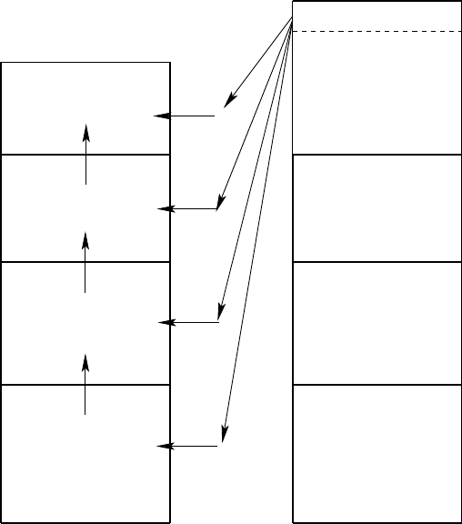
192
CHAPTER 14. CROSS-LAND INSERTION
For the thinner column, all cells within the specified range 1 ≤k≤kr are
affected
∂t
η
thin =Rthin
∂t(h
ρ
C)thin
1=Rthin [(
δ ρ
C)thin
2+
δ
1
ρ
oCthick
1]
∂t(h
ρ
C)thin
k=Rthin [(
δ ρ
C)thin
k+1−(
δ ρ
C)thin
k+
δ
k
ρ
oCthick
1]
∂t(h
ρ
C)thin
kr =Rthin [−(
δ ρ
C)thin
kr +
δ
kr
ρ
oCthick
1]
(14.13)
These tendencies are implemented in MOM4 via sources for thickness weighted
tracer and surface height.
R C
R C
R C
R C
R C
R C
R C2
3
4
δ
δ
δ
δ
δ
δ
δ
1
2
3
4
4
3
2
k=4
k=3
k=2
k=1
thick
thick
thick
thick
k=4
k=3
k=2
Cthick
k=1
Figure 14.1: Schematic of the cross-land insertion algorithm. An amount of seawa-
ter is extracted from the surface cell in a column with greater surface height. This
water is inserted into the adjacent column with smaller surface height. Insertion to
cells with k>1 requires a bubbling upwards of water in order to conserve volume,
since only the top cell can change its volume. This figure is directly analogous to
Figre 12.1 which illustrates the method used to discharge river water at depth. Note
that insertion from the top cell to the top cell is often used in practice. An example
is provided in Section 14.4.
14.3 An example: insertion to three cells
It is useful to work through an explicit example to get a sense for how the scheme is
expected to work. For this purpose, consider the initial configuration shown in Fig-
14.3. AN EXAMPLE: INSERTION TO THREE CELLS
193
ure 14.2, in which the thick column has an excess surface height H. For simplicity,
we take this excess height to also equal to the thickness of the cells with a resting
ocean surface. Assume that the horizontal cross-sectional area of the cells is all the
same. Hence, the rate of water transfer, R, is the same for the two columns, and is
given by
R=H/
τ
(14.14)
with
τ
the damping time. Three cells in the vertical into which to transfer the water
yields the fraction
δ
=1/3. (14.15)
The conservation equations for the top cell in the thick column are
∂t
η
thick =−R(14.16)
∂t(h C)thick
1=−R Cthick
1(14.17)
where his the time dependent thickness of the thick upper cell, and we assumed a
Boussinesq fluid for simplicity. Note that the concentration on the right hand side
of the tracer equation is evaluated at the present time step,
τ
. As noted in Section
14.2, the tracer concentration remains unchanged in the top thick cell, since
h∂tCthick
1=−R Cthick
1−Cthick
1∂t
η
thick
=Cthick
1(−R+R)
=0.
(14.18)
Conservation equations for the three cells in the thin column are
∂t
η
thin =R(14.19)
∂t(h C)thin
1=R
δ
(Cthin
2+Cthick
1)(14.20)
∂t(H C)thin
2=R
δ
(Cthin
3−Cthin
2+Cthick
1)(14.21)
∂t(H C)thin
3=R
δ
(−Cthin
3+Cthick
1). (14.22)
Using ∂ththin =Rin the first tracer equation leads to
h∂tCthin
1=R(
δ
Cthin
2+
δ
Cthick
1−Cthin
1). (14.23)
The deep cells have time independent thickness h=H. For the surface cell, its
thickness is assumed to initially have the same value, hthin(
τ
) = H. Bringing these
results together leads to the three tracer concentration equations
∂tCthin
1=
τ
−1(
δ
Cthin
2+
δ
Cthick
1−Cthin
1)(14.24)
∂tCthin
2=
τ
−1
δ
(Cthin
3−Cthin
2+Cthick
1)(14.25)
∂tCthin
3=
τ
−1
δ
(−Cthin
3+Cthick
1). (14.26)
Now consider the initial tracer concentration values of
Cthin
k(
τ
) = 24 (14.27)
Cthick
1(
τ
) = 36, (14.28)
194
CHAPTER 14. CROSS-LAND INSERTION
where the units are, for example, psu if the tracer represents salt. The first time step
with these initial conditions leads to the following budgets for tracer concentration.
The top cell has the budget
τ
∂tCthin
1= (24
δ
+36
δ
−24)
=−4. (14.29)
The second cell’s budget is
τ
∂tCthin
2=
δ
(24 −24 +36)
=12. (14.30)
The third cell’s budget is
τ
∂tCthin
3=
δ
(−24 +36)
=4. (14.31)
Notice how the surface cell in the thin column has a negative tendency for
its concentration, whereas the surface thick cell has its concentration remain un-
changed. The surface cell in the thin column has its concentration reduced since
its surface height increases by the amount of fluid that is moved from the thick
cell. This result may appear counter-intuitive since we are moving water with high
tracer concentration from the thick column to the thin column. But it is important
to remember that all the water that left the thick column inflates just the top cell
(since the interior cells in mom4 have fixed thicknesses), and this inflation acts to
reduce to the tracer concentration in this cell. Additionally, only a fraction of the
tracer that left the thick cell is bubbled up to the top of the thin column. Hence,
the negative tendency for the top cell in the thin column can change to a positive
tendency if the ratio
δ
becomes large enough. That is, when we insert into fewer
cells. The example in Section 14.4 considers this point further.
14.4 An example: insertion to just the top cell
Consider now the case where the transfer is from the top cell of the thick column
to just the top cell of the thin column. Here, the surface height tendencies are the
same, and the tracer budget for the thick cell is the same. For the thin column, only
the top cell is affected. The budget equations are thus given by
∂t
η
thick =−R(14.32)
∂t(h C)thick
1=−R Cthick
1(14.33)
∂t
η
thin =R(14.34)
∂t(h C)thin
1=R Cthick
1. (14.35)
Converting the tracer equations to tracer concentration equations leads to
∂tCthick
1=0 (14.36)
∂tCthin
1= (R/h) (Cthick
1−Cthin
1). (14.37)
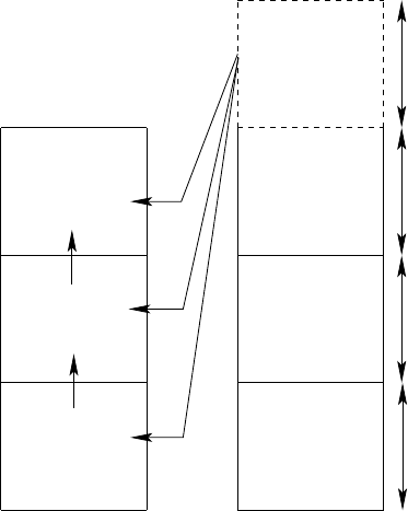
14.4. AN EXAMPLE: INSERTION TO JUST THE TOP CELL
195
ThickThin
3
1
2
3
2
excess
H
H
H
H
1
Figure 14.2: Example for how the cross-land insertion method works. In the thicker
column, we assume an initial excess of water equal to the amount of water in one of
the equally sized interior cells. This excess is transported into the thinner column.
With Cthick
1=36 and Cthin
1=24, the tendency for Cthin
1is 12/
τ
, whereas it was −4/
τ
in the 3-cell insertion example discussed in Section 14.3.
In general, recall that the rate of transfer, R, is a function of the difference in
surface heights. For larger surface height differences, the rate increases. This exam-
ple provides a clear illustration of the difference between the cross-land insertion
process and the cross-land mixing of Chapter 13. Namely, when mixing from top
cell to top cell, the cross-land mixing process does so at a rate that is fixed. For
the cross-land insertion process, this rate changes as the surface height between the
two columns changes.

CHAPTER
FIFTEEN
Sigma tracer diffusion
Contents
15.1 Motivation for the scheme . . . . . . . . . . . . . . . . . . . . . . 197
15.2 Diffusivities . . . . . . . . . . . . . . . . . . . . . . . . . . . . . . . 198
15.3 Implementation . . . . . . . . . . . . . . . . . . . . . . . . . . . . . 198
The purpose of this chapter is to detail the method for diffusing tracers along
the bottom topography within the bottom-most model grid cells.
15.1 Motivation for the scheme
As described by Winton et al. (1998), coarse resolution z-coordinate models gener-
ally have a difficult time moving dense water from shallow to deep regions. This
problem has prompted modelers to formulate ways to embed sigma-coordinate-
like bottom-layer transport into z-coordinate models. The papers by Beckmann and D¨oscher
(1997) and D¨oscher and Beckmann (2000) present one of the simplest approaches.
They prescribe changes only to the tracer equation, in which there is advection and
diffusion within a bottom sigma-layer instead of in the usual horizontal/vertical
orientation. More complete and physically based approaches, in which the mo-
mentum equations are also affected, tend to have problems with spurious horizon-
tal pressure gradients within the sigma-layer, much as found with sigma-models
(see Griffies et al. (2000a)). These approaches remain a topic of ongoing research.
Advection and neutral transport schemes often have a difficult time maintain-
ing positive-definite tracer values next to rough topography. Without either a large
amount of implicit mixing via the advection scheme, or some added diffusion such
as through sigma-diffusion, the tracer field can soon move outside its physically
realistic range. Sigma diffusion in the model thus works where there is indeed en-
hanced mixing in the real ocean, and where the numerical ocean requires such.
197
198
CHAPTER 15. SIGMA TRACER DIFFUSION
15.2 Diffusivities
When applying sigma-diffusion, the diffusive flux between two adjacent cells living
at the ocean bottom is given by
F
σ
=−A∇
σ
T, (15.1)
with ∇
σ
the horizontal gradient operator taken between cells in the bottom sigma-
layer. We follow the approach of D¨oscher and Beckmann (2000) in which sigma-
diffusion dominates when favorable according to densities of the participating cells.
That is, the following diffusivity is used
A=Amax if ∇
σρ
·∇H<0
Amin if ∇
σρ
·∇H≥0, (15.2)
where z=−H(x,y)is the bottom depth. Note that in practice, this constraint is
applied separately in the two horizontal directions. That is, the zonal diffusivity
is large if
ρ
,xH,x<0 and the meridional diffusivity is large if
ρ
,yH,y<0. A ratio
of the two diffusivities Amax/Amin has been taken as ≈106, as suggested by
D¨oscher and Beckmann (2000).
An additional velocity dependent diffusion was also found by D¨oscher and Beckmann
(2000) to be of use. In this case, an added sigma-diffusive flux in the zonal direction
is computed using the diffusivity
A=|u|∆xif
ρ
,xH,x<0 and u H,x>0
Amin otherwise. (15.3)
In this expression, |u|is the magnitude of the zonal velocity component and ∆xis
the zonal grid spacing. An analogous meridional flux is computed as well.
15.3 Implementation
The bottom sigma-layer in MOM3 was appended to the very bottom of the model
and effectively lived beneath the deepest rock. This approach has its advantages.
However, it makes for awkward analyses; it precludes direct comparison between
models run with and without sigma-physics since the grid used by the respec-
tive models is different; and it makes it difficult to consider convergence when
refining the grid mesh. For these reasons, the bottom sigma-layer in MOM4 is
included along with the rest of the model domain. This is the approach used by
Beckmann and D¨oscher (1997) (e.g., see their Figures 1 and 2). The disadvantage is
that the sigma-layer thickness bbl thickness in MOM4 has a generally non-constant
thickness determined by the thickness of the model grid cell next to topography.
To address the limitation of having bbl thickness constrained by the bottom par-
tial cell thickness dht, we suggest two approaches. For the simple case where dht is
thick, then we set
bbl thickness =min(dht,sigma thickness max), (15.4)
where sigma thickness max is a namelist parameter. Values on the order of 50m are
suggested.
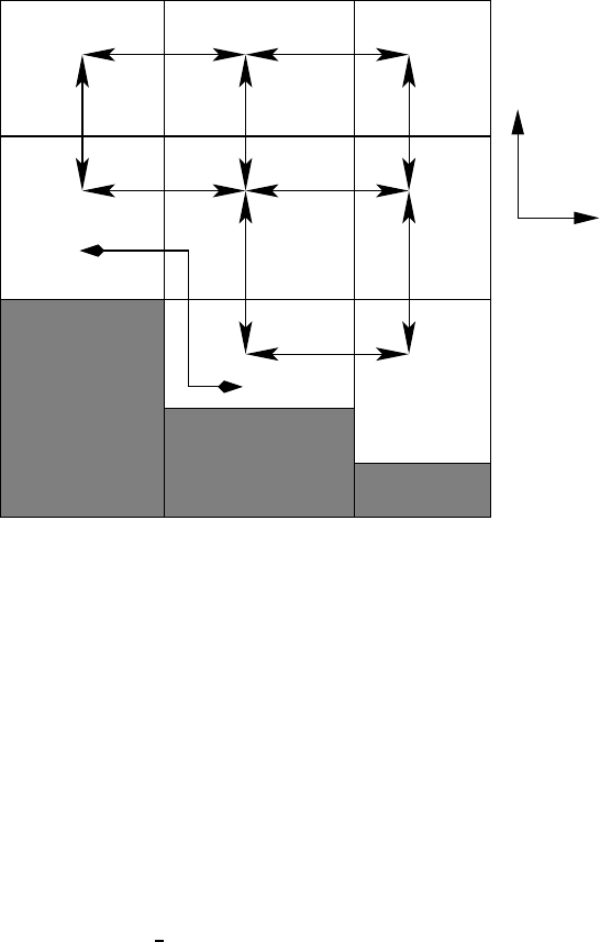
15.3. IMPLEMENTATION
199
σσ
σ
vert
horz
Figure 15.1: Schematic of the extra along-topography pathway for diffusive trans-
port afforded by the sigma-diffusion scheme applied to the bottom-most model
cells. Darkened regions denote land cells. Tracers in the z-level cells communicate
with their horizontal and vertical neighbors via the usual advection, diffusion, and
convective processes. Tracers in the bottom “sigma-layer” can also communicate
with their sigma-neighbors via sigma-diffusion.
For the more complicated case where dht is thin, then we have no work-around
since doing so involves allowing the sigma-diffusion process to take place between
arbitrary numbers of grid cells laterally adjacent within the sigma layer. The only
option at present is to limit the partial cell thicknesses dht to be no smaller than
ones desired minimum bbl thickness. This approach reduces the fidelity of the bot-
tom topography representation, but perhaps by gaining a better transport by sigma
diffusion. Such issues remain an ongoing research topic at GFDL.
Consistent with Beckmann and D ¨oscher (1997), the sigma-layer momentum equa-
tions remain the same as interior z-level cells. We now just allow tracers in the
bottom-most cell to be affected by diffusion with their “sigma-neighbors” in ad-
dition to their horizontal and vertical neighbors. If desired, communication with
horizontal and vertical neighbors can be removed for the sigma cells. Figure 15.1
provides a schematic of the extra sigma-pathway available with sigma tracer diffu-
sion.

CHAPTER
SIXTEEN
Discharging overflow waters into the deep
Contents
16.1 The ubiquitous cliffs in coarse z-models . . . . . . . . . . . . . . 201
16.2 The Campin and Goosse (1999) algorithm . . . . . . . . . . . . . 202
16.2.1 Finding the depth of neutral buoyancy . . . . . . . . . . . 202
16.2.2 Prescribing the downslope flow . . . . . . . . . . . . . . . 203
16.2.3 Mass conservation and tracer transport . . . . . . . . . . . 204
16.3 Implementation in MOM4 . . . . . . . . . . . . . . . . . . . . . . 205
16.3.1 Start of the integration . . . . . . . . . . . . . . . . . . . . . 205
16.3.2 During a time step . . . . . . . . . . . . . . . . . . . . . . . 206
16.4 Comments on the two overflow schemes in MOM4 . . . . . . . . 207
This chapter documents the MOM4 implementation of the Campin and Goosse
(1999) scheme that discharges dense overflow waters into the deep. The goal of the
scheme is similar to that of the sigma-diffusion scheme of Beckmann and D¨oscher
(1997), as described in Chapter 15. We discuss differences between the two methods
in Section 16.4.
16.1 The ubiquitous cliffs in coarse z-models
We start this chapter by mentioning some of the limitations inherent in the respre-
sentation of steeply sloping topography in coarse z-models. Consider the case in
Figure 16.1, which shows a typical situation where a steeply sloping topographic
feature is represented in a coarse z-model via a vertical cliff, with many vertical
cells sitting next to the wall. To better resolve such finite, yet steep, topography re-
quires greatly enhanced horizontal resolution. As discussed by Winton et al. (1998),
“resolving” the topography requires a grid spacing that satisfies
∆z/∆s≥ |∇H|, (16.1)
with ∆zthe vertical grid spacing, ∆sthe horizontal grid spacing, and |∇H|the mag-
nitude of the bottom topography slope. Resolving a slope of 1/100 with vertical res-
olution of ∆z=20m thus requires ∆s≈2km, which is some 50-100 times smaller
201
202
CHAPTER 16. DISCHARGING OVERFLOW WATERS INTO THE DEEP
than the typical resolution of the 1-2 degree ocean climate models commonly used
today. Note that refined vertical resolution, desired for resolving/parameterizating
vertical physical processes, requires one to further refine the horizontal resolution
required to resolve the slope. Notably, there is little difference between the rep-
resentation of steeply sloping features via either full or partial cells in z-models.
Hence, such cliff features remain ubiquitous in the typical ocean climate z-model.
It due to our inability to fully resolve such steeply sloping topographic features
that we require enhanced bottom mixing/transport whose aim is to allow dense
water to move into the deep, rather than sitting on top of the shelf.
16.2 The Campin and Goosse (1999) algorithm
Consider a heavy water parcel sitting on top of a shelf/cliff that is horizontally ad-
jacent to a lighter parcel sitting over a deeper water column. We may expect that
the dense parcel will move off the shelf, down the slope, and into the deep. Along
the way, entrainment will occur, with many important processes determining the
details of the final water mass. This is indeed a cartoon of an important oceanic
process forming much of the deep and intermediate waters in the ocean. Unfor-
tunately, without some extra “engineering” help, Winton et al. (1998) show that
coarse resolution z-models are incapable of providing the proper dynamical path-
ways for this transfer of dense shelf water into the deep. Beckmann and D¨oscher
(1997) suggest one means to enhance the representation of this process in z-models
(see Chapter 15). Campin and Goosse (1999) propose yet another, which we detail
in this chapter. Both schemes only affect the tracer equation. Killworth and Edwards
(1999) discuss a more physically complete, yet numerically difficult, scheme that al-
ters both the momentum and tracer equations.
16.2.1 Finding the depth of neutral buoyancy
Figure 16.1 illustrates a typical situation in a horizontal-vertical plane. Here, we
see a heavy parcel of in situ density
ρ
so(k=kup)sitting horizontally adjacent to a
lighter parcel of in situ density
ρ
do(k=kup). The superscript “so” refers to water
in the “shallow ocean” column, whereas “do” refers to water in the “deep ocean”
column.
If the heavy parcel is allowed to adiabatically move off the shelf and then ver-
tically within the deep column, it will equilibrate at its depth of neutral buoyancy.
To compute the depth of neutral buoyancy, we evaluate the in situ density for the
parcel taken at the local value for the in situ pressure of the environment where it
may potentially equilibrate. For the example shown in Figure 16.1, with (i,j)set-
ting the horizontal position of the shelf parcel and (i+1, j)setting the horizontal
position of the deep column, we have
ρ
so(kup,kup) =
ρ
(si,j,kup,
θ
i,j,kup,pi,j,kup)(16.2)
ρ
so(kup,kdw −1) =
ρ
(si,j,kup,
θ
i,j,kup,pi+1, j,kdw−1)(16.3)
ρ
so(kup,kdw) =
ρ
(si,j,kup,
θ
i,j,kup,pi+1, j,kdw)(16.4)
ρ
so(kup,kdw +1) =
ρ
(si,j,kup,
θ
i,j,kup,pi+1, j,kdw+1). (16.5)
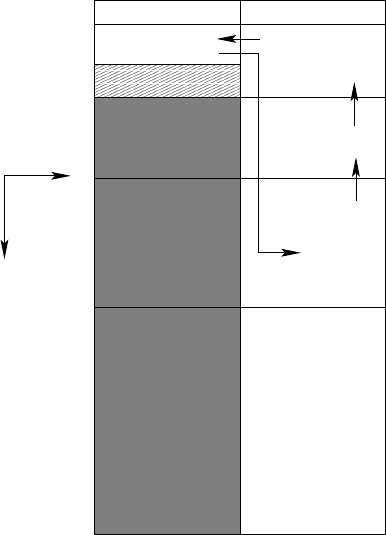
16.2. THE CAMPIN AND GOOSSE (1999) ALGORITHM
203
5
4
3
ρ(
ρ(
ρ(
kdw−1
kdw+1
kup
)
)
)
do
do
do
deep ocean(do)
shallow ocean(so)
ρ(
so
ρ(
so
ρ(
so
ρ(
so
kup,kdw)>ρ(
do
kdw)
kup,kdw+1)<ρ(
do
kdw+1)
kup,kdw−1 >ρ(
do
kdw−1
)
kup,kup)>ρ(
do
kup)
i,j
k
)
so
ρ(kup,kup)
2
1
ρ(
do
kdw)
Figure 16.1: Schematic of the Campin and Goosse (1999) overflow method in the
horizontal-vertical plane. The darkly filled region represents bottom topography
using MOM4’s full cells. The lightly filled region represents topography filled by a
partial cell. Generally, the thickness of a cell sitting on top of a topographic feature,
as the k=2 cell in the “so” column, is thinner than the corresponding cell in the
deep-ocean column (the k=2 cell in the “do” column). Shown are tracer cells, with
arrows representing the sense of the scheme’s upstream advective transport. This
figure is based on Figure 1 of Campin and Goosse (1999).
That is, we compute the density at the salinity and potential temperature of the
shallow ocean parcel, (si,j,kup,
θ
i,j,kup), but at the in situ pressure for the respective
grid cell in the deep column. The density is then compared to the density of the
parcel at the in situ salinity, temperature, and pressure of the cells in the deep ocean
column.
16.2.2 Prescribing the downslope flow
Following Campin and Goosse (1999), we assume that the dense parcel has a downs-
lope momentum imparted to it. This momentum is proportional to the topographic
slope, H,x, the acceleration from gravity,g, the amount of fluid within the cell par-
ticipating in the downslope flow,
0≤
δ
≤1, (16.6)
and the positive density difference
∆
ρ
=
ρ
so(kup,kup)−
ρ
do(kup)>0. (16.7)

204
CHAPTER 16. DISCHARGING OVERFLOW WATERS INTO THE DEEP
The momentum is retarded by frictional dissipation,
µ
(in units of inverse time).
These considerations then lead to the momentum balance1
ρ
oV(t)
µ
uslope =g
δ
V(t)∆
ρ
|H,x|(16.8)
where
V(t)=dxt ∗dyt ∗dht (16.9)
is the volume of the dense parcel’s tracer cell. Equation (16.8) is also used to de-
termine a meridionally directed downslope transport, with the meridional topo-
graphic slope H,yreplacing H,x, and ∆
ρ
the density difference between meridion-
ally adjacent parcels.
Solving equation (16.8) for the speed uslope yields
uslope =g
δ
ρ
o
µ
|H,x|∆
ρ
. (16.10)
If the depth Hrefers to the depth of a tracer cell, then the absolute slope |H,x|is
naturally defined at the zonal face of the tracer cell. Hence, the speed, uslope, is
likewise positioned at the zonal face. This is the desired position for an advective
tracer transport velocity.
Campin and Goosse (1999) suggest the values
µ
=10−4sec−1and
δ
=1/3.
These parameters are set as namelists in MOM4. Using these numbers, with an
absolute topographic slope of |H,x| ≈ 10−3and density difference ∆
ρ
≈1 kg m−3,
leads to the speed
uslope ≈.03 m sec−1. (16.11)
Associated with this downslope speed is a volume transport of fluid leaving the
cell
Uslope =uslope dhtmin dyt. (16.12)
In this equation, dhtmin is the minimum thickness of the shelf cell and the adjacent
cell. This minimum operation is necessary when considering MOM4’s bottom par-
tial cells, whereby the bottom-most cell in a column can have arbitrary thickness
(Figure 16.1). With uslope ≈.03m s−1corresponding to the speed of fluid leaving a
grid cell that is one-degree in width and 50 m in depth, we have a volume transport
Uslope ≈0.2Sv. Larger values are easily realized for steeper slopes, larger density
differences, and larger grid cells.
16.2.3 Mass conservation and tracer transport
To conserve mass throughout the system, the mass flux exiting the shelf cell and
entering the deep cell must itself be returned from the adjacent cell. This situa-
tion then sets up a mass flux throughout the participating cells, where there is zero
convergence of the flux and so zero net increase or decrease in mass. For the Boussi-
nesq fluid, mass conservation is replaced by volume conservation. This redirected
plumbing is shown in Figure 16.1.
1The appearance of the constant density,
ρ
o, on the left hand side, rather than the in situ density,
ρ
,
is described in Chapter 3 as well as Griffies (2004). In those discussions we show that
ρ
ois appropriate
for either the Boussinesq or non-Boussinesq forms of MOM4.

16.3. IMPLEMENTATION IN MOM4
205
The convergence-free seawater mass flux carries with it tracer mass. If there are
differences in the tracer content of the cells, then the tracer flux will have a nonzero
convergence, and so it moves tracer throughout the system. We use first-order up-
stream advective transport as a discretization of this process. First-order upstream
advection is the simplest form of advection. Its large level of numerical diffusion is
consistent with our belief that the bottom layer flows in the real ocean near steep
topography are quite turbulent. Hence, although inappropriate for interior flows,
we are satisfied with the use of upstream advection for the overflow scheme.
16.3 Implementation in MOM4
This section details the implementation of the Campin and Goosse (1999) scheme
in MOM4.
16.3.1 Start of the integration
At the start of the model integration, it is necessary to determine those grid points
where it is possible to have a downslope flow. For this purpose, we introduce the
array topog step(i,j,m), with m=1, 2, 3, 4 specifying in a counter-clockwise di-
rection the four surrounding columns whose depths are to be compared to that at
the central (i,j)point. Figure 16.2 illustrates this notation. If the adjacent column
is deeper than the central point, thus representing a possible direction for downs-
lope flow, then topog step(i,j,m)for this value of mis set to unity. Otherwise,
topog step(i,j,m)for this mis zero. Note that with partial bottom cells, it is possi-
ble for an adjacent column to be deeper yet for the number of vertical cells to be the
same in both columns. To initiate the downslope scheme of Campin and Goosse
(1999), we insist that there be at least one more grid cell in the adjacent column.
(i,j,3) (i,j,1)
(i,j,2)
(i,j,4)
i
j
T(i,j)
Figure 16.2: Plan view (x-y plane) of a tracer grid cell at (i,j)and its horizontally
adjacent tracer cells. We label the adjacent cells (i+1, j),(i,j+1),(i−1, j),(i,j−1)
as m=1, 2, 3, 4. Notice that we do not consider downslope flow along a diagonal
direction.

206
CHAPTER 16. DISCHARGING OVERFLOW WATERS INTO THE DEEP
16.3.2 During a time step
During each time step, we locate where downslope flow is favorable for points sit-
ting on the ocean bottom at (i,j,kmt(i,j)). For each of the four directions (m=
1, 2, 3, 4) where topog step(i,j,m) = 1, we check the density difference between
the central point and the adjacent point. If the density of the central point is larger,
then the Campin and Goosse (1999) scheme is used to initiate downslope transport.
For these directions, we locate the depth of neutral buoyancy for the central point
according to the discussion in Section 16.2.1, and so specify the number of vertical
cells, kdw, participating in the transport. Note that we allow for downslope trans-
port to occur in more than one direction, as occurs in those cases for a fixed (i,j)
where topog step(i,j,m)has more than a single nonzero element.
Our prescription is mindful of the possibility for the shallow-cell to be a par-
tially filled cell sitting on the topography. For this reason, the convergence-free
volume transport associated with the downslope flow is weighted by the mini-
mum vertical thickness of the two cells (equation (16.12)). Otherwise, it would be
possible to flood a thin partial cell with a huge amount of tracer (e.g., heat).
We incorporate the effects from the Campin and Goosse (1999) overflow scheme
into MOM4’s tracer source array. To derive the source, we proceed as for the river-
mixing and cross-land mixing formulations (Chapter 12 and 13) by focusing on the
time evolution due to just the overflow process. For the particular zonal-vertical
case illustrated in Figure 16.2, we prescribe
∂t(V(t)
ρ
C)so
i,j,kup =
ρ
oUslope (Cdo
i+1, j,kup −Cso
i,j,kup)(16.13)
∂t(V(t)
ρ
C)do
i+1, j,kup =
ρ
oUslope (Cdo
i+1, j,kdw−1−Cdo
i+1, j,kup)(16.14)
∂t(V(t)
ρ
C)do
i+1, j,kdw−1=
ρ
oUslope (Cdo
i+1, j,kdw −Cdo
i+1, j,kdw−1)(16.15)
∂t(V(t)
ρ
C)do
i+1, j,kdw =
ρ
oUslope (Cso
i,j,kup −Cdo
i+1, j,kdw), (16.16)
where again Uslope =uslope dhtmin dyt, with
dht(min)=min(dhti,j,kup,dhti+1, j,kup)(16.17)
the minimum thickness of the two cells at k=kup. For the Boussinesq case,
ρ
factors on the left hand side are set to the constant reference density
ρ
o. Setting
the tracer concentration to the same uniform value leads to vanishing time tenden-
cies for
ρ
V(t)in each cell, thus reflecting volume/mass conservation. Additionally,
summing these four equations leads to a vanishing right hand side, thus reflecting
conservation of total tracer in the system. Since the downslope mixing has the form
of an upstream advection, we discretize temporally by evaluating the tracer and
density on the right hand side at the lagged time
τ
−1.
As implemented in MOM4, the tracer source array is modified in the following
manner to account for the downslope flow from Campin and Goosse (1999)
[A(t)dht ·tracer-sourceso]i,j,kup =Uslope (Cdo
i+1, j,kup −Cso
i,j,kup)(16.18)
[A(t)dht ·tracer-sourcedo]i+1, j,kup =Uslope (Cdo
i+1, j,kdw−1−Cdo
i+1, j,kup)(16.19)
[A(t)dht ·tracer-sourcedo]i+1, j,kdw−1=Uslope (Cdo
i+1, j,kdw −Cdo
i+1, j,kdw−1)(16.20)
[A(t)dht ·tracer-sourcedo]i+1, j,kdw =Uslope (Cso
i,j,kup −Cdo
i+1, j,kdw)(16.21)
16.4. COMMENTS ON THE TWO OVERFLOW SCHEMES IN MOM4
207
where
A(t)=dxt ∗dyt (16.22)
is the time independent horizontal area of a tracer cell.
16.4 Comments on the two overflow schemes in MOM4
As mentioned at the start of this chapter, there are two methods implemented in
MOM4 whose aim is to enhance the ability of the simulated fluid to form dense
deep water: (1) the Campin and Goosse (1999) scheme described in this chapter,
and (2) the sigma diffusion scheme from Beckmann and D¨oscher (1997) and D¨oscher and Beckmann
(2000) as described in Chapter 15. Both are quasi-physical engineering approaches
to the problem of simulating deep water formation near topography. Each pro-
vides plumbing routes beyond the local horizontal-vertical routes available in z-
models. In this way, these methods provide a new means for representing the flows.
Questions such as parameterizing the rates of entrainment, volume flux, etc. (e.g.,
Killworth and Edwards (1999)) are not directly addressed by these schemes.
Climate modelers generally gauge the utility of overflow schemes on the overall
results: Do they indeed provide a route for deep water formation near topographic
gradients in a manner expected from observations? Yet details of the transport are
often not the first priority. This situation is unsatisfying from a process physics
perspective. Given the coarseness of ocean climate models (circa year 2003) relative
to the small scales of typical high-latitude overflow dynamics, we may not be able
to do better with the z-models.
The density structure in Figure 16.3 illustrates a case where the Beckmann and D¨oscher
(1997) scheme does not prescribe enhanced downslope transport. The reason is that
their scheme only works with density within the bottommost tracer cell. For this ex-
ample, density at the bottom of the deeper column is greater than that on the shelf,
and so there is no enhanced transport prescribed. In contrast, the Campin and Goosse
(1999) scheme prescribes a downslope transport, with the dense shelf water moving
to its neutral buoyancy depth.
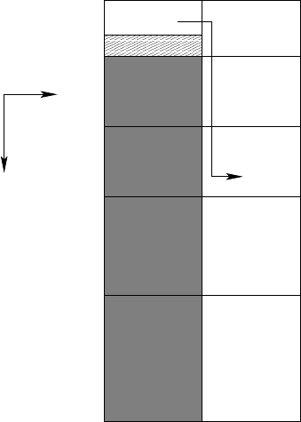
208
CHAPTER 16. DISCHARGING OVERFLOW WATERS INTO THE DEEP
ρ=
ρ=
ρ=
ρ=
1033
1034
1036
1037
3
4
5
2
1
k
i,j
ρ=1035
ρ=1035
Figure 16.3: Schematic of a situation where a dense parcel sits on a shelf next to
a column whose upper portion is light, but whose deeper portion is denser than
the shelf. For this case, the Campin and Goosse (1999) scheme prescribes a trans-
port between the shelf water at level 1 and the deeper water at level 3, with wa-
ter bubbling upward to conserve mass as shown in Figure 16.1. In contrast, the
Beckmann and D¨oscher (1997) scheme will not prescribe any enhanced transport,
since here the bottom of the deep column is denser than the shelf.
Part VI
Some diagnostics
209
211
SOME DIAGNOSTICS
MOM4 makes extensive use of the FMS diagnostic manager, whereby any field
that is carried by the model can be trivially output to a diagnostics file via the reg-
istration of that field with the diagnostics manager, and the associated entry of the
field’s name within the diagnostics table. This part of the MOM4 Guide does not
describe this aspect of diagnostics. Instead, we focus here on the formulation and
computation of certain diagnostics that have proven of use for research with z-
coordinate models.

CHAPTER
SEVENTEEN
Streamfunctions
Contents
17.1 Meridional-overturning streamfunction . . . . . . . . . . . . . . 213
17.1.1 Summary of continuity and notation . . . . . . . . . . . . . 213
17.1.2 Meridional and vertical transport . . . . . . . . . . . . . . 214
17.1.3 Overturning streamfunction . . . . . . . . . . . . . . . . . 215
17.1.4 Choosing the reference values . . . . . . . . . . . . . . . . 216
17.1.5 Transport beneath an arbitrary surface . . . . . . . . . . . . 217
17.1.6 Transport from GM90 . . . . . . . . . . . . . . . . . . . . . 218
17.2 Vertically integrated transport . . . . . . . . . . . . . . . . . . . . 218
17.2.1 Summary of the rigid lid . . . . . . . . . . . . . . . . . . . . 218
17.2.2 General case of divergent flow . . . . . . . . . . . . . . . . 219
The purpose of this chapter is to present the mathematical formulation of stream-
functions commonly used to summarize the overturning circulation as well as the
vertically integrated circulation.
17.1 Meridional-overturning streamfunction
The meridional overturning streamfunction is commonly used to diagnose features
of the thermohaline circulation. For the Boussinesq model, it provides a direct pic-
ture of zonally integrated volume transport for both steady-state and transient mo-
tions. For non-Boussinesq models, it provides a picture of mass transport only for
steady-state motions.
17.1.1 Summary of continuity and notation
We follow the formulation of non-Boussinesq z-coordinate ocean models presented
by Griffies (2004). In this case, a non-Boussinesq ensemble averaged fluid leads to
the continuum model continuity equation
ρ
,t+
ρ
o∇· v=0. (17.1)
213
214
CHAPTER 17. STREAMFUNCTIONS
In orthogonal horizontal coordinates, velocity field divergence takes the form (see
Griffies (2004))
∇· v= (dydz)−1(dydz u),x+ (dxdz)−1(dxdz v),y+ (dxdy)−1(dxdy w),z
(17.2)
which then leads to the continuity equation
(dV/
ρ
o)
ρ
,t+dx(dydz u),x+dy(dxdz v),y+dz(dxdy w),z=0, (17.3)
where
dV =dxdydz(17.4)
corresponds to the volume of a model grid cell. Note that the volume of grid cells in
the top levels of MOM4 are time dependent due to the use of a free surface. Hence,
it is not generally valid to bring dV inside the time derivative.
To set the notation, the distance between two infinitesimally close points on the
sphere is written
(dx)2= (h1d
ξ
1)2+ (h2d
ξ
2)2+ (h3d
ξ
3)2(17.5)
when using generalized orthogonal coordinates (
ξ
1,
ξ
2,
ξ
3). For a Traditional Ap-
proximation continuum system (see Griffies (2004)), the stretching functions h1and
h2are dependent on horizontal position alone, and h3is unity. However, to allow
the following manipulations to incorporate MOM4’s partial cells, we maintain a
horizontal and vertical position dependence to h3.
17.1.2 Meridional and vertical transport
To proceed, introduce the transports
V= (dz)−1
ξ
1
b
Z
ξ
1
a
dx(vdz)(17.6)
W= (dy)−1
ξ
1
b
Z
ξ
1
a
dx(wdy). (17.7)
Integration is taken along a line of constant
ξ
1, where
ξ
1is the generalized orthog-
onal coordinate corresponding to the spherical longitude
λ
. Integration endpoints
ξ
1
aand
ξ
1
bare assumed to be at land-sea boundaries, where uvanishes, or over a pe-
riodic domain. As in the spherical coordinate case, we refer to Vas the generalized
meridional transport. To motivate the definition of the transport streamfunction,

17.1. MERIDIONAL-OVERTURNING STREAMFUNCTION
215
take the generalized meridional derivative of dzVto render
(dzV),y=∂y
ξ
1
b
Z
ξ
1
a
dx(dz v)
=1
h2
ξ
1
b
Z
ξ
1
a
∂2(dxdz v)
=1
dy
ξ
1
b
Z
ξ
1
a
dy(dxdz v),y(17.8)
These steps made use of the properties of orthogonal coordinates whereby ∂2com-
mutes with the zonal integration, since it is orthogonal to the integration pathway
taken along a line of constant
ξ
1. However, ∂2does not commute with the distances
dxand dz, each of which can be functions of the generalized meridional coordinate
ξ
2. Use of continuity in the form (17.3) yields
−dy(dzV),y=
ξ
1
b
Z
ξ
1
a
[dz(dxdy w),z+ (dV/
ρ
o)
ρ
,t]
=dz(dyW),z+
ξ
1
b
Z
ξ
1
a
(dV/
ρ
o)
ρ
,t. (17.9)
To reach this relation, we used
ξ
1
b
Z
ξ
1
a
dx(dydz u),x=0, (17.10)
which follows from the chosen zonal boundaries.
17.1.3 Overturning streamfunction
In summary, the zonally integrated transports satisfy the balance
(dz)−1(dzV),y+ (dy)−1(dyW),z+ (dydz)−1
ξ
1
b
Z
ξ
1
a
(dV/
ρ
o)
ρ
,t=0. (17.11)
This relation indicates that meridional and vertical transports are balanced by fluc-
tuations in mass. In a steady state, or for the Boussinesq models, the mass fluctua-
tions vanish, thus leading to volume conservation manifesting as the two-dimensional
non-divergence condition
dy(dzV),y+dz(dyW),z=d
ξ
2d
ξ
3∂(h3V)
∂
ξ
2+∂(h2W)
∂
ξ
3=0. (17.12)

216
CHAPTER 17. STREAMFUNCTIONS
The second equality follows by the orthogonal nature of the coordinates, whereby
∂(d
ξ
2)
∂
ξ
3=∂(d
ξ
3)
∂
ξ
2=0. (17.13)
for the steady state , or for the Boussinesq models,We are thus motivated to intro-
duce an overturning streamfunction that satisfies
V=−Ψ,z(17.14)
W=Ψ,y. (17.15)
The streamfunction Ψsummarizes the meridional-depth volume transport for a
Boussinesq fluid, or for a steady-state non-Boussinesq fluid. It has dimensions
volume/time, and so it represents the volume transport of water in the (y,z)plane.
The typical dimensions are Sverdrups, where 1 Sv =106m3sec−1. Multiplication
by
ρ
oproduces a mass transport streamfunction
ρ
oΨin units of kg sec−1.
We can solve for the streamfunction via integration of its defining relation and
setting a boundary condition. Integration of equation (17.14) leads to
Ψ(y,z) = Ψ(y,zo)−
z
Z
zo
dz0V(y,z0), (17.16)
where zois a reference depth. Similar integration of equation (17.15) leads to
Ψ(y,z) = Ψ(yo,z) +
y
Z
yo
dy0W(y0,z), (17.17)
where yois a reference latitude. It is now possible to develop two equivalent expres-
sions for the overturning streamfunction. The first is found through substituting
the expression (17.16) into (17.17)
Ψ(y,z) = Ψ(yo,zo)−Zz
zo
dz0V(yo,z0) + Zy
yo
dy0W(y0,z). (17.18)
The second is found by substituting equation (17.17) into (17.16)
Ψ(y,z) = Ψ(yo,zo)−Zz
zo
dz0V(y,z0) + Zy
yo
dy0W(y0,zo). (17.19)
17.1.4 Choosing the reference values
The question is how to choose the reference values yoand zoto simplify the com-
putation of the overturning streamfunction. In general, evaluation of the vertical
transport term is more difficult than the meridional transport term. One is there-
fore motivated to focus on equation (17.19) when computing the streamfunction,
rather than equation (17.18). For choosing the reference value zo, it is useful to
consider the water budget and how it closes. In the rigid lid, the water budget is
closed within the ocean domain. As such, so long as the value of zocorresponds to
a value anywhere completely outside the ocean domain, the vertical transport term
17.1. MERIDIONAL-OVERTURNING STREAMFUNCTION
217
Ry
yody0W(y0,zo)vanishes. For the free surface, however, the possibility of surface
water fluxes allows for an open water budget above the ocean surface. Since there
is no attempt here to account for water cycling through the rock beneath the ocean,
one can assume all water transport in rock vanishes. Hence, by taking zoto be some
value completely beneath the ocean bottom, the vertical transport term can again
be dropped with the free surface. As a consequence, a general expression for the
overturning streamfunction, valid for both the free surface and rigid lid, is given
just by the meridional transport term
Ψ(y,z) = −
z
Z
zo
dz0V(y,z0) = −
z
Z
zo
xb
Z
xa
dxdz0v. (17.20)
In practice, it is not necessary to evaluate the integral anyplace beneath the ocean
bottom, since the water velocity vanishes there. On the bottom, the vertical coor-
dinate takes on the non-constant value z=−H(x,y). Therefore, when integrating
just to the ocean bottom, it is necessary to perform the vertical integral first, and
then the zonal integral
Ψ(y,z) = −
xb
Z
xa
dx
z
Z
−H
dz0v. (17.21)
Beneath the ocean surface, the no-normal flow condition implies that the over-
turning streamfunction is a constant along the side and bottom land-sea bound-
aries. For the rigid lid, the absence of fresh water input to the ocean surface also
implies that its overturning streamfunction is a constant at the ocean surface. The
choice Ψ(yo,zo) = 0 means that the rid lid overturning streamfunction is zero along
all the boundaries. For the free surface, however, the overturning streamfunction
need not be a constant on the ocean surface, due to the presence of surface water
fluxes, whereas it remains zero on the sides/bottom just as for the rigid lid.
17.1.5 Transport beneath an arbitrary surface
As shown in Section 40.9 of Pacanowski and Griffies (1999), we can extend the
above considerations to the case of generalized vertical coordinates. In this case,
we are concerned with the meridional transport of fluid beneath some generalized
vertical coordinate surface. It is a straightforward matter to extend the definition of
the overturning streamfunction to this case, where
Ψ(y,s) = −
xb
Z
xa
s(z)
Z
−s(H)
dxdz0v, (17.22)
with s=s(x,y,z,t)the generalized vertical coordinate (see Griffies (2004) for de-
tails). Surfaces that are physically of interest include various potential density sur-
faces, which are especially relevant when the flow is adiabatic. See Section 40.9 of
Pacanowski and Griffies (1999) for more discussion.
218
CHAPTER 17. STREAMFUNCTIONS
17.1.6 Transport from GM90
The parameterization of Gent et al. (1995) provides a volume transport in addition
to the resolved scale Eulerian mean transport. The total meridional-overturning
streamfunction takes the form
Ψ(tot)(y,z) = −
xb
Z
xa
dx
z
Z
−H
dz0(v+vgm), (17.23)
where
vgm =−∂z(
κ
Sy)(17.24)
is the eddy-induced velocity with Sy=−∂y
ρ
/∂z
ρ
the neutral slope in the y-direction
and
κ
a diffusivity. Performing the vertical integral on the GM90 piece leads to
Ψ(tot)(y,z) = Ψ(y,z) + Ψgm(y,z)(17.25)
where
Ψgm(y,z) =
xb
Z
xa
dx(
κ
Sy)(17.26)
with
κ
Sy=0 at z=−H. Hence, the Gent et al. (1995) parameterization adds a
contribution that scales linearly with basin size, isopyncal slope, and diffusivity
Ψgm ∼L S
κ
. (17.27)
As an example, let
κ
=103m2s−1,S=10−3, and L=107m, which yields T ≈
10Sv. Such transport can represent a nontrivial addition to that from the resolved
scale velocity field.
17.2 Vertically integrated transport
The purpose of this section is to discuss the streamfunction used to summarize
the vertically integrated transport. Only when vertically integrated flow is non-
divergent, such as for the Boussinesq rigid lid case, will a streamfunction be suf-
ficient. In general, it only approximates the flow. However, for many cases the
approximate streamfunction is quite useful.
17.2.1 Summary of the rigid lid
With the rigid lid method of Bryan (1969), it is assumed that the vertically inte-
grated velocity in a Boussinesq fluid is non-divergent ∇ · U=0. Hence, it can
be described via a scalar streamfunction U=ˆz∧ ∇ ˜
ψ
. In this case, the vertically
integrated advective transport between two points is given by
Tab =Zb
adl ˆn·Z0
−Hdzu=
ψ
a−
ψ
b, (17.28)
where dl is the line element along any path connecting the points aand b, and ˆnis a
unit vector pointing perpendicular to the path in a rightward direction when facing

17.2. VERTICALLY INTEGRATED TRANSPORT
219
the direction of integration. As written, Tab has units of volume per time, and so it
represents a volume transport. Therefore, the difference between the streamfunc-
tion at two points represents the vertically integrated volume transport between
the two points. It is for this reason that the streamfunction is sometimes called
the volume transport streamfunction. Note that Bryan (1969) defined the barotropic
streamfunction with an extra factor of the Boussinesq density
ρ
o, such that his mass
transport streamfunction has the dimensions of mass per time rather than volume
per time. The difference is trivial for a Boussinesq fluid.
17.2.2 General case of divergent flow
The vertically integrated horizontal momentum density
ρ
oU=
η
Z
−H
ρ
u(17.29)
generally has a non-zero divergence due to fluctuations of mass and/or volume
within the vertical column. Hence, it corresponds to both a streamfunction ˜
ψ
and a
velocity potential
χ
U=ˆz∧ ∇ ˜
ψ
+∇
χ
. (17.30)
Only for a Boussinesq rigid-lid model with zero fresh water flux will
χ
vanish.
Hence, to compute the precise vertically integrated transport passing between two
points, a direct evaluation of the integral
Tab =Zb
adl ˆn·U(17.31)
is given. Although accurate and complete, this integral does not readily provide a
horizontal map of transport, and so it looses much of the appeal associated with
the transport streamfunction used with a rigid lid.
However, for many practical situations, maps of the function
ψ
(x,y) = −Zy
yo
dy0U(x,y0)(17.32)
are quite useful, where the lower limit yois taken at the southern boundary of the
domain, generally given by a solid wall for ocean climate models. By its definition,
the meridional derivative of
ψ
yields the zonal transport
ψ
,y=U. (17.33)
The zonal derivative, however, does not yield the meridional transport due to the
divergent nature of the vertically integrated flow. To see what it does yield, let us
restrict attention to the Boussinesq case with spherical coordinates, where
1
Rcos
φψ
,
λ
=V−R
cos
φ
Z
φ
φ
o
d
φ
0cos
φ
0∇· U. (17.34)
To reach this result we used where cos
φ
oV(
λ
,
φ
o) = 0. With volume conservation
in the Boussinesq model leading to
∇· U=−
η
t+qw, (17.35)
220
CHAPTER 17. STREAMFUNCTIONS
we see that ∇·Uvanishes only when there is zero time tendency of the free surface
height and zero fresh water flux through the surface. Hence, the zonal derivative
leads to the meridional transport plus a term that vanishes in the case of a steady
state (
η
t=0) and a zero fresh water flux. It is useful to see how large the extra term
might be. For this purpose, zonally integrate the derivative
ψ
,
λ
to find
ψ
(
λ
,
φ
)−
ψ
(
λ
o,
φ
) = Rcos
φ
Z
λ
λ
o
d
λ
0V(
λ
0,
φ
)
−R2Z
λ
λ
o
d
λ
0Z
φ
φ
o
d
φ
0cos
φ
0(−
η
t+qw). (17.36)
For example, with −
η
t+qw=1m/year applied over a 1000km ×1000km area,
the extra term contributes much less than a Sv to the streamfunction. Cases where
the differences are larger certainly can be constructed. But for many diagnostic
purposes, the differences are negligible.
By construction,
ψ
reduces to the transport streamfunction in the case of a rigid
lid where ∇· U=0. However, this is not a unique choice and alternatives do exist.
For example,
ψ
∗(x,y) =
ψ
(xo,y) + Zx
xo
dx0V(x0,y), (17.37)
gives
V=
ψ
∗
,x. (17.38)
ψ
∗has the advantage that zonal derivatives give the exact meridional transport, yet
the meridional derivative deviates from the zonal transport. In the end, it might be
useful to plot
ψ
and
ψ
∗and compare.
As each streamfunction is defined only up to an arbitrary constant, it is useful
to specify this constant in a manner to correspond to that resulting from the rigid
lid approximation. To do so, it is recommended that one normalizes each stream-
function by the value at
λ
=300◦and
φ
=−20◦, which corresponds to a point over
South America. This convention corresponds to taking the Americas as the zeroth
island in the rigid lid method.

CHAPTER
EIGHTEEN
Diagnosing tracer transport
Contents
18.1 Introduction . . . . . . . . . . . . . . . . . . . . . . . . . . . . . . . 221
18.2 Integrated mass budget . . . . . . . . . . . . . . . . . . . . . . . . 222
18.3 Integrated tracer budget . . . . . . . . . . . . . . . . . . . . . . . . 223
18.4 Northward tracer transport . . . . . . . . . . . . . . . . . . . . . . 224
18.4.1 Decomposition of the meridional advective tracer flux . . 224
18.4.2 Interpretation of terms . . . . . . . . . . . . . . . . . . . . . 225
18.4.2.1 Mean advecting mean . . . . . . . . . . . . . . . . 225
18.4.2.2 Barotropic gyre transport . . . . . . . . . . . . . . 225
18.4.2.3 Baroclinic overturning transport . . . . . . . . . . 226
18.4.2.4 Baroclinic gyre transport . . . . . . . . . . . . . . 226
18.4.3 Ekman component . . . . . . . . . . . . . . . . . . . . . . . 226
The purpose of this chapter is to present diagnostics of integrated forms for
tracer transport.
18.1 Introduction
Diagnosing the transport of tracers across a particular section or through a straight
provides a useful means to compare simulations with observations. It also allows
one to summarize a large amount of information thus integrating together many
processes. As described in various papers, such as Bryan (1987), one common inte-
grated diagnostic is the meridional tracer transport. Furthermore, when coupling
to an atmospheric model, Gordon et al. (2000) found it crucial to roughly match
the ocean meridional heat transport to that expected by the atmospheric model.
Motivated by the importance of meridional tracer transport to climate modeling,
we focus mostly on meridional transport, though all results can be generalized to
arbitrary directions. For the tripolar grid supported by MOM4 (Section 4.2), the fol-
lowing diagnostics represent true northward transport for regions south of 65◦N.
221

222
CHAPTER 18. DIAGNOSING TRACER TRANSPORT
18.2 Integrated mass budget
Prior to developing budgets for tracer, we revisit some issues discussed in Section
17.1 with mass budgets integrated over certain domains. For this purpose, recall
that conservation of mass for an infinitesimal parcel of model fluid is given by (see
Section 3.3)
ρ
,t+
ρ
o∇· v=0, (18.1)
where
ρ
is the density and v= (u,w)is the three-dimensional advection velocity
discretized according to the needs of the energetic analysis described in Section 6.2.
Integrating this local budget vertically over the depth of a fluid column leads to the
budget
∂t
η
Z
−H
dz
ρ
+
ρ
o∇· U=
ρ
oqw. (18.2)
In this equation,
U=
η
Z
−H
dz u= (H+
η
)u(18.3)
is the depth integrated velocity, qwis the volume per area per time of fresh water
entering the ocean surface (qw>0 means water enters the ocean domain), z=−H
is the ocean bottom, and is z=
η
the free surface deviation from z=0. Derivation
of equation (18.2) required the use of the surface and bottom kinematic boundary
conditions (see Section 3.4). In a semi-discrete form appropriate for the discrete
numerical model, the column mass budget is given by
∂t ∑
k
h
ρ
!+
ρ
o∇· U=
ρ
oqw(18.4)
with hthe tracer cell thickness.
Integrating zonally and assuming either no-normal flow at the side boundaries,
or periodic boundary conditions, leads to the zonal and vertically integrated mass
budget
∂t
xe
Z
xw
dx
η
Z
−H
dz
ρ
+
ρ
o
xe
Z
xw
dx ∂yV=
ρ
o
xe
Z
xw
dx qw. (18.5)
At steady state, the zonally integrated divergence of the vertically integrated merid-
ional velocity balances the zonally integrated fresh water flux
xe
Z
xw
dx ∂yV=
xe
Z
xw
dx qwsteady state. (18.6)
If we first integrate from a southern latitude y=yswhere V(ys) = 0 northward to
some latitude y=yn, and then zonally, we have the balance
∂t
xe
Z
xw
dx
yn
Z
ys
dy
η
Z
−H
dz
ρ
+
ρ
o
xe
Z
xw
dx V(yn) =
ρ
o
xe
Z
xw
yn
Z
ys
dx dy qw. (18.7)
18.3. INTEGRATED TRACER BUDGET
223
At steady state, the zonal and vertical integrated velocity at a particular latitude
balances the zonal and vertical integrated fresh water flux
xe
Z
xw
dx V(yn) =
xe
Z
xw
yn
Z
ys
dx dy qwsteady state. (18.8)
In the absence of a fresh water flux,
Zxe
xw
dx V(yn) = 0 steady state with qw=0. (18.9)
18.3 Integrated tracer budget
Following in a manner similar to the mass budget, we recall that the budget of
tracer for a semi-discrete parcel of model water (see Griffies (2004) for derivation)
∂t(
ρ
h T) = −
ρ
o∇· (hF)−
ρ
oh∂zFz, (18.10)
where we drop tracer source terms for simplicity. In this equation, his the thickness
of the model grid cell, and F= (Fh,Fz)is the combined advective and sub-grid-
scale tracer fluxes
F=vT+Fsgs. (18.11)
Integration over the depth of the ocean and along an i-line (the zonal direction
when using spherical coordinates), and assuming either solid walls or periodic
boundary conditions, renders
∂t ∑
i,k
dx dy h
ρ
T!=−
ρ
o∑
i,k
δ
j(dx h Fy)−
ρ
o∑
i
dx dy Fz
k=0, (18.12)
where
δ
jΦ=Φj+1−Φj(18.13)
is a difference operator acting on the fluxes passing across the meridional faces of
the tracer cells, and we employed the discrete divergence operator introduced in
Section 6.2. The vertical flux at k=0 is given by (see Griffies (2004))
Fz
k=0=−qwTw+Qturb
T, (18.14)
with Twthe tracer concentration in the fresh water, and Qturb
Tthe turbulent flux of
tracer associated with sub-grid-scale processes.
At a steady state, the zonal integrated surface flux at a particular latitude is
balanced by the depth and zonal integrated meridional tracer flux convergence
∑
i,k
δ
j(dx h Fy) = −∑
i
dx dy Fz
k=0steady state. (18.15)
In the absence of surface tracer fluxes, the steady state flux moving northward must
balance that moving southward. The result reduces to equation (18.8) in the case
224
CHAPTER 18. DIAGNOSING TRACER TRANSPORT
of tracer concentration is uniform. Note that only for coordinates where dy is inde-
pendent of i(such as spherical coordinates) can dy be transferred to the right hand
side.
Now integrate from a southern row j=js where the meridional flux vanishes,
such as the Antarctic continent. At the northern row j=jn, the meridional and
zonal integrated surface flux is balanced at steady state by the net meridional flux
entering southward through the northern j-row boundary
∑
i,k
(dx h Fy)j=jn =−∑
i
j=jn
∑
j=js
dx dy Fz
k=0steady state. (18.16)
This result reduces to equation (18.9) in the case of uniform tracer concentration
and zero surface tracer fluxes.
18.4 Northward tracer transport
In regions of the model where grid lines are spherically oriented, the zonally and
vertically integrated northward tracer transport is given by
Fnorth =
ρ
o∑
i,k
dx h Fy=
ρ
o∑
i,k
dx (v h T +h Fy
sgs). (18.17)
Typically this transport is dominated by the advective component. However, for
regions such as the Southern Ocean, contributions from neutral physics, contained
in Fy
sgs, can be nontrivial.
18.4.1 Decomposition of the meridional advective tracer flux
It is often useful to decompose the zonal and depth integrated meridional advec-
tive transport into various components. Because of the generally nontrivial bottom
topography and surface height, we find it convenient to decompose the thickness
weighted meridional velocity according to
v h = (v h −V/nk) + V/nk =c
v h +V/nk (18.18)
where
Φ=1
H+
η
η
Z
−H
dz Φ−→ 1
H+
η
nk
∑
k=1
hΦ(18.19)
is the depth average, and U= (U,V) = (H+
η
)uis the depth integrated hori-
zontal velocity. With this decomposition, the northward advective tracer transport
becomes
ρ
−1
oFnorth
advect =∑
i
dx ∑
k
(v h)T(18.20)
=∑
i
dx ∑
k
(V/nk +c
v h) (T+b
T)(18.21)
=∑
i
dx V T +∑
i
dx ∑
kc
v h b
T. (18.22)
18.4. NORTHWARD TRACER TRANSPORT
225
We now decompose fields according to their zonal mean and deviations therefrom
Φ= (Φ−Φx) + Φx=Φx0+Φx(18.23)
where
Φx=1
L
x2
Z
x1
dx Φ−→ 1
L∑
i
dx Φ(18.24)
is the zonal mean. Introducing this decomposition yields
ρ
−1
oFnorth
advect =∑
i
dx V T+∑
i
dx ∑
kc
v h b
T
=Lk=0VxTx+∑
i
dx Vx0Tx0
+∑
k∑
i
dx (c
v hxb
Tx+c
v hx0
b
Tx0)
=Lk=0VxTx+∑
i
dx Vx0Tx0
+∑
k
Lkc
v hxb
Tx+∑
k∑
i
dx c
v hx0
b
Tx0(18.25)
where Lkis the distance as a function of vertical depth level over which the zonal
integration takes place within sea water (i.e., land is not included).
18.4.2 Interpretation of terms
The utility of the above decomposition is that we can ascribe useful interpretations
for the different terms.
18.4.2.1 Mean advecting mean
The term
Fnorth
mean−mean =
ρ
oLk=0VxTx(18.26)
represents the zonal and depth mean meridional velocity advecting the zonal and
depth mean tracer. In a steady state with no surface forcing, equation (18.9) showed
that mass conservation leads to Vx=0, and so Fnorth
mean−mean =0. In general, however,
this transport is not zero.
18.4.2.2 Barotropic gyre transport
The term
Fnorth
bt−gyre =
ρ
o∑
i
dx Vx0Tx0
(18.27)
is called the barotropic gyre transport. The gyre adjective refers to the presence of
zonal anomalies in both the vertically integrated velocity and vertically integrated
tracer. Such anomalies typically arise from wind forcing in ocean basins. This term
vanishes in a domain with zero zonal anomalies and/or with zero vertically inte-
grated flow.

226
CHAPTER 18. DIAGNOSING TRACER TRANSPORT
18.4.2.3 Baroclinic overturning transport
The term
Fnorth
bc−over =
ρ
o∑
k
Lkc
v hxb
Tx(18.28)
is called the baroclinic overturning transport. The overturning adjective refers to
the presence of zonal averaged vertical shear terms for both the thickness weighted
velocity and the tracer. This transport typically arises from zonally averaged over-
turning circulation, such as that associated with thermohaline forcing. Note that
often one extracts from this term an Ekman component described in Section 18.4.3.
18.4.2.4 Baroclinic gyre transport
The term
Fnorth
bc−gyre =
ρ
o∑
k∑
k
dx c
v hx0
b
Tx0(18.29)
is called the baroclinic gyre transport. Again, often one extracts from this term an
Ekman component described in Section 18.4.3.
18.4.3 Ekman component
A further decomposition is often made to the shear component of the velocity b
vin
regions bounded away from the equator. Here, we decompose the velocity accord-
ing to
b
v= (b
v−b
vE) + b
vE=b
vB+b
vE, (18.30)
where
b
vE=
τλ
ρ
of hE
(18.31)
is the meridional Ekman velocity over a depth of thickness hE. The thickness of the
Ekman layer is often taken as the thickness of the first model level, though this is
not always appropriate, especially with models of fine vertical resolution.

CHAPTER
NINETEEN
Effective dianeutral diffusivity
Contents
19.1 Potential energy and APE in Boussinesq fluids . . . . . . . . . . 228
19.2 Effective dianeutral mixing . . . . . . . . . . . . . . . . . . . . . . 229
19.2.1 Global effective dianeutral diffusivity . . . . . . . . . . . . 230
19.2.2 Finite difference approximation . . . . . . . . . . . . . . . . 230
19.2.3 Relevant vertical stratification range . . . . . . . . . . . . . 231
19.2.4 A useful test case . . . . . . . . . . . . . . . . . . . . . . . . 232
19.2.5 Computational precision . . . . . . . . . . . . . . . . . . . . 232
19.2.6 Negative
κ
e f f .......................... 232
19.2.7 A comment on convection . . . . . . . . . . . . . . . . . . . 233
19.2.8 The experimental design . . . . . . . . . . . . . . . . . . . . 233
19.3 An example with vertical density gradients . . . . . . . . . . . . 233
19.3.1 Evolution of the unsorted state . . . . . . . . . . . . . . . . 234
19.3.2 Evolution of the sorted state . . . . . . . . . . . . . . . . . . 236
19.3.3 Caveat about weakly stratified regions . . . . . . . . . . . 239
19.4 An example with vertical and horizontal gradients . . . . . . . . 239
19.4.1 Vertical diffusion . . . . . . . . . . . . . . . . . . . . . . . . 240
19.4.1.1 Evolution of the unsorted state . . . . . . . . . . . 240
19.4.1.2 Evolution of the sorted state . . . . . . . . . . . . 241
19.4.2 Horizontal diffusion . . . . . . . . . . . . . . . . . . . . . . 242
19.4.2.1 Evolution of the unsorted state . . . . . . . . . . . 242
19.4.2.2 Evolution of the sorted state . . . . . . . . . . . . 244
The purpose of this chapter is to detail a method to quantify water mass mix-
ing in MOM without detailed knowledge of the numerical transport scheme. The
method is restricted to experiments with a Boussinesq fluid, flat bottom ocean,
linear equation of state, and without buoyancy forcing. Extensions are possible,
yet not implemented. Momentum forcing via winds is allowed. Much of the
fundamentals in this chapter are guided by the work of Winters et al. (1995) and
227
228
CHAPTER 19. EFFECTIVE DIANEUTRAL DIFFUSIVITY
Winters and D’Asaro (1995). Griffies et al. (2000b) applied these methods to vari-
ous idealized model configurations.
We assume the linear equation of state for an incompressible fluid is written in
the form
ρ
=
ρ
0(1−
α θ
), (19.1)
where
θ
is potential temperature,
ρ
ois a constant density associated with the Boussi-
nesq approximation, and
α
is a constant thermal expansion coefficient. The system
is open to momentum fluxes yet closed to buoyancy fluxes.
19.1 Potential energy and APE in Boussinesq fluids
The purpose of this section is to introduce the notion of a sorted density profile in
the context of potential energy and available potential energy (APE). This profile is
of particular relevance when considering the effective mixing occuring throughout
a column of sorted fluid in Section 19.2.
Potential energy of the ocean is given by
Ep=ZdV
ρ
P, (19.2)
where
P=g z (19.3)
is the potential energy per mass of a fluid parcel, gis the acceleration of gravity, z
is the vertical position of a fluid parcel, and
ρ
dV=
ρ
dxdydzis the parcel mass.
Available potential energy (APE) is the difference between the potential energy
of the fluid in its natural state, and the potential energy of a corresponding stably
stratified reference state. The reference state is reached by adiabatically rearranging
the fluid to a state of minimum potential energy, which is a state that contains zero
horizontal gradients. This rearrangement, or sorting, provides a non-local mapping
between the unsorted fluid density and the sorted density
ρ
(x,t) =
ρ
(z∗(x,t),t). (19.4)
The sorting map determines a vertical position field z∗(x,t)which is the vertical
height in the sorted state occupied by a parcel at (x,t)in the unsorted state. Due
to the monotonic arrangement of density in the sorted state, z∗(x,t)is a monotonic
function of density
ρ
(x,t).
It is convenient to set the origin of the vertical coordinate at the ocean bottom so
to keep potential energy of the unsorted state non-negative. This convention also
allows for z∗(x,t)to be defined as a monotonically decreasing function of density.
That is,
ρ
(x1,t)<
ρ
(x2,t)⇒z∗(x1,t)>z∗(x2,t). (19.5)
Conservation of volume in a flat bottom ocean implies that the sorted fluid state
has the same vertical extent as the unsorted fluid, which renders
0≤z,z∗≤H, (19.6)
where His the ocean depth.
19.2. EFFECTIVE DIANEUTRAL MIXING
229
In the following, it proves convenient to denote the density profile in the sorted
reference state using the symbols
ρ
(z∗,t) =
ρ
re f (z=z∗,t). (19.7)
Given this notation, the non-local sorting map between the unsorted and sorted
fluid states provides the equivalence
ρ
(x,t) =
ρ
(z∗(x,t),t) =
ρ
re f (z=z∗,t). (19.8)
In turn, potential energy for the sorted fluid state can be written in two equivalent
manners
Ere f =gZdV z
ρ
re f (z,t)(19.9)
=gZdV z∗(x,t)
ρ
(x,t). (19.10)
Equation (19.9) represents an integral over the sorted fluid state, in which the den-
sity of this state is a function only of the depth. The horizontal area integral is thus
trivial to perform. Equation (19.10) represents an integral over the unsorted fluid
state, where the density
ρ
(x,t)of an unsorted parcel is weighted by the vertical
position z∗(x,t)that the parcel occupies in the sorted state. It follows that the APE
can be written in two equivalent ways
EAPE =gZdV z [
ρ
(x,t)−
ρ
re f (z,t)] (19.11)
=gZdV
ρ
(x,t) [z−z∗(x,t)]. (19.12)
19.2 Effective dianeutral mixing
In this section we formulate a method to empirically quantify the effects on water
masses arising from various simulated tracer transport processes. A similar ap-
plication was advocated by Winters et al. (1995) and Winters and D’Asaro (1995)
for the purpose of diagnosing mixing in direct numerical simulations of unstable
fluid flows. Their focus was on physically motivated mixing such as that occuring
with breaking waves. The main focus here is on spurious mixing due to numeri-
cal errors. The procedure is identical, however, in that for each case, one considers
the evolution of the reference density profile,
ρ
re f (z,t), in a fluid system closed to
buoyancy fluxes ∂t
ρ
re f =∂z∗(
κ
e f f ∂z∗
ρ
re f ). (19.13)
Again, in this equation z∗is the vertical position in the sorted fluid state. Therefore,
constant z∗surfaces represent constant density surfaces in the unsorted state. As
such, the effective diffusivity
κ
e f f summarizes the total amount of mixing across
constant density surfaces. If the simulation does not change the water mass distri-
bution, then D
ρ
/Dt =0, the sorted reference density is static ∂t
ρ
re f =0, and the
effective diffusivity is zero. In turn, any temporal change in the reference density
represents changes in the water mass distribution. These changes are the result of
dianeutral mixing, and so have an associated non-zero
κ
e f f (z∗,t). This is the basic
idea that is pursued in the following sections.
230
CHAPTER 19. EFFECTIVE DIANEUTRAL DIFFUSIVITY
19.2.1 Global effective dianeutral diffusivity
In addition to the diffusivity
κ
e f f (z∗,t), which is local in density space, it is useful
to garner a summary of the overall dianeutral mixing occuring in an ocean model.
A vertical integral of
κ
e f f (z∗,t)would provide such information. A quicker com-
putation of a global effective dianeutral diffusivity can be obtained by inverting the
variance equation for the sorted density
∂tZdV
ρ
2
re f =−2ZdV
κ
e f f (∂z
ρ
re f )2. (19.14)
This result, derived for a closed fluid system, suggests the introduction of a global
effective diffusivity
κ
global (t) = − ∂tRdV
ρ
2
re f
2RdV(∂z
ρ
re f )2!. (19.15)
This diffusivity provides one number that can be used to represent the total amount
of dianeutral diffusion acting over the full model domain. It vanishes when the
simulation is adiabatic, as does the effective diffusivity
κ
e f f (z∗,t). However it is
generally different from the vertical average of
κ
e f f (z∗,t).
19.2.2 Finite difference approximation
In the following, assume that the discrete sorted density is equally spaced in the
vertical with a separation ∆z∗, and let the vertical coordinate increase upwards
from zero at the flat bottom ocean floor. Note that in general, ∆z∗<< ∆z, where
∆zis the ocean model’s grid spacing. The reason is that all the Nx×Ny×Nzgrid
points in the ocean model are sorted into the reference vertical profile, which has
a vertical range over the same extent as the ocean model: 0 ≤z,z∗≤H. As
a consequence, the vertical resolution of the sorted profile is Nx×Nytimes finer
than the Nzpoints resolving the profile at a particular horizontal position in the
unsorted state.
On the discrete lattice, the vertical diffusive flux of the sorted density
Fz∗(z∗,t) = −
κ
e f f (z∗,t)∂z∗
ρ
re f (z∗,t)(19.16)
is naturally defined at the top face of the density cell whose center is at z∗. As such,
the diffusion operator at the lattice point z∗, which is constructed as the conver-
gence of the diffusive flux across a density grid cell, takes the discrete form
−(∂z∗Fz∗)(z∗,t)≈ −Fz∗(z∗,t−∆t)−Fz∗(z∗−∆z∗,t−∆t)
∆z∗. (19.17)
The time lag is necessary to provide for a stable discretization of the diffusion equa-
tion. The discretization of the flux is given by
Fz∗(z∗,t) = −
κ
e f f (z∗,t)∂z∗
ρ
re f (z∗,t)
≈ −
κ
e f f (z∗,t)
ρ
re f (z∗+∆∗z,t)−
ρ
re f (z∗,t)
∆z∗. (19.18)
19.2. EFFECTIVE DIANEUTRAL MIXING
231
Since the flux is located at the top face of the density grid cell whose center is at
the position z∗, the effective diffusivity is located at this face as well. Each of these
difference operators is consistent with those used in MOM when discretizing the
diffusion equation for the unsorted fluid.
As with the unsorted tendency, the time derivative in the effective diffusion
equation can be approximated using a leap-frog differencing:
∂t
ρ
re f (z∗,t)≈
ρ
re f (z∗,t+∆t)−
ρ
re f (z∗,t−∆t)
2∆t. (19.19)
Piecing these results together yields the expression for the vertical flux at the
top of the density cell z∗+∆z∗
Fz∗(z∗,t−∆t) = Fz∗(z∗−∆z∗,t−∆t)−∆z∗
2∆t[
ρ
re f (z∗,t+∆t)−
ρ
re f (z∗,t−∆t)].
(19.20)
This flux can be determined starting from the ocean bottom, where is vanishes, and
working upwards. Without surface buoyancy fluxes, it also vanishes at the top of
the water column, resulting in conservation of Rdz∗
ρ
re f (z∗,t). After diagnosing
the flux from the tendency, the effective diffusivity can be diagnosed from
κ
e f f (z∗,t) = −Fz∗(z∗,t)∆z∗
ρ
re f (z∗+∆z∗,t)−
ρ
re f (∗z,t). (19.21)
The issues of what to do when the density gradient becomes small, as in weakly
stratified regions, is discussed in Sections 19.2.3 and 19.2.5.
19.2.3 Relevant vertical stratification range
In the stratified portions of the upper ocean, periods 2
π
/Nfor buoyancy oscilla-
tions are roughly 10-30 minutes, smaller in the pycnocline, and in the deep ocean
periods are roughly 5-6 hours (see pages 55-56 of Pickard and Emery (1990)). The
squared buoyancy frequency for the sorted reference state is given by
N2
∗=−g
ρ
o
d
ρ
re f
dz∗
=−g
1000
ρ
o
d
σ
re f
dz∗, (19.22)
where
σ
re f =1000 (
ρ
re f −1)is the sigma value for the sorted density
ρ
re f (g/cm3).
Working with
σ
re f is desirable for accuracy reasons. The observed range in buoy-
ancy periods provides a range over the sorted vertical profile’s stratification for
which a calculation of the model’s effective diffusivity will be performed:
d
ρ
re f
dz∗=−1.035g/cm3
980cm/sec2
4
π
2
T2, (19.23)
where T(sec)is the period. With 1 ×60secs <T<6×60 ×60secs defining the
period range, the corresponding vertical density gradient range is
10−10 g/cm4≤
d
ρ
re f
dz ≤10−5g/cm4, (19.24)

232
CHAPTER 19. EFFECTIVE DIANEUTRAL DIFFUSIVITY
and the corresponding range for the sigma gradient is
10−7g/cm4≤
d
σ
re f
dz ≤10−2g/cm4. (19.25)
19.2.4 A useful test case
When coding the effective diffusivity algorithm, it has been found useful to com-
pare results with those from a different approach. Here, we horizontally average
(i.e., homogenize) the density field along a particular depth surface. In a model
with stable stratification, rigid lid, flat bottom, no-flux boundary, potential density
evolution takes the form
∂th
ρ
ix,y=−∂zhw
ρ
ix,y+∂zh
κ ρ
,zix,y(19.26)
where
κ
is a vertical diffusivity and the angled-brackets indicate horizontally aver-
aged quantities. With zero advection, evolution occurs solely via vertical diffusion.
Hence, backing out an effective diffusivity for this horizontally homogenized sys-
tem yields
κ
, regardless the horizontal/vertical stratification. It turns out that this
algorithm is far simpler to implement numerically, since it does not require sorting
nor interpolation to a prespecified sorted coordinate z∗. Its results are in turn more
robust. Yet, importantly, they are relevant only for the case of no-advection, which
is not so interesting in general yet serves as a good check for specific cases.
19.2.5 Computational precision
Models run with pure horizontal and/or vertical diffusion theoretically show
κ
e f f ≥
0 (see Winters and D’Asaro (1995) and Griffies et al. (2000b)). However, if the strati-
fication range given by equations (19.24) or (19.25) is violated by more than roughly
an order of magnitude, then spurious values of
κ
e f f tend to arise. These spurious
values include unreasonably large values for
κ
e f f in regions of very low stratifica-
tion, and negative values in regions of very large stratification. However, within
the range given by equations (19.24) or (19.25), the computation yields reasonable
values. For stratification outside this range,
κ
e f f is arbitrarily set to zero.
Another point to consider is that the stratification of
ρ
re f shows much fine-scale
step-liked structure. Computing an effective diffusivity based on such a profile will
in turn show lots of noise. Averaging over the fine scales is therefore necessary to
garner robust answers. That is, the spurious mixing diagnostic is smoother when
having coarser vertical resolution. An objective means of averaging is to average
ρ
re f vertically onto the same vertical grid used by the forward model in computing
the unsorted density state. If this vertical stratification is itself very fine, then spuri-
ous values of
κ
e f f may still result, again due to not enough points of
ρ
re f averaged
into a single layer.
19.2.6 Negative
κ
e f f
Those advection schemes which contain dispersion, such as centered differenced
advection, have leading order error terms that are not second order, but rather
third order differential operators. Hence, the diagnosis of
κ
e f f for these schemes
19.3. AN EXAMPLE WITH VERTICAL DENSITY GRADIENTS
233
will likely to contain a fair amount of negative values. In turn, negative
κ
e f f may be
interpreted as a sign of dispersion errors, which can create or destroy water masses.
Upon introducing convection into the model, much of these undershoots and over-
shoots created by dispersion are rapidly mixed. In turn, the resulting
κ
e f f should
become positive upon introducing convection.
Another source of negative
κ
e f f apparently can arise simply due to the finite
sampling time and discrete grid, even in the case of pure diffusion. For example,
if there is a mixing event, and if this event is under-sampled in time, it is possible
that the sorted state may have density appear in a non-local manner. Such mixing
events will lead to negative
κ
e f f . The ability to realize such values for
κ
e f f motivates
a sampling time ∆tequal to time step used to evolve the unsorted density.
19.2.7 A comment on convection
Although the relaxation experiments allow for a focus on adiabatic physics, in a
z-coordinate model there is no guarantee that an experiment will remain vertically
stable, especially if running with a nonzero wind stress. If convective adjustment is
then allowed, water mass mixing will occur. Hence, the experiments which focus
on advection must remove convective adjustment. In turn, the presence of convec-
tion is actually quite an important element in determining the effective amount of
spurious water mass mixing occuring in the model. The reason is that certain ad-
vection schemes, through dispersion errors, introduce unstable water which is then
mixed-out through convection. After determining the effective diffusivity from the
pure advection experiments, it is appropriate to then allow convection to occur and
to compare the amount of convection appearing with the various advection dis-
cretizations.
19.2.8 The experimental design
The framework developed in this section applies most readily to an ocean model
with a linear equation of state run without any buoyancy forcing. Since the model is
to be run with zero buoyancy forcing, it is necessary to spin-up to some interesting
state and perform various relaxation experiments. As a test of the algorithm to
compute
κ
e f f , it is useful to run a set of tests with pure horizontal and vertical
diffusion; no advection or convection. These experiments are necessary to establish
a baseline for later comparison. After being satisfied, a set of relaxation experiments
should be run with advection and/or other transport processes enabled.
19.3 An example with vertical density gradients
It is useful to present some examples which can be readily worked through by hand.
These examples highlight many of the points raised in the previous discussion, and
provide some guidance for interpreting the three-dimensional MOM results. Each
of these examples considers the dynamics of the unsorted and sorted density fields
when the unsorted field is affected by vertical and horizontal diffusion.
The first example considers the initial density field shown in Figure 19.1. There
are a total of N=NxNyNz= (4×1)×3 grid cells in this two-dimensional exam-
ple. The density field has zero baroclinicity. So the question is: How does this state,
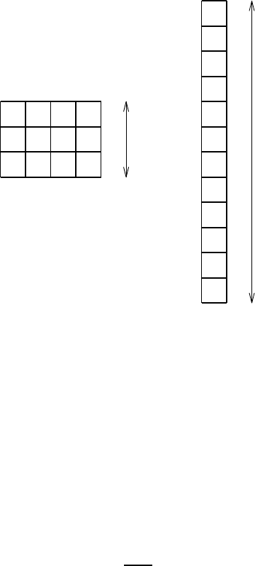
234
CHAPTER 19. EFFECTIVE DIANEUTRAL DIFFUSIVITY
and the corresponding sorted density state, evolve under the effects of vertical dif-
fusion? Note the grid dimensions for the two states are related through
∆z=4∆z∗, (19.27)
where zis the vertical coordinate for the unsorted state, and z∗is the vertical coor-
dinate for the sorted state. For the following, it is convenient to define this state as
that at time (t−∆t). The potential energies of the unsorted and sorted states are
easily computed to be
Ep(t−∆t) = 56
ρ
og∆z V (19.28)
Ere f (t−∆t) = 56
ρ
og∆z V (19.29)
EAPE(t−∆t) = 0 (19.30)
where Vis the volume of the grid cells, and
ρ
ois the density scale. The zero APE is
due to the absence of horizontal density gradients.
6 6 6 6
2
3 ∆z12
∆z* 3
∆z=
2
2
2
4
4
4
4
6
6
6
6
2 2 2 2
4 4 4 4
Figure 19.1: The initial density field for the first example. The number in each
box represents the density, given in units of
ρ
o. The left panel shows the density
ρ
(x,z,t−∆t)in the unsorted fluid state, and the right panel shows the density
ρ
re f (z∗,t−∆t)in the sorted state. Note that the vertical scale ∆z∗=∆z/4 for the
sorted state has been expanded for purposes of display.
19.3.1 Evolution of the unsorted state
Evolution of the unsorted density is given by the discrete equation
ρ
(x,z,t+∆t) =
ρ
(x,z,t−∆t)−2∆t
∆z[Fz(x,z,t−∆t)−Fz(x,z−∆z,t−∆t)],
(19.31)
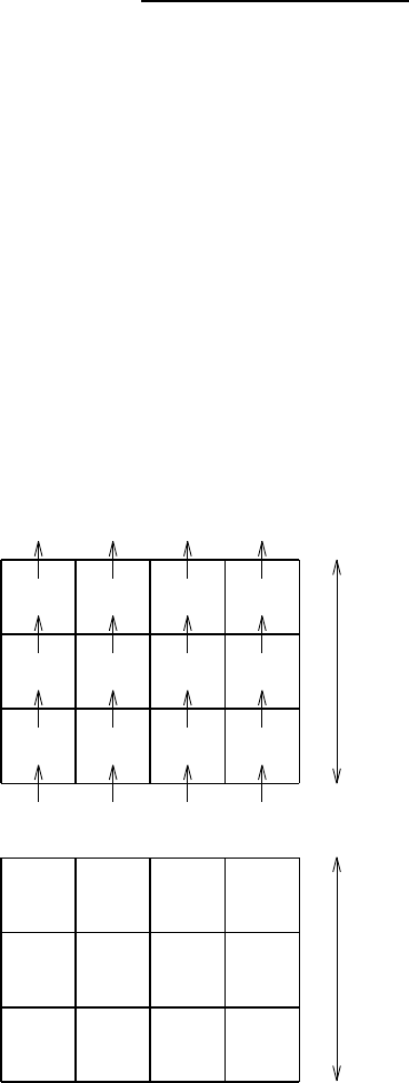
19.3. AN EXAMPLE WITH VERTICAL DENSITY GRADIENTS
235
where the vertical diffusive flux is given by
Fz(x,z,t) = −
κ δ
z
ρ
(x,z,t)
≈ −
κ
ρ
(x,z+∆z,t)−
ρ
(x,z,t)
∆z.(19.32)
Fz(x,z,t)is defined at the top face of the density grid cell whose center has position
(x,z). In the following, it is useful to introduce the dimensionless quantity
δ
(v)=2
κ
∆t/(∆z)2. (19.33)
This number arises from the chosen discretization of the diffusion equation. For
linear stability of the discretization,
δ
(v)<1 must be maintained.
The top panel of Figure 19.2 shows the vertical diffusive flux through the cell
faces at time t−∆t, and the bottom panel shows the resulting density field
ρ
(z,z,t+
∆t). Density in the middle row does not change, whereas the upper row density
increases and the lower row density decreases. The potential energy of this state is
Ep(t+∆t) =
ρ
og∆z V (56 +8
δ
(v)). (19.34)
This increase in potential energy is a result of the raised center of mass arising from
the vertical diffusive fluxes.
δ
0
2
2
0 0 0
2 2
2 2
00
2
2
0
0
6-
4
2+ δ
3∆z
3∆z
δ
2+ 2+ 2+
δδ δ
4 4 4
6- 6- 6-
δδ
Figure 19.2: Top panel: The vertical diffusive flux Fz(x,z,t−∆t), in units of
ρ
o
κ
/∆z, passing through the faces of the unsorted density grid cells. Bottom panel:
The unsorted density field
ρ
(x,z,t+∆t), in units of
ρ
o, where the dimensionless
increment
δ
is given by
δ
=2
δ
(v)=4
κ
∆t/(∆z)2. This density field results from
the vertical convergence of the flux Fz(x,z,t−∆t).
236
CHAPTER 19. EFFECTIVE DIANEUTRAL DIFFUSIVITY
19.3.2 Evolution of the sorted state
Corresponding to the evolution of the unsorted density, there is an evolution of the
sorted density
ρ
re f (z∗,t+∆t) =
ρ
re f (z∗,t−∆t)−2∆t
∆z∗[Fz∗(z∗,t−∆t)−Fz∗(z∗−∆z∗,t−∆t)].
(19.35)
The dianeutral diffusive flux is
Fz∗(z∗,t) = −
κ
e f f (z∗,t)
δ
z∗
ρ
re f (z∗,t)
≈ −
κ
e f f (z∗,t)
ρ
re f (z∗+∆z∗,t)−
ρ
re f (z∗,t)
∆z∗,(19.36)
where
ρ
re f (z∗,t)is the sorted state’s density. Fz∗(z∗,t)is defined at the top face of
the sorted density grid cell whose center has height z∗. Given the time tendency for
the sorted state, the flux is diagnosed through
Fz∗(z∗,t−∆t) = Fz∗(z∗−∆z∗,t−∆t)−∆z∗
2∆t[
ρ
re f (z∗,t+∆t)−
ρ
re f (z∗,t−∆t)].
(19.37)
The left panel of Figure 19.3 shows the sorted density field
ρ
re f (z∗,t+∆t), and
the second panel shows the diagnosed vertical diffusive flux Fz∗(z∗,t−∆t). The
third panel shows the vertical density gradient [
ρ
re f (z∗+∆z∗,t−∆t)−
ρ
re f (z∗,t−
∆t)]/∆z∗. The fourth panel shows the effective diffusivity
κ
e f f (z∗,t−∆t), which is
diagnosed from the relation
κ
e f f (z∗,t−∆t) = −Fz∗(z∗,t−∆t)∆z∗
ρ
re f (z∗+∆z∗,t−∆t)−
ρ
re f (z∗,t−∆t).
(19.38)
The units for
κ
e f f (z∗,t−∆t)are (∆z∗)2/∆t. Hence, a value for
κ
e f f (z∗,t−∆t)of
2
δ
in Figure 19.3 indicates a dimensional value of
κ
e f f (z∗,t−∆t) = 2
δ
(∆z∗)2
∆t
=
κ
4∆t
(∆z)2
(∆z∗)2
∆t
=
κ
/4.
(19.39)
This example illustrates a problem with unstratified parts of the sorted profile.
As evident from Figures 19.1 and 19.3, the 12 sorted boxes are actually three larger
homogeneous boxes, and so the calculation should compute fluxes and diffusivi-
ties for these three boxes rather than for the 12 boxes. Figure 19.4 shows such a
combined system, where there are three boxes each of height ∆zcomprising the
sorted state. Repeating the previous calculation for this configuration recovers the
expected
κ
e f f =
κ
on the two interior interfaces. Note that there is no ad hoc setting
to zero certain values of
κ
e f f associated with unstratified portions of the profile.
As a final note, the potential energy of the sorted state at time t+∆tis
Ere f (t+∆t) =
ρ
og∆z V (56 +16
δ
(v)), (19.40)
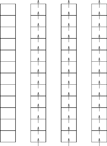
19.3. AN EXAMPLE WITH VERTICAL DENSITY GRADIENTS
237
δ
2 + δ
0
0
0
0
0
0
0
0
0
δ
0
0
0
0
0
2 +
2 +
2 +
δ
δ
δ
444
4
4
4
6 -
6 -
6 -
6 -
δ
δ
δ
2
3
4
4
4
4
4
3
2
δ
δ
δ
δ
δ
δ
δ
δ
δ
δ
0
0
-2
0
0
-2
0
0
0
2δ
0
0
2δ
0
Figure 19.3: First panel (left): The sorted density field
ρ
re f (z∗,t+∆t), in units of
ρ
o.
Second panel: The vertical diffusive flux Fz∗(z∗,t−∆t), in units of
ρ
o∆z∗/(2∆t),
passing through the faces of the sorted density grid cells. Third panel: The vertical
density gradient [
ρ
re f (z∗+∆z∗,t−∆t)−
ρ
re f (z∗,t−∆t)]/∆z∗in units of
ρ
o/∆z∗.
Fourth panel: The effective diffusivity
κ
e f f (z∗,t−∆t)in units of (∆z∗)2/∆t.
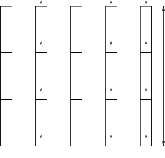
238
CHAPTER 19. EFFECTIVE DIANEUTRAL DIFFUSIVITY
z
4
- 2
- 2
δ
δ
2+
δ
δ
4
6−
2
6
0
0
0
0
κ
κ
0
0
3∆
Figure 19.4: First panel (far left): The initial density field
ρ
re f (z∗,t−∆t), consisting
of the combination of the three groups of four homogeneous cells. The values are
given in units of
ρ
o. In this recombined arrangement, ∆z∗=∆z. Second panel:
The vertical density gradient [
ρ
re f (z∗+∆z∗,t−∆t)−
ρ
re f (z∗,t−∆t)]/∆z∗, in units
of
ρ
o/∆z∗. Third panel: The density
ρ
re f (z∗,t+∆t)in units of
ρ
o. Fourth panel:
The diffusive flux Fz∗(z∗,t−∆t). Fifth panel (far right): The effective diffusivity
κ
e f f (z∗,t−∆t).
19.4. AN EXAMPLE WITH VERTICAL AND HORIZONTAL GRADIENTS
239
which is higher than the initial potential energy as a result of the raised center of
mass. The APE remains unchanged
EAPE(t+∆t) = 0, (19.41)
as it should since there remains zero baroclinicity in the final state.
19.3.3 Caveat about weakly stratified regions
Note that in this example, the same set of boxes are perfectly homogenized at each
time step. As such, it is straightforward to combine the boxes in order to derive
their effective diffusivities. In general, this simple situation will not be true, and
so the effective height of the combined boxes will differ. Furthermore, most cases
of homogenization are approximate (Sections 19.2.3 and 19.2.5), which introduces
even more time dependence to the interfaces between effectively homogeneous
boxes. In order to compute an effective diffusivity, however, our algorithm needs
to evaluate all quantities at the same depth level z∗. Time dependent z∗is problem-
atical.
The current example suggestes that one possibile way to account for homoge-
nization is to count the number of nearly homogeneous boxes occuring in a par-
ticular section of the sorted column. When the first interface is reached that has
a nontrivial stratification, then the effective diffusivity computed for this interface
is multiplied by the number of trailing boxes which are homogeneous. This trick
works for the example just considered (
κ
/4×4=
κ
). However, in the example
considered in Section 19.4.2, it leads to an effective diffusivity which can be larger
than the horizontal diffusivity. Such is not possible, and so one is led to reject the
proposed patch. A clean way to proceed is to try to resolve as best as possible
the stratification within the sorted fluid state. For those regions which are simply
too weakly stratified, it must be recognized that the computed effective diffusivity
might be smaller than a more refined computation.
An alternative approach is to average the sorted density field onto the discrete
levels realized in the unsorted state. Indeed, this resolution of the sorted state is
arguably that which is relevant for diagnosing the effective diffusivity. This is the
approach taken with the MOM experiments documented in Griffies et al. (2000b).
19.4 An example with vertical and horizontal gradients
This example considers the initial unsorted density configuration is shown in Fig-
ure 19.5. There are three rows of four boxes stacked on top of one another, and there
are both vertical and horizontal density gradients. Also shown is the correspond-
ing sorted state. As with the example in Section 19.3, the grid dimensions for the
two states are related through ∆z=4∆z∗, where zis the vertical coordinate for the
unsorted state, and z∗is the vertical coordinate for the sorted state. The potential
energies are
Ep(t−∆t) = 110
ρ
og∆z V (19.42)
Ere f (t−∆t) = 98
ρ
og∆z V (19.43)
EAPE(t−∆t) = 12
ρ
og∆z V, (19.44)
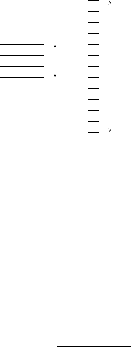
240
CHAPTER 19. EFFECTIVE DIANEUTRAL DIFFUSIVITY
where Vis the volume of the boxes and
ρ
ois the density scale.
=
2
4
4
6
6
6
8
8
8
10
10
12
2 4 6 8
4 6 8 10
6 8 10 12
3 ∆z12
∆z* 3
∆z
Figure 19.5: The initial density field for the horizontal and vertical diffusion ex-
amples. The number in each box represents the density, given in units of
ρ
o. The
left panel shows the density
ρ
(x,z,t−∆t)in the unsorted fluid state, and the right
panel shows the density
ρ
re f (z∗,t−∆t)in the sorted state. Note that the vertical
scale ∆z∗=∆z/4 for the sorted state has been expanded for purposes of display.
19.4.1 Vertical diffusion
Consider first just vertical diffusion acting on the unsorted state. The vertical diffu-
sivity
κ
acting on the unsorted state is assumed to be uniform and constant.
19.4.1.1 Evolution of the unsorted state
Evolution of the unsorted density is given by the discrete equation
ρ
(x,z,t+∆t) =
ρ
(x,z,t−∆t)−2∆t
∆z[Fz(x,z,t−∆t)−Fz(x,z−∆z,t−∆t)],
(19.45)
where the vertical diffusive flux is given by
Fz(x,z,t) = −
κ δ
z
ρ
(x,z,t)
≈ −
κ
ρ
(x,z+∆z,t)−
ρ
(x,z,t)
∆z.(19.46)
Fz(x,z,t)is defined at the top face of the density grid cell whose center has height
z. The top panel of Figure 19.6 shows the vertical diffusive flux through these faces
at time t−∆t, and the bottom panel shows the resulting density field
ρ
(x,z,t+
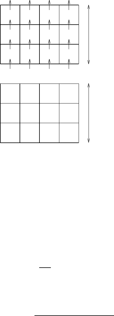
19.4. AN EXAMPLE WITH VERTICAL AND HORIZONTAL GRADIENTS
241
∆t). Density in the middle row does not change, whereas the upper row density
increases and the lower row density decreases. The potential energy of this state is
Ep(t+∆t) =
ρ
og∆z V (110 +16
δ
(v)), (19.47)
which is higher than the initial potential energy as a result of the raised center of
mass.
z
0
2
2
0 0 0
2 2
2 2
00
2
2
0
0
6- 8- 10- 12-
8
6
4
2+ 4+ 6+ 8+
10
δδ
δ
δ
δδ δ δ
3∆z
3∆
Figure 19.6: Top panel: The vertical diffusive flux Fz(x,z,t−∆t), in units of
ρ
o
κ
/∆z, passing through the faces of the unsorted density grid cells. Bottom
panel: The unsorted density field
ρ
(x,z,t+∆t), in units of
ρ
o, where
δ
=2
δ
(v)=
4
κ
∆t/(∆z)2. This is the density field resulting from the vertical convergence
of the flux Fz(x,z,t−∆t). The potential energy of this field is Ep(t+∆t) =
ρ
og∆z V (110 +16
δ
(v)).
19.4.1.2 Evolution of the sorted state
Corresponding to the evolution of the unsorted density, there is an evolution of the
sorted density which is given by
ρ
re f (z∗,t+∆t) =
ρ
re f (z∗,t−∆t)−2∆t
∆z∗[Fz∗(z∗,t−∆t)−Fz∗(z∗−∆z,t−∆t)].
(19.48)
The dianeutral diffusive flux is given by
Fz∗(z∗,t) = −
κ
e f f (z∗,t)
δ
z∗
ρ
re f (z∗,t)
≈ −
κ
e f f (z∗,t)
ρ
re f (z∗+∆z∗,t)−
ρ
re f (z∗,t)
∆z∗,(19.49)

242
CHAPTER 19. EFFECTIVE DIANEUTRAL DIFFUSIVITY
where
ρ
re f (z∗,t)is the sorted state’s density. Fz∗(z∗,t)is defined at the top face of
the sorted density grid cell whose center has height z∗. Given the time tendency for
the sorted state, the flux is diagnosed through
Fz∗(z∗,t−∆t) = Fz∗(z∗−∆z∗,t−∆t)−∆z∗
2∆t[
ρ
re f (z∗,t+∆t)−
ρ
re f (z∗,t−∆t)].
(19.50)
The left panel of Figure 19.7 shows the sorted density field
ρ
re f (z∗,t+∆t), and
the second panel shows the diagnosed vertical diffusive flux Fz∗(z∗,t−∆t). The
third panel shows the vertical density gradient [
ρ
re f (z∗+∆z∗,t−∆t)−
ρ
re f (z∗,t−
∆t)]/∆z∗. Note the regions of zero stratification. The fourth panel shows the effec-
tive diffusivity
κ
e f f (z∗,t−∆t), which is diagnosed from the relation
κ
e f f (z∗,t−∆t) = −Fz∗(z∗,t−∆t)∆z∗
ρ
re f (z∗+∆z∗,t−∆t)−
ρ
re f (z∗,t−∆t).
(19.51)
The units for
κ
e f f (z∗,t−∆t)are (∆z∗)2/∆t. In addition, consistent with the dis-
cussion in Section 19.3.2, the effective diffusivity for the interfaces on top of un-
stratified water are multiplied by the number of unstratified boxes. A value for
κ
e f f (z∗,t−∆t)of
δ
in Figure 19.7 indicates a dimensional value of
κ
e f f (z∗,t−∆t) =
δ
(∆z∗)2
∆t
=
κ
4∆t
(∆z)2
(∆z∗)2
∆t
=
κ
/4. (19.52)
As a final note, the potential energy of the sorted state at time t+∆tis
Ere f (t+∆t) =
ρ
og∆z V (98 +7
δ
(v)), (19.53)
which is higher than the initial potential energy as a result of the raised center of
mass. The APE is therefore given by
EAPE(t+∆t) =
ρ
og∆z V (12 +11
δ
(v)), (19.54)
which is larger than EAPE(t−∆t)given in equation (19.44).
19.4.2 Horizontal diffusion
Consider now just horizontal diffusion acting on the unsorted state. The horizontal
diffusivity Aacting on the unsorted state is assumed to be uniform and constant.
19.4.2.1 Evolution of the unsorted state
Evolution of the unsorted density is given by the discrete equation
ρ
(x,z,t+∆t) =
ρ
(x,z,t−∆t)−2∆t
∆x[Fx(x,z,t−∆t)−Fx(x−∆x,z,t−∆t)],
(19.55)
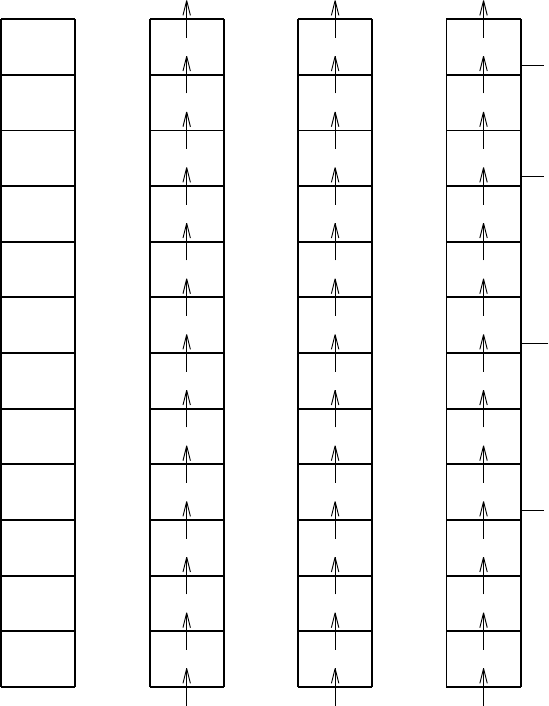
19.4. AN EXAMPLE WITH VERTICAL AND HORIZONTAL GRADIENTS
243
δ
2 + δ
4
4 + δ
6 - δ
6
6 + δ
8 - δ
8
8 +
10 - δ
10
12 - δ
δ
0
δ
2δ
δ
δ
2δ
δ
δ
2δ
δ
δ
0
0
-2
0
-2
0
0
-2
0
0
-2
0
-2
0
0
δ δ/2
0
δ
0
0
δ
0
0
δ
0
δ/2
0
2
δ
3
3δ
δ
Figure 19.7: Left panel: The sorted density field
ρ
re f (z∗,t+∆t), in units of
ρ
o. Sec-
ond panel: The vertical diffusive flux Fz∗(z∗,t−∆t), in units of
ρ
o∆z∗/∆t, passing
through the faces of the sorted density grid cells. Third panel: The vertical density
gradient [
ρ
re f (z∗+∆z∗,t−∆t)−
ρ
re f (z∗,t−∆t)]/∆z∗in units of
ρ
o/∆z∗. Fourth
panel: The effective diffusivity
κ
e f f (z∗,t−∆t)in units of (∆z∗)2/∆t. The four
κ
e f f
values which are on top of unstratified portions of the
ρ
re f (z∗,t−∆t)profile have
been multiplied by the number of unstratified boxes which lie directly beneath it.
244
CHAPTER 19. EFFECTIVE DIANEUTRAL DIFFUSIVITY
where the horizontal diffusive flux is given by
Fx(x,z,t) = −A
δ
x
ρ
(x,z,t)
≈ −A
ρ
(x+∆x,z,t)−
ρ
(x,z,t)
∆x.(19.56)
Fx(x,z,t)is defined at the east face of the density grid cell whose center has position
(x,z). The top panel of Figure 19.8 shows the horizontal diffusive flux through
these faces at time t−∆t, and the bottom panel shows the resulting density field
ρ
(x,z,t+∆t). The potential energy of this state is the same as the initial potential
energy, since the horizontal fluxes are parallel to the geopotential
Ep(t+∆t) = Ep(t−∆t) = 110
ρ
og∆z V. (19.57)
19.4.2.2 Evolution of the sorted state
Corresponding to the evolution of the unsorted density, there is an evolution of the
sorted density which is given by
ρ
re f (z∗,t+∆t) =
ρ
re f (z∗,t−∆t)−2∆t
∆z∗[Fz∗(z∗,t−∆t)−Fz∗(z∗−∆z,t−∆t)].
(19.58)
The dianeutral diffusive flux is given by
Fz∗(z∗,t) = −
κ
e f f (z∗,t)
δ
z∗
ρ
re f (z∗,t)
≈ −
κ
e f f (z∗,t)
ρ
re f (z∗+∆z∗,t)−
ρ
re f (z∗,t)
∆z∗,(19.59)
where
ρ
re f (z∗,t)is the sorted state’s density. Fz∗(z∗,t)is defined at the top face of
the sorted density grid cell whose center has height z∗. Given the time tendency for
the sorted state, the flux is diagnosed through
Fz∗(z∗,t−∆t) = Fz∗(z∗−∆z∗,t−∆t)−∆z∗
2∆t[
ρ
re f (z∗,t+∆t)−
ρ
re f (z∗,t−∆t)].
(19.60)
The left panel of Figure 19.4.2.2 shows the sorted density field
ρ
re f (z∗,t+∆t), and
the second panel shows the diagnosed vertical diffusive flux Fz∗(z∗,t−∆t). The
third panel shows the vertical density gradient [
ρ
re f (z∗+∆z∗,t−∆t)−
ρ
re f (z∗,t−
∆t)]/∆z∗. Note the regions of zero stratification. The fourth panel shows the effec-
tive diffusivity
κ
e f f (z∗,t−∆t), which is diagnosed from the relation
κ
e f f (z∗,t−∆t) = −Fz∗(z∗,t−∆t)∆z∗
ρ
re f (z∗+∆z∗,t−∆t)−
ρ
re f (z∗,t−∆t).
(19.61)
19.4. AN EXAMPLE WITH VERTICAL AND HORIZONTAL GRADIENTS
245
δ
3∆z
3∆z
0
0
0 δ
δ
δ
δ
δ
δ
δ
δ
δ
0
0
0
68
2+ δ4 6 8 -
10 -
12 -
810
6 +
4 + δ
δ
δ
δ
Figure 19.8: Top panel: The horizontal diffusive flux Fx(x,z,t−∆t), in units of
ρ
oA/∆x, passing through the faces of the unsorted density grid cells. Bottom
panel: The unsorted density field
ρ
(x,z,t+∆t), in units of
ρ
o, where
δ
=2
δ
(h)=
4A∆t/(∆x)2. This is the density field resulting from the vertical convergence of the
flux Fx(x,z,t−∆t). The potential energy of this field is Ep(t+∆t) = 110
ρ
og∆z V.
246
CHAPTER 19. EFFECTIVE DIANEUTRAL DIFFUSIVITY
The units for
κ
e f f (z∗,t−∆t)are (∆z∗)2/∆t. For example, a value for
κ
e f f (z∗,t−∆t)
of 3
δ
/2 in Figure 19.4.2.2 indicates a dimensional value of
κ
e f f (z∗,t−∆t) = (3
δ
/2)(∆z∗)2
∆t
=6A∆t
(∆x)2
(∆z∗)2
∆t
=6A∆z∗
∆x2
.
(19.62)
For the special case of ∆x=∆z=4∆z∗, the effective diffusivity is 3A/8. Note
that if the patch proposed in Section 19.3.3 is used, then the 3
δ
/2 diffusivity would
become 9
δ
/2, leading to the possibility for an effective diffusivity of 9 A/8, which
is impossible.
As a final note, the potential energy of the sorted state at time t+∆tis
Ere f (t+∆t) =
ρ
og∆z V (98 +19
δ
(h)/2), (19.63)
which is higher than the initial potential energy as a result of the raised center of
mass. The APE is given by
EAPE(t+∆t) =
ρ
og∆z V (12 −19
δ
(h)/2), (19.64)
which is smaller than EAPE(t−∆t)given in equation (19.44).
19.4. AN EXAMPLE WITH VERTICAL AND HORIZONTAL GRADIENTS
247
δ
2 + δ
4
4 + δ
6
8 - δ
8
10 - δ
10
12 - δ0
δ
2δ
δ
δ
δ
δ
0
0
-2
0
-2
0
0
-2
0
0
-2
0
-2
0
0
δ δ/2
0
δ
0
0
0
0
δ
0
δ/2
0
6
8
δ2
δ
2
3
δ2
δ2
2
3δ/2
6 +
Figure 19.9: First panel (far left): The sorted density field
ρ
re f (z∗,t+∆t)in units of
ρ
o. Second panel: The vertical diffusive flux Fz∗(z∗,t−∆t), in units of
ρ
o∆z∗/∆t,
passing through the faces of the sorted density grid cells. Third panel: The vertical
density gradient [
ρ
re f (z∗+∆z∗,t−∆t)−
ρ
re f (z∗,t−∆t)]/∆z∗in units of
ρ
o/∆z∗.
Fourth panel: The effective diffusivity
κ
e f f (z∗,t−∆t)in units of (∆z∗)2/∆t. The
four
κ
e f f values which are on top of unstratified portions of the
ρ
re f (z∗,t−∆t)
profile have been multiplied by the number of unstratified boxes which lie directly
beneath it.

CHAPTER
TWENTY
Age tracers
Contents
20.1 Fundamental considerations . . . . . . . . . . . . . . . . . . . . . 249
20.2 Age tracers . . . . . . . . . . . . . . . . . . . . . . . . . . . . . . . . 250
Age tracers are perhaps the simplest nontrivial passive tracers commonly used
in ocean modeling. They provide the modeler with a visual means to deduce the
time that a water parcel has spent circulating after having been in contact with a
certain part of the domain. The purpose of this chapter is to present the basics for
how mom4 computes age tracers.
20.1 Fundamental considerations
Fluid parcels generally contain material constituents that are transported as the
parcel moves through the ocean. These constituents are commonly termed tracers
since they are useful for tracing pathways of fluid transport.
Material tracers have a total mass within a fluid parcel written
dMC= (dM)C= (
ρ
dV)C, (20.1)
where dM=
ρ
dVis the total mass of the parcel of seawater, and C=dMC/dM
is the mass of tracer per mass of seawater. Cis often termed the tracer concentration
or tracer mass fraction. Notably, since the seawater mass and tracer mass are both
scalar quantities, the tracer concentration is likewise a scalar field. Hence, trac-
ers are often called scalars in the fluid dynamics literature. Additionally, when the
tracer concentration Cis uniform throughout the ocean, the budget for tracer mass
reduces to the budget for seawater mass. This observation, which follows from
the definition of C, provides an important compatibility constraint between mass
and tracer budgets that should be maintained in numerical simulations. Otherwise,
spurious source/sinks can cause tracer or mass to form in unphysical manners.
249

250
CHAPTER 20. AGE TRACERS
Conserving tracer mass within a parcel of seawater leads to the conservation
statement
d[(
ρ
dV)C]
dt= (
ρ
dV)dC
dt
=0,
(20.2)
where we used mass conservation d(
ρ
dV)/dt=0. Combining the Eulerian form
of material tracer conservation dC/dt= (∂t+v·∇)C=0 with mass conservation
ρ
,t+∇·(
ρ
v) = 0 leads to the Eulerian conservation law for tracer mass per volume
ρ
Cwithin in a seawater parcel
(
ρ
C),t+∇· (
ρ
Cv) = 0. (20.3)
Additional terms appear on the right hand side when sources or sinks of tracer are
found within the fluid or at the boundaries.
For purposes of establishing the momentum and tracer budgets, the mass of
a Boussinesq seawater parcel is given by dM=
ρ
odV. Material conservation of
tracer mass (
ρ
odV)Cstill leads to material conservation of tracer concentration:
dC/dt=0, since now the parcel’s volume is conserved. Combining material con-
servation of tracer concentration with parcel volume conservation, ∇ ·v=0, leads
to the Eulerian conservation law
C,t+∇· (vC) = 0. (20.4)
There are two main ways that the mass of tracer within a seawater parcel can
change. First, there can be tracer-dependent sources or sinks of tracer mass
ρ
S(C)
within the fluid domain or at the boundaries. Second, there can be irreversible
molecular or turbulent mixing effects that move tracer mass between parcels. Many
of these mixing effects can be mathematically represented by the convergence of
a density weighted tracer flux
ρ
F. Hence, for a non-Boussinesq fluid, the time
tendency for density weighted tracer concentration is written
(
ρ
C),t=−∇ · (
ρ
Cv+
ρ
F) +
ρ
S(C), (20.5)
whereas for a Boussinesq fluid it is
C,t=−∇ ·(Cv+F) + S(C). (20.6)
20.2 Age tracers
As discussed in many places, such as Thiele and Sarmiento (1990) and England
(1995), age tracers are defined by the source term S(C)appearing in equations (20.5)
and (20.6), as well as the initial and boundary conditions. The source is set to unity
everywhere within the ocean fluid
S(C)=1. (20.7)
This prescription specifies that the age field Chas units of time. Hence, the age
tracer is somewhat distinct from the material tracers discussed in Section 20.1,
20.2. AGE TRACERS
251
where Cfor material tracers is a dimensionless field (such as salinity). At a re-
gion of interest, say the ocean surface, the boundary condition for the age tracer is
zero. In mom4, one defines various age tracers that differ by the region that their
boundary condition is set to zero. For all of the age tracers, the age is set to zero at
the initial time of the experiment.
Given these prescriptions, Cmeasures the age, in units of time, that a water
parcel has spent away from the region where it was set to zero. Therefore, visual
maps of Care useful to deduce such physically interesting properties as ventilation
times.
Part VII
Miscellaneous Topics
253
255
MISCELLANEOUS TOPICS
This part of the MOM4 Guide contains discussions of various topics that do not
cleanly fall into other parts.

CHAPTER
TWENTYONE
Equation of state considerations
Contents
21.1 Introduction . . . . . . . . . . . . . . . . . . . . . . . . . . . . . . . 257
21.2 Comments on highly accurate equations of state . . . . . . . . . 258
21.3 Linear equation of state . . . . . . . . . . . . . . . . . . . . . . . . 258
21.4 McDougall, Jackett, Wright, and Feistel’s EOS . . . . . . . . . . . 259
The purpose of this chapter is to present certain issues related to the equation
of state used to compute density and its partial derivatives. The discussion follows
that in Jackett et al. (2006).
21.1 Introduction
Density is needed to compute the hydrostatic pressure. Additionally, it determines
the static stability of a vertical fluid column. Finally, its derivatives with respect to
potential temperature and salinity
ρ
,
θ
=∂
ρ
∂
θ
p,s
(21.1)
ρ
,s=∂
ρ
∂sp,
θ
(21.2)
set the neutral directions used for sub-grid-scale tracer transport. Therefore, it is im-
portant that the equation of state be accurate over the range of temperature, salinity,
and pressure values occurring in ocean simulations.
In early versions of MOM, density was computed according to the Bryan and Cox
(1972) cubic polynomial approximation to the UNESCO equation of state (Gill (1982)).
That approach was quite useful for certain problems. Unfortunately, it has limita-
tions that are no longer acceptable for global climate modeling. First, the polyno-
mials are fit at discrete depth levels. The use of partial cells makes this approach
cumbersome since with partial cells it is necessary to generally compute density at
arbitrary depths. Second, the cubic approximation is inaccurate for many regimes
257
258
CHAPTER 21. EQUATION OF STATE CONSIDERATIONS
of ocean climate modeling, such as wide ranges in salinity associated with rivers
and sea ice. For these two reasons, a more accurate method is desired.
Two equations of state (EOS) are currently available in MOM4 for computing
density. The first is a linear equation of state whereby density is a linear function
of potential temperature and salinity. This EOS is relevant only for idealized sim-
ulations with the Boussinesq approximation. The second EOS is that proposed by
McDougall et al. (2003b) and updated by Jackett et al. (2006). As they argue, their
EOS is more accurate than the UNESCO EOS due to the use of more accurate empir-
ical data as reported in Feistel (1993), Feistel and Hagen (1995), and Feistel (2003).
Even given its high degree of accuracy, this EOS has been found to be relatively
efficient.
21.2 Comments on highly accurate equations of state
Although there are portions of ocean climate models that are computed less ac-
curately than density resulting from the McDougall et al. (2003b) or Jackett et al.
(2006) equation of state, there is little reason to compromise the integrity of the den-
sity calculation to remain equitable with the less accurate algorithms. In particular,
there are three main reasons favoring the use of accurate EOS formulations.
•Many important details of deep water transformations, thermal wind com-
putations, and tracer transport depend on an accurate EOS. Furthermore, re-
alistic ocean climate models with increasing resolutions are put into regimes
where temperature, salinity, and pressures vary over broad ranges. Hence, it
is important to employ an EOS that can span this range without compromis-
ing the integrity of the computed density or density partial derivatives.
•The McDougall et al. (2003b) EOS is very efficient, so its cost is much less
than earlier experiences coding the UNESCO form taken from Gill (1982) or
Jackett and McDougall (1995).
•Use of a realistic EOS in a z-coordinate model comes without the price of com-
plex algorithms, in contrast to the situation with isopycnal models. Hence, it
makes sense to provide z-models with the capability of computing highly ac-
curate equilibrium thermodynamic properties.
21.3 Linear equation of state
The default linear equation of state in MOM4 assumes that density is a linear func-
tion of potential temperature and salinity. There is no pressure dependence. The
form used is
ρ
(x,t) =
ρ
0−˜
α θ
(x,t) + ˜
β
s(x,t). (21.3)
The default settings are
˜
α
=0.255 kg/m3/◦K (21.4)
˜
β
=0 (21.5)
ρ
0=1035 kg/m3. (21.6)

21.4. MCDOUGALL, JACKETT, WRIGHT, AND FEISTEL’S EOS
259
Hence, the density partial derivatives are given by
ρ
,
θ
=−˜
α
(21.7)
ρ
,s=˜
β
. (21.8)
Due to the absence of pressure effects, this density is most correctly thought of as a
potential density. Hence, without compressibility, its use for computing pressure is
self-consistent only when employing the Boussinesq approximation.
21.4 McDougall, Jackett, Wright, and Feistel’s EOS
Feistel (1993), Feistel and Hagen (1995), and Feistel (2003) studied the equilibrium
thermodynamics of seawater and produced a more accurate EOS than UNESCO
by using more recent empirical data. McDougall et al. (2003b) produced a fit to
Feistel and Hagen (1995) to render an expression convenient for use in ocean mod-
els, and Jackett et al. (2006) updated this equation of state based on Feistel (2003).
MOM4.0 has the McDougall et al. (2003b) equation of state, with future versions
of MOM moving to the Jackett et al. (2006) version. Either EOS is highly recom-
mended for purposes of realistic ocean climate simulations, where accuracy over a
wide range temperature, salinity, and pressure is crucial. The following equation
has been fit over the range
0psu ≤s≤40psu (21.9)
−3◦C≤
θ
≤40◦C (21.10)
0db ≤p≤8000db. (21.11)
The EOS has 25 terms. Its general form is motivated by that of Wright (1997).
Appendix B to McDougall et al. (2003b) provides the following equation for in situ
density
ρ
written in terms of pressure, salinity, and potential temperature
ρ
(s,
θ
,p) = P1(s,
θ
,p)
P2(s,
θ
,p), (21.12)
where pis the guage pressure in units of decibars,
θ
is the potential temperature
referenced to zero pressure in units of Celsius, and sis salinity in psu. Note the
conversion between mks pressure and decibars is given by
10−4db =1 Pa. (21.13)
The gauge pressure is given by
p=Pabsolute −10.1325dbars (21.14)
where the absolute pressure is the in situ pressure measured in the ocean. Salinity
is measured in practical salinity units (psu), consistent with modern oceanographic
measurements. As emphasized in Jackett et al. (2006), this salinity is distinct from
the salt concentration in parts per thousand. To a good approximation, a constant
factor distinguishes the two
s(ppt) = 1.004867 s(psu)(21.15)
260
CHAPTER 21. EQUATION OF STATE CONSIDERATIONS
The salinity variable in mom4 is interpreted as psu salinity, since this facilitates
a more direct comparison with observations. Notably, to perform salt budgets for
diagnostic purposes, it is necessary to multiply by 1.004867 to generate salt budgets
in terms of mass of salt.
A check value for this equation is
ρ
=1033.213387 kg. m−3with s=35psu,
θ
=20◦C, and p=2000db =2×10⁷Pa. The polynomial functions P1and P2are
given by
P1=ao+a1
θ
+a2
θ
2+a3
θ
3+a4s+a5s
θ
+a6s2
+a7p+a8p
θ
2+a9p s +a10 p2+a11 p2
θ
2(21.16)
P2=bo+b1
θ
+b2
θ
2+b3
θ
3+b4
θ
4+b5s+b6s
θ
+b7s
θ
3+b8s3/2+b9s3/2
θ
2
+b10 p+b11 p2
θ
3+b12 p3
θ
. (21.17)
The coefficients anand bnare tabulated in Appendix B of McDougall et al. (2003b).
Rearrangement in order to reduce multiplications leads to
P1=ao+
θ
(a1+
θ
(a2+a3
θ
)) + s(a4+a5
θ
+a6s)
+p(a7+a8
θ
2+a9s+p(a10 +a11
θ
2)) (21.18)
P2=bo+
θ
(b1+
θ
(b2+
θ
(b3+
θ
b4))) + s(b5+
θ
(b6+b7
θ
2) + s1/2(b8+b9
θ
2))
+p(b10 +p
θ
(b11
θ
2+b12 p)). (21.19)
The density partial derivatives are
∂
ρ
∂
θ
s,p
=
ρ
1
P1∂P1
∂
θ
s,p−1
P2∂P2
∂
θ
s,p!(21.20)
∂
ρ
∂s
θ
,p
=
ρ
1
P1∂P1
∂s
θ
,p−1
P2∂P2
∂s
θ
,p!. (21.21)
Since divisions are computationally more expensive than multiplications, we find
it useful to rearrange these results to
∂
ρ
∂
θ
s,p
= (P2)−1"∂P1
∂
θ
s,p−
ρ
∂P2
∂
θ
s,p#(21.22)
∂
ρ
∂s
θ
,p
= (P2)−1"∂P1
∂s
θ
,p−
ρ
∂P2
∂s
θ
,p#(21.23)
where (P2)−1can be saved in a temporary array, thus reducing the number of divi-
21.4. MCDOUGALL, JACKETT, WRIGHT, AND FEISTEL’S EOS
261
sions from four to one.1The partial derivatives are given by
∂P1
∂
θ
s,p
=a1+2a2
θ
+3a3
θ
2+a5s+2a8p
θ
+2a11 p2
θ
(21.24)
∂P1
∂s
θ
,p
=a4+a5
θ
+2a6s+a9p(21.25)
∂P2
∂
θ
s,p
=b1+2b2
θ
+3b3
θ
2+4b4
θ
3+b6s+3b7s
θ
2+2b9s3/2
θ
(21.26)
+3b11 p2
θ
2+b12 p3
∂P2
∂s
θ
,p
=b5+b6
θ
+b7
θ
3+ (3/2)b8s1/2+ (3/2)b9s1/2
θ
2(21.27)
with rearrangement leading to
∂P1
∂
θ
s,p
=a1+
θ
(2a2+3a3
θ
) + a5s+2p
θ
(a8+a11 p)(21.28)
∂P1
∂s
θ
,p
=a4+a5
θ
+2a6s+a9p(21.29)
∂P2
∂
θ
s,p
=b1+
θ
(2b2+
θ
(3b3+4b4
θ
)) + s(b6+
θ
(3b7
θ
+2b9s1/2)) (21.30)
+p2(3b11
θ
2+b12 p)
∂P2
∂s
θ
,p
=b5+
θ
(b6+b7
θ
2) + (3/2)s1/2(b8+b9
θ
2). (21.31)
1We thank Trevor McDougall for pointing out this simplification.

CHAPTER
TWENTYTWO
Tidal forcing from the moon and sun
Contents
22.1 Tidal consituents and tidal forcing . . . . . . . . . . . . . . . . . 263
22.2 Implementation in MOM4 . . . . . . . . . . . . . . . . . . . . . . 264
The purpose of this chapter is to describe the formulation of lunar and solar
tidal forcing implemented in mom4. This chapter was written by Harper Simmons
(hsimmons@iarc.uaf.edu)
22.1 Tidal consituents and tidal forcing
Without tidal forcing, the equation for the vertically integrated transport, U, in
MOM4 takes the form (Griffies (2004))
(∂t+fˆz∧)U=−(H+
η
)∇(ps+pa)/
ρ
o+G, (22.1)
where Gis the vertically integrated forcing arising from baroclinic effects, psis the
pressure associated with undulations of the surface height, pais the atmospheric
pressure, His the depth of the ocean, and
η
is the surface height deviation from a
resting state with z=0.
Tidal forcing arising from the eight primary constituents (M2, S2, N2, K2, K1,
O1, P1, Q1) (see Gill (1982)) have been added to the forcing for U. The formula-
tion follows Marchuk and Kagan (1989), by considering a tide generating potential
(g
η
eq) with corrections due to both the earth tide (1 +k−h) and self-attraction and
loading (
α
). In this approach, we have
∇(ps+pa)→ ∇(ps+pa) + g∇(1−
α
)
η
−(1+k−h)
η
eq. (22.2)
The equilibrium tide,
η
eq, arises from the astronomically derived gravity producing
forces. It is modified by several factors. The Love numbers, kand h, named for
the physicist A.L. Love, account for the reduction of the ocean tide because of the
deformation of the solid earth by tidal forces. The Love numbers are frequency
dependent, with 1 +k−hgenerally close to 0.7 (Wahr (1998)).
263
264
CHAPTER 22. TIDAL FORCING FROM THE MOON AND SUN
The term
α
in equation (22.2) accounts for a modification of the ocean’s tidal
response as a result of self-attraction and loading (SAL) (Hendershott (1972)). Self
attraction is the modification of the tidal potential as a result of the redistribution of
the earth and ocean due to the equilibrium tidal forcing. Loading refers to the de-
pression of the earth’s crust by the mounding of tides. Calculation of the SAL term
requires an extremely cumbersome integration over the earth surface, rendering
equation (22.2) an integro-differential equation (Ray (1998)).
Instead of solving the integro-differential form of equation (22.2), MOM4 uses
the scalar approximation to SAL. We feel this is justified since our purpose in in-
troducing tidal forcing is to study the effects of tides on the general circulation, not
the details of the tides themselves. The conjecture is that precise calculation of the
SAL term is not needed for to understand tidal effects on the general circulation.
For the scalar approximation,
α
is usually set between 0.940 −0.953. MOM4 uses
α
=0.948. Limitations of the scalar approximation to SAL are discussed by Ray
(1998), who concluded that the scalar approximation introduces phase errors of up
to 30◦and amplitude errors of 10% into a global scale tidal simulation.
22.2 Implementation in MOM4
The equilibrium tide is written for the nth diurnal tidal constituent as
η
eq,n=Hnsin 2
φ
cos(
ω
nt+
λ
), (22.3)
and for the nth semi-diurnal constituent as
η
eq,n=Hncos2
φ
cos(
ω
nt+2
λ
), (22.4)
where
φ
is latitude and
λ
is longitude. Recognizing that equation (22.3) and (22.4)
require the evaluation of trigonometric functions at every grid point and every
time-step, tidal forcing is introduced into MOM4 in the following mathematically
equivalent form. Making use of the identity
cos(A+B) = cos(A)cos(B)−sin(A)sin(B), (22.5)
we can write the eight tidal forcing constituents as
η
eq =Σ4
n=1h
β
nancos2
φ
[cos(
ω
nt)cos 2
λ
−sin(
ω
nt)sin 2
λ
]+
β
n+4an+4sin 2
φ
[cos(
ω
n+4t)cos 2
λ
−sin(
ω
n+4t)sin 2
λ
] ] ,
(22.6)
which allows all the trigonometric functions of
φ
and
λ
to be precomputed. Note
that we have written
β
n=1+kn−hn. The frequencies (
ω
n), amplitudes (an) and
Love numbers are listed in Table 22.1.

22.2. IMPLEMENTATION IN MOM4
265
constituent name origin
ω
(1/day) 1 +k−h a (m)
1K1Luni-solar declinational 0.7292117 0.736 0.141565
2O1Principal lunar declinational 0.6759774 0.695 0.100661
3P1Principal solar declinational 0.7252295 0.706 0.046848
4Q1Larger lunar elliptic 0.6495854 0.695 0.019273
5M2Principal lunar 1.405189 0.693 0.242334
6S2Principal solar 1.454441 0.693 0.112743
7N2Largerl lunar elliptic 1.378797 0.693 0.046397
8K2Luni-solar declinational 1.458423 0.693 0.030684
Table 22.1: Frequencies, Love numbers, and amplitude functions for the eight prin-
ciple constituents of tidal forcing available in MOM4.

CHAPTER
TWENTYTHREE
Eddy-topography interaction via Neptune
Contents
23.1 Introduction . . . . . . . . . . . . . . . . . . . . . . . . . . . . . . . 267
23.2 Basics of the parameterization . . . . . . . . . . . . . . . . . . . . 267
23.3 As implemented in MOM4 . . . . . . . . . . . . . . . . . . . . . . 268
The purpose of this chapter is to present a method for parameterizing the inter-
actions between unresolved mesoscale eddies and topography.
23.1 Introduction
Based on statistical mechanics arguments, Holloway (1992) proposed that inter-
actions between mesoscale eddies and topography result in a stress on the ocean
with two important consequences: (1) the ocean is not driven toward a state of rest,
(2) the resulting motion may have scales much larger than the eddy scales. That
is, eddy-topography interactions can generate coherent mean flows on the scale of
the topography. When Holloway described coastal currents that persistently flow
against both the wind forcing and pressure gradient, the response was that it must
be due to King Neptune. Who else? Hence, the effect is referred to colloquially as
the Neptune effect.
The magnitude of the associated topographic stress is dependent on the cor-
relation between pressure pand topographic gradients ∇H, and this correlation
is largely unknown. But even if it is no larger than 0.1, the resulting topographic
stress could be comparable in magnitude to that from the surface wind.
23.2 Basics of the parameterization
If the view is taken that equations of motion are solved for moments of probable
flow, then those moments are forced in part by derivatives of the entropy distri-
bution with respect to the realized moments. The entropy gradient is estimated
as proportional to a departure of the realized moments from a state in which the
267

268
CHAPTER 23. EDDY-TOPOGRAPHY INTERACTION VIA NEPTUNE
entropy gradient is weak. This latter state is approximated by a transport stream-
function
ψ
nep and maximum entropy velocity unep given by
ψ
nep =−f L H
unep =ˆz∧∇
ψ
nep (23.1)
where fis the Coriolis parameter, His the ocean depth, and Lis an adjustable
length scale on the order of 10 km. If model resolution is coarse relative to the first
deformation radius, unep is roughly depth independent. Depth independence is as-
sumed in the MOM4 implementation of Neptune. To parameterize the unresolved
driving of the mean flow by eddy-topography interactions, the Neptune parame-
terization drives flow towards towards unep using an eddy stress proportional to
(unep −u).
23.3 As implemented in MOM4
The Neptune parameterization is implemented in MOM4 for Laplacian friction.1
Neptune systematically damps the deformation rates towards a state of approxi-
mate maximum entropy. Notably, Neptune increases the kinetic energy as it damps
the flow toward its maximum entropy state. Such occurs even for flows at rest ex-
periencing no external forcing. As a result. Neptune spins-up the flow with shallow
depths to the right of the downstream direction.
Kinetic energy input via a sub-grid scale (SGS) parameterization is perhaps the
central weakness of the Neptune parameterization, where a more complete theory
provides for total energy conservation (forcing and dissipation) at the SGS. No-
tably, no such SGS theory presently exists. Instead, numerical modelers tradition-
ally employ energy sinks via frictional dissipation toward a state of rest, as well
as thickness diffusion to a state of zero available potential energy, both with no
corresponding source except that available via forcing by surface momentum and
buoyancy fluxes. Holloway (1992) argues that such is not an appropriate modeling
practice, thus motivating the use of Neptune as a interim approach until a more
complete theory is available.
There is concern about the stepwise representation of bottom topography in z-
coordinate models. The use of partial cells in MOM4 enhances the model’s ability
to represent the topographic slope in a more faithful manner than with full cells.
In general, however, the Neptune parameterization is an attempt to instruct the
simulation about physical consequences due to eddy-topography interactions. The
hope is that if the model can be suitably informed about these effects, it matters
little that topography is only approximately represented.
1It could be easily generalized to biharmonic friction.

CHAPTER
TWENTYFOUR
Temporal treatment of the Coriolis force
Contents
24.1 Inertial oscillations . . . . . . . . . . . . . . . . . . . . . . . . . . . 269
24.2 Explicit temporal discretization . . . . . . . . . . . . . . . . . . . 270
24.3 Semi-implicit temporal discretization . . . . . . . . . . . . . . . . 271
24.4 As implemented in MOM4 . . . . . . . . . . . . . . . . . . . . . . 272
24.4.1 Algorithm in the code . . . . . . . . . . . . . . . . . . . . . 272
24.4.2 Namelist parameters . . . . . . . . . . . . . . . . . . . . . . 273
24.4.3 Energy analysis . . . . . . . . . . . . . . . . . . . . . . . . . 273
The purpose of this chapter is to present the two methods used in MOM4 for
temporally discretizing the Coriolis force.
24.1 Inertial oscillations
The inviscid momentum equation in the absence of pressure is given by
(d/dt+fˆz∧)u=0, (24.1)
which is equivalent to the second order free oscillator equation
(d2/dt2+f2)u=0. (24.2)
Here, d/dtis the material time derivative relevant for Lagrangian observers. Mo-
tions which satisfy this equation are termed inertial oscillations and they have period
given by
Tinertial =2
π
f=11.97
sin
φ
hour (24.3)
where Ω=7.292 ×10⁻⁵s−1is the earth’s angular speed. The period of inertial
oscillations is smallest at the North pole where
φ
=
π
/2 and Tsmallest ≈12 hour.
An explicit temporal discretization of the inertial oscillation equation (24.1) will
be unstable if the time step is longer than some fraction of the inertial period, where
269

270
CHAPTER 24. TEMPORAL TREATMENT OF THE CORIOLIS FORCE
the fraction depends on details of the time stepping. Coarse resolution models
(models with resolutions on the order of 4-5 degrees) may find this time step con-
straint is the most stringent of the model’s baroclinic momentum processes. To get
around this limitation, a semi-implicit temporal treatment has been traditionally
considered, as in Bryan (1969).
Additional issues with coupling to sea ice may warrant an implicit treatment
even for ocean models run with a momentum time step that well resolves the iner-
tial period. In these cases, temporal details of ocean-ice coupling have been found
to cause enhanced energy at the inertial period. Semi-implicit time stepping of the
Coriolis force may assist in damping this energy.
It is for these reasons that MOM4 provides an option to time step the Coriolis
force either explicitly or semi-implicitly in the baroclinic portion of the model. The
namelist parameter acor sets the level of implicitness, as described in Section 24.4.2.
24.2 Explicit temporal discretization
Consider now just the linear part of the inertial oscillation equation, where advec-
tion is dropped
(∂t+ˆz∧)u=0. (24.4)
Following the time integration discussions in O’Brien (1986) and Bryan (1989) (see
also Section 2.3 of Durran (1999)), introduce the complex velocity
w=u+i v (24.5)
where i=√−1 and wshould not be confused with the vertical velocity component.
In terms of w, equation (24.4) takes the form
∂tw=−i f w (24.6)
which has an oscillatory solution
w=woeift (24.7)
with period
Tinertial =2
π
f−1. (24.8)
Time discretizing equation (24.6) with a centered leap-frog scheme leads to
w(
τ
+∆
τ
) = w(
τ
−∆
τ
)−i
λ
w(
τ
)(24.9)
with
λ
=2f∆
τ
(24.10)
a dimensionless number. We can write the finite difference solution in terms of an
amplification factor
w(
τ
+∆
τ
) = G w(
τ
). (24.11)
Substituting this ansatz into equation (24.9) leads to the quadratic equation
G2+i
λ
G−1=0 (24.12)
24.3. SEMI-IMPLICIT TEMPORAL DISCRETIZATION
271
whose solution is
G=−i
λ
±√−
λ
2+4
2. (24.13)
If
λ
/2=f∆
τ
<1, (24.14)
then |G|=1, which means the two finite difference solutions are neutral and stable.
One root is an unphysical mode, known as the leap-frog computational mode, and the
other corresponds to the physical solution. If
λ
>2 then |G|>1 which means both
roots are unstable. Hence, stability requires a time step satisfying
∆
τ
<f−1. (24.15)
That is, Tinertial
∆
τ
=2
π
f∆
τ
>2
π
, (24.16)
meaning the leap-frog scheme remains stable if there are at least 2
π
time steps per
inertial period. At the North Pole, this constraint means
∆
τ
<1.9 hours. (24.17)
For the baroclinic part of the model algorithm, ∆
τ
<1.9 hours can be the limit-
ing time step for coarse resolution global models, thus motivating an alternative
approach discussed in Section 24.3.
24.3 Semi-implicit temporal discretization
To overcome the time-step constraint (24.17) on the baroclinic time step, we now
consider a semi-implicit time stepping scheme within the leap-frog portion of the
baroclinic algorithm. As with any implicit approach, stability can be enhanced rel-
ative to explicit schemes. The price to pay is dissipation of the inertial motions. See
section 2.3 of Durran (1999) for discussion.
A semi-implicit treatment of the Coriolis force, within a leap-frog scheme, leads
to
w(
τ
+∆
τ
)−w(
τ
−∆
τ
) = −i
λ
[(1−
γ
)w(
τ
−∆
τ
) +
γ
w(
τ
+∆
τ
)] (24.18)
where 0 ≤
γ
≤1 is a dimensionless number whose value is set according to stabil-
ity considerations. We can write w(
τ
+∆
τ
) = G w(
τ
−∆
τ
), with the semi-implicit
scheme yielding the amplification factor
G=1−i
λ
(1−
γ
)
1+i
λ γ
. (24.19)
The squared modulus |G|2is used to determine conditions for stability
|G|2=[1−
γ λ
2(1−
γ
)]2+
λ
2
[1+ (
γ λ
)2]2. (24.20)
For
γ
=0, |G|>1 which leads to an unstable scheme. For
γ
=1/2, |G|=1
and so the scheme is neutral. With 1/2<
γ
≤1, |G|<1, and so the scheme is

272
CHAPTER 24. TEMPORAL TREATMENT OF THE CORIOLIS FORCE
unconditionally stable. Hence, we arrive at the stability range for the semi-implicit
parameter
1/2≤
γ
≤1, (24.21)
with
γ
=1 yielding the most stable scheme.
24.4 As implemented in MOM4
Both an explicit and semi-implicit treatment of the Coriolis force in the baroclinic
equations are available in MOM4. The semi-implicit piece is handled at the end of
a baroclinic time step, after the implicit treatment of vertical mixing. The logic used
in the code is a bit confusing, so it is useful to expose some details here.
24.4.1 Algorithm in the code
Let us separate that portion of the Coriolis force proportional to
γ
from the portion
independent of
γ
in order to ease coding for the case with a fully explicit Coriolis
force. Hence, we temporally discretize the Coriolis force as
−fˆz∧u→ −fˆz∧[(1−
γ
)u(
τ
−∆
τ
) +
γ
u(
τ
+∆
τ
)]
=−fˆz∧u(
τ
−∆
τ
)−f
γ
ˆz∧(u[
τ
+∆
τ
)−u(
τ
−∆
τ
)].(24.22)
For the explicit case,
γ
=0 and
−fˆz∧u→ −fˆz∧u(
τ
). (24.23)
We now consider time stepping the velocity using all accelerations except that por-
tion of the Coriolis force proportional to
γ
. The corresponding time tendency is
given by
δτ
u∗=2∆
τ
F(24.24)
where Fincludes the acceleration from advection, horizontal pressure gradient
force, friction force (both explicit and implicit), as well as that piece of the Cori-
olis force independent of
γ
. If the Coriolis force is computed explicitly, then
δτ
u∗
is the full time tendency for the baroclinic velocity. For the semi-implicit treatment,
we require those contributions proportional to
γ
, thus leading to
u(
τ
+∆
τ
) = u(
τ
−∆
τ
) + 2∆
τ δτ
u∗−
λ γ
ˆz∧(u[
τ
+∆
τ
)−u(
τ
−∆
τ
)] (24.25)
where again
λ
=2f∆
τ
. (24.26)
Writing out the components leads to
u(
τ
+∆
τ
) = u(
τ
−∆
τ
) + 2∆
τ δτ
u∗+
λ γ
[v(
τ
+∆
τ
)−v(
τ
−∆
τ
)] (24.27)
v(
τ
+∆
τ
) = v(
τ
−∆
τ
) + 2∆
τ δτ
v∗−
λ γ
[u(
τ
+∆
τ
)−u(
τ
−∆
τ
)], (24.28)
and solving for u(
τ
+∆
τ
)renders
u(
τ
+∆
τ
) = u(
τ
−∆
τ
) + 2∆
τ
δτ
u∗+
λ δτ
v∗
1+ (
λ γ
)2(24.29)
v(
τ
+∆
τ
) = v(
τ
−∆
τ
) + 2∆
τ
δτ
v∗−
λ δτ
u∗
1+ (
λ γ
)2. (24.30)
24.4. AS IMPLEMENTED IN MOM4
273
24.4.2 Namelist parameters
In the code,
∆
τ
=dtuv (24.31)
is the baroclinic time step, and
γ
=acor (24.32)
is a namelist parameter setting the level of implicit treatment for the Coriolis force.
The method for discretizing the Coriolis force in the baroclinic part of the model is
set according to the value of acor, with
acor =0⇒fully explicit Coriolis (24.33)
1/2≤acor ≤1⇒semi-implicit Coriolis. (24.34)
As the vertically integrated part of the model algorithm typically uses a time step
much smaller than f−1, MOM4 discretizes the Coriolis force explicitly when time
stepping the vertically integrated equations. That is, acor is relevant only for the
baroclinic equations.
24.4.3 Energy analysis
In the continuum, the Coriolis force does no work on a fluid parcel since it is always
directed orthogonal to the flow direction
v·fˆz∧u=0. (24.35)
This property is respected on the B-grid when we discretize the Coriolis force ex-
plicitly in time
v(
τ
)·fˆz∧u(
τ
) = 0. (24.36)
However, the semi-implicit treatment does not respect this property since in general
the product
v(
τ
)·fˆz∧[(1−
γ
)u(
τ
−∆
τ
) +
γ
u(
τ
+∆
τ
)] (24.37)
does not vanish. The only time it will vanish is when the flow is in a steady state.
This limitation of the semi-implicit approach is to be expected, since implicit time
discretizations generally do not conserve energy.

CHAPTER
TWENTYFIVE
Checkerboard null mode
Contents
25.1 Introduction . . . . . . . . . . . . . . . . . . . . . . . . . . . . . . . 275
25.2 Experiences with the checkerboard null mode . . . . . . . . . . . 276
25.2.1 A caveat concerning filtering the surface height . . . . . . 277
25.2.2 Suggestions . . . . . . . . . . . . . . . . . . . . . . . . . . . 278
25.2.2.1 Laplacian at the end of the barotropic loop . . . . 278
25.2.2.2 Laplacian added within the barotropic loop . . . 278
25.3 Polar filtering . . . . . . . . . . . . . . . . . . . . . . . . . . . . . . 279
25.4 The checkerboard damping module in MOM4-beta . . . . . . . 279
The purpose of this chapter is to discuss issues related to the presence of a
checker-board null mode present with a B-grid that appears most prominently in
the surface height field. Much of this discussion follows that given by Pacanowski and Griffies
(1999).
25.1 Introduction
As discussed by Killworth et al. (1991), discretization of gravity waves on a B-grid
can admit a stationary grid scale checkerboard pattern (see also Messinger (1973)
and Janji´c (1974) for atmospheric discussions). This pattern is associated with an
unsuppressed grid splitting that can be initiated through grid scale forcing, such
as topography. That is, the discrete equations admit a checkerboard null mode.
Beckers (1999) also discusses subtleties associated with traditional linear stability.
In our experience, when the model goes unstable due to CFL violations, this grid
mode is the spatial pattern associated with the instability.
Strictly, the grid mode is present only when the surface pressure gradient takes
the form ∇hps=
ρ
g∇h
η
, where
ρ
is an averaged surface density. For example,
in the implementation of Killworth et al. (1991), ∇hps=
ρ
og∇h
η
, and so the null
mode is always present. Tests with the alternative expression ps=
ρ
k=1g
η
used in
MOM, in which surface pressure gradients arise from gradients in both the surface
275
276
CHAPTER 25. CHECKERBOARD NULL MODE
density
ρ
k=1and surface height, suggest that the null mode is slightly suppressed.
A more significant means to suppress the mode, however, is provided through the
use of time averaging over the barotropic time steps, as well as with nonlinearity
in the shallow water system present when the undulating surface height is fully
incorporated to the dynamics.
Hence, for many purposes, the grid mode is absent or mild. Nonetheless, some
experiments do experience a nontrivial checkerboard pattern in the surface height,
especially in enclosed seas such as the Mediterranean Sea and Hudson Bay. In this
case, the checkerboard mode is continually excited by surface forcing and topogra-
phy, yet there is not enough grid resolution to allow the noise to radiate outward or
as boundary waves. The checkerboard pattern can also be initiated by fresh water
forcing. Although the typical forcing from the atmosphere is large scale, there will
always be some projection onto the grid scale, thus pumping energy into the null
mode. In this case, we have seen the checkerboard pattern appear even over large
basins.
For those cases where the noise is unacceptable, we have considered various
means to suppress it. The following relates our experience provides suggestions
and caveats. We remain incompletely satisfied with the following methods, and so
welcome other suggestions.
25.2 Experiences with the checkerboard null mode
Under certain circumstances, Killworth et al. (1991) noted that the checkerboard
pattern can appear in the vertically integrated velocity. In order to dissipate this
mode, they suggested that horizontal friction acting on the barotropic velocity be
updated each barotropic time step, instead of only during the baroclinic time steps.
This approach was found to be especially appropriate in simulations with strong
eddy activity.
Updating frction on each barotropic time step can be quite costly. Therefore,
in practice, one is restricted to the use of a constant viscosity Laplacian friction for
both the barotropic and baroclinic modes. Notably, use of a biharmonic viscosity,
updated each barotropic time step, could be prohibitively costly. As discussed by
such authors as Semtner and Mintz (1977) and Griffies and Hallberg (2000), Lapla-
cian friction for eddy-permitting simulations significantly under-utilizes the model
grid as it strongly suppresses mesoscale eddy formation. Hence, restricting the
model to constant viscosity Laplacian friction is not an acceptable solution to the
grid splitting problem. Relatedly, barotropically updating a depth dependent vis-
cosity, such as that arising from the Smagorinsky scheme (Griffies and Hallberg
(2000)), is very cumbersome due to the need to maintain self-consistency between
friction applied in the barotropic and baroclinic equations.
For the time stepping procedure used in MOM4, regions where the barotropic
fields are evolving experience an effective spatial averaging associated with the
barotropic time averaging. Eddy-rich regions are therefore preferentially smoothed.
Consequently, time averaging provides for an effective suppression of the grid
splitting in both the surface height and vertically integrated velocity.
Since the surface height evolution is given by the inviscid continuity equation,
the checkerboard pattern tends to appear most prominently in this field. To sup-
25.2. EXPERIENCES WITH THE CHECKERBOARD NULL MODE
277
press the surface height noise, Killworth et al. (1991) proposed the addition of the
so-called “del-plus / del-cross” operator to the prognostic equation for the free sur-
face height. Their approach is an extension of that suggested by Janji´c (1974). The
operator is basically the difference between Laplacians computed in two different
manners, and it preferentially removes the checkerboard pattern by coupling the
grids. This coupling occurs in a scale-selective manner so that the larger scales are
only modestly affected. The construction of this operator requires the definition of
time dependent image points over land to allow for it to conserve volume.
25.2.1 A caveat concerning filtering the surface height
Various surface height filters have been tested, such as the del-plus / del-cross oper-
ator, as well as a two-dimensional Shapiro filter designed to conserve volume with
arbitrary geography. Either spatial filter successfully removes noisy patterns from
the surface height. However, their effects on other model fields, such as vertical ve-
locity, can be dependent on the strength of the surface height filter. In particular, for
many cases where the filter was sufficient to suppress noise in the surface height, it
had detrimental effects on the vertical velocity.
The reason for this sensitivity can be seen by considering the equations for
gravity waves on a B-grid using a forward-backward time stepping scheme as in
MOM3 (the following considerations do not depend on the choice of time stepping
schemes). To better expose the main points, assume ps=
ρ
og
η
,D=H+
η
≈H,
and omit fresh water forcing. The discretized equations take the form
η
(tn+1) =
η
(tn)−∆t[∇h·U(tn)−F(
η
) ] (25.1)
U(tn+1) = U(tn)−H g ∆t
δ
x
η
(tn+1)y(25.2)
V(tn+1) = V(tn)−H g ∆t
δ
y
η
(tn+1)x, (25.3)
where F(
η
)represents a spatial filter applied to the surface height.
Consider a case in which the free surface contains power in the checkerboard
pattern, as well as longer waves, yet there is no spatial filter and so F=0. The dis-
cretized surface pressure gradient does not feel the checkerboard pattern since this
pattern is a null mode of the discrete derivative operators
δ
x()yand
δ
y()x. There-
fore, discrete pressure gradients are determined only by longer waves, and so the
gradients are smooth. Since the checkerboard pattern is stationary in time, it does
not contribute to the vertical velocity. Neglecting the time varying top cell volume
in the baroclinic and tracer equations, as in the constant volume free surface meth-
ods of Killworth et al. (1991) and Dukowicz and Smith (1994), renders the checker-
board pattern dynamically irrelevant. Instead, it is simply an esthetic nuisance. Yet
when solving the more general equations with undulating top cell thicknesses, as in
MOM4, the noise cannot be ignored as it potentially will influence the other model
fields.
Now consider the addition of a spatial filter designed to preferentially remove
the checkerboard grid noise in the surface height. Unlike the unfiltered and noisy
η
,
the filter Fwill generally not be invisible to the discretized pressure gradients, and
so these gradients are now affected by a new source. In practice, these new sources
can be nontrivial, especially when using the Shapiro filter, which is the strongest
278
CHAPTER 25. CHECKERBOARD NULL MODE
available grid scale filtering. Tests in MOM3 with the del plus / del minus filter,
using the weighting factor suggested by Killworth et al. (1991), transformed large
amount of noise to the vertical velocity field near the surface. Again, the reason
is that this filter is not invisible to the discretized gradients, and so while it acts to
smooth the surface height, it correspondingly adds noise to the surface pressure
gradients which then affect the barotropic velocity.
One attempt to suppress the transfer of noise was to also filter ∇h·Uin order
to counteract the noisy pressure gradients. Unfortunately, this approach is prob-
lematic, since doing so breaks the precise connection between the barotropic and
baroclinic systems. As a result, spatially filtering ∇h·Uproduces a nontrivial spuri-
ous vertical velocity throughout the ocean, and in particular it creates unacceptable
spurious advective fluxes through the ocean bottom.
25.2.2 Suggestions
As mentioned at the beginning of this section, we find the need for filtering to be
greatly reduced due to the use of a nonlinear free surface in which the barotropic
time steps are time averaged. Nevertheless, for those cases in which filtering is
needed, such as for inland seas and when using fresh water forcing, we have found
it sufficient to add a straightforward Laplacian to the free surface height equation
with a reasonably small diffusivity. The more sophisticated Shapiro filter or del-
plus minus del-minus operator have been found to be no better, and often much
worse in their affects on vertical velocity. Note that a Laplacian, using no-flux
boundary conditions, conserves volume. Therefore, adding a Laplacian to the free
surface equation is trivial to implement relative to the del plus / del minus oper-
ator, which requires the specification of time dependent image points in order to
preserve volume in arbitrary geometry.
25.2.2.1 Laplacian at the end of the barotropic loop
One way to apply the filter to the surface height is at the end of the barotropic time
steps. In addition to the Laplacian added to the surface height, the needs of to-
tal tracer conservation necessitate a compensating additional horizontal diffusion
be added to tracers in the surface model grid cells. Similar issues of tracer and
volume/mass compatibility were described for the cross-land mixing scheme in
Chapter 13. This approach has lost favor among the developers due to the nontriv-
ial effects it has on tracer concentration in the k=1 level.
25.2.2.2 Laplacian added within the barotropic loop
Another way to add a Laplacian filter is to filter the surface height within the
barotropic time loop. In this way, the surface height is continually being smoothed.
This method increases the cost of the barotropic system due to the added compu-
tations and extra communication (for parallel computers). Yet it removes the need
to concern ourselves with tracers, since compatibility is not a problem so long as
the surface height is updated consistenty with the tracer (see chapter 7). This is the
approach implemented in MOM4.
25.3. POLAR FILTERING
279
25.3 Polar filtering
The CFL time step requirements for the barotropic mode can be quite stringent
when reaching the pole on a spherical grid. Instead of reducing the time steps,
it is common to prescribe a spatial filtering in order to remove the small scale fea-
tures. This filtering traditionally takes the form of Fourier filtering (e.g., Bryan et al.
(1975)). Experience in MOM3 indicates that one-dimenstional Shapiro filtering is
preferable due to its increased speed. Nevertheless, as such filtering is necessary
for each of the small barotropic mode time steps, the computational cost can be
high and it can render strong load imbalances between adjacent parallel computer
processors. Indeed, the cost can be higher than the cost of simply reducing the
barotropic time step in order to satisfy the CFL constraint. Additionally, for rea-
sons related to the mechanism discussed above, tests have shown that polar fil-
tering of the surface height can result in a nontrivial amount of grid noise in the
vertical velocity field within the polar filtering regions. As a result, polar filtering
the barotropic fields is not recommended, even when using the spherical form of
MOM4. Indeed, polar filtering is supported in MOM4 only for use within the tracer
equation. In general, polar filtering is not recommended, and it is becoming obso-
lete in ocean climate models via the use of non-spherical grids such as the tripolar
grid discussed in Chapter 4.
25.4 The checkerboard damping module in MOM4-beta
As mentioned in Section 13.8, some care must be exercised in the specification
of points between which the cross-land mixing scheme is used. Otherwise, mix-
ing surface height can add to the problems associated with the checker-board null
mode. Turning this problem into a solution is something that the researcher may
wish to investigate. That is, cross-land mixing can be considered an ad hoc method
to suppress the checker-board mode in enclosed seas. By construction, this scheme
allows for one to mix in a manner that conserves total tracer. Taking this approach
globally is what the MOM4-beta checkerboard module does, where now the mod-
ule introduces a local Laplacian mixing of surface height aimed to suppress the
mode. As discussed in Section 13.2 when describing the cross-land mixing scheme,
mixing surface height must be accompanied by a mixing of tracer in the ocean’s
surface grid cell in order to conserve total model tracer. It is because of this added
tracer mixing in the surface cell, which can generally be nontrivial, that the checker-
board module has recently grown out of favor with researchers at GFDL. Indeed, it
is not supported in MOM4.0, though it is available in the beta releases of MOM4.
BIBLIOGRAPHY
Adcroft, A., C. Hill, and J. Marshall, 1999: A new treatment of the coriolis terms
in c-grid models at both high and low resolutions. Monthly Weather Review, 127,
1928–1936.
Aris, R., 1962: Vectors, Tensors and the Basic Equations of Fluid Mechanics. Dover Pub-
lishing.
Beckers, J. M., 1999: On some stability properties of the discretisation of the damped
propagation of shallow-water inertia-gravity waves on the arakawa b-grid. Ocean
Modelling, 1, 53–69.
Beckmann, A., and R. D¨oscher, 1997: A method for improved representation of
dense water spreading over topography in geopotential-coordinate models. Jour-
nal of Physical Oceanography, 27, 581–591.
Bryan, F., 1987: Parameter sensitivity of primitive equation ocean general circula-
tion models. Journal of Physical Oceanography, 17, 970–985.
Bryan, K., 1969: A numerical method for the study of the circulation of the world
ocean. Journal of Computational Physics, 4, 347–376.
Bryan, K., 1984: Accelerating the convergence to equilibrium of ocean-climate mod-
els. Journal of Physical Oceanography, 14, 666–673.
Bryan, K., 1991: Michael cox (1941-1989): his pioneering contributions to ocean
circulation modeling. Journal of Physical Oceanography, 21, 1259–1270.
Bryan, K., and M. D. Cox, 1972: An approximate equation of state for numerical
models of the ocean circulation. Journal of Physical Oceanography, 4, 510–514.
Bryan, K., and L. J. Lewis, 1979: A water mass model of the world ocean. Journal of
Geophysical Research, 84, 2503–2517.
Bryan, K., S. Manabe, and R. C. Pacanowski, 1975: A global ocean-atmosphere cli-
mate model. Part II. The oceanic circulation. Journal of Physical Oceanography, 5,
30–46.
Campin, J.-M., and H. Goosse, 1999: Parameterization of density-driven downslop-
ing flow for a coarse-resolution ocean model in z-coordinate. Tellus, 51A, 412–
430.
281
282
BIBLIOGRAPHY
Cox, M. D., 1984: A Primitive Equation, 3-Dimensional Model of the Ocean.
NOAA/Geophysical Fluid Dynamics Laboratory.
Danabasoglu, G., J. C. McWilliams, and W. G. Large, 1996: Approach to equilibrium
in accelerated global oceanic models. Journal of Climate, 9, 1092–1110.
Denman, K., 1973: A time-dependend model of the upper ocean. Journal of Physical
Oceanography, 3, 173–184.
Dewar, W. K., Y. Hsueh, T. J. McDougall, and D. Yuan, 1998: Calculation of pressure
in ocean simulations. Journal of Physical Oceanography, 28, 577–588.
D¨oscher, R., and A. Beckmann, 2000: Effects of a bottom boundary layer param-
eterization in a coarse-resolution model of the North Atlantic Ocean. Journal of
Atmospheric and Oceanic Technology, 17, 698–707.
Dukowicz, J. K., and R. D. Smith, 1994: Implicit free-surface method for the Bryan-
Cox-Semtner ocean model. Journal of Geophysical Research, 99, 7991–8014.
Dukowicz, J. K., R. D. Smith, and R. C. Malone, 1993: A reformulation and imple-
mentation of the Bryan-Cox-Semtner ocean model on the connection machine.
Journal of Atmospheric and Oceanic Technology, 10, 195–208.
Durran, D. R., 1999: Numerical Methods for Wave Equations in Geophysical Fluid Dy-
namics. Springer Verlag.
England, M. H., 1995: The age of water and ventilation timescales in a global ocean
model. Journal of Physical Oceanography, 25, 2756–2777.
Favre, A., 1965: ´
Equations des gaz turbulents compressibles. Parts I and II. Journel
de M´echanic, 4, 361–421.
Feistel, R., 1993: Equilibrium thermodynamics of seawater revisited. Progress in
Oceanography, 31, 101–179.
Feistel, R., 2003: A new extended Gibbs thermodynamic potential of seawater.
Progress in Oceanography, 58, 43–114.
Feistel, R., and E. Hagen, 1995: On the Gibbs thermodynamic potential of seawater.
Progress in Oceanography, 36, 249–327.
Gent, P. R., and J. C. McWilliams, 1990: Isopycnal mixing in ocean circulation mod-
els. Journal of Physical Oceanography, 20, 150–155.
Gent, P. R., J. Willebrand, T. J. McDougall, and J. C. McWilliams, 1995: Parameteriz-
ing eddy-induced tracer transports in ocean circulation models. Journal of Physical
Oceanography, 25, 463–474.
Gill, A., 1982: Atmosphere-Ocean Dynamics. International Geophysics Series, Vol. 30,
Academic Press.
Goosens, M., F. Mittelbach, and A. Samarin, 1994: The L
A
T
E
XCompanion. Addison-
Wesley.
BIBLIOGRAPHY 283
Gordon, C., C. Cooper, C. A. Senior, H. Banks, T. C. J. J. M. Gregory, J. F. B. Mitchell,
and R. A. Wood, 2000: The simulation of SST, sea ice extents and ocean heat trans-
ports in a version of the Hadley Centre coupled model without flux adjustments.
Climate Dynamics, 16, 147–168.
Greatbatch, R. J., Y. Lu, and Y. Cai, 2001: Relaxing the Boussinesq approximation in
ocean circulation models. Journal of Atmospheric and Oceanic Technology, 18, 1911–
1923.
Griffies, S. M., 1998: The Gent-McWilliams skew-flux. Journal of Physical Oceanogra-
phy, 28, 831–841.
Griffies, S. M., 2004: Fundamentals of ocean climate models. Princeton University
Press.
Griffies, S. M., and Coauthors, 2000a: Developments in ocean climate modelling.
Ocean Modelling, 2, 123–192.
Griffies, S. M., A. Gnanadesikan, R. C. Pacanowski, V. Larichev, J. K. Dukowicz,
and R. D. Smith, 1998: Isoneutral diffusion in a z-coordinate ocean model. Journal
of Physical Oceanography, 28, 805–830.
Griffies, S. M., and R. W. Hallberg, 2000: Biharmonic friction with a Smagorinsky
viscosity for use in large-scale eddy-permitting ocean models. Monthly Weather
Review, 128, 2935–2946.
Griffies, S. M., R. Pacanowski, M. Schmidt, and V. Balaji, 2001: Tracer conserva-
tion with an explicit free surface method for z-coordinate ocean models. Monthly
Weather Review, 129, 1081–1098.
Griffies, S. M., R. C. Pacanowski, and R. W. Hallberg, 2000b: Spurious diapycnal
mixing associated with advection in a z-coordinate ocean model. Monthly Weather
Review, 128, 538–564.
Hallberg, R. W., 1997: Stable split time stepping schemes for large-scale ocean mod-
eling. Journal of Computational Physics, 135, 54–65.
Haltiner, G. T., and R. T. Williams, 1980: Numerical Prediction and Dynamic Meteorol-
ogy. John Wiley and Sons.
Held, I. M., and V. D. Larichev, 1996: A scaling theory for horizontally homoge-
neous baroclinically unstable flow on a beta plane. Journal of Atmospheric Sciences,
53, 946–952.
Hendershott, M., 1972: The effects of solid earth deformation on global ocean tide.
Geophysical Journal of the Royal Astronomical Society, 29, 389–402.
Hinze, J. O., 1975: Turbulence. McGraw-Hill Publishers.
Holland, W. R., J. C. Chow, and F. O. Bryan, 1998: Application of a third-order
upwind scheme in the ncar ocean model. Journal of Climate, 11, 1487–1493.
Holloway, G., 1992: Representing topographic stress for large-scale ocean models.
Journal of Physical Oceanography, 22, 1033–1046.
284
BIBLIOGRAPHY
Huang, R. X., 1993: Real freshwater flux as a natural boundary condition for the
salinity balance and thermohaline circulation forced by evaporation and precipi-
tation. Journal of Physical Oceanography, 23, 2428–2446.
Jackett, D. R., and T. J. McDougall, 1995: Minimal adjustment of hydrographic pro-
files to achieve static stablilty. Journal of Atmospheric and Oceanic Technology, 12,
381–389.
Jackett, D. R., T. J. McDougall, R. Feistel, D. G. Wright, and S. M. Griffies, 2006:
Algorithms for density, potential temperature, conservative temperature, and
freezing temperature of seawater. Journal of Atmospheric and Oceanic Technology,
23, 1709–1728.
Janji´c, Z. I., 1974: A stable centered difference scheme free of two-grid-interval
noise. Monthly Weather Review, 102, 319–323.
Jerlov, N. G., 1968: Optical Oceanography. Elsevier, 194 pp.
Killworth, P., 1989: On the parameterisation of deep convection in ocean models.
P. M ¨uller and G. Holloway, Eds., Parameterizing small scale processes in the ocean,
Proceeding of the 5th ’Aha Huliko’a Hawaiian Winter Workshop, University of
Hawaii at Manoa, 59–74.
Killworth, P. D., and N. Edwards, 1999: A turbulent bottom boundary layer code for
use in numerical ocean models. Journal of Physical Oceanography, 29, 1221–1238.
Killworth, P. D., J. M. Smith, and A. E. Gill, 1984: Speeding up ocean circulation
models. Ocean Modelling, 56, 1–5.
Killworth, P. D., D. Stainforth, D. J. Webb, and S. M. Paterson, 1991: The devel-
opment of a free-surface Bryan-Cox-Semtner ocean model. Journal of Physical
Oceanography, 21, 1333–1348.
Klinger, B. A., J. Marshall, and U. Send, 1996: Representation of convective plumes
by vertical adjustment. Journal of Geophysical Research, 101, 18 175–18 182.
Lamport, L., 1994: L
A
T
E
X: A Documentation Preparation System User’s Guide and Refer-
ence Manual. Addison-Wesley.
Landau, L. D., and E. M. Lifshitz, 1987: Fluid Mechanics. Pergamon Press.
Large, W. G., G. Danabasoglu, J. C. McWilliams, P. R. Gent, and F. O. Bryan, 2001:
Equatorial circulation of a global ocean climate model with anisotropic horizontal
viscosity. Journal of Physical Oceanography, 31, 518–536.
Large, W. G., J. C. McWilliams, and S. C. Doney, 1994: Oceanic vertical mixing: A
review and a model with a nonlocal boundary layer parameterization. Reviews of
Geophysics, 32, 363–403.
Levitus, S., 1982: Climatological atlas of the world ocean. U.S. Government Printing
Office 13, NOAA, Washington, D.C. 163 pp.
KEY: Levitus82
ANNOTATION: 17 mircofiches
BIBLIOGRAPHY 285
Lin, S. J., and R. B. Rood, 1996: Multidimensional flux-form semi-Lagrangian trans-
port schemes. Monthly Weather Review, 124, 2046–2070.
Losch, M., A. Adcroft, and J.-M. Campin, 2004: How sensitive are coarse general
circulation models to fundamental approximations in the equations of motion?
Journal of Physical Oceanography, 34, 306–319.
Lu, Y., 2001: Including non-Boussinesq effects in Boussinesq ocean circulation mod-
els. Journal of Physical Oceanography, 31, 1616–1622.
Marchuk, and Kagan, 1989: Dynamics of Ocean Tides. Kluwer Academic, 327 pp.
Marotzke, J., 1991: Influence of convective adjustment on the stability of the ther-
mohaline circulation. Journal of Physical Oceanography, 21, 903–907.
Marshall, J., A. Adcroft, J.-M. Campin, and C. Hill, 2004: Atmosphere-ocean mod-
eling exploiting fluid isomorphisms. Journal of Physical Oceanography. In press.
Marshall, J., C. Hill, L. Perelman, and A. Adcroft, 1997: Hydrostatic, quasi-
hydrostatic, and nonhydrostatic ocean modeling. Journal of Geophysical Research,
102, 5733–5752.
McDougall, T. J., R. J. Greatbatch, and Y. Lu, 2003a: On conservation equations in
oceanography: How accurate are Boussinesq ocean models? Journal of Physical
Oceanography, 32, 1574–1584.
McDougall, T. J., D. R. Jackett, D. G. Wright, and R. Feistel, 2003b: Accurate and
computationally efficient algorithms for potential temperature and density of
seawater. Journal of Atmospheric and Oceanic Technology, 20, 730–741.
Morel, A., 1988: Optical modeling of the upper ocean in relation to its biogenous
matter content (case-i waters). JGR, 93, 10 749–10 768.
Morel, A., and D. Antoine, 1994: Heating rate within the upper ccean in relation to
its bio-optical state. Journal of Physical Oceanography, 24, 1652–1665.
Morel, A., and J.-F. Berthon, 1989: Surface pigments, algal biomass profiles, and
potential production of the euphotic layer: relationship reinvestigated in view of
remote-sensing applications. Limnology and Oceanography, 34, 1542–1562.
Murray, R. J., 1996: Explicit generation of orthogonal grids for ocean models. Journal
of Computational Physics, 126, 251–273.
O’Brien, J. J., 1986: Advanced Physical Oceanographic Numerical Modelling. D. Reidel
Publishing Company.
Ohlmann, J., and D. Siegel, 2000: Ocean radiant heating. Part i: Optical influences.
JPO, 30, 1833–1848.
Pacanowski, R. C., 1995: MOM2 Documentation, User’s Guide, and Reference Manual.
NOAA/Geophysical Fluid Dynamics Laboratory.
Pacanowski, R. C., K. Dixon, and A. Rosati, 1991: The GFDL Modular Ocean Model
User Guide. NOAA/Geophysical Fluid Dynamics Laboratory.
286
BIBLIOGRAPHY
Pacanowski, R. C., and A. Gnanadesikan, 1998: Transient response in a z-level
ocean model that resolves topography with partial-cells. Monthly Weather Review,
126, 3248–3270.
Pacanowski, R. C., and S. M. Griffies, 1999: The MOM3 Manual.
NOAA/Geophysical Fluid Dynamics Laboratory.
Pacanowski, R. C., and G. Philander, 1981: Parameterization of vertical mixing in
numerical models of the tropical ocean. Journal of Physical Oceanography, 11, 1442–
1451.
Paulson, E. A., and J. J. Simpson, 1977: Irradiance measurements in the upper
ocean. Journal of Physical Oceanography, 7, 952–956.
Pedlosky, J., 1987: Geophysical Fluid Dynamics. 2nd ed., Springer-Verlag.
Pickard, G. L., and W. J. Emery, 1990: Descriptive Physical Oceanography. 5th ed.,
Pergamon Press.
Press, W. H., S. A. Teukolsky, W. T. Vetterling, and B. P. Flannery, 1992: Numerical
Recipes in FORTRAN: The Art of Scientific Computing. 2nd ed., Cambridge Univer-
sity Press.
Rahmstorf, S., 1993: A fast and complete convection scheme for ocean models.
Ocean Modelling, 101, 9–11.
Ray, R. D., 1998: Ocean self-attraction and loading in numerical tidal models. Ma-
rine Geodesy, 21, 181–192.
Rosati, A., and K. Miyakoda, 1988: A general circulation model for upper ocean
simulation. Journal of Physical Oceanography, 18, 1601–1626.
Semtner, A. J., 1974: An oceanic general circulation model with bottom topogra-
phy. Numerical Simulation of Weather and Climate, Technical Report No. 9, UCLA
Department of Meteorology.
Semtner, A. J., and Y. Mintz, 1977: Numerical simulation of the Gulf Stream and
mid-ocean eddies. Journal of Physical Oceanography, 7, 208–230.
Smith, R. D., 1999: The primitive equations in the stochastic theory of adiabatic
stratified turbulence. Journal of Physical Oceanography, 29, 1865–1880.
Smith, R. D., J. K. Dukowicz, and R. C. Malone, 1992: Parallel ocean general circu-
lation modeling. Physica D, 60, 38–61.
Smith, R. D., and J. C. McWilliams, 2003: Anisotropic horizonal viscosity for ocean
models. Ocean Modelling, 5, 129–156.
Thiele, G., and J. L. Sarmiento, 1990: Tracer dating and ocean ventilation. Journal of
Geophysical Research, 95, 9377–9391.
Veronis, G., 1973: Large scale ocean circulation. Advances in Applied Mechanics, 13,
2–92.
BIBLIOGRAPHY 287
Visbeck, M., J. C. Marshall, T. Haine, and M. Spall, 1997: Specification of eddy trans-
fer coefficients in coarse resolution ocean circulation models. Journal of Physical
Oceanography, 27, 381–402.
Wahr, J., 1998: Body tides on an elliptical, rotating, elastic and oceanless earth. Geo-
physical Journal of the Royal Astronomical Society, 64, 677–703.
Webb, D. J., A. C. Coward, B. A. de Cuevas, and C. S. Gwilliam, 1998: The first main
run of the OCCAM global ocean model. Internal Document No. 34, Southampton
Oceanography Centre.
Winters, K. B., and E. A. D’Asaro, 1995: Diascalar flux and the rate of fluid mixing.
Journal of Fluid Mechanics, 317, 179–193.
Winters, K. B., P. N. Lombard, J. J. Riley, and E. A. D’Asaro, 1995: Available potential
energy and mixing in density-stratified fluids. Journal of Fluid Mechanics, 289, 115–
128.
Winton, M., R. W. Hallberg, and A. Gnanadesikan, 1998: Simulation of density-
driven frictional downslope flow in z-coordinate ocean models. Journal of Physical
Oceanography, 28, 2163–2174.
Wright, D. G., 1997: An equation of state for use in ocean models: Eckart’s formula
revisited. Journal of Atmospheric and Oceanic Technology, 14, 735–740.
INDEX
Adcroft et al. (1999), 127, 128, 281
Aris (1962), 56, 281
Beckers (1999), 275, 281
Beckmann and D¨oscher (1997), 24, 197–
199, 201, 202, 207, 208, 281
Bryan and Cox (1972), 257, 281
Bryan and Lewis (1979), 23, 281
Bryan et al. (1975), 279, 281
Bryan (1969), 19, 67, 88, 98, 137, 218, 219,
270, 281
Bryan (1984), 121, 281
Bryan (1987), 221, 281
Bryan (1989), 270, 281
Campin and Goosse (1999), 24, 201–208,
281
Cox (1984), 16, 109, 138, 282
Danabasoglu et al. (1996), 121, 282
Denman (1973), 135, 282
Dewar et al. (1998), 23, 282
Dukowicz and Smith (1994), 19, 277, 282
Dukowicz et al. (1993), 19, 282
Durran (1999), 147, 270, 271, 282
D¨oscher and Beckmann (2000), 24, 197,
198, 207, 282
England (1995), 250, 282
Favre (1965), 61, 282
Feistel and Hagen (1995), 258, 259, 282
Feistel (1993), 258, 259, 282
Feistel (2003), 258, 259, 282
Gent and McWilliams (1990), 23, 282
Gent et al. (1995), 23, 218, 282
Gill (1982), 56, 60, 257, 258, 263, 282
Goosens et al. (1994), 2, 282
Gordon et al. (2000), 221, 283
Greatbatch et al. (2001), 23, 58, 62, 65,
119, 124, 139, 283
Griffies and Hallberg (2000), 23, 276, 283
Griffies et al. (1998), 23, 283
Griffies et al. (2000a), 67, 127, 128, 197,
283
Griffies et al. (2000b), 109, 228, 232, 239,
283
Griffies et al. (2001), 20, 23, 26, 89, 121,
122, 126, 128, 283
Griffies (1998), 23, 283
Griffies (2004), 16, 17, 20, 23, 24, 53, 55,
58, 62, 67, 87, 88, 98–102, 116,
118–120, 123, 124, 127, 128, 139,
159, 169, 185, 204, 213, 214, 217,
223, 263, 283
Hallberg (1997), 127, 283
Haltiner and Williams (1980), 117, 283
Held and Larichev (1996), 23, 283
Hendershott (1972), 264, 283
Hinze (1975), 61, 283
Holland et al. (1998), 24, 283
Holloway (1992), 24, 267, 268, 283
Huang (1993), 102, 284
Jackett and McDougall (1995), 258, 284
Jackett et al. (2006), 257–259, 284
Janji´c (1974), 275, 277, 284
Jerlov (1968), 134, 284
Killworth and Edwards (1999), 202, 207,
284
Killworth et al. (1984), 121, 284
Killworth et al. (1991), 19, 275–278, 284
Killworth (1989), 143, 284
Klinger et al. (1996), 137, 138, 284
Lamport (1994), 2, 284
Landau and Lifshitz (1987), 56, 284
Large et al. (1994), 23, 138, 284
Large et al. (2001), 24, 284
Levitus (1982), 33, 284
Lin and Rood (1996), 145, 146, 285
288
BIBLIOGRAPHY 289
Losch et al. (2004), 26, 285
Lu (2001), 61, 285
Marchuk and Kagan (1989), 263, 285
Marotzke (1991), 143, 285
Marshall et al. (1997), 57, 137, 285
Marshall et al. (2004), 26, 285
McDougall et al. (2003a), 61, 62, 65, 285
McDougall et al. (2003b), 23, 258–260, 285
Messinger (1973), 275, 285
Morel and Antoine (1994), 133, 135, 136,
285
Morel and Berthon (1989), 136, 285
Morel (1988), 135, 285
Murray (1996), 22, 47, 71, 75, 78, 79, 285
O’Brien (1986), 270, 285
Ohlmann and Siegel (2000), 135, 285
Pacanowski and Gnanadesikan (1998), 22,
104, 286
Pacanowski and Griffies (1999), 16, 17,
24, 68, 70, 88, 121, 143, 150, 217,
275, 286
Pacanowski and Philander (1981), 23, 138,
286
Pacanowski et al. (1991), 16, 286
Pacanowski (1995), 16, 286
Paulson and Simpson (1977), 134, 135,
286
Pedlosky (1987), 56, 286
Pickard and Emery (1990), 231, 286
Press et al. (1992), 143, 286
Rahmstorf (1993), 138, 143, 286
Ray (1998), 264, 286
Rosati and Miyakoda (1988), 134, 286
Semtner and Mintz (1977), 276, 286
Semtner (1974), 101, 286
Smith and McWilliams (2003), 24, 286
Smith et al. (1992), 19, 286
Smith (1999), 61, 286
Thiele and Sarmiento (1990), 250, 287
Veronis (1973), 56, 287
Visbeck et al. (1997), 23, 287
Wahr (1998), 263, 287
Webb et al. (1998), 68, 287
Winters and D’Asaro (1995), 228, 229, 232,
287
Winters et al. (1995), 227, 229, 287
Winton et al. (1998), 197, 201, 202, 287
Wright (1997), 259, 287
acor parameter, 273
adjustments for tracer conservation, 122–
127
advection velocity components
discrete, 87–96
T-cell faces, 104–106
age tracers, 249–251
available potential energy, 228
B-grid computational modes, 187, 275–
279
B-grid variable placement, 68
bipolar Arctic
grid defined, 71
fold, 71
redundancy, 71
bit-wise exact, 48–49
boundary conditions, 32–33
changing processors, 48–49
checkerboard mixing, 279
checkerboard mode, 275
chlorophyll, 134–136
communicating with developers, 19
commutator, 57
compatibility between mass and tracer,
178, 185
constant volume ocean, 162–164
convective adjustment, 143
coordinates, 56–57
cartesian and spherical, 56
general orthogonal
infinitesimal distances, 56–57
key formulae, 56–57
metric tensor, 56–57
partial derivatives, 56–57
Coriolis force, 269–273
coupling tracer to velocity cells, 87–96
cross-land insertion, 189–195
cross-land mixing, 177–187
null modes, 187, 279
partial cells and free surface, 183–185
tracer and mass compatibility, 178
tracer and volume compatibility, 178
data override, 32–33
density
constant for Boussinesq, 60
expansion coefficients, 257
290
INDEX
linear equation of state, 258–259
derived types, 21–22, 28
development with MOM4, 25–26
discrete operators, 103–106, 110–112
dynamic memory, 45–46
dynamics
mapping to model variables, 64–65
summary of averaged, 62–64
Eddy-topography interactions, 267–268
efficiency, 45–46
energetics
B-grid conversions, 97–114
external and internal kinetic energy,
113–114
kinetic energy conversion, 109
ensemble averages, 61
equation of state, 257–261
external mode solvers, 19–20
features of MOM4, 19–24
Flexible Modeling System (FMS), 17–19
FMS, 17–19
frazil, 157–159
fresh water from sea ice, 160–161
full convection, 143
gauge pressure, 259–260
grid
description, 68–71
distance calculations, 69–71
distances carried in the model, 71
four fundamental points, 68–69
grid distances, 89–91
grid generation, 32
grid specification file, 32
halos, 77–83
southern-most row, 96
specifying fields, 77–83
specifying grid distances, 77–83
summary of relations for bipolar, 83
heat budget in coupled models, 164–165
hydrostatic pressure
discrete calculation, 106
ifdef options, 20–21
implicit vertical advection, 145–152
implicit vertical mixing, 139–143
non-Boussinesq, 139–143
inertial oscillations, 269–273
initial conditions, 32–33
kinetic energy budget, 99
kinetic energy conversion, 112
lever-rule, 90
linear momentum density, 62
Love numbers, 263–264
lunar tidal forcing, 263–264
managing tracers, 33–45
mass budget, 185, 221–223
memory, 45–46
metric tensor, 56–57
mixed layers, 162
model printout, 46–47
Modeling frameworks, 17–19
MOM4 characteristics, 19–24
computational aspects, 21–22, 28
derived types, 21–22, 28
numerical aspects, 22
physical aspects, 22–24
MOM4 history, 15–16
MOM4 on the web, 19
momentum balance
summary of semi-discrete, 100–101
Murray tripolar grid, 71
namelists, 48
Neptune, 267–268
null modules, 20–21
ocean vertical resolution, 162
ocean vertical resolution and sea ice, 161–
162
ocean-sea ice constraints, 161–162
option streamlining, 19–20
overflows, 201–207
partial cells, 104
physical tensor components, 56–57
polar filtering, 278–279
potential energy, 228
preprocessing capabilities, 32–33
pressure coordinate models, 164
pressure from sea ice, 161
pressure in equation of state, 259–260
BIBLIOGRAPHY 291
pressure work conversion
B-grid, 103–108
continuum, 101–103
primitive equations, 55–65
summary of model equations, 99
unaveraged, 58–60
regridding, 32–33
remapping error, 95
remapping operators, 89–96
reproducibility, 48–49
river mixing, 167–171
Robert time filter, 115, 117–118
salinity in equation of state, 259–260
salinity in mom4, 259–260
sea ice models, 157–164
pressure, 161
fresh water flux, 160–161
horizontal extent, 162
limiting thickness, 162
mass budget, 159–160
vertical resolution in ocean, 161–162
virtual salt flux, 162–164
semi-lagrangian transport, 145–152
SGI Origin, 45
SGI Origin), 46
shortwave
boundary conditions, 134
shortwave heating, 136
shorwave heating, 133
sigma tracer diffusion, 197–199
solar tidal forcing, 263–264
SourceForge, 19
southern-most row and halos, 96
spin-up, 121
static memory, 45–46
steric effects, 60
streamfunctions, 213–220
surface height noise, 275–279
surface mixed layers, 162
surface tracer flux, 223–224
temperature in water, 164–165
test cases, 47–48
tidal forcing, 263–264
time stepping, 127–128
topography generation, 32
tracer budget, 185, 223–224
steady state, 223–224
tracer transport, 221–226
tracers
comments on time stepping, 127–128
total ocean content, 115–128
transport diagnostics, 221–226
tracers in MOM4, 33–45
traditional approximation
geometric restrictions, 55–57
thin shell approximation, 55–56
tripolar grid, 71
bipolar Arctic, 79–83
diagnosed energy conversions, 114
remapping error, 95
verbosity, 46–47
vertical adjustments, 137–143
vertical advection, 145–152
implicit, 145–152
vertical flux discretized, 140–141
vertical velocity at ocean bottom, 88
virtual salt flux, 162–164
volume budget for Boussinesq fluid, 159
What is MOM?, 15–16
