MOM4p1 Manual
MOM4p1_manual
User Manual:
Open the PDF directly: View PDF ![]() .
.
Page Count: 377 [warning: Documents this large are best viewed by clicking the View PDF Link!]
Elements of mom4p1
Stephen M. Griffies
NOAA Geophysical Fluid Dynamics Laboratory
Princeton, USA
STEPHEN.GRIFFIES@NOAA.GOV
WITH CONTRIBUTIONS FROM
MARTIN SCHMIDT (WARNEM ¨
UNDE, GERMANY)
MIKE HERZFELD (CSIRO-HOBART, AUSTRALIA)
ii
This document is freely distributed for ocean scientists interested in understand-
ing the fundamentals of version 4.1 of the Modular Ocean Model (MOM). This
document should be referenced as
ELEMENTS OF MOM4P1
GFDL OCEAN GROUP TECHNICAL REPORT NO. 6
Stephen M. Griffies
NOAA/Geophysical Fluid Dynamics Laboratory
Version prepared on September 27, 2007
Code and documentation available online at www.gfdl.noaa.gov
Information about how to download and run MOM4 can be found at the GFDL
Flexible Modeling System (FMS) web site accessible from WWW.GFDL.NOAA.GOV.

Contents
Chapter 1. Executive summary of mom4p1 1
1.1 General features 1
1.2 Relating mom4p1 to MOM4.0 5
Chapter 2. Synopsis of mom4p1 7
2.1 What is MOM? 7
2.2 First release of MOM4.0: October 2003 8
2.3 First release of MOM4p1: Late 2007 8
2.4 Fundamentals of mom4p1 9
2.5 Tracer features 12
2.6 Subgrid scale parameterizations 15
2.7 Miscellaneous features 17
2.8 Short bibliography of mom4 documents 17
2.9 The future of MOM 18
PART 1. FORMULATION OF THE OCEAN EQUATIONS 19
Chapter 3. The fundamental equations 21
3.1 Fluid kinematics 21
3.2 Material time changes over finite regions 36
3.3 Basics of the finite volume method 38
3.4 Mass and tracer budgets over finite regions 40
3.5 Forces from pressure 50
3.6 Linear momentum budget 55
3.7 The Boussinesq budgets 60
Chapter 4. The hydrostatic pressure force 63
4.1 Hydrostatic pressure forces at a point 63
4.2 The pressure gradient body force 64
4.3 The pressure gradient body force in B-grid mom4p1 70
Chapter 5. Parameterizations with generalized vertical coordinates 73
5.1 Friction 73
5.2 Diffusion and skew diffusion 77
Chapter 6. Depth and pressure based vertical coordinates 83
6.1 Depth based vertical coordinates 83
6.2 Pressure based coordinates 90

iv CONTENTS
PART 2. NUMERICAL FORMULATIONS 95
Chapter 7. Quasi-Eulerian Algorithms 97
7.1 Pressure and geopotential at tracer points 97
7.2 Initializing Boussinesq and nonBoussinesq models 99
7.3 Vertical dimensions of grid cells 103
7.4 Vertically integrated volume/mass budgets 112
7.5 Compatibility between tracer and mass 114
7.6 Diagnosing the dia-surface velocity component 115
7.7 Vertically integrated horizontal momentum budget 121
Chapter 8. Time stepping schemes 125
8.1 Split between fast and slow motions 125
8.2 Time stepping the model equations as in MOM4.0 126
8.3 Smoothing the surface height and bottom pressure 132
8.4 Introduction to time stepping in mom4p1 134
8.5 Basics of staggered time stepping in mom4p1 134
8.6 A predictor-corrector for the barotropic system 135
8.7 The Griffies (2004) scheme 137
8.8 Algorithms motivated from the predictor-corrector 138
8.9 Closed algorithms enforcing compatibility 143
Chapter 9. Mechanical energy budgets and conversions 149
9.1 Energetic conversions in the continuum 149
9.2 Conservation, consistency, and accuracy 152
9.3 Thickness weighted volume and mass budgets 153
9.4 Discrete Boussinesq pressure work conversions 153
9.5 Discrete non-Boussinesq pressure work conversions 160
9.6 Discrete Boussinesq kinetic energy advection 165
9.7 Discrete non-Boussinesq kinetic energy advection 169
Chapter 10. Temporal treatment of the Coriolis force 171
10.1 Inertial oscillations 171
10.2 Explicit temporal discretization with leap frog 172
10.3 Semi-implicit time discretization with leap frog 173
10.4 Semi-implicit time discretization with forward step 173
10.5 As implemented in MOM4 174
Chapter 11. Open boundary conditions 177
11.1 Introduction 177
11.2 Types of open boundary conditions 178
11.3 Implementation of sea level radiation conditions 183
11.4 OBC for tracers 187
11.5 The namelist obc nml 191
11.6 Topography generation - Preparation of boundary data 193
Chapter 12. Tidal forcing from the moon and sun 197
12.1 Tidal consituents and tidal forcing 197
12.2 Formulation in nonBoussinesq models 198
12.3 Implementation in MOM4 198
CONTENTS v
PART 3. SUBGRID SCALE PARAMETERIZATIONS 201
Chapter 13. Mixing related to tidal energy dissipation 203
13.1 Formulation 203
13.2 Dianeutral diffusivities from internal wave breaking 204
13.3 Dianeutral diffusivities from bottom drag 206
Chapter 14. Calculation of buoyancy forcing 209
14.1 Fundamentals 209
14.2 The formulation as in Large et al. (1994) 212
14.3 Buoyancy forcing for KPP in MOM 213
14.4 Bug in MOM4.0 214
Chapter 15. Neutral physics and boundary layers 215
15.1 Regions affecting neutral physics 215
15.2 Quasi-Stokes streamfunction 219
15.3 Specializing the quasi-Stokes streamfunction 224
15.4 Regarding the TEM approach and vertical stresses 226
15.5 Discussion of some details 227
15.6 Lateral diffusive parameterization 229
15.7 Computation of the Rossby radius 230
15.8 Method for obtaining low pass filtered fields 231
15.9 The importance of regularized slopes 231
Chapter 16. Overflow schemes 233
16.1 Motivation for overflow schemes 233
16.2 The sigma transport scheme 234
16.3 The Campin and Goosse (1999) scheme 240
16.4 Neutral depth over extended horizontal columns 245
16.5 Sigma friction 247
Chapter 17. Cross-land mixing 249
17.1 Introduction 249
17.2 Tracer and mass/volume compatibility 249
17.3 Tracer mixing in a Boussinesq fluid with fixed boxes 250
17.4 Mixing of mass/volume 251
17.5 Tracer and mass mixing 253
17.6 Formulation with multiple depths 254
17.7 Suppression of B-grid null mode 257
PART 4. DIAGNOSTIC CAPABILITIES 259
Chapter 18. Effective dianeutral diffusivity 261
18.1 Potential energy and APE in Boussinesq fluids 261
18.2 Effective dianeutral mixing 263
18.3 Modifications for time dependent cell thicknesses 267
18.4 An example with vertical density gradients 267
18.5 An example with vertical and horizontal gradients 273
Chapter 19. Diagnosing the dianeutral velocity component 281
vi CONTENTS
19.1 Dianeutral velocity component 281
19.2 Kinematic method 281
19.3 Thermodynamic method 282
19.4 Some comments on idealized cases and scaling 284
19.5 Comments on numerical discretization 284
Chapter 20. Diagnosing the contributions to sea level evolution 285
20.1 Mass budget for a column of water 285
20.2 Evolution of sea level 287
20.3 Diagnosing terms contributing to the surface height 288
Chapter 21. Balancing the hydrological cycle in ocean-ice models 291
21.1 Transfer of water between sea ice and ocean 291
21.2 Balancing the hydrological cycle 291
21.3 Water mass flux from salt mass flux 292
Chapter 22. Gyre and overturning contributions to tracer transport 295
22.1 Formulation 295
22.2 Enabling the diagnostic 296
PART 5. TEST CASES 299
Chapter 23. Torus test case 301
Chapter 24. Symmetric box test case 305
Chapter 25. Box sector test case 309
Chapter 26. Box-channel test case 313
Chapter 27. Wind driven gyre test case 317
Chapter 28. DOME test case 321
Chapter 29. Bowl test case 327
Chapter 30. Indian Ocean Model 331
Chapter 31. CSIRO Mark 3.5 test 333
Chapter 32. Global ocean ice model with tripolar grid 335
32.1 Three different vertical coordinates 335
32.2 Age tracer and sensitivity to overflow parameterizations 337
Chapter 33. Global ocean-ice-biogeochemistry model 347
Chapter 34. Eastern upwelling area test case 349
BIBLIOGRAPHY 361
Chapter One
Executive summary of mom4p1
MOM4p1 is a B-grid hydrostatic nonBoussinesq ocean model, with a Boussinesq
option. This chapter provides an itemized summary of various code features.
More discussion is provided in subsequent chapters. Note that items written in
small capitals are new or substantially updated relative to MOM4.0.
1.1 GENERAL FEATURES
•GENERALIZED DEPTH AND PRESSURE BASED VERTICAL COORDINATES.
–Full support for the quasi-horizontal coordinates
s=z
s=z∗=Hz−
η
H+
η
s=p
s=p∗=po
bp−pa
pb−pa
–Partial support for the terrain following coordinates
s=
σ
(z)=z−
η
H+
η
s=
σ
(p)=p−pa
pb−pa
There is presently no support for terrain following coordinates using
neutral physics and sophisticated horizontal pressure gradient solvers.
•Generalized horizontal coordinates, with the tripolar grid of Murray (1996)
supported in test cases. Other orthogonal grids have been successfully em-
ployed with MOM4 (e.g., Australian BLUELINK project).
•Parallel programming: mom4p1 follows the parallel programming approach
of MOM4.0, and is written with arrays ordered (i,j,k)for straightforward
processor domain decomposition. As with MOM4.0, mom4p1 relies on the
GFDL Flexible Modeling System (FMS) infrastructure and superstructure
code for computations on multiple parallel machines, with the code having
been successfully run on dozens of computer platforms.
•EXPLICIT FREE SURFACE AND EXPLICIT BOTTOM PRESSURE SOLVER: MOM4
employs a split-explicit time stepping scheme where fast two-dimensional
2CHAPTER 1
dynamics is sub-cycled within the slower three dimensional dynamics. The
method follows ideas detailed in Chapter 12 of Griffies (2004), which are
based on Killworth et al. (1991), Griffies et al. (2001). Chapter 7 in this docu-
ment presents the details for mom4p1.
•Time stepping schemes: The time tendency for tracer and baroclinic velocity
can be discretized two ways.
–The first approach uses the traditional leap-frog method for the invis-
cid/dissipationless portion of the dynamics, along with a Robert As-
selin time filter. This method is not fully supported, but is retained for
legacy purposes.
–The preferred method discretizes the time tendency with a two-level
forward step, which eliminates the need to time filter. Tracer and ve-
locity are staggered in time, thus providing second order accuracy in
time. For certain model configurations, this scheme has been found to
be twice as efficient as the leap-frog based scheme since one can take
twice the time step with the two-level approach. Furthermore, without
the time filtering needed with the leap-frog, the new scheme conserves
total tracer to within numerical roundoff. This scheme is discussed in
Griffies et al. (2005) and Chapter 7 of this document, and detailed in
Chapter 12 of Griffies (2004).
•EQUATION OF STATE: The equation of state in mom4p1 follows the formu-
lation of Jackett et al. (2006), where the coefficients from McDougall et al.
(2003b) are updated to new empirical data.
•UPDATED FREEZING TEMPERATURE FOR FRAZIL: Accurate methods for com-
puting the freezing temperature of seawater are provided by Jackett et al.
(2006). These methods allow, in particular, for the computation of the freez-
ing point at arbitrary depth, which is important for ice shelf modelling.
•CONSERVATIVE TEMPERATURE: mom4p1 time steps the conservative tem-
perature described by McDougall (2003) to provide a measure of heat in the
ocean. This variable is about 100 times more conservative than the tradi-
tional potential temperature variable. An option exists to set either conser-
vative temperature or potential temperature prognostic, with the alternative
temperature variable carried as a diagnostic tracer.
•PRESSURE GRADIENT CALCULATION: The pressure gradient calculation has
been updated in mom4p1 to allow for the use of generalized vertical coordi-
nates. A description of the formulation is given in Chapter 4. None of the
sophisticated methods described by Shchepetkin and McWilliams (2002) are
implemented in mom4p1, and so terrain following vertical coordinates may
suffer from unacceptably large pressure gradients errors in mom4p1.
•Partial bottom steps: mom4p1 employs the partial bottom step technology
of Pacanowski and Gnanadesikan (1998) to facilitate the representation of
bottom topography. This approach is implemented for all of the vertical co-
ordinates.
EXECUTIVE SUMMARY OF MOM4P1 3
•TRACER ADVECTION: mom4p1 comes with the following array of tracer ad-
vection schemes.
–First order upwind; this scheme is available with either time stepping
scheme.
–Second order centred differences; this scheme is unstable for the two-
level scheme, so is only available for the three-level (leapfrog) time step-
ping.
–Fourth order centred differences; this scheme is unstable for the two-
level scheme, so is only available for the three-level (leapfrog) time step-
ping. This scheme assumes the grid is uniformly spaced (in metres),
and so is less than fourth order accurate when the grid is stretched, in
either the horizontal or vertical.
–Sixth order centred differences; this scheme is unstable for the two-level
scheme, so is only available for the three-level (leapfrog) time stepping.
This scheme assumes the grid is uniformly spaced (in metres), and so
is less than sixth order accurate when the grid is stretched, in either
the horizontal or vertical. This scheme is experimental, and so not sup-
ported for general use.
–Quicker scheme is third order upwind biased and based on the work
of Leonard (1979). Holland et al. (1998) and Pacanowski and Griffies
(1999) discuss implementations in ocean climate models. This scheme
does not have flux limiters, so it is not monotonic. It is available with
either time stepping scheme.
–Quicker scheme in mom4p1 differs slightly from that in MOM3, and so
the MOM3 algorithm has also been ported to mom4p1. It is available
with either time stepping scheme.
–Multi-dimensional third order upwind biased approach of Hundsdor-
fer and Trompert (1994), with Super-B flux limiters. The scheme is avail-
able in mom4p1 with either time stepping scheme.
–Multi-dimensional third order upwind biased approach of Hundsdor-
fer and Trompert (1994), with flux limiters of Sweby (1984). It is avail-
able in mom4p1 with either time stepping scheme.
–The second moment scheme of Prather (1986) has been implemented in
mom4p1. It is available without limiters, or with the limiters of Merry-
field and Holloway (2003). It is available in mom4p1 with either time
stepping scheme.
–The piece-wise parabolic method has been implemented in mom4p1. It
is available in mom4p1 with either time stepping scheme.
•TRACER PACKAGES: mom4p1 comes with an array of tracer packages of use
for understanding water mass properties and for building more sophisti-
cated tracer capabilities, such as for ocean ecosystem models. These pack-
ages include the following.
4CHAPTER 1
–Idealized passive tracer module with internally generated initial condi-
tions. These tracers are ideal for testing various advection schemes, for
example, as well as to diagnose pathways of transport.
–An ideal age tracer, with various options for specifying the initial and
boundary conditions.
–The OCMIP2 protocol tracers (CO2, CFC, biotic).
–A new model of oceanic ecosystems and biogeochemical cycles is a state
of the art model that considers 22 tracers including three phytoplankton
groups, two forms of dissolved organic matter, heterotrophic biomass,
and dissolved inorganic species for C,N,P,Si,Fe,CaCO3and O2cy-
cling. The model includes such processes as gas exchange, atmospheric
deposition, scavenging, N2fixation and water column and sediment
denitrification, and runoff of C,N,Fe,O2, alkalinity and lithogenic ma-
terial. The phytoplankton functional groups undergo co-limitation by
light, nitrogen, phosphorus and iron with flexible physiology. Loss of
phytoplankton is parameterized through the size-based relationship of
Dunne et al. (2005). Particle export is described through size and tem-
perature based detritus formation and mineral protection during sink-
ing with a mechanistic, solubility-based representation alkalinity addi-
tion from rivers, CaCO3sedimentation and sediment preservation and
dissolution.
•Penetration of shortwave radiation as discussed in Sweeney et al. (2005).
•Horizontal friction: mom4p1 has a suite of horizontal friction schemes, such
as Smagorinsky laplacian and biharmonic schemes described in Griffies and
Hallberg (2000) and the anisotropic laplacian scheme from Large et al. (2001)
and Smith and McWilliams (2003).
•Convection: There are various convective methods available for producing
a gravitationally stable column. The scheme used most frequently at GFDL
is that due to Rahmstorf (1993).
•NEUTRAL PHYSICS AND BOUNDARY REGIONS: There are new options avail-
able for treating neutral physics within boundary regions, as motivated from
ideas proposed by Ferrari and McWilliams (2007). The mom4p1 formulation
is given in Chapter 15
•FORM DRAG: MOM4p1 has an implementation of the transformed Eulerian
mean approach of Greatbatch and Lamb (1990) and Greatbatch (1998), fol-
lowing the methods from Ferreira and Marshall (2006). Also, an alternative
form drag scheme from Aiki et al. (2004) is available.
•TIDAL MIXING PARAMETERIZATION: The tidal mixing parameterization of
Simmons et al. (2004) has been implemented as a means to parameterize the
diapycnal mixing effects from breaking internal gravity waves, especially
those waves influenced by rough bottom topography. Additionally, this
scheme has been combined with that used by Lee et al. (2006), who discuss
the importance of barotropic tidal energy on shelves for dissipating energy
and producing tracer mixing. Chapter 13 presents the mom4p1 formulation.
EXECUTIVE SUMMARY OF MOM4P1 5
•Other vertical mixing schemes: mom4p1 comes with an array of vertical mix-
ing schemes, such as the following.
–Constant background diffusivity proposed by Bryan and Lewis (1979).
–Richardson number dependent scheme from Pacanowski and Philan-
der (1981).
–The KPP scheme from Large et al. (1994).
–GENERAL OCEAN TURBULENCE MODEL (GOTM) (Umlauf et al., 2005),
with numerous options, has been ported for use with mom4p1.
•UPDATE OF OVERFLOW SCHEMES: mom4p1 comes with various methods of
use for parameterizing, or at least facilitating the representation of, dense
water moving into the abyss. These schemes are documented in Chapter 16.
•REFINED OPEN BOUNDARY CONDITIONS MODULE: The open boundary con-
ditions module has been updated for mom4p1 to facilitate its use for regional
modelling. This scheme is documented in Chapter 11.
•UPDATED SPURIOUS MIXING DIAGNOSTIC: Griffies et al. (2000b) describe an
empirical diagnostic method to diagnose the levels of mixing occurring in
a model. This diagnostic required some upgrades to allow for the use of
thickness weighting for time stepping the prognostic fields. This diagnostic
is described in Chapter 18.
•STERIC SEA LEVEL DIAGNOSTIC: We compute the steric sea level diagnos-
tically for the case when running a Boussinesq model. The formulation is
given in Chapter 20.
•REVISED TEST CASES: All of the test cases have been revised as well as the
addition of some new tests. Documentation of these tests is presented in Part
5 of this document.
•UPDATED FMS INFRASTRUCTURE AND PREPROCESSING TOOLS: As with all
releases of mom4, it comes with updated infrastructure, preprocessing code,
coupling code, etc. supported by an array of scientists and engineers at
GFDL.
1.2 RELATING MOM4P1 TO MOM4.0
•Backward compatibility
There is no option that will provide bitwise agreement between mom4p1 sim-
ulations and MOM4.0 simualations. Providing this feature was deemed too
onerous on the development of mom4p1, in which case many of the algo-
rithms were rewritten, reorganized, and modified.
Nonetheless, some features have been preserved, with the aim to provide
a reasonable path towards backward checking. In particular, the mom4p0
neutral physics algorithm has been retained, and indeed is recommended for
6CHAPTER 1
production runs rather than the more recently developed mom4p1 altorithm
(Chapter 15). Additionally, changes to KPP mentioned below are provided
in the mom4p1 version of this module, with the MOM4.0 version ported to
mom4p1.
•Bug fixes
1. The shortwave penetration module in MOM4.0 failed to account for the
undulating surface height when computing the attenuation of short-
wave entering the ocean. For many cases this bug is of minor conse-
quence. But when refining the vertical resolution, the surface height
undulations must be accounted for when attentuating shortwave. Ad-
ditionally, for general vertical coordinates, undulating depths are the
norm, so the shortwave algorithm needed to be updated.
2. The KPP vertical mixing scheme included many places where the verti-
cal grid was assumed to be rigid and one dimensional. As for the short-
wave, this code was originally developed for a rigid lid z-model. When
generalizing to free surface, partial bottom steps, and generalized verti-
cal, the vertical grid becomes a dynamic three dimensional array, which
required some modifications to the code.
•General cleanup and additions
1. Numerous additional diagnostic features
2. Basic code clean up with bit more tidy code style in most places
3. Thoroughly updated documentation of mom4p1 as a complement to
the MOM4 Technical Guide of Griffies et al. (2004)
•Unresolved issues and minimally tested features
1. The open boundary conditions (Chapter 11) have been tested only with
depth-based vertical coordinates, with emphasis on geopotential. In
principle, the code should work transparently for the z∗and z(
σ
)coor-
dinates as well, since the barotropic algorithms are all the same. The
OBCs with pressure based vertical coordinates, however, will need to
be revisited.
2. As stated in Section 1.1, there is only partial support for the terrain fol-
lowing vertical coordinates in mom4p1. There are no active research
applications at GFDL with this coordinate, so its features are less devel-
oped than the quasi-horizontal general vertical coordinates.

Chapter Two
Synopsis of mom4p1
The purpose of this document is to detail the formulation, methods, and selected
SGS parameterizations of mom4p1. This document complements many of the dis-
cussions in the MOM3 Manual of Pacanowski and Griffies (1999), the MOM4 Tech-
nical Guide of Griffies et al. (2004), and the monograph by Griffies (2004).
The equations and methods of mom4p1 are based on the hydrostatic and non-
Boussinesq equations of the ocean along with a selection of subgrid scale (SGS)
parameterizations. The model is written with rudimentary general vertical coor-
dinate capabilities employing a quasi-Eulerian algorithm. Notably, this approach
precludes it from running as a traditional isopycnal layered model, which gener-
ally use quasi-Lagrangian algorithms. Nonetheless, the generalized vertical co-
ordinate features of mom4p1 distinguish it most noticeably from MOM4.0. The
purpose of this chapter is to summarize the basic elements of mom4p1. Features
new relative to MOM4.0 are highlighted in smallcaps.
2.1 WHAT IS MOM?
The Modular Ocean Model (MOM) is a numerical representation of the ocean’s
hydrostatic primitive equations. It is designed primarily as a tool for studying the
ocean climate system. Additionally, MOM has been used in regional and coastal
applications, with many new features in mom4p1 aimed at supporting this work.
The model is developed by researchers from around the world, with the main algo-
rithm development and software engineering provided by NOAA’s Geophysical
Fluid Dynamics Laboratory (GFDL). The model is freely available via
http ://www.gfdl.noaa.gov/fms
MOM evolved from numerical ocean models developed in the 1960’s-1980’s by
Kirk Bryan and Mike Cox at GFDL. Most notably, the first internationally released
and supported primitive equation ocean model was developed by Mike Cox (Cox
(1984)). It cannot be emphasized enough how revolutionary it was in 1984 to freely
release, support, and document code for use in numerical ocean climate modeling.
The Cox-code provided scientists worldwide with a powerful tool to investigate
basic and applied questions about the ocean and its interactions with other compo-
nents of the climate system. Previously, rational investigations of such questions
by most scientists were limited to restrictive idealized models and analytical meth-
ods. Quite simply, the Cox-code started what has today become a right-of-passage
for every high-end numerical model of dynamical earth systems.
Upon the untimely passing of Mike Cox in 1990, Ron Pacanowski, Keith Dixon,
and Tony Rosati rewrote the Cox code with an eye on new ideas of modular pro-
gramming using Fortran 77. The result was the first version of MOM (Pacanowski
8CHAPTER 2
et al. (1991)). Version 2 of MOM (Pacanowski (1995)) introduced the memory win-
dow idea, which was a generalization of the vertical-longitudinal slab approach
used in the Cox-code and MOM1. Both of these methods were driven by the de-
sires of modelers to run large experiments on machines with relatively small mem-
ories. The memory window provided enhanced flexibility to incorporate higher
order numerics, whereas slabs used in the Cox-code and MOM1 restricted the nu-
merics to second order. MOM3 (Pacanowski and Griffies (1999)) even more fully
exploited the memory window with a substantial number of physics and numerics
options.
The Cox-code and each version of MOM came with a manual. Besides describ-
ing the elements of the code, these manuals aimed to provide transparency to
the rationale underlying the model’s numerics. Without such, the model could in
many ways present itself as a black box, thus greatly hindering its utility to the
scientific researcher. This philosophy of documentation saw its most significant
realization in the MOM3 Manual, which reaches to 680 pages. The present docu-
ment is written with this philosophy in mind, yet allows itself to rely somewhat on
details provided in the previous manuals as well as theoretical discussions given
by Griffies (2004).
The most recent version of MOM is version 4. The origins of MOM4 date back
to a transition from vector to parallel computers at GFDL, starting in 1999. Other
models successfully made the transition some years earlier (e.g., The Los Alamos
Parallel Ocean Program (POP) and the OCCAM model from Southampton, UK).
New computer architectures generally allow far more memory than previously
available, thus removing many of the reasons for the slabs and memory window
approaches used in earlier versions of MOM. Hence, we concluded that the mem-
ory window should be jettisoned in favor of a straightforward horizontal 2D do-
main decomposition. Thus began the project to redesign MOM for use on parallel
machines.
2.2 FIRST RELEASE OF MOM4.0: OCTOBER 2003
As may be anticipated, when physical scientists aim to rewrite code based on soft-
ware engineering motivations, more than software issues are addressed. During
the writing of MOM4, numerous algorithmic issues were also addressed, which
added to the development time. Hence, the task of rewriting MOM3 into MOM4.0
took roughly four years to complete.
2.3 FIRST RELEASE OF MOM4P1: LATE 2007
Griffies spent much of 2005 in Hobart, Australia as a NOAA representative at the
CSIRO Marine and Atmospheric Research Laboratory, as well as with researchers
at the University of Tasmania. This period saw focused work to upgrade MOM4
to include certain features of generalized vertical coordinates. An outline of these,
and other features, is given in the following sections.
By allowing for the use of a suite of vertical coordinates, mom4p1 is algorith-
mically more flexible than any previous version of MOM. This work, however,

SYNOPSIS OF MOM4P1 9
did not fundamentally alter the overall computational structure relative to the last
release of MOM4.0 (the mom4p0d release in May 2005). In particular, mom4p1
is closer in “look and feel” to mom4p0d than mom4p0a is to MOM3.1. Given this
similarity, it was decided to retain the MOM4 name for the mom4p1 release, rather
switch to MOM5. However, it is notable that the nomenclature uses the smaller
case “mom4p1”, which is indicative of the more experimental nature of the code
than the MOM4.0 version. That is, mom4p1, with its multitude of extended op-
tions, should be considered an experimental code. This situation then encourages
a more critical examination of simulation integrity from the user than warranted
with the more mature algorithms in MOM4.0.
2.4 FUNDAMENTALS OF MOM4P1
In this section, we outline fundamental features of mom4p1; that is, features that
are always employed when using the code.
•GENERALIZED VERTICAL COORDINATES: Various vertical coordinates have
been implemented in mom4p1. We have focused attention on vertical coor-
dinates based on functions of depth or pressure, which means in particualar
that mom4p1 does not support thermodynamic or isopycnal based vertical
coordinates.∗
The following list summarizes the coordinates presently implemented in
mom4p1. Extensions to other vertical coordinates are straightforward, given
the framework available for the coordinates already present. Full details of
the vertical coordinates are provided in Chapter 6.
–Geopotential coordinate as in MOM4.0, including the undulating free
surface at z=
η
and bottom partial cells approximating the bottom
topography at z=−H
s=z. (2.1)
–Quasi-horizontal rescaled height coordinate of Stacey et al. (1995) and
Adcroft and Campin (2004)
s=z∗
=Hz−
η
H+
η
.(2.2)
–Depth based terrain following “sigma” coordinate, popular for coastal
applications
s=
σ
(z)
=z−
η
H+
η
.(2.3)
∗The Hallberg Isopycnal Model (HIM) is available from GFDL for those wishing to use layered
models. HIM is a Fortran code that is fully supported by GFDL scientists and engineers. Information
about HIM is available at http://www.gfdl.noaa.gov/fms/.
10 CHAPTER 2
–Pressure coordinate
s=p(2.4)
was shown by Huang et al. (2001), DeSzoeke and Samelson (2002), Mar-
shall et al. (2004), and Losch et al. (2004) to be a useful way to transform
Boussinesq z-coordinate models into nonBoussinesq pressure coordi-
nate models.
–Quasi-horizontal rescaled pressure coordinate
s=p∗
=po
bp−pa
pb−pa,(2.5)
where pais the pressure applied at the ocean surface from the atmo-
sphere and/or sea ice, pbis the hydrostatic pressure at the ocean bot-
tom, and po
bis a time independent reference bottom pressure.
–Pressure based terrain following coordinate
s=
σ
(p)
=p−pa
pb−pa.(2.6)
Note the following points:
–All depth based vertical coordinates implement the volume conserving,
Boussinesq, ocean primitive equations.
–All pressure based vertical coordinates implement the mass conserving,
nonBoussinesq, ocean primitive equations.
–There has little effort focused on reducing pressure gradient errors in
the terrain following coordinates (Section 4.2). Researchers intent on
using terrain following coordinates may find it necessary to implement
one of the more sophisticated pressure gradient algorithms available in
the literature, such as that from Shchepetkin and McWilliams (2002).
–Use of neutral physics parameterizations (Section 5.2.3 and Chapter
15) with terrain following coordinates is not recommended with the
present implementation. There are formulation issues which have not
been addressed, since the main focus of neutral physics applications at
GFDL centres on vertical coordinates which are quasi-horizontal.
–Most of the vertical coordinate dependent code is in the
mom4/ocean core/ocean thickness mod
module, where the thickness of a grid cell is updated according to the
vertical coordinate choice. The developer intent on introducing a new
vertical coordinate may find it suitable to emulate the steps taken in
this module for other vertical coordinates. The remainder of the model
code is generally transparent to the specific choice of vertical coordi-
nate, and such has facilitated a straightforward upgrade of the code
from MOM4.0 to mom4p1.
SYNOPSIS OF MOM4P1 11
•Generalized horizontal coordinates: mom4p1 is written using generalized
horizontal coordinates. The formulation in this document follows this ap-
proach as well. For global ocean climate modelling, mom4p1 comes with
test cases (the OM3 test cases) using the tripolar grid of Murray (1996). Other
orthogonal grids have been successfully employed with MOM4.0.
Code for reading in the grid and defining mom4 specific grid factors is found
in the module
mom4/ocean core/ocean grids mod.
MOM comes with preprocessing code suitable for generating grid specifica-
tion files of various complexity, including the Murray (1996) tripolar grid.
Note that the horizontal grid in mom4 is static (time independent), whereas
the vertical grid is generally time dependent, hence the utility in separating
the horizontal from the vertical grids.
•Parallel programming: mom4p1 follows the parallel programming approach
of MOM4.0, and is written with arrays ordered (i,j,k)for straightforward
processor domain decomposition.
•EXPLICIT FREE SURFACE AND EXPLICIT BOTTOM PRESSURE SOLVER: MOM4
employs a split-explicit time stepping scheme where fast two-dimensional
dynamics is sub-cycled within the slower three dimensional dynamics. The
method follows ideas detailed in Chapter 12 of Griffies (2004), which are
based on Killworth et al. (1991), Griffies et al. (2001). Chapter 7 presents the
details for mom4p1, and the code is on the module
mom4/ocean core/ocean barotropic mod.
•Time stepping schemes: The time tendency for tracer and baroclinic veloc-
ity can be discretized two ways. (1) The first approach uses the traditional
leap-frog method for the inviscid/dissipationless portion of the dynamics,
along with a Robert-Asselin time filter. (2) The preferred method discretizes
the time tendency with a two-level forward step, which eliminates the need
to time filter. Tracer and velocity are staggered in time, thus providing sec-
ond order accuracy in time. For certain model configurations, this scheme
has been found to be twice as efficient as the leap-frog based scheme since
one can take twice the time step with the two-level approach. Furthermore,
without the time filtering needed with the leap-frog, the new scheme con-
serves total tracer to within numerical roundoff. This scheme is discussed in
Griffies et al. (2005) and Chapter 7 of this document, and detailed in Chapter
12 of Griffies (2004). The code implementing these ideas in mom4p1 can be
found in
mom4/ocean core/ocean velocity mod
mom4/ocean tracers/ocean tracer mod
•Time stepping the Coriolis force: As discussed in Chapter 10, there are vari-
ous methods available for time stepping the Coriolis force on the B-grid used
in mom4. The most commonly used method for global climate simulations
at GFDL is the semi-implicit approach in which half the force is evaluated at
the present time and half at the future time.
12 CHAPTER 2
•EQUATION OF STATE: The equation of state in mom4p1 follows the formu-
lation of Jackett et al. (2006), where the coefficients from McDougall et al.
(2003b) are updated to new empirical data. The code for computing density
is found in the module
mom4/ocean core/ocean density mod.
•CONSERVATIVE TEMPERATURE: mom4p1 time steps the conservative tem-
perature described by McDougall (2003) to provide a measure of heat in the
ocean. This variable is about 100 times more conservative than the tradi-
tional potential temperature variable. An option exists to set either conser-
vative temperature or potential temperature prognostic, with the alternative
temperature variable carried as a diagnostic tracer. This code for computing
conservative temperature is within the module
mom4/ocean tracers/ocean tempsalt mod.
•PRESSURE GRADIENT CALCULATION: The pressure gradient calculation has
been updated in mom4p1 to allow for the use of generalized vertical coordi-
nates. A description of the formulation is given in Chapter 4, and the code is
in the module
mom4/ocean core/ocean pressure mod.
Notably, none of the sophisticated methods described by Shchepetkin and
McWilliams (2002) are implemented in mom4p1, and so terrain following
vertical coordinates may suffer from unacceptably large pressure gradients
errors in mom4p1. Researchers are advised to perform careful tests prior to
using these coordinates.
•Partial bottom steps: mom4p1 employs the partial bottom step technology
of Pacanowski and Gnanadesikan (1998) to facilitate the representation of
bottom topography, with the code in the module
mom4/ocean core/ocean topog mod.
2.5 TRACER FEATURES
Here, we outline some of the features available for tracers in mom4p1.
•Tracer advection: mom4p1 comes with the following array of tracer advec-
tion schemes.
–First order upwind; this scheme is available with either time stepping
scheme.
–Second order centred differences; this scheme is unstable for the two-
level scheme, so is only available for the three-level (leapfrog) time step-
ping.
–Fourth order centred differences; this scheme is unstable for the two-
level scheme, so is only available for the three-level (leapfrog) time step-
ping. This scheme assumes the grid is uniformly spaced (in metres),
and so is less than fourth order accurate when the grid is stretched, in
either the horizontal or vertical.

SYNOPSIS OF MOM4P1 13
–Sixth order centred differences; this scheme is unstable for the two-level
scheme, so is only available for the three-level (leapfrog) time stepping.
This scheme assumes the grid is uniformly spaced (in metres), and so
is less than sixth order accurate when the grid is stretched, in either
the horizontal or vertical. This scheme is experimental, and so not sup-
ported for general use.
–Quicker scheme is third order upwind biased and based on the work
of Leonard (1979). Holland et al. (1998) and Pacanowski and Griffies
(1999) discuss implementations in ocean climate models. This scheme
does not have flux limiters, so it is not monotonic. It is available with
either time stepping scheme.
–Quicker scheme in mom4p1 differs slightly from that in MOM3, and so
the MOM3 algorithm has also been ported to mom4p1. It is available
with either time stepping scheme.
–Multi-dimensional third order upwind biased approach of Hundsdor-
fer and Trompert (1994), with Super-B flux limiters.∗The scheme is
available in mom4p1 with either time stepping scheme.
–Multi-dimensional third order upwind biased approach of Hundsdor-
fer and Trompert (1994), with flux limiters of Sweby (1984).†It is avail-
able in mom4p1 with either time stepping scheme.
–The second order moment scheme of Prather (1986) has been imple-
mented in mom4p1. It can be run without limiters or with the lim-
iters suggested by Merryfield and Holloway (2003). It is available in
mom4p1 with either time stepping scheme.
–The piece-wise parabolic method has been implemented in mom4p1. It
is available in mom4p1 with either time stepping scheme.
Both of the MIT-based schemes are non-dispersive, preserve shapes in three
dimensions, and preclude tracer concentrations from moving outside of their
natural ranges in the case of a purely advective process. They are modestly
more expensive than the Quicker scheme, and it do not significantly alter
the simulation relative to Quicker in those regions where the flow is well
resolved. The Sweby limiter code was used for the ocean climate model
documented by Griffies et al. (2005).
The code for tracer advection schemes are in the module
mom4/ocean tracers/ocean tracer advect mod.
•TRACER PACKAGES: mom4p1 comes with an array of tracer packages of use
for understanding water mass properties and for building more sophisti-
cated tracer capabilities, such as from ecosystem models. These packages
include the following.
∗This scheme was ported to mom4 by Alistair Adcroft, based on his implementation in the MIT-
gcm. The online documentation of the MITgcm at http://mitgcm.org contains useful discussions and
details about this advection scheme.
†This scheme was ported to mom4 by Alistair Adcroft, based on his implementation in the MIT-
gcm. The online documentation of the MITgcm at http://mitgcm.org contains useful discussions and
details about this advection scheme.
14 CHAPTER 2
–Idealized passive tracer module with internally generated initial condi-
tions. These tracers are ideal for testing various advection schemes, for
example, as well as to diagnose pathways of transport.
–An ideal age tracer, with various options for specifying the initial and
boundary conditions.
–The OCMIP2 protocol tracers (CO2, CFC, biotic).
–A new model of oceanic ecosystems and biogeochemical cycles is a state
of the art model that considers 22 tracers including three phytoplankton
groups, two forms of dissolved organic matter, heterotrophic biomass,
and dissolved inorganic species for C,N,P,Si,Fe,CaCO3and O2cy-
cling. The model includes such processes as gas exchange, atmospheric
deposition, scavenging, N2fixation and water column and sediment
denitrification, and runoff of C,N,Fe,O2, alkalinity and lithogenic ma-
terial. The phytoplankton functional groups undergo co-limitation by
light, nitrogen, phosphorus and iron with flexible physiology. Loss of
phytoplankton is parameterized through the size-based relationship of
Dunne et al. (2005). Particle export is described through size and tem-
perature based detritus formation and mineral protection during sink-
ing with a mechanistic, solubility-based representation alkalinity addi-
tion from rivers, CaCO3sedimentation and sediment preservation and
dissolution.
The modules for these tracers are in the directory
mom4/ocean tracers.
•UPDATED FREEZING TEMPERATURE FOR FRAZIL: Accurate methods for com-
puting the freezing temperature of seawater are provided by Jackett et al.
(2006). These methods allow, in particular, for the computation of the freez-
ing point at arbitrary depth, which is important for ice shelf modelling.
These methods have been incorporated into the frazil module
mom4/ocean tracers/ocean frazil mod,
with heating due to frazil formation treated as a diagnostic tracer.
•Penetration of shortwave radiation: Sweeney et al. (2005) compile a seasonal
climatology of chlorophyll based on measurements from the NASA SeaW-
IFS satellite. They used this data to develop two parameterizations of visible
light absorption based on the optical models of Morel and Antoine (1994)
and Ohlmann (2003). The two models yield quite similar results when used
in global ocean-only simulations, with very small differences in heat trans-
port and overturning.
The Sweeney et al. (2005) chlorophyll climatology is available with the dis-
tribution of mom4. The code available in the module
mom4/ocean param/sources/ocean shortwave mod
implements the optical model of Morel and Antoine (1994). This method for
attenuating shortwave radiation was employed in the CM2 coupled climate
SYNOPSIS OF MOM4P1 15
model, as discussed by Griffies et al. (2005). In mom4p1, we updated the
algorithm relative to MOM4.0 by including the time dependent nature of
the vertical position of a grid cell. The MOM4.0 implementation used the
vertical position appropriate only for the case of a static ocean free surface.
There is an additional shortwave penetration module prepared at CSIRO
Marine and Atmospheric Research in Australia. This module makes a few
different assumptions and optimizations. It is supported in mom4p1 by
CSIRO researchers.
2.6 SUBGRID SCALE PARAMETERIZATIONS
Here, we outline some features of the subgrid scale parameterizations available in
mom4p1.
•Horizontal friction: mom4p1 has a suite of horizontal friction schemes, such
as Smagorinsky laplacian and biharmonic schemes described in Griffies and
Hallberg (2000) and the anisotropic laplacian scheme from Large et al. (2001)
and Smith and McWilliams (2003). Code for these schemes is found in the
modules
mom4/ocean param/mixing/ocean lapgen friction mod
mom4/ocean param/mixing/ocean bihgen friction mod.
•Convection: There are various convective methods available for producing
a gravitationally stable column, with the code found in the module
mom4/ocean param/mixing/ocean convect mod.
The scheme used most frequently at GFDL is that due to Rahmstorf (1993).
•NEUTRAL PHYSICS AND BOUNDARY REGIONS: There are new options avail-
able for treating neutral physics within boundary regions, as motivated from
ideas proposed by Ferrari and McWilliams (2007). A discussion of these
ideas is given in Chapter 15 of this document, and the code is available in
the module
mom4/ocean param/mixing/ocean nphysics mom4p1 mod,
with the MOM4.0 methods remaining in
mom4/ocean param/mixing/ocean nphysics mom4p0 mod.
•FORM DRAG: MOM4p1 has an implementation of the transformed Eulerian
mean approach of Greatbatch and Lamb (1990) and Greatbatch (1998), fol-
lowing the methods from Ferreira and Marshall (2006). This scheme is coded
in the module
mom4/ocean param/mixing/ocean nphysics mod.
Also, an alternative form drag scheme from Aiki et al. (2004) is available in
the module
mom4/ocean param/mixing/ocean form drag mod.
16 CHAPTER 2
•TIDAL MIXING PARAMETERIZATION: The tidal mixing parameterization of
Simmons et al. (2004) has been implemented as a means to parameterize the
diapycnal mixing effects from breaking internal gravity waves, especially
those waves influenced by rough bottom topography. Additionally, this
scheme has been combined with that used by Lee et al. (2006), who discuss
the importance of barotropic tidal energy on shelves for dissipating energy
and producing tracer mixing. Chapter 13 presents the model formulation,
and
mom4/ocean param/mixing/ocean vert tidal mod
contains the code.
•Other vertical mixing schemes: mom4p1 comes with an array of vertical mix-
ing schemes, such as the following.
–Constant background diffusivity proposed by Bryan and Lewis (1979),
with code in
mom4/ocean param/mixing/ocean vert mix mod
–Richardson number dependent scheme from Pacanowski and Philan-
der (1981), with code in
mom4/ocean param/mixing/ocean vert pp mod
–The KPP scheme from Large et al. (1994), with code in
mom4/ocean param/mixing/ocean vert kpp mod
–GENERAL OCEAN TURBULENCE MODEL (GOTM): Coastal simulations
require a suite of vertical mixing schemes beyond those available in
MOM4.0. GOTM (Umlauf et al., 2005) is a public domain Fortran90 free
software supported by European scientists and used by a number of
coastal ocean modellers (see http ://www.gotm.net/). GOTM includes
many of the most sophisticated turbulence closure schemes available
today. It is continually upgraded and will provide users of mom4p1
with leading edge methods for computing vertical diffusivities and ver-
tical viscosities. GOTM has been coupled to mom4p1 by scientists at
CSIRO in Australia in collaboration with German and GFDL scientists.
The mom4p1 wrapper for GOTM is
mom4/ocean param/mixing/ocean vert gotm mod
with the GOTM source code in the directory
mom4/ocean param/gotm.
•UPDATE OF OVERFLOW SCHEMES: mom4p1 comes with various methods of
use for parameterizing, or at least facilitating the representation of, dense
water moving into the abyss. These schemes are documented in Chapter 16,
with the following modules implementing these methods
mom4/ocean param/mixing/ocean sigma transport mod
mom4/ocean param/mixing/ocean mixdownslope mod
mom4/ocean param/sources/ocean overflow mod
mom4/ocean param/sources/ocean overexchange mod.
SYNOPSIS OF MOM4P1 17
2.7 MISCELLANEOUS FEATURES
Here, we outline some miscellaneous features of mom4p1.
•REFINED OPEN BOUNDARY CONDITIONS MODULE: The open boundary con-
ditions module has been updated for mom4p1 to facilitate its use for regional
modelling. This code is found in the module
mom4/ocean core/ocean obc mod.
and is documented in Chapter 11.
•UPDATED SPURIOUS MIXING DIAGNOSTIC: Griffies et al. (2000b) describe an
empirical diagnostic method to diagnose the levels of mixing occurring in
a model. This diagnostic required some upgrades to allow for the use of
thickness weighting for time stepping the prognostic fields (see Chapter 18,
especially Section 18.3). This code is available in the module
mom4/ocean diag/ocean tracer diag mod.
•STERIC SEA LEVEL DIAGNOSTIC: We now compute the steric sea level diag-
nostically for the case when running a Boussinesq model. The formulation
is given in Chapter 20.
•REVISED TEST CASES: All of the test cases have been revised as well as the
addition of some new tests. As in MOM4.0, the tests are not sanctioned
for their physical realism. Instead, they are provided for computations and
numerical evaluation, and as starting points for those wishing to design and
implement their own research models.
•UPDATED FMS INFRASTRUCTURE AND PREPROCESSING TOOLS: As with all
releases of mom4, it comes with updated infrastructure, preprocessing code,
coupling code, etc. supported by an array of scientists and engineers at
GFDL.
2.8 SHORT BIBLIOGRAPHY OF MOM4 DOCUMENTS
The following is an incomplete list of documents that may prove useful for those
wishing to learn more about the mom4 code, and some of its uses at GFDL.
•The MOM3 Manual of Pacanowski and Griffies (1999) continues to contain
useful discussions about issues that remain relevant for mom4.
•The MOM4 Technical Guide of Griffies et al. (2004) aims to document the
MOM4.0 code and its main features.
•The present document, Griffies (2007), presents the fundamental formulation
and model algorithms of use for the generalized vertical coordinate code
mom4p1.
•The monograph by Griffies (2004) presents a pedagogical treatment of many
areas relevant for ocean climate modellers.
18 CHAPTER 2
•The paper by Griffies et al. (2005) provides a formulation of the ocean climate
model used in the GFDL CM2 climate model for the study of global climate
variability and change. The ocean code is based on MOM4.0.
•The paper by Gnanadesikan et al. (2006a) describes the ocean simulation
characteristics from the coupled climate model CM2.
•The paper by Delworth et al. (2006) describes the coupled climate model
CM2.
•The paper by Wittenberg et al. (2006) focuses on the tropical simulations in
the CM2 coupled climate model.
•The paper by Stouffer et al. (2006) presents some idealized climate change
simulations with the coupled climate model CM2.
2.9 THE FUTURE OF MOM
MOM has had a relatively long and successful history. The release of mom4p1
represents a major step at GFDL to move into the world of generalized vertical
coordinate models. It is anticipated that mom4p1 will be used at GFDL and abroad
for many process, coastal, regional, and global studies. It is, quite simply, the most
versatile of the MOM codes produced to date.
Nonetheless, there are many compelling reasons to move even further along the
generalization path, in particular to include isopycnal layered models in the same
code base as z-like vertical coordinates. As discussed in Griffies et al. (2000a),
there remain many systematic problems with each vertical coordinate class, and
such warrants the development of a single code base that can examine these issues
in a controlled setting.
GFDL employs the developers of three of the world’s most successful ocean
model codes: (1) Alistair Adcroft, who developed the MITgcm, which has non-
hydrostatic and hydrostatic options; (2) Bob Hallberg, who developed the Hall-
berg Isopycnal Model, which has been used for process studies and global cou-
pled modelling, and (3) Stephen Griffies, who has been working on MOM devel-
opment. A significant step forward in ocean model code will be found by merging
various features of the MITgcm, HIM, and MOM. Therefore, Adcroft, Griffies, and
Hallberg have each agreed to evolve their efforts, starting in 2007, towards the goal
of producing a GFDL Unified Ocean Model. The name of this model is yet to be
determined.
PART 1
Formulation of the ocean equations
Descriptive methods provide a foundation for physical oceanography. Indeed,
many observational oceanographers are masters at weaving a physical story of
the ocean. Once a grounding in observations and experimental science is estab-
lished, it is the job of the theorist to rationalize the phenomenology using funda-
mental principles of physics. For oceanography, these fundamentals largely rest
in the realm of classical physics. That is, for a fundamental understanding, it is
necessary to combine the descriptive, and more generally the experimental, ap-
proaches with theoretical methods based on mathematical physics. Together, the
descriptive/experimental and theoretical methods render deep understanding of
physical phenomena, and allow us to provide rational, albeit imperfect, predictions
of unobserved phenomena, including the state of future ocean climate.
Many courses in physics introduce the student to mathematical tools required to
garner a quantative understanding of physical phenomena. Mathematical methods
add to the clarity, conciseness, and precision of our description of physical phe-
nomena, and so enhance our ability to unravel the essential physical processes
involved with a phenomenon.
The purpose of this part of the document is to mathematically formulate the fun-
damental equations providing the rational basis of the mom4p1 ocean code. It is
assumed that the reader has a basic understanding of calculus and fluid mechan-
ics.

Chapter Three
The fundamental equations
The purpose of this chapter is to formulate the kinematic and dynamic equations
which form the basis for mom4p1. Much of this material is derived from lec-
tures of Griffies (2005) at the 2004 GODAE School on Operational Oceanography.
The proceedings of this school have been put together by Chassignet and Verron
(2005), and this book contains many pedagogical reviews of ocean modelling.
3.1 FLUID KINEMATICS
The purpose of this section is to derive some of the basic equations of fluid kine-
matics applied to the ocean. Kinematics is the study of the intrinsic properties of
motion, without concern for dynamical laws. As considered here, fluid kinematics
is concerned with balances of mass for infinitesimal fluid parcels or finite regions of
the ocean. It is also concerned with the behaviour of a fluid as it interacts with ge-
ometrical boundaries of the domain, such as the land-sea and air-sea boundaries
of an ocean basin.
3.1.1 Mass conserving fluid parcels
Consider an infinitesimal parcel of seawater contained in a volume∗
dV=dxdydz(3.1)
with a mass
dM=
ρ
dV. (3.2)
In these equations,
ρ
is the in situ mass density of the parcel and x= (x,y,z)is
the Cartesian coordinate of the parcel with respect to an arbitrary origin. As the
parcel moves through space-time, we measure its velocity
v=dx
dt(3.3)
by considering the time changes in its position.†
∗A parcel of fluid is macroscopically small yet microscopically large. That is, from a macroscopic
perspective, the parcel’s thermodynamic properties may be assumed uniform, and the methods of
continuum mechanics are applicable to describing the mechanics of an infinite number of these parcels.
However, from a microscopic perspective, these fluid parcels contain many molecules (on the order of
Avogodro’s number), and so it is safe to ignore the details of molecular interactions. Regions of a fluid
with length scales on the order of 10−3cm satisfy these properties of a fluid parcel.
†The three dimensional velocity vector is written v= (u,w)throughout these notes, with u=
(u,v)the horizontal components and wthe vertical component.
22 CHAPTER 3
The time derivative d/dtintroduced in equation (3.3) measures time changes of
a fluid property as one follows the parcel. That is, we place ourselves in the par-
cel’s moving frame of reference. This time derivative is thus directly analogous to
that employed in classical particle mechanics (Landau and Lifshitz, 1976; Marion
and Thornton, 1988). Describing fluid motion from the perspective of an observer
moving with fluid parcels affords us with a Lagrangian description of fluid mechan-
ics. For many purposes, it is useful to take a complementary perspective in which
we measure fluid properties from a fixed space frame, and so allow fluid parcels
to stream by the observer. The fixed space frame affords one with an Eulerian
description of fluid motion. To relate the time tendencies of scalar properties mea-
sured in the moving and fixed frames, we perform a coordinate transformation, the
result of which is (see Section 2.3.3 of Griffies (2004) for details)
d
dt=∂t+v·∇,(3.4)
where ∂tmeasures time changes at a fixed space point. The transport term v· ∇
reveals the fundamentally nonlinear character of fluid dynamics. It is known as the
advection term in geophysical fluids, whereas it is often termed convection in the
classical fluids literature.∗
It is convenient, and conventional, to formulate the mechanics of fluid parcels
that conserve mass. Choosing to do so allows many notions from classical parti-
cle mechanics to transfer over to continuum mechanics of fluids, especially when
formulating the equations of motion from a Lagrangian perspective. We thus focus
on kinematics satisfied by mass conserving fluid parcels. In this case, the mass of
a parcel changes only if there are sources within the continuous fluid, so that
d
dtln (dM) = S(M)(3.5)
where S(M)is the rate at which mass is added to the fluid, per unit mass. Mass
sources are often assumed to vanish in textbook formulations of fluid kinematics,
but they can be nonzero in certain cases for ocean modelling, so it is convenient
to carry them around in our formulation.
Equation (3.5) expresses mass conservation for fluid parcels in a Lagrangian
form. To derive the Eulerian form of mass conservation, start by substituting the
mass of a parcel given by equation (3.2) into the mass conservation equation (3.5)
to derive
d
dtln
ρ
=−∇ ·v+S(M). (3.6)
That is, the density of a parcel increases when the velocity field converges onto
the parcel. To reach this result, we first note the expression
d
dtln (dV) = ∇· v, (3.7)
which says that the infinitesimal volume of a fluid parcel increases in time if the
velocity of the parcel diverges from the location of the parcel. Imagine the parcel
expanding in response to the diverging velocity field.
∗Convection in geophysical fluid dynamics generally refers to the rapid vertical motions that act to
stabilize fluids that are gravitationally unstable.
THE FUNDAMENTAL EQUATIONS 23
Upon deriving the material evolution of density as given by equation (3.6), rear-
rangement renders the Eulerian form of mass conservation
ρ
,t+∇· (
ρ
v) =
ρ
S(M). (3.8)
A comma is used here as shorthand for the partial time derivative taken at a fixed
point in space
ρ
,t=∂
ρ
∂t. (3.9)
We use an analogous notation for other partial derivatives throughout these notes.
Rewriting mass conservation in terms of the density time tendency
ρ
,t=−∇ · (
ρ
v) +
ρ
S(M), (3.10)
reveals that at each point in the fluid, the mass density increases if the linear
momentum per volume of the fluid parcel,
p=
ρ
v, (3.11)
converges to the point.
3.1.2 Volume conserving fluid parcels
Fluids that are comprised of parcels that conserve their mass, as considered in the
previous discussion, satisfy non-Boussinesq kinematics. In ocean climate mod-
elling, it has been traditional to exploit the large degree to which the ocean fluid
is incompressible, in which case the volume of fluid parcels is taken as constant.
These fluids are said to satisfy Boussinesq kinematics.
For the Boussinesq fluid, conservation of volume for a fluid parcel leads to
d
dtln(dV) = S(V), (3.12)
where S(V)is the volume source per unit volume present within the fluid. It is
numerically the same as the mass source S(M)defined in equation (3.5). This
statetment of volume conservation is equivalent to the mass conservation state-
ment (3.5) if we assume the mass of the parcel is given by
dM=
ρ
odV, (3.13)
where
ρ
ois a constant reference density.
Using equation (3.7) in the Lagrangian volume conservation statement (3.12)
leads to the following constraint for the Boussinesq velocity field
∇· v=S(V). (3.14)
Where the volume source vanishes, the three dimensional velocity field is non-
divergent
∇ · v=0for Boussinesq fluids with S(V)=0. (3.15)
24 CHAPTER 3
3.1.3 Mass conservation for finite domains
Now consider a finite sized region of ocean extending from the free surface at
z=
η
(x,y,t)to the solid earth boundary at z=−H(x,y), and allow the fluid
within this region to respect the mass conserving kinematics of a non-Boussinesq
fluid. The total mass of fluid inside the region is given by
M=Zdxdy
η
Z
−H
ρ
dz. (3.16)
Conservation of mass for this region implies that the time tendency
M,t=Zdxdy∂t
η
Z
−H
dz
ρ
(3.17)
changes due to imbalances in the flux of seawater passing across the domain
boundaries, and from sources within the region.∗For a region comprised of a ver-
tical fluid column, the only means of affecting the mass are through fluxes crossing
the ocean free surface, convergence of mass brought in by horizontal ocean cur-
rents through the vertical sides of the column, and sources within the column.
These considerations lead to the balance
M,t=Zdxdy
qw
ρ
w+
η
Z
−H
dz
ρ
S(M)− ∇ ·
η
Z
−H
dz
ρ
u
. (3.18)
The term qw
ρ
wdxdyrepresents the mass flux of water (mass per unit time) cross-
ing the free surface, where
ρ
wis the in situ density of the water crossing the sur-
face.†We provide a more detailed accounting of this flux in Section 3.1.7. Equating
the time tendencies given by equations (3.17) and (3.18) leads to a mass balance
within each vertical column of fluid
∂t
η
Z
−H
dz
ρ
+∇· U
ρ
=qw
ρ
w+
η
Z
−H
dz
ρ
S(M), (3.19)
where
U
ρ
=
η
Z
−H
dz
ρ
u(3.20)
is a shorthand notation for the vertically integrated horizontal momentum per vol-
ume.
Setting density factors in the mass conservation equation (3.19) to the constant
reference density
ρ
orenders the volume conservation equation
η
,t+∇· U=qw+
η
Z
−H
dzS(V)(3.21)
∗We assume no water enters the domain through the solid-earth boundaries.
†Water crossing the ocean surface is typically quite fresh, such as for precipitation or evaporation.
However, rivers and ice melt can generally contain a nonzero salinity.
THE FUNDAMENTAL EQUATIONS 25
appropriate for a Boussinesq fluid, where fluid parcels conserve volume rather
than mass. In this equation
U=
η
Z
−H
dzu(3.22)
is the vertically integrated horizontal velocity. In the next section, we highlight an
important difference between mass and volume conserving fluids.
3.1.4 Evolution of ocean sea level
By introducing the vertically averaged density
ρ
=D−1
η
Z
−H
dz
ρ
(3.23)
to the mass conservation equation (3.19), we can derive the following prognostic
equation for the thickness
D=H+
η
(3.24)
of a fluid column
D,t=1
ρ
−∇ ·U
ρ
+qw
ρ
w+
η
Z
−H
dz
ρ
S(M)
−D∂tln
ρ
. (3.25)
This equation partitions the time evolution for the total thickness of a column of
seawater into a set of distinct, though not fully independent, physical processes.
These processes are the following.
•Dynamical effects: The term −
ρ
−1∇ · U
ρ
increases the column thickness
when ocean currents cause mass to converge onto the column. We term this
adynamical effect, as it is largely a function of the changing ocean currents.
Notably, however, if the currents have no convergence, yet the density has
a nontrivial gradient, this term remains nonzero as well. So the appellation
dynamical should be taken with this caveat. When considering a Boussinesq
fluid, the analog is the term −∇ · U(see the volume conservation equation
(3.21)), which vanishes only when the currents are divergence-free. Hence,
the name dynamical is precise for the Boussinesq fluid.
•Mass exchange with other components of the climate system: The term
ρ
−1qw
ρ
walters the column thickness when water is transported across the
ocean surface via interactions with other components of the climate system,
such as rivers, precipitation, evaporation, ice melt, etc. This effect has its
analog in Boussinesq models, in which a nonzero qwalters the volume of the
fluid.
•Mass sources: The term
ρ
−1R
η
−Hdz
ρ
S(M)increases the column thickness
whenever there are mass sources within the column, and similarly for the
Boussinesq case with volume sources.
26 CHAPTER 3
•Steric effect: The term −D∂tln
ρ
adds a positive contribution to the column
thickness when the vertically averaged in situ density within a column de-
creases. Conversely, when the vertically averaged density increases, the
column thickness shrinks. We term this a steric effect, as it arises only
from changes in the ocean hydrography within a fluid column. Hydrography
changes are affected by movements of the ocean fluid (advection), small
scale processes such as mixing, or local sources. Notably, the steric term is
absent in the Boussinesq fluid’s prognostic equation for its surface height, as
can be seen by its absence in the volume conservation equation (3.21).
Anthropogenic ocean warming causes the thickness of ocean columns to ex-
pand, thus raising sea level. This effect is contained in the steric term. Changes
in the mass transport into the ocean due to glacial melt water are also important,
and likely will increase in importance as more land ice melts. Fluctuations in the
mass convergence cause fluctuations in sea level, and such may be systematic if
the surface forcing, say from the atmospheric winds, has a trend.
In many modelling studies of sea level rise due to global warming, only the global
averaged sea level is considered, as this provides a single number for comparison
between various model projections of future climate change. It is also something
that can be diagnosed in either the Boussinesq or non-Boussinesq ocean models
used in the climate projections. Reconsidering equation (3.25), the mass budget
for the global ocean is given by
∂th
ρ
Di=hqw
ρ
wi, (3.26)
where we dropped the source term for simplicity, and
hFi=Rdxdy F
Rdxdy(3.27)
is the global area average of a field. Without sources, the global seawater mass will
change only when there is mass entering the ocean via a nonzero qw. Performing
the time derivative in equation (3.26) allows us to isolate the column thickness
h
ρ
D,ti=−hD
ρ
,ti+hqw
ρ
wi. (3.28)
Focusing on the steric effect by setting qw=0leads to
h
ρ
D,ti=−hD
ρ
,ti. (3.29)
To garner an approximate sense for the effects from steric changes on the globally
averaged column thickness, we approximate this equation with
hD,ti ≈ −hD∂tln
ρ
i
≈ −hD
ρ
,ti
ρ
o
(3.30)
These expressions are accurate to within a few percent, and they are readily diag-
nosed in either a non-Boussinesq or Boussinesq model.
3.1.5 Solid earth kinematic boundary condition
To continue with our presentation of fluid kinematics, we establish expressions
for the transport of fluid through a specified surface. The specification of such
THE FUNDAMENTAL EQUATIONS 27
transport arises in many areas of oceanography and ocean model design. We
start with the simplest surface: the time independent solid earth boundary. This
surface is commonly assumed to be impenetrable to fluid.∗The expression for
fluid transport at the lower surface leads to the solid earth kinematic boundary
condition.
As there is no fluid crossing the solid earth lower boundary, a no-normal flow
condition is imposed at the solid earth boundary at the depth
z=−H(x,y). (3.31)
To develop a mathematical expression for the boundary condition, we note that the
outward unit normal pointing from the ocean into the underlying rock is given by†
(see Figure 3.1)
ˆnH=−∇(z+H)
|∇(z+H)|. (3.32)
Furthermore, we assume that the bottom topography can be represented as a
continuous function H(x,y)that does not possess “overturns.” That is, we do not
consider caves or overhangs in the bottom boundary where the topographic slope
becomes infinite. Such would make it difficult to consider the slope of the bottom
in our formulations. This limitation is common for ocean models.‡
A no-normal flow condition on fluid flow at the ocean bottom implies
v·ˆnH=0at z=−H(x,y).v(3.33)
Expanding this constraint into its horizontal and vertical components yields
u·∇H+w=0at z=−H(x,y). (3.34)
Furthermore, introducing a material time derivative (3.4) allows us to write this
boundary condition as
d(z+H)
dt=0at z=−H(x,y).(3.35)
Equation (3.35) expresses in a material or Lagrangian form the impenetrable na-
ture of the solid earth lower surface, whereas equation (3.34) expresses the same
constraint in an Eulerian form.
3.1.6 Generalized vertical coordinates
We now consider the form of the bottom kinematic boundary condition in gener-
alized vertical coordinates. Generalized vertical coordinates provide the ocean
theorist and modeler with a powerful set of tools to describe ocean flow, which in
∗This assumption may be broken in some cases. For example, when the lower boundary is a
moving sedimentary layer in a coastal estuary, or when there is seeping ground water. We do not
consider such cases here.
†The three dimensional gradient operator ∇= (∂x,∂y,∂z)reduces to the two dimensional horizon-
tal operator ∇z= (∂x,∂y, 0)when acting on functions that depend only on the horizontal directions.
To reduce notation clutter, we do not expose the zsubscript in cases where it is clear that the horizontal
gradient is all that is relevant.
‡For hydrostatic models, the solution algorithms rely on the ability to integrate vertically from the
ocean bottom to the top, uninterrupted by rock in between. Non-hydrostatic models do not employ
such algorithms, and so may in principle allow for arbitrary bottom topography, including overhangs.
28 CHAPTER 3
x,y
n
^H
z=−H(x,y)
z
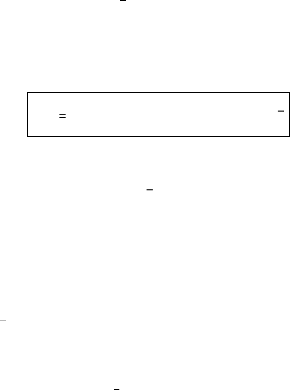
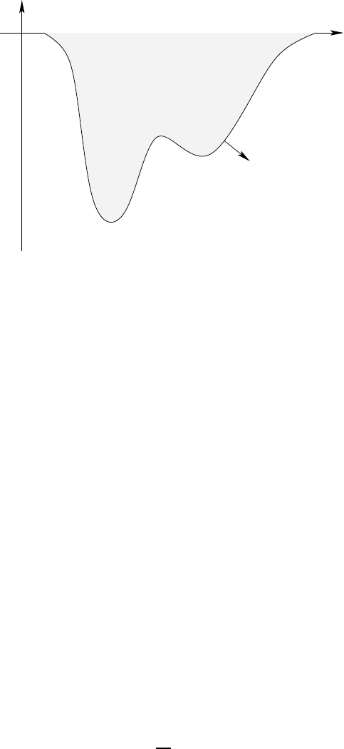
Figure 3.1 Schematic of the ocean’s bottom surface with a smoothed undulating solid earth
topography at z=−H(x,y)and outward normal direction ˆnH. Undulations of
the solid earth can reach from the ocean bottom at 5000m-6000m to the surface
over the course of a few kilometers (slopes on the order of 0.1 to 1.0). These
ranges of topography variation are far greater than the surface height (see Figure
3.2). It is important for simulations to employ numerics that facilitate an accurate
representation of the ocean bottom.
many situations is far more natural than the more traditional geopotential coordi-
nates (x,y,z)that we have been using thus far. Therefore, it is important for the
student to gain some exposure to the fundamentals of these coordinates, as they
are ubiquitous in ocean modelling today.
Chapter 6 of Griffies (2004) develops a calculus for generalized vertical coor-
dinates. Experience with these methods is useful to nurture an understanding
for ocean modelling in generalized vertical coordinates. Most notably, these co-
ordinates, when used with the familiar horizontal coordinates (x,y), form a non-
orthogonal triad, and thus lead to some relationships that may be unfamiliar. To
proceed in this section, we present some salient results of the mathematics of
generalized vertical coordinates, and reserve many of the derivations for Griffies
(2004).
When considering generalized vertical coordinates in oceanography, we always
assume that the surfaces cannot overturn on themselves. This constraint means
that the Jacobian of transformation between the generalized vertical coordinate
s=s(x,y,z,t)(3.36)
and the geopotential coordinate z, must be one signed. That is, the specific thick-
ness ∂z
∂s=z,s(3.37)
is of the same sign throughout the ocean fluid. The name specific thickness arises
from the property that
dz=z,sds(3.38)
THE FUNDAMENTAL EQUATIONS 29
is an expression for the thickness of an infinitesimal layer of fluid bounded by two
constant ssurfaces.
Deriving the bottom kinematic boundary condition in s-coordinates requires a
relation between the vertical velocity component used in geopotential coordinates,
w=dz/dt, and the pseudo-velocity component ds/dt. For this purpose, we refer
to some results from Section 6.5.5 of Griffies (2004). As in that discussion, we
derive the isomorphic relations
˙
z= (∂t+u· ∇s+˙
s∂s)z(3.39)
˙
s= (∂t+u· ∇z+˙
z∂z)s, (3.40)
where
˙
z=dz
dt(3.41)
˙
s=ds
dt(3.42)
are useful shorthands for the vertical velocity components, motivated from similar
notation used in classical particle mechanics. Note that the partial time derivative
appearing in each of the expressions is taken with the corresponding space vari-
ables held fixed. That is, ∂tin equation (3.39) is taken with sheld fixed, whereas
∂tin equation (3.40) is taken with zheld fixed.
Rearrangement of equations (3.39) and (3.40) leads to
˙
z=z,s(d/dt−∂t−u·∇z)s. (3.43)
This expression is relevant when measurements are taken on surfaces of constant
geopotential, or depth. To reach this result, we made use of the triple product
identities
z,t=−s,tz,s(3.44)
z,x=−s,xz,s(3.45)
z,y=−s,yz,s. (3.46)
A derivation of these identities is given in Section 6.5.4 of Griffies (2004). These
relations should be familiar to those having studied thermodynamics, where the
analogous expressions are known as the Maxwell relations (Callen, 1985).
We now apply relation (3.43) to the ocean bottom, which is generally not a sur-
face of constant depth. It is thus necessary to transform the constant depth gra-
dient ∇zto a horizontal gradient taken along the bottom. To do so, proceed as
in Section 6.5.3 of Griffies (2004) and consider the time-independent coordinate
transformation
(x,y,z,t) = (x,y,−H(x,y),t). (3.47)
The horizontal gradient taken on constant depth surfaces, ∇z, and the horizontal
gradient along the bottom, ∇z, are thus related by
∇z=∇z−(∇H)∂z. (3.48)
Using this result in equation (3.43) yields
s,z(w+u· ∇H) = (d/dt−∂t−u·∇z)sat z=−H. (3.49)

30 CHAPTER 3
The left hand side vanishes due to the kinematic boundary condition (3.34), which
then leads to
ds/dt= (∂t+u· ∇z)sat s=s(x,y,z=−H(x,y),t). (3.50)
The value of the generalized coordinate at the ocean bottom can be written in the
shorthand form
sbot(x,y,t) = s(x,y,z=−H,t)(3.51)
which leads to
d(s−sbot)
dt=0at s=sbot.(3.52)
This relation is analogous to equation (3.35) appropriate to z-coordinates. Indeed,
it is actually a basic statement of the impenetrable nature of the solid earth lower
boundary, which is true regardless the vertical coordinates.
The various mathematical steps that led to the very simple result (3.52) could
have been dispensed with if we already understood some notions of generalized
vertical coordinates. Nonetheless, the steps introduced some of the formalism re-
quired to work with generalized vertical coordinates, and as such provide a useful
testing ground for later manipulations where the answer is less easy to anticipate.
This strategy is highly recommended to the student working with new formalisms.
That is, first test your mathematical skills with problems where the answer is either
known, or can be readily judged correct with basic physical understanding. Af-
ter garnering experience and confidence, one may then approach genuinely new
problems using the methods.
3.1.7 Upper surface kinematic condition
To formulate budgets for mass, tracer, and momentum in the ocean, we consider
the upper ocean surface to be a time dependent permeable membrane through
which precipitation, evaporation, ice melt, and river runoff∗pass. The expression
for fluid transport at the upper surface leads to the upper ocean kinematic bound-
ary condition.
To describe the kinematics of water transport into the ocean, it is useful to intro-
duce an effective transport through a smoothed ocean surface, where smoothing
is performed via an ensemble average. We assume that this averaging leads to a
surface absent overturns or breaking waves, thus facilitating a mathematical de-
scription analogous to the ocean bottom just considered. The vertical coordinate
takes on the value
z=
η
(x,y,t)(3.53)
at this idealized ocean surface.
∗River runoff generally enters the ocean at a nonzero depth rather than through the surface. Many
global models, however, have traditionally inserted river runoff to the top model cell. Such can become
problematic numerically and physically when the top grid cells are refined to levels common in coastal
modelling. Hence, more applications are now considering the input of runoff throughout a nonzero
depth. Likewise, sea ice can melt at depth, thus necessitating a mass transport to occur within the
ocean between the liquid and solid water masses.
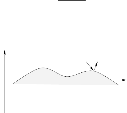
THE FUNDAMENTAL EQUATIONS 31
We furthermore assume that density of the water crossing the ocean surface
ρ
wis a function of the temperature, salinity, and pressure. There are generally
different water densities for precipitation, evaporation, runoff, and ice melt. Such
level of detail is generally not considered, and we make approximations below. For
now, we note that the mass transport crossing the ocean surface can be written
(MASS/TIME)THROUGH SURFACE =
−dA
η
ˆn
η
·(ˆnPP
ρ
P+ˆnEE
ρ
E+ˆnRR
ρ
R+ˆnII
ρ
I).(3.54)
In this expression, ˆnPP
ρ
Pis the mass per time per area of precipitation oriented
in the direction specified by ˆnP, where
ρ
Pis the mass density of the precipitation
and Pis the volume per time per area of precipitation. Likewise, ˆnEE
ρ
Eis the
evaporative mass flux, ˆnRR
ρ
Ris the river mass flux, and ˆnII
ρ
Iis the ice melt
mass flux. The unit normal
ˆn
η
=∇(z−
η
)
|∇(z−
η
)|(3.55)
points from the ocean surface at z=
η
into the overlying atmosphere (see Figure
3.2). Finally, the area element dA
η
measures an infinitesimal area element on the
ocean surface z=
η
, and it is given by (see Section 20.13.2 of Griffies (2004))
dA
η
=|∇(z−
η
)|dxdy. (3.56)
^
x,y
z
nη
^
nw
z=η
Figure 3.2 Schematic of the ocean’s upper surface with a smoothed undulating surface at
z=
η
(x,y,t), outward normal direction ˆn
η
, and normal direction ˆnworienting
the passage of water across the surface. Undulations of the surface height are
on the order of a few metres due to tidal fluctuations in the open ocean, and or-
der 10m-20m in certain embayments (e.g., Bay of Fundy in Nova Scotia). When
imposing the weight of sea ice onto the ocean surface, the surface height can de-
press even further, on the order of 5m-10m, with larger values possible in some
cases. It is important for simulations to employ numerical schemes facilitating
such wide surface height undulations.
We now make a common assumption about the orientation of the water trans-
ported across the surface. Namely, precipitation generally enters the ocean, so
that we write
Pˆn
η
·ˆnP≈ −P(3.57)
since ˆn
η
·ˆnP≈ −1. We make similar approximations for the other mass flux
components, with the conventions that P>0is the volume per time per area

32 CHAPTER 3
of precipitation entering the ocean, E>0is the evaporation leaving the ocean,
R>0is the river runoff entering the ocean, and I>0is the ice melt entering the
ocean (signs are reversed on each of these fluxes for cases where water fluxes
are in opposite directions). Additionally, for notational convenience, we assume
the density of the water transported across the surface is generically written
ρ
w.
Hence, the mass flux takes the more compact form
(MASS/TIME)THROUGH SURFACE = (P−E+R+I)
ρ
wdA
η
. (3.58)
We next exploit the assumption that the ocean surface has no overturns. In this
case, we can define
qwdA= (P−E+R+I)dA
η
, (3.59)
where
dA=dxdy(3.60)
is the horizontal projection of the surface area element dA
η
. The volume per time
per horizontal area of fluid crossing the ocean surface is therefore defined by
qw=(P−E+R+I)dA
η
dA
=(VOLUME/TIME)THROUGH FREE SURFACE
HORIZONTAL AREA UNDER FREE SURFACE .
(3.61)
This is the surface water flux that appears in ocean model budgets for mass, tracer,
and momentum. The assumptions leading up to this simple expression can be
readily dropped in cases where more information is available (e.g., separate den-
sities for the precipitation, evaporation, runoff, ice melt). Indeed, in realistic climate
models, these densities may be available. However, for purposes of mathemati-
cal formulation, it is more convenient to employ the terse expression derived here.
Note that in Section 3.4.7, we derive an alternative expression (3.152) for qwwhich
connects it to the dia-surface velocity component discussed in Section 3.1.8.
To develop the surface kinematic boundary condition, return to the expression
(3.19) for mass conservation, rewritten here for completeness
∂t
η
Z
−H
dz
ρ
+∇·
η
Z
−H
dz
ρ
u
=qw
ρ
w+
η
Z
−H
dz
ρ
S(M). (3.62)
Next, we perform the derivative operations on the integrals, keeping in mind Leib-
nitz’s Rule when differentiating an integral. The first step of the derivation leads
to
[
ρ
(∂t+u·∇)
η
]z=
η
+ [
ρ
∇H·u]z=−H+
η
Z
−H
dz[
ρ
,t+∇· (
ρ
u)] =
ρ
wqw+
η
Z
−H
dz
ρ
S(M).
(3.63)
The Eulerian mass conservation relation (3.8) and bottom kinematic boundary
condition (3.34) render the surface kinematic boundary condition
ρ
(∂t+u·∇)
η
=
ρ
wqw+
ρ
wat z=
η
.(3.64)
THE FUNDAMENTAL EQUATIONS 33
This relation can also be written in the material form
ρ
d(z−
η
)
dt=−
ρ
wqwat z=
η
. (3.65)
Contrary to the solid earth condition (3.35), where z+His materially constant,
permeability of the ocean surface leads to a nontrivial material evolution of z−
η
.
To derive the analogous s-coordinate boundary condition, we proceed as for the
bottom in Section 3.1.6. Here, the coordinate transformation is time dependent
(x,y,z,t) = (x,y,
η
(x,y,t),t). (3.66)
The horizontal gradient and time derivative operators are therefore related by
∇z=∇z+ (∇
η
)∂z(3.67)
∂t=∂t+
η
,t∂z. (3.68)
Hence, the relation (3.43) between vertical velocity components takes the following
form at the ocean surface
w=z,s(d/dt−∂t−u·∇z)s+ (∂t+u·∇)
η
at z=
η
.(3.69)
Substitution of the z-coordinate kinematic boundary condition (3.64) leads to
ρ
z,s(d/dt−∂t−u·∇z)s=−
ρ
wqwat s=stop (3.70)
where stop =s(x,y,z=
η
,t)is the value of the generalized vertical coordinate
at the ocean surface. Reorganizing the result (3.70) leads to the material time
derivative form
ρ
z,sd(s−stop)
dt=−
ρ
wqwat s=stop (3.71)
which is analogous to the z-coordinate result (3.65). Indeed, it can be derived
trivially by noting that dz/dt=z,sds/dt. Even so, just as for the bottom kine-
matic boundary condition considered in Section 3.1.6, it is useful to have gone
through these manipulations to garner experience and confidence with the for-
malism. Such confidence is of particular use in the next section focusing on the
dia-surface flux.
3.1.8 Dia-surface transport
A surface of constant generalized vertical coordinate, s, is of importance when
establishing the balances of mass, tracer, and momentum within a layer of fluid
whose upper and lower bounds are determined by surfaces of constant s. Fluid
transport through this surface is said to constitute the dia-surface transport. This
transport plays a fundamental role in generalized vertical coordinate modelling.
At an arbitrary point on a surface of constant generalized vertical coordinate
(see Figure 3.3), the flux of fluid in the direction normal to the surface is given by
SEAWATER FLUX IN DIRECTION ˆn=v·ˆn, (3.72)
with
ˆn=∇s|∇s|−1(3.73)
34 CHAPTER 3
the surface unit normal direction. Introducing the material time derivative ds/dt=
s,t+v·∇sleads to the equivalent expression
v·ˆn=|∇s|−1(d/dt−∂t)s. (3.74)
That is, the normal component to a fluid parcel’s velocity is proportional to the
difference between the material time derivative of the surface and its partial time
derivative.
Since the surface is generally moving, the net flux of seawater penetrating the
surface is obtained by subtracting the velocity of the surface v(ref)in the ˆndirection
from the velocity component v·ˆnof the fluid parcels
FLUX OF SEAWATER THROUGH SURFACE =ˆn·(v−v(ref)). (3.75)
The velocity v(ref)is the velocity of a reference point fixed on the surface, and it is
written
v(ref)=u(ref)+w(ref)ˆz. (3.76)
Since the reference point remains on the same s=const surface, ds/dt=0for
the reference point. Consequently, we can write the vertical velocity component
w(ref)as
w(ref)=−z,s(∂t+u(ref)· ∇z)s, (3.77)
where equation (3.43) was used with ds/dt=0. This result then leads to
ˆn·v(ref)=ˆn·u(ref)+ˆn·ˆzw(ref)
=−s,t|∇s|−1,(3.78)
which says that the normal component of the surface’s velocity vanishes when the
surface is static, as may be expected. When interpreting the dia-surface velocity
component below, we find it useful to note that relation (3.78) leads to
z,s∇s·v(ref)=z,t. (3.79)
To reach this result, we used the identity s,tz,s=−z,t, with z,tthe time tendency
for the depth of a particular constant ssurface.
Expression (3.78) then leads to the following expression for the net flux of sea-
water crossing the surface
ˆn·(v−v(ref)) = |∇s|−1(∂t+v· ∇)s
=|∇s|−1ds/dt.(3.80)
Hence, the material time derivative of the generalized surface vanishes if and only
if no water parcels cross it. This important result is used throughout ocean theory
and modelling. It measures the volume of seawater crossing a generalized surface,
per time, per area. The area normalizing the volume flux is that area dA(ˆn)of an
infinitesimal patch on the surface of constant generalized vertical coordinate with
outward unit normal ˆn. This area can be written (see equation (6.58) of Griffies
(2004))
dA(ˆn)=|z,s∇s|dA, (3.81)
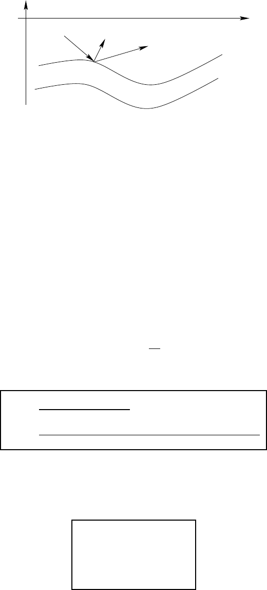
THE FUNDAMENTAL EQUATIONS 35
z
n
^
s=constant
vvref
x,y
Figure 3.3 Surfaces of constant generalized vertical coordinate living interior to the ocean.
An upward normal direction ˆnis indicated on one of the surfaces. Also shown is
the orientation of a fluid parcel’s velocity vand the velocity v(ref)of a reference
point living on the surface.
where
dA=dxdy(3.82)
is the horizontal projection of the area element. Hence, the volume per time of fluid
passing through the generalized surface is
(VOLUME/TIME)THROUGH SURFACE =ˆn·(v−v(ref))dA(ˆn)
=|z,s|(ds/dt)dxdy,(3.83)
and the magnitude of this flux is
|ˆn·(v−v(ref))dA(ˆn)| ≡ |w(s)|dxdy. (3.84)
We introduced the expression
w(s)=z,sds
dt, (3.85)
which measures the volume of fluid passing through the surface, per unit area
dA=dxdyof the horizontal projection of the surface, per unit time. That is,
w(s)≡ˆn·(v−v(ref))dA(ˆn)
dA
=(VOLUME/TIME)OF FLUID THROUGH SURFACE
AREA OF HORIZONTAL PROJECTION OF SURFACE .
(3.86)
The quantity w(s)is called the dia-surface velocity component. It is directly anal-
ogous to the fresh water flux qwdefined in equation (3.59), which measures the
volume of freshwater crossing the ocean surface, per unit time per horizontal area.
To gain some experience with the dia-surface velocity component, it is useful to
write it in the equivalent forms
w(s)=z,sds/dt
=z,s∇s·(v−v(ref))
= (ˆz−∇sz)·v−z,t
=w−(∂t+u·∇s)z
(3.87)

36 CHAPTER 3
where the penultimate step used the identity (3.79), and where
S=∇sz
=−z,s∇zs(3.88)
is the slope of the ssurface as projected onto the horizontal directions. For ex-
ample, if the slope vanishes, then the dia-surface velocity component measures
the flux of fluid moving vertically relative to the motion of the generalized surface.
When the surface is static and flat, then the dia-surface velocity component is
simply the vertical velocity component w=dz/dt.
The expression (3.85) for w(s)brings the material time derivative (3.4) into the
following equivalent forms
d
dt=∂
∂tz
+u·∇z+w∂
∂z(3.89)
=∂
∂ts
+u·∇s+ds
dt∂
∂s(3.90)
=∂
∂ts
+u·∇s+w(s)∂
∂z, (3.91)
where
∂s=z,s∂z, (3.92)
relates the vertical coordinate partial derivatives. The form given by equation
(3.91) motivates some to refer to w(s)as a vertical velocity component that mea-
sures the rate at which fluid parcels penetrate the surface of constant generalized
coordinate (see Appendix A to McDougall (1995)). One should be mindful, how-
ever, to distinguish w(s)from the generally different vertical velocity component
w=dz/dt, which measures the water flux crossing constant geopotential sur-
faces.
We close with a few points of clarification for the case where no fluid parcels
cross the generalized surface. Such occurs, in particular, in the case of adiabatic
flows with s=
ρ
an isopycnal coordinate. In this case, the material time derivative
(3.91) only has a horizontal two-dimensional advective component u· ∇s. This
result should not be interpreted to mean that the velocity of a fluid parcel is strictly
horizontal. Indeed, it generally is not, as the form (3.89) should make clear. Rather,
it means that the transport of fluid properties occurs along surfaces of constant s,
and such transport is measured by the convergence of horizontal advective fluxes
as measured along surfaces of constant s. We revisit this point in Section 3.4.2
when discussing tracer transport (see in particular Figure 3.5).
3.2 MATERIAL TIME CHANGES OVER FINITE REGIONS
In the following sections, we focus on the mass, tracer, and momentum budgets
formulated over a finite domain. The domain, or control volume, of interest is that
of an ocean model grid cell. The budget for a grid cell is distinct from budgets for
infinitesimal mass conserving Lagrangian fluid parcels moving with the fluid. Mass
conserving fluid parcels form the fundamental system for which the budgets of

THE FUNDAMENTAL EQUATIONS 37
mass, tracer, momentum, and energy are generally formulated from first principles
(see, for example, chapters 3-5 in Griffies, 2004). Grid cell budgets are then
derived from the fundamental parcel budgets.
The grid cells of concern for mom4p1 have vertical sides fixed in space-time,
but with the top and bottom generally moving. In particular, the top and bottom
either represent the ocean top, ocean bottom, or a surface of constant generalized
vertical coordinate. We furthermore assume that at no place in the fluid do the
top or bottom surfaces of the grid cell become vertical. This assumption allows for
a one-to-one relation to exist between geopotential depth zand the generalized
vertical coordinate sintroduced in Section 3.1.6 (i.e., the relation is invertible).
To establish the grid cell budget, we integrate the budget for mass conserving
fluid parcels over the volume of the cell. This section is focused on the mathemat-
ics required for integrating the density weighted material time derivative acting on
an arbitrary field
ψ
ρ
d
ψ
dt= (
ρ ψ
),t+∇· (
ρ
v
ψ
). (3.93)
We start with the partial time derivative on the right hand side, and introduce Carte-
sian coordinates (x,y,z)for the purpose of performing the grid cell integral
ZZZ dV(
ρ ψ
),t=ZZZ dxdydz(
ρ ψ
),t
=ZZ dxdy
z2
Z
z1
dz(
ρ ψ
),t
=ZZ dxdy
−(
ρ ψ
)2∂tz2+ (
ρ ψ
)1∂tz1+∂t
z2
Z
z1
dz(
ρ ψ
)
.
(3.94)
The second equality follows by noting that the horizontal extent of a grid cell re-
mains static, thus allowing for the horizontal integral to be brought outside of the
time derivative. In contrast, the vertical extent has a time dependence, which ne-
cessitates the use of Leibniz’s Rule. We now use equation (3.44)
z,t=−s,tz,s(3.95)
which relates time tendencies of the depth of a generalized surface to time ten-
dencies of the surface itself. Equation (3.78) is next used to write
z,t=−s,tz,s
=z,s|∇s|ˆn·v(ref),(3.96)
in which we introduced the reference velocity v(ref)for a point sitting on the gen-
eralized surface. Finally, recall equation (3.81), which relates the area element on
the surface to the horizontal projection dA=dxdyof the surface
dA(ˆn)=|z,s∇s|dA. (3.97)
Introducing this area then renders
z,tdA=ˆn·v(ref)dA(ˆn)(3.98)
38 CHAPTER 3
This equation relates the time tendency of the depth of the generalized surface
to the normal component of the velocity at a point on the surface. The two are
related through the ratio of the area elements. This result is now used for the top
and bottom boundary terms in relation (3.94), yielding
ZZZ dV(
ρ ψ
),t=∂tZZZ
ρ
dV
ψ
−ZZ dA(ˆn)ˆn·v(ref)(
ρ ψ
). (3.99)
Hence, the domain integrated Eulerian time tendency of the density weighted field
equals the time tendency of the density weighted field integrated over the domain,
minus a boundary integral over the domain arising from the general time depen-
dence of the domain.
The next step needed for volume integrating the density weighted material time
derivative in equation (3.93) involves the divergence of the density weighted field
ZZZ dV∇ · (
ρ
v
ψ
) = ZZ dA(ˆn)ˆn·v(
ρ ψ
), (3.100)
which follows from Gauss’ Law. Combining this result with equation (3.99) leads
to the relation
ZZZ
ρ
dVd
ψ
dt=∂tZZZ
ρ
dV
ψ
+ZZ dA(ˆn)ˆn·(v− ·v(ref)) (
ρ ψ
). (3.101)
Hence, the mass weighted grid cell integral of the material time derivative of a
field is given by the time derivative of the mass weighted field integrated over the
domain, plus a boundary term that accounts for the transport across the domain
boundaries, with allowance made for moving domain boundaries. The manipula-
tions leading to this result focused on an interior grid cell. The result, however,
holds in general for a cell that abuts either the ocean surface or ocean bottom.
For the ocean bottom, the boundary term vanishes since the bottom has a zero
reference velocity, and there is no normal flow of fluid across the bottom. For the
ocean surface, we employ relation (3.152) which defines the dia-surface trans-
port of mass across the ocean surface in a manner analogous to the dia-surface
transport (3.86) across an interior surface.
3.3 BASICS OF THE FINITE VOLUME METHOD
The finite volume method of formulating the discrete equations of an ocean model
is relatively new, having been incorporated to the ocean modelling literature only
since the late 1990’s. The work of Adcroft et al. (1997) is a canonical example
of how this method can be used to garner a better representation of the solid
earth boundary. In this section, we briefly outline the basis for this method. The
interested reader may wish to look at chapter 6 of the book by Hirsch (1988) for a
more thorough introduction, or one of the growing number of monographs devoted
exclusively to the method.
The general equations of fluid mechanics can be represented as conservation
equations for scalar quantities (e.g., seawater mass and tracer mass) and vector
quantities (e.g., linear momentum). As just detailed in Section 3.2, the conserva-
tion law for a scalar Ψover an arbitrary fluid region can be put in the form
∂tZZZ ΨdV=−ZZ dA(ˆn)ˆn·F+ZZZ SdV. (3.102)
THE FUNDAMENTAL EQUATIONS 39
The volume integral is taken over an arbitrary fluid region, and the area integral
is taken over the bounding surface to that volume, with outward normal ˆn. The
flux Fpenetrates the surface and acts to alter the scalar, whereas internal sources
Scontribute to changes in the scalar throughout the interior of the domain. The
budget for the vector linear momentum can be written in this form, with the addition
of body forces that act similar to the source term written here (see Section 3.6).
Fundamental to the finite volume method is that the fluxes contribute only at the
boundary to the domain, and not within the interior as well. Hence, the domain can
be subdivided into arbitrary shapes, with budgets over the subdivisions summing
to recover the global budget.
A discrete finite volume analog to equation (3.102), for a region labeled with the
integer J, takes the form
∂t(VJΨJ) = −∑
sides
(A(ˆn)ˆn·F) + VJSJ. (3.103)
Quantities with the integer Jsubscript refer to the discrete analogs to the contin-
uum fields and the geometric factors in equation (3.102). In particular, we define
the discrete finite volume quantities
VJ≡ZZZ dV(3.104)
ΨJ≡RRR dVΨ
RRR dV(3.105)
SJ≡RRR dVS
RRR dV. (3.106)
Again, it is due to the conservation form of the fundamental fluid dynamic equation
(3.102) that allows for a straightforward finite volume interpretation of the discrete
equations. Notably, once formulated as such, the problem shits from fundamentals
to details, with details differing on how one represents the subgrid scale behaviour
of the continuum fields. This then leads to the multitude of discretization methods
available for such processes as transport, time stepping, etc. In the following,
we endeavour to write the fluid equations of the ocean in the conservation form
(3.102). Doing so then renders a finite volume framework for the resulting discrete
or semi-discrete equations.
When working with nonBoussinesq budgets, the finite volume interpretation ap-
plies directly to the tracer mass per volume,
ρ
C, rather than to the tracer concen-
tration C. The same applies to the linear momentum per volume,
ρ
v, rather than to
the velocity v. That is, the finite volume model carries the discrete fields
ρ
J,(
ρ
C)J
and (
ρ
v)J, defined as
ρ
J≡RRR dV
ρ
RRR dV(3.107)
(
ρ
C)J≡RRR dV
ρ
C
RRR dV(3.108)
(
ρ
v)J≡RRR dV
ρ
v
RRR dV. (3.109)
As we will see in the discussions in Sections 3.4 and 3.6, we actually work with
a slightly modified finite volumve suite of variables, whereby the finite volume in-
terpretation applies to the seawater mass per horizontal area, the tracer mass per
40 CHAPTER 3
horizontal area and linear momentum per horizontal area
(dz
ρ
)J≡RR dARdz
ρ
RR dA(3.110)
(dz
ρ
C)J≡RR dARdz
ρ
C
RR dA(3.111)
(dz
ρ
v)J≡RR dARdz
ρ
v
RR dA, (3.112)
where dzis the thickness of a grid cell, and dA=dxdyis the horizontal projection
of its area. The inclusion of thickness facilitates the treatment of grid cells whose
thickness is a function of time, such as in mom4p1. Note that to reduce notational
clutter, we employ the same symbol for the continuum field as for the discrete, so
we drop the Jsubscript in the following.
3.4 MASS AND TRACER BUDGETS OVER FINITE REGIONS
The purpose of this section is to extend the kinematics discussed in the previous
sections to the case of mass and tracer budgets for finite domains within the ocean
fluid. In the formulation of ocean models, these domains are thought of as discrete
model grid cells.
3.4.1 General formulation
The tracer concentration Crepresents a mass of tracer per mass of seawater
for material tracers such as salt or biogeochemical tracers. Mathematically, this
definition means that for each fluid parcel,
C=mass of tracer
mass of seawater
=
ρ
CdV
ρ
dV,
(3.113)
where
ρ
Cis the mass density of tracer within the fluid parcel. In addition to ma-
terial tracers, we are concerned with a thermodynamical tracer that measures the
heat within a fluid parcel. In this case, Cis typically taken to be the potential
temperature. However, the work of McDougall (2003) prompts us to consider a
modified temperature known as conservative temperature, which more accurately
measures the heat within a fluid parcel and is transported, to within a very good
approximation, in a manner directly analogous to material tracers.
Given these considerations, the total tracer mass within a finite region of seawa-
ter is given by the integral.
tracer mass in a region =ZZZ
ρ
CdV
=ZZZ C
ρ
dV.
(3.114)
Correspondingly, the evolution of tracer mass within a Lagrangian parcel of mass
conserving fluid is given by (see Section 5.1 of Griffies, 2004)
ρ
dC
dt=−∇ · J+
ρ
S(C), (3.115)
THE FUNDAMENTAL EQUATIONS 41
where S(C)is a tracer source in the region, with units of tracer concentration per
time. The tracer flux Jarises from subgrid scale transport of tracer in the absence
of mass transport. Such transport in mom4p1 consists of diffusion and/or unre-
solved advection. As this flux is not associated with mass transport, it vanishes
when the tracer concentration is uniform, in which case the tracer budget reduces
to the mass budget (3.5).
Now develop a regional budget for tracer mass over a grid cell. For this pur-
pose, we apply the general result (3.101) relating the material time derivative to a
regional budget, to render
∂tZZZ C
ρ
dV=ZZZ S(C)
ρ
dV−ZZ dA(ˆn)ˆn·[(v−vref)
ρ
C+J]. (3.116)
Again, the left hand side of this equation is the time tendency for tracer mass within
the finite sized grid cell region. When the tracer concentration is uniform, the SGS
flux vanishes, in which case the tracer budget (3.116) reduces to the finite domain
mass budget
∂tZZZ
ρ
dV=ZZZ S(M)
ρ
dV−ZZ dA(ˆn)ˆn·[(v−vref)
ρ
]. (3.117)
In addition to the tracer flux J, it is convenient to define the tracer concentration
flux Fvia
J=
ρ
F, (3.118)
where the dimensions of Fare velocity ×tracer concentration.
In a manner analogous to our definition of a dia-surface velocity component in
Section 3.1.8, it is useful to introduce the dia-surface SGS flux component. For
this purpose, consider the tracer mass per time crossing a surface of constant
generalized vertical coordinate, where this transport arises from SGS processes.
Manipulations similar to those used to derive the dia-surface velocity component
lead to
(SGS tracer mass through surface)/(time) = dA(ˆn)ˆn·J
=z,s∇s·Jdxdy
= (ˆz−S)·Jdxdy,
(3.119)
where Sis the slope vector for the generalized surface defined in equation (3.88).
We are therefore led to introduce the dia-surface SGS tracer flux
J(s)≡dA(ˆn)ˆn·J
dA
=z,s∇s·J
= (ˆz−S)·J,
(3.120)
where dA=dxdyis the horizontal cross-sectional area. In words, J(s)is the
tracer mass per time per horizontal area penetrating surfaces of constant gen-
eralized vertical coordinate via processes that are unresolved by the dia-surface
velocity component w(s).
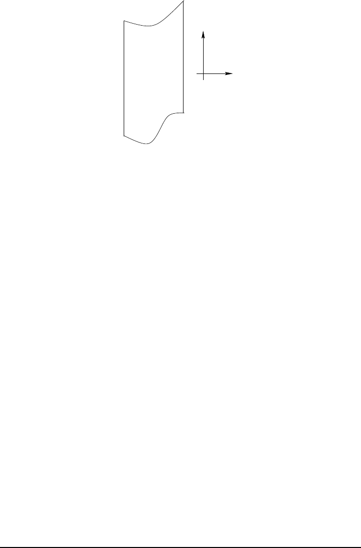
42 CHAPTER 3
Grid cell k x,y
z
s=s
s=s
k−1
k
Figure 3.4 Schematic of an ocean grid cell labeled by the vertical integer k. Its sides are
vertical and oriented according to ˆxand ˆy, and its horizontal position is fixed
in time. The top and bottom surfaces are determined by constant generalized
vertical coordinates sk−1and sk, respectively. Furthermore, the top and bottom
are assumed to always have an outward normal with a nonzero component in
the vertical direction ˆz. That is, the top and bottom are never vertical. We take
the convention that the discrete vertical label kincreases as moving downward
in the column, and grid cell kis bounded at its upper face by s=sk−1and lower
face by s=sk.
3.4.2 Budget for an interior grid cell
Consider the budget for a region bounded away from the ocean surface and bot-
tom, such as that shown in Figure 3.4. We have in mind here a grid cell within a
discrete numerical model. There are two assumptions which define a grid cell for
our purposes.
•The sides of the cell are vertical, so they are parallel to ˆzand aligned with the
horizontal coordinate directions (ˆx, ˆy). Their horizontal positions are fixed in
time.
•The top and bottom of the cell are defined by surfaces of constant gener-
alized vertical coordinate s=s(x,y,z,t). The generalized surfaces do not
overturn, which means that s,zis single signed throughout the ocean.
These assumptions lead to the following results for the sides of the grid cell
TRACER M A S S E N T E R I N G C E L L W E S T FA C E =ZZ
x=x1
dydz(u
ρ
C+
ρ
Fx)(3.121)
TRACER M A S S LEAVI N G C E L L E A S T FA C E =−ZZ
x=x2
dydz(u
ρ
C+
ρ
Fx)(3.122)
where x1≤x≤x2defines the domain boundaries for the east-west coordinates.∗
Similar results hold for the tracer mass crossing the cell in the north-south direc-
∗We use generalized horizontal coordinates, such as those discussed in Griffies (2004). Hence,
the directions east, west, north, and south may not correspond to the usual geographic directions.
Nonetheless, this terminology is useful for establishing the budgets, whose validity is general.
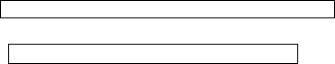
THE FUNDAMENTAL EQUATIONS 43
tions. At the top and bottom of the grid cell
TRACER M A S S ENTERING C E L L BOTTOM FACE =ZZ
s=sk
dxdy
ρ
(w(s)C+F(s))(3.123)
TRACER MASS L E AVING CELL TOP FA C E =−ZZ
s=sk−1
dxdy
ρ
(w(s)C+F(s)). (3.124)
To reach this result, we used a result from Section 3.1.8 to write the volume flux
passing through the top face of the grid cell
dA(ˆn)ˆn·(v−vref) = w(s)dxdy, (3.125)
with w(s)=z,sds/dtthe dia-surface velocity component. A similar relation holds
for the bottom face of the cell. The form of the SGS flux passing across the top
and bottom is correspondingly given by
dA(ˆn)ˆn·J=J(s)dxdy, (3.126)
which follows from the general expression (3.120) for the dia-surface tracer flux.
In a model using the generalized coordinate sfor the vertical, it is sometimes
convenient to do the vertical integrals over sinstead of z. For this purpose, recall
that with z,ssingle signed, the vertical thickness of a grid cell is given by equation
(3.38), repeated here for completeness
dz=z,sds. (3.127)
Bringing these results together, and taking the limit as the volume of the cell in
(x,y,s)space goes to zero (i.e., dxdyds→0) leads to
∂t(z,s
ρ
C) = z,s
ρ
S(C)−∇s·[z,s
ρ
(uC+F)] −∂s[
ρ
(w(s)C+F(s))] (3.128)
Notably, the horizontal gradient operator ∇sis computed on surfaces of constant
s, and so it is distinct generally from the horizontal gradient ∇ztaken on surfaces
of constant z.
As indicated at the end of Section 3.3, we prefer to work with thickness weighted
quantities, given the general time dependence of a model grid cell in mom4p1.
Hence, as an alternative to taking the limit as dxdyds→0, consider instead the
limit as the time independent horizontal area dxdygoes to zero, thus maintaining
the time dependent thickness dz=z,sdsinside the derivative operators. In this
case, the thickness weighted tracer mass budget takes the form
∂t(dz
ρ
C) = dz
ρ
S(C)− ∇s·[dz
ρ
(uC+F)] −[
ρ
(w(s)C+F(s))]s=sk−1+ [
ρ
(w(s)C+F(s))]s=sk.
(3.129)
Similarly, the thickness weighted mass budget is
∂t(dz
ρ
) = dz
ρ
S(M)−∇s·(dz
ρ
u)−(
ρ
w(s))s=sk−1+ (
ρ
w(s))s=sk. (3.130)
In these relations, S(M)is a mass source with units of inverse time that, for self-
consistency, must be related to the tracer source via
S(M)=S(C)(C=1). (3.131)
Additionally, the SGS tracer flux vanishes with a uniform tracer
F(C=1) = 0. (3.132)

44 CHAPTER 3
Note that by setting the tracer concentration in equation (3.129) to a uniform con-
stant, SGS transort fluxes vanish, thus revealing the mass conservation budget.
This procedure for deriving the mass budget from the tracer budget follows triv-
ially from the definition of the tracer concentration given by equation (3.113). It
represents a compatibility condition between the discrete budgets, and this condi-
tion is critical to maintain within a numerical model in order to respect tracer and
mass conservation in the simulation. We have more to say about the compatibility
condition in Section 3.4.8.
One reason that the thickness weighted budget given by equation (3.129) is
more convenient than equation (3.128) is that equation (3.129) expresses the
budget in terms of the grid cell thickness dz, rather than the specific thickness
z,s. Nonetheless, this point is largely one of style and convenience, as there is no
fundamental reason to prefer one form over the other for purposes of developing
the discrete equations of an ocean model.
3.4.3 Fresh water budget
Seawater is comprised of freshwater with a relatively fixed ratio of various salts.
It is common to consider the budget for the concentration of these salts, which is
described by the tracer equation (3.129). As a complement, it may be of interest
to formulate a budget for freshwater. In this case, we consider the mass of fresh
water within a fluid parcel
mass of fresh water =mass of seawater −mass of salt
=
ρ
dV(1−S)
=
ρ
dV W,
(3.133)
where Sis the salinity (mass of salt per mass of seawater), and
W≡1−S(3.134)
is the mass of fresh water per mass of seawater. Results from the tracer budget
considered in Section 3.4.2 allow us to derive the following budget for fresh water
within an interior ocean model grid cell
∂t(dz
ρ
W) = dz
ρ
(S(M)−S(S))− ∇s·[dz
ρ
(uW−F)]
−[
ρ
(w(s)W−F(s))]s=sk−1+ [
ρ
(w(s)W−F(s))]s=sk.(3.135)
In these relations, the SGS tracer flux components Fand F(s)are those for salt,
and S(S)is the salt source. Equation (3.135) is very similar to the tracer equation
(3.129), with modified source term and negative signs on the SGS flux compo-
nents.
3.4.4 The ideal age tracer
Thiele and Sarmiento (1990) and England (1995) consider an ideal age tracer for
Boussinesq fluids. We consider the generalization here to nonBoussinesq fluids,
in which
ρ
dA
dt+∇· J=
ρ
S(A), (3.136)
THE FUNDAMENTAL EQUATIONS 45
where the age tracer Ahas dimensions of time and it is initialized globally to zero.
It is characterized by the dimensionless clock source S(A), which takes the values
S(A)=0if z=
η
1if z<
η
,(3.137)
In a finite difference model, the boundary condition at z=
η
is applied at the top
grid cell k=1. In mom4p1, various age tracers can be defined that differ by the
region that their boundary condition is set to zero. Given these prescriptions, A
measures the age, in units of time, that a water parcel has spent away from the
region where it was set to zero. Therefore, visual maps of Aare useful to deduce
such physically interesting properties as ventilation times.
From equation (3.129), the budget for tracer mass per area in a grid cell is given
by
∂t(dz
ρ
A) = dz
ρ
S(A)−∇s·[dz
ρ
(uA+F)]
−[
ρ
(w(s)A+F(s))]s=sk−1+ [
ρ
(w(s)A+F(s))]s=sk.(3.138)
In practice, the clock source is added to the age tracer at the very end of the time
step, so that it is implemented as an adjustment process. In this way, we remove
the ambiguity regarding the time step to evaluate the
ρ
dzfactor that multiplies the
age source.
3.4.5 Budgets without dia-surface fluxes
To garner some experience with tracer budgets, it is useful to consider the special
case of zero dia-surface transport, either via advection or SGS fluxes, and zero
tracer/mass sources. In this case, the thickness weighted mass and tracer mass
budgets take the simplified form
∂t(dz
ρ
) = − ∇s·(dz
ρ
u)(3.139)
∂t(dz
ρ
C) = − ∇s·[dz
ρ
(uC+F)]. (3.140)
The first equation says that the time tendency of the thickness weighted density
(mass per area) at a point between two surfaces of constant generalized verti-
cal coordinate is given by the horizontal convergence of mass per area onto that
point. The transport is quasi-two-dimensional in the sense that it is only a two-
dimensional convergence that determines the evolution. The tracer equation has
an analogous interpretation. We illustrate this situation in Figure 3.5. As empha-
sized in our discussion of the material time derivative (3.91), this simplification
of the transport equation does not mean that fluid parcels are strictly horizontal.
Indeed, such is distinctly not the case when the surfaces are moving.
A further simplification of the mass and tracer mass budgets ensues when con-
sidering adiabatic and Boussinesq flow in isopycnal coordinates. We consider
ρ
now to represent the constant potential density of the finitely thick fluid layer. In
this case, the mass and tracer budgets reduce to
∂t(dz) = − ∇
ρ
·(dzu)(3.141)
∂t(dz C) = − ∇
ρ
·[dz(uC+F)]. (3.142)
Equation (3.141) provides a relation for the thickness of the density layers, and
equation (3.142) is the analogous relation for the tracer within the layer. These
expressions are commonly used in the construction of adiabatic isopycnal models,
which are often used in the study of geophysical fluid mechanics of the ocean.
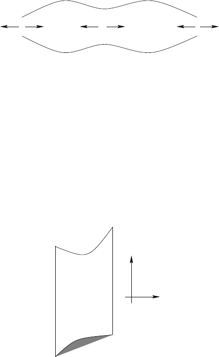
46 CHAPTER 3
k−1
diverge
converge converge
s=sk
s=s
Figure 3.5 Schematic of the horizontal convergence of mass between two surfaces of con-
stant generalized vertical coordinates. As indicated by equation (3.139), when
there is zero dia-surface transport, it is just the horizontal convergence that de-
termines the time evolution of mass between the layers. Evolution of thick-
ness weighted tracer concentration in between the layers is likewise evolved
just by the horizontal convergence of the thickness weighted advective and dif-
fusive tracer fluxes (equation (3.140)). In this way, the transport is quasi-two-
dimensional when the dia-surface transports vanish. A common example of this
special system is an adiabatic ocean where the generalized surfaces are defined
by isopycnals.
3.4.6 Cells adjacent to the ocean bottom
z=−H
x,y
z
s=skbot−1
Grid cell k=kbot
bot
s=s
Figure 3.6 Schematic of an ocean grid cell next to the ocean bottom labeled by k=kbot.
Its top face is a surface of constant generalized vertical coordinate s=skbot−1,
and the bottom face is determined by the ocean bottom topography at z=−H
where sbot(x,y,t) = s(x,y,z=−H,t).
For a grid cell adjacent to the ocean bottom (Figure 3.6), we assume that just
the bottom face of this cell abuts the solid earth boundary. The outward normal ˆnH
to the bottom is given by equation (3.32), and the area element along the bottom
is
dAH=|∇(z+H)|dxdy. (3.143)
Hence, the transport across the solid earth boundary is
−ZZ dAHˆnH·(v
ρ
C+J) = ZZ dxdy(∇H+ˆz)·(v
ρ
C+J). (3.144)
We assume that there is zero advective mass flux across the bottom, in which case
the advective flux drops out since v·(∇H+ˆz) = 0(equation (3.34)). However,
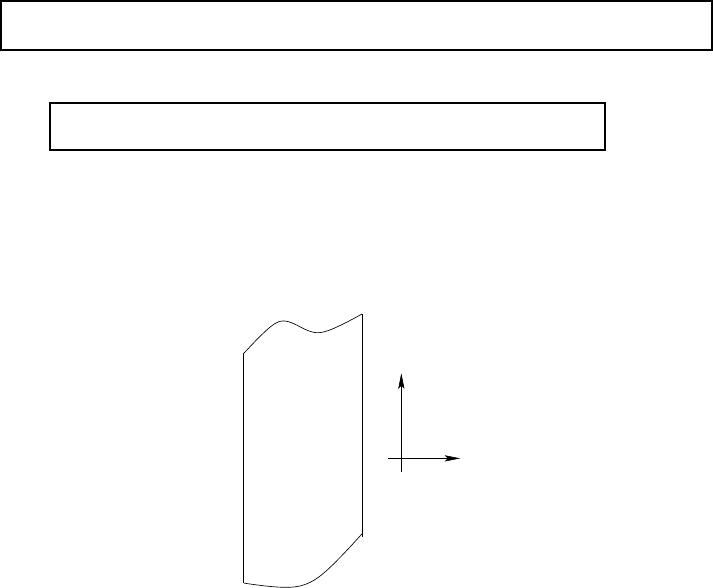
THE FUNDAMENTAL EQUATIONS 47
the possibility of a nonzero geothermal tracer transport warrants a nonzero SGS
tracer flux at the bottom, in which case the bottom tracer flux is written
Q(C)
(bot)= (∇H+ˆz)·J. (3.145)
The corresponding thickness weighted budget is given by
∂t(dz
ρ
C) = dz
ρ
S(C)− ∇s·[dz
ρ
(uC+F)] −h
ρ
(w(s)C+z,s∇s·F)is=skbot−1
+Q(C)
(bot),
(3.146)
and the corresponding mass budget is
∂t(dz
ρ
) = dz
ρ
S(M)− ∇s·(dz
ρ
u)−(
ρ
ws))s=skbot−1+Q(M)
(bot), (3.147)
where Q(M)
(bot)allows for the possibility of mass entering through geothermal bound-
ary sources. For brevity, we drop this term in the following.
3.4.7 Cells adjacent to the ocean surface
Grid cell k=1
x,y
z
z=−H
s=s
k=1
s=stop z=η
Figure 3.7 Schematic of an ocean grid cell next to the ocean surface labeled by k=1. Its
top face is at z=
η
, and the bottom is a surface of constant generalized vertical
coordinate s=sk=1.
For a grid cell adjacent to the ocean surface (Figure 3.7), we assume that just the
upper face of this cell abuts the boundary between the ocean and the atmosphere
or sea ice. The ocean surface is a time dependent boundary with z=
η
(x,y,t).
The outward normal ˆn
η
is given by equation (3.55), and its area element dA
η
is
given by equation (3.56).
As the surface can move, we must measure the advective transport with respect
to the moving surface. Just as in the dia-surface transport discussed in Section
3.1.8, we consider the velocity of a reference point on the surface
vref =uref +ˆzwref. (3.148)
Since z=
η
represents the vertical position of the reference point, the vertical
component of the velocity for this point is given by
wref = (∂t+uref · ∇)
η
(3.149)

48 CHAPTER 3
which then leads to
vref ·∇(z−
η
) =
η
,t. (3.150)
Hence, the advective transport leaving the ocean surface is
ZZ
z=
η
dA(ˆn)ˆn·(v−vref)
ρ
C=ZZ
z=
η
dxdy(−
η
,t+w−u·∇
η
)
ρ
C
=−ZZ
z=
η
dxdy
ρ
wqwC,
(3.151)
where the surface kinematic boundary condition (3.64) was used. The negative
sign on the right hand side arises from our convention that qw>0represents an
input of water to the ocean domain. We can summarize this result with the local
relation
ρ
wqw=−
ρ
dA(ˆn)ˆn·(v−vref)
dAat z=
η
,(3.152)
where again dA=dxdyis the horizontal area element. This relation exposes the
connection between the water flux qwat the ocean surface, and the more general
dia-surface velocity component defined by equation (3.86). In summary, the tracer
flux leaving the ocean free surface is given by
ZZ
z=
η
dA(ˆn)ˆn·[(v−vref)
ρ
C+J] = ZZ
z=
η
dxdy(−
ρ
wqwC+∇(z−
η
)·J). (3.153)
In equation (3.153), we formally require the tracer concentration precisely at
the ocean surface z=
η
. However, as mentioned at the start of Section 3.1.7,
it is actually a fiction that the ocean surface is a smooth mathematical function.
Furthermore, seawater properties precisely at the ocean surface, known generally
as skin properties, are generally not what an ocean model carries as its prognostic
variable in its top grid cell. Instead, the model carries a bulk property averaged over
roughly the upper few tens of centimeters.
To proceed in formulating the boundary condition for an ocean climate model, we
consider there to be a boundary layer model that provides us with the total tracer
flux passing through the ocean surface. Developing such a model is a nontrivial
problem in air-sea and ice-sea interaction theory and phenomenology. For present
purposes, we do not focus on these details, and instead just introduce this flux in
the form
Q(C)=−
ρ
wqwCw+Q(C)
(turb)(3.154)
where Cwis the tracer concentration within the incoming water qw. The first term
represents the advective transport of tracer through the surface with the fresh wa-
ter (i.e., ice melt, rivers, precipitation, evaporation). The term Q(C)
(turb)arises from
parameterized turbulence and/or radiative fluxes, such as sensible, latent, short-
wave, and longwave heating appropriate for the temperature equation. A positive
value for Q(C)
(turb)signals tracer leaving the ocean through its surface. In the special
case of zero fresh water flux, then
∇(z−
η
)·J=Q(C)
(turb)if qw=0. (3.155)
THE FUNDAMENTAL EQUATIONS 49
In general, it is not possible to make this identification. Instead, we must settle for
the general expression
ZZ
z=
η
dA(ˆn)ˆn·[(v−vref)
ρ
C+J] = ZZ
z=
η
dxdy(−
ρ
wqwCw+Q(C)
(turb)). (3.156)
The above results lead to the thickness weighted tracer budget for the ocean sur-
face grid cell
∂t(dz
ρ
C) = dz
ρ
S(C)− ∇s·[dz
ρ
(uC+F)]
+h
ρ
(w(s)C+z,s∇s·F)is=sk=1
+ (
ρ
wqwCw−Q(turb)
(C)),(3.157)
and the corresponding mass budget
∂t(dz
ρ
) = dz
ρ
S(M)−∇s·(dz
ρ
u) + (
ρ
w(s))s=sk=1+
ρ
wqw.(3.158)
3.4.8 Compatability between vertically integrated mass and tracer budgets
We spoke in Section 3.4.2 about the compatibility between the tracer and mass
budgets within a grid cell. Such compatibility follows trivially from the definition of
tracer concentration given in Section 3.4.1. We briefly revisit compatibility here, by
focusing on the vertically integrated tracer and mass budgets.
Combining the surface tracer budget (3.158), the bottom budget (3.146), and
interior budget (3.129), renders the vertically integrated tracer budget
∂t ∑
k
dz
ρ
C!=∑
k
dz
ρ
S(C)−∇s· ∑
k
dz
ρ
(uC+F)!
+
ρ
wqwCw−Q(turb)
(C)+Q(bott)
(C).
(3.159)
As expected, the only contributions from vertical fluxes come from the top and
bottom boundaries. Furthermore, by setting the tracer concentration to a uniform
constant, in which case the SGS turbulent terms vanish, the tracer budget reduces
to the vertically integrated mass budget
∂t ∑
k
dz
ρ
!=∑
k
dz
ρ
S(M)− ∇s·U
ρ
+
ρ
wqw, (3.160)
where
U
ρ
=∑
k
dz
ρ
u(3.161)
is the discrete form of the vertically integrated horizontal momentum per volume
defined by equation (3.20). As for the individual grid cells, this vertically integrated
compatiblity between tracer and mass budgets must be carefully maintained by the
space and time discretizations used in an ocean model. Otherwise, conservation
properties of the model will be compromised (Griffies et al., 2001).
50 CHAPTER 3
3.5 FORCES FROM PRESSURE
Pressure is a contact force per area that acts in a compressive manner on the
boundary of a finite fluid domain (e.g., see Figure 3.8). Mathematically, we have
Fpress =−ZZ dA(ˆn)ˆnp, (3.162)
where pis the pressure (with units of a force per area) acting on the boundary
of the domain with outward normal ˆnand area element dA(ˆn). The minus sign
accounts for the compressive behaviour of pressure. The accumulation of con-
tact pressure forces acting over the bounding area of the domain leads to a net
pressure force acting on the domain.
Through use of the Green-Gauss theorem of vector calculus, we can equiva-
lently consider pressure to exert a body force per area at each point within the
domain, so that
Fpress =−ZZZ dV∇p, (3.163)
where dVis the volume element. That is, the volume integral of the pressure
gradient body force over the domain yields the net pressure force.
In the continuum, the two formulations (3.162) and (3.163) yield identical pres-
sure forces. Likewise, in a finite volume discretization, the two forms are identical
(e.g., Section 6.2.2 of Hirsch, 1988). But with finite differences, as used in earlier
versions of MOM for pressure forces, the two forms can lead to different numeri-
cal methods. In the remainder of this section, we further explore the computation
of pressure forces according to the two different formulations. Further details of
discrete expressions are presented in Chapter 4.
3.5.1 The accumulation of contact pressure forces
Pressure acts as a contact or interfacial stress on the sides of a finite region of
fluid. In particular, the total pressure force acting on the grid cell in Figure 3.8 is
given by summing the pressure forces acting on the six cell faces
Fpressure =Fx=x1+Fx=x2+Fy=y1+Fy=y2+Fs=s1+Fs=s2. (3.164)
The pressure acting on faces with a zonal normal can be written
Fx=x1=ˆx
Zdy
z1
Z
z2
dz p
x=x1
(3.165)
Fx=x2=−ˆx
Zdy
z1
Z
z2
dz p
x=x2
, (3.166)
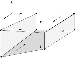
THE FUNDAMENTAL EQUATIONS 51
z
y
x
Figure 3.8 Schematic of a grid cell bounded at its top and bottom in general by sloped
surfaces and vertical side walls. The top and bottom surfaces can represent lin-
ear piecwise approximations to surfaces of constant generalized vertical coordi-
nates, with s=s1at the top surface and s=s2at the bottom surface. They
could also represent the ocean surface (for the top face) or the ocean bottom (for
the bottom face). The arrows represent the pressure contact forces which act in
a compressive manner along the boundaries of the grid cell and in a direction
normal to the boundaries. These forces arise from contact between the shown
fluid volume and adjacent regions. Due to Newton’s Third Law, the pressure
acting on an arbitrary fluid parcel Adue to contact with a parcel Bis equal and
opposite to the pressure acting on parcel Bdue to contact with parcel A. If coded
according to finite volume budgets, as in Lin (1997), this law extends to the pres-
sure forces acting between grid cells in an ocean model.
where the vertical integral extends from the botom face at z2=z(x,y,s=s2,t)to
the top face at z1=z(x,y,s=s1,t). Likewise, the meridional pressure forces are
Fy=y1=ˆy
Zdx
z1
Z
z2
dz p
y=y1
(3.167)
Fy=y2=−ˆy
Zdx
z1
Z
z2
dz p
y=y2
. (3.168)
On the top face, the pressure force is given by
Fs=s1=−ZdyZdx p z,s∇ss=s1
=−ZdyZdx p (−∇sz+ˆz)s=s1
.
(3.169)
Note the contribution from the generally non-horizontal top face as represented by
the two dimensional vector
∇sz=S, (3.170)
which is the slope of the surface of constant generalized vertical coordinate rela-
tive to the horizontal plane. The pressure force on the bottom face has a similar
appearance
Fs=s2=ZdyZdx p (−∇sz+ˆz)s=s2
. (3.171)
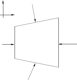
52 CHAPTER 3
If the top and bottom faces are horizontal, as for z-models, the pressure force
acting at s=s1and s=s2acts solely in the vertical direction. More generally, the
pressure force per area on the top and bottom faces is oriented according to the
slope of the faces and so has a nontrivial projection into all three directions.
x
A
B
C
D
p(x1,s)
p(x,s1)
p(x2,s)
p(x,s2)
z
Figure 3.9 The sides of the grid cell, with the slopes top and bottom surfaces more enhanced
here than in Figure 3.9. The corners are denoted A, B, C, and D, and oriented in
a counterclockwise manner. This is the orientation appropriate for performing a
contour integral in order to compute the pressure force acting on the area.
To garner a sense for how pressure acts on the face of a grid cell, consider the
case where the top surface of a grid cell rises to the east as shown in Figure 3.9.
In this case, the pressure force per area in the x−zplane takes the form
PRESSURE FORCE PER AREA O N TOP FA C E =−p[ˆz−(∂z/∂x)sˆx]. (3.172)
Since (∂z/∂x)s>0for this example, the pressure force per area has a positive
component in the ˆxdirection, as indicated by the arrow normal to the top surface
in Figure 3.9.
When the top surface represents the surface of the ocean at z=
η
, the pressure
pis the applied pressure paarising from any media above the ocean, such as the
atmosphere and sea ice. In this case,
PRESSURE FORCE PER A R E A O N O C E A N S U R FA C E =−pa∇(z−
η
)
=−pa(ˆz−∇
η
),(3.173)
where ∇
η
is the slope of the ocean surface. Likewise, if the bottom of the grid cell
is bounded by the solid earth boundary,
PRESSURE FORCE PER AREA O N O C E A N B O T T O M =pb∇(z+H)
=pb(ˆz+∇H),(3.174)
where ∇His the bottom slope.
A sum of the pressure forces acting on the six faces of the grid cell determines
the acceleration due to pressure acting on a grid cell. Organizing the forces into
THE FUNDAMENTAL EQUATIONS 53
the three directions leads to
Fx
pressure =
Zdy
z1
Z
z2
dz p
x=x1
−
Zdy
z1
Z
z2
dz p
x=x2
(3.175)
+
Zdy
x2
Z
x1
dx z,xp
s=s1
−
Zdy
x2
Z
x1
dx z,xp
s=s2
(3.176)
Fy
pressure =
Zdx
z1
Z
z2
dz p
y=y1
−
Zdx
z1
Z
z2
dz p
y=y2
(3.177)
+
Zdx
y2
Z
y1
dy z,yp
s=s1
−
Zdx
y2
Z
y1
dy z,yp
s=s2
(3.178)
Fz
pressure =ZZ dxdy ps=s2−ZZ dxdy ps=s1
. (3.179)
Making the hydrostatic approximation, whereby the vertical momentum equation
maintains the inviscid hydrostatic balance, allows us to note that the difference in
pressure between the top and bottom surfaces of the region is determined by the
weight of fluid between the surfaces,
ZZ
s=s2
dxdy p −ZZ
s=s1
dxdy p =gZ
ρ
dV. (3.180)
It is notable that this expression relates the difference in contact forces acting on
the domain boundaries to the integral of a body force (the gravitational force) acting
throughout the domain interior.
We now work on reformulating the horizontal pressure forces into a manner
amenable to finite volume discretization. Referring to Figure 3.9, we can write
the horizontal forces in a manner than builds in the orientation of pressure via a
counterclockwise contour integral
Fx
pressure =−
Zdy
z2
Z
z1
dz p
x=x1
−
Zdy
x2
Z
x1
dx z,xp
s=s2
−
Zdy
z1
Z
z2
dz p
x=x2
−
Zdy
x1
Z
x2
dx z,xp
s=s1
=−
Zdy
z2
Z
z1
dz p
x=x1
−
Zdy
x2
Z
x1
dz p
s=s2
−
Zdy
z1
Z
z2
dz p
x=x2
−
Zdy
x1
Z
x2
dz p
s=s1
=−ZdyI
ABCD
dz p.
(3.181)
54 CHAPTER 3
In the penultimate step, we set z,xdx=dz, which is an relation valid along the
particular contour ABCD. That is, in all the integrals, the differential increment dz
is taken along the contour surrounding the cell. The counter-clockwise orientation
of the integral follows from the compressive nature of pressure. Since the contour
of integration is closed, we have the identity
Fx
pressure =−ZdyI
ABCD
pdz
=ZdyI
ABCD
zdp.
(3.182)
The contour integral form of the pressure force is key to providing a finite vol-
ume discretization that is consistent with Newton’s Third Law (Lin, 1997). What is
needed next is an assumption about the subgrid profiles for pressure and geopo-
tential Φ=g z in order to evaluate the contour integral.
3.5.2 Pressure gradient body force in hydrostatic fluids
In the early finite difference formulations of the pressure force, modelers dis-
cretized the gradient of pressure and performed certain grid averages so that the
gradient occurs at the appropriate grid point. Guidance to the discretization details
was provided by concerns of energetic consistency (Chapter 9), whereby work
done by pressure in the discrete algorithm is balanced by buoyancy work (Bryan,
1969). This general philosophy still guides the formulation of the pressure force in
mom4p1.
As with the contact forces formulation, in a hydrostatic fluid we are only con-
cerned with horizontal pressure gradients, since the vertical momentum equation
is reduced to the inviscid hydrostatic balance. Hence, we are concerned with the
horizontal acceleration arising from pressure differences in a hydrostatic and non-
Boussinesq fluid, and this acceleration can be written∗
ρ
−1∇zp=
ρ
−1(∇s− ∇sz∂z)p
=
ρ
−1∇sp+g∇sz
=
ρ
−1∇sp+∇sΦ,
(3.183)
where the hydrostatic relation p,z=−
ρ
gwas used to reach the second equality,
and
Φ=g z (3.184)
is the geopotential. To reach this result, we used the expression
∇z=∇s−∇sz∂z, (3.185)
which relates the lateral gradient operator acting on constant depth surfaces, ∇z,
to the lateral operator acting on surfaces of constant generalized vertical coordi-
nate, ∇s.
∗For a Boussinesq fluid, equation (3.183) is modified by a factor of
ρ
/
ρ
o.
THE FUNDAMENTAL EQUATIONS 55
Discretizations of the pressure gradient body force result in both terms in equa-
tion (3.183) being large and of opposite sign in many regions, especially regions
of nontrivial topographic slope. Hence, this calculation exposes the calculation to
nontrivial numerical truncation errors which can lead to spurious numerical pres-
sure gradients and thus to incorrect simulated currents. Significant effort has gone
into reducing such pressure gradient errors, especially in terrain following models
where undulations of the coordinate surfaces can be large with realistic topogra-
phy (e.g., see Figure 6.3). Some of these issues are summarized in Section 2 of
Griffies et al. (2000a).
The pressure gradient force acting at a point represents the infinitesimal limit of
a body force. We see this fact by multiplying the pressure gradient acceleration by
the mass of a fluid parcel, which leads to the pressure force acting at a point in the
continuum
PRESSURE G R A D I E N T F O R C E =−(
ρ
dV)
ρ
−1∇zp
=−dV∇zp
=−dV(∇sp+
ρ
∇sΦ).
(3.186)
Hence, the pressure force acting on a finite region is given by the integral over the
extent of the region
PRESSURE G R A D I E N T F O R C E O V E R REGION =−ZZZ (
ρ
dV)
ρ
−1∇zp
=−ZZZ dV∇zp.
(3.187)
As stated earlier, a finite volume discretization of this force will take the same
form as the finite volume discretization of the pressure contact force discussed in
Section 3.5.1, as it should due to the Green-Gauss Theorem invoked to go from
equation (3.162) to (3.163). Other discretizations, in general, fail to maintain this
self-consistency. However, these formulations generally do not provide for a clear
energetic interpretation as promoted by the finite difference formulation of Bryan
(1969).
3.6 LINEAR MOMENTUM BUDGET
The purpose of this section is to formulate the budget for linear momentum over
a finite region of the ocean, with specific application to ocean model grid cells.
The material here requires many of the same elements as in Section 3.4, but with
added richness arising from the vector nature of momentum, and the additional
considerations of forces from pressure, friction, gravity, and planetary rotation.
Note that we initially formulate the equations using the pressure contact force,
as this provides a general formulation. Afterwards, we specialize to hydrostatic flu-
ids, and thus write the pressure force as a gradient (Section 3.5.2), as commonly
done in primitive equation ocean models

56 CHAPTER 3
3.6.1 General formulation
The budget of linear momentum for a finite region of fluid is given by the following
relation based on Newton’s second and third laws
∂tZZZ dV
ρ
v=ZZZ dVS(v)−ZZ dA(ˆn)[ˆn·(v−vref)]
ρ
v
+ZZ dA(ˆn)(ˆn·
τ
−ˆnp)−ZZZ dV
ρ
[gˆz+ ( f+M)ˆz∧v].
(3.188)
The left hand side is the time tendency of the region’s linear momentum. The first
term on the right hand side, S(v), is a momentum source, with units momentum
per volume per time. This term is nonzero if, for example, the addition of mass to
the ocean via a source occurs with a nonzero momentum. Often, it is assumed
that mass is added with zero velocity, and so does not appear as a momentum
source. The second term is the advective transport of linear momentum across the
boundary of the region, with recognition that the region’s boundaries are generally
moving with velocity vref. The third term is the integral of the contact stresses due
to friction and pressure. These stresses act on the boundary of the fluid domain.
We already discussed the forces from pressure in Section 3.5. The stress tensor
τ
is a symmetric second order tensor that parameterizes subgrid scale transport
of momentum. The final term on the right hand side is the volume integral of body
forces due to gravity and the Coriolis force.∗In addition, there is a body force
arising from the nonzero curvature of the spherical space. This curvature leads to
the advection metric frequency (see equation (4.49) of Griffies (2004))
M=v∂xln dy−u∂yln dx. (3.189)
In spherical coordinates where
dx= (rcos
φ
)d
λ
(3.190)
dy=rd
φ
, (3.191)
with rthe distance from the earth’s center,
λ
the longitude, and
φ
the latitude, the
advective metric frequency takes the form
M= (u/r)tan
φ
. (3.192)
The advection metric frequency arises since linear momentum is not conserved
on the sphere.†Hence, the linear momentum budget picks up this extra term that
is a function of the chosen lateral coordinates.
3.6.2 An interior grid cell
At the west side of a grid cell, ˆn=−ˆxwhereas ˆn=ˆxon the east side. Hence, the
advective transport of linear momentum entering through the west side of the grid
∗The wedge symbol ∧represents a vector cross product, also commonly written as ×. The wedge
is typically used in the physics literature, and is preferred here to avoid confusion with the horizontal
coordinate x.
†Angular momentum is conserved for frictionless flow on the sphere in the absence of horizontal
boundaries (see Section 4.11.2 of Griffies (2004)).

THE FUNDAMENTAL EQUATIONS 57
cell and that which is leaving through the east side are given by
TRANSPORT E N T E R I N G F R O M W E S T =ZZ
x=x1
dyds z,su(
ρ
v)(3.193)
TRANSPORT L E AVING T H R O U G H E A S T =−ZZ
x=x2
dyds z,su(
ρ
v). (3.194)
Similar results hold for momentum crossing the cell boundaries in the north and
south directions. Momentum crossing the top and bottom surfaces of an interior
cell is given by
TRANSPORT E N T E R I N G F R O M THE B O T T O M =ZZ
s=s2
dxdy w(s)(
ρ
v)(3.195)
TRANSPORT L E AVING FROM T H E TOP =−ZZ
s=s1
dxdy w(s)(
ρ
v). (3.196)
Forces due to the contact stresses at the west and east sides are given by
CONTACT FORCE ON W E S T SIDE =−ZZ
x=x1
dyds z,s(ˆx·
τ
−ˆxp)(3.197)
CONTACT FORCE ON E A S T SIDE =ZZ
x=x2
dyds z,s(ˆx·
τ
−ˆxp)(3.198)
with similar results at the north and south sides. At the top of the cell, dA(ˆn)ˆn=
∇sdxdywhereas dA(ˆn)ˆn=−∇sdxdyat the bottom. Hence,
CONTACT FORCE O N C E L L TOP =ZZ
s=sk−1
dxdy z,s(∇s·
τ
−p∇s)(3.199)
CONTACT FORCE ON C E L L B O T TOM =−ZZ
s=sk
dyds z,s(∇s·
τ
−p∇s). (3.200)
Bringing these results together, and taking limit as the time independent horizontal
area dxdy→0, leads to the thickness weighted budget for the momentum per
horizontal area of an interior grid cell
∂t(dz
ρ
v) = dzS(v)− ∇s·[dzu(
ρ
v)] + (w(s)
ρ
v)s=sk−(w(s)
ρ
v)s=sk−1
+∂x[dz(ˆx·
τ
−ˆxp)] + ∂y[dz(ˆy·
τ
−ˆyp)]
+ [z,s(∇s·
τ
−p∇s)]s=sk−1−[z,s(∇s·
τ
−p∇s)]s=sk
−
ρ
dz[gˆz+ ( f+M)ˆz∧v].
(3.201)
Note that both the time and horizontal partial derivatives are for positions fixed
on a constant generalized vertical coordinate surface. Also, the pressure force
as written here is a shorthand for the more complete contour integral formulation
provided in Section 3.5 (e.g., equation (3.182)). Additionally, we have yet to take
the hydrostatic approximation, so these equations are written for the three compo-
nents of the velocity.
58 CHAPTER 3
The first term on the right hand side of the thickness weighted momentum bud-
get (3.201) is the momentum source, and the second is the convergence of advec-
tive momentum fluxes occurring within the layer. We discussed the analogous flux
convergence for the tracer and mass budgets in Section 3.4.5. The third and fourth
terms arise from the transport of momentum across the upper and lower constant
sinterfaces. The fifth and sixth terms arise from the horizontal convergence of
pressure and viscous stresses. The seventh and eigth terms arise from the fric-
tional and pressure stresses acting on the constant generalized surfaces. These
forces provide an interfacial stress between layers of constant s. Note that even
in the absence of frictional stresses, interfacial stresses from pressure acting on
the generally curved ssurface can transmit momentum between vertically stacked
layers. The final term arises from the gravitational force, the Coriolis force, and the
advective frequency.
3.6.3 Cell adjacent to the ocean bottom
As for the tracer and mass budgets, we assume zero mass flux through the ocean
bottom at z=−H(x,y). However, there is generally a nonzero stress at the
bottom due to both the pressure between the fluid and the bottom, and unresolved
features in the flow which can correlate or anti-correlate with bottom topographic
features (Holloway (1999)). The area integral of the stresses lead to a force on the
fluid at the bottom
Fbottom =−ZZ
z=−H
dxdy[∇(z+H)·
τ
−p∇(z+H)]. (3.202)
Details of the stress term requires fine scale information that is generally unavail-
able. For present purposes we assume that some boundary layer model provides
information that is schematically written
τ
bot =∇(z+H)·
τ
(3.203)
where
τ
bot is a vector bottom stress. Taking the limit as the horizontal area van-
ishes leads to the thickness weighted budget for momentum per horizontal area of
a grid cell next to the ocean bottom
∂t(dz
ρ
v) = dzS(v)− ∇s·[dzu(
ρ
v)] −(w(s)
ρ
v)s=skbot−1
+∂x[dz(ˆx·
τ
−ˆxp)] + ∂y[dz(ˆy·
τ
−ˆyp)]
+ [z,s(∇s·
τ
−p∇s)]s=skbot−1
−
τ
bot +pb∇(z+H)
−
ρ
dz[gˆz+ ( f+M)ˆz∧v].
(3.204)
3.6.4 Cell adjacent to the ocean surface
There is a nonzero mass and momentum flux through the upper ocean surface
at z=
η
(x,y,t), and contact stresses are applied from resolved and unresolved
processes involving interactions with the atmosphere and sea ice. Following the
discussion of the tracer budget at the ocean surface in Section 3.4.7 leads to the

THE FUNDAMENTAL EQUATIONS 59
expression for the transport of momentum into the ocean due to mass transport at
the surface
−ZZ dA(ˆn)ˆn·[(v−vref)
ρ
v=ZZ
z=
η
dxdy
ρ
wqwv. (3.205)
The force arising from the contact stresses at the surface is written
Fcontact =ZZ
z=
η
dxdy[∇(z−
η
)·
τ
−p∇(z−
η
)]. (3.206)
Bringing these results together leads to the force acting at the ocean surface
Fsurface =ZZ
z=
η
dxdy[∇(z−
η
)·
τ
−p∇(z−
η
) +
ρ
wqwv]. (3.207)
Details of the various terms in this force are generally unknown. Therefore, just as
for the tracer at z=
η
in Section 3.4.7, we assume that a boundary layer model
provides information about the total force, and that this force is written
Fsurface =ZZ
z=
η
dxdy[
τ
top −pa∇(z−
η
) +
ρ
wqwvw], (3.208)
where vwis the velocity of the fresh water. This velocity is typically taken to be
equal to the velocity of the ocean currents in the top cells of the ocean model, but
such is not necessarily the case when considering the different velocities of, say,
river water and precipitation. The stress
τ
top is that arising from the wind, as well
as interactions between the ocean and sea ice. Letting the horizontal area vanish
leads to the thickness weighted budget for a grid cell next to the ocean surface
∂t(dz
ρ
v) = dzS(v)− ∇s·[dzu(
ρ
v)] + (w(s)
ρ
v)s=sk=1
+∂x[dz(ˆx·
τ
−ˆxp)] + ∂y[dz(ˆy·
τ
−ˆyp)]
−[z,s(∇s·
τ
−p∇s)]s=sk=1
+ [
τ
top −pa∇(z−
η
) +
ρ
wqwvw]
−
ρ
dz[gˆz+ ( f+M)ˆz∧v].
(3.209)
3.6.5 Horizontal momentum equations for hydrostatic fluids
We now assume the fluid to maintain a hydrostatic balance, which is the case for
primitive equation ocean general circulation models. In this case, we exploit the
pressure gradient body force as discussed in Section 3.5.2. Specializing the mo-
mentum budgets from Sections 3.6.2, 3.6.3, and 3.6.4 to use the hydrostatic pres-
sure gradient force (again, interpreted according to the finite volume form given in
Section 3.5) leads to the horizontal linear momentum budget for interior, bottom,
and surface grid cells
[∂t+ ( f+M)ˆz∧] (
ρ
dzu) = dzS(u)− ∇s·[dzu(
ρ
u)]
−dz(∇sp+
ρ
∇sΦ)
+∂x(dzˆx·
τ
) + ∂y(dzˆy·
τ
)
−[w(s)
ρ
v−z,s∇s·
τ
]s=sk−1
+ [w(s)
ρ
v−z,s∇s·
τ
]s=sk.
(3.210)

60 CHAPTER 3
[∂t+ ( f+M)ˆz∧] (
ρ
dzu) = dzS(u)− ∇s·[dzu(
ρ
u)]
−dz(∇sp+
ρ
∇sΦ)
+∂x(dzˆx·
τ
) + ∂y(dzˆy·
τ
)
−[w(s)
ρ
u−z,s∇s·
τ
]s=skbot−1
−
τ
bottom
(3.211)
[∂t+ ( f+M)ˆz∧] (
ρ
dzu) = dzS(u)− ∇s·[dzu(
ρ
u)]
−dz(∇sp+
ρ
∇sΦ)
+∂x(dzˆx·
τ
) + ∂y(dzˆy·
τ
)
+ [
τ
wind +
ρ
qwuw]
+ [ w(s)
ρ
u−z,s∇s·
τ
]s=s1.
(3.212)
3.7 THE BOUSSINESQ BUDGETS
We consider various depth-based vertical coordinates in Section 6.1. These coor-
dinates are used to discretize the Boussinesq model equations where the volume
of a parcel is conserved rather than the mass. A detailed discussion of the inter-
pretation of the Boussinesq equations in terms of density weighted fields is given
by McDougall et al. (2003a) and Griffies (2004). For now, we gloss over those
details by quoting the Boussinesq equations for volume, tracer, and momentum as
arising from setting all density factors to the constant
ρ
o, except when multiplied by
the gravitational acceleration in the hydrostatic balance (i.e., for calculation of pres-
sure and geopotential, the full density is used). The density
ρ
ois a representative
density of the ocean fluid. In mom4 we set
ρ
o=1035 kgm−3, (3.213)
although this value can be changed via altering a parameter statement and thus
recompiling the code). For much of the ocean, the in situ density deviates less
than 3% from 1035 kg m−3(see page 47 of Gill (1982)).
The replacement of density in the mass, tracer, and linear momentum budgets
over a grid cell in the ocean interior leads to the following budgets for the hydro-

THE FUNDAMENTAL EQUATIONS 61
static model
∂t(dz) = dzS(V)− ∇s·(dzu)−(w(s))s=sk−1+ (w(s))s=sk.
∂t(dz C) = dzS(C)−∇s·[dz(uC+F)]
−(w(s)C+F(s))s=sk−1
+ (w(s)C+F(s))s=sk
[∂t+ ( f+M)ˆz∧] (
ρ
odzu) = dzS(u)− ∇s·[dzu(
ρ
ou)]
−dz(∇sp+
ρ
∇sΦ)
+∂x(dzˆx·
τ
) + ∂y(dzˆy·
τ
)
−[w(s)
ρ
ov−z,s∇s·
τ
]s=sk−1
+ [w(s)
ρ
ov−z,s∇s·
τ
]s=sk.
(3.214)
The first equation reduces to a volume budget rather than a mass budget found for
the non-Boussinesq system. In this equation, S(V)is a volume source with units
of inverse time. Likewise, S(u)is a velocity source (with units of acceleration). The
Boussinesq equations for a grid cell adjacent to the ocean bottom are given by
∂t(dz) = dzS(V)− ∇s·(dzu)−(w(s))s=skbot−1
∂t(dz C) = dzS(C)− ∇s·[dz(uC+F)]
−(w(s)C+F(s))s=skbot−1
+Q(C)
(bot)
[∂t+ ( f+M)ˆz∧] (
ρ
odzu) = dzS(u)− ∇s·[dzu(
ρ
ou)]
−dz(∇sp+
ρ
∇sΦ)
+∂x(dzˆx·
τ
) + ∂y(dzˆy·
τ
)
−[w(s)
ρ
ou−z,s∇s·
τ
]s=skbot−1
−
τ
bottom
(3.215)
and the equations for a cell next to the ocean surface are
∂t(dz) = dzS(V)− ∇s·(dzu) + (w(s))s=sk=1+
ρ
oqw
∂t(dz C) = dzS(C)−∇s·[dz(uC+F)]
+ (w(s)C+F(s))s=sk=1
+ (
ρ
oqwCw−Q(turb)
(C))
[∂t+ ( f+M)ˆz∧] (
ρ
odzu) = dzS(u)− ∇s·[dzu(
ρ
ou)]
−dz(∇sp+
ρ
∇sΦ)
+∂x(dzˆx·
τ
) + ∂y(dzˆy·
τ
)
+ [
τ
wind +
ρ
oqwuw]
+ [ w(s)
ρ
ou−z,s∇s·
τ
]s=s1.
(3.216)

Chapter Four
The hydrostatic pressure force
The purpose of this chapter is to detail issues related to computing the pressure
force in hydrostatic ocean models. Care is taken to split the pressure force into its
slow and fast components, thus facilitating a split of the momentum equation for
use in an explicit time stepping scheme for the momentum equation.
In Section 3.5, we encountered two formulations of the pressure force. The
first computes the pressure gradient body force (Section 3.5.2), and considers
the pressure force to be acting at a point. This interpretation follows from a finite
difference interpretation of the velocity equation, following the energetic approach
of Bryan (1969) and all versions of MOM. The second formulation applies a finite
volume interpretation advocated in Chapter 3, with particular attention given to the
contour integral form of pressure as derived in Section 3.5.1. The finite volume
approach does not lend itself to straightforward energetic conversion arguments
(Chapter 9). It is for this reason that we maintain the finite difference approach of
Bryan (1969) in mom4p1.
4.1 HYDROSTATIC PRESSURE FORCES AT A POINT
A hydrostatic fluid maintains the balance
p,z=−
ρ
g. (4.1)
This balance means that the pressure at a point in a hydrostatic fluid is deter-
mined by the weight of fluid above this point. This relation is maintained quite
well in the ocean on spatial scales larger than roughly 1km. Precisely, when the
squared ratio of the vertical to horizontal scales of motion is small, then the hy-
drostatic approximation is well maintained. In this case, the vertical momentum
budget reduces to the hydrostatic balance, in which case vertical acceleration and
friction are neglected. If we are interested in explicitly representing such motions
as Kelvin-Helmholtz billows and flow within a convective chimney, vertical acceler-
ations are nontrivial and so the non-hydrostatic momentum budget must be used.
The hydrostatic balance greatly affects the algorithms used to numerically solve
the equations of motion. Marshall et al. (1997) highlight these points in the context
of developing an algorithm suited for both hydrostatic and non-hydrostatic simula-
tions. However, so far in ocean modelling, no global simulations have been run at
resolutions sufficiently refined to require the non-hydrostatic equations. Addition-
ally, many regional and coastal models, even some with grid resolutions finer than
1km, still maintain the hydrostatic approximation, and thus they must parameterize
the unrepresented non-hydrostatic motions.

64 CHAPTER 4
As discussed in Section 3.5.2, at a point in the continuum, the horizontal accel-
eration arising from pressure differences in a hydrostatic and non-Boussinesq fluid
can be written∗
ρ
−1∇zp=
ρ
−1(∇s− ∇sz∂z)p
=
ρ
−1∇sp+g∇sz
=
ρ
−1(∇sp+
ρ
∇sΦ)
(4.2)
where the hydrostatic relation p,z=−
ρ
gwas used to reach the second equality,
and
Φ=g z (4.3)
is the geopotential. For cases where the density is constant on ssurfaces, we can
combine the two terms into a single gradient, thus rendering a pressure gradient
force with a zero curl. This special case holds for geopotential and pressure co-
ordinates in general, and isopycnal coordinates in the case of an idealized linear
equation of state. However, it does not hold in the more general case, in which
the difficulty of numerically computing the acceleration from pressure arises when
there are contributions from both terms. Generally, both terms can be large and of
opposite sign in many regions. In this case, the simulation is exposed to nontriv-
ial numerical truncation errors which can, for example, lead to spurious pressure
gradients that spin up an unforced fluid with initially flat isopycnals.
Significant effort has gone into reducing such pressure gradient errors, espe-
cially in terrain following models where undulations of the coordinate surfaces can
be large with realistic bottom topography (e.g., see Figure 6.3). Some of these
issues are summarized in Section 2 of Griffies et al. (2000a). Perhaps the most
promising approach is that proposed by Shchepetkin and McWilliams (2002). It is
notable that difficulties with pressure gradient errors have largely been responsi-
ble for the near absence of sigma models being used for long term global ocean
climate simulations.†
4.2 THE PRESSURE GRADIENT BODY FORCE
The presence of both the pressure gradient and density weighted geopotential
gradient in the horizontal linear momentum budgets (3.210), (3.211), and (3.212)
complicates the numerical implementation of the pressure gradient force. The
problem is that numerical errors in one term are often not compensated by the
other term, and such can lead to spurious flows. For the quasi-horizontal depth
based and pressure based coordinates supported by mom4p1 (i.e., s=z,s=z∗,
s=p, or s=p∗; see Chapter 6), these errors are quite small. The reason is that
these choices ensure that one of the two terms is significantly smaller than the
other. Nonetheless, it is useful to provide a formulation that even further reduces
the potential for errors for both the quasi-horizontal coordinates, as well as the
terrain following coordinates
σ
(z)and
σ
(p)(Chapter 6).
∗To obtain this result for a Boussinesq fluid, multiply both sides of equation (4.2) by
ρ
/
ρ
o.
†The work of Diansky et al. (2002) is the only case known by the author of a global sigma model
used for climate purposes.
THE HYDROSTATIC PRESSURE FORCE 65
In addition to reducing errors associated with a numerical computation of the
pressure gradient, we aim to split the pressure gradient into terms that can be
conveniently associated with the slowly evolving internal modes from the faster
barotropic mode. Details of this split are a function of the vertical coordinate.
This split in the pressure gradient then facilitates our treatment of the vertically
integrated momentum equations, as discussed in Section 7.7.
In the following, we are motivated by the formulation of the pressure gradient
commonly applied to z-models. Adcroft and Campin (2004) extended this treat-
ment to the z∗vertical coordinate. We take it one more step in order to handle all
vertical coordinates supported by mom4p1. Hallberg (1997) goes further by treat-
ing the pressure gradient in isopycnal layered models using a realistic equation of
state.
4.2.1 Depth based vertical coordinates
As mentioned on page 47 of Gill (1982), in situ density in the bulk of the ocean
deviates less than 3% from the constant density
ρ
o=1035 kg m−3. (4.4)
The hydrostatic pressure associated with this constant density has no horizontal
gradients, and so it does not contribute to horizontal pressure gradient forces.
For increased accuracy computing the horizontal pressure gradient, it is useful to
remove this term from the calculation of hydrostatic pressure. For this purpose, we
write the hydrostatic balance as
p,z=−g
ρ
=−g(
ρ
o+
ρ
0),(4.5)
which has an associated split in the hydrostatic pressure field
p=pa+po(z) + p0(x,y,z,t). (4.6)
We can solve for the pressures by assuming
po(z=
η
) = 0 (4.7)
p0(z=
η
) = 0, (4.8)
which leads to
po=−g
ρ
o(z−
η
)
=−
ρ
oΦ+g
ρ
o
η
,(4.9)
p0=gZ
η
z
ρ
0dz, (4.10)
and thus
p=pa+g
ρ
o
η
−
ρ
oΦ+p0.(4.11)
Splitting off the free surface height is advantageous as it allows for a split of the
pressure gradient into its fast two dimensional barotropic contributions and slow
three dimensional baroclinic contributions. This split in pressure gradient facili-
tates the development of a split-explicit time stepping method for the momentum
equations considered in Section 7.7. Details of the split in pressure are dependent
on the vertical coordinate choice. We now discuss the three depth based vertical
coordinates used in mom4p1.
66 CHAPTER 4
4.2.1.1 Geopotential vertical coordinates
The simplest form of the pressure gradient is realized with geopotential vertical
coordinates. We are here motivated by the desire to split the dynamics into fast
and slow portions, as approximated by depth integrating the momentum equation
(Section 7.7).
The anomalous pressure p0maintains a dependence on surface height through
the upper limit on the vertical integral in equation (4.10). When working with geopo-
tential vertical coordinates, it is very convenient to isolate this dependence by ex-
ploiting a very accurate approximation described below. This split then allows us
to exclusively place the surface height dependent pressure gradient into the ver-
tically integrated momentum equation. The slow component to the pressure gra-
dient then has no dependence on the surface height; it is instead just a function
of the anomalous density. The slow pressure gradient component thus vanishes
when the density is horizontally unstratified; i.e., when there is no baroclinicity.
To facilitate the split described above, we proceed in the following manner
p0=gZ
η
z
ρ
0dz
=gZ0
z
ρ
0dz+gZ
η
0
ρ
0dz
≈gZ0
z
ρ
0dz+g
η ρ
0
surf
≡p0
clinic +p0
surf.
(4.12)
The approximation made in the third step remains good where density is well mixed
between z=0and z=
η
, and this is generally the case for large scale modelling.
Here, density in the surface region of the ocean is assumed to take on the value
ρ
surf =
ρ
o+
ρ
0
surf, (4.13)
which is a function of horizontal position and time. The anomalous pressure p0
has therefore been separated into two pressures, where the anomalous surface
pressure
p0
surf =
ρ
0
surf g
η
(4.14)
is a function of the surface height and surface density, and the pressure
p0
clinic =gZ0
z
ρ
0dz(4.15)
is the anomalous hydrostatic baroclinic pressure within the region from a depth
z<0to z=0. Again, the baroclinic pressure is independent of the surface height,
and so its horizontal gradients are only a function of density.
This split of pressure thus renders the horizontal pressure gradient
(∇zp)approx ≈ ∇(pa+g
ρ
o
η
+p0
surf) + ∇sp0
clinic +
ρ
0∇sΦ
=∇(pa+g
ρ
surf
η
)
|{z }
fast
+∇sp0
clinic +
ρ
0∇sΦ.
|{z }
slow
(4.16)
In a geopotential vertical coordinate model, interior grid cells are discretized at
levels of constant geopotential. Hence, the gradient ∇sreduces to the constant
THE HYDROSTATIC PRESSURE FORCE 67
geopotential gradient ∇z. In this case the horizontal gradient of the geopotential
vanishes, ∇zΦ=0. At the bottom, however, mom4p1 employs bottom partial step
topography (Pacanowski and Gnanadesikan, 1998). The bottom cells are thus not
discretized along a constant geopotential. Hence, just at the bottom, there is a
nontrivial gradient of the geopotential Φ(see Figure 6.1).
4.2.1.2 z∗and
σ
(z)vertical coordinate
The new issue that arises when moving away from geopotential coordinates is
that the geopotential Φ=g z has a nonzero along coordinate gradient in the
interior, whereas with geopotential coordinates it remains nonzero only along the
partial bottom stepped topography. The presence of Φgradients in the interior is
fundamental.
Following the discussion in Section 4.2.1, we are led to the following expressions
for the horizontal pressure gradient. The exact expression relevant for the z∗and
σ
(z)coordinates is given by
(∇zp)exact =∇sp+
ρ
∇sΦ
=∇s(pa+po+p0) +
ρ
∇sΦ
=∇(pa+g
ρ
o
η
)
|{z }
fast
+∇sp0+
ρ
0∇sΦ
|{z }
slow
.(4.17)
Note that we have assumed that the geopotential falls inside the slow portion of
the pressure gradient. This assumption is made even though the depth of a grid
point is a function of the undulating surface height. The validity of this assumption
can be assessed by the integrity and stability of the simulation.
To facilitate a unified treatment in subsequent manipulations, we define
psurf =
ρ
surf g
η
s=z
psurf =
ρ
0g
η
s=z∗,
σ
(z)(4.18)
and
p0=gR0
z
ρ
0dz s =z
p0=gR
η
z
ρ
0dz s =z∗,
σ
(z).(4.19)
In both the exact and aproximated pressure gradient expressions, the geopoten-
tial gradient ∇sΦin the ocean interior is weighted by the small density deviation
ρ
0=
ρ
−
ρ
o. For quasi-horizontal depth-based vertical coordinates supported in
mom4p1 (Section 6.1), the horizontal gradient of the geopotential is small, and the
ρ
0weighting further reduces its contribution. For terrain following coordinates, the
horizontal gradient term is not small, and the
ρ
0weighting is essential to reduce its
magnitude.
4.2.2 A test case for zero cross-coordinate flow
In the development of generalized vertical coordinates, a useful test case was
suggested by Alistair Adcroft. We focus here on the special case of s=z∗. In
this test, initialize the density field as a function only of the vertical coordinate z∗.
The domain is flat bottomed and doubly periodic in the horizontal, thus precluding
68 CHAPTER 4
pressure gradients due to side boundaries or topography. In a state of rest, there
is no horizontal pressure gradients, and so no motion. As a body force is applied
to the barotropic equations, such as through an ideal tidal forcing, there will now
be a nontrivial surface height field
η
as well as a nontrivial barotropic velocity. Both
pieces of the slow contribution to the horizontal pressure gradient (4.17) develop
a nontrivial vertical structure, and this will initiate baroclinic structure and thus a
nonzero cross coordinate vertical velocity w(s). This cross coordinate velocity will
be much smaller in the s=z∗case than with s=z, given than z∗follows the
motion of the free surface.
In order to further test the integrity of the z∗implementation, we wish to truncate
the pressure calculation in this test so that there will be no slow pressure gradients
developed when the tidal forcing is applied, and hence there will be no cross coor-
dinate motion. For this purpose, truncate the slow piece of the horizontal pressure
gradient (4.17) as
∇sp0+
ρ
0∇sΦ→ ∇sp0
truncate. (4.20)
In this truncation, we drop the geopotential term
ρ
0∇sΦ, as this will produce non-
trivial horizontal gradients as the surface height undulates. We also introduce a
truncated perturbation pressure determined by
p0=gZ
η
z
ρ
0dz
=gZs(
η
)
s(z)
ρ
0z,sds
=g(1+
η
/H)Z0
z∗
ρ
0dz∗
=p0
truncate + (g
η
/H)Z0
z∗
ρ
0dz∗.
(4.21)
To reach the penultimate step, we used z,s= (1+
η
/H)for s=z∗. The coor-
dinate increments used to define the pressure field p0
truncate are static in a model
discretizing the vertical according to s=z∗. Hence, ∇sp0
truncate =0if the density is
a function only of z∗. So when the model’s slow pressure field is comprised of just
p0
truncate, the ideal tidal test in the torus should maintain zero cross coordinate flow,
wz∗=0, even as the surface height fluctuates. Testing to see that this property is
maintained is a useful means of evaluating the integrity of the algorithm.
4.2.3 Pressure based vertical coordinates
A complementary discussion to the above is now given for pressure based vertical
coordinates. Since for pressure based vertical coordinates we solve for the bottom
pressure, it is useful to formulate the geopotential in terms of the bottom pressure
rather than the atmospheric pressure. For this purpose, consider the following
THE HYDROSTATIC PRESSURE FORCE 69
identities
Φ+g H =g
z
Z
−H
dz
=g
p
Z
pb
z,pdp
=−
p
Z
pb
ρ
−1dp
=−
p
Z
pb
(
ρ
−1
o+
ρ
−1−
ρ
−1
o)dp
= (pb−p)/
ρ
o+
ρ
−1
o
p
Z
pb
(
ρ
0/
ρ
)dp
= (pb−p)/
ρ
o−(g/
ρ
o)
z
Z
−H
ρ
0dz.
(4.22)
We are thus led to
ρ
oΦ=pb−p+
ρ
o(Φb+Φ0),(4.23)
where
ρ
oΦ0=−g
z
Z
−H
ρ
0dz. (4.24)
is an anomalous geopotential similar to the anomalous hydrostatic pressure intro-
duced in Section 4.2.1, and
Φb=−g H (4.25)
is the geopotential at the ocean bottom. The horizontal pressure force is therefore
written
∇sp+
ρ
∇sΦ=∇sp+ (
ρ
/
ρ
o)∇(pb+
ρ
oΦb)−(
ρ
/
ρ
o)∇sp+
ρ
∇sΦ0
= (
ρ
/
ρ
o)∇(pb+
ρ
oΦb)
| {z }
fast
+
ρ
∇sΦ0−(
ρ
0/
ρ
o)∇sp
| {z }
slow
.(4.26)
Note that the three-dimensional pressure term (
ρ
0/
ρ
o)∇spis weighted by the
generallly very small density deviation
ρ
0=
ρ
−
ρ
o. For the non-terrain following
quasi-horizontal pressure-based vertical coordinates supported in mom4p1 (Sec-
tion 6.2), the horizontal gradient of the pressure is small, and the weighting by
(
ρ
0/
ρ
o)further reduces its contribution. Also note that the fast contribution is here
weighted by the density, and so this term may appear to require further splitting
into
ρ
=
ρ
o+
ρ
0before identifying the fast two dimensional contribution. However,

70 CHAPTER 4
as the nonBoussinesq formulation here considers momentum per area, the baro-
clinic velocity includes density weighting (see equation (8.1)). This is how we are
to split the horizontal momentum equations into fast two dimensional motions and
slow three dimensional motions for purposes of time stepping. We consider these
issues further in Sections 7.7 and 8.1.
During the testing of this formulation for the pressure gradient, we found it useful
to write the anomalous geopotential in the following form
−(
ρ
o/g)Φ0=
z
Z
−H
ρ
0dz
=
η
Z
−H
ρ
0dz−
η
Z
z
ρ
0dz
=pb−pa
g−
ρ
o(H+
η
)−
η
Z
z
ρ
0dz
=pb−pa−p0
g−
ρ
o(H+
η
).
(4.27)
To reach this result, we used the hydrostatic balance for the full ocean column,
η
Z
−H
ρ
0dz=pb−pa
g−
ρ
o(H+
η
)(4.28)
as well as the definition (4.10) of the anomalous hydrostatic pressure
p0=g
η
Z
z
ρ
0dz(4.29)
used in Section 4.2.1 for the depth based vertical coordinates. These results then
lead to the identiy
pb+
ρ
o(Φb+Φ0) = p0+pa+
ρ
og
η
. (4.30)
4.3 THE PRESSURE GRADIENT BODY FORCE IN B-GRID MOM4P1
We now detail how the pressure gradient body force is represented in the B-grid
generalized vertical coordinate version of mom4p1. As the pressure force acts
to accelerate a fluid parcel, our aim is to determine the pressure force acting at
the velocity cell point. Much in the derivation of the pressure force depends on
assumptions regarding where pressure is computed in the discrete model. For the
B-grid version of mom4p1, hydrostatic pressure is coincident with the tracer fields
as shown in Figure 3.9, which illustrates a typical case where a grid cell is bounded
by vertical sidewalls with generally nonhorizontal tops and bottoms.
As mentioned in Section 3.5.2, we prefer to discretize the pressure gradient body
force as it facilitates the splitting of the pressure force into fast and slow compo-
nents. The result here is a derivation of the Pacanowski and Gnanadesikan (1998)
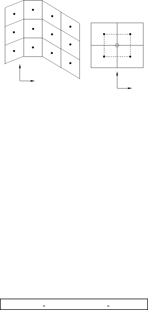
THE HYDROSTATIC PRESSURE FORCE 71
discrete pressure gradient body force as originally implemented for the treatment
of partial step bottom topography. Their discussion is relevant here, since the
pressure gradient force in the presence of partial step bottoms must account for
the pressure between cells that live at different depths. This is also the essential
issue for the treatment of pressure with generalized vertical coordinates.
z
x
TT
T
T
x
y
U
Figure 4.1 The left panel shows a set of grid cells in the x-z plane for a generalized vertical
coordinate version of mom4. The center point represents a tracer point. As ac-
tive tracers determine density, and as density determines hydrostatic pressure,
the hydrostatic pressure is coincident with tracer. For the x-y plane shown in
the right panel, the velocity and tracer are offset, with the velocity at the north-
east corner of the tracer cell according to the B-grid arrangement. The velocity
cell, shown surrounding the velocity point, has a thickness set according to the
minimum of the surrounding four tracer cell thicknesses. Hence, a velocity point
and tracer point with the same discrete vertical index kgenerally live at different
depths.
4.3.1 Depth based vertical coordinates
The aim here is to discretize the pressure gradient body force written in the forms
(4.17) and (4.16)
∇sp+
ρ
∇sΦ=∇(pa+psurf) + ∇sp0+
ρ
0∇sΦ, (4.31)
where psurf and p0are defined according to equations (4.18) and (4.19), respec-
tively. Our focus here is the slowly evolving three dimensional terms ∇sp0+
ρ
0∇sΦ. The first term is straightforward to discretize according to the assump-
tions regarding the placement of pressure given in Figure 4.1. In the right panel
of this figure, we see that pressure is available at the corners of the velocity cell.
Hence, to approximate pressure at the west and east faces of the cell, one can
average the pressure found at the corners. A grid weighted average may be ap-
propriate, but the simplest method is an unweighted average in which
∇sp0≈ˆxFDX NT(FAY(p0)) + ˆyFDY ET(FAX(p0)) (4.32)
72 CHAPTER 4
The averaging operators are defined according to
2aix= (ai+1+ai)
=FAX(a)(4.33)
and
2ajy= (aj+1+aj)
=FAY(a)(4.34)
with the second expression in each equation exposing the notation used in the
ocean model code. Additionally, finite difference operators have been introduced
FDX NT(a) = ai+1−ai
dxui,j
.
FDY ET(a) = aj+1−aj
dyui,j
.
(4.35)
These operators are used for fields that live at the north face and east face, re-
spectively, of a tracer cell.
The geopotential contribution in (4.31) is computed using the geopotential val-
ues at the tracer points, and so its gradient is located at the tracer cell faces. To
have the density multiplier at the same point requires that it be averaged prior to
multiplying. Finally, an orthogonal spatial average is required to place the product
onto the velocity point. The result is given by
ρ
0∇sΦ≈ˆxFAY[
δ
iΦFAX(
ρ
0)]/dxui,j+ˆyFAX[
δ
jΦFAY(
ρ
0)]/dyui,j.
(4.36)
4.3.2 Pressure based vertical coordinates
The aim is to discretize the pressure gradient body force written in the form (4.26)
∇sp+
ρ
∇sΦ= (
ρ
/
ρ
o)∇(pb+
ρ
oΦb) +
ρ
∇sΦ0−(
ρ
0/
ρ
o)∇sp(4.37)
and to do so in a manner analogous to the Boussinesq case. In particular, we
consider here the slow three dimensional contribution
ρ
∇sΦ0−(
ρ
0/
ρ
o)∇spand
write for the pressure term
ρ
0∇sp≈ˆxFAY[
δ
ip FAX(
ρ
0)]/dxui,j+ˆyFAX[
δ
jp FAY(
ρ
0)]/dyui,j, (4.38)
which is analogous to the discrete
ρ
0∇sΦcontribution in equation (4.36). The
geopotential term is discretized as
ρ
∇sΦ0≈ˆx
ρ
FDX NT (FAY(Φ0)) + ˆy
ρ
FDY ET (FAX(Φ0)), (4.39)
which is analogous to the discrete version of ∇sp0in equation (4.32). Note that
the density
ρ
in equation (4.39) is centered on the velocity cell.

Chapter Five
Parameterizations with generalized vertical coordinates
The parameterization of subgrid scale (SGS) processes is of fundamental im-
portance to ocean models. Details of how these processes are parameterized
depend on the choice of vertical coordinates. The purpose of this chapter is to
describe how various SGS parameterizations are formulated with generalized ver-
tical coordinates in mom4p1. As we will see, by diagnosing the vertical grid cell
thicknesses according to the methods described in Section 7.3, parameterizations
implemented in the geopotential MOM4.0 code remain algorithmically unaltered
when converting to the generalized vertical coordinate mom4p1.
5.1 FRICTION
The convergence of frictional stress leads to a friction force acting on fluid parcels.
The purpose of this section is to detail the form of friction appearing in the general-
ized vertical coordinate models. For this purpose, we follow much of the discussion
in Chapter 17 of Griffies (2004). In particular, Section 17.3.4 leads us to take the
physical components to the frictional stress tensor in the form
τ
=
τ
xx
τ
xy
ρ κ
u,z
τ
xy −
τ
xx
ρ κ
v,z
ρ κ
u,z
ρ κ
v,z0
, (5.1)
where
κ
is a non-negative viscosity with units m2s−1. Taking
τ
33 =0is consistent
with use of the hydrostatic approximation, which reduces the vertical momentum
equation to the inviscid hydrostatic balance. We comment in Section 5.1.3 on the
form of the two-dimensional transverse elements
τ
xx and
τ
xy.
5.1.1 Vertical friction
As the gravitational force is so critical to stratified fluids close to a hydrostatic bal-
ance, it is typical in ocean modelling to single out the vertical direction. In particu-
lar, closures for the unresolved vertical exchange of momentum are usually taken
to be proportional to the vertical derivative, or shear, of the horizontal velocity field.
This argument leads to the form of the stress tensor given by equation (5.1). For a
generalized vertical coordinate model, the vertical shear elements take the form
ρ κ
u,z=
ρ κ
s,zu,s. (5.2)
In mom4p1, the left hand side of this expression is numerically evaluated for pur-
poses of computing the vertical shear. That is, vertical derivatives are computed

74 CHAPTER 5
for arbitrary vertical coordinates just as in geopotential coordinates. This result fol-
lows by diagnosing the vertical grid cell thicknesses using the methods described
in Section 7.3, where we make use of the relation between vertical coordinates
dz=z,sds. (5.3)
Now return to the thickness weighted momentum budget for a grid cell discussed
in Section 3.6. The above considerations lead us to write the frictional stress acting
on a generalized surface as
z,s∇s·
τ
= (ˆz−S)·
τ
≈ˆz·
τ
=
ρ κ
u,z.
(5.4)
The second step used the small angle approximation to drop the extra slope term.
Alternatively, we can interpret the dia-surface frictional stress z,s∇s·
τ
as param-
eterized by
ρ κ
u,z. Either way, the result (5.4) is the form that vertical frictional
stress is implemented in mom4p1.
5.1.2 A comment on nonlinear vertical friction
As noted above, we choose in mom4p1 to implement vertical friction, and vertical
tracer diffusion (Section 5.2.1) just as in a geopotential coordinate model. This
method is facilitated by diagnosing the vertical thickness of a grid cell according to
equation (5.3) (see Section 7.3), prior to computing vertical derivatives.
We now mention an alternative method, not implemented in mom4p1, since this
method is often seen in the literature. The alternative is to compute the vertical
shear according to the right hand side of equation (5.2). The density weighted in-
verse specific thickness
ρ
/z,sadds a nonlinear term to the vertical friction, and this
complicates the numerical treatment (Hallberg, 2000). It is reasonable to approx-
imate this factor by a constant for the dimensionful quasi-horizontal coordinates
considered in Sections 6.1 and 6.2.∗For the Boussinesq case with depth-based
vertical coordinates, this approximation results in
ρ κ
/z,s≈
ρ
o
κ
, (5.5)
where z,s≈1follows from the results for all but the sigma coordinate in Table 6.1.
The vertical friction therefore becomes
(
ρ κ
u,z),z≈
ρ
os,z(
κ
s,zu,s),s
≈
ρ
o(
κ
u,s),s.(5.6)
Likewise, dimensionful pressure-based coordinates used for non-Boussinesq flu-
ids have
ρ κ
/z,s≈ −g
ρ
2
o
κ
, (5.7)
as follows for all but the sigma coordinate in Table 6.2. The vertical friction there-
fore becomes
(
ρ κ
u,z),z≈
ρ
o(g
ρ
o)2(
κ
u,s),s. (5.8)
∗Terrain following sigma coordinates, which are dimensionless, are notable exceptions to this re-
sult.
PARAMETERIZATIONS WITH GENERALIZED VERTICAL COORDINATES 75
The above approximations are well motivated physically since the value of the
vertical viscosity is not known to better than 10%, and the above approximations
are well within this range for vertical coordinates whose iso-surfaces are quasi-
horizontal. Similar arguments were presented by Losch et al. (2004). Addition-
ally, the approximations are very conveinent numerically since they allow us to
continue implementing vertical physical processes in a linear manner as tradition-
ally handled in z-models. Such facilitates straightforward time implicit methods to
stably handle large vertical viscosities. Without these approximations, or without
use of the geopotential-based approach described above in Section 5.1.1, vertical
physical processes are nonlinear. Arbitrarily stable numerical methods for such
processes require an iterative scheme such as that discussed by Hallberg (2000)
employed in isopycnal models.
5.1.3 Lateral friction
There is no fundamental theory to prescribe the form of lateral friction at the resolu-
tions available for large scale ocean modelling. Indeed, many argue that the form
commonly used in models is wrong (Holloway, 1992). We take the perspective
that lateral friction in ocean models provides a numerical closure. This perspec-
tive motivates us to prescribe friction in a manner that maintains basic symmetry
properties of the physical system, and which is convenient to implement.
The deformation rates are a basic element of the lateral frictional stress. Using
generalized orthogonal horizontal coordinates and zfor the vertical, the deforma-
tion rates given in Section 17.7.1 of Griffies (2004) take the form
eT= (dy) (u/dy),x−(dx) (v/dx),y(5.9)
eS= (dx) (u/dx),y+ (dy) (v/dy),x(5.10)
where dxand dyare the infinitesimal horizontal grid increments. Consistent with
lateral friction being considered a numerical closure, we place no fundamental im-
portance on the horizontal derivatives being taken on constant zsurfaces. Hence,
we propose to use the same mathematical form for the deformation rates regard-
less the vertical coordinate. That is, for a generalized vertical coordinate model,
the deformation rates are computed according to the lateral strains within surfaces
of constant vertical coordinate.
As shown in the Appendix to Griffies and Hallberg (2000), and further detailed in
Section 17.10 of Griffies (2004), the divergence of the thickness weighted lateral
stress within a layer, ∇ ·
τ
, leads to the thickness weighted forces per volume
acting in the generalized horizontal directions
dz
ρ
Fx= (dy)−2[(dy)2dz
τ
xx],x+ (dx)−2[(dx)2dz
τ
xy],y
dz
ρ
Fy= (dx)−2[(dx)2dz
τ
yy],y+ (dy)−2[(dy)2dz
τ
xy],x.(5.11)
We extend the forms for the stress tensor given in Chapter 17 of Griffies (2004)
by assuming that all horizontal derivatives appearing in the stress tensor are taken
along surfaces of constant generalized vertical coordinate. Notably, the forms all
have an overall density factor, such as the general form given by equation (17.119)
in Griffies (2004)
τ
xx
τ
xy
τ
xy −
τ
xx =
ρ
(A eT+D∆Rx
x) (A eS+D∆Rx
y)
(A eS+D∆Ry
x) (−A eT+D∆Ry
y), (5.12)
76 CHAPTER 5
with Ra rotation matrix
R(m)
(n)=sin 2
θ
−cos 2
θ
−cos 2
θ
−sin 2
θ
, (5.13)
Ais a non-negative viscosity weighting the isotropic stress tensor, and Dis a
non-negative viscosity weighting the aniostropic stress tensor. For the Boussinesq
fluid, the density factor in the stress tensor is set to the constant
ρ
o. Further-
more, recall that the specific thickness z,sis a depth independent function when
using the vertical coordinates discussed in Section 6.1. For the non-Boussinesq
cases which use pressure-based vertical coordinates, the density weighted spe-
cific thickness
ρ
z,sis a depth independent function, which then simplifies the den-
sity weighted thickness of a grid cell
ρ
dz=
ρ
z,sds. These results are familiar from
the analogous simplifications arising for other terms in the scalar and momentum
budgets discussed in Chapter 3.
5.1.4 Bottom stress
We exposed the form of bottom stress in Section 3.6.3, and it generally leads to a
bottom force given by
Fbottom =−ZZ
z=−H
dxdy∇(z+H)·
τ
=−ZZ
z=−H
dxdy
τ
bottom.
(5.14)
A common method to parameterize this force is to consider unresolved small scale
processes to give rise to a dissipative drag written in the form
Fbottom =−ZZ
z=−H
dxdy[
ρ
CDvb(u2
b+u2
tide)1/2](5.15)
In this equation, CDis a dimensionless drag coefficient with common values taken
as
CD≈10−3. (5.16)
Because the precise value of CDis not well known, the product
ρ
CDis approxi-
mated in mom4p1 as
ρ
CD≈
ρ
oCD. (5.17)
The velocity utide represents a residual horizontal velocity that is not resolved in
models running without tidal forcing. Hence, even with the bottom flow weak, the
residual velocity keeps the drag nontrivial. A common value for the residual velocity
is
|utide| ≈ 0.05 ms−1. (5.18)
The velocity vbis formally the velocity within the bottom boundary layer, but it is
commonly taken in models as the velocity at the grid cell adjacent to the bottom.
Note that our assumed form of the unresolved bottom stresses take the form of a
bottom drag. See Holloway (1999) for more general forms where the unresolved
bottom stresses may act to accelerate the resolved flow field.

PARAMETERIZATIONS WITH GENERALIZED VERTICAL COORDINATES 77
5.1.5 Summary of the linear momentum budget
The horizontal linear momentum budgets for interior, bottom, and surface grid cells
are given by equations (3.201), (3.204), and (3.209). We rewrite them here for
future reference, incorporating the more detailed form for friction appropriate for
hydrostatic models
[∂t+ ( f+M)ˆz∧] (dz
ρ
u) =
ρ
dzS(u)−∇s·[dzu(
ρ
u)]
−dz(∇sp+
ρ
∇sΦ) + dz
ρ
F
−[
ρ
(w(s)u−
κ
u,z) ]s=sk−1
+ [
ρ
(w(s)u−
κ
u,z) ]s=sk
(5.19)
[∂t+ ( f+M)ˆz∧] (dz
ρ
u) =
ρ
dzS(u)−∇s·[dzu(
ρ
u)]
−dz(∇sp+
ρ
∇sΦ) + dz
ρ
F
−[
ρ
(w(s)u−
κ
u,z) ]s=skbot−1
−
τ
bottom
(5.20)
[∂t+ ( f+M)ˆz∧] (dz
ρ
u) =
ρ
dzS(u)−∇s·[dzu(
ρ
u)]
−dz(∇sp+
ρ
∇sΦ) + dz
ρ
F
+ [
τ
wind +
ρ
wqwuw]
+ [
ρ
(w(s)u−
κ
u,z) ]s=sk=1.
(5.21)
As discussed in Section 3.5.2, we prefer to work with the pressure gradient body
force acting within the grid cell of a primitive equation ocean model, rather than the
accumulation of contact pressures acting at the faces. This formulation in terms of
body forces is convenient in a hydrostatic fluid as it facilitates a numerical treatment
of pressure in the discrete ocean climate model (Section 4.3).
5.2 DIFFUSION AND SKEW DIFFUSION
Some of the results for friction are also applicable for diffusion. However, neutral
diffusion and skew diffusion require some added considerations.
5.2.1 Vertical diffusion
Dianeutral tracer transport is often parameterized with a diffusive closure, and
these closures require the dianeutral derivative of tracer. For most parameteriza-
tions, dianeutral derivatives are computed with a vertical derivative (see Section
7.4 of Griffies (2004)), and these derivatives are computed in mom4p1 just as
done for the velocity shears for vertical friction described in Section 5.1.1. Hence,
vertical diffusion of tracer concentration is implemented by a direct computation of
the finite differenced vertical derivative
(
ρ κ
C,z),z≈
δ
z(
ρ κ
C,z)(5.22)
where Cis the tracer concentration and
κ
is the vertical diffusivity.
78 CHAPTER 5
5.2.2 Horizontal diffusion
Horizontal diffusion is used infrequently in the interior regions of the ocean in
mom4, since neutral physics is preferred for physical reasons. However, near
the surface boundary, arguments presented in Section 15.1 motivate orienting lat-
eral diffusive processes along surfaces of constant generalized vertical coordinate
when in the surface turbulent boundary, and along topography following coordi-
nates for the bottom turbulent boundary layer. Hence, it is useful to consider the
form that horizontal diffusion takes in generalized vertical coordinates.
When computing the horizontal fluxes as downgradient along surfaces of con-
stant generalized vertical coordinate s, we consider
ρ
F=−
ρ
A∇sC, (5.23)
with Aa horizontal diffusivity. The thickness weighted horizontal diffusion operator
is therefore given by
Rhorz =−∇s·(dz
ρ
F). (5.24)
5.2.3 Neutral physics
As for horizontal and vertical diffusion, we compute the tracer flux from neutral
physics as
ρ
F, where Fis the tracer concentration flux formulated as in a Boussi-
nesq model, and
ρ
is the in situ density for a non-Boussinesq model and
ρ
ofor
a Boussinesq model. Hence, there are no nontrivial issues involved with imple-
menting this scheme in a non-Boussinesq model. The only issue arising with gen-
eralized vertical coordinates thus relates to the computation of neutral direction
slopes.
Neutral diffusion fluxes are oriented relative to neutral directions. Hence, the
slope of the neutral direction relative to the surface of constant generalized vertical
coordinate is required to construct the neutral diffusion flux.
The scheme of Gent and McWilliams (1990) requires the slope of the neutral
direction relative to the geopotential surface, since this slope provides a measure
of the available potential energy. For simplicity, we use the same slope for both
neutral diffusion and skew diffusion in mom4p1. Doing so facilitates a straightfor-
ward extension of the neutral physics technology employed in the z-model MOM4.0
to the generalized vertical coordinates supported for mom4p1. It however pro-
duces a modified Gent and McWilliams (1990) scheme in which skew diffusion re-
laxes neutral directions toward surfaces of constant generalized vertical coordinate
rather than constant geopontential surfaces. For surfaces of constant generalized
vertical coordinate that are quasi-horizontal, the modified skew diffusion scheme
should act in a manner quite similar to that in a z-model. However, for the terrain
following coordinates
σ
(z)and
σ
(p), novel issues arise which have have not been
considered in the mom4p1 formulation of Gent and McWilliams (1990) skewsion.
Hence, the use of neutral physics parameterizations with terrain following vertical
coordinates is not recommended in mom4p1.
5.2.3.1 Neutral slopes
A key to the implementation of neutral physics is the slope of a neutral direction
relative to either the geopotential or a surface of constant generalized vertical co-
PARAMETERIZATIONS WITH GENERALIZED VERTICAL COORDINATES 79
ordinate. Implicit in the following is the assumption that the neutral slope is finite
relative to each surface.
The neutral slope relative to the geopotential is
S(
ρ
/z)=∇
ρ
z
=−z,
ρ
∇z
ρ
(5.25)
with
ρ
the locally referenced potential density. The (
ρ
/z)subscript notation high-
lights that the neutral slope is computed relative to a geopotential. The relation
between this slope and the others can be seen by noting that in generalized ver-
tical coordinates, the horizontal gradient ∇zis computed using the transformation
(6.33) in Griffies (2004) so that
S(
ρ
/z)=−z,
ρ
(∇s−S(s/z)∂z)
ρ
=S(
ρ
/s)+S(s/z).(5.26)
This equation identifies the slope of the generalized vertical coordinate surface
relative to the geopotential
S(s/z)=∇sz
=−z,s∇zs(5.27)
and the slope of the neutral direction relative to the generalized vertical coordinate
surface
S(
ρ
/s)=∇
ρ
s
=−z,
ρ
∇s
ρ
=−z,ss,
ρ
∇s
ρ
.
(5.28)
In words, equation (5.26) says that the slope of the neutral direction relative to the
geopotential equals to the slope of the neutral direction relative to the generalized
vertical coordinate surface plus the slope of the generalized vertical coordinate sur-
face relative to the geopotential. In isopycnal models, the slope S(
ρ
/s)is very small
for much of the ocean. Except for the sigma coordinates, each of the depth-based
and pressure-based vertical coordinates discussed in Sections 6.1 and 6.2 have
S(s/z)typically less than 10−4and S(
ρ
/s)less than 10−2. For sigma coordinates,
both S(
ρ
/s)and S(s/z)can be nontrivial in much of the model domain affected by
topography.
Figure 5.1 illustrates the relation (5.26) between slopes. This figure shows a par-
ticular zonal-vertical slice, with slope given by the tangent of the indicated angle.
That is, the x-component of the slope vectors are given by
S(s/z)=tan
α
(s/z)
S(
ρ
/z)=tan
α
(
ρ
/z)
S(
ρ
/s)=tan
α
(
ρ
/s).
(5.29)
In this example, S(s/z)<0whereas S(
ρ
/z)>0. Note that the angle between the
generalized surface and the isopycnal surface, S(
ρ
/s), is larger in absolute value
for this example than S(
ρ
/z). This case may be applicable to certain regions of
σ
-
models, whereas for isopycnal models S(
ρ
/s)will generally be smaller than S(
ρ
/z).
The generally nontrivial angle S(
ρ
/s)found in sigma models is yet another reason
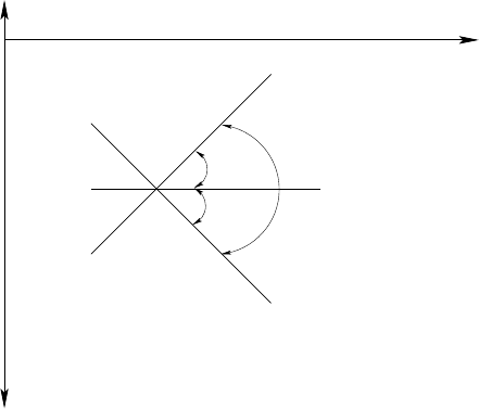
80 CHAPTER 5
we do not recommend the use of neutral physics as implemented in mom4p1 along
with terrain following vertical coordinates. Significant work is required to ensure a
proper treatment of neutral physics with terrain following coordinates, and we are
not prepared to support such in mom4.
−surface
ρ
α(ρ/
s−surface
z−surface
α(ρ/
α(
z) s)
s/z)
z
x
Figure 5.1 Relationship between the slopes of surfaces of constant depth, constant general-
ized vertical coordinate s, and potential density
ρ
. Shown here is a case where
the slope is projected onto a single horizontal direction, so that the slope is given
by the tangent of the indicated angle. This figure is taken from Figure 6.5 of
Griffies (2004).
5.2.3.2 Fluxes for neutral diffusion
The relative slope between the neutral direction and generalized vertical coordi-
nate is required to compute the neutral diffusion flux. We assume here that this
slope is small, thus allowing us to approximate the full diffusion tensor of Redi
(1982) with the small slope approximated tensor of Gent and McWilliams (1990).
To lend mathematical support for these comments, we start with the neutral diffu-
sion flux as written for the small slope approximation in z-models. As discussed in
Section 14.1.4 of Griffies (2004), this flux has horizontal and vertical components
given by
F(h)=−AI∇
ρ
C(5.30)
F(z)=−AIS(
ρ
/z)·∇
ρ
C. (5.31)
Converting this flux to a form appropriate for generalized vertical coordinates re-
quires a transformation of the gradient operator
∇
ρ
=∇z+S(
ρ
/z)∂z
=∇s+ [S(
ρ
/z)−S(s/z)]∂z
=∇s+S(
ρ
/s)∂z.
(5.32)
PARAMETERIZATIONS WITH GENERALIZED VERTICAL COORDINATES 81
The third equality used the slope relation (5.26).
As seen in Section 3.4, the thickness weighted tracer budget contains a contri-
bution from the convergence of a SGS flux in the form
R=−∇s·(dz
ρ
F)−[
ρ
z,s∇s·F]s=sk−1+ [
ρ
z,s∇s·F]s=sk. (5.33)
We are therefore led to consider the dia-surface flux component
F(s)=z,s∇s·F
= (ˆz−S(s/z))·F
=−AI(S(
ρ
/z)−S(s/z))·∇
ρ
C
=−AIS(
ρ
/s)·∇
ρ
C
=S(
ρ
/s)·F(h).
(5.34)
This flux component, as well as the horizontal flux component, take forms isomor-
phic to those for the specific case of s=zgiven by equations (5.30) and (5.31).
This isomorphism follows from the need to only have information about the relative
slope between the generalized surfaces of constant sand the neutral directions.
5.2.3.3 Fluxes for skew diffusion
An arbitrary tracer has a Gent and McWilliams (1990) skew flux in the form
F=Agm (S(
ρ
/z)C,z−ˆz S(
ρ
/z)·∇zC), (5.35)
where Agm is a non-negative skew diffusivity. The horizontal component of this flux
is converted to generalized vertical coordinates via
F(h)=Agm (S(
ρ
/s)+S(s/z))C,z
≈Agm S(
ρ
/s)C,z.(5.36)
Consistent with this same approximation, we are led to the dia-surface component
of the skew flux
z,s∇s·F= (ˆz−S(s/z))·F
=−Agm (S(
ρ
/z)·∇z+S(
ρ
/z)·S(s/z)∂z)C
=−Agm S(
ρ
/z)·(∇s−S(s/z)∂z)C−Agm S(
ρ
/z)·S(s/z)∂zC
=−Agm S(
ρ
/z)· ∇sC
≈ −Agm S(
ρ
/s)·∇sC.
(5.37)
These approximations are reasonable where |S(s/z)|is much smaller than |S(
ρ
/z)|
if S(
ρ
/z)is nontrivial. When the neutral slope S(
ρ
/z)vanishes, as for regions of
zero baroclinicity, this approximation may not be valid when s6=z. However, in re-
gions of vanishing baroclinicity, we expect the error to be of minimal consequence
to the simulation since either the zor sbased skew fluxes are close to zero. In
general, approximating the slope as proposed here leads the modified Gent and
McWilliams (1990) scheme to dissipate neutral slopes as they deviate from sur-
faces of constant generalized vertical coordinate. So long as these surfaces are
quasi-horizontal, the modified scheme should perform in a physically relevant man-
ner.
82 CHAPTER 5
5.2.3.4 Summary of the neutral fluxes
The horizontal and dia-surface components to the small angle neutral diffusion flux
take the form
F(h)=−AI(∇s+S(
ρ
/s)∂z)C
F(s)=S(
ρ
/s)·F(h)(5.38)
where the slope is given by
S(
ρ
/s)=∇
ρ
s
=−z,
ρ
∇s
ρ
.(5.39)
The horizontal and dia-surface skew flux components are approximated by
F(h)≈Agm S(
ρ
/s)C,z
F(s)≈ −Agm S(
ρ
/s)·∇sC.(5.40)
Each of these neutral fluxes are isomorphic to the fluxes used in the z-model
MOM4.0. This isomorphism enables us to transfer the neutral physics technol-
ogy from MOM4.0 directly to mom4p1.

Chapter Six
Depth and pressure based vertical coordinates
The purpose of this chapter is to document issues related to the choice of verti-
cal coordinates. In mom4p1, only depth-based and pressure-based coordinates
are supported. Isopycnal coordinates are not supported. Furthermore, terrain fol-
lowing sigma coordinates are coded in mom4p1. However, more work is required
to reduce pressure gradient errors (Section 4.2) and consistently employ neutral
physics (Section 5.2.3 and Chapter 15). Much in this chapter is derived from lec-
tures of Griffies (2005) at the 2004 GODAE School.
6.1 DEPTH BASED VERTICAL COORDINATES
We use depth based vertical coordinates in this section to discretize the Boussi-
nesq equations.∗Depth based coordinates are also known as volume based coor-
dinates, since for a Boussinesq model which uses depth as the vertical coordinate,
the volume of interior grid cells is constant in the absence of sources. Correspond-
ingly, depth based coordinates are naturally suited for Boussinesq fluids.
6.1.1 Depth coordinate
With a free surface, the vertical domain over which the z-coordinate
s=z(6.1)
ranges is given by the time dependent interval −H≤z≤
η
. Consequently, the
sum of the vertical grid cell increments equals to the total depth of the column
∑
k
dz=H+
η
. (6.2)
The trivial form of the specific thickness z,s=1greatly simplifies the Boussinesq
budgets.
The depth coordinate is very useful for many purposes in global climate mod-
elling, and models based on depth are the most popular ocean climate models.
Their advantages include the following.
•Simple numerical methods have been successfully used in this framework.
•For a Boussinesq fluid, the horizontal pressure gradient can be easily repre-
sented in an accurate manner.
∗Greatbatch and McDougall (2003) discuss an algorithm for non-Boussinesq dynamics in a z-
model. Their methods are implemented in mom4p0a and mom4p0b of Griffies et al. (2004). This
approach may be of special use for non-Boussinesq non-hydrostatic z-models. However, when focus-
ing on hydrostatic models as we do here, pressure based vertical coordinates discussed in Section 6.2
are more convenient to realize non-Boussinesq dynamics.

84 CHAPTER 6
•The equation of state for ocean water can be accurately represented in a
straightforward manner (e.g., Jackett et al. (2006)).
•The upper ocean mixed layer is well parameterized using a z-coordinate.
Unfortunately, these models have some well known disadvantages, which include
the following.
•Representation of tracer transport within the quasi-adiabatic interior is cum-
bersome, with problems becoming more egregious as mesoscale eddies are
admitted (Griffies et al. (2000b)).
•Representation and parameterization of bottom boundary layer processes
and flow are unnatural.
Grid cells have static vertical increments ds=dzwhen s=z, except for the
top. At the top, ∂t(dz) =
η
,t. Hence, the thickness of the top cell grows when the
surface height grows, and it thins when the surface height becomes negative. The
time dependent vertical range of the coordinate slightly complicates a numerical
treatment of the surface cell in z-models (see Griffies et al. (2001) for details of
one such treatment). More problematic, however, is the possibility of a vanishing
top grid cell. That is, the surface cell can be lost (i.e., can become dry) if the free
surface depresses below the depth of the top grid cell’s bottom face. This is a very
inconvenient feature that limits the use of z-coordinates.∗In particular, the follow-
ing studies may require very refined vertical resolution and/or large undulations of
the surface height, and so would not be accessible with a conventional free surface
z-model.
•Process studies of surface mixing and biological cycling may warrant very
refined upper ocean grid cell thickness, some as refined as 1m.
•Realistic tidal fluctuations in some parts of the World Ocean can reach 10m-
20m.
•Coastal models tend to require refined vertical resolution to represent shal-
low coastal processes along the continental shelves and near-shore.
•When coupled to a sea ice model, the weight of the ice will depress the
ocean free surface.
6.1.2 An example of depth coordinates
In some of the following discussion, we illustrate aspects of vertical coordinates by
diagnosing the values for the coordinates from a realistic z-model run with partial
step thicknesses. Partial steps have arbitrary thickness which are set to accurately
represent the bottom topography. The partial step technology was introduced by
Adcroft et al. (1997) in the C-grid MITgcm, and further discussed by Pacanowski
∗Linearized free surfaces, in which the budgets for tracer and momentum are formulated assuming
a constant top cell thickness, avoid problems with vanishing top cells. However, such models do not
conserve total tracer or volume, and so are of limited use for long term climate studies (see Griffies
et al. (2001) and Campin et al. (2004) for discussion).
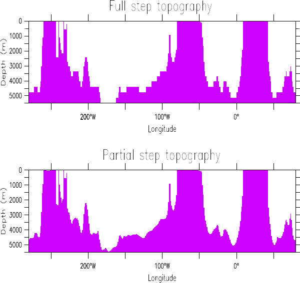
DEPTH AND PRESSURE BASED VERTICAL COORDINATES 85
and Gnanadesikan (1998) for the B-grid Modular Ocean Model (MOM). Figure 6.1
compares the representation of topography in a z-model using partial steps as
realized in the MOM code of Griffies et al. (2004). Many z-models have incorpo-
rated the partial step technology as it provides an important facility to accurately
represent flow and waves near topography.
Because of partial steps, the level next to the ocean bottom has grid cell centers
that are generally at different depths. Hence, the bottom cell in a partial step z-
model computes its pressure gradient with two terms: one due to gradients across
cells with the same grid cell index k, and another due to slopes in the bottom
topography. Details of the pressure gradient calculation are provided in Chapter 4.
All other cells, including the surface, have grid cell centers that are at fixed depths.
Figure 6.2 illustrates the lines of constant partial step depth for this model.
Figure 6.1 Comparison of the partial step versus full step representation of topography as
realized in the z-model discussed by Griffies et al. (2005). This vertical section
is taken along the equator. The model horizontal grid has one degree latitudinal
resolution. The main differences are in the deep ocean in regions where the
topographic slope is gradual. Steep sloped regions, and those in the upper ocean
with refined vertical resolution, show less distinctions.
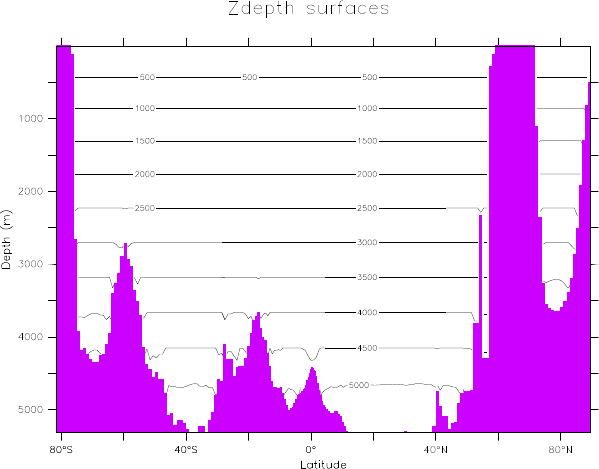
86 CHAPTER 6
Figure 6.2 This figure contours the depth of grid cell centers used in a modern geopotential
ocean model. Deviations from the horizontal occur next to the bottom due to
use of a partial bottom step representation of topography, as illustrated in Fig-
ure 6.1. In this case, the bottom cell has an arbitrary thickness according to the
methods of Adcroft et al. (1997) and Pacanowski and Gnanadesikan (1998). This
technology is common in modern geopotential ocean models, as it provides a
more faithful and robust representation of the ocean bottom. Shown here is a
north-south section along 150◦W.
6.1.3 Depth deviation coordinate
The depth deviation coordinate
s=z−
η
(6.3)
removes the restriction on upper ocean grid cell resolution present with s=z. That
is, s=0is the time independent coordinate value of the ocean surface, no matter
how much the free surface depresses or grows. Hence, no surface cells vanish so
long as
η
>−H. If
η
<−H, the bottom topography is exposed, in which case
the model’s land-sea boundaries are altered. Such necessitates a model that can
allow for wetting and drying of grid cells. Alternatively, it requires a model where
ocean is extended globally, with infinitesimally thin ocean layers present over land.
We do not have such features in mom4p1.
The depth deviation coordinate ranges between −(H+
η
)≤s≤0. The only
time dependent interface in s-space is at the bottom of the column. Consequently,

DEPTH AND PRESSURE BASED VERTICAL COORDINATES 87
by solving the problem at the ocean surface, the deviation coordinate introduces
a problem to the ocean bottom where bottom cells can now vanish. To see this
problem, discretize the deviation coordinate saccording to time independent val-
ues sk. For example, the skvalues can be set as the depths of cells in a model
with s=z. When
η
evolves, depth zand s=z−
η
become different, and so the
depth of a grid cell must be diagnosed based on the time independent value of sk
and the time dependent surface height
zk=sk+
η
. (6.4)
If the time dependent depth of the upper interface of a bottom grid cell is diag-
nosed to be deeper than the actual bottom depth z=−H, then we know that the
bottom grid cell has vanished and so there are problems. To maintain nonvan-
ishing cells requires a limit on how negative
η
can become. For example, if the
upper interface of a bottom cell is −5000m and the bottom interface (at the ocean
bottom) is H=5005m, then the bottom cell is lost if
η
<−5m. This restriction is
of some consequence when aiming to use partial bottom steps (see Figure 6.1)
along with tides and sea ice. In practice, if one is interested in allowing thick sea
ice and nontrivial tidal fluctuations, then it will be necessary to keep the bottom
partial steps thicker than roughly 10m-20m. This is arguably a less onerous con-
straint on the model’s vertical grid spacing than the complementary problem at the
ocean surface encountered with the traditional z-coordinate s=z.
In summary, grid cells have static grid increments ds=dzfor all cells except the
bottom. At the bottom, ∂t(dz) = ∂t(ds) =
η
,t. Hence, the thickness of the bottom
cell grows when the surface height grows, and it thins when the surface height
becomes negative. The bottom cell can be lost if
η
becomes too negative. The
sum of the vertical increments yields the total depth of the column ∑kds= (H+
η
). Because the surface height fluctuations are so much smaller than changes in
bottom topography, the depth deviation coordinate appears nearly the same as the
depth coordinate when viewed over the full depth range of a typical model such as
in Figure 6.2.
The author knows of no model routinely using the depth deviation coordinate. It
does appear to have advantages for certain applications over the depth coordinate.
However, the zstar coordinate discussed next resolves problems at both the top
and bottom, and so is clearly preferable. The depth deviation coordinate is not
implemented in mom4p1 for these reasons.
6.1.4 Zstar coordinate
To overcome problems with vanishing surface and/or bottom cells, we consider the
zstar coordinate
z∗=Hz−
η
H+
η
. (6.5)
This coordinate is closely related to the “eta” coordinate used in many atmospheric
models (see Black (1994) for a review of eta coordinate atmospheric models). It
was originally used in ocean models by Stacey et al. (1995) for studies of tides
next to shelves, and it has been recently promoted by Adcroft and Campin (2004)
for global climate modelling.

88 CHAPTER 6
The surfaces of constant z∗are quasi-horizontal. Indeed, the z∗coordinate re-
duces to zwhen
η
is zero. In general, when noting the large differences between
undulations of the bottom topography versus undulations in the surface height, it
is clear that surfaces constant z∗are very similar to the depth surfaces shown
in Figure 6.2. These properties greatly reduce difficulties of computing the hori-
zontal pressure gradient relative to terrain following sigma models discussed next.
Additionally, since z∗=zwhen
η
=0, no flow is spontaneously generated in an
unforced ocean starting from rest, regardless the bottom topography.∗This behav-
ior is in contrast to the case with sigma models, where pressure gradient errors in
the presence of nontrivial topographic variations can generate nontrivial sponta-
neous flow from a resting state, depending on the sophistication of the pressure
gradient solver.†The quasi-horizontal nature of the coordinate surfaces also facil-
itates the implementation of neutral physics parameterizations in z∗models using
the same techniques as in z-models (see Chapters 13-16 of Griffies (2004) for a
discussion of neutral physics in z-models, as well as Section 5.2.3 and Chapter 15
in this document for treatment in mom4p1).
The range over which z∗varies is time independent −H≤z∗≤0. Hence, all
cells remain nonvanishing, so long as the surface height maintains
η
>−H. This
is a minor constraint relative to that encountered on the surface height when using
s=zor s=z−
η
.
Because z∗has a time independent range, all grid cells have static increments
ds, and the sum of the vertical increments yields the time independent ocean
depth ∑kds=H. The z∗coordinate is therefore invisible to undulations of the
free surface, since it moves along with the free surface. This property means that
no spurious vertical transport is induced across surfaces of constant z∗by the
motion of external gravity waves. Such spurious transport can be a problem in
z-models, especially those with tidal forcing. Quite generally, the time independent
range for the z∗coordinate is a very convenient property that allows for a nearly
arbitrary vertical resolution even in the presence of large amplitude fluctuations of
the surface height, again so long as
η
>−H.
6.1.5 Depth sigma coordinate
The depth-sigma coordinate
σ
=z∗/H
=z−
η
H+
η
(6.6)
is the canonical terrain following coordinate. Figure 6.3 illustrates this coordinate
in a realistic model. The sigma coordinate has a long history of use in coastal
modelling. For reviews, see Greatbatch and Mellor (1999) and Ezer et al. (2002).
Models based on the sigma coordinate have also been successfully extended to
basinwide studies, as well as recent global work by Diansky et al. (2002).
∗Because of the use of partial bottom steps, there are two terms contributing to horizontal pressure
gradients within the bottom level when s=z. As discussed by Pacanowski and Gnanadesikan (1998),
these two terms lead to modest pressure gradient errors. These errors, however, are far smaller than
those encountered with
σ
coordinates.
†Shchepetkin and McWilliams (2002) provide a thorough discussion of pressure gradient solvers
along with methods for reducing the pressure gradient error.

DEPTH AND PRESSURE BASED VERTICAL COORDINATES 89
Just as for z∗, the range over which the sigma coordinate varies is time indepen-
dent. Here, it is given by the dimensionless range −1≤
σ
≤0. Hence, all cells
have static grid increments ds, and the sum of the vertical increments yields unity
∑kds=1. So long as the surface height is not depressed deeper than the ocean
bottom (i.e., so long as
η
>−H), then all cells remain nonvanishing.∗
Some further key advantages of the sigma coordinate are the following.
•It provides a natural framework to represent bottom influenced flow and to
parameterize bottom boundary layer processes.
•Thermodynamic effects associated with the equation of state are well repre-
sented with this coordinate.
However, some of the disadvantages are the following:
•As with the z-models, representation of the quasi-adiabatic interior is cum-
bersome due to numerical truncation errors inducing unphysically large lev-
els of spurious mixing, especially in the presence of vigorous mesoscale
eddies. Parameterization of these processes using neutral physics schemes
may be more difficult numerically than in the z-models. The reason is that
neutral directions generally have slopes less than 1/100 relative to the hori-
zontal, but can have order unity slopes relative to sigma surfaces. The larger
relative slopes precludes the small slope approximation commonly made
with z-model implementations of neutral physics. The small slope approx-
imation provides for simplification of the schemes, and improves computa-
tional efficiency.
•Sigma models have difficulty accurately representing the horizontal pressure
gradient in the presence of realistic topography, where slopes are commonly
larger than 1/100 (see Section 3.5 for a discussion of the pressure gradient
calculation).
Griffies et al. (2000a) notes that there are few examples of global climate models
running with terrain following vertical coordinates. Diansky et al. (2002) is the only
exception known to the author. This situation is largely due to problems represent-
ing realistic topography without incurring unacceptable pressure gradient errors, as
well as difficulties implementing parameterizations of neutral physical processes.
There are notable efforts to resolve these problems, such as the pressure gradient
work of Shchepetkin and McWilliams (2002). Continued efforts along these lines
may soon facilitate the more common use of terrain following coordinates for global
ocean climate modelling. At present, the sigma coordinate is coded in mom4p1
in hopes that it will motivate researchers to further investigate its utility for ocean
modelling.
6.1.6 Summary of the depth based vertical coordinates
Depth based vertical coordinates are natural for Boussinesq equations. These co-
ordinates and their specific thicknesses z,sare summarized in Table 6.1. Notably,
∗If
η
<−H, besides drying up a region of ocean, the specific thickness z,s=H+
η
changes
sign, which signals a singularity in the vertical grid definition. The same problem occurs for the z∗
coordinate.
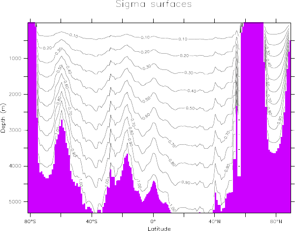
90 CHAPTER 6
Figure 6.3 Constant sigma surfaces as diagnosed in a z-model. Shown here is a section
along 150◦W, as in Figure 6.2. Note the strong variations in the contours, as
determined by changes in the bottom topography.
both the sigma and zstar coordinates have time independent ranges, but time
dependent specific thicknesses. In contrast, the depth and depth deviation coor-
dinates have time dependent depth ranges and time independent specific thick-
nesses. If plotted with the same range as those given in Figure 6.2, surfaces of
constant depth deviation and constant zstar are indistinguishable from surfaces
of constant depth. This result follows since the surface height undulations are so
much smaller than undulations in the bottom topography, thus making the depth
deviation and zstar coordinates very close to horizontal in most parts of the ocean.
6.2 PRESSURE BASED COORDINATES
The second class of vertical coordinates that we discuss is based on pressure.
Pressure-based coordinates are used to discretize the non-Boussinesq equations,
and these coordinates are also known as mass based coordinates. This name
is based on noting that for a non-Boussinesq fluid using pressure, the mass of
interior grid cells is constant without sources (e.g., see equation (3.180)).
Pressure coordinates provide a straightforward way to generalize Boussinesq
z-models to non-Boussinesq pressure models (Huang et al., 2001; DeSzoeke and
DEPTH AND PRESSURE BASED VERTICAL COORDINATES 91
COORD DEFINITION RANGE z,s
geopotential z−H≤z≤
η
1
z-deviation z0=z−
η
−(H+
η
)≤z0≤0 1
z-star z∗=H(z−
η
)/(H+
η
)−H≤z∗≤0 1 +
η
/H
z-sigma
σ
(z)= (z−
η
)/(H+
η
)−1≤
σ
≤0H+
η
Table 6.1 Table of vertical coordinates based on depth. These coordinates are naturally used
for discretizing the Boussinesq equations. Note that the specific thickness z,sis
depth independent. This property proves to be important for developing numer-
ical algorithms in Section 7.6. The coordinates s=z,s=z∗, and s=
σ
(z)are
coded in mom4p1, whereas the depth deviation coordinate is not.
Samelson, 2002; Marshall et al., 2004; Losch et al., 2004). The reason is that
there is an isomorphism between the Boussinesq equations written in depth based
coordinates and non-Boussinesq equations written in pressure based coordinates.
The root of this isomorphism is the simplification of the density weighted specific
thickness
ρ
z,sfor pressure based coordinates. We detail this point in the following
discussions.
Pressure based vertical coordinates that we consider include the following:
s=ppressure (6.7)
s=p−papressure-deviation (6.8)
s=p−pa
pb−papressure-sigma (6.9)
s=po
bp−pa
pb−papressure-star. (6.10)
In these equations, pis the hydrostatic pressure at some depth within the ocean
fluid, pais the pressure applied at the ocean surface z=
η
from any media above
the ocean, such as the atmosphere and sea ice, pbis the hydrostatic pressure
at the solid-earth lower boundary arising from all fluid above the bottom (ocean
water and paabove the ocean), and po
bis a time independent reference pressure,
usually taken to be the bottom pressure in a resting ocean.∗Since p,z=−
ρ
g<0
is single signed for the hydrostatic fluid, pressure provides a well defined vertical
coordinate. Strengths and weaknesses of the corresponding depth based coordi-
nates also hold for the pressure based coordinates, with the main difference being
that pressure based models are non-Boussinesq.
6.2.1 Pressure coordinate
With a free surface, the vertical domain over which the p-coordinate
s=p(6.11)
∗Note that equation (11.64) of Griffies (2004) used the time dependent pbrather than the time
independent reference pressure po
b. The former vertical coordinate has not been used in practice, and
so we focus here on that coordinate defined with the reference pressure po
b.
92 CHAPTER 6
ranges is given by pa≤p≤pb. Hence, the surface and bottom boundaries are
time dependent, whereas the density weighted specific thickness is constant
ρ
z,s=−g−1(6.12)
where the hydrostatic equation p,z=−
ρ
gwas used. The relation (6.12) is
the root of the isomorphism between Boussinesq depth based models and non-
Boussinesq pressure based models.
The time dependent range for the pressure coordinate complicates the treatment
of both the top and bottom cells. In particular, if the bottom pressure is less than the
time independent discrete pressure level at the top interface of the lowest cell, then
there is no mass within the bottom cell. Likewise, if the applied pressure is greater
than the discrete pressure level at the bottom interface of the top cell, then there
is no mass in the top cell. These results mean that grid cells have static vertical
coordinate increments ds=dpfor all cells except the top and bottom. At the top,
∂t(ds) = ∂tpaand at the bottom ∂t(ds) = −∂tpb. The associated mass per unit
area in the cells evolves according to ∂t(
ρ
dz) = −g−1∂tpaat the surface, and
∂t(
ρ
dz) = g−1∂tpbat the bottom. Hence, the mass within the top cell decreases
when the applied pressure increases, and the mass in the bottom cell increases
when the bottom pressure increases. Both the surface and the bottom cells can
therefore vanish depending on the applied and bottom pressures.
The sum of the vertical coordinate increments can be found by noting the total
mass per area is given by
g−1(pb−pa) = ∑
ρ
dz
=∑
ρ
z,sds
=−g−1∑ds,
(6.13)
thus yielding the time dependent result
∑ds=−(pb−pa). (6.14)
6.2.2 Pressure deviation coordinate
The pressure deviation coordinate
s=p−pa(6.15)
removes the restriction on upper ocean grid cell resolution since s=0is the time
independent value of the ocean surface. That is, this coordinate ranges between
0≤s≤pb−pa. This coordinate is isomorphic to the depth deviation coordi-
nate s=z−
η
discussed in Section 6.1.3, and shares the same limitations which
prompt us not to have this coordinate coded in mom4p1.
In summary, grid cells have static vertical coordinate increments dsfor all cells
except the bottom. At the bottom ∂t(ds) = −∂t(pb−pa). The associated mass
per unit area in the bottom cell evolves according to ∂t(
ρ
dz) = g−1∂t(pb−pa).
As for the pressure coordinate, the sum of the vertical coordinate increments yields
∑ds=−(pb−pa). (6.16)

DEPTH AND PRESSURE BASED VERTICAL COORDINATES 93
6.2.3 Pstar coordinate
The pstar coordinate is given by
p∗=po
bp−pa
pb−pa, (6.17)
where po
bis a time independent reference pressure generally chosen as
po
b=g
η
Z
−H
dz
ρ
init, (6.18)
This coordinate is isomorphic to the z∗coordinate, with p∗extending over the time
independent range 0≤p∗≤po
b.
The sum of the vertical coordinate increments can be found by noting the total
mass per area is given by
g−1(pb−pa) = ∑
ρ
dz
=∑
ρ
z,sds
=−pb−pa
g po
b∑ds,
(6.19)
thus yielding the time independent result
∑ds=−po
b. (6.20)
6.2.4 Pressure sigma coordinate
The pressure-sigma terrain following coordinate
σ
(p)=p−pa
pb−pa(6.21)
is the pressure analog to the depth based sigma coordinate
σ
(z)= (z−
η
)/(H+
η
). This coordinate has been used by Huang et al. (2001), and it shares the same
advantages and disadvantages as the depth-based sigma coordinate. Grid cells
have static vertical coordinate increments dsfor all cells. The associated mass per
unit area never vanishes in any cell, so long as the bottom pressure is greater than
the applied pressure.
The sum of the vertical coordinate increments can be found by noting the total
mass per area is given by
g−1(pb−pa) = ∑
ρ
dz
=∑
ρ
z,sds
=−g−1(pb−pa)∑ds,
(6.22)
thus yielding the time independent result
∑ds=−1. (6.23)

94 CHAPTER 6
COORD DEFINITION RANGE g
ρ
z,s
pressure p pa≤p≤pb−1
p-deviation p0=p−pa0≤p0≤pb−pa−1
pstar p∗=po
b(p−pa)/(pb−pa)0≤p∗≤po
b−(pb−pa)/po
b
p-sigma
σ
(p)= (p−pa)/(pb−pa)0≤
σ
≤1−(pb−pa)
Table 6.2 Table of vertical coordinates based on pressure. These coordinates are naturally
used for non-Boussinesq dynamics. Note that the density weighted specific thick-
ness
ρ
z,sis depth independent. This property proves to be important for devel-
oping numerical algorithms in Section 7.6. The coordinates s=p,s=p∗, and
s=
σ
(p)are coded in mom4p1, whereas the pressure deviation coordinate is not.
6.2.5 Summary of the pressure based vertical coordinates
A technical reason that the pressure based coordinates considered here are so
useful for non-Boussinesq hydrostatic modelling is that
ρ
z,sis either a constant or
a two-dimensional field. In contrast, for depth based models
ρ
z,sis proportional
to the three-dimensional in situ density
ρ
, thus necessitating special algorithmic
treatment for non-Boussinesq z-models (see Greatbatch and McDougall (2003)
and Griffies (2004)). Table 6.2 summarizes the pressure-based coordinates dis-
cussed in this section. The pressure and pressure deviation coordinates have
time dependent ranges but time independent specific thicknesses
ρ
z,s. The sigma
and pstar coordinates have time independent range but time dependent specific
thickness.
As Table 6.2 reveals, the specific thickness z,sis negative for the pressure-based
coordinates, whereas it is positive for the depth-based coordinate (Table 6.1). The
sign change arises since upward motion in a fluid column increases the geopoten-
tial coordinate zyet decreases the hydrostatic pressure p. To establish a conven-
tion, we assume that the thickness of a grid cell in zspace is always positive
dz=z,sds>0 (6.24)
as is the case in the conventional z-models. With z,s<0for the pressure-based
vertical coordinates, the thickness of grid cells in sspace is negative
ds<0for pressure-based coordinates with z,s<0.(6.25)
PART 2
Numerical formulations
The purpose of this part of the document is to describe algorithms used to nu-
merically solve the ocean primitive equations in mom4p1.

Chapter Seven
Quasi-Eulerian Algorithms
There are two types of ocean models as distinguished by their solution algorithms
(Adcroft and Hallberg, 2006). Eulerian vertical coordinate algorithms diagnose the
dia-surface velocity component from the continuity equation. Lagrangian vertical
coordinate algorithms specify the dia-surface velocity component (e.g., zero di-
apycnal velocity in adiabatic simulations with isopycnal coordinates). Eulerian in
this context does not mean that a grid cell has a time constant vertical position.
Hence, the term quasi-Eulerian is often used. This chapter develops the semi-
discrete budgets of a hydrostatic ocean model and then presents quasi-Eulerian
solution algorithms. Notably, as implemented in mom4p1, the quasi-Eulerian al-
gorithms are formulated assuming a time independent number of grid cells. That
is, mom4p1 does not allow for vanishing cell thickness. Such simplifies the algo-
rithms in many ways, but in turn limits the extent to which this code can be used
for simulations where water masses change in a nontrivial manner (e.g., wetting
and drying is not handled in mom4p1).
7.1 PRESSURE AND GEOPOTENTIAL AT TRACER POINTS
We discussed the discrete pressure gradient body force appropriate for a finite
difference discretization in Sections 4.2 and 4.3. We require the anomalous hydro-
static pressure in the depth based models, and the anomalous geopotential height
in the pressure based models. That is, for depth based vertical coordinate models,
we need a discretization of the anomalous hydrostatic pressure (equation (4.19))
p0=gR0
z
ρ
0dz s =z
p0=gR
η
z
ρ
0dz s =z∗,
σ
(z).(7.1)
For pressure based vertical coordinate models, we need a discretization of the
anomalous geopotential (equation (4.24))
Φ0=−(g/
ρ
o)
z
Z
−H
ρ
0dz. (7.2)
The vertical integrals involve some ambguity for the finite difference formulation,
since the tracer point is not vertically centred within the tracer cell for the case of
a vertically nonuniform grid. In this case, we may choose to compute the pressure
and geopotential at the tracer point using a more accurate vertical integration that
accounts for the non-centred placement of the tracer point.
The purpose of this section is to describe two methods used for the calculation of
the pressure and geopotential at the tracer grid point. Details of this discretization

98 CHAPTER 7
affect the manner used for diagnosing the pressure conversion to buoyancy work,
as described in Sections 9.4 and 9.5. The mom4p1 code provides both choices,
with both producing analogous results for the surface height and bottom pressure.
7.1.1 Pressure at tracer point: energetic method
If the equation of state is linear, and both density and velocity are advected with
second order centered differences, then the conversion of pressure work to buoy-
ancy work will balance potential energy changes. This equality led Bryan (1969)
to formulate the hydrostatic pressure calculation according to
p0
k+1=p0
k+gdzwtk
ρ
0
k
z. (7.3)
That is, anomalous hydrostatic pressure is computed given knowledge of the thick-
nesses dzwt and the density
ρ
0
k. In this equation, primes refer to anomalies relative
to the background Boussinesq density
ρ
0=
ρ
−
ρ
o(7.4)
and
ρ
0
k
z= (
ρ
0
k+
ρ
0
k+1)/2 (7.5)
is the simple vertical average of density. This average is the same as a finite
volume average only if the grid cell thicknesses are uniform. With stretched ver-
tical grids, the simple average differs from the finite volume average presented in
Section 7.1.1. At the ocean surface, no average is available, so we use the finite
volume value for the pressure
p0
k=1=gdzwtk=0
ρ
0
k=1. (7.6)
Given this surface value, we then iterate downwards according to equation (7.3) to
diagnose the anomalous hydrostatic pressure at each discrete k-level.
7.1.2 Pressure at a tracer point: finite volume considerations
Although the finite volume method for computing the pressure force requires the
pressure and geopotential to be computed at the bottom of the tracer cells, we
may choose to use a finite volume motivated approach for computing the pressure
and geopotential at the tracer point. Referring to the right hand panel in Figure
7.1, a finite volume motivated computation of hydrostatic pressure at a tracer point
is given by
p0
k=1=gdztupk=1
ρ
0
k=1
p0
k+1=p0
k+gdztlok
ρ
0
k+gdztupk+1
ρ
0
k+1.(7.7)
The pressure at k=1is the same as prescribed in the energetic method. However,
for stretched vertical grid cells, the interior cells have a different discrete pressure
from that computed in the energetic method. The finite volume approach is more
accurate for stretched vertical grids.

QUASI-EULERIAN ALGORITHMS 99
7.1.3 Discrete geopotential based on energetic considerations
Following in a manner analogous to the anomalous hydrostatic pressure in Section
7.1.1, we have the discretized anomalous geopotential
Φ0
k=kbot =−(g/
ρ
o)dzwtkbot
ρ
0
k=kbot
Φ0
k=Φ0
k+1−(g/
ρ
o)dzwtk
ρ
0
k
z.(7.8)
Iteration starts from the bottom at k=kbot using the finite volume expression, and
moves upward in the column towards the surface.
7.1.4 Discrete geopotential based on finite volume considerations
Following in a manner completely analogous to the anomalous hydrostatic pres-
sure in Section 7.1.2, we have the discretized anomalous geopotential
Φ0
k=kbot =−(g/
ρ
o)dztlokbot
ρ
0
k=kbot
Φ0
k=Φ0
k+1−(g/
ρ
o)dztupk+1
ρ
0
k+1−(g/
ρ
o)dztlok
ρ
0
k.(7.9)
Iteration starts from the bottom at k=kbot using the finite volume expression, and
moves upward in the column towards the surface.
7.2 INITIALIZING BOUSSINESQ AND NONBOUSSINESQ MODELS
When initializing a Boussinesq model, we place a fluid with initial in situ density
ρ
init onto a grid with vertical increments dzt. Hence, both the density and volume
of the grid cells are specified. The initial mass of fluid is thus implied from this
initialization method. Furthermore, by definition, the surface elevation
η
is zero.
For the nonBoussinesq model, we place a fluid with initial in situ density
ρ
init
onto a grid with vertical pressure increments dst. Hence, both the density and
mass of the grid cells are specified. The initial volume of fluid is thus implied from
this initialization method. Furthermore, by definition, the bottom pressure anomaly,
pbot t −pbot0, is zero, since we choose pbot0 as the initial bottom pressure.
The initialization methods are isomorphic. Notably, when initializing the Boussi-
nesq model, there is no guarantee that its bottom pressure anomaly will be intially
zero. Likewise, there is no guarantee that the surface elevation
η
will be zero with
the nonBoussinesq initialization. If one wishes to ensure that such is the case,
an extra step is required. We outline these considerations for the nonBoussinesq
model.
7.2.1 Three general approaches
There are three general ways to approach nonBoussinesq initialization in order to
maintain a zero initial surface height. First, we can modify the vertical pressure
increments dst of the grid cells to accomodate the initial density and to retain
a zero surface height. This approach generally requires nontrivial horizontal de-
viations in the dst array, so that it has full grid dependence dst(i,j,k). Such
dependence is generally acceptable for the bottom, where partial cells introduce
this three-dimensional dependence to the vertical grid increments. However, with
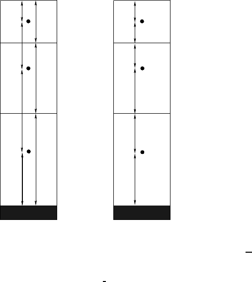
100 CHAPTER 7
dztlo(k=kbot)
dzt(k=1)
dzt(k=2)
dzt(k=kbot)
dzwt(k=kbot)
dzwt(k=2)
dzwt(k=1)
dzwt(k=0) dztup(1)
dztlo(1)
dztup(2)
dztlo(2)
dztup(k=kbot)
Figure 7.1 A vertical column of three tracer cells and the corresponding verti-
cal cell dimensions. In mom4p1, the vertical spacing is related by
dztk= (dzwtk−1+dzwtk)/2. With this specification, the average tracer Tz=
(Tk+Tk+1)/2 lives at the bottom of the tracer cell Tkand so is co-located with
the dia-surface velocity component w btk. The right column exposes the half-
distances, which measure the distance from the tracer cell point to the top and
bottom faces of the tracer cell. The half-distances are used in the finite volume
formulation of pressure and geopotential computed at the tracer points (Sec-
tions 7.1.2 and 7.1.4), whereas the grid spacing dzwt is used for the energetically
based computation of pressure and geopotential computed at the tracer points
(Sections 7.1.1 and 7.1.3).
this added dependence in the ocean interior, there is a possibility for introducing
pressure gradient errors, depending on the magnitude of the horizontal variations.
If the variations are minor, then this approach may be acceptable. Also, if varia-
tions are isolated to marginal seas which have no direct connection to the interior
ocean, then one may choose to do so.
A second approach is to modify the initial density field. This approach, however,
may fail after some time integration, depending on the surface forcing. That is,
over time the model may be forced towards a density structure similar to the initial
structure, in which case the possibility exists for losing the bottom cell in the model
if the evolved bottom pressure becomes lighter than the pressure at the top of the
bottom cell. It is interesting, nonetheless, to note that most ocean analyses are
taken on pressure levels, not depth levels, so interpolation to pressure levels may
provide an option that the user wishes to exercise with initialization. We do not
provide options in mom4p1 for this interpolation.
A third approach is motivated by one used with the MITgcm, and it is facilitated
in the mom4p1 code as an option. Here, we deepen the bottom topography so that
QUASI-EULERIAN ALGORITHMS 101
the initial mass (as set by the pressure increments) and density result in vertical
columns with zero initial surface height. Depending on details of the initial density
field and the pressure increments, the changes in the bottom topography are often
quite minor.
These issues of initializing the nonBoussinesq model are fundamental to how
the vertical grid increments are determined for the model. So we turn to a dis-
cussion of these increments in Section 7.3. Before doing so, we step through an
example to illustrate the issues that arise with nonBoussinesq initialization.
7.2.2 Initializing a column: an explicit example
Consider an explicit example where we wish to initialize a non-Boussinesq ocean
column with three cells. The methods discussed in Section 7.3 follow the basic ap-
proach given here. First, we define the vertical cell thicknesses dzt0according to
the methods of a Boussinesq model. In particular, the bottom cell has a thickness
that is potentially quite small, according to the details of the bottom topography.
Let us assume that the cells are found to have the following thicknesses
dz0
k=1=∆(7.10)
dz0
k=2=8∆(7.11)
dz0
k=3=∆, (7.12)
where ∆is a nonzero thickness, and H=10 ∆is the ocean depth. With this
configuration of vertical cells, the top and bottom cells are thin, whereas the interior
cell is thick.
Next, we define the mass within a layer, or more precisely the mass per horizon-
tal area. This is done by assuming the density of the column is a constant
ρ
o, so
that the vertical hydrostatic pressure increments are given by
ds0
k=1=−
ρ
og∆(7.13)
ds0
k=2=−8
ρ
og∆(7.14)
ds0
k=3=−
ρ
og∆, (7.15)
where the minus sign arises since pressure of a parcel increases downward,
whereas the height of a parcel increases upward. Note that the pressure increment
at the bottom cell is a function of (i,j,k), due to the partial bottom cell methods,
whereas the pressure increments in the interior cells are independent of horizontal
position.
The next step acknowledges that the initial density is not
ρ
o, but can be deter-
mined by knowledge of the initial temperature, salinity, and pressure as given by
ds0. Let us assume these densities are as follows
ρ
init
k=1= (5/10)
ρ
o(7.16)
ρ
init
k=2=
ρ
o(7.17)
ρ
init
k=3= (15/10)
ρ
o. (7.18)
This density then allows us to recompute the thicknesses of the grid cells according

102 CHAPTER 7
to
dz1
k=−ds0
k
g
ρ
init
=
ρ
o
ρ
init dz0
k.
(7.19)
For the present example, we have
dz1
k=1=2∆(7.20)
dz1
k=2=8∆(7.21)
dz1
k=3= (2/3)∆, (7.22)
This example highlights a common occurance. That is, the initial thickness of the
column, ∑kdz1
k, is not equal to the thickness H=∑kdz0
kof a resting ocean. We
have various options.
•NONZERO SURFACE HEIGHT: The initial surface height is given by
η
init =−H+∑
k
dz1
k, (7.23)
which can be positive or negative.
•ADDING MASS TO BRING NEGATIVE SURFACE HEIGHT ANOMALY TO ZERO:
When the thickness of the column is less than H, we may choose to add
more mass to the bottom partial cell in order to fill the column to have the
same volumn as a Boussinesq column. In this case, we extend the bottom
cell so that its thickness is
dz∗
k=kmt =H−
kmt−1
∑
k=1
dz1
k(7.24)
and then the bottom pressure increment is also modified to
ds∗
k=kmt =−
ρ
init gdz∗
k=kmt. (7.25)
This method is generally performed during the mom4p1 initialization.
•REMOVING MASS TO BRING POSITIVE SURFACE HEIGHT ANOMALY TO ZERO:
As a complement to the above, we may choose to reduce the thickness of
a bottom partial cell in order to bring the initial surface height to zero. Cor-
respondingly, we will reduce the mass of this cell. The same equations are
relevant as above
dz∗
k=kmt =H−
kmt−1
∑
k=1
dz1
k(7.26)
and then the bottom pressure increment is
ds∗
k=kmt =−
ρ
init gdz∗
k=kmt. (7.27)
Importantly, this method is available only if the bottom partial cell has suffi-
cient volume and mass. Additionally, we may choose to maintain a minimum
thickness in the bottom cell, so to not stress the integrity of the numerics with
a very thin bottom cell. For relatively thin partial cells, we may not be able to
remove volume and mass without producing an unacceptably thin, or nega-
tive, bottom cell. We then must live with a nonzero surface iniitial height, or
we could change the bottom depth.

QUASI-EULERIAN ALGORITHMS 103
•DEEPEN THE TOPOGRAPHY: When the thickness of a column is greater than
H, we may choose to deepen the ocean bottom in order to allow for the
surface height to remain with an initial zero anomaly.
•MODIFY INITIAL DENSITY: We may choose to modify the initial temperature
and salinity in order to change the initial density so that the mass of a column
is consistent with a zero surface height. This option has not been exercised
in mom4p1.
Of the above methods for initialization, our preference is to fill in mass so that
there are no negative initial surface height anomalies. Additionally, we aim to re-
move mass when available so to reduce the occurance of positive surface height
anomalies. Where there is not enough mass for this removal, such as in thin par-
tial cells, we allow for the surface height to be positive. Additionally, for inland
seas, such as the Black Sea in the GFDL OM3 model, we may choose to modify
the initial
ρ
oused to define the mass within the column. The Black Sea is a case
where its initial density is somewhat less than
ρ
o, and the presence of thin bottom
partial cells can lead to huge (order 20m) initial surface height anomalies. So a bit
of fine tuning has been found to be useful in this basin. Finally, there are options
for determining the modified bottom depth for those cases when it is necessary
to deepen the topography. This option should be exercised only when the other
approaches fail.
7.3 VERTICAL DIMENSIONS OF GRID CELLS
The density weighted thickness of a grid cell is of fundamental importance in the
formulation presented in this document. In particular, density weighted thickness
of a tracer cell is a basic ingredient and the values on a velocity cell are diagnosed
according to the minimum surrounding tracer cell values. Given these fields, most
of the equations for the ocean model retain the same appearance for arbitrary ver-
tical coordinates. The technology of generalized vertical coordinates then resides
in the module specifying
ρ
dz(the mom4p1 ocean thickness module), with extra
work also needed for the pressure and grid modules.
In addition to the density weighted thicknesses, we are in need of the depth of a
grid cell center, depth of the grid cell bottom, and vertical dimensions within the grid
cell. Information is needed for these distances both in depth space (z-coordinate),
and coordinate space (s-coordinate). These needs introduce new arrays which are
to be updated and saved for restarts.
Figure 7.1 defines notation for the grid cell thicknesses used in mom4p1. Here,
the left figure exposes the vertical dimensions of the tracer grid cell, dzt and
the distance between the T-cell points, dzwt. The right figure exposes the half-
distances, which measure the distance from the T-cell point to the upper face of
the cell, dztup, and the lower face, dztlo.
7.3.1 Thickness of a grid cell
The thickness of a grid cell is written
dz=z,sds. (7.28)

104 CHAPTER 7
COORD DEFINITION CELL THICKNESS
geopotential zdz
zstar z∗=H(z−
η
)/(H+
η
)dz= (1+
η
/H)dz∗
z-sigma
σ
(z)= (z−
η
)/(H+
η
)dz= (H+
η
)d
σ
(z)
pressure pdz=−(
ρ
g)−1dp
pstar p∗=po
b(p−pa)/(pb−pa)dz=−[(pb−pa)/(
ρ
g po
b)] dp∗
p-sigma
σ
(p)= (p−pa)/(pb−pa)dz=−[(pb−pa)/(
ρ
g)] d
σ
(p)
Table 7.1 Table of vertical thicknesses dzfor grid cells as determined on the tracer grid
using the vertical coordinates discussed in Chapter 6. The vertical coordinate
increments are specified, and the vertical thicknesses dzare diagnosed.
For a tracer cell, this is written in the mom4p1 code as
dzt =dzt dst ∗dst. (7.29)
Inspection of the results from Tables 6.1 and 6.2 lead to the thicknesses given in
Table 7.1, which are again applied to the tracer grid. The corresponding velocity
cell thicknesses are diagnosed based on the tracer cell values.
For the finite volume approach to computing the pressure and geopotential, as
discussed in Section 7.1.2, we need a method to compute the half-thicknesses.
For this purpose, we assume the specific thickness factor dzt dst is constant
across the thickness of a tracer cell. We also assume knowledge of the half-s-
thicknesses dstlo and dstup, thus leading to
dztlo =dzt dst ∗dstlo (7.30)
dztup =dzt dst ∗dstup. (7.31)
The full cell thickness is then recovered by setting
dzt =dztlo +dztup, (7.32)
where
dst =dstlo +dstup. (7.33)
7.3.2 Vertical distance between tracer points
Through summation from the ocean surface, knowledge of the tracer cell thick-
nesses dztkwithin a vertical column provides the depth of the bottom of any tracer
cell within the column. For many purposes, it is also important to know the depth
where the tracer point is located. This information is obtained via vertical summa-
tion from the distance between two vertically adjacent tracer cell points. As seen
in Section 7.1 when discussing the hydrostatic pressure and the geopotential, the
vertical distance between tracer points is known as dzwt and the corresponding
velocity cell vertical distance is dzwu.
7.3.2.1 Energetic based approach
For depth based vertical coordinates, dzwt is computed according to the results
in Table 7.1 given the corresponding coordinate thicknesses dswt. For pressure

QUASI-EULERIAN ALGORITHMS 105
based vertical coordinates using the energetic approach from Section 7.1.1, we
are guided by the result (7.3) for the hydrostatic pressure computed in a depth
based vertical coordinate model. In general, this expression takes the form
ds= (s,z)zdz(7.34)
where az= (ak+ak+1)/2is an unweighted discrete vertical average. Introducing
model arrays leads to
dzwtk=2
(s,z)k+ (s,z)k+1dswtk.(7.35)
For example, with s=p, this relation takes the form
dzwtk=−2
g(
ρ
k+
ρ
k+1)dswtk, (7.36)
where dswt is known and is negative, since pressure decreases upward, whereas
geopotential increases upward.
7.3.2.2 Finite volume approach
From the finite volume approach described in Section 7.3.1, we follow expressions
(7.30) and (7.31) for the thickness of a grid cell to write
dzwtk=0=dztupk=1(7.37)
dzwtk>1=dztlok−1+dztupk(7.38)
dzwtk=kbot =dztlok=kbot. (7.39)
7.3.3 Summary of grid increments
We now summarize the previous results for the vertical coordinates z,z∗,
σ
(z),p,
p∗, and
σ
(p). The notation used in mom4 is used here to allow for ready imple-
mentation in the model code.
7.3.3.1 Geopotential vertical coordinate
The geopotential vertical coordinate has the following grid dimensions
dzt dst(i,j,k) = 1
dzwt(i,j,k=0) = zt(k=1) + eta t(i,j)
dzt(i,j,k=1) = zw(k=1) + eta t(i,j).
(7.40)
The initial values of the depth of tracer points, depth zt, remain unchanged in
time. However, the thickness of the top cell is time dependent.
7.3.3.2 z∗vertical coordinate
The z∗coordinate has the grid dimensions
dzt dst(i,j,k) = 1+eta t(i,j)/ht(i,j)
dst(i,j,k) = dzt(i,j,k)|
τ
=0
dswt(i,j,k) = dzwt(i,j,k)|
τ
=0
dzt(i,j,k) = dzt dst(i,j,k)∗dst(i,j,k).
(7.41)
106 CHAPTER 7
For the energetically based computation of hydrostatic pressure (Section 7.1.1),
the distance between tracer points is computed according to
dzwt(i,j,k=0) = dswt(i,j,k=0)
dst dzt(i,j,k=1)
dzwt(i,j,k=1,kmt −1) = 2 dswt(i,j,k)
dst dzt(i,j,k) + dst dzt(i,j,k+1)
dzwt(i,j,k=kmt) = dswt(i,j,k=kmt)
dst dzt(i,j,k=kmt).
(7.42)
For the finite volume based computation of hydrostatic pressure (Section 7.1.2),
the distance between tracer points is computed according to equations (7.37)-
(7.39). Notice how the s-grid increments are constant in time, and are set by the
z-grid increments at the initial model time step.
7.3.3.3 Terrain following
σ
(z)vertical coordinate
For the terrain following
σ
(z)coordinate, we proceed in a different manner than for
the geopotential and z∗coordinates. Here, a dimensionless partition of the
σ
(z)
coordinate is prescribed during initialization, and then the vertical grid dimensions
deduced from knowledge of the depth field ht. The partitioning of
σ
(z)can be
chosen in many ways. We choose to base this partition on the vertical grid dimen-
sions dzt(k)and dzw(k)available in the Grid derived type. These are the full cell
grid dimensions, which thus make dst and dswt independent of horizontal position
(i,j).
dzt dst(i,j,k) = ht(i,j) + eta t(i,j)
dst(i,j,k) = dzt(k)/zw(nk)
dswt(i,j,k) = dzw(k)/zw(nk)
dzt(i,j,k) = dzt dst(i,j,k)∗dst(i,j,k).
(7.43)
For the energetically based computation of hydrostatic pressure (Section 7.1.1),
the distance between tracer points is computed according to
dzwt(i,j,k=0) = dswt(i,j,k=0)
dst dzt(i,j,k=1)
dzwt(i,j,k=1,kmt −1) = 2∗dswt(i,j,k)
dst dzt(i,j,k) + dst dzt(i,j,k+1)
dzwt(i,j,k=kmt) = dswt(i,j,k=kmt)
dst dzt(i,j,k=kmt).
(7.44)
For the finite volume based computation of hydrostatic pressure (Section 7.1.2),
the distance between tracer points is computed according to equations (7.37)-
(7.39).
7.3.3.4 Non-terrain following pressure vertical coordinate
As described in Section 7.2, initialization of the nonBoussinesq model takes place
in a manner different from the Boussinesq model. That is, specifying the vertical

QUASI-EULERIAN ALGORITHMS 107
grid increments with pressure vertical coordinates introduces a fundamentally new
consideration. Namely, the vertical grid dimensions dzt are a function of the initial
in situ density
ρ
init. However, with the present structure of mom4p1, we only know
the initial density after an initial grid structure is established.
The first step of the initialization takes the initial temperature and salinity fields,
and initial grid specification file, all generated using the familiar MOM4 preprocess-
ing code that assumes geopotential vertical coordinates. From this information, we
compute a vertical density profile function
ρ
o(k) = ∑i,jdati,jdzt0(i,j,k)
ρ
init
∑i,jdati,jdzt0(i,j,k). (7.45)
Here, the initial density
ρ
init is assumed to live on the initial grid specified by thick-
nesses dzt0(i,j,k)that are created just as if the model vertical coordinate were
geopotential (including bottom partial cells). The model is run for a time step to
allow for this function to be generated and written to a netCDF file. Then the model
is rerun, now reading in this function as an input file for use in subsequent steps of
the initialization.
Note that the vertical density profile function
ρ
o(k)takes account of the possibility
for larger averaged density in the deep ocean, in which case the vertical pressure
increments increase at depth even moreso than suggested by the generally larger
vertical depth increments towards the deeper ocean. The utility of the density
profile for specifying the pressure levels is a function of many model details. For
example, in the global one degree model described in Section 32.1.1, using a
reference profile proved to be detrimental to the abbyssal flow in the tropics. We
hypothesize that the profile produced a vertical grid spacing that was much coarser
than otherwise provided with a depth basic vertical coordinate. Another possibility
is there is a bug with the nontrivial
ρ
o(k)profile. Hence, we recommend the trivial
choice
ρ
o(k) =
ρ
o. (7.46)
Other model configurations may find different profiles to be more useful.
We now proceed to generate the vertical grid increments dst. As the model
is pressure-based, these increments should be a function only of the vertical grid
index k, with the only exception being at the bottom where partial bottom steps
allow for i,jdependence
dstlo(i,j,k) = −g
ρ
o(k)dztlo0(i,j,k)(7.47)
dstup(i,j,k) = −g
ρ
o(k)dztup0(i,j,k)(7.48)
dst(i,j,k) = dstlo(k) + dstup(k), (7.49)
where again
dzt0(i,j,k) = dztlo0(i,j,k) + dztup0(i,j,k)(7.50)
are generated by assuming the model is a geopotential model so that the i,jde-
pendence arises just from the bottom partial cell adjustments.
Now that we have the vertical pressure increments dst(i,j,k),dstlo(i,j,k),
and dstup(i,j,k), and the initial density
ρ
init, we recompute the vertical depth in-
108 CHAPTER 7
crements so that
dztlo1(i,j,k) = −dstlo(i,j,k)
g
ρ
init(i,j,k)(7.51)
dztup1(i,j,k) = −dstup(i,j,k)
g
ρ
init(i,j,k)(7.52)
dzt1(i,j,k) = dztlo(i,j,k) + dztup(i,j,k). (7.53)
MAINTAINING ZERO INITIAL SURFACE HEIGHT
Now if we insist on maintaining a zero initial surface height, then some work
must be done, as ∑kdzt1(i,j,k)generally does not equal the static depth ht(i,j).
The default in mom4p1 is to allow the surface height to be nonzero on initialization.
But if one insists on maintaining a zero surface height, a mom4p1 option exists
initialize zero eta =.true.
We describe the issues of this option now. The fundamental question is whether
the above procedure allows for the same number of vertical grid cells to exist in a
column with the pressure coordinate model as for the analog geopotential model,
with zero surface height. A general aim followed here is to include pressure coordi-
nate models in mom4p1 in a manner that represents an overall modest adjustment
to what is commonly done for initializing geopotential models. Given this aim, we
assume that both the geopotential model and pressure model have the same num-
ber of vertical grid cells within each column. That is, the kmt(i,j)array computed
for the geopotential model is the same as for the pressure model. This assumption
is self-consistent with the same bottom topography array ht(i,j)only if
k=kmt(i,j)
∑
k=1
dzt(i,j,k)≤ht(i,j). (7.54)
More stringently, we aim to allow for a nontrivial bottom cell thickness dztmin in
the pressure model in order to regularize the numerical calculations in this cell, so
that
k=kmt(i,j)−1
∑
k=1
dzt(i,j,k)≤ht(i,j)−dztmin. (7.55)
If this condition fails, then we are unable to initialize the pressure model with the
same density distribution, bottom depths, and zero surface height as in the geopo-
tential model. There are three options: allow for a nonzero surface height (the
mom4p1 default), modify the density, or modify the bottom. The option of modi-
fying the bottom is simpler than modifying the density, and that is what the option
initialize zero eta =.true.provides. Depending on details of the initial den-
sity and dztmin, the modifications of the bottom are generally modest, and mostly
localized to shallow ocean shelf regions. There is no general rule, and the re-
searcher may wish to iterate somewhat to refine the choice of bottom topography
for use with the pressure model. To appreciate the problem a bit more, we write
QUASI-EULERIAN ALGORITHMS 109
the above sum as
k=kmt(i,j)−1
∑
k=1
dzt(i,j,k) = −
k=kmt(i,j)−1
∑
k=1
dst(i,j,k)
g
ρ
init(i,j,k)
=
k=kmt(i,j)−1
∑
k=1
dzt0(i,j,k)
ρ
o(k)
ρ
init(i,j,k).
(7.56)
Thus, if we admit regions of the ocean where density is far less than the profile
ρ
o(k), then the vertical column will be relatively thick. Hence, in order to maintain
a zero initial surface height, as chosen in the geopotential model, we depress the
bottom topography by some nonzero amount.
An additional option has been implemented for the case of an inland sea, such
as the Black Sea. This basin is fully enclosed in the GFDL OM3 grid, so it is con-
nected to the World Ocean only through cross land options (see Chapter 17). We
can therefore consider specifying different pressure increments dswithout compro-
mising the desire to have no horizontal variation of dsin the ocean interior. This
fine tuning step has been implemented in mom4p1, and can be used for the Black
Sea or any other isolated basin presenting special problems with the initialization.
GENERAL CONSIDERATIONS FOR COMPLETING THE INITIALIZATION
Assuming the bottom topography is chosen appropriately, we have the following
means for computing the grid increments with the pressure vertical coordinate
model. Here are the equations which summarize this step
dzt dst(i,j,k) = −(g∗rho(i,j,k))−1
dswt(i,j,k=1,kmt −1) = −g∗rho o(k)∗dzwt(i,j,k)|
τ
=0
dst(i,j,k=2,kmt −1) = −g∗rho o(k)∗dzt(i,j,k)|
τ
=0
dswt(i,j,k=0) = −st(i,j,k=1) + patm(i,j)
dswt(i,j,k=kmt) = st(i,j,k=kmt)−pbot(i,j)
dst(i,j,k=1) = −sw(i,j,k=1) + patm(i,j)
dst(i,j,k=kmt) = sw(i,j,k=kmt −1)−pbot(i,j)
dzt(i,j,k) = dzt dst(i,j,k)∗dst(i,j,k).
(7.57)
For the energetically based computation of hydrostatic pressure (Section 7.1.1),
the distance between tracer points is computed according to
dzwt(i,j,k=0) = dswt(i,j,k=0)
dst dzt(i,j,k=1)
dzwt(i,j,k=1,kmt −1) = 2∗dswt(i,j,k)
dst dzt(i,j,k) + dst dzt(i,j,k+1)
dzwt(i,j,k=kmt) = dswt(i,j,k=kmt)
dst dzt(i,j,k=kmt).
(7.58)
For the finite volume based computation of hydrostatic pressure (Section 7.1.2),
the distance between tracer points is computed according to equations (7.37)-
(7.39).
110 CHAPTER 7
7.3.3.5 p∗vertical coordinate
The same initialization procedure is followed for p∗as for pressure. Following the
initialization, the model employs the following equations for setting the vertical grid
increments
dzt dst(i,j,k) = −pbot(i,j)−patm(i,j)
g∗rho(i,j,k)∗pbot0(i,j)
dswt(i,j,k) = dswt(i,j,k)|
τ
=0
dst(i,j,k) = dst(i,j,k)|
τ
=0
dzt(i,j,k) = dzt dst(i,j,k)∗dst(i,j,k)
(7.59)
For the energetically based computation of hydrostatic pressure (Section 7.1.1),
the distance between tracer points is computed according to
dzwt(i,j,k=0) = dswt(i,j,k=0)
dst dzt(i,j,k=1)
dzwt(i,j,k=1,kmt −1) = 2∗dswt(i,j,k)
dst dzt(i,j,k) + dst dzt(i,j,k+1)
dzwt(i,j,k=kmt) = dswt(i,j,k=kmt)
dst dzt(i,j,k=kmt).
(7.60)
For the finite volume based computation of hydrostatic pressure (Section 7.1.2),
the distance between tracer points is computed according to equations (7.37)-
(7.39).
7.3.3.6 Steps to initialize pressure and p∗based models
We now summarize the steps required to initialize the pressure and p∗based
models.
•Determine dzt0(i,j,k)as in geopotential model, with ∑kmt(i,j)
k=1dzt0(i,j,k) =
ht(i,j)
•Determine the density profile function rho o(k)according to equation (7.45),
with default rho o(k) =
ρ
o.
•Set the pressure increments according to
dstlo(i,j,k) = −grho o(k)dztlo0(i,j,k)(7.61)
dstup(i,j,k) = −grho o(k)dztup0(i,j,k)(7.62)
dst(i,j,k) = dstlo(k) + dstup(k), (7.63)
•Insert the initial temperature and salinity to the grid points (i,j,k). This then
determines the initial density
ρ
init(i,j,k).
•Determine the modified thickness of the grid cells according to
dztlo1(i,j,k) = −dstlo(i,j,k)
g
ρ
init(i,j,k)(7.64)
dztup1(i,j,k) = −dstup(i,j,k)
g
ρ
init(i,j,k)(7.65)
dzt1(i,j,k) = dztlo(i,j,k) + dztup(i,j,k). (7.66)
QUASI-EULERIAN ALGORITHMS 111
•If initialize zero eta =.true.(not the mom4p1 default), then determine
if
k=kmt(i,j)−1
∑
k=1
dzt(i,j,k)≤ht(i,j)−dztmin. (7.67)
If so, then make no modifications to the bottom topography. If not, then
deepen the bottom topography so that the equality is satisfied
ht(i,j)mod =
k=kmt(i,j)−1
∑
k=1
dzt(i,j,k) + dztmin. (7.68)
•If initialize zero eta =.true.(not the mom4p1 default), then determine
the bottom cell thickness according to
dzt(i,j,kmt) = ht(i,j)−
k=kmt(i,j)−1
∑
k=1
dzt(i,j,k). (7.69)
7.3.3.7 Terrain following
σ
(p)coordinate
For the terrain following
σ
(p)coordinate, we use the same dimensionless partition
as for the
σ
(z)coordinate to initialize the grid arrangement. However, we have
been unable to derive a self-consistent method to incorporate the in situ density
into the algorithm, since to compute the bottom pressure we must know dzt, but
to know dzt requires the bottom pressure. Hence, we expect there to be a large
and spurious deviation in surface height just after initialization for runs with
σ
(p)
coordinate.
During the integration, we make use of the following grid increments
dzt dst(i,j,k) = −pbot(i,j)−patm(i,j)
g∗rho(i,j,k)
dswt(i,j,k) = −dzw(k)/zw(nk)
dst(i,j,k) = −dzt(k)/zw(nk)
dzt(i,j,k) = dzt dst(i,j,k)∗dst(i,j,k)
(7.70)
For the energetically based computation of hydrostatic pressure (Section 7.1.1),
the distance between tracer points is computed according to
dzwt(i,j,k=0) = dswt(i,j,k=0)
dst dzt(i,j,k=1)
dzwt(i,j,k=1,kmt −1) = 2∗dswt(i,j,k)
dst dzt(i,j,k) + dst dzt(i,j,k+1)
dzwt(i,j,k=kmt) = dswt(i,j,k=kmt)
dst dzt(i,j,k=kmt).
(7.71)
For the finite volume based computation of hydrostatic pressure (Section 7.1.2),
the distance between tracer points is computed according to equations (7.37)-
(7.39).

112 CHAPTER 7
7.3.4 Surface height diagnosed in pressure based models
For models using a pressure based vertical coordinate, the surface height
η
is
diagnosed, whereas for depth based models it is computed prognostically (Section
7.4). To diagnose the surface height, we use the identity
η
=−H+∑dz(7.72)
given the thickness dzof each cell determined via Table 7.1. This is the original
calculation provided in mom4p1 for
η
. Another method, identical in the continuum
but differing numerically due to finite precision, uses the following identity valid for
the three pressure-based vertical coordinates supported in mom4p1
H+
η
=pb−pa
ρ
og−
ρ
−1
o
η
Z
−H
ρ
0dz. (7.73)
This alternative calculation is preferable computationally as it separates the smaller
density contribution arising from density anomaly
ρ
0=
ρ
−
ρ
o, from the larger bot-
tom pressure contribution. This separation facilitates a more precise calculation
by reducing numerical roundoff.
It is useful to note a common occurrance with pressure based models. Namely,
the surface height will generally have a nonzero areal average even in the absence
of mass fluxes. Such should be expected since the pressure based models con-
serve mass, not volume. For example, surface height can actually decrease even
when mass is added to a column, so long as the column density increases by a
sufficient amount. Hence, we are unable to make a general statement regarding
the sign of the surface height without knowledge of both the mass per area in the
column (as determined by the bottom pressure) as well as the vertical sum of the
inverse density. Relatedly, the steric effect will cause the surface height to rise in
regions of heating/freshing and decrease in regions of cooling/evaporation.
7.3.5 Bottom pressure diagnosed in depth based models
For models using a depth based vertical coordinate, it is necessary to diagnose
the bottom pressure pbusing the following identity
pb=pa+g∑
ρ
dz. (7.74)
Here, we use the in situ density
ρ
and the thickness dzof each cell.
7.4 VERTICALLY INTEGRATED VOLUME/MASS BUDGETS
The vertically integrated mass and volume budgets determine, respectively, the
bottom pressure and the surface height. The purpose of this section is to derive
these budgets for use with depth based and pressure based vertical coordinates.
7.4.1 Vertically integrated volume budget
The budget for the volume per unit horizontal area for a Boussinesq fluid integrated
over the depth of a grid cell takes the following forms, depending on whether the
QUASI-EULERIAN ALGORITHMS 113
cell is in the interior, the bottom, or the surface
∂t(dz) = −∇s·(dzu)−(w(s))s=sk−1+ (w(s))s=sk+dzS(V)(7.75)
∂t(dz) = −∇s·(dzu)−(w(s))s=skbot−1+dzS(V)(7.76)
∂t(dz) = −∇s·(dzu) + (w(s))s=sk=1+qw+dzS(V)(7.77)
We obtained these equations from the mass budgets (3.130), (3.147), and (3.158),
with density set to the constant Boussinesq reference value
ρ
o, and with S(V)a
volume source (with units of inverse time). The vertical sum of these budgets
leads to
∂t(H+
η
) = −∇ ·U+qw+∑
k
dzS(V), (7.78)
where we used
∑
k
dz=H+
η
, (7.79)
which is the total thickness of the water column, and we introduced the depth
integrated horizontal velocity ∑
k
dzu=U. (7.80)
Since His the time independent ocean bottom, equation (7.78) provides a prog-
nostic relation for the surface height
η
,t=−∇ ·U+qw+∑
k
dzS(V).(7.81)
This is the free surface equation used for depth based vertical coordinate Boussi-
nesq models.
7.4.2 Vertically integrated mass budget
The budget of the mass per unit horizontal area for a non-Boussinesq fluid inte-
grated over the depth of a grid cell takes the following forms, depending on whether
the cell is in the interior, the bottom, or the surface
∂t(dz
ρ
) = −∇s·(dz
ρ
u)−(
ρ
w(s))s=sk−1+ (
ρ
w(s))s=sk+dz
ρ
S(M)(7.82)
∂t(dz
ρ
) = −∇s·(dz
ρ
u)−(
ρ
w(s))s=skbot−1+dz
ρ
S(M)(7.83)
∂t(dz
ρ
) = −∇s·(dz
ρ
u) + (
ρ
w(s))s=sk+
ρ
wqw+dz
ρ
S(M). (7.84)
These are equations (3.130), (3.147), and (3.158). The vertical sum of these
budgets lead to the vertically integrated balance of mass per area for a column of
fluid
∂t ∑
k
dz
ρ
!=−∇ · ∑
k
dz
ρ
u!+
ρ
wqw+∑
k
dz
ρ
S(M). (7.85)
The vertical integral ∑kdz
ρ
is the total mass per area in the fluid column. In a
hydrostatic fluid, this mass per area is equal to the difference in pressure between
the bottom and top of the column
∑
k
dz
ρ
=g−1(pb−pa). (7.86)

114 CHAPTER 7
Consequently, the mass budget generally takes the form
∂t(pb−pa) = −g∇· ∑
k
dz
ρ
u!+g
ρ
wqw+g∑
k
dz
ρ
S(M)
=−g∇· U
ρ
+g
ρ
wqw+g∑
k
dz
ρ
S(M)
(7.87)
where
U
ρ
=∑
k
dz
ρ
u(7.88)
is the vertically integrated density weighted horizontal velocity. The time tendency
for the applied pressure could be provided by another component model. Without
this information, it can be approximated by, for example,
∂tpa≈pa(t)−pa(t−1)
∆t. (7.89)
For the vertical integral of the horizontal momentum per volume,
ρ
u, note that
z,s
ρ
is depth independent for either choice of pressure based coordinates given in
Table 6.2. In summary, for the pressure based coordinates in Table 6.2, the depth
integrated mass balance (7.85) takes the form
∂t(pb−pa) = −g∇·U
ρ
+g
ρ
wqw+g∑
k
ρ
dzS(M). (7.90)
7.4.3 Summary of the vertically integrated volume/mass budgets
In summary, the vertically integrated volume and mass budgets take on the iso-
morphic form
η
,t=−∇ ·U+qw+∑
k
dzS(V)
g−1∂t(pb−pa) = −∇ ·U
ρ
+
ρ
wqw+∑
k
ρ
dzS(M).(7.91)
These budgets provide prognostic relations for the surface height
η
in the Boussi-
nesq case, and the bottom pressure pbin the non-Boussinesq case. The tendency
for the applied pressure must be determined by another component model, or ap-
proximated via equation (7.89).
7.5 COMPATIBILITY BETWEEN TRACER AND MASS
Although we do not time step the vertically integrated tracer budget in an ocean
model, it is useful to write it down for diagnostic purposes. Furthermore, it allows
us to introduce a compatibility condition between tracer and mass budgets. To do
so, recall the tracer budgets for the interior, bottom, and surface grid cells, given

QUASI-EULERIAN ALGORITHMS 115
by equations (3.129), (3.146), and (3.157)
∂t(dz
ρ
C) = dz
ρ
S(C)−∇s·[dz
ρ
(uC+F)]
−[
ρ
(w(s)C+F(s))]s=sk−1
+ [
ρ
(w(s)C+F(s))]s=sk.
∂t(dz
ρ
C) = dz
ρ
S(C)−∇s·[dz
ρ
(uC+F)]
−h
ρ
(w(s)C+F(s))is=skbot−1
+Q(C)
(bot)
∂t(dz
ρ
C) = dz
ρ
S(C)−∇s·[dz
ρ
(uC+F)]
+h
ρ
(w(s)C+F(s))is=sk=1
+
ρ
wqwCw−Q(turb)
(C).
Summing these budgets over a vertical column leads to
∂t ∑
k
dz
ρ
C!=∑
k
dz
ρ
S(C)−∇s· ∑
k
dz
ρ
(uC+F)!
+
ρ
wqwCw−Q(turb)
(C)+Q(bott)
(C).
(7.92)
As expected, the only contributions from vertical fluxes come from the top and
bottom boundaries. Furthermore, by setting the tracer concentration to a uniform
constant, all the turbulent flux terms vanish, in which case the budget reduces to
the vertically integrated mass budget discussed in Section 7.4.2. This compatiblity
between tracer and mass budgets must be carefully maintained by the discrete
model equations.∗
7.6 DIAGNOSING THE DIA-SURFACE VELOCITY COMPONENT
The key distinction between Eulerian vertical coordinates and Lagrangian vertical
coordinates is how they treat the dia-surface velocity component
w(s)=z,s˙
s. (7.93)
The Lagrangian models prescribe it whereas Eulerian models diagnose it. The
purpose of this section is develop Eulerian algorithms for diagnosing the dia-
surface velocity component for the depth based and pressure based vertical coor-
dinates of Chapter 6. As we will see, a crucial element for the utility of these al-
gorithms is that the specific thickness z,sis depth independent using depth based
coordinates in a Boussinesq fluid, and
ρ
z,sis depth independent using pressure
based coordinates in a non-Boussinesq fluid.
∗As discussed by Griffies et al. (2001), local conservation of an algorithm for tracer and vol-
ume/mass can readily be checked by running a model with uniform tracer concentration and blowing
winds across the ocean surface. Surface height undulations will ensue, thus causing changes in volume
for the grid cells. But the tracer concentration should remain uniform in the absence of surface fluxes.
Changes in tracer concentration will not occur if the volume/mass and tracer budgets are compatible
in the sense defined in this section.
116 CHAPTER 7
7.6.1 Depth based vertical coordinates
Rearrange the grid cell volume budgets (7.75)-(7.77) to express the dia-surface
velocity component for the top cell, interior cells, and bottom cell as
(w(s))s=sk=1=∂t(dz)−dzS(V)+∇s·(dzu)−qw(7.94)
(w(s))s=sk=∂t(dz)−dzS(V)+∇s·(dzu) + (w(s))s=sk−1(7.95)
0=∂t(dz)−dzS(V)+∇s·(dzu) + (w(s))s=skbot−1. (7.96)
These equations are written from the surface to the bottom, with this order familiar
from the z−coordinate version of mom4p0. Equation (7.96) indicates that there
is no transport through the ocean bottom. In a numerical model, this equation
provides a useful diagnostic to check that dia-surface velocity components in the
cells above the bottom have been diagnosed correctly. A nonzero result at the
bottom signals a code bug.
We now detail how the dia-surface velocity component is diagnosed for the depth
based vertical coordinates discussed in Section 6.1. To do so, we determine diag-
nostic relations for the time tendency ∂t(dz)of the grid cell thickness as a function
of vertical coordinate. Because z,sis independent of depth for these coordinates,
we are able to express ∂t(dz)as a function of
η
,t, which in turn can be diagnosed
using the vertically integrated volume budget.
7.6.1.1 Depth coordinate
For s=z, the only grid cell that admits a non-zero ∂t(dz)is the surface cell, where
∂t(dz) = ∂t
η
. Also, in mom4p0 we assumed that there are no volume sources for
k>1. But this assumption is not fundamental. Indeed, volume sources through-
out the column are not a problem, so long as their affects on volume conservation
for the cell are properly handled in the diagnosis of the vertical velocity compo-
nent. These results lead to the following expressions for the dia-surface velocity
component w(s)=˙
z=w
(w(s))z=zk=1=∂t
η
−dzS(V)+∇z·(dzu)−qw(7.97)
(w(s))z=zk=−dzS(V)+∇z·(dzu) + (w(s))z=zk−1(7.98)
0=−dzS(V)+∇z·(dzu) + (w(s))z=znbot−1. (7.99)
The right hand side of the surface height equation (7.81) can be used to eliminate
η
,tin equation (7.97), thus leading to a purely diagnostic set of equations
(w(s))z=zk=1=−dzS(V)+∇z·(dzu) + ∑
k
dzS(V)− ∇ · U(7.100)
(w(s))z=zk=−dzS(V)+∇z·(dzu) + (w(s))z=zk−1(7.101)
0=−dzS(V)+∇z·(dzu) + (w(s))z=zkbot−1. (7.102)
The algorithm starts at k=1given knowledge of the right hand side terms in
equation (7.100). Movement down the vertical column leads to the diagnosis of w
for the full column.
QUASI-EULERIAN ALGORITHMS 117
7.6.1.2 Depth deviation coordinate
For s=z−
η
, the only grid cell that admits a non-zero ∂t(dz)is the bottom cell
where ∂t(dz) = ∂t
η
. The dia-surface velocity component (w(s)) = ˙
s=w−˙
η
thus
is diagnosed via
(w(s))s=sk=1=−dzS(V)+∇s·(dzu)−qw(7.103)
(w(s))s=sk=−dzS(V)+∇s·(dzu) + (w(s))s=sk−1(7.104)
0=∂t
η
−dzS(V)+∇s·(dzu) + (w(s))s=skbot−1. (7.105)
As with the depth coordinate s=z, we use the surface height equation (7.81) to
eliminate
η
,tin equation (7.105) and so lead to a fully diagnostic set of equations
(w(s))s=sk=1=−dzS(V)−qw+∇z·(dzu)(7.106)
(w(s))z=zk=−dzS(V)+ (w(s))z=zk−1+∇z·(dzu)(7.107)
0=−dzS(V)+ (w(s))z=zkbot−1+∇z·(dzu)
+qw+∑
k
dzS(V)−∇ · U. (7.108)
7.6.1.3 Zstar coordinate
For s=z∗=H(z−
η
)/(H+
η
), all grid cells have time independent dssince the
range for z∗is time independent. However, the specific thickness z,s=1+
η
/H
is time dependent. The dia-surface velocity component is thus diagnosed via the
equations
(w(s))s=sk=1=ds H−1
η
,t−dzS(V)+∇s·(dzu)−qw(7.109)
(w(s))s=sk=ds H−1
η
,t−dzS(V)+∇s·(dzu) + (w(s))s=sk−1(7.110)
0=ds H−1
η
,t−dzS(V)+∇s·(dzu) + (w(s))s=skbot−1. (7.111)
The surface height equation (7.81) is used to eliminate
η
,tfrom each of these equa-
tions. Note that in verifying the correctness of these results, recall that ∑kds=H
for s=z∗.
7.6.1.4 Depth-sigma coordinate
For s=
σ
(z)= (z−
η
)/(H+
η
), all grid cells have constant dssince the range
for
σ
is time independent. However, it has a time dependent specific thickness
z,s=H+
η
. These results lead to the following expressions for the dia-surface
velocity component
(w(s))s=sk=1=ds
η
,t−dzS(V)+∇s·(dzu)−qw(7.112)
(w(s))s=sk=ds
η
,t−dzS(V)+∇s·(dzu) + (w(s))s=sk−1(7.113)
0=ds
η
,t−dzS(V)+∇s·(dzu) + (w(s))s=skbot−1. (7.114)
The surface height equation (7.81) is used to eliminate
η
,tfrom each of these
equations. In verifying the correctness of these results, recall that ∑kds=1for
s=
σ
(z).
118 CHAPTER 7
7.6.1.5 General expression for dia-surface velocity component
In summary, for depth based vertical coordinates, the dia-surface velocity compo-
nent is diagnosed via
(w(s))s=sk=1=∂t(dz)−dzS(V)+∇s·(dzu)−qw
(w(s))s=sk=∂t(dz)−dzS(V)+∇s·(dzu) + (w(s))s=sk−1
0=∂t(dz)−dzS(V)+∇s·(dzu) + (w(s))s=skbot−1
(7.115)
where the thickness of a grid cell evolves according to
∂t(dz) =
δ
k,1
η
,ts=z
∂t(dz) =
δ
k,kbot
η
,ts=z−
η
∂t(dz) = ds(
η
,t/H)s=H(z−
η
)/(H+
η
)
∂t(dz) = ds
η
,ts= (z−
η
)/(H+
η
).
(7.116)
The surface height evolution
η
,t=−∇ ·U+qw+∑
k
dzS(V)(7.117)
embodies volume conservation for a Boussinesq fluid column. The right hand side
of (7.117) is used in equations (7.116) to produce a purely diagnostic expression
for the dia-surface velocity components.
7.6.2 Pressure based vertical coordinates
We now diagnose the dia-surface velocity component for pressure based vertical
coordinates. For this purpose, rearrange the grid cell mass budgets (7.82)-(7.84)
to express the vertical velocity component as
(
ρ
w(s))s=sk=1=∂t(dz
ρ
)−dz
ρ
S(M)+∇s·(dz
ρ
u)−
ρ
wqw(7.118)
(
ρ
w(s))s=sk=∂t(dz
ρ
)−dz
ρ
S(M)+∇s·(dz
ρ
u) + (
ρ
w(s))s=sk−1(7.119)
0=∂t(dz
ρ
)−dz
ρ
S(M)+∇s·(dz
ρ
u) + (
ρ
w(s))s=skbot−1. (7.120)
As for the depth based vertical coordinates, we write these equations from the sur-
face to the bottom. Equation (7.120) indicates that there is no transport through
the ocean bottom. In a numerical model, this equation provides a useful diag-
nostic to check that velocity components in the cells above the bottom have been
diagnosed correctly. A nonzero result at the bottom signals a code bug.
We proceed as for depth based vertical coordinates by determining diagnostic
relations for ∂t(
ρ
dz)as a function of the pressure based vertical coordinates dis-
cussed in Section 6.2. Because
ρ
z,sis independent of depth for these coordinates,
we are able to express ∂t(
ρ
dz)as a function of ∂tpaand ∂tpb. The time tendency
of the applied pressure is set according to other component models, or approxi-
mated as (7.89). The time tendency for the bottom pressure is set according to
the vertically integrated mass budget (7.90). Finally, we note that it is the density
weighted dia-surface velocity component
ρ
w(s)which is most naturally diagnosed
in this approach. Conveniently, it is
ρ
w(s)that is required for the non-Boussinesq
tracer and momentum budgets discussed in Sections 3.4 and 3.6.

QUASI-EULERIAN ALGORITHMS 119
7.6.2.1 Pressure coordinate
For s=p, the density weighted specific thickness is a constant for all grid cells
ρ
z,s=−g−1, (7.121)
but both the surface and bottom grid cells admit a non-zero ∂t(
ρ
dz). At the sur-
face∗,
ρ
dz=−g−1dp
=−g−1(pa−pbottom of cell k=1)(7.122)
which then leads to
∂t(
ρ
dz) = −g−1∂tpa. (7.123)
That is, the top cell mass per area decreases when the applied pressure increases.
This result follows since the bottom face of the top cell has a fixed pressure, but
the top face is at the applied pressure pa. As noted in Section 6.2, if the applied
pressure becomes greater than pbottom of cell k=1, then the top cell vanishes. For the
bottom cell,
ρ
dz=−g−1dp
=−g−1(ptop of cell k=kbot −pb),(7.124)
and so
∂t(
ρ
dz) = g−1∂tpb. (7.125)
Hence, the bottom cell thickness increases as the bottom pressure increases. If
the bottom pressure decreases below ptop of cell k=kbot, then the bottom cell van-
ishes. These results lead to the following expressions for the density weighted
dia-surface velocity component
(
ρ
w(s))s=sk=1=∂tpa−dsS(M)+∇s·(dsu) + g
ρ
wqw(7.126)
(
ρ
w(s))s=sk=−dsS(M)+∇s·(dsu) + (
ρ
w(s))s=sk−1(7.127)
0=−∂tpb−dsS(M)+∇s·(dzu) + (
ρ
w(s))s=skbot−1. (7.128)
As a check, a sum of these equations leads to the vertically integrated mass bud-
get (7.90) written in pressure coordinates. These equations are converted to di-
agnostic expressions for the dia-surface velocity component by substituting the
known time tendencies for the applied pressure ∂tpa(e.g., equation (7.89)) and
the bottom pressure ∂tpbvia the column integrated mass budget (7.90).
7.6.2.2 Pressure deviation coordinate
For s=p−pa, the only grid cell that admits a non-zero ∂t(
ρ
dz)is the bottom cell.
At this cell,
ρ
dz=−g−1dp
=−g−1[ptop of cell k=kbot −(pb−pa)],(7.129)
∗Recall that our convention in equation (6.25) is that ds<0 for pressure based vertical co-
ordinates. At the surface with pressure coordinates s=p, the coordinate increment is dp=
pa−pbottom of cell k=1. This increment is negative since the applied pressure is less than the pres-
sure at the bottom interface to cell k=1. For the bottom cell, dp=ptop of cell k=kbot −pb, which is
negative when the bottom pressure is greater than the pressure just above it.

120 CHAPTER 7
and so
∂t(
ρ
dz) = g−1∂t(pb−pa). (7.130)
The right hand side can be diagnosed via the column integrated mass budget
(7.90). These results lead to the following expressions for the dia-surface velocity
component
(
ρ
w(s))s=sk=1=−dsS(M)+∇s·(dsu) + g
ρ
wqw(7.131)
(
ρ
w(s))s=sk=−dsS(M)+∇s·(dsu) + (
ρ
w(s))s=sk−1(7.132)
0=−∂t(pb−pa)−dzS(M)+∇s·(dsu) + (
ρ
w(s))s=skbot−1. (7.133)
As a check, the sum of these equations recovers the vertically integrated mass
budget (7.90) written in pressure coordinates.
7.6.2.3 Pstar coordinate
For s=p∗with
p∗=po
b(p−pa)/(pb−pa), (7.134)
all grid cells have time independent constant ds. We are then led to the following
mass per horizontal volume of a grid cell
ρ
dz=
ρ
z,sds
=−(g po
b)−1(pb−pa)ds.(7.135)
The time tendency
∂t(
ρ
dz) = −ds(g po
b)−1∂t(pb−pa)(7.136)
can be diagnosed via the column integrated mass budget (7.90). We then use
these results in the general expressions (7.118)-(7.120) to generate the algorithm
for diagnosing the vertical velocity components. As a check, the sum of these
equations recovers the vertically integrated mass budget (7.90) written in pressure
coordinates. Note that in verifying this identity, it is important to note that ∑kds=
−po
bfor the pstar coordinate, which results from the following identities
pb−pa=g∑
k
ρ
dz
=g∑
k
ρ
z,sds
=−pb−pa
po
b∑
k
ds,
(7.137)
where we used the hydrstatic balance (7.86) for the first equality.
7.6.2.4 Pressure sigma coordinate
For s=
σ
(p)= (p−pa)/(pb−pa), all grid cells have time independent dssince the
range for
σ
is time independent. However, this coordinate has a time dependent
density weighted specific thickness, thus leading to
ρ
dz=
ρ
z,sds
=−g−1(pb−pa)ds.(7.138)
QUASI-EULERIAN ALGORITHMS 121
We use these results in the general expressions (7.118)-(7.120) to generate the
algorithm for diagnosing the vertical velocity components. As a check, the sum
of these equations recovers the vertically integrated mass budget (7.90) written in
pressure coordinates. In verifying this identity, it is important to note that ∑kds=
−1for s=
σ
(p).
7.6.2.5 General expression for the dia-surface velocity component
In summary, for pressure based vertical coordinates, the dia-surface velocity com-
ponent is diagnosed via
(
ρ
w(s))s=sk=1=∂t(dz
ρ
)−dz
ρ
S(M)+∇s·(dz
ρ
u)−
ρ
wqw
(
ρ
w(s))s=sk=∂t(dz
ρ
)−dz
ρ
S(M)+∇s·(dz
ρ
u) + (
ρ
w(s))s=sk−1
0=∂t(dz
ρ
)−dz
ρ
S(M)+∇s·(dz
ρ
u) + (
ρ
w(s))s=skbot−1.
(7.139)
where the density weighted thickness of a grid cell evolves according to
g∂t(
ρ
dz) = −
δ
k,1 ∂tpa+
δ
k,kbot ∂tpbs=p
g∂t(
ρ
dz) =
δ
k,kbot ∂t(pb−pa)s=p−pa
g∂t(
ρ
dz) = −(ds/po
b)∂t(pb−pa)s=po
b(p−pa)/(pb−pa)
g∂t(
ρ
dz) = −ds∂t(pb−pa)s= (p−pa)/(pb−pa)
(7.140)
and the bottom pressure evolution
∂t(pb−pa) = −g∇ · U
ρ
+g
ρ
wqw+g∑
k
ρ
dzS(M)(7.141)
embodies mass conservation for a non-Boussinesq fluid column.
7.6.3 Comments about diagnosing the dia-surface velocity component
We emphasize again that a critical element in the Eulerian algorithms for diagnos-
ing the vertical velocity components is the ability to exploit the depth independence
of the specific thickness z,sfor the depth based coordinates for a Boussinesq fluid,
and the density weighted specific thickness
ρ
z,sfor the pressure based coordi-
nates for a non-Boussinesq fluid. These properties allow us to remove the time
tendencies for surface height and pressure from the respective diagnostic relations
by substituting the depth integrated budgets (7.81) for the depth based models,
and (7.90) for the pressure based models. Absent the depth independence, one
would be forced to consider another approach, such as the time extrapolation ap-
proach to approximate the time tendency proposed by Greatbatch and McDougall
(2003) for implementing a non-Boussinesq algorithm within a Boussinesq model.
7.7 VERTICALLY INTEGRATED HORIZONTAL MOMENTUM BUDGET
We now outline the split between the fast vertically integrated dynamics from the
slower depth dependent dynamics. This split forms the basis for the split-explicit
method used in mom4 to time step the momentum equation. For this purpose, we
formulate the budget for the vertically integrated momentum budget.
122 CHAPTER 7
7.7.1 Budget using contact pressures on cell boundaries
Before proceeding with a formulation directly relevant for mom4, we note the form
of the vertically integrated budget arising when we consider pressure acting on a
cell as arising from the accumulation of contact stresses. For this purpose, we
vertically sum the momentum budgets given by equations (3.201), (3.204) and
(3.209), which leads to
(∂t+fˆz∧)∑(dz
ρ
u) = −∑ˆz∧(dzM
ρ
u) + ∇s·[dzu(
ρ
u)]
+∑−∇s(pdz) + dz
ρ
F
+ [ pa∇
η
+
τ
wind +
ρ
wqwuw]
+ [pb∇H−
τ
bottom].
(7.142)
Contact pressures on the top and bottom of the grid cells cancel throughout the
column, just as other vertical fluxes from momentum and friction. The remaining
contact pressures are from the bottom and top of the ocean column and the ver-
tically integrated contact pressures on the sides of the fluid column. Correspond-
ingly, if we integrate over the horizontal extent of the ocean domain, we are left only
with contact pressures acting on the solid boundaries and undulating free surface.
Such is to be expected, since the full ocean domain experiences a pressure force
only from its contact with other components of the earth climate system.
7.7.2 Budget using the pressure gradient body force
As discussed in Section 3.5.2, we prefer to formulate the contribution of pressure to
the linear momentum balance as a body force, whereby we exploit the hydrostatic
balance. Hence, to develop the vertically integrated horizontal momentum budget,
we start from the form of the budget given by equations (5.19), (5.20), and (5.21),
rewritten here for the interior, bottom, and surface grid cells
[∂t+ ( f+M)ˆz∧] (dz
ρ
u) =
ρ
dzS(u)−∇s·[dzu(
ρ
u)]
−dz(∇sp+
ρ
∇sΦ) + dz
ρ
F
−[
ρ
(w(s)u−
κ
u,z) ]s=sk−1
+ [
ρ
(w(s)u−
κ
u,z) ]s=sk
(7.143)
[∂t+ ( f+M)ˆz∧] (dz
ρ
u) =
ρ
dzS(u)−∇s·[dzu(
ρ
u)]
−dz(∇sp+
ρ
∇sΦ) + dz
ρ
F
−[
ρ
(w(s)u−
κ
u,z) ]s=skbot−1
−
τ
bottom
(7.144)
[∂t+ ( f+M)ˆz∧] (dz
ρ
u) =
ρ
dzS(u)−∇s·[dzu(
ρ
u)]
−dz(∇sp+
ρ
∇sΦ) + dz
ρ
F
+ [
τ
wind +
ρ
wqwuw]
+ [
ρ
(w(s)u−
κ
u,z) ]s=sk=1.
(7.145)
QUASI-EULERIAN ALGORITHMS 123
A vertical sum of the momentum budgets leads to
(∂t+fˆz∧)∑(dz
ρ
u) = ∑
ρ
dzS(u)
−∑ˆz∧(dzM
ρ
u) + ∇s·[dzu(
ρ
u)]
+∑dz−∇sp−
ρ
∇sΦ+
ρ
F
+
τ
wind −
τ
bottom +
ρ
wqwuw.
(7.146)
Fluctuations in the surface height contribute both to fluctuations in the horizontal
pressure gradient and the geopotential gradient. These fluctuations lead to fast
barotropic or external gravity waves, and so they must be integrated with a small
time step. In contrast, the slower baroclinic or internal motions can be integrated
with a larger time step, upwards of 100 times longer depending on details of the
motions. Hence, it is advantageous for ocean climate modeling to develop an al-
gorithm that splits between the motions when time stepping the equations. Details
of this split depend on whether we work with a depth based or pressure based
vertical coordinate.
7.7.3 Depth based vertical coordinates
We follow the discussion in Section 4.2.1 where the pressure gradient is split ac-
cording to either equation (4.17) for s=z∗or s=
σ
(z), and equation (4.16) for
s=z. For geopotential coordinates s=zthis split takes the form
∇sp+
ρ
∇sΦ=∇(pa+psurf)
|{z }
fast
+∇sp0
clinic +
ρ
0∇sΦ
|{z }
slow
(7.147)
where psurf =
ρ
(z=0)g
η
,
ρ
=
ρ
o+
ρ
0and p0
clinic =gR0
z
ρ
0dz.For zstar or sigma
coordinates, this split takes the form
∇sp+
ρ
∇sΦ=∇(pa+
ρ
0g
η
)
|{z }
fast
+∇sp0+
ρ
0∇sΦ
|{z }
slow
(7.148)
where
p0=gZ
η
z
ρ
0dz(7.149)
is the anomalous pressure field. The Boussinesq form of the vertically integrated
momentum budget (7.146) thus takes the form
ρ
o(∂t+fˆz∧)∑(dzu) = G−(H+
η
)∇(pa+psurf)(7.150)
for s=zcoordinates, and similarly for s=z∗and s=
σ
(z)coordinates. In
either case, Gis the vertical integral of the depth dependent terms on the right
hand side of equation (7.146). Gembodies all contributions which are generally
evolving on the slower baroclinic time scale. This equation, along with the vertically
integrated volume budget discussed in Section 7.4, form the barotropic system for
the Boussinesq fluid in mom4p1. These equations are time stepped to resolve the
fast waves using a predictor-corrector or leap-frog scheme discussed in Chapter

124 CHAPTER 7
12 of Griffies (2004) (see also Section 8.2), where Gis held fixed over the course
of the barotropic cycle. Note that the predictor-corrector is preferred due to its
enhanced dissipation of small spatial scale features, which are of some concern
on the B-grid due to the gravity wave null mode (Killworth et al., 1991; Griffies
et al., 2001).
7.7.4 Pressure based vertical coordinates
We now follow the discussion in Section 4.2.3 where the pressure gradient is split
according to equation (4.26) into a slow three dimensional term and fast two di-
mensional term
∇sp+
ρ
∇sΦ=
ρ
∇sΦ0−(
ρ
0/
ρ
o)∇sp
|{z }
slow
+ (
ρ
/
ρ
o)∇(pb+
ρ
oΦb)
|{z }
fast
. (7.151)
where
Φ0=−(g/
ρ
o)
z
Z
−H
ρ
0dz. (7.152)
The vertically integrated pressure gradient can be written
∑dz(∇sp+
ρ
∇sΦ) = ∑dz[
ρ
∇sΦ0−(
ρ
0/
ρ
o)∇sp]
+∇(pb+
ρ
oΦb)∑(
ρ
/
ρ
o)dz
=∑dz[
ρ
∇sΦ0−(
ρ
0/
ρ
o)∇sp]
+ (g
ρ
o)−1(pb−pa)∇(pb+
ρ
oΦb),
(7.153)
where we used the hydrostatic balance to write
g∑
ρ
dz=pb−pa(7.154)
The vertically integrated momentum budget (7.146) thus takes the form
(∂t+fˆz∧)∑(dz
ρ
u) = G−(g
ρ
o)−1(pb−pa)∇(pb+
ρ
oΦb), (7.155)
where Gis the vertical integral of the depth dependent terms on the right hand side
of equation (7.146), including the slow contribution to the pressure gradient force.
The time stepping of equation (7.158) then proceeds as for the Boussinesq case
discussed in Section 8.2. To help reduce errors in the calculation of the pressure
gradient, it is useful to consider the following split of the bottom pressure
pb=p0
b+
ρ
og H, (7.156)
so that the vertically integrated mass and momentum budgets take the form
∂t(p0
b−pa) = −g∇·U
ρ
+g
ρ
wqw+g∑
k
ρ
dzS(M)(7.157)
(∂t+fˆz∧)U
ρ
=G−(g
ρ
o)−1(pb−pa)∇p0
b. (7.158)
The advantage of this formulation is that we remove the time independent bottom
geopotential
ρ
og H from the pressure gradient contribution to the vertically inte-
grated velocity. As this contribution is huge, its removal enhances the numerical
accuracy of the resulting pressure gradient.
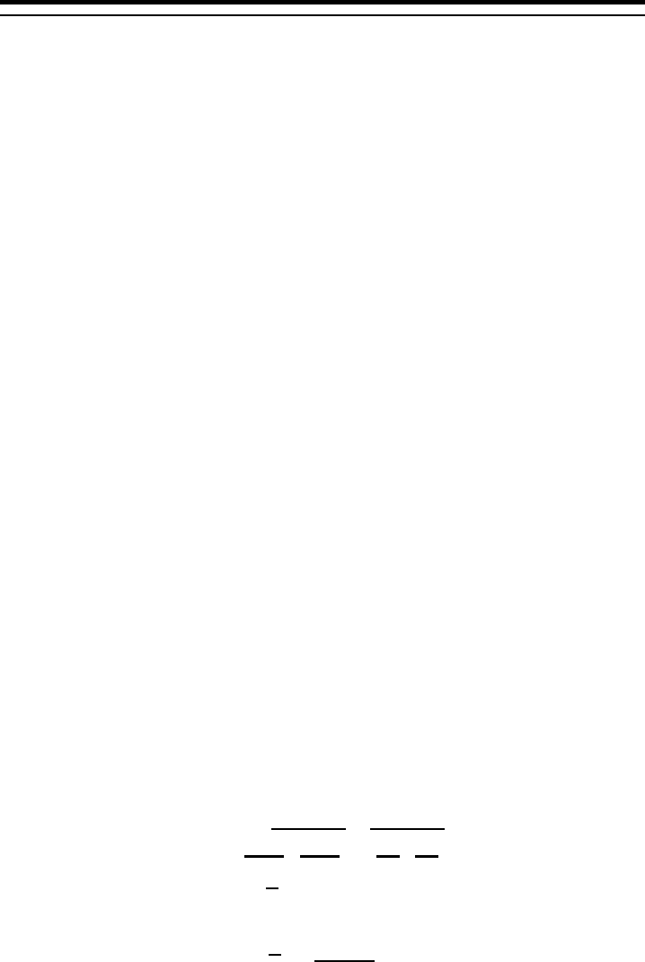
Chapter Eight
Time stepping schemes
The purpose of this chapter is to detail various issues of time stepping the discrete
equations of mom4p1. It is written in two main parts, with the first part focusing on
details of the scheme inherited from MOM4.0, and successfully used for climate
modelling. The second part revisits the MOM4.0 scheme, and proposes some
alternatives which are presently under investigation in mom4p1. The motivation
for revisiting the MOM4.0 schemes is that they show problems when used with
radiating open boundary conditions. Martin Schmidt led the studies into these
alternative time stepping schemes.
8.1 SPLIT BETWEEN FAST AND SLOW MOTIONS
An algorithm of practical utility for climate modeling must split the fast and slow
dynamics so that the slow dynamics can be updated with a much longer time step
than the fast dynamics. These algorithms are known as split-explicit methods. Al-
ternatives exist whereby the fast dynamics are time stepped implicitly and so may
use the same time step as the slow dynamics. We prefer split-explicit methods
since they are more efficient on parallel computers and arguably more straightfor-
ward (Griffies et al., 2001).
For a hydrostatic fluid, the fast motions can be approximated by the vertically
integrated dynamics of Section 7.7 and the vertically integrated mass or volume
budgets of Section 7.4. The remainder constitutes an approximation to the slower
dynamics. Motions constituting the fast dynamics are embodied by the barotropic
or external mode, and the slower motions are embodied by advection as well as the
baroclinic or internal mode. Given the fundamental nature of the mass conserving
non-Boussinesq flow, we formulate the split between the fast and slow modes
using density weighting. For the Boussinesq flow, the density weighting reduces
to an extra
ρ
ofactor which trivially cancels.
Following the discussion in Section 12.3.5 of Griffies (2004), we consider the
following split of the velocity
u=u−∑k
ρ
dzu
∑k
ρ
dz
| {z }
slow
+∑k
ρ
dzu
∑k
ρ
dz
| {z }
fast
≡ˆu+uz.
(8.1)
The fast barotropic velocity
uz=U
ρ
∑k
ρ
dz(8.2)

126 CHAPTER 8
is updated according to the vertically integrated momentum equation of Section
7.7. The slow baroclinic velocity ˆuhas zero density weighted vertical sum, and so
its update is independent of any depth independent forcing, such as fast fluctua-
tions in the surface height associated with external gravity waves. Therefore, we
choose to update the slow dynamics using all pieces of the momentum equation
forcing, except contributions from the rapid pressure and geopotential fluctuations.
This update produces a velocity u0which is related to the baroclinic velocity via
ˆu=u0−∑k
ρ
dzu0
∑k
ρ
dz. (8.3)
A similar relation was discussed in Section 12.4.2 of Griffies (2004). For global
climate simulations, the time step available for the update of the slow dynamics
is much larger (50 to 100 times larger) than the fast dynamics. It is this large
time split, and the attendant improved model efficiency, that motivates the added
complication arising from splitting the modes. Completing the updates of u0and
U
ρ
allows for an update of the full horizontal velocity via
u=u0−∑k
ρ
dzu0
∑k
ρ
dz+U
ρ
∑k
ρ
dz. (8.4)
8.2 TIME STEPPING THE MODEL EQUATIONS AS IN MOM4.0
We present here some details of the time stepping schemes available in mom4p1.
Much of this section is taken from the paper Griffies et al. (2005) which documents
two ocean climate models developed at GFDL; the OM3.0 and OM3.1 models.
Time stepping in OM3.0 is based on the standard MOM approach originating from
the work of Bryan (1969), and detailed for an explicit free surface by Killworth et al.
(1991) and Griffies et al. (2001). An alternative was developed for OM3.1.
The main motivation for developing an alternative was to address tracer non-
conservation associated with time filtering used to suppress the leap frog compu-
tational mode appearing in the standard method. The proposed time staggered
method has much in common with that used by Hallberg (1997) for his isopyc-
nal model, as well as by Marshall et al. (1997) and Campin et al. (2004) for their
hydrostatic and non-hydrostatic z-coordinate models.
The purpose of this section is to detail features of the time stepping schemes
employed in OM3.0 and OM3.1. Further details are provided in Chapter 12 of
Griffies (2004). We also refer the reader to the pedagogical treatments of time
stepping given by Mesinger and Arakawa (1976), Haltiner and Williams (1980),
and Durran (1999). For simplicity, we focus here on the Boussinesq system as-
suming z-coordinates for the vertical. The more general case of arbitrary vertical
coordinates with Boussinesq or nonBoussinesq equations follows trivially from the
discussions here.
8.2.1 The standard scheme used in OM3.0
We start by describing the standard approach used in MOM for time stepping
tracers and baroclinic velocity. For the thickness weighted tracer equation, this
TIME STEPPING SCHEMES 127
update takes the form
(h T)
τ
+1−(h T)
τ
−1
2∆
τ
leap
=− ∇z·[ (hu)
τ
T
τ
,
τ
−1+h
τ
F
τ
−1]
−
δ
k[w
τ
T
τ
,
τ
−1+F
τ
+1
z].
(8.5)
Here, his the time dependent thickness of a tracer cell and Tis the associated
tracer concentration. Horizontal and vertical advection velocity components are
written (u,w), and (F,Fz)are the horizontal and vertical SGS flux components.
The horizontal gradient operator is written ∇z, and
δ
kis the vertical finite difference
operator acting across a discrete level k. Prognostic fields are updated in time
increments of ∆
τ
leap. The thickness of a tracer cell is updated analogously to the
tracer, as required to maintain compatiblity between volume and tracer evolution
(see Section (Griffies et al., 2001).
The time tendency in equation (8.5) has been aproximated with a centred in time
discrete operator. Skipping the central time step
τ
introduces a spurious compu-
tational mode, where even and odd steps decouple. We choose time filtering to
suppress the associated instability, with hand Tdenoting the time filtered thick-
ness and tracer concentration. Absent time filtering, the discrete time tendency
has a second order global truncation error, whereas time filtering degrades the
truncation error to first order (see Section 2.3.5 of Durran (1999)). We comment
further on time filtering in the subsequent discussion, as it is central to why we
considered alternative time stepping schemes.
Global ocean models generally employ anisotropic grids, with significantly more
refined vertical spacing than horizontal. When admitting realistically fast vertical
mixing processes, parameterized by Fz, a time implicit method is used to overcome
the stringent time step constraints of an explicit approach. Hence, Fzis evaluated
at the future time
τ
+∆
τ
leap. In contrast, coarser grid spacing in the horizontal
generally allows for an explicit implementation of the horizontal SGS fluxes. Due
to the dissipative nature of SGS fluxes, stability considerations require them to
be evaluated at the lagged time
τ
−∆
τ
leap, with evaluation at the central time
τ
numerically unstable. That is, the horizontal SGS fluxes are implemented with a
forward time step of size 2∆
τ
leap.
In contrast to dissipative terms, numerical stability dictates that tracer concen-
tration in the advection operator be evaluated at the central time
τ
if using central
spatial differencing. As reviewed by Griffies et al. (2000a), this approach has been
common in z-models for decades. This form of the time stepping gives rise to the
commonly referred name leap frog applied to the standard time stepping used in
MOM. However, it is important to note that leap frog in the tracer equation is used
only for advection, and only for central spatial discretizations of advection. Dis-
sipative terms are implemented with either a forward or an implicit time step as
described above.
We found the dispersive errors from central differenced tracer advection to be
unacceptable, due to the introduction of spurious tracer extrema and the large lev-
els of spurious dianeutral mixing when convective adjustment acts on dispersion
errors (Griffies et al., 2000b). We chose the third order upwind biased scheme to
address these issues. As reviewed in Durran (1999), upwind biasing introduces a
128 CHAPTER 8
damping or dissipative element to numerical advection. Consequently, upwind bi-
ased fluxes must be evaluated at the lagged time
τ
−∆
τ
leap just like the dissipative
horizontal SGS fluxes. A similar situation arises when implementing the Quicker
advection scheme, in which one separates a dissipative portion evaluated at the
lagged time step from a non-dissipative piece evaluated at
τ
(Holland et al., 1998;
Pacanowski and Griffies, 1999). This is the origin of the two time labels placed on
the tracer concentration for the advective flux in equation (8.5).
For the Sweby advection scheme, the split into dissipative and non-dissipative
terms is not possible. The full advective flux is thus evaluated at the lagged time
step. This result may suggest increased levels of dissipation using Sweby relative
to Quicker. Indeed, this is the case in regions where dissipation is welcomed, such
as near river mouths where Quicker was found to introduce unacceptable tracer
extrema. In other regions of the simulation, we have seen negligible differences
between the two advection schemes.
An update of the thickness weighted baroclinic velocity using the standard time
stepping scheme in MOM takes the form
h
τ
+1u
τ
+1−h
τ
−1u
τ
−1
2∆
τ
=− M
τ
ˆz×h
τ
u
τ
+ (w
τ
u
τ
)k−(w
τ
u
τ
)k−1
− ∇z·(h
τ
u
τ
u
τ
)
−h
τ
(fˆz×u)trapezoidal
−h
τ
∇z(p
τ
/
ρ
o)
+h
τ
(Fu)(
τ
−1,
τ
+1). (8.6)
As for the tracer update, time filtering is applied to the lagged values of velocity and
velocity cell thickness to suppress time splitting. Central differences are used to
spatially discretize velocity self-advection, thus necessitating its evaluation at the
central time step. Pressure is temporally evaluated likewise. The friction operator
(Fu)(
τ
−1,
τ
+1)arises from horizontal and vertical fluid deformations. Analogous
to the treatment of tracer SGS fluxes, horizontal deformations are evaluated at
τ
−∆
τ
leap (forward time step) and vertical deformations at
τ
+∆
τ
leap (implicit time
step).
Inertial energy is realistic in the climate model since it includes a diurnal cycle of
solar insolation, and the atmosphere and sea ice fields passed to the ocean (wind
stress, fresh water, turbulent and radiative fluxes)∗are updated every two hours.
Inertial energy has important contributions to the mixing coefficients determined
by the model’s boundary layer scheme.
The model’s baroclinic time step is smaller than that needed to resolve inertial
oscillations (e.g., Section 12.8.3 of Griffies (2004)). We nonetheless encountered
an inertial-like instability in the climate model’s Arctic sector when implementing
the Coriolis force explicitly in time. This instability is presumably related to the
coupling between the ocean and sea ice, although the precise mechanism re-
mains under investigation. The climate model remained stable, however, when
implementing the ocean’s Coriolis force with a trapezoidal or semi-implicit method
(Section 10.3). Hence, this is the method employed in both OM3.0 and OM3.1.
∗As recommended by Pacanowski (1987), wind stress applied to the ocean surface is computed
using the relative velocity between the atmospheric winds and the ocean currents.
TIME STEPPING SCHEMES 129
8.2.2 Problems related to tracer conservation
Consider now the discrete time tracer equation in the abbreviated form
(h T)
τ
+∆
τ
leap = (h T)
τ
−∆
τ
leap +2∆
τ
G, (8.7)
where Gsymbolizes the advective and diffusive terms as well as boundary fluxes
(we ignore source/sink terms for brevity). Thickness at the lagged time step results
from a time average as described in Griffies et al. (2001), whereas time filtering of
tracer concentration is taken in the form suggested by Robert (1966) and Asselin
(1972) (see also Section 2.3.5 of Durran (1999)).∗Integrating equation (8.7) over
the model domain leads to the balance of total tracer content in the model. Total
tracer at time
τ
+∆
τ
leap is determined by the input of tracer through boundaries
during the 2∆
τ
leap time step, plus the volume integrated product of the time filtered
thickness and tracer concentration, h T, at the lagged time
τ
−∆
τ
leap. Notably,
because of time filtering, the model’s total tracer changes even in the case of zero
boundary fluxes.
The magnitude of tracer change associated with time filtering can be negligible
for many purposes, as discussed in Griffies et al. (2001). However, we found
the changes unacceptable when developing ecosystem models, where precise
conservation is desired. Additionally, filtering contributed to a globally averaged
heat non-conservation in the climate model on the order of ±0.03W m−2. This non-
conservative heat flux is a few percent of the surface insolation change expected
from doubling greenhouse gas concentrations in the atmosphere. It is therefore of
concern for our climate change simulations. Consequently, alternative approaches
were investigated.
8.2.3 The time staggered scheme used in OM3.1
The alternative scheme we employ in OM3.1 discretizes the time derivative with a
forward time step. That is, it does not skip any time levels. Additionally, it staggers
tracer and velocity fields by one-half time step in a manner analogous to spatial
staggering on Arakawa grids. We therefore refer to this method as a time stag-
gered scheme.
Forward time stepping does not admit time splitting, and so no time filters are
needed. The alternative scheme therefore ensures tracer is conserved, which
is our primary motivation for moving away from the standard method involving the
leap frog. There are other consequences of changing the time tendency discretiza-
tion, and the purpose of this section is to expose these issues.
A time staggered update of thickness weighted tracer is given by
(h T)
τ
+1/2−(h T)
τ
−1/2
∆
τ
stag
=−∇z·[ (hu)
τ
T
τ
−1/2+h
τ
F
τ
−1/2]
−
δ
k[w
τ
T
τ
−1/2+F
τ
+1/2
z].
(8.8)
∗We chose filtering for tracer over the alternative of periodically using a forward or backward time
step, which was the method used by Cox (1984). The use of a periodic forward or backward time step
introduces an unphysical periodicity to the simulation, and in particular was found by Marotzke (1991)
to interact in unphysical ways with convective adjustment.
130 CHAPTER 8
The two equations (8.5) and (8.8) become identical when (a) the time steps are
related by ∆
τ
stag =2∆
τ
leap, (b) time filtering in the standard method is not used,
and (c) tracer advection employs an upwind biased scheme. In effect, the time
staggered method stays on just one of the two leap frog branches. This is the
fundamental reason that the two methods should be expected, for many purposes,
to yield similar solutions.
Centred spatial differencing of advection is unstable with a forward time step.
Hence, for tracer advection we must employ an upwind biased advection scheme.
For our purposes with global ocean climate modelling, such advection schemes
are motivated to resolve problems with other schemes. Nonetheless, this conse-
quence of changing the time stepping scheme may be unacceptable for certain ap-
plications. An alternative method is to retain the ability to discretize advection with
centred spatial differences, but to alter the temporal evaluation of the advection op-
erator according to Adams-Bashforth methods (Durran, 1999), or other schemes.
In particular, we chose a temporally third order accurate Adams-Bashforth method
for velocity self-advection, thus maintaining the traditional centred spatial differ-
ences of this operator. The third order Adams-Bashforth method requires the
advection operator at time steps
τ
,
τ
−1, and
τ
−2, thus increasing memory
requirements.
Another consequence of choosing a forward time step for the tendency is that
the Coriolis force must be computed using an implicit or semi-implicit approach,
such as that described in Chapter 10. In contrast, the standard approach with the
leap frog allows for an explicit leap frog time stepping of the Coriolis force.
A leap frog discretization of the time tendency updates the ocean state by ∆
τ
leap
through taking a 2∆
τ
leap step for the discrete time tendency. Consequently, gravity
waves and dissipative operators (i.e., diffusion, friction, and upwind biased ad-
vection) are time step constrained based on 2∆
τ
leap. In constrast, the staggered
scheme updates the ocean state by ∆
τ
stag and it employs ∆
τ
stag to compute ten-
dencies. It is therefore time step constrained based on a ∆
τ
stag time step. Hence,
the staggered time step ∆
τ
stag can generally be twice that of the leap frog ∆
τ
leap
∆
τ
stag =2∆
τ
leap. (8.9)
The computational cost of OM3.1 with the staggered scheme is therefore one-half
that of OM3.0 using the standard scheme.
8.2.4 Sensitivity to the time stepping scheme
During the bulk of our development, the ocean model employed the standard time
stepping scheme for tracer, baroclinic, and barotropic equations. Upon developing
the staggered time stepping scheme for the tracer and baroclinic equations, we
became convinced that the modified scheme has utility for our climate modelling
applications. The question arose whether switching time stepping schemes would
require retuning of the physical parameterizations.
Tests were run with the ocean and ice models using an annually repeating at-
mospheric forcing with daily synoptic variability, again repeating annually. Runs
using the staggered scheme had a two hour time step for both tracer and baro-
clinic momentum, and a predictor-corrector scheme (e.g., Killworth et al., 1991;
TIME STEPPING SCHEMES 131
Griffies, 2004) for the barotropic equations with a 90s time step.∗The compari-
son was made to the standard time stepping scheme using one hour time steps
for the tracer and baroclinic equations, and (3600/64)s for the leap frog barotropic
equations.
Analysis of these solutions after 10 years revealed that regions with relatively
high frequency temporal variability, such as the equatorial wave guide, exhibit the
most differences instantanously. Figure 8.1 illustrates the situation along the equa-
tor in the East Pacific. The standard simulation exhibits substantial time splitting,
even with a nontrivial level of time filtering from a Robert-Asselin time filter. Mov-
ing just five degrees north of the equator, however, reveals that the simulation
has much less relative variability, and a correspondingly negligible amount of time
splitting. Even though the simulation along the equator showed substantial time
splitting, over longer periods of time, the large scale patterns and annual cycles
showed negligible differences between time stepping schemes. Indeed, time av-
eraging, even over just a day, seems sufficient to smooth over most of the instan-
taneous differences.
Tests were then run with the GFDL coupled climate models CM2.0 (using OM3.0
as the ocean component) and CM2.1 (using OM3.1). Instantaneous differences
were much larger, as expected due to the nontrivial natural variability in the cou-
pled system with a freely evolving atmospheric component. Nonetheless, differ-
ences for large scale patterns and seasonal or longer time averages were within
levels expected from the model’s natural variability.
8.2.5 Dissipative aspects of the predictor-corrector
The purpose of this section is to expose the dissipative aspects of the predictor-
corrector scheme available for use in the barotropic equations in mom4p1. A sim-
ilar treatment is given in Section 12.8.1 of Griffies (2004).
In two space dimensions, the predictor-corrector equations for an update of the
surface height and vertically integrated horizontal velocity in a Boussinesq model
are
η
∗−
η
n
∆t=−
γ
∇ · Un(8.10)
Un+1−Un
∆t=−c2∇
η
∗(8.11)
η
n+1−
η
n
∆t=−∇ ·Un+1, (8.12)
where nsymbolizes the barotropic time step. For brevity we dropped the fresh
water and source terms appearing in the free surface equation (7.81), and we
assumed an unforced linear shallow water system with squared wave speed c2=
g H. Setting the dimensionless dissipation parameter
γ
≥0to zero recovers a
forward-backward scheme discussed by Killworth et al. (1991). Keeping
γ
>0
was useful in our simulations and was motivated by similar experiences in the
Hallberg Isopycnal Model (Hallberg, 1997).
∗We found the predictor-corrector to be suitable for the barotropic equations due to our ability to
increase the barotropic time step beyond that of the leap frog. Additionally, it preferentially dissipates
grid scale features, which are commonly found when discretizing gravity waves on a B-grid (Killworth
et al., 1991; Griffies et al., 2001). We present an analysis of the dissipative aspects in Section 8.2.5.

132 CHAPTER 8
Eliminating the predicted surface height
η
∗leads to
Un+1−Un
∆t=−c2∇
η
n+
γ
c2∆t∇[∇·Un](8.13)
η
n+1−
η
n
∆t=−∇ ·Un+1. (8.14)
To directly see how the surface height evolves, eliminate Uto find
η
n+1−2
η
n+
η
n−1
(∆t)2= (c∇)2
η
n+
γ
(c∇)2
η
n−
η
n−1. (8.15)
Taking the limit ∆t→0, yet with
γ
∆tconstant, leads to a dissipative wave equation
(∂tt −c2∇2)
η
= (
γ
∆t) (c∇)2∂t
η
. (8.16)
A single spatial Fourier mode with wavenumber amplitude
κ
thus satisfies
d2/dt2+
γ
∆t(c
κ
)2d/dt+ (c
κ
)2
η
=0. (8.17)
This is the equation for a damped harmonic oscillator with inverse e-folding time
(1/2)
γ
∆t(c
κ
)2. With
γ
>0, external gravity waves are selectively dissipated in
regions where the surface height is changing in time, and where the spatial scales
are small. Faster waves are damped more readily than slower waves. These
properties are useful when aiming to suppress the B-grid computational null mode
discussed in Killworth et al. (1991) and Griffies et al. (2001).
8.3 SMOOTHING THE SURFACE HEIGHT AND BOTTOM PRESSURE
As discussed by Mesinger (1973), Killworth et al. (1991), Pacanowski and Griffies
(1999), Griffies et al. (2001), and Section 12.9 of Griffies (2004), there is a ubiq-
uitous problem with B-grid models due to a null mode present when discretizing
inviscid gravity waves. This mode manifests in the velocity field when using a rel-
atively small viscosity. Additionally, it manifests in the surface height or bottom
pressure, especially in coarsely represented enclosed or semi-enclosed embay-
ments where waves tend to resonate rather than to propagate. The pattern is
stationary∗and appears as a plus-minus pattern; i.e., as a checkerboard. As there
is generally no dissipation in the surface height budget
η
,t=∇· U+qw, (8.18)
suppression of the null mode requires some form of artificial dissipation. An anlo-
gous situation exists with the bottom pressure equation in a pressure based verti-
cal coordinate model.
Various methods have been described in the literature (e.g., Killworth et al.,
1991; Griffies et al., 2001) to address this problem. The following constraints guide
how we specify the filter.
•For the Boussinesq fluid, the tracer and surface height budgets must remain
compatible in the sense defined in Section 7.5. Hence, if a filter is added
to the surface height equation, one must correspondingly be added to the
tracer equation. Likewise, the non-Boussinesq tracer equation must have a
filter added if the bottom pressure equation has a filter.
∗Hence the term “null,” thus indicating it has a zero eigenvalue.

TIME STEPPING SCHEMES 133
•The filter should be zero in the case that the surface height is locally a con-
stant, or if the bottom pressure remains locally the same as the reference
bottom pressure.
The following filter for the surface height in a depth based vertical coordinate
model has been found suitable for suppressing noise∗in the model of Griffies et al.
(2004), and a variant on this form sufficient for geopotential vertical coordinates
was described in Section 12.9 of Griffies (2004)
∂t
η
= [∂t
η
]no filter+∇·(A∇
η
∗)
δ
∇
η
(8.19)
∂t(dzt T) = [∂t(dzt T)]no filter+
δ
k,1 ∇ ·[A∇(
η
∗T)]
δ
∇
η
. (8.20)
In these equations, A>0is a diffusivity,
δ
∇
η
vanishes if the surface height is
locally constant, and
δ
k,1 vanishes for all but the surface grid cell at k=1. The
surface height
η
∗is defined by
η
∗=
η
+|
η
min|+
η
off (8.21)
where
η
min is the global minimum of the surface height, and
η
off is a nonzero offset.
The use of
η
∗rather than
η
does not alter the filter acting on the surface height,
since ∇
η
∗=∇
η
. However,
η
∗is important for the tracer, since it ensures that
η
∗T
has the same sign as T. If we instead diffused
η
T, regions where
η
<0could lead
to negative diffusion, which results in tracer extrema and potential instabilities. The
alternative
δ
k,1 ∇·[A∇(dzt T)] is not desirable for z∗and
σ
vertical coordinates, in
which case the bottom topography potentially adds a nontrivial level of smoothing
even when the surface height is a uniform constant.
Global conservation of volume and tracer is ensured by using no-flux conditions
at the side boundaries. Local conservation is ensured since the tracer and volume
equations are compatible, as evidenced by setting the tracer concentration to unity
in the tracer equation which, upon vertical integration, recovers the surface height
equation (see Section 7.5). Note that a more conventional treatment of the filter
in the tracer equation is given by the convergence of the thickness weighted flux
−
η
A∇T. However, ∇ · (
η
A∇T)is not compatible with the filter applied to the
surface height, and so this alternative approach will lead to local non-conservation.
For pressure based vertical coordinates, we use the following filter
∂tpb= [∂tpb]no filter +∇ · (A∇p∗
b)
δ
∇p∗
b(8.22)
∂t(
ρ
dzt T) = [∂t(
ρ
dzt T)]no filter+
δ
k,kb ∇ ·[A∇(g−1p∗
bT)]
δ
∇p∗
b, (8.23)
where
δ
∇p∗
bvanishes where ∇p∗
bvanishes. The modified bottom pressure p∗
b>0
is defined by
p∗
b=pb−po
b+|min(pb−po
b)|+poff
b, (8.24)
where poff
bis a nonzero offset pressure. The positive pressure p∗
bis defined in
a manner analogous to the definition of
η
∗given by equation (8.21). Note that
subtracting out the reference bottom pressure po
bis useful prior to performing the
∗For added scale selectivity, it is sometimes useful to employ a biharmonic operator instead of a
Laplacian. However, much care should be exercised when using the biharmonic, as it is not positive
definite and so can lead to negative tracer concentrations. Therefore, the biharmonic, although present
in the mom4p1 code, is not recommended for general use.
134 CHAPTER 8
Laplacian operations. Doing so ensures that the filter does not overly smooth
the bottom pressure in regions where its undulations arise from variations in the
bottom topography. Such variations are physical, and do not reflect a problem with
the B-grid and so should not be filtered. The term g−1p∗
bappearing in the tracer
equation acts like an effective mass per area
(
ρ
dzt)eff ≡g−1p∗
b, (8.25)
which is positive since p∗
b>0. That is, the filter on the bottom pressure equation
acts like a mass source in the bottom cell. Hence, tracer must be rearranged in
the bottom cell in order to maintain compatibility (see Section 7.5). This filter sat-
isfies the global and local conservation constraints, while adding a level of filtering
needed to smooth the bottom pressure.
8.4 INTRODUCTION TO TIME STEPPING IN MOM4P1
For the remainder of this chapter, we step back from the OM3 simulations and
revisit some of the basic algorithmic details of the time stepping schemes used in
mom4p1. Before doing so, let us summarize advantages of the staggered time
stepping scheme employed by MOM4p0. For climate modelling, this scheme has
proven to be a great improvement over the traditional leap-frog based methods
found in earlier GFDL ocean codes, as well as many other ocean circulation mod-
els (Griffies et al. (2000a)). The improvements include the following.
•There is no need to employ explicit time filters (e.g., Robert-Asselin filter)
with the staggered scheme, thus enhancing temporal accuracy over the time
filtered leap-frog scheme.
•The time staggered scheme conserves seawater mass and tracer mass to
within numerical roundoff, whereas the leap-frog based methods, due to the
use of explicit time filtering, fail to conserve.
•The time staggered scheme updates the state of the ocean one time step
by employing tendencies based on that one time step. In contrast, leap-frog
based schemes update the state over one time step by using tendencies
based on two time steps. Hence, the leap-frog based schemes have a CFL
stability constraint based on the two time step tendencies, and so can be run
at only one-half the time step of the staggered scheme. Thus, the staggered
scheme is generally one half the computational cost of the leap-frog based
schemes.
The purpose of the following sections of this chapter is to expose salient points
regarding the time stepping algorithm that have been raised when developing the
radiating open boundary condition.
8.5 BASICS OF STAGGERED TIME STEPPING IN MOM4P1
Fundamental to the time staggered method is the need to provide a surface height
η
at integer time steps
η
(
τ
)as well as half integer time steps
η
(
τ
+∆
τ
/2). The

TIME STEPPING SCHEMES 135
surface height at integer time steps is needed to couple to velocity variables, which
are placed on integer time steps, whereas half integer time steps provide a sur-
face height for tracers. In addition, due to the split between barotropic and baro-
clinic modes, the surface height is updated over the small barotropic time steps
η
(b)(
τ
,tn), where a raised (b) denotes a field evaluated on the small barotropic
time step. The first time label
τ
designates which baroclinic branch the cycle
started, and
tn=
τ
+n∆t(8.26)
is the barotropic time step. The relation between the large time step ∆
τ
and small
time step ∆tis given by
2∆
τ
=N∆t. (8.27)
The barotropic time stepping procedes from the intitial barotropic time t0=
τ
to the
final time tN=
τ
+2∆
τ
. The integer Nis a function of the split between barotropic
and baroclinic gravity waves, which can be on the order of 100 in a global model.
Deducing the connection between
η
(
τ
),
η
(
τ
+∆
τ
/2), and
η
(b)(
τ
,tn)is a focus
of these notes. Correspondingly, we require a connection between the barotropic
time cycled vertically integrated velocity U(b)and U(
τ
).
The barotropic cycle integrates over time 2∆
τ
for every ∆
τ
update of the baro-
clinic system. Why the doubling of the time integration? This method is based
on experience with split-explicit time stepping schemes, where we have found it
important to provide sufficient time averaging to damp instabilities arising from the
incomplete split between the fast and slow motions available with a vertical inte-
gration. Longer time averaging is possible, though less convenient algorithmically,
less accurate, and more expensive.
A fundamental constraint of any time stepping scheme is that the tracer and
volume equations must remain compatible with one another. Compatibility means
that the tracer concentration equation reduces to the volume conservation equa-
tion when setting the tracer concentration to a constant. Without compatibility,
tracer and volume conservation are lost, and the algorithm is of little use for ocean
climate modelling.
After completing the barotropic cycle, which extends from t0=
τ
to tN=
τ
+
2∆
τ
, we aim to have a prescription for updating the vertically integrated velocity
U(
τ
+∆
τ
), the free surface height
η
(
τ
+∆
τ
/2), as well as
η
(
τ
+∆
τ
).
8.6 A PREDICTOR-CORRECTOR FOR THE BAROTROPIC SYSTEM
The preferred barotropic time stepping algorithm is the predictor-corrector scheme.
The first step in the algorithm “predicts” the surface height via
η
(∗)(
τ
,tn+1)−
η
(b)(
τ
,tn)
γ
∆t=−∇ ·U(b)(
τ
,tn) + E, (8.28)
where Eis the fresh water forcing or volume source, both of which are held con-
stant over the course of the barotropic cycle. We expose the time labels on these
fields in later discussions. The raised (∗)denotes an intermediate value of the
surface height. This is the “predicted” value, to be later “corrected.” The nondi-
mensional parameter 0≤
γ
acts to dissipate the small scales of motion (see

136 CHAPTER 8
Section 12.8 of Griffies (2004)). Setting
γ
=0recovers a second order accurate
forward-backward scheme, in which case the predictor step (8.28) is eliminated.
Larger values of
γ
reduce the order of accuracy, yet provide effective damping.
However, as shown in Section 12.8 of Griffies (2004), values of
γ
larger than 1/4
can compromise the scheme’s stability. The value
γ
=1/5has been found useful
for many purposes.
The predicted surface height
η
(∗)(
τ
,tn+1)is used to compute the surface pres-
sure via
ρ
o˜
p(∗)
s(
τ
,tn+1) = g
η
(∗)(
τ
,tn+1)
ρ
(
τ
+1/2)
k=1(8.29)
where the applied pressure pahas been dropped for brevity but can be trivially
added. The surface pressure is used to update the vertically integrated velocity
U(b)(
τ
,tn+1)−U(b)(
τ
,tn)
∆t="−fˆz∧U(b)(
τ
,tn) + U(b)(
τ
,tn+1)
2
−D(
τ
)∇z˜
p(∗)
s(
τ
,tn+1) + G(
τ
)i. (8.30)
For the vertically integrated transport, the Coriolis force is evaluated using the
Crank-Nicholson semi-implicit time scheme in equation (8.30). Inverting provides
an explicit update of the vertically integrated transport
U(b)(
τ
,tn+1) = [1+ ( f∆t/2)2]−1[U(#)(
τ
,tn+1) + ( f∆t/2)V(#)(
τ
,tn+1)] (8.31)
V(b)(
τ
,tn+1) = [1+ ( f∆t/2)2]−1[V(#)(
τ
,tn+1)−(f∆t/2)U(#)(
τ
,tn+1)] (8.32)
where U(#)(
τ
,tn+1)is updated just with the time-explicit tendencies
U(#)(
τ
,tn+1)−U(b)(
τ
,tn)
∆t= ( f/2)V(b)(
τ
,tn)−D(
τ
)∂x˜
p(∗)
s(
τ
,tn+1) + Gx(
τ
)
(8.33)
V(#)(
τ
,tn+1)−V(b)(
τ
,tn)
∆t=−(f/2)U(b)(
τ
,tn)−D(
τ
)∂y˜
p(∗)
s(
τ
,tn+1) + Gy(
τ
).
(8.34)
The “corrector” part of the scheme steps the surface height using the updated
transport
η
(b)(
τ
,tn+1)−
η
(b)(
τ
,tn)
∆t=−∇ ·U(b)(
τ
,tn+1) + E. (8.35)
Note that
η
(b)(
τ
,tn+1)is used rather than the predicted height
η
(∗)(
τ
,tn+1), since
η
(∗)(
τ
,tn+1)is computed with the altered time step
γ
∆t. Temporal dissipation
is localized to the predictor portion of the time stepping, with the corrector part
hidden from this dissipation. Because of the predictor step, the convergence of the
vertically integrated transport is computed twice in the predictor-corrector scheme,
thus increasing the cost relative to a forward-backward approach where
γ
=0.
The payoff is an extra parameter that can be used to tune the level of dissipation.
Additionally, there is added stability towards representing gravity waves so that ∆t
can be longer than when using the leap-frog method.
Let us detail how the barotropic steps accumulate over the course of a particular
barotropic cycle. For this purpose, write out the first and second corrector steps

TIME STEPPING SCHEMES 137
(8.35) for the surface height
η
(b)(
τ
,tn=1)−
η
(b)(
τ
,tn=0)
∆t=F(tn=1)(8.36)
η
(b)(
τ
,tn=2)−
η
(b)(
τ
,tn=1)
∆t=F(tn=2), (8.37)
where the right-hand side of equation (8.35) is abbreviated as F. Adding these two
equations leads to
η
(b)(
τ
,tn=2)−
η
(b)(
τ
,tn=0)
∆t=F(tn=1) + F(tn=2), (8.38)
where the intermediate value
η
(b)(
τ
,tn=1)has identically cancelled. This result
easily generalizes, so that
η
(b)(
τ
,tn=N)−
η
(b)(
τ
,tn=0)
N∆t=1
N
N
∑
n=1
F(tn). (8.39)
This result does not hold for a leap-frog algorithm, since the intermediate values
of the surface height do not generally cancel completely, as they do here for the
predictor-corrector.
8.7 THE GRIFFIES (2004) SCHEME
The only piece of the forcing F(tn)that changes during the barotropic cycle is the
convergence of the vertically integrated velocity. The result (8.39) then suggests
that the time averaged vertically integrated velocity should be given back to the
baroclinic part of the model upon completion of the barotropic cycle. To have
this velocity centered on the integer time step
τ
+∆
τ
, it is necessary to run the
barotropic cycle to
τ
+2∆
τ
. Hence, upon reaching the last barotropic time step
tn=N=
τ
+2∆
τ
, (8.40)
the vertically integrated velocity is time averaged,
˜
U=1
N
N
∑
n=1
U(b)(
τ
,tn). (8.41)
To produce the updated vertically integrated velocity at baroclinic time
τ
+∆
τ
, the
vertically integrated velocity U(
τ
+∆
τ
)is identified with this time averaged value,
U(
τ
+∆
τ
)≡˜
U. (8.42)
The surface height is needed at the integer time steps in order to specify the
thickness of the velocity cells. There are two options for updating the surface
height to time step
τ
+∆
τ
. First, we could take the instantaneous value from the
barotropic portion of the cycle
η
(
τ
+∆
τ
)≡
η
(b)(
τ
,tn=N/2). (8.43)
This approach has not been tried, since it likely leads to a meta-stable algorithm
due to the absence of time averaging, depending on the predictor-corrector dissi-
pation parameter
γ
. In contrast, extensive experience indicates that added stability
is realized by using the time averaged surface height
η
(
τ
+∆
τ
) = 1
N+1
N
∑
n=0
η
(b)(
τ
,tn). (8.44)

138 CHAPTER 8
Notably, tracer and volume conservation is not compromised by this specification
since it is only used to define the surface height carried by the velocity cells. How-
ever, the surface height at half integer timesteps needed for the tracer equation is
diagnosed using equation (8.41),
η
(
τ
+∆
τ
/2)−
η
(
τ
−∆
τ
/2)
∆
τ
=−∇ ·U(
τ
) + qw(
τ
) + S(
η
)(
τ
). (8.45)
As described in Section 8.8, this approach may cause divergence of sea level at
integer and half integer time steps.
8.8 ALGORITHMS MOTIVATED FROM THE PREDICTOR-CORRECTOR
The previous algorithm makes a distinction between how the integer and half-
integer surface heights are updated. This distinction exposes the algorithm to
possible time splitting between these surface heights. The splitting has been found
to be unacceptable for models with radiating open boundary conditions, whereas
other boundary conditions have shown no problem. Given the interest in radiating
boundary conditions, we consider here an alternative approach which is motivated
from details of the barotropic predictor-corrector method. It will turn out that the
schemes developed here are not algorithmically closed. However, approximations
are considered in 8.9.2 to close the algorithms.
8.8.1 Barotropic time stepping and surface height on integer time steps
The predictor step in the predictor-corrector algorithm updates the surface height
according to
η
(b)(
τ
,tn+1)−
η
(b)(
τ
,tn) = ∆t F(tn+1). (8.46)
We now expose the time labels on all terms appearing in the forcing, whereby we
set volume sources
F(tn+1) = −∇ · U(b)(
τ
,tn+1) + qw(
τ
+∆
τ
/2) + S(
η
)(
τ
+∆
τ
/2). (8.47)
Only the convergence of the vertically integrated velocity U(b)(
τ
,tn+1)changes on
each barotropic time step, whereas the water forcing qw(
τ
+∆
τ
/2)and source
S(
η
)(
τ
+∆
τ
/2)are held fixed.
To begin the barotropic integration of the surface height, it is necessary to pre-
scribe an initial condition. We choose to set
η
(b)(
τ
,t0) =
η
(
τ
)(8.48)
for the surface height, and
U(b)(
τ
,t0) = U(
τ
)(8.49)
for the vertically integrated velocity. This choice of the starting point is essential
for
η
, but different approximations are possible for the vertically integrated velocity.
Here,
η
(
τ
)and U(
τ
)are centred at an integer baroclinic time step, which again is
the time step where the velocity field is centred using the mom4p1 time staggered
method. These two prescriptions lead us to ask how to compute the updated
TIME STEPPING SCHEMES 139
surface height
η
(
τ
+∆
τ
)and vertically integrated velocity U(
τ
+∆
τ
). Experience
with various versions of the split-explicit time stepping in MOM motivates us to
take for the surface height a time average over the full suite of barotropic surface
heights according to
η
(
τ
+∆
τ
) = 1
N+1
N
∑
n=0
η
(b)(
τ
,tn). (8.50)
We choose this simple form of time filtering, in which all terms within the barotropic
time stepping contribute equally. Although more sophisticated time filters are avail-
able, this one has been found suitable for our purposes. Without time filtering, the
algorithm can be very unstable and thus is unsuitable for large scale modelling. As
shown below, this time averaging for the surface height motivates a different form
for the time averaging of the vertically integrated velocity field.
8.8.2 Surface height on half-integer time steps
The fundamental prescription (8.50) for the integer time step surface height is read-
ily extended to the half-integer surface height by setting
η
(
τ
+∆
τ
/2)≡
η
(
τ
) +
η
(
τ
+∆
τ
)
2.(8.51)
This prescription couples the integer and half-integer time steps, and ensures that
both are determined by time averages over the barotropic cycle. The question
then arises how to make this prescription compatible with the time stepping for
the tracer concentration. Compatibility is required for conservation of volume and
tracer, and so is of fundamental importance. Compatibility is also needed with the
baroclinic velocity scheme, but keeping in mind the uncertainties of wind stress pa-
rameterisation, minor approximation should be possible. Addressing these issues
forms the remainder of this section.
To proceed, we first deduce the time stepping algorithm for the integer time
steps which is implied from the barotropic time stepping (8.46) and the time aver-
age (8.50). For this purpose, start by using the initial condition (8.48) in the time
average (8.50) to find
η
(
τ
+∆
τ
) = 1
N+1
N
∑
n=0
η
(b)(
τ
,tn)(8.52)
=
η
(
τ
)
N+1+1
N+1
N
∑
n=1
η
(b)(
τ
,tn). (8.53)
Iterating the barotropic time stepping equation (8.46) and using the initial condition
(8.48) renders
η
(b)(
τ
,tn) =
η
(
τ
) + ∆t
n
∑
i=1
F(ti). (8.54)
Substitution of this result into equation (8.53) then leads to
η
(
τ
+∆
τ
)−
η
(
τ
) = ∆t
N+1
N
∑
n=1
n
∑
i=1
F(ti). (8.55)
140 CHAPTER 8
The double sum on the right hand side arises from the need to ensure that over the
course of the barotropic cycle, changes in volume correspond to changes in forc-
ing; in particular, with changes in the convergence of the depth integrated trans-
port. To facilitate computing the double sum within the barotropic time stepping
scheme, we employ the following identity to reduce the double sum to a single
sum
N
∑
n=1
n
∑
i=1
F(ti) =
N
∑
n=1
(N−n+1)F(ti),(8.56)
which can be readily verified by induction.
The sum (8.56) does not represent a straightforward time average. It does,
nonetheless, motivate defining a “modified average” forcing that is implied by the
barotropic cycle running from tn=0=
τ
to tN=
τ
+2∆
τ
. In particular, the relation
2∆
τ
=N∆tbetween baroclinic and barotropic time steps motivates the following
definition for the averaged forcing
F≡2
N(N+1)
N
∑
n=1
n
∑
i=1
F(ti),
≡2
N(N+1)
N
∑
n=1
(N−n+1)F(ti),
(8.57)
which renders
η
(
τ
+∆
τ
)−
η
(
τ
)
∆
τ
=F. (8.58)
Note that the average operator (8.57) reduces to the trivial result F=Fin the
special case when each of the barotropic time steps see a constant forcing F(ti)≡
F. That is,
N
∑
n=1
n
∑
i=1
F(ti) = F
N
∑
n=1
n(8.59)
=F(N/2) (N+1), (8.60)
where the last step used a common summation identity. This special case supports
our definition of the averaging operator, and furthermore checks the integrity of the
manipulations. In particular, since the fresh water and volume source are assumed
to be constant over the barotropic time steps, we have
F=2
N(N+1)
N
∑
n=1
n
∑
i=1
F(ti)(8.61)
=−2
N(N+1)
N
∑
n=1
n
∑
i=1∇· U(b)(
τ
,ti) + qw(
τ
+∆
τ
/2) + S(
η
)(
τ
+∆
τ
/2)(8.62)
which leads to
η
(
τ
+∆
τ
)−
η
(
τ
)
∆
τ
=−∇ ·U+qw(
τ
+∆
τ
/2) + S(
η
)(
τ
+∆
τ
/2). (8.63)
TIME STEPPING SCHEMES 141
So far, we have avoided placing a time label on the modified average operator.
In particular, the question arises how the averaged vertically integrated velocity
U=2
N(N+1)
N
∑
n=1
n
∑
i=1
U(b)(
τ
,ti)(8.64)
is related to the updated velocity U(
τ
+∆
τ
)or U(
τ
+∆
τ
/2). Absent the sec-
ond summation, the resulting average would be closely centred on the time step
τ
+∆
τ
, but the barycenter of the double sum is at
τ
+∆
τ
/2. We now discuss
algorithms based on both approximations.
8.8.3 Method A: U(
τ
+∆
τ
) = U
In this method, we consider U(
τ
+∆
τ
) = U, so that
U(
τ
+∆
τ
) = 2
N(N+1)
N
∑
n=1
n
∑
i=1
U(b)(
τ
,ti). (8.65)
Given this assumed time labelling of U, we are able to update the three dimen-
sional velocity to the new time step
τ
+∆
τ
after the baroclinic velocity is updated.
The prescription (8.65) implies that the integer time step surface height, which is
computed as the time average in equation (8.50), also satisfies the following time
tendency equation
η
(
τ
+∆
τ
)−
η
(
τ
)
∆
τ
=−∇ · U(
τ
+∆
τ
) + qw(
τ
+∆
τ
/2) + S(
η
)(
τ
+∆
τ
/2). (8.66)
The definition (8.51) of the half-integer time step surface height then implies that it
satisfies the tendency equation
η
(
τ
+∆
τ
/2)−
η
(
τ
−∆
τ
/2)
∆
τ
=−∇ ·U(
τ
+∆
τ
/2) + qw(
τ
) + S(
η
)(
τ
), (8.67)
where
U(
τ
+∆
τ
/2) = U(
τ
) + U(
τ
+∆
τ
)
2(8.68)
qw(
τ
) = qw(
τ
+∆
τ
/2) + qw(
τ
−∆
τ
/2)
2(8.69)
S(
η
)(
τ
) = S(
η
)(
τ
+∆
τ
/2) + S(
η
)(
τ
−∆
τ
/2)
2. (8.70)
8.8.3.1 Compatibile tracer concentration
For the surface height on half integer time steps, we must maintain compatibility
with tracer concentration fields, which are also centered on half-integer time steps.
Compatibility means that time stepping the surface height must take the identical
form to time stepping tracer concentration, so that the two equations agree in the
special case of a constant tracer concentration. Without such compatibility, tracer
and volume are not conserved by the discrete model. This point was emphasized
by Griffies et al. (2001) in the context of the leap-frog based algorithm exclusively
used in earlier versions of MOM.
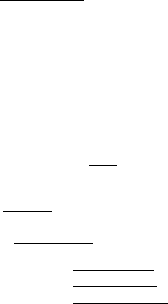
142 CHAPTER 8
Compatibility implies that the tracer concentration must be forced with the wa-
ter source (8.69), the volume source (8.70), and, because of equation (8.67), with
the half-integer advection velocity. Given these considerations, a compatible stag-
gered time discretization of thickness weighted tracer, absent subgrid scale pro-
cesses, takes the form (note the shorthand used for the time labels)
h
τ
+1/2C
τ
+1/2−h
τ
−1/2C
τ
−1/2
∆
τ
=−∇s·[(hu)
τ
+1/2C
τ
−1/2](8.71)
+ [w
τ
+1/2C
τ
−1/2]k−[w
τ
+1/2C
τ
−1/2]k−1, (8.72)
where the thickness weighted advection velocity on half-integer time steps is given
by
(hu)
τ
+1/2=(hu)
τ
+1+ (hu)
τ
2. (8.73)
8.8.3.2 Why this scheme is not closed
This algorithm is not closed, and so is not practical. The reason is that the com-
patible tracer equation (8.72) requires the thickness weighted advection velocity
(hu)
τ
+1/2. However, this velocity requires the updated thickness weighted ve-
locity (hu)
τ
+1, but the velocity at time u
τ
+1is not known until the momentum is
updated.
8.8.4 Method B: U(
τ
+∆
τ
/2) = U
Since the barycenter of the double sum (8.56) is
τ
+∆
τ
/2, it is reasonable to
prescribe U(
τ
+∆
τ
/2) = U, so that
U(
τ
+∆
τ
/2) = 2
N(N+1)
N
∑
n=1
n
∑
i=1
U(b)(
τ
,ti). (8.74)
The prescription (8.65) implies that the integer time step surface height, which is
computed as the time average in equation (8.50), also satisfies the following time
tendency equation
η
(
τ
+∆
τ
)−
η
(
τ
)
∆
τ
=−∇ ·U(
τ
+∆
τ
/2) + qw(
τ
+∆
τ
/2) + S(
η
)(
τ
+∆
τ
/2).
(8.75)
The definition (8.51) of the half-integer time step surface height then implies
η
(
τ
+∆
τ
/2)−
η
(
τ
−∆
τ
/2)
∆
τ
=−∇ ·U(
τ
) + qw(
τ
) + S(
η
)(
τ
), (8.76)
where
U(
τ
) = U(
τ
+∆
τ
/2) + U(
τ
−∆
τ
/2)
2(8.77)
qw(
τ
) = qw(
τ
+∆
τ
/2) + qw(
τ
−∆
τ
/2)
2(8.78)
S(
η
)(
τ
) = S(
η
)(
τ
+∆
τ
/2) + S(
η
)(
τ
−∆
τ
/2)
2. (8.79)

TIME STEPPING SCHEMES 143
8.8.4.1 Compatibile tracer concentration
Compatibility implies that in contrast to Section 8.8.3.1, the tracer concentration
must be forced with the water source (8.78), the volume source (8.79), and, be-
cause of Equation (8.76) with the integer advection velocity. The compatible stag-
gered time discretization of thickness weighted tracer, absent subgrid scale pro-
cesses, takes the form
h
τ
+1/2C
τ
+1/2−h
τ
−1/2C
τ
−1/2
∆
τ
=−∇s·[(hu)
τ
C
τ
−1/2](8.80)
+ [w
τ
C
τ
−1/2]k−[w
τ
C
τ
−1/2]k−1, (8.81)
where the thickness weighted advection velocity on integer time steps is given by
(hu)
τ
=(hu)
τ
+1/2+ (hu)
τ
−1/2
2. (8.82)
8.8.4.2 Why this scheme is not closed
This scheme is not closed algorithmically. That is, the velocity scheme cannot be
completed after the barotropic sequence is ready, because U(
τ
+∆
τ
)is still un-
known. The compatible tracer equation (8.81) requires also the thickness weighted
advection velocity (hu)
τ
+1/2, which itself requires the updated thickness weighted
velocity (hu)
τ
+1. The velocity at time u
τ
+1, however, is not known until the mo-
mentum is updated which in turn requres the barotropic scheme to be completed.
Yet the momentum is updated only after the tracer is updated. The repeated map-
ping between integer to half integer steps would reduce accuracy. A significant
rearrangement of the baroclinic and tracer equation may facilitate the use of this
algorithm. However, many attempts have failed.
8.9 CLOSED ALGORITHMS ENFORCING COMPATIBILITY
We present three methods for time stepping the equations in mom4p1. Method
I is that one discussed in Section 8.7 based on Griffies (2004) and Griffies et al.
(2005). Method III is a modification to Method I, and Method II is a closed algo-
rithm based on the barotropic predictor-corrector from Section 8.8. Methods II and
III each aim to provide a closed and compatible scheme that maintains stability
with the radiating open boundary condition. Methods I and II are implemented in
mom4p1, with Method III remaining untested.
8.9.1 Method I: Griffies (2004)
We first summarize the method of Griffies (2004) and Griffies et al. (2005), as de-
scribed in Section 8.7. To produce an algorithm that maintains compatibility with
tracer concentration, and is algorithmically closed, we take the philosophy here
that the fundamental fields are those which live on the baroclinic time steps (includ-
ing baroclinic velocity and tracer fields). The barotropic fields are coupled to the
baroclinic and tracer fields, but details of the barotropic algorithm do not dictate de-
tails of the baroclinic and tracer algorithm. In particular, details of whether we use
144 CHAPTER 8
a barotropic leap-frog or predictor-corrector are unimportant, nor are details of the
initial values used for the surface height and vertically integrated velocity (so long
as the initial values are reasonable). This philosophy is in contrast to that taken
in Section 8.8, and further described in Method III below, where the barotropic
predictor-corrector motivated details of the baroclinic and tracer updates.
The main steps of this scheme prescribe an updated vertically integrated velocity
and updated surface height, both as time averages over the barotropic time steps
U(
τ
+∆
τ
) = 1
N
N
∑
n=1
U(b)(
τ
,tn)(8.83)
η
(
τ
+∆
τ
) = 1
N+1
N
∑
n=0
η
(b)(
τ
,tn). (8.84)
The half-integer time step surface height is driven by the convergence of the time
averaged vertically integrated velocity, as well as surface boundary fluxes and in-
terior volume sources
η
(
τ
+∆
τ
/2)−
η
(
τ
−∆
τ
/2)
∆
τ
=−∇ ·U(
τ
) + qw(
τ
) + S(
η
)(
τ
). (8.85)
The compatible evolution equation for the tracer concentration follows from the
update to the half-integer surface height
h
τ
+1/2C
τ
+1/2−h
τ
−1/2C
τ
−1/2
∆
τ
=−∇s·[(hu)
τ
C
τ
−1/2](8.86)
+ [w
τ
C
τ
−1/2]k−[w
τ
C
τ
−1/2]k−1. (8.87)
There is a distinction in this method between
η
(
τ
+∆
τ
), which is based on a time
average, and
η
(
τ
+∆
τ
/2), which is based on a baroclinic forward time step. This
dichotomy has been found to allow splitting between the surface heights when
using radiating open boundary conditions.
8.9.2 Method II: Closed algorithm based on barotropic predictor-corrector
We were led to the non-closed algorithms in Section 8.8 by aiming to treat the
barotropic system in a systematic manner, and by prescribing the use of a particu-
lar form of time averaging for the surface height. Alternative methods can be found
by altering the form of the time average, or by jettisoning time averaged operators
altogether. However, we are not in favour of jettisoning the time average, as past
explorations of this approach have led to unacceptably unstable schemes. Instead,
we consider approximations described in the following that close the algorithm.
To start, we follow the scheme proposed in Section 8.8.4, in which the integer
time step surface height is updated via a time average as in equation (8.84)
η
(
τ
+∆
τ
) = 1
N+1
N
∑
n=0
η
(b)(
τ
,tn), (8.88)
TIME STEPPING SCHEMES 145
and the half-integer time step surface height is also a time average via
η
(
τ
+∆
τ
/2)≡
η
(
τ
) +
η
(
τ
+∆
τ
)
2.(8.89)
Following the details of the barotropic predictor-corrector, we are led to the up-
dated vertically integrated velocity via the sum in equation (8.74) and using the
barycenter for the time step placement as in Section 8.8.4
U(
τ
+∆
τ
/2) = 2
N(N+1)
N
∑
n=1
n
∑
i=1
U(b)(
τ
,ti)
=2
N(N+1)
N
∑
n=1
(N−n+1)U(b)(
τ
,ti).
(8.90)
As described in Section 8.8.2, this sum arises from the need to maintain consis-
tency with volume fluxes passing across the radiating open boundaries, and thus
for providing a stable scheme with radiating open boundaries.
As noted in Section 8.8.4, the prescription (8.90) does not lead to a closed
algorithm, since we need to know the updated velocity U(
τ
+∆
τ
)at the end of the
barotropic cycle in order to update the three dimensional velocity field u(
τ
+∆
τ
).
The following approximation which closes the algorithm has also been found to
lead to a stable scheme with radiating open boundaries
U(
τ
+∆
τ
)≈U(
τ
+∆
τ
/2). (8.91)
The half-integer time step surface height, which is defined by the time average
(8.89), also satisfies the time tendency equation
η
(
τ
+∆
τ
/2)−
η
(
τ
−∆
τ
/2)
∆
τ
=−∇ · U(
τ
) + qw(
τ
) + S(
η
)(
τ
). (8.92)
It follows that the compatible tracer equation is given by
h
τ
+1/2C
τ
+1/2−h
τ
−1/2C
τ
−1/2
∆
τ
=−∇s·[(hu)
τ
C
τ
−1/2](8.93)
+ [w
τ
C
τ
−1/2]k−[w
τ
C
τ
−1/2]k−1. (8.94)
The discrete tracer equation thus takes the same form as in Methods I and III.
8.9.3 Method III: Modified Griffies (2004)
To possibly resolve the problem of splitting between the integer and half-integer
time steps encountered with Method I in radiating open boundary problems, we
consider here an alternative approach, whereby the integer time step surface
height is prescribed as the time average of the half-integer time step surface height
2
η
(
τ
+∆
τ
) =
η
(
τ
+∆
τ
/2) +
η
(
τ
+3∆
τ
/2). (8.95)
That is, the integer time step surface height is no longer based on a time average,
but instead evolves according to
η
(
τ
+∆
τ
)−
η
(
τ
)
∆
τ
=−∇ · U(
τ
+∆
τ
/2) + qw(
τ
+∆
τ
/2) + S(
η
)(
τ
+∆
τ
/2),
(8.96)
146 CHAPTER 8
where
2U(
τ
+∆
τ
/2) = U(
τ
+∆
τ
) + U(
τ
)(8.97)
2qw(
τ
+∆
τ
/2) = qw(
τ
+∆
τ
) + qw(
τ
)(8.98)
2S(
η
)(
τ
+∆
τ
/2) = S(
η
)(
τ
+∆
τ
) + S(
η
)(
τ
). (8.99)
The problem with this prescription is that it is not closed, since the surface bound-
ary condition module only provides information about the surface forcing at the
present time step. Likewise, we do not know the updated volume source. Hence,
to close the algorithm we make the following approximation
qw(
τ
+∆
τ
/2)≈qw(
τ
)(8.100)
S(
η
)(
τ
+∆
τ
/2)≈S(
η
)(
τ
), (8.101)
which amounts to saying that the boundary forcing and volume source term remain
constant over the course of a baroclinic time step; i.e., we cannot obtain informa-
tion at higher frequency for these fields. Hence, we are led to the following update
for the integer time step surface height
η
(
τ
+∆
τ
)−
η
(
τ
)
∆
τ
=−∇ · U(
τ
+∆
τ
/2) + qw(
τ
) + S(
η
)(
τ
). (8.102)
Although of some interest, this scheme has not yet been coded in mom4p1. It thus
remains untested.
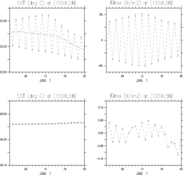
TIME STEPPING SCHEMES 147
Figure 8.1 Upper left panel: Instantaneous sea surface temperature over January 1 at
(105◦W, 0◦N)as realized in a simulation using the standard time stepping
scheme with an hour tracer time step (noisy time series) and the staggered
scheme with a two hour tracer time step (smooth time series). Upper right
panel: Surface heating applied at (105◦W, 0◦N)from the Robert-Asselin time
filter used to damp the leap frog splitting. Lower left panel: Instantaneous sea
surface temperature over a single day at (105◦W, 5◦N)as realized in a simula-
tion using the standard scheme with an hour tracer time step and the staggered
scheme with a two hour tracer time step. Note the width of the temperature
range is set the same as at the equator. In general, the agreement of the solution
off the equator, where the leap frog splitting is minimal, is far greater than on the
equator. Lower right panel: Surface heating applied at (105◦W, 5◦N)from the
Robert-Asselin filter. Note the much smaller magnitude relative to the values on
the equator.

Chapter Nine
Mechanical energy budgets and conversions
The purpose of this chapter is to discuss energetic balances. Here are the as-
sumptions made for the manipulations of this chapter.
•Choosing to maintain the integrity of certain energetic balances on the B-
grid lattice prescribes the form of the discrete advection velocity components
located on the sides of tracer cells.
•Second order finite differenced advective fluxes are used for momentum.
Tracer fluxes can remain arbitrarily discretized.
•A finite difference computation of the pressure gradient force, as described
in Sections 4.1, 4.2, and 4.3. The finite volume method for computing the
pressure force, as described in Section 3.5.1, does not lend itself to the
results of this chapter. Consequently, they have not been coded in mom4p1.
•Details of the time stepping scheme play a role in determining the form of the
energy diagnostics.
Energy balance diagnostics are important for checking the integrity of certain finite
difference algorithms.
9.1 ENERGETIC CONVERSIONS IN THE CONTINUUM
In the continuum, the horizontal momentum equation for a shallow ocean fluid is
given by (see chapter 4 of Griffies, 2004)
(
ρ
u),t+∇· (
ρ
v u) + ( f+M) (ˆz∧
ρ
u) = −∇zp+
ρ
F(9.1)
for the non-Boussinesq case, and
(u),t+∇· (v u) + ( f+M) (ˆz∧u) = −∇z(p/
ρ
o) + F(9.2)
for the Boussinesq case. The evolution of horizontal kinetic energy can be found
by taking the scalar product of horizontal velocity uwith the momentum equation.
When globally integrating the kinetic energy evolution, the forcing terms can be
transformed into terms that highlight physically interesting processes. These ma-
nipulations identify conversions between one form of energy and another. The
form of these conversions can be deduced from the momentum equations, bound-
ary conditions, mass or volume conservation, and integration by parts. Maintaining
an analog of these energetic conversions on the discrete lattice has been found to
be very useful in the development of ocean model algorithms. The reason is that
these conversions provide the modeler with a powerful set of diagnostics to test
the integrity of the numerics.

150 CHAPTER 9
There are three forms of energy conversion of interest in mom4. The first in-
volves the pressure gradient term, the second involves the advection term, and
the third involves friction. We address only the inviscid terms in this chapter. Part
5 of Griffies (2004) describes how friction dissipates kinetic energy in both the
continuous case and for a particular friction algorithm available in mom4.
9.1.1 Pressure work conversions in Boussinesq fluids
Let us first examine how pressure work is converted to other processes in Boussi-
nesq fluids. For this purpose, consider the following identities found using zfor the
vertical coordinate
ZdVu·∇ p=ZdV(v· ∇p−w p,z)
=ZdV[∇· (vp)−w p,z]
=ZdA(ˆn)p(ˆn·v) + gZdV w
ρ
=ZdA(ˆn)p(ˆn·v) + ZdV
ρ
dΦ/dt
(9.3)
where dV=dxdydzis the volume element and dΦ/dtis the material time
derivative of the geopotential Φ=g z. To reach these results required volume
conservation for a parcel in the form of the constraint ∇ · v=0, the hydrostatic
relation p,z=−
ρ
g, and the definitions
g w =gdz/dt
=dΦ/dt.(9.4)
Assuming no-normal flow at the solid boundaries leaves only the surface boundary
at z=
η
for the surface integral. The surface kinematic boundary condition, and
volume conservation, lead to∗
dA(ˆn)ˆn·v=−dxdy∇· U, (9.5)
and so
ZdVu·∇p=−Z
z=
η
dxdy pa∇ ·U+ZdV
ρ
dΦ/dt. (9.6)
In a rigid lid model, the first term vanishes. For the free surface model it represents
the work done by atmospheric pressure on the depth integrated flow. The second
term is the volume integrated work done by vertical currents against the buoyancy
force. In generalized vertical coordinates, the buoyancy term takes the form
dΦ/dt= (∂t+u· ∇s+w(s)∂z)Φ
= (∂t+u· ∇s)Φ+g w(s),(9.7)
where equation (6.72) of Griffies (2004) was used to express the material time
derivative in general vertical coordinates. Hence, the pressure conversion be-
comes
ZdVu·∇p=−Z
z=
η
dxdy p ∇· U+ZdV
ρ
[ (∂t+u· ∇s)Φ+g w(s)]. (9.8)
∗See Section 3.4 of Griffies (2004) for derivation.
MECHANICAL ENERGY BUDGETS AND CONVERSIONS 151
Buoyancy contributions now comprise three terms instead of the one found with z-
coordinates. This result reflects the non-orthogonal nature of generalized vertical
coordinates.
9.1.2 Pressure work conversions in non-Boussinesq fluids
For non-Boussinesq flows, pressure conversion takes the form
ZdVu·∇p=Z
z=
η
pˆn·v+ZdV(
ρ
dΦ/dt−p∇·v). (9.9)
The p∇·vterm represents pressure work on the changing volume of fluid parcels
found in the compressible non-Boussinesq fluid. The boundary condition
dA(ˆn)ˆn·v=dxdy(
η
,t−
ρ
wqw/
ρ
)(9.10)
is discussed in Section 3.4.3 of Griffies (2004). The generalized vertical coordinate
form of equation (9.9) follows similarly to the Boussinesq case, where extra terms
arise from expanding the material time derivative.
9.1.3 Boussinesq kinetic energy advection conversion
Just as for the pressure gradient term, the scalar product of the horizontal velocity
and the advection of momentum can be converted into alternative forms. To see
this conversion in the continuum, write the advection of horizontal velocity in the
Boussinesq fluid as
A≡ −∇ ·(v u)−M ˆz∧v. (9.11)
The scalar product of Awith the horizontal currents leads to
u·A=−u·∇·(v u)
=−∇ ·(vK),(9.12)
where K=u·u/2is the horizontal kinetic energy per mass. Integrating over the
volume of the domain, and using the surface and solid wall boundary conditions,
leads to
A ≡ ZdVu·A
=Z
z=
η
dxdyK∇ · U.(9.13)
Consequently, the global integral of kinetic energy advection reduces to a bound-
ary term, which vanishes in the rigid lid model but remains nontrivial in a free
surface model.
9.1.4 Non-Boussinesq kinetic energy advection conversion
For the non-Boussinesq fluid, we consider
A≡ −∇ · (
ρ
v u)− M ˆz∧
ρ
v. (9.14)
152 CHAPTER 9
The scalar product of Awith the horizontal currents leads to
u·A=−u·∇·(
ρ
v u)
=−∇ ·(vK)− K ∇ ·(
ρ
v),(9.15)
and integrating over the volume of the domain yields
A ≡ ZdVu·A
=−Z
z=
η
dA(ˆn)K
ρ
ˆn·v−ZdVK∇ · (
ρ
v)
=−Z
z=
η
dxdyK(
ρ η
,t−
ρ
wqw)−ZdVK∇· (
ρ
v),
(9.16)
where we used the surface boundary condition (9.10) for the last step.
9.2 CONSERVATION, CONSISTENCY, AND ACCURACY
Accuracy is often a primary consideration for numerical methods. Additionally,
ease of analysis and interpretation are also important. The presence of discrete
analogs to continuous conservation properties assists in the interpretation of the
numerical simulation. Unfortunately, conservation and accuracy are often incom-
patible.
Traditionally, climate modelers have chosen conservation properties over accu-
racy. For example, conservation of scalar properties are essential to ensure that
heat and salt are conserved over the course of a long climate integration. Another
property that certain models claim is conservation of mechanical energy. This
claim, however, is unfounded for the space-time discrete equations in all models
discussed in Griffies et al. (2000a). All ocean climate models break kinetic en-
ergy conservation when discretizing in time. This point is explained below in the
discussion of equation (9.17).
What is often meant by energy conservation statements is the more qualified
property whereby certain spatially discrete terms are discretized so they do not
alter global kinetic energy in the absence of boundary forcing. Deriving energet-
ically consistent numerical schemes requires some care. In particular, ensuring
that pressure work transfers into vertical buoyancy work in the Boussinesq model
necessitates a particular form for the discrete advection velocity. We discuss this
point in Section 9.4.
When considering energetic issues using alternative time stepping schemes,
one often encounters the situation where certain terms, such as advection and
pressure gradients, are evaluated at staggered time steps. Indeed, the preferred
method discussed in Chapter 12 of Griffies (2004) staggers the velocity and tracer
one-half time step relative to one another. Hence, pressure gradients, whose tem-
poral placement is set by density, is off-set in time from momentum advection, the
Coriolis force, and friction. These details are important when interpreting energetic
consistency of a space-time discrete model. Often the more sophisticated the time
stepping scheme (e.g., the three-time level Adams-Bashforth method discussed in
Chapter 12 of Griffies (2004)), the more difficult it is to maintain energetic consis-
tency.
MECHANICAL ENERGY BUDGETS AND CONVERSIONS 153
Energetic consistency is necessary but not sufficient for ensuring the discrete
system conserves mechanical energy in the unforced inviscid limit. For example,
time stepping according to the leap-frog method, which possesses useful energy
consistency properties, precludes mechanical energy conservation. The Robert-
Asselin time filter breaks energy conservation in a manner analogous to its corrup-
tion of global tracer conservation (Section 12.5.4 of Griffies (2004)). Furthermore,
even without time filtering, the continuum identity
2u·∂tu=∂t(u·u)(9.17)
is generally not satisfied by discrete time stepping schemes. As noted on page
158 of Durran (1999), trapezoidal time differencing allows for this property. Other
schemes commonly used do not. As trapezoidal time differencing is semi-implicit
and not readily implemented for the primitive equations, it is not considered in the
following.
9.3 THICKNESS WEIGHTED VOLUME AND MASS BUDGETS
We make use of the thickness weighted volume budgets for the Boussinesq fluid
when deriving the discrete energetic balances. The volume budgets are given by
equations (7.94), (7.95), and (7.96). We expose them here for completeness
(w(s))s=sk=1=∂t(dz)−dzS(V)+∇s·(dzu)−qw(9.18)
(w(s))s=sk=∂t(dz)−dzS(V)+∇s·(dzu) + (w(s))s=sk−1(9.19)
0=∂t(dz)−dzS(V)+∇s·(dzu) + (w(s))s=skbot−1. (9.20)
We also make use of the thickness weighted mass budgets for the non-Boussinesq
case, given by equations (7.118), (7.119), and (7.120). We expose them here for
completeness
(
ρ
w(s))s=sk=1=∂t(dz
ρ
)−
ρ
dzS(M)+∇s·(dz
ρ
u)−
ρ
wqw(9.21)
(
ρ
w(s))s=sk=∂t(dz
ρ
)−
ρ
dzS(M)+∇s·(dz
ρ
u) + (
ρ
w(s))s=sk−1(9.22)
0=∂t(dz
ρ
)−
ρ
dzS(M)+∇s·(dz
ρ
u) + (
ρ
w(s))s=skbot−1. (9.23)
As described in Section 7.6.1, depth based vertical coordinates used in mom4p1
(Section 6.1) allow for the time derivative ∂t(dz)to be diagnosed from the verti-
cally integrated volume budget. Likewise, the pressure based vertical coordinates
(Section 6.2) allow for the time derivative ∂t(
ρ
dz)to be diagnosed from the ver-
tically integrated mass budget. These two properties are important to ensure the
utility of the Eulerian algorithms employed by mom4p1.
9.4 DISCRETE BOUSSINESQ PRESSURE WORK CONVERSIONS
We now consider manipulations of the globally integrated discrete B-grid represen-
tation of u· ∇zpfor the Boussinesq case. In this section, discrete grid labels are
exposed when needed, with many labels suppressed to reduce clutter. The ma-
terial in this Section is based on a similar z-coordinate discussion given in Griffies
et al. (2004).
154 CHAPTER 9
Consider the domain integrated scalar product of
u·∇zp=u·(∇sp+
ρ
∇sΦ)
=u·∇(pa+psurf) + u·(∇sp0+
ρ
0∇sΦ).(9.24)
To reach this result we use equation (4.17) with s=z∗or s=
σ
(z), in which case
psurf =g
ρ
o
η
when s=z∗or s=
σ
(z)(9.25)
is the rapidly fluctuating surface pressure term, and
p0=g
η
Z
z
ρ
0dzwhen s=z∗or s=
σ
(z)(9.26)
is the slower fluctuating pressure anomaly where
ρ
0=
ρ
−
ρ
0. When s=zis the
vertical coordinate, equation (4.16) is used, in which case
psurf =g
ρ
surf
η
when s=z(9.27)
and
p0=g
0
Z
z
ρ
0dzwhen s=z. (9.28)
On the discrete lattice we consider
−ZdVu·∇zp→ P, (9.29)
where
P ≡− ∑
i,j,k
dvu u FDX NT(FAY(pa+psurf))
−∑
i,j,k
dvu v FDY ET(FAX(pa+psurf))
−∑
i,j,k
dvu [u FDX NT(FAY(p0)) + v FDY ET(FAX(p0)) ]
−∑
i,j,k
dvu [u FAY(FAX(
ρ
0)
δ
iΦ)/dxu +v FAX(FAY(
ρ
0)
δ
jΦ)/dyu ]
(9.30)
with
dvu =dau dzu (9.31)
the U-cell volume. MOM4 employs the following discrete forward derivative opera-
tors
FDX NT(a) = ai+1−ai
dxu (9.32)
FDY ET(a) = aj+1−aj
dyu , (9.33)
where the derivatives live on the east and north faces, respectively, of a tracer cell.
The operators
δ
iaand
δ
jacompute the forward difference
δ
ia=ai+1−ai(9.34)
δ
ja=aj+1−aj(9.35)
MECHANICAL ENERGY BUDGETS AND CONVERSIONS 155
of a discrete field. MOM4 also employs the following forward averaging operators
FAX(a) = ai+1+ai
2(9.36)
FAY(a) = aj+1+aj
2. (9.37)
The first group of terms in equation (9.30) arises from applied pressure and
surface geopotential acting on the vertically integrated velocity. The second rep-
resents the constant slateral pressure gradient taken between cells living on the
same discrete k-level. The third arises from the use of generalized vertical coordi-
nates, where the depth of a k-level is generally a function of horizontal position.
9.4.1 The vertically integrated term P1
The first term in equation (9.30) can be vertically integrated to yield
P1≡− ∑
i,j,k
dau dzu u FDX NT(FAY(pa+psurf))
−∑
i,j,k
dau dzu v FDY ET(FAX(pa+psurf))
=−∑
i,j
dau U FDX NT(FAY(pa+psurf))
−∑
i,j
dau V FDY ET(FAX(pa+psurf))
(9.38)
where
(U,V) = ∑
k
dzu (u,v)(9.39)
is the vertically integrated horizontal velocity field. The P1term represents the
effects of applied pressure and geopotential working on moving vertical columns
of fluid.
9.4.2 Advection velocity components for tracers
Focus on the zonal piece of the second term, where
P2x≡− ∑
i,j,k
dau dzu u FDX NT(FAY(p0))
=−1
2∑dyu dzu u
δ
i(p0
j+p0
j+1)
=−∑BAY(dyu dzu u)
δ
ip0
j.
(9.40)
The boundary terms were dropped since they vanish for either periodic or solid
wall conditions. We also introduced the backward meridional average operator
BAY(a) = aj+aj−1
2. (9.41)
Now define the zonal thickness weighted advective transport velocity on the east-
ern face of a tracer cell as
uh eti,j,k=BAY(dyu dzu u)
dytei,j
,(9.42)
156 CHAPTER 9
where dytei,jis the meridional width of the tracer cell’s east side (see Figure 9.2
for definitions of grid distances). Doing so leads to
P2x=−∑
δ
ip0(dyte uh et)
=∑p0
δ
i(dyte uh et)
=∑p0dat BDX ET(uh et),
(9.43)
where boundary terms vanish, and
BDX ET(a) = ai,jdytei,j−ai−1, jdytei−1, j
dati,j
(9.44)
is a backwards finite difference operator for fields defined on the east face of tracer
cells. Similar manipulations with the meridional term v∂yp0leads to
P2=∑
i,j,k
p0dat (BDX ET(uh et) + BDY NT(vh nt)), (9.45)
with
vh nti,j,k=BAX(dxu dzu v)
dxtni,j
(9.46)
the meridional tracer advective velocity on the north face of the tracer cell. Finally,
BDY NT(a) = ai,jdxtni,j−ai,j−1dxtni,j−1
dati,j
(9.47)
is a backwards finite difference operator for fields defined on the north face of
tracer cells.
The horizontal velocity components uh et and vh nt are defined at the sides of
the tracer cells. They are the discrete representation of the thickness weighted
advective velocity components that transport tracer and volume through the east
and north cell faces. When fluid volume converges horizontally to a tracer cell,
there is a corresponding dia-surface velocity component and a generally nonzero
time tendency for the cell thickness. The thickness weighted volume budgets given
by equations (9.18), (9.19), and (9.20) describe these effects.
Given that the advective velocity components uh et and vh nt are defined at
the sides of the tracer cells, we are led to define a dia-surface velocity component
w btkat the bottom of the cell. It can generally be written by the discrete form of
equation (9.19)
w btk=∂t(dztk)−dztkS(V)
+BDX ET(uh etk) + BDY NT(vh ntk) + w btk−1.(9.48)
Again, the time tendency on tracer cell thickness dztkis known in mom4p1 from
information about the vertically integrated volume budget (Section 7.6.1.5). So this
expression is indeed a diagnostic expression for w btk, evaluated from the surface
down to the bottom. At the ocean surface, the dia-surface velocity component is
determined by the input of water to the system
w btk=0=−qw. (9.49)
MECHANICAL ENERGY BUDGETS AND CONVERSIONS 157
The minus sign is a convention, where positive wrepresents upward transport
whereas positive qwrepresents downward transport of fresh water through the
ocean surface into the ocean domain. Note that in general, water can enter the
ocean domain at any depth through the source term S(V). At the ocean bottom,
we are ensured of a proper discretization so long as
w btk=kbot =0 (9.50)
is diagnosed. This statement is valid on the B-grid since the ocean bottom on
tracer cells is flat. It has proven to be a very useful diagnostic to verify the integrity
of the volume conservation discretization throughout a vertical column.
9.4.3 Completing the manipulations for P2
Substituting expression (9.48) for the vertical advective velocity component into
equation (9.45) leads to
P2=∑
i,j,k
p0
kdat (wbtk−w btk−1−∂tdztk+dztkS(V)). (9.51)
Now move the vertical difference operator from the dia-surface velocity to the hy-
drostatic pressure via the following identity
kbot
∑
k=1
p0
kdat (wbtk−w btk−1) = −p0
k=1w btk=0dat −
kbot
∑
k=1
dat w btk(p0
k+1−p0
k),
(9.52)
where we used the lower boundary condition p0
kbot+1wbtkbot =0to reach this
result. The next step requires us to specify how the hydrostatic pressure is com-
puted. There are two ways, described in Sections 7.1.1 and 7.1.2.
9.4.3.1 Energetic approach
Section 7.1.1 noted that the older energetically based method specifies the hydro-
static pressure at the tracer point depth (Figure 9.1) according to
p0
k=1=gdztupk=1
ρ
0
k=1k=1
p0
k+1=p0
k+gdzwtk
ρ
0
k
zk>1, (9.53)
where
ρ
0
k
z= (
ρ
0
k+
ρ
0
k+1)/2 (9.54)
is the algebraically averaged density over the region between two tracer points Tk
and Tk+1, and dzwtkis the vertical distance between the tracer points (Section
7.3). Substituting this result into equation (9.52) renders
kbot
∑
k=1
p0
kdat (wbtk−w btk−1) = −p0
k=1w btk=0dat −g
kbot
∑
k=1
dat dzwtkwbtk
ρ
0
k
z.
(9.55)
This result then leads to
P2=−g∑
i,j,k
dat dzwtkw btk
ρ
0
k
z
−∑
i,j
dat p0
k=1wbtk=0−∑
i,j,k
dat p0
k[∂tdztk−dztkS(V)].(9.56)
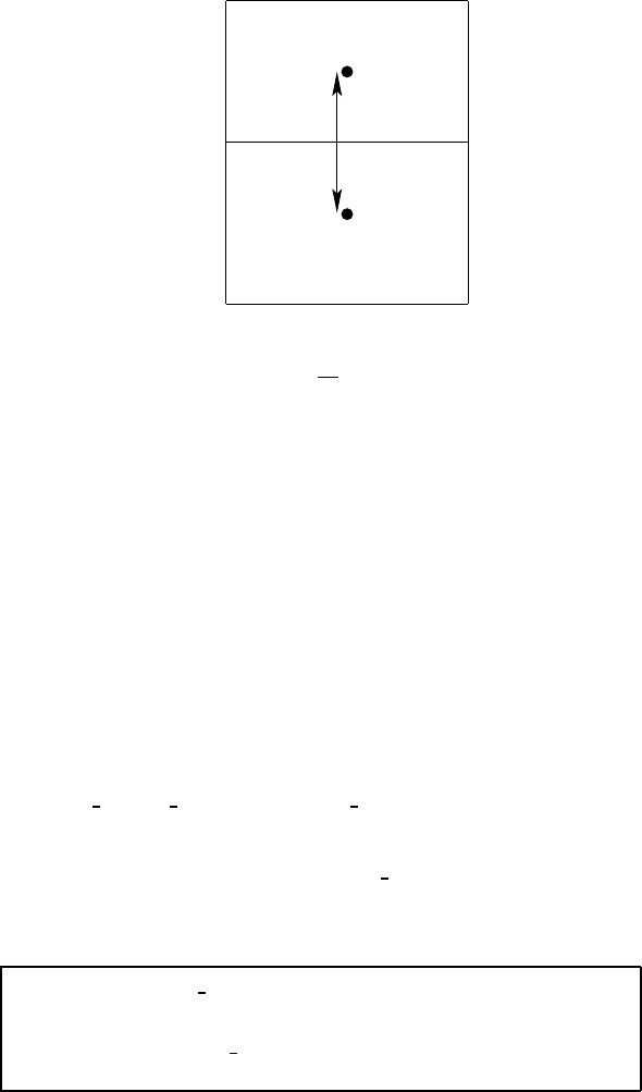
158 CHAPTER 9
k+1
k
dhwt(k)
Figure 9.1 Schematic of the vertical grid cell arrangment used for computing the hydro-
static pressure at a depth k+1 in terms of the pressure at depth kusing the
equation p0
k+1=p0
k+gdzwtk
ρ
0
k
z. The vertical average of density is meant to
account for the part of density within each of the two adjacent cells. The factor
of 1/2 used in the average operator yields an approximate average when verti-
cal cells are non-uniform. Yet the 1/2 factor is used for all vertical grid spacing
since it renders a simple conversion of discrete pressure work to discrete gravity
work.
9.4.3.2 Finite volume approach
Section 7.1.2 noted that a finite volume based method specifies the hydrostatic
pressure at the tracer point depth according to
p0
k=1=gdztupk=1
ρ
0
k=1
p0
k+1=p0
k+gdztlok
ρ
0
k+gdztupk+1
ρ
0
k+1.(9.57)
Substituting this result into equation (9.52) renders
kbot
∑
k=1
p0
kdat (wbtk−w btk−1) = −p0
k=1w btk=0dat
−g
kbot
∑
k=1
dat w btk(dztlok
ρ
0
k+gdztupk+1
ρ
0
k+1).
(9.58)
This result then leads to
P2=−g∑
i,j,k
dat w btk(dztlok
ρ
0
k+gdztupk+1
ρ
0
k+1)
−∑
i,j
dat p0
k=1wbtk=0−∑
i,j,k
dat p0
k[∂tdztk−dztkS(V)].(9.59)
9.4.4 The geopotential gradient term P3
Now consider the zonal piece of the geopotential gradient from equation (9.30)
P3x=−∑
i,j,k
dxu dyu dzu u FAY(FAX(
ρ
0)
δ
iΦ)/dxu. (9.60)
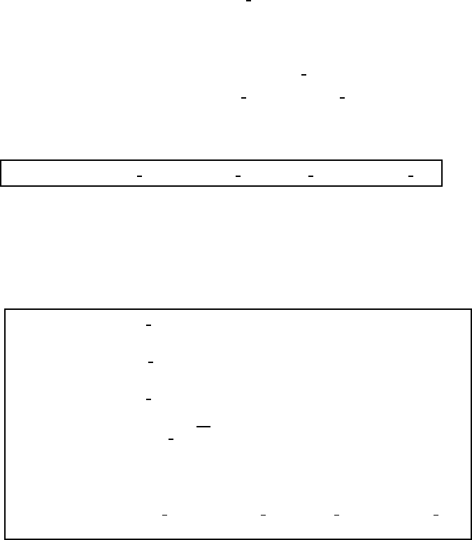
MECHANICAL ENERGY BUDGETS AND CONVERSIONS 159
Transferring the forward average FAY to a backward average BAY leads to
P3x=−∑BAY(dyu dzu u)FAX(
ρ
0)
δ
iΦ, (9.61)
where boundary terms vanish. Introducing the zonal thickness weighted advective
transport velocity (9.42) yields
P3x=−∑dyte uh et FAX(
ρ
0)
δ
iΦ. (9.62)
Moving the difference operator
δ
iΦ=Φi+1−Φifrom the geopotential to the re-
maining terms gives
P3x=∑Φ
δ
i(dyte FAX(
ρ
0)uh et)
=∑Φdat BDX ET(FAX(
ρ
0)uh et),(9.63)
where boundary terms vanish. Similar manipulations with the meridional piece of
P3lead to
P3=∑Φdat [BDX ET(FAX(
ρ
0)uh et) + BDY NT(FAY(
ρ
0)vh nt)] (9.64)
9.4.5 Summary for the Boussinesq pressure conversion
In summary, for the older energetically based method for computing hydrostatic
pressure, the projection of the horizontal velocity onto the downgradient pressure
field is given by
P=−∑
i,j
dau U FDX NT(FAY(pa+psurf))
−∑
i,j
dau V FDY ET(FAX(pa+psurf))
−∑
i,j
dat p0
k=1w btk=0
−g∑
i,j,k
dat dzwtkwbtk
ρ
0
k
z
−∑
i,j,k
dat p0
k[∂tdztk−dztkS(V)]
+∑
i,j,k
Φdat [BDX ET(FAX(
ρ
0)uh et) + BDY NT(FAY(
ρ
0)vh nt)].
(9.65)
Within the MOM4 energy analysis diagnostic, the code computes the left hand
side of equation (9.65) and compares to the right hand side. Differences are due
to coding errors. This diagnostic is very effective because it involves advective
velocities on the tracer cells, both tracer and velocity cell distances, the calcula-
tion of pressure, and details of partial steps. Each require precise discretization in
order to ensure an energy conversion error at the roundoff level. In a similar man-
ner, for the finite volume approach to computing hydrostatic pressure, we have the
projection of the horizontal velocity onto the downgradient pressure field is given
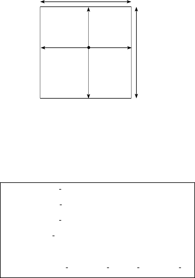
160 CHAPTER 9
T(i,j)
dxt(i,j) dyte(i,j)
dxtn(i,j)
dyt(i,j)
Figure 9.2 Time independent horizontal grid distances (meters) used for the tracer cell Ti,j
in MOM4. dxti,jand dyti,jare the grid distances of the tracer cell in the general-
ized zonal and meridional directions, and dati,j=dxti,jdyti,jis the area of the
cell. The grid distance dxtni,jis the zonal width of the north face of a tracer cell,
and dytei,jis the meridional width of the east face. Note that the tracer point Ti,j
is not generally at the center of the tracer cell. Distances are functions of both i
and jdue to the use of generalized orthogonal coordinates.
by
P=−∑
i,j
dau U FDX NT(FAY(pa+psurf))
−∑
i,j
dau V FDY ET(FAX(pa+psurf))
−∑
i,j
dat p0
k=1w btk=0
−g∑
i,j,k
dat w btk(dztlok
ρ
0
k+gdztupk+1
ρ
0
k+1)
−∑
i,j,k
dat p0
k[∂tdztk−dztkS(V)]
+∑
i,j,k
Φdat [BDX ET(FAX(
ρ
0)uh et) + BDY NT(FAY(
ρ
0)vh nt)].
(9.66)
9.5 DISCRETE NON-BOUSSINESQ PRESSURE WORK CONVERSIONS
Now consider manipulations of the globally integrated discrete B-grid representa-
tion of u· ∇zpfor the non-Boussinesq case. Here, we are concerned with the
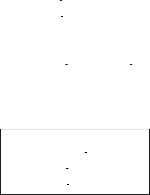
MECHANICAL ENERGY BUDGETS AND CONVERSIONS 161
domain integrated scalar product
u·∇zp=u·(∇sp+
ρ
∇sΦ)
= (
ρ
/
ρ
o)u·∇(pb+
ρ
oΦb) + u·[−(
ρ
0/
ρ
o)∇sp+
ρ
∇sΦ0],(9.67)
where equation (4.26) was used for the pressure gradient as implemented in pres-
sure based vertical coordinate models. In order to maintain a clean analog to the
Boussinesq case, we were led in Section 4.3.2 to introduce the discrete represen-
tations of the pressure gradient so that
−ZdVu·∇zp→ P (9.68)
becomes in the discrete case
ρ
oP ≡ − ∑
i,j,k
dau rhodzu u FDX NT(FAY(pb+
ρ
oΦb))
−∑
i,j,k
dau rhodzu v FDY ET(FAX(pb+
ρ
oΦb))
+∑
i,j,k
dau dzu u FAY(FAX(
ρ
0)
δ
ip)/dxu
+∑
i,j,k
dau dzu v FAX(FAY(
ρ
0)
δ
jp)/dyu
−∑
i,j,k
dau rhodzu [u FDX NT(FAY(Φ0)) + v FDY ET(FAX(Φ0))].
(9.69)
We now consider these terms individually.
9.5.1 The vertically integrated term P1
The first term in equation (9.69) can be vertically integrated as
P1≡− ∑
i,j,k
dau rhodzu u FDX NT(FAY(pb/
ρ
o+Φb))
−∑
i,j,k
dau rhodzu v FDY ET(FAX(pb/
ρ
o+Φb))
=−∑
i,j
dau U
ρ
FDX NT(FAY(pb/
ρ
o+Φb))
−∑
i,j
dau V
ρ
FDY ET(FAX(pb/
ρ
o+Φb))
(9.70)
where
(U
ρ
,V
ρ
) = ∑
k
rhodzu (u,v)(9.71)
is the vertically integrated density weighted horizontal velocity field. The P1term
represents the effects of applied pressure and geopotential working on moving
vertical columns of fluid.
162 CHAPTER 9
9.5.2 Defining the advection velocities
To motivate the definition of the advection velocity for the non-Boussinesq case,
we focus on the zonal part of the geopotential term
P3x≡− ∑
i,j,k
dau rhodzu u FDX NT(FAY(Φ0))
=−1
2∑dyu rhodzu u
δ
i(Φ0
j+Φ0
j+1)
=−∑BAY(dyu rhodzu u)
δ
iΦ0
j.
(9.72)
The boundary terms were dropped since they vanish for either periodic or solid
wall conditions. Now define the zonal thickness weighted and density weighted
advective transport velocity on the eastern face of a tracer cell
uhrho eti,j,k=BAY(dyu rhodzu u)
dytei,j
.(9.73)
This definition of the non-Boussinesq advection velocity component leads to
P3x=−∑
δ
iΦ0(dyte uhrho et)
=∑Φ0
δ
i(dyte uhrho et)
=∑Φ0dat BDX ET(uhrho et),
(9.74)
where boundary terms vanish. Similar manipulations with the meridional term
v∂yp, and reintroducing the two-dimensional pieces, leads to
P3=∑Φ0dat (BDX ET(uhrho et) + BDY NT(vhrho nt)), (9.75)
with
vhrho nti,j,k=BAX(dxu rhodzu v)
dxtni,j
(9.76)
the meridional density and thickness weighted advective tracer velocity on the
north face of the tracer cell.
As for the Boussinesq case, the horizontal advective velocities uhrho et and
vhrho nt are defined at the sides of the tracer cells. They are the discrete rep-
resentation of the thickness and density weighted advective velocity transporting
tracer and volume through the east and north cell faces. When mass converges
horizontally to a tracer cell, there is a corresponding dia-surface velocity compo-
nent and a generally nonzero time tendency for the cell thickness. The thickness
weighted mass budgets given by equations (9.21), (9.22), and (9.23) describe
these effects.
Given that the advective velocities uhrho et and vhrho nt are defined at the
sides of the tracer cells, we are led to define a density weighted dia-surface velocity
component wrho btkat the bottom of the cell. It is determined by the discrete form
of equation (9.22)
wrho btk=∂t(rhodzt)k−rhodzt S(M)
+BDX ET(uhrho etk) + BDY NT(vhrho ntk) + wrho btk−1.
(9.77)
MECHANICAL ENERGY BUDGETS AND CONVERSIONS 163
As for the velocity cells, we use vertical coordinates so that the tracer cells maintain
ρ
dzt = (
ρ
z,s)(t)dst (9.78)
where (
ρ
z,s)(t)is depth independent. The time tendency on density weighted
tracer cell thickness (rhodzt)kis known in mom4p1 from information about the
vertically integrated mass budget (Section 7.4.2). So equation (9.77) is indeed a
diagnostic expression for wrho btk, evaluated from the surface down to the bottom.
At the ocean surface, the dia-surface velocity component is determined by the
input of fresh water to the system
wrho btk=0=−
ρ
wqw.(9.79)
At the ocean bottom, we are ensured of a proper discretization so long as
wrho btk=kbot =0 (9.80)
is diagnosed.
9.5.3 Completing the manipulations for P3
Substituting expression (9.77) for the vertical advective velocity component into
equation (9.75) leads to
P3=∑Φ0
kdat (wrho btk−wrho btk−1−∂t(rhodzt)k+rhodztkS(M)). (9.81)
Now move the vertical difference operator from the dia-surface velocity to the hy-
drostatic pressure via the following identity
kbot
∑
k=1
Φ0
kdat (wrho btk−wrho btk−1) = −dat Φ0
k=1wrho btk=0
+
kbot
∑
k=1
dat wrho btk(Φ0
k−Φ0
k+1),
(9.82)
where we used the lower boundary condition Φ0
kbot+1wrho btkbot =0to reach this
result. The next step requires us to specify how the anomalous geopotential height
is computed. There are two ways, described in Sections 7.1.3 and 7.1.4.
9.5.3.1 Energetic approach
In Section 7.1.3, we noted that the older energetically based method specifies the
anomalous geopotential height at the tracer point depth (Figure 9.1) according to
Φ0
k=Φ0
k+1−(g/
ρ
o)dzwtk
ρ
0
k
z. (9.83)
In contrast to the hydrostatic pressure calculation (9.53), the geopotential calcula-
tion procedes from the bottom upwards. Substituting equation (9.83) into equation
(9.82) renders
kbot
∑
k=1
Φ0
kdat (wrho btk−wrho btk−1) = −Φ0
k=1wrho btk=0dat
−(g/
ρ
o)
kbot
∑
k=1
dat dzwtkwrho btk
ρ
0
k
z,
(9.84)
164 CHAPTER 9
which then leads to
P3=−(g/
ρ
o)∑
i,j,k
dat dzwtkwrho btk
ρ
0
k
z
−∑
i,j
dat Φ0
k=1wrho btk=0
+∑
i,j,k
dat Φ0[ (rhodzt)kS(M)−∂t(rhodzt)k]
(9.85)
9.5.3.2 Finite volume approach
Section 7.1.4 noted that the finite volume based method specifies the anomalous
geopotential height at the tracer point depth (Figure 9.1) according to
Φ0
k=kbot =−(g/
ρ
o)dztlokbot
ρ
0
k=kbot
Φ0
k=Φ0
k+1−(g/
ρ
o)dztupk+1
ρ
0
k+1−(g/
ρ
o)dztlok
ρ
0
k.(9.86)
Substituting equation (9.86) into equation (9.82) renders
kbot
∑
k=1
Φ0
kdat (wrho btk−wrho btk−1) = −Φ0
k=1wrho btk=0dat
−(g/
ρ
o)
kbot
∑
k=1
dat wrho btk(dztupk+1
ρ
0
k+1+dztlok
ρ
0
k),
(9.87)
which then leads to
P3=−(g/
ρ
o)∑
i,j,k
dat wrho btk(dztupk+1
ρ
0
k+1+dztlok
ρ
0
k)
−∑
i,j
dat Φ0
k=1wrho btk=0
+∑
i,j,k
dat Φ0[ (rhodzt)kS(M)−∂t(rhodzt)k].
(9.88)
9.5.4 The pressure gradient term P2
Now consider the zonal piece of the geopotential gradient from equation (9.69)
ρ
oP2x=∑
i,j,k
dxu dyu dzu u FAY(FAX(
ρ
0)
δ
ip)/dxu (9.89)
Transferring the forward average FAY to a backward average BAY leads to
ρ
oP2x=−∑BAY(dyu dzu u)FAX(
ρ
0)
δ
ip, (9.90)
where boundary terms vanish. Further manipulations, analogous to the Boussi-
nesq case in Section 9.4.4, do not appear possible since the density weighted
advection velocity will not appear. Instead, the
ρ
0weighted velocity appears, and
this is not relevant. So we simply write this term in its unmanipulated form
P2=
ρ
−1
o∑
i,j,k
dau dzu u FAY(FAX(
ρ
0)
δ
ip)/dxu
+
ρ
−1
o∑
i,j,k
dau dzu v FAX(FAY(
ρ
0)
δ
jp)/dyu.(9.91)
MECHANICAL ENERGY BUDGETS AND CONVERSIONS 165
9.5.5 Summary for the non-Boussinesq pressure conversion
In summary, for the older energetically based method for computing the anoma-
lous geopotential, the projection of the horizontal velocity onto the downgradient
pressure field in the non-Boussinesq case is given by
P=−∑
i,j
dau U
ρ
FDX NT(FAY(pb/
ρ
o+Φb))
−∑
i,j
dau V
ρ
FDY ET(FAX(pb/
ρ
o+Φb))
−∑
i,j
dat Φ0
k=1wrho btk=0
−(g/
ρ
o)∑
i,j,k
dat dzwtkwrho btk
ρ
0
k
z
−∑
i,j,k
dat Φ0
k[∂t(rhodzt)k−
ρ
dztkS(M)]
+
ρ
−1
o∑
i,j,k
dau dzu u FAY(FAX(
ρ
0)
δ
ip)/dxu
+
ρ
−1
o∑
i,j,k
dau dzu v FAX(FAY(
ρ
0)
δ
jp)/dyu.
(9.92)
In a similar manner, for the finite volume approach to computing anomalous geopo-
tential height, the projection of the horizontal velocity onto the downgradient pres-
sure field is given by
P=−∑
i,j
dau U
ρ
FDX NT(FAY(pb/
ρ
o+Φb))
−∑
i,j
dau V
ρ
FDY ET(FAX(pb/
ρ
o+Φb))
−∑
i,j
dat Φ0
k=1wrho btk=0
−(g/
ρ
o)∑
i,j,k
dat wrho btk(dztupk+1
ρ
0
k+1+dztlok
ρ
0
k)
−∑
i,j,k
dat Φ0
k[∂t(rhodzt)k−rhodztkS(M)]
+
ρ
−1
o∑
i,j,k
dau dzu u FAY(FAX(
ρ
0)
δ
ip)/dxu
+
ρ
−1
o∑
i,j,k
dau dzu v FAX(FAY(
ρ
0)
δ
jp)/dyu.
(9.93)
9.6 DISCRETE BOUSSINESQ KINETIC ENERGY ADVECTION
We now consider how kinetic energy is advected in the discrete case. For this pur-
pose, we assume that momentum advection is evaluated at a single time step, as is
the case for a leap-frog version of mom4. But for the preferred staggered scheme,
166 CHAPTER 9
momentum advection is implemented according to a third order Adams-Bashforth
(chapter 12 of Griffies, 2004). In this case, the following results are understood
to be relevant when we take the scalar product of the horizontal velocity with one
of the three Adams-Bashforth terms contributing to the advection tendency. Even
though the conversion properties are compromised, the utility of the kinetic energy
conversion diagnostic remains. A second assumption made here is that velocity
advection is discretized using second order centered advection. The following is a
generalization of material presented in Griffies et al. (2004).
9.6.1 Coriolis force
We first verify that the scalar product of horizontal velocity and the advection metric
term trivially vanishes at each grid point on the B-grid. Written as in the numerical
model, keeping only grid labels of relevance, we have
u·M(ˆz∧v)→
2
∑
n=1
unu3−n(u1dh1dy −u2dh2dx) = 0. (9.94)
In this equation,
dh1dy =∂yln dx (9.95)
dh2dx =∂xln dy (9.96)
are the model arrays carrying information about the partial derivatives of the grid
spacing in the two orthogonal directions. The sum in equation (9.94) vanishes
trivially at each grid point upon writing out the two terms. Similar manipulations
are appropriate for the Coriolis force, so long as the Coriolis force is evaluated
explicitly in time. When semi-implicit time stepping is used, the cancellation is
broken.
9.6.2 Horizontal convergence
Next consider the scalar product of the horizontal convergence term with the hori-
zontal velocity u, and integrate over the full ocean
Ahorz =−∑
i,j,k
dau u·BDX EU(uh eu ∗FAX(u))
−∑
i,j,k
dau u·BDY NU(vh nu ∗FAY(u)).(9.97)
Note the use of thickness weighted advection velocity components uh eu and
vh nu provides for the vertical grid increment dzu needed for the discrete volume
integral. The forward averaging operators FAX and FAY are the unweighted aver-
ages used to estimate velocity on the velocity cell faces. They are used to define
the centered difference advective fluxes of velocity. MOM4 also uses the backward
derivative operators
BDX EU(a) = dyuei,jai−dyuei−1, jai−1
daui,j
(9.98)
BDY NU(a) = dxuei,jaj−dxuei,j−1aj−1
daui,j
. (9.99)
These backward derivative operators act on fields defined at the east and north
face of velocity cells, respectively (see Figure 9.3 for definitions of grid distances).
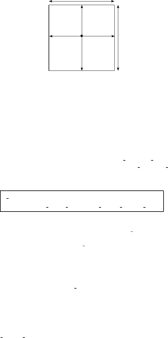
MECHANICAL ENERGY BUDGETS AND CONVERSIONS 167
U(i,j)
dyu(i,j)
dxu(i,j)
dxun(i,j)
dyue(i,j)
Figure 9.3 Time independent horizontal grid distances (meters) used for the velocity cell
Ui,jin MOM4. dxui,jand dyui,jare the grid distances of the velocity cell in
the generalized zonal and meridional directions, and daui,j=dxui,jdyui,jis the
area of the cell. The grid distance dxuei,jis the zonal width of the north face of
a velocity cell, and dyuei,jis the meridional width of the east face. Note that the
velocity point Ui,jis not generally at the center of the velocity cell. Distances are
functions of both iand jdue to the use of generalized orthogonal coordinates.
9.6.3 Diagnosing the vertical transport for U-cells
Thickness weighted horizontal advective velocities uh eu and vh nu are defined in
MOM4 by remapping the horizontal advective velocities uh et and vh nt, defined
in Section 9.4.2, onto the velocity cell faces. The satisfy continuity via a U-grid
version of the T-grid result (9.48)
w buk=∂t(dzuk)−dzukS(V)
+BDX EU(uh euk) + BDY NU(vh nuk) + w buk−1,(9.100)
where the volume source S(V)and tendency ∂t(dzuk)have been mapped from
their counterparts on the tracer grid. In this equation, w bu is the dia-surface ad-
vective velocity component defined at the bottom face of a velocity cell.
To diagnose the vertical transport w bu, we need to start at either the bottom or
top of the ocean column, given a boundary condition. On the B-grid, the bottom of
the bottom-most U-cell does not live on the ocean bottom, unless the ocean bottom
is flat. Hence, a nontrivial mass or volume transport generally occurs through the
bottom of a velocity cell column. That is, in general
w buk=kbot 6=0, (9.101)
which contrasts with the case on the T-cells (equations (9.50) and (9.80)).
A thorough discussion of this issue is provided in Section 22.3.3.2 of the MOM3
Manual (Pacanowski and Griffies, 1999). For present purposes, we note that it is
sufficient to start the integration at the ocean surface and integrate downwards, just
as for the tracer cells. Equivalently, we can use the remapping operator in MOM to
map w btkto w buk. Either way, the continuity equation (9.100) is maintained.
168 CHAPTER 9
9.6.4 Discrete integration by parts on horizontal convergence
We now perform the discrete analog of integration by parts. For this purpose,
expand the backwards derivative and average operators on the zonal flux terms,
dropping the j,klabels for brevity
2∑
i
dau ui·BDX EU(uh eu FAX(u)) =
∑ui·[dyueiuh euiui+1+dyueiuh euiui
−dyuei−1uh eui−1ui−dyuei−1uh eui−1ui−1]
=∑ui·ui(dyueiuh eui−dyuei−1uh eui−1)
+∑ui·(dyueiuh euiui+1−dyuei−1uh eui−1ui−1). (9.102)
Focus now on the second group of terms, where shifting sum labels leads to
nx
∑
i=1
ui·ui+1dyueiuh eui−
nx
∑
i=1
ui·ui−1dyuei−1uh eui−1=
nx+1
∑
i=2
ui−1·uidyuei−1uh eui−1−
nx
∑
i=1
ui·ui−1dyuei−1uh eui−1
=unx ·unx+1dyuenx uh eunx −u1·u0dyue0uh eu0. (9.103)
This result vanishes for either solid wall or periodic boundary conditions. Similar
manipulations apply for the meridional term, thus leading to
Ahorz =−∑K(dyueiuh eui−dyuei−1uh eui−1)
−∑K(dxuejvh nuj−dxuej−1vh nuj−1)
=−∑dau K[BDX EU(uh eu) + BDY NU(vh nu)],
(9.104)
where
Ki,j,k=1
2ui,j,k·ui,j,k(9.105)
is the discrete kinetic energy per mass.
9.6.5 Discrete integration by parts on vertical convergence
Now focus on the vertical advection term, which takes the form
2Avert =
kbot
∑
k=1
dau uk·[−w buk−1(uk−1+uk) + w buk(uk+uk+1)]
=
kbot
∑
k=1
dau uk·uk(wbuk−w buk−1)
+
kbot
∑
k=1
dau (wbukuk+1·uk−w buk−1uk·uk−1)
=2
kbot
∑
k=1
dau Kk(wbuk−w buk−1)
−∑dau w bu0(u0·u1) + ∑dau w bukbot (ukbot+1·ukbot).
(9.106)
MECHANICAL ENERGY BUDGETS AND CONVERSIONS 169
The horizontal velocity at k=kbot +1vanishes
ukbot+1=0, (9.107)
since k=kbot +1is interpreted as part of the solid earth. In contrast,
uk=0=uw(9.108)
is the horizontal velocity of the fresh water. This velocity is often set equal to
the surface ocean velocity uw=u1, yet mom4 retains the option of providing a
different value. This result then leads to
2Avert =2
kbot
∑
k=1
dau Kk(wbuk−w buk−1)−∑
i,j
dau w bu0(u1·uw). (9.109)
9.6.6 Final result
Combining the results for Ahorz and Avert renders
Ahorz +Avert =−(1/2)∑dau w bu0(u1·uw)
−
nk
∑
k=1
dau K[BDX EU(uh eu) + BDY NU(vh nu)]
−
nk
∑
k=1
dau K(wbuk−1−w buk)
=−(1/2)∑dau w bu0(u1·uw)
+∑
i,j,k
dau K[∂t(dzuk)−dzukS(V)],
(9.110)
where we applied volume conservation over each U-cell as given by equation
(9.100).
9.7 DISCRETE NON-BOUSSINESQ KINETIC ENERGY ADVECTION
Building on the results from Section 9.6, we now consider the conversion of kinetic
energy advection in the discret non-Boussinesq discete. For this purpose, consider
Ahorz =−∑
i,j,k
dau dzu u·BDX EU(uhrho eu ∗FAX(u))/dzu
−∑
i,j,k
dau dzu u·BDY NU(vhrho nu ∗FAY(u))/dzu.(9.111)
Thickness weighted and density weighted horizontal advective velocities uhrho eu
and vhrho nu are defined in MOM4 by remapping the horizontal advective veloc-
ities uhrho et and vhrho nt, defined by equations (9.73) and (9.76), onto the ve-
locity cell faces. These horizontal transports satisfy continuity via a U-grid version
of the T-grid result (9.77)
wrho buk=∂t(rho dzu)k−rho dzu S(M)
+BDX EU(uhrho euk) + BDY NU(vhrho nuk) + wrho buk−1.
(9.112)

170 CHAPTER 9
where the mass source has been mapped from the tracer to the velocity grid.
In this equation, wrho bu is the density weighted dia-surface advective velocity
component defined at the bottom face of a velocity cell. As in the Boussinesq case
discussed in Section 9.6, this vertical transport is diagnosed using the continuity
equation, or equivalently via the MOM remap operator.
In general, results for the Boussinesq case transparently generalize to the non-
Boussinesq case, which allows us to write by inspection
A=−(1/2)∑dau wrho bu0(u1·uw)
−
nk
∑
k=1
dau K[BDX EU(uhrho eu) + BDY NU(vhrho nu)]
−
nk
∑
k=1
dau K(wrho buk−1−wrho buk)
=−(1/2)∑dau wrho bu0(u1·uw)
+∑
i,j,k
dau K[∂t(rho dzuk)−rho dzukS(M)].
(9.113)

Chapter Ten
Temporal treatment of the Coriolis force
The purpose of this chapter is to present the two methods used in MOM4 for
temporally discretizing the Coriolis force. Much of this material was presented
in the MOM4 Guide of Griffies et al. (2004). It is useful to repeat this material,
however, in the context of the density and thickness weighting used in mom4p1 as
well as the preferred forward time step for the tendencies rather than the leap frog.
10.1 INERTIAL OSCILLATIONS
The inviscid momentum equation in the absence of pressure is given by
(d/dt+fˆz∧)u=0, (10.1)
which is equivalent to the second order free oscillator equation
(d2/dt2+f2)u=0. (10.2)
Here, d/dtis the material time derivative relevant for Lagrangian observers. Mo-
tions which satisfy this equation are termed inertial oscillations and they have pe-
riod given by
Tinertial =2
π
f=11.97
sin
φ
hour (10.3)
where Ω=7.292 ×10⁻⁵s−1is the earth’s angular speed. The period of inertial
oscillations is smallest at the North pole where
φ
=
π
/2and Tsmallest ≈12 hour.
An explicit temporal discretization of the inertial oscillation equation (10.1) will be
unstable if the time step is longer than some fraction of the inertial period, where
the fraction depends on details of the time stepping. Coarse resolution models
(models with resolutions on the order of 4-5 degrees) may find this time step con-
straint is the most stringent of the model’s baroclinic momentum processes. To
get around this limitation, a semi-implicit temporal treatment has been traditionally
considered, as in Bryan (1969).
Additional issues with coupling to sea ice may warrant an implicit treatment even
for ocean models run with a momentum time step that well resolves the inertial
period. In these cases, temporal details of ocean-ice coupling have been found to
cause enhanced energy at the inertial period. Semi-implicit time stepping of the
Coriolis force may assist in damping this energy.
It is for these reasons that MOM4 provides an option to time step the Corio-
lis force either explicitly or semi-implicitly in the baroclinic portion of the model.
The namelist parameter acor sets the level of implicitness, as described in Section
10.5.2.
172 CHAPTER 10
10.2 EXPLICIT TEMPORAL DISCRETIZATION WITH LEAP FROG
Consider now just the linear part of the inertial oscillation equation, where advec-
tion is dropped
(∂t+ˆz∧)u=0. (10.4)
Following the time integration discussions in O’Brien (1986) and Bryan (1991) (see
also Section 2.3 of Durran (1999)), introduce the complex velocity
w=u+i v (10.5)
where i=√−1and wshould not be confused with the vertical velocity compo-
nent. In terms of w, equation (10.4) takes the form
∂tw=−i f w (10.6)
which has an oscillatory solution
w=woei f t (10.7)
with period
Tinertial =2
π
f−1. (10.8)
Time discretizing equation (10.6) with a centered leap-frog scheme leads to
w(
τ
+∆
τ
) = w(
τ
−∆
τ
)−i
λ
w(
τ
)(10.9)
with
λ
=2f∆
τ
(10.10)
a dimensionless number. We can write the finite difference solution in terms of an
amplification factor
w(
τ
+∆
τ
) = G w(
τ
). (10.11)
Substituting this ansatz into equation (10.9) leads to the quadratic equation
G2+i
λ
G−1=0 (10.12)
whose solution is
G=−i
λ
±√−
λ
2+4
2. (10.13)
If
λ
/2=f∆
τ
<1, (10.14)
then |G|=1, which means the two finite difference solutions are neutral and sta-
ble. One root is an unphysical mode, known as the leap-frog computational mode,
and the other corresponds to the physical solution. If
λ
>2then |G|>1which
means both roots are unstable. Hence, stability requires a time step satisfying
∆
τ
<f−1. (10.15)
That is,
Tinertial
∆
τ
=2
π
f∆
τ
>2
π
, (10.16)
meaning the leap-frog scheme remains stable if there are at least 2
π
time steps
per inertial period. At the North Pole, this constraint means
∆
τ
<1.9 hours. (10.17)
For the baroclinic part of the model algorithm, ∆
τ
<1.9 hours can be the limit-
ing time step for coarse resolution global models, thus motivating an alternative
approach discussed in Section 10.3.

TEMPORAL TREATMENT OF THE CORIOLIS FORCE 173
10.3 SEMI-IMPLICIT TIME DISCRETIZATION WITH LEAP FROG
To overcome the time-step constraint (10.17) on the baroclinic time step, we now
consider a semi-implicit time stepping scheme within the leap-frog portion of the
baroclinic algorithm. As with any implicit approach, stability can be enhanced
relative to explicit schemes. The price to pay is dissipation of the inertial motions.
See section 2.3 of Durran (1999) for discussion.
A semi-implicit treatment of the Coriolis force, within a leap-frog scheme, leads
to
w(
τ
+∆
τ
)−w(
τ
−∆
τ
) = −i
λ
[(1−
γ
)w(
τ
−∆
τ
) +
γ
w(
τ
+∆
τ
)] (10.18)
where 0≤
γ
≤1is a dimensionless number whose value is set according to
stability considerations. We can write w(
τ
+∆
τ
) = G w(
τ
−∆
τ
), with the semi-
implicit scheme yielding the amplification factor
G=1−i
λ
(1−
γ
)
1+i
λ γ
. (10.19)
The squared modulus |G|2is used to determine conditions for stability
|G|2=[1−
γ λ
2(1−
γ
)]2+
λ
2
[1+ (
γ λ
)2]2. (10.20)
For
γ
=0,|G|>1which leads to an unstable scheme. For
γ
=1/2,|G|=1
and so the scheme is neutral. With 1/2<
γ
≤1,|G|<1, and so the scheme is
unconditionally stable. Hence, we arrive at the stability range for the semi-implicit
parameter
1/2≤
γ
≤1, (10.21)
with
γ
=1yielding the most stable scheme. Section 2.3.2 of Durran (1999) details
the impact on the phase and amplitude of inertial waves depending on the value
of
γ
. That analysis shows that
γ
=1/2is the most accurate, with zero amplitude
error and favorable phase errors relative to other methods.
10.4 SEMI-IMPLICIT TIME DISCRETIZATION WITH FORWARD STEP
As discussed in Section 12.8.3 of Griffies (2004) (see also page 51 of Durran
(1999)), the Coriolis force with a forward time step is unstable, and so an alterna-
tive must be considered. We apply here the semi-implicit approach from Section
10.3 with a forward time step rather than the leap frog. Here, we consider
w(
τ
+∆
τ
)−w(
τ
) = −iΛ[(1−
γ
)w(
τ
) +
γ
w(
τ
+∆
τ
)] (10.22)
where again 0≤
γ
≤1is a dimensionless number whose value is set according
to stability considerations. The dimensionless parameter Λis given by
Λ=f∆
τ
. (10.23)
Note the factor of 2needed for the leap frog scheme (equation (10.10)) is now
absent for the forward scheme. All of the analysis in Section 10.3 follows through,
with the factor of 2the only distinction.
174 CHAPTER 10
10.5 AS IMPLEMENTED IN MOM4
Both an explicit and semi-implicit treatment of the Coriolis force in the baroclinic
equations are available in MOM4 when using leap frog tendencies, with the semi-
implicit treatment required when using the forward tendencies. For both cases,
the semi-implicit piece is handled at the end of a baroclinic time step, even after
the implicit treatment of vertical mixing. The logic used in the code can be a bit
confusing, so it is useful to expose some details here.
10.5.1 Algorithm in the code
Let us separate that portion of the Coriolis force proportional to
γ
from the portion
independent of
γ
in order to ease coding for the case with a fully explicit Coriolis
force. We also expose the thickness and density weighting used in mom4p1. Since
velocity is updated first as the density and thickness weighted velocity, it is useful
to introduce a shorthand
e
u≡(
ρ
dz)u. (10.24)
We consider now three cases for handling the Coriolis force.
•An explicit treatment of the Coriolis force with the leap frog takes the form
−fˆz∧e
u→ −fˆz∧e
u(
τ
), (10.25)
•whereas a semi-implicit Coriolis force with the leap frog is
−fˆz∧e
u→ −fˆz∧[(1−
γ
)e
u(
τ
−∆
τ
) +
γ
e
u(
τ
+∆
τ
)]
=−fˆz∧e
u(
τ
−∆
τ
)−f
γ
ˆz∧[e
u(
τ
+∆
τ
)−e
u(
τ
−∆
τ
) ],
(10.26)
•and a semi-implicit Coriolis force with a forward time step is
−fˆz∧e
u→ −fˆz∧[ (1−
γ
)e
u(
τ
) +
γ
e
u(
τ
+∆
τ
) ]
=−fˆz∧e
u(
τ
)−f
γ
ˆz∧[e
u(
τ
+∆
τ
)−e
u(
τ
) ].(10.27)
We now consider the remaining terms in the equations of motion. As stated
earlier, when treating the Coriolis force with an implicit piece (i.e., with
γ
>0), this
is handled last. We write those accelerations independent of
γ
in the form
δτ
e
u∗=F(10.28)
where Fincludes the thickness weighted and density weighted accelerations from
velocity self-advection, the horizontal pressure gradient force, friction force (both
explicit and implicit), as well as that piece of the Coriolis force independent of
γ
.
If the Coriolis force is computed explicitly, then Fis the full time tendency for the
baroclinic velocity. For the semi-implicit treatment, we require those contributions
proportional to
γ
. For the leap frog, this leads to
e
u(
τ
+∆
τ
) = e
u(
τ
−∆
τ
) + 2∆
τ δτ
e
u∗−
λ γ
ˆz∧[e
u(
τ
+∆
τ
)−e
u(
τ
−∆
τ
) ] (10.29)
where again
λ
=2f∆
τ
. Writing out the components leads to
e
u(
τ
+∆
τ
) = e
u(
τ
−∆
τ
) + 2∆
τ δτ
e
u∗+
λ γ
[e
v(
τ
+∆
τ
)−e
v(
τ
−∆
τ
) ] (10.30)
e
v(
τ
+∆
τ
) = e
v(
τ
−∆
τ
) + 2∆
τ δτ
e
v∗−
λ γ
[e
u(
τ
+∆
τ
)−e
u(
τ
−∆
τ
)], (10.31)
TEMPORAL TREATMENT OF THE CORIOLIS FORCE 175
and solving for e
u(
τ
+∆
τ
)renders
e
u(
τ
+∆
τ
) = e
u(
τ
−∆
τ
) + 2∆
τ
δτ
e
u∗+
λ δτ
e
v∗
1+ (
λ γ
)2(10.32)
e
v(
τ
+∆
τ
) = e
v(
τ
−∆
τ
) + 2∆
τ
δτ
e
u∗−
λ δτ
e
u∗
1+ (
λ γ
)2. (10.33)
The forward time stepping scheme is handled analogously, which leads to the
update for the two components
e
u(
τ
+∆
τ
) = e
u(
τ
) + ∆
τ
δτ
e
u∗+Λ
δτ
e
v∗
1+ (Λ
γ
)2(10.34)
e
v(
τ
+∆
τ
) = e
v(
τ
) + ∆
τ
δτ
e
u∗−Λ
δτ
e
u∗
1+ (Λ
γ
)2, (10.35)
where again Λ=f∆
τ
.
10.5.2 Namelist parameters
In the code,
∆
τ
=dtuv (10.36)
is the baroclinic time step, and
γ
=acor (10.37)
is a namelist parameter setting the level of implicit treatment for the Coriolis force.
The method for discretizing the Coriolis force in the baroclinic part of the model is
set according to the value of acor, with
acor =0⇒explicit Coriolis: only stable for leap frog (10.38)
1/2≤acor ≤1⇒semi-implicit Coriolis: required if using forward step. (10.39)
The vertically integrated part of the model algorithm typically uses a time step
much smaller than f−1. Hence, it is not necessary to discretize the Coriolis force
semi-implicitly when time stepping the vertically integrated equations with a leap
frog algorithm. However, when using the predictor-corrector described in Section
12.7 of Griffies (2004), 1/2≤
γ
≤1is required for stability, and we choose
γ
=
1/2.
10.5.3 Energy analysis
In the continuum, the Coriolis force does no work on a fluid parcel since it is always
directed orthogonal to the flow direction
v·fˆz∧u=0. (10.40)
This property is respected on the B-grid when we discretize the Coriolis force
explicitly in time
v(
τ
)·fˆz∧u(
τ
) = 0. (10.41)
However, the semi-implicit treatment does not respect this property since in gen-
eral the product
v(
τ
)·fˆz∧[(1−
γ
)u(
τ
−∆
τ
) +
γ
u(
τ
+∆
τ
)] (10.42)
does not vanish unless the flow is in time independent steady state.

Chapter Eleven
Open boundary conditions
The purpose of this chapter is to present the method used in mom4p1 for pre-
scribing open boundary conditions (OBCs). The numerical schemes for OBCs are
very much dependent on details of the model setup. Hence, mom4p1 is provided
with many options. Note that the OBC code remains under revision. So the user
should be mindful of scrutinizing results. Feedback to the developers is greatly
appreciated.
This chapter was written by Michael Herzfeld, Martin Schmidt, and Stephen
Griffies. The algorithm and code developers for the mom4p1 OBC are
Mike.Herzfeld@csiro.au
Martin.Schmidt@io-warnemuende.de
Zhi.Liang@noaa.gov
Please email them directly for queries about the documentation or the OBC code.
11.1 INTRODUCTION
Numerical circulation models of marginal seas with biological, chemical and sed-
iment dynamic components require a high model resolution and involve a large
number of variables. Working with regional models is one method to meet this
challenge with a reasonable amount of computer resource consumption. Mostly,
the exchange of mass, heat, momentum and dissolved or suspended matter with
the outer ocean is important. At the model boundary an open boundary condition
(OBC) must apply, which permits flux out of - and into the model area.
This chapter describes the numerical schemes implemented for this purpose in
mom4p1. They are described in detail in the corresponding literature. It seems,
that an universal open boundary condition suitable for all kinds of regional models
does not exist. Hence, we have chosen to implement several schemes, which can
be selected and modified by namelist parameters.
Open boundary conditions for a regional model reveal as a complex problem. To
be more specific, consider a large model ocean, subdivided by a virtual boundary
into a western and an eastern sub-basin. Wind forcing, heat flux or fresh water flux
in the eastern subbasin drives elevation of the sea surface, currents and changes
in the density field as well. The information on such events in the eastern part
is transmitted to the west by waves, at large time scales also by advection. If
the virtual boundary is replaced with the open western boundary of a regional
submodel of the eastern subbasin, the results of the regional submodel and those
of the larger model must be the same. Hence, waves generated in the eastern
178 CHAPTER 11
subbasin must be able to pass an open boundary without reflection and refraction,
just as if it was not there. In the same manner, processes forced in the western
subbasin influence the eastern part by waves too. If this is of importance for the
eastern model part, the western open boundary condition must generate these
waves.
Hence, the required boundary condition is solution of the hydrodynamic equa-
tions at the boundary itself and is basically unknown. Simplifying assumptions
on the nature of the flow near the boundary are needed to close the numerical
schemes at the boundary. For ocean models many different methods are known.
Here we confine ourselves to methods, which combine a radiation condition, to
facilitate outward directed wave propagation through open boundaries in combina-
tion with relaxation to prescribed values of ocean variables, to simulate the influ-
ences from outside the model domain. Relaxation of boundary values helps also to
eliminate numerical errors of the boundary scheme and to prevent the model from
divergence by the accumulation of numerical errors over longer model integration
time.
11.2 TYPES OF OPEN BOUNDARY CONDITIONS
The purpose of this section is to describe the sorts of boundary conditions im-
plemented in mom4p1. For realistic applications the numerical solution near a
boundary is always a superposition of outgoing and incoming waves, which can-
not be separated. Applying the radiation condition and relaxation of boundary val-
ues to this complex variables, turns OBC into a mathematically ill-posed problem
and there is no universally perfect scheme for open boundary conditions. Hence,
often the OBC configuration must be established by trial and error on a case by
case basis. So what may work fine in one application may not work if one alters
the bathymetry, geography, forcing, subgrid scale parameterizations, or numerical
implementation of the OBC.
11.2.1 Open boundaries in the ARAKAWA B-grid
Because mom4p1 uses the ARAKAWA B-grid, tracers and sea level points are
the outmost points, where the numerical scheme has to be closed by an open
boundary condition. Velocity points are within the model domain. At points adja-
cent to the boundary the non-linear advective terms and diffusion terms are un-
defined. To close the numerical scheme for these terms, velocity points beyond
the boundaries are defined by appropriate extrapolation. The remaining terms in
the momentum equations can be calculated using pre-existing fields. This formu-
lation of the open boundary conforms to a stencil originally proposed by Stevens
(1990),Stevens (1991). This approach effectively limits any error introduced by the
OBC to the two non-linear terms, thus preventing any error associated with the
OBC from rapidly propagating into the interior via the Coriolis terms.
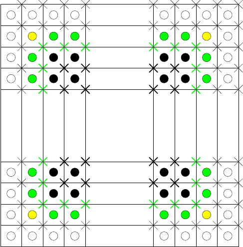
OPEN BOUNDARY CONDITIONS 179
B−1
B+1 B
B+1 B−1
B+1
BB
B+1
B−1
B−2 B−1
B−2
B−1
B
B+1
B
B−1
B+1
B+1BB−1 B+1BB−1B−2B
Figure 11.1 Open boundary conditions in the Arakawa B-grid. Circles mark tracer points,
crosses velocity points. Open boundary conditions apply at green points.
180 CHAPTER 11
11.2.1.1 Notation
Boundary points are marked with a capital B. The first points beyond the boundary
outside the model domain is B+1, the first internal point in the model domain is
B−1. See also Figure 11.1!
11.2.1.2 Boundary conditions for the sea level
The boundary conditions presented here refer to circulation models which use
explicit solvers for the sea surface height where the variablity of the sea level is
governed by waves. Hence, the boundary condition for the sea level is based on
the wave like properties of the solution and has the form of a radiation condition
for outgoing waves. Boundary conditions for the sea level apply at points marked
with green circles in Figure figure:grid.
11.2.1.3 Boundary conditions for tracers
The tracer propagation is described by an advection-diffusion equation, which
does not have a wave like solution itself. However, the underlying velocity field
may be wave like. Hence, especially vertical tracer advection, which is not well de-
fined near an open boundary, can be approximated by a radiation condition. The
boundary condition used here combines a radiation condition, approximations for
horizontal advection and relaxation towards prescribed data. Boundary conditions
for the tracers apply at points marked with green circles in Figure 11.1.
11.2.1.4 Boundary conditions for velocity
Boundary conditions for velocity vectors apply at points marked with a green cross
in Figure figure:grid. At these points horizontal and vertical velocity advection is
set to zero. An exception is the metric term, which is well defined. Removing it
implies horizontal inhomogeneity in the flow fields, which show up especially in
nearly uniform flow.
To get a well defined friction operator, velocity beyond the boundary must be
defined too. This is done with a no gradient condition. This condition applies at
points marked with a this black cross in Figure 11.1.
For some application it may help, to take vertical advection of tracers at bound-
ary points into consideration. A no gradient condition for the tangential velocity en-
hances ±-structures, which are typical for the Arakawa B-grid, and couples such
structures into the tracer equations. Hence, the tangential velocity at points be-
yond the boundary should be set to the value of the second interiour point, which
prevents infiltration of ±-structures from the velocity field into the tracer fields from
the OBC.
11.2.2 Sommerfeld radiation condition
Most open boundary conditions are based on the Sommerfeld radiation condition
(Sommerfeld, 1949). This kind of boundary condition was originally derived for the

OPEN BOUNDARY CONDITIONS 181
theory of electromagnetic waves to remove incoming waves from the far field so-
lution for an oscillating dipole antenna. The Sommerfeld radiation condition takes
the form:
η
,t=−c
η
,xat x=xB. (11.1)
In this equation,
η
(x,t)is the space-time dependent free surface height, cis the
wave phase speed determined via a method discussed in Section 11.3, x=xBis
the spatial position of the open boundary in question. Finally, we use the shorthand
notation
η
,t=∂
η
∂t
η
,x=∂
η
∂x
(11.2)
to denote partial derivatives. The performance of OBC’s based on the Sommerfeld
condition (11.1) has been extensively assessed in the literature (see, for exam-
ple Chapman, 1985; Roed and Cooper, 1987; Tang and Grimshaw, 1996; Palma
and Matano, 1998, 2001). Unfortunately, OBC’s based on the Sommerfeld con-
dition often exhibit inaccuracies. The key reason is that the model solution is a
superposition of several waves which have different phase speeds and which are
dispersive (in contrast to the linear electromagnetic waves that Sommerfeld was
concerned). However, the Sommerfeld condition is based on just a single wave
condition. The OBC behaviour in practice is thus very sensitive to how the phase
speed in equation (11.1) is determined.
We can classify the boundary conditions as passive, in which case the OBC
is determined solely from information within the computational domain, or active,
so that data is prescribed from an external source. Since the behaviour of the
model interior is rarely consistent with data prescribed at the boundary, the model
may become prone to errors due to under-specification (not enough information
describing external processes is provided) or over-specification (OBC information
is incompatible with interior equations). Marchesiello and Shchepetkin (2001) pro-
vide a thorough discussion of the active versus passive boundaries, and over ver-
sus under-specification of data.
To alleviate problems with over-specification, an active boundary condition may
be rendered partially passive by coupling to a radiation condition. This approach
was used by Blumberg and Kantha (1985). Here, relaxation towards externally
prescribed data is performed with an associated relaxation timescale, so that
η
,t=−c
η
,x−(
η
−
η
o)/
τ
f. (11.3)
Here,
η
ois the prescribed data for the surface height, and
τ
fis a timescale. Even
with this prescription for the OBC, the behaviour of the simulation can be sensitive
to the choice of radiation condition and relaxation timescale used.
Likewise a fresh water flux may be added, but its influence will most probably
disappear behind the relaxation term.
11.2.3 Clamped boundary conditions
A simple boundary condition is the clamped boundary condition, i.e., sea level
or tracers are kept at a fixed value. For the sea level no physical justification is
182 CHAPTER 11
given for using this condition. It is motivated solely from the fact that it keeps the
numerical scheme stable. For salinity and temperature it may be a reasonable ap-
proximation. The clamped condition requires the user to supply a single time and
space independent value to be imposed on the boundary. This type of condition
corresponds to a zero phase speed, c=0, in the Sommerfeld radiation condition
(11.1). It creates many reflections at the boundary, which can be undesirable.
In a modified form time and space dependent values for the sea level or trac-
ers may be prescribed. Keeping in mind, that most ocean flow is geostropically
balanced, this defines the baroclinic and barotropic geostrophic transport through
the boundary. This may be desired, but implies also the possibility of unwanted
numerical effects, which may corrupt the numerical solution in the model domain.
11.2.4 No gradient boundary conditions
This condition imposes a smooth solution near the boundary. The no-gradient
OBC assumes that there does not exist a gradient of a variable across the open
boundary. It is sometimes referred to as a Neumann boundary condition. This
condition corresponds to setting the phase speed to infinity in the Sommerfeld
radiation condition (11.1). It is specified by setting the value at the open boundary
equal to the value immediately adjacent to the open boundary in the model interior,
so that
η
(t+1, xB) =
η
(t+1, xB−1). (11.4)
In this equation, t+1is the updated time step, xBsignifies the spatial position of
the open boundary, with
η
(t+1, xB)is the surface height at that boundary. As
shown in Figure 11.1 xB−1signifies the spatial position of the nearest point interior
from the open boundary, with the sign determined by the relative position of the
open boundary.
For velocity a no gradient boundary condition applies across the boundary, to
get a defined viscosity operator
u(t+1, xB+1) = u(t+1, xB). (11.5)
11.2.5 Interior cell no gradient boundary conditions
This condition is similar to the no-gradient boundary condition (11.4). However,
instead of using the value at the nearest interior grid cell, the boundary is set to
the value at the next nearest interior (B−2) cell (i.e., two grid points away from the
boundary)
η
(t+1, xB) =
η
(t+1, xB−2). (11.6)
For the tangetial velocity a no gradient boundary condition across the boundary
is used to get a defined viscosity operator
u(t+1, xB+1) = u(t+1, xB−1). (11.7)
11.2.6 Enhanced friction and diffusion near the boundary
This method increases the dissipation from tracer diffusion and momentum friction
in regions near the open boundary. This approach acts to dissipate spurious re-
flections at the boundary. It also may be useful to remove artificial currents near
OPEN BOUNDARY CONDITIONS 183
the boundary, which may grow to be large in some cases. However, this approach
has the detrimental effect of slowing cross boundary transport.
11.3 IMPLEMENTATION OF SEA LEVEL RADIATION CONDITIONS
In this section, we discuss various radiation conditions that are used to specify
the phase speed. We also discuss how to specify the tracers across the open
boundary.
11.3.1 Sign convention for the phase speed
The phase speed is a vector quantity. Here it is always directed perpendicularly
to the model boundary and notation can simplified considerably by considering
the projection of the phase speed onto the normal vector of the model boundary.
The sign of the phase speed is positive for eastward or northward travelling waves
and negative for westward or southward directed waves. However, the quantity of
interest is the projection of the phase speed onto the boundary normal vector. In
all radiation conditions given below, phase speed means this projection, which is
positive for outgoing waves and negative for incoming waves.
11.3.2 Gravity wave radiation condition for the phase speed
This formulation computes a phase speed relevant for a flat bottom barotropic
shallow water configuration, so that
c=pg DB, (11.8)
where gis the acceleration from gravity, and DBis the depth at the boundary
(Chapman, 1985)). Hence, in this approximation it is assumed, that processes
near the boundary are always governed by outgoing waves. The OBC is imple-
mented in an implicit form, so that
η
(t+1, xB) =
η
(t,xB) +
µ η
(t+1, xB−1)
1+
µ
, (11.9)
where
µ
=c∆t
∆x, (11.10)
where ∆xis the horizontal grid spacing. That is, equation (11.9) is the implicit
solution to equation (11.1) using cas the gravity wave speed.
Note: phase speed is always positive for gravity wave radiation, implying that
waves are always outgoing. This means that outgoing relaxation ,
τ
out, is always
used when relaxing to data (see Section 11.3.9.3).
11.3.3 Orlanski radiation condition for the phase speed
We aim to account for the most important part of the wave spectrum. There are
various means for doing so, with the Orlanski radiation condition (Orlanski, 1976)
one of the most common. Here, the the phase speed of disturbances approaching

184 CHAPTER 11
the boundary is diagnosed at every time-step from the distribution of the interior
values of the surface height near the boundary, so that
~c=−
η
,t/
η
,x. (11.11)
The Orlanski radiation condition theoretically has a zero reflection coefficient. This
property is desired to reduce spurious reflected waves at the open boundary. Un-
fortunately, in practice reflections occur due to inaccuracies in the phase speed
computation.
The form employed by mom4p1 is the implicit formulation based on (Chapman,
1985)
η
(t+1, xB) = (1−
µ
)
η
(t−1, xB) + 2
µ η
(t,xB−1)
1+
µ
. (11.12)
Here, the dimensionless parameter
µ
is set according to
µ
=
1if C≥1
Cif 0<C<1
0if C≤0,
(11.13)
where
C=
η
(t−1, xB−1)−
η
(t+1, xB−1)
η
(t+1, xB−1) +
η
(t−1, xB−1)−2
η
(t,xB−2). (11.14)
11.3.4 Camerlengo and O’Brien radiation condition
Camerlengo and O’Brien (1980) suggested a modified form of the Orlanski radia-
tion condition, where only the extreme values of the phase speed, zero or h/t, so
that;
η
(t+1, xB) =
η
(t,xB−1)if C>0
η
(t−1, xB)if C≤0, (11.15)
with Cgiven by equation (11.14).
11.3.5 Radiation condition after Miller & Thorpe
The Orlanski scheme is modified here so that time differences are evaluated using
a forward scheme and space differences with an upwind scheme (see equation 15
in Miller and Thorpe, 1981)
η
(t+1, xB) =
η
(t,xB)−
µ
(
η
(t,xB)−
η
(t,xB−1)). (11.16)
In this case, the dimensionless coefficient
µ
=
µ
1+
µ
2+
µ
3, (11.17)
with
µ
1=
η
(t+1, xB−1)−
η
(t,xB−1)
η
(t,xB−2)−
η
(t,xB−1)(11.18)
µ
2=
η
(t,xB)−
η
(t−1, xB)
η
(t−1, xB−1)−
η
(t−1, xB)(11.19)
µ
3=
η
(t,xB−1)−
η
(t−1, xB−1)
η
(t−1, xB−2)−
η
(t−1, xB−1). (11.20)
The scheme is implemented in an explicit temporal form.
OPEN BOUNDARY CONDITIONS 185
11.3.6 Raymond and Kuo radiation condition
This radiation condition was introduced by Raymond and Kuo (1984) and used in
adaptive form by Marchesiello et al. (2001). This scheme calculates the phase
velocity for multidimensional flows using a projection of each coordinate direction,
i.e. not just the normal component. The scheme is implemented in implicit form.
The Sommerfeld radiation condition takes the form:
η
,t=−cx
η
,x−cy
η
,y(11.21)
where xand yare directions normal and tangential to the boundary respectively.
The phase speeds cxand cyare projections given by:
cx=−
η
,t
η
,x
η
2
,x+
η
2
,y
, (11.22)
cy=−
η
,t
η
,y
η
2
,x+
η
2
,y
. (11.23)
This is discretised following Marchesiello et al (2001);
η
(t+1, xB,yB) = 1
1+rx
η
(t,xB,yB) + rx
η
(t+1, xB−1,yB)−ry(
η
(t,xB,yB)−
η
(t,xB,yB−1))ry>0,
η
(t,xB,yB) + rx
η
(t+1, xB−1,yB)−ry(
η
(t,xB,yB+1)−
η
(t,xB,yB))ry<0.
(11.24)
where:
rx=−∆
η
t∆
η
x
∆
η
2
x+∆
η
2
y
ry=−∆
η
t∆
η
y
∆
η
2
x+∆
η
2
y
(11.25)
∆
η
t=
η
(t+1, xB−1,yB)−
η
(t,xB−1,yB)(11.26)
∆
η
x=
η
(t+1, xB−1,yB)−
η
(t+1, xB−2,yB)(11.27)
∆
η
y=
η
(t,xB−1,yB)−
η
(t,xB−1,yB−1)if D>0,
η
(t,xB−1,yB+1)−
η
(t,xB−1,yB)if D<0
D=∆
η
t(
η
(t,xB−1,yB+1)−
η
(t+1, xB−1,yB−1))(11.28)
The adaptive for relaxation takes on a form similar to Equation (11.3),
η
,t=−cx
η
,x−cy
η
,y−(
η
−
η
o)/
τ
f. (11.29)
where
τ
f=
τ
out if cx>0and
τ
f=
τ
in with cx=cy=0if cx<0. The relax-
ation time scale
τ
out
τ
in such that during outward phase propagation a weak
relaxation exists to avoid boundary values drifting excessively but also preventing
problems of over-specification, while during inward phase propagation stronger
relaxation is applied that avoids shock issues.
11.3.7 The IOW-radiation condition
As for the gravity wave radiation condition an implicite scheme is used,
η
(t+1, xB) =
η
(t,xB) +
µ η
(t+1, xB−1)
1+
µ
, (11.30)
186 CHAPTER 11
where
µ
=C∆t
∆x. (11.31)
The spatial and time derivative of
η
are
∆
η
,x=
η
(t+1, xB−1)−
η
(t+1, xB−2)
∆x, (11.32)
∆
η
,t=
η
(ts,xB−1)−
η
(t+1, xB−1)
∆t. (11.33)
If the predictor-corrector scheme is used, the phase speed is calculated twice. In
this case
η
(ts)denotes
η
at the starting time step of this scheme. In the predictor
step ∆tis the reduced time step ∆t=
γ
dt. For the leapfrog scheme ts=t−1and
∆t=2dt.
To ensure a well defined phase speed for small horizontal gradients this case is
treated separately,
C(t+1) = C∗(t+1)if ∆
η
x>a,
0.99 e
C(t)if ∆
η
x≤a,(11.34)
where ∆
η
x=|
η
(t+1, xB−1)−
η
(t+1, xB−2)|and ais a small length, typically
10−8m. e
Cis the time smoothed phase speed from the previous time step. The
scheme allows to control the minium and maximum value of the phase speed. For
incoming waves, negative phase speed, positive values (or zero) are assumed,
C∗(t+1) =
Cinc if C+<0,
Cmin if C+<Cmin,
C+if Cmax >C+>Cmin,
Cmax if C+>Cmax.
(11.35)
C+(t+1)is calculated from the derivatives of
η
,
C+(t+1) = ∆
η
,t
∆
η
,x. (11.36)
Cmax,Cmin and Cinc are defined in terms of the gravity wave speed,
Cmax =cmaxpg DB(11.37)
Cmin =cminpg DB(11.38)
Cinc =cincpg DB. (11.39)
The factors cmax,cmin and cinc can be modified via the namelist.
Relaxation is done as described in Section 11.3.9.
11.3.8 Phase speed smoothing
The diagnosed phase speed may be very noisy with altering sign every time step.
A time smoother
e
C(t+1) = Fe
C(t) + (1−F)C(t+1), (11.40)
helps to reduce numerical noise. The default value is F=0.7. The application of
the smoother requires to save e
Cin a restart file, to ensure reproducibility across
model restarts.
OPEN BOUNDARY CONDITIONS 187
11.3.9 Relaxation to data
11.3.9.1 Relaxation towards prescribed profiles
The radiation conditions may be coupled to prescribed data as described by Equa-
tion (11.3). This approach is implemented implicitly as
η
(t+1, xB) = e
η
(t+1, xB) +
η
o∆t
τ
f
1+∆t
τ
f
, (11.41)
where e
η
(t+1, xB)is the solution on the boundary derived from the radiation con-
ditions.
τ
fis the time scale for the relaxation process.
The relaxation may occur a given number of cells into the interior, in which case
e
η
(t+∆t,xB)is the interior solution to the continuity equation.
11.3.9.2 Relaxation of the sea level average - conservation of geostrophic currents
If the model area is a semi-enclosed sea, which is connected to the ocean by a
narrow channel, the open boundary may be placed within this channel. By pre-
scribing the sea level profile across the channel, one defines also the geostrophic
volume transport through this channel. In this case the incertitude of the OBC may
dominate the volume budget of the model. To overcome this serious shortcoming,
an alternative relaxation scheme may be used, which prescribes only the average
sea level at the boundary. Doing so, the geostropic transport defined by the cross
channel sea level gradient is not affected by the relaxation. Only the ageostropic
flow may react to the prescribed sea level variation, geostrophic adjustment hap-
pens through the internal model dynamics. The scheme works explicitly,
η
(t+1, xB) = e
η
(t+1, xB) + ∆t
τ
f
(
η
o−he
η
(t+1, xB)i)(11.42)
he
η
(t+1, xB)iis sea level averaged over the boundary.
11.3.9.3 Variable relaxation for incoming and outgoing waves
Likewise, the value of
τ
fmay be different for prevailing incoming or outgoing
waves,
τ
−1
f=r
τ
−1
out + (1−r)
τ
−1
in , (11.43)
r(t) = e
C(t)
Cmax . (11.44)
11.4 OBC FOR TRACERS
11.4.1 Reduced tracer equations at open boundaries
The tracer equations in mom4p1 are strongly linked with the sea level equation and
tracers and sea level are treated consistently. Because the radiation condition for

188 CHAPTER 11
the sea level is a rough approximation, a similar consistency cannot be achieved
for boundary points. Hence, the tracer equations at the boundaries are simplified.
To avoid double coding, the normal code should be used at boundaries as far as
possible. Tracers are updated as
T(t+1)
ρ
(t+1)h(t+1) = T(t)
ρ
(t)h(t) + ∆t
δ
(h(t)
ρ
(t)T(t)) (11.45)
The time tendency of the vertically integrated tracer in the grid cell
δ
(
ρ
T)is the
combined time tendency of tracer concentration, density and cell thickness. It
consists of an advective and diffusive contribution and eventually of source terms
from radiation and special convective schemes (kpp). We rewrite these terms
in such a manner, that for a constant tracer the sea level equation is retained.
Especially for a uniform tracer T=1,
δ
(h
ρ
T)must be the time tendency of the cell
thickness,
δ
(h
ρ
), i.e.
δ
(h
ρ
1)→
δ
(h
ρ
) = ∆h
ρ
∆t.
δ
(h
ρ
T)k=−(∇s·h
ρ
(uT+F))k−(
ρ
(wT +F(s)))k−1+ (
ρ
(wT +F(s)))k+ (h
ρ
ST)k
δ
(h
ρ
)k=−(∇s·h
ρ
u)k−(
ρ
w)k−1+ (
ρ
w)k+ (h
ρ
SM)k(11.46)
Advection is rewritten to separate the different contributions to the time tendency,
Adv(T)k=−(∇s·h
ρ
uT)k−(
ρ
wT)k−1+ (
ρ
wT)k
=−(T∇s·h
ρ
u)k−(
ρ
wT)k−1+ (
ρ
wT)k−(h
ρ
u·∇sT)k. (11.47)
Applying approximations for open boundaries, the first three terms have to be kept
consistent with the equation for the level thickness. The level thickness is calcu-
lated from approximations only and it is appropriate to express the convergence of
the flow in terms of the level thickness time tendency. With of
−(∇s·h
ρ
u)k=
δ
(h
ρ
)k+ (
ρ
w)k−1−(
ρ
w)k−(h
ρ
SM)k(11.48)
this renders to
δ
(h
ρ
T)k=
δ
(h
ρ
)kTk+ (h
ρ
(ST−SMT))k+SGS
−(h
ρ
u·∇sT)k−(
ρ
wT)k−1+ (
ρ
wT)k+ ((
ρ
w)k−1−(
ρ
w)k)Tk.(11.49)
i.e., which ensures consistency between tracers and layer thickness for a uniform
tracer. Also the approximation of zero vertical advection and horizontal advec-
tion with an upwind scheme is consistent with the thickness equation for cells of
constant thickness. Diffusion and source terms apply unchanged and will not be
specified here.
For surface cells the vertical advection at the surface is expressed in terms of
sea level variation, fresh water flux and turbulent tracer flux,
δ
(h
ρ
T)1= (
δ
(h
ρ
)1T1+
ρ
wqw(Tw−T1) + (h
ρ
(ST−SMT))1−Qturb
T+SGS
−(h
ρ
u·∇sT)1+ (
ρ
wT)1−(
ρ
w)1T1. (11.50)
With this approximation the tracer concentration remains unchanged, if only the
sea surface height is undulating. If currents are zero, but fresh water flux and
diffusion are present, a horizontally uniform tracer distribution will not be disturbed
near an open boundary. The consistency between sea level equation and tracer
equation is not broken, if approximations for the horizontal advection term are
made, or if radiation terms are added. Those terms vanish for horizontally uniform
tracers especially for T=1and the sea level time tendency is trivially retained.
OPEN BOUNDARY CONDITIONS 189
Because vertical velocity is not well defined it is left out of consideration. It
is replaced by a radiation term, which accounts for the propagation of wave like
undulations of internal interfaces from baroclinic waves.
δ
(h
ρ
T)k=
δ
(h
ρ
)kTk+ (h
ρ
(ST−SMT))k+SGS
−(h
ρ
u·∇sT)k+c
ρ
h∂Tk
∂x+
ρ
hTre f −Tk
τ
f
(11.51)
δ
(h
ρ
T)1≈(
δ
(h
ρ
)1T1+
ρ
wqw(Tw−T1) + (h
ρ
(ST−SMT))1−Qturb
T+SGS
−(h
ρ
u·∇sT)1+c
ρ
h∂T1
∂x+
ρ
hTre f −T1
τ
f
. (11.52)
Implementation of the radiation condition and of the relaxation towards prescribed
data is documented below. Diagnostics of the phase speed is based on the tracer
concentration, because the total tracer contend may undulate rapidly from the
barotropic mode in the cell thickness variability.
11.4.2 Upstream advection of tracers near the boundary
For advection across the open boundary, an upstream scheme with
T(xB+1) = T(xB)(11.53)
means that the incoming tracer has the same concentration as the tracer at the
boundary point. This approximation may give poor results for long model runs and
can cause model drifts.
After running a passive boundary over a long period, the tracer near the bound-
ary will be determined completely by processes in the model domain. As an ex-
ample consider a marginal sea with a strong fresh water surplus. There will be an
estuarine circulation with a more or less permanent outflow of brackish water in
a surface layer and inflow near the bottom. However, the salinity of the inflowing
water will be reduced as well after some time by vertical mixing processes. The
model results will suffer from underestimated stratification. To overcome this prob-
lem, information on the tracer concentration in the adjacent sea must be provided
for the model. The simple approximation
T(xB+1) = T(x0)(11.54)
where T0may stem from a database, improves the performance of the diffusion
and the advection operators, which in turn may invoke wave like processes spread-
ing from the boundary into the model. Using an upstream formulation for the
tracer gradient in the advective term, this can switch on an inflow through the
open boundary. However, waves of a small amplitude but with a high phase speed
may disturb this scheme. Thus, the tracer source term STcan be used for a con-
trolled restoring to prescribed boundary values. The upstream advection condition
is discretized as:
T(t+1, xB) = T(t,xB)
+∆t
∆x[(un− |un|) (T(t,xB−1)−T(t,xB)) + (un+|un|) (T(t,xB)−T(t,x0))]
(11.55)

190 CHAPTER 11
where unis the velocity normal to the boundary times density and the cell height,
T(xB)is the tracer on the boundary, T(xB−1)is the tracer one cell into the interior
and T(x0)is a tracer value that must be supplied externally.
11.4.3 Relaxation towards external data
If external data are prescribed boundary values may be relaxed towards there data
as
T(t+1, xB) = (T0−T(t,xB))∆t
τ
f
. (11.56)
The relaxation time
τ
fdepends on the flow direction near the boundary. If the
sum of advection velocity and phase speed at the boundary is directed inwards,
one has
τ
f=
τ
in
fand
τ
f=
τ
out
fotherwise.
τ
in
fand
τ
out
fcan be specified in the
namelist for each tracer and boundary separately.
11.4.4 Flow relaxation scheme of Martinsen and Engedahl
The flow relaxation scheme of Martinsen and Engedahl (1987) has been included
to relax boundary data to interior data. This is accomplished over a region NN
cells wide (typically NN=10) where the tracer variables are updated according to:
T=
α
iTB+ (1−
α
i)TB±i(11.57)
where TBis the boundary specified value, TB±iare the interior variable values and
α
iis a relaxation parameter given by:
α
iTB=1−tanh i−1
2i=1, 2, ..NN (11.58)
Note that the flow relaxation scheme is used in conjunction with another boundary
condition and TBmay be obtained from the FILEIN or NOGRAD condition; whatever
is specified on the boundary is relaxed to the model integrated values over NN
cells. The flow relaxation scheme is only implemented if UPSTRM is included in the
tracer obc. If TBis equal to zero (clamped boundary condition) then this flow relax-
ation scheme acts as a sponge type condition. An example of the flow relaxation
scheme implementation in the namelist is given below:
obc_flow_relax(:,1) = 10, 1, 1
obc_flow_relax(:,2) = 10, 1, 1
11.4.5 Radiation conditions
If the velocity field near the boundary is wave like, vertical advection may result in
a wave like tracer motion. Hence, a radiation condition may improve the numerical
scheme at the boundary.
The radiation condition for tracers is applied implicitly,
T(t+1, xB) = T(t,xB) +
µ
T(t+1, xB−1)
1+
µ
, (11.59)
OPEN BOUNDARY CONDITIONS 191
where
µ
=C∆t
∆x. (11.60)
The phase speed Cis set to zero for incoming waves and is limited by Cmax,
µ
=
0if C∗<0,
C∗if 0<C∗<Cmax,
Cmax if C∗>Cmax.
(11.61)
C∗is calculated either bei the Orlanski scheme,
C∗=∆x
∆t
T(t−1, xB−1)−T(t+1, xB−1)
T(t+1, xB−1) + T(t−1, xB−1)−2T(t,xB−2), (11.62)
or by used in MOM-31 (IOW).
C∗=∆x
∆t
T(t−1, xB−1)−T(t+1, xB−1)
T(t,xB−1)−T(t,xB−2). (11.63)
For the time staggered scheme the index t−1points to the same filed as t. The
maximum phase speed, Cmax, is given by the CFL-criterion,
Cmax =∆x
∆t. (11.64)
11.4.6 Vertical mixing and viscosity co-efficients
Vertical mixing at boundary points my be enabled or diabled. However, the mix-
ing co-efficients at these points are used to define viscosity at adjacent veloc-
ity points. The namelist parameter obc mix specifies, how the mixing coefficient
at boundary points is defined. Options are NOTHIN,NOGRAD,INGRAD and CLAMPD,
obc mix=NOGRAD is the default.
11.4.7 Enhanced horizontal mixing and viscosity co-efficients
To damp unwanted numerically generated flow patterns near open boundaries
viscosity and diffusivity may be enhanced within a stripe near the boundary.
11.5 THE NAMELIST OBC NML
Mom4p1 requires that two components of velocity be prescribed on each open
boundary (normal and tangential velocities to the boundary) for both the 3D and 2D
modes. Surface elevation and the values of any tracers present are also required.
Here are the flags that specify the various fields:
•Normal velocity: obc nor
•Tangential velocity: obc tan
•Sea level elevation: obc eta
•Tracers: obc tra(:).

192 CHAPTER 11
The OBC specification is determined via text strings as listed in Table 11.1, where
the variables these conditions may be applied to are listed as un = normal velocity,
ut = tangential velocity,
η
= surface elevation, and T= tracers. The condition
specified for velocities is used for both the 2D and 3D modes. Note that the text
identifier strings have have been truncated to the same length while attempting to
describe the OBC condition to accommodate neat alignment in the namelist.
CONDITION NAME TEXT IDENTIFIER APPLICABLE VARIABLES
Relaxation to data FILEIN
η
,T
Relaxation of mean MEANIN
η
Clamped CLAMPD un,ut,
η
No-gradient NOGRAD un,ut,
η
,T
Interior-gradient INGRAD un,ut
Linear extrapolation LINEAR un,ut
Gravity wave radiation GRAVTY
η
Orlanski ORLANS
η
,T
Camerlengo and O-Brien CAMOBR
η
Miller and Thorpe MILLER
η
Raymond and Kuo RAYMND
η
Schmidt MARTIN
η
,T
Upstream advection UPSTRM T
Table 11.1 Namelist settings for the OBC specification.
An example of open boundary specification for a domain containing three open
boundaries and two tracers is given below:
nobc = 3
direction =’west’, ’south’, ’north’
is = 2, 2, 2
ie = 2, 10, 10
js = 2, 2, 20
je = 20, 2, 20
obc_nor =’NOGRAD’, ’NOGRAD’, ’NOGRAD’
obc_tan =’INGRAD’, ’INGRAD’, ’INGRAD’
obc_eta =’GRAVTY’, ’FILEIN’, ’MEANIN|ORLANS’
obc_tra(:,1) =’UPSTRM|FILEIN’, ’UPSTRM|FILEIN’,’UPSTRM|FILEIN’
obc_tra(:,1) =’NOGRAD’, ’NOGRAD’,’UPSTRM|NOGRAD’
Note that by ’or-ing’ two conditions together then these two conditions will be
invoked sequentially (order is not important). Hence the condition UPSTRM|FILEIN
will invoke an upstream advection condition, using data from file when flow is into
the domain. The condition UPSTRM|NOGRAD will invoke an upstream advection con-
dition, using the value one cell into the domain when flow is into the domain. A
wave-like contribution to the OBC can also be added for tracers, e.g. invoked by
UPSTRM|FILEIN|ORLANS. This wave-like contribution is added implicitly.
If partially passive conditions are to be used for elevation, then the FILEIN or
MEANIN condition is ’or-ed’ with the desired radiation condition, e.g. using the Or-
lanski partially passive condition with data prescribed from file use FILEIN|ORLANS.
OPEN BOUNDARY CONDITIONS 193
Note that in-going and out-coming relaxation timescales are also required to be
prescribed for these partially passive conditions.
Some compilers do not like the colon (:) syntax in field specifications. In this
case each element must be specified separately.
11.6 TOPOGRAPHY GENERATION - PREPARATION OF BOUNDARY DATA
11.6.1 Topography generation with open boundaries
Open boundary conditions require modifications of the topography near the bound-
ary. Gradients of the depth normal to the boundary should be zero to avoid large
vertical velocity in the boundary area. Because vertical velocity usually is set to
zero at boundary points, this approximation is less serious, if vertical velocity is
zero anyway.
The grid and topography generator ocean grid generator closes all model bound-
aries, if the model is neither cyclic or global. This has to be modified for open
boundaries. Hence, open boundaries need to be specified in this early stage of
model preparation. This ensures, that initial fields and boundary values, which may
use the information in the grid specification file grid spec.nc, are fully consistent with
the topography used during model run time. For this purpose, the ocean grid gen-
erator ocean grid generator is able to read those parts of the namelist obc nml, which
define the open boundaries geographically. Here is an example:
\&obc_nml
nobc = 3
direction = ’north’, ’south’, ’west’,
is = 2, 2, 2,
ie = 39, 63, 2,
js = 74, 2, 2,
je = 74, 2, 74,
name = ’northern’, ’southern’, ’western’
It is not recommended, to define the boundary conditions at outmost model points.
11.6.2 Preparation of input data files
Having the grid spec.nc file ready, one may proceed with preparing obc input data
files. The grid of input data files should match exactly the size of the open bound-
ary. However, it is also possible, that the grid of the input files may cover a larger
area. In this case, those start and end index of the model grid, which matches the
first and the last index in the input file, must be specified in the namelist obc nml
(but not for ocean grid generator). The default is, that the input data files match the
size of the boundary exactly. In the example below, the input files for sea level and
tracers have the same size as the model itself, 75 ×65. They may be either pre-
processed as decribed below, or used directly with help of namelist specifications:
\&obc_nml
nobc = 3
194 CHAPTER 11
direction = ’north’, ’south’, ’west’,
is = 2, 2, 2,
ie = 39, 63, 2,
js = 74, 2, 2,
je = 74, 2, 74,
name = ’northern’, ’southern’, ’western’
iers = 1, 1, 2,
iere = 65, 65, 2,
jers = 2, 2, 1,
jere = 2, 2, 75,
itrs = 1, 1, 2,
itre = 65, 65, 2,
jtrs = 74, 2, 1,
jtre = 74, 2, 75,
It is supposed, that some data suitable for OBC are ready in netcdf-format.
There are many tools to process such files, here ferret is used. Alternatives may be
grads and possibly matlab in combination with the netcdf toolbox.Ferret is available
from http://ferret.wrc.noaa.gov/Ferret. It is recommended to use Ferret 6 or
a later version, because previous versious do not permit full access to all netcdf
attributes. However, as long as the file are not to large, some fine tuning in the file
structure could also be done with a combination of the programs ncdump, a good
editor, which can handle large files and ncgen.ncdump and ncgen come with the
netcdf library. Also the nco-tools are of great help.
Examples for ferret scripts are given below. For details of the syntax visit
http://ferret.wrc.noaa.gov/Ferret.
The following directory structure is assumed:
preprocessing/grid_spec.nc
preprocessing/OBCDATA
preprocessing/OBCDATA/1999/your_input.dta.nc
preprocessing/OBCDATA/2000/your_input.dta.nc
...
The working directory is for example
preprocessing/OBC/2000/
Then the following ferret commands should sufficient to generate the input file
for the sea level at a northern boundary at j=74:
SET MEMORY/SIZE=30
use "../../grid_spec.nc"
use "../OBCDATA/2000/your_input.dta.nc"
! the input file has units "cm", mom4 needs "m"
let/units=m/title=eta_t eta_t = eta[d=3,gx=wet[d=1,j=74]]/100
can axis/modulo ‘eta_t,return=xaxis‘
! add a calendar
SET AXIS/CALENDAR=JULIAN ‘eta_t,return=taxis‘
save/clobber/file=obc_trop_north.dta.nc/2:39 eta_t
OPEN BOUNDARY CONDITIONS 195
It may happen, that the model landmask differs from the land mask in the input
data. In this case one may have land information from the input file at ocean
points in the OBC input file, which would let the model crash. In this case ferret
functions could be used to fill these values with ocean data. Suitable tools are the
@fnr transformation or the new external function fill xy which is in the latest Ferret
6release.
For depth dependent data as temperature and salinity more care is needed to
avoid gaps in the input data near the bottom. Most likely, topography representa-
tion in the model differes from topography representation in the input data. So two
things or needed, to organise the input data
- a mask, to define ocean points in your model
- an input data set, which covers all model ocean points with ocean data.
The mask can be derived from the grid spec.nc file:
SET MEMORY/SIZE=30
use "../../grid_spec.nc"
let mask_t=if k[gz=zb] le NUM_LEVELS then 1 else (-1)/0
save/clobber/file=tempfile.nc mask_t
For velocity data NUM LEVELS C can be used in the same manner.
Extrapolation into the bottom should be mostly sufficient, to extend the input
data, so that all model ocean points are covered with input ocean data later:
use "../OBCDATA/2000/your_input.dta.nc"
let temp_n = temp[k=@fnr:5] ! 5 should sufficient
let salt_n = salinity[k=@fnr:5]
save/append/file=tempfile.nc temp_n, salt_n
The names of variables in the input file may be different. Saving into a temporary
file is not needed in any case, but it helps to avoid problems from ambiguous
indecees in variables with different co-ordinate definitions.
Now use tempfile.nc as new input file:
can data/all
can/var/all
!__________________________________________________________________
SET MEMORY/SIZE=55
use tempfile.nc
let/unit=Celsius/title=temperature temp = temp_n[g=mask_t]*mask_t[j=74]
let/unit=PSU/title=salinity salt = salt_n[g=mask_t]*mask_t[j=74]
save/clobber/file=obc_clin_north.dta.nc/2:39 temp, salt
Multiplying with the mask ensures, that only model ocean points contain tracer
information. The grid information is implicitely in mask t. Do not specify the range
of the grid index for writing tempfile.nc. This may disturb the horizontal interpolation.

196 CHAPTER 11
11.6.3 Consistency of input data and model configuration
11.6.3.1 The sea level in external data and the model zero level
The models zero motion sea level is the average of the initial sea level. This
value needs to be consistent with boundary sea level data. If boundary and initial
data come from a larger model, this should be the trivially the case. Otherwise
some adjustment is needed, because because even small artificial gradients be-
tween boundaries and the model interiour may drive large currents, which would
rapidly corrupt the initial stratification. This requires an initial run, with advection
of tracers switched off. This can be done with the options zero tracer advect horz
and zero tracer advect vert enabled in ocean tracer advect nml. The resulting model
sea level should be a reasonable choice for model initialisation. Eventually the
procedure could be repeated.
11.6.3.2 The sea level and the problem of air pressure
Air pressure gradients are part of geostrophic balance of current systems. If the air
pressure gradients vary only slowly, a corresponding negative sea level gradient
develops, which may compensate its influence, so that the currents calculated with
and without air pressure are approximately the same. This is the reason, why air
pressure is often ommited in circulation models.
The sea level however may differ considerably in both cases. This has to be
taken into account, if sea level data are prescribed at open boundaries. MOM-4
permits the input of sea level air pressure, which is added to the sea level elevation.
Hence, after geostrophic adjustment air pressure gradients and sea level gradients
partially balance each other.

Chapter Twelve
Tidal forcing from the moon and sun
The purpose of this chapter is to describe the formulation of lunar and solar tidal
forcing implemented in mom4. This chapter was written by Harper Simmons (hsim-
mons@iarc.uaf.edu) with some additions and edits by Stephen.Griffies@noaa.gov.
12.1 TIDAL CONSITUENTS AND TIDAL FORCING
As formulated by Marchuk and Kagan (1989), tidal forcing appears in the momen-
tum equations as a depth independent acceleration. Consequently, tide dynamics
can be isolated in the vertically integrated momentum budget. As shown in Section
7.7.3, the equation for the vertically integrated transport Uin a Boussinesq version
of mom4p1 takes the form (equation (7.150))
ρ
o(∂t+fˆz∧)∑(dzu) = G−(H+
η
)∇(pa+psurf). (12.1)
In this equation, Gis the vertically integrated forcing arising from baroclinic effects,
psis the pressure associated with undulations of the surface height, pais the
applied pressure from the atmosphere and sea ice, His the depth of the ocean,
and
η
is the surface height deviation from a resting state with z=0. Our goal is
to modify this equation to account for gravitational forcing that give rise to ocean
tides.
Tidal forcing arising from the eight primary constituents (M2, S2, N2, K2, K1,
O1, P1, Q1) (see Gill (1982)) can be added to the forcing for Uin mom4p1. The
formulation follows Marchuk and Kagan (1989), by considering a tide generating
potential (g
η
eq) with corrections due to both the earth tide (1+k−h) and self-
attraction and loading (
α
). In this approach, the depth independent pressure gra-
dient acceleration is modified to the form
ρ
−1
o∇(ps+pa)→
ρ
−1
o∇(ps+pa) + g∇(1−
α
)
η
−(1+k−h)
η
eq. (12.2)
The term
η
eq is known as the equilibrium tide, and it arises from the astronomically
derived gravity producing forces. It is modified by several factors. The Love num-
bers, kand h, named for the physicist A.L. Love, account for the reduction of the
ocean tide because of the deformation of the solid earth by tidal forces. The Love
numbers are frequency dependent, with 1+k−hgenerally close to 0.7 (Wahr
(1998)).
The term
α
in equation (12.2) accounts for a modification of the ocean’s tidal re-
sponse as a result of self-attraction and loading (SAL) (Hendershott (1972)). Self
attraction is the modification of the tidal potential as a result of the redistribution of
the earth and ocean due to the equilibrium tidal forcing. Loading refers to the de-
pression of the earth’s crust by the mounding of tides. Calculation of the SAL term

198 CHAPTER 12
requires an extremely cumbersome integration over the earth surface, rendering
equation (12.2) an integro-differential equation (Ray (1998)).
Instead of solving the integro-differential form of equation (12.2), MOM4 uses
the scalar approximation to SAL. We feel this is justified since our purpose in
introducing tidal forcing is to study the effects of tides on the general circulation, not
the details of the tides themselves. The conjecture is that precise calculation of the
SAL term is not needed for to understand tidal effects on the general circulation.
For the scalar approximation,
α
is usually set between 0.940 −0.953. MOM4 uses
α
=0.948. Limitations of the scalar approximation to SAL are discussed by Ray
(1998), who concluded that the scalar approximation introduces phase errors of
up to 30◦and amplitude errors of 10% into a global scale tidal simulation.
12.2 FORMULATION IN NONBOUSSINESQ MODELS
The horizontal acceleration from pressure gradients is given by the two terms (see
Section 7.7.4, where we drop here the tilde notation used in that section)
ρ
−1(∇zp)without tidal forcing =
ρ
−1∇sp+∇sΦ. (12.3)
In this equation, pis the hydrostatic pressure at a grid point, Φis the geopotential
at this point, and sis the generalized vertical coordinate. The
ρ
−1factor is set to
ρ
−1
ofor Boussinesq models, but remains nontrivial for nonBoussinesq, pressure-
based vertical coordinates in mom4p1. As noted in Section 12.1, gravitational
forces giving rise to ocean tides can be incorporated into mom4p1 by adding a
depth independent acceleration throughout the water column. Following the ap-
proach used for the Boussinesq case, we add to the nonBoussinesq pressure
gradient a term due to tidal acceleration
ρ
−1(∇zp)with tidal forcing =
ρ
−1∇sp+∇sΦ+g∇(1−
α
)
η
−(1+k−h)
η
eq,
(12.4)
where the tidal term is taken from equation (12.2). Inserting this modified acceler-
ation into the vertically integrated momentum equation (7.158) yields
(∂t+fˆz∧)∑(dz
ρ
u) = G−pb−pa
g
ρ
o∇(pb+
ρ
oΦb+g
ρ
ohtide), (12.5)
where
htide = (1−
α
)
η
−(1+k−h)
η
eq (12.6)
is shorthand for the tidal term, pbis the pressure at the ocean bottom, and Φb=
−g H is the geopotential at the bottom.
12.3 IMPLEMENTATION IN MOM4
The equilibrium tide is written for the nth diurnal tidal constituent as
η
eq,n=Hnsin 2
φ
cos(
ω
nt+
λ
), (12.7)
and for the nth semi-diurnal constituent as
η
eq,n=Hncos2
φ
cos(
ω
nt+2
λ
), (12.8)

TIDAL FORCING FROM THE MOON AND SUN 199
constit name origin
ω
(1/day) 1 +k−h a (m)
1K1Luni-solar declinational 0.7292117 0.736 0.141565
2O1Principal lunar declinational 0.6759774 0.695 0.100661
3P1Principal solar declinational 0.7252295 0.706 0.046848
4Q1Larger lunar elliptic 0.6495854 0.695 0.019273
5M2Principal lunar 1.405189 0.693 0.242334
6S2Principal solar 1.454441 0.693 0.112743
7N2Largerl lunar elliptic 1.378797 0.693 0.046397
8K2Luni-solar declinational 1.458423 0.693 0.030684
Table 12.1 Frequencies, Love numbers, and amplitude functions for the eight principle con-
stituents of tidal forcing available in MOM4.
where
φ
is latitude and
λ
is longitude. Recognizing that equation (12.7) and (12.8)
require the evaluation of trigonometric functions at every grid point and every time-
step, tidal forcing is introduced into MOM4 in the following mathematically equiva-
lent form. Making use of the identity
cos(A+B) = cos(A)cos(B)−sin(A)sin(B), (12.9)
we can write the eight tidal forcing constituents as
η
eq =Σ4
n=1h
β
nancos2
φ
[cos(
ω
nt)cos 2
λ
−sin(
ω
nt)sin 2
λ
]+
β
n+4an+4sin 2
φ
[cos(
ω
n+4t)cos 2
λ
−sin(
ω
n+4t)sin 2
λ
] ] ,
(12.10)
which allows all the trigonometric functions of
φ
and
λ
to be precomputed. Note
that we have written
β
n=1+kn−hn. The frequencies (
ω
n), amplitudes (an) and
Love numbers are listed in Table 12.1.
PART 3
Subgrid scale parameterizations
The purpose of this part of the manual is to describe certain of the subgrid scale
(SGS) parameterizations used in mom4p1.

Chapter Thirteen
Mixing related to tidal energy dissipation
The purpose of this chapter is to summarize the mom4 implementation of the
dianeutral parameterization of Simmons et al. (2004) and Lee et al. (2006). Both
schemes are available in mom4p1. These schemes provide a physically based
replacement for the vertical tracer diffusivity of Bryan and Lewis (1979).
Throughout this chapter, we assume that the mixing of interest occurs with a
unit Prandtl number∗, thus enhancing both the dianeutral tracer diffusivity and mo-
mentum viscosity by equal amounts. This issue was not discussed in the work of
Simmons et al. (2004).
Hyun-Chul Lee and Harper Simmons provided valuable comments and sugges-
tions in this chapter.
13.1 FORMULATION
Dianeutral mixing of tracer and momentum arises when energy dissipates at the
small scales. There are two sources of energy dissipation considered here: (1)
breaking internal gravity waves, where the gravity wave energy source is from
barotropic tidal energy scattered into internal tidal energy occuring when tides in-
teract with rough bottom topography, (2) frictional bottom drag as tides encounter
continental shelves (whose depths are generally 500m or less). To resolve both of
these dissipation processes explicitly in a numerical model requires grid resolution
no coarser than meters in the vertical (throughout the water column), and 1-10
kilometers in the horizontal. This very fine resolution is not generally accessible to
global climate models, in which case it is necessary to consider a parameteriza-
tion.
Bottom drag is typically parameterized as
Dbottom drag =CDu|u|, (13.1)
where CDis a dimensionless drag coefficient taken as 2.4 ×10⁻³by Lee et al.
(2006). As discussed by Lee et al. (2006), the velocity dominating this drag is
associated with energy input to the ocean via the barotropic tides as they en-
counter continental shelves and other shallow ocean regions. The energy dissipa-
tion (W m−2) associated with this bottom drag is given by
Ebottom drag =CD
ρ
ohu2i|u|(13.2)
where the angle bracket symbolizes a time or ensemble average. This energy
dissipation represents energy taken out of the barotropic tide and into small scale
dissipation within the ocean bottom boundary layer. We assume that the dissipated
∗The Prandlt number is the ratio of viscosity to diffusivity.
204 CHAPTER 13
energy due to bottom drag contributes to enhanced dianeutral mixing locally, with
a form for the dianeutral diffusivity described in Section 13.3.
A wave drag associated with breaking internal gravity waves is written by Jayne
and St.Laurent (2001) as
Dwave drag = (1/2)Nb
κ
h2u, (13.3)
where Nbis the buoyancy frequency at the ocean bottom, and (
κ
,h)are wavenum-
ber and amplitude scales for the topography. The product
κ
h2has dimensions of
length and thus defines a roughness length
Lrough =
κ
h2(13.4)
to be specified according to statistics of the observed ocean bottom topography.
The energy dissipation (W m−2) associated with breaking internal gravity waves
is given by
Ewave drag = (
ρ
o/2)NbLrough hu2i. (13.5)
As with the bottom drag, the wave drag energy dissipation represents energy taken
out of the barotropic tides, with the energy here transferred into the baroclinic tides.
Some of the energy transferred into the baroclinic tides dissipates locally due to
local wave breaking, and this then leads to enhanced dianeutral mixing locally.
The remaining baroclinic energy propogates away (i.e., it is nonlocal). The ratio of
local to nonlocal energy is not well known, and is the focus of research.
13.2 DIANEUTRAL DIFFUSIVITIES FROM INTERNAL WAVE BREAKING
When mechanical energy is dissipated, it is associated with dianeutral mixing.
The relation between energy dissipation and mixing is not known precisely, though
some empirical formulations have proven useful.
For energy dissipation due to breaking internal gravity waves, we follow Sim-
mons et al. (2004), who compute a tracer diffusivity∗
κ
waves =
κ
0+qΓEwaves(x,y)F(z)
ρ
N2, (13.6)
where Ewave drag is the wave energy flux from scattered barotropic to baroclinic
waves, given by equation (13.5). Vertical stratification
ρ
N2=−g
ρ
,z(13.7)
acts to suppress vertical mixing, hence its presence in the denominator of equation
(13.6). The energy flux in equation (13.5) is evaluated as follows.
•Nbis computed from the model’s evolving buoyancy frequency at the top
face of the bottom-most tracer cell (the frequency at the bottom face of the
bottom-most cell is zero, by definition).
•The effective roughness length Lrough =
κ
h2is computed using the following
methods.
∗As stated at the start of this chapter, we assume a unit Prandtl number. This means the vertical
viscosity is enhanced along with the diffusivity when considering internal wave breaking. Simmons
et al. (2004) do not discuss vertical viscosity in their study.
MIXING RELATED TO TIDAL ENERGY DISSIPATION 205
–For regions poleward of 72◦, we take the roughness length as
Lrough =2
π
qdx(∂xH)2+dy(∂yH)2, (13.8)
where the bottom topography His taken from the 1/30◦dataset avail-
able at Scripps Institution of Oceanography at
http ://topex.ucsd.edu/WWW html/srtm30 plus.html.
–Equatorward of 72◦we take the topography amplitude hprovided by the
dataset of Smith and Sandwell (1997), and assume a wavenumber
κ
=
(2
π
/10)km−1. Note that although Smith and Sandwell (1997) provide
the bottom topography Hon 1/30◦grid, the topography amplitude his
only on a 1/4◦grid.
The dimensionless parameter Γin equation (13.6) measures the efficiency that
wave energy dissipation translates into dianeutral mixing. It is chosen as
Γ=0.2 (13.9)
based on Osborn (1980). Another dimensionless parameter, q, is used to measure
the amount of energy dissipated locally, and thus contributes to local dianeutral
mixing. Simmons et al. (2004) chose
q=1/3 (13.10)
based on the work of St.Laurent et al. (2002). The remaining 2/3 of the energy
propagates away. This nonlocal dissipation of internal tidal energy, as well as
the dissipation of internal energy from other sources (e.g., wind energy), are ac-
counted for in an ad hoc manner via the background diffusivity
κ
0(and viscosity).
The value
κ
0=0.1 ×10⁻⁴m2s−1(13.11)
is recommended based on the measurements of Ledwell et al. (1993). Note that
this value does not account for mixing in a planetary boundary layer, such as that
discussed by Large et al. (1994).
The bottom intensified vertical profile, or deposition function,F(z)is taken as
F=e−(D−h)/
ζ
ζ
(1−e−D/
ζ
)
=eh/
ζ
ζ
(e−D/
ζ
−1).
(13.12)
In this expression,
D=H+
η
(13.13)
is the time dependent thickness of water between the free surface at z=
η
and
the ocean bottom at z=−H, and
h=−z+
η
(13.14)
is the time dependent distance from the free surface to a point within the water col-
umn.∗The chosen form of the deposition function is motivated by the microstruc-
ture measurements of Laurent et al. (2001) in the abyssal Brazil Basin, and the
∗We emphasize that with a free surface, Dand hare generally time dependent. Furthermore, with
general vertical coordinates, his time dependent for all grid cells.

206 CHAPTER 13
continental slope measurements of Moum et al. (2002). This profile respects the
observation that mixing from breaking internal gravity waves, generated by scat-
tered barotropic tidal energy, is exponentially trapped within a distance
ζ
from the
bottom. An ad hoc decay scale of
ζ
=500 m(13.15)
is suggested by Simmons et al. (2004) for use with internal gravity wave breaking
in the abyssal ocean.
The diffusivities resulting from this parameterization can reach levels upwards
of the maximum around 20 ×10−4m2s−1seen in the Polzin et al. (1997) results.
Due to numerical resolution issues, the scheme can in practice produce values
larger as well. We thus limit the diffusivity to be no larger than a maximum value,
defaulted to 50 ×10−4m2s−1in mom4p1.
Simmons et al. (2004) cutoff their scheme in waters shallower than 1000m. For
the continental shelves, the scheme Lee et al. (2006) described in Section 13.3
dominates. Hence, in principle, there is nothing wrong with using the Simmons
et al. (2004) scheme all the way to shallow waters. So one may wish to naively
use q=1/3without a 1000m depth cutoff. Likewise,
ζ
=500m globally may be
a reasonable choice. The structure function will do the right thing and integrate to
unity, whether or not the ocean depth His greater or less than
ζ
.
We end this section by noting that setting q=1/3globally is incorrect. The
actual value is related to the modal content of the excited internal tide, which is
related to the roughness spectrum of topography. The redder the mode/roughness
spectrum, the lower q. For example, Hawaii has been modelled as a knife-edge by
(St.Laurent et al., 2003). This topography excites predominantly low modes, and
these modes are stable, propogate quickly, and have long interaction times. That
is, they propagate to the far field. Klymak et al. (2005) argue that q=0.1 for Hawaii
from the Hawaiian Ocean Mixing Experiment (HOME) data. For the mid-Atlantic
ridge, the use of q=1/3, as in Simmons et al. (2004), may be more suitable.
13.3 DIANEUTRAL DIFFUSIVITIES FROM BOTTOM DRAG
The Lee et al. (2006) scheme does not consider energetic arguments for determin-
ing the diffusivity associated with barotropic tides dissipated by the bottom bound-
ary layer. Instead, they follow the ideas of Munk and Anderson (1948), whereby a
dianeutral diffusivity is given by
κ
drag =
κ
max (1+
σ
Ri)−p. (13.16)
Here, we take the dimensionless parameters
σ
and pto have the default values
σ
=3.0 (13.17)
p=1/4. (13.18)
The Richardson number is given by
Ri =N2
|∂zu|2. (13.19)
Small Richardson numbers give larger vertical diffusivities, with the maximum dif-
fusivity set by
κ
max. Following Lee et al. (2006), we set the default for the maximum

MIXING RELATED TO TIDAL ENERGY DISSIPATION 207
diffusivity arising from bottom drag dissipation as
κ
max =5×10⁻³m2s−1. (13.20)
Since we do not generally resolve the bottom boundary layer in global models, we
must approximate the vertical shear to compute the Richardson number, and here
we use the form
2|∂zu|2=A
D−h2
, (13.21)
with the scaled tidal speed Agiven by
A=Utide √Cd/
κ
von Karman. (13.22)
Here, Cd is the bottom drag coefficient, taken as 2.4 ×10⁻³by Lee et al. (2006),
κ
von Karman =0.41 (13.23)
is the von Karman constant, and Utide is the tidal speed taken from a barotropic
tidal model. These speeds are largest in the shallow regions.

Chapter Fourteen
Calculation of buoyancy forcing
This chapter documents the conventions used for computing the buoyancy forc-
ing. This forcing is fundamental to some of the mom4p1 mixed layer schemes,
such as the KPP scheme of Large et al. (1994) and the scheme of Chen et al.
(1994). For the KPP scheme, Martin Schmidt noted that the MOM4.0 code com-
puted the contribution from fresh water with an incorrect sign. Hence, adding fresh
water reduced the buoyancy forcing in the KPP scheme, thus altering the mixing
coefficients produced by the scheme. The effects of this bug are enhanced in the
high latitudes, where fresh water has more of an effect on buoyancy than at lower
latitudes.
14.1 FUNDAMENTALS
Buoyancy is defined as
B=−g
ρ
, (14.1)
where gis the gravitational acceleration and
ρ
is the in situ density. Buoyancy is
thus minus the weight per volume of a fluid parcel. The minus sign is motivated
by noting that as Bincreases, a water parcel tends to rise to a higher level in the
water column; that is, it is more buoyant.
Forcing at the ocean surface that affects the density of a parcel thus affects the
buoyancy. For example, surface heating increases the buoyancy since it reduces
density, as does the introduction of fresh water. In contrast, cooling increases
density and so reduces buoyancy, as does evaporation. If the buoyancy forcing
succeeds in making a surface water parcel denser than deeper parcels, vertical
convective motions will occur. Such processes constitute a critical aspect of the
World Ocean’s thermohaline circulation.
As mom4p1 is a hydrostatic model, the effects of negative buoyancy forcing must
be parameterized, as the vertical motions associated with convection are filtered
out from the resolved dynamical equations. There are two general manners for pa-
rameterizing convection. First, there are convective adjustment schemes, whereby
adiabatic comparisons of vertically adjacent water parcels determine whether to
perform some form of adjustment. This adjustment amounts to a form of mixing
between the two parcels, with full mixing one end of the spectrum, and swapping
of water parcels the other end. The mom4p1 code defaults its convective adjust-
ment scheme to that from Rahmstorf (1993), with the older scheme of Cox (1984)
an option retained for legacy purposes. The second parameterization of vertical
convection is handled via a mixed layer scheme, such as Chen et al. (1994) or
Large et al. (1994). Here, mixing coefficients are enhanced in regions of negative
210 CHAPTER 14
buoyancy forcing. Additionally, the KPP scheme establishes a level of nonlocal
penetrative mixing which is a function of the buoyancy forcing.
In order to compute the level of mixing from KPP or Chen due to buoyancy
forcing, it is necessary to be precise about what is the buoyancy forcing. For this
purpose, focus on the evolution of temperature and salinity in the top model grid
cell, with effects from surface boundary conditions of focus. The tracer and mass
budget for a surface model grid cell was derived in Section 3.4.7, in which case we
have (again, dropping all terms except those from surface buoyancy forcing)
∂t(
ρ
dz
θ
) = Qw
θ
w−Q
θ
/Cp(14.2)
∂t(
ρ
dz S) = QwSw−QS(14.3)
∂t(
ρ
dz) = Qw. (14.4)
In these equations,
•
θ
is the potential temperature;
•Sis the salinity;
•Qwis the mass flux (kg m−2sec−1)of water crossing the ocean surface,
with Qw>0for water entering the ocean (as when precipitation exceeds
evaporation);
•
ρ
dzis the mass per horizontal area of seawater in the grid cell;
•
θ
wis the temperature of water crossing the ocean surface;
•Swis the salinity of water crossing the ocean surface;
•QSis the turbulent flux of salt (kg m−2sec−1)that leaves the ocean through
the ocean surface;
•Q
θ
is the turbulent and radiative heat flux (W m−2) leaving the ocean (Q
θ
>0
for heat leaving the ocean surface as when cooling);
•Cpis the seawater heat capacity at constant pressure (J kg−1◦C−1).
The turbulent mass flux of salt QS(kg m−2sec−1)is positive for salt leaving
the ocean surface. There is transport of salt across the ocean surface when sea
ice forms and melts, due to the nonzero salt content in sea ice. Otherwise, the
surface salt flux is generally zero for the large scale ocean. For ocean models,
however, it can be nonzero when formulating the surface boundary in terms of
virtual salt fluxes rather than real water fluxes (Huang, 1993; Griffies et al., 2001).
This formulation is not recommended, as it is distinctly unphysical and unnatural
when using an explicit free surface as in MOM4.
The heat flux Q
θ
(W m−2) is positive for heat leaving the ocean. This flux is
comprised of the following contributions (see page 34 of Gill, 1982)
Q
θ
=Qlong +L E +Qsens −Qshort, (14.5)
where Qshort is the shortwave radiative heat entering the ocean, Qlong is the long-
wave radiation leaving the ocean in the form of the
σ
T4Stefan-Boltzmann Law, L
is the latent heat of vaporization of water
L=2.5 ×10⁶J kg−1(14.6)
CALCULATION OF BUOYANCY FORCING 211
with Ethe mass flux (kg m−2sec−1)of water leaving the ocean due to evapora-
tion, and Qsens is the sensible heat transfer proportional to the difference between
atmosphere and ocean temperatures.
When considering time changes in buoyancy (14.1), we are concerned with the
constant pressure changes, as buoyancy is used as such when comparing two wa-
ter parcels for determining vertical stability. Hence, the time tendency of buoyancy
is given by
−g−1B,t=
ρ
,
θθ
,t+
ρ
,SS,t(14.7)
where
ρ
,
θ
=∂
ρ
∂
θ
S,p
(14.8)
ρ
,S=∂
ρ
∂S
θ
,p
(14.9)
are the partial derivatives of density with respect to potential temperature and salin-
ity, respectively, each with pressure held constant. We wish to form an evolution
equation for buoyancy at the ocean surface due to the effects of surface forcing.
For this purpose, multiply the temperature equation (14.2) by
ρ
,
θ
and add to the
surface salinity equation (14.3) multiplied by
ρ
,S
ρ
,
θ
(
ρ
dz
θ
),t+
ρ
,S(
ρ
dz S),t=Qw(
θ ρ
,
θ
+S
ρ
,S)−g−1
ρ
dz B,t(14.10)
where we used the mass budget (14.4) and introduced the buoyancy tendency
according to equation (14.7). We thus have the expression for the time tendency
of the surface ocean buoyancy
g−1
ρ
dz B,t=Qw(
θ ρ
,
θ
+S
ρ
,S)−
ρ
,
θ
(
ρ
dz
θ
),t−
ρ
,S(
ρ
dz S),t(14.11)
=Qw(
θ ρ
,
θ
+S
ρ
,S)−
ρ
,
θ
(Qw
θ
w−Q
θ
/Cp)−
ρ
,S(QwSw−QS)
(14.12)
=
ρ
,
θ
Qw(
θ
−
θ
w) +
ρ
,SQw(S−Sw) +
ρ
,
θ
Q
θ
/Cp+
ρ
,SQS, (14.13)
where we used the surface temperature and salt budgets (14.2) and (14.3). Again,
the temperature and salinity appearing on the right hand side are those of the sur-
face ocean cell. We now introduce the thermal expansion and saline contraction
coefficients
α
=−∂ln
ρ
∂
θ
S,p
(14.14)
β
=∂ln
ρ
∂S
θ
,p
(14.15)
with each of these coefficients positive for most applicable ranges of seawater (see
Table A3.1 of Gill, 1982). The buoyancy equation thus takes the form
dz B,t=−g
α
Qw(
θ
−
θ
w) + Q
θ
/Cp+g
β
[Qw(S−Sw) + QS]. (14.16)
For future comparison to the Large et al. (1994) formulation in their Appendix A,
we write
dz B,t=Bf(14.17)
212 CHAPTER 14
where Bfis the buoyancy forcing of Large et al. (1994) with units of kgm−1s−3.
We are now in a position to provide physical interpretations of the buoyancy
tendency in equation (14.16). First, as water is added to the ocean (Qw>0) with
temperature less than that of the ocean surface temperature (
θ
−
θ
w>0), the
buoyancy is decreased due to the introduction of the cooler fresh water. In most
applications, the water crossing the ocean surface is assumed to be at the ocean
surface temperature, in which case g
α
Qw(
θ
−
θ
w) = 0and so does not contribute
to buoyancy changes. Second, as water is added to the ocean with salinity less
than that of the ocean surface salinity (S−Sw>0), the buoyancy is increased due
to the introduction of fresher water. In most applications, the water crossing the
ocean surface is assumed to have zero salinity, in which case g
β
QwSrepresents
a positive buoyancy forcing when fresh water is added to the ocean. Third, as heat
leaves the ocean (Q
θ
>0), buoyancy is decreased due to the cooling, whereas
when salt leaves the ocean (QS>0), buoyancy is increased due to the freshening.
Equation (14.16) provides the mathematical basis for determining how buoy-
ancy is affected in the ocean surface due to water and heat transfers between the
ocean and other components of the climate system. The four processes identified
in this equation act on the ocean surface, with some regions feeling the effects
from fresh water more than heat, such as in the high latitudes where
α
is small
and Arctic rivers and sea ice forcing are nontrivial sources of buoyancy forcing,
whereas other regions are dominated by heat fluxes. The calculation of these
buoyancy forces is an important part of the mixing parameterization of KPP and
Chen, as the buoyancy forcing is used in these schemes to determine details of
the mixing coefficients and nonlocal transfer.
14.2 THE FORMULATION AS IN LARGE ET AL. (1994)
To help understand the KPP code in mom4p1, it is useful to revisit the formulation
of Appendix A in Large et al. (1994). The notation is quite different from the above
formulation, so it is useful to redefine symbols in this section for clarity. Large et al.
(1994) introduce the turbulent buoyancy flux at the ocean surface (equation (A3b))
−w bo=g
ρ
,
θ
w
θ
+
ρ
,Sw S, (14.18)
where wis positive upwards, and −w bo>0implies an increase in buoyancy
forcing on the ocean surface. Now introduce
α
L=−∂
ρ
∂
θ
S,p
(14.19)
β
L=∂
ρ
∂S
θ
,p
(14.20)
as shorthand, with both
α
Land
β
Lpositive numbers (Table A3.1 in Gill, 1982),
and write the turbulent temperature and salinity fluxes at the ocean surface as
(equations (A2c) and (A2d))
w
θ
=−Qt
ρ
(0)Cp(14.21)
w S =QwS(0)
ρ
w
+Fs(S(0)−SI)
ρ
I
, (14.22)

CALCULATION OF BUOYANCY FORCING 213
with
•Qt(W m−2) the turbulent heat flux with Qt>0heating the ocean (radiative
heating is handled separately);
•Qw(kg m−2s−1) the mass flux of water, with Qw>0for water entering the
ocean;
•Fs(kg m−2s−1) the mass flux of water due to melting sea ice, with Fs>0for
sea ice melt water entering the ocean;
•S(0)the salinity of the ocean surface grid cell with density
ρ
(0);
•SIthe salinity of the sea ice with density
ρ
I;
•
ρ
wthe density of fresh water.
Inserting these fluxes into the buoyancy flux leads to
−w bo=g
α
LQt
ρ
(0)Cp
+
β
LQwS(0)
ρ
w
+
β
LFs(S(0)−SI)
ρ
I
. (14.23)
Note that Large et al. (1994) assume the temperature of water passed across the
ocean surface is the same as the sea surface temperature, thus eliminating the
Qw(
θ
−
θ
w)term appearing in the buoyancy equation (14.16). They also assume
the salinity of water in the evaporation and precipitation to be zero, yet allow for a
nonzero salinity of the sea ice.
14.3 BUOYANCY FORCING FOR KPP IN MOM
In the KPP scheme of MOM, we compute an array Bo defined by
Bo =g
α
Lwsfc(temp)−g
β
Lwsfc(salt) + gfrazil/(
ρ
oCp∆t), (14.24)
with
ρ
othe constant Boussinesq density, ∆tthe model time step, frazil the heat-
ing of seawater (in Joules) due to frazil formation, and wsfc kinematic fluxes given
by
wsfc(temp) = stf(temp)−pme (T(k=1)−Tpme)−river (T(k=1)−Triver)
(14.25)
wsfc(salt) = stf(salt)−pme (S(k=1)−Spme)−river (S(k=1)−Sriver).
(14.26)
In MOM, the flux array stf is positive for tracer entering the ocean. The array
Bo thus corresponds to the buoyancy forcing Bfdefined by equation (14.17). It
includes the radiative and turbulent heating, as well as the forcing from water and
salt fluxes.
214 CHAPTER 14
14.4 BUG IN MOM4.0
Martin Schmidt noted that the signs in front of the water terms in equations (14.25)
and (14.26) are wrong in MOM4.0 (they were mistakenly set to plus rather than mi-
nus). The mom4p1 code has corrected the error. Users of the MOM4.0 code may
wish to test the sensitivity of their simulations, especially if their domain includes
high latitudes with sea ice.
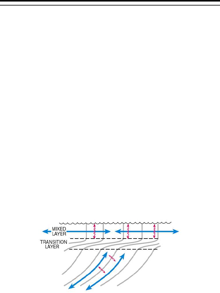
Chapter Fifteen
Neutral physics and boundary layers
As noted by Griffies (2004) and Ferrari and McWilliams (2007), the treatment of
neutral physics in boundary regions is traditionally ad hoc and largely determined
by numerical considerations. Griffies (2004) summarizes the methods used in
mom4p0, which are perhaps the most physically based of the methods employed
in the recent IPCC ocean climate models (e.g., Griffies et al. (2005)). Nonethe-
less, Gnanadesikan et al. (2006b) note that there remain arbitrary choices within
the mom4p0 methods that have nontrivial influences on the climate in a coupled
climate model. There is hence strong motivation to seek a method that is more
physically based and involves less ad hoc parameter inputs. The methods of Fer-
rari and McWilliams (2007) are promising from this perspective. The purpose of
this chapter is to discuss the mom4p1 treatment of neutral physics within boundary
regions.
15.1 REGIONS AFFECTING NEUTRAL PHYSICS
Ferrari and McWilliams (2007) identify five distinct regions in the vertical where
treatment of the neutral physics parameterization is distinct. Figure 15.1 illustrates
the three regions in the upper ocean, with the reflection of this treatment relevant
for the bottom. The mom4p1 treatment of neutral physics considers all of these
regions. The purpose of this section is to describe these regions and how they are
computed in mom4p1.
Figure 15.1 Surface region of the ocean as discussed by Ferrari and McWilliams (2007) (this
figure is taken from their preprint). Isopycnals are drawn here, along with
directions whereby tracer transport dominates.
We will make much use in the following of the vertical distance from the ocean

216 CHAPTER 15
free surface to a depth z<0:
h=thickness of water between free surface and depth z<0
=−z+
η
,(15.1)
where z=
η
is the time dependent free surface height. In particular, the mom4p1
code denotes the thickness between the free surface and the bottom of a tracer
cell as depth zwt, and the distance to the tracer cell point as depth zt. These
arrays are functions of the horizontal grid cell labelled by i,jand the vertical cell
labelled by k, where kincreases downward. These thickness arrays are evaluated
for all vertical coordinate choices in mom4p1.∗
It is convenient in the following to consider the streamfunction’s vertical depen-
dence as a dependence on hrather than z. Note, however, that it is important to
keep in mind the sign change in the vertical derivative operator
∂z=−∂h. (15.2)
15.1.1 Upper turbulent boundary layer
The near ocean surface is dominated by three dimensional nonhydrostatic tur-
bulent processes. The distance from the free ocean surface to the base of the
turbulent zone is written
hsurf =surface turbulent layer thickness, (15.3)
and the thickness region
0≤h≤hsurf surface turbulent boundary layer (15.4)
defines the surface turbulent boundary layer (see Figure 15.2). The boundary
layer thickness hsurf is determined in a hydrostatic model by a boundary layer pa-
rameterization scheme such as KPP (Large et al., 1994). The boundary layer
scheme parameterizes vertical mixing processes. When the mixing is strong, such
as occurs with intense momentum forcing and/or buoyancy loss, the upper ocean
destabilizes and results in vertical isopycnals as shown in Figure 15.1. The tur-
bulent boundary layer thickness can be thin (order tens of metres) during daytime
warming in the tropics which stabilizes the ocean, or thick (order a few hundred to
few thousand metres) for late winter deep convection in regions of large buoyancy
loss such as the Labrador Sea and Weddell Sea (Marshall and Schott, 1999).
Mesoscale eddies that penetrate to the ocean surface feel the geometric effect
from the surface boundary. Treguier et al. (1997) discussed this point in the context
of ocean mesoscale eddy parameterizations, and Held and Schneider (1999) de-
scribed similar issues for synoptic atmospheric variability. Following suggestions
in these papers, Ferrari and McWilliams (2007) propose that the lateral diffusive
effects from the mesoscale eddies should be parameterized by downgradient hori-
zontal tracer diffusion within the surface turbulent boundary layer, rather than neu-
tral diffusion considered in the ocean interior. Indeed, neutral diffusion in a region
of vertical isopycnals will compete with, and perhaps dominate over, the turbulent
∗As mom4p1 employes a suite of possible vertical coordinates, it is important that the code carry
arrays that are zero at the ocean free surface, rather than at the rigid lid surface defined by z=0, in
order to measure the time dependent thickness of the water column from the free surface to a grid cell.
NEUTRAL PHYSICS AND BOUNDARY LAYERS 217
parameterizations from KPP or other diabatic schemes. Hence, it is not sensible
to continue retaining neutral diffusion in the surface boundary layer. In a similar
manner, subgrid scale advective effects should be parameterized by an eddy in-
duced velocity that has zero vertical shear within the surface boundary layer. More
vertical structure for the eddy induced velocity is unwarranted in a region of weak
or zero vertical stratification. Equivalently, the quasi-Stokes streamfunction (Mc-
Dougall and McIntosh, 2001; Griffies, 2004) used to compute the eddy induced
velocity is linearly tapered to zero as the ocean surface is approached. Finally, the
diffusivity used to parameterize lateral diffusive and advective processes is taken
from the diffusivity computed in the ocean interior.
15.1.2 Transition between surface boundary layer and interior
Beneath the surface turbulent layer lies a transition region of enhanced stratifica-
tion. Notably, this transition region is generally not represented in coarse resolution
models, and it remains a topic of research with nonhydrostatic models to further
explore the physics active in this region (R. Ferrari 2005 personal communication),
and in particular how to parameterie the thickness of this layer.
Mesoscale eddies sporadically penetrate the transition region and interact with
processes in the turbulent surface layer. Tracer transport from mesoscale eddies
is modified by these interactions in manners that remain a topic of research. Even
so, because of this modification, we are motivated to alter the treatment of neutral
physics in this region using some basic ideas from Ferrari and McWilliams (2007),
who were the first emphasize the importance of the transition region for mesoscale
eddy parameterization schemes.
The thickness of the surface transition region is denoted by
Dsurf =surface transition layer thickness, (15.5)
and the transition region is defined for thickness ranges
hsurf ≤h≤hsurf +Dsurf surface transition region. (15.6)
Scaling arguments provided by Large et al. (1997), Smith and Vallis (2002), and
Griffies (2004) were used by Ferrari and McWilliams (2007) to provide an approxi-
mation to the thickness Dsurf. We describe these arguments now.
If the tracer cell labelled by integer kis beneath the surface turbulent layer, we
compute the absolute value of the neutral slope Skand multiply it by the Rossby
radius Rrossby (details of how mom4p1 computes the Rossby radius are give in
Section 15.7). As discussed by Large et al. (1997), Smith and Vallis (2002), and
Griffies (2004), this product is representative of the vertical excursion of a typical
mesoscale eddy. The first ocean model depth, denoted by k=k(+), that is just
deeper than hsurf +Rrossby Sk(+) defines the transition layer thickness Dsurf, so that
Dsurf ≈Rrossby Sk(+) . (15.7)
Again, mesoscale eddies deeper than hsurf +Dsurf are thought, on average, to
never reach the surface turbulent layer, whereas eddies shallower typically do
reach this layer and so their transport effects are modified relative to the interior.
In the subsequent discussion, the depth level k(+), and the quasi-Stokes stream-
function at this depth, play important roles in determining the strength of the neutral
physics fluxes in the region shallower than hsurf +Dsurf.
218 CHAPTER 15
15.1.3 Ocean interior
Motivated from the above discussion, the ocean interior is defined for present pur-
poses as regions where mesoscale eddies do not reach into the surface turbulent
layer or to the bottom turbulent layer. That is, the ocean interior is defined for water
column thicknesses satisfying
hsurf +Dsurf ≤h≤Hbott −(hbott +Dbott). (15.8)
In this expression, Hbott is the total water column thickness from the free surface
at z=
η
to the ocean bottom topography at z=−H
Hbott =
η
+H. (15.9)
The bottom transition layer and bottom turbulent boundary layer are discussed in
Sections 15.1.4 and 15.1.5. In the ocean interior, mesoscale eddy parameteri-
zations used in mom4p1 act without modification from their theoretical prescrip-
tion, which generally assumes adiabatic dynamics. We provide more discussion
of these parameterizations in Sections 15.2 and 15.6.
15.1.4 Transition between the interior and bottom boundary layer
As eddies interact with the bottom boundary layer, their tracer transport effects
are modified relative to their effects in the interior. We note that the local normal
at the bottom grid cell in mom4 is treated as normal to the generalized vertical
coordinate. Hence, the treatment of the bottom transition layer remains analogous
kinematically to the surface.
The bottom transition thickness
Dbott =bottom transition layer thickness (15.10)
is used to define the bottom transition layer, whose thickness hsatisfies
Hbott −(hbott +Dbott)≤h≤Hbott −hbott, (15.11)
where hbott is the bottom boundary layer thickness discussed in Section 15.1.5.
We have two choices in mom4p1 for determining Dbott: (1) an algorithm analogous
to that used to compute Dsurf, (2) specify Dbott according to a constant namelist
value, similar to how hbott is presently set in the absence of a prognostic bottom
boundar layer scheme. Modification of the neutral physics transport from the inte-
rior through the bottom transition layer is directly analogous to the surface transi-
tion layer.
15.1.5 Bottom turbulent boundary layer
Topography orients tracer transport near the ocean bottom, and considerations
analogous to the ocean surface turbulent layer arise in this region. That is, lateral
diffusive processes are oriented according to the topography, and eddy-induced
velocities have zero vertical shear in this region.
Thickness of the bottom turbulent layer,
hbott =bottom turbulent layer thickness, (15.12)

NEUTRAL PHYSICS AND BOUNDARY LAYERS 219
is sometimes specified via a namelist parameter often taken to be roughly 50m. Al-
ternatively, using the methods discussed in Chapter 16, we can compute a space-
time dependent bottom boundary layer thickness. In general, this thickness is used
to specify a bottom boundary layer region where the column thickness satisfies
Hbott −hbott ≤h≤Hbott. (15.13)
15.1.6 Comments on the treatment in mom4p0
The treatment of neutral physics in mom4p0 is detailed in Griffies (2004) and
Griffies et al. (2005). This treatment failed to consider the two transition regions
described above. Instead, the depth
Dmom4p0 =max(hsurf,D1,D2)(15.14)
is used to define a surface region over which the neutral diffusive fluxes are ta-
pered to horizontal downgradient fluxes, and the eddy induced velocity has zero
vertical shear with strength determined by that at the base of the boundary layer.
Here, D1is defined just as in the mom4p1 specification of the surface transition
depth Dsurf (equation (15.7)). In contrast, D2is the depth below which the neutral
slope becomes less than some specified maximum value Smax. That is, D2is de-
termined by the stratification whereas D1is determined by both the stratification
and the Rossby radius. There is no bottom boundary layer considered for the neu-
tral physics scheme in mom4p0, though in practice neutral fluxes were reduced to
downgradient horizontal diffusion next to the bottom and sides, according to the
suggestions from Gerdes et al. (1991).
An unsatisfying element of the mom4p0 method is the introduction of the depth
D2, since this depth is determined by an ad hoc maximum slope Smax.∗Notably,
D1is generally larger or smaller than D2depending on the arbitrary choice of the
maximum slope. The nontrivial sensitivity of a coupled climate model simulation to
the value of this slope is documented in Gnanadesikan et al. (2006b).
Without the extra depth D2used to determine Dmom4p0, the mom4p0 method
becomes similar to that proposed for mom4p1. However, as discussed below,
the Ferrari and McWilliams (2007) transition regions, used in mom4p1, ensures
that the eddy induced velocity linearly interpolates from the boundary layer values
to the interior values. As mom4p0 does not consider this transition region, the
eddy induced velocity does not possess this interpolation behaviour, and instead
exhibits a jump at the boundary layer base. This jump is non-physical and can
potentially cause unsatisfying numerical and physical effects in the simulation.
15.2 QUASI-STOKES STREAMFUNCTION
.
∗Additionally, one of the slope tapering schemes proposed by Gerdes et al. (1991) (a quadratic
tapering scheme) or Danabasoglu and McWilliams (1995) (an exponential tapering scheme) is used to
taper the neutral diffusive fluxes to horizontal in the depths shallower than Dmom4p0. Sensitivity of
the simulation to the transition from neutral diffusion to horizontal diffusion has generally been found
to be far less than sensitivity to the treatment of the eddy induced skew transport.
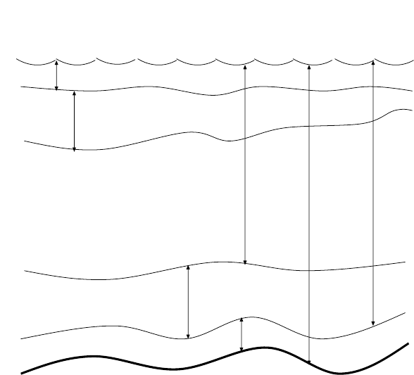
220 CHAPTER 15
bottbott hH
surf
h
bott
h
surf
D
ocean interior
surface transition layer
surface turbulent layer
bottom transition layer
bottom turbulent layer
bottbottbott DhH
bott
H
bott
D
Figure 15.2 Summary of the regions for treating the neutral physics parameterizations, ac-
cording to the notions described in Ferrari and McWilliams (2007).
As discussed in Griffies (1998), McDougall and McIntosh (2001), and Griffies
(2004), the introduction of a divergence-free eddy induced velocity v∗is more con-
veniently formulated and numerically implemented in terms of its vector stream-
function Ψ, where
v∗=∇ ∧ Ψ. (15.15)
McDougall and McIntosh (2001) motivate the name quasi-Stokes streamfunction
for Ψ. Following the discussion in Section 9.2.2 of Griffies (2004), we identify the
skew tracer flux associated with the quasi-Stokes streamfunction
F=−∇C∧Ψ. (15.16)
In component form, using the summation convention, this flux can be written
Fm=−
mnp C,nΥp
=−Amn C,n
(15.17)
where the skew-symmetric tensor Amn represents a reorganization of the vector
streamfunction
Amn =
mnp Υp
=
0Ψ3−Ψ2
−Ψ30Ψ1
Ψ2−Ψ10
,(15.18)
and
mnp is the totally antisymmetric Levi-Civita tensor. It is sufficient to work with
the vertical gauge described in Section 9.2.2 of Griffies (2004), whereby only the
horizontal components of Ψare non-zero
Ψ3=0. (15.19)
NEUTRAL PHYSICS AND BOUNDARY LAYERS 221
In the remainder of this section, we detail the form that the quasi-Stokes stream-
function takes within the regions identified in Section 15.1. This discussion fol-
lows Ferrari and McWilliams (2007). In Section 15.3, we specialize the results to
the quasi-Stokes streamfunction prescribed by the parameterization of Gent and
McWilliams (1990) and Gent et al. (1995)
15.2.1 Surface turbulent boundary layer
For the upper surface turbulent boundary layer discussed in Section 15.1.1, we
assume the eddy induced velocity has zero vertical shear, which means that the
streamfunction is a linear function of water column thickness within this region.
Because the streamfunction has the kinematic interpretation of a horizontal trans-
port beneath a given depth (see for example Sections 9.3.5 and 9.5.2 of Griffies
(2004) as well as McDougall and McIntosh (2001)), the quasi-Stokes streamfunc-
tion vanishes at the ocean surface. Hence, the linear thickness dependence of Ψ
within the surface turbulent region takes the form
Ψsurf =h
hsurf Φsurf(x,y,t)for 0≤h≤hsurf.(15.20)
The streamfunction Φsurf is determined by matching conditions across the tran-
sition region into the ocean interior. Note that this form for the streamfunction
assumes a nonzero surface boundary layer thickness.
15.2.2 Surface transition region
To ensure that the eddy induced velocity is smoothly interpolated from the inte-
rior into the surface turbulent boundary layer, it is necessary for the quasi-Stokes
streamfunction to satisfy the following boundary conditions
Ψsurf-trans =Ψsurf h=hsurf
Ψinterior h=hsurf +Dsurf,(15.21)
and for its vertical derivative to satisfy
∂hΨsurf-trans =∂hΨinterior h=hsurf +Dsurf.(15.22)
Matching first at the bottom of the surface turbulent boundary layer, where h=
hsurf and where we insist on continuity of the streamfunction, leads us to take the
surface transition region streamfunction in the form
Ψsurf-trans =h−hsurf
Dsurf 2
Φsurf-trans +h
hsurf 2
Φsurf. (15.23)
The quadratic depth dependence is chosen to provide a linear interpolation of the
eddy induced velocity from the interior to the surface turbulent boundary layer.
Matching now at the bottom of the surface transition layer, where h=hsurf +Dsurf
and we insist on continuity of the streamfunction and its vertical derivative, leads
to
Φsurf =hsurf
hsurf +Dsurf Ψ(+)
interior −Dsurf
2∂hΨ(+)
interior(15.24)
Φsurf-trans =−Dsurf
hsurf Ψ(+)
interior −hsurf +Dsurf
2∂hΨ(+)
interior, (15.25)
222 CHAPTER 15
where again ∂h=−∂z, and where
Ψ(+)
interior =Ψinterior(h=hsurf +Dsurf)(15.26)
is the interior streamfunction at the top of the interior region; i.e., base of the
surface transition layer, and ∂hΨ(+)
interior is its derivative. As a check on the manip-
ulations, note that as the transition layer thickness vanishes, the streamfunctions
reduce to Φsurf =Ψ(+)
interior and Φsurf-trans =0. In order for this limit to be well
defined for the quasi-Stokes streamfunction Φsurf-trans, we add a positive number
=10−20 to Dsurf in the denominator of the first term on the right side of equation
(15.23).
15.2.3 Bottom transition region
Just as for the surface transition region, the eddy induced velocity is smoothly
interpolated from the interior into the bottom turbulent boundary layer so long as
the quasi-Stokes streamfunction satisfies
Ψbott-trans =Ψbott h=H∗
bott
Ψinterior h=H∗
bott −Dbott,(15.27)
and its vertical derivative satisfies
∂hΨbott-trans =∂hΨinterior h=H∗
bott −Dbott,(15.28)
where
H∗
bott =Hbott −hbott (15.29)
is a useful shorthand.
Matching first at the top of the bottom turbulent boundary layer, where h=H∗
bott
and where we insist on continuity of the streamfunction, leads us to take the bottom
transition region streamfunction in the form
Ψbott-trans =H∗
bott −h
Dbott 2
Φbott-trans +Hbott −h
hbott 2
Φbott. (15.30)
As for the surface, the quadratic depth dependence is chosen to provide a linear
interpolation of the eddy induced velocity from the interior to the bottom turbulent
boundary layer.
Matching now at the top of the bottom transition region, where h=H∗
bott −Dbott
and we insist on continuity of the streamfunction and its vertical derivative, leads
to
Φbott =hbott
hbott +Dbott Ψ(−)
interior +Dbott
2∂hΨ(−)
interior(15.31)
Φbott-trans =−Dbott
hbott Ψ(−)
interior +hbott +Dbott
2∂hΨ(−)
interior, (15.32)
where
Ψ(−)
interior =Ψinterior(h=H∗
bott −Dbott)(15.33)
is the interior streamfunction at the bottom of the interior region (i.e., top of the
bottom transition layer).
NEUTRAL PHYSICS AND BOUNDARY LAYERS 223
15.2.4 Bottom turbulent boundary layer
Just as for the surface, the quasi-Stokes stremfunction vanishes at the ocean bot-
tom, and we assume it has a linear thickness dependence within the bottom tur-
bulent boundary layer, thus leading to
Ψbott =Hbott −h
hbott Φbott for Hbott −hbott ≤h≤Hbott.(15.34)
The streamfunction Φbott (equation (15.31)) was determined by matching across
the bottom transition region.
15.2.5 Summary of the streamfunction algorithm
Based on the previous derivation, the quasi-Stokes streamfunction Ψcan be writ-
ten in the form
Ψ=Hsurf h
hsurf Φsurf
+Hsurf-trans "h−hsurf
Dsurf 2
Φsurf-trans +h
hsurf 2
Φsurf#
+Hinterior Ψinterior
+Hbott-trans "H∗
bott −h
Dbott 2
Φbott-trans +Hbott −h
hbott 2
Φbott#
+Hbott Hbott −h
hbott Φbott.
(15.35)
Here, the on-off functions Hare unity in the labelled region, and zero outside. The
regional streamfunctions are given by
Φsurf =hsurf
hsurf +Dsurf Ψ(+)
interior +Dsurf
2∂zΨ(+)
interior(15.36)
Φsurf-trans =−Dsurf
hsurf Ψ(+)
interior +hsurf +Dsurf
2∂zΨ(+)
interior(15.37)
Φbott-trans =−Dbott
hbott Ψ(−)
interior −hbott +Dbott
2∂zΨ(−)
interior(15.38)
Φbott =hbott
hbott +Dbott Ψ(−)
interior −Dbott
2∂zΨ(−)
interior, (15.39)
where
Ψ(+)
interior =Ψinterior(h=hsurf +Dsurf)(15.40)
Ψ(−)
interior =Ψinterior(h=Hbott −hbott −Dbott)(15.41)
are the interior streamfunctions evaluated at the transition region boundaries (see
Figure 15.2).
There are two main subroutines in mom4p1 used to compute this streamfunc-
tion.
224 CHAPTER 15
•neutral blayer: This routine computes properties of the various boundary
and transition regions. It is a tedious calculation due to the multiple regions
that must be characterized.
–Thicknesses: hsurf,Dsurf,hbott,Dbott; each are a function of (i,j,triad),
where “triad” refers to the four triads surrounding each grid point.
–Quasi-Stokes streamfunctions: Φsurf,Φsurf-trans,Φbott-trans, and Φbott;
each are a function of (i,j,triad).
–Quasi-Stokes streamfunction accumulated over the boundary regions.
This streamfunction is zero in the interior, and nonzero within the bound-
ary layers. It is a function of (i,j,k)
•fz terms,fx flux,fy flux, and fz flux: These routines compute the flux
components for the neutral physics parameterization, including the interior
quasi-Stokes streamfunction Ψinterior. These fluxes are computed using in-
formation from the neutral blayer routine. As detailed in Griffies (2004),
the fluxes for each (i,j,k)point are the grid weighted sum of the four triads
surrounding each point.
15.3 SPECIALIZING THE QUASI-STOKES STREAMFUNCTION
We discuss here some specific forms for the quasi-Stokes streamfunction.
15.3.1 GM90 streamfunction
The quasi-Stokes streamfunction for the parameterization of Gent and McWilliams
(1990) and Gent et al. (1995) is given by
Ψinterior =ˆz∧Agm S
=Agm (−Syˆx+Sxˆy),(15.42)
which is equivalent to a skew-symmetric tensor (Section 13.5 of Griffies (2004))
A=Agm
0 0 −Sx
0 0 −Sy
SxSy0
. (15.43)
In these equations, S= (Sx,Sy, 0)is the neutral slope vector computed as
S=−
ρ
,s∇zs+
ρ
,
θ
∇z
θ
ρ
,ss,z+
ρ
,
θθ
,z. (15.44)
The diffusivity Agm can be computed one of many ways, with options described
in Section 14.4 of Griffies (2004). In principle, the mom4p1 implementation of the
quasi-Stokes streamfunction (15.42) can be generalized to other streamfunctions
motivated by other theoretical arguments.
NEUTRAL PHYSICS AND BOUNDARY LAYERS 225
15.3.2 Streamfunction in completely unstratified regions
For regions that are completely unstratified in the vertical, such as in regions of
strong surface buoyancy forcing and/or in shallow shelf regions, we specify the fol-
lowing quadratic dependence for the quasi-Stokes streamfunction, with zero val-
ues at the top and bottom boundaries
Ψ(h) = 4h(H−h)
H2Ψmax, (15.45)
where His the thickness of the fully turbulent column, and
h=
η
−z(15.46)
is the thickness of the fluid between depth zand the surface at z=
η
.
Two methods are available to determine the maximum absolute value of the
streamfunction Ψmax. The first sets Ψmax according to a namelist specified max-
imum slope parameter, with 1/100 a typical value. The problem with this specifi-
cation is that it will provide a nontrivial streamfunction in regions where both the
vertical and horizontal density stratification are small. In contrast, one may expect
the streamfunction in an eddying model to remain quite small in such regions, due
to the absence of horizontal density gradients. This observation motivates an al-
ternative, whereby the streamfunction is set according to the vertical average of
the diffusivity times the horizontal density gradient∗
Ψmax =−ˆz∧Agm ∇z
ρ
(z)
ρ
o
,z
, (15.47)
where
ρ
o
,zis a constant reference vertical density derivative,
Agm ∇z
ρ
(z)=∑kbot
k=1dzt Agm ∇z
ρ
∑kbot
k=1dzt (15.48)
is the vertically averaged diffusivity times the horizontal density gradient, averaged
over the depth of the vertically unstratified region. So that we are computing the
horizontal stratification, rather than the horizontal gradient of the in situ density, we
compute the horizontal density gradient according to
∇z
ρ
=
ρ
,
θ
∇z
θ
+
ρ
,S∇zS, (15.49)
with
θ
the potential or conservative temperature, Sthe salinity, and
ρ
,
θ
and
ρ
,Sthe
density expansion coefficients whose values are determined by the temperature,
salinity, and pressure at a common point for each vertical level. The streamfunction
(15.47) corresponds to the following anti-symmetric transport tensor
Amn =1
−
ρ
o
,z
0 0 −Agm
ρ
,x
(z)
0 0 −Agm
ρ
,y
(z)
Agm
ρ
,x
(z)Agm
ρ
,y
(z)0
. (15.50)
∗This streamfunction has a form analogous to that considered with the TEM approach in Section
15.4.
226 CHAPTER 15
15.3.3 Local N2dependent diffusivity
Ferreira et al. (2005) and Ferreira and Marshall (2006) argue for the relevance of a
local N2dependence to the diffusivity used to compute the quasi-Stokes stream-
function. That is,
Agm =A2d
gm (N/No)2(15.51)
where A2d
gm can be any two-dimensional diffusivity, Nis the buoyancy frequency,
and Nois a reference buoyancy frequency. This choice for the diffusivity greatly
simplifies the quasi-Stokes streamfunction, which now takes the form
Ψ=ˆz∧Agm S
=−ˆz∧A2d
gm ∇z
ρ
ρ
o
,z
,(15.52)
which corresponds to the anti-symmetric tensor
Amn = A2d
gm
−
ρ
o
,z!
0 0 −
ρ
,x
0 0 −
ρ
,y
ρ
,x
ρ
,y0
. (15.53)
In these expressions,
ρ
o
,zis a reference vertical density stratification corresponding
to the reference buoyancy frequency No.
Numerical treatment of vertically unstratified regions becomes trivial with this
streamfunction, since it is only the horizontal stratification which is required and
there are no divisions by small numbers. We have implemented this streamfunc-
tion in mom4p1 using the namelist option agm local n2.
Initial tests, however, are unclear as to whether the scheme was implemented
properly. Further tests are warranted.
15.4 REGARDING THE TEM APPROACH AND VERTICAL STRESSES
We comment here on the relevance of implementing the Gent and McWilliams
(1990) scheme via the tracer equation, as done in mom4p1 as motivated by Gent
et al. (1995) and Griffies (1998), versus the alternative, which adds a vertical stress
to the horizontal momentum equation, as recently implemented in a global model
by Ferreira and Marshall (2006). When adding a stress to the momentum equation,
the prognostic velocity variable is interpreted as the residual mean, or effective, ve-
locity rather than the traditional Eulerian mean velocity. This transformed Eulerian
mean (TEM) interpretation is quite elegant, since it is the residual mean velocity
that advects tracers in a coarsely resolved (i.e., no mesoscale eddies) z-model,
not the Eulerian mean velocity. The elegance is maintained so long as one need
not compute the Eulerian mean velocity.
For many purposes, we do not require the Eulerian mean velocity, and so the
TEM momentum equation provides all the variables required to run an ocean
model. However, the following considerations point a need for the Eulerian mean
velocity in cases of realistic ocean climate modeling.
•In computing the air-sea stress in realistic coupled climate models, it is im-
portant for many purposes to include the velocity of the ocean currents ac-
cording to the discussion in Pacanowski (1987). The relevant currents for
this calculation are the Eulerian mean currents, not the residual mean.
NEUTRAL PHYSICS AND BOUNDARY LAYERS 227
•When computing the Richardson number commonly required for mixed layer
parameterizations, we require the vertical shear of the Eulerian mean veloc-
ity, not the vertical shear of the residual mean velocity.
The Eulerian mean velocity is available within a TEM ocean model, given the
prognostic residual mean velocity plus a prescribed mesoscale eddy closure to
compute the eddy induced velocity. Its calculation requires derivatives of the quasi-
Stokes streamfunction to obtain the eddy-induced velocity, and one further deriva-
tive to compute the vertical shear. As discussed by Griffies (1998), this calculation
can produce a rather noisy eddy induced velocity, especially near boundaries. Fur-
thermore, there is no general principle guiding us in formulating a particular choice
of discretization for the eddy induced velocity from a streamfunction. A noisy eddy
induced velocity produces a noisy diagnosed Eulerian mean velocity, which then
puts noise in the air-sea stress as well as the Richardson number. These numeri-
cal sources of noise are unacceptable for realistic climate modeling.
A final consideration makes note of the fact that even with the TEM velocity
equation, it is still necessary to implement neutral diffusion in a coarsely resolved
ocean climate model. As noted by Griffies (1998), the numerical technology for
neutral diffusion is largely the same as for skew diffusion motivated by Gent et al.
(1995), albeit with important differences arising from details of boundary layer
treatment described in Sections 15.2 and 15.6. Given the great degree of over-
lap between the methods, it is sensible to retain a focus on the tracer equation
implementation of the eddy advective effects.
In summary, whether to focus the mesoscale eddy parameterization implemen-
tation within the tracer equation, as proposed by Gent et al. (1995) and Griffies
(1998), or the momentum equation, as implemented by Ferreira and Marshall
(2006), largely depends on the model application. The mom4p1 code is designed
for many applications, with the primary use at GFDL being realistic ocean climate
simulations. Hence, the reasons listed above prejudice us to implement mesoscale
eddy parameterizations within the tracer equation, rather than within a TEM veloc-
ity equation.
15.5 DISCUSSION OF SOME DETAILS
During the development of the algorithm described in this chapter, tests were run
with an idealized sector model forced with temperature restoring at the surface.
This forcing produced deep convection at the poleward end of the domain, thus
ensuring a deep mixed layer in this region. There was no seasonal nor diurnal
cycle, and thus no active mixed layer processes other than deep convection driven
by buoyancy forcing. This test problem exposed many sensitivities that helped
to guide the development of neutral physics within the boundary layer. Notably,
much of this sensitivity is removed in realistic simulations possessing an active
mixed layer. The purpose of this section is to summarize some of the issues and
methods used to address the issues.

228 CHAPTER 15
15.5.1 Step-like features in the upper ocean
The presence of a nontrivial quasi-Stokes streamfunction within the upper ocean
can lead to step-like features in the density field. These steps resulted in (or were
the result of) large neutral slopes mixed with small slopes. To overcome this dif-
ficulty, it is useful to compute the turbulent boundary layer depth according to the
parameterized mixed layer physics plus any region beneath this “mixed layer” that
has huge neutral slopes. For idealized simulations, an objective specification of
the surface turbulent boundary layer must be based on the neutral slopes.
15.5.2 Handling the triads of slopes
The scheme of Griffies et al. (1998) employs four triad slopes for each of the two
horizontal directions at each tracer point. One may be motivated to then produce
a corresponding set of streafunctions and boundary layer regions for each triad.
Doing so introduces a tremendous level of added computation, which is arguably
unwarranted. Alternatively, the method chosen in mom4p1 is to determine the
boundary layer regions based on the maximum absolute slope from amongst the
triad slopes occurring at each tracer point. Additionally, we smoothed the resulting
region thicknesses and corresponding streamfunctions in order to ensure that the
scheme produces parameterized transport that has large spatial scales.
15.5.3 Ensuring there are no negatively stratified regions
The Gent and McWilliams (1990) scheme assumes a stably stratified column. Our
aims in this chapter are to merge their methods into the boundary regions where
stratification can be zero or negative. In an ocean model run with convective ad-
justment, such as the complete adjustment scheme of Rahmstorf (1993), there are
no regions of negative stratification. Ensuring nonnegative stratification has been
found to be essential when allowing for a nontrivial Gent and McWilliams (1990)
quasi-Stokes streamfunction in weakly stratified regions of the model. If negative
stratification is allowed, the quasi-Stokes streamfunction will further destabilize the
profile, with the resulting simulation rapidly degenerating into unphysical noise.
In MOM4.0, we recommended the use of Rahmstorf (1993) convection as a
follow-on to the use of large vertical diffusivities commonly found in mixed layer
parameterizations. This approach then ensures proper behaviour of the quasi-
Stokes streamfunction in boundary regions. In mom4p1, we recommend an alter-
native that does not rely on the convective adjustment scheme. Here, for purposes
of computing the neutral slope, we numerically compute the vertical stratification
as
∂
ρ
∂zeffective
=min ∂
ρ
∂z,−
. (15.54)
That is, we only employ stable vertical stratification for purposes of computing the
neutral slope vector used in the neutral physics scheme. This trick facilitates the
use of neutral physics for all slopes, without incurring spurious numerical artefacts
in those regions of negative stratification.
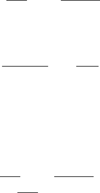
NEUTRAL PHYSICS AND BOUNDARY LAYERS 229
15.6 LATERAL DIFFUSIVE PARAMETERIZATION
.The lateral diffusive parameterization is simpler to characterize than the quasi-
Stokes streamfunction, since there is no quadratic region. Instead, the diffusive
fluxes are linearly tapered from their internal neutral direction form, through the
transition regions into the boundary oriented form in the turbulent boundary layers.
These considerations lead to the following downgradient lateral diffusive tracer
fluxes.
•Surface turbulent boundary layer: 0≤h≤hsurf. The diffusive flux is oriented
parallel to the surfaces of constant generalized vertical coordinate s, which
in mom4p1 are quasi-horizontal within the upper ocean. Therefore,
Fsurf =−AI∇sC, (15.55)
where ∇sis the lateral gradient along surfaces of constant generalized verti-
cal coordinate.
•Surface transition region: hsurf ≤h≤hsurf +Dsurf. The diffusive flux linearly
tapers from the interior form to the surface form
Fsurf-trans =h−hsurf
Dsurf Finterior +hsurf +Dsurf −h
Dsurf Fsurf. (15.56)
•Ocean interior: hsurf +Dsurf ≤h≤Hbott −(hbott +Dbott). Here, the flux is
taken from the small slope neutral diffusion operator (Section 5.2.3)
Finterior =−AI(∇
ρ
C+ˆz S · ∇
ρ
C). (15.57)
•Bottom transition region: Hbott −(hbott +Dbott)≤h≤Hbott −hbott. As with
the surface transition region, we prescribe a linear tapering from the interior
flux to the bottom turbulent boundary layer flux
Fbott-trans =h−(H∗
bott −Dbott)
Dbott Fbott +H∗
bott −h
Dbott Finterior, (15.58)
where again H∗
bott =Hbott −hbott is the thickness of water above the bottom
turbulent boundary layer.
•Bottom turbulent boundary layer: Hbott −hbott ≤h≤Hbott. Here, the topog-
raphy orients the lateral diffusive flux, and so we take
Fbott =−A
σ
∇
σ
C, (15.59)
where
σ
= (z−
η
)/(H+
η
)is the topography following
σ
-coordinate, and A
σ
is a diffusivity that may be enhanced when dense water lies above light water
within the bottom turbulent layer, as prescribed by Beckmann and D¨
oscher
(1997). Further details on this method are discussed in Chapter 16.
The diffusive flux in the transition regions can be simplified, and doing so al-
lows for a very simple numerical implementation. For this purpose, write equation
(15.56) in the form
Fsurf-trans =h−hsurf
Dsurf Finterior +hsurf +Dsurf −h
Dsurf Fsurf
=Fsurf +h−hsurf
Dsurf (Finterior −Fsurf).
(15.60)
230 CHAPTER 15
Now substitute the tensor form of the interior flux taken from the small-angle neu-
tral diffusion tensor (see Section 14.1.4 of Griffies (2004)) to find
Fsurf-trans =Fsurf −AIh−hsurf
Dsurf
0 0 Sx
0 0 Sy
SxSyS2
C,x
C,y
C,z
. (15.61)
Hence, it is only the off-diagonal piece of the flux which is linearly scaled, along
with the (3,3) diagonal term. The diagonal piece in the horizontal remains un-
scaled. In practice, we implement the same relation at the bottom, which means
that if sigma transport is used (Chapter 16), we will have both horizontal and sigma
oriented diffusion in the bottom turbulent layer.
15.7 COMPUTATION OF THE ROSSBY RADIUS
The Rossby radius is needed for computing the transition layer thickness using
the algorithm described in Section 15.1.2. We detail here the methods used in
mom4p1 for its computation.
Outside an equatorial band of roughly ±5◦, the mth-mode Rossby radius takes
the form
λ
m=cm
|f|, (15.62)
where cmis the phase speed of the mth-mode (m≥1) gravity wave in a non-
rotating, continuously stratified flat bottom ocean (Gill, 1982). Within an equatorial
band of ±5◦, the Rossby radius is given by
λ
m=cm
2
β
1/2
, (15.63)
where
β
=f,yis the meridional derivative of the Coriolis parameter. An approxi-
mate gravity wave phase speed can be obtained by methods described in Chelton
et al. (1998), and it takes the form∗
cm≈1
m
π
η
Z
−H
Ndz. (15.64)
The squared buoyancy frequency is written
N2=−(g/
ρ
) (
ρ
,ss,z+
ρ
,
θθ
,z)
=g(
β
s,z−
α θ
,z),(15.65)
where
α
=∂
θ
ln
ρ
(15.66)
β
=∂sln
ρ
(15.67)
∗Even though the gravity wave speed feels the bottom, since the vertical integral in equation (15.64)
extends over the full depth range, the study by Chelton et al. (1998) showed that the Rossby radius over
the bulk of the World Ocean is dominated by the inverse Coriolis dependence (see their Figure 6).

NEUTRAL PHYSICS AND BOUNDARY LAYERS 231
are the thermal expansion and saline contraction coefficients, respectively. The
Rossby radius used in mom4p1 for the transition layer thickness in Section 15.1.2
is taken to be the first baroclinic wave (m=1) in equaion (15.64).
In addition to computing the Rossby radius as just described, we follow Large
et al. (1997) by restricting the computed Rossby radius within the range
Rmin ≤Rrossby ≤Rmax, (15.68)
where Large et al. (1997) set
Rmin ≈15km (15.69)
Rmax ≈100km. (15.70)
15.8 METHOD FOR OBTAINING LOW PASS FILTERED FIELDS
For determining the upper and lower turbulent boundary layer thicknesses, we
take values from other portions of the model, such as the turbulent mixed layer
schemes. These schemes produce boundary layer thicknesses which have rela-
tively rapid time scales for fluctuations, such as days. In contrast, for the neutral
physics scheme, we are interested in low pass or time filtered variations in the
boundary layers, on the order of weeks to months. Obtaining the low pass filtered
boundary layer information is cumbersome if we aim to save previous time step
values and form the traditional time average.
Instead, we prefer a method suggested by Anand Gnanadesikan (personal com-
munication 2005), whereby the low pass, or slow, variable Aslow is obtained by
solving the first order equation
∂Aslow
∂t=−Aslow −Afast
τ
damp , (15.71)
where Afast is the rapidly varying boundary layer depth, and
τ
damp is a damping
time on the order
τ
damp ≈30 days. (15.72)
Taking a forward time step for this equation leads to the discrete form
Aslow(
τ
+∆
τ
) = (1−
γ
)Aslow(
τ
) +
γ
Afast (15.73)
where
γ
=∆
τ
/
τ
damp. (15.74)
We use the same algorithm for evolving the diffusivity computed for the neutral
physics scheme based on any of the closure ideas discussed in Section 14.4 of
Griffies (2004). In this way, the diffusivity fluctuations are damped in time, with
major changes occurring only on the slower time scale set by
γ
.
15.9 THE IMPORTANCE OF REGULARIZED SLOPES
In general, a model such as mom4p1 can realize any value for the density, which
contrasts with an isopycnal model where densities are quantized. The continu-
ous range of density allows, in particular, for very fine structure in the vertical. This
232 CHAPTER 15
structure is sometimes the result of numerical methods and roundoff, and can lead
to small step-like features in the vertical. In the presence of these steps, the verti-
cal derivative of density, needed to compute the neutral slopes and the buoyancy
frequency, can exhibit discontiuous features, with, say, infinite slopes interspersed
with finite slopes. This behaviour creates difficulties with the neutral diffusion and
skew diffusion fluxes, especially with the quasi-Stokes streamfunction.
To regularize the slopes computed in the neutral physics scheme, we perform
two forms of smoothing: one in the horizontal (via a laplacian diffusion) and one in
the vertical (via a 1-2-1 filter). The smoothing is performed on the vertical deriva-
tive of density prior to computing the slopes. Formally, this smoothing breaks the
integrity of the temperature and salinity triads described in Griffies et al. (1998).
However, the payoff is to produce neutral fluxes that are well behaved, and perform
in a manner consistent with that expected from the physics. We have therefore
found it critical to smooth the vertical density derivative before computing neutral
slopes, especially when considering the interactions between neutral physics and
boundary layer physics as described in this chapter.
Chapter Sixteen
Overflow schemes
The purpose of this chapter is to detail various methods available in mom4p1 for
enhancing the transport of dense water downslope. Some of methods are im-
plementations of schemes from the literature, some are unique to mom4p1, and
some remain incomplete methods which are part of mom4p1 only for use by those
actively pursuing research into overflow algorithms. We present our prejudices in
Section 16.4, though the user should recognize that much research still is under-
way towards finding a suitable overflow scheme for global ocean climate modelling.
There are four methods implemented in mom4p1 described in this chapter, with
the following modules containing the code:
mom4/ocean param/mixing/ocean sigma transport mod
mom4/ocean param/mixing/ocean mixdownslope mod
mom4/ocean param/sources/ocean overflow mod
mom4/ocean param/sources/ocean overexchange mod.
16.1 MOTIVATION FOR OVERFLOW SCHEMES
As described by Winton et al. (1998), coarse resolution z-coordinate models gen-
erally have difficulty moving dense water from shallow to deep regions. The key
problem is that too much dense water spuriously entrains with the ambient lighter
fluid. Only when the topographic slope is resolved so that the grid spacing satisfies
|∇ H| ≤ ∆z
∆s, (16.1)
does the simulation begin to reach negligible levels of spurious entrainment. Re-
solving a slope of 1/100 with vertical resolution of ∆z=20m thus requires hori-
zontal grid spacing ∆s≈2km. This resolution is one or two orders finer than the
typical resolution of the 1-2 degree ocean climate models commonly used today.
Furthermore, refined vertical resolution, desired for representing vertical physical
processes, requires one to further refine the horizontal resolution required to re-
solve the slope. Notably, there is little difference between the representation of
steeply sloping features via either full or partial steps in z-models (Section 6.1.2).
Hence, steep “cliff” features remain ubiquitous in the typical ocean climate model
using vertical coordinates with quasi-horizontal isosurfaces. Short of respecting
the constraint (16.1), traditional tracer transport schemes (i.e., vertical convection;
horizontal and vertical diffusion; and horizontal and vertical advection) are gen-
erally unable to transport dense waters into the abyss to the extent observed in
Nature. This problem with spurious entrainment is shared by the quasi-horizontal
vertical coordinates such as those discussed in Chapter 6.

234 CHAPTER 16
In an attempt to resolve the spurious entrainment problem, modelers have for-
mulated ways to embed terrain following transport schemes into geopotential or
pressure coordinate models. These schemes generally assume the bottom ocean
region is turbulent, and so well mixed and not subject to geostrophy. The resulting
dynamics act to bring water downslope, eventually being entrained at a neutral
buoyancy depth.
Some approaches aim to modify both the momentum and tracer equations, with
Killworth and Edwards (1999) documenting a most promising approach. Unfor-
tunately, when modifying the momentum equation so that pressure gradients are
computed within the bottom boundary layer, difficulties handling this calculation
have resulted in nontrivial problems with spurious transport, especially near the
equator. It is for this reason that no global ocean climate model presently em-
ploys the Killworth and Edwards (1999), or analogous, scheme. Motivated by this
difficulty, we do not consider any scheme in mom4p1 that modifies the momen-
tum equation. Instead, we focus exclusively on methods restricted to the tracer
equation.
16.2 THE SIGMA TRANSPORT SCHEME
This section documents the scheme available in the module
mom4/ocean param/mixing/ocean sigma transport mod
The papers by Beckmann and D¨
oscher (1997) and D¨
oscher and Beckmann
(2000) propose a method to incorporate a rudimentary terrain following turbulent
layer in z-models, or more generally into any model with vertical coordinates hav-
ing quasi-horizontal isosurfaces (e.g., pressure based vertical coordinates). They
prescribe changes only to the tracer equation, in which there is advection and dif-
fusion within a bottom turbulent layer. We term these transport mechanisms sigma
diffusion and sigma advection, since the sigma vertical coordinate (Section 6.1.5)
is terrain following.
By enabling a terrain oriented route for tracer transport, in addition to the usual
grid oriented transport, the quasi-horizontal vertical coordinate models are now
afforded an extra pathway for transporting dense water into the abyss.
16.2.1 Sigma diffusion
Diffusion oriented according to the bottom topography is referred to as sigma dif-
fusion in the following. The diffusive flux between two adjacent cells living at the
ocean bottom is given by
F
σ
=−A∇
σ
T, (16.2)
with ∇
σ
the horizontal gradient operator taken between cells in the sigma layer.
Note that this flux vanishes if the tracer concentration is the same between two
adjacent cells within the sigma layer. We follow the approach of D¨
oscher and
Beckmann (2000) in which sigma diffusion is strong when densities of the partici-
pating cells favors downslope motion. That is, the following diffusivity is used
A=Amax if ∇
σρ
· ∇H<0
Amin if ∇
σρ
·∇H≥0, (16.3)
OVERFLOW SCHEMES 235
where z=−H(x,y)is the bottom depth. Note that in practice, this constraint is
applied separately in the two horizontal directions. That is, the zonal diffusivity is
large if
ρ
,xH,x<0and the meridional diffusivity is large if
ρ
,yH,y<0. A ratio of
the two diffusivities Amax/Amin is a namelist parameter in mom4p1, with ≈106the
default value as suggested by D¨
oscher and Beckmann (2000).
An additional velocity dependent diffusion was also found by D¨
oscher and Beck-
mann (2000) to be of use. In this case, an added sigma-diffusive flux in the zonal
direction is computed using the diffusivity
A=|u|∆xif
ρ
,xH,x<0and u H,x>0
Amin otherwise.(16.4)
In this expression, |u|is the magnitude of the model’s resolved zonal velocity com-
ponent within the sigma layer, and ∆xis the zonal grid spacing. An analogous
meridional flux is computed as well.
Sigma diffusion can be specified to occur over an arbitrary layer thickness, even
if this layer encompasses a non-integer number of bottom cells. If sigma diffusion
is enabled without sigma advection, then this bottom layer is time independent.
16.2.2 Sigma advection
In addition to sigma diffusion, mom4p1 allows for an advective contribution to the
bottom boundary layer flow. This portion of the algorithm is experimental, and so
it is not recommended for general use. We present the discussion here only to
expose some initial thoughts on a possible new method, but recognize that the
method as discussed here is incomplete. Note that the sigma advection scheme
discussed here is distinct from the method proposed by Beckmann and D¨
oscher
(1997). Instead, the Campin and Goosse (1999) scheme discussed in Section
16.3 employs an analogous advective transport method which has been imple-
mented in mom4p1.
In the sigma advection scheme in mom4p1, there are two ways to determine
the advective velocity components acting on tracers within the sigma layer. In both
cases, if the deeper parcel within the sigma layer is denser than the shallower
parcel, then the sigma advective transport is set to zero. Otherwise, it is active and
thus contributes to the downslope tracer transport. This criteria translates into the
constraint
∇
σρ
· ∇ H<0for density driven downslope flow, (16.5)
where
ρ
is the density within the bottom sigma layer. This constraint is the same
as used to determine the value for the diffusivity discussed in Section 16.2.1.
16.2.2.1 Sigma velocity derived from resolved velocity
Beckmann and D¨
oscher (1997) and D¨
oscher and Beckmann (2000) determine the
advective velocity components acting in the sigma layer from the model’s resolved
velocity components. In mom4p1, these velocity components are found by inte-
grating the model’s resolved horizontal advective velocity components within the
bottom turbulent sigma layer.

236 CHAPTER 16
16.2.2.2 Sigma velocity from a parameterization
Campin and Goosse (1999) suggest an additional approach to enhance the hor-
izontal velocity available for downslope flow. In mom4p1, we add this velocity to
the resolved velocity within the sigma layer determine as above.
Following Campin and Goosse (1999), assume the dense shallow parcel has a
subgrid scale momentum associated with its downslope motion. The zonal mo-
mentum is assumed to be proportional to the topographic slope, H,x, the accelera-
tion from gravity, g, the amount of fluid within the cell participating in the downslope
flow,
0≤
δ
≤1, (16.6)
and the density difference
∆
ρ
=dx ∂
ρ
∂x
σ
(16.7)
as measured in the zonal direction within the sigma layer. The momentum is re-
tarded by frictional dissipation,
µ
(with units of inverse time). These considerations
then lead to the momentum balance
ρ
V(t)
µ
uslope =−g
δ
V(t)∆
ρ
H,xsign(H,x)(16.8)
where
V(t)=dxt ∗dyt ∗dzt
σ
(16.9)
is the volume of the dense parcel within the sigma layer, we assume ∆
ρ
H,x<0,
as required for density favorable downslope flow (equation (16.5)), and sign(H,x)
sets the sign for the downslope velocity. Equation (16.8) is also used to determine
a meridionally directed downslope transport, with the meridional topographic slope
H,yreplacing H,x, and ∆
ρ
=dy
ρ
,ythe density difference between meridionally
adjacent parcels.
Solving equation (16.8) for the velocity component uslope yields
ρ
dzt
σ
uslope =−g
δ
µ
H,x∆
ρ
dzt
σ
sign(H,x). (16.10)
With the depth Hrefering to the depth of a tracer cell, the slope H,xis defined at
the zonal face of the tracer cell. Hence, the velocity component uslope is likewise
positioned at the zonal face. This is the desired position for the zonal advective
tracer transport velocity component.
Campin and Goosse (1999) suggest the values for frictional drag
µ
=10−4sec−1(16.11)
and fraction of a cell participating in the transport
δ
=1/3. (16.12)
These parameters are namelists in MOM4. Using these numbers, with an absolute
topographic slope of |H,x| ≈ 10−3and density difference ∆
ρ
≈1kg m−3, leads to
uslope ≈.03 m sec−1(16.13)
and the associated volume transport
Uslope =uslope ×thickness sigma ×dyt, (16.14)

OVERFLOW SCHEMES 237
where thickness sigma is the thickness of the sigma layer. With uslope ≈.03m s−1
corresponding to the speed of fluid within a sigma layer that is one-degree in width
and 50m in thickness, we have a volume transport Uslope ≈0.2Sv. Larger values
are realized for steeper slopes, larger density differences, larger grid cells, and
thicker sigma layers.
16.2.2.3 Maintaining mass conservation
Introducing horizontal advection within the sigma layer necessitates the considera-
tion of mass conservation within this layer. Our focus here is just on the additional
mass conservation issues arising from sigma advective transport.
The balance of mass within an arbitrary layer is detailed in Section 7.6. Assum-
ing there is no transport through the bottom of the sigma layer into rock, we are
led to the mass budget for the sigma layer (equation (7.120))
0=∂t(dz
ρ
)−dz
ρ
S(M)+∇
σ
·(dz
ρ
u) + (
ρ
w(
σ
))top of sigma layer. (16.15)
Again, each term in this equation is associated just with the sigma transport pro-
cess. Hence, the horizontal velocity uas that obtained from the considerations
given earlier in this section. However, the remaining terms have not been speci-
fied yet, and so must be set according to physical arguments and/or convenience.
16.2.2.4 Dia-sigma transport
First, consider the case of zero mass source arising from sigma transport, and a
zero time tendency term ∂t(dz
ρ
)(such as occurs in the Boussinesq case assum-
ing a constant sigma layer thickness). The mass budget within the sigma layer is
thus closed by a dia-sigma transport
(
ρ
w(
σ
))top of sigma layer =−∇
σ
·(dz
ρ
u). (16.16)
This transport measures the amount of water that crosses the sigma layer from the
surrounding fluid. This choice was taken by Beckmann and D¨
oscher (1997) and
D¨
oscher and Beckmann (2000), and it was also employed by Campin and Goosse
(1999).
Furthermore, Beckmann and D¨
oscher (1997) suggest that to reduce the spuri-
ous entrainment associated with tracer advection aligned with the model’s grid, it
is appropriate to reduce, or remove, this advective transport within the sigma layer
in favour of the sigma advection transport. Tang and Roberts (2005) also take this
approach. Nonetheless, we do not follow this suggestion for the following reasons.
First, it complicates the treatment of the advection operator by introducing an ad
hoc parameter that partitions between sigma advection and grid aligned advection.
Second, and primarily, we take the perspective that the sigma advection process
is subgrid scale. Hence, it should act only in those cases where the resolved, grid
aligned, velocity is unable to provide a sufficient downslope transport. We should
thus not remove the grid aligned advective transport using an ad hoc specification.
That is, we do not aim to remedy spurious entrainment arising from grid aligned
advective transport by removing this transport altogether.
Given these objections, we do not pursue this approach further in mom4p1.

238 CHAPTER 16
16.2.2.5 Mass sources
Next, consider the case where all mass is advected downslope within the sigma
layer, with a zero time tendency term ∂t(dz
ρ
)and zero dia-sigma transport.∗This
assumption then leads to the sigma layer mass budget
dz
ρ
S(M)=∇
σ
·(dz
ρ
u). (16.17)
That is, the divergent horizontal advective transport within the sigma layer is bal-
anced by a nonzero mass source. The horizontal integral of the mass source over
the sigma layer vanishes, since the sigma advection velocity satisfies either the
no-normal boundary condition at land/sea interfaces, or periodicity. Hence, the
introduction of the nonzero mass source does not corrupt global mass conserva-
tion. It does, however, come at the cost of also requiring nonzero tracer sources;
the introduction of new fluid locally requires also the introduction of nonzero tracer
locally, since the fluid has some tracer content (e.g., a temperature). These tracer
sources do not necessarily lead to a zero global net introduction of tracer. This
approach is thus unacceptable.
16.2.2.6 Undulating sigma layer thickness
The time tendency ∂t(dz
ρ
)represents changes in the density weighted sigma
layer thickness. It vanishes for a Boussinesq case if the sigma layer has constant
thickness. However, if the sigma layer can inflate or deflate, this term remains
nonzero. That is, without mass sources or without dia-sigma transport, the mass
budget within the sigma layer takes the form
∂t(dz
ρ
) = −∇
σ
·(dz
ρ
u). (16.18)
Hence, the sigma layer undulates according to the convergence or divergence of
mass advected within the layer. Its undulations are of just the magnitude needed
to keep a zero dia-sigma transport. So the picture is of a blob of heavy fluid moving
downslope, causing the sigma layer to undulate in order to accomodate the fluid
motion. See Figure 3.5 for an illustration of this fluid motion. This approach is
available only for models such as mom4p1 that allow an arbitrary time dependent
thickness for the sigma layer.
During some initial research, we have favoured this approach in mom4p1 as
it avoids objections raised about the previous alternatives. We do make some
simplifications, and note that the approach has only recently (as of 2006) been
tested, with some unfortunate problems discussed below. Here are some things
to note.
•For the nonBoussinesq case, we replace the in situ density appearing in the
time tendency with the constant Boussinesq density
ρ
o. Given uncertainties
in many of the scheme’s parameters, this replacement is justified.
•The sigma layer thickness is bounded from above and below by user spec-
ified values. Allowing the thickness to vary too far can lead to noisy be-
haviour. Settings bounds amounts to an implicit specification of detrainment
whenever the thickness gets too large, and entrainment when it gets to small.
∗Grid aligned advection generally leads to transport across the sigma layer.

OVERFLOW SCHEMES 239
•It has proven useful to smooth the sigma layer thickness. An option is avail-
able to smooth the layer thickness with a Laplacian diffusion operator.
16.2.2.7 Problems with the mom4p1 sigma advection scheme
The most fundamental problem with the mom4p1 sigma advection scheme, as im-
plemented according to equation (16.18), is that as mass converges to a region to
thus expand the sigma layer, there is no corresponding dynamical mechanism to
carry this perturbation away, and thus allow for an adjustment process. Instead, by
only considering the mass conservation equation, with no dynamical equations,
the sigma layer will generally grow without bound in regions where mass con-
verges, or disapper in regions of divergence. This situation is not encountered in
an isopycnal model, since these models have dynamical processes to adjust the
fluctuating thicknesses.
Absent a dynamical mechanism for the adjustment, the sigma advection scheme
must employ artificial limits on the layer thickness. These limiters impose, in ef-
fect, a detrainment or entrainment process to keep the layer thickness within the
specified bounds. Such processes, however, have not yet been implemented in
mom4p1, so the present scheme is incomplete. Without the entrainment and de-
trainment processes, the artificial limits, when imposed, allow for the tracer to re-
alize extrema, since its time tendency is artificially altered. This is unacceptable,
and so the scheme as presently implemented is unusable.
16.2.3 Implementation of sigma transport
Consistent with Beckmann and D¨
oscher (1997), the turbulent bottom layer mo-
mentum equations remain the same as interior k-level cells. We now just allow
tracers in the bottom turbulent layer to be affected by transport with their “sigma-
neighbors” in addition to their horizontal and vertical neighbors. Figure 16.1 pro-
vides a schematic of the extra pathway available with sigma tracer transport.
The bottom turbulent sigma layer in MOM3 was appended to the very bottom
of the model, and so effectively lived beneath the deepest rock. This approach is
inconvenient for the following reasons.
•It makes for awkward analyses.
•It precludes direct comparison between models run with and without sigma-
physics since the grid used by the two models is different.
•It makes it difficult to consider convergence when refining the grid mesh.
For these reasons, the bottom turbulent layer in mom4 is included within the regular
model domain. This is the approach used by Beckmann and D¨
oscher (1997) (e.g.,
see their Figures 1 and 2).
The disadvantage of the mom4p0 approach is that the bottom turbulent layer
thickness thickness sigma has a generally non-constant thickness and is deter-
mined by the thickness of the grid cell next to topography. In particular, with partial
bottom steps, the effective turbulent layer thickness could be very thin, in which
case thin cells act as a bottle-neck bo bottom transport. This implementation is
inconvenient.
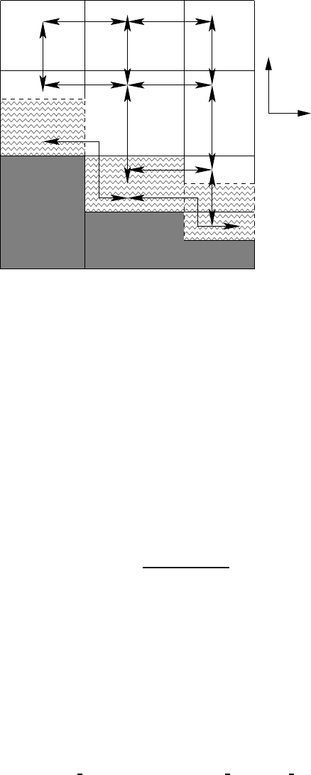
240 CHAPTER 16
horz
vert
Figure 16.1 Schematic of the along-topography pathway for tracer transport afforded by
the sigma transport scheme in mom4p1. Darkened regions denote land cells,
and lightly hatched regions are within the bottom turbulent boundary region.
This boundary layer generally can fit within a single bottom cell, as in the left
turbulent boundary region; occupy a full cell, as in the middle region; or require
more than one of the bottom cells, as in the right region. Tracers communicate
with their grid aligned horizontal and vertical neighbors via the usual advec-
tion, diffusion, and convective processes. Tracers in the bottom turbulent layer
can additionally communicate with their neighbors within the turbulent region
via sigma diffusion and sigma advection.
In mom4p1, we allow for an arbitrarily thick bottom turbulent layer. We do so
by incorporating the required grid cells into the bottom turbulent sigma layer. This
approach requires some added accounting, but it is straightforward. In particular,
the tracer concentration within the bottom turbulent layer is computed by
Tsigma =∑sigma
ρ
dzt T
∑sigma
ρ
dzt , (16.19)
where the sum extends over the cells, including cell fractions, contained in the
bottom turbulent layer. A time tendency is computed for sigma transport of Tsigma
within the bottom turbulent sigma layer. The relative fraction of a grid cell partic-
ipating in the bottom turbulent layer determines the magnitude of the tracer time
tendency added to this cell.
16.3 THE CAMPIN AND GOOSSE (1999) SCHEME
This section documents the scheme available in the module
mom4/ocean param/sources/ocean overflow mod.
Consider a heavy water parcel sitting on top of a shelf/cliff that is horizontally ad-
jacent to a lighter parcel sitting over a deeper water column. We may expect that
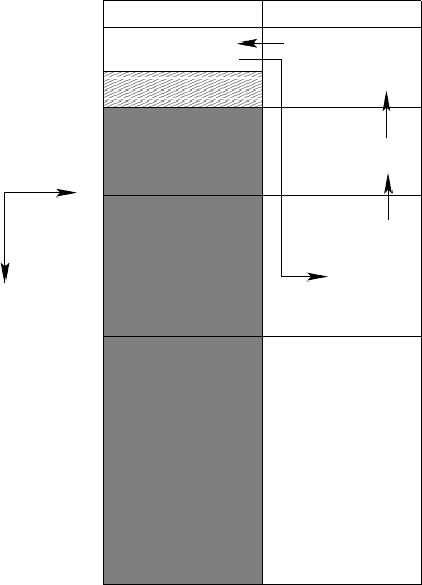
OVERFLOW SCHEMES 241
the dense parcel will move off the shelf, down the slope, and into the deep. Along
the way, entrainment will occur, with many important processes determining the
details of the final water mass. This is indeed a cartoon of an important oceanic
process forming much of the deep and intermediate waters in the ocean. Unfor-
tunately, without some extra “engineering” help, Winton et al. (1998) show that
coarse resolution z-models are incapable of providing the proper dynamical path-
ways for this transfer of dense shelf water into the deep. Beckmann and D¨
oscher
(1997) suggest one means to enhance the representation of this process, and
we discussed this scheme in Section 16.2. Campin and Goosse (1999) propose
yet another, which we detail in this section. Both schemes only affect the tracer
equation.
5
4
3
ρ(
ρ(
ρ(
kdw−1
kdw+1
kup
)
)
)
do
do
do
deep ocean(do)
shallow ocean(so)
ρ(
so
ρ(
so
ρ(
so
ρ(
so
kup,kdw)>ρ(
do
kdw)
kup,kdw+1)<ρ(
do
kdw+1)
kup,kdw−1 >ρ(
do
kdw−1
)
kup,kup)>ρ(
do
kup)
i,j
k
)
so
ρ(kup,kup)
2
1
ρ(
do
kdw)
Figure 16.2 Schematic of the Campin and Goosse (1999) overflow method in the horizontal-
vertical plane. The darkly filled region represents bottom topography using
MOM4’s full cells. The lightly filled region represents topography filled by a
partial cell. Generally, the thickness of a cell sitting on top of a topographic
feature, as the k=2 cell in the “so” column, is thinner than the corresponding
cell in the deep-ocean column (the k=2 cell in the “do” column). Shown
are tracer cells, with arrows representing the sense of the scheme’s upstream
advective transport. This figure is based on Figure 1 of Campin and Goosse
(1999).
242 CHAPTER 16
16.3.1 Finding the depth of neutral buoyancy
Figure 16.2 illustrates a typical situation in a horizontal-vertical plane. Here, we
see a heavy parcel of in situ density
ρ
so (k=kup)sitting horizontally adjacent to a
lighter parcel of in situ density
ρ
do(k=kup). The superscript “so” refers to water
in the “shallow ocean” column, whereas “do” refers to water in the “deep ocean”
column.
If the heavy parcel is allowed to adiabatically move off the shelf and then verti-
cally within the deep column, it will equilibrate at its depth of neutral buoyancy. To
compute the depth of neutral buoyancy, we evaluate the in situ density for the par-
cel taken at the local value for the in situ pressure of the environment where it may
potentially equilibrate. For the example shown in Figure 16.2, with (i,j)setting the
horizontal position of the shelf parcel and (i+1, j)setting the horizontal position
of the deep column, we have
ρ
so(kup,kup) =
ρ
(si,j,kup,
θ
i,j,kup,pi,j,kup)(16.20)
ρ
so(kup,kdw −1) =
ρ
(si,j,kup,
θ
i,j,kup,pi+1, j,kdw−1)(16.21)
ρ
so(kup,kdw) =
ρ
(si,j,kup,
θ
i,j,kup,pi+1, j,kdw)(16.22)
ρ
so(kup,kdw +1) =
ρ
(si,j,kup,
θ
i,j,kup,pi+1, j,kdw+1). (16.23)
That is, we compute the density at the salinity and potential temperature of the
shallow ocean parcel, (si,j,kup,
θ
i,j,kup), but at the in situ pressure for the respective
grid cell in the deep column. The density is then compared to the density of the
parcel at the in situ salinity, temperature, and pressure of the cells in the deep
ocean column.
16.3.2 Prescribing the downslope flow
Following Campin and Goosse (1999), we assume that the dense parcel has a
downslope momentum imparted to it. This momentum is proportional to the topo-
graphic slope, H,x, the acceleration from gravity,g, the amount of fluid within the
cell participating in the downslope flow,
0≤
δ
≤1, (16.24)
and the positive density difference
∆
ρ
=
ρ
so (kup,kup)−
ρ
do(kup)>0. (16.25)
The momentum is retarded by frictional dissipation,
µ
(in units of inverse time).
These considerations then lead to the momentum balance
ρ
oV(t)
µ
uslope =g
δ
V(t)∆
ρ
|H,x|(16.26)
where
V(t)=dxt ∗dyt ∗dzt (16.27)
is the volume of the dense parcel’s tracer cell. Equation (16.26) is also used to
determine a meridionally directed downslope transport, with the meridional topo-
graphic slope H,yreplacing H,x, and ∆
ρ
the density difference between meridion-
ally adjacent parcels.

OVERFLOW SCHEMES 243
Solving equation (16.26) for the speed uslope yields
uslope =g
δ
ρ
o
µ
|H,x|∆
ρ
. (16.28)
If the depth Hrefers to the depth of a tracer cell, then the absolute slope |H,x|is
naturally defined at the zonal face of the tracer cell. Hence, the speed, uslope, is
likewise positioned at the zonal face. This is the desired position for an advective
tracer transport velocity.
Campin and Goosse (1999) suggest the values
µ
=10−4sec−1and
δ
=1/3.
These parameters are set as namelists in MOM4. Using these numbers, with an
absolute topographic slope of |H,x| ≈ 10−3and density difference ∆
ρ
≈1kg m−3,
leads to the speed
uslope ≈.03 m sec−1. (16.29)
Associated with this downslope speed is a volume transport of fluid leaving the
cell
Uslope =uslope dztmin dyt. (16.30)
In this equation, dztmin is the minimum thickness of the shelf cell and the adjacent
cell. This minimum operation is necessary when considering MOM4’s bottom par-
tial cells, whereby the bottom-most cell in a column can have arbitrary thickness
(Figure 16.2). With uslope ≈.03m s−1corresponding to the speed of fluid leaving a
grid cell that is one-degree in width and 50 m in depth, we have a volume transport
Uslope ≈0.2Sv. Larger values are easily realized for steeper slopes, larger density
differences, and larger grid cells.
16.3.3 Mass conservation and tracer transport
To conserve mass throughout the system, the mass flux exiting the shelf cell and
entering the deep cell must itself be returned from the adjacent cell. This situation
then sets up a mass flux throughout the participating cells, where there is zero
convergence of the flux and so zero net increase or decrease in mass. For the
Boussinesq fluid, mass conservation is replaced by volume conservation. This
redirected plumbing is shown in Figure 16.2.
The convergence-free seawater mass flux carries with it tracer mass. If there
are differences in the tracer content of the cells, then the tracer flux will have a
nonzero convergence, and so it moves tracer throughout the system. We use first-
order upstream advective transport as a discretization of this process. First-order
upstream advection is the simplest form of advection. Its large level of numerical
diffusion is consistent with our belief that the bottom layer flows in the real ocean
near steep topography are quite turbulent. Hence, although inappropriate for in-
terior flows, we are satisfied with the use of upstream advection for the overflow
scheme.
16.3.4 Implementation in MOM4
This section details the implementation of the Campin and Goosse (1999) scheme
in MOM4.
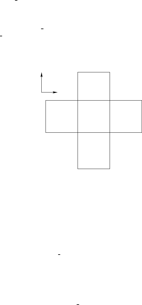
244 CHAPTER 16
16.3.4.1 Start of the integration
At the start of the model integration, it is necessary to determine those grid points
where it is possible to have a downslope flow. For this purpose, we introduce the
array topog step(i,j,m), with m=1, 2, 3, 4 specifying in a counter-clockwise di-
rection the four surrounding columns whose depths are to be compared to that at
the central (i,j)point. Figure 16.3 illustrates this notation. If the adjacent column
is deeper than the central point, thus representing a possible direction for downs-
lope flow, then topog step(i,j,m) for this value of mis set to unity. Otherwise,
topog step(i,j,m) for this mis zero. Note that with partial bottom cells, it is pos-
sible for an adjacent column to be deeper yet for the number of vertical cells to
be the same in both columns. To initiate the downslope scheme of Campin and
Goosse (1999), we insist that there be at least one more grid cell in the adjacent
column.
(i,j,3) (i,j,1)
(i,j,2)
(i,j,4)
i
j
T(i,j)
Figure 16.3 Plan view (x-y plane) of a tracer grid cell at (i,j)and its horizontally adjacent
tracer cells. We label the adjacent cells (i+1, j),(i,j+1),(i−1, j),(i,j−1)as
m=1, 2, 3, 4. Notice that we do not consider downslope flow along a diagonal
direction.
16.3.4.2 During a time step
During each time step, we locate where downslope flow is favorable for points
sitting on the ocean bottom at (i,j,kmt(i,j)). For each of the four directions
(m=1, 2, 3, 4) where topog step(i,j,m)=1, we check the density difference be-
tween the central point and the adjacent point. If the density of the central point
is larger, then the Campin and Goosse (1999) scheme is used to initiate downs-
lope transport. For these directions, we locate the depth of neutral buoyancy for
the central point according to the discussion in Section 16.3.1, and so specify the
number of vertical cells, kdw, participating in the transport. Note that we allow
for downslope transport to occur in more than one direction, as occurs in those
cases for a fixed (i,j)where topog step(i,j,m) has more than a single nonzero
element.

OVERFLOW SCHEMES 245
Our prescription is mindful of the possibility for the shallow-cell to be a partially
filled cell sitting on the topography. For this reason, the convergence-free volume
transport associated with the downslope flow is weighted by the minimum vertical
thickness of the two cells (equation (16.30)). Otherwise, it would be possible to
flood a thin partial cell with a huge amount of tracer (e.g., heat).
We incorporate effects from the Campin and Goosse (1999) overflow scheme
into MOM4’s tracer time tendency array. To derive the tendency, we proceed as
for the river-mixing and cross-land mixing formulations discussed in Griffies et al.
(2004) by focusing on the time evolution due to just the overflow process. For the
particular zonal-vertical case illustrated in Figure 16.3, we prescribe
∂t(V(t)
ρ
C)so
i,j,kup =
ρ
Uslope (Cdo
i+1, j,kup −Cso
i,j,kup)(16.31)
∂t(V(t)
ρ
C)do
i+1, j,kup =
ρ
Uslope (Cdo
i+1, j,kdw−1−Cdo
i+1, j,kup)(16.32)
∂t(V(t)
ρ
C)do
i+1, j,kdw−1=
ρ
Uslope (Cdo
i+1, j,kdw −Cdo
i+1, j,kdw−1)(16.33)
∂t(V(t)
ρ
C)do
i+1, j,kdw =
ρ
Uslope (Cso
i,j,kup −Cdo
i+1, j,kdw), (16.34)
where
ρ
Uslope =uslope rho dztmin dyt, (16.35)
with
rho dzt(min)=min(rho dzti,j,kup,rho dzti+1, j,kup)(16.36)
the minimum density weighted thickness of the two cells at k=kup. For the
Boussinesq case,
ρ
factors are set to the constant reference density
ρ
o. Setting
the tracer concentration to the same uniform value leads to vanishing time tenden-
cies in each cell, thus reflecting volume/mass conservation. Additionally, summing
these four equations leads to a vanishing right hand side, thus reflecting conser-
vation of total tracer in the system. Since the downslope mixing has the form of an
upstream advection, we discretize temporally by evaluating the tracer and density
on the right hand side at the lagged time
τ
−1.
16.4 NEUTRAL DEPTH OVER EXTENDED HORIZONTAL COLUMNS
Both Campin and Goosse (1999) and Beckmann and D¨
oscher (1997) provide
quasi-physical approaches to the problem of simulating deep water formation near
topography. Each provides plumbing routes beyond the local horizontal-vertical
routes available in geopotential or pressure models. In this way, these methods
afford a new means for representing the flows. Questions such as parameterizing
the rates of entrainment, volume flux, etc. (e.g., Killworth and Edwards (1999)) are
not directly addressed by these schemes, although the present schemes can be
extended a bit to include such details.
Climate modelers generally gauge the utility of overflow schemes on the overall
results. Namely, do the schemes provide a route for deep water formation near
topographic gradients in a manner expected from observations? Details of the
transport are often not the first priority. This situation is unsatisfying from a process
physics perspective. It may, nonetheless, be the best available for many coarse
resolution models.

246 CHAPTER 16
In this section, we discuss our prejudices with mom4p1 development. To start,
consider the density structure in Figure 16.4. This figure illustrates a case where
the sigma transport scheme of Section 16.2 does not prescribe enhanced downs-
lope transport. The reason is that the sigma transport scheme only works with
density within the bottom “sigma layer”. For this example, density at the bottom
of the deeper column is greater than that on the shelf, and so there is no en-
hanced transport prescribed. In contrast, the Campin and Goosse (1999) scheme
prescribes a downslope transport, with the dense shelf water moving to its neu-
tral buoyancy depth. It is for this reason that we favour, in mom4p1, downslope
schemes where the depth of neutral buoyancy is determined, with this depth pos-
sibly above the ocean bottom.
Even within this example, however, there remain limitations of the Campin and
Goosse (1999) scheme. The limitation is that their scheme only reaches out one
grid box in the horizontal. That is, although the scheme is non-local in the vertical,
it remains local in the horizontal. What can happen is the dense parcel will find
itself denser than any parcel in the adjacent column, and so its resting place, with
the Campin and Goosse (1999) algorithm, is at the bottom of the adjacent column,
rather than at a neutral buoyancy depth. If given the opportunity to exchange
with columns further removed from the central column, the parcel is afforded the
opportunity to find a more suitable neutral buoyancy layer. This general result
motivates us to consider two experimental schemes, whereby the notions of a
neutral buoyancy level motivated from Campin and Goosse (1999) are extended
to columns removed from the central column. As the parcel finds a more suitable
resting place, it is assumed to exchange properties with the intermediate parcels,
in a manner meant to represent entrainment as it moves downslope. The rates of
transport remain a function of the topographic slope and the difference in density,
just like the Campin and Goosse (1999) scheme.
There are two methods available in mom4p1 for realizing these ideas. The first
is implemented in the module
mom4/ocean param/sources/ocean overexchange mod.
In this scheme, a dense shallow parcel is allowed to be transported horizontally
over more than a single column, so long as it continues to remain on the bottom of
the adjacent columns, thus affording it more opportunity to find its neutral buoyancy
level. The exchange results in no net mass exchange between parcels, and so
there is no need for an advective replumbing to be implemented, in contrast to the
Campin and Goosse (1999) scheme. Here, the resolved dynamics adjust based
on mixing of the water masses and the associated changes in density structure.
This process then becomes directly analogous to the cross-land mixing formulation
discussed in Griffies et al. (2004) and in Chapter 17. That is, we remove the
intermediate cells from the process described in Section 16.3.4.2, and just focus
on the single shallow and deep cell, thus leading to
∂t(V(t)
ρ
C)so
i,j,kup =
ρ
Uslope (Cdo
i+1, j,kdw −Cso
i,j,kup)(16.37)
∂t(V(t)
ρ
C)do
i+1, j,kdw =
ρ
Uslope (Cso
i,j,kup −Cdo
i+1, j,kdw), (16.38)
This parameterization is simpler to implement than the Campin and Goosse (1999)
scheme, since we omit the intermediate cells from the process. This approach
OVERFLOW SCHEMES 247
also does not rely on assumptions of a flow that may be set up in response to the
exchange of fluid.
The second method is implemented in the module
mom4/ocean param/mixing/ocean mixdownslope mod.
In this scheme, exchange of tracer occurs as a partial convective mixing process.
We assume that a part of the shallow dense cell is transported downslope, and
this then mixes with the intermediate cells with an efficiency proportional to the to-
pographic slope and the density difference. In equations, we compute a combined
mass of the mixed water according to
Msum =M(s) + M(d), (16.39)
where
M(s) =
γ
rho dzt(s)dat(s)(16.40)
is the mass of water in the shallow dense cell participating in the exchange, and
M(d) =
δ
rho dzt(d)dat(d)(16.41)
is the mass of deep cell participating. In these equations, dat is the horizontal
area of the cells,
γ
is the fraction of the shallow dense cell that is assumed to take
part in the downslope transport, and
δ
is proportional to the topographic slope and
the density difference between the shallow and deep parcel. If assumed to mix
completely over a time step, then the resulting tracer concentration Cmix would be
given by
Msum Cmix =
γ
rho dzt(s)dat(s)C(s) +
δ
rho dzt(d)dat(d)C(d). (16.42)
Instead of mixing completely, which would require an adjustment process as in
convection, we use the tracer concentration Cmix to deduce the following time ten-
dencies which drive the cells toward the mixed concentration
dat(s)tend(s) = M(s)
γ
∆t(Cmix −C(s)) (16.43)
dat(d)tend(d) = M(d)
δ
∆t(Cmix −C(d)). (16.44)
Given the mixed tracer concentration (16.42), we have
dat(s)tend(s) + dat(d)tend(d) = 0, (16.45)
which reflects the conservation of tracer.
16.5 SIGMA FRICTION
The previous schemes introduce a new transport pathway for tracers. Nothing is
done to the momentum equation. Another idea is to consider an enhancement
of the vertical friction acting near to the bottom, with the friction introduced via a
vertical viscosity. The effects of vertical friction are related, through geostrophy, to
those from Gent et al. (1995), whereby density slopes are reduced without mixing
of density classes (Greatbatch and Lamb, 1990). Alternatively, enhancing the ver-
tical viscosity next to the bottom increases the Ekman layer thickness next to the
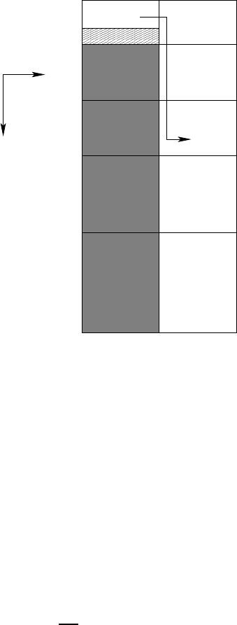
248 CHAPTER 16
ρ=
ρ=
ρ=
ρ=
1033
1034
1036
1037
3
4
5
2
1
k
i,j
ρ=1035
ρ=1035
Figure 16.4 Schematic of a situation where a dense parcel sits on a shelf next to a column
whose upper portion is light, but whose deeper portion is denser than the shelf.
For this case, the Campin and Goosse (1999) scheme prescribes a transport be-
tween the shelf water at level 1 and the deeper water at level 3, with water
bubbling upward to conserve mass as shown in Figure 16.2. In contrast, the
sigma transport scheme will not prescribe any enhanced transport, since here
the bottom of the deep column is denser than the shelf.
bottom, and this breaks geostrophy, thus allowing for an easier downslope transit
of the fluid. The scheme described in this section is not available in mom4p1. We
mention it, nonetheless, as it may prove to be of use for some applications.
Following the scaling from Campin and Goosse (1999) discussed in Section
16.3.2, we define a vertical viscosity according to equation (16.26)
κσ
=dzt
σ
uslope
=−g
δ
µ ρ
H,x∆
ρ
dzt
σ
sign(H,x).(16.46)
Using the parameters from Section 16.3.2 leads to a vertical visosity of
κσ
=0.15 m s−2, (16.47)
with larger values for steeper topographic slopes and stronger density contrasts.
We propose to introduce this viscosity throughout the sigma layer, and exponen-
tially decrease it above the layer, with a relatively short decay scale
κσ
decay =10m. (16.48)
We suggest computing this viscosity separately for the two horizontal directions,
and take the maximum of the two for the parameterization.

Chapter Seventeen
Cross-land mixing
The purpose of this chapter is to present the method used in MOM4 for mixing
tracers and mass/volume across land separated points, such as across an unre-
solved Strait of Gibraltar. The material here is taken from the MOM4 Technical
Guide of Griffies et al. (2004), with slight modifications to account for generalized
vertical coordinates used in mom4p1.
17.1 INTRODUCTION
In climate modeling, it is often necessary to allow water masses that are separated
by land to exchange properties. This situation arises in models when the grid
mesh is too coarse to resolve narrow passageways that in reality provide crucial
connections between water masses. For example, coarse grid spacing typically
closes off the Mediterranean from the Atlantic at the Straits of Gibraltar. In this
case, it is important for climate models to include the effects of salty water entering
the Atlantic from the Mediterranean. Likewise, it is important for the Mediterranean
to replenish its supply of water from the Atlantic to balance the net evaporation
occurring over the Mediterranean region.
We describe here a method used in MOM4 to establish communication between
bodies of water separated by land. The communication consists of mixing tracers
and mass/volume between non-adjacent water columns. Momentum is not mixed.
The scheme conserves total tracer content, total mass or volume (depending on
whether using the non-Boussinesq or Boussinesq versions of MOM4), and main-
tains compatibility between the tracer and mass/volume budgets. It’s only restric-
tion is that no mixing occur between cells if their time independent thicknesses
differ. This constraint is of little practical consequence.
17.2 TRACER AND MASS/VOLUME COMPATIBILITY
Consider two boxes with fluid masses M(1)=
ρ
(1)V(1)and M(2)=
ρ
(2)V(2)and
tracer concentrations (tracer mass per mass of fluid) T(1)and T(2)(for a Boussi-
nesq fluid, the density is set to the constant Boussinesq density
ρ
o). A mixing
process that conserves total tracer mass and total fluid mass must satisfy
∂t(T(1)
ρ
(1)V(1)+T(2)
ρ
(2)V(2)) = 0 (17.1)
∂t(
ρ
(1)V(1)+
ρ
(2)V(2)) = 0. (17.2)
Notably, mass conservation can be considered a special case of total tracer con-
servation when the tracer concentration is uniform and constant: T≡1. This re-
250 CHAPTER 17
sult provides an important compatibility constraint between the discrete tracer and
mass/volume budgets. For constant volume boxes with a Boussinesq fluid, such
as considered in rigid lid models, compatibility is trivial. For boxes which change
in time, such as the top cells in MOM4p0 free surface or any box in mom4p1, then
compatibility provides an important constraint on the methods used to discretize
the budgets for mass/volume and tracer. The remainder of this chapter incorpo-
rates these ideas into the proposed cross-land mixing scheme.
17.3 TRACER MIXING IN A BOUSSINESQ FLUID WITH FIXED BOXES
To start in our formulation of cross-land mixing, let us consider mixing of two vol-
umes of Boussinesq fluid, where the separate volumes remain constant in time
∂tV(1)=∂tV(2)=0. (17.3)
An example is the mixing between two constant volume grid cells. If the mixing
takes place instantaneously and between the full contents of both boxes, as in
convective adjustment, then the final tracer concentration in both boxes is given by
Tf inal =T(1)V(1)+T(2)V(2)
V(1)+V(2). (17.4)
It is assumed in convective mixing that the volumes of the two boxes remains
unchanged. The picture is of an equal volume of water rapidly mixing from one
box to the other, without any net transport between the boxes.
Instead of instantaneous and complete convective mixing, consider mixing of
the two boxes at a volume rate U. That is, Urepresents an equal volume per
time of water mixing between the boxes, with no net transport. As shown in Figure
17.1, Uis chosen based on the observed amount of water exchanged through
the passageway. Just as for convective adjustment, the volumes of the two boxes
remains fixed. But the tracer concentrations now have a time tendency. One form
for this tendency relevant for constant volume cells is given by
∂t(V(1)T(1)) = U(T(2)−T(1))(17.5)
∂t(V(2)T(2)) = U(T(1)−T(2)). (17.6)
Since the volumes are constant, we can write these budgets in the form
∂tT(1)=U
V(1)(T(2)−T(1))(17.7)
∂tT(2)=U
V(2)(T(1)−T(2)), (17.8)
This is the form of cross-land tracer mixing used in the rigid lid full cell MOM1.
In the real world, transport is often comprised of stacked flows where deep wa-
ter flows one way and shallow water oppositely (e.g., see Figure 17.1). Hence,
a more refined form of cross-land mixing may consist of upwind advective fluxes
acting between non-local points in the model, where the advective velocity is spec-
ified based on observations. Such sophistication, however, is not implemented in
MOM4. Indeed, it is arguable that one may not wish to have more details than
provided by the simpler form above, since more details also further constrain the
solution.
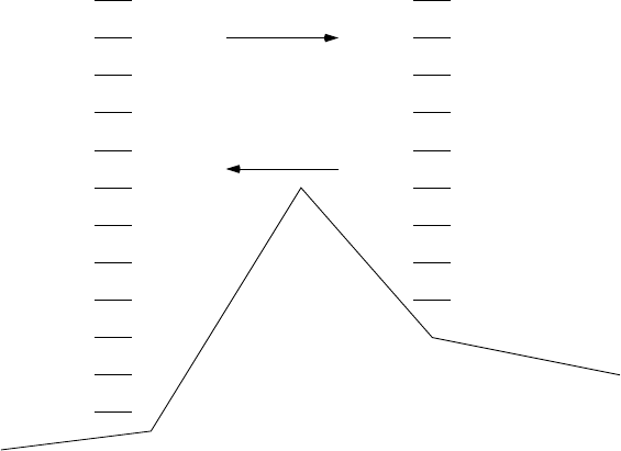
CROSS-LAND MIXING 251
kbot kbot
ktop ktop
U1
U2
Figure 17.1 Schematic of cross-land mixing. The model’s grid mesh is assumed too coarse
to explicitly represent the lateral exchange of water masses. For this schematic,
we consider an observed sub-grid scale transport U1moving in one direction,
and U2in another. To represent the mixing effects on tracers by these trans-
ports, we suggest taking the exchange rate Uin MOM4’s cross-land mixing to
be the average of the transports U= (U1+U2)/2. Cross-land mixing occurs
between the user-specified depth levels k=ktop and k=kbot. If ktop =1, then
cross-land mixing of volume in the top cell must be considered, in addition to
tracer transport, in order to maintain compatibility between volume and tracer
budgets.
17.4 MIXING OF MASS/VOLUME
In a model with a coarse mesh, the Mediterranean is typically land-locked. Hence,
the net evaporation experienced over the Mediterranean region will cause the sim-
ulated ocean volume in this region to decrease without bound. In a model resolv-
ing the Straits of Gibraltar, there is a transfer of mass across the Strait from the
Atlantic. This mass transfer creates a change in the height of the free surface.
Our goal is to have a parameterized mass transfer associated just with a differ-
ence in the free surface height. That is, if the densities are different yet the free
surface heights are equal, then there is no mixing. By transferring masses of wa-
ter, we must also recognize that the water contains tracer. Hence, mass and tracer
mixing must maintain the compatibility mentioned in Section 17.2. In this section,
however, we only introduce a basic form for mass transfer. Full compatibility with
tracer transfer is achieved in Section 17.5

252 CHAPTER 17
17.4.1 Instantaneous and complete mixing
To start by considering what form for mixing is appropriate, consider a convec-
tive analog whereby a complete mixing of masses
ρ
(1)A(1)h(1)and
ρ
(2)A(2)h(2)
leaves the final mass per area in both cells given by
(
ρ
h)f inal =
ρ
(1)A(1)h(1)+
ρ
(2)A(2)h(2)
A(1)+A(2), (17.9)
where A(1)and A(2)are the temporally constant horizontal areas of the two grid
cells and h(1)and h(2)are their generally time dependent thicknesses.
There are two problems with this mixing. First, it is too rapid and too complete.
We prefer a method that allows for some control in the rate of mixing. Second, it
changes the mass within a grid cell in cases where the initial masses per area are
equal yet the constant horizontal areas of the cells differ.
17.4.2 A finite time incomplete mixing
A finite time and incomplete mixing is analogous to that taken for the tracers in
Section 17.3. Here, we consider the time tendencies for the mass per area within
a cell
∂t(
ρ
(1)h(1)) =
γ
(1)(
ρ
(2)h(2)−
ρ
(1)h(1))(17.10)
∂t(
ρ
(2)h(2)) =
γ
(2)(
ρ
(1)h(1)−
ρ
(2)h(2)), (17.11)
where
γ
(1)and
γ
(2)are inverse damping times. This proposed mixing results in
a transfer of mass only when the mass per area within the two boxes differs. The
total mass of the two-box system is conserved if the following constraint is satisfied
∂t[(
ρ
h A)(1)+ (
ρ
h A)(2)] = (A(1)
γ
(1)−A(2)
γ
(2)) (
ρ
(2)h(2)−
ρ
(1)h(1)) = 0.
(17.12)
This relation places a constraint on the inverse damping times
γ
(1)and
γ
(2)
A(1)
γ
(1)=A(2)
γ
(2)(17.13)
which is easily satisfied.
The problem with the mixing prescribed by equations (17.10) and (17.11) is that
mixing will ensue in the following two undesirable cases. First, if the densities of
the two cells are initially the same
ρ
(1)=
ρ
(2)=
ρ
, yet the cells have different thick-
nesses, then density change is driven solely by the difference in cell thicknesses
h(1)∂t
ρ
(1)=
ρ γ
(1)(h(2)−h(1))(17.14)
h(2)∂t
ρ
(2)=
ρ γ
(2)(h(1)−h(2)). (17.15)
Such is acceptable in our scheme only for the surface ocean grid cell.
Another problem with the mixing prescribed by equations (17.10) and (17.11) is
seen by considering the situation whereby two top model grid cells have initially
equal thicknesses h(1)=h(2)=hyet different densities. The model grid cell
thickness will evolve because of the difference in densities
ρ
(1)∂th(1)=h
γ
(1)(
ρ
(2)−
ρ
(1))(17.16)
ρ
(2)∂th(2)=h
γ
(2)(
ρ
(1)−
ρ
(2)). (17.17)
However, as stated at the beginning of this section, we aim to prescribe a mixing
process that occurs only when the tracer concentration and/or free surface heights
differ. Therefore, we must consider an alternative to equations (17.10) and (17.11)
CROSS-LAND MIXING 253
17.4.3 A finite time incomplete mixing for surface cells
We consider the following prescription for the surface grid cells, in which mixing
occurs only when the surface heights differ
∂t(
ρ
(1)h(1)) =
γ
(1)
ρ
(h(2)−h(1))(17.18)
∂t(
ρ
(2)h(2)) =
γ
(2)
ρ
(h(1)−h(2)). (17.19)
When considered over interior model grid cells, then we prescribe no mass trans-
fer. The density factor
ρ
can be given by anything convenient, such as
ρ
=
ρ
(1)+
ρ
(2)
2, (17.20)
or the even simpler prescription
ρ
=
ρ
o. (17.21)
17.5 TRACER AND MASS MIXING
The general case of mixing tracers and mass is now considered. The following are
the aims of the formulation.
•Total fluid mass in the two boxes is conserved.
•Total tracer mass in the two boxes is conserved.
•In the rigid lid Boussinesq full cell case, the tracer tendency reduces to equa-
tions (17.7) and (17.8) used in MOM1.
•Mass is exchanged only between top grid cells, in which case if the tracer
concentration in the two boxes is the same yet the mass differs, then mixing
of mass will leave the tracer concentrations unchanged.
•The time tendency for the mass exchange in the top cells is proportional
to the difference in surface height eta tbetween the cells, rather than the
generally smaller difference between the cell thickness dzt.
Mixing that satisfies these constraints is given by the following for the surface grid
cells with k=1
∂t(
ρ
(1)h(1)T(1)) = 2U
ρ
o
A(1)(H(1)+H(2))(h(2)T(2)−h(1)T(1))(17.22)
∂t(
ρ
(2)h(2)T(2)) = 2U
ρ
o
A(2)(H(1)+H(2))(h(1)T(1)−h(2)T(2))(17.23)
∂t(
ρ
(1)h(1)) = 2U
ρ
o
A(1)(H(1)+H(2))(h(2)−h(1))(17.24)
∂t(
ρ
(2)h(2)) = 2U
ρ
o
A(2)(H(1)+H(2))(h(1)−h(2))(17.25)
254 CHAPTER 17
Likewise, for interior cells with k>1, we prescribe
∂t(
ρ
(1)h(1)T(1)) = 2Urho dzt
A(2)(H(1)+H(2))(T(2)−T(1))(17.26)
∂t(
ρ
(2)h(2)T(2)) = 2Urho dzt
A(2)(H(1)+H(2))(T(1)−T(2))(17.27)
∂t(
ρ
(1)h(1)) = 0 (17.28)
∂t(
ρ
(2)h(2)) = 0. (17.29)
In these equations, His the depth of a column with a resting ocean surface. For
the k>1equations, rho dzt is the averaged thickness weighted density for the
two cells. For the k=1equations,
h(k=1) = Grd%dztk=1+eta t (17.30)
is the thickness of the top cell for the case of a geopotential vertical coordinate. The
general Thickness%dzti,j,k=1thickness varies much less rapidly in the horizontal
when employing zstar or pstar as the vertical coordinate. In order to employ sim-
ilar mixing rates for the geopotential model as for the general vertical coordinate
models, we prefer the more restricted definition (17.30) of thickness based on the
geopotential model. The mass per area equations (17.24) and (17.25) result from
the tracer equations (17.22) and (17.23) upon setting the tracer concentrations to
a constant, as required for compatible budgets.
17.6 FORMULATION WITH MULTIPLE DEPTHS
We now consider the case where there are multiple boxes in the vertical. We
restrict attention to situations where mixing occurs between boxes at the same
vertical level, as shown in Figure 17.1.
17.6.1 MOM1 formulation of cross-land tracer mixing
In MOM1, the vertical cells all have time independent thicknesses (i.e., rigid lid
geopotential coordinate model), and the fluid is Boussinesq. It is useful to start
with this case prior to considering the more general case.
In the full cell rigid lid case, we follow the approach given by equations (17.7) and
(17.8), where the relevant volume now becomes that for the respective column.
The volumes for the two columns lx =1, 2 are given by
V(lx)=A(lx)ktop
∑
k=kbot
dztk=A(lx)H(lx), (17.31)
where
A(lx)=dxti,j(lx)dyti,j(lx)(17.32)
are the generally different horizontal cross-sectional areas of the tracer cells in the
two columns, and H(1)=H(2)is the vertical thickness of the two columns. The
top and bottom k-levels for the columns are set by k=ktop and k=kbot. As
CROSS-LAND MIXING 255
mentioned earlier, the formulation here allows for mixing only between boxes that
live on the same k-level, so k=ktop and k=kbot are the same for both columns
lx =1, 2.
Use of these volumes in equations (17.7) and (17.8) leads to the tracer time
tendencies for a particular k-level
∂tT(1)
k=B(1)(T(2)
k−T(1)
k)(17.33)
∂tT(2)
k=B(2)(T(1)
k−T(2)
k), (17.34)
where
B(lx)=U
V(lx)(17.35)
represents the rate (B(lx)has units of inverse time) at which the two columns par-
ticipate in the mixing. Conservation of total tracer is maintained between two hor-
izontally adjacent boxes within the two columns. We see such conservation via
multiplying the above tendencies by the respective time independent volumes of
the two cells, and adding
∂t(V(1)
kT(1)
k+V(2)
kT(2)
k) = (T(2)
k−T(1)
k) (A(1)B(1)h(1)
k−A(2)B(2)h(2)
k) = 0,
(17.36)
where
A(1)B(1)h(1)
k=U(h(1)
k/H(1))
=U(h(2)
k/H(2))
=A(2)B(2)h(2)
k
(17.37)
was used.
17.6.2 Generalizing to free surface and non-Boussinesq
We now generalize to the case of time varying grid cells with generalized vertical
coordinates. Based on the considerations of Section 17.5 and the form used in
MOM1, we write for the general case for a surface grid cell with k=1
∂t(
ρ
(1)
kh(1)
kT(1)
k) = 2U
ρ
o
A(1)(H(1)+H(2))(h(2)
kT(2)
k−h(1)
kT(1)
k)(17.38)
∂t(
ρ
(2)
kh(2)
kT(2)
k) = 2U
ρ
o
A(2)(H(1)+H(2))(h(1)
kT(1)
k−h(2)
kT(2)
k), (17.39)
where again H(1)and H(2)are the generally different static resting depths of the
two columns, and
h(k=1) = Grd%dztk=1+eta t (17.40)
according to our prescription given by equation (17.30). Setting the tracers to
uniform constants leads to the transfer of mass per area between two surface cells
∂t(
ρ
(1)
kh(1)
k) = 2U
ρ
o
A(1)(H(1)+H(2))(h(2)
k−h(1)
k)(17.41)
∂t(
ρ
(2)
kh(2)
k) = 2U
ρ
o
A(2)(H(1)+H(2))(h(1)
k−h(2)
k), (17.42)
256 CHAPTER 17
For interior cells with k>1, we prescribe
∂t(
ρ
(1)
kh(1)
kT(1)
k) = 2Urho dztk
A(1)(H(1)+H(2))(T(2)
k−T(1)
k)(17.43)
∂t(
ρ
(2)
kh(2)
kT(2)
k) = 2Urho dztk
A(2)(H(1)+H(2))(T(1)
k−T(2)
k), (17.44)
where
rho dztk=rho dzt(1)
k+rho dzt(2)
k
2(17.45)
is the average thickness weighted density of the adjacent cells, and
h=Thickness%dzti,j,k(17.46)
is the general thickness of the tracer cell. By inspection, for each k-level this for-
mulation conserves total tracer mass and total fluid mass (recall Section 17.4).
Setting the tracers to uniform constants leads to a zero transfer of mass per area
between two interior cells.
These budgets can be written in a form familiar from other damping processes,
in which for k=1we have
∂t(
ρ
(1)h(1)T(1)) =
γ
(1)
ρ
o(h(2)T(2)−h(1)T(1))(17.47)
∂t(
ρ
(2)h(2)T(2)) =
γ
(2)
ρ
o(h(1)T(1)−h(2)T(2))(17.48)
∂t(
ρ
(1)h(1)) =
γ
(1)
ρ
o(h(2)−h(1))(17.49)
∂t(
ρ
(2)h(2)) =
γ
(2)
ρ
o(h(1)−h(2))(17.50)
where the depth label kwas omitted for brevity, and
γ
(1)=2U
A(1)(H(1)+H(2))(17.51)
γ
(2)=2U
A(2)(H(1)+H(2))(17.52)
defines the damping coefficients. For interior cells, only tracer concentration is
mixed, in which case
∂t(
ρ
(1)h(1)T(1)) =
γ
(1)rho dzt (T(2)−T(1))(17.53)
∂t(
ρ
(2)h(2)T(2)) =
γ
(2)rho dzt (T(1)−T(2)), (17.54)
with
γ
(1)and
γ
(2)as for the surface cell.
The damping coefficients (17.51) and (17.52) are generally time dependent for
cases with mixing in the top cell and where the free surface height is included
when computing the column thicknesses H(1)and H(2). One may alternatively be
motivated to keep the damping coefficients constant in time by setting H(1)and
H(2)to be the time independent depth of the respective columns. This choice
is appropriate when using cross-land mixing between columns in shallow regions
where the free surface height is some nontrivial fraction of the full column depth.
MOM4 generally sets the thicknesses to their time independent depths.
To get a sense for the strength of the mixing, consider the case of a one-degree
horizontal grid mesh where the upper thousand meters of the water column is

CROSS-LAND MIXING 257
mixed across Gibraltar with U=1.75 ×10⁶m3s−1, which is a reasonable value.
With H(1)=H(2)≈1000mwe have
V(1)≈V(2)≈1.2 ×10¹³m3, (17.55)
and to the damping coefficient
γ
(1)≈
γ
(2)=U
V≈1.5 ×10⁻⁷s−1≈77 days−1. (17.56)
Just as for any other form of mixing, if the damping coefficients are too large, then
it is possible for there to be numerical instabilities. MOM4 provides a check so that
no more than one-half of a particular grid cell is mixed per model time step.
17.7 SUPPRESSION OF B-GRID NULL MODE
When mixing the free surface height across an unresolved strait, it has been found
essential to mix between two pairs of adjacent columns in order to suppress the
checkerboard null mode present on the B-grid (see Chapter 26 of Griffies et al.
(2004)). For the Mediterranean example, this means choosing any two adjacent
points on each side of Gibraltar and setting the volume transport for each column
to U= (1/2)1.75 ×106m3s−1.
PART 4
Diagnostic capabilities
The purpose of this part of the manual is to describe some of the diagnostic
capabilities in mom4p1.

Chapter Eighteen
Effective dianeutral diffusivity
The purpose of this chapter is to detail a method to quantify water mass mixing in
MOM without detailed knowledge of the numerical transport scheme. The method
is restricted to experiments configured with the following:
•Boussinesq fluid;
•geopotential vertical coordinate;
•linear free surface, so that the thickness of a grid cell remains constant in
time;
•flat bottom ocean;
•linear equation of state;
•zero buoyancy forcing.
Extensions are possible, yet not implemented. Momentum forcing via winds is al-
lowed. Much of the fundamentals in this chapter are guided by the work of Winters
et al. (1995) and Winters and D’Asaro (1995). Griffies et al. (2000b) applied these
methods to various idealized model configurations in a rigid lid version of MOM3.
We assume the linear equation of state for an incompressible fluid is written in
the form
ρ
=
ρ
0(1−
α θ
), (18.1)
where
θ
is potential temperature,
ρ
ois a constant density associated with the
Boussinesq approximation, and
α
is a constant thermal expansion coefficient. The
system is open to momentum fluxes yet closed to buoyancy fluxes.
18.1 POTENTIAL ENERGY AND APE IN BOUSSINESQ FLUIDS
The purpose of this section is to introduce the notion of a sorted density profile in
the context of potential energy and available potential energy (APE). This profile is
of particular relevance when considering the effective mixing occuring throughout
a column of sorted fluid in Section 18.2.
Potential energy of the ocean is given by
Ep=ZdV
ρ
P, (18.2)
where
P=g z (18.3)
262 CHAPTER 18
is the potential energy per mass of a fluid parcel, gis the acceleration of gravity, z
is the vertical position of a fluid parcel, and
ρ
dV=
ρ
dxdydzis the parcel mass.
Available potential energy (APE) is the difference between the potential energy
of the fluid in its natural state, and the potential energy of a corresponding stably
stratified reference state. The reference state is reached by adiabatically rearrang-
ing the fluid to a state of minimum potential energy, which is a state that contains
zero horizontal gradients. This rearrangement, or sorting, provides a non-local
mapping between the unsorted fluid density and the sorted density
ρ
(x,t) =
ρ
(z∗(x,t),t). (18.4)
The sorting map determines a vertical position field z∗(x,t)which is the vertical
height in the sorted state occupied by a parcel at (x,t)in the unsorted state. Due
to the monotonic arrangement of density in the sorted state, z∗(x,t)is a monotonic
function of density
ρ
(x,t).
It is convenient to set the origin of the vertical coordinate at the ocean bottom so
to keep potential energy of the unsorted state non-negative. This convention also
allows for z∗(x,t)to be defined as a monotonically decreasing function of density.
That is,
ρ
(x1,t)<
ρ
(x2,t)⇒z∗(x1,t)>z∗(x2,t). (18.5)
Conservation of volume in a flat bottom ocean implies that the sorted fluid state
has the same vertical extent as the unsorted fluid, which renders
0≤z,z∗≤H, (18.6)
where His the ocean depth.
In the following, it proves convenient to denote the density profile in the sorted
reference state using the symbols
ρ
(z∗,t) =
ρ
re f (z=z∗,t). (18.7)
Given this notation, the non-local sorting map between the unsorted and sorted
fluid states provides the equivalence
ρ
(x,t) =
ρ
(z∗(x,t),t) =
ρ
re f (z=z∗,t). (18.8)
In turn, potential energy for the sorted fluid state can be written in two equivalent
manners
Ere f =gZdV z
ρ
re f (z,t)(18.9)
=gZdV z∗(x,t)
ρ
(x,t). (18.10)
Equation (18.9) represents an integral over the sorted fluid state, in which the den-
sity of this state is a function only of the depth. The horizontal area integral is thus
trivial to perform. Equation (18.10) represents an integral over the unsorted fluid
state, where the density
ρ
(x,t)of an unsorted parcel is weighted by the vertical
position z∗(x,t)that the parcel occupies in the sorted state. It follows that the APE
can be written in two equivalent ways
EAPE =gZdV z [
ρ
(x,t)−
ρ
re f (z,t)] (18.11)
=gZdV
ρ
(x,t) [z−z∗(x,t)]. (18.12)

EFFECTIVE DIANEUTRAL DIFFUSIVITY 263
18.2 EFFECTIVE DIANEUTRAL MIXING
In this section we formulate a method to empirically quantify the effects on water
masses arising from various simulated tracer transport processes. A similar ap-
plication was advocated by Winters et al. (1995) and Winters and D’Asaro (1995)
for the purpose of diagnosing mixing in direct numerical simulations of unstable
fluid flows. Their focus was on physically motivated mixing such as that occuring
with breaking waves. The main focus here is on spurious mixing due to numerical
errors. The procedure is identical, however, in that for each case, one considers
the evolution of the reference density profile,
ρ
re f (z,t), in a fluid system closed to
buoyancy fluxes
∂t
ρ
re f =∂z∗(
κ
e f f ∂z∗
ρ
re f ). (18.13)
Again, in this equation z∗is the vertical position in the sorted fluid state. Therefore,
constant z∗surfaces represent constant density surfaces in the unsorted state. As
such, the effective diffusivity
κ
e f f summarizes the total amount of mixing across
constant density surfaces. If the simulation does not change the water mass distri-
bution, then D
ρ
/Dt =0, the sorted reference density is static ∂t
ρ
re f =0, and the
effective diffusivity is zero. In turn, any temporal change in the reference density
represents changes in the water mass distribution. These changes are the result
of dianeutral mixing, and so have an associated non-zero
κ
e f f (z∗,t). This is the
basic idea that is pursued in the following sections.
18.2.1 Global effective dianeutral diffusivity
In addition to the diffusivity
κ
e f f (z∗,t), which is local in density space, it is useful
to garner a summary of the overall dianeutral mixing occuring in an ocean model.
A vertical integral of
κ
e f f (z∗,t)would provide such information. A quicker com-
putation of a global effective dianeutral diffusivity can be obtained by inverting the
variance equation for the sorted density
∂tZdV
ρ
2
re f =−2ZdV
κ
e f f (∂z
ρ
re f )2. (18.14)
This result, derived for a closed fluid system, suggests the introduction of a global
effective diffusivity
κ
global(t) = − ∂tRdV
ρ
2
re f
2RdV(∂z
ρ
re f )2!. (18.15)
This diffusivity provides one number that can be used to represent the total amount
of dianeutral diffusion acting over the full model domain. It vanishes when the
simulation is adiabatic, as does the effective diffusivity
κ
e f f (z∗,t). However it is
generally different from the vertical average of
κ
e f f (z∗,t).
18.2.2 Finite difference approximation
In the following, assume that the discrete sorted density is equally spaced in the
vertical with a separation ∆z∗, and let the vertical coordinate increase upwards
from zero at the flat bottom ocean floor. Note that in general, ∆z∗<< ∆z, where
264 CHAPTER 18
∆zis the ocean model’s grid spacing. The reason is that all the Nx×Ny×Nz
grid points in the ocean model are sorted into the reference vertical profile, which
has a vertical range over the same extent as the ocean model: 0≤z,z∗≤H.
As a consequence, the vertical resolution of the sorted profile is Nx×Nytimes
finer than the Nzpoints resolving the profile at a particular horizontal position in
the unsorted state.
On the discrete lattice, the vertical diffusive flux of the sorted density
Fz∗(z∗,t) = −
κ
e f f (z∗,t)∂z∗
ρ
re f (z∗,t)(18.16)
is naturally defined at the top face of the density cell whose center is at z∗. As
such, the diffusion operator at the lattice point z∗, which is constructed as the
convergence of the diffusive flux across a density grid cell, takes the discrete form
−(∂z∗Fz∗)(z∗,t)≈− Fz∗(z∗,t−∆t)−Fz∗(z∗−∆z∗,t−∆t)
∆z∗!. (18.17)
The time lag is necessary to provide for a stable discretization of the diffusion
equation. The discretization of the flux is given by
Fz∗(z∗,t) = −
κ
e f f (z∗,t)∂z∗
ρ
re f (z∗,t)
≈−
κ
e f f (z∗,t)
ρ
re f (z∗+∆∗z,t)−
ρ
re f (z∗,t)
∆z∗!. (18.18)
Since the flux is located at the top face of the density grid cell whose center is at
the position z∗, the effective diffusivity is located at this face as well. Each of these
difference operators is consistent with those used in MOM when discretizing the
diffusion equation for the unsorted fluid.
As with the unsorted tendency, the time derivative in the effective diffusion equa-
tion can be approximated using a leap-frog differencing:
∂t
ρ
re f (z∗,t)≈
ρ
re f (z∗,t+∆t)−
ρ
re f (z∗,t−∆t)
2∆t. (18.19)
Piecing these results together yields the expression for the vertical flux at the
top of the density cell z∗+∆z∗
Fz∗(z∗,t−∆t) = Fz∗(z∗−∆z∗,t−∆t)−∆z∗
2∆t[
ρ
re f (z∗,t+∆t)−
ρ
re f (z∗,t−∆t)].
(18.20)
This flux can be determined starting from the ocean bottom, where is vanishes,
and working upwards. Without surface buoyancy fluxes, it also vanishes at the top
of the water column, resulting in conservation of Rdz∗
ρ
re f (z∗,t). After diagnosing
the flux from the tendency, the effective diffusivity can be diagnosed from
κ
e f f (z∗,t) = −Fz∗(z∗,t) ∆z∗
ρ
re f (z∗+∆z∗,t)−
ρ
re f (z∗,t)!. (18.21)
The issues of what to do when the density gradient becomes small, as in weakly
stratified regions, is discussed in Sections 18.2.3 and 18.2.5.
EFFECTIVE DIANEUTRAL DIFFUSIVITY 265
18.2.3 Relevant vertical stratification range
In the stratified portions of the upper ocean, periods 2
π
/Nfor buoyancy oscilla-
tions are roughly 10-30 minutes, smaller in the pycnocline, and in the deep ocean
periods are roughly 5-6 hours (see pages 55-56 of Pickard and Emery (1990)).
The squared buoyancy frequency for the sorted reference state is given by
N2
∗=−g
ρ
o
d
ρ
re f
dz∗
=−g
1000
ρ
o
d
σ
re f
dz∗, (18.22)
where
σ
re f =1000 (
ρ
re f −1)is the sigma value for the sorted density
ρ
re f (g/cm3).
Working with
σ
re f is desirable for accuracy reasons. The observed range in buoy-
ancy periods provides a range over the sorted vertical profile’s stratification for
which a calculation of the model’s effective diffusivity will be performed:
d
ρ
re f
dz∗=−1.035g/cm3
980cm/sec2
4
π
2
T2, (18.23)
where T(sec)is the period. With 1×60secs <T<6×60 ×60secs defining the
period range, the corresponding vertical density gradient range is
10−10g/cm4≤
d
ρ
re f
dz ≤10−5g/cm4, (18.24)
and the corresponding range for the sigma gradient is
10−7g/cm4≤
d
σ
re f
dz ≤10−2g/cm4. (18.25)
18.2.4 A useful test case
When coding the effective diffusivity algorithm, it has been found useful to com-
pare results with those from a different approach. Here, we horizontally average
(i.e., homogenize) the density field along a particular depth surface. In a model
with stable stratification, rigid lid, flat bottom, no-flux boundary, potential density
evolution takes the form
∂th
ρ
ix,y=−∂zhw
ρ
ix,y+∂zh
κ ρ
,zix,y(18.26)
where
κ
is a vertical diffusivity and the angled-brackets indicate horizontally aver-
aged quantities. With zero advection, evolution occurs solely via vertical diffusion.
Hence, backing out an effective diffusivity for this horizontally homogenized sys-
tem yields
κ
, regardless the horizontal/vertical stratification. It turns out that this
algorithm is far simpler to implement numerically, since it does not require sorting
nor interpolation to a prespecified sorted coordinate z∗. Its results are in turn more
robust. Yet, importantly, they are relevant only for the case of no-advection, which
is not so interesting in general yet serves as a good check for specific cases.
18.2.5 Computational precision
Models run with pure horizontal and/or vertical diffusion theoretically show
κ
e f f ≥0
(see Winters and D’Asaro (1995) and Griffies et al. (2000b)). However, if the
266 CHAPTER 18
stratification range given by equations (18.24) or (18.25) is violated by more than
roughly an order of magnitude, then spurious values of
κ
e f f tend to arise. These
spurious values include unreasonably large values for
κ
e f f in regions of very low
stratification, and negative values in regions of very large stratification. However,
within the range given by equations (18.24) or (18.25), the computation yields
reasonable values. For stratification outside this range,
κ
e f f is arbitrarily set to
zero.
Another point to consider is that the stratification of
ρ
re f shows much fine-scale
step-liked structure. Computing an effective diffusivity based on such a profile will
in turn show lots of noise. Averaging over the fine scales is therefore necessary
to garner robust answers. That is, the spurious mixing diagnostic is smoother
when having coarser vertical resolution. An objective means of averaging is to
average
ρ
re f vertically onto the same vertical grid used by the forward model in
computing the unsorted density state. If this vertical stratification is itself very fine,
then spurious values of
κ
e f f may still result, again due to not enough points of
ρ
re f
averaged into a single layer.
18.2.6 Negative
κ
e f f
Those advection schemes which contain dispersion, such as centered differenced
advection, have leading order error terms that are not second order, but rather
third order differential operators. Hence, the diagnosis of
κ
e f f for these schemes
will likely to contain a fair amount of negative values. In turn, negative
κ
e f f may
be interpreted as a sign of dispersion errors, which can create or destroy water
masses. Upon introducing convection into the model, much of these undershoots
and overshoots created by dispersion are rapidly mixed. In turn, the resulting
κ
e f f
should become positive upon introducing convection.
Another source of negative
κ
e f f apparently can arise simply due to the finite
sampling time and discrete grid, even in the case of pure diffusion. For example,
if there is a mixing event, and if this event is under-sampled in time, it is possible
that the sorted state may have density appear in a non-local manner. Such mixing
events will lead to negative
κ
e f f . The ability to realize such values for
κ
e f f motivates
a sampling time ∆tequal to time step used to evolve the unsorted density.
18.2.7 A comment on convection
Although the relaxation experiments allow for a focus on adiabatic physics, in a
z-coordinate model there is no guarantee that an experiment will remain vertically
stable, especially if running with a nonzero wind stress. If convective adjustment is
then allowed, water mass mixing will occur. Hence, the experiments which focus
on advection must remove convective adjustment. In turn, the presence of con-
vection is actually quite an important element in determining the effective amount
of spurious water mass mixing occuring in the model. The reason is that certain
advection schemes, through dispersion errors, introduce unstable water which is
then mixed-out through convection. After determining the effective diffusivity from
the pure advection experiments, it is appropriate to then allow convection to occur
and to compare the amount of convection appearing with the various advection
discretizations.
EFFECTIVE DIANEUTRAL DIFFUSIVITY 267
18.2.8 The experimental design
The framework developed in this section applies most readily to an ocean model
with a linear equation of state run without any buoyancy forcing. Since the model is
to be run with zero buoyancy forcing, it is necessary to spin-up to some interesting
state and perform various relaxation experiments. An interesting alternative is to
run with zero buoyancy forcing but nonzero wind forcing, such as in a wind driven
gyre.
As a test of the implementation for the algorithm to compute
κ
e f f , it is useful
to run a set of tests with pure horizontal and vertical diffusion; no advection or
convection. These experiments are necessary to establish a baseline for later
comparison. After being satisfied, a set of relaxation experiments should be run
with advection and/or other transport processes enabled.
18.3 MODIFICATIONS FOR TIME DEPENDENT CELL THICKNESSES
There is presently no formulation of this diagnostic for the general case of a time
dependent cell thickness. The problem is that the one-dimensional effective diffu-
sion equation, written as
∂t(∆z∗
ρ
re f ) = Fz∗
n−Fz∗
n+1(18.27)
to account for time dependent thicknesses, no longer satisfies the compatibility
condition of Griffies et al. (2001). That is, for cases with all fluxes vanishing in the
unsorted state, there is no guarantee that fluxes likewise vanish in the sorted state,
since the evolution of ∆z∗is no longer tied properly to its neighbor.
18.4 AN EXAMPLE WITH VERTICAL DENSITY GRADIENTS
It is useful to present some examples which can be readily worked through by
hand. These examples highlight many of the points raised in the previous discus-
sion, and provide guidance for interpreting the three-dimensional MOM results.
Each of these examples considers the dynamics of the unsorted and sorted den-
sity fields when the unsorted field is affected by vertical and horizontal diffusion.
For simplicity, we assume the thickness of all grid cells remains time independent.
Extensions to the more general case were discussed in Section 18.3. We also
assume a leap frog time stepping, though the analysis follows trivially for a forward
time step, with
τ
−∆
τ
converted to
τ
, and 2∆
τ
converted to ∆
τ
.
The first example considers the initial density field shown in Figure 18.1. There
are a total of N=NxNyNz= (4×1)×3grid cells in this two-dimensional ex-
ample. The density field has zero baroclinicity. So the question is: How does
this state, and the corresponding sorted density state, evolve under the effects of
vertical diffusion? Note the grid dimensions for the two states are related through
∆z=4∆z∗, (18.28)
where zis the vertical coordinate for the unsorted state, and z∗is the vertical
coordinate for the sorted state. For the following, it is convenient to define this
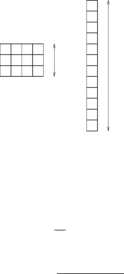
268 CHAPTER 18
state as that at time (t−∆t). The potential energies of the unsorted and sorted
states are easily computed to be
Ep(t−∆t) = 56
ρ
og∆z V (18.29)
Ere f (t−∆t) = 56
ρ
og∆z V (18.30)
EAPE(t−∆t) = 0 (18.31)
where Vis the volume of the grid cells, and
ρ
ois the density scale. The zero APE
is due to the absence of horizontal density gradients.
6 6 6 6
2
3 ∆z12
∆z* 3
∆z=
2
2
2
4
4
4
4
6
6
6
6
2 2 2 2
4 4 4 4
Figure 18.1 The initial density field for the first example. The number in each box rep-
resents the density, given in units of
ρ
o. The left panel shows the density
ρ
(x,z,t−∆t)in the unsorted fluid state, and the right panel shows the den-
sity
ρ
re f (z∗,t−∆t)in the sorted state. Note that the vertical scale ∆z∗=∆z/4
for the sorted state has been expanded for purposes of display.
18.4.1 Evolution of the unsorted state
Evolution of the unsorted density is given by the discrete equation
ρ
(x,z,t+∆t) =
ρ
(x,z,t−∆t)−2∆t
∆z[Fz(x,z,t−∆t)−Fz(x,z−∆z,t−∆t)],
(18.32)
where the vertical diffusive flux is given by
Fz(x,z,t) = −
κ δ
z
ρ
(x,z,t)
≈ −
κ
ρ
(x,z+∆z,t)−
ρ
(x,z,t)
∆z.(18.33)
EFFECTIVE DIANEUTRAL DIFFUSIVITY 269
Fz(x,z,t)is defined at the top face of the density grid cell whose center has posi-
tion (x,z). In the following, it is useful to introduce the dimensionless quantity
δ
(v)=2
κ
∆t/(∆z)2. (18.34)
This number arises from the chosen discretization of the diffusion equation. For
linear stability of the discretization,
δ
(v)<1must be maintained.
The top panel of Figure 18.2 shows the vertical diffusive flux through the cell
faces at time t−∆t, and the bottom panel shows the resulting density
ρ
(z,z,t+
∆t). Density in the middle row does not change, whereas the upper row density
increases and the lower row density decreases. The potential energy of this state
is
Ep(t+∆t) =
ρ
og∆z V (56 +8
δ
(v)). (18.35)
This increase in potential energy is a result of the raised center of mass arising
from the vertical diffusive fluxes.
δ
0
2
2
0 0 0
2 2
2 2
00
2
2
0
0
6-
4
2+ δ
3∆z
3∆z
δ
2+ 2+ 2+
δδ δ
4 4 4
6- 6- 6-
δδ
Figure 18.2 Top panel: The vertical diffusive flux Fz(x,z,t−∆t), in units of
ρ
o
κ
/∆z, pass-
ing through the faces of the unsorted density grid cells. Bottom panel: The
unsorted density field
ρ
(x,z,t+∆t), in units of
ρ
o, where the dimensionless
increment
δ
is given by
δ
=2
δ
(v)=4
κ
∆t/(∆z)2. This density field results
from the vertical convergence of the flux Fz(x,z,t−∆t).

270 CHAPTER 18
18.4.2 Evolution of the sorted state
Corresponding to the evolution of the unsorted density, there is an evolution of the
sorted density
ρ
re f (z∗,t+∆t) =
ρ
re f (z∗,t−∆t)−2∆t
∆z∗[Fz∗(z∗,t−∆t)−Fz∗(z∗−∆z∗,t−∆t)].
(18.36)
The dianeutral diffusive flux is
Fz∗(z∗,t) = −
κ
e f f (z∗,t)
δ
z∗
ρ
re f (z∗,t)
≈ −
κ
e f f (z∗,t)
ρ
re f (z∗+∆z∗,t)−
ρ
re f (z∗,t)
∆z∗!,(18.37)
where
ρ
re f (z∗,t)is the sorted state’s density. Fz∗(z∗,t)is defined at the top face of
the sorted density grid cell whose center has height z∗. Given the time tendency
for the sorted state, the flux is diagnosed through
Fz∗(z∗,t−∆t) = Fz∗(z∗−∆z∗,t−∆t)−∆z∗
2∆t[
ρ
re f (z∗,t+∆t)−
ρ
re f (z∗,t−∆t)].
(18.38)
The left panel of Figure 18.3 shows the sorted density field
ρ
re f (z∗,t+∆t), and
the second panel shows the diagnosed vertical diffusive flux Fz∗(z∗,t−∆t). The
third panel shows the vertical density gradient [
ρ
re f (z∗+∆z∗,t−∆t)−
ρ
re f (z∗,t−
∆t)]/∆z∗. The fourth panel shows the effective diffusivity
κ
e f f (z∗,t−∆t), which is
diagnosed from the relation
κ
e f f (z∗,t−∆t) = −Fz∗(z∗,t−∆t) ∆z∗
ρ
re f (z∗+∆z∗,t−∆t)−
ρ
re f (z∗,t−∆t)!.
(18.39)
The units for
κ
e f f (z∗,t−∆t)are (∆z∗)2/∆t. Hence, a value for
κ
e f f (z∗,t−∆t)of
2
δ
in Figure 18.3 indicates a dimensional value of
κ
e f f (z∗,t−∆t) = 2
δ
(∆z∗)2
∆t
=
κ
4∆t
(∆z)2
(∆z∗)2
∆t
=
κ
/4.
(18.40)
This example illustrates a problem with unstratified parts of the sorted profile. As
evident from Figures 18.1 and 18.3, the 12 sorted boxes are actually three larger
homogeneous boxes, and so the calculation should compute fluxes and diffusivi-
ties for these three boxes rather than for the 12 boxes. Figure 18.4 shows such
a combined system, where there are three boxes each of height ∆zcomprising
the sorted state. Repeating the previous calculation for this configuration recovers
the expected
κ
e f f =
κ
on the two interior interfaces. Note that there is no ad hoc
setting to zero certain values of
κ
e f f associated with unstratified portions of the
profile.
As a final note, the potential energy of the sorted state at time t+∆tis
Ere f (t+∆t) =
ρ
og∆z V (56 +16
δ
(v)), (18.41)
EFFECTIVE DIANEUTRAL DIFFUSIVITY 271
δ
2 + δ
0
0
0
0
0
0
0
0
0
δ
0
0
0
0
0
2 +
2 +
2 +
δ
δ
δ
444
4
4
4
6 -
6 -
6 -
6 -
δ
δ
δ
2
3
4
4
4
4
4
3
2
δ
δ
δ
δ
δ
δ
δ
δ
δ
δ
0
0
-2
0
0
-2
0
0
0
2δ
0
0
2δ
0
Figure 18.3 First panel (left): The sorted density field
ρ
re f (z∗,t+∆t), in units of
ρ
o. Sec-
ond panel: The vertical diffusive flux Fz∗(z∗,t−∆t), in units of
ρ
o∆z∗/(2∆t),
passing through the faces of the sorted density grid cells. Third panel: The
vertical density gradient [
ρ
re f (z∗+∆z∗,t−∆t)−
ρ
re f (z∗,t−∆t)]/∆z∗in units
of
ρ
o/∆z∗. Fourth panel: The effective diffusivity
κ
e f f (z∗,t−∆t)in units of
(∆z∗)2/∆t.
272 CHAPTER 18
z
4
- 2
- 2
δ
δ
2+
δ
δ
4
6−
2
6
0
0
0
0
κ
κ
0
0
3∆
Figure 18.4 First panel (far left): The initial density field
ρ
re f (z∗,t−∆t), consisting of the
combination of the three groups of four homogeneous cells. The values are
given in units of
ρ
o. In this recombined arrangement, ∆z∗=∆z. Second panel:
The vertical density gradient [
ρ
re f (z∗+∆z∗,t−∆t)−
ρ
re f (z∗,t−∆t)]/∆z∗, in
units of
ρ
o/∆z∗. Third panel: The density
ρ
re f (z∗,t+∆t)in units of
ρ
o. Fourth
panel: The diffusive flux Fz∗(z∗,t−∆t). Fifth panel (far right): The effective
diffusivity
κ
e f f (z∗,t−∆t).
EFFECTIVE DIANEUTRAL DIFFUSIVITY 273
which is higher than the initial potential energy as a result of the raised center of
mass. The APE remains unchanged
EAPE(t+∆t) = 0, (18.42)
as it should since there remains zero baroclinicity in the final state.
18.4.3 Caveat about weakly stratified regions
Note that in this example, the same set of boxes are perfectly homogenized at
each time step. As such, it is straightforward to combine the boxes in order to de-
rive their effective diffusivities. In general, this simple situation will not be true, and
so the effective height of the combined boxes will differ. Furthermore, most cases
of homogenization are approximate (Sections 18.2.3 and 18.2.5), which introduces
even more time dependence to the interfaces between effectively homogeneous
boxes. In order to compute an effective diffusivity, however, our algorithm needs to
evaluate all quantities at the same depth level z∗. Time dependent z∗is problem-
atical.
The current example suggestes that one possibile way to account for homoge-
nization is to count the number of nearly homogeneous boxes occuring in a par-
ticular section of the sorted column. When the first interface is reached that has
a nontrivial stratification, then the effective diffusivity computed for this interface
is multiplied by the number of trailing boxes which are homogeneous. This trick
works for the example just considered (
κ
/4×4=
κ
). However, in the example
considered in Section 18.5.2, it leads to an effective diffusivity which can be larger
than the horizontal diffusivity. Such is not possible, and so one is led to reject the
proposed patch. A clean way to proceed is to try to resolve as best as possible
the stratification within the sorted fluid state. For those regions which are simply
too weakly stratified, it must be recognized that the computed effective diffusivity
might be smaller than a more refined computation.
An alternative approach is to average the sorted density field onto the discrete
levels realized in the unsorted state. Indeed, this resolution of the sorted state is
arguably that which is relevant for diagnosing the effective diffusivity. This is the
approach taken with the MOM experiments documented in Griffies et al. (2000b).
18.5 AN EXAMPLE WITH VERTICAL AND HORIZONTAL GRADIENTS
This example considers the initial unsorted density configuration is shown in Figure
18.5. There are three rows of four boxes stacked on top of one another, and there
are both vertical and horizontal density gradients. Also shown is the corresponding
sorted state. As with the example in Section 18.4, the grid dimensions for the two
states are related through ∆z=4∆z∗, where zis the vertical coordinate for the
unsorted state, and z∗is the vertical coordinate for the sorted state. The potential
energies are
Ep(t−∆t) = 110
ρ
og∆z V (18.43)
Ere f (t−∆t) = 98
ρ
og∆z V (18.44)
EAPE(t−∆t) = 12
ρ
og∆z V, (18.45)
where Vis the volume of the boxes and
ρ
ois the density scale.
274 CHAPTER 18
=
2
4
4
6
6
6
8
8
8
10
10
12
2 4 6 8
4 6 8 10
6 8 10 12
3 ∆z12
∆z* 3
∆z
Figure 18.5 The initial density field for the horizontal and vertical diffusion examples. The
number in each box represents the density, given in units of
ρ
o. The left panel
shows the density
ρ
(x,z,t−∆t)in the unsorted fluid state, and the right panel
shows the density
ρ
re f (z∗,t−∆t)in the sorted state. Note that the vertical scale
∆z∗=∆z/4 for the sorted state has been expanded for purposes of display.
18.5.1 Vertical diffusion
Consider first just vertical diffusion acting on the unsorted state. The vertical diffu-
sivity
κ
acting on the unsorted state is assumed to be uniform and constant.
18.5.1.1 Evolution of the unsorted state
Evolution of the unsorted density is given by the discrete equation
ρ
(x,z,t+∆t) =
ρ
(x,z,t−∆t)−2∆t
∆z[Fz(x,z,t−∆t)−Fz(x,z−∆z,t−∆t)],
(18.46)
where the vertical diffusive flux is given by
Fz(x,z,t) = −
κ δ
z
ρ
(x,z,t)
≈ −
κ
ρ
(x,z+∆z,t)−
ρ
(x,z,t)
∆z.(18.47)
Fz(x,z,t)is defined at the top face of the density grid cell whose center has height
z. The top panel of Figure 18.6 shows the vertical diffusive flux through these faces
at time t−∆t, and the bottom panel shows the resulting density field
ρ
(x,z,t+
∆t). Density in the middle row does not change, whereas the upper row density
increases and the lower row density decreases. The potential energy of this state
is
Ep(t+∆t) =
ρ
og∆z V (110 +16
δ
(v)), (18.48)

EFFECTIVE DIANEUTRAL DIFFUSIVITY 275
which is higher than the initial potential energy as a result of the raised center of
mass.
z
0
2
2
0 0 0
2 2
2 2
00
2
2
0
0
6- 8- 10- 12-
8
6
4
2+ 4+ 6+ 8+
10
δδ
δ
δ
δδ δ δ
3∆z
3∆
Figure 18.6 Top panel: The vertical diffusive flux Fz(x,z,t−∆t), in units of
ρ
o
κ
/∆z,
passing through the faces of the unsorted density grid cells. Bottom panel:
The unsorted density field
ρ
(x,z,t+∆t), in units of
ρ
o, where
δ
=2
δ
(v)=
4
κ
∆t/(∆z)2. This is the density field resulting from the vertical convergence
of the flux Fz(x,z,t−∆t). The potential energy of this field is Ep(t+∆t) =
ρ
og∆z V (110 +16
δ
(v)).
18.5.1.2 Evolution of the sorted state
Corresponding to the evolution of the unsorted density, there is an evolution of the
sorted density which is given by
ρ
re f (z∗,t+∆t) =
ρ
re f (z∗,t−∆t)−2∆t
∆z∗[Fz∗(z∗,t−∆t)−Fz∗(z∗−∆z,t−∆t)].
(18.49)
The dianeutral diffusive flux is given by
Fz∗(z∗,t) = −
κ
e f f (z∗,t)
δ
z∗
ρ
re f (z∗,t)
≈ −
κ
e f f (z∗,t)
ρ
re f (z∗+∆z∗,t)−
ρ
re f (z∗,t)
∆z∗!,(18.50)
where
ρ
re f (z∗,t)is the sorted state’s density. Fz∗(z∗,t)is defined at the top face of
the sorted density grid cell whose center has height z∗. Given the time tendency
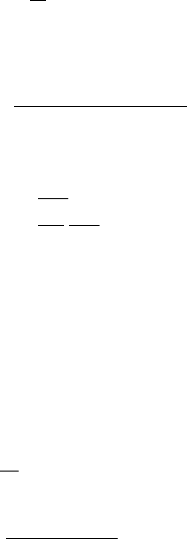
276 CHAPTER 18
for the sorted state, the flux is diagnosed through
Fz∗(z∗,t−∆t) = Fz∗(z∗−∆z∗,t−∆t)−∆z∗
2∆t[
ρ
re f (z∗,t+∆t)−
ρ
re f (z∗,t−∆t)].
(18.51)
The left panel of Figure 18.7 shows the sorted density field
ρ
re f (z∗,t+∆t), and
the second panel shows the diagnosed vertical diffusive flux Fz∗(z∗,t−∆t). The
third panel shows the vertical density gradient [
ρ
re f (z∗+∆z∗,t−∆t)−
ρ
re f (z∗,t−
∆t)]/∆z∗. Note the regions of zero stratification. The fourth panel shows the
effective diffusivity
κ
e f f (z∗,t−∆t), which is diagnosed from the relation
κ
e f f (z∗,t−∆t) = −Fz∗(z∗,t−∆t) ∆z∗
ρ
re f (z∗+∆z∗,t−∆t)−
ρ
re f (z∗,t−∆t)!.
(18.52)
The units for
κ
e f f (z∗,t−∆t)are (∆z∗)2/∆t. In addition, consistent with the discus-
sion in Section 18.4.2, the effective diffusivity for the interfaces on top of unstratified
water are multiplied by the number of unstratified boxes. A value for
κ
e f f (z∗,t−∆t)
of
δ
in Figure 18.7 indicates a dimensional value of
κ
e f f (z∗,t−∆t) =
δ
(∆z∗)2
∆t
=
κ
4∆t
(∆z)2
(∆z∗)2
∆t
=
κ
/4. (18.53)
As a final note, the potential energy of the sorted state at time t+∆tis
Ere f (t+∆t) =
ρ
og∆z V (98 +7
δ
(v)), (18.54)
which is higher than the initial potential energy as a result of the raised center of
mass. The APE is therefore given by
EAPE(t+∆t) =
ρ
og∆z V (12 +11
δ
(v)), (18.55)
which is larger than EAPE(t−∆t)given in equation (18.45).
18.5.2 Horizontal diffusion
Consider now just horizontal diffusion acting on the unsorted state. The horizontal
diffusivity Aacting on the unsorted state is assumed to be uniform and constant.
18.5.2.1 Evolution of the unsorted state
Evolution of the unsorted density is given by the discrete equation
ρ
(x,z,t+∆t) =
ρ
(x,z,t−∆t)−2∆t
∆x[Fx(x,z,t−∆t)−Fx(x−∆x,z,t−∆t)],
(18.56)
where the horizontal diffusive flux is given by
Fx(x,z,t) = −A
δ
x
ρ
(x,z,t)
≈ −A
ρ
(x+∆x,z,t)−
ρ
(x,z,t)
∆x.(18.57)
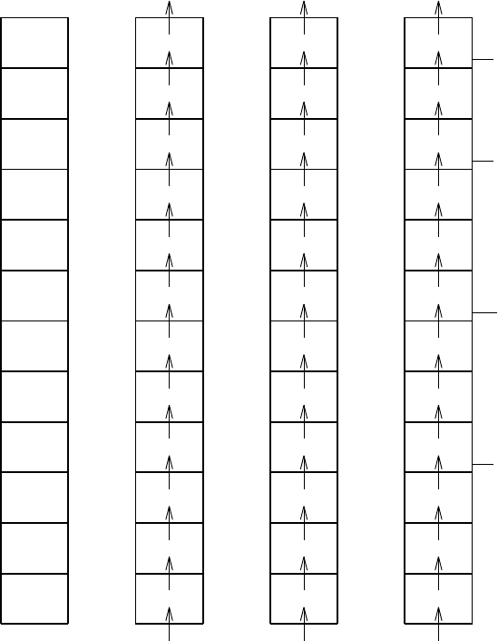
EFFECTIVE DIANEUTRAL DIFFUSIVITY 277
δ
2 + δ
4
4 + δ
6 - δ
6
6 + δ
8 - δ
8
8 +
10 - δ
10
12 - δ
δ
0
δ
2δ
δ
δ
2δ
δ
δ
2δ
δ
δ
0
0
-2
0
-2
0
0
-2
0
0
-2
0
-2
0
0
δ δ/2
0
δ
0
0
δ
0
0
δ
0
δ/2
0
2
δ
3
3δ
δ
Figure 18.7 Left panel: The sorted density field
ρ
re f (z∗,t+∆t), in units of
ρ
o. Second
panel: The vertical diffusive flux Fz∗(z∗,t−∆t), in units of
ρ
o∆z∗/∆t, pass-
ing through the faces of the sorted density grid cells. Third panel: The ver-
tical density gradient [
ρ
re f (z∗+∆z∗,t−∆t)−
ρ
re f (z∗,t−∆t)]/∆z∗in units
of
ρ
o/∆z∗. Fourth panel: The effective diffusivity
κ
e f f (z∗,t−∆t)in units of
(∆z∗)2/∆t. The four
κ
e f f values which are on top of unstratified portions of
the
ρ
re f (z∗,t−∆t)profile have been multiplied by the number of unstratified
boxes which lie directly beneath it.
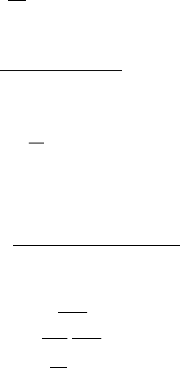
278 CHAPTER 18
Fx(x,z,t)is defined at the east face of the density grid cell whose center has posi-
tion (x,z). The top panel of Figure 18.8 shows the horizontal diffusive flux through
these faces at time t−∆t, and the bottom panel shows the resulting density field
ρ
(x,z,t+∆t). The potential energy of this state is the same as the initial potential
energy, since the horizontal fluxes are parallel to the geopotential
Ep(t+∆t) = Ep(t−∆t) = 110
ρ
og∆z V. (18.58)
18.5.2.2 Evolution of the sorted state
Corresponding to the evolution of the unsorted density, there is an evolution of the
sorted density which is given by
ρ
re f (z∗,t+∆t) =
ρ
re f (z∗,t−∆t)−2∆t
∆z∗[Fz∗(z∗,t−∆t)−Fz∗(z∗−∆z,t−∆t)].
(18.59)
The dianeutral diffusive flux is given by
Fz∗(z∗,t) = −
κ
e f f (z∗,t)
δ
z∗
ρ
re f (z∗,t)
≈ −
κ
e f f (z∗,t)
ρ
re f (z∗+∆z∗,t)−
ρ
re f (z∗,t)
∆z∗!,(18.60)
where
ρ
re f (z∗,t)is the sorted state’s density. Fz∗(z∗,t)is defined at the top face of
the sorted density grid cell whose center has height z∗. Given the time tendency
for the sorted state, the flux is diagnosed through
Fz∗(z∗,t−∆t) = Fz∗(z∗−∆z∗,t−∆t)−∆z∗
2∆t[
ρ
re f (z∗,t+∆t)−
ρ
re f (z∗,t−∆t)].
(18.61)
The left panel of Figure 18.5.2.2 shows the sorted density field
ρ
re f (z∗,t+∆t), and
the second panel shows the diagnosed vertical diffusive flux Fz∗(z∗,t−∆t). The
third panel shows the vertical density gradient [
ρ
re f (z∗+∆z∗,t−∆t)−
ρ
re f (z∗,t−
∆t)]/∆z∗. Note the regions of zero stratification. The fourth panel shows the
effective diffusivity
κ
e f f (z∗,t−∆t), which is diagnosed from the relation
κ
e f f (z∗,t−∆t) = −Fz∗(z∗,t−∆t) ∆z∗
ρ
re f (z∗+∆z∗,t−∆t)−
ρ
re f (z∗,t−∆t)!.
(18.62)
The units for
κ
e f f (z∗,t−∆t)are (∆z∗)2/∆t. For example, a value for
κ
e f f (z∗,t−
∆t)of 3
δ
/2in Figure 18.5.2.2 indicates a dimensional value of
κ
e f f (z∗,t−∆t) = (3
δ
/2)(∆z∗)2
∆t
=6A∆t
(∆x)2
(∆z∗)2
∆t
=6A∆z∗
∆x2
.
(18.63)
For the special case of ∆x=∆z=4∆z∗, the effective diffusivity is 3A/8. Note
that if the patch proposed in Section 18.4.3 is used, then the 3
δ
/2diffusivity would
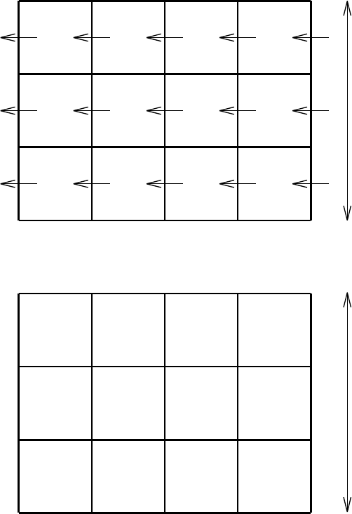
EFFECTIVE DIANEUTRAL DIFFUSIVITY 279
δ
3∆z
3∆z
0
0
0 δ
δ
δ
δ
δ
δ
δ
δ
δ
0
0
0
68
2+ δ4 6 8 -
10 -
12 -
810
6 +
4 + δ
δ
δ
δ
Figure 18.8 Top panel: The horizontal diffusive flux Fx(x,z,t−∆t), in units of
ρ
oA/∆x,
passing through the faces of the unsorted density grid cells. Bottom panel:
The unsorted density field
ρ
(x,z,t+∆t), in units of
ρ
o, where
δ
=2
δ
(h)=
4A∆t/(∆x)2. This is the density field resulting from the vertical convergence
of the flux Fx(x,z,t−∆t). The potential energy of this field is Ep(t+∆t) =
110
ρ
og∆z V.
280 CHAPTER 18
become 9
δ
/2, leading to the possibility for an effective diffusivity of 9A/8, which
is impossible.
As a final note, the potential energy of the sorted state at time t+∆tis
Ere f (t+∆t) =
ρ
og∆z V (98 +19
δ
(h)/2), (18.64)
which is higher than the initial potential energy as a result of the raised center of
mass. The APE is given by
EAPE(t+∆t) =
ρ
og∆z V (12 −19
δ
(h)/2), (18.65)
which is smaller than EAPE(t−∆t)given in equation (18.45).
δ
2 + δ
4
4 + δ
6
8 - δ
8
10 - δ
10
12 - δ0
δ
2δ
δ
δ
δ
δ
0
0
-2
0
-2
0
0
-2
0
0
-2
0
-2
0
0
δ δ/2
0
δ
0
0
0
0
δ
0
δ/2
0
6
8
δ2
δ
2
3
δ2
δ2
2
3δ/2
6 +
Figure 18.9 First panel (far left): The sorted density field
ρ
re f (z∗,t+∆t)in units of
ρ
o. Sec-
ond panel: The vertical diffusive flux Fz∗(z∗,t−∆t), in units of
ρ
o∆z∗/∆t,
passing through the faces of the sorted density grid cells. Third panel: The
vertical density gradient [
ρ
re f (z∗+∆z∗,t−∆t)−
ρ
re f (z∗,t−∆t)]/∆z∗in units
of
ρ
o/∆z∗. Fourth panel: The effective diffusivity
κ
e f f (z∗,t−∆t)in units of
(∆z∗)2/∆t. The four
κ
e f f values which are on top of unstratified portions of
the
ρ
re f (z∗,t−∆t)profile have been multiplied by the number of unstratified
boxes which lie directly beneath it.
Chapter Nineteen
Diagnosing the dianeutral velocity component
The purpose of this chapter is to detail the diagnostic method used in mom4p1
to compute the dianeutral velocity component. This diagnostic provides a direct
measure of the water being transported across neutral directions.
19.1 DIANEUTRAL VELOCITY COMPONENT
The dia-surface velocity component w(s)is defined by
w(s)=z,sds
dt, (19.1)
where s=s(x,y,z,t)is an arbitrary smooth surface in the ocean interior. The utility
of a dia-surface velocity component is predicated on assuming that the surfaces
of constant snever become vertical, so that the mapping between sand depth
remains well defined. We are particularly interested in computing s,zw(s)where
sis a locally referenced potential density surface, symbolized here by
γ
. In this
case,
γ
,zw(
γ
)=
γ
,
θ
d
θ
dt+
γ
,S
dS
dt, (19.2)
where w(
γ
)is known as the dianeutral velocity component,Sis the salinity,
θ
is
the potential temperature (or conservative temperature),
γ
,
θ
=∂
γ
/∂
θ
, and
γ
,S=
∂
γ
/∂S. Note that the pressure term
ρ
,pdp/dt, which appears in the material time
derivative for in situ density
ρ
, is dropped here since we are focused on the locally
referenced potential density
γ
.
In the following sections, we consider two ways to compute
γ
,zw(
γ
). The meth-
ods differ by how they evaluate the material time derivative. They yield identical
results in the continuum, but differ on the lattice due to numerical truncation errors.
19.2 KINEMATIC METHOD
Expanding the material time derivatives in equation (19.2) leads to
γ
,zw(
γ
)=
γ
,
θ
(∂t+u·∇z+w∂z)
θ
+
γ
,S(∂t+u·∇z+w∂z)S. (19.3)
Dividing by
γ
,z=
γ
,
θθ
,z+
γ
,SS,z(19.4)
leads to
w(
γ
)=w+
γ
,
θ
(∂t+u·∇z)
θ
+
γ
,S(∂t+u· ∇z)S
γ
,z
=w−S·u+
γ
,
θθ
,t+
γ
,SS,t
γ
,z
(19.5)
282 CHAPTER 19
where
S=−
γ
,
θ
∇z
θ
+
γ
,S∇zS
γ
,
θθ
,z+
γ
,SS,z(19.6)
is the slope of the neutral directions with respect to constant geopotential surfaces.
Each term on the right hand side of equation (19.5) can be diagnosed, thus pro-
viding an approximation to w(
γ
). We term this a kinematic method, since it only
depends on the geometric properties of the flow relative to the temperature and
salinity surfaces, as well as the time tendency of the active tracers. Note that in
equation (19.3), we assumed the model’s vertical coordinate to be geopotential.
However, any of the vertical coordinates in mom4p1 may be used to expand the
material time derivative, so that in general
w(
γ
)=w(s)−S·u+
γ
,
θθ
,t+
γ
,SS,t
γ
,z(19.7)
where sis the surface of constant general vertical coordinate (e.g., s=pfor a
pressure coordinate version of mom4p1), the time tendency operator ∂tis taken
on surfaces of constant s, and
S=−
γ
,
θ
∇s
θ
+
γ
,S∇sS
γ
,
θθ
,z+
γ
,SS,z(19.8)
is the slope of the neutral directions with respect to the constant ssurfaces.
An application of the kinematic method for computing w(
γ
)includes a determi-
nation of the dianeutral transport across a particular potential density surface. In
this case, w(
γ
)is first computed on the model’s vertical grid, then interpolated to
a chosen potential density surface. As shown in Section 19.3, the levels of such
transport are directly related to physical processes, such as SGS diffusion and
advection, as well as spurious sources of numerical mixing.
19.3 THERMODYNAMIC METHOD
An alternative approach to computing
γ
,zw(
γ
)can be derived by returning to the
definition given by equation (19.2). Rather than expanding the material time deriva-
tive, we introduce the subgrid scale (SGS) fluxes Jfor temperature and salinity
ρ
d
θ
dt=−∇ ·J
θ
(19.9)
ρ
dS
dt=−∇ ·JS, (19.10)
where
ρ
is the in situ density, and
J=
ρ
F(19.11)
consists of SGS fluxes arising from lateral and dia-surface advective and diffusive
processes.∗In writing the material evolution as in equations (19.9) and (19.10),
we have ignored non-local transport, as in the KPP scheme (Large et al., 1994),
∗For depth-based vertical coordinates in mom4p1, which integrate the Boussinesq equations, the
factors of
ρ
in equations (19.9)-(19.11) are replaced by the constant reference density
ρ
o.
DIAGNOSING THE DIANEUTRAL VELOCITY COMPONENT 283
as well as heat and salt sources. These assumptions are typically appropriate in
the ocean interior.
Diagnosis of flux divergences ∇ · J
θ
and ∇·JSis required to realize this method
for computing
γ
,zw(
γ
), in which case
ρ γ
,zw(
γ
)=−
γ
,
θ
∇ · J
θ
−
γ
,S∇· JS. (19.12)
Defining a SGS flux for locally referenced potential density
J
γ
=
γ
,
θ
J
θ
+
γ
,SJS(19.13)
allows us to write equation (19.12) as
ρ γ
,zw(
γ
)=−∇ ·J
γ
+J
θ
·∇
γ
,
θ
+JS·∇
γ
,S. (19.14)
The non-flux terms on the right hand side of equation (19.14) arise from cabbel-
ing, thermobaricity, and halobaricity (McDougall, 1987). Note that neutral diffu-
sive fluxes for temperature and salinity do not contribute to J
γ
(Griffies et al.,
1998). However, other lateral SGS processes, such as eddy advection (Gent and
McWilliams, 1990; Gent et al., 1995) or skew diffusion (Griffies, 1998), remain a
nontrivial contributor to J
γ
.
We term the method (19.12), or the equivalent (19.14), the thermodynamic
method for computing the dianeutral velocity component. This terminology is moti-
vated by noting that the method requires information about the SGS heat and salt
fluxes. The thermodynamic method is general, though less straigtforward than the
kinematic method. Difficulties arise in practice since we generally have multiple
physical processes contributing to the flux J, and these individual fluxes are often
not saved in the process of updating an ocean model. Furthermore, the vertical
processes are generally handled implicitly in time, whereas lateral processes are
explicit. With a number of approximations, however, we can reduce this complexity.
First, note that the source terms in equation (19.14) from cabbeling, thermo-
baricity, and halobaricity disappear for a linear equation of state (EOS), in which
case
ρ γ
,zw(
γ
)=−∇ ·J
γ
linear EOS. (19.15)
SGS advection is a nontrivial component in ocean climate models that do not ex-
plicitly represent mesoscale eddies. Nonetheless, consider the case when we
ignore SGS advection, such as may be appropriate in fine resolution eddying mod-
els. In this case, we are left just with vertical diffusion
ρ γ
,zw(
γ
)=−∂zJ
γ
zlinear EOS and no eddy advection, (19.16)
with the vertical flux
ρ
−1J
γ
z=−
γ
,
θκθθ
,z−
γ
,S
κ
SS,z(19.17)
where
κθ
and
κ
Sare vertical diffusivities for temperature and salinity. Finally, equat-
ing these two diffusivities, and making the Boussinesq approximation, leads to
γ
,zw(
γ
)=∂z(
κ γ
,z)linear EOS, no eddy advection, and Boussinesq. (19.18)

284 CHAPTER 19
19.4 SOME COMMENTS ON IDEALIZED CASES AND SCALING
The thermodynamic method is simplest with a linear EOS, Boussinesq simulation
with no SGS advection, no SGS nonlocal transport, and no tracer sources. Such is
often the case for idealized eddying geopotential coordinate ocean models, where
tracers are acted on only by vertical diffusion and three dimensional numerical
advection. In this case, the two forms for the dianeutral velocity component are
given by
γ
,zw(
γ
)=(∂t+u·∇z+w∂z)
γ
=∂z(
κ γ
,z).(19.19)
Disagreements between the two expressions arise in practice from numerical trun-
cation errors. In particular, spurious diffusion from numerical advection can cause
the effective diffusivity to differ from the model’s imposed diffusivity
κ
(Griffies et al.,
2000b). Assuming the truncation errors for the kinematic method are indepen-
dent of advection scheme, the disagreement between the kinematic and thermo-
dynamic methods can be used as an indirect measure of the level of spurious
mixing active in a simulation.
Even though the relation (19.18) is an approximation, it can be used to garner
a scaling behaviour for the effective diffusivity, given a value for the vertical grid
spacing and the dianeutral velocity. That is,
κ
∼∆z w(
γ
)(19.20)
For example, with w(
γ
)diagnosed from the kinematic method to have a value
w(
γ
)≈10−6m s−1, a vertical grid spacing of ∆z=10m corresponds to an ef-
fective diffusivity on the order of
κ
≈10−5m2s−1.
19.5 COMMENTS ON NUMERICAL DISCRETIZATION
Only the kinematic method is discretized in mom4p1. The fields needed to com-
pute
w(
γ
)=w(s)−S·u+
γ
,
θθ
,t+
γ
,SS,t
γ
,z(19.21)
are generally located on different parts of a grid cell. We are, however, not too con-
cerned about exact averaging to bring all fields to the same point. The diagnostic
calculation is thus not as exact in a numerical sense as the analogous calculations
employed by the neutral physics module. Hence, the code employs a minimal set
of averaging operations. Note, however, that the vertical neutral density deriva-
tive,
γ
,z, is smoothed in the vertical. As with the neutral physics calculation, such
smoothing has been found necessary to ensure reasonably smooth results for the
slope vector, and hence for the resulting dianeutral velocity component.

Chapter Twenty
Diagnosing the contributions to sea level evolution
The purpose of this chapter is to discuss the diagnostic in mom4p1 that diagnoses
the contribution to sea level time tendencies due to changing currents, surface
water forcing, and the steric effect. The discussion follows that given in Section
3.4 of Griffies (2004).
20.1 MASS BUDGET FOR A COLUMN OF WATER
Consider a column of mass conserving fluid extending from the ocean bottom at
z=−Hto the ocean surface at z=
η
. The total mass of fluid, M, inside the
column is given by
M=ZdA
η
Z
−H
ρ
dz, (20.1)
where
ρ
is the mass density (the in situ density) of seawater, and
dA=dxdy(20.2)
is the time independent horizontal area of the column. For a hydrostatic fluid, in
which
p,z=−
ρ
g, (20.3)
the total mass per area in a column of seawater is given by the difference in pres-
sure at the ocean bottom and the pressure applied at the ocean surface
g
η
Z
−H
ρ
dz=pb−pa. (20.4)
That is, the total mass in the column is
M=g−1ZdA(pb−pa). (20.5)
In Section 7.4, we developed a budget for the mass of fluid in a column. Repeat-
ing some of those steps here for completeness, we note that the time tendency of
mass within a fluid column
M,t=ZdA∂t
η
Z
−H
dz
ρ
(20.6)
arises when a net amount of seawater mass passes across boundaries of the fluid
column, or when there are sources within the column. We generally assume in cli-
mate modelling that no seawater mass enters through the ocean bottom. Hence,
286 CHAPTER 20
the only means of affecting seawater mass in the fluid column are through mass
fluxes crossing the ocean free surface, from the convergence of mass into the
column from ocean currents, and from sources within the column. These consid-
erations lead to the time tendency
M,t=ZdA
qw
ρ
w− ∇ ·
η
Z
−H
dz
ρ
u
+ZdA
η
Z
−H
ρ
dzS(M). (20.7)
The surface term
qw
ρ
wdA=ˆn(
η
)·ˆnw(P−E+R)
ρ
wdA(
η
)(20.8)
represents the mass flux of fresh water (mass per unit time per unit horizontal
area) crossing the free surface, where
ρ
wis the in situ density of the fresh water.
Equivalently, qw
ρ
wdAis the momentum density of the fresh water in the direction
normal to the ocean surface. The first volume term arises from the convergence
of mass into the column from within the ocean fluid, and the second volume term
arises from mass sources.
Equating the time tendencies given by equations (20.6) and (20.7) leads to a
mass balance within each vertical column of fluid
∂t
η
Z
−H
dz
ρ
+∇·
η
Z
−H
dz
ρ
u
=qw
ρ
w+
η
Z
−H
dz
ρ
S(M). (20.9)
We can make this equation a bit more succinct by introducing the notation for
density weighted vertically integrated horizontal velocity
U
ρ
=
η
Z
−H
dz
ρ
u, (20.10)
which then leads to the following expression for mass conservation of a fluid col-
umn
∂t
η
Z
−H
dz
ρ
+∇ · U
ρ
=qw
ρ
w+
η
Z
−H
dz
ρ
S(M). (20.11)
In ocean climate modelling, it is common to assume a Boussinesq fluid, in which
case the seawater parcels conserve volume rather than mass. In this case, the
budget for volume within a fluid column takes the form
∂t
η
Z
−H
dz
+∇· U=qw+
η
Z
−H
dzS(V)(20.12)
where density factors appearing in the mass conservation equation (20.11) have
been dropped, and
U=
η
Z
−H
udz(20.13)
is the vertically integrated horizontal velocity.
DIAGNOSING THE CONTRIBUTIONS TO SEA LEVEL EVOLUTION 287
20.2 EVOLUTION OF SEA LEVEL
The previous discussion provides integral budgets for a column of seawater ex-
tending from the surface to the bottom. For many purposes, one may desire an
evolution equation for the surface height or sea level. The purpose of this section
is to derive relations that isolate the surface height and identify various physical
processes affecting this height.
For this purpose, it will be useful to introduce the vertically averaged density
ρ
z=1
H+
η
η
Z
−H
dz
ρ
. (20.14)
This density can be readily computed within the prognostic model, or as a post-
processing step assuming knowledge of the grid and in situ density. Introducing
this density in the column mass budget (20.11) leads to
ρ
z
η
,t=−∇ · U
ρ
+
ρ
wqw+
η
Z
−H
dz
ρ
S(M)−D∂t
ρ
z, (20.15)
where
D=H+
η
(20.16)
is the total thickness of the fluid column from the sea surface to the ocean bottom.
Dividing equation (20.15) by the vertically averaged density
ρ
zyields the surface
height equation for a mass conserving fluid
η
nonBouss
,t=−1
ρ
z∇· U
ρ
| {z }
dynamics
+
ρ
w
ρ
zqw
|{z }
water forcing
+1
ρ
z
η
Z
−H
dz
ρ
S(M)
| {z }
source
−D∂tln
ρ
z.
| {z }
steric
(20.17)
The analogous result for the volume conserving Boussinesq fluid follows from
equation (20.12), and is given by
η
Bouss
,t=−∇ ·U
|{z }
dynamics
+qw
|{z}
water forcing
+
η
Z
−H
dzS(V).
| {z }
source
(20.18)
The dynamical, surface forcing, and source terms appearing in the two sur-
face height equations (20.17) and (20.18) are directly analogous for both the non-
Bousinesq and Boussinesq fluids. That is, the convergence arises from changes
across a column in the vertically integrated fluid column motion (i.e., the “dynam-
ics”). In a non-Boussinesq fluid, the convergence is also affected by variations in
density, whereas no such effects are present in the Boussinesq fluid. The fresh
water term arises from surface boundary forcing in both the Boussinesq and non-
Boussinesq fluids, and the source term arises from mass or volume sources. The
term −D∂tln
ρ
zappearing in the non-Boussinesq surface height equation repre-
sents a fundamentally new process that changes the ocean surface height when
288 CHAPTER 20
the vertically averaged density changes. For example, if the vertically averaged
density decreases, the surface height increases, and vice versa. This process
is commonly called the steric effect. It is an important contributor to sea level
in the real ocean, and is of particular interest given the observed increases in
ocean temperature arising from anthropogenic climate change. Unfortunately, the
steric effect is absent from the Boussinesq fluid’s prognostic surface height equa-
tion (20.18). As discussed in Section 20.3, we propose approximate methods to
diagnostically compute the steric effect in Boussinesq models.
20.3 DIAGNOSING TERMS CONTRIBUTING TO THE SURFACE HEIGHT
In summary, the previous derivations have led to a surface height evolution equa-
tion for a mass conserving fluid that can be partitioned into four terms
η
nonBouss
,t=−1
ρ
z∇ · U
ρ
| {z }
dynamics
+
ρ
w
ρ
zqw
|{z }
water forcing
+1
ρ
z
η
Z
−H
dz
ρ
S(M)
|{z }
source
−D∂tln
ρ
z
| {z }
steric
.
(20.19)
Each term on the right hand side is a time tendency that contributes to the evolution
of the ocean surface height. For diagnostic purposes, we split the surface height
into the non-steric and steric terms
η
nonBouss =
η
nonsteric +
η
steric, (20.20)
where the surface heights are defined according to their time tendencies
η
nonsteric
,t=−1
ρ
z∇· U
ρ
+
ρ
w
ρ
zqw+1
ρ
z
η
Z
−H
dz
ρ
S(M)(20.21)
η
steric
,t=−D∂tln
ρ
z. (20.22)
We diagnostically time step each of these two surface heights in order to monitor
the instantaneous contributions to the full surface height arising from the physically
distinct processes.
We next consider the details of how to diagnose these terms within a non-
Boussinesq mass conserving version of mom4p1, using a pressure based ver-
tical coordinate, as well as a Boussinesq version of mom4p1 using a depth based
vertical coordinate. This formulation also provides guidance for diagnosing these
terms from commonly saved model output.
20.3.1 Pressure based vertical coordinates
As the pressure based version of mom4p1 integrates the mass conserving non-
Boussinesq equations, each term on the right hand side of equation (20.19) can
be diagnosed in a straightforward manner. The result of the diagnostic calcula-
tion for
η
nonBouss will be, to within numerical truncation error, the same as the
model’s prognostic calculation, which computes the surface height after having
time stepped the bottom pressure (see Section 7.3.4). Verifying that this is realized
in the model is a good way to check both the theory and the model formulation.

DIAGNOSING THE CONTRIBUTIONS TO SEA LEVEL EVOLUTION 289
20.3.2 Depth based vertical coordinates
For a depth based version of mom4p1, the surface height is determined from a dis-
crete form of equation (20.18), which omits steric effects. However, it is possible to
diagnose the terms appearing on the right hand side of the non-Boussinesq sur-
face height equation (20.19), and in particular to approximate the non-Boussinesq
surface height. To do so requires some approximations, which we list here.
•For purposes of performing the vertical integrals to compute the depth aver-
aged density
ρ
z, as well as the density weighted horizontal velocity U
ρ
, we
assume the currents, surface height, and density computed in the Boussi-
nesq model are reasonably close to those computed in a non-Boussinesq
model. This approximation is motivated by the results from a careful com-
parison of non-Boussinesq effects in a steady state coarse resolution model
by Losch et al. (2004). The approximation breaks down when (a) currents
are ageostrophic as near boundaries and the equator, (b) flows are strongly
nonlinear, as in eddying simulations. Nonetheless, for many purposes, es-
pecially for large scale patterns, the approximation remains sufficiently accu-
rate. Hence, it is possible to again diagnose the tendency terms appearing
on the right hand side of equation (20.19) as in the non-Boussinesq model.
•To further approximate the calculation, we employ the constant Boussinesq
density
ρ
owhen computing the dynamical contribution, and drop the density
ratio when computing the water forcing term and source term. Hence, the
only place than in situ density is maintained is for computation of the steric
term.
In summary, we propose the approximation
η
nonBouss ≈
η
Bouss +
η
steric, (20.23)
where
η
Bouss is the prognostic surface height computed by the Boussinesq model,
η
Bouss ≈
η
nonsteric (20.24)
and
η
steric is the steric sea level diagnosed in the Boussinesq model, as described
above.

Chapter Twenty One
Balancing the hydrological cycle in ocean-ice models
The purpose of this chapter is to discuss issues of how to balance the hydrological
cycle in ocean-ice simulations using mom4p1 and the FMS coupler. In particular,
we detail how the liquid water flux transferred between sea ice and liquid ocean is
diagnosed in mom4p1, given the salt mass flux transferred between the media.
21.1 TRANSFER OF WATER BETWEEN SEA ICE AND OCEAN
As sea ice forms, water is extracted from the liquid ocean and passed to the solid
sea ice. Additionally, there is generally a nonzero salt mass transferred from ocean
to ice, thus producing a nonzero salinity for sea ice. Conversely, as sea ice melts,
liquid water and salt are added to the ocean.
The GFDL Sea Ice Simulator (SIS) generally simulates sea ice with a nonzero
salt content. For example, in the coupled climate model simulations discussed by
Delworth et al. (2006), sea ice is assumed to have a salinity
S ice =kg salt in sea ice
kg sea ice (21.1)
of S ice =0.005 (five parts per thousand).
21.2 BALANCING THE HYDROLOGICAL CYCLE
When running ocean-ice simulations, we are not explicitly representing land pro-
cesses, such as rivers, catchment areas, snow accumulation, etc. However, to
reduce model drift, it is important to balance the hydrological cycle in ocean-ice
models. We thus need to prescribe some form of global normalization to the
precipitation minus evaporation plus river runoff. The result of the normalization
should be a global integrated zero net water input to the ocean-ice system over a
chosen time scale.
How often the normalization is done is a matter of choice. In mom4p1, we
choose to do so at each model time step, so that there is always a zero net input
of water to the ocean-ice system. Others choose to normalize over an annual
cycle, in which case the net imbalance over an annual cycle is used to alter the
subsequent year’s water budget in an attempt to damp the annual water imbalance.
Note that the annual budget approach may be inappropriate with interannually
varying precipitation forcing.
When running ocean-ice coupled models, it is incorrect to include the water
transport between the ocean and ice models when aiming to balance the hydro-
logical cycle. The reason is that it is the sum of the water in the ocean plus ice that
292 CHAPTER 21
should be balanced when running ocean-ice models, not the water in any one sub-
component. As an extreme example to illustrate the issue, consider an ocean-ice
model with zero initial sea ice. As the ocean-ice model spins up, there should be a
net accumulation of water in the growing sea ice, and thus a net loss of water from
the ocean. The total water contained in the ocean plus ice system is constant,
but there is an exchange of water between the subcomponents. This exchange
should not be part of the normalization used to balance the hydrological cycle in
ocean-ice models.
21.3 WATER MASS FLUX FROM SALT MASS FLUX
Balancing the hydrological cycle in an ocean-ice model run with the FMS coupler
requires an indirect method. The reason is that melt water from the ice model is
added to the precipitation field prior to being added to the ocean model. So prior
to balancing the water fluxes, we must remove the ice melt from the precipitation.
The namelist option for performing this normalization is
zero net water coupler
found in the module
mom4p1/ocean core/ocean sbc mod.
An alternative namelist option is
zero net water couple restore
which balances the water due to precipitation minus evaporation plus runoff plus
restoring flux water. Note that in MOM4p0, ice melt was not removed from precip-
itation prior to computing the water normalization using zero net water coupler.
This bug compromised the integrity of the ocean-ice models run with MOM4p0
which used the option zero net water coupler.
To obtain the water mass flux between sea ice and ocean, we could consider two
approaches. First, we could alter the FMS sea ice code so that it carries explicit in-
formation about the water flux in question. This approach requires modifying code
that lives outside of mom4p1, and so is not desirable from a mom4-centred per-
spective. Alternatively, we can make use of the salt mass flux passed between the
ocean and sea ice. This approach is limitated to cases where the ice is assumed
to have a uniform bulk salinity, as presently assumed in the GFDL sea ice model.
In mom4p1, we have access to the following salt flux
salt flux to ice =Sice
ρ
sea ice Tice melt
∆t. (21.2)
In this equation,
ρ
sea ice is the density of sea ice, taken as
ρ
sea ice =905 kgm−3
in the GFDL ice model, and Tice melt/∆tis the thickness (in meters) of ice that
melts over the time step (in seconds) of the ice model. By convention, this salt
flux is positive when there is growth in sea ice, thus representing a passage of salt
from the liquid ocean into the sea ice. Correspondingly, this flux is positive when
there is a mass flux of water to the sea ice. Since we are here working from an
ocean perspective, we prefer to measure the flux of salt entering the ocean from
the melting sea ice
salt flux to ocean =−salt flux to ice. (21.3)
BALANCING THE HYDROLOGICAL CYCLE IN OCEAN-ICE MODELS 293
Dividing the salt flux by the salinity of sea ice yields the mass flux of water that
melts (i.e., mass flux of water transferred from sea ice to the ocean)
mass melt =salt flux to ocean
S ice
=kg ice melt
area sea ice ×Tice melt Tice melt
∆t
=kg ice melt
area sea ice ×∆t.
(21.4)
This mass of melting sea ice represents a gain of liquid water for the ocean.
Chapter Twenty Two
Gyre and overturning contributions to tracer transport
The purpose of this chapter is to discuss the diagnostic in mom4p1 that computes
the contribution to advective tracer transport in the j-direction (generalized merid-
ional) associated with gyre and overturning components of the flow. Bryan and
Lewis (1979) were amongst the first to make use of this diagnostic, and Peixoto
and Oort (1992) (page 342) describe the decomposition in more detail. The gyre
component has traditionally been associated with wind driven processes, and
overturning associated with thermohaline processes. However, this physical as-
sociation is not clean, as it is generally not possible to split the transport into two
distinct physical processes. For example, removing wind forcing does not nec-
essarily mean the gyre contribution is zero. Nonetheless, this decomposition is
commonly performed, and such has provided some physical insight into the flow
characteristics. It is for this reason that mom4p1 provides a subroutine inside
ocean tracer advect.F90 to perform this decomposition.
22.1 FORMULATION
The meridional advective transport of a tracer within a particular ocean basin is
given by the integral
H(y,t) =
x2
Z
x1
dx
η
Z
−H
dz
ρ
C v, (22.1)
where vis the meridional velocity component,
ρ
is the in situ density, Cis the tracer
concentration, z=−H(x,y)is the ocean bottom, z=
η
(x,y,t)is the ocean sur-
face, and x1and x2are the longitudinal boundaries of the basin or global ocean.
With the generalized horizontal coordinates in mom4p1, the coordinate yis as-
sumed to be aligned with the jgrid lines. For the purposes of this diagnostic, we
do not perform a rotation of the flow to the geographical longitude and latitude.
For the tripolar grid commonly used for global modeling with mom4p1, generalized
zonal integrals along i-lines yield j-transport, and this is sufficient for most diag-
nostic purposes. Note the term north will continue to be used, with this generally
denoting the j-direction, which corresponds to the geographical north when j-lines
are parallel to longitudes.
In mom4p1, the density and thickness weighted advective velocity component
V=v
ρ
dz(22.2)
is computed and held in the array vhrho nt, where
ρ
reduces to the constant
Boussinesq density
ρ
ofor the Boussinesq version of mom4p1, but it remains the
in situ density for the nonBoussinesq version. The product dxVmeasures the

296 CHAPTER 22
mass per time of seawater leaving the north face of the grid cell, with dxVCthus
measuring the mass per time of tracer leaving the north face. We now consider the
following decomposition of this transport by defining the zonal average transport
and zonal average tracer concentration as follows
[V] = ∑idxV
∑idx(22.3)
[C] = ∑idx C
∑idx, (22.4)
along with the deviations from zonal average
V= [V] + V∗(22.5)
C= [C] + C∗. (22.6)
The discrete i-sum extends over the basin or global domain of interest, so that
∑idxVis the total meridional transport of seawater at this zonal band at a partic-
ular k-level. The resulting meridional tracer transport becomes
H(y,t) = ∑
i∑
k
dxVC(22.7)
=∑
i∑
k
dx([V] [C] + V∗C∗), (22.8)
where the ksum extends over the depth of a column.
We identify three components in the code:
merid flux advect =∑
i∑
k
dxVC(22.9)
merid flux over =∑
i∑
k
dx[V] [C](22.10)
merid flux gyre =∑
i∑
k
dxV∗C∗. (22.11)
Note that
merid flux gyre =merid flux advect −merid flux over. (22.12)
This identity follows very simply when the advective flux takes on the simple form
of either first order upwind or second order centered differences. It becomes
more involved when considering higher order, or flux limited, advection schemes.
Nonetheless, we use this as a defintion of the gyre component, so that the advec-
tive flux is built from the advection scheme used in the model.
22.2 ENABLING THE DIAGNOSTIC
The following is necessary to enable this diagnostic.
•Set the ocean tracer advect nml logical
compute gyre overturn diagnose =.true.
This logical is introduced since a number of global arrays must be defined,
and it is simplest to determine the need for these arrays by setting a single
logical.
GYRE AND OVERTURNING CONTRIBUTIONS TO TRACER TRANSPORT 297
•Set any of the following within the diagnostic table:
“tracer00 merid flux advect 00basin00
“tracer00 merid flux over 00basin00
“tracer00 merid flux gyre 00basin00
where “tracer” is the mom4p1 shortname for the tracer (e.g., “temp” or “salt”),
and “basin” is one of the names “global”, “southern”,“atlantic”, “pacific”, “arc-
tic”, or “indian”.
•To get the transport diagnostic partitioned into basins in the World Ocean, it
is necessary to read in a netCDF basin mask. A sample mask is provided
with the OM3-CORE test case discussed in Chapter 32. The logical to read
in this mask is
read basin mask =.true.
The convention is that the basins are defined by the following values in the
mask:
Southern =1.0
Atlantic =2.0
Pacific =3.0
Arctic =4.0
Indian =5.0.
PART 5
Test Cases
The purpose of this part of the manual is to introduce the mom4p1 test cases.
Test cases are offered as a means of exploring various numerical and physical
options, thus allowing the user to verify that the code is performing in a manner
consistent with that at GFDL. This form of verification is critical as one adopts the
code for his or her particular research purposes. The test cases also provide a
sense for some of the options available in in the code, though by no means are all
options exercised in the test cases.
REGRESSION TESTING FOR COMPUTATIONAL INTEGRITY
Output from the test cases provided with the mom4p1 distribution is based on
short integrations that verify the computational integrity of a simulation. The asso-
ciated runscripts are provided that allow the user to rerun the regressions. These
regression test suites (RTS) aim to verify that the following identities hold, with
precision maintained to all computational bits:
•Stopping and then restarting the integration will not change answers. That
is, we insist on the identity
X day integration =X/2 day integration +X/2 day integration. (22.13)
This test verifies that all the relevant fields are properly stored in the restart
files, and that no spurious reinitialization step is performed during the begin-
ning of the second leg.
•Changing the number of computer processors will not change the answers.
This test examines whether the code is properly written for parallel machines.
Its satisfaction requires that all message passing be correctly performed so
that accessed halo points are filled with their proper values. In the early days
of parallel computing with MOM, this test was very tedious to satisfy, since
our experience was based on seriel computing. Now, after some years of
experience, it is generally straightforward to code in a manner that ensures
answers do not change when processor counts change.
Satisfaction of these two tests is critical to maintain computational integrity of the
code.
It is important to note that the runscripts for the regressions are distributed with
the following settings:
300
•diag step is set to a small number, such as 1, in various diagnostic mod-
ules. This setting means that various numerical diagnostics are run at a very
high frequency. These diagnostics can be expensive. It is therefore strongly
recommended that the setting for diag step be increased to a much larger
number when running experiments for long periods of simulation time. Oth-
erwise, the model will be unreasonably slow.
•The diagnostic tables are setup to output netCDF diagnostics at a very high
frequency, such as daily. Again, this high frequency is unreasonable when
running simulations for long periods of time. The output produced will be
enormous, and the model will run at a much slower pace. Additionally, a
large number of diagnostics are included in the diag table, many of which
may not be of interest to the user. Therefore, prior running an experiment, it
is important to edit the diag table to refine the desired output.
COMMENTS ON THE TEST CASES
The chapters in this part of the manual represent a rough guide to the various
test cases. We present a sprinkling of model output to allow interested users to
run simulations at their institution to verify that the code has been properly ported.
Many details of the experiments are omitted, with examination of the supplied run-
scripts providing more details. Furthermore, a full accounting of the test cases,
both their design and simulation characteristics, is beyond the scope of this doc-
ument. Indeed, a full discussion would constitute a research paper. We thus
present a taste, with further details readily found by diving into the model, running
experiments, and performing analysis.
Some test cases are based on research experiments conducted at GFDL and
elsewhere. They may thus serve as useful starting points for research using
mom4p1. It is nonetheless critical that the user not blindly assume that a test case
is precisely appropriate for a particular research project. Instead, one is strongly
encouraged to scrutinize each option in a test case before concluding that it is
relevant.
As there are many options in mom4p1, it is not feasible to exercise all options
with only a few test cases. Hence, some tests are distributed with more options en-
abled than scientifically appropriate. Conversely, many options are not fully exem-
plified by the test cases. Omitted options include the experimental options which
are sprinkled through mom4p1, with these options not supported for general use.
The developers are aware of the limitations in the test cases, but choose to release
the incomplete suite of tests in hopes that something is preferable to nothing.

Chapter Twenty Three
Torus test case
The torus test case mom4 torus consists of a flat bottom square domain on the
F-plane with doubly periodic boundary conditions. It provides an idealized test bed
for implementing various numerical schemes, with applications to tracer advection
frequently exercised at GFDL. The flow field can be specified to have uniform hor-
izontal velocity. For the illustration considered here, we consider a zonal flow with
(u,v) = (0.25m s−1, 0).
There are various options in
mom4/ocean tracers/ocean passive mod
for specifying the initial profile of idealized passive tracers. We consider two pro-
files shown in the top panel of Figure 23.1. The first profile is a square wave or
pulse, and the second is a smooth Gaussian bump. The initial tracer concentra-
tions all live within the range [0, 1]. Numerical solutions that fall outside this range
constitute spurious unphysical results arising from errors in the advection scheme.
A perfect advection scheme would advect the profiles without alteration.
The tracer profiles are advected with the following Courant number
C=u∆t
∆x
=0.25m s−1×10800s
1.04 ×10⁵m
≈0.5
(23.1)
using the staggered time stepping scheme standard in mom4p1 (Section 8.2). For
the centred 2nd order and 4th order advection schemes, however, stability requires
leap-frog time stepping, in which case the Courant number is ≈1since the time
step for advection is 2∆t. We consider the following advection schemes available
with mom4p1:
•2nd: The second order centred differences scheme has been the traditional
scheme employed in earlier versions of MOM. It is available only with the
leap-frog version of mom4p1, since it is unstable with a forward time step
used with the forward-backward method (Section 8.2).
•4th: The fourth order centred scheme also is available only for the leap-frog
version of mom4p1. This scheme assumes the grid is uniformly spaced (in
metres), and so is less than fourth order accurate when the grid is stretched,
in either the horizontal or vertical.
•Upwind: This is a first order upwind scheme, which is highly diffusive yet
monotonic.

302 CHAPTER 23
•Quicker: The quicker scheme is third order upwind biased and based on the
work of Leonard (1979). Holland et al. (1998) and Pacanowski and Griffies
(1999) discuss implementations in ocean climate models. This scheme does
not have flux limiters, so it is not monotonic.
•MDPPM: The piece-wise parabolic method with flux limiters.
•Super B: Multi-dimensional third order upwind biased approach of Hunds-
dorfer and Trompert (1994), with Super-B flux limiters.∗
•Sweby: Multi-dimensional third order upwind biased approach of Hundsdor-
fer and Trompert (1994), with flux limiters of Sweby (1984).†
•PSOM unlimited: The second order moment scheme of Prather (1986).
•PSOM limited: The second order moment scheme of Prather (1986) with
flux limiters from Merryfield and Holloway (2003).
After 100 days, the tracer concentration profiles have evolved to those in the sec-
ond, third, and fourth panels of Figure 23.1. There are clear differences between
the various schemes.
The 2nd and 4th order schemes exhibit nontrivial extrema for the square pulse.
Extrema arise from the dispersion errors intrinsic to these schemes. The errors are
especially large when advecting profiles with strong gradients, such as the square
pulse. In contrast, they perform much better for the Gaussian pulse, due to the
pulse’s much more smooth initial profile. The first order upwind scheme produces
no extrema, yet it is highly dissipative, with the square pulse nearly as damped
as the Gaussian pulse after 100 days. The Quicker scheme is somewhat of a
compromise between the upwind scheme and the 2nd and 4th order schemes.
It contains diffusion intrinsic to the algorithm, which smooths the profile to help
maintain a more reasonable level of boundedness. However, its performance for
the square pulse remains unsatisfying, as there remain some nontrivial unphysical
extrema.
In the third panel, the Sweby, Super B, and MDPPM schemes all show similar
behaviour to each other. In particular, each maintains the tracer within its physi-
cal bounds, since these schemes are flux limited. More detailed analysis reveals
that MDPPM is a bit less dissipative than the other two schemes, thus allowing
for a slightly better maintenance of the square pulse shape. It is interesting that
each scheme converts the initially smooth Gaussian pulse into a more square fea-
ture over time. Such is a property common to many advection schemes with flux
limiters.
The fourth panel shows results for the limited and unlimited PSOM schemes.
The unlimited PSOM scheme produces extrema for the square pulse, but with far
smaller amplitude than Quicker, 2nd, or 4th order advection. Even so, it does
∗This scheme was ported to mom4 by Alistair Adcroft, based on his implementation in the MIT-
gcm. The online documentation of the MITgcm at http://mitgcm.org contains useful discussions and
details about this advection scheme.
†This scheme was ported to mom4 by Alistair Adcroft, based on his implementation in the MIT-
gcm. The online documentation of the MITgcm at http://mitgcm.org contains useful discussions and
details about this advection scheme.
TORUS TEST CASE 303
a wonderful job maintaining the shape of the square pulse. The limited PSOM
scheme also maintains the square pulse, but clips the extrema thus retaining tracer
concentrations within their physically relevant bounds.
Based on performance in the square pulse test, the limited PSOM scheme ap-
pears to be the best if we insist on maintaining boundedness of the tracer, with
the unlimited PSOM scheme preferable if slight extrema are allowed. Use of the
PSOM schemes come at the price of adding 10 extra three-dimensional arrays for
each tracer. This added memory may preclude PSOM for some models, depend-
ing on computer platform and number of tracers. One approach to reducing the
memory overhead is to employ the PSOM scheme for the active tracers (tempera-
ture and salinity), and another scheme, such as MDPPM, for the passive tracers.
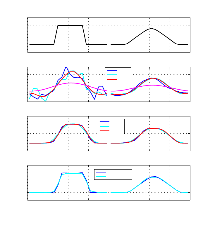
304 CHAPTER 23
0 5 10 15 20 25 30 35 40
0
0.5
1
Tracer concentration
Initial tracer profiles at y=20N
0 5 10 15 20 25 30 35 40
0
0.5
1
Tracer concentration
Tracer concentration at 100 days
0 5 10 15 20 25 30 35 40
0
0.5
1
Tracer concentration
Tracer concentration at 100 days
0 5 10 15 20 25 30 35 40
0
0.5
1
Degrees longitude
Tracer concentration
Tracer concentration at 100 days
2nd
4th
Quicker
Upwind
MDPPM
Sweby
Super B
PSOM unlimited
PSOM limited
Figure 23.1 Top panel: Initial passive tracer profile for the torus test case. The two profiles
are artificially offset in the zonal direction for purposes of clarity in presenta-
tion. Shown here is a plot through y=20◦N. Second panel: passive tracer
profiles after 100 days of integration using 2nd, 4th, Quicker, and Upwind ad-
vection schemes. Third panel: Results using MDPPM, Sweby, and Super B.
Fourth panel: Results from the limited and unlimited PSOM scheme.

Chapter Twenty Four
Symmetric box test case
The symmetric box test case mom4 symmetric box consists of a flat bottom domain
which is symmetric across the equator. It has solid walls and is forced with zonally
constant forcing. The initial conditions are constant temperature and salinity. The
surface restoring fields are show in Figure 26.1. There is zero wind stress applied.
Density is determined by the realistic equation of state of Jackett et al. (2006), and
the prognostic temperature variable is the conservative temperature of McDougall
(2003).
The aim of this test case is to examine numerical methods with respect sym-
metry across the equator. Small discretization errors which are not symmetric
will accumulate and become visible in flow features. This test provides a useful
means to measure this accumulation. Consequently, there is a relatively large
suite of physical parameterizations enabled, many of which are incompatible with
one another. The purpose of enabling so many options is to thoroughly examine
symmetry properties of the schemes.
Figure 24.2 shows the surface height and zonally averaged temperature and
zonal velocity after 1000 days of simulation. The surface height shows signs of
asymmetry, whereas the zonally averaged temperature and zonal velocity are rea-
sonably symmetric.
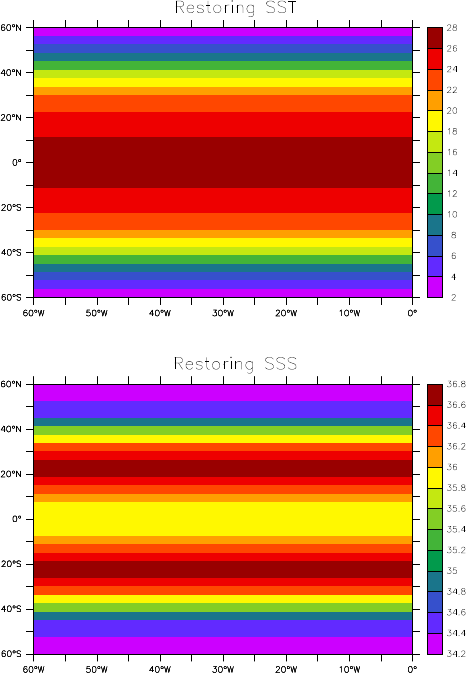
306 CHAPTER 24
Figure 24.1 Restoring temperature and salinity for the symmetric box test case.
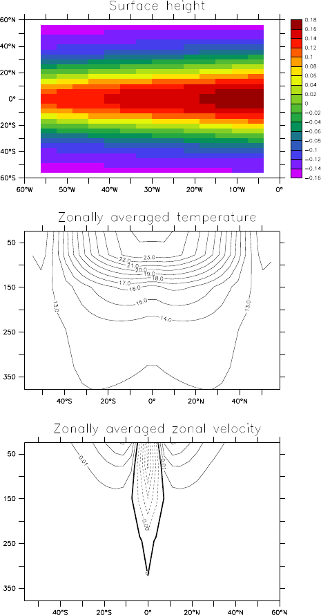
SYMMETRIC BOX TEST CASE 307
Figure 24.2 Snapshots of simulation features after 1000 days. Top panel: surface height in
metres; Middle panel: zonally averaged temperature; bottom panel: zonally
averaged zonal velocity.
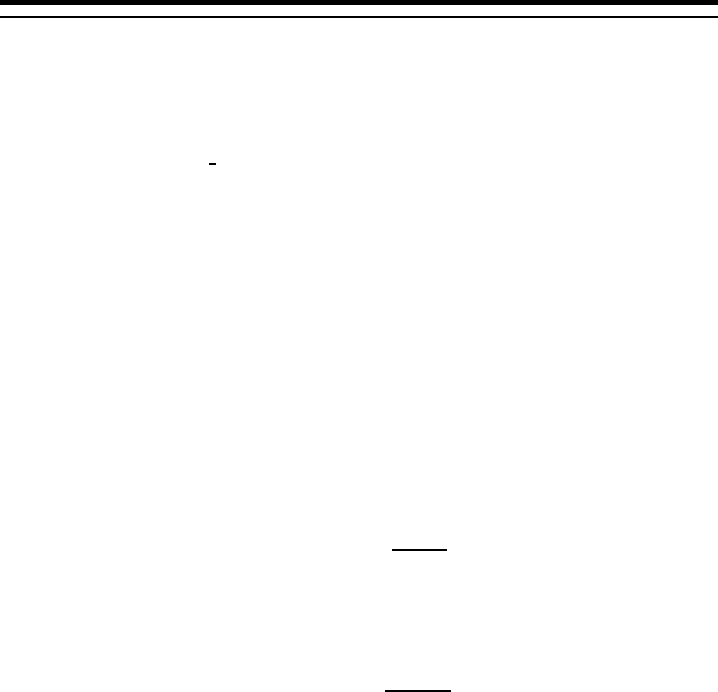
Chapter Twenty Five
Box sector test case
The box test case mom4 box consists of a flat bottom northern hemisphere sector
domain with thermohaline forcing at the upper boundary (Figure 25.1). There is
zero wind stress. The initial salinity is constant, and the initial temperature has a
nontrivial zonally symmetric thermocline structure (Figure 25.1). Density is a linear
function of temperature, and is independent of salinity and pressure.
The domain and grid are of a modest size (24(x)×35(y)×18(z)), thus allowing
this test to be run on most any computer. The resulting circulation is driven by
density gradients set up by the thermohaline forcing. It exhibits an overturning
circulation, with sinking in the north and rising throughout the domain, which is
reminscient of many similar idealized simulations run in the 1980s and 1990s.
We illustrate the behaviour of this test with the four following vertical coordinates
(see Chapter 6):
•Geopotential vertical coordinate, as in MOM4.0;
•The depth based vertical coordinate
z∗=Hz−
η
H+
η
(25.1)
•The pressure coordinate;
•The pressure based vertical coordinate
p∗=po
bp−pa
pb−pa, (25.2)
with po
bthe initial bottom pressure, pbthe bottom pressure, and pathe applied
pressure at the ocean surface, which is set to zero for this suite of tests.
Figures 25.2, 25.3, and 25.4 illustrate the zonal averaged temperature, salin-
ity, and age tracer (see Section 3.4.4), each averaged over years 901-1000. The
differences in the simulations is very minor, especially when recognizing the differ-
ent vertical axes extents for the pressure versus depth based vertical coordinates.
Figure 25.5 shows the meridional overturning streamfunction for the simulations,
again revealing very minor differences.
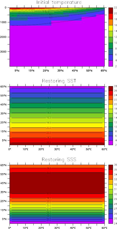
310 CHAPTER 25
Figure 25.1 Initial and boundary conditions for the box test case. Upper panel: initial tem-
perature. Middle panel: SST used for computing the restoring flux of heat.
Lower panel: SSS used for computing restoring flux of salt or fresh water.
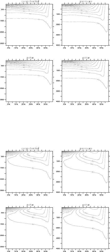
BOX SECTOR TEST CASE 311
Figure 25.2 Zonal averaged temperature time averaged over the years 901-1000 in the box
test case. Shown here are results for the four vertical coordinates considered
in this chapter. Note that for the depth based coordinates, the vertical refers to
metres, whereas for the pressure based it is dbars. This accounts for the slight
offset in the vertical extent of the domains.
Figure 25.3 As in Figure 25.2, but for salinity.
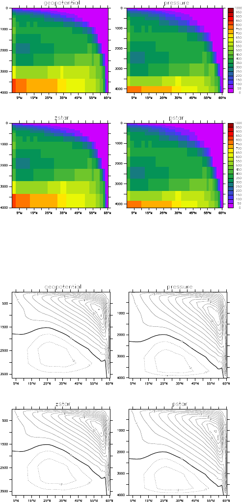
312 CHAPTER 25
Figure 25.4 As in Figure 25.2, but for the age tracer.
Figure 25.5 As in Figure 25.2, but for the meridional overturning streamfunction.

Chapter Twenty Six
Box-channel test case
The box-channel test case mom4 box channel consists of a flat bottom southern
hemisphere sector domain with a channel to the south of the sector. This ideal-
ized domain is useful for certain studies of geometries analogous to that in Nature,
where a southern channel feature (i.e., the Antarctic Circumpolar Current) navi-
gates around the globe and connects to the three main basins (Atlantic, Indian,
and Pacific). This geometry was constructed by Rongrong Zhao at GFDL and
used by her to study elements of subgrid scale (SGS) parameterizations.
The initial conditions and surface restoring fields are show in Figure 26.1. There
is zero wind stress applied. Density is a linear function of temperature, and is
independent of salinity and pressure. Circulation arises just due to the buoyancy
forcing.
The main features highlighted in this test case involve sensitivity of the deep
water formation to the SGS parameterizations in the tracer equation. We consider
four cases:
•No lateral SGS parameterization; only the Sweby advection scheme for tem-
perature, PSOM for salinity, and MDPPM for age.
•Horizontal diffusion as an SGS parameterization; otherwise the same as
above.
•Replace the horizontal diffusion with the neutral physics scheme with bound-
ary layer determined as in MOM4.0 (see Chapter 15).
•Replace the horizontal diffusion with the neutral physics scheme with bound-
ary layer determined as in Ferrari and McWilliams (2007) (see Chapter 15).
Figure 26.2 shows the zonally averaged temperature as time averaged over years
901-1000. Note the large increase in vertical stratification as neutral physics is
enabled. Indeed, the Ferrari and McWilliams (2007) scheme appears to fully shut-
down ventilation. Such is reflected in Figure 26.3, which shows the zonally aver-
aged age tracer (Section 3.4.4).
Another feature to note is the colder deep temperatures using the Ferrari and
McWilliams (2007) boundary layer formulation. This latter result is spurious, since
the initial conditions and surface restoring are all warmer than 4C. The mom4p1
implementation of the Ferrari and McWilliams (2007) introduces an unacceptable
level of spurious extrema. Such extrema are difficult to control with rotated physics
schemes, although they generally not as egregious as seen here with the new
boundary layer formulation.
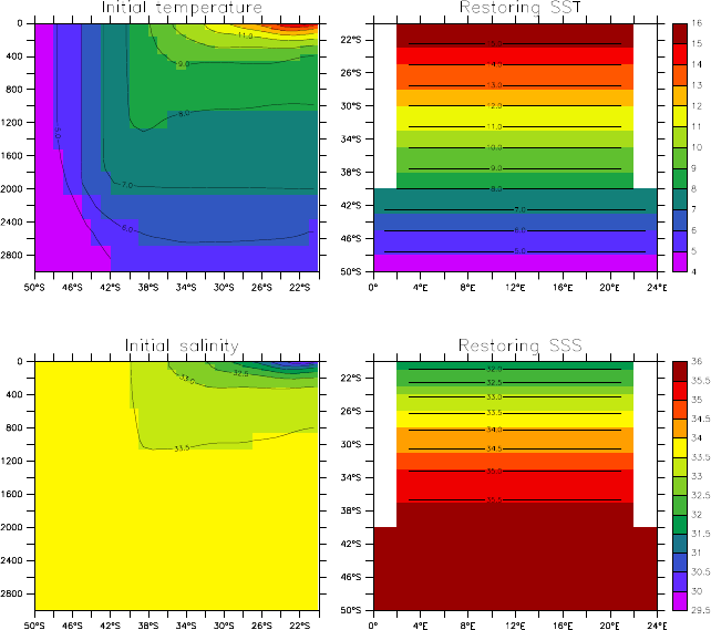
314 CHAPTER 26
Figure 26.1 Initial and boundary conditions for the box test case. Upper panel: initial tem-
perature. Middle panel: SST used for computing the restoring flux of heat.
Lower panel: SSS used for computing restoring flux of salt or fresh water.
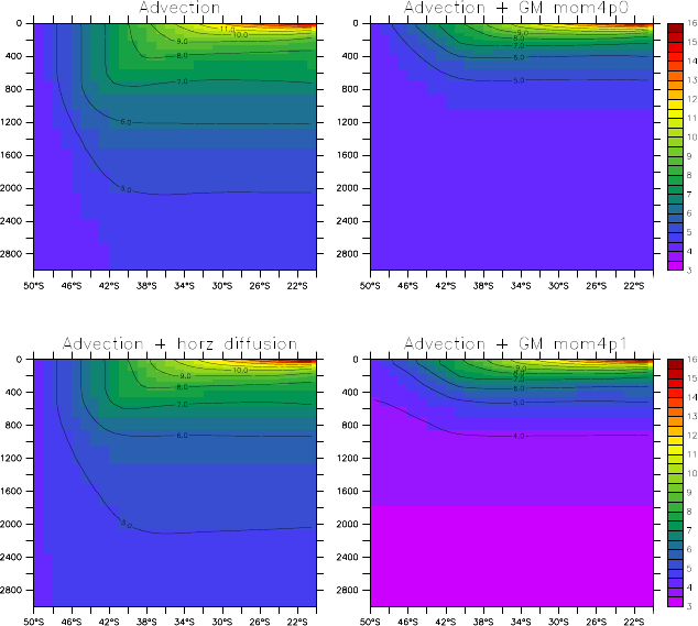
BOX-CHANNEL TEST CASE 315
Figure 26.2 Time mean and zonally averaged temperature from years 901-1000 for the box
channel test case. Upper left panel: results with advection yet without lateral
SGS parameterization; lower left panel: advection plus horizontal diffusion;
upper right: advection plus MOM4p0 neutral physics; lower right: advection
plus MOM4p0 neutral physics.
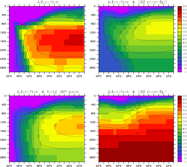
316 CHAPTER 26
Figure 26.3 Time mean and zonally averaged age from years 901-1000 for the box chan-
nel test case. Upper left panel: results with advection yet without lateral SGS
parameterization; lower left panel: advection plus horizontal diffusion; upper
right: advection plus MOM4p0 neutral physics; lower right: advection plus
MOM4p0 neutral physics.

Chapter Twenty Seven
Wind driven gyre test case
The test case mom4 gyre consists of a flat bottom middle latitude domain driven
by a zonal wind stress. The temperature is initially stratified in the vertical (Figure
27.1), with density a linear function of temperature and independent of pressure
and salinity. We employ the modified pressure coordinate
p∗=po
bp−pa
pb−pa(27.1)
for the vertical coordinate, with the applied pressure pa=0, and the static refer-
ence bottom pressure
p0
b=gZ0
−Hdz
ρ
init (27.2)
determined by the initial density profile
ρ
init.
This test case has been used at GFDL for examining the spurious mixing proper-
ties of various advection schemes. For this purpose, we initialize to unity a passive
tracer on each of the 50 vertical levels, with zero value off the chosen level (Figure
27.1). As the initial temperature profile is independent of horizontal position, the
passive tracers are initialized on surfaces of constant density. We use the mom4p1
MDPPM scheme for the test shown here.
During spinup of the circulation (Figure 27.2), passive tracers are advected
around the gyre. Horizontal gradients on a temperature surface arise from in-
homogeneous stretching and compression of the surface as a function of the level
of eddy activity. The near surface has an Ekman layer, where vertical overturn-
ing occurs, as parameterized with convective adjustment. This overturning is in
response to the Ekman suction.
Beneath the Ekman layer, spreading of passive tracer across surfaces of con-
stant temperature (Figure 27.3) occurs for two reasons:
•nonzero vertical diffusivity, set here to 10−5m2s−1,
•spurious mixing from numerical advection.
Quantifying levels of spurious mixing is straightforward. We do so by matching
the evolution of passive tracer in density space to the evolution achieved with pure
vertical diffusion, with a diffusivity fit to match that from the spurious mixing. This
approach is a complement to the more complex sorting approach employed by
Griffies et al. (2000b) (see Chapter 18).
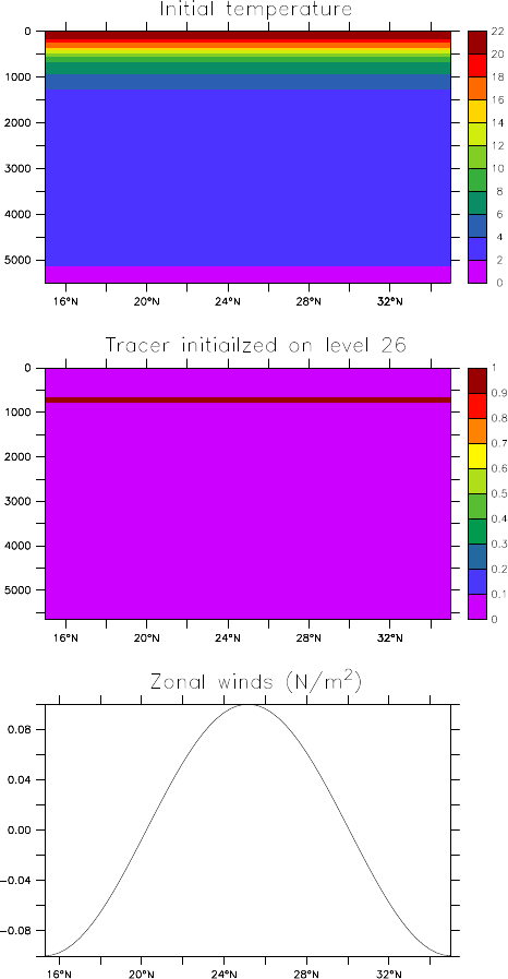
318 CHAPTER 27
Figure 27.1 Upper panel: Section illustrating the initial temperature for the gyre exper-
iment, with no horizontal variation in the initial temperature field. Middle
panel: Illustration of an initial passive tracer, placed in this case on model level
26. Lower panel: The zonal wind stress applied to the gyre model, which spins
up a two-gyre circulation within a few years.
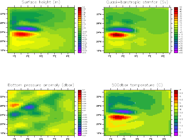
WIND DRIVEN GYRE TEST CASE 319
Figure 27.2 Simulation characteristics at 12 months. Shown here are monthly means for
the following fields. Upper left panel: surface height (metre); Lower left panel:
bottom pressure anomaly (dbar) pb−p0
b; upper right panel: quasi-barotropic
streamfunction; Lower right: Temperature at 500dbar depth. Note the very
small bottom pressure anomalies, relative to the surface height undulations, is
consistent with the circulation being largely isolated to the upper ocean.
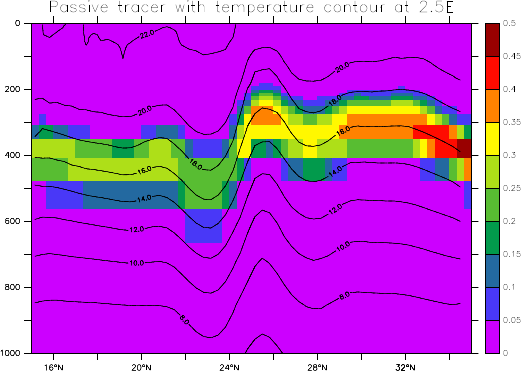
320 CHAPTER 27
Figure 27.3 Monthly averaged passive tracer at 2.5E, overlaid with contours of constant
temperature. Notice how the tracer undulates with the undulating temperature
surfaces. Also, the tracer has spread across surfaces of constant density, with
this spread associated with the nonzero vertical diffusivity and the spurious
mixing from numerical advection errors.
Chapter Twenty Eight
DOME test case
The experiment mom4 dome is based on the idealized overflow test established for
the project Dynamics of Overflow, Mixing, and Entrainment (DOME). Details of the
experiment are provided in various published papers, such as Legg et al. (2006).
As with the bowl test case mom4 bowl discussed in Chapter 29, the DOME test
case provides a means to test various overflow parameterizations. In both tests,
the simulations highlight the ability, or inability, of the simulated flow to overcome
the geostrophic balance, which aims to align the flow along isobaths. In coarsely
resolved level models, spuriously large levels of ambient waters tend to be en-
trained to the dense pulse, thus compromising the ability of the simulation to form
dense deep water, and to feel the effects of the bottom (Winton et al., 1998). The
main difference between mom4 dome and mom4 bowl is that mom4 dome allows for a
steady state to be achieved, since dense water continues to be injected from the
embayment. The mom4 bowl test, in contrast, is an adjustment experiment, with no
boundary forcing considered.
Coarse resolution level models are notoriously poor at representing overflow
processes (Winton et al., 1998). Various approaches have thus been proposed
to resolve, or to reduce, the problem. Chapter 16 details the methods available
in mom4p1. For the simulations discussed in this chapter, we employ the quasi-
horizontal coordinate p∗detailed in Section 6.2.3. Any of the other quasi-horizontal
coordinates, such as z,z∗, or p(Sections 6.1.1, 6.1.4, and 6.2.1) would show
similar results. In contrast, the terrain following coordinates
σ
(z)or
σ
(p)(Sections
6.1.5 and 6.2.4) show much more downslope flow, due to their ability to better
represent the interaction between the flow and the terrain (not shown).
The configuration consists of a shelf in the north with a shallow embayment. We
use 1/2◦grid resolution in both latitude and longitude, which yields two zonal grid
points in the embayment. The vertical grid is the same 50 levels used in the global
OM3 configuration described in Chapter 32.
Temperature is initialized with a zonally symmetric profile shown in Figure 28.1.
Cold water in the north lives at the bottom of the embayment. It is injected south-
ward by a transport imposed at the embayment’s northern boundary. Salinity is
initialized to zero everywhere, but it is given a value of unity for water that is in-
jected from the embayment. Density is a linear function of temperature, with no
dependence on salinity and pressure. Salinity thus provides a passive marker for
injected water that is transported southward and into the abyss. Both tempera-
ture and salinity are damped to their initial conditions at the eastern and west-
ern boundaries. This damping, applied through a sponge condition, eliminates
the Kelvin wave signals. Finally, for tracer advection, we use the Prather (1986)
scheme, employed without flux limiters.
We test the following five cases in this chapter:

322 CHAPTER 28
•No lateral or downslope parameterization; just advective transport;
•Advection plus sigma diffusion acting in the bottom grid cell;
•Advection plus sigma diffusion acting in the bottom grid cell plus the overflow
scheme of Campin and Goosse (1999) (Section 16.3);
•Advection plus sigma diffusion acting in the bottom grid cell plus the overex-
change scheme discussed in Section 16.4;
•Advection plus sigma diffusion acting in the bottom grid cell plus the mix-
downslope scheme discussed in Section 16.4.
Four months of integration is sufficient to highlight differences between various
overflow options available in mom4p1. Figure 28.2 shows salinity at the bottom of
the domain, averaged over the last five days of the four month experiment. The
case with pure advection (plus some vertical diffusion) shows little downslope flow,
as well as some extrema (values less than zero) arising from the absence of flux
limiters on the advection scheme. Adding sigma diffusion allows for salinity to pen-
etrate further south. There are also no tracer extrema, likely due to the smoothing
of the otherwise strong gradients near the bottom. Adding the overflow scheme
of Campin and Goosse (1999) reduces the depth where salinity penetrates. Ap-
parently it is acting in a manner that handicaps the penetration of dense water
southwards, perhaps due to over dilution. In contrast, the overexchange scheme
allows for the salinity to penetrate further southward and hence deeper. For this
test, we applied the overexchange scheme in four adjacent grid cells. Finally, the
mixdownslope also allows for penetration further southward, although with a local
extrema a few points away from the embayment, perhaps due to the nonlocal man-
ner of transport. The penetration of salinity southward is reflected in the zonally
averaged temperature shown in Figure 28.3. Consistent with the salinity tracer,
the densest waters arise from the case with the overexchange and mixdownslope
schemes. The different density profiles give rise to differences in flow characteris-
tics. Figure 28.4 shows the barotropic quasi-streamfunction (see Section 17.2 of
Griffies et al. (2004))
ψ
(x,y) = −Zy
ysouth
dy0U(x,y0), (28.1)
where
U=
η
Z
−H
dz u (28.2)
is the vertically integrated zonal transport.∗The vertically integrated transport is
far stronger in the cases with dense shelf water penetrating into the deep.
∗In a rigid lid model, or a free surface model having reached a steady state in the absence of surface
boundary fluxes of mass, then
ψ
is a vertically integrated streamfunction. For the present case, with
a transient free surface model,
ψ
is only a direct correlate to the true vertically integrated transport,
hence the qualifier quasi.
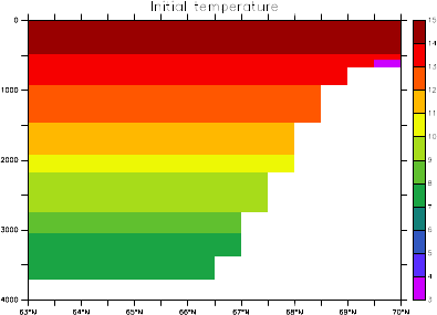
DOME TEST CASE 323
Figure 28.1 Initial temperature for the DOME test case. The cold water in the far north is
at the bottom of the embayment. Southward flow is injected from this embay-
ment, allowing for the cold and dense water to leave the embayment and enter
the abyss.
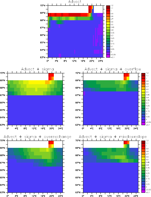
324 CHAPTER 28
Figure 28.2 Bottom salinity averaged over the last five days of a four month integration.
Top panel: no lateral or terrain following parameterization. Middle left: ad-
vection plus sigma diffusion applied in the bottom grid cell. Middle right: ad-
vection plus sigma diffusion plus the overflow scheme of Campin and Goosse
(1999) (Section 16.3). Bottom left: advection plus sigma diffusion plus the
overexchange scheme (Section 16.4) Bottom right: advection plus sigma diffu-
sion plus the mixdownslope scheme (Section 16.4).
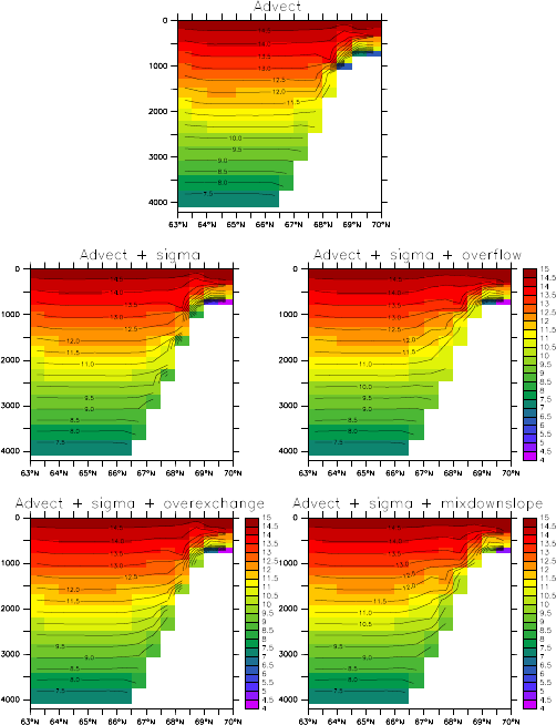
DOME TEST CASE 325
Figure 28.3 Zonally averaged temperature for the DOME test case, with panels correspond-
ing to those in Figure 28.2.
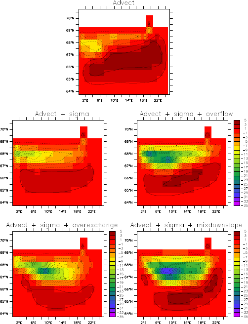
326 CHAPTER 28
Figure 28.4 Quasi-streamfunction (Sv) for the vertically integrated transport in the four
DOME simulations, with panels corresponding to those in Figure 28.2.
Chapter Twenty Nine
Bowl test case
The bowl test case mom4 bowl is based on a configuration built for studies of over-
flow processes by Winton et al. (1998). It consists of a shallow shelf in the northern
portion of the domain, with a deeper bowl to the south (Figure 29.1). The initial
conditions place cold dense water on the shelf (Figure 29.2). Density is a linear
function of temperature, and is independent of salinity and pressure.
Integration proceeds with no surface forcing. Hence, this is a relaxation or ad-
justment experiment, with no steady state realized. The initial pressure forces set
up acceleration which causes the water to move off the shelf and into the deeper
portion of the domain. The numerical and physical processes active in this relax-
ation experiment are described by Winton et al. (1998). In particular, the test case
is useful to examine the sensitivity of the deep water formed to various numeri-
cal and physical options. It can be used in tandem with the test case mom4 dome
described in Chapter 28.
Level models are notoriously poor at representing overflow processes (Winton
et al., 1998). Various approaches have thus been proposed to resolve, or reduce,
the problems. Chapter 16 details the methods available in mom4p1. We test the
following four configurations here:
•Terrain following pressure based vertical coordinate
σ
(p)=p−pa
pb−pa, (29.1)
with pbthe bottom pressure, and pathe applied pressure at the ocean sur-
face, which is set to zero for this suite of tests. For this vertical coordinate,
we transport tracer just by advection plus some vertical diffusion.
•Quasi-horizontal pressure based vertical coordinate
p∗=po
bp−pa
pb−pa, (29.2)
with po
bthe initial bottom pressure. In this test, we also just employ advection
plus vertical diffusion.
•In this test, we use p∗with the addition of nontrivial sigma diffusion in the
bottom cell, as described in Section 16.2.1.
•In this test, we use p∗with the addition of nontrivial sigma diffusion in the
bottom cell, as described in Section 16.2.1, as well as the overexchange
scheme discussed in Section 16.4.
Figures 29.3 and 29.4 show the salinity (a passive tracer) and temperature at the
botom of the domain, after one year as averaged over the last five days of the year.
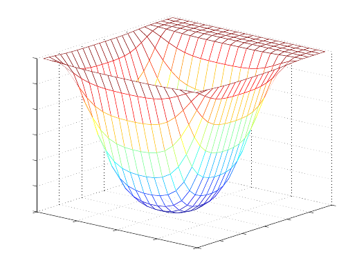
328 CHAPTER 29
Both of the cases without any added subgrid scale methods show advection trans-
porting the tracers southwards along the western boundary. The terrain following
σ
(p)case brings the tracer further into the abyss than the p∗case. When adding
sigma diffusion or overexchange to the p∗cases, the bottom signal is greatly dif-
fusved, as expected since these parameterizations are diffusive. They also cause
the tracer to bleed into the abyss more uniformly, rather than following the path
along the wester wall.
0
5
10
15
20 60 62 64 66 68 70 72
−3500
−3000
−2500
−2000
−1500
−1000
−500
Latitude
Topography for Bowl test case
Longitude
Depth (metre)
Figure 29.1 Geometry of the bowl test case, with shallow shelf in the north and deeper bowl
to the south.
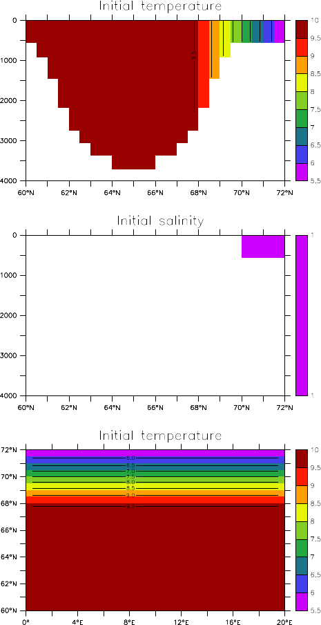
BOWL TEST CASE 329
Figure 29.2 Initial conditions for temperature and salinity in the bowl test case. Upper
panel: meridional-depth slice of the zonally symmetric initial temperature.
Middle panel: Initial salinity, which has a unit value on the shelf and zero else-
where. Lower panel: Plan view of the initial SST.
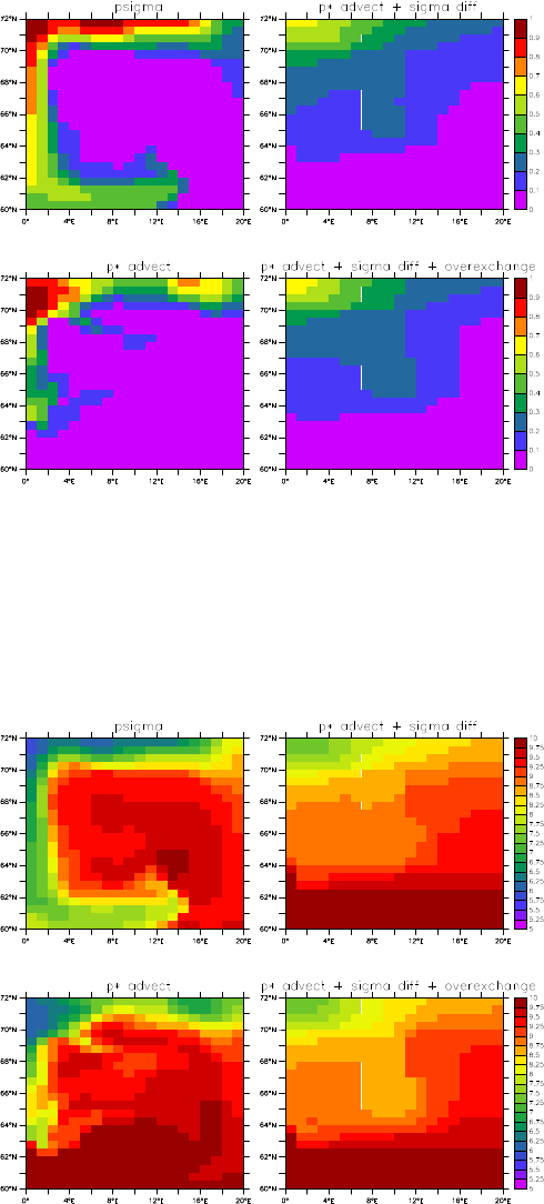
330 CHAPTER 29
Figure 29.3 Salinity at the bottom of the domain after one year, as averaged over the last
five days of the year. Upper left panel: results from
σ
(p)vertical coordinate
using advection alone for the tracer transport; Lower left panel: results from p∗
vertical coordinate using advection alone for the tracer transport; Upper right
panel: p∗with advection and sigma diffusion applied in the bottom cell; Lower
right panel: p∗with advection and sigma diffusion applied in the bottom cell
and the overexchange scheme.
Figure 29.4 As in Figure 29.3, but for temperature.

Chapter Thirty
Indian Ocean Model
The test case mom4 iom consists of a realistic regional model of the Indian Ocean.
The lateral regional boundaries are damped to climatology using sponges. This
model was originally developed as part of a course on large scale ocean modelling
in Bangalore, India during October 2004. The model remains a useful starting point
for certain Indian Ocean research efforts using MOM. It is essentially the mom4p1
implementation of Version 1.0 of that model configuration. The model is forced
with a full suite of realistic atmospheric products, and employs a relatively modern
suite of physical parameterizations.
One point of departure from the standard MOM4.0 configuration is to employ
the depth based vertical coordinate (Chapter 6)
z∗=H(z−
η
)/(H+
η
). (30.1)
This coordinate is useful in cases where it is desired to refine the vertical resolution
in the upper ocean. Such enhanced vertical resolution may be of use for the Indian
Ocean, where important vertical gradients exist especially near river mouths.
Figure 30.1 shows the SST, SSS, and surface height fields for the simulation
after only two days of integration. As this model is not actively run at GFDL, we
have not run it ourselves for much longer periods. Researchers interested in using
this model configuration should consult with the mom4 user community to be able
to access the experience of others in running this model.
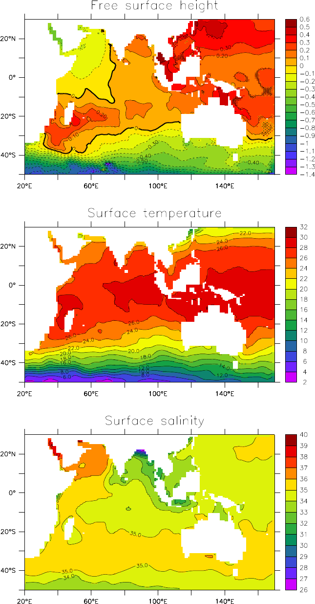
332 CHAPTER 30
Figure 30.1 Daily averaged surface fields after two days integration of the Indian Ocean
Model. Top panel: free surface height (metre); middle panel: surface tempera-
ture (C); bottom panel: surface salinity (psu).

Chapter Thirty One
CSIRO Mark 3.5 test
The test case mom4 mk3p5 consists of a realistic global model with spherical coor-
dinates. This model was developed at the CSIRO Marine and Atmospheric Re-
search in Aspendale, Australia. It is routinely used as the ocean component for
the Australian contribution to the IPCC report.
It is notable that this model was originally developed for a rigid lid algorithm in
MOM1. For that algorithm, a heavy dose of polar filtering was employed. The
present configuration in mom4p1, employing a free surface, removes all polar fil-
tering, yet it takes a longer time step than the polar filtered rigid lid configuration.
This result is indicative of the often paradoxical results found with polar filtering.
We strongly recommend that all polar filtering be removed from global simulations.
Indeed, although a polar filtering module remains as part of mom4p1, it is not sup-
ported by GFDL scientists. The main reason is that is breaks local conservation of
tracer, thus leading to spurious surface fluxes and poor high latitude simulations.

Chapter Thirty Two
Global ocean ice model with tripolar grid
The test case mom4 om3 core consists of a realistic global ocean and ice model
using the tripolar grid of Murray (1996) (Figure 32.1). Griffies et al. (2005) pro-
vides extensive details of the model configuration. We thus only provide a brief
introduction in this chapter.
The global coupled ocean-ice configuration is very similar to that used as part
of the climate model developed at GFDL for the 4th IPCC assessment of climate
change (Griffies et al., 2005; Gnanadesikan et al., 2006a). The ocean-ice config-
uration is also the basis for the GFDL-MOM contribution to the Coordinate Ocean-
ice Reference Experiments (COREs) documented in Griffies et al. (2007). These
experiments employ the boundary forcing from Large and Yeager (2004), which
was developed for the purpose of running global coupled ocean-ice simulations
without an interactive atmosphere. This Large and Yeager (2004) dataset is avail-
able through the GFDL web site
http://nomads.gfdl.noaa.gov/nomads/forms/mom4/CORE.html.
It has been part of the MOM4 distribution for a few years. In addition to using an
updated version of MOM relative to Griffies et al. (2005) and Griffies et al. (2007),
some model details have been modified in order to more thoroughly test various
features of the simulation for this test case.
32.1 THREE DIFFERENT VERTICAL COORDINATES
In this section, we illustrate certain characteristics after 100 years of integration
with focus on results for the three different vertical coordinates (Chapter 6)
s=z(32.1)
s=z∗=H(z−
η
)/(H+
η
)(32.2)
s=p∗=po
bp−pa
pb−pa. (32.3)
We show how results from zand z∗are very close for the full global domain. The p∗
differ in some regards that may be attributable to differences in the dynamics and
SGS parameterization as treated with Boussinesq and nonBoussinesq models.
32.1.1 Initialization of the p∗simulation
In Section 7.2, we detailed how to initialize the non-Boussinesq models, such as
the p∗simulation. In the p∗simulation, the vertical grid is based on increments of
336 CHAPTER 32
p∗, which are pressure increments. Our choice for setting these increments is the
simplest approach, whereby the vertical coordinate increment is set according to
ds=−g
ρ
odz0. (32.4)
The initial vertical depth increment dz0is set according to the MOM4 procedure for
determining the depth increments in depth-based vertical coordinate simulations.
Through the hydrostatic balance, specifying the pressure increments dsdeter-
mines mass within a coordinate layer. Placing initial temperature and salinity, such
as from the World Ocean Atlas, in these layers then sets the density of the layers.
The mass and density of a layer then determines the actual thickness dzinit, which
is generally different from dz0.
Hence, the sum of thickness dzinit over the column will generally not yield a
zero surface height
η
. This result may not be a problem, and indeed the default
mom4p1 approach is to allow for such nonzero surface heights to exist. However,
in the following we illustrate what is required if we insist on maintaining a nonzero
surface height. In this case, an iterative process is required, with some modifica-
tion needed to leave
η
=0at the initial condition. Our choice, as discussed in
Section 7.2, is to modify the bottom depths. To remove the instability possible from
thin bottom cells, we deepen those cells that are too shallow to fit the chosen ini-
tial column mass, if the bottom partial step is determined to be below a threshold
thickness (chosen as 10m for this test case). For columns that can fit the chosen
initial mass with the given bottom depth, we do not modify the bottom depth at
all. So the initial procedure only deepens some cells. As shown in Figure 32.2,
it only deepens cells by a small amount, with the exception of a few cells in the
Black Sea. These columns occur in a relatively shallow marginal sea, and contain
relatively light water.
32.1.2 Brief analysis for the simulations
We show the following figures on the subsequent pages:
•Figure 32.3: Anamolous surface temperature obtained by time averaging
over years 81-100 of the simulation, with anomalies relative to the World
Ocean Atlas (WOA).
•Figure 32.4: Anamolous surface salinity obtained by time averaging over
years 81-100 of the simulation, with anomalies relative to the World Ocean
Atlas (WOA).
•Figure 32.5: Anomalies for SST and SSS for the z∗and p∗simulations rela-
tive to the geopotential simulation.
•Figure 32.6: Time series for the temperature and salinity biases relative to
WOA, as a function of depth for the geopotential and z∗simulation, and as a
function of pressure for the p∗simulation.
•Figure 32.7: Meridional overturning circulation for the Atlantic basin aver-
aged over years 81-100, as well as the time series for the maximum over-
turning at 45◦N.
GLOBAL OCEAN ICE MODEL WITH TRIPOLAR GRID 337
In general, differences are small between the geopotential and z∗simulations,
whereas they are more noticeable between these two Boussinesq models and the
p∗simulation. For surface properties, the main differences are near the boundary
current extensions in the Pacific and Atlantic, with this difference signaling a slight
shift in the boundary current with the p∗model relative to the depth based models.
Overall, the larger spread with the p∗model may be attributed to accumulation
of slightly different forcing, where the Boussinesq model normalizes by
ρ
oto con-
vert stresses (N/m2), heating (W/m2), and hydrological mass fluxes (kg/(m2s)
to accelerations, temperature fluxes, and moisture volume fluxes. The p∗model
normalizes by the in situ surface density of the model. Additionally, the nonBoussi-
nesq equations are slightly different, and accumulation of these differences may
be possible for realistic simulations, such as the OM3 CORE test case.
32.2 AGE TRACER AND SENSITIVITY TO OVERFLOW PARAMETERIZA-
TIONS
We saw in Chapter 28 how sigma diffusion acting in the bottom grid cell, plus
the overexchange scheme discussed in Section 16.4, affect the transfer of dense
water into the abyss in the idealized DOME configuration. We pursue that result
here within the OM3 configuration using geopotential vertical coordinate. In par-
ticular, we compare three MOM simulations plus an isopycnal simulation using the
Hallberg Isopycnal Model:
•Standard configuration using the Sweby advection scheme of Hundsdorfer
and Trompert (1994), with flux limiters of Sweby (1984). This configuration
employs the sigma diffusion scheme in the model’s bottom grid cells.
•Switch from Sweby to the second order moment scheme of Prather (1986).
•Keep Prather (1986) and enable the overexchange scheme discussed in
Section 16.4.
•Hallberg Isopycnal Model (HIM): This simulation is analogous to the MOM
simulations, with the exception that it employs three times larger restoring of
the salinity field. A run with the same restoring is underway and will replace
this simulation when available.
All three MOM simulations are quite similar in broad patterns. There are dif-
ferences when focusing on certain boundary regions, as may be expected from
the differences in the overflow parameterization. But the broad scale patterns are
quite similar. In contrast, the HIM simulation is far more venitilated, especially in
the Southern Ocean. This result is consistent with the coarse resolution results
documented by Legg et al. (2006).
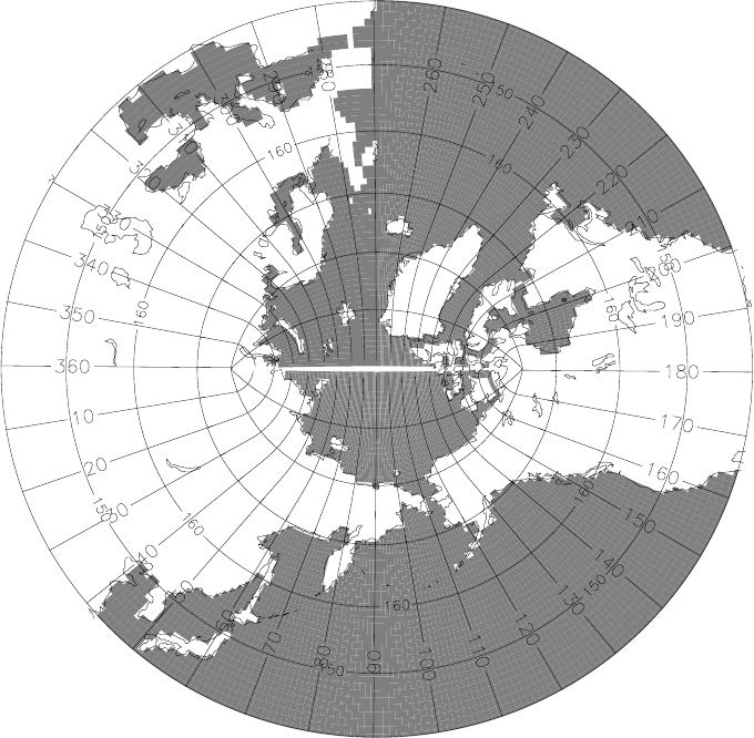
338 CHAPTER 32
Figure 32.1 Illustration of the bipolar Arctic as prescribed by Murray (1996) (see his Figure
7) and realized in OM3. The transition from the bipolar Arctic to the spherical
grid occurs at 65◦N. We denote horizontal grid cells by (i,j)indices. As in
the spherical coordinate region of the grid, lines of constant i−index move in a
generalized eastward direction within the bipolar region. They start from the
bipolar south pole at i=0, which is identified with i=ni, where ni is the num-
ber of points along a latitude circle and ni =360 in OM3. The bipolar north
pole is at i=ni/2, which necessitates that ni be an even number. Both poles are
centered at a velocity point on the B-grid used in MOM4.0. Lines of constant j
move in a generalized northward direction. The bipolar prime-meridian is situ-
ated along the j-line with j=n j, where n j =200 in OM3. This line defines the
bipolar fold that bisects the tracer grid. Care must be exercised when mapping
fields across this fold. As noted by Griffies et al. (2004), maintaining the exact
identity of fields computed redundantly along the fold is essential for model
stability. Note that the cut across the bipolar fold is a limitation of the graphics
package, and does not represent a land-sea boundary in the model domain.
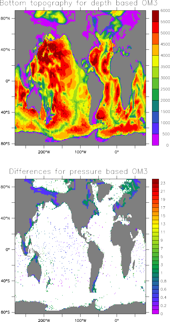
GLOBAL OCEAN ICE MODEL WITH TRIPOLAR GRID 339
Figure 32.2 Top panel: Topography used in an earlier depth based version of the OM3
test case. Bottom panel: Deepening of the topography required to start the p∗
simulation with a zero initial surface height. The modifications are very minor
in most of the World Ocean, with a few points in the Black Sea most prominent.
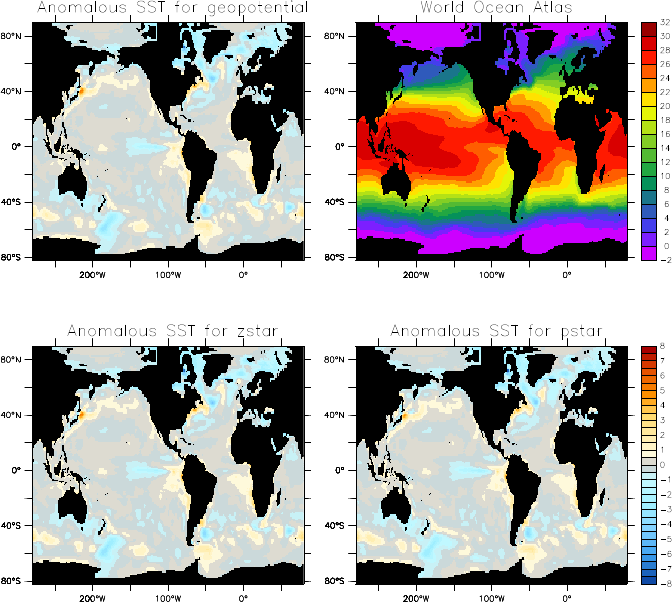
340 CHAPTER 32
Figure 32.3 Surface temperature anomalies for the depth, z∗, and p∗simulations. Values
are computed from 20 year mean over years 81-100.
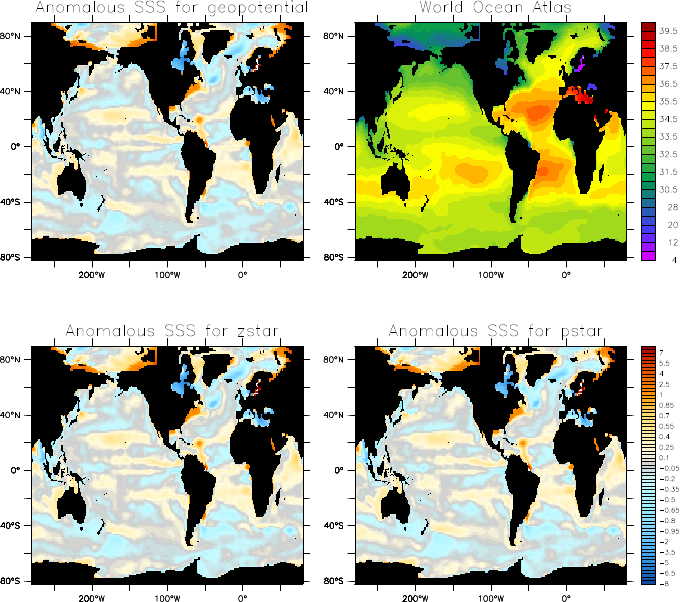
GLOBAL OCEAN ICE MODEL WITH TRIPOLAR GRID 341
Figure 32.4 Surface salinity anomalies for the depth, z∗, and p∗simulations. Values are
computed from 20 year mean over years 81-100.
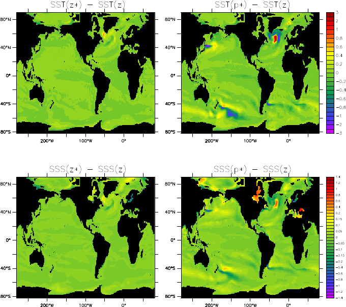
342 CHAPTER 32
Figure 32.5 Difference in surface temperature and surface salinity between the z∗and
geopotential, and p∗and geopotential. Values are computed from 20 year mean
over years 81-100.
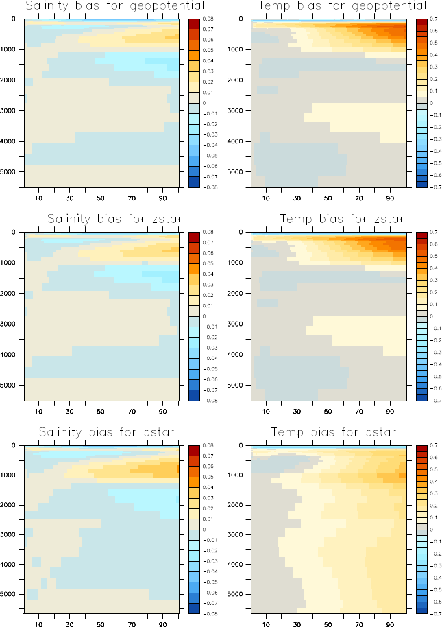
GLOBAL OCEAN ICE MODEL WITH TRIPOLAR GRID 343
Figure 32.6 Drift for the geopotential, z∗, and p∗simulations in annual mean temperature
and salinity as a function of depth and time. This drift is defined as Tdrift(z,t) =
∑xy dxdydz(Tmodel −Tinitial/∑xy dxdydz.
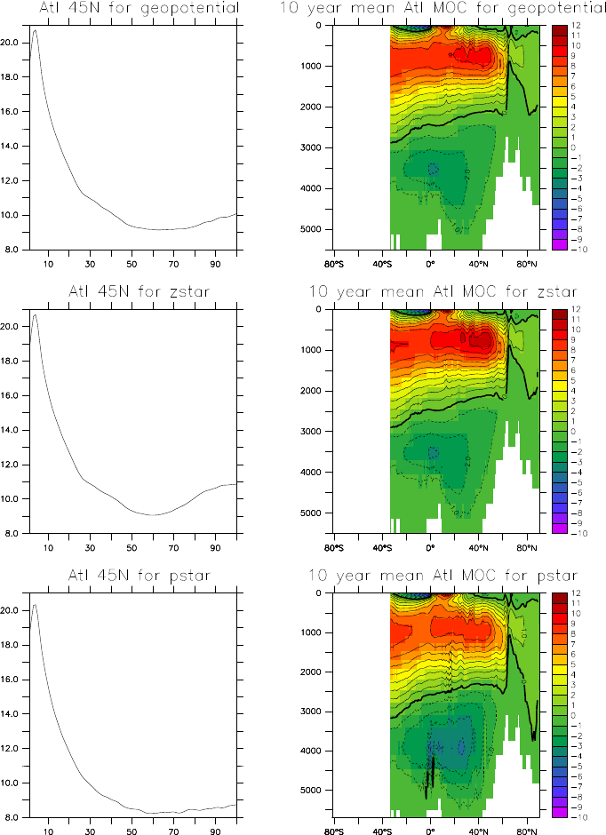
344 CHAPTER 32
Figure 32.7 Meridional overturning circulation for the Atlantic basin averaged over years
81-100, as well as the time series for the maximum overturning at 45◦N.
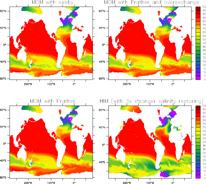
GLOBAL OCEAN ICE MODEL WITH TRIPOLAR GRID 345
Figure 32.8 Age tracer averaged over the depths 800m-1200m and years 81-100. Top left:
Integration with Sweby advection. Bottom left: Prather advection. Top right:
Prather with overexchange. Bottom right: HIM.
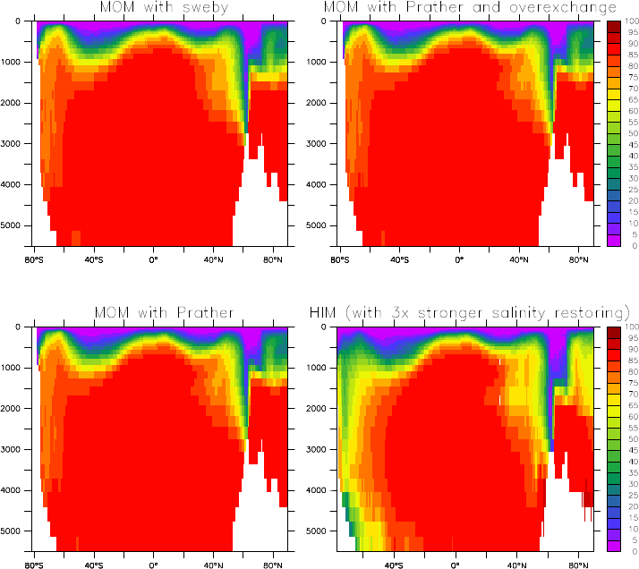
346 CHAPTER 32
Figure 32.9 Zonally averaged age tracer averaged over years 81-100. Top left: Integration
with Sweby advection. Bottom left: Prather advection. Top right: Prather with
overexchange. Bottom right: HIM.

Chapter Thirty Three
Global ocean-ice-biogeochemistry model
The test case mom4 om3 ecosystem consists of the same realistic global ocean
and ice model used for the mom4 om3 core simulation (Chapter 32). The physical
components are forced as in mom4 om3 core. In addition, we enable the GFDL
Ocean Biogeochemistry (GOB) model. This is a model of oceanic ecosystems
and biogeochemical cycles which considers 22 tracers including the following:
•three phytoplankton groups
•two forms of dissolved organic matter
•heterotrophic biomass
•dissolved inorganic species for C,N,P,Si,Fe,CaCO3and O2cycling.
The model includes such processes as
•gas exchange
•atmospheric deposition
•scavenging
•N2fixation and water column and sediment denitrification
•runoff of C,N,Fe,O2, alkalinity and lithogenic material.
The phytoplankton functional groups undergo co-limitation by light, nitrogen, phos-
phorus and iron with flexible physiology. Loss of phytoplankton is parameterized
through the size-based relationship of Dunne et al. (2005). Particle export is de-
scribed through size and temperature based detritus formation and mineral pro-
tection during sinking with a mechanistic, solubility-based representation alkalinity
addition from rivers, CaCO3sedimentation and sediment preservation and disso-
lution.
Chapter Thirty Four
Eastern upwelling area test case
This chapter was contributed by Martin Schmidt
martin.schmidt@io −warnemuende.de
The test case mom4 atlantic is derived from a regional ecosystem model of the
Benguela Upwelling area. It consists of a rectangular box delimited at the east-
ern side by the Namibian shelf, but by three open boundaries to the south, west
and north respectively. The topography is derived from the etopo5 dataset. The
circulation in the model area is driven by local wind fields, but is also influenced
by coastal trapped waves originating from the equatorial current system. For ex-
periments covering several model years a large model domain is needed, which
includes the equatorial current system. However, in the framework of an ecosys-
tem model with many nutrient, phytoplankton and zooplankton variables such a
model system appears to be computationally expensive. In detail, it needs to much
compute time for sophisticated sensitivity studies. For this purpose, regional sub-
models may be of great help and the original purpose of this model configuration
is to perform such sensitivity studies. The large model is implemented with MOM-31
as an ecosystem model, but the regional test case configured with mom4 atlantic
has only the temperature and salinity tracer enabled.
The circulation at the shelf has three main components, a westward Ekman
transport in connection with a coastal jet driven by the trade winds, an intermittent
southward undercurrent and an Ekman compensation current which drives deep
circulation onto the shelf. The more or less permanent off-shore Ekman transport
implies strong coastal upwelling.
The regional model should reproduce these features. The specific boundary
conditions at the open model boundaries (OBC) apply for tracer points and involve
a radiation condition and relaxation to prescribed values as well. In the ARAKAWA
B-grid used with mom4p1, velocity points are internal points, but momentum advec-
tion is not well defined and requires approximations. Hence, only information on
tracers and sea level is passed from the large model to the regional sub-model.
Grid and topography in the sub-model and the large model are the same in
the sub-model domain. Also the atmosphere forcing is similar and this test case
could also be considered as a one sides nesting problem. However, the numer-
ical schemes of the large and the regional model are different. Open boundary
conditions are one method to control inconsistency near the boundaries, which
eventually may grow large with nesting.
The large model is implemented with MOM-31. It is a regional model itself and
covers the area from 10◦W to 18◦E and 35◦S to 8◦N. Boundary values for
temperature, salinity and sea level are taken from the ECCO-model. The OBC for
350 CHAPTER 34
the large model are very similar to those used in mom4p1. 10 day averages of most
model variables can be found at the LAS-server
http ://las.io −warnemuende.de :8080/las/servlets/dataset.
Some details on the large model will be given below, which may be helpful to
understand differences to the regional mom4p1 implementation:
- coupled model with atmosphere data provided from external files,
- leapfrog time stepping with Robert time filter, time step 720 s,
- tracer conserving time stepping scheme as described in Griffies et al. (2001),
explicit fresh water flux from rivers and precipitation,
- tracer advection with the quicker scheme, in mom4p1 this is quickermom3,
- vertical diffusion with a modified kpp-scheme. Only that part of the short
wave radiation, which is absorbed to a certain depth is added to the non-
local vertical heat flux. This avoids numerical artifacts with unstable water
column at daytime.
- horizontal diffusion and viscosity using the Smagorinsky closure scheme with
a Prandl number of 10, and a Smagorinski factor of 4. Background values
for viscosity and mixing are chosen as small as possible.
- Ocean-atmosphere fluxes are updated every hour and are kept constant in-
between.
- The wind stress is calculated from composites of three day QuikSCAT based
wind fields with high spatial resolution superimposed with a daily cycle de-
rived from NCEP reanalysis data. The wind stress is parametrized following
Large and Pond (1981).
- Short wave radiation is calculated from the top atmosphere insolation mod-
ified by total cloud cover taken from NCEP reanalysis data. Transmissivity
depends on sun angle and absorption is calculated from the optical path
length. The albedo is calculated from Fresnel’s formula.
- Long-wave upward radiation is calculated from a gray body formula with an
emissivity of 0.96. Long-wave downward radiation is taken from a gray body
radiation formula with atmosphere 10 m temperature, modified by humidity
and cloud coverage.
- Latent heat flux is calculated from virtual air temperature and SST by a usual
bulk formula.
- Evaporation is calculated from 2m water vapor pressure. Specific humidity
and air temperature are from NCEP reanalysis data. The enthalpy correspond-
ing to the mass flux with evaporation is also taken into account.
- Precipitation data from NCEP reanalysis are used. To calculate the heat flux
from precipitation (heavy rain falls are possible in the model domain) the rain
temperature is approximated by the air temperature.
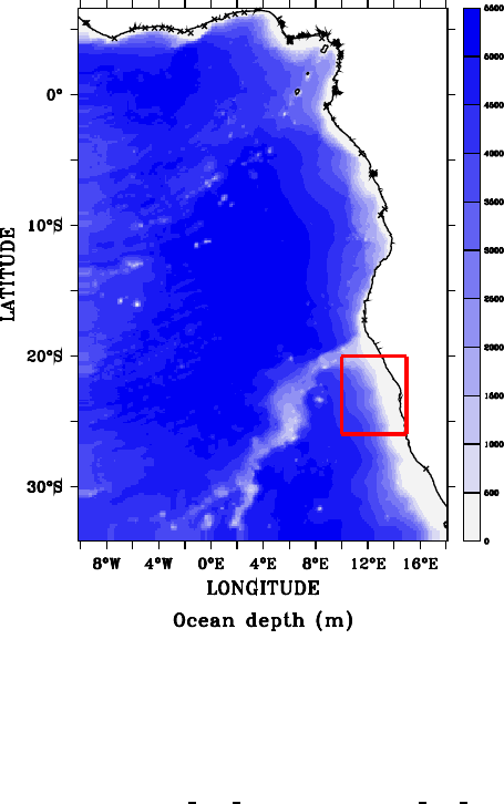
EASTERN UPWELLING AREA TEST CASE 351
- Atmosphere bottom pressure gradients are taken into account from ocean
model pressure gradients. This point is important for the performance of the
OBC scheme.
Figure 34.1 The topography of the large model and the embedded region of the sub-model.
Figure 34.1 shows the topography of the large model and the embedded sub-
model area for this test case. Along the sub-model boundaries time averages of
sea level and tracers were stored every 6 model hours. For the western boundary
these data are in the input files obc trop west.dta.nc and obc clin west.dta.nc. Similar
files are written for the northern and southern boundary. For mom4p1 a calendar
attribute was added to the time axis and the sea level values are transformed to
be given in meters.
Subsequently some corner points for the regional mom4p1 implementation are
given. The namelist specifies more details:
- coupled model with atmosphere data provided from external files by data
overriding,
- two-level (Adams-Bashford) time stepping with a baroclinic time-step of 1200
s,
- predictor-corrector free surface scheme,
- explicit fresh water flux precipitation, rivers are not in the model domain,
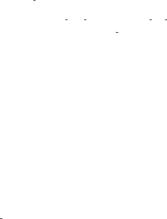
352 CHAPTER 34
- geopotential coordinates. z∗-coordinates have been also verified to work, but
OBC are not ready for pressure coordinates.
- The model domain is an upwelling area. The baroclinic Rossby radius is
almost resolved. Hence, sigma-diffusion and neutral physics are dis-
abled.
- Vertical diffusion is calculated from the kpp-scheme. This differs slightly from
the method used in MOM-31, but the consequences have not been investi-
gated yet.
- Horizontal diffusion is calculated from the Laplacian scheme, with a small
value for vel micom =0.001m s−1.
- Horizontal friction is calculated from the Laplacian Smagorinsky scheme,
with a small value for vel micom iso =0.0005m s−1and k smag iso =4.0.
- Tracer advection is carried out with the mdfl sweby-scheme for all tracers.
- Atmosphere data to calculate ocean atmosphere fluxes are the same as
used for the large model. However, in mom4p1 the ocean surface velocity is
taken into account in the wind stress calculation, which is based on Monin-
Obukhov similarity theory.
- Downward short- and long-wave radiation is not calculated but overridden
from file instead. 6 hourly NCEP reanalysis data are used, with a coarse 4
degree spatial resolution. The daily cycle will be represented less accurate
than in the large model. Long-wave upward radiation is approximated by a
black body formula.
Remarks on file on file preprocessing
The input files of this test case do not fulfill all requirements for fms netcdf input
files, but they are recognized correctly. A calendar attribute was added to the time
axis if missing. Most files are preprocessed with ferret,
http ://ferret.pmel.noaa.gov/Ferret/,
which adds information on axis boundaries. Possibly the bnds-specification is not
recognized by the fms axis tools. For this reason the bnds-specification has been
removed from all input files.
Plots of the input wind fields in windx.mom.dta.nc and windy.mom.dta.nc look
strange near the coasts. The reason is, that the wind fields are based on scat-
terometer data with missing values at land points which let the horizontal interpo-
lation tools of fms fail. Replacing missing values by zero should be a bad choice.
Hence, ocean values are extrapolates into land. This can be done with the function
fill xy of ferret which is undocumented part of version 6 and later and may be
used as follows:
use windx_inp.nc ! missing values at land
let mask = missing(windx_in,0)*0 + 1 ! do not mask anything
let windx = fill_xy(windx_in,mask,5) ! fill with 5 passes
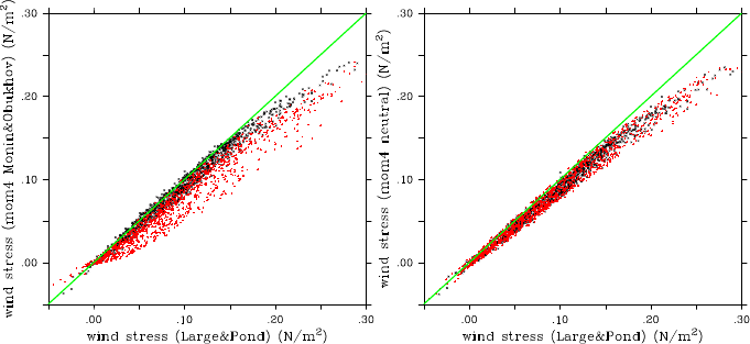
EASTERN UPWELLING AREA TEST CASE 353
Experiments
The regional model was run with several choices of the namelist parameters over
11 model month. To demonstrate the influence of the wind stress parameterization
on the results, the parameterization according the Monin-Obukhov similarity theory
and the neutral approximation are used.
Open boundary conditions with a radiation condition and prescribed external
data are mathematically ill-posed. Hence, a prefect scheme does not exist and
the optimal choice of the boundary conditions needs experiments with boundary
code parameters. It is suggested to vary the parameters used for OBC, especially
modify the strength of the relaxation toward external data and to test the different
schemes for the calculation of the phase speed of baroclinic and barotropic waves.
Remarks on the wind stress parameterization
The scheme to calculate air-sea fluxes differs in many ways for the large and the
regional model. The OBC should be robust against such inconsistency. A detailed
discussion of the surface flux schemes in mom4p1 is out of the scope of this test
case, but some details need attention.
Figure 34.2 Scatter plots of the wind stress calculated in the large model (Large and Pond,
1981) versus the parameterization in fms, left: Monin-Obukhov similarity ap-
proach, right: neutral approximation. Black dots at 11◦E and 21◦S, where the
boundary layer is often unstable, red dots from 14◦E and 25◦S in the upwelling
area with low SST and a stable boundary layer.
Vertical momentum fluxes in the large model are estimated for a neutral bound-
ary layer. This should be appropriate in a region of more or less permanent trade
winds. In the regional model boundary layer stability was taken into account. Be-
cause there is no feedback from the ocean to the atmosphere, radiation can drive
the SST away from the 2 m air temperature. Indeed this happens, because the
cold band of upwelled water near the coast does not have its counterpart in the
coarse NCEP data. On the other hand, calculated SST appears warmer than in
remote sensing based data in the open ocean, which in turn leads to an unstable
boundary layer.
Figure 34.2 shows scatter plots of the wind stress from the large scale model
(LARGE AND POND, 1981, neutral boundary layer) and the fms schemes used in

354 CHAPTER 34
the regional model. Generally, the wind stress in fms is lower than in the large scale
model. Especially for high wind speed large deviations can be seen. Results from
the upwelling area (shown in red) show the influence of the stable boundary layer.
It can be suspected, that the coarse NCEP reanalysis data do not resolve the narrow
upwelling band and have to high atmosphere temperature. This corresponds to a
very stable boundary layer in the upwelling band an in the tendency to reduced
upwelling compared with a model driven by wind stress calculated for a neutral
atmosphere-ocean boundary layer.
Here neither the neutral nor the Monin-Obukhov approach should be favored,
but the differences should be mentioned as a source of differences between the
large model and the regional model with open boundaries.
The mixing layer depth in the regional model is smaller than in the large model.
The vertical mixing scheme is configured similarly and the differences should be
traced back to the different wind stress scheme.
Remarks on the heat flux parameterization
Using the downward radiation from NCEP reanalysis data together with the default
heat flux parameterization implemented infms, the calculated SST becomes to
high within several model days. The resulting discrepancy between boundary data
and the model interior, drives currents along the boundary. Comparing with the
parameterization, used in the large scale model, it seems appropriate to introduce
an albedo factor of .9 for the long wave radiation in the data table. Such a ad
hoc correction should be appropriate for a test case and removes the artificial
boundary currents.
Mixing layer depth
The mixing layer depth in the regional model is smaller than in the large model.
The vertical mixing scheme is configured similarly and the differences should be
traced back to the different wind stress scheme.
The differences between the large model and the regional model are significant,
especially at 14◦E and 25◦S. The reduced wind stress in the regional model
compared with the large scale model should be the major reason. However, a
detailed investigation and evaluation with field data will be done elsewhere.
Ekman transport
Figures 34.4 and 34.5 show the wind driven transport in the mixing surface layer.
Apparently, the parameterization in mom4p1 gives smaller results than the large
scale model based on MOM-31. The eddy like structure appearing in September
2000 are similar in all three models, but the amplitude in mom4p1 is smaller. Notably,
the open boundaries in the regional model permit a smooth solution. An exception
is the strong northward current to be seen in September in the model with Monin-
Obukhov wind stress at the western boundary at about 24◦S, which tends to erode
also the salinity field. With a neutral boundary layer the wind stress is enhanced
and this feature disappears.
Undercurrent at the shelf
A typical feature for eastern boundary currents is an undercurrent at the shelf.
Figure 34.6 shows an example. During strong upwelling it merges with the coastal
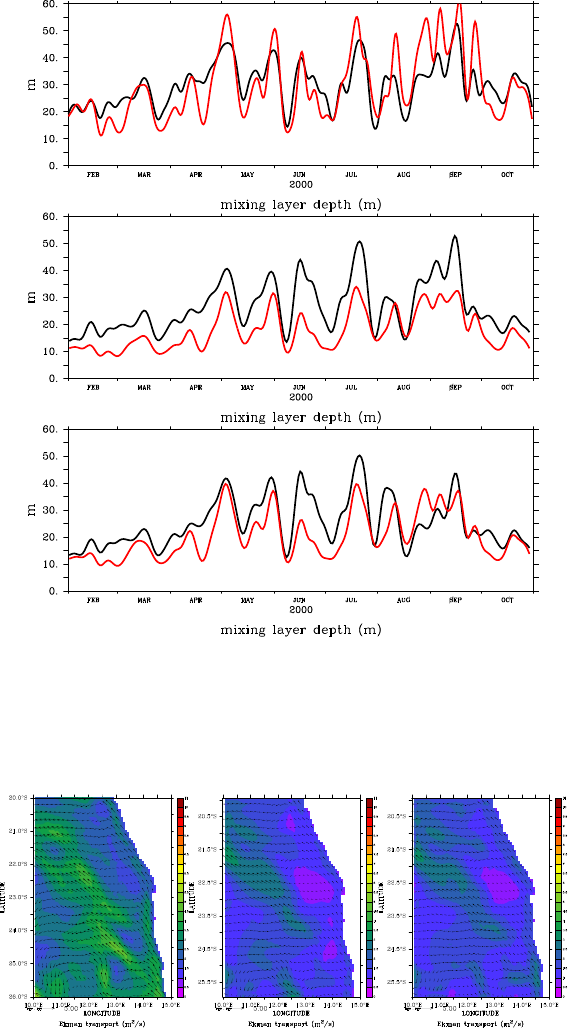
EASTERN UPWELLING AREA TEST CASE 355
Figure 34.3 The mixing layer depth for the large scale model (upper part), mom4p1 and
wind stress from Monin-Obukhov similarity approach (middle) and mom4p1
and wind stress for a neutral boundary layer. Black lines for 11◦E and 21◦S,
where the boundary layer is often unstable, red dots from 14◦E and 25◦S in
the upwelling area with cold SST and a stable boundary layer.
Figure 34.4 The vertically integrated transport in the mixing layer averaged from 2th March
2000 to 12th March 2000. Colours show the modulus. Left hand side the large
scale model, middle mom4p1 with Monin-Obukhov wind stress, right hand side
mom4p1 with neutral wind stress.

356 CHAPTER 34
Figure 34.5 The vertically integrated transport in the mixing layer averaged from 2th
September 2000 to 12th September 2000. Colours show the modulus. Left hand
side the large scale model, middle mom4p1 with Monin-Obukhov wind stress,
right hand side mom4p1 with neutral wind stress.
jet and the direction may be reversed as shown in Figure 34.7.
Figure 34.6 Salinity and undercurrent in 80 m depth averaged from 2th March 2000 to 12th
March 2000. Left hand side the large scale model, middle mom4p1 with Monin-
Obukhov wind stress, right hand side mom4p1 with neutral wind stress.
The regional model performs well at the shelf, but the strong salinity signal at
the western boundary cannot enter the model domain properly. Instead a strong
along boundary current develops, which balances the pressure baroclinic pressure
gradient. Again, the regional model with the stronger wind stress (neutral boundary
layer scheme) is closer to the large scale model.
The cross shelf circulation
For the Namibian shelf the cross shelf circulation is an essential feature for the
ecosystem dynamics. With the cross shelf circulation oxygen is advected onto the
shelf which ventilates the shelf bottom water. The ability of the regional model to
reproduce this part of the circulation system is very important.
Figures 34.8 and 34.9 show a typical upwelling dominated circulation. For March
2000 results from the large scale and the regional model are very similar. Note the
tongue of more saline water in 60 m depth generated by the differential advection,
which is also verified by field data. Upwelling goes along with a northward coastal
jet within a narrow band at the coast. The figures reveal the vertical structure of the
poleward undercurrent which is detached from the coast. In September 2000 its
deeper parts move off-shore, but there develops a new core near the coast in about
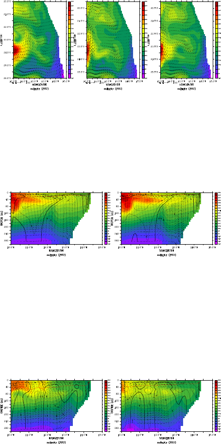
EASTERN UPWELLING AREA TEST CASE 357
Figure 34.7 Salinity and current in 80 m depth averaged from 2th September 2000 to 12th
September 2000. Left hand side the large scale model, middle mom4p1 with
Monin-Obukhov wind stress, right hand side mom4p1 with neutral wind stress.
Figure 34.8 Salinity and cross shelf circulation at 23◦S averaged from 2th March 2000 to
12th March 2000. Left hand side the large scale model, right hand side mom4p1
with neutral wind stress. The red line marks the mixing layer depth, the con-
tours the meridional currents. The vertical velocity is scaled with the figures
aspect ratio.
Figure 34.9 Salinity and cross shelf circulation at 23◦S averaged from 2th September 2000
to 12th September 2000. Left hand side the large scale model, right hand side
mom4p1 with neutral wind stress. The red line marks the mixing layer depth,
the contours the meridional currents. The vertical velocity is scaled with the
figures aspect ratio.
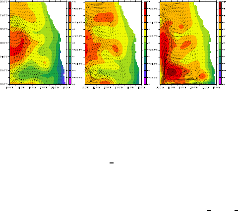
358 CHAPTER 34
40 m depth. There are differences between the large scale and the regional model
in many details, but the general structure of the circulation pattern and the salinity
distribution is the same. Especially near the western boundary the saline water
appears deflected to the west in the regional model. Some strong upward vertical
current develops, which is not in the large scale model. It should stem mostly from
the inconsistency in the forcing of both models, which has to be smoothed by the
open boundary condition.
A remark about the atmosphere pressure
Inclusion of atmosphere pressure gradients to the surface forcing is often consid-
ered as a marginal issue and minor correction because the sea level elevation
rapidly adjusts to the air pressure. Slowly varying air pressure gradients are com-
pensated by sea level elevations of the opposite sign and geostrophic currents bal-
anced by surface pressure gradients should not be very different with and without
air pressure. However, for a regional model with prescribed sea level elevation at
the open boundaries a reference level for the sea level is defined. An air pressure
gradient imposed to the model acts in the same manner as a prescribed sea level
gradient at the boundary, if the boundary data are not produced consistently with
this model configuration. This may happen, when the boundary data come from
a model, which does not include air pressure gradients, but the regional model is
run with air pressure “switched on”, or vice versa.
Figure 34.10 The sea level elevation in m and the vertically integrated velocity in m2s−1
averaged from 2th September 2000 to 12th September 2000. Left hand side the
large scale model, middle mom4p1 with air pressure taken into account, right
hand side mom4p1 with no air pressure gradients in the surface pressure.
The regional model of test case mom4 atlantic covers parts of the St.-Helena
high pressure are, whose persistent pressure gradients are responsible for the
permanent trade winds off Namibia. The boundary data from the large scale
model consider air pressure, but the default of mom4p1 is to have air pressure dis-
abled. For the experiments discussed above, it is enabled in ice model nml defining
slp2ocean=.true..
In the surface currents, the influence of the wind stress dominates, but the
deeper currents depend strongly on the a consistent treatment of air pressure
in the boundary conditions. This should be clearly shown by Figure 34.10, where
the regional model drifts away from the large model, when air pressure is not con-
sidered. However, in this case the eddy does not appear, which develops near the
northern boundary in the regional model with air pressure.
EASTERN UPWELLING AREA TEST CASE 359
Skills, shortcomings and limitations
The test case demonstrates, that OBC are suitable to drive a regional model with
boundary data taken from another model. Many deviations between the results of
the large reference model and the regional model can be traced back to different
numerics and parameters. The numerical scheme used at the boundaries can be
configured, to keep the influence of these deviations small and allows for reliable
experiments with the regional model. However, one must be aware, that some
perturbations generated near the boundaries may propagate as eddies into the
model interior. Hence, mesoscale processes may be modified by perturbations
from the OBC. The probability of such effects is increasing with the inconsistency
between regional model dynamics and prescribed boundary values.
This test case is an extreme application in so far, that the length of open bound-
aries is large. For a semi-enclosed sea with a small connection to the open ocean
the influence of the OBC scheme on the model results should be smaller.
It must be also noted, that the model area is situated within an eastern boundary
current. Hence, artificial Rossby waves generated at the open boundaries are
leaving the model domain. A similar test case within a western boundary current
was not tested yet.

Bibliography
Adcroft, A. and Campin, J.-M.: Rescaled height coordinates for accurate repre-
sentation of free-surface flows in ocean circulation models, Ocean Modelling, 7,
269–284, 2004.
Adcroft, A. and Hallberg, R. W.: On methods for solving the oceanic equations of
motion in generalized vertical coordinates, Ocean Modelling, 11, 224–233, 2006.
Adcroft, A., Hill, C., and Marshall, J.: Representation of topography by shaved
cells in a height coordinate ocean model, Monthly Weather Review, 125, 2293–
2315, 1997.
Aiki, H., Jacobson, T., and Yamagata, T.: Parameterizing ocean eddy transports
from surface to bottom, Journal of Geophysical Research, 31, 2004.
Asselin, R.: Frequency filter for time integrations, Monthly Weather Review, 100,
487–490, 1972.
Beckmann, A. and D¨oscher, R.: A method for improved representation of dense
water spreading over topography in geopotential-coordinate models, Journal of
Physical Oceanography, 27, 581–591, 1997.
Black, T. L.: The new NMC mesoscale eta model: description and forecast exam-
ples, Weather and Forecasting, 9, 265–278, 1994.
Blumberg, A. and Kantha, L.: Open boundary condition for circulation models,
Journal of Hydraulic Engineering, 111, 237–255, 1985.
Bryan, K.: A numerical method for the study of the circulation of the world ocean,
Journal of Computational Physics, 4, 347–376, 1969.
Bryan, K.: Michael Cox (1941-1989): his pioneering contributions to ocean circula-
tion modeling, Journal of Physical Oceanography, 21, 1259–1270, 1991.
Bryan, K. and Lewis, L. J.: A water mass model of the world ocean, Journal of
Geophysical Research, 84, 2503–2517, 1979.
Callen, H. B.: Thermodynamics and an Introduction to Thermostatics, John Wiley
and Sons, New York, 493 + xvi pp, 1985.
Camerlengo, A. and O’Brien, J.: Open boundary condition in rotating fluids, Jour-
nal of Computational Physics, 35, 12–35, 1980.
362 BIBLIOGRAPHY
Campin, J.-M. and Goosse, H.: Parameterization of density-driven downsloping
flow for a coarse-resolution ocean model in z-coordinate, Tellus, 51A, 412–430,
1999.
Campin, J.-M., Adcroft, A., Hill, C., and Marshall, J.: Conservation of properties
in a free-surface model, Ocean Modelling, 6, 221–244, 2004.
Chapman, D.: Numerical treatment of cross-shelf boundaries in a barotropic
coastal ocean model, Journal of Physical Oceanography, 103(C1), 1060–1075,
1985.
Chassignet, E. P. and Verron, J.: Ocean Weather Forecasting: an Integrated View of
Oceanography, Springer Publishers, 2005.
Chelton, D. B., DeSzoeke, R. A., Schlax, M. G., Naggar, K. E., and Siwertz, N.:
Geographical Variability of the First Baroclinic Rossby Radius of Deformation,
Journal of Physical Oceanography, 28, 433–460, 1998.
Chen, D., Rothstein, L., and Busalacchi, A.: A hybrid vertical mixing scheme and
its application to tropical ocean models, Journal of Physical Oceanography, 24,
2156–2179, 1994.
Cox, M. D.: A Primitive Equation, 3-Dimensional Model of the Ocean,
NOAA/Geophysical Fluid Dynamics Laboratory, Princeton, USA, 1984.
Danabasoglu, G. and McWilliams, J. C.: Sensitivity of the global ocean circulation
to parameterizations of mesoscale tracer transports, Journal of Climate, 8, 2967–
2987, 1995.
Delworth, T. L., Broccoli, A. J., Rosati, A., Stouffer, R. J., Balaji, V., Beesley, J. A.,
Cooke, W. F., Dixon, K. W., Dunne, J., Dunne, K. A., Durachta, J. W., Findell,
K. L., Ginoux, P., Gnanadesikan, A., Gordon, C., Griffies, S. M., Gudgel, R.,
Harrison, M. J., Held, I. M., Hemler, R. S., Horowitz, L. W., Klein, S. A., Knutson,
T. R., Kushner, P. J., Langenhorst, A. L., Lee, H.-C., Lin, S., Lu, L., Malyshev,
S. L., Milly, P., Ramaswamy, V., Russell, J., Schwarzkopf, M. D., Shevliakova, E.,
Sirutis, J., Spelman, M., Stern, W. F., Winton, M., Wittenberg, A. T., Wyman, B.,
Zeng, F., and Zhang, R.: GFDL’s CM2 Global Coupled Climate Models - Part
1: Formulation and Simulation Characteristics, Journal of Climate, 19, 643–674,
2006.
DeSzoeke, R. A. and Samelson, R. M.: The duality between the Boussinesq and
Non-Boussinesq Hydrostatic Equations of Motion, Journal of Physical Oceanog-
raphy, 32, 2194–2203, 2002.
Diansky, N., Bagno, A., and Zalensy, V.: Global ocean circulation sigma-model
and its sensitivity to the wind stress forcing., Izvestia, Atmospheric and Oceanic
Physics, 38, 477–494, 2002.
D¨oscher, R. and Beckmann, A.: Effects of a bottom boundary layer parameteriza-
tion in a coarse-resolution model of the North Atlantic Ocean, Journal of Atmo-
spheric and Oceanic Technology, 17, 698–707, 2000.
BIBLIOGRAPHY 363
Dunne, J. P., Armstrong, R., Gnanadesikan, A., and Sarmiento, J.: Empirical and
mechanistic models for the particle export ratio, Global Biogeochemical Cycles,
19, doi:10.1029/2004GB002390, 2005.
Durran, D. R.: Numerical Methods for Wave Equations in Geophysical Fluid Dy-
namics, Springer Verlag, Berlin, 470 pp, 1999.
England, M. H.: The age of water and ventilation timescales in a global ocean
model, Journal of Physical Oceanography, 25, 2756–2777, 1995.
Ezer, T., Arango, H., and Shchepetkin, A. F.: Developments in terrain-following
ocean models: Intercomparisons of numerical aspects, Ocean Modelling, 4, 249–
267, 2002.
Ferrari, R. and McWilliams, J.: Parameterization of eddy fluxes near oceanic
boundaries, Journal of Climate, submitted, 2007.
Ferreira, D. and Marshall, J.: Formulation and implementation of a residual-mean
ocean circulation model, Ocean Modelling, 13, 86–107, 2006.
Ferreira, D., Marshall, J., and Heimbach, P.: Estimating eddy stresses by fitting
dynamics to observations using a residual-mean ocean circulation model and
its adjoint, Journal of Physical Oceanography, 35, 1891–1910, 2005.
Gent, P. R. and McWilliams, J. C.: Isopycnal mixing in ocean circulation models,
Journal of Physical Oceanography, 20, 150–155, 1990.
Gent, P. R., Willebrand, J., McDougall, T. J., and McWilliams, J. C.: Parameterizing
eddy-induced tracer transports in ocean circulation models, Journal of Physical
Oceanography, 25, 463–474, 1995.
Gerdes, R., K¨oberle, C., and Willebrand, J.: The influence of numerical advection
schemes on the results of ocean general circulation models., Climate Dynamics,
5, 211–226, 1991.
Gill, A.: Atmosphere-Ocean Dynamics, vol. 30 of International Geophysics Series,
Academic Press, London, 662 + xv pp, 1982.
Gnanadesikan, A., Dixon, K. W., Griffies, S. M., Balaji, V., Beesley, J. A., Cooke,
W. F., Delworth, T. L., Gerdes, R., Harrison, M. J., Held, I. M., Hurlin, W. J., Lee,
H.-C., Liang, Z., Nong, G., Pacanowski, R. C., Rosati, A., Russell, J., Samuels,
B. L., Song, S. M., , Spelman, M. J., Stouffer, R. J., Sweeney, C. O., Vecchi, G.,
Winton, M., Wittenberg, A. T., Zeng, F., and Zhang, R.: GFDL’s CM2 Global
Coupled Climate Models-Part 2: The Baseline Ocean Simulation, Journal of Cli-
mate, 19, 675–697, 2006a.
Gnanadesikan, A., Griffies, S., and Samuels, B.: Effects in a climate model of slope
tapering in neutral physics schemes, Ocean Modelling, accepted, 2006b.
Greatbatch, R. J.: Exploring the relationship between eddy-induced transport ve-
locity, vertical momentum transfer, and the isopycnal flux of potential vorticity,
Journal of Physical Oceanography, 28, 422–432, 1998.
364 BIBLIOGRAPHY
Greatbatch, R. J. and Lamb, K. G.: On parameterizing vertical mixing of momen-
tum in non-eddy resolving ocean models, Journal of Physical Oceanography, 20,
1634–1637, 1990.
Greatbatch, R. J. and McDougall, T. J.: The non-Boussinesq temporal-residual-
mean, Journal of Physical Oceanography, 33, 1231–1239, 2003.
Greatbatch, R. J. and Mellor, G. L.: An overview of coastal ocean models, in Coastal
Ocean Prediction, edited by C. Mooers, vol. 56 of Coastal and Estuarine Studies,
pp. 31–57, American Geophysical Union, 1999.
Griffies, S. M.: The Gent-McWilliams skew-flux, Journal of Physical Oceanogra-
phy, 28, 831–841, 1998.
Griffies, S. M.: Fundamentals of ocean climate models, Princeton University Press,
Princeton, USA, 518+xxxiv pages, 2004.
Griffies, S. M.: Some Ocean Model Fundamentals, in GODAE Summer School,
edited by E. P. Chassignet and J. Verron, pp. 19–74, Springer/Kluwer, 2005.
Griffies, S. M.: Elements of mom4p1, NOAA/Geophysical Fluid Dynamics Labo-
ratory, Princeton, USA, 346 pp, 2007.
Griffies, S. M. and Hallberg, R. W.: Biharmonic friction with a Smagorinsky vis-
cosity for use in large-scale eddy-permitting ocean models, Monthly Weather
Review, 128, 2935–2946, 2000.
Griffies, S. M., Gnanadesikan, A., Pacanowski, R. C., Larichev, V., Dukowicz, J. K.,
and Smith, R. D.: Isoneutral diffusion in a z-coordinate ocean model, Journal of
Physical Oceanography, 28, 805–830, 1998.
Griffies, S. M., B¨oning, C., Bryan, F. O., Chassignet, E. P., Gerdes, R., Hasumi,
H., Hirst, A., Treguier, A.-M., and Webb, D.: Developments in Ocean Climate
Modelling, Ocean Modelling, 2, 123–192, 2000a.
Griffies, S. M., Pacanowski, R. C., and Hallberg, R. W.: Spurious diapycnal mix-
ing associated with advection in a z-coordinate ocean model, Monthly Weather
Review, 128, 538–564, 2000b.
Griffies, S. M., Pacanowski, R., Schmidt, R., and Balaji, V.: Tracer Conservation
with an Explicit Free Surface Method for z-coordinate Ocean Models, Monthly
Weather Review, 129, 1081–1098, 2001.
Griffies, S. M., Harrison, M. J., Pacanowski, R. C., and Rosati, A.: A Technical
Guide to MOM4, NOAA/Geophysical Fluid Dynamics Laboratory, Princeton,
USA, 337 pp, 2004.
Griffies, S. M., Gnanadesikan, A., Dixon, K. W., Dunne, J. P., Gerdes, R., Harrison,
M. J., Rosati, A., Russell, J., Samuels, B. L., Spelman, M. J., Winton, M., and
Zhang, R.: Formulation of an ocean model for global climate simulations, Ocean
Science, 1, 45–79, 2005.
BIBLIOGRAPHY 365
Griffies, S. M., Biastoch, A., B ¨oning, C., Bryan, F., Chassignet, E., England, M.,
Gerdes, R., Haak, H., Hallberg, R. W., Hazeleger, W., Jungclaus, J., Large, W. G.,
Madec, G., Samuels, B. L., Scheinert, M., Severijns, C. A., Simmons, H. L.,
Treguier, A. M., Winton, M., Yeager, S., and Yin, J.: Coordinated Ocean-ice Ref-
erence Experiments (COREs), in prep, 2007.
Hallberg, R. W.: Stable split time stepping schemes for large-scale ocean modeling,
Journal of Computational Physics, 135, 54–65, 1997.
Hallberg, R. W.: Time integration of diapycnal diffusion and Richardson number-
dependent mixing in isopycnal coordinate ocean models., Monthly Weather Re-
view, 128, 1402–1419, 2000.
Haltiner, G. T. and Williams, R. T.: Numerical Prediction and Dynamic Meteorol-
ogy, John Wiley and Sons, New York, USA, 1980.
Held, I. M. and Schneider, T.: The surface branch of the zonally averaged mass
transport circulation in the troposphere, Journal of Atmospheric Sciences, 56,
1688–1697, 1999.
Hendershott, M.: The effects of solid earth deformation on global ocean tide, Geo-
physical Journal of the Royal Astronomical Society, 29, 389–402, 1972.
Hirsch, C.: Numerical Computation of Internal and External Flows, John Wiley
and Sons, 1988.
Holland, W. R., Chow, J. C., and Bryan, F. O.: Application of a third-order upwind
scheme in the NCAR ocean model, Journal of Climate, 11, 1487–1493, 1998.
Holloway, G.: Representing Topographic Stress for Large-Scale Ocean Models,
Journal of Physical Oceanography, 22, 1033–1046, 1992.
Holloway, G.: Moments of probable seas: statistical dynamics of Planet Ocean,
Physica D, 133, 199–214, 1999.
Huang, R. X.: Real freshwater flux as a natural boundary condition for the salinity
balance and thermohaline circulation forced by evaporation and precipitation,
Journal of Physical Oceanography, 23, 2428–2446, 1993.
Huang, R. X., Jin, X., and Zhang, X.: An oceanic general circulation model in pres-
sure coordinates, Advances in Atmospheric Physics, 18, 1–22, 2001.
Hundsdorfer, W. and Trompert, R.: Method of lines and direct discretization: a
comparison for linear advection, Applied Numerical Mathematics, pp. 469–490,
1994.
Jackett, D. R., McDougall, T. J., Feistel, R., Wright, D. G., and Griffies, S. M.: Algo-
rithms for density, potential temperature, conservative temperature, and freez-
ing temperature of seawater, Journal of Atmospheric and Oceanic Technology,
23, 1709–1728, 2006.
Jayne, S. and St.Laurent, L. C.: Parameterizing tidal dissipation over rough topog-
raphy, Geophysical Research Letters, 28, 811–814, 2001.
366 BIBLIOGRAPHY
Killworth, P. D. and Edwards, N.: A turbulent bottom boundary layer code for use
in numerical ocean models, Journal of Physical Oceanography, 29, 1221–1238,
1999.
Killworth, P. D., Stainforth, D., Webb, D. J., and Paterson, S. M.: The development
of a free-surface Bryan-Cox-Semtner ocean model, Journal of Physical Oceanog-
raphy, 21, 1333–1348, 1991.
Klymak, J., Moum, J., Nash, J., Kunze, E., Girton, J., Carter, G., Lee, C., Sanford, T.,
and Gregg, M.: An estimate of tidal energy lost to turbulence at the Hawaiian
Ridge, Journal of Physical Oceanography, submitted, 2005.
Landau, L. D. and Lifshitz, E. M.: Mechanics, Pergamon Press, Oxford, UK, 170
pp, 1976.
Large, W. and Yeager, S.: Diurnal to decadal global forcing for ocean and
sea-ice models: the data sets and flux climatologies, NCAR Technical Note:
NCAR/TN-460+STR, CGD Division of the National Center for Atmospheric Re-
search, 2004.
Large, W. G. and Pond, S.: Open ocean momentum flux measurements in moder-
ate to strong winds, Journal of Physical Oceanography, 11, 324–336, 1981.
Large, W. G., McWilliams, J. C., and Doney, S. C.: Oceanic vertical mixing: A
review and a model with a nonlocal boundary layer parameterization, Reviews
of Geophysics, 32, 363–403, 1994.
Large, W. G., Danabasoglu, G., Doney, S. C., and McWilliams, J. C.: Sensitivity
to surface forcing and boundary layer mixing in a global ocean model: annual-
mean climatology, Journal of Physical Oceanography, 27, 2418–2447, 1997.
Large, W. G., Danabasoglu, G., McWilliams, J. C., Gent, P. R., and Bryan, F. O.:
Equatorial circulation of a global ocean climate model with anisotropic horizon-
tal viscosity, Journal of Physical Oceanography, 31, 518–536, 2001.
Laurent, L. C. S., Toole, J., and Schmitt, R.: Buoyancy forcing by turbulence above
rough topography in the abyssal Brazil Basin, Journal of Physical Oceanogra-
phy, 31, 3476–3495, 2001.
Ledwell, J. R., Watson, A. J., and Law, C. S.: Evidence for slow mixing across the
pycnocline from an open-ocean tracer-release experiment, Nature, 364, 701–703,
1993.
Lee, H.-C., Rosati, A., and Spelman, M.: Barotropic tidal mixing effects in a cou-
pled climate model: Oceanic conditions in the northern Atlantic, Ocean Mod-
elling, 3-4, 464–477, 2006.
Legg, S., Hallberg, R., and Girton, J.: Comparison of entrainment in overflows
simulated by z-coordinate, isopycnal and non-hydrostatic models, Ocean Mod-
elling, 11, 69–97, 2006.
BIBLIOGRAPHY 367
Leonard, B. P.: A stable and accurate convective modelling procedure based on
quadratic upstream interpolation, Computer Methods in Applied Mechanics
and Engineering, 19, 59–98, 1979.
Lin, S. J.: A finite volume integration method for computing pressure gradient
force in general vertical coordinates, Quarterly Journal of the Royal Meteoro-
logical Society, 123, 1749–1762, 1997.
Losch, M., Adcroft, A., and Campin, J.-M.: How sensitive are coarse general cir-
culation models to fundamental approximations in the equations of motion?,
Journal of Physical Oceanography, 34, 306–319, 2004.
Marchesiello, J. M. P. and Shchepetkin, A.: Open boundary conditions for long-
term integration of regional oceanic models, Ocean Modelling, 3, 1–20, 2001.
Marchuk and Kagan: Dynamics of Ocean Tides, Kluwer Academic, 1989.
Marion, J. B. and Thornton, S. T.: Classical Dynamics of Particles and Systems,
Harcourt Brace Jovanovich, San Diego, USA, 602 pp, 1988.
Marotzke, J.: Influence of convective adjustment on the stability of the thermoha-
line circulation, Journal of Physical Oceanography, 21, 903–907, 1991.
Marshall, J. and Schott, F.: Open-ocean convection: observations, theory, and mod-
els, Reviews of Geophysics, 37, 1–64, 1999.
Marshall, J., Hill, C., Perelman, L., and Adcroft, A.: Hydrostatic, quasi-hydrostatic,
and nonhydrostatic ocean modeling, Journal of Geophysical Research, 102,
5733–5752, 1997.
Marshall, J., Adcroft, A., Campin, J.-M., and Hill, C.: Atmosphere-Ocean model-
ing exploiting fluid isomorphisms, Journal of Physical Oceanography, in press,
2004.
Martinsen, E. and Engedahl, H.: Implementation and testing of a lateral boundary
scheme as an open boundary condition in a barotropic ocean model, Coastal
Engineering, 11, 603–627, 1987.
McDougall, T. J.: Thermobaricity, cabbeling, and water-mass conversion, Journal
of Geophysical Research, 92, 5448–5464, 1987.
McDougall, T. J.: The influence of ocean mixing on the absolute velocity vector,
Journal of Physical Oceanography, 25, 705–725, 1995.
McDougall, T. J.: Potential enthalpy: a conservative oceanic variable for evaluating
heat content and heat fluxes., Journal of Physical Oceanography, 33, 945–963,
2003.
McDougall, T. J. and McIntosh, P. C.: The temporal-residual-mean velocity. Part
II: isopycnal interpretation and the tracer and momentum equations., Journal of
Physical Oceanography, 31, 1222–1246, 2001.
368 BIBLIOGRAPHY
McDougall, T. J., Greatbatch, R. J., and Lu, Y.: On conservation Equations in
Oceanography: How Accurate are Boussinesq Ocean Models?, Journal of Phys-
ical Oceanography, 32, 1574–1584, 2003a.
McDougall, T. J., Jackett, D. R., Wright, D. G., and Feistel, R.: Accurate and com-
putationally efficient algorithms for potential temperature and density of sea-
water., Journal of Atmospheric and Oceanic Technology, 20, 730–741, 2003b.
Merryfield, W. J. and Holloway, G.: Application of an accurate advection algo-
rithm to sea-ice modelling, Ocean Modelling, 5, 1–15, 2003.
Mesinger, F.: A method for construction of second-order accurate difference
schemes permitting no false two-grid-interval waves in the height field., Tellus,
25, 444–457, 1973.
Mesinger, F. and Arakawa, A.: Numerical Methods used in Atmospheric Models,
in GARP Publication Series, vol. 1, p. 66 pages, 1976.
Miller, M. and Thorpe, A.: Radiation conditions for the lateral boundaries of
limited-area numerical models, Quarterly Journal of the Royal Meteorological
Society, 107, 615–628, 1981.
Morel, A. and Antoine, D.: Heating rate within the upper ccean in relation to its
bio-optical state, Journal of Physical Oceanography, 24, 1652–1665, 1994.
Moum, J., Caldwell, D., Nash, J., and Gunderson, G.: Observations of boundary
mixing over the continental slope, Journal of Physical Oceanography, 32, 2113–
2130, 2002.
Munk, W. and Anderson, E.: Notes on a theory of the thermocline, Journal of
Marine Research, 3, 276–295, 1948.
Murray, R. J.: Explicit generation of orthogonal grids for ocean models, Journal of
Computational Physics, 126, 251–273, 1996.
O’Brien, J. J.: Advanced Physical Oceanographic Numerical Modelling, D. Reidel
Publishing Company, 1986.
Ohlmann, J.: Ocean Radiant Heating in Climate Models, JOC, 16, 1337–1351, 2003.
Orlanski, I.: A simple boundary condition for unbounded hyberbolic flows, Jour-
nal of Computational Physics, 21, 251–269, 1976.
Osborn, T. R.: Estimates of the local rate of vertical diffusion from dissipation
measurements, Journal of Physical Oceanography, 10, 83–89, 1980.
Pacanowski, R. C.: Effect of equatorial currents on surface stress, Journal of Phys-
ical Oceanography, 17, 833–838, 1987.
Pacanowski, R. C.: MOM2 Documentation, User’s Guide, and Reference Manual,
NOAA/Geophysical Fluid Dynamics Laboratory, Princeton, USA, 216 pp, 1995.
BIBLIOGRAPHY 369
Pacanowski, R. C. and Gnanadesikan, A.: Transient response in a z-level ocean
model that resolves topography with partial-cells, Monthly Weather Review,
126, 3248–3270, 1998.
Pacanowski, R. C. and Griffies, S. M.: The MOM3 Manual, NOAA/Geophysical
Fluid Dynamics Laboratory, Princeton, USA, 680 pp, 1999.
Pacanowski, R. C. and Philander, G.: Parameterization of vertical mixing in nu-
merical models of the tropical ocean, Journal of Physical Oceanography, 11,
1442–1451, 1981.
Pacanowski, R. C., Dixon, K., and Rosati, A.: The GFDL Modular Ocean Model
User Guide, NOAA/Geophysical Fluid Dynamics Laboratory, Princeton, USA,
16 pp, 1991.
Palma, E. and Matano, R.: On the implementation of passive open boundary con-
ditions for a general circulation model: The barotropic mode, Journal of Geo-
physical Research, 103(C1), 1319–1341, 1998.
Palma, E. and Matano, R.: Dynamical impacts associated with radiation boundary
conditions, Journal of Sea Research, 46, 117–132, 2001.
Peixoto, J. P. and Oort, A. H.: Physics of Climate, American Institute of Physics,
520 + xxxix pp, 1992.
Pickard, G. L. and Emery, W. J.: Descriptive Physical Oceanography, Pergamon
Press, Oxford, 5th edn., 1990.
Polzin, K. L., Toole, J. M., Ledwell, J. R., and Schmitt, R. W.: Spatial variability of
turbulent mixing in the abyssal ocean, Science, 276, 93–96, 1997.
Prather, M.: Numerical advection by conservation of second-order moments, Jour-
nal of Geophysical Research, 91, 6671–6681, 1986.
Rahmstorf, S.: A fast and complete convection scheme for ocean models, Ocean
Modelling, 101, 9–11, 1993.
Ray, R. D.: Ocean self-attraction and loading in numerical tidal models, Marine
Geodesy, 21, 181–192, 1998.
Raymond, W. and Kuo, H.: A radiation boundary condition for multidimensional
flows, Quaterly Journal of the Royal Meterological Society, 110, 535–551, 1984.
Redi, M. H.: Oceanic isopycnal mixing by coordinate rotation., Journal of Physical
Oceanography, 12, 1154–1158, 1982.
Robert, A.: The integration of a low order spectral form of the primitive meteo-
rological equations, Journal of the Meteorological Society of Japan, 44, 237–244,
1966.
Roed, L. and Cooper, C.: A study of various open boundary conditions for wind-
forced barotropic numerical ocean models, in Three-dimensional Models of ma-
rine and Estuarine Dynamics, edited by J. Nihoul and B. Jamart, pp. 305–335,
Elsevier, 1987.
370 BIBLIOGRAPHY
Shchepetkin, A. and McWilliams, J.: A method for computing horizontal pressure-
gradient force in an ocean model with a non-aligned vertical coordinate, Journal
of Geophysical Research, 108, 35.1–35.34, 2002.
Simmons, H. L., Jayne, S. R., Laurent, L. C. S., and Weaver, A. J.: Tidally driven
mixing in a numerical model of the ocean general circulation, Ocean Modelling,
6, 245–263, 2004.
Smith, K. S. and Vallis, G. K.: The scales and equilibration of midocean eddies:
forced-dissipative flow, Journal of Physical Oceanography, 32, 1699–1721, 2002.
Smith, R. D. and McWilliams, J. C.: Anisotropic horizonal viscosity for ocean mod-
els, Ocean Modelling, 5, 129–156, 2003.
Smith, W. H. F. and Sandwell, D. T.: Global seafloor topography from satellite
altimetry and ship depth soundings, Science, 277, 1957–1962, 1997.
Sommerfeld, A.: Partial differential equations. Lectures in Theoretical Physics 6,
Academic Press, New York, 1949.
Stacey, M. W., Pond, S., and Nowak, Z. P.: A Numerical Model of the Circulation
in Knight Inlet, British Columbia, Canada, Journal of Physical Oceanography,
25, 1037–1062, 1995.
Stevens, D. P.: On open boundary conditions for three dimensional primitive equa-
tion ocean circulation models, Geophysical and Astrophysical Fluid Dynamics,
51, 103–133, 1990.
Stevens, D. P.: The open boundary conditions in the United Kingdom Fine-
Resolution Antarctic Model, Journal of Physical Oceanography, 21, 1494–1499,
1991.
St.Laurent, L. C., Simmons, H., and Jayne, S.: Estimating tidally driven energy in
the deep ocean, Geophysical Research Letters, 29, 2106–2110, 2002.
St.Laurent, L. C., Stringer, S., Garrett, C., and Perrault-Joncas, D.: The generation
of internal tides at abrupt topography, Deep-Sea Research, 50, 987–1003, 2003.
Stouffer, R. J., Broccoli, A., Delworth, T., Dixon, K., Gudgel, R., Held, I., Hemler,
R., Knutsn, T., Lee, H.-C., Schwarzkopf, M., Soden, B., Spelman, M., Winton,
M., and Zeng, F.: GFDL’s CM2 Global coupled climate models: Part 4: idealized
climate response, Journal of Climate, 19, 723–740, 2006.
Sweby, P.: High-resolution schemes using flux limiters for hyperbolic
conservation-laws, SIAM Journal of Numerical Analysis, 21, 995–1011, 1984.
Sweeney, C., Gnanadesikan, A., Griffies, S. M., Harrison, M., Rosati, A., and
Samuels, B.: Impacts of shortwave penetration depth on large-scale ocean cir-
culation and heat transport, Journal of Physical Oceanography, 35, 1103–1119,
2005.
Tang, Y. and Grimshaw, R.: Radiation boundary conditions in barotropic coastal
ocean numerical models, Journal of Computational Physics, 123, 96–110, 1996.
BIBLIOGRAPHY 371
Tang, Y. and Roberts, M.: The impact of a bottom boundary layer scheme on the
North Atlantic Ocean in a global coupled climate model, Journal of Physical
Oceanography, 35, 202–217, 2005.
Thiele, G. and Sarmiento, J. L.: Tracer dating and ocean ventilation, Journal of
Geophysical Research, 95, 9377–9391, 1990.
Treguier, A. M., Held, I. M., and Larichev, V. D.: On the parameterization of
quasi-geostrophic eddies in primitive equation ocean models, Journal of Physi-
cal Oceanography, 27, 567–580, 1997.
Umlauf, L., Burchard, H., and Bolding, K.: GOTM: source code and test case doc-
umentation: version 3.2, 231pp, 2005.
Wahr, J.: Body Tides on an elliptical, rotating, elastic and oceanless earth, Geo-
physical Journal of the Royal Astronomical Society, 64, 677–703, 1998.
Winters, K. B. and D’Asaro, E. A.: Diascalar flux and the rate of fluid mixing,
Journal of Fluid Mechanics, 317, 179–193, 1995.
Winters, K. B., Lombard, P. N., Riley, J. J., and D’Asaro, E. A.: Available potential
energy and mixing in density-stratified fluids, Journal of Fluid Mechanics, 289,
115–128, 1995.
Winton, M., Hallberg, R. W., and Gnanadesikan, A.: Simulation of density-driven
frictional downslope flow in z-coordinate ocean models, Journal of Physical
Oceanography, 28, 2163–2174, 1998.
Wittenberg, A., Rosati, A., Lau, G., and Ploshay, J.: GFDL’s CM2 global coupled
climate models - Part 3: Tropical Pacific climate and ENSO, Journal of Climate,
19, 698–722, 2006.
