A Student's Guide To R MOSAIC Student
User Manual:
Open the PDF directly: View PDF ![]() .
.
Page Count: 121 [warning: Documents this large are best viewed by clicking the View PDF Link!]
- Introduction
- Getting Started with RStudio
- One Quantitative Variable
- One Categorical Variable
- Two Quantitative Variables
- Two Categorical Variables
- Quantitative Response, Categorical Predictor
- Categorical Response, Quantitative Predictor
- Survival Time Outcomes
- More than Two Variables
- Probability Distributions & Random Variables
- Power Calculations
- Data Management
- Health Evaluation (HELP) Study
- Exercises and Problems
- Bibliography
- Index
Nicholas J. Horton
Randall Pruim
Daniel T. Kaplan
A Student's
Guide to
R
Project MOSAIC
2 horton,kaplan,pruim
Copyright (c) 2018 by Nicholas J. Horton, Randall
Pruim, & Daniel Kaplan.
Edition 1.3, June 2018
This material is copyrighted by the authors under a
Creative Commons Attribution 3.0Unported License.
You are free to Share (to copy, distribute and transmit
the work) and to Remix (to adapt the work) if you
attribute our work. More detailed information about
the licensing is available at this web page: http:
//www.mosaic-web.org/go/teachingRlicense.html.
Cover Photo: Maya Hanna.
About These Notes
We present an approach to teaching introductory and in-
termediate statistics courses that is tightly coupled with
computing generally and with Rand RStudio in particular.
These activities and examples are intended to highlight
a modern approach to statistical education that focuses
on modeling, resampling based inference, and multivari-
ate graphical techniques. A secondary goal is to facilitate
computing with data through use of small simulation
studies and appropriate statistical analysis workflow. This
follows the philosophy outlined by Nolan and Temple
Lang1. The importance of modern computation in statis- 1D. Nolan and D. Temple Lang.
Computing in the statistics
curriculum. The American
Statistician,64(2):97–107,2010
tics education is a principal component of the recently
adopted American Statistical Association’s curriculum
guidelines2.2ASA Undergraduate Guide-
lines Workgroup. 2014 cur-
riculum guidelines for under-
graduate programs in statisti-
cal science. Technical report,
American Statistical Associa-
tion, November 2014.http:
//www.amstat.org/education/
curriculumguidelines.cfm
Throughout this book (and its companion volumes),
we introduce multiple activities, some appropriate for
an introductory course, others suitable for higher levels,
that demonstrate key concepts in statistics and modeling
while also supporting the core material of more tradi-
tional courses.
A Work in Progress
Caution!
Despite our best efforts, you
WILL find bugs both in this
document and in our code.
Please let us know when you
encounter them so we can call
in the exterminators.
These materials were developed for a workshop entitled
Teaching Statistics Using R prior to the 2011 United States
Conference on Teaching Statistics and revised for US-
COTS 2011, USCOTS 2013, eCOTS 2014, ICOTS 9, and
USCOTS 2015. We organized these workshops to help
instructors integrate R(as well as some related technolo-
gies) into statistics courses at all levels. We received great
feedback and many wonderful ideas from the participants
and those that we’ve shared this with since the work-
shops.
6 horton,kaplan,pruim
Consider these notes to be a work in progress. We ap-
preciate any feedback you are willing to share as we con-
tinue to work on these materials and the accompanying
mosaic package. Drop us an email at pis@mosaic-web.
org with any comments, suggestions, corrections, etc.
Updated versions will be posted at http://mosaic-web.
org.
Two Audiences
We initially developed these materials for instructors of
statistics at the college or university level. Another audi-
ence is the students these instructors teach. Some of the
sections, examples, and exercises are written with one or
the other of these audiences more clearly at the forefront.
This means that
1. Some of the materials can be used essentially as is with
students.
2. Some of the materials aim to equip instructors to de-
velop their own expertise in Rand RStudio to develop
their own teaching materials.
Although the distinction can get blurry, and what
works “as is" in one setting may not work “as is" in an-
other, we’ll try to indicate which parts fit into each cate-
gory as we go along.
R, RStudio and R Packages
Rcan be obtained from http://cran.r-project.org/.
Download and installation are quite straightforward for
Mac, PC, or linux machines.
RStudio is an integrated development environment
(IDE) that facilitates use of Rfor both novice and expert
users. We have adopted it as our standard teaching en-
vironment because it dramatically simplifies the use of R
for instructors and for students. RStudio can be installed
More Info
Several things we use that
can be done only in RStudio,
for instance manipulate() or
RStudio’s integrated support for
reproducible research).
as a desktop (laptop) application or as a server applica-
tion that is accessible to users via the Internet. RStudio server version works
well with starting students. All
they need is a web browser,
avoiding any potential prob-
lems with oddities of students’
individual computers.
In addition to Rand RStudio, we will make use of sev-
eral packages that need to be installed and loaded sep-
arately. The mosaic package (and its dependencies) will
a student’s guide to r 7
be used throughout. Other packages appear from time to
time as well.
Marginal Notes
Marginal notes appear here and there. Sometimes these Have a great suggestion for a
marginal note? Pass it along.
are side comments that we wanted to say, but we didn’t
want to interrupt the flow to mention them in the main
text. Others provide teaching tips or caution about traps,
pitfalls and gotchas.
What’s Ours Is Yours – To a Point
This material is copyrighted by the authors under a Cre-
ative Commons Attribution 3.0Unported License. You
are free to Share (to copy, distribute and transmit the
work) and to Remix (to adapt the work) if you attribute
our work. More detailed information about the licensing
is available at this web page: http://www.mosaic-web.
org/go/teachingRlicense.html.Digging Deeper
If you know L
A
T
EX as well as
R, then knitr provides a nice
solution for mixing the two. We
used this system to produce
this book. We also use it for
our own research and to intro-
duce upper level students to
reproducible analysis methods.
For beginners, we introduce
knitr with RMarkdown, which
produces PDF, HTML, or Word
files using a simpler syntax.
Document Creation
This document was created on June 13,2018, using
•knitr, version 1.20
•mosaic, version 1.2.0
•mosaicData, version 1.2.0
• R version 3.5.0(2018-04-23)
Inevitably, each of these will be updated from time to
time. If you find that things look different on your com-
puter, make sure that your version of Rand your pack-
ages are up to date and check for a newer version of this
document.
Kudos to Joseph Cappelleri for many useful com-
ments on earlier drafts of these materials and to Margaret
Chien for her work updating the examples to ggformula.
Project MOSAIC
This book is a product of Project MOSAIC, a community
of educators working to develop new ways to introduce
mathematics, statistics, computation, and modeling to
students in colleges and universities.
The goal of the MOSAIC project is to help share ideas
and resources to improve teaching, and to develop a cur-
ricular and assessment infrastructure to support the dis-
semination and evaluation of these approaches. Our goal
is to provide a broader approach to quantitative stud-
ies that provides better support for work in science and
technology. The project highlights and integrates diverse
aspects of quantitative work that students in science, tech-
nology, and engineering will need in their professional
lives, but which are today usually taught in isolation, if at
all.
In particular, we focus on:
Modeling The ability to create, manipulate and investigate
useful and informative mathematical representations of
a real-world situations.
Statistics The analysis of variability that draws on our
ability to quantify uncertainty and to draw logical in-
ferences from observations and experiment.
Computation The capacity to think algorithmically, to
manage data on large scales, to visualize and inter-
act with models, and to automate tasks for efficiency,
accuracy, and reproducibility.
Calculus The traditional mathematical entry point for col-
lege and university students and a subject that still has
the potential to provide important insights to today’s
students.
10 horton,kaplan,pruim
Drawing on support from the US National Science
Foundation (NSF DUE-0920350), Project MOSAIC sup-
ports a number of initiatives to help achieve these goals,
including:
Faculty development and training opportunities, such as the
USCOTS 2011, USCOTS 2013, eCOTS 2014, eCOTS
2016, eCOTS 2018, and ICOTS 9workshops on Teaching
Statistics Using Rand RStudio, our 2010 Project MO-
SAIC kickoff workshop at the Institute for Mathemat-
ics and its Applications, and our Modeling: Early and
Often in Undergraduate Calculus AMS PREP workshops
offered in 2012,2013, and 2015.
M-casts, a series of regularly scheduled webinars, de-
livered via the Internet, that provide a forum for in-
structors to share their insights and innovations and
to develop collaborations to refine and develop them.
Recordings of M-casts are available at the Project MO-
SAIC web site, http://mosaic-web.org.
The construction of syllabi and materials for courses that
teach MOSAIC topics in a better integrated way. Such
courses and materials might be wholly new construc-
tions, or they might be incremental modifications of
existing resources that draw on the connections be-
tween the MOSAIC topics.
More details can be found at http://www.mosaic-web.
org. We welcome and encourage your participation in all
of these initiatives.
Computational Statistics
There are at least two ways in which statistical software
can be introduced into a statistics course. In the first ap-
proach, the course is taught essentially as it was before
the introduction of statistical software, but using a com-
puter to speed up some of the calculations and to prepare
higher quality graphical displays. Perhaps the size of
the data sets will also be increased. We will refer to this
approach as statistical computation since the computer
serves primarily as a computational tool to replace pencil-
and-paper calculations and drawing plots manually.
In the second approach, more fundamental changes in
the course result from the introduction of the computer.
Some new topics are covered, some old topics are omit-
ted. Some old topics are treated in very different ways,
and perhaps at different points in the course. We will re-
fer to this approach as computational statistics because
the availability of computation is shaping how statistics is
done and taught. Computational statistics is a key com-
ponent of data science, defined as the ability to use data
to answer questions and communicate those results.
Students need to see aspects of
computation and data science
early and often to develop
deeper skills. Establishing
precursors in introductory
courses help them get started.
In practice, most courses will incorporate elements of
both statistical computation and computational statistics,
but the relative proportions may differ dramatically from
course to course. Where on the spectrum a course lies
will depend on many factors including the goals of the
course, the availability of technology for student use, the
perspective of the text book used, and the comfort-level of
the instructor with both statistics and computation.
Among the various statistical software packages avail-
able, Ris becoming increasingly popular. The recent addi-
tion of RStudio has made Rboth more powerful and more
accessible. Because Rand RStudio are free, they have be-
come widely used in research and industry. Training in R
12 horton,kaplan,pruim
and RStudio is often seen as an important additional skill
that a statistics course can develop. Furthermore, an in-
creasing number of instructors are using Rfor their own
statistical work, so it is natural for them to use it in their
teaching as well. At the same time, the development of R
and of RStudio (an optional interface and integrated de-
velopment environment for R) are making it easier and
easier to get started with R.
Information about the mosaic
package, including vignettes
demonstrating features and
supplementary materials (such
as this book) can be found at
https://cran.r-project.org/
web/packages/mosaic.
We developed the mosaic Rpackage (available on
CRAN) to make certain aspects of statistical computation
and computational statistics simpler for beginners, with-
out limiting their ability to use more advanced features of
the language. The mosaic package includes a modelling
approach that uses the same general syntax to calculate
descriptive statistics, create graphics, and fit linear mod-
els.
1
Introduction
In this reference book, we briefly review the commands
and functions needed to analyze data from introductory
and second courses in statistics. This is intended to com-
plement the Start Teaching with R and Start Modeling with
Rbooks.
Most of our examples will use data from the HELP
(Health Evaluation and Linkage to Primary Care) study:
a randomized clinical trial of a novel way to link at-risk
subjects with primary care. More information on the
dataset can be found in chapter 14.
Since the selection and order of topics can vary greatly
from textbook to textbook and instructor to instructor, we
have chosen to organize this material by the kind of data
being analyzed. This should make it straightforward to
find what you are looking for. Some data management
skills are needed by students1. A basic introduction to 1N.J. Horton, B.S. Baumer, and
H. Wickham. Setting the stage
for data science: integration
of data management skills
in introductory and second
courses in statistics (http:
//arxiv.org/abs/1401.3269).
CHANCE,28(2):40–50,2015
key idioms is provided in Chapter 13.
This work leverages initiatives undertaken by Project
MOSAIC (http://www.mosaic-web.org), an NSF-funded
effort to improve the teaching of statistics, calculus, sci-
ence and computing in the undergraduate curriculum.
In particular, we utilize the mosaic package, which was
written to simplify the use of Rfor introductory statis-
tics courses, and the mosaicData package which includes
a number of data sets. The ggformula package provides
support for high quality graphics using the mosaic mod-
eling language. A paper describing the mosaic approach
to teaching statistics and data science can be found at
https://journal.r-project.org/archive/2017/RJ-2017-024.
A short summary of the Rcommands needed to teach in-
troductory statistics can be found in the mosaic package
vignette: https://cran.r-project.org/web/packages/

14 horton,kaplan,pruim
mosaic.
Other related resources from Project MOSAIC may be
helpful, including an annotated set of examples from a
number of textbooks (see https://cran.r-project.org/
web/packages/mosaic/vignettes/mosaic-resources.
html).
To use a package within R, it must be installed (one
time), and loaded (each session). The mosaic package can
be installed using the following commands:
>install.packages("mosaic")# note the quotation marks
The #character is a comment in R, and all text after that
RStudio features a simplified
package installation tab (in the
bottom right panel).
on the current line is ignored.
Once the package is installed (one time only), it can be
loaded by running the command:
>library(mosaic)
># require(mosaic) can also be used to load packages
The knitr/L
A
T
EX system allows
experienced users to combine
Rand L
A
T
EX in the same docu-
ment. The reward for learning
this more complicated system
is much finer control over the
output format. But RMarkdown
is much easier to learn and is
adequate even for professional-
level work.
Using Markdown or
knitr/L
A
T
EX requires that the
markdown package be installed.
The RMarkdown system provides a simple markup
language and renders the results in PDF, Word, or HTML.
This allows students to undertake their analyses using a
workflow that facilitates “reproducibility” and avoids cut
and paste errors.
We typically introduce students to RMarkdown very
early, requiring students to use it for assignments and
reports2.2B.S. Baumer, M. Çetinkaya
Rundel, A. Bray, L. Loi, and
N. J. Horton. R Markdown:
Integrating a reproducible
analysis tool into introductory
statistics. Technology Innovations
in Statistics Education,8(1):281–
283,2014
2
Getting Started with RStudio
RStudio is an integrated development environment (IDE)
for Rthat provides an alternative interface to Rthat has
several advantages over other the default Rinterfaces:
A series of getting started
videos are available at
https://nhorton.people.
amherst.edu/rstudio.
•RStudio runs on Mac, PC, and Linux machines and pro-
vides a simplified interface that looks and feels identical
on all of them.
The default interfaces for Rare quite different on the
various platforms. This is a distractor for students and
adds an extra layer of support responsibility for the
instructor.
•RStudio can run in a web browser.
In addition to stand-alone desktop versions or in RStudio.
cloud,RStudio can be set up as a server application
that is accessed via the internet.
The web interface is nearly identical to the desktop
version. As with other web services, users login to Caution!
The desktop and server version
of RStudio are so similar that
if you run them both, you will
have to pay careful attention
to make sure you are working
in the one you intend to be
working in.
access their account. If students logout and login in
again later, even on a different machine, their session
is restored and they can resume their analysis right
where they left off. With a little advanced set up, in-
structors can save the history of their classroom Ruse
and students can load those history files into their own
environment. Note
Using RStudio in a browser is
like Facebook for statistics.
Each time the user returns, the
previous session is restored and
they can resume work where
they left off. Users can login
from any device with internet
access.
•RStudio provides support for reproducible research.
RStudio makes it easy to include text, statistical
analysis (Rcode and Routput), and graphical displays
all in the same document. The RMarkdown system
provides a simple markup language and renders the
results in HTML. The knitr/L
A
T
EX system allows users
16 horton,kaplan,pruim
to combine Rand L
A
T
EX in the same document. The
reward for learning this more complicated system is
much finer control over the output format. Depending
on the level of the course, students can use either of
these for homework and projects. To use Markdown or
knitr/L
A
T
EX requires that the
knitr package be installed on
your system.
•RStudio provides an integrated support for editing and
executing Rcode and documents.
•RStudio provides some useful functionality via a graph-
ical user interface.
RStudio is not a GUI for R, but it does provide a
GUI that simplifies things like installing and updating
packages; monitoring, saving and loading environ-
ments; importing and exporting data; browsing and
exporting graphics; and browsing files and documenta-
tion.
•RStudio provides access to the manipulate package.
The manipulate package provides a way to create
simple interactive graphical applications quickly and
easily.
While one can certainly use Rwithout using RStudio,
RStudio makes a number of things easier and we highly
recommend using RStudio. Furthermore, since RStudio is
in active development, we fully expect more useful fea-
tures in the future.
We primarily use an online version of RStudio.RStudio
is a innovative and powerful interface to Rthat runs in a
web browser or on your local machine. Running in the
browser has the advantage that you don’t have to install
or configure anything. Just login and you are good to go.
Furthermore, RStudio will “remember” what you were
doing so that each time you login (even on a different
machine) you can pick up right where you left off. This
is “Rin the cloud" and works a bit like GoogleDocs or
Facebook for R.
Rcan also be obtained from http://cran.r-project.
org/. Download and installation are pretty straightfor-
ward for Mac, PC, or Linux machines. RStudio is available
from http://www.rstudio.org/.
a student’s guide to r 17
2.1Connecting to an RStudio server
RStudio servers have been set up at a number of schools to
facilitate cloud-based computing.
RStudio servers have been in-
stalled at many institutions.
More details about (free) aca-
demic licenses for RStudio
Server Pro as well as setup
instructions can be found at
http://www.rstudio.com/
resources/faqs under the
Academic tab.
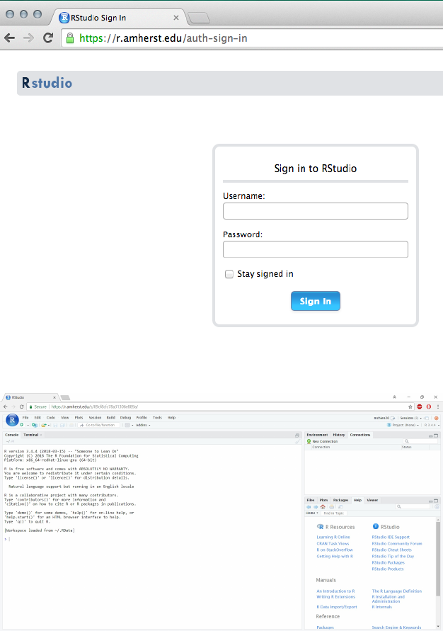
Once you connect to the server, you should see a login
screen:
The RStudio server doesn’t tend
to work well with Internet
Explorer.
Once you authenticate, you should see the RStudio
interface:
Notice that RStudio divides its world into four panels.
Several of the panels are further subdivided into multi-
ple tabs. Which tabs appear in which panels can be cus-
tomized by the user.
Rcan do much more than a simple calculator, and we

18 horton,kaplan,pruim
will introduce additional features in due time. But per-
forming simple calculations in Ris a good way to begin
learning the features of RStudio.
Commands entered in the Console tab are immediately
executed by R. A good way to familiarize yourself with
the console is to do some simple calculator-like compu-
tations. Most of this will work just like you would expect
from a typical calculator. Try typing the following com-
mands in the console panel.
>5+3
[1] 8
>15.3 *23.4
[1] 358.02
>sqrt(16)# square root
[1] 4
This last example demonstrates how functions are
called within Ras well as the use of comments. Com-
ments are prefaced with the #character. Comments can
be very helpful when writing scripts with multiple com-
mands or to annotate example code for your students.
You can save values to named variables for later reuse.
It’s probably best to settle on
using one or the other of the
right-to-left assignment opera-
tors rather than to switch back
and forth. We prefer the arrow
operator because it represents
visually what is happening in
an assignment and because it
makes a clear distinction be-
tween the assignment operator,
the use of =to provide values to
arguments of functions, and the
use of == to test for equality.
> product = 15.3 *23.4 # save result
> product # display the result
[1] 358.02
> product <- 15.3 *23.4 # <- can be used instead of =
> product
[1] 358.02
Once variables are defined, they can be referenced in
other operations and functions.

a student’s guide to r 19
>0.5 *product # half of the product
[1] 179.01
>log(product) # (natural) log of the product
[1] 5.880589
>log10(product) # base 10 log of the product
[1] 2.553907
>log2(product) # base 2 log of the product
[1] 8.483896
>log(product, base =2)# base 2 log of the product, another way
[1] 8.483896
The semi-colon can be used to place multiple com-
mands on one line. One frequent use of this is to save and
print a value all in one go:
> product <- 15.3 *23.4; product # save result and show it
[1] 358.02
2.1.1Version information
At times it may be useful to check what version of the
mosaic package, R, and RStudioyou are using. Running
sessionInfo() will display information about the version
of R and packages that are loaded and RStudio.Version()
will provide information about the version of RStudio.
>sessionInfo()
R version 3.5.0 (2018-04-23)
Platform: x86_64-apple-darwin15.6.0 (64-bit)
Running under: macOS High Sierra 10.13.4
Matrix products: default
BLAS: /Library/Frameworks/R.framework/Versions/3.5/Resources/lib/libRblas.0.dylib

20 horton,kaplan,pruim
LAPACK: /Library/Frameworks/R.framework/Versions/3.5/Resources/lib/libRlapack.dylib
locale:
[1] en_US.UTF-8/en_US.UTF-8/en_US.UTF-8/C/en_US.UTF-8/en_US.UTF-8
attached base packages:
[1] grid stats graphics grDevices utils datasets
[7] methods base
other attached packages:
[1] mosaic_1.2.0 Matrix_1.2-14 mosaicData_0.16.0
[4] ggformula_0.7.0 ggplot2_2.2.1 dplyr_0.7.5
[7] lattice_0.20-35 knitr_1.20
loaded via a namespace (and not attached):
[1] Rcpp_0.12.17 highr_0.6 pillar_1.2.3
[4] compiler_3.5.0 plyr_1.8.4 bindr_0.1.1
[7] tools_3.5.0 evaluate_0.10.1 tibble_1.4.2
[10] gtable_0.2.0 nlme_3.1-137 pkgconfig_2.0.1
[13] rlang_0.2.1 psych_1.8.4 parallel_3.5.0
[16] ggdendro_0.1-20 bindrcpp_0.2.2 gridExtra_2.3
[19] stringr_1.3.1 tidyselect_0.2.4 mosaicCore_0.5.0
[22] glue_1.2.0 R6_2.2.2 foreign_0.8-70
[25] reshape2_1.4.3 purrr_0.2.4 tidyr_0.8.1
[28] magrittr_1.5 scales_0.5.0 MASS_7.3-50
[31] splines_3.5.0 assertthat_0.2.0 mnormt_1.5-5
[34] colorspace_1.3-2 stringi_1.2.2 lazyeval_0.2.1
[37] munsell_0.4.3 broom_0.4.4
2.2Working with Files
2.2.1Working with RScript Files
As an alternative, Rcommands can be stored in a file.
RStudio provides an integrated editor for editing these
files and facilitates executing some or all of the com-
mands. To create a file, select File, then New File, then R
Script from the RStudio menu. A file editor tab will open
in the Source panel. Rcode can be entered here, and but-
tons and menu items are provided to run all the code
(called sourcing the file) or to run the code on a single
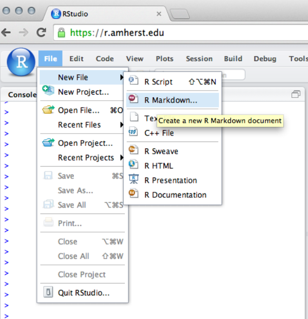
a student’s guide to r 21
line or in a selected section of the file.
2.2.2Working with RMarkdown, and knitr/L
A
T
EX
A third alternative is to take advantage of RStudio’s sup-
port for reproducible research. If you already know L
A
T
EX,
you will want to investigate the knitr/L
A
T
EX capabili-
ties. For those who do not already know L
A
T
EX, the sim-
pler RMarkdown system provides an easy entry into the
world of reproducible research methods. It also provides
a good facility for students to create homework and re-
ports that include text, Rcode, Routput, and graphics.
To create a new RMarkdown file, select File, then New
File, then RMarkdown. The file will be opened with a short
template document that illustrates the mark up language.
The mosaic package includes two useful RMarkdown
templates for getting started: fancy includes bells and
whistles (and is intended to give an overview of features),
while plain is useful as a starting point for a new analy-
sis. These are accessed using the Template option when
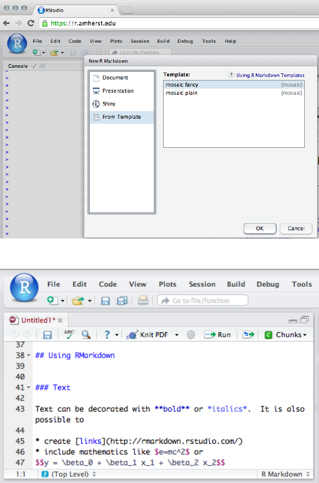
22 horton,kaplan,pruim
creating a new RMarkdown file.
Click on the Knit button to convert to an HTML, PDF,
or Word file.
This will generate a formatted version of the docu-
ment.
a student’s guide to r 23
There is a button (marked with a question mark)
which provides a brief description of the supported markup
commands. The RStudio web site includes more extensive
tutorials on using RMarkdown. Caution!
RMarkdown, and knitr/L
A
T
EX
files do not have access to the
console environment, so the
code in them must be self-
contained.
It is important to remember that unlike Rscripts,
which are executed in the console and have access to
the console environment, RMarkdown and knitr/L
A
T
EX
files do not have access to the console environment This
is a good feature because it forces the files to be self-
contained, which makes them transferable and respects
good reproducible research practices. But beginners, es-
pecially if they adopt a strategy of trying things out in the
console and copying and pasting successful code from the
console to their file, will often create files that are incom-
plete and therefore do not compile correctly.
2.3The Other Panels and Tabs
2.3.1The History Tab
As commands are entered in the console, they appear in
the History tab. These histories can be saved and loaded,
there is a search feature to locate previous commands,
and individual lines or sections can be transferred back to
the console. Keeping the History tab open will allow you

24 horton,kaplan,pruim
to go back and see the previous several commands. This
can be especially useful when commands produce a fair
amount of output and so scroll off the screen rapidly.
2.3.2Communication between tabs
RStudio provides several ways to move Rcode between
tabs. Pressing the Run button in the editing panel for an R
script or RMarkdown or other file will copy lines of code
into the Console and run them.
2.3.3The Files Tab
The Files tab provides a simple file manager. It can be
navigated in familiar ways and used to open, move, re-
name, and delete files. In the browser version of RStudio,
the Files tab also provides a file upload utility for moving
files from the local machine to the server. In RMarkdown
and knitr files one can also run the code in a particular
chunk or in all of the chunks in a file. Each of these fea-
tures makes it easy to try out code “live” while creating a
document that keeps a record of the code.
In the reverse direction, code from the history can be
copied either back into the console to run them again
(perhaps after editing) or into one of the file editing tabs
for inclusion in a file.
2.3.4The Help Tab
The Help tab is where RStudio displays Rhelp files. These
can be searched and navigated in the Help tab. You can
also open a help file using the ?operator in the console.
For example the following command will provide the
help file for the logarithm function.
> ?log
2.3.5The Environment Tab
The Environment tab shows the objects available to the
console. These are subdivided into data, values (non-
a student’s guide to r 25
dataframe, non-function objects) and functions. The
broom icon can be used to remove all objects from the en-
vironment, and it is good to do this from time to time, es-
pecially when running in RStudio server or if you choose
to save the environment when shutting down RStudio
since in these cases objects can stay in the environment
essentially indefinitely.
2.3.6The Plots Tab
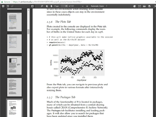
Plots created in the console are displayed in the Plots tab.
For example, the following commands display the num-
ber of births in the United States for each day in 1978.
>library(mosaic)
>gf_point(births ~ dayofyear, data = Births78)
●
●
●
●
●
●
●
●
●
●
●
●
●
●
●
●
●
●
●
●
●
●
●
●
●
●
●
●
●
●
●
●
●
●
●
●
●
●
●
●
●
●
●
●
●
●
●
●
●
●
●
●
●
●
●
●
●
●
●
●
●
●
●
●
●
●
●
●
●
●
●
●
●
●
●
●
●
●
●
●
●
●
●
●
●
●
●
●
●
●
●
●
●
●
●
●
●
●
●
●
●
●
●
●
●
●
●
●
●
●
●
●
●
●
●
●
●
●
●
●
●
●
●
●
●
●
●
●
●
●
●
●
●
●
●
●
●
●
●
●
●
●
●
●
●
●
●
●
●
●
●
●
●
●
●
●
●
●
●
●
●
●
●
●
●
●
●
●
●
●
●
●
●
●
●
●
●
●
●
●
●
●
●
●
●
●
●
●
●
●
●
●
●
●
●
●
●
●
●
●
●
●
●
●
●
●
●
●
●
●
●
●
●
●
●
●
●
●
●
●
●
●
●
●
●
●
●
●
●
●
●
●
●
●
●
●
●
●
●
●
●
●
●
●
●
●
●
●
●
●
●
●
●
●
●
●
●●
●
●
●
●
●
●
●
●
●
●
●
●
●
●
●
●
●
●
●
●
●
●
●
●
●
●
●
●
●
●
●
●
●
●
●
●
●
●
●
●
●
●
●
●
●
●
●
●
●
●
●
●
●
●
●
●
●
●
●
●
●
●
●
●
●
●
●
●
●
●
●
●
●
●
●
●
●
●
●
●
●
●
●
●
●
●
●
●
●
●
●
●
●
●
●
●
●
●
●
●
●
●
●
●
●
●
●
7000
8000
9000
10000
0 100 200 300
dayofyear
births
From the Plots tab, you can navigate to previous plots and
also export plots in various formats after interactively
resizing them.
2.3.7The Packages Tab
Much of the functionality of Ris located in packages,
many of which can be obtained from a central clearing
house called CRAN (Comprehensive R Archive Network).
The Packages tab facilitates installing and loading pack-
ages. It will also allow you to search for packages that
have been updated since you installed them.

3
One Quantitative Variable
3.1Numerical summaries
Rincludes a number of commands to numerically sum-
marize variables. These include the capability of calculat-
ing the mean, standard deviation, variance, median, five
number summary, interquartile range (IQR) as well as ar-
bitrary quantiles. We will illustrate these using the CESD
(Center for Epidemiologic Studies–Depression) measure
of depressive symptoms (which takes on values between
0and 60, with higher scores indicating more depressive
symptoms).
To improve the legibility of output, we will also set the
default number of digits to display to a more reasonable
level (see ?options() for more configuration possibilities).
>library(mosaic)
>options(digits =4)
>mean(~ cesd, data = HELPrct)
[1] 32.85
Note that the mean() function in the mosaic package
supports a formula interface common to lattice graphics
and linear models (e.g., lm()). The mosaic package pro-
vides many other functions that use the same notation,
which we will be using throughout this document.
Digging Deeper
If you have not seen the for-
mula notation before, the com-
panion book, Start Teaching with
Rprovides a detailed presen-
tation. Start Modeling with R,
another companion book, de-
tails the relationship between
the process of modeling and the
formula notation.
The same output could be created using the following
commands (though we will use the MOSAIC versions
when available).

28 horton,kaplan,pruim
>with(HELPrct, mean(cesd))
[1] 32.85
>mean(HELPrct$cesd)
[1] 32.85
Similar functionality exists for other summary statistics.
>sd(~ cesd, data = HELPrct)
[1] 12.51
>sd(~ cesd, data = HELPrct)^2
[1] 156.6
>var(~ cesd, data = HELPrct)
[1] 156.6
It is also straightforward to calculate quantiles of the
distribution.
>median(~ cesd, data = HELPrct)
[1] 34
By default, the quantile() function displays the quar-
tiles, but can be given a vector of quantiles to display. Caution!
Not all commands have been
upgraded to support the for-
mula interface. For these
functions, variables within
dataframes must be accessed
using with() or the $ operator.
>with(HELPrct, quantile(cesd))
0% 25% 50% 75% 100%
1 25 34 41 60
>with(HELPrct, quantile(cesd, c(.025,.975)))
2.5% 97.5%
6.3 55.0
a student’s guide to r 29
Finally, the favstats() function in the mosaic package
provides a concise summary of many useful statistics.
>favstats(~ cesd, data = HELPrct)
min Q1 median Q3 max mean sd n missing
1 25 34 41 60 32.85 12.51 453 0
3.2Graphical summaries
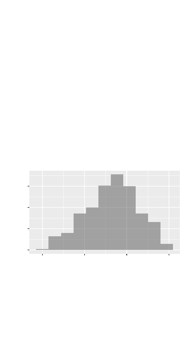
The gf_histogram() function is used to create a his-
togram. Here we use the formula interface (as discussed
in the Start Modeling with R book) to specify that we want
a histogram of the CESD scores.
>gf_histogram(~ cesd, data = HELPrct, binwidth =5.9)
0
25
50
75
0 20 40 60
cesd
count
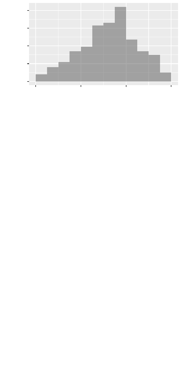
We can use the binwidth() and center() options to
control the location of the bins.
>gf_histogram(~ cesd, data = HELPrct, binwidth =5,center =2.5)
30 horton,kaplan,pruim
0
20
40
60
80
0 20 40 60
cesd
count
In the HELPrct dataset, approximately one quarter of
the subjects are female.
>tally(~ sex, data = HELPrct)
sex
female male
107 346
>tally(~ sex, format ="percent",data = HELPrct)
sex
female male
23.62 76.38
It is straightforward to restrict our attention to just
the female subjects. If we are going to do many things
with a subset of our data, it may be easiest to make a new
dataframe containing only the cases we are interested
in. The filter() function in the dplyr package can be
used to generate a new dataframe containing just the
women or just the men (see also section 13.5). Once this
is created, the the stem() function is used to create a stem
and leaf plot. Caution!
Note that the tests for equality
use two equal signs
> Female <- filter(HELPrct, sex == 'female')
> Male <- filter(HELPrct, sex == 'male')
>with(Female, stem(cesd))
The decimal point is 1 digit(s) to the right of the |
a student’s guide to r 31
0|3
0 | 567
1|3
1 | 555589999
2 | 123344
2 | 66889999
3 | 0000233334444
3 | 5556666777888899999
4 | 00011112222334
4 | 555666777889
5 | 011122222333444
5 | 67788
6|0
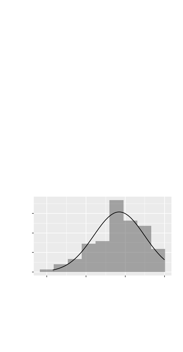
Subsets can also be generated and used “on the fly"
(this time including an overlaid normal density):
>gf_dhistogram(~ cesd, data =filter(HELPrct, sex == "female"), binwidth =7.1) %>%
gf_fitdistr(dist = dnorm)
0.00
0.01
0.02
0.03
0 20 40 60
cesd
density
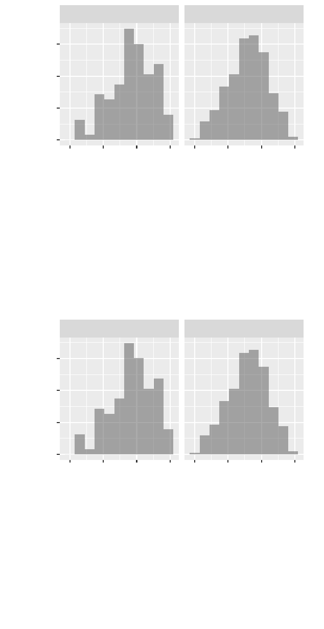
Alternatively, we can make side-by-side plots to com-
pare multiple subsets.
>gf_dhistogram(~ cesd, data = HELPrct, binwidth =5.9) %>%
gf_facet_wrap(~ sex)
32 horton,kaplan,pruim
female
male
0 20 40 60 0 20 40 60
0.00
0.01
0.02
0.03
cesd
density
The layout can be rearranged.
>gf_dhistogram(~ cesd, data = HELPrct, binwidth =5.9) %>%
gf_facet_wrap(~ sex)
female
male
0 20 40 60 0 20 40 60
0.00
0.01
0.02
0.03
cesd
density
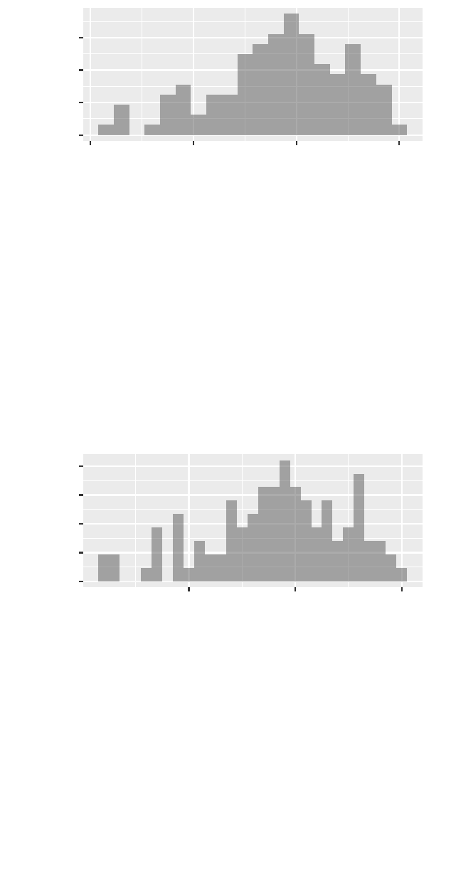
We can control the number of bins in a number of ways.
These can be specified as the total number.
>gf_dhistogram(~ cesd, bins =20,data = Female)
a student’s guide to r 33
0.00
0.01
0.02
0.03
0 20 40 60
cesd
density
The width of the bins can be specified.
>gf_dhistogram(~ cesd, binwidth =2,data = Female)
0.00
0.01
0.02
0.03
0.04
20 40 60
cesd
density
The gf_dotplot() function is used to create a dotplot
for a smaller subset of subjects (homeless females). We
also demonstrate how to change the x-axis label.
>gf_dotplot(~ cesd, binwidth =3,data =filter(HELPrct,
sex == "female", homeless == "homeless")) %>%
gf_labs(x="CESD score")
34 horton,kaplan,pruim
● ●
●
●
● ●
●
●
●
●●
●
●
●
●
●
●
●
●
●
●
●
●
●
●
●
●●
●
●
●
●
●●
●
●
●
●
●
●
0.00
0.25
0.50
0.75
1.00
20 40 60
CESD score
count
3.3Density curves
Density plots are also sensi-
tive to certain choices. If your
density plot is too jagged or
too smooth, try changing the
adjust argument: larger than 1
for smoother plots, less than 1
for more jagged plots.
One disadvantage of histograms is that they can be sensi-
tive to the choice of the number of bins. Another display
to consider is a density curve.
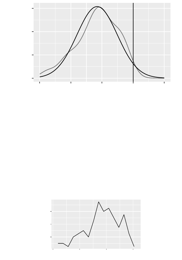
Here we adorn a density plot with some additions to
demonstrate how to build up a graphic for pedagogical
purposes. We add some text, a superimposed normal
density as well as a vertical line. A variety of line types
and colors can be specified, as well as line widths. Digging Deeper
The plotFun() function can
also be used to annotate plots
(see section 10.2.1).
>gf_dens(~ cesd, data = Female) %>%
gf_refine(annotate(geom ="text",x=10,y=.025,
label ="only females")) %>%
gf_fitdistr(dist = dnorm) %>%
gf_vline(xintercept =60) +
xlim(0,80)
a student’s guide to r 35
only females
0.00
0.01
0.02
0.03
0 20 40 60 80
cesd
density
3.4Frequency polygons
A third option is a frequency polygon, where the graph is
created by joining the midpoints of the top of the bars of
a histogram.
>gf_freqpoly(~ cesd, data = Female, binwidth =3.8)
4
8
12
0 20 40 60
cesd
count
3.5Normal distributions
xis for eXtra.
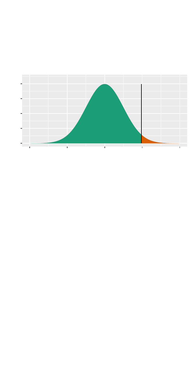
The most famous density curve is a normal distribution.
The xpnorm() function displays the probability that a ran-
dom variable is less than the first argument, for a normal
distribution with mean given by the second argument
and standard deviation by the third. More information
about probability distributions can be found in section 11.
36 horton,kaplan,pruim
>xpnorm(1.96,mean =0,sd =1)
If X ~ N(0, 1), then
P(X <= 1.96) = P(Z <= 1.96) = 0.975
P(X > 1.96) = P(Z > 1.96) = 0.025
[1] 0.975
z = 1.96
0.0
0.1
0.2
0.3
0.4
−4 −2 0 2 4
x
density
3.6Inference for a single sample
We can calculate a 95% confidence interval for the mean
CESD score for females by using a t-test:
>t.test(~ cesd, data = Female)
One Sample t-test
data: cesd
t = 29, df = 110, p-value <2e-16
alternative hypothesis: true mean is not equal to 0
95 percent confidence interval:
34.39 39.38
sample estimates:
mean of x
36.89
>confint(t.test(~ cesd, data = Female))
mean of x lower upper level
1 36.89 34.39 39.38 0.95

a student’s guide to r 37
Digging Deeper
More details and examples can
be found in the mosaic package
Resampling Vignette.
But it’s also straightforward to calculate this using a
bootstrap. The statistic that we want to resample is the
mean.
>mean(~ cesd, data = Female)
[1] 36.89
One resampling trial can be carried out:
Here we sample with re-
placement from the original
dataframe, creating a resam-
pled dataframe with the same
number of rows.
>mean(~ cesd, data =resample(Female))
[1] 39.15
Even though a single trial is
of little use, it’s smart having
students do the calculation to
show that they are (usually!)
getting a different result than
without resampling.
Another will yield different results:
>mean(~ cesd, data =resample(Female))
[1] 36.03
Now conduct 1000 resampling trials, saving the results
in an object called trials:
> trials <- do(1000)*mean(~ cesd, data =resample(Female))
>head(trials, 3)
mean
1 36.72
2 37.70
3 34.93
>qdata(~ mean, c(.025,.975), data = trials)
quantile p
2.5% 34.27 0.025
97.5% 39.38 0.975

4
One Categorical Variable
4.1Numerical summaries
Digging Deeper
The Start Teaching with R com-
panion book introduces the for-
mula notation used throughout
this book. See also Start Teach-
ing with R for the connections to
statistical modeling.
The tally() function can be used to calculate counts,
percentages and proportions for a categorical variable.
>tally(~ homeless, data = HELPrct)
homeless
homeless housed
209 244
>tally(~ homeless, margins =TRUE,data = HELPrct)
homeless
homeless housed Total
209 244 453
>tally(~ homeless, format ="percent",data = HELPrct)
homeless
homeless housed
46.14 53.86
>tally(~ homeless, format ="proportion",data = HELPrct)
homeless
homeless housed
0.4614 0.5386

40 horton,kaplan,pruim
4.2The binomial test
An exact confidence interval for a proportion (as well as
a test of the null hypothesis that the population propor-
tion is equal to a particular value [by default 0.5]) can be
calculated using the binom.test() function. The standard
binom.test() requires us to tabulate.
>binom.test(209,209 +244)
data: 209 out of 209 + 244
number of successes = 210, number of trials = 450, p-value =
0.1
alternative hypothesis: true probability of success is not equal to 0.5
95 percent confidence interval:
0.4147 0.5085
sample estimates:
probability of success
0.4614
The mosaic package provides a formula interface that
avoids the need to pre-tally the data.
> result <- binom.test(~ (homeless == "homeless"), data = HELPrct)
> result
data: HELPrct$(homeless == "homeless") [with success = TRUE]
number of successes = 210, number of trials = 450, p-value =
0.1
alternative hypothesis: true probability of success is not equal to 0.5
95 percent confidence interval:
0.4147 0.5085
sample estimates:
probability of success
0.4614
As is generally the case with commands of this sort,
there are a number of useful quantities available from the
object returned by the function.

a student’s guide to r 41
>names(result)
[1] "statistic" "parameter" "p.value" "conf.int"
[5] "estimate" "null.value" "alternative" "data.name"
These can be extracted using the $operator or an extrac-
tor function. For example, the user can extract the confi-
dence interval or p-value.
> result$statistic
number of successes
209
>confint(result)
probability of success lower upper level
1 0.4614 0.4147 0.5085 0.95
>pval(result)
p.value
0.1101
Digging Deeper
Most of the objects in Rhave
aprint() method. So when
we get result, what we are
seeing displayed in the console
is print(result). There may
be a good deal of additional
information lurking inside the
object itself.
In some situations, such as
graphics, the object is returned
invisibly, so nothing prints. That
avoids your having to look at
a long printout not intended
for human consumption. You
can still assign the returned
object to a variable and pro-
cess it later, even if nothing
shows up on the screen. This is
sometimes helpful for lattice
graphics functions.
4.3The proportion test
A similar interval and test can be calculated using the
function prop.test(). Here is a count of the number of
people at each of the two levels of homeless
>tally(~ homeless, data = HELPrct)
homeless
homeless housed
209 244
The prop.test() function will carry out the calcula-
tions of the proportion test and report the result.
>prop.test(~ (homeless == "homeless"), correct =FALSE,
data = HELPrct)

42 horton,kaplan,pruim
1-sample proportions test without continuity correction
data: HELPrct$(homeless == "homeless") [with success = TRUE]
X-squared = 2.7, df = 1, p-value = 0.1
alternative hypothesis: true p is not equal to 0.5
95 percent confidence interval:
0.4160 0.5074
sample estimates:
p
0.4614
In this statement, prop.test is examining the homeless
variable in the same way that tally() would. prop.test() More Info
We write
homeless=="homeless" to de-
fine unambiguously which
proportion we are considering.
We could also have written
homeless=="housed".
can also work directly with numerical counts, the way
binom.test() does.
prop.test() calculates a Chi-
squared statistic. Most intro-
ductory texts use a z-statistic.
They are mathematically equiv-
alent in terms of inferential
statements, but you may need
to address the discrepancy with
your students.
>prop.test(209,209 +244,correct =FALSE)
1-sample proportions test without continuity correction
data: 209 out of 209 + 244
X-squared = 2.7, df = 1, p-value = 0.1
alternative hypothesis: true p is not equal to 0.5
95 percent confidence interval:
0.4160 0.5074
sample estimates:
p
0.4614
4.4Goodness of fit tests
A variety of goodness of fit tests can be calculated against
a reference distribution. For the HELP data, we could
test the null hypothesis that there is an equal proportion
of subjects in each substance abuse group back in the
original populations.
>tally(~ substance, format ="percent",data = HELPrct)
substance
alcohol cocaine heroin
39.07 33.55 27.37

a student’s guide to r 43
> observed <- tally(~ substance, data = HELPrct)
> observed
substance
alcohol cocaine heroin
177 152 124 Caution!
In addition to the format op-
tion, there is an option margins
to include marginal totals in the
table. The default in tally() is
margins=FALSE. Try it out!
> p <- c(1/3,1/3,1/3)# equivalent to rep(1/3, 3)
>chisq.test(observed, p= p)
Chi-squared test for given probabilities
data: observed
X-squared = 9.3, df = 2, p-value = 0.01
> total <- sum(observed)
> total
[1] 453
> expected <- total*p
> expected
[1] 151 151 151
We can also calculate the χ2statistic manually, as a
function of observed and expected values.
> chisq <- sum((observed - expected)^2/(expected))
> chisq
[1] 9.311
>1-pchisq(chisq, df=2)
[1] 0.009508
The pchisq() function calcu-
lates the probability that a χ2
random variable with df() de-
grees is freedom is less than or
equal to a given value. Here
we calculate the complement to
find the area to the right of the
observed Chi-square statistic.
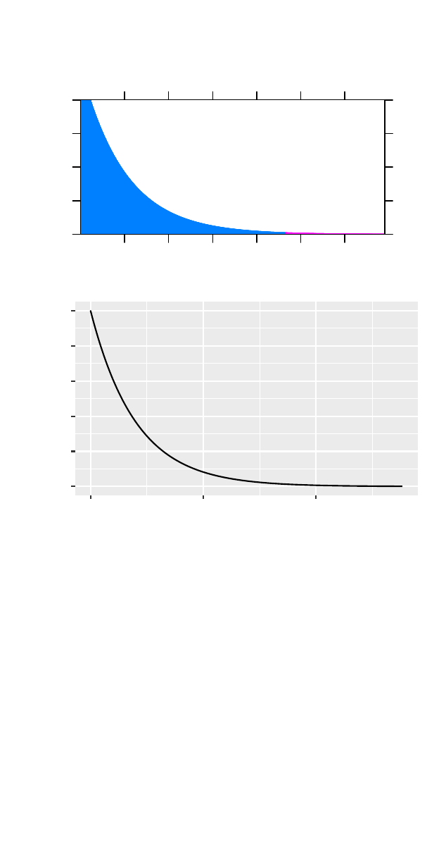
It may be helpful to consult a graph of the statistic,
where the shaded area represents the value to the right of
the observed value.
44 horton,kaplan,pruim
>plotDist("chisq",df =2,groups =x>9.31,type ="h")
>gf_dist("chisq",df =2)
0.1
0.2
0.3
2 4 6 8 10 12
0.0
0.1
0.2
0.3
0.4
0.5
0 5 10
x
density
Alternatively, the mosaic package provides a version
of chisq.test() with more verbose output.
>xchisq.test(observed, p= p)
Chi-squared test for given probabilities
data: x
X-squared = 9.3, df = 2, p-value = 0.01
177 152 124
(151.00) (151.00) (151.00)
[4.4768] [0.0066] [4.8278]
< 2.116> < 0.081> <-2.197>

a student’s guide to r 45
key:
observed
(expected)
[contribution to X-squared]
<Pearson residual> xin xchisq.test() stands for
eXtra.
Objects in the workspace are
listed in the Environment tab
in RStudio. If you want to clean
up that listing, remove objects
that are no longer needed with
rm().
># clean up variables no longer needed
>rm(observed, p, total, chisq)
5
Two Quantitative Variables
5.1Scatterplots
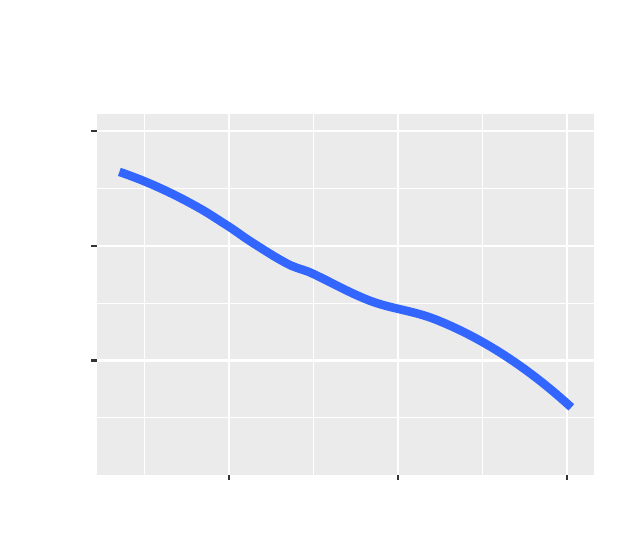
We always encourage students to start any analysis by
graphing their data. Here we augment a scatterplot of
the CESD (a measure of depressive symptoms, higher
scores indicate more symptoms) and the MCS (mental
component score from the SF-36, where higher scores
indicate better functioning) for female subjects with a
lowess (locally weighted scatterplot smoother) line, using
a circle as the plotting character and slightly thicker line.
The lowess line can help to as-
sess linearity of a relationship.
This is added by specifying
both points (using ‘p’) and a
lowess smoother.
> Female <- filter(HELPrct, female == 1)
>gf_point(cesd ~ mcs, data = Female, shape =1) %>%
gf_smooth(se =FALSE,size =2)
●
●
●
●
●
●
●
●
●
●
●
●
●
●
●
●
●
●
●
●
●
●
●
●
●
●
●
●
●
●
●
●
●
●
●
●
●
● ●
●
●
●
●
●
●
●
●
●
●
●
●
●●
●
●
●●
●
●
●
●
●
●
●
●
●
●●
●
●
●
●
●
●
●
●
●
●
●
●●
●
●
●
●
●
●
●
●
●
●
● ●
●
●
●
●
●
●
●
●
●
●
●
●
●
●
20
40
60
20 40 60
mcs
cesd
48 horton,kaplan,pruim
Digging Deeper
The Start Modeling with R com-
panion book will be helpful
if you are unfamiliar with the
modeling language. The Start
Teaching with R also provides
useful guidance in getting
started.
It’s straightforward to plot something besides a char-
acter in a scatterplot. In this example, the USArrests can
be used to plot the association between murder and as-
sault rates, with the state name displayed. This requires a
panel function to be written.
> panel.labels <- function(x,y,labels ='x',...) {
panel.text(x, y, labels, cex =0.4, ...)
}
>gf_text(Murder ~ Assault, panel = panel.labels,
label =rownames(USArrests), data = USArrests,
size =2)
Alabama
Alaska
Arizona
Arkansas California
Colorado
Connecticut
Delaware
Florida
Georgia
Hawaii
Idaho
Illinois
Indiana
Iowa
Kansas
Kentucky
Louisiana
Maine
Maryland
Massachusetts
Michigan
Minnesota
Mississippi
Missouri
Montana
Nebraska
Nevada
New Hampshire
New Jersey
New Mexico
New York
North Carolina
North Dakota
Ohio Oklahoma
Oregon
Pennsylvania
Rhode Island
South Carolina
South Dakota
Tennessee
Texas
Utah
Vermont
Virginia
Washington
West Virginia
Wisconsin
Wyoming
0
5
10
15
100 200 300
Assault
Murder
5.2Correlation
Correlations can be calculated for a pair of variables, or
for a matrix of variables.
>cor(cesd ~ mcs, data = Female)
[1] -0.6738
> smallHELP <- select(Female, cesd, mcs, pcs)
>cor(smallHELP)
cesd mcs pcs
cesd 1.0000 -0.6738 -0.3685
mcs -0.6738 1.0000 0.2664
pcs -0.3685 0.2664 1.0000
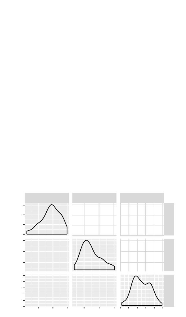
a student’s guide to r 49
By default, Pearson correlations are provided. Other
variants (e.g., Spearman) can be specified using the method
option.
>cor(cesd ~ mcs, method ="spearman",data = Female)
[1] -0.6662
5.3Pairs plots
A pairs plot (scatterplot matrix) can be calculated for each
pair of a set of variables.
The GGally package has sup-
port for more elaborate pairs
plots.
>library(GGally)
Attaching package: ’GGally’
The following object is masked from ’package:dplyr’:
nasa
>ggpairs(smallHELP)
●
●
●
●
●
●
●
●
●
●
●
●
●
●
●
●
●
●
●
●●●
●
●●
●
●
●
●
●
●
●
●●
●
●
●
●
●●
●
●
●●
●
●
●
●
●
●
●
●
●
●
●
●
●
●
●
●
●●
●
●
●
●
●
●
●
●
●
●
●
●
●
●
●
●
●
●
●
●
●
●
●
●
●
●
●
●
●
●
●
●
●
●
●
●
●
●
●
●
●
●
●
●
●
●
●
●
●
●
●
●
●
●
●
●
●
●●
●●
●●
●
●●●
●●
●
●
●
●
●
●●
●
●●
●●
●
●
●●●
●
●
●
●
●
●
●
●
●
●
●
●
●
●
●
●
●
●
●
●
●
●●
●
●
●
●
●
●
●
●
●
●
●
●
●
●
●
●
●
●
●
●
●
●
●
●
●
●
●
●
●
●
●
●
●
●
●
●
●
●
●
●
●
●
●
Corr:
−0.674
●
●
●
●
●
●●
●●
●
●
●
●
●
●
●
●
●●
●
●
●
●
●
●
●
●
●
●●
●
●
●
●
●
●
●
●
●●
●
●●
●
●
●
●
●
●
●
●
●●
●
●
●
●
●●
●
●
●
●
●
●
●
●
●
●
●
●●
●
●●
●
●
●
●
●●
●
●●
●
●
●
●
●
●
●
●
●
●
●●
●
●
●
●
●●
●
●
●
●
●
Corr:
−0.369
Corr:
0.266
cesd
mcs
pcs
cesd
mcs
pcs
20 40 60 20 40 6020 30 40 50 60 70
0.00
0.01
0.02
0.03
20
40
60
20
30
40
50
60
70

50 horton,kaplan,pruim
5.4Simple linear regression
We tend to introduce linear re-
gression early in our courses, as
a purely descriptive technique.
Linear regression models are described in detail in Start
Modeling with R. These use the same formula interface
introduced previously for numerical and graphical sum-
maries to specify the outcome and predictors. Here we
consider fitting the model cesd ∼mcs.
> cesdmodel <- lm(cesd ~ mcs, data = Female)
>coef(cesdmodel)
(Intercept) mcs
57.349 -0.707
It’s important to pick good
names for modeling objects.
Here the output of lm() is
saved as cesdmodel, which
denotes that it is a regression
model of depressive symptom
scores.
To simplify the output, we turn off the option to dis-
play significance stars.
>options(show.signif.stars =FALSE)
>coef(cesdmodel)
(Intercept) mcs
57.349 -0.707
>msummary(cesdmodel)
Estimate Std. Error t value Pr(>|t|)
(Intercept) 57.3485 2.3806 24.09 < 2e-16
mcs -0.7070 0.0757 -9.34 1.8e-15
Residual standard error: 9.66 on 105 degrees of freedom
Multiple R-squared: 0.454,Adjusted R-squared: 0.449
F-statistic: 87.3 on 1 and 105 DF, p-value: 1.81e-15
>coef(summary(cesdmodel))
Estimate Std. Error t value Pr(>|t|)
(Intercept) 57.349 2.38062 24.090 1.425e-44
mcs -0.707 0.07566 -9.344 1.813e-15
>confint(cesdmodel)
2.5 % 97.5 %
(Intercept) 52.6282 62.069
mcs -0.8571 -0.557
>rsquared(cesdmodel)
[1] 0.454
a student’s guide to r 51
>class(cesdmodel)
[1] "lm"
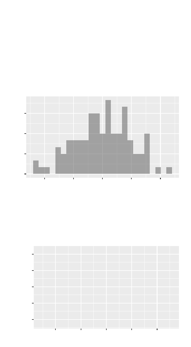
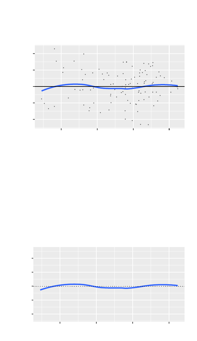
The return value from lm() is a linear model object. A
number of functions can operate on these objects, as seen
previously with coef(). The function residuals() re-
turns a vector of the residuals.
The function residuals()
can be abbreviated resid().
Another useful function is
fitted(), which returns a vec-
tor of predicted values.
>gf_histogram(~ residuals(cesdmodel), density=TRUE)
0
3
6
9
−20 −10 0 10 20
residuals(cesdmodel)
count
>gf_qq(~ resid(cesdmodel))
●●
●●
●●
●
●
●
●
●
●
●
●
●
●
●
●
●
●
●
●
●
●
●
●
●
●
●
●
●
●
●
●
●
●
●●
●
●
●
●
●
●
●
●
●
●
●
●
●
●
●
●
●
●
●
●
●
●
●
●
●
●
●
●
●
●
●
●
●
●
●
●
●
●
●
●
●
●
●
●
●
●
●
●
●
●
●
●
●
●
●
●
●
●
●
●
●
●
●
●●●●
●
●
−20
−10
0
10
20
−2 −1 0 1 2
theoretical
sample
52 horton,kaplan,pruim
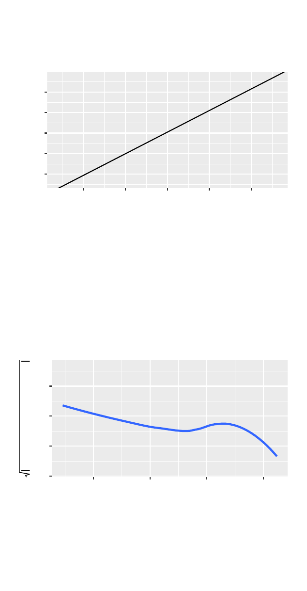
>gf_point(resid(cesdmodel) ~ fitted(cesdmodel),
alpha =0.5,cex =0.3,pch =20) %>%
gf_smooth(se =FALSE) %>%
gf_hline(yintercept =0)
−20
−10
0
10
20
20 30 40 50
fitted(cesdmodel)
resid(cesdmodel)
The mplot() function can facilitate creating a variety
of useful plots, including the same residuals vs. fitted
scatterplots, by specifying the which = 1 option.
>mplot(cesdmodel, which =1)
[[1]]
●
●
●
●
●
●
●
●
●
●
●
●●
●
●
●
●
●
●
●
●
●
●
●
●
●
●
●
●
●
●
●
●
●●
●
●
●
●
●●
●
●
●
●
●
●
●
●
●
●
●
●
●
●
●
●
●
●
●
●
●
●●
●
●
●
●
●
●
●
●
●
●
●●
●
●
●
●
●
●
●
●
●
●
●
●
●●
●
●
●
●
●
●
●
●
●
●
●
●
●
●
●
●
●
100
103
9
−20
−10
0
10
20
20 30 40 50
Fitted Values
Residual
Residuals vs Fitted
It can also generate a normal quantile-quantile plot
(which = 2),
a student’s guide to r 53
>mplot(cesdmodel, which =2)
●●●●
●●
●
●
●
●
●
●
●
●
●
●
●
●
●
●
●
●
●
●
●
●
●
●
●
●
●
●
●
●
●
●
●
●
●
●
●
●
●
●
●
●
●
●
●
●
●
●
●
●
●
●
●
●
●
●
●
●
●
●
●
●
●
●
●
●
●
●
●
●
●
●
●
●
●
●
●
●
●
●
●
●
●
●
●
●
●
●
●
●
●
●
●
●
●
●
●
●●●●
●
●
100
1039
−2
−1
0
1
2
−2 −1 0 1 2
Theoretical Quantiles
Standardized Residuals
Normal Q−Q
scale vs. location,
>mplot(cesdmodel, which =3)
●
●
●
●
●
●
●
●
●
●
●
●●
●
●
●
●
●
●
●
●
●
●
●
●
●
●
●
●
●
●
●
●
●●
●
●
●
●
●●
●
●
●
●
●
●
●
●
●
●
●
●
●
●
●
●
●
●
●
●
●
●●
●
●●
●
●
●
●
●
●
●
●
●
●
●
●●
●
●
●
●
●
●
●
●
●●
●
●
●
●
●
●
●●
●
●
●
●
●
●
●
●
●
100 103
9
0.0
0.5
1.0
1.5
20 30 40 50
Fitted Values
Standardized residuals
Scale−Location
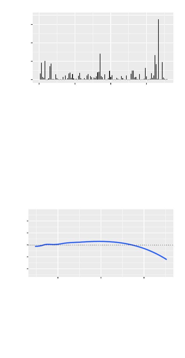
Cook’s distance by observation number,
>mplot(cesdmodel, which =4)
54 horton,kaplan,pruim
●
●
●
●
●
●
●
●
●
●
●
●
●
●
●
●
●
●
●
●
●
●
●
●
●
●
●
●
●
●
●
●
●
●
●
●
●
●
●
●
●
●
●
●
●
●
●
●
●
●
●
●
●
●
●
●
●
●
●
●
●
●
●
●
●
●
●
●
●
●
●
●
●
●
●
●
●
●
●
●
●
●
●
●
●
●
●
●
●
●
●
●
●
●
●
●
●
●
●
●
●
●
●
●
●
●
●
100
51 97
0.00
0.05
0.10
0.15
0 30 60 90
Observation Number
Cook's distance
Cook's Distance
residuals vs. leverage,
>mplot(cesdmodel, which =5)
●●
●
●
●
●
●
●
●
●
●
●
●
●
●
●
●
●
●
●
●
●
●
●
●
●
●
●
●
●
●
●
●
●
●
●
●
●
●
●●
●
●
●
●
●
●
●
●
●●
●
●
●
●
●
●
●
●
●
●
●
●
●
●
●
●
●
●
●
●
●
●
●
●●
●
●
●
●
●
●
●
●
●
●
●
●
●
●
●
●
●
●
●
●●
●
●
●
●●
●
●
●
●
●
100
103
9
−2
−1
0
1
2
0.02 0.04 0.06
Leverage
Standardized Residuals
Residuals vs Leverage
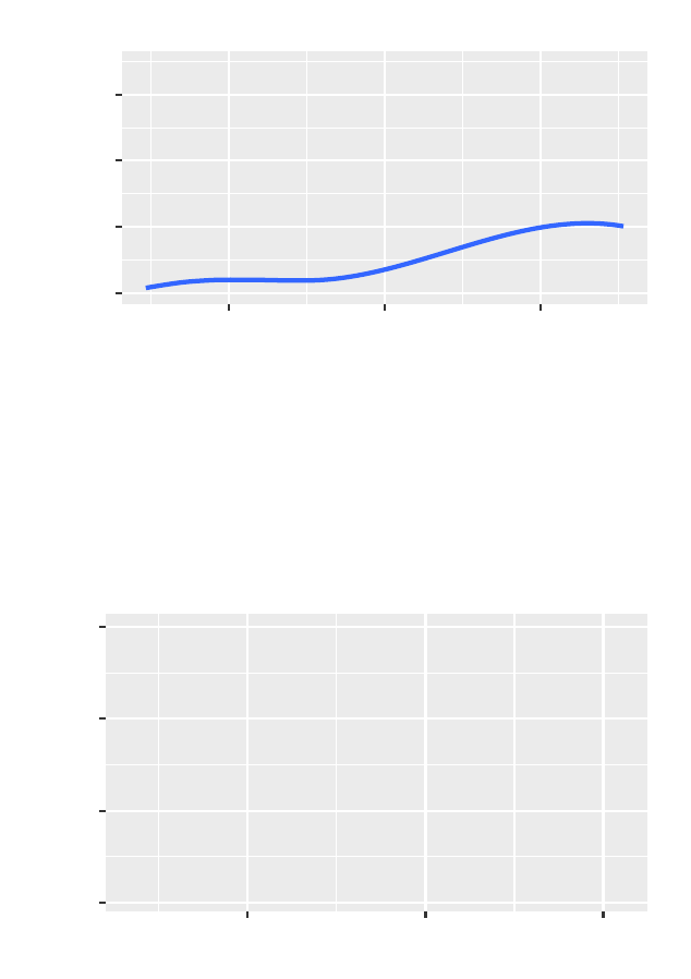
and Cook’s distance vs. leverage.
>mplot(cesdmodel, which =6)
a student’s guide to r 55
●
●
●
●
●
●
●●
●●
●
●
●
●
●●
●●
●●
●
●
●
●
●
●
●
●
●●
●
●
●●
●●
●●
●
●●
●
●●
●
●●
●
●●
●
●
●●
●
●
●●
●
●
●
●●
●●●
●
●
●
●●
●
●
●
●●
●
●●
●
●●
●
●
●
●
●
●
●
●
●●
●
●
●
●
●
●
●
●
●●
●
●●●
●
100
103
9
0.00
0.05
0.10
0.15
0.02 0.04 0.06
Leverage
Cook's distance
Cook's dist vs Leverage
Prediction bands can be added to a plot using the
panel.lmbands() function.
>gf_point(cesd ~ mcs, panel = panel.lmbands,
cex =0.2,band.lwd =2,data = HELPrct)
●
●
●
●
●
●
●
●
●
● ●
●
●
●
●
●
●
●
●
●
●
●
●
●
●
●
●
●
●
●
●
●
●
●
●
●
●
●
●
●
●
●
●
●
●
●
●
●
●
●
●
●
●
●
●
●
●
●
●
●
●
●
●
●
●
●
●
●
●
●
●
●
●
●
●
●
●
●
●
●
●
●
●
●
●
●
●
●
●
●
●
●
●
●
●
●
●
●
●
●
●
●
●
●
●
●
●
●
●
●
●
●
●
●
●
●
●
●
●
●
●
●
●
●
●
●
● ●
●
●
●
●
●
● ●
●
●
●
●
●
●
●
●
●
●
●
●
●
●
●
●
●
●
●
●
●
●
●
●
●
●
●
●
●
●
●
●
●
●
●
●
●
●
●
●
●
●
●
●
●
●
●
●
●
●
●
●
●
●
●
●
●
●
●
●
●
●●
●
●
●
●
●
●
●
●
●
●
●
●
●
●
●
●
●
●
●
●
●
●
●
●
●
●
●
●
●
●
●
●
●
●
●
●
●
●
●
●
●
●
●
●
●
●
●
●
●
●
●
●
●
●
●
●
●
●
●
●
●
●
●
●
●
●
●
●
●
●
●
●
●
●
●
●
●
●
●
●
●
●
●
●
●
●
●
●
●
●
●
●
●
●
●
●
●
●
●
●
●
●
●
●
●
●
●
●
●
●
●
●
●
●
●
●
●
●
●
●
●
●
●
●
●
●●
●
●
●
●
●
●
●
●
●
●
●
●
●
●
●
●
●
●
●
●
●
●
●
●
●
●
●
●
●
●
●
●
●
●
●
●
●
●
●
●
●
●
●
●
●
● ●
●
●
●
●
●
●
●
●
●
●
●
●
●
●
●
●
●
●
●
●
●
●
●
●
●
●
●
●
●
●
●
●
●
●
●
●
●
●
●
●
●
●
●
●
●
●
●
●
●
●
●
●
●
●
●
●
●
●
●
●●
●
●
●
●
●
●
●
●
●
●
●
●
●
●
●
●
●
●
●
●
0
20
40
60
20 40 60
mcs
cesd

6
Two Categorical Variables
6.1Cross classification tables
Cross classification (two-way or Rby C) tables can be
constructed for two (or more) categorical variables. Here
we consider the contingency table for homeless status
(homeless one or more nights in the past 6months or
housed) and sex.
>tally(~ homeless + sex, margins =FALSE,data = HELPrct)
sex
homeless female male
homeless 40 169
housed 67 177
We can also calculate column percentages:
>tally(~ sex | homeless, margins =TRUE,format ="percent",
data = HELPrct)
homeless
sex homeless housed
female 19.14 27.46
male 80.86 72.54
Total 100.00 100.00
We can calculate the odds ratio directly from the table:

58 horton,kaplan,pruim
> OR <- (40/169)/(67/177)
> OR
[1] 0.6253
The mosaic package has a function which will calcu-
late odds ratios:
>oddsRatio(tally(~ (homeless == "housed") + sex, margins =FALSE,
data = HELPrct))
[1] 0.6253
The CrossTable() function in the gmodels package
also displays a cross classification table.
>library(gmodels)
Error in library(gmodels): there is no package called
’gmodels’
>with(HELPrct, CrossTable(homeless, sex,
prop.r =FALSE,prop.chisq =FALSE,prop.t =FALSE))
Error in CrossTable(homeless, sex, prop.r = FALSE,
prop.chisq = FALSE, : could not find function "CrossTable"
Graphical summaries of cross classification tables may
be helpful in visualizing associations. Mosaic plots are
one example, where the total area (all observations) is
proportional to one. Here we see that males tend to be Caution!
The jury is still out regarding
the utility of mosaic plots (also
known as eikosograms), relative
to the low data to ink ratio. We
have found them to be helpful
to reinforce understanding of a
two way contingency table.
E. R. Tufte. The Visual Dis-
play of Quantitative Information.
Graphics Press, Cheshire, CT,
2nd edition, 2001
over-represented amongst the homeless subjects (as rep-
resented by the horizontal line which is higher for the
homeless rather than the housed).
The mosaic() function in the
vcd package makes mosaic
plots.
> mytab <- tally(~ homeless + sex, margins =FALSE,
data = HELPrct)
> vcd::mosaic(mytab, shade =TRUE)
> vcd::mosaic(~ homeless + substance, data = HELPrct,
shade =TRUE)#example with color
a student’s guide to r 59
−1.3
0.0
1.2
Pearson
residuals:
p−value =
0.038
sex
homeless
housed homeless
female male
−2.2
0.0
2.0
Pearson
residuals:
p−value =
2e−04
substance
homeless
housed homeless
alcoholcocaineheroin
6.2Creating tables from summary statistics
Tables can be created from summary statistics using the
do() function.

60 horton,kaplan,pruim
> HELPtable <- rbind(
do(40)*data.frame(sex ="female",homeless ="homeless"),
do(169)*data.frame(sex ="male",homeless ="homeless"),
do(67)*data.frame(sex ="female",homeless ="housed"),
do(177)*data.frame(sex ="male",homeless ="housed")
)
>tally(~ homeless + sex, data = HELPtable)
sex
homeless female male
homeless 40 169
housed 67 177
6.3Chi-squared tests
>chisq.test(tally(~ homeless + sex, margins =FALSE,
data = HELPrct), correct =FALSE)
Pearson's Chi-squared test
data: tally(~homeless + sex, margins = FALSE, data = HELPrct)
X-squared = 4.3, df = 1, p-value = 0.04
There is a statistically significant association found:
it is unlikely that we would observe an association this
strong if homeless status and sex were independent in the
population.
When a student finds a significant association, it’s im-
portant for them to be able to interpret this in the context
of the problem. The xchisq.test() function provides
additional details (observed, expected, contribution to
statistic, and residual) to help with this process.
xis for eXtra.
>xchisq.test(tally(~ homeless + sex, margins =FALSE,
data = HELPrct), correct =FALSE)
Pearson's Chi-squared test

a student’s guide to r 61
data: x
X-squared = 4.3, df = 1, p-value = 0.04
40 169
( 49.37) (159.63)
[1.78] [0.55]
<-1.33> < 0.74>
67 177
( 57.63) (186.37)
[1.52] [0.47]
< 1.23> <-0.69>
key:
observed
(expected)
[contribution to X-squared]
<Pearson residual>
We observe that there are fewer homeless women, and
more homeless men that would be expected.
6.4Fisher’s exact test
An exact test can also be calculated. This is computation-
ally straightforward for 2by 2tables. Options to help
constrain the size of the problem for larger tables exist
(see ?fisher.test()). Digging Deeper
Note the different estimate of
the odds ratio from that seen in
section 6.1. The fisher.test()
function uses a different estima-
tor (and different interval based
on the profile likelihood).
>fisher.test(tally(~ homeless + sex, margins =FALSE,
data = HELPrct))
Fisher's Exact Test for Count Data
data: tally(~homeless + sex, margins = FALSE, data = HELPrct)
p-value = 0.05
alternative hypothesis: true odds ratio is not equal to 1
95 percent confidence interval:
0.3895 0.9968
sample estimates:
odds ratio
0.6259
62 horton,kaplan,pruim

7
Quantitative Response, Categorical Predictor
7.1A dichotomous predictor: numerical and
graphical summaries
Here we will compare the distributions of CESD scores
by sex. The mean() function can be used to calculate the
mean CESD score separately for males and females.
>mean(cesd ~ sex, data = HELPrct)
female male
36.89 31.60
The favstats() function can provide more statistics by
group.
>favstats(cesd ~ sex, data = HELPrct)
sex min Q1 median Q3 max mean sd n missing
1 female 3 29 38.0 46.5 60 36.89 13.02 107 0
2 male 1 24 32.5 40.0 58 31.60 12.10 346 0
Boxplots are a particularly helpful graphical display
to compare distributions. The gf_boxplot() function can
be used to display the boxplots for the CESD scores sepa-
rately by sex. We see from both the numerical and graph-
ical summaries that women tend to have slightly higher
CESD scores than men.
Although we usually put ex-
planatory variables along the
horizontal axis, page layout
sometimes makes the other
orientation preferable for these
plots.
>gf_boxplot(cesd ~ sex, data = HELPrct) %>%
gf_refine(coord_flip())
64 horton,kaplan,pruim
female
male
0 20 40 60
cesd
sex
When sample sizes are small, there is no reason to
summarize with a boxplot since gf_point() can handle
categorical predictors. Even with 10–20 observations in a
group, a scatter plot is often quite readable. Setting the
alpha level helps detect multiple observations with the
same value.
One of us once saw a biologist
proudly present side-by-side
boxplots. Thinking a major vic-
tory had been won, he naively
asked how many observations
were in each group. “Four,”
replied the biologist.
>gf_point(sex ~ length, alpha =.6,cex =1.4,
data = KidsFeet)
B
G
22 24 26
length
sex
7.2A dichotomous predictor: two-sample t
The Student’s two sample t-test can be run without (de-
fault) or with an equal variance assumption.
>t.test(cesd ~ sex, var.equal =FALSE,data = HELPrct)
Welch Two Sample t-test
data: cesd by sex
t = 3.7, df = 170, p-value = 3e-04
alternative hypothesis: true difference in means is not equal to 0
95 percent confidence interval:

a student’s guide to r 65
2.493 8.087
sample estimates:
mean in group female mean in group male
36.89 31.60
We see that there is a statistically significant difference
between the two groups.
We can repeat using the equal variance assumption.
>t.test(cesd ~ sex, var.equal =TRUE,data = HELPrct)
Two Sample t-test
data: cesd by sex
t = 3.9, df = 450, p-value = 1e-04
alternative hypothesis: true difference in means is not equal to 0
95 percent confidence interval:
2.610 7.969
sample estimates:
mean in group female mean in group male
36.89 31.60
The groups can also be compared using the lm() func-
tion (also with an equal variance assumption). The mo-
saic command msummary() provides a slightly terser ver-
sion of the typical output from summary().
>msummary(lm(cesd ~ sex, data = HELPrct))
Estimate Std. Error t value Pr(>|t|)
(Intercept) 36.89 1.19 30.96 < 2e-16
sexmale -5.29 1.36 -3.88 0.00012
Residual standard error: 12.3 on 451 degrees of freedom
Multiple R-squared: 0.0323,Adjusted R-squared: 0.0302
F-statistic: 15.1 on 1 and 451 DF, p-value: 0.00012
The lm() function is part of a
much more flexible modeling
framework while t.test() is
essentially a dead end. lm()
uses of the equal variance as-
sumption. See the companion
book, Start Modeling in R for
more details.
7.3Non-parametric 2group tests
The same conclusion is reached using a non-parametric
(Wilcoxon rank sum) test.

66 horton,kaplan,pruim
>wilcox.test(cesd ~ sex, data = HELPrct)
Wilcoxon rank sum test with continuity correction
data: cesd by sex
W = 23000, p-value = 1e-04
alternative hypothesis: true location shift is not equal to 0
7.4Permutation test
Here we extend the methods introduced in section 3.6to
undertake a two-sided test comparing the ages at baseline
by gender. First we calculate the observed difference in
means:
>mean(age ~ sex, data = HELPrct)
female male
36.25 35.47
> test.stat <- diffmean(age ~ sex, data = HELPrct)
> test.stat
diffmean
-0.7841
We can calculate the same statistic after shuffling the
group labels:
>do(1)*diffmean(age ~ shuffle(sex), data = HELPrct)
diffmean
1 -0.209
>do(1)*diffmean(age ~ shuffle(sex), data = HELPrct)
diffmean
1 0.415
>do(3)*diffmean(age ~ shuffle(sex), data = HELPrct)
diffmean
1 -1.359219
2 -0.111150
3 -0.001026
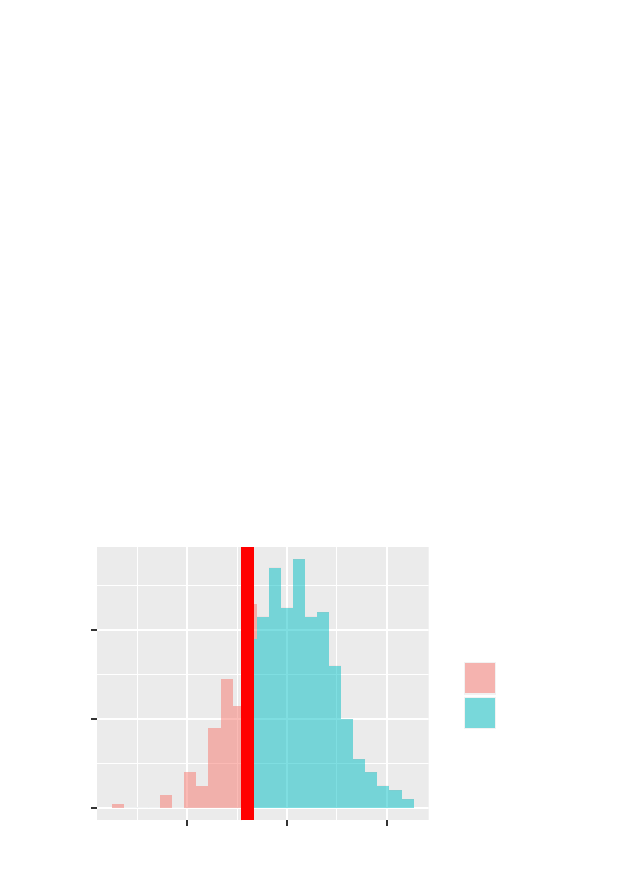
a student’s guide to r 67
Digging Deeper
More details and examples can
be found in the mosaic package
Resampling Vignette.
> rtest.stats <- do(500)*diffmean(age ~ shuffle(sex),
data = HELPrct)
> rtest.stats <- mutate(rtest.stats,
diffmeantest =ifelse(diffmean >= test.stat, TRUE,FALSE))
>head(rtest.stats, 3)
diffmean diffmeantest
1 -0.6251 TRUE
2 -1.3225 FALSE
3 0.4028 TRUE
>favstats(~ diffmean, data = rtest.stats)
min Q1 median Q3 max mean sd n missing
-3.305 -0.6495 0.01121 0.6108 2.507 -0.01838 0.8981 500 0
>gf_histogram(~ diffmean, n=40,xlim =c(-6,6),
fill = ~ diffmeantest, pch =16,cex =.8,
data = rtest.stats) %>%
gf_vline(xintercept = ~ test.stat, color ="red",lwd =3)
0
20
40
−2 0 2
diffmean
count
diffmeantest
FALSE
TRUE
Here we don’t see much evidence to contradict the
null hypothesis that men and women have the same
mean age in the population.
7.5One-way ANOVA
Earlier comparisons were between two groups. We can
also consider testing differences between three or more
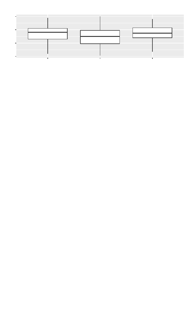
68 horton,kaplan,pruim
groups using one-way ANOVA. Here we compare CESD
scores by primary substance of abuse (heroin, cocaine, or
alcohol) with a line rather a dot to indicate the median.
>gf_boxplot(cesd ~ substance, data = HELPrct)
●
0
20
40
60
alcohol cocaine heroin
substance
cesd
>mean(cesd ~ substance, data = HELPrct)
alcohol cocaine heroin
34.37 29.42 34.87
> anovamod <- aov(cesd ~ substance, data = HELPrct)
>summary(anovamod)
Df Sum Sq Mean Sq F value Pr(>F)
substance 2 2704 1352 8.94 0.00016
Residuals 450 68084 151
While still high (scores of 16 or more are generally con-
sidered to be “severe” symptoms), the cocaine-involved
group tend to have lower scores than those whose pri-
mary substances are alcohol or heroin.
> modintercept <- lm(cesd ~ 1,data = HELPrct)
> modsubstance <- lm(cesd ~ substance, data = HELPrct)
The anova() command can summarize models.
>anova(modsubstance)
Analysis of Variance Table
Response: cesd
Df Sum Sq Mean Sq F value Pr(>F)
substance 2 2704 1352 8.94 0.00016
Residuals 450 68084 151

a student’s guide to r 69
In this setting the results are identical (since there is
only one predictor, with 2df).
The anova() function can also be used to formally
compare two (nested) models.
>anova(modintercept, modsubstance)
Analysis of Variance Table
Model 1: cesd ~ 1
Model 2: cesd ~ substance
Res.Df RSS Df Sum of Sq F Pr(>F)
1 452 70788
2 450 68084 2 2704 8.94 0.00016
7.6Tukey’s Honest Significant Differences
There are a variety of multiple comparison procedures
that can be used after fitting an ANOVA model. One of
these is Tukey’s Honest Significant Differences (HSD).
Other options are available within the multcomp package.
>favstats(cesd ~ substance, data = HELPrct)
substance min Q1 median Q3 max mean sd n missing
1 alcohol 4 26 36 42 58 34.37 12.05 177 0
2 cocaine 1 19 30 39 60 29.42 13.40 152 0
3 heroin 4 28 35 43 56 34.87 11.20 124 0
> HELPrct <- mutate(HELPrct, subgrp =factor(substance,
levels =c("alcohol","cocaine","heroin"),
labels =c("A","C","H")))
> mod <- lm(cesd ~ subgrp, data = HELPrct)
> HELPHSD <- TukeyHSD(mod, "subgrp")
> HELPHSD
Tukey multiple comparisons of means
95% family-wise confidence level
Fit: aov(formula = x)
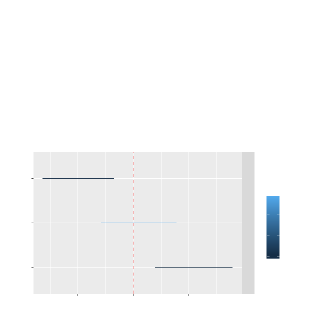
70 horton,kaplan,pruim
$subgrp
diff lwr upr p adj
C-A -4.9518 -8.150 -1.753 0.0009
H-A 0.4981 -2.889 3.885 0.9362
H-C 5.4499 1.950 8.950 0.0008
>mplot(HELPHSD)
●
●
●
subgrp
−5 0 5
H−C
H−A
C−A
difference in means
−3
−2
−1
log10(pval)
95% family−wise confidence level
Again, we see that the cocaine group has significantly
lower CESD scores than either of the other two groups.

8
Categorical Response, Quantitative Predictor
8.1Logistic regression
Logistic regression is available using the glm() function,
which supports a variety of link functions and distribu-
tional forms for generalized linear models, including lo-
gistic regression.
The glm() function has argu-
ment family, which can take
an option link. The logit
link is the default link for the
binomial family, so we don’t
need to specify it here. The
more verbose usage would be
family=binomial(link=logit).
> logitmod <- glm(homeless ~ age + female,
family = binomial, data = HELPrct)
>msummary(logitmod)
Coefficients:
Estimate Std. Error z value Pr(>|z|)
(Intercept) 0.8926 0.4537 1.97 0.049
age -0.0239 0.0124 -1.92 0.055
female 0.4920 0.2282 2.16 0.031
(Dispersion parameter for binomial family taken to be 1)
Null deviance: 625.28 on 452 degrees of freedom
Residual deviance: 617.19 on 450 degrees of freedom
AIC: 623.2
Number of Fisher Scoring iterations: 4
>exp(coef(logitmod))
(Intercept) age female
2.4415 0.9764 1.6355
>exp(confint(logitmod))
Waiting for profiling to be done...

72 horton,kaplan,pruim
2.5 % 97.5 %
(Intercept) 1.0081 5.988
age 0.9527 1.000
female 1.0501 2.574
We can compare two models (for multiple degree of
freedom tests). For example, we might be interested in
the association of homeless status and age for each of the
three substance groups.
> mymodsubage <- glm((homeless == "homeless") ~ age + substance,
family = binomial, data = HELPrct)
> mymodage <- glm((homeless == "homeless") ~ age, family = binomial,
data = HELPrct)
>msummary(mymodsubage)
Coefficients:
Estimate Std. Error z value Pr(>|z|)
(Intercept) -0.0509 0.5164 -0.10 0.9215
age 0.0100 0.0129 0.77 0.4399
substancecocaine -0.7496 0.2303 -3.25 0.0011
substanceheroin -0.7780 0.2469 -3.15 0.0016
(Dispersion parameter for binomial family taken to be 1)
Null deviance: 625.28 on 452 degrees of freedom
Residual deviance: 607.62 on 449 degrees of freedom
AIC: 615.6
Number of Fisher Scoring iterations: 4
>exp(coef(mymodsubage))
(Intercept) age substancecocaine substanceheroin
0.9504 1.0101 0.4725 0.4593
>anova(mymodage, mymodsubage, test ="Chisq")
Analysis of Deviance Table
Model 1: (homeless == "homeless") ~ age
Model 2: (homeless == "homeless") ~ age + substance
Resid. Df Resid. Dev Df Deviance Pr(>Chi)
1 451 622
2 449 608 2 14.3 0.00078

a student’s guide to r 73
We observe that the cocaine and heroin groups are sig-
nificantly less likely to be homeless than alcohol involved
subjects, after controlling for age. (A similar result is seen
when considering just homeless status and substance.)
>tally(~ homeless | substance, format ="percent",
margins =TRUE,data = HELPrct)
substance
homeless alcohol cocaine heroin
homeless 58.19 38.82 37.90
housed 41.81 61.18 62.10
Total 100.00 100.00 100.00
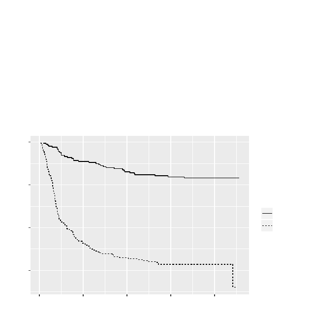
9
Survival Time Outcomes
Extensive support for survival (time to event) analysis is
available within the survival package.
9.1Kaplan-Meier plot
>library(survival)
>library(broom)
> fit <- survfit(Surv(dayslink, linkstatus) ~ treat,
data = HELPrct)
> fit <- broom::tidy(fit)
>gf_step(fit, estimate ~ time, linetype = ~ strata,
title ="Product-Limit Survival Estimates (time to linkage)",
xlab ="time (in days)",ylab ="P(not linked)")
0.4
0.6
0.8
1.0
0 100 200 300 400
time (in days)
P(not linked)
strata
treat=no
treat=yes
Product−Limit Survival Estimates (time to linkage)

76 horton,kaplan,pruim
We see that the subjects in the treatment (Health Eval-
uation and Linkage to Primary Care clinic) were signif-
icantly more likely to link to primary care (less likely to
“survive”) than the control (usual care) group.
9.2Cox proportional hazards model
>require(survival)
>summary(coxph(Surv(dayslink, linkstatus) ~ age + substance,
data = HELPrct))
Call:
coxph(formula = Surv(dayslink, linkstatus) ~ age + substance,
data = HELPrct)
n= 431, number of events= 163
(22 observations deleted due to missingness)
coef exp(coef) se(coef) z Pr(>|z|)
age 0.00893 1.00897 0.01026 0.87 0.38
substancecocaine 0.18045 1.19775 0.18100 1.00 0.32
substanceheroin -0.28970 0.74849 0.21725 -1.33 0.18
exp(coef) exp(-coef) lower .95 upper .95
age 1.009 0.991 0.989 1.03
substancecocaine 1.198 0.835 0.840 1.71
substanceheroin 0.748 1.336 0.489 1.15
Concordance= 0.55 (se = 0.023 )
Rsquare= 0.014 (max possible= 0.988 )
Likelihood ratio test= 6.11 on 3 df, p=0.1
Wald test = 5.84 on 3 df, p=0.1
Score (logrank) test = 5.91 on 3 df, p=0.1
Neither age nor substance group was significantly
associated with linkage to primary care.
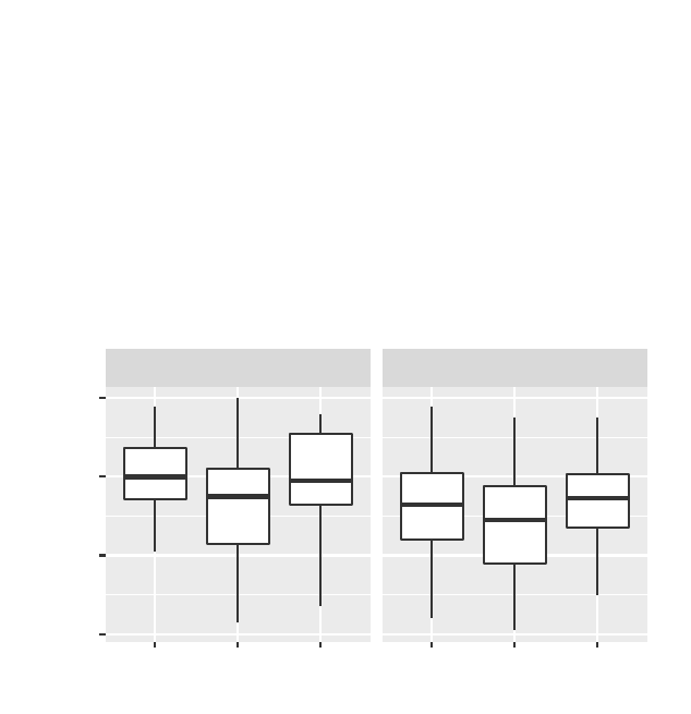
10
More than Two Variables
10.1Two (or more) way ANOVA
We can fit a two (or more) way ANOVA model, without
or with an interaction, using the same modeling syntax.
> HELPrct <- mutate(HELPrct, subgrp =factor(substance,
levels =c("alcohol","cocaine","heroin"),
labels =c("A","C","H")))
>median(cesd ~ substance | sex, data = HELPrct)
alcohol.female cocaine.female heroin.female alcohol.male
40.0 35.0 39.0 33.0
cocaine.male heroin.male female male
29.0 34.5 38.0 32.5
>gf_boxplot(cesd ~ subgrp | sex, data = HELPrct)
●
female
male
A C H A C H
0
20
40
60
subgrp
cesd
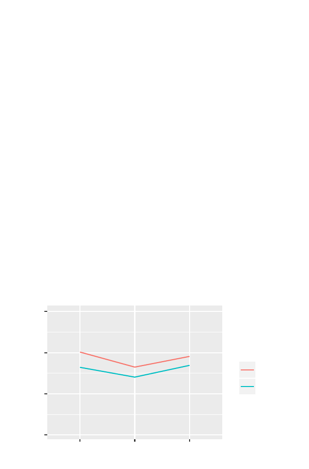
78 horton,kaplan,pruim
>summary(aov(cesd ~ substance + sex, data = HELPrct))
Df Sum Sq Mean Sq F value Pr(>F)
substance 2 2704 1352 9.27 0.00011
sex 1 2569 2569 17.61 3.3e-05
Residuals 449 65515 146
>summary(aov(cesd ~ substance *sex, data = HELPrct))
Df Sum Sq Mean Sq F value Pr(>F)
substance 2 2704 1352 9.25 0.00012
sex 1 2569 2569 17.57 3.3e-05
substance:sex 2 146 73 0.50 0.60752
Residuals 447 65369 146
There’s little evidence for the interaction, though there are
statistically significant main effects terms for substance
group and sex.
> mod <- lm(cesd ~ substance + sex + substance*sex, data = HELPrct)
>plotModel(mod)
●
●
●
●
●
●
●
●
●
●●
●
●
●
●
●
●
●
●
●●
●
●
●
●
●
●
●
●
●
●
●
●
●
●
●
●
●
●
●
●
●
●
●
●
●
●
●
●
●
●
●
●
●
●
●
●
●
●
●
●
●
●
●
●
●●
●
●
●
●
●
●
●
●
●
●
●
●
●
●
●
●●
●
●
●
●
●
●●
●
●
●
●
●
●
●
●
●
●
●
●
●
●
●
●
●
●
●
●
●
●
●
●
●
●
●
●
●
●
●
●
●
●
●
●●
●
●
●
●
●
●●
●●
●
●
●
●
●
●
●
●
●
●
●
●
●
●
●
●
●
●
●
●
●
●●
●
●
●
●
●
●
●
●
●●
●
●
●
●
●
●
●
●
●
●
●
●
●
●
●
●
●
●
●
●
●
●
●
●
●
●
● ●
●
●
●●
●
●
●
●
●
●●
●
●
●
●
●
●
●
●
●
●
●
●
●
●
●
●
●
●
●
●
●
●
●
●
●
●
●
●
●
●
●
●
●
●
●
●
●
●
●
●
●
●
●
●
●
●
●
●
●
●
●
●
●
●
●
●
●
●
●
●
●
●
●
●
●●
●
●
●
●
●
●
●
●
●
●
●
●
●
●
●
●
●
●
●
●
●
●
●
●
●
●
●
●
●
●
●
●
●
●
●
●
●
●
●
●
●
●
●
●
●
●
●
●
● ●
●
●
●
●
●
●
●
●
●
●
●
●
●
●
●
●
●
●
●
●
●
●
●
●
●
●
●●
●
●
●
●
●
●●
●
●
●
●
●
●
●
●
●
●
●●
●
●
●
●
●
●
●
●
●
●
●
●
●
●
●
●
●
●
●
●
●
●
●
●
●
●
●●
●
●
●
●
●
●
●
●
●
●
●
●
●
●
●
●
●
●
●
●●
●
●
●
●
●
●
●
●
●
●
●●
●
●
●
●
●
●
●
●
●
●
●
●
●
●
●
●
●
●
●
●
0
20
40
60
alcohol cocaine heroin
substance
cesd
.color
●
●
female
male
10.2Multiple regression
Multiple regression is a logical extension of the prior
commands, where additional predictors are added. This
allows students to start to try to disentangle multivariate
relationships.
We tend to introduce multiple
linear regression early in our
courses, as a purely descriptive
technique, then return to it
regularly. The motivation for
this is described at length in
the companion volume Start
Modeling with R.

a student’s guide to r 79
Here we consider a model (parallel slopes) for depres-
sive symptoms as a function of Mental Component Score
(MCS), age (in years) and sex of the subject.
> lmnointeract <- lm(cesd ~ mcs + age + sex, data = HELPrct)
>msummary(lmnointeract)
Estimate Std. Error t value Pr(>|t|)
(Intercept) 53.8303 2.3617 22.79 <2e-16
mcs -0.6548 0.0336 -19.50 <2e-16
age 0.0553 0.0556 1.00 0.3200
sexmale -2.8993 1.0137 -2.86 0.0044
Residual standard error: 9.09 on 449 degrees of freedom
Multiple R-squared: 0.476,Adjusted R-squared: 0.473
F-statistic: 136 on 3 and 449 DF, p-value: <2e-16
We can also fit a model that includes an interaction be-
tween MCS and sex.
> lminteract <- lm(cesd ~ mcs + age + sex + mcs:sex, data = HELPrct)
>msummary(lminteract)
Estimate Std. Error t value Pr(>|t|)
(Intercept) 55.3906 2.9903 18.52 <2e-16
mcs -0.7082 0.0712 -9.95 <2e-16
age 0.0549 0.0556 0.99 0.324
sexmale -4.9421 2.6055 -1.90 0.058
mcs:sexmale 0.0687 0.0807 0.85 0.395
Residual standard error: 9.09 on 448 degrees of freedom
Multiple R-squared: 0.477,Adjusted R-squared: 0.472
F-statistic: 102 on 4 and 448 DF, p-value: <2e-16
>anova(lminteract)
Analysis of Variance Table
Response: cesd
Df Sum Sq Mean Sq F value Pr(>F)
mcs 1 32918 32918 398.27 <2e-16
age 1 107 107 1.29 0.2563
sex 1 676 676 8.18 0.0044
mcs:sex 1 60 60 0.72 0.3952
Residuals 448 37028 83

80 horton,kaplan,pruim
>anova(lmnointeract, lminteract)
Analysis of Variance Table
Model 1: cesd ~ mcs + age + sex
Model 2: cesd ~ mcs + age + sex + mcs:sex
Res.Df RSS Df Sum of Sq F Pr(>F)
1 449 37088
2 448 37028 1 59.9 0.72 0.4
There is little evidence for an interaction effect, so we
drop this from the model.
10.2.1Visualizing the results from the regression
The makeFun() and plotFun() functions from the mosaic
package can be used to display the predicted values from
a regression model. For this example, we might display
the predicted CESD values for a range of MCS (mental
component score) values a hypothetical 36 year old male
and female subject might have from the parallel slopes
(no interaction) model.
> lmfunction <- makeFun(lmnointeract)
We can now plot the predicted values separately for
male and female subjects over a range of MCS (mental
component score) values, along with the observed data
for all of the 36 year olds.
>gf_point(cesd ~ mcs, color = ~ sex,
data =filter(HELPrct, age == 36),
ylab ="predicted CESD") %>%
gf_fun(lmfunction(mcs, age =36,sex ="male") ~ mcs,
xlim =c(0,60), size =1.5) %>%
gf_fun(lmfunction(mcs, age =36,sex ="female") ~ mcs,
xlim =c(0,60), linetype =2,size =2)
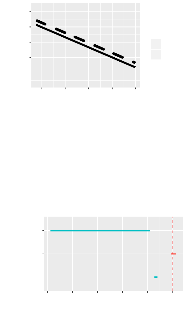
a student’s guide to r 81
●
●
●
●
●
●
●
●
●
●
●●
●●
●
●
●
●
●
●
●
●
●
10
20
30
40
50
20 30 40 50 60
mcs
predicted CESD
sex
●
●
female
male
10.2.2Coefficient plots
It is sometimes useful to display a plot of the coefficients
for a multiple regression model (along with their associ-
ated confidence intervals).
>mplot(lmnointeract, rows = -1,which =7)
●
●
●
mcs
age
sexmale
−5 −4 −3 −2 −1 0
estimate
coefficient
95% confidence intervals
Darker dots indicate regression
coefficients where the 95%
confidence interval does not
include the null hypothesis
value of zero.
Caution!
Be careful when fitting re-
gression models with missing
values (see also section 13.11).
10.2.3Residual diagnostics
It’s straightforward to undertake residual diagnostics
for this model. We begin by adding the fitted values and
residuals to the dataset.
The mplot() function can also
be used to create these graphs.
Here we are adding two new
variables into an existing
dataset. It’s often a good
practice to give the resulting
dataframe a new name.
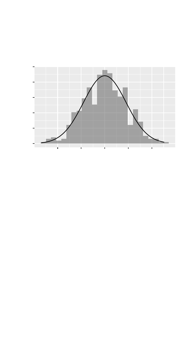
82 horton,kaplan,pruim
> HELPrct <- mutate(HELPrct,
residuals =resid(lmnointeract),
pred =fitted(lmnointeract))
>gf_dhistogram(~ residuals, data = HELPrct) %>%
gf_fitdistr(dist = dnorm)
0.00
0.01
0.02
0.03
0.04
0.05
−20 −10 0 10 20
residuals
density
We can identify the subset of observations with ex-
tremely large residuals.
>filter(HELPrct, abs(residuals) > 25)
age anysubstatus anysub cesd d1 daysanysub dayslink drugrisk e2b
1 43 0 no 16 15 191 414 0 NA
2 27 NA <NA> 40 1 NA 365 3 2
female sex g1b homeless i1 i2 id indtot linkstatus link mcs
1 0 male no homeless 24 36 44 41 0 no 15.86
2 0 male no homeless 18 18 420 37 0 no 57.49
pcs pss_fr racegrp satreat sexrisk substance treat avg_drinks
1 71.39 3 white no 7 cocaine yes 24
2 37.75 8 white yes 3 heroin no 18
max_drinks subgrp residuals pred
1 36 C -26.92 42.92
2 18 H 25.22 14.78
>gf_point(residuals ~ pred, cex =.3,xlab ="predicted values",
title ="predicted vs. residuals",data = HELPrct) %>%
gf_smooth(se =FALSE) %>%
gf_hline(yintercept =0)
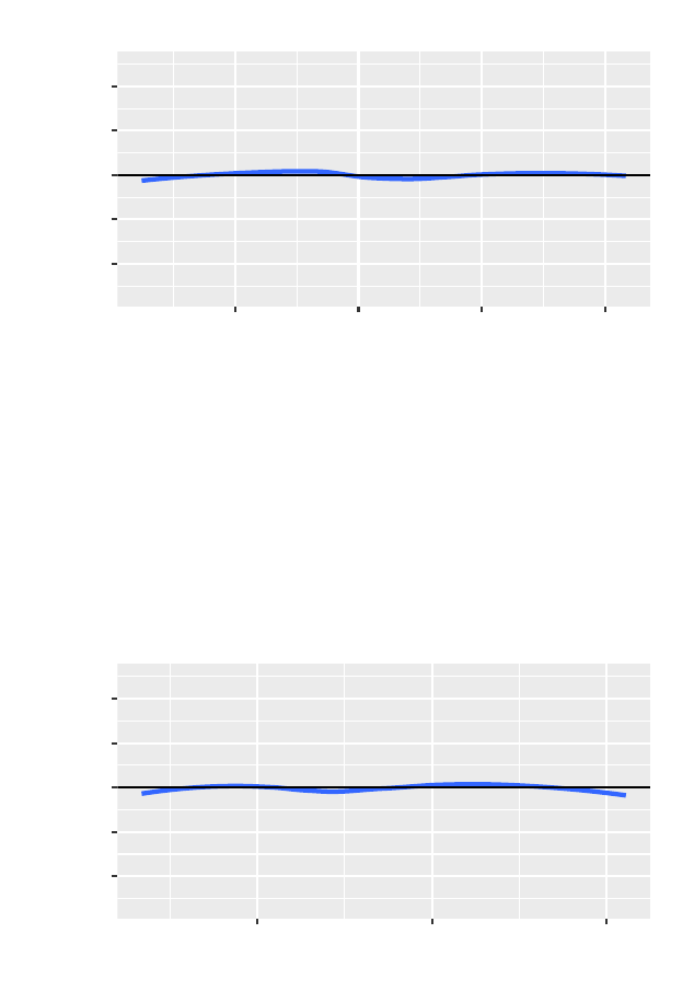
a student’s guide to r 83
●
●
●
●
●
●
●
●
●
●
●
●
●
●
●
●
●
●
●
●
●
●●
●
●
●
●
●
●
●
●
●
●
●
●
●
●
●
●
●
●
●
●
●
●
●
●
●
●
●
●
●
●
●
●
●
●
●●
●
●
●
●
●
●
●
●
●
●●
●
●
●
●
●
●
●
●
●
●
●
●
●
●
●
●
●
●
●
●
●
●
●
●
●
●
●
●
●
●
●
●
●
●
●
●
●
●
●
●
●
●
●
●
●
●
●
●
●
●
●
●
●
●
●
●
●
●
●
●
●
●
●
●
●
●
●
●
●
●
●
●
●
●
●
●
●
●
●
●
●
●●
●
●
●
●
●
●
●●
●
●
●
●
●
●
●
●
●
●
●
●
●
●
●
●
●
●
●
●
●
●
●
●
●
●
●
●
●
●
●
●
●
●
●
●
●
●
●
●
●
●
●
●
●
●
●
●
●
●
●
●
●
●
●
●
●
●●
●
●
●
●
●
●
●
●
●
●
●
●
●
●
●
●
●
●
●
●
●
●
●
●
●
●
●
●
●
●
●
●
●●
●
●
●
●
●
●
●
●
●
●
●
●
●
●
●
●
●
●
●
●
●
●
●
●
●
●
●
●
●
●
●
●
●
●
●
●
●
●
●
●
●
●
●
●
●
●
●
●
●
●
●
●
●
●
●
●
●
●
●
●
●
●
●
●
●
●
●
●
●
●
●
●
●
●
●
●
●
●
●
●
●
●
●
●
●
●
●
●
●
●
●
●●
●
●
●
●
●
●
●
●
●
●
●
●
●
●
●
●
●
●
●
●
●
●
●
●
●
●
●
●
●
●
●
●
●
●
●
●
●
●
●
●
●
●
●
●
●
●
●
●
●
●
●
●
●
●
●
●
●
●
●
●
●
●
●
●
●
●
●
●
●
●
●
●
●
●
●
●
●
●
●
●
●
●
●
●
●
●
●
●●
●
●
●
●
●
●
●
●
●
●●
●
●
●
●
●
●
−20
−10
0
10
20
20 30 40 50
predicted values
residuals
predicted vs. residuals
>gf_point(residuals ~ mcs, cex =.3,
xlab ="mental component score",
title ="predicted vs. residuals",data = HELPrct) %>%
gf_smooth(se =FALSE) %>%
gf_hline(yintercept =0)
●
●
●
●
●
●
●
●
●
●
●
●●
●
●
●
●
●
●
●
●●
●
●
●
●
●
●
●
●
●
●
●
●
●
●
●
●
●
●
●
●
●
●
●
●
●
●
●
●
●
●
●
●
●
●
●
●
●
●
●
●
●
●
●
●
●
●
●
●
●
●
●
●
●
●
●
●
●
●
●
●
●
●
●
●
●
●
●
●
●
●
●
●
●
●
●
●
●
●
●
●
●
●
●
●
●
●
●
●
●
●
●
●●
●
●
●
●
●
●
●
●
●
●
●
●
●
●
●●
●●
●
●
●
●
●
●
●
●
●
●
●
●
●
●
●
●
●
●
●
●
●
●
●
●
●
●
●●
●
●
●
●
●
●
●
●
●
●
●
●
●
●
●
●
●
●
●
●
●
●
●
●
●
●
●
●
●
●
●
●
●●
●
●
●
●
●
●
●
●
●
●
●
●
●
●
●
●
●
●
●
●
●
●
●
●
●
●
●
●
●
●
●
●
●
●
●
●
●
●
●
●
●
●
●
●
●
●
●●
●
●
●
●
●
●
●
●
●
●
●
●
●
●
●
●
●
●
●
●
●
●
●
●
●
●
●
●
●
●
●
●
●
●
●
●
●
●
●
●
●
●
●
●
●
●
●
●
●
●
●
●
●
●
●
●
●
●
●
●
●
●
●
●
●
●
●
●
●
●
●
●●
●
●
●
●
●
●
●
●
●
●
●
●
●
●
●
●
●
●
●
●
●●
●
●●
●
●
●
●
●
●
●
●
●
●
●
●
●
●
●
●
●
●
●
●
●
●
●
●
●
●
●
●
●
●
●
●
●
●
●
●
●
●
●
●
●●
●
●
●
●
●
●
●
●
●
●
●
●
●
●
●
●
●
●
●
●
●
●
●
●
●
●
●
●
●
●
●
●
●
●
●
●●
●
●
●
●
●
●
●
●
●
●
●
●
●
●
●
●
●
●
●
●
●
●
●
●
●
●
●
●
●
●
●
●
●
−20
−10
0
10
20
20 40 60
mental component score
residuals
predicted vs. residuals
The assumptions of normality, linearity and homoscedas-
ticity seem reasonable here.
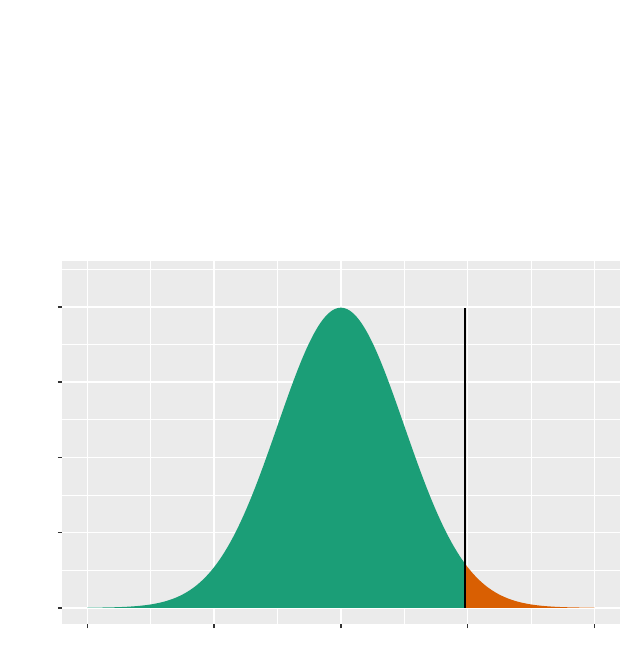
11
Probability Distributions & Random Variables
Rcan calculate quantities related to probability distribu-
tions of all types. It is straightforward to generate ran-
dom samples from these distributions, which can be used
for simulation and exploration.
>xpnorm(1.96,mean =0,sd =1)# P(Z < 1.96)
If X ~ N(0, 1), then
P(X <= 1.96) = P(Z <= 1.96) = 0.975
P(X > 1.96) = P(Z > 1.96) = 0.025
[1] 0.975
z = 1.96
0.0
0.1
0.2
0.3
0.4
−4 −2 0 2 4
x
density
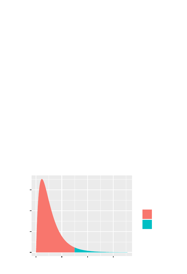
86 horton,kaplan,pruim
># value which satisfies P(Z < z) = 0.975
>qnorm(.975,mean =0,sd =1)
[1] 1.96
>integrate(dnorm, -Inf,0)# P(Z < 0)
0.5 with absolute error < 4.7e-05
A similar display is available for the F distribution.
>xpf(3,df1 =4,df2 =20)
[1] 0.9568
0.0
0.2
0.4
0.6
0 2 4 6
density
probability
A:0.957
B:0.043
The following table displays the basenames for prob-
ability distributions available within base R. These func-
tions can be prefixed by dto find the density function
for the distribution, pto find the cumulative distribution
function, qto find quantiles, and rto generate random
draws. For example, to find the density function of an ex-
ponential random variable, use the command dexp(). The
qDIST() function is the inverse of the pDIST() function,
for a given basename DIST.
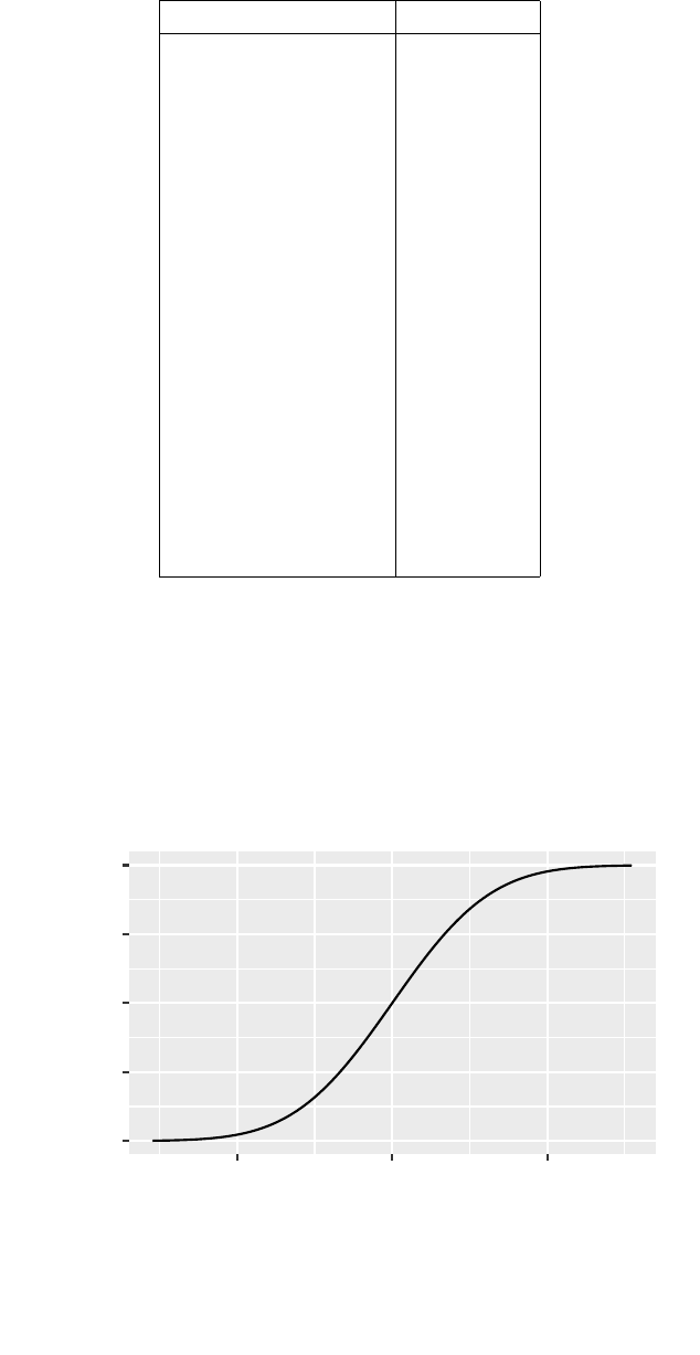
a student’s guide to r 87
Distribution Basename
Beta beta
binomial binom
Cauchy cauchy
chi-square chisq
exponential exp
Ff
gamma gamma
geometric geom
hypergeometric hyper
logistic logis
lognormal lnorm
negative binomial nbinom
normal norm
Poisson pois
Student’s t t
Uniform unif
Weibull weibull
Digging Deeper
The gf_fitdistr() within
the MASS package facilitates
estimation of parameters for
many distributions.
The gf_dist() can be used to display distributions in a
variety of ways.
>gf_dist('norm',mean =100,sd =10,kind ='cdf')
0.00
0.25
0.50
0.75
1.00
80 100 120
x
cumulative_density
>gf_dist('exp',kind ='histogram',xlab ="x")
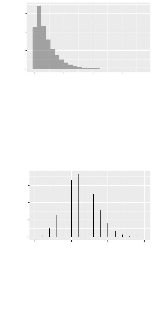
88 horton,kaplan,pruim
0.0
0.2
0.4
0.6
0.0 2.5 5.0 7.5
x
density
Note that this sets the rate parameter to 1by default and
is equivalent to the following command.
>gf_dist('exp',rate =1,kind ='histogram',xlab ="x")
>gf_dist('binom',size =25,prob =0.25,xlim =c(-1,26))
●●
●
●
●
●
●
●
●
●
●
●
●●●●
0.00
0.05
0.10
0.15
0 5 10 15
x
density
Multiple distributions can be plotted on the same plot.
>gf_dist("binom",size =100,prob =.3,col ="black",lwd =1.5,pch =16)
>plotDist("norm",mean =30,sd =sqrt(100 *.3 *.7),
groups =abs(x-30)>6,type ="h",under =TRUE)
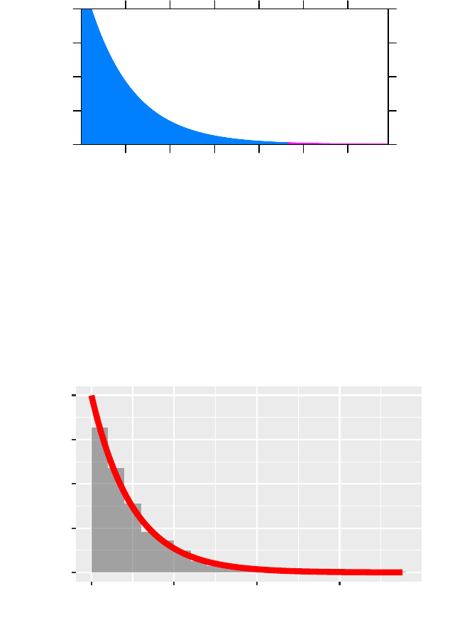
a student’s guide to r 89
0.1
0.2
0.3
2 4 6 8 10 12
The gf_fun() function can be used to plot an arbitrary
function (in this case an exponential random variable).
> f <- makeFun(2*exp(-2*x) ~ x) # exponential with rate parameter 2
> x <- rexp(1000,rate =2)
>gf_dhistogram(~ x, binwidth =0.2,center =0.1) %>%
gf_fun(f(x) ~ x, color ="red",size =2,xlim =c(0,3))
0.0
0.5
1.0
1.5
2.0
0123
x
density

12
Power Calculations
While not generally a major topic in introductory courses,
power and sample size calculations help to reinforce key
ideas in statistics. In this section, we will explore how R
can be used to undertake power calculations using ana-
lytic approaches. We consider a simple problem with two
tests (t-test and sign test) of a one-sided comparison.
We will compare the power of the sign test and the
power of the test based on normal theory (one sample
one sided t-test) assuming that σis known. Let X1, ..., X25
be i.i.d. N(0.3, 1)(this is the alternate that we wish to
calculate power for). Consider testing the null hypothesis
H0:µ=0 versus HA:µ>0 at significance level α=.05.
12.1Sign test
We start by calculating the Type I error rate for the sign
test. Here we want to reject when the number of pos-
itive values is large. Under the null hypothesis, this is
distributed as a Binomial random variable with n=25 tri-
als and p=0.5probability of being a positive value. Let’s
consider values between 15 and 19.
> xvals <- 15:19
> probs <- 1-pbinom(xvals, size =25,prob =0.5)
>cbind(xvals, probs)
xvals probs
[1,] 15 0.114761
[2,] 16 0.053876
[3,] 17 0.021643
[4,] 18 0.007317
[5,] 19 0.002039
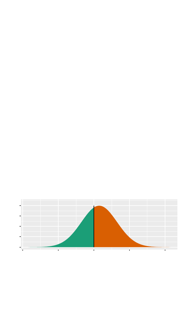
92 horton,kaplan,pruim
>qbinom(.95,size =25,prob =0.5)
[1] 17
So we see that if we decide to reject when the number of
positive values is 17 or larger, we will have an αlevel of
0.054, which is near the nominal value in the problem.
We calculate the power of the sign test as follows. The
probability that Xi>0, given that HAis true is given by:
>1-pnorm(0,mean =0.3,sd =1)
[1] 0.6179
We can view this graphically using the command:
>xpnorm(0,mean =0.3,sd =1,lower.tail =FALSE)
If X ~ N(0.3, 1), then
P(X <= 0) = P(Z <= -0.3) = 0.3821
P(X > 0) = P(Z > -0.3) = 0.6179
[1] 0.6179
z = −0.3
0.0
0.1
0.2
0.3
0.4
−4 −2 0 2 4
x
density
The power under the alternative is equal to the proba-
bility of getting 17 or more positive values, given that
p=0.6179:
>1-pbinom(16,size =25,prob =0.6179)
[1] 0.3378
The power is modest at best.
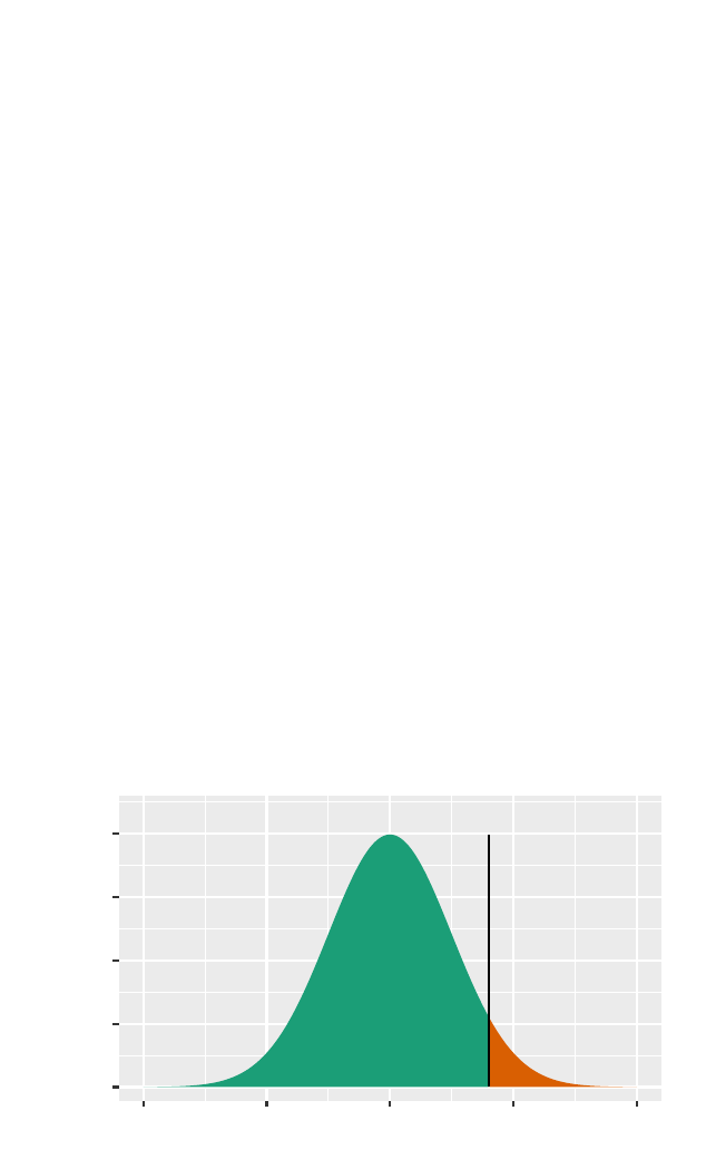
a student’s guide to r 93
12.2T-test
We next calculate the power of the test based on normal
theory. To keep the comparison fair, we will set our α
level equal to 0.05388.
> alpha <- 1-pbinom(16,size =25,prob =0.5)
> alpha
[1] 0.05388
First we find the rejection region.
>n<-25
> sigma <- 1# given
> stderr <- sigma/sqrt(n)
> zstar <- xqnorm(1- alpha, mean =0,sd =1)
If X ~ N(0, 1), then
P(X <= 1.608) = 0.9461
P(X > 1.608) = 0.05388
> zstar
[1] 1.608
> crit <- zstar *stderr
> crit
[1] 0.3217
z = 1.61
0.0
0.1
0.2
0.3
0.4
−4 −2 0 2 4
x
density

94 horton,kaplan,pruim
Therefore, we reject for observed means greater than
0.322.
To calculate the power of this one-sided test we find
the probability under the alternative hypothesis to the
right of this cutoff.
> power <- 1-pnorm(crit, mean =0.3,sd = stderr)
> power
[1] 0.4568
The power of the test based on normal theory is 0.457.
To provide a check (or for future calculations of this sort)
we can use the power.t.test() function.
>power.t.test(n=25,delta =.3,sd =1,sig.level = alpha,
alternative ="one.sided",
type ="one.sample")$power
[1] 0.4408
This analytic (formula-based approach) yields a simi-
lar estimate to the value that we calculated directly.
Overall, we see that the t-test has higher power than
the sign test, if the underlying data are truly normal.
Calculating power empirically
demonstrates the power of
simulations.

13
Data Management
The Start Teaching with R book
features an extensive section on
data management, including
use of the read.file() function
to load data into Rand RStudio.
Data management is a key capacity to allow students
(and instructors) to “compute with data” or as Diane
Lambert of Google has stated, “think with data”. We tend
to keep student data management to a minimum during
the early part of an introductory statistics course, then
gradually introduce topics as needed. For courses where
students undertake substantive projects, data manage-
ment is more important. This chapter describes some key
data management tasks.
The dplyr and tidyr packages
provide an elegant approach
to data management and fa-
cilitate the ability of students
to compute with data. Hadley
Wickham, author of the pack-
ages, suggests that there are six
key idioms (or verbs) imple-
mented within these packages
that allow a large set of tasks
to be accomplished: filter (keep
rows matching criteria), select
(pick columns by name), ar-
range (reorder rows), mutate
(add new variables), summarise
(reduce variables to values),
and group by (collapse groups).
See https://nhorton.people.
amherst.edu/precursors for
more details and resources.
13.1Inspecting dataframes
The inspect() function can be helpful in describing the
variables in a dataframe (the name for a dataset in R).
>inspect(iris)
categorical variables:
name class levels n missing
1 Species factor 3 150 0
distribution
1 setosa (33.3%), versicolor (33.3%) ...
quantitative variables:
name class min Q1 median Q3 max mean sd n
1 Sepal.Length numeric 4.3 5.1 5.80 6.4 7.9 5.843 0.8281 150
2 Sepal.Width numeric 2.0 2.8 3.00 3.3 4.4 3.057 0.4359 150
3 Petal.Length numeric 1.0 1.6 4.35 5.1 6.9 3.758 1.7653 150
4 Petal.Width numeric 0.1 0.3 1.30 1.8 2.5 1.199 0.7622 150
missing
1 0
2 0

96 horton,kaplan,pruim
3 0
4 0
The iris dataframe includes one categorical and four
quantitative variables.
13.2Adding new variables to a dataframe
We can add additional variables to an existing dataframe
using mutate(). But first we create a smaller version of
the iris dataframe.
> irisSmall <- select(iris, Species, Sepal.Length)
># cut places data into bins
> irisSmall <- mutate(irisSmall,
Length =cut(Sepal.Length, breaks =4:8))
Multiple commands can be chained together using the
%>% (pipe) operator:
> irisSmall <- iris %>%
select(Species, Sepal.Length) %>%
mutate(Length =cut(Sepal.Length, breaks =4:8))
Note that in this usage the first argument to select() is
the first variable (as it inherits the data from the previous
pipe).
The cut() function has an op-
tion labels which can be used
to specify more descriptive
names for the groups.
>head(irisSmall)
Species Sepal.Length Length
1 setosa 5.1 (5,6]
2 setosa 4.9 (4,5]
3 setosa 4.7 (4,5]
4 setosa 4.6 (4,5]
5 setosa 5.0 (4,5]
6 setosa 5.4 (5,6]
The CPS85 dataframe contains data from a Current
Population Survey (current in 1985, that is). Two of the

a student’s guide to r 97
variables in this dataframe are age and educ. We can
estimate the number of years a worker has been in the
workforce if we assume they have been in the workforce
since completing their education and that their age at
graduation is 6more than the number of years of educa-
tion obtained. We can add this as a new variable in the
dataframe using mutate().
> CPS85 <- mutate(CPS85, workforce.years =age-6- educ)
>favstats(~ workforce.years, data = CPS85)
min Q1 median Q3 max mean sd n missing
-4 8 15 26 55 17.81 12.39 534 0
In fact this is what was done for all but one of the cases to
create the exper variable that is already in the CPS85 data.
>tally(~ (exper - workforce.years), data = CPS85)
(exper - workforce.years)
0 4
533 1
13.3Dropping variables
Since we already have the exper variable, there is no rea-
son to keep our new variable. Let’s drop it. Notice the
clever use of the minus sign.
>names(CPS85)
[1] "wage" "educ" "race"
[4] "sex" "hispanic" "south"
[7] "married" "exper" "union"
[10] "age" "sector" "workforce.years"
> CPS1 <- select(CPS85, select = -matches("workforce.years"))
>names(CPS1)
[1] "wage" "educ" "race" "sex" "hispanic" "south"
[7] "married" "exper" "union" "age" "sector"

98 horton,kaplan,pruim
Any number of variables can be dropped or kept in a
similar manner.
> CPS1 <- select(CPS85, select = -matches("workforce.years|exper"))
13.4Renaming variables
The column (variable) names for a dataframe can be
changed using the rename() function in the dplyr pack-
age.
>names(CPS85)
[1] "wage" "educ" "race"
[4] "sex" "hispanic" "south"
[7] "married" "exper" "union"
[10] "age" "sector" "workforce.years"
> CPSnew = rename(CPS85, workforce = workforce.years)
>names(CPSnew)
[1] "wage" "educ" "race" "sex" "hispanic"
[6] "south" "married" "exper" "union" "age"
[11] "sector" "workforce"
The row names of a dataframes can be changed by
simple assignment using row.names().
The faithful data set (in the datasets package, which
is always available) has very unfortunate names.
It’s a good idea to establish
practices for choice of variable
names from day one.
>names(faithful)
[1] "eruptions" "waiting"
The measurements are the duration of an eruption
and the time until the subsequent eruption, so let’s give it
some better names.
> faithful <- rename(faithful,
duration = eruptions,
time.til.next = waiting)
>names(faithful)
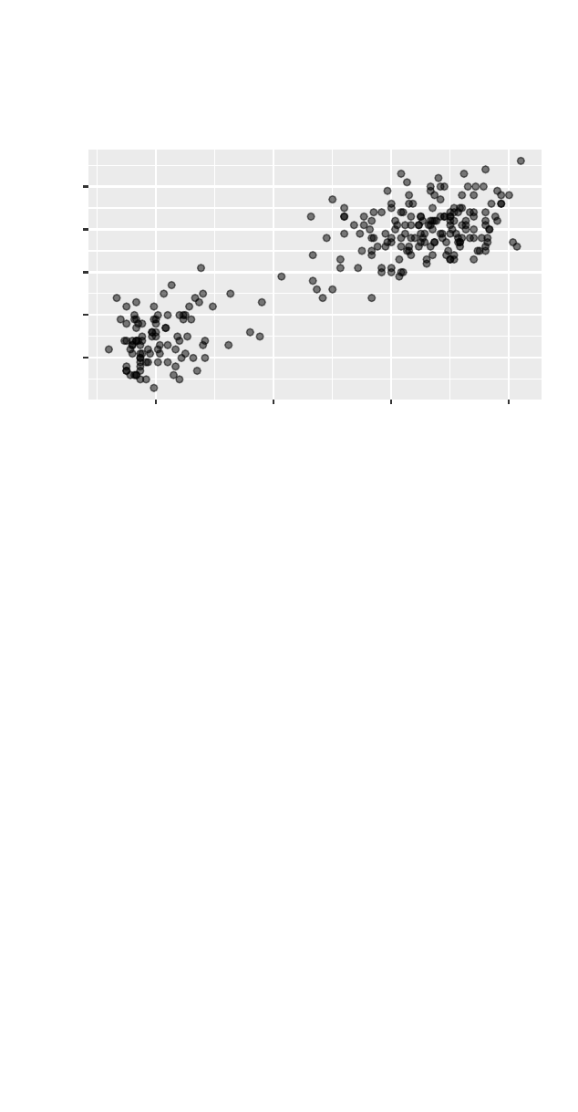
a student’s guide to r 99
[1] "duration" "time.til.next"
>gf_point(time.til.next ~ duration, alpha =0.5,data = faithful)
50
60
70
80
90
2345
duration
time.til.next
If the variable containing a dataframe is modified or used
to store a different object, the original data from the pack-
age can be recovered using data().
>data(faithful)
>head(faithful, 3)
eruptions waiting
1 3.600 79
2 1.800 54
3 3.333 74
13.5Creating subsets of observations
We can also use filter() to reduce the size of a dataframe
by selecting only certain rows.
>data(faithful)
>names(faithful) <- c('duration','time.til.next')
># any logical can be used to create subsets
> faithfulLong <- filter(faithful, duration > 3)
>gf_point(time.til.next ~ duration, data = faithfulLong)
100 horton,kaplan,pruim
●
●
●
●
● ●
●
●
●●
●
●
●
●
●
●
●●
●
●
●
●
●
●
●
●
●
●
●
●
●
●
●
●
●
●
●
●
●
●
●
● ●
●
●
●
●
●
●
●
●
●
●
●
●
●
●
●
●
●
●
●
●
●
●
●
●
●
●
●
●
●
●
●
●
●
●
●
●
●
●●
●
●
●
●
●
●
●●
●
●
●
●
●●
●
●●
●
●
●
●
●
●
●
●
●
●
●
● ●
●
●
●
●
●●
●
●●
●
●
●
●
●
●
●●
●
●
●
●
●●
●
●
●
●
●
●
●
●
●●
● ●
●
●
●
●
●
●
●
●
●
●
● ●
●
●
● ●
●
●
●
●
●●
●
●
●
●
●
●
70
80
90
3.0 3.5 4.0 4.5 5.0
duration
time.til.next
13.6Sorting dataframes
Data frames can be sorted using the arrange() function.
>head(faithful, 3)
duration time.til.next
1 3.600 79
2 1.800 54
3 3.333 74
> sorted <- arrange(faithful, duration)
>head(sorted, 3)
duration time.til.next
1 1.600 52
2 1.667 64
3 1.700 59
Caution!
It is usually better to make new
datasets rather than modifying
the original.
13.7Merging datasets
The fusion1 dataframe in the fastR package contains
genotype information for a SNP (single nucleotide poly-
morphism) in the gene TCF7L2. The pheno dataframe
contains phenotypes (including type 2diabetes case/control
status) for an intersecting set of individuals. We can join

a student’s guide to r 101
(or merge) these together to explore the association be-
tween genotypes and phenotypes using merge().
>library(fastR)
> fusion1 <- arrange(fusion1, id)
>head(fusion1, 3)
id marker markerID allele1 allele2 genotype Adose Cdose Gdose Tdose
1 1002 RS12255372 1 3 3 GG 0 0 2 0
2 1009 RS12255372 1 3 3 GG 0 0 2 0
3 1012 RS12255372 1 3 3 GG 0 0 2 0
>head(pheno, 3)
id t2d bmi sex age smoker chol waist weight height whr sbp dbp
1 1002 case 32.86 F 70.76 former 4.57 112.0 85.6 161.4 0.9868 135 77
2 1009 case 27.39 F 53.92 never 7.32 93.5 77.4 168.1 0.9397 158 88
3 1012 control 30.47 M 53.86 former 5.02 104.0 94.6 176.2 0.9327 143 89
>library(tidyr)
> fusion1m <- inner_join(fusion1, pheno, by ='id')
>head(fusion1m, 3)
id marker markerID allele1 allele2 genotype Adose Cdose Gdose Tdose t2d bmi
1 1002 RS12255372 1 3 3 GG 0 0 2 0 case 32.86
2 1009 RS12255372 1 3 3 GG 0 0 2 0 case 27.39
3 1012 RS12255372 1 3 3 GG 0 0 2 0 control 30.47
sex age smoker chol waist weight height whr sbp dbp
1 F 70.76 former 4.57 112.0 85.6 161.4 0.9868 135 77
2 F 53.92 never 7.32 93.5 77.4 168.1 0.9397 158 88
3 M 53.86 former 5.02 104.0 94.6 176.2 0.9327 143 89
Now we are ready to begin our analysis.
>tally(~t2d + genotype, data = fusion1m)
genotype
t2d GG GT TT
case 737 375 48
control 835 309 27

102 horton,kaplan,pruim
13.8Slicing and dicing
The tidyr package provides a flexible way to change the
arrangement of data. It was designed for converting be-
tween long and wide versions of time series data and its
arguments are named with that in mind.
The vignettes that accompany
the tidyr and dplyr packages
feature a number of useful
examples of common data
manipulations.
A common situation is when we want to convert from
a wide form to a long form because of a change in per-
spective about what a unit of observation is. For example,
in the traffic dataframe, each row is a year, and data for
multiple states are provided.
> traffic
year cn.deaths ny cn ma ri
1 1951 265 13.9 13.0 10.2 8.0
2 1952 230 13.8 10.8 10.0 8.5
3 1953 275 14.4 12.8 11.0 8.5
4 1954 240 13.0 10.8 10.5 7.5
5 1955 325 13.5 14.0 11.8 10.0
6 1956 280 13.4 12.1 11.0 8.2
7 1957 273 13.3 11.9 10.2 9.4
8 1958 248 13.0 10.1 11.8 8.6
9 1959 245 12.9 10.0 11.0 9.0
We can reformat this so that each row contains a mea-
surement for a single state in one year.
> longTraffic <- traffic %>%
gather(state, deathRate, ny:ri)
>head(longTraffic)
year cn.deaths state deathRate
1 1951 265 ny 13.9
2 1952 230 ny 13.8
3 1953 275 ny 14.4
4 1954 240 ny 13.0
5 1955 325 ny 13.5
6 1956 280 ny 13.4
We can also reformat the other way, this time having
all data for a given state form a row in the dataframe.

a student’s guide to r 103
> stateTraffic <- longTraffic %>%
select(year, deathRate, state) %>%
mutate(year =paste("deathRate.", year, sep ="")) %>%
spread(year, deathRate)
> stateTraffic
state deathRate.1951 deathRate.1952 deathRate.1953 deathRate.1954 deathRate.1955
1 cn 13.0 10.8 12.8 10.8 14.0
2 ma 10.2 10.0 11.0 10.5 11.8
3 ny 13.9 13.8 14.4 13.0 13.5
4 ri 8.0 8.5 8.5 7.5 10.0
deathRate.1956 deathRate.1957 deathRate.1958 deathRate.1959
1 12.1 11.9 10.1 10.0
2 11.0 10.2 11.8 11.0
3 13.4 13.3 13.0 12.9
4 8.2 9.4 8.6 9.0
13.9Derived variable creation
A number of functions help facilitate the creation or re-
coding of variables.
13.9.1Creating categorical variable from a quantita-
tive variable
Next we demonstrate how to create a three-level categor-
ical variable with cuts at 20 and 40 for the CESD scale
(which ranges from 0to 60 points).
>favstats(~ cesd, data = HELPrct)
min Q1 median Q3 max mean sd n missing
1 25 34 41 60 32.85 12.51 453 0
> HELPrct <- mutate(HELPrct, cesdcut =cut(cesd,
breaks =c(0,20,40,60), include.lowest =TRUE))
>gf_boxplot(cesd ~ cesdcut, data = HELPrct)
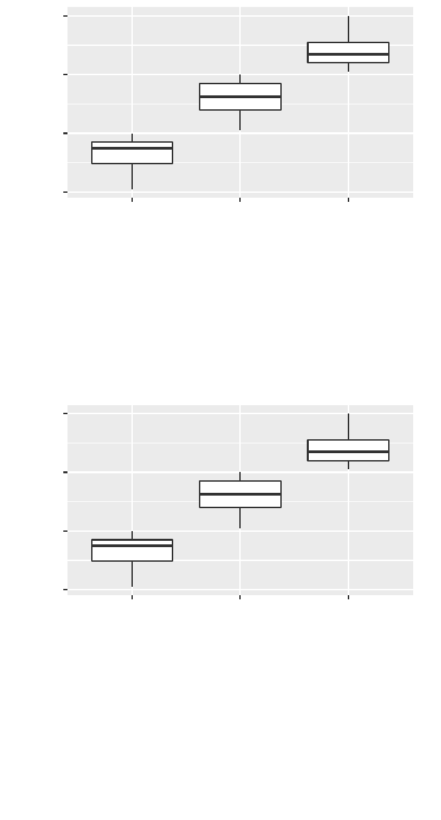
104 horton,kaplan,pruim
0
20
40
60
[0,20] (20,40] (40,60]
cesdcut
cesd
The ntiles() function can be
used to automate creation of
groups in this manner.
It might be preferable to give better labels.
> HELPrct <- mutate(HELPrct, cesdcut =cut(cesd,
labels =c("low","medium","high"),
breaks =c(0,20,40,60), include.lowest =TRUE))
>gf_boxplot(cesd ~ cesdcut, data = HELPrct)
0
20
40
60
low medium high
cesdcut
cesd
The case_when() function is even more general and
can also be used for this purpose.
> HELPrct <- mutate(HELPrct,
anothercut =case_when(
cesd >= 0& cesd <= 20 ~"low",
cesd > 20 & cesd <= 40 ~"medium",
cesd > 40 ~"high"))

a student’s guide to r 105
13.9.2Reordering factors
By default R uses the first level in lexicographic order as
the reference group for modeling. This can be overriden
using the relevel() function (see also reorder()).
>tally(~ substance, data = HELPrct)
substance
alcohol cocaine heroin
177 152 124
>coef(lm(cesd ~ substance, data = HELPrct))
(Intercept) substancecocaine substanceheroin
34.3729 -4.9518 0.4981
> HELPrct <- mutate(HELPrct, subnew =relevel(substance,
ref ="heroin"))
>coef(lm(cesd ~ subnew, data = HELPrct))
(Intercept) subnewalcohol subnewcocaine
34.8710 -0.4981 -5.4499
13.10 Group-wise statistics
It can often be useful to calculate summary statistics by
group, and add these into a dataset. The group_by()
function in the dplyr package facilitates this process.
Here we demonstrate how to add a variable containing
the median age of subjects by substance group.
>favstats(age ~ substance, data = HELPrct)
substance min Q1 median Q3 max mean sd n missing
1 alcohol 20 33 38.0 43.00 58 38.20 7.652 177 0
2 cocaine 23 30 33.5 37.25 60 34.49 6.693 152 0
3 heroin 19 27 33.0 39.00 55 33.44 7.986 124 0
> ageGroup <- HELPrct %>%
group_by(substance) %>%
summarise(agebygroup =mean(age))
> ageGroup

106 horton,kaplan,pruim
# A tibble: 3 x 2
substance agebygroup
<fct> <dbl>
1 alcohol 38.2
2 cocaine 34.5
3 heroin 33.4
>nrow(ageGroup)
[1] 3
>nrow(HELPrct)
[1] 453
> HELPmerged <- left_join(ageGroup, HELPrct, by ="substance")
>favstats(agebygroup ~ substance, data = HELPmerged)
substance min Q1 median Q3 max mean sd n missing
1 alcohol 38.20 38.20 38.20 38.20 38.20 38.20 0 177 0
2 cocaine 34.49 34.49 34.49 34.49 34.49 34.49 0 152 0
3 heroin 33.44 33.44 33.44 33.44 33.44 33.44 0 124 0
>nrow(HELPmerged)
[1] 453
13.11 Accounting for missing data
Missing values arise in almost all real world investiga-
tions. R uses the NA character as an indicator for missing
data. The HELPmiss dataframe within the mosaicData
package includes all n=470 subjects enrolled at baseline
(including the n=17 subjects with some missing data
who were not included in HELPrct).
> smaller <- select(HELPmiss, cesd, drugrisk, indtot, mcs, pcs,
substance)
>dim(smaller)
[1] 470 6
>summary(smaller)
cesd drugrisk indtot mcs pcs

a student’s guide to r 107
Min. : 1.0 Min. : 0.00 Min. : 4.0 Min. : 6.76 Min. :14.1
1st Qu.:25.0 1st Qu.: 0.00 1st Qu.:32.0 1st Qu.:21.66 1st Qu.:40.4
Median :34.0 Median : 0.00 Median :37.5 Median :28.56 Median :48.9
Mean :32.9 Mean : 1.87 Mean :35.7 Mean :31.55 Mean :48.1
3rd Qu.:41.0 3rd Qu.: 1.00 3rd Qu.:41.0 3rd Qu.:40.64 3rd Qu.:57.0
Max. :60.0 Max. :21.00 Max. :45.0 Max. :62.18 Max. :74.8
NA's :2 NA's :14 NA's :2 NA's :2
substance
alcohol:185
cocaine:156
heroin :128
missing: 1
Of the 470 subjects in the 6variable dataframe, only
the drugrisk,indtot,mcs, and pcs variables have missing
values.
>favstats(~ mcs, data = smaller)
min Q1 median Q3 max mean sd n missing
6.763 21.66 28.56 40.64 62.18 31.55 12.78 468 2
>with(smaller, sum(is.na(mcs)))
[1] 2
> nomiss <- na.omit(smaller)
>dim(nomiss)
[1] 453 6
>nrow(nomiss)
[1] 453
>ncol(nomiss)
[1] 6
>favstats(~ mcs, data = nomiss)
min Q1 median Q3 max mean sd n missing
6.763 21.79 28.6 40.94 62.18 31.7 12.82 453 0

108 horton,kaplan,pruim
Alternatively, we could generate the same dataset us-
ing logical conditions.
> nomiss <- filter(smaller,
(!is.na(mcs) & !is.na(indtot) & !is.na(drugrisk)))
>dim(nomiss)
[1] 453 6
14
Health Evaluation (HELP) Study
Many of the examples in this guide utilize data from the
HELP study, a randomized clinical trial for adult inpa-
tients recruited from a detoxification unit. Patients with
no primary care physician were randomized to receive
a multidisciplinary assessment and a brief motivational
intervention or usual care, with the goal of linking them
to primary medical care. Funding for the HELP study
was provided by the National Institute on Alcohol Abuse
and Alcoholism (R01-AA10870, Samet PI) and National
Institute on Drug Abuse (R01-DA10019, Samet PI). The
details of the randomized trial along with the results from
a series of additional analyses have been published1.1J. H. Samet, M. J. Larson, N. J.
Horton, K. Doyle, M. Winter,
and R. Saitz. Linking alcohol
and drug dependent adults to
primary medical care: A ran-
domized controlled trial of a
multidisciplinary health inter-
vention in a detoxification unit.
Addiction,98(4):509–516,2003;
J. Liebschutz, J. B. Savetsky,
R. Saitz, N. J. Horton, C. Lloyd-
Travaglini, and J. H. Samet. The
relationship between sexual and
physical abuse and substance
abuse consequences. Journal
of Substance Abuse Treatment,
22(3):121–128,2002; and S. G.
Kertesz, N. J. Horton, P. D.
Friedmann, R. Saitz, and J. H.
Samet. Slowing the revolving
door: stabilization programs
reduce homeless persons’ sub-
stance use after detoxification.
Journal of Substance Abuse Treat-
ment,24(3):197–207,2003
Eligible subjects were adults, who spoke Spanish or
English, reported alcohol, heroin or cocaine as their first
or second drug of choice, resided in proximity to the pri-
mary care clinic to which they would be referred or were
homeless. Patients with established primary care rela-
tionships they planned to continue, significant dementia,
specific plans to leave the Boston area that would prevent
research participation, failure to provide contact informa-
tion for tracking purposes, or pregnancy were excluded.
Subjects were interviewed at baseline during their
detoxification stay and follow-up interviews were under-
taken every 6months for 2years. A variety of continuous,
count, discrete, and survival time predictors and out-
comes were collected at each of these five occasions. The
Institutional Review Board of Boston University Medical
Center approved all aspects of the study, including the
creation of the de-identified dataset. Additional privacy
protection was secured by the issuance of a Certificate of
Confidentiality by the Department of Health and Human

110 horton,kaplan,pruim
Services.
The mosaicData package contains several forms of the
de-identified HELP dataset. We will focus on HELPrct,
which contains 27 variables for the 453 subjects with min-
imal missing data, primarily at baseline. Variables in-
cluded in the HELP dataset are described in Table 14.1.
More information can be found at: https://nhorton.
people.amherst.edu/r2. A copy of the study instruments
can be found at: https://nhorton.people.amherst.edu/
help.
Table 14.1: Annotated description of variables in the
HELPrct dataset
VARIABLE DESCRIPTION (VALUES) NOTE
age age at baseline (in years) (range
19–60)
anysub use of any substance post-detox see also
daysanysub
cesd Center for Epidemiologic Stud-
ies Depression scale (range 0–60,
higher scores indicate more depres-
sive symptoms)
d1 how many times hospitalized for
medical problems (lifetime) (range
0–100)
daysanysub time (in days) to first use of any
substance post-detox (range 0–268)
see also
anysubstatus
dayslink time (in days) to linkage to primary
care (range 0–456)
see also
linkstatus
drugrisk Risk-Assessment Battery (RAB)
drug risk score (range 0–21)
see also sexrisk
e2b number of times in past 6months
entered a detox program (range
1–21)
female gender of respondent (0=male,
1=female)
g1b experienced serious thoughts of
suicide (last 30 days, values 0=no,
1=yes)
homeless 1or more nights on the street or
shelter in past 6months (0=no,
1=yes)

a student’s guide to r 111
i1 average number of drinks (standard
units) consumed per day (in the
past 30 days, range 0–142)
see also i2
i2 maximum number of drinks (stan-
dard units) consumed per day (in
the past 30 days range 0–184)
see also i1
id random subject identifier (range
1–470)
indtot Inventory of Drug Use Conse-
quences (InDUC) total score (range
4–45)
linkstatus post-detox linkage to primary care
(0=no, 1=yes)
see also dayslink
mcs SF-36 Mental Component Score
(range 7-62, higher scores are bet-
ter)
see also pcs
pcs SF-36 Physical Component Score
(range 14-75, higher scores are
better)
see also mcs
pss_fr perceived social supports (friends,
range 0–14)
racegrp race/ethnicity (black, white, his-
panic or other)
satreat any BSAS substance abuse treat-
ment at baseline (0=no, 1=yes)
sex sex of respondent (male or female)
sexrisk Risk-Assessment Battery (RAB) sex
risk score (range 0–21)
see also drugrisk
substance primary substance of abuse (alco-
hol, cocaine or heroin)
treat randomization group (randomize to
HELP clinic, no or yes)
Notes: Observed range is provided (at baseline) for con-
tinuous variables.

15
Exercises and Problems
The first part of the exercise number indicates which
chapter it comes from.
3.1.Using the HELPrct dataset, create side-by-side his-
tograms of the CESD scores by substance abuse group,
just for the male subjects, with an overlaid normal den-
sity.
5.1.Using the HELPrct dataset, fit a simple linear regres-
sion model predicting the number of drinks per day as
a function of the mental component score. This model
can be specified using the formula: i1 ∼mcs. Assess the
distribution of the residuals for this model.
10.1.The RailTrail dataset within the mosaic package
includes the counts of crossings of a rail trail in Northamp-
ton, Massachusetts for 90 days in 2005. City officials are
interested in understanding usage of the trail network,
and how it changes as a function of temperature and
day of the week. Describe the distribution of the variable
avgtemp in terms of its center, spread and shape.
>favstats(~ avgtemp, data = RailTrail)
min Q1 median Q3 max mean sd n missing
33 48.62 55.25 64.5 84 57.43 11.33 90 0
>gf_dens(~ avgtemp, xlab ="Average daily temp(degrees F)",data = RailTrail)
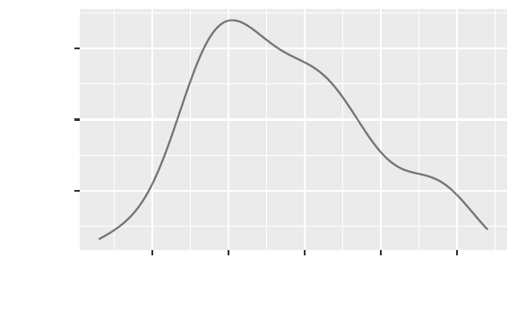
114 horton,kaplan,pruim
0.01
0.02
0.03
40 50 60 70 80
Average daily temp(degrees F)
density
10.2.The RailTrail dataset also includes a variable called
cloudcover. Describe the distribution of this variable in
terms of its center, spread and shape.
10.3.The variable in the RailTrail dataset that provides
the daily count of crossings is called volume. Describe the
distribution of this variable in terms of its center, spread
and shape.
10.4.The RailTrail dataset also contains an indicator of
whether the day was a weekday (weekday==1) or a week-
end/holiday (weekday==0). Use tally() to describe the
distribution of this categorical variable. What percentage
of the days are weekends/holidays?
10.5.Use side-by-side boxplots to compare the distribu-
tion of volume by day type in the RailTrail dataset. Hint:
you’ll need to turn the numeric weekday variable into a
factor variable using as.factor() or use the horizontal=FALSE
option. What do you conclude?
10.6.Use overlapping densityplots to compare the distri-
bution of volume by day type in the RailTrail dataset.
What do you conclude?
10.7.Create a scatterplot of volume as a function of avgtemp
using the RailTrail dataset, along with a regression line
and scatterplot smoother (lowess curve). What do you
observe about the relationship?
10.8.Using the RailTrail dataset, fit a multiple regres-
sion model for volume as a function of cloudcover,avgtemp,

a student’s guide to r 115
weekday and the interaction between day type and aver-
age temperature. Is there evidence to retain the interac-
tion term at the α=0.05 level?
10.9.Use makeFun() to calculate the predicted number
of crossings on a weekday with average temperature 60
degrees and no clouds. Verify this calculation using the
coefficients from the model.
>coef(fm)
(Intercept) cloudcover avgtemp
378.834 -17.198 2.313
weekdayTRUE avgtemp:weekdayTRUE
-321.116 4.727
10.10.Use makeFun() and gf_fun() to display predicted
values for the number of crossings on weekdays and
weekends/holidays for average temperatures between
30 and 80 degrees and a cloudy day (cloudcover=10).
10.11.Using the multiple regression model, generate a
histogram (with overlaid normal density) to assess the
normality of the residuals.
10.12.Using the same model generate a scatterplot of the
residuals versus predicted values and comment on the
linearity of the model and assumption of equal variance.
10.13.Using the same model generate a scatterplot of
the residuals versus average temperature and comment
on the linearity of the model and assumption of equal
variance.
11.1.Generate a sample of 1000 exponential random vari-
ables with rate parameter equal to 2, and calculate the
mean of those variables.
11.2.Find the median of the random variable X, if it is
exponentially distributed with rate parameter 10.
12.1.Find the power of a two-sided two-sample t-test
where both distributions are approximately normally
distributed with the same standard deviation, but the
group differ by 50% of the standard deviation. Assume

116 horton,kaplan,pruim
that there are 25 observations per group and an alpha
level of 0.0539.
12.2.Find the sample size needed to have 90% power
for a two group t-test where the true difference between
means is 25% of the standard deviation in the groups
(with α=0.05).
13.1.Using faithful dataframe, make a scatter plot of
eruption duration times vs. the time since the previous
eruption.
13.2.The fusion2 data set in the fastR package contains
genotypes for another SNP. Merge fusion1,fusion2, and
pheno into a single data frame.
Note that fusion1 and fusion2 have the same columns.
>names(fusion1)
[1] "id" "marker" "markerID" "allele1" "allele2" "genotype" "Adose"
[8] "Cdose" "Gdose" "Tdose"
>names(fusion2)
[1] "id" "marker" "markerID" "allele1" "allele2" "genotype" "Adose"
[8] "Cdose" "Gdose" "Tdose"
You may want to use the suffixes argument to merge()
or rename the variables after you are done merging to
make the resulting dataframe easier to navigate.
Tidy up your dataframe by dropping any columns
that are redundant or that you just don’t want to have in
your final dataframe.
16
Bibliography
[BcRB+14] B.S. Baumer, M. Çetinkaya Rundel, A. Bray,
L. Loi, and N. J. Horton. R Markdown: In-
tegrating a reproducible analysis tool into
introductory statistics. Technology Innovations
in Statistics Education,8(1):281–283,2014.
[HBW15] N.J. Horton, B.S. Baumer, and H. Wickham.
Setting the stage for data science: integration
of data management skills in introductory and
second courses in statistics (http://arxiv.
org/abs/1401.3269). CHANCE,28(2):40–50,
2015.
[KHF+03] S. G. Kertesz, N. J. Horton, P. D. Friedmann,
R. Saitz, and J. H. Samet. Slowing the re-
volving door: stabilization programs reduce
homeless persons’ substance use after detox-
ification. Journal of Substance Abuse Treatment,
24(3):197–207,2003.
[LSS+02] J. Liebschutz, J. B. Savetsky, R. Saitz, N. J. Hor-
ton, C. Lloyd-Travaglini, and J. H. Samet.
The relationship between sexual and physi-
cal abuse and substance abuse consequences.
Journal of Substance Abuse Treatment,22(3):121–
128,2002.
[MM07] D. S. Moore and G. P. McCabe. Introduction
to the Practice of Statistics. W.H.Freeman and
Company, 6th edition, 2007.
118 horton,kaplan,pruim
[NT10] D. Nolan and D. Temple Lang. Computing
in the statistics curriculum. The American
Statistician,64(2):97–107,2010.
[RS02] F. Ramsey and D. Schafer. Statistical Sleuth: A
Course in Methods of Data Analysis. Cengage,
2nd edition, 2002.
[SLH+03] J. H. Samet, M. J. Larson, N. J. Horton,
K. Doyle, M. Winter, and R. Saitz. Linking
alcohol and drug dependent adults to primary
medical care: A randomized controlled trial
of a multidisciplinary health intervention in a
detoxification unit. Addiction,98(4):509–516,
2003.
[Tuf01] E. R. Tufte. The Visual Display of Quantitative
Information. Graphics Press, Cheshire, CT, 2nd
edition, 2001.
[Wor14] ASA Undergraduate Guidelines Workgroup.
2014 curriculum guidelines for undergradu-
ate programs in statistical science. Techni-
cal report, American Statistical Association,
November 2014.http://www.amstat.org/
education/curriculumguidelines.cfm.
17
Index
%>%,96
abs(),82
adding variables, 96
all.x option,101
alpha option,52,64
analysis of variance, 67
annotate(),34
anova(), 79
anova(),68,72
aov(),68,77
arrange(),100,101
band.lwd option,55
binom.test(),40
binomial test, 40
bins option,32
binwidth option,33,89
bootstrapping, 37
breaks option,103
by.x option,101
case_when(),104
categorical variables, 39
center option,89
cex option,64,82
chisq.test(),43,60
class(),51
coef(),50,105
coefficient plots, 81
color option,80,89
confint(),36,41,50
contingency tables, 39,57
Cook’s distance, 53
cor(),48
correct option,41
correlation, 48
Cox proportional hazards
model, 76
coxph(),76
CPS85 dataset, 96,97
creating subsets, 99
cross classification tables, 57
CrossTable(),58
cut(),96,103
data management, 95
data(),99
dataframe, 96
dataframes
inspecting, 95
merging, 100
reshaping, 102
sorting, 100
subsetting, 99
density option,51
derived variables, 103
diffmean(),66
dim(),106
display first few rows, 96
dist option,31,34
dnorm(),85
do(),37
dplyr package,30,31
dropping variables, 97
exp(),71
factor reordering, 105
factor(),69,77
failure time analysis, 75
faithful dataset, 98,99
family option,71
favstats(),28,63,105,107
fill option,67
filter(),30,97
Fisher’s exact test, 61
fisher.test(),61
fitted(),81
format option,30
function(),48
fusion1dataset, 101
gather(),102
geom option,34
gf_boxplot(),63,68,77
gf_dens(),34
gf_dhistogram,31
gf_dhistogram(),81
gf_dist(),43,87
gf_dotplot(),33
gf_facet_wrap,31
gf_fitdistr(),31,34,81
gf_freqpoly(),35
gf_fun(),80,89
gf_histogram(),29,67,89
120 horton,kaplan,pruim
gf_hline(),52
gf_labs(),33
gf_point(),47,64,80
gf_qq(),51
gf_refine(),34,63
gf_smooth(),47
gf_step(),75
gf_text(),48
gf_vline(),34,67
ggpairs(),49
glm(),71
group-wise statistics, 105
group_by(),105
groups option,88
head(),96
Health Evaluation and Linkage
to Primary Care study, 109
HELP study, 109
HELPmiss dataset, 106
HELPrct dataset, 27
honest significant differences,
69
include.lowest option,103
incomplete data, 106
inspect(),95
inspecting dataframes, 95
install.packages(),14
installing packages, 14
integrate(),85
interactions, 79
iris dataset, 96
is.na(),107
Kaplan-Meier plot, 75
knitr, 14
label option,48
labels option,69
left_join(),105
levels option,69
leverage, 54
library(),14,27
linear regression, 50
linearity, 47
linetype option,75,80
lm(),50,69
loading packages, 14
logistic regression, 71
lowess, 47
lwd option,88
makeFun(),80,89
margins option,39
markdown, 14
mean(),27,63
median(),28,77
merging dataframes, 100
missing data, 106
model comparison, 69
Modeling with R,27
mosaic package,27
mosaic(),58
mplot(),52,70,81
msummary(), 79
msummary(),50,65,71
multiple comparisons, 69
multiple regression, 78
multivariate relationships, 78
mutate(),69,77,96,97,103,
105
NA character,106
na.omit(),107
names(),98
ncol(),107
nrow(),105,107
ntiles(),104
oddsRatio(),58
one-way ANOVA, 67
options(),27
pairs plot, 49
panel.labels(),48
panel.lmbands(),55
panel.text(),48
paste(),103
pbinom(),92
pch option,88
pchisq(),43
Pearson correlation, 48
permutation test, 66
pipe operator, 96
plotFun(),80
plotModel(),78
pnorm(),85
polygons, 35
power.t.test(),94
prediction bands, 55
print(),41
prop.test(),41
proportional hazards model,
76
pval(),41
qdata(),37
qnorm(),85,93
quantile(),28
quantiles, 28
random variables, 85
read.file(), 95
regression, 50
regression diagnostics, 81
relevel(),105
rename(),98
renaming variables, 98
reordering factors, 105
reproducible analysis, 14
require(),14
resample(),37
resampling, 37,66
reshaping dataframes, 102
resid(),81
residual diagnostics, 81
residuals(),51
rexp(),89
rnorm(),85
row.names(),98
rownames(),48
rsquared(),50
RStudio.Version(),19
a student’s guide to r 121
scale versus location, 53
scatterplot matrix, 49
scatterplots, 47
sd(),28
select option,97
select(),96,103,105,106
sessionInfo(),19
shape option,47
shuffle(),66
significance stars, 50
size option,47,80,89
smoothers, 47
sorting dataframes, 100
Spearman correlation, 48
spread(),103
Start Modeling with R,27
Start Teaching with R,27
stem(),30
subsetting dataframes, 99
sum(),43,107
summarise(),105
summary(),65
Surv(),75
survfit(),75
survival analysis, 75
t.test(),36,64
tables, 39,57
tally(),30,39,57,105
Teaching with R,27
test option,72
thinking with data, 95
tidyr package,31,101
time to event analysis, 75
title option,75
transforming dataframes, 102
transposing dataframes, 102
Tukey’s HSD, 69
TukeyHSD(),69
type option,88
under option,88
var(),28
var.equal option,64
vignettes, 13
which option,52
wilcox.test(),65
with(),27,107
xchisq.test(),44,60
xintercept option,34
xlab option,75
xlim option,67,80,89
xpnorm(),85
xqnorm(),93
ylab option,75,80