MSc Lab Manual

User Manual:

Open the PDF directly: View PDF .
Page Count: 43

Introduction and Information
List of Experiments
Writing a laboratory report
Gamma-Ray Source Activities
Summary of Statistical Formulae (+ Knoll ch. 3)

Postgraduate Nuclear Laboratory

2018/2019

MSc – Nuclear Decommissioning and Waste

Management

MSc – Physics and

Technology of Nuclear Reactors

Laboratory Manual

Contents

1 Introduction and Information 1

1.1 General Introduction . . . . . . . . . . . . . . . . . . . . . . . . . . 1

1.2 Aims and Objectives . . . . . . . . . . . . . . . . . . . . . . . . . . 2

1.3 Health and Safety . . . . . . . . . . . . . . . . . . . . . . . . . . . 3

1.3.1 General precautions . . . . . . . . . . . . . . . . . . . . . . 3

1.3.2 Radioactive sources . . . . . . . . . . . . . . . . . . . . . . 3

1.3.3 Toxic materials . . . . . . . . . . . . . . . . . . . . . . . . . 4

1.3.4 High voltage and cables . . . . . . . . . . . . . . . . . . . . 4

1.3.5 Notes on radiation units and dose limits . . . . . . . . . . . . 4

1.3.6 Radioactive sources requiring special handling . . . . . . . . 5

1.4 Assessment . . . . . . . . . . . . . . . . . . . . . . . . . . . . . . 7

1.4.1 Laboratory Reports . . . . . . . . . . . . . . . . . . . . . . 8

1.4.2 Laboratory Notebook . . . . . . . . . . . . . . . . . . . . . . 9

1.5 Plagiarism . . . . . . . . . . . . . . . . . . . . . . . . . . . . . . . 9

1.6 Notes on Detectors . . . . . . . . . . . . . . . . . . . . . . . . . . 10

1.6.1 Poisson statistics and energy resolution . . . . . . . . . . . . 10

1.6.2 Detection efﬁciency . . . . . . . . . . . . . . . . . . . . . . 11

1.6.3 Statistics of counting . . . . . . . . . . . . . . . . . . . . . . 12

1.6.4 Errors on centroids and FWHM . . . . . . . . . . . . . . . . 13

1.6.5 The ROOT Analyis Framework . . . . . . . . . . . . . . . . 13

1.6.6 Deadtime in counting systems . . . . . . . . . . . . . . . . . 15

1.6.7 Random rates in coincidence measurements . . . . . . . . . 15

1.7 Notes on Electronics . . . . . . . . . . . . . . . . . . . . . . . . . . 16

1.7.1 Description of the Various Electronics Units . . . . . . . . . . 17

1.7.2 Trouble-Shooting . . . . . . . . . . . . . . . . . . . . . . . . 18

1.8 Data acquisition systems . . . . . . . . . . . . . . . . . . . . . . . 19

1.9 General measurements for gamma spectroscopy . . . . . . . . . . . 20

1.10 Bibliography . . . . . . . . . . . . . . . . . . . . . . . . . . . . . . 22

1.11 Acknowledgements . . . . . . . . . . . . . . . . . . . . . . . . . . 22

2 List of Experiments 23

2.1 Neutron Diffusion in Graphite using BF3or 3He detectors . . . . . . 24

2.2 Positron annihilation detection . . . . . . . . . . . . . . . . . . . . . 27

2.3 X-ray ﬂuorescence . . . . . . . . . . . . . . . . . . . . . . . . . . . 28

2.4 Photon spectrometry with proportional counters . . . . . . . . . . . 29

2.5 Gamma spectrometry of environmental radioactivity . . . . . . . . . 30

2.6 Neutron activation analysis . . . . . . . . . . . . . . . . . . . . . . 31

2.7 Gamma-ray attenuation and build up . . . . . . . . . . . . . . . . . 32

2.8 Alpha-particle stopping powers in gases . . . . . . . . . . . . . . . 33

2.9 Absolute activity determination . . . . . . . . . . . . . . . . . . . . 34

2.10 Gamma-ray spectroscopy using scintillators . . . . . . . . . . . . . 35

3 Writing a laboratory report 36

4 Gamma-Ray Source Activities 39

5 Summary of Statistical Formulae (+ Knoll ch. 3) 40

1 Introduction and Information

1.1 General Introduction

Welcome to the Nuclear Laboratory, which takes place in R11 on the ﬁrst ﬂoor, and

PB2K in the basement, of the Poynting building. The laboratory module consists of

∼6 hours work per week, that you are in the University, and is combined with work

outside the laboratory which involves reading about radiation detection, researching

the physics of your experiments, analysing your data, and writing up your laboratory

reports. The laboratory hours are 10 am to 5 pm on Friday (as per your timetable)

with a 1 hour lunch break between 1 pm and 2 pm. PTNR students attend the

nuclear laboratory in both the Autumn and Spring Terms, while NDAWM students

attend during the Autumn Term only.

The course assessment is via written (word processed) reports (see section 1.4).

PTNR students will submit two reports, one at the end of the Autumn Term, and one

at the end of the Spring Term. NDAWM students will also submit two reports, one at

the beginning of the Spring Term and one during the Easter vacation. The deadlines

for these will be announced on the relevant Canvas page and via email. A further

contribution to the ﬁnal mark will be derived from an assessment of the laboratory

notebook which should be handed in at the same time as the ﬁnal laboratory report.

Material received after these dates may not be assessed, unless accompanied by

an extenuating circumstances note.

Important: The laboratory shares the laboratory facilities with both the MSc

courses and the Year 3 laboratories in both Nuclear Physics and Nuclear En-

gineering in the ﬁrst semester. Therefore, you should check carefully whether

any apparatus has been left on when you begin your session, in case any high

voltages are set. When you ﬁnish the session, please take care to wind down

any high voltages to zero and restore the experiment to how you found it. Be

sure to note any settings of the electronics, so that you can reset them on

the next laboratory session. Do not move equipment from one experiment to

another.

1.2 Aims and Objectives

The aims of this laboratory are that:-

• You discover lots of interesting physics which are useful and relevant to your

future careers.

• Improve your knowledge and skills in both physics and in written communica-

tions.

• Correlate material learnt in lecture courses with the practical applications in

the laboratory.

• Develop new skills learnt in other sections of the course, e.g. numerical anal-

ysis, statistics, Monte-Carlo etc.

The objectives for this laboratory are that you will acquire the following skills:-

• A familiarity with basic concepts of nuclear physics.

• An understanding of the physical processes in the interactions of, and detec-

tion of, ionizing radiations.

• The use of standard nuclear electronics and simple data acquisition systems,

the planning of measurements, and the analysis of data.

• The ability to start from a brief description of the experiment allowing you to

plan how to set up the apparatus and to make it work.

• The ability to research properly an unfamiliar topic, by searching books, refer-

ences, websites etc. when required.

• The important self-discipline to monitor the performance of your apparatus

and your command of it in an on-line fashion, ensuring that the results you

are obtaining are sensible, and that your analysis of the data is proceeding

correctly during the experiment.

• The ability to keep a coherent and up-to-date record of your laboratory work

and of your data analysis as the experiment is proceeding.

• The ability to extract the maximum physics output from your data, and to com-

pare your results, in a critical fashion, with what is expected from previous

work on the topic.

• The ability to write scientiﬁc reports.

• The ability to critically examine your own work.

1.3 Health and Safety

Your health and safety and the health and safety of those around you are of utmost

importance. In addition to the usual safety precautions applicable to all laboratory

work, please make a careful note of the following rules that apply in the Nuclear

Laboratory. It is your responsibility to adhere to these rules to ensure a safe working

environment for everyone in the laboratory.

1.3.1 General precautions

• Eating and drinking are not permitted anywhere within the laboratory.

• Wash your hands at the end of the laboratory session and before taking a tea

break.

1.3.2 Radioactive sources

• Radioactive sources are issued from a metal cupboard in the source room.

• A radioactive source may only be removed from the cupboard after it has

been signed out. You are personally responsible for any source that you have

signed out and you must ensure that it is returned at the end of a session.

• A demonstrator must be present when a source is signed out. All sources

must also be returned to a demonstrator when you have ﬁnished with them.

Only demonstrators can sign sources in/out of the source cupboard.

• Students may need to remove sources from the main laboratory (e.g. 90Sr

sources for use in PB2K). When checked out, the source location must be

recorded.

• Care must be taken not to lose or damage sources. If you damage a source

or a source appears to be damaged, inform a member of staff IMMEDIATELY.

• The sources you will use are relatively weak and are quite safe if handled

intelligently. A list of available sources is kept in the metal cupboard.

• The majority of our γ-ray sources are sealed in plastic and any αor βparticles

that are produced by the source do not get out. Sources of αor βparticles are

unsealed, also known as open sources, and these must be handled carefully

to avoid transferring radioactive material to hands or clothing. Gloves should

be worn and tweezers used when handling open sources.

• Demonstrators will inform you if you need to use an open source. If you are

unhappy or unwilling to handle the source yourself, just ask the demonstrator

to mount the source in your experiment for you.

• Where stronger sources are in use for a physics experiment, or when appara-

tus may be counting for a long time, you should avoid sitting near the source

for long periods. Adhere to the ALARP principle to ensure that the dose you,

and those around you, receive in the laboratory is As Low As Reasonably

Practicable.

• If you leave your experiment running overnight display a notice advising the

type and location of source that is present.

1.3.3 Toxic materials

• A small number of materials in use in the laboratory are toxic to the human

body. These comprise lead (used as shielding), cadmium (used to absorb

thermal neutrons) and bismuth (used as an absorber of γ-rays). Use gloves

when handling any of these materials and make a habit of washing your hands

after each laboratory session and before taking a tea break.

• If using lead bricks to shield your apparatus, take care not to overload the

bench Please adhere to a maximum of 10 bricks per bench.

• Be aware of the potential for crushing injuries when handling lead bricks. Do

not carry more than one lead brick at a time. Do not place lead bricks close

to the edge of the bench where they may topple onto the ﬂoor.

1.3.4 High voltage and cables

• Many detectors use High Voltage (HV) power supplies. ALWAYS turn off the

HV before disconnecting cables or before performing any examination of your

detector. NEVER turn off the 240 V mains power supply to ANY apparatus

that is supplying high voltage to a detector without ﬁrst reducing the HV supply

setting to zero. Failure to observe this precaution may destroy the delicate

electronics incorporated in your detector.

• To avoid the risk of electric shock, be careful to use only specially designed

HV cables to connect your detector to its power supply. There are four types

of connectors used in the laboratory: SHV (Safe High Voltage), BNC (low

voltage signal cables used to connect NIM electronics units), LEMO (compact

signal connectors used in some electronics units) and MCX (micro coaxial

signal connectors used solely on the CAEN digitiser modules). It is easy to

confuse SHV and BNC connectors. If in doubt, ask a demonstrator.

• Beware of the potential for trip hazards caused by dangling cables. Choose

appropriate cable lengths to connect modules and detectors. Do not allow

cables to trail on the ﬂoor.

Above all, watch out for the safety of yourself and your fellow students. If you are

unsure about any of the safety aspects of your experiment, or you see someone

behaving irresponsibly, please consult a demonstrator.

1.3.5 Notes on radiation units and dose limits

Units given in italics are now obsolete but may be encountered.

• Activity – measure of decay rate. The SI unit of activity is the Becquerel (Bq) =

1 disintegration per second. Activities of the various sources in the laboratory

are often quoted in Curies (Ci). 1 Ci = 3.7 ×1010Bq

• Absorbed dose – energy deposited per unit mass. The SI unit of absorbed

dose is the Gray (Gy) = 1 J/kg 1 rad = 0.01 Gy; 1 Gy = 100 rad

• Equivalent dose – Absorbed dose ×radiation weighting factor. The SI unit

of equivalent dose is the Sievert (Sv) The weighting factor of X-rays, gamma-

rays, electrons, positrons and muons of all energies is equal to unity. For

neutrons, the weighting factor depends on energy and has a maximum value

of 20 in the energy range 100 keV < E < 2 MeV. For alpha particles and heavy

nuclei, the weighting factor is also 20. So, 1 Gy of X-rays = 1 Sv, but 1 Gy of

alphas = 20 Sv. 1 rem = 0.01 Sv; 1 Sv = 100 rem

The Ionising Radiations Regulations (IRR99) limits the annual whole body effec-

tive dose (which is the same as the equivalent dose for whole body exposures) for

classiﬁed radiation workers to 20 milliSieverts (mSv). For members of the public

the recommended annual effective dose limit is 1 mSv. (These limits exclude the

dose you receive from natural background sources and medical procedures. For

reference, the typical annual dose from background radiation in the UK is around

2 mSv.) Although there are exemptions for students, the University treats them as

members of the public. This means that students and demonstrators do not have to

wear a personal dosimeter to work in the teaching laboratories.

To ensure that the total dose is below 1 mSv from a full time exposure of 2000 hours

per year (40 hour week for 50 weeks per year) requires the average dose rate be

less than 1 mSv/2000 = 0.5 µSv/hr. Masters students typically spend 120 hours in

the laboratory (6 hours per week for 20 weeks). Undergraduate physics students

also spend no more than 120 hours in the laboratory (8 hours per week for 15

weeks). Over this period the average dose rate becomes 1 mSv/120 = 8.3 µSv/hr.

No experiment will expose you to an average dose rate larger than this value. In

most cases the dose rate will be well below 1 µSv/hr.

1.3.6 Radioactive sources requiring special handling

The majority of radioactive sources that you will encounter in the laboratory are

gamma-ray sources with individual activities typically less than 500 kBq. No special

precautions need to be taken when using these sources, although you should al-

ways consider the placement and shielding of sources to ensure that your exposure

to radiation is As Low As Reasonably Practicable.

There are a small number of strong sources for which special handling precautions

should be taken. These sources are:

• C3N 19/22/1, collimated 137Cs source used in the Compton Scattering exper-

iment

• C3N 19/65, strong 137Cs source sometimes used in absorption experiments

• ANS 46, annular 241Am source used in the X-ray ﬂuorescence experiment

• C3N 19/87, open 241Am source can be used for X-ray ﬂuorescence or as an

αsource.

• AMN 1000, 1 Ci Am-Be neutron source located in the water bath in R11

• ANS 1, 0.3 Ci Am-Be neutron source located in PB2K used in the graphite

stack experiment.

• ANS 2, 1 Ci Am-Be neutron source located in PB2K used in the neutron acti-

vation experiment.

• ANS 3, 3 Ci Am-Be neutron source located in PB2K used in the graphite stack

experiment.

These sources may only be handled by a demonstrator. The demonstrator will

instruct you how to use the sources safely and ensure that the source is safely

installed in the experiment at the start of the session and removed at the end of the

session.

1.4 Assessment

Students are expected to work in pairs or threes because the number of separate

experiments is limited, but the written reports must be written individually.

A good report needs planning; your lab reports should be written in the same struc-

tured style as a professional research paper, with a title, abstract, introduction, some

sections in the middle, and ﬁnally some conclusions. Try to illustrate the text with

ﬁgures of your results, so that the reader can follow the ﬂow of the project without

having to continuously ﬂip to the appendices. Lastly, you must make a critical sum-

mary in your conclusions, discussing your results with reference to previous work

and to the experimental errors and, perhaps, present some ideas for improvements.

Don’t forget to include ALL your references (books/journals/www etc.)! Note that

references are NOT the same as a bibliography.

The reports should be written so as to be understood by a physicist who does not

know in advance anything about the experiment which you have done, so you must

explain what the purpose of the experiment was, how you did it, what the results are,

and their signiﬁcance. Reports should be written in clear English and in sentences.

Conventionally, descriptions of what you did are generally written in the past tense

using a passive style (“The detector was connected to an MCA...")

While you may wish to explain brieﬂy the relevance of your experiment to practical

applications, do not spend too much time on background but concentrate on the

underlying physics phenomena. You need not give all the details of your measure-

ments or of your calculations, but you should explain what you did in sufﬁcient detail

that someone else would be able to reproduce your measurements and get essen-

tially the same results. Some additional details may be given in appendices. When

you state results, always give units and always give uncertainties. If you quote a

published result (e.g. the accepted value of a particular quantity, or a formula) then

give a numbered reference in sufﬁcient detail that the reader can look it up (i.e.

if the reference is to a book then give the page number). The report should be

word-processed, but neat hand-drawn graphs are also acceptable.

PTNR students are expected to complete approximately seven experiments through-

out the year, and present written reports for two of them. These reports, along with

the laboratory notebook, provide the formal assessment for this laboratory mod-

ule. The deadlines for submission of the reports will be announced on the relevant

Canvas page and by email.

NDAWM students are expected to produce two written reports about their investiga-

tions. The ﬁrst will be submitted at the start of semester 2 and will be used to provide

formative feedback on what was done well, and what could be improved. The sec-

ond report will be submitted after the end of semester 2 in the Easter vacation, and

will contribute 50% to the module mark.

Material received after these dates may not be assessed, unless accompanied

by an extenuating circumstances note approved by Dr Ian Stevens.

1.4.1 Laboratory Reports

This should take the form of a formal write-up, normally to be handed in by the

deadline given on Canvas. However, you can submit this report at any time during

the laboratory. The report should be about 20 pages in length (including ﬁgures, ta-

bles and appendices). Marks are awarded in three general categories with different

weights:

1. Theoretical background, research and references (30%): You should make

good use of the references cited in this manual and may need to do further

reading relevant to your particular experiment. Where possible, you should

compare and discuss your experiment and the results with previous measure-

ments or other experiments.

2. The account of your experimental work, including marks for presentation and

style (40%): You should make it clear how you actually performed the exper-

iment. Marks are allocated to reward conscientious effort and for attention

to detail, such as optimisation of shielding in some experiments, or demon-

strating your understanding of detectors or electronics. Marks will be awarded

for how you have organized your report and presented the information to the

reader. You should be careful to label diagrams, and number all ﬁgures and

tables (and pages); and label axes on histograms.

3. Analysis and interpretation of your results (30%): We will be looking for a clear

and concise description of the principles of your experiment and the method of

your analysis, including some consideration of the experimental uncertainties

(e.g. statistical errors). A summary or conclusions section should include your

main results with a discussion of the outcome of your experiment in light of

your experience. You may wish to suggest ways in which your experiment

could be improved.

4. The School’s policy is that all reports must be prepared electronically, so that

they can be submitted to the Turnitin plagiarism checking system. Your report

should demonstrate your understanding of the physics involved in the experi-

ment, your competence as an experimental scientist, and should demonstrate

your participation in the degree programme as evidenced by background in-

formation and methods.

1.4.2 Laboratory Notebook

The notebook should be handed in with the ﬁnal laboratory report. Assessment will

be based on the following criteria:

1. Completeness of the note taking. The notebook should contain a brief de-

scription of the main ideas behind the measurements (e.g. theory and main

objectives). The details of the experimental equipment should be complete

and should be sufﬁcient for someone else to reconstruct the setup exactly.

2. The notebook should contain a clear record of measurements made, the pro-

cedure and errors (uncertainties).

3. The analysis of the data should be recorded, this would include graphs, cal-

culations, error analysis, ﬁts with models.

4. There should be a short discussion on the main conclusions of the measure-

ments, documenting references to any relevant literature used.

5. The notebook should have a record of 6–7 experiments for PTNR students,

and all experiments for NDAWM students.

1.5 Plagiarism

Plagiarism is taken very seriously at the University, and any offenders will face sanc-

tions ranging from loss of marks up to exclusion from the University for more extreme

cases. You must reference all material that you have used or adapted from external

sources – i.e. anything that you have not produced entirely by yourself – including

ﬁgures.

You can quote or paraphrase sources, as long as you indicate that you are doing

so. However, this does not demonstrate your own understanding of the topic, and is

therefore not worth much credit. The lab reports are your opportunity to show your

understanding of the phenomena you have investigated, not someone elses!

All reports are submitted electronically to the Turnitin plagiarism checking system

to identify plagiarised material. The markers are also very familiar with the relevant

sections of the standard textbooks, so will recognize copied or paraphrased text and

expect to see appropriate references.

Further information and guidelines can be found in the Plagiarism section in the

Practical Skills Module on Canvas.

1.6 Notes on Detectors

The general principles of the detectors that you use are described in the compre-

hensive book by Knoll, Radiation Detection and Measurement. The brief information

in this manual should be reinforced by further reading from the bibliography in sec-

tion 1.10.

1.6.1 Poisson statistics and energy resolution

It is important that you understand the process by which the signal from the detector

is produced, because this affects the properties of the output signals. Detectors use

the interactions of ionizing radiation to convert the energy of the radiation into an

output signal. You need to distinguish between the particle that you are trying to

detect and what creates the signal in the detector.

For example, if you detect a gamma ray with a germanium counter, the energy,

E, of the gamma ray is converted into fast moving electrons, which ionize atoms

in the crystal releasing a number,Ns, of electron-hole (e-h) pairs which are then

captured at electrodes. In other types of detection media such as scintillators, Ns

is the number of photons produced by excitation, whilst in gas-ﬁlled detectors, Ns

is the number of electron-ion pairs. The number of e-h or ion pairs, or scintillation

photons, is determined by the energy per signal carrier,ω, so that

Ns=E/ω (1)

It is Ns, the number of signal carriers, which is ampliﬁed to form the output analogue

signal, and the amplitude of the output signal is directly proportional to this original

number. It is the Poisson statistics of Nswhich determines the ultimate energy

resolution of the output signal, and hence the width of the peak that you see on the

computer display of the energy spectrum.

Following Poisson statistics, the standard deviation of Nscounts is

σ(Ns) = N1/2

s(2)

so the detector energy resolution must be proportional to σ(Ns)if only statistical

factors are involved. For large Ns, the Poisson distribution tends towards the nor-

mal distribution, also called a Gaussian error curve. The resolution of a Gaussian

distribution is usually measured as the Full Width at Half Maximum , or FWHM,

which is given by:

FWHM(Ns) = 2√2 ln 2 σ(Ns)=2.35N1/2

s(3)

We can also see that, for a given normal distribution, the ratio Rof the FWHM(Ns)

to its centroid value must be

RP oisson =FWHM(Ns)/Ns= 2.35N1/2

s/Ns= 2.35N−1/2

s(4)

In the case of semiconductor detectors such as silicon and germanium it is found

that the value of Rmay be 3 or 4 times smaller than expected from Poisson statis-

tics, and a factor F(Fano factor) has been introduced to quantify this effect on the

observed variance. Accordingly, this results in a modiﬁed equation

RStatistical =FWHM(Ns)/Ns= 2.35[F Ns]1/2/Ns= 2.35F1/2N−1/2

s(5)

Typical values of F are about 0.1 or less for Si and Ge.

Since E, the energy deposited, is proportional to Ns, it is obvious that the FWHM

resolution in energy units must also be proportional to N1/2

sand that the ratio REof

the energy resolution FWHM(E) to the energy Emust be

RE=FWHM(E)/E = 2.35E−1/2(6)

assuming that there are no other contributions to the energy resolution from detector

or ampliﬁer noise.

Thus a plot of ln(RE)versus ln(E)for various energy peaks in your spectra should

yield a gradient of −1/2if the energy resolution is limited by Poisson statistics or a

gradient of −1if the energy resolution is limited by noise.

Note that there are some detectors, such as Geiger Counters, and also Fission

Counters for neutrons, whose output signals are almost independent of the energy

of the incident radiation, so that usually these detector system emit only a digital

signal which gives the time of arrival of the radiation, but carries no information

about the energy of the particle.

1.6.2 Detection efﬁciency

In order for a quantum of radiation (α,β,γ, neutron etc.) to be counted, it must

interact with the detector and produce a sufﬁcient number of signal carriers (ion

pairs, electron-hole pairs, scintillation photons etc.) to create an output pulse large

enough to be measured. As charged particles, such as αand βradiation, lose

energy rapidly by ionizing or exciting the detector material directly, they can be de-

tected with 100% efﬁciency. However, neutral radiation such as neutrons or γ-rays

must have an interaction within the detector, producing charged secondary radiation

that can then be detected. As the probability of such an interaction can be small,

there is a chance that some of the incident radiation will not interact at all – produc-

ing no output signal – or that only some of the incident energy is deposited in the

detector, giving a smaller output signal than expected.

There are two usual measures of how well a detector converts incident radiation into

an output signal proportional to the incident energy: peak absolute efﬁciency,abs,

and peak intrinsic efﬁciency,int. The peak absolute efﬁciency gives the fraction

of all emitted radiation of the energy of interest that deposits its full energy in the

detector. So if a source has activity ABq (i.e. there are Adisintegrations per

second) and a fraction γ(called the branching ratio or intensity) of these decays

results in the radiation of interest, then the rate at which this radiation is produced

is Aγ. If the measured count rate for the full energy peak is Rpcounts per second,

then the peak absolute efﬁciency is:

abs =Rp

Aγ (7)

However, unless the detector completely surrounds the source, not all of the emitted

radiation will actually reach the detector, so the peak absolute efﬁciency depends

on the geometry of the setup – basically the distance between the source and de-

tector. The peak intrinsic efﬁciency takes this geometrical factor into account, giving

a measure of how effective a particular detector is for capturing the full energy of

the incident radiation. If the solid angle covered by the detector is Ω, then the frac-

tion of all emitted radiation that can hit the detector is Ω/4π(assuming an isotropic,

point source). Therefore the rate at which the radiation of interest actually hits the

detector is AγΩ/4π. Again, if the measured count rate in the full energy peak is Rp

counts/s, then the peak intrinsic efﬁciency is:

int =Rp

Aγ

4π

Ω=abs

4π

Ω(8)

The calculation of Ωfor most of the circumstances encountered in the laboratory is

covered in Knoll [Knoll 118–121].

1.6.3 Statistics of counting

If we try to measure the count rate from a detector, we may measure a count value,

N, whose error is again governed by Poisson statistics, so that σ(N) = N1/2. If

this count is taken over tseconds then the count rate is

R=N/t (9)

with a standard deviation in Rof

σ(R) = N1/2/t (10)

Averaging is good for your experiment. A number of repeated measurements, m,

may be taken to obtain an average

N=1

i=1

Ni(11)

This is valid as long as the statistical error on each of the readings, σ(Ni), is approx-

imately the same, otherwise a weighted average is more appropriate. An estimate

for the error on the mean value, σ, may be obtained from the deviation of the indi-

vidual readings, Ni, from the average value, N:

σ2=1

m−1

i=1

(Ni−N)2(12)

Remember that the total area under the standard Gaussian curve is 1.0, whereas

the area between the values of N+σ(N)and N−σ(N)is 0.68. This is the

probability that the true value of your measurement lies between ±σ(N)around the

value N. It therefore follows that there is a probability of 0.32 (or 1 in 3) that the value

will lie outside the ±σband, even if there is nothing wrong with the experiment.

1.6.4 Errors on centroids and FWHM

The gamma rays emitted from a source are to a good approximation monoener-

getic. The measured peak shape is then due to the statistical and electronic noise

added to the signal in the detection process. This measured peak shape can thus

be regarded as the probability distribution for measuring that particular gamma ray

energy, with each count in the peak being a sample from this distribution.

Using the standard statistical results, the centroid of this distribution gives the best

estimate of the average value (in this case the actual energy of the gamma ray),

while the standard deviation, σx, gives the standard error of a single measurement.

The error on the centroid, σC, is therefore the same as the error on the mean aver-

age of the distribution, which as usual will be given by σC=σx/√A, where Ais the

net area of the peak, i.e. the total number of measurements in the distribution (the

background is not part of the probability distribution, so we must use the net area,

not gross area).

Since for a Normal (Gaussian) distribution the FWHM = 2.35σx, we get that the

uncertainty on the centroid is given by:

σC=FWHM

2.35√A(13)

The uncertainty on the FWHM can be estimated from:

σ(FWHM)

FWHM ≈1

σ(A)

A(14)

i.e. the fractional error in the FWHM is usually about 1/2 the fractional error on the

net area.

A much better way to estimate the errors on the centroid and FWHM is to ﬁt a

Gaussian lineshape to the data. This can also allow overlapping peaks to be ﬁtted

using several Gaussians This can be particularly useful when using detectors with

poor resolution, such as gas-ﬁlled proportional counters for X-ray detection. Peak

ﬁtting software is available in the laboratory, as described below, and you should use

it whenever possible to get robust estimates for the uncertainties on the parameters

of interest.

1.6.5 The ROOT Analyis Framework

A peak ﬁtting macro has been written in C++ to run in a UNIX program called ROOT,

which is installed on the Physics UNIX servers. The macros you need (see below)

are available from the LM PH605 Practical Skills for Reactor Physics section of

Canvas and must be downloaded to your ADF user directory or folder where you

will run ROOT.

To use the ROOT ﬁtting program, you will need to have saved your spectra in ASCII

(human readable) format. To do this, choose ﬁle type ASCII *.Spe in Maestro, or

Toolkit File *.TKA in Genie, after selecting File/Save As. Remember to save your

spectra to the same ADF user directory as the ROOT macro, not to the local disk.

Accessing the UNIX servers

Instructions on how to access the physics UNIX server from the laboratory, comput-

ing cluster or from home, are given in the Using the Computing Facilities document

in the LM PH605 Practical Skills for Reactor Physics section of Canvas.

Peak Fitting in ROOT

Start the ROOT analysis package by typing root at the command prompt in the SSH

Secure Shell terminal window.

Load the peak ﬁtting macro into ROOT by typing .L Bufﬁt.C at the prompt. The

macro Bufﬁt.C must be downloaded from the LM PH605 Practical Skills for Reactor

Physics section of Canvas to the folder where you will run ROOT and where you

have saved your MAESTRO or GENIE spectra.

Execute the ﬁtting routine by typing the command Bufﬁt(“MySpectrum”). Substi-

tute MySpectrum with the full ﬁlename of your spectrum ﬁle: e.g. Spectrum1.Spe

for Maestro, or Spectrum1.TKA for Genie ASCII ﬁles. Bufﬁt cannot identify the Ge-

nie ﬁles just from the name, so you will be prompted to tell Bufﬁt what kind of ﬁle it

is. Simply enter TKA at the prompt and the spectrum will be loaded.

TIP: If you hit the TAB key while you are writing the ﬁlename, ROOT will attempt to

autocomplete the ﬁlename, which is very handy for long ﬁlenames

Zoom in on a peak or group of peaks by typing ZoomIn() and follow the on-screen

instructions. The range of channels should be wide enough to see the background

on either side of the peak(s). You can also provide two arguments to the ZoomIn()

function specifying the lower and upper bin or channel number, respectively. For

example, ZoomIn(1050,1275) will display channels in the range 1050 to 1275, in-

clusive. This feature allows you to zoom consistently to the same region of the his-

togram if you are doing ﬁts of the same energy peak(s) in several different spectra.

You can see the whole spectrum again by typing ZoomOut().

Once you have zoomed in on a peak you can perform a ﬁt by typing the command

Fit(). You will then be prompted to give a rough value for the FWHM of the peaks

and the number of peaks you want to ﬁt (maximum of 4). The underlying background

is assumed to be linear. Follow the on-screen instructions and select the peaks by

clicking close to the centroid positions of each of the peaks.

TIP: For neighbouring, isolated (not overlapping) peaks you will get a better ﬁt by

zooming in on each peak individually. Where neighbouring peaks are overlapping

you can ﬁt up to 4 Gaussians simultaneously in an attempt to extract the yield (num-

ber of counts) within each peak.

By default, Bufﬁt allows the width of each peak to be a free parameter. You can

optionally force Bufﬁt to ﬁt each peak using the same FWHM by typing the com-

mand SetFixedFWHM() before calling Bufﬁt(). This feature may help to deconvolve

overlapping peaks. This feature can be turned off by typing UnSetFixedFWHM().

Note, although this option uses only one ﬁt parameter for the width, the other peak

widths are deduced by scaling (roughly) by √E. In this way, all peak widths are

constrained in a physical way.

You can save a copy of the ﬁt by selecting File/Save As... from the histogram

window menu bar. Make sure that the ﬁle type is changed to GIF, as this is readily

imported into MS Word. The default is PostScript, which is not (but can be imported

into LaTeX documents).

1.6.6 Deadtime in counting systems

In all counting systems there is a deadtime. During this time, following the arrival of

a pulse, there is a period of time where the electronics cannot process any pulses.

After this period, the electronics reset themselves, and counting can proceed again.

For most experiments the main deadtime results from the computer systems, and

you will see a ﬁgure displayed on the screen which gives you the value of the dead-

time as a percentage of the total time. The relationship between the measured

count N0and the true count Nfor a ﬁxed deadtime, τ, is:

N=N0/(1 −N0τ)(15)

with a similar equation relating the true count rate Rto the measured rate R0. If you

have set the computer to count livetime,tlive, rather than realtime,treal, then the

computer software subtracts the total deadtime N0τto calculate the livetime

tlive =treal −N0τ(16)

The deadtime N0τper second is displayed as a percentage. However, this algorithm

becomes unreliable at deadtimes above about 20%, so that you should try to keep

the deadtime below 20%.

1.6.7 Random rates in coincidence measurements

Some experiments use more than one detector in coincidence to measure, for ex-

ample, gamma rays which are emitted simultaneously (e.g. 22Na) or successively

(e.g. 60Co ) in radioactive decays. In the electronic systems for this type of experi-

ment, you need to use one coincidence unit (see next section) to measure real coin-

cidences and another coincidence unit to measure random coincidences of gamma

rays from the source or from background gamma rays or cosmic rays.

If the resolving time of the coincidence unit of the system is τ, and the individual

count rates in channels 1 and 2 are R1and R2respectively, then the random coin-

cidence rate is given by

R(random) = R1×R2×2×τ(17)

However, if you use a time-to amplitude unit (TAC - see next section) to generate a

spectrum of time on the data acquisition system, then the time spectrum will show

both the real coincidence events (as a peak) and random events (as a background

underneath the peak) in the same spectrum.

1.7 Notes on Electronics

The information from the detector (output signal) is carried by short electrical pulses,

with widths that vary from a few nanoseconds to many microseconds. These pulses

may be analogue pulses, which carry information through both their time (i.e. when

they arrive) and their height (i.e. how many Volts they are at their peak), or digital

pulses, which are always the same height, and carry information only through their

time.

The ﬁrst analogue pulses you encounter are at the output of the detector. In almost

all cases, the pulses are fed directly from the detector to a preampliﬁer, which may

be used for impedance matching rather than ampliﬁcation for some detectors. The

output of the preampliﬁer is the most convenient place to look at these pulses. They

are usually negative, but this depends on the detector and preampliﬁer design. The

height again depends on the detector, but is usually no more than a few hundred mV

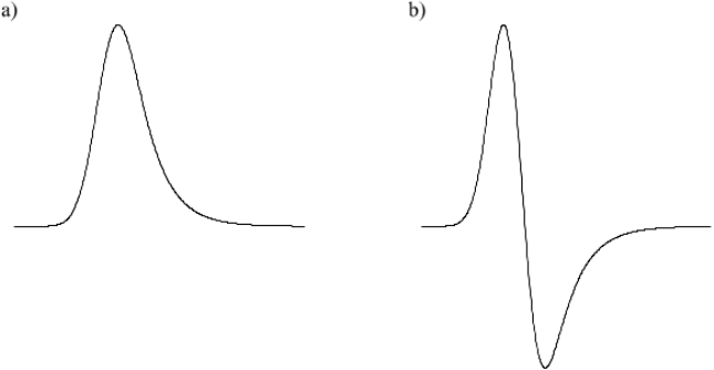
and may be much less. The pulses then pass through an ampliﬁer, which produces

an output pulse of up to 10 V. This output pulse may be a) unipolar (positive) or b)

bipolar:

Figure 1: Output pulse shapes. a) Unipolar pulse, b) Bipolar pulse

The unipolar pulse gives the best energy resolution, but the ampliﬁer may need to

be adjusted so that the ‘pole-zero’ compensation is correct [Knoll 633]. The bipolar

pulse has some advantages at high count rates; you should use it where possible.

Most ampliﬁers deliver a pulse between 1 and 4 µsec wide, which is suitable for

most purposes; think whether you need a wider or narrower pulse.

Digital pulses are usually generated by discriminators, or timing single channel anal-

ysers. Some units we have in the lab produce negative pulses (usually ∼0.5 V)

and some give positive pulses (usually larger). Make sure that the pulse outputs

you have are correct for the device you want to feed them into.

Almost all the electronics you use are packaged in “NIM" modules [Knoll 801], which

ﬁt into “NIM bins", which have built-in power supplies. Thus, when a module is

plugged into a bin, it is automatically provided with power ±12 V, ±24 V and

sometimes also ±6 V. Some units require a ±6 V supply, and so are incompatible

with those crates having only ±12 V and ±24 V. The basic operation of any of

these devices is obvious enough. But beware – almost all modules have knobs

on the front to change the parameters of the device. The settings of these are

important and should be recorded in your notebook; think about the most suitable

settings of each module for your experiment. Observe on the oscilloscope how the

output signal changes when the settings are varied.

1.7.1 Description of the Various Electronics Units

Here is a brief summary of the various units you may encounter in the Laboratory:

Preampliﬁer Usually a charge-sensitive ampliﬁer which accepts the low-level out-

put signal from a detector and delivers an ampliﬁed step-function pulse shape

to the output line with a 50 Ωimpedance.

Ampliﬁer Ampliﬁes pulses, usually up to 10 V (unipolar or bipolar), and shapes

them (with time constants of between 0.25 to 8 µs) so that the duration of the

pulses is reasonably short and suitable for input to the Analog to Digital Con-

verter (ADC) which is contained within the PC-based Multi-Channel Analyser

(MCA).

Discriminator Gives a digital output pulse when the input signal exceeds a preset

threshold.

Single-channel analyser (SCA) Gives a digital output pulse when the input signal

lies between two preset levels.

Timing SCA Same as an SCA, but is designed so that the time of the output pulse

relative to the input is carefully controlled.

Multichannel analyser (MCA) Rather like a set of many SCAs; the internal ADC

sorts the input pulses according to their pulse height and stores a spectrum of

these pulse heights - usually within a computer based data acquisition system

(next section).

If the pulse heights are proportional to the energy of the radiation, (as they are

for most detectors), then the spectrum on the MCA is therefore a representa-

tion of the energy spectrum of the radiation, and you will need to calibrate the

channels in the MCA in terms of the energy of the radiation.

As mentioned in section 1.6.1, Geiger Counters (and Fission Counters), pro-

duce a digital output pulse which may be counted by a simple scaler/timer

module, making an MCA irrelevant for these types of detector.

Time-to-Amplitude Converter (TAC) Also called a Time to Pulse Height Converter.

Requires two input logic pulses called “start" and “stop". The unit gives an

analogue output pulse whose height is proportional to the time difference be-

tween the start and stop pulses. This analogue pulse can then be processed

by the computer based MCA, and therefore can display a spectrum which now

represents a spectrum of time; you will need to calibrate the channels in the

MCA spectrum in terms of time.

1.7.2 Trouble-Shooting

Some common problems in operating nuclear physics apparatus are listed below.

1. Detectors always need an applied voltage (HV for a photomultiplier tube, bias

voltage for a solid-state detector, etc.).

Be careful to apply the correct polarity for this voltage.

Be careful to raise and lower this voltage slowly; some detectors can be

damaged by rapid changes in voltage.

Usually, detectors need at least a preampliﬁer, a main ampliﬁer and either a

single-channel analyser (SCA) or a multi-channel analyser (MCA) – see next

subsection.

2. In a few cases, where timing is more important than energy resolution, the

anode signals of a photomultiplier tube are fed directly into a discriminator,

without ampliﬁer or preampliﬁer. In this case, you need to select a discrimina-

tor which takes negative input pulses of a few hundred mV, rather than positive

pulses up to 10 V.

3. Although most electronics are mounted in NIM modules, which plug into bins

with built-in power supplies, a few modules (e.g. preampliﬁers) need power

from a separate source.

4. Most signal cables have BNC plugs, but a few units use the smaller LEMO

plugs. High-voltage cables usually have different plugs. Some of these are

MHV plugs, which look rather like BNC plugs but are not interchangeable

(and may be damaged if you try to). Other high-voltage equipment uses SHV

plugs. These different plugs are not just to create difﬁculties, they exist for

safety reasons. Remember that Murphy’s law applies here; the cable you

have to hand never has the right connector on it.

5. If you use a vacuum pump, be sure that the valve to allow air into the vacuum

equipment is opened immediately after switching off the vacuum pump. Make

sure any detector bias is off.

6. Observe the safety instructions concerning radioactive sources. Choose your

sources carefully to match your experiment; simple calibration procedures

rarely need strong sources. You should expect to make extensive use of the

reference books in the laboratory to research the decay schemes of sources.

Sources from the cupboard must be signed out to you by a demonstrator

and a demonstrator must check that the source is returned when you

have ﬁnished with it.

7. Geiger counters must ﬁrst be “plateaued" before use, i.e., ﬁnd a voltage where

the counting rate from a source is independent of bias voltage.

8. MOST IMPORTANT - always use an oscilloscope to look at the pulses at

all points in your electronics. Don’t assume that the pulses must be there

and have the right size, shape and polarity, just because you connected up

the equipment. Make sure that pulses have the shape that you expect at the

outputs of preampliﬁers, ampliﬁers, etc. A 20 MHz oscilloscope is suitable for

looking at analogue pulses from ampliﬁers, but you may need to use a faster

oscilloscope (100 MHz) to look at fast NIM logic pulses of a few ns width.

1.8 Data acquisition systems

The lab is equipped with PCs, which act as Multi Channel Analysers running the

Genie or Maestro software. All the PCs run Windows 10 and have Microsoft Ofﬁce

installed providing word processor (Word) and spreadsheet (Excel) facilities. Data

should always be saved onto a ﬂash drive or to your own networked area. Files

saved on the local hard disks (C:) will be removed on a regular basis. Flash drives

brought into the lab must be checked for viruses.

It is worth spending some time getting familiar with the Maestro or Genie pulse

height analysis programs before starting your experiment.

1.9 General measurements for gamma spectroscopy

There are several different type of gamma-ray detector around the laboratory, with

the two main types being germanium semiconductor (HPGe), or NaI(Tl) scintillator

detectors. These detectors can be used for a variety of experiments, but here are

some general experiments that you should consider for all γ-ray detectors.

1. The signal from the preampliﬁer has a fast leading edge, dictated by the decay

time of the signal carriers of the detector. This voltage will reach a maximum

and subsequently return to ground with a characteristic exponential decay

given by the preampliﬁer RC network. Use an oscilloscope to observe these

pulses and determine the decay time constant of the preampliﬁer.

2. The signals from the preampliﬁer are fed into a main ampliﬁer, one of whose

functions is to replace this long period decay with a much shorter one. As a

general rule, the charge integration time should be at least a factor of 4 longer

than the preampliﬁer decay time constant (98% conﬁdence limit in detecting

all signal carriers). What is the minimum shaping time you can use - note

that you may need to adjust the ‘pole-zero’ compensation [Knoll 633] as the

shaping time of the ampliﬁer is reduced - and therefore what is the maximum

count rate achievable with this system? You may also wish to investigate

energy resolution as a function of shaping time.

3. Knowing the duration of the pulse from the main ampliﬁer, and assuming this

is longer than the dead-time of the MCA (so it is the dominant source of dead-

time), estimate the percentage dead-time as a function of count rate. You can

investigate this for a range of source activities, or by changing the source to

detector distance. What parameters are affected by increased dead-time and

why?

4. Investigate the energy resolution of the photopeak as a function of bias volt-

age. Use this information to choose an optimum bias voltage which should

remain ﬁxed for the rest of your experiments.

5. Measure a statistically signiﬁcant spectrum from a γ-ray source placed near

the detector. Correlate the oscilloscope display with what you observe on the

MCA (it may be useful to use a monoenergetic source for clarity). Identify and

explain the features in the measured spectrum; as a general rule you should

be able to locate around 10 features even for a monoenergetic source (see

the detector physics exam questions). Investigate the effect of changing the

upper and lower level discriminators in the MCA settings. How signiﬁcant is

electronic noise?

6. Usually, you will want to measure the energy of a particular feature in your

spectra. Assuming that the detector response is linear with energy measure

the positions of the photopeaks for a number of calibrated (known) sources

using the peak ﬁtting software of your choice. Perform a (weighted) linear

least-squares ﬁt to the data to provide an empirical energy calibration for your

detector setup (remember that this is liable to change if you alter any of the

detector settings). How linear is the detector response, and how might you

test this? Measure a number of other sources and conﬁrm your calibration.

7. What is the dynamic range of your detector system, i.e. what are the lowest

and highest energies that you can measure? How might you change this

range, and why might this be useful experimentally?

8. Investigate the energy resolution as a function of γ-ray energy. How does

this compare with what you have been taught about Poisson statistics? The

energy resolution may have many contributing factors including statistical vari-

ation, electronic noise and student error. What is the dominant factor for your

detector? Bear in mind that all of the detectors in this laboratory have subtle

differences, so a direct comparison to other detectors may be meaningless,

even for the same types.

9. Investigate the absolute photopeak efﬁciency as function of source-detector

geometry, and of γ-ray energy. How does the absolute efﬁciency scale with

source to detector distance? Use your results to determine the intrinsic ef-

ﬁciency of the detector. How does this scale with source–detector distance,

and is this surprising? Can you explain how the efﬁciency behaves as a func-

tion of incident energy, and what does this tell you about gamma interaction

mechanisms?

1.10 Bibliography

If you haven’t yet done a course on Nuclear Physics, you will need to learn the

physics background information to the experiments. Most of the experimental de-

tails are covered in Knoll’s comprehensive book. There is much information about

individual NIM modules in the EG&G Ortec manual, whilst the Ortec Application

Notes have details of many experiments and how to set them up. Other textbooks

that give adequate coverage of detectors are those by Krane and also Burcham

and Jobes. Both the texts by Krane and Lilley have excellent chapters on the appli-

cations of nuclear science. The classic textbook for nuclear reactors is Glasstone

and Sesonske, but the diffusion of neutrons and reactors are also covered in Lilley’s

book.

General Reference Textbooks

W E Burcham and M Jobes; Nuclear and Particle Physics, Longman, 1995.

S Glasstone and A Sesonske; Nuclear Reactor Engineering, Van Nostrand Rhein-

hold 1967.

J S Lilley; Nuclear Physics: Principles and Applications, J Wiley, 2001.

G F Knoll; Radiation detection and measurement, 4th edition, J Wiley, 2010.

K S Krane; Introductory nuclear physics, 2nd Edition, J Wiley, 2000.

R D Evans The Atomic Nucleus, McGraw-Hill, 1972.

ORTEC reference material

ORTEC, Experiments in Nuclear Science Laboratory Manuals:

http://www.ortec-online.com/Service-Support/Library/Educational-Experiments.aspx

ORTEC Application Notes (AN). For example:

AN58 - How Histogramming and Counting Statistics Affect Peak Position Precision.

AN59 - How Counting Statistics Controls Detection Limits and Peak Precision.

http://www.ortec-online.com/Service-Support/Library/index.aspx

Useful online resources

NIST Physical Reference Data:

http://www.nist.gov/pml/productsservices/physical-reference-data/

This contains information on X-ray and gamma-ray attenuation coefﬁcients.

National Nuclear Data Centre (NNDC): http://www.nndc.bnl.gov

This contains a comprehensive list of nuclear decay schemes for any isotope.

1.11 Acknowledgements

This document is the product of the effort of many people over the many years the

laboratory has operated. Particular thanks to Peter Jones for the sections on ROOT

and the peak ﬁtting routine.

2 List of Experiments

The descriptions of the experiments follow in sections 2.1 to 2.7, but for the most

part, there is little detail, so that you will need to research these topics in reference

works. There are more detailed notes for the neutron diffusion experiment, since

the reference material may not be available in some current textbooks.

The experiments available are:

1. Neutron diffusion in graphite (or water tank) using BF3or 3He detectors.

2. Coincidence detection of positron annihilation photons.

3. X-ray ﬂuorescence analysis using Si(Li) detector.

4. Photon spectrometry with proportional counters.

5. γ-ray spectrometry of radioactive objects using a Ge detector.

6. Neutron activation analysis using Geiger or Ge detectors.

7. Attenuation of γ-rays in iron, etc. using a NaI detector.

8. Stopping powers, dE/dx, of αparticles in air using a silicon detector.

9. Absolute activity measurement using coincidence techniques.

10. γ-ray spectroscopy using scintillators.

2.1 Neutron Diffusion in Graphite using BF3or 3He detectors

In a nuclear reactor, fast neutrons emitted during ﬁssion have to be slowed down by

collisions with light nuclei in a moderator, until they attain thermal equilibrium with

the atoms of the moderator. They are then described as thermal neutrons. The be-

haviour of thermal neutrons is analogous to that of gas molecules, and they diffuse

from regions of high concentration into regions of lower concentration. There is also

a signiﬁcant probability that a thermal neutron will be captured by a nucleus. The

balance of these two processes determines the “diffusion length" of thermal neu-

trons in a given moderator. Early British reactors used graphite as the moderator.

The aim of this experiment is to determine the diffusion length Lof thermal neutrons

in graphite, by measuring the relative thermal neutron ﬂux at various points in a large

graphite moderator stack using a BF3detector.

There are three stages:-

1. Set up and understand the BF3detector [Knoll 523–531] using the 0.3 Ci

Am/Be neutron source in the stack – use the oscilloscope to observe the

pulse height variation with HV bias to determine the proportional region of the

detector, and then use the SCA to correlate the scaler counts vs SCA setting

to determine the energy spectrum of the signals. Use this information to set

up the SCA + scaler to count only neutrons.

2. Make measurements of the thermal neutron ﬂux at various positions in the

stack arising from the 3 Ci Am/Be source at the centre of the base. Because

your detector is also sensitive to fast neutrons you will have to make two mea-

surements, with and without the cadmium shield which absorbs thermal neu-

trons.

3. Fit your results in terms of neutron diffusion theory. The relevant equations

are given on the next page. Basically, to determine Lyou must determine

the constants α,βand γ;γcan be determined from the vertical variation in

ﬂux, αcan be determined from the horizontal variation (this is a non-linear

least squares ﬁtting problem). You cannot determine βdirectly from your

measurements but must make an intelligent estimate based on your value of

α.

Safety notes: The neutron sources give signiﬁcant dose rates from both neutrons

and gamma rays. The length of the handle on each source gives an indication

of the safe working distance and you should remain beyond this distance at all

times. Do not remain within twice this distance for prolonged periods. If you are

using a source in a bucket it is your responsibility to ensure that others cannot be

inadvertently exposed, so place the source as far from everyone else in the lab as

possible and mark it with a radiation sign. Do not move the strong (3 Ci) source

without permission from a demonstrator. Graphite is very slippery (and messy!)

and you are advised to wear gloves when handling it.

Neutron diffusion theory

The thermal neutron ﬂux, φ(r), at point ris given by n(r)v, where n(r)is the number

of thermal neutrons per unit volume at this point, and vis their average speed.

If the ﬂux is non-uniform, diffusion leads to a net ﬂow Jof neutrons given by Fick’s

law

J=−D∇φ(18)

where Dis the ﬂux diffusion coefﬁcient.

If Jis itself non-uniform then the difference between the ﬂow into and out of a given

region causes the number of neutrons in that region to vary with time. This can be

expressed in differential form as

∂n

∂t =−∇.J(19)

and substitution for Jgives the diffusion equation

∂n

∂t =D∇2φ(20)

However, the number of neutrons being captured per unit volume per unit time is

equal to nNσavwhere σais the microscopic capture cross section per atom and N

is the number of atoms per unit volume in the moderator.

The product Nσais referred to as the macroscopic cross section, Σa, so that the

capture rate per unit volume can be written as Σaφ.

Combining the effect of diffusion with the effect of capture, and neglecting higher

order terms, gives the equation:

∂n

∂t =D∇2φ−Σaφ(21)

which describes the variation in the neutron ﬂux in regions where there are no neu-

tron sources. In the steady state, ∂n/∂t = 0, so that the equation reduces to the

screened Poisson equation:

∇2φ= [Σa/D]φ(22)

The diffusion length, L, is deﬁned as

L= [D/Σa]1/2(23)

so that we may ﬁnally write:

∇2φ=1

L2φ(24)

The boundary conditions are that the ﬂux must be non-negative everywhere and

must approach zero at the edges of the graphite stack (the ﬂux is not actually zero

at the edge of the stack, as some neutrons leak out – this means that the solutions

can be extrapolated to zero a little way outside the stack).

Using Cartesian coordinates (x, y, z), solutions to this equation with appropriate

boundary conditions can be found by separation of variables: if φcan be written as

the product of three functions, φ(r) = X(x)Y(y)Z(z), then these must satisfy:

d2X

dx2+1

d2Y

dy2+1

d2Z

dz2=1

L2(25)

and since each term depends only on a single coordinate, each term must be equal

to a constant:

d2X

dx2=A, 1

d2Y

dy2=B, 1

d2Z

dz2=C(26)

where

A+B+C=1

L2(27)

Thus the solutions are either sinusoidal or exponential, depending on whether the

constants are negative or positive respectively. The boundary conditions dictate that

in the two horizontal directions (xand y) the ﬂux must approach zero at both sides

of the stack, so the solution cannot be exponential in form.

Hence both Aand Bmust be negative, and it is convenient to write A=−α2and

B=−β2. Since Cmust be positive (so that A+B+Cis positive), we write

C=γ2.

The general solutions are then:

X=Pcos(αx) + Qsin(αx)

Y=Rcos(βy) + Ssin(βy)

Z=T eγz +Ue−γz (28)

Since we expect the ﬂux to be symmetric about the centre of the stack (x=y=

0), we are only interested in the cosine terms for Xand Y. Since the ﬂux must

decrease with height, we are only interested in the e−γz term, giving for the neutron

ﬂux as a function of position:

φ(x, y, z) = Icos(αx) cos(βy)e−γz (29)

where Iis a combination of P,Rand U, and gives an overall scaling factor that

depends on the strength of the neutron source.

2.2 Positron annihilation detection

The positron emitted in β+decay slows down by collisions with atomic electrons.

Then, when it is almost at rest, it annihilates with an electron, giving two 511 keV

photons which are emitted almost exactly 180◦apart. Coincident detection of these

enables localisation of the source and is the basis of the imaging technique of

positron emission tomography.

The aim of this experiment is to use a pair of NaI detectors operating in coincidence

to detect the two photons and to demonstrate that they are approximately back-to-

back. It is also intended to introduce you to features of coincidence counting, such

as the effect of resolving time upon the numbers of real and random coincidences.

You will use a 22Na source. First use a single NaI(Tl) detector [Knoll 239–241],

observe the pulse height spectrum with an MCA, investigate the dependence on

PM voltage, and set a SCA window on the 511 keV peak. Repeat this for the

second detector. Then set up the coincidence circuit and measure coincidence

counts versus delay in one arm for detectors at 180◦, in order to ﬁnd the optimum

settings, using a strong source as well as the original weak source and observing

the contribution of random coincidences [Knoll 688–694]. Then vary the geometry

to conﬁrm that the photons are approximately back-to-back.

2.3 X-ray ﬂuorescence

Low energy γ-rays interact mainly by photoelectric absorption, knocking out an inner

shell electron and creating a vacancy which may subsequently be ﬁlled by an outer

electron with emission of a characteristic X-ray. This is the phenomenon of X-ray

ﬂuorescence (XRF) which can be used to identify the presence of heavy elements

within samples. The aim of this experiment is to understand the phenomenon of

XRF, its usefulness as an analytical technique and the complications involved in

making quantitative measurements. You will use a Si(Li) detector [Knoll 467–485]

to identify the emitted X-rays.

You should ﬁrst investigate the performance of this detector (NB bias must be ap-

plied very slowly) using the variable X-ray source (e.g. energy resolution vs bias,

and energy resolution vs X-ray energy), and should calibrate the PC MCA system –

you should understand the origin of Kαand KβX-rays.

You should then investigate Moseley’s Law for K X-ray energies versus atomic num-

ber, Z. In 1913, Henry Gwyn Jeffreys Moseley observed that the frequency (en-

ergy) of K X-ray transitions increased monotonically with increasing atomic number,

Z. In this way, he was able to reorder the periodic table of chemical elements

based on increasing atomic number, rather than increasing atomic mass as had

been done previously. This laid the foundation for identifying elements using X-ray

spectroscopy. You can then use the annular 241Am source to excite ﬂuorescent X-

rays from samples of unknown materials (e.g. coinage), and qualitatively analyse

their composition via Moseley’s Law.

You can then study the attenuation of different X-ray energies in (e.g.) Al or Zr foils

and should be able to see the difference in absorption either side of the K edge.

Warning! Do not switch on any part of this experiment until you have been properly

instructed by a demonstrator – the detector can be damaged if voltage is changed

too suddenly.

Safety notes: The annular sources used for XRF are quite active and care should

be taken to avoid unnecessary exposure (but the low energy photons are strongly

attenuated by a few mm of lead so there is no need for massive shielding).

2.4 Photon spectrometry with proportional counters

Low energy photons interact mainly by photoelectric absorption, where a tightly

bound electron is emitted from the absorber atom; this may also be accompanied

by characteristic photon emission. The aim of this experiment is to investigate how

photoelectric absorption is exploited for radiation detection, and to characterise two

similar detectors.

Set up and calibrate both the Kr and Xe ﬁlled proportional tubes [Knoll 159–195]

using a low energy X-ray source. Investigate peak amplitude and energy resolution

as a function of bias voltage. Compare the detection efﬁciencies which can be

obtained for a range of X-ray energies. How does the relative efﬁciency for each

detector compare over the measured energy range? Why do you see a difference?

Observe and explain any escape peaks which occur.

2.5 Gamma spectrometry of environmental radioactivity

Many everyday materials contain natural radioactivity. The aim of this experiment is

to identify and quantify the radioisotopes present by detecting their γ-ray emissions.

You will use a germanium detector [Knoll Chapter 12].

You should set up and calibrate the HPGe detector – investigate energy resolution

vs bias and γ-ray energy – and should determine the absolute efﬁciency vs energy

both for sources mounted against the detector face and for sources mounted a ﬁxed

distance away (using calibrated sources).

You will then be given some samples containing low-level activity to analyse. An

interesting exercise is to estimate the natural 40K activity of the human body, given

that a typical adult contains about 140 g of potassium.

Warning! The bias voltage must be applied and removed slowly – the detector

can be damaged if voltage is changed too suddenly.

2.6 Neutron activation analysis

A thermal neutron may be captured by a stable nucleus, creating a new radioactive

isotope, whose subsequent decay can be detected. This is the basis of neutron

activation analysis, which provides an accurate way of detecting low levels of certain

substances.

The aim of this experiment is to understand neutron activation analysis and to use

it to identify a mystery material.

The experiment can be performed in two ways. In the ﬁrst, a Geiger counter is

used to detect the induced radioactivity and observe its decay with time and its

dependence on activation time. In the second, a germanium detector is used to

identify a radioisotope on the basis of the emitted γ-rays. Neutron activation can be

carried out using the 1 Ci Am/Be neutron source in the water tank as a source of

thermal neutrons.

First plateau the Geiger counter [Knoll 207–215] using a 90Sr beta source. Then

activate a sample of indium or silver (approx 5 g pieces are ideal) and detect the

induced activity with the Geiger counter – repeated measurements on a single ac-

tivated sample should enable the half life of the decaying product to be determined

(more than one component may be seen). Then study the effect of varying the acti-

vation time.

Safety notes: The 90Sr beta sources are potentially unsealed and care should be

taken in handling them to avoid any risk of ingesting contamination: do not touch

the active area of the source and wash your hands after use.

The dose rate immediately around the water tank (in which samples are activated)

is signiﬁcant so do not linger in this area. When you have ﬁnished with an activated

sample check whether it is signiﬁcantly active and if so place it in the bottom of the

small source cupboard (by the next day it should no longer be active and may be

retrieved).

2.7 Gamma-ray attenuation and build up

The aim of this experiment is to observe and understand the processes by which

gamma rays are attenuated in passing through matter, and the effects of shielding

geometry.

The experiment divides into two parts. In the ﬁrst, an ionisation chamber is used to

measure dose rate as a function of shielding thickness, while in the second a sodium

iodide (NaI) detector is used to provide information on the spectrum of transmitted

γ-rays.

Start by building a well shielded enclosure and inserting the 7MBq 60Co source at

one end – use the ionisation chamber to measure gamma dose rate at the other end

of the enclosure. Place iron plates between, and measure attenuation vs iron thick-

ness, for at least two shielding geometries (well collimated and open), and compare

with an exponential falloff to investigate whether build-up is signiﬁcant [Knoll 53].

Then repeat using a NaI(Tl) scintillation detector [Knoll 239–241] coupled to a photo-

multiplier tube – ﬁrst investigate the response of the NaI to weak gamma ray sources

(study variations in gain and energy resolution as a function of PM voltage, and

variation in energy resolution with γ-ray energy) [Knoll Chap 10] – then repeat the

attenuation measurements in different geometries.

Attenuation of materials other than Fe, can also be studied.

Safety notes: The strong 60Co source used in this experiment should be trans-

ported in its carrying brick, always handled remotely and requires appropriate shield-

ing to reduce the dose rate at all exposed areas to less than 2.5 mSv/hr. Do not han-

dle this source until you have been instructed in the use of an appropriate radiation

monitor.

2.8 Alpha-particle stopping powers in gases

The aim is to determine the stopping power, dE/dx, for alpha particles in various

gases as a function of energy, and compare with the predictions of the Bethe-Bloch

formula.

You will use an ion-implanted silicon detector [Knoll Chap 11]. Its behaviour should

ﬁrst be investigated in the small vacuum chamber using the Am/Cm/Pu triple al-

pha source, which can provide a rough energy calibration (do not touch the active

surface of the source).

A larger chamber containing a motorised 241Am source should be used to investi-

gate the effect of gas (He or Ar) between source and detector, and determine the

energy at the detector as a function of the amount of material traversed. You can

then differentiate this function to determine dE/dx as a function of E.

The 241Am source sealed into the larger chamber only provides monoenergetic al-

pha particles, so cannot provide an energy calibration by itself. However, the full

energy signals from the detector can be simulated by an electronic pulser. As this

output pulse amplitude can be precisely attenuated by known amounts, a “match-

stick” spectrum can be produced that gives a calibration from just one measured

energy.

The Bethe-Bloch stopping power formula

The Bethe-Bloch formula in SI units

dx = (−)e4

(4π0)2

4πz2NZ

mec2β2ln 2mec2β2

I−ln(1 −β2)−β2(30)

relates the stopping power (in Jm−1) of an ion of charge ze travelling through a

medium of atomic number Zto its velocity, v, which appears in the formula as

β=v/c.Nis the number of atoms per unit volume (in m−3) in the medium, so that

the product NZ simply represents the number of electrons per unit volume; meis

the mass of the electron. Iis the average ionisation potential for all the electrons in

the medium, usually approximated by I= 11 ×ZeV (electron volts).

In many books the equation appears with Nreplaced by NAρ/A, where ρis the

density of the medium and Aits atomic mass. You should note, however, that to

give results in SI units the constant NAmust be 6×1026 : i.e. 103times Avogadro’s

number.

Safety notes: The α-particle sources are potentially unsealed and care should be

taken in handling them to avoid any risk of ingesting contamination: do not touch

the active area of the source and wash your hands after use. The gas cylinders

are potentially hazardous and care should be taken to avoid pressurising the cham-

ber – do not operate regulator valves until you have been properly instructed by

a demonstrator, and read the document STANDARD OPERATING PROCEDURE FOR

HANDLING PRESSURISED GASES in the laboratory section of LM PH605 PRACTI-

CAL SKILLS FOR REACTOR PHYSICS on Canvas.

2.9 Absolute activity determination

The activity of an unknown source can be estimated easily if a high quality cali-

bration of the detector has been carried out. However, the determinations of the

solid angle covered by the detector, and its intrinsic efﬁciency, introduce the largest

sources of error. This experiment introduces the use of coincidence techniques for

absolute activity measurements where these are no longer limiting factors.

Set up and calibrate both of the NaI(Tl) detectors (study variations in gain and en-

ergy resolution as a function of bias voltage) paying particular attention to efﬁciency

measurements. Estimate the activity of unknown sources using the detector efﬁ-

ciency method and estimate the error on these results.

Read about absolute activity measurements using gamma-gamma coincidence in

Knoll [Knoll 694–695]. Set up your detectors with suitable single channel scalers as

described and connect up the coincidence circuit. Measure single and coincidence

(prompt and delayed) count rates for the same sources as above and compare

measurements. How do the errors on activity compare using the two methods?

2.10 Gamma-ray spectroscopy using scintillators

The teaching laboratory has several different types of scintillator detectors, including

sodium iodide (NaI), cerium(III) bromide (CeBr3), lanthanum(III) bromide (LaBr3)

and lanthanum(III) chloride (LaCl3) solid state detectors. These are often used for

speciﬁc experiments, but can be used for other investigations as required. Each

type has its own characteristics which can make one preferable over another, and

you can investigate the similarities and differences of each:

Investigate PM tube gain as a function of bias voltage. How does the overall multi-

plication factor scale and what does this tell you about your detector construction?

Find the characteristics of the detectors, as outlined in section 1.9. Measure the

energy resolution and efﬁciency as a function of γ-ray energy, and calibrate your

detectors.

Measure the background radiation ﬁeld in the lab. Ensure that you have a statisti-

cally signiﬁcant sample. What are the main features in this spectrum and where do

they originate? You may wish to try this at different times of day or on different days.

Identify the photopeak and Compton continuum for your measured spectra. Does

the energy of the Compton edge correlate with what you know about Compton scat-

tering? What about the backscatter peak (if it is easily identiﬁable). Measure the

areas covered by the photopeak and Compton continuum, giving the peak to Comp-

ton ratio. How does this behave for different energy sources?

You may wish to compare many of the measurements done using scintillators with

similar experiments using other types of detectors in the lab when you change ex-

periments. As always be sure to keep a careful record of what you have measured,

and how, so that you can include these results as part of other experiments (and in

your lab reports).

3 Writing a laboratory report

This section gives some guidelines and suggestions for writing laboratory reports. It

is written in the style of a report. The report itself should contain the following sec-

tions; abstract, introduction, theory, description of apparatus, method or procedure,

results and analysis, discussion and conclusion. As a rule data should be presented

in the results section, and appendices may be used if there are very long tables.

Abstract

As a general rule, the abstract should not be longer than about ten sentences,

and should contain a concise description of your work, and any important results

that you wish to present. This should include numerical results and the associated

uncertainties. The abstract should not contain any description of experimental ap-

paratus, unless its success or failure is the actual result, nor should the abstract

contain any equations.

Introduction

The introduction should be just that – a section which introduces the reader to what

you have been doing. It may contain some historical information if the experiments

have been performed by others in the past, or if there have been other measure-

ments reported in the research literature, or in textbooks, or of course if similar work

has been presented on a website. In these cases, report the previous work and

refer to the appropriate journal, book or website. The other function of the intro-

duction is to introduce the area of experimentation that you are investigating, and

set the framework of the physics involved and the methods you are going to use

in order to make your measurements. Remember that you might also have another

section called Experimental equipment or Experimental details etc., so do not ﬁll the

introduction with great details about the experimental work. If the theory behind the

experiment is fairly simple and brief it might be appropriate to put such theory into

the Introduction, but if there are lots of equations, it might be better to have a second

section which could be called Theory,Theory of the measurements on XYZ. Simi-

larly, if there is a need to explain carefully about a complicated experimental setup,

another section called Background information on measurements XYZ,Detection

systems for measurements on XYZ, etc. could be inserted into the text, probably

after the Theory section.

Theory

The reports should be written so as to be understood by a physicist who does not

know in advance anything about the experiment which you have done, so you must

explain what the purpose of the experiment was, how you did it, what the results

are, and what their signiﬁcance is. Reports should be written in clear English, and

in sentences, i.e. do not use bullet points. Conventionally, descriptions of what you

did are generally written in the past tense using a passive style (“The detector was

connected to an MCA...")

In a theory section, you need to encapsulate all the necessary theory with as few

equations as possible; do not include equations that you never use. Be sure to dis-

cuss the main physical processes which are involved in your experiment, so that the

reader is aware of what is involved, and if necessary can go away and read some

background information, hopefully from one of the excellent references that you

have listed at the back of your report. Make sure all your equations are numbered

and are in a clear font so that they are unambiguous; make sure that numerators

and denominators are clearly separated, powers of numbers or variables are in su-

perscript, and indices of variables are in subscript etc. Be very careful to distinguish

variables which are vectors from other variables by using a line above the variable

or use a bold font.

In between the equations, you need to link, or summarise, the relevance of each

equation to the physics and the experiment which you have performed, so that the

reader is aware of its importance. Remember that the report is telling a story about

your experiment, and you need to keep the reader interested and involved.

Background to detection techniques for XYZ

If your experiment involves a large amount of complicated apparatus, then this sec-

tion might provide the reader with some valuable background information about the

detection system for example. Try to get in some pictures to illustrate what you are

planning to use, so that when you come to describe your speciﬁc experimental de-

tails, the reader will feel familiar with what you are talking about. However, bear in

mind that photographs are not necessarily as instructive as schematic diagrams to

explain your thinking. Try to link what you are discussing back to the equations in

the Theory section if appropriate, but you could also include further equations in this

section if they are applicable to the methods or operation of the detection systems.

Try and be as speciﬁc as possible, e.g. if you used a particular power supply, then

state the manufacturer, the model number/name and what the voltage range used

was, and why you chose that range.

Experimental measurements of XYZ

Describe the experimental equipment brieﬂy, and then move onto the way in which

the experiment was carried out. Try to show that the way you tackled the experiment

was actually planned in a reasonable way to produce the correct results. Discuss the

results you obtained, illustrating your results with ﬁgures within the text, so that the

reader does not need to keep ﬂipping over into the appendices. Do not put all your

experimental measurements within the text of the report; you may have hundreds

of values which can usefully go into an appendix of the report. Remember that one

picture is worth a thousand words. So, try and summarise all your results in a few

simple ﬁgures.

Results of the detection of XYZ

In this section you should analyse the results, making reference to the equations in

the theory section and to the sections on the background and experimental details.

One of the best ways to summarise your results is either with a ﬁgure, or with a table

which contains all the main results. You should also tackle the subject of errors on

measurements in general and on your measurements in particular. Try to work out

what errors can occur in your measurements and the relevant magnitudes of these

errors. Remember that Physicists are the greatest sceptics – there is no truth, just

measurement with errors. Try to justify the conclusions that you have drawn from

your results, and comment on whether your measured values are consistent with

other measurements (within errors).

Conclusions

In this section you need to summarise all your results, and most importantly, discuss

your results and compare with other measurements, or previous work. A summary

table of your own results compared with other measurements is sometimes useful.

Lastly, you could make some critical comments about the experiment and suggest

ways in which it might be improved, or ways in which you might have tackled the

experiment if you were to do it again. Remember that for some readers, the only

pages they may read are the title page with the abstract and the conclusions.

References

Don’t forget to include ALL of your references (books/journals/www etc). There are

two schemes of referencing papers, either by numbering[1] or by referring to the

authors and the data [Bloggs et al. 1969]

1. Bloggs et al., 1969. Referencing techniques for publications, Proceedings

of the International Conference on Publications, Lynchburg, Moore County,

Tennessee, U.S.A., ed. J. Daniels, Hic! Books Inc, St Louis, Missouri, U.S.A.

Bibliography

Note that references are NOT the same as a bibliography, which should come in a

separate section.

Appendices

This section should contain all the tables which are too long to put in the text, or raw

data which you might think could be useful for some readers, or bits of theory which

are useful but not really important to the ﬂow of the report.

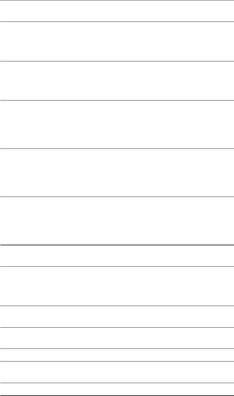
4 Gamma-Ray Source Activities

Set Source ID Activity on 21/11/13 Accuracy

(Bq) (%)

Year 3 Box 1

60Co A0732 1640 ±31 1.9

133Ba A0445 24800 ±1190 4.8

137Cs A0468 149000 ±5520 3.7

152Eu 1D058 64700 ±3480 5.4

Year 3 Box 2

22Na 1X515 64 ±2 3.7

60Co 1U577 5530 ±105 1.9

133Ba 1R479 52200 ±2500 4.8

241Am 1Q532 374000 ±18700 5.0

Year 3 Box 3

60Co 2U270 12100 ±230 1.9

133Ba A0877 23900 ±1150 4.8

137Cs A0697 142000 ±5270 3.7

152Eu EW617 149000 ±7460 5.0

241Am 1Q599 402000 ±20100 5.0

MSc Box 1

60Co 1U630 6240 ±120 1.9

133Ba 1R545 45600 ±2190 4.8

137Cs 1S684 191000 ±7080 3.7

152Eu 1D157 83200 ±4160 5.0

241Am 1Q598 415000 ±20700 5.0

MSc Box 2

60Co 1U629 5850 ±110 1.9

133Ba 1R548 45400 ±2180 4.8

137Cs 1S681 184000 ±6800 3.7

152Eu 1D152 81800 ±4090 5.0

241Am 1Q596 398000 ±19900 5.0

Individual 22Na C3N.19/91 38100 ±1960 5.1

Individual 22Na C3N.19/61 29000 ±1430 4.9

Individual 44Ti UOB08121 22800 ±1190 5.2

Individual 44Ti UOB08122 22800 ±1200 5.2

Individual 44Ti UOB08123 22700 ±1190 5.2

Individual 44Ti UOB08124 23300 ±1220 5.2

Individual 60Co C3N.19/18 248000 ±10500 4.2

Individual 60Co C3N.19/62 35200 ±1500 4.3

Individual 68Ge UOB101012 136000 ±7210 5.3

Individual 68Ge UOB221111 68900 ±3720 5.4

Individual 108mAg UOB931201B2 8510 ±490 5.8

Individual 137Cs C3N.19/65 5300000 ±205000 3.9

Individual 137Cs C3N.19/76 38100 ±2090 5.5

Individual 207Bi C3N.19/89 20300 ±1030 5.1

5 Summary of Statistical Formulae (+ Knoll ch. 3)

Sample Mean

¯x=

i=1

Standard Deviation

σ(x)s(x) =

i=1

(xi−¯x)2

n−1

(error on a single measurement)

Error in Mean

σ(¯x) = σ(x)

√n

Goodness of Fit

χ2=

i=1

(yobs

i−yth

i)2

σ2(yobs

(0.5≤χ2/(n−p)≤1.5for a good ﬁt to ndata points with pfree parameters)

Propagation of Errors

1. F =k.x ⇒σ(F) = |k|σ(x)

2. F =xn⇒σ(F)

F=|n|σ(x)

3. F =x+y+z⇒σ(F) = pσ2(x) + σ2(y) + σ2(z)

4. F =x.y

z⇒σ(F)

F2

=σ(x)

x2

+σ(y)

y2

+σ(z)

z2

5. F =xp.yq

zr⇒σ(F)

F2

=pσ(x)

x2

+qσ(y)

y2

+rσ(z)

z2

In general: σ2(F) = σ(x)∂F

∂x 2

+σ(y)∂F

∂y 2

+σ(z)∂F

∂z 2

+...

+ 2cov(x, y)∂F

∂x ∂F

∂y + 2cov(x, z)∂F

∂x ∂F

∂z +...

MSc Lab Manual

Navigation menu

Versions of this User Manual:

Views

Navigation