Machine Learning Guide Patel MK
User Manual:
Open the PDF directly: View PDF ![]() .
.
Page Count: 121 [warning: Documents this large are best viewed by clicking the View PDF Link!]
- Table of contents
- Machine learning terminologies
- Multiclass classification
- Binary classification
- Regression
- Cross validation
- Clustering
- Dimensionality reduction
- Preprocessing of the data using Pandas and SciKit
- Pipeline
- Clustering with dimensionality reduction
- Image recognition
- More examples on Supervised learning
- Performance analysis of models
- Quick reference guide

Table of contents
Table of contents i
1 Machine learning terminologies 2
1.1 Introduction ................................................. 2
1.2 Machine learning .............................................. 2
1.3 Basic terminology .............................................. 3
1.3.1 Data: samples and features .................................... 3
1.3.2 Target ................................................ 3
1.3.3 Load the inbuilt data ....................................... 3
1.4 Types of machine learning ......................................... 4
1.4.1 Supervised learning ........................................ 4
1.4.2 Unsupervised learning ....................................... 5
1.5 Conclusion ................................................. 6
2 Multiclass classification 7
2.1 Introduction ................................................. 7
2.2 Iris-dataset ................................................. 7
2.2.1 Load the dataset .......................................... 7
2.2.2 Split the data as ‘training’ and ‘test’ data ............................ 8
2.3 Conclusion ................................................. 9
3 Binary classification 10
3.1 Introduction ................................................. 10
3.2 Dataset ................................................... 10
3.3 Extract the data i.e. ‘features’ and ‘targets’ ............................... 12
3.4 Prediction .................................................. 14
3.5 Rock vs Mine example ........................................... 17
3.6 Conclusion ................................................. 18
4 Regression 19
4.1 Noisy sine wave dataset .......................................... 19
4.2 Regression model .............................................. 21
4.3 Conclusion ................................................. 23
5 Cross validation 24
5.1 Introduction ................................................. 24
5.2 Cross validation ............................................... 25
5.3 Splitting of data .............................................. 27
5.3.1 Manual shuffling .......................................... 27
5.3.2 Automatic shuffling (KFold, StratifiedKFold and ShuffleSplit) ................. 28
5.4 Template for comparing algorithms .................................... 30
6 Clustering 32
i

Table of contents
6.1 Introduction ................................................. 32
6.2 KMeans ................................................... 32
7 Dimensionality reduction 36
7.1 Introduction ................................................. 36
7.2 Principal component analysis (PCA) ................................... 36
7.2.1 Create dataset ........................................... 36
7.2.2 Reduce dimension using PCA ................................... 37
7.2.3 Compare the performances .................................... 38
7.3 Usage of PCA for dimensionality reduction method ........................... 41
7.4 PCA limitations .............................................. 41
7.5 Conclusion ................................................. 41
8 Preprocessing of the data using Pandas and SciKit 42
8.1 Chronic kidney disease ........................................... 42
8.2 Saving targets with different color names ................................. 43
8.3 Basic PCA analysis ............................................. 44
8.3.1 Preparing data for PCA analysis ................................. 44
8.3.2 dimensionality reduction ...................................... 45
8.4 Preprocessing using SciKit library .................................... 46
8.5 Preprocessing using Pandas library .................................... 48
9 Pipeline 51
9.1 Introduction ................................................. 51
9.2 Pipeline ................................................... 51
10 Clustering with dimensionality reduction 53
10.1 Introduction ................................................. 53
10.2 Read and clean the data .......................................... 53
10.3 Clustering using KMean .......................................... 54
10.4 Dimensionality reduction ......................................... 55
10.5 Plot the results ............................................... 55
11 Image recognition 58
11.1 Introduction ................................................. 58
11.2 Fetch the dataset .............................................. 58
11.3 Plot the images ............................................... 59
11.4 Prediction using SVM model ....................................... 61
11.5 Convert features to images ......................................... 64
12 More examples on Supervised learning 69
12.1 Introduction ................................................. 69
12.2 Visualizing the Iris dataset ........................................ 69
12.2.1 Load the Iris dataset ........................................ 69
12.2.2 Histogram .............................................. 70
12.2.3 Scatter plot ............................................. 71
12.2.4 Scatter-matrix plot ......................................... 72
12.2.5 Fit a model and test accuracy ................................... 74
12.2.6 Plot the incorrect prediction ................................... 76
12.3 Linear and Nonlinear classification .................................... 79
12.3.1 Create ‘make_blob’ dataset .................................... 79
12.3.2 Linear classification ........................................ 80
12.3.3 classification boundary for linear classifier ............................ 81
12.3.4 Nonlinear classification and boundary .............................. 82
13 Performance analysis of models 85
13.1 Introduction ................................................. 85
13.2 Performance of classification problem ................................... 85
13.2.1 Accuracy .............................................. 85
ii PythonDSP

Table of contents
13.2.2 Logarithmic loss .......................................... 86
13.2.3 Classification report ........................................ 87
13.2.4 Confusion matrix (Binary classification) ............................. 87
13.2.5 Area under ROC (AUC) ...................................... 88
13.3 Performance of regression problem .................................... 89
13.3.1 MAE, MSE and R2 ........................................ 89
13.3.2 Problem with cross-validation ................................... 90
14 Quick reference guide 92
14.1 Introduction ................................................. 92
14.2 Understand the data ............................................ 92
14.2.1 Load the data and add headers .................................. 92
14.2.2 Check for the null values ...................................... 93
14.2.3 Check the data types ........................................ 94
14.2.4 Statistics of the data ........................................ 95
14.2.5 Output distribution for classification problem .......................... 96
14.2.6 Correlation between features ................................... 96
14.3 Visualizing the data ............................................ 97
14.3.1 Univariate plots .......................................... 97
14.3.2 Multivariate plots: ......................................... 99
14.4 Preprocessing of the data ......................................... 104
14.4.1 Statistics of data .......................................... 105
14.4.2 StandardScaler ........................................... 105
14.4.3 MinMax scaler ........................................... 106
14.4.4 Normalizer ............................................. 107
14.5 Feature selection .............................................. 107
14.5.1 SelectKBest ............................................. 108
14.5.2 Recursive Feature Elimination (RFE) .............................. 108
14.5.3 Principal component analysis (PCA) ............................... 109
14.6 Algorithms ................................................. 109
14.6.1 Classification algorithms ...................................... 109
14.6.2 Regression algorithms ....................................... 111
iii Meher Krishna Patel
Chapter 1
Machine learning terminologies
Codes and Datasets
The datasets and the codes of the tutorial can be downloaded from the repository
1.1 Introduction
In this chapter, we will understand the basic building blocks of SciKit-Learn library. Further, we will discuss the
various types of machine learning algorithms. Also, we will see several terms which are used in machine learning
process.
Machine learning algorithms is a part of data analysis process. The data analysis process involves following steps,
•Collecting the data from various sources
•Cleaning and rearranging the data e.g. filling the missing values from the dataset etc.
•Exploring the data e.g. checking the statistical values of the data and visualizing the data using plots etc.
•Modeling the data using correct machine learning algorithms.
•Lastly, check the performance of the newly created model.
In this tutorial we will see all the steps of data analysis process except the first step i.e. data
collection process. We will use the data which are available on the various websites.
Important: Data analysis requires the knowledge of multiple field e.g. data cleaning using Python or R language.
Good knowledge of mathematics for measuring the statistical parameter of the data. Also, we need to have the
knowledge of some specific field on which we want to apply the machine learning algorithm. Lastly, we must have
the understanding of the machine learning algorithms.
1.2 Machine learning
In general programming methods, we write the codes to solve the problem; and the code can solve a particular
types of problem only. This is known as ‘hard coding’ method. But in the machine learning process, the codes are
designed to see the patterns in the datasets to solve the problems, therefore it is more generalizes and can make
the decisions on the new problems as well. This difference is shown in Table 1.1.
Table 1.1: Hard coding vs Machine learning
Type Description
Hard coding can solve a particular type of problems
Machine learning sees the pattern in the data and solve the new problem by itself
2
Chapter 1. Machine learning terminologies
Lastly, the Machine learning can be defined as the process of extracting knowledge from the data, such that an
accurate predication can be made on the future data. In the other words, machine learning algorithms are able to
predict the outcomes of the new data based on their training.
1.3 Basic terminology
In this section, we will see basic building blocks of SciKit library along with several terms used in machine learning
process.
1.3.1 Data: samples and features
Data is stored in two dimensional form in the SciKit, which are known as the ‘samples’ and ‘features’.
Note:
•Samples: Each data has certain number of samples.
•Features: Each sample has some features, e.g if we have samples of lines, then features of this lines can be
‘x’ and ‘y’ coordinates.
•All the features should be identical in SciKit. For example, all the lines should have only two features i.e.
‘x’ and ‘y’ coordinates. If some lines have third feature as ‘thickness of line’, then we need to append/delete
this feature to all the lines.
1.3.2 Target
•Target: There may be the certain numbers of possible outputs for the data, which is known as ‘target’. For
example, the the points can be on the ‘straight line’ or on the ‘curve line’. Therefore, the possible targets
for this case are ‘line’ and ‘curve’.
•Different names are used for ‘targets’ and ‘features’ as shown in Table 1.2,
Table 1.2: Other names for ‘targets’ and ‘features’
Name Other names
Features Inputs, Attributes, Predictors, Independent variable, Input variables
Target Outputs, Outcomes, Responses, Labels, Dependent variables
1.3.3 Load the inbuilt data
Let’s understand this with an example. The SciKit library includes some input data as well. First we will use
these data and later we will read the data from the files for the data analysis.
•The stored datasets in the SciKit library can be used as below,
>>> from sklearn.datasets import load_iris # import 'iris'dataset
>>> iris =load_iris() # save data set in 'iris'
•Now, we can see the data stored in the ‘iris’. Note that dataset is stored in the form of ‘dictionary’.
>>> iris.keys()
dict_keys(['data','target','target_names','DESCR','feature_names'])
Following is the description of above keys,
•‘feature_names’: This contains the information about the features (optional).
3Meher Krishna Patel
1.4. Types of machine learning
>>> iris.feature_names
['sepal length (cm)','sepal width (cm)','petal length (cm)','petal width (cm)']
•‘data’: It contains certain numbers of samples for the data e.g. this dataset contains 150 samples and each
sample has four features. In the below results, the first three entries of the data is shown. The name of
the columns (i.e. features of the data) are shown by the ‘feature_names’ e.g. the first column stores the
speal-length.
>>> iris.data.shape # 150 samples, 4 features
(150, 4)
>>> iris.data[0:3]# display 3 samples of stored data
array([[ 5.1, 3.5, 1.4, 0.2],
[ 4.9, 3. , 1.4, 0.2],
[ 4.7, 3.2, 1.3, 0.2]])
•‘target_names’: This contains the details about the target (optional).
>>> iris.target_names # flower categories
array(['setosa','versicolor','virginica'],
dtype='<U10')
•‘target’: It is the possible outputs for the data (optional). This is required for supervised learning, which
will be discussed in this chapter. Here ‘0’ represents the ‘setoas’ family of the Iris-flower.
>>> iris.target
array([0, 0, 0, 0, ..., 0, 1, 1, 1, ..., 2, 2, 2])
•‘DESCR’: It contains the description about the data set(optional).
>>> iris.DESCR
'Iris Plants Database\n====================\n [...]
Note: Following are the important points about the dataset, which we discussed in this section,
•Datasets have samples of data, which includes some features of the data.
•All the features should be available in every data. If there are missing/extra features in some data, the we
need to add/remove those features from the data for SciKit.
•Also, the dataset may contain the ‘target’ values in it.
1.4 Types of machine learning
Machine learning can be divided into two categories i.e. supervised and unsupervised, as shown in this section,
1.4.1 Supervised learning
In Supervised Learning, we have a dataset which contains both the input ‘features’ and output ‘target’, as discussed
in Section 1.3.3, where Iris flower dataset has both ‘features’ and ‘target’.
1.4.1.1 Classification and regression
The supervised learning can be further divided into two categories i.e. classification and regression.
•Classification: In classification the targets are discrete i.e. there are fixed number of values of the outputs
e.g. in Section 1.3.3 there are only three types of flower. Also, these outputs are represented using strings
e.g. (Male/Female) or with fixed number of integers as shown for ‘iris’ dataset in Section 1.3.3 where 0,
1 and 2 are used for three types of flower.
–If the target has only two possible values, then it is known as ‘binary classification’.
4PythonDSP
Chapter 1. Machine learning terminologies
–If the target has more than two possible values, then it is known as ‘multiclass classification’.
•Regression: In regression the targets are continuous e.g. we want the calculate the ‘age of the animal (i.e.
target)’ with the help of the ‘fossil dataset (i.e. feature)’. In this case, the problem regression problem as
the age is a continuous quantity as it does not have fixed number of values.
1.4.2 Unsupervised learning
In Unsupervised Learning, the dataset contains only ‘features’ and ‘no target’. Here, we need to find the relationship
between the various types of data. In the other words, we have to find the labels from the given dataset.
Unsupervised learning can be divided into three categories i.e. Clustering, Dimensionality reduction and Anomaly
detection.
•Clustering: It is process of reducing the observations. This is acheived by collecting the simialar data in one
class.
•Dimensionality reduction: This is the reduction of higher dimensional data to 2 dimensional or 3 dimensional
data, as it is easy to visualize the data in 2 dimensional and 3 dimensional form.
•Anomaly detection: This is the process of removal of undesired data from the dataset.
Note: Sometimes these two methods, i.e. supervised and unsupervised learning, are combined. For example the
unsupervised learning can be used to find useful features and targets; and then these features can be used by the
supervised training method.
For example, we have a the ‘titanic’ dataset, where we have all the information about the passengers e.g. age,
gender, traveling-class and number of people died during accident etc. Here, we need to find the relationship
between various types of data e.g. people who are traveling in higher-class must have higher chances of survival
etc.
Important: Please note the following points,
•Not all the problems can be solved using Machine learning algorithms.
•If a problem can be solved directly, then do not use machine learning algorithms.
•Each machine learning algorithms has it’s own advantages and disadvantages. In the other words, we need
to choose the correct machine learning algorithms to solve the problem.
•We need not to be expert in the mathematics behind the machine learning algorithms; but we should be
aware of pros and cons of the algorithms.
•Below is the summery of this section. Table 1.3 shows the types of machine learning, and Table 1.4 shows
the types of variable in machine learning algorithms.
Table 1.3: Classification of Machine learning
Machine learning Subtypes
Supervised Binary classification, multiclass classification, regression
Unsupervised Clustering, Dimensionality reduction, Anomaly detection
Table 1.4: Types of variable
Type Description
categorical or factor string (e.g. Male/Female), or fixed number of integers 0/1/2
numeric floating point values
5Meher Krishna Patel

Chapter 2
Multiclass classification
2.1 Introduction
In this chapter, we will use the ‘Iris-dataset’ which is available in the ‘SciKit library’. Here, we will use ‘KNeigh-
borsClassifier’ for training the data and then trained models is used to predict the outputs for the test data. And
finally, predicted outputs are compared with the desired outputs.
2.2 Iris-dataset
2.2.1 Load the dataset
Lets see the Iris-dataset which has following features and target available in it, which are show in Listing 2.1.
•Features:
–sepal length in cm
–sepal width in cm
–petal length in cm
–petal width in cm
•Targets:
–Iris Setosa
–Iris Versicolour
–Iris Virginica
7

2.2. Iris-dataset
Listing 2.1: Iris-dataset
>>> from sklearn.datasets import load_iris
>>> iris =load_iris()
>>> iris.keys()
dict_keys(['data','target','target_names','DESCR','feature_names'])
>>> iris.feature_names
['sepal length (cm)','sepal width (cm)','petal length (cm)','petal width (cm)']
>>> iris.target_names
array(['setosa','versicolor','virginica'],
dtype='<U10')
>>> iris.data.shape # 150 samples with 4 features
(150, 4)
2.2.2 Split the data as ‘training’ and ‘test’ data
We have 150 samples in our data. We can divide it into two parts i.e. ‘training dataset’ and ‘testing
dataset’. A good choices can be 80% training data and 20% test data.
Important: The training data set must included all the possible ‘targets’ in it, otherwise the machine
will not be trained for all the ‘targets’; and will generate huge errors when those datasets will appear
in the test. We can use “stratify” in the ‘train_test_split’ which takes care of this, as shown in Listing
2.2.
Here we will use the ‘KNeighborsClasssifier’ class of ‘sklearn’ for training the machine. Lets write the code in the
file. Here Lines 17-27 are used to create the training and test datasets. Then Line 36 instantiates an object of
KNeighborsClasssifier, which fits the models based on training data at Line 38. Next, the trained model is used
to predict the outcome of the test data at Line 40. Finally, prediction error is calculated at Line 44.
Listing 2.2: Training and test data
1# multiclass_ex.py
2
3import numpy as np
4from sklearn.datasets import load_iris
5from sklearn.neighbors import KNeighborsClassifier
6from sklearn.model_selection import train_test_split
7
8# create object of class 'load_iris'
9iris =load_iris()
10
11 # save features and targets from the 'iris'
12 features, targets =iris.data, iris.target
13
14 # both train_size and test_size are defined when we do not want to
15 # use all the data for training and testing e.g. in below example we can
16 # use train_size=0.4 and test_size=0.2
17 train_features, test_features, train_targets, test_targets =train_test_split(
18 features, targets,
19 train_size=0.8,
20 test_size=0.2,
21 # random but same for all run, also accurancy depends on the
22 # selection of data e.g. if we put 10 then accuracy will be 1.0
23 # in this example
24 random_state=23,
25 # keep same proportion of 'target'in test and target data
26 stratify=targets
27 )
(continues on next page)
8PythonDSP

Chapter 2. Multiclass classification
(continued from previous page)
28
29 print("Proportion of 'targets'in the dataset")
30 print("All data:", np.bincount(train_targets) /float(len(train_targets)))
31 print("Training:", np.bincount(train_targets) /float(len(train_targets)))
32 print("Training:", np.bincount(test_targets)/float(len(test_targets)))
33
34
35 # use KNeighborsClassifier for classification
36 classifier =KNeighborsClassifier()
37 # training using 'training data'
38 classifier.fit(train_features, train_targets) # fit the model for training data
39 # predict the 'target'for 'test data'
40 prediction_targets =classifier.predict(test_features)
41
42 # check the accuracy of the model
43 print("Accuracy:", end=' ')
44 print(np.sum(prediction_targets == test_targets) /float(len(test_targets)))
•Following are the outputs of the code,
$ python multiclass_ex.py
Proportion of 'targets'in the dataset
All data: [ 0.33333333 0.33333333 0.33333333]
Training: [ 0.33333333 0.33333333 0.33333333]
Training: [ 0.33333333 0.33333333 0.33333333]
Accuracy: 0.933333333333
Note: We need to follow the below steps for training and testing the machine,
•Get the inputs i.e. ‘features’ from the datasets.
•Get the desired output i.e. ‘targets’ from the datasets ‘targets’.
•Next, split the dataset into ‘training’ and ‘testing’ data.
•Then train the model using ‘fit’ method on the ‘training’ data.
•Finally, predict the outputs for the ‘test data’, and print and plot the outputs in different formats. This
printing and plotting operation will be discussed in next chapter.
2.3 Conclusion
In this chapter, we learn to split the dataset into ‘training’ and ‘test’ data. Then the training data is used to fit
the model and finally the models is used for predicting the outputs for the test data for a ‘classification problem’.
In the next chapter, we will discuss the ‘binary classification problem’. Also, we will read the from the file, instead
of using inbuilt dataset of SciKit.
9Meher Krishna Patel
Chapter 3
Binary classification
3.1 Introduction
In Chapter 2, we see the example of ‘classification’, which was performed on the data which was already available
in the SciKit. In this chapter, we will read the data from external file. Here the “Hill-Valley ” dataset is used
which is available at UCI Repository, which contains 100 input points (i.e. features) in it. Based on these points,
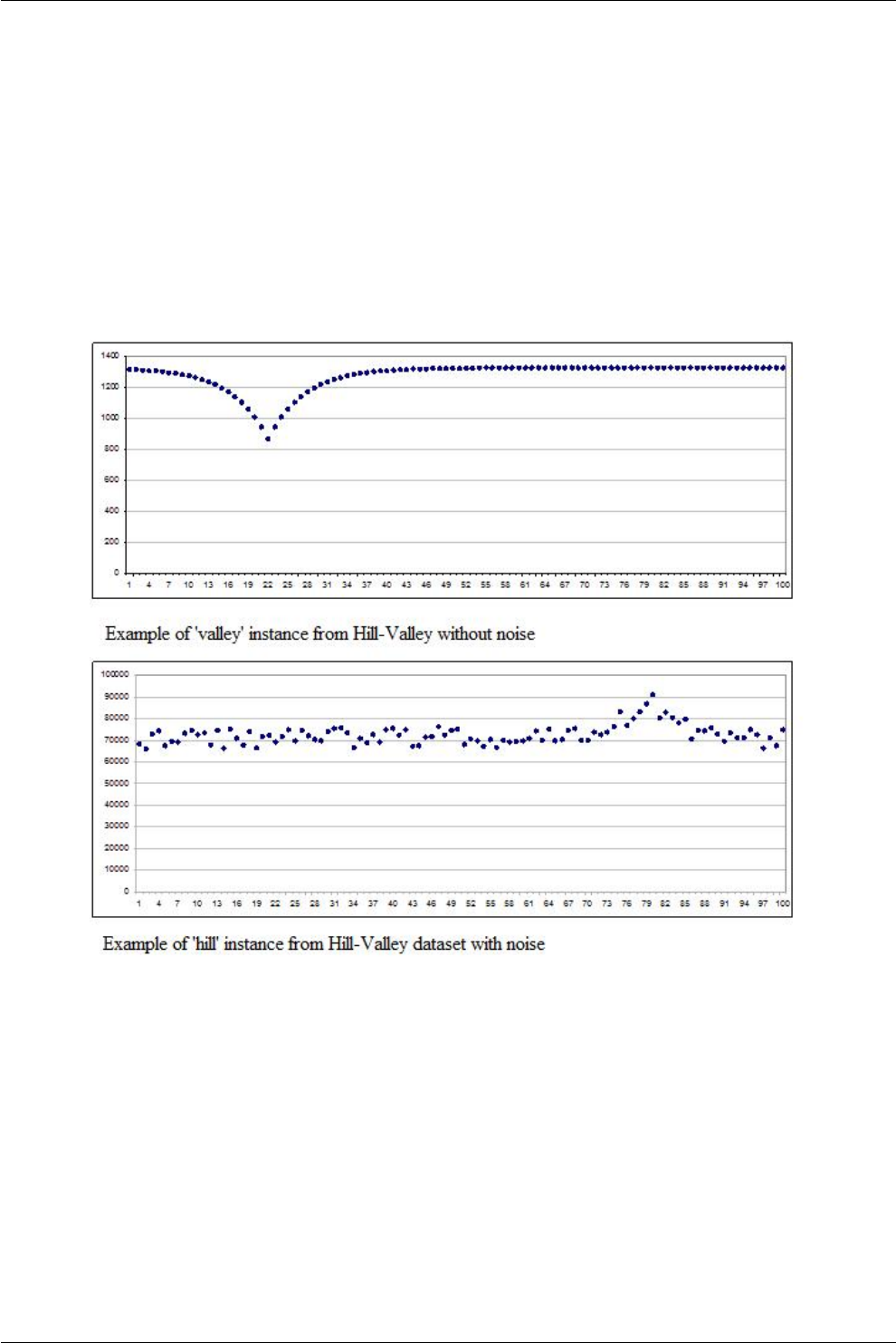
the output (i.e. ‘target’) is assigned with one of the two values i.e. “1 for Hill” or “0 for Valley”. Fig. 3.1 shows the
graph of these points for the Valley and the hill. Further, we will use “LogisticRegression” model for classification
in this chapter. It is a linear model, which finds a line to separate the ‘hill’ from the ‘valley’.
Note that, there are different datasets available on the website i.e. noisy and without noise. In this chapter, we
will use the dataset without any noise. Lastly, we can download different data from the website according to our
study e.g. data for regression problem, classification problem or mixed problem etc.
3.2 Dataset
Lets quickly see the contents of the dataset “Hill_Valley_without_noise_Training.data”, as shown in Listing 3.1.
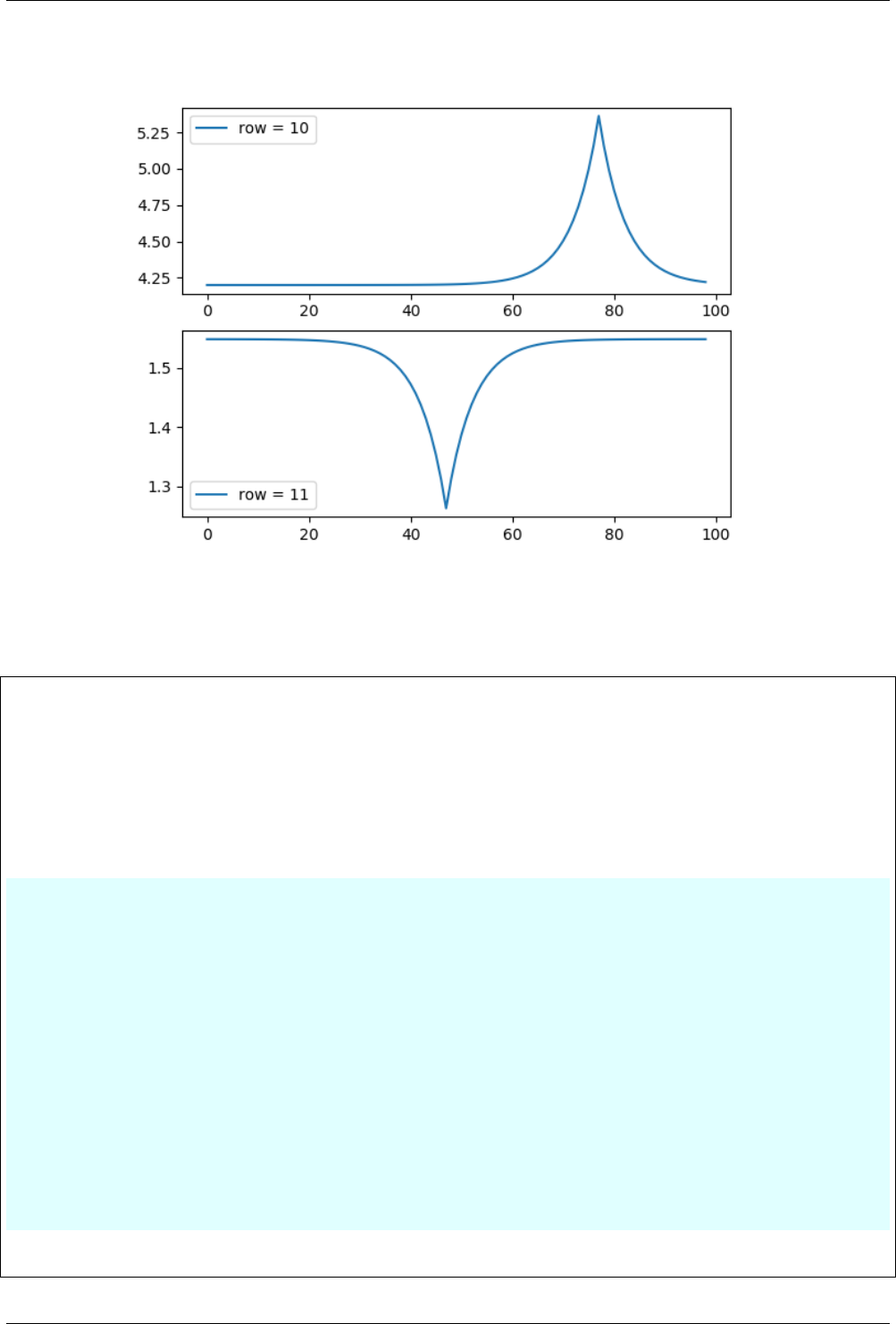
The Fig. 3.2 shows the plot of the Rows 10 and 11 of the data, which represents the “hill” and “valley” respectively.
In Listing 3.1, the Lines 12-23 are reading the data, cleaning it (i.e. removing the header line and line-breaks
etc.) and changing it into desired format (i.e making list of list and then numpy array). This process is known as
Data-cleaning and Data-transformation, which constitute 70%-90% of the work in machine-learning tasks.
Listing 3.1: Quick analysis of data in
“Hill_Valley_without_noise_Training.data”
1# hill_valley.py
2
3# 1:hill, 0:valley
4
5import matplotlib.pyplot as plt
6import numpy as np
7
8f=open("data/Hill_Valley_without_noise_Training.data",'r')
9data =f.read()
10 f.close()
11
12 data =data.split() # split on \n
13 data =data[1:-1]# remove 0th row as it is header
14
15 # save data as list i.e. list of list will be created
16 data_list =[]
(continues on next page)
10
Chapter 3. Binary classification
Fig. 3.1: Hill and valley according to the input points
11 Meher Krishna Patel

3.3. Extract the data i.e. ‘features’ and ‘targets’
(continued from previous page)
17 for din data:
18 # split on comma
19 row =d.split(",")
20 data_list.append(row)
21
22 # convert list into numpy array, as it allows more direct-operations
23 data_list =np.array(data_list, float)
24
25 print("Number of samples:",len(data_list))
26 print("(row, column):", data_list.shape) # 100 features + 1 target = 101
27
28 # print the last value at row = 10
29 row =10
30 row_last_element =data_list[row][-1]# 1:hill, 0:valley
31 print("data_list[{0}][100]: {1}".format(row,row_last_element)) # 1
32
33 # plot row and row+1 i.e 10 and 11 here
34 plt.subplot(2,1,1)# plot row
35 plt.plot(data_list[row][1:-1], label="row = {}".format(row))
36 plt.legend() # show legends
37
38 plt.subplot(2,1,2)# plot row+1
39 plt.plot(data_list[row+1][1:-1], label="row = {}".format(row+1))
40 plt.legend() # show legends
41
42 plt.show()
Following is the output of the above code,
$ python hill_valley.py
Number of samples: 607
(row, column): (607, 101)
data_list[10][100]: 1.0
3.3 Extract the data i.e. ‘features’ and ‘targets’
In Chapter 2, it is shown that the machine-learning tasks require the ‘features’ and ‘targets’. In the current data,
both are available in the dataset in the combined form i.e. ‘target’ is available at the end of each data sample.
Now, our task is to extract the ‘features’ and ‘targets’ in separate variables, so that the further code can be written
easily. This can be done as shown in Listing 3.2,
Listing 3.2: Extract the data i.e. ‘features’ and ‘targets’
1# hill_valley.py
2
3# 1:hill, 0:valley
4
5import matplotlib.pyplot as plt
6import numpy as np
7
8f=open("data/Hill_Valley_without_noise_Training.data",'r')
9data =f.read()
10 f.close()
11
12 data =data.split() # split on \n
13 data =data[1:-1]# remove 0th row as it is header
14
(continues on next page)
12 PythonDSP
Chapter 3. Binary classification
Fig. 3.2: Plot for data at Rows 10 and 11
(continued from previous page)
15 # save data as list i.e. list of list will be created
16 data_list =[]
17 for din data:
18 # split on comma
19 row =d.split(",")
20 data_list.append(row)
21
22 # convert list into numpy array, as it allows more direct-operations
23 data_list =np.array(data_list, float)
24
25 # print("Number of samples:", len(data_list))
26 # print("(row, column):", data_list.shape) # 100 features + 1 target = 101
27
28 # # print the last value at row = 10
29 # row = 10
30 # row_last_element = data_list[row][-1] # 1:hill, 0:valley
31 # print("data_list[{0}][100]: {1}".format(row,row_last_element)) # 1
32
33 # # plot row and row+1 i.e 10 and 11 here
34 # plt.subplot(2,1,1) # plot row
35 # plt.plot(data_list[row][1:-1], label="row = {}".format(row))
36 # plt.legend() # show legends
37
38 # plt.subplot(2,1,2) # plot row+1
39 # plt.plot(data_list[row+1][1:-1], label="row = {}".format(row+1))
40 # plt.legend() # show legends
41
42 # plt.show()
43
44
(continues on next page)
13 Meher Krishna Patel

3.4. Prediction
(continued from previous page)
45 # extract targets
46 row_sample, col_sample =data_list.shape # extract row and columns in dataset
47
48 # features : last column i.e. target value will be removed form the dataset
49 features =np.zeros((row_sample, col_sample-1), float)
50 # target : store only last column
51 targets =np.zeros(row_sample, int)
52
53 for i, data in enumerate(data_list):
54 targets[i] =data[-1]
55 features[i] =data[:-1]
56 # print(targets)
57 # print(features)
58
59 # recheck the plot
60 row =10
61 plt.subplot(2,1,1)# plot row
62 plt.plot(features[row], label="row = {}".format(row))
63 plt.legend() # show legends
64
65 plt.subplot(2,1,2)# plot row+1
66 plt.plot(features[row +1], label="row = {}".format(row+1))
67 plt.legend() # show legends
68
69 plt.show()
3.4 Prediction
Once data is transformed in the desired format, the prediction task is quite straight forward as shown in Listing
3.3. Here following steps are performed for prediction,
•Split the data for training and testing (Lines 77-88).
•Select the classifier for modeling, and fit the data (Lines 90-93).
•Check the accuracy of prediction for the training set itself (Lines 95-98).
•Finally check the accuracy of the prediction for the test-data (Lines 100-103).
Note: The ‘accuracy_score’ is used here to calculate the accuracy (see Lines 97 and 102).
Listing 3.3: Prediction
1# hill_valley.py
2
3# 1:hill, 0:valley
4
5import matplotlib.pyplot as plt
6import numpy as np
7
8from sklearn.linear_model import LogisticRegression
9from sklearn.metrics import accuracy_score
10 from sklearn.model_selection import train_test_split
11
12
13 f=open("data/Hill_Valley_without_noise_Training.data",'r')
14 data =f.read()
15 f.close()
16
17 data =data.split() # split on \n
(continues on next page)
14 PythonDSP

Chapter 3. Binary classification
(continued from previous page)
18 data =data[1:-1]# remove 0th row as it is header
19
20 # save data as list i.e. list of list will be created
21 data_list =[]
22 for din data:
23 # split on comma
24 row =d.split(",")
25 data_list.append(row)
26
27 # convert list into numpy array, as it allows more direct-operations
28 data_list =np.array(data_list, float)
29
30 # print("Number of samples:", len(data_list))
31 # print("(row, column):", data_list.shape) # 100 features + 1 target = 101
32
33 # # print the last value at row = 10
34 # row = 10
35 # row_last_element = data_list[row][-1] # 1:hill, 0:valley
36 # print("data_list[{0}][100]: {1}".format(row,row_last_element)) # 1
37
38 # # plot row and row+1 i.e 10 and 11 here
39 # plt.subplot(2,1,1) # plot row
40 # plt.plot(data_list[row][1:-1], label="row = {}".format(row))
41 # plt.legend() # show legends
42
43 # plt.subplot(2,1,2) # plot row+1
44 # plt.plot(data_list[row+1][1:-1], label="row = {}".format(row+1))
45 # plt.legend() # show legends
46
47 # plt.show()
48
49
50 # extract targets
51 row_sample, col_sample =data_list.shape # extract row and columns in dataset
52
53 # features : last column i.e. target value will be removed form the dataset
54 features =np.zeros((row_sample, col_sample-1), float)
55 # target : store only last column
56 targets =np.zeros(row_sample, int)
57
58 for i, data in enumerate(data_list):
59 targets[i] =data[-1]
60 features[i] =data[:-1]
61 # print(targets)
62 # print(features)
63
64 # # recheck the plot
65 # row = 10
66 # plt.subplot(2,1,1) # plot row
67 # plt.plot(features[row], label="row = {}".format(row))
68 # plt.legend() # show legends
69
70 # plt.subplot(2,1,2) # plot row+1
71 # plt.plot(features[row + 1], label="row = {}".format(row+1))
72 # plt.legend() # show legends
73
74 # plt.show()
75
76
77 # split the training and test data
78 train_features, test_features, train_targets, test_targets =train_test_split(
(continues on next page)
15 Meher Krishna Patel
3.4. Prediction
(continued from previous page)
79 features, targets,
80 train_size=0.8,
81 test_size=0.2,
82 # random but same for all run, also accuracy depends on the
83 # selection of data e.g. if we put 10 then accuracy will be 1.0
84 # in this example
85 random_state=23,
86 # keep same proportion of 'target'in test and target data
87 stratify=targets
88 )
89
90 # use LogisticRegression
91 classifier =LogisticRegression()
92 # training using 'training data'
93 classifier.fit(train_features, train_targets) # fit the model for training data
94
95 # predict the 'target'for 'training data'
96 prediction_training_targets =classifier.predict(train_features)
97 self_accuracy =accuracy_score(train_targets, prediction_training_targets)
98 print("Accuracy for training data (self accuracy):", self_accuracy)
99
100 # predict the 'target'for 'test data'
101 prediction_test_targets =classifier.predict(test_features)
102 test_accuracy =accuracy_score(test_targets, prediction_test_targets)
103 print("Accuracy for test data:", test_accuracy)
Following are the results for the above code,
$ python hill_valley.py
Accuracy for training data (self accuracy): 0.997933884298
Accuracy for test data: 1.0
Note: In Iris-data set in Chapter 2 , the target depends directly on the input features i.e. width and length
of petal and sepal. But in Hill-valley problem, the output does not directly depends on the location of the input
values, but on the relative-positions of the certain inputs with all other inputs.
LogisticRegression assign a weight to each of the features and then calculate the sum for making decisions e.g. if
sum is greater than 0 then ‘hill’ and if less than 0 then ‘valley’. The coefficients which are assigned to each feature
can be seen as below,
$ python -i hill_valley.py
Accuracy for training data (self accuracy): 0.997933884298
Accuracy for test data: 1.0
>>> classifier.coef_
array([[-0.75630448, -0.70813863, -0.64901487, -0.57633845, -0.48687761,
[...]
-0.6593235 , -0.719707 , -0.76843887, -0.8077998 , -0.83961794]])
Also, the KNeighborsClassifier will not work here, as it looks for the features which are nearer to the ‘targets’,
and then decide the boundaries. But, in Hill-Valley case, a valley can be at the top of the graph as shown in
Fig. 3.1, or at the bottom of the graph. Similarly a Hill can be at the top of graph or at the bottom location.
Therefore it is not possible to find the nearest points for the Hill-Valley problem, which can distinguish a Hill from
a Vally. Hence, KNeighborsClassifier will have the accuracy_score = 0.5 (i.e. random guess). We can verify it by
importing the “KNeighborsClassifier” and replacing the “LogisticRegression” to “KNeighborsClassifier” in Listing
3.3.
16 PythonDSP

Chapter 3. Binary classification
3.5 Rock vs Mine example
The file “sonar.all-data” contains the patterns obtained by bouncing sonar signals off a metal cylinder and the
rocks under similar conditions. Last column contains the target names i.e. ‘R’ and ‘M’, where ‘R’ and ‘M’ are
rocks and metals respectively.
Note: Remember that, in classification problems the targets must be descrete; and can have the value as ‘string’
or ‘number’ as shown in Table 1.4.
As oppose to previous section, here the ‘targets’ has the direct relationship with ‘features’, therefore we can use
both the classifier i.e. “LogisticRegression” and “KNeighborsClassifier” as shown in Listing 3.4.
Since, the target is not the numeric value, therefore targets are stored in the list as shown in Line 33 (instead of
numpy-array). Select any one of the classifier from Lines 55-56 and run the code to see the prediction accuracy.
Listing 3.4: Rock vs Mine
1# rock_mine.py
2
3#'R': Rock, 'M': Mine
4
5import matplotlib.pyplot as plt
6import numpy as np
7
8from sklearn.linear_model import LogisticRegression
9from sklearn.metrics import accuracy_score
10 from sklearn.model_selection import train_test_split
11 from sklearn.neighbors import KNeighborsClassifier
12
13
14 f=open("data/sonar.all-data",'r')
15 data =f.read()
16 f.close()
17
18 data =data.split() # split on \n
19
20 # save data as list i.e. list of list will be created
21 data_list =[]
22 for din data:
23 # split on comma
24 row =d.split(",")
25 data_list.append(row)
26
27 # extract targets
28 row_sample, col_sample =len(data_list), len(data_list[0])
29
30 # features : last column i.e. target value will be removed form the dataset
31 features =np.zeros((row_sample, col_sample-1), float)
32 # target : store only last column
33 targets =[] # targets are 'R'and 'M'
34
35 for i, data in enumerate(data_list):
36 targets.append(data[-1])
37 features[i] =data[:-1]
38 # print(targets)
39 # print(features)
40
41 # split the training and test data
42 train_features, test_features, train_targets, test_targets =train_test_split(
43 features, targets,
(continues on next page)
17 Meher Krishna Patel

3.6. Conclusion
(continued from previous page)
44 train_size=0.8,
45 test_size=0.2,
46 # random but same for all run, also accuracy depends on the
47 # selection of data e.g. if we put 10 then accuracy will be 1.0
48 # in this example
49 random_state=23,
50 # keep same proportion of 'target'in test and target data
51 stratify=targets
52 )
53
54 # select classifier
55 classifier =LogisticRegression()
56 # classifier = KNeighborsClassifier()
57
58 # training using 'training data'
59 classifier.fit(train_features, train_targets) # fit the model for training data
60
61 # predict the 'target'for 'training data'
62 prediction_training_targets =classifier.predict(train_features)
63 self_accuracy =accuracy_score(train_targets, prediction_training_targets)
64 print("Accuracy for training data (self accuracy):", self_accuracy)
65
66 # predict the 'target'for 'test data'
67 prediction_test_targets =classifier.predict(test_features)
68 test_accuracy =accuracy_score(test_targets, prediction_test_targets)
69 print("Accuracy for test data:", test_accuracy)
Following are the outputs for the above code,
(for LogisticRegression)
$ python rock_mine.py
Accuracy for training data (self accuracy): 0.795180722892
Accuracy for test data: 0.761904761905
(for KNeighborsClassifier)
$ python rock_mine.py
Accuracy for training data (self accuracy): 0.843373493976
Accuracy for test data: 0.785714285714
3.6 Conclusion
In this chapter, we read the data from the file, and then converted the data into the format which is used by SciKit
library for further operations. Further, we used the class ‘LogisticRegression’ for modeling the system, and check
the accuracy of the model for the training and test data.
18 PythonDSP
Chapter 4
Regression
In previous chapters, we saw the example of supervised learning for ‘classification’ problems; i.e. the ‘targets’ had
the fixed number of values. In this section, we will see the another class of supervised learning i.e. ‘regression’,
where ‘targets’ can have continuous values. Note the ‘features’ can have continuous values in both the cases.
Also, in previous chapters, we used the SciKit’s inbuilt-dataset and read the dataset from the file. In this chapter,
we will create the dataset by ourselves.
4.1 Noisy sine wave dataset
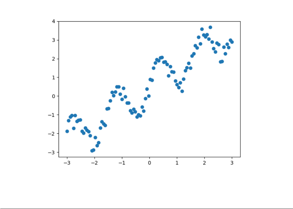
Let’s create a dataset where the ‘features’ are the samples of the cooridantes of the x-axis, whereas the ‘targets’
are the noisy samples of the sine waves i.e. uniformly distributed noise samples will be added to the sine-wave;
and the corresponding waveforms are shown in Fig. 4.1. This can be achieved as below,
Fig. 4.1: Sine wave + Uniformly distributed noise generated by Listing 4.1
19

4.1. Noisy sine wave dataset
Listing 4.1: Generation of noisy sine wave as shown in Fig. 4.1
1# regression_ex.py
2
3import numpy as np
4import matplotlib.pyplot as plt
5
6
7N=100 # 100 samples
8x=np.linspace(-3,3, N) # coordinates
9noise_sample =np.random.RandomState(20)# constant random value
10 # growing sinusoid with random fluctuation
11 sine_wave =x+np.sin(4*x) +noise_sample.uniform(N)
12 plt.plot(x, sine_wave, 'o');
13 plt.show()
Note: For SciKit library, the features must be in 2-dimensional format, i.e. features are the ‘list of list’, whereas
target must be in 1-dimensional format. Currently, we have both in 1-dimensional format, therefore we need to
convert the ‘features’ into 2-dimensional format as shown in Listing 4.2.
Listing 4.2: converting ‘x’ into 2D
1# regression_ex.py
2
3import numpy as np
4import matplotlib.pyplot as plt
5
6
7N=100 # 100 samples
8x=np.linspace(-3,3, N) # coordinates
9noise_sample =np.random.RandomState(20)# constant random value
10 # growing sinusoid with random fluctuation
11 sine_wave =x+np.sin(4*x) +noise_sample.uniform(N)
12 # plt.plot(x, sine_wave, 'o');
13 # plt.show()
14
15 # convert features in 2D format i.e. list of list
16 print('Before: ', x.shape)
17 features =x[:, np.newaxis]
18 print('After: ', features.shape)
19
20 # uncomment below line to see the differences
21 # print(x)
22 # print(features)
23
24 # save sine wave in variable 'targets'
25 targets =sine_wave
Below is the output for above code,
$ python regression_ex.py
Before: (100,)
After: (100, 1)
20 PythonDSP

Chapter 4. Regression
4.2 Regression model
Now, we test the regression model i.e. “LinearRegression” on the dataset as below, which has the similar steps as
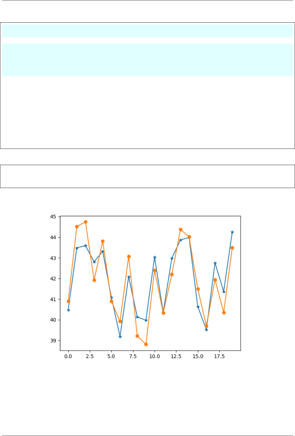
classification problems. The predicted and actual points of the sine wave is shown in Fig. 4.2.
Important: Please note the following important points,
•The ‘stratify’ can not be used for single features as shown in Line 40.
•The ‘score’ uses ‘feature and target (not predicted target)’ for scoring in Regression. This calculates the
score which is known as 𝑅2score.
•The ‘accuracy_score’ uses ‘feature and ‘predicted target’ for scoring in Classification.
Listing 4.3: Score of regression model
1# regression_ex.py
2
3import numpy as np
4import matplotlib.pyplot as plt
5
6from sklearn.model_selection import train_test_split
7from sklearn.linear_model import LinearRegression
8
9N=100 # 100 samples
10 x=np.linspace(-3,3, N) # coordinates
11 noise_sample =np.random.RandomState(20)# constant random value
12 # growing sinusoid with random fluctuation
13 sine_wave =x+np.sin(4*x) +noise_sample.uniform(N)
14 # plt.plot(x, sine_wave, 'o');
15 # plt.show()
16
17 # convert features in 2D format i.e. list of list
18 # print('Before: ', x.shape)
19 features =x[:, np.newaxis]
20 # print('After: ', features.shape)
21
22 # uncomment below line to see the differences
23 # print(x)
24 # print(features)
25
26 # save sine wave in variable 'targets'
27 targets =sine_wave
28
29
30 # split the training and test data
31 train_features, test_features, train_targets, test_targets =train_test_split(
32 features, targets,
33 train_size=0.8,
34 test_size=0.2,
35 # random but same for all run, also accuracy depends on the
36 # selection of data e.g. if we put 10 then accuracy will be 1.0
37 # in this example
38 random_state=23,
39 # keep same proportion of 'target'in test and target data
40 # stratify=targets # can not used for single feature
41 )
42
43 # training using 'training data'
44 regressor =LinearRegression()
45 regressor.fit(train_features, train_targets) # fit the model for training data
46
(continues on next page)
21 Meher Krishna Patel
4.2. Regression model
(continued from previous page)
47 # predict the 'target'for 'training data'
48 prediction_training_targets =regressor.predict(train_features)
49
50 # note that 'score'uses 'feature and target (not predict_target)'
51 # for scoring in Regression
52 # whereas 'accuracy_score'uses 'features and predict_targets'
53 # for scoring in Classification
54 self_accuracy =regressor.score(train_features, train_targets)
55 print("Accuracy for training data (self accuracy):", self_accuracy)
56
57 # predict the 'target'for 'test data'
58 prediction_test_targets =regressor.predict(test_features)
59 test_accuracy =regressor.score(test_features, test_targets)
60 print("Accuracy for test data:", test_accuracy)
61
62 # plot the predicted and actual target for test data
63 plt.plot(prediction_test_targets, '-*')
64 plt.plot(test_targets, '-o')
65 plt.show()
Following are the outputs of above code,
$ python regression_ex.py
Accuracy for training data (self accuracy): 0.843858910263
Accuracy for test data: 0.822872868183
Fig. 4.2: Actual and predicted points of the sine wave
22 PythonDSP

Chapter 4. Regression
4.3 Conclusion
In this chapter, we saw the example of Regression problems. Also, we saw the basic differences between the scoring
in the Regression and Classification problems.
23 Meher Krishna Patel

Chapter 5
Cross validation
5.1 Introduction
In this chapter, we will enhance the Listing 2.2 to understand the concept of ‘cross validation’. Let’s comment the
Line 24 of the Listing 2.2 as shown below and and excute the code 7 times.
1# multiclass_ex.py
2
3import numpy as np
4from sklearn.datasets import load_iris
5from sklearn.neighbors import KNeighborsClassifier
6from sklearn.model_selection import train_test_split
7
8# create object of class 'load_iris'
9iris =load_iris()
10
11 # save features and targets from the 'iris'
12 features, targets =iris.data, iris.target
13
14 # both train_size and test_size are defined when we do not want to
15 # use all the data for training and testing e.g. in below example we can
16 # use train_size=0.4 and test_size=0.2
17 train_features, test_features, train_targets, test_targets =train_test_split(
18 features, targets,
19 train_size=0.8,
20 test_size=0.2,
21 # random but same for all run, also accurancy depends on the
22 # selection of data e.g. if we put 10 then accuracy will be 1.0
23 # in this example
24 # random_state=23,
25 # keep same proportion of 'target'in test and target data
26 stratify=targets
27 )
28
29 # print("Proportion of 'targets'in the dataset")
30 # print("All data:", np.bincount(train_targets) / float(len(train_targets)))
31 # print("Training:", np.bincount(train_targets) / float(len(train_targets)))
32 # print("Training:", np.bincount(test_targets)/ float(len(test_targets)))
33
34
35 # use KNeighborsClassifier for classification
36 classifier =KNeighborsClassifier()
37 # training using 'training data'
38 classifier.fit(train_features, train_targets) # fit the model for training data
(continues on next page)
24

Chapter 5. Cross validation
(continued from previous page)
39 # predict the 'target'for 'test data'
40 prediction_targets =classifier.predict(test_features)
41
42 # check the accuracy of the model
43 print("Accuracy:", end=' ')
44 print(np.sum(prediction_targets == test_targets) /float(len(test_targets)))
•Now execute the code 7 times and we will get different ‘accuracy’ at different run.
$ python multiclass_ex.py
Accuracy: 0.966666666667
$ python multiclass_ex.py
Accuracy: 1.0
$ python multiclass_ex.py
Accuracy: 1.0
$ python multiclass_ex.py
Accuracy: 0.966666666667
$ python multiclass_ex.py
Accuracy: 1.0
$ python multiclass_ex.py
Accuracy: 0.966666666667
$ python multiclass_ex.py
Accuracy: 0.933333333333
Note:
•The ‘accuracy’ may be changed dramatically for some other datasets for different ‘train’ and ‘test’ dataset.
Therefore it is not a good measure to compare the two models.
•Also, in this method of finding the accuracy, we have very few data as the ‘test-data’. Further, we have less
train-data as well due to splitting.
To avoid these problems, the ‘cross-validation’ method is used for calculating the accuracy.
5.2 Cross validation
In the below code, the cross-validation value is set to 7 i.e. ‘cv=7’ at Line 48.
Note: Following are the operations performed by the cross-validation method,
•The ‘cv=7’ will partition the data into 7 parts.
•Then it will use ‘first’ part as ‘test set’ and others as ‘training set’.
•Next, it will use ‘second’ part as ‘test set’ and others as ‘training set’ and so on.
•In this way, each sample will be in test-dataset exactly one time.
•Also, in this method, we have more training and testing data.
•Lastly, we need not to split the data manually in the cross-validation method.
1# multiclass_ex.py
2
3import numpy as np
(continues on next page)
25 Meher Krishna Patel

5.2. Cross validation
(continued from previous page)
4from sklearn.datasets import load_iris
5from sklearn.neighbors import KNeighborsClassifier
6from sklearn.model_selection import cross_val_score
7from sklearn.model_selection import train_test_split
8
9# create object of class 'load_iris'
10 iris =load_iris()
11
12 # save features and targets from the 'iris'
13 features, targets =iris.data, iris.target
14
15 # both train_size and test_size are defined when we do not want to
16 # use all the data for training and testing e.g. in below example we can
17 # use train_size=0.4 and test_size=0.2
18 # train_features, test_features, train_targets, test_targets = train_test_split(
19 # features, targets,
20 # train_size=0.8,
21 # test_size=0.2,
22 # # random but same for all run, also accurancy depends on the
23 # # selection of data e.g. if we put 10 then accuracy will be 1.0
24 # # in this example
25 # # random_state=23,
26 # # keep same proportion of 'target'in test and target data
27 # stratify=targets
28 # )
29
30 # print("Proportion of 'targets'in the dataset")
31 # print("All data:", np.bincount(train_targets) / float(len(train_targets)))
32 # print("Training:", np.bincount(train_targets) / float(len(train_targets)))
33 # print("Training:", np.bincount(test_targets)/ float(len(test_targets)))
34
35
36 # use KNeighborsClassifier for classification
37 classifier =KNeighborsClassifier()
38 # training using 'training data'
39 # classifier.fit(train_features, train_targets) # fit the model for training data
40 # predict the 'target'for 'test data'
41 # prediction_targets = classifier.predict(test_features)
42
43 # check the accuracy of the model
44 # print("Accuracy:", end=' ')
45 # print(np.sum(prediction_targets == test_targets) / float(len(test_targets)))
46
47 # cross-validation
48 scores =cross_val_score(classifier, features, targets, cv=7)
49 print("Cross validation scores:", scores)
50 print("Mean score:", np.mean(scores))
•Below are the outputs for above code, which are the same for each run,
$ python multiclass_ex.py
Cross validation scores: [ 0.95833333 1. 0.95238095
0.9047619 0.95238095 1. 1. ]
Mean score: 0.966836734694
$ python multiclass_ex.py
Cross validation scores: [ 0.95833333 1. 0.95238095
0.9047619 0.95238095 1. 1. ]
Mean score: 0.966836734694
$ python multiclass_ex.py
(continues on next page)
26 PythonDSP

Chapter 5. Cross validation
(continued from previous page)
Cross validation scores: [ 0.95833333 1. 0.95238095
0.9047619 0.95238095 1. 1. ]
Mean score: 0.966836734694
5.3 Splitting of data
Warning:
•Note that, in cross-validation, the data is not split randomly, therefore it is not good for the data where
the ‘targets’ are nicely arranged. Therefore, it is good to shuffle the targets before applying the ‘cross-
validation’ as shown in Listing 5.1.
•Further, it does not create the model to predict the new samples; it only gives an idea about the accuracy
of model.
•It takes time to cross validate the dataset as number of iterations are increased e.g. for cv=7, the data
will be split in 7 parts and each part will be tested with respect to others. Further, the data will be
iterated 7 times, therefore total 49 checks will be performed.
5.3.1 Manual shuffling
•Targets can be shuffled manually as below,
Listing 5.1: Shuffle the targets
1# multiclass_ex.py
2
3import numpy as np
4from sklearn.datasets import load_iris
5from sklearn.neighbors import KNeighborsClassifier
6from sklearn.model_selection import cross_val_score
7from sklearn.model_selection import train_test_split
8
9# create object of class 'load_iris'
10 iris =load_iris()
11
12 # save features and targets from the 'iris'
13 features, targets =iris.data, iris.target
14
15 # both train_size and test_size are defined when we do not want to
16 # use all the data for training and testing e.g. in below example we can
17 # use train_size=0.4 and test_size=0.2
18 # train_features, test_features, train_targets, test_targets = train_test_split(
19 # features, targets,
20 # train_size=0.8,
21 # test_size=0.2,
22 # # random but same for all run, also accurancy depends on the
23 # # selection of data e.g. if we put 10 then accuracy will be 1.0
24 # # in this example
25 # # random_state=23,
26 # # keep same proportion of 'target'in test and target data
27 # stratify=targets
28 # )
29
30 # print("Proportion of 'targets'in the dataset")
31 # print("All data:", np.bincount(train_targets) / float(len(train_targets)))
32 # print("Training:", np.bincount(train_targets) / float(len(train_targets)))
(continues on next page)
27 Meher Krishna Patel

5.3. Splitting of data
(continued from previous page)
33 # print("Training:", np.bincount(test_targets)/ float(len(test_targets)))
34
35
36 # use KNeighborsClassifier for classification
37 classifier =KNeighborsClassifier()
38 # training using 'training data'
39 # classifier.fit(train_features, train_targets) # fit the model for training data
40 # predict the 'target'for 'test data'
41 # prediction_targets = classifier.predict(test_features)
42
43 # check the accuracy of the model
44 # print("Accuracy:", end=' ')
45 # print(np.sum(prediction_targets == test_targets) / float(len(test_targets)))
46
47 print("Targets before shuffle:\n", targets)
48 rng =np.random.RandomState(0)
49 permutation =rng.permutation(len(features))
50 features, targets =features[permutation], targets[permutation]
51 print("Targets after shuffle:\n", targets)
52
53 # cross-validation
54 scores =cross_val_score(classifier, features, targets, cv=7)
55 print("Cross validation scores:", scores)
56 print("Mean score:", np.mean(scores))
•Below is the output of above code. In the iris dataset we have equal number of samples for each target,
therefore the effect of shuffle and no-shuffle is almost same, but may vary when targets do not have equal
distribution.
$ python multiclass_ex.py
Targets before shuffle:
[0000000...00000
11111111...11111
22222222...22222
]
Targets after shuffle:
[21020201112111...
111202001222212...
102101210222200...
]
Cross validation scores: [ 1. 0.95238095 0.9047619 1.
1. 0.95238095 0.95238095]
Mean score: 0.965986394558
5.3.2 Automatic shuffling (KFold, StratifiedKFold and ShuffleSplit)
The shuffling can be performed using inbuilt functions as well as shown in below code.
Note: The data are not shuffled in the Listing 5.2, but chosen random during splitting the data into the ‘training
data’ and ‘test data’. Following 3 options are available for splitting (select any one from the Lines 55, 56 and 58),
•KFold(n_splits=3, shuffle=True) : Shuffle the data and split the data into 3 equal part (same as Listing
5.1).
•StratifiedKFold(n_splits=3, shuffle=True) : KFold with ‘stratify’ option (see Listing 2.2 for details).
•ShuffleSplit(n_splits=3, test_size=0.2) : Randomly splits the data. Also, it has the option to define the
size of the test data.
28 PythonDSP

Chapter 5. Cross validation
Warning: Note that in the Iris data set, the targets are equally distributed, therefore if we use the option
KFold(n_splits=3), i.e. no shuffling, then we will have the accuracy ‘0’; as the data will be trained on only one
set. Hence it is a good idea to keep shuffle on.
Listing 5.2: KFold, StratifiedKFold and ShuffleSplit
1# multiclass_ex.py
2
3import numpy as np
4from sklearn.datasets import load_iris
5from sklearn.neighbors import KNeighborsClassifier
6from sklearn.model_selection import cross_val_score
7from sklearn.model_selection import train_test_split
8from sklearn.model_selection import KFold, StratifiedKFold, ShuffleSplit
9
10 # create object of class 'load_iris'
11 iris =load_iris()
12
13 # save features and targets from the 'iris'
14 features, targets =iris.data, iris.target
15
16 # both train_size and test_size are defined when we do not want to
17 # use all the data for training and testing e.g. in below example we can
18 # use train_size=0.4 and test_size=0.2
19 # train_features, test_features, train_targets, test_targets = train_test_split(
20 # features, targets,
21 # train_size=0.8,
22 # test_size=0.2,
23 # # random but same for all run, also accurancy depends on the
24 # # selection of data e.g. if we put 10 then accuracy will be 1.0
25 # # in this example
26 # # random_state=23,
27 # # keep same proportion of 'target'in test and target data
28 # stratify=targets
29 # )
30
31 # print("Proportion of 'targets'in the dataset")
32 # print("All data:", np.bincount(train_targets) / float(len(train_targets)))
33 # print("Training:", np.bincount(train_targets) / float(len(train_targets)))
34 # print("Training:", np.bincount(test_targets)/ float(len(test_targets)))
35
36
37 # use KNeighborsClassifier for classification
38 classifier =KNeighborsClassifier()
39 # training using 'training data'
40 # classifier.fit(train_features, train_targets) # fit the model for training data
41 # predict the 'target'for 'test data'
42 # prediction_targets = classifier.predict(test_features)
43
44 # check the accuracy of the model
45 # print("Accuracy:", end=' ')
46 # print(np.sum(prediction_targets == test_targets) / float(len(test_targets)))
47
48 # print("Targets before shuffle:\n", targets)
49 # rng = np.random.RandomState(0)
50 # permutation = rng.permutation(len(features))
51 # features, targets = features[permutation], targets[permutation]
52 # print("Targets after shuffle:\n", targets)
53
54 # cross-validation
(continues on next page)
29 Meher Krishna Patel
5.4. Template for comparing algorithms
(continued from previous page)
55 # cv = KFold(n_splits=3, shuffle=True) # shuffle and divide in 3 equal parts
56 cv =StratifiedKFold(n_splits=3, shuffle=True)# KFold with 'stratify'option
57 # # test_size is available in ShuffleSplit
58 # cv = ShuffleSplit(n_splits=3, test_size=0.2)
59 scores =cross_val_score(classifier, features, targets, cv=cv)
60 print("Cross validation scores:", scores)
61 print("Mean score:", np.mean(scores))
Important: In ‘ShuffleSplit’, the data do appear in the ‘test set’ equally.
It is always better to use “KFold with shuffling” i.e. “cv = KFold(n_splits=3, shuffle=True)” or “StratifiedK-
Fold(n_splits=3, shuffle=True)”.
5.4 Template for comparing algorithms
As discussed before, the main usage of cross-validation is to compare various algorithms, which can be done as
below, where 4 algorithms (Lines 9-12) are compared.
1# cross_valid_ex.py
2
3import numpy as np
4import matplotlib.pyplot as plt
5from sklearn.datasets import load_iris
6from sklearn.model_selection import cross_val_score
7from sklearn.model_selection import StratifiedKFold
8
9from sklearn.linear_model import LogisticRegression
10 from sklearn.neighbors import KNeighborsClassifier
11 from sklearn.svm import SVC
12 from sklearn.tree import DecisionTreeClassifier
13
14 # create object of class 'load_iris'
15 iris =load_iris()
16
17 # save features and targets from the 'iris'
18 features, targets =iris.data, iris.target
19
20 models =[]
21 models.append(('LogisticRegression', LogisticRegression()))
22 models.append(('KNeighborsClassifier', KNeighborsClassifier()))
23 models.append(('SVC', SVC()))
24 models.append(('DecisionTreeClassifier', DecisionTreeClassifier()))
25
26 # KFold with 'stratify'option
27 cv =StratifiedKFold(n_splits=7, shuffle=True, random_state=23)
28 for name, model in models:
29 score =cross_val_score(model, features, targets, cv=cv)
30 print("Model:{0}, Score: mean={1:0.5f}, var={2:0.5f}".format(
31 name,
32 score.mean(),
33 score.var()
34 )
35 )
•Below is the output of above code, where we can see that SVC performs better than other algorithms.
30 PythonDSP

Chapter 5. Cross validation
$ python cross_valid_ex.py
Model:LogisticRegression, Score: mean=0.96088, var=0.00141
Model:KNeighborsClassifier, Score: mean=0.96088, var=0.00141
Model:SVC, Score: mean=0.97449, var=0.00164
Model:DecisionTreeClassifier, Score: mean=0.95408, var=0.00115
Warning: Note that different values of ‘cv’ will give different results, e.g. if we put cv=3 at Line 29 (instead
of cv=cv), then we will get following results, which shows that ‘KNeighborsClassifier’ has the best performance.
$ python cross_valid_ex.py
Model:LogisticRegression, Score: mean=0.94690, var=0.00032
Model:KNeighborsClassifier, Score: mean=0.98693, var=0.00009
Model:SVC, Score: mean=0.97345, var=0.00008
Model:DecisionTreeClassifier, Score: mean=0.96732, var=0.00111
31 Meher Krishna Patel
Chapter 6
Clustering
6.1 Introduction
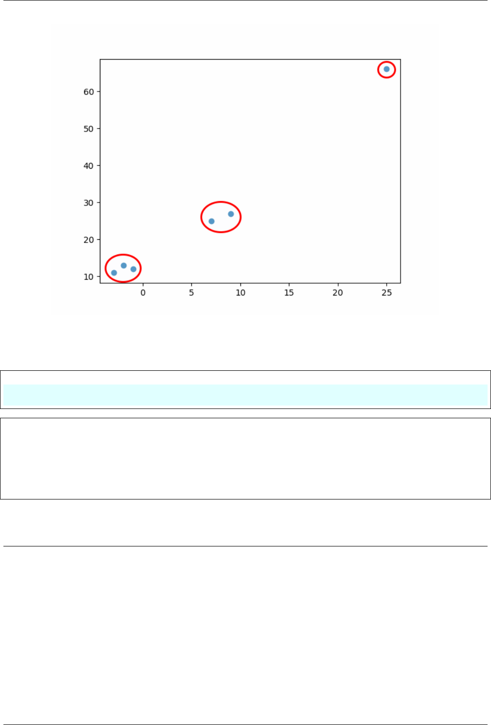
In this chapter, we will see the examples of clustering. Lets understand the clustering with an example first. In
the Listing 6.1, two lists i.e. x and y are plotted using ‘scatter’ plot. We can see that the data can be divided into
three clusters as shown in Fig. 6.1.
Note: In Fig. 6.1, it is easy to see the clusters as samples are very small; but it can not visualize so easily if we
have a huge number of samples, as shown in this chapter. In those cases, the machine learning approach can be
quite useful.
Listing 6.1: Clusters
# cluster_ex.py
import matplotlib.pyplot as plt
x=[-3,25,-2,7,-1,9]
y=[11,66,13,25,12,27]
plt.scatter(x, y)
plt.show()
6.2 KMeans
Now, we will cluster our data using “KMeans” algorithms.
•Similar to previous chapters, first we need to transform the data in 2-dimensional format, so that is can be
used by SciKit library. In the below code, the lists ‘x’ and ‘y’ are merged together, so that a ‘list of list’ will
be created,
1# cluster_ex.py
2
3import matplotlib.pyplot as plt
4import numpy as np
5
6x=[-3,25,-2,7,-1,9]
7y=[11,66,13,25,12,27]
8# plt.scatter(x, y)
9# plt.show()
10
(continues on next page)
32
Chapter 6. Clustering
Fig. 6.1: Clusters
(continued from previous page)
11 # convert list into array based on columns
12 data =np.column_stack((x, y))
13 print(data)
$ python cluster_ex.py
[[-3 11]
[25 66]
[-2 13]
[ 7 25]
[-1 12]
[ 9 27]]
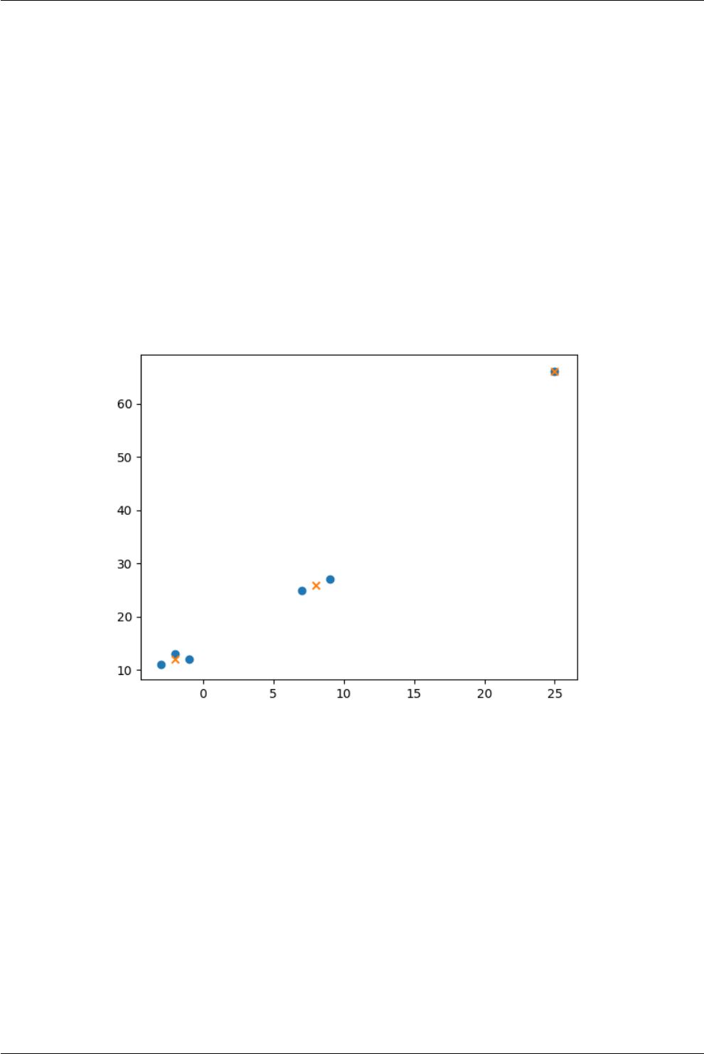
•Now, we can use the “KMeans” algorithm to the transformed data as shown in Listing 6.2. The clusters
generated by the algorithm is shown in Fig. 6.2.
Note:
•Centroids are the location of mean points generated by KMeans algorithm, which can be generated using
‘cluster_centers_’.
•Also, each points can be assigned a label using ‘labels_’. Note that, once we get the labels, then we can use
supervised learning for further analysis.
•Number of samples should be higher than the number of clusters. For example, currently we have 6 samples,
if we use “n_clusters=7”, then error will be generated.
•We should increase the value of “n_clusters” to remove the outliers from the clustering. For example, in the
current dataset, the points location i.e. [25, 66] can be seen as outliers i.e. it may be in the dataset due to
measurement error or noise. Since, it is present in the dataset, it will affect the final locations of clusters. In
the other words, if we put “n_clusters=2”, then one cluster will locate the point [25, 66], and second cluster
will take the mean the of rest of the points, which may not be desirable, therefore, we need to decide the
value of “n_clusters” according to dataset.
33 Meher Krishna Patel
6.2. KMeans
Listing 6.2: Clusters generated by KMeans algorithm
1# cluster_ex.py
2
3import matplotlib.pyplot as plt
4import numpy as np
5from sklearn.cluster import KMeans
6
7
8x=[-3,25,-2,7,-1,9]
9y=[11,66,13,25,12,27]
10 # plt.scatter(x, y)
11 # plt.show()
12
13 # convert list into array based on columns
14 data =np.column_stack((x, y))
15 # print(data)
16
17 model =KMeans(n_clusters=3)# separate data in 3 clusters
18 model.fit(data)
19 model.predict(data)
20 # model.fit_predict(data) # combine above two steps in one
21
22 # locations of the means generated by the KMeans
23 centroids =model.cluster_centers_
24 print("Centroids:\n", centroids)
25
26 # each sample is labelled as well
27 targets =model.labels_
28 print("Targets or Lables:\n", targets)
29
30 # plot the data
31 plt.scatter(x, y)
32 plt.scatter(x =centroids[:, 0], y =centroids[:, 1], marker='x')
33 plt.show()
$ python cluster_ex.py
Centroids:
[[ -2. 12.]
[ 25. 66.]
[ 8. 26.]]
Targets or Lables:
[0 1 0 2 0 2]
Tip: KMeans algorithm should be used for the number of samples less than 10000. If there are more than 10000
samples, then MiniBatchKMeans algorithm must be used, which converge faster than the KMeans, but the quality
of the results may reduce.
34 PythonDSP
Chapter 6. Clustering
Fig. 6.2: Clusters generated by KMeans algorithm
35 Meher Krishna Patel

Chapter 7
Dimensionality reduction
7.1 Introduction
During the data collection process, our aim is to collect as much as data possible. During this process, it might
possible some of the ‘features’ are correlated. If the dataset has lots of features, then it is good to remove some of
the correlated features, so that the data can be processed faster; but at the same time the accuracy of the model
may reduced.
7.2 Principal component analysis (PCA)
PCA is one of the technique to reduce the dimensionality of the data, as shown in this section.
7.2.1 Create dataset
•Lets create a dataset first,
# dimension_ex.py
import numpy as np
import pandas as pd
# feature values
x=np.random.randn(1000)
y=2*x
z=np.random.randn(1000)
# target values
t=len(x)*[0]# list of len(x)
for i, val in enumerate(z):
if x[i]+y[i]+z[i] <0:
t[i] ='N'# negative
else:
t[i] ='P'
# create the dataframe
df =np.column_stack((x, y, z, t))
df =pd.DataFrame(df)
print(df.head())
36
Chapter 7. Dimensionality reduction
Warning: The output ‘t’ depends on the the variables ‘x’, ‘y’ and ‘z’, therefore if these variables are not
correlated, then dimensionality reduction will result in severe performance degradation as shown in this chapter.
•Following is the output of above code,
$ python dimension_ex.py
0 1 2 3
0 1.619558594848966 3.239117189697932 -1.7181741395151733 P
1 0.7926656328473467 1.5853312656946934 -0.5003026519806438 P
2 -0.40666904321652636 -0.8133380864330527 -0.5233957097467451 N
3 -1.813173189559588 -3.626346379119176 -1.418416461398814 N
4 0.4357818365640018 0.8715636731280036 1.7840245820080853 P
7.2.2 Reduce dimension using PCA
Now, we create the PCA model as shown Listing 7.1, which will transform the above datasets into a new dataset
which will have only 2 features (instead of 3).
Note: The PCA can have inputs which have only ‘numeric features’, therefore we need to ‘drop’ the ‘categorical’
features as shown in Line 26.
Next we need to instantiate an object of class PCA (Line 27) and the apply ‘fit’ method (Line 28).
Finally, we can transform our data using ‘transform’ method as shown in Line 29.
Listing 7.1: Dimensionality reduction using PCA
1# dimension_ex.py
2
3import numpy as np
4import pandas as pd
5from sklearn.decomposition import PCA
6
7# feature values
8x=np.random.randn(1000)
9y=2*x
10 z=np.random.randn(1000)
11
12 # target values
13 t=len(x)*[0]# list of len(x)
14 for i, val in enumerate(z):
15 if x[i]+y[i]+z[i] <0:
16 t[i] ='N'# negative
17 else:
18 t[i] ='P'
19
20 # create the dataframe
21 df =np.column_stack((x, y, z, t))
22 df =pd.DataFrame(df)
23 # print(df.head())
24
25 # dataframe for PCA : PCA can not have 'categorical'features
26 df_temp =df.drop(3, axis=1)# drop 'categorical'feature
27 pca =PCA(n_components=2)# 2 dimensional PCA
28 pca.fit(df_temp)
29 df_pca =pca.transform(df_temp)
30 print(df_pca)
•Following is the output of above code, where the dataset has only two features,
37 Meher Krishna Patel

7.2. Principal component analysis (PCA)
$ python dimension_ex.py
[[-2.54693351 -0.07879497]
[ 0.42820972 -0.90158131]
[-1.94145497 -1.70738801]
...,
[-0.92088711 0.54590025]
[-2.44899588 -1.403821 ]
[-1.94568343 -0.50371273]]
7.2.3 Compare the performances
Now, we will compare the performances of the system with and without dimensionality reduction.
Note: Please note the following points in this section,
•If the features are highly correlated, then performance after ‘dimensionality reduction’ will be same as the
without ‘dimensionality reduction’.
•If the features have good correlation, then performance after ‘dimensionality reduction’ will be reduced
slightly than the without ‘dimensionality reduction’.
•If the features have no correlation, then performance after ‘dimensionality reduction’ will be reduced signifi-
cantly than the without ‘dimensionality reduction’.
The code which is added to Listing 7.1 is exactly same as the code which is discussed in Listing 3.3; i.e. split of
dataset into ‘test’ and ‘training’ and then check the score, as shown in below code.
Here Lines 42-70 calculates the score for ‘without dimensionality reduction’ case, whereas Lines 73-103 calculates
the score of “dimensionality reduction using PCA”.
Listing 7.2: Dimensionality reduction using PCA
1# dimension_ex.py
2
3import numpy as np
4import pandas as pd
5from sklearn.decomposition import PCA
6from sklearn.linear_model import LogisticRegression
7from sklearn.metrics import accuracy_score
8from sklearn.model_selection import train_test_split
9
10
11 # feature values
12 x=np.random.randn(1000)
13 y=2*x
14 z=np.random.randn(1000)
15
16 # target values
17 t=len(x)*[0]# list of len(x)
18 for i, val in enumerate(z):
19 if x[i]+y[i]+z[i] <0:
20 t[i] ='N'# negative
21 else:
22 t[i] ='P'
23
24 # create the dataframe
25 df =np.column_stack((x, y, z, t))
26 df =pd.DataFrame(df)
27 # print(df.head())
28
29 # dataframe for PCA : PCA can not have 'categorical'features
(continues on next page)
38 PythonDSP

Chapter 7. Dimensionality reduction
(continued from previous page)
30 df_temp =df.drop(3, axis=1)# drop 'categorical'feature
31 pca =PCA(n_components=2)# 2 dimensional PCA
32 pca.fit(df_temp)
33 df_pca =pca.transform(df_temp)
34 # print(df_pca)
35
36 # assign targets and features values
37 # targets
38 targets =df[3]
39 # features
40 features =pd.concat([df[0], df[1], df[2]], axis=1)
41
42 #### Results for the without reduction case
43 # split the training and test data
44 train_features, test_features, train_targets, test_targets =train_test_split(
45 features, targets,
46 train_size=0.8,
47 test_size=0.2,
48 # random but same for all run, also accuracy depends on the
49 # selection of data e.g. if we put 10 then accuracy will be 1.0
50 # in this example
51 random_state=23,
52 # keep same proportion of 'target'in test and target data
53 stratify=targets
54 )
55
56 # use LogisticRegression
57 classifier =LogisticRegression()
58 # training using 'training data'
59 classifier.fit(train_features, train_targets) # fit the model for training data
60
61 print("Without dimensionality reduction:")
62 # predict the 'target'for 'training data'
63 prediction_training_targets =classifier.predict(train_features)
64 self_accuracy =accuracy_score(train_targets, prediction_training_targets)
65 print("Accuracy for training data (self accuracy):", self_accuracy)
66
67 # predict the 'target'for 'test data'
68 prediction_test_targets =classifier.predict(test_features)
69 test_accuracy =accuracy_score(test_targets, prediction_test_targets)
70 print("Accuracy for test data:", test_accuracy)
71
72
73
74 #### Results for the without reduction case
75 # updated features after dimensionality reduction
76 features =df_pca
77 # split the training and test data
78 train_features, test_features, train_targets, test_targets =train_test_split(
79 features, targets,
80 train_size=0.8,
81 test_size=0.2,
82 # random but same for all run, also accuracy depends on the
83 # selection of data e.g. if we put 10 then accuracy will be 1.0
84 # in this example
85 random_state=23,
86 # keep same proportion of 'target'in test and target data
87 stratify=targets
88 )
89
90 # use LogisticRegression
(continues on next page)
39 Meher Krishna Patel

7.2. Principal component analysis (PCA)
(continued from previous page)
91 classifier =LogisticRegression()
92 # training using 'training data'
93 classifier.fit(train_features, train_targets) # fit the model for training data
94
95 print("After dimensionality reduction:")
96 # predict the 'target'for 'training data'
97 prediction_training_targets =classifier.predict(train_features)
98 self_accuracy =accuracy_score(train_targets, prediction_training_targets)
99 print("Accuracy for training data (self accuracy):", self_accuracy)
100
101 # predict the 'target'for 'test data'
102 prediction_test_targets =classifier.predict(test_features)
103 test_accuracy =accuracy_score(test_targets, prediction_test_targets)
104 print("Accuracy for test data:", test_accuracy)
•Following is the output of the above code.
Note: Since the ‘x’ and ‘y’ are completely correlated (i.e. y = 2*x), therefore the performance of dimensionality
reduction is exactly same as the without reduction case.
Also, we will get different results for different execution of code, as the ‘x’, ‘y’ and ‘z’ are randomly generated on
each run.
$ python dimension_ex.py
Without dimensionality reduction:
Accuracy for training data (self accuracy): 0.99875
Accuracy for test data: 1.0
After dimensionality reduction:
Accuracy for training data (self accuracy): 0.99875
Accuracy for test data: 1.0
•Next replace the value of ‘y’ at Line 13 of Listing 7.2 with following value, and run the code
again,
[...]
y=2*x+np.random.randn(1000)
[...]
As, noise is added to ‘x’ as noise is added, therefore the ‘x’ and ‘y’ are not completely correlated (but still highly
correlated), therefore the performance of the system will reduce slightly, as shown in below results,
Note: Remember, the ‘target’ variable depends on ‘x’, ‘y’ and ‘z’ i.e. it is the sign of the sum of these variables.
Therefore, if the correlation between the ‘features’ will reduce, the performance of the dimensionality reduction
will also reduce.
$ python dimension_ex.py
Without dimensionality reduction:
Accuracy for training data (self accuracy): 0.9925
Accuracy for test data: 0.99
After dimensionality reduction:
Accuracy for training data (self accuracy): 0.9775
Accuracy for test data: 0.97
40 PythonDSP
Chapter 7. Dimensionality reduction
•Again, replace the value of ‘y’ at Line 13 of Listing 7.2 with following value, and run the code
again,
[...]
y=np.random.randn(1000)
[...]
Now ‘x’, ‘y’ and ‘z’ are completely independent of each other, therefore the performance will reduce significantly
as shown below,
Note: Each run will give different result, below is the worst case result, where test data accuracy is 0.575 (i.e.
probability 0.5), which is equivalent to the random guess of the target.
$ python dimension_ex.py
Without dimensionality reduction:
Accuracy for training data (self accuracy): 0.995
Accuracy for test data: 0.995
After dimensionality reduction:
Accuracy for training data (self accuracy): 0.64125
Accuracy for test data: 0.575
7.3 Usage of PCA for dimensionality reduction method
Important: Below are the usage of dimensionality reduction technique,
•Dimensionality reduction is used to reduce the complexity of data.
•It allows faster data processing, but reduces the accuracy of the model.
•It can be used as noise reduction process.
•It can be used as ‘preprocessor of the data’ for the supervised leaning process i.e. regression and classification.
7.4 PCA limitations
Warning: Note that the PCA is very sensitive to scaling operations, more specifically it maximizes variability
based on the variances of the features.
Due to this reason, it gives more weight to ‘high variance features i.e. high-variance-feature will dominate the
overall performance.
To avoid this problem, it is better to normalized the features before applying the PCA model as shown in
Section 8.4.
7.5 Conclusion
In this chapter, we learn the concept of dimensionality reduction and PCA. In the next chapter, we will see the
usage of PCA in a practical problem.
41 Meher Krishna Patel

Chapter 8
Preprocessing of the data using Pandas
and SciKit
In previous chapters, we did some minor preprocessing to the data, so that it can be used by SciKit library. In
this chapter, we will do some preprocessing of the data to change the ‘statitics’ and the ‘format’ of the data, to
improve the results of the data analysis.
8.1 Chronic kidney disease
The “chronic_kidney_disease.arff” dataset is used for this tutorial, which is available at the UCI Repository.
•Lets read and clean the data first,
Listing 8.1: Read the data
# kidney_dis.py
import pandas as pd
import numpy as np
# create header for dataset
header =['age','bp','sg','al','su','rbc','pc','pcc',
'ba','bgr','bu','sc','sod','pot','hemo','pcv',
'wbcc','rbcc','htn','dm','cad','appet','pe','ane',
'classification']
# read the dataset
df =pd.read_csv("data/chronic_kidney_disease.arff",
header=None,
names=header
)
# dataset has '?'in it, convert these into NaN
df =df.replace('?', np.nan)
# drop the NaN
df =df.dropna(axis=0, how="any")
# print total samples
print("Total samples:",len(df))
# print 4-rows and 6-columns
print("Partial data\n", df.iloc[0:4,0:6])
•Below is the output of above code,
42

Chapter 8. Preprocessing of the data using Pandas and SciKit
$ python kidney_dis.py
Total samples: 157
Partial data
age bp sg al su rbc
30 48 70 1.005 4 0 normal
36 53 90 1.020 2 0 abnormal
38 63 70 1.010 3 0 abnormal
41 68 80 1.010 3 2 normal
8.2 Saving targets with different color names
In this dataset we have two ‘targets’ i.e. ‘ckd’ and ‘notckd’ in the last column (‘classification’). It is better to save
the ‘targets’ of classification problem with some ‘color-name’ for the plotting purposes. This helps in visualizing
the scatter-plot as shown in this chapter.
Listing 8.2: Alias the ‘target-values’ with ‘color-values’
1# kidney_dis.py
2
3import pandas as pd
4import numpy as np
5
6# create header for dataset
7header =['age','bp','sg','al','su','rbc','pc','pcc',
8'ba','bgr','bu','sc','sod','pot','hemo','pcv',
9'wbcc','rbcc','htn','dm','cad','appet','pe','ane',
10 'classification']
11 # read the dataset
12 df =pd.read_csv("data/chronic_kidney_disease.arff",
13 header=None,
14 names=header
15 )
16 # dataset has '?'in it, convert these into NaN
17 df =df.replace('?', np.nan)
18 # drop the NaN
19 df =df.dropna(axis=0, how="any")
20
21 # print total samples
22 # print("Total samples:", len(df))
23 # print 4-rows and 6-columns
24 # print("Partial data\n", df.iloc[0:4, 0:6])
25
26 targets =df['classification'].astype('category')
27 # save target-values as color for plotting
28 # red: disease, green: no disease
29 label_color =['red'if i=='ckd'else 'green'for iin targets]
30 print(label_color[0:3], label_color[-3:-1])
Note: We can convert the ‘categorical-targets (i.e. strings ‘ckd’ and ‘notckd’) into ‘numeric-targets (i.e. 0 and
1’) using “.cat.codes” command, as shown below,
# covert 'ckd'and 'notckd'labels as '0'and '1'
targets =df['classification'].astype('category').cat.codes
# save target-values as color for plotting
# red: disease, green: no disease
label_color =['red'if i==0else 'green'for iin targets]
print(label_color[0:3], label_color[-3:-1])
43 Meher Krishna Patel

8.3. Basic PCA analysis
•Below is the first three and last two samples of the ‘label_color’,
$ python kidney_dis.py
['red','red','red'] ['green','green']
8.3 Basic PCA analysis
Let’s perform the dimensionality reduction using PCA, which is discussed in Section 7.2.
8.3.1 Preparing data for PCA analysis
Note that, for PCA the features should be ‘numerics’ only. Therefore we need to remove the ‘categorical’ features
from the dataset.
Listing 8.3: Drop categorical features
1# kidney_dis.py
2
3import pandas as pd
4import numpy as np
5
6# create header for dataset
7header =['age','bp','sg','al','su','rbc','pc','pcc',
8'ba','bgr','bu','sc','sod','pot','hemo','pcv',
9'wbcc','rbcc','htn','dm','cad','appet','pe','ane',
10 'classification']
11 # read the dataset
12 df =pd.read_csv("data/chronic_kidney_disease.arff",
13 header=None,
14 names=header
15 )
16 # dataset has '?'in it, convert these into NaN
17 df =df.replace('?', np.nan)
18 # drop the NaN
19 df =df.dropna(axis=0, how="any")
20
21 # print total samples
22 # print("Total samples:", len(df))
23 # print 4-rows and 6-columns
24 # print("Partial data\n", df.iloc[0:4, 0:6])
25
26 targets =df['classification'].astype('category')
27 # save target-values as color for plotting
28 # red: disease, green: no disease
29 label_color =['red'if i=='ckd'else 'green'for iin targets]
30 # print(label_color[0:3], label_color[-3:-1])
31
32 # list of categorical features
33 categorical_ =['rbc','pc','pcc','ba','htn',
34 'dm','cad','appet','pe','ane'
35 ]
36
37 # drop the "categorical" features
38 # drop the classification column
39 df =df.drop(labels=['classification'], axis=1)
40 # drop using 'inplace'which is equivalent to df = df.drop()
41 df.drop(labels=categorical_, axis=1, inplace=True)
42 print("Partial data\n", df.iloc[0:4,0:6]) # print partial data
44 PythonDSP

Chapter 8. Preprocessing of the data using Pandas and SciKit
•Below is the output of the above code. Note that, if we compare the below results with the results of Listing
8.1, we can see that the ‘rbc’ column is removed.
$ python kidney_dis.py
Partial data
age bp sg al su bgr
30 48 70 1.005 4 0 117
36 53 90 1.020 2 0 70
38 63 70 1.010 3 0 380
41 68 80 1.010 3 2 157
8.3.2 dimensionality reduction
Let’s perform dimensionality reduction using the PCA model as shown in Listing 8.4. The results are shown in
Fig. 8.1, where we can see that the model can fairly classify the kidney disease based on the provided features. In
the next section we will improve this performance by some more preprocessing of the data.
Listing 8.4: dimensionality reduction using PCA
1# kidney_dis.py
2
3import pandas as pd
4import numpy as np
5import matplotlib.pyplot as plt
6from sklearn.decomposition import PCA
7
8# create header for dataset
9header =['age','bp','sg','al','su','rbc','pc','pcc',
10 'ba','bgr','bu','sc','sod','pot','hemo','pcv',
11 'wbcc','rbcc','htn','dm','cad','appet','pe','ane',
12 'classification']
13 # read the dataset
14 df =pd.read_csv("data/chronic_kidney_disease.arff",
15 header=None,
16 names=header
17 )
18 # dataset has '?'in it, convert these into NaN
19 df =df.replace('?', np.nan)
20 # drop the NaN
21 df =df.dropna(axis=0, how="any")
22
23 # print total samples
24 # print("Total samples:", len(df))
25 # print 4-rows and 6-columns
26 # print("Partial data\n", df.iloc[0:4, 0:6])
27
28 targets =df['classification'].astype('category')
29 # save target-values as color for plotting
30 # red: disease, green: no disease
31 label_color =['red'if i=='ckd'else 'green'for iin targets]
32 # print(label_color[0:3], label_color[-3:-1])
33
34 # list of categorical features
35 categorical_ =['rbc','pc','pcc','ba','htn',
36 'dm','cad','appet','pe','ane'
37 ]
38
39 # drop the "categorical" features
40 # drop the classification column
41 df =df.drop(labels=['classification'], axis=1)
42 # drop using 'inplace'which is equivalent to df = df.drop()
(continues on next page)
45 Meher Krishna Patel
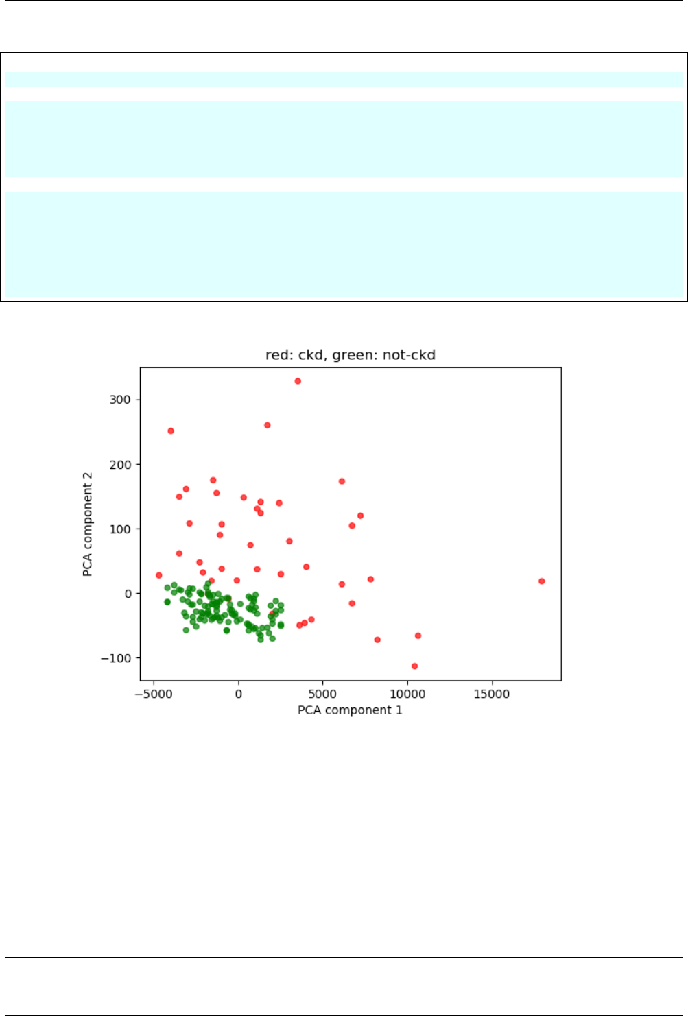
8.4. Preprocessing using SciKit library
(continued from previous page)
43 df.drop(labels=categorical_, axis=1, inplace=True)
44 # print("Partial data\n", df.iloc[0:4, 0:6]) # print partial data
45
46 pca =PCA(n_components=2)
47 pca.fit(df)
48 T=pca.transform(df) # transformed data
49 # change 'T'to Pandas-DataFrame to plot using Pandas-plots
50 T=pd.DataFrame(T)
51
52 # plot the data
53 T.columns =['PCA component 1','PCA component 2']
54 T.plot.scatter(x='PCA component 1', y='PCA component 2', marker='o',
55 alpha=0.7,# opacity
56 color=label_color,
57 title="red: ckd, green: not-ckd" )
58 plt.show()
Fig. 8.1: Chronic Kidney Disease
8.4 Preprocessing using SciKit library
It is shown in Section 7.4, that the overall performance of the PCA is dominated by ‘high variance features’.
Therefore features should be normalized before using the PCA model.
In the below code ‘StandardScalar’ preprocessing module is used to normalized the features, which sets the
‘mean=0’ and ‘variance=1’ for all the features. Note that the improvement in the results in Fig. 8.2, just by
adding one line in Listing 8.5.
Important: Currently, we are using preprocessing for the ‘unsupervised learning’.
46 PythonDSP

Chapter 8. Preprocessing of the data using Pandas and SciKit
If we want to use the preprocessing in the ‘supervised learning’, then it is better to ‘split’ the dataset as ‘test and
train’ first; and then apply the preprocessing to the ‘training data’ only. This is the good practice as in
real-life problems we will not have the future data for preprocessing.
Listing 8.5: Scale the features using “StandardScalar”
1# kidney_dis.py
2
3import pandas as pd
4import numpy as np
5import matplotlib.pyplot as plt
6from sklearn.decomposition import PCA
7from sklearn import preprocessing
8
9# create header for dataset
10 header =['age','bp','sg','al','su','rbc','pc','pcc',
11 'ba','bgr','bu','sc','sod','pot','hemo','pcv',
12 'wbcc','rbcc','htn','dm','cad','appet','pe','ane',
13 'classification']
14 # read the dataset
15 df =pd.read_csv("data/chronic_kidney_disease.arff",
16 header=None,
17 names=header
18 )
19 # dataset has '?'in it, convert these into NaN
20 df =df.replace('?', np.nan)
21 # drop the NaN
22 df =df.dropna(axis=0, how="any")
23
24 # print total samples
25 # print("Total samples:", len(df))
26 # print 4-rows and 6-columns
27 # print("Partial data\n", df.iloc[0:4, 0:6])
28
29 targets =df['classification'].astype('category')
30 # save target-values as color for plotting
31 # red: disease, green: no disease
32 label_color =['red'if i=='ckd'else 'green'for iin targets]
33 # print(label_color[0:3], label_color[-3:-1])
34
35 # list of categorical features
36 categorical_ =['rbc','pc','pcc','ba','htn',
37 'dm','cad','appet','pe','ane'
38 ]
39
40 # drop the "categorical" features
41 # drop the classification column
42 df =df.drop(labels=['classification'], axis=1)
43 # drop using 'inplace'which is equivalent to df = df.drop()
44 df.drop(labels=categorical_, axis=1, inplace=True)
45 # print("Partial data\n", df.iloc[0:4, 0:6]) # print partial data
46
47 # StandardScaler: mean=0, variance=1
48 df =preprocessing.StandardScaler().fit_transform(df)
49
50 pca =PCA(n_components=2)
51 pca.fit(df)
52 T=pca.transform(df) # transformed data
53 # change 'T'to Pandas-DataFrame to plot using Pandas-plots
54 T=pd.DataFrame(T)
55
(continues on next page)
47 Meher Krishna Patel
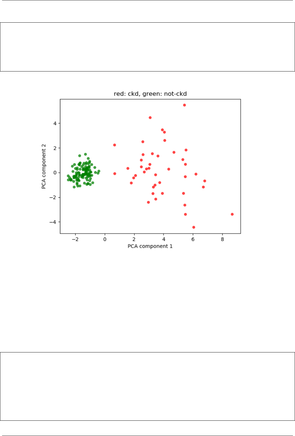
8.5. Preprocessing using Pandas library
(continued from previous page)
56 # plot the data
57 T.columns =['PCA component 1','PCA component 2']
58 T.plot.scatter(x='PCA component 1', y='PCA component 2', marker='o',
59 alpha=0.7,# opacity
60 color=label_color,
61 title="red: ckd, green: not-ckd" )
62 plt.show()
Fig. 8.2: Chronic Kidney Disease results using “StandardScalar”
8.5 Preprocessing using Pandas library
Note that, in Section 8.3.1, we dropped several ‘categorical features’ as these can not be used by PCA. But we can
convert these features to ‘numeric features’ and use them in PCA model.
Again, see the further improvement in the results in Fig. 8.3, just by adding one line in Listing 8.6.
Listing 8.6: Convert ‘categorical features’ to ‘numeric features’ us-
ing Pandas
1# kidney_dis.py
2
3import pandas as pd
4import numpy as np
5import matplotlib.pyplot as plt
6from sklearn.decomposition import PCA
7from sklearn import preprocessing
8
9# create header for dataset
10 header =['age','bp','sg','al','su','rbc','pc','pcc',
(continues on next page)
48 PythonDSP

Chapter 8. Preprocessing of the data using Pandas and SciKit
(continued from previous page)
11 'ba','bgr','bu','sc','sod','pot','hemo','pcv',
12 'wbcc','rbcc','htn','dm','cad','appet','pe','ane',
13 'classification']
14 # read the dataset
15 df =pd.read_csv("data/chronic_kidney_disease.arff",
16 header=None,
17 names=header
18 )
19 # dataset has '?'in it, convert these into NaN
20 df =df.replace('?', np.nan)
21 # drop the NaN
22 df =df.dropna(axis=0, how="any")
23
24 # print total samples
25 # print("Total samples:", len(df))
26 # print 4-rows and 6-columns
27 # print("Partial data\n", df.iloc[0:4, 0:6])
28
29 targets =df['classification'].astype('category')
30 # save target-values as color for plotting
31 # red: disease, green: no disease
32 label_color =['red'if i=='ckd'else 'green'for iin targets]
33 # print(label_color[0:3], label_color[-3:-1])
34
35 # list of categorical features
36 categorical_ =['rbc','pc','pcc','ba','htn',
37 'dm','cad','appet','pe','ane'
38 ]
39
40 # drop the "categorical" features
41 # drop the classification column
42 df =df.drop(labels=['classification'], axis=1)
43 # drop using 'inplace'which is equivalent to df = df.drop()
44 # df.drop(labels=categorical_, axis=1, inplace=True)
45
46 # convert categorical features into dummy variable
47 df =pd.get_dummies(df, columns=categorical_)
48 # print("Partial data\n", df.iloc[0:4, 0:6]) # print partial data
49
50 # StandardScaler: mean=0, variance=1
51 df =preprocessing.StandardScaler().fit_transform(df)
52
53 pca =PCA(n_components=2)
54 pca.fit(df)
55 T=pca.transform(df) # transformed data
56 # change 'T'to Pandas-DataFrame to plot using Pandas-plots
57 T=pd.DataFrame(T)
58
59 # plot the data
60 T.columns =['PCA component 1','PCA component 2']
61 T.plot.scatter(x='PCA component 1', y='PCA component 2', marker='o',
62 alpha=0.7,# opacity
63 color=label_color,
64 title="red: ckd, green: not-ckd" )
65 plt.show()
Important: Let’s summarize what we did in this chapter. We had a dataset which had a large number of
features. PCA looks for the correlation between these features and reduces the dimensionality. In this example,
we reduce the number of features to 2 using PCA.
After the dimensionality reduction, we had only 2 features, therefore we can plot the scatter-plot, which is easier
49 Meher Krishna Patel
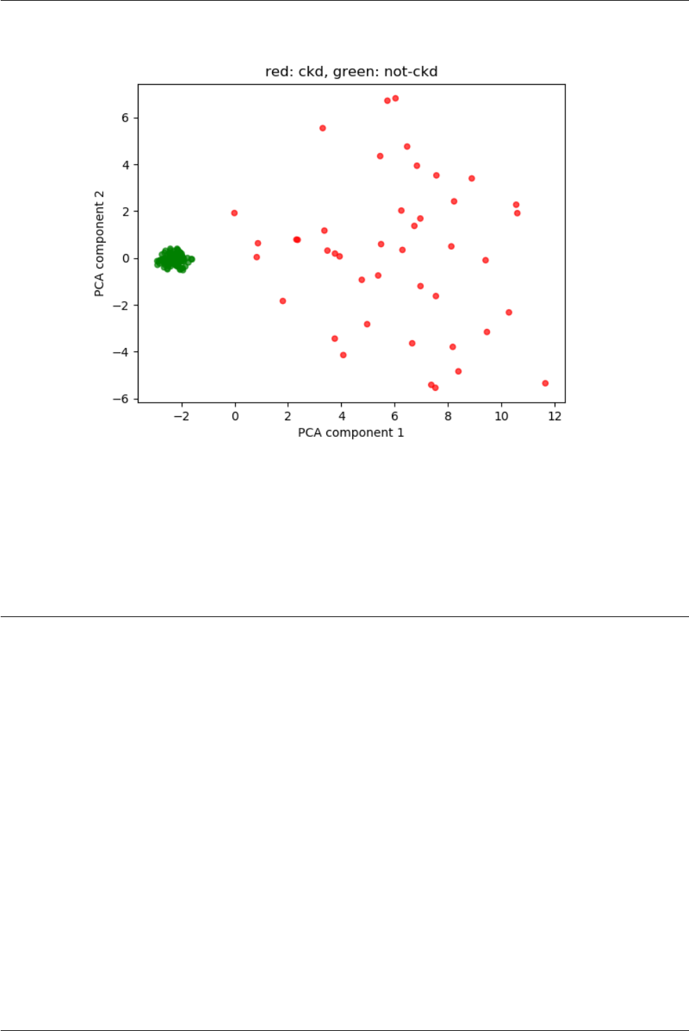
8.5. Preprocessing using Pandas library
Fig. 8.3: Chronic Kidney Disease results using “get_dummies”
to visualize. For example, we can clearly see the differences between the ‘ckd’ and ‘not ckd’ in the current example.
In conclusion, dimensionality reduction methods, such as PCA and Isomap, are used to reduce the dimensionality
of the features to 2 or 3. Next, these 2 or 3 features can be plotted to visualize the information.
It is important that the plot should be 2D or 3D format, otherwise it is very difficult for the eyes to visualize it
and interpret the information.
50 PythonDSP
Chapter 9
Pipeline
9.1 Introduction
Pipelines takes ‘a list of tranforms’ along with ‘one estimator at the end’ as the inputs. In this chapter, we will
use the ‘Pipeline’ to reimplement the Listing 8.6.
9.2 Pipeline
In this section, Listing 8.6 is reimplemented using ‘Pipeline’. In Listing 9.1 the Pipeline ‘pca’ is defined at Lines
56-60. When ‘pca.fit(df)’ operation is applied at Line 62, the ‘df’ is send to Pipeline for processing and model is
fit, and finally used by Line 63. This can be very handy tool when we have a chain of preprocessing.
Listing 9.1: Pipeline
1# kidney_dis.py
2
3import pandas as pd
4import numpy as np
5import matplotlib.pyplot as plt
6from sklearn.decomposition import PCA
7from sklearn import preprocessing
8from sklearn.pipeline import Pipeline
9
10 # create header for dataset
11 header =['age','bp','sg','al','su','rbc','pc','pcc',
12 'ba','bgr','bu','sc','sod','pot','hemo','pcv',
13 'wbcc','rbcc','htn','dm','cad','appet','pe','ane',
14 'classification']
15 # read the dataset
16 df =pd.read_csv("data/chronic_kidney_disease.arff",
17 header=None,
18 names=header
19 )
20 # dataset has '?'in it, convert these into NaN
21 df =df.replace('?', np.nan)
22 # drop the NaN
23 df =df.dropna(axis=0, how="any")
24
25 # print total samples
26 # print("Total samples:", len(df))
27 # print 4-rows and 6-columns
28 # print("Partial data\n", df.iloc[0:4, 0:6])
(continues on next page)
51

9.2. Pipeline
(continued from previous page)
29
30 targets =df['classification'].astype('category')
31 # save target-values as color for plotting
32 # red: disease, green: no disease
33 label_color =['red'if i=='ckd'else 'green'for iin targets]
34 # print(label_color[0:3], label_color[-3:-1])
35
36 # list of categorical features
37 categorical_ =['rbc','pc','pcc','ba','htn',
38 'dm','cad','appet','pe','ane'
39 ]
40
41 # drop the "categorical" features
42 # drop the classification column
43 df =df.drop(labels=['classification'], axis=1)
44 # drop using 'inplace'which is equivalent to df = df.drop()
45 # df.drop(labels=categorical_, axis=1, inplace=True)
46
47 # convert categorical features into dummy variable
48 df =pd.get_dummies(df, columns=categorical_)
49 # print("Partial data\n", df.iloc[0:4, 0:6]) # print partial data
50
51 # StandardScaler: mean=0, variance=1
52 # df = preprocessing.StandardScaler().fit_transform(df)
53
54 # pca = PCA(n_components=2)
55
56 # add list of transforms in Pipeline and finally the 'estimator'
57 pca =Pipeline([
58 ('scalar', preprocessing.StandardScaler()),
59 ('dim_reduction', PCA(n_components=2))
60 ])
61
62 pca.fit(df)
63 T=pca.transform(df) # transformed data
64 # change 'T'to Pandas-DataFrame to plot using Pandas-plots
65 T=pd.DataFrame(T)
66
67 # plot the data
68 T.columns =['PCA component 1','PCA component 2']
69 T.plot.scatter(x='PCA component 1', y='PCA component 2', marker='o',
70 alpha=0.7,# opacity
71 color=label_color,
72 title="red: ckd, green: not-ckd" )
73 plt.show()
52 PythonDSP
Chapter 10
Clustering with dimensionality reduction
10.1 Introduction
In previous chapters, we saw the examples of ‘clustering Chapter 6’, ‘dimensionality reduction (Chapter 7 and
Chapter 8)’, and ‘preprocessing (Chapter 8)’. Further, in Chapter 8, the performance of the dimensionality
reduction technique (i.e. PCA) is significantly improved using the preprocessing of data.
Remember, in Chapter 7 we used the PCA model to reduce the dimensionality of the features to 2, so that a 2D
plot can be plotted, which is easy to visualize. In this chapter, we will combine these three techniques together,
so that we can get much information from the scatter plot.
Note: In this chapter, we will use a ‘whole sale customer’ dataset, which is available at UCI Repository.
Our aim is to cluster the data so that we can see the products, which are bought by the customer together. For
example, if a person went to shop to buy some grocery, then is is quite likely that he will but the ‘milk’ as well,
therefore we can put the ‘milk’ near the grocery items; similarly it is quite unlikely that the same person will buy
the fresh vegetables at the same time.
If we can predict such behavior of the customer, then we can arrange the shop accordingly, which will increase the
sell of the items. In this chapter, we will do the same.
10.2 Read and clean the data
•First the the dataset and drop the columns which have “Null” values,
# whole_sale.py
import pandas as pd
df =pd.read_csv('data/Wholesale customers data.csv')
print(df.isnull().sum()) # print the sum of null values
•Following is the output of above code. Note that there is no ‘Null’ value, therefore we need not to drop
anything.
$ python whole_sale.py
Channel 0
Region 0
Fresh 0
Milk 0
Grocery 0
(continues on next page)
53
10.3. Clustering using KMean
(continued from previous page)
Frozen 0
Detergents_Paper 0
Delicatessen 0
dtype: int64
•Next, our aim is to find the buying-patterns of the customers, therefore we do not need the columns ‘Channel’
and ‘Region’ for this analysis. Hence we will drop these two columns,
1# whole_sale.py
2
3import pandas as pd
4
5df =pd.read_csv('data/Wholesale customers data.csv')
6print(df.isnull().sum()) # print the sum of null values
7
8df =df.drop(labels=['Channel','Region'], axis=1)
9# print(df.head())
10.3 Clustering using KMean
•Now perform the clustering as below. Note that, the ‘Normalizer()’ is used at Line 14 for the preprocessing.
We can try the different preprocessing-methods as well, to visualize the outputs.
Note: After completing the chapter, try following as well and see the outputs,
•Use different ‘preprocessing’ methods e.g ‘MaxAbsScaler’ and ‘StandardScaler’ etc. and see the performance
of the code.
•Use different values of n_clusters e.g 2, 3 and 4 etc.
1# whole_sale.py
2
3import pandas as pd
4from sklearn import preprocessing
5from sklearn.cluster import KMeans
6
7df =pd.read_csv('data/Wholesale customers data.csv')
8# print(df.isnull().sum()) # print the sum of null values
9
10 df =df.drop(labels=['Channel','Region'], axis=1)
11 # print(df.head())
12
13 # preprocessing
14 T=preprocessing.Normalizer().fit_transform(df)
15
16 # change n_clusters to 2, 3 and 4 etc. to see the output patterns
17 n_clusters =3# number of cluster
18
19 # Clustering using KMeans
20 kmean_model =KMeans(n_clusters=n_clusters)
21 kmean_model.fit(T)
22 centroids, labels =kmean_model.cluster_centers_, kmean_model.labels_
23 # print(centroids)
24 # print(labels)
54 PythonDSP

Chapter 10. Clustering with dimensionality reduction
10.4 Dimensionality reduction
Now, we will perform the dimensionality reduction using PCA. We will reduce the dimensions to 2.
Important:
•Currently, we are performing the clustering first and then dimensionality reduction as we have few features
in this example.
•If we have a very large number of features, then it is better to perform dimensionality reduction first and
then use the clustering algorithm e.g. KMeans.
1# whole_sale.py
2
3import pandas as pd
4from sklearn import preprocessing
5from sklearn.cluster import KMeans
6from sklearn.decomposition import PCA
7
8df =pd.read_csv('data/Wholesale customers data.csv')
9# print(df.isnull().sum()) # print the sum of null values
10
11 df =df.drop(labels=['Channel','Region'], axis=1)
12 # print(df.head())
13
14 # preprocessing
15 T=preprocessing.Normalizer().fit_transform(df)
16
17 # change n_clusters to 2, 3 and 4 etc. to see the output patterns
18 n_clusters =3# number of cluster
19
20 # Clustering using KMeans
21 kmean_model =KMeans(n_clusters=n_clusters)
22 kmean_model.fit(T)
23 centroids, labels =kmean_model.cluster_centers_, kmean_model.labels_
24 # print(centroids)
25 # print(labels)
26
27 # Dimesionality reduction to 2
28 pca_model =PCA(n_components=2)
29 pca_model.fit(T) # fit the model
30 T=pca_model.transform(T) # transform the 'normalized model'
31 # transform the 'centroids of KMean'
32 centroid_pca =pca_model.transform(centroids)
33 # print(centroid_pca)
10.5 Plot the results
Finally plot the results as below. The scatter plot is shown in Fig. 10.1.
•Lines 36-39 assign colors to each ‘label’, which are generated by KMeans at Line 24.
•Lines 41-45, plots the components of PCA model using the scatter-plot. Note that, KMeans generates
3-clusters, which are used by ‘PCA’, therefore total 3 colors are displayed by the plot.
•Lines 47-51, plots the ‘centroids’ generated by the KMeans.
•Line 53-66 plots the ‘features names’ along with the ‘arrows’.
Important:
55 Meher Krishna Patel

10.5. Plot the results
•The arrows are the projection of each feature on the principle component axis. These arrows represents
the level of importance of each feature in the multidimensional scaling. For example, ‘Frozen’ and ‘Fresh’
contribute more that the other features.
•In Fig. 10.1 we can conclude that the ‘Fresh items such as fruits and vegetables’ should be places place
separately; whereas ‘Grocery’, ‘Detergents_Paper’ and ‘Milk’ should be placed close to each other.
1# whole_sale.py
2
3import pandas as pd
4import matplotlib.pyplot as plt
5from sklearn import preprocessing
6from sklearn.cluster import KMeans
7from sklearn.decomposition import PCA
8
9df =pd.read_csv('data/Wholesale customers data.csv')
10 # print(df.isnull().sum()) # print the sum of null values
11
12 df =df.drop(labels=['Channel','Region'], axis=1)
13 # print(df.head())
14
15 # preprocessing
16 T=preprocessing.Normalizer().fit_transform(df)
17
18 # change n_clusters to 2, 3 and 4 etc. to see the output patterns
19 n_clusters =3# number of cluster
20
21 # Clustering using KMeans
22 kmean_model =KMeans(n_clusters=n_clusters)
23 kmean_model.fit(T)
24 centroids, labels =kmean_model.cluster_centers_, kmean_model.labels_
25 # print(centroids)
26 # print(labels)
27
28 # Dimesionality reduction to 2
29 pca_model =PCA(n_components=2)
30 pca_model.fit(T) # fit the model
31 T=pca_model.transform(T) # transform the 'normalized model'
32 # transform the 'centroids of KMean'
33 centroid_pca =pca_model.transform(centroids)
34 # print(centroid_pca)
35
36 # colors for plotting
37 colors =['blue','red','green','orange','black','brown']
38 # assign a color to each features (note that we are using features as target)
39 features_colors =[ colors[labels[i]] for iin range(len(T)) ]
40
41 # plot the PCA components
42 plt.scatter(T[:, 0], T[:, 1],
43 c=features_colors, marker='o',
44 alpha=0.4
45 )
46
47 # plot the centroids
48 plt.scatter(centroid_pca[:, 0], centroid_pca[:, 1],
49 marker='x', s=100,
50 linewidths=3, c=colors
51 )
52
53 # store the values of PCA component in variable: for easy writing
54 xvector =pca_model.components_[0]*max(T[:,0])
55 yvector =pca_model.components_[1]*max(T[:,1])
(continues on next page)
56 PythonDSP
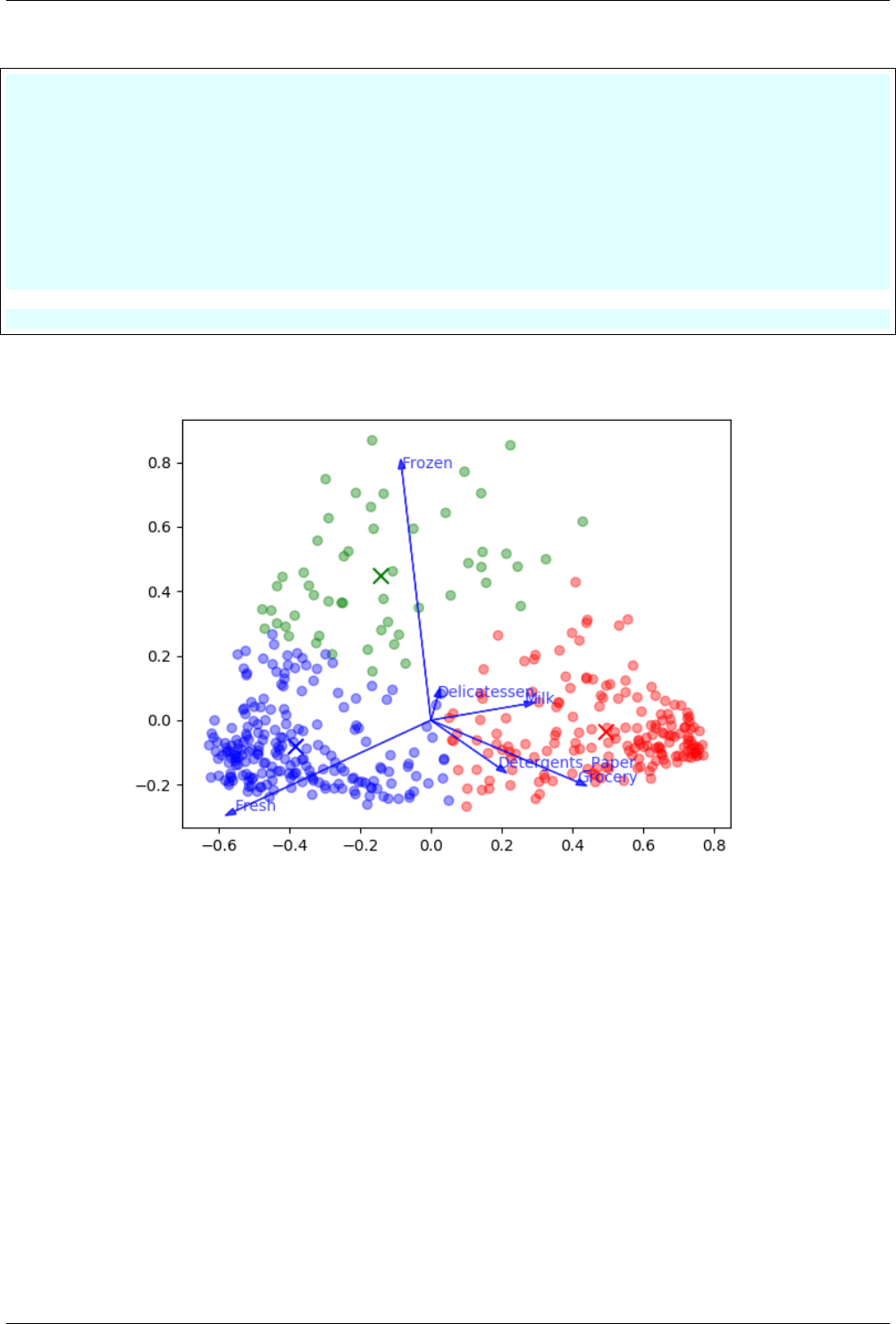
Chapter 10. Clustering with dimensionality reduction
(continued from previous page)
56 columns =df.columns
57
58 # plot the 'name of individual features'along with vector length
59 for iin range(len(columns)):
60 # plot arrows
61 plt.arrow(0,0, xvector[i], yvector[i],
62 color='b', width=0.0005,
63 head_width=0.02, alpha=0.75
64 )
65 # plot name of features
66 plt.text(xvector[i], yvector[i], list(columns)[i], color='b', alpha=0.75)
67
68 plt.show()
Fig. 10.1: Scatter plot for ‘Wholesale dataset’
57 Meher Krishna Patel
Chapter 11
Image recognition
11.1 Introduction
In previous chapters, we saw the examples of ‘classification’, ‘regression’, ‘preprocessing’, ‘dimensionality reduction’
and ‘clustering’. In these examples we considered the numeric and categorical features. In this chapter, we will
use the ‘numerical features’, but these features will represent the images.
Note: In Chapter 2, we used the the Iris-dataset which was available in the SciKit library package; and the
dataset which is available in the SciKit library starts with prefix ‘load_’ e.g. load_iris.
In this chapter, we will use the dataset whose names are available in the dataset. And we need Internet connection
to load them on the computer. These datasets start with ‘fetch_’ e.g. ‘fetch_olivetti_faces’, as shown in next
section.
When the dataset ‘fetch_olivetti_faces’ is instantiated, then the data will be downloaded and will be saved in
~/scikit_learn_data. Further, once the data set is downloaded then it will be used from this directory.
11.2 Fetch the dataset
Lets download the dataset and see the contents of it. Note that the dataset will be downloaded during instantiation
(Line 4), and not by the Line 2.
Note: In the dataset, there are images of 40 people with 10 different poses e.g. smiling and angry faces etc.
Therefore, there are total 400 samples (i.e. 40x10).
Listing 11.1: Download the data
1# faces_ex.py
2
3import matplotlib.pyplot as plt
4from sklearn.datasets import fetch_olivetti_faces
5
6faces =fetch_olivetti_faces() # download the dataset at ~/scikit_learn_data
7print("Keys:", faces.keys()) # display keys
8print("Total samples and image size:", faces.images.shape)
9print("Total samples and features:", faces.data.shape)
10 print("Total samples and targets:", faces.target.shape)
58

Chapter 11. Image recognition
Following is the output of above code. Note that there are total 400 samples and the images size is (64, 64), which
is stored as features of size 4096 (i.e. 64x64).
$ python faces_ex.py
Keys: dict_keys(['data','images','target','DESCR'])
Total samples and image size: (400, 64, 64)
Total samples and features: (400, 4096)
Total samples and targets: (400,)
Note: Please look at the values of the ‘images’, ‘data’ and ‘targets’ as well as below,
$ python -i faces_ex.py
>>> # Sizes
>>> print(faces.images[0].shape)
(64, 64)
>>> print(faces.data[0].shape)
(4096,)
>>> print(faces.target[0].size)
1
>>> # Contents
>>> print(faces.images[0])
[[ 0.30991736 0.36776859 0.41735536 ..., 0.37190083 0.33057851
0.30578512]
[ 0.3429752 0.40495867 0.43801653 ..., 0.37190083 0.33884299
0.3140496 ]
[ 0.3429752 0.41735536 0.45041323 ..., 0.38016528 0.33884299
0.29752067]
...,
[ 0.21487603 0.20661157 0.22314049 ..., 0.15289256 0.16528925
0.17355372]
[ 0.20247933 0.2107438 0.2107438 ..., 0.14876033 0.16115703
0.16528925]
[ 0.20247933 0.20661157 0.20247933 ..., 0.15289256 0.16115703
0.1570248 ]]
>>> print(faces.data[0]) # list size =
[ 0.30991736 0.36776859 0.41735536 ..., 0.15289256 0.16115703
0.1570248 ]
>>> print(faces.target[0]) # person 0
0
11.3 Plot the images
Let’s plot the images of first 20 images, which are shown in Fig. 11.1,
Listing 11.2: Plot the images
1# faces_ex.py
2
3import matplotlib.pyplot as plt
4from sklearn.datasets import fetch_olivetti_faces
5
(continues on next page)
59 Meher Krishna Patel
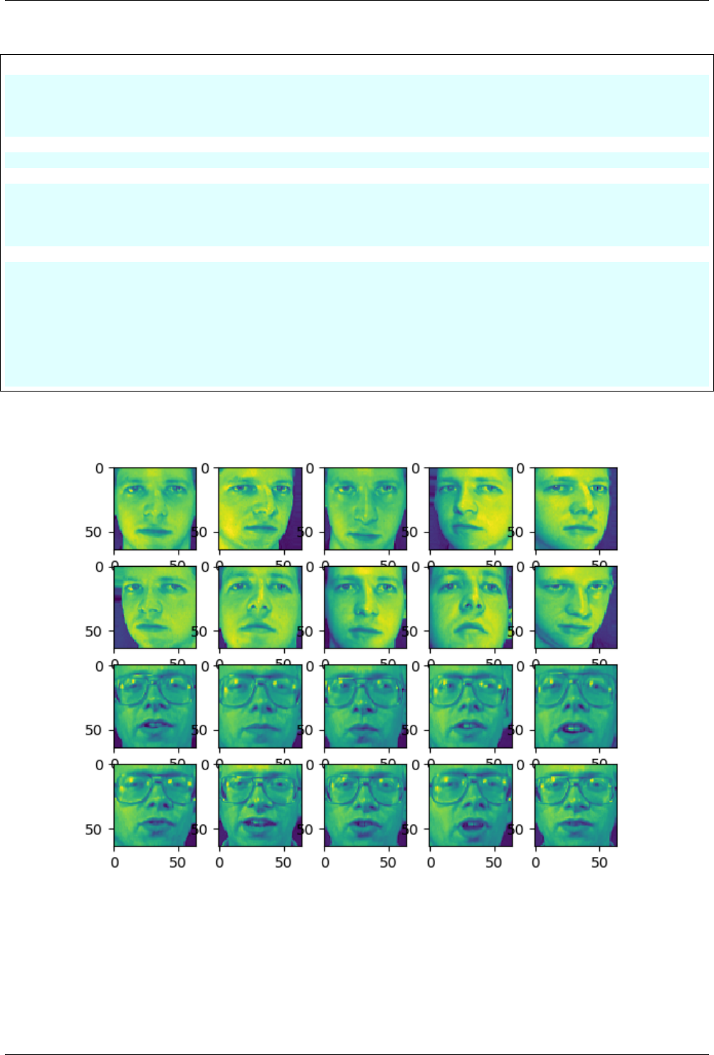
11.3. Plot the images
(continued from previous page)
6faces =fetch_olivetti_faces() # download the dataset at ~/scikit_learn_data
7# print("Keys:", faces.keys()) # display keys
8# print("Total samples and image size:", faces.images.shape)
9# print("Total samples and features:", faces.data.shape)
10 # print("Total samples and targets:", faces.target.shape)
11
12 images =faces.images # save images
13
14 # note that images can not be saved as features, as we need 2D data for
15 # features, whereas faces.images are 3D data i.e. (samples, pixel-x, pixel-y)
16 features =faces.data # features
17 targets =faces.target # targets
18
19 fig =plt.figure() # create a new figure window
20 for iin range(20): # display 20 images
21 # subplot : 4 rows and 5 columns
22 img_grid =fig.add_subplot(4,5, i+1)
23 # plot features as image
24 img_grid.imshow(images[i])
25
26 plt.show()
Fig. 11.1: First 20 images in the dataset
•Before moving further, let’s convert the Listing 11.2 into a function, so that the code can be reused. Listing
11.3 is the function which can be used to plot any number of images with desired number of rows and columns
e.g. Line 26 plots 10 images with 2 rows and 5 columns.
60 PythonDSP
Chapter 11. Image recognition
Listing 11.3: Function for plotting the images
1# faces_ex.py
2
3import matplotlib.pyplot as plt
4from sklearn.datasets import fetch_olivetti_faces
5
6# function for plotting images
7def plot_images(images, total_images=20, rows=4, cols=5):
8fig =plt.figure() # create a new figure window
9for iin range(total_images): # display 20 images
10 # subplot : 4 rows and 5 columns
11 img_grid =fig.add_subplot(rows, cols, i+1)
12 # plot features as image
13 img_grid.imshow(images[i])
14
15 faces =fetch_olivetti_faces() # download the dataset at ~/scikit_learn_data
16 # print("Keys:", faces.keys()) # display keys
17 # print("Total samples and image size:", faces.images.shape)
18 # print("Total samples and features:", faces.data.shape)
19 # print("Total samples and targets:", faces.target.shape)
20
21 images =faces.images # save images
22
23 # note that images can not be saved as features, as we need 2D data for
24 # features, whereas faces.images are 3D data i.e. (samples, pixel-x, pixel-y)
25 features =faces.data # features
26 targets =faces.target # targets
27
28 # plot 10 images with 2 rows and 5 columns
29 plot_images(images, 10,2,5)
30 plt.show()
11.4 Prediction using SVM model
Since there are images of 10 people here, therefore the number of different target values are fixed, hence the problem
is a ‘classification’ problem. In Chapter 2 and Chapter 3, we used the ‘KNeighborsClassifier’ and ‘LogisticRegres-
sion’ for the classification problems; in this chapter we will used the ‘Support Vector Machine (SVM)’ model for
the classification.
Note: SVM looks for the line that seperates the two classes in the best way.
The code for prediction is exactly same as in Chapter 2 and Chapter 3, the only difference is that the ‘SVC (from
SVM)’ model is used with ‘ kernel=”linear” (Line 49)’. Note that, by default ‘ kernel=”rbf” ‘ is used in SVC, which
is required for the non-linear problems.
Listing 11.4: Prediction using SVC
1# faces_ex.py
2
3import matplotlib.pyplot as plt
4from sklearn.datasets import fetch_olivetti_faces
5from sklearn.svm import SVC
6from sklearn.metrics import accuracy_score
7from sklearn.model_selection import train_test_split
8
9# function for plotting images
(continues on next page)
61 Meher Krishna Patel

11.4. Prediction using SVM model
(continued from previous page)
10 def plot_images(images, total_images=20, rows=4, cols=5):
11 fig =plt.figure() # create a new figure window
12 for iin range(total_images): # display 20 images
13 # subplot : 4 rows and 5 columns
14 img_grid =fig.add_subplot(rows, cols, i+1)
15 # plot features as image
16 img_grid.imshow(images[i])
17
18 faces =fetch_olivetti_faces() # download the dataset at ~/scikit_learn_data
19 # print("Keys:", faces.keys()) # display keys
20 # print("Total samples and image size:", faces.images.shape)
21 # print("Total samples and features:", faces.data.shape)
22 # print("Total samples and targets:", faces.target.shape)
23
24 images =faces.images # save images
25
26 # note that images can not be saved as features, as we need 2D data for
27 # features, whereas faces.images are 3D data i.e. (samples, pixel-x, pixel-y)
28 features =faces.data # features
29 targets =faces.target # targets
30
31 # # plot 10 images with 2 rows and 5 columns
32 # plot_images(images, 10, 2, 5)
33 # plt.show()
34
35 # split the training and test data
36 train_features, test_features, train_targets, test_targets =train_test_split(
37 features, targets,
38 train_size=0.8,
39 test_size=0.2,
40 # random but same for all run, also accuracy depends on the
41 # selection of data e.g. if we put 10 then accuracy will be 1.0
42 # in this example
43 random_state=23,
44 # keep same proportion of 'target'in test and target data
45 stratify=targets
46 )
47
48 # use SVC
49 classifier =SVC(kernel="linear")# default kernel=rbf
50 # training using 'training data'
51 classifier.fit(train_features, train_targets) # fit the model for training data
52
53 # predict the 'target'for 'training data'
54 prediction_training_targets =classifier.predict(train_features)
55 self_accuracy =accuracy_score(train_targets, prediction_training_targets)
56 print("Accuracy for training data (self accuracy):", self_accuracy)
57
58 # predict the 'target'for 'test data'
59 prediction_test_targets =classifier.predict(test_features)
60 test_accuracy =accuracy_score(test_targets, prediction_test_targets)
61 print("Accuracy for test data:", test_accuracy)
•Below is the output of above code,
$ python faces_ex.py
Accuracy for training data (self accuracy): 1.0
Accuracy for test data: 0.9875
•Let’s print the locations of first 20 images, where the test-images and the predicted-images are different from
each other. Also, plot the images to see the differences in the images.
62 PythonDSP

Chapter 11. Image recognition
Listing 11.5: Plot first 20 images from the test-images and
predicted-images
1# faces_ex.py
2
3import matplotlib.pyplot as plt
4import numpy as np
5from sklearn.datasets import fetch_olivetti_faces
6from sklearn.svm import SVC
7from sklearn.metrics import accuracy_score
8from sklearn.model_selection import train_test_split
9
10 # function for plotting images
11 def plot_images(images, total_images=20, rows=4, cols=5):
12 fig =plt.figure() # create a new figure window
13 for iin range(total_images): # display 20 images
14 # subplot : 4 rows and 5 columns
15 img_grid =fig.add_subplot(rows, cols, i+1)
16 # plot features as image
17 img_grid.imshow(images[i])
18
19 faces =fetch_olivetti_faces() # download the dataset at ~/scikit_learn_data
20 # print("Keys:", faces.keys()) # display keys
21 # print("Total samples and image size:", faces.images.shape)
22 # print("Total samples and features:", faces.data.shape)
23 # print("Total samples and targets:", faces.target.shape)
24
25 images =faces.images # save images
26
27 # note that images can not be saved as features, as we need 2D data for
28 # features, whereas faces.images are 3D data i.e. (samples, pixel-x, pixel-y)
29 features =faces.data # features
30 targets =faces.target # targets
31
32 # # plot 10 images with 2 rows and 5 columns
33 # plot_images(images, 10, 2, 5)
34 # plt.show()
35
36 # split the training and test data
37 train_features, test_features, train_targets, test_targets =train_test_split(
38 features, targets,
39 train_size=0.8,
40 test_size=0.2,
41 # random but same for all run, also accuracy depends on the
42 # selection of data e.g. if we put 10 then accuracy will be 1.0
43 # in this example
44 random_state=23,
45 # keep same proportion of 'target'in test and target data
46 stratify=targets
47 )
48
49 # use SVC
50 classifier =SVC(kernel="linear")# default kernel=rbf
51 # training using 'training data'
52 classifier.fit(train_features, train_targets) # fit the model for training data
53
54 # predict the 'target'for 'training data'
55 prediction_training_targets =classifier.predict(train_features)
56 self_accuracy =accuracy_score(train_targets, prediction_training_targets)
57 print("Accuracy for training data (self accuracy):", self_accuracy)
58
(continues on next page)
63 Meher Krishna Patel
11.5. Convert features to images
(continued from previous page)
59 # predict the 'target'for 'test data'
60 prediction_test_targets =classifier.predict(test_features)
61 test_accuracy =accuracy_score(test_targets, prediction_test_targets)
62 print("Accuracy for test data:", test_accuracy)
63
64
65 # location of error for first 20 images in test data
66 print("Wrongly detected image-locations: ", end=' ')
67 for iin range (20):
68 # if images are not same then print location of images
69 if test_targets[i] != prediction_test_targets[i]:
70 print(i)
71
72 # store test images in list
73 faces_test =[]
74 for iin test_targets:
75 faces_test.append(images[i])
76
77 # store predicted images in list
78 faces_predict =[]
79 for iin prediction_test_targets:
80 faces_predict.append(images[i])
81
82 # plot the first 20 images from the list
83 plot_images(faces_test, total_images=20)
84 plot_images(faces_predict, total_images=20)
85 plt.show()
•Below are the outputs of above code. The plotted test-images and predicted-images are shown in Fig. 11.2
and Fig. 11.3 respectively, where we can see that the image at location 14 (see red boxes) is at error.
$ python faces_ex.py
Accuracy for training data (self accuracy): 1.0
Accuracy for test data: 0.9875
Wrongly detected image-locations: 14
11.5 Convert features to images
Note: In Listing 11.5, we have used the ‘images (i.e. faces_test.append(images[i]))’ at Lines 75 and 80, to plot
the images.
Also, we can convert the ‘features’ into images for plotting the images as shown in Lines 77 and 84 of Listing 11.6.
Listing 11.6: Convert features to images
1# faces_ex.py
2
3import matplotlib.pyplot as plt
4import numpy as np
5from sklearn.datasets import fetch_olivetti_faces
6from sklearn.svm import SVC
7from sklearn.metrics import accuracy_score
8from sklearn.model_selection import train_test_split
9
10 # function for plotting images
11 def plot_images(images, total_images=20, rows=4, cols=5):
12 fig =plt.figure() # create a new figure window
(continues on next page)
64 PythonDSP
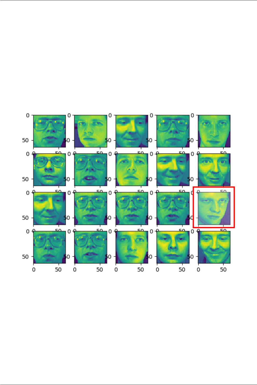
Chapter 11. Image recognition
Fig. 11.2: Test-images
65 Meher Krishna Patel

Chapter 11. Image recognition
(continued from previous page)
13 for iin range(total_images): # display 20 images
14 # subplot : 4 rows and 5 columns
15 img_grid =fig.add_subplot(rows, cols, i+1)
16 # plot features as image
17 img_grid.imshow(images[i])
18
19 faces =fetch_olivetti_faces() # download the dataset at ~/scikit_learn_data
20 # print("Keys:", faces.keys()) # display keys
21 # print("Total samples and image size:", faces.images.shape)
22 # print("Total samples and features:", faces.data.shape)
23 # print("Total samples and targets:", faces.target.shape)
24
25 images =faces.images # save images
26
27 # note that images can not be saved as features, as we need 2D data for
28 # features, whereas faces.images are 3D data i.e. (samples, pixel-x, pixel-y)
29 features =faces.data # features
30 targets =faces.target # targets
31
32 # # plot 10 images with 2 rows and 5 columns
33 # plot_images(images, 10, 2, 5)
34 # plt.show()
35
36 # split the training and test data
37 train_features, test_features, train_targets, test_targets =train_test_split(
38 features, targets,
39 train_size=0.8,
40 test_size=0.2,
41 # random but same for all run, also accuracy depends on the
42 # selection of data e.g. if we put 10 then accuracy will be 1.0
43 # in this example
44 random_state=23,
45 # keep same proportion of 'target'in test and target data
46 stratify=targets
47 )
48
49 # use SVC
50 classifier =SVC(kernel="linear")# default kernel=rbf
51 # training using 'training data'
52 classifier.fit(train_features, train_targets) # fit the model for training data
53
54 # predict the 'target'for 'training data'
55 prediction_training_targets =classifier.predict(train_features)
56 self_accuracy =accuracy_score(train_targets, prediction_training_targets)
57 print("Accuracy for training data (self accuracy):", self_accuracy)
58
59 # predict the 'target'for 'test data'
60 prediction_test_targets =classifier.predict(test_features)
61 test_accuracy =accuracy_score(test_targets, prediction_test_targets)
62 print("Accuracy for test data:", test_accuracy)
63
64
65 # location of error for first 20 images in test data
66 print("Wrongly detected image-locations: ", end=' ')
67 for iin range (20):
68 # if images are not same then print location of images
69 if test_targets[i] != prediction_test_targets[i]:
70 print(i)
71
72 # store test images in list
73 faces_test =[]
(continues on next page)
67 Meher Krishna Patel

11.5. Convert features to images
(continued from previous page)
74 for iin test_targets:
75 # faces_test.append(images[i])
76 # convert 'features'to images
77 faces_test.append(np.reshape(features[i], (64,64)))
78
79 # store predicted images in list
80 faces_predict =[]
81 for iin prediction_test_targets:
82 # faces_predict.append(images[i])
83 # convert 'features'to images
84 faces_predict.append(np.reshape(features[i], (64,64)))
85
86 # plot the first 20 images from the list
87 plot_images(faces_test, total_images=20)
88 plot_images(faces_predict, total_images=20)
89 plt.show()
68 PythonDSP

Chapter 12
More examples on Supervised learning
12.1 Introduction
In this chapter, some more examples are added for Supervised learning.
12.2 Visualizing the Iris dataset
In this section, we will visualize the dataset using ‘numpy’ and ‘matplotlib’ which is available in the Scikit dataset.
12.2.1 Load the Iris dataset
•First load the data set and quickly see the contents of it,
# visualization_ex1.py
# plotting the Iris dataset
import numpy as np
import matplotlib.pyplot as plt
from sklearn.datasets import load_iris
iris =load_iris() # load the iris dataset
print("Keys:", iris.keys()) # print keys of dataset
# shape of data and target
print("Data shape", iris.data.shape) # (150, 4)
print("Target shape", iris.target.shape) # (150,)
print("data:", iris.data[:4]) # first 4 elements
# unique targets
print("Unique targets:", np.unique(iris.target)) # [0, 1, 2]
# counts of each target
print("Bin counts for targets:", np.bincount(iris.target))
print("Feature names:", iris.feature_names)
print("Target names:", iris.target_names)
•Below is the output of above code,
69

12.2. Visualizing the Iris dataset
$ python visualization_ex1.py
Keys: dict_keys(['data','target','target_names','DESCR','feature_names'])
Data shape (150, 4)
Target shape (150,)
data: [[ 5.1 3.5 1.4 0.2]
[ 4.9 3. 1.4 0.2]
[ 4.7 3.2 1.3 0.2]
[ 4.6 3.1 1.5 0.2]]
Unique targets: [0 1 2]
Bin counts for targets: [50 50 50]
Feature names: ['sepal length (cm)','sepal width (cm)',
'petal length (cm)','petal width (cm)']
Target names: ['setosa' 'versicolor' 'virginica']
12.2.2 Histogram
•Let’s plot the histogram of the ‘targets’ with respect to each feature of the dataset,
1# visualization_ex1.py
2
3# plotting the Iris dataset
4
5import numpy as np
6import matplotlib.pyplot as plt
7from sklearn.datasets import load_iris
8
9iris =load_iris() # load the iris dataset
10 # print("Keys:", iris.keys()) # print keys of dataset
11
12 # # shape of data and target
13 # print("Data shape", iris.data.shape) # (150, 4)
14 # print("Target shape", iris.target.shape) # (150,)
15
16 # print("data:", iris.data[:4]) # first 4 elements
17
18 # # unique targets
19 # print("Unique targets:", np.unique(iris.target)) # [0, 1, 2]
20 # # counts of each target
21 # print("Bin counts for targets:", np.bincount(iris.target))
22
23 # print("Feature names:", iris.feature_names)
24 # print("Target names:", iris.target_names)
25
26 colors =['blue','red','green']
27 # plot histogram
28 for feature in range(iris.data.shape[1]): # (shape = 150, 4)
29 plt.subplot(2,2, feature+1)# subplot starts from 1 (not 0)
30 for label, color in zip(range(len(iris.target_names)), colors):
31 # find the label and plot the corresponding data
32 plt.hist(iris.data[iris.target==label, feature],
33 label=iris.target_names[label],
34 color=color)
(continues on next page)
70 PythonDSP
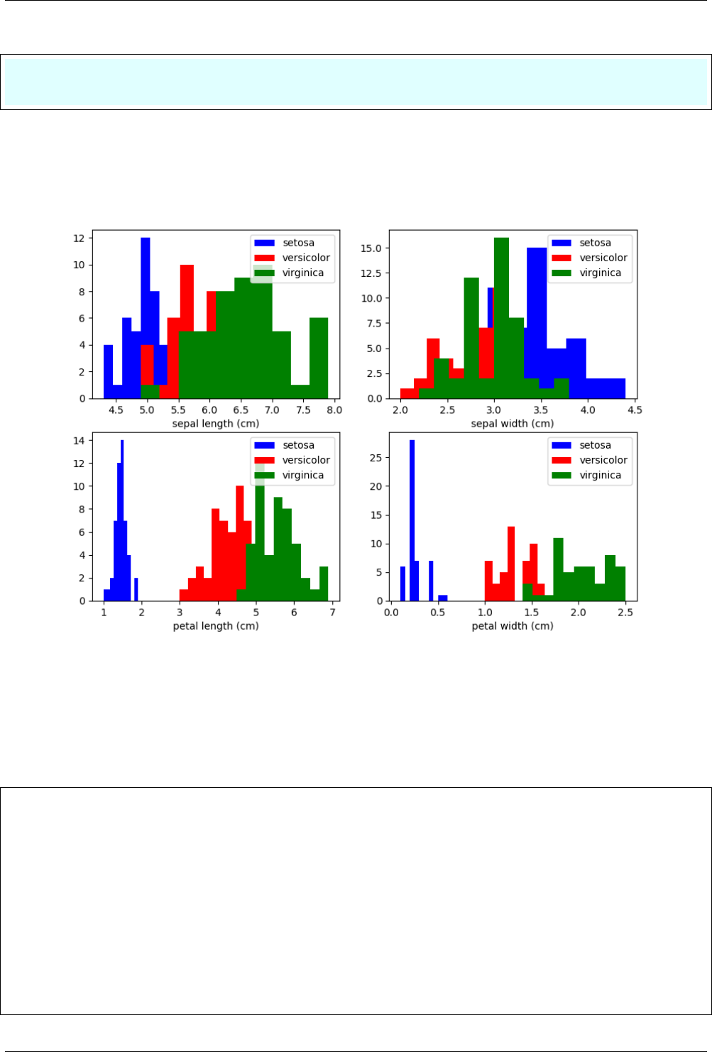
Chapter 12. More examples on Supervised learning
(continued from previous page)
35 plt.xlabel(iris.feature_names[feature])
36 plt.legend()
37 plt.show()
•The Fig. 12.1 shows the histogram of the targets with resepct to each feature. We can clear see that the
feature ‘petal widht’ can distinguish the targets better that other features.
Fig. 12.1: histogram of targets with resepct to each feature
12.2.3 Scatter plot
•Now, we will plot the scatter-plot between ‘petal-width’ and ‘all other features’.
1# visualization_ex1.py
2
3# plotting the Iris dataset
4
5import numpy as np
6import matplotlib.pyplot as plt
7from sklearn.datasets import load_iris
8
9iris =load_iris() # load the iris dataset
10 # print("Keys:", iris.keys()) # print keys of dataset
11
12 # # shape of data and target
13 # print("Data shape", iris.data.shape) # (150, 4)
14 # print("Target shape", iris.target.shape) # (150,)
(continues on next page)
71 Meher Krishna Patel

12.2. Visualizing the Iris dataset
(continued from previous page)
15
16 # print("data:", iris.data[:4]) # first 4 elements
17
18 # # unique targets
19 # print("Unique targets:", np.unique(iris.target)) # [0, 1, 2]
20 # # counts of each target
21 # print("Bin counts for targets:", np.bincount(iris.target))
22
23 # print("Feature names:", iris.feature_names)
24 # print("Target names:", iris.target_names)
25
26 colors =['blue','red','green']
27 # # plot histogram
28 # for feature in range(iris.data.shape[1]): # (shape = 150, 4)
29 # plt.subplot(2, 2, feature+1) # subplot starts from 1 (not 0)
30 # for label, color in zip(range(len(iris.target_names)), colors):
31 # # find the label and plot the corresponding data
32 # plt.hist(iris.data[iris.target==label, feature],
33 # label=iris.target_names[label],
34 # color=color)
35 # plt.xlabel(iris.feature_names[feature])
36 # plt.legend()
37
38 # plot scatter plot : petal-width vs all features
39 feature_x=3# petal width
40 for feature_y in range(iris.data.shape[1]):
41 plt.subplot(2,2, feature_y+1)# subplot starts from 1 (not 0)
42 for label, color in zip(range(len(iris.target_names)), colors):
43 # find the label and plot the corresponding data
44 plt.scatter(iris.data[iris.target==label, feature_x],
45 iris.data[iris.target==label, feature_y],
46 label=iris.target_names[label],
47 alpha =0.45,# transparency
48 color=color)
49 plt.xlabel(iris.feature_names[feature_x])
50 plt.ylabel(iris.feature_names[feature_y])
51 plt.legend()
52 plt.show()
•The Fig. 12.2 shows the scatter-plots between ‘petal width’ and ‘all other features’. Here we can see that
some of the ‘setosa’ can be clearly disntinguish from ‘versicolor’ and ‘virginica’; but the ‘versicolor’ and
‘virginica’ can not be completely separated with each other with any combinations of ‘x’ and ‘y’ axis.
12.2.4 Scatter-matrix plot
•In Fig. 12.2, we plotted the scatter-plots between ‘petal width’ and ‘all other features’; however, many other
combinations are still possible e.g. ‘petal length’ and ‘all other features’. Pandas library provides a method
‘scatter_matrix’, which plots the scatter plot for all the possible combinations along with the histogram, as
shown below,
1# visualization_ex1.py
2
3# plotting the Iris dataset
4
5import numpy as np
6import pandas as pd
7import matplotlib.pyplot as plt
8from sklearn.datasets import load_iris
9
(continues on next page)
72 PythonDSP
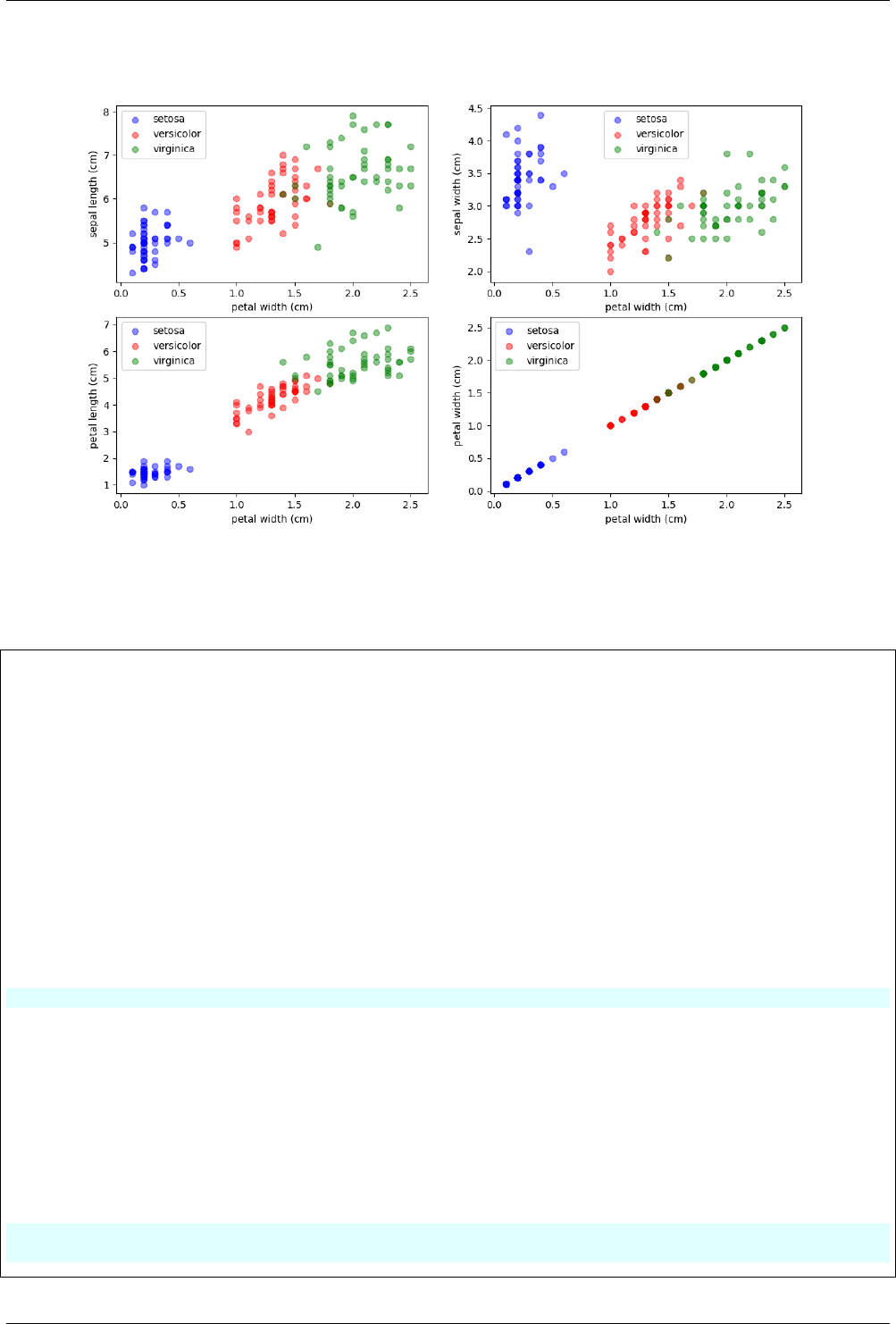
Chapter 12. More examples on Supervised learning
Fig. 12.2: Scatter plot : ‘petal-width’ vs ‘all other features’
(continued from previous page)
10 iris =load_iris() # load the iris dataset
11 # print("Keys:", iris.keys()) # print keys of dataset
12
13 # # shape of data and target
14 # print("Data shape", iris.data.shape) # (150, 4)
15 # print("Target shape", iris.target.shape) # (150,)
16
17 # print("data:", iris.data[:4]) # first 4 elements
18
19 # # unique targets
20 # print("Unique targets:", np.unique(iris.target)) # [0, 1, 2]
21 # # counts of each target
22 # print("Bin counts for targets:", np.bincount(iris.target))
23
24 # print("Feature names:", iris.feature_names)
25 # print("Target names:", iris.target_names)
26
27 # colors = ['blue','red','green']
28 # # plot histogram
29 # for feature in range(iris.data.shape[1]): # (shape = 150, 4)
30 # plt.subplot(2, 2, feature+1) # subplot starts from 1 (not 0)
31 # for label, color in zip(range(len(iris.target_names)), colors):
32 # # find the label and plot the corresponding data
33 # plt.hist(iris.data[iris.target==label, feature],
34 # label=iris.target_names[label],
35 # color=color)
36 # plt.xlabel(iris.feature_names[feature])
37 # plt.legend()
38
39 # plot scatter plot : petal-width vs all features
40 # feature_x= 3 # petal width
(continues on next page)
73 Meher Krishna Patel
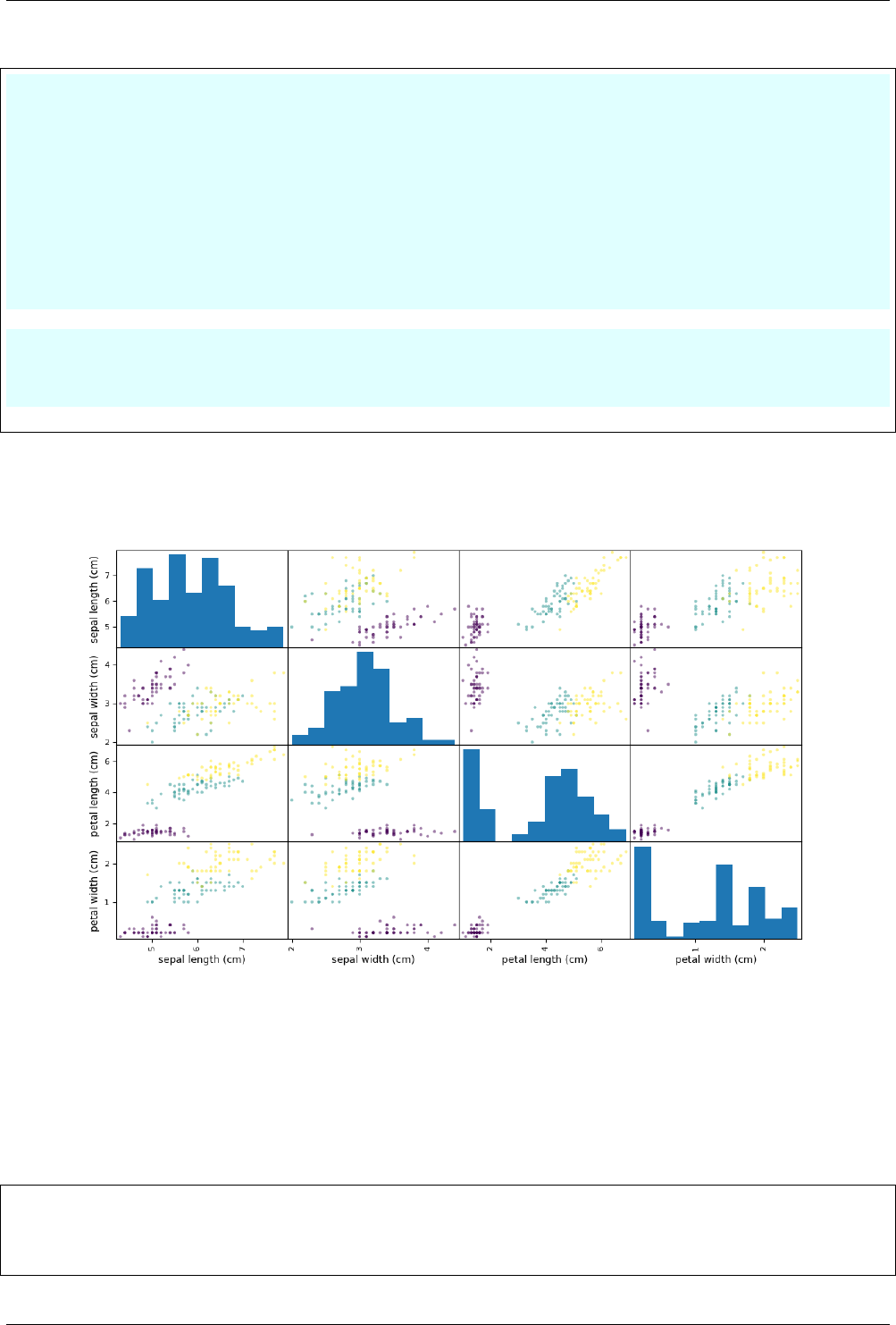
12.2. Visualizing the Iris dataset
(continued from previous page)
41 # for feature_y in range(iris.data.shape[1]):
42 # plt.subplot(2, 2, feature_y+1) # subplot starts from 1 (not 0)
43 # for label, color in zip(range(len(iris.target_names)), colors):
44 # # find the label and plot the corresponding data
45 # plt.scatter(iris.data[iris.target==label, feature_x],
46 # iris.data[iris.target==label, feature_y],
47 # label=iris.target_names[label],
48 # alpha = 0.45, # transparency
49 # color=color)
50 # plt.xlabel(iris.feature_names[feature_x])
51 # plt.ylabel(iris.feature_names[feature_y])
52 # plt.legend()
53
54 # create Pandas-dataframe
55 iris_df =pd.DataFrame(iris.data, columns=iris.feature_names)
56 # print(iris_df.head())
57 pd.plotting.scatter_matrix(iris_df, c=iris.target, figsize=(8,8));
58 plt.show()
•Below are the histogram and scatter plot generated by above code,
Fig. 12.3: Scatter matrix for Iris dataset
12.2.5 Fit a model and test accuracy
•Next, split the data as ‘training’ and ‘test’ data. Then, we will fit the training-data to the model “KNeigh-
borsClassifier”, and check the accuracy of the model on the test-data.
1# visualization_ex1.py
2
3# plotting the Iris dataset
4
(continues on next page)
74 PythonDSP

Chapter 12. More examples on Supervised learning
(continued from previous page)
5import numpy as np
6import pandas as pd
7import matplotlib.pyplot as plt
8from sklearn.datasets import load_iris
9from sklearn.model_selection import train_test_split
10 from sklearn.metrics import accuracy_score
11 from sklearn.neighbors import KNeighborsClassifier
12
13 iris =load_iris() # load the iris dataset
14 # print("Keys:", iris.keys()) # print keys of dataset
15
16 # # shape of data and target
17 # print("Data shape", iris.data.shape) # (150, 4)
18 # print("Target shape", iris.target.shape) # (150,)
19
20 # print("data:", iris.data[:4]) # first 4 elements
21
22 # # unique targets
23 # print("Unique targets:", np.unique(iris.target)) # [0, 1, 2]
24 # # counts of each target
25 # print("Bin counts for targets:", np.bincount(iris.target))
26
27 # print("Feature names:", iris.feature_names)
28 # print("Target names:", iris.target_names)
29
30 # colors = ['blue','red','green']
31 # # plot histogram
32 # for feature in range(iris.data.shape[1]): # (shape = 150, 4)
33 # plt.subplot(2, 2, feature+1) # subplot starts from 1 (not 0)
34 # for label, color in zip(range(len(iris.target_names)), colors):
35 # # find the label and plot the corresponding data
36 # plt.hist(iris.data[iris.target==label, feature],
37 # label=iris.target_names[label],
38 # color=color)
39 # plt.xlabel(iris.feature_names[feature])
40 # plt.legend()
41
42 # plot scatter plot : petal-width vs all features
43 # feature_x= 3 # petal width
44 # for feature_y in range(iris.data.shape[1]):
45 # plt.subplot(2, 2, feature_y+1) # subplot starts from 1 (not 0)
46 # for label, color in zip(range(len(iris.target_names)), colors):
47 # # find the label and plot the corresponding data
48 # plt.scatter(iris.data[iris.target==label, feature_x],
49 # iris.data[iris.target==label, feature_y],
50 # label=iris.target_names[label],
51 # alpha = 0.45, # transparency
52 # color=color)
53 # plt.xlabel(iris.feature_names[feature_x])
54 # plt.ylabel(iris.feature_names[feature_y])
55 # plt.legend()
56
57 # # create Pandas-dataframe
58 # iris_df = pd.DataFrame(iris.data, columns=iris.feature_names)
59 # # print(iris_df.head())
60 # pd.plotting.scatter_matrix(iris_df, c=iris.target, figsize=(8, 8));
61 # plt.show()
62
63
64 # save 'features'and 'targets'in X and y respectively
65 X,y=iris.data, iris.target
(continues on next page)
75 Meher Krishna Patel

12.2. Visualizing the Iris dataset
(continued from previous page)
66
67 # split data into 'test'and 'train'data
68 train_X, test_X, train_y, test_y =train_test_split(X, y,
69 train_size=0.5,
70 test_size=0.5,
71 random_state=23,
72 stratify=y
73 )
74
75 # select classifier
76 cls =KNeighborsClassifier()
77 cls.fit(train_X, train_y)
78
79 # predict the 'target'for 'test data'
80 pred_y =cls.predict(test_X)
81 test_accuracy =accuracy_score(test_y, pred_y)
82 print("Accuracy for test data:", test_accuracy)
•Below is the accuracy of the model,
$ python visualization_ex1.py
Accuracy for test data: 0.946666666667
12.2.6 Plot the incorrect prediction
•Finally we will plot the incorrectly detected test-samples as shown below,
1# visualization_ex1.py
2
3# plotting the Iris dataset
4
5import numpy as np
6import pandas as pd
7import matplotlib.pyplot as plt
8from sklearn.datasets import load_iris
9from sklearn.model_selection import train_test_split
10 from sklearn.metrics import accuracy_score
11 from sklearn.neighbors import KNeighborsClassifier
12
13 iris =load_iris() # load the iris dataset
14 # print("Keys:", iris.keys()) # print keys of dataset
15
16 # # shape of data and target
17 # print("Data shape", iris.data.shape) # (150, 4)
18 # print("Target shape", iris.target.shape) # (150,)
19
20 # print("data:", iris.data[:4]) # first 4 elements
21
22 # # unique targets
23 # print("Unique targets:", np.unique(iris.target)) # [0, 1, 2]
24 # # counts of each target
25 # print("Bin counts for targets:", np.bincount(iris.target))
26
27 # print("Feature names:", iris.feature_names)
28 # print("Target names:", iris.target_names)
29
30 # colors = ['blue','red','green']
31 # # plot histogram
(continues on next page)
76 PythonDSP

Chapter 12. More examples on Supervised learning
(continued from previous page)
32 # for feature in range(iris.data.shape[1]): # (shape = 150, 4)
33 # plt.subplot(2, 2, feature+1) # subplot starts from 1 (not 0)
34 # for label, color in zip(range(len(iris.target_names)), colors):
35 # # find the label and plot the corresponding data
36 # plt.hist(iris.data[iris.target==label, feature],
37 # label=iris.target_names[label],
38 # color=color)
39 # plt.xlabel(iris.feature_names[feature])
40 # plt.legend()
41
42 # plot scatter plot : petal-width vs all features
43 # feature_x= 3 # petal width
44 # for feature_y in range(iris.data.shape[1]):
45 # plt.subplot(2, 2, feature_y+1) # subplot starts from 1 (not 0)
46 # for label, color in zip(range(len(iris.target_names)), colors):
47 # # find the label and plot the corresponding data
48 # plt.scatter(iris.data[iris.target==label, feature_x],
49 # iris.data[iris.target==label, feature_y],
50 # label=iris.target_names[label],
51 # alpha = 0.45, # transparency
52 # color=color)
53 # plt.xlabel(iris.feature_names[feature_x])
54 # plt.ylabel(iris.feature_names[feature_y])
55 # plt.legend()
56
57 # # create Pandas-dataframe
58 # iris_df = pd.DataFrame(iris.data, columns=iris.feature_names)
59 # # print(iris_df.head())
60 # pd.plotting.scatter_matrix(iris_df, c=iris.target, figsize=(8, 8));
61 # plt.show()
62
63
64 # save 'features'and 'targets'in X and y respectively
65 X,y=iris.data, iris.target
66
67 # split data into 'test'and 'train'data
68 train_X, test_X, train_y, test_y =train_test_split(X, y,
69 train_size=0.5,
70 test_size=0.5,
71 random_state=23,
72 stratify=y
73 )
74
75 # select classifier
76 cls =KNeighborsClassifier()
77 cls.fit(train_X, train_y)
78
79 # predict the 'target'for 'test data'
80 pred_y =cls.predict(test_X)
81 # test_accuracy = accuracy_score(test_y, pred_y)
82 # print("Accuracy for test data:", test_accuracy)
83
84 incorrect_idx =np.where(pred_y != test_y)
85 print('Wrongly detected samples:', incorrect_idx[0])
86
87 # scatter plot to show correct and incorrect prediction
88 # plot scatter plot : sepal-width vs all features
89 colors =['blue','orange','green']
90 feature_x=1# sepal width
91 for feature_y in range(iris.data.shape[1]):
92 plt.subplot(2,2, feature_y+1)# subplot starts from 1 (not 0)
(continues on next page)
77 Meher Krishna Patel
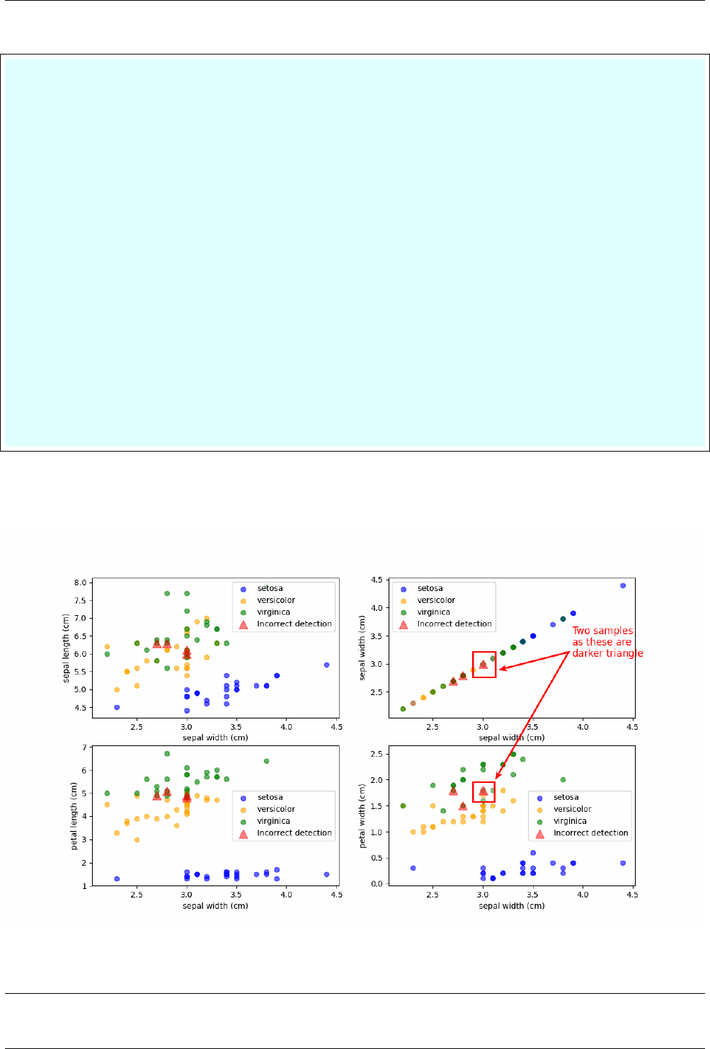
12.2. Visualizing the Iris dataset
(continued from previous page)
93 for i, color in enumerate(colors):
94 # indices for each target i.e. 0, 1 & 2
95 idx =np.where(test_y == i)[0]
96 # find the label and plot the corresponding data
97 plt.scatter(test_X[idx, feature_x],
98 test_X[idx, feature_y],
99 label=iris.target_names[i],
100 alpha =0.6,# transparency
101 color=color
102 )
103
104 # overwrite the test-data with red-color for wrong prediction
105 plt.scatter(test_X[incorrect_idx, feature_x],
106 test_X[incorrect_idx, feature_y],
107 color="red",
108 marker='^',
109 alpha=0.5,
110 label="Incorrect detection",
111 s=120 # size of marker
112 )
113
114 plt.xlabel('{0}'.format(iris.feature_names[feature_x]))
115 plt.ylabel('{0}'.format(iris.feature_names[feature_y]))
116 plt.legend()
117 plt.show()
•Results for above code are shown in Fig. 12.4. In the two subplots, there are only 3 triangles, as two of these
are overlapped with each other; also the overlapped triangles will look darker as we are using the ‘alpha’
parameter.
Fig. 12.4: Correct and incorrect prediction
Overlapped points
78 PythonDSP

Chapter 12. More examples on Supervised learning
The overlapping points can be understood from below results.
•Line 3-4 shows the features of the incorrectly detected targets.
•The Lines 7 and 13 have same ‘sepal-width (col 1)’ and ‘petal-width (col 3)’, therefore two triangles are
overlapped in the scatter plot “sepal-width vs petal-width”.
•Similarly, Lines 7 and 13 have the same ‘sepal-width (col 1)’, therefore the triangles are overlapped in the
scatter plot of “sepal-width vs sepal-width”.
1$ python -i visualization_ex1.py
2
3>>> print(np.where(pred_y != test_y)[0]) # error locations
4[11 48 66 72]
5
6>>> test_X[11] # see values at error locations
7array([ 6.1, 3. , 4.9, 1.8])
8>>> test_X[48]
9array([ 6.3, 2.8, 5.1, 1.5])
10 >>> test_X[66]
11 array([ 6.3, 2.7, 4.9, 1.8])
12 >>> test_X[72]
13 array([ 6. , 3. , 4.8, 1.8])
12.3 Linear and Nonlinear classification
In this section, we see the classification-boundaries of the ‘linear’ and ‘nonlinear’ classification models.
12.3.1 Create ‘make_blob’ dataset
•Let’s create the dataset ‘make_blob’ with two centers and plot the scatter-plot for it,
# make_blob_ex.py
import matplotlib.pyplot as plt
from sklearn.datasets import make_blobs
X,y=make_blobs(centers=2, random_state=0)
print('X.shape (samples x features):', X.shape)
print('y.shape (samples):', y.shape)
print('First 5 samples:\n', X[:5, :])
print('First 5 labels:', y[:5])
plt.scatter(X[y == 0,0], X[y == 0,1], c='red', s=40, label='0')
plt.scatter(X[y == 1,0], X[y == 1,1], c='green', s=40, label='1')
plt.xlabel('first feature')
plt.ylabel('second feature')
plt.legend()
plt.show()
•Below is the output of the above code. The Fig. 12.5 is the scatter plot which is generated by above code,
$ python make_blob_ex.py
X.shape (samples x features): (100, 2)
(continues on next page)
79 Meher Krishna Patel
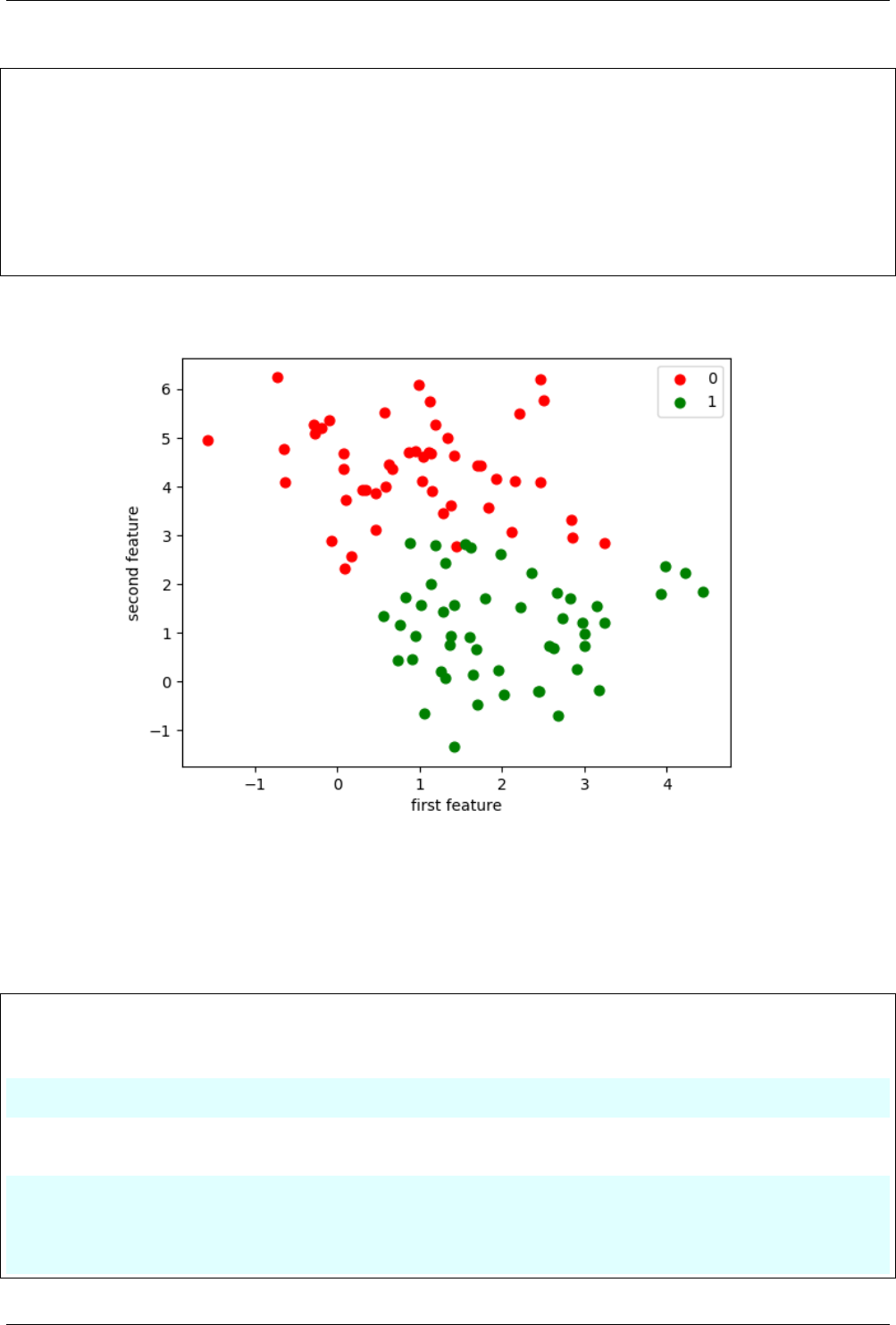
12.3. Linear and Nonlinear classification
(continued from previous page)
y.shape (samples): (100,)
First 5 samples:
[[ 4.21850347 2.23419161]
[ 0.90779887 0.45984362]
[-0.27652528 5.08127768]
[ 0.08848433 2.32299086]
[ 3.24329731 1.21460627]]
First 5 labels: [1 1 0 0 1]
Fig. 12.5: Scatter plot for make_blob
12.3.2 Linear classification
Let’s use the model ‘LogisticRegression()’ to perform the linear classification,
1# make_blob_ex.py
2
3import matplotlib.pyplot as plt
4from sklearn.datasets import make_blobs
5from sklearn.model_selection import train_test_split
6from sklearn.linear_model import LogisticRegression
7
8X,y=make_blobs(centers=2, random_state=0)
9
10 # print('X.shape (samples x features):', X.shape)
11 # print('y.shape (samples):', y.shape)
12
13 # print('First 5 samples:\n', X[:5, :])
14 # print('First 5 labels:', y[:5])
(continues on next page)
80 PythonDSP

Chapter 12. More examples on Supervised learning
(continued from previous page)
15
16 # plt.scatter(X[y == 0, 0], X[y == 0, 1], c='red', s=40, label='0')
17 # plt.scatter(X[y == 1, 0], X[y == 1, 1], c='green', s=40, label='1')
18
19 # plt.xlabel('first feature')
20 # plt.ylabel('second feature')
21 # plt.legend()
22 # plt.show()
23
24 X_train, X_test, y_train, y_test =train_test_split(X, y,
25 test_size=0.2,
26 random_state=23,
27 stratify=y)
28
29 # Linear classifier
30 cls =LogisticRegression()
31 cls.fit(X_train, y_train)
32 prediction =cls.predict(X_test)
33 score =cls.score(X_test, y_test)
34 print("Accuracy:", score)
•Below is the accuracy for the above model,
$ python make_blob_ex.py
Accuracy: 0.9
12.3.3 classification boundary for linear classifier
Since the model is linear, therefore it will use the ‘straight line’ for defining the boundary for the classification.
The boundary can be drawn using ‘plot_2d_separator’ as shown in below code,
Listing 12.1: Decision bounadary for linear classifier
1# make_blob_ex.py
2
3import matplotlib.pyplot as plt
4from sklearn.datasets import make_blobs
5from sklearn.model_selection import train_test_split
6from sklearn.linear_model import LogisticRegression
7from figures import plot_2d_separator
8
9X,y=make_blobs(centers=2, random_state=0)
10
11 # print('X.shape (samples x features):', X.shape)
12 # print('y.shape (samples):', y.shape)
13
14 # print('First 5 samples:\n', X[:5, :])
15 # print('First 5 labels:', y[:5])
16
17 # plt.scatter(X[y == 0, 0], X[y == 0, 1], c='red', s=40, label='0')
18 # plt.scatter(X[y == 1, 0], X[y == 1, 1], c='green', s=40, label='1')
19
20 # plt.xlabel('first feature')
21 # plt.ylabel('second feature')
22 # plt.legend()
23 # plt.show()
24
25 X_train, X_test, y_train, y_test =train_test_split(X, y,
(continues on next page)
81 Meher Krishna Patel
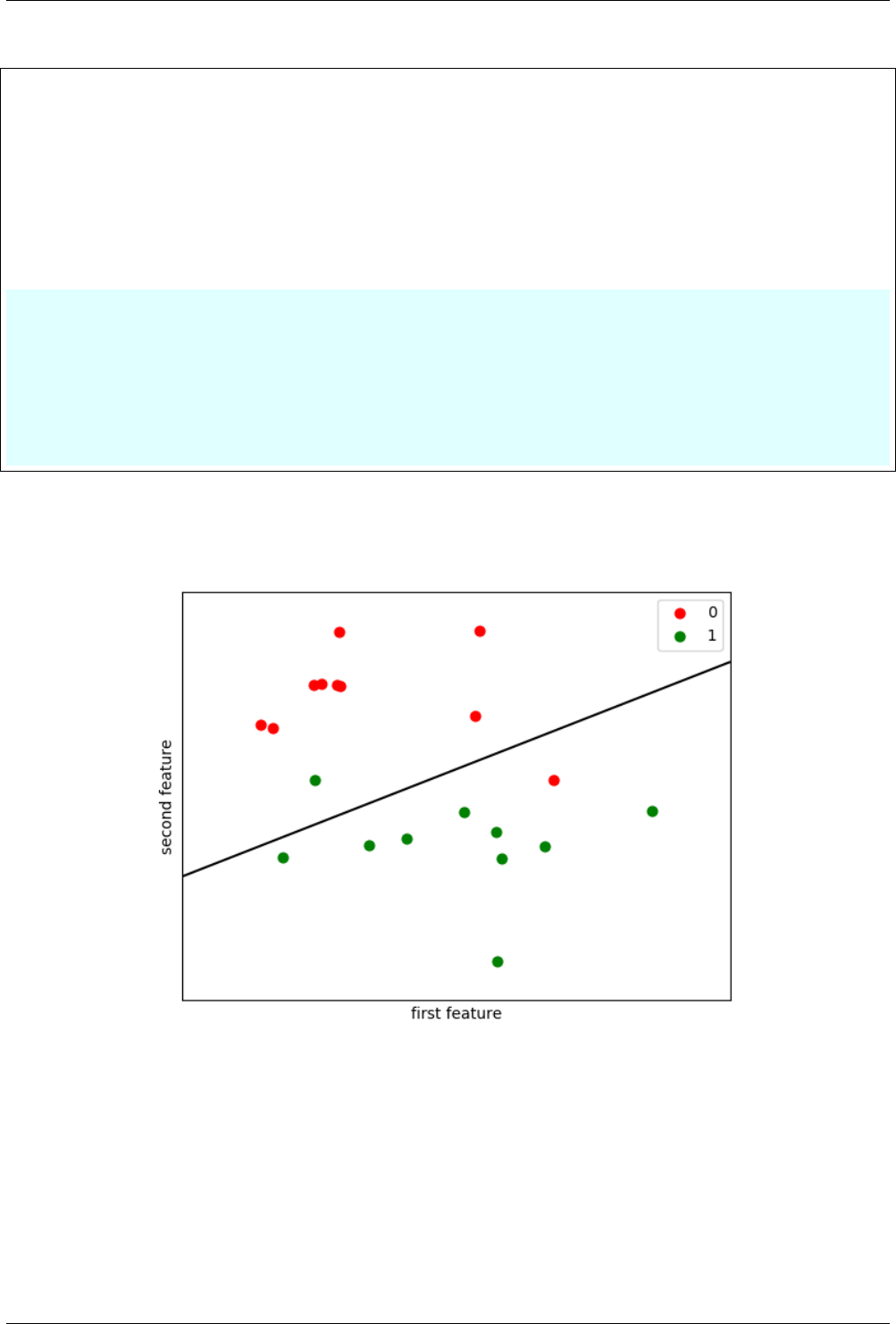
12.3. Linear and Nonlinear classification
(continued from previous page)
26 test_size=0.2,
27 random_state=23,
28 stratify=y)
29
30 # Linear classifier
31 cls =LogisticRegression()
32 cls.fit(X_train, y_train)
33 prediction =cls.predict(X_test)
34 score =cls.score(X_test, y_test)
35 print("Accuracy:", score)
36
37 plt.scatter(X_test[y_test == 0,0], X_test[y_test == 0,1],
38 c='red', s=40, label='0')
39 plt.scatter(X_test[y_test == 1,0], X_test[y_test == 1,1],
40 c='green', s=40, label='1')
41 plot_2d_separator(cls, X_test) # plot the boundary
42 plt.xlabel('first feature')
43 plt.ylabel('second feature')
44 plt.legend()
45 plt.show()
•The Fig. 12.6 shows the decision boundary generated by above code,
Fig. 12.6: Decision boundary for linear classifier
12.3.4 Nonlinear classification and boundary
Let’s use the nonlinear classifier i.e. ‘KNeighborsClassifier’ and see the decision boundary for it,
82 PythonDSP

Chapter 12. More examples on Supervised learning
Listing 12.2: Decision bounadary for nonlinear classifier
1# make_blob_ex.py
2
3import matplotlib.pyplot as plt
4from sklearn.datasets import make_blobs
5from sklearn.model_selection import train_test_split
6from sklearn.linear_model import LogisticRegression
7from sklearn.neighbors import KNeighborsClassifier
8from figures import plot_2d_separator
9
10 X,y=make_blobs(centers=2, random_state=0)
11
12 # print('X.shape (samples x features):', X.shape)
13 # print('y.shape (samples):', y.shape)
14
15 # print('First 5 samples:\n', X[:5, :])
16 # print('First 5 labels:', y[:5])
17
18 # plt.scatter(X[y == 0, 0], X[y == 0, 1], c='red', s=40, label='0')
19 # plt.scatter(X[y == 1, 0], X[y == 1, 1], c='green', s=40, label='1')
20
21 # plt.xlabel('first feature')
22 # plt.ylabel('second feature')
23 # plt.legend()
24 # plt.show()
25
26 X_train, X_test, y_train, y_test =train_test_split(X, y,
27 test_size=0.2,
28 random_state=23,
29 stratify=y)
30
31 # Linear classifier
32 # cls = LogisticRegression()
33
34 # Nonlinear classifier
35 cls =KNeighborsClassifier()
36 cls.fit(X_train, y_train)
37 prediction =cls.predict(X_test)
38 score =cls.score(X_test, y_test)
39 print("Accuracy:", score)
40
41 plt.scatter(X_test[y_test == 0,0], X_test[y_test == 0,1],
42 c='red', s=40, label='0')
43 plt.scatter(X_test[y_test == 1,0], X_test[y_test == 1,1],
44 c='green', s=40, label='1')
45 plot_2d_separator(cls, X_test) # plot the boundary
46 plt.xlabel('first feature')
47 plt.ylabel('second feature')
48 plt.legend()
49 plt.show()
•Below is the output of above code. The Fig. 12.7 shows the nonlinear decision boundary generate by the
code.
$ python make_blob_ex.py
Accuracy: 1.0
Note:
•Now, increase the noise (i.e. cluster_std) in the make_blobs dataset by replacing the Line 10 of Listing 12.2
83 Meher Krishna Patel
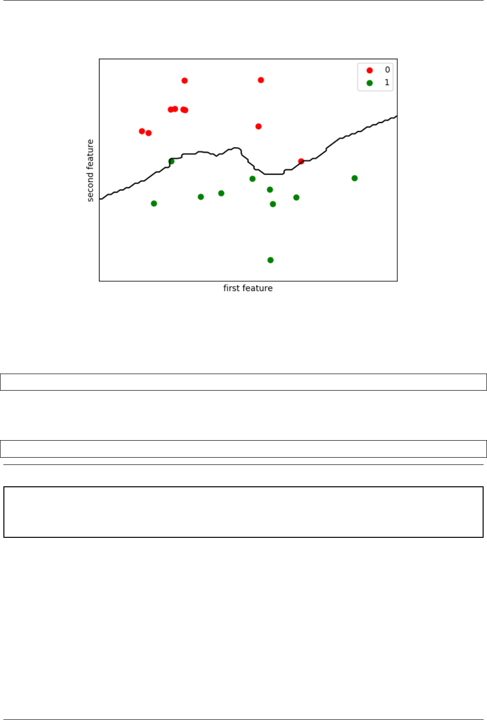
12.3. Linear and Nonlinear classification
Fig. 12.7: Decision boundary for nonlinear classifier
with below line, and see the decision boundary again,
X,y=make_blobs(centers=2, random_state=0, cluster_std=2.0)
•Note that, we may get multiple boundaries in nonlinear classification, when the noise is high; which will
reduce the performance of the system. Those multiple boundaries can be removed by increasing the number
of neighbors at Line 35 for ‘KNeighborsClassifier’ as shown below,
cls =KNeighborsClassifier(n_neighbors=25)
Warning: Increasing the ‘n_neighbors’ in ‘KNeighborsClassifier’ does not mean that it will increase the
performance all the time. It may reduce the performance as well.
For better results, we must have higher number of samples to reduce the variability in the performance metrics.
84 PythonDSP
Chapter 13
Performance analysis of models
13.1 Introduction
In the previous chapters, we saw the examples of ‘supervised machine learning’, i.e. classification and regression
models. Also, we calculated the ‘score’ to see the performance of these models. But there are several other standard
methods to evaluate the performance of the models. Table 13.1 shows the list of metrics which can be used to
measure the performance of different types of model, , which are discussed in the chapter.
Table 13.1: Metrics to measure the performance
Problem Performance metric
Classifica-
tion
Accuracy, Receiver operating curve (ROC), Area under ROC,
Logarithmic loss, Confusion matrix, Classification report
Regression Mean square error (MSE), Root MSE (RMSE), Mean absolute error,
𝑅2
13.2 Performance of classification problem
In this section, we will see the performance measurement of the classification problem.
Note: Cross-validation is used in this section, which is discussed in Chapter 5.
Remember, cross-validation does not create the model to predict the new samples; it only gives an idea about the
accuracy of model.
13.2.1 Accuracy
The ‘accuracy’ is the ratio of the ‘correct predictions’ and ‘all the predictions’. By default, the scoring is done
based on ‘accuracy’,
Note: In previous chapters, we already calculated ‘accuracy’ for the ‘training’ and ‘test’ datasets. For
easy analysis, the ‘Cross-validation’ class have in-built performance-measurement methods e.g. ‘accuracy’,
‘mean_squared_error and r2_score’ etc. as shown in this chapter.
>>> import numpy as np
>>> from sklearn.datasets import load_iris
>>> from sklearn.neighbors import KNeighborsClassifier
(continues on next page)
85

13.2. Performance of classification problem
(continued from previous page)
>>> from sklearn.model_selection import cross_val_score
>>>
>>> # create object of class 'load_iris'
... iris =load_iris()
>>>
>>> # save features and targets from the 'iris'
... features, targets =iris.data, iris.target
>>>
>>> # use KNeighborsClassifier for classification
... classifier =KNeighborsClassifier()
>>>
>>> # cross-validation
... scores =cross_val_score(classifier,
... features, targets,
... cv=7, scoring="accuracy")
>>> print("Cross validation scores:", scores)
Cross validation scores: [ 0.95833333 1. 0.95238095
0.9047619 0.95238095 1. 1.]
>>> print("Mean={0:0.4f}, Var={1:0.4f}".format(
... np.mean(scores),
... np.var(scores)))
Mean=0.9668, Var=0.0011
13.2.2 Logarithmic loss
It measures the probability of having the correct predictions, and prints the logarithmic value of the probability.
Since the probability has the range between 0 and 1, therefore ‘Logarithmic loss’ has the range between 0 and
‘-infinity’.
Note: Higher the ‘Logarithmic loss’ value, better is the model. Perfect model will have the maximum value i.e.
‘0’.
>>> import numpy as np
>>> from sklearn.datasets import load_iris
>>> from sklearn.neighbors import KNeighborsClassifier
>>> from sklearn.model_selection import cross_val_score
>>>
>>> # create object of class 'load_iris'
... iris =load_iris()
>>>
>>> # save features and targets from the 'iris'
... features, targets =iris.data, iris.target
>>>
>>> # use KNeighborsClassifier for classification
... classifier =KNeighborsClassifier()
>>>
>>> # cross-validation
... scores =cross_val_score(classifier,
... features, targets,
... cv=7, scoring="neg_log_loss")
>>> print("Cross validation scores:", scores)
Cross validation scores: [-1.45771098 -0.03187765
-0.07858381 -0.14654173 -1.66902867 -0.02125177
-0.03495091]
>>> print("Mean={0:0.4f}, Var={1:0.4f}".format(
... np.mean(scores),
... np.var(scores)))
Mean=-0.4914, Var=0.4644
86 PythonDSP

Chapter 13. Performance analysis of models
13.2.3 Classification report
Classification report gives the ‘precision’, ‘recall’, ‘F1-score’ and ‘support’ values for each class as shown below,
>>> from sklearn.datasets import load_iris
>>> from sklearn.model_selection import train_test_split
>>> from sklearn.linear_model import LogisticRegression
>>> from sklearn.metrics import classification_report
>>>
>>> iris =load_iris()
>>>
>>> X, y =iris.data, iris.target
>>>
>>> X_train, X_test, y_train, y_test =train_test_split(X, y,
... test_size=0.2,
... random_state=23,
... stratify=y)
>>>
>>> # Linear classifier
... cls =LogisticRegression()
>>> cls.fit(X_train, y_train)
LogisticRegression(C=1.0, class_weight=None, dual=False, fit_intercept=True,
intercept_scaling=1, max_iter=100, multi_class='ovr', n_jobs=1,
penalty='l2', random_state=None, solver='liblinear', tol=0.0001,
verbose=0, warm_start=False)
>>>
>>> prediction =cls.predict(X_test)
>>> report =classification_report(y_test, prediction)
>>> print(report) # print classification_report
precision recall f1-score support
0 1.00 1.00 1.00 10
1 0.90 0.90 0.90 10
2 0.90 0.90 0.90 10
avg / total 0.93 0.93 0.93 30
13.2.4 Confusion matrix (Binary classification)
Let’s understand the Confusion matrix first, which is the basis for ROC, which can be used with ‘binary (not
multiclass) classification’. Confusion matrix is a 2×2matrix, whose columns are shown in Table 13.2 and
explained below,
•True positive : Actual value is positive, and predicted value is also positive.
•False negative : Actual value is positive, and predicted value is negative.
•False positive : Actual value is negative, and predicted value is positive.
•True negative : Actual value is negative, and predicted value is negative.
Table 13.2: Confusion matrix
Predicted value
Positive Negative
Actual value Positive True Positive False Negative
Negative False Positive True Negative
Note: Clearly the desired results are the ‘True positive’ and ‘True negative’ columns. Therefore, for better
performance, these values should be higher than the ‘False negative’ and ‘False positive’ columns.
Below is an example of Confusion matrix. Here results have following values
87 Meher Krishna Patel

13.2. Performance of classification problem
•True positive = 9
•True negative = 9
•False positive = 1
•False negative = 1
>>> from sklearn.datasets import make_blobs
>>> from sklearn.model_selection import train_test_split
>>> from sklearn.linear_model import LogisticRegression
>>> from sklearn.metrics import confusion_matrix
>>>
>>> X, y =make_blobs(centers=2, random_state=0)
>>>
>>> X_train, X_test, y_train, y_test =train_test_split(X, y,
... test_size=0.2,
... random_state=23,
... stratify=y)
>>>
>>> # Linear classifier
... cls =LogisticRegression()
>>> cls.fit(X_train, y_train)
LogisticRegression(C=1.0, class_weight=None, dual=False, fit_intercept=True,
intercept_scaling=1, max_iter=100, multi_class='ovr', n_jobs=1,
penalty='l2', random_state=None, solver='liblinear', tol=0.0001,
verbose=0, warm_start=False)
>>> prediction =cls.predict(X_test)
>>> c_matrix =confusion_matrix(y_test, prediction)
>>> print(c_matrix) # print confusion_matrix
[[9 1]
[1 9]]
13.2.5 Area under ROC (AUC)
ROC is the plot between the ‘true positive rate’ and ‘false positive rate’, which are defined as below,
•True positive rate = (True positive) / (True positive + False negative)
•False positive rate = (False positive) / (False positive + True negative)
Note: ROC and AUC are used for ‘binary (not multiclass) classification’ problem; and ‘AUC = 1’ represents the
perfect model,
>>> import numpy as np
>>> from sklearn.datasets import make_blobs
>>> from sklearn.model_selection import cross_val_score
>>> from sklearn.linear_model import LogisticRegression
>>>
>>> X, y =make_blobs(centers=2, random_state=0)
>>>
>>> # use KNeighborsClassifier for classification
... classifier =LogisticRegression()
>>>
>>> # cross-validation
... scores =cross_val_score(classifier,
... X, y,
... cv=7, scoring="roc_auc")
>>>
>>> print("Cross validation scores:", scores)
Cross validation scores: [ 1. 1. 0.97959184 0.91836735 0.97959184 1. 1. ␣
˓→]
>>> print("Mean={0:0.4f}, Var={1:0.4f}".format(
(continues on next page)
88 PythonDSP

Chapter 13. Performance analysis of models
(continued from previous page)
... np.mean(scores),
... np.var(scores)))
Mean=0.9825, Var=0.0008
13.3 Performance of regression problem
The code used in this section is discussed in Chapter 4.
13.3.1 MAE, MSE and R2
Note:
•By default, Scikit library calculates the ‘r2_score’ as shown in Lines 44-46. The ‘r2_score’ has the values
between 0 (no fit) and 1 (perfect fit).
•Mean absolute error (MAE) is the sum of the ‘absolute differences’ between the predicted and the actual
values, and calculated at Lines 48-50.
•Mean square error (MSE) is the sum of squares of the errors, where errors are the differences between
the ‘predicted’ and ‘actual’ values. This is calculated at Lines 53-55.
1>>> import numpy as np
2>>> from sklearn.model_selection import train_test_split
3>>> from sklearn.linear_model import LinearRegression
4>>> from sklearn.metrics import mean_squared_error, mean_absolute_error
5>>> from sklearn.metrics import r2_score
6>>>
7>>> N=100 # 100 samples
8>>> x=np.linspace(-3,3, N) # coordinates
9>>> noise_sample =np.random.RandomState(20)# constant random value
10 >>> # growing sinusoid with random fluctuation
11 ... sine_wave =x+np.sin(4*x) +noise_sample.uniform(N)
12 >>>
13 >>> # convert features in 2D format i.e. list of list
14 ... features =x[:, np.newaxis]
15 >>>
16 >>> # save sine wave in variable 'targets'
17 ... targets =sine_wave
18 >>>
19 >>> # split the training and test data
20 ... train_features, test_features, train_targets, test_targets =train_test_split(
21 ... features, targets,
22 ... train_size=0.8,
23 ... test_size=0.2,
24 ... # random but same for all run, also accuracy depends on the
25 ... # selection of data e.g. if we put 10 then accuracy will be 1.0
26 ... # in this example
27 ... random_state=23,
28 ... # keep same proportion of 'target'in test and target data
29 ... # stratify=targets # can not used for single feature
30 ... )
31 >>>
32 >>> # training using 'training data'
33 ... regressor =LinearRegression()
34 >>> regressor.fit(train_features, train_targets) # fit the model for training data
35 LinearRegression(copy_X=True, fit_intercept=True, n_jobs=1, normalize=False)
36 >>>
(continues on next page)
89 Meher Krishna Patel
13.3. Performance of regression problem
(continued from previous page)
37 >>>
38 >>> # predict the 'target'for 'test data'
39 ... prediction_test_targets =regressor.predict(test_features)
40 >>> test_accuracy =regressor.score(test_features, test_targets)
41 >>> print("Accuracy for test data:", test_accuracy)
42 Accuracy for test data: 0.822872868183
43 >>>
44 >>> r2_score =r2_score(test_targets, prediction_test_targets)
45 >>> print("r2_score: ", r2_score)
46 r2_score: 0.822872868183
47 >>>
48 >>> mean_absolute_error =mean_absolute_error(test_targets, prediction_test_targets)
49 >>> print("mean_absolute_error: ", mean_absolute_error)
50 mean_absolute_error: 0.680406590952
51 >>>
52 >>>
53 >>> mean_squared_error =mean_squared_error(test_targets, prediction_test_targets)
54 >>> print("mean_squared_error: ", mean_squared_error)
55 mean_squared_error: 0.584535345592
13.3.2 Problem with cross-validation
Below is the issue with ‘regressor-performances’ with ‘cross-validation’ method,
Error:
•Mean score for ‘r2’ is calculated as ‘-7.7967’, which is negative. Note that, the negative value is not
possible for ‘r2’ score.
•Similarly, replace ‘r2’ with ‘neg_mean_squared_error’ and ‘neg_mean_absolute_error’, and it may give
some undesired results.
•Please clarify the reason.
1>>> import numpy as np
2>>> from sklearn.model_selection import cross_val_score
3>>> from sklearn.model_selection import KFold
4>>> from sklearn.linear_model import LinearRegression
5>>>
6>>> N=100 # 100 samples
7>>> x=np.linspace(-3,3, N) # coordinates
8>>> noise_sample =np.random.RandomState(20)# constant random value
9>>> # growing sinusoid with random fluctuation
10 ... sine_wave =x+np.sin(4*x) +noise_sample.uniform(N)
11 >>>
12 >>>
13 >>> # convert features in 2D format i.e. list of list
14 ... features =x[:, np.newaxis]
15 >>>
16 >>> # save sine wave in variable 'targets'
17 ... targets =sine_wave
18 >>>
19 >>> # cross-validation
20 ... regressor =LinearRegression()
21 >>>
22 >>> cv =KFold(n_splits=10, random_state=7)
23 >>> scores =cross_val_score(regressor, features, targets, cv=cv,
24 ... scoring="r2")
25 >>>
(continues on next page)
90 PythonDSP

Chapter 13. Performance analysis of models
(continued from previous page)
26 >>> print("Cross validation scores:", scores)
27 Cross validation scores: [-13.91006325 -20.21043299 0.36952646
28 -1.92292726 -3.30936741 -3.30936741 -1.92292726
29 0.36952646 -20.21043299 -13.91006325]
30 >>> print("Mean={0:0.4f}, Var={1:0.4f}".format(
31 ... np.mean(scores),
32 ... np.var(scores)))
33 Mean=-7.7967, Var=62.5597
91 Meher Krishna Patel
Chapter 14
Quick reference guide
14.1 Introduction
In previous chapters, we saw several examples of machine learning methods. In this chapter, we will summarize
those methods along with several other useful ways to analyze the data.
14.2 Understand the data
When we get the data, we need to see the data and it’s statistics. Then we need to perform certain clean/transform
operations e.g. filling the null values etc. In this section, we will see several steps which may be useful to understand
the data,
14.2.1 Load the data and add headers
Although we can use Python or Numpy to load the data, but it is better to use Pandas library to load the data.
•Add header to data : In the below code, the first 29 rows are skipped as these lines do not contain samples
but the information about the each sample.
>>> import pandas as pd
>>>
>>> # create header for dataset
... header =['age','bp','sg','al','su','rbc','pc','pcc',
... 'ba','bgr','bu','sc','sod','pot','hemo','pcv',
... 'wbcc','rbcc','htn','dm','cad','appet','pe','ane',
... 'classification']
>>>
>>> # read the dataset
... df_kidney =pd.read_csv("data/chronic_kidney_disease.arff",
... header=None,# use header=0 to replace the existing header
... skiprows=29,# skip first 29 rows
... names=header
... )
>>>
>>> df_kidney.shape # shape of data : 400 rows and 25 columns
(400, 25)
•Replace existing header from the data
>>> import pandas as pd
>>> # new headers
(continues on next page)
92

Chapter 14. Quick reference guide
(continued from previous page)
... header =["channel","area","fresh","milk","grocery",
... "frozen","detergent","delicatessen"]
>>>
>>> # replace existing headers
... df_whole_sale =pd.read_csv("data/Wholesale customers data.csv",
... header=0,# replace existing header; use this or below
... # skiprows=1, # skip the first row i.e. header
... names=header # use new header
... )
>>>
>>> df_whole_sale.shape # shape of data: 440 rows and 8 columns
(440, 8)
>>>
>>> df_whole_sale.head(3)# show first three rows
channel area fresh milk grocery frozen detergent delicatessen
0 2 3 12669 9656 7561 214 2674 1338
1 2 3 7057 9810 9568 1762 3293 1776
2 2 3 6353 8808 7684 2405 3516 7844
>>>
>>> df_whole_sale.tail(2)# show last two rows
channel area fresh milk grocery frozen detergent delicatessen
438 1 3 10290 1981 2232 1038 168 2125
439 1 3 2787 1698 2510 65 477 52
14.2.2 Check for the null values
•Check if the null value exist,
1>>> df_kidney.isnull().sum()
2age 0
3bp 0
4sg 0
5al 0
6su 0
7rbc 0
8pc 0
9pcc 0
10 ba 0
11 bgr 0
12 bu 0
13 sc 0
14 sod 0
15 pot 0
16 hemo 0
17 pcv 0
18 wbcc 0
19 rbcc 0
20 htn 0
21 dm 1
22 cad 0
23 appet 0
24 pe 0
25 ane 0
26 classification 0
27 dtype: int64
•Check the location of null value
93 Meher Krishna Patel

14.2. Understand the data
>>> df_kidney[df_kidney.dm.isnull()]
age bp sg al su rbc pc pcc ba bgr \
369 75 70 1.020 0 0 normal normal notpresent notpresent 107
... pcv wbcc rbcc htn dm cad appet pe ane classification
369 ... 46 10300 4.8 no NaN no no good no no
[1 rows x 25 columns]
>>>
>>> df_kidney[df_kidney.dm.isnull()].iloc[:, 0:2]# display only two columns
age bp
369 75 70
14.2.3 Check the data types
Sometimes the datatypes are not correctly read by the Pandas, therefore it is better to check the data types of
each columns.
•In the below results are all the types are ‘object’ (not numeric), because samples have ‘?’ in it, therefore we
need to replace the ‘?’ values with some other values,
>>> df_kidney.dtypes
age object
bp object
sg object
al object
su object
rbc object
pc object
pcc object
ba object
bgr object
bu object
sc object
sod object
pot object
hemo object
pcv object
wbcc object
rbcc object
htn object
dm object
cad object
appet object
pe object
ane object
classification object
dtype: object
•If we perform the ‘conversion’ operation at this moment, then error will be generate due to ‘?’ in the data,
>>> df_kidney.bgr =pd.to_numeric(df_kidney.bgr)
Traceback (most recent call last):
ValueError: Unable to parse string "?" at position 1
•Replace the ‘?’ with ‘NaN’ value using ‘replace’ command; and change the ‘type’ of ‘bgr’ column,
>>> import numpy as np
>>> df_kidney =df_kidney.replace('?', np.nan)
>>> df_kidney.bgr =pd.to_numeric(df_kidney.bgr)
(continues on next page)
94 PythonDSP

Chapter 14. Quick reference guide
(continued from previous page)
>>> df_kidney.dtypes
[...]
ba object
bgr float64
[...]
classification object
dtype: object
•Next, we can drop or fill the ‘NaN’ values. In the below code we dropped the NaN values,
>>> df_kidney.isnull().sum() # check the NaN
age 9
bp 12
sg 47
[...]
classification 0
dtype: int64
>>>
>>> # drop the NaN
>>> df_kidney =df_kidney.dropna(axis=0, how="any")
>>>
>>> df_kidney.isnull().sum() # check NaN again
age 0
bp 0
sg 0
[...]
classification 0
dtype: int64
14.2.4 Statistics of the data
•The ‘describe’ can be used to see the statistics of the data.
>>> df_whole_sale.describe()
channel area fresh milk grocery \
count 440.000000 440.000000 440.000000 440.000000 440.000000
mean 1.322727 2.543182 12000.297727 5796.265909 7951.277273
std 0.468052 0.774272 12647.328865 7380.377175 9503.162829
min 1.000000 1.000000 3.000000 55.000000 3.000000
25% 1.000000 2.000000 3127.750000 1533.000000 2153.000000
50% 1.000000 3.000000 8504.000000 3627.000000 4755.500000
75% 2.000000 3.000000 16933.750000 7190.250000 10655.750000
max 2.000000 3.000000 112151.000000 73498.000000 92780.000000
frozen detergent delicatessen
count 440.000000 440.000000 440.000000
mean 3071.931818 2881.493182 1524.870455
std 4854.673333 4767.854448 2820.105937
min 25.000000 3.000000 3.000000
25% 742.250000 256.750000 408.250000
50% 1526.000000 816.500000 965.500000
75% 3554.250000 3922.000000 1820.250000
max 60869.000000 40827.000000 47943.000000
•See output of first 2 columns only,
>>> df_whole_sale.iloc[:, 0:2].describe()
channel area
count 440.000000 440.000000
(continues on next page)
95 Meher Krishna Patel

14.2. Understand the data
(continued from previous page)
mean 1.322727 2.543182
std 0.468052 0.774272
min 1.000000 1.000000
25% 1.000000 2.000000
50% 1.000000 3.000000
75% 2.000000 3.000000
max 2.000000 3.000000
>>> df_whole_sale.describe().iloc[:,0:2]
channel area
count 440.000000 440.000000
mean 1.322727 2.543182
std 0.468052 0.774272
min 1.000000 1.000000
25% 1.000000 2.000000
50% 1.000000 3.000000
75% 2.000000 3.000000
max 2.000000 3.000000
•Display the output of specific-columns,
>>> df_whole_sale[['milk','fresh']].describe()
milk fresh
count 440.000000 440.000000
mean 5796.265909 12000.297727
std 7380.377175 12647.328865
min 55.000000 3.000000
25% 1533.000000 3127.750000
50% 3627.000000 8504.000000
75% 7190.250000 16933.750000
max 73498.000000 112151.00000
14.2.5 Output distribution for classification problem
It is better to see the distributions of the outputs for the classification problem. In the below output, we can see
that we have more data for ‘no chronic kidney disease (nockd)’ than ‘chronic kidney disease (ckd)’,
>>> df_kidney.groupby("classification").size()
classification
ckd 43
notckd 114
dtype: int64
14.2.6 Correlation between features
It is also good see the correlation between the features. In the below results we can see that the correlation of
‘milk’ is higher with ‘grocery’ and ‘detergent’, which indicates that customers who are buying ‘milk’ are more likely
to buy ‘grocery’ and ‘detergent’ as well. See Chapter 10 for more details about this relationship.
>>> df_whole_sale[['fresh','milk','grocery','frozen',
... 'detergent','delicatessen']].corr()
fresh milk grocery frozen detergent delicatessen
fresh 1.000000 0.100510 -0.011854 0.345881 -0.101953 0.244690
milk 0.100510 1.000000 0.728335 0.123994 0.661816 0.406368
grocery -0.011854 0.728335 1.000000 -0.040193 0.924641 0.205497
frozen 0.345881 0.123994 -0.040193 1.000000 -0.131525 0.390947
(continues on next page)
96 PythonDSP
Chapter 14. Quick reference guide
(continued from previous page)
detergent -0.101953 0.661816 0.924641 -0.131525 1.000000 0.069291
delicatessen 0.244690 0.406368 0.205497 0.390947 0.069291 1.000000
14.3 Visualizing the data
In the tutorial, we already saw several data-visualization techniques such as ‘histogram’ and ‘scatter plot’ etc. In
this section, we will summarize these techniques.
Table 14.1: Types of plots
Type Example
Univariate Histogram, Density plot, Box and Whisker plot
Multivariate Scatter plot , Correlation matrix plot
The plots can be divided into two categories as shown in Table 14.1. These plots are described below,
14.3.1 Univariate plots
The univariate plots are the plots which are used to visualize the data independently. In this section we will some
of the important univariate plots,
14.3.1.1 Histogram
Histograms are the quickest way to visualize the distributions of the data as shown below,
>>> import matplotlib.pyplot as plt
>>> df_whole_sale.hist()
array([[<matplotlib.axes._subplots.AxesSubplot object at 0xa7d6af4c>,
<matplotlib.axes._subplots.AxesSubplot object at 0xa7aa0c2c>,
<matplotlib.axes._subplots.AxesSubplot object at 0xa7a4d6cc>],
[<matplotlib.axes._subplots.AxesSubplot object at 0xa7a1038c>,
<matplotlib.axes._subplots.AxesSubplot object at 0xa79c85ac>,
<matplotlib.axes._subplots.AxesSubplot object at 0xa79c85ec>],
[<matplotlib.axes._subplots.AxesSubplot object at 0xa798b96c>,
<matplotlib.axes._subplots.AxesSubplot object at 0xa796912c>,
<matplotlib.axes._subplots.AxesSubplot object at 0xa78b754c>]], dtype=object)
>>> plt.show()
14.3.1.2 Density Plots
Density plots can be seen as smoothed Histogram as shown below,
>>> df_whole_sale.plot(kind='density', sharex=False, subplots=True, layout=(3,3))
array([[<matplotlib.axes._subplots.AxesSubplot object at 0xa8e00eec>,
<matplotlib.axes._subplots.AxesSubplot object at 0xa794c6cc>,
<matplotlib.axes._subplots.AxesSubplot object at 0xa7f1aa6c>],
[<matplotlib.axes._subplots.AxesSubplot object at 0xa7a2acac>,
<matplotlib.axes._subplots.AxesSubplot object at 0xa8c23b4c>,
<matplotlib.axes._subplots.AxesSubplot object at 0xa8c2342c>],
[<matplotlib.axes._subplots.AxesSubplot object at 0xa7ad8aac>,
<matplotlib.axes._subplots.AxesSubplot object at 0xa57ad5cc>,
<matplotlib.axes._subplots.AxesSubplot object at 0xa8dd364c>]], dtype=object)
>>> plt.show()
97 Meher Krishna Patel
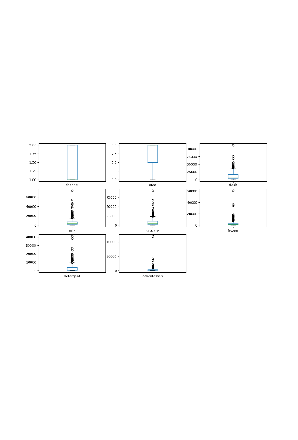
Chapter 14. Quick reference guide
14.3.1.3 Box and Whisker plot
Box and Whisker plots draws a line at the median-value and a box around the 25th and 75th percentiles.
>>> df_whole_sale.plot(kind='box', sharex=False, subplots=True, layout=(3,3))
channel Axes(0.125,0.653529;0.227941x0.226471)
area Axes(0.398529,0.653529;0.227941x0.226471)
fresh Axes(0.672059,0.653529;0.227941x0.226471)
milk Axes(0.125,0.381765;0.227941x0.226471)
grocery Axes(0.398529,0.381765;0.227941x0.226471)
frozen Axes(0.672059,0.381765;0.227941x0.226471)
detergent Axes(0.125,0.11;0.227941x0.226471)
delicatessen Axes(0.398529,0.11;0.227941x0.226471)
dtype: object
>>> plt.show()
Fig. 14.3: Box and Whisker plot of wholesale data
14.3.2 Multivariate plots:
The multivariate plots are the plots which are used to visualize the relationship between two or more data.
14.3.2.1 Scatter plot
Important: Note that we need to convert the numpy-array into Pandas DataFrame for plotting it using Pandas.
This is applicable to both ‘univariate’ and ‘multivariate’ plots
•Below is the code to convert the ‘numpy array’ into ‘DataFrame’,
99 Meher Krishna Patel

14.3. Visualizing the data
>>> from sklearn.datasets import load_iris
>>> iris =load_iris()
>>> features, targets =iris.data, iris.target
>>> type(features)
<class 'numpy.ndarray'>
>>>
>>> import pandas as pd
>>> df_features =pd.DataFrame(features) # convert to DataFrame
>>> type(df_features)
<class 'pandas.core.frame.DataFrame'>
>>> df_features.head()
0 1 2 3
0 5.1 3.5 1.4 0.2
1 4.9 3.0 1.4 0.2
2 4.7 3.2 1.3 0.2
3 4.6 3.1 1.5 0.2
4 5.0 3.6 1.4 0.2
•Now, we can plot the scatter-plot as below,
>>> from pandas.plotting import scatter_matrix
>>> scatter_matrix(df_features)
array([[<matplotlib.axes._subplots.AxesSubplot object at 0xa8166a6c>,
<matplotlib.axes._subplots.AxesSubplot object at 0xa747948c>,
<matplotlib.axes._subplots.AxesSubplot object at 0xa7437f2c>,
<matplotlib.axes._subplots.AxesSubplot object at 0xa745d08c>],
[<matplotlib.axes._subplots.AxesSubplot object at 0xa73ac44c>,
<matplotlib.axes._subplots.AxesSubplot object at 0xa73ac48c>,
<matplotlib.axes._subplots.AxesSubplot object at 0xa73b842c>,
<matplotlib.axes._subplots.AxesSubplot object at 0xa7353acc>],
[<matplotlib.axes._subplots.AxesSubplot object at 0xa73126ac>,
<matplotlib.axes._subplots.AxesSubplot object at 0xa72c6b2c>,
<matplotlib.axes._subplots.AxesSubplot object at 0xa728bd2c>,
<matplotlib.axes._subplots.AxesSubplot object at 0xa723d32c>],
[<matplotlib.axes._subplots.AxesSubplot object at 0xa71fe6ac>,
<matplotlib.axes._subplots.AxesSubplot object at 0xa71b07ec>,
<matplotlib.axes._subplots.AxesSubplot object at 0xa71d24ec>,
<matplotlib.axes._subplots.AxesSubplot object at 0xa71243cc>]],
dtype=object)
>>> plt.show()
Note: We can plot the multicolor ‘Scatter plot’ and ‘Histogram’ as show in Section 12.2, which is easier to
visualize as compare to single color plots.
For colorful scatter_matrix plot, we can use below code,
>>> scatter_matrix(df_features, c=iris.target) # colorful scatter plot
14.3.2.2 Correlation matrix plot
•Below is the code, which plots the correlation values of the data, which is known as correlation-matrix plot,
>>> corr_whole_sale =df_whole_sale[['fresh','milk','grocery','frozen',
... 'detergent','delicatessen']].corr()
>>> plt.matshow(corr_whole_sale)
<matplotlib.image.AxesImage object at 0xa697f64c>
>>> plt.show()
•Also, we can add ‘colorbar’ to see the relationship between the color and the correlation values,
100 PythonDSP
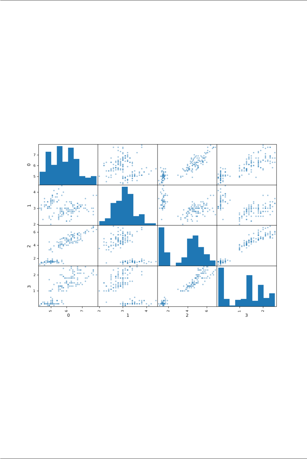
Chapter 14. Quick reference guide
Fig. 14.4: Scatter plot for iris data
101 Meher Krishna Patel
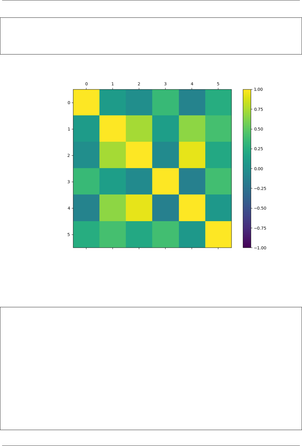
Chapter 14. Quick reference guide
>>> plt.matshow(corr_whole_sale, vmin=-1, vmax=1)
<matplotlib.image.AxesImage object at 0xa5d9270c>
>>> plt.colorbar()
<matplotlib.colorbar.Colorbar object at 0xa5d928ec>
>>> plt.show()
Fig. 14.6: Correlation-matrix plot with ‘colorbar’ for the wholesale data
•Finally, we can add ‘headers’ to the plot so that it will more readable. Below is the complete code for plotting
the data,
>>> import numpy as np
>>> import pandas as pd
>>> import matplotlib.pyplot as plt
>>> # new headers
... header =["channel","area","fresh","milk","grocery",
... "frozen","detergent","delicatessen"]
>>>
>>> # replace existing headers
... df_whole_sale =pd.read_csv("data/Wholesale customers data.csv",
... header=0,# replace existing header; use this or below
... # skiprows=1, # skip the first row i.e. header
... names=header # use new header
... )
>>>
>>>
>>> names =['fresh','milk','grocery','frozen','detergent','delicatessen']
>>> corr_whole_sale =df_whole_sale[names].corr()
>>>
(continues on next page)
103 Meher Krishna Patel
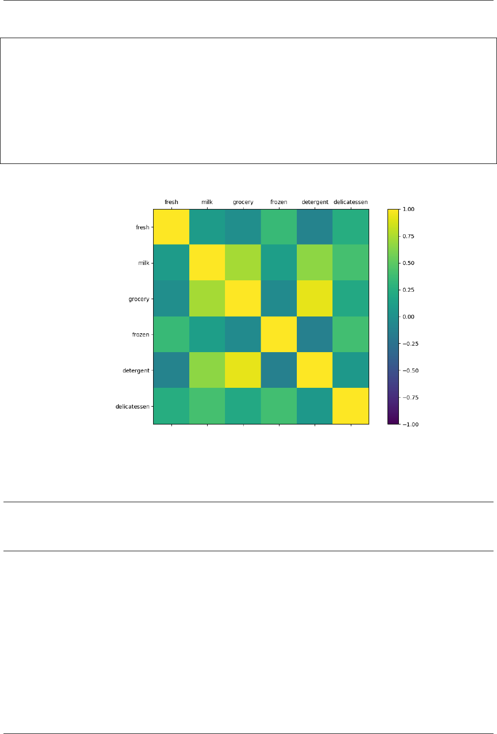
14.4. Preprocessing of the data
(continued from previous page)
>>> # plot the data
>>> fig =plt.figure()
>>> ax =fig.add_subplot(111)
>>> corr_plot =ax.matshow(corr_whole_sale, vmin=-1, vmax=1)
>>> fig.colorbar(corr_plot)
>>> ticks =np.arange(0,6,1)# total 6 items
>>> ax.set_xticks(ticks)
>>> ax.set_yticks(ticks)
>>> ax.set_xticklabels(names)
>>> ax.set_yticklabels(names)
>>> plt.show()
Fig. 14.7: Correlation-matrix plot with ‘colorbar’ and ‘tick-name’ for the wholesale data
Note: From the correlation-matrix plot it is quite clear that the people are buying the ‘grocery’ and ‘detergent’
together.
See Chapter 10 for more details about these relationships, where scatter plot is used to visualize the relationships.
14.4 Preprocessing of the data
In Chapter 8, we saw the examples of preprocessing of the data and saw the performance improvement in the
model. Further, we learn that the some of the algorithm are sensitive to statistics of the features, e.g. PCA
algorithm gives more weight age to the feature which has high variances. In the other words, the feature with high
variance will dominate the performance of the PCA. In this section, we will summarize some of the preprocessing
methods.
104 PythonDSP

Chapter 14. Quick reference guide
14.4.1 Statistics of data
•Let’s read the samples from the ‘Whole sale data’ first, and we will preprocess this data in this section,
>>> import pandas as pd
>>>
>>> # new headers
... header =["channel","area","fresh","milk","grocery",
... "frozen","detergent","delicatessen"]
>>>
>>> # replace existing headers
... df_whole_sale =pd.read_csv("data/Wholesale customers data.csv",
... header=0,# replace existing header; use this or below
... # skiprows=1, # skip the first row i.e. header
... names=header # use new header
... )
•Next see the mean and variance of the each features,
>>> # mean and variance
... import numpy as np
>>> np.mean(df_whole_sale)
channel 1.322727
area 2.543182
fresh 12000.297727
milk 5796.265909
grocery 7951.277273
frozen 3071.931818
detergent 2881.493182
delicatessen 1524.870455
dtype: float64
>>>
>>> np.var(df_whole_sale)
channel 2.185744e-01
area 5.981353e-01
fresh 1.595914e+08
milk 5.434617e+07
grocery 9.010485e+07
frozen 2.351429e+07
detergent 2.268077e+07
delicatessen 7.934923e+06
dtype: float64
14.4.2 StandardScaler
We used the ‘StandardScaler’ in Chapter 8 and saw the performance improvement in the model with it. It sets
the ‘mean = 0’ and ‘variance = 1’ for all the features,
•Now, process the data using StandardScaler,
>>> # preprocessing StandardScaler : mean=0, var=1
... from sklearn.preprocessing import StandardScaler
>>> scaler =StandardScaler().fit(df_whole_sale)
>>> df_temp =scaler.transform(df_whole_sale)
Also, we can combine the above two steps (i.e. fit and transform) into one step as below,
>>> # preprocessing StandardScaler : mean=0, var=1
... from sklearn.preprocessing import StandardScaler
>>> df_temp =StandardScaler().fit_transform(df_whole_sale)
105 Meher Krishna Patel

14.4. Preprocessing of the data
•Note that the type of the ‘df_temp’ is ‘numpy.ndarray’, therefore we need to loop through each column
to calculate mean and variance as shown below,
>>> type(df_temp) # numpy array
<class 'numpy.ndarray'>
>>>
>>> # mean and var of each column
... for iin range(df_temp.shape[1]):
... print("row {0}: mean={1:<5.2f} var={2:<5.2f}".format(i,
... np.mean(df_temp[:,i]),
... np.var(df_temp[:,i])
... )
... )
...
row 0: mean=0.00 var=1.00
row 1: mean=0.00 var=1.00
row 2: mean=-0.00 var=1.00
row 3: mean=-0.00 var=1.00
row 4: mean=-0.00 var=1.00
row 5: mean=0.00 var=1.00
row 6: mean=0.00 var=1.00
row 7: mean=-0.00 var=1.00
•Also, we can convert the numpy-array to Pandas-DataFrame and then calculate the mean and variance,
>>> # convert numpy-array to Pandas-dataframe
... df =pd.DataFrame(df_temp, columns=header)
>>>
>>> type(df) # Pandas DataFrame
<class 'pandas.core.frame.DataFrame'>
>>>
>>> np.mean(df) # mean = 0
channel -2.523234e-18
area 2.828545e-16
fresh -3.727684e-17
milk -8.815549e-18
grocery -5.197665e-17
frozen 3.587724e-17
detergent 2.618250e-17
delicatessen -2.508450e-18
dtype: float64
>>>
>>> np.var(df)
channel 1.0
area 1.0
fresh 1.0
milk 1.0
grocery 1.0
frozen 1.0
detergent 1.0
delicatessen 1.0
dtype: float64
14.4.3 MinMax scaler
MinMax scaler scales the features in the range (0 to 1) i.e. minimum and maximum values are scaled to 0 and 1
respectively.
>>> from sklearn.preprocessing import MinMaxScaler
>>> df_temp =MinMaxScaler().fit_transform(df_whole_sale)
>>> df =pd.DataFrame(df_temp, columns=header)
(continues on next page)
106 PythonDSP

Chapter 14. Quick reference guide
(continued from previous page)
>>> np.min(df)
channel 0.0
area 0.0
fresh 0.0
milk 0.0
grocery 0.0
frozen 0.0
detergent 0.0
delicatessen 0.0
dtype: float64
>>> np.max(df)
channel 1.0
area 1.0
fresh 1.0
milk 1.0
grocery 1.0
frozen 1.0
detergent 1.0
delicatessen 1.0
dtype: float64
14.4.4 Normalizer
Normalizer process the row such that the sum of each row is ‘1’, as shown in below code,
>>> from sklearn.preprocessing import Normalizer
>>> df_temp =Normalizer().fit_transform(df_whole_sale)
>>> df =pd.DataFrame(df_temp, columns=header)
>>> # check the sum of each row
>>> for iin range(df_temp.shape[0]):
... print("row {0}: sum={1:0.2f}".format(
... i, # row number
... np.sqrt(np.cumsum(df_temp[i,:]**2)[-1])
... )
... )
...
row 0: sum=1.00
row 1: sum=1.00
row 2: sum=1.00
row 3: sum=1.00
row 4: sum=1.00
row 5: sum=1.00
[...]
14.5 Feature selection
In Chatper 7, we saw an example of feature selection, where the PCA analysis is done to reduce the dimension of
the features.
Note: While collecting the data, our aim is to collect the data without thinking the relationship between the
‘features’ and the ‘targets’. It is possible that some of these data has no impact on the target e.g. ‘First name’ of
the person has no relationship with the ‘chronic kidney disease’. If we use this feature, i.e. First name, to predict
the ‘chronic kidney disease’, then we will have the wrong results.
Feature selection is the process of ‘removing’ or ‘giving less weight’ to irrelevant or partially relevant features. In
this way we can achieve following,
107 Meher Krishna Patel

14.5. Feature selection
1. Reduce overfitting: as the partially relevant data is removed from the dataset.
2. Reduce training time: as we have less features after feature selection.
14.5.1 SelectKBest
The ‘SelectKBest’ class can be used to find the best ‘K’ features from the dataset. In the below code, the
‘new_features’ contains the last two columns of the ‘features’,
>>> from sklearn.datasets import load_iris
>>> iris =load_iris()
>>> features, targets =iris.data, iris.target
>>>
>>> from sklearn.feature_selection import SelectKBest
>>> selector =SelectKBest(k=2)
>>> selector.fit(features, targets)
SelectKBest(k=2, score_func=<function f_classif at 0xb3cd49bc>)
>>> new_features =selector.transform(features)
>>> print(new_features[0:5, :]) # selected last 2 columns
[[ 1.4 0.2]
[ 1.4 0.2]
[ 1.3 0.2]
[ 1.5 0.2]
[ 1.4 0.2]]
>>> print(features[0:5, :])
[[ 5.1 3.5 1.4 0.2]
[ 4.9 3. 1.4 0.2]
[ 4.7 3.2 1.3 0.2]
[ 4.6 3.1 1.5 0.2]
[ 5. 3.6 1.4 0.2]]
14.5.2 Recursive Feature Elimination (RFE)
RFE recursively checks the accuracy of the model and removes attributes which result in lower accuracy,
>>> from sklearn.datasets import load_iris
>>> iris =load_iris()
>>> features, targets =iris.data, iris.target
>>>
>>> from sklearn.linear_model import LogisticRegression
>>> from sklearn.feature_selection import RFE
>>> model =LogisticRegression()
>>> selector =RFE(model, 2)
>>> fit =selector.fit(features, targets)
>>> new_features =fit.transform(features)
>>> print(new_features[0:5, :]) # selected 2nd and 4th column
[[ 3.5 0.2]
[ 3. 0.2]
[ 3.2 0.2]
[ 3.1 0.2]
[ 3.6 0.2]]
>>> print(features[0:5, :])
[[ 5.1 3.5 1.4 0.2]
[ 4.9 3. 1.4 0.2]
[ 4.7 3.2 1.3 0.2]
[ 4.6 3.1 1.5 0.2]
[ 5. 3.6 1.4 0.2]]
108 PythonDSP

Chapter 14. Quick reference guide
14.5.3 Principal component analysis (PCA)
Please see the Chatper 7 where PCA is discussed in detail. Note that, it does not select the features but transform
the features.
14.6 Algorithms
In this section, we will see some of the widely use algorithms for the ‘classification’ and ‘regression’ problems.
Important: Note that all the models do not work well in all the cases. Therefore, we need to check the
performance of various machine learning algorithms before finalizing the model.
14.6.1 Classification algorithms
Table 14.2 shows some of the widely used classification algorithms. We already see the examples of ‘Logistic
Regression (Chapter 3)’, ‘K-nearest neighbor (Chapter 2)’ and ‘SVM (Chapter 11)’. In this section we will discuss
LDA, Naive Bayes and Regression tree algorithms.
Table 14.2: Classification algorithms
Type Algorithm
Linear Logistic Regression, Linear Discriminant Analysis (LDA)
Non-linear K-nearest neighbor, Support vector machines (SVM),
Naive Bayes, Decision Tree
14.6.1.1 Linear Discriminant Analysis (LDA)
The below code is same as Listing 3.4 but LDA is used instead of ‘K-nearest’ and ‘LogisticRegression’ algorithms,
1# rock_mine2.py
2
3#'R': Rock, 'M': Mine
4
5import numpy as np
6from sklearn.metrics import accuracy_score
7from sklearn.model_selection import train_test_split
8from sklearn.discriminant_analysis import LinearDiscriminantAnalysis
9
10 f=open("data/sonar.all-data",'r')
11 data =f.read()
12 f.close()
13
14 data =data.split() # split on \n
15
16 # save data as list i.e. list of list will be created
17 data_list =[]
18 for din data:
19 # split on comma
20 row =d.split(",")
21 data_list.append(row)
22
23 # extract targets
24 row_sample, col_sample =len(data_list), len(data_list[0])
25
26 # features : last column i.e. target value will be removed form the dataset
(continues on next page)
109 Meher Krishna Patel

14.6. Algorithms
(continued from previous page)
27 features =np.zeros((row_sample, col_sample-1), float)
28 # target : store only last column
29 targets =[] # targets are 'R'and 'M'
30
31 for i, data in enumerate(data_list):
32 targets.append(data[-1])
33 features[i] =data[:-1]
34 # print(targets)
35 # print(features)
36
37 # split the training and test data
38 train_features, test_features, train_targets, test_targets =train_test_split(
39 features, targets,
40 train_size=0.8,
41 test_size=0.2,
42 # random but same for all run, also accuracy depends on the
43 # selection of data e.g. if we put 10 then accuracy will be 1.0
44 # in this example
45 random_state=23,
46 # keep same proportion of 'target'in test and target data
47 stratify=targets
48 )
49
50 # select classifier
51 classifier =LinearDiscriminantAnalysis()
52
53 # training using 'training data'
54 classifier.fit(train_features, train_targets) # fit the model for training data
55
56 # predict the 'target'for 'training data'
57 prediction_training_targets =classifier.predict(train_features)
58 self_accuracy =accuracy_score(train_targets, prediction_training_targets)
59 print("Accuracy for training data (self accuracy):", self_accuracy)
60
61 # predict the 'target'for 'test data'
62 prediction_test_targets =classifier.predict(test_features)
63 test_accuracy =accuracy_score(test_targets, prediction_test_targets)
64 print("Accuracy for test data:", test_accuracy)
•Below is the results for above code,
$ python rock_mine2.py
Accuracy for training data (self accuracy): 0.885542168675
Accuracy for test data: 0.809523809524
Note: Both LogisticRegression and LinearDiscriminantAnalysis algorithms assume that input features have
Gaussian distributions.
14.6.1.2 Naive Bayes
It assumes that all the features are independent of each other and have Gaussian distribution. Below is the example
of the Naive Bayes algorithm,
# multiclass_ex.py
import numpy as np
from sklearn.datasets import load_iris
(continues on next page)
110 PythonDSP

Chapter 14. Quick reference guide
(continued from previous page)
from sklearn.naive_bayes import GaussianNB
from sklearn.model_selection import cross_val_score
# create object of class 'load_iris'
iris =load_iris()
# save features and targets from the 'iris'
features, targets =iris.data, iris.target
# select classifier
classifier =GaussianNB()
# cross-validation
scores =cross_val_score(classifier, features, targets, cv=3)
print("Cross validation scores:", scores)
print("Mean score:", np.mean(scores))
•Below is the results for above code,
$ python multiclass_ex.py
Cross validation scores: [ 0.92156863 0.90196078 0.97916667]
Mean score: 0.934232026144
14.6.1.3 Decision Tree Classifier
It creates a binary decision tree from the training data to minimize the cost function,
# multiclass_ex.py
import numpy as np
from sklearn.datasets import load_iris
from sklearn.tree import DecisionTreeClassifier
from sklearn.model_selection import cross_val_score
# create object of class 'load_iris'
iris =load_iris()
# save features and targets from the 'iris'
features, targets =iris.data, iris.target
# select classifier
classifier =DecisionTreeClassifier()
# cross-validation
scores =cross_val_score(classifier, features, targets, cv=3)
print("Cross validation scores:", scores)
print("Mean score:", np.mean(scores))
•Below is the output for above code,
$ python multiclass_ex.py
Cross validation scores: [ 0.98039216 0.92156863 1.]
Mean score: 0.96732026143
14.6.2 Regression algorithms
Table 14.3 shows some of the widely used regression algorithms. We already see the examples of ‘Linear regression
(Chapter 3)’. Also we saw the examples of ‘K-nearest neighbor (Chapter 2)’, ‘SVM (Chapter 11)’ and Decision Tree
111 Meher Krishna Patel

14.6. Algorithms
(Section 14.6.1.3) for ‘classification problems; in this section we will use these algorithms for regression problems.
Further, we will discuss ‘Ridge’, ‘LASSO’ and ‘Elastic-net’ algorithms.
Table 14.3: Regression algorithms
Type Algorithm
Linear Linear regression, Ridge, LASSO, Elastic-net
Non-linear K-nearest neighbor, Support vector machines (SVM), Decision Tree
14.6.2.1 Ridge regression
It is the extended version of the Linear regression, where the ridge coefficients minimize a penalized residual sum
of square known as L2 norm.
1# regression_ex.py
2
3import numpy as np
4from sklearn.model_selection import train_test_split
5from sklearn.linear_model import Ridge
6
7N=100 # 100 samples
8x=np.linspace(-3,3, N) # coordinates
9noise_sample =np.random.RandomState(20)# constant random value
10 # growing sinusoid with random fluctuation
11 sine_wave =x+np.sin(4*x) +noise_sample.uniform(N)
12
13 # convert features in 2D format i.e. list of list
14 features =x[:, np.newaxis]
15
16 # save sine wave in variable 'targets'
17 targets =sine_wave
18
19 # split the training and test data
20 train_features, test_features, train_targets, test_targets =train_test_split(
21 features, targets,
22 train_size=0.8,
23 test_size=0.2,
24 # random but same for all run, also accuracy depends on the
25 # selection of data e.g. if we put 10 then accuracy will be 1.0
26 # in this example
27 random_state=23,
28 # keep same proportion of 'target'in test and target data
29 # stratify=targets # can not used for single feature
30 )
31
32 # training using 'training data'
33 regressor =Ridge()
34 regressor.fit(train_features, train_targets) # fit the model for training data
35
36 # predict the 'target'for 'test data'
37 prediction_test_targets =regressor.predict(test_features)
38 test_accuracy =regressor.score(test_features, test_targets)
39 print("Accuracy for test data:", test_accuracy)
•Below is the output for above code,
$ python regression_ex.py
Accuracy for test data: 0.82273039102
112 PythonDSP

Chapter 14. Quick reference guide
14.6.2.2 LASSO regression
It is the extended version of the Linear regression, where the ridge coefficients minimize the sum of absolute values
which is known as L1 norm.
1# regression_ex.py
2
3import numpy as np
4from sklearn.model_selection import train_test_split
5from sklearn.linear_model import Lasso
6
7N=100 # 100 samples
8x=np.linspace(-3,3, N) # coordinates
9noise_sample =np.random.RandomState(20)# constant random value
10 # growing sinusoid with random fluctuation
11 sine_wave =x+np.sin(4*x) +noise_sample.uniform(N)
12
13 # convert features in 2D format i.e. list of list
14 features =x[:, np.newaxis]
15
16 # save sine wave in variable 'targets'
17 targets =sine_wave
18
19 # split the training and test data
20 train_features, test_features, train_targets, test_targets =train_test_split(
21 features, targets,
22 train_size=0.8,
23 test_size=0.2,
24 # random but same for all run, also accuracy depends on the
25 # selection of data e.g. if we put 10 then accuracy will be 1.0
26 # in this example
27 random_state=23,
28 # keep same proportion of 'target'in test and target data
29 # stratify=targets # can not used for single feature
30 )
31
32 # training using 'training data'
33 regressor =Lasso()
34 regressor.fit(train_features, train_targets) # fit the model for training data
35
36 # predict the 'target'for 'test data'
37 prediction_test_targets =regressor.predict(test_features)
38 test_accuracy =regressor.score(test_features, test_targets)
39 print("Accuracy for test data:", test_accuracy)
•Below is the output for above code,
$ python regression_ex.py
Accuracy for test data: 0.70974672729
14.6.2.3 Elastic-net regression
It minimizes both the L1 norm and L2 norm,
1# regression_ex.py
2
3import numpy as np
4from sklearn.model_selection import train_test_split
5from sklearn.linear_model import ElasticNet
6
7N=100 # 100 samples
(continues on next page)
113 Meher Krishna Patel

14.6. Algorithms
(continued from previous page)
8x=np.linspace(-3,3, N) # coordinates
9noise_sample =np.random.RandomState(20)# constant random value
10 # growing sinusoid with random fluctuation
11 sine_wave =x+np.sin(4*x) +noise_sample.uniform(N)
12
13 # convert features in 2D format i.e. list of list
14 features =x[:, np.newaxis]
15
16 # save sine wave in variable 'targets'
17 targets =sine_wave
18
19 # split the training and test data
20 train_features, test_features, train_targets, test_targets =train_test_split(
21 features, targets,
22 train_size=0.8,
23 test_size=0.2,
24 # random but same for all run, also accuracy depends on the
25 # selection of data e.g. if we put 10 then accuracy will be 1.0
26 # in this example
27 random_state=23,
28 # keep same proportion of 'target'in test and target data
29 # stratify=targets # can not used for single feature
30 )
31
32 # training using 'training data'
33 regressor =ElasticNet()
34 regressor.fit(train_features, train_targets) # fit the model for training data
35
36 # predict the 'target'for 'test data'
37 prediction_test_targets =regressor.predict(test_features)
38 test_accuracy =regressor.score(test_features, test_targets)
39 print("Accuracy for test data:", test_accuracy)
•Below is the output for above code,
$ python regression_ex.py
Accuracy for test data: 0.744348295083
14.6.2.4 Support vector machines (SVM)
Note: Note that SVR is used for regression problem, whereas SVC was used in classification problem. Same is
applicable for ‘Decision tree’ and ‘K-nearest neighbor’ algorithms.
1# regression_ex.py
2
3import numpy as np
4from sklearn.model_selection import train_test_split
5from sklearn.svm import SVR
6
7N=100 # 100 samples
8x=np.linspace(-3,3, N) # coordinates
9noise_sample =np.random.RandomState(20)# constant random value
10 # growing sinusoid with random fluctuation
11 sine_wave =x+np.sin(4*x) +noise_sample.uniform(N)
12
13 # convert features in 2D format i.e. list of list
14 features =x[:, np.newaxis]
(continues on next page)
114 PythonDSP

Chapter 14. Quick reference guide
(continued from previous page)
15
16 # save sine wave in variable 'targets'
17 targets =sine_wave
18
19 # split the training and test data
20 train_features, test_features, train_targets, test_targets =train_test_split(
21 features, targets,
22 train_size=0.8,
23 test_size=0.2,
24 # random but same for all run, also accuracy depends on the
25 # selection of data e.g. if we put 10 then accuracy will be 1.0
26 # in this example
27 random_state=23,
28 # keep same proportion of 'target'in test and target data
29 # stratify=targets # can not used for single feature
30 )
31
32 # training using 'training data'
33 regressor =SVR()
34 regressor.fit(train_features, train_targets) # fit the model for training data
35
36 # predict the 'target'for 'test data'
37 prediction_test_targets =regressor.predict(test_features)
38 test_accuracy =regressor.score(test_features, test_targets)
39 print("Accuracy for test data:", test_accuracy)
•Below is the output for above code,
$ python regression_ex.py
Accuracy for test data: 0.961088256595
14.6.2.5 Decision tree regression
1# regression_ex.py
2
3import numpy as np
4from sklearn.model_selection import train_test_split
5from sklearn.tree import DecisionTreeRegressor
6
7N=100 # 100 samples
8x=np.linspace(-3,3, N) # coordinates
9noise_sample =np.random.RandomState(20)# constant random value
10 # growing sinusoid with random fluctuation
11 sine_wave =x+np.sin(4*x) +noise_sample.uniform(N)
12
13 # convert features in 2D format i.e. list of list
14 features =x[:, np.newaxis]
15
16 # save sine wave in variable 'targets'
17 targets =sine_wave
18
19 # split the training and test data
20 train_features, test_features, train_targets, test_targets =train_test_split(
21 features, targets,
22 train_size=0.8,
23 test_size=0.2,
24 # random but same for all run, also accuracy depends on the
25 # selection of data e.g. if we put 10 then accuracy will be 1.0
26 # in this example
(continues on next page)
115 Meher Krishna Patel

14.6. Algorithms
(continued from previous page)
27 random_state=23,
28 # keep same proportion of 'target'in test and target data
29 # stratify=targets # can not used for single feature
30 )
31
32 # training using 'training data'
33 regressor =DecisionTreeRegressor()
34 regressor.fit(train_features, train_targets) # fit the model for training data
35
36 # predict the 'target'for 'test data'
37 prediction_test_targets =regressor.predict(test_features)
38 test_accuracy =regressor.score(test_features, test_targets)
39 print("Accuracy for test data:", test_accuracy)
•Below is the output for above code,
$ python regression_ex.py
Accuracy for test data: 0.991442971888
14.6.2.6 K-nearest neighbor regression
1# regression_ex.py
2
3import numpy as np
4from sklearn.model_selection import train_test_split
5from sklearn.neighbors import KNeighborsRegressor
6
7N=100 # 100 samples
8x=np.linspace(-3,3, N) # coordinates
9noise_sample =np.random.RandomState(20)# constant random value
10 # growing sinusoid with random fluctuation
11 sine_wave =x+np.sin(4*x) +noise_sample.uniform(N)
12
13 # convert features in 2D format i.e. list of list
14 features =x[:, np.newaxis]
15
16 # save sine wave in variable 'targets'
17 targets =sine_wave
18
19 # split the training and test data
20 train_features, test_features, train_targets, test_targets =train_test_split(
21 features, targets,
22 train_size=0.8,
23 test_size=0.2,
24 # random but same for all run, also accuracy depends on the
25 # selection of data e.g. if we put 10 then accuracy will be 1.0
26 # in this example
27 random_state=23,
28 # keep same proportion of 'target'in test and target data
29 # stratify=targets # can not used for single feature
30 )
31
32 # training using 'training data'
33 regressor =KNeighborsRegressor()
34 regressor.fit(train_features, train_targets) # fit the model for training data
35
36 # predict the 'target'for 'test data'
37 prediction_test_targets =regressor.predict(test_features)
38 test_accuracy =regressor.score(test_features, test_targets)
39 print("Accuracy for test data:", test_accuracy)
116 PythonDSP

Chapter 14. Quick reference guide
•Below is the output for above code,
$ python regression_ex.py
Accuracy for test data: 0.991613506388
117 Meher Krishna Patel


