Magnetism Guide

User Manual:

Open the PDF directly: View PDF .
Page Count: 39

Preface
Terminology
Variables
Equations

Last modiﬁed April 25, 2019

Galactic Magnetism PhD Study Guide

Jessica Campbell, Dunlap Institute for Astronomy & Astrophysics (UofT)

Contents

1 Preface 1

2 Terminology 2

3 Variables 30

4 Equations 33

1 Preface

The interstellar medium (ISM) is a complex environment of gas and dust with varying degrees of ion-

ization, densities, and spatial distributions called phases. It accounts for ∼10 −15% of the mass and

1−2% of the volume of our Galaxy. From the largest of Galactic scales to the smallest scales of star and

planet formation, this tenuous plasma is threaded with magnetic ﬁeld lines and exhibits large degrees of

turbulence, both of which are believed to be major driving forces in shaping the structure and dynamics

of our Galaxy. These magnetic ﬁelds, along with cosmic rays, exert outward pressures on the ISM which

are counterbalanced by the gravitational attraction provided by the ordinary matter. The ordinary mat-

ter, cosmic rays, and magnetic ﬁelds are therefore in a state of pressure equilibrium. Turbulence is an

important aspect of the ISM as it not only transports energy from large (∼kpc) to small (∼pc) scales,

but also ampliﬁes magnetic ﬁelds and accelerates cosmic rays, explaining the observed µG magnetic ﬁeld

strengths as well as the ∼GeV cosmic ray energies in our Galaxy. Turbulence itself is a complex non-

linear ﬂuid phenomenon which results in an extreme range of correlated spatial and temporal scales in

the multi-phase ISM, and is driven by a variety of large- and small-scale energy sources. While magnetic

ﬁelds and turbulence are generally understood to play fundamental roles in shaping the structure and

dynamics of our Galaxy, the degree to which they do so across diﬀerent phases and spatial scales of the

ISM remains poorly understood.

Galactic Magnetism Study Guide Page 1 / 39

2 Terminology

Advection: The transport of a substance by bulk motion.

Advection operator:

Alfv´en Mach number: A commonly used parameter of turbulence used to obtain information on gas

compressibility and magnetization given by

MA≡|~v|

where |~v|is the local velocity and vAis the Alfv´en speed.

Alfv´en speed (vA): Given by

vA=|~

4πρn

[m s−1],

where |~

B|is the magnetic ﬁeld strength and ρis the density of neutral particles. When the Alfv´en speed

is greater than the sound speed, the fast and Alfv´en wave families are damped at or below the ambipolar

diﬀusion scale LAD; when the Alfv´en speed is less than the sound speed, the slow and Alfv´en wave

families are damped.

Alfv´en wave: In 1942, Hannes Alfv´en combined the mathematics of ﬂuid mechanics and electromag-

netism to predict that plasmas could support wave-like variation in the magnetic ﬁeld, a wave phenomenon

that now bears his name, Alfv´en waves. These are a type of magnetohydrodynamic (MHD) wave in which

ions oscillate in response to a restoring force provided by an eﬀective tension on the magnetic ﬁeld lines.

The waves initially proposed by Alfv´en are considered “basic”. They have a characteristic that they are

compressional, which means that magnetic ﬁeld variation of the Alfv´en waves is in the direction of the

wave motion. Charged particles moving through a plasma with these waves have very little alteration

of their trajectory. But Alfv´en waves can exhibit more variety. A variant is the “kinetic” Alfv´en wave

which is transverse, with strong magnetic ﬁeld variation perpendicular to the wave motion, so can trade

energy between the diﬀerent frequencies which might propagate through a plasma. This also means it

can exchange energy with the particles in the plasma, in some cases, trapping particles in the troughs of

the waves and carrying them along.

Ambipolar diﬀusion: Also known as ion-neutral drift or ion-neutral friction. In many situations, ideal

MHD is not a suﬃciently good assumption and additional eﬀects need to be accounted for. In many

contexts, the dominant correction is the so-called ambipolar diﬀusion. Since the neutrals are not charged

they are not subject to the Lorentz force which applies only on the ions. However, through collisions

the neutrals and the ions exchange momentum and therefore the Lorentz force has an inﬂuence on the

neutrals through the ions. If the number of ions is large (i.e., if the ionization is high) the number of

collisions is expected to be large and ideal MHD remains a good approximation. However in regions

like molecular clouds, the ionization is usually of the order of 10−7and therefore the two ﬂuids are not

perfectly coupled. The ions drag the ﬁeld lines and drift with respect to the neutrals implying that the

latter can cross the ﬁeld lines. The ﬁeld is not frozen in the gas anymore. The drift of neutral particles

towards the central gravitational potential through the ionized particles tied to the magnetic ﬁeld. This is

often invoked as a source of dissipation of the MHD energy cascade. The scale at which ions and neutral

particles decouple is called the ambipolar diﬀusion scale. The application of ambipolar diﬀusion extends

beyond direct studies of star formation and to include general studies of magnetic ﬁelds. Ambipolar

diﬀusion has been proposed to damp particular families of MHD waves.

Ambipolar diﬀusion scale (LAD): The scale at which ions and neutral particles decouple through

the process of ambipolar diﬀusion. It can be estimated as the scale at which the Reynolds number, with

diﬀusivity given by ambipolar diﬀusivity, is equal to unity. The ambipolar diﬀusion scale has been thought

to set the dissipation scale of turbulence in molecular clouds and set a fundamental characteristic scale

for gravitational collapse in star formation. When the Alfv´en speed is greater than the sound speed, the

fast and Alfv´en wave families are damped at or below the ambipolar diﬀusion scale LAD; when the Alfv´en

speed is less than the sound speed, the slow and Alfv´en wave families are damped. On scales larger than

LAD, it was also predicted that two-ﬂuid turbulence (ion-neutral) acts like single-ﬂuid MHD turbulence.

The ambipolar diﬀusivity is given by

νAD =B2

4πρiρnα[mss−1],

where ρiand ρnare the density of the ions and neutrals, respectively, Bis the magnetic ﬁeld strength,

and αis the frictional coupling coeﬃcient between the ions and neutrals. The Reynolds number for

ion-neutral drift is deﬁned as

Galactic Magnetism Study Guide Page 2 / 39

RAD =LV

νAD

[dimensionless],

where Vis a characteristic velocity (e.g., for trans-Alfv´enic turbulence it is the Alfv´en speed,vA=B

4πρn

)

and L=LAD when RAD = 1. This gives the form of the ambipolar diﬀusion scale as often found in the

literature:

LAD =VA

αρi

[m].

It has been shown that the plane-of-sky magnetic ﬁeld can be estimated using the ambipolar diﬀusion

length scale.

Autocorrelation: The correlation of a signal with a delayed copy of itself as a function of delay.

Informally, it is the similarity between observations as a function of the time lag between them. The

autocorrelation of an observable Awith position rand position increment δr is given by

C(δr) = hf(r)f(r+δr)i[dimensionless].

Axi-symmetric spiral (ASS) model:

Azimuthal magnetic ﬁeld ( ~

Bθ): Often the Galactic magnetic ﬁeld is expressed in cylindrical coordi-

nates (θ, r, z). The azimuthal component ( ~

Bθ) dominates the Galactic disk where the radial ( ~

Br) and

vertical ( ~

Bz) components are generally weak.

Balbus-Hawley instability: See magnetorotational instability.

Bandwidth depolarization: A type of external depolarization where the polarization vector is sub-

stantially rotated within the observing bandwidth if the Faraday depth is large enough.

Beam depolarization: A type of external depolarization due to ﬂuctuations in the foreground screen

within the observing beam: unresolved density or magnetic ﬁeld inhomogeneities of the media through

which the radiation propagates induces unresolved spatial variations in the Faraday rotation measure.

Biermann battery mechanism: The process by which a weak seed magnetic ﬁeld can be produced from

zero magnetic ﬁeld initial conditions via perpendicular density and temperature gradients. The Biermann

mechanism can explain the generation of a ∼10−20 G ﬁeld after recombination, but it is questionable

whether turbulent dynamo growth alone can explain ampliﬁcation up to the 10 µG ﬁelds seen today

throughout the ISM. A possible solution to this problem may be provided by the potential role played by

kinetic instabilities in the ampliﬁcation of magnetic ﬁelds. One such instability is the Weibel instability.

Temperature gradients form perpendicular to astrophysical shocks (hotter in the center of the shock),

while density gradients form parallel to the shock, once again allowing the Biermann battery to take place.

The Biermann mechanism is also the presumed cause of self-generated magnetic ﬁelds (∼106G) found

in laser-solid interaction experiments. The laser generates an expanding bubble of plasma by hitting and

ionizing a solid foil of metal or plastic. This bubble thus has a temperature gradient perpendicular to

the beam (hottest closest to the beam axis), and a density gradient in the direction normal to the foil,

allowing for the Biermann battery mechanism to take place. Assuming a two-ﬂuid description of a plasma

with massless electrons, the magnetic ﬁeld evolution is given by the generalized induction equation:

∂~

∂t =∇ × (~v ×~

B) + ηc2

4π∇2~

B−1

en∇ × (~

j×~

B)−c

ne∇n× ∇Te,

which shows the evolution of magnetic ﬁeld ~

B, based on the ﬂuid velocity ~v, the current density ~

c∇ × ~

B/4π, the number density n, and the electron temperature Te=Pe/n, where Peis the electron

plasma pressure. Here, cis the speed of light, ηis the resistivity, and eis the charge of an electron. The

terms on the RHS from left to right are the convective term, the resistive term, the Hall term, and the

Biermann battery term. Starting with ~

B= 0, all terms on the RHS except for the Biermann term can

be ignored, and thus ~

Bgrows linearly. Based on scaling, given Te=mev2

th, we ﬁnd

B(t)≈mec

LTLn

t[G],

where Lis more precisely deﬁned by the length of the gradients (Ln≡n/∇n,LT≡Te/∇Te, which can

be assumed to be approximately comparable).

Birefringence: The optical property of a medium to have a refractive index that is dependent on the

polarization and direction of propagation of light. Birefringence implies that there are two natural wave

modes which may be described by their polarizations, which are necessarily orthogonal to each other, and

by ∆k, the diﬀerence in their wavenumbers. The magnetoionic medium is an example of such a medium

as the polarization angle of light becomes rotated as it propagates via Faraday rotation as a function of

frequency.

Galactic Magnetism Study Guide Page 3 / 39

Bi-symmetric spiral (BSS) model:

Bonnor-Ebert sphere:

Bremsstrahlung radiation: Also known as “braking radiation”. This radiation is produced by the

deceleration of a charged particle after being deﬂected by another charged particle, typically an electron

by an atomic nucleus. The particle being deﬂected loses energy which is lost via radiation of a photon. For

example, when free electrons within an HII region pass near a positive ion (H+, He+) they are accelerated

by the Coulomb ﬁeld and emit bremsstrahlung radiation. Bremsstrahlung emission is a source of polarized

continuum radiation and is a type of free-free radiation.

βparameter: The squared ratio of the sound speed to the Alfv´ens speen:

β≡c2

[dimensionless].

Cascade rate:

Central molecular zone (CMZ): The inner ∼500 pc of the Galaxy which contains .10% of the

MW’s molecular gas but ∼80% of the dense (n&103cm−3) gas: a reservoir of 2 −6×107Mof

molecular material. The physical properties of the ISM in the CMZ diﬀer substantially from those in

the disc. Gas column and volume densities can be ∼2 orders of magnitude greater, velocity dispersions

measured for a given physical size are larger, and although there exists a signiﬁcant fraction of cold dust,

gas temperatures can range from 50 −400 K.

Chandrasekhar-Fermi method: Originally proposed by Chandrasekhar & Fermi (1953) to estimate

the ﬁeld strength in spiral arms, the Chandrasekhar-Fermi method uses starlight polarization to estimate

the average ﬁeld strength hBiin a region. The method relates the line-of-sight velocity dispersion to

the dispersion of starlight polarization angles about a mean component. Assuming that turbulence

isotropically randomizes the magnetic ﬁeld in the region, the mean ﬁeld strength is given by

CF ≡¯

B2=ξ4πρ σ(vlos)2

σ(tan(δ∗))2,

where

δ∗≡θ∗−¯

θ∗,

ρis the gas density, θ∗is the mean starlight polarization angle, and ξis a correction factor representing

the ratio of turbulent magnetic to turbulent kinetic energy. The validity of the method depends critically

on the presence of a signiﬁcant mean ﬁeld component.

Chaotic system:

Coherent magnetic ﬁeld: See ordered magnetic ﬁeld.

Cold neutral medium (CNM): A thermally-stable phase of the atomic ISM with a typical density and

kinetic temperature of n∼7−70 cm−3and TK∼60 −260 K, respectively. It seems almost certain that

the CNM transitions to the DMM before transitioning to the classical MM. Our current knowledge of

physical conditions and morphology in the CNM depends overwhelmingly on results from the Millennium

survey of Heiles & Troland (2005), who used Arecibo with long integration times suitable for detecting

Zeeman splitting. For the HI line in absorption, they derived column densities, temperatures, turbulent

Mach number, and magnetic ﬁelds. HI CNM column densities are usually below 1020 cm−2with a

median value N(HI) ∼0.5×1020 cm−2. The median spin temperature is Ts∼50 K, median turbulent

Mach number is Ms∼3.7, and median magnetic ﬁeld is ∼6µG. By assuming reasonable values for

the thermal gas pressure and comparing observed column densities, shapes and angular sizes as seen

on the sky, Heiles & Troland (2003) ﬁnd that interstellar CNM structures cannot be characterized as

isotropic. The major argument is that a reasonable interstellar pressure, combined with the measured

kinetic temperature, determines the volume density; this, combined with the observed column density,

determines the thickness of the cloud along the line of sight. This dimension is almost always much

smaller than the linear sizes inferred from the angular sizes seen on the sky. They characterize the typical

structures as “blobby sheets”, which applies for angular scales of arcseconds to degrees.

It has been shown by numerical studies that CNM can be formed in a shock-compressed layer of the

WNM.

Complex conjugate (f(x)∗or ¯

f(x)): The number with an equal real part and an imaginary part equal

in magnitude but opposite in sign.

Compressible turbulence:

Compton scattering: The inelastic scattering of a photon by a free charged particle (usually an

electron) in which energy is lost from the photon (typically a gamma ray or X-ray) which is in part

transferred to recoiling the charged particle.

Cosmic rays: Extremely energetic and electrically charged particles pervading the ISM. The Galactic

origin of the most energetic cosmic rays and their widespread distribution throughout the Milky Way

Galactic Magnetism Study Guide Page 4 / 39

was not recognized until the observed Galactic radio emission was correctly identiﬁed with synchrotron

radiation emitted by cosmic-ray electrons gyrating about the local Galactic magnetic ﬁeld. Cosmic rays

impinge on the ISM in three important ways: (1) they contribute to its ionization through direct collisions

with gas particles, (2) they constitute a triple source of heating arising from the excess energy carried

away by the electrons released in cosmic-ray ionization, from Coulomb encounters with charged particles

of gas particles, and from the damping of Alfv´en waves excited by cosmic rays streaming along magnetic

ﬁeld lines, and (3) they are dynamically coupled to the ISM via the magnetic ﬁeld.

Dark molecular medium (DMM): Molecular gas in which hydrogen is molecular but the usual H2

tracer, CO emission, is absent. Generally, the mass of DMM is found to be comparable to that of the

CO-bright molecular medium (MM). It seems almost certain that the DMM is a transition state between

the CNM and classical MM. Moreover, we expect the details of the DMM transition region to depend

not only on physical conditions but also cloud morphology as it determines whether UV photons can

penetrate to destroy molecules via photodissociation or photoionization. It seems very unlikely that one

can understand the transition between atomic and molecular gas without understanding the eﬀect of UV

photons, and thus cloud morphology. In addition, there are hints that cloud morphology is aﬀected by

the magnetic ﬁeld; after all, magnetic forces are one of the important forces on the ISM (the others being

turbulent pressure, cosmic ray pressure (coupled to the gas by the magnetic ﬁeld), thermal pressure, and

gravity).

Delta variance (σ2

∆(L)): A way to measure power on various scales deﬁned as

σ2

∆(L) = *3L/2

(A[r+x]− hAi)(x)2dx+,

for a two-step function

(x) = πL

2−2

×(1,if x < (L/2)

−0.125,if (L/2)x < (3L/2) .

The delta variance is related to the power spectrum P(k): for an emission distribution with a power

spectrum P(k)∝k−nfor wavenumber k, the delta variance is σ2

∆(L)∝rn−2for r= 1/k.

Depolarization: A reduction in the degree of polarization, measured as the ratio of the observed to the

intrinsic polarization, either at a given frequency or when comparing two frequencies. Such depolarization

can be caused by Faraday rotation in two diﬀerent circumstances: internal depolarization or external

depolarization. In order to distinguish between internal and external depolarization, very high resolution

and sensitive polarization data at multiple frequencies are needed. The key diﬀerence is that internal

depolarization should be correlated with the Faraday RM (such that regions with small RM exhibit low

amounts of depolarization) whereas external depolarization should be correlated with the gradient of the

RM.

Depolarization canals: Caused either by resolution-element or line-of-sight eﬀects.

Depth depolarization:

Dispersion measure (DM):

DM = −

observer

source

ne~

d`[pc cm−3]

Dust-to-gas mass ratio (r):

Dust polarization: The polarization angle of dust emission is conventionally taken to be 90◦from the

orientation of the local Galactic magnetic ﬁeld.

Dynamo theory: The mechanism by which a magnetic ﬁeld is produced in which a rotating, convecting,

and electrically conducting ﬂuid can generate and maintain a magnetic ﬁeld over astronomical timescales.

The dynamo that creates the large-scale magnetic ﬁeld acts by violation of the reﬂection symmetry of

the turbulence in rotating galaxies; this violation is associated, in turn, with dominance of, for example,

right-handed helical motions in the turbulent ﬂow.

Eddies:

Eddy interaction rate:

Emission cross section per H nucleon (σe(ν)): Also called the “opacity” of the interstellar material,

the emission cross-section reﬂects the eﬃciency of thermal dust emission per unit mass. It is related to

the mass absorption/emission coeﬃcient via

σe(ν)µmHκν[cm2].

Galactic Magnetism Study Guide Page 5 / 39

Emission measure (EM): The square of the number density of free electrons integrated over the volume

of plasma:

EM = −

observer

source

d`[pc cm−6].

The EM along a path is related to IHαin the following way:

EM = 2.75 Te

104K0.9IHα

Reτ[cm−6pc],

where Teis the electron temperature, IHαis in rayleighs where 1 R = 106/4πphotons s−1cm−2sr−1, and

eτis a correction term for dust extinction where the optical depth is τ= 2.44 ×EB−V.

Emissivity index (β): A spectral index related to the mass absorption coeﬃcient via:

κν=κ0ν

ν0β

[cm2g−1].

The local ISM SED can be ﬁt well with β= 1.8 for the diﬀuse medium.

Energy cascade:

Energy spectrum (E(k)): The term energy refers to any squared quantity, not necessarily velocity.

Epicycles: Small oscillations that Galactic disk stars experience about a perfectly circular orbit in the

Galactic plane due to their velocity dispersion of ∼10 −40 km s−1about their '220 km s−1rotational

velocity.

External depolarization: Depolarization induced by the limitations of the instrumental capabilities.

For example, beamwidth depolarization is due to ﬂuctuations in the foreground screen within the observing

beam: unresolved density or magnetic ﬁeld inhomogeneities of the media through which the radiation

propagates induces unresolved spatial variations in the Faraday rotation measure. Another form of

external depolarization is bandwidth depolarization which can occur when a signiﬁcation rotation of the

polarization angle is produced across the observing bandwidth.

Faraday depth (φ):The Faraday depth of a source is deﬁned as

φ(r) = −0.81

observer

source

ne~

B·~

dr[rad m−2],

where neis the electron density in cm−3,~

Bis the magnetic ﬁeld strength in µG, and ~

dris an inﬁnitesimal

path length in pc. The negative sign sets the convention that φis positive for a Bdirection pointing

towards the observer. Most compact sources like pulsars and extremely compact extragalactic sources

show a single value of φ, called the rotation measure (RM). The Faraday depth (or RM) does not increase

monotonically with distance along the line of sight.

Faraday dispersion: A type of internal depolarization caused by emission at diﬀerent Faraday depths

along the same line of sight.

Faraday dispersion function (F(φ)): Also referred to as the Faraday spectrum introduced by Burn

(1966) which describes the complex polarization vector as a function of Faraday depth as

F(φ) =

∞

P(λ2)e−2iφλ2dλ2[rad m−2],

where F(φ) is the complex polarized surface brightness per unit Faraday depth and P(λ2) = p(λ2)I(λ2)

is the complex polarized surface brightness. To obtain the Faraday dispersion function, rotation measure

(RM) synthesis is used to Fourier transform the observed polarized surface brightness into the Faraday

spectrum. This Faraday dispersion function is not straightforward to interpret; in particular, there is no

direct relationship between Faraday depth and physical depth. Further, the Faraday dispersion function

suﬀers from sidelobes of the main components caused by limited coverage of the observed wavelength

space. Burn (1966) assumes that F(φ) is independent of frequency. The equation for P(λ2) is very similar

to a Fourier transform; a fundamental diﬀerence is that P(λ2) only has physical meaning for λ≥0. Since

P(λ2) cannot be measured for λ < 0, it is only invertible if one makes assumptions about the values of

Pfor λ2<0 based on those for λ2≥0 (Burn 1966). For example, assuming that P(λ2) is Hermitian

corresponds to assuming that F(φ) is strictly real.

Faraday rotation: A frequency-dependent magneto-optical phenomenon (i.e., an interaction between

light and a magnetic ﬁeld) in which the plane of polarization is rotated by an amount that is linearly

proportional to the strength of the magnetic ﬁeld in the direction of propagation. The Faraday eﬀect is

Galactic Magnetism Study Guide Page 6 / 39

very useful in studies of galactic magnetism because it allows one to determine not only the strength but

also the direction of a magnetic ﬁeld. A linearly polarized electromagnetic wave propagating along the

magnetic ﬁeld of an ionized medium can be decomposed into two circularly polarized modes: a right-

hand mode, whose ~

Evector rotates about the magnetic ﬁeld in the same sense as the free electrons

gyrate around it, and a left-hand mode, whose ~

Evector rotates in the opposite direction. As a result

of the interaction between the ~

Evector and the free electrons, the right-hand mode travels faster than

the left-hand mode; consequently the plane of linear polarization experiences Faraday rotation as the

wave propagates. Faraday rotation results from the fact that right-handed circularly (RHC) and left-

handed circularly (LHC) polarized light experience diﬀerent phase velocities when traveling through a

magnetoionic medium. Faraday rotation is induced by thermal electrons (not synchrotron radiation)

coincident with a magnetic ﬁeld which is at least partially oriented along the line of sight between the

source and the observer. Non-thermal electrons have linear (not circular) modes, and produce generalized

Faraday rotation. The Faraday rotation is used to measure the parallel component of the magnetic ﬁeld

via ionized gas. Given an initial polarization angle χ0and an observing frequency λ2, the observed

polarization angle is a function of the Faraday depth φof the medium at a given physical distance rgiven

χ=χ0+φ(r)λ2[rad].

When a straight line is ﬁt to this equation to provide a single value for φ(r), this is traditionally called the

rotation measure (RM). This would only be a valid approximation for the simplest of cases, for example, a

single foreground medium inducing Faraday rotation that is itself not emitting its own polarized emission.

In more complex scenarios, polarized synchrotron emission may originate from volumes that are also

inducing Faraday rotation which leads to polarized synchrotron emission at a range of Faraday depths.

In such situations, rotation measure synthesis (RM-synthesis) must be done to obtain the Faraday depth

as a function of physical distance, φ(r). The Faraday depth φ(r) is a proportionality constant that

encapsulates the physics of the situation:

φ(r) = −0.81

observer

source

ne~

B·~r [rad m−2].

Additional complications may arise if the Faraday depth is large enough to substantially rotate the

polarization vector within the observing bandwidth, an eﬀect known as bandwidth depolarization.

Faraday spectrum: See Faraday dispersion function.

Faraday screen: Faraday screens are simple Faraday rotating regions that aﬀect the synchrotron emis-

sion that is produced from behind them (along the line-of-sight). Faraday screens by deﬁnition do not

produce polarized (or any, for that matter) emission themselves. Instead they rotate the background

polarization angle, and/or reduce the polarized intensity through depolarization eﬀects. In this case,

rotation measure (RM) and Faraday depth are identical, otherwise Rotation Measure Synthesis would be

needed.

Sun et al. (2007) provide a model for determining the Faraday rotation that occurs due to the presence of

a Faraday screen. This Faraday screen model is visualized in Figure 1. In this scenario, an observer can

measure polarization either ‘on’ or ‘oﬀ’ the screen. The terms ‘on?’and ‘oﬀ’ refer to whether the polarized

emission has been aﬀected by the Faraday screen or not, respectively. In either case the model assumes

that the observer will measure the superposition of the polarized emission from the ‘background’ and

‘foreground’, relative to the screen. When observing ‘on’ the screen the background polarized emission

will be perturbed. Speciﬁcally, the polarized intensity will be multiplied by the depolarization factor

(<1), and the polarization angle will be rotated by an amount deﬁned by the Faraday rotation.

Faraday thick: A source is Faraday thick if the wavelength squared times the extent of the object in

units of Faraday depth is much greater than 1: λ2∆φ1. In the case of Faraday thick, objects are

extended in Faraday space and substantially depolarized at wavelength squared. Remember that whether

an object is Faraday thin or Faraday thick is wavelength dependent.

Faraday thin: A source is Faraday thin if the wavelength squared times the extent of the object in

units of Faraday depth is much less than 1: λ2∆φ1. In the case of Faraday thin, objects are well

approximated by a Dirac-delta function in Faraday space. Remember that whether an object is Faraday

thin or Faraday thick is wavelength dependent.

Filling factor: See volume ﬁlling factor.

First moment: See mean.

Fluid turbulence:

Flux freezing: The coupling between the cold neutral medium (CNM) and the magnetic ﬁeld due to its

non-zero ionization fraction.

Galactic Magnetism Study Guide Page 7 / 39

Figure 1: Cartoon of the

Faraday screen model. The

‘foreground’/‘background’ di-

vide refers to the line-of-sight

region where the polarized

emission is produced, relative

to the screen. The ‘on’/‘oﬀ’ di-

vide refers to whether the line-

of-sight observes through the

screen or not. In both the

‘on’ and ‘oﬀ’ case the measured

polarization is the superposi-

tion of the ‘background’ and

‘foreground’ emission. In the

‘on’ case, however, the back-

ground emission is perturbed

by the screen. Figure taken

from Thomson (2018).

Forbidden line: Also known as a forbidden mechanism or a forbidden transition. A spectral line

associated with the emission or absorption of light by atomic nuclei, atoms, or molecules which undergo a

transition that is not allowed by a particular selection rule but does occur if the approximation associated

with that rule is not made. Forbidden emission lines have been observed in extremely low-density gas

and plasma in which collisions are infrequent. Under such conditions, once an atom or molecule has been

excited for any reason into a meta-stable state, it is almost certain to decay by emission of a forbidden-

line photon. Since meta-stable states are rather common, forbidden transitions account for a signiﬁcant

percentage of the photons emitted by the ultra-low density gas in space.

Fourier transform ( ˆ

f(x)): Decomposes a function of time (a signal) into the frequencies that make it

up. The Fourier transform (FT) of a function f(x) is given by

f(x) =

∞

−∞

f(x0)e−2πixx0dx0.

The reason for the negative sign convention in the deﬁnition of ˆ

f(x) is that the integral produces the

amplitude and phase of the function f(x0)e−2πxx0at frequency zero (0), which is identical to the amplitude

and phase of the function f(x0) at frequency x0, which is what ˆ

f(x) is supposed to represent. The function

f(x) can be reconstructed from its Fourier transform ˆ

f(x), which is known as the Fourier inverse theorem.

Fourth moment: See kurtosis.

Fractional polarization (p(α)):

Galactic magnetic ﬁeld (GMF): Often the GMF is expressed in cylindrical coordinates (θ, r, z). The

azimuthal magnetic ﬁeld (~

Bθ) dominates the Galactic disk where the radial ( ~

Br) and vertical ( ~

Bz) com-

ponents are generally weak. The toroidal magnetic ﬁeld refers to the structures (without ~

Bzcomponents)

conﬁned to a plane parallel to the Galactic plane, while the poloidal magnetic ﬁeld refers to the axisym-

metric ﬁeld structure around z(without ~

Bθcomponents) such as dipole ﬁelds. These terms are artiﬁcially

designed for convenience when studying magnetic ﬁelds. Real magnetic ﬁelds would be all connected in

space, with all components everywhere.

The RM sky is dominated by the GMF, with negligible contributions from the intergalactic medium and

the RM intrinsic to the radio source (whether it be extragalactic radio sources or pulsars). A prominent

feature of the RM sky is the antisymmetry in the inner Galactic quadrants (|`|<90◦). The positive RMs

in the regions of (0◦< ` < 90◦, b > 0◦) and (270◦< ` < 360◦, b < 0◦) indicate that the magnetic ﬁelds

point away from us. Such a high symmetry to the Galactic plane as the Galactic meridian through the

Galactic center cannot simply be caused by localized features as previously thought. The antisymmetric

pattern is very consistent with the magnetic ﬁeld conﬁguration of an A0 dynamo, which provides such

toroidal ﬁelds with reversed directions above and below the Galactic plane. The toroidal ﬁelds possibly

extend to the inner Galaxy, even towards the central molecular zone (CMZ). This magnetic ﬁeld model is

also supported by the non-thermal radio ﬁlaments observed in the Galactic center region for a long time,

which have been thought to be indications for the poloidal ﬁeld in dipole form. The antisymmetric RM

sky is also shown by pulsar RMs at high Galactic latitudes (|b|>8◦). This implies that the magnetic

Galactic Magnetism Study Guide Page 8 / 39

ﬁeld responsible for the antisymmetry pattern could be nearer than the pulsars.

Generalized Faraday rotation: In a medium whose natural modes are linearly or elliptically polarized,

the counterpart of Faraday rotation, referred to as “generalized Faraday rotation”, can lead to a partial

conversion of linear into circular polarization.

Great circle: A circle on the surface of a sphere that lies in a plane passing through the sphere’s center

which represents the shortest distance between any two points on the surface of a sphere.

Gyration frequency (ω): The angular frequency of circular motion.

Hot ionized medium (HIM): Diﬀuse interstellar gas with a typical temperature of T∼105−106K.

This hot interstellar gas is believed to have been generated mainly by supernovae and stellar winds from

massive stars, forming as the shock wave sweeps through the interstellar medium.

Hydrogen spectral series: Six named Hydrogen line series describing the emission spectrum of Hy-

drogen as dictated by the Rydberg equation. Includes the Lyman series (n0= 1), Balmer series (n0= 2),

Paschen (or Bohr) series (n0= 3), Brackett series (n0= 4), Pfund series (n0= 5), Humphreys series

(n0= 6).

HI ﬁbers: Clark et al. (2014, 2015) identiﬁed slender, linear HI features called “ﬁbers” in the Galactic

Arecibo L-Band Feed Array HI (GALFA-HI) survey data. By developing a new machine vision transfor-

mation technique named the Rolling Hough Transform (RHT), they identiﬁed the ﬁbers and found that

they are oriented along the interstellar magnetic ﬁelds probed by both starlight and dust polarization.

They also showed that angular dispersion of the ﬁbers can be used to measure the magnetic ﬁeld strength

through the Chandrasekhar-Fermi method. Based on the observed properties such as column density and

line width, the HI ﬁbers are suggested to be the CNM with density ∼10 cm−3, temperature ∼200 K,

and width ∼0.1 pc and are embedded in a shell of the local bubble. From the theoretical point of view,

neither the origin of the HI ﬁbers nor the mechanism of the alignment of the ﬁbers and magnetic ﬁeld is

yet understood.

t is known that when gas condensation is triggered by the thermal instability from a static thermally

unstable medium, a CNM is formed that is ﬂattened perpendicular to the magnetic ﬁeld because magnetic

pressure prevents the gas condensation except in the direction along the local magnetic ﬁeld. Using three-

dimensional MHD simulations, Inoue & Inutsuka (2016) showed that shock sweeping of the magnetized

WNM via supernova explosions creates thermally unstable gas in which fragmented HI clouds are formed

as a consequence of the thermal instability. First, the shock compression creates a thermally unstable gas

slab in which magnetic pressure balances upstream ram pressure. Then, the thermal instability develops

to create the CNM in a cooling timescale of ∼1 Myr. Because the timescale of the thermal instability

that enhances gas density is governed by the cooling timescale, the thermal pressure is decreased down

to the initial upstream level by the time of the CMN formation. This leads to the formation of a CNM

with density n.100 cm−3. The CMN is formed via the thermal instability that drives runaway gas

condensation along the local magnetic ﬁeld. This is why the CNM clumps basically have a ﬂattened

shape. If the initial magnetic ﬁeld is in the same direction as the shock propagation, or if the magnetic

ﬁeld is neglected, the CNM forms at much higher densities.

HI shell/bubble: HI shells, bubbles, supershells, and superbubbles are large structures in the interstellar

medium (ISM) blown out by hot OB star clusters and supernovae. Both a supernova and the winds from

a massive star in its main sequence lifetime will each inject around 1051 −1053 ergs into the ISM. These

winds and shocks ionize what will become the cavity of the shell, and sweep out the neutral material.

It is now understood that these objects are strongly inﬂuenced by magnetic ﬁelds in their formation.

Magnetic ﬁelds both oppose the expansion of the shell from the exterior, and prevent the collapse of the

swept up shell walls. HI shells have been discovered throughout our Galaxy as well as external galaxies.

These objects play a large role in determining the dynamics, evolution, and overall structure of the ISM.

Supershells and superbubbles are the largest classiﬁcation of HI shells, with radii between 102and 103pc.

HII region: The ionized clouds around massive OB stars which are responsible for ionizing most of the

hydrogen around such stars. The boundaries of HII regions are determined by the volume in which the

rate of UV photoionization equals the rate of recombination of electrons. When free electrons within an

HII region pass near a positive ion (H+, He+) they are accelerated by the Coulomb ﬁeld and emit radiation

known as “free-free” or bremsstrahlung emission which is a source of polarized continuum emission. The

average electron density of an HII region is ∼103cm−3.

Ideal magnetohydrodynamics (MHD): Ideal MHD implies that ﬂuid particles are attached to their

ﬁeld lines, that is to say they can ﬂow along the ﬁeld lines but cannot go across them. In a turbulent

ﬂuid, given the stochastic nature of the motions, such a situation would lead to a ﬁeld that would be so

tangled, that motions would quickly become prohibited. This implies that ideal MHD cannot, strictly

speaking, be correct for a turbulent ﬂuid and that some reconnection (i.e., some changes of the ﬁeld lines

topology) must be occurring. The physical origin of this reconnection is still debated but an appealing

model has been proposed by Lazarian & Vishniac (1999). In this view the reconnection is driven by

turbulence and is a multi-scale process, that is unrelated to the details of the microphysical processes. It

Galactic Magnetism Study Guide Page 9 / 39

is certainly the case, at least in numerical simulations of MHD turbulence, where the numerical diﬀusivity

is often controlling the reconnection, that the MHD is far to be ideal. This process in particular induces

an eﬀective diﬀusion of the magnetic ﬂux, that is therefore not not fully frozen as one would expect if

MHD was truly ideal.

Incompressible turbulence: The Kolmogorov power spectrum for incompressible turbulence in three

dimensions is P(k)∝k−11/3while its energy spectrum is E(k)∝k−5/3. In two dimensions, P(k)∝k−8/3

and E(k)∝k−5/3(unchanged). For one dimension, P(k)∝k−5/3and E(k)∝k−5/3(unchanged).

Induction equation: Assuming a two-ﬂuid description of a plasma with massless electrons, the magnetic

ﬁeld evolution is given by the generalized induction equation

∂~

∂t =∇ × (~v ×~

B) + ηc2

4π∇2~

B−1

en∇ × (~

j×~

B)−c

ne∇n× ∇Te,

which shows the evolution of magnetic ﬁeld ~

B, based on the ﬂuid velocity ~v, the current density ~

c∇ × ~

B/4π, the number density n, and the electron temperature Te=Pe/n, where Peis the electron

plasma pressure. Here, cis the speed of light, ηis the resistivity, and eis the charge of an electron. The

terms on the RHS from left to right are the convective term, the resistive term, the Hall term, and the

Biermann battery term. The induction equation is often simpliﬁed by assuming that the system size L

is large compared to all kinetic scales, and only considering the convective term on the RHS.

Infrared polarization: The same large-scale alignment of aspherical, spinning dust grains that causes

starlight polarization also causes polarization of far-infrared emission.

Intensity of thermal dust emission (Iν): The intensity of the thermal dust emission, when optically

thin, is given by

Iν=τνBν(T) [W m−2Hz−1sr−1]

≡σe(ν)NHBν(T) [W m−2Hz−1sr−1]

=rµmHNHκνBν(T) [W m−2Hz−1sr−1],

where τνis the dust optical depth at frequency ν,Bν(T) is the Planck function, σe(ν) is the emission

cross section per H nucleon (or “opacity”), NHis the total hydrogen column density (H in any form), r

is the dust-to-gas mass ratio, µis the mean molecular weight of the gas, mHis the hydrogen mass, and

κνis the dust mass (or emission) coeﬃcient (or “opacity”).

Intergalactic medium (IGM):

Internal depolarization: Depolarization due to the spatial extent of the source and occurs even if

the intervening media are completely homogenous. Along the line of sight, the emission from individual

electrons within a source arrive from diﬀerent depths and suﬀer diﬀerent Faraday rotation angles due

to diﬀerent path lengths. For the total radiation emitted by a source, this results in a reduction of the

observed degree of polarization.

Interstellar medium (ISM): A tenuous medium throughout galaxies that consists of three basic con-

stituents: (1) ordinary matter, (2) relativistic charged particles called cosmic rays, and (3) magnetic

ﬁelds. These three basic constituents have comparable pressures and are bound together by electromag-

netic forces. The ordinary matter itself consists of gas (atoms, molecules, ions, and electrons) and dust

(tiny solid particles) which can exist in a number of phases: molecular, cold atomic, warm atomic, warm

ionized, and hot ionized. Apart from the densest parts of molecular clouds whose degree of ionization

is exceedingly low, virtually all interstellar regions are suﬃciently ionized for their neutral component

to remain tightly coupled to the charged component and hence to the local magnetic ﬁeld. Cosmic rays

and magnetic ﬁelds inﬂuence both the dynamics of the ordinary matter and its spatial distribution at all

scales, providing, in particular, an eﬃcient support mechanism against gravity. Conversely, the weight

of the ordinary (i.e., baryonic) matter conﬁnes magnetic ﬁelds and, hence, cosmic rays to the Galaxy,

while its turbulent motion can be held responsible for the ampliﬁcation of magnetic ﬁelds and for the

acceleration of cosmic rays. Studies of the diﬀuse (n∼0.1−100 cm−3) HI suggests that the magnetic ﬁeld

strength is relatively independent of its volume density, in contrast to magnetic ﬁelds in molecular clouds.

The Galactic origin of the most energetic cosmic rays and their widespread distribution throughout the

Milky Way was not recognized until the observed Galactic radio emission was correctly identiﬁed with

synchrotron radiation emitted by cosmic-ray electrons gyrating about the local Galactic magnetic ﬁeld.

The ISM encloses but a small fraction of the total mass of the Galaxy. Moreover, it does not shine in the

sky as visibly as stars do, yet it plays a vital role in many of the physical and chemical processes taking

place in the Galactic ecosystem. The ISM is not merely a passive substrate within which stars evolve;

it constitutes their direct partner in the Galactic ecosystem, continually exchanging matter and energy

with them and controlling many of their properties. It is the spatial distribution of the ISM together

with its thermal and chemical characteristics that determines where new stars form as well as their mass

and luminosity spectra. These in turn govern the overall structure, optical appearance, and large-scale

Galactic Magnetism Study Guide Page 10 / 39

dynamics of our Galaxy. Hence understanding the present-day properties of our Galaxy and being able to

predict its long-term evolution requires a good knowledge of the dynamics, energetics, and chemistry of

the ISM. Table 1outlines the diﬀerent phases of the interstellar gas, including their typical temperature,

number density, mass density, and total mass.

The MW is not a closed system. The evolution of the MW is signiﬁcantly impacted by the two-way ﬂow of

gas and energy between the Galactic disk, halo, and IGM. We have long known that the atomic hydrogen

halo extends far beyond the disk of the Galaxy. In recent years we have come to realize that the halo is

also a highly structured and dynamic component of the Galaxy. Although we can now detect hundreds

of clumped clouds in the atomic medium of the halo, we are far from understanding the halo?s origin

and its interaction with the disk of the Galaxy. It seems that a signiﬁcant fraction of the structure of

gas in the Galactic halo may be attributed to the outﬂow of structures formed in the disk, but extending

into the halo. An example of such a structure may be an HI supershell. There are several examples

of HI supershells that have grown large enough to eﬀectively outgrow the Galactic HI disk. When this

happens, the rapidly decreasing density of the Galactic halo does not provide suﬃcient resistance to the

shell’s expansion and it will expand unimpeded into the Galactic halo, creating a chimney from disk to

halo. These chimneys supply hot, metal-enriched gas to the Galactic halo and may act as a mechanism

for spreading metals across the disk. It has been theorized that HI chimneys in the disk of the Galaxy

may be a dominant source of structure for the halo through a Galactic Fountain model. Some Fountain

models predict that cold cloudlets should develop out of the hot gas expelled by chimneys on timescales

of tens of millions of years. Other Fountain theories suggest that the cool caps of an HI supershell will

extend to large heights above the Galactic plane before they break. Once broken, the remains of the

shell caps could be an alternate source of small clouds for the lower halo. Recent observational work

has placed this theory on ﬁrmer footing, showing that the clumped clouds that populate the lower halo

are not only more prevalent in regions of the Galaxy showing massive star formation than in less active

regions, but that they extend higher into the halo in these regions.

Table 1: Descriptive parameters of the diﬀerent components of the interstellar gas. Tis the temperature, nis the true (as

opposed to space-averaged) number density of hydrogen nuclei near the Sun, Σis the azimuthally averaged mass density

per unit area at the solar circle, and Mis the mass contained in the entire Milky Way. Both Σand Minclude 70.4%

hydrogen, 28.1% helium, and 1.5% heavier elements. All values were rescaled to R= 8.5 kpc Table taken from Ferri´ere

(2001).

Inverse Compton scattering: The upscattering of radio photons to become optical or X-ray photons

by means of the inelastic scattering of a charged particle (usually an electron).

Inverse Fourier transform (IFT): The reconstruction of a function from its decomposition into the

frequencies that make it up. The inverse Fourier transform (IFT) is given by

f(x) =

∞

−∞

f(x0)e2πixx0dx0.

The fact that a function f(x) can be reconstructed from its Fourier transform ˆ

f(x) is known as the

Fourier inverse theorem.

Ion-neutral drift: See ambipolar diﬀusion.

Ion-neutral friction: See ambipolar diﬀusion.

Kelvin-Helmholtz instability:

Kolmogorov microscale:

Kolmogorov spectrum:

Kurtosis (βx): The fourth order statistical moment which is a measure of whether the data are heavy-

tailed or light-tailed relative to a normal distribution. That is, data sets with high kurtosis tend to have

Galactic Magnetism Study Guide Page 11 / 39

heavy tails, or outliers. Data sets with low kurtosis tend to have light tails, or lack of outliers. Kurtosis

is deﬁned as

βx=1

i=1 xi−µx

σ3

[dimensionless],

where µxis the statistical mean and σis the standard deviation. Like the skewness, it is a dimensionless

quantity.

Large scale magnetic ﬁeld: How large is the “large” scale? Obviously it should be a scale, relatively

much larger than some kind of standard. For example, the large-scale magnetic ﬁeld of the Sun refers

to the global scale ﬁeld or the ﬁeld with a scale length comparable to the size of the Sun, up to 109m,

rather than small-scale magnetic ﬁelds on the Solar surface. For the magnetic ﬁelds of our Galaxy, we

should deﬁne the “large” scale as being a scale larger than the separation between spiral arms. That is to

say, large scale means a scale larger than 2 −3 kpc. Note that in the literature, “large” scale is sometimes

used for large angular scale when discussing the structures or prominent plane-of-the-sky features (e.g.,

the large-scale features in radio continuum surveys). These large angular scale features are often very

localized phenomena, and not very large in linear scale.

Lorentz factor (γ): The factor by which time, length, and relativistic mass change for an object while

that object is moving with speed v:

γ=r1−(v/c)2

c2.

For non-relativistic motion γ≈1, while for relativistic motion γ > 1. For example, γ(v= 0.9c)≈2 and

γ(v= 0.99c)≈7.

Lorentz force: The combination of electric and magnetic force on a point charge due to electromagnetic

ﬁelds. A particle of mass mand charge qmoving with a velocity vwithin a magnetic ﬁeld Bexperiences

a force

F=d

dτ(mγ~v) = q~

E+~v

c×~

B[N],

where τis the retarded time and γis the Lorentz factor. Of course, the Lorentz force only acts on charged

particles but its eﬀect is then transmitted to neutral particles via ion-neutral collisions.

Luminosity per H atom (L): A key quantity is the luminosity per H atom emitted by dust grains

(equal to the absorbed power) computed by integrating the SED over ν:

L=Z4πκ0(ν/ν0)βµmHBν(T) dν[W H−1].

Mach number (M):

Magnetic buoyancy: See Rayleigh-Taylor instability.

Magnetic reconnection:

Magnetohydrodynamic (MHD) equations: The equations of ideal MHD assume that the ﬂuids are

perfect conductors. The Lorentz force, which is the force that the EM ﬁelds ~

Eand ~

Bexert on the ﬂuid

must be taken into account. The EM ﬁeld evolution is described by Maxwell equations. Written in CGS

units, these equations are

∇ · ~

B= 0

∇ · ~

E= 4πρe

∇ × ~

E=−∂~

∂t

∇ × ~

B= 4π~

j+∂~

∂t ,

where ρeand ~

jare the ﬂuid charge and current densities. The equation for charge conservation links

these two quantities:

∂ρe

∂t +~

∇ ·~

j= 0.

Magnetohydrodynamics (MHD): Magnetohydrodynamics (MHD) denotes the study of the dynamics

of electrically conducting ﬂuids. It establishes a coupling between the Navier-Stokes equations for ﬂuid

dynamics and Maxwell’s equations for electromagnetism. The main concept behind MHD is that magnetic

Galactic Magnetism Study Guide Page 12 / 39

ﬁelds can induce currents in a moving conductive ﬂuid, which in turn create forces on the ﬂuid and

inﬂuence the magnetic ﬁeld itself.

Magnetoionic medium (MIM):

Magnetorotational instability: See Balbus-Hawley instability.

Mass absorption coeﬃcient (κν): Also called the “opacity” of the interstellar material:

κν=κ0ν

ν0β

[cm2g−1].

It is related to the mass emission cross section per H nucleon via

κν=σe(ν)

µmH

[cm2g−1].

κν=κ0ν

ν0β

[cm2g−1]

Mean (µx): The ﬁrst order statistical moment which is a measure of the central tendency. The mean is

deﬁned as

µx=1

i=1

and has the same dimensions as xi.

Mean molecular weight (µ):

Meridian: A circle of constant longitude passing through a given place on Earth’s surface and the

terrestrial poles.

Microturbulence:

Milky Way Galaxy (MWG): We see the Milky Way as a narrow band encircling us because the Galaxy

has the shape of a ﬂattened disk within which we are deeply embedded. Our Galaxy comprises a thin disk

with radius ∼25 −30 kpc and eﬀective thickness ∼400 −600 pc, plus a spherical system itself composed

of a bulge with radius ∼2−3 kpc and a halo extending out to more than 30 kpc from the center. The Sun

resides in the Galactic disk, approximately 15 pc from the midplane and 8.5 kpc away from the center.

The stars belonging to the disk rotate around the Galactic center in nearly circular orbits. Their angular

rotation rate is a decreasing function of their radial distance. At the Sun’s orbital distance, the Galactic

rotation velocity is '220 km s−1, corresponding to a rotational period of '240×106years. Disk stars also

have a velocity dispersion of ∼10 −40 km s−1which causes them to experience small oscillations about

a perfectly circular orbit both in the Galactic plane (epicycles) and the vertical direction. In contrast,

stars in the bulge and the halo rotate slowly and often have very eccentric orbits. Radio observations

of interstellar neutral hydrogen indicate that the Milky Way possesses a spiral structure similar to those

seen in optical wavelengths of external galaxies. The exact spiral structure of our own Galaxy is diﬃcult

to determine from within; the best radio data to date points to a structure characterized by a bulge of

intermediate size and a moderate winding of the spiral arms. Infrared (IR) images of the Galactic center

clearly display the distinctive signature of a bar. Our position in the spiral pattern can be derived from

local optical measurements which give quite an accurate outline of the three closest arms; they locate

the Sun between the inner Sagittarius arm and the outer Perseus arm, near the inner edge of the local

Orion-Cygnus arm.

Molecular medium (MM): Molecular gas is explored primarily with the 2.6 mm and other radio

emission lines of the second most abundant molecule, CO, and secondarily with radio emission and

absorption lines of less abundant molecules, such as OH, H2O, and NH3. Historically, molecular lines

were seen mainly in emission towards the standard dense molecular clouds, and CO was emphasized

to the extent that its presence deﬁned molecular gas. While Spatially, the molecular gas is conﬁned

to discrete clouds, which are roundish, gravitationally bound, and organized hierarchically from large

complexes (size ∼20 −80 pc and mass ∼105−106M) down to small clumps (size .0.5 pc, mass

.103M). Along the vertical direction, the molecular gas is the most strongly conﬁned to the Galactic

plane, with a HWHM thickness near the Sun ∼70 −80 pc. Horizontally, all the gas components tend

to concentrate along the spiral arms, this tendency being probably most pronounced for the molecular

gas. Upon averaging along Galactic circles, through spiral arms and interarm regions, it is found that

most of the molecular gas resides in a ring extending radially between 3.5−7 kpc from the Galactic

center. It seems almost certain that the DMM is a transition state between the CNM and classical

MM. Moreover, we expect the details of the DMM transition region to depend not only on physical

conditions but also cloud morphology as it determines whether UV photons can penetrate to destroy

molecules via photodissociation or photoionization. It seems very unlikely that one can understand the

Galactic Magnetism Study Guide Page 13 / 39

transition between atomic and molecular gas without understanding the eﬀect of UV photons, and thus

cloud morphology. In addition, there are hints that cloud morphology is aﬀected by the magnetic ﬁeld;

after all, magnetic forces are one of the important forces on the ISM (the others being turbulent pressure,

cosmic ray pressure (coupled to the gas by the magnetic ﬁeld), thermal pressure, and gravity).

nπambiguity: The inability to distinguish between polarization angles modulo πradians, rendering

traditional linear RM ﬁts often arbitrary. One way to deal with this ambiguity is to rely on resolving

smooth spatial gradients in the polarization angle at each wavelength. With this assumption, the appro-

priate value of ncan be resolved for each spatial pixel, yielding the correct polarization angle at each

wavelength and thus the true value of RM. This is the basis of the PACERMAN routine developed by

Dolag et al., (2005). However, routines like PACERMAN cannot deal with the second and third problems

listed above since it is ultimately based on ﬁtting a single value of RM along each line of sight.

Open cluster: A rather loose, irregular grouping of 102−103stars conﬁned to the Galactic disk and

therefore also known as Galactic clusters.

Optical depth (τν):

Ordered magnetic ﬁeld: Also known as “coherent magnetic ﬁeld”. Whether a magnetic ﬁeld is ordered

or random depends on the scales concerned. A uniform ﬁeld at a 1 kpc scale could be part of random

ﬁelds on a 10 kpc scale, while it is of a very large scale relative to the pc scale magnetic ﬁelds in molecular

clouds. Uniform ﬁelds are ordered ﬁelds. Regularly ordered ﬁelds can coherently change their directions,

so they may not be uniform ﬁelds.

Paramagnetism: Paramagnetic materials have unpaired electrons which, when in the presence of an

external magnetic ﬁeld such as the interstellar magnetic ﬁeld, align in the same direction causing grain

alignment.

Parker instability:

Partially ionized plasma (PIP): It is assumed that a PIP is composed of multiple kind of particles

such as electrons, ions that can have diﬀerent ionization states, neutral particles with zero ionization, as

well as dust grains, positively or negatively charged. The concept of a ﬂuid can be applied separately to

each of these components in all the environments of interest. Therefore the behavior of such a plasma

can be described by a set of equations of mass, momentum, and energy conservation for each of the

components.

Passive mixing:

Pitch angle: The angle between a charged particle’s velocity vector and the local magnetic ﬁeld.

Photodissociation region (PDR): Also known as photon-dominated regions or PDRs. Predominantly

neutral regions of the ISM in which UV photons strongly inﬂuence the gas chemistry and act as the

dominant energy source. They occur in any region of interstellar gas that is dense and cold enough to

remain neutral, but that has too low of a column density to prevent penetration of far-UV photons from

massive stars. They are also associated with HII regions. All of the atomic gas and most of the molecular

gas is found in photodissociation regions.

Photon-dominated region (PDR): See photodissociation region.

Pitch angle: The angle between a charged particle’s velocity vector and the local magnetic ﬁeld.

Planck function (Bν(T) or Bλ(T)): The spectral radiance of an object at a given temperature as a

function of frequency or wavelength:

Bν(T) = 2hν3

c21

ehν/kBT−1[W m−2Hz−1sr−1]

Bλ(T) = 2hc2

λ51

ehc/λkBT−1[W m−2m−1sr−1].

Plasma beta (βth): The ratio of the gas to magnetic pressure:

βth =Pth

Pmag

[dimensionless].

For a mixture of warm neutral medium (WNM) and warm ionized medium (WIM), this becomes

βth =hPth,ii+hPth,ni

(B2

tot/8π)[dimensionless]

=2hneikBTi+hnHikBTn

(B2

tot/8π)[dimensionless]

=2fene+hnHikBTn

(B2

tot/8π)[dimensionless],

where hPth,iiand hPth,niare the ionized and neutral thermal pressures, respectively.

Galactic Magnetism Study Guide Page 14 / 39

For either high or low β, it was predicted that Alfv´en waves should should damp at the ambipolar diﬀusion

scale LAD and thus the magnetohydrodynamic (MHD) cascade should damp past the ambipolar diﬀusion

scale.

Poincar´e sphere:

Polarized intensity (P): A measure of the total linear polarization in radio emission given as

P≡pQ2+U2[Jy],

where Qis the Stokes Q polarization and Uthe Stokes U polarization. The images of P(as well as Q

and U) are often ﬁlled with complex structures that bear little resemblance to the Stokes I image of total

intensity. The intensity variations seen in P(as well as Qand U) are the result of small-scale angular

structure in the Faraday rotation induced by ionized gas, and are thus an indirect representation of

turbulent ﬂuctuations in the free-electron density and magnetic ﬁeld throughout the interstellar medium.

while Qand Uexhibit Gaussian noise properties, this is not true for P. The noise in Qand Uis squared

when calculating P, having a Ricean distribution, and this causes the observed polarization intensity to

be biased toward larger values

Polarization angle (χ):Given by

χ≡1

2arctan U

Q[rad],

where Qis the Stokes Q polarization vector and Uthe Stokes U polarization vector. The arctan2

function is generally used to determine χover the full ±nπ range. The polarization angle (likewise with

the amplitude of polarized intensity) is not preserved under arbitrary rotations and translations of the

Q-U plane. In the most general case, then, the observed values of χ(and P≡pQ2+U2) do not have

any physical signiﬁcance; only measurements of quantities that are both rotationally and translationally

invariant in the Q−Uplane can provide insight into the physical conditions that produce the observed

polarization distribution.

Polarization fraction (p(λ2)):

p(λ2) = P(λ2)

I(λ2)[dimensionless],

where P(λ2) is the polarized surface brightness and I(λ2) is the total surface brightness.

Polarization gradient (|~

∇~

P|): The rate at which the polarized intensity complex vector ~

P≡pQ2+U2

traces out a trajectory in the Q-U plane as a function of position on the sky given by

∇~

P|=s∂Q

∂x 2

+∂U

∂x 2

+∂Q

∂y 2

+∂U

∂y 2

[Jy beam−1],



∂~

∂s max

2"∂Q

∂x 2

+∂U

∂x 2

+∂U

∂x 2

+∂U

∂y 2#+1

"∂Q

∂x 2

+∂U

∂x 2

+∂U

∂x 2

+∂U

∂y 2#2

−4∂Q

∂x

∂U

∂y −∂Q

∂y

∂U

∂x 2

where Qand Uare the complex Stokes vectors and xand yare the Cartesian axes of the image plane.

Note that |∇~

P|cannot be constructed from the scalar quantity P≡pQ2+U2, but is derived from

the vector ﬁeld ~

P≡(Q, U). The amplitude of the polarization gradient |~

∇~

P|provides an image of

magnetized turbulence in diﬀuse, ionized gas manifested as a complex ﬁlamentary web of discontinuities

in gas density and magnetic ﬁeld strength. This quantity is rotationally and translationally invariant

in the Q−Uplane, and so has the potential to reveal properties of the polarized distribution that

might otherwise be hidden by excess foreground emission or Faraday rotation, or in data sets from which

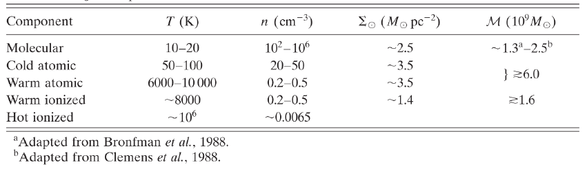
large-scale structure is missing. The polarization gradient is shown in Figure 2.

Using polarization gradients of isothermal MHD turbulence, the supersonic case (Figure 3c) was found

to show localized groupings of very high-gradient ﬁlaments, corresponding to ensembles of intersecting

shocks. By contrast, the subsonic (Figure 3a) and tran-sonic (Figure 3b) cases showed more diﬀuse

networks of ﬁlaments, representing the cusps and discontinuities characteristic of any turbulent velocity

ﬁeld.

In the ISM, ﬂuctuations in density and magnetic ﬁeld will occur as a result of MHD turbulence, which will

be visible in polarimetric maps. In the case of taking gradients of a turbulent ﬁeld, one would expect to

ﬁnd ﬁlamentary structure created by shock fronts, jumps, and discontinuities. Figure 4shows a schematic

Galactic Magnetism Study Guide Page 15 / 39

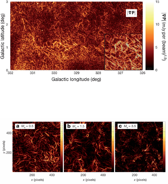
Figure 2: |~

∇~

P|for an 18-deg2region of the Southern Galactic Plane Survey which reveals a complex network of tangled

ﬁlaments. In particular, all regions in which |∇ ~

P|is high consists of elongated, narrow structures rather than extended

patches. In the inset, the direction of |∇P|is shown for a small subregion of the image, demonstrating that |∇ ~

P|changes

most rapidly along directions oriented perpendicular to the ﬁlaments. Figure taken from Gaensler (2011).

Figure 3: |~

∇~

P|derived from propagation of linear radio polarization through three diﬀerent isothermal simulations of

magnetized turbulence. Figure taken from Gaensler (2011).

illustrating these three separate cases of a possible proﬁle and its respective derivative. The cases are as

follows:

•A H¨older continuous proﬁle that is not diﬀerentiable at a given point (e.g., the absolute value

function at the origin): common for all types of MHD turbulence. It is known that the turbulent

velocity ﬁeld in a Kolmogorov-type inertial range both in hydro and MHD is not diﬀerentiable, but

only H¨older continuous. This case can be found in both subsonic- and supersonic turbulence.

•A jump proﬁle: weak shocks, strong ﬂuctuations, or edges (e.g., a cloud in the foreground which

suddenly stops). This case creates a structure in the gradient by a shock jump or a large ﬂuctuation

in either neor ~

B. Here again, this type of enhancement in |∇~

P|could be found in supersonic-

and subsonic turbulence, and is due either to large random spatial increases or decreases due to

turbulent ﬂuctuations along the LOS or weak shocks. We expect weak shock turbulence to show a

larger amplitude in |∇~

P|than the subsonic case due to increases in density ﬂuctuations.

•A spike proﬁle (e.g., delta function): strong shock regime. This case is unique to supersonic

turbulence in that it represents a very sharp spike in neand/or ~

Bacross a shock front. The

diﬀerence between this case and what might be seen in case two is that here we are dealing with

interactions of strong shock fronts, which are known to create delta function-like distributions in

density, creating a “double jump” proﬁle across the shock front.

Of great interest is the question of which quantity is providing the dominant contribution to the structures

in |∇~

P|:|∇ne,LOS|,|∇~

BLOS|, or both equally? Especially in the case of compressible turbulence, the

magnetic energy is correlated with density: denser regions contain stronger magnetic ﬁelds due to the

compressibility of the gas and the potential dynamo ampliﬁcation of the magnetic ﬁeld in dense gas. This

causes the magnetic ﬁeld to follow the ﬂow of plasma if the magnetic tension is negligible. The compressed

Galactic Magnetism Study Guide Page 16 / 39

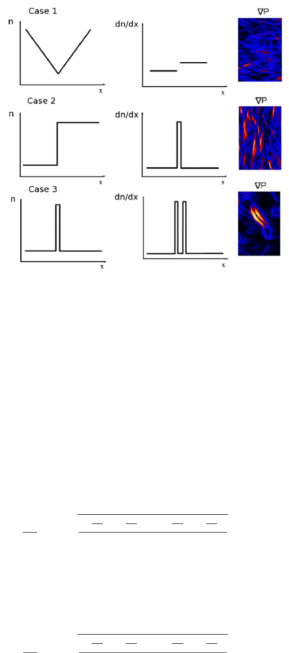
Figure 4: Schematic example of three possible scenarios for enhancements in a generic image “n,” where “n” could be |~

P|,

RM, or ρ/N/EM (density, column density, emission measure). Case one (top row) shows an example of a H¨older continuous

function that is not diﬀerentiable at the origin (applicable to all turbulent ﬁelds). Case two (middle row) shows an example

of a jump resulting from strong turbulent ﬂuctuations along the LOS or weak shocks. Case three (bottom row) shows a

delta function proﬁle resulting from interactions of strong shocks. In this case, the derivative gives a double jump proﬁle

which produces morphology that is distinctly diﬀerent from the previous cases. In all cases we show examples from |~

simulations. Figure taken from Burkhart (2012).

regions are dense enough to distort the magnetic ﬁeld lines, enhance the magnetic ﬁeld intensity, and

eﬀectively trap the magnetic energy due to the frozen-in condition. Thus, for the supersonic cases, the

intensity of the structures seen in |∇~

P|is more pronounced than in the subsonic case. However, in

the case of subsonic turbulence, there are no compressive motions. In this case, random ﬂuctuations in

density and magnetic ﬁeld will create structures in |∇~

P|. It’s been shown using MHD simulations that in

the case of subsonic turbulence, |∇~

P|correlates with |∇~

B|while in the supersonic case |∇~

P|correlates

with density ﬂuctuations. This is because density enhancements are dominant due to shock fronts in the

case of supersonic turbulence, while in subsonic turbulence density is marginally incompressible.

Polarization gradient (radial component): The radial component quantiﬁes how changes in polar-

ization intensity contribute to the directional derivative |∂~

P /∂s|:



∂~

∂s rad

=s(Q∂Q

∂x +U∂U

∂x )2+ (Q∂Q

∂y +U∂U

∂y )2

Q2+U2[Jy pc−1]

If changes in polarization intensity are dominant for a feature, then this could imply that the amount

of depolarization due to the addition of polarization vectors along the line of sight varies signiﬁcantly

between diﬀerent positions, and it follows that the medium producing the polarized emission may be very

turbulent. This is true for both thermal dust emission and for synchrotron emission.

Polarization gradient (tangential component): The tangential component quantiﬁes how changes

in polarization angle, weighted by polarization intensity, contribute to the directional derivative |∂~

P /∂s|:



∂~

∂s tan

=s(Q∂U

∂x −U∂Q

∂x )2+ (Q∂U

∂y −U∂Q

∂y )2

Q2+U2[Jy pc−1]

If changes in polarization angle are dominant, then this could indicate changes in the regular magnetic

ﬁeld threading the observed region, as this would produce signiﬁcant changes in the emitted polarization

angle in the case of thermal dust emission or synchrotron emission. Additionally, changes in the regular

magnetic ﬁeld may also cause the amount of Faraday rotation along diﬀerent lines of sight to vary

signiﬁcantly, in the case of synchrotron emission.

Polarization gradient direction (arg~

∇~

P):The direction of the polarization gradient at a given spatial

Galactic Magnetism Study Guide Page 17 / 39

position deﬁned as

arg(~

∇~

P)≡arctan 





sign ∂Q

∂x

∂Q

∂y +∂U

∂x

∂U

∂y s∂Q

∂y 2

+∂U

∂y 2

s∂Q

∂x 2

+∂U

∂x 2







[rad],

where Qand Uare the complex Stokes vectors.

Polarization horizon: The furthest distance we can see diﬀuse polarized emission. This quantity is

a function of the instrumental features (i.e., beam size, observing frequency), as well as of the physical

conditions of the probed medium (causing an intrinsic degree of depolarization), and depends on the

viewing direction in the Milky Way. The smaller the beam and/or the higher the observing frequency,

the farther the polarization horizon; the brighter and/or more coherent the synchrotron emission, the

farther the corresponding polarization horizon.

Polarized surface brightness (P(λ2)):

P(λ2) = p(λ2)I(λ2) = Q+iU [Jy],

where p(λ2) is the polarization fraction, I(λ) is the total surface brightness, and Qand Uare the complex

Stokes vectors. The absolute value of this complex vector is given by

||P(λ2)|| =pQ2+U2[Jy],

where Qand Uare the complex Stokes vectors.

Poloidal magnetic ﬁeld: Often the GMF is expressed in cylindrical coordinates (θ, r, z). The poloidal

magnetic ﬁeld refers to the axisymmetrical ﬁeld structure around z(without ~

Bθcomponents) such as

dipole ﬁelds.

Power spectrum (P(k)): Describes the distribution of power into frequency components composing

that signal deﬁned as

P(k) = ˆ

f(k)ˆ

f(k)∗,

for wavenumber kwhere ˆ

f(k) denotes the Fourier transform (FT) and ˆ

f(k) its complex conjugate. The

power spectrum is the Fourier transform (FT) of the autocorrelation function.

Prandtl number: The ratio of momentum diﬀusivity (kinematic viscosity) to thermal diﬀusivity:

Pr = ν

α=µcp

k[dimensionless],

where ν=µ/ρ is the momentum diﬀusivity (kinematic viscosity) in m2s−1,α=k/(cpρ) is the thermal

diﬀusivity in m2s−1,µis the dynamic viscosity in Ps s, kis the thermal conductivity in W m−1K, cpis

the speciﬁc heat in J kg−1K, and ρis the density in kg m−3.

Q−Uplane: Translations and rotations within the Q−Uplane can result from one or more of a smooth

distribution of intervening polarized emission, a uniform screen of foreground Faraday rotation, and the

eﬀects of missing large-scale structure in an interferometric data set.

Random magnetic ﬁeld: See turbulent magnetic ﬁeld.

Rayleigh-Taylor instability: Also known as magnetic buoyancy.

Reynolds number (Re): An important dimensionless quantity in ﬂuid mechanics used to help predict

ﬂow patterns in diﬀerent ﬂuid ﬂow situations which characterizes the relative importance of inertial

(resistant to change or motion) and viscous (heavy and gluey) forces:

Re = ρvL

µ[dimensionless],

where ρis the density in kg m−3,vis the velocity in m s−1,Lis the characteristic length in m, and µis the

dynamic viscosity coeﬃcient in Ps s. At low Reynolds numbers, ﬂows tend to be dominated by laminar

(sheet-like) ﬂow, while at high Reynolds numbers, turbulence results from diﬀerences in the ﬂuid’s speed

and direction, which may sometimes intersect or even move counter to the overall direction of the ﬂow

(eddy currents).

Rolling Hough Transform (RHT): A machine vision algorithm designed for detecting and parameter-

izing linear structure in astronomical data, originally applied to HI images. The detection of astronomical

linear structure is approached in various ways depending on the context. Because HI structures are not

objects with distinct boundaries, the problem is fundamentally diﬀerent from many others. As these dif-

fuse HI ﬁbers were not formed by gravitational forces, there is no reason to require that they must be, or

bridge, local overdensities. Indeed, these ﬁbers are found often to be in groups of parallel structures, very

Galactic Magnetism Study Guide Page 18 / 39

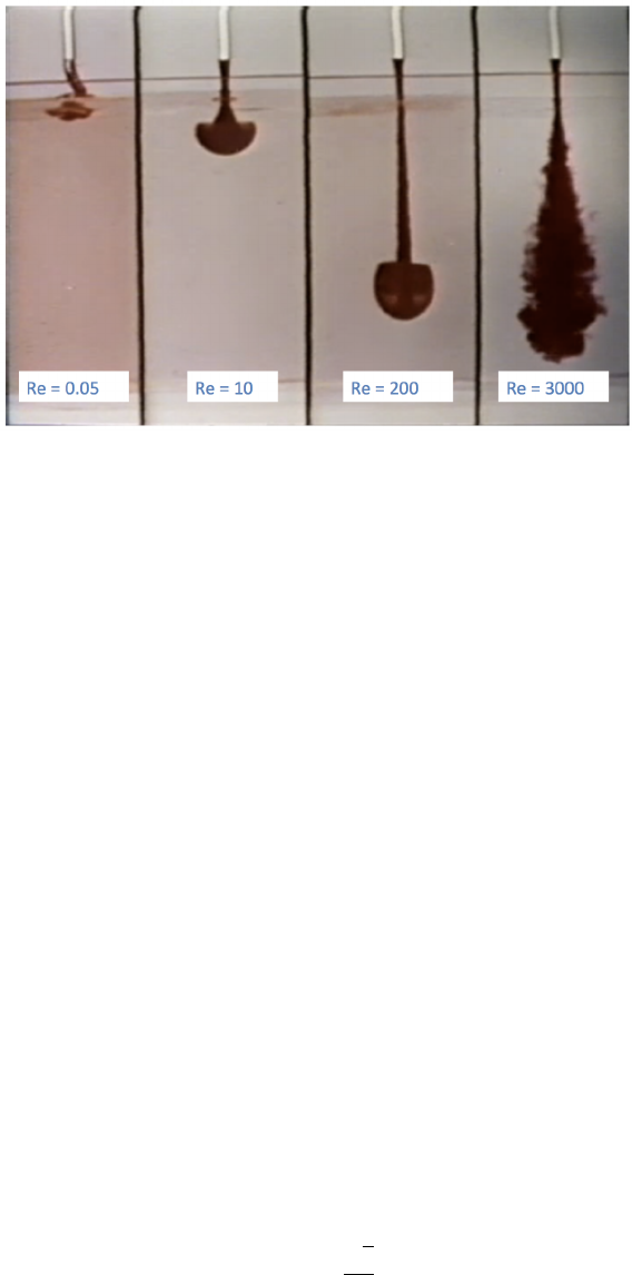
Figure 5: Flows at vary-

ing Reynolds number Re. In

each panel, a ﬂuid that has

been dyed red is injected from

the top into the clear ﬂuid

on the bottom. The ﬂu-

ids are glycerin-water mixture,

for which the viscosity can be

changed by altering the glyc-

erin to water ratio. By chang-

ing the viscosity and the in-

jection speed, it is possible to

alter the Reynolds number of

the injected ﬂow. The frames

show how the ﬂow develops as

the Reynolds number is varied.

This image is a still from the

National Committee for Fluid

Mechanics Film series (Tay-

lor, 1964), which, once you get

past the distinctly 1960s pro-

duction values, are a wonderful

resource for everything related

to ﬂuids.

unlike the cosmic web. Thus, methods developed for gravitationally dominated systems are not optimal

for these purposes. The RHT is, as its name suggests, a modiﬁcation of the Hough transform. The Hough

transform was ﬁrst introduced in in a patent for the detection of complex patterns in bubble chamber

photographs. It was soon recognized as a powerful line detection technique, and has found wide applica-

tions in image processing and machine vision. The adaption of the Hough transform with the RHT is a

rolling version that is particularly well suited to the detection and quantization of speciﬁc linear features

in astronomical data. The RHT does not merely identify ﬁbers; it encodes the probability that any given

image pixel is part of a coherent linear structure. This allows the user to quantify the linearity of regions

of sky without specifying ﬁbers as discrete entities. The RHT operates on two-dimensional data and is

designed to be sensitive to linear structure irrespective of the overall brightness of the region. The ﬁrst

step is to unsharp mask the image. The image is convolved with a two-dimensional top-hat smoothing

kernel of a user-deﬁned diameter, DK. The smoothed data is then subtracted from the original data and

the resulting map is thresholded at 0 to obtain a bitmask. The subtraction of the smoothed component

can be considered a suppression of large-scale structure, or a high-pass Fourier ﬁlter. Each straight line is

parameterized in terms of the angle θof its normal, and its minimum Euclidean distance from the origin

ρ,

ρ=xcos θ+ysin θ[pixels].

Every possible line in the image space is uniquely speciﬁed by a point in the ρ−θspace. The RHT

mapping is performed on a circular domain, diameter DW, centered on each image-space pixel (x0, y0)

in turn. Then a Hough transform is performed on this area, limited to ρ= 0. Thus the ρ−θspace is

reduced to a one-dimensional space on θfor each pixel. All intensity over a set intensity threshold Z

is stored as R(θ, x0, y0): RHT intensity as a function of θfor that pixel. Zis a percentage. In every

direction θ,Z×DWpixels must contain signal in order for the transform to record the data in that

direction. We use the canonical binning for the number of theta bins:

nθ="π√2

2(DW−1)#[dimensionless].

By iterating (“rolling”) over the entire image space we produce the RHT output, R(θ, x, y). A visu-

alization of the linear structures identiﬁed by the RHT, the backprojection R(x, y), is obtained by

integrating R(θ, x, y) over θ:

R(x, y) = ZR(θ, x, y)dθ[dimensionless].

One advantage of the RHT is that the input parameters of the transform can be chosen to highlight

speciﬁc linear features of interest. One deﬁnes, for a given run of the RHT, a smoothing kernel diameter

(DK), a window diameter (DW), and an intensity threshold (Z). The rolling nature of the RHT ensures

that linear structure at least as long as DWwill be identiﬁed. Thus DW, along with the Z, sets a lower

limit for the spatial length of the linear features. Thresholding below 100% (Z < 1) reﬂects the fact that

Galactic Magnetism Study Guide Page 19 / 39

structures can be physically coherent even if they are not visibly connected. R(θ, x, y) is intensity as a

function of angle on a domain θ∈[0, π), as a 0◦orientation is equivalent to a 180◦orientation. R(θ, x, y)

can be sampled in a circular region around each star in the ﬁeld as

R∗(x, y) = Z Zdisk

R(θ, x, y)dxdy[dimensionless].

To estimate the direction of a given region of the backrprojection R∗(θ, x, y), the expectation value is

given by

hθi0=1

2arctan Rsin(2θ)R∗(θ)dθ

Rcos(2θ)R∗(θ)dθ[rad]

where the equivalent value is found on the interval θ∈[0, π) via

hθi=π−mod(hθi0+π, π) [rad].

Linear polarization data can be fully described by either a polarization angle χand polarized intensity

Por by the Stokes parameters Qand U, where χ= (1/2) arctan(U/Q) and P=pQ2+U2. From the

RHT output, similar ‘Stokes vectors’ can be deﬁned via

QRHT =Zcos(2θ)R(θ)dθ[Jy]

URHT =Zsin(2θ)R(θ)dθ[Jy].

This allows for an estimate of the orientation of the magnetic ﬁeld to be derived solely from HI data via

θRHT =1

2arctan URHT

QRHT [rad].

Rotation measure (RM): Characterizes the amount of Faraday rotation that polarized light experi-

ences while passing through thermal electrons. Most compact polarized sources like pulsars and extremely

compact extragalactic sources show a single value of Faraday rotation which is the RM. This is commonly

deﬁned as the slope of the polarization angle χversus λ2plot:

RM = dχ(λ2)

dλ2[rad m−2],

where

χ=1

2arctan U

Q[rad].

The RM, then, modiﬁes the polarization angle χfrom it’s initial value χ0as

χ=χ0+ RMλ2[rad].

The value of RM is the integral of the line-of-sight component of the magnetic ﬁeld weighted by the

line-of-sight distribution of electron density, given by

RM = −0.81

observer

source

ne~

B·~

dl[rad m−2],

where ~

Bhas units of µG, nehas cm−3, and ~

dlhas pc. The RM can be measured towards distant

extragalactic radio sources and pulsars. The RM of an extragalactic radio source consists of an RM

contribution intrinsic to the source, the RM from the intergalactic space from the source to the Galaxy,

and the RM within the Galaxy. The ﬁrst term (i.e., the extragalactic radio source) should be random

and hence reasonably small on average, because a source can be randomly oriented in space with any

possible ﬁeld conﬁguration; thus we observe a random quantity. The second term (i.e., the intergalactic

source) is negligible on average. Intergalactic magnetic ﬁelds are too weak to be detected with current

technology. Even if there is a weak ﬁeld in intergalactic space, an integration over the path-length of

the intergalactic magnetic ﬁeld with random directions with extremely thin gas should give quite a small

contribution. Therefore, the common contribution of RMs of extragalactic radio sources is from our own

Galaxy.

The RM does not increase monotonically with distance along the line of sight. Traditionally, the RM is

obtained by performing a least-squares ﬁt to the data to determine the slope. There are however three

potential problems to this method: (1) the observed polarization angle is only known modulo πradians;

thus with measurements in only a few wavelength bands, the RM is often ambiguous (known as the nπ

Galactic Magnetism Study Guide Page 20 / 39

ambiguity), (2) polarized emission with diﬀerent RM values can be present along a single line of sight;

the signal from these regions mix, making a single linear ﬁt inappropriate, and (3) faint sources with high

RM will be undetectable in individual channels due to low signal to noise and will remain undetectable

even after integrating all channels due to bandwidth depolarization; thus, no χ(λ2) data will be available

for the traditional linear ﬁt.

Rotation measure (RM) synthesis: A robust method for determining the Faraday dispersion function

as proposed by Burn (1966). It was seldom used until Brentjens and de Bruyn (2005) who coined the term

RM Synthesis. This technique involves Fourier transforming the observed polarized surface brightness

P(λ2) into the Faraday dispersion function F(φ) (also referred to as the Faraday spectrum) which is

the complex polarized surface brightness as a function of Faraday depth. As shown by Burn (1966), the

the observed complex polarization vector can be written as P(λ2) = pIe2iχ, where pis the polarization

fraction and Iis the Stokes I vector. Substituting the expression χ(λ2) = χ0+φλ2for the polarization

angle χas a function of Faraday depth φ, we obtain

P(λ2) = pIe2i(χ0+φλ2)

=pIe2iχ0e2iφλ2

=pIe2iχ0e2iφλ2

=F(φ)e2iφλ2[Jy],

where F(φ) is the Faraday dispersion function which describes the intrinsic polarized ﬂux as a function

of Faraday depth. Since the observed polarization originates from emission along all Faraday depths,

integrating this over φgives the ﬁnal form

P(λ2) =

∞

−∞

F(φ)e2iφλ2dφ[Jy].

Thus there is a simple expression that relates the intrinsic quantity F(φ) to the observable P(λ2) which

takes the form of a Fourier transform. This can now be inverted to obtain the Faraday dispersion function

F(φ) =

∞

−∞

P(λ2)e−2iφλ2dλ2[rad m−2].

However, one is confronted with a problem: namely, that we cannot observe at wavelengths λ < 0, nor

do we observe for all wavelengths λ > 0. To resolve this issue, Brentjens & de Bruyn (2005) introduce

a window function W(λ2) which is non-zero only at wavelengths sampled by the telescope. They show

that the observed polarized surface brightness can be rewritten as

P(λ2)≡W(λ2)P(λ2) = W(λ2)

∞

−∞

F(φ)e2iφ(λ2−λ2

0)dφ[Jy],

and the reconstructed Faraday dispersion function as

F(φ)≡

∞

−∞

P(λ2)e−2iφ(λ2−λ2

0)dλ2

∞

−∞

W(λ2)dλ2

=F(φ)∗R(φ) [rad m−2],

where ∗denotes convolution. ˜

F(φ) is an approximate reconstruction of F(φ). More precisely, it is F(φ)

convolved with R(φ) after Fourier ﬁltering by the weight function W(lambda2). R(φ) is the rotation

measure transfer function (RMTF) which is a crucially important quantity deﬁned by

R(φ)≡

∞

−∞

W(λ2)e−2iφ(λ2−λ2

0)dλ2

∞

−∞

W(λ2)dλ2

[rad m−2],

which is normalized to unity at φ= 0. It is a complex valued function. The real part corresponds

to the response of the transform parallel to the (Q, U) vector at λ0=λwhile the imaginary part

corresponds to the response orthogonal to it. Taking a look at the equations above for ˜

F(φ) and R(φ),

these can be seen as applications of the Fourier shift theorem – since the shift theorem only aﬀects the

argument and not the absolute value of the resulting complex vector function, de-rotating these equations

Galactic Magnetism Study Guide Page 21 / 39

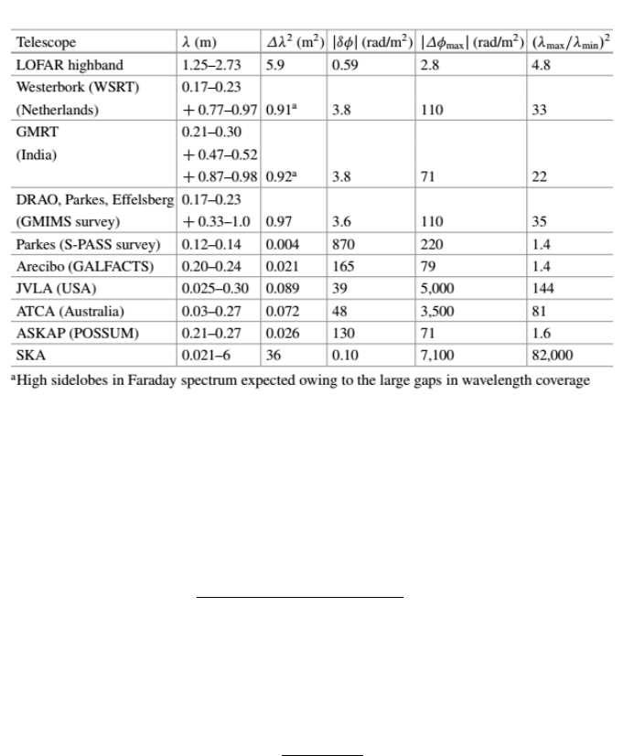
to λ06= 0 does not change their amplitude. The Faraday spectrum is not straightforward to interpret;

in particular, there is no direct relationship between Faraday depth and physical depth. Further, the

Faraday dispersion function suﬀers from sidelobes of the main components caused by limited coverage of

the observed wavelength space. RM Synthesis is required when multiple emitting and rotating regions

are located along the line of sight, as opposed to a single emitting region (i.e., Faraday screen) behind a

single rotating region. RM synthesis was applied to an entire ﬁeld of view for the ﬁrst time by de Bruyn

(1966) using pulsar observations. When applied to a complete ﬁeld of view instead of just a single line

of sight, the output of RM synthesis is referred to as an “RM cube”. RM synthesis is characterized by

four parameters: (1) the resolution in Faraday space, which is inversely proportional to the coverage in

wavelength space, (2) the maximum observable of a point-like source in Faraday space, which is inversely

proportional to the width of a single frequency channel, (3) the maximum width of extended structures

in Faraday space (Faraday rotating and synchrotron emitting sources), which is inversely proportional

to the square of the minimum observable wavelength; wide-band observations at long wavelengths yield

high resolution in Faraday space but cannot detect extended structures, and (4) the ratio of maximum to

minimum wavelengths which is crucial to recognize a range of diﬀerent scales in Faraday space. Table 2

these parameters for a variety of radio telescopes. The highest resolution in Faraday space are for those

with the largest wavelength coverage (LOFAR and SKA) while the largest range of scales in Faraday

space are for those with the greatest ratio of maximum to minimum wavelengths (ATCA, JVLA, SKA).

Table 2: Spectral ranges of various radio telescopes and parameters crucial for RM synthesis. Table from Beck et al.

(2012).

Rotation measure transfer function (RMTF): A crucially important quantity introduced by de

Bruyn (1966) and deﬁned by

R(φ)≡

∞

−∞

W(λ2)e−2iφ(λ2−λ2

0)dλ2

∞

−∞

W(λ2)dλ2

[rad m−2],

which is normalized to unity at φ= 0. For a simple weight function W(λ2) that is a top-hat (boxcar)

fuction centered on λ2

cwith width ∆λ2=λ2

2−λ2

1, the corresponding RMTF is a sinc function with a

phase wind:

R(φ) = eiφλ2

csin(φ∆λ2)

φ∆λ2[rad m−2]

It is a complex valued function; the real part corresponds to the response of the transform parallel to the

(Q, U) vector at λ0=λwhile the imaginary part corresponds to the response orthogonal to it. Ideally,

the response in the entire main peak of the RMTF should be parallel to the actual polarization vector at

λ0. Brentjens & de Bruyn (2005) show that this optimal choice of λ2

0is the mean of the sampled λ2values

weighted by W(λ2). However, since the shift theorem of Fourier theory only applies to the argument,

changing the value of λ0will not change the absolute value of the RMTF. A drawback of having λ06= 0

Galactic Magnetism Study Guide Page 22 / 39

is that the polarization angle that one derives still needs to be transformed to a polarization angle at

λ= 0 if one wants information on the electric or magnetic ﬁeld direction of the source. In the case of a

high S/N, this is easy:

χ0=χ(λ2

0)−φλ2

0[rad].

However, if the S/N is low, the uncertainty in φusually prevents accurate de-rotation to λ= 0.

Scintillation:

Second moment: See variance.

Skewness (γx): The degree of asymmetry of a distribution, and can be quantiﬁed to deﬁne the extent

to which a distribution diﬀers from a normal distribution. Skewness is deﬁned as

γx=1

i=1 xi−µx

σ4

−3 [dimensionless],

where µxis the statistical mean and σis the standard deviation. It can be negative, positive, zero or

undeﬁned, and like the kurtosis, is a dimensionless quantity.

Sonic Mach number (Ms): The ratio of the ﬂow speed to that of the sound speed of the interstellar

medium given by

Ms=|~v|

cs[dimensionless],

where |~v|is the local velocity and csis the sound speed. This number is a commonly used parameter

of turbulence used to obtain information on gas compressibility and magnetization. The statistical

determination of the sonic Mach number is possible because of the relationship between turbulence regimes

and the probability distribution functions (PDFs) of the image intensity distribution. The probability

distribution function of an image distribution gives the frequency of occurrence of intensities values and

can be described by the main statistical moments: mean, variance, skewness, and kurtosis. The higher

order moments (skewness and kurtosis) measure the degree of deviation of the PDF from a Gaussian, and

are sensitive to the imprints of turbulence encoded in the image intensity distribution. For this reason,

their use constitutes a common diagnostic for astrophysical turbulence. Using polarization gradients of

synchrotron radiation, it was shown by Gaensler (2011) that the turbulence of the WIM has a relatively

low sonic Mach number,Ms.2.

Spectral index (α): A measure of the dependence of radiative ﬂux density on frequency. Between any

two frequencies (ν) with total intensity (I), the spectral index is given by:

α≡log(I1/I2)

log(ν1/ν2)[dimensionless].

If ﬂux does not follow a power-law distribution, the spectral index itself is a function of frequency. In the

radio regime, a spectral index of α= 0 −2 indicates thermal emission while a steep negative spectrum

indicates synchrotron radiation.

Spectral correlation function (Sx,y): The average over all neighboring spectra of the normalized rms

diﬀerence between brightness temperatures Tbfor pairs of velocity channels (vi, vj) deﬁned as

Sx,y ≡Svi,vj=1

a=1

Tb([x, y]a, vi)Tb([x, y]a, vj),

where nis the number of positions in the map. A histogram of Sx,y reveals the autocorrelation properties:

if Sx,y is close to unity, the spectra do not vary much.

Spectral irradiance (Eν(T) or Eλ(T)): The Planck function multiplied by the total solid angle of a

sphere (4πsr) which describes the power per area per frequency or the power per area per wavelength:

Eν(T) = 8πhν3

c21

ehν/kBT−1[W m−2Hz−1]

Eλ(T) = 8πhc2

λ51

ehc/λkBT−1[W m−2m−1].

Starlight polarization: The polarization of initially unpolarized starlight which becomes polarized as it

passes through dust grains aligned by an external magnetic ﬁeld. Paramagnetic materials have unpaired

electrons which, when in the presence of an external magnetic ﬁeld such as the interstellar magnetic ﬁeld,

align in the same direction causing grain alignment. In the case of elongated dust grains, if the shortest

axis is aligned with the direction of the magnetic ﬁeld, then the grains will absorb light polarized along

the long axis of the grain which is perpendicular to the ﬁeld. This results in transmitted radiation having

Galactic Magnetism Study Guide Page 23 / 39

a polarization direction parallel to the magnetic ﬁeld. Optical polarization of starlight was ﬁrst imaged

by Hall & Mikesell (1949) and Hiltner (1949). They found that polarized light from nearby stars had

similar orientation, indicating that the polarizing mechanism was a source other than the individual stars.

Shortly thereafter, Davis & Greenstein (1951) published a theory on the origin of polarized starlight. They

proposed that an elongated dust grain spinning about its shortest axis would have a preferred orientation

when located in a magnetic ﬁeld. Starlight polarization is most useful for detecting magnetic ﬁelds in

the Solar neighbourhood out to about 1 −3 kpc. The same large-scale alignment of spinning, aspherical

dust grains that causes starlight polarization also causes infrared polarization.

Stellar wind bubble (SWB): A cavity light years across ﬁlled with hot gas blown into the interstellar

medium by high-velocity (several thousand km s−1) stellar wind from a single massive O or B star. The

heliosphere blown by the Solar wind, within which all of the major planets of the Solar System are

embedded, is a small example of a stellar wind bubble.

Stochastic system:

Stokes parameters:

Stokes I (I): A measure of the total intensity of radio emission.

Stokes Q (Q): A measure of the linear polarization of radio emission. The images of Stokes Q (and Stokes

U) as well as the linear polarized intensity P≡p(Q2+U2) are often ﬁlled with complex structures

that bear little resemblance to the Stokes I image of total intensity. The intensity variations seen in Q

(as well as Uand P) are the result of small-scale angular structure in the Faraday rotation induced by

ionized gas, and are thus an indirect representation of turbulent ﬂuctuations in the free-electron density

and magnetic ﬁeld throughout the interstellar medium.

Stokes U (U): A measure of the linear polarization of radio emission. The images of Stokes U (and Stokes

Q) as well as the linear polarized intensity P≡p(Q2+U2) are often ﬁlled with complex structures that

bear little resemblance to the Stokes I image of total intensity. The intensity variations seen in U(as well

as Qand P) are the result of small-scale angular structure in the Faraday rotation induced by ionized

gas, and are thus an indirect representation of turbulent ﬂuctuations in the free-electron density and

magnetic ﬁeld throughout the interstellar medium.

Stokes V (V): A measure of circular polarization of radio emission. If V > 0, then the electromagnetic

wave is right-handed circularly polarized (RCP), while if V < 0, then the electromagnetic wave is left-

handed circularly polarized (LCP). Stokes V is related to the line-of-sight magnetic ﬁeld in the following

manner:

V(ν)∝Bk×dI

dν[Jy],

where Iis Stokes I and νis the observed frequency.

Striation:

Str¨omgren sphere: A sphere of ionized hydrogen (HII) around young OB stars.

Structure function (Sp(δr)): The structure function of order pfor an observable Ais given by

Sp(δr) = h|A(r)−A(r+δr)|pi,

for position rand position increment δr. The power-law ﬁt to this, Sp(δe)∝δrζ

p, gives the slope ζp.

Superbubble: Also known as a supershell. Supershells and superbubbles are the largest classiﬁcation

of HI shells, with radii between 102and 103pc, blown into the ISM by multiple SNe and stellar winds

from clusters and associations of massive O and B stars. Such objects occupy an intermediate size-scale

within the ISM; a scale at which the role of magnetic ﬁelds in the magneto-ionic medium (MIM) is not

well understood. Supershells are most commonly found in HI surveys, and appear as cavities in the

neutral hydrogen; but they can also have multi-wavelength properties. Supershells can have associated

emission in Hα, soft X-rays, far ultra-violet, polarized radio continuum, and 100 µm. It is thought that

once bubbles expand far enough to break out of the gas of the Galactic plane, the shell breaks open into

a Galactic chimney, allowing the ﬂow of hot gas into the halo. This transition from bubble to chimney is

slowed by the presence of magnetic ﬁelds, which tend to conﬁne the expanding shell in the disc.

A superbubble behaves qualitatively like an individual supernova remnant, except that it has a con-

tinuous supply of energy. For the ﬁrst 3 Myrs at least, their energy supply is exclusively due to stellar

winds, whose cumulative power rises rapidly with time. Supernovae start exploding after &3 Myrs, and

within ∼2 Myrs, they overpower the stellar winds. From then on, the successive supernovae explosions

continue to inject energy into the superbubble at a slowly decreasing rate, depending on the initial mass

function (IMF) of the progenitor stars, until ∼40 Myrs. Altogether, stellar winds account for a fraction

comprising between ∼12% and ∼17% of the total energy input. The Solar System lies near the center

of an old superbubble known as the Local Bubble whose boundary can be traced by a sudden rise in dust

extinction.

Galactic Magnetism Study Guide Page 24 / 39

Supernova: A supernova is a transient astronomical event that occurs during the last stellar evolutionary

stages of a star’s life, either a massive star or a white dwarf, whose destruction is marked by one ﬁnal,

titanic explosion. Supernovae come in two types. Type-I supernovae arise from old, degenerate low-mass

stars which supposedly are accreting from a companion and undergoes a thermonuclear instability upon

accumulation of a critical mass. Type-II supernovae arise from young stars with initial masses &8 M

whose core gravitationally collapses once it has exhausted all of its fuel. Like the bright, massive stars,

Type-II supernovae are tightly conﬁned to the spiral arms while Type-I supernovae have a more spread-

out distribution similar to the general stellar population. Type-I supernovae are less frequent than their

Type-II counterparts. All of them are uncorrelated in space and have basically the same repercussions

on the ISM as isolated Type-II supernovae. The hot gas created by supernovae explosions (and stellar

winds) in the Galactic disk rises into the halo under the inﬂuence of its own buoyancy. In the course

of its upward motion, it cools down (almost adiabatically at ﬁrst, then by radiative transport), and

eventually condenses into cold neutral clouds. Once formed, these clouds fall ballistically towards the

Galactic plane. This convective cycle of interstellar material between the disk and the halo is known as

the Galactic fountain.

Supershell: See superbubble.

Synchrotron radiation: The radio emission produced by relativistic cosmic rays when accelerated

radially (e.g., by magnetic ﬁelds) which is one of the most commonly used tracers of the Galactic mag-

netic ﬁeld. Synchrotron radio emission is a tool to measure the total strength of magnetic ﬁeld on the

assumption that the magnetic energy-density (pressure) is in equipartition with the thermal and cosmic

ray energy densities. This method requires information about the depth of emitting region in order to

calculate the synchrotron emissivity per volume, as the intensity is an integration of the emissivity along

the line-of-sight.

Synchrotron emission has a steep spectral index of α∼ −2.75, which results in much brighter emission

at lower frequencies (this applies to both linear polarization and total intensity). For a single electron,

the critical frequency of synchrotron radiation can be expressed as

νc=3

4π

mcγ2(Bsin θ) [Hz],

νc∼γ2eB

2πm0

[Hz],

where γis the Lorentz factor,eand m0are the charge and rest mass of the cosmic ray electron, and Bis

the magnetic ﬁeld strength. As the cosmic ray gyrates around the local magnetic ﬁeld, it generates the

synchrotron radiation beamed within the shape of a cone at an angle of

θ=±mcc2

E[rad].

On the surface of the cone, the radiation is 100% linearly polarized with an electric ﬁeld Ethat has

a direction of −v×B. Synchrotron radiation from the Galaxy was the ﬁrst emission detected in radio

astronomy by Jansky (1933), however, it was not until the 1950’s when detailed radio maps of the Galaxy

were produced that the connection was made between radio emission and the synchrotron mechanism.

Linear polarization of synchrotron radiation can be used to trace ordered magnetic ﬁelds in the plane of

the sky (B⊥). Unpolarized synchrotron emission can be indicative of a turbulent magnetic ﬁeld causing

depolarization via Faraday rotation of thermal electrons (synchrotron radiation cannot cause Faraday

rotation). The radiated power from an accelerating charge qwith mass mby a magnetic ﬁeld Bat an

observing frequency νis

P=2

m2c5(γν)2(Bsin θ)2[Jy].

Since synchrotron radiation is proportional to the charge-to-mass ratio, electrons dominate synchrotron

radiation over protons and ions by several orders of magnitude. Synchrotron radiation peaks at a char-

acteristic frequency of

νc=3

4π

mcγ2(Bsin θ) [Hz].

For radio observations with typical frequencies at or above tens of MHz and with typical magnetic

ﬁeld strengths of order µG, the observed population of synchrotron electrons have γ1. Synchrotron

emission has a steep negative spectral index in the radio regime. Assuming that the electrons are moving

isotropically, Le Roux (1961) showed that the maximum intrinsic degree of polarization (i.e., polarization

fraction) of synchrotron radiation from plasma in a uniform magnetic ﬁeld is a function of the electron’s

Galactic Magnetism Study Guide Page 25 / 39

spectral index γgiven by

p=3γ+ 3

3γ+ 7 [dimensionless],

independent of frequency and observing angle. Using observations of the Crab Nebula, Woltjer (1958)

and Westfold (1959) showed that γ≈5/3 and therefore p≈67%. Le Roux (1961) gives a full derivation

of synchrotron radiation. Figure 6shows the Galactic synchrotron emission at 408 MHz.

Figure 6: The synchrotron emission at 408 MHz across the entire sky in Galactic coordinates. As expected, the emission

is concentrated along the Galactic plane. However, the feature known as Loop I, is clearly arching up from `= 55◦towards

the North Galactic Pole. This Figure is adapted from Haslam et al. (1981). Figure taken from Newton-McGee (2009).

Taylor scale:

Third moment: See skewness.

Toroidal magnetic ﬁeld: Often the GMF is expressed in cylindrical coordinates (θ, r, z). The toroidal

magnetic ﬁeld refers to the structures (without ~

Bzcomponents) conﬁned to a plane parallel to the Galactic

plane. The toroidal ﬁelds possibly extend to the inner Galaxy, even towards the central molecular zone

(CMZ).

Tsallis distribution: A function that can be ﬁt to incremental probability distribution functions (PDFs)

of turbulent density, magnetic ﬁeld, and velocity. The Tsallis distribution was originally derived by

Tsallis (1988) as a means to extend traditional Boltzmann-Gibbs mechanics to fractal and multifractal

systems. The complex dynamics of multifractal systems apply to many natural environments, such as

ISM turbulence. The Tsallis function of an arbitrary incremental PDF ∆fhas the form

Rq=a1+(q−1)∆f(r)2

w2−1/(q−1)

The ﬁt is described by three dependent variables. The aparameter describes the amplitude while wis

related to the width or dispersion of the distribution. Parameter q, referred to as the “non-extensivity

parameter” or “entropic index” describes the sharpness and tail size of the distribution. The Tsallis ﬁt

parameters are in many ways similar to statistical moments. Moments, more speciﬁcally the third- and

fourth-order moments, have been used to describe the density distributions and have shown sensitivities

to simulation compressibility. The ﬁrst- and second-order moments simply correspond to the mean and

variance of a distribution. Skewness, or third-order moment, describes the asymmetry of a distribution

about its mode. Skewness can have positive or negative values corresponding to right and left shifts of

a distribution, respectively. The fourth-order moment, kurtosis, is a measure of a distributions peaked

or ﬂatness compared to a Gaussian distribution. Like skewness, kurtosis can have positive or negative

values corresponding to increased sharpness or ﬂatness. With regard to the Tsallis ﬁtting parameters, the

w parameter is similar to the second-order moment variance while q is closely analogous to fourth-order

Galactic Magnetism Study Guide Page 26 / 39

moment kurtosis. Unlike higher order moments, however, the Tsallis ﬁtting parameters are dependent

least-squares ﬁt coeﬃcients and are more sensitive to subtle changes in the PDF.

Turbulence: Astrophysical turbulence is a complex nonlinear ﬂuid phenomenon that can occur in a

multiphase medium which results in the excitation of an extreme range of correlated spatial and temporal

scales. There are many injection sources on scales ranging from kp down to sub-AU. The physical

processes by which kinetic energy is converted into turbulence are not well understood for the ISM. The

main sources for large-scale motions are: (a) stars, whose energy input is in the form of protostellar winds,

expanding HII regions, O star and Wolf-Rayet winds, supernovae, and combinations of these producing

superbubbles; (b) Galactic rotation in the shocks of spiral arms or bars, in the Balbus-Hawley instability

(also known as the magnetorotational instability), and in the gravitational scattering of cloud complexes at

diﬀerent epicyclic phases; (c) gaseous self-gravity through swing-ampliﬁed instabilities and cloud collapse;

(d) Kelvin-Helmholtz and other ﬂuid instabilities; and (e) Galactic gravity during disk-halo circulation,

the Parker instability, and galaxy interactions. Interstellar turbulence has been characterized by structure

functions,correlation functions (e.g., spatial power spectrum), autocorrelations,power spectra,energy

spectra, and delta variance. Sources for small-scale turbulence observed by radio scintillation include sonic

reﬂections of shock waves hitting clouds, cosmic ray streaming and other instabilities, ﬁeld star motions

and winds, and energy cascades from larger scales. Turbulence aﬀects the structure and motion of nearly

all temperature and density regimes of the interstellar gas. Magnetohydrodynamic (MHD) turbulence

is a key element in the study of star formation, molecular cloud structure, magnetic reconnection, heat

transport, and cosmic ray propagation. MHD turbulence is known to be diﬀerent from a collection of

linear Alfv´enic waves. Does MHD turbulence, speciﬁcally the Alfv´en wave modes, damp at the decoupling

scale of the ambipolar diﬀusion scale LAD? Cascading rates and the anisotropy of turbulence should be

accounted for carefully before a deﬁnitive conclusion about turbulent damping in the partially ionized

media. Despite the importance of turbulence for ISM studies, many mysteries remain including the nature

of turbulence driving and damping. The most common observational techniques for studying turbulence

include scintillation studies (which are limited to ﬂuctuations in ionized plasmas), density ﬂuctuations

via column density maps, and radio spectroscopic observations via centroids of spectral lines. Position-

position-velocity (PPV) spectroscopic data have the advantage over column density maps in that it

contains information on the turbulent velocity ﬁeld. However, this type of data provides contributions

of both velocity and density ﬂuctuations entangled together, and the process of separating the two has

proven to be a challenging problem. One of the main approaches for characterizing ISM turbulence

is based on using statistical techniques and descriptions (e.g., spatial power spectrum). Although the

power spectrum is useful for obtaining information about energy transfer over scales, it does not provide

a full picture of turbulence, partly because it only contains information on Fourier amplitudes (i.e., two

substantially diﬀerent density distributions can have the same power spectrum). Probability distribution

functions (PDFs) of turbulence in PPV and column density data have been studied for decades and have

proven to be very useful to show that turbulence is present in the ISM, providing insight into the eﬀects of

turbulent driving and characterizing the type of turbulence in question. Many studies on turbulence focus

on obtaining parameters such as sonic and Alfv´en Mach numbers,injection scale, gas temperature, and

Reynolds number. In particular, the sonic and Alfv´en Mach numbers provide much coveted information

on the gas compressibility and magnetization.

Turbulent fragmentation:

Turbulent magnetic ﬁeld: Also known as “random magnetic ﬁeld”. Deviations from coherent or

ordered ﬁelds are taken as turbulent ﬁelds. The ﬂuctuations of ﬁelds at scales 10 times smaller than a

concerned scale are often also taken as turbulent ﬁelds.

Turbulent pressure:

Two-ﬂuid turbulence: The turbulence of a partially ionized plasma where the ions are decoupled from

the neutrals (i.e., at the scale below the ambipolar diﬀusion scale).

Type-I Supernova: Arises from old, degenerate low-mass stars which supposedly are accreting from a

companion and undergoes a thermonuclear instability upon accumulation of a critical mass. Like Type-II

supernovae, releases an amount of energy of '1051 ergs.

Type-II Supernova: Arises from young stars with initial masses &8 Mwhose core gravitationally

collapses once it has exhausted all of its fuel. Like Type-I supernovae, releases an amount of energy of

'1051 ergs.

Unstable neutral medium (UNM): A thermally-unstable phase of the atomic ISM. Figure 7shows the

thermal pressure function p(n). This curve has several familiar features, described in the classic paper on

this subject by Field, Goldsmith & Habing (1969). These include separate branches for warm intercloud

(red) and cold cloud (green) components, a maximum intercloud thermal pressure (4400 cm−3K for the

curve shown), a minimum cloud thermal pressure (1700 cm−3K for this example), and a range of density

(0.8−7 cm−3), or more fundamentally temperature (roughly 270−5500 K), between these two (blue) that

is regarded as forbidden in equilibrium because at constant thermal pressure it is thermally unstable. In

Galactic Magnetism Study Guide Page 27 / 39

the unstable region, gas slightly above the curve is too hot for its density and cools. But at constant

thermal pressure, cooling moves it to the right, to higher density, taking it further from the curve and

making it cool faster, until it reaches the stable cloud branch. Similarly, gas slightly below the curve

has excess heating and at constant thermal pressure moves horizontally to the left until it joins the

stable intercloud component. For the standard curve, the mean midplane interstellar density in the Solar

Neighbourhood (slightly over 1 cm−3) is in the unstable regime. This appears to guarantee that both the

cloud and intercloud branches will be populated.

Figure 7: The Two-Phase

Medium thermal pressure ver-

sus density curve is shown in

the red-blue-green curve. The

red segment is the thermally

stable warm component, the

green the corresponding stable

cold component, and the blue

the thermally unstable regime.

The black dashed line is the to-

tal midplane pressure, the or-

ange dashed line represents the

magnetic pressure, the dashed

aqua line shows how the p(n)

curve shifts when the heating

rate is raised by a factor of 10,

and the dashed purple rectan-

gle outlines the regime of essen-

tially zero bulk modulus. Fig-

ure taken from Cox (2005).

One of the most interesting features of p(n)fis that over a density range of a factor of 350, from 0.2 to

70 cm−3, the thermal pressure variation is less than a factor of three. In Figure 7, this region is shown

enclosed by a dashed purple rectangle. It is a regime in which the thermal pressure oﬀers essentially

zero bulk modulus. This means that if, for some reason, the ISM had a totally random distribution of

densities within this range, the corresponding distribution of thermal pressures would be observationally

indistinguishable from one in which thermal pressure had an active role in arranging things, except there

would be no range of forbidden densities. The small variation in thermal pressure between regions of

diﬀering density can be compensated by slight changes in the somewhat stronger magnetic ﬁeld pressure.

This is true when establishing pressure uniformity across the magnetic ﬁeld lines, but equilibrium parallel

to the ﬁeld cannot be established in this way.

Variance (νxor σ2): The second order statistical moment which is a measure of the deviation from the

mean. The variance is deﬁned as

µx=1

N−1

i=1

(xi−¯x)

and, like the mean, has the same dimensions as xi.

Volume ﬁlling factor (f): A correction factor such that a fraction fof the line of sight intersects

clouds of uniform density N. There are three eﬀects of the interstellar magnetic ﬁeld that conspire to

lower the ﬁlling factor of hot cavities: (1) the background magnetic pressure acting on the surrounding

shells directly opposes their expansion, (2) the magnetic tension in the swept-up ﬁeld lines gives rise to

an inward restoring force, while the associated magnetic pressure prevents the shells from fully collapsing

and, therefore, keeps them relatively thick, and (3) the enhanced external “signal speed” causes the shells

to merge earlier than they would in an unmagnetized medium.

Warm ionized medium (WIM): A diﬀuse phase of the interstellar medium with a typical temperature

of T∼8,000 K and average electron density of ∼0.2−0.5 cm−3. The ionized gas has mostly been

mapped using the Hαline. One limitation of the Hαline comes from the obscuration caused by dust,

which restricts visibility to within 2 −3 kpc from the Sun. Using polarization gradients of synchrotron

radiation, it was shown by Gaensler (2011) that the turbulence of the WIM has a relatively low sonic

Mach number,Ms.2.

Warm neutral medium (WNM): A thermally-stable phase of the atomic ISM with a typical density

and kinetic temperature of n∼0.2−0.9 cm−3and TK∼5000 −8300 K, respectively.

Warm partially ionized medium (WPIM):

Wave turbulence:

Galactic Magnetism Study Guide Page 28 / 39

Zeeman eﬀect: The eﬀect of a single spectral line splitting into multiple components in the presence of

a static magnetic ﬁeld due to the degeneracy between various electron energy levels that become broken

when exposed to an external magnetic ﬁeld. In an astrophysical context, a magnetic ﬁeld produces small

frequency shifts in the left- and right-handed circular polarized components of a given spectral line with

respect to the intrinsic central frequency of the atom of molecule. Zeeman splitting is used to measure

the parallel component of the magnetic ﬁeld via atomic and molecular gas. The ﬁrst measurement of

an astrophysical magnetic ﬁeld was using Zeeman splitting. The 21 cm line of atomic hydrogen is the

most widespread, and it provides an opportunity to measure splitting in both emission and absorption.

Zeeman splitting is a powerful tool as the magnetic ﬁeld can be directly determined from the energy

diﬀerence between the electron levels. The separation in energy of the magnetic hyperﬁne levels from the

unsplit level of the zero magnetic ﬁeld case is given by

∆E=−µBmFgB [J],

where µBis the Bohr magneton, mFis the quantum number of the Zeeman splitting, Bis the magnetic

ﬁeld strength, and gis the Land´e g-factor. However, the eﬀect is diﬃcult to observe since the frequency

shift (∆ν) in the spectral lines is small:

∆ν=µBmFgB

h[Hz].

Such a frequency shift is usually smaller than the spectral linewidth, making Zeeman splitting observations

resolution limited. Lower frequencies produce better Zeeman splitting results because, although the

splitting is independent of the line frequency itself, the higher the frequency, the broader the linewidth.

The statistical sample of measured Zeeman splittings is woefully small and desperately needs to be

expanded. Zeeman-splitting observations are time-consuming: typically tens of hours are required for

each source. In addition, Zeeman splitting observations cannot be related to the large-scale GMF.

Zenith: The point in the sky or celestial sphere directly above an observer.

Zeroth moment:

Galactic Magnetism Study Guide Page 29 / 39

3 Variables

Alfv´en Mach number:MA[dimensionless]

Alfv´en speed:vA[m s−1]

Ambipolar diﬀusion scale:LAD [m]

Ambipolar diﬀusivity:νAD

Angle:θ[rad]

Autocorrelation:C(δr) [dimensionless]

Bandwidth in frequency: ∆ν[Hz]

Bandwidth in wavelength: ∆λ[Hz]

Bohr magneton:µB

βparameter:β

Channel central frequency:νc[Hz]

Channel width in frequency:δν [Hz]

Channel central wavelength:λc[m]

Channel width in wavelength:δλ [m]

Charge density:ρe[C m−3]

Complex conjugate:f(x)∗or ¯

f(x)

Current density:~

j[A m−3]

Delta function:δ(x)

Delta variance:σ2

∆(L)

Density:ρ[m−3]

Density of electrons:ρe[m−3]

Density of ions:ρi[m−3]

Density of neutrals:ρn[m−3]

Diameter of window (RHT):DW[pixels]

Dirac delta function:δ(x)

Dispersion measure: DM [pc cm−3]

Dust-to-gas mass ratio:r[dimensionless]

Dynamic viscosity:µ[Ps s]

Electron charge:e[C]

Electron mass:em[kg]

Electron plasma pressure:Pe[Pa]

Electron temperature:Te[K]

Emission cross section per H nucleon:σe(ν) [cm2]

Emission measure: EM [pc cm−6]

Emissivity index:β[dimensionless]

Energy spectrum:E(k) [Jy m−1]

Expectation value of θon any domain (RHT):hθi0[rad]

Expectation value of θon θ∈[0, π)(RHT):hθi[rad]

Faraday depth:φ[rad m−2]

Faraday dispersion function (no spectral dependence):F(φ) [rad m−2]

Faraday dispersion function (general form):F(φ, λ) [rad m−2]

Frequency:ν[Hz]

Frictional coupling coeﬃcient between ions and neutrals:α[dimensionless]

FWHM of RMTF main peak: ∆φ[rad m−2]

Fourier transform (FT):ˆ

f(x)

Hydrogen column density:NH[cm−2]

HI column density:NHI [cm−2]

HI density:nHI [cm−3]

Incremental position:δr [m]

Intensity of thermal dust emission:Iν[W m−2Hz−1sr−1]

Intensity threshold:Z[dimensionless]

Jansky: Jy [unit]

Joule: J [unit]

Land´e g-factor:g

Lorentz factor:γ[dimensionless]

Luminosity per H atom: L[W H−1]

Mach number:M[dimensionless]

Magnetic ﬁeld:~

B[µG]

Galactic Magnetism Study Guide Page 30 / 39

Magnetic ﬁeld strength (parallel component):|~

Bk|[µG]

Magnetic ﬁeld strength (tangential component):|~

B⊥|[µG]

Magnetic ﬁeld strength (total):|~

Btot|[µG]

Magnetic pressure:Pmag [Pa]

Mass absorption coeﬃcient: κν[cm2g−1]

Mean:µx

Mean molecular weight: µ[dimensionless]

Momentum diﬀusivity:ν[m2s−1]

Number density:n[m−3]

Number of θbins (RHT):n[dimensionless]

Optical depth:τν[dimensionless]

Order:p[dimensionless]

Planck constant:h[J s]

Planck constant (reduced):~[J s]

Planck function:Bν(T) [W m−2Hz−1sr−1] or Bλ(T) [W m−2m−1sr−1]

Plasma beta:βth [dimensionless]

Polarization angle:χ[rad]

Polarization angle (RHT):χRHT [rad]

Polarization angle at λ= 0: χ0[rad]

Polarization fraction:p(λ2) [dimensionless]

Polarization gradient:

∂~

∂s 

or |~

∇~

P|[Jy beam−1]

Polarization gradient (maximum value):

∂~

∂s max

or |~

∇~

P|max [Jy beam−1]

Polarization gradient (radial component; maximum value):

∂~

∂s rad

[Jy beam−1]

Polarization gradient (tangential component; maximum value):

∂~

∂s tan

[Jy beam−1]

Polarization gradient (direction): arg(~

∇~

P) [rad]

Polarized intensity:P[Jy]

Polarized surface brightness:P(λ2) [Jy]

Polarized surface brightness (observed):˜

P(λ2) [Jy]

Position:r[m]

Power spectrum:P(k)

Quantum number of Zeeman splitting:mF

Radial component of polarization gradient:∂P

∂s rad [Jy pc−1]

Rayleigh: R [unit]

Resistivity:η[Ω m]

Rest mass:m0[kg]

Reynolds number: Re [dimensionless]

Reynolds number for ambipolar diﬀusion: RAD [dimensionless]

RHT angle:θ[rad]

RHT backprojection:R(x, y) [dimensionless]

RHT backprojection sampling disk around star:R∗(x, y) [dimensionless]

RHT distance:ρ[pixels]

RHT intensity vs angle:R(θ, x0, y0) [dimensionless]

Rotation measure: RM [rad m−2]

Rotation measure transfer function (RMTF):R(φ)[rad m−2]

Sonic Mach number:Ms[dimensionless]

Sound speed:cs[m s−1]

Speciﬁc heat:cp[J kg−1K]

Spectral correlation function:Sx,y [dimensionless]

Spectral index:α[dimensionless]

Spectral irradiance: Eν(T) [W m−2Hz−1] or Eλ(T) [W m−2m−1]

Speed of light:c[m s−1]

Standard deviation:σ(x)

Stokes I:I[Jy]

Galactic Magnetism Study Guide Page 31 / 39

Stokes Q:Q[Jy]

Stokes Q (RHT):QRHT [Jy]

Stokes U:U[Jy]

Stokes U (RHT):URHT [Jy]

Stokes V:V[Jy]

Structure function:Sp

Structure function power-law slope:ζp

Tangential component of polarization gradient:∂P

∂s tan [Jy pc−1]

Thermal conductivity:k[W m−1K]

Thermal diﬀusivity:α[m2s−1]

Thermal electron density:ne[cm−3]

Thermal electron fraction:xe[dimensionless]

Thermal pressure:Pth [Pa]

Thermal pressure (ionized):Pth,i[Pa]

Thermal pressure (neutral):Pth,n[Pa]

Variance:νxor σ2

Velocity:~v [m s−1]

Viscosity coeﬃcient:µ[Pa s]

Wavelength:λ[m]

Wavelength to which all polarization vectors are de-rotated:λ0[m]

Wavenumber:k[m−1]

Weight function:W(λ2) [dimensionless]

Zeeman splitting energy diﬀerence: ∆E[J]

Zeeman splitting frequency diﬀerence: ∆ν[Hz]

Galactic Magnetism Study Guide Page 32 / 39

4 Equations

Alfv´en Mach number:

MA=|~v|

vA[dimensionless]

Alfv´en speed:

vA=|~

√ρ[m s−1]

Ambipolar diﬀusion scale:

LAD =VA

αρi

[m]

Ambipolar diﬀusivity:

νAD =B2

4πρiρnα[mss−1]

Autocorrelation: C(δr) = hf(r)f(r+δr)i[dimensionless]

βparameter:

β≡c2

[dimensionless]

Channel central wavelength:

λ2

c≈c2

ν2

c 1 + 3

4δν

νc2![m2]

(Brentjens & de Bruyn, 2005)

Charge conservation: ∂ρe

∂t +~

∇ ·~

j= 0

Channel width in wavelength:

δλ2≈2c2δν

ν3

c 1 + 1

2δν

νc2![m2]

(Brentjens & de Bruyn, 2005)

Current density:

j=c∇ × ~

4π[A m−2]

(Schoeﬄer et al., 2016)

Delta variance:

σ2

∆(L) = *3L/2

(A[r+x]− hAi)(x)2dx+,

Dispersion measure (DM):

DM = −

observer

source

ne~

d`[pc cm−3]

Electron plasma pressure:Pe=Teη[Pa]

(Schoeﬄer et al., 2016)

Electron temperature:

Te=Pe

η[K]

(Schoeﬄer et al., 2016)

Emission cross section per H nucleon:

σe(ν) = τν

[cm2]

(Roy et al., 2013)

Galactic Magnetism Study Guide Page 33 / 39

Emission measure:

EM = −

observer

source

d`[pc cm−6]

EM(IHα)=2.75 Te

104K0.9IHα

Reτ[pc cm−6]

(Reynolds 1988)

Expectation value of θon any domain (RHT):

hθi0=1

2arctan Rsin(2θ)R∗(θ)dθ

Rcos(2θ)R∗(θ)dθ

Expectation value of θon θ∈[0, π)(RHT):

hθi=π−mod(hθi0+π, π) [rad]

Faraday depth:

φ(~r) = −0.81

observer

source

ne~

B·~

dr[rad m−2]

Faraday depth standard error:

σφ=1

N−2Piχ2

Pi(λ2

i)2−N−1(Piλ2

i)2−1

="1

N−2

(N−1)(σ2

χ+



hχi)

Pi(λ2

i)2−N−1(Piλ2

i)2#−1

="N−1

N−2

σ2

Pi(λ2

i)2−N−1(Piλ2

i)2#−1

≈"σ2

Q≈σ2

U≈σ2

4(N−2)||P||2σ2

λ2#−1

[rad m−2]

(Brentjens & de Bruyn, 2005)

Faraday dispersion function:

F(φ) =

∞

P(λ2)e−2iφλ2dλ2[rad m−2]

Faraday dispersion function (reconstructed):

F(φ)≡

∞

−∞

P(λ2)e−2iφ(λ2−λ2

0)dλ2

∞

−∞

W(λ2)dλ2

=F(φ)∗R(φ) [rad m−2]

Fourier transform (FT):

f(x) =

∞

−∞

f(x0)e−2πxx0dx0

Hydrogen column density:

NH= (11.5±0.5) ×1021 E(J −Ks) [cm−2] (NH.5×1021 cm−2)

(Martin et al., 2012)

Induction equation:

∂~

∂t =∇ × (~v ×~

B) + ηc2

4π∇2~

B−1

en∇ × (~

j×~

B)−c

ne∇n× ∇Te

(Schoeﬄer et al., 2016)

Intensity of thermal dust emission:

Iν=τνBν(T) [W m−2Hz−1sr−1]

≡σe(ν)NHBν(T) [W m−2Hz−1sr−1]

=rµmHNHκνBν(T) [W m−2Hz−1sr−1]

Inverse Fourier transform (FT):

f(x) =

∞

−∞

f(x0)e2πixx0dx0

Galactic Magnetism Study Guide Page 34 / 39

Kurtosis:

βx=1

i=1 xi−µx

σ3

[dimensionless]

Lorentz factor:

γ=r1−(v/c)2

c2[dimensionless]

Luminosity per H atom:

L=Z4πκ0(ν/ν0)βµmHBν(T) dν[W H−1]

Magnetic ﬁeld strength (parallel component):

Bk|=RM

0.81√EM√fL [µG]

Magnetic ﬁeld strength (total):

Btot|=√3|~

Bk|[µG]

Magnetic pressure:

Pmag =|~

Btot|2

8π[Pa]

Magnetohydrodynamic (MHD) equations:

∇ · ~

B= 0

∇ · ~

E= 4πρe

∇ × ~

E=−∂~

∂t

∇ × ~

B= 4π~

j+∂~

∂t

Mass absorption coeﬃcient:

κν=κ0ν

ν0β

[cm2g−1]

=σe(ν)

µmH

[cm2g−1]

Mean:

µx=1

i=1

Number of θbins (RHT):

nθ="π√2

2(DW−1)#[dimensionless]

Optical depth:

τν= 3.28 ×10−7Te

104K−1.35 ν

GHz−2.1EM

pc cm−6

(Oster 1961)

Planck function:

Bν(T) = 2hν3

c21

ehν/kBT−1[W m−2Hz−1sr−1]

Bλ(T) = 2hc2

λ51

ehc/λkBT−1[W m−2m−1sr−1]

Plasma beta:

βth =Pth

Pmag

[dimensionless]

=hPth,ii+hPth,ni

(B2

tot/8π)[dimensionless]

=2hneikBTi+hnHikBTn

(B2

tot/8π)[dimensionless]

=2fene+hnHikBTn

(B2

tot/8π)[dimensionless]

Galactic Magnetism Study Guide Page 35 / 39

Polarization angle:

χ=1

2arctan U

Q[rad]

=χ0+ RMλ2[rad]

Polarization angle (RHT):

χRHT =1

2arctan URHT

QRHT [rad]

Polarization angle distribution standard error:

σχ="1

N−1X

χ2

i− hχi#−1

[rad]

(Brentjens & de Bruyn, 2005)

Polarization angle standard error:

σχ=s∂χ

∂Q2

σ2

Q+∂χ

∂U 2

σ2

t ∂1

2arctan U

∂Q !2

σ2

Q+ ∂1

2arctan U

∂U !2

σ2

=s1

(Q2+U2)2σ2

Q+1

(Q2+U2)2σ2

=U2σ2

Q+Q2σ2

4||P||4[rad]

(Brentjens & de Bruyn, 2005)

Polarization angle at λ= 0 standard error:

σχ0="σ2

Q≈σ2

U≈σ2

4(N−2)||P||2N−1

N+λ4

σ2

λ2#−1

[rad]

(Brentjens & de Bruyn, 2005)

Polarization gradient:



∂~

∂s 

tcos2θ ∂Q

∂x 2

+∂U

∂x 2!+ 2 cos θsin θ∂Q

∂x

∂Q

∂y +∂U

∂x

∂U

∂y + sin2θ ∂Q

∂y 2

+∂U

∂y 2![Jy beam−1]

(Herron, 2005)

Polarization gradient (direction):

arg(~

∇~

P)≡arctan 





sign ∂Q

∂x

∂Q

∂y +∂U

∂x

∂U

∂y s∂Q

∂y 2

+∂U

∂y 2

s∂Q

∂x 2

+∂U

∂x 2







[rad]

(Herron, 2005)

Polarization gradient (maximum value):



∂~

∂s max

2"∂Q

∂x 2

+∂U

∂x 2

+∂U

∂x 2

+∂U

∂y 2#+1

"∂Q

∂x 2

+∂U

∂x 2

+∂U

∂x 2

+∂U

∂y 2#2

−4∂Q

∂x

∂U

∂y −∂Q

∂y

∂U

∂x 2

(Herron, 2005)

Polarization gradient (radial component):



∂~

∂s rad

= cos arctan U

Q∂Q

∂x cos θ+∂Q

∂y sin θ+ sin arctan U

Q∂U

∂x cos θ+∂U

∂y sin θ[Jy beam−1]

(Herron, 2005)

Polarization gradient (radial component; maximum value):



∂~

∂s rad,max

tQ∂Q

∂x +U∂U

∂x 2+Q∂Q

∂y +U∂U

∂y 2

Q2+U2[Jy beam−1]

Galactic Magnetism Study Guide Page 36 / 39

(Herron, 2005)

Polarization gradient (tangential component):



∂~

∂s tan

=−sin arctan U

Q∂Q

∂x cos θ+∂Q

∂y sin θ+ cos arctan U

Q∂U

∂x cos θ+∂U

∂y sin θ[Jy beam−1]

(Herron, 2005)

Polarization gradient (tangential component; maximum value):



∂~

∂s tan,max

tQ∂U

∂x −U∂Q

∂x 2+Q∂U

∂y −U∂Q

∂y 2

Q2+U2[Jy beam−1]

(Herron, 2005)

Polarization fraction:

p(λ2) = P(λ2)

I(λ2)[dimensionless]

Polarized intensity:

P≡pQ2+U2[Jy]

Polarized intensity standard error:

σP=s∂||P||

∂Q 2

σ2

Q+∂||P||

∂U 2

σ2

=sQ2

Q2+U2σ2

Q+U2

Q2+U2σ2

=sQ2

||P||2σ2

Q+U2

||P||2σ2

U[Jy]

(Brentjens & de Bruyn, 2005)

Polarized surface brightness:

P(λ2) = ||p(λ2)||Ie2iχ =p(λ2)I(λ2) = Q+iU [Jy]

∞

−∞

F(φ)e2iφλ2dφ[Jy]

Polarized surface brightness (absolute):

||P(λ2)|| =pQ2+U2[Jy]

Polarized surface brightness (observed):

P(λ2)≡W(λ2)P(λ2) = W(λ2)

∞

−∞

F(φ)e2iφ(λ2−λ2

0)dφ[Jy]

Power spectrum:

P(k) = ˆ

f(k)ˆ

f(k)∗

Rayleigh:

1 R = 106

4πphotons s−1cm−2sr−1

Reynolds number:

Re = ρvL

µ[dimensionless]

Reynolds number for ambipolar diﬀusion:

RAD =LV

νAD

[dimensionless]

RHT backprojection:

R(x, y) = ZR(θ, x, y)dθ[dimensionless]

RHT backprojection sampling disk around star:

R∗(x, y) = Z Zdisk

R(θ, x, y)dxdy[dimensionless]

RHT distance: ρ=xcos θ+ysin θ[pixels]

Galactic Magnetism Study Guide Page 37 / 39

Rotation measure:

RM = dχ(λ2)

dλ2[rad m−2]

RM = −0.81

observer

source

ne~

B·~

dl[rad m−2]

Rotation measure transfer function (RMTF):

R(φ)≡

∞

−∞

W(λ2)e−2iφ(λ2−λ2

0)dλ2

∞

−∞

W(λ2)dλ2

[rad m−2]

Rotation measure transfer function (RMTF) for box-car weight function W(λ2):

R(φ) = eiφλ2

csin(φ∆λ2)

φ∆λ2[rad m−2]

Skewness:

γx=1

i=1 xi−µx

σ4

−3 [dimensionless]

Sonic Mach number:

Ms=|~v|

cs[dimensionless]

Spectral correlation function:

Sx,y ≡Svi,vj=1

a=1

T([x, y]a, vi)T([x, y]a, vj)

Spectral irradiance:

Eν(T) = 8πhν3

c21

ehν/kBT−1[W m−2Hz−1]

Eλ(T) = 8πhc2

λ51

ehc/λkBT−1[W m−2m−1]

Spectral index:

α≡log(I1/I2)

log(ν1/ν2)[dimensionless]

Stokes Q (RHT):

QRHT =Zcos(2θ)R(θ)dθ[Jy]

Stokes Q (RHT):

URHT =Zsin(2θ)R(θ)dθ[Jy]

Stokes V magnetic ﬁeld:

V(ν)∝Bk×dI

dν[Jy]

Structure function: Sp(δr) = h|A(r)−A(r+δr)|pi,

Synchrotron radiation angle:

θ=±mcc2

E[rad]

Synchrotron radiation characteristic frequency:

νc=3

4π

mcγ2(Bsin θ) [Hz]

νc∼γ2eB

2πm0

[Hz]

Synchrotron radiation maximum polarization:

p=3γ+ 3

3γ+ 7 [dimensionless]

Synchrotron radiation power:

P=2

m2c5(γν)2(Bsin θ)2[Jy]

Galactic Magnetism Study Guide Page 38 / 39

Thermal electron density:

ne=sEM

fL [cm−3]

(Harvey-Smith et al., 2011)

ne=xenHI [cm−3]

Thermal electron fraction:

xe=hnei

hnei+hnHIi∼hnei

hnHIi[dimensionless]

Thermal pressure:Pth =hPth,ii+hPth,ni[Pa]

= 2hneikBTi+hnHikBTn[Pa]

Thermal pressure (ionized):Pth,i= 2hneikBTi[Pa]

Thermal pressure (neutral):Pth,n=hnHikBTn[Pa]

Variance:

νx=σ2=1

N−1

i=1

(xi−¯x)

Wavelength squared distribution standard error:

σλ2="1

N−1 X

λ4

i−N−1(X

λ2

i)2!#−1

[m−2]

Zeeman splitting energy diﬀerence: ∆E=−µBmFgB [J]

Zeeman splitting frequency diﬀerence:

∆ν=µBmFgB

h[Hz]

Galactic Magnetism Study Guide Page 39 / 39

Magnetism Guide

Navigation menu

Versions of this User Manual:

Views

Navigation