Mandelbulber Manual
User Manual:
Open the PDF directly: View PDF ![]() .
.
Page Count: 79
- About this Handbook
- What are fractals?
- Distance Estimation
- Ray-marching - Maximum number of iterations vs. distance threshold condition
- Iteration loop
- Navigation
- Interpolation
- Animation
- NetRender
- OpenCL
- Developer information
- Case study
- Miscellaneous
- Using ``Anim By Sound'' with multiple tracks
- Thanks
Mandelbulber
End User Manual
Version 2.14.0.0 (2018-June)
Download: https://sourceforge.net/projects/mandelbulber/
Development: https://github.com/buddhi1980/mandelbulber2/
Community: http://www.fractalforums.com/mandelbulber/
https://www.facebook.com/groups/mandelbulber/
Editors
Krzysztof Marczak: buddhi1980@gmail.com
Graeme McLaren: mclarekin@gmail.com
Sebastian Jennen: sebastian.jennen@gmx.de
Robert Pancoast: RobertPancoast77@gmail.com
background image by Torsten Stier (2017)
Table of contents
1 About this Handbook 5
2 What are fractals? 6
2.1 Mandelbrotset..................................... 6
2.2 3Dfractals....................................... 7
2.3 MandelbulberProgram................................. 8
3 Distance Estimation 9
4 Ray-marching - Maximum number of iterations vs. distance threshold condition 12
5 Iteration loop 14
5.1 Singleformulafractals................................. 14
5.1.1 MandelbulbPower2.............................. 15
5.1.2 MengerSponge ................................ 15
5.1.3 BoxFoldBulbPow2 ............................. 15
5.1.4 Processing of single formula fractals . . . . . . . . . . . . . . . . . . . . . . 17
5.2 Hybridfractals..................................... 17
5.2.1 Iteration loop of hybrid fractals . . . . . . . . . . . . . . . . . . . . . . . . 17
5.2.2 One iteration for each slot . . . . . . . . . . . . . . . . . . . . . . . . . . . 19
5.2.3 More iterations for each slot . . . . . . . . . . . . . . . . . . . . . . . . . . 21
5.2.4 Range of iterations for slot . . . . . . . . . . . . . . . . . . . . . . . . . . 22
5.2.5 Changed order in sequence . . . . . . . . . . . . . . . . . . . . . . . . . . 23
6 Navigation 25
6.1 Camera and Target movement step . . . . . . . . . . . . . . . . . . . . . . . . . . 25
6.1.1 Relativestepmode............................... 25
6.1.2 Absolutestepmode .............................. 25
6.2 Linear camera and target movement modes using the arrow buttons . . . . . . . . . 25
6.2.1 Move camera and target mode . . . . . . . . . . . . . . . . . . . . . . . . 26
6.2.2 Movecameramode .............................. 26
6.2.3 Movetargetmode............................... 26
6.3 Linear camera and target movement modes using the mouse pointer . . . . . . . . . 27
6.3.1 Move camera and target mode . . . . . . . . . . . . . . . . . . . . . . . . 27
1
6.3.2 Movecameramode .............................. 27
6.3.3 Movetargetmode............................... 27
6.4 Camera rotation modes using the arrow buttons . . . . . . . . . . . . . . . . . . . 27
6.4.1 Rotatecamera................................. 27
6.4.2 Rotatearoundtarget.............................. 28
6.5 ResetView....................................... 28
6.6 Calculation of rotation angles modes . . . . . . . . . . . . . . . . . . . . . . . . . 28
6.6.1 Fixed-rollangle................................. 28
6.6.2 Straightrotation................................ 28
6.7 Camera rotation in animations . . . . . . . . . . . . . . . . . . . . . . . . . . . . . 29
7 Interpolation 30
7.1 Interpolationtypes................................... 30
7.1.1 Interpolation-None.............................. 31
7.1.2 Interpolation - Linear . . . . . . . . . . . . . . . . . . . . . . . . . . . . . 31
7.1.3 Interpolation - Linear angle . . . . . . . . . . . . . . . . . . . . . . . . . . 32
7.1.4 Interpolation - Akima . . . . . . . . . . . . . . . . . . . . . . . . . . . . . 32
7.1.5 Interpolation - Akima angle . . . . . . . . . . . . . . . . . . . . . . . . . . 32
7.1.6 Interpolation - Catmul-Rom . . . . . . . . . . . . . . . . . . . . . . . . . . 32
7.1.7 Interpolation - Catmul-Rom angle . . . . . . . . . . . . . . . . . . . . . . . 33
7.2 Catmul-Rom / Akima interpolation - Advices . . . . . . . . . . . . . . . . . . . . . 33
7.2.1 Collision .................................... 33
7.2.2 Flythroughthegap .............................. 34
7.2.3 Proper conduct cameras between objects . . . . . . . . . . . . . . . . . . . 34
7.3 Changing interpolation types . . . . . . . . . . . . . . . . . . . . . . . . . . . . . 34
8 Animation 36
8.1 Flight animation - workflow . . . . . . . . . . . . . . . . . . . . . . . . . . . . . . 36
8.2 Flight animation - more options . . . . . . . . . . . . . . . . . . . . . . . . . . . . 38
8.2.1 Adding more parameters to animation . . . . . . . . . . . . . . . . . . . . . 38
8.2.2 Editing animation in the table . . . . . . . . . . . . . . . . . . . . . . . . . 38
8.3 Keyframe animation - workflow . . . . . . . . . . . . . . . . . . . . . . . . . . . . 39
9 NetRender 40
9.1 StartingNetRender .................................. 40
9.1.1 Serverconfiguration .............................. 40
2
9.1.2 Configuring the clients . . . . . . . . . . . . . . . . . . . . . . . . . . . . . 40
9.1.3 Rendering ................................... 42
10 OpenCL 43
10.1SetupofOpenCL ................................... 43
10.1.1 Setup of OpenCL on Windows . . . . . . . . . . . . . . . . . . . . . . . . . 43
10.1.2 Setup of OpenCL on Linux . . . . . . . . . . . . . . . . . . . . . . . . . . 43
10.1.3 Setup of OpenCL on MacOS . . . . . . . . . . . . . . . . . . . . . . . . . 43
10.2ConfiguringOpenCL.................................. 43
10.3TroubleshootingOpenCL ............................... 45
10.3.1 Driver crash under Windows . . . . . . . . . . . . . . . . . . . . . . . . . . 45
10.3.2 Artifacts from glow and fog . . . . . . . . . . . . . . . . . . . . . . . . . . 46
11 Developer information 47
11.1Setup.......................................... 47
11.1.1 SetupDebian/Ubuntu............................. 47
11.1.2 SetupWindows ................................ 47
11.2Building ........................................ 47
11.2.1 BuildingwithMSVC.............................. 47
11.2.2 Building with qtcreator . . . . . . . . . . . . . . . . . . . . . . . . . . . . 48
11.3 Writing own formulas in Mandelbulber . . . . . . . . . . . . . . . . . . . . . . . . 48
11.3.1 Writingformulacode ............................. 48
11.3.2 Designing user interface . . . . . . . . . . . . . . . . . . . . . . . . . . . . 49
11.3.3 Autogeneration of opencl formula code . . . . . . . . . . . . . . . . . . . . 50
12 Case study 51
12.1Examples........................................ 51
12.1.1 Example of MandelboxMenger UI . . . . . . . . . . . . . . . . . . . . . . . 51
12.1.2 Example of using Transform Menger Fold to make Hybrid . . . . . . . . . . 53
13 Miscellaneous 55
13.1Q&A. ......................................... 55
13.2Hints.......................................... 57
14 Using “Anim By Sound” with multiple tracks 65
14.1AudioFiles....................................... 66
3
14.2Addingaparameter................................... 67
14.3LoadingtheAudioFile................................. 67
14.4UsingSoundPitchmode. ............................... 68
14.5Testingtheparameter ................................. 69
14.6UsingAmplitude.................................... 70
14.7Renderingtheanimation. ............................... 71
14.8 Now render the trial animation. . . . . . . . . . . . . . . . . . . . . . . . . . . . . 72
15 Thanks 73
4
1 About this Handbook
This handbook has been crafted for both new users and experts to assure confidence and ease of
usability for Mandelbulber fractal design. We wish you a Happy Experience!
This handbook is still being written. The most recent version can be downloaded from here:
https://github.com/buddhi1980/mandelbulber_doc/releases
5
2 What are fractals?
Fractals are objects with self-similarity, where the smaller fragments are similar to those on a larger
scale. A characteristic feature about fractals are subtle details even at very high (up to infinite)
magnification.
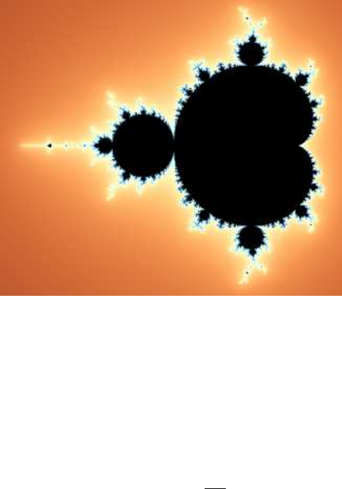
2.1 Mandelbrot set
Figure 2.1: Mandelbrot Set
This is a typical example of a two-dimensional fractal generated mathematically. This image is
created with a very simple formula, which is calculated in many iterations:
zn+1 =z2
n+c
•zis a complex number (a+ ib), where iis the imaginary number.
i=√−1
The number is made of two parts: athe real part and ibthe imaginary part.
•cis the coordinates of the image point to be iterated.
In 2D, zis a vector containing two complex number coordinates, x and y, ( these points represent
the pixel location where x represents the real part of the number [a] and y represents the imaginary
part of the number [b]). Because they are complex numbers, they can be positive or negative, but
also there will still be a mathematical solution if a function requires the square root of a negative
number.
Each original point (pixel position) is tested in the formula iteration loop, to determine if it belongs
to the formula specific mathematical fractal set.
The initial value of point zis assigned to equal c, (z0=c), this parameter is then used repeatedly
in the iteration loop.
6
zn+1 =z2
n+c
zn+2 =z2
n+1 +c
zn+3 =z2
n+2 +c
etc.
The program has to determine if these series are convergent. To do this iterations should be
repeated an infinite number of times. But since a computer cannot infinitely repeat in practice the
convergence is determined with a simplification.
Termination conditions are applied to ensure the formula does not iterate to infinity. The most
common conditions used are called Bailout and Maxiter.
The Bailout condition stops the iteration loop if the formula transforms (moves) the point further
than a set distance away from an “origin”. This detects if series are convergent (calculated point is
outside the fractal body)
Maxiter is simply a condition to stop iterating when a maximum numbers of iterations is reached
(just to not do iterations infinite times)
In the Mandelbrot formula, after each iteration, the modulus of a complex number is calculated; in
other words, the length of the vector from the origin (x= 0, y= 0) to the current zpoint. This
vector length is often called rfor it is the radius from the center (origin) to the current zpoint.
In this example, when the length r> 2 (i.e Bailout = 2), the termination condition has been
met, then the iteration process is stopped and the resulting image point is marked with a light
color. When, after many repeated iterations, ris still less than 2, then it can be considered for
simplicity that such a result will continue indefinitely. Iterations are therefore interrupted after a
certain number of iterations (Maxiter). This point is marked on the image with black. This results
in a “set” of points that do not reach bailout termination (black) and the rest of the points given
lighter colors (dependent on a chosen coloring method).
With traditional 2D fractals, every point is given a color. With 3D fractals, only the points that
are found to belong to the set, are given a color. One simple method is to assign a different color
depending on the distance of the point from the origin.
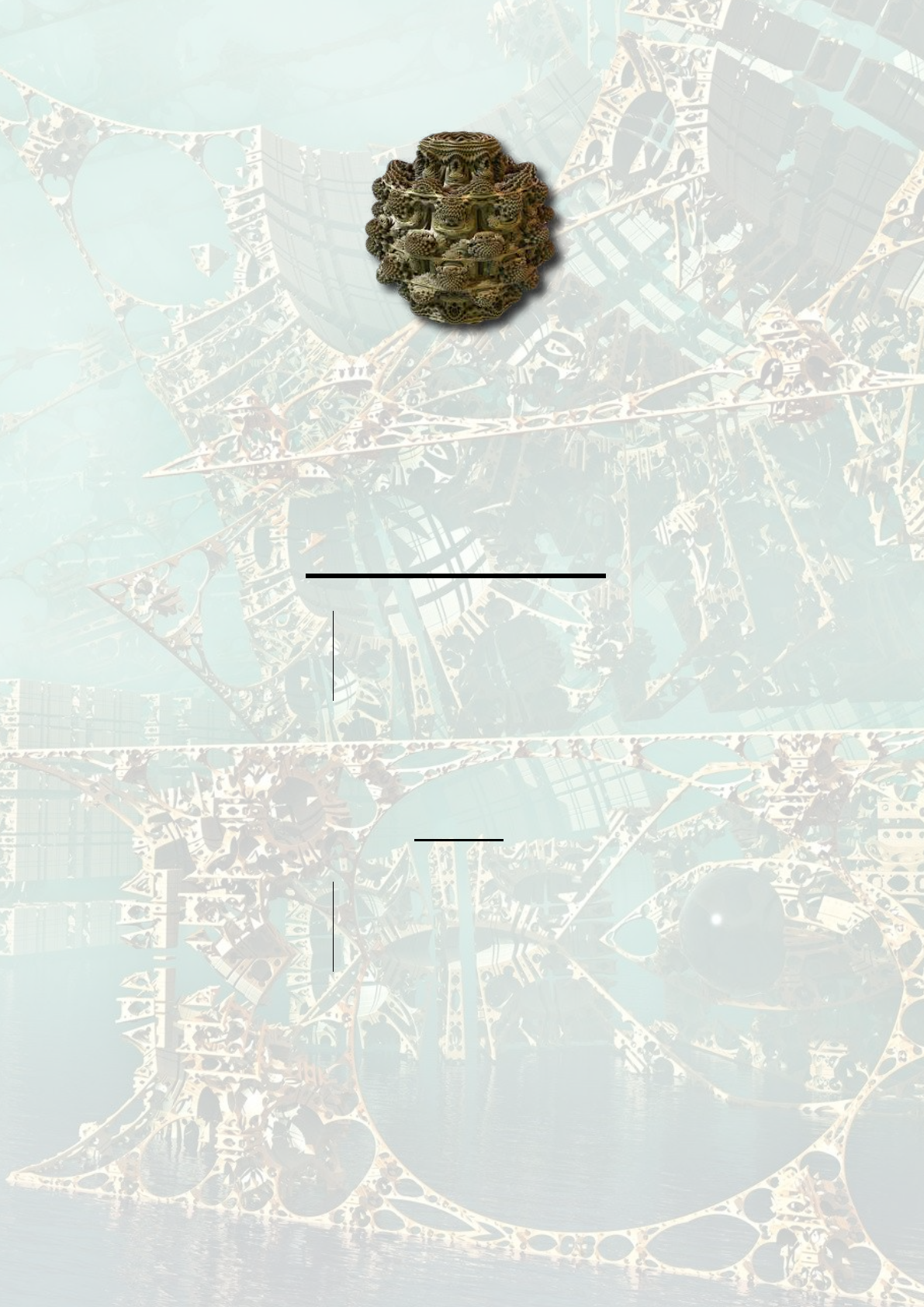
2.2 3D fractals
The three dimensional fractal type, the “Mandelbulb” is calculated from a fairly similar pattern to
the Mandelbrot set. The difference is that the vector zcontains three components (x,y,z) or
four dimensions (x,y,z,w). As they are part of the zvector, they are denoted as (z.x,z.y,z.z).
Examples being Hypercomplex numbers and quaternions.
They can also be created by modification of quaternions or by a specific representation of trigono-
metric vectors.
Generally, common math operators are used (e.g.: addition, multiplication, squaring, and power)
and also conditional functions (e.g., if z.x >z.y,then z.x =something).
Some other types of 3D fractal objects are based on iterative algorithms (IFS - Iterated Function
7
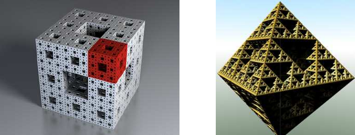
Systems). An example would be the famous Menger Sponge.
Figure 2.2: Menger Sponge Figure 2.3: Sierpinski
2.3 Mandelbulber Program
Mandelbulber is an easy to use, handy application designed to help you render 3D Mandelbrot
fractals called Mandelbulb and some other kind of 3D fractals like Mandelbox, Bulbbox, Juliabulb,
Menger Sponge, . . . The following sections cover the program interface and give useful information
about how to use it.
8

3 Distance Estimation
Distance Estimation (DE) is the calculation of an estimated distance from the given point to the
nearest surface of the fractal. As suggested by the word ’estimate’, it is an approximate value. It is
calculated using simplified algorithms based on analytical (Analytical DE) or numerical (Delta DE)
calculations of gradients.
DE is the most important algorithm required to render three-dimensional fractals within a reasonable
time. It achieves a great reduction in the number of steps needed to find the exact area of the fractal
while tracking a “photon” traveling toward the object along a ray (a simulated beam of light from
the camera eye). A ray is generated for each pixel (1000 x 1000 resolution = 1,000,000 rays). They
match FOV from the camera eye (i.e. they are not parallel).
Without the DE calculation, the proximity of the photon to the fractal surface would need to be
repeatedly calculated after each of many very small steps. For example, without an estimate of
where the fractal surface is, you may need up to 10,000 steps to trace a ray of light, for every pixel
of the image.
Using DE, the size of the steps along the ray of light can be increased, based on the calculated
estimate of where the fractal surface should approximately be located. The process of moving along
the ray and testing for the surface location is called ray-marching.
Ray marching looks like the illustration below. In each step, an estimation on the distance to the
nearest fractal surface is calculated. The photon is moved along the ray by this distance. The next
step is re-calculated based on the estimated distance. This distance is less so this time the “photon”
is moved a smaller distance. The ray-marching becomes more accurate closer to the surface of the
fractal. The ray marching ceases when the “photon” becomes within a set “distance threshold”
from the surface or after a maximum number of iteration if the option “stop at maximum iteration”
is enabled.
Figure 3.1: Distance Estimation with DE factor 1
Since the estimation contains some error (sometimes quite large), there is a risk that the step of
moving the “photon” will be too large, and incorrectly the step will go past the fractal surface. This
may result in visible noise in the rendered image.
To prevent this, the “photon” can be moved by the estimated distance multiplied by a number
between 0 and 1 (ray-marching step multiplier). Steps are then smaller, so there is less risk of
“overstepping” the surface (better image quality), but the rendering time increases due to more
9
steps being required.
Figure 3.2: Distance Estimation with DE factor 0.5
Each formula has assigned a DE mode and function (“preferred”). In most cases the preferred mode
is Analytical DE (fastest).
The preferred function is assigned based on whether the formula is transforming in a linear or
logarithmic manner. These setting can be varied on the Render Engine tab.
Analytical DE mode is faster than Delta DE mode to calculate. However with some formulas only
Delta DE mode will produce a good quality image. The DE modes can be used with either linear
or logarithmic DE functions.
Example linear out: distance =r
|DE|
Example logarithmic: distance =0.5rlog(r)
DE
The quality produced by the DE mode and function combinations is formula specific. The setting of
formula parameters can also greatly affect the quality produced by the DE. In some cases the choice
of fractal image is determined by what location and parameters can produce good DE quality.
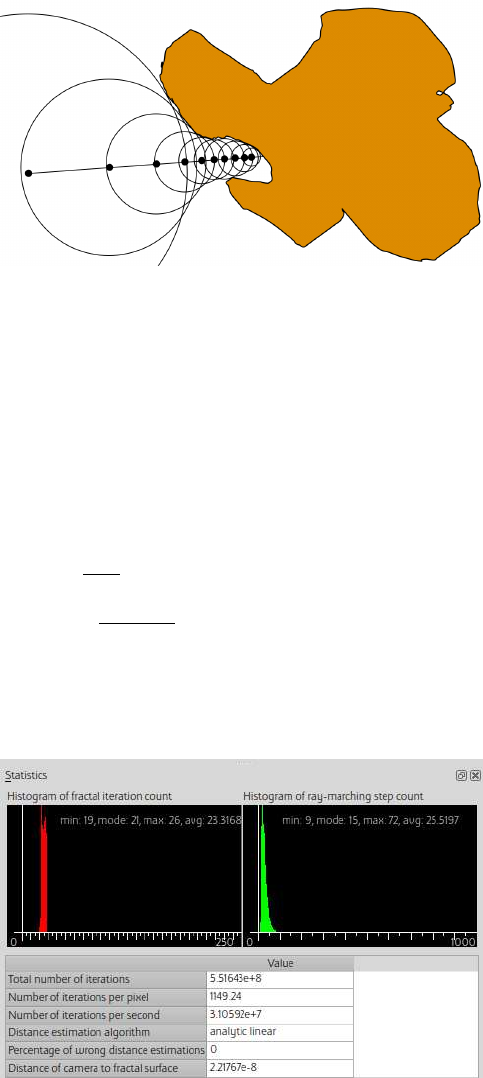
Figure 3.3: Statistics Tab with histogram data
In the Statistics (enable in View menu) you can see Percentage of Wrong Distance Estimations
(“Bad DE”). This number is the percentage of image pixels which potentially have big errors in
distance estimation calculation (estimated distance was much too high). It is visible as a noise on
the image. As a general rule less than 0.1 is good, but it is case specific and 3.0 sometimes is OK
and 0.0001 sometimes is not.
Figure 3.4 below, is an example of Bad DE due to over-stepping. It starts to occur at the corner
nearest to the camera, resulting in the black areas and distintegration of the fractal. If the ray-
10
marching step multiplier is set even higher, the fractal will entirely disintegrate. This disintegration
will generally be reflected in the Percentage of Wrong Distance Estimations statistic.
Figure 3.4: Example of over-stepping
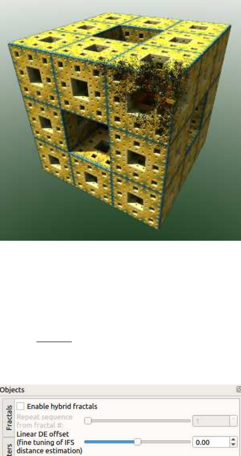
Figure 3.5 below, shows the Linear DE offset parameter located in the Hybrids tab. For standard
mandelbox types and IFS there are two similar analytic distance estimation calculations used. When
making a hybrid that mixes these types, then adjusting the Linear DE offset parameter can assist in
fine tuning the DE calculation.
Generic linear out: distance =r−of f set
|DE|
The Linear DE offset is normally used in the range from 0.0 (mandelbox) to 2.0 (IFS).
Figure 3.5: Linear DE offset parameter
11
4 Ray-marching - Maximum number of iterations vs. dis-
tance threshold condition
The ray marching distance threshold is the condition where the photon marching along the ray
comes within a specified distance from the fractal surface and the ray-marching stops. This controls
the size of the detail in the image, and is normally set to vary such that greater detail is obtained for
the surface closest to the camera, (in the further regions of the fractal the distance threshold will
be larger such that only bigger details are visible). Enabling Constant Detail Size on the Rendering
Engine tab will make the distance threshold uniform.
There are two modes of stopping the ray-marching of each image pixel.
1st case: Stop ray-marching at distance threshold (Stop at maximum iteration is disabled).
2nd case: Stop ray-marching at point when a maximum number of iterations is reached (Stop at
maximum iteration is enabled).
First important note: Stop at maximum iteration doesn’t control the fractal iteration loop. It
controls only ray-marching. The iteration loop always runs to achieve Bailout, (then if bailout is not
reached the iteration stops at Maxiter). (see page 7)
On figure 4.1 ray-marching stops at distance threshold. In most cases the fractal iteration loop
stops on bailout condition, (because away from surface it is not possible to reach Maxiter). It makes
rendering of fractals much faster.
On figure 4.2 ray-marching stops at the photon step when the maximum number of iterations is
reached (ray-marching distance threshold is ignored). In many cases iteration loop stops on bailout
condition (away from fractal surface), but on the fractal surface the maximum number of iterations
is calculated (when bailout is not reached).
Figure 4.1: Example for 1st case - stop ray-
marching at distance threshold
Figure 4.2: Example for 2nd case: Stop ray-
marching at Maxiter
12
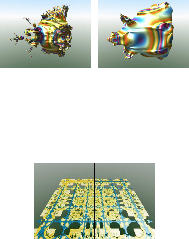
Figure 4.3: Example for 1st case: Stop ray-
marching at bailout with low Maxiter
Figure 4.4: Example for 2nd case: Stop ray-
marching at maxiter with low maxiter
Figure 4.3 shows what happens if maximum number of iterations is set to 4. Even if Maxiter is
reached the ray-marching is continued until the ray marching distance threshold is reached.
Figure 4.4 shows case when maximum number of iterations is reached. Ray-marching is stopped
even if distance threshold is not reached.
Enabling Constant Detail Size on the Rendering Engine tab will make the distance threshold uniform.
This takes longer, but gives a more accurate representation of detail in the distance, and can be
used to address color variation over distance like in the image below.
Figure 4.5: Constant detail size
13
5 Iteration loop
In section 2.1 it was mentioned that fractals are calculated by repeating a formula (iterating) in an
iteration loop. The integer iis used to represent the iteration count number.
The iteration count starts with i= 0, then at the end of each iteration the count number is increased
by 1, and the next iteration of the formula commences (e.g. iteration count 0, 1, 2, 3, ...). The
iterating continues until termination conditions are met, which is either when the iteration count i
=maxiter or when the bailout condition is achieved.
This section explains the calculations within the iteration loop.
A fractal formula is built from mathematical equations. These equations can be modifications of
the Mandelbrot Set equation (e.g Mandelbulb) and also other mathematical equations.
The equations are made from mathematical operators (+,−,∗, /) and can include mathematical
functions (e.g. sin, cos, tan, exp, log, sqrt, pow, abs) and also mathematical conditions (e.g. if x
> y then “compute following equation(s)”, if i > 4 then “compute following equation(s)”).
The equations are applied to vector z or any parts of z (i.e the z.x, z.y and z.z components)
Examples:
z.x = fabs(z.x ); is using the function fabs() (which is floating-point version of abs()), where
z.x is assigned the absolute value of z.x.
if (z.x -z.y < 0.0) swap(z.x,z.y ); is using the conditional function if() to determine if
the values of z.x and z.y should be swapped.
z*= 3.0 is using the operator * to multiply the all components of vector z by 3.0.
A set of equations that have a specific function within the formula are called transforms, e.g rotation,
scale.
The generally a formula is constructed from one or more transforms, which are constructed from
equations.
With each iteration of the formula, the point being iterated is mapped (moved) to new coordinates
as a result of the mathematical equations.
5.1 Single formula fractals
The simplest 3D fractals are calculated by iterating a single fractal formula. More complex fractals are
made by iterating a mix of formulas, adding extra transforms, and/or including additional conditions.
Below there are 3 examples of fractals formulas written in C language code
14
5.1.1 Mandelbulb Power 2
This formula is a modified Mandelbrot Set equation, expanded to 3rd dimension. A cross section at
zz= 0 looks exactly the same as Mandelbrot Set.
Listing 1: Formula > Mandelbulb Power 2
double x2 = z .x * z .x ;
double y2 = z .y * z .y ;
double z2 = z .z * z .z ;
double temp = 1.0 - z2 / ( x2 + y2 );
double ne wx = ( x2 - y2 ) * t emp ;
double newy = 2.0 * z . x * z .y * temp ;
double newz = -2.0 * z . z * sq rt (x2 + y2 );
z. x = new x ;
z. y = new y ;
z. z = new z ;
5.1.2 Menger Sponge
This formula is an Iterated Function System (IFS). It contains several transforms, some of them
conditions.
Listing 2: Formula > Menger Sponge
z .x = f abs ( z .x );
z .y = f abs ( z .y );
z .z = f abs ( z .z );
if ( z .x - z . y < 0 .0 ) sw ap ( z .x , z . y );
if ( z .x - z . z < 0 .0 ) sw ap ( z .x , z . z );
if ( z .y - z . z < 0 .0 ) sw ap ( z .y , z . z );
z *= 3.0;
z. x -= 2.0;
z. y -= 2.0;
if ( z .z > 1.0) z . z -= 2.0;
5.1.3 Box Fold Bulb Pow 2
This formula is made from a set of different transforms. It is a good example of how a fractal
formula can be more complicated than the Mandelbrot Set formula.
First part is a “box fold” transform which conditionally maps the point in x,y,z directions. Second
part is a “spherical fold” which does conditional scaling in a radial direction. The end of formula is
the same as Mandelbulb Power 2.
15
Listing 3: Formula > Box fold Power 2
// box fold
if ( fab s (z .x) > frac tal -> f ol di ng In tP ow . f ol dF actor )
z. x = sign (z . x) * fractal -> foldingIn t P ow . foldFactor
* 2.0 - z.x ;
if ( fab s (z .y) > frac tal -> f ol di ng In tP ow . f ol dF actor )
z. y = sign (z . y) * fractal -> foldingIn t P ow . foldFactor
* 2.0 - z.y ;
if ( fab s (z .z) > frac tal -> f ol di ng In tP ow . f ol dF actor )
z. z = sign (z . z) * fractal -> foldingIn t P ow . foldFactor
* 2.0 - z.z ;
// spherical fold
double fR 2_2 = 1.0;
double mR 2_2 = 0.25;
double r2 _2 = z. Do t (z );
double tglad_ f a c tor1 _ 2 = f R2_2 / mR 2_2 ;
if ( r2_ 2 < mR 2_2 )
{
z = z * tgla d _ f a ctor 1 _ 2 ;
}
else if ( r 2_2 < fR2 _2 )
{
double tgl ad _f ac to r2 _2 = fR2_ 2 / r2 _2 ;
z = z * tgla d _ f a ctor 2 _ 2 ;
}
// Mandelbulb powe r 2
z = z * 2 .0;
double x2 = z .x * z .x ;
double y2 = z .y * z .y ;
double z2 = z .z * z .z ;
double temp = 1.0 - z2 / ( x2 + y2 );
zT emp .x = ( x2 - y2 ) * temp ;
zT emp .y = 2.0 * z . x * z. y * temp ;
zT emp . z = -2.0 * z .z * sqrt ( x2 + y2 );
z = zT emp ;
z. z *= fractal -> f oldi ngIntP ow . zFactor ;
16
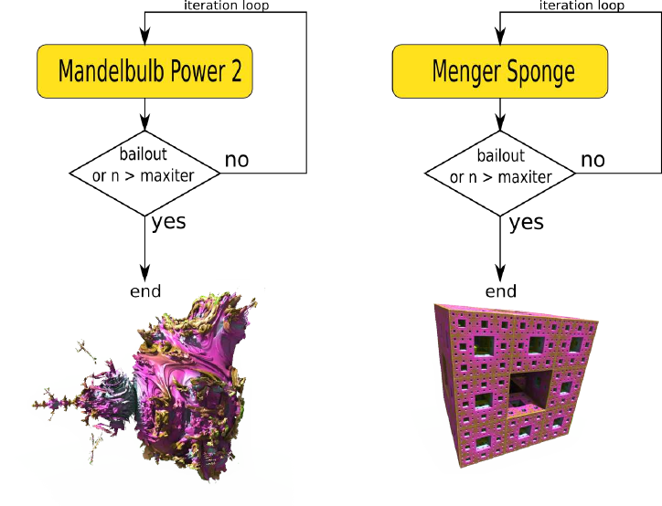
5.1.4 Processing of single formula fractals
Single formula fractals are simply iterated several times until termination conditions are met, as
shown in figure 5.1.
Figure 5.1: Examples of simple Iteration loops with one formula
When the calculation of the iteration loop finishes the resulting final value of zis used to estimate
the distance to the fractal body and to calculate the color of the surface.
5.2 Hybrid fractals
Hybrid fractals are constructed by using more than one formula in the iteration loop. This way
new variations of fractal shapes can be achieved. There are many different fractal formulas and
transforms available in the Mandelbulber program, which allows the user to create a vast variety of
hybrid shapes.
5.2.1 Iteration loop of hybrid fractals
In general hybrid fractals are calculated in a similar way to single formula fractals. The calculation
consists of the iteration loop, maxiter and bailout condition. The difference is that when hybrid
mode is enabled, a user can create a sequence of up to nine different fractal formulas (or transforms)
inside the iteration loop.
By default the program works in single fractal formula mode, where you can only configure the
parameters of the formula tab in the first slot, (#1).
17
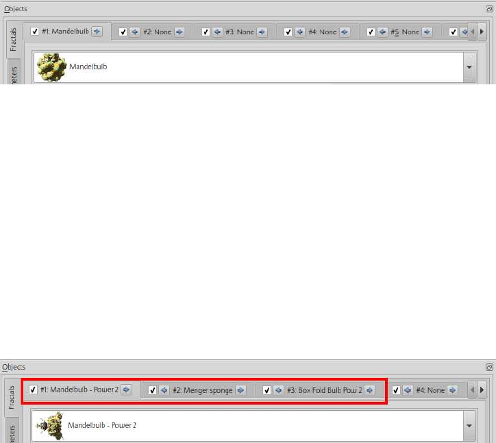
Figure 5.2: Fractal Tab - Formula only in first slot
There are two ways to enable hybrid fractals:
•Click in any slot with a number higher than one. The program will ask if you want to enable
hybrid fractals or boolean mode. Select Enable hybrid fractals
•Go to Objects /Hybrid tab. Tick Enable hybrid fractals checkbox.
Once hybrid fractals has been enabled, a user can select additional formulas from the dropdown
menus in any of the nine formula slots, as shown in figure 5.3. In this figure Mandelbulb - Power 2
is selected in slot #1, Menger Sponge in slot #2 and Box Fold Bulb Pow 2 in slot #3. These
formulas will be used in the next examples.
Figure 5.3: Fractal Tab - Multiple formula slots filled
Each formula’s parameters can be configured in the formula tab opened in an enabled slot.
The iteration count numbers determine when in the sequence each formula is calculated.
The sequence is in the order of the enabled formula slots from #1 to slot #9, (e.g. If the sequence
is calculating formulas in slots #1 and #5, then the iteration loop repeats the sequence of slot #1
calculation followed by slot #5 calculation.)
How the sequence will work depends on the following selections:
•Which fractal formulas are selected in the formula slots
•How many iterations are assigned to each formula
•The range of iteration numbers when the formula will be used
•From which fractal slot the sequence will be repeated
18
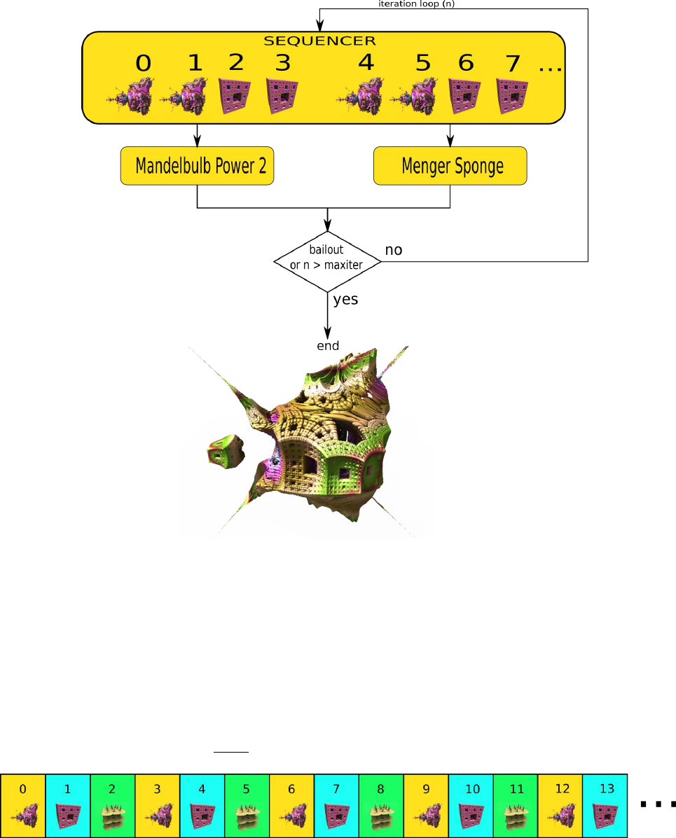
Figure 5.4: Complex Iteration loop with hybrid fractal
5.2.2 One iteration for each slot
The simplest way to create a hybrid fractal is a sequence where formulas are calculated one after
another, then the sequence is repeated until termination conditions are met.
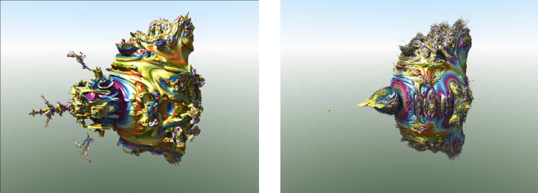
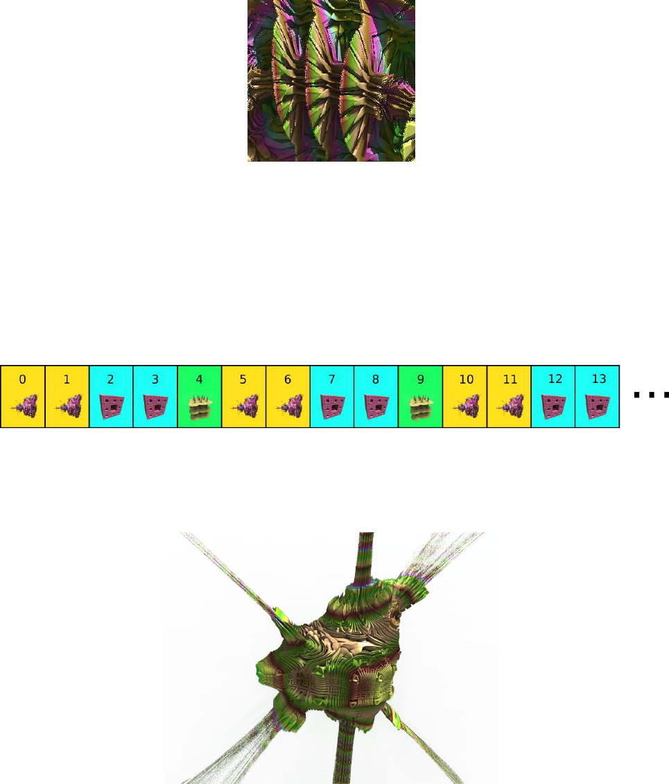
In figure 5.5, the sequence consists of one Mandelbulb - Power 2, one Menger Sponge and one Box
Fold Bulb Pow 2. The length of the sequence is three iterations, so after every third iteration the
sequence repeats from the first slot. The numbers shown are the Iteration Count, starting at i = 0.
The count increases by 1 after every iteration performed in the iteration loop.
Figure 5.5: Hybrid sequence - Simple sequence using three different formulas
This sequence gives a shape combining properties of all three formulas, see figure 5.6.
19
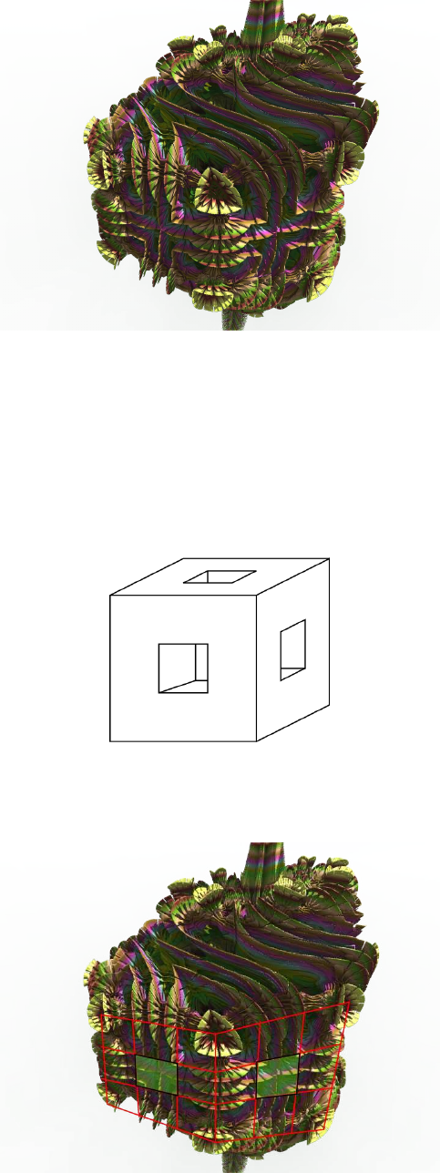
Figure 5.6: Hybrid sequence render - Simple sequence using three different formulas
Because the first iteration is (slot #1) Mandelbulb - Power 2, the general shape of the fractal will
be simlar in shape to the Mandelbulb - Power 2.
Note: Generally, the first few iterations of a fractal strongly influence the final hybrid fractal shape.
In the next iteration Menger Sponge formula is used. A single iteration of this formula produces the
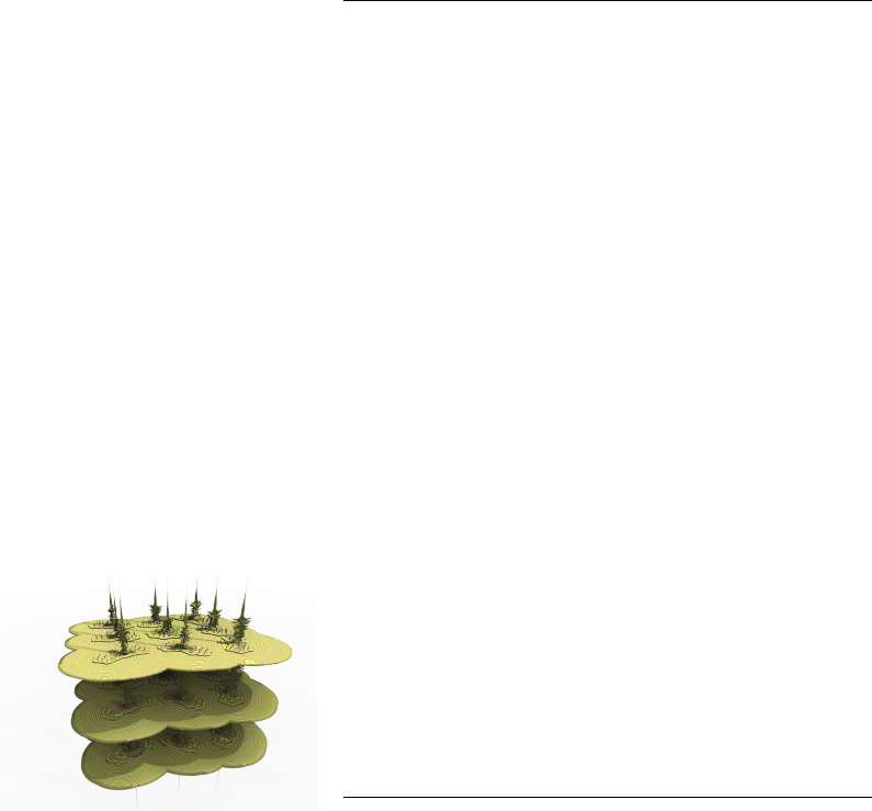
shape of figure 5.7.
Figure 5.7: Single iteration of the Menger Sponge
Some features of this shape are transferred to the generated shape of the hybrid fractal.
Figure 5.8: Hybrid with Menger Sponge features marked in red
The Menger Sponge shape is distorted, because Mandelbulb - Power 2 has already deformed the
space.
20
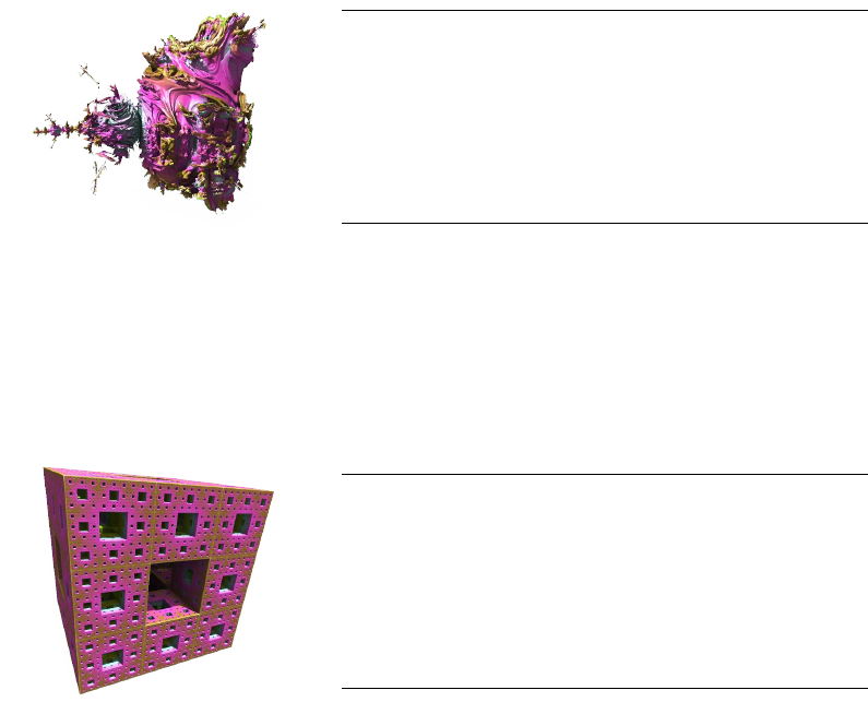
The third formula Box Fold Bulb Pow 2 adds leaf-like features to the shape.
Figure 5.9: Hybrid close up of leaf-like shapes produced by ’Box Fold Bulb Pow 2’ formula
5.2.3 More iterations for each slot
With each slot a user can define how many times each fractal formula will be used in the sequence.
On each of the formula tabs there is a parameter named Iterations which is set to 1 by default. This
is the number of iterations (repeats) of the formula performed before the loop moves on to the next
formula slot in the sequence. If this value is increased to 2 on the first and second formula slots in
our example, then the sequence of the formulas will be as shown in figure 5.10.
Figure 5.10: Hybrid sequence - The first and second slots set to 2 repeat iterations
The first and second formulas are repeated twice and the third formula only once. The resulting
fractal shape is shown in figure 5.11:
Figure 5.11: Hybrid sequence result - The first and second slots set to 2 repeat iterations
Because the Mandelbulb - Power 2 calculation is repeated for two iterations at the beginning, the
shape of this initial formula strongly influences the final shape of the hybrid fractal.
If the parameter Iterations on the second slot is set to 10, then the Menger Sponge formula is used
from iteration 2 to iteration 11.
21
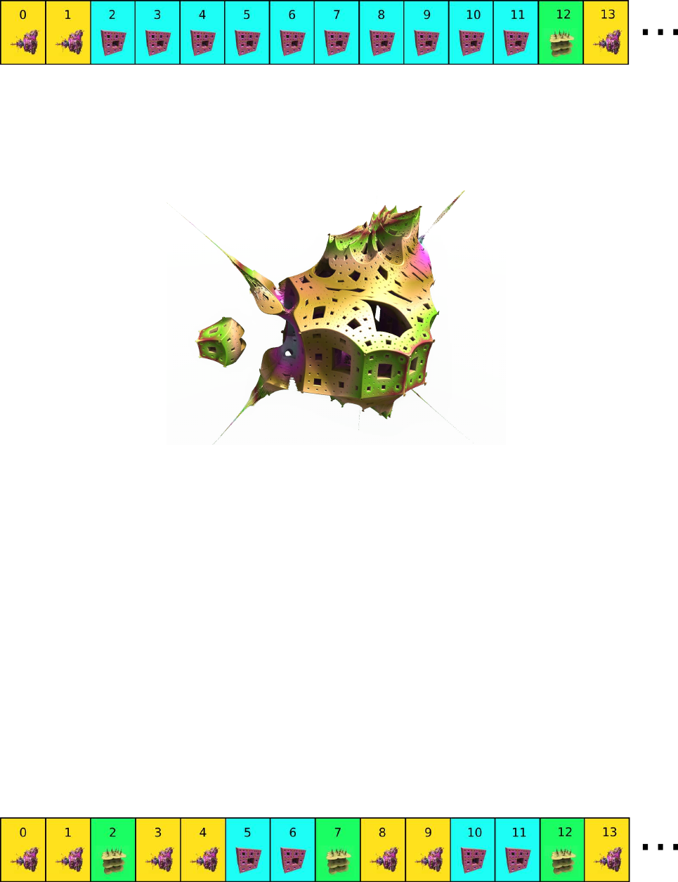
Figure 5.12: Hybrid sequence - The second slot set to 10 repeat iterations
As above, the initial shape is mainly defined by the first two iterations of Mandelbulb - Power 2,
but the high number of Menger Sponge iterations makes the Menger Sponge features become more
apparent.
Figure 5.13: Hybrid sequence result - The second slot set to 10 repeat iterations
5.2.4 Range of iterations for slot
The sequences can become more complicated by specifying the range of iterations when a formula
will be calculated in the loop.
On each formula tab the parameters Start at iteration and Stop at iteration are used to define this
range.
When computing the iteration loop, the program is moving through the enabled formula slots,
checking formula iteration range conditions. If the current Iteration Count number is within the
range then a calculation of that formula is performed, and the Iteration Count is increased by 1. If
the Iteration Count number is outside the iteration range condition, then the formula is skipped (i.e.
no calculation and therefore the iteration count remains unchanged). The program then moves to
the next enabled slot in the sequence.
The second formula slot (Menger Sponge) in the sequence shown in figure 5.14, has the iteration
range set to from 4 to 250.
Figure 5.14: Hybrid sequence - Range of iteration set to 4-250 on second slot
During the first pass of the sequence Menger Sponge formula could not be used at iterations 2 and
3, because Start at iteration was when i = 4 for this formula, and therefore the slot was skipped.
22
During the second pass of the sequence Menger Sponge formula was used at iterations 5 and 6,
because those iterations were inside the defined range of iterations.
The shape of the resulting fractal is shown in figure 5.15
Figure 5.15: Hybrid sequence result - Range of iteration set to 4-250 on second formula slot
Because at iteration number 2 Menger Sponge formula was skipped, Box Fold Bulb Pow 2 formula
has much more influence on the final shape.
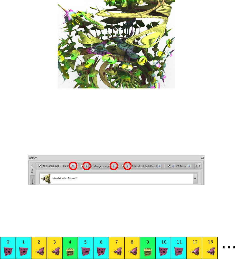
5.2.5 Changed order in sequence
The order of fractal formulas can be easily changed between slots with the use of the arrow buttons.
Figure 5.16: Fractal tabs with highlighted tab-arrows
These buttons swap the fractal tabs between the slots, and therefore the formula’s position inside
the sequence will change. All formula parameters setting are moved in the swap.
Example based on first case shown in section 5.2.3: Swapped Mandelbulb - Power 2 and Menger
Sponge creates the sequence shown in figure 5.17.
Figure 5.17: Hybrid sequence - Swapped tab one and two
As evident in figure 5.18, the shape of the fractal is completely different.
23
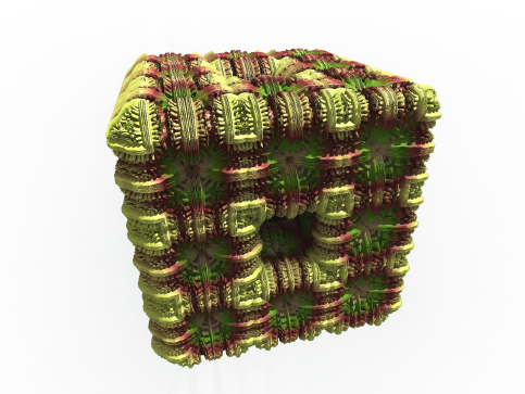
Figure 5.18: Hybrid sequence render - Swapped tab one and two
Now the first Menger Sponge formula creates the initial shape of the fractal, and Mandelbulb -
Power 2 only modifies the details.
Even if the same fractal formulas are used in each slot, and for the same number of iterations, the
final shape will strongly depend on the parameter settings of the first few formulas that are iterated
in the sequence.
There are also a few formulas and transforms which have a very strong influence on the final shape,
and these are often run for just 1 or 2 iterations during the iterating of the fractal.
24
6 Navigation
To set the current view there are two elements:
Camera represents a point where the camera is located
Target represents the point onto which the camera will focus (the camera is always looking at the
target.)
6.1 Camera and Target movement step
The relationship between the camera point and the target point can be altered manually by changing
the numbers in the edit fields, or by navigating with distance and rotation “steps” defined by the
user.
For rotations, the camera is moved by the parameter rotation step (default 15 degrees). For
movements of the camera and/or the target in a linear direction, the parameter step (default 0.5)
is used. There are two modes for its use:
6.1.1 Relative step mode
The step for moving the camera and/or target in a linear direction is calculated relative to the
estimated distance from the surface of the fractal. The closer to the surface that the camera is
located, the smaller the step. This prevents the camera moving to a location beneath the surface
of the fractal.
The actual step is equal to the distance from the fractal multiplied by the parameter step.
Example: If the step is set at 0.5 and the nearest point of the fractal is 3.0, the camera will be
moved 1.5 (no matter in which direction).
Relative step mode makes navigation easier, because a user does not need to think about the
movement size required to avoid the camera moving into the fractal.
In animations this mode is recommended when camera is approaching the surface of the fractal.
6.1.2 Absolute step mode
Step movement of the camera and/or target is fixed. Therefore if the step is set at 0.5, the movement
will be 0.5 in the direction of the arrow key or mouse pointer.
This mode is recommended for flight animation with the camera flying at a fixed (or strictly con-
trolled) speed.
6.2 Linear camera and target movement modes using the arrow buttons
A user can navigate by operating the arrow buttons on the Navigation dock, with the user defined
steps.
There are three modes for changing the relationship between camera and target:
25
•move camera and target •move only camera •move only target
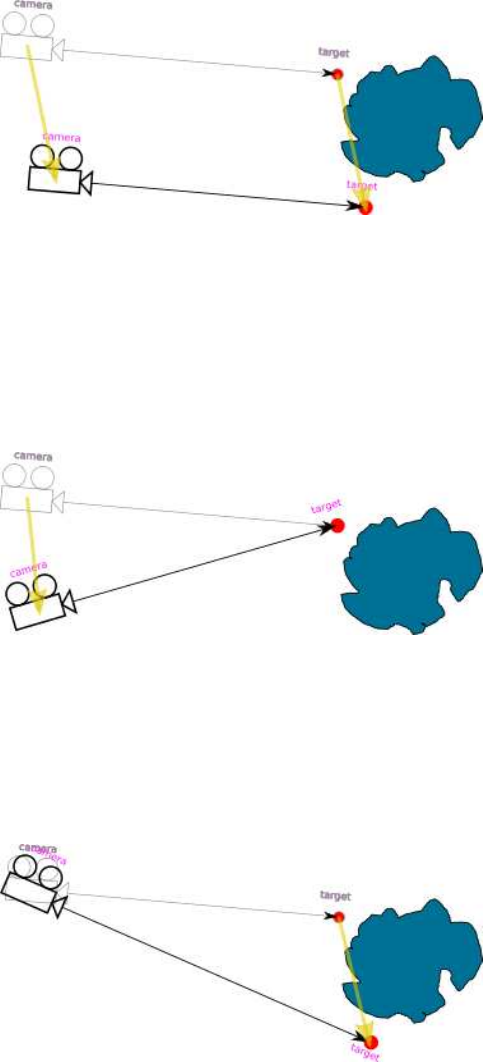
6.2.1 Move camera and target mode
Figure 6.1: Movement mode - camera and target
Arrows move both the camera and the target by the same distance in the same direction. The angle
of camera rotation does not change.
6.2.2 Move camera mode
Figure 6.2: Movement mode - camera
Moves only the camera and rotates it in respect to the motionless target.
6.2.3 Move target mode
Figure 6.3: Movement mode - target
Moves only the target while maintaining a fixed camera position. The camera rotates following the
target. Note: In Relative Step Mode, the target is moved by distance related to distance of target
to fractal surface. If target is inside the fractal (distance = 0), then this option will not work with
Relative Step Mode.
26

6.3 Linear camera and target movement modes using the mouse pointer
A user can move the camera by selecting a point on the image with the mouse pointer, and then
using either left mouse button (move forward) or right button (move backward).
6.3.1 Move camera and target mode
The target is moved to the point selected by the mouse. The camera is moved towards selected
point by a user defined step, and rotated.
In relative step mode, the camera is moved by distance equals to distance_to_indicated_point
multiplied by step parameter.
In absolute step mode, the camera is moved by distance equals to step parameter.
6.3.2 Move camera mode
The camera is moved by the step (absolute or relative) in the direction of the mouse pointer, rotating
the camera to look at the target. The target remains stationary.
6.3.3 Move target mode
The target is moved to the point selected by the mouse. The camera remains at the same point
but rotates following the target.
6.4 Camera rotation modes using the arrow buttons
6.4.1 Rotate camera
Figure 6.4: Rotation mode - around camera
The camera is rotated by the rotation step around its axis and the target is moved accordingly. This
is the standard mode for rotation of the camera.
27
6.4.2 Rotate around target
Figure 6.5: Rotation mode - around target
The camera is moved around the stationary target by the rotation step, maintaining a constant
distance to the target. The camera is rotated to look at the target.
6.5 Reset View
Camera Position is reset, by being zoomed out from the fractal but still maintaing the camera angles.
If the rotations are changed to zero before using Reset View, the camera will then be zoomed out
from the target, and rotated to look down the y axis.
6.6 Calculation of rotation angles modes
6.6.1 Fixed-roll angle
In this mode, the angle gamma (roll) is constant. Pan the camera left or right always takes place
around the global vertical Z-axis (not the render window vertical axis).
This mode can be likened to an aircrafts controls, where all turns are relative to the aircraft’s axis,
not the ground below. Rotate up / down raises / lowers the nose of the aircraft. Rotate left / right
turns in the directions of the wings. Tilting the camera buttons tilts the aircraft
When the camera is pointing straight up or down, or when it is upside down in this mode, it is quite
difficult to predict the result of the turn.
6.6.2 Straight rotation
The camera is rotated around its own local axis (local vertical axis is the render window vertical
axis.)
This mode is a more intuitive way to rotate the camera, e.g., turn the camera left always give
the visual effect of the camera rotating in that direction. The rotation angles are automatically
converted so they are appropriate for the selected direction. This mode changes the gamma angle
(roll).
28
6.7 Camera rotation in animations
With animation, the camera point and the target point can move independently following their
own trajectories, with the camera always looking towards the target point. It is important to be
aware that the rotation angle of the camera is the result of the camera coordinates and the target
coordinates.
There are various ways of animating, depending on the objective.
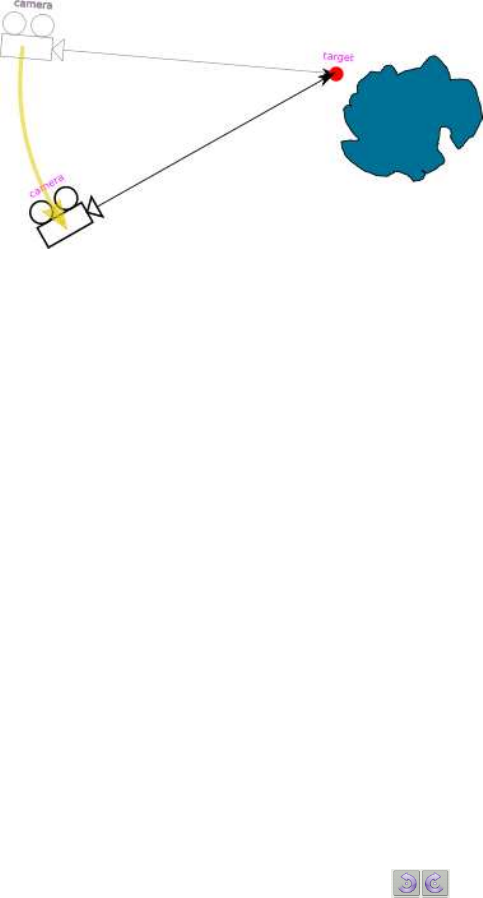
The following example is a flight animation, with the camera trajectory approaching a location, with
the camera rotating simultaneously so that the location is always observed, (as shown in the figure
6.6). The camera positions represent three keyframes.
Figure 6.6: Keyframe Animation with differing distances camera to target
Between the first and second keyframes, the camera and target both move large distances. But
between the second and third keyframes, the camera moves a much greater distance than the
target. This can sometimes lead to unexpected camera rotations between keyframes.
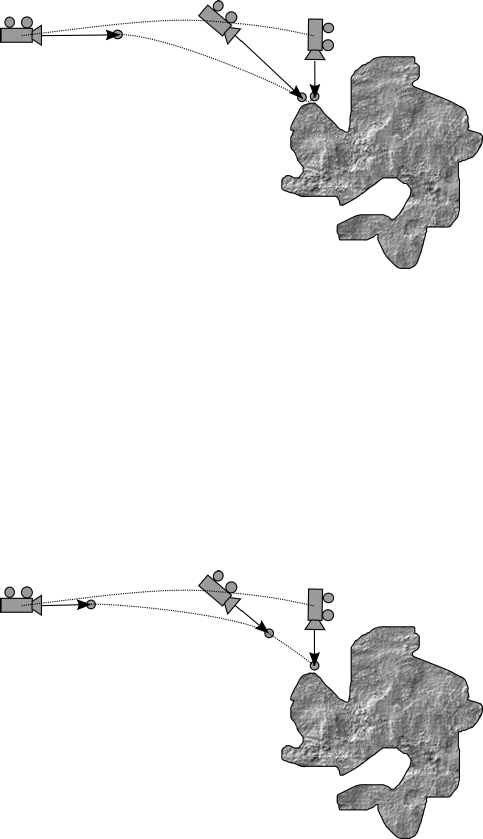
To compensate for this, on the Keyframe navigation tab use the button Set the same distance from
the camera for all the frames This adjusts all keyframes by setting a constant distance between
camera and target. It is important to note that the use of this function does not change the visual
effect for the keyframes, and will help correct interpolation. See figure 6.7.
Figure 6.7: Keyframe Animation with equal distances camera to target
29
7 Interpolation
Interpolation functions, which calculate intermediate values, are used to make smooth parameter
transitions between keyframes. There is no need for manual editing of every animation camera
position and fractal parameters. frame. A limited number of keyframes is enough to define good
looking animation.
7.1 Interpolation types
Parameters in Mandelbulber can be transitioned using several interpolation modes:
1. None
2. Linear
3. Linear angle
4. Akima
5. Akima angle
6. Catmul-Rom
7. Catmul-Rom angle
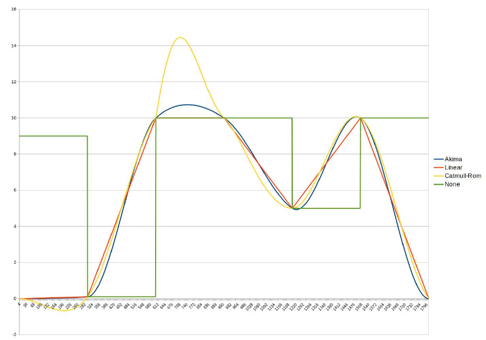
The chart in figure 7.1 shows a comparison between different interpolation modes.
The choice of mode, greatly effects the animation.
Figure 7.1: Interpolation types
30
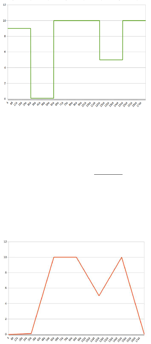
7.1.1 Interpolation - None
The parameter remains constant between keyframes. The parameter will change abrubtly at the any
keyframe that has a change in value. This mode can be used with boolean values or with variables
which have to be kept at a constant value for a number of keyframes.
Figure 7.2: Interpolation - None
7.1.2 Interpolation - Linear
The value of the parameter is interpolated using linear functions.
y(x) = yi+ (x−xi)yi+1 −yi
xi+1 −xi
xi≤x≤xi+1
Changes of parameters are easy to predict. There are no overshoots. This interpolation mode is
good for fractal parameters and material properties. It is generally not recommended to be used for
camera or object movement paths, because of the abrubt changes of speed.
Figure 7.3: Interpolation - Linear
31
7.1.3 Interpolation - Linear angle
This interpolation mode works like Linear, but is prepared of angular parameters. If value exceed
360 degrees, then will go back to zero.
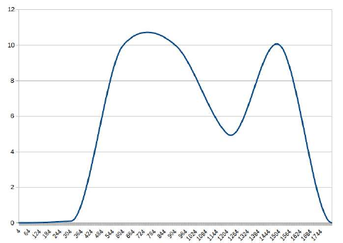
7.1.4 Interpolation - Akima
The Akima interpolation is a continuously differentiable sub-spline interpolation. It is built from
piecewise third order polynomials.
y(x) = a0+a1(x−xi) + a2(x−xi)2+a3(x−xi)3
xi≤x≤xi+1
This interpolation function produces smooth transitioning through the keyframes. It is very good
for most animated parameters. It is used for camera and target animation and for many other
parameters which should be animated in a smooth way.
Figure 7.4: Interpolation - Akima
7.1.5 Interpolation - Akima angle
This interpolation mode works like Akima, but is written for angular parameters. If a value exceeds
360 degrees, then it will reset back to zero.
7.1.6 Interpolation - Catmul-Rom
Catmull-Rom splines are cubic interpolating splines formulated such that the tangent at each point
yi(xi)is calculated using the previous and next point on the spline.
y(x) = 0.5h1x−xi(x−xi)2(x−xi)3i
0200
−1 0 1 0
2−5 4 −1
−1 3 −3 1
yi−1
yi
yi+1
yi+2
32
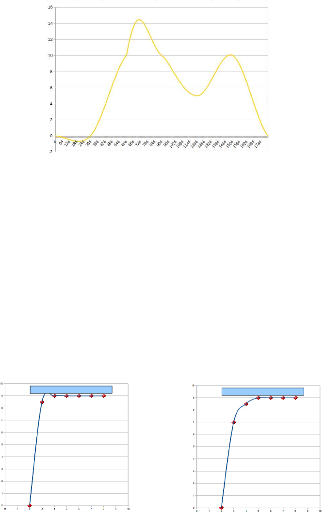
This interpolation gives very smooth results. Animated objects looks likethey are made of springy
materials. It can be used to animate fractal parameters and also the camera path. This interpolation
mode can produce oscillations, so it has to be used carefully. Figure 7.5, shows where interpolated
values went below zero, where all of the keyframe values were higher than zero. The ocsillation
problem is commonly seen near the begining and end of an animation
Figure 7.5: Interpolation - Catmul-Rom
7.1.7 Interpolation - Catmul-Rom angle
This interpolation mode works like Catmul-Rom, but is prepared of angular parameters. If value
exceed 360 degrees, then will go back to zero.
7.2 Catmul-Rom / Akima interpolation - Advices
7.2.1 Collision
Fast approaching the obstacle may cause inadvertent drag to the camera towards the center of the
object. It is recommended to maintain the principle that one keyframe does not reduce the distance
to the object more than five times.
Figure 7.6: Catmul-Rom with collision Figure 7.7: Catmul-Rom without collision
33

7.2.2 Fly through the gap
It is recommended to place a keyframe at the point where the camera flies through a hole / gap in
the fractal.
Figure 7.8: Interpolation - Catmul-Rom path through a hole
7.2.3 Proper conduct cameras between objects
Figure 7.9 shows how keyframes should be located between objects to avoid collisions caused by
interpolation functions.
Figure 7.9: Interpolation - Catmul-Rom path evading different obstacles
7.3 Changing interpolation types
To change the interpolation algorithm, right click on the parameter list and the options appear. In
this example the main_DE_factor have been changed from Akima to Linear. Interpolation type is
color coded e.g. Linear parameters are highlighted in grey.
34
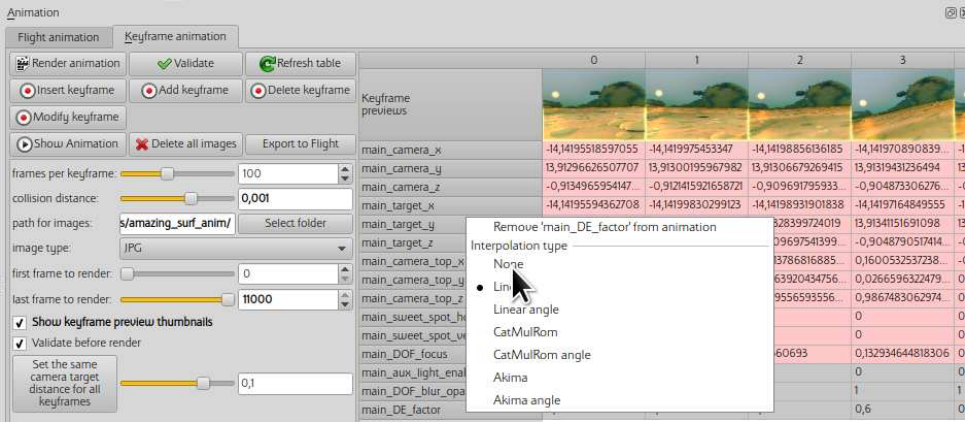
Figure 7.10: Changing an interpolation type
35
8 Animation
8.1 Flight animation - workflow
This section explains the necessary steps required to create flight animation. Flight animation in
Mandelbulber is like a camera motion track recorded in some kind of flight simulator. The camera
can go through interiors of fractal objects. Recording is normally initially done by navigating with
the image set at a low resolution (e.g 320 x 240). After previewing and making any changes, the
final rendering is undertaken with the image resolution set to a suitable higher size.
The parameters of every single animation frame recorded in Flight Animation mode, can be edited
in the animation table.
Workflow:
1. Define fractal object (or many objects).
Create a fractal with interesting features for the flight animation, (e.g. interesting shapes,
geometric structure, texture, coloring, possibly holes where the camera can navigate into).
It is advisable to select a fractal object that is relatively fast to render. Using a fast rendering
fractal at a low resolution, results in the navigation and flight path recording being happening
at almost real time (or slow motion). A fast rendering fractal will also increase the speed of
the final frame rendering process.
2. Place the camera at the point where the flight is to start from.
3. Set a low image resolution. At a low image resolution, the frames-per-second value can be
set higher for the flight path recording. It is reasonable to use a resolution like 320x240 or
160x120
4. Disable all effects which can slow down rendering, like ambient occlusion, reflections, trans-
parency, volumetric lights, etc. All these effects can be re-enabled before commencing the
final rendering of the animation.
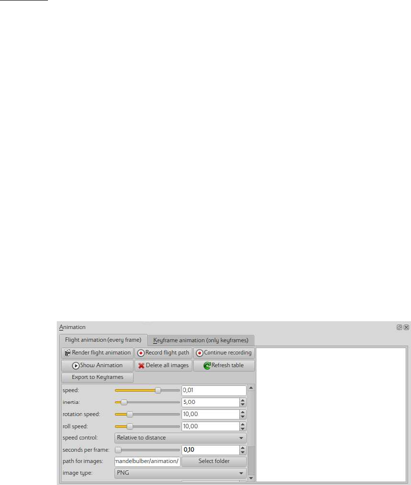
5. Open Flight animation editor. It can be opened from top pull-down-menu by activating View
/Show animation dock. The dock will appear at the bottom of the application window, with
Flight animation (every frame) tab (showed on picture 8.1)
Figure 8.1: Flight animation dock
36
6. Set parameters of animation
speed defines how fast the camera will fly. This parameter can be changed during the
recording of the flight path.
inertia defines how heavy is the camera. A heavy camera will make a smoother motion, but
it will be more difficult to control.
rotation speed defines thereaction speed of mouse pointer movements. A higher value will
allow for the camera to be turned faster.
roll speed defines the speed of the reaction for the Z and X keys, which rotate the camera.
speed control defines how the speed of the camera will be controlled.
•In Relative to distance mode, the camera speed will decrease relatively to the near-
ness of the fractal surface. This mode will help you to not collide with the fractal.
In this mode you can control the relative speed by the speed parameter and by the
mouse buttons.
•In Constant mode, the camera speed is only controlled by the speed parameter and
the mouse buttons
second per frame defines the frame rate during flight path recording. Higher values give
slower rendering but images are more detailed. The value of this parameter is used only
during recording, and is ignored during the rendering of the final animation.
path for images defines where the rendered animation frames will be stored.
image type defines the image format for saving the rendered frames. Detailed settings for
image format are in File /Program preferences
show thumbnails enables previews of frames in animation table
add flight and rotation speed to parameters enables possibility to continue recording of
animation after recording is completely stopped.
7. Press Record flight path button. After 3 seconds recording will be started. During this 3
seconds waiting time the mouse cursor should be placed in the center of image.
8. Use mouse pointer movements to turn camera left / right and up / down. Camera behaves
like airplane in flight simulator
Use Z and X key to rotate the camera
Use arrow keys to move camera left / right / up / down. Without Shift key the camera
still goes forward (movement at 45 degree angle). With Shift key the camera is not moving
forward (movement at straight angle)
Use the left mouse button to increase flight speed or the right button to decrease speed.
9. Press space key to pause recording. When recording is paused, animation parameters can be
changed.
10. Press STOP button to stop recording. It is good to pause the recording using the (space key)
before stopping. This is because by moving the mouse pointer towards STOP button, can
turn the camera.
37
11. Recording of animation can be continued if add flight and rotation speed to parameters is
enabled. If Continue recording is pressed, the recording of flight will resume from the point
stored in the last frame. The camera linear and rotation speed will be maintained.
12. Increase image resolution and enable all required effects. There can be added light sources,
fog, materials, textures, etc.
13. Press Render flight animation to commence final rendering process for the animation. This
can take a very long time depending on the image resolution and the number of frames.
Rendering of the animation can be stopped at any time and continued later. When Render
flight animation is pressed, there will be rendered only the frames which are missing from the
image frame folder. Any existing rendered frames will be skipped.
8.2 Flight animation - more options
8.2.1 Adding more parameters to animation
It is possible to animate almost any parameter in Mandelbulber. Each edit field has an assigned
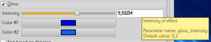
parameter. If you place the mouse pointer on an edit field a tooltip will be displayed.
Figure 8.2: Example tooltip with parameter name
Below the parameter description there is the Parameter name (in this example it is glow_intensity)
The parameter can be added to Flight animation. Right click on an edit field, then use Add to flight
animation from context menu, and the parameter will appear in the animation table (picture 8.3)
8.2.2 Editing animation in the table
It is possible to edit every single animation frame in the animation table. Every cell in the table is
editable. When a value is being edited, the preview is refreshed.
38
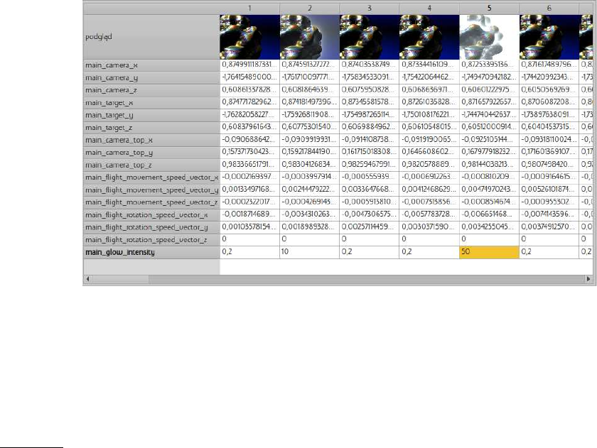
Figure 8.3: Animation table with all recorded frames and one additional parameter
This picture (picture 8.3) shows changes to main_glow_intensity. On frame 2 it is changed to 10
and on frame 5 it is changed to 50.
To get a smooth change of value within the selected range of frames, there is an option to do linear
interpolation of values.
Example: We would like to have smooth transition of glow intensity starting from frame 30 (glow
= 0.2) and ending on frame 100 (glow = 10)
•Right click in the table on cell for glow intensity at frame 100
•Use option Interpolate next frames
•Last frame number set to 100
•Value for last frame set to 10
•When you press OK, you should see that in the table the glow intensity parameter is increasing
to 10 from frame 30 to frame 100
To cut the animation at the start or at the end, there is an option to delete a range of frames. If
you right click on the frame number, there are two options:
•Delete all frames to here - deletes all frames from first to selected frame
•Delete all frames from here - deletes all frames from selected frame to the end
8.3 Keyframe animation - workflow
This section will be written soon
39

9 NetRender
NetRender is a tool that allows you to render the same image or animation on multiple computers
simultaneously. If you have multiple computers connected to an Ethernet network, you can greatly
increase overall computing power.
One of the computers (server) manages the process of rendering. It sends a requests to the connected
computers (clients) and collects the results of rendering. Other computers (clients) render different
portions of the image and send it to the server. There can be only one server (master) but clients
(slaves) can be any number. The more clients, the faster the rendering will be.
The Server is also the computer which renders the combined image .
The total number of CPUs (cores) used is the sum of server’s CPUs cores + all client’s CPUs cores.
9.1 Starting NetRender
9.1.1 Server configuration
On the computer which will be used as the Server, Mode is set to Server.
Figure 9.1: NetRender in ’Server’ mode
Local server port should be set to one which is not used by other applications, and is passed through
routers (if any are used) and firewall. The default is 5555.
If settings are correct, press Launch server and watch for clients button to connect server to existing
clients.
At this point, the server is ready to work
Alternative way to launch the server is to use command line. Example:
$ mandelbulber2 --server --port 5555 pathToFileToRender.fract
9.1.2 Configuring the clients
On the computers which will be used as Clents, Mode is set to Client
40
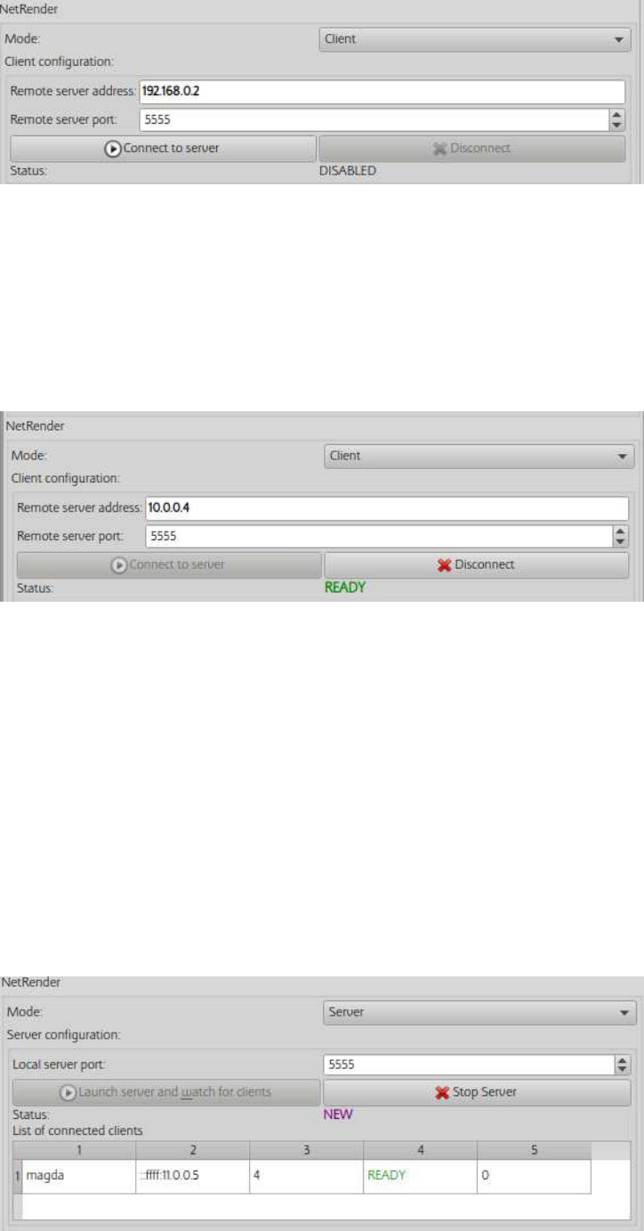
Figure 9.2: NetRender in ’Client’ mode
The remote server address must be set to the same as the Server computer which is running
Mandelbulber in Server mode. The address can be given as an IP address or a computer name.
The remote server port number must be exactly the same as the setting on the Server.
Press Connect to server button to connect to the server
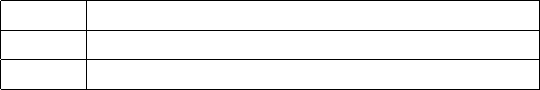
Once the connection is established correctly, the client application should show the status READY
Figure 9.3: NetRender in ’Client’ mode connected to the server
Alternative way to establish NetRender client is to use command line:
$ mandelbulber2 --nogui --host 10.0.0.4 --port 5555
when connection is successfully established the program should return following message:
NetRender - Client Setup, link to server: 10.0.0.4, port: 5555
NetRender - version matches (2090), connection established
On the Server computer, in the table "List of connected clients" should be shown the name and
address of the connected clients and the number of available processors (cores).
i.e in figure 9.4 “magda” computer has 4 cores and is READY.
Figure 9.4: NetRender in ’Server’ mode with a connected client
41
9.1.3 Rendering
Only the Server can initiate rendering on the computers connected using NetRender. When the
RENDER button is pressed on the server, all the connected computers commence rendering.
In the table List of connected clients in the column Done lines will be shown the number of lines
the image rendered by each of the computers.
when rendering is finished, the Server computer, will display the complete image. On the Client
computers, only that portion of the image which was rendered by that client will be displayed.
42
10 OpenCL
The use of OpenCL enables offloading the rendering of the fractal to the GPU or to an accelerator
card. This can highly reduce the render time. OpenCL itself is an industry standard developed by
the Khronos group and is a well established framework. The two mayor GPU vendors (ATI / Nvidia)
among others implement the OpenCL specification in their drivers. OpenCL uses single precision
floating point accuracy, so the minimum camera to surface distance is about 1e-05, whereas this
distance can be reduced to about 1e-09 with openCL disabled. Therefore openCL is not suitable for
zooming down into fine detailed areas.
10.1 Setup of OpenCL
To render in Mandelbulber with OpenCL you will need to install a recent driver. The newest GPU
driver available can be obtained from the links in the next table. Choose your operation system and
misc settings. Then download and install the driver image.
AMD http://support.amd.com/en-us/download/
Nvidia http://www.nvidia.de/Download/index.aspx
Intel https://downloadcenter.intel.com
You should also be able to use free drivers, if they support OpenCL. Sadly the performance of those
drivers is typically below the performance of the proprietary ones.
10.1.1 Setup of OpenCL on Windows
With a recent driver, a capable GPU and the Mandelbulber OpenCL version you are already set.
Proceed with 10.2. Note: Windows users may need to edit the registry to avoid timeout errors,
refer 10.3
10.1.2 Setup of OpenCL on Linux
With a recent driver, a capable GPU and the Mandelbulber OpenCL version you are already set.
Proceed with 10.2. If you are a developer and compile your own Mandelbulber version you need to
have the package opencl-headers installed in the system. See also the corresponding README.
10.1.3 Setup of OpenCL on MacOS
TODO
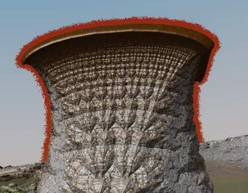
10.2 Configuring OpenCL
Open Mandelbulber and navigate to: Menu > File > Program Preferences > OpenCL (GPU). You
will find the configuration page in figure 10.1.
43
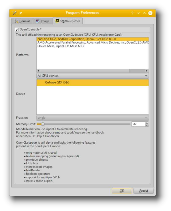
Figure 10.1: OpenCL Tab in preferences
•First you need to enable OpenCL by enabling the checkbox
•Then you need to select the platform and device to identify the OpenCL hardware element to
render with.
•Memory Limit - Memory limit in MB for the device. Most graphics cards cannot handle
memory objects larger than 512MB. If you observe that SSAO or DOF effects fail during
rendering you can try to decrease this limit. When the program needs more memory (image
resolution too high), then the effects will be rendered using CPU.
•Mode - This setting is located in the Navigation dock just below the RENDER button. It
switches the rendering engine between different levels of shader extent.
– no OpenCL - temporarily disables OpenCL Rendering is done by CPU.
– fast - renders preview of the fractal shape. The appearance of the fractal is not realistic,
but the rendering is very fast.
44

– medium - image is rendered with correct surface colors, but volumetric effects, reflec-
tion and refraction of light is not calculated. There is used only first defined material.
This mode offers more realistic rendering than in fast mode and uses less graphics card
resources than in full mode.
– full - renders all effects
Note: When openCL is enabled the image will be rendered in fast mode, a user must change
to limited or full modes to get a realistic appearance. The default setting is fast mode
because on low cost gfx cards (like built-in Intel), full mode doesn’t work and can cause the
gfx driver to crash.
Figure 10.2: OpenCL Mode in Navigation dock
10.3 Trouble shooting OpenCL
10.3.1 Driver crash under Windows
When Mandelbulber is run under Windows, the OS will monitor the GPU with a watchdog. When
the card becomes unresponsive for more than two seconds, the driver will shutdown and crash with
a message like:
The NVIDIA OpenGL driver lost connection with the display driver due to exceeding the
Windows Time-Out limit and is unable to continue.
It can happen when there are enabled effects which make rendering of each pixel very long.
A workaround for this problem is to increase this timeout limit. To do so you need to add or modify
two keys in the windows registry. Beware: Do this at your own risk, changing any wrong keys in the
windows registry may cause windows to stop working properly!
Change of registry takes effect after restart of Windows.
1. Open registry editor: [Start] > Run > Type in "Regedit" > Hit Enter
2. Navigate to key: Open HKEY_LOCAL_MACHINE > System > CurrentControlSet > Con-
trol > GraphicsDrivers
3. Create the keys (Modify if exist):
(a) Create key of type DWORD (32-bit) and name TdrDelay with a value of 30 as
Decimal value.
45
(b) Create key of type DWORD (32-bit) and name TdrDdiDelay with a value of 30 as
Decimal value.
4. Reboot
IMPORTANT. Some updates have appeared to remove these changes to the registry, this maybe
Win10 OS and/or Nvidia driver updates. If OpenCL begins to crash after an update, then check
the registry.
You can find more information about this topic in the following resources:
The original Blogpost in Fragmentarium, which has been used as the source of this article: http:
//blog.hvidtfeldts.net/index.php/2011/12/fragmentarium-faq/
Microsoft Explanation about the affected registry keys: https://docs.microsoft.com/en-us/
windows-hardware/drivers/display/tdr-registry-keys
Conversation about this topic in the fractalforums Mandelbulber group: http://www.fractalforums.
com/feature-requests/render-bucket-size-control-for-opencl/msg102868/#new
Battlefield trouble shooting with same problem: https://www.reddit.com/r/battlefield_4/
comments/1xzzn4/tdrdelay_10_fixed_my_crashes_since_last_patch/
10.3.2 Artifacts from glow and fog
Limited floating point accuracy can cause artifacts can when using glow or fog, if the Maximum
View Distance is too large. In the image below the distance was set at 192, reducing this to 30
removes the visible artifacts.
Figure 10.3: artifacts from glow or fog.png
46
11 Developer information
The Mandelbulber team welcomes everyone who likes to help us with the development of the
software. Whether you are a C++ fan and want to implement new features or you like to tweak
the fractal formulas. The code base is well structured and can be compiled with most common
compilers and operation systems. No magic involved, you just need to learn the tools and utilities
to modify and run your own version of Mandelbulber.
The following chapters will help you get ready for development.
11.1 Setup
Mandelbulber is using git as version control system and github as the hoster. If you do not know
git yet, you may find the following ressource helpful:
https://git-scm.com/book/en/v1/Getting-Started
Anyway the following setup steps will assume you git cloned the repository:
https://github.com/buddhi1980/mandelbulber2
locally to a project folder. This folder will be referenced as MANDELBULBER2_DIR.
11.1.1 Setup Debian/Ubuntu
To setup the system for development in debian and ubuntu you can use the files:
[MANDELBULBER2_DIR]/mandelbulber2/tools/prepare_for_dev_ubuntu.sh
[MANDELBULBER2_DIR]/mandelbulber2/tools/prepare_for_dev_debian_testing.sh
Please make sure you read them before execution!
11.1.2 Setup Windows
TODO
11.2 Building
11.2.1 Building with MSVC
Download and install latest MS Visual Studio version (tested with Visual Studio Community 2017).
Make sure you enable nuget support as an installed software.
Then open the project file
[MANDELBULBER2_DIR]/mandelbulber2/msvc/mandelbulber2.sln
and compile. Good luck!
47

11.2.2 Building with qtcreator
Compilation in QtCreator
•open [MANDELBULBER2_DIR]/mandelbulber2/qmake folder in File Manager
•open mandelbulber.pro in Qt Creator
•when it’s open, click Configure Project
•unfold Compiler Messages window (on the bottom of window)
•click hammer icon (build - left/bottom corner) the program will be compiled. If you did all
steps correctly, you shouldn’t receive any error
•try to run the program using the green arrow
11.3 Writing own formulas in Mandelbulber
11.3.1 Writing formula code
Adding new formulas:
- fractal_list.hpp:45 - enum enumFractalFormula - here is the list of formulas. Add new formula at
the end with unique number.
- fractal_list.cpp:41 - void DefineFractalList(QList<sFractalDescription> *fractalList) - here is de-
tailed list of formulas
example:
fr acta lLis t -> append ( s Fr ac ta lD es cri pt ion ( " Kaleidos c o pic ␣ IFS ","kaleidoscopic_ifs",
kale i d o s c o picIfs , Ka l e i d o scopic I f s I t eratio n , a n alyticDEType , linea r D E F u nction ,
c pi x el D is a bl e dB y De f au l t , 1 00 , a n al y ti c Fu n ct io n IF S , c o l o ri n gF u n ct i o nI F S )) ;
•1st field: Displayed name of the fractal
•2nd field: internal name of the fractal. The same name is used for UI files
•3rd field: the same name as in enumFractalFormula
•4th field: The function name as defined in fractal_formulas.cpp
•5th parameter: Preferred distance estimation method. The deltaDE method needs more
computation time but doesn’t need analytical DE coding knowledge.
•6th field: Preferred distance estimation function
•7th field: TODO
•8th field: Default bailout value
•9th field: Final calculation type
48

•10th field: Coloring function
- fractal_formulas.cpp - here are definitions of functions which calculate single fractal iteration.
There is no adding of C constant and bailout condition here.
example:
Listing 4: Formula > Mandelbulb formula
void MandelbulbIteration(CVector4 &z, co nst sFractal * frac tal , s Ex te nd ed Au x & aux )
{
double th0 = asin ( z. z / aux . r) + fr actal - > bul b . be ta An gl eO ffset ;
double ph0 = a tan2 ( z.y , z .x ) + fract al -> b ulb . a lp ha An gl eO ff set ;
double rp = pow ( aux . r, frac tal - > bul b . po wer - 1. 0);
double th = th0 * frac tal -> bul b . pow er ;
double ph = ph0 * frac tal -> bul b . pow er ;
double cth = cos (th );
aux . r_ dz = ( rp * aux . r _dz ) * fract al -> b ulb . p ower + 1.0 ;
rp *= aux . r ;
z. x = cth * cos (ph ) * rp ;
z. y = cth * sin (ph ) * rp ;
z .z = s in ( th ) * r p ;
}
The arguments are the same for each formula:
•CVector4 &z: input / output variable containing iteration vector
•const sFractal * fractal: read only container with all fractal parameters
•sExtendedAux & aux: input / output auxiliary structure containing values needed for in-
stance to calculate estimated distance
All parameters and data structures are defined in fractal.h
- fractal_formulas.hpp - here are tehe header declaration of the functions
- initparameters.cpp:499
void In it Fr ac ta lP ar am s ( c Pa ram et er Co nt ai ne r * par )
- here are definition of names of parameters which are used in UI and settings files. If you add new
formula then try to utilize existing names. If there is nothing which fits to your needs, then add a
new one
- fractal.cpp, fractal.hpp - here are data structures for fractal parameters. There is also copying of
values from internal parameter representation to data structures which you use in fractal functions
11.3.2 Designing user interface
To create UI files you can use Qt Designer application. The best would be if you make them based
on existing files. All ui files are located in formula/ui folder. Names start with fractal_ and the
rest of name is the same as internal fractal name. Even if a formula doesn’t use any parameters,
you need to create an UI file with no adjustable input fields, see fractal_quaternion.ui for example
(some kind of dummy).
In the UI files the names of the edit fields define their type and their parameter reference. The
program connects automatically edit fields with adequate parameters and with sliders / knobs. But
to make it working first part of the name must describe type of edit widget. Use following prefixes:
49
•spinbox_ - scalar value
•slider_ - slider for scalar value
•checkBox_ - boolean value
•spinboxd3_ - edit field for knob for angle. This is for 3 dimensions, where angles are stored
in CVector3 data type. Last letter of name must indicate axis name (_x, _y, _z)
•dial3 - knob for spinboxd3
•spinboxInt - spinbox for integer value
•sliderInt - slider for spinboxInt
•logedit - edit field for high variation value (only positive)
•logslider - slider for logedit which changes value in logarithmic scale
•vect3 - 3d vector (related to CVector3 data type). Name must ends with axis name
The rest of the names of the edit field must be the same as defined in initparameters.cpp
11.3.3 Autogeneration of opencl formula code
TODO
50
12 Case study
12.1 Examples
12.1.1 Example of MandelboxMenger UI
Example settings
(copy to clipboard, then load in Mandelbulber using : File –Load settings from clipboard):
# Mandelbulber settings file
# version 2.08
# only modified parameters
[main_parameters]
ambient_occlusion_enabled true;
camera 1.872135433718922 -2.023030528885091 1.871963531652841;
camera_distance_to_target 0.005814178381115117;
camera_rotation -28.76425655707408 26.3550335393397 3.450283685696816;
camera_top -0.1604796308669786 -0.4174088010201082 0.894436236356597;
DE_factor 0.6;
dont_add_c_constant_1 true;
flight_last_to_render 0;
formula_1 91;
formula_2 61;
formula_iterations_2 5;
formula_start_iteration_2 4;
formula_stop_iteration_2 5;
fractal_constant_factor 0.9 0.9 0.9;
fractal_enable_2 false;
fractal_rotation 0 -90 0;
keyframe_last_to_render 0;
main_light_beta 44.34;
main_light_intensity 2;
mat1_coloring_palette_offset 12.83;
mat1_coloring_palette_size 255;
mat1_surface_color_palette fd6029 698403 fff59c 000000 0b5e87 c68876 a51c64 3b9fee d4ffd4 aba53c;
SSAO_random_mode true;
target 1.874642452030676 -2.018463533070165 1.874544631933419;
view_distance_max 28.58330790625501;
volumetric_fog_colour_1_distance 3.55841069795292e-06;
volumetric_fog_colour_2_distance 7.116821395905841e-06;
volumetric_fog_distance_factor 7.116821395905841e-06;
[fractal_1]
fold_color_comp_fold 0.3;
mandelbox_color -0.27 0.05 0.07000000000000001;
mandelbox_rotation_main 9 1.74 3;
mandelbox_scale -1.5;
transf_addCpixel_enabled_false true;
transf_int_1 12;
transf_scaleB_1 0;
transf_scaleC_1 0;
transf_start_iterations_M 4;
transf_stop_iterations_M 5;
In the example the MengerSponge part is run only on iteration 4. A single iteration of another
fractal to make a hybrid is often the best practice.
In the Statistics (enable in View menu) in figure 12.1 you can see Percentage of Wrong Distance
Estimations ("Bad DE") is 0, which is good! As a general rule less than 0.01 is good, but it is case
specific and 3.0 sometimes is OK and .0001 sometimes is not.
51
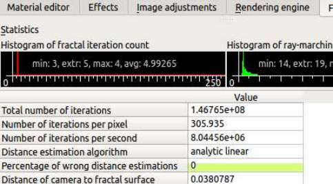
Figure 12.1: Statistics tab of the MandelboxMenger formula
The Raymarching step multiplier (Rendering Engine tab) or fudge factor is set at 0.6, which is good
for a hybrid. If I change it to 0.7 the Percentage of Bad DE leaps up to 0.25 and you can see the
areas of quality loss on your image.
Now if we disable the addCpixel Axis swap Constant Multiplier, we find we can now increase the
Raymarching Step Multiplier to 0.9, and get a faster render and visually the same quality. So
monitoring Percentage of Wrong Distance Estimations is a guide to managing quality. (Note when
doing animations you may want to drop the Raymarching step down a bit to allow for what might
happen between keyframes.)
MandelboxMenger Hybrids can behave a bit differently to a lot of hybrids, in the fact that the
Percentage Bad DE often improves when you zoom in.
52
12.1.2 Example of using Transform Menger Fold to make Hybrid
# Mandelbulber settings file
# version 2.08
# only modified parameters
[main_parameters]
ambient_occlusion_enabled true;
camera -1.528388569045064 -1.23063017895654 -0.0251755516595821;
camera_distance_to_target 0.0004503351519815117;
camera_rotation -14.07789975269277 -44.28785609194563 3.773777260910995;
camera_top 0.2333184436621841 0.6598138513697914 0.7142885869084139;
DE_factor 0.7;
flight_last_to_render 0;
formula_1 1052;
formula_2 1010;
formula_3 1052;
formula_4 1009;
formula_iterations_1 5;
formula_start_iteration_4 45;
formula_stop_iteration_2 12;
formula_stop_iteration_4 5;
fractal_constant_factor 0.9 0.9 0.9;
fractal_enable_4 false;
hdr true;
hybrid_fractal_enable true;
keyframe_last_to_render 0;
main_light_alpha 2.6;
main_light_beta 1.59;
mat1_coloring_palette_offset 46.51;
mat1_coloring_palette_size 255;
mat1_coloring_random_seed 647723;
SSAO_random_mode true;
target -1.528310155903731 -1.230317492741513 -0.02549000429402527;
volumetric_fog_colour_1_distance 3.55841069795292e-06;
volumetric_fog_colour_2_distance 7.116821395905841e-06;
volumetric_fog_distance_factor 7.116821395905841e-06;
[fractal_1]
transf_addition_constantA_000 -0.071633 0 0;
transf_function_enabledy false;
transf_int_1 12;
transf_scale 0.5;
transf_scaleC_1 0;
transf_stop_iterations_1 2;
[fractal_2]
transf_scale3D_333 1.055556 1.027778 0.861111;
[fractal_3]
transf_function_enabledx false;
On this transform UI, the standard menger sponge formula is split into a start and end function.
The simplest way to use this transform is in Hybrid Mode, having the menger fold transform in
slots 1 and 3. In slot 2 place any linear type formula or transform. (ie more mengers, kifs, mboxes,
amazing surf, folds, rotation , Benesi T1 etc).
In slot 1 disable the stop function and in slot 3 disable the start function, resulting in a standard
menger sponge with something in the middle.
BTW in fact you can mix around with the start and stop functions have all enabled if you wish.
Generally linear functions all work well together in making hybrids.
In Statistics, maximum is approx. 80 iterations. Generally hybrids take longer to render than
standard formulas. As well as adjusting formula parameters, you can use the iteration controls to
tweak hybrids. In this example the first slot is set to repeat for 5 iterations before moving to slot 2.
Slot 2 is set to stop at iteration 12, whereas slots 1 and 3 can continue to termination conditions
are met (bailout or maximum number of iterations).
In the example above, slot2 of the hybrid sequenced ended at iteration 12. 12 was chosen because
53
how it fitted into the iteration sequence, as follows:
•Slot 1 x 5 – iterations: 0, 1, 2, 3, 4 (note first iteration is iteration number 0)
•Slot 2 – iteration 5
•Slot 3 – iteration 6
•Slot 1 – iterations 7, 8, 9, 10, 11
•Slot 2 – iteration 12 (last use of Slot 2)
Sequence continues Slot 1 x 5, Slot 3, . . . to bailout.
As you see Slot 2 is used only twice in the iteration process. If I had entered 11 instead of 12 for
Slot 2’s stop iterations, then the slot would have been used only once, if I entered 19 then it would
run three times.
54
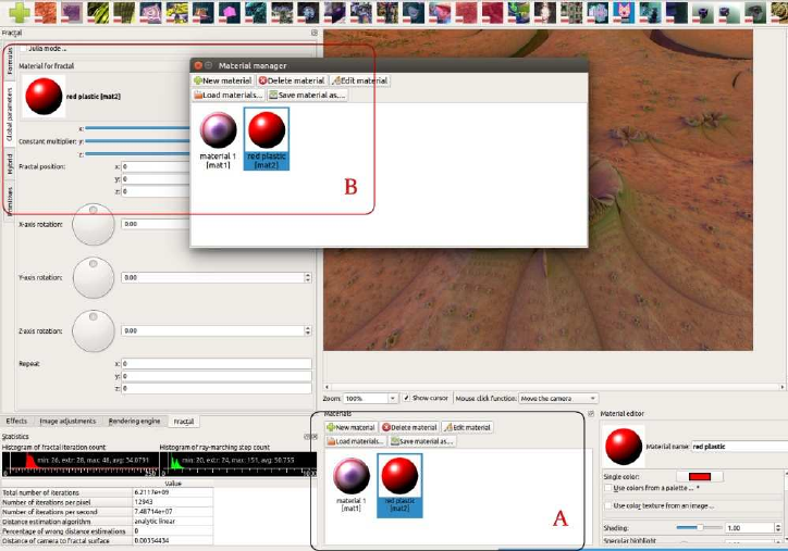
13 Miscellaneous
This chapter contains miscellaneous information like Q&A and Hints. Some of this information will
be relocated if a new chapter is written that covers the subject.
13.1 Q&A .
How do you get different materials on different shapes? This is how I have been doing it,
see also figure 13.1:
Rectangle at the bottom marked A.
This is where you start a new material or load an existing. The active material is highlighted in
blue. Meaning it is active in the material editor where you create or modify the material.
Rectangle at top left marked B.
One way to use a material is to go to Global Parameters, click on the material preview image, and
the Material Manager UI will appear with the materials you have loaded or created. Click on the
one you want to use, then close that UI.
Similarly with primitives, click on the material preview image. And with Boolean Mode each frac-
tal/transform has it’s own material preview image when you scroll down.
Figure 13.1: Material selection
100% CPU even it’s not rendering anything May 2017
Q. New version freezes my machine. After launching an application, it started to use 100% CPU
even it’s not rendering anything. I’m on Linux Mint 18 with i7 CPU and 8gb of RAM
A. Maybe the program is re-rendering all top toolbar preset icons (with fractal previews). You may
need to wait some time for this to finish. (SOLVED)
55
Morphing between fractals May 2017.
Q. I want to animate a fly through different fractals, smoothly merging with each other. For example,
"Amazing box" fractal slowly transforming to "Beth 323" and then to other fractal. Also changing
backgrounds would be awesome.
A. See (https://youtu.be/RHVCt1WXuAU) And, from menu bar select File Load examples, and
load example called mandelbox_menger_morph, this is the settings file for that video, and you will
be able to see how it was done.
For morphing between fractals the "weight" parameter is used. Weight determines the influence
each formula has in the image at each frame. Weight = 0 (0% influence), weight = 1 (100%).
So as the weight is adjusted from 0 up to 1, then the influence of that formula is introduced. At
the same time, the other formulas weight is being reduced from 1 down to 0.
Good practice would be to find a good setting for a "halfway: keyframe.
keyframe#0 formula1 weight = 1 and formula 2 weight = 0
keyframe#1 formula1 weight = A and formula 2 weight = B // the halfway keyframe
keyframe#2 formula1 weight = 0 and formula 2 weight = 1
The values of A and B that are chosen, control the way morphing works between keyframe#0 and
keyframe#2.
Using weight controls has hardly been tested yet, even though it has been available in the program
for a while
Some combination of formulas morph better than others
Animation/morphing takes a lot of render time, so render initial draft animations at low resolution,
and choose fast formulas.
In Mandelbulber nearly all parameter can be animated, (and also animated in response to audio
files), but integers can not normally be animated therefore you can not morph smoothly between
iteration count numbers
Different Materials for Hybrids May 2017
Q. I cannot find any information on how to assign different material on different fractals? I enabled
hybrids, for morphing animation and I want two fractals to look differently. Users guide method
gives me the same material on both fractals. I’m changing materials in global parameters>material
manager .What am I doing wrong?
A. In hybrid mode we are making a single fractal so the color is the same at a single frame. We can
only change color over time (frames)
Several Fractals in one image May 2017
Q. Is it possible to put few fractals in same scene, not as hybrids but just close to each other?
A. In boolean mode, you can place up to nine different fractals in your image, you can assign each
fractal a different material.
Can the priority of GPU be set November 2017
56
Q. Rendering anything using OpenCL currently brings my system to a crawl, graphically speaking.
Anything elsewhere only progresses once a square of fractal image has been rendered and Mandel-
bulber moves onto the next one. If the render is especially complex my system feels like it has frozen
completely as I can’t interact with anything until the next square is done.
Is there any way to reduce the priority of the GPU processing? Admittedly I don’t even know if
OpenCL processes work in this way but it makes GPU rendering near unusable for me for more
complex images.
Using Ubuntu 16.04 and 17.10 (Unity 7 and GNOME 3) with a GeForce GTX 750 Ti (need a new
one!), driver version 384.90. Current git build of Mandelbulber.
A. Graphics drivers have no capability to set priorities for tasks. In general they are not so well
prepared for multitasking. It’s also not possible to reduce allocation of GPU.
Actually there is used CL_KERNEL_PREFERRED_WORK_GROUP_SIZE_MULTIPLE to run the
program with optimal global_work_size. If will be used lower size, rendering will be slower, but you
will not see difference in multitasking. It’s because rendering of each pixel will still take the same
time, but amount of simultaneously rendered pixel will be lower. For that time GPU is busy.So in
general as fast the enqueued work is executed as the system is more responsive.
Calculation of 3D fractals is computation extensive, so it’s not possible to get quick calculation.
This is big disadvantage of computation on GPUs. If you want to have system well running with
background GPU computation, you need to have second graphics card which will be used only for
computation.
13.2 Hints
Optimizing of maximum view distance Located : Rendering Engine - Common Rendering
settings
It is important to optimize this setting to minimize render time. You can reduce until the furthest
part of the 3D object(s) starts to disappear. However with animation an allowance should be made
for changes between keyframes.
Note! When navigating in Relative step mode, mouse click on spherical_inversion, camera zooms
out, and maximum view distance becomes set at a big number like maybe 280. If you do not reset
this parameter then your render times will be unnecessarily increased.
Magic Angle Benesi Mag Transforms In mathematics the Magic Angle = 54.7356◦.
When rendering basic mag transforms the image does not render parallel to the standard x,y,z global
axis. On the fractal dock, in “Global parameters” set y-axis rotation to 35.2644◦(= 90◦- 54.7356◦).
The fractal will then render parallel to the x-y plane.
Formulas containing a varying scale functions Some function allow the variation of a param-
eter over iteration time.
aux.actualScale
This scale varying transform is initialized by the Scale value (parameter name: mandelbox.scale) in
Slot1. It is found in the formulas listed below :
57
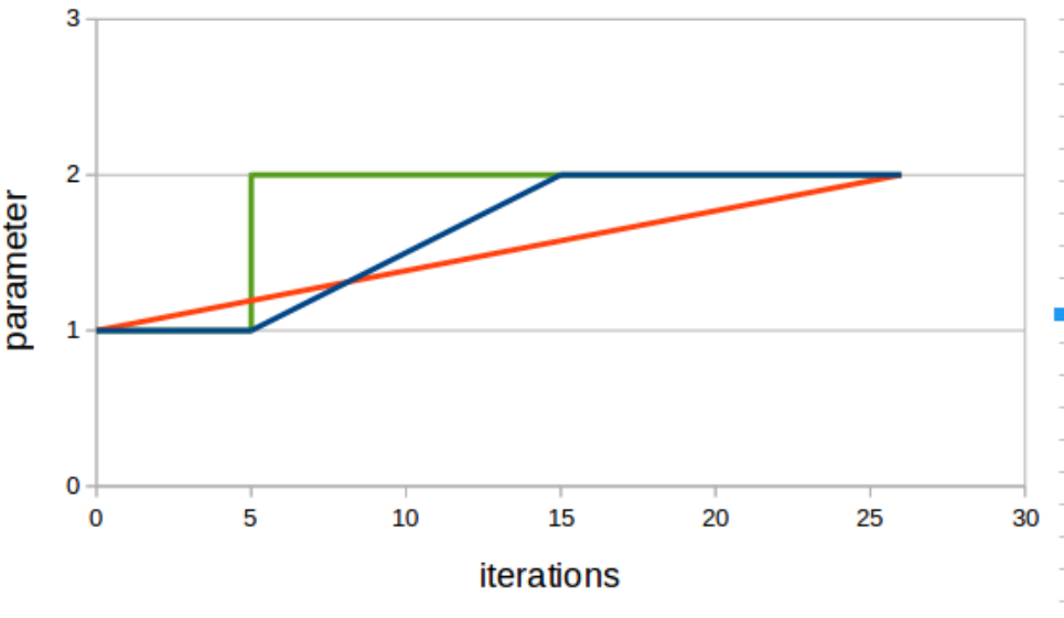
•Abox - Mod 1, Mod 2 , Mod 11, 4D and VS icen1
•Mandelbox Vary Scale 4D
•Amazing Surf and Amazing Surf - Mod 1
The program looks in slot1 only, for the initial value of mandelbox.scale.
Because of this, when in Hybrid Mode it is best to place these formulas in slot1.
However, these formulas can be used in other slots, but the program will always look for parameter
name: mandelbox.scale in slot1 to set an initial value. If the parameter does not exist, then the
program will use a default value of 2.0.
aux.actualScaleA
There is a newer version which can be used in any slot. Currently this function is used in the
following:
•Abox - Mod 12, Fold Box - Mod 1
•T>Spherical Fold Parab
•T>Scale Vary V2.12 and T>Scale Vary Multi
With both aux.scale and aux.scaleA, it is often best to use them only once in a Hybrid Mode setup.
T>Scale VaryV1
This is a simple linear scale variation.
Figure 13.2: Transform Scale VaryV1
58
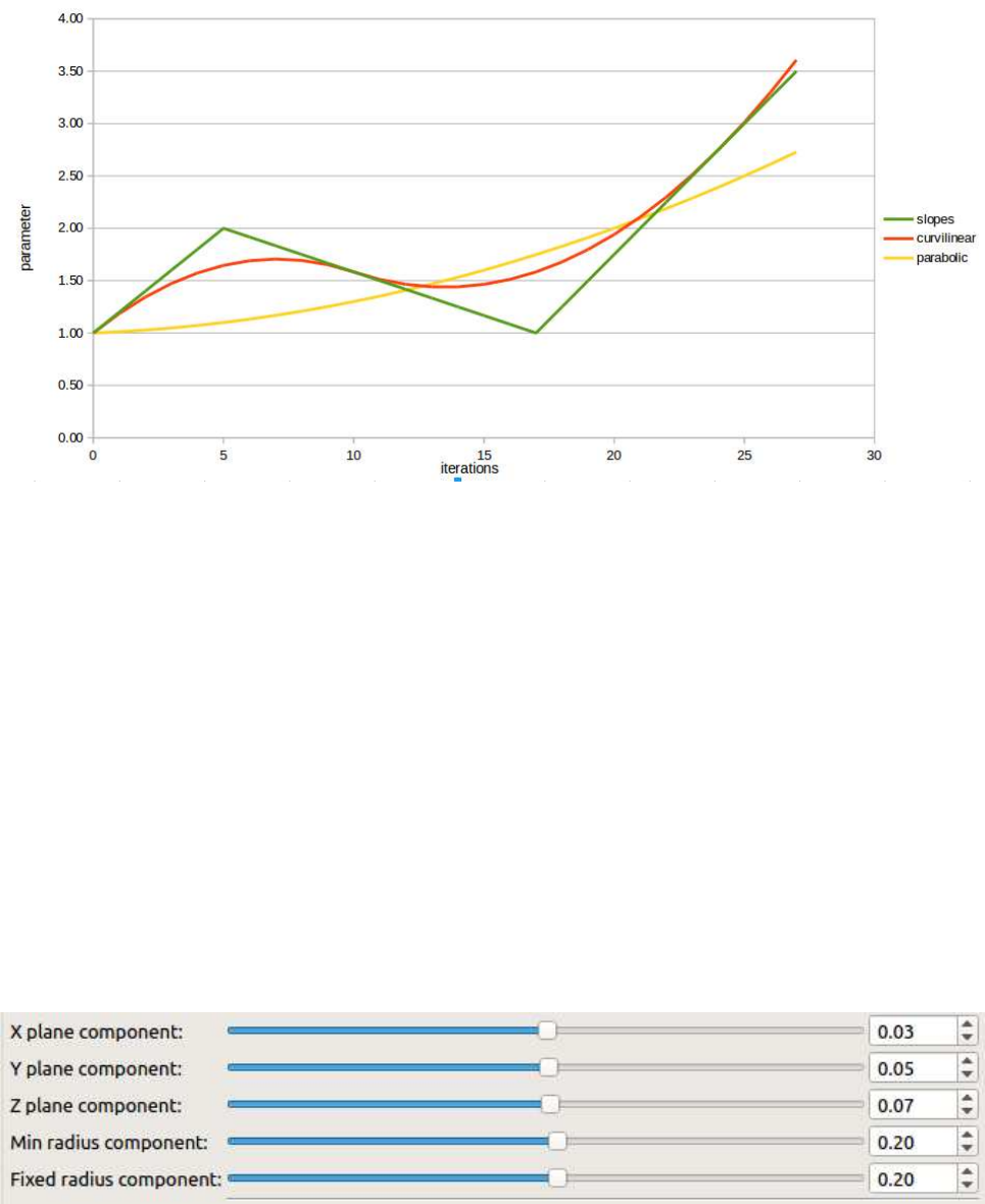
T>Scale VaryVCL
VCL is short for vary curvi-linear. With this transform there is the options to use linear slopes(green),
curvi-linear (red) or parabolic (yellow).
Figure 13.3: Transform Scale Vary VCL
Color functions There are various ways of creating the color for each point in the set. Coloring
possibilities can be just as complex as fractal formulas. Color data can be obtained from anywhere
within the iteration loop. Two common methods are using the value of a color component at
termination, or using the minimum value recorded while iterating. Color components can be mixed
together to make more complicated colorings.
A common way to obtain a color value is by the use of orbit traps. An example is the color value
equals the closest distance from the point to a cube, or a sphere, surrounding the fractal.
The examples below are some basic ways of creating color components. These examples are with a
standard mandelbox, (the results can be very different with other formulas.)
aux.color aux.color is a cumulative number that is in many formulas and transforms, where there is
conditional folding, e.g. box folds and sphere folds. Note that color based on conditional functions
can cause unwanted cuts in color layout.
The parameter controls are generally like this :
Figure 13.4: Aux.color parameters
When the iteration loop is running, this number is increased each time a condition is met. The
59
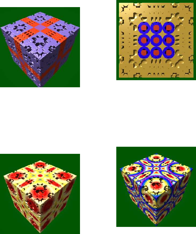
result is dependent on how many times before termination that the condition is met.
Currently there are two types of algorithms that use aux.color. In V2.13 Amazing Surf Mod2 has
different aux.color calulations. In V2.14 Mandelbox Variable, PseudoKleinian Mod2 and some basic
transforms, have aux.color mode 2 and 3 options.
Example maths (mode 1):
Box Fold if (z > limit OR z < -limit) aux.color += boxFoldComponent.
Note that the box fold component can create speckly areas with mandelbox type fractals.
Sphere Fold. if (rr < minR2) aux.color += minR2Component. else if (rr < maxR2) aux.color +=
maxR2Component.
And therefore if(rr> maxR2 ) there is no addition of a component.
With a standard mandelbox we need to cut open the fractal to see the result of this component
acting on their own. Red is the minR2 component and blue the maxR2 component.
Figure 13.5: Box fold coloring component
Figure 13.6: Sphere fold minR2 and maxR2
coloring component
Radius or radius squared
A component value is added based on the distance of the point from the origin at termination.
Figure 13.7: Radius coloring component
Figure 13.8: Radius squared coloring compo-
nent
Distance Estimation (DE) (sliced view)
60
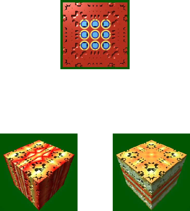
A component value is added based on the DE value of the point at termination.
Figure 13.9: DE color component
Axis Bias
These functions are tools to globally manipulate/distort the color. Examples maths:
XY Zbiascomponent =abs(z.x)∗biasScale.x;P lanebiascomponent =z.y
astz.z ∗biasScale.y;
Figure 13.10: XYZ coloring component Figure 13.11: Plane bias coloring component
Iteration count
The final color value, after adding up all the components, is scaled by a function of the iteration
count.
Example maths:
colorV alue =sumofallcomponents ∗(1.0 + iterScale/(iter + 1.0));
Left image below is with iterScale = 0.0, the right image has the function disabled.
61
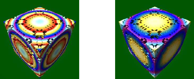
Figure 13.12: With iterartion count coloring
component
Figure 13.13: Without iterartion count coloring
componen
Addition of constant "c" in functions (z = fn(z) + c) This is just a general bit about formula
structure.
A lot of standard formulas add a constant at the end of the iteration loop, i.e. "do some maths
then add a constant", and repeat until termination conditions are met.
Bulbs, abox/surf, quaternion, pseudo kleinians do
Menger, prism, sierpinski and alot of other IFS do not.
Boxbulbs are often best without but they can still have a constant added.
But you can carefully add any constant to any formula anywhere in the loop.
The standard constants added at the end of the loop are either a Julia constant(coordinates) or the
original-point-being-iterated often referred to as c pixel.
The standard approach is to either add c pixel OR julia constant
if (julia enabled) z += vec3(julia); else z += vec3(c pixel) * vec3(constant multiplier);
Mandelbulber is historically set up the standard way, ( choice of c pixel OR Julia at the end of the
loop). However there are plenty of formulas in the list where you can use both or just build a formula
out of transforms in hybrid mode.
Summary. How standard fractals are constructed is just a safe starting point, you can mix it all up,
the aim is achieving "a quality image in a reasonable time".
Added by user (thankyou). Some additional info for those less familiar with Mandelbulber: These
parameters are set in the Objects palette. The Fractals tab (where you select the formula(s)) has a
checkbox to select whether or not to use the constant. For formulas where the constant is normally
used, it will be labeled "Don’t add global C constant"; for formulas where the constant is not
normally used, it will be labeled "Add global C constant". Leave unchecked for the normal behavior
or check for the opposite.
The Global parameters tab has a checkbox for "Julia mode" to select whether to add the Julia
constant (if checked) or the current pixel (if not), as well as the Constant multiplier. The Fractals
tab will have a remark at the top if Julia is checked.
Two notes:
1. Julia mode and the Constant multiplier are ignored if the global C constant is not used.
62
2. If you use multiple formulas (hybrid mode), the Julia mode setting applies to all of them where
the global C constant is used. In Boolean Mode, additional parameters appear at the bottom of the
formula UI. These include parameters for the addition of constant for each boolean mode fractal.
Antialiasing with photo editing software Added by user (thankyou).
When there are subpixel size details, image quality benefits hugely from antialiasing, which can be
done in photo editing software. Default blending uses a formula post gamma correction, which makes
green and red blur to brown, for example. A setting in some photo editing software (e.g. photoshop)
allows calculation pre gamma, which blends to yellow as it should! This makes a difference when
using bicubic smoothing for shrinking images - especially 4x shrink.
Some notes on using "Multiple rays with light map" for coloring. Added by user (thankyou).
Menno Jansen Mandelbulber facebook.11 May at 20:23
Note. Multiple rays with light map Ambient Occlusion (AO) is slow so it is best to be used with
OpenCL.
1) Materials Editor: disable “Use colors from a palette ..” and use the default gray with the Single
Color.
2) Effects/Ray-tracing: Type > choose “Multiple rays with light map” and choose which map you
want to use as “Light map texture”. Also make the Intensity value higher. Note: you can choose
any photo you want as Light Map. But make sure that it is a photo/image with some dominant
colors. A photo/image with all kind of colors will result in a bland render. A photo/image with a
blue sky, green grass and red ball for example will result in a more defined color setting with render.
Also I disable Glow under Volumetric. But this is a personal taste I guess
3) Effects/Lights: Main light source > set the Intensity to a lower value, 0,5 for example
4) Image Adjustment: Picture > Lower the Gamma value and set the Saturation value higher (how
much depends on the light map you used at step 2.
5) Rendering Engine: - Shape Control > Enable “Stop at maximum iteration (at maxiter)”. Then set
a very low value (4 for example) to start with at “Maximum number of fractal iterations (maxiter)”.
Playing around with this value really makes the difference together with step 6!!
6) Rendering Engine: play around with the “Raymarching step mult. (controls quality)” and “Detail
level” values.
Also, you could try to add Extra Light source in dark areas. When your dominant color of the Light
Map is for example red, try to add extra Light Source(s) that is blue at a not too high intensity.
This can give a very cool result.
Monte Carlo MC Global Illumination. Global Illumination is a part of the Monte Carlo (MC)
DOF algorithm, located in the Depth of Field (DOF)combobox. It cannot be rendered without MC
DOF. If the DOF blurred image is not required, then reduce the DOF radius to produce only the
Global Illumination effect.
About estimated rendering time: at the beginning it can be very long, because there is an initial
assumption that is needed to calculate the maximum number of MC samples. But during rendering
there is an estimated "actual noise level" for each image tile. If the noise level for a given tile is
63
satisfactory, then it is no longer rendered. More samples are only calculated on tiles where the
noise level is still too high. When many tiles get low noise level, then rendering progress is faster.
Statistical noise estimation optimizes the MC effects a lot.
What this means is that initial "estimated to end" time shown on the progress bar can be very
conservative. The actual render time can be much smaller (e.g maybe 3 to 8 times faster).
64

14 Using “Anim By Sound” with multiple tracks
Note. The following "walk through" tutorial is for using Anim By Sound with multiple tracks. This
tutorial is based on my initial experiments with Anim by Sound and may be revised as I gain more
experience. The tutorial demonstrates using sound to animate a fractal offset parameter and the
material color. The settings file also includes animation of some other parameters, and produces an
animation just over a minute long, at 300 x 300, 45 minutes to render.
Animations can take many hours to render, so it is best when learning the controls, to keep it simple.
Choose fractals and/or primitives that render fast. Do not use slow effects like Volumetric Light of
Multi Ray Ambient Occlusion. I drop the resolution to 400 x 300 Detail Level 0.5, or 200 x 150
Detail Level 0.25.
The animation value of an object (or an effect) at each frame, is the sum of the parameter value,
(generated from the keyframe animation table), and the sound value at that frame.
animVal = paraVal + soundVal.
This tutorial is about the basics of using soundVal to vary animVal. So I will keep paraVal constant
and use only sound data to direct the animation of parameters.
A cool thing about using only soundVal (no keyframe animation) is that we can set up a trial with
just two keyframes (beginning and end).
Note. You can create an audio file for the single purpose of directing animation, where the audio
file is not used at all in the final song mix. You can use Anim by Sound to create silent videos.
Keyframe animation requires changes to be made at keyframes. It is possible with Sound animation
to make changes at any frame, (i.e. a change at any 1 / 30 of a second time interval, when at
30fps.)
Previously, choreographing parameters with spreadsheets was very time consuming and I was limited
to what I could achieve, so I stopped and have waited. Anim by Sound has made this process much
more simpler, and has infinite possibilities.
All files used in this example can be downloaded from mandelbulber.org
http://cdn.mandelbulber.org/doc/audio/9%20tut.zip
unzip and place “9 tut” folder in home/mandelbulber/animations/
65
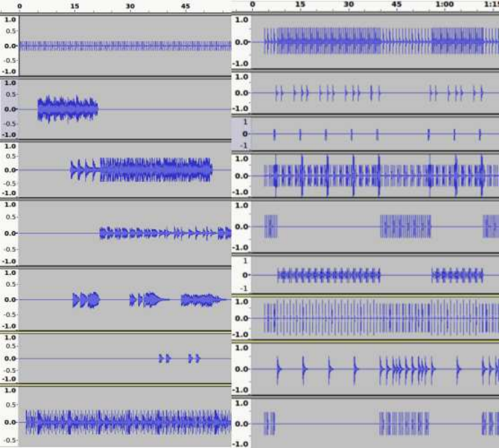
14.1 Audio Files
The following formats are supported:
- *.wav (wave form audio format)
- *.ogg (Ogg Vorbis)
- *.flac (Free Lossless Audio Format)
- *.mp3 (MPEG II Audio Layer 3)
I used Hydrogen Drum Kit emulator to make all the individual drum track files. These are .wav files
but as I am using Linux I converted them to .mp3 to use in Mandelbulber. These are mono working
files, when I make the video in VirtualDub I then use the final song mix .wav file.
The guitar tracks have also been recorded as .wav, and a .mp3 copy made to use with Mandelbulber.
The audio file data is sampled at every frame point, the data is then converted to a sound number
ranging between 0 (silent) and 1 (maximum) which can represent Amplitude or Pitch. This value
is shown in the Sound Animation chart on the Audio Selector UI. We can use either the default
Amplitude mode or choose Sound Pitch mode to animate.
For this example I used Pitch with lead guitar (melody line) creating the fractal movement, and
Amplitude for a drum to alternate the color. The fractal shape will respond to the free flowing
melody line and the color change as a repetitive rhythm event.
This is a screen-shot from Audacity showing some of the instrument tracks I had available. I only
used one drum (a kick drum), but normally I would be using more percussion instruments.
66
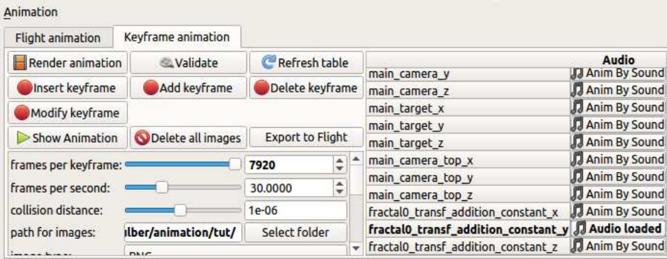
14.2 Adding a parameter.
Firstly, have the Animation Dock open. ( i.e. from menu select View - show animation dock.)
Then go to the dock or tab for the parameter you wish to animate (e.g. fractal, material, effect
etc). Right mouse click on the parameter field, and select Add to Keyframe Animation.
The parameter will then be listed in the keyframe animation table, with Anim By Sound in the next
column.
Here I have chosen to animate parameter Menger_Mod1 offset y
fractal0_transf_addition_constant_y
i.e parameter name transf_addition_constant_y; from formula slot fractal0.
Parameters x & z are also added because this parameter is part of a vector3.
14.3 Loading the Audio File
Left mouse click on Anim By Sound and the Audio Selector UI will open. The name of the parameter
will be in the description along the top.
Select an Audio file and three charts will appear.
Enable Animation by Sound and the options will appear.
67
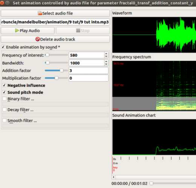
Animation of a parameter is created by applying an addition-factor and/or a multiplication-factor.
animVal = paraVal + soundVal.
soundVal = (paraVal * multiplication-factor * sound) + ( addition-factor * sound)
It is less complicated when learning, to use only the addition factor, so we change multiplication
factor to 0.0.
14.4 Using Sound Pitch mode.
I set frequency at 580Hz and bandwidth to 1000Hz, this covers the range of the fundamental
frequencies of my lead guitar notes ( I am removing higher harmonic frequencies, although this may
not be necessary).
Make further adjustment if the Sound Animation charts shows that the pitch is contained only in
the top or bottom of the chart, (resulting from a melody line only using high notes or only using
low notes.) Push the Play Sound button and check that the chart line is following the pitch of the
audio track.
The main point is not to limit the Pitch by having a small band width that does not cover the full
spectrum of the fundamental notes used in the audio track.
In Pitch mode the Sound Animation chart rises from silent to high pitch.
68
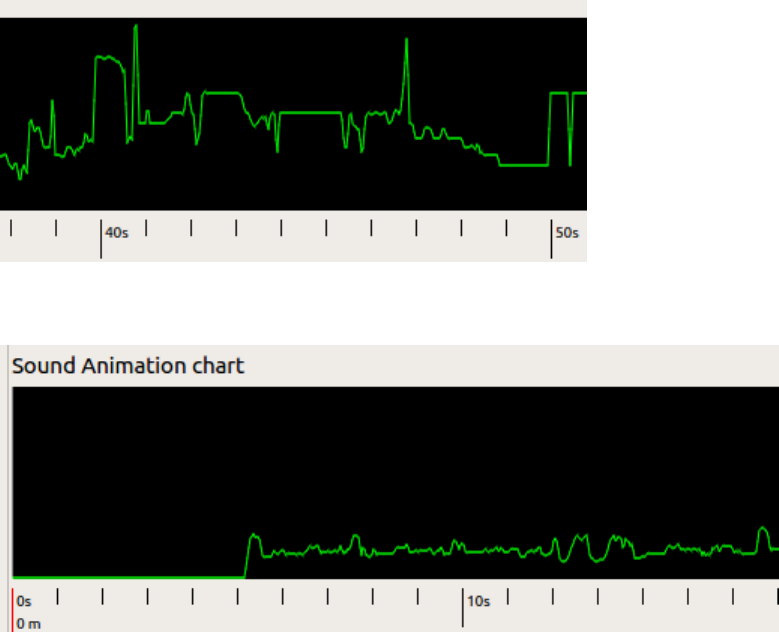
In this image the sound varies from about 0.2 up to almost 1.0 (maximum sound). Therefore the
sound will have a wide effect on the parameter animation.
In this image the sound is fairly constant at around 0.2, so it will have a narrow effect on the
animation.
14.5 Testing the parameter
Close the Audio Selection UI and go the Menger_Mod1 fractal tab and test the parameter through
a range of values.
If a parameter belongs to a fractal formula, you may notice that the ray marching step multiplier
needs to be adjusted to produce a good image throughout the animation range.
As a guide for adjusting the ray marching step multiplier, open View - Show statistics, and monitor
Percentage of wrong distance estimations.
69
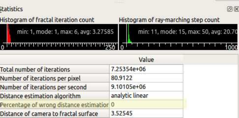
Now I decide on the appropriate size of the addition factor to use for animating the parameter.
I have paraVal “offset y” set at a constant value of 0.0, and I test an addition factor of 3.0. The
sound will increase the soundVal in the range of 0.0 to 3.0 maximum. However for the effect I want,
I am be using Negative influence mode, which will subtract the soundVal from paraVal instead of
adding it, therefore the possible range to be tested is 0.0 to -3.0.
The audio file I used only creates sound between 0.0 and about 0.2, so the offset values I will be
testing are the actual range between 0 and -0.6, i.e. 0.0 = 0.0 * -3.0 max, -0.6 = 0.2 * -3.0 max.
Note: There are two types of parameters in this program. The first type can have negative values
entered, the second type cannot. It is important when animating a parameter of the second type,
that the functions and settings used, do not result in a negative number.
View the Sound Animation chart to see the what values you are likely to get from sound at different
parts of the instruments music.
Remember to set the parameter back to the original value when you have finished testing.
14.6 Using Amplitude
Example: Animate the color of the fractal on every beat of the kick drum.
Add material 1 parameter “Palette_offset” to the Keyframe animation table.
Open Anim By Sound, load audio file and Enable Animation by sound.
Adjust Frequency of interest and bandwidth.
Enable “Binary filter” and adjust the threshold so that all the beats are shown in the Sound Animation
chart.
Here I am creating an event (at every kick drum beat), that lasts for a minimum duration of 7 extra
frames (7/30 seconds). The event is using Addition factor * sound and is triggered every time the
sound amplitude increases above the threshold (0.400) and will last for 7/30 seconds. Events that
last less than “say” 7 frames are difficult to observe at 30 fps.
70
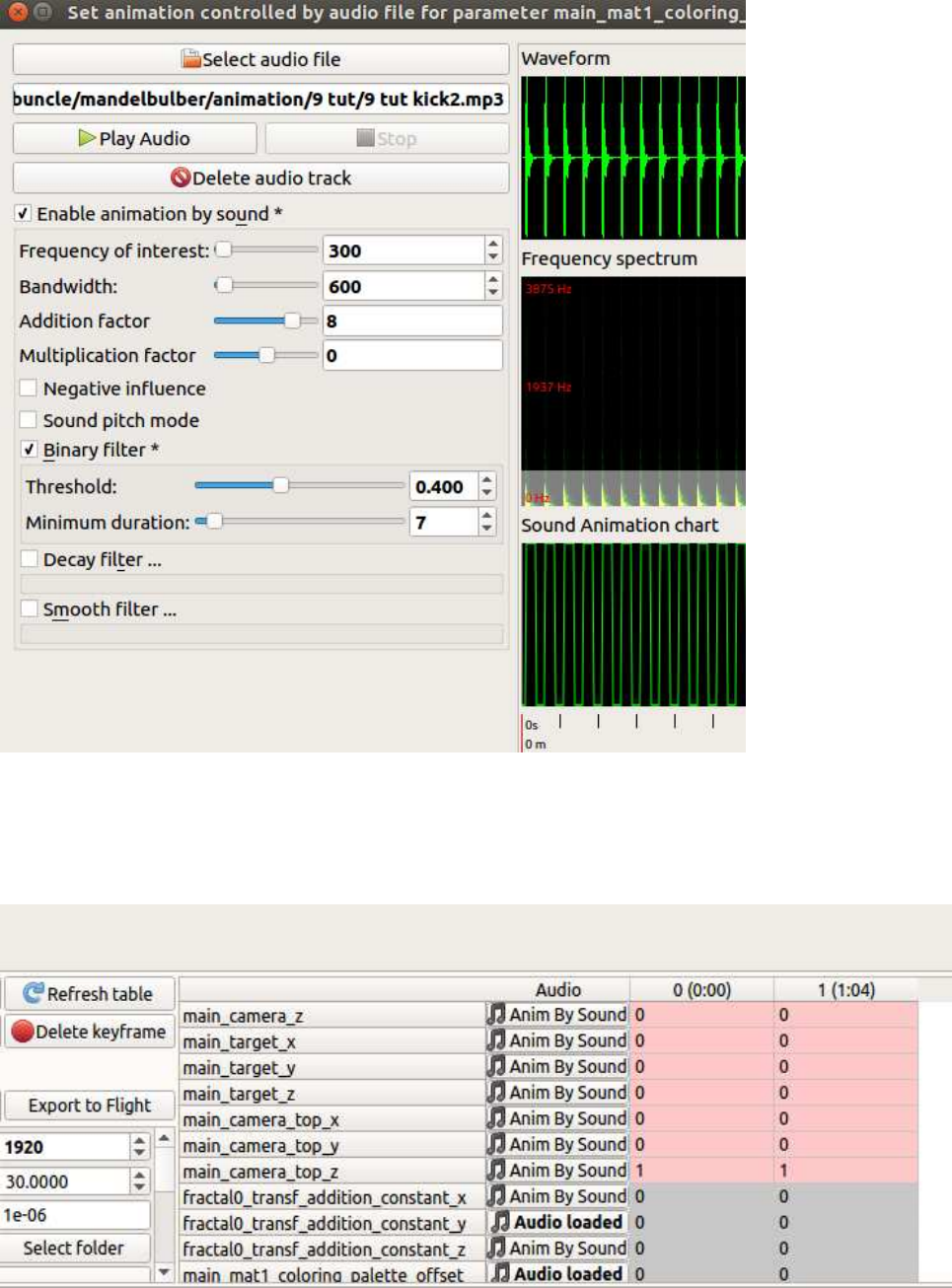
14.7 Rendering the animation.
First add two identical keyframes to the Keyframe Animation table,
and set “frames per keyframe” to a number that will cover the length of the trial, i.e. for 64 seconds
at 30 fps it would be:
71
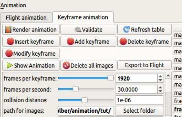
64sec * 30fps = 1920 frames per keyframe.
Make sure that the “path for images” is linked to the correct folder, and ensure that the folder is
empty, “Delete all images” button.
14.8 Now render the trial animation.
When rendering is finished (note the time it took) , press “Show animation” button for a preview
(you can also use “Show animation” while rendering is in progress.)
I also create a video with VirtualDub and the audio file, to ensure that the animation is working
correctly with the sound. If the animation is satisfactory, then set the resolution and detail level to
your final settings and wait.
72
15 Thanks
Thanks to the fractal community for your ongoing support!
Sincerely,
Mandelbulber Team
73
List of Figures
2.1 Mandelbrot Set ..................................... 6
2.2 Menger Sponge .................................... 8
2.3 Sierpinski ........................................ 8
3.1 Distance Estimation with DE factor 1 ......................... 9
3.2 Distance Estimation with DE factor 0.5 ........................ 10
3.3 Statistics Tab with histogram data .......................... 10
3.4 Example of over-stepping ............................... 11
3.5 Linear DE offset parameter .............................. 11
4.1 Example for 1st case - stop ray-marching at distance threshold ............ 12
4.2 Example for 2nd case: Stop ray-marching at Maxiter ................. 12
4.3 Example for 1st case: Stop ray-marching at bailout with low Maxiter ........ 13
4.4 Example for 2nd case: Stop ray-marching at maxiter with low maxiter ........ 13
4.5 Constant detail size .................................. 13
5.1 Examples of simple Iteration loops with one formula ................. 17
5.2 Fractal Tab - Formula only in first slot ........................ 18
5.3 Fractal Tab - Multiple formula slots filled ....................... 18
5.4 Complex Iteration loop with hybrid fractal ...................... 19
5.5 Hybrid sequence - Simple sequence using three different formulas .......... 19
5.6 Hybrid sequence render - Simple sequence using three different formulas ....... 20
5.7 Single iteration of the Menger Sponge ......................... 20
5.8 Hybrid with Menger Sponge features marked in red .................. 20
5.9 Hybrid close up of leaf-like shapes produced by ’Box Fold Bulb Pow 2’ formula . . . 21
5.10 Hybrid sequence - The first and second slots set to 2 repeat iterations ........ 21
5.11 Hybrid sequence result - The first and second slots set to 2 repeat iterations . . . . 21
5.12 Hybrid sequence - The second slot set to 10 repeat iterations ............ 22
5.13 Hybrid sequence result - The second slot set to 10 repeat iterations ......... 22
5.14 Hybrid sequence - Range of iteration set to 4-250 on second slot .......... 22
5.15 Hybrid sequence result - Range of iteration set to 4-250 on second formula slot . . . 23
5.16 Fractal tabs with highlighted tab-arrows ........................ 23
5.17 Hybrid sequence - Swapped tab one and two ..................... 23
5.18 Hybrid sequence render - Swapped tab one and two ................. 24
6.1 Movement mode - camera and target ......................... 26
75
6.2 Movement mode - camera ............................... 26
6.3 Movement mode - target ............................... 26
6.4 Rotation mode - around camera ............................ 27
6.5 Rotation mode - around target ............................ 28
6.6 Keyframe Animation with differing distances camera to target ............ 29
6.7 Keyframe Animation with equal distances camera to target ............. 29
7.1 Interpolation types ................................... 30
7.2 Interpolation - None .................................. 31
7.3 Interpolation - Linear ................................. 31
7.4 Interpolation - Akima ................................. 32
7.5 Interpolation - Catmul-Rom .............................. 33
7.6 Catmul-Rom with collision ............................... 33
7.7 Catmul-Rom without collision ............................. 33
7.8 Interpolation - Catmul-Rom path through a hole ................... 34
7.9 Interpolation - Catmul-Rom path evading different obstacles ............. 34
7.10 Changing an interpolation type ............................ 35
8.1 Flight animation dock ................................. 36
8.2 Example tooltip with parameter name ......................... 38
8.3 Animation table with all recorded frames and one additional parameter ....... 39
9.1 NetRender in ’Server’ mode .............................. 40
9.2 NetRender in ’Client’ mode .............................. 41
9.3 NetRender in ’Client’ mode connected to the server ................. 41
9.4 NetRender in ’Server’ mode with a connected client ................. 41
10.1 OpenCL Tab in preferences .............................. 44
10.2 OpenCL Mode in Navigation dock ........................... 45
10.3 artifacts from glow or fog.png ............................. 46
12.1 Statistics tab of the MandelboxMenger formula .................... 52
13.1 Material selection ................................... 55
13.2 Transform Scale VaryV1 ................................ 58
13.3 Transform Scale Vary VCL ............................... 59
13.4 Aux.color parameters .................................. 59
13.5 Box fold coloring component ............................. 60
13.6 Sphere fold minR2 and maxR2 coloring component .................. 60
13.7 Radius coloring component .............................. 60
76
13.8 Radius squared coloring component .......................... 60
13.9 DE color component .................................. 61
13.10XYZ coloring component ............................... 61
13.11Plane bias coloring component ............................ 61
13.12With iterartion count coloring component ....................... 62
13.13Without iterartion count coloring componen ..................... 62
77
Index
animation
rotation, 29
Developer Information, 47
distance estimation, 9
analytical, 9,10
delta DE, 9,10
fractal, 6
hybrid, 17,52,53
IFS, 8
interpolation, 30
Akima, 32
Catmul-Rom, 32
linear, 31
none, 31
Mandelbrot Set, 6
Mandelbulb, 7,15
Menger Sponge, 8,15
navigation
absolute step, 25
camera, 25,26
relative step, 25
reset view, 28
rotate, 27
target, 25,26
NetRender, 40
OpenCL, 43
ray marching, 9
constant detail size, 12,13
distance threshold, 9,12
maximum view distance, 57
step multiplier, 9,52
statistics
wrong distance estimations, 51
termination condition
bailout, 7,12
maxiter, 7,12,13
transform
box fold, 15
spherical fold, 15
78
