Manual
User Manual:
Open the PDF directly: View PDF ![]() .
.
Page Count: 347 [warning: Documents this large are best viewed by clicking the View PDF Link!]
- Introduction
- General remarks on notation
- ac: Accelerator bounds
- an: Annihilation cross sections (general, 0 and )
- an1l: Annihilation cross sections (1-loop)
- Annihilation cross sections at 1-loop -- general
- Routine headers -- fortran files
- dsanggim.f
- dsanggimpar.f
- dsanggre.f
- dsanggrepar.f
- dsanglglim.f
- dsanglglre.f
- dsanzg.f
- dsanzgpar.f
- dsdilog.f
- dsdilogp.f
- dsfl1c1.f
- dsfl1c2.f
- dsfl2c1.f
- dsfl2c2.f
- dsfl3c1.f
- dsfl3c2.f
- dsfl4c1.f
- dsfl4c2.f
- dsi_12.f
- dsi_13.f
- dsi_14.f
- dsi_22.f
- dsi_23.f
- dsi_24.f
- dsi_32.f
- dsi_33.f
- dsi_34.f
- dsi_41.f
- dsi_42.f
- dsilp2.f
- dsj_1.f
- dsj_2.f
- dsj_3.f
- dslp2.f
- dspi1.f
- dspiw2.f
- dspiw2i.f
- dspiw3.f
- dspiw3i.f
- dsrepfbox.f
- dsrepgh.f
- dsrepw.f
- dsslc1.f
- dsslc2.f
- dssubka.f
- dssubkb.f
- dssubkc.f
- dsti_214.f
- dsti_224.f
- dsti_23.f
- dsti_33.f
- dsti_5.f
- anstu: t, u and s diagrams for ff-annihilation
- Annihilation amplitudes for fermion-fermion annihilation
- Routine headers -- fortran files
- dsansffsff.f
- dsansffsss.f
- dsansffssv.f
- dsansffsvs.f
- dsansffsvv.f
- dsansffvff.f
- dsansffvss.f
- dsansffvsv.f
- dsansffvvs.f
- dsansffvvv.f
- dsantfffss.f
- dsantfffssex.f
- dsantfffssin.f
- dsantfffsv.f
- dsantfffsvin.f
- dsantfffvs.f
- dsantfffvsex.f
- dsantfffvv.f
- dsantfffvvex.f
- dsantfffvvin.f
- dsantffsff.f
- dsanufffss.f
- dsanufffssin.f
- dsanufffsv.f
- dsanufffsvin.f
- dsanufffvs.f
- dsanufffvv.f
- dsanufffvvex.f
- dsanufffvvin.f
- dsanuffsff.f
- as: Annihilation cross sections (with sfermions)
- Annihilation cross sections with sfermions -- general
- Routine headers -- fortran files
- dsaschicasea.f
- dsaschicaseb.f
- dsaschicasec.f
- dsaschicased.f
- dsaschizero.f
- dsascolset.f
- dsasdepro.f
- dsasdwdcossfchi.f
- dsasdwdcossfsf.f
- dsasfer.f
- dsasfercode.f
- dsasfercol.f
- dsasfere.f
- dsasferecol.f
- dsasff.f
- dsasffcol.f
- dsasgbgb.f
- dsasgbgb1exp.f
- dsasgbgb2exp.f
- dsasgbhb.f
- dsashbhb.f
- dsaskinset.f
- dsaskinset1.f
- dsaskinset2.f
- dsaskinset3.f
- dsasphghb.f
- dsasscscsSHffb.f
- dsasscscsSHffbcol.f
- dsasscscsSVffb.f
- dsasscscsSVffbcol.f
- dsasscscsTCffb.f
- dsasscscsTCffbcol.f
- dsasscscTCff.f
- dsasscscTCffcol.f
- dsasscscUCff.f
- dsasscscUCffcol.f
- dsassfercode.f
- dsaswcomp.f
- bsg: b s
- b s -- theory
- b s -- routines
- Routine headers -- fortran files
- dsbsgalpha3.f
- dsbsgalpha3int.f
- dsbsgammafull.f
- dsbsgat0.f
- dsbsgat1.f
- dsbsgbofe.f
- dsbsgc41h2.f
- dsbsgc41susy.f
- dsbsgc70h2.f
- dsbsgc70susy.f
- dsbsgc71chisusy.f
- dsbsgc71h2.f
- dsbsgc71phi1susy.f
- dsbsgc71phi2susy.f
- dsbsgc71wsusy.f
- dsbsgc80h2.f
- dsbsgc80susy.f
- dsbsgc81chisusy.f
- dsbsgc81h2.f
- dsbsgc81phi1susy.f
- dsbsgc81phi2susy.f
- dsbsgc81wsusy.f
- dsbsgckm.f
- dsbsgd1td.f
- dsbsgd2d.f
- dsbsgd2td.f
- dsbsgd7chi1.f
- dsbsgd7chi2.f
- dsbsgd7h.f
- dsbsgd8chi1.f
- dsbsgd8chi2.f
- dsbsgd8h.f
- dsbsgeb.f
- dsbsgechi.f
- dsbsgeh.f
- dsbsget0.f
- dsbsgf71.f
- dsbsgf72.f
- dsbsgf73.f
- dsbsgf81.f
- dsbsgf82.f
- dsbsgf83.f
- dsbsgft0.f
- dsbsgft1.f
- dsbsgfxy.f
- dsbsgg.f
- dsbsgg7chi2.f
- dsbsgg7chij1.f
- dsbsgg7h.f
- dsbsgg7w.f
- dsbsgg8chi2.f
- dsbsgg8chij1.f
- dsbsgg8h.f
- dsbsgg8w.f
- dsbsggxy.f
- dsbsgh1x.f
- dsbsgh2xy.f
- dsbsgh3x.f
- dsbsghd.f
- dsbsghtd.f
- dsbsgkc.f
- dsbsgkt.f
- dsbsgmtmuw.f
- dsbsgmtmuwint.f
- dsbsgri.f
- dsbsgud.f
- dsbsgutd.f
- dsbsgwud.f
- dsbsgwxy.f
- dsbsgyt.f
- dsphi22a.f
- dsphi22b.f
- dsphi27a.f
- dsphi27b.f
- db: Anti-deuteron fluxes from the halo
- dd: Direct detection
- ep: Positron fluxes from the halo
- Positrons from the halo -- theory
- Positrons from the halo -- routines
- Routine headers -- fortran files
- dsembg.f
- dsepbg.f
- dsepdiff.f
- dsepdsigv_de.f
- dsepeecut.f
- dsepeeuncut.f
- dsepf.f
- dsepfrsm.f
- dsepgalpropdiff.f
- dsepgalpropig.f
- dsepgalpropig2.f
- dsepgalpropline.f
- dsephalodens2.f
- dsepideltavint.f
- dsepimage_sum.f
- dsepipol.f
- dsepkt.f
- dsepktdiff.f
- dsepktig.f
- dsepktig2.f
- dsepktline.f
- dseploghalodens2.f
- dsepmake_tables.f
- dsepmake_tables2.f
- dsepmsdiff.f
- dsepmsig.f
- dsepmsig2.f
- dsepmsline.f
- dsepmstable.f
- dseprsm.f
- dsepset.f
- dsepsigvdnde.f
- dsepspec.f
- dseptab.f
- dsepvvcut.f
- dsepvvuncut.f
- dsepwcut.f
- dsepwuncut.f
- dsgalpropig.f
- dsgalpropig2.f
- dsgalpropset.f
- ep2: Positron fluxes from the halo (alternative solution)
- ge: General routines
- ha: Halo annihilation yields
- hm: Halo models
- Halo models -- theory
- Halo model -- routines
- Routine headers -- fortran files
- dshmabgrho.f
- dshmaxiprob.f
- dshmaxirho.f
- dshmboerrho.f
- dshmboerrhoaxi.f
- dshmburrho.f
- dshmdfisotr.f
- dshmdfisotrnum.f
- dshmhaloprof.f
- dshmj.f
- dshmjave.f
- dshmjavegc.f
- dshmjavepar1.f
- dshmjavepar2.f
- dshmjavepar3.f
- dshmjavepar4.f
- dshmjavepar5.f
- dshmjpar1.f
- dshmn03rho.f
- dshmnumrho.f
- dshmrescale_rho.f
- dshmrho.f
- dshmrho2cylint.f
- dshmset.f
- dshmsphrho.f
- dshmudf.f
- dshmudfearth.f
- dshmudfearthtab.f
- dshmudfgauss.f
- dshmudfiso.f
- dshmudfnum.f
- dshmudfnumc.f
- dshmudftab.f
- dshmvelearth.f
- hr: Halo rates from annihilation
- ini: Initialization routines
- mu: Muon neutrino yields from annihilation in the Sun/Earth
- nt: Neutrino and muon rates from annihilation in the Sun/Earth
- Neutrinos from the Sun and Earth -- theory
- Neutrino yield from annihilations
- Evolution of the number density in the Earth/Sun
- Approximate capture rate expressions
- Earth and Sun composition
- More accurate capture rate expressions
- Accurate capture rates in the Earth for general velocity distributions
- Accurate capture rates for the Earth for a Maxwell-Boltzmann velocity distribution
- A possible new population of neutralinos
- Effects of WIMP diffusion in the solar system
- Neutrinos from Sun and Earth -- routines
- Routine headers -- fortran files
- dsai.f
- dsaip.f
- dsatm_mu.f
- dsbi.f
- dsbip.f
- dsff.f
- dsff2.f
- dsff3.f
- dsfff2.f
- dsfff3.f
- dsgauss1.f
- dshiprecint.f
- dshiprecint2.f
- dshonda.f
- dslnff.f
- dsntannrate.f
- dsntcapcom.f
- dsntcapearth.f
- dsntcapearth2.f
- dsntcapearthfull.f
- dsntcapearthnum.f
- dsntcapearthnumi.f
- dsntcapearthtab.f
- dsntcapsun.f
- dsntcapsunnum.f
- dsntcapsunnumi.f
- dsntcapsuntab.f
- dsntceint.f
- dsntceint2.f
- dsntcsint.f
- dsntcsint2.f
- dsntctabcreate.f
- dsntctabget.f
- dsntctabread.f
- dsntctabwrite.f
- dsntdiffrates.f
- dsntdkannrate.f
- dsntdkcapea.f
- dsntdkcapeafull.f
- dsntdkcapearth.f
- dsntdkcom.f
- dsntdkfbigu.f
- dsntdkfoveru.f
- dsntdkgtot10.f
- dsntdkka.f
- dsntdkyf.f
- dsntdqagse.f
- dsntdqagseb.f
- dsntdqk21.f
- dsntdqk21b.f
- dsntearthdens.f
- dsntearthdenscomp.f
- dsntearthmass.f
- dsntearthmassint.f
- dsntearthne.f
- dsntearthpot.f
- dsntearthpotint.f
- dsntearthvesc.f
- dsntedfunc.f
- dsntepfunc.f
- dsntfoveru.f
- dsntfoveruearth.f
- dsntismbkg.f
- dsntismrd.f
- dsntlitlf_e.f
- dsntlitlf_s.f
- dsntmoderf.f
- dsntmuonyield.f
- dsntnuism.f
- dsntnusun.f
- dsntrates.f
- dsntse.f
- dsntsefull.f
- dsntset.f
- dsntspfunc.f
- dsntss.f
- dsntsunbkg.f
- dsntsuncdens.f
- dsntsuncdensint.f
- dsntsuncdfunc.f
- dsntsundens.f
- dsntsundenscomp.f
- dsntsunmass.f
- dsntsunmfrac.f
- dsntsunne.f
- dsntsunne2x.f
- dsntsunpot.f
- dsntsunpotint.f
- dsntsunread.f
- dsntsunvesc.f
- dsntsunx2z.f
- dsntsunz2x.f
- Neutrinos from the Sun and Earth -- theory
- pb: Antiproton fluxes from the halo
- Antiprotons -- theory
- Antiprotons from the halo -- routines
- Routine headers -- fortran files
- dspbaddterm.f
- dspbbeupargc.f
- dspbbeupargs.f
- dspbbeuparh.f
- dspbbeuparm.f
- dspbcharpar1.f
- dspbcharpar2.f
- dspbgalpropdiff.f
- dspbgalpropig.f
- dspbgalpropig2.f
- dspbkdiff.f
- dspbkdiffm.f
- dspbset.f
- dspbsigmavpbar.f
- dspbtd15.f
- dspbtd15beu.f
- dspbtd15beucl.f
- dspbtd15beuclsp.f
- dspbtd15beum.f
- dspbtd15char.f
- dspbtd15comp.f
- dspbtd15point.f
- dspbtd15x.f
- dspbtpb.f
- rd: Relic density routines (general)
- Relic density -- theoretical background
- Relic density -- numerical integration of the density equation
- Relic density -- routines
- Routine headers -- fortran files
- dsrdaddpt.f
- dsrdcom.f
- dsrddof150.f
- dsrddpmin.f
- dsrdens.f
- dsrdeqn.f
- dsrdfunc.f
- dsrdfuncs.f
- dsrdlny.f
- dsrdnormlz.f
- dsrdqad.f
- dsrdqrkck.f
- dsrdrhs.f
- dsrdspline.f
- dsrdstart.f
- dsrdtab.f
- dsrdthav.f
- dsrdthclose.f
- dsrdthlim.f
- dsrdthtest.f
- dsrdwdwdcos.f
- dsrdwfunc.f
- dsrdwintp.f
- dsrdwintpch.f
- dsrdwintprint.f
- dsrdwintrp.f
- dsrdwprint.f
- dsrdwres.f
- rge: mSUGRA interface (Isasugra) to DarkSUSY
- rn: Relic density of neutralinos (wrapper for rd routines)
- su: General SUSY model setup: masses, vertices etc
- Supersymmetric model
- General supersymmetry -- routines
- Routine headers -- fortran files
- dsb0loop.f
- dschasct.f
- dsfeynhiggsfast.f
- dsfindmtmt.f
- dsg0loop.f
- dsg4set.f
- dsg4set12.f
- dsg4set1234.f
- dsg4set13.f
- dsg4set23.f
- dsg4set34.f
- dsg4setc.f
- dsg4setc12.f
- dsg4setc1234.f
- dsg4setc13.f
- dsg4setc23.f
- dsg4setc34.f
- dsgive_model.f
- dshgfu.f
- dshigferqcd.f
- dshigsct.f
- dshigwid.f
- dshlf2.f
- dshlf3.f
- dsmodelsetup.f
- dsmqpole1loop.f
- dsneusct.f
- dspole.f
- dsprep.f
- dsqindx.f
- dsralph3.f
- dsralph31loop.f
- dsrghm.f
- dsrmq.f
- dsrmq1loop.f
- dssettopmass.f
- dssfesct.f
- dsspectrum.f
- dssuconst.f
- dssusy.f
- dsvertx.f
- dsvertx1.f
- dsvertx3.f
- dswhwarn.f
- dswspectrum.f
- dswunph.f
- dswvertx.f
- g4p.f
- suspect: mSUGRA interface (suspect) to DarkSUSY
- xcern: CERN routines needed by DarkSUSY
- xcmlib: CMLIB routines needed by DarkSUSY
- xfeynhiggs: FeynHiggs interface to DarkSUSY
- xhdecay: HDecay interface to DarkSUSY
- Acknowledgements
- Bibliography

1
DarkSUSY trunk
Manual and long description of routines
Created automatically by headers2tex.pl
Wed Jun 28 16:00:58 2006
http://www.physto.se/~edsjo/darksusy
Paolo Gondoloa∗, Joakim Edsj¨ob†, Lars Bergstr¨omb‡,
Piero Ullioc§, Mia Schelked¶and Edward A. Baltzek
aUtah
bDepartment of Physics, Stockholm University, SCFAB, SE-106 91 Stockholm, Sweden
cSISSA, via Beirut 4, 34014 Trieste, Italy
dTorino
eSLAC
∗E-mail address: gondolo@mppmu.mpg.de
†E-mail address: edsjo@physto.se
‡E-mail address: lbe@physto.se
§E-mail address: ullio@he.sissa.it
¶E-mail address: schelke@...
kE-mail address: eabaltz@physics.columbia.edu

2
Abstract
DarkSUSY is a program package for supersymmetric dark matter calculations. This manual de-
scribes the theretical background as well as details about the actual routines. Everything is not
covered, but it should hopefully prove useful if you need more information than in our published
articles.
Contents
1 Introduction 19
2 General remarks on notation 21
3 ac: Accelerator bounds 23
3.1 Accelerator bounds . . . . . . . . . . . . . . . . . . . . . . . . . . . . . . . . . . . . . 23
3.2 Routine headers – fortran files . . . . . . . . . . . . . . . . . . . . . . . . . . . . . . . 23
dsacbnd.f . . . . . . . . . . . . . . . . . . . . . . . . . . . . . . . . . . . . . . . . . . 23
dsacbnd1.f . . . . . . . . . . . . . . . . . . . . . . . . . . . . . . . . . . . . . . . . . . 24
dsacbnd2.f . . . . . . . . . . . . . . . . . . . . . . . . . . . . . . . . . . . . . . . . . . 24
dsacbnd3.f . . . . . . . . . . . . . . . . . . . . . . . . . . . . . . . . . . . . . . . . . . 25
dsacbnd4.f . . . . . . . . . . . . . . . . . . . . . . . . . . . . . . . . . . . . . . . . . . 25
dsacbnd5.f . . . . . . . . . . . . . . . . . . . . . . . . . . . . . . . . . . . . . . . . . . 26
dsacbnd6.f . . . . . . . . . . . . . . . . . . . . . . . . . . . . . . . . . . . . . . . . . . 27
dsacset.f . . . . . . . . . . . . . . . . . . . . . . . . . . . . . . . . . . . . . . . . . . . 28
dsbsgamma.f . . . . . . . . . . . . . . . . . . . . . . . . . . . . . . . . . . . . . . . . 28
dsbsgf1.f . . . . . . . . . . . . . . . . . . . . . . . . . . . . . . . . . . . . . . . . . . . 28
dsbsgf2.f . . . . . . . . . . . . . . . . . . . . . . . . . . . . . . . . . . . . . . . . . . . 28
dsbsgf3.f . . . . . . . . . . . . . . . . . . . . . . . . . . . . . . . . . . . . . . . . . . . 28
dsbsgf4.f . . . . . . . . . . . . . . . . . . . . . . . . . . . . . . . . . . . . . . . . . . . 28
dsgm2muon.f . . . . . . . . . . . . . . . . . . . . . . . . . . . . . . . . . . . . . . . . 29
dswexcl.f . . . . . . . . . . . . . . . . . . . . . . . . . . . . . . . . . . . . . . . . . . . 29
4 an: Annihilation cross sections (general, χ0and χ±) 31
4.1 Annihilation cross sections – theory . . . . . . . . . . . . . . . . . . . . . . . . . . . 31
4.1.1 Annihilation cross sections . . . . . . . . . . . . . . . . . . . . . . . . . . . . . 31
4.1.2 Coannihilation diagrams . . . . . . . . . . . . . . . . . . . . . . . . . . . . . . 31
4.1.3 Neutralino and chargino annihilation . . . . . . . . . . . . . . . . . . . . . . . 32
4.1.4 Squark-squark annihilation . . . . . . . . . . . . . . . . . . . . . . . . . . . . 33
4.1.5 Squark-neutralino annihilation . . . . . . . . . . . . . . . . . . . . . . . . . . 37
4.1.6 Squark-chargino annihilation . . . . . . . . . . . . . . . . . . . . . . . . . . . 37
4.1.7 Degrees of freedom . . . . . . . . . . . . . . . . . . . . . . . . . . . . . . . . . 38
4.2 Annihilation routines - general remarks . . . . . . . . . . . . . . . . . . . . . . . . . 38
4.2.1 General routines . . . . . . . . . . . . . . . . . . . . . . . . . . . . . . . . . . 39
4.2.2 Neutralino and chargino (co)annihilation cross sections . . . . . . . . . . . . . 39
4.3 Routine headers – fortran files . . . . . . . . . . . . . . . . . . . . . . . . . . . . . . . 39
dsanalbe.f . . . . . . . . . . . . . . . . . . . . . . . . . . . . . . . . . . . . . . . . . . 39
dsanclearaa.f . . . . . . . . . . . . . . . . . . . . . . . . . . . . . . . . . . . . . . . . 39
dsandwdcos.f . . . . . . . . . . . . . . . . . . . . . . . . . . . . . . . . . . . . . . . . 39
dsandwdcoscc.f . . . . . . . . . . . . . . . . . . . . . . . . . . . . . . . . . . . . . . . 40
dsandwdcoscn.f . . . . . . . . . . . . . . . . . . . . . . . . . . . . . . . . . . . . . . . 41
3

4CONTENTS
dsandwdcosd.f . . . . . . . . . . . . . . . . . . . . . . . . . . . . . . . . . . . . . . . 41
dsandwdcosnn.f . . . . . . . . . . . . . . . . . . . . . . . . . . . . . . . . . . . . . . . 41
dsandwdcoss.f . . . . . . . . . . . . . . . . . . . . . . . . . . . . . . . . . . . . . . . . 42
dsandwdcosy.f . . . . . . . . . . . . . . . . . . . . . . . . . . . . . . . . . . . . . . . . 42
dsankinvar.f . . . . . . . . . . . . . . . . . . . . . . . . . . . . . . . . . . . . . . . . . 43
dsanset.f . . . . . . . . . . . . . . . . . . . . . . . . . . . . . . . . . . . . . . . . . . . 43
dsansumaa.f . . . . . . . . . . . . . . . . . . . . . . . . . . . . . . . . . . . . . . . . . 43
dsantucc.f . . . . . . . . . . . . . . . . . . . . . . . . . . . . . . . . . . . . . . . . . . 43
dsantucn.f . . . . . . . . . . . . . . . . . . . . . . . . . . . . . . . . . . . . . . . . . . 43
dsantunn.f . . . . . . . . . . . . . . . . . . . . . . . . . . . . . . . . . . . . . . . . . . 44
dsantures.f . . . . . . . . . . . . . . . . . . . . . . . . . . . . . . . . . . . . . . . . . . 44
dsanwriteaa.f . . . . . . . . . . . . . . . . . . . . . . . . . . . . . . . . . . . . . . . . 44
dsanwx.f . . . . . . . . . . . . . . . . . . . . . . . . . . . . . . . . . . . . . . . . . . . 44
dsanwxint.f . . . . . . . . . . . . . . . . . . . . . . . . . . . . . . . . . . . . . . . . . 45
dssigmav.f . . . . . . . . . . . . . . . . . . . . . . . . . . . . . . . . . . . . . . . . . . 45
5 an1l: Annihilation cross sections (1-loop) 47
5.1 Annihilation cross sections at 1-loop – general . . . . . . . . . . . . . . . . . . . . . 47
5.2 Routine headers – fortran files . . . . . . . . . . . . . . . . . . . . . . . . . . . . . . . 47
dsanggim.f . . . . . . . . . . . . . . . . . . . . . . . . . . . . . . . . . . . . . . . . . . 47
dsanggimpar.f . . . . . . . . . . . . . . . . . . . . . . . . . . . . . . . . . . . . . . . . 47
dsanggre.f . . . . . . . . . . . . . . . . . . . . . . . . . . . . . . . . . . . . . . . . . . 48
dsanggrepar.f . . . . . . . . . . . . . . . . . . . . . . . . . . . . . . . . . . . . . . . . 48
dsanglglim.f . . . . . . . . . . . . . . . . . . . . . . . . . . . . . . . . . . . . . . . . . 49
dsanglglre.f . . . . . . . . . . . . . . . . . . . . . . . . . . . . . . . . . . . . . . . . . 49
dsanzg.f . . . . . . . . . . . . . . . . . . . . . . . . . . . . . . . . . . . . . . . . . . . 49
dsanzgpar.f . . . . . . . . . . . . . . . . . . . . . . . . . . . . . . . . . . . . . . . . . 50
dsdilog.f . . . . . . . . . . . . . . . . . . . . . . . . . . . . . . . . . . . . . . . . . . . 50
dsdilogp.f . . . . . . . . . . . . . . . . . . . . . . . . . . . . . . . . . . . . . . . . . . 51
dsfl1c1.f . . . . . . . . . . . . . . . . . . . . . . . . . . . . . . . . . . . . . . . . . . . 51
dsfl1c2.f . . . . . . . . . . . . . . . . . . . . . . . . . . . . . . . . . . . . . . . . . . . 51
dsfl2c1.f . . . . . . . . . . . . . . . . . . . . . . . . . . . . . . . . . . . . . . . . . . . 51
dsfl2c2.f . . . . . . . . . . . . . . . . . . . . . . . . . . . . . . . . . . . . . . . . . . . 52
dsfl3c1.f . . . . . . . . . . . . . . . . . . . . . . . . . . . . . . . . . . . . . . . . . . . 52
dsfl3c2.f . . . . . . . . . . . . . . . . . . . . . . . . . . . . . . . . . . . . . . . . . . . 52
dsfl4c1.f . . . . . . . . . . . . . . . . . . . . . . . . . . . . . . . . . . . . . . . . . . . 52
dsfl4c2.f . . . . . . . . . . . . . . . . . . . . . . . . . . . . . . . . . . . . . . . . . . . 53
dsi 12.f . . . . . . . . . . . . . . . . . . . . . . . . . . . . . . . . . . . . . . . . . . . . 53
dsi 13.f . . . . . . . . . . . . . . . . . . . . . . . . . . . . . . . . . . . . . . . . . . . . 53
dsi 14.f . . . . . . . . . . . . . . . . . . . . . . . . . . . . . . . . . . . . . . . . . . . . 53
dsi 22.f . . . . . . . . . . . . . . . . . . . . . . . . . . . . . . . . . . . . . . . . . . . . 54
dsi 23.f . . . . . . . . . . . . . . . . . . . . . . . . . . . . . . . . . . . . . . . . . . . . 54
dsi 24.f . . . . . . . . . . . . . . . . . . . . . . . . . . . . . . . . . . . . . . . . . . . . 54
dsi 32.f . . . . . . . . . . . . . . . . . . . . . . . . . . . . . . . . . . . . . . . . . . . . 54
dsi 33.f . . . . . . . . . . . . . . . . . . . . . . . . . . . . . . . . . . . . . . . . . . . . 54
dsi 34.f . . . . . . . . . . . . . . . . . . . . . . . . . . . . . . . . . . . . . . . . . . . . 55
dsi 41.f . . . . . . . . . . . . . . . . . . . . . . . . . . . . . . . . . . . . . . . . . . . . 55
dsi 42.f . . . . . . . . . . . . . . . . . . . . . . . . . . . . . . . . . . . . . . . . . . . . 55
dsilp2.f . . . . . . . . . . . . . . . . . . . . . . . . . . . . . . . . . . . . . . . . . . . . 55
dsj 1.f . . . . . . . . . . . . . . . . . . . . . . . . . . . . . . . . . . . . . . . . . . . . 56
dsj 2.f . . . . . . . . . . . . . . . . . . . . . . . . . . . . . . . . . . . . . . . . . . . . 56
dsj 3.f . . . . . . . . . . . . . . . . . . . . . . . . . . . . . . . . . . . . . . . . . . . . 56

CONTENTS 5
dslp2.f . . . . . . . . . . . . . . . . . . . . . . . . . . . . . . . . . . . . . . . . . . . . 56
dspi1.f . . . . . . . . . . . . . . . . . . . . . . . . . . . . . . . . . . . . . . . . . . . . 57
dspiw2.f . . . . . . . . . . . . . . . . . . . . . . . . . . . . . . . . . . . . . . . . . . . 57
dspiw2i.f . . . . . . . . . . . . . . . . . . . . . . . . . . . . . . . . . . . . . . . . . . . 57
dspiw3.f . . . . . . . . . . . . . . . . . . . . . . . . . . . . . . . . . . . . . . . . . . . 57
dspiw3i.f . . . . . . . . . . . . . . . . . . . . . . . . . . . . . . . . . . . . . . . . . . . 58
dsrepfbox.f . . . . . . . . . . . . . . . . . . . . . . . . . . . . . . . . . . . . . . . . . 58
dsrepgh.f . . . . . . . . . . . . . . . . . . . . . . . . . . . . . . . . . . . . . . . . . . 58
dsrepw.f . . . . . . . . . . . . . . . . . . . . . . . . . . . . . . . . . . . . . . . . . . . 58
dsslc1.f . . . . . . . . . . . . . . . . . . . . . . . . . . . . . . . . . . . . . . . . . . . . 59
dsslc2.f . . . . . . . . . . . . . . . . . . . . . . . . . . . . . . . . . . . . . . . . . . . . 59
dssubka.f . . . . . . . . . . . . . . . . . . . . . . . . . . . . . . . . . . . . . . . . . . 59
dssubkb.f . . . . . . . . . . . . . . . . . . . . . . . . . . . . . . . . . . . . . . . . . . 59
dssubkc.f . . . . . . . . . . . . . . . . . . . . . . . . . . . . . . . . . . . . . . . . . . 60
dsti 214.f . . . . . . . . . . . . . . . . . . . . . . . . . . . . . . . . . . . . . . . . . . 60
dsti 224.f . . . . . . . . . . . . . . . . . . . . . . . . . . . . . . . . . . . . . . . . . . 60
dsti 23.f . . . . . . . . . . . . . . . . . . . . . . . . . . . . . . . . . . . . . . . . . . . 60
dsti 33.f . . . . . . . . . . . . . . . . . . . . . . . . . . . . . . . . . . . . . . . . . . . 61
dsti 5.f . . . . . . . . . . . . . . . . . . . . . . . . . . . . . . . . . . . . . . . . . . . . 61
6 anstu: t,uand sdiagrams for ff-annihilation 63
6.1 Annihilation amplitudes for fermion-fermion annihilation . . . . . . . . . . . . . . . . 63
6.2 Routine headers – fortran files . . . . . . . . . . . . . . . . . . . . . . . . . . . . . . . 63
dsansffsff.f . . . . . . . . . . . . . . . . . . . . . . . . . . . . . . . . . . . . . . . . . . 63
dsansffsss.f . . . . . . . . . . . . . . . . . . . . . . . . . . . . . . . . . . . . . . . . . . 64
dsansffssv.f . . . . . . . . . . . . . . . . . . . . . . . . . . . . . . . . . . . . . . . . . 64
dsansffsvs.f . . . . . . . . . . . . . . . . . . . . . . . . . . . . . . . . . . . . . . . . . 64
dsansffsvv.f . . . . . . . . . . . . . . . . . . . . . . . . . . . . . . . . . . . . . . . . . 64
dsansffvff.f . . . . . . . . . . . . . . . . . . . . . . . . . . . . . . . . . . . . . . . . . . 65
dsansffvss.f . . . . . . . . . . . . . . . . . . . . . . . . . . . . . . . . . . . . . . . . . 65
dsansffvsv.f . . . . . . . . . . . . . . . . . . . . . . . . . . . . . . . . . . . . . . . . . 65
dsansffvvs.f . . . . . . . . . . . . . . . . . . . . . . . . . . . . . . . . . . . . . . . . . 65
dsansffvvv.f . . . . . . . . . . . . . . . . . . . . . . . . . . . . . . . . . . . . . . . . . 66
dsantfffss.f . . . . . . . . . . . . . . . . . . . . . . . . . . . . . . . . . . . . . . . . . . 66
dsantfffssex.f . . . . . . . . . . . . . . . . . . . . . . . . . . . . . . . . . . . . . . . . 66
dsantfffssin.f . . . . . . . . . . . . . . . . . . . . . . . . . . . . . . . . . . . . . . . . . 67
dsantfffsv.f . . . . . . . . . . . . . . . . . . . . . . . . . . . . . . . . . . . . . . . . . 67
dsantfffsvin.f . . . . . . . . . . . . . . . . . . . . . . . . . . . . . . . . . . . . . . . . 67
dsantfffvs.f . . . . . . . . . . . . . . . . . . . . . . . . . . . . . . . . . . . . . . . . . 67
dsantfffvsex.f . . . . . . . . . . . . . . . . . . . . . . . . . . . . . . . . . . . . . . . . 68
dsantfffvv.f . . . . . . . . . . . . . . . . . . . . . . . . . . . . . . . . . . . . . . . . . 68
dsantfffvvex.f . . . . . . . . . . . . . . . . . . . . . . . . . . . . . . . . . . . . . . . . 68
dsantfffvvin.f . . . . . . . . . . . . . . . . . . . . . . . . . . . . . . . . . . . . . . . . 68
dsantffsff.f . . . . . . . . . . . . . . . . . . . . . . . . . . . . . . . . . . . . . . . . . . 69
dsanufffss.f . . . . . . . . . . . . . . . . . . . . . . . . . . . . . . . . . . . . . . . . . 69
dsanufffssin.f . . . . . . . . . . . . . . . . . . . . . . . . . . . . . . . . . . . . . . . . 69
dsanufffsv.f . . . . . . . . . . . . . . . . . . . . . . . . . . . . . . . . . . . . . . . . . 70
dsanufffsvin.f . . . . . . . . . . . . . . . . . . . . . . . . . . . . . . . . . . . . . . . . 70
dsanufffvs.f . . . . . . . . . . . . . . . . . . . . . . . . . . . . . . . . . . . . . . . . . 70
dsanufffvv.f . . . . . . . . . . . . . . . . . . . . . . . . . . . . . . . . . . . . . . . . . 70
dsanufffvvex.f . . . . . . . . . . . . . . . . . . . . . . . . . . . . . . . . . . . . . . . . 71
dsanufffvvin.f . . . . . . . . . . . . . . . . . . . . . . . . . . . . . . . . . . . . . . . . 71
6CONTENTS
dsanuffsff.f . . . . . . . . . . . . . . . . . . . . . . . . . . . . . . . . . . . . . . . . . . 71
7 as: Annihilation cross sections (with sfermions) 73
7.1 Annihilation cross sections with sfermions – general . . . . . . . . . . . . . . . . . . 73
7.2 Routine headers – fortran files . . . . . . . . . . . . . . . . . . . . . . . . . . . . . . . 73
dsaschicasea.f . . . . . . . . . . . . . . . . . . . . . . . . . . . . . . . . . . . . . . . . 73
dsaschicaseb.f . . . . . . . . . . . . . . . . . . . . . . . . . . . . . . . . . . . . . . . . 74
dsaschicasec.f . . . . . . . . . . . . . . . . . . . . . . . . . . . . . . . . . . . . . . . . 75
dsaschicased.f . . . . . . . . . . . . . . . . . . . . . . . . . . . . . . . . . . . . . . . . 75
dsaschizero.f . . . . . . . . . . . . . . . . . . . . . . . . . . . . . . . . . . . . . . . . . 76
dsascolset.f . . . . . . . . . . . . . . . . . . . . . . . . . . . . . . . . . . . . . . . . . 76
dsasdepro.f . . . . . . . . . . . . . . . . . . . . . . . . . . . . . . . . . . . . . . . . . 76
dsasdwdcossfchi.f . . . . . . . . . . . . . . . . . . . . . . . . . . . . . . . . . . . . . . 76
dsasdwdcossfsf.f . . . . . . . . . . . . . . . . . . . . . . . . . . . . . . . . . . . . . . . 77
dsasfer.f . . . . . . . . . . . . . . . . . . . . . . . . . . . . . . . . . . . . . . . . . . . 77
dsasfercode.f . . . . . . . . . . . . . . . . . . . . . . . . . . . . . . . . . . . . . . . . 78
dsasfercol.f . . . . . . . . . . . . . . . . . . . . . . . . . . . . . . . . . . . . . . . . . 78
dsasfere.f . . . . . . . . . . . . . . . . . . . . . . . . . . . . . . . . . . . . . . . . . . 78
dsasferecol.f . . . . . . . . . . . . . . . . . . . . . . . . . . . . . . . . . . . . . . . . . 78
dsasff.f . . . . . . . . . . . . . . . . . . . . . . . . . . . . . . . . . . . . . . . . . . . . 79
dsasffcol.f . . . . . . . . . . . . . . . . . . . . . . . . . . . . . . . . . . . . . . . . . . 79
dsasgbgb.f . . . . . . . . . . . . . . . . . . . . . . . . . . . . . . . . . . . . . . . . . . 79
dsasgbgb1exp.f . . . . . . . . . . . . . . . . . . . . . . . . . . . . . . . . . . . . . . . 80
dsasgbgb2exp.f . . . . . . . . . . . . . . . . . . . . . . . . . . . . . . . . . . . . . . . 81
dsasgbhb.f . . . . . . . . . . . . . . . . . . . . . . . . . . . . . . . . . . . . . . . . . . 82
dsashbhb.f . . . . . . . . . . . . . . . . . . . . . . . . . . . . . . . . . . . . . . . . . . 82
dsaskinset.f . . . . . . . . . . . . . . . . . . . . . . . . . . . . . . . . . . . . . . . . . 83
dsaskinset1.f . . . . . . . . . . . . . . . . . . . . . . . . . . . . . . . . . . . . . . . . . 83
dsaskinset2.f . . . . . . . . . . . . . . . . . . . . . . . . . . . . . . . . . . . . . . . . . 84
dsaskinset3.f . . . . . . . . . . . . . . . . . . . . . . . . . . . . . . . . . . . . . . . . . 84
dsasphghb.f . . . . . . . . . . . . . . . . . . . . . . . . . . . . . . . . . . . . . . . . . 84
dsasscscsSHffb.f . . . . . . . . . . . . . . . . . . . . . . . . . . . . . . . . . . . . . . . 84
dsasscscsSHffbcol.f . . . . . . . . . . . . . . . . . . . . . . . . . . . . . . . . . . . . . 85
dsasscscsSVffb.f . . . . . . . . . . . . . . . . . . . . . . . . . . . . . . . . . . . . . . . 85
dsasscscsSVffbcol.f . . . . . . . . . . . . . . . . . . . . . . . . . . . . . . . . . . . . . 85
dsasscscsTCffb.f . . . . . . . . . . . . . . . . . . . . . . . . . . . . . . . . . . . . . . . 85
dsasscscsTCffbcol.f . . . . . . . . . . . . . . . . . . . . . . . . . . . . . . . . . . . . . 86
dsasscscTCff.f . . . . . . . . . . . . . . . . . . . . . . . . . . . . . . . . . . . . . . . . 86
dsasscscTCffcol.f . . . . . . . . . . . . . . . . . . . . . . . . . . . . . . . . . . . . . . 86
dsasscscUCff.f . . . . . . . . . . . . . . . . . . . . . . . . . . . . . . . . . . . . . . . . 86
dsasscscUCffcol.f . . . . . . . . . . . . . . . . . . . . . . . . . . . . . . . . . . . . . . 87
dsassfercode.f . . . . . . . . . . . . . . . . . . . . . . . . . . . . . . . . . . . . . . . . 87
dsaswcomp.f . . . . . . . . . . . . . . . . . . . . . . . . . . . . . . . . . . . . . . . . . 87
8 bsg: b→sγ 89
8.1 b→sγ – theory . . . . . . . . . . . . . . . . . . . . . . . . . . . . . . . . . . . . . . . 89
8.2 b→sγ – routines . . . . . . . . . . . . . . . . . . . . . . . . . . . . . . . . . . . . . . 89
8.3 Routine headers – fortran files . . . . . . . . . . . . . . . . . . . . . . . . . . . . . . . 90
dsbsgalpha3.f . . . . . . . . . . . . . . . . . . . . . . . . . . . . . . . . . . . . . . . . 90
dsbsgalpha3int.f . . . . . . . . . . . . . . . . . . . . . . . . . . . . . . . . . . . . . . . 90
dsbsgammafull.f . . . . . . . . . . . . . . . . . . . . . . . . . . . . . . . . . . . . . . . 90
dsbsgat0.f . . . . . . . . . . . . . . . . . . . . . . . . . . . . . . . . . . . . . . . . . . 90
CONTENTS 7
dsbsgat1.f . . . . . . . . . . . . . . . . . . . . . . . . . . . . . . . . . . . . . . . . . . 91
dsbsgbofe.f . . . . . . . . . . . . . . . . . . . . . . . . . . . . . . . . . . . . . . . . . 91
dsbsgc41h2.f . . . . . . . . . . . . . . . . . . . . . . . . . . . . . . . . . . . . . . . . . 91
dsbsgc41susy.f . . . . . . . . . . . . . . . . . . . . . . . . . . . . . . . . . . . . . . . . 92
dsbsgc70h2.f . . . . . . . . . . . . . . . . . . . . . . . . . . . . . . . . . . . . . . . . . 92
dsbsgc70susy.f . . . . . . . . . . . . . . . . . . . . . . . . . . . . . . . . . . . . . . . . 92
dsbsgc71chisusy.f . . . . . . . . . . . . . . . . . . . . . . . . . . . . . . . . . . . . . . 92
dsbsgc71h2.f . . . . . . . . . . . . . . . . . . . . . . . . . . . . . . . . . . . . . . . . . 93
dsbsgc71phi1susy.f . . . . . . . . . . . . . . . . . . . . . . . . . . . . . . . . . . . . . 93
dsbsgc71phi2susy.f . . . . . . . . . . . . . . . . . . . . . . . . . . . . . . . . . . . . . 93
dsbsgc71wsusy.f . . . . . . . . . . . . . . . . . . . . . . . . . . . . . . . . . . . . . . . 94
dsbsgc80h2.f . . . . . . . . . . . . . . . . . . . . . . . . . . . . . . . . . . . . . . . . . 94
dsbsgc80susy.f . . . . . . . . . . . . . . . . . . . . . . . . . . . . . . . . . . . . . . . . 94
dsbsgc81chisusy.f . . . . . . . . . . . . . . . . . . . . . . . . . . . . . . . . . . . . . . 94
dsbsgc81h2.f . . . . . . . . . . . . . . . . . . . . . . . . . . . . . . . . . . . . . . . . . 95
dsbsgc81phi1susy.f . . . . . . . . . . . . . . . . . . . . . . . . . . . . . . . . . . . . . 95
dsbsgc81phi2susy.f . . . . . . . . . . . . . . . . . . . . . . . . . . . . . . . . . . . . . 95
dsbsgc81wsusy.f . . . . . . . . . . . . . . . . . . . . . . . . . . . . . . . . . . . . . . . 96
dsbsgckm.f . . . . . . . . . . . . . . . . . . . . . . . . . . . . . . . . . . . . . . . . . 96
dsbsgd1td.f . . . . . . . . . . . . . . . . . . . . . . . . . . . . . . . . . . . . . . . . . 96
dsbsgd2d.f . . . . . . . . . . . . . . . . . . . . . . . . . . . . . . . . . . . . . . . . . . 96
dsbsgd2td.f . . . . . . . . . . . . . . . . . . . . . . . . . . . . . . . . . . . . . . . . . 97
dsbsgd7chi1.f . . . . . . . . . . . . . . . . . . . . . . . . . . . . . . . . . . . . . . . . 97
dsbsgd7chi2.f . . . . . . . . . . . . . . . . . . . . . . . . . . . . . . . . . . . . . . . . 97
dsbsgd7h.f . . . . . . . . . . . . . . . . . . . . . . . . . . . . . . . . . . . . . . . . . . 97
dsbsgd8chi1.f . . . . . . . . . . . . . . . . . . . . . . . . . . . . . . . . . . . . . . . . 98
dsbsgd8chi2.f . . . . . . . . . . . . . . . . . . . . . . . . . . . . . . . . . . . . . . . . 98
dsbsgd8h.f . . . . . . . . . . . . . . . . . . . . . . . . . . . . . . . . . . . . . . . . . . 98
dsbsgeb.f . . . . . . . . . . . . . . . . . . . . . . . . . . . . . . . . . . . . . . . . . . 98
dsbsgechi.f . . . . . . . . . . . . . . . . . . . . . . . . . . . . . . . . . . . . . . . . . . 99
dsbsgeh.f . . . . . . . . . . . . . . . . . . . . . . . . . . . . . . . . . . . . . . . . . . 99
dsbsget0.f . . . . . . . . . . . . . . . . . . . . . . . . . . . . . . . . . . . . . . . . . . 99
dsbsgf71.f . . . . . . . . . . . . . . . . . . . . . . . . . . . . . . . . . . . . . . . . . . 99
dsbsgf72.f . . . . . . . . . . . . . . . . . . . . . . . . . . . . . . . . . . . . . . . . . . 100
dsbsgf73.f . . . . . . . . . . . . . . . . . . . . . . . . . . . . . . . . . . . . . . . . . . 100
dsbsgf81.f . . . . . . . . . . . . . . . . . . . . . . . . . . . . . . . . . . . . . . . . . . 100
dsbsgf82.f . . . . . . . . . . . . . . . . . . . . . . . . . . . . . . . . . . . . . . . . . . 100
dsbsgf83.f . . . . . . . . . . . . . . . . . . . . . . . . . . . . . . . . . . . . . . . . . . 101
dsbsgft0.f . . . . . . . . . . . . . . . . . . . . . . . . . . . . . . . . . . . . . . . . . . 101
dsbsgft1.f . . . . . . . . . . . . . . . . . . . . . . . . . . . . . . . . . . . . . . . . . . 101
dsbsgfxy.f . . . . . . . . . . . . . . . . . . . . . . . . . . . . . . . . . . . . . . . . . . 102
dsbsgg.f . . . . . . . . . . . . . . . . . . . . . . . . . . . . . . . . . . . . . . . . . . . 102
dsbsgg7chi2.f . . . . . . . . . . . . . . . . . . . . . . . . . . . . . . . . . . . . . . . . 102
dsbsgg7chij1.f . . . . . . . . . . . . . . . . . . . . . . . . . . . . . . . . . . . . . . . . 102
dsbsgg7h.f . . . . . . . . . . . . . . . . . . . . . . . . . . . . . . . . . . . . . . . . . . 103
dsbsgg7w.f . . . . . . . . . . . . . . . . . . . . . . . . . . . . . . . . . . . . . . . . . . 103
dsbsgg8chi2.f . . . . . . . . . . . . . . . . . . . . . . . . . . . . . . . . . . . . . . . . 103
dsbsgg8chij1.f . . . . . . . . . . . . . . . . . . . . . . . . . . . . . . . . . . . . . . . . 103
dsbsgg8h.f . . . . . . . . . . . . . . . . . . . . . . . . . . . . . . . . . . . . . . . . . . 104
dsbsgg8w.f . . . . . . . . . . . . . . . . . . . . . . . . . . . . . . . . . . . . . . . . . . 104
dsbsggxy.f . . . . . . . . . . . . . . . . . . . . . . . . . . . . . . . . . . . . . . . . . . 104
dsbsgh1x.f . . . . . . . . . . . . . . . . . . . . . . . . . . . . . . . . . . . . . . . . . . 105
8CONTENTS
dsbsgh2xy.f . . . . . . . . . . . . . . . . . . . . . . . . . . . . . . . . . . . . . . . . . 105
dsbsgh3x.f . . . . . . . . . . . . . . . . . . . . . . . . . . . . . . . . . . . . . . . . . . 105
dsbsghd.f . . . . . . . . . . . . . . . . . . . . . . . . . . . . . . . . . . . . . . . . . . 105
dsbsghtd.f . . . . . . . . . . . . . . . . . . . . . . . . . . . . . . . . . . . . . . . . . . 106
dsbsgkc.f . . . . . . . . . . . . . . . . . . . . . . . . . . . . . . . . . . . . . . . . . . . 106
dsbsgkt.f . . . . . . . . . . . . . . . . . . . . . . . . . . . . . . . . . . . . . . . . . . . 106
dsbsgmtmuw.f . . . . . . . . . . . . . . . . . . . . . . . . . . . . . . . . . . . . . . . . 106
dsbsgmtmuwint.f . . . . . . . . . . . . . . . . . . . . . . . . . . . . . . . . . . . . . . 107
dsbsgri.f . . . . . . . . . . . . . . . . . . . . . . . . . . . . . . . . . . . . . . . . . . . 107
dsbsgud.f . . . . . . . . . . . . . . . . . . . . . . . . . . . . . . . . . . . . . . . . . . 107
dsbsgutd.f . . . . . . . . . . . . . . . . . . . . . . . . . . . . . . . . . . . . . . . . . . 107
dsbsgwud.f . . . . . . . . . . . . . . . . . . . . . . . . . . . . . . . . . . . . . . . . . 108
dsbsgwxy.f . . . . . . . . . . . . . . . . . . . . . . . . . . . . . . . . . . . . . . . . . . 108
dsbsgyt.f . . . . . . . . . . . . . . . . . . . . . . . . . . . . . . . . . . . . . . . . . . . 108
dsphi22a.f . . . . . . . . . . . . . . . . . . . . . . . . . . . . . . . . . . . . . . . . . . 108
dsphi22b.f . . . . . . . . . . . . . . . . . . . . . . . . . . . . . . . . . . . . . . . . . . 109
dsphi27a.f . . . . . . . . . . . . . . . . . . . . . . . . . . . . . . . . . . . . . . . . . . 109
dsphi27b.f . . . . . . . . . . . . . . . . . . . . . . . . . . . . . . . . . . . . . . . . . . 109
9 db: Anti-deuteron fluxes from the halo 111
9.1 Anti-deuteron fluxes from annihilation in the halo . . . . . . . . . . . . . . . . . . . 111
9.2 Routine headers – fortran files . . . . . . . . . . . . . . . . . . . . . . . . . . . . . . . 111
dsdbsigmavdbar.f . . . . . . . . . . . . . . . . . . . . . . . . . . . . . . . . . . . . . . 111
dsdbtd15.f . . . . . . . . . . . . . . . . . . . . . . . . . . . . . . . . . . . . . . . . . . 111
dsdbtd15beu.f . . . . . . . . . . . . . . . . . . . . . . . . . . . . . . . . . . . . . . . . 112
dsdbtd15beucl.f . . . . . . . . . . . . . . . . . . . . . . . . . . . . . . . . . . . . . . . 112
dsdbtd15beuclsp.f . . . . . . . . . . . . . . . . . . . . . . . . . . . . . . . . . . . . . . 113
dsdbtd15beum.f . . . . . . . . . . . . . . . . . . . . . . . . . . . . . . . . . . . . . . . 113
dsdbtd15comp.f . . . . . . . . . . . . . . . . . . . . . . . . . . . . . . . . . . . . . . . 114
dsdbtd15point.f . . . . . . . . . . . . . . . . . . . . . . . . . . . . . . . . . . . . . . . 114
dsdbtd15x.f . . . . . . . . . . . . . . . . . . . . . . . . . . . . . . . . . . . . . . . . . 115
10 dd: Direct detection 117
10.1 Direct detection – theory . . . . . . . . . . . . . . . . . . . . . . . . . . . . . . . . . 117
10.2 Direct detection – routines . . . . . . . . . . . . . . . . . . . . . . . . . . . . . . . . . 119
10.3 Routine headers – fortran files . . . . . . . . . . . . . . . . . . . . . . . . . . . . . . . 119
dsdddn1.f . . . . . . . . . . . . . . . . . . . . . . . . . . . . . . . . . . . . . . . . . . 119
dsdddn2.f . . . . . . . . . . . . . . . . . . . . . . . . . . . . . . . . . . . . . . . . . . 120
dsdddn3.f . . . . . . . . . . . . . . . . . . . . . . . . . . . . . . . . . . . . . . . . . . 120
dsdddn4.f . . . . . . . . . . . . . . . . . . . . . . . . . . . . . . . . . . . . . . . . . . 120
dsdddrde.f . . . . . . . . . . . . . . . . . . . . . . . . . . . . . . . . . . . . . . . . . . 120
dsddeta.f . . . . . . . . . . . . . . . . . . . . . . . . . . . . . . . . . . . . . . . . . . 121
dsddffsd.f . . . . . . . . . . . . . . . . . . . . . . . . . . . . . . . . . . . . . . . . . . 121
dsddffsi.f . . . . . . . . . . . . . . . . . . . . . . . . . . . . . . . . . . . . . . . . . . . 121
dsddgpgn.f . . . . . . . . . . . . . . . . . . . . . . . . . . . . . . . . . . . . . . . . . 121
dsddlim.f . . . . . . . . . . . . . . . . . . . . . . . . . . . . . . . . . . . . . . . . . . 122
dsddlimits.f . . . . . . . . . . . . . . . . . . . . . . . . . . . . . . . . . . . . . . . . . 122
dsddneunuc.f . . . . . . . . . . . . . . . . . . . . . . . . . . . . . . . . . . . . . . . . 122
dsddo.f . . . . . . . . . . . . . . . . . . . . . . . . . . . . . . . . . . . . . . . . . . . . 123
dsddset.f . . . . . . . . . . . . . . . . . . . . . . . . . . . . . . . . . . . . . . . . . . . 123
dsddsigmaff.f . . . . . . . . . . . . . . . . . . . . . . . . . . . . . . . . . . . . . . . . 123
dsddsigsi.f . . . . . . . . . . . . . . . . . . . . . . . . . . . . . . . . . . . . . . . . . . 123

CONTENTS 9
dsddvearth.f . . . . . . . . . . . . . . . . . . . . . . . . . . . . . . . . . . . . . . . . . 124
11 ep: Positron fluxes from the halo 125
11.1 Positrons from the halo – theory . . . . . . . . . . . . . . . . . . . . . . . . . . . . . 125
11.1.1 Propagation and the interstellar flux . . . . . . . . . . . . . . . . . . . . . . . 125
11.1.2 Solar modulation . . . . . . . . . . . . . . . . . . . . . . . . . . . . . . . . . . 127
11.2 Positrons from the halo – routines . . . . . . . . . . . . . . . . . . . . . . . . . . . . 127
11.3 Routine headers – fortran files . . . . . . . . . . . . . . . . . . . . . . . . . . . . . . . 127
dsembg.f . . . . . . . . . . . . . . . . . . . . . . . . . . . . . . . . . . . . . . . . . . . 127
dsepbg.f . . . . . . . . . . . . . . . . . . . . . . . . . . . . . . . . . . . . . . . . . . . 127
dsepdiff.f . . . . . . . . . . . . . . . . . . . . . . . . . . . . . . . . . . . . . . . . . . 128
dsepdsigv de.f . . . . . . . . . . . . . . . . . . . . . . . . . . . . . . . . . . . . . . . . 128
dsepeecut.f . . . . . . . . . . . . . . . . . . . . . . . . . . . . . . . . . . . . . . . . . 129
dsepeeuncut.f . . . . . . . . . . . . . . . . . . . . . . . . . . . . . . . . . . . . . . . . 129
dsepf.f . . . . . . . . . . . . . . . . . . . . . . . . . . . . . . . . . . . . . . . . . . . . 129
dsepfrsm.f . . . . . . . . . . . . . . . . . . . . . . . . . . . . . . . . . . . . . . . . . . 129
dsepgalpropdiff.f . . . . . . . . . . . . . . . . . . . . . . . . . . . . . . . . . . . . . . 130
dsepgalpropig.f . . . . . . . . . . . . . . . . . . . . . . . . . . . . . . . . . . . . . . . 130
dsepgalpropig2.f . . . . . . . . . . . . . . . . . . . . . . . . . . . . . . . . . . . . . . 130
dsepgalpropline.f . . . . . . . . . . . . . . . . . . . . . . . . . . . . . . . . . . . . . . 130
dsephalodens2.f . . . . . . . . . . . . . . . . . . . . . . . . . . . . . . . . . . . . . . . 130
dsepideltavint.f . . . . . . . . . . . . . . . . . . . . . . . . . . . . . . . . . . . . . . . 131
dsepimage sum.f . . . . . . . . . . . . . . . . . . . . . . . . . . . . . . . . . . . . . . 131
dsepipol.f . . . . . . . . . . . . . . . . . . . . . . . . . . . . . . . . . . . . . . . . . . 131
dsepkt.f . . . . . . . . . . . . . . . . . . . . . . . . . . . . . . . . . . . . . . . . . . . 132
dsepktdiff.f . . . . . . . . . . . . . . . . . . . . . . . . . . . . . . . . . . . . . . . . . 132
dsepktig.f . . . . . . . . . . . . . . . . . . . . . . . . . . . . . . . . . . . . . . . . . . 132
dsepktig2.f . . . . . . . . . . . . . . . . . . . . . . . . . . . . . . . . . . . . . . . . . . 132
dsepktline.f . . . . . . . . . . . . . . . . . . . . . . . . . . . . . . . . . . . . . . . . . 133
dseploghalodens2.f . . . . . . . . . . . . . . . . . . . . . . . . . . . . . . . . . . . . . 133
dsepmake tables.f . . . . . . . . . . . . . . . . . . . . . . . . . . . . . . . . . . . . . . 133
dsepmake tables2.f . . . . . . . . . . . . . . . . . . . . . . . . . . . . . . . . . . . . . 134
dsepmsdiff.f . . . . . . . . . . . . . . . . . . . . . . . . . . . . . . . . . . . . . . . . . 134
dsepmsig.f . . . . . . . . . . . . . . . . . . . . . . . . . . . . . . . . . . . . . . . . . . 134
dsepmsig2.f . . . . . . . . . . . . . . . . . . . . . . . . . . . . . . . . . . . . . . . . . 135
dsepmsline.f . . . . . . . . . . . . . . . . . . . . . . . . . . . . . . . . . . . . . . . . . 135
dsepmstable.f . . . . . . . . . . . . . . . . . . . . . . . . . . . . . . . . . . . . . . . . 135
dseprsm.f . . . . . . . . . . . . . . . . . . . . . . . . . . . . . . . . . . . . . . . . . . 135
dsepset.f . . . . . . . . . . . . . . . . . . . . . . . . . . . . . . . . . . . . . . . . . . . 136
dsepsigvdnde.f . . . . . . . . . . . . . . . . . . . . . . . . . . . . . . . . . . . . . . . 136
dsepspec.f . . . . . . . . . . . . . . . . . . . . . . . . . . . . . . . . . . . . . . . . . . 136
dseptab.f . . . . . . . . . . . . . . . . . . . . . . . . . . . . . . . . . . . . . . . . . . 137
dsepvvcut.f . . . . . . . . . . . . . . . . . . . . . . . . . . . . . . . . . . . . . . . . . 137
dsepvvuncut.f . . . . . . . . . . . . . . . . . . . . . . . . . . . . . . . . . . . . . . . . 137
dsepwcut.f . . . . . . . . . . . . . . . . . . . . . . . . . . . . . . . . . . . . . . . . . . 137
dsepwuncut.f . . . . . . . . . . . . . . . . . . . . . . . . . . . . . . . . . . . . . . . . 138
dsgalpropig.f . . . . . . . . . . . . . . . . . . . . . . . . . . . . . . . . . . . . . . . . 138
dsgalpropig2.f . . . . . . . . . . . . . . . . . . . . . . . . . . . . . . . . . . . . . . . . 138
dsgalpropset.f . . . . . . . . . . . . . . . . . . . . . . . . . . . . . . . . . . . . . . . . 139

10 CONTENTS
12 ep2: Positron fluxes from the halo (alternative solution) 141
12.1 Routine headers – fortran files . . . . . . . . . . . . . . . . . . . . . . . . . . . . . . . 141
dsepintgreen.f . . . . . . . . . . . . . . . . . . . . . . . . . . . . . . . . . . . . . . . . 141
dsepspecm.f . . . . . . . . . . . . . . . . . . . . . . . . . . . . . . . . . . . . . . . . . 141
dsepvofeps.f . . . . . . . . . . . . . . . . . . . . . . . . . . . . . . . . . . . . . . . . . 142
13 ge: General routines 143
13.1 General routines . . . . . . . . . . . . . . . . . . . . . . . . . . . . . . . . . . . . . . 143
13.2 Routine headers – fortran files . . . . . . . . . . . . . . . . . . . . . . . . . . . . . . . 143
cosd.f . . . . . . . . . . . . . . . . . . . . . . . . . . . . . . . . . . . . . . . . . . . . 143
dsabsq.f . . . . . . . . . . . . . . . . . . . . . . . . . . . . . . . . . . . . . . . . . . . 143
dsbessei0.f . . . . . . . . . . . . . . . . . . . . . . . . . . . . . . . . . . . . . . . . . . 143
dsbessei1.f . . . . . . . . . . . . . . . . . . . . . . . . . . . . . . . . . . . . . . . . . . 143
dsbessek0.f . . . . . . . . . . . . . . . . . . . . . . . . . . . . . . . . . . . . . . . . . 144
dsbessek1.f . . . . . . . . . . . . . . . . . . . . . . . . . . . . . . . . . . . . . . . . . 144
dsbessek2.f . . . . . . . . . . . . . . . . . . . . . . . . . . . . . . . . . . . . . . . . . 144
dsbessjw.f . . . . . . . . . . . . . . . . . . . . . . . . . . . . . . . . . . . . . . . . . . 144
dscharadd.f . . . . . . . . . . . . . . . . . . . . . . . . . . . . . . . . . . . . . . . . . 144
dsf2s.f . . . . . . . . . . . . . . . . . . . . . . . . . . . . . . . . . . . . . . . . . . . . 145
dsf int.f . . . . . . . . . . . . . . . . . . . . . . . . . . . . . . . . . . . . . . . . . . . 145
dsf int2.f . . . . . . . . . . . . . . . . . . . . . . . . . . . . . . . . . . . . . . . . . . . 145
dshiprecint3.f . . . . . . . . . . . . . . . . . . . . . . . . . . . . . . . . . . . . . . . . 145
dshunt.f . . . . . . . . . . . . . . . . . . . . . . . . . . . . . . . . . . . . . . . . . . . 145
dsi2s.f . . . . . . . . . . . . . . . . . . . . . . . . . . . . . . . . . . . . . . . . . . . . 146
dsi trim.f . . . . . . . . . . . . . . . . . . . . . . . . . . . . . . . . . . . . . . . . . . 146
dsidtag.f . . . . . . . . . . . . . . . . . . . . . . . . . . . . . . . . . . . . . . . . . . . 146
dsisnan.f . . . . . . . . . . . . . . . . . . . . . . . . . . . . . . . . . . . . . . . . . . . 146
dsquartic.f . . . . . . . . . . . . . . . . . . . . . . . . . . . . . . . . . . . . . . . . . . 146
dsrnd1.f . . . . . . . . . . . . . . . . . . . . . . . . . . . . . . . . . . . . . . . . . . . 146
dsrndlin.f . . . . . . . . . . . . . . . . . . . . . . . . . . . . . . . . . . . . . . . . . . 146
dsrndlog.f . . . . . . . . . . . . . . . . . . . . . . . . . . . . . . . . . . . . . . . . . . 146
dsrndsgn.f . . . . . . . . . . . . . . . . . . . . . . . . . . . . . . . . . . . . . . . . . . 146
dswrite.f . . . . . . . . . . . . . . . . . . . . . . . . . . . . . . . . . . . . . . . . . . . 147
erf.f . . . . . . . . . . . . . . . . . . . . . . . . . . . . . . . . . . . . . . . . . . . . . 147
erfc.f . . . . . . . . . . . . . . . . . . . . . . . . . . . . . . . . . . . . . . . . . . . . . 147
sind.f . . . . . . . . . . . . . . . . . . . . . . . . . . . . . . . . . . . . . . . . . . . . . 147
spline.f . . . . . . . . . . . . . . . . . . . . . . . . . . . . . . . . . . . . . . . . . . . . 147
splint.f . . . . . . . . . . . . . . . . . . . . . . . . . . . . . . . . . . . . . . . . . . . . 147
14 ha: Halo annihilation yields 149
14.1 Annihilation in the halo, yields – theory . . . . . . . . . . . . . . . . . . . . . . . . . 149
14.1.1 Monte Carlo simulations . . . . . . . . . . . . . . . . . . . . . . . . . . . . . . 149
14.2 Routine headers – fortran files . . . . . . . . . . . . . . . . . . . . . . . . . . . . . . . 149
dshacom.f . . . . . . . . . . . . . . . . . . . . . . . . . . . . . . . . . . . . . . . . . . 149
dshadec.f . . . . . . . . . . . . . . . . . . . . . . . . . . . . . . . . . . . . . . . . . . 149
dshadydth.f . . . . . . . . . . . . . . . . . . . . . . . . . . . . . . . . . . . . . . . . . 150
dshadyh.f . . . . . . . . . . . . . . . . . . . . . . . . . . . . . . . . . . . . . . . . . . 150
dshaemean.f . . . . . . . . . . . . . . . . . . . . . . . . . . . . . . . . . . . . . . . . . 150
dshaifind.f . . . . . . . . . . . . . . . . . . . . . . . . . . . . . . . . . . . . . . . . . . 150
dshainit.f . . . . . . . . . . . . . . . . . . . . . . . . . . . . . . . . . . . . . . . . . . 151
dshapbyieldf.f . . . . . . . . . . . . . . . . . . . . . . . . . . . . . . . . . . . . . . . . 151
dshawspec.f . . . . . . . . . . . . . . . . . . . . . . . . . . . . . . . . . . . . . . . . . 151

CONTENTS 11
dshayield.f . . . . . . . . . . . . . . . . . . . . . . . . . . . . . . . . . . . . . . . . . . 151
dshayield int.f . . . . . . . . . . . . . . . . . . . . . . . . . . . . . . . . . . . . . . . . 152
dshayielddec.f . . . . . . . . . . . . . . . . . . . . . . . . . . . . . . . . . . . . . . . . 153
dshayieldf.f . . . . . . . . . . . . . . . . . . . . . . . . . . . . . . . . . . . . . . . . . 153
dshayieldfth.f . . . . . . . . . . . . . . . . . . . . . . . . . . . . . . . . . . . . . . . . 154
dshayieldget.f . . . . . . . . . . . . . . . . . . . . . . . . . . . . . . . . . . . . . . . . 154
dshayieldh.f . . . . . . . . . . . . . . . . . . . . . . . . . . . . . . . . . . . . . . . . . 154
dshayieldh2.f . . . . . . . . . . . . . . . . . . . . . . . . . . . . . . . . . . . . . . . . 154
dshayieldh3.f . . . . . . . . . . . . . . . . . . . . . . . . . . . . . . . . . . . . . . . . 155
dshayieldh4.f . . . . . . . . . . . . . . . . . . . . . . . . . . . . . . . . . . . . . . . . 155
15 hm: Halo models 157
15.1 Halo models – theory . . . . . . . . . . . . . . . . . . . . . . . . . . . . . . . . . . . . 157
15.1.1 Rescaling of the neutralino density . . . . . . . . . . . . . . . . . . . . . . . . 158
15.2 Halo model – routines . . . . . . . . . . . . . . . . . . . . . . . . . . . . . . . . . . . 159
15.3 Routine headers – fortran files . . . . . . . . . . . . . . . . . . . . . . . . . . . . . . . 159
dshmabgrho.f . . . . . . . . . . . . . . . . . . . . . . . . . . . . . . . . . . . . . . . . 159
dshmaxiprob.f . . . . . . . . . . . . . . . . . . . . . . . . . . . . . . . . . . . . . . . . 159
dshmaxirho.f . . . . . . . . . . . . . . . . . . . . . . . . . . . . . . . . . . . . . . . . 160
dshmboerrho.f . . . . . . . . . . . . . . . . . . . . . . . . . . . . . . . . . . . . . . . . 160
dshmboerrhoaxi.f . . . . . . . . . . . . . . . . . . . . . . . . . . . . . . . . . . . . . . 161
dshmburrho.f . . . . . . . . . . . . . . . . . . . . . . . . . . . . . . . . . . . . . . . . 161
dshmdfisotr.f . . . . . . . . . . . . . . . . . . . . . . . . . . . . . . . . . . . . . . . . 161
dshmdfisotrnum.f . . . . . . . . . . . . . . . . . . . . . . . . . . . . . . . . . . . . . . 162
dshmhaloprof.f . . . . . . . . . . . . . . . . . . . . . . . . . . . . . . . . . . . . . . . 162
dshmj.f . . . . . . . . . . . . . . . . . . . . . . . . . . . . . . . . . . . . . . . . . . . 163
dshmjave.f . . . . . . . . . . . . . . . . . . . . . . . . . . . . . . . . . . . . . . . . . . 164
dshmjavegc.f . . . . . . . . . . . . . . . . . . . . . . . . . . . . . . . . . . . . . . . . 164
dshmjavepar1.f . . . . . . . . . . . . . . . . . . . . . . . . . . . . . . . . . . . . . . . 165
dshmjavepar2.f . . . . . . . . . . . . . . . . . . . . . . . . . . . . . . . . . . . . . . . 165
dshmjavepar3.f . . . . . . . . . . . . . . . . . . . . . . . . . . . . . . . . . . . . . . . 165
dshmjavepar4.f . . . . . . . . . . . . . . . . . . . . . . . . . . . . . . . . . . . . . . . 165
dshmjavepar5.f . . . . . . . . . . . . . . . . . . . . . . . . . . . . . . . . . . . . . . . 165
dshmjpar1.f . . . . . . . . . . . . . . . . . . . . . . . . . . . . . . . . . . . . . . . . . 166
dshmn03rho.f . . . . . . . . . . . . . . . . . . . . . . . . . . . . . . . . . . . . . . . . 166
dshmnumrho.f . . . . . . . . . . . . . . . . . . . . . . . . . . . . . . . . . . . . . . . . 166
dshmrescale rho.f . . . . . . . . . . . . . . . . . . . . . . . . . . . . . . . . . . . . . . 167
dshmrho.f . . . . . . . . . . . . . . . . . . . . . . . . . . . . . . . . . . . . . . . . . . 167
dshmrho2cylint.f . . . . . . . . . . . . . . . . . . . . . . . . . . . . . . . . . . . . . . 167
dshmset.f . . . . . . . . . . . . . . . . . . . . . . . . . . . . . . . . . . . . . . . . . . 167
dshmsphrho.f . . . . . . . . . . . . . . . . . . . . . . . . . . . . . . . . . . . . . . . . 168
dshmudf.f . . . . . . . . . . . . . . . . . . . . . . . . . . . . . . . . . . . . . . . . . . 168
dshmudfearth.f . . . . . . . . . . . . . . . . . . . . . . . . . . . . . . . . . . . . . . . 169
dshmudfearthtab.f . . . . . . . . . . . . . . . . . . . . . . . . . . . . . . . . . . . . . 169
dshmudfgauss.f . . . . . . . . . . . . . . . . . . . . . . . . . . . . . . . . . . . . . . . 170
dshmudfiso.f . . . . . . . . . . . . . . . . . . . . . . . . . . . . . . . . . . . . . . . . . 171
dshmudfnum.f . . . . . . . . . . . . . . . . . . . . . . . . . . . . . . . . . . . . . . . . 171
dshmudfnumc.f . . . . . . . . . . . . . . . . . . . . . . . . . . . . . . . . . . . . . . . 172
dshmudftab.f . . . . . . . . . . . . . . . . . . . . . . . . . . . . . . . . . . . . . . . . 173
dshmvelearth.f . . . . . . . . . . . . . . . . . . . . . . . . . . . . . . . . . . . . . . . 173

12 CONTENTS
16 hr: Halo rates from annihilation 175
16.1 Gamma rays from the halo – theory . . . . . . . . . . . . . . . . . . . . . . . . . . . 175
16.1.1 χχ →γγ . . . . . . . . . . . . . . . . . . . . . . . . . . . . . . . . . . . . . . 176
16.1.2 χχ →Zγ . . . . . . . . . . . . . . . . . . . . . . . . . . . . . . . . . . . . . . 177
16.1.3 Gamma rays with continuum energy spectrum . . . . . . . . . . . . . . . . . 178
16.1.4 Sources and fluxes . . . . . . . . . . . . . . . . . . . . . . . . . . . . . . . . . 178
16.2 Neutrinos from halo – theory . . . . . . . . . . . . . . . . . . . . . . . . . . . . . . . 179
16.3 Routine headers – fortran files . . . . . . . . . . . . . . . . . . . . . . . . . . . . . . . 180
dshaloyield.f . . . . . . . . . . . . . . . . . . . . . . . . . . . . . . . . . . . . . . . . . 180
dshaloyielddb.f . . . . . . . . . . . . . . . . . . . . . . . . . . . . . . . . . . . . . . . 180
dshrdbardiff.f . . . . . . . . . . . . . . . . . . . . . . . . . . . . . . . . . . . . . . . . 180
dshrdbdiff0.f . . . . . . . . . . . . . . . . . . . . . . . . . . . . . . . . . . . . . . . . 181
dshrgacdiffsusy.f . . . . . . . . . . . . . . . . . . . . . . . . . . . . . . . . . . . . . . 181
dshrgacont.f . . . . . . . . . . . . . . . . . . . . . . . . . . . . . . . . . . . . . . . . . 182
dshrgacontdiff.f . . . . . . . . . . . . . . . . . . . . . . . . . . . . . . . . . . . . . . . 182
dshrgacsusy.f . . . . . . . . . . . . . . . . . . . . . . . . . . . . . . . . . . . . . . . . 183
dshrgaline.f . . . . . . . . . . . . . . . . . . . . . . . . . . . . . . . . . . . . . . . . . 183
dshrgalsusy.f . . . . . . . . . . . . . . . . . . . . . . . . . . . . . . . . . . . . . . . . 184
dshrmudiff.f . . . . . . . . . . . . . . . . . . . . . . . . . . . . . . . . . . . . . . . . . 184
dshrmuhalo.f . . . . . . . . . . . . . . . . . . . . . . . . . . . . . . . . . . . . . . . . 185
dshrpbardiff.f . . . . . . . . . . . . . . . . . . . . . . . . . . . . . . . . . . . . . . . . 185
dshrpbdiff0.f . . . . . . . . . . . . . . . . . . . . . . . . . . . . . . . . . . . . . . . . 186
dsnsigvgacdiff.f . . . . . . . . . . . . . . . . . . . . . . . . . . . . . . . . . . . . . . . 186
dsnsigvgacont.f . . . . . . . . . . . . . . . . . . . . . . . . . . . . . . . . . . . . . . . 187
dsnsigvgaline.f . . . . . . . . . . . . . . . . . . . . . . . . . . . . . . . . . . . . . . . 187
17 ini: Initialization routines 189
17.1 Initialization routines . . . . . . . . . . . . . . . . . . . . . . . . . . . . . . . . . . . 189
17.2 Routine headers – fortran files . . . . . . . . . . . . . . . . . . . . . . . . . . . . . . . 189
dscval.f . . . . . . . . . . . . . . . . . . . . . . . . . . . . . . . . . . . . . . . . . . . 189
dsfval.f . . . . . . . . . . . . . . . . . . . . . . . . . . . . . . . . . . . . . . . . . . . . 189
dsinit.f . . . . . . . . . . . . . . . . . . . . . . . . . . . . . . . . . . . . . . . . . . . . 189
dsival.f . . . . . . . . . . . . . . . . . . . . . . . . . . . . . . . . . . . . . . . . . . . . 189
dskillsp.f . . . . . . . . . . . . . . . . . . . . . . . . . . . . . . . . . . . . . . . . . . . 190
dslowcase.f . . . . . . . . . . . . . . . . . . . . . . . . . . . . . . . . . . . . . . . . . 190
dslval.f . . . . . . . . . . . . . . . . . . . . . . . . . . . . . . . . . . . . . . . . . . . . 190
dsreadpar.f . . . . . . . . . . . . . . . . . . . . . . . . . . . . . . . . . . . . . . . . . 190
18 mu: Muon neutrino yields from annihilation in the Sun/Earth 191
18.1 Muon yields from annihilation in the Earth/Sun – theory . . . . . . . . . . . . . . . 191
18.1.1 Monte Carlo simulations . . . . . . . . . . . . . . . . . . . . . . . . . . . . . . 191
18.2 Routine headers – fortran files . . . . . . . . . . . . . . . . . . . . . . . . . . . . . . . 192
dsmucom.f . . . . . . . . . . . . . . . . . . . . . . . . . . . . . . . . . . . . . . . . . . 192
dsmudydth.f . . . . . . . . . . . . . . . . . . . . . . . . . . . . . . . . . . . . . . . . . 192
dsmuemean.f . . . . . . . . . . . . . . . . . . . . . . . . . . . . . . . . . . . . . . . . 192
dsmuifind.f . . . . . . . . . . . . . . . . . . . . . . . . . . . . . . . . . . . . . . . . . 192
dsmuinit.f . . . . . . . . . . . . . . . . . . . . . . . . . . . . . . . . . . . . . . . . . . 193
dsmuyield.f . . . . . . . . . . . . . . . . . . . . . . . . . . . . . . . . . . . . . . . . . 193
dsmuyield int.f . . . . . . . . . . . . . . . . . . . . . . . . . . . . . . . . . . . . . . . 193
dsmuyieldf.f . . . . . . . . . . . . . . . . . . . . . . . . . . . . . . . . . . . . . . . . . 194
dsmuyieldfth.f . . . . . . . . . . . . . . . . . . . . . . . . . . . . . . . . . . . . . . . . 194
dsmuyieldh.f . . . . . . . . . . . . . . . . . . . . . . . . . . . . . . . . . . . . . . . . 194

CONTENTS 13
dsmuyieldh2.f . . . . . . . . . . . . . . . . . . . . . . . . . . . . . . . . . . . . . . . . 194
dsmuyieldh3.f . . . . . . . . . . . . . . . . . . . . . . . . . . . . . . . . . . . . . . . . 195
dsmuyieldh4.f . . . . . . . . . . . . . . . . . . . . . . . . . . . . . . . . . . . . . . . . 195
19 nt: Neutrino and muon rates from annihilation in the Sun/Earth 197
19.1 Neutrinos from the Sun and Earth – theory . . . . . . . . . . . . . . . . . . . . . . . 197
19.1.1 Neutrino yield from annihilations . . . . . . . . . . . . . . . . . . . . . . . . . 197
19.1.2 Evolution of the number density in the Earth/Sun . . . . . . . . . . . . . . . 198
19.1.3 Approximate capture rate expressions . . . . . . . . . . . . . . . . . . . . . . 199
19.1.4 Earth and Sun composition . . . . . . . . . . . . . . . . . . . . . . . . . . . . 200
19.1.5 More accurate capture rate expressions . . . . . . . . . . . . . . . . . . . . . 201
19.1.6 Accurate capture rates in the Earth for general velocity distributions . . . . . 201
19.1.7 Accurate capture rates for the Earth for a Maxwell-Boltzmann velocity distribution203
19.1.8 A possible new population of neutralinos . . . . . . . . . . . . . . . . . . . . 204
19.1.9 Effects of WIMP diffusion in the solar system . . . . . . . . . . . . . . . . . . 205
19.2 Neutrinos from Sun and Earth – routines . . . . . . . . . . . . . . . . . . . . . . . . 205
19.3 Routine headers – fortran files . . . . . . . . . . . . . . . . . . . . . . . . . . . . . . . 207
dsai.f . . . . . . . . . . . . . . . . . . . . . . . . . . . . . . . . . . . . . . . . . . . . . 207
dsaip.f . . . . . . . . . . . . . . . . . . . . . . . . . . . . . . . . . . . . . . . . . . . . 207
dsatm mu.f . . . . . . . . . . . . . . . . . . . . . . . . . . . . . . . . . . . . . . . . . 207
dsbi.f . . . . . . . . . . . . . . . . . . . . . . . . . . . . . . . . . . . . . . . . . . . . . 207
dsbip.f . . . . . . . . . . . . . . . . . . . . . . . . . . . . . . . . . . . . . . . . . . . . 207
dsff.f . . . . . . . . . . . . . . . . . . . . . . . . . . . . . . . . . . . . . . . . . . . . . 208
dsff2.f . . . . . . . . . . . . . . . . . . . . . . . . . . . . . . . . . . . . . . . . . . . . 208
dsff3.f . . . . . . . . . . . . . . . . . . . . . . . . . . . . . . . . . . . . . . . . . . . . 208
dsfff2.f . . . . . . . . . . . . . . . . . . . . . . . . . . . . . . . . . . . . . . . . . . . . 208
dsfff3.f . . . . . . . . . . . . . . . . . . . . . . . . . . . . . . . . . . . . . . . . . . . . 208
dsgauss1.f . . . . . . . . . . . . . . . . . . . . . . . . . . . . . . . . . . . . . . . . . . 208
dshiprecint.f . . . . . . . . . . . . . . . . . . . . . . . . . . . . . . . . . . . . . . . . . 208
dshiprecint2.f . . . . . . . . . . . . . . . . . . . . . . . . . . . . . . . . . . . . . . . . 208
dshonda.f . . . . . . . . . . . . . . . . . . . . . . . . . . . . . . . . . . . . . . . . . . 208
dslnff.f . . . . . . . . . . . . . . . . . . . . . . . . . . . . . . . . . . . . . . . . . . . . 209
dsntannrate.f . . . . . . . . . . . . . . . . . . . . . . . . . . . . . . . . . . . . . . . . 209
dsntcapcom.f . . . . . . . . . . . . . . . . . . . . . . . . . . . . . . . . . . . . . . . . 210
dsntcapearth.f . . . . . . . . . . . . . . . . . . . . . . . . . . . . . . . . . . . . . . . . 210
dsntcapearth2.f . . . . . . . . . . . . . . . . . . . . . . . . . . . . . . . . . . . . . . . 210
dsntcapearthfull.f . . . . . . . . . . . . . . . . . . . . . . . . . . . . . . . . . . . . . . 210
dsntcapearthnum.f . . . . . . . . . . . . . . . . . . . . . . . . . . . . . . . . . . . . . 211
dsntcapearthnumi.f . . . . . . . . . . . . . . . . . . . . . . . . . . . . . . . . . . . . . 212
dsntcapearthtab.f . . . . . . . . . . . . . . . . . . . . . . . . . . . . . . . . . . . . . . 212
dsntcapsun.f . . . . . . . . . . . . . . . . . . . . . . . . . . . . . . . . . . . . . . . . . 212
dsntcapsunnum.f . . . . . . . . . . . . . . . . . . . . . . . . . . . . . . . . . . . . . . 213
dsntcapsunnumi.f . . . . . . . . . . . . . . . . . . . . . . . . . . . . . . . . . . . . . . 213
dsntcapsuntab.f . . . . . . . . . . . . . . . . . . . . . . . . . . . . . . . . . . . . . . . 213
dsntceint.f . . . . . . . . . . . . . . . . . . . . . . . . . . . . . . . . . . . . . . . . . . 214
dsntceint2.f . . . . . . . . . . . . . . . . . . . . . . . . . . . . . . . . . . . . . . . . . 214
dsntcsint.f . . . . . . . . . . . . . . . . . . . . . . . . . . . . . . . . . . . . . . . . . . 214
dsntcsint2.f . . . . . . . . . . . . . . . . . . . . . . . . . . . . . . . . . . . . . . . . . 214
dsntctabcreate.f . . . . . . . . . . . . . . . . . . . . . . . . . . . . . . . . . . . . . . . 214
dsntctabget.f . . . . . . . . . . . . . . . . . . . . . . . . . . . . . . . . . . . . . . . . 215
dsntctabread.f . . . . . . . . . . . . . . . . . . . . . . . . . . . . . . . . . . . . . . . . 215
dsntctabwrite.f . . . . . . . . . . . . . . . . . . . . . . . . . . . . . . . . . . . . . . . 215

14 CONTENTS
dsntdiffrates.f . . . . . . . . . . . . . . . . . . . . . . . . . . . . . . . . . . . . . . . . 216
dsntdkannrate.f . . . . . . . . . . . . . . . . . . . . . . . . . . . . . . . . . . . . . . . 216
dsntdkcapea.f . . . . . . . . . . . . . . . . . . . . . . . . . . . . . . . . . . . . . . . . 217
dsntdkcapeafull.f . . . . . . . . . . . . . . . . . . . . . . . . . . . . . . . . . . . . . . 217
dsntdkcapearth.f . . . . . . . . . . . . . . . . . . . . . . . . . . . . . . . . . . . . . . 218
dsntdkcom.f . . . . . . . . . . . . . . . . . . . . . . . . . . . . . . . . . . . . . . . . . 218
dsntdkfbigu.f . . . . . . . . . . . . . . . . . . . . . . . . . . . . . . . . . . . . . . . . 218
dsntdkfoveru.f . . . . . . . . . . . . . . . . . . . . . . . . . . . . . . . . . . . . . . . . 218
dsntdkgtot10.f . . . . . . . . . . . . . . . . . . . . . . . . . . . . . . . . . . . . . . . 218
dsntdkka.f . . . . . . . . . . . . . . . . . . . . . . . . . . . . . . . . . . . . . . . . . . 219
dsntdkyf.f . . . . . . . . . . . . . . . . . . . . . . . . . . . . . . . . . . . . . . . . . . 219
dsntdqagse.f . . . . . . . . . . . . . . . . . . . . . . . . . . . . . . . . . . . . . . . . . 219
dsntdqagseb.f . . . . . . . . . . . . . . . . . . . . . . . . . . . . . . . . . . . . . . . . 222
dsntdqk21.f . . . . . . . . . . . . . . . . . . . . . . . . . . . . . . . . . . . . . . . . . 225
dsntdqk21b.f . . . . . . . . . . . . . . . . . . . . . . . . . . . . . . . . . . . . . . . . 226
dsntearthdens.f . . . . . . . . . . . . . . . . . . . . . . . . . . . . . . . . . . . . . . . 227
dsntearthdenscomp.f . . . . . . . . . . . . . . . . . . . . . . . . . . . . . . . . . . . . 228
dsntearthmass.f . . . . . . . . . . . . . . . . . . . . . . . . . . . . . . . . . . . . . . . 229
dsntearthmassint.f . . . . . . . . . . . . . . . . . . . . . . . . . . . . . . . . . . . . . 229
dsntearthne.f . . . . . . . . . . . . . . . . . . . . . . . . . . . . . . . . . . . . . . . . 229
dsntearthpot.f . . . . . . . . . . . . . . . . . . . . . . . . . . . . . . . . . . . . . . . . 229
dsntearthpotint.f . . . . . . . . . . . . . . . . . . . . . . . . . . . . . . . . . . . . . . 230
dsntearthvesc.f . . . . . . . . . . . . . . . . . . . . . . . . . . . . . . . . . . . . . . . 230
dsntedfunc.f . . . . . . . . . . . . . . . . . . . . . . . . . . . . . . . . . . . . . . . . . 230
dsntepfunc.f . . . . . . . . . . . . . . . . . . . . . . . . . . . . . . . . . . . . . . . . . 230
dsntfoveru.f . . . . . . . . . . . . . . . . . . . . . . . . . . . . . . . . . . . . . . . . . 230
dsntfoveruearth.f . . . . . . . . . . . . . . . . . . . . . . . . . . . . . . . . . . . . . . 231
dsntismbkg.f . . . . . . . . . . . . . . . . . . . . . . . . . . . . . . . . . . . . . . . . . 231
dsntismrd.f . . . . . . . . . . . . . . . . . . . . . . . . . . . . . . . . . . . . . . . . . 231
dsntlitlf e.f . . . . . . . . . . . . . . . . . . . . . . . . . . . . . . . . . . . . . . . . . 231
dsntlitlf s.f . . . . . . . . . . . . . . . . . . . . . . . . . . . . . . . . . . . . . . . . . . 232
dsntmoderf.f . . . . . . . . . . . . . . . . . . . . . . . . . . . . . . . . . . . . . . . . . 232
dsntmuonyield.f . . . . . . . . . . . . . . . . . . . . . . . . . . . . . . . . . . . . . . . 232
dsntnuism.f . . . . . . . . . . . . . . . . . . . . . . . . . . . . . . . . . . . . . . . . . 233
dsntnusun.f . . . . . . . . . . . . . . . . . . . . . . . . . . . . . . . . . . . . . . . . . 233
dsntrates.f . . . . . . . . . . . . . . . . . . . . . . . . . . . . . . . . . . . . . . . . . . 233
dsntse.f . . . . . . . . . . . . . . . . . . . . . . . . . . . . . . . . . . . . . . . . . . . 234
dsntsefull.f . . . . . . . . . . . . . . . . . . . . . . . . . . . . . . . . . . . . . . . . . . 234
dsntset.f . . . . . . . . . . . . . . . . . . . . . . . . . . . . . . . . . . . . . . . . . . . 234
dsntspfunc.f . . . . . . . . . . . . . . . . . . . . . . . . . . . . . . . . . . . . . . . . . 234
dsntss.f . . . . . . . . . . . . . . . . . . . . . . . . . . . . . . . . . . . . . . . . . . . 234
dsntsunbkg.f . . . . . . . . . . . . . . . . . . . . . . . . . . . . . . . . . . . . . . . . . 235
dsntsuncdens.f . . . . . . . . . . . . . . . . . . . . . . . . . . . . . . . . . . . . . . . 235
dsntsuncdensint.f . . . . . . . . . . . . . . . . . . . . . . . . . . . . . . . . . . . . . . 235
dsntsuncdfunc.f . . . . . . . . . . . . . . . . . . . . . . . . . . . . . . . . . . . . . . . 236
dsntsundens.f . . . . . . . . . . . . . . . . . . . . . . . . . . . . . . . . . . . . . . . . 236
dsntsundenscomp.f . . . . . . . . . . . . . . . . . . . . . . . . . . . . . . . . . . . . . 236
dsntsunmass.f . . . . . . . . . . . . . . . . . . . . . . . . . . . . . . . . . . . . . . . . 237
dsntsunmfrac.f . . . . . . . . . . . . . . . . . . . . . . . . . . . . . . . . . . . . . . . 237
dsntsunne.f . . . . . . . . . . . . . . . . . . . . . . . . . . . . . . . . . . . . . . . . . 237
dsntsunne2x.f . . . . . . . . . . . . . . . . . . . . . . . . . . . . . . . . . . . . . . . . 238
dsntsunpot.f . . . . . . . . . . . . . . . . . . . . . . . . . . . . . . . . . . . . . . . . . 238
CONTENTS 15
dsntsunpotint.f . . . . . . . . . . . . . . . . . . . . . . . . . . . . . . . . . . . . . . . 238
dsntsunread.f . . . . . . . . . . . . . . . . . . . . . . . . . . . . . . . . . . . . . . . . 239
dsntsunvesc.f . . . . . . . . . . . . . . . . . . . . . . . . . . . . . . . . . . . . . . . . 239
dsntsunx2z.f . . . . . . . . . . . . . . . . . . . . . . . . . . . . . . . . . . . . . . . . . 239
dsntsunz2x.f . . . . . . . . . . . . . . . . . . . . . . . . . . . . . . . . . . . . . . . . . 240
20 pb: Antiproton fluxes from the halo 241
20.1 Antiprotons – theory . . . . . . . . . . . . . . . . . . . . . . . . . . . . . . . . . . . . 241
20.1.1 The Antiproton Source Function . . . . . . . . . . . . . . . . . . . . . . . . . 242
20.1.2 Propagation model . . . . . . . . . . . . . . . . . . . . . . . . . . . . . . . . . 242
20.1.3 Solar Modulation . . . . . . . . . . . . . . . . . . . . . . . . . . . . . . . . . . 244
20.2 Antiprotons from the halo – routines . . . . . . . . . . . . . . . . . . . . . . . . . . . 244
20.3 Routine headers – fortran files . . . . . . . . . . . . . . . . . . . . . . . . . . . . . . . 245
dspbaddterm.f . . . . . . . . . . . . . . . . . . . . . . . . . . . . . . . . . . . . . . . 245
dspbbeupargc.f . . . . . . . . . . . . . . . . . . . . . . . . . . . . . . . . . . . . . . . 245
dspbbeupargs.f . . . . . . . . . . . . . . . . . . . . . . . . . . . . . . . . . . . . . . . 245
dspbbeuparh.f . . . . . . . . . . . . . . . . . . . . . . . . . . . . . . . . . . . . . . . . 245
dspbbeuparm.f . . . . . . . . . . . . . . . . . . . . . . . . . . . . . . . . . . . . . . . 246
dspbcharpar1.f . . . . . . . . . . . . . . . . . . . . . . . . . . . . . . . . . . . . . . . 246
dspbcharpar2.f . . . . . . . . . . . . . . . . . . . . . . . . . . . . . . . . . . . . . . . 246
dspbgalpropdiff.f . . . . . . . . . . . . . . . . . . . . . . . . . . . . . . . . . . . . . . 246
dspbgalpropig.f . . . . . . . . . . . . . . . . . . . . . . . . . . . . . . . . . . . . . . . 247
dspbgalpropig2.f . . . . . . . . . . . . . . . . . . . . . . . . . . . . . . . . . . . . . . 247
dspbkdiff.f . . . . . . . . . . . . . . . . . . . . . . . . . . . . . . . . . . . . . . . . . . 247
dspbkdiffm.f . . . . . . . . . . . . . . . . . . . . . . . . . . . . . . . . . . . . . . . . . 247
dspbset.f . . . . . . . . . . . . . . . . . . . . . . . . . . . . . . . . . . . . . . . . . . . 247
dspbsigmavpbar.f . . . . . . . . . . . . . . . . . . . . . . . . . . . . . . . . . . . . . . 248
dspbtd15.f . . . . . . . . . . . . . . . . . . . . . . . . . . . . . . . . . . . . . . . . . . 248
dspbtd15beu.f . . . . . . . . . . . . . . . . . . . . . . . . . . . . . . . . . . . . . . . . 248
dspbtd15beucl.f . . . . . . . . . . . . . . . . . . . . . . . . . . . . . . . . . . . . . . . 248
dspbtd15beuclsp.f . . . . . . . . . . . . . . . . . . . . . . . . . . . . . . . . . . . . . . 249
dspbtd15beum.f . . . . . . . . . . . . . . . . . . . . . . . . . . . . . . . . . . . . . . . 250
dspbtd15char.f . . . . . . . . . . . . . . . . . . . . . . . . . . . . . . . . . . . . . . . 250
dspbtd15comp.f . . . . . . . . . . . . . . . . . . . . . . . . . . . . . . . . . . . . . . . 250
dspbtd15point.f . . . . . . . . . . . . . . . . . . . . . . . . . . . . . . . . . . . . . . . 251
dspbtd15x.f . . . . . . . . . . . . . . . . . . . . . . . . . . . . . . . . . . . . . . . . . 252
dspbtpb.f . . . . . . . . . . . . . . . . . . . . . . . . . . . . . . . . . . . . . . . . . . 252
21 rd: Relic density routines (general) 253
21.1 Relic density – theoretical background . . . . . . . . . . . . . . . . . . . . . . . . . . 253
21.1.1 The Boltzmann equation and thermal averaging . . . . . . . . . . . . . . . . 253
21.1.2 Review of the Boltzmann equation with coannihilations . . . . . . . . . . . . 253
21.1.3 Thermal averaging . . . . . . . . . . . . . . . . . . . . . . . . . . . . . . . . . 255
21.1.4 Internal degrees of freedom . . . . . . . . . . . . . . . . . . . . . . . . . . . . 259
21.1.5 Reformulation of the Boltzmann equation . . . . . . . . . . . . . . . . . . . . 264
21.2 Relic density – numerical integration of the density equation . . . . . . . . . . . . . . 265
21.3 Relic density – routines . . . . . . . . . . . . . . . . . . . . . . . . . . . . . . . . . . 267
21.3.1 Neutralino relic density . . . . . . . . . . . . . . . . . . . . . . . . . . . . . . 267
21.3.2 General relic density routines . . . . . . . . . . . . . . . . . . . . . . . . . . . 267
21.3.3 Brief description of the internal routines . . . . . . . . . . . . . . . . . . . . . 268
21.4 Routine headers – fortran files . . . . . . . . . . . . . . . . . . . . . . . . . . . . . . . 270
dsrdaddpt.f . . . . . . . . . . . . . . . . . . . . . . . . . . . . . . . . . . . . . . . . . 270
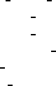
16 CONTENTS
dsrdcom.f . . . . . . . . . . . . . . . . . . . . . . . . . . . . . . . . . . . . . . . . . . 271
dsrddof150.f . . . . . . . . . . . . . . . . . . . . . . . . . . . . . . . . . . . . . . . . . 271
dsrddpmin.f . . . . . . . . . . . . . . . . . . . . . . . . . . . . . . . . . . . . . . . . . 271
dsrdens.f . . . . . . . . . . . . . . . . . . . . . . . . . . . . . . . . . . . . . . . . . . . 271
dsrdeqn.f . . . . . . . . . . . . . . . . . . . . . . . . . . . . . . . . . . . . . . . . . . 272
dsrdfunc.f . . . . . . . . . . . . . . . . . . . . . . . . . . . . . . . . . . . . . . . . . . 272
dsrdfuncs.f . . . . . . . . . . . . . . . . . . . . . . . . . . . . . . . . . . . . . . . . . . 273
dsrdlny.f . . . . . . . . . . . . . . . . . . . . . . . . . . . . . . . . . . . . . . . . . . . 273
dsrdnormlz.f . . . . . . . . . . . . . . . . . . . . . . . . . . . . . . . . . . . . . . . . . 273
dsrdqad.f . . . . . . . . . . . . . . . . . . . . . . . . . . . . . . . . . . . . . . . . . . 274
dsrdqrkck.f . . . . . . . . . . . . . . . . . . . . . . . . . . . . . . . . . . . . . . . . . 274
dsrdrhs.f . . . . . . . . . . . . . . . . . . . . . . . . . . . . . . . . . . . . . . . . . . . 274
dsrdspline.f . . . . . . . . . . . . . . . . . . . . . . . . . . . . . . . . . . . . . . . . . 275
dsrdstart.f . . . . . . . . . . . . . . . . . . . . . . . . . . . . . . . . . . . . . . . . . . 275
dsrdtab.f . . . . . . . . . . . . . . . . . . . . . . . . . . . . . . . . . . . . . . . . . . . 275
dsrdthav.f . . . . . . . . . . . . . . . . . . . . . . . . . . . . . . . . . . . . . . . . . . 276
dsrdthclose.f . . . . . . . . . . . . . . . . . . . . . . . . . . . . . . . . . . . . . . . . . 276
dsrdthlim.f . . . . . . . . . . . . . . . . . . . . . . . . . . . . . . . . . . . . . . . . . 276
dsrdthtest.f . . . . . . . . . . . . . . . . . . . . . . . . . . . . . . . . . . . . . . . . . 276
dsrdwdwdcos.f . . . . . . . . . . . . . . . . . . . . . . . . . . . . . . . . . . . . . . . 277
dsrdwfunc.f . . . . . . . . . . . . . . . . . . . . . . . . . . . . . . . . . . . . . . . . . 277
dsrdwintp.f . . . . . . . . . . . . . . . . . . . . . . . . . . . . . . . . . . . . . . . . . 277
dsrdwintpch.f . . . . . . . . . . . . . . . . . . . . . . . . . . . . . . . . . . . . . . . . 277
dsrdwintprint.f . . . . . . . . . . . . . . . . . . . . . . . . . . . . . . . . . . . . . . . 277
dsrdwintrp.f . . . . . . . . . . . . . . . . . . . . . . . . . . . . . . . . . . . . . . . . . 278
dsrdwprint.f . . . . . . . . . . . . . . . . . . . . . . . . . . . . . . . . . . . . . . . . . 278
dsrdwres.f . . . . . . . . . . . . . . . . . . . . . . . . . . . . . . . . . . . . . . . . . . 278
22 rge: mSUGRA interface (Isasugra) to DarkSUSY 281
22.1 mSUGRA (ISASUGRA) interface to DarkSUSY . . . . . . . . . . . . . . . . . . . . 281
22.2 Routine headers – fortran files . . . . . . . . . . . . . . . . . . . . . . . . . . . . . . . 281
dsgive model isasugra.f . . . . . . . . . . . . . . . . . . . . . . . . . . . . . . . . . . . 281
dsisasugra check.f . . . . . . . . . . . . . . . . . . . . . . . . . . . . . . . . . . . . . . 282
dsisasugra darksusy.f . . . . . . . . . . . . . . . . . . . . . . . . . . . . . . . . . . . . 282
dsmodelsetup isasugra.f . . . . . . . . . . . . . . . . . . . . . . . . . . . . . . . . . . 282
dsrge isasugra.f . . . . . . . . . . . . . . . . . . . . . . . . . . . . . . . . . . . . . . . 282
dssusy isasugra.f . . . . . . . . . . . . . . . . . . . . . . . . . . . . . . . . . . . . . . 283
23 rn: Relic density of neutralinos (wrapper for rd routines) 285
23.1 Relic density of neutralinos . . . . . . . . . . . . . . . . . . . . . . . . . . . . . . . . 285
23.2 Routine headers – fortran files . . . . . . . . . . . . . . . . . . . . . . . . . . . . . . . 285
dsrdomega.f . . . . . . . . . . . . . . . . . . . . . . . . . . . . . . . . . . . . . . . . . 285
dsrdres.f . . . . . . . . . . . . . . . . . . . . . . . . . . . . . . . . . . . . . . . . . . . 286
dsrdthr.f . . . . . . . . . . . . . . . . . . . . . . . . . . . . . . . . . . . . . . . . . . . 286
dsrdwrate.f . . . . . . . . . . . . . . . . . . . . . . . . . . . . . . . . . . . . . . . . . 286
24 su: General SUSY model setup: masses, vertices etc 289
24.1 Supersymmetric model . . . . . . . . . . . . . . . . . . . . . . . . . . . . . . . . . . . 289
24.1.1 Parameters . . . . . . . . . . . . . . . . . . . . . . . . . . . . . . . . . . . . . 289
24.1.2 Mass spectrum . . . . . . . . . . . . . . . . . . . . . . . . . . . . . . . . . . . 289
24.1.3 Three-particle vertices . . . . . . . . . . . . . . . . . . . . . . . . . . . . . . . 292
24.1.4 Accelerator bounds . . . . . . . . . . . . . . . . . . . . . . . . . . . . . . . . . 294

CONTENTS 17
24.2 General supersymmetry – routines . . . . . . . . . . . . . . . . . . . . . . . . . . . . 295
24.3 Routine headers – fortran files . . . . . . . . . . . . . . . . . . . . . . . . . . . . . . . 297
dsb0loop.f . . . . . . . . . . . . . . . . . . . . . . . . . . . . . . . . . . . . . . . . . . 297
dschasct.f . . . . . . . . . . . . . . . . . . . . . . . . . . . . . . . . . . . . . . . . . . 297
dsfeynhiggsfast.f . . . . . . . . . . . . . . . . . . . . . . . . . . . . . . . . . . . . . . 297
dsfindmtmt.f . . . . . . . . . . . . . . . . . . . . . . . . . . . . . . . . . . . . . . . . 298
dsg0loop.f . . . . . . . . . . . . . . . . . . . . . . . . . . . . . . . . . . . . . . . . . . 298
dsg4set.f . . . . . . . . . . . . . . . . . . . . . . . . . . . . . . . . . . . . . . . . . . . 298
dsg4set12.f . . . . . . . . . . . . . . . . . . . . . . . . . . . . . . . . . . . . . . . . . 298
dsg4set1234.f . . . . . . . . . . . . . . . . . . . . . . . . . . . . . . . . . . . . . . . . 299
dsg4set13.f . . . . . . . . . . . . . . . . . . . . . . . . . . . . . . . . . . . . . . . . . 299
dsg4set23.f . . . . . . . . . . . . . . . . . . . . . . . . . . . . . . . . . . . . . . . . . 299
dsg4set34.f . . . . . . . . . . . . . . . . . . . . . . . . . . . . . . . . . . . . . . . . . 299
dsg4setc.f . . . . . . . . . . . . . . . . . . . . . . . . . . . . . . . . . . . . . . . . . . 299
dsg4setc12.f . . . . . . . . . . . . . . . . . . . . . . . . . . . . . . . . . . . . . . . . . 299
dsg4setc1234.f . . . . . . . . . . . . . . . . . . . . . . . . . . . . . . . . . . . . . . . . 300
dsg4setc13.f . . . . . . . . . . . . . . . . . . . . . . . . . . . . . . . . . . . . . . . . . 300
dsg4setc23.f . . . . . . . . . . . . . . . . . . . . . . . . . . . . . . . . . . . . . . . . . 300
dsg4setc34.f . . . . . . . . . . . . . . . . . . . . . . . . . . . . . . . . . . . . . . . . . 300
dsgive model.f . . . . . . . . . . . . . . . . . . . . . . . . . . . . . . . . . . . . . . . . 300
dshgfu.f . . . . . . . . . . . . . . . . . . . . . . . . . . . . . . . . . . . . . . . . . . . 301
dshigferqcd.f . . . . . . . . . . . . . . . . . . . . . . . . . . . . . . . . . . . . . . . . 301
dshigsct.f . . . . . . . . . . . . . . . . . . . . . . . . . . . . . . . . . . . . . . . . . . 301
dshigwid.f . . . . . . . . . . . . . . . . . . . . . . . . . . . . . . . . . . . . . . . . . . 302
dshlf2.f . . . . . . . . . . . . . . . . . . . . . . . . . . . . . . . . . . . . . . . . . . . . 302
dshlf3.f . . . . . . . . . . . . . . . . . . . . . . . . . . . . . . . . . . . . . . . . . . . . 302
dsmodelsetup.f . . . . . . . . . . . . . . . . . . . . . . . . . . . . . . . . . . . . . . . 302
dsmqpole1loop.f . . . . . . . . . . . . . . . . . . . . . . . . . . . . . . . . . . . . . . . 303
dsneusct.f . . . . . . . . . . . . . . . . . . . . . . . . . . . . . . . . . . . . . . . . . . 303
dspole.f . . . . . . . . . . . . . . . . . . . . . . . . . . . . . . . . . . . . . . . . . . . 303
dsprep.f . . . . . . . . . . . . . . . . . . . . . . . . . . . . . . . . . . . . . . . . . . . 303
dsqindx.f . . . . . . . . . . . . . . . . . . . . . . . . . . . . . . . . . . . . . . . . . . 304
dsralph3.f . . . . . . . . . . . . . . . . . . . . . . . . . . . . . . . . . . . . . . . . . . 304
dsralph31loop.f . . . . . . . . . . . . . . . . . . . . . . . . . . . . . . . . . . . . . . . 304
dsrghm.f . . . . . . . . . . . . . . . . . . . . . . . . . . . . . . . . . . . . . . . . . . . 304
dsrmq.f . . . . . . . . . . . . . . . . . . . . . . . . . . . . . . . . . . . . . . . . . . . 304
dsrmq1loop.f . . . . . . . . . . . . . . . . . . . . . . . . . . . . . . . . . . . . . . . . 304
dssettopmass.f . . . . . . . . . . . . . . . . . . . . . . . . . . . . . . . . . . . . . . . 304
dssfesct.f . . . . . . . . . . . . . . . . . . . . . . . . . . . . . . . . . . . . . . . . . . . 304
dsspectrum.f . . . . . . . . . . . . . . . . . . . . . . . . . . . . . . . . . . . . . . . . 305
dssuconst.f . . . . . . . . . . . . . . . . . . . . . . . . . . . . . . . . . . . . . . . . . 305
dssusy.f . . . . . . . . . . . . . . . . . . . . . . . . . . . . . . . . . . . . . . . . . . . 305
dsvertx.f . . . . . . . . . . . . . . . . . . . . . . . . . . . . . . . . . . . . . . . . . . . 305
dsvertx1.f . . . . . . . . . . . . . . . . . . . . . . . . . . . . . . . . . . . . . . . . . . 306
dsvertx3.f . . . . . . . . . . . . . . . . . . . . . . . . . . . . . . . . . . . . . . . . . . 306
dswhwarn.f . . . . . . . . . . . . . . . . . . . . . . . . . . . . . . . . . . . . . . . . . 307
dswspectrum.f . . . . . . . . . . . . . . . . . . . . . . . . . . . . . . . . . . . . . . . . 307
dswunph.f . . . . . . . . . . . . . . . . . . . . . . . . . . . . . . . . . . . . . . . . . . 307
dswvertx.f . . . . . . . . . . . . . . . . . . . . . . . . . . . . . . . . . . . . . . . . . . 307
g4p.f . . . . . . . . . . . . . . . . . . . . . . . . . . . . . . . . . . . . . . . . . . . . . 308

18 CONTENTS
25 suspect: mSUGRA interface (suspect) to DarkSUSY 309
25.1 Routine headers – fortran files . . . . . . . . . . . . . . . . . . . . . . . . . . . . . . . 309
dssuspecterr.f . . . . . . . . . . . . . . . . . . . . . . . . . . . . . . . . . . . . . . . . 309
dssuspectsugra.f . . . . . . . . . . . . . . . . . . . . . . . . . . . . . . . . . . . . . . . 309
suspect2.f . . . . . . . . . . . . . . . . . . . . . . . . . . . . . . . . . . . . . . . . . . 310
26 xcern: CERN routines needed by DarkSUSY 313
26.1 Routine headers – fortran files . . . . . . . . . . . . . . . . . . . . . . . . . . . . . . . 313
besj064.f . . . . . . . . . . . . . . . . . . . . . . . . . . . . . . . . . . . . . . . . . . . 313
bsir364.f . . . . . . . . . . . . . . . . . . . . . . . . . . . . . . . . . . . . . . . . . . . 313
dbzejy.f . . . . . . . . . . . . . . . . . . . . . . . . . . . . . . . . . . . . . . . . . . . 313
ddilog.f . . . . . . . . . . . . . . . . . . . . . . . . . . . . . . . . . . . . . . . . . . . 314
dgadap.f . . . . . . . . . . . . . . . . . . . . . . . . . . . . . . . . . . . . . . . . . . . 314
drkstp.f . . . . . . . . . . . . . . . . . . . . . . . . . . . . . . . . . . . . . . . . . . . 314
eisrs1.f . . . . . . . . . . . . . . . . . . . . . . . . . . . . . . . . . . . . . . . . . . . . 315
gpindp.f . . . . . . . . . . . . . . . . . . . . . . . . . . . . . . . . . . . . . . . . . . . 315
mtlprt.f . . . . . . . . . . . . . . . . . . . . . . . . . . . . . . . . . . . . . . . . . . . 316
tql2.f . . . . . . . . . . . . . . . . . . . . . . . . . . . . . . . . . . . . . . . . . . . . . 316
tred2.f . . . . . . . . . . . . . . . . . . . . . . . . . . . . . . . . . . . . . . . . . . . . 316
27 xcmlib: CMLIB routines needed by DarkSUSY 317
27.1 Routine headers – fortran files . . . . . . . . . . . . . . . . . . . . . . . . . . . . . . . 317
d1mach.f . . . . . . . . . . . . . . . . . . . . . . . . . . . . . . . . . . . . . . . . . . . 317
dqagse.f . . . . . . . . . . . . . . . . . . . . . . . . . . . . . . . . . . . . . . . . . . . 317
dqagseb.f . . . . . . . . . . . . . . . . . . . . . . . . . . . . . . . . . . . . . . . . . . 320
dqelg.f . . . . . . . . . . . . . . . . . . . . . . . . . . . . . . . . . . . . . . . . . . . . 323
dqk21.f . . . . . . . . . . . . . . . . . . . . . . . . . . . . . . . . . . . . . . . . . . . . 324
dqk21b.f . . . . . . . . . . . . . . . . . . . . . . . . . . . . . . . . . . . . . . . . . . . 325
dqpsrt.f . . . . . . . . . . . . . . . . . . . . . . . . . . . . . . . . . . . . . . . . . . . 326
28 xfeynhiggs: FeynHiggs interface to DarkSUSY 329
28.1 Routine headers – fortran files . . . . . . . . . . . . . . . . . . . . . . . . . . . . . . . 329
dsfeynhiggs.f . . . . . . . . . . . . . . . . . . . . . . . . . . . . . . . . . . . . . . . . 329
dsfeynhiggsdummy.f . . . . . . . . . . . . . . . . . . . . . . . . . . . . . . . . . . . . 330
FeynHiggsSub ds.f . . . . . . . . . . . . . . . . . . . . . . . . . . . . . . . . . . . . . 330
Hhmasssr2 ds.f . . . . . . . . . . . . . . . . . . . . . . . . . . . . . . . . . . . . . . . 331
29 xhdecay: HDecay interface to DarkSUSY 333
29.1 Routine headers – fortran files . . . . . . . . . . . . . . . . . . . . . . . . . . . . . . . 333
dshdecay.f . . . . . . . . . . . . . . . . . . . . . . . . . . . . . . . . . . . . . . . . . . 333
hdecay.f . . . . . . . . . . . . . . . . . . . . . . . . . . . . . . . . . . . . . . . . . . . 333
Acknowledgements 337
Bibliography 337
Chapter 1
Introduction
DarkSUSY is a set of Fortran routine to make calculations for supersymmetric dark matter in
the Minimal Supersymmetric Standard Model, the MSSM. The physics involved is covered in the
DarkSUSY paper [1]. In this manual we will mainly cover the more techincal aspects of DarkSUSY,
i.e. how to call different subroutines and how to change switches and options. We will only briefly
review the necessary physics involved when needed and refer the reader to [1] and the original papers
behind DarkSUSY [2] for more details. If you use DarkSUSY please consider the original physics
work behind and give proper credit to [1] and the relevant references in [2]. If you use non-standard
options, e.g. a different propagation model for antiprotons, please remember to give proper credit
to that model.
19
20 CHAPTER 1. INTRODUCTION

Chapter 2
General remarks on notation
In an attempt to keep this manual reasonably easy to follow we will need to specify our notation.
We will use the following convention for fonts,
Convention for fonts
text This font is used for normal text.
variable This font is used for variables or other things in the code that is mentioned.
routine This font is used for subroutine or function names or for header file names.
dump This font will be used for screen dumps of outputs.
input This font will be used for user input, i.e. where you are supposed to write
something.
Subroutines and functions will be described with the following structure
subroutine example(in1,in2,in3,in4,in5,in6,in7,out1)
Purpose: Here the routine will be explained.
Inputs:
in1 i This is an input argument, declared as integer.
in2 r This is an input argument, declared as real.
in3 r8 This is an input argument, declared as real*8.
in4 c This is an input argument, declared as complex.
in5 c16 This is an input argument, declared as complex*16.
in6 ch2 This is an input argument, declared as character*2.
in7 ch* This is an input argument, declared as character*(*).
Outputs
out1 r8 This is an output argument, declared as real*8
where the shorthand notation for the type of the arguments is indicated. For functions, the type is
indicated on the first line,
function fun(arg) r8
Purpose: Here the function will be explained.
Inputs:
arg i This is an input argument, declared as integer.
i.e., in this case the function is declared as real*8.
The subroutines always reside in a file with the same name as the subroutine/function. Rou-
tines that belong together are put in separate subdirectories in the src directory. The different
subdirectories are
Subdirectories in src/
ac accelerator constraints
an driver routines for neutralino and chargino annihilation
21

22 CHAPTER 2. GENERAL REMARKS ON NOTATION
an1l 1-loop neutralino annihilation amplitudes
anstu tree-level neutralino and chargino annihilation amplitudes
dd direct detection and neutralino scattering
ep positron fluxes from the halo
ge general routines
ha yields of halo annihilation products (from Pythia simulations in vacuum)
hm halo models
hr driver routines for rates from the halo
ini initialization routines
mu neutrino and muon yields from the neutralino annihilations in the Earth/Sun
(from Pythia simulations in medium)
nt driver routines for rates and fluxes in neutrino telescopes
pb antiprotons from annihilation in the halo
rd relic density routines (general)
rn driver routines for neutralino relic density
su general MSSM routines, couplings, masses, etc.
xcern routines from CERNLIB
xcmlib routines from CMLIB
Common blocks are all declared in header files in the inc directory. When discussing switches and
parameters in common blocks we will, instead of describing the common blocks in detail, mention
which header file they reside in. If you want to access these variables, you should then include the
corresponding header file. E.g., it can look like this
Example parameters in headerfile.h
Purpose: Description of this set of variables.
par1 r8 Description of a real*8 parameter.

Chapter 3
src/ac:
Accelerator bounds
3.1 Accelerator bounds
DarkSUSY contains a set of routines to check if a given model is excluded by accelerator constraints.
These routines are called dsacbnd[number]. The policy is that when we update DarkSUSY with
new accelerator constraints, we keep the old routine, and add a new routine with the last number
incremented by one. Which routine that is called is determined by calling dsacset with a tag
determining which routine to call. To check the accelerator constraints, then call dsacbnd which
calls the right routine for you. Upon return, dsacbnd returns an exclusion flag, excl. If zero, the
model is OK, if non-zero, the model is excluded. The cause for the exclusion is coded in the bits of
excl according to table 3.1
excl
Bit set Octal value Decimal value Reason for exclusion
0 1 1 Chargino mass
1 2 2 Gluino mass
2 4 4 Squark mass
3 10 8 Slepton mass
4 20 16 Invisible Zwidth
5 40 32 Higgs mass
6 100 64 Neutralino mass
7 200 128 b→sγ
8 400 256 ρparameter
Table 3.1: The bits of excl are set to indicate by which process this particular model is excluded.
Check if a bit is set with btest(excl,bit).
3.2 Routine headers – fortran files
dsacbnd.f
c-----------------------------------------------------------------------
c This is a wrapper routine which selects which accelerator constraint
c routine, dsacbnd* to call. Whenever the accelerator constraints are
c upgraded, a new function dsacbnd*.f is created, meaning that all old
23

24 CHAPTER 3. AC: ACCELERATOR BOUNDS
c versions are kept for backward checks. The user can select which
c routine to use with a call to dsacset.
c
c Available options (in the call to dsacset) are:
c pdg2002c = default, these are the latest implemented
c accelerator bounds
c pdg2002b
c pdg2002
c pdg2000
c mar2000
c pdg1999
c-----------------------------------------------------------------------
subroutine dsacbnd(excl)
dsacbnd1.f
subroutine dsacbnd1(excl)
c_______________________________________________________________________
c check if accelerator data exclude the present point.
c output:
c excl - code of the reason for exclusion (integer); 0 if allowed
c common:
c ’dssusy.h’ - file with susy common blocks
c author: paolo gondolo 1994-1999
c history:
c 940407 first version paolo gondolo
c 950323 update paolo gondolo
c 971200 partial update joakim edsjo
c 980428 update joakim edsjo
c 990719 update paolo gondolo
c=======================================================================
dsacbnd2.f
subroutine dsacbnd2(excl)
c_______________________________________________________________________
c check if accelerator data exclude the present point.
c output:
c excl - code of the reason for exclusion (integer); 0 if allowed
c if not allowed, the reasons are coded as follows
c dsbit set dec. oct. reason
c ------- ---- ---- ------
c 0 1 1 chargino mass
c 1 2 2 gluino mass
c 2 4 4 squark mass
c 3 8 10 slepton mass
c 4 16 20 invisible z width
c 5 32 40 higgs mass
c 6 64 100 neutralino mass
c 7 128 200 b -> s gamma
c 8 256 400 rho parameter
c common:

3.2. ROUTINE HEADERS – FORTRAN FILES 25
c ’dssusy.h’ - file with susy common blocks
c author: paolo gondolo 1994-1999
c history:
c 940407 first version paolo gondolo
c 950323 update paolo gondolo
c 971200 partial update joakim edsjo
c 980428 update joakim edsjo
c 990719 update paolo gondolo
c 000310 update piero ullio
c 000424 added delrho joakim edsjo
c=======================================================================
dsacbnd3.f
subroutine dsacbnd3(excl)
c_______________________________________________________________________
c check if accelerator data exclude the present point.
c output:
c excl - code of the reason for exclusion (integer); 0 if allowed
c if not allowed, the reasons are coded as follows
c dsbit set dec. oct. reason
c ------- ---- ---- ------
c 0 1 1 chargino mass
c 1 2 2 gluino mass
c 2 4 4 squark mass
c 3 8 10 slepton mass
c 4 16 20 invisible z width
c 5 32 40 higgs mass
c 6 64 100 neutralino mass
c 7 128 200 b -> s gamma
c 8 256 400 rho parameter
c common:
c ’dssusy.h’ - file with susy common blocks
c author: paolo gondolo 1994-1999
c history:
c 940407 first version paolo gondolo
c 950323 update paolo gondolo
c 971200 partial update joakim edsjo
c 980428 update joakim edsjo
c 990719 update paolo gondolo
c 000310 update piero ullio
c 000424 added delrho joakim edsjo
c 000904 update according to pdg2000 lars bergstrom
c 010214 mh2 limits corrected, joakim edsjo
c=======================================================================
dsacbnd4.f
subroutine dsacbnd4(excl)
c_______________________________________________________________________
c check if accelerator data exclude the present point.
c output:

26 CHAPTER 3. AC: ACCELERATOR BOUNDS
c excl - code of the reason for exclusion (integer); 0 if allowed
c if not allowed, the reasons are coded as follows
c dsbit set dec. oct. reason
c ------- ---- ---- ------
c 0 1 1 chargino mass
c 1 2 2 gluino mass
c 2 4 4 squark mass
c 3 8 10 slepton mass
c 4 16 20 invisible z width
c 5 32 40 higgs mass
c 6 64 100 neutralino mass
c 7 128 200 b -> s gamma
c 8 256 400 rho parameter
c common:
c ’dssusy.h’ - file with susy common blocks
c author: paolo gondolo 1994-1999
c history:
c 940407 first version paolo gondolo
c 950323 update paolo gondolo
c 971200 partial update joakim edsjo
c 980428 update joakim edsjo
c 990719 update paolo gondolo
c 000310 update piero ullio
c 000424 added delrho joakim edsjo
c 000904 update according to pdg2000 lars bergstrom
c 010214 mh2 limits corrected, joakim edsjo
c 020927 higgs limits update according to pdg2002 mia schelke
c 021001 susy part. mass limits update to pdg2002 je/ms
c=======================================================================
dsacbnd5.f
subroutine dsacbnd5(excl)
c_______________________________________________________________________
c check if accelerator data exclude the present point.
c output:
c excl - code of the reason for exclusion (integer); 0 if allowed
c if not allowed, the reasons are coded as follows
c dsbit set dec. oct. reason
c ------- ---- ---- ------
c 0 1 1 chargino mass
c 1 2 2 gluino mass
c 2 4 4 squark mass
c 3 8 10 slepton mass
c 4 16 20 invisible z width
c 5 32 40 higgs mass
c 6 64 100 neutralino mass
c 7 128 200 b -> s gamma
c 8 256 400 rho parameter
c common:
c ’dssusy.h’ - file with susy common blocks
c author: paolo gondolo 1994-1999

3.2. ROUTINE HEADERS – FORTRAN FILES 27
c history:
c 940407 first version paolo gondolo
c 950323 update paolo gondolo
c 971200 partial update joakim edsjo
c 980428 update joakim edsjo
c 990719 update paolo gondolo
c 000310 update piero ullio
c 000424 added delrho joakim edsjo
c 000904 update according to pdg2000 lars bergstrom
c 010214 mh2 limits corrected, joakim edsjo
c 020927 higgs limits update according to pdg2002 mia schelke
c 021001 susy part. mass limits update to pdg2002 je/ms
c=======================================================================
dsacbnd6.f
subroutine dsacbnd6(excl)
c_______________________________________________________________________
c check if accelerator data exclude the present point.
c output:
c excl - code of the reason for exclusion (integer); 0 if allowed
c if not allowed, the reasons are coded as follows
c dsbit set dec. oct. reason
c ------- ---- ---- ------
c 0 1 1 chargino mass
c 1 2 2 gluino mass
c 2 4 4 squark mass
c 3 8 10 slepton mass
c 4 16 20 invisible z width
c 5 32 40 higgs mass
c 6 64 100 neutralino mass
c 7 128 200 b -> s gamma
c 8 256 400 rho parameter
c common:
c ’dssusy.h’ - file with susy common blocks
c author: paolo gondolo 1994-1999
c history:
c 940407 first version paolo gondolo
c 950323 update paolo gondolo
c 971200 partial update joakim edsjo
c 980428 update joakim edsjo
c 990719 update paolo gondolo
c 000310 update piero ullio
c 000424 added delrho joakim edsjo
c 000904 update according to pdg2000 lars bergstrom
c 010214 mh2 limits corrected, joakim edsjo
c 020927 higgs limits update according to pdg2002 mia schelke
c 021001 susy part. mass limits update to pdg2002 je/ms
c 031204 standard model higgs like mh2 limit for msugra models
c=======================================================================

28 CHAPTER 3. AC: ACCELERATOR BOUNDS
dsacset.f
***********************************************************************
*** This routine selects which set of accelerator constraints to use
*** when dsacbnd is called. For available options, see dsacbnd.f
***********************************************************************
subroutine dsacset(a)
dsbsgamma.f
subroutine dsbsgamma(ratio,flag)
c_______________________________________________________________________
c b -> s + gamma branching ratio
c common:
c ’dssusy.h’ - file with susy common blocks
c input:
c flag : 0 no qcd correction -- 1 qcd corrections
c output:
c ratio : branching ratio
c author: paolo gondolo (gondolo@lpthe.jussieu.fr) 1994,1995
c 28-nov-94 formulas in bertolini et al, nucl phys b353 (1991) 591
c modified: joakim edsjo, 2000-09-03, vertices from dsvertx.f
c correctly implemented
c=======================================================================
dsbsgf1.f
function dsbsgf1(x)
c_______________________________________________________________________
c function in bertolini et al, nucl phys b353 (1991) 591
c author: paolo gondolo (gondolo@lpthe.jussieu.fr) 1994
c=======================================================================
dsbsgf2.f
function dsbsgf2(x)
c_______________________________________________________________________
c function in bertolini et al, nucl phys b353 (1991) 591
c author: paolo gondolo (gondolo@lpthe.jussieu.fr) 1994
c=======================================================================
dsbsgf3.f
function dsbsgf3(x)
c_______________________________________________________________________
c function in bertolini et al, nucl phys b353 (1991) 591
c author: paolo gondolo (gondolo@lpthe.jussieu.fr) 1994
c=======================================================================
dsbsgf4.f
function dsbsgf4(x)

3.2. ROUTINE HEADERS – FORTRAN FILES 29
c_______________________________________________________________________
c function in bertolini et al, nucl phys b353 (1991) 591
c author: paolo gondolo (gondolo@lpthe.jussieu.fr) 1994
c=======================================================================
dsgm2muon.f
function dsgm2muon()
c supersymmetric contribution to (g-2)_muon
c output:
c gm2amp : susy contribution to g-2 amplitude = (g-2)/2
c according to T Moroi hep-ph/9512396 v3
c (T. Moroi, PRD 1996; (E) 1997)
c author: paolo gondolo 2001-02-08
c reference: e a baltz and p gondolo, hep-ph/0102147
dswexcl.f
subroutine dswexcl(unit,excl)
c_______________________________________________________________________
c write reasons for exclusion to specified unit.
c input:
c unit - logical unit to write on (integer)
c excl - code of the reason for exclusion (integer); 0 if allowed
c author: paolo gondolo (gondolo@lpthe.jussieu.fr) 1994
c=======================================================================
30 CHAPTER 3. AC: ACCELERATOR BOUNDS
Chapter 4
src/an:
Annihilation cross sections
(general, χ0and χ±)
4.1 Annihilation cross sections – theory
For the relic density calculations, we need all possible (co)annihilation cross sections between neu-
tralinos, charginos and sfermions.
4.1.1 Annihilation cross sections
We have calculated all two-body final state cross sections at tree level for involving netralinos,
charginos, sneutrinos, sleptons and squarks in the initial state. A complete list is given below.
Since we have so many different diagrams contributing, we have to use some method where
the diagrams can be calculated efficiently. To achive this, we calculate the diagrams with general
expressions for vertices, masses etc so that they can be reused for other processes. How we do this
in practice differs a bit between different sets of annihilation diagrams.
For neutralino-neutralino, neutralino-chargino and chargino-chargino annihilation, we classify
the diagrams according to their topology (s-, t- or u-channel) and to the spin of the particles
involved. We then compute the helicity amplitudes for each type of diagram analytically with
Reduce [71] using general expressions for the vertex couplings.
The strength of the helicity amplitude method is that the analytical calculation of a given type
of diagram has to be performed only once and the sum of the contributing diagrams for each set of
initial and final states can be done numerically afterwards.
For the diagrams involving sfermions, Form is used to analytically calculate the amplitudes.
This output is then converted into Fortran with a Perl script, form2f [173].
4.1.2 Coannihilation diagrams
All Feynman diagrams for which we calculate the annihilation cross section are listed in the coming
sections. s(x), t(x) and u(x) denote a tree-level Feynman diagram in which particle xis exchanged
in the s-, t- and u-channel respectively.
The convention used in this list of included coannihilation diagrams is that if a sfermion is
denoted ˜
f, then it’s antiparticle is denoted ˜
f∗.
31

32 CHAPTER 4. AN: ANNIHILATION CROSS SECTIONS (GENERAL, χ0AND χ±)
4.1.3 Neutralino and chargino annihilation
Indices i, j, k run from 1 to 4, and indices c, d, e from 1 to 2. u, ˜u,d,˜
d,ν, ˜ν,ℓ,˜
ℓ,fand ˜
fare generic
notations for up-type quarks, up-type squarks, down-type quarks, down-type squarks, neutrinos,
sneutrinos, leptons, sleptons, fermions and sfermions. A sum of diagrams over (s)fermion generation
indices and over the neutralino and chargino indices kand eis understood (no sum over indices
i, j, c, d).
Neutralino-neutralino annihilation
Initial state Final state Feynman diagrams
H1H1,H1H2,H2H2,H3H3t(χ0
k), u(χ0
k), s(H1,2)
H1H3,H2H3t(χ0
k), u(χ0
k), s(H3), s(Z0)
H−H+t(χ+
e), u(χ+
e), s(H1,2), s(Z0)
Z0H1,Z0H2t(χ0
k), u(χ0
k), s(H3), s(Z0)
χ0
iχ0
jZ0H3t(χ0
k), u(χ0
k), s(H1,2)
W−H+,W+H−t(χ+
e), u(χ+
e), s(H1,2,3)
Z0Z0t(χ0
k), u(χ0
k), s(H1,2)
W−W+t(χ+
e), u(χ+
e), s(H1,2), s(Z0)
f¯
f t(˜
fL,R), u(˜
fL,R), s(H1,2,3), s(Z0)
Neutralino-chargino annihilation
Initial state Final state Feynman diagrams
H+H1,H+H2t(χ0
k), u(χ+
e), s(H+), s(W+)
H+H3t(χ0
k), u(χ+
e), s(W+)
W+H1,W+H2t(χ0
k), u(χ+
e), s(H+), s(W+)
W+H3t(χ0
k), u(χ+
e), s(H+)
χ+
cχ0
iH+Z0t(χ0
k), u(χ+
e), s(H+)
γH+t(χ+
c), s(H+)
W+Z0t(χ0
k), u(χ+
e), s(W+)
γW +t(χ+
c), s(W+)
u¯
d t(˜
dL,R), u(˜uL,R), s(H+), s(W+)
ν¯
ℓ t(˜
ℓL,R), u(˜νL), s(H+), s(W+)

4.1. ANNIHILATION CROSS SECTIONS – THEORY 33
Chargino-chargino annihilation
Initial state Final state Feynman diagrams
H1H1,H1H2,H2H2,H3H3t(χ+
e), u(χ+
e), s(H1,2)
H1H3,H2H3t(χ+
e), u(χ+
e), s(H3), s(Z0)
H+H−t(χ0
k), s(H1,2), s(Z0, γ)
Z0H1,Z0H2t(χ+
e), u(χ+
e), s(H3), s(Z0)
Z0H3t(χ+
e), u(χ+
e), s(H1,2)
H+W−,W+H−t(χ0
k), s(H1,2,3)
χ+
cχ−
dZ0Z0t(χ+
e), u(χ+
e), s(H1,2)
W+W−t(χ0
k), s(H1,2), s(Z0, γ)
γγ (only for c=d)t(χ+
c), u(χ+
c)
Z0γ t(χ+
d), u(χ+
c)
u¯u t(˜
dL,R), s(H1,2,3), s(Z0, γ)
ν¯ν t(˜
ℓL,R), s(Z0)
¯
dd t(˜uL,R), s(H1,2,3), s(Z0, γ)
¯
ℓℓ t(˜νL), s(H1,2,3), s(Z0, γ)
H+H+t(χ0
k), u(χ0
k)
χ+
cχ+
dH+W+t(χ0
k), u(χ0
k)
W+W+t(χ0
k), u(χ0
k)
4.1.4 Squark-squark annihilation
We will here denote squarks as ˜qi
aand ˜qj
bwhere iand jare the family indices and aand bare
the mass eigenstate indices (running from 1 to 2). kand lwill also be used as family indices for
processes including more squarks. Colour indices are suppressed. ˜uiis used as a generic notation for
any up-type squark where idenotes the family index. Down-type squarks are denoted analogously.
Note that we will not (except in rare occations) show processes for ˜νand ˜
ℓseparately since they
can easily be obtained from the squark processes by replacing ˜uwith ˜νand ˜
dwith ˜
ℓ(and noting
that we only have one mass eigenstate for the ˜ν. Also note that the ˜ν−˜
ℓ–sector is assumed not to
be flavour-changing.

34 CHAPTER 4. AN: ANNIHILATION CROSS SECTIONS (GENERAL, χ0AND χ±)
˜
di
a˜
di∗
bannihilation
Initial state Final state Diagrams Note
˜
di
a˜
di∗
bγγ,Zγ t(˜
di
1,2), u(˜
di
1,2), p
˜
di
a˜
di∗
bZZ t(˜
di
1,2), u(˜
di
1,2), p,s(H1, H2)
˜
di
a˜
di∗
bW−W+p,s(H1, H2, Z, γ), t(˜uk
1,2) Only k=iat present
˜
di
a˜
di∗
bZH2,ZH1t(˜
di
1,2), u(˜
di
1,2), s(Z, H3)
˜
di
a˜
di∗
bZH3t(˜
di
1,2), u(˜
di
1,2), s(H1, H2)
˜
di
a˜
di∗
bγH2,γH1,γH3t(˜
di
1,2), u(˜
di
1,2)
˜
di
a˜
di∗
bH2H2,H1H1,H1H2t(˜
di
1,2), u(˜
di
1,2), p,s(H1, H2)
˜
di
a˜
di∗
bH2H3,H1H3s(Z, H3), t(˜
di
1,2), u(˜
di
1,2)
˜
di
a˜
di∗
bH3H3s(H1, H2), p,t(˜
di
1,2), u(˜
di
1,2)
˜
di
a˜
di∗
bW−H+s(H1, H2, H3), t(˜uk
1,2) Only k=iat present
˜
di
a˜
di∗
bH−H+s(H1, H2, Z, γ), p,t(˜uk
1,2) Only k=iat present
˜
di
a˜
di∗
bf¯
f(f6=di)s(H⋆
1, H⋆
2, H⋆
3, Z, γ⋆, g‡), t(χ+
c)††) Only if f=uk(only
k=iat present), ⋆) Not
for f=ν,‡) Only for
squarks/quarks
˜
di
a˜
di∗
bdi¯
dis(H1, H2, H3, Z, γ, g†), t( ˜χ0
k,˜g†)†) Only for squarks
˜
di
a˜
di∗
bZg t(˜
di
1,2), u(˜
di
1,2), p Only for squarks
˜
di
a˜
di∗
bgg t(˜
di
1,2), u(˜
di
1,2), s(g), p Only for squarks
˜
di
a˜
di∗
bgγ t(˜
di
1,2), u(˜
di
1,2), p Only for squarks
˜
di
a˜
di∗
bgH1, gH2, gH3t(˜
di
1,2), u(˜
di
1,2) Only for squarks
˜
di
a˜
dj∗
bannihilation (i6=j)
Initial state Final state Diagrams Note
˜
di
a˜
dj∗
bW+W−t(˜uk
1,2)†Not included at present
˜
di
a˜
dj∗
bW+H−t(˜uk
1,2)†Not included at present
˜
di
a˜
dj∗
bH+H−t(˜uk
1,2)†Not included at present
˜
di
a˜
d∗j
bdi¯
djt(˜χ0
k,˜g†)†) Only for squarks
˜
di
a˜
d∗j
buk¯ult( ˜χ+
c) Only k=i, l =jat present
˜
di
a˜
di
bannihilation
Initial state Final state Diagrams Note
˜
di
a˜
di
bdidit(˜χ0
k,˜g†), u(˜χ0
k,˜g†)†) Only for squarks
˜
di
a˜
dj
bannihilation (i6=j)
Initial state Final state Diagrams Note
˜
di
a˜
dj
bdidjt(˜χ0
k,˜g†)†) Only for squarks
˜ui
a˜ui∗
bannihilation

4.1. ANNIHILATION CROSS SECTIONS – THEORY 35
Initial state Final state Diagrams Note
˜ui
a˜ui∗
bγγ†,Zγ†t(˜ui
1,2), u(˜ui
1,2), p†) Not for ˜ν
˜ui
a˜ui∗
bZZ t(˜ui
1,2), u(˜ui
1,2), p,s(H1, H2)
˜ui
a˜ui∗
bW−W+p,s(H1, H2, Z, γ†), u(˜
dk
1,2) Only k=iat present, †) Not
for ˜ν
˜ui
a˜ui∗
bZH2,ZH1t(˜ui
1,2), u(˜ui
1,2), s(Z, H†
3)†) Not for ˜ν
˜ui
a˜ui∗
bZH3t(˜ui
1,2)†,u(˜ui
1,2)†,s(H1, H2)†) Not for ˜ν
˜ui
a˜ui∗
bγH†
2,γH†
1,γH†
3t(˜ui
1,2), u(˜ui
1,2)†) Not for ˜ν
˜ui
a˜ui∗
bH2H2,H1H1,H1H2t(˜ui
1,2), u(˜ui
1,2), p,s(H1, H2)
˜ui
a˜ui∗
bH2H3,H1H3s(Z, H†
3), t(˜ui
1,2)†,u(˜ui
1,2)††) Not for ˜ν
˜ui
a˜ui∗
bH3H3s(H1, H2), p,t(˜ui
1,2)†,u(˜ui
1,2)††) Not for ˜ν
˜ui
a˜ui∗
bW−H+s(H1, H2, H†
3), u(˜
dk
1,2) Only k=iat present, †) Not
for ˜ν
˜ui
a˜ui∗
bH+H−s(H1, H2, Z, γ†), p,t(˜
dk
1,2) Only k=iat present, †) Not
for ˜ν
˜ui
a˜ui∗
bf¯
f(f6=ui)s(H×
1, H×
2, H†×
3, Z, γ†×, g‡), t(χ+
c)⋆†) Not for ˜ν,⋆) If f=dk
(only k=iat present), ‡)
Only for squarks/quarks, ×)
Not for ν
˜ui
a˜ui∗
bui¯uis(H×
1, H×
2, H×
3, Z, γ×, g‡), t( ˜χ0
k,˜g‡)×) Not for ν,‡) Only for
squarks
˜ui
a˜ui∗
bZg t(˜ui
1,2), u(˜ui
1,2), p Only for squarks
˜ui
a˜ui∗
bgg t(˜ui
1,2), u(˜ui
1,2), s(g), p Only for squarks
˜ui
a˜ui∗
bgγ t(˜ui
1,2), u(˜ui
1,2), p Only for squarks
˜ui
a˜ui∗
bgH1, gH2, gH3t(˜ui
1,2), u(˜ui
1,2) Only for squarks
˜ui
a˜uj∗
bannihilation (i6=j)
Initial state Final state Diagrams Note
˜ui
a˜uj∗
bW+W−t(˜
dk
1,2)†Not included at present, †) Not for ˜
ℓ
˜ui
a˜uj∗
bW+H−t(˜
dk
1,2)†Not included at present, †) Not for ˜
ℓ
˜ui
a˜uj∗
bH+H−t(˜
dk
1,2)†Not included at present, †) Not for ˜
ℓ
˜ui
a˜uj∗
bui¯ujt( ˜χ0
k, g†)†) Only for squarks
˜ui
a˜uj∗
bdk¯
dlt(˜χ+
c) Only k=i, l =jat present
˜ui
a˜ui
bannihilation
Initial state Final state Diagrams Note
˜ui
a˜ui
buiuit(˜χ0
k,˜g†), u(˜χ0
k,˜g†)†) Only for squarks
˜ui
a˜uj
bannihilation (i6=j)
Initial state Final state Diagrams Note
˜ui
a˜uj
buiujt(˜χ0
k,˜g†)†) Only for squarks

36 CHAPTER 4. AN: ANNIHILATION CROSS SECTIONS (GENERAL, χ0AND χ±)
˜ui
a˜
di∗
bannihilation
Initial state Final state Diagrams Note
˜ui
a˜
di∗
bH+H1,H+H2t(˜
di
1,2), u(˜ui
1,2), p,s(W+, H+)
˜ui
a˜
di∗
bH+H3t(˜
di
1,2), u(˜ui
1,2)†,p,s(W+)†) Not for ˜
ℓ
˜ui
a˜
di∗
bγH+t(˜ui
1,2)†,u(˜
di
1,2), s(H+)†) Not for ˜
ℓ
˜ui
a˜
di∗
bZH+t(˜ui
1,2), u(˜
di
1,2), s(H+)
˜ui
a˜
di∗
bW+H1,W+H2t(˜
di
1,2), u(˜ui
1,2), s(W+, H+)
˜ui
a˜
di∗
bW+H3t(˜
di
1,2), u(˜ui
1,2)†,s(H+)†) Not for ˜
ℓ
˜ui
a˜
di∗
bW+γ t(˜
di
1,2), u(˜ui
1,2)†,s(W+), p†) Not for ˜
ℓ
˜ui
a˜
di∗
bW+Z t(˜
di
1,2), u(˜ui
1,2), s(W+), p
˜ui
a˜
di∗
buk¯
dls(H+, W +)⋆,t( ˜χ0
m,˜g†)δikδil †) Not for ˜
ℓ,⋆) Only k=l
at present
˜ui
a˜
di∗
bW+g t(˜
di
1,2), u(˜ui
1,2), pOnly for squarks
˜ui
a˜
di∗
bgH+t(˜ui
1,2), u(˜
di
1,2) Only for squarks
˜ui
a˜
dj∗
bannihilation (i6=j)
For squarks we can have the following processes
Initial state Final state Diagrams Note
˜ui
a˜
dj∗
bH+H1,H+H2t(˜
dj
1,2), u(˜ui
1,2), p,s(W+, H+) Not included at present
˜ui
a˜
dj∗
bH+H3t(˜
dj
1,2), u(˜ui
1,2), p,s(W+) Not included at present
˜ui
a˜
dj∗
bH+γ t(˜
dj
1,2), u(˜ui
1,2), s(H+) Not included at present
˜ui
a˜
dj∗
bH+Z t(˜
dj
1,2), u(˜ui
1,2), s(H+) Not included at present
˜ui
a˜
dj∗
bW+H1,W+H2t(˜
dj
1,2), u(˜ui
1,2), s(W+, H+) Not included at present
˜ui
a˜
dj∗
bW+H3t(˜
dj
1,2), u(˜ui
1,2), s(H+) Not included at present
˜ui
a˜
dj∗
bW+γ t(˜
dj
1,2), u(˜ui
1,2), s(W+), pNot included at present
˜ui
a˜
dj∗
bW+Z t(˜
dj
1,2), u(˜ui
1,2), s(W+), pNot included at present
˜ui
a˜
dj∗
buk¯
dls(H+, W +)†,t( ˜χ0
m,˜g)δikδjl †) Not included at present
whereas for sneutrinos and sleptons, we can only have the process
Initial state Final state Diagrams Note
˜νi˜
ℓj∗
bνi¯
ℓjt(˜χ0
k)
˜ui
a˜
di
bannihilation
Initial state Final state Diagrams Note
˜ui
a˜
di
bukdlt(˜χ0
m,˜g†)δikδil,u( ˜χ+
c)⋆†) Only for squarks, ⋆)
Only i=k=lat present
˜ui
a˜
dj
bannihilation (i6=j)
Initial state Final state Diagrams Note
˜ui
a˜
dj
bukdlt(˜χ0
m,˜g†)δikδjl ,u( ˜χ+
c)×⋆†) Only for squarks, ×)
For ˜ν˜
ℓonly when i=
l, j =k,⋆) Only included
when i=l, j =kat
present

4.1. ANNIHILATION CROSS SECTIONS – THEORY 37
4.1.5 Squark-neutralino annihilation
We will here denote squarks as ˜ui
aand ˜
di
awhere iis the family index and ais the mass eigenstate
index (running from 1 to 2).
˜ui
a˜χ0
jannihilation
Initial state Final state Diagrams Note
˜ui
a˜χ0
jγuis(ui), t(˜ui
1,2) Only for squarks
˜ui
a˜χ0
jZuis(ui), t(˜ui
1,2), u(˜χ0
k)
˜ui
a˜χ0
jH1ui,H2uis(ui)†,t(˜ui
1,2), u(˜χ0
k)†) Only for squarks
˜ui
a˜χ0
jH3uis(ui)†,t(˜ui
1,2)†,u(˜χ0
k)†) Only for squarks
˜ui
a˜χ0
jW+dks(ui), t(˜
dk
1,2), u(˜χ+
c) Only k=iat present,
˜ui∗
a˜χ0
j→W−¯
dkin the
code
˜ui
a˜χ0
jH+dks(ui), t(˜
dk
1,2), u(˜χ+
c) Only k=iat present,
˜ui∗
a˜χ0
j→H−¯
dkin the
code
˜ui
a˜χ0
jguis(ui), t(˜ui
1,2)
˜
di
a˜χ0
jannihilation
Initial state Final state Diagrams Note
˜
di
a˜χ0
jγdis(di), t(˜
di
1,2)
˜
di
a˜χ0
jZdis(di), t(˜
di
1,2), u(˜χ0
k)
˜
di
a˜χ0
jH1di,H2dis(di), t(˜
di
1,2), u(˜χ0
k)
˜
di
a˜χ0
jH3dis(di), t(˜
di
1,2), u(˜χ0
k)
˜
di
a˜χ0
jW−uks(di), t(˜uk
1,2), u(˜χ+
c) Only k=iat present
˜
di
a˜χ0
jH−uks(di), t(˜uk
1,2), u(˜χ+
c) Only k=iat present
˜
di
a˜χ0
jgdis(di), t(˜
di
1,2)
4.1.6 Squark-chargino annihilation
We will here denote squarks as ˜qi
awhere iis the family index and ais the mass eigenstate index
(running from 1 to 2).
˜ui
a˜χ+
cannihilation
Initial state Final state Diagrams Note
˜ui
a˜χ+
cW+ukt(˜
dl
1,2), u(˜χ0
c)δik Only k=l=iat present
˜ui
a˜χ+
cH+ukt(˜
dl
1,2), u(˜χ0
c)δik Only k=l=iat present

38 CHAPTER 4. AN: ANNIHILATION CROSS SECTIONS (GENERAL, χ0AND χ±)
˜ui∗
a˜χ+
cannihilation
Initial state Final state Diagrams Note
˜ui∗
a˜χ+
cZ¯
dks(¯
dk), t(˜ui
1,2), u(˜χ+
c) Only k=iat present
˜ui∗
a˜χ+
cγ¯
dks(¯
dk), t(˜ui
1,2)†,u(˜χ+
c) Only k=iat present, †) Only for squarks
˜ui∗
a˜χ+
cH1¯
dk,H2¯
dks(¯
dk), t(˜ui
1,2), u(˜χ+
c) Only k=iat present
˜ui∗
a˜χ+
cH3¯
dks(¯
dk), t(˜ui
1,2)†,u(˜χ+
c) Only k=iat present, †) Only for squarks
˜ui∗
a˜χ+
cW+¯uks(¯
dl), u(˜χ0
c)δik Only k=l=iat present
˜ui∗
a˜χ+
cH+¯uks(¯
dl), u(˜χ0
c)δik Only k=l=iat present
˜ui∗
a˜χ+
cg¯
dks(¯
dk), t(˜ui
a) Only k=iat present, only for squarks
˜
di
a˜χ+
cannihilation
Initial state Final state Diagrams Note
˜
di
a˜χ+
cZuks(uk), t(˜
di
1,2), u(˜χ+
c) Only k=iat present
˜
di
a˜χ+
cγuks(uk)†,t(˜
di
1,2), u(˜χ+
c) Only k=iat present, †) Only for squarks
˜
di
a˜χ+
cH1uk,H2uks(uk)†,t(˜
di
1,2), u(˜χ+
c) Only k=iat present, †) Only for squarks
˜
di
a˜χ+
cH3uks(uk)†,t(˜
di
1,2), u(˜χ+
c) Only k=iat present, †) Only for squarks
˜
di
a˜χ+
cW+dks(ul), u(˜χ0
c)δik Only k=l=iat present
˜
di
a˜χ+
cH+dks(ul), u(˜χ0
c)δik Only k=l=iat present
˜
di
a˜χ+
cguks(uk), t(˜
di
a) Only k=iat present, only for squarks
˜
di∗
a˜χ+
cannihilation
Initial state Final state Diagrams Note
˜
di∗
a˜χ+
cW+¯
dkt(˜ul
1,2), u(˜χ0
c)δik Only k=l=iat present
˜
di∗
a˜χ+
cH+¯
dkt(˜ul
1,2), u(˜χ0
c)δik Only k=l=iat present
4.1.7 Degrees of freedom
We have to be careful with the internal degrees of freedom, g, of the particles. We can either treat
e.g. a χ+
iand a χ−
ias two separate particles with two degrees of freedom each, or we can treat
them as one particle χ±
iwith four degrees of freedom. The latter approach has an advantage that
we simplify our expressions for the effective annihilation cross sections when coannihilations are
needed. Hence, we use that approach here. For a more detailed discussion about this, see Section
21.1.4.
4.2 Annihilation routines - general remarks
The annihilation cross section routines is divided into several parts, mostly for historical reasons.
The layout is roughly as follows:
src/an Here we keep the main routins for both neutralino- neutralino annihilation cross sections
and the effective annihilation cross section in the relic density calculations. The steering
routines for neutralino and chargino coannihilations are also kept here.
src/anstu Here keep the t−,u−and s−diagram expressions for fermion-fermion coannihilations
(i.e. neutralino and chargino coannihilations).
src/as Here all the coannihilation cross sections including sfermions are kept.
We will here describe the src/an-routines.

4.3. ROUTINE HEADERS – FORTRAN FILES 39
4.2.1 General routines
The general routine to call for an effective annihilation cross section (to be used for relic density
calculations) is dsanwx, which returns the invariant annihilation rate (integrated over cos θ). The
actual cross section, differential in cos θis calculated by dsandwdcos which includes all the coanni-
hilations needed. This is set up in rn/dsrdomega which determines which coannhilating particles
to include.
For other applications where the annihilation rate is needed, e.g. annihilation in the galactic
halo, one can call the specific annihilation rate routine directly. The main one is dsandwdcosnn
for neutralino-neutralino annihilation. To simplify this task, we supply a routine dssigmav which
calls dsandwdcosnn for neutralino-neutralino annihilation at zero relative velocity and returns the
result, either as the total annihilation cross section, or the cross section for a specific channel. See
the header of dssigmav for details.
4.2.2 Neutralino and chargino (co)annihilation cross sections
The routines dsandwdcosnn,dsandwdcoscn and dsandwdcoscc calculate the annihilation cross
sections (returning the invariant annihilation rate) for neutralino-neutralino, neutralino-chargino
and chargino-chargino annihilations. Which particles the cross section is calculated for is given by
particle indices as defined in inc/dssusy.h.
All the annihilation routines return the invariant rate instead of the cross section. The invariant
annihilation rate between particle iand jis defined as
Wij = 4pij√sσij = 4σij q(pi·pj)2−m2
im2
j= 4EiEjσij vij .(4.1)
See chapter 21 for more details.
4.3 Routine headers – fortran files
dsanalbe.f
subroutine dsanalbe(alph,bet)
c_______________________________________________________________________
c determine alph and bet for the integration.
c modified: joakim edsjo (edsjo@physto.se) 97-09-09
c=======================================================================
dsanclearaa.f
subroutine dsanclearaa
c_______________________________________________________________________
c clear the amplitude matrix
c author: joakim edsjo (edsjo@physto.se) 95-10-25
c paolo gondolo 99-1-15 factor of 3.7 faster
c called by: dwdcos
c=======================================================================
dsandwdcos.f
function dsandwdcos(p,costheta)
c_______________________________________________________________________
c annihilation differential invariant rate.
c input:

40 CHAPTER 4. AN: ANNIHILATION CROSS SECTIONS (GENERAL, χ0AND χ±)
c p - initial cm momentum (real) for lsp annihilations
c costheta - cosine of c.m. annihilation angle
c common:
c ’dssusy.h’ - file with susy common blocks
c Output:
dWij
dcos θ
where
Wij = 4pij √sσij = 4σij q(pi·pj)2−m2
im2
j= 4EiEjσij vij
c The returned dW/dcos(theta) is unitless
c uses dsandwdcosnn, dsandwdcoscn and dsandwdcoscc and
c routines in src/as
c called by dsanwx.
c author: joakim edsjo (edsjo@physto.se)
c date: 96-02-21
c modified: 97-05-12 Joakim Edsjo (edsjo@physto.se)
c modified: 01-01-30 paolo gondolo (paolo@mamma-mia.phys.cwru.edu)
c modified: 02-03-09 Joakim Edsjo (edsjo@physto.se)
c modified: 06-02-22 Paolo Gondolo (paolo@physics.utah.edu)
c=======================================================================
dsandwdcoscc.f
function dsandwdcoscc(p,costheta,kp1,kp2)
c_______________________________________________________________________
c annihilation differential invariant rate between particle kp1
c and kp2 where kp1 and kp2 are charginos
c input:
c p - initial cm momentum (real)
c costheta - cosine of c.m. annihilation angle
c kp1 - particle code, particle 1
c kp2 - particle code, particle 2
c common:
c ’dssusy.h’ - file with susy common blocks
c ’diacom.h’ - file with kinematical variables
c Output:
dWij
dcos θ
where
Wij = 4pij √sσij = 4σij q(pi·pj)2−m2
im2
j= 4EiEjσij vij
c The returned dW/dcos(theta) is unitless
c uses dsanclearaa,dsansumaa
c called by dsandwdcos.
c author: joakim edsjo (edsjo@physto.se)
c date: 96-08-06
c modified: 01-09-12
c=======================================================================

4.3. ROUTINE HEADERS – FORTRAN FILES 41
dsandwdcoscn.f
function dsandwdcoscn(p,costheta,kp1,kp2)
c_______________________________________________________________________
c annihilation differential invariant rate between particle kp1
c and kp2 where kp1 is a chargino and kp2 is a neutralino.
c input:
c p - initial cm momentum (real)
c costheta - cosine of c.m. annihilation angle
c kp1 - particle code, particle 1
c kp2 - particle code, particle 2
c common:
c ’dssusy.h’ - file with susy common blocks
c ’diacom.h’ - file with kinematical variables
c Output:
dWij
dcos θ
where
Wij = 4pij √sσij = 4σij q(pi·pj)2−m2
im2
j= 4EiEjσij vij
c The returned dW/dcos(theta) is unitless
c uses dsanclearaa,dsansumaa
c called by dsandwdcos.
c author: joakim edsjo (edsjo@physto.se)
c date: 96-08-06
c modified: 01-09-12
c=======================================================================
dsandwdcosd.f
function dsandwdcosd(costheta)
c_______________________________________________________________________
c 10^15*annihilation differential invariant rate.
c input:
c p - initial cm momentum (real) for lsp annihilations via common
c costheta - cosine of c.m. annihilation angle
c common:
c ’dssusy.h’ - file with susy common blocks
c uses dwdcos
c used for gaussian integration with gadap.f
c author: joakim edsjo (edsjo@physto.se)
c date: 97-01-09
c=======================================================================
dsandwdcosnn.f
function dsandwdcosnn(p,costheta,kp1,kp2)
c_______________________________________________________________________
c Annihilation differential invariant rate between particle kp1
c and kp2 where kp1 and kp2 are neutralinos
c Input:

42 CHAPTER 4. AN: ANNIHILATION CROSS SECTIONS (GENERAL, χ0AND χ±)
c p - initial cm momentum (real)
c costheta - cosine of c.m. annihilation angle
c kp1 - particle code for particle 1
c kp2 - particle code for particle 2
c common:
c ’dssusy.h’ - file with susy common blocks
c ’diacom.h’ - file with kinematical variables
c Output:
dWij
dcos θ
where
Wij = 4pij √sσij = 4σij q(pi·pj)2−m2
im2
j= 4EiEjσij vij
c The returned dW/dcos(theta) is unitless.
c
c uses dsanclearaa,dsansumaa
c called by dsandwdcos.
c note: the 32pi in the partial cross sections is 8pi g_1^2, g_1=2
c author: joakim edsjo (edsjo@physto.se)
c date: 96-02-21
c modified: 01-09-12
c=======================================================================
dsandwdcoss.f
function dsandwdcoss(costheta)
c_______________________________________________________________________
c 10^15*annihilation differential invariant rate.
c input:
c p - initial cm momentum (real) for lsp annihilations via common
c costheta - cosine of c.m. annihilation angle
c common:
c ’dssusy.h’ - file with susy common blocks
c uses dwdcos
c used for gaussian integration with gadap.f
c author: joakim edsjo (edsjo@physto.se)
c date: 97-01-09
c=======================================================================
dsandwdcosy.f
function dsandwdcosy(y)
c_______________________________________________________________________
c 10^15*annihilation differential invariant rate.
c the integration variable is changed from cos(theta) to
c y=1/(mx^2+2p^2(1-cos(theta))) for cos(theta)>0 and to
c y=1/(mx^2+2p^2(1-cos(theta))) for cos(theta)<0.
c this avoids the poles at cos(theta)=+-1
c integrate this function from 1/(mx^2+2p^2) to 1/mx^2 to get
c 1d15 times the integral from cos(theta)=0 to 1.

4.3. ROUTINE HEADERS – FORTRAN FILES 43
c input:
c y - initial cm momentum (real) for lsp annihilations via common
c common:
c ’dssusy.h’ - file with susy common blocks
c uses dwdcos
c used for gaussian integration with gadap.f
c author: joakim edsjo (edsjo@physto.se)
c date: 98-05-03
c=======================================================================
dsankinvar.f
subroutine dsankinvar(p,costheta,kp1,kp2,kpk,kp3,kp4)
c=======================================================================
c calculate kinematical variables for s-, t-, and u-diagram
c author: joakim edsjo, edsjo@physto.se
c date: 97-01-09
c=======================================================================
dsanset.f
subroutine dsanset(c)
c...set parameters for annihilation routines
c... c - character string specifying choice to be made
c...author: joakim edsjo, 2001-09-12
dsansumaa.f
real*8 function dsansumaa()
c_______________________________________________________________________
c sum the amplitude matrix
c author: joakim edsjo (edsjo@physto.se) 96-02-02
c paolo gondolo 99-1-15 factor of 3 faster
c called by: dwdcos
c=======================================================================
dsantucc.f
subroutine dsantucc(p,ind1,ind2)
c_______________________________________________________________________
c routine to check for t- or u-channel resonances.
c called by dwdcosopt.
c author: joakim edsjo (edsjo@physto.se)
c date: 97-09-17
c=======================================================================
dsantucn.f
subroutine dsantucn(p,ind1,ind2)
c_______________________________________________________________________
c routine to check when t- or u-resonances occur.

44 CHAPTER 4. AN: ANNIHILATION CROSS SECTIONS (GENERAL, χ0AND χ±)
c called by dwdcosopt.
c author: joakim edsjo (edsjo@physto.se)
c date: 97-09-17
c=======================================================================
dsantunn.f
subroutine dsantunn(p,ind1,ind2)
c_______________________________________________________________________
c routine to check if t- or u-resonances occur for neutralino-neutralino
c annihilation
c called by dwdcosopt.
c author: joakim edsjo (edsjo@physto.se)
c date: 97-09-17
c=======================================================================
dsantures.f
integer function dsantures(kp1,kp2,kp3,kp4,p)
c=======================================================================
c determine if t- or u-resonances can occur for a given 2 ->2
c scattering. if t_max>0 or u_max>0, then tures=1, otherwise tures=0
c author: joakim edsjo, edsjo@physto.se
c date: 97-09-17
c=======================================================================
dsanwriteaa.f
subroutine dsanwriteaa
c_______________________________________________________________________
c write out the amplitude matrix
c author: joakim edsjo (edsjo@physto.se) 95-10-25
c called by: different routines during debugging
c=======================================================================
dsanwx.f
real*8 function dsanwx(p)
c_______________________________________________________________________
c Neutralino self-annihilation invariant rate.
c Input:
c p - initial cm momentum (real) for lsp annihilations
c Common:
c ’dssusy.h’ - file with susy common blocks
c Output
Weff =X
ij
pij
p11
gigj
g2
1
Wij =X
ij s[s−(mi−mj)2][s−(mi+mj)2]
s(s−4m2
1)
gigj
g2
1
Wij .
where the p’s are the momenta, the g’s are the internal degrees of freedom, the m’s are the masses
and Wij is the invariant annihilation rate for the included subprocess.

4.3. ROUTINE HEADERS – FORTRAN FILES 45
c uses dsabsq.
c called by dsrdfunc, wirate, dsrdwintrp.
c author: paolo gondolo (gondolo@lpthe.jussieu.fr) 1994
c modified: joakim edsjo (edsjo@physto.se) 97-09-09
c=======================================================================
dsanwxint.f
function dsanwxint(p,a,b)
c_______________________________________________________________________
c neutralino self-annihilation invariant rate integrated between
c cos(theta)=a and cos(theta)=b.
c input:
c p - initial cm momentum (real) for lsp annihilations
c integration limits a and b
c common:
c ’dssusy.h’ - file with susy common blocks
c uses dsabsq.
c called by wx.
c author: paolo gondolo (gondolo@lpthe.jussieu.fr) 1994
c modified slightly by joakim edsjo (edsjo@physto.se) 96-04-10
c=======================================================================
dssigmav.f
**********************************************************************
*** function dssigmav returns the annihilation cross section
*** sigma v at p=0 for neutralino-neutralino annihilation.
*** if partch=0, the full sigma v is obtained and if partch>0, the
*** cross section to channel partch is obtained, where is defined
*** as follows:
***
*** partch process
*** ------ -------
*** 0 All processes, i.e. the full annihilation cross section
*** 1 H1 H1
*** 2 H1 H2
*** 3 H2 H2
*** 4 H3 H3
*** 5 H1 H3
*** 6 H2 H3
*** 7 H- H+
*** 8 H1 Z
*** 9 H2 Z
*** 10 H3 Z
*** 11 W- H+ and W+ H-
*** 12 Z0 Z0
*** 13 W+ W-
*** 14 nu_e nu_e-bar
*** 15 e+ e-
*** 16 nu_mu nu_mu-bar
*** 17 mu+ mu-
46 CHAPTER 4. AN: ANNIHILATION CROSS SECTIONS (GENERAL, χ0AND χ±)
*** 18 nu_tau nu_tau-bar
*** 19 tau+ tau-
*** 20 u u-bar
*** 21 d d-bar
*** 22 c c-bar
*** 23 s s-bar
*** 24 t t-bar
*** 25 b b-bar
*** 26 gluon gluon (1-loop)
*** 27 q q gluon (not implemented yet, put to zero)
*** 28 gamma gamma (1-loop)
*** 29 Z gamma (1-loop)
***
*** Units of returned cross section: cm^-3 s^-1
**********************************************************************
function dssigmav(partch)

Chapter 5
src/an1l:
Annihilation cross sections (1-loop)
5.1 Annihilation cross sections at 1-loop – general
The annihilation cross sections at 1-loop that we have implemented in DarkSUSY are those to γγ,
Zγ and gg. The derivation of these is described in the works [?, 175].
To see how these routines are called, see the file src/an/dsandwdcosnn.f where the γγ,Zγ and
gg contributions are added to the annihilation cross section at the end.
5.2 Routine headers – fortran files
dsanggim.f
c====================================================================
c
c this subroutine gives the imaginary part of the amplitude of the
c process of neutralino annihilation into two photons in the limit
c of vanishing relative velocity of the neutralino pair
c
c l. bergstrom & p. ullio, nucl. phys. b 504 (1997) 27
c
c imres: imaginary part
c imfbxg: contribution from diagram 1a divided by imres
c imftxg: contribution from diagrams 1c & 1d divided by imres
c imgbxg: contribution from diagram 3a divided by imres
c
c author: piero ullio (piero@tapir.caltech.edu)
c
c____________________________________________________________________
subroutine dsanggim(imres)
dsanggimpar.f
c====================================================================
c
47

48 CHAPTER 5. AN1L: ANNIHILATION CROSS SECTIONS (1-LOOP)
c this subroutine gives the imaginary part of the amplitude of the
c process of neutralino annihilation into two photons in the limit
c of vanishing relative velocity of the neutralino pair
c
c l. bergstrom & p. ullio, nucl. phys. b 504 (1997) 27
c
c see header of dsanggim.f for details
c
c author: piero ullio (piero@tapir.caltech.edu)
c
c____________________________________________________________________
subroutine dsanggimpar(imres,imfbx,imftx,imgbx)
dsanggre.f
c====================================================================
c
c this subroutine gives the real part of the amplitude of the
c process of neutralino annihilation into two photons in the limit
c of vanishing relative velocity of the neutralino pair
c
c l. bergstrom & p. ullio, nucl. phys. b 504 (1997) 27
c
c reres: real part
c refbxg: contribution from diagram 1a & 1b divided by reres
c reftxg: contribution from diagrams 1c & 1d divided by reres
c rehbxg: contribution from diagram 2a & 2b divided by reres
c rehtxg: contribution from diagrams 2c & 2d divided by reres
c regbxg: contribution from diagram 3a - 3c & 4a -4b divided by
c reres
c
c author: piero ullio (piero@tapir.caltech.edu)
c
c____________________________________________________________________
subroutine dsanggre(reres)
dsanggrepar.f
c====================================================================
c
c this subroutine gives the imaginary part of the amplitude of the
c process of neutralino annihilation into two photons in the limit
c of vanishing relative velocity of the neutralino pair
c
c l. bergstrom & p. ullio, nucl. phys. b 504 (1997) 27
c
c see header of dsanggre.f for details
c
c author: piero ullio (piero@tapir.caltech.edu)

5.2. ROUTINE HEADERS – FORTRAN FILES 49
c
c____________________________________________________________________
subroutine dsanggrepar(reres,refbx,reftx,rehbx,rehtx,regbx)
dsanglglim.f
c====================================================================
c
c this subroutine gives the imaginary part of the amplitude of the
c process of neutralino annihilation into two gluons in the limit
c of vanishing relative velocity of the neutralino pair
c
c l. bergstrom & p. ullio, nucl. phys. b 504 (1997) 27
c
c imres: imaginary part
c
c author: piero ullio (piero@tapir.caltech.edu)
c
c____________________________________________________________________
subroutine dsanglglim(imres)
dsanglglre.f
c====================================================================
c
c this subroutine gives the real part of the amplitude of the
c process of neutralino annihilation into two gluons in the limit
c of vanishing relative velocity of the neutralino pair
c
c l. bergstrom & p. ullio, nucl. phys. b 504 (1997) 27
c
c reres: real part
c
c author: piero ullio (piero@tapir.caltech.edu)
c
c____________________________________________________________________
subroutine dsanglglre(reres)
dsanzg.f
c====================================================================
c
c this subroutine gives the real and imaginary parts of the
c amplitude of the process of neutralino annihilation into
c one photon and one z boson in the limit of vanishing relative
c velocity of the neutralino pair
c
c p. ullio & l. bergstrom, phys. rev. d 57 (1998) 1962
c
c the present version assumes equal sfermion mass eigenstates in

50 CHAPTER 5. AN1L: ANNIHILATION CROSS SECTIONS (1-LOOP)
c fermion - sfermion loop diagrams
c
c imres: imaginary part
c imfbxz: contribution to imres from diagram 1a - 1c divided by
c imres
c imftxz: contribution to imres from diagrams 1e - 1h divided by
c imres
c imgbxz: contribution to imres from diagram 3a & 3b divided by
c imres
c reres: real part
c refbxz: contribution to reres from diagram 1a - 1d divided by
c reres
c reftxz: contribution to reres from diagrams 1e - 1h divided by
c reres
c rehbxz: contribution to reres from diagram 2a - 2d divided by
c reres
c rehtxz: contribution to reres from diagrams 2e - 2h divided by
c reres
c regbxz: contribution from diagram 3a - 3f & 4a -4f divided by
c reres
c
c author: piero ullio (piero@tapir.caltech.edu)
c
c____________________________________________________________________
subroutine dsanzg(reres,imres)
dsanzgpar.f
c====================================================================
c
c this subroutine gives the real and imaginary parts of the
c amplitude of the process of neutralino annihilation into
c one photon and one z boson in the limit of vanishing relative
c velocity of the neutralino pair
c
c p. ullio & l. bergstrom, phys. rev. d 57 (1998) 1962
c
c see header of dsanzg.f for details
c
c author: piero ullio (piero@tapir.caltech.edu)
c
c____________________________________________________________________
subroutine dsanzgpar(imres,imfbx,imftx,imgbx,reres,refbx,reftx,
& rehbx,rehtx,regbx)
dsdilog.f
c====================================================================
c
c dsdilogarithm function

5.2. ROUTINE HEADERS – FORTRAN FILES 51
c argument should be between -1 and 1
c
c author: lars bergstrom (lbe@physto.se)
c
c____________________________________________________________________
real*8 function dsdilog(x)
dsdilogp.f
c====================================================================
c
c auxiliary function used in:
c dsdilog.f
c
c author: lars bergstrom (lbe@physto.se)
c
c____________________________________________________________________
real*8 function dsdilogp(x)
dsfl1c1.f
c====================================================================
c
c auxiliary function used in:
c dsti_5.f
c
c author: piero ullio (piero@tapir.caltech.edu)
c
c____________________________________________________________________
real*8 function dsfl1c1(r1,r2,r3,r4,r5)
dsfl1c2.f
c====================================================================
c
c auxiliary function used in:
c dsti_5.f
c
c author: piero ullio (piero@tapir.caltech.edu)
c
c____________________________________________________________________
real*8 function dsfl1c2(r1,r2,r3,r4,r5)
dsfl2c1.f
c====================================================================
c
c auxiliary function used in:
c dsti_5.f

52 CHAPTER 5. AN1L: ANNIHILATION CROSS SECTIONS (1-LOOP)
c
c author: piero ullio (piero@tapir.caltech.edu)
c
c____________________________________________________________________
real*8 function dsfl2c1(r1,r2,r3,r4,r5)
dsfl2c2.f
c====================================================================
c
c auxiliary function used in:
c dsti_5.f
c
c author: piero ullio (piero@tapir.caltech.edu)
c
c____________________________________________________________________
real*8 function dsfl2c2(r1,r2,r3,r4,r5)
dsfl3c1.f
c====================================================================
c
c auxiliary function used in:
c dsti_5.f
c
c author: piero ullio (piero@tapir.caltech.edu)
c
c____________________________________________________________________
real*8 function dsfl3c1(r1,r2,r3,r4,r5)
dsfl3c2.f
c====================================================================
c
c auxiliary function used in:
c dsti_5.f
c
c author: piero ullio (piero@tapir.caltech.edu)
c
c____________________________________________________________________
real*8 function dsfl3c2(r1,r2,r3,r4,r5)
dsfl4c1.f
c====================================================================
c
c auxiliary function used in:
c dsti_5.f
c

5.2. ROUTINE HEADERS – FORTRAN FILES 53
c author: piero ullio (piero@tapir.caltech.edu)
c
c____________________________________________________________________
real*8 function dsfl4c1(r1,r2,r3,r4,r5)
dsfl4c2.f
c====================================================================
c
c auxiliary function used in:
c dsti_5.f
c
c author: piero ullio (piero@tapir.caltech.edu)
c
c____________________________________________________________________
real*8 function dsfl4c2(r1,r2,r3,r4,r5)
dsi 12.f
c====================================================================
c
c auxiliary function used in:
c not used, this is here just for notation
c
c author: piero ullio (piero@tapir.caltech.edu)
c
c____________________________________________________________________
real*8 function dsi_12(r1,r2)
dsi 13.f
c====================================================================
c
c auxiliary function used in:
c dsanzgpar.f dsi_13.f
c
c author: piero ullio (piero@tapir.caltech.edu)
c
c____________________________________________________________________
real*8 function dsi_13(r1,r2,r3)
dsi 14.f
c====================================================================
c
c auxiliary function used in:
c dsanzgpar.f dsi_13.f
c
c author: piero ullio (piero@tapir.caltech.edu)

54 CHAPTER 5. AN1L: ANNIHILATION CROSS SECTIONS (1-LOOP)
c
c____________________________________________________________________
real*8 function dsi_14(r1,r2,r3,r4)
dsi 22.f
c====================================================================
c
c auxiliary function used in:
c not used, this is equivalent to dspiw2.f
c
c author: piero ullio (piero@tapir.caltech.edu)
c
c____________________________________________________________________
real*8 function dsi_22(r1,r2)
dsi 23.f
real*8 function dsi_23(r1,r2,r3)
No header found.
dsi 24.f
real*8 function dsi_24(r1,r2,r3,r4)
No header found.
dsi 32.f
c====================================================================
c
c auxiliary function used in:
c not used, this is equivalent to dspiw3.f
c
c author: piero ullio (piero@tapir.caltech.edu)
c
c____________________________________________________________________
real*8 function dsi_32(r1,r2)
dsi 33.f
c====================================================================
c
c auxiliary function used in:
c dsanzgpar.f
c
c author: piero ullio (piero@tapir.caltech.edu)
c
c____________________________________________________________________
real*8 function dsi_33(r1,r2,r3)

5.2. ROUTINE HEADERS – FORTRAN FILES 55
dsi 34.f
c====================================================================
c
c auxiliary function used in:
c dsanzgpar.f dsi_32.f dsi_33.f
c
c author: piero ullio (piero@tapir.caltech.edu)
c
c____________________________________________________________________
real*8 function dsi_34(r1,r2,r3,r4)
dsi 41.f
c====================================================================
c
c auxiliary function used in:
c dsanzgpar.f
c
c author: piero ullio (piero@tapir.caltech.edu)
c
c____________________________________________________________________
real*8 function dsi_41(a,b,c)
dsi 42.f
c====================================================================
c
c auxiliary function used in:
c dsanzgpar.f
c
c author: piero ullio (piero@tapir.caltech.edu)
c
c____________________________________________________________________
real*8 function dsi_42(a,b,d,c)
dsilp2.f
c====================================================================
c
c auxiliary function used in:
c dslp2.f
c
c author: piero ullio (piero@tapir.caltech.edu)
c
c____________________________________________________________________
real*8 function dsilp2(x)

56 CHAPTER 5. AN1L: ANNIHILATION CROSS SECTIONS (1-LOOP)
dsj 1.f
c====================================================================
c
c auxiliary function used in:
c dsanzgpar.f
c
c author: piero ullio (piero@tapir.caltech.edu)
c
c____________________________________________________________________
real*8 function dsj_1(a,b)
dsj 2.f
c====================================================================
c
c auxiliary function used in:
c dsanzgpar.f
c
c author: piero ullio (piero@tapir.caltech.edu)
c
c____________________________________________________________________
real*8 function dsj_2(b,c)
dsj 3.f
c====================================================================
c
c auxiliary function used in:
c dsanzgpar.f
c
c author: piero ullio (piero@tapir.caltech.edu)
c
c____________________________________________________________________
real*8 function dsj_3(a,b,c)
dslp2.f
c====================================================================
c
c auxiliary function used in:
c dsi_14.f dsi_24.f dsi_34.f dsilp2.f dsti_5.f
c
c author: piero ullio (piero@tapir.caltech.edu)
c
c____________________________________________________________________
real*8 function dslp2(c1,c2)
c this function compute the integral between 0 and 1 of 1/x*log(1+c1*x+c2*x**2)

5.2. ROUTINE HEADERS – FORTRAN FILES 57
dspi1.f
c====================================================================
c
c auxiliary function used in:
c dsanggrepar.f dsanglglre.f dsi_12.f dsrepfbox.f dsrepgh.f dsrepw.f
c
c author: piero ullio (piero@tapir.caltech.edu)
c
c____________________________________________________________________
real*8 function dspi1(a,b)
dspiw2.f
c====================================================================
c
c auxiliary function used in:
c dsanglglre.f dsrepfbox.f dsrepgh.f dsrepw.f
c
c author: piero ullio (piero@tapir.caltech.edu)
c
c____________________________________________________________________
real*8 function dspiw2(a,b)
dspiw2i.f
c====================================================================
c
c auxiliary function used in:
c dspiw2.f
c
c author: piero ullio (piero@tapir.caltech.edu)
c
c____________________________________________________________________
real*8 function dspiw2i(x)
dspiw3.f
c====================================================================
c
c auxiliary function used in:
c dsanglglre.f dsrepfbox.f dsrepgh.f dsrepw.f
c
c author: piero ullio (piero@tapir.caltech.edu)
c
c____________________________________________________________________
real*8 function dspiw3(a,b)

58 CHAPTER 5. AN1L: ANNIHILATION CROSS SECTIONS (1-LOOP)
dspiw3i.f
c====================================================================
c
c auxiliary function used in:
c dspiw3.f
c
c author: piero ullio (piero@tapir.caltech.edu)
c
c____________________________________________________________________
real*8 function dspiw3i(x)
dsrepfbox.f
c====================================================================
c
c auxiliary function used in:
c dsanggrepar.f
c
c author: piero ullio (piero@tapir.caltech.edu)
c
c____________________________________________________________________
real*8 function dsrepfbox(a,b,sq,dq,signm)
dsrepgh.f
c====================================================================
c
c auxiliary function used in:
c dsanggrepar.f
c
c author: piero ullio (piero@tapir.caltech.edu)
c
c____________________________________________________________________
real*8 function dsrepgh(a,b,sq,dq,signm)
dsrepw.f
c====================================================================
c
c auxiliary function used in:
c dsanggrepar.f
c
c author: piero ullio (piero@tapir.caltech.edu)
c
c____________________________________________________________________
real*8 function dsrepw(a,b,sq,dq,signm)

5.2. ROUTINE HEADERS – FORTRAN FILES 59
dsslc1.f
c====================================================================
c
c auxiliary function used in:
c dsi_14.f dsi_24.f dsi_34.f
c
c author: piero ullio (piero@tapir.caltech.edu)
c
c____________________________________________________________________
real*8 function dsslc1(r1,r2,r3)
c this function gives the coefficient c1 of slog
dsslc2.f
c====================================================================
c
c auxiliary function used in:
c dsi_14.f dsi_24.f dsi_34.f
c
c author: piero ullio (piero@tapir.caltech.edu)
c
c____________________________________________________________________
real*8 function dsslc2(r1,r2,r3)
c this function gives the coefficient c2 of slog
dssubka.f
c====================================================================
c
c auxiliary function used in:
c dsi_41.f dsi_42.f
c
c author: piero ullio (piero@tapir.caltech.edu)
c
c____________________________________________________________________
real*8 function dssubka(r,delta)
dssubkb.f
c====================================================================
c
c auxiliary function used in:
c dsi_41.f dsi_42.f
c
c author: piero ullio (piero@tapir.caltech.edu)
c
c____________________________________________________________________
subroutine dssubkb(r1,r2,delta,res1,res2)

60 CHAPTER 5. AN1L: ANNIHILATION CROSS SECTIONS (1-LOOP)
dssubkc.f
c====================================================================
c
c auxiliary function used in:
c dsi_42.f
c
c author: piero ullio (piero@tapir.caltech.edu)
c
c____________________________________________________________________
subroutine dssubkc(r1,delta,res1,res2)
dsti 214.f
c====================================================================
c
c auxiliary function used in:
c dsanzgpar.f
c
c author: piero ullio (piero@tapir.caltech.edu)
c
c____________________________________________________________________
real*8 function dsti_214(r1,r2,r3,r4)
dsti 224.f
c====================================================================
c
c auxiliary function used in:
c dsanzgpar.f
c
c author: piero ullio (piero@tapir.caltech.edu)
c
c____________________________________________________________________
real*8 function dsti_224(r1,r2,r3,r4)
dsti 23.f
c====================================================================
c
c auxiliary function used in:
c dsanzgpar.f
c
c author: piero ullio (piero@tapir.caltech.edu)
c
c____________________________________________________________________
real*8 function dsti_23(r1,r2,r3)

5.2. ROUTINE HEADERS – FORTRAN FILES 61
dsti 33.f
c====================================================================
c
c auxiliary function used in:
c dsanzgpar.f
c
c author: piero ullio (piero@tapir.caltech.edu)
c
c____________________________________________________________________
real*8 function dsti_33(r1,r2,r3)
dsti 5.f
c====================================================================
c
c auxiliary function used in:
c dsti_214.f dsti_224.f dsti_23.f dsti_33.f
c
c author: piero ullio (piero@tapir.caltech.edu)
c
c____________________________________________________________________
real*8 function dsti_5(r1,r2,r3,r4,r5)
62 CHAPTER 5. AN1L: ANNIHILATION CROSS SECTIONS (1-LOOP)

Chapter 6
src/anstu:
t,uand sdiagrams for
ff-annihilation
6.1 Annihilation amplitudes for fermion-fermion annihila-
tion
In this directory, all the helicity amplitudes needed for neutralino-neutralino, neutralino-chargino
and chargino-chargino annihilation are calculated. The helicity amplitudes have been calculated
with general expressions for vertices, masses etc. in Reduce and converted to Fortran files. The
calculation of these are described in more detail in [35].
Each routine here adds the contribution to the helicity amplitudes from one particular diagram
and the sum over contributed diagrams is done in the routines an/dsandwdcosnn,an/dsandwdcoscn
and an/dsandwdcoscc. The naming convention for the routines here is the following: The first part
of the routine name is dsan to indicate that they deal with annihilations in DarkSUSY. The next
character tells which kind of process it is s-, t- or u-channel and the next two caracters tell which
initial state particles we have (ffor fermion), the next character is the kind of propagating particle
(ffor fermion, sfor scalar and vfor vector boson), and finally, the last two characters tell the
kind of final state particles. So, to take an example, the routine dsansffsvv calculates the helicity
amplitudes for annihilation of two fermions to two vector bosons via s-channel exchange of a scalar.
There are also a few special cases (routines ending in ex or in) for diagrams with clashing arrows.
6.2 Routine headers – fortran files
dsansffsff.f
****************************************************
*** subroutine dsansffsff ***
*** fermion + fermion -> fermion + fermion in ***
*** s-channel scalar exchange (index k) ***
*** 1 - arrow in, 2 - arrow out, k intermediate ***
*** this code is computer generated by reduce ***
*** and gentran. ***
*** author: joakim edsjo, edsjo@physto.se ***
****************************************************
63

64 CHAPTER 6. ANSTU: T,UAND SDIAGRAMS FOR F F -ANNIHILATION
subroutine dsansffsff(p,costheta,kp1,kp2,kpk,kp3,kp4)
dsansffsss.f
****************************************************
*** subroutine dsansffsss ***
*** fermion + fermion -> scalar + scalar in ***
*** s-channel scalar exchange (index k) ***
*** 1 - arrow in, 2 - arrow out, k intermediate ***
*** this code is computer generated by reduce ***
*** and gentran. ***
*** author: joakim edsjo, edsjo@physto.se ***
****************************************************
subroutine dsansffsss(p,costheta,kp1,kp2,kpk,kp3,kp4)
dsansffssv.f
****************************************************
*** subroutine dsansffssv ***
*** fermion + fermion -> scalar + gauge boson in ***
*** s-channel scalar exchange (index k) ***
*** 1 - arrow in, 2 - arrow out, k intermediate ***
*** this code is computer generated by reduce ***
*** and gentran. ***
*** author: joakim edsjo, edsjo@physto.se ***
****************************************************
subroutine dsansffssv(p,costheta,kp1,kp2,kpk,kp3,kp4)
dsansffsvs.f
****************************************************
*** subroutine dsansffsvs ***
*** fermion + fermion -> scalar + gauge boson in ***
*** s-channel scalar exchange (index k) ***
*** 1 - arrow in, 2 - arrow out, k intermediate ***
*** this code is computer generated by reduce ***
*** and gentran. ***
*** author: joakim edsjo, edsjo@physto.se ***
****************************************************
subroutine dsansffsvs(p,costheta,kp1,kp2,kpk,kp3,kp4)
dsansffsvv.f
*********************************************************
*** subroutine dsansffsvv ***
*** fermion + fermion -> gauge boson + gauge boson in ***
*** s-channel scalar exchange (index k) ***
*** 1 - arrow in, 2 - arrow out, k intermediate ***
*** this code is computer generated by reduce ***

6.2. ROUTINE HEADERS – FORTRAN FILES 65
*** and gentran. ***
*** author: joakim edsjo, edsjo@physto.se ***
*********************************************************
subroutine dsansffsvv(p,costheta,kp1,kp2,kpk,kp3,kp4)
dsansffvff.f
********************************************************
*** subroutine dsansffvff ***
*** fermion + fermion -> fermion + fermion in ***
*** s-channel gauge boson exchange (index k) ***
*** 1 - arrow in, 2 - arrow out, k intermediate ***
*** this code is computer generated by reduce ***
*** and gentran. ***
*** author: joakim edsjo, edsjo@physto.se ***
********************************************************
subroutine dsansffvff(p,costheta,kp1,kp2,kpk,kp3,kp4)
dsansffvss.f
********************************************************
*** subroutine dsansffvss ***
*** fermion + fermion -> scalar + scalar in ***
*** s-channel gauge boson exchange (index k) ***
*** 1 - arrow in, 2 - arrow out, k intermediate ***
*** this code is computer generated by reduce ***
*** and gentran. ***
*** author: joakim edsjo, edsjo@physto.se ***
********************************************************
subroutine dsansffvss(p,costheta,kp1,kp2,kpk,kp3,kp4)
dsansffvsv.f
********************************************************
*** subroutine dsansffvsv ***
*** fermion + fermion -> scalar + gauge boson in ***
*** s-channel gauge boson exchange (index k) ***
*** 1 - arrow in, 2 - arrow out, k intermediate ***
*** this code is computer generated by reduce ***
*** and gentran. ***
*** author: joakim edsjo, edsjo@physto.se ***
********************************************************
subroutine dsansffvsv(p,costheta,kp1,kp2,kpk,kp3,kp4)
dsansffvvs.f
********************************************************
*** subroutine dsansffvvs ***
*** fermion + fermion -> scalar + gauge boson in ***

66 CHAPTER 6. ANSTU: T,UAND SDIAGRAMS FOR F F -ANNIHILATION
*** s-channel gauge boson exchange (index k) ***
*** 1 - arrow in, 2 - arrow out, k intermediate ***
*** this code is computer generated by reduce ***
*** and gentran. ***
*** author: joakim edsjo, edsjo@physto.se ***
********************************************************
subroutine dsansffvvs(p,costheta,kp1,kp2,kpk,kp3,kp4)
dsansffvvv.f
*********************************************************
*** subroutine dsansffvvv ***
*** fermion + fermion -> gauge boson + gauge boson in ***
*** s-channel gauge boson exchange (index k) ***
*** 1 - arrow in, 2 - arrow out, k intermediate ***
*** this code is computer generated by reduce ***
*** and gentran. ***
*** author: joakim edsjo, edsjo@physto.se ***
*********************************************************
subroutine dsansffvvv(p,costheta,kp1,kp2,kpk,kp3,kp4)
dsantfffss.f
****************************************************
*** subroutine dsantfffss ***
*** fermion + fermion -> scalar + scalar in ***
*** t-channel fermion exchange (index k) ***
*** 1 - arrow in, 2 - arrow out, k intermediate ***
*** this code is computer generated by reduce ***
*** and gentran. ***
*** author: joakim edsjo, edsjo@physto.se ***
****************************************************
subroutine dsantfffss(p,costheta,kp1,kp2,kpk,kp3,kp4)
dsantfffssex.f
****************************************************
*** subroutine dsantfffssex ***
*** fermion + fermion -> scalar + scalar in ***
*** t-channel fermion exchange (index k) ***
*** label 3 & 4 exchanged compared to tfffss ***
*** 1 - arrow in, 2 - arrow out, k intermediate ***
*** this code is computer generated by reduce ***
*** and gentran. ***
*** author: joakim edsjo, edsjo@physto.se ***
****************************************************
subroutine dsantfffssex(p,costheta,kp1,kp2,kpk,kp3,kp4)

6.2. ROUTINE HEADERS – FORTRAN FILES 67
dsantfffssin.f
****************************************************
*** subroutine dsantfffssin ***
*** fermion + fermion -> scalar + scalar in ***
*** t-channel fermion exchange (index k) ***
*** 1 - arrow in, 2 - arrow out, k intermediate ***
*** both fermion arrows point inwards ***
*** this code is computer generated by reduce ***
*** and gentran. ***
*** author: joakim edsjo, edsjo@physto.se ***
****************************************************
subroutine dsantfffssin(p,costheta,kp1,kp2,kpk,kp3,kp4)
dsantfffsv.f
****************************************************
*** subroutine dsantfffsv ***
*** fermion + fermion -> scalar + gauge boson in ***
*** t-channel fermion exchange (index k) ***
*** 1 - arrow in, 2 - arrow out, k intermediate ***
*** this code is computer generated by reduce ***
*** and gentran. ***
*** author: joakim edsjo, edsjo@physto.se ***
****************************************************
subroutine dsantfffsv(p,costheta,kp1,kp2,kpk,kp3,kp4)
dsantfffsvin.f
****************************************************
*** subroutine dsantfffsvin ***
*** fermion + fermion -> scalar + gauge boson in ***
*** t-channel fermion exchange (index k) ***
*** 1 - arrow in, 2 - arrow out, k intermediate ***
*** both fermion arrows point inwards ***
*** this code is computer generated by reduce ***
*** and gentran. ***
*** author: joakim edsjo, edsjo@physto.se ***
****************************************************
subroutine dsantfffsvin(p,costheta,kp1,kp2,kpk,kp3,kp4)
dsantfffvs.f
****************************************************
*** subroutine dsantfffvs ***
*** fermion + fermion -> scalar + gauge boson in ***
*** t-channel fermion exchange (index k) ***
*** 1 - arrow in, 2 - arrow out, k intermediate ***
*** this code is computer generated by reduce ***
*** and gentran. ***
*** author: joakim edsjo, edsjo@physto.se ***

68 CHAPTER 6. ANSTU: T,UAND SDIAGRAMS FOR F F -ANNIHILATION
****************************************************
subroutine dsantfffvs(p,costheta,kp1,kp2,kpk,kp3,kp4)
dsantfffvsex.f
****************************************************
*** subroutine dsantfffvsex ***
*** fermion + fermion -> gauge boson + scalar in ***
*** t-channel fermion exchange (index k) ***
*** 1 - arrow in, 2 - arrow out, k intermediate ***
*** label 3 & 4 exchanged compared to tfffsv ***
*** this code is computer generated by reduce ***
*** and gentran. ***
*** author: joakim edsjo, edsjo@physto.se ***
****************************************************
subroutine dsantfffvsex(p,costheta,kp1,kp2,kpk,kp3,kp4)
dsantfffvv.f
*********************************************************
*** subroutine dsantfffvv ***
*** fermion + fermion -> gauge boson + gauge boson in ***
*** t-channel fermion exchange (index k) ***
*** 1 - arrow in, 2 - arrow out, k intermediate ***
*** this code is computer generated by reduce ***
*** and gentran. ***
*** author: joakim edsjo, edsjo@physto.se ***
*********************************************************
subroutine dsantfffvv(p,costheta,kp1,kp2,kpk,kp3,kp4)
dsantfffvvex.f
*********************************************************
*** subroutine dsantfffvvex ***
*** fermion + fermion -> gauge boson + gauge boson in ***
*** t-channel fermion exchange (index k) ***
*** 1 - arrow in, 2 - arrow out, k intermediate ***
*** label 3 & 4 exchanged compared to tfffvv ***
*** this code is computer generated by reduce ***
*** and gentran. ***
*** author: joakim edsjo, edsjo@physto.se ***
*********************************************************
subroutine dsantfffvvex(p,costheta,kp1,kp2,kpk,kp3,kp4)
dsantfffvvin.f
*********************************************************
*** subroutine dsantfffvvin ***
*** fermion + fermion -> gauge boson + gauge boson in ***

6.2. ROUTINE HEADERS – FORTRAN FILES 69
*** t-channel fermion exchange (index k) ***
*** 1 - arrow in, 2 - arrow out, k intermediate ***
*** both fermion arrows point inwards ***
*** this code is computer generated by reduce ***
*** and gentran. ***
*** author: joakim edsjo, edsjo@physto.se ***
*********************************************************
subroutine dsantfffvvin(p,costheta,kp1,kp2,kpk,kp3,kp4)
dsantffsff.f
****************************************************
*** subroutine dsantffsff ***
*** fermion + fermion -> fermion + fermion in ***
*** t-channel scalar exchange (index k) ***
*** 1 - arrow in, 2 - arrow out, k intermediate ***
*** this code is computer generated by reduce ***
*** and gentran. ***
*** author: joakim edsjo, edsjo@physto.se ***
****************************************************
subroutine dsantffsff(p,costheta,kp1,kp2,kpk,kp3,kp4)
dsanufffss.f
****************************************************
*** subroutine dsanufffss ***
*** fermion + fermion -> scalar + scalar in ***
*** u-channel fermion exchange (index k) ***
*** 1 - arrow in, 2 - arrow out, k intermediate ***
*** this code is computer generated by reduce ***
*** and gentran. ***
*** author: joakim edsjo, edsjo@physto.se ***
****************************************************
subroutine dsanufffss(p,costheta,kp1,kp2,kpk,kp3,kp4)
dsanufffssin.f
****************************************************
*** subroutine dsanufffssin ***
*** fermion + fermion -> scalar + scalar in ***
*** u-channel fermion exchange (index k) ***
*** 1 - arrow in, 2 - arrow out, k intermediate ***
*** both fermion arrows point inwards ***
*** this code is computer generated by reduce ***
*** and gentran. ***
*** author: joakim edsjo, edsjo@physto.se ***
****************************************************
subroutine dsanufffssin(p,costheta,kp1,kp2,kpk,kp3,kp4)

70 CHAPTER 6. ANSTU: T,UAND SDIAGRAMS FOR F F -ANNIHILATION
dsanufffsv.f
****************************************************
*** subroutine dsanufffsv ***
*** fermion + fermion -> scalar + gauge boson in ***
*** u-channel fermion exchange (index k) ***
*** 1 - arrow in, 2 - arrow out, k intermediate ***
*** this code is computer generated by reduce ***
*** and gentran. ***
*** author: joakim edsjo, edsjo@physto.se ***
****************************************************
subroutine dsanufffsv(p,costheta,kp1,kp2,kpk,kp3,kp4)
dsanufffsvin.f
****************************************************
*** subroutine dsanufffsvin ***
*** fermion + fermion -> scalar + gauge boson in ***
*** u-channel fermion exchange (index k) ***
*** 1 - arrow in, 2 - arrow out, k intermediate ***
*** both fermion arrows point inwards ***
*** this code is computer generated by reduce ***
*** and gentran. ***
*** author: joakim edsjo, edsjo@physto.se ***
****************************************************
subroutine dsanufffsvin(p,costheta,kp1,kp2,kpk,kp3,kp4)
dsanufffvs.f
****************************************************
*** subroutine dsanufffvs ***
*** fermion + fermion -> scalar + gauge boson in ***
*** u-channel fermion exchange (index k) ***
*** 1 - arrow in, 2 - arrow out, k intermediate ***
*** this code is computer generated by reduce ***
*** and gentran. ***
*** author: joakim edsjo, edsjo@physto.se ***
****************************************************
subroutine dsanufffvs(p,costheta,kp1,kp2,kpk,kp3,kp4)
dsanufffvv.f
*********************************************************
*** subroutine dsanufffvv ***
*** fermion + fermion -> gauge boson + gauge boson in ***
*** u-channel fermion exchange (index k) ***
*** 1 - arrow in, 2 - arrow out, k intermediate ***
*** this code is computer generated by reduce ***
*** and gentran. ***
*** author: joakim edsjo, edsjo@physto.se ***
*********************************************************

6.2. ROUTINE HEADERS – FORTRAN FILES 71
subroutine dsanufffvv(p,costheta,kp1,kp2,kpk,kp3,kp4)
dsanufffvvex.f
*********************************************************
*** subroutine dsanufffvvex ***
*** fermion + fermion -> gauge boson + gauge boson in ***
*** u-channel fermion exchange (index k) ***
*** label 3 & 4 exchanged compared to ufffvv ***
*** 1 - arrow in, 2 - arrow out, k intermediate ***
*** this code is computer generated by reduce ***
*** and gentran. ***
*** author: joakim edsjo, edsjo@physto.se ***
*********************************************************
subroutine dsanufffvvex(p,costheta,kp1,kp2,kpk,kp3,kp4)
dsanufffvvin.f
*********************************************************
*** subroutine dsanufffvvin ***
*** fermion + fermion -> gauge boson + gauge boson in ***
*** u-channel fermion exchange (index k) ***
*** 1 - arrow in, 2 - arrow out, k intermediate ***
*** both fermion arrows point inwards ***
*** this code is computer generated by reduce ***
*** and gentran. ***
*** author: joakim edsjo, edsjo@physto.se ***
*********************************************************
subroutine dsanufffvvin(p,costheta,kp1,kp2,kpk,kp3,kp4)
dsanuffsff.f
****************************************************
*** subroutine dsanuffsff ***
*** fermion + fermion -> fermion + fermion in ***
*** u-channel scalar exchange (index k) ***
*** 1 - arrow in, 2 - arrow out, k intermediate ***
*** this code is computer generated by reduce ***
*** and gentran. ***
*** author: joakim edsjo, edsjo@physto.se ***
****************************************************
subroutine dsanuffsff(p,costheta,kp1,kp2,kpk,kp3,kp4)
72 CHAPTER 6. ANSTU: T,UAND SDIAGRAMS FOR F F -ANNIHILATION

Chapter 7
src/as:
Annihilation cross sections (with
sfermions)
7.1 Annihilation cross sections with sfermions – general
In this directory, all the (co)annihilation cross sections involving one or more sfermions in the initial
state are calculated. The code here is based upon the work described in [177]. All the cross sections
are calculated with Form and converted to Fortran with a script form2f [173].
The main routines here are
Routine Purpose
dsasdwdcossfsf Calculates the invariant annihilation rate between two sfermions in the initial
state.
dsasdwdcossfchi Calculates the invariant annihilation rate between one sfermion and one fermion
(neutralino or chargino) in the iniital state.
7.2 Routine headers – fortran files
dsaschicasea.f
c...This subroutine is automatically generated from form output by
c...parsing it through form2f (version 1.34, October 8, 2001, edsjo@physto.se)
c....Template file for dsaschicasea begins here
**************************************************************
*** SUBROUTINE dsaschicasea ***
*** computes dW_{ij}/dcostheta ***
*** ***
*** sfermion(i) + neutralino(j)/chargino^+(j) ***
*** -> gauge-boson + fermion ***
*** ***
*** The sfermion must be the first mentioned ***
*** particle (kp1) and the neutralino/chargino ***
*** the other (kp2) -- not the opposite. ***
*** For the final state the gauge boson must be mentioned ***
73

74 CHAPTER 7. AS: ANNIHILATION CROSS SECTIONS (WITH SFERMIONS)
*** first (i.e. kp3) and next the fermion (kp4) -- ***
*** not the opposite. ***
*** ***
*** ***
*** Author:Mia Schelke, schelke@physto.se ***
*** Date: 01-10-05 ***
*** QCD included: 02-03-21 ***
*** comment added by Piero Ullio, 02-07-01 ***
**************************************************************
***** Note that it is assumed that coupling constants that do
***** not exist have already been set to zero!!!!!
***** Thus, many of the coefficients defined in this code
***** simplify when the diagrams contain sneutrinos
***** or neutrinos.
subroutine dsaschicasea(kp1,kp2,kp3,kp4,par)
dsaschicaseb.f
c...This subroutine is automatically generated from form output by
c...parsing it through form2f (version 1.34, October 8, 2001, edsjo@physto.se)
c....Template file for dsaschicaseb begins here
**************************************************************
*** SUBROUTINE dsaschicaseb ***
*** computes dW_{ij}/dcostheta ***
*** ***
*** anti-sfermion(i) + neutralino(j)/chargino^+(j) ***
*** -> gauge-boson + anti-fermion ***
*** ***
*** The anti-sfermion must be the first mentioned ***
*** particle (kp1) and the neutralino/chargino ***
*** the other (kp2) -- not the opposite. ***
*** For the final state the gauge boson must be mentioned ***
*** first (i.e. kp3) and next the anti-fermion (kp4) -- ***
*** not the opposite. ***
*** ***
*** ***
*** Author:Mia Schelke, schelke@physto.se ***
*** Date: 01-10-03 ***
*** QCD included: 02-03-21 ***
*** comment added by Piero Ullio, 02-07-01 ***
**************************************************************
***** Note that it is assumed that coupling constants that do
***** not exist have already been set to zero!!!!!
***** Thus, many of the coefficients defined in this code
***** simplify when the diagrams contain sneutrinos
***** or neutrinos.
subroutine dsaschicaseb(kp1,kp2,kp3,kp4,par)

7.2. ROUTINE HEADERS – FORTRAN FILES 75
dsaschicasec.f
c...This subroutine is automatically generated from form output by
c...parsing it through form2f (version 1.34, October 8, 2001, edsjo@physto.se)
c....Template file for dsaschicasec begins here
**************************************************************
*** SUBROUTINE dsaschicasec ***
*** computes dW_{ij}/dcostheta ***
*** ***
*** sfermion(i) + neutralino(j)/chargino^+(j) ***
*** -> higgs-boson + fermion ***
*** ***
*** The sfermion must be the first mentioned ***
*** particle (kp1) and the neutralino/chargino ***
*** the other (kp2) -- not the opposite. ***
*** For the final state the higgs boson must be mentioned ***
*** first (i.e. kp3) and next the fermion (kp4) -- ***
*** not the opposite. ***
*** ***
*** ***
*** Author:Mia Schelke, schelke@physto.se ***
*** Date: 01-10-10 ***
*** Trivial color factors included: 02-03-21 ***
**************************************************************
***** Note that it is assumed that coupling constants that do
***** not exist have already been set to zero!!!!!
***** Thus, many of the coefficients defined in this code
***** simplify when the diagrams contain sneutrinos
***** or neutrinos.
subroutine dsaschicasec(kp1,kp2,kp3,kp4,par)
dsaschicased.f
c...This subroutine is automatically generated from form output by
c...parsing it through form2f (version 1.34, October 8, 2001, edsjo@physto.se)
c....Template file for dsaschicased begins here
**************************************************************
*** SUBROUTINE dsaschicased ***
*** computes dW_{ij}/dcostheta ***
*** ***
*** anti-sfermion(i) + neutralino(j)/chargino^+(j) ***
*** -> higgs-boson + anti-fermion ***
*** ***
*** The anti-sfermion must be the first mentioned ***
*** particle (kp1) and the neutralino/chargino ***
*** the other (kp2) -- not the opposite. ***
*** For the final state the higgs boson must be mentioned ***
*** first (i.e. kp3) and next the anti-fermion (kp4) -- ***
*** not the opposite. ***

76 CHAPTER 7. AS: ANNIHILATION CROSS SECTIONS (WITH SFERMIONS)
*** ***
*** ***
*** Author:Mia Schelke, schelke@physto.se ***
*** Date: 01-10-11 ***
*** Trivial color factors included: 02-03-21 ***
**************************************************************
***** Note that it is assumed that coupling constants that do
***** not exist have already been set to zero!!!!!
***** Thus, many of the coefficients defined in this code
***** simplify when the diagrams contain sneutrinos
***** or neutrinos.
subroutine dsaschicased(kp1,kp2,kp3,kp4,par)
dsaschizero.f
**************************************************************
*** SUBROUTINE dsaschizero ***
*** computes dW_{ij}/dcostheta ***
*** sfermion(i) + neutralino(j) -> gamma/gluon + fermion ***
*** ampl2 obtained with sum over physical polarizations ***
*** ***
*** input askin variables: p12,costheta ***
*** AUTHOR: Piero Ullio, ullio@sissa.it ***
*** Date: 02-06-13 ***
**************************************************************
SUBROUTINE dsaschizero(kp1,kp2,kp3,kp4,result)
dsascolset.f
subroutine dsascolset(type)
No header found.
dsasdepro.f
**************************************************************
*** FUNCTION dsasdepro ***
*** computes the denominator of a propagator ***
*** ***
*** input: mom2 is S,T,U; ***
*** kkpp is the number of the particle in the propagator ***
*** AUTHOR: Piero Ullio, ullio@sissa.it ***
*** Date: 01-02-28 ***
**************************************************************
complex*16 function dsasdepro(mom2,kkpp)
dsasdwdcossfchi.f
************************************************************************
*** SUBROUTINE dsasdwdcossfchi ***

7.2. ROUTINE HEADERS – FORTRAN FILES 77
*** computes dW_{ij}/dcostheta ***
*** for sfermion(1) + neutralino(2) (or chargino(2)) ***
*** plus sfermion(1) + neutralino(2) (or chargino(2)) ***
*** ***
*** AUTHOR: Piero Ullio, ullio@sissa.it ***
*** Date: 01-11-04 ***
*** Modified: Joakim Edsjo, Mia Schelke ***
*** to include gluon final states, 2002-03-21 ***
*** Modified: Piero Ullio ***
*** to switch to ampl2 with physical polarizations, 02-07-01 ***
************************************************************************
real*8 function dsasdwdcossfchi(p,costhe,kp1,kp2)
dsasdwdcossfsf.f
************************************************************************
*** SUBROUTINE dsasdwdcossfsf ***
*** computes dW_{ij}/dcostheta ***
*** for sfermion(1) + antisfermion(2) plus sfermion(1) + sfermion(2) ***
*** ***
*** AUTHOR: Piero Ullio, ullio@sissa.it ***
*** Date: 01-08-10 ***
*** modified: Joakim Edsjo, Mia Schelke to include squarks with ***
*** gauge and Higgs boson final states and gluons ***
*** 02-05-22 ***
*** bug with switching of initial states fixed 020613 (edsjo) ***
*** modified: Piero Ullio ***
*** 02-03-22 ***
*** modified: Piero Ullio ***
*** 02-07-01 ***
************************************************************************
real*8 function dsasdwdcossfsf(p,costhe,kp1,kp2)
dsasfer.f
**************************************************************
*** SUBROUTINE dsasfer ***
*** computes dW_{ij}/dcostheta ***
*** sfermion(i) + antisfermion(j) ***
*** -> fermion(k1) + antifermion(k2) ***
*** version to be used if i or j has non-zero lepton # ***
*** ***
*** input askin variables: p12,costheta ***
*** kpk1 and kpk2 are the fermion code ***
*** AUTHOR: Piero Ullio, ullio@sissa.it ***
*** Date: 01-08-10 ***
**************************************************************
SUBROUTINE dsasfer(kpi,kpj,kpk1,kpk2,result)

78 CHAPTER 7. AS: ANNIHILATION CROSS SECTIONS (WITH SFERMIONS)
dsasfercode.f
**************************************************************
*** SUBROUTINE dsasfercode ***
*** finds fermion kfer in a given family iifamv ***
*** chow variable equal to ***
*** ’same’ : routine returns fermion code for the ***
*** particles with the same iifamv ***
*** ’diff’ : routine returns fermion code for the ***
*** particles with the same iifamv+1 or iifamv-1 ***
*** ***
*** AUTHOR: Piero Ullio, ullio@sissa.it ***
*** Date: 01-08-09 ***
**************************************************************
subroutine dsasfercode(chow,iifamv,kfer)
dsasfercol.f
**************************************************************
*** SUBROUTINE dsasfercol ***
*** computes dW_{ij}/dcostheta ***
*** sfermion(i) + antisfermion(j) ***
*** -> fermion(k1) + antifermion(k2) ***
*** version to be used if i or j are both squarks ***
*** ***
*** input askin variables: p12,costheta ***
*** kpk1 and kpk2 are the fermion code ***
*** AUTHOR: Piero Ullio, ullio@sissa.it ***
*** Date: 01-08-10 ***
**************************************************************
SUBROUTINE dsasfercol(kpi,kpj,kpk1,kpk2,result)
dsasfere.f
**************************************************************
*** SUBROUTINE dsasfere ***
*** computes dW_{ij}/dcostheta ***
*** sfermion(i) + sfermion(j) ***
*** -> fermion(k1) + fermion(k2) ***
*** version to be used if i or j has non-zero lepton # ***
*** ***
*** input askin variables: p12,costheta ***
*** kpk1 and kpk2 are the fermion code ***
*** AUTHOR: Piero Ullio, ullio@sissa.it ***
*** Date: 01-08-10 ***
**************************************************************
SUBROUTINE dsasfere(kpi,kpj,kpk1,kpk2,result)
dsasferecol.f
**************************************************************

7.2. ROUTINE HEADERS – FORTRAN FILES 79
*** SUBROUTINE dsasferecol ***
*** computes dW_{ij}/dcostheta ***
*** sfermion(i) + sfermion(j) ***
*** -> fermion(k1) + fermion(k2) ***
*** version to be used if i or j are both squarks ***
*** ***
*** input askin variables: p12,costheta ***
*** kpk1 and kpk2 are the fermion code ***
*** AUTHOR: Piero Ullio, ullio@sissa.it ***
*** Date: 01-08-10 ***
**************************************************************
SUBROUTINE dsasferecol(kpi,kpj,kpk1,kpk2,result)
dsasff.f
**************************************************************
*** SUBROUTINE dsasff ***
*** computes the amplitude squared of the process ***
*** scalar(1) + scalar(2) -> fermion(3) + fermion(4) ***
*** ***
*** input: ***
*** asparmass, askin, askinder variables ***
*** complex vectors ASxpl(i), ASxpr(i), ASyl, ASyr ***
*** AUTHOR: Piero Ullio, ullio@sissa.it ***
*** Date: 01-02-28 ***
**************************************************************
SUBROUTINE dsasff(ampl2)
dsasffcol.f
**************************************************************
*** SUBROUTINE dsasffcol ***
*** computes the amplitude squared of the process ***
*** scalar(1) + scalar(2) -> fermion(3) + fermion(4) ***
*** ***
*** input: ***
*** asparmass, askin, askinder variables ***
*** complex vectors: ***
*** ASxplc(j,i), ASxprc(j,i), ASylc(j), ASyrc(j) ***
*** AUTHOR: Piero Ullio, ullio@sissa.it ***
*** Date: 01-02-28 ***
**************************************************************
SUBROUTINE dsasffcol(ampl2)
dsasgbgb.f
c...This subroutine is automatically generated from form output by
c...parsing it through form2f (version 1.35, May 23, 2002, edsjo@physto.se)
c....Template file for dsasgbgb begins here

80 CHAPTER 7. AS: ANNIHILATION CROSS SECTIONS (WITH SFERMIONS)
**************************************************************
*** SUBROUTINE dsasgbgb ***
*** computes dW_{ij}/dcostheta ***
*** ***
*** sfermion(i) + anti-sfermion(j) ***
*** -> MASSIVE gauge-boson + MASSIVE gauge-boson ***
*** ***
*** for one massive and one massless gb use dsasgbgb1exp ***
*** for two massless gb use code dsasgbgb2exp ***
*** ***
*** The first mentioned particle (kp1) will be taken as ***
*** a sfermion and the second particle (kp2) as an ***
*** anti-sfermion -- not the opposite. ***
*** ***
*** When kp1 and kp2 have different ***
*** weak isospin (T^3=+,-1/2), then kp1 must be an ***
*** up-type-sfermion and kp2 a down-type-anti-sfermion. ***
*** ***
*** When one gauge boson have electric charge while the ***
*** other is neutral, then the charged one must be ***
*** mentioned first (kp3) and then the neutral one (kp4) ***
*** -- not the opposite. ***
*** ***
*** Author:Mia Schelke, schelke@physto.se ***
*** Date: 01-10-23 rewritten:02-03-12 ***
*** QCD included: 02-03-20 ***
*** Ghost term excluded: 02-05-22 ***
*** rewritten: 02-07-04 (now only massive gb) ***
*** added flavour changing charged exchange for W^-W^+: ***
*** added by Mia Schelke 2005-06-14 ***
*** terms rearranged by Paolo Gondolo, 2005-06 ***
**************************************************************
subroutine dsasgbgb(kp1,kp2,kp3,kp4,par)
dsasgbgb1exp.f
c...This subroutine is automatically generated from form output by
c...parsing it through form2f (version 1.35, May 23, 2002, edsjo@physto.se)
c....Template file for dsasgbgb1exp begins here
**************************************************************
*** SUBROUTINE dsasgbgb1exp ***
*** computes dW_{ij}/dcostheta ***
*** ***
*** sfermion(i) + anti-sfermion(j) ***
*** -> massive gauge-boson + massless gauge-boson ***
*** ***
*** ***
*** The first mentioned particle (kp1) will be taken as ***
*** a sfermion and the second particle (kp2) as an ***

7.2. ROUTINE HEADERS – FORTRAN FILES 81
*** anti-sfermion -- not the opposite. ***
*** ***
*** When kp1 and kp2 have different ***
*** weak isospin (T^3=+,-1/2), then kp1 must be an ***
*** up-type-sfermion and kp2 a down-type-anti-sfermion. ***
*** ***
*** NOTE: for the gauge bosons, the MASSIVE must be ***
*** mentioned first (kp3) and then the MASSLESS one (kp4) ***
*** -- not the opposite. ***
*** ***
*** Author:Mia Schelke, schelke@physto.se ***
*** Date: 01-10-23 rewritten:02-03-12 ***
*** QCD included: 02-03-20 ***
*** rewritten: 02-07-04 (to have exactly one massless gb) ***
*** explicite pol. vectors introduced: 02-07-05 ***
*** sum over massless pol. moved from ***
*** fortran to form: 02-07-09 ***
*** ***
**************************************************************
subroutine dsasgbgb1exp(kp1,kp2,kp3,kp4,par)
dsasgbgb2exp.f
c...This subroutine is automatically generated from form output by
c...parsing it through form2f (version 1.35, May 23, 2002, edsjo@physto.se)
c....Template file for dsasgbgb2exp begins here
**************************************************************
*** SUBROUTINE dsasgbgb2exp ***
*** computes dW_{ij}/dcostheta ***
*** ***
*** sfermion(i) + anti-sfermion(j) ***
*** -> gluon+gluon, photon+photon, photon+gluon ***
*** ***
*** The first mentioned particle (kp1) will be taken as ***
*** a sfermion and the second particle (kp2) as an ***
*** anti-sfermion -- not the opposite. ***
*** ***
*** ***
*** ***
*** Author:Mia Schelke, schelke@physto.se ***
*** Date: 02-05-21 ***
*** Rewritten: 02-07-03 (to have exactly two massless gb) ***
*** explicite pol. vectors introduced: 02-07-08 ***
*** sum over pol. moved from fortran to form: 02-07-09 ***
*** two colour factors(c.f.) made complex: 02-07-10 ***
***(+these c.f. changed for g+g as ggg vertex code changed)***
*** ***
**************************************************************
subroutine dsasgbgb2exp(kp1,kp2,kp3,kp4,par)

82 CHAPTER 7. AS: ANNIHILATION CROSS SECTIONS (WITH SFERMIONS)
dsasgbhb.f
**************************************************************
*** SUBROUTINE dsasgbhb ***
*** computes dW_{ij}/dcostheta ***
*** up-sfermion(i) + down-antisfermion(j) -> ***
*** gauge boson + Higgs boson ***
*** ampl2 obtained summing over physical polarizations ***
*** ***
*** input askin variables: p12,costheta ***
*** iifam(1),iifam(2),mass1,mass2 ***
*** AUTHOR: Piero Ullio, ullio@sissa.it ***
*** Date: 02-06-13 ***
*** This routine has been compared with the routine of ***
*** Mia Schelke and the agreement is perfect, except in ***
*** the low-p limit (due to widths in propagators) ***
*** as expected. ***
*** added flavour changing charged exchange for W^-H^+: ***
*** added by Mia Schelke 2006-06-07 ***
**************************************************************
SUBROUTINE dsasgbhb(kp1,kp2,kp3,kp4,result)
dsashbhb.f
c...This subroutine is automatically generated from form output by
c...parsing it through form2f (version 1.35, May 23, 2002, edsjo@physto.se)
c....Template file for dsashbhb begins here
**************************************************************
*** SUBROUTINE dsashbhb ***
*** computes dW_{ij}/dcostheta ***
*** ***
*** sfermion(i) + anti-sfermion(j) ***
*** -> higgs-boson + higgs-boson ***
*** ***
*** The first mentioned particle (kp1) will be taken as ***
*** a sfermion and the second particle (kp2) as an ***
*** anti-sfermion -- not the opposite. ***
*** ***
*** When kp1 and kp2 have different ***
*** weak isospin (T^3=+,-1/2), then kp1 must be an ***
*** up-type-sfermion and kp2 a down-type-anti-sfermion. ***
*** ***
*** For the cases with one charged and one neutral higgs ***
*** in the final state, the charged higgs must be ***
*** mentioned first (i.e. kp3) and next the neutral ***
*** higgs-boson (kp4) -- not the opposite. ***
*** ***
*** ***
*** Author:Mia Schelke, schelke@physto.se ***
*** Date: 01-10-19 ***
*** Rewritten: 02-07-03 (because FORM input file now ***

7.2. ROUTINE HEADERS – FORTRAN FILES 83
*** only gives the amplitude) ***
*** added flavour changing charged exchange for H^+H^-: ***
*** added by Mia Schelke 2006-06-08 ***
**************************************************************
*** ***
*** NOTE: The FORM input file only gives the amplitude ***
*** not the amplitude squared ***
*** THE FOLLOWING THEREFORE HAS TO BE CHANGED BY HAND ***
*** after running of the PERL script ***
*** ***
*** the form result should be denoted amplitude instead ***
*** of dsashbhbas ***
*** the amplitude squared calculation should be added ***
*** -- the lines are written in the end of ***
*** the template file ***
**************************************************************
subroutine dsashbhb(kp1,kp2,kp3,kp4,par)
dsaskinset.f
**************************************************************
*** subroutine dsaskinset ***
*** set askinder variables: the kinematic variables and ***
*** the scalar products of the four vectors ***
*** p(1), p(2), k(3) and k(4) related by ***
*** p(1) + p(2) = k(3) + k(4) ***
*** in the center of mass frame ***
*** input: asparmass, askin variables ***
*** ***
*** AUTHOR: Piero Ullio, ullio@sissa.it ***
*** Date: 01-02-28 ***
**************************************************************
subroutine dsaskinset
dsaskinset1.f
**************************************************************
*** subroutine dsaskinset1 ***
*** sets: ep1, ep2, and Svar ***
*** input: mass1, mass2, p12 ***
*** ***
*** AUTHOR: Piero Ullio, ullio@sissa.it ***
*** Date: 01-02-28 ***
**************************************************************
subroutine dsaskinset1

84 CHAPTER 7. AS: ANNIHILATION CROSS SECTIONS (WITH SFERMIONS)
dsaskinset2.f
**************************************************************
*** subroutine dsaskinset2 ***
*** sets: k34, ek3, ek4, Tvar, Uvar ***
*** you must call dsaskinset1 before calling dsaskinset2 ***
*** input: mass3, mass4, costheta ***
*** ***
*** AUTHOR: Piero Ullio, ullio@sissa.it ***
*** Date: 01-02-28 ***
**************************************************************
subroutine dsaskinset2
dsaskinset3.f
**************************************************************
*** subroutine dsaskinset3 ***
*** sets the scalar products of the four vectors ***
*** p(1), p(2), k(3) and k(4) related by ***
*** p(1) + p(2) = k(3) + k(4) ***
*** in the center of mass frame ***
*** you must call dsaskinset1 and dsaskinset2 ***
*** before calling dsaskinset3 ***
*** ***
*** AUTHOR: Piero Ullio, ullio@sissa.it ***
*** Date: 01-02-28 ***
**************************************************************
subroutine dsaskinset3
dsasphghb.f
c...This subroutine is automatically generated from form output by
c...parsing it through form2f (version 1.35, May 23, 2002, edsjo@physto.se)
c....Template file for dsasphghb begins here
subroutine dsasphghb(kp1,kp2,kp3,kp4,par)
dsasscscsSHffb.f
**************************************************************
*** SUBROUTINE dsasscscsSHffb ***
*** computes ASx and ASy coefficients for ***
*** scalar(1) + scalar*(2) -> fermion(3) + fermionbar(4) ***
*** for a Higgs boson in the S channel ***
*** ***
*** AUTHOR: Piero Ullio, ullio@sissa.it ***
*** Date: 01-03-03 ***
**************************************************************
SUBROUTINE dsasscscsSHffb(kp1,kp2,kp3,kp4,kph)

7.2. ROUTINE HEADERS – FORTRAN FILES 85
dsasscscsSHffbcol.f
**************************************************************
*** SUBROUTINE dsasscscsSHffbcol ***
*** computes ASx and ASy coefficients for ***
*** scalar(1) + scalar*(2) -> fermion(3) + fermionbar(4) ***
*** for a Higgs boson in the S channel ***
*** ***
*** AUTHOR: Piero Ullio, ullio@sissa.it ***
*** Date: 01-03-03 ***
**************************************************************
SUBROUTINE dsasscscsSHffbcol(kp1,kp2,kp3,kp4,kph)
dsasscscsSVffb.f
**************************************************************
*** SUBROUTINE dsasscscsSVffb ***
*** computes ASx and ASy coefficients for ***
*** scalar(1) + scalar*(2) -> fermion(3) + fermionbar(4) ***
*** for a vector boson in the S channel ***
*** ***
*** AUTHOR: Piero Ullio, ullio@sissa.it ***
*** Date: 01-03-03 ***
**************************************************************
SUBROUTINE dsasscscsSVffb(kp1,kp2,kp3,kp4,kpv)
dsasscscsSVffbcol.f
**************************************************************
*** SUBROUTINE dsasscscsSVffbcol ***
*** computes ASx and ASy coefficients for ***
*** scalar(1) + scalar*(2) -> fermion(3) + fermionbar(4) ***
*** for a vector boson in the S channel ***
*** ***
*** AUTHOR: Piero Ullio, ullio@sissa.it ***
*** Date: 01-03-03 ***
**************************************************************
SUBROUTINE dsasscscsSVffbcol(kp1,kp2,kp3,kp4,kpv)
dsasscscsTCffb.f
**************************************************************
*** SUBROUTINE dsasscscsTCffb ***
*** computes ASx and ASy coefficients for ***
*** scalar(1) + scalar*(2) -> fermion(3) + fermionbar(4) ***
*** for a neutralino or chargino in the T channel ***
*** ***
*** AUTHOR: Piero Ullio, ullio@sissa.it ***
*** Date: 01-03-03 ***
**************************************************************

86 CHAPTER 7. AS: ANNIHILATION CROSS SECTIONS (WITH SFERMIONS)
SUBROUTINE dsasscscsTCffb(kp1,kp2,kp3,kp4,kpchi)
dsasscscsTCffbcol.f
**************************************************************
*** SUBROUTINE dsasscscsTCffbcol ***
*** computes ASx and ASy coefficients for ***
*** scalar(1) + scalar*(2) -> fermion(3) + fermionbar(4) ***
*** for a neutralino or chargino in the T channel ***
*** ***
*** AUTHOR: Piero Ullio, ullio@sissa.it ***
*** Date: 01-03-03 ***
**************************************************************
SUBROUTINE dsasscscsTCffbcol(kp1,kp2,kp3,kp4,kpchi)
dsasscscTCff.f
**************************************************************
*** SUBROUTINE dsasscscTCff ***
*** computes ASx and ASy coefficients for ***
*** scalar(1) + scalar(2) -> fermion(3) + fermion(4) ***
*** for a neutralino or chargino in the T channel ***
*** ***
*** AUTHOR: Piero Ullio, ullio@sissa.it ***
*** Date: 01-03-03 ***
**************************************************************
SUBROUTINE dsasscscTCff(kp1,kp2,kp3,kp4,kpchi)
dsasscscTCffcol.f
**************************************************************
*** SUBROUTINE dsasscscTCffcol ***
*** computes ASx and ASy coefficients for ***
*** scalar(1) + scalar(2) -> fermion(3) + fermion(4) ***
*** for a neutralino or chargino in the T channel ***
*** ***
*** AUTHOR: Piero Ullio, ullio@sissa.it ***
*** Date: 01-03-03 ***
**************************************************************
SUBROUTINE dsasscscTCffcol(kp1,kp2,kp3,kp4,kpchi)
dsasscscUCff.f
**************************************************************
*** SUBROUTINE dsasscscTCff ***
*** computes ASx and ASy coefficients for ***
*** scalar(1) + scalar(2) -> fermion(3) + fermion(4) ***
*** for a neutralino or chargino in the U channel ***
*** ***
*** AUTHOR: Piero Ullio, ullio@sissa.it ***

7.2. ROUTINE HEADERS – FORTRAN FILES 87
*** Date: 01-03-03 ***
**************************************************************
SUBROUTINE dsasscscUCff(kp1,kp2,kp3,kp4,kpchi)
dsasscscUCffcol.f
**************************************************************
*** SUBROUTINE dsasscscTCffcol ***
*** computes ASx and ASy coefficients for ***
*** scalar(1) + scalar(2) -> fermion(3) + fermion(4) ***
*** for a neutralino or chargino in the U channel ***
*** ***
*** AUTHOR: Piero Ullio, ullio@sissa.it ***
*** Date: 01-03-03 ***
**************************************************************
SUBROUTINE dsasscscUCffcol(kp1,kp2,kp3,kp4,kpchi)
dsassfercode.f
**************************************************************
*** SUBROUTINE dsassfercode ***
*** finds sfermions ksfer1,ksfer2 in a given family iifamv ***
*** chow variable equal to ***
*** ’same’ : routine returns sfermion code for the ***
*** particles with the same iifamv ***
*** ’diff’ : routine returns sfermion code for the ***
*** particles with the same iifamv+1 or iifamv-1 ***
*** ***
*** AUTHOR: Piero Ullio, ullio@sissa.it ***
*** Date: 01-08-09 ***
**************************************************************
subroutine dsassfercode(chow,iifamv,ksfer1,ksfer2)
dsaswcomp.f
subroutine dsaswcomp(p,costheta,kp1,kp2,dwbsmax,dmbsmax)
c_______________________________________________________________________
c Routine to compare annihilation cross sections to find
c out how big they are
c p - initial cm momentum (real) for lsp annihilations
c costheta - cosine of c.m. annihilation angle
c common:
c ’dssusy.h’ - file with susy common blocks
c uses dsandwdcosnn, dsandwdcoscn and dsandwdcoscc
c author: joakim edsjo (edsjo@physto.se)
c date: 02-05-23
c modified: Joakim Edsjo, 02-10-22
c=======================================================================
88 CHAPTER 7. AS: ANNIHILATION CROSS SECTIONS (WITH SFERMIONS)
Chapter 8
src/bsg:
b→sγ
8.1 b→sγ – theory
The rare decay b→sγ can have large contributions from loops of suersymmetric particles and
one therefore has to check that a particular supersymmetric model does not violate the observed
branching ratio for bdecay to sγ. In DarkSUSY we have several expressions for calculations of the
b→sγ decay. In ac/, some older obsolte expressions are found (kept only for historical reasons).
In this directory, bsg/, we have our best implementation of the b→sγ decay.
Our estimate of this process includes the complete next-to-leading order (NLO) correction for
the SM contribution and the dominant NLO corrections for the SUSY term. The NLO QCD SM
calculation is performed following the analysis in Ref. [178], modified according to [179], and gives a
branching ratio BR[B→Xsγ] = 3.72×10⁻⁴for a photon energy greater than mb/20. In the SUSY
contribution, we include the NLO contributions in the two Higgs doublet model, following [180], and
the corrections due to SUSY particles. The latter are calculated under the assumption of minimal
flavour violation, with the dominant LO contributions from Ref. [181], and with the NLO QCD term
with expressions of [182] modified in the large tan βregime according to [181]. In the mSUGRA
framework (see, e.g., [183]), the largest discrepancy between the LO and the NLO SUSY corrections
are found for signµ > 0, large tan βand low values of m1/2: in this case the SUSY contribution
to the decay rate is negative, and the discrimination of models based on the NLO analysis is less
restrictive than the one in the LO analysis. We will assume as allowed range of branching ratios
2.0×10⁻⁴≤BR[B→Xsγ]≤4.6×10⁻⁴, which is obtained adding a theoretical uncertainty of
±0.5×10⁻⁴to the experimental value quoted by the Particle Data Group 2002 [184].
8.2 b→sγ – routines
The main routine is dsbsgammafull which returns the b→sγ branching ratio. The routine can
calculate either only the standard model contribution or also include the SUSY contribution (which
is of course the default when this routine is called from dsacbnd). The reaming (large) set or
routines are the various contributions to the decay as given in the references listed above.
89

90 CHAPTER 8. BSG: B→Sγ
8.3 Routine headers – fortran files
dsbsgalpha3.f
function dsbsgalpha3(m)
***********************************************************************
* The coupling constant alpha_3 evaluated at the scale m *
* using nf effective quark flavours (usually taken to be nf=5) *
* Uses eq. (42) of Ciuchini et al. hep-ph/9710335 *
* for the calculation of b --> s gamma *
* Note: This routines is strictly speaking only valid for mass scales *
* between mb and mt where nf=5 should be used. *
* author:Mia Schelke, schelke@physto.se, 2003-04-03 *
***********************************************************************
dsbsgalpha3int.f
function dsbsgalpha3int(al,mstart,m,nf)
***********************************************************************
* The coupling constant alpha_3 evaluated at the scale m *
* given the value at a given scale mstart. nf effective quark flavours*
* are used in the running (if nf=7, 6 quark flavours and one squark *
* flavor are used) *
* Uses eq. (42) of Ciuchini et al. hep-ph/9710335 *
* author:Mia Schelke, schelke@physto.se, 2003-04-03 *
***********************************************************************
dsbsgammafull.f
subroutine dsbsgammafull(ratio,flag)
***********************************************************************
* Routine that calculates the b-->s+gamma branching rate *
* The Standard Model contribution is taken from *
* Gambino and Misiak,Nucl. Phys. B611 (2001) 338 *
* with new ’magic numbers’ from Buras et al., hep-ph/0203135 *
* Input: flag: 0 = only standard model *
* 1 = standard model plus SUSY corrections *
* Output: ratio = BR(b -> s gamma) *
* author:Mia Schelke, schelke@physto.se, 2003-03-27 *
***********************************************************************
dsbsgat0.f
function dsbsgat0(x,flag)
***********************************************************************
* Function A^t_0(x) in (2.7) of Gambino and Misiak, *

8.3. ROUTINE HEADERS – FORTRAN FILES 91
* Nucl. Phys. B611 (2001) 338 *
* x must be a positive number *
* for the calculation of b --> s gamma *
* author:Mia Schelke, schelke@physto.se, 2003-03-12 *
* updated by Mia Schelke 2003-04-10 to include the susy contribution *
* as explained in eq. (5.1) *
* (the references used for the susy contributions can be found in *
* the different fortran codes) *
* Input: flag: 0 = only standard model *
* 1 = standard model plus SUSY corrections *
***********************************************************************
dsbsgat1.f
function dsbsgat1(x,flag)
***********************************************************************
* Function A^t_1(x) p. 11 in Gambino and Misiak, *
* Nucl. Phys. B611 (2001) 338 *
* x must be a positive number *
* for the calculation of b --> s gamma *
* author:Mia Schelke, schelke@physto.se, 2003-03-13 *
* updated by Mia Schelke 2003-04-10 to include the susy contribution *
* as explained in eq. (5.1) *
* (the references used for the susy contributions can be found in *
* the different fortran codes) *
* Input: flag: 0 = only standard model *
* 1 = standard model plus SUSY corrections *
***********************************************************************
dsbsgbofe.f
function dsbsgbofe(flag)
c program dsacbofe
***********************************************************************
* Program that calculates B(E_0) in (E.1) of Gambino and Misiak, *
* Nucl. Phys. B611 (2001) 338 *
* for the calculation of b --> s gamma *
* Input: flag: 0 = only standard model *
* 1 = standard model plus SUSY corrections *
* author:Mia Schelke, schelke@physto.se, 2003-03-12 *
***********************************************************************
dsbsgc41h2.f
function dsbsgc41h2()
***********************************************************************
* The next to leading order contribution to the Wilson coefficient C_4*
* from the two-Higgs doublet model *

92 CHAPTER 8. BSG: B→Sγ
* Eq. (58) of Ciuchini et al., *
* hep-ph/9710335 *
* for the calculation of b --> s gamma *
* author:Mia Schelke, schelke@physto.se, 2003-03-31 *
***********************************************************************
dsbsgc41susy.f
function dsbsgc41susy()
***********************************************************************
* The next to leading order contribution to *
* the Wilson coefficient C_4 from susy *
* Eq (10) of Ciuchini et al., *
* hep-ph/9806308 *
* for the calculation of b --> s gamma *
* author:Mia Schelke, schelke@physto.se, 2003-04-07 *
***********************************************************************
dsbsgc70h2.f
function dsbsgc70h2()
***********************************************************************
* The leading order contribution to the Wilson coefficient C_7 *
* from the two-Higgs doublet model *
* Eq. (53) of Ciuchini et al., *
* hep-ph/9710335 *
* for the calculation of b --> s gamma *
* author:Mia Schelke, schelke@physto.se, 2003-03-31 *
***********************************************************************
dsbsgc70susy.f
function dsbsgc70susy()
***********************************************************************
* The leading order contribution to the Wilson coefficient C_7 *
* from susy *
* Eq (31) of Degrassi et al., *
* hep-ph/0009337 *
* for the calculation of b --> s gamma *
* author:Mia Schelke, schelke@physto.se, 2003-04-04 *
***********************************************************************
dsbsgc71chisusy.f
function dsbsgc71chisusy()

8.3. ROUTINE HEADERS – FORTRAN FILES 93
***********************************************************************
* The next to leading order contribution to *
* the Wilson coefficient C_7 from chargino (susy) *
* Eq (13) of Ciuchini et al., *
* hep-ph/9806308 *
* for the calculation of b --> s gamma *
* author:Mia Schelke, schelke@physto.se, 2003-04-08 *
***********************************************************************
dsbsgc71h2.f
function dsbsgc71h2() ! (muw)
***********************************************************************
* The next to leading order contribution to the Wilson coefficient C_7*
* from the two-Higgs doublet model *
* Eq. (59) of Ciuchini et al., *
* hep-ph/9710335 *
* for the calculation of b --> s gamma *
* The input parameter muw=\mu_W is the matching scale *
* author:Mia Schelke, schelke@physto.se, 2003-03-31 *
***********************************************************************
dsbsgc71phi1susy.f
function dsbsgc71phi1susy()
***********************************************************************
* The next to leading order contribution to *
* the Wilson coefficient C_7 from the susy renormalization effect in *
* the charged scalar,\phi_1, coupling *
* Eq (25) of Ciuchini et al., *
* hep-ph/9806308 *
* for the calculation of b --> s gamma *
* author:Mia Schelke, schelke@physto.se, 2003-04-08 *
***********************************************************************
dsbsgc71phi2susy.f
function dsbsgc71phi2susy()
***********************************************************************
* The next to leading order contribution to *
* the Wilson coefficient C_7 from the susy renormalization effect in *
* the unphysical charged scalar,\phi_2, coupling *
* Eq (26) of Ciuchini et al., *
* hep-ph/9806308 *
* for the calculation of b --> s gamma *

94 CHAPTER 8. BSG: B→Sγ
* author:Mia Schelke, schelke@physto.se, 2003-04-08 *
***********************************************************************
dsbsgc71wsusy.f
function dsbsgc71wsusy()
***********************************************************************
* The next to leading order contribution to *
* the Wilson coefficient C_7 from the susy renormalization effect in *
* the W coupling *
* Eq (23) of Ciuchini et al., *
* hep-ph/9806308 *
* for the calculation of b --> s gamma *
* author:Mia Schelke, schelke@physto.se, 2003-04-08 *
***********************************************************************
dsbsgc80h2.f
function dsbsgc80h2()
***********************************************************************
* The leading order contribution to the Wilson coefficient C_8 *
* from the two-Higgs doublet model *
* Eq. (53) of Ciuchini et al., *
* hep-ph/9710335 *
* for the calculation of b --> s gamma *
* author:Mia Schelke, schelke@physto.se, 2003-03-31 *
***********************************************************************
dsbsgc80susy.f
function dsbsgc80susy()
***********************************************************************
* The leading order contribution to the Wilson coefficient C_8 *
* from susy *
* Eq (31) of Degrassi et al., hep-ph/0009337 *
* Differs from dsbsgc70susy only by a few changes described p.11 *
* for the calculation of b --> s gamma *
* author:Mia Schelke, schelke@physto.se, 2003-04-04 *
***********************************************************************
dsbsgc81chisusy.f
function dsbsgc81chisusy()
***********************************************************************

8.3. ROUTINE HEADERS – FORTRAN FILES 95
* The next to leading order contribution to *
* the Wilson coefficient C_8 from chargino (susy) *
* Eq (14) of Ciuchini et al., *
* hep-ph/9806308 *
* for the calculation of b --> s gamma *
* author:Mia Schelke, schelke@physto.se, 2003-04-08 *
***********************************************************************
dsbsgc81h2.f
function dsbsgc81h2() ! (muw)
***********************************************************************
* The next to leading order contribution to the Wilson coefficient C_8*
* from the two-Higgs doublet model *
* Eq. (59) of Ciuchini et al., *
* hep-ph/9710335 *
* for the calculation of b --> s gamma *
* The input parameter muw=\mu_W is the matching scale *
* author:Mia Schelke, schelke@physto.se, 2003-03-31 *
***********************************************************************
dsbsgc81phi1susy.f
function dsbsgc81phi1susy()
***********************************************************************
* The next to leading order contribution to *
* the Wilson coefficient C_8 from the susy renormalization effect in *
* the charged scalar,\phi_1, coupling *
* Eq (25) of Ciuchini et al., *
* hep-ph/9806308 *
* for the calculation of b --> s gamma *
* author:Mia Schelke, schelke@physto.se, 2003-04-08 *
***********************************************************************
dsbsgc81phi2susy.f
function dsbsgc81phi2susy()
***********************************************************************
* The next to leading order contribution to *
* the Wilson coefficient C_8 from the susy renormalization effect in *
* the unphysical charged scalar,\phi_2, coupling *
* Eq (26) of Ciuchini et al., *
* hep-ph/9806308 *
* for the calculation of b --> s gamma *
* author:Mia Schelke, schelke@physto.se, 2003-04-08 *
***********************************************************************

96 CHAPTER 8. BSG: B→Sγ
dsbsgc81wsusy.f
function dsbsgc81wsusy()
***********************************************************************
* The next to leading order contribution to *
* the Wilson coefficient C_8 from the susy renormalization effect in *
* the W coupling *
* Eq (24) of Ciuchini et al., *
* hep-ph/9806308 *
* for the calculation of b --> s gamma *
* author:Mia Schelke, schelke@physto.se, 2003-04-08 *
***********************************************************************
dsbsgckm.f
function dsbsgckm()
***********************************************************************
* The ratio,|V_ts^* V_tb/V_cb|^2, of ckm elements *
* with susy corrections *
* Eq (34) of Ciuchini et al., hep-ph/9806308 *
* for the calculation of b --> s gamma *
* author:Mia Schelke, schelke@physto.se, 2003-04-22 *
***********************************************************************
dsbsgd1td.f
function dsbsgd1td(x1)
***********************************************************************
* Function \Delta^(1)_{t,d}(x_1) in app A p. 17 of *
* Ciuchini et al., hep-ph/9806308 *
* x1 must be a positive number *
* x1=m^2(sq_1 of flavour d)/m^2(kgluin) *
* Note that this function can also be used for \Delta^(1)_d(x_2) *
* but in that case x1 should be identified with *
* x2=m^2(sq_2 of flavour d)/m^2(kgluin) *
* for the calculation of b --> s gamma *
* author:Mia Schelke, schelke@physto.se, 2003-04-07 *
***********************************************************************
dsbsgd2d.f
function dsbsgd2d()
***********************************************************************

8.3. ROUTINE HEADERS – FORTRAN FILES 97
* Function \Delta^(2)_d (with d=b) in app A p. 17 of *
* Ciuchini et al., hep-ph/9806308 *
* Note that we have inserted d=b *
* for the calculation of b --> s gamma *
* author:Mia Schelke, schelke@physto.se, 2003-04-07 *
***********************************************************************
dsbsgd2td.f
function dsbsgd2td(famd)
***********************************************************************
* Function \Delta^(2)_{t,d} in app A p. 17 of *
* Ciuchini et al., hep-ph/9806308 *
* The input parameter famd is the family of the down sector *
* it should be 1 for the first family, 2 for the 2nd and 3 for the 3rd*
* for the calculation of b --> s gamma *
* author:Mia Schelke, schelke@physto.se, 2003-04-07 *
***********************************************************************
dsbsgd7chi1.f
function dsbsgd7chi1(x)
***********************************************************************
* Function \Delta_7^{\chi,1} eq (20) of *
* Ciuchini et al., hep-ph/9806308 *
* for the calculation of b --> s gamma *
* author:Mia Schelke, schelke@physto.se, 2003-04-08 *
***********************************************************************
dsbsgd7chi2.f
function dsbsgd7chi2(x)
***********************************************************************
* Function \Delta_7^{\chi,2} eq (20) of *
* Ciuchini et al., hep-ph/9806308 *
* for the calculation of b --> s gamma *
* author:Mia Schelke, schelke@physto.se, 2003-04-08 *
***********************************************************************
dsbsgd7h.f
function dsbsgd7h(y)
***********************************************************************
* Function \Delta_7^H(y) in (61) of Ciuchini et al., *

98 CHAPTER 8. BSG: B→Sγ
* hep-ph/9710335 *
* y must be a positive number *
* for the calculation of b --> s gamma *
* author:Mia Schelke, schelke@physto.se, 2003-03-31 *
***********************************************************************
dsbsgd8chi1.f
function dsbsgd8chi1(x)
***********************************************************************
* Function \Delta_8^{\chi,1} eq (21) of *
* Ciuchini et al., hep-ph/9806308 *
* for the calculation of b --> s gamma *
* author:Mia Schelke, schelke@physto.se, 2003-04-08 *
***********************************************************************
dsbsgd8chi2.f
function dsbsgd8chi2(x)
***********************************************************************
* Function \Delta_8^{\chi,2} eq (21) of *
* Ciuchini et al., hep-ph/9806308 *
* for the calculation of b --> s gamma *
* author:Mia Schelke, schelke@physto.se, 2003-04-08 *
***********************************************************************
dsbsgd8h.f
function dsbsgd8h(y)
***********************************************************************
* Function \Delta_8^H(y) in (63) of Ciuchini et al., *
* hep-ph/9710335 *
* y must be a positive number *
* for the calculation of b --> s gamma *
* author:Mia Schelke, schelke@physto.se, 2003-03-31 *
***********************************************************************
dsbsgeb.f
function dsbsgeb()
***********************************************************************
* Function \epsilon_b in (10) of Degrassi et al., *
* hep-ph/0009337 *
* for the calculation of b --> s gamma *

8.3. ROUTINE HEADERS – FORTRAN FILES 99
* author:Mia Schelke, schelke@physto.se, 2003-04-03 *
***********************************************************************
dsbsgechi.f
function dsbsgechi(y)
***********************************************************************
* Function E_\chi(y) in (11) of Ciuchini et al., *
* hep-ph/9806308 *
* y must be a positive number *
* for the calculation of b --> s gamma *
* author:Mia Schelke, schelke@physto.se, 2003-04-04 *
***********************************************************************
dsbsgeh.f
function dsbsgeh(y)
***********************************************************************
* Function E^H(y) in (64) of Ciuchini et al., *
* hep-ph/9710335 *
* y must be a positive number *
* for the calculation of b --> s gamma *
* author:Mia Schelke, schelke@physto.se, 2003-03-31 *
***********************************************************************
dsbsget0.f
function dsbsget0(x,flag)
***********************************************************************
* Function E^t_0(x) p. 11 in Gambino and Misiak, *
* Nucl. Phys. B611 (2001) 338 *
* x must be a positive number *
* for the calculation of b --> s gamma *
* author:Mia Schelke, schelke@physto.se, 2003-03-13 *
* updated by Mia Schelke 2003-04-10 to include the susy contribution *
* as explained in eq. (5.1) *
* (the references used for the susy contributions can be found in *
* the different fortran codes) *
* Input: flag: 0 = only standard model *
* 1 = standard model plus SUSY corrections *
***********************************************************************
dsbsgf71.f
function dsbsgf71(y)

100 CHAPTER 8. BSG: B→Sγ
***********************************************************************
* Function F_7^(1)(y) in (29) of Ciuchini et al., *
* hep-ph/9710335 *
* y must be a positive number *
* for the calculation of b --> s gamma *
* author:Mia Schelke, schelke@physto.se, 2003-03-31 *
***********************************************************************
dsbsgf72.f
function dsbsgf72(y)
***********************************************************************
* Function F_7^(2)(y) in (54) of Ciuchini et al., *
* hep-ph/9710335 *
* y must be a positive number *
* for the calculation of b --> s gamma *
* author:Mia Schelke, schelke@physto.se, 2003-03-31 *
***********************************************************************
dsbsgf73.f
function dsbsgf73(y)
***********************************************************************
* Function F_7^(3)(y) in (21) of Degrassi et al., *
* hep-ph/0009337 *
* y must be a positive number *
* for the calculation of b --> s gamma *
* author:Mia Schelke, schelke@physto.se, 2003-04-03 *
***********************************************************************
dsbsgf81.f
function dsbsgf81(y)
***********************************************************************
* Function F_8^(1)(y) in (30) of Ciuchini et al., *
* hep-ph/9710335 *
* y must be a positive number *
* for the calculation of b --> s gamma *
* author:Mia Schelke, schelke@physto.se, 2003-03-31 *
***********************************************************************
dsbsgf82.f
function dsbsgf82(y)

8.3. ROUTINE HEADERS – FORTRAN FILES 101
***********************************************************************
* Function F_8^(2)(y) in (55) of Ciuchini et al., *
* hep-ph/9710335 *
* y must be a positive number *
* for the calculation of b --> s gamma *
* author:Mia Schelke, schelke@physto.se, 2003-03-31 *
***********************************************************************
dsbsgf83.f
function dsbsgf83(y)
***********************************************************************
* Function F_8^(3)(y) in (22) of Degrassi et al., *
* hep-ph/0009337 *
* y must be a positive number *
* for the calculation of b --> s gamma *
* author:Mia Schelke, schelke@physto.se, 2003-04-03 *
***********************************************************************
dsbsgft0.f
function dsbsgft0(x,flag)
***********************************************************************
* Function F^t_0(x) in (2.7) of Gambino and Misiak, *
* Nucl. Phys. B611 (2001) 338 *
* x must be a positive number *
* for the calculation of b --> s gamma *
* author:Mia Schelke, schelke@physto.se, 2003-03-12 *
* updated by Mia Schelke 2003-04-10 to include the susy contribution *
* as explained in eq. (5.1) *
* (the references used for the susy contributions can be found in *
* the different fortran codes) *
* Input: flag: 0 = only standard model *
* 1 = standard model plus SUSY corrections *
***********************************************************************
dsbsgft1.f
function dsbsgft1(x,flag)
***********************************************************************
* Function F^t_1(x) p. 11 in Gambino and Misiak, *
* Nucl. Phys. B611 (2001) 338 *
* x must be a positive number *
* for the calculation of b --> s gamma *

102 CHAPTER 8. BSG: B→Sγ
* author:Mia Schelke, schelke@physto.se, 2003-03-13 *
* updated by Mia Schelke 2003-04-10 to include the susy contribution *
* as explained in eq. (5.1) *
* (the references used for the susy contributions can be found in *
* the different fortran codes) *
* Input: flag: 0 = only standard model *
* 1 = standard model plus SUSY corrections *
***********************************************************************
dsbsgfxy.f
function dsbsgfxy(x,y)
***********************************************************************
* Function F’(x,y) in app. B p. 18 of *
* Ciuchini et al., hep-ph/9806308 *
* for the calculation of b --> s gamma *
* author:Mia Schelke, schelke@physto.se, 2003-04-22 *
***********************************************************************
dsbsgg.f
function dsbsgg(t)
***********************************************************************
* Function G(t) in (E.8) of Gambino and Misiak, *
* Nucl. Phys. B611 (2001) 338 *
* t must be a positive number *
* for the calculation of b --> s gamma *
* author:Mia Schelke, schelke@physto.se, 2003-03-05 *
***********************************************************************
dsbsgg7chi2.f
function dsbsgg7chi2(x)
***********************************************************************
* Function G^{chi,2}_7(x) in eq. (16) of *
* Ciuchini et al., hep-ph/9806308 *
* for the calculation of b --> s gamma *
* author:Mia Schelke, schelke@physto.se, 2003-04-07 *
***********************************************************************
dsbsgg7chij1.f
function dsbsgg7chij1(x,j)

8.3. ROUTINE HEADERS – FORTRAN FILES 103
***********************************************************************
* Function G^{chi,1}_7(x) in eq. (15) of *
* Ciuchini et al., hep-ph/9806308 *
* The expression has been extended to large tanbe, by replacing *
* ln(m^2(kgluin)/m^2(\chi_j)) by ln((mu_w)^2)/m^2(\chi_j)) *
* as explained in Degrassi et al., hep-ph/0009337 p.11 *
* The input, j, is the nb of the chargino, it must be 1 or 2 *
* for the calculation of b --> s gamma *
* author:Mia Schelke, schelke@physto.se, 2003-04-07 *
***********************************************************************
dsbsgg7h.f
function dsbsgg7h(y)
***********************************************************************
* Function G_7^H(y) in (60) of Ciuchini et al., *
* hep-ph/9710335 *
* y must be a positive number *
* for the calculation of b --> s gamma *
* author:Mia Schelke, schelke@physto.se, 2003-03-31 *
***********************************************************************
dsbsgg7w.f
function dsbsgg7w(x)
***********************************************************************
* Function G^W_7(x) in eq. (27) of *
* Ciuchini et al., hep-ph/9806308 *
* for the calculation of b --> s gamma *
* author:Mia Schelke, schelke@physto.se, 2003-04-08 *
***********************************************************************
dsbsgg8chi2.f
function dsbsgg8chi2(x)
***********************************************************************
* Function G^{chi,2}_8(x) in eq. (18) of *
* Ciuchini et al., hep-ph/9806308 *
* for the calculation of b --> s gamma *
* author:Mia Schelke, schelke@physto.se, 2003-04-07 *
***********************************************************************
dsbsgg8chij1.f
function dsbsgg8chij1(x,j)

104 CHAPTER 8. BSG: B→Sγ
***********************************************************************
* Function G^{chi,1}_8(x) in eq. (17) of *
* Ciuchini et al., hep-ph/9806308 *
* The expression has been extended to large tanbe, by replacing *
* ln(m^2(kgluin)/m^2(\chi_j)) by ln((mu_w)^2)/m^2(\chi_j)) *
* as explained in Degrassi et al., hep-ph/0009337 p.11 *
* The input, j, is the nb of the chargino, it must be 1 or 2 *
* for the calculation of b --> s gamma *
* author:Mia Schelke, schelke@physto.se, 2003-04-07 *
***********************************************************************
dsbsgg8h.f
function dsbsgg8h(y)
***********************************************************************
* Function G_8^H(y) in (62) of Ciuchini et al., *
* hep-ph/9710335 *
* y must be a positive number *
* for the calculation of b --> s gamma *
* author:Mia Schelke, schelke@physto.se, 2003-03-31 *
***********************************************************************
dsbsgg8w.f
function dsbsgg8w(x)
***********************************************************************
* Function G^W_8(x) in eq. (27) of *
* Ciuchini et al., hep-ph/9806308 *
* for the calculation of b --> s gamma *
* author:Mia Schelke, schelke@physto.se, 2003-04-08 *
***********************************************************************
dsbsggxy.f
function dsbsggxy(x,y)
***********************************************************************
* Function G’(x,y) in app. B p. 18 of *
* Ciuchini et al., hep-ph/9806308 *
* for the calculation of b --> s gamma *
* author:Mia Schelke, schelke@physto.se, 2003-04-22 *
***********************************************************************

8.3. ROUTINE HEADERS – FORTRAN FILES 105
dsbsgh1x.f
function dsbsgh1x(x)
***********************************************************************
* Function H_1(x) in app A p. 16 of Ciuchini et al., hep-ph/9806308 *
* x must be a positive number *
* for the calculation of b --> s gamma *
* author:Mia Schelke, schelke@physto.se, 2003-04-07 *
***********************************************************************
dsbsgh2xy.f
function dsbsgh2xy(x,y)
***********************************************************************
* Function H_2(x,y) in (12) of Degrassi et al., *
* hep-ph/0009337 *
* x and y must be positive numbers *
* for the calculation of b --> s gamma *
* author:Mia Schelke, schelke@physto.se, 2003-04-03 *
***********************************************************************
dsbsgh3x.f
function dsbsgh3x(x)
***********************************************************************
* Function H_3(x) in app A p. 17 of Ciuchini et al., hep-ph/9806308 *
* x must be a positive number *
* for the calculation of b --> s gamma *
* author:Mia Schelke, schelke@physto.se, 2003-04-07 *
***********************************************************************
dsbsghd.f
function dsbsghd()
***********************************************************************
* Function H_d (with d=b) in app A p. 16 of *
* Ciuchini et al., hep-ph/9806308 *
* Note that we have inserted d=b *
* for the calculation of b --> s gamma *
* author:Mia Schelke, schelke@physto.se, 2003-04-08 *
***********************************************************************

106 CHAPTER 8. BSG: B→Sγ
dsbsghtd.f
function dsbsghtd(famd)
***********************************************************************
* Function H_t^d in app A p. 16 of *
* Ciuchini et al., hep-ph/9806308 *
* The input parameter famd is the family of the down sector *
* it should be 1 for the first family, 2 for the 2nd and 3 for the 3rd*
* for the calculation of b --> s gamma *
* author:Mia Schelke, schelke@physto.se, 2003-04-08 *
***********************************************************************
dsbsgkc.f
function dsbsgkc()
***********************************************************************
* Program that calculates K_c in (3.7) of Gambino and Misiak, *
* Nucl. Phys. B611 (2001) 338 *
* for the calculation of b --> s gamma *
* author:Mia Schelke, schelke@physto.se, 2003-03-25 *
***********************************************************************
dsbsgkt.f
function dsbsgkt(flag)
c program dsackt
***********************************************************************
* Program that calculates K_t in (3.8) of Gambino and Misiak, *
* Nucl. Phys. B611 (2001) 338 *
* for the calculation of b --> s gamma *
* Input: flag: 0 = only standard model *
* 1 = standard model plus SUSY corrections *
* author:Mia Schelke, schelke@physto.se, 2003-03-24 *
***********************************************************************
dsbsgmtmuw.f
function dsbsgmtmuw(m)
***********************************************************************
* The running top mass evaluated at a weak scale m=mu_w *
* using nf effective quark flavours (taken to be nf=5 here) *
* Uses eq. (32) of Ciuchini et al. hep-ph/9710335 *
* for the calculation of b --> s gamma *
* author:Mia Schelke, schelke@physto.se, 2003-04-03 *
***********************************************************************

8.3. ROUTINE HEADERS – FORTRAN FILES 107
dsbsgmtmuwint.f
function dsbsgmtmuwint(mtstart,mstart,m,nf)
***********************************************************************
* The running top mass from value mtstart at scale mstart. *
* The running is done with nf effective active quark flavours. *
* Uses eq. (32) of Ciuchini et al. hep-ph/9710335 *
* for the calculation of b --> s gamma *
* author:Mia Schelke, schelke@physto.se, 2003-04-03 *
***********************************************************************
dsbsgri.f
function dsbsgri(famd)
***********************************************************************
* Function R_i in eq. (19) of *
* Ciuchini et al., hep-ph/9806308 *
* The expression has been extended to large tanbe, by dropping *
* ln((mu_w)^2)/m^2(kgluin)) *
* as explained in Degrassi et al., hep-ph/0009337 p.11 *
* The input parameter famd is the family of the down sector *
* it should be 1 for the first family, 2 for the 2nd and 3 for the 3rd*
* for the calculation of b --> s gamma *
* author:Mia Schelke, schelke@physto.se, 2003-04-07 *
***********************************************************************
dsbsgud.f
function dsbsgud()
***********************************************************************
* Function U_d (with d=b) in app A p. 15-6 of *
* Ciuchini et al., hep-ph/9806308 *
* Note that we have inserted d=b *
* for the calculation of b --> s gamma *
* author:Mia Schelke, schelke@physto.se, 2003-04-08 *
***********************************************************************
dsbsgutd.f
function dsbsgutd(famd)
***********************************************************************
* Function U_t^d in app A p. 16 of *
* Ciuchini et al., hep-ph/9806308 *
* The input parameter famd is the family of the down sector *
* it should be 1 for the first family, 2 for the 2nd and 3 for the 3rd*

108 CHAPTER 8. BSG: B→Sγ
* for the calculation of b --> s gamma *
* author:Mia Schelke, schelke@physto.se, 2003-04-08 *
***********************************************************************
dsbsgwud.f
function dsbsgwud(famu,famd)
***********************************************************************
* Function W_u^d in app A p. 15 of *
* Ciuchini et al., hep-ph/9806308 *
* The input parameters famu and famd are the families of the up- and *
* down sector respectively, and they should be 1 for the first family,*
* 2 for the 2nd and 3 for the 3rd *
* for the calculation of b --> s gamma *
* author:Mia Schelke, schelke@physto.se, 2003-04-08 *
***********************************************************************
dsbsgwxy.f
function dsbsgwxy(x,y)
***********************************************************************
* Function W[x,y] in app. A p. 15 of *
* Ciuchini et al., hep-ph/9806308 *
* for the calculation of b --> s gamma *
* author:Mia Schelke, schelke@physto.se, 2003-04-08 *
***********************************************************************
dsbsgyt.f
function dsbsgyt(m)
***********************************************************************
* Function that calculates y_t(m=mu_susy), the top Yukawa coupling *
* at the scale m=mu_susy *
* Note that m=mu_susy should be of the order of 1TeV, e.g. m_gluino *
* Uses eq (23) of Degrassi et al., hep-ph/0009337 *
* Note that y_t(susy)=\tilde{y}_t(susy) (see text in the ref.) *
* for the calculation of b --> s gamma *
* author:Mia Schelke, schelke@physto.se, 2003-04-03 *
***********************************************************************
dsphi22a.f
function dsphi22a(t)
***********************************************************************
* The first integrand of \phi_22 in (E.2) of Gambino and Misiak, *

8.3. ROUTINE HEADERS – FORTRAN FILES 109
* Nucl. Phys. B611 (2001) 338 *
* for the calculation of b --> s gamma *
* author:Mia Schelke, schelke@physto.se, 2003-03-10 *
***********************************************************************
dsphi22b.f
function dsphi22b(t)
***********************************************************************
* The 2nd integrand of \phi_22 in (E.2) of Gambino and Misiak, *
* Nucl. Phys. B611 (2001) 338 *
* for the calculation of b --> s gamma *
* author:Mia Schelke, schelke@physto.se, 2003-03-10 *
***********************************************************************
dsphi27a.f
function dsphi27a(t)
***********************************************************************
* The first integrand of \phi_27 in (E.3) of Gambino and Misiak, *
* Nucl. Phys. B611 (2001) 338 *
* for the calculation of b --> s gamma *
* author:Mia Schelke, schelke@physto.se, 2003-03-10 *
***********************************************************************
dsphi27b.f
function dsphi27b(t)
***********************************************************************
* The 2nd integrand of \phi_27 in (E.3) of Gambino and Misiak, *
* Nucl. Phys. B611 (2001) 338 *
* for the calculation of b --> s gamma *
* author:Mia Schelke, schelke@physto.se, 2003-03-10 *
***********************************************************************
110 CHAPTER 8. BSG: B→Sγ

Chapter 9
src/db:
Anti-deuteron fluxes from the halo
9.1 Anti-deuteron fluxes from annihilation in the halo
The anti-deuteron fluxes are calculated here following the approach of [185]. This means that we
calculate the anti-deuteron fluxes based on a merging model of antiprotons and antineutrons in
quark jets. Apart from this, the anti-deuterons are propagated in the same way as antiprotons.
9.2 Routine headers – fortran files
dsdbsigmavdbar.f
real*8 function dsdbsigmavdbar(en)
c total inelastic cross section dbar + h
c Yad.Fiz.14:134-136,1971
c check Review of Particle Properties of 1992, rev [9] in DFS
dsdbtd15.f
real*8 function dsdbtd15(tp,howinp)
**********************************************************************
*** function dsdbtd15 is the containment time in 10^15 sec
*** input:
*** tp - kinetic energy per nucleon in gev
*** how - 1 calculate t_diff only for requested momentum
*** 2 tabulate t_diff for first call and use table for
*** subsequent calls
*** 3 as 2, but also write the table to disk as dbtd.dat
*** 4 read table from disk on first call, and use that for
*** subsequent calls
*** output:
*** t_diff in units of 10^15 sec
*** calls dsdbtd15x for the actual calculation.
*** author: joakim edsjo (edsjo@physto.se)
*** uses piero ullios propagation routines.
111

112 CHAPTER 9. DB: ANTI-DEUTERON FLUXES FROM THE HALO
*** date: dec 16, 1998
*** modified: 98-07-13 paolo gondolo
**********************************************************************
dsdbtd15beu.f
**********************************************************************
*** function called in dsdbtd15x
*** it gives the antiproton diffusion time in units of 10^15 sec
*** it assumes the diffusion model in:
*** bergstrom, edsjo & ullio, ajp 526 (1999) 215
*** inputs:
*** td - kinetic energy per nucleon (gev)
***
*** author: piero ullio (piero@tapir.caltech.edu)
*** date: 00-07-13
*** modified: 04-01-22 (pu)
**********************************************************************
real*8 function dsdbtd15beu(td)
dsdbtd15beucl.f
**********************************************************************
*** function that gives the dbar diffusion time per unit volume
*** (units of 10^15 sec kpc^-3) for a dbar point source located
*** at rcl, zcl, thetacl (in the cylidrical framework with the sun
*** located at r=r_0, z=0 theta=0) and some small "angular width"
*** deltathetacl which makes the routine converge much faster
*** rcl, zcl, thetacl and deltathetacl are in the dspb_clcom.h common
*** blocks and must be before calling this routine. rcl and zcl are in
*** kpc, thetacl and deltathetacl in rad.
*** numerical convergence gets slower for rcl->0 or zcl->0
***
*** it assumes the diffusion model in:
*** bergstrom, edsjo & ullio, ajp 526 (1999) 215
*** inputs:
*** td - dbar kinetic energy (gev)
***
*** the conversion from this source function to the local dbar flux
*** is the same as for dsdbtd15beu(td), except that dsdbtd15beucl(td)
*** must be multiplied by:
*** int dV (rho_cl(\vec{x}_cl)/rho0)**2
*** where the integral is over the volume of the clump,
*** rho_cl(\vec{x}_cl) is the density profile in the clump
*** and the local halo density rho0 is the normalization scale used
*** everywhere
***
*** author: piero ullio (ullio@sissa.it)
*** date: 04-01-22
**********************************************************************

9.2. ROUTINE HEADERS – FORTRAN FILES 113
real*8 function dsdbtd15beucl(td)
dsdbtd15beuclsp.f
**********************************************************************
*** function which makes a tabulation of dsdbtd15beucl as function
*** the distance between source and observer L, and neglecting the
*** weak dependence of dsdbtd15beucl over the vertical coordinate for
*** the source zcl
***
*** for every td dsdbtd15beuclsp is tabulated on first call in L, with
*** L between:
*** Lmin=0.9d0*(r_0-pbrcy) and
*** Lmax=1.1d0*dsqrt((r_0+pbrcy)**2+pbzcy**2)
*** and stored in spline tables.
***
*** pbrcy and pbzcy in kpc are passed through a common block in
*** dspb_clcom.h and should be set before the calling this routine.
***
*** there is no internal check to verify whether between to consecutive
*** calls, with the same td, pbrcy and pbzcy, or halo parameters, or
*** propagation parameters are changed. If this is done make sure,
*** before calling this function, to reinitialize to zero the integer
*** parameter clspset in the common block:
***
*** real*8 tdsetup
*** integer clspset
*** common/clspsetcom/tdsetup,clspset
***
*** input: L in kpc, td in GeV
*** output in 10^15 s kpc^-3
***
*** author: piero ullio (ullio@sissa.it)
*** date: 04-01-22
**********************************************************************
real*8 function dsdbtd15beuclsp(L,td)
dsdbtd15beum.f
**********************************************************************
*** function called in dsdbtd15x
*** it gives the antiproton diffusion time in units of 10^15 sec
*** it assumes the diffusion model in:
*** bergstrom, edsjo & ullio, ajp 526 (1999) 215
*** but with the DC-like setup as in moskalenko et al.
*** ApJ 565 (2002) 280
*** inputs:
*** td - kinetic energy per nucleon (gev)
***
*** author: piero ullio (piero@tapir.caltech.edu)

114 CHAPTER 9. DB: ANTI-DEUTERON FLUXES FROM THE HALO
*** date: 00-07-13
**********************************************************************
real*8 function dsdbtd15beum(td)
dsdbtd15comp.f
**********************************************************************
*** function which computes the dbar diffusion time term corresponding
*** to the axisymmetric diffuse source within a cylinder of radius
*** pbrcy and height 2* pbzcy.
*** This routine assumes also that the Green function of
*** the diffusion equation dsdbtd15beuclsp(L,tp) does depend just
*** on kinetic energy tp and distance from the observer L, neglecting
*** a weak dependence on the cylindrical coordinate z.
*** For every tp, dsdbtd15beuclsp is tabulated on first call in L and
*** stored in spline tables.
*** In this function and in dsdbtd15beuclsp, pbrcy and pbzcy in kpc are
*** passed through a common block in dspbcom.h. There is no check
*** in dsdbtd15beuclsp on whether, pbrcy and pbzcy which define the
*** interval of tabulation are changed. Check header dsdbtd15beuclsp
*** for more details on this and other warnings, and how to get the
*** right implementation is such parameters are changed while running
*** our own code
*** After the tabulation, the following integral is performed:
***
*** 2 int_0^{pbzcy} int_0^{pbrcy} dr r int_0^{2\pi} dphi
*** (dshmaxirho(r,zint)/rho0)^2 * dsdbtd15beuclsp(L(z,r,theta),tp)
***
*** The triple integral is splitted into a double integral on r and
*** theta, this result is tabulated in z and then this integral is
*** performed. The tabulation in z has at least 100 points on a
*** regular grid between 0 and pbzcy (this is set by the parameter
*** incompnpoints in the dspbcompint1 function), however points are
*** added as long as the values of the function in two nearest
*** neighbour points differs more than 10% (this is set by the
*** parameter reratio in the dspbcompint1 function)
***
*** input: scale in kpc, tp in GeV
*** output in 10^15 s
***
*** author: piero ullio (ullio@sissa.it)
*** date: 04-01-22
**********************************************************************
real*8 function dsdbtd15comp(tp)
dsdbtd15point.f
**********************************************************************
*** function which approximates the function dsdbtd15comp by
*** estimating that diffusion time term supposing to have a point

9.2. ROUTINE HEADERS – FORTRAN FILES 115
*** source located at the galactic center but then weighting it with
*** the emission over a whole cylinder of radius scale and
*** height 2*scale, i.e. rho2int (to be given in kpc^3).
*** The goodness of the approximation should be checked by comparing
*** dsdbtd15point(rho2int,db) with
*** dsdbtd15comp(db) for different value of db and scale,
*** and depending on the halo profile chosen and level of precision
*** required. The comparison has to be performed but setting
*** rho2int=dshmrho2cylint(scale,scale) and each
*** pbrcy and pbzcy pair equal to scale before calling dspbtd15comp,
*** possibly resetting the parameter clspset as well, see the header
*** of the function dspbtd15beuclsp
***
*** input: rho2int=dshmrho2cylint(scale,scale) in kpc^3, db in GeV
*** output in 10^15 s
***
*** author: piero ullio (ullio@sissa.it)
*** date: 04-01-22
**********************************************************************
real*8 function dsdbtd15point(rho2int,db)
dsdbtd15x.f
real*8 function dsdbtd15x(tp)
**********************************************************************
*** antideuteron propagation according to various models
*** dspbtd15x is containment time in 10^15 sec
*** inputs:
*** tp - kinetic energy per nucleon (gev)
*** from common blocks
*** pbpropmodel - 2 bergstrom,edsjo,ullio diffusion
*** 3 bergstrom,edsjo,ullio diffusion
*** but with the DC-like setup as in moskalenko
*** et al. ApJ 565 (2002) 280
***
*** author: paolo gondolo 99-07-13
*** modified: piero ullio 00-07-13
**********************************************************************
116 CHAPTER 9. DB: ANTI-DEUTERON FLUXES FROM THE HALO

Chapter 10
src/dd:
Direct detection
10.1 Direct detection – theory
(WE MUST DECIDE WHAT TO INCLUDE IN THE DIRECT DETECTION ROU-
TINES. PRESENTLY, ONLY THE NEUTRALINO-PROTON AND NEUTRALINO-
NEUTRON CROSS SECTIONS SHOULD BE MADE AVAILABLE. ALTHOUGH
THE CROSS SECTIONS OFF NUCLEI ARE ON THE AGENDA, DO WE REALLY
WANT TO MENTION THEM HERE? (PG))
If neutralinos are indeed the CDM needed on galaxy scales and larger, there should be a sub-
stantial flux of these particles in the Milky Way halo. Since the interaction strength is essentially
given by the same weak couplings as, e.g., for neutrinos there is a non-negligible chance of detecting
them in low-background counting experiments [78]. Due to the large parameter space of MSSM,
even with the simplifying assumptions above, there is a rather wide span of predictions for the event
rate in detectors of various types. It is interesting, however, that the models giving the largest rates
are already starting to be probed by present direct detection experiments [46, 79].
The rate for direct detection of galactic neutralinos, integrated over deposited energy assuming
no energy threshold, is
R=X
i
Ninχhσiχvi,(10.1)
where Niis the number of nuclei of species iin the detector, nχis the local galactic neutralino
number density, σiχ is the neutralino-nucleus elastic cross section, and the angular brackets denote
an average over v, the neutralino speed relative to the detector as described in Section 15.1.
In DarkSUSY, the basic quantities computed are the neutralino-nucleon cross sections, which
are free of complications related to nuclear structure, and various experimental details like energy
threshold, efficiencies etc. However, as a crude estimate of the expected rates in realistic detectors,
the total neutralino-nucleus scattering rates can be obtained for 76Ge, Al2O3(sapphire) and NaI.
Usually, it is the spin-independent interaction that gives the most important contribution in target
materials such as Na, Cs, Ge, I, or Xe, due to the enhancement caused by the coherence of all
nucleons in the target nucleus.
The neutralino-nucleus elastic cross section can be written as
σiχ =1
4πv2Z4m2
iχv2
0
dq2G2
iχ(q2),(10.2)
where miχ is the neutralino-nucleus reduced mass, qis the momentum transfer and Giχ(q2) is the
117

118 CHAPTER 10. DD: DIRECT DETECTION
effective neutralino-nucleus vertex. We write
G2
iχ(q2) = A2
iF2
S(q2)G2
S+ 4Λ2
iF2
A(q2)G2
A,(10.3)
which shows the coherent enhancement factor A2
ifor the spin-independent cross section (often
Λ2
iis written as λ2J(J+ 1) ). We assume gaussian nuclear form factors [80] (WE ARE NOT
CURRENTLY PROVIDING FORM FACTORS. (PG)) COMMENT #1: Use better form
factors?
FS(q2) = FA(q2) = exp(−q2R2
i/6¯h2),(10.4)
Ri= (0.3 + 0.89A1/3
i)fm,(10.5)
which should provide us with a good approximation of the integrated detection rate [83], in which we
are only interested. (To obtain the differential rate with reasonable accuracy, better approximations
are needed [84].)
Using heavy-squark effective lagrangians [85], we get
GS=X
q=u,d,s,c,b,th¯qqi
X
h=H1,H2
ghχχghqq
m2
h−1
2
6
X
k=1
gL˜qkχq gR˜qkχq
m2
˜qk
(10.6)
and
GA=X
q=u,d,s
∆q gZχχgZqq
m2
Z
+1
8
6
X
k=1
g2
L˜qkχq +g2
R˜qkχq
m2
˜qk!.(10.7)
The g’s are elementary vertices involving the particles indicated by the indices, and they read
ghχχ =(gZχ2−gyZχ1) (−Zχ3cos α+Zχ4sin α),for H1,
(gZχ2−gyZχ1) (Zχ3sin α+Zχ4cos α),for H2,(10.8)
ghqq =−Yqcos α/√2,for H1,
+Yqsin α/√2,for H2,(10.9)
gZχχ =g
2 cos θWZ2
χ3−Z2
χ4(10.10)
gZqq =−g
2 cos θW
T3q,(10.11)
gL˜qkχq =gLLΓkq
QL +gRLΓkq
QR,(10.12)
gR˜qkχq =gLRΓkq
QL +gRRΓkq
QR,(10.13)
with
gLL =−1
√2T3qgZχ2+1
3gyZχ1,(10.14)
gRR =√2eqgyZχ1,(10.15)
gLR =gRL =−YqZχ3,for q= u,c,t,
−YqZχ4,for q= d,s,b,(10.16)
and
Yq=mq/v2,for q= u,c,t,
mq/v1,for q= d,s,b.(10.17)
Defining (N=n, p)
fN
T q ≡hN|mq¯qq|Ni
mN
,(10.18)

10.2. DIRECT DETECTION – ROUTINES 119
we take in DarkSUSY the numerical values [86]
fp
T u = 0.023, f p
T d = 0.034,
fp
T c = 0.0595, fp
T s = 0.14,
fp
T t = 0.0595, f p
T b = 0.0595 (10.19)
and
fn
T u = 0.019, f n
T d = 0.041,
fn
T c = 0.0592 fn
T s = 0.14,
fn
T t = 0.0592, f n
T b = 0.0592.(10.20)
For the quark contributions to the nucleon spin we take [87]
∆u = 0.77,∆d = −0.40,∆s = −0.12.(10.21)
However, the older set of data [88]
∆u = 0.77,∆d = −0.49,∆s = −0.15 (10.22)
can optionally be used.
Moreover, we take for the Λ factors
Λ2
Al = 0.087,Λ2
Na = 0.041 and Λ2
I= 0.007,(10.23)
according to the odd-group model [89].
COMMENT #2: Change our direct detection routines?
10.2 Direct detection – routines
subroutine dsddneunuc(sigsip,sigsin,sigsdp,sigsdn)
Purpose: Calculate the spin-independent and spin-dependent scattering cross sections for
neutralinos on neutrons and protons.
Output:
sigsip r8 The spin-independent neutralino-proton scattering cross section, σSI
χp , in units
of cm3s−1.
sigsin r8 The spin-independent neutralino-neutron scattering cross section, σSI
χn, in units
of cm3s−1.
sigsip r8 The spin-dependent neutralino-proton scattering cross section, σSD
χp , in units of
cm3s−1.
sigsin r8 The spin-dependent neutralino-neutron scattering cross section, σSD
χn , in units
of cm3s−1.
10.3 Routine headers – fortran files
dsdddn1.f
function dsdddn1(ms,mq,mx)
c
c auxiliary function replacing the propagator for heavy squarks in
c the drees-nojiri treatment of neutralino-nucleon scattering
c a^2-b^2 terms
c dsdddn1 = 3/2 mq^2 I1 - mq^2 mx^2 I3
c

120 CHAPTER 10. DD: DIRECT DETECTION
dsdddn2.f
function dsdddn2(ms,mq,mx)
c
c auxiliary function replacing the propagator for heavy squarks in
c the drees-nojiri treatment of neutralino-nucleon scattering
c a^2+b^2 terms
c dsdddn2 = I5 + 2 mx^2 I4 - 3 I2
c
dsdddn3.f
function dsdddn3(ms,mq,mx)
c
c auxiliary function replacing the propagator for heavy squarks in
c the drees-nojiri treatment of neutralino-nucleon scattering
c twist-2 a^2-b^2 terms
c dsdddn3 = - mq^2 mx^2 I3
c
dsdddn4.f
function dsdddn4(ms,mq,mx)
c
c auxiliary function replacing the propagator for heavy squarks in
c the drees-nojiri treatment of neutralino-nucleon scattering
c twist-2 a^2+b^2 terms
c dsdddn4 = I5 + 2 mx^2 I4
c
dsdddrde.f
subroutine dsdddrde(t,e,n,a,z,stoich,rsi,rsd,modulation)
c_______________________________________________________________________
c differential recoil rate
c common:
c ’dssusy.h’ - file with susy common blocks
c input:
c e : real*8 : nuclear recoil energy in keV
c n : integer : number of nuclear species
c a : n-dim integer array : atomic numbers
c z : n-dim integer array : charge numbers
c stoich : n-dim integer array : stoichiometric coefficients
c t : real*8 : time in days from 12:00UT Dec 31, 1999
c modulation : integer : 0=no modulation 1=annual modulation
c with no modulation (ie without earth velocity), t is irrelevant
c output:
c rsi : real*8 : spin-independent differential rate
c rsd : real*8 : spin-dependent differential rate
c units: counts/kg-day-keV
c author: paolo gondolo (paolo@physics.utah.edu) 2004
c=======================================================================

10.3. ROUTINE HEADERS – FORTRAN FILES 121
dsddeta.f
subroutine dsddeta(vmin,t,eta)
c_______________________________________________________________________
c eta function entering the differential rate: eta = \int {f(v)/v} d^3 v
c
c Truncated Maxwellian.
c
c input:
c vmin : minimum velocity to deposit energy e, in km/s
c vmin=sqrt(M*E/2/mu^2)
c t : time, in fraction of the year
c output:
c eta : in (km/s)^{-1}
c authors: paolo gondolo (paolo@physics.utah.edu) 2004
c piero ullio (ullio@sissa.it) 2004
c=======================================================================
dsddffsd.f
subroutine dsddffsd(q,a,z,s00,s01,s11,j)
c_______________________________________________________________________
c Spin-dependent structure functions for direct detection.
c input:
c q : real*8 : momentum transfer in GeV ( q=sqrt(M*E/2/mu^2) )
c a : integer : atomic number
c z : integer : charge number
c output:
c s00, s01, s11 : the spin-dependent structure functions S_{00}(q),
c S_{01}(q), S_{11}(q) as defined by Engel, PRL
c j : total nuclear spin
c author: paolo gondolo (paolo@physics.utah.edu) 2004
c modified: pg 040605 switched s01 and s11 in Na-23
c=======================================================================
dsddffsi.f
subroutine dsddffsi(q,a,z,ff)
c_______________________________________________________________________
c Spin-independent form factor for direct detection.
c input:
c q : real*8 : momentum transfer in GeV ( q=sqrt(M*E/2/mu^2) )
c a : integer : atomic number
c z : integer : charge number
c output:
c ff : |F(q)|^2, the square of the form factor
c author: paolo gondolo (paolo@physics.utah.edu) 2004
c=======================================================================
dsddgpgn.f
subroutine dsddgpgn(gps,gns,gpa,gna)
c_______________________________________________________________________

122 CHAPTER 10. DD: DIRECT DETECTION
c neutralino nucleon four-fermion couplings
c common:
c ’dssusy.h’ - file with susy common blocks
c output:
c gps, gns : proton and neutron scalar four-fermion couplings
c gpa, gna : proton and neutron axial four-fermion couplings
c units: GeV^-4
c author: paolo gondolo (paolo@physics.utah.edu) 2004
c=======================================================================
dsddlim.f
function dsddlim(mx,iexp)
c
c limits on scattering cross section on nucleons from
c direct dark matter searches
c
c input: mx - wimp mass
c iexp - experiment
c 1 = future cawo_4 cresst
c 2 = future genius
c 3 = dama 1997, plb389, 757
c output: dsddlim - upper limit or sensitivity limit on wimp-nucleon
c spin-independent cross section in pb
c (returns 10^99 if no limit)
c
c author: paolo gondolo 1999
c
dsddlimits.f
**********************************************************************
*** function dsddlimits gives the limits on f*sigma as a function
*** of neutralino mass. f is the halo fraction of dm (f=1 for 0.3
*** gev/cm^3) and sigma is the cross section in pb.
*** input: mx (wimp mass in gev)
*** type (1=spin-independent, 2=spin-dependent)
*** output: limit on f*sigma (pb)
*** based upon r. bernabei et al, plb 389 (1996) 757.
*** author: j. edsjo
*** date: 98-03-19
**********************************************************************
real*8 function dsddlimits(mx,type)
dsddneunuc.f
subroutine dsddneunuc(sigsip,sigsin,sigsdp,sigsdn)
c_______________________________________________________________________
c neutralino nucleon cross section.
c common:
c ’dssusy.h’ - file with susy common blocks
c output:

10.3. ROUTINE HEADERS – FORTRAN FILES 123
c sigsip, sigsin : proton and neutron spin-independent cross sections
c sigsdp, sigsdn : proton and neutron spin-dependent cross sections
c units: cm^2
c author: paolo gondolo (gondolo@lpthe.jussieu.fr) 1994,1995,2002
c 13-sep-94 pg no drees-nojiri twist-2 terms
c 22-apr-95 pg important bug corrected [ft -> ft mp/mq]
c 06-apr-02 pg drees-nojiri treatment added
c=======================================================================
dsddo.f
function dsddo(k,z,qsq)
c k=0 Og, k=1 Ou, k=2 Od, ...... k=6 Ob
c z=1 proton, z=2 neutron
dsddset.f
subroutine dsddset(sisd,cs)
c...set parameters for scattering cross section
c... c - character string specifying choice to be made
c...author: paolo gondolo 2000-07-07
dsddsigmaff.f
subroutine dsddsigmaff(e,n,a,z,siff,sdff)
c_______________________________________________________________________
c neutralino nucleus cross sections times form factors.
c NOTE: the spin-dependent cross section is available only for a
c limited number of nuclei
c common:
c ’dssusy.h’ - file with susy common blocks
c input:
c e : real*8 : nuclear recoil energy in keV
c n : integer : number of nuclear species
c a : n-dim integer array : atomic numbers
c z : n-dim integer array : charge numbers
c output:
c siff : n-dim real*8 array : spin-independent cross
c section times form factor
c sdff : n-dim real*8 array : spin-dependent cross
c section times form factor
c units: cm^2
c author: paolo gondolo (paolo@physics.utah.edu) 2004
c modified: pg 040605 added missing factor of 4 in spin-dependent
c=======================================================================
dsddsigsi.f
subroutine dsddsigsi(n,a,z,si)
c_______________________________________________________________________
c neutralino nucleus cross section.
c common:

124 CHAPTER 10. DD: DIRECT DETECTION
c ’dssusy.h’ - file with susy common blocks
c input:
c n : number of nuclear species
c a : n-dim integer array with atomic numbers
c z : n-dim integer array with charge numbers
c output:
c si : n-dim real*8 array with spin-independent cross sections
c units: cm^2
c author: paolo gondolo (paolo@physics.utah.edu) 2004
c=======================================================================
dsddvearth.f
subroutine dsddvearth(t,vearth)
c
c speed of the earth relative to the galaxy in km/s at
c time t in days from 12:00 UT Dec 31, 1999
c
c formulas from Green, astro-ph/0304446, originally by Lewin and Smith
c
Chapter 11
src/ep:
Positron fluxes from the halo
11.1 Positrons from the halo – theory
Neutralino annihilations in the halo will give rise to positrons either directly or from decaying
mesons in hadron jets. We thus expect to get both monochromatic positrons (at an energy of mχ)
from direct annihilation into e+e−and continuum positrons from the other annihilation channels.
In general, the branching ratio for annihilation directly into e+e−is rather small due to the helicity-
flip suppression ∝mefor S-wave annihilation in the halo, but for some classes of models one can
still obtain a large enough branching ratio for the line to be observable.
The computation of the positron flux from neutralino annihilations used in DarkSUSY resembles
the calculation of the antiproton flux, with some important changes due to other mechanisms of
energy loss with different energy dependence. Due to the fact that energy losses for positrons are
more rapid than for antiprotons, the computed signal is less sensitive to the global structure of the
dark matter halo. (On the other hand, it is more sensitive to possible local sources of background,
such as supernova remnants etc.)
The calculation of the neutralino-induced positron flux performed in DarkSUSY follows the
analysis in [121]. For continuum positrons, we have again simulated the decay and/or hadronization
with the Lund Monte Carlo Pythia as described in section ??. We have included all two-body
final states in DarkSUSY (except the three lightest quarks which are completely negligible) at tree
level and the Zγ [176] and gg [112] final states which arise at one-loop level.
11.1.1 Propagation and the interstellar flux
We consider a standard diffusion model, somewhat less sophisticated than in the case of antiprotons,
for the propagation of positrons in the galaxy. Charged particles move under the influence of the
galactic magnetic field. For the relevant energies the magnetic gyroradii of the particles are quite
small. However, the magnetic field is tangled, and even with small gyroradii, particles can jump to
nearby field lines which will drastically alter their courses. This entire process can be modeled as
a random walk, which can be described by a diffusion equation.
Positron propagation is complicated by the fact that light particles lose energy quickly due to
inverse Compton and synchrotron processes. Diffuse starlight and the Cosmic Microwave Back-
ground (CMB) both contribute appreciably to the energy loss rate of high energy electrons and
positrons via inverse Compton scattering. Electrons and positrons also lose energy by synchrotron
radiation as they spiral around the galactic magnetic field lines.
Our detailed treatment of positron diffusion employed in DarkSUSY is as follows. First define
125

126 CHAPTER 11. EP: POSITRON FLUXES FROM THE HALO
a dimensionless energy variable ε=E/(1 GeV), and the dimensionless mass ˜mχ=mχ/(1 GeV).
The standard diffusion-loss equation for the space density of cosmic rays per unit energy, dn/dε, is
then given by
∂
∂t
dn
dε =~
∇ · K(ε, ~x)~
∇dn
dε +∂
∂ε b(ε, ~x)dn
dε +Q(ε, ~x),(11.1)
where Kis the diffusion constant, bis the energy loss rate and Qis the source term. We consider
only steady state solutions, setting the left hand side of Eq. (11.1) to zero.
We assume that the diffusion constant Kis constant in space throughout a “diffusion zone”,
but it may vary with energy. At energies above a few GeV, we can represent the diffusion constant
as a power law in energy [123],
K(ε) = K0εα≈3×1027ε0.6cm2s−1.(11.2)
However, at energies below about 3 GeV, there is a cutoff in the diffusion constant that can be
modeled as
K(ε) = K0[C+εα]≈3×1027 30.6+ε0.6cm2s−1.(11.3)
Both of these models for the diffusion constant can be used in DarkSUSY but the second expression
is the default.∗The function b(ε) represents the (time) rate of energy loss. We allow energy loss
via synchrotron emission and inverse Compton scattering. The rms magnetic field in the diffusion
zone is about 3 µG, an energy density of about 0.2 eV cm−3. We allow inverse Compton scattering
on both the cosmic microwave background and diffuse starlight, which have energy densities of 0.3
and 0.6 eV cm−3respectively. These two processes combined give an energy loss rate [125]
b(ε)e±=1
τE
ε2≈10−16ε2s−1,(11.4)
where we have neglected the space dependence of the energy loss rate. Lastly, the function Qis the
source of positrons in units of cm−3s−1.
We model the diffusion zone as a slab of thickness 2L. We fix Lto be 3 kpc, which fits
observations of the cosmic ray flux [123]. We impose free escape boundary conditions, namely that
the cosmic ray density drops to zero on the surfaces of the slab, which we let be the planes z=±L.
We neglect the radial boundary usually considered in diffusion models. This is justified when the
sources of cosmic rays are nearer than the boundary, as is usually the case with galactic sources.
We will see that the positron flux at Earth, especially at higher energies, mostly originates within
a few kpc and hence this approximation is well justified in our case. (This is different from the
case of antiprotons, where the flux from the Galactic center can be very important at the Earth’s
location [108].) The spatial part of the Green’s function is performed once, independently of the
supersymmetric model, yielding an energy dependent diffusion time
τD(ε, ε′) = 1
4K0∆v
∞
X
n=−∞ X
±
erf (−1)nL+ 2Ln ±z
√4K0τE∆v×(11.5)
Z∞
0
dr′r′f(r′)I02rr′
4K0τE∆vexp r2+r′2
4K0τE∆vθ(∆v),
where f(r) is the effective halo profile squared, and the expression is evaluated for rand zappro-
priate for the observer. The function v(ε) depends on the diffusion model: the default model has
v(ε) = C/ε +εα−1/(1 −α). The function τDis the effective diffusion time for particles emitted
at energy ε′and observed at energy ε. Of course if the observed energy is larger than the emitted
energy, τD= 0. The spatial integrand is smooth, and is computed for a range of values, equally
spaced in log(∆v) for use in DarkSUSY. Likewise, the series of image charges used in the Green’s
∗In fact, a third option can be chosen in DarkSUSY as well, employing the propagation model of [124].

11.2. POSITRONS FROM THE HALO – ROUTINES 127
function converges rapidly, and with the range of ∆vvalues we are concerned with, need not be
taken past n=±10. The total positron spectrum is now given by
dn
dε =n2
0hσvitot
1
ε2(BlineτD(ε, ˜mχ) + Z˜mχ
ε
dε′dφ
dε cont.
τD(ε, ε′)),(11.6)
where Bline is the branching ratio directly to e+e−, and dφ/dε|cont.is the spectrum of continuum
positrons per annihilation. Remembering that this is an expression for the number density of
positrons, the flux is given by
dΦ
dε =βc
4π
dn
dε ≃c
4π
dn
dε ,(11.7)
where βc is the velocity of a positron of energy ε. For the energies we are interested in, βc ≃cis a
very well justified approximation.
11.1.2 Solar modulation
Again there is a complication in that interactions with the solar wind and magnetosphere, solar
modulation, alter the spectrum. This can be neglected at high energies, but at energies below about
10 GeV, the effects of solar modulation become important. However, its effects can be reduced by
considering the positron fraction, e+/(e++e−), instead of the absolute positron fluxes. This is
possible to obtain from DarkSUSY, since included in the package is an estimate of the background
e+and e−flux taken from [126].
11.2 Positrons from the halo – routines
................
11.3 Routine headers – fortran files
dsembg.f
**********************************************************************
*** function dsembg gives the differential flux of electrons from the
*** halo coming from primary and secondary (background) sources.
*** these background fluxes are a parameterization by j. edsjo to
*** the results of moskalenko & strong for a model without
*** reacceleration (08-005). ref.: apj 493 (1998) 694.
*** input: positron energy in gev.
*** output: flux in cm^-2 sec^-1 gev^-1 sr^-1
*** author: joakim edsjo, edsjo@physto.se
*** date: 98-07-21
**********************************************************************
real*8 function dsembg(egev)
dsepbg.f
**********************************************************************
*** function dsepbg gives the differential flux of positrons from the
*** halo coming from secondary sources.
*** these background fluxes are a parameterization by j. edsjo to

128 CHAPTER 11. EP: POSITRON FLUXES FROM THE HALO
*** the results of moskalenko & strong for a model without
*** reacceleration (08-005). ref.: apj 493 (1998) 694.
*** input: positron energy in gev.
*** output: flux in cm^-2 sec^-1 gev^-1 sr^-1
*** author: joakim edsjo, edsjo@physto.se
*** date: 98-07-21
**********************************************************************
real*8 function dsepbg(egev)
dsepdiff.f
**********************************************************************
*** function dsepdiff calculates the differential flux of
*** positrons for the energy egev as a result of
*** neutralino annihilation in the halo.
*** input: egev - positron energy in gev
*** how = 1 - dsepsigvdnde is used directly
*** 2 - dsepsigvdnde is tabulated on first call, and then
*** interpolated. (default)
*** dhow = 2 - diffusion model is tabulated on first call, and then
*** interpolated
*** 3 - as 2, but also write the table to disk at the
*** first call
*** 4 - read table from disk on first call, and use that for
*** subsequent calls. If the file does not exist, it will
*** be created (as in 3). (default)
*** units: gev^-1 cm^-2 sec^-1 sr^-1
*** author: e.a. baltz (eabaltz@astron.berkeley.edu)
*** joakim edsjo, edsjo@physto.se
*** date: jun-02-98
*** modified: 99-07-02 paolo gondolo : order of calls to hrsetup
*** modified: 01-10-19 add moskalenko + strong option (eab)
*** modified: 04-01-27 J. Edsjo: added file handling (dhow=3,4)
**********************************************************************
real*8 function dsepdiff(egev,how,dhow)
dsepdsigv de.f
************************************************************************
*** positron propagation routines.
*** author: e.a. baltz (eabaltz@astron.berkeley.edu)
*** modified slightly by joakim edsjo (edsjo@physto.se)
*** date: jun-02-98
*** modified: jun-09-98
************************************************************************
c this is a power law e^-2
c this function is [d<sigma velocity>/de](v)
real*8 function dsepdsigv_de(v,vmin)

11.3. ROUTINE HEADERS – FORTRAN FILES 129
dsepeecut.f
************************************************************************
*** positron propagation routines.
*** author: e.a. baltz (eabaltz@astron.berkeley.edu)
*** modified slightly by joakim edsjo (edsjo@physto.se)
*** date: jun-02-98
*** modified: jun-09-98
*** jul-06-99 paolo gondolo - calls to dshunt, ee, vv
************************************************************************
************************************************************************
real*8 function dsepeecut(v,tabindx)
************************************************************************
dsepeeuncut.f
************************************************************************
*** positron propagation routines.
*** author: e.a. baltz (eabaltz@astron.berkeley.edu)
*** modified slightly by joakim edsjo (edsjo@physto.se)
*** date: jun-02-98
*** modified: jun-09-98
************************************************************************
************************************************************************
real*8 function dsepeeuncut(v)
************************************************************************
dsepf.f
************************************************************************
*** This is the average of the halo density squared from
*** z=-l_h to z=+l_h.
*** It is the function f(r) given in Eq. (20) in Baltz & Edsjo,
*** PRD 59(1999)023511, except that g(r) here is the NORMALIZED
*** halo density. Consequently, n_c=1.
*** Author: Joakim Edsjo, edsjo@physto.se
*** Date: 2000-09-03
************************************************************************
************************************************************************
real*8 function dsepf(r)
************************************************************************
dsepfrsm.f
***********************************************************************
*** real*8 function dsepfrsm solar modulates the positron fraction at a
*** given energy (eep). only gives results for a+ cycle.
*** input: epfr - interstellar solar modulation fraction

130 CHAPTER 11. EP: POSITRON FLUXES FROM THE HALO
*** eep - positron energy in gev
*** qa - solar modulation cycle. >0 for positrons in a+ cycle and
*** <0 for a- cycle.
*** output: dsepfrsm - solar modulated positron fraction
*** ref: clem et al, apj 464 (1997) 507.
*** author: joakim edsjo, edsjo@physto.se
***********************************************************************
real*8 function dsepfrsm(epfr,eep,qa)
dsepgalpropdiff.f
**********************************************************************
*** function dsepgalpropdiff calculates the differential flux of
*** positrons for the energy egev as a result of
*** neutralino annihilation in the halo.
*** units: gev^-1 cm^-2 sec^-1 sr^-1
*** author: edward baltz (eabaltz@alum.mit.edu), joakim edsjo
*** date: 4/28/2006
**********************************************************************
real*8 function dsepgalpropdiff(egev)
dsepgalpropig.f
real*8 function dsepgalpropig(eep)
No header found.
dsepgalpropig2.f
real*8 function dsepgalpropig2(eep)
No header found.
dsepgalpropline.f
**********************************************************************
*** function dsepgalpropline calculates the flux of e+ from the line
*** annihilation, from GALPROP
*** units: gev^-1 cm^-2 sec^-1 sr^-1
*** author: joakim edsjo, edsjo@physto.se,
*** e.a. baltz, eabaltz@alum.mit.edu
*** date: 4/27/2006
*** Modified: Joakim Edsjo (edsjo@physto.se) 03-01-21, factor of 1/2
*** in annihilation rate added
**********************************************************************
real*8 function dsepgalpropline(egev)
dsephalodens2.f
************************************************************************
*** Halo density squared. This function is a function of z and calls

11.3. ROUTINE HEADERS – FORTRAN FILES 131
*** the standard halo density routine dshmrho.
*** Author: Joakim Edsjo, edsjo@physto.se
*** Date: 2000-09-03
************************************************************************
************************************************************************
real*8 function dsephalodens2(z)
************************************************************************
dsepideltavint.f
************************************************************************
*** positron propagation routines.
*** the integrand in the integration for i(delta v).
*** To speed up the integration, u=ln(r) is used as an integration variable
*** Author: J. Edsjo (edsjo@physto.se), based on routines by
*** e.a. baltz (eabaltz@astron.berkeley.edu)
*** Date: 2004-01-26
************************************************************************
************************************************************************
real*8 function dsepideltavint(u)
************************************************************************
dsepimage sum.f
************************************************************************
*** positron propagation routines.
*** author: e.a. baltz (eabaltz@astron.berkeley.edu)
*** modified slightly by joakim edsjo (edsjo@physto.se)
*** date: jun-02-98
*** modified: jun-09-98, dec-04-02 (eb)
************************************************************************
************************************************************************
real*8 function dsepimage_sum(deltav)
************************************************************************
dsepipol.f
**********************************************************************
*** function dsepipol interpolates in the table of
*** <sigma v> dn/de to speed up the
*** positron flux routines.
*** input: eep - positron energy
*** output: <sigma v> dn/de in units of cm^3 s^-1 gev^-1
*** author: joakim edsjo, edsjo@physto.se
*** date: jun-02-98
**********************************************************************
real*8 function dsepipol(eep)

132 CHAPTER 11. EP: POSITRON FLUXES FROM THE HALO
dsepkt.f
**********************************************************************
*** function dsepkt calculates the integrated flux of positrons
*** between energy ea and eb from neutralino annihilation in the halo.
*** NOTE. This routine uses the Kamionkowski and Turner expressions.
*** from prd 43(1991)1774. Only included for comparison.
*** units: cm^-2 sec^-1 sr^-1
*** author: joakim edsjo, edsjo@physto.se
*** date: 98-02-10
**********************************************************************
real*8 function dsepkt(ea,eb,istat)
dsepktdiff.f
**********************************************************************
*** function dsepktdiff calculates the differential flux of
*** positrons for the energy egev as a result of
*** neutralino annihilation in the halo.
*** NOTE. This routine uses the Kamionkowski and Turner expressions.
*** from prd 43(1991)1774. Only included for comparison.
*** units: gev^-1 cm^-2 sec^-1 sr^-1
*** author: joakim edsjo, edsjo@physto.se
*** date: 98-02-10
**********************************************************************
real*8 function dsepktdiff(egev)
dsepktig.f
**********************************************************************
*** function dsepktig is the positron spectrum times the greens
*** function from kamionkowski & turner, prd 43(1991)1774.
*** this routine is integrated by dsepktdiff to give the differential
*** positron flux at earth.
*** units: gev^-2 cm^-2 sec^-1 sr^-1
*** author: joakim edsjo, edsjo@physto.se
*** date: 98-02-10
*** Modified: Joakim Edsjo (edsjo@physto.se) 03-01-21, factor of 1/2
*** in annihilation rate added
**********************************************************************
real*8 function dsepktig(eep)
dsepktig2.f
**********************************************************************
*** function dsepktig2 is the positron spectrum times the greens
*** function from kamionkowski & turner, prd 43(1991)1774.
*** this routine is integrated by dsepktdiff to give the differential
*** positron flux at earth. the independent variable for this
*** routine is x=1/e**2 instead of e as in dsepktig.

11.3. ROUTINE HEADERS – FORTRAN FILES 133
*** units: gev^-2 cm^-2 sec^-1 sr^-1
*** author: joakim edsjo, edsjo@physto.se
*** date: 98-02-10
*** Modified: Joakim Edsjo (edsjo@physto.se) 03-01-21, factor of 1/2
*** in annihilation rate added
**********************************************************************
real*8 function dsepktig2(x)
dsepktline.f
**********************************************************************
*** function dsepktline calculates the flux of e+ from the line
*** annihilation.
*** from kamionkowski & turner, prd 43(1991)1774.
*** units: gev^-1 cm^-2 sec^-1 sr^-1
*** author: joakim edsjo, edsjo@physto.se
*** date: 98-02-10
*** Modified: Joakim Edsjo (edsjo@physto.se) 03-01-21, factor of 1/2
*** in annihilation rate added
**********************************************************************
real*8 function dsepktline(egev)
dseploghalodens2.f
************************************************************************
*** Halo density squared. This function is a function of log(z) and calls
*** the standard halo density routine dshmrho.
*** The jacobian z for integration is also included
*** u = log(z)
*** Author: Joakim Edsjo, edsjo@physto.se
*** Date: 2000-09-03
************************************************************************
************************************************************************
real*8 function dseploghalodens2(u)
************************************************************************
dsepmake tables.f
************************************************************************
*** positron propagation routines.
*** author: e.a. baltz (eabaltz@astron.berkeley.edu)
*** modified slightly by joakim edsjo (edsjo@physto.se)
*** date: jun-02-98
*** modified: jun-09-98, 2002-11-19
*** 2004-01-26 (better r integration)
************************************************************************
************************************************************************

134 CHAPTER 11. EP: POSITRON FLUXES FROM THE HALO
subroutine dsepmake_tables
*** creates a table of i(delta v) versus delta v.
************************************************************************
dsepmake tables2.f
************************************************************************
*** positron propagation routines.
*** author: e.a. baltz (eabaltz@astron.berkeley.edu)
*** modified slightly by joakim edsjo (edsjo@physto.se)
*** date: jun-02-98
*** modified: jun-09-98, 2002-11-19
*** 2004-01-26 (better r integration)
************************************************************************
************************************************************************
subroutine dsepmake_tables2
*** creates auxiliary tables
************************************************************************
dsepmsdiff.f
**********************************************************************
*** function dsepmsdiff calculates the differential flux of
*** positrons for the energy egev as a result of
*** neutralino annihilation in the halo.
*** NOTE. This routine uses the Moskaleno and Strong expressions
*** from PRD 60 (1999) 063003 for z_h=4 kpc, isothermal halo
*** units: gev^-1 cm^-2 sec^-1 sr^-1
*** author: edward baltz (eabaltz@alum.mit.edu), joakim edsjo
*** date: 10/18/2001
**********************************************************************
real*8 function dsepmsdiff(egev)
dsepmsig.f
**********************************************************************
*** function dsepmsig is the positron spectrum times the greens
*** function from moskalenko and strong prd 60, 063003 (1999)
*** this routine is integrated by dsepmsdiff to give the differential
*** positron flux at earth.
*** units: gev^-2 cm^-2 sec^-1 sr^-1
*** author: joakim edsjo, edsjo@physto.se,
*** edward baltz eabaltz@alum.mit.edu
*** date: 2001 10/18
*** Modified: Joakim Edsjo (edsjo@physto.se) 03-01-21, factor of 1/2
*** in annihilation rate added
**********************************************************************
real*8 function dsepmsig(eep)

11.3. ROUTINE HEADERS – FORTRAN FILES 135
dsepmsig2.f
**********************************************************************
*** function dsepmsig2 is the positron spectrum times the greens
*** function from moskalenko and strong, prd 60(1999)063003.
*** this routine is integrated by dsepmsdiff to give the differential
*** positron flux at earth. the independent variable for this
*** routine is x=1/e**2 instead of e as in dsepmsig.
*** units: gev^-2 cm^-2 sec^-1 sr^-1
*** author: joakim edsjo, edsjo@physto.se,
*** e.a. baltz, eabaltz@alum.mit.edu
*** date: 01-10-18
*** Modified: Joakim Edsjo (edsjo@physto.se) 03-01-21, factor of 1/2
*** in annihilation rate added
**********************************************************************
real*8 function dsepmsig2(x)
dsepmsline.f
**********************************************************************
*** function dsepmsline calculates the flux of e+ from the line
*** annihilation.
*** from moskaleno & strong, prd 60(1999)063003.
*** units: gev^-1 cm^-2 sec^-1 sr^-1
*** author: joakim edsjo, edsjo@physto.se,
*** e.a. baltz, eabaltz@alum.mit.edu
*** date: 01-10-19
*** Modified: Joakim Edsjo (edsjo@physto.se) 03-01-21, factor of 1/2
*** in annihilation rate added
**********************************************************************
real*8 function dsepmsline(egev)
dsepmstable.f
************************************************************************
*** positron propagation routines.
*** author: e.a. baltz eabaltz@alum.mit.edu
*** date: 2001 10/18
************************************************************************
************************************************************************
subroutine dsepmstable(eep,aa,bb,cc,ww,xx,yy)
************************************************************************
dseprsm.f
***********************************************************************
*** real function dseprsm gives the ratio of electro+positron flux in an
*** a+ cycle to that in an a- cycle as a function of positron energy
*** in gev.

136 CHAPTER 11. EP: POSITRON FLUXES FROM THE HALO
*** from clem et al, apj 464 (1996) 507.
*** author: joakim edsjo, edsjo@physto.se
***********************************************************************
real*8 function dseprsm(eep)
dsepset.f
subroutine dsepset(c)
c...set parameters for positron routines
c... c - character string specifying choice to be made
c...author: joakim edsjo, 2000-07-09
c...modified: paolo gondolo, 2000-07-19
c... joakim edsjo, 2000-08-15
dsepsigvdnde.f
**********************************************************************
*** function dsepsigvdnde gives the differential spectrum of positrons
*** when they are created.
*** input: eep in gev
*** output: <sigma v> dn/de in units of cm^3 s^-1 gev^-1
*** author: joakim edsjo, edsjo@physto.se
*** date: jun-01-98
*** modified: 99-07-02 paolo gondolo
**********************************************************************
real*8 function dsepsigvdnde(eep)
dsepspec.f
************************************************************************
*** positron propagation routines.
*** author: e.a. baltz (eabaltz@astron.berkeley.edu)
*** modified slightly by joakim edsjo (edsjo@physto.se)
*** date: jun-02-98
*** modified: jun-09-98
*** jul-06-99 paolo gondolo - calls to dshunt, ee, vv
*** Modified: Joakim Edsjo (edsjo@physto.se) 03-01-21, factor of 1/2
*** in annihilation rate added
************************************************************************
************************************************************************
*** real*8 function dsepspec calculates the differential positron
*** spectrum from neutralino annihilation in the halo.
*** input: e - positron kinetic energy in gev
*** mchi - neutralino mass in gev
*** sigvline - <sigma v>_e+e- in cm^3 s^-1
*** sigvdnde(eep) - <sigma v> dn/de in cm^3 s^-1 gev^-1
*** ee - r8 function that gives energy as a fcn of v

11.3. ROUTINE HEADERS – FORTRAN FILES 137
*** vv - r8 function that gives v as function of energy
*** metric - r8 function that gives metric as fcn of v
*** output: spectrum in units of cm^-2 s^-1 sr^-1 gev^-1
************************************************************************
real*8 function dsepspec(e,mchi,sigvline,sigvdnde,ee,vv,metric)
dseptab.f
**********************************************************************
*** subroutine dseptab tabulates <sigma v> dn/de to speed up the
*** positron flux routines. the interpolation is done with dsepipol.
*** input: emin - minimal energy for table
*** npts - number of points for the table
*** author: joakim edsjo, edsjo@physto.se
*** date: jun-02-98
**********************************************************************
subroutine dseptab(em,npts)
dsepvvcut.f
************************************************************************
*** positron propagation routines.
*** author: e.a. baltz (eabaltz@astron.berkeley.edu)
*** modified slightly by joakim edsjo (edsjo@physto.se)
*** date: jun-02-98
*** modified: jun-09-98
************************************************************************
************************************************************************
real*8 function dsepvvcut(e)
************************************************************************
dsepvvuncut.f
************************************************************************
*** positron propagation routines.
*** author: e.a. baltz (eabaltz@astron.berkeley.edu)
*** modified slightly by joakim edsjo (edsjo@physto.se)
*** date: jun-02-98
*** modified: jun-09-98
************************************************************************
************************************************************************
real*8 function dsepvvuncut(e)
************************************************************************
dsepwcut.f
************************************************************************

138 CHAPTER 11. EP: POSITRON FLUXES FROM THE HALO
*** positron propagation routines.
*** author: e.a. baltz (eabaltz@astron.berkeley.edu)
*** modified slightly by joakim edsjo (edsjo@physto.se)
*** date: jun-02-98
*** modified: jun-09-98
*** jul-06-99 paolo gondolo - calls to dshunt, ee, vv
************************************************************************
************************************************************************
real*8 function dsepwcut(v,tabindx)
************************************************************************
dsepwuncut.f
************************************************************************
*** positron propagation routines.
*** author: e.a. baltz (eabaltz@astron.berkeley.edu)
*** modified slightly by joakim edsjo (edsjo@physto.se)
*** date: jun-02-98
*** modified: jun-09-98
************************************************************************
************************************************************************
real*8 function dsepwuncut(v)
************************************************************************
dsgalpropig.f
**********************************************************************
*** function dsgalpropig is the positron spectrum times the greens
*** function from galprop
*** this routine is integrated by dsepgalpropdiff to give the differential
*** positron flux at earth.
*** units: gev^-2 cm^-2 sec^-1 sr^-1
*** author: joakim edsjo, edsjo@physto.se,
*** edward baltz eabaltz@alum.mit.edu
*** date: 2006 4/27
*** Modified: Joakim Edsjo (edsjo@physto.se) 03-01-21, factor of 1/2
*** in annihilation rate added
**********************************************************************
real*8 function dsgalpropig(eep,pbar)
dsgalpropig2.f
**********************************************************************
*** function dsgalpropig2 is the positron spectrum times the greens
*** function from galprop
*** this routine is integrated by dsepgalpropdiff to give the differential
*** positron flux at earth. the independent variable for this

11.3. ROUTINE HEADERS – FORTRAN FILES 139
*** routine is x=1/e**2 instead of e as in dsepgalpropig.
*** units: gev^-2 cm^-2 sec^-1 sr^-1
*** author: joakim edsjo, edsjo@physto.se,
*** edward baltz eabaltz@alum.mit.edu
*** date: 2006 4/27
*** Modified: Joakim Edsjo (edsjo@physto.se) 03-01-21, factor of 1/2
*** in annihilation rate added
**********************************************************************
real*8 function dsgalpropig2(x,pbar)
dsgalpropset.f
subroutine dsgalpropset(c)
c...set parameters for positron routines
c... c - character string specifying choice to be made
c...author: joakim edsjo, 2006-02-21
140 CHAPTER 11. EP: POSITRON FLUXES FROM THE HALO

Chapter 12
src/ep2:
Positron fluxes from the halo
(alternative solution)
12.1 Routine headers – fortran files
dsepintgreen.f
real*8 function dsepintgreen(DeltaV)
****************************************************************
*** ***
*** function which gives the integral over volume of the ***
*** positron green function times dsephaloterm (which is the ***
*** square of the density normalized to the local halo ***
*** density for a smooth halo profile, i.e. for hclumpy = 1, ***
*** and the density probability of clumps normalized to the ***
*** local halo density for a clumpy halo, i.e. hclumpy = 2) ***
*** as a function of: ***
*** DeltaV = 4 * K0 * tau_E * deltav in units of kpc**2 ***
*** i.e. of a given deltav = v(Eps)- v(Epsprime) this should ***
*** be called with: ***
*** DeltaV=4.0d0*k27*tau16*deltav*10.d0/kpc**2 ***
*** where kpc=3.08567802d0 and the 10/kpc**2 converts from ***
*** units of 10**43 cm**2 to units of kpc**2 ***
*** ***
*** Author: Piero Ullio ***
*** Date: 2004-02-03 ***
****************************************************************
dsepspecm.f
real*8 function dsepspecm(eps,how)
****************************************************************
*** ***
*** function which computes the differential flux of ***
*** positrons for the energy eps as a result of ***
141

142CHAPTER 12. EP2: POSITRON FLUXES FROM THE HALO (ALTERNATIVE SOLUTION)
*** neutralino annihilation in the halo. ***
*** input: eps - positron energy in gev ***
*** how = 2 - diffusion model is tabulated on first ***
*** call, and then interpolated ***
*** 3 - as 2, but also write the table to disk ***
*** at the first call ***
*** 4 - read table from disk on first call, and ***
*** use the subsequent calls. If the file ***
*** does not exist, it will be created ***
*** (as in 3). (default) ***
*** ***
*** rescaling is not included ***
*** ***
*** Author: Piero Ullio ***
*** Date: 2004-02-03 ***
*** Modified: Joakim Edsjo, modifications to file loading ***
****************************************************************
dsepvofeps.f
****************************************************************
*** ***
*** functions which give conversions between the variables ***
*** eps - u - v for the positron flux calculation ***
*** the conversion between eps and v and viceversa is done ***
*** through a tabulation, to reset this tabulation ***
*** reinitialize the variable vofeset ***
*** ***
*** Author: Piero Ullio ***
*** Date: 2004-02-03 ***
****************************************************************
real*8 function dsepuofeps(eps)
c this is the definition of the function u(eps)
c u = int_eps^epsmax depsp 1/(tau*b(epsp))
c NOTE: this assumes u=1/eps, change this when you implement the general
c formula

Chapter 13
src/ge:
General routines
13.1 General routines
In ge/, we collect routines that are of general interest to many other routines in DarkSUSY. E.g.,
we have routins to find elements in arrays (used for interpolation), Bessel functions, error functions,
spline routines, etc.
13.2 Routine headers – fortran files
cosd.f
function cosd(x)
No header found.
dsabsq.f
c_______________________________________________________________________
c abs squared of a complex*16 number.
c called by dwdcos.
c author: paolo gondolo (gondolo@lpthe.jussieu.fr) 1994
c=======================================================================
function dsabsq(z)
dsbessei0.f
************************************************************************
real*8 function dsbessei0(x)
************************************************************************
c exp(-|x|) i_0(x)
dsbessei1.f
real*8 function dsbessei1(x)
c exp(-|x|) i1(x)
143

144 CHAPTER 13. GE: GENERAL ROUTINES
dsbessek0.f
***********************************************************************
*** function dsbessek0 returns the value of the modified bessel ***
*** function of the second kind of order 0 times exp(x) ***
*** works for positive real x ***
*** coefficients from abramovitz and stegun. ***
*** e-mail: edsjo@physto.se ***
*** date: 98-04-29 ***
***********************************************************************
real*8 function dsbessek0(x)
dsbessek1.f
***********************************************************************
*** function dsbessek1 returns the value of the modified bessel ***
*** function of the second kind of order 1 times exp(x). ***
*** works for positive real x ***
*** coefficients from abramovitz and stegun. ***
*** e-mail: edsjo@physto.se ***
*** date: 98-04-29 ***
***********************************************************************
real*8 function dsbessek1(x)
dsbessek2.f
***********************************************************************
*** function bessk2 returns the value of the modified bessel ***
*** function of the second kind of order 2 times exp(x) ***
*** works for positive real x ***
*** recurrence relation ***
*** e-mail: gondolo@mppmu.mpg.de ***
*** date: 00-07-07 ***
***********************************************************************
real*8 function dsbessek2(x)
dsbessjw.f
c....Various bessel functions
c....from P. Ullio
real*8 function dsbessjw(n,x)
dscharadd.f
***********************************************************************
*** dscharadd takes a string str, adds a string add to it
*** and returns the concatenated string with spaces removed.
*** Author: Joakim Edsjo, edsjo@physto.se
*** Date: 2004-01-19
***********************************************************************

13.2. ROUTINE HEADERS – FORTRAN FILES 145
subroutine dscharadd(str,add)
dsf2s.f
character*12 function dsf2s(x)
No header found.
dsf int.f
real*8 function dsf_int(f,a,b,eps)
c_______________________________________________________________________
c integrate function f between a and b
c input
c integration limits a and b
c called by different routines
c author: joakim edsjo (edsjo@physto.se) 96-05-16
c 2000-07-19 paolo gondolo added eps as argument
c based on paolo gondolos wxint.f routine.
c=======================================================================
dsf int2.f
real*8 function dsf_int2(f,a,b,eps)
c_______________________________________________________________________
c integrate function f between a and b
c input
c integration limits a and b
c called by different routines
c author: joakim edsjo (edsjo@physto.se) 96-05-16
c 2000-07-19 paolo gondolo added eps as argument
c based on paolo gondolos wxint.f routine.
c the same routine as dsf_int but used when double integration is needed.
c=======================================================================
dshiprecint3.f
subroutine dshiprecint3(fun,lowlim,upplim,result)
No header found.
dshunt.f
************************************************************************
subroutine dshunt(xx,n,x,indx)
*** returns the lowest index indx for which x>xx(indx).
*** if x<= xx(i) it returns 0,
*** if x>xx(n) it returns indx=n
************************************************************************

146 CHAPTER 13. GE: GENERAL ROUTINES
dsi2s.f
character*8 function dsi2s(x)
No header found.
dsi trim.f
function dsi_trim(s)
No header found.
dsidtag.f
character*12 function dsidtag()
No header found.
dsisnan.f
**********************************************************************
*** function to check if a real*8 number is NaN, returns true if it is
**********************************************************************
logical function dsisnan(a)
dsquartic.f
subroutine dsquartic(a3,a2,a1,a0,z1,z2,z3,z4)
c_______________________________________________________________________
c analytic solution of z^4 + a3 z^3 + a2 z^2 + a1 z + a0 = 0
c author: paolo gondolo (gondolo@lpthe.jussieu.fr) 1994
c=======================================================================
dsrnd1.f
function dsrnd1(idum)
c_______________________________________________________________________
c uniform deviate between 0 and 1.
c input:
c idum - seed (integer); enter negative integer at first call
c=======================================================================
dsrndlin.f
function dsrndlin(idum,a,b)
No header found.
dsrndlog.f
function dsrndlog(idum,a,b)
No header found.
dsrndsgn.f
function dsrndsgn(idum)
No header found.

13.2. ROUTINE HEADERS – FORTRAN FILES 147
dswrite.f
subroutine dswrite(level,opt,message)
c_______________________________________________________________________
c handle writing onto standard output in darksusy
c input:
c level - print message if prtlevel is >= level
c opt - print (1) the model tag or not (0)
c message - string containing the text to print
c common:
c ’dsio.h’ - i/o units numbers and prtlevel
c author: paolo gondolo 1999
c=======================================================================
erf.f
function erf(x)
No header found.
erfc.f
function erfc(x)
No header found.
sind.f
function sind(x)
No header found.
spline.f
SUBROUTINE spline(x,y,n,yp1,ypn,y2)
c spline routine, double precision
splint.f
SUBROUTINE splint(xa,ya,y2a,n,x,y)
c spline routine, double precision
148 CHAPTER 13. GE: GENERAL ROUTINES

Chapter 14
src/ha:
Halo annihilation yields
14.1 Annihilation in the halo, yields – theory
Here we calculate yields from annihilation in the halo.
14.1.1 Monte Carlo simulations
We need to evaluate the yield of different particles per neutralino annihilation. The hadronization
and/or decay of the annihilation products are simulated with Pythia [90] 6.154. The simulations
are done for a set of 18 neutralino masses, mχ= 10, 25, 50, 80.3, 91.2, 100, 150, 176, 200, 250, 350,
500, 750, 1000, 1500, 2000, 3000 and 5000 GeV. We tabulate the yields and then interpolate these
tables in DarkSUSY.
The simulations are here simpler than those for annihilation in the Sun/Earth since we don’t
have a surrounding medium that can stop the annihilation products. We here simulate for 8
‘fundamental’ annihilation channels c¯c,b¯
b,t¯
t,τ+τ−,W+W−,Z0Z0,gg and µ+µ−. Compared
to the simulations in the Earth and the Sun, we now let pions and kaons decay and we also
let antineutrons decay to antiprotons. For each mass we simulate 2.5×10⁶annihilations and
tabulate the yield of antiprotons, positrons, gamma rays (not the gamma lines), muon neutrinos
and neutrino-to-muon conversion rates and the neutrino-induced muon yield, where in the last two
cases the neutrino-nucleon interactions has been simulated with Pythia as outlined in section 18.1.1
With these simulations, we can calculate the yield for any of these particles for a given MSSM
model. For the Higgs bosons, which decay in flight, an integration over the angle of the decay
products with respect to the direction of the Higgs boson is performed. Given the branching ratios
for different annihilation channels it is then straightforward to compute the muon flux above any
given energy threshold and within any angular region around the Sun or the center of the Earth.
14.2 Routine headers – fortran files
dshacom.f
No header found.
dshadec.f
*****************************************************************
*** suboutine dshadec decomposes yieldcode yieldk to flyxtype
149

150 CHAPTER 14. HA: HALO ANNIHILATION YIELDS
*** fltype and fi
*****************************************************************
subroutine dshadec(yieldk,fltyp,fi)
dshadydth.f
*****************************************************************************
*** function dshadydth is the differential yield dyield/dcostheta in the
*** cm system boosted to the lab system (including proper jacobians if
*** we are dealing with a differential yield.
*** the function should be integrated from -1 to 1, by e.g.
*** the routine gadap.
*** units: (annihilation)**-1
*****************************************************************************
real*8 function dshadydth(cth)
dshadyh.f
*****************************************************************************
*** function dshadyh is the differential yield dyield/dcostheta in the
*** cm system boosted to the lab system (including proper jacobians if
*** we are dealing with a differential yield. all decay channels of the
*** higgs boson in question are summed.
*** the function should be integrated from -1 to 1, by e.g.
*** the routine gadap.
*** units: (annihilation)**-1
*** author: joakim edsjo (edsjo@physto.se)
*** date: 1998
*** modified: 98-04-15
*****************************************************************************
real*8 function dshadyh(cth)
dshaemean.f
******************************************************************************
*** function dshaemean is used to calculate the mean energy of a decay product
*** when a moving particle decays. e0 and m0 are the energy and mass of
*** the moving particle and m1 and m2 are the masses of the decay products.
*** it is the mean energy of m1 that is returned. all energies and masses
*** should be given in gev.
******************************************************************************
real*8 function dshaemean(e0,m0,m1,m2)
dshaifind.f
**********************************************************
*** routine to find the index of an entry ***
*** the closest lowest hit is given ***
*** author: joakim edsjo (edsjo@physics.berkeley.edu) ***

14.2. ROUTINE HEADERS – FORTRAN FILES 151
*** date: 98-01-26
**********************************************************
subroutine dshaifind(value,array,ipl,ii,imin,imax)
dshainit.f
*****************************************************************************
*** subroutine dshainit initializes and loads (from disk) the common
*** block variables needed by the other halo yield routines. yieldk is
*** the yield type (51,52 or 53 (or 151, 152, 153)) for
*** positron yields, cont. gamma or muon neutrino yields respectively.
*** yieldk is used to check that the provided data file is of the
*** correct type. if yieldk=51,52 or 53 integrated yields are loaded and
*** if yieldk =151, 152 or 153, differential yields are loaded.
*** author: joakim edsjo
*** edsjo@physto.se date: 96-10-23 (based on dsmuinit.f version
*** 3.21)
*** modified: 98-01-26
*****************************************************************************
subroutine dshainit(yieldk)
dshapbyieldf.f
***********************************************************************
*** function dshapbyieldf gives the distributions of antiprotons for ***
*** basic annihilation channels chi=1-8. parameterizations to the ***
*** distributions are used. ***
*** input: mx - neutralino mass (gev) ***
*** tp - antiproton kinetic energy (gev) ***
*** chi - annihilation channel, 1-8, (short version) ***
*** output: differential distribution, p-bar gev^-1 annihilation^-1 ***
*** author: joakim edsjo, edsjo@physto.se ***
*** date: 1998-10-27 ***
***********************************************************************
real*8 function dshapbyieldf(mx,tp,chi)
dshawspec.f
**********************************************************************
*** subroutine dshawspec dumps the spectrum for which dshayield_int failed
*** to the file haspec.dat
**********************************************************************
subroutine dshawspec(f,a,b,n)
dshayield.f
*****************************************************************************
*** function dshayield calculates the yield above threshold
*** or the differential flux, for the

152 CHAPTER 14. HA: HALO ANNIHILATION YIELDS
*** fluxtype given by yieldk, according to the following table.
***
*** particle integrated yield differential yield
*** -------- ---------------- ------------------
*** positron 51 151
*** cont. gamma 52 152
*** nu_mu and nu_mu-bar 53 153
*** antiproton 54 154
*** cont. gamma w/o pi0 55 155
*** nu_e and nu_e-bar 56 156
*** nu_tau and nu_tau-bar 57 157
*** pi0 58 158
*** nu_mu and nu_mu-bar 71 171 (same as 53/153)
*** muons from nu at creation 72 172
*** muons from nu at detector 73 173
***
*** channels ch=1-14 are supported.
*** The annihilation channels are
*** ch = 1 - c c-bar
*** 2 - b b-bar
*** 3 - t t-bar
*** 4 - tau+ tau-
*** 5 - W+ W-
*** 6 - Z0 Z0
*** 7 - H1 H3
*** 8 - Z0 H1
*** 9 - Z0 H2
*** 10 - W+- H-+
*** 11 - H2 H3
*** 12 - gluon gluon
*** 13 - mu+ mu-
*** 14 - Z0 gamma
***
*** the units are (annihilation)**-1
*** for the differential yields, the units are the same plus gev**-1.
***
*** note. The correct data files need to be loaded. This is handled by
*** a call to dshainit. It is done automatically here upon first call.
***
*** author: joakim edsjo (edsjo@physics.berkeley.edu)
*** date: 98-01-26
*** modified: 98-02-18
*****************************************************************************
real*8 function dshayield(mneu,emuthr,ch,yieldk,istat)
dshayield int.f
real*8 function dshayield_int(f,a,b)
c_______________________________________________________________________
c integrate function f between a and b
c input

14.2. ROUTINE HEADERS – FORTRAN FILES 153
c integration limits a and b
c called by dshayieldfth
c author: joakim edsjo (edsjo@physto.se) 96-05-16
c based on paolo gondolos wxint.f routine.
c integration in log, paolo gondolo 99
c=======================================================================
dshayielddec.f
*****************************************************************************
*** function dshayielddec integrates dshadyh over cos theta.
*** the higgs decay channels are summed in dshadyh
*** units: (annihilation)**-1
*****************************************************************************
real*8 function dshayielddec(eh,hno,emuth,yieldk,istat)
dshayieldf.f
*****************************************************************************
*** function dshayieldf calculates the yield above threshold (or differential
*** at that energy) for the annihilation channel ch and the
*** fluxtype given by yieldk, according to the following table.
***
*** particle integrated yield differential yield
*** -------- ---------------- ------------------
*** positron 51 151
*** cont. gamma 52 152
*** nu_mu and nu_mu-bar 53 153
*** antiproton 54 154
*** cont. gamma w/o pi0 55 155
*** nu_e and nu_e-bar 56 156
*** nu_tau and nu_tau-bar 57 157
*** pi0 58 158
*** nu_mu and nu_mu-bar 71 171 (same as 53/153)
*** muons from nu at creation 72 172
*** muons from nu at detector 73 173
***
*** only channels chi = 1-8 are supported.
*** chi = 1 - c c-bar
*** 2 - b b-bar
*** 3 - t t-bar
*** 4 - tau+ tau-
*** 5 - W+ W-
*** 6 - Z0 Z0
*** 7 - mu+ mu-
*** 8 - gluon gluon
*** units: (annihilation)**-1 integrated
*** units: gev**-1 (annihilation)**1 differential
***
*** Note: if this routine is called directly, without calling dshayield
*** first, one needs to load the correct yield tables manually first

154 CHAPTER 14. HA: HALO ANNIHILATION YIELDS
*** with a call to dshainit(yieldk) (only needs to be done once).
*****************************************************************************
real*8 function dshayieldf(mneu,emuthr,ch,yieldk,istat)
dshayieldfth.f
*****************************************************************************
*** function dshayieldfth integrates dshadydth over cos theta.
*** it is the yield from particle 1 (which decays from m0)
*** that is calculated. particle one corresponds to channel ch.
*** units: (annihilation)**-1
*****************************************************************************
real*8 function dshayieldfth(e0,m0,mp1,mp2,emuthr,ch,yieldk,
& istat)
dshayieldget.f
*****************************************************************************
*** function dshayieldget gives the information in the differential and
*** integrated arrays phiit and phidiff for given array indices.
*** compared to getting the results directly from the array, this
*** routine performs smoothing if requested.
*** the smoothing is controlled by the parameter hasmooth in the
*** following manner.
*** hasmooth = 0 - no smoothing
*** 1 - smoothing of zi-1,zi and zi+1 bins if z>.3
*** 2 - smoothing of zi-2,zi-1,zi,zi+1 and zi+2 if z>0.3
*****************************************************************************
real*8 function dshayieldget(zi,mxi,ch,fi,ftype,istat)
dshayieldh.f
*****************************************************************************
*** function dshayieldh calculates the yield above threshold (yieldk=1) or the
*** differential yield (yieldk=2) from a given higgs
*** boson decaying in flight, the energy of the higgs boson should be given
*** in eh.
*** higgses hno = 1-4 are supported (h10, h20, h30 and h+/h-)
*** units: (annihilation)**-1
*****************************************************************************
real*8 function dshayieldh(eh,emuth,hno,yieldk,istat)
dshayieldh2.f
*****************************************************************************
*** function dshayieldh2 calculates the yield above threshold (yieldk=1) or the
*** differential yield (yieldk=2) from a given higgs
*** boson decaying in flight, the energy of the higgs boson should be given

14.2. ROUTINE HEADERS – FORTRAN FILES 155
*** in eh.
*** higgses hno = 1-4 are supported (h10, h20, h30 and h+/h-)
*** units: 1.0e-30 m**-2 (annihilation)**-1
*****************************************************************************
real*8 function dshayieldh2(eh,emuth,hno,yieldk,istat)
dshayieldh3.f
*****************************************************************************
*** function dshayieldh3 calculates the yield above threshold (yieldk=1) or the
*** differntial yield (yieldk=2) from a given higgs
*** boson decaying in flight, the energy of the higgs boson should be given
*** in eh.
*** higgses hno = 1-4 are supported (h10, h20, h30 and h+/h-)
*** units: 1.0e-30 m**-2 (annihilation)**-1
*****************************************************************************
real*8 function dshayieldh3(eh,emuth,hno,yieldk,istat)
dshayieldh4.f
*****************************************************************************
*** function dshayieldh4 calculates the yield above threshold (yieldk=1) or the
*** differential yield (yieldk=2) from a given higgs
*** boson decaying in flight, the energy of the higgs boson should be given
*** in eh.
*** higgses hno = 1-4 are supported (h10, h20, h30 and h+/h-)
*** units: 1.0e-30 m**-2 (annihilation)**-1
*****************************************************************************
real*8 function dshayieldh4(eh,emuth,hno,yieldk,istat)
156 CHAPTER 14. HA: HALO ANNIHILATION YIELDS

Chapter 15
src/hm:
Halo models
15.1 Halo models – theory
All the dark matter detection rates depend in one way or another on the properties of the Milky Way
dark matter halo. We will here outline the halo model that by default is included with DarkSUSY.
The mass distribution in the Milky Way and the relative importance of its three components,
the bulge, the disk and the halo, are poorly constrained by available observational data. Although
the dynamics of the satellites of the galaxy clearly indicates the presence of a non-luminous matter
component, a discrimination among the different radial dark matter halo profiles proposed in the
literature is not possible at the time being [127]. One approach is to assume that dark matter
profiles are of a universal functional form and to infer the Milky Way dark matter distribution from
the results of N-body simulations of hierarchical clustering in cold dark matter cosmologies. The
predicted profiles in these scenarios have been tested to a sample of dark matter dominated dwarf
and low-surface brightness galaxies which provide the best opportunities to test the spatial distri-
bution of dark matter. Actually this field of research is in rapid evolution and slightly discrepant
results have recently been presented [113, 128, 129, 130].
In DarkSUSY, we include a dark matter halo profile of the form
ρ(r)∝1
(r/a)γ[1 + (r/a)α](β−γ)/α .(15.1)
With this family of profiles, we have a parameterization of most spherically symmetric profiles in
the literature. In Table 15.1 we list the corresponding values of α,βand γfor some popular profiles.
One should keep in mind that some of these profiles are very steep at the center of the galaxy
which might be in conflict with observations. In fact, this is a topic under rapid evolution at present.
Some researchers have taken the view that the steep profiles seen in simulations are impossible to
Model (α, β, γ)a(kpc)
Isothermal sphere [129] (2,2,0)
Kravtsov et al. [129] (2,3,0.2−0.4)
Navarro, Frenk and White [113] (1,3,1)
Moore et al. [130] (?,?,?)
Table 15.1: Different halo dark matter profiles and their corresponding parameters. COMMENT
#4: Include a-values here as well?!?
157

158 CHAPTER 15. HM: HALO MODELS
match with observations, and therefore drastic modifications of the cold dark matter scenario have
been proposed. Examples are self-interacting [136] or strongly self-annihilating [137] dark matter
models. None of these proposals can be made to work in MSSM models, so we do not consider
them in DarkSUSY. It should also be noted that there could be other, astrophysics-related solutions
to these problems, which involve the interplay between the baryons and the dark matter.
Our galactocentric distance R0is not entirely known. Estimates for R0range from 7.1 kpc to
8.5 kpc [145, 144, ?] and in DarkSUSY we use R0= 8.5 kpc as a default. COMMENT #5: Check
R0default. (JE) We also choose the modified isothermal distribution as a default, but this can
be changed by the user.
As a further uncertainty, it is unknown precisely how the black hole at the galactic center would
have interacted with the halo neutralino distribution. In fact, there are indications that a profile
more singular than NFW would cause a very steep cusp (a “spike”) near the Galactic center, with a
high enough density that even the flux of neutrinos from that population could be detected [138]. If
this really exists, essentially all MSSM models may already be excluded through the non-detection
of radio emission from electrons and positrons generated in the annihilations [139]. It should be
noted though that these estimates involve many uncertainties.
We only consider spherical profiles; introducing a flattening parameter may enhance the value
of the flux but the effect is not expected to be dramatic for this neutralino detection method and
we prefer not to introduce another factor of uncertainty.
We also need to specify the normalization constant of the halo profile, which we choose as the
value of the halo density ρ0at our galactocentric distance R0, the core radius aand R0. One should
keep in mind that there is correlation between the allowed values of aand ρ0and the chosen halo
profile [176, 140] due to constraints on e.g. the total mass of the galaxy within 100 pc and the dark
matter contribution to the local rotation curve. In Table ?? we list typical values of aand ρ0that
we have chosen based on these constraints for the different profiles. For more details about these
arguments, see [176, 140]. The DarkSUSY default value for ρ0is 0.3 GeV/cm3.
Usually, the local galactic dark matter velocity distribution is taken to be a truncated gaussian,
which in the detector frame moving at speed vOrelative to the galactic halo reads
f(v) = 1
Ncut
v2
uvOσexp −(u−vO)2
2σ2−exp −min(u+vO, vcut)2
2σ2 (15.2)
for vesc < v < pv2
esc + (vO+vcut)2and zero otherwise, with u=pv2+v2
esc and
Ncut =vcut
σexp −v2
cut
2σ2−rπ
2erf vcut
√2σ.(15.3)
As default, we have taken the halo line-of-sight (one-dimensional) velocity dispersion σ=120 km/s,∗
the galactic escape speed vcut = 600 km/s, the relative Earth-halo speed vO= 264 km/s (a yearly
average) and the Earth escape speed vesc = 11.9 km/s. These parameters can be changed by the
user. In some instances, like neutralino capture in the Earth, the user can specify an arbitrary
velocity distribution by providing a subroutine.
15.1.1 Rescaling of the neutralino density
It is natural to assume that the neutralinos make up most of the dark matter in our galaxy. One
may therefore only consider MSSM models which are cosmologically interesting, i.e. where the
neutralinos can make up a major fraction of the dark matter in the Universe without overclosing
it. This range is usually chosen to be 0.025 <Ωχh2<1. However, the user may want to either
enlarge or narrow this range. If, as is perhaps most natural, the neutralino alone contributes the
major fraction of non-baryonic dark matter in the Universe, one may want to refer to the current
∗Other authors write exp(−3v2/2v2), in which case v=√3σ.

15.2. HALO MODEL – ROUTINES 159
values of cosmological parameters and fix Ωχh2to be in the interval between, say 0.1 and 0.3. If
there are other components of the dark matter, one may want to tolerate smaller numbers. If one
makes use of the poor knowledge of how galaxy halos were formed, all the range down to 0.025
may be taken as acceptable. However, if Ωχh2drops below 0.025, it cannot account for all the dark
matter associated with galaxy halos. A frequently used recipe is then to rescale the estimated local
dark matter density ρ0∼0.3 GeV/cm3by Ωχh2/0.025, giving a lower local density in the form of
neutralinos. Although this may seem a harmless procedure, one should keep in mind that it is very
ad hoc and that it may overestimate the preponderance of models with large direct detection rates.
This is because of the general result that Ωχh2∼1/σannv, and crossing symmetry generally relates
a large annihilation cross section to a large scattering cross section. (For indirect detection in the
halo, the effect is moderated by the fact that the rates are proportional to the square of the density,
which thus involves the square of the rescaling factor.) In DarkSUSY, the user can set the value
of the local dark matter density (the default is 0.3 GeV/cm3) and determine whether rescaling is
to be used or not, and in that case the lowest tolerable Ωmin
χh2below which rescaling should take
place. If rescaling is used, all output detection rates are computed with the rescaled value when
appropriate.
15.2 Halo model – routines
The most important routine is dshmset which sets the chosen halo profile.
15.3 Routine headers – fortran files
dshmabgrho.f
****************************************************************
*** dark matter halo density profile in case of the ***
*** (alphah,beta,gamma) zhao model. ***
*** it is a double power law profile, where - gamma is ***
*** the slope towards the galactic centre, - beta is ***
*** the slope at large galactocentric distances and ***
*** alphah determines the width of the transition zone. ***
*** e.g.: modified isothermal sphere profile = (2,2,0); ***
*** nfw profile = (1,3,1); ***
*** moore et al. profile = (1.5,3,1.5) ***
*** ***
*** radialdist = galactocentric distance in kpc ***
*** ah = length scale in kpc ***
*** rhoref = dark matter density in gev/cm**3 at the ***
*** galactocentric distance Rref (in kpc) ***
*** ***
*** Author: Piero Ullio (ullio@sissa.it) ***
*** Date: 2004-01-12 ***
****************************************************************
real*8 function dshmabgrho(radialdist)
dshmaxiprob.f
****************************************************************
*** axisymmetric probability distribution function for ***

160 CHAPTER 15. HM: HALO MODELS
*** equal and small (i.e. unresolved) dark matter clumps ***
*** ***
*** Input: radcoord = radial coordinate in kpc ***
*** vertcoord = vertical coordinate in kpc ***
*** in a cylindrical coordinate system centered in ***
*** the Galactic Center ***
*** Output: dshmaxiprob in GeV/cm^3, i.e. for the moment ***
*** the normalization has to be such that ***
*** dshmaxiprob(r_0,0.d0)=local halo density=rho0 ***
*** ***
*** Author: Piero Ullio (ullio@sissa.it) ***
*** Date: 2004-01-12 ***
****************************************************************
real*8 function dshmaxiprob(radcoord,vertcoord)
dshmaxirho.f
****************************************************************
*** axisymmetric dark matter halo density profile ***
*** ***
*** Input: radcoord = radial coordinate in kpc ***
*** vertcoord = vertical coordinate in kpc ***
*** in a cylindrical coordinate system centered in ***
*** the Galactic Center ***
*** Output: dshmaxirho = density in GeV/cm^3 ***
*** e.g.: local halo density = rho0 = dshmaxirho(r_0,0.d0) ***
*** ***
*** Author: Piero Ullio (ullio@sissa.it) ***
*** Date: 2004-01-12 ***
****************************************************************
real*8 function dshmaxirho(radcoord,vertcoord)
dshmboerrho.f
****************************************************************
*** Dark matter density profile for the de Boer et al fit
*** as reported in astro-ph/0508617.
*** The profile has a triaxial smooth halo and two
*** rings of dark matter.
***
*** Input: x - distance from galactic center towards the Earth (kpc)
*** y - distance from GC in the galactic plane
*** perpendicular to x (kpc)
*** z - height above galactic plane (kpc)
The density profile of de Boer et al. consists of a dark matter halo with the following ingredients:
•a triaxial smooth halo,
•an inner ring at about 4.15 kpc with a density falling off as ρ∼e−|z|/σz,1;σz,1= 0.17 kpc,
and

15.3. ROUTINE HEADERS – FORTRAN FILES 161
•an outer ring at about 12.9 kpc with a density falling off as ρ∼e−|z|/σz,2;σz,2= 1.7 kpc.
*** The parameters of the profile are set in dshmset.
*** Author: Joakim Edsjo, edsjo@physto.se
*** Date: 2005-12-08
****************************************************************
real*8 function dshmboerrho(x,y,z)
dshmboerrhoaxi.f
****************************************************************
*** A symmetrized (avergaed over phi) version of de Boers profile
*** as reported in astro-ph/0508617.
*** The profile has a triaxial smooth halo and two
*** rings of dark matter.
***
*** Input: r - cylindrical radius from galactic center (kpc)
*** z - height above galactic plane (kpc)
*** how - 1: returns the average <rho> over phi
*** 2: returns the average sqrt(<rho^2>) suitable
*** for symmetrization for annihilation rates (like pbar)
*** The paramters of the profile are set in dshmset.
*** Author: Joakim Edsjo, edsjo@physto.se
*** Date: 2005-12-08
****************************************************************
real*8 function dshmboerrhoaxi(r,z,how)
dshmburrho.f
****************************************************************
*** dark matter halo density profile in case of the ***
*** burkert model. ***
*** ***
*** radialdist = galactocentric distance in kpc ***
*** ah = length scale in kpc ***
*** rhoref = dark matter density in gev/cm**3 at the ***
*** galactocentric distance Rref (in kpc) ***
*** ***
*** Author: Piero Ullio (ullio@sissa.it) ***
*** Date: 2004-01-12 ***
****************************************************************
real*8 function dshmburrho(radialdist)
dshmdfisotr.f
****************************************************************
*** ***
*** halo local velocity distribution function DF(\vec{v}) ***
*** for the case of an isotropic distribution, i.e. for ***
*** DF(\vec{v}) = DF(|\vec{v}|) = DF(v) ***

162 CHAPTER 15. HM: HALO MODELS
*** ***
*** dshmDFisotr is normalized such that ***
*** int d^3v DF(v) = 4 pi int_0^\infty dv v^2 DF(v) = 1 ***
*** ***
*** Input: |\vec{v}| = Speed in km/s ***
*** Output: DF(|\vec{v}|) in (km/s)^(-3) ***
*** ***
*** Calls other routines depending of choice of velocity ***
*** distribution function (as set by isodf in the common ***
*** blocks in dshmcom.h) ***
*** ***
*** Author: Piero Ullio ***
*** Date: 2004-01-30 ***
****************************************************************
real*8 function dshmDFisotr(v)
dshmdfisotrnum.f
****************************************************************
*** ***
*** halo local velocity distribution function DF(\vec{v}) ***
*** for the case of an isotropic distribution, i.e. for ***
*** DF(\vec{v}) = DF(|\vec{v}|) = DF(v) ***
*** as loaded from table in file provided by user ***
*** ***
*** on first call the function loads from file a table of ***
*** values and then interpolates between them. ***
*** ***
*** the file name is set by the isodfnumfile variable ***
*** it is assumed that this file has no header and v DF(v) ***
*** are given with the format 1000 below ***
*** ***
*** to reload a (different) file the int. flag dfisonumset ***
*** into the DFisosetcom common block has to be manually ***
*** reset to 0 ***
*** ***
*** v in km s**-1 ***
*** DF(v) in km**-3 s**3 ***
*** ***
*** Author: Piero Ullio ***
*** Date: 2004-01-30 ***
****************************************************************
real*8 function dshmDFisotrnum(v)
dshmhaloprof.f
****************************************************************
*** ***
*** mod: 04-01-12 pu, this is obsolete and should not ***
*** be used anymore !!!!!!!!!!!!! ***

15.3. ROUTINE HEADERS – FORTRAN FILES 163
*** ***
*** dark matter halo density profile ***
*** it assumes that the halo ***
*** 1) is spherically symmetric ***
*** 2) has a double power law profile: the ***
*** (alphah,beta,gamma) zhao model, where - gammah is ***
*** the slope towards the galactic centre, - beta is ***
*** the slope at large galactocentric distances and ***
*** alphah determines the width of the transition zone. ***
*** e.g.: modified isothermal sphere profile = (2,2,0); ***
*** nfw profile = (1,3,1); ***
*** moore et al. profile = (1.5,3,1.5) ***
*** ***
*** rr = galactocentric distance in kpc ***
*** a = length scale in kpc ***
*** r_0 = galactocentric distance of the sun in kpc ***
*** rho0 = local dark matter density (=val(r_0)) in gev/cm**3***
*** ***
*** the profile is truncated at 10**-5 kpc assuming ***
*** val(rr<10**-5 kpc) = val(rr=10**-5 kpc) ***
*** ***
*** author: piero ullio (piero@tapir.caltech.edu) ***
*** date: 00-07-13 ***
****************************************************************
subroutine dshmhaloprof(rr,val)
dshmj.f
****************************************************************
*** function dshmj: line of sight integral which enters in the ***
*** computation of the gamma-ray and neutrino fluxes from ***
*** pair annihilations of wimps in the halo. ***
*** ***
*** see definition in e.g. bergstrom et al., ***
*** phys. rev d59 (1999) 043506 ***
*** in case of the many unresolved clump scenario the term ***
*** fdelta is factorized out ***
*** ***
*** it is valid for a spherical dark matter halo ***
*** psi0 is the angle between direction of observation ***
*** and the direction of the galactic center; cospsi0 is ***
*** its cosine. ***
*** ***
*** author: piero ullio (piero@tapir.caltech.edu) ***
*** date: 00-07-13 ***
****************************************************************
real*8 function dshmj(cospsi0in)

164 CHAPTER 15. HM: HALO MODELS
dshmjave.f
****************************************************************
*** function dshmjave: average over the solid angle ***
*** delta (sr) of the function dshmj(cospsi0) ***
*** ***
*** dshmj is the line of sight integral which enters in the ***
*** computation of the gamma-ray and neutrino fluxes from ***
*** pair annihilations of wimps in the halo. ***
*** ***
*** see definition in e.g. bergstrom et al., ***
*** phys. rev. d59 (1999) 043506 ***
*** in case of the many unresolved clump scenario the term ***
*** fdelta is factorized out ***
*** ***
*** it is valid for a spherical dark matter halo ***
*** psi0 is the angle between direction of observation ***
*** and the direction of the galactic center; cospsi0 is ***
*** its cosine. ***
*** ***
*** author: piero ullio (piero@tapir.caltech.edu) ***
*** date: 00-07-13 ***
****************************************************************
real*8 function dshmjave(cospsi0in,deltain)
dshmjavegc.f
****************************************************************
*** function dshmjavegc: average over the solid angle ***
*** delta (sr) of the function dshmj(cospsi0) in case of the ***
*** galactic center ***
*** ***
*** dshmj is the line of sight integral which enters in the ***
*** computation of the gamma-ray and neutrino fluxes from ***
*** pair annihilations of wimps in the halo. ***
*** ***
*** see definition in e.g. bergstrom et al., ***
*** phys. rev. d59 (1999) 043506 ***
*** in case of the many unresolved clump scenario the term ***
*** fdelta is factorized out ***
*** ***
*** it is valid for a spherical dark matter halo ***
*** psi0, which must be 0.d0 is the angle between direction ***
*** of observation and the direction of the galactic center; ***
*** cospsi0 is its cosine. ***
*** ***
*** author: piero ullio (piero@tapir.caltech.edu) ***
*** date: 00-07-13 ***
****************************************************************

15.3. ROUTINE HEADERS – FORTRAN FILES 165
real*8 function dshmjavegc(cospsi0in,deltain)
dshmjavepar1.f
****************************************************************
*** function integrated in dshmjave ***
*** ***
*** author: piero ullio (piero@tapir.caltech.edu) ***
*** date: 00-07-13 ***
****************************************************************
real*8 function dshmjavepar1(rrtmp)
dshmjavepar2.f
****************************************************************
*** function integrated in dshmjavepar1 ***
*** ***
*** author: piero ullio (piero@tapir.caltech.edu) ***
*** date: 00-07-13 ***
*** mod: 04-01-13 pu ***
****************************************************************
real*8 function dshmjavepar2(cospsi)
dshmjavepar3.f
****************************************************************
*** function integrated in dshmjavegc ***
*** ***
*** author: piero ullio (piero@tapir.caltech.edu) ***
*** date: 00-07-13 ***
****************************************************************
real*8 function dshmjavepar3(cospsiin)
dshmjavepar4.f
****************************************************************
*** function integrated in dshmjavepar3 ***
*** ***
*** author: piero ullio (piero@tapir.caltech.edu) ***
*** date: 00-07-13 ***
****************************************************************
real*8 function dshmjavepar4(rrin)
dshmjavepar5.f
****************************************************************
*** function integrated in dshmjavegc ***
*** integration in cos(phi) performed in here, the result ***

166 CHAPTER 15. HM: HALO MODELS
*** still needs to be multiplied by 2 pi ***
*** ***
*** author: piero ullio (ullio@sissa.it) ***
*** date: 01-10-10 ***
****************************************************************
real*8 function dshmjavepar5(rrin)
dshmjpar1.f
****************************************************************
*** function integrated in dshmj ***
*** ***
*** author: piero ullio (piero@tapir.caltech.edu) ***
*** date: 00-07-13 ***
*** mod: 04-01-13 pu ***
****************************************************************
real*8 function dshmjpar1(rr)
dshmn03rho.f
****************************************************************
*** dark matter halo density profile in case of the ***
*** navarro et al. (2003) model. ***
*** ***
*** radialdist = galactocentric distance in kpc ***
*** an03 = length scale in kpc ***
*** rhoref = dark matter density in gev/cm**3 at the ***
*** galactocentric distance Rref (in kpc) ***
*** ***
*** Author: Piero Ullio (ullio@sissa.it) ***
*** Date: 2004-01-12 ***
****************************************************************
real*8 function dshmn03rho(radialdist)
dshmnumrho.f
****************************************************************
*** dark matter halo density profile in case of the ***
*** profile is loaded from a file. ***
*** ***
*** radialdist = galactocentric distance in kpc ***
*** ***
*** Author: Piero Ullio (ullio@sissa.it) ***
*** Date: 2004-01-12 ***
****************************************************************
real*8 function dshmnumrho(radialdist)

15.3. ROUTINE HEADERS – FORTRAN FILES 167
dshmrescale rho.f
subroutine dshmrescale_rho(oh2,oh2min)
No header found.
dshmrho.f
****************************************************************
*** dark matter halo density profile ***
*** ***
*** Input: r = galactocentric distance in kpc ***
*** Output: dshmrho = density in GeV/cm^3 ***
*** ***
*** links to dshmsphrho where the profile is calculated ***
*** Author: Joakim Edsjo ***
*** Date: 2000-09-02 ***
*** mod: 04-01-13 pu ***
****************************************************************
real*8 function dshmrho(r)
dshmrho2cylint.f
**********************************************************************
*** function which gives the integral of the square of the
*** axisymmetric density profile dshmaxirho, normalized to the local
*** halo density, over a cylindrical volume of radius rmax and height
*** 2*zmax, in the frame with the galactic center as its origin,
*** i.e.:
*** 2 \pi * int_{-zmax}^{+zmax} dz
*** * int_0^{rmax} dr * r (dshmaxirho(r,zint)/rho0)^2
*** = 2 \pi * 2 int_0^{+zmax} dz
*** * int_0^{rmax} dr * r (dshmaxirho(r,zint)/rho0)^2
***
*** zmax and rmax in kpc
*** dshmrho2cylint in kpc^3
***
*** author: piero ullio (ullio@sissa.it)
*** date: 04-01-22
**********************************************************************
real*8 function dshmrho2cylint(rmax,zmax)
dshmset.f
subroutine dshmset(c)
****************************************************************
*** subroutine dshmset: ***
*** initialize the density profile and or the small clump ***
*** probability distribution ***
*** type of halo: ***
*** hclumpy=1 smooth, hclumpy=2 clumpy ***
*** ***

168 CHAPTER 15. HM: HALO MODELS
*** a few sample cases are given; specified values of the ***
*** local halo density ’rho0’ and of the length scale ***
*** parameter ’a’ should be considered just indicative ***
*** ***
*** author: piero ullio (piero@tapir.caltech.edu) ***
*** date: 00-07-13 ***
*** small modif: paolo gondolo 00-07-19 ***
*** mod: 03-11-19 je, 04-01-13 pu ***
****************************************************************
dshmsphrho.f
****************************************************************
*** spherically symmetric dark matter halo density profile ***
*** ***
*** Input: radialdist = radial coordinate in kpc ***
*** in a spherically symmetric coordinate system ***
*** centered in the Galactic Center ***
*** if radialdist lower than the cut radius rhcut, ***
*** radialdist is shifted to rhcut ***
*** Output: dshmsphrho = density in GeV/cm^3 ***
*** e.g.: local halo density = rho0 = dshmsphrho(r_0) ***
*** ***
*** Author: Piero Ullio (ullio@sissa.it) ***
*** Date: 2004-01-12 ***
****************************************************************
real*8 function dshmsphrho(radialdist)
dshmudf.f
****************************************************************
*** Dark matter halo velocity profile. ***
*** This routine gives back u*DF(u) in units of (km/s)^(-2) ***
*** ***
*** u is the modulus of \vec{u} = \vec{v} - \vec{v}_{MY} ***
*** with \vec{v} the 3-d velocity of a WIMP in the ***
*** galactic frame, and \vec{v}_{MY} the projection on ***
*** the frame you are considering ***
*** ***
*** DF(u) = int dOmega DF(\vec{v}), where ***
*** DF(\vec{v}) is the halo local velocity distribution ***
*** function in the galactic frame ***
*** ***
*** Note: u*DF(u) is the same as f(u)/u, where f(u) is the ***
*** one-dimensional distribution function as defined in e.g. ***
*** Gould, ApJ 321 (1987) 571. ***
*** ***
*** Note: it is also the same as the one-dimensional ***
*** distribution function g(u) as defined in, e.g., ***
*** Ullio & Kamionkowski, JHEP .... ***
*** ***

15.3. ROUTINE HEADERS – FORTRAN FILES 169
*** dshmuDF is normalized such that ***
*** int_0^\infty u*dshmuDF du = int_0^\infty u^2 DF(u) du = ***
*** int_0^\infty f(u) du = 1 ***
*** ***
*** Input: u = Speed in km/s ***
*** Output: u*DF(u) in (km/s)^(-2) ***
*** ***
*** Calls other routines depending of choice of velocity ***
*** distribution function (as set by veldf in the common ***
*** blocks in dshmcom.h) ***
*** Author: Joakim Edsjo ***
*** Date: 2004-01-29 ***
****************************************************************
real*8 function dshmuDF(u)
dshmudfearth.f
****************************************************************
*** Dark matter halo velocity profile as seen from the ***
*** Earth. Compared to dshmuDF, this routine also includes ***
*** the possibility to use distribution functions where ***
*** solar system diffusion is included. ***
*** ***
*** This routine gives back u*DF(u) in units of (km/s)^(-2) ***
*** DF(u) = int dOmega DF(abs(v)) where DF(abs(v-vector)) is ***
*** the three-dimensional distribution function in the halo ***
*** and v = v_us + u with u being the velocity relative us ***
*** (Earth/Sun). ***
*** Note: u*DF(u) is the same as f(u)/u, where f(u) is the ***
*** one-dimensional distribution function as defined in e.g. ***
*** Gould, ApJ 321 (1987) 571. ***
*** ***
*** dshmuDF is normalized such that ***
*** int_0^\infty u*dshmuDF du = int_0^\infty u^2 DF(u) du = ***
*** int_0^\infty f(u) du = 1 ***
*** ***
*** Input: u = Speed in km/s ***
*** Output: u*DF(u) in (km/s)^(-2) ***
*** ***
*** Calls other routines depending of choice of velocity ***
*** distribution function (as set by veldfearth in the ***
*** common blocks in dshmcom.h) ***
*** Author: Joakim Edsjo ***
*** Date: 2004-01-29 ***
****************************************************************
real*8 function dshmuDFearth(u)
dshmudfearthtab.f
***********************************************************************
*** dshmudfearthtab returns the halo velocity distribution

170 CHAPTER 15. HM: HALO MODELS
*** (same as dshmudfearth.f), but reads it from a file.
*** The file should have two header lines (with arbitrary content)
*** and then lines with two columns each with u and u*DF(u).
*** u should be in units of km/s and u*DF(u) (or f(u)/u) in units
*** of (km/s)^(-2).
***
*** The file loaded is given by the option type.
*** Some possible types are velocity distributions as obtained from
*** numerical simulations of WIMP propagation in the solar system
*** including solar capture.
***
*** For the simulations made by Johan Lundberg, see astro-ph/0401113,
*** available options are
*** type = 1, reads file <ds-root>/dat/vdfearth-sdbest.dat :
*** best estimate of distribution at Earth from numerical sims
*** type = 2, reads file <ds-root>/dat/vdfearth-sdconserv.dat :
*** conservative estimate, only including free orbits and
*** jupiter-crossing orbits
*** type = 3, reads file <ds-root>/dat/vdfearth-sdultraconserv.dat :
*** ultraconservative estimate, only including free orbits
*** type = 4, reads file <ds-root>/dat/vdfearth-sdgauss.dat :
*** as if Earth was in free space, i.e. gaussian approx.
*** Note: tot.txt is the best estimate of the distribution at Earth
*** and should be used as a default
***
*** There are also other options, like
*** type = 5, read a user-supplied file with file name given
*** by udfearthfile in dshmcom.h. If you change the file or
*** for any other reason want to reload it here, you have to
*** set the flag udfearthload to true, in which case it will
*** be loaded here on next call.
***
*** Input: velocity relative to earth [ km s^-1 ]
*** Output: f(u) / u [ (km/s)^(-2) ]
*** Date: January 30, 2004
***********************************************************************
real*8 function dshmuDFearthtab(u,type)
dshmudfgauss.f
***********************************************************************
*** The halo velocity profile in the Maxwell-Boltzmann (Gaussian)
*** approximation.
*** input: velocity relative to earth [ km s^-1 ]
*** output: f(u) / u [ (km/ s)^(-2) ]
*** date: april 6, 1999
*** Modified: 2004-01-29
***********************************************************************
real*8 function dshmuDFgauss(u)

15.3. ROUTINE HEADERS – FORTRAN FILES 171
dshmudfiso.f
****************************************************************
*** ***
*** function which gives u*DF(u) where: ***
*** ***
*** u is the modulus of \vec{u} = \vec{v} - \vec{v}_{ob} ***
*** with \vec{v} the 3-d velocity of a WIMP in the ***
*** galactic frame, and \vec{v}_{ob} the projection on ***
*** the frame you are considering ***
*** ***
*** DF(u) = int dOmega DF(\vec{v}), where ***
*** DF(\vec{v}) is the halo local velocity distribution ***
*** function in the galactic frame ***
*** ***
*** the function implemented here is valid for: ***
*** a) an isothermal sphere profile ***
*** b) an isotropic profile, i.e. ***
*** DF(\vec{v}) = DF(|\vec{v}|) ***
*** condition b) implies that the integral is performed by ***
*** setting |\vec{v}|^2 = u^2 + |\vec{v}_ob|^2 ***
*** + 2*cos(alpha)*|\vec{v}_ob|*u ***
*** and then integrating in d(cos(alpha)) ***
*** ***
*** u in km s**-1 ***
*** u*DF(u) in km**-2 s**2 ***
*** ***
*** Author: Piero Ullio ***
*** Date: 2004-01-29 ***
****************************************************************
real*8 function dshmuDFiso(u)
dshmudfnum.f
****************************************************************
*** ***
*** function which gives u*DF(u) where: ***
*** ***
*** u is the modulus of \vec{u} = \vec{v} - \vec{v}_{ob} ***
*** with \vec{v} the 3-d velocity of a WIMP in the ***
*** galactic frame, and \vec{v}_{ob} the projection on ***
*** the frame you are considering ***
*** ***
*** DF(u) = int dOmega DF(\vec{v}), where ***
*** DF(\vec{v}) is the halo local velocity distribution ***
*** function in the galactic frame ***
*** ***
*** on first call the function loads from file a table of ***
*** values and then interpolates between them. ***
*** ***
*** the file name is set by the udfnumfile variable ***
*** it is assumed that this file has no header and u uDF(u) ***

172 CHAPTER 15. HM: HALO MODELS
*** are given with the format 1000 below ***
*** ***
*** to reload a (different) file the integer flag uDFnumset ***
*** into the uDFnumsetcom common block has to be manually ***
*** reset to 0 ***
*** ***
*** u in km s**-1 ***
*** u*DF(u) in km**-2 s**2 ***
*** ***
*** Author: Piero Ullio ***
*** Date: 2004-01-30 ***
****************************************************************
real*8 function dshmuDFnum(u)
dshmudfnumc.f
****************************************************************
*** ***
*** function which gives u*DF(u) where: ***
*** ***
*** u is the modulus of \vec{u} = \vec{v} - \vec{v}_{ob} ***
*** with \vec{v} the 3-d velocity of a WIMP in the ***
*** galactic frame, and \vec{v}_{ob} the projection on ***
*** the frame you are considering ***
*** ***
*** DF(u) = int dOmega DF(\vec{v}), where ***
*** DF(\vec{v}) is the halo local velocity distribution ***
*** function in the galactic frame ***
*** ***
*** on first call the function tabulates uDF(u) and saves ***
*** the tabulated values in the file whose name is set by ***
*** the udfnumfile variable in dshmcom.h ***
*** interpolation between tabulated values are then used ***
*** the tabulation has at least 200 points, and more points ***
*** are added if there are jumps in u*DF which are more than ***
*** 10%; this can be adjusted by changing the reratio ***
*** variable which is hard coded in the file ***
*** ***
*** the implementation is valid only for an isotropic ***
*** profile, i.e. for ***
*** DF(\vec{v}) = DF(|\vec{v}|) ***
*** with the integral performed by setting ***
*** |\vec{v}|^2 = u^2 + |\vec{v}_ob|^2 ***
*** + 2*cos(alpha)*|\vec{v}_ob|*u ***
*** and then integrating in d(cos(alpha)) ***
*** ***
*** u in km s**-1 ***
*** u*DF(u) in km**-2 s**2 ***
*** ***
*** Author: Piero Ullio ***
*** Date: 2004-01-30 ***

15.3. ROUTINE HEADERS – FORTRAN FILES 173
****************************************************************
real*8 function dshmuDFnumc(u)
dshmudftab.f
***********************************************************************
*** dshmudftab returns the halo velocity distribution
*** (same as dshmudf.f), but reads it from a file.
*** The file should have two header lines (with arbitrary content)
*** and then lines with two columns each with u and u*DF(u).
*** u should be in units of km/s and u*DF(u) (or f(u)/u) in units
*** of (km/s)^(-2).
***
*** The file loaded is given by the option type.
*** Some possible types are velocity distributions as obtained from
*** numerical simulations of WIMP propagation in the solar system
*** including solar capture.
***
*** Available options
*** type = 1, read a user-supplied file with file name given
*** by udffile in dshmcom.h. If you change the file or
*** for any other reason want to reload it here, you have to
*** set the flag udfload to true, in which case it will
*** be loaded here on next call.
***
*** Input: velocity relative to earth [ km s^-1 ]
*** Output: f(u) / u [ (km/s)^(-2) ]
*** Date: January 30, 2004
***********************************************************************
real*8 function dshmudftab(u,type)
dshmvelearth.f
subroutine dshmvelearth(tdays)
No header found.
174 CHAPTER 15. HM: HALO MODELS
Chapter 16
src/hr:
Halo rates from annihilation
16.1 Gamma rays from the halo – theory
Among the yields of pair annihilations of halo dark matter particles, the role played by gamma-
rays could be a major one. Unlike the cases involving charged particles, for gamma-rays it is
straightforward to relate the distribution of sources and the expected flux at the earth. Most flux
estimated can be obtained just by summing over the contributions along lines of sight (or better,
geodesics): gamma-rays have a low enough cross section on gas and dust and therefore the Galaxy
is essentially transparent to them (except perhaps in the innermost part, very close to the region
where a massive black hole is inferred); absorption by starlight and infrared background becomes
effecient only for very far away sources (redshift larger than about 1).
It follows that in case the gamma-ray signal is detectable, this might be the only chance for
mapping the fine structure of a dark halo, with a much better resolution for inomogenities (clumps)
with respect what is accevable through dynamical measurements or lensing effects. Turning the
latter argument around, if the fine structure of the Galactic halo is clumpy, or if a large density
enhancement is present towards the Galactic center, as seen in N-body simulations of dark matter
halos, this dark matter detection tecnique is much more promising than indicated by the earliest
estimates in which smooth non-singular halo scenarios were considered (recall that the fluxes per
unit volume are proportional to the square of the dark matter density locally in space).
A further reason to examine in details this detection methods is that we are approaching what
will probably be the golden age for gamma-ray observations, with a several new experiments that
are going to map the gamma-ray sky. These experiments will have unprecendented sensitivities and
cover an energy range, namely 10 GeV – few hundred GeV, in which very scarce data are available
at the time being and which may turn out to be the most interesting for dark matter detection.
The hypothesis of a gamma-ray signal from neutralino annihilations will be tested for both by the
upcoming space experiments (GLAST, AMS, AGILE) and by the new generation of ground-based
air cherenkov telescopes (ACTs) being built (Magic, Hess, Veritas).
The bulk of the gamma-ray yield from neutralino annihilations arise in the decay of neutral pions
produced in the fragmetation processes initiated by tree level final states [148, 73, 155] (analogously
to the other halo signals, in DarkSUSY we include all tree level final states and make use of a
Monte Carlo simulation for fragmentation and decay processes, see Section ??). Unfortunately the
π0intermediate state is common to other astrophysical processes, and this may turn out to be a
limiting factor to disentangle dark matter sources. At the same time, however, a relevant gamma-ray
contribution may arise directly (at one-loop level) in two body final states; although such photons are
much fewer than those from π0decays they have a much better signature: neutralinos annihilating
175

176 CHAPTER 16. HR: HALO RATES FROM ANNIHILATION
in the galactic halos move with a velocity of the order v/c ∼10−3, hence these outgoing photons (as
any particle in any of the allowed two body final states) will then be nearly monochromatic, with
energy of the order of the neutralino mass[149, 150, 151, 112, 110, 73]. There is no other known
astrophysical source with such a signature: the detection of a line signal out of a spectrally smooth
gamma-ray background would be a spectacular confirmation of the existence of dark matter in form
of exotic massive particles.
If dark matter is in form of neutralinos, there are two processes givin rise to line signals, the
annihilation into two photons and into one photon and a Z boson. Both of them are included in
the DarkSUSY package, as well as the contribution with a continuum energy spectrum. We review
them briefly here, focussing first on annihilation rates and giving then expressions for gamma-ray
fluxes.
16.1.1 χχ →γγ
In DarkSUSY the full expression for the annihilation cross section of the process
˜χ0
1+ ˜χ0
1→γ+γ(16.1)
is computed at full one loop level, in the limit of vanishing relative velocity of the neutralino pair,
i.e. the case of interest for neutralinos in galactic halos; the outgoing photons have an energy equal
to the mass of χ0
1:
Eγ=Mχ.(16.2)
The neutralino pair must be in an S wave state with pseudoscalar quantum numbers; projecting
out of the amplitude the 1S0state simplifies the calculation, and a further simplification is obtained
by computing the amplitude in the non linear gauge defined in [152], which is a slight variant of
the usual linear R-gauge (or ’t Hooft gauge).
The amplitude of the annihilation process can be factorized in the form
A=e2
2√2π2ǫ(ǫ1, ǫ2, k1, k2)˜
A(16.3)
where ǫ1,ǫ2and k1,k2are respectively the polarization tensors and the momenta of the two
outgoing photons. The cross section is then given, as a function of ˜
A, by the formula
vσ2γ=α2M2
χ
16π3˜
A
2.(16.4)
The total amplitude is implemented in DarkSUSY as the sum of the contributions obtained from
four different classes of diagrams:
˜
A=˜
Af˜
f+˜
AH++˜
AW+˜
AG,
where the indices label the particles in the internal loops, i.e., respectively, fermions and sfermions,
charged Higgs and charginos, W-bosons and charginos, and, in the gauge we chose, charginos
and Goldstone bosons. For every Aterm, real and imaginary parts are splitted; the full set of
analytic formulas are given in [112], following the notation of [168], where some of the contributions
were first computed. They are rather lengthy expressions with non trivial dependences on various
combinations of parameters in the MSSM. We reproduce here, as an example, the formulas for the
diagrams with W bosons and charginos, which, in most cases, give the dominant contribution to
the cross section as discovered in [112]. The sum over χ+
iincludes the two chargino eigenstates:
Re ˜
AW=X
χ+
i
1
M2
χ2(a−b)SχW
1 + a−bI1(a, b) + SχW −2√a DχW
1−a−bI1(a, 1)

16.1. GAMMA RAYS FROM THE HALO – THEORY 177
+2SχW −2√a DχW
1−a−b−3SχW −4√a DχW
1−bI2(a, b)
+(2 + b)SχW −4√a DχW
1−b−2(1 −a+b)SχW
1 + a−bI3(a, b)(16.5)
Im ˜
AW=−πX
χ+
i
1
M2
χ2(a−b)SχW
1 + a−b·
·log 1 + p1−b/a
1−p1−b/a!θ1−m2
W/ M2
χ(16.6)
where we defined:
a=M2
χ0
1
M2
χ+
i
b=m2
W
M2
χ+
i
SχW =1
2gL
W1igL∗
W1i+gR
W1igR∗
W1iDχW =1
2gL
W1igR∗
W1i+gR
W1igL∗
W1i,
and the functions I1(a, b), I2(a, b) and I3(a, b), which arise from the loop integrations, are given
by:
I1(a, b) = Z1
0
d x
xlog
4a x2−4a x +b
b(16.7)
I2(a, b) = Z1
0
d x
xlog −a x2+ (a+b−1) x+ 1
a x2+ (−a+b−1) x+ 1(16.8)
I3(a, b) = Z1
0
d x
xlog −a x2+ (a+ 1 −b)x+b
a x2+ (−a+ 1 −b)x+b.(16.9)
I1(a, b) is the well known three point function that appears in triangle diagrams; it is an analytic
function of a/b. I2(a, b) and I3(a, b) may be expressed in terms of dilogarithms. In DarkSUSY,
they are computed in the integral form as, for any physically interesting value of the parameters a
and b, the integrands are smooth functions of x.
The branching ratio for neutralino annihilations into 2γis typically not larger than 1%, with
the largest values of vσ2γ, for neutralinos with a cosmologically significant relic aboundance, in the
range 10−29–10−28 cm3s−1. Such values may be large enough for the discovery of this signal in
upcoming measurements; at the same time it should be kept in mind that very low values for the
cross section are feasible as well.
16.1.2 χχ →Zγ
The process of neutralino annihilation into a photon and a Z0boson [110]
˜χ0
1+ ˜χ0
1→γ+Z0(16.10)
also gives a nearly monochromatic line (with a small smearing caused by the finite width of the Z0
boson), with energy
Eγ=Mχ−m2
Z
4Mχ
.(16.11)

178 CHAPTER 16. HR: HALO RATES FROM ANNIHILATION
The steps followed in DarkSUSY to compute the cross section are essentially the same as those
described for the 2γcase. Again the total amplitude is obtained by summing the contribution from
four classes of diagrams and by splitting for each of them real and imaginary parts. The analytic
formulas were derived in [110], and are much less compact than those obtained for the process of
neutralino annihilation into two photons.
The maximum value of vσZγ , for neutralinos with a cosmologically significant relic aboundance,
is around 2·10−28 cm3s−1and occurs for a nearly pure Higgsinos. In the heavy mass range, the value
of vσZγ reaches a plateau of around 0.6·10−28 cm3s−1. This interesting effect of a non-diminishing
cross section with higgsino mass (which is due to a contribution to the real part of the amplitude)
is also valid for the 2γfinal state in the corresponding limit, with a value of 1 ·10−28 cm3s−1[112].
Since the gamma-ray background drops rapidly with increasing photon energy, these processes may
be interesting for detecting dark matter neutralinos near the upper range of allowed neutralino
masses.
Whenever the lightest neutralino contain a significant Wino or Higgsino component the value
of vσZγ maybe as large as, or even larger than, twice the value of vσ2γ. It is therefore usually not
a good approximation to neglect the Zγ state compared to 2γ.
16.1.3 Gamma rays with continuum energy spectrum
The advantage with the gamma-ray lines discussed in the previous Sections is the distinctive spectral
signature, which has no plausible astrophysical counterpart.
Compared to the monochromatic flux, the gamma-ray flux produced in π0decays is much larger
but has less distinctive features. The photon spectrum in the process of a pion decaying into 2γis,
independent of the pion energy, peaked at half of the π0mass, about 70 MeV, and symmetric with
respect to this peak if plotted in logaritmic variables. Of course, this is true both for pions produced
in neutralino annihilations and, e.g., for those generated by cosmic ray protons interacting with the
interstellar medium.
When considered together with to the cosmic ray induced Galactic gamma-ray background, the
neutralino induced signal looks like a component analogous to the secondary flux due to nucleon
nucleon interactions: it is drowned into the Bremsstrahlung component at low energy, while it may
be the dominant contribution at energies above 1 GeV or so. In fact, if the exotic component
is indeed significant an option to disentangle it would be to search for a break in the energy
spectrum at about the neutralino mass, where the line feature might be present as well: while the
maximal energy for a photon emitted in neatralino pair annihilations is equal to the neutralino
mass, the component from cosmic ray protons extends to much higher energies, essentially with
the same spectral index as for the proton spectrum (the role played by the third main background
component, inverse Compton emission, has still to settled at the time being and may worsen the
problem of discrimitation against background).
Besides this (weak) spectral feature, another way to disentangle the dark matter signal may be
to exploit a directional signature: data with a wide angular coverage should be analyzed to seach
for a gamma-ray flux component following the shape and density profile of the dark halo, including
eventual contributions from clumps.
16.1.4 Sources and fluxes
Given a density distribution of dark matter neutralinos along some line of sight l, the monochromatic
gamma-ray flux per unit solid angle in that direction is:
dΦγ(ψ)
dΩ=NγvσX0γ
4πM2
χZline of sight
ρ2
χ(l)d l(ψ),(16.12)
where ψis an angle to label the direction of observation and where Nγ= 2 for χ χ →γ γ,Nγ= 1
for χ χ →Z γ. Analogously, the gamma-ray flux with continuum energy spectrum is obtained

16.2. NEUTRINOS FROM HALO – THEORY 179
by replacing NγvσX0γwith PfdNf
γ/dE vσf, where the sum is over all tree level final states.
Separating the dependence on the dark matter distribution from the part which is related to values
of the cross section and the neutralino mass, we rewrite Eq. (16.12) as:
dΦγ(ψ)
dΩ≃1.87 ·10−11 NγvσX0γ
10−29 cm3s−110 GeV
Mχ2
·J(ψ) cm−2s−1sr−1,(16.13)
where we have defined the dimensionless function
J(ψ) = 1
8.5 kpc ·1
0.3 GeV/cm32Zline of sight
ρ2
χ(l)d l(ψ).(16.14)
The relevant quantity for a measurement is, rather than J(ψ), the integral of J(ψ) over the solid
angle given by the angular acceptance ∆Ω of a detector which is pointing in the direction ψ.
Defining:
hJ(ψ)i∆Ω =1
∆Ω Z∆Ω
dΩ′J(ψ′),(16.15)
the flux measured in a detector is:
Φγ(ψ, ∆Ω) = 1.87 ·10−11 NγvσX0γ
10−29 cm3s−110 GeV
Mχ2
hJ(ψ)i∆Ω ×∆Ω cm−2s−1sr−1.(16.16)
Finally, the formalism we introduced can be used also to estimate the flux in the simple case of a
single source which, for the given detector, can be approximated as point-like (see examples below).
If such source is in the direction ψat a distance d, Eq. (16.15) becomes:
hJ(ψ)i∆Ω =1
8.5 kpc ·1
0.3 GeV/cm32
·1
d2·1
∆Ω Zd3r ρ2
χ(~r) (16.17)
where the integral is over the extention of the source (much smaller than d).
Several targets have been discussed as sources of gamma-rays from the annihilation of dark
matter particles. An obvious source is the dark halo of our own galaxy [153] and in particular
the Galactic center, as the dark matter density profile is expected, in most models, to be picked
towards it, possibly with huge enhancements close to te central black hole. The Galactic center is
an ideal target for both ground- and space-based gamma-ray telescopes. As satellite experiments
have much wider field of views and will provide a full sky coverage, they will test the hypothesis of
gamma-rays emitted in clumps of dark matter which may be present in the halo [154, 155, 114, 156].
Another possibility which has been considered is the case of gamma-ray fluxes from external nearby
galaxies [157]. Furthermore, it has been proposed to search for an extragalactic flux originated by
all cosmological annihilations of dark matter particles [158, 159].
DarkSUSY is suitable to compute the gamma-ray flux from all these (and possibly other) sources.
Two cases are fully included in the package: assuming neutralinos are smoothly distributed in the
Galactic halo with ρχequal to the dark matter density profile, in DarkSUSY Eq. 16.15 is computed
for a specified halo profile and any given ψand ∆Ω [73]. The second option deals with the case of
a portion of dark matter being in the form of clumps, each of which is treated as a non-resolvable
source in the detector, distributed in the Galaxy according to a probability distribution which
follows the dark matter density profile (see [114] for details). It is straightforward to extend this
to all other astrophysical sources; in case of cosmological sources one has just to pay attention to
include redshift effects and absoption on starlight and infrared background, see [159].
16.2 Neutrinos from halo – theory
Usually, the flux of neutrinos from annihilation of neutralinos in the Milky Way halo is too small
to be detectable, but for some clumpy or cuspy models, it might be detectable. The calculation of

180 CHAPTER 16. HR: HALO RATES FROM ANNIHILATION
the neutrino-flux follows closely the calculation of the continuous gamma ray flux, with the main
addition that neutrino interactions close to the detector are also included. Hence, both the neutrino
flux and the neutrino-induced muon flux can be obtained. The neutrino to muon conversion rate
in the Earth can also be obtained.
16.3 Routine headers – fortran files
dshaloyield.f
*****************************************************************************
*** function dshaloyield gives the total yield of positrons, cont. gammas
*** or neutrinos coming from neutralino annihilation in the halo
*** the yields are given as number / annihilation. the energy egev
*** is the threshold for integrated yields and the energy for
*** differential yields. the yields are
*** yieldk = 51: integrated positron yields
*** yieldk = 52: integrated cont. gammas
*** yieldk = 53: integrated muon neutrinos
*** yieldk = 54: integrated antiproton yields
*** yieldk = 71: integrated neutrino yields (same as 53)
*** yieldk = 72: integrated muon yields at creation
*** yieldk = 73: integrated muon yields in ice
*** yieldk = above+100: differential in energy
*** the annihilation branching ratios and
*** higgs parameters are extracted from susy.h and by calling dsandwdcosnn
*** if istat=1 upon return,
*** some inaccesible parts the differential muon spectra has been wanted,
*** and the returned yield should then be treated as a lower bound.
*** if istat=2 energetically forbidden annihilation channels have been
*** wanted. if istat=3 both of these things has happened.
*** author: joakim edsjo edsjo@physics.berkeley.edu
*** date: 98-01-29
*** modified: 98-04-15
*****************************************************************************
real*8 function dshaloyield(egev,yieldk,istat)
dshaloyielddb.f
*****************************************************************************
*** function dshaloyielddb is the version of dshaloyield appropriate
*** for antideuterons
*** yieldk = 159 - antideuteron differential yield
*** author: piero ullio, ullio@sissa.it
*** date: 03-01-14
*****************************************************************************
real*8 function dshaloyielddb(egev,yieldk,istat)
dshrdbardiff.f
real*8 function dshrdbardiff(td,solarmod,how)

16.3. ROUTINE HEADERS – FORTRAN FILES 181
**********************************************************************
*** function dshrdbardiff calculates the differential flux of
*** antideuterons for the antideuteron kinetic energy per nucleon td
*** as a result of neutralino annihilation in the halo.
*** compared to dshrdbdiff0, dshrdbardiff uses the rescaled local density
*** input:
*** td - antideuteron kinetic energy per nucleon in gev
*** solarmod - 0 no solar modulation
*** 1 solar modulation a la perko
*** how - 1 calculate t_diff only for requested momentum
*** 2 tabulate t_diff for first call and use table for
*** subsequent calls
*** 3 as 2, but also write the table to disk as pbtd.dat
*** at the first call
*** 4 read table from disk on first call, and use that for
*** subsequent calls
*** units: gev^-1 cm^-2 s^-1 sr^-1
*** author: 00-07-19 paolo gondolo
**********************************************************************
dshrdbdiff0.f
real*8 function dshrdbdiff0(td,solarmod,how)
**********************************************************************
*** function dshrdbdiff0 calculates the differential flux of
*** antideuterons for the kinetic energy per nucleon td as a result of
*** neutralino annihilation in the halo.
*** dshrdbdiff0 uses the unrescaled local density
*** see dshrdbardiff for rescaling the local density
*** input:
*** td - antideuteron kinetic energy per nucleon in gev
*** solarmod - 0 no solar modulation
*** how - 1 calculate t_diff only for requested momentum
*** 2 tabulate t_diff for first call and use table for
*** subsequent calls
*** 3 as 2, but also write the table to disk as pbtd.dat
*** at the first call
*** 4 read table from disk on first call, and use that for
*** subsequent calls
*** units: gev^-1 cm^-2 s^-1 sr^-1
*** author: joakim edsjo
*** date: 98-02-10
*** modified: joakim edsjo, edsjo@physto.se
*** modified: 98-07-13, 00-07-19 paolo gondolo
**********************************************************************
dshrgacdiffsusy.f
**********************************************************************

182 CHAPTER 16. HR: HALO RATES FROM ANNIHILATION
*** function dshrgacdiffsusy gives the susy dependent term in the
*** flux of gamma-rays with continuum energy spectrum per gev
*** at the energy egam (gev) from neutralino annihilation in the halo.
***
*** dshrgacdiffsusy in unit of gev^-1
***
*** the flux in a solid angle delta in the direction psi0 is given by:
*** cm^-2 s^-1 sr^-1 * dshrgacdiffsusy(egam,istat)
*** * dshmjave(cospsi0,delta) * delta (in sr)
***
*** the flux per solid angle in the direction psi0 is given by:
*** cm^-2 s^-1 sr^-1 * dshrgacdiffsusy(egam,istat)
*** * dshmj(cospsi0)
***
*** in case of a clumpy halo the factor fdelta has to be added
***
*** author: joakim edsjo, edsjo@physto.se
*** modified: piero ullio (piero@tapir.caltech.edu) 00-07-13
*** Joakim Edsjo (edsjo@physto.se) 03-01-21, factor of 1/2
*** in annihilation rate added
**********************************************************************
real*8 function dshrgacdiffsusy(egam,istat)
dshrgacont.f
real*8 function dshrgacont(egath,jpsi,istat)
**********************************************************************
*** function dshrgacont gives the flux of gamma-rays with continuum
*** energy spectrum above the threshold egath (gev) from neutralino
*** annihilation in the halo.
***
*** jpsi is the value of the integral of rho^2 along the line of
*** sight, and can be obtained with a call to dshmj. jpsi can also be
*** the averaged value of j over a solid angle delta, obtained with a
*** call to dshmjave.
***
*** dshrgacont uses the rescaled local density, while j uses the
*** unrescaled local density
***
*** dshrgacont in units of cm^-2 s^-1 sr^-1
***
*** in case of a clumpy halo the factor fdelta has to be added
***
*** author: paolo gondolo (gondolo@mppmu.mpg.de) 00-07-19
**********************************************************************
dshrgacontdiff.f
real*8 function dshrgacontdiff(egam,jpsi,istat)
**********************************************************************
*** function dshrgacontdiff gives the flux of gamma-rays with continuum

16.3. ROUTINE HEADERS – FORTRAN FILES 183
*** energy spectrum per gev at the energy egam (gev) from neutralino
*** annihilation in the halo.
***
*** jpsi is the value of the integral of rho^2 along the line of
*** sight, and can be obtained with a call to dshmj. jpsi can also be
*** the averaged value of j over a solid angle delta, obtained with a
*** call to dshmjave.
***
*** dshrgacontdiff uses the rescaled local density, while j uses the
*** unrescaled local density
***
*** dshrgacontdiff in units of cm^-2 s^-1 sr^-1
***
*** in case of a clumpy halo the factor fdelta has to be added
***
*** author: paolo gondolo (gondolo@mppmu.mpg.de) 00-07-19
**********************************************************************
dshrgacsusy.f
**********************************************************************
*** function dshrgacsusy gives the susy dependent term in the
*** flux of gamma-rays with continuum energy spectrum above the
*** threshold egath (gev) from neutralino annihilation in the halo.
***
*** dshrgacsusy is dimensionless
***
*** the flux in a solid angle delta in the direction psi0 is given by:
*** cm^-2 s^-1 sr^-1 * dshrgacsusy(egath,istat)
*** * dshmjave(cospsi0,delta) * delta (in sr)
***
*** the flux per solid angle in the direction psi0 is given by:
*** cm^-2 s^-1 sr^-1 * dshrgacsusy(egath,istat)
*** * dshmj(cospsi0)
***
*** in case of a clumpy halo the factor fdelta has to be added
***
*** author: joakim edsjo, edsjo@physto.se
*** modified: piero ullio (piero@tapir.caltech.edu) 00-07-13
*** Joakim Edsjo (edsjo@physto.se) 03-01-21, factor of 1/2
*** in annihilation rate added
**********************************************************************
real*8 function dshrgacsusy(egath,istat)
dshrgaline.f
subroutine dshrgaline(jpsi,gaga,gaz)
**********************************************************************
*** subroutine dshrgaline gives the flux of monoenergetic gamma-rays
*** from neutralino annihilation in the halo.
***

184 CHAPTER 16. HR: HALO RATES FROM ANNIHILATION
*** jpsi is the value of the integral of rho^2 along the line of
*** sight, and can be obtained with a call to dshmj. jpsi can also be
*** the averaged value of j over a solid angle delta, obtained with a
*** call to dshmjave.
***
*** dshrgaline uses the rescaled local density, while j uses the
*** unrescaled local density
***
*** dshrgaline in units of cm^-2 s^-1 sr^-1
***
*** in case of a clumpy halo the factor fdelta has to be added
***
*** author: paolo gondolo (gondolo@mppmu.mpg.de) 00-07-19
**********************************************************************
dshrgalsusy.f
**********************************************************************
*** subroutine dshrgalsusy gives the susy dependent term in the
*** flux of monoenergetic gamma-rays from neutralino annihilation
*** in the halo.
***
*** dshrgalsusy is dimensionless
***
*** the flux in a solid angle delta in the direction psi0 is given by:
*** cm^-2 s^-1 sr^-1 * gagarate (or gazrate)
*** * dshmjave(cospsi0,delta) * delta (in sr)
***
*** the flux per solid angle in the direction psi0 is given by:
*** cm^-2 s^-1 sr^-1 * gagarate (or gazrate)
*** * dshmj(cospsi0)
***
*** in case of a clumpy halo the factor fdelta has to be added
***
*** author: joakim edsjo, edsjo@physto.se
*** modified: piero ullio (piero@tapir.caltech.edu) 00-07-13
*** Joakim Edsjo (edsjo@physto.se) 03-01-21, factor of 1/2
*** in annihilation rate added
**********************************************************************
subroutine dshrgalsusy(gagarate,gazrate)
dshrmudiff.f
**********************************************************************
*** function dshrmudiff calculates the flux of diffuse neutrino-
*** induced muons from neutralino annihilation in the halo.
*** the flux given, is the differential flux at the requested energy.
*** there are some approximations going on for the higgses assuming
*** de/dx for muons are constant to simplify the integration. the
*** errors for this shouldn’t be too big.
*** units: km^-2 yr^-1 sr^-1 gev^-1 (if jpsi is given as 1st arg.)

16.3. ROUTINE HEADERS – FORTRAN FILES 185
*** units: km^-2 yr^-1 gev^-1 (if jpsi*delta is given as 1st arg.)
*** dnsigma is also returned, which is
*** dN_mu/dE_mu * (sigma v) / (10^-29 cm^3 s^-1)
*** in units of GeV^-1.
*** author: joakim edsjo, edsjo@physto.se
*** date: 98-05-07
*** modified: 00-09-03
**********************************************************************
real*8 function dshrmudiff(jpsi,emu,dnsigma,istat)
dshrmuhalo.f
**********************************************************************
*** function dshrmuhalo calculates the flux of diffuse neutrino-
*** induced muons from neutralino annihilation in the halo.
*** the flux given, is the total flux above a given threshold.
*** there are some approximations going on for the higgses assuming
*** de/dx for muons are constant to simplify the integration. the
*** errors for this shouldn’t be too big.
*** units: km^-2 yr^-1 sr^-1 (if jpsi is given as 1st arg.)
*** km^-2 yr^-1 (if jpsi*delta is given as 1st arg.)
*** dnsigma is also returned, which is the dimensionless number
*** N_mu * (sigma v) / (10^-29 cm^3 s^-1)
*** author: joakim edsjo, edsjo@physto.se
*** date: 98-05-07
*** modified: 00-09-03
*** Joakim Edsjo (edsjo@physto.se) 03-01-21, factor of 1/2
*** in annihilation rate added
**********************************************************************
real*8 function dshrmuhalo(jpsi,eth,dnsigma,istat)
dshrpbardiff.f
real*8 function dshrpbardiff(tp,solarmod,how)
**********************************************************************
*** function dshrpbardiff calculates the differential flux of
*** antiprotons for the antiproton kinetic energy tp as a result of
*** neutralino annihilation in the halo.
*** compared to dshrpbdiff0, dshrpbardiff uses the rescaled local density
*** input:
*** tp - antiproton kinetic energy in gev
*** solarmod - 0 no solar modulation
*** 1 solar modulation a la perko
*** how - 1 calculate t_diff only for requested momentum
*** 2 tabulate t_diff for first call and use table for
*** subsequent calls
*** 3 as 2, but also write the table to disk as pbtd.dat
*** at the first call
*** 4 read table from disk on first call, and use that for

186 CHAPTER 16. HR: HALO RATES FROM ANNIHILATION
*** subsequent calls
*** units: gev^-1 cm^-2 s^-1 sr^-1
*** author: 00-07-19 paolo gondolo
**********************************************************************
dshrpbdiff0.f
real*8 function dshrpbdiff0(tp,solarmod,how)
**********************************************************************
*** function dshrpbdiff0 calculates the differential flux of
*** antiprotons for the antiproton kinetic energy tp as a result of
*** neutralino annihilation in the halo.
*** dshrpbdiff0 uses the unrescaled local density
*** see dshrpbardiff for rescaling the local density
*** input:
*** tp - antiproton kinetic energy in gev
*** solarmod - 0 no solar modulation
*** 1 solar modulation a la perko
*** how - 1 calculate t_diff only for requested momentum
*** 2 tabulate t_diff for first call and use table for
*** subsequent calls
*** 3 as 2, but also write the table to disk as pbtd.dat
*** at the first call
*** 4 read table from disk on first call, and use that for
*** subsequent calls
*** units: gev^-1 cm^-2 s^-1 sr^-1
*** author: joakim edsjo
*** date: 98-02-10
*** modified: joakim edsjo, edsjo@physto.se
*** modified: 98-07-13, 00-07-19 paolo gondolo
*** Joakim Edsjo (edsjo@physto.se) 03-01-21, factor of 1/2
*** in annihilation rate added
**********************************************************************
dsnsigvgacdiff.f
**********************************************************************
*** subroutine dsnsigvgacdiff gives the number of contiuous gammas
*** per GeV at the energy ega (in GeV) times the annihilation cross
*** section.
*** The result given is the number
*** N_gamma * (sigma * v) / (10-29 cm^3 s^-1)
*** in units of GeV^-1.
***
*** author: joakim edsjo, edsjo@physto.se
*** date: 00-09-03
**********************************************************************
subroutine dsnsigvgacdiff(ega,nsigvgacdiff)

16.3. ROUTINE HEADERS – FORTRAN FILES 187
dsnsigvgacont.f
**********************************************************************
*** subroutine dsnsigvgacont gives the number of photons above
*** the threshold egath (in GeV) times the annihilation cross section
*** into continuous gammas.
*** The result given is the dimensionless number
*** N_gamma * (sigma * v) / (10-29 cm^3 s^-1)
***
*** author: joakim edsjo, edsjo@physto.se
*** date: 00-09-03
**********************************************************************
subroutine dsnsigvgacont(egath,nsigvgacont)
dsnsigvgaline.f
**********************************************************************
*** subroutine dsnsigvgaline gives the number of photons times
*** the annihilation cross section into gamma gamma and Z gamma
*** respectively. The result given is the dimensionless number
*** N_gamma * (sigma * v) / (10-29 cm^3 s^-1)
***
*** author: joakim edsjo, edsjo@physto.se
*** date: 00-09-03
**********************************************************************
subroutine dsnsigvgaline(nsigvgaga,nsigvgaz)
188 CHAPTER 16. HR: HALO RATES FROM ANNIHILATION

Chapter 17
src/ini:
Initialization routines
17.1 Initialization routines
Before DarkSUSY is used for some calculations, it needs to be initialized. This is done with a call to
dsinit. This routine makes sure that all standard parameters are defined, such as standard model
parameters and particle codes. It also calls the different ds*set routines with the argument default.
E.g., the halo model is set to the default choice with a call to dshmset(’default’). Analogously, all
other routines with a ds*set routine is also called to set them up to the default model/parameters.
This means that the call to dsinit should be the first call in any program using DarkSUSY. Any
calls the user makes to other routines, either to calculte things or select a different model (e.g. a
different halo model) should come after the call to dsinit.
17.2 Routine headers – fortran files
dscval.f
function dscval(a)
No header found.
dsfval.f
function dsfval(a)
No header found.
dsinit.f
subroutine dsinit
No header found.
dsival.f
function dsival(a)
No header found.
189

190 CHAPTER 17. INI: INITIALIZATION ROUTINES
dskillsp.f
function dskillsp(a1,a2)
No header found.
dslowcase.f
subroutine dslowcase(a)
No header found.
dslval.f
function dslval(a)
No header found.
dsreadpar.f
subroutine dsreadpar(unit)
No header found.
Chapter 18
src/mu:
Muon neutrino yields from
annihilation in the Sun/Earth
18.1 Muon yields from annihilation in the Earth/Sun – the-
ory
We need to take into account all processes that yield muon neutrinos from annihilation in the
Earth/Sun.
18.1.1 Monte Carlo simulations
We need to evaluate the yield of different particles per neutralino annihilation. The hadronization
and/or decay of the annihilation products are simulated with Pythia [90] 6.154 and we here describe
how the simulations are done. For annihilation in the Sun/Earth the simulations are done for a
set of 18 neutralino masses, mχ= 10, 25, 50, 80.3, 91.2, 100, 150, 176, 200, 250, 350, 500, 750,
1000, 1500, 2000, 3000 and 5000 GeV. We tabulate the yields and then interpolate these tables in
DarkSUSY.
We are mainly interested in the flux of high energy muon neutrinos and neutrino-induced muons
at a neutrino telescope. We simulate 6 ‘fundamental’ annihilation channels, c¯c,b¯
b,t¯
t,τ+τ−,W+W−
and Z0Z0for each mass (where kinematically allowed) above. The lighter leptons and quarks don’t
contribute significantly and can safely be neglected. COMMENT #6: Include gg?Pions and
kaons get stopped before they decay and are thus made stable in the Pythia simulations so that
they don’t produce any neutrinos. For annihilation channels containing Higgs bosons, we can
calculate the yield from these fundamental channels by letting the Higgs bosons decaying in flight
(see below). We also take into account the energy losses of B-mesons in the Sun and the Earth by
following the approximate treatment of [91] but with updated B-meson interaction cross sections
as given in [76]. We also take neutrino-interactions on the way out of the Sun into account by
considering the charged-current interaction as a neutrino-loss and the neutral current interactions
are simulated with Pythia. The neutrino-nucleon charged current interactions close to the detector
are also simulated with Pythia and finally the multiple Coulomb scattering of the muon on its
way to the detector is calculated using distributions from [55]. We have used the ??? structure
functions in these simulations. For more details on these simulations, see [92, 93].
COMMENT #7: Structure functions?
For each annihilation channel and mass we simulate 1.25 ×10⁶annihilations and tabulate the
191

192CHAPTER 18. MU: MUON NEUTRINO YIELDS FROM ANNIHILATION IN THE SUN/EARTH
final results as a neutrino-yield, neutrino-to-muon conversion rate and a muon yield differential in
energy and angle from the center of the Sun/Earth. We also tabulate the integrated yield above a
given threshold and below an open-angle θ. We assumed throughout that the surrounding medium
is water with a density of 1.0 g/cm3. Hence, the neutrino-to-muon conversion rates have to be
multiplied by the density of the medium. In the muon fluxes, the density cancels out (to within a
few percent). COMMENT #8: Neutrino-nucleon cross sections? COMMENT #9: Simulate
for rock?
With these simulations, we can calculate the yield for any of these particles for a given MSSM
model. For the Higgs bosons, which decay in flight, an integration over the angle of the decay
products with respect to the direction of the Higgs boson is performed. Given the branching ratios
for different annihilation channels it is then straightforward to compute the muon flux above any
given energy threshold and within any angular region around the Sun or the center of the Earth.
18.2 Routine headers – fortran files
dsmucom.f
No header found.
dsmudydth.f
*****************************************************************************
*** function dsmudydth is the differential yield dyield/dtheta which
*** should be integrated (by the routine gadap).
*** units: 1.0e-15 m**-2 (annihilation)**-1
*****************************************************************************
real*8 function dsmudydth(th)
dsmuemean.f
******************************************************************************
*** function dsmuemean is used to calculate the mean energy of a decay product
*** when a moving particle decays. e0 and m0 are the energy and mass of
*** the moving particle and m1 and m2 are the masses of the decay products.
*** it is the mean energy of m1 that is returned. all energies and masses
*** should be given in gev.
******************************************************************************
real*8 function dsmuemean(e0,m0,m1,m2)
dsmuifind.f
***********************************************
*** routine to find the index of an entry ***
*** the closest lowest hit is given ***
***********************************************
subroutine dsmuifind(value,array,ipl,ii,imin,imax)

18.2. ROUTINE HEADERS – FORTRAN FILES 193
dsmuinit.f
*****************************************************************************
*** subroutine dsmuinit initializes and loads (from disk) the common
*** block variables needed by the other muon yield routines.
*** flxk is the yield type (1,2 or 3 (or 101, 102, 103)) for neutrino yields
*** muon distributions at creation or muon yields at a detector respectively.
*** flxk is used to check that the provided data file is of the correct type.
*** if flxk=1,2 or 3 integrated yields are loaded and if flxk=101, 102 or
*** 103, differential yields are loaded
*** author: joakim edsjo edsjo@physto.se
*** date: 96-10-23
*** modified: 97-12-03
*****************************************************************************
subroutine dsmuinit(flxk)
dsmuyield.f
*****************************************************************************
*** function yield calculates the yield above threshold (flxk=1,2 or 3)
*** or the differential yield (flxk=101, 102 or 103) from a given
*** annihilation channel. channels ch=1-14 are supported.
*** Note. Gluons (channel 12) are not included yet, this channel
*** returns a zero yield. Channel 13 (mu+ mu-) never yields anything,
*** but is included for compatibility with the halo annihilation routines.
*** if flxk = 1 or 101 - neutrino yields are given
*** 2 or 102 - muon distributions at creation are given
*** 3 or 103 - muon yields at the detector are given
*** the units are 1e-30 m**-2 (annihilation)**-1 for 1 and 3, and
*** 1e-30 m**-3 (annihilation)**-1 for 2.
*** For the differential yields, the units are the same plus
*** gev**-1 degree**-1.
***
*** author: joakim edsjo (edsjo@physics.berkeley.edu)
*** date: 1995
*** modified: dec 03, 1997
*****************************************************************************
real*8 function dsmuyield(mneu,emuthr,thmax,ch,wh,flxk,istat)
dsmuyield int.f
real*8 function dsmuyield_int(f,a,b)
c_______________________________________________________________________
c integrate function f between a and b
c input
c integration limits a and b
c called by dsmuyieldfth
c author: joakim edsjo (edsjo@physto.se) 96-05-16
c based on paolo gondolos wxint.f routine.
c=======================================================================

194CHAPTER 18. MU: MUON NEUTRINO YIELDS FROM ANNIHILATION IN THE SUN/EARTH
dsmuyieldf.f
*****************************************************************************
*** function dsmuyieldf calculates the muon yield above threshold and within
*** the selected angular window (yieldk=1) or the differential yield
*** (yieldk=2) for channel ch.
*** yieldv=1 (nu flux), yieldv=2 (nu-to-mu conv.rate), yieldv=3 (mu flux)
*** only channels ch = 1-6 are supported.
*** units: 1.0e-30 m**-2 (annihilation)**-1 integrated
*** units: 1.0e-30 m**-2 gev**-1 (degree)**-1 (annihilation)**1 differential
*** author: joakim edsjo, edsjo@physics.berkeley.edu
*** date: 1995
*** modified: dec 03, 1997.
*****************************************************************************
real*8 function dsmuyieldf(mneu,emuthr,thmax,ch,wh,yieldk,
& yieldv,istat)
dsmuyieldfth.f
*****************************************************************************
*** function phiith integrates dsmudydth over the angle theta.
*** it is the yield from particle 1 (which decays from m0)
*** that is calculated. particle one corresponds to channel ch.
*** units: 1.0e-30 m**-2 (annihilation)**-1
*****************************************************************************
real*8 function dsmuyieldfth(e0,m0,mp1,mp2,emuthr,thmax,ch,wh,
& yieldk,yieldv,istat)
dsmuyieldh.f
*****************************************************************************
*** function dsmuyieldh calculates the yield above threshold (yieldk=1) or the
*** differential yield (yieldk=2) from a given higgs
*** boson decaying in flight, the energy of the higgs boson should be given
*** in eh.
*** higgses hno = 1-4 are supported (h10, h20, h30 and h+/h-)
*** units: 1.0e-30 m**-2 (annihilation)**-1
*****************************************************************************
real*8 function dsmuyieldh(eh,emuth,thmax,hno,wh,yieldk,
& yieldv,istat)
dsmuyieldh2.f
*****************************************************************************
*** function dsmuyieldh2 calculates the yield above threshold (yieldk=1) or the
*** differential yield (yieldk=2) from a given higgs
*** boson decaying in flight, the energy of the higgs boson should be given
*** in eh.
*** higgses hno = 1-4 are supported (h10, h20, h30 and h+/h-)
*** units: 1.0e-30 m**-2 (annihilation)**-1

18.2. ROUTINE HEADERS – FORTRAN FILES 195
*****************************************************************************
real*8 function dsmuyieldh2(eh,emuth,thmax,hno,wh,
& yieldk,yieldv,istat)
dsmuyieldh3.f
*****************************************************************************
*** function dsmuyieldh3 calculates the yield above threshold (yieldk=1) or the
*** differntial yield (yieldk=2) from a given higgs
*** boson decaying in flight, the energy of the higgs boson should be given
*** in eh.
*** higgses hno = 1-4 are supported (h10, h20, h30 and h+/h-)
*** units: 1.0e-30 m**-2 (annihilation)**-1
*****************************************************************************
real*8 function dsmuyieldh3(eh,emuth,thmax,hno,wh,
& yieldk,yieldv,istat)
dsmuyieldh4.f
*****************************************************************************
*** function dsmuyieldh4 calculates the yield above threshold (yieldk=1) or the
*** differential yield (yieldk=2) from a given higgs
*** boson decaying in flight, the energy of the higgs boson should be given
*** in eh.
*** higgses hno = 1-4 are supported (h10, h20, h30 and h+/h-)
*** units: 1.0e-30 m**-2 (annihilation)**-1
*****************************************************************************
real*8 function dsmuyieldh4(eh,emuth,thmax,hno,wh,
& yieldk,yieldv,istat)
196CHAPTER 18. MU: MUON NEUTRINO YIELDS FROM ANNIHILATION IN THE SUN/EARTH

Chapter 19
src/nt:
Neutrino and muon rates from
annihilation in the Sun/Earth
19.1 Neutrinos from the Sun and Earth – theory
There are several indirect methods for detection of neutralinos. One of the most promising [94] is
to make use of the fact that scattering of halo neutralinos by the Sun and the planets, in particular
the Earth, during the several billion years that the Solar system has existed, will have trapped
these neutralinos within these astrophysical bodies. Being trapped within the Solar or terrestrial
material, they will sink towards the center, where a considerable enrichment and corresponding
increase of annihilation rate will occur.
Searches for neutralino annihilation into neutrinos will be subject to extensive experimental
investigations in view of the new neutrino telescopes (AMANDA, IceCube, Baikal, NESTOR,
ANTARES) planned or under construction [95]. A high-energy neutrino signal in the direction
of the centre of the Sun or Earth is an excellent experimental signature which may stand up against
the background of neutrinos generated by cosmic-ray interactions in the Earth’s atmosphere.
There are several different approximations one could do, or processes to include when calculating
the capture rates in the Earth/Sun and many of these are coded into DarkSUSY. The default in
DarkSUSY is always to use the best calculations available, but more approximate (older) routines are
also available, as well as more speculative signals, like the Damour-Krauss signal (not included by
default). If you want to use something else than the defaults, or want to call more internal rotuines
(more internal than dsntrates or dsntdiffrates), you should read the following sections carefully.
19.1.1 Neutrino yield from annihilations
The differential neutrino flux from neutralino annihilation is
dNν
dEν
=ΓA
4πD2X
f
Bf
χ
dNf
ν
dEν
(19.1)
where ΓAis the annihilation rate, Dis the distance of the detector from the source (the central
region of the Earth or the Sun), fis the neutralino pair annihilation final states, and Bf
χare the
branching ratios into the final state f.dNf
ν/dEνare the energy distributions of neutrinos generated
by the final state fand are obtained from the Pythia simulations described in section ??.
In comparison with calculations using the results of [91] (e.g. [96]), this Monte Carlo treatment
of the neutrino propagation through the Sun does not need the simplifying assumptions previously
197

198CHAPTER 19. NT: NEUTRINO AND MUON RATES FROM ANNIHILATION IN THE SUN/EARTH
made, namely neutral currents are no more assumed to be much weaker than charged currents and
energy loss is no more considered continuous.
The neutrino-induced muon flux may be detected in a neutrino telescope by measuring the
muons that come from the direction of the centre of the Sun or Earth. For a shallow detector,
this usually has to be done in the case of the Sun by looking (as always the case for the Earth)
at upward-going muons, since there is a huge background of downward-going muons created by
cosmic-ray interactions in the atmosphere. There is always in addition a more isotropic background
coming from muon neutrinos created on the other side of the Earth in such cosmic-ray events (and
also from cosmic-ray interactions in the outer regions of the Sun). The flux of muons at the detector
is given by
dNµ
dEµ
=NAZ∞
Eth
µ
dEνZ∞
0
dλ ZEν
Eµ
dE′
µP(Eµ, E′
µ;λ)dσν(Eν, E′
µ)
dE′
µ
dNν
dEν
,(19.2)
where λis the muon range in the medium (ice or water for the large detectors in the ocean or at
the South Pole, or rock which surrounds the smaller underground detectors), dσν(Eν, E′
µ)/dE′
µis
the weak interaction cross section for production of a muon of energy E′
µfrom a parent neutrino of
energy Eν, and P(Eµ, E′
µ;λ) is the probability for a muon of initial energy E′
µto have a final energy
Eµafter passing a path–length λinside the detector medium. Eth
µis the detector threshold energy,
which for “small” neutrino telescopes like Baksan, MACRO and Super-Kamiokande is around 1
GeV. Large area neutrino telescopes in the ocean or in Antarctic ice typically have thresholds of
the order of tens of GeV, which makes them sensitive mainly to heavy neutralinos (above 100 GeV)
[97].
The integrand in Eq. (19.2) is weighted towards high neutrino energies, both because the cross
section σνrises approximately linearly with energy and because the average muon energy, and
therefore the range λ, also grow approximately linearly with Eν. Therefore, final states which give
a hard neutrino spectrum (such as heavy quarks, τleptons and Wor Zbosons) are usually more
important than the soft spectrum arising from light quarks and gluons.
19.1.2 Evolution of the number density in the Earth/Sun
Neutralinos are steadily being trapped in the Sun or Earth by scattering, whereas annihilations
take them away. Let N(t) be the total number of neutralinos trapped, at time t, in the core of, for
example, the Earth. The annihilation rate of neutralino pairs can be written as
Γa(t) = 1
2CaN2(t).(19.3)
The evolution of N(t) is the result of the competition between capture and annihilation:
dN
dt =Cc(t)−CaN2(19.4)
The constant Ccis the capture rate, and Caentering equations (19.3) and (19.4) is linked to the
annihilation cross-section σa, and to some effective volumes Vj,j= 1,2, taking into account the
quasi-thermal distribution of neutralinos in the Earth core:
Ca=hσaviV2
V2
1
,(19.5)
Vj≃2.3×1025 j mX
10 GeV−3/2
cm3.(19.6)
This has the solution for the annihilation rate implemented in DarkSUSY
ΓA=Cc
2tanh2t
τ,(19.7)

19.1. NEUTRINOS FROM THE SUN AND EARTH – THEORY 199
where the equilibration time scale τ= 1/√CcCa. In most cases for the Sun, and in the cases of
observable fluxes for the Earth, τis much smaller than a few billion years, and therefore equilibrium
is often a good approximation ( ˙
N(t) = 0). This means that it is the capture rate which is the
important quantity that determines the neutrino flux. However, in the program we keep the exact
formula (19.7), with some modifications discussed in Sec. 19.1.8).
19.1.3 Approximate capture rate expressions
The capture rate induced by scalar (spin-independent) interactions between the neutralinos and
the nuclei in the interior of the Earth or Sun is the most difficult one to compute, since it depends
sensitively on the Higgs mass, form factors, and other poorly known quantities. However, this
spin-independent capture rate calculation is the same as for direct detection treated in Section ??.
Therefore, there is a strong correlation between the neutrino flux expected from the Earth (which
is mainly composed of spin-less nuclei) and the signal predicted in direct detection experiments
[97, 98]. It seems that even the large (kilometer-scale) neutrino telescopes planned, when searching
for neutralino annihilation in the Earth, will not be competitive with the next generation of direct
detection experiments when it comes to detecting neutralino dark matter. However, the situation
concerning the Sun is more favourable. Due to the low counting rates for the spin-dependent
interactions in terrestrial detectors, high-energy neutrinos from the Sun constitute a competitive
and complementary neutralino dark matter search. Of course, even if a neutralino is found through
direct detection, it will be extremely important to confirm its identity and investigate its properties
through indirect detection. In particular, the mass can be determined with reasonable accuracy by
looking at the angular distribution of the detected muons [99, 100].
For the Sun, dominated by hydrogen, the axial (spin-dependent) cross section is important and
relatively easy to compute. A reasonably good approximation is given by [3]
Csd
⊙
(1.3·1023 s−1) (270 km s−1/¯v)=ρχ
0.3 GeV cm−3100 GeV
mχ σsd
pχ
10−40 cm2!(19.8)
where σsd
pχ is the cross section for neutralino-proton elastic scattering via the axial-vector interac-
tion, ¯vis the dark-matter velocity dispersion, and ρχis the local dark matter mass. The capture
rate in the Earth is dominated by scalar interactions, where there may be kinematic and other
enhancements, in particular if the mass of the neutralino almost matches one of the heavy elements
in the Earth. For this case, a more detailed analysis is called for, which is available in [80] with
convenient approximations in [3]. In fact, also for the Sun the spin-independent contribution can
be important, in particular iron may contribute non-negligibly. For the Sun, the approximation in
[3] is also available,
Csi
⊙
(4.8·1022 s−1) (270 km s−1/¯v)=ρχ
0.3 GeV cm−3100 GeV
mχ×
X
Aσsi
A
10−40 cm2FA(mχ)fAφAS(mχ/mA)/mA,(19.9)
where fAis the mass fraction of element Aand φAis the typical gravitational potential (relative to
the surface) for that element. I.e. an element that is concentrated in the core will have a higher φA
than an element at the surface. Ais the atomic number of the element and MAis its mass. The
factor Sis a kinematical suppression factor [3, 161]. In the next subsection we will go through the
compositions of the Earth/Sun that we use.
The approximate capture rate expressions above are coded into the routines dsntcapsun and
dsntcapearth. More accurate expressions will follow in the coming subsections.

200CHAPTER 19. NT: NEUTRINO AND MUON RATES FROM ANNIHILATION IN THE SUN/EARTH
Average parameters
Element Mass number (A)fiφi
Hydrogen, H 1 0.670 3.15
Helium-4, 4He 4 0.311 3.40
Carbon, C 12 0.00237 2.85
Nitrogen, N 14 0.00188 3.83
Oxygen, O 16 0.00878 3.25
Neon, Ne 20 0.00193 3.22
Magnesium, Mg 24 0.000733 3.22
Silicon, Si 28 0.000798 3.22
Sulphur, S 32 0.000550 3.22
Iron, Fe 56 0.00142 3.22
Table 19.1: The composition of the Sun with average parameters to be used in the approximative
relations given in [3]. These values are updated with the solar model of [190] and differs slightly
from the values used in [3].
Mass Mass fraction Average parameters
Element number (A) Core Mantle fiφi
Oxygen, O 16 0.0 0.440 0.298 1.20
Silicon, Si 28 0.06 0.210 0.162 1.24
Magnesium, Mg 24 0.0 0.228 0.154 1.20
Iron, Fe 56 0.855 0.0626 0.319 1.546
Calcium, Ca 40 0.0 0.0253 0.0171 1.20
Phosphor, P 30 0.002 0.00009 0.00071 1.56
Sodium, Na 23 0.0 0.0027 0.00183 1.20
Sulphur, S 32 0.019 0.00025 0.0063 1.59
Nickel, Ni 59 0.052 0.00196 0.0181 1.57
Aluminum, Al 27 0.0 0.0235 0.0159 1.20
Chromium, Cr 52 0.009 0.0026 0.0047 1.44
Table 19.2: The composition of the Earth’s core and mantle. The core mass fractions are from
[172][Table 4] and the mantle mass fractions are from [172][Table 2]. The average mass fractions
and potentials in the last two columns are weighted averages assuming a core mass of 1.93 ·1024 kg
and a mantle mass of 4.04 ·1024 kg with average potentials (relative to the surface) of 1.6 in the
core and 1.2 in the mantle [80].
19.1.4 Earth and Sun composition
When the capture rates are calculated, we need to know the composition and density of the
Earth/Sun as a function of depth.
In [3] they used average mass fractions and potentials for the location of the various elements
in the Sun. We have updated these to the BP2000 [190] values instead, as given in Table 19.1
For the Earth, we have also implemented more accurate density profiles and more up-to date
chemical distributions within the Earth. We use the estimates for the Earth composition given in
[172][Table 2 for the mantle and Table 4 for the core]. In Table 19.2 we list these values together with
the average parameters fiand φithat should be used in the expressions for the approximate capture
rates in the previous section. Note that using these average parameters instead of integrating over
the full radius is equivalent to putting all the elements of the give type at the gravitational potential
φi.
We also need the density profile of the Earth, and for this we use the values in [107]. Using this
density profile, we can calculate the gravitational potential, φ(r) inside the Earth and from this one
19.1. NEUTRINOS FROM THE SUN AND EARTH – THEORY 201
0
2
4
6
8
10
12
14
Density (g/cm3)
a)
11
11.5
12
12.5
13
13.5
14
14.5
15
0 1000 2000 3000 4000 5000 6000
Radius (km)
Escape velocity (km/s)
b)
Figure 19.1: In a) the density profile and in b) the escape velocity in the Earth is shown.
the escape velocity vinside the Earth,
v= 11.2sφ(r)
φ(R⊕)km/s. (19.10)
In Fig. 19.1 we show the density profile and escape velocity inside the Earth.
19.1.5 More accurate capture rate expressions
Another complicating factor when calculating the capture rates is the integration over the velocity
distribution. In [80], parts of the integrations are performed analytically for a Gaussian veolocity
distributions. These expressions are also coded in DarkSUSYfor the Earth and give a more accurate
calculation of the capture rate in the Earth than the approximations given above. The routine
dsntcapearth2 performs these calculations for the Earth.
19.1.6 Accurate capture rates in the Earth for general velocity distribu-
tions
If one wants even more accurate and general expressions for the capture rates in the Sun/Earth,
we have also implemented the full expressions in [80], but without assuming that the velocity dis-
tribution is a Gaussian (or Maxwell-Boltzmann). These routines are now the default in DarkSUSY.
We will here outline how these expressions look like for the Earth and how they can be used
both for a Maxwell-Boltzmann distribution and for a general velocity distribution. The expressions
will of course look analogously for the Sun. We start with the general case and study the special
case of a Maxwell-Boltzmann distribution in the next section.
We will divide the Earth into shells and calculate the capture from element iin each shell
individually. At the end we will integrate over all the shells and sum over all the elements in the

202CHAPTER 19. NT: NEUTRINO AND MUON RATES FROM ANNIHILATION IN THE SUN/EARTH
Earth. The capture rate from element iper unit shell volume is given by [80][Eq. (2.8)]
dCi
dV =Zumax
0
du f(u)
uwΩ−
v,i (w) (19.11)
where f(u) is the velocity distribution (normalized such that R∞
0f(u) = nχwhere nχis the number
density of WIMPs. The expression Ω−
v,i(w) is related to the probability that we scatter to orbits
below the escape velocity. wis the velocity at the given shell and it is related to the velocity at
infinity uand the escape velocity vby
w=pu2+v2.(19.12)
The upper limit of integration is a priori set to umax =∞, but we will see below that due to
kinematical reasons we can set it to a lower value (Eq. (19.17) below). If we allow for a form factor
suppression of the form [80][Eq. (A3)]
|F(q2)|2= exp −∆E
E0(19.13)
with [80][Eq. (A4)]
E0=3¯h2
2mχR2(19.14)
we can evaluate wΩ−
v,i(w) and arrive at the expression [80][Eq. (A6)]
wΩ−
v,i (w) = σini
µ2
+
µ2E0"e−mχu2
2E0−e−µ
µ2
+
mχu2+v2
2E0#Θµ
µ2
+−u2
u2+v2(19.15)
where we have introduced
µ=mχ
mi
;µ±=µ±1
2(19.16)
with mithe mass of element i. The Heaviside step function Θ plays the role of only including
WIMPs that can scatter to a velocity lower then the escape velocity v. To simplify our calculations
we can drop this step function in Eq. (19.15) and instead set the upper limit of integration in
Eq. (19.11) to
umax =rµ
µ2
−
v(19.17)
We also need the scattering cross section on element i, which can be written as [3][Eq. (9-25)]
σi=σpA2
i
(mχmi)2
(mχ+mi)2
(mχ+mp)2
(mχmp)2(19.18)
where Aiis the atomic number of the element, mpis the proton mass and σpis the scattering cross
section on protons.
We now have what we need to calculate the capture rate. In Eq. (19.11) we integrate over the
velocity for our chosen velocity distribution. We then integrate this equation over the radius of the
Earth and sum over all the different elements in the Earth,
C=ZR⊕
0
dr X
i
dCi
dV 4πr2(19.19)
Note that we have not assumed anything special about our velocity distribution, it doesn’t even
have to be isotropic since the distribution of elements evenly in the shells will make an anisotropic
distribution on average to behave as an isotropic one.

19.1. NEUTRINOS FROM THE SUN AND EARTH – THEORY 203
The routines that calculate the capture rates with these general (and accurate) expressions are
dsntcapearthnum and dsntcapsunnum. As these calculations are somewhat time-consuming, we have
also added a possibility to tabulate the result and interpolate in these tables. To use (or create, if
the table files are missing) instead call dsntcapearthtab and dsntcapsuntab. These last two routines
are the default in DarkSUSY. The velocity distribution used is determined by a switch when the
halo model is set (i.e. when dshmset is called).
19.1.7 Accurate capture rates for the Earth for a Maxwell-Boltzmann
velocity distribution
We will here give some more information on how the approximations introduced in the beginning
of this chapter are derived from the general expressions in the preceeding section.
If the velocity distribution is of Maxwell-Boltzmann type we can greatly simplify our expressions
above as we can perform the integration over velocity analytically. The integration over radius can
also be further simplified by using the average mass fractions fiand potentials φiin Tables 19.1–
19.2.
If the velocity distribution in the halo is Maxwell-Boltzmann, it looks like
fh(u)du =nχ
4
√π3
23
2u2
¯v3e−3
2
u2
¯v2du (19.20)
where ¯vis the three-dimensional velocity dispersion and nχis the number density of WIMPs in the
halo. However, the solar system moves through the halo with a velocity v∗and the distribution on
observer with this velocity through the halo will see is
f∗(u) = fh(u)e−3
2
v2
∗
¯v2sinh 3uv∗
¯v2
3uv∗
¯v2
=nχr3
2π
u
¯vv∗e−3
2
(u−v∗)2
¯v2−e−3
2
(u+v∗)2
¯v2(19.21)
Now one would naively believe that this is not the distribution that an observer at the Earth will
see. First of all, the Earth is moving with respect to the Sun and secondly, the WIMPs have
gained speed by the gravitational attraction of the Sun when they reach the Earth. Both of these
arguments are true and the distribution of WIMPs in the halo will not look like Eq. (19.21) to an
observer on the Earth. However, Gould [104] showed that WIMPs from the halo can diffuse into
the solar system due to gravitational interactions with the planets and this distribution of WIMPs
will roughly look like as if the Earth was in free space moving through the halo with the velocity
of the solar system, i.e. Eq. (19.21). We will later scrutinize this statement, as it turns out that it
does not quite hold, but as a first guess it is a reasonable approximation. For the Sun, though, the
velocity distribution give above is the correct one for a Maxwell-Boltzmann distribution.
With the distribution Eq. (19.21) we can analytically perform the integration over velocity in
Eq. (19.11). After some algebra we arrive at [80][Eq. (A10)]
dCi
dV =8
3π1
2σininχ¯v
2bη
"e−aˆη2
√1 + ah2f
erf(ˆη)−f
erf( ˆ
A+) + f
erf( ˆ
A−)i
−e−bˇη2
√1 + be−(a−b)A2h2f
erf(ˇη)−f
erf( ˇ
A+) + f
erf( ˇ
A−)i#(19.22)
where f
erf is the modified error function,
f
erf(x) = √π
2erf(x) ; erf(x) = 2
√πZx
0
e−y2dy. (19.23)

204CHAPTER 19. NT: NEUTRINO AND MUON RATES FROM ANNIHILATION IN THE SUN/EARTH
Following Gould [80], we have in Eq. (19.22) introduced the following shorthand notation:
η=q3
2
v2
∗
¯v2;a=mchi¯v2
3E0;b=µ
µ2
+
a
ˆη=η
√1+a; ˇη=η
√1+b
A2=3
2
v2
¯v2
µ
µ2
−;ˆ
A=A√1 + a;ˇ
A=A√1 + b
ˆ
A±=ˆ
A±ˆη;ˇ
A±=ˇ
A±ˇη
(19.24)
If we wish, we can now integrate Eq. (19.22) over radius just like in the previous section, but we
can without loosing too much accuracy, replace this integration with a sum over the elements in
the Earth with their respective typical location. I.e. we can write
C=X
i
dCi
dV
1
ni
fiM⊕
mi
(19.25)
where we instead of the number density niuse the total number of atoms of the given type fiM⊕/mi.
Note that for each element in the sum we should evaluate this expression at the given typical
gravitational potential φiof the element, i.e. with the escape velocity given by Eq. (19.10). The
mass fractions fiand typical potentials φiare listed in Table 19.2 (and analogously in Table 19.1
for the Sun). This approximation introduces an error of no more than about 1–2% for a Maxwell-
Boltzmann distribution∗
The capture rate evaluated with the expressions shown here are encoded into the routine dsnt-
capearth2. Note that we have not coded the corresponding approximate expressions for the Sun.
Instead, as given in the preceeding section, we now have more accurate expressions for both the
Sun and the Earth.
19.1.8 A possible new population of neutralinos
Recently, it has been shown that the scattering process in the Sun can populate orbits which
subsequently result in a bound Solar System population of WIMPs [101, 102] and which can be
comparable in spectral density, in the region of the Earth, to the Galactic halo WIMP population.
This new population consists of WIMPs that have scattered in the outer layers of the Sun and
due to perturbations by the other planets (mainly Venus and Jupiter) evolve into bound orbits
which do not cross the Sun but do cross the Earth’s orbit. This population of WIMPs should have
a completely different velocity distribution than halo WIMPs and will thus have quite different
capture probabilities in the Earth. The predicted WIMP abundance, and spectrum, relevant for
direct detection have been calculated in [101, 102], where it was shown that although the total
rates may not change by a large amount, there could be a striking directional effect, which could
be of impoertance once detectors with directional sensitivity are built. Also for capture in the
Earth, and the predicted indirect neutrino signature, there are poissibly large effects, incorporated
as an optional choice in DarkSUSY, coming from this new population [77]. (Other studies of solar
system populations of WIMPs can be found in [103, 104]. See also the comments in [105] about the
uncertainties involved in estimating these effects.)
The enhancement caused by the new population is only important for neutralino mass less than
150 - 170 GeV (the exact number depending on details about the angular momentum distribution
[77]).
Following the notation of [101, 102] one can write the contribution from the new population of
neutralinos to the usual halo neutralino density as
δE≡n(a1)
nX≡(secondary) neutralino density at the Earth
halo neutralino density at infinity ,(19.26)
∗Note that it is not advisable to use this approximation for general velocity distributions. If one e.g. has a lower
limit on possible velocities, umin , for heavy WIMPs capture will then only be possible very close to the central core.
Replacing the actual distribution of potentials φ(r) with the typical value φimay then introduce larger errors. We
will encounter these kind of distributions shortly.

19.2. NEUTRINOS FROM SUN AND EARTH – ROUTINES 205
where
δE=5.44 ×1036
(vo/220 km s−1)×gtot GeV cm−2=0.212
(vo/220 km s−1)g(−10)
tot .(19.27)
Here, g(−10)
tot ≡1010 gtot(GeV)3, and gtot =PA(fA/mA)σAφs
A, where fAis the mass fraction of
element Ain the Sun, and φs
Ais the surface value of the capture function on the element of mass
number Ain the Sun [102].
The scattering rate of neutralinos in the outer layers of the Sun (which causes the fast halo
neutralinos to lose enough energy to enter bound orbits close to the Earth’s orbit) is proportional
to σAφs
A, which can be calculated once the parameters of the SUSY neutralino in question are fixed.
(For the elemental abundances in the Sun, we use the compilation in [106].)
The values of g(−10)
tot can in some cases approach unity. The spread is very large, however, and
some models give orders of magnitude smaller values. As would be expected, the models with the
highest values of g(−10)
tot are the same models which give high scattering rates in direct detection
experiments. As mentioned, the integrated effect of the new population in direct experiments is not
very prominent (see refs. [101, 102]). On the other hand, they can imply a large effect on indirect
detection neutrino rates.
The total capture rate is computed according to the formulas in [77], which take into account
that the annihilation rates from the earth will, in general depend on time in a different way than
the simple result in Eq. (19.7).
Due to this nonlinear nature of the capture rate, there is no simple scaling of the computed
detection rates with the local halo density. Therefore, it is advisable that the user rescales the local
halo density (see section 15.1.1) before calculating the rates in neutrino telescopes.
The new population can cause an increase of the detection rates by as much as a factor of 100
when the neutralino mass is less than around 150 GeV.
19.1.9 Effects of WIMP diffusion in the solar system
As the Earth has a rather low escape velocity, the Earth will only be able to capture WIMPs that
have a rather low velocity with respect to the Earth. However, WIMPs from the halo have gained
speed in the gravitaional potential from the Sun and will essentially be impossible to capture by the
Earth. Hence, the Earth will only capture WIMPs that have diffused around in the solar system (by
gravitational interactions with the other planets). Gould showed [187] that effectively this diffusion
will lead to the same phase space distribution at the Earth as if the Earth was in free space (i.e.
neglecting the solar potential). However, numerical simulations of asteroids showed that they are
thrown into the Sun due to perturbations of the orbits by other planets, see e.g. [188]. These
analyses led to worried that maybe the population of WIMPs diffusing around in the solar system
is not as big as thought [189]. In [186], Lundberg and Edsj¨o investigated this issue with detailed
numerical simulations of WIMP orbits in the solar system, showing that the annihilation rate in
the Earth is typically reduced by up to two orders of magnitude. In DarkSUSY, we include these
results for the neutrino rates from the Earth by using the velocity distribution at the Earth (as
obtained in [186]). This velocity distribution is then used as input for our numerical capture rate
routines instead of the usual approximation of using the halo velocity distribution directly. Using
these new velocity distributions for the Earth is the default in DarkSUSY.
19.2 Neutrinos from Sun and Earth – routines
COMMENT #10: NOTE: This section is not up-to date with the current DarkSUSY release.
This set of routines contain routines to calculate the neutrino-induced muon flux from the Earth
and the Sun in various models. It also includes routines that calculate the neutrino-induced muon
flux from other sources, like the Sun’s atmosphere, the Earth’s atmosphere . COMMENT #11:
(include these???)

206CHAPTER 19. NT: NEUTRINO AND MUON RATES FROM ANNIHILATION IN THE SUN/EARTH
There are three different methods of calculation available (determined by ntcalcmet in dsntcom.h).
Method 1 uses the approximate formulae for the capture rates in the Earth/Sun from the Jungman,
Kamionkowski and Griest review [3]. Method 2, uses the same expression for the Sun, but the full
expression from Gould [169] for capture in the Earth (this is the default). Method 3, finally, is
the same as 2, but it also includes capture in the Earth from the Damour-Krauss population of
WIMPs that have scattered in the outscirts of the Sun. The easiest way to select method is by
calling dsntset, with the argument ’jkg’ for method 1, ’gould’ or ’default’ for method 2 and ’dk’
for method 3. A call to dsntset(’default’) is made in dsinit, but can be changed by the user
by calling dsntset after dsinit.
To calculate the neutrino-induced muon flux from the Earth, you call
subroutine dsntrates(emuth,thmax,rtype,rateea,ratesu,istat)
Purpose: Calculate the rate of neutrinos or neutrino-induced muons in a neutrino tele-
scope from neutralino annihilation in the Earth and the Sun.
Input:
emuth r8 The neutrino or muon energy threshold in GeV.
thmax r8 The half-aperture opening angle (in degrees) towards the center of the Sun or
the Earth (i.e. the flux will be summed in a cone towards the center of the Sun
or the Earth, where the top-angle of the cone is 2*thmax).
rtype i Type of flux to calculate:
=1: muon neutrino-flux (neutrino and anti-neutrino summed) in units of km−2
yr−1.
=2: neutrino-to-muon conversion rate (muons and anti-muons summed) in units
of km−3yr−1.
=3: muon flux (muons and anti-muons summed) in units of km−2yr−1.
Output:
rateea r8 The rate from neutralino annihilation in the Earth in the above units.
ratesu r8 The rate from neutralino annihilation in the Sun in the above units.
istat i =0: Everything went OK.
6= 0: Some of the tables of neutrino or muon yields had to be used outside their
tabulated regions. Extrapolations have been used.
subroutine dsntdiffrates(emu,theta,rtype,rateea,ratesu,istat)
Purpose: Calculate the differential rate of neutrinos or neutrino-induced muons in a neu-
trino telescope from neutralino annihilation in the Earth and the Sun.
Input:
emu r8 The neutrino or muon energy in GeV.
theta r8 The angle (in degrees) from the center of the Sun or the Earth.
rtype i Type of flux to calculate:
=1: muon neutrino-flux (neutrino and anti-neutrino summed) in units of km−2
yr−1GeV−1degrees−1.
=2: neutrino-to-muon conversion rate (muons and anti-muons summed) in units
of km−3yr−1GeV−1degrees−1.
=3: muon flux (muons and anti-muons summed) in units of km−2yr−1GeV−1
degrees−1.
Output:
rateea r8 The rate from neutralino annihilation in the Earth in the above units.
ratesu r8 The rate from neutralino annihilation in the Sun in the above units.
istat i =0: Everything went OK.
6= 0: Some of the tables of neutrino or muon yields had to be used outside their
tabulated regions. Extrapolations have been used.

19.3. ROUTINE HEADERS – FORTRAN FILES 207
19.3 Routine headers – fortran files
dsai.f
real*8 function dsai(x)
c dsairy function
c lb 990224
dsaip.f
real*8 function dsaip(x)
c dsairy function derivative
c lb 990224
dsatm mu.f
real*8 function dsatm_mu(e_mu,c_th,flt)
c ***********************************************************************
c gives muon flux from atmospheric neutrinos. uses dshonda.f and
c dsgauss1.f.
c based on the approximation in gaisser and stanev prd30 (1984) 985.
c variables:
c e_mu muon energy in gev
c c_th cosine of zenith angle
c fltype - 1 flux of muons in units of cm^-2 s^-1 sr^-1 gev^-1
c 2 cont. event rates in units of cm^-3 s^-1 sr^-1 gev^-1
c
c output is dn/de_mu in muons per cm**2(3) per sec per sr per gev
c l. bergstrom 1996-09-02
c modified by j. edsjo (edsjo@physto.se)
c date: jun-03-98
c
c ***********************************************************************
dsbi.f
real*8 function dsbi(x)
c dsairy function
c lb 990224
dsbip.f
real*8 function dsbip(x)
c dsairy function derivative
c lb 990224

208CHAPTER 19. NT: NEUTRINO AND MUON RATES FROM ANNIHILATION IN THE SUN/EARTH
dsff.f
real*8 function dsff(x)
No header found.
dsff2.f
real*8 function dsff2(x)
No header found.
dsff3.f
real*8 function dsff3(x)
No header found.
dsfff2.f
real*8 function dsfff2(x)
No header found.
dsfff3.f
real*8 function dsfff3(x)
No header found.
dsgauss1.f
subroutine dsgauss1(f,a,b,result,eps,lambda)
dshiprecint.f
subroutine dshiprecint(fun,foveru,lowlim,upplim,result)
dshiprecint2.f
subroutine dshiprecint2(fun,foveru,lowlim,upplim,result)
dshonda.f
c ***********************************************************************
real*8 function dshonda(nu_type,e_nu,c_th)
c ***********************************************************************
c
c gives atmospheric neutrino flux according to m. dshonda et al.,
c phys. rev. d52 (1995) 4985, by interpolating their tables iv
c and v in log(e_nu) and cos_theta.
c
c variables:
c nu_type - type of neutrino:
c
c nu_type=1 muon neutrino

19.3. ROUTINE HEADERS – FORTRAN FILES 209
c nu_type=2 muon antineutrino
c nu_type=3 electron antineutrino (not yet implemented)
c nu_type=4 electron antineutrino (not yet implemented)
c
c
c e_nu - neutrino energy in gev
c c_th - cosine of zenith angle
c output: dshonda returns neutrino differential flux dn_nu/de in units
c of cm^(-2)sec^(-1)sr^(-1)gev^(-1).
c
c allowed energy range: 1 gev to 3.9 tev (above 3.1 tev extrapolation
c is made)
c
c lars bergstrom 1996-09-02
c
c
c ***********************************************************************
dslnff.f
real*8 function dslnff(x)
No header found.
dsntannrate.f
subroutine dsntannrate(mx,sigsip,sigsdp,sigma_v,arateea,
& aratesu)
c_______________________________________________________________________
c
c wimp annihilation rate in the sun and in the earth
c in units of 10^24 annihilations per year
c
c also gives the capture rate and the annih/capt equilibration time
c
c november, 1995
c uses routines by p. gondolo and j. edsjo
c modified by l. bergstrom and j. edsjo and p. gondolo
c capture rate routines are written by l. bergstrom
c input: mx - wimp mass
c sigsip - spin-indep wimp-proton cross section in cm^2
c sigsdp - spin-dep wimp-proton cross section in cm^2
c sigma_v - wimp self-annihilation cross section in cm^3/s
c rescale - rescale factor for local density
c output: arateea - 10^24 annihilations per year, earth
c aratesu - 10^24 annihilations per year, sun
c slightly modified by j. edsjo.
c modified by j. edsjo 97-05-15 to match new inv. rate convention
c modified by j. edsjo 97-12-03 to match muflux3.21 routines.
c modified by p. gondolo 98-03-04 to detach it from susy routines.
c
c=======================================================================

210CHAPTER 19. NT: NEUTRINO AND MUON RATES FROM ANNIHILATION IN THE SUN/EARTH
dsntcapcom.f
No header found.
dsntcapearth.f
***********************************************************************
*** note. this routine assumes a maxwell-boltzmann velocity
*** distribution and uses approximations in the jkg review,
*** Jungman, Kamionkowski and Griest, Phys. Rep. 267 (1996) 195.
*** In particular, it is assumed that the Sun’s velocity is
*** sqrt(2/3)*vd_3d.
*** for more accurate results, use dsntcapearthfull instead.
*** for an arbitrary velocity distribution, use dsntcapearthnumi instead.
***********************************************************************
real*8 function dsntcapearth(mx,sigsi)
c----------------------------------------------------------------------
c capture rate in the earth
c based on jungman, kamionkowski, griest review
c mx: neutralino mass
c sigsi: spin independent cross section in units of cm^2
c vobs: average halo velocity
c lars bergstrom 1995-12-14
c----------------------------------------------------------------------
dsntcapearth2.f
***********************************************************************
*** note. this routine uses the full expressions for the capture
*** rate in the earth from gould, apj 521 (1987) 571.
*** this routine replaces dsntcapearth which use the approximations
*** given in the jkg review.
***********************************************************************
real*8 function dsntcapearth2(mx,sigsi)
c----------------------------------------------------------------------
c capture rate in the earth
c uses the full routines instead of jkg (as in dsntcapearth).
c *** full: use formulas by gould as reported in jkg
c
c mx: neutralino mass
c sigsi: spin independent cross section in units of cm^2
c vbar: 3D WIMP velocity dispersion in the halo
c vstar: Sun’s velocity through the halo
c lars bergstrom 1998-09-15
c----------------------------------------------------------------------
dsntcapearthfull.f
***********************************************************************
*** full capture rate routines for the earth.

19.3. ROUTINE HEADERS – FORTRAN FILES 211
*** this set of routines use the full expressions for the capture rate
*** in the earth as given in gould, apj 321 (1987) 571.
*** dsntcapearthfull thus replaces dsntcapearth which use the approximations
*** given in the jkg review. these routines assume a maxwell-
*** boltmann velocity distribution. for the damour-krauss population
*** of wimps, the routine dsntcapearthnumi should be used instead.
***********************************************************************
real*8 function dsntcapearthfull(mx,sigsi,v_star,v_bar,rho_x)
c----------------------------------------------------------------------
c capture rate in the earth
c *** full: use formulas by gould ap.j. 321 (1987) 571
c mass fractions and phi_i from jkg review
c mx: neutralino mass
c sigsi: spin independent cross section in units of cm^2
c v_star: solar system velocity through halo (220 km/s in standard case)
c v_bar: 3D velocity dispersion of wimps (270 km/s in standard case)
c rho_x: local wimp density (units of gev/cm**3)
c lars bergstrom 1998-09-21
c Modified by J. Edsjo, 2003-11-22
c References: gould: Gould ApJ 321 (1987) 571
c----------------------------------------------------------------------
dsntcapearthnum.f
***********************************************************************
*** dsntcapearthnum calculates the capture rate at present.
*** Intead of using the assumptions of Gould (i.e. capture as in
*** free space), a tabulted velocity distribution based on detailed
*** numerical simulations of Johan Lundberg is used.
*** A numerical intregration has to be performed instead of the
*** convenient expressions in jkg.
*** Input: mx = neutralino mass in GeV
*** sigsi = spin-independent scattering cross section in cm^2
*** type = type of velocity distribution
*** 1 = best estimate of distribution at Earth form numerical sims
*** 2 = conservative estimate, only including free orbits and
*** jupiter-crossing orbits
*** 3 = ultraconservative estimate, only including free orbits
*** 4 = as if Earth was in free space, i.e. with a Gaussian
*** (Gaussian provided by dsntsdfoveru)
*** 5 = as if Earth was in free space, i.e. with a Gaussian
*** (Gaussian provided by dsntdkfoverugauss)
*** 6 = Damour-Krauss population (this is per gtot10), i.e.
*** multiply with gtot10 to get the full capture rate
*** Note: 1 is the best estimate of the distribution at Earth
*** and should be used as a default
*** author: joakim edsjo (edsjo@physto.se)
*** date: July 10, 2003
***********************************************************************
real*8 function dsntcapearthnum(mx,sigsi)

212CHAPTER 19. NT: NEUTRINO AND MUON RATES FROM ANNIHILATION IN THE SUN/EARTH
dsntcapearthnumi.f
c dsntcapearthnumi.f:
***********************************************************************
*** dsntcapearthnumi gives the capture rate of neutralinos in the earth
*** given a specified velocity distribution. the integrations over
*** the earth’s radius and over the velocity distribution are
*** performed numerically
*** input: mx [ gev ]
*** sigsi [ cm^2 ]
*** foveru [ cm^-3 (cm s^-1)^-2 ] external function f(u)/u with
*** velocity u [ km s^-1 ] as argument.
*** vt (velocity type): 1=general type, 2=DK-type (i.e. only
*** include non-zero parts )
*** output: capture rate [ s^-1 ]
*** l.b. and j.e. 1999-04-06
*** Modified by Joakim Edsjo 2003-07-10 to allow for arbitrary external
*** velocity distributions foveru.
***********************************************************************
real*8 function dsntcapearthnumi(mx,sigsi,foveru,vt)
dsntcapearthtab.f
***********************************************************************
*** This routine calculates the capture rates in the Earth.
*** It does the same thing as dsntcapearthnum (i.e. dsntcapearthnumi),
*** except that it uses tabulted versions of the results intead
*** of performing a numerical integration every time.
*** Inputs: mx - neutralino mass in GeV
*** sigsi - spin-independent capture rate in cm^2
*** type - type of distribution (same as in dsntcapearthnum)
*** Author: Joakim Edsjo
*** Date: 2003-11-27
***********************************************************************
real*8 function dsntcapearthtab(mx,sigsi)
dsntcapsun.f
real*8 function dsntcapsun(mx,sigsi,sigsd)
c----------------------------------------------------------------------
c capture rate in the sun
c based on jungman, kamionkowski, griest review
c mx: neutralino mass
c sigsi: spin independent cross section in units of cm^2
c sigsd: spin dependent cross section in units of cm^2
c vobs: average halo velocity
c output:
c capture rate in s^-1
c lars bergstrom 1995-12-12

19.3. ROUTINE HEADERS – FORTRAN FILES 213
c----------------------------------------------------------------------
dsntcapsunnum.f
***********************************************************************
*** dsntcapsunnum calculates the capture rate at present.
*** Instead of using the approximations in jkg, i.e. a gaussian
*** velocity distribution and approximating all elements as being
*** at their typical radius, we here integrate numerically over
*** the actual velocity distribution and over the Sun’s radius.
*** The velocity distribution used is the one set up by the
*** option veldf in dshmcom.h (see src/hm/dshmudf.f for details)
*** Input: mx = neutralino mass in GeV
*** sigsi = spin-independent scattering cross section (cm^2)
*** sgisd = spin-dependent scattering cross section on protons (cm^2)
*** author: joakim edsjo (edsjo@physto.se)
*** date: 2003-11-26
***********************************************************************
real*8 function dsntcapsunnum(mx,sigsi,sigsd)
dsntcapsunnumi.f
c dsntcapsunnumi.f:
***********************************************************************
*** dsntcapsunnumi gives the capture rate of neutralinos in the sun
*** given a specified velocity distribution. the integrations over
*** the sun’s radius and over the velocity distribution are
*** performed numerically
*** input: mx [ gev ]
*** sigsi [ cm^2 ]
*** sgisd [ cm^2 ]
*** foveru [ cm^-3 (cm s^-1)^-2 ] external function f(u)/u with
*** velocity u [ km s^-1 ] as argument.
*** Author: Joakim Edsjo
*** Date: 2003-11-26
***********************************************************************
real*8 function dsntcapsunnumi(mx,sigsi,sigsd,foveru)
dsntcapsuntab.f
***********************************************************************
*** This routine calculates the capture rates in the Sun.
*** It does the same thing as dsntcapsunnum (i.e. dsntcapsunnumi),
*** except that it uses tabulted versions of the results intead
*** of performing a numerical integration every time.
*** Inputs: mx - neutralino mass in GeV
*** sigsi - spin-independent capture rate in cm^2
*** type - type of distribution (same as in dsntcapsunnum)
*** Author: Joakim Edsjo
*** Date: 2003-11-27
***********************************************************************

214CHAPTER 19. NT: NEUTRINO AND MUON RATES FROM ANNIHILATION IN THE SUN/EARTH
real*8 function dsntcapsuntab(mx,sigsi,sigsd)
dsntceint.f
***********************************************************************
*** l.b. and j.e. 1999-04-06
*** auxiliary function for r-integration
*** input: radius in centimeters
*** output: integrand in cm^-1 s^-1
***********************************************************************
real*8 function dsntceint(r,foveru)
dsntceint2.f
c...
c...auxiliary function for inner integrand
c...input: velocity relaitve to earth in km/s
c...output: integrand in cm^-4
c...We here follow the analysis in Gould, ApJ 321 (1987) 571 and more
c...specifically the more general expressions in appendix A.
real*8 function dsntceint2(u,foveru)
dsntcsint.f
***********************************************************************
*** l.b. and j.e. 1999-04-06
*** auxiliary function for r-integration
*** input: radius in centimeters
*** output: integrand in cm^-1 s^-1
*** Adapted for the Sun by J. Edsjo, 2003-11-26
***********************************************************************
real*8 function dsntcsint(r,foveru)
dsntcsint2.f
c...
c...auxiliary function for inner integrand
c...input: velocity relaitve to sun in km/s
c...output: integrand in cm^-4
c...We here follow the analysis in Gould, ApJ 321 (1987) 571 and more
c...specifically the more general expressions in appendix A.
real*8 function dsntcsint2(u,foveru)
dsntctabcreate.f
subroutine dsntctabcreate(wh,i)

19.3. ROUTINE HEADERS – FORTRAN FILES 215
***********************************************************************
*** Creates tabulated capture rates (apart from cross section)
*** Input: wh = ’su’ or ’ea’ for sun or earth
*** i = table number to store the results in
*** Author: Joakim Edsjo
*** Date: 2003-11-27
***********************************************************************
dsntctabget.f
real*8 function dsntctabget(wh,st,mx)
***********************************************************************
*** Interpolates in capture rate tables and returns the capture
*** rate (apart from the cross section)
*** Input: wh (’su’ or ’ea’ for sun or earth)
*** st, spin-type (1:spin-independent, 2:spin-dependent)
*** mx neutralino mass in GeV
*** Hidden input: velocity distribution model as given in
*** veldf (for the Sun) and veldfearth (for the Earth)
*** Author: Joakim Edsjo
*** Date: 2003-11-27
***********************************************************************
dsntctabread.f
subroutine dsntctabread(wh,i,file)
***********************************************************************
*** Reads in tabulated capture rates (apart from cross section)
*** Input: wh = ’su’ or ’ea’ for sun or earth
*** i = table number to read
*** file = file name to read
*** Author: Joakim Edsjo
*** Date: 2003-11-27
*** Modified: 2004-02-01
***********************************************************************
dsntctabwrite.f
subroutine dsntctabwrite(wh,i,file)
***********************************************************************
*** Writes out tabulated capture rates (apart from cross section)
*** Input: wh = ’su’ or ’ea’ for sun or earth
*** i = table number to write
*** file = file to write to
*** Author: Joakim Edsjo
*** Date: 2003-11-27

216CHAPTER 19. NT: NEUTRINO AND MUON RATES FROM ANNIHILATION IN THE SUN/EARTH
*** Modified: 2004-02-01
***********************************************************************
dsntdiffrates.f
subroutine dsntdiffrates(emu,theta,rtype,rateea,
& ratesu,istat)
c_______________________________________________________________________
c
c neutralino branching ratios
c and capture rate in the sun
c muon flux calculated
c november, 1995
c uses routines by p. gondolo and j. edsjo
c modified by l. bergstrom and j. edsjo
c capture rate routines are written by l. bergstrom
c input: emu - muon (neutrino) energy in gev
c theta - muon (neutrino) angle from the center of the earth/sun
c in degrees
c rtype - 1 = neutrino flux, km^-2 yr^-1 gev^-1 degree^-1
c 2 = contained events km^-3 yr^-1 gev^-1 degree^-1
c 3 = through-going events km^-2 yr^-1 gev^-1 degree^-1
c hidden input: ntcalcmet - 1 use jkg approximations
c 2 use jkg for sun, full gould for earth
c 3 use jkg for sun, full gould+dk for earth
c 4 use full numerical calculations for Sun, Earth
c output: rateea - events from earth ann. km^-2(-3) yr^-1 gev^-1 deg^-1
c ratesu - events from sun ann. per km^-2(-3) yr^-1 gev^-1 deg^-1
c slightly modified by j. edsjo.
c modified by j. edsjo 97-05-15 to match new inv. rate convention
c modified by j. edsjo 97-12-03 to match muflux3.21 routines.
c modified by p. gondolo 98-03-04 to detach dsntannrate from susy
c routines.
c modified by j. edsjo 98-09-07 to fix istat bug.
c modified by j. edsjo 98-09-23 to use damour-krauss distributions
c and full earth formulas.
c modified by j. edsjo 99-03-17 to include better damour-krauss
c velocity distributions and numerical capture rate integrations
c for these non-gaussian distributions
c
c=======================================================================
dsntdkannrate.f
subroutine dsntdkannrate(m_x,sigsip,sigsdp,sigma_v,arateea,
& aratesu)
c_______________________________________________________________________
c
c wimp annihilation rate in the sun and in the earth
c in units of 10^24 annihilations per year
c

19.3. ROUTINE HEADERS – FORTRAN FILES 217
c also gives the capture rate and the annih/capt equilibration time
c
c november, 1995
c uses routines by p. gondolo and j. edsjo
c modified by l. bergstrom and j. edsjo and p. gondolo
c capture rate routines are written by l. bergstrom
c input: m_x - wimp mass
c sigsip - spin-indep wimp-proton cross section in cm^2
c sigsdp - spin-dep wimp-proton cross section in cm^2
c sigma_v - wimp self-annihilation cross section in cm^3/s
c rescale - rescale factor for local density
c output: arateea - 10^24 annihilations per year, earth
c aratesu - 10^24 annihilations per year, sun
c aratedk - 10^24 annihilations per year, earth including dk
c slightly modified by j. edsjo.
c modified by j. edsjo 97-05-15 to match new inv. rate convention
c modified by j. edsjo 97-12-03 to match muflux3.21 routines.
c modified by p. gondolo 98-03-04 to detach it from susy routines.
c added damour-krauss population l.bergstrom 98-09-15
c added better damour-krauss velocity distribution and numerical
c integration of the capture rate for these non-gaussian
c distributions. j. edsjo 99-03-17.
c=======================================================================
dsntdkcapea.f
real*8 function dsntdkcapea(mx,sigsi,sigsd)
c----------------------------------------------------------------------
c capture rate in the earth
c low-velocity population described by damour and krauss (1998)
c *** simple version: only change vobs -> v_dk \sim 3*v_esc_earth
c *** in a factor (9.22) in jkg
c based on jungman, kamionkowski, griest review
c mx: neutralino mass
c sigsi: spin independent cross section in units of cm^2
c vobs: average halo velocity
c lars bergstrom 1998-09-15
c----------------------------------------------------------------------
dsntdkcapeafull.f
real*8 function dsntdkcapeafull(mx,sigsi,sigsd)
c----------------------------------------------------------------------
c capture rate in the earth
c low-velocity population described by damour and krauss (1998)
c *** full: use formulas by gould as reported in jkg
c
c mx: neutralino mass
c sigsi: spin independent cross section in units of cm^2
c vobs: average halo velocity
c lars bergstrom 1998-09-15
c----------------------------------------------------------------------

218CHAPTER 19. NT: NEUTRINO AND MUON RATES FROM ANNIHILATION IN THE SUN/EARTH
dsntdkcapearth.f
***********************************************************************
*** dsntdkcapearth calculates the capture rate at present from the
*** damour-krauss distribution of wimps. a numerical integration
*** has to be performed instead of the convenient expressions in jkg.
*** author: joakim edsjo (edsjo@physto.se)
*** date: march 18, 1999
***********************************************************************
real*8 function dsntdkcapearth(mx,sigsi,sigsd)
dsntdkcom.f
No header found.
dsntdkfbigu.f
**********************************************************************
*** dsntdkfbigu is the velocity distribution in terms of big u=(u/v_e)^2.
c damour’s velocity distribution
c l. bergstrom 99-03-12
c u = (u/v_e)^2
c lambda = j_z^{now}/j_z^0
**********************************************************************
real*8 function dsntdkfbigu(bigu)
dsntdkfoveru.f
***********************************************************************
*** dsntdkfoveru is the velocity distribution for the damour-krauss
*** distribution of wimps divided by u, i.e. f(u)/u.
*** the normalization is such that int_0^infinity f(u) du = 1/gtot10
*** where gtot10 is a normalization factor that depends on how effectively
*** the WIMPs scatter off the Sun into these orbits.
*** Multiplying by (rhox/mx) and gtot10 gives the full f(u)/u.
*** The first factor is added in dsntfoveru.f and the second in
*** dsntdkcapearth.f
*** author: j. edsjo (edsjo@physto.se)
*** input: velocity relative to earth [ km s^-1 ]
*** output: f(u) / u [ (km/s)^2 ]
*** date: april 6, 1999
*** modified: 2004-01-30, gtot10 normalization taken out
***********************************************************************
real*8 function dsntdkfoveru(u)
dsntdkgtot10.f
real*8 function dsntdkgtot10(mx,sigsi,sigsd)
c----------------------------------------------------------------------

19.3. ROUTINE HEADERS – FORTRAN FILES 219
c gtot used in damour-krauss calculation
c units of 10**(-10) gev**(-2)
c mx: neutralino mass
c sigsi: spin-indep cross section in cm**2
c sigsd: spin-dep cross section in cm**2
c lars bergstrom 1998-09-15
c----------------------------------------------------------------------
dsntdkka.f
real*8 function dsntdkka(aa,mx)
c--------------------------------------------------------------------------
c solar fringe capture rate constant k_a^s for given mass number aa
c for low-velocity population described by damour and krauss (1998)
c
c lars bergstrom 1995-12-12
c--------------------------------------------------------------------------
dsntdkyf.f
real*8 function dsntdkyf(xi,xf)
c y_f according to damour (gamma^{tot}_a = \half\alpha y_f^2 )
c lb 1998-02-24
dsntdqagse.f
* ======================================================================
* nist guide to available math software.
* fullsource for module dqagse from package cmlib.
* retrieved from camsun on wed oct 8 08:26:30 1997.
* ======================================================================
subroutine dsntdqagse(f,foveru,
& a,b,epsabs,epsrel,limit,result,abserr,neval,
1 ier,alist,blist,rlist,elist,iord,last)
c***begin prologue dqagse
c***date written 800101 (yymmdd)
c***revision date 830518 (yymmdd)
c***category no. h2a1a1
c***keywords (end point) singularities,automatic integrator,
c extrapolation,general-purpose,globally adaptive
c***author piessens, robert, applied math. and progr. div. -
c k. u. leuven
c de doncker, elise, applied math. and progr. div. -
c k. u. leuven
c***purpose the routine calculates an approximation result to a given
c definite integral i = integral of f over (a,b),
c hopefully satisfying following claim for accuracy
c abs(i-result).le.max(epsabs,epsrel*abs(i)).
c***description
c
c computation of a definite integral
c standard fortran subroutine
220CHAPTER 19. NT: NEUTRINO AND MUON RATES FROM ANNIHILATION IN THE SUN/EARTH
c real*8 version
c
c parameters
c on entry
c f - real*8
c function subprogram defining the integrand
c function f(x). the actual name for f needs to be
c declared e x t e r n a l in the driver program.
c
c a - real*8
c lower limit of integration
c
c b - real*8
c upper limit of integration
c
c epsabs - real*8
c absolute accuracy requested
c epsrel - real*8
c relative accuracy requested
c if epsabs.le.0
c and epsrel.lt.max(50*rel.mach.acc.,0.5d-28),
c the routine will end with ier = 6.
c
c limit - integer
c gives an upperbound on the number of subintervals
c in the partition of (a,b)
c
c on return
c result - real*8
c approximation to the integral
c
c abserr - real*8
c estimate of the modulus of the absolute error,
c which should equal or exceed abs(i-result)
c
c neval - integer
c number of integrand evaluations
c
c ier - integer
c ier = 0 normal and reliable termination of the
c routine. it is assumed that the requested
c accuracy has been achieved.
c ier.gt.0 abnormal termination of the routine
c the estimates for integral and error are
c less reliable. it is assumed that the
c requested accuracy has not been achieved.
c error messages
c = 1 maximum number of subdivisions allowed
c has been achieved. one can allow more sub-
c divisions by increasing the value of limit
c (and taking the according dimension
c adjustments into account). however, if
19.3. ROUTINE HEADERS – FORTRAN FILES 221
c this yields no improvement it is advised
c to analyze the integrand in order to
c determine the integration difficulties. if
c the position of a local difficulty can be
c determined (e.g. singularity,
c discontinuity within the interval) one
c will probably gain from splitting up the
c interval at this point and calling the
c integrator on the subranges. if possible,
c an appropriate special-purpose integrator
c should be used, which is designed for
c handling the type of difficulty involved.
c = 2 the occurrence of roundoff error is detec-
c ted, which prevents the requested
c tolerance from being achieved.
c the error may be under-estimated.
c = 3 extremely bad integrand behaviour
c occurs at some points of the integration
c interval.
c = 4 the algorithm does not converge.
c roundoff error is detected in the
c extrapolation table.
c it is presumed that the requested
c tolerance cannot be achieved, and that the
c returned result is the best which can be
c obtained.
c = 5 the integral is probably divergent, or
c slowly convergent. it must be noted that
c divergence can occur with any other value
c of ier.
c = 6 the input is invalid, because
c epsabs.le.0 and
c epsrel.lt.max(50*rel.mach.acc.,0.5d-28).
c result, abserr, neval, last, rlist(1),
c iord(1) and elist(1) are set to zero.
c alist(1) and blist(1) are set to a and b
c respectively.
c
c alist - real*8
c vector of dimension at least limit, the first
c last elements of which are the left end points
c of the subintervals in the partition of the
c given integration range (a,b)
c
c blist - real*8
c vector of dimension at least limit, the first
c last elements of which are the right end points
c of the subintervals in the partition of the given
c integration range (a,b)
c
c rlist - real*8
c vector of dimension at least limit, the first

222CHAPTER 19. NT: NEUTRINO AND MUON RATES FROM ANNIHILATION IN THE SUN/EARTH
c last elements of which are the integral
c approximations on the subintervals
c
c elist - real*8
c vector of dimension at least limit, the first
c last elements of which are the moduli of the
c absolute error estimates on the subintervals
c
c iord - integer
c vector of dimension at least limit, the first k
c elements of which are pointers to the
c error estimates over the subintervals,
c such that elist(iord(1)), ..., elist(iord(k))
c form a decreasing sequence, with k = last
c if last.le.(limit/2+2), and k = limit+1-last
c otherwise
c
c last - integer
c number of subintervals actually produced in the
c subdivision process
c***references (none)
c***routines called d1mach,dqelg,dqk21,dqpsrt
c***end prologue dqagse
c
dsntdqagseb.f
* ======================================================================
* nist guide to available math software.
* fullsource for module dqagse from package cmlib.
* retrieved from camsun on wed oct 8 08:26:30 1997.
* ======================================================================
subroutine dsntdqagseb(f,foveru,
& a,b,epsabs,epsrel,limit,result,abserr,neval,
1 ier,alist,blist,rlist,elist,iord,last)
c***begin prologue dqagse
c***date written 800101 (yymmdd)
c***revision date 830518 (yymmdd)
c***category no. h2a1a1
c***keywords (end point) singularities,automatic integrator,
c extrapolation,general-purpose,globally adaptive
c***author piessens, robert, applied math. and progr. div. -
c k. u. leuven
c de doncker, elise, applied math. and progr. div. -
c k. u. leuven
c***purpose the routine calculates an approximation result to a given
c definite integral i = integral of f over (a,b),
c hopefully satisfying following claim for accuracy
c abs(i-result).le.max(epsabs,epsrel*abs(i)).
c***description
c
c computation of a definite integral
19.3. ROUTINE HEADERS – FORTRAN FILES 223
c standard fortran subroutine
c real*8 version
c
c parameters
c on entry
c f - real*8
c function subprogram defining the integrand
c function f(x). the actual name for f needs to be
c declared e x t e r n a l in the driver program.
c
c a - real*8
c lower limit of integration
c
c b - real*8
c upper limit of integration
c
c epsabs - real*8
c absolute accuracy requested
c epsrel - real*8
c relative accuracy requested
c if epsabs.le.0
c and epsrel.lt.max(50*rel.mach.acc.,0.5d-28),
c the routine will end with ier = 6.
c
c limit - integer
c gives an upperbound on the number of subintervals
c in the partition of (a,b)
c
c on return
c result - real*8
c approximation to the integral
c
c abserr - real*8
c estimate of the modulus of the absolute error,
c which should equal or exceed abs(i-result)
c
c neval - integer
c number of integrand evaluations
c
c ier - integer
c ier = 0 normal and reliable termination of the
c routine. it is assumed that the requested
c accuracy has been achieved.
c ier.gt.0 abnormal termination of the routine
c the estimates for integral and error are
c less reliable. it is assumed that the
c requested accuracy has not been achieved.
c error messages
c = 1 maximum number of subdivisions allowed
c has been achieved. one can allow more sub-
c divisions by increasing the value of limit
c (and taking the according dimension
224CHAPTER 19. NT: NEUTRINO AND MUON RATES FROM ANNIHILATION IN THE SUN/EARTH
c adjustments into account). however, if
c this yields no improvement it is advised
c to analyze the integrand in order to
c determine the integration difficulties. if
c the position of a local difficulty can be
c determined (e.g. singularity,
c discontinuity within the interval) one
c will probably gain from splitting up the
c interval at this point and calling the
c integrator on the subranges. if possible,
c an appropriate special-purpose integrator
c should be used, which is designed for
c handling the type of difficulty involved.
c = 2 the occurrence of roundoff error is detec-
c ted, which prevents the requested
c tolerance from being achieved.
c the error may be under-estimated.
c = 3 extremely bad integrand behaviour
c occurs at some points of the integration
c interval.
c = 4 the algorithm does not converge.
c roundoff error is detected in the
c extrapolation table.
c it is presumed that the requested
c tolerance cannot be achieved, and that the
c returned result is the best which can be
c obtained.
c = 5 the integral is probably divergent, or
c slowly convergent. it must be noted that
c divergence can occur with any other value
c of ier.
c = 6 the input is invalid, because
c epsabs.le.0 and
c epsrel.lt.max(50*rel.mach.acc.,0.5d-28).
c result, abserr, neval, last, rlist(1),
c iord(1) and elist(1) are set to zero.
c alist(1) and blist(1) are set to a and b
c respectively.
c
c alist - real*8
c vector of dimension at least limit, the first
c last elements of which are the left end points
c of the subintervals in the partition of the
c given integration range (a,b)
c
c blist - real*8
c vector of dimension at least limit, the first
c last elements of which are the right end points
c of the subintervals in the partition of the given
c integration range (a,b)
c
c rlist - real*8

19.3. ROUTINE HEADERS – FORTRAN FILES 225
c vector of dimension at least limit, the first
c last elements of which are the integral
c approximations on the subintervals
c
c elist - real*8
c vector of dimension at least limit, the first
c last elements of which are the moduli of the
c absolute error estimates on the subintervals
c
c iord - integer
c vector of dimension at least limit, the first k
c elements of which are pointers to the
c error estimates over the subintervals,
c such that elist(iord(1)), ..., elist(iord(k))
c form a decreasing sequence, with k = last
c if last.le.(limit/2+2), and k = limit+1-last
c otherwise
c
c last - integer
c number of subintervals actually produced in the
c subdivision process
c***references (none)
c***routines called d1mach,dqelg,dqk21,dqpsrt
c***end prologue dqagse
c
dsntdqk21.f
subroutine dsntdqk21(f,foveru,a,b,result,abserr,resabs,resasc)
c***begin prologue dqk21
c***date written 800101 (yymmdd)
c***revision date 830518 (yymmdd)
c***category no. h2a1a2
c***keywords 21-point gauss-kronrod rules
c***author piessens, robert, applied math. and progr. div. -
c k. u. leuven
c de doncker, elise, applied math. and progr. div. -
c k. u. leuven
c***purpose to compute i = integral of f over (a,b), with error
c estimate
c j = integral of abs(f) over (a,b)
c***description
c
c integration rules
c standard fortran subroutine
c real*8 version
c
c parameters
c on entry
c f - real*8
c function subprogram defining the integrand
c function f(x). the actual name for f needs to be

226CHAPTER 19. NT: NEUTRINO AND MUON RATES FROM ANNIHILATION IN THE SUN/EARTH
c declared e x t e r n a l in the driver program.
c
c a - real*8
c lower limit of integration
c
c b - real*8
c upper limit of integration
c
c on return
c result - real*8
c approximation to the integral i
c result is computed by applying the 21-point
c kronrod rule (resk) obtained by optimal addition
c of abscissae to the 10-point gauss rule (resg).
c
c abserr - real*8
c estimate of the modulus of the absolute error,
c which should not exceed abs(i-result)
c
c resabs - real*8
c approximation to the integral j
c
c resasc - real*8
c approximation to the integral of abs(f-i/(b-a))
c over (a,b)
c***references (none)
c***routines called d1mach
c***end prologue dqk21
c
dsntdqk21b.f
subroutine dsntdqk21b(f,foveru,a,b,result,abserr,resabs,resasc)
c***begin prologue dqk21
c***date written 800101 (yymmdd)
c***revision date 830518 (yymmdd)
c***category no. h2a1a2
c***keywords 21-point gauss-kronrod rules
c***author piessens, robert, applied math. and progr. div. -
c k. u. leuven
c de doncker, elise, applied math. and progr. div. -
c k. u. leuven
c***purpose to compute i = integral of f over (a,b), with error
c estimate
c j = integral of abs(f) over (a,b)
c***description
c
c integration rules
c standard fortran subroutine
c real*8 version
c
c parameters

19.3. ROUTINE HEADERS – FORTRAN FILES 227
c on entry
c f - real*8
c function subprogram defining the integrand
c function f(x). the actual name for f needs to be
c declared e x t e r n a l in the driver program.
c
c a - real*8
c lower limit of integration
c
c b - real*8
c upper limit of integration
c
c on return
c result - real*8
c approximation to the integral i
c result is computed by applying the 21-point
c kronrod rule (resk) obtained by optimal addition
c of abscissae to the 10-point gauss rule (resg).
c
c abserr - real*8
c estimate of the modulus of the absolute error,
c which should not exceed abs(i-result)
c
c resabs - real*8
c approximation to the integral j
c
c resasc - real*8
c approximation to the integral of abs(f-i/(b-a))
c over (a,b)
c***references (none)
c***routines called d1mach
c***end prologue dqk21
c
dsntearthdens.f
c program test
c implicit none
c integer i
c real*8 radius,dsntearthdens,dsntearthmassint,dsntearthmass,
c & dsntearthpotint,dsntearthpot,tmp,dsntearthvesc,
c & dsntearthdenscomp
c real*8 depth(42)
c data depth/0.0d0,3.0d0,15.0d0,24.0d0,80.0d0,
c & 219.99d0,220.0d0,399.99d0,400.0d0,500.0d0,
c & 600.0d0,669.99d0,670.0d0,770.0d0,1000.0d0,
c & 1250.0d0,1500.0d0,1750.0d0,2000.0d0,2250.0d0,
c & 2500.0d0,2750.0d0,2899.99d0,2900.0d0,3000.0d0,
c & 3250.0d0,3500.0d0,3750.0d0,4000.0d0,4250.0d0,
c & 4500.0d0,4750.0d0,5000.0d0,5149.99d0,5150.0d0,
c & 5250.0d0,5500.0d0,5750.0d0,6000.0d0,6250.0d0,
c & 6371.0d0,6379.0d0/ ! in km

228CHAPTER 19. NT: NEUTRINO AND MUON RATES FROM ANNIHILATION IN THE SUN/EARTH
c
cc do i=42,1,-1
cc radius=max((6378.140-depth(i))*1.0d3,0.0d0)
cc write(*,*) radius,dsntearthpotint(radius)
cc enddo
c
c do i=0,1100
c radius=dble(i)/dble(1000.0d0)*6378.14d0*1.0d3
c write(*,’(10(x,e12.6))’) radius,dsntearthdens(radius),
c & dsntearthmassint(radius)/1.0d24,
c & dsntearthmass(radius)/1.0d24,
c & dsntearthpotint(radius),dsntearthpot(radius),
c & dsntearthvesc(radius)
c
c write(*,’(10(x,e12.6))’) radius,
c & dsntearthdenscomp(radius,16),
c & dsntearthdenscomp(radius,24),
c & dsntearthdenscomp(radius,28),
c & dsntearthdenscomp(radius,56)
c enddo
c
c end
***********************************************************************
*** dsntearthdens gives the density in the earth as a function of radius
*** the radius should be given in m and the density is returned in
*** g/cm^3
*** author: joakim edsjo
*** date: march 19, 1999
***********************************************************************
real*8 function dsntearthdens(r)
dsntearthdenscomp.f
***********************************************************************
*** dsntearthdenscomp gives the number density of nucleons of mass
*** number a per cm^3
*** input: radius - in meters
*** mass number - 16 for o
*** 24 for mg
*** 28 for si
*** 56 for fe JE UPDATE!
*** the radius should be given in m and the density is returned in
*** g/cm^3
*** author: joakim edsjo
*** date: april 6, 1999
*** Updated with new values by J. Edsjo, 2003-11-21

19.3. ROUTINE HEADERS – FORTRAN FILES 229
***********************************************************************
real*8 function dsntearthdenscomp(r,a)
dsntearthmass.f
**********************************************************************
*** dsntearthmass gives the mass of the earth in units of kg within
*** a sphere with of radius r meters.
*** author: joakim edsjo (edsjo@physto.se)
*** date: april 1, 1999
**********************************************************************
real*8 function dsntearthmass(r)
dsntearthmassint.f
**********************************************************************
*** dsntearthmassint gives the mass of the earth in units of kg within
*** a sphere with of radius r meters.
*** in this routine, the actual integration is performed. for speed,
*** use dsntearthmass instead which uses a tabulation of this result.
*** author: joakim edsjo (edsjo@physto.se)
*** date: april 1, 1999
**********************************************************************
real*8 function dsntearthmassint(r)
dsntearthne.f
***********************************************************************
*** dsntearthne gives the number density of electrons as a function
*** of the Earth’s radius.
*** Input: Earth radius [m]
*** Output: n_e [cm^-3]
*** Author: Joakim Edsjo, edsjo@physto.se
*** Date: 2006-04-21
***********************************************************************
real*8 function dsntearthne(r)
dsntearthpot.f
**********************************************************************
*** dsntearthpot gives the gravitational potential inside and outside
*** of the earth as a function of the radius r (in meters).

230CHAPTER 19. NT: NEUTRINO AND MUON RATES FROM ANNIHILATION IN THE SUN/EARTH
*** input: radius in meters
*** output units: s^-1
*** author: joakim edsjo (edsjo@physto.se)
*** date: april 1, 1999
**********************************************************************
real*8 function dsntearthpot(r)
dsntearthpotint.f
**********************************************************************
*** dsntearthpotint gives the gravitational potential inside and outside
*** of the earth as a function of the radius r (in meters).
*** in this routine, the actual integration is performed. for speed,
*** use dsntearthpot instead which uses a tabulation of this result.
*** author: joakim edsjo (edsjo@physto.se)
*** date: april 1, 1999
**********************************************************************
real*8 function dsntearthpotint(r)
dsntearthvesc.f
**********************************************************************
*** dsntearthvesc gives the escape velocity in km/s as a function of
*** the radius r (in meters) from the earth’s core.
*** author: joakim edsjo (edsjo@physto.se)
*** input: radius in m
*** output escape velocity in km/s
*** date: april 1, 1999
**********************************************************************
real*8 function dsntearthvesc(r)
dsntedfunc.f
*************************
real*8 function dsntedfunc(r)
dsntepfunc.f
*************************
real*8 function dsntepfunc(r)
dsntfoveru.f
***********************************************************************
*** input: velocity relative to Sun [ km s^-1 ]
*** output: f(u) / u [ cm^-3 (cm/s)^(-2) ]
*** Date: 2004-01-28

19.3. ROUTINE HEADERS – FORTRAN FILES 231
***********************************************************************
real*8 function dsntfoveru(u)
dsntfoveruearth.f
***********************************************************************
*** input: velocity relative to Earth [ km s^-1 ]
*** output: f(u) / u [ cm^-3 (cm/s)^(-2) ]
*** Date: 2004-01-28
***********************************************************************
real*8 function dsntfoveruearth(u)
dsntismbkg.f
***********************************************************************
*** dsntismbkg calculats the differential background of muons cosmic
*** ray interactions with the interstellar medium.
*** the muon neutrino fluxes are from
*** g. ingelman and m. thunman, hep-ph/9604286.
*** input:
*** emu - muon energy in gev
*** fltype = 1 - flux of muons
*** 2 - contained event rate
*** rdelta = column density in units of nucleons / cm^2 kpc/cm
*** output:
*** muon flux in units of gev^-1 km^-2(3) yr^-1 sr^-1
*** partly based on routines by l. bergstrom.
*** author: j. edsjo (edsjo@physto.se)
*** date: 1998-09-20
***********************************************************************
real*8 function dsntismbkg(emu,flt,rdelta)
dsntismrd.f
***********************************************************************
*** function dsntismrd gives the column density of interstellar matter
*** along the line of sight. the model is from ingelman & thunman with
*** rho=rho_0 exp(z/z_0) with rho_0=1.0 nucleon/cm^3 and z_0=0.26 kpc
*** input: b = galactic latitude (degrees)
*** psi = angle (in the plane) from the galactic centre (degrees)
*** output: column density in units of nucleons / cm^2 kpc/cm.
*** author: joakim edsjo (edsjo@physto.se)
*** date: 1998-09-20
**********************************************************************
real*8 function dsntismrd(b,psi)
dsntlitlf e.f
real*8 function dsntlitlf_e(mx,vbar)

232CHAPTER 19. NT: NEUTRINO AND MUON RATES FROM ANNIHILATION IN THE SUN/EARTH
c_______________________________________________________________________
c
c dsntlitlf_e is used by capearth to calculate the capture rate
c in the earth.
c mx is the neutralino mass in gev
c written by l. bergstrom 1995-12-12
c
c=======================================================================
dsntlitlf s.f
real*8 function dsntlitlf_s(mx,vbar)
c----------------------------------------------------------------------
c dsntlitlf_s used by capsun
c mx: neutralino mass
c lars bergstrom 1995-12-12
c----------------------------------------------------------------------
dsntmoderf.f
real*8 function dsntmoderf(x)
c =================================================================
c error function
c modified by l. bergstrom 98-09-15
c modified by p. gondolo 2000-07-19
c see test output below
c used for damour-krauss calculations
c =================================================================
dsntmuonyield.f
*****************************************************************************
*** function dsntmuonyield gives the total yield of muons above threshold for
*** a given neutralino mass or the differential muon yield for a given
*** energy and a given angle. put yieldk=3 for integrated yield above
*** given thresholds and put yieldk=103 for differntial yield.
*** the annihilation branching ratios and
*** higgs parameters are extracted from susy.h and by calling dsandwdcosnn
*** wh=’su’ corresponds to annihilation in the sun and wh=’ea’ corresponds
*** to annihilation in the earth. if istat=1 upon return,
*** some inaccesible parts the differential muon spectra has been wanted,
*** and the returned yield should then be treated as a lower bound.
*** if istat=2 energetically forbidden annihilation channels have been
*** wanted. if istat=3 both of these things has happened.
*** units: 1.0e-30 m**-2 (annihilation)**-1 for integrated yield.
*** 1.0e-30 m**-2 gev**-1 (degree)^-1 (annihilation)**-1 for
*** differential yield.
*** author: joakim edsjo edsjo@physto.se
*** date: 96-03-19
*** modified: 96-09-03 to include new index order
*** modified: 97-12-03 to include new muyield routines (v3.21)

19.3. ROUTINE HEADERS – FORTRAN FILES 233
*****************************************************************************
real*8 function dsntmuonyield(emuth0,thmax,wh,yieldk,istat)
dsntnuism.f
real*8 function dsntnuism(enu)
c... with enu in gev, the flux is returned in units o
c... gev^-1 cm^-2 s^-1 sr^-1
dsntnusun.f
real*8 function dsntnusun(enu)
c... with enu in gev, the flux is returned in units of gev^-1 cm^-2 s^-1
dsntrates.f
subroutine dsntrates(emuth0,thmax0,rtype,rateea,
& ratesu,istat)
c_______________________________________________________________________
c
c neutralino branching ratios
c a n d c a p t u r e r a t e i n t h e s u n
c m u o n f l u x c a l c u l a t e d
c november, 1995
c uses routines by p. gondolo and j. edsjo
c modified by l. bergstrom and j. edsjo
c capture rate routines are written by l. bergstrom
c input: emuth0 - muon energy threshold in gev
c thmax0 - muon angel cut in degrees
c rtype - 2 = contained events km^-3 yr^-1
c 3 = through-going events km^-2 yr^-1
c hidden input: ntcalcmet - 1 use jkg approximations
c 2 use jkg for sun, full gould for earth
c 3 use jkg for sun, full gould+dk for earth
c 4 use full numerical calculations for Sun, Earth
c output: rateea - events from earth ann. per km^2(3) per yr
c ratesu - events from sun ann. per km^2(3) per yr
c slightly modified by j. edsjo.
c modified by j. edsjo 97-05-15 to match new inv. rate convention
c modified by j. edsjo 97-12-03 to match muflux3.21 routines.
c modified by p. gondolo 98-03-04 to detach dsntannrate from susy
c routines.
c modified by j. edsjo 98-09-07 to fix istat bug.
c modified by j. edsjo 98-09-23 to use damour-krauss distributions
c and full earth formulas.
c modified by j. edsjo 99-03-17 to include better damour-krauss
c velocity distributions and numerical capture rate integrations
c for these non-gaussian distributions
c
c=======================================================================

234CHAPTER 19. NT: NEUTRINO AND MUON RATES FROM ANNIHILATION IN THE SUN/EARTH
dsntse.f
real*8 function dsntse(x,vbar)
c----------------------------------------------------------------------
c dsntse
c x: mx/m(i)
c vbar: three-dimensional velocity dispersion of WIMPs in the halo
c lars bergstrom 1995-12-12
c----------------------------------------------------------------------
dsntsefull.f
real*8 function dsntsefull(mx,m_a,v_star,v_bar,phi)
c--------------------------------------------------------------------------
c the gould function for capture in the earth, as given by the expression
c (a10) in gould ap.j. 321 (1987) 571
c mx: neutralino mass in gev
c m_a: nuclear mass
c v_star: velocity of earth with respect to wimps
c v_bar: velocity dispersion of wimps
c output in natural units (power of gev)
c l. bergstrom 1998-09-21
c Modified by J. Edsjo, 2003-11-22
c References:
c dk: Damour and Krauss, Phys. Rev. D59 (1999) 063509.
c jkg: Jungman, Kamionkowski and Griest, Phys. Rep. 267 (1996) 195.
c gould: Gould, ApJ 321 (1987) 571.
c--------------------------------------------------------------------------
dsntset.f
subroutine dsntset(c)
c...set parameters for neutrino telescope routines
c... c - character string specifying choice to be made
c...author: joakim edsjo, 2000-08-16
dsntspfunc.f
*************************
real*8 function dsntspfunc(r)
dsntss.f
real*8 function dsntss(x,vbar)
c----------------------------------------------------------------------
c dsntss used by capsun and litlf_s
c x=mx/m(i)
c lars bergstrom 1995-12-12
c----------------------------------------------------------------------

19.3. ROUTINE HEADERS – FORTRAN FILES 235
dsntsunbkg.f
***********************************************************************
*** dsntsunbkg calculats the differential background of muons cosmic
*** ray interactions in the sun’s corona. the muon neutrino fluxes are from
*** g. ingelman and m. thunman, prd 54 (1996) 4385.
*** input:
*** emu - muon energy in gev
*** fltype = 1 - flux of muons
*** 2 - contained event rate
*** output:
*** muon flux in units of gev^-1 km^-2(3) yr^-1
*** partly based on routines by l. bergstrom.
*** author: j. edsjo (edsjo@physto.se)
*** date: 1998-06-03
***********************************************************************
real*8 function dsntsunbkg(emu,flt)
dsntsuncdens.f
***********************************************************************
*** This routine uses a derived column density from the BP2000 model
*** The data in sdcens() is calculated by dsntsunread.f.
***********************************************************************
***********************************************************************
*** dsntsuncdens gives the column density in the Sun from the
*** centre out the tha given radius r (in meters).
*** The radius should be given in m and the column density is returned in
*** g/cm^2
*** if type = ’N’, the total column density (up to that r) is calculated
*** = ’p’, the column density on protons is calculated
*** = ’n’, the column density on neutrons is calculated
***
*** Author: Joakim Edsjo, edsjo@physto.se
*** Date: 2005-11-25
***********************************************************************
real*8 function dsntsuncdens(r,type)
dsntsuncdensint.f
**********************************************************************
*** dsntsuncdensint gives the column density in the Sun from the
*** centre out the tha given radius r (in meters)
*** if type = ’N’, the total column density (up to that r) is calculated
*** = ’p’, the column density on protons is calculated
*** = ’n’, the column density on neutrons is calculated
*** in this routine, the actual integration is performed. for speed,
*** use dsntsuncdens instead which uses a tabulation of this result.
*** Author: joakim edsjo (edsjo@physto.se)
*** Date: November 24, 2005

236CHAPTER 19. NT: NEUTRINO AND MUON RATES FROM ANNIHILATION IN THE SUN/EARTH
**********************************************************************
real*8 function dsntsuncdensint(r,type)
dsntsuncdfunc.f
***********************************************************************
*** dsntsuncdfunc returns the density of protons, neutrons or the total
*** density depending on the common block variable cdt. If
*** cdt=’N’: the total density is returned
*** cdt=’p’: the density in protons is returned
*** cdt=’n’: the density in neutrons is returned
*** the radius should be given in m and the density is returned in
*** g/cm^3.
*** This routine is used by dsntsuncdensint to calculate the column
*** density in the Sun.
***
*** Author: Joakim Edsjo, edsjo@physto.se
*** Date: 2005-11-24
***********************************************************************
real*8 function dsntsuncdfunc(r)
dsntsundens.f
***********************************************************************
*** dsntsundens gives the density in the Sun as a function of radius
*** the radius should be given in m and the density is returned in
*** g/cm^3
*** Density and element mass fractions up to O16 are from the standard
*** solar model BP2000 of Bahcall, Pinsonneault and Basu,
*** ApJ 555 (2001) 990.
*** The mass fractions for heavier elements are from N. Grevesse and
*** A.J. Sauval, Space Science Reviews 85 (1998) 161 normalized such that
*** their total mass fractions matches that of the heavier elements in
*** the BP2000 model.
***
*** Author: Joakim Edsjo, edsjo@physto.se
*** Date: 2003-11-25
***********************************************************************
real*8 function dsntsundens(r)
dsntsundenscomp.f
***********************************************************************
*** dsntsundenscomp gives the number density of nucleons of atomic
*** number Z per cm^3
*** input: radius - in meters
*** itype: internal element number (def. in dsntsunread.f)
*** Author: joakim edsjo
*** Date: 2003-11-26
*** Modified: 2006-03-21 (atomic mass unit fix (was off by 6%)) JE

19.3. ROUTINE HEADERS – FORTRAN FILES 237
***********************************************************************
real*8 function dsntsundenscomp(r,itype)
dsntsunmass.f
***********************************************************************
*** dsntsunmass gives the mass of the Sun as a function of radius
*** the radius should be given in m and the mass is given in kg
*** up to the specified radius.
*** Density and element mass fractions up to O16 are from the standard
*** solar model BP2000 of Bahcall, Pinsonneault and Basu,
*** ApJ 555 (2001) 990.
*** The mass fractions for heavier elements are from N. Grevesse and
*** A.J. Sauval, Space Science Reviews 85 (1998) 161 normalized such that
*** their total mass fractions matches that of the heavier elements in
*** the BP2000 model.
***
*** Author: Joakim Edsjo, edsjo@physto.se
*** Date: 2003-11-25
***********************************************************************
real*8 function dsntsunmass(r)
dsntsunmfrac.f
***********************************************************************
*** dsntsunmfrac gives the mass fraction of element i (see dsntsunread.f
*** for definition of i) as a function of the solar radius r.
*** the radius should be given in m and returned is the mass fraction.
***
*** Element mass fractions up to O16 are from the standard
*** solar model BP2000 of Bahcall, Pinsonneault and Basu,
*** ApJ 555 (2001) 990.
*** The mass fractions for heavier elements are from N. Grevesse and
*** A.J. Sauval, Space Science Reviews 85 (1998) 161 normalized such that
*** their total mass fractions matches that of the heavier elements in
*** the BP2000 model.
***
*** Author: Joakim Edsjo, edsjo@physto.se
*** Date: 2003-11-26
***********************************************************************
real*8 function dsntsunmfrac(r,itype)
dsntsunne.f
***********************************************************************
*** dsntsunne gives the number density of electrons as a function
*** of the Sun’s radius.
*** Input: solar radius [m]
*** Output: n_e [cm^-3]
*** See dsntsunread for information about which solar model is used.

238CHAPTER 19. NT: NEUTRINO AND MUON RATES FROM ANNIHILATION IN THE SUN/EARTH
*** Author: Joakim Edsjo, edsjo@physto.se
*** Date: 2006-03-27
***********************************************************************
real*8 function dsntsunne(r)
dsntsunne2x.f
***********************************************************************
*** dsntsunne2x takes an input number density of electrons and
*** converts this to a fractional solar radius, x.
*** Input: n_e [cm^-3]
*** Output: x = r/r_sun [0,1]
*** See dsntsunread for information about which solar model is used.
*** Author: Joakim Edsjo, edsjo@physto.se
*** Date: 2006-03-27
***********************************************************************
real*8 function dsntsunne2x(ne)
dsntsunpot.f
***********************************************************************
*** This routine uses a derived potential from the BP2000 model
*** The data in sdphi() is calculated by dsntsunread.f.
***********************************************************************
***********************************************************************
*** dsntsunpot gives the potential in the Sun as a function of radius
*** the radius should be given in m and the potential is returned in
*** m^2 s^-2
*** Density and element mass fractions up to O16 are from the standard
*** solar model BP2000 of Bahcall, Pinsonneault and Basu,
*** ApJ 555 (2001) 990.
*** The mass fractions for heavier elements are from N. Grevesse and
*** A.J. Sauval, Space Science Reviews 85 (1998) 161 normalized such that
*** their total mass fractions matches that of the heavier elements in
*** the BP2000 model.
***
*** Author: Joakim Edsjo, edsjo@physto.se
*** Date: 2003-11-26
***********************************************************************
real*8 function dsntsunpot(r)
dsntsunpotint.f
**********************************************************************
*** dsntsunpotint gives the gravitational potential inside and outside
*** of the sun as a function of the radius r (in meters).
*** in this routine, the actual integration is performed. for speed,
*** use dsntsunpot instead which uses a tabulation of this result.

19.3. ROUTINE HEADERS – FORTRAN FILES 239
*** author: joakim edsjo (edsjo@physto.se)
*** date: april 1, 1999
**********************************************************************
real*8 function dsntsunpotint(r)
dsntsunread.f
subroutine dsntsunread
***********************************************************************
*** Reads in data about the solar model used and stores it in a
*** common block (as described in dssun.h).
*** Author: Joakim Edsjo
*** Date: 2003-11-25
*** Modified: 2004-01-28 (calculates potential instead of reading file)
***********************************************************************
dsntsunvesc.f
**********************************************************************
*** dsntsunvesc gives the escape velocity in km/s as a function of
*** the radius r (in meters) from the sun’s core.
*** author: joakim edsjo (edsjo@physto.se)
*** input: radius in m
*** output escape velocity in km/s
*** date: 2003-11-26
**********************************************************************
real*8 function dsntsunvesc(r)
dsntsunx2z.f
***********************************************************************
*** The Sun routines uses different variables to describe position
*** in the Sun:
*** r: radius (in meters) [0,r_sun]
*** x: radius in units of r_sun [0,1]
*** z: fraction of total column density traversed [0,1]
*** the column density is either of p or n or the total
*** and the totals are stored in cd_sun
***
*** This routine converts from x to z (in p, n or total)
***
*** Inputs
*** x = radius in units of r_sun [0,1]
*** type = ’N’, the total column density (up to that r) is calculated
*** = ’p’, the column density on protons is calculated
*** = ’n’, the column density on neutrons is calculated
***

240CHAPTER 19. NT: NEUTRINO AND MUON RATES FROM ANNIHILATION IN THE SUN/EARTH
*** Outputs
*** z = fraction of total column density (for chosen type) that
*** has been traversed from the centre of the Sun out to x.
***
*** Author: Joakim Edsjo, edsjo@physto.se
*** Date: 2005-11-25
***********************************************************************
real*8 function dsntsunx2z(x,type)
dsntsunz2x.f
***********************************************************************
*** The Sun routines uses different variables to describe position
*** in the Sun:
*** r: radius (in meters) [0,r_sun]
*** x: radius in units of r_sun [0,1]
*** z: fraction of total column density traversed [0,1]
*** the column density is either of p or n or the total
*** and the totals are stored in cd_sun
***
*** This routine converts from z (in p, n or total) to x
***
*** Inputs
*** z = = fraction of total column density (for chosen type) that
*** has been traversed from the centre of the Sun
*** type = ’N’, the total column density (up to that r) is calculated
*** = ’p’, the column density on protons is calculated
*** = ’n’, the column density on neutrons is calculated
***
*** Outputs
*** x = radius in units of r_sun [0,1] that corresponds to the
*** supplied z value
***
*** Author: Joakim Edsjo, edsjo@physto.se
*** Date: 2005-11-25
***********************************************************************
real*8 function dsntsunz2x(z,type)
Chapter 20
src/pb:
Antiproton fluxes from the halo
20.1 Antiprotons – theory
Neutralinos can annihilate each other in the halo producing leptons, quarks, gluons, gauge bosons
and Higgs bosons. The quarks, gauge bosons and Higgs bosons will decay and/or form jets that will
give rise to antiprotons (and antineutrons which decay shortly to antiprotons). Since antiprotons are
not very abundant in the Universe, this could in principle be a good signature for supersymmetric
dark matter. However, the cosmic rays (mainly protons) may produce secondary antiprotons in
collisions with the interstellar medium, giving an important background. It was hoped that the
difference in kinematics between such secondary antiprotons and the primary ones generated in
neutralino annihilations would give an unambiguous signature at low antiproton energy. However,
recent calculations indicate that other effects spoil this picture to a large degree [108, 109]. It still
remains true, however, that present measurements and upper limits to the antiproton flux may be
used as a constraint to rule out some MSSM configurations with large rates.
Unfortunately, there is a larger uncertainty in limits thus obtained than, for example, for the
signal from neutrinos from the Earth and Sun. This is due to the severe astrophysical uncertainties
about the phase space structure of the dark matter halo, in particular the density profile towards
the Galactic center. This uncertainty will plague all indirect detection signals from the halo: an-
tiprotons, positrons and gamma-rays. Therefore, the limits that can be put generally involve a
combination of MSSM and halo model parameters, and are therefore of limited use constraining
the MSSM alone.
At tree level the relevant final states for ¯pproduction are q¯q,ℓ¯
ℓ,W+W−,Z0Z0,W+H−,ZH0
1,
ZH0
2,H0
1H0
3and H0
2H0
3. We have included in DarkSUSY all the heavier quarks (c,band t), gauge
bosons and Higgs boson final states. In addition, we have included the Zγ ([110]) and the 2 gluon
([111]; [112]) final states which occur at one loop-level.
The hadronization and/or decay of all final states (including) gluons is simulated with Pythia
as described in section ??. A word of caution should be raised, however, that antiproton data is
not very abundant, in particular not at the lowest antiproton lab energies which tend to dominate
the signal. Therefore an uncertainty in normalization, probably of the order of a factor 2, cannot
be excluded at least in the low energy region.
241

242 CHAPTER 20. PB: ANTIPROTON FLUXES FROM THE HALO
20.1.1 The Antiproton Source Function
The source function Qχ
¯pgives the number of antiprotons per unit time, energy and volume element
produced in annihilation of neutralinos locally in space. It is given by
Qχ
¯p(T, ~x ) = (σannv)ρχ(~x )
mχ2X
f
dNf
dT Bf(20.1)
where Tis the ¯pkinetic energy. For a given annihilation channel f,Bfand dNf/dT are, respectively,
the branching ratio and the fragmentation function, and (σannv) is the annihilation rate at v= 0
(which is very good approximation since the velocity of the neutralinos in the halo is so low). As
dark matter neutralinos annihilate in pairs, the source function is proportional to the square of the
neutralino number density nχ=ρχ/mχ. Assuming that most of the dark matter in the Galaxy is
made up of neutralinos and that these are smoothly distributed in the halo, one can directly relate
the neutralino number density to the dark matter density profile in the galactic halo ρ. Although
what is implemented is a smooth distribution of dark matter particles in the halo, an extension to
a clumpy distribution is potentially interesting as well ([114]; [115]).
20.1.2 Propagation model
In the absence of a well established theory to describe the interactions of charged particles with
the magnetic field of the Galaxy and the interstellar medium, the propagation of cosmic rays has
generally been treated by postulating a semiempirical model and fitting the necessary set of unknown
parameters to available data. A common approach is to use a diffusion approximation defined by
a transport equation and an appropriate choice of boundary conditions (see e.g. [116]; [117] and
references therein).
We have chosen to compute the propagation of cosmic rays in the Galaxy by means of a transport
equation of the diffusion type (see [116]; [117]). In the case of a stationary solution, the number
density Nof a stable cosmic ray species whose distribution of sources is defined by the function of
energy and space Q(E, ~x), is given by:
∂N(E, ~x)
∂t = 0 = ∇·(D(R, ~x)∇N(E, ~x)) −∇·(~u(~x)N(E, ~x)) −p(E, ~x)N(E, ~x) + Q(E, ~x).(20.2)
On the right hand side of Eq. (20.2) the first term implements the diffusion approximation for
a given diffusion coefficient D, generally assumed to be a function of rigidity R, while the second
term describes a large-scale convective motion of velocity ~u. The third term is added to take into
account losses due to to collisions with the interstellar matter. It is a very good approximation to
include in this term only the interactions with interstellar hydrogen, in this case pis given by:
p(E, ~x) = nH(~x)v(E)σin
cr p(E) (20.3)
where nHis the hydrogen number density in the Galaxy, vis the velocity of the cosmic ray particle
considered ‘cr’, while σin
cr p is the inelastic cross section for cr-proton collisions.
The propagation region is assumed to have a cylindrical symmetry: the Galaxy is split into two
parts, a disk of radius Rhand height 2 ·hg, where most of the interstellar gas is confined, and a
halo of height 2 ·hhand the same radius. We assume that the diffusion coefficient is isotropic with
possibly two different values in the disk and in the halo, reflecting the fact that in the disk there
may be a larger random component of the magnetic fields. The spatial dependence is then:
D(~x) = D(z) = Dgθ(hg− |z|) + Dhθ(|z| − hg).(20.4)
Regarding the rigidity dependence, we consider the same functional form as in [118] and [119]:
Dl(R) = D0
l1 + R
R00.6
(20.5)

20.1. ANTIPROTONS – THEORY 243
where l=g, h.
The convective term has been introduced in Eq. (20.2) to describe the effect of particle motion
against the wind of cosmic rays leaving the disk, assuming a galactic wind of velocity
~u(~x) = (0,0, u(z)) (20.6)
where
u(z) = sign(z)uhθ(|z| − hg).(20.7)
An analytic solution is possible also in the case of a linearly increasing wind ([115]). The distribution
of gas in the Galaxy is for convenience assumed to have the very simple zdependence
nH(~x) = nH(z) = nH
gθ(hg− |z|) + nH
hθ(|z| − hg) (20.8)
where nh≪ng(in practice, nh= 0 is taken) and an average in the radial direction is performed.
As boundary condition, it is usually assumed that cosmic rays can escape freely at the border
of the propagation region, i.e.
N(Rh, z) = N(r, hh) = N(r, −hh) = 0 (20.9)
as the density of cosmic rays is assumed to be negligibly small in the intergalactic space.
The cylindrical symmetry and the free escape at the boundaries makes it possible to solve in
DarkSUSY the transport equation expanding the number density distribution Nin a Fourier-Bessel
series:
N(r, z, θ) = ∞
X
k=0
∞
X
s=1
Jkνk
s
r
Rh·hMk
s(z) cos(kθ) + ˜
Mk
s(z) sin(kθ)i(20.10)
which automatically satisfies the boundary condition at r=Rh,νk
sbeing the s-th zero of Jk(the
Bessel function of the first kind and of order k). In the same way the source function can be
expanded as:
Q(r, z, θ) = ∞
X
k=0
∞
X
s=1
Jkνk
s
r
Rh·hQk
s(z) cos(kθ) + ˜
Qk
s(z) sin(kθ)i(20.11)
where
Qk
s(z) = 2
Rh2Jk+12(νk
s)
Rh
Z
0
dr′r′Jkνk
s
r′
Rh1
αkπ
π
Z
−π
dθ′cos(kθ′)Q(r′, z, θ′).(20.12)
The equation relevant for the propagation in the zdirection is [108]:
∂
∂z D(z)∂
∂z Mk
s(z)−D(z)νk
s
Rh2
Mk
s(z)−∂
∂z u(z)Mk
s(z)−p(z)Mk
s(z) + Qk
s(z) = 0 .(20.13)
For −hg≤z≤hgthe solution is given by:
Mk
s(z) = Mk
s(0) cosh(λks
gz)−1
Dgλks
g
z
Z
0
dz′sinh λks
g(z−z′)Qk
s(z′) (20.14)
where
Mk
s(0) = 1
cosh(λks
ghg)(IH
sinh λks
h(hh−hg)+DhIGS
Dgλks
gγh+λks
hcoth λks
h(hh−hg)+IGC )
×Dgλks
gtanh λks
ghg+Dhγh+Dhλks
hcoth λks
h(hh−hg)−1(20.15)

244 CHAPTER 20. PB: ANTIPROTON FLUXES FROM THE HALO
with
λks
g=sνk
s
Rh2
+nH
gvσin
cr p
Dg
, λks
h=sνk
s
Rh2
+nH
hvσin
cr p
Dh
+γh2, γh=uh
2Dh
(20.16)
and
IH=
hh
Z
hg
dz′sinh λks
h(hh−z′)exp (γh(hg−z′)) ·Qk
s(z′) + Qk
s(−z′)
2
IGS =
hg
Z
0
dz′sinh λks
g(hg−z′)·Qk
s(z′) + Qk
s(−z′)
2
IGC =
hg
Z
0
dz′cosh λks
g(hg−z′)·Qk
s(z′) + Qk
s(−z′)
2.(20.17)
In DarkSUSY we have also as an option included the propagation models by Chardonnay et al.
[166] and Bottino et al. [167].
20.1.3 Solar Modulation
A complication when comparing predictions of a theoretical model with data on cosmic rays taken
at Earth is given by the solar modulation effect. During their propagation from the interstellar
medium through the solar system, charged particles are affected by the solar wind and tend to lose
energy. The net result of the modulation is a shift in energy between the interstellar spectrum and
the spectrum at the Earth and a substantial depletion of particles with non-relativistic energies.
The simplest way to describe the phenomenon is the analytical force-field approximation by
Gleeson & Axford [160] for a spherically symmetric model. The prescription of this effective treat-
ment is that, given an interstellar flux at the heliospheric boundary, dΦb/dTb, the flux at the Earth
is related to this by
dΦ⊕
dT⊕
(T⊕) = p2
⊕
p2
b
dΦb
dTb
(Tb) (20.18)
where the energy at the heliospheric boundary is given by
Eb=E⊕+|Ze|φF(20.19)
and p⊗and pbare the momenta at the Earth and the heliospheric boundary respectively. Here e
is the absolute value of the electron charge and Zthe particle charge in units of e(e.g. Z=−1 for
antiprotons).
An alternative approach is to solve numerically the propagation equation of the spherically
symmetric model ([120]): the solar modulation parameter one has to introduce with this method
roughly corresponds to φFas given above. When computing solar modulated antiproton fluxes,
the two treatments seem not to be completely equivalent in the low energy regime. Keeping this in
mind, we have anyway implemented the force field approximation in DarkSUSY avoiding the CPU
time-consuming problem of having to solve a partial differential equation for each supersymmetric
model.
20.2 Antiprotons from the halo – routines
................

20.3. ROUTINE HEADERS – FORTRAN FILES 245
20.3 Routine headers – fortran files
dspbaddterm.f
**********************************************************************
*** auxiliary function needed in dspbtd15beucl
***
*** diffusion constant in units of 10^27 cm^2 s^-1
*** axec in mb*10^10 cm s^-1
*** lambdag, lambdah in 10^-21 cm^-1
*** addterm in 1/(10^27 cm^2 s^-1 * 10^-21 cm^-1)
*** = 1/10^6 s/cm
**********************************************************************
real*8 function dspbaddterm(k,nusk,Jklocal,Jkplus1squared)
dspbbeupargc.f
**********************************************************************
*** function called in dspbbeuparm
*** it is integrated in the cylindrical coordinate z from 0 to
*** pbhg/pbhh (linear change of variables such that z=1 => z=pbhh
*** (half height of the diffusion box)) - part associated with cosh
*** version valid in case of constant galactic wind in the z direction
***
*** author: piero ullio (piero@tapir.caltech.edu)
*** date: 00-07-13
*** modified: 04-01-22 (pu)
**********************************************************************
real*8 function dspbbeupargc(z)
dspbbeupargs.f
**********************************************************************
*** function called in dspbbeuparm
*** it is integrated in the cylindrical coordinate z from 0 to
*** pbhg/pbhh (linear change of variables such that z=1 => z=pbhh
*** (half height of the diffusion box)) - part associated with sinh
*** version valid in case of constant galactic wind in the z direction
***
*** author: piero ullio (piero@tapir.caltech.edu)
*** date: 00-07-13
*** modified: 04-01-22 (pu)
**********************************************************************
real*8 function dspbbeupargs(z)
dspbbeuparh.f
**********************************************************************
*** function called in dspbbeuparm
*** it is integrated in the cylindrical coordinate z from

246 CHAPTER 20. PB: ANTIPROTON FLUXES FROM THE HALO
*** pbhg/pbhh to 1 (linear change of variables such that z=1 => z=pbhh
*** (half height of the diffusion box))
*** version valid in case of constant galactic wind in the z direction
***
*** author: piero ullio (piero@tapir.caltech.edu)
*** date: 00-07-13
*** modified: 04-01-22 (pu)
**********************************************************************
real*8 function dspbbeuparh(z)
dspbbeuparm.f
**********************************************************************
*** function called in dspbtd15beum
*** it is integrated in the cylindrical coordinate r from 0 to 1
*** (linear change of variables such that r=1 corresponds to r=pbrh
*** (radial extent of the diffusion box))
***
*** author: piero ullio (piero@tapir.caltech.edu)
*** date: 00-07-13
*** modified: 04-01-22 (pu)
**********************************************************************
real*8 function dspbbeuparm(r)
dspbcharpar1.f
**********************************************************************
*** function called in dspbtd15char
***
*** author: piero ullio (piero@tapir.caltech.edu)
*** date: 00-07-13
**********************************************************************
real*8 function dspbcharpar1(x)
dspbcharpar2.f
**********************************************************************
*** function called in dspbcharpar1
***
*** author: piero ullio (piero@tapir.caltech.edu)
*** date: 00-07-13
**********************************************************************
real*8 function dspbcharpar2(y)
dspbgalpropdiff.f
**********************************************************************
*** function dspbgalpropdiff calculates the differential flux of

20.3. ROUTINE HEADERS – FORTRAN FILES 247
*** antiprotons for the energy egev as a result of
*** neutralino annihilation in the halo.
*** units: gev^-1 cm^-2 sec^-1 sr^-1
*** author: edward baltz (eabaltz@alum.mit.edu), joakim edsjo
*** date: 4/28/2006
**********************************************************************
real*8 function dspbgalpropdiff(egev)
dspbgalpropig.f
real*8 function dspbgalpropig(eep)
No header found.
dspbgalpropig2.f
real*8 function dspbgalpropig2(eep)
No header found.
dspbkdiff.f
**********************************************************************
*** diffusion constant in units of 10^27 cm^2 s^-1
*** n=1 value in the halo, n=2 value in the gas disk
***
*** author: piero ullio (piero@tapir.caltech.edu)
*** date: 00-07-13
**********************************************************************
real*8 function dspbkdiff(rig,n)
dspbkdiffm.f
**********************************************************************
*** diffusion constant in units of 10^27 cm^2 s^-1
*** n=1 value in the halo, n=2 value in the gas disk
*** form needed for routine dspbtd15beum
***
*** author: piero ullio (piero@tapir.caltech.edu)
*** date: 00-07-13
**********************************************************************
real*8 function dspbkdiffm(beta,rig,n)
dspbset.f
subroutine dspbset(c)
c...set parameters for antiproton routines
c... c - character string specifying choice to be made
c...author: paolo gondolo 1999-07-14

248 CHAPTER 20. PB: ANTIPROTON FLUXES FROM THE HALO
dspbsigmavpbar.f
real*8 function dspbsigmavpbar(en)
c total inelastic cross section pbar + h
c tan and ng, j.phys.g 9 (1983) 227. formula 3.7
dspbtd15.f
real*8 function dspbtd15(tp,howinp)
**********************************************************************
*** function dspbtd15 is the containment time in 10^15 sec
*** input:
*** tp - antiproton kinetic energy in gev
*** how - 1 calculate t_diff only for requested momentum
*** 2 tabulate t_diff for first call and use table for
*** subsequent calls
*** 3 as 2, but also write the table to disk as
*** pbtd-<mode>-<haloid>.dat
*** 4 read table from disk on first call, and use that for
*** subsequent calls
*** output:
*** t_diff in units of 10^15 sec
*** calls dspbtd15x for the actual calculation.
*** author: joakim edsjo (edsjo@physto.se)
*** uses piero ullios propagation routines.
*** date: dec 16, 1998
*** modified: 98-07-13 paolo gondolo
**********************************************************************
dspbtd15beu.f
**********************************************************************
*** function called in dspbtd15x
*** it gives the antiproton diffusion time in units of 10^15 sec
*** it assumes the diffusion model in:
*** bergstrom, edsjo & ullio, ajp 526 (1999) 215
*** inputs:
*** tp - antiproton kinetic energy (gev)
***
*** author: piero ullio (piero@tapir.caltech.edu)
*** date: 00-07-13
*** modified: 04-01-22 (pu)
**********************************************************************
real*8 function dspbtd15beu(tp)
dspbtd15beucl.f
**********************************************************************
*** function that gives the antiproton diffusion time per unit volume

20.3. ROUTINE HEADERS – FORTRAN FILES 249
*** (units of 10^15 sec kpc^-3) for an antiproton point source located
*** at rcl, zcl, thetacl (in the cylidrical framework with the sun
*** located at r=r_0, z=0 theta=0) and some small "angular width"
*** deltathetacl which makes the routine converge much faster
*** rcl, zcl, thetacl and deltathetacl are in the dspbcom.h common
*** blocks and must be before calling this routine. rcl and zcl are in
*** kpc, thetacl and deltathetacl in rad.
*** numerical convergence gets slower for rcl->0 or zcl->0
***
*** it assumes the diffusion model in:
*** bergstrom, edsjo & ullio, ajp 526 (1999) 215
*** inputs:
*** tp - antiproton kinetic energy (gev)
***
*** the conversion from this source function to the local antiproton flux
*** is the same as for dspbtd15beu(tp), except that dspbtd15beucl(tp)
*** must be multiplied by:
*** int dV (rho_cl(\vec{x}_cl)/rho0)**2
*** where the integral is over the volume of the clump,
*** rho_cl(\vec{x}_cl) is the density profile in the clump
*** and the local halo density rho0 is the normalization scale used
*** everywhere
***
*** author: piero ullio (ullio@sissa.it)
*** date: 04-01-22
**********************************************************************
real*8 function dspbtd15beucl(tp)
dspbtd15beuclsp.f
**********************************************************************
*** function which makes a tabulation of dspbtd15beucl as function
*** the distance between source and observer L, and neglecting the
*** weak dependence of dspbtd15beucl over the vertical coordinate for
*** the source zcl
***
*** for every tp dspbtd15beuclsp is tabulated on first call in L, with
*** L between:
*** Lmin=0.9d0*(r_0-pbrcy) and
*** Lmax=1.1d0*dsqrt((r_0+pbrcy)**2+pbzcy**2)
*** and stored in spline tables.
***
*** pbrcy and pbzcy in kpc are passed through a common block in
*** dspbcom.h and should be set before the calling this routine.
***
*** there is no internal check to verify whether between to consecutive
*** calls, with the same tp, pbrcy and pbzcy, or halo parameters, or
*** propagation parameters are changed. If this is done make sure,
*** before calling this function, to reinitialize to zero the integer
*** parameter clspset in the common block:
***

250 CHAPTER 20. PB: ANTIPROTON FLUXES FROM THE HALO
*** real*8 tpsetup
*** integer clspset
*** common/clspsetcom/tpsetup,clspset
***
*** input: L in kpc, tp in GeV
*** output in 10^15 s kpc^-3
***
*** author: piero ullio (ullio@sissa.it)
*** date: 04-01-22
**********************************************************************
real*8 function dspbtd15beuclsp(L,tp)
dspbtd15beum.f
**********************************************************************
*** function called in dspbtd15x
*** it gives the antiproton diffusion time in units of 10^15 sec
*** it assumes the diffusion model in:
*** bergstrom, edsjo & ullio, ajp 526 (1999) 215
*** but with the DC-like setup as in moskalenko et al.
*** ApJ 565 (2002) 280
*** inputs:
*** tp - antiproton kinetic energy (gev)
***
*** author: piero ullio (piero@tapir.caltech.edu)
*** date: 00-07-13
**********************************************************************
real*8 function dspbtd15beum(tp)
dspbtd15char.f
**********************************************************************
*** function called in dspbtd15x
*** it gives the antiproton diffusion time in units of 10^15 sec
*** it assumes the diffusion model in:
*** chardonnet et al., phys. lett. b384 (1996) 161
*** bottino et al., phys. rev. d58 (1998) 123503
*** inputs:
*** tp - antiproton kinetic energy (gev)
***
*** author: piero ullio (piero@tapir.caltech.edu)
*** date: 00-07-13
**********************************************************************
real*8 function dspbtd15char(tp)
dspbtd15comp.f
**********************************************************************

20.3. ROUTINE HEADERS – FORTRAN FILES 251
*** function which computes the pbar diffusion time term corresponding
*** to the axisymmetric diffuse source within a cylinder of radius
*** pbrcy and height 2* pbzcy.
*** This routine assumes also that the Green function of
*** the diffusion equation dspbtd15beuclsp(L,tp) does depend just
*** on kintic energy tp and distance from the observer L, neglecting
*** a weak dependence on the cylindrical coordinate z.
*** For every tp, dspbtd15beuclsp is tabulated on first call in L and
*** stored in spline tables.
*** In this function and in dspbtd15beuclsp, pbrcy and pbzcy in kpc are
*** passed through a common block in dspbcom.h. There is no check
*** in dspbtd15beuclsp on whether, pbrcy and pbzcy which define the
*** interval of tabulation are changed. Check header dspbtd15beuclsp
*** for more details on this and other warnings, and how to get the
*** right implementation is such parameters are changed while running
*** our own code
*** After the tabulation, the following integral is performed:
***
*** 2 int_0^{pbzcy} int_0^{pbrcy} dr r int_0^{2\pi} dphi
*** (dshmaxirho(r,zint)/rho0)^2 * dspbtd15beuclsp(L(z,r,theta),tp)
***
*** The triple integral is splitted into a double integral on r and
*** theta, this result is tabulated in z and then this integral is
*** performed. The tabulation in z has at least 100 points on a
*** regular grid between 0 and pbzcy (this is set by the parameter
*** incompnpoints in the dspbcompint1 function), however points are
*** added as long as the values of the function in two nearest
*** neighbour points differs more than 10% (this is set by the
*** parameter reratio in the dspbcompint1 function)
***
*** input: scale in kpc, tp in GeV
*** output in 10^15 s
***
*** author: piero ullio (ullio@sissa.it)
*** date: 04-01-22
**********************************************************************
real*8 function dspbtd15comp(tp)
dspbtd15point.f
**********************************************************************
*** function which approximates the function dspbtd15comp by
*** estimating that diffusion time term supposing to have a point
*** source located at the galactic center but then weighting it with
*** the emission over a whole cylinder of radius scale and
*** height 2*scale, i.e. rho2int (to be given in kpc^3).
*** The goodness of the approximation should be checked by comparing
*** dspbtd15point(rho2int,tp) with
*** dspbtd15comp(tp) for different value of tp and scale,
*** and depending on the halo profile chosen and level of precision
*** required. The comparison has to be performed but setting

252 CHAPTER 20. PB: ANTIPROTON FLUXES FROM THE HALO
*** rho2int=dshmrho2cylint(scale,scale) and each
*** pbrcy and pbzcy pair equal to scalebefore calling dspbtd15comp,
*** possibly resetting the parameter clspset as well, see the header
*** of the function dspbtd15beuclsp
***
*** input: rho2int=dshmrho2cylint(scale,scale) in kpc^3, tp in GeV
*** output in 10^15 s
***
*** author: piero ullio (ullio@sissa.it)
*** date: 04-01-22
**********************************************************************
real*8 function dspbtd15point(rho2int,tp)
dspbtd15x.f
real*8 function dspbtd15x(tp)
**********************************************************************
*** antiproton propagation according to various models
*** dspbtd15x is containment time in 10^15 sec
*** inputs:
*** tp - antiproton kinetic energy (gev)
*** from common blocks
*** pbpropmodel - 0 leaky box with energy dependent esc. time
*** 1 chardonnet et al diffusion
*** 2 bergstrom,edsjo,ullio diffusion
*** 3 bergstrom,edsjo,ullio diffusion
*** but with the DC-like setup as in moskalenko
*** et al. ApJ 565 (2002) 280
*** author: paolo gondolo 99-07-13
*** modified: piero ullio 00-07-13
*** modified: piero ullio 04-01-22
**********************************************************************
dspbtpb.f
**********************************************************************
*** function dspbtpb gives the antiproton kinetic energy at the helio-
*** sphere as a function of the kinetic energy at the earth.
*** input:
*** tp - antiproton kinetic energy in gev
*** date: 98-02-10
**********************************************************************
real*8 function dspbtpb(tp)

Chapter 21
src/rd:
Relic density routines (general)
21.1 Relic density – theoretical background
21.1.1 The Boltzmann equation and thermal averaging
Griest and Seckel [171] have worked out the Boltzmann equation when coannihilations are included.
We start by reviewing their expressions and then continue by rewriting them into a more convenient
form that resembles the familiar case without coannihilations. This allows us to use similar expres-
sions for calculating thermal averages and solving the Boltzmann equation whether coannihilations
are included or not. The implementation in DarkSUSY is based upon the work done in [35]. We
will later in this chapter, for the sake of clarification, assume that we work with supersymmetric
dark matter with the lightest neutralino being the LSP. The routines here are completely general
though and the interface between supersymmetry and the relic density routines is handled by the
routines in src/rn.
21.1.2 Review of the Boltzmann equation with coannihilations
Consider annihilation of Nsupersymmetric particles χi(i= 1,...,N) with masses miand internal
degrees of freedom (statistical weights) gi. Also assume that m1≤m2≤ ··· ≤ mN−1≤mNand
that R-parity is conserved. Note that for the mass of the lightest neutralino we will use the notation
mχand m1interchangeably.
The evolution of the number density niof particle iis
dni
dt =−3Hni−
N
X
j=1hσij vij ininj−neq
ineq
j
−X
j6=ihσ′
Xij vij i(ninX−neq
ineq
X)− hσ′
Xjivij injnX−neq
jneq
X
−X
j6=iΓij (ni−neq
i)−Γji nj−neq
j.(21.1)
The first term on the right-hand side is the dilution due to the expansion of the Universe. His the
Hubble parameter. The second term describes χiχjannihilations, whose total annihilation cross
section is
σij =X
X
σ(χiχj→X).(21.2)
253

254 CHAPTER 21. RD: RELIC DENSITY ROUTINES (GENERAL)
The third term describes χi→χjconversions by scattering off the cosmic thermal background,
σ′
Xij =X
Y
σ(χiX→χjY) (21.3)
being the inclusive scattering cross section. The last term accounts for χidecays, with inclusive
decay rates
Γij =X
X
Γ(χi→χjX).(21.4)
In the previous expressions, Xand Yare (sets of) standard model particles involved in the inter-
actions, vij is the ‘relative velocity’ defined by
vij =q(pi·pj)2−m2
im2
j
EiEj
(21.5)
with piand Eibeing the four-momentum and energy of particle i, and finally neq
iis the equilibrium
number density of particle χi,
neq
i=gi
(2π)3Zd3pifi(21.6)
where piis the three-momentum of particle i, and fiis its equilibrium distribution function. In the
Maxwell-Boltzmann approximation it is given by
fi=e−Ei/T .(21.7)
The thermal average hσij vij iis defined with equilibrium distributions and is given by
hσij vij i=Rd3pid3pjfifjσij vij
Rd3pid3pjfifj
(21.8)
Normally, the decay rate of supersymmetric particles χiother than the lightest which is stable
is much faster than the age of the universe. Since we have assumed R-parity conservation, all of
these particles decay into the lightest one. So its final abundance is simply described by the sum
of the density of all supersymmetric particles,
n=
N
X
i=1
ni.(21.9)
For nwe get the following evolution equation
dn
dt =−3Hn −
N
X
i,j=1hσij vij ininj−neq
ineq
j(21.10)
where the terms on the second and third lines in Eq. (21.1) cancel in the sum.
The scattering rate of supersymmetric particles off particles in the thermal background is much
faster than their annihilation rate, because the scattering cross sections σ′
Xij are of the same order
of magnitude as the annihilation cross sections σij but the background particle density nXis much
larger than each of the supersymmetric particle densities niwhen the former are relativistic and the
latter are non-relativistic, and so suppressed by a Boltzmann factor. In this case, the χidistributions
remain in thermal equilibrium, and in particular their ratios are equal to the equilibrium values,
ni
n≃neq
i
neq .(21.11)

21.1. RELIC DENSITY – THEORETICAL BACKGROUND 255
We then get dn
dt =−3Hn − hσeff vin2−n2
eq(21.12)
where
hσeff vi=X
ij hσij vij ineq
i
neq
neq
j
neq .(21.13)
21.1.3 Thermal averaging
So far the reviewing. Now let’s continue by reformulating the thermal averages into more convenient
expressions.
We rewrite Eq. (21.13) as
hσeff vi=Pij hσij vij ineq
ineq
j
n2
eq
=A
n2
eq
.(21.14)
For the denominator we obtain, using Boltzmann statistics for fi,
neq =X
i
neq
i=X
i
gi
(2π)3Zd3pie−Ei/T =T
2π2X
i
gim2
iK2mi
T(21.15)
where K2is the modified Bessel function of the second kind of order 2.
The numerator is the total annihilation rate per unit volume at temperature T,
A=X
ij hσij vij ineq
ineq
j=X
ij
gigj
(2π)6Zd3pid3pjfifjσij vij (21.16)
It is convenient to cast it in a covariant form,
A=X
ij ZWij
gifid3pi
(2π)32Ei
gjfjd3pj
(2π)32Ej
.(21.17)
Wij is the (unpolarized) annihilation rate per unit volume corresponding to the covariant normal-
ization of 2Ecolliding particles per unit volume. Wij is a dimensionless Lorentz invariant, related
to the (unpolarized) cross section through∗
Wij = 4pij√sσij = 4σij q(pi·pj)2−m2
im2
j= 4EiEjσij vij .(21.18)
Here
pij =s−(mi+mj)21/2s−(mi−mj)21/2
2√s(21.19)
is the momentum of particle χi(or χj) in the center-of-mass frame of the pair χiχj.
Averaging over initial and summing over final internal states, the contribution to Wij of a general
n-body final state is
Wn−body
ij =1
gigjSfX
internal d.o.f.Z|M|2(2π)4δ4(pi+pj−Pfpf)Y
f
d3pf
(2π)32Ef
,(21.20)
where Sfis a symmetry factor accounting for identical final state particles (if there are Ksets of
Nkidentical particles, k= 1, . . . , K, then Sf=QK
k=1 Nk!). In particular, the contribution of a
two-body final state can be written as
W2−body
ij→kl =pkl
16π2gigjSkl√sX
internal d.o.f.Z|M(ij →kl)|2dΩ,(21.21)
∗The quantity wij in Ref. [65] is Wij /4.

256 CHAPTER 21. RD: RELIC DENSITY ROUTINES (GENERAL)
where pkl is the final center-of-mass momentum, Skl is a symmetry factor equal to 2 for identical
final particles and to 1 otherwise, and the integration is over the outgoing directions of one of the
final particles. As usual, an average over initial internal degrees of freedom is performed.
We now reduce the integral in the covariant expression for A, Eq. (21.17), from 6 dimensions to
1. Using Boltzmann statistics for fi(a good approximation for T∼
<m)
A=X
ij ZgigjWij e−Ei/T e−Ej/T d3pi
(2π)32Ei
d3pj
(2π)32Ej
,(21.22)
where piand pjare the three-momenta and Eiand Ejare the energies of the colliding particles.
Following the procedure in Ref. [68] we then rewrite the momentum volume element as
d3pid3pj= 4π|pi|EidEi4π|pj|EjdEj
1
2dcos θ(21.23)
where θis the angle between piand pj. Then we change integration variables from Ei,Ej,θto
E+,E−and s, given by
E+=Ei+Ej
E−=Ei−Ej
s=m2
i+m2
j+ 2EiEj−2|pi||pj|cos θ,
(21.24)
whence the volume element becomes
d3pi
(2π)32Ei
d3pj
(2π)32Ej
=1
(2π)4
dE+dE−ds
8,(21.25)
and the integration region {Ei≥mi, Ej≥mj,|cos θ| ≤ 1}transforms into
s≥(mi+mj)2,(21.26)
E+≥√s, (21.27)
E−−E+
m2
j−m2
i
s≤2pij rE2
+−s
s.(21.28)
Notice now that the product of the equilibrium distribution functions depends only on E+and
not E−due to the Maxwell-Boltzmann approximation, and that the invariant rate Wij depends
only on sdue to the neglect of final state statistical factors. Hence we can immediately integrate
over E−,ZdE−= 4pij rE2
+−s
s.(21.29)
The volume element is now
d3pi
(2π)32Ei
d3pj
(2π)32Ej
=1
(2π)4
pij
2rE2
+−s
sdE+ds (21.30)
We now perform the E+integration. We obtain
A=T
32π4X
ij Z∞
(mi+mj)2
dsgigjpij Wij K1√s
T(21.31)
where K1is the modified Bessel function of the second kind of order 1.
We can take the sum inside the integral and define an effective annihilation rate Weff through
X
ij
gigjpij Wij =g2
1peff Weff (21.32)

21.1. RELIC DENSITY – THEORETICAL BACKGROUND 257
with
peff =p11 =1
2qs−4m2
1.(21.33)
In other words
Weff =X
ij
pij
p11
gigj
g2
1
Wij =X
ij s[s−(mi−mj)2][s−(mi+mj)2]
s(s−4m2
1)
gigj
g2
1
Wij .(21.34)
Because Wij (s) = 0 for s≤(mi+mj)2, the radicand is never negative.
In terms of cross sections, this is equivalent to the definition
σeff =X
ij
p2
ij
p2
11
gigj
g2
1
σij .(21.35)
Eq. (21.31) then reads
A=g2
1T
32π4Z∞
4m2
1
dspeff Weff K1√s
T(21.36)
This can be written in a form more suitable for numerical integration by using peff instead of sas
integration variable. From Eq. (21.33), we have ds = 8peff dpeff , and
A=g2
1T
4π4Z∞
0
dpeff p2
eff Weff K1√s
T(21.37)
with
s= 4p2
eff + 4m2
1(21.38)
So we have succeeded in rewriting Aas a 1-dimensional integral.
From Eqs. (21.37) and (21.15), the thermal average of the effective cross section results
hσeff vi=R∞
0dpeff p2
eff Weff K1√s
T
m4
1ThPi
gi
g1
m2
i
m2
1K2mi
Ti2.(21.39)
This expression is very similar to the case without coannihilations, the differences being the de-
nominator and the replacement of the annihilation rate with the effective annihilation rate. In
the absence of coannihilations, this expression correctly reduces to the formula in Gondolo and
Gelmini [68].
The definition of an effective annihilation rate independent of temperature is a remarkable
calculational advantage. As in the case without coannihilations, the effective annihilation rate can
in fact be tabulated in advance, before taking the thermal average and solving the Boltzmann
equation.
In the effective annihilation rate, coannihilations appear as thresholds at √sequal to the sum of
the masses of the coannihilating particles. We show an example in Fig. 21.1 where it is clearly seen
that the coannihilation thresholds appear in the effective invariant rate just as final state thresholds
do. For the same example, Fig. 21.2 shows the differential annihilation rate per unit volume
dA/dpeff , the integrand in Eq. (21.37), as a function of peff . We have chosen a temperature T=
mχ/20, a typical freeze-out temperature. The Boltzmann suppression contained in the exponential
decay of K1at high peff is clearly visible. At higher temperatures the peak shifts to the right
and at lower temperatures to the left. For the particular model shown in Figs. 21.1–21.2, the relic
density results Ωχh2= 0.030 when coannihilations are included and Ωχh2= 0.18 when they are
not. Coannihilations have lowered Ωχh2by a factor of 6.
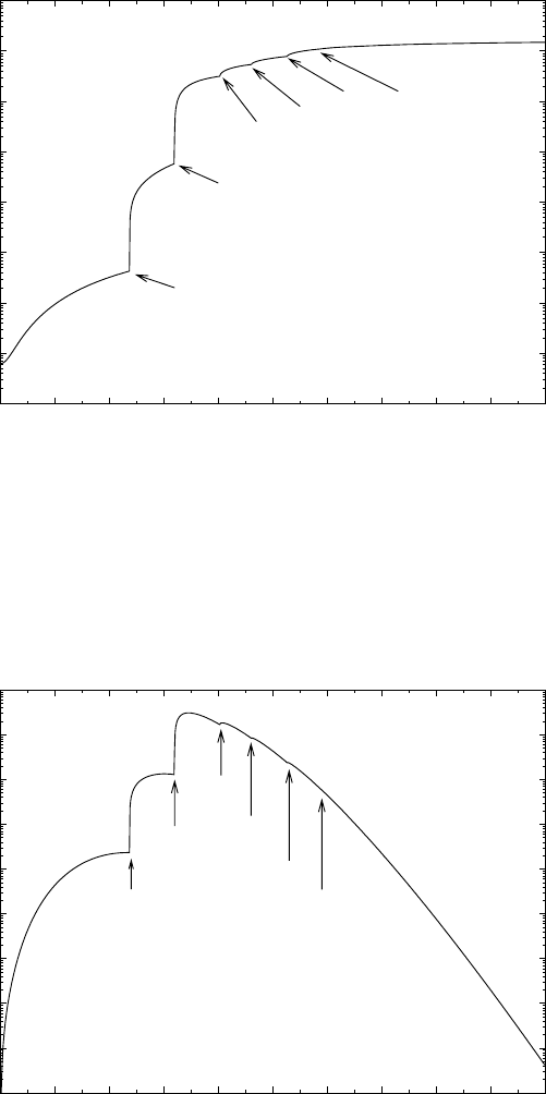
258 CHAPTER 21. RD: RELIC DENSITY ROUTINES (GENERAL)
10-8
10-7
10-6
10-5
10-4
10-3
10-2
10-1
100
0 10 20 30 40 50 60 70 80 90 100
Weff
peff [GeV]
W+ W- final state
χ1
0 χ1
+
χ1
0 χ2
0χ1
+ χ1
-χ2
0 χ1
+χ2
0 χ2
0
mχ1
0 = 76.3 GeV
mχ2
0 = 96.3 GeV
mχ1
+ = 89.2 GeV
Figure 21.1: The effective invariant annihiliation rate Weff as a function of peff for an example
model. The final state threshold for annihilation into W+W−and the coannihilation thresholds,
as given by Eq. (21.34), are indicated. The χ0
2χ0
2coannihilation threshold is too small to be seen.
1037
1038
1039
1040
1041
1042
1043
1044
1045
1046
0 10 20 30 40 50 60 70 80 90 100
dA/dpeff [cm-3 s-1 GeV-1]
peff [GeV]
W+ W- final state
χ1
0 χ1
+
χ1
0 χ2
0
χ1
+ χ1
-
χ2
0 χ1
+
χ2
0 χ2
0
mχ1
0 = 76.3 GeV
mχ2
0 = 96.3 GeV
mχ1
+ = 89.2 GeV
T = mχ/20
Figure 21.2: Total differential annihilation rate per unit volume dA/dpeff for the same model as
in Fig. 21.1, evaluated at a temperature T=mχ/20, typical of freeze-out. Notice the Boltzmann
suppression at high peff .

21.1. RELIC DENSITY – THEORETICAL BACKGROUND 259
21.1.4 Internal degrees of freedom
If we look at Eqs. (21.34) and (21.39) we see that we have a freedom on how to treat particles
degenerate in mass, e.g. a chargino can be treated either
a) as two separate species χ+
iand χ−
i, each with internal degrees of freedom gχ+=gχ−= 2, or,
b) as a single species χ±
iwith gχ±
i= 4 internal degrees of freedom.
Of course the two views are equivalent, we just have to be careful including the gi’s consistently
whichever view we take. In a), we have the advantage that all the Wij that enter into Eq. (21.34)
enter as they are, i.e. without any correction factors for the degrees of freedom. On the other hand
we get many terms in the sum that are identical and we need some book-keeping machinery to
avoid calculating identical terms more than once. On the other hand, with option b), the sum over
Wij in Eq. (21.34) is much simpler only containing terms that are not identical (except for the
trivial identity Wij =Wji which is easily taken care of). However, the individual Wij will be some
linear combinations of the more basic Wij entering in option a), where the coefficients have to be
calculated for each specific type of initial condition.
Below we will perform this calculation to show how the Wij look like in option b) for different
initial states. We will use a prime on the Wij when they refer to these combined states to indicate
the difference.
Neutralino-chargino annihilation
The starting point is Eq. (21.34) which we will use to define the Wij in option b) such that Weff
is the same as in option a). Eq. (21.39) is then guaranteed to be the same in both cases since the
sum in the denominator is linear in gi.
Now consider annihilation between χ0
iand χ+
cor χ−
c. The corresponding terms in Eq. (21.34)
does for option a) read
Weff =X
ij
pij
p11
gigj
g2
1
Wij =pic
p11
2·2
22Wχ0
iχ+
c+Wχ0
iχ−
c+Wχ+
cχ0
i
|{z }
Wχ0
iχ+
c
+Wχ−
cχ0
i
|{z }
Wχ0
iχ−
c
= 2 pic
p11 Wχ0
iχ+
c+Wχ0
iχ−
c
|{z }
Wχ0
iχ+
c
= 4 pic
p11
Wχ0
iχ+
c(21.40)
For option b), we instead get
Weff =X
ij
pij
p11
gigj
g2
1
Wij =pic
p11
2·4
22W′
χ0
iχ±
c+W′
χ±
cχ0
i
|{z }
W′
χ0
iχ±
c
= 4 pic
p11
W′
χ0
iχ±
c(21.41)
Comparing Eq. (21.41) and Eq. (21.40) we see that they are indentical if we make the identification
W′
χ0
iχ±
c≡Wχ0
iχ+
c(21.42)
Chargino-chargino annihilation
First consider the case where we include the terms in the sum for which we have annihilation
between χ+
cor χ−
cand χ+
dor χ−
dwith c6=d.

260 CHAPTER 21. RD: RELIC DENSITY ROUTINES (GENERAL)
In option a), the corresponding terms in Eq. (21.34) reads
Weff =X
ij
pij
p11
gigj
g2
1
Wij
=pcd
p11
2·2
22Wχ+
cχ+
d+Wχ+
cχ−
d+Wχ−
cχ+
d+Wχ−
cχ−
d
+Wχ+
dχ+
c
|{z }
Wχ+
cχ+
d
+Wχ+
dχ−
c
| {z }
Wχ−
cχ+
d
+Wχ−
dχ+
c
| {z }
Wχ+
cχ−
d
+Wχ−
dχ−
c
| {z }
Wχ−
cχ−
d
= 2 pcd
p11 Wχ+
cχ+
d+Wχ+
cχ−
d+Wχ−
cχ+
d
|{z }
Wχ+
cχ−
d
+Wχ−
cχ−
d
| {z }
Wχ+
cχ+
d
= 4 pcd
p11 Wχ+
cχ+
d+Wχ+
cχ−
d(21.43)
In option b), the corresponding terms would instead read
Weff =X
ij
pij
p11
gigj
g2
1
W′
ij =pcd
p11
4·4
22W′
χ±
cχ±
d
+W′
χ±
dχ±
c
|{z }
W′
χ±
cχ±
d
= 8 pcd
p11
W′
χ±
cχ±
d
(21.44)
Comparing Eq. (21.43) and Eq. (21.44) we see that they are identical if we make the following
identifcation
W′
χ±
cχ±
d≡1
2Wχ+
cχ+
d+Wχ+
cχ−
d(21.45)
For clarity, let’s also consider the case where c=d. In option a), the terms in Weff are
Weff =X
ij
pij
p11
gigj
g2
1
Wij =pcc
p11
2·2
22Wχ+
cχ+
c+Wχ+
cχ−
c+Wχ−
cχ+
c
|{z }
Wχ+
cχ−
c
+Wχ−
cχ−
c
|{z }
Wχ+
cχ+
c
= 2 pcc
p11 Wχ+
cχ+
c+Wχ+
cχ−
c(21.46)
In option b), the corresponding term would instead read
Weff =X
ij
pij
p11
gigj
g2
1
W′
ij =pcc
p11
4·4
22W′
χ±
cχ±
c+ = 4 pcc
p11
W′
χ±
cχ±
c(21.47)
Comparing Eq. (21.46) and Eq. (21.47) we see that they are identical if we make the following
identifcation
W′
χ±
cχ±
c≡1
2Wχ+
cχ+
c+Wχ+
cχ−
c(21.48)
i.e. the same identification as in the case c6=d.
Neutralino-sfermion annihilation
For each sfermion we have in total four different states, ˜
f1,˜
f2,˜
f∗
1and ˜
f∗
2. Of these, the ˜
f1
and ˜
f2in general have different masses and have to be treated separately. Considering only one
mass eigenstate ˜
fk, option a) then means that we treat ˜
fkand ˜
f∗
kas two separate species with
gi= 1 degree of freedom each, whereas option b) means that we treat them as one species ˜
f′
kwith

21.1. RELIC DENSITY – THEORETICAL BACKGROUND 261
gi= 2 degrees of freedom. As before, the prime indicates that we mean both the particle and the
antiparticle state.
Note, that for squarks we also have the number of colours Nc= 3 to take into account. In
option a) we should choose to treat even colour state differently, i.e. gi= 1, whereas gi= 6 in
case b). The expressions would be the same as above except that both the expression in a) and b)
would be multiplied by the colour factor Nc= 3. The expression relating case a) and case b) is
thus unaffected by this colour factor. Note however, that in option b) we take the average over the
squark colours (or in this case calculate it only for one colour. See sections 21.1.4 and 21.1.4 below
for more details.
For option a), Eq. (21.34) then reads
Weff =X
ij
pij
p11
gigj
g2
1
Wij =pik
p11
2·1
22Wχ0
i˜
fk+Wχ0
i˜
f∗
k+W˜
fkχ0
i
|{z}
Wχ0
i˜
fk
+W˜
f∗
kχ0
i
|{z }
Wχ0
i˜
f∗
k
=pik
p11 Wχ0
i˜
fk+Wχ0
i˜
f∗
k
|{z }
Wχ0
i˜
fk
= 2 pik
p11
Wχ0
i˜
fk(21.49)
whereas for option b), Eq. (21.34) reads
Weff =X
ij
pij
p11
gigj
g2
1
W′
ij =pik
p11
2·2
22W′
χ0
i˜
f′k+W′
˜
f′kχ0
i
|{z }
W′
χ0
i
˜
f′k
= 2 pik
p11
W′
χ0
i˜
f′k(21.50)
Comparing Eq. (21.50) and Eq. (21.49) we see that they are indentical if we make the identification
W′
χ0
i˜
f′k≡Wχ0
i˜
fk(21.51)
For clarity, for squarks the corresponding expression would be
W′
χ0
i˜
q′k≡1
3
3
X
a=1
Wχ0
i˜qa
k(21.52)
where ais a colour index.
Chargino-sfermion annihilation
In option a) the chargino has gi= 2 and the sfermion has gi= 1 degrees of freedom, whereas in
option b), the chargino has gi= 4 and the sfermion has gi= 2 degrees of freedom
For option a), Eq. (21.34) then reads
Weff =X
ij
pij
p11
gigj
g2
1
Wij
=pck
p11
2·1
22Wχ+
c˜
fk+Wχ+
c˜
f∗
k+Wχ−
c˜
fk+Wχ−
c˜
f∗
k
+W˜
fkχ+
c
|{z }
Wχ+
c˜
fk
+W˜
f∗
kχ+
c
|{z }
Wχ+
c˜
f∗
k
+W˜
fkχ−
c
|{z }
Wχ−
c˜
fk
+W˜
f∗
kχ−
c
|{z }
Wχ−
c˜
f∗
k
=pck
p11 Wχ+
c˜
fk+Wχ+
c˜
f∗
k+Wχ−
c˜
fk
|{z }
Wχ+
c˜
f∗
k
+Wχ−
c˜
f∗
k
|{z }
Wχ+
c˜
fk
= 2 pck
p11 Wχ+
c˜
fk+Wχ+
c˜
f∗
k(21.53)

262 CHAPTER 21. RD: RELIC DENSITY ROUTINES (GENERAL)
In option b), Eq. (21.34) reads
Weff =X
ij
pij
p11
gigj
g2
1
W′
ij =pck
p11
4·2
22W′
χ±
c˜
f′k+W′
˜
f′kχ±
c
|{z }
W′
χ±
c˜
f′k
= 4 pck
p11
W′
χ±
c˜
f′k(21.54)
Comparing Eq. (21.54) and Eq. (21.53) we see that they are indentical if we make the identifi-
cation
W′
χ±
c˜
f′k≡1
2Wχ+
c˜
fk+Wχ+
c˜
f∗
k(21.55)
For clarity, for squarks the corresponding expression would be
W′
χ±
c˜
q′k≡1
2
1
3
3
X
a=1 Wχ+
c˜qa
k+Wχ+
c˜qa∗
k(21.56)
where ais a colour index.
Sfermion-sfermion annihilation
First consider the case where we have annihilation between sfmerions of different types, i.e. annihi-
lation between ˜
fkor ˜
f∗
kand ˜
flor ˜
f∗
l.
For option a), Eq. (21.34) then reads
Weff =X
ij
pij
p11
gigj
g2
1
Wij
=pkl
p11
1·1
22W˜
fk˜
fl+W˜
fk˜
f∗
l+W˜
f∗
k˜
fl+W˜
f∗
k˜
f∗
l
+W˜
fl˜
fk
|{z}
W˜
fk˜
fl
+W˜
fl˜
f∗
k
|{z}
W˜
f∗
k˜
fl
+W˜
f∗
l˜
fk
|{z}
W˜
fk˜
f∗
l
+W˜
f∗
l˜
f∗
k
|{z }
W˜
f∗
k˜
f∗
l
=1
2
pkl
p11 W˜
fk˜
fl+W˜
fk˜
f∗
l+W˜
f∗
k˜
fl
|{z}
W˜
fk˜
f∗
l
+W˜
f∗
k˜
f∗
l
|{z }
W˜
fk˜
fl
=pkl
p11 W˜
fk˜
fl+W˜
fk˜
f∗
l(21.57)
In option b) we would get
Weff =X
ij
pij
p11
gigj
g2
1
W′
ij
=pkl
p11
2·2
22W′
˜
f′k˜
f′l+W′
˜
f′l˜
f′k
|{z }
W′
˜
f′k˜
f′l
= 2 pkl
p11 W′
˜
f′k˜
f′l(21.58)
Comparing Eq. (21.58) and Eq. (21.57) we see that they are indentical if we make the identification
W′
˜
f′k˜
f′l≡1
2W˜
fk˜
fl+W˜
fk˜
f∗
l(21.59)
It is easy to show that this relation holds true even if k=l.

21.1. RELIC DENSITY – THEORETICAL BACKGROUND 263
Squark-squark annihilation
Even though we treated sfermion-sfermion annihilation in the previous subsection, squarks have
colour which can complicate things, so let’s for clarity consider squarks separately.
Let’s denote the squarks ˜qa
kwhere ais now a colour index. In option a) we will let each colour
be a seprate species, which means that gi= 1 in this case. In option b) we will instead have gi= 6.
In option a) we would have
Weff =X
ij
pij
p11
gigj
g2
1
Wij
=pkl
p11
1·1
22
3
X
a,b=1 W˜qa
k˜qb
l+W˜qa
k˜qb∗
l+W˜qa∗
k˜qb
l+W˜qa∗
k˜qb∗
l
+W˜qa
l˜qb
k
|{z}
W˜qa
k˜qb
l
+W˜qa
l˜qb∗
k
|{z }
W˜qa∗
k˜qb
l
+W˜qa∗
l˜qb
k
|{z }
W˜qa
k˜qb∗
l
+W˜qa∗
l˜qb∗
k
|{z }
W˜qa∗
k˜qb∗
l
=1
2
pkl
p11
3
X
a,b=1 W˜qa
k˜
fb
l+W˜qa
k˜
fb∗
l+W˜qa∗
k˜qb
l
|{z }
W˜qa
k˜qb∗
l
+W˜qa∗
k˜qb∗
l
| {z }
W˜qa
k˜qb
l
=pkl
p11
3
X
a,b=1 W˜qa
k˜qb
l+W˜qa
k˜qb∗
l
(21.60)
In option b) we would get
Weff =X
ij
pij
p11
gigj
g2
1
W′
ij
=pkl
p11
6·6
22W′
˜
q′k˜
q′l+W′
˜
q′l˜
q′k
|{z }
W′
˜
q′k˜
q′l
= 18 pkl
p11 W′
˜
q′k˜
q′l(21.61)
Comparing Eq. (21.61) and Eq. (21.60) we see that they are indentical if we make the identification
W′
˜
q′k˜
q′l≡1
2
1
9
3
X
a,b=1 W˜qa
k˜qb
l+W˜qa
k˜qb∗
l(21.62)
i.e. we get the same relation as for other sfermions, the only difference being that we in option b)
should also take the average over the colour states.
Sfermion-squark annihilation
For clarity, if we have annihilation between a non-coloured sfermion and a squark, we would in the
same way as in the previous subsection get
W′
˜
f′k˜
q′l≡1
2
1
3
3
X
b=1 W˜
fk˜qb
l+W˜
fk˜qb∗
l(21.63)

264 CHAPTER 21. RD: RELIC DENSITY ROUTINES (GENERAL)
Summary of degrees of freedom
We have found above the following relations between option b) and option a),
W′
χ0
iχ±
j≡Wχ0
iχ+
j=Wχ0
iχ−
j,∀i= 1,...,4, j = 1,2
W′
χ±
iχ±
j≡1
2hWχ+
iχ+
j+Wχ+
iχ−
ji=1
2hWχ−
iχ−
j+Wχ−
iχ+
ji,∀i= 1,2, j = 1,2
W′
χ0
i˜
f′k≡Wχ0
i˜
fk,∀i= 1,...4, k = 1,2
W′
χ±
c˜
f′k≡1
2hWχ+
c˜
fk+Wχ+
c˜
f∗
ki,∀c= 1,2, k = 1,2
W′
˜
f′k˜
f′l≡1
2hW˜
fk˜
fl+W˜
fk˜
f∗
li,∀k= 1,2, l = 1,2
W′
˜
q′k˜
q′l≡1
2
1
9P3
a,b=1 hW˜qa
k˜qb
l+W˜qa
k˜qb∗
li,∀k= 1,2, l = 1,2
(21.64)
We don’t list all the possible cases with squarks explicitly, the principle being that we in option
b) should take the average over the squark colour states (see the squark-squark entry in the list
above).
We will choose option b) and the code (dsandwdcoscn,dsandwdcoscn,dsasdwdcossfsf and dsasd-
wdcossfchi) should thus return W′as defined above. Note again that squarks are assumed to have
gi= 6 degrees of freedom in this convention and the summing over colours should also be taken
into account in the code.
21.1.5 Reformulation of the Boltzmann equation
We now follow Gondolo and Gelmini [68] to put Eq. (21.12) in a more convenient form by considering
the ratio of the number density to the entropy density,
Y=n
s.(21.65)
Consider dY
dt =d
dt n
s=˙n
s−n
s2˙s(21.66)
where dot means time derivative. In absence of entropy production, S=R3sis constant (Ris the
scale factor). Differentiating with respect to time we see that
˙s=−3˙
R
Rs=−3Hs (21.67)
which yields
˙
Y=˙n
s+ 3Hn
s.(21.68)
Hence we can rewrite Eq. (21.12) as
˙
Y=−shσeff viY2−Y2
eq.(21.69)
The right-hand side depends only on temperature, and it is therefore convenient to use temper-
ature Tinstead of time tas independent variable. Defining x=m1/T we have
dY
dx =−m1
x2
1
3H
ds
dT hσeff viY2−Y2
eq.(21.70)
where we have used 1
˙
T=1
˙s
ds
dT =−1
3Hs
ds
dT (21.71)

21.2. RELIC DENSITY – NUMERICAL INTEGRATION OF THE DENSITY EQUATION 265
which follows from Eq. (21.67). With the Friedmann equation in a radiation dominated universe
H2=8πGρ
3,(21.72)
where Gis the gravitational constant, and the usual parameterization of the energy and entropy
densities in terms of the effective degrees of freedom geff and heff ,
ρ=geff (T)π2
30 T4, s =heff (T)2π2
45 T3,(21.73)
we can cast Eq. (21.70) into the form [68]
dY
dx =−rπ
45G
g1/2
∗m1
x2hσeff viY2−Y2
eq(21.74)
where Yeq can be written as
Yeq =neq
s=45x2
4π4heff (T)X
i
gimi
m12
K2xmi
m1,(21.75)
using Eqs. (21.15), (21.65) and (21.73).
The parameter g1/2
∗is defined as
g1/2
∗=heff
√geff 1 + T
3heff
dheff
dT (21.76)
For geff ,heff and g1/2
∗we use the values in Ref. [68] with a QCD phase-transition temperature
TQCD = 150 MeV. Our results are insensitive to the value of TQCD, because due to a lower limit
on the neutralino mass the neutralino freeze-out temperature is always much larger than TQCD.
To obtain the relic density we integrate Eq. (21.79) from x= 0 to x0=mχ/T0where T0is the
photon temperature of the Universe today. The relic density today in units of the critical density
is then given by
Ωχ=ρ0
χ/ρcrit =mχs0Y0/ρcrit (21.77)
where ρcrit = 3H2/8πG is the critical density, s0is the entropy density today and Y0is the result
of the integration of Eq. (21.79). With a background radiation temperature of T0= 2.726 K we
finally obtain
Ωχh2= 2.755 ×10⁸mχ
GeV Y0.(21.78)
21.2 Relic density – numerical integration of the density
equation
Let us write the evolution equation for the density,
dY
dx =−rπ
45G
g1/2
∗m1
x2hσeff viY2−Y2
eq(21.79)
as dY
dx =λ(Y2−q2),(21.80)
where λcontains the annihilation rate and qrepresents the thermal-equilibrium density.
This equation is stiff and an explicit method, like Euler or Runge-Kutta, fails to converge. To
obtain a numerical solution, we use an adaptive implicit trapezoidal method which we explain in the

266 CHAPTER 21. RD: RELIC DENSITY ROUTINES (GENERAL)
following. Basically we discretize the equation first with a trapezoidal then with an Euler method,
and adapt the step size according to the difference in the updated function values.
For simplicity we denote the right hand wide of eq. (21.80) as f(x). We further write fi=f(xi)
and similarly for the other functions λ(x) and q(x). Given Yi=Y(xi) we find Yi+1 =Y(xi+1) with
xi+1 =xi+has follows.
First we discretize the evolution equation as
Yi+1 −Yi=hfi+fi+1
2.(21.81)
We insert
fi=λiY2
i−q2
i,(21.82)
fi+1 =λi+1 Y2
i+1 −q2
i+1,(21.83)
and solve the resulting quadratic equation for Yi+1 to obtain
Yi+1 =c
1 + √1 + uc,(21.84)
where
c= 2Yi+u(q2
i+1 +ρq2
i)−ρY 2
i,(21.85)
u=hλi+1,(21.86)
ρ=λi/λi+1.(21.87)
In the expression for cwe have explicitly indicated the order of evaluation which we found avoids
round-off errors. If in eq. (21.84) 1 + uc is negative, we simply reduce the step hto h/2 and try
again.
Secondly we discretize the evolution equation as
Yi+1 −Yi=hfi+1.(21.88)
We insert the expression for fi+1 and solve the quadratic equation for Yi+1 to obtain
Y′
i+1 =1
2
c′
1 + √1 + uc′,(21.89)
where
c′= 4 Yi+uq2
i+1.(21.90)
Again if in eq. (21.89) 1 + uc′<0, we reduce the step hto h/2 and try again.
We then adapt the step size according to the relative difference of Yi+1 and Y′
i+1,
d=
Yi+1 −Y′
i+1
Yi+1 .(21.91)
If the difference is larger than a prefixed ǫ, set at 0.01, we reduce the step size hto hs/√ǫbut never
to less than h/10. sis a safety factor set to 0.9. If d < ǫ, we increase the step size by a factor
s/√ǫbut never by more than a factor of 5. We do not allow the step size to become smaller than
hmin = 10−9. Error code 5 is reported if this happens. Error code 4 occurs when xi+1 is numerically
equal to xibecause of round-off. Error code 6 occurs when the number of steps exceeds a maximum
of 100000. Finally the initial step size is taken to be 0.01.

21.3. RELIC DENSITY – ROUTINES 267
21.3 Relic density – routines
In src/rd, the general relic density routines are found. These routines can be used for any dark
matter candidate and the interface to neutralino dark matter is in src/rn. We will first discuss how
the routines for neutralino relic density are used and then how the general routines work.
21.3.1 Neutralino relic density
function dsrdomega(coann,fast,xf,ierr,iwar,nfc) r8
Purpose: Calculate the relic density of the lightest neutralino, possibly including coanni-
hilations between different neutralinos, neutralinos and charginos and between
charginos.
Input:
coann i =1: include coannihilations between neutralino–neutralino, neutralino–chargino
and chargino–chargino.
=2: do not include coannihilations.
fast i =1: Do a faster calculation, with slightly less accuracy in the numerical integra-
tions and only including coannihilations (if coann=1) with other particles up to
1.3 times heavier than the lightest neutralino.
=2: Do a more accurate calculation, with higher accuracy in the numerical in-
tegrations and including coannihilations (if coann=1) with other particles up to
2.1 times heavier than the lightest neutralino.
Output:
xf r8 xis defined as x=mχ/T and xf is the xat which freeze-out occurs (defined as
the temperature at which the number density is a factor of two higher than the
equilibrium density). COMMENT #12: Check!
ierr i =0: Calculation went OK.
6= 0: Somethig went wrong. COMMENT #13: Describe!
iwar i =0: Calculation went OK.
6= 0: A slight inaccuracy may have occured at a resonance or threshold for
numerical reasons. Usually, this doesn’t affect the result, but one should keep
it in mind in case the returned relic density seems strange.
nfc i The number of points (in peff ) at which the cross section was evaluated.
subroutine dsrdwrate(unit1,unit2,ich)
Purpose: Writes a table of the partial annihilation rates WF(p, cos θ) into each final chan-
nel Fas a function of the center-of-mass momentum pand at cos θ= 0.1 to
unit2.
Inputs:
unit1 i What is this?
unit2 i Unit number to write output to.
ich i What initial state channel to use:
=1: neutralino–neutralino annihilation
=2: neutralino–chargino coannihilation
=3: chargino–chargino coannihilations.
Comment: Only annihilation between the lightest neutralinos and charginos are included.
21.3.2 General relic density routines
The routine that performs the actual relic density calculation is
subroutines dsrdens(wx,ncoann,mcoann,dof,nrs,rm,rw,nt,tm,oh2,tf,ierr,iwar)
Purpose: Calculate the relic density of a dark matter candidte.
Input:

268 CHAPTER 21. RD: RELIC DENSITY ROUTINES (GENERAL)
wx r8 User-defined function that returns the effective invariant annihilation rate, Weff ,
as a function of the effective momentum peff . The function has to be declared
external in the calling routine.
ncoann i Number of particles that coannihilate.
mcoann r8 An array with the masses (in GeV) that can coannihilate.
dof r8 Number of internal degrees of freedom for the coannihilating particles.
nrs i Number of resonances.
rm r8 An array with the masses of the resonances (in GeV).
rw r8 An array with the widths of the resonances (in GeV).
nt i Number of thresholds.
tm r8 An array with the √s(in GeV) at which the thresholds occur.
Output:
oh2 r8 The relic density, Ωh2where his the Hubble constant in units of 100 km s−1
Mpc−1.
tf r8 The temperature (in GeV) at which the freeze-out occured. Freeze-out is defined
to occur when the number density is 2 times the equlibrium density.
ierr i =0: Calculation went OK.
6= 0: Somethig went wrong. COMMENT #14: Describe!
iwar i =0: Calculation went OK.
6= 0: A slight inaccuracy may have occured at a resonance or threshold for
numerical reasons. Usually, this doesn’t affect the result, but one should keep
it in mind in case the returned relic density seems strange.
It is up to the user to prepare the input function and arrays accordingly before calling the routine.
All internal settings of the relic density routines are set in common blocks in dsrdcom.h. The
most important parameters that can be changed by the user are
Important parameters in dsrdcom.h
Purpose: Provide a set of parameters, with which the internal behaviour of the relic
density routines can be changed.
Parameters
tharsi i Size of the coannihilation, resonance and threshold arrays (default=50). In-
crease this size if you have more than 50 coannihilating particles, more than 50
resonances or more than 50 thresholds.
rdluerr i Logical unit number where error messages are printed.
rdtag c*12 Idtag that is printed in case of errors.
cosmin r8 ...
waccd r8 ...
dpminr r8 ...
dpthr r8 ...
wdiffr r8 ...
wdifft r8 ...
hstep r8 ...
When the relic density has been calculated, the integer variable copart in dsandwcom.h is set to
indicate which coannihilating particles that have been included in the calculation. In Table 21.1,
the meaning if this variable is shown.
21.3.3 Brief description of the internal routines
Below, the remaining routines related to the relic density calculation are briefly mentioned. For
more details, we refer to the routines themselves.
Routine Purpose
dsrdaddpt To add one point in the Weff -peff table.

21.3. RELIC DENSITY – ROUTINES 269
copart PAW variables
Bit set Octal value Decimal value cop1 bit cop2 bit Particle
0 1 1 0 – ˜χ0
1
1 2 2 1 – ˜χ0
2
2 4 4 2 – ˜χ0
3
3 10 8 3 – ˜χ0
4
4 20 16 4 – ˜χ±
1
5 40 32 5 – ˜χ±
2
6 100 64 6 – ˜e1
7 200 128 7 – ˜µ1
8 400 256 8 – ˜τ1
9 1 000 512 9 – ˜e2
10 2 000 1 024 10 – ˜µ2
11 4 000 2 048 11 – ˜τ2
12 10 000 4 096 12 – ˜νe
13 20 000 8 192 13 – ˜νµ
14 40 000 16 384 14 – ˜ντ
15 100 000 32 768 – 0 ˜u1
16 200 000 65 536 – 1 ˜c1
17 400 000 131 072 – 2 ˜
t1
18 1 000 000 262 144 – 3 ˜u2
19 2 000 000 524 288 – 4 ˜c2
20 4 000 000 1 048 576 – 5 ˜
t2
21 10 000 000 2 097 152 – 6 ˜
d1
22 20 000 000 4 197 304 – 7 ˜s1
23 40 000 000 8 388 608 – 8 ˜
b1
24 100 000 000 16 777 216 – 9 ˜
d2
25 200 000 000 33 554 432 – 10 ˜s2
26 400 000 000 67 108 864 – 11 ˜
b2
Table 21.1: The bits of copart are set to indicate which initial states that are included in the
coannihilation calculation. In the output file *.omegaco, the value of copart is written in octal
format. In PAW cop1 and cop2 are available. Check if a bit is set with btest(cop1,bit).
dsrdcom To initialize parameters in the common blocks in dsrdcom.h. If you want to
change these parameters yourself, include dsrdcom.h in your code and change
the parameters you want.
dsrddof150 To prepare a table of the degrees of freedom as a function of the temperature
in the early Universe.
dsrddpmin To return the allowed minimal distance in peff between two points in the Weff -
peff plane. The returned value depends on if there is a resonance present or not
at the given peff .
dsrdeqn To solve the relic density equation by means of an implicit trapezoidal method
with adaptive stepsize and termination.
dsrdfunc To return the invariant annihilation rate times the thermal distribution.
dsrdfuncs To provide dsrdfunc in a form suitable for numerical integration.
dsrdlny To return ln(Weff for a given peff .
dsrdnormlz To return a unit vector in a given direction.
dsrdqad To calculate the relic density with a quick-and-dirty method. It uses the ap-

270 CHAPTER 21. RD: RELIC DENSITY ROUTINES (GENERAL)
proximative expressions in Kolb & Turner with the cross section expaned in
v.
dsrdqrkck To numerically integrate a function with a Runge-Kutta method
dsrdrhs To calculate terms on the right-hand side in the Boltzmann equation.
dsrdspline To set up the table Weff -peff for spline interpolation.
dsrdstart To sort and store information about coannihilations, resonances and thresholds
in common blocks.
dsrdtab To set up the table Weff -peff .
dsrdthav To calculate the thermally averaged annihilation cross section at a given tem-
perature.
dsrdthclose ???COMMENT #15: What does this function do?
dsrdthlim To determine the end-points for the thermal average integration.
dsrdthtest To check if a given entry in the Weff -peff table is at a threshold.
dsrdwdwdcos To write out a table of dWeff /d cos θas a function of cos θfor a given peff .
dsrdwfunc To write out dsrdfunc for a given x=mχ/T .
dsrdwintp To return the invariant rate Weff for any given peff by performing a spline
interpolation in the Weff -peff table.
dsrdwintpch To check the spline interpolation in the Weff -peff table and compare with a linear
interpolation.
dsrdwintrp To write out a table of the invariant rate Weff and some internal integration
variables and expressions.
dsrdwres To write out the table Weff -peff .
Below are brief descriptions of routines in src/rn not mentioned above
Routine Purpose
dsrdres To prepare the array of resonances needed before the call to dsrdens.
dsrdthr To prepare the array of thresholds needed before the call to dsrdens.
21.4 Routine headers – fortran files
dsrdaddpt.f
subroutine dsrdaddpt(wrate,pres,deltap)
c_______________________________________________________________________
c add a point in rdrate table
c input:
c wrate - invariant annihilation rate (real, external)
c pres - momentum of the point to add
c deltap - scaling factor used in dsrdtab
c pmax - maximum p used in dsrdtab (from common block)
c common:
c ’dsrdcom.h’ - included common blocks
c used by dsrdtab
c author: joakim edsjo (edsjo@physto.se)
c modified: 01-01-31 paolo gondolo (paolo@mamma-mia.phys.cwru.edu)
c=======================================================================

21.4. ROUTINE HEADERS – FORTRAN FILES 271
dsrdcom.f
No header found.
dsrddof150.f
subroutine dsrddof150
c_______________________________________________________________________
c table of effective degrees of freedom in the early universe
c
c t [gev] g_{\star}^{1/2} g_{entropy} for t_{qcd} = 150 mev
c
c common:
c ’dsrdcom.h’ - included common blocks
c
c author: paolo gondolo (gondolo@lpthe.jussieu.fr) 1994
c=======================================================================
dsrddpmin.f
real*8 function dsrddpmin(p,dpmin)
c_______________________________________________________________________
c routine to determine if there is a narrow resonance present which
c jusifies changing dpmin to some fraction of lambda
c author: joakim edsjo, edsjo@physto.se
c date: april 30, 1998
c modified: april 30, 1998.
c=======================================================================
dsrdens.f
subroutine dsrdens(wrate,npart,mgev,dof,nrs,rm,rw,
& nt,tm,oh2,tf,ierr,iwar)
c_______________________________________________________________________
c present density in units of the critical density times the
c hubble constant squared.
c input:
c wrate - invariant annihilation rate (real, external)
c npart - number of particles coannihilating
c mgev - relic and coannihilating mass in gev
c dof - internal degrees of freedom of the particles
c nrs - number of resonances to take special care of
c rm - mass of resonances in gev
c rw - width of resonances in gev
c nt - number of thresholds to take special care of
c do not include coannihilation thresholds (that’s automatic)
c tm - sqrt(s) of the thresholds in gev
c output:
c oh2 - relic density parameter times h**2 (real*8)
c tf - freeze-out temperature in gev (real*8)
c ierr - error code (integer)
c dsbit 0 (1) = array capacity exceeded. increase nrmax in dsrdcom.h
c 1 (2) = a zero vector is given to dsrdnormlz.

272 CHAPTER 21. RD: RELIC DENSITY ROUTINES (GENERAL)
c 2 (4) = step size underflow in dsrdeqn
c 3 (8) = stepsize smaller than minimum hmin in dsrdeqn
c 4 (16) = too many steps in dsrdeqn
c 5 (32) = step size underflow in dsrdqrkck
c 6 (64) = step size smaller than miminum in dsrdqrkck
c 7 (128) = too many steps in dsrdqrkck
c 8 (256) = gpindp integration failed in dsrdthav
c 9 (512) = threshold array too small. increase tharsi in dsrdcom.h
c iwar - warning code (integer)
c dsbit 0 (1) = a difference of >5waccd in the ratio of w_spline
c and w_linear is obtained due to delta_p<dpmin.
c 1 (2) = a difference of >10waccd in the ratio of w_spline
c and w_linear is obtained due to delta_p<dpmin.
c 2 (4) = a difference of >15waccd in the ratio of w_spline
c and w_linear is obtained due to delta_p<dpmin.
c 3 (8) = wimp too heavy, d.o.f. table needs to be
c extended to higher temperatures. now the solution
c is started at a higher x than xinit (=2).
c 4 (16) = spline interpolated value too high (overflow) during
c check of interpolation accuracty (dsrdwintpch)
c common:
c ’dsrdcom.h’ - included common blocks
c uses dsrdtab, dsrdeqn.
c authors: paolo gondolo (gondolo@lpthe.jussieu.fr) 1994-1996 and
c joakim edsjo (edsjo@physto.se) 30-april-98
c=======================================================================
dsrdeqn.f
subroutine dsrdeqn(wrate,x0,x1,y1,xf,nfcn)
c_______________________________________________________________________
c solve the relic density evolution equation by means of an implicit
c trapezoidal method with adaptive stepsize and termination.
c input:
c wrate - invariant annihilation rate (real, external)
c x0 - initial mass/temperature (real)
c x1 - final mass/temperature (real)
c y1 - final number/entropy densities (real)
c nfcn - number of calls to wrate (integer)
c common:
c ’dsrdcom.h’ - included common blocks
c uses dsrdrhs.
c called by dsrdens.
c author: paolo gondolo (gondolo@lpthe.jussieu.fr) 1994-1996
c modified: joakim edsjo (edsjo@physto.se) 961212
c Paolo Gondolo, factor added 2003
c=======================================================================
dsrdfunc.f
function dsrdfunc(u,x,wrate)
c_______________________________________________________________________

21.4. ROUTINE HEADERS – FORTRAN FILES 273
c invariant annihilation rate times thermal distribution.
c when integrated over u, the effective thermal average times
c m_chi^2 is obtained.
c input:
c u - integration variable (real)
c x - mass/temperature (real)
c wrate - invariant annihilation rate (real, external)
c common:
c ’dsrdcom.h’ - included common blocks
c called by dsrdrhs, wirate, dsrdwintrp.
c author: paolo gondolo (gondolo@lpthe.jussieu.fr) 1994-1996
c modified: joakim edsjo (edsjo@physto.se) 98-04-29
c=======================================================================
dsrdfuncs.f
function dsrdfuncs(u)
c_______________________________________________________________________
c 10^15 * dsrdfunc.
c input:
c u - integration variable
c uses dsrdfunc
c used for gaussian integration with gadap.f
c author: joakim edsjo (edsjo@physto.se)
c date: 97-01-17
c=======================================================================
dsrdlny.f
function dsrdlny(p,wrate)
c_______________________________________________________________________
c logarithm of the invariant rate.
c input:
c p - initial cm momentum (real)
c wrate - invariant annihilation rate (real, external)
c called by dsrdtab.
c author: paolo gondolo (gondolo@lpthe.jussieu.fr) 1994
c=======================================================================
dsrdnormlz.f
subroutine dsrdnormlz(x,y,nx,ny)
c_______________________________________________________________________
c find the unit vector (nx,ny) in the same direction as (x,y).
c input:
c x,y - coordinates of the vector (real)
c output:
c nx,ny - coordinates of the versor (real)
c common:
c ’dsrdcom.h’ - included common blocks
c called by dsrdtab.
c author: paolo gondolo (gondolo@lpthe.jussieu.fr) 1994

274 CHAPTER 21. RD: RELIC DENSITY ROUTINES (GENERAL)
c=======================================================================
dsrdqad.f
subroutine dsrdqad(wrate,mgev,oh2,ierr)
c_______________________________________________________________________
c present density in units of the critical density times the
c hubble constant squared. quick and dirty method
c input:
c wrate - invariant annihilation rate (real, external)
c mgev - relic and coannihilating mass in gev
c output:
c oh2 - relic density parameter times h**2 (real)
c ierr - error code (integer)
c common:
c ’dsrdcom.h’ - included common blocks
c uses dsrdtab, dsrdeqn.
c author: paolo gondolo (gondolo@lpthe.jussieu.fr) 1994-1996
c modified: joakim edsjo (edsjo@physto.se) 97-05-12
c=======================================================================
dsrdqrkck.f
subroutine dsrdqrkck(f,p,wrate,x1,x2,s)
c_______________________________________________________________________
c numerical integration with runge-kutta method.
c input:
c f - integrand (real,external)
c p - parameter mass/temperature (real)
c wrate - invariant rate (real,external)
c x1 - lower limit (real)
c x2 - upper limit (real)
c output:
c s - integral (real)
c common:
c ’dsrdcom.h’ - included common blocks
c author: paolo gondolo (gondolo@lpthe.jussieu.fr) 1994
c=======================================================================
dsrdrhs.f
subroutine dsrdrhs(x,wrate,lambda,yeq,nfcn)
c_______________________________________________________________________
c adimensional annihilation rate lambda in the boltzmann equation
c y’ = -lambda (y**2-yeq**2) and equilibrium dm density in units
c of the entropy density.
c input:
c x - mass/temperature (real)
c wrate - invariant annihilation rate (real)
c output:
c lambda - adimensional parameter in the evolution equation (real)
c yeq - equilibrium number/entropy densities (real)

21.4. ROUTINE HEADERS – FORTRAN FILES 275
c nfcn - number of calls to wrate (integer)
c common:
c ’dsrdcom.h’ - included common blocks
c uses qrkck or dgadap.
c called by dsrdeqn.
c author: paolo gondolo (gondolo@lpthe.jussieu.fr) 1994-1996
c modified: joakim edsjo (edsjo@physto.se) 98-04-28
c bug fix 98-04-28: y_eq was too small by a factor of 2 (je)
c=======================================================================
dsrdspline.f
subroutine dsrdspline
c_______________________________________________________________________
c set up 2nd derivatives for cubic dsrdspline interpolation.
c common:
c ’dsrdcom.h’ - included common blocks
c called by dsrdtab.
c author: paolo gondolo (gondolo@lpthe.jussieu.fr) 1994
c modified by joakim edsjo, edsjo@physto.se, to split spline
c at thresholds.
c modified: april 30, 1998.
c=======================================================================
dsrdstart.f
************************************************************************
*** dsrdstart stores coannihilation, resonance and threshold information
*** in common blocks and sort them
*** author: joakim edsjo (edsjo@physto.se)
*** date: 03-march-98
*** modifed: 08-may-98
*** 08-may-98: bug with mdof not being sorted correctly fixed.
*** 27-feb-02: bug with allocation of threshold array fixed.
*** increased number of possible coannihilations
************************************************************************
subroutine dsrdstart(npart,mgev,dof,nrs,rm,rw,nt,tm)
dsrdtab.f
subroutine dsrdtab(wrate,xmin)
c_______________________________________________________________________
c tabulate the invariant annihilation rate as a function of p.
c input:
c wrate - invariant annihilation rate (real*8, external)
c xmin - minimum mass/temperature needed (real*8)
c common:
c ’dsrdcom.h’ - included common blocks
c uses dsrdnormlz, dsrdlny, dsrdspline.
c authors: paolo gondolo (gondolo@lpthe.jussieu.fr) 1994 and

276 CHAPTER 21. RD: RELIC DENSITY ROUTINES (GENERAL)
c joakim edsjo (edsjo@physto.se) 06-march-98
c=======================================================================
dsrdthav.f
real*8 function dsrdthav(x,wrate)
c_______________________________________________________________________
c the thermal average of the effective annihilation cross section.
c input:
c x - mass/temperature (real)
c wrate - invariant annihilation rate (real)
c output:
c dsrdthav - thermal averged cross section
c common:
c ’dsrdcom.h’ - included common blocks
c uses qrkck or dgadap.
c called by dsrdrhs
c author: joakim edsjo (edsjo@physto.se) 98-05-01
c=======================================================================
dsrdthclose.f
real*8 function dsrdthclose(p)
c_______________________________________________________________________
c returns
c author: joakim edsjo, edsjo@physto.se
c date: april 30, 1998
c modified: april 30, 1998.
c=======================================================================
dsrdthlim.f
subroutine dsrdthlim
c_______________________________________________________________________
c determine which limits in p_eff (or rather u) to use when
c integrating for the thermal average
c author: joakim edsjo (edsjo@physto.se)
c date: 98-04-30
c=======================================================================
dsrdthtest.f
logical function dsrdthtest(i)
c_______________________________________________________________________
c routine to check if the momentum p with index i is below a
c threshold and p with index i+1 is above it. if that is the case,
c .true. is returned, otherwise .false.
c author: joakim edsjo, edsjo@physto.se
c date: april 30, 1998
c modified: april 30, 1998.
c=======================================================================

21.4. ROUTINE HEADERS – FORTRAN FILES 277
dsrdwdwdcos.f
subroutine dsrdwdwdcos(p,n)
****************************************************************
** write out a table of dsandwdcos as a function of costheta for **
** the given p and with n number of steps (n+1 points) **
****************************************************************
dsrdwfunc.f
************************************************************************
subroutine dsrdwfunc(x,wrate)
c_______________________________________________________________________
c write out dsrdfunc for the given x = mass/temperature
c common:
c ’dsrdcom.h’ - included common blocks
c uses dsrdfunc
c author: joakim edsjo (edsjo@physto.se)
c date: 97-01-20
c=======================================================================
dsrdwintp.f
function dsrdwintp(p)
c_______________________________________________________________________
c interpolation of tabulated invariant rate.
c input:
c p - initial cm momentum (real)
c common:
c ’dsrdcom.h’ - included common blocks
c called by dsrdfunc.
c author: paolo gondolo (gondolo@lpthe.jussieu.fr) 1994
c=======================================================================
dsrdwintpch.f
subroutine dsrdwintpch(p,wspline,wlin)
c_______________________________________________________________________
c check of interpolation of tabulated invariant rate.
c input:
c p - initial cm momentum (real)
c common:
c ’dsrdcom.h’ - included common blocks
c called by dsrdtab.
c author: joakim edsjo 96-04-10
c based on wintp.f by p. gondolo but wlin is also calculated
c=======================================================================
dsrdwintprint.f
subroutine dsrdwintprint(unit)

278 CHAPTER 21. RD: RELIC DENSITY ROUTINES (GENERAL)
***********************************************************************
*** Print out a the table of invariant rate with the points
*** that are tabulated. The output is printed to unit.
***
*** Author: Joakim Edsjo, edsjo@physto.se
*** Date: 2005-10-31
***********************************************************************
dsrdwintrp.f
************************************************************************
subroutine dsrdwintrp(wrate,unit)
c_______________________________________________________________________
c write out a table of
c initial cm momentum p
c invariant annihilation rate w
c integration variable u
c integrand f
c interpolated integrand g
c interpolation relative error f/g-1
c input:
c unit - logical unit to write on (integer)
c wrate - invariant annihilation rate (real, external)
c common:
c ’dssusy.h’ - file with susy common blocks
c ’dsrdcom.h’ - included common blocks
c uses dsrdtab,dsrdfunc
c author: paolo gondolo (gondolo@lpthe.jussieu.fr) 1994
c=======================================================================
dsrdwprint.f
subroutine dsrdwprint(unit,np,wrate,p_min,p_max)
***********************************************************************
*** Print out a the table of invariant rate starting at p_min, ending
*** at p_max and with np+1 number of points. The rate routine called is
*** wrate. The output is printed to unit.
***
*** Author: Joakim Edsjo, edsjo@physto.se
*** Date: 2005-10-31
***********************************************************************
dsrdwres.f
************************************************************************
subroutine dsrdwres
c_______________________________________________________________________
c write out dsrdtab and check the interpolation routine
21.4. ROUTINE HEADERS – FORTRAN FILES 279
c common:
c ’dsrdcom.h’ - included common blocks
c uses dsrdtab,dsrdwintp.f
c author: joakim edsjo (edsjo@physto.se)
c date: 96-03-26
c=======================================================================
280 CHAPTER 21. RD: RELIC DENSITY ROUTINES (GENERAL)

Chapter 22
src/rge:
mSUGRA interface (Isasugra) to
DarkSUSY
22.1 mSUGRA (ISASUGRA) interface to DarkSUSY
If Isasugra is available, DarkSUSY can use Isasugra to generate mSUGRA models. In src/rge/,
routines are avaible to transfer the mSUGRA parameters from DarkSUSY to Isasugra, call Isasugra
and then transfer back the results to DarkSUSY. The philosophy of this interface is that whenever
a user uses Isasugra, we should use all the results of Isasugra also in DarkSUSY. That means that
instead of calculating the mass spectrum from the low-energy parameters obtained from Isasugra,
we extract the masses and mixings from Isasugra.
22.2 Routine headers – fortran files
dsgive model isasugra.f
subroutine dsgive_model_isasugra(m0,mhf,a0,sgnmu,tgbeta)
c----------------------------------------------------------------------
c
c To specify the supersymmetric parameters of a model.
c Inputs:
c m0 - m0 parameter (GeV)
c mhf - m_{1/2} parameter (GeV)
c a0 - trilinear term (GeV)
c sgnmu - sign of mu (+1.0d0 or -1.0d0)
c tgbeta - ratio of Higgs vacuum expecation values, tan(beta)
c Outputs:
c The common blocks are set corresponding to the values above
c Author: Joakim Edsjo, edsjo@physto.se
c 2002-03-12
c----------------------------------------------------------------------
281

282 CHAPTER 22. RGE: MSUGRA INTERFACE (ISASUGRA) TO DARKSUSY
dsisasugra check.f
subroutine dsisasugra_check(valid)
c=======================================================================
c This routine checks that the neutralino, chargino and neutralino
c mixing matrices extracted from ISASUGRA are consistent with the
c DarkSUSY convention. It does this by checking that they really
c do diagonlize the mass matrices. If any inconsistencies (apart
c from small numerical differences are found), an error message
c is written.
c Author: J. Edsjo and M. Schelke, 2002-12-03
c=======================================================================
dsisasugra darksusy.f
subroutine dsisasugra_darksusy(valid)
c=======================================================================
c interface between ISASUGRA and DarkSUSY common blocks
c author: E.A.Baltz, 2001 eabaltz@alum.mit.edu
c modified by J. Edsjo, 2002-03-19 to set alph3
c updated to Isajet 7.74 by J. Edsjo and E.A. Baltz, 2006-02-20
c modified by P. Ullio 02-07-10, 02-11-21
c=======================================================================
dsmodelsetup isasugra.f
subroutine dsmodelsetup_isasugra
c=======================================================================
c replacement for dsmodelsetup for using ISASUGRA
c author: E.A.Baltz, 2001 eabaltz@alum.mit.edu
c=======================================================================
dsrge isasugra.f
subroutine dsrge_isasugra(unphys,valid)
c=======================================================================
c interface to ISASUGRA (ISAJET 7.74) routines for SUSY spectra
c author: E.A.Baltz, 2001 eabaltz@alum.mit.edu
c
c if valid is non-zero, the model is no good
c the valid flag is equal to the isasugra nogood flag:
c valid reason for model being bad
c ----- --------------------------
c 1 TACHYONIC PARTICLES
c 2 NO EW SYMMETRY BREAKING
c 3 M(H_P)^2<0
c 4 YUKAWA>10
c 5 Z1SS NOT LSP
c 7 XT EWSB IS BAD
c 8 MHL^2<0
c 9 if in our check any Higgs mass is NaN
c The following are not set, but can be set by uncommenting

22.2. ROUTINE HEADERS – FORTRAN FILES 283
c the appropriate lines in dsisasugra_check.f
c 10-14 dsisasugra_check has reported a possible error in the interface
c while checking that chargino, neutralino and sfermion mass
c matrices are diagonlized by isasugra
c Updated to ISAJET 7.74 by J. Edsjo and E.A. Baltz, 2006-02-20
c=======================================================================
dssusy isasugra.f
subroutine dssusy_isasugra(unphys,valid)
c--------------------------------------------------------------------
c replacement for dssusy for using ISASUGRA RGE evolution
c author: E.A. Baltz, 2001 eabaltz@alum.mit.edu
c====================================================================
284 CHAPTER 22. RGE: MSUGRA INTERFACE (ISASUGRA) TO DARKSUSY

Chapter 23
src/rn:
Relic density of neutralinos
(wrapper for rd routines)
23.1 Relic density of neutralinos
The relic density routines in src/rd solve the Boltzmann equation for any cold dark matter particle
and it is up to us to tell it what kind of particles that can participate in coannihilations and what
the effective annihilation rate is. This set-up for neutralino dark matter is done in dsrdomega.
This routine is therefor the main routine the user should call, when the relic density of neutralinos
is wanted.
What it does internally is the following:
•It determines which particles that can coannihilate (based on their mass differences) and puts
these particles into a common block for the annihlation rate routines (dsanwx) and an array
for the relic density routines. The relic density routines need to know their masses and internal
degrees of freedom.
•It checks where we have resonances and thresholds and adds these to an array, which is
passed to the relic density routines. The relic density routines then use this knowledge to
make sure the tabulation of the cross section and the integrations are performed correctly at
these difficult points.
•It then calls the relic density routines to calculate the relic density.
The returned value is Ωχh2.
23.2 Routine headers – fortran files
dsrdomega.f
real*8 function dsrdomega(omtype,fast,xf,ierr,iwar,nfc)
**********************************************************************
*** function dsrdomega calculates omega h^2 for the mssm neutralino
*** uses the mssm routines and the relic density routines
*** input:
285

286CHAPTER 23. RN: RELIC DENSITY OF NEUTRALINOS (WRAPPER FOR RD ROUTINES)
*** omtype = 0 - no coann
*** 1 - include all relevant coannihilations (charginos,
*** neutralinos and sleptons)
*** 2 - include only coannihilations betweeen charginos
*** and neutralinos
*** 3 - include only coannihilations between sfermions
*** and the lightest neutralino
*** fast = 0 - standard accurate calculation (accuracy better than 1%)
*** 1 - faster calculation: (recommended unless extreme accuracy
*** is needed).
*** * requires less accuracy in tabulation of w_eff
*** 2 - quick and dirty method, i.e. expand the annihilation
*** cross section in x (not recommended)
*** output:
*** ierr = error from dsrdens or dsrdqad
*** authors: joakim edsjo, paolo gondolo
*** date: 98-03-03
*** modified: 98-03-03
*** 99-07-30 pg
*** 02-02-27 joakim edsjo: including sfermion coanns
*** 06-02-22 paolo gondolo: streamlined inclusion of coanns
**********************************************************************
dsrdres.f
***********************************************************************
*** subroutine dsrdres sets up the resonances before calling
*** dsrdens.
*** author: joakim edsjo, (edsjo@physto.se)
*** date: 98-03-03
***********************************************************************
subroutine dsrdres(npart,mgev,nres,rgev,rwid)
dsrdthr.f
***********************************************************************
*** subroutine dsrdthr sets up the thresholds before calling
*** dsrdens.
*** author: joakim edsjo, (edsjo@physto.se)
*** date: 98-03-03
***********************************************************************
subroutine dsrdthr(npart,mgev,nth,thgev)
dsrdwrate.f
************************************************************************
subroutine dsrdwrate(unit1,unit2,ich)
c_______________________________________________________________________
c write out a table of
c initial cm momentum p
23.2. ROUTINE HEADERS – FORTRAN FILES 287
c invariant annihilation rate w
c input:
c unit1 - logical unit to write total rate to (integer)
c unit2 - logical unit to write partial differ. rates to (integer)
c ich - what initial channel to look at:
c ich=1 nn-ann. ich=2 cn-ann. ich=3 cc-ann
c common:
c ’dssusy.h’ - file with susy common blocks
c author: paolo gondolo (gondolo@lpthe.jussieu.fr) 1994
c changes by je to include prtial in partials and coannihilation routines
c=======================================================================
288CHAPTER 23. RN: RELIC DENSITY OF NEUTRALINOS (WRAPPER FOR RD ROUTINES)
Chapter 24
src/su:
General SUSY model setup:
masses, vertices etc
24.1 Supersymmetric model
We will here review the definition of the MSSM as given in [1].
24.1.1 Parameters
In our notation, the superpotential and the soft supersymmetry-breaking scalar potential minimal
supersymmetric standard model (MSSM) with R-parity conservation [4] read respectively
W=ǫij −ˆe∗
RhEˆ
li
Lˆ
Hj
1−ˆ
d∗
RhDˆqi
Lˆ
Hj
1+ˆu∗
RhUˆqi
Lˆ
Hj
2−µˆ
Hi
1ˆ
Hj
2,(24.1)
Vsoft =ǫij −˜e∗
RAEhE˜
li
LHj
1−˜
d∗
RADhD˜qi
LHj
1+˜u∗
RAUhU˜qi
LHj
2−BµHi
1Hj
2
+h.c.)
+Hi∗
1m2
1Hi
1+Hi∗
2m2
2Hi
2
+˜qi∗
LM2
Q˜qi
L+˜
li∗
LM2
L
˜
li
L+˜u∗
RM2
U˜uR+˜
d∗
RM2
D˜
dR+˜e∗
RM2
E˜eR.(24.2)
Here iand jare SU(2) indices (ǫ12 = +1), h’s, A’s and M’s are 3 ×3 matrices in generation space,
and the other boldface letters are vectors in generation space.
The current version of DarkSUSY uses only a restricted set of parameters. Namely the number
of free parameters (a grand total of 124 [9]) is reduced by setting the off-diagonal elements of the
A’s and M’s to zero and imposing CP conservation (except in the CKM matrix).
24.1.2 Mass spectrum
For easy reference, we now give the particle mass matrices, together with our convention for the
mixing matrices.
Concerning the Higgs sector, we choose as independent parameters tan βand the mass mAof
the CP-odd Higgs boson. The code provides six options for the calculation of the Higgs masses:
higloop=0: tree level formulas; higloop=1: the effective potential approach in [10, 11] (correcting
the sign of µin eq. (4) of [11]); higloop=2: the effective potential approach in [12] with addition
289

290 CHAPTER 24. SU: GENERAL SUSY MODEL SETUP: MASSES, VERTICES ETC
Higgs boson
Channel H0
1H0
2H0
3H+
i= j=1 j=2 j=3 j=4
1c¯c c¯c c¯c u ¯
d
2b¯
b b¯
b b¯
b u¯s
3t¯
t t¯
t t¯
t u¯
b
4τ+τ−τ+τ−τ+τ−c¯
d
5W+W−W+W−–c¯s
6Z0Z0Z0Z0–c¯
b
7 – H0
1H0
1–t¯
d
8H0
2H0
2– – t¯s
9H0
3H0
3H0
3H0
3–t¯
b
10 H+H−H+H−–νee+
11 – – ZH0
1νµµ+
12 – – ZH0
2νττ+
13 ZH0
3ZH0
3–W+H0
1
14 W+H−/W −H+W+H−/W −H+W+H−/W −H+W+H0
2
15 µ+µ−µ+µ−µ+µ−W+H0
3
16 s¯s s¯s s¯s–
17 gg gg gg –
18 γγ γγ γγ –
19 Z0γ Z0γ Z0γ–
20 ˜
f˜
f′˜
f˜
f′˜
f˜
f′˜
f˜
f′
Table 24.1: Higgs partial widths hdwidth(i,j). Index irefers to the decay channel and index jto the
Higgs boson. All widths are given in GeV. Note that typically we have that mH2< mH3< mH+<
mH1so many of these decay channels are not kinematically allowed, but included for completeness.
If the HDECAY interface is used, the channels where mH2< mH3< mH+< mH1is not satisfied
are not included. Channels 16–19 are only included if HDECAY is used.
of D-terms and correction of some signs and numerical factors; higloop=3: the analytical approx-
imations to the RGE-improved effective potential in [13]; higloop=4: the pole mass calculation in
[14]; higloop=5: FeynHiggs (requires FeynHiggs to be installed) [163]; higloop=6: FeynHiggsFast
(default) [164].
The masses of the Higgs bosons are obtained from
M2
H=m2
Zcos2β+m2
Asin2β+ ∆11 −sin βcos β(m2
Z+m2
A) + ∆12
−sin βcos β(m2
Z+m2
A) + ∆21 m2
Zsin2β+m2
Acos2β+ ∆22 (24.3)
m2
H±=m2
A+m2
W+ ∆±.(24.4)
The quantities ∆ij and ∆±are the one-loop radiative corrections, calculated acording to the value
of higloop as described above. Diagonalization of M2
Hgives the two CP-even Higgs boson masses,
mH1,2, and their mixing angle α(−π/2< α < 0). For higloop=4, the pole masses are then obtained
solving m2pole
Hi=m2
Hi+ Πii(m2pole
Hi)−Πii(0), where Πii(p2) is HiHithe self-energy. In this case,
mH3is the pole mass and mAis the running mass.
The Higgs widths are calculated at tree level, but with QCD corrections [165]. The decays to
supersymmetric particles are also included in the total width, so the sum of the partial widths in
Table 24.1 does not necessarily sum up to the total width given in width(k). The loop corrections
are also available via an interface to HDECAY.
The neutralinos ˜χ0
iare linear combinations of the neutral gauginos ˜
B,˜
W3and of the neutral

24.1. SUPERSYMMETRIC MODEL 291
higgsinos ˜
H0
1,˜
H0
2. In this basis, we write their mass matrix as
M˜χ0
1,2,3,4=
M10−mZsWcβ+mZsWsβ
0M2+mZcWcβ−mZcWsβ
−mZsWcβ+mZcWcβδ33 −µ
+mZsWsβ−mZcWsβ−µ δ44
,(24.5)
with cW= cos θW,sW= sin θW,cβ= cos β, and sβ= sin β. Here δ33 and δ44 are radiative
corrections important when two higgsinos are close in mass. Their explicit expressions are from
ref. [15]. To neglect these radiative corrections set neuloop=0 instead of neuloop=1 (default). The
neutralino mass eigenstates are written as
˜χ0
i=Ni1˜
B+Ni2˜
W3+Ni3˜
H0
1+Ni4˜
H0
2.(24.6)
The phases of Nij are chosen so that the neutralino masses m˜χ0
i≥0.
The charginos are linear combinations of the charged gauge bosons ˜
W±and of the charged
higgsinos ˜
H−
1,˜
H+
2. Their mass matrix,
M˜χ±=M2√2mWsin β
√2mWcos β µ ,(24.7)
is diagonalized by the following linear combinations
˜χ−
i=Ui1˜
W−+Ui2˜
H−
1,(24.8)
˜χ+
i=Vi1˜
W++Vi2˜
H+
1.(24.9)
We choose det(U) = 1 and U∗M˜χ±V†= diag(m˜χ±
1, m˜χ±
2) with non-negative chargino masses
m˜χ±
i≥0.
When discussing the squark mass matrix including mixing, it is convenient to choose a basis
where the squarks are rotated in the same way as the corresponding quarks in the standard model.
We follow the conventions of the particle data group [32] and put the mixing in the left-handed
d-quark fields, so that the definition of the Cabibbo-Kobayashi-Maskawa matrix is K=V1V†
2,
where V1(V2) rotates the interaction left-handed u-quark (d-quark) fields to mass eigenstates. For
sleptons we choose an analogous basis, but due to the masslessness of neutrinos no analog of the
CKM matrix appears.
We then obtain the general 6 ×6 ˜u- and ˜
d-squark mass matrices:
M2
˜u=M2
Q+m†
umu+Du
LL1 m†
u(A†
U−µ∗cot β)
(AU−µcot β)muM2
U+mum†
u+Du
RR1,(24.10)
M2
˜
d=K†M2
QK+mdm†
d+Dd
LL1 m†
d(A†
D−µ∗tan β)
(AD−µtan β)mdM2
D+m†
dmd+Dd
RR1,(24.11)
and the general sneutrino and charged slepton mass matrices
M2
˜ν=M2
L+Dν
LL1(24.12)
M2
˜e=M2
L+mem†
e+De
LL1 m†
e(A†
E−µ∗tan β)
(AE−µtan β)meM2
E+m†
eme+De
RR1.(24.13)
Here
Df
LL =m2
Zcos 2β(T3f−efsin2θw),(24.14)
Df
RR =m2
Zcos 2βefsin2θw.(24.15)
In the chosen basis, mu= diag(mu, mc, mt), md= diag(md, ms, mb) and me= diag(me, mµ, mτ).

292 CHAPTER 24. SU: GENERAL SUSY MODEL SETUP: MASSES, VERTICES ETC
Table 24.2: Particle codes (synonyms are separated by commas).
νeknue,knu(1) γkgamma ˜χ0
ikn(i)i= 1 ...4 ˜u1ksu(1),ksqu(1)
eke,kl(1) W±kw ˜χ±
kkcha(k)k= 1,2 ˜u2ksu(2),ksqu(4)
νµknumu,knu(2) Z0kz ˜gkgluin ˜
d1ksd(1),ksqd(1)
µkmu,kl(2) gkgluon ˜νeksnue,ksnu(1) ˜
d2ksd(2),ksqd(4)
ντknutau,knu(3) ˜e1kse(1),ksl(1) ˜c1ksc(1),ksqu(2)
τktau,kl(3) ˜e2kse(2),ksl(4) ˜c2ksc(2),ksqu(5)
uku,kqu(1) H0kh1 ˜νµksnumu,ksnu(2) ˜s1kss(1),ksqd(2)
dkd,kqd(1) h0kh2 ˜µ1ksmu(1),ksl(2) ˜s2kss(2),ksqd(5)
ckc,kqu(2) A0kh3 ˜µ2ksmu(2),ksl(5) ˜
b1ksb(1),ksqd(3)
sks,kqd(2) H±khc ˜ντksnuta,ksnu(3) ˜
b2ksb(2),ksqd(6)
bkb,kqd(3) G0kgold0 ˜τ1kstau(1),ksl(3) ˜
t1kst(1),ksqu(3)
tkt,kqu(3) G±kgoldc ˜τ2kstau(2),ksl(6) ˜
t2kst(2),ksqu(6)
The slepton and squark mass eigenstates ˜
fk(˜νkwith k= 1,2,3 and ˜ek, ˜ukand ˜
dkwith k=
1,...,6) diagonalize the previous mass matrices and are related to the current sfermion eigenstates
˜
fLand ˜
fRvia (a= 1,2,3)
˜
fLa =
6
X
k=1
˜
fkΓ∗ka
F L ,(24.16)
˜
fRa =
6
X
k=1
˜
fkΓ∗ka
F R .(24.17)
The squark and charged slepton mixing matrices ΓUL,R,ΓDL,R and ΓEL,R have dimension 6 ×3,
while the sneutrino mixing matrix ΓνL has dimension 3 ×3.
This version of DarkSUSY allows only for diagonal matrices AU,AD,AE,MQ,MU,MD,ME,
and ML. This ansatz, while not being the most general one, implies the absence of tree-level flavor
changing neutral currents in all sectors of the model. In this case, the squark mass matrices can
be diagonalized analytically. For example, for the top squark one has, in terms of the top squark
mixing angle θ˜
t,
Γ˜
t1˜
t
UL = Γ˜
t2˜
t
UR = cos θ˜
t,Γ˜
t2˜
t
UL =−Γ˜
t1˜
t
UR = sin θ˜
t.(24.18)
Special values of the sfermion masses can be set with the parameters msquarks, and msleptons.
If msquarks=msleptons=0, the sfermion masses are obtained with the diagonalization described
above. If msquarks>0 (or msleptons>0), all squark masses are set to msquarks (or all slepton
masses to msleptons). Finally, if msquarks<0 (or msleptons<0), the squark (or slepton) masses are
set equal to the neutralino mass but never less than |msquarks|(or |msleptons|). This is to provide
the lightest possible sfermions compatible with a neutralino LSP. In all of these cases, there is no
mixing between sfermions.
The particle masses are available in an array mass(p), where pis the particle code from table
24.1.2. Similarly, particle decay width are available as width(p), but currently only the width of the
Higgs bosons are calculated, the other particles having fictitious widths of 1 or 5 GeV (for the sole
purpose of regularizing annihilation amplitudes close to poles).
24.1.3 Three-particle vertices
We define three-particle vertices gl(i,j,k)=gL
ijk and gr(i,j,k)=gR
ijk as follows. We adopt the con-
vention that the order of the particles in the indices is the order in which they appear in the

24.1. SUPERSYMMETRIC MODEL 293
corresponding lagrangian term, so the last particle is always entering. If there are charged particles
in the vertex, they are both assumed positively charged, and the particle that exits the vertex is
indexed before the particle that enters.
•Three scalar bosons:
Lint =gφiφjφkmWφiφjφk(24.19)
where φiis a Higgs or a Goldstone boson. In this case, gl=gr=g. Available vertices are φiφjφk
=H0
iH0
jH0
k,H0
iH−H+,H0
iA0A0,H0
iG0G0,H0
iG−G+,H0
iG−H+,H0
iG−G+,A0G−H+,
A0G0H0
i, and permutations.
•Two scalar and one vector bosons:
Lint =gV φ1φ2Vµφ1i↔
∂µφ2.(24.20)
Available vertices are V φ1φ2=Z0H0
iA0,Z0H−H+,γH−H+,W−H+A0,W−H+H0
i, and
permutations.
•One scalar and two vector bosons:
Lint =gφV1V2mWgµν φV µ
1Vν
2(24.21)
Available vertices are φV1V2=H0
iW−W+,H0
iZ0Z0.
•Three vector bosons:
igV1V2V3[(k1−k3)νgµλ + (k3−k2)µgλν + (k2−k1)gµν ] (24.22)
with all momenta incoming and assigned as Vµ
1(k1), Vν
2(k2) and Vλ
3(k3). Available vertices
are Z0W−W+and γW −W+.
•One scalar boson and two Dirac fermions:
Lint =φψ1(gL
φψ1ψ2PL+gR
φψ1ψ2PR)ψ2(24.23)
Available vertices are φψ1ψ2=
•One vector boson and two Dirac fermions:
Lint =Vµψ1γµ(gL
V ψ1ψ2PL+gR
V ψ1ψ2PR)ψ2(24.24)
Available vertices are V ψ1ψ2=
•One scalar boson, one Dirac and one Majorana fermion:
Lint =φψ(gL
φψχPL+gR
φψχPR)χ(24.25)
Available vertices are φψχ =
•One vector boson, one Dirac and one Majorana fermion:
Lint =Vµψγµ(gL
V ψχPL+gR
V ψχPR)χ(24.26)
Available vertices are V ψχ =
•One scalar boson and two Majorana fermions:
Lint = (24.27)
Available vertices are. . .

294 CHAPTER 24. SU: GENERAL SUSY MODEL SETUP: MASSES, VERTICES ETC
•One vector boson and two Majorana fermions:
Lint = (24.28)
Explicit expressions for the coupling constants gijk can be obtained in [4], with radiative cor-
rections to trilinear scalar couplings in [33]. We have rederived from the superpotential all vertices
we have implemented.
Implemented vertices: those listed above plus Z0W±W∓,Z0H0
iH0
i,W±H∓A0,W±H∓H0
i,
H0
iW±W∓,H0
iZ0Z0,Z0A0H,H0
iA0A0,A0ff ,H0
iff,Z0ff,Z0˜χ0˜χ0,H0
i˜χ0˜χ0,Z0˜χ0˜χ0,W∓˜χ0˜χ±,
H∓˜χ0˜χ±, ˜q˜gq,˜
f˜χ0f,H0
i˜χ±˜χ∓,A0˜χ±˜χ∓,W±ff′,H±ff′,γW ±W∓,γH±H∓,Z0˜χ±˜χ∓,γ˜χ±˜χ∓,
γff,GHH,GGH,G∓˜
χ0˜χ±.
In appendix ??, most of the Feynman rules and the explicit expressions for the g’s are found.
24.1.4 Accelerator bounds
Accelerator bounds can be checked by a call to dsacbnd(p), where p=0 checks all implemented
bounds, p=1 leaves out the bound from b→sγ, and p=2 checks only b→sγ. The accelerator
bounds implemented in version 3.10.2 (July 1999) are listed in table 24.3. The branching ratio
BR(b→sγ) is calculated to 1-loop using the expressions in ref. [16], including or not including
1-loop QCD corrections according to the switch bsgqcd (=0 without, =1 with [default]).
Table 24.3: Accelerator bounds implemented in version 3.10.2 (July 1999) COMMENT #17:
Update? Include? Throw away?
Bound Ref.
mH±>59.5GeV [17]
mh>[82.5 + 10.5 sin2(β−α)]GeV [18]
m˜χ+
2>91GeV if m˜χ0
1−m˜χ+
2>4GeV [19]
m˜χ+
2>64GeV if m˜χ0
1>43GeV and m˜χ+
2> m˜χ0
2[20]
m˜χ+
2>47GeV if m˜χ0
1>41GeV [21]
m˜χ+
1>99GeV [22]
m˜χ0
1>23GeV if tan β > 3 [23]
m˜χ0
1>20GeV if tan β > 2 [23]
m˜χ0
1>12.8GeV if m˜ν<200GeV [24]
m˜χ0
1>10.9GeV [25]
m˜χ0
2>44GeV [26]
m˜χ0
3>102GeV [26]
m˜χ0
4>127GeV [23]
m˜g>212GeV if m˜qk< m˜g[27]
m˜g>162GeV [28]
m˜qk>90GeV if m˜g<410GeV [29]
m˜qk>176GeV if m˜g<300GeV [27]
m˜qk>224GeV if m˜g> m˜g[30]
m˜e>78GeV if m˜χ0
1<73GeV [31]
m˜µ>71GeV if m˜χ0
1<66GeV [31]
m˜τ>65GeV if m˜χ0
1<55GeV [31]
m˜ν>44.4GeV [32]
1×10⁻⁴<BR(b→sγ)<4×10⁻⁴[32]
Γinv
Z<502.4MeV [32]

24.2. GENERAL SUPERSYMMETRY – ROUTINES 295
24.2 General supersymmetry – routines
Input parameters, options, results, etc. are contained in common blocks in the file dssusy.h, which
the user has to include. The input parameters are (a= 1,2,3)
ma=mA,tanbe= tan β,mu=µ,m1=M1,
m2=M2,m3=M3,asofte(a)=AEaa, asoftu(a)= AUaa,
asoftd(a)=ADaa,mass2q(a)=M2
Qaa,mass2l(a)=M2
Laa,mass2u(a)=M2
Uaa,
mass2d(a)=M2
Daa,mass2e(a)=M2
Eaa.
The options are (see previous subsections for a description)
higloop choice of tree-level or radiatively corrected Higgs boson masses;
neuloop choice of tree-level or radiatively corrected neutralino masses;
msquarks,msleptons choice of squark and slepton masses.
To initialize DarkSUSY for a new model, you should call
subroutine dssusy(unphys,hwarning)
Purpose: To calculate the particle spectrum, widths and couplings.
Output:
unphys i non-zero if the model is unphysical
hwarning i non-zero if the Higgs code has issued a warning.
which calculates couplings, masses and some basic cross sections.
The following subroutines specify the values of the model parameters, and read/write them to
a file. The user should create his own versions by editing a copy of them. Please call them with a
different name.
subroutine dsgive model(mu,m2,ma,tanbe,msq,atm,abm)
Purpose: Set the MSSM parameters as specified by the arguments.
Inputs:
mu r8 The µparameter in GeV.
m2 r8 The M2parameter in GeV.
ma r8 The mass of the CP-odd Higgs boson, mAin GeV.
tanbe r8 tan β.
msq r8 Sets MQ, etc. to a common mass scale m0in GeV.
atm r8 Sets Atin units of m0(range: -3 — 3).
abm r8 Sets Abin units of m0(range: -3 — 3).
subroutine dsrndm model(mftyp)
Purpose: Sets the susy parameters in a random way. Parameter ranges and probability
distributions are set inside.
Inputs:
mftyp i =1: M1is related to M2through GUT relations.
=2: M1and M2are generated independently.
function rnduni(iseed,a,b) r8
Purpose: To give a random number uniformly distributed between aand b.
Inputs:
iseed i Seed for the random number generator. Must be a negative number at the first
call and should not be changed from call to call.
a r8 Lower limit of returned number.
b r8 Upper limit of returned number.
function rndlog(iseed,a,b) r8
Purpose: To give a random number logarithmically distributed between aand b.
Inputs:
iseed i Seed for the random number generator. Must be a negative number at the first
call and should not be changed from call to call.

296 CHAPTER 24. SU: GENERAL SUSY MODEL SETUP: MASSES, VERTICES ETC
a r8 Lower limit of returned number.
b r8 Upper limit of returned number.
function rndsgn(iseed) r8
Purpose: Returns ±1 with equal probability.
Inputs:
iseed i Seed for the random number generator. Must be a negative number at the first
call and should not be changed from call to call.
subroutine write model(lunit,mftyp)
Purpose: Writes out the model parameters to the file opened as unit lunit (formatted).
Inputs:
lunit i Unit number to write output to.
mftyp i =1: Only M2is written since M1is related to M2through GUT relations.
=2: Both M1and M2are written.
subroutine read model(lunit,nmodel,mftyp)
Purpose: Reads in the model parameters from the file opened as unit unit (formatted).
Inputs:
lunit i Unit number to read from.
nmodel i =0: The next model is read.
=n: Only the n:th model is read.
mftyp i =1: Only M2is read since M1is related to M2through GUT relations.
=2: Both M1and M2are read.
The following subroutines are useful in the analysis.
subroutine widtag(unit)
Purpose: Write the model identification tag to unit unit.
Inputs:
unit i Unit number to write to.
subroutine wspctm(unit)
Purpose: Write the particle mass spectrum and mixing matrices to unit unit.
Inputs:
unit i Unit number to write to.
subroutine wvertx(unit)
Purpose: Write all non-vanishing three-particle vertices to unit unit.
Inputs:
unit i Unit number to write to.
subroutine wunph(unit)
Purpose: Write the reason for which the model is not physically acceptable (tachyons,
etc.) to unit unit.
Inputs:
unit i Unit number to write to.
subroutine wexcl(unit)
Purpose: Write the reason(s) for which the model is experimentally excluded to unit ⁀unit.
Inputs:
unit i Unit number to write to.
subroutine dswhwar(unit)
Purpose: Write the reason(s) for which the Higgs calculation issued warnings to unit unit.
Inputs:
unit i Unit number to write to.

24.3. ROUTINE HEADERS – FORTRAN FILES 297
24.3 Routine headers – fortran files
dsb0loop.f
complex*16 function dsb0loop(q,m1,m2)
c_______________________________________________________________________
c the two-point function b0(q,m1,m1).
c uses two-point function b_0 from m. drees, k. hagiwara and a.
c yamada, phys. rev. d45 (1992) 1725.
c author: joakim edsjo (edsjo@physto.se) 97-02-11
c=======================================================================
dschasct.f
subroutine dschasct
c_______________________________________________________________________
c chargino masses and mixings.
c common:
c ’dssusy.h’ - file with susy common blocks
c called by susyin or mrkin.
c author: paolo gondolo (gondolo@lpthe.jussieu.fr) 1994,1995
c 940407 correction to chargino mixing
c 990724 drop v1,v2 (pg)
c=======================================================================
dsfeynhiggsfast.f
subroutine dsfeynhiggsfast(hwar,HM,mh,hc,halpha,drho,
& ATop,ABot,inmt,inmb,my,M2,mqtl,mqtr,mqbl,mqbr,
& mgluino,mh3,tanb)
c
c -----------------------------------------------------------------
c Implementation of FeynHiggsFast in DarkSUSY by J. Edsjo 2000-04-25
c
c All names of subroutines and functions that clashed with the
c full FeynHiggs names have _fast appended to them. In most cases,
c they are probably the same routines though, but to be on the
c safe side, the names were changed.
c Output: mh is lighter scalar Higgs mass, HM is heavier Higgs mass
c -----------------------------------------------------------------
c
c FeynHiggsFast
c =============
c
c Calculation of the masses of the neutral CP-even
c Higgs bosons in the MSSM
c
c Author: Sven Heinemeyer
c
c Based on hep-ph/9903404
c by S. Heinemeyer, W. Hollik, G. Weiglein
c

298 CHAPTER 24. SU: GENERAL SUSY MODEL SETUP: MASSES, VERTICES ETC
c In case of problems or questions,
c contact Sven Heinemeyer :-)
c email: Sven.Heinemeyer@desy.de
c
c FeynHiggs homepage:
c http://www-itp.physik.uni-karlsruhe.de/feynhiggs/
c
c --------------------------------------------------------------
c
c Warnings implemented by J. Edsjo, 2000-04-25
c
c Bit Value
c Bits of hwar: 0 - 1: Potential numerical problems at 1-loop
c 1 - 2: Potential numerical problems at 2-loop
c 2 - 4: Error with not used H2 mass expression 1-loop
c 3 - 8: Error with not used H2 mass expression 2-loop
c 4 - 16: Error with not used H2 mass expression 2-loop
c 5 - 32: 1-loop Higgs sector not OK
c 6 - 64: 2-loop Higgs sector not OK
c 7 - 128: Stop or sbottom masses not OK
c---------------------------------------------------------------
dsfindmtmt.f
subroutine dsfindmtmt
No header found.
dsg0loop.f
function dsg0loop(qsq,m1sq,m2sq)
c a loop function
dsg4set.f
subroutine dsg4set(kp1,kp2,kp3,kp4,rvrtx,ivrtx)
c_______________________________________________________________________
c auxiliary subroutine to dsvertx for quartic couplings
c set the value of the 4-particle vertex to vrtx=rcrtx+I*ivrtx
c author: paolo gondolo (pxg26@po.cwru.edu) 2001
c=======================================================================
dsg4set12.f
subroutine dsg4set12(kp1,kp2,kp3,kp4,rvrtx,ivrtx)
c_______________________________________________________________________
c auxiliary subroutine to dsvertx for quartic couplings
c set the value of the 4-particle vertex to vrtx=rcrtx+I*ivrtx
c case of two neutral particles (1 and 2)
c author: paolo gondolo (pxg26@po.cwru.edu) 2001
c=======================================================================

24.3. ROUTINE HEADERS – FORTRAN FILES 299
dsg4set1234.f
subroutine dsg4set1234(kp1,kp2,kp3,kp4,rvrtx,ivrtx)
c_______________________________________________________________________
c auxiliary subroutine to dsvertx for quartic couplings
c set the value of the 4-particle vertex to vrtx=rcrtx+I*ivrtx
c case of four neutral particles
c author: paolo gondolo (pxg26@po.cwru.edu) 2001
c=======================================================================
dsg4set13.f
subroutine dsg4set13(kp1,kp2,kp3,kp4,rvrtx,ivrtx)
c_______________________________________________________________________
c auxiliary subroutine to dsvertx for quartic couplings
c set the value of the 4-particle vertex to vrtx=rcrtx+I*ivrtx
c case of two neutral particles (1 and 3)
c author: paolo gondolo (pxg26@po.cwru.edu) 2001
c=======================================================================
dsg4set23.f
subroutine dsg4set23(kp1,kp2,kp3,kp4,rvrtx,ivrtx)
c_______________________________________________________________________
c auxiliary subroutine to dsvertx for quartic couplings
c set the value of the 4-particle vertex to vrtx=rcrtx+I*ivrtx
c case of two neutral particles (2 and 3)
c author: paolo gondolo (pxg26@po.cwru.edu) 2001
c=======================================================================
dsg4set34.f
subroutine dsg4set34(kp1,kp2,kp3,kp4,rvrtx,ivrtx)
c_______________________________________________________________________
c auxiliary subroutine to dsvertx for quartic couplings
c set the value of the 4-particle vertex to vrtx=rcrtx+I*ivrtx
c case of two neutral particles (3 and 4)
c author: paolo gondolo (pxg26@po.cwru.edu) 2001
c=======================================================================
dsg4setc.f
subroutine dsg4setc(kp1,kp2,kp3,kp4,vrtx)
c_______________________________________________________________________
c auxiliary subroutine to dsvertx for quartic couplings
c set the value of the 4-particle vertex to vrtx
c author: paolo gondolo (pxg26@po.cwru.edu) 2001
c=======================================================================
dsg4setc12.f
subroutine dsg4setc12(kp1,kp2,kp3,kp4,vrtx)

300 CHAPTER 24. SU: GENERAL SUSY MODEL SETUP: MASSES, VERTICES ETC
c_______________________________________________________________________
c auxiliary subroutine to dsvertx for quartic couplings
c set the value of the 4-particle vertex to vrtx
c case of two neutral particles (1 and 2)
c author: paolo gondolo (pxg26@po.cwru.edu) 2001
c=======================================================================
dsg4setc1234.f
subroutine dsg4setc1234(kp1,kp2,kp3,kp4,vrtx)
c_______________________________________________________________________
c auxiliary subroutine to dsvertx for quartic couplings
c set the value of the 4-particle vertex to vrtx
c case of four neutral particles
c author: paolo gondolo (pxg26@po.cwru.edu) 2001
c=======================================================================
dsg4setc13.f
subroutine dsg4setc13(kp1,kp2,kp3,kp4,vrtx)
c_______________________________________________________________________
c auxiliary subroutine to dsvertx for quartic couplings
c set the value of the 4-particle vertex to vrtx
c case of two neutral particles (1 and 3)
c author: paolo gondolo (pxg26@po.cwru.edu) 2001
c=======================================================================
dsg4setc23.f
subroutine dsg4setc23(kp1,kp2,kp3,kp4,vrtx)
c_______________________________________________________________________
c auxiliary subroutine to dsvertx for quartic couplings
c set the value of the 4-particle vertex to vrtx
c case of two neutral particles (2 and 3)
c author: paolo gondolo (pxg26@po.cwru.edu) 2001
c=======================================================================
dsg4setc34.f
subroutine dsg4setc34(kp1,kp2,kp3,kp4,vrtx)
c_______________________________________________________________________
c auxiliary subroutine to dsvertx for quartic couplings
c set the value of the 4-particle vertex to vrtx
c case of two neutral particles (3 and 4)
c author: paolo gondolo (pxg26@po.cwru.edu) 2001
c=======================================================================
dsgive model.f
subroutine dsgive_model(amu,am2,ama,atanbe,amsq,atm,abm)
c----------------------------------------------------------------------
c

24.3. ROUTINE HEADERS – FORTRAN FILES 301
c To specify the supersymmetric parameters of a model.
c Inputs:
c amu - mu parameter (GeV)
c am2 - M2 parameter (GeV)
c ama - Mass of the CP-odd Higgs boson A (or H3)
c atanbe - ratio of Higgs vacuum expecation values, tan(beta)
c amsq - common sfermion mass scale, M_sq_tilde (GeV)
c atm - trilinear term in units of amsq, top sector
c atb - trilinear term in units of amsq, bottom sector
c Outputs:
c The common blocks are set corresponding to the values above
c Author: Paolo Gondolo, gondolo@mppmu.mpg.de
c Date: 2000
c Modified: Joakim Edsjo, edsjo@physto.se
c 2001-02-13 - setting of idtag taken away
c----------------------------------------------------------------------
dshgfu.f
subroutine dshgfu(ma,tanb,mq,mur,md,mtop,at,ab,mu,vh,
& stop1,stop2,v,mz,alpha1,alpha2,alpha3z)
c
c carena, quiros, wagner gfun -- adapted to darksusy by gondolo
c
dshigferqcd.f
subroutine dshigferqcd
c_______________________________________________________________________
c THIS ROUTINE IS OBSOLETE. USE DSHIGWID INSTEAD.
c qcd corrections to the widths of the decays H^0_i --> c cbar, b bbar,
c t tbar and to the corresponding vertices
c
c ’dssusy.h’ - file with susy common blocks
c
c typed in from formulas in Djouadi, Spira and Zerwas, astro-ph/9511344
c and Spira, astro-ph/9705337
c
c author: piero ullio, ullio@sissa.it, 02-09-13
c=======================================================================
dshigsct.f
subroutine dshigsct(unphys,hwarning)
c_______________________________________________________________________
c higgs bosons masses and mixings
c common:
c ’dssusy.h’ - file with susy common blocks
c called by dssusy.
c needs dssfesct.
c higloop = 0 tree-level

302 CHAPTER 24. SU: GENERAL SUSY MODEL SETUP: MASSES, VERTICES ETC
c 1 brignole-ellis-ridolfi-zwirner eff. pot.
c 2 drees-nojiri eff. pot.
c 3 carena-espinosa-quiros-wagner rg-impr. eff. pot.
c (uses subh.f.)
c 4 carena-quiros-wagner impr. eff. pot.
c (uses subhpole2.f)
c 5 use FeynHiggs by Heinemeyer, Hollik and Weiglein
c requires full FeynHiggs to be installed (see below)
c 6 use FeynHiggsFast by Heinemeyer, Hollik and Weiglein
c author: paolo gondolo (gondolo@lpthe.jussieu.fr) 1994,1995
c modified by: joakim edsjo, edsjo@physto.se, 2000-09-01
c modified by: paolo gondolo, 1999-2000
c=======================================================================
dshigwid.f
subroutine dshigwid
c_______________________________________________________________________
c common:
c ’dssusy.h’ - file with susy common blocks
c needs chasct, neusct, sfesct, higsct, vertx.
c merging of dshwidths and dshigferqcd
c author: Piero Ullio (ullio@sissa.it) 020917
c partly based on dshwidth by P. Gondolo and J. Edsjo
c formulas from higgs hunters guide,
c Djouadi, Spira and Zerwas, hep-ph/9511344
c and Spira, hep-ph/9705337
c=======================================================================
dshlf2.f
function dshlf2(x,y)
c paolo gondolo
dshlf3.f
function dshlf3(p2,y1,y2)
c paolo gondolo
dsmodelsetup.f
subroutine dsmodelsetup(unphys,hwarning)
c_______________________________________________________________________
c set up global variables for the supersymmetric model routines.
c If rate routines are going to be called afterwards, dsprep should
c be called after this routine, like it is done in dssusy.
c You should only call this routine directly yourself if you know
c what you are doing. If you are the least unsure, call dssusy instead.
c common:
c ’dssusy.h’ - file with susy common blocks
c uses sconst, sfesct, chasct, higsct,
c neusct, vertx, hwidths.

24.3. ROUTINE HEADERS – FORTRAN FILES 303
c author: paolo gondolo (gondolo@lpthe.jussieu.fr) 1994,1995
c=======================================================================
dsmqpole1loop.f
real*8 function dsmqpole1loop(mqmq)
No header found.
dsneusct.f
subroutine dsneusct
c_______________________________________________________________________
c neutralino masses and mixings. base is b-ino, w3-ino, h1-ino, h2-ino.
c common:
c ’dssusy.h’ - file with susy common blocks
c uses quartic.
c called by susyin or mrkin.
c author: paolo gondolo (gondolo@lpthe.jussieu.fr) 1994,1995
c history:
c 940528 readability improvement (pg)
c 950316 order by increasing mass (pg)
c 951110 positive mass convention (pg)
c 970211 loop corrections via switch neuloop (joakim edsjo)
c 990724 drop v1,v2 and change mass scale to max(mz,m1,m2,mu) (pg)
c=======================================================================
dspole.f
subroutine dspole(mchi,ma,tanb,mq,mur,mdr,
& mtop,at,ab,mu,mh,mhp,hm,hmp,amp,sa,ca,
& v,mz,alpha1,alpha2,alpha3z,sint,lambda,prtlevel,ierr)
c
c carena, quiros, wagner -- adapted to darksusy by gondolo
c
dsprep.f
*****************************************************************************
*** subroutine dsprep calculates different frequently used cross
*** sections, annihilation branching ratios and sets different common
*** block variable when a new model has been defined. this routine
*** hasto be called before the relic density or any rates are
*** calculated and is called from dssusy.
***
*** author: joakim edsjo edsjo@physics.berkeley.edu
*** date: 98-02-27
*** modified: 99-02-23 pg, 00-08-09 je
*****************************************************************************
subroutine dsprep

304 CHAPTER 24. SU: GENERAL SUSY MODEL SETUP: MASSES, VERTICES ETC
dsqindx.f
function dsqindx(kp1,kp2,kp3,kp4)
c_______________________________________________________________________
c auxiliary function to dsvertx for quartic couplings
c author: paolo gondolo (pxg26@po.cwru.edu) 2001
c=======================================================================
dsralph3.f
real*8 function dsralph3(mscale)
No header found.
dsralph31loop.f
real*8 function dsralph31loop(mscale)
No header found.
dsrghm.f
subroutine dsrghm(mchi,ma,tanb,mq,mur,md,mtop,au,ad,mu,
& mhp,hmp,sa,ca,tanba,v,mz,alpha1,alpha2,alpha3z,
& lambda,prtlevel)
c
c carena, quiros, wagner -- adapted to darksusy by gondolo
c
dsrmq.f
real*8 function dsrmq(mscale,kpart)
No header found.
dsrmq1loop.f
real*8 function dsrmq1loop(mscale,kpart)
No header found.
dssettopmass.f
subroutine dssettopmass(mtoppole)
No header found.
dssfesct.f
subroutine dssfesct(unphys)
c_______________________________________________________________________
c sfermion masses and mixings.
c options:
c msquarks=0 : squark masses and mixing from mass matrix
c msquarks>0 : all squark masses equal to msquarks, no mixing
c msquarks<0 : all squark masses = max(lsp,-msquarks), no mixing
c msleptons=0 : squark masses and mixing from mass matrix

24.3. ROUTINE HEADERS – FORTRAN FILES 305
c msleptons>0 : all squark masses equal to msleptons, no mixing
c msleptons<0 : all squark masses = max(lsp,-msleptons), no mixing
c common:
c ’dssusy.h’ - file with susy common blocks
c called by susyin.
c needs neusct.
c author: paolo gondolo 1994-1999
c 981000 correction to diagonalization of mass matrices
c 941100 addition of generation-mixing for squarks
c 950100 correction to charged slepton mass matrix
c 990715 pg options msquarks and msleptons added
c 990724 pg drop chankowski constants
c 020219 pg better reporting of unphys
c 020405 pg matrix diagonalization rewritten to handle degenerate case
c=======================================================================
dsspectrum.f
subroutine dsspectrum(unphys,hwarning)
c_______________________________________________________________________
c particle spectrum and mixing matrices
c common:
c ’dssusy.h’ - file with susy common blocks
c uses sconst, sfesct, chasct, higsct, neusct
c author: paolo gondolo (gondolo@lpthe.jussieu.fr) 1994-1999
c=======================================================================
dssuconst.f
subroutine dssuconst
c_______________________________________________________________________
c useful constants
c common:
c ’dssusy.h’ - file with susy common blocks
c author: paolo gondolo 1994-1999
c modified: 031105 neutrino’s yukawa fixed (pg)
c=======================================================================
dssusy.f
subroutine dssusy(unphys,hwarning)
c_______________________________________________________________________
c set up global variables for the supersymmetric model routines
c and prepares the rate routines for a new model.
c author: Joakim Edsjo, edsjo@physto.se, 2001
c=======================================================================
dsvertx.f
subroutine dsvertx
c_______________________________________________________________________
c some couplings used in DarkSUSY

306 CHAPTER 24. SU: GENERAL SUSY MODEL SETUP: MASSES, VERTICES ETC
c author: paolo gondolo (gondolo@lpthe.jussieu.fr) 1994--
c history:
c 951110 complex vertex constants
c 970213 joakim edsjo
c 990724 paolo gondolo trilinear higgs and goldstone couplings
c=======================================================================
c
c vertices included:
c see individual routines dsvertx1 and dsvertx3
c
dsvertx1.f
subroutine dsvertx1
c_______________________________________________________________________
c some couplings used in neutralino-neutralino, neutralino-chargino
c and chargino-chargino annihilation.
c common:
c ’dssusy.h’ - file with susy common blocks
c called by susyin.
c needs neusct, chasct, sfesct, higsct.
c author: paolo gondolo (gondolo@lpthe.jussieu.fr) 1994-1999
c history:
c 951110 complex vertex constants
c 970213 joakim edsjo
c 990724 paolo gondolo trilinear higgs and goldstone couplings
c 020710 Joakim Edsjo, chargino-(up-squark)-(down-quark) sign-change
c 020903 Mia Schelke, Higgs-squark-squark, A-terms sign-change
c=======================================================================
c
c vertices included:
c z-w-w, z-h-h, w-h-a, w-h-h, h-w-w, h-z-z, z-a-h, h-h-h, h-a-a,
c h-h-h, a-f-f, h-f-f, z-f-f, a-n-n, h-n-n, z-n-n, w-n-c, h-n-c,
c squark-gluino-quark, sf-n-f, h-c-c, a-c-c, squark-squark-higgs,
c w-f-f’, h-f-f’, gamma-w-w, gamma-h-h, z-c-c, gamma-c-c
c gamma-f-f
c gld-h-h, gld-gld-h, gld-n-c
c Z-f~-f~, gamma-f~-f~, gluon-f~-f~
c
dsvertx3.f
subroutine dsvertx3
c_______________________________________________________________________
c some couplings used in sfermion coannihilations
c common:
c ’dssusy.h’ - file with susy common blocks
c author: paolo gondolo (pxg26@po.cwru.edu) 2001
c history:
c 0110XX-020618 paolo gondolo
c 020903 Mia Schelke, Higgs-sfermion-sfermion, A-terms sign-change
c=======================================================================

24.3. ROUTINE HEADERS – FORTRAN FILES 307
c
c vertices included:
c Z-f~-f~, gamma-f~-f~, gluon-f~-f~, W-f~-F~, h-f~-f~
c quartic vertices included:
c Z-Z-h-h, W-W-h-h, Z-W-h-h, W-W-f~-f~,
c gamma-gamma-f~-f~, Z-Z-f~-f~, gamma-Z-f~-f~, gamma-W-f~-F~,
c gluon-gluon-f~-f~, gluon-W-f~-F~, gluon-gamma-f~-f~, gluon-Z-f~-f~,
c h-h-f~-f~, h-goldstone-f~-f~, goldstone-goldstone-f~-f~,
c h-h-h-h, h-h-h-goldstone, h-h-goldstone-goldstone,
c h-goldstone-goldstone-goldstone, 4 x goldstone
c
dswhwarn.f
subroutine dswhwarn(unit,hwarning)
c_______________________________________________________________________
c write reasons for unphys<>0 to specified unit.
c input:
c unit - logical unit to write on (integer)
c author: paolo gondolo (gondolo@lpthe.jussieu.fr) 1994
c=======================================================================
dswspectrum.f
************************************************************************
subroutine dswspectrum(unit)
c_______________________________________________________________________
c write out a table of the mass spectrum.
c input:
c unit - logical unit to write on (integer)
c common:
c ’dssusy.h’ - file with susy common blocks
c author: paolo gondolo (gondolo@lpthe.jussieu.fr) 1994
c=======================================================================
dswunph.f
subroutine dswunph(unit,unphys)
c_______________________________________________________________________
c write reasons for unphys<>0 to specified unit.
c input:
c unit - logical unit to write on (integer)
c author: paolo gondolo (gondolo@lpthe.jussieu.fr) 1994
c=======================================================================
dswvertx.f
************************************************************************
subroutine dswvertx(unit)
c_______________________________________________________________________
c write out a table of the vertices constants.
c input:
c unit - logical unit to write on (integer)

308 CHAPTER 24. SU: GENERAL SUSY MODEL SETUP: MASSES, VERTICES ETC
c common:
c ’dssusy.h’ - file with susy common blocks
c author: paolo gondolo (gondolo@lpthe.jussieu.fr) 1994
c=======================================================================
g4p.f
function g4p(kp1,kp2,kp3,kp4)
c_______________________________________________________________________
c function returning the 4-particle vertex
c author: paolo gondolo (pxg26@po.cwru.edu) 2001
c=======================================================================

Chapter 25
src/suspect:
mSUGRA interface (suspect) to
DarkSUSY
25.1 Routine headers – fortran files
dssuspecterr.f
subroutine dssuspecterr(unit,unphys,errmess)
c_______________________________________________________________________
c write reasons for unphys<>0 in suspect output to specified unit.
c input:
c unit - logical unit to write on (integer)
c author: paolo gondolo (gondolo@lpthe.jussieu.fr) 1994
c adapted from suspect by: piero ullio, ullio@sissa.it, september 2001
c=======================================================================
dssuspectsugra.f
subroutine dssuspectsugra(unphys,errmess)
c_______________________________________________________________________
c interface subroutine between Suspect & Darksusy in mSUGRA case
c this routine should be called instead of dssusy
c
c call for each given set of mSUGRA variables:
c m0var,mhfvar,a0var,tgbetavar,sgnmuvar
c given in the sugrainput common block; additional standard inputs for
c Suspect are set in this routine as specified in the body below.
c
c if error checks in Suspect are all ok, the routine sets up:
c 1) SM inputs in Darksusy according to SM standard inputs in Suspect
c 2) Darksusy SUSY variables and soft terms
c 3) full mass spectrum and mixing matrices according to Suspect output
c 4) global constants needed to run Darksusy (relic density + detection
c rates + constraint checks), set with dssuconst
c 5) interaction vertices, set with dsvertx
309

310 CHAPTER 25. SUSPECT: MSUGRA INTERFACE (SUSPECT) TO DARKSUSY
c 6) particle widths, set with dshwidths + plus a few set explicitly in
c this routine
c 7) prepares the rate routines for a new model, calling dsprep
c
c in output if unphys=0, everything is ok
c if unphys < 0, one or more errmess(10) are <0, check error message
c with dssuspecterr.f
c
c expanded from a version by Emmanuel NEZRI, nezri@in2p3.fr,
c February 2001
c
c author: Piero Ullio, ullio@sissa.it, September 2001
c=======================================================================
suspect2.f
subroutine SUSPECT2(iknowl,input,ichoice,errmess)
c VERSION 2.002
c: last changes : September 10 2001
c+++++++++++++++++++++++++++++++++++++++++++++++++++++++++++
c J.-L. Kneur, A. Djouadi, G. Moultaka
c see home page:
c http://www.lpm.univ-montp2.fr:7082/~kneur/
c for manual, updated info and maintenance
c++++++++++++++++++++++++++++++++++++++++++++++++++++++++++++
c
c||||||||||||||||||||||||||||||||||||||||||||||||||||||||||||
c Calculates the MSSM mass spectrum (charginos, neutralinos,
c squarks, sleptons and Higgs bosons (h,H,A,H+));
c including RG evolution of parameters, with different
c options on models, approximations used, etc (see below).
c (with some routines taken from
c already existing codes, in particular Higgs masses from
c M. Carena, C. Quiros, C. Wagner available routine;
c some Higgs-related routines also common with "HDECAY" code.)
c|||||||||||||||||||||||||||||||||||||||||||||||||||||||||||||||
c EXAMPLE OF CALL: SEE THE ACCOMPANYING FILE suspect2_call.f
c where new (2) version options and detailed calling examples are
c given
c------------------------------------------------------
c * Notations, definitions, analytic expressions based (mostly) on
c a mixture of: ** Castano,Ramond,Piard Phys. Rev. D49(1994)4882.
c ** Barger,Berger,Ohmann Phys.Rev. D49(1994)4908.
c EXCEPT for some SIGN CONVENTIONS changed (see conventions below!)
c|||||||||||||||||||||||||||||||||||||||||||||||||||||||||||||
c------DEFINITION OF PARAMETERS AND CONVENTIONS USED ---- |
c|||||||||||||||||||||||||||||||||||||||||||||||||||||||||||||
c INPUT parameters: there are 3 CLASS of "input" parameters
c 1) *** OPTION FLAG PARAMETERS (driven from input file) ***
c =ICHOICE(1--10) (see suspect2_call.f for more explanations)
c
c 2)‘‘Standard Model" parameters (not to be changed normally)
25.1. ROUTINE HEADERS – FORTRAN FILES 311
C ALFINV: 1/ALPHA(MZ): QED Coupling (at MZ scale, MSbar scheme)
c ( reference latest value is ALFINV = 127.938 )
C SW2: sin^2(theta)_W(MZ) in the MSbar scheme
c (reference value: SW2= .23117 for MTOP =175 GeV)
C ALPHAS: VALUE FOR ALPHA_S(M_Z) (at the MZ scale)
c (reference value: ALPHAS= .119 )
C MT: TOP POLE MASS (reference value is MT= 174.3 GeV)
c MB: BOttom pole mass (ref. value 4.62 GeV)
c MC: Charm pole mass (ref. value 1.4 GeV)
c
c 3) MSSM models physical parameters:
c m0, m1/2, A0, tan(beta), sign(MU) in minimal SUGRA;
c or arbitrary soft-breaking terms in non-universal models
c (see input file suspect2.in for more details and examples)
c|||||||||||||||||||||||||||||||||||||||||||||||||||||||||
c **** IMPORTANT: MU SIGN (AND OTHER) CONVENTIONS ***** :
c|||||||||||||||||||||||||||||||||||||||||||||||||||||||||
c 1) WE DEFINE THE SUPERPOTENTIAL with the sign of MU conventions
c as: W = MU (H_u . H_d) +.. =(def)= MU *eps(i,j) H^i_u H^j_d +..;
c eps(1,2) = 1 = -eps(2,1)
c where H_u, H_d are chiral (Higgs, Higgsinos)_u,d SUPERfields;
c 2) WE DEFINE the susy-breaking MU-term in the scalar potential
c with the convention: V = B* MU eps(i,j) h^i_u * h^j_d (h_u,d are now
c ordinary scalar fields, h_u=(h^1_u, h^2_u)=(h^{+}_u, h^0_u),
c h_d=(h^1_d, h^2_d)=(h^0_d, h^{-}_d)
c
c MU signs in relevant terms then follow as:
c
c -Sfermions: mixing terms = m_LR = A_i - MU *(TBETA or 1/TBETA)
c where A_i = A_b, A_tau or A_top
c - Chargino: +MU in mass matrix mixing terms
c - Neutralinos: -MU in mass matrix mixing terms;
c - ALSO, Higgs potential minimization condition
c (radiative SU(2)xU(1) breaking) takes then the following form:
c MZ^2/2 =(m1^2 - m2^2 * tbeta^2)/(tbeta^2 -1)
c B* MU = (m1^2+m2^2)/2 * sin( 2 beta)
c (where m1^2 =(m_phi_d)^2 +MU^2 +one-loop corrections
c m2^2 =(m_phi_u)^2 +MU^2 +one-loop corrections )
c OTHER RELEVANT CONVENTIONS :
c 3) sign of M1,M2,M3: -M_i * Gbar G in Lagrangien (i.e.
c ‘‘normal" fermion mass signs), where G,Gbar are gaugino fields.
c 4) TGBETA = vu/vd (Q=MZ); (INPUT);
c 5) v = sqrt(vu^2+vd^2) = 1/sqrt(2*sqrt(2)*GF) =174.** GeV
c i.e. MW^2 = g2^2 * v^2/2 and there are NO 1/sqrt(2)
c factor in phi_u,d: <phi_u> = vu ; <phi_d> = vd
c
c -------------------------------------------------------
c Main RG relevant variables:
c y(n) = vector containing all (RG evolving) parameters,
c at various possible scales depending on evolution stages.
c n = number of RG-evolved parameters (may be different from
312 CHAPTER 25. SUSPECT: MSUGRA INTERFACE (SUSPECT) TO DARKSUSY
c the initial free parameters)
c Those RG-evolving, scale-dependent parameters are:
c y(1) = g1^2 U(1) gauge coupling
c y(2) = g2^2 SU(2)_L gauge coupling
c y(3) = g3^2 = 4*pi*alphas SU(3) gauge coupling
c
c y(4) = Y_tau tau Yukawa coupling
c y(5) = Y_b bottom Yukawa coupling
c y(6) = Y_top top Yukawa coupling
c
c y(7) = Ln(vu) Logarithm of vu
c y(8) = Ln(vd) Logarithm of vd
c
c y(9) = A_tau
c y(10)= A_b
c y(11)=A_top
c
c y(12) = (m_phi_u)^2 scalar phi_u "mass" term (in potential)
c y(13) = (m_phi_d)^2 scalar phi_d "mass" term (in potential)
c
c y(14) = MTAUR^2 right-handed Stau Lagrangian mass^2 term
c y(15) = MSL^2 left-handed Stau lagrangian mass^2 term
c y(16) = MBR^2 right-handed Sbottom lagrangian mass^2 term
c y(17) = MTR^2 right-handed Stop Lagrangian mass^2 term
c y(18) = MSQ^2 left-handed Stop Lagrangian mass^2 term
c
c y(19) = B The (dimensionful) B parameter in scalar mixing
c
c y(20) = Ln(M1) Log of Bino mass term
c y(21) = Ln(M2) Log of Wino mass term
c y(22) = Ln(M3) Log of gluino mass term
c
c y(23) = Ln(MU) Log of the MU parameter, as defined above.
c
c y(24) = MER^2 right-handed Selectron(Smuon) Lagrangian mass^2
c y(25) = MEL^2 left-handed Selctron(Smuon) Lagrangian mass^2
c y(26) = MDR^2 right-handed Sdown(Sstrange) Lagrangian mass^2
c y(27) = MUR^2 right-handed Sup(Scharm) Lagrangian mass^2
c y(28) = MUQ^2 left-handed Sup(Scharm) Lagrangian mass^2
c
c******************************************************
c PROGRAM COMMAND LINES START HERE
c******************************************************

Chapter 26
src/xcern:
CERN routines needed by
DarkSUSY
26.1 Routine headers – fortran files
besj064.f
*
* $Id: besj064.F,v 1.1.1.1 1996/04/01 15:01:59 mclareni Exp $
*
* $Log: besj064.F,v $
* Revision 1.1.1.1 1996/04/01 15:01:59 mclareni
* Mathlib gen
*
*
FUNCTION DBESJ0(X)
bsir364.f
*
* $Id: bsir364.F,v 1.1.1.1 1996/04/01 15:02:07 mclareni Exp $
*
* $Log: bsir364.F,v $
* Revision 1.1.1.1 1996/04/01 15:02:07 mclareni
* Mathlib gen
*
*
FUNCTION DBSIR3(X,NU)
dbzejy.f
SUBROUTINE DBZEJY(A,N,MODE,REL,X)
C Computes the first n positive (in the case Jo’(x) the first n
C non-negative) zeros of the Bessel functions
313

314 CHAPTER 26. XCERN: CERN ROUTINES NEEDED BY DARKSUSY
C Ja(x), Ya(x), Ja’(x), Ya’(x),
C where a >= 0 and ’ = d/dx.
C
C Based on Algol procedures published in
C
C N.M. TEMME, An algorithm with Algol 60 program for the compu-
C tation of the zeros of ordinary Bessel functions and those of
C their derivatives, J. Comput. Phys. 32 (1979) 270-279, and
C
C N.M. TEMME, On the numerical evaluation of the ordinary Bessel
C function of the second kind, J. Comput. Phys. 21 (1976) 343-350.
ddilog.f
CDECK ID>, DDILOG.
DOUBLE PRECISION FUNCTION DDILOG(X)
C
C FROM CERN PROGRAM LIBRARY
C
dgadap.f
c#######################################################################
c
c one- and two-dimensional adaptive gaussian integration routines.
c
c **********************************************************************
subroutine dgadap(a0,b0,f,eps0,sum)
c
c purpose - integrate a function f(x)
c method - adaptive gaussian
c usage - call gadap(a0,b0,f,eps,sum)
c parameters a0 - lower limit (input,real)
c b0 - upper limit (input,real)
c f - function f(x) to be integrated. must be
c supplied by the user. (input,real function)
c eps0 - desired relative accuracy. if sum is small eps
c will be absolute accuracy instead. (input,real)
c sum - calculated value for the integral (output,real)
c precision - single (see below)
c req’d prog’s - f
c author - t. johansson, lund univ. computer center, 1973
c reference(s) - the australian computer journal,3 p.126 aug. -71
c
c made real*8 by j. edsjo 97-01-17
drkstp.f
SUBROUTINE DRKSTP(N,H,X,Y,SUB,W)
No header found.

26.1. ROUTINE HEADERS – FORTRAN FILES 315
eisrs1.f
CDECK ID>, EISRS1.
SUBROUTINE EISRS1(NM,N,AR,WR,ZR,IERR,WORK)
C ALL EIGENVALUES AND CORRESPONDING EIGENVECTORS OF A REAL
C SYMMETRIC MATRIX
C FROM CERN PROGRAM LIBRARY
C
gpindp.f
real*8 function gpindp(a,b,epsin,epsout,func,iop)
c
c parameters
c
c a = lower boundary
c b = upper boundary
c epsin = accuracy required for the approxination
c epsout = improved error estimate for the approximation
c func = function routine for the function func(x).to be de-
c clared external in the calling routine
c iop = option parameter , iop=1 , modified romberg algorithm,
c ordinary case
c iop=2 , modified romberg algorithm,
c cosine transformed case
c iop=3 , modified clenshaw-curtis al
c gorithm
c
c parameters in common block / gpint /
c
c tend = upper bound for value of integral
c umid = lower bound for value of integralc
c n = the number of integrand values used in the calculation
c line = line no in romberg table (related to n through
c n-1=2**(line-1) , applicable only for iop=1 or 2)
c iout = element no in line (applicable only for iop=1 or 2)
c jop = option parameter , jop=0 , no printing of intermediate
c calculations
c jop=1 , print intermediate calcula-
c tions
c kop = option parameter , kop=0 , no time estimate
c kop=1 , estimate time
c t = time used for calculation in msec.
c
c integration parameters
c
c nupper = 9 , corresponds to 1024 sub-intervals for the unfolded
c integral.the max.no of function evaluations thus beeing
c 1025.the highest end-point approximation is thus using
c 1024 intervals while the highest mid-point approxima-
c tion is using 512 intervals.
c

316 CHAPTER 26. XCERN: CERN ROUTINES NEEDED BY DARKSUSY
c input/output parameters
c
mtlprt.f
*
* Dummy routine to easily integrate bsir364.f with DarkSUSY
* Author: Joakim Edsjo, edsjo@physto.se
* Date: September 13, 2000
*
SUBROUTINE MTLPRT(NAME,ERC,TEXT)
tql2.f
CDECK ID>, TQL2.
SUBROUTINE TQL2(NM,N,D,E,Z,IERR)
C FROM CERN PROGRAM LIBRARY
tred2.f
CDECK ID>, TRED2.
SUBROUTINE TRED2(NM,N,A,D,E,Z)
C FROM CERN PROGRAM LIBRARY

Chapter 27
src/xcmlib:
CMLIB routines needed by
DarkSUSY
27.1 Routine headers – fortran files
d1mach.f
real*8 function d1mach(i)
dqagse.f
* ======================================================================
* nist guide to available math software.
* fullsource for module dqagse from package cmlib.
* retrieved from camsun on wed oct 8 08:26:30 1997.
* ======================================================================
subroutine dqagse(f,a,b,epsabs,epsrel,limit,result,abserr,neval,
1 ier,alist,blist,rlist,elist,iord,last)
c***begin prologue dqagse
c***date written 800101 (yymmdd)
c***revision date 830518 (yymmdd)
c***category no. h2a1a1
c***keywords (end point) singularities,automatic integrator,
c extrapolation,general-purpose,globally adaptive
c***author piessens, robert, applied math. and progr. div. -
c k. u. leuven
c de doncker, elise, applied math. and progr. div. -
c k. u. leuven
c***purpose the routine calculates an approximation result to a given
c definite integral i = integral of f over (a,b),
c hopefully satisfying following claim for accuracy
c abs(i-result).le.max(epsabs,epsrel*abs(i)).
c***description
c
c computation of a definite integral
317
318 CHAPTER 27. XCMLIB: CMLIB ROUTINES NEEDED BY DARKSUSY
c standard fortran subroutine
c real*8 version
c
c parameters
c on entry
c f - real*8
c function subprogram defining the integrand
c function f(x). the actual name for f needs to be
c declared e x t e r n a l in the driver program.
c
c a - real*8
c lower limit of integration
c
c b - real*8
c upper limit of integration
c
c epsabs - real*8
c absolute accuracy requested
c epsrel - real*8
c relative accuracy requested
c if epsabs.le.0
c and epsrel.lt.max(50*rel.mach.acc.,0.5d-28),
c the routine will end with ier = 6.
c
c limit - integer
c gives an upperbound on the number of subintervals
c in the partition of (a,b)
c
c on return
c result - real*8
c approximation to the integral
c
c abserr - real*8
c estimate of the modulus of the absolute error,
c which should equal or exceed abs(i-result)
c
c neval - integer
c number of integrand evaluations
c
c ier - integer
c ier = 0 normal and reliable termination of the
c routine. it is assumed that the requested
c accuracy has been achieved.
c ier.gt.0 abnormal termination of the routine
c the estimates for integral and error are
c less reliable. it is assumed that the
c requested accuracy has not been achieved.
c error messages
c = 1 maximum number of subdivisions allowed
c has been achieved. one can allow more sub-
c divisions by increasing the value of limit
c (and taking the according dimension
27.1. ROUTINE HEADERS – FORTRAN FILES 319
c adjustments into account). however, if
c this yields no improvement it is advised
c to analyze the integrand in order to
c determine the integration difficulties. if
c the position of a local difficulty can be
c determined (e.g. singularity,
c discontinuity within the interval) one
c will probably gain from splitting up the
c interval at this point and calling the
c integrator on the subranges. if possible,
c an appropriate special-purpose integrator
c should be used, which is designed for
c handling the type of difficulty involved.
c = 2 the occurrence of roundoff error is detec-
c ted, which prevents the requested
c tolerance from being achieved.
c the error may be under-estimated.
c = 3 extremely bad integrand behaviour
c occurs at some points of the integration
c interval.
c = 4 the algorithm does not converge.
c roundoff error is detected in the
c extrapolation table.
c it is presumed that the requested
c tolerance cannot be achieved, and that the
c returned result is the best which can be
c obtained.
c = 5 the integral is probably divergent, or
c slowly convergent. it must be noted that
c divergence can occur with any other value
c of ier.
c = 6 the input is invalid, because
c epsabs.le.0 and
c epsrel.lt.max(50*rel.mach.acc.,0.5d-28).
c result, abserr, neval, last, rlist(1),
c iord(1) and elist(1) are set to zero.
c alist(1) and blist(1) are set to a and b
c respectively.
c
c alist - real*8
c vector of dimension at least limit, the first
c last elements of which are the left end points
c of the subintervals in the partition of the
c given integration range (a,b)
c
c blist - real*8
c vector of dimension at least limit, the first
c last elements of which are the right end points
c of the subintervals in the partition of the given
c integration range (a,b)
c
c rlist - real*8

320 CHAPTER 27. XCMLIB: CMLIB ROUTINES NEEDED BY DARKSUSY
c vector of dimension at least limit, the first
c last elements of which are the integral
c approximations on the subintervals
c
c elist - real*8
c vector of dimension at least limit, the first
c last elements of which are the moduli of the
c absolute error estimates on the subintervals
c
c iord - integer
c vector of dimension at least limit, the first k
c elements of which are pointers to the
c error estimates over the subintervals,
c such that elist(iord(1)), ..., elist(iord(k))
c form a decreasing sequence, with k = last
c if last.le.(limit/2+2), and k = limit+1-last
c otherwise
c
c last - integer
c number of subintervals actually produced in the
c subdivision process
c***references (none)
c***routines called d1mach,dqelg,dqk21,dqpsrt
c***end prologue dqagse
c
dqagseb.f
* ======================================================================
* nist guide to available math software.
* fullsource for module dqagse from package cmlib.
* retrieved from camsun on wed oct 8 08:26:30 1997.
* ======================================================================
subroutine dqagseb(f,a,b,epsabs,epsrel,limit,result,abserr,neval,
1 ier,alist,blist,rlist,elist,iord,last)
c***begin prologue dqagse
c***date written 800101 (yymmdd)
c***revision date 830518 (yymmdd)
c***category no. h2a1a1
c***keywords (end point) singularities,automatic integrator,
c extrapolation,general-purpose,globally adaptive
c***author piessens, robert, applied math. and progr. div. -
c k. u. leuven
c de doncker, elise, applied math. and progr. div. -
c k. u. leuven
c***purpose the routine calculates an approximation result to a given
c definite integral i = integral of f over (a,b),
c hopefully satisfying following claim for accuracy
c abs(i-result).le.max(epsabs,epsrel*abs(i)).
c***description
c
c computation of a definite integral
27.1. ROUTINE HEADERS – FORTRAN FILES 321
c standard fortran subroutine
c real*8 version
c
c parameters
c on entry
c f - real*8
c function subprogram defining the integrand
c function f(x). the actual name for f needs to be
c declared e x t e r n a l in the driver program.
c
c a - real*8
c lower limit of integration
c
c b - real*8
c upper limit of integration
c
c epsabs - real*8
c absolute accuracy requested
c epsrel - real*8
c relative accuracy requested
c if epsabs.le.0
c and epsrel.lt.max(50*rel.mach.acc.,0.5d-28),
c the routine will end with ier = 6.
c
c limit - integer
c gives an upperbound on the number of subintervals
c in the partition of (a,b)
c
c on return
c result - real*8
c approximation to the integral
c
c abserr - real*8
c estimate of the modulus of the absolute error,
c which should equal or exceed abs(i-result)
c
c neval - integer
c number of integrand evaluations
c
c ier - integer
c ier = 0 normal and reliable termination of the
c routine. it is assumed that the requested
c accuracy has been achieved.
c ier.gt.0 abnormal termination of the routine
c the estimates for integral and error are
c less reliable. it is assumed that the
c requested accuracy has not been achieved.
c error messages
c = 1 maximum number of subdivisions allowed
c has been achieved. one can allow more sub-
c divisions by increasing the value of limit
c (and taking the according dimension
322 CHAPTER 27. XCMLIB: CMLIB ROUTINES NEEDED BY DARKSUSY
c adjustments into account). however, if
c this yields no improvement it is advised
c to analyze the integrand in order to
c determine the integration difficulties. if
c the position of a local difficulty can be
c determined (e.g. singularity,
c discontinuity within the interval) one
c will probably gain from splitting up the
c interval at this point and calling the
c integrator on the subranges. if possible,
c an appropriate special-purpose integrator
c should be used, which is designed for
c handling the type of difficulty involved.
c = 2 the occurrence of roundoff error is detec-
c ted, which prevents the requested
c tolerance from being achieved.
c the error may be under-estimated.
c = 3 extremely bad integrand behaviour
c occurs at some points of the integration
c interval.
c = 4 the algorithm does not converge.
c roundoff error is detected in the
c extrapolation table.
c it is presumed that the requested
c tolerance cannot be achieved, and that the
c returned result is the best which can be
c obtained.
c = 5 the integral is probably divergent, or
c slowly convergent. it must be noted that
c divergence can occur with any other value
c of ier.
c = 6 the input is invalid, because
c epsabs.le.0 and
c epsrel.lt.max(50*rel.mach.acc.,0.5d-28).
c result, abserr, neval, last, rlist(1),
c iord(1) and elist(1) are set to zero.
c alist(1) and blist(1) are set to a and b
c respectively.
c
c alist - real*8
c vector of dimension at least limit, the first
c last elements of which are the left end points
c of the subintervals in the partition of the
c given integration range (a,b)
c
c blist - real*8
c vector of dimension at least limit, the first
c last elements of which are the right end points
c of the subintervals in the partition of the given
c integration range (a,b)
c
c rlist - real*8

27.1. ROUTINE HEADERS – FORTRAN FILES 323
c vector of dimension at least limit, the first
c last elements of which are the integral
c approximations on the subintervals
c
c elist - real*8
c vector of dimension at least limit, the first
c last elements of which are the moduli of the
c absolute error estimates on the subintervals
c
c iord - integer
c vector of dimension at least limit, the first k
c elements of which are pointers to the
c error estimates over the subintervals,
c such that elist(iord(1)), ..., elist(iord(k))
c form a decreasing sequence, with k = last
c if last.le.(limit/2+2), and k = limit+1-last
c otherwise
c
c last - integer
c number of subintervals actually produced in the
c subdivision process
c***references (none)
c***routines called d1mach,dqelg,dqk21b,dqpsrt
c***end prologue dqagse
c
dqelg.f
subroutine dqelg(n,epstab,result,abserr,res3la,nres)
c***begin prologue dqelg
c***refer to dqagie,dqagoe,dqagpe,dqagse
c***routines called d1mach
c***revision date 830518 (yymmdd)
c***keywords convergence acceleration,epsilon algorithm,extrapolation
c***author piessens, robert, applied math. and progr. div. -
c k. u. leuven
c de doncker, elise, applied math. and progr. div. -
c k. u. leuven
c***purpose the routine determines the limit of a given sequence of
c approximations, by means of the epsilon algorithm of
c p.wynn. an estimate of the absolute error is also given.
c the condensed epsilon table is computed. only those
c elements needed for the computation of the next diagonal
c are preserved.
c***description
c
c epsilon algorithm
c standard fortran subroutine
c real*8 version
c
c parameters
c n - integer

324 CHAPTER 27. XCMLIB: CMLIB ROUTINES NEEDED BY DARKSUSY
c epstab(n) contains the new element in the
c first column of the epsilon table.
c
c epstab - real*8
c vector of dimension 52 containing the elements
c of the two lower diagonals of the triangular
c epsilon table. the elements are numbered
c starting at the right-hand corner of the
c triangle.
c
c result - real*8
c resulting approximation to the integral
c
c abserr - real*8
c estimate of the absolute error computed from
c result and the 3 previous results
c
c res3la - real*8
c vector of dimension 3 containing the last 3
c results
c
c nres - integer
c number of calls to the routine
c (should be zero at first call)
c***end prologue dqelg
c
dqk21.f
subroutine dqk21(f,a,b,result,abserr,resabs,resasc)
c***begin prologue dqk21
c***date written 800101 (yymmdd)
c***revision date 830518 (yymmdd)
c***category no. h2a1a2
c***keywords 21-point gauss-kronrod rules
c***author piessens, robert, applied math. and progr. div. -
c k. u. leuven
c de doncker, elise, applied math. and progr. div. -
c k. u. leuven
c***purpose to compute i = integral of f over (a,b), with error
c estimate
c j = integral of abs(f) over (a,b)
c***description
c
c integration rules
c standard fortran subroutine
c real*8 version
c
c parameters
c on entry
c f - real*8
c function subprogram defining the integrand

27.1. ROUTINE HEADERS – FORTRAN FILES 325
c function f(x). the actual name for f needs to be
c declared e x t e r n a l in the driver program.
c
c a - real*8
c lower limit of integration
c
c b - real*8
c upper limit of integration
c
c on return
c result - real*8
c approximation to the integral i
c result is computed by applying the 21-point
c kronrod rule (resk) obtained by optimal addition
c of abscissae to the 10-point gauss rule (resg).
c
c abserr - real*8
c estimate of the modulus of the absolute error,
c which should not exceed abs(i-result)
c
c resabs - real*8
c approximation to the integral j
c
c resasc - real*8
c approximation to the integral of abs(f-i/(b-a))
c over (a,b)
c***references (none)
c***routines called d1mach
c***end prologue dqk21
c
dqk21b.f
subroutine dqk21b(f,a,b,result,abserr,resabs,resasc)
c***begin prologue dqk21b
c***date written 800101 (yymmdd)
c***revision date 830518 (yymmdd)
c***category no. h2a1a2
c***keywords 21-point gauss-kronrod rules
c***author piessens, robert, applied math. and progr. div. -
c k. u. leuven
c de doncker, elise, applied math. and progr. div. -
c k. u. leuven
c***purpose to compute i = integral of f over (a,b), with error
c estimate
c j = integral of abs(f) over (a,b)
c***description
c
c integration rules
c standard fortran subroutine
c real*8 version
c

326 CHAPTER 27. XCMLIB: CMLIB ROUTINES NEEDED BY DARKSUSY
c parameters
c on entry
c f - real*8
c function subprogram defining the integrand
c function f(x). the actual name for f needs to be
c declared e x t e r n a l in the driver program.
c
c a - real*8
c lower limit of integration
c
c b - real*8
c upper limit of integration
c
c on return
c result - real*8
c approximation to the integral i
c result is computed by applying the 21-point
c kronrod rule (resk) obtained by optimal addition
c of abscissae to the 10-point gauss rule (resg).
c
c abserr - real*8
c estimate of the modulus of the absolute error,
c which should not exceed abs(i-result)
c
c resabs - real*8
c approximation to the integral j
c
c resasc - real*8
c approximation to the integral of abs(f-i/(b-a))
c over (a,b)
c***references (none)
c***routines called d1mach
c***end prologue dqk21b
c
dqpsrt.f
subroutine dqpsrt(limit,last,maxerr,ermax,elist,iord,nrmax)
c***begin prologue dqpsrt
c***refer to dqage,dqagie,dqagpe,dqawse
c***routines called (none)
c***revision date 810101 (yymmdd)
c***keywords sequential sorting
c***author piessens, robert, applied math. and progr. div. -
c k. u. leuven
c de doncker, elise, applied math. and progr. div. -
c k. u. leuven
c***purpose this routine maintains the descending ordering in the
c list of the local error estimated resulting from the
c interval subdivision process. at each call two error
c estimates are inserted using the sequential search
c method, top-down for the largest error estimate and
27.1. ROUTINE HEADERS – FORTRAN FILES 327
c bottom-up for the smallest error estimate.
c***description
c
c ordering routine
c standard fortran subroutine
c real*8 version
c
c parameters (meaning at output)
c limit - integer
c maximum number of error estimates the list
c can contain
c
c last - integer
c number of error estimates currently in the list
c
c maxerr - integer
c maxerr points to the nrmax-th largest error
c estimate currently in the list
c
c ermax - real*8
c nrmax-th largest error estimate
c ermax = elist(maxerr)
c
c elist - real*8
c vector of dimension last containing
c the error estimates
c
c iord - integer
c vector of dimension last, the first k elements
c of which contain pointers to the error
c estimates, such that
c elist(iord(1)),..., elist(iord(k))
c form a decreasing sequence, with
c k = last if last.le.(limit/2+2), and
c k = limit+1-last otherwise
c
c nrmax - integer
c maxerr = iord(nrmax)
c***end prologue dqpsrt
c
328 CHAPTER 27. XCMLIB: CMLIB ROUTINES NEEDED BY DARKSUSY

Chapter 28
src/xfeynhiggs:
FeynHiggs interface to DarkSUSY
28.1 Routine headers – fortran files
dsfeynhiggs.f
subroutine dsfeynhiggs(hwar,HM,mh,hc,halpha,drho,
& ATop,ABot,inmt,inmb,my,M2,mqtl,mqtr,mqbl,mqbr,
& mgluino,mh3,tanb,inmsbarselec)
c -----------------------------------------------------------------
c Implementation of FeynHiggs in DarkSUSY by S. Heinemeyer, 06/13/02
c
c All names of subroutines and functions that clashed with the
c full FeynHiggs names have _fh appended to them. In most cases,
c they are probably the same routines though, but to be on the
c safe side, the names were changed.
c Output: mh is lighter scalar Higgs mass, HM is heavier Higgs mass
c -----------------------------------------------------------------
c --------------------------------------------------------------
c
c FeynHiggs
c =========
c
c Calculation of the masses of the neutral CP-even
c Higgs bosons in the MSSM
c
c Authors: Sven Heinemeyer (one-, two-loop part, new renormalization)
c Andreas Dabelstein (one-loop part)
c Markus Frank (new renormalization)
c
c Based on hep-ph/9803277, hep-ph/9807423, hep-ph/9812472,
c hep-ph/9903404, hep-ph/9910283
c by S. Heinemeyer, W. Hollik, G. Weiglein
c and on hep-ph/0001002
329

330 CHAPTER 28. XFEYNHIGGS: FEYNHIGGS INTERFACE TO DARKSUSY
c by M. Carena, H. Haber, S. Heinemeyer, W. Hollik,
c C. Wagner and G. Weiglein
c new non-log O(alpha_t^2) corrections taken from hep-ph/0112177
c by A. Brignole, G. Degrassi, P. Slavich and F. Zwirner
c
c new renormalization implemented based on hep-ph/0202166
c by M. Frank, S. Heinemeyer, W. Hollik and G. Weiglein
c
c In case of problems or questions,
c contact Sven Heinemeyer
c email: Sven.Heinemeyer@physik.uni-muenchen.de
c
c FeynHiggs homepage:
c http://www.feynhiggs.de
c
c --------------------------------------------------------------
c --------------------------------------------------------------
c
c Warnings implemented by .......
c
c Bit Value
c Bits of hwar: 0 - 1: Potential numerical problems at 1-loop
c 1 - 2: Potential numerical problems at 2-loop
c 2 - 4: Error with not used H2 mass expression 1-loop
c 3 - 8: Error with not used H2 mass expression 2-loop
c 4 - 16: Error with not used H2 mass expression 2-loop
c 5 - 32: 1-loop Higgs sector not OK
c 6 - 64: 2-loop Higgs sector not OK
c 7 - 128: Stop or sbottom masses not OK
c---------------------------------------------------------------
dsfeynhiggsdummy.f
subroutine dsfeynhiggs(hwar,HM,mh,hc,halpha,drho,
& ATop,ABot,inmt,inmb,my,M2,mqtl,mqtr,mqbl,mqbr,
& mgluino,mh3,tanb,inmsbarselec)
c -----------------------------------------------------------------
c Dummy routine for those folks who do not have FeynHiggs
c -----------------------------------------------------------------
FeynHiggsSub ds.f
subroutine feynhiggssub(mh1,mh2,mh12,mh22)

28.1. ROUTINE HEADERS – FORTRAN FILES 331
Hhmasssr2 ds.f
c %%%%%%%%%%%%%%%%%%%%%% geaendert! %%%%%%%%%%%%%%%%%%%%%%%%%
DOUBLE PRECISION FUNCTION DELTA (EPSILON,MUEE,MASS)
C
332 CHAPTER 28. XFEYNHIGGS: FEYNHIGGS INTERFACE TO DARKSUSY

Chapter 29
src/xhdecay:
HDecay interface to DarkSUSY
29.1 Routine headers – fortran files
dshdecay.f
c----------------------------------------------------------------------
c Interface between DarkSUSY and HDECAY.
c HDECAY is called and the results transferred to the DarkSUSY
c common blocks.
c Author: Joakim Edsjo, edsjo@physto.se
c Date: September 12, 2002
c----------------------------------------------------------------------
subroutine dshdecay
hdecay.f
C Modified by Joakim Edsjo 2002-09-12 to interface it with DarkSUSY.
C See README.TXT for more details
C Last modification on July 11th 2001 by M.S.
C ==================================================================
C ================= PROGRAM HDECAY: COMMENTS =======================
C ==================================================================
C
C ***************
C * VERSION 2.0 *
C ***************
C
C
C This program calculates the total decay widths and the branching
C ratios of the C Standard Model Higgs boson (HSM) as well as those
C of the neutral (HL= the light CP-even, HH= the heavy CP-even, HA=
C the pseudoscalar) and the charged (HC) Higgs bosons of the Minimal
C Supersymmetric extension of the Standard Model (MSSM). It includes:
C
333
334 CHAPTER 29. XHDECAY: HDECAY INTERFACE TO DARKSUSY
C - All the decay channels which are kinematically allowed and which
C have branching ratios larger than 10**(-4).
C
C - All QCD corrections to the fermionic and gluonic decay modes.
C Most of these corrections are mapped into running masses in a
C consistent way with some freedom for including high order terms.
C
C - Below--threshold three--body decays with off--shell top quarks
C or ONE off-shell gauge boson, as well as some decays with one
C off-shell Higgs boson in the MSSM.
C
C - Double off-shell decays: HSM,HL,HH --> W*W*,Z*Z* -->4 fermions,
C which could be important for Higgs masses close to MW or MZ.
C
C - In the MSSM, the radiative corrections with full squark mixing and
C uses the RG improved values of Higgs masses and couplings with the
C main NLO corrections implemented (based on M.Carena, M. Quiros and
C C.E.M. Wagner, Nucl. Phys. B461 (1996) 407, hep-ph/9508343).
C
C - In the MSSM, all the decays into CHARGINOS, NEUTRALINOS, SLEPTONS
C and SQUARKS (with mixing in the stop and sbottom sectors).
C
C - Chargino, slepton and squark loops in the 2 photon decays and squark
C loops in the gluonic decays (including QCD corrections).
C
C ===================================================================
C This program has been written by A.Djouadi, J.Kalinowski and M.Spira.
C For details on how to use the program see: Comp. Phys. Commun. 108
C (1998) 56, hep-ph/9704448. For any question, comment, suggestion or
C complaint, please contact us at:
C djouadi@lpm.univ-montp2.fr
C kalino@fuw.edu.pl
C Michael.Spira@cern.ch
C ================ IT USES AS INPUT PARAMETERS:
C
C IHIGGS: =0: CALCULATE BRANCHING RATIOS OF SM HIGGS BOSON
C =1: CALCULATE BRANCHING RATIOS OF MSSM h BOSON
C =2: CALCULATE BRANCHING RATIOS OF MSSM H BOSON
C =3: CALCULATE BRANCHING RATIOS OF MSSM A BOSON
C =4: CALCULATE BRANCHING RATIOS OF MSSM H+ BOSON
C =5: CALCULATE BRANCHING RATIOS OF ALL MSSM HIGGS BOSONS
C
C TGBET: TAN(BETA) FOR MSSM
C MABEG: START VALUE OF M_A FOR MSSM AND M_H FOR SM
C MAEND: END VALUE OF M_A FOR MSSM AND M_H FOR SM
C NMA: NUMBER OF ITERATIONS FOR M_A
C ALS(MZ): VALUE FOR ALPHA_S(M_Z)
C MSBAR(1): MSBAR MASS OF STRANGE QUARK AT SCALE Q=1 GEV
C MC: CHARM POLE MASS
C MB: BOTTOM POLE MASS
29.1. ROUTINE HEADERS – FORTRAN FILES 335
C MT: TOP POLE MASS
C MTAU: TAU MASS
C MMUON: MUON MASS
C ALPH: INVERSE QED COUPLING
C GF: FERMI CONSTANT
C GAMW: W WIDTH
C GAMZ: Z WIDTH
C MZ: Z MASS
C MW: W MASS
C VUS: CKM PARAMETER V_US
C VCB: CKM PARAMETER V_CB
C VUB/VCB: RATIO V_UB/V_CB
C 1ST AND 2ND GENERATION:
C MSL1: SUSY BREAKING MASS PARAMETERS OF LEFT HANDED SLEPTONS
C MER1: SUSY BREAKING MASS PARAMETERS OF RIGHT HANDED SLEPTONS
C MQL1: SUSY BREAKING MASS PARAMETERS OF LEFT HANDED SUPS
C MUR1: SUSY BREAKING MASS PARAMETERS OF RIGHT HANDED SUPS
C MDR1: SUSY BREAKING MASS PARAMETERS OF RIGHT HANDED SDOWNS
C 3RD GENERATION:
C MSL: SUSY BREAKING MASS PARAMETERS OF LEFT HANDED STAUS
C MER: SUSY BREAKING MASS PARAMETERS OF RIGHT HANDED STAUS
C MSQ: SUSY BREAKING MASS PARAMETERS OF LEFT HANDED STOPS
C MUR: SUSY BREAKING MASS PARAMETERS OF RIGHT HANDED STOPS
C MDR: SUSY BREAKING MASS PARAMETERS OF RIGHT HANDED SBOTTOMS
C AL: STAU TRILINEAR SOFT BREAKING TERMS
C AU: STOP TRILINEAR SOFT BREAKING TERMS.
C AD: SBOTTOM TRILINEAR SOFT BREAKING TERMS.
C MU: SUSY HIGGS MASS PARAMETER
C M2: gaugino MASS PARAMETER.
C
C NNLO (M): =0: USE O(ALPHA_S) FORMULA FOR POLE MASS --> MSBAR MASS
C =1: USE O(ALPHA_S**2) FORMULA FOR POLE MASS --> MSBAR MASS
C
C ON-SHELL: =0: INCLUDE OFF_SHELL DECAYS H,A --> T*T*, A --> Z*H,
C H --> W*H+,Z*A, H+ --> W*A, W*H, T*B
C =1: EXCLUDE THE OFF-SHELL DECAYS ABOVE
C
C ON-SH-WZ: =0: INCLUDE DOUBLE OFF-SHELL PAIR DECAYS PHI --> W*W*,Z*Z*
C =1: INCLUDE ONLY SINGLE OFF-SHELL DECAYS PHI --> W*W,Z*Z
C
C IPOLE: =0 COMPUTES RUNNING HIGGS MASSES (FASTER)
C =1 COMPUTES POLE HIGGS MASSES
C
C OFF-SUSY: =0: INCLUDE DECAYS (AND LOOPS) INTO SUPERSYMMETRIC PARTICLES
C =1: EXCLUDE DECAYS (AND LOOPS) INTO SUPERSYMMETRIC PARTICLES
C
C INIDEC: =0: PRINT OUT SUMS OF CHARGINO/NEUTRALINO/hdsfermion DECAYS
C =1: PRINT OUT INDIVIDUAL CHARGINO/NEUTRALINO/hdsfermion DECAYS
C
C NF-GG: NUMBER OF LIGHT FLAVORS INCLUDED IN THE GLUONIC DECAYS
C PHI --> GG* --> GQQ (3,4 OR 5)
C
336 CHAPTER 29. XHDECAY: HDECAY INTERFACE TO DARKSUSY
C =====================================================================
C =========== BEGINNING OF THE SUBROUTINE FOR THE DECAYS ==============
C !!!!!!!!!!!!!! Any change below this line is at your own risk!!!!!!!!
C =====================================================================
SUBROUTINE HDEC(TGBET)
Acknowledgements
P. Gondolo created DarkSUSY in 1994, took care of its organization, arranged it for release, and
prepared the documentation. He contributed [34] the routines on the supersymmetric spectrum and
mixing, the original calculation of the neutralino relic density without coannihilations, the direct
detection rates and the accelerator bounds. P. Gondolo and J. Edsj¨o [35] included coannihilations
in the relic density routines. J. Edsj¨o contributed the package for the neutrino–induced muons
from the Sun and the Earth [36], and organized the routines for annihilations in the galactic halo,
incorporating the code for the gamma-ray continuum by himself, for the antiprotons [37] and the
gamma-ray lines [38] by P. Ullio, and for the positrons by E. Baltz [39]. Finally, DarkSUSY includes
adapted versions of (1) routines by Carena, Quir´os and Wagner on the Higgs boson masses, (2)
routines from CMLIB (URL: http://www.netlib.org), specifically dqagse and its dependencies, (3)
routines from CERNLIB, specifically gpindp by X and gadap by T. Johansson.
337
338 CHAPTER 29. XHDECAY: HDECAY INTERFACE TO DARKSUSY
Bibliography
[1] P. Gondolo, J. Edsj¨o, L. Bergstr¨om, P. Ullio and E.A. Baltz, astro-ph/???????.
[2] The original papers for the different processes in DarkSUSY are
General MSSM, direct detction L. Bergstr¨om and P. Gondolo, ???.
Relic density P. Gondolo and G. Gelmini, Nucl. Phys. ???; J. Edsj¨o and P. Gondolo, Phys.
Rev. D?? (1997) ???.
Neutrino telescopes L. Bergstr¨om, J. Edsj¨o and P. Gondolo, Phys. Rev. D?? (????) ???.
Positrons E.A. Baltz and J. Edsj¨o, Phys. Rev. D?? (????) ???.
Antiprotons L. Bergstr¨om, J. Edsj¨o and P. Ullio, ApJ ??? (????) ???.
Gamma lines L. Bergstr¨om and P. Ullio, ???, x2.
Continuous gammas L. Bergstr¨om, J. Edsj¨o and P. Ullio, ???.
[3] G. Jungman, M. Kamionkowski and K. Griest, Phys. Rep. 267 (1996) 195.
[4] H.E. Haber and G.L. Kane, Phys. Rep. 117 (1985) 75; J.F. Gunion and H.E. Haber, Nucl.
Phys. B272 (1986) 1 [Erratum: ibid. B402 91993) 567]; H.E. Haber and D. Wyler, Nucl. Phys.
B323 (1989) 267.
[5] H.E. Haber and G.L. Kane, Phys. Rep. 117 (1985) 75.
[6] J.F. Gunion and H.E. Haber, Nucl. Phys. B272 (1986) 1 [Erratum: ibid. B402 91993) 567].
[7] Derived from the rules in Fig. 83 in Ref. [5] or directly from the Lagrangian.
[8] F. Mandl and G. Shaw, Quantum Field Theory, John Wiley & Sons, 1984.
[9] S. Dimopoulos and D. Sutter, Nucl. Phys. B465 (1995) 23.
[10] J. Ellis, G. Ridolfi and F. Zwirner, Phys. Lett. B257 (1991) 83; ibid. B262 (1991) 477.
[11] A. Brignole, J. Ellis, G. Ridolfi and F. Zwirner, Phys. Lett. B271 (1991) 123.
[12] M. Drees, M. Nojiri, Phys. Rev. D45 (1992) 2482.
[13] M. Carena, Espinosa, M. Quir´os, and C. Wagner, Phys. Lett. B355 (1995) 209.
[14] M. Carena, M. Quir´os, and C. Wagner, Nucl. Phys. B461 (1996) 407.
[15] M. Drees, M. Nojiri, Yamada, (1997) astro-ph/970129
[16] S. Bertolini, F. Borzumati, A. Masiero and G. Ridolfi, Nucl. Phys. B353 (1991) 591.
[17] Abbiendi et al. (OPAL Collab.), Europ. Phys. J. C7 (1999) 407.
339
340 BIBLIOGRAPHY
[18] Gao and Gay (ALEPH Collab.), in “High Energy Physics 99,” Tampere, Finland, July 1999.
[19] J. Carr et al. (ALEPH Collab.), talk to LEPC, 31 March 1998 (URL:
http://alephwww.cern.ch/ALPUB/seminar/carrlepc98/index.html).
[20] Acciarri et al. (L3 Collab.), Phys. Lett. B377 (1996) 289.
[21] Decamp et al. (ALEPH Collab.), Phys. Rep. 216 (1992) 253.
[22] Hidaka, Phys. Rev. D44 (1991) 927.
[23] Acciarri et al. (L3 Collab.), Phys. Lett. B350 (1995) 109.
[24] Buskulic et al. (ALEPH Collab.), Zeitschrift f¨ur Physik C72 (1996) 549.
[25] Acciarri et al. (L3 Collab.), Europ. Phys. J. C4 (1998) 207.
[26] Abbiendi et al. (OPAL Collab.), Europ. Phys. J. C8 (1999) 255.
[27] Abachi et al. (D0 Collab.), Phys. Rev. Lett. 75 (1995) 618.
[28] Abe et al. (CDF Collab.), Phys. Rev. D56 (1997) R1357.
[29] Abe et al. (CDF Collab.), Phys. Rev. Lett. 69 (1992) 3439.
[30] Abe et al. (CDF Collab.), Phys. Rev. Lett. 76 (1996) 2006.
[31] Barate et al. (ALEPH Collab.), Phys. Lett. B433 (1998) 176.
[32] C. Caso et al. (Particle Data Group), Europ. Phys. J. C3 (1998) 1, and 1999 partial update
for edition 2000 (URL: http://pdg.lbl.gov)
[33] H.E. Haber, in Perspectives on Higgs Physics II, ed. G. Kane (World Scientific, Singapore,
1997).
[34] L. Bersgstr¨om and P. Gondolo, Astropart. Phys. 5 (1996) 263.
[35] J. Edsj¨o and P. Gondolo, Phys. Rev. D56 (1997) 1879.
[36] J. Edsj¨o, Diploma Thesis, Uppsala University preprint TSL/ISV-93-0091 (1993); J. Edsj¨o,
Nucl. Phys. Proc. Suppl. 43 (1995) 265; J. Edsj¨o and P. Gondolo, Phys. Lett. B357 (1995) 595;
L. Bergstr¨om, J. Edsj¨o, and P. Gondolo, Phys. Rev. D55 (1997) 1765; ibid. D58 (1998) 103519.
[37] L. Bergstr¨om, J. Edsj¨o, and P. Ullio, astro-ph/9902012.
[38] L. Bergstr¨om and P. Ullio, Nucl. Phys. B504 (1997) 27; Phys. Rev. D57 (1998) 1962.
[39] E. Baltz and J. Edsj¨o, Phys. Rev. D59 (1999) 023511.
[40] N. Bahcall, J.P. Ostriker, S. Perlmutter and P.J. Steinhardt, Science 284, 1481 (1999).
[41] L. Bergstr¨om, Rep. Prog. Phys. 63 (2000) 793.
[42] H. Goldberg, Phys. Rev. Lett. 50 (1983) 1419.
[43] L.M. Krauss, Nucl. Phys. B227 (1983) 556.
[44] J. Ellis et al., Nucl. Phys. B238 (1984) 453.
[45] G. Raffelt, Nucl. Phys. Proc. Suppl. 77 (1999) 456.
[46] L. Bergstr¨om and P. Gondolo, Astrop. Phys. 5(1996) 263.
BIBLIOGRAPHY 341
[47] H.E. Haber and G.L. Kane, Phys. Rep. 117 (1985) 75; J.F. Gunion and H.E. Haber, Nucl.
Phys. B272 (1986) 1 [Erratum-ibid. B402 (1993) 567].
[48] S. Dimopoulos and D. Sutter, Nucl. Phys. B465 (1995 23.
[49] S. Heinemeyer, W. Hollik and G. Weiglein, Comp. Phys. Comm. 124 (2000) 76; hep-
ph/0002213.
[50] S. Heinemeyer, W. Hollik and G. Weiglein, Phys. Rev. D58 (1998) 091701; Eur. Phys. J. C9
(1999) 343; Phys. Lett. B455 (1999) 179.
[51] J. Ellis, G. Ridolfi and F. Zwirner, Phys. Lett. B257 (1991) 83; ibid. B262 (1991) 477; A.
Brignole, J. Ellis, G. Ridolfi and F. Zwirner, Phys. Lett. B271 (1991) 123.
[52] M. Drees, M.M. Nojiri, D.P. Roy and Y. Yamada, Phys. Rev. D56 (1997) 276 [hep-ph/9701219].
[53] D. Pierce and A. Papadopoulos, Phys. Rev. D50 (1994) 565, Nucl. Phys. B430 (1994) 278;
A.B. Lahanas, K. Tamvakis and N.D. Tracas, Phys. Lett. B324 (1994) 387.
[54] M. Drees, K. Hagiwara and A. Yamada, Phys. Rev. D45 (1992) 1725.
[55] Particle Data Group, D.E. Groom et al, The European Physical Journal C15 (2000) 1.
[56] S. Bertolini, F. Borzumati, A. Masiero and G. Ridolfi, Nucl. Phys. B353 (1991) 591.
[57] M. Kado (Aleph Collaboration), Talk given at the XXXVth Recontre de Moriond,
CERN/ALEPH PUB-2000-6.
[58] P. de Bernardis et al. Nature 404 (2000) 995; S. Hanany et al., astro-ph/0005123.
[59] A. E. Lange et al., astro-ph/0005004 (2000); M. Tegmark and M. Zaldarriaga, astro-ph/0004393
(2000); A. Balbi et al., astro-ph/0005124 (2000); W. Hu, M. Fukugita, M. Zaldarriaga, and M.
Tegmark, astro-ph/0006436 (2000); A. Jaffe et al., astro-ph/0007333 (2000); W. Kinney, A.
Melchiorri, and A. Riotto, astro-ph/0007375 (2000).
[60] S. Perlmutter et al., Astrophys. J. 517 (1999) 565; P.M. Garnavich et al., Astrophys. J. 509
(1998) 74.
[61] K. Griest and D. Seckel, Phys. Rev. D43 (1991) 3191.
[62] K. Griest, Phys. Rev. D38 (1988) 2357 [erratum ibid D39 (1989) 3802]; J. Scherrer and
M.S. Turner, Phys. Rev. D33 (1986) 1585 [erratum ibid D34 (1986) 3263]; M. Srednicki,
R. Watkins and K.A. Olive, Nucl. Phys. B310 (1988) 693; K. Griest, M. Kamionkowski and
M.S. Turner, Phys. Rev. D41 (1990) 3565; G.B. Gelmini, P. Gondolo, and E. Roulet, Nucl.
Phys. B351 (1991) 623; A. Bottino et al., Astropart. Phys. 1(1992) 61, ibid. 2(1994) 67;
R. Arnowitt and P. Nath, Phys. Lett. B299 (1993) 58, B307 (1993) 403(E), Phys. Rev. Lett.
70 (1993) 3696; H. Baer and M. Brhlik, Phys. Rev. D53 (1996) 597.
[63] J. McDonald, K.A. Olive and M. Srednicki, Phys. Lett. B283 (1992) 80.
[64] S. Mizuta and M. Yamaguchi, Phys. Lett. B298 (1993) 120.
[65] M. Srednicki, R. Watkins and K.A. Olive, Nucl. Phys. B310 (1988) 693.
[66] M. Drees and M. Nojiri, Phys. Rev. D47 (1993) 376.
[67] E.W. Kolb and M.S. Turner, The Early Universe, Addison-Wesley (1990).
[68] P. Gondolo and G. Gelmini, Nucl. Phys. B360 (1991) 145.
342 BIBLIOGRAPHY
[69] J. Edsj¨o and P. Gondolo, Phys. Rev. D56 (1997) 1879 [hep-ph/9704361].
[70] J. Ellis, T. Falk and K. A. Olive, Phys. Lett. B444 (1998) 367; J. Ellis, T. Falk, K. A. Olive
and M. Srednicki, Astropart. Phys. 13 (2000) 181.
[71] Reduce 3.5. A.C. Hearn, RAND, 1993.
[72] L. Bergstr¨om, J. Edsj¨o and P. Ullio, astro-ph/9804050, Phys.Rev. D58 (1998) 083507.
[73] L. Bergstr¨om, P. Ullio and J. Buckley, Astrop. Phys. in press, astro-ph/9712318.
[74] L. Bergstr¨om, J. Edsj¨o and P. Gondolo, Phys. Rev. D55 (1997) 1765.
[75] J. Edsj¨o and P. Gondolo, Phys. Lett. B357 (1995) 595.
[76] J. Edsj¨o, PhD Thesis, hep-ph/9704384.
[77] L. Bergstrom, T. Damour, J. Edsjo, L. M. Krauss and P. Ullio, indirect detection rates,” JHEP
9908, 010 (1999) [hep-ph/9905446].
[78] M.W. Goodman and E. Witten, Phys. Rev. D31 (1985) 3059.
[79] A. Bottino et al., Phys. Lett. B402 (1997) 113.
[80] A. Gould, Astrophys. J. 321 (1987) 571.
[81] A. Gould, Astrophys. J. 368 (1991) 610
[82] A. Gould, Astrophys. J. 388 (1992) 338.
[83] J. Ellis and R. Flores, Nucl. Phys. B307 (1988) 883; Phys. Lett B263 (1991) 259.
[84] J. Engel, Phys. Lett. B264 (1991) 114.
[85] K. Griest, Phys. Rev. D28 (1988) 2357; R. Barbieri, M. Frigeni and G.F. Giudice, Nucl. Phys.
B313 (1989) 725; G. Gelmini, P. Gondolo and E. Roulet, Nucl. Phys. B351 (1991) 623; M.
Kamionkowski, Phys. Rev. D44 (1991) 3021; A. Bottino et al., Astropart. Phys. 2 (1994) 77.
[86] J. Gasser, H. Leutwyler and M.E. Sainio, Phys. Lett. B253 (1991) 252.
[87] D. Adams et al, Phys. Lett. B357 (1995) 248.
[88] R.L. Jaffe and A. Manohar, Nucl. Phys. 337 (1990) 509.
[89] J. Engel and P. Vogel, Phys. Rev. D40 (1989) 3132; J. Engel, S. Pittel and P. Vogel, Int. J.
Mod. Phys. E1 (1992) 1.
[90] T. Sj¨ostrand, Comm. Phys. Comm. 82 (1994) 74; T. Sj¨ostrand, PYTHIA 5.7 and JETSET
7.4. Physics and Manual, CERN-TH.7112/93, hep-ph/9508391 (revised version).
[91] S. Ritz and D. Seckel, Nucl. Phys. B304 (1988) 877.
[92] J. Edsj¨o, Diploma Thesis, Uppsala University preprint TSL/ISV-93-0091 (ISSN 0284-2769),
can be downloaded from http://www.physto.se/~edsjo/articles/index.html.
J. Edsj¨o, in Trends in Astroparticle Physics, Stockholm, Sweden, 1994, eds. L. Bergstr¨om,
P. Carlson, P.O. Hulth and H. Snellman, Nucl. Phys. (Proc. Suppl.) B43 (1995) 265.
[93] J. Edsj¨o and P. Gondolo, Phys. Lett. B357 (1995) 595.
BIBLIOGRAPHY 343
[94] L. Krauss, Cold dark matter candidates and the solar neutrino problem, Harvard preprint
HUTP-85/A008a (1985);
W.H. Press and D.N Spergel, Astrophys. J. 296 (1985) 679;
J. Silk, K. Olive and M. Srednicki, Phys. Rev. Lett. 55 (1985) 257;
L. Krauss, M. Srednicki and F. Wilczek, Phys. Rev. D33 (1986) 2079;
T. Gaisser, G. Steigman and S. Tilav, Phys. Rev. D34 (1986) 2206;
K. Griest and S. Seckel, Nucl. Phys. B283 (1987) 681, erratum ibid. B296 (1988) 1034;
L.M. Krauss, K. Freese, D.N. Spergel and W.H. Press, Astrophys. J. 299 (1985) 1001;
J. Hagelin, K. Ng and K. Olive, Phys. Lett. B180 (1987) 375;
K. Freese, Phys. Lett. B167 (1986) 295;
M. Kamionkowski, Phys. Rev. D44 (1991) 3021;
F. Halzen, T. Stelzer and M. Kamionkowski, Phys. Rev. D45 (1992) 4439;
A. Bottino, V. de Alfaro, N. Fornengo, G. Mignola and M. Pignone, Phys. Lett. B265
(1991) 57; A. Bottino, N. Fornengo, G. Mignola, L. Moscoso, Astropart. Phys. 3(1995) 65
[hep-ph/9408391];
R. Gandhi, J.L. Lopez, D.V. Nanopoulos, K. Yuan and A. Zichichi, Phys. Rev. D49 (1994)
3691 [astro-ph/9309048];
L. Bergstr¨om, J. Edsj¨o and P. Gondolo, Phys. Rev. D55 (1997) 1765 [hep-ph/9607237];
L. Bergstrom, J. Edsjo and P. Gondolo, Phys. Rev. D58, 103519 (1998) [hep-ph/9806293].
[95] F. Halzen, Comments Nucl. Part. Phys. 22 (1997) 155.
[96] G.F. Giudice and E. Roulet, Nucl. Phys. B316 (1989) 429.
F. Halzen, T. Stelzer and M. Kamionkowski, Phys. Rev. D45 (1992) 4439.
M. Drees, G. Jungman, M. Kamionkowski and M.M. Nojiri, Phys. Rev. D49 (1994) 636.
R. Gandhi, J.L. Lopez, D.V. Nanopoulos, K. Yuan and A. Zichichi, Phys. Rev. D49 (1994)
3691.
A. Bottino, N. Fornengo, G. Mignola and L. Moscoso, Astropart. Phys. 3(1995) 65.
G. Jungman and M. Kamionkowski, Phys. Rev. D51 (1995) 328.
V. Berezinsky, A. Bottino, J. Ellis, N. Fornengo, G. Mignola and S. Scopel, hep-ph/9603342.
[97] L. Bergstr¨om, J. Edsj¨o and P. Gondolo, Phys. Rev. D58
[98] M. Kamionkowski, G. Jungman, K. Griest and B. Sadoulet, Phys. Rev. Lett. 74 (1995) 5174.
[99] J. Edsj¨o and P. Gondolo, Phys. Lett. B357 (1995) 595.
[100] L. Bergstr¨om, J. Edsj¨o and M. Kamionkowski, Astropart. Phys. 7(1997) 147.
[101] T. Damour and L.M. Krauss, Phys. Rev. Lett. 81 (1998) 5726 [astro-ph/9806165].
[102] T. Damour and L.M. Krauss, Phys. Rev. D59 (1999) 063509 [astro-ph/9807099].
[103] G. Steigman, C.L. Sarazin, H. Quintana and J. Faulkner, Astrophys. J. 83 (1978) 1050;
K. Griest, Phys. Rev. D37 (1988) 2703;
A. Gould, J.A. Frieman and K. Freese, Phys. Rev. D39 (1989) 1029;
J.I. Collar, Phys. Rev. D59 (1999) 063514 [astro-ph/9808058].
[104] A. Gould, Astrophys. J. 368 (1991) 610.
[105] A. Gould and S. M. Khairul Alam, astro-ph/9911288.
[106] J.N. Bahcall and M.H. Pinsonneault, Rev. Mod. Phys. 64 (1992) 885.
344 BIBLIOGRAPHY
[107] The Earth: its properties, composition, and structure. Britannica CD, Version 99 c
1994–
1999. Encyclopædia Britannica, Inc.
[108] L. Bergstr¨om, J. Edsj¨o and P. Ullio, Astrophys. J. 526 (1999) 215.
[109] J.W. Bieber et al., Phys. Rev. Lett. 83 (1999) 674.
[110] Ullio, P. & Bergstr¨om, L. 1998, Phys. Rev., D57, 1962.
[111] Drees, M., Jungman, G., Kamionkowski, M. & Nojiri, M.M. 1994, Phys. Rev., D49, 636.
[112] L. Bergstr¨om and P. Ullio, Nucl. Phys. B504 (1997) 27; see also Z. Bern, P. Gondolo and M.
Perelstein, Phys. Lett. B411 (1997) 86.
[113] J.F. Navarro, C.S. Frenk and S.D.M. White, Ap. J. 462 (1996) 563.
[114] Bergstr¨om, L., Edsj¨o, J., Gondolo, P. & Ullio, P. 1999, Phys. Rev., D59, 043506.
[115] P. Ullio, astro-ph/9904086.
[116] Berezinskii, V.S., Bulanov, S., Dogiel, V., Ginzburg, V. & Ptuskin, V. 1990, Astrophysics of
cosmic rays, North-Holland, Amsterdam.
[117] Gaisser, T.K. 1990, Cosmic rays and particle physics, Cambridge University Press, Cambridge.
[118] Chardonnet, P., Mignola, G., Salati, P. & Taillet, R. 1996, Phys. Lett., B384, 161.
[119] Bottino, A., Donato, F., Fornengo, N. & Salati, P. 1998, Phys. Rev. D58 123503.
[120] Fisk, L.A. 1971, J. Geophys. Res., 76, 221.
[121] E.A. Baltz and J. Edsj¨o, Phys. Rev. D59 (1999) 023511.
[122] Bergstr¨om, L., Ullio, P. & Buckley, J.H. 1998, Astrop. Phys. 9, 137.
[123] W.R. Webber, M.A. Lee and M. Gupta, Astrophys. J. 390 (1992) 96.
[124] M. Kamionkowski and M. S. Turner, Phys. Rev. D43 (1991) 1774.
[125] M.S. Longair, High Energy Astrophysics, (Cambridge University Press, New York, 1994), Vol.
2, Chap. 19.
[126] I.V. Moskalenko and A.W. Strong, Astrophys. J. 493 (1998) 694.
[127] W. Dehnen and J. Binney, astro-ph/9612059 (1997).
[128] R. Carlberg, Astrophys. J. 433 (1994) 468.
[129] A.V. Kravtsov et al., Ap. J. in press, astro-ph/9708176.
[130] B. Moore et al., astro-ph/9709051, Astrophys. J. Lett., submitted.
[131] V.S. Berezinsky, A.V. Gurevich and K.P. Zybin, Phys. Lett. B294 (1992) 221.
[132] R.A. Flores and J.R. Primack, Astrophys. J. 427 (1994) L1.
[133] A. Burkert and J. Silk, astro-ph/9707343 (1997).
[134] T. Fukushige and J. Makino, Astrophys. J. 487 (1997) L9.
[135] N.W. Evans and J.L. Collett, astro-ph/9702085.
BIBLIOGRAPHY 345
[136] D. N. Spergel and P. J. Steinhardt, Phys. Rev. Lett. 84 (2000) 3760.
[137] M. Kaplinghat, L. Knox and M. S. Turner, astro-ph/0005210.
[138] P. Gondolo and J. Silk, Phys. Rev. Lett. 83 (1999) 1719 [astro-ph/9906391].
[139] P. Gondolo, hep-ph/0002226.
[140] P. Ullio, PhD thesis, Physics Department, Stockholm University, 1999.
[141] C.S. Kochanek, Astrophys. J. 457 (1996) 228.
[142] D.N.C. Lin, B.F. Jones and A.R. Klemola, Astrophys. J. 439 (1995) 652.
[143] F.J. Kerr and D. Lynden-Bell, MNRAS 221 (1986) 1023.
[144] M.J. Reid, ARA&A 31 (1993) 345.
[145] R.P. Olling and M.R. Merrifield, aspro-ph/9711157, to appear in proceedings of the Workshop
on Galactic Halos, Santa Cruz, August 1997 (ASP conference Series).
[146] K. Kuijken and G. Gilmore Astrophys. J. 367 (1991) L9.
[147] A. Gould, MNRAS 244 (1990) 25.
[148] J. Silk and M. Srednicki, Phys. Rev. Lett 53 (1984) 624;
J. Silk and H. Bloemen, Astrophys. J. 313 (1987) L47;
S. Rudaz and F.W. Stecker, Astrophys. J. 325 (1988) 16;
F.W. Stecker and A. Tylka, Astrophys. J. 343 (1989) 169;
H.-U. Bengtsson, P. Salati and J. Silk, Nucl Phys. B346 (1990) 129;
E. Diehl, G.L. Kane, C. Kolda and J.D. Wells, Phys. Rev. D52 (1994) 4223;
P. Chardonnet, P. Salati, J. Silk, I. Grenier, and G. Smoot, Astrophys. J. 454 (1995) 774.
[149] M. Srednicki, S. Theisen and J. Silk, Phys. Rev. Lett. 56, 263 (1986); Erratum-ibid. 56, 1883
(1986);
S. Rudaz, Phys. Rev. Lett. 56, 2128 (1986).
[150] L. Bergstr¨om and H. Snellman, Phys. Rev. D37 (1988) 3737;
S. Rudaz, Phys. Rev. D39 (1989) 3549;
G.F. Giudice and K. Griest, Phys. Rev. D40 (1989) 2549;
A. Bouquet, P. Salati and J. Silk, Phys. Rev. D40 (1989) 3168;
V. Berezinsky, A. Bottino and V. de Alfaro, Phys. Lett. B274 (1992) 122;
M. Urban et al., Phys. Lett. B293 (1992) 149;
L. Bergstr¨om and J. Kaplan, Astropart. Phys. 2(1994) 261.
[151] G. Jungman and M. Kamionkowski, Phys. Rev. D51 (1995) 3121.
[152] K. Fujikawa, Phys. Rev. D7 (1973) 393.
[153] M.S. Turner, Phys. Rev. D34 (1986) 1921;
J.R. Ipser and P. Sikivie, Phys. Rev. D35 (1987) 3695;
K. Freese and J. Silk, Phys. Rev. D40 (1989) 3828;
V. Berezinsky, A. Bottino and G. Mignola, Phys. Lett. B325 (1994) 136.
[154] G. Lake, Nature 346 (1990) 39;
J. Silk and A. Stebbins, Astrophys. J. 411 (1993) 439;
C. Calcaneo-Roldan and B. Moore, Phys. Rev. D62 (2000) 123005.
[155] L. Bergstr¨om, J. Edsj¨o and P. Ullio, Phys. Rev. D 58, (1998) 083507.
346 BIBLIOGRAPHY
[156] L. Bergstr¨om, J. Edsj¨o and C. Gunnarsson, Phys. Rev. D 63, 083515 (2001).
[157] E. A. Baltz, C. Briot, P. Salati, R. Taillet and J. Silk, Phys. Rev. D 61, 023514 (2000).
[158] D.B. Cline and Y.-T. Gao, Astronomy and Astrophys. 231 (1990) L23;
Y.-T. Gao, F.W. Stecker and D.B. Cline, Astronomy and Astrophys. 249, 1 (1991).
[159] L. Bergstr¨om, J. Edsj¨o and P. Ullio, Phys. Rev. Lett. (2001) in press.
[160] Gleeson, L.J. & Axford, W.I. 1967, ApJ, 149, L115.
[161] M. Kamionkowski, Phys. Rev. D44 (1991) 3021.
[162] X. Chen, M. Kamionkowski and X. Zhang, Phys. Rev. D64 (2001) 021302; S. Hofmann,
D.J. Schwarz and H. Stocker, Phys. Rev. D64 (2001) 083507.
[163] Feynhiggs.
[164] FeynHiggsFast.
[165] higgsqcd.
[166] chardonnay.
[167] bottinopbar.
[168] linejk.
[169] Gould321.
[170] P. Gondolo, private communication.
[171] K. Griest and D. Seckel, Phys. Rev. D43 (1991) 3191.
[172] W.F. Mcdonough, Treatise on Geochemistry, Vol 2, Elsevier, 2003. (The values for the Earth
composition are very close to those in The Encyclopedia of Geochemistry, Eds. Marshall and
Fairbridge, Klower Acadmic Publ, 1998.)
[173] Perl script form2f to convert from Form output to Fortran output, written by J. Edsj¨o.
[174] L. Bergstr¨om and P. Ullio, Nucl. Phys. B504 (1997) 27.
[175] P. Ullio and L. Bergstr¨om, Phys. Rev. D57 (1998) 1962.
[176] L. Bergstr¨om, P. Ullio and J. Buckley, Astrop. Phys. 9(1998) 137.
[177] J. Edsj¨o, ... SFCOANN.
[178] P. Gambino and M. Misiak, Nucl. Phys. B611 (2001) 338.
[179] A. J. Buras, A. Czarnecki, M. Misiak and J. Urban, Nucl. Phys. B631 (2002) 219.
[180] M. Ciuchini, G. Degrassi, P. Gambino and G. F. Giudice, Nucl. Phys. B527 (1998) 21.
[181] G. Degrassi, P. Gambino and G. F. Giudice, JHEP 0012 (2000) 009.
[182] M. Ciuchini, G. Degrassi, P. Gambino and G. F. Giudice, Nucl. Phys. B534 (1998) 3.
[183] K. Okumura and L. Roszkowski, hep-ph/0212007, Proceedings SUSY02.
[184] K. Hagiwara et al., Phys. Rev. D66 (2002) 010001.
BIBLIOGRAPHY 347
[185] F. Donato, N. Fornengo and P. Salati, Phys. Rev. D62 (2000) 043003.
[186] J. Lundberg and J. Edsj¨o, Phys. Rev. D69(2004) 123505. [astro-ph/0401113]
[187] A. Gould, Gravitational diffusion of solar system WIMPs, Astrophys. J. 368 (1991) 610.
[188] P. Farinella, C. Froeschl´e, C. Froeschl´e, R. Gonczi, G. Hahn, A. Morbidelli and G.B. Velsecchi,
Asteroids falling into the Sun, Nature 371 (1994) 314).
[189] A. Gould and S.M.K Alam, Can heavy WIMPs be captured by the Earth?, Astrophys. J. 549
(2001) 72.
[190] BP2000 solar model.
