Manual
User Manual:
Open the PDF directly: View PDF ![]() .
.
Page Count: 7

Manual for
ModelScanning3DXRD.py v. 1.0
-a casual guide for a general use case
Axel Henningsson
This is a casual manual to use and understand the
code for ModelScanning3DXRD.py.
University of Lund
Sweden
November 16, 2018

November 16, 2018- LTH, Lund University N. A. Henningsson
Background
The central ideas of Scanning-3DXRD is described in Hayashi et al. (2015) and Hayashi
et al. (2017). The goal of the here provided algorithm is to forward model a diffraction
pattern based on a per-voxel definition of the sample. This means that the sample is
built up from a number of cubic voxels with side equal to the beam size. Each voxel
can carry position, orientation and strain. Currently, the main use case for the forward
model is to evaluate the accuracy of various reconstruction techniques.
The model that exists in this repository is called ModelScanning3DXRD and was derived
from PolyXSim which is documented at sourceforge.net/p/fable/wiki/PolyXSim/.
The documentation for PolyXSim applies in general to ModelScanning3DXRD.
In general, the reader will have to know her or his way with python, Linux, the general
theory of 3DXRD and file formats used for 3DXRD at the ESRF. The code is, and was,
developed for scientific use and is not the most user friendly so to speak. This means
that apart from reading this handy dandy manual, you will most likely end up doing
some trial and error runs.
ModelScanning3DXRD has been used , by the author, with success as described in Hen-
ningsson (2018). In the thesis the reader may find more details regarding the background
and use case. The thesis can be found at git-hub (https://github.com/FABLE-3DXRD/
S3DXRD) at the same location where this document can be found. If not, it is intended
to be included in the repository as soon as possible.
Getting Started
To forward model a diffraction pattern the user must supply an input file to ModelScan-
ning3DXRD.py. The input file is a text file that defines the sample and experimental
setup. The format of the input file is mostly described at (sourceforge.net/p/fable/
wiki/PolyXSim%20-%20input/). The main differences are that the keyword "voxel" is
used instead of "grain" and that the user must supply a map that maps the voxels to-
gether and defines the grains. The reader should be aware of that not all (read: quite
few) features originally included in PolyXSim has been tested in ModelScanning3DXRD,
and thus you are expected to encounter bugs moving away from the standard use cases
described in the example below.
In order to run ModelScanning3DXRD the user must set up their environment in the
same fashion as is done for ImageD11, PolyXSim, etc. Documentation for this can be
found at the git-hub page. After this is done the user must also install xfab, ImageD11
and FitAllB. Potentially only xfab is needed but you might as well get all the goodness
while your at it.
Assuming that you have a conda version of python installed (https://conda.io/docs/
user-guide/install/linux.html) the following series of commands will hopefully work
(tested with a Ubuntu distribution).
sudo apt-get install git-core
conda create -n fable python=2.7.15
source activate fable
conda install numpy scipy pillow matplotlib ipython scikit-image h5py
pip install fabio --no-deps
pip install cython
pip install pmw
pip install pyopengltk
cd ..
mkdir fable
cd fable/
git clone http://github.com/FABLE-3DXRD/xfab
git clone https://github.com/FABLE-3DXRD/FitAllB.git
1

November 16, 2018- LTH, Lund University N. A. Henningsson
git clone http://github.com/FABLE-3DXRD/PolyXSim
git clone http://github.com/FABLE-3DXRD/ImageD11
git clone http://github.com/FABLE-3DXRD/fabian
git clone https://github.com/FABLE-3DXRD/S3DXRD.git
cd xfab
python setup.py build install
cd ../FitAllB/
python setup.py build install
cd ../PolyXSim/
python setup.py build install
cd ../fabian/
python setup.py build install
cd ../ImageD11/
python setup.py build install
cd ../S3DXRD/ModelScanning3DXRD/
python setup.py build install
You could try and run the tests.py file located in S3DXRD/ModelScanning3DXRD/test_
voxelated/ to see if everything is healthy.
python tests.py
The test will take approximately 60 seconds to run and should output all OK for three
tests at the end.
Example
We will now simulate the diffraction pattern of a single grain located at the origin. The
grain is composed of five by five voxels which all have the same orientation. The strain
is varied to simulate a gradient across the grain. The input file always defines a slice in
the sample, and to simulate a three dimensional structure several input files have to be
produced and simulations run for each of them. The first thing to put in the input file
is information of how we want to save our data
direc ’Tin’
stem ’Sn_diffrac’
make_image 0
output ’.flt’ ’.gve’ ’.par’ ’.ubi’
This will save the output in a folder named ’Tin’ with the base file name ’Sn_diffrac’.
Files of the types ’.flt’’.gve’’.par’’.ubi’ will be saved. We may now specify the
nature of the studied material via a .cif file as
structure_phase_0 ’<absolutr file path to .cif file>’
For more information on crystallographic input files the reader is refereed to google
:). Also the reader may find one or two examples of crystallographic input files in the
repository for reference. They are basically text files that specify unit cell parameters
atomic type etc.
Now it is time to specify the experimental setup. For information on the below key-
words go to the PolyXSim documentation at (https://sourceforge.net/p/fable/
wiki/PolyXSim%20-%20input/)
y_size 0.0500
z_size 0.0500
dety_size 2048
detz_size 2048
distance 162.888383321
tilt_x -0.00260053595757
tilt_y -0.00366923010272
tilt_z 0.00463564130438
2
November 16, 2018- LTH, Lund University N. A. Henningsson
o11 1
o12 0
o21 0
o22 -1
noise 0
intensity_const 1
lorentz_apply 1
beampol_apply 1
peakshape 0
wavelength 0.21878
beamflux 1e-12
beampol_factor 1
beampol_direct 0
dety_center 1048.20100238
detz_center 1041.55049636
omega_start 0
omega_end 180
omega_step 1.0
omega_sign 1
wedge -0.0142439915706
gen_size 1 -0.001240713 0.00000100.000000000
sample_xyz 0.006000.006000.003000000
gen_U 0
We also specify the width of the beam as
beam_width 0.001000000
This means that the beam has a square cross section with the side of 0.001 mm.
Now we must define the sample on a per-voxel basis. This is done by specifying each
voxel position and state as:
pos_voxels_0 -0.00200-0.002000.000000000
U_voxels_0 1.000 0.000 0.000 0.000 1.000 0.000 0.000 0.000 1.000
eps_voxels_0 -0.0200 0.000 0.000 0.000 0.000 0.000
After listing all the voxels from zero to the total number of voxels we specify the total
number of voxels as
no_voxels 25
Then we map each voxel to a grain by inputting the dictionary as
voxel_grain_map {0:0,1:0,2:0,3:0,4:0,5:0,6:0,7:0,8:0,9:0,10:0,11:0,1
2:0,13:0,14:0,15:0,16:0,17:0,18:0,19:0,20:0,21:0,22:0,23:0,24:0}
the format is here:
{voxel_number:grain_number, voxel_number:grain_number, voxel_number:grain_number,...}
Such that the above example maps all 25 voxels to a single grain labelled with 0.
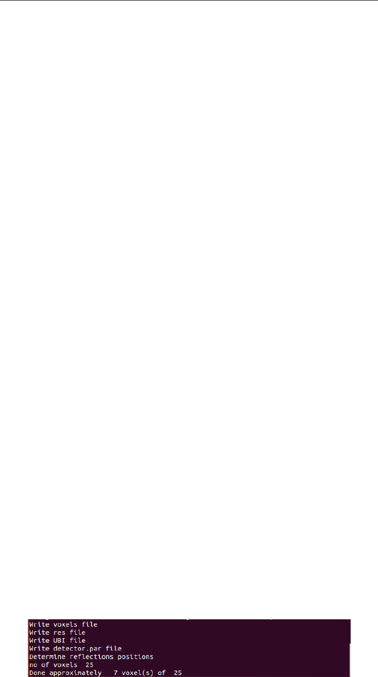
We may now run the forward model with the input file as
python ModelScanning3DXRD.py --input <path to input file>
This will run the simulation and printout the progress to the active terminal window.
You should see something like
3

November 16, 2018- LTH, Lund University N. A. Henningsson
As the simulation finished it will save any output files to the directory specified in the
input file. The files are of the same format as those which can be retrived at beamline
ID11 at the ESRF.
After deploying some preferred reconstruction algorithms it is possible to receive geome-
tries that reassembles the input sample state. The below reconstruction was retrieved
with FBP and a per-voxel local refinement.
Extra Features
For large samples it is recommend to use the "parallel" keyword as an additional input
to ModelScanning3DXRD.
python ModelScanning3DXRD.py --input <path to input file> --parallel
ModelScanning3DXRD will then start several parallel threads for computing the diffrac-
tion patterns. In general, for any sample with say 100+ voxels, it is worth while to use
the parallel keyword. You will see which voxels are treated by which thread
ModelScanning3DXRD also has a profiler mode for anyone who wants to try and make
the algorithm run faster. You can run in profiler mode as
python ModelScanning3DXRD.py --input <path to input file> --profile
This will run the algorithm and save a file with statistics. The file will look something
like this
2030420 function calls in 6.512 seconds
Ordered by: cumulative time
4

November 16, 2018- LTH, Lund University N. A. Henningsson
ncalls tottime percall cumtime percall filename:lineno(function)
1 1.361 1.361 6.512 6.512 find_refl.py:69(run)
36450 1.395 0.000 1.917 0.000 find_refl.py:350(find_omega_general)
82182 0.832 0.000 1.396 0.000 find_refl.py:422(det_coor)
35800 0.746 0.000 0.970 0.000 find_refl.py:447(calc_int_mod)
689978 0.806 0.000 0.806 0.000 {numpy.core.multiarray.dot}
416389 0.597 0.000 0.597 0.000 {numpy.core.multiarray.array}
The relevant colon is here the cumtime, which states how much time was spent executing
respective function in total.
Pitfalls/Limitations/Bugs
Like mentioned earlier, not all of the extensions used in PolyXSim has been tested with
the modified code. The model used at the writing time (November 16, 2018) is fairly
simple. Especially the calculation of the intensity is heavily simplified, basically the
structure factors and voxel beam overlap is used. Future versions should take more
physics into account.
Another simplification is the fact that peaks are assumed to never overlap and that the
detector is assumed to have an infinite resolution. This means that the .flt file gets huge
since what would normally be a single peak might be many many many delta peaks
clustered together. Work is currently put into taking detector pixel size into account
and computing peaks as centre of mass of continuous regions of intensity. Hopefully this
feature will arrive in a near future. If the .flt files get to big, the reader might want to
throw some python code together to parse and split the .flt into several files in order to
be a able to read them into matrix format without running out of RAM.
In general more details on the used assumptions and how the algorithm can be used is
found in the thesis (Henningsson 2018). The thesis will be made available at the git-hub
page as soon as possible. Most likely it will be up before the end of January 2019.
Finally a general disclaimer is announced, as the user may very well find flaws (and
hopefully will) and bugs throughout the code. Together we can build something that
keeps getting better and better, both from a physics perspective, discussing how these
models should be built, as well as from a coding perspective, writing better and more
solid code together.
Develop and Adapt
In reality any one who reads this will probably need to modify the code for their specific
scientific use. To run the altered code you will need to first run the
python setup.py build
command, followed by the
python setup.py install
command. This make sure that the python interpreter is importing the updated modules
and not uses the old ones.
Mostly it is the find_refl.py script that contains the diffraction model algorithm while
the other scripts deal with file handling, parallel runs, input parsing etc. If you would
like to improve the model/adapt it this is most likely the place to add some code.
5

November 16, 2018- LTH, Lund University N. A. Henningsson
References
Hayashi, Y., Hirose, Y., and Seno, Y. (2015). Polycrystal orientation mapping using
scanning three-dimensional X-ray diffraction microscopy. Journal of Applied Crystal-
lography, 48(4):1094–1101.
Hayashi, Y., Setoyama, D., and Seno, Y. (2017). Scanning three-dimensional x-ray
diffraction microscopy with a high-energy microbeam at spring-8. Materials Science
Forum, 905:157–164.
Henningsson, N. A. (2018). 3dxrd reconstructions for intragranular resolution - a forward
model for scanning-3dxr.
6
