MOA Manual
User Manual:
Open the PDF directly: View PDF ![]() .
.
Page Count: 67
- Titlepage
- Contents
- Introduction
- Installation
- Using MOA
- Using the API
- Tasks in MOA
- Evolving data streams
- Streams
- Streams Generators
- generators.AgrawalGenerator
- generators.HyperplaneGenerator
- generators.LEDGenerator
- generators.LEDGeneratorDrift
- generators.RandomRBFGenerator
- generators.RandomRBFGeneratorDrift
- generators.RandomTreeGenerator
- generators.SEAGenerator
- generators.STAGGERGenerator
- generators.WaveformGenerator
- generators.WaveformGeneratorDrift
- Classifiers
- Bi-directional interface with WEKA

Massive Online
Analysis
Manual
Albert Bifet, Richard Kirkby,
Philipp Kranen, Peter Reutemann
March 2012
Contents
1 Introduction 1
1.1 Data streams Evaluation . . . . . . . . . . . . . . . . . . . . . . . . . 2
2 Installation 5
2.1 WEKA . . . . . . . . . . . . . . . . . . . . . . . . . . . . . . . . . . . . 6
3 Using MOA 7
3.1 Using the GUI . . . . . . . . . . . . . . . . . . . . . . . . . . . . . . . 7
3.1.1 Classification . . . . . . . . . . . . . . . . . . . . . . . . . . . 7
3.1.2 Regression . . . . . . . . . . . . . . . . . . . . . . . . . . . . . 8
3.1.3 Clustering . . . . . . . . . . . . . . . . . . . . . . . . . . . . . 8
3.2 Using the command line . . . . . . . . . . . . . . . . . . . . . . . . . 12
3.2.1 Comparing two classifiers . . . . . . . . . . . . . . . . . . . 14
4 Using the API 17
4.1 Creating a new classifier . . . . . . . . . . . . . . . . . . . . . . . . . 17
4.2 Compiling a classifier . . . . . . . . . . . . . . . . . . . . . . . . . . . 22
5 Tasks in MOA 25
5.1 WriteStreamToARFFFile . . . . . . . . . . . . . . . . . . . . . . . . . 25
5.2 MeasureStreamSpeed . . . . . . . . . . . . . . . . . . . . . . . . . . 25
5.3 LearnModel . . . . . . . . . . . . . . . . . . . . . . . . . . . . . . . . . 26
5.4 EvaluateModel . . . . . . . . . . . . . . . . . . . . . . . . . . . . . . . 26
5.5 EvaluatePeriodicHeldOutTest . . . . . . . . . . . . . . . . . . . . . . 27
5.6 EvaluateInterleavedTestThenTrain . . . . . . . . . . . . . . . . . . . 27
5.7 EvaluatePrequential . . . . . . . . . . . . . . . . . . . . . . . . . . . 28
5.8 EvaluateInterleavedChunks . . . . . . . . . . . . . . . . . . . . . . . 29
6 Evolving data streams 31
6.1 Streams . . . . . . . . . . . . . . . . . . . . . . . . . . . . . . . . . . . 31
6.1.1 ArffFileStream . . . . . . . . . . . . . . . . . . . . . . . . . . 31
6.1.2 ConceptDriftStream . . . . . . . . . . . . . . . . . . . . . . . 32
6.1.3 ConceptDriftRealStream . . . . . . . . . . . . . . . . . . . . 33
6.1.4 FilteredStream . . . . . . . . . . . . . . . . . . . . . . . . . . 34
6.1.5 AddNoiseFilter . . . . . . . . . . . . . . . . . . . . . . . . . . 34
6.2 Streams Generators . . . . . . . . . . . . . . . . . . . . . . . . . . . . 34
6.2.1 generators.AgrawalGenerator . . . . . . . . . . . . . . . . . 34
6.2.2 generators.HyperplaneGenerator . . . . . . . . . . . . . . . 35
6.2.3 generators.LEDGenerator . . . . . . . . . . . . . . . . . . . . 36
i
CONTENTS
6.2.4 generators.LEDGeneratorDrift . . . . . . . . . . . . . . . . . 36
6.2.5 generators.RandomRBFGenerator . . . . . . . . . . . . . . 37
6.2.6 generators.RandomRBFGeneratorDrift . . . . . . . . . . . 37
6.2.7 generators.RandomTreeGenerator . . . . . . . . . . . . . . 38
6.2.8 generators.SEAGenerator . . . . . . . . . . . . . . . . . . . . 39
6.2.9 generators.STAGGERGenerator . . . . . . . . . . . . . . . . 39
6.2.10 generators.WaveformGenerator . . . . . . . . . . . . . . . . 40
6.2.11 generators.WaveformGeneratorDrift . . . . . . . . . . . . . 40
7 Classifiers 41
7.1 Bayesian Classifiers . . . . . . . . . . . . . . . . . . . . . . . . . . . . 42
7.1.1 NaiveBayes . . . . . . . . . . . . . . . . . . . . . . . . . . . . 42
7.1.2 NaiveBayesMultinomial . . . . . . . . . . . . . . . . . . . . . 42
7.2 Decision Trees . . . . . . . . . . . . . . . . . . . . . . . . . . . . . . . 43
7.2.1 DecisionStump . . . . . . . . . . . . . . . . . . . . . . . . . . 43
7.2.2 HoeffdingTree . . . . . . . . . . . . . . . . . . . . . . . . . . . 43
7.2.3 HoeffdingOptionTree . . . . . . . . . . . . . . . . . . . . . . 45
7.2.4 HoeffdingAdaptiveTree . . . . . . . . . . . . . . . . . . . . . 47
7.2.5 AdaHoeffdingOptionTree . . . . . . . . . . . . . . . . . . . . 47
7.3 Meta Classifiers . . . . . . . . . . . . . . . . . . . . . . . . . . . . . . 47
7.3.1 OzaBag . . . . . . . . . . . . . . . . . . . . . . . . . . . . . . . 47
7.3.2 OzaBoost . . . . . . . . . . . . . . . . . . . . . . . . . . . . . . 48
7.3.3 OCBoost . . . . . . . . . . . . . . . . . . . . . . . . . . . . . . 48
7.3.4 OzaBagASHT . . . . . . . . . . . . . . . . . . . . . . . . . . . 49
7.3.5 OzaBagADWIN . . . . . . . . . . . . . . . . . . . . . . . . . . 50
7.3.6 AccuracyWeightedEnsemble . . . . . . . . . . . . . . . . . . 51
7.3.7 AccuracyUpdatedEnsemble . . . . . . . . . . . . . . . . . . 52
7.3.8 LimAttClassifier . . . . . . . . . . . . . . . . . . . . . . . . . . 52
7.3.9 LeveragingBag . . . . . . . . . . . . . . . . . . . . . . . . . . 53
7.4 Function Classifiers . . . . . . . . . . . . . . . . . . . . . . . . . . . . 54
7.4.1 MajorityClass . . . . . . . . . . . . . . . . . . . . . . . . . . . 54
7.4.2 Perceptron . . . . . . . . . . . . . . . . . . . . . . . . . . . . . 54
7.4.3 SGD . . . . . . . . . . . . . . . . . . . . . . . . . . . . . . . . . 54
7.4.4 SPegasos . . . . . . . . . . . . . . . . . . . . . . . . . . . . . . 54
7.5 Drift Classifiers . . . . . . . . . . . . . . . . . . . . . . . . . . . . . . . 55
7.5.1 SingleClassifierDrift . . . . . . . . . . . . . . . . . . . . . . . 55
8 Bi-directional interface with WEKA 57
8.1 WEKA classifiers from MOA . . . . . . . . . . . . . . . . . . . . . . . 57
8.1.1 WekaClassifier . . . . . . . . . . . . . . . . . . . . . . . . . . 58
8.1.2 SingleClassifierDrift . . . . . . . . . . . . . . . . . . . . . . . 58
ii

1
Introduction
Massive Online Analysis (MOA) is a software environment for implementing
algorithms and running experiments for online learning from evolving data
streams. MOA is designed to deal with the challenging problems of scaling up
the implementation of state of the art algorithms to real world dataset sizes
and of making algorithms comparable in benchmark streaming settings.
MOA contains a collection of offline and online algorithms for both classifi-
cation and clustering as well as tools for evaluation. Researchers benefit from
MOA by getting insights into workings and problems of different approaches,
practitioners can easily compare several algorithms and apply them to real
world data sets and settings.
MOA supports bi-directional interaction with WEKA, the Waikato Environ-
ment for Knowledge Analysis, which is an award-winning open-source work-
bench containing implementations of a wide range of batch machine learning
methods. WEKA is also written in Java. The main benefits of Java are porta-
bility, where applications can be run on any platform with an appropriate Java
virtual machine, and the strong and well-developed support libraries. Use of
the language is widespread, and features such as the automatic garbage col-
lection help to reduce programmer burden and error.
One of the key data structures used in MOA is the description of an exam-
ple from a data stream. This structure borrows from WEKA, where an example
is represented by an array of double precision floating point values. This pro-
vides freedom to store all necessary types of value – numeric attribute values
can be stored directly, and discrete attribute values and class labels are repre-
sented by integer index values that are stored as floating point values in the
1
CHAPTER 1. INTRODUCTION
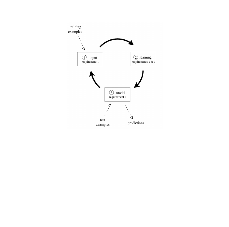
Figure 1.1: The data stream classification cycle
array. Double precision floating point values require storage space of 64 bits,
or 8 bytes. This detail can have implications for memory usage.
1.1 Data streams Evaluation
A data stream environment has different requirements from the traditional
setting. The most significant are the following:
Requirement 1 Process an example at a time, and inspect it only once (at
most)
Requirement 2 Use a limited amount of memory
Requirement 3 Work in a limited amount of time
Requirement 4 Be ready to predict at any time
We have to consider these requirements in order to design a new experimental
framework for data streams. Figure 1.1 illustrates the typical use of a data
stream classification algorithm, and how the requirements fit in a repeating
cycle:
2
1.1. DATA STREAMS EVALUATION
1. The algorithm is passed the next available example from the stream (re-
quirement 1).
2. The algorithm processes the example, updating its data structures. It
does so without exceeding the memory bounds set on it (requirement
2), and as quickly as possible (requirement 3).
3. The algorithm is ready to accept the next example. On request it is able
to predict the class of unseen examples (requirement 4).
In traditional batch learning the problem of limited data is overcome by an-
alyzing and averaging multiple models produced with different random ar-
rangements of training and test data. In the stream setting the problem of
(effectively) unlimited data poses different challenges. One solution involves
taking snapshots at different times during the induction of a model to see how
much the model improves.
The evaluation procedure of a learning algorithm determines which exam-
ples are used for training the algorithm, and which are used to test the model
output by the algorithm. The procedure used historically in batch learning has
partly depended on data size. As data sizes increase, practical time limitations
prevent procedures that repeat training too many times. It is commonly ac-
cepted with considerably larger data sources that it is necessary to reduce the
numbers of repetitions or folds to allow experiments to complete in reasonable
time. When considering what procedure to use in the data stream setting, one
of the unique concerns is how to build a picture of accuracy over time. Two
main approaches arise:
•Holdout: When traditional batch learning reaches a scale where cross-
validation is too time consuming, it is often accepted to instead measure
performance on a single holdout set. This is most useful when the di-
vision between train and test sets have been pre-defined, so that results
from different studies can be directly compared.
•Interleaved Test-Then-Train or Prequential: Each individual example
can be used to test the model before it is used for training, and from
this the accuracy can be incrementally updated. When intentionally per-
formed in this order, the model is always being tested on examples it has
not seen. This scheme has the advantage that no holdout set is needed
for testing, making maximum use of the available data. It also ensures
a smooth plot of accuracy over time, as each individual example will
become increasingly less significant to the overall average.
3
CHAPTER 1. INTRODUCTION
As data stream classification is a relatively new field, such evaluation practices
are not nearly as well researched and established as they are in the traditional
batch setting. The majority of experimental evaluations use less than one mil-
lion training examples. In the context of data streams this is disappointing,
because to be truly useful at data stream classification the algorithms need to
be capable of handling very large (potentially infinite) streams of examples.
Demonstrating systems only on small amounts of data does not build a con-
vincing case for capacity to solve more demanding data stream applications.
MOA permits adequately evaluate data stream classification algorithms on
large streams, in the order of tens of millions of examples where possible,
and under explicit memory limits. Any less than this does not actually test
algorithms in a realistically challenging setting.
4
2
Installation
The following manual is based on a Unix/Linux system with Java 6 SDK or
greater installed. Other operating systems such as Microsoft Windows will be
similar but may need adjustments to suit.
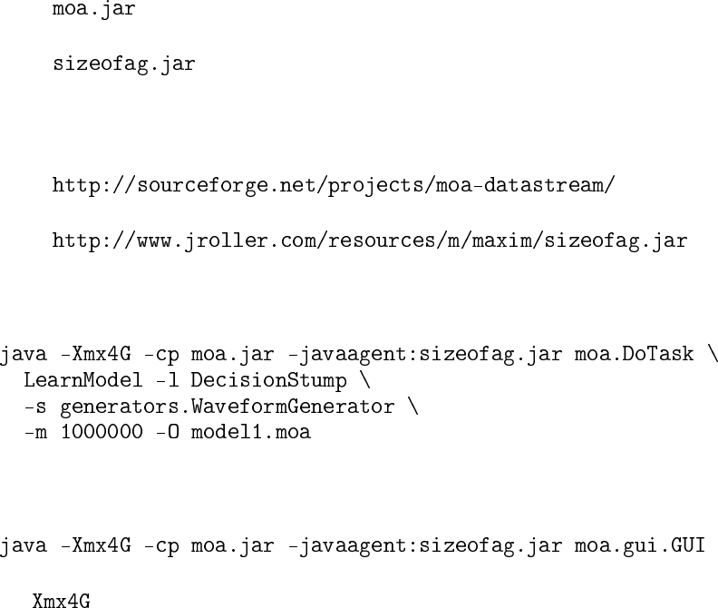
MOA needs the following files:
•
•
They are available from
•
•
These files are needed to run the MOA software from the command line:
and the graphical interface:
increases the maximum heap size to 4GB for your java engine, as
the default setting of 16 to 64MB may be too small.
5
CHAPTER 2. INSTALLATION
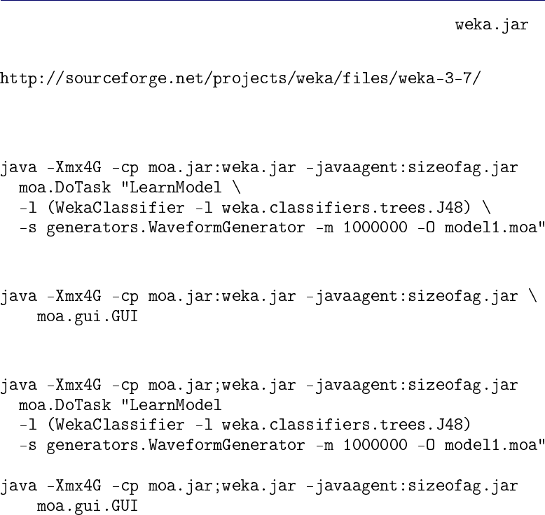
2.1 WEKA
It is possible to use the classifiers available in WEKA 3.7. The file is
available from
This file is needed to run the MOA software with WEKA from the command
line:
and the graphical interface:
or, using Microsoft Windows:
6
3
Using MOA
3.1 Using the GUI
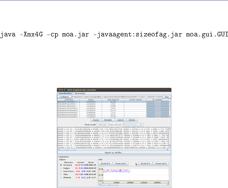
A graphical user interface for configuring and running tasks is available with
the command:
There are two main tabs: one for classification and one for clustering.
3.1.1 Classification
Figure 3.1: Graphical user interface of MOA
Click ’Configure’ to set up a task, when ready click to launch a task click
’Run’. Several tasks can be run concurrently. Click on different tasks in the
list and control them using the buttons below. If textual output of a task is
7
CHAPTER 3. USING MOA
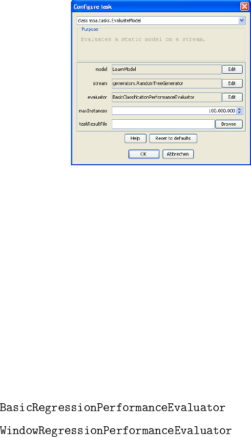
Figure 3.2: Options to set up a task in MOA
available it will be displayed in the bottom half of the GUI, and can be saved
to disk.
Note that the command line text box displayed at the top of the window
represents textual commands that can be used to run tasks on the command
line as described in the next chapter. The text can be selected then copied
onto the clipboard. In the bottom of the GUI there is a graphical display of the
results. It is possible to compare the results of two different tasks: the current
task is displayed in red, and the selected previously is in blue.
3.1.2 Regression
It is now possible to run regression evaluations using the evaluators
•
•
Currently, it is only possible to use the regressors in the IBLStreams extension
of MOA or in WEKA. See Section 2.1 and Chapter 8for more information how
to use WEKA learners.
3.1.3 Clustering
The stream clustering tab of MOA has the following main components:
•data generators for stream clustering on evolving streams (including
events like novelty, merge, etc.),
8
3.1. USING THE GUI
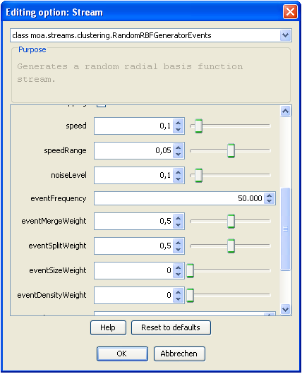
Figure 3.3: Option dialog for the RBF data generator (by storing and loading
settings benchmark streaming data sets can be shared for repeatability and
comparison).
•a set of state-of-the-art stream clustering algorithms,
•evaluation measures for stream clustering,
•visualization tools for analyzing results and comparing different settings.
Data feeds and data generators
Figure 3.3 shows a screenshot of the configuration dialog for the RBF data
generator with events. Generally the dimensionality, number and size of clus-
ters can be set as well as the drift speed, decay horizon (aging) and noise rate
etc. Events constitute changes in the underlying data model such as growing
of clusters, merging of clusters or creation of new clusters. Using the event
frequency and the individual event weights, one can study the behaviour and
performance of different approaches on various settings. Finally, the settings
for the data generators can be stored and loaded, which offers the opportunity
of sharing settings and thereby providing benchmark streaming data sets for
repeatability and comparison.
9
CHAPTER 3. USING MOA
Stream clustering algorithms
Currently MOA contains several stream clustering methods including:
•StreamKM++: It computes a small weighted sample of the data stream
and it uses the k-means++ algorithm as a randomized seeding tech-
nique to choose the first values for the clusters. To compute the small
sample, it employs coreset constructions using a coreset tree for speed
up.
•CluStream: It maintains statistical information about the data using
micro-clusters. These micro-clusters are temporal extensions of clus-
ter feature vectors. The micro-clusters are stored at snapshots in time
following a pyramidal pattern. This pattern allows to recall summary
statistics from different time horizons.
•ClusTree: It is a parameter free algorithm automatically adapting to the
speed of the stream and it is capable of detecting concept drift, novelty,
and outliers in the stream. It uses a compact and self-adaptive index
structure for maintaining stream summaries.
•Den-Stream: It uses dense micro-clusters (named core-micro-cluster) to
summarize clusters. To maintain and distinguish the potential clusters
and outliers, this method presents core-micro-cluster and outlier micro-
cluster structures.
•CobWeb. One of the first incremental methods for clustering data. It
uses a classification tree. Each node in a classification tree represents a
class (concept) and is labeled by a probabilistic concept that summarizes
the attribute-value distributions of objects classified under the node.
Visualization and analysis
After the evaluation process is started, several options for analyzing the out-
puts are given:
•the stream can be stopped and the current (micro) clustering result can
be passed as a data set to the WEKA explorer for further analysis or
mining;
•the evaluation measures, which are taken at configurable time intervals,
can be stored as a .csv file to obtain graphs and charts offline using a
program of choice;
10
3.1. USING THE GUI
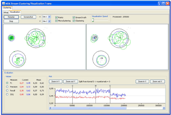
Figure 3.4: Visualization tab of the clustering MOA graphical user interface.
•last but not least both the clustering results and the corresponding mea-
sures can be visualized online within MOA.
MOA allows the simultaneous configuration and evaluation of two differ-
ent setups for direct comparison, e.g. of two different algorithms on the same
stream or the same algorithm on streams with different noise levels etc.
The visualization component allows to visualize the stream as well as the
clustering results, choose dimensions for multi dimensional settings, and com-
pare experiments with different settings in parallel. Figure 3.4 shows a screen
shot of the visualization tab. For this screen shot two different settings of the
CluStream algorithm were compared on the same stream setting (including
merge/split events every 50000 examples) and four measures were chosen for
online evaluation (F1, Precision, Recall, and SSQ).
The upper part of the GUI offers options to pause and resume the stream,
adjust the visualization speed, choose the dimensions for x and y as well as the
components to be displayed (points, micro- and macro clustering and ground
truth). The lower part of the GUI displays the measured values for both set-
tings as numbers (left side, including mean values) and the currently selected
measure as a plot over the arrived examples (right, F1 measure in this exam-
ple). For the given setting one can see a clear drop in the performance after
the split event at roughly 160000 examples (event details are shown when
11
CHAPTER 3. USING MOA
choosing the corresponding vertical line in the plot). While this holds for both
settings, the left configuration (red, CluStream with 100 micro clusters) is
constantly outperformed by the right configuration (blue, CluStream with 20
micro clusters).
3.2 Using the command line
In this section we are going to show some examples of tasks performed using
the command line.
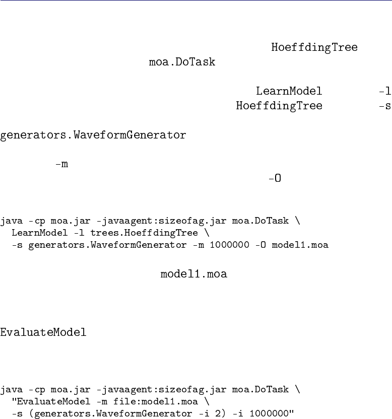
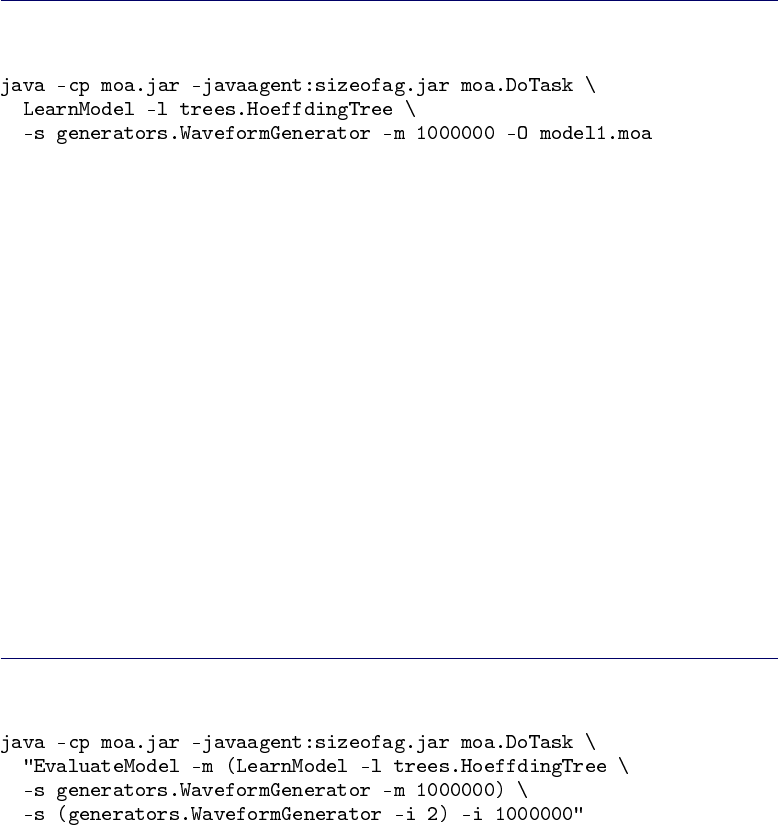
The first example will command MOA to train the classi-
fier and create a model. The class is the main class for running
tasks on the command line. It will accept the name of a task followed by any
appropriate parameters. The first task used is the task. The
parameter specifies the learner, in this case the class. The
parameter specifies the data stream to learn from, in this case it is specified
, which is a data stream generator that
produces a three-class learning problem of identifying three types of wave-
form. The option specifies the maximum number of examples to train the
learner with, in this case one million examples. The option specifies a file
to output the resulting model to:
This will create a file named that contains the decision stump
model that was induced during training.
The next example will evaluate the model to see how accurate it is on
a set of examples that are generated using a different random seed. The
task is given the parameters needed to load the model pro-
duced in the previous step, generate a new waveform stream with a random
seed of 2, and test on one million examples:
This is the first example of nesting parameters using brackets. Quotes have
been added around the description of the task, otherwise the operating system
may be confused about the meaning of the brackets.
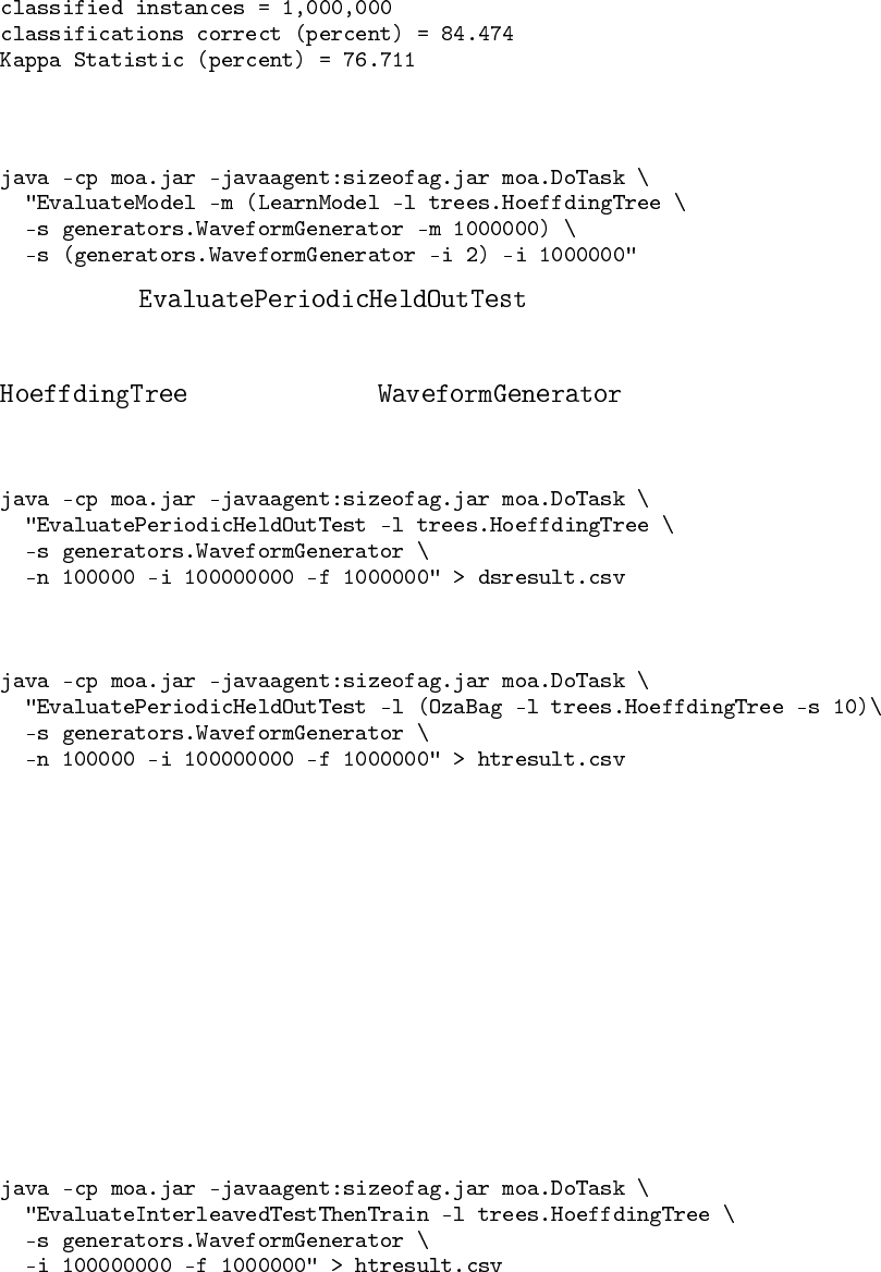
After evaluation the following statistics are output:
12
3.2. USING THE COMMAND LINE
Note the the above two steps can be achieved by rolling them into one,
avoiding the need to create an external file, as follows:
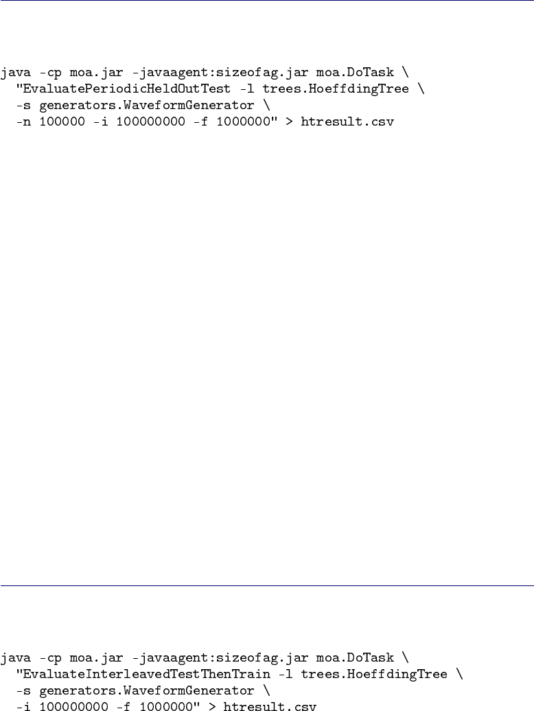
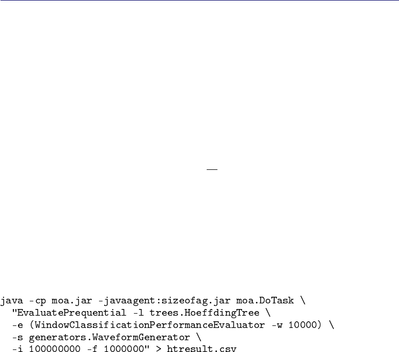
The task will train a model while tak-
ing snapshots of performance using a held-out test set at periodic intervals.
The following command creates a comma separated values file, training the
classifier on the data, using the first
100 thousand examples for testing, training on a total of 100 million examples,
and testing every one million examples:
For the purposes of comparison, a bagging learner using ten decisions trees
can be trained on the same problem:
Another evaluation method implemented in MOA is Interleaved Test-Then-
Train or Prequential: Each individual example is used to test the model before
it is used for training, and from this the accuracy is incrementally updated.
When intentionally performed in this order, the model is always being tested
on examples it has not seen. This scheme has the advantage that no holdout
set is needed for testing, making maximum use of the available data. It also
ensures a smooth plot of accuracy over time, as each individual example will
become increasingly less significant to the overall average.
An example of the EvaluateInterleavedTestThenTrain task creating a comma
separated values file, training the HoeffdingTree classifier on the Waveform-
Generator data, training and testing on a total of 100 million examples, and
testing every one million examples, is the following:
13
CHAPTER 3. USING MOA
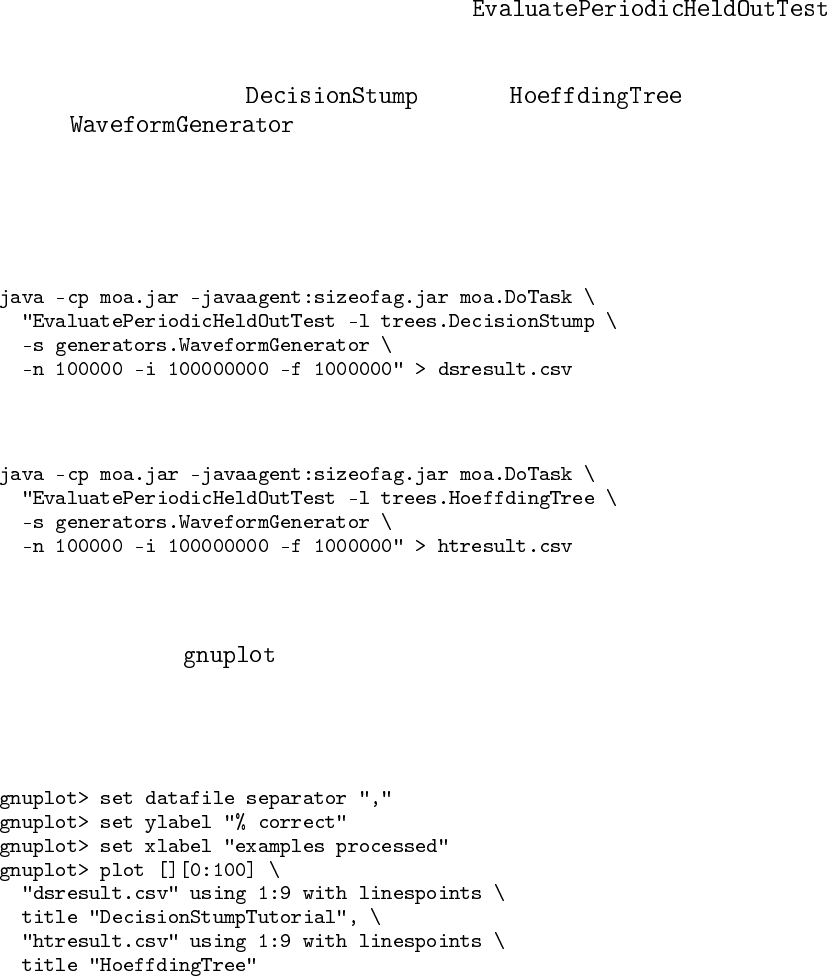
3.2.1 Comparing two classifiers
Suppose we would like to compare the learning curves of a decision stump and
a Hoeffding Tree. First, we will execute the task
to train a model while taking snapshots of performance using a held-out test
set at periodic intervals. The following commands create comma separated
values files, training the and the classifier
on the data, using the first 100 thousand examples for
testing, training on a total of 100 million examples, and testing every one
million examples:
Assuming that is installed on the system, the learning curves can
be plotted with the following commands:
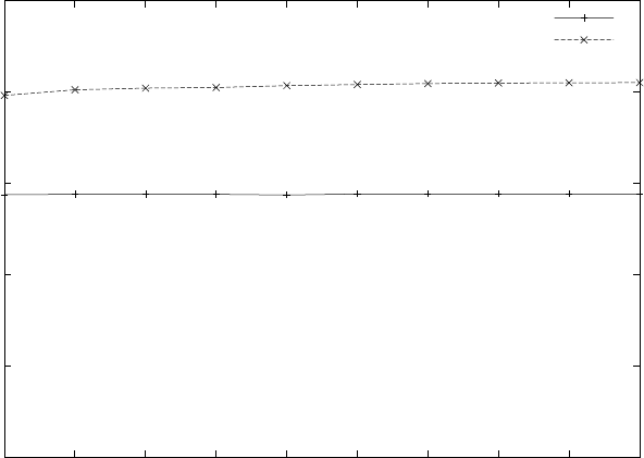
This results in the following graph:
14
3.2. USING THE COMMAND LINE
0
20
40
60
80
100
1e+06 2e+06 3e+06 4e+06 5e+06 6e+06 7e+06 8e+06 9e+06 1e+07
% correct
examples processed
DecisionStumpTutorial
HoeffdingTree
For this problem it is obvious that a full tree can achieve higher accuracy
than a single stump, and that a stump has very stable accuracy that does not
improve with further training.
15

4
Using the API
It’s easy to use the methods of MOA inside Java Code. For example, this is the
Java code for a prequential evaluation:
Listing 4.1: Java Code Example
1int numInstances=10000;
2
3 C l a s s i f i e r l ear ne r =new Ho ef fd in gT re e ( ) ;
4 RandomRBFGenerator stream =new RandomRBFGenerator ();
5 stream . pr ep areF orUs e ( ) ;
6
7 l ear ne r . s etMo delC onte xt ( stream . g etHeader ( ) ) ;
8 l e ar n e r . p re pare ForU se ( ) ;
9
10 int numberSamplesCorrect=0;
11 int numberSamples=0;
12 boolean isTesting =t ru e ;
13 while ( stream . has More Instances () && numberSamples <numInstances){
14 I ns tance t r a i n I n s t =stream . n e xt I nst a nce ( ) ;
15 i f (isTesting){
16 i f ( l earner . c o r r e c t l y C l a s s i f i e s ( t r a in I n s t ) ){
17 numberSamplesCorrect++;
18 }
19 }
20 numberSamples++;
21 l earne r . tra inOnI nstan ce ( t r a i n I n s t ) ;
22 }
23 double accuracy =100.0∗(double) numberSamplesCorrect /(double) numberSamples ;
24 System . o ut . p r i n t l n ( numberSamples+" i n s tances processed with "+accuracy+"% a cc ura cy " ) ;
4.1 Creating a new classifier
To demonstrate the implementation and operation of learning algorithms in
the system, the Java code of a simple decision stump classifier is studied. The
classifier monitors the result of splitting on each attribute and chooses the
attribute the seems to best separate the classes, based on information gain.
The decision is revisited many times, so the stump has potential to change
over time as more examples are seen. In practice it is unlikely to change after
sufficient training.
To describe the implementation, relevant code fragments are discussed in
turn, with the entire code listed (Listing 4.8) at the end. The line numbers
from the fragments match up with the final listing.
17
CHAPTER 4. USING THE API
A simple approach to writing a classifier is to extend
(line 10), which will take care of
certain details to ease the task.
Listing 4.2: Option handling
14 public IntOption gracePeriodOption =new IntOpti on ( " gr acePe r iod " , ’ g ’ ,
15 " The number of ins tance s t o o bs erve between model changes . " ,
16 1000 , 0 , I nteg er . MAX_VALUE) ;
17
18 public FlagOption binarySplitsOption =new Fl ag Op ti on ( " b i n a r y S p l i t s " , ’ b ’ ,
19 " Only allow bi nary s p l i t s . " ) ;
20
21 public C la ssO pti on s p l i t C r i t e r i o n O p t i o n =new Cl as sO pt io n ( " s p l i t C r i t e r i o n " ,
22 ’ c ’ , " S p l i t c r i t e r i o n to use . " , S p l i t C r i t e r i o n . class ,
23 " I n f o G a i n S p l i t C r i t e r i o n " ) ;
To set up the public interface to the classifier, the options available to the
user must be specified. For the system to automatically take care of option
handling, the options need to be public members of the class, that extend the
type.
The decision stump classifier example has three options, each of a different
type. The meaning of the first three parameters used to construct options are
consistent between different option types. The first parameter is a short name
used to identify the option. The second is a character intended to be used on
the command line. It should be unique—a command line character cannot be
repeated for different options otherwise an exception will be thrown. The third
standard parameter is a string describing the purpose of the option. Additional
parameters to option constructors allow things such as default values and valid
ranges to be specified.
The first option specified for the decision stump classifier is the “grace pe-
riod”. The option is expressed with an integer, so the option has the type
. The parameter will control how frequently the best stump is
reconsidered when learning from a stream of examples. This increases the
efficiency of the classifier—evaluating after every single example is expensive,
and it is unlikely that a single example will change the decision of the current
best stump. The default value of 1000 means that the choice of stump will
be re-evaluated only after 1000 examples have been observed since the last
evaluation. The last two parameters specify the range of values that are al-
lowed for the option—it makes no sense to have a negative grace period, so
the range is restricted to integers 0 or greater.
The second option is a flag, or a binary switch, represented by a
. By default all flags are turned off, and will be turned on only
when a user requests so. This flag controls whether the decision stumps should
only be allowed to split two ways. By default the stumps are allowed have
more than two branches.
The third option determines the split criterion that is used to decide which
stumps are the best. This is a that requires a particular Java
18
4.1. CREATING A NEW CLASSIFIER
class of the type . If the required class happens to be an
then those options will be used to configure the object that
is passed in.
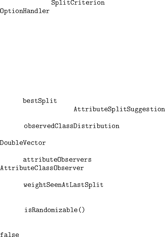
Listing 4.3: Miscellaneous fields
25 protect ed A t t r i b u t e S p l i t S u g g e s t i o n b e s t S p l i t ;
26
27 protect ed DoubleVector obser v e d C lassDi s t r i bution ;
28
29 protect ed AutoExpandVector<AttributeClassObserver>attributeObservers ;
30
31 protect ed double weightSeenAtLastSplit;
32
33 pub lic boolean isRandomizable () {
34 ret ur n f a l s e ;
35 }
Four global variables are used to maintain the state of the classifier.
The field maintains the current stump that has been chosen by
the classifier. It is of type , a class used to split
instances into different subsets.
The field remembers the overall distri-
bution of class labels that have been observed by the classifier. It is of type
, which is a handy class for maintaining a vector of floating
point values without having to manage its size.
The field stores a collection of
s, one for each attribute. This is the information
needed to decide which attribute is best to base the stump on.
The field records the last time an evaluation
was performed, so that it can be determined when another evaluation is due,
depending on the grace period parameter.
The function needs to be implemented to specify
whether the classifier has an element of randomness. If it does, it will au-
tomatically be set up to accept a random seed. This classifier is does not, so
is returned.
Listing 4.4: Preparing for learning
37 @Override
38 pub lic void resetLearningImpl() {
39 t h i s . b e s t S p l i t =n u ll ;
40 t h i s . observedClassDistribution =new DoubleVector ();
41 t h i s . attributeObservers =new AutoExpandVector<AttributeClassObserver >();
42 t h i s . weightSeenAtLastSplit =0.0;
43 }
This function is called before any learning begins, so it should set the de-
fault state when no information has been supplied, and no training examples
have been seen. In this case, the four global fields are set to sensible defaults.
Listing 4.5: Training on examples
45 @Override
46 pub lic void trai nOn Inst ance Impl ( I n st a nce i n s t ) {
47 t h i s . o b s ervedC l a s s Distri b u t i on . addToValue (( int ) i n s t . c lassValu e ( ) , i n s t
19
CHAPTER 4. USING THE API
48 . w eig ht ( ) ) ;
49 for (int i=0; i <i n s t . num At tr ib ut es () −1; i++){
50 int instAttIndex =modelAttIndexToInstanceAttIndex(i , inst );
51 AttributeClassObserver obs =t h i s . attributeObservers .get( i );
52 i f ( obs == n u l l ){
53 obs =i n s t . a t t r i b u t e ( i ns tAt tIn dex ) . isN omin al ( ) ?
54 newNominalClassObserver () : newNumericClassObserver ();
55 t h i s . a t t ribut e O b serve r s . s e t ( i , obs ) ;
56 }
57 obs . o b s er veA ttr ibu teCl ass ( i n s t . val ue ( i nst Att Ind ex ) , ( int ) i n s t
58 . c l assValue ( ) , i n s t . weight ( ) ) ;
59 }
60 i f (t h i s . trainingWeightSeenByModel −t h i s . weightSeenAtLastSplit >=
61 t h i s . grac ePer iodO ption . getValu e ()) {
62 t h i s . b e s t S p l i t =f i n d B e s t S p li t ( ( S p l i t C r i t e r i o n )
63 g etPre pared ClassO ption ( t h i s . s p l i t C r i t e r i o n O p t i o n ) ) ;
64 t h i s . weightSeenAtLastSplit =t h i s . trainingWeightSeenByModel ;
65 }
66 }
This is the main function of the learning algorithm, called for every training
example in a stream. The first step, lines 47-48, updates the overall recorded
distribution of classes. The loop from line 49 to line 59 repeats for every
attribute in the data. If no observations for a particular attribute have been
seen previously, then lines 53-55 create a new observing object. Lines 57-58
update the observations with the values from the new example. Lines 60-61
check to see if the grace period has expired. If so, the best split is re-evaluated.
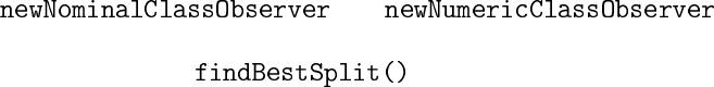
Listing 4.6: Functions used during training
79 protect ed A ttributeCl a s s O b server newNominalClassObserver () {
80 return new NominalAttributeClassObserver ();
81 }
82
83 protect ed A ttributeCl a s s O b server newNumericClassObserver ( ) {
84 return new GaussianNumericAttributeClassObserver ();
85 }
86
87 protect ed A t t r i b u t e S p l i t S u g g e s t i o n f i n d B e s t S p l i t ( S p l i t C r i t e r i o n c r i t e r i o n ) {
88 A t t r i b u t e S p l i t S u g g e s t i o n be stF oun d =n ull ;
89 double bestMerit =Double . NEGATIVE_INFINITY ;
90 double[] preSplitDist =t h i s . o b serv edC las sDis tri buti on . g etArrayC opy ( ) ;
91 for (int i=0; i <t h i s . a tt ri bu t eO bs er ve rs . s i z e ( ) ; i ++){
92 AttributeClassObserver obs =t h i s . attributeObservers .get( i );
93 i f ( obs !=null ){
94 A t t r i b u t e S p l i t S u g g e s t i o n s u gge s t ion =
95 obs . getBestEvaluatedSplitSuggestion(
96 c r i t e r i o n ,
97 p r e S p l i t D i s t ,
98 i ,
99 t h i s . binarySplitsOption . isSet ());
100 i f ( s uggestion . merit >bestMerit) {
101 bes t M e r it =suggest i o n . meri t ;
102 bestFound =suggestion ;
103 }
104 }
105 }
106 return bestFound;
107 }
These functions assist the training algorithm.
and are respon-
sible for creating new observer objects for nominal and numeric attributes,
respectively. The function will iterate through the possi-
ble stumps and return the one with the highest ‘merit’ score.
Listing 4.7: Predicting class of unknown examples
68 pub li c double [ ] getVotesForInstance(Instance inst) {
20
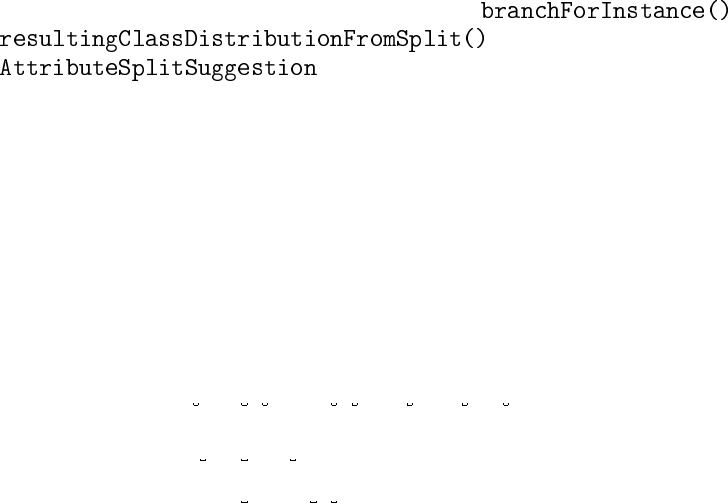
4.1. CREATING A NEW CLASSIFIER
69 i f (t h i s . b e s t S p l i t !=nul l ){
70 int branch =t h i s . b e s tS p l it . s p l i t T e s t . bran chF or Ins ta nce ( i n s t ) ;
71 i f (branch >= 0) {
72 r et ur n t h i s . b e s t S p l i t
73 . r e s u l t i n g C l a s s D i s t r i b u t i o n F r o m S p l i t ( b ran ch ) ;
74 }
75 }
76 r et ur n t h i s . o b serv edC las sDis tri buti on . g etArrayC opy ( ) ;
77 }
This is the other important function of the classifier besides training—using
the model that has been induced to predict the class of examples. For the de-
cision stump, this involves calling the functions and
that are implemented by the
class.
Putting all of the elements together, the full listing of the tutorial class is
given below.
Listing 4.8: Full listing
1package moa. classifiers ;
2
3import moa. core . AutoExpandVector ;
4import moa. core . DoubleVector ;
5import moa. opt i ons . Class Option ;
6import moa. opt i ons . FlagOption ;
7import moa. opt i ons . I ntOpt ion ;
8import weka . co re . Instance ;
9
10 p ub l i c c l a s s DecisionStumpTutorial extends AbstractClassifier {
11
12 p ri vat e s t a t i c f i n a l long serialVersionUID =1L ;
13
14 public IntOption gracePeriodOption =new In tO pti on ( " gra ceP erio d " , ’ g ’ ,
15 " The number of ins tance s t o o bs erve between model changes . " ,
16 1000 , 0 , I nteg er . MAX_VALUE) ;
17
18 public FlagOption binarySplitsOption =new Fl ag Op ti on ( " b i n a r y S p l i t s " , ’ b ’ ,
19 " Only allow bi nary s p l i t s . " ) ;
20
21 public C la ssO pti on s p l i t C r i t e r i o n O p t i o n =new Cl as sO pt io n ( " s p l i t C r i t e r i o n " ,
22 ’ c ’ , " S p l i t c r i t e r i o n to use . " , S p l i t C r i t e r i o n . class ,
23 " I n f o G a i n S p l i t C r i t e r i o n " ) ;
24
25 protect ed A t t r i b u t e S p l i t S u g g e s t i o n b e s t S p l i t ;
26
27 protect ed DoubleVector obser v e d C lassDi s t r i bution ;
28
29 protect ed AutoExpandVector<AttributeClassObserver>attributeObservers ;
30
31 protect ed double weightSeenAtLastSplit;
32
33 pub lic boolean isRandomizable () {
34 ret ur n f a l s e ;
35 }
36
37 @Override
38 pub lic void resetLearningImpl() {
39 t h i s . b e s t S p l i t =n u ll ;
40 t h i s . o b s ervedC l a s s Distri b u t i on =new DoubleVector ();
41 t h i s . attributeObservers =new AutoExpandVector<AttributeClassObserver >();
42 t h i s . weightSeenAtLastSplit =0.0;
43 }
44
45 @Override
46 pub lic void trai nOn Inst ance Impl ( I n st a nce i n s t ) {
47 t h i s . obser vedClas sDistri bution . addToValue (( int ) i n s t . c lassValue ( ) , i n s t
48 . w eig ht ( ) ) ;
49 for (int i=0; i <i n s t . num At tr ib ut es () −1; i++){
50 int instAttIndex =modelAttIndexToInstanceAttIndex(i , inst );
51 AttributeClassObserver obs =t h i s . attributeObservers .get( i );
52 i f ( obs == n u l l ){
53 obs =i n s t . a t t r i b u t e ( i ns tAt tIn dex ) . isN omin al ( ) ?
54 newNominalClassObserver () : newNumericClassObserver ();
55 t h i s . a t t ribut e O b serve r s . s e t ( i , obs ) ;
21
CHAPTER 4. USING THE API
56 }
57 obs . o b s er veA ttr ibu teCl ass ( i n s t . val ue ( i nst Att Ind ex ) , ( int ) i n s t
58 . c l assValue ( ) , i n s t . weight ( ) ) ;
59 }
60 i f (t h i s . trainingWeightSeenByModel −t h i s . weightSeenAtLastSplit >=
61 t h i s . grac ePer iodO ption . getValu e ()) {
62 t h i s . b e s t S p l i t =f i n d B e s t S p li t ( ( S p l i t C r i t e r i o n )
63 g etPre pared ClassO ption ( t h i s . s p l i t C r i t e r i o n O p t i o n ) ) ;
64 t h i s . weightSeenAtLastSplit =t h i s . trainingWeightSeenByModel ;
65 }
66 }
67
68 pub li c double [ ] getVotesForInstance(Instance inst) {
69 i f (t h i s . b e s t S p l i t !=nul l ){
70 int branch =t h i s . b e s tS p l it . s p l i t T e s t . bran chF or Ins ta nce ( i n s t ) ;
71 i f (branch >= 0) {
72 r et ur n t h i s . b e s t S p l i t
73 . r e s u l t i n g C l a s s D i s t r i b u t i o n F r o m S p l i t ( b ran ch ) ;
74 }
75 }
76 r et ur n t h i s . o b s ervedC l a s s Distri b u t i on . getArrayCopy ( ) ;
77 }
78
79 protect ed A ttributeCl a s s O b server newNominalClassObserver () {
80 return new NominalAttributeClassObserver ();
81 }
82
83 protect ed A ttributeCl a s s O b server newNumericClassObserver ( ) {
84 return new GaussianNumericAttributeClassObserver ();
85 }
86
87 protect ed A t t r i b u t e S p l i t S u g g e s t i o n f i n d B e s t S p l i t ( S p l i t C r i t e r i o n c r i t e r i o n ) {
88 A t t r i b u t e S p l i t S u g g e s t i o n be stF oun d =n ull ;
89 double bestMerit =Double . NEGATIVE_INFINITY ;
90 double[] preSplitDist =t h i s . o b serv edC las sDis tri buti on . g etArrayC opy ( ) ;
91 for (int i=0; i <t h i s . a tt ri bu t eO bs er ve rs . s i z e ( ) ; i ++){
92 AttributeClassObserver obs =t h i s . attributeObservers .get( i );
93 i f ( obs !=null ){
94 A t t r i b u t e S p l i t S u g g e s t i o n s u gge s t ion =
95 obs . getBestEvaluatedSplitSuggestion(
96 c r i t e r i o n ,
97 p r e S p l i t D i s t ,
98 i ,
99 t h i s . binarySplitsOption . isSet ());
100 i f ( s uggestion . merit >bestMerit) {
101 bes t M e r it =suggest i o n . meri t ;
102 bestFound =suggestion ;
103 }
104 }
105 }
106 return bestFound;
107 }
108
109 pub lic void get Model Descri ption ( Str i n g Builde r out , int inde nt ) {
110 }
111
112 protect ed moa . c or e . Measurement [ ] getModelMeasurementsImpl() {
113 return n u ll ;
114 }
115
116 }
4.2 Compiling a classifier
The following five files are assumed to be in the current working directory:
The example source code can be compiled with the following command:
22
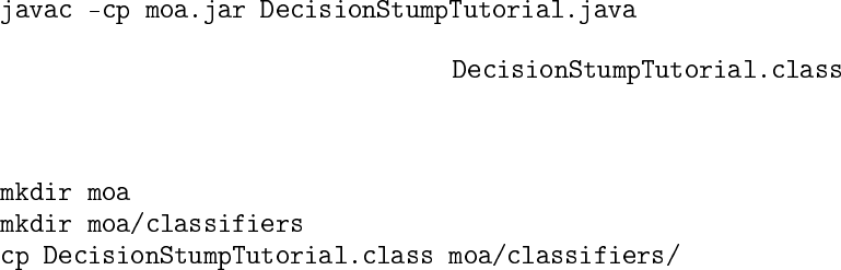
4.2. COMPILING A CLASSIFIER
This produces compiled java class file .
Before continuing, the commands below set up directory structure to re-
flect the package structure:
The class is now ready to use.
23
5
Tasks in MOA
The main Tasks in MOA are the following:
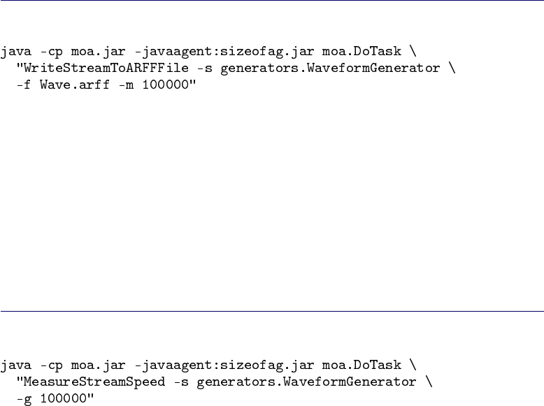
5.1 WriteStreamToARFFFile
Outputs a stream to an ARFF file. Example:
Parameters:
•-s : Stream to write
•-f : Destination ARFF file
•-m : Maximum number of instances to write to file
•-h : Suppress header from output
5.2 MeasureStreamSpeed
Measures the speed of a stream. Example:
Parameters:
•-s : Stream to measure
•-g : Number of examples
•-O : File to save the final result of the task to
25
CHAPTER 5. TASKS IN MOA
5.3 LearnModel
Learns a model from a stream. Example:
Parameters:
•-l : Classifier to train
•-s : Stream to learn from
•-m : Maximum number of instances to train on per pass over the data
•-p : The number of passes to do over the data
•-b : Maximum size of model (in bytes). -1 =no limit
•-q : How many instances between memory bound checks
•-O : File to save the final result of the task to
5.4 EvaluateModel
Evaluates a static model on a stream. Example:
Parameters:
•-l : Classifier to evaluate
•-s : Stream to evaluate on
•-e : Classification performance evaluation method
•-i : Maximum number of instances to test
•-O : File to save the final result of the task to
26
5.5. EVALUATEPERIODICHELDOUTTEST
5.5 EvaluatePeriodicHeldOutTest
Evaluates a classifier on a stream by periodically testing on a heldout set.
Example:
Parameters:
•-l : Classifier to train
•-s : Stream to learn from
•-e : Classification performance evaluation method
•-n : Number of testing examples
•-i : Number of training examples, <1=unlimited
•-t : Number of training seconds
•-f : Number of training examples between samples of learning perfor-
mance
•-d : File to append intermediate csv results to
•-c : Cache test instances in memory
•-O : File to save the final result of the task to
5.6 EvaluateInterleavedTestThenTrain
Evaluates a classifier on a stream by testing then training with each example
in sequence. Example:
Parameters:
•-l : Classifier to train
27
CHAPTER 5. TASKS IN MOA
•-s : Stream to learn from
•-e : Classification performance evaluation method
•-i : Maximum number of instances to test/train on (-1 =no limit)
•-t : Maximum number of seconds to test/train for (-1 =no limit)
•-f : How many instances between samples of the learning performance
•-b : Maximum size of model (in bytes). -1 =no limit
•-q : How many instances between memory bound checks
•-d : File to append intermediate csv results to
•-O : File to save the final result of the task to
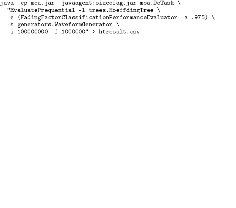
5.7 EvaluatePrequential
Evaluates a classifier on a stream by testing then training with each example
in sequence. It may use a sliding window or a fading factor forgetting mecha-
nism.
This evaluation method using sliding windows and a fading factor was
presented in
[C]João Gama, Raquel Sebastião and Pedro Pereira Rodrigues. Issues in
evaluation of stream learning algorithms. In KDD’09, pages 329–338.
The fading factor αis used as following:
Ei=Si
Bi
with
Si=Li+α×Si−1
Bi=ni+α×Bi−1
where niis the number of examples used to compute the loss function Li.
ni=1 since the loss Liis computed for every single example.
Examples:
28
5.8. EVALUATEINTERLEAVEDCHUNKS
Parameters:
•Same parameters as EvaluateInterleavedTestThenTrain
•-e : Classification performance evaluation method
–WindowClassificationPerformanceEvaluator
∗-w : Size of sliding window to use with WindowClassification-
PerformanceEvaluator
–FadingFactorClassificationPerformanceEvaluator
∗-a : Fading factor to use with FadingFactorClassificationPerfor-
manceEvaluator
–EWMAFactorClassificationPerformanceEvaluator
∗-a : Fading factor to use with FadingFactorClassificationPerfor-
manceEvaluator
5.8 EvaluateInterleavedChunks
Evaluates a classifier on a stream by testing then training with chunks of data
in sequence.
Parameters:
•-l : Classifier to train
•-s : Stream to learn from
•-e : Classification performance evaluation method
•-i : Maximum number of instances to test/train on (-1 =no limit)
•-c : Number of instances in a data chunk.
•-t : Maximum number of seconds to test/train for (-1 =no limit)
•-f : How many instances between samples of the learning performance
•-b : Maximum size of model (in bytes). -1 =no limit
29
CHAPTER 5. TASKS IN MOA
•-q : How many instances between memory bound checks
•-d : File to append intermediate csv results to
•-O : File to save the final result of the task to
30

6
Evolving data streams
MOA streams are build using generators, reading ARFF files, joining several
streams, or filtering streams. MOA streams generators allow to simulate po-
tentially infinite sequence of data. There are the following :
•Random Tree Generator
•SEA Concepts Generator
•STAGGER Concepts Generator
•Rotating Hyperplane
•Random RBF Generator
•LED Generator
•Waveform Generator
•Function Generator
.
6.1 Streams
Classes available in MOA to obtain input streams are the following:
6.1.1 ArffFileStream
A stream read from an ARFF file. Example:
Parameters:
•-f : ARFF file to load
•-c : Class index of data. 0 for none or -1 for last attribute in file
31
CHAPTER 6. EVOLVING DATA STREAMS
t
f(t)
f(t)α
α
t0
W
0.5
1
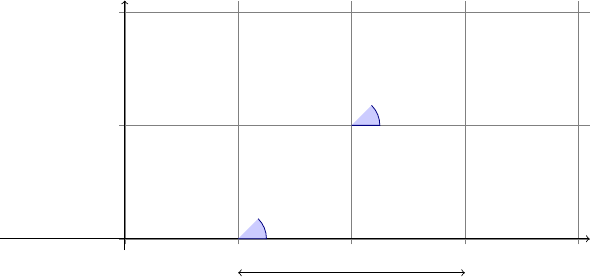
Figure 6.1: A sigmoid function f(t) = 1/(1+e−s(t−t0)).
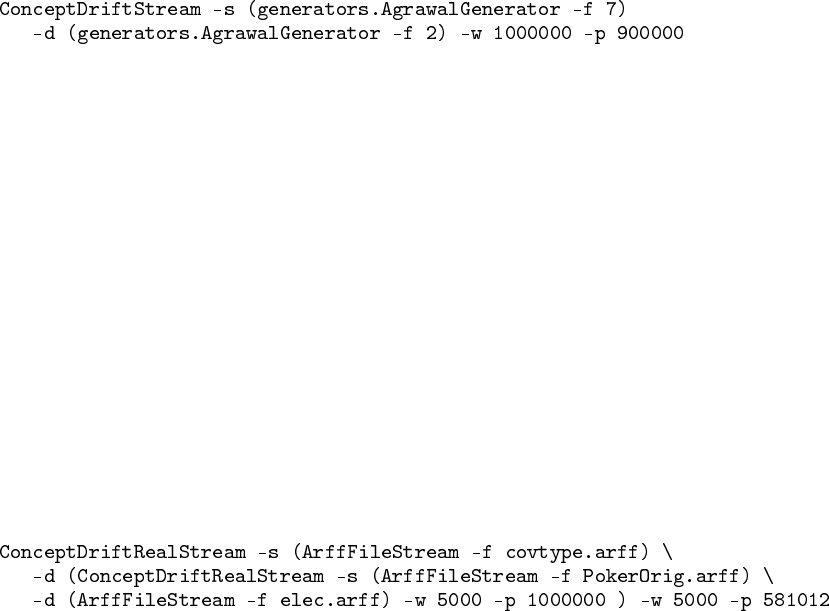
6.1.2 ConceptDriftStream
Generator that adds concept drift to examples in a stream.
Considering data streams as data generated from pure distributions, MOA
models a concept drift event as a weighted combination of two pure distribu-
tions that characterizes the target concepts before and after the drift. MOA
uses the sigmoid function, as an elegant and practical solution to define the
probability that every new instance of the stream belongs to the new concept
after the drift.
We see from Figure 6.1 that the sigmoid function
f(t) = 1/(1+e−s(t−t0))
has a derivative at the point t0equal to f0(t0) = s/4. The tangent of angle α
is equal to this derivative, tan α=s/4. We observe that tan α=1/W, and as
s=4tanαthen s=4/W. So the parameter sin the sigmoid gives the length
of Wand the angle α. In this sigmoid model we only need to specify two
parameters : t0the point of change, and Wthe length of change. Note that
for any positive real number β
f(t0+β·W) = 1−f(t0−β·W),
and that f(t0+β·W)and f(t0−β·W)are constant values that don’t depend
on t0and W:
f(t0+W/2) = 1−f(t0−W/2) = 1/(1+e−2)≈88.08%
f(t0+W) = 1−f(t0−W) = 1/(1+e−4)≈98.20%
f(t0+2W) = 1−f(t0−2W) = 1/(1+e−8)≈99.97%
32
6.1. STREAMS
Definition 1. Given two data streams a, b, we define c =a⊕W
t0b as the data
stream built joining the two data streams a and b, where t0is the point of change,
W is the length of change and
•Pr[c(t) = a(t)] = e−4(t−t0)/W/(1+e−4(t−t0)/W)
•Pr[c(t) = b(t)] = 1/(1+e−4(t−t0)/W).
Example:
Parameters:
•-s : Stream
•-d : Concept drift Stream
•-p : Central position of concept drift change
•-w : Width of concept drift change
6.1.3 ConceptDriftRealStream
Generator that adds concept drift to examples in a stream with different classes
and attributes. Example: real datasets
Example:
Parameters:
•-s : Stream
•-d : Concept drift Stream
•-p : Central position of concept drift change
•-w : Width of concept drift change
33

CHAPTER 6. EVOLVING DATA STREAMS
6.1.4 FilteredStream
A stream that is filtered.
Parameters:
•-s : Stream to filter
•-f : Filters to apply : AddNoiseFilter
6.1.5 AddNoiseFilter
Adds random noise to examples in a stream. Only to use with FilteredStream.
Parameters:
•-r : Seed for random noise
•-a : The fraction of attribute values to disturb
•-c : The fraction of class labels to disturb
6.2 Streams Generators
The classes available to generate streams are the following:
6.2.1 generators.AgrawalGenerator
Generates one of ten different pre-defined loan functions
It was introduced by Agrawal et al. in
[A]R. Agrawal, T. Imielinski, and A. Swami. Database mining: A perfor-
mance perspective. IEEE Trans. on Knowl. and Data Eng., 5(6):914–925,
1993.
It was a common source of data for early work on scaling up decision tree
learners. The generator produces a stream containing nine attributes, six nu-
meric and three categorical. Although not explicitly stated by the authors,
a sensible conclusion is that these attributes describe hypothetical loan ap-
plications. There are ten functions defined for generating binary class labels
from the attributes. Presumably these determine whether the loan should be
approved.
A public C source code is available. The built in functions are based on the
paper (page 924), which turn out to be functions pred20 thru pred29 in the
34
6.2. STREAMS GENERATORS
public C implementation Perturbation function works like C implementation
rather than description in paper
Parameters:
•-f : Classification function used, as defined in the original paper.
•-i : Seed for random generation of instances.
•-p : The amount of peturbation (noise) introduced to numeric values
•-b : Balance the number of instances of each class.
6.2.2 generators.HyperplaneGenerator
Generates a problem of predicting class of a rotating hyperplane.
It was used as testbed for CVFDT versus VFDT in
[C]G. Hulten, L. Spencer, and P. Domingos. Mining time-changing data
streams. In KDD’01, pages 97–106, San Francisco, CA, 2001. ACM
Press.
A hyperplane in d-dimensional space is the set of points xthat satisfy
d
X
i=1
wixi=w0=
d
X
i=1
wi
where xi, is the ith coordinate of x. Examples for which Pd
i=1wixi≥w0are
labeled positive, and examples for which Pd
i=1wixi<w0are labeled negative.
Hyperplanes are useful for simulating time-changing concepts, because we can
change the orientation and position of the hyperplane in a smooth manner by
changing the relative size of the weights. We introduce change to this dataset
adding drift to each weight attribute wi=wi+dσ, where σis the probability
that the direction of change is reversed and dis the change applied to every
example.
Parameters:
•-i : Seed for random generation of instances.
•-c : The number of classes to generate
•-a : The number of attributes to generate.
•-k : The number of attributes with drift.
35
CHAPTER 6. EVOLVING DATA STREAMS
•-t : Magnitude of the change for every example
•-n : Percentage of noise to add to the data.
•-s : Percentage of probability that the direction of change is reversed
6.2.3 generators.LEDGenerator
Generates a problem of predicting the digit displayed on a 7-segment LED
display.
This data source originates from the CART book. An implementation in
C was donated to the UCI machine learning repository by David Aha. The
goal is to predict the digit displayed on a seven-segment LED display, where
each attribute has a 10% chance of being inverted. It has an optimal Bayes
classification rate of 74%. The particular configuration of the generator used
for experiments (led) produces 24 binary attributes, 17 of which are irrelevant.
Parameters:
•-i : Seed for random generation of instances.
•-n : Percentage of noise to add to the data
•-s : Reduce the data to only contain 7 relevant binary attributes
6.2.4 generators.LEDGeneratorDrift
Generates a problem of predicting the digit displayed on a 7-segment LED
display with drift.
Parameters:
•-i : Seed for random generation of instances.
•-n : Percentage of noise to add to the data
•-s : Reduce the data to only contain 7 relevant binary attributes
•-d : Number of attributes with drift
36
6.2. STREAMS GENERATORS
6.2.5 generators.RandomRBFGenerator
Generates a random radial basis function stream.
This generator was devised to offer an alternate complex concept type that
is not straightforward to approximate with a decision tree model. The RBF
(Radial Basis Function) generator works as follows: A fixed number of ran-
dom centroids are generated. Each center has a random position, a single
standard deviation, class label and weight. New examples are generated by
selecting a center at random, taking weights into consideration so that centers
with higher weight are more likely to be chosen. A random direction is chosen
to offset the attribute values from the central point. The length of the displace-
ment is randomly drawn from a Gaussian distribution with standard deviation
determined by the chosen centroid. The chosen centroid also determines the
class label of the example. This effectively creates a normally distributed hy-
persphere of examples surrounding each central point with varying densities.
Only numeric attributes are generated.
Parameters:
•-r : Seed for random generation of model
•-i : Seed for random generation of instances
•-c : The number of classes to generate
•-a : The number of attributes to generate
•-n : The number of centroids in the model
6.2.6 generators.RandomRBFGeneratorDrift
Generates a random radial basis function stream with drift. Drift is introduced
by moving the centroids with constant speed.
Parameters:
•-r : Seed for random generation of model
•-i : Seed for random generation of instances
•-c : The number of classes to generate
•-a : The number of attributes to generate
•-n : The number of centroids in the model
•-s : Speed of change of centroids in the model.
•-k : The number of centroids with drift
37
CHAPTER 6. EVOLVING DATA STREAMS
6.2.7 generators.RandomTreeGenerator
Generates a stream based on a randomly generated tree.
This generator is based on that proposed in
[D]P. Domingos and G. Hulten. Mining high-speed data streams. In Knowl-
edge Discovery and Data Mining, pages 71–80, 2000.
It produces concepts that in theory should favour decision tree learners. It
constructs a decision tree by choosing attributes at random to split, and as-
signing a random class label to each leaf. Once the tree is built, new examples
are generated by assigning uniformly distributed random values to attributes
which then determine the class label via the tree.
The generator has parameters to control the number of classes, attributes,
nominal attribute labels, and the depth of the tree. For consistency between
experiments, two random trees were generated and fixed as the base concepts
for testingâ˘
Aˇ
Tone simple and the other complex, where complexity refers to
the number of attributes involved and the size of the tree.
A degree of noise can be introduced to the examples after generation. In
the case of discrete attributes and the class label, a probability of noise param-
eter determines the chance that any particular value is switched to something
other than the original value. For numeric attributes, a degree of random noise
is added to all values, drawn from a random Gaussian distribution with stan-
dard deviation equal to the standard deviation of the original values multiplied
by noise probability.
Parameters:
•-r: Seed for random generation of tree
•-i: Seed for random generation of instances
•-c: The number of classes to generate
•-o: The number of nominal attributes to generate
•-u: The number of numeric attributes to generate
•-v: The number of values to generate per nominal attribute
•-d: The maximum depth of the tree concept
•-l: The first level of the tree above maxTreeDepth that can have leaves
•-f: The fraction of leaves per level from firstLeafLevel onwards
38
6.2. STREAMS GENERATORS
6.2.8 generators.SEAGenerator
Generates SEA concepts functions. This dataset contains abrupt concept drift,
first introduced in paper:
[S]W. N. Street and Y. Kim. A streaming ensemble algorithm (SEA) for
large-scale classification. In KDD ’01, pages 377–382, New York, NY,
USA, 2001. ACM Press.
It is generated using three attributes, where only the two first attributes are
relevant. All three attributes have values between 0 and 10. The points of the
dataset are divided into 4 blocks with different concepts. In each block, the
classification is done using f1+f2≤θ, where f1and f2represent the first two
attributes and θis a threshold value. The most frequent values are 9, 8, 7 and
9.5 for the data blocks.
Parameters:
•-f: Classification function used, as defined in the original paper
•-i: Seed for random generation of instances
•-b: Balance the number of instances of each class
•-n: Percentage of noise to add to the data
6.2.9 generators.STAGGERGenerator
Generates STAGGER Concept functions. They were introduced by Schlimmer
and Granger in
[ST]J. C. Schlimmer and R. H. Granger. Incremental learning from noisy
data. Machine Learning, 1(3):317–354, 1986.
The STAGGER Concepts are boolean functions of three attributes encoding
objects: size (small, medium, and large), shape (circle, triangle, and rectan-
gle), and colour (red,blue, and green). A concept description covering ei-
ther green rectangles or red triangles is represented by (shape=rectangle and
colour=green) or (shape=triangle and colour=red).
Parameters:
1. -i: Seed for random generation of instances
2. -f: Classification function used, as defined in the original paper
3. -b: Balance the number of instances of each class
39
CHAPTER 6. EVOLVING DATA STREAMS
6.2.10 generators.WaveformGenerator
Generates a problem of predicting one of three waveform types.
It shares its origins with LED, and was also donated by David Aha to the
UCI repository. The goal of the task is to differentiate between three differ-
ent classes of waveform, each of which is generated from a combination of
two or three base waves. The optimal Bayes classification rate is known to
be 86%. There are two versions of the problem, wave21 which has 21 nu-
meric attributes, all of which include noise, and wave40 which introduces an
additional 19 irrelevant attributes.
Parameters:
•-i: Seed for random generation of instances
•-n: Adds noise, for a total of 40 attributes
6.2.11 generators.WaveformGeneratorDrift
Generates a problem of predicting one of three waveform types with drift.
Parameters:
•-i: Seed for random generation of instances
•-n: Adds noise, for a total of 40 attributes
•-d: Number of attributes with drift
40

7
Classifiers
The classifiers implemented in MOA are the following:
•Bayesian classifiers
–Naive Bayes
–Naive Bayes Multinomial
•Decision trees classifiers
–Decision Stump
–Hoeffding Tree
–Hoeffding Option Tree
–Hoeffding Adaptive Tree
•Meta classifiers
–Bagging
–Boosting
–Bagging using
–Bagging using Adaptive-Size Hoeffding Trees.
–Perceptron Stacking of Restricted Hoeffding Trees
–Leveraging Bagging
•Function classifiers
–Perceptron
–SGD: Stochastic Gradient Descent
–Pegasos
•Drift classifiers
–SingleClassifierDrift
41

CHAPTER 7. CLASSIFIERS
7.1 Bayesian Classifiers
7.1.1 NaiveBayes
Performs classic bayesian prediction while making naive assumption that all
inputs are independent.
Naïve Bayes is a classifier algorithm known for its simplicity and low com-
putational cost. Given nCdifferent classes, the trained Naïve Bayes classifier
predicts for every unlabelled instance Ithe class Cto which it belongs with
high accuracy.
The model works as follows: Let x1,..., xkbe kdiscrete attributes, and
assume that xican take nidifferent values. Let Cbe the class attribute, which
can take nCdifferent values. Upon receiving an unlabelled instance I= (x1=
v1,..., xk=vk), the Naïve Bayes classifier computes a “probability” of Ibeing
in class cas:
Pr[C=c|I]∼
=
k
Y
i=1
Pr[xi=vi|C=c]
=Pr[C=c]·
k
Y
i=1
Pr[xi=vi∧C=c]
Pr[C=c]
The values Pr[xi=vj∧C=c]and Pr[C=c]are estimated from the train-
ing data. Thus, the summary of the training data is simply a 3-dimensional
table that stores for each triple (xi,vj,c)a count Ni,j,cof training instances
with xi=vj, together with a 1-dimensional table for the counts of C=c. This
algorithm is naturally incremental: upon receiving a new example (or a batch
of new examples), simply increment the relevant counts. Predictions can be
made at any time from the current counts.
Parameters:
•-r : Seed for random behaviour of the classifier
7.1.2 NaiveBayesMultinomial
Multinomial Naive Bayes classifier. Performs text classic bayesian prediction
while making naive assumption that all inputs are independent. For more
information see,
[MCN]Andrew Mccallum, Kamal Nigam. A Comparison of Event Models for
Naive Bayes Text Classification. In AAAI-98 Workshop on ’Learning for
Text Categorization’, 1998.
42

7.2. DECISION TREES
The core equation for this classifier:
P[Ci|D] = (P[D|Ci]x P[Ci])/P[D](Bayes rule)
where Ciis class iand Dis a document.
Parameters:
•-l : Laplace correction factor
7.2 Decision Trees
7.2.1 DecisionStump
Decision trees of one level.
Parameters:
•-g : The number of instances to observe between model changes
•-b : Only allow binary splits
•-c : Split criterion to use. Example : InfoGainSplitCriterion
•-r : Seed for random behaviour of the classifier
7.2.2 HoeffdingTree
Decision tree for streaming data.
AHoeffding tree is an incremental, anytime decision tree induction algo-
rithm that is capable of learning from massive data streams, assuming that the
distribution generating examples does not change over time. Hoeffding trees
exploit the fact that a small sample can often be enough to choose an optimal
splitting attribute. This idea is supported mathematically by the Hoeffding
bound, which quantifies the number of observations (in our case, examples)
needed to estimate some statistics within a prescribed precision (in our case,
the goodness of an attribute). More precisely, the Hoeffding bound states that
with probability 1 −δ, the true mean of a random variable of range Rwill
not differ from the estimated mean after nindependent observations by more
than:
ε=rR2ln(1/δ)
2n.
A theoretically appealing feature of Hoeffding Trees not shared by other incre-
mental decision tree learners is that it has sound guarantees of performance.
43
CHAPTER 7. CLASSIFIERS
Using the Hoeffding bound one can show that its output is asymptotically
nearly identical to that of a non-incremental learner using infinitely many ex-
amples. See for details:
[C]G. Hulten, L. Spencer, and P. Domingos. Mining time-changing data
streams. In KDD’01, pages 97–106, San Francisco, CA, 2001. ACM
Press.
Parameters:
•-m : Maximum memory consumed by the tree
•-n : Numeric estimator to use. Example:
–Gaussian approximation evaluating 10 splitpoints
–Gaussian approximation evaluating 100 splitpoints
–Greenwald-Khanna quantile summary with 10 tuples
–Greenwald-Khanna quantile summary with 100 tuples
–Greenwald-Khanna quantile summary with 1000 tuples
–VFML method with 10 bins
–VFML method with 100 bins
–VFML method with 1000 bins
–Exhaustive binary tree
•-e : How many instances between memory consumption checks
•-g : The number of instances a leaf should observe between split at-
tempts
•-s : Split criterion to use. Example : InfoGainSplitCriterion
•-c : The allowable error in split decision, values closer to 0 will take
longer to decide
•-t : Threshold below which a split will be forced to break ties
•-b : Only allow binary splits
•-z : Stop growing as soon as memory limit is hit
•-r : Disable poor attributes
•-p : Disable pre-pruning
44
7.2. DECISION TREES
•-q : The number of instances a leaf should observe before permitting
Naive Bayes
•-l : Leaf classifier to use at the leaves: Majority class, Naive Bayes, Naive
Bayes Adaptive. By default: Naive Bayes Adaptive.
In old versions of MOA, a HoeffdingTreeNB was a HoeffdingTree with
Naive Bayes classification at leaves, and a HoeffdingTreeNBAdaptive was a
HoeffdingTree with adaptive Naive Bayes classification at leaves. In the cur-
rent version of MOA, there is an option to select wich classification perform
at leaves: Majority class, Naive Bayes, Naive Bayes Adaptive. By default, the
option selected is Naive Bayes Adaptive, since it is the classifier that gives bet-
ter results. This adaptive Naive Bayes prediction method monitors the error
rate of majority class and Naive Bayes decisions in every leaf, and chooses to
employ Naive Bayes decisions only where they have been more accurate in
past cases.
To run experiments using the old default version of HoeffdingTree, with a
majority class learner at leaves, use “HoeffdingTree -l MC”.
7.2.3 HoeffdingOptionTree
Decision option tree for streaming data
Hoeffding Option Trees are regular Hoeffding trees containing additional
option nodes that allow several tests to be applied, leading to multiple Hoeffd-
ing trees as separate paths. They consist of a single structure that efficiently
represents multiple trees. A particular example can travel down multiple paths
of the tree, contributing, in different ways, to different options.
See for details:
[OP]B. Pfahringer, G. Holmes, and R. Kirkby. New options for hoeffding trees.
In AI, pages 90–99, 2007.
Parameters:
•-o : Maximum number of option paths per node
•-m : Maximum memory consumed by the tree
•-n : Numeric estimator to use :
–Gaussian approximation evaluating 10 splitpoints
–Gaussian approximation evaluating 100 splitpoints
–Greenwald-Khanna quantile summary with 10 tuples
45
CHAPTER 7. CLASSIFIERS
–Greenwald-Khanna quantile summary with 100 tuples
–Greenwald-Khanna quantile summary with 1000 tuples
–VFML method with 10 bins
–VFML method with 100 bins
–VFML method with 1000 bins
–Exhaustive binary tree
•-e : How many instances between memory consumption checks
•-g : The number of instances a leaf should observe between split at-
tempts
•-s : Split criterion to use. Example : InfoGainSplitCriterion
•-c : The allowable error in split decision, values closer to 0 will take
longer to decide
•-w : The allowable error in secondary split decisions, values closer to 0
will take longer to decide
•-t : Threshold below which a split will be forced to break ties
•-b : Only allow binary splits
•-z : Memory strategy to use
•-r : Disable poor attributes
•-p : Disable pre-pruning
•-d : File to append option table to.
•-q : The number of instances a leaf should observe before permitting
Naive Bayes
•-l : Leaf classifier to use at the leaves: Majority class, Naive Bayes, Naive
Bayes Adaptive. By default: Naive Bayes Adaptive.
In old versions of MOA, a HoeffdingOptionTreeNB was a HoeffdingTree with
Naive Bayes classification at leaves, and a HoeffdingOptionTreeNBAdaptive
was a HoeffdingOptionTree with adaptive Naive Bayes classification at leaves.
In the current version of MOA, there is an option to select wich classification
perform at leaves: Majority class, Naive Bayes, Naive Bayes Adaptive. By de-
fault, the option selected is Naive Bayes Adaptive, since it is the classifier that
46
7.3. META CLASSIFIERS
gives better results. This adaptive Naive Bayes prediction method monitors
the error rate of majority class and Naive Bayes decisions in every leaf, and
chooses to employ Naive Bayes decisions only where they have been more
accurate in past cases.
To run experiments using the old default version of HoeffdingOptionTree,
with a majority class learner at leaves, use “HoeffdingOptionTree -l MC”.
7.2.4 HoeffdingAdaptiveTree
This adaptive Hoeffding Tree uses ADWIN to monitor performance of branches
on the tree and to replace them with new branches when their accuracy de-
creases if the new branches are more accurate. For more information, see:
[HAT]Albert Bifet, Ricard Gavaldá. Adaptive Learning from Evolving Data
Streams In IDA 2009.
7.2.5 AdaHoeffdingOptionTree
Adaptive decision option tree for streaming data with adaptive Naive Bayes
classification at leaves.
An Adaptive Hoeffding Option Tree is a Hoeffding Option Tree with the fol-
lowing improvement: each leaf stores an estimation of the current error. It
uses an EWMA estimator with α=.2. The weight of each node in the voting
process is proportional to the square of the inverse of the error.
Example:
Parameters:
•Same parameters as HoeffdingOptionTree
7.3 Meta Classifiers
7.3.1 OzaBag
Incremental on-line bagging of Oza and Russell.
Oza and Russell developed online versions of bagging and boosting for
Data Streams. They show how the process of sampling bootstrap replicates
from training data can be simulated in a data stream context. They observe
that the probability that any individual example will be chosen for a replicate
tends to a Poisson(1) distribution.
47
CHAPTER 7. CLASSIFIERS
[OR]N. Oza and S. Russell. Online bagging and boosting. In Artificial Intelli-
gence and Statistics 2001, pages 105–112. Morgan Kaufmann, 2001.
Parameters:
•-l : Classifier to train
•-s : The number of models in the bag
7.3.2 OzaBoost
Incremental on-line boosting of Oza and Russell.
See details in:
[OR]N. Oza and S. Russell. Online bagging and boosting. In Artificial Intelli-
gence and Statistics 2001, pages 105–112. Morgan Kaufmann, 2001.
For the boosting method, Oza and Russell note that the weighting proce-
dure of AdaBoost actually divides the total example weight into two halves
– half of the weight is assigned to the correctly classified examples, and the
other half goes to the misclassified examples. They use the Poisson distribu-
tion for deciding the random probability that an example is used for training,
only this time the parameter changes according to the boosting weight of the
example as it is passed through each model in sequence.
Parameters:
•-l : Classifier to train
•-s : The number of models to boost
•-p : Boost with weights only; no poisson
7.3.3 OCBoost
Online Coordinate Boosting.
Pelossof et al. presented Online Coordinate Boosting, a new online boost-
ing algorithm for adapting the weights of a boosted classifier, which yields
a closer approximation to Freund and Schapire’s AdaBoost algorithm. The
weight update procedure is derived by minimizing AdaBoost’s loss when viewed
in an incremental form. This boosting method may be reduced to a form sim-
ilar to Oza and Russell’s algorithm.
See details in:
48

7.3. META CLASSIFIERS
[PJ]Raphael Pelossof, Michael Jones, Ilia Vovsha, and Cynthia Rudin. Online
coordinate boosting. 2008.
Example:
Parameters:
•-l : Classifier to train
•-s : The number of models to boost
•-e : Smoothing parameter
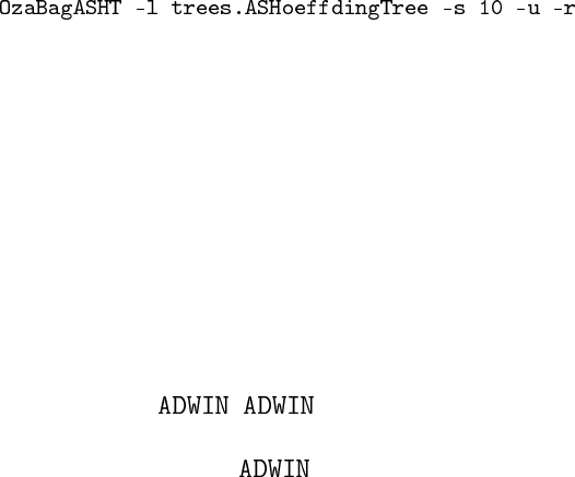
7.3.4 OzaBagASHT
Bagging using trees of different size. The Adaptive-Size Hoeffding Tree (ASHT)
is derived from the Hoeffding Tree algorithm with the following differences:
•it has a maximum number of split nodes, or size
•after one node splits, if the number of split nodes of the ASHT tree is
higher than the maximum value, then it deletes some nodes to reduce
its size
The intuition behind this method is as follows: smaller trees adapt more
quickly to changes, and larger trees do better during periods with no or little
change, simply because they were built on more data. Trees limited to size s
will be reset about twice as often as trees with a size limit of 2s. This creates
a set of different reset-speeds for an ensemble of such trees, and therefore a
subset of trees that are a good approximation for the current rate of change.
It is important to note that resets will happen all the time, even for stationary
datasets, but this behaviour should not have a negative impact on the ensem-
ble’s predictive performance.
When the tree size exceeds the maximun size value, there are two different
delete options:
•delete the oldest node, the root, and all of its children except the one
where the split has been made. After that, the root of the child not
deleted becomes the new root
•delete all the nodes of the tree, i.e., restart from a new root.
49
CHAPTER 7. CLASSIFIERS
The maximum allowed size for the n-th ASHT tree is twice the maximum
allowed size for the (n−1)-th tree. Moreover, each tree has a weight propor-
tional to the inverse of the square of its error, and it monitors its error with an
exponential weighted moving average (EWMA) with α=.01. The size of the
first tree is 2.
With this new method, it is attempted to improve bagging performance by
increasing tree diversity. It has been observed that boosting tends to produce a
more diverse set of classifiers than bagging, and this has been cited as a factor
in increased performance.
See more details in:
[BHPKG]Albert Bifet, Geoff Holmes, Bernhard Pfahringer, Richard Kirkby, and
Ricard Gavaldà. New ensemble methods for evolving data streams. In
15th ACM SIGKDD International Conference on Knowledge Discovery and
Data Mining, 2009.
The learner must be ASHoeffdingTree, a Hoeffding Tree with a maximum
size value.
Example:
Parameters:
•Same parameters as OzaBag
•-f : the size of first classifier in the bag.
•-u : Enable weight classifiers
•-r : Reset trees when size is higher than the max
7.3.5 OzaBagADWIN
Bagging using . is a change detector and estimator that solves in
a well-specified way the problem of tracking the average of a stream of bits or
real-valued numbers. keeps a variable-length window of recently seen
items, with the property that the window has the maximal length statistically
consistent with the hypothesis “there has been no change in the average value
inside the window".
More precisely, an older fragment of the window is dropped if and only if
there is enough evidence that its average value differs from that of the rest of
the window. This has two consequences: one, that change reliably declared
50
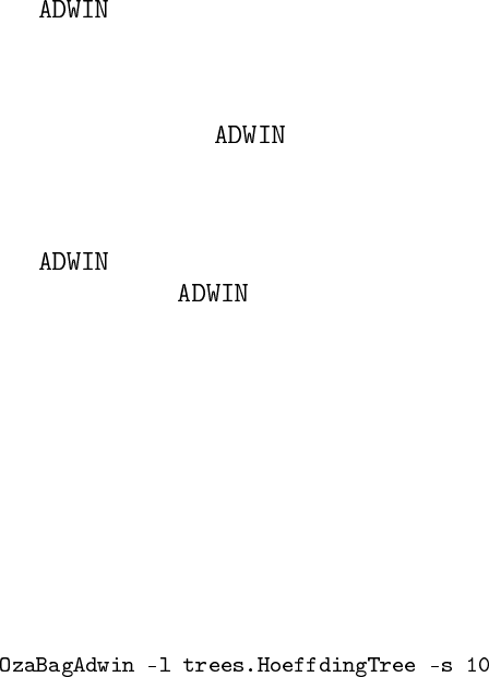
7.3. META CLASSIFIERS
whenever the window shrinks; and two, that at any time the average over the
existing window can be reliably taken as an estimation of the current average
in the stream (barring a very small or very recent change that is still not sta-
tistically visible). A formal and quantitative statement of these two points (a
theorem) appears in
[BG07c]Albert Bifet and Ricard Gavaldà. Learning from time-changing data with
adaptive windowing. In SIAM International Conference on Data Mining,
2007.
is parameter- and assumption-free in the sense that it automati-
cally detects and adapts to the current rate of change. Its only parameter is a
confidence bound δ, indicating how confident we want to be in the algorithm’s
output, inherent to all algorithms dealing with random processes.
Also important, does not maintain the window explicitly, but com-
presses it using a variant of the exponential histogram technique. This means
that it keeps a window of length Wusing only O(logW)memory and O(logW)
processing time per item.
Bagging is the online bagging method of Oza and Rusell with the
addition of the algorithm as a change detector and as an estimator
for the weights of the boosting method. When a change is detected, the worst
classifier of the ensemble of classifiers is removed and a new classifier is added
to the ensemble.
See details in:
[BHPKG]Albert Bifet, Geoff Holmes, Bernhard Pfahringer, Richard Kirkby, and
Ricard Gavaldà. New ensemble methods for evolving data streams. In
15th ACM SIGKDD International Conference on Knowledge Discovery and
Data Mining, 2009.
Example:
Parameters:
•-l : Classifier to train
•-s : The number of models in the bag
7.3.6 AccuracyWeightedEnsemble
The Accuracy Weighted Ensemble classifier as proposed by Wang et al. in
"Mining concept-drifting data streams using ensemble classifiers", KDD 2003.
51

CHAPTER 7. CLASSIFIERS
7.3.7 AccuracyUpdatedEnsemble
The Accuracy Updated Ensemble classifier as proposed by Brzezinski and Ste-
fanowski in "Accuracy Updated Ensemble for Data Streams with Concept Drift",
HAIS 2011.
7.3.8 LimAttClassifier
Ensemble Combining Restricted Hoeffding Trees using Stacking. It produces a
classification model based on an ensemble of restricted decision trees, where
each tree is built from a distinct subset of the attributes. The overall model is
formed by combining the log-odds of the predicted class probabilities of these
trees using sigmoid perceptrons, with one perceptron per class. In contrast
to the standard boosting approach, which forms an ensemble classifier in a
greedy fashion, building each tree in sequence and assigning corresponding
weights as a by-product, our method generates each tree in parallel and com-
bines them using perceptron classifiers by adopting the stacking approach.
For more information see
[BFHP]Albert Bifet, Eibe Frank, Geoffrey Holmes, Bernhard Pfahringer Accu-
rate Ensembles for Data Streams: Combining Restricted Hoeffding Trees
using Stacking. In Journal of Machine Learning Research - Proceedings
Track 13, 225-240 (2010).
Example:
Parameters:
•-l : Classifier to train.
•-n : The number of attributes to use per model.
•-w : The number to multiply the weight misclassified counts.
•-a : Delta of Adwin change detection
•-o : Offset for odds to avoid probabilities that are zero.
•-p : Enable pruning.
•-b : Use m-n attributes on the trees.
•-m : The pruned number of classifiers to use to predict.
•-z : When one Adwin detects change, replace worst classifier.
52

7.3. META CLASSIFIERS
7.3.9 LeveragingBag
Leveraging Bagging for evolving data streams using ADWIN and Leveraging
Bagging MC using Random Output Codes ( -o option).
These methods leverage the performance of bagging, with two randomiza-
tion improvements: increasing resampling and using output detection codes.
Algorithm 1 Leveraging Bagging for Mmodels
1: Initialize base models hmfor all m∈ {1,2, ..., M}
2: Compute coloring µm(y)
3: for all training examples (x,y)do
4: for m=1,2,..., Mdo
5: Set w=Poisson(λ)
6: Update hmwith the current example with weight wand class µm(y)
7: end for
8: end for
9: if detects change in error of one of the classifiers then
10: Replace classifier with higher error with a new one
11: end if
12: anytime output:
13: return hypothesis: hf in(x) = argmaxy∈YPT
t=1I(ht(x) = µt(y))
For more information see
[BHP]Albert Bifet, Geoffrey Holmes, Bernhard Pfahringer Leveraging Bagging
for Evolving Data Streams In Machine Learning and Knowledge Discovery
in Databases, European Conference, ECML PKDD, 2010.
Parameters:
•-l : Classifier to train.
•-s : The number of models in the bagging
•-w : The number to use to compute the weight of new instances.
•-a : Delta of Adwin change detection
•-o : Use Output Codes to use binary classifiers
•-m : Leveraging Bagging to use:
–Leveraging Bagging ME using weight 1 if misclassified, otherwise
error/(1-error)
53

CHAPTER 7. CLASSIFIERS
–Leveraging Bagging Half using resampling without replacement half
of the instances
–Leveraging Bagging WT without taking out all instances.
–Leveraging Subagging using resampling without replacement.
7.4 Function Classifiers
7.4.1 MajorityClass
Always predicts the class that has been observed most frequently the in the
training data.
Parameters:
•-r : Seed for random behaviour of the classifier
7.4.2 Perceptron
Single perceptron classifier. Performs classic perceptron multiclass learning
incrementally.
Parameters:
•-r : Learning ratio of the classifier
7.4.3 SGD
Implements stochastic gradient descent for learning various linear models:
binary class SVM, binary class logistic regression and linear regression.
7.4.4 SPegasos
Implements the stochastic variant of the Pegasos (Primal Estimated sub-GrAdient
SOlver for SVM) method of Shalev-Shwartz et al. (2007). For more informa-
tion, see:
[SSS]S. Shalev-Shwartz, Y. Singer, N. Srebro. Pegasos: Primal Estimated
sub-GrAdient SOlver for SVM. In 4th International Conference on Ma-
chineLearning, 807-814, 2007.
54

7.5. DRIFT CLASSIFIERS
7.5 Drift Classifiers
7.5.1 SingleClassifierDrift
Class for handling concept drift datasets with a wrapper on a classifier.
The drift detection method (DDM) proposed by Gama et al. controls the
number of errors produced by the learning model during prediction. It com-
pares the statistics of two windows: the first one contains all the data, and
the second one contains only the data from the beginning until the number
of errors increases. Their method doesn’t store these windows in memory. It
keeps only statistics and a window of recent errors.
They consider that the number of errors in a sample of examples is mod-
eled by a binomial distribution. A significant increase in the error of the algo-
rithm, suggests that the class distribution is changing and, hence, the actual
decision model is supposed to be inappropriate. They check for a warning
level and a drift level. Beyond these levels, change of context is considered.
The number of errors in a sample of nexamples is modeled by a binomial
distribution. For each point iin the sequence that is being sampled, the error
rate is the probability of misclassifying (pi), with standard deviation given
by si=ppi(1−pi)/i. A significant increase in the error of the algorithm,
suggests that the class distribution is changing and, hence, the actual decision
model is supposed to be inappropriate. Thus, they store the values of piand
siwhen pi+sireaches its minimum value during the process (obtaining ppmin
and smin). And it checks when the following conditions trigger:
•pi+si≥pmin +2·smin for the warning level. Beyond this level, the
examples are stored in anticipation of a possible change of context.
•pi+si≥pmin +3·smin for the drift level. Beyond this level, the model
induced by the learning method is reset and a new model is learnt using
the examples stored since the warning level triggered.
Baena-García et al. proposed a new method EDDM in order to improve
DDM. It is based on the estimated distribution of the distances between classi-
fication errors. The window resize procedure is governed by the same heuris-
tics.
See more details in:
[GMCR]J. Gama, P. Medas, G. Castillo, and P. Rodrigues. Learning with drift
detection. In SBIA Brazilian Symposium on Artificial Intelligence, pages
286–295, 2004.
55

CHAPTER 7. CLASSIFIERS
[BDF]Manuel Baena-García, José del Campo-Ávila, Raúl Fidalgo, Albert Bifet,
Ricard Gavaldá, and Rafael Morales-Bueno. Early drift detection method.
In Fourth International Workshop on Knowledge Discovery from Data Streams,
2006.
Example:
Parameters:
•-l : Classifier to train
•-d : Drift detection method to use: DDM or EDDM
56

8
Bi-directional interface with WEKA
Now, it is easy to use MOA classifiers and streams from WEKA, and WEKA clas-
sifiers from MOA. The main difference between using incremental classifiers
in WEKA and in MOA will be the evaluation method used.
8.1 WEKA classifiers from MOA
Weka classifiers may be incremental or non incremental methods.
To use the Weka classifiers from MOA it is necessary to use one of the
following classes:
57
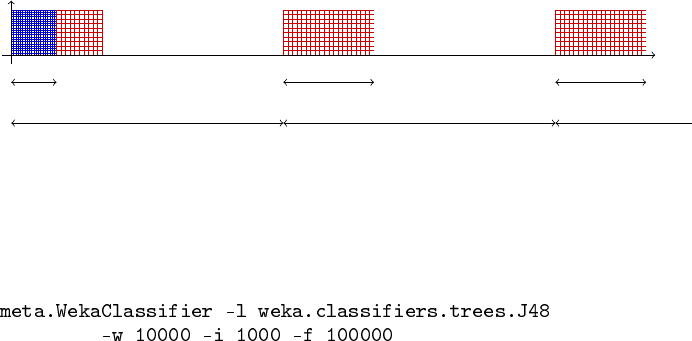
CHAPTER 8. BI-DIRECTIONAL INTERFACE WITH WEKA
8.1.1 WekaClassifier
A classifier to use classifiers from WEKA.
T T
WiW W
WEKAClassifier builds a model of Winstances every Tinstances only for
non incremental methods. For WEKA incremental methods the WEKA classifier
is trained for every instance.
Example:
Parameters:
•-l : Classifier to train
•-w : Size of Window for training learner
•-i : Size of first Window for training learner
•-f : How many instances between samples of the learning performance
8.1.2 SingleClassifierDrift
Class for handling concept drift datasets with a wrapper on a classifier.
The drift detection method (DDM) proposed by Gama et al. controls the
number of errors produced by the learning model during prediction. It com-
pares the statistics of two windows: the first one contains all the data, and
the second one contains only the data from the beginning until the number
of errors increases. Their method doesn’t store these windows in memory. It
keeps only statistics and a window of recent errors.
They consider that the number of errors in a sample of examples is mod-
eled by a binomial distribution. A significant increase in the error of the algo-
rithm, suggests that the class distribution is changing and, hence, the actual
decision model is supposed to be inappropriate. They check for a warning
level and a drift level. Beyond these levels, change of context is considered.
The number of errors in a sample of nexamples is modeled by a binomial
distribution. For each point iin the sequence that is being sampled, the error
58
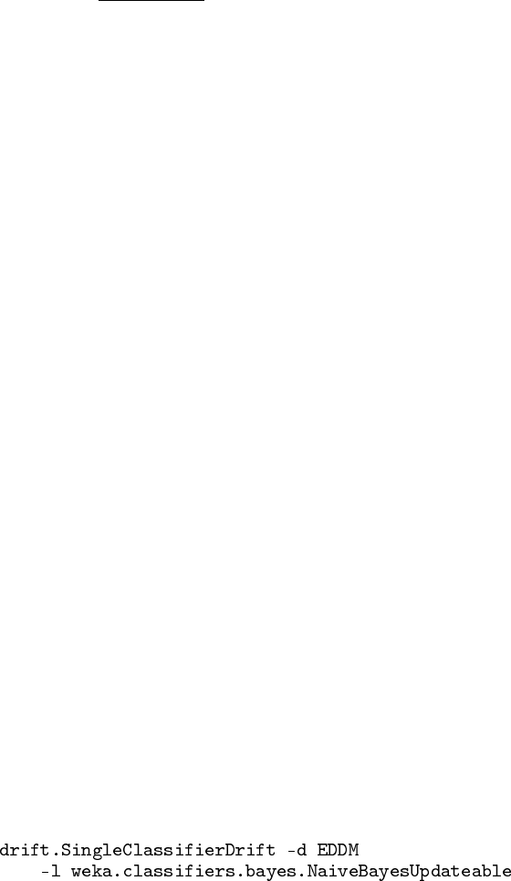
8.1. WEKA CLASSIFIERS FROM MOA
rate is the probability of misclassifying (pi), with standard deviation given
by si=ppi(1−pi)/i. A significant increase in the error of the algorithm,
suggests that the class distribution is changing and, hence, the actual decision
model is supposed to be inappropriate. Thus, they store the values of piand
siwhen pi+sireaches its minimum value during the process (obtaining ppmin
and smin). And it checks when the following conditions trigger:
•pi+si≥pmin +2·smin for the warning level. Beyond this level, the
examples are stored in anticipation of a possible change of context.
•pi+si≥pmin +3·smin for the drift level. Beyond this level, the model
induced by the learning method is reset and a new model is learnt using
the examples stored since the warning level triggered.
Baena-García et al. proposed a new method EDDM in order to improve
DDM. It is based on the estimated distribution of the distances between classi-
fication errors. The window resize procedure is governed by the same heuris-
tics.
See more details in:
[GMCR]J. Gama, P. Medas, G. Castillo, and P. Rodrigues. Learning with drift
detection. In SBIA Brazilian Symposium on Artificial Intelligence, pages
286–295, 2004.
[BDF]Manuel Baena-García, José del Campo-Ávila, Raúl Fidalgo, Albert Bifet,
Ricard Gavaldá, and Rafael Morales-Bueno. Early drift detection method.
In Fourth International Workshop on Knowledge Discovery from Data Streams,
2006.
Example:
Parameters:
•-l : Classifier to train
•-d : Drift detection method to use: DDM or EDDM
59
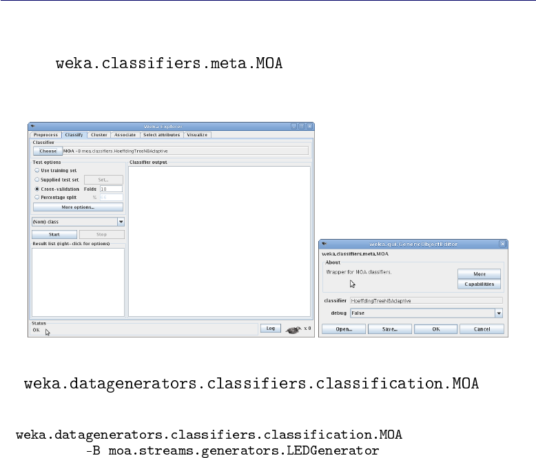
CHAPTER 8. BI-DIRECTIONAL INTERFACE WITH WEKA
8.2 MOA classifiers from WEKA
You can use MOA classifiers quite easily as incremental classifiers within the
WEKA Explorer, Knowledge Flow interface or command-line interface, us-
ing the meta-classifier. This meta-classifier
is just a wrapper for MOA classifiers, translating the WEKA method calls into
MOA ones.
You can use MOA streams within the WEKA framework using the
data generator. For example:
In order to manipulate the MOA classifiers in the GUI, like Explorer or
Experimenter, you need to register a new editor for the GenericObjectEditor.
The following steps are necessary to integrate the MOA classifiers:
1. Determine the location of your home directory:
•Windows in a command prompt, run the following command: echo
%USERPROFILE%
•Linux/Unix in a terminal (bash), run the following command: echo
$HOME
2. Copy the "GUIEdtitors.props.addon" file, contained in the MOA project
in the source directory "src/main/java/weka/gui" or in the moa.jar in
"weka/gui", into your home directory. Rename the extension from ".props.addon"
to ".props". If the home directory already contains such a file, then just
append the content of the version in MOA file to the already existing
one.
60
8.2. MOA CLASSIFIERS FROM WEKA
3. Restart WEKA from the MOA project, e.g., using the "run-explorer" target
of the ANT build file.
61
