Manual
User Manual:
Open the PDF directly: View PDF ![]() .
.
Page Count: 37

arTeMiDe ver.1.4
Alexey A. Vladimirov
January 21, 2019
User manual for arTeMiDe package, which evaluated TMDs and related cross-sections.
Manual is updating.
This work is licensed under the Creative Commons Attribution-NonCommercial-ShareAlike 4.0 International
License. To view a copy of this license, visit http://creativecommons.org/licenses/by-nc-sa/4.0/ or send a
letter to Creative Commons, PO Box 1866, Mountain View, CA 94042, USA.
If you use the arTeMiDe, please, quote [1].
If you find mistakes, have suggestions, or have questions write to:
Alexey Vladimirov: Alexey.Vladimirov@physik.uni-regensburg.de or vladimirov.aleksey@gmail.com
Contents
Glossary 4
I. General structure and user input of arTeMiDe 5
A. General structure 5
B. User defined functions and options 5
C. Setup 6
II. QCDinput module 7
III. TMDX DY module 8
A. Initialization 8
B. Setting up the parameters of cross-section 9
C. Cross-section evaluation 9
D. Parallel computation 11
E. LeptonCutsDY 12
F. Variation of scale 12
G. Power corrections 12
H. Enumeration of processes 13
IV. TMDX SIDIS module 14
A. Setting up the parameters of cross-section 14
B. Cross-section evaluation 15
C. Power corrections 16
D. Enumeration of processes 16
V. TMDF module 17
A. Initialization 17
B. NP parameters and scale variation 17
C. Evaluating Structure functions 18
D. Enumeration of structure functions 19
VI. TMDs module 21
A. Initialization 21
B. Definition of low-scales 22
C. Evaluating TMDs 22
D. Products of TMDs 23
E. Grid construction 23

2
F. Theoretical uncertainties 23
VII. TMDs inKT module 24
VIII. TMDR module 25
A. Theory 25
B. Initialization 25
C. NP input and NP parameters 26
D. Evaluating TMD evolution kernel 26
E. Inverted evolution and the lowest available Q 27
IX. uTMDPDF module 28
A. Initialization 28
B. Definition of non-perturbative part, fNP and parameters 28
C. Evaluating unpolarized TMD PDFs 29
D. Grid construction 30
E. Theoretical uncertainties 30
X. uTMDFF module 31
XI. Supplementary codes 31
A. Drell-Yan cross-section 31
XII. Harpy 32
References 33
XIII. Version history 34
A. Backup 36
TO DO LIST 36
B. arTeMiDe structure before v1.3 37
3
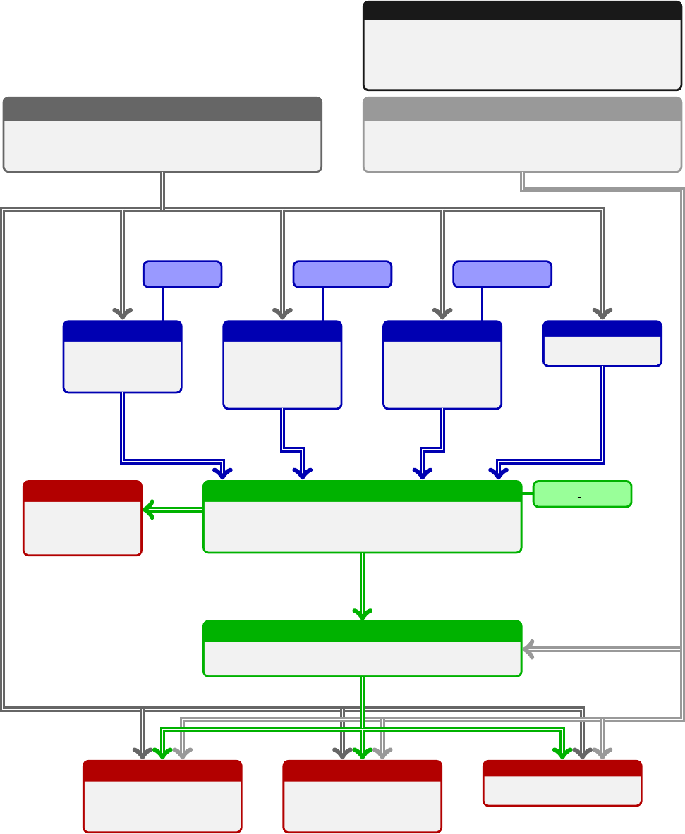
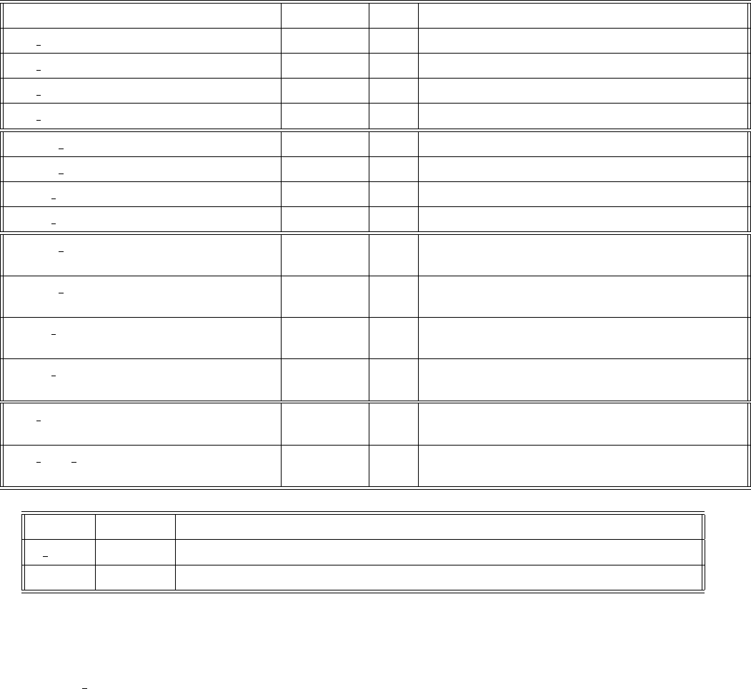
QCDinput
User code that provides αs, PDFs, FFs, etc.
Default version is interfaced to LHAPDF.
EWinput
User code that provides αQED,gV,MZ, etc.
Default version has PDG definitions.
constants
Text file that contains definitions and inputs
necessary to define the TMD scheme to works,
working parameters, etc.
TMDR
TMD
evolution.
TMDR model
uTMDPDF
optimal
unpolarized
TMDPDF
uTMDPDF model
uTMDFF
optimal
unpolarized
TMDFF
uTMDFF model
...
...
TMDs
Combines TMD distributions, and interfaces to
lower modules.
TMDs inKT
TMDs in
kT-space.
TMDS model
TMDF
Evaluate structure functions.
TMDX DY
DY-like cross-
sections.
TMDX SIDIS
SIDIS-like cross-
sections.
...
...
4
Glossary
TMD = Transverse Momentum Dependent
PDF = Parton Distribution Function
FF = Fragmentation Function
NP = Non-perturbative

5
I. GENERAL STRUCTURE AND USER INPUT OF ARTEMIDE
A. General structure
The arTeMiDe package is a set of libraries for evaluation of individual TMD distributions, TMD evolution factors,
and other ingredients of TMD factorization theorem. The final goal is the evaluation of cross-section within the TMD
factorization theorem, including all needed integrations, and factor, i.e. such that it can be directly compared to the
data. It also includes several tools for analysis of the obtained values, such as variation of scales, search for limiting
parameters, etc. The structure of modules dependencies is presented on the diagram (shown on the previous page).
The usage of the higher order module excludes the direct operation with a lower modules, because
the higher order module controls parameters of the lower modules (which can be in contradiction to the
direct operation).
The ultimate goal of the arTeMiDe is to evaluate the observables in the TMD factorization framework, such as
cross-section, asymmetries, etc. The general structure of the TMD factorized fully differential cross-section is
dσ
dX =dσ(qT) = prefactor1×prefactor2×F, (1.1)
where prefactor1 a process-dependent prefactor, prefactor2 is the experiment dependent prefactor, and Fis the
reduced structure function. The role of prefactors 1 and 2 is naturally interchangeable, however, we expect that all
universal factorization dependence (such as hard parts, parton cross-sections) is concentrated in prefactor1, while
non-universal dependence on the particular measurement (e.g phase space multiplies, cut functions) is concentrated
in the prefactor2. Example, for the photon induced Drell-Yan process one has for dσ/dqT
prefactor1 = 4π
9sQ2|CV(Q, µH)|2
prefactor2 = 1 + q2
T
2Q2
F=Zbdb
2J0(bqT)X
f|ef|2Ff(xA, b;µH, ζA)F¯
f(xB, b;µH, ζB).
The structure function Fis generally defined as
F(qT, x1, x2;µ, ζ1, ζ2) = Zbdb
2bnJn(bqT)X
ff0
zff0Ff
1(x1, b;µ, ζ1)Ff0
2(x2, b;µ, ζ2),(1.2)
where F1,2are TMD distributions (of any origin and polarization), zf f 0is the process dependent flavor mixing factor.
The number nis also process dependent, e.g. for unpolarized observables it is n= 0, while for SSA’s it is n= 1.
Evaluation structure functions Fis performed in the module TMDF. The evaluation of cross-sections is performed in
the modules TMDX. The TMD distributions are evaluated by the module TMDs and related submodules.
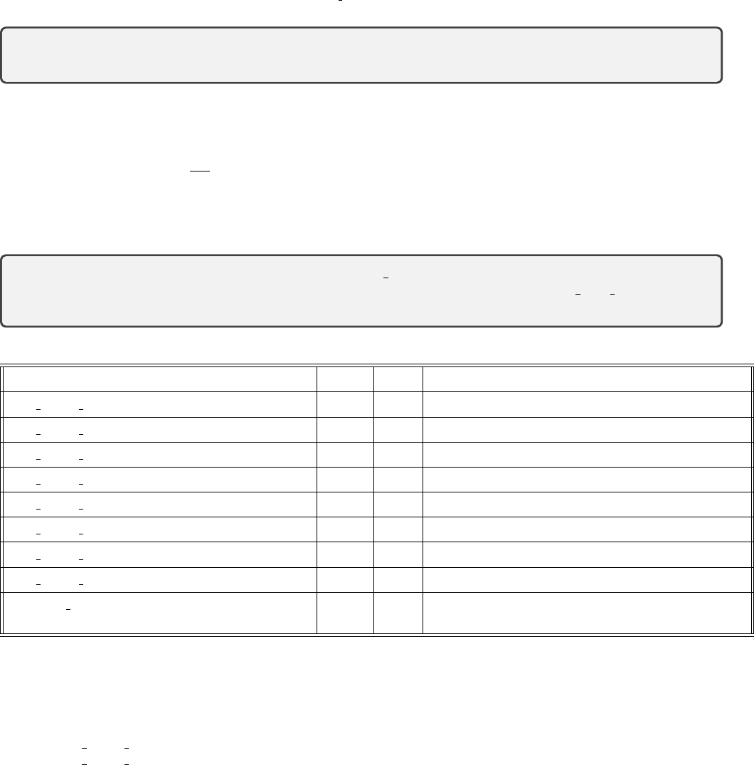
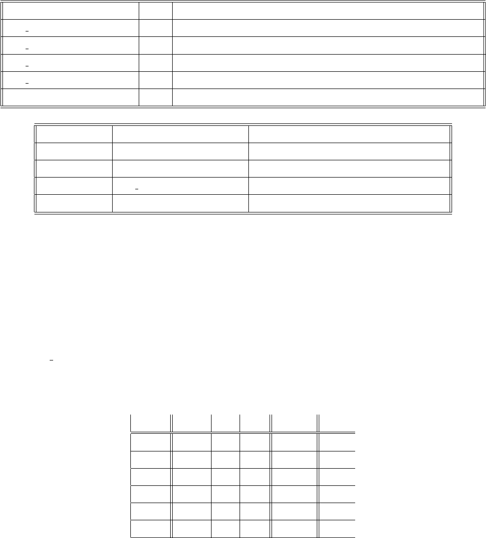
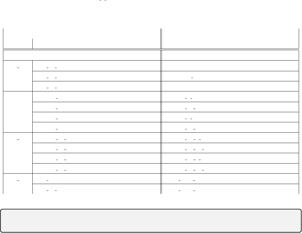
Nesting structure of arTeMiDe and responsible modules
Quantity Rough formula Name Module
dσ Rd[bin](prefactors)×Fcross-section TMDX
FRbdb
2bnJn(bqT)Pff0zf f 0Ff
1Ff0
2structure function TMDF
Ff
iRf(µf→µi)Ff
i(µi) evolved TMD distribution TMDs
RTMD evolution factor TMDR
Ff
i(µi)C⊗ffNP model for TMD distribution depends on kind
B. User defined functions and options

6
The arTeMiDe package has been created such that it allows to control each aspect of TMD factorization
theorem. The TMD factorization has a large number of free, and “almost-free” parameters. It is a generally
difficult task to provide a convenient interface for all these inputs. I do my best to make the interface convenient,
however, some parts (e.g. setup of fNP ) could not be simpler (at least within FORTRAN). Also, take care
arTeMiDe is evolving, and I do not really care about back compatibility.
The user has to provide (or use the default values) the set of parameters, that control various aspects of
evaluation. It includes PDF sets, fN P , perturbative scales, parameters of numerics, non-QCD inputs, etc. There are
three input sources for statical parameters.
General parameters: These are working parameters of the arTeMiDe library, such as amount of output
tolerance of integration routines, number of NP parameters, type of evolution, griding parameters, triggering of
particular contributions, etc. There are many of them, and typically they are unchanged. These are set in the
file (in text format) : constants.Changes do not require recompilation.
External physics input: It includes the definition of αs, collinear PDFs, and other distributions. They are
provided by user via the ”interface” module QCDinput. Default version is uses LHAPDF interface [4]. For non-
QCD parameters, e.g. αQED, SM parameters, there is a module QEDinput.Changes require recompilation.
For further information see sec.II.
NP model: The NP model consists in NP profiles of TMD distributions, NP model for large-b evolution,
selection of scales µ, etc. These parameter and functions enter nearly each low level module. The code for corre-
sponding functions is provided by user, in appropriate files, which are collected in the subdirectory src/Model.
The name of files are shown on diagram in colored blobs adjusted to the related module. Changes require
recompilation. See also section of corresponding modules.
Comments:
•constants must be in the same directory as the executing file.
•NP functions are typically defined with a number of numeric parameters. The value of these parameters
could be changed without restart (or recompilation) of the arTeMiDe by appropriate command. E.g. (call
TMDs SetNPParameters(lambda)) on the level of TMDs module. See sections of corresponding modules.
•The maximum number of parameters in the model for each module is set in constants-file.
•The directory /Model is convenient to keep as is. We provide our extraction as such directories. However,
QCDinput and QEDinput are not a part of model (although, in bigger sense they are).
C. Setup
Download and unpack arTeMiDe. The actual code is in the /src. Check the makefile. You have to fix options FC
and FOPT, which are defined in the top of it. FC is the FORTRAN compiler, FOPT is additional options for compiler
(e.g. linking to LHAPDF library).
There is no actual installation procedure, there is just compilation. If model, inputs, etc, are set correctly (typical
problem is linking to LHAPDF, be sure that it is installed correctly), then make compiles the library. The result are
object files (*.o) (which are collected in /obj) and module files (*.mod) (which are collected in /mod).
Next, do your code, include appropriate modules of arTeMiDe, and compile it together with object-files (do not
forget to add proper references to module files -I/mod). It should work! It could be done automatically if you put
your code in directory /Prog, and call for make program TARGET=..., where ... is the name of the file with code.

7
II. QCDINPUT MODULE
The module QCDinput gives an interface to external function provided by the user, such as PDF, FF, values of
alpha-strong. It is completely user defined. In particular, in the default version it is linked to LHAPDF library [4].
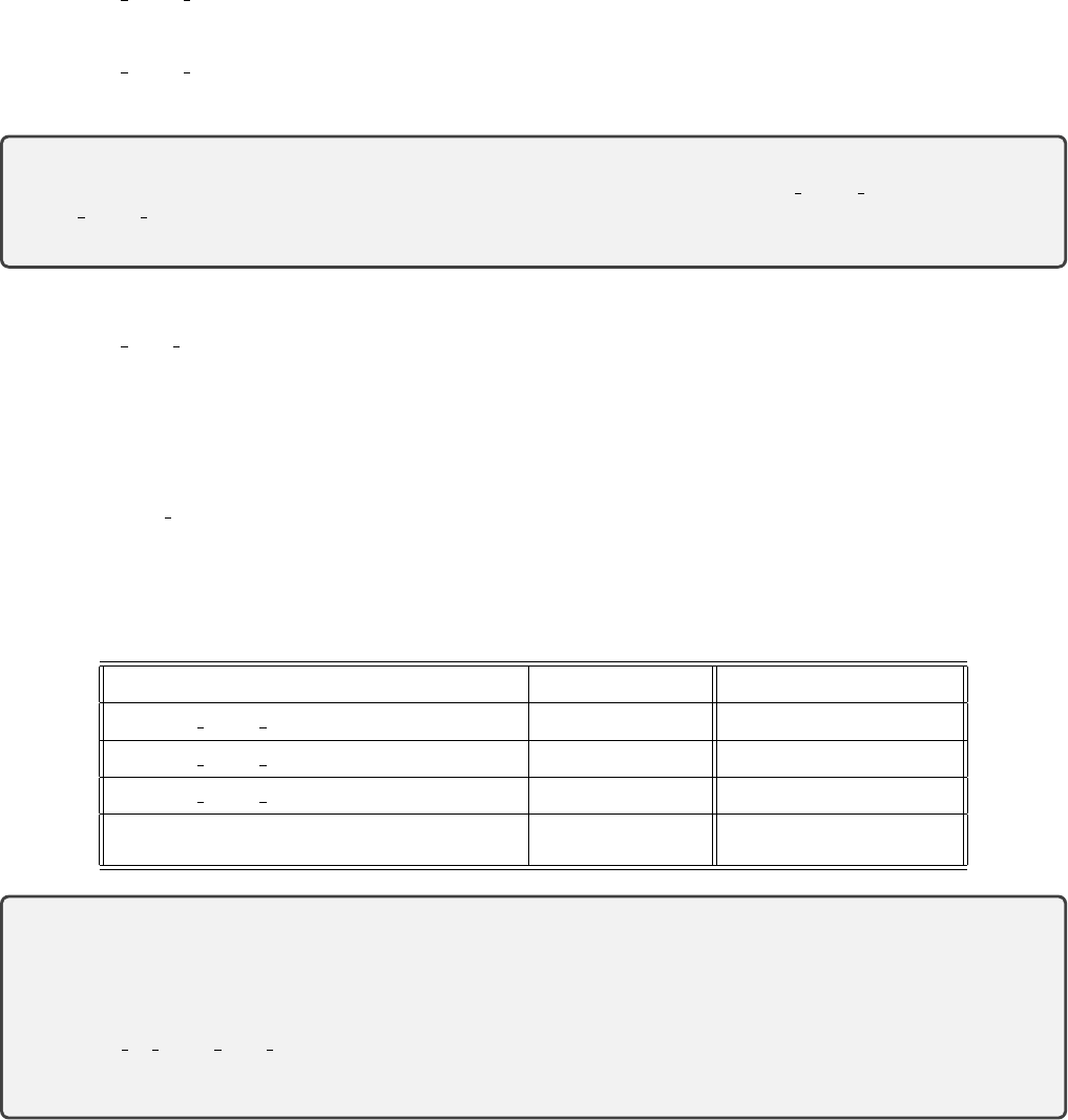
List of available commands
Command Description
QCDinput Initialize(order) Subroutine to initialize anything what is needed. (string) param-
eter order is passed from arTeMiDe modules and conventionally
takes values LO,LO+,NLO,NLO+,NNLO,NNLO+ (see e.g. secVIII B).
According to this variable the QCD input should be initialized.
As(Q) Returns the (real*8) value of αs(Q)/(4π). Qis (real*8).
xPDF(x,Q,hadron) Returns the (real*8(-5:5)) value of xf(x, Q) for given hadron. x,
Qare (real*8), hadron is (integer).
xFF(x,Q,hadron) Returns the (real*8(-5:5)) value of xd(x, Q) for given hadron. x,
Qare (real*8), hadron is (integer).

8
III. TMDX DY MODULE
This module evaluates cross-sections with the Drell-Yan-like kinematics. I.e. it expects the following kinematic
input, (s, Q, y) which defines the variables x’s, etc.
The general structure of the cross-section is
dσ
dX =dσ(qT) = prefactor1Z[bin]prefactor2×F, (3.1)
where dX ∼dQdsdydqT. The pref actor2 is expected to be x−independent1. All x-dependence is set into F.
Generally, the prefactor2 ×Fis
prefactor2×F= (cuts for lepton pair) ×H(Q, µH)F(Q, qT, x1, x2, µ, ζ1, ζ),(3.2)
where Fis defined in (5.1). There are following feature of current implementation
•In the current version the scaling variables are set as
µ2=ζ1=ζ2=Q2.(3.3)
Currently, it is hard coded and could not be easily modified. However, there is a possibility to vary the value of
µas µ=c2Q, where c2is variation parameter (see sec.III F).
•For the definition of (cuts for lepton pair)-function see [1]. It is evaluated within module LeptonCutsDY.f90.
The presence of cuts, and their parameters are set by the SetCuts subroutine.
•The expression for the hard factor His taken from [10]. It is the function of ln(Q/µH) and as(µH)). Since in
the current realization µH=Q, the logarithm is replaced by ln(c2), where c2is the variation constant.
This section is to be updated by definition of kinematics
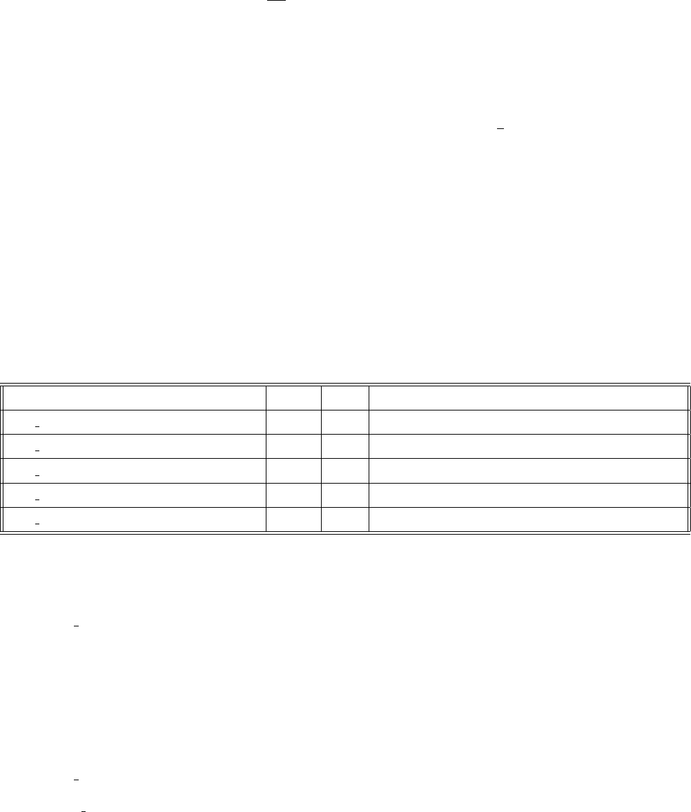
List of available commands
Command Type Sec. Short description
TMDX DY Initialize(order) subrout. III A Initialization of module.
TMDX DY SetNPParameters(...) subrout. III B Set new NP parameters to the modules
TMDX DY SetProcess(p) subrout. III B Set the process
SetCuts(inc,pT,eta1,eta2) subrout. III B Set the current evaluation of cut for lepton pair.
TMDX DY XSetup(s,Q,y) subrout. III B Set the kinematic variables
TMDX DY SetScaleVariations(c1,c2,c3,c4) subrout. – Set new values for the scale-variation constants.
TMDX DY ShowStatistic() subrout. – Print current statistic on the number of calls.
CalcXsec DY... subrout. III C Evaluates cross-section. Many overloaded versions
see sec.III C.
A. Initialization
Prior the usage module is to be initialized (once per run) by
call TMDX DY Initialize(order)
here: order is the declaration of order. It can be ’LO’,’LO+’,’NLO’,’NLO+’,’NNLO’ or ’NNLO+’. This is a complex
declaration, which implies particular orders for coefficient functions, PDFs, anomalous dimension, etc. For detailed
definition see other sections.
1Not necessary in ver.1.4.

9
B. Setting up the parameters of cross-section
Prior to evaluation of cross-section one must declare which process is considered and to set up the kinematics. The
declaration of the process is made by
call TMDX DY SetProcess(p1,p2,p3)
call TMDX DY SetProcess(p0)
where p0=(/p1,p2,p3/) and
p1 (integer) Defines the prefactor1 that contains the phase space elements, and generally experimental dependent.
It also influence the bin-integration definition.
p2 (integer) Defines the prefactor2 that contains the universal part of factorization formula.
p3 (integer) Defines the structure function F. See sec.V D.
Alternatively, process can be declared by a shorthand version
call TMDX DY SetProcess(p)
where p(integer) corresponds to particular combinations of p1,p2,p3. See table III H.
The kinematic of the process is declared by
call TMDX DY XSetup(s,Q,y)
where sis the Mandelshtam variable s,Qis hard virtuality Q,yis the rapidity parameter y. Note, that these values
will be used for the evaluation of the cross-section. In the case, the integration over the bin is made these values are
overridden. Also in the case of the parallel computation these variables are overridden. So, often there is little sense
in this command, nonetheless it set initial values.
All non-perturbative parameters are defined in the TMDs and lower-level modules. For user convenience there is a
subroutine, which passes the values of parameters to TMDs. It is
call TMDX DY SetNPParameters(lambda/n)
where lambda is real*8(1:number of parameters) or nis the label of replica. See also VI C.
Finally, one must specify the fiducial cuts on the lepton pair. It is made by calling
call SetCuts(inc,pT,eta1,eta2)
where parameter inc is (logical). If inc=.true. the evaluation of cuts will be done, otherwise it will be ignored.
The cuts are defined as
|lT|,|l0
T|<pT,eta1 < η, η0,eta2,(3.4)
where land l0are the momenta of produced leptons, with lT’s being their transverse components and η’s being their
rapidities. For accurate definition of the cut-function see sec.2.6 of [1] (particularly equations (2.40)-(2.42)). For
asymmetric cuts use call SetCuts(inc,pT1,pT2,eta1,eta2).
Current realization prevents usage of different cuts in parallel computation. Will be fixed in later
versions.
C. Cross-section evaluation
After the parameters of cross-section are set up, the values of the cross-section at different qTcan be obtained by
call CalcXsec DY(X,qt)
where Xis real*8 variable where cross-section will be stored, qt is real*8 is the list of values of qT’s at which the X
is to be calculated. There exists an overloaded version with X(real*8)(1:N) and qT(real*8)(1:N), which evaluates the
array of crossections over array of qT.
Typically, one needs to integrate over bin. There is a whole set of subroutines which evaluate various integrals over
bin they are

10
Subroutine integral Comment
CalcXsec DY Yint(X,qt) Ry0
−y0dydσ(qT)y0is maximum allowed
yby kinematics, y0=
ln(s/Q2)/2.
CalcXsec DY Yint(X,qt,yMin,yMax) Rymax
ymin dydσ(qT)|ymax/min|< y0
CalcXsec DY Qint (X,qt,Qmin,Qmax) RQmax
Qmin 2QdQdσ(qT)
CalcXsec DY Qint Yint (X,qt,Qmin,Qmax) RQmax
Qmin 2QdQ Ry0
−y0dydσ(qT)
CalcXsec DY Qint Yint
(X,qt,Qmin,Qmax,yMin,yMax) RQmax
Qmin 2QdQ Rymax
ymin dydσ(qT)
CalcXsec DY PTint Qint Yint
(X,qtmin,qtmax,Qmin,Qmax) RqTmax
qTmin 2qTdqTRQmax
Qmin 2QdQ Ry0
−y0dydσ(qT) Integration over qTis
Simpsons by default num-
ber of sections.
CalcXsec DY PTint Qint Yint
(X,qtmin,qtmax,Qmin,Qmax,yMin,yMax) RqTmax
qTmin 2qTdqTRQmax
Qmin 2QdQ Rymax
ymin dydσ(qT) Integration over qTis
Simpsons by default num-
ber of sections.
CalcXsec DY PTint Qint Yint
(X,qtmin,qtmax,Qmin,Qmax,N) RqTmax
qTmin 2qTdqTRQmax
Qmin 2QdQ Ry0
−y0dydσ(qT) Integration over qTis
Simpsons by N-section.
CalcXsec DY PTint Qint Yint
(X,qtmin,qtmax,Qmin,Qmax,yMin,yMax,N) RqTmax
qTmin 2qTdqTRQmax
Qmin 2QdQ Rymax
ymin dydσ(qT) Integration over qTis
Simpsons by N-section.
More to be added
In version 1.3
CalcXsec DY XFint(X,qt,xfMin,xfMax) RxFmax
xFmin dxFdσ(qT)xF=2√Q2+q2
T
√ssinh y
dxF=2√Q2+q2
T
√scosh y dy
CalcXsec DY Qint XFint
(X,qt,Qmin,Qmax,xfMin,xfMax) RQmax
Qmin 2QdQ RxFmax
xFmin dxFdσ(qT)
CalcXsec DY PTint Qint XFint
(X,qtmin,qtmax,Qmin,Qmax,xfMin,xfMax) RqTmax
qTmin 2qTdqTRQmax
Qmin 2QdQ RxFmax
xFmin dxF dσ(qT)Integration over qTis
Simpsons by default num-
ber of sections.
CalcXsec DY PTint Qint XFint
(X,qtmin,qtmax,Qmin,Qmax,xfMin,xfMax,N)
RqTmax
qTmin 2qTdqTRQmax
Qmin 2QdQ RxFmax
xFmin dxFdσ(qT) Integration over qTis
Simpsons by N-section.
Note 1: Each command has overloaded version with arrays for X and qt.
Note 2: Cross-section integrated over qTbins have overloaded versions with X,qtmin and qtmax being arrays.
Then the integral is done for X(i) from qtmin(i) to qtmax(i).
Note 2+: There exists an overloaded version for CalcXsec DY PTint Qint Yint with X,qtmin and qtmax,
yMin,yMax being arrays. Then the integral is done for X(i) from qtmin(i) to qtmax(i),yMin(i) to yMax(i).
Note 3: There exist special overloaded case for integrated over qT-bins, with successive bins. I.e. for bins
that adjust to each other. In this case only one argument qtlist is required (instead of qtmin,qtmax).
E.g. CalcXsec DY PTint Qint Yint (X,qtList,Qmin,Qmax). The length of qtlist must be larger then the
length of Xby one. The integration for X(i) is done from qtlist(i) till qtlist(i+1). This function saves
boundary values and therefore somewhat faster than the usual evaluation. (Improvement takes a place is only
for un-parallel calculation).
Take care that every next function is heavier to evaluate then the previous one. The integrations over Qand yare
adaptive Simpsons. We have found that it is the fastest (adaptive) method for typical cross-sections with tolerance
10−3−10−4. Naturally, it is not suitable for higher precision, which however is not typically required. The integration
over pt is not adaptive, since typically pT-bins are rather smooth and integral is already accurate if approximated

11
by 4-8 points (default minimal value is set in constants, which is automatically increased for larger bins). For
unexceptionally large qT-bins, or very rapid behavior we suggest to use overloaded versions with manual set of N
(number of integral sections).
There is a subroutine that evaluate cross-section without preliminary call of
SetCuts,TMDX DY SetProcess,TMDX DY XSetup.It is called xSec DY and it have the following interface:
xSec DY(X,process,s,qT,Q,y,includeCuts,CutParameters,Num)
where
•Xis (real*8) value of cross-section.
•process is integer p, or (integer)array (p1,p2,p3).
•sis Mandelshtam variable s
•qT is (real*8)array (qtmin,qtmax)
•Qis (real*8)array (Qmin,Qmax)
•yis (real*8)array (ymin,ymax)
•includeCuts is logical
•CutParameters is (real*8) array (k1,k2,eta1,eta2) OPTIONAL
•Num is even integer that determine number of section in qTintegral OPTIONAL
Note, that optional variables could be omit during the call.
IMPORTANT: Practically, the call of this function coincides with Xevaluated by the following set of commands
call TMDX DY SetProcess(process)
call TMDX DY XSetup(s,any,any)
call SetCuts(includeCuts,k1,k2,eta1,eta2)
call CalcXsec DY PTint Qint Yint (X,qtmin,qtmax,Qmin,Qmax,yMin,yMax,Num)
However, there is an important difference. The values of s, process, cutParameters set by routines ..Set..
are global. And thus could not be used in parallel computation. In the function xSec DY they are set locally and thus
this function can be used in parallel computations.
?BUG?: Take care that some Fortran compilers, do not understand the usage of arrays directly within function
with optional arguments. E.g. xSec DY(p,s,(/q1,q2/),Q,y,iC,CutParameters=cc). Although it compiles with-
out problems but lead to a freeze during the calculation. In this case, it helps to define: qT=(/q1,q2/) and call
xSec DY(p,s,qT,Q,y,iC,CutParameters=cc). The same problem can appear if xSec DY is used as argument of
another function. I guess there is some problem with memory references.
There is also analogous subroutine that evaluate cross-section by list. It is called xSec DY List and
it have the following interface:
xSec DY List(X,process,s,qT,Q,y,includeCuts,CutParameters,Num)
All variables are analogues to those of xSec DY, but should come in lists, i.e. Xis (1:n), process is (1:n,1:3),
sis (1:n), qT,Q,yare (1:n,1:2), includeCuts is (1:n), CutParameters is (1:n,1:4), and Num is (1:n). Only the
Num argument is OPTIONAL arguments. The argument CutParameters must be presented. This
command compiled by OPENMP, so runs in parallel on multi-core computers.
D. Parallel computation
For the historical reasons the initial code of arTeMiDe did not allow parallelization (it was due to intensive usage of
shared grids). I am working on this problem, improving different parts of code and excluding/encapsulating sharing

12
constructions. After ver.1.32 there is a limited parallelization on the level of computation of the cross-section (the
most expansive level of computation). The parallelization option is planned to improve in the future, making possible
to evaluate large cross-experiment lists of cross-sections in parallel.
Currently, the parallel evaluation is used within the commands CalcXsec DY ... with array variable qt (see Note
1in sec.TMDX:xsec). Basically, in this case, individual values for the list of cross-sections are evaluated in parallel.
The parallelization is made with OPENMP library. To make the parallel computation possible, add -fopenmp
option in the compilation instructions. The maximum number of allowed threads is set constants-file, in the section
6.
WARNING: the parallel operation is possible only together with grid option, otherwise it will cause a running
condition in TMD modules (which typically results into the program crush). There is no check for grid option
trigger, check it manually.
E. LeptonCutsDY
The calculation of cut prefactor is made in LeptonCutsDY.f90. It has two public procedures: SetCutParameters,
and CutFactor4.
•The subroutine SetCutParameters(kT,eta1,eta2) set a default version of cut parameters: p1,2< kTand
η1< η < η2.
•The overloaded version of the subroutine SetCutParameters(k1,k2,eta1,eta2) set a default version of asym-
metric cut parameters. p1< k1,p2< k2and η1< η < η2.
•Function CutFactor4(qT,Q in,y in, CutParameters) calculates the cut prefactor at the point qT,Q,y. The
argument CutParameters is optional. If it is not present, cut parameters are taken from default values (which
are set by SetCutParameters). CutParameters is array (/ k1,k2,eta1,eta2/). The usage of global definition
for CutParameters is not recommended, since it can result into running condition during parallel computation.
This is interface is left fro compatibility with earlier version of artemide.
F. Variation of scale
TO BE WRITTEN
G. Power corrections
There are many sources of power corrections. For a moment there is no systematic studies of power corrections for
TMD factorization. Nonetheless I include some options in artemide, and plan to make more systematic treatment in
the future.
Exact values of x1,2for DY: The TMD distributions enter the cross-section with x1and x2equal to
x1=q+
p+
1
=Q
√seys1 + q2
T
Q2'Q
√sey,(3.5)
x1=q+
p+
1
=Q
√se−ys1 + q2
T
Q2'Q
√se−y.
Traditionally, the corrections ∼qT/Q are dropped, since they are power corrections. Nonetheless, they could be
included since they have different sources in comparison to power corrections to the factorized cross-section. Usage
of one or another version of x1,2is switched by the parameter 5.A.1) in constants.

13
H. Enumeration of processes
List of enumeration for prefactor1
p1
p1 prefactor1 Short description
1 1 dX =dydQ2dq2
T.
22√Q2+q2
T
√scosh y dX =dxFdQ2dq2
Twhere xF=2√Q2+q2
T
√ssinh yis Feynman x.Important:
In this case the integration yis preplaced by the integration over xF. I.e.
... Yint(..., a, b, ..) which usually evaluates Rb
ady evaluates Rb
adxF.
List of enumeration for prefactor2
p2
p2 prefactor2 Short description
14π
9
α2
em (Q)
sQ2|CDY
V(c2Q)|2R×cut(qT) DY-cross-section dσ
dQ2dyd(q2
T). cut(qT) is the weight for the lepton tensor with
fiducial cuts (see sec.2.6 in [1]). Corresponds to DY-cross-section dσ
dQ2dyd(q2
T).
Process declared y↔ −ysymmetric. The result is in pb/GeV2
24π
9
α2
em (Q)
sQ2|CDY
V(c2Q)|2R×cut(qT) DY-cross-section dσ
dQ2dyd(q2
T). cut(qT) is the weight for the lepton tensor with
fiducial cuts (see sec.2.6 in [1]). Process declared y↔ −ynon-symmetric.
The result is in pb/GeV2
34π2
3
αem (Q)
sBrZ|CDY
V(c2Q)|2R×cut(qT) DY-cross-section dσ
dQ2dyd(q2
T)for the Z-boson production in the narrow width
approximation. BrZ= 0.03645 is Z-boson branching ration to leptons. cut(qT)
is the weight for the lepton tensor with fiducial cuts (see sec.2.6 in [1]). Process
declared y↔ −ysymmetric. The result is in pb/GeV2
Here R= 0.3893379 ·109the transformation factor from GeV to pb.
List of shorthand enumeration for processes
p p1 p2 p3 Description
1 1 1 5 p+p→Z+γ∗→ll. Standard DY process measured in the vicinity of the
Z-peak. E.g. for LHC measurements.
2 1 1 6 p+ ¯p→Z+γ∗→ll. Standard DY process measured in the vicinity of the
Z-peak. E.g. for Tevatron measurements.
14
IV. TMDX SIDIS MODULE
In ver.1.4, this module has not been checked for bugs, and errors so well as DY module. I do
not guaranty all correct factors. I hope to do so in ver. 1.5.
This module evaluates cross-sections with the SIDIS-like kinematics. I.e. it expects the following kinematic input,
(Q, x, z) or (Q, y, z) or (x, y, z), that are equivalent.
The general structure of the cross-section is
dσ
dX =dσ(qT) = prefactor1Z[bin]prefactor2×F, (4.1)
where dX ∼dl0, with l0momentum of scattered lepton.
The prefactor2 is expected to be x−independent. All x-dependence is set into F.
This section is to be updated by definition of kinematics
The structure of the module repeats the structure of TMDX DY module, with the main change in the kinematic
definition. Most part of routines has the same input and output with only replacement DY→SIDIS. We do
not comment such commands. They marked by ∗in the following table.
List of available commands
Command Type Sec. Short description
TMDX SIDIS Initialize(order) subrout. III A * Initialization of module.
TMDX SIDIS SetNPParameters(...) subrout. III B * Set new NP parameters to the modules
TMDX SIDIS SetProcess(p) subrout. IV A Set the process
TMDX SIDIS SetTargetMass(M) subrout. IV A Set the mass of target hadron
TMDX SIDIS SetProducedMass(M) subrout. IV A Set the mass of produced hadron
TMDX SIDIS XSetup(s,Q,y) subrout. IV A Set the kinematic variables
TMDX SIDIS SetScaleVariations(c1,c2,c3,c4) subrout. – * Set new values for the scale-variation constants.
TMDX SIDIS ShowStatistic() subrout. – * Print current statistic on the number of calls.
CalcXsec SIDIS... subrout. IV B Evaluates cross-section. Many overloaded versions
see sec.III C.
A. Setting up the parameters of cross-section
Prior to evaluation of cross-section one must declare which process is considered and to set up the kinematics.
The declaration of the process is made by
call TMDX SIDIS SetProcess(p1,p2,p3)
call TMDX SIDIS SetProcess(p0)
where p0=(/p1,p2,p3/) and
p1 (integer) Defines the prefactor1 that contains the phase space elements, and generally experimental dependent.
Could be set outside of bin-integration.
p2 (integer) Defines the prefactor2 that contains the universal part of factorization formula. Participate in the
bin-integration
p3 (integer) Defines the structure function F. See sec.V D.
15
Alternatively, process can be declared by shorthand version
call TMDX SIDIS SetProcess(p)
where p(integer) corresponds to particular combinations of p1,p2,p3. See table.
The kinematic of the process is declared by variables (s, Q, x, z)
call TMDX SIDIS XSetup(s,Q,x,z)
where sis Mandeschtan variable s, Qis hard virtuality Q, and (x,z) are standard SIDIS variables. The variable y
is derived by y=Q2/(xs).
There is a possibility to account the target mass corrections within the phase factors. This possibility
is switched on in the constants file. The masses of hadrons are set by TMDX SIDIS SetTargetMass &
TMDX SIDIS SetProducedMass subroutines. Masses must be set after the initialization of package (default
cases target=nucleon, produced =pion).
All non-perturbative parameters are defined in the TMDs and lower-level modules. For user convenience there is a
subroutine, which passes the values of parameters to TMDs. It is
call TMDX SIDS SetNPParameters(lambda/)
where lambda is real*8(1:number of parameters)/ or nis the number of replica. See also VI C.
B. Cross-section evaluation
After the parameters of cross-section are set up, the values of the cross-section at different qTcan be obtained by
call CalcXsec DY(X,qt)
where Xis real*8 variable where cross-section will be stored, qt is real*8 is the list of values of qT’s at which the X
is to be calculated. There exists an overloaded version with X(real*8)(1:N) and qT(real*8)(1:N), which evaluates the
array of crossections over array of qT.
Typically, one needs to integrate over bin. There is a whole set of subroutines which evaluate various integrals over
bin they are
Subroutine integral Comment
CalcXsec SIDIS Xint(X,qt,xMin,xMax) Rxmax
xmin dxdσ(qT) 0 < xmin < xmax <1
CalcXsec SIDIS Zint(X,qt,zMin,zMax) Rzmax
zmin dzdσ(qT) 0 < zmin < zmax <1
CalcXsec SIDIS Qint (X,qt,Qmin,Qmax) RQmax
Qmin 2QdQdσ(qT)
More to be added
Note 1: Each command has overloaded version with arrays for X and qt.
Note 2: Cross-section integrated over qTbins have overloaded versions with X,qtmin and qtmax being arrays.
Then the integral is done for X(i) from qtmin(i) to qtmax(i).
Note 3: There exist special overloaded case for integrated over qT-bins, with successive bins. I.e. for bins
that adjust to each other. In this case only one argument qtlist is required (instead of qtmin,qtmax). E.g.
CalcXsec DY PTint Qint Yint (X,qtList,Qmin,Qmax). The length of qtlist must be larger then the length
of Xby one. The integration for X(i) is done from qtlist(i) till qtlist(i+1). This function saves boundary
values and therefore somewhat faster than the usual evaluation.
Take care that every next function is heavier to evaluate then the previous one. The integrations over Qand yare
adaptive Simpsons. We have found that it is the fastest (adaptive) method for typical cross-sections with tolerance
10−3−10−4. Naturally, it is not suitable for higher precision, which however is not typically required. The integration
over pt is not adaptive, since typically pT-bins are rather smooth and integral is already accurate if approximated by
5-7 points (default value is set in constants). For larger pT-bins we suggest to use overloaded versions with manual
set of N(number of integral sections).

16
C. Power corrections
There are many sources of power corrections. For a moment there is no systematic studies of of effect of power
corrections for TMD factorization. Nonetheless we include some options in artemide, and plan to make systematic
treatment in the future.
Exact values of x1and z1for SIDIS: The TMD distributions enter the cross-section with x1and z1equal to
x1=−q+
P+=
2x1−q2
T
Q2
1 + r1 + 1−p2
T
Q2γ2
,(4.2)
z1=−p−
h
q−=z(1 + p1−ρ2γ2)
1 + r1 + 1−p2
T
Q2γ2
.
Traditionally, the corrections ∼qT/Q are dropped, since they are power corrections. Nonetheless, they could be
included since they have different sources in comparison to power corrections to the factorized cross-section. Usage
of one or another version of x1,2is switched by the parameter 5.A.1) in constants.
Target mass correction in kinematics and phase volumes: These is a set of (small) variables that are
proportional to Mand mand pTwhich enter cross-section independently of factorization order. They are
γ=2Mx
Q, ρ =m
zQ .(4.3)
They are switched on/off in constants. Note, that swithching them on, also modify the variable of Bessel transform
to a correct one:
J|b||pT|
z1
N2, N2=s1 + γ2
1−γ2ρ2.(4.4)
D. Enumeration of processes
List of enumeration for prefactor1
p1
p1 prefactor1 Short description
1 1 No comments.
List of enumeration for prefactor2
p2
p2 prefactor2 Short description
1πα2
em (Q)
Q2
y
1−ε|CSIDIS
V(c2Q)|2RSIDIS-cross-section dσ
dxdydzd(q2
T).
2πα2
em (Q)
Q4
y2
1−ε|CSIDIS
V(c2Q)|2RSIDIS-cross-section dσ
dxdQ2dzd(q2
T).
3πα2
em (Q)
Q4
xy
1−ε|CSIDIS
V(c2Q)|2RSIDIS-cross-section dσ
dQ2dydzd(q2
T).
Here R= 0.3893379109the transformation factor from GeV to pb.
List of shorthand enumeration for processes
p p1 p2 p3 Description
1 1 1 5 p+p→Z+γ∗→ll. Standard DY process measured in the vicinity of the
Z-peak. E.g. for LHC measurements.
2 1 1 6 p+ ¯p→Z+γ∗→ll. Standard DY process measured in the vicinity of the
Z-peak. E.g. for Tevatron measurements.
17
V. TMDF MODULE
This module evaluates the structure functions, that are universally defined as
F(Q2, qT, x1, x2, µ, ζ1, ζ2) = Z∞
0
bdb
2bnJn(bqT)X
ff0
zff0(Q2)Ff
1(x1, b;µ, ζ1)Ff0
2(x2, b;µ, ζ2),(5.1)
where
•Q2is hard scale.
•qTis transverse momentum in the factorization frame. It coincides with measured qTin center-mass frame for
DY, but qT∼pT/z for SIDIS.
•x1and x2are parts of collinear parton momenta. I.e. for DY x1,2'Qe±y/√s, while for SIDIS x2∼z. It can
also obtain power correction, ala Nachmann variables.
•µis the hard factorization scale µ∼Q
•ζ1,2are rapidity factorization scales. In the standard factorization scheme ζ1ζ2=Q4.
•f, f0are parton flavors.
•zff0is the process related function. E.g. for photon DY on p+ ¯p,zf f 0=δf f 0|ef|2.
•nThe order of Bessel transformation is defined by structure function. E.g. for unpolarized DY n= 1. For
SSA’s n= 1. In general for angular modulation ∼cos(nθ).
•Ff
1,2TMD distribution (PDF or FF) of necessary polarization and flavor.
The module has simple structure since it evaluates only this integral and does not require any exra input.
List of available commands
Command Type Sec. Short description
TMDF Initialize(order) subrout. V A Initialization of module.
TMDF SetNPParameters(...) subrout. V A Set new NP parameters to the modules
TMDF SetScaleVariations(c1,c3,c4) subrout. ?? Set new values for the scale-variation constants.
TMDF ShowStatistic()) subrout. – Print current statistic on the number of calls.
TMDF F(Q2,qT,x1,x2,mu,zeta1,zeta2,N) (real*8) V C Evaluates the structure function
A. Initialization
Prior the usage module is to be initialized (once per run) by
call TMDF Initialize(order)
here:
order declaration of order the order used by package. It can be ’LO’,’LO+’,’NLO’,’NLO+’,’NNLO’ and ’NNLO+’.
This declaration is passed to the lower packages, where is should be defined.
B. NP parameters and scale variation
To set particular values of these NP parameters, and to vary the scales use
call TMDF SetNPParameters(lambda/n)
and
call TMDFs SetScaleVariations(c1,c3,c4)
respectively. In fact, this subroutine just pass the initialization request to the module TMDs, see VI A
and VI F. The arguments of subroutines also defines in these sections.

18
C. Evaluating Structure functions
The value of the structure function is obtained by
(real*8)TMDF F(Q2,qT,x1,x2,mu,zeta1,zeta2,N)
where
Q2 (real*8) hard scale.
qT (real*8) modulus of transverse momentum in the factorization frame in GeV, qT>0
x1 (real*8) xpassed to the first TMD distribution (0 < x1<1)
x2 (real*8) xpassed to the first TMD distribution (0 < x2<1)
mu (real*8) The hard scale µin GeV. Typically, µ=Q.
zeta1 (real*8) The scale ζfin GeV2for the first TMD distribution. Typically, ζf=Q2.
zeta2 (real*8) The scale ζfin GeV2for the second TMD distribution. Typically, ζf=Q2.
N(integer) The number of process.
The function returns the value of
FN(Q2, qT, x1, x2, µ, ζ1, ζ2) = Z∞
0
bdb
2bnJn(bqT)X
ff0
zN
ff0(Q2)Ff
1(x1, b;µ, ζ1)Ff0
2(x2, b;µ, ζ2).(5.2)
The parameter ndepends on the argument Nand uniformly defined as
n= 0 for N<10000
n= 1 for N∈[10000,20000]
n= 2 for N∈[20000,30000]
n= 3 for N>30000
The particular values of zf f 0and F1,2are given in the following table. User function can be implemented by code
modification.
Notes on the integral evaluation:
•The integral is uniformly set to 0 for qT<10−7.
•If for any element of evaluation (including TMD evolution factors and convolution integrals, and the integral
of the structure function it-self) obtained divergent value. The trigger is set to ON. In this case, the integral
returns uniformly large value 10100 for all integrals without evaluation. The trigger is reset by new values of NP
parameters. It is done in order to cut the improper values of NP parameters in the fastest possible way, which
speed up fitting procedures.
•The Fourier is made by Ogata quadrature, which is double exponential quadrature. I.e.
Z∞
0
bdb
2bnI(b)Jn(qTb)'1
qn+2
T
∞
X
k=1
˜ωnkbn+1
nk Ibnk
qT,(5.3)
where
bnk =ψ(˜
h˜
ξnk)
˜
h=˜
ξnk tanh(π
2sinh(˜
h˜
ξnk))
˜ωnk =Jn(˜
bnk)
˜
ξnkJ2
n+1(˜
ξnk)ψ0(˜
h˜
ξnk)
Here, ˜
ξnk is k’th zero of Jn(x) function. Note, that ˜
h=h/π in the original Ogata’s notation.

19
•The sum over kis restricted by Nmax where Nmax is hard coded number, Nmax = 100.
•The sum over kis evaluated until the sum of absolute values of last four terms is less then tolerance. If M > Nmax
the integral declared divergent, and the trigger is set to ON.
WARNING!
The error for Ogata quadrature is defined by parameters hand M(number of terms in the sum over k). In
the parameter Mquadrature is double-exponential, i.e. converges fast as Mapproaches Nmax. And the
convergence of the sum can be simply checked. In the parameter hthe quadrature is quadratic (the
convergence is rather poor). The convergence to the true value of integral is very expensive especially at
large qT(it requires the complete reevaluation of integral at all nodes). Unfortunately, Nmax ∼h−1, and has
to find the balance value for h. In principle, TMD functions decays rather fast, and suggested default value
h= 0.005 is trustful. Nonetheless, we suggest to test other values (*/2) of hto validate the
obtained values in your model.
The adaptive check of convergence will implemented in the future versions.
D. Enumeration of structure functions
List of enumeration of structures functions
N<10000
Nzff0F1F2Short description Gluon req.
0 – – – Test case no
1δ¯
ff0|ef|2f1f1(unpol.)p+p→γno
2δff0|ef|2f1f1(unpol.)p+ ¯p→γno
3δ¯
ff0
(1 −2|ef|s2
w)2−4e2
fs4
w
8s2
wc2
w
f1f1(unpol.)p+p→Zno
4δff0
(1 −2|ef|s2
w)2−4e2
fs4
w
8s2
wc2
w
f1f1(unpol.)p+ ¯p→Zno
5δ¯
ff0
zll0zf f 0
α2
em
given in (2.8) of [1] f1f1(unpol.)p+p→Z+γno
6δff0
zll0zf f 0
α2
em
given in (2.8) of [1] f1f1(unpol.)p+ ¯p→Z+γno
1001 RCu
¯
ff0efef0see (3.1) of [1] f1fCu
1(unpol.)p+Cu →γ(roughly simulates isostructure
of Cu, used to describe E288 experiment in [1])
no
1002 R2H
¯
ff0efef0see (3.1) of [1] with Z= 1
and A= 2
f1f2H
1(unpol.)p+2H→γ(roughly simulates isostructure
of 2H, used to describe E772 experiment
no
2001 δff0|ef|2f1d1(unpol)h1+γ→h2no
100006N<20000

20
Nzff0F1F2Short description Gluon req.
10000 – – – Test case no
200006N<30000
Nzff0F1F2Short description Gluon req.
20000 – – – Test case no
300006N
Nzff0F1F2Short description Gluon req.
30000 – – – Test case no
Notes on parameters and notation: s2
w= 0.2313, MZand ΓZare defined in constants
f1-unpolarized TMDPDF
21
VI. TMDS MODULE
The module TMDs joins the lower modules and performs the evaluation of various TMD distributions in the ζ-
prescription. Generally a TMD distribution is given by the expression
Ff(x, b;µ, ζ) = Rf[b, (µ, ζ)→(µi, ζµi)] ˜
Ff(x, b),(6.1)
where Ris the TMD evolution kernel, ˜
Fis a TMD distribution at low scale. The scale µiis dependent on the
evolution type, and could be out of use. Note, that TMDs initializes the lower modules automatically. Therefore, no
special initializations should be done.
List of available commands
Command Type Sec. Short description
TMDs Initialize(order) subrout. VI A Initialization of module.
TMDs SetNPParameters(lambda) subrout. VI A Set new NP parameters to the modules
TMDs SetNPParameters(n) subrout. VI A Set NP parameters corresponding to replica n.
TMDs SetScaleVariations(c1,c3,c4) subrout. VI F Set new values for the scale-variation constants.
uTMDPDF 5(x,b,mu,zeta,h) (real*8(-5:5)) VI C Unpolarized TMD PDF (gluon term undefined)
uTMDPDF 50(x,b,mu,zeta,h) (real*8(-5:5)) VI C Unpolarized TMD PDF (gluon term defined)
uTMDFF 5(x,b,mu,zeta,h) (real*8(-5:5)) VI C Unpolarized TMD FF (gluon term undefined)
uTMDFF 50(x,b,mu,zeta,h) (real*8(-5:5)) VI C Unpolarized TMD FF (gluon term defined)
uTMDPDF 5(x,b,h) (real*8(-5:5)) VI C Unpolarized TMD PDF at optimal line (gluon term
undefined)
uTMDPDF 50(x,b,,h) (real*8(-5:5)) VI C Unpolarized TMD PDF at optimal line (gluon term
defined)
uTMDFF 5(x,b,h) (real*8(-5:5)) VI C Unpolarized TMD FF at optimal line(gluon term un-
defined)
uTMDFF 50(x,ba,h) (real*8(-5:5)) VI C Unpolarized TMD FF at optimal line (gluon term
defined)
uPDF uPDF(x1,x2,b,mu,zeta,h1,h2) (real*8(-5:5)) VI D Product of Unpolarized TMD PDF fq←h1(x1)f¯q←h1
at the same scale (gluon term undefined)
uPDF anti uPDF(x1,x2,b,mu,zeta,h1,h2) (real*8(-5:5)) VI D Product of Unpolarized TMD PDF fq←h1(x1)fq←h1
at the same scale (gluon term undefined)
List of inputs
Input Setup by Short description
mu LOW(b) write-in The value of µiused in the evolutions of type 1 and 2 (improved Dand γ). See [3].
mu0(b) write-in The value of µ0used in the evolution of type 1 (improved D). See [3].
A. Initialization
Prior the usage module is to be initialized (once per run) by
call TMDs Initialize(order)
here:
order declaration of order the order used by package. It can be ’LO’,’LO+’,’NLO’,’NLO+’,’NNLO’ and ’NNLO+’.
This declaration is passed to the lower packages, where is should be defined.

22
This subroutine also initializes modules for individual TMDs according to the number of NP param-
eters.
The important part of the initialization is the number of NP parameters for each TMD under consideration. Each
TMD-evaluating module (say, uTMDPDF,uTMDFF, etc.) requires ninumber of parameters. We expect ni>0, i.e. fN P
is at least 1-parametric (if it is not so, just do not use the parameter in the definition of fNP , but keep ni>0). The
numbers niare read from the constants-file, in fixed order, i.e. n0is for TMDR,n1is for uTMDPDF,n2is for uTMDFF,
and so on (see constants-file). These numbers are read during the initialization procedure TMDs Initialize.
If ni= 0 (i > 0) the corresponded module would be not-initialized and not available in calculation.
To set particular values of these parameters use
call TMDs SetNPParameters(lambda)
where
{λi}real*8(1:Pini)The set of parameters which define the non-perturbative functions fN P with in modules. It
is split into parts and send to corresponding modules. I.e. lambda(1:n0)→uTMDR, lambda(n0+ 1:n0+n1)
→uTMDPDF, lambda(n0+n1+ 1:n0+n1+n2)→uTMDFF, etc.
Important: There is a check on the minimal input length of lambda. It should be at least Pini. Otherwise,
the command is ignored (with warning).
Optional: There exist the overloaded version of TMDs SetNPParameters(n), with nbeing an integer. It attempt
to load user defined set of NP parameters associated with number n. Practically, it calls submodules with request to
set replica n.
B. Definition of low-scales
The low scales µiand µ0are defined in the functions mu LOW(bt) and mu0(bt) which can be found in the end of
TMDs.f90 code. Modify it if needed.
C. Evaluating TMDs
The expression for unpolarized TMD PDF is obtained by the functions
(real*8(-5:5))uTMDPDF 5(x,b,mu,zeta,h)
where
x(real*8) Bjorken-x(0 <x<1)
b(real*8) Transverse distance (b > 0) in GeV
mu (real*8) The scale µfin GeV. Typically, µf=Q.
zeta (real*8) The scale ζfin GeV2. Typically, ζf=Q2.
h(integer) The hadron type.
This function return the vector real*8(-5:5) for ¯
b, ¯c, ¯s, ¯u, ¯
d, ?, d, u, s, c, b.
•Gluon contribution in uTMDPDF 5 is undefined, but taken into account in the mixing contribution. The point is
that evaluation of gluons slow down the procedure approximately by 40%, and often is not needed. To calculate
the full flavor vector with the gluon TMD, call uTMDPDF 50(x,b,mu,zeta,h), where all arguments defined in
the same way.
•The other TMDs, such as unpolarized TMDFF, transversity, etc. are obtained by similar function see the table
in the beginning of the section.
•Each function has version without parameters mu and zeta. It corresponds to the evaluation of a TMS at
optimal line [3]. Practically, it just transfers the outcome of corresponding TMD module, e.g.module uTMDPDF,
see sec.IX.

23
D. Products of TMDs
The the evaluation of majority of cross-sections one needs the product of two TMDs at the same scale. There are
set of functions which return these products. They are slightly faster then just evaluation and multiplication, due to
the flavor blindness of the TMD evolution. The function have common interface
(real*8(-5:5)) uPDF uPDF(x1,x2,b,mu,zeta,h1,h2)
where
x1,x2 (real*8) Bjorken-x’s (0 <x<1)
b(real*8) Transverse distance (b > 0) in GeV
mu (real*8) The scale µfin GeV. Typically, µf=Q.
zeta (real*8) The scale ζfin GeV2. Typically, ζf=Q2.
h1,h2 (integer) The hadron’s types.
The function return a product ofthe form Ff1←h1(x1, b;µ, ζ)Ff2←h2(x2, b;µ, ζ), where f1,2and the type of TMDs
depend on the function.
E. Grid construction
For fitting procedure one often needs to evaluate TMDs multiple times. For example, for fit performed in [1] the
evaluation of singe χ2entry requires ∼16 ×106calls of uTMDPDF ... Every call of uTMDPDF .. at NNLO order,
requires ∼200 calls of pdfs, depending on x,band λ’s. Therefore, in such situations it is much more cheaper to make
a grid of TMD distributions for given set of non-pertrubative parameters (i.e. the grid is in xand b), and then use
this grid for the interpolation of TMD values.
The griding procedure is switches by the changing makeGrid in the file constants. If grid precalculation is ON,
then every change of non-perturbative parameters activate the procedure of grid calculation (long). After that (until
the next change of non-perturbative) the TMD values will be extracted from the grid (fast).
F. Theoretical uncertainties
TMDs SetScaleVariations(c1,c3,c4) changes the scale multiplicative factors ci(see [3], sec.6). The default set
of arguments is (1,1,1), i.e. the scales as they given in corresponding functions. This subroutine changes c1 and c3
constants and call corresponding subroutines for variation of c4 in TMD defining packages. Note, that in some types
of evolution particular variations absent.

24
VII. TMDS INKT MODULE
The module TMDs inKT is derivative of the module TMDs that provides the TMD in the transverse momentum space.
We define
F(x, kT;µ, ζ) = Zd2b
(2π)2F(x, b;µ, ζ)e−i(kTb).(7.1)
Since all evaluated TMDs depends only on the modulus of b, within the module we evaluate
F(x, |kT|;µ, ζ) = Zd|b|
2π|b|J0(|b||kT|)F(x, |b|;µ, ζ).(7.2)
The module TMDs inKT uses all functions from the module TMDs. In fact, all technical commands (like Initialize)
just transfer the request to TMDs. Thus, the information on these commands can be found in the section VI. For the
evaluation of Hankel integral we use the Ogata quadrature see V C (the parameters for it are set in corresponding
section of constants.
List of available commands
Command Type Sec. Short description
TMDs inKT Initialize(order) subrout. VI A Initialization of module.
TMDs inKT SetNPParameters(lambda) subrout. VI A Set new NP parameters to the modules
TMDs inKT SetNPParameters(n) subrout. VI A Set NP parameters corresponding to replica n.
TMDs inKT SetScaleVariations(c1,c3,c4) subrout. VI F Set new values for the scale-variation constants.
TMDs inKT ShowStatistic subrout. - Print current statistic on the number of calls.
uTMDPDF kT 5(x,kT,h) (real*8(-5:5)) VI C Unpolarized TMD PDF at the optimal line (gluon
term undefined)
uTMDPDF kT 50(x,kT,h) (real*8(-5:5)) VI C Unpolarized TMD PDF at the optimal line (gluon
term defined)
uTMDPDF kT 5(x,kT,mu,zeta,h) (real*8(-5:5)) VI C Unpolarized TMD PDF (gluon term undefined)
uTMDPDF kT 50(x,kT,mu,zeta,h) (real*8(-5:5)) VI C Unpolarized TMD PDF (gluon term defined)
uTMDFF kT 5(x,kT,h) (real*8(-5:5)) VI C Unpolarized TMD FF at the optimal line (gluon
term undefined)
uTMDFF kT 50(x,kT,h) (real*8(-5:5)) VI C Unpolarized TMD FF at the optimal line (gluon
term defined)
uTMDFF kT 5(x,kT,mu,zeta,h) (real*8(-5:5)) VI C Unpolarized TMD FF (gluon term undefined)
uTMDFF kT 50(x,kT,mu,zeta,h) (real*8(-5:5)) VI C Unpolarized TMD FF (gluon term defined)
Comments:
•The value of kTis expected bigger 1MeV for smaller values the function evaluates at 1MeV.
•For gluonless TMDs ( 5) the gluon term is identically 0.
•The convergence of the integral is checked by convergence of |u|+|d|+|g|combination.
25
VIII. TMDR MODULE
The module TMDR performs the evaluation of the TMD evolution kernel in the (µ, ζ)-plane.
List of available commands
Command Sec. Short description
TMDR Initialize(order) VIII B Initialization of module.
TMDR setNPparameter(...) VIII C Set new NP parameters used in DNP and zetaNP.
TMDR R(...) VIII D Evolution kernel from (µf, ζf) to (µi, ζi).
TMDR Rzeta(...) VIII D Evolution kernel from (µf, ζf) to (µi, ζµi).
LowestQ() VIII E Returns the values of Q (and the band) for which the evolution inverts.
List of inputs
Input Setup by Short description
DNP(mu,b,f) write-in NP-model for DNP.
zetaNP(mu,b,f) write-in NP-model for ζµ. Should follow equipotential.
NPparam TMDR setNPparameter(input) NP parameters used in DNP and zetaNP.
asdefined in QCDinput Strong coupling. See sec.II
A. Theory
The detailed theory is given in the article [3]. The NLO rapidity anomalous dimension has been evaluated in [7].
The NNLO rapidity anomalous dimension has been evaluated in [8, 9].
TO BE WRITTEN
B. Initialization
Prior the usage module is to be initialized (once per run prior to any other module-related command). By
call TMDR Initialize(order)
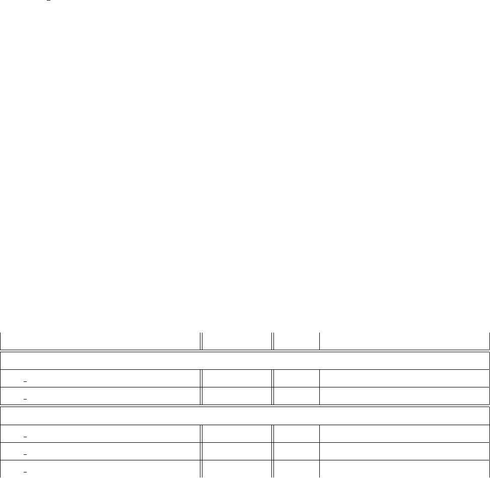
This command read the input from the constants-file, and set the other parameters according to
order (string) declaration of order for the evolution kernel. Typically, one set Γcusp one order higher then the rest of
anomalous dimensions. There are following set of orders
order Γcusp γVD*Dresum ζµ**
LO a1
sa0
sa0
sa0
sa0
s
LO+ a1
sa1
sa1
sa0
sa0
s
NLO a2
sa1
sa1
sa1
sa1
s
NLO+ a2
sa2
sa2
sa1
sa1
s
NNLO a3
sa2
sa2
sa2
sa2
s
NNLO+ a3
sa3
sa3
sa2
sa2
s
*Dresum starts from a0
s, it already contains Γ0.
** Definition of ζµis correct only in the natural ordering, i.e. LO,NLO,NNLO. Proper definition in +orders would
make the function too heavy. The resumed version has the same counting.
26
C. NP input and NP parameters
The NP parameters are used in the definition of the function DNP. Their number is read from the constants-file,
and allocated (and set = 0) during the initialization procedure. Their values are set by command
call TMDR setNPparameter(input)
where input is real*8 list NP parameters, with the length equals to the number of NP parameters.
–DNP –
The important part of TMD evolution is the rapidity anomalous dimension. It has a NP part which is to be
parameterized by user. It should be done in the function DNP(mu,b,f) in the end of the file, where mu is (real*8)
scale, bis (real*8) parameter b, fis (integer) flavor. This functions is used for all evolution kernels. Specifying
it, you can use build-in functions Dpert(mu,b,f) and Dresum(mu,b,f) for the perturbative expressions of D. Also
the NP parameters from the set which are given by variables NPparam(i).
–zetaNP –
The arTeMiDe is founded on the notion of ζ-prescription, therefore, the ζµline plays essential role. For D 6=DNP
(which is standard situation), the ζµline is different from the perturbative. It should be set within the arTeMiDe.
It is done by user in the function zetaNP(mu,b,f), with the same arguments as for DNP. Note, that it MUST
approach ζµperturbation in small-bregeme. Otherwise, the evolution is calculated incorrectly. E.g.
if DNP =Dpert(b∗) + gKb2the ζNP =ζperp(b∗) + .., where dots are power suppressed, and thus can be dropped.
Defining this function you can use zetaMUpert and zetaMUresum for perturbative and resumed versions of ζµ, as well
as, NPparam(i).
In the model code user can provide the ReplicaParameters(n), which returns the array of NP parameters corre-
sponding to integer number n. It is convenient to specify initializing values here, or indeed, the values for fit replicas.
i
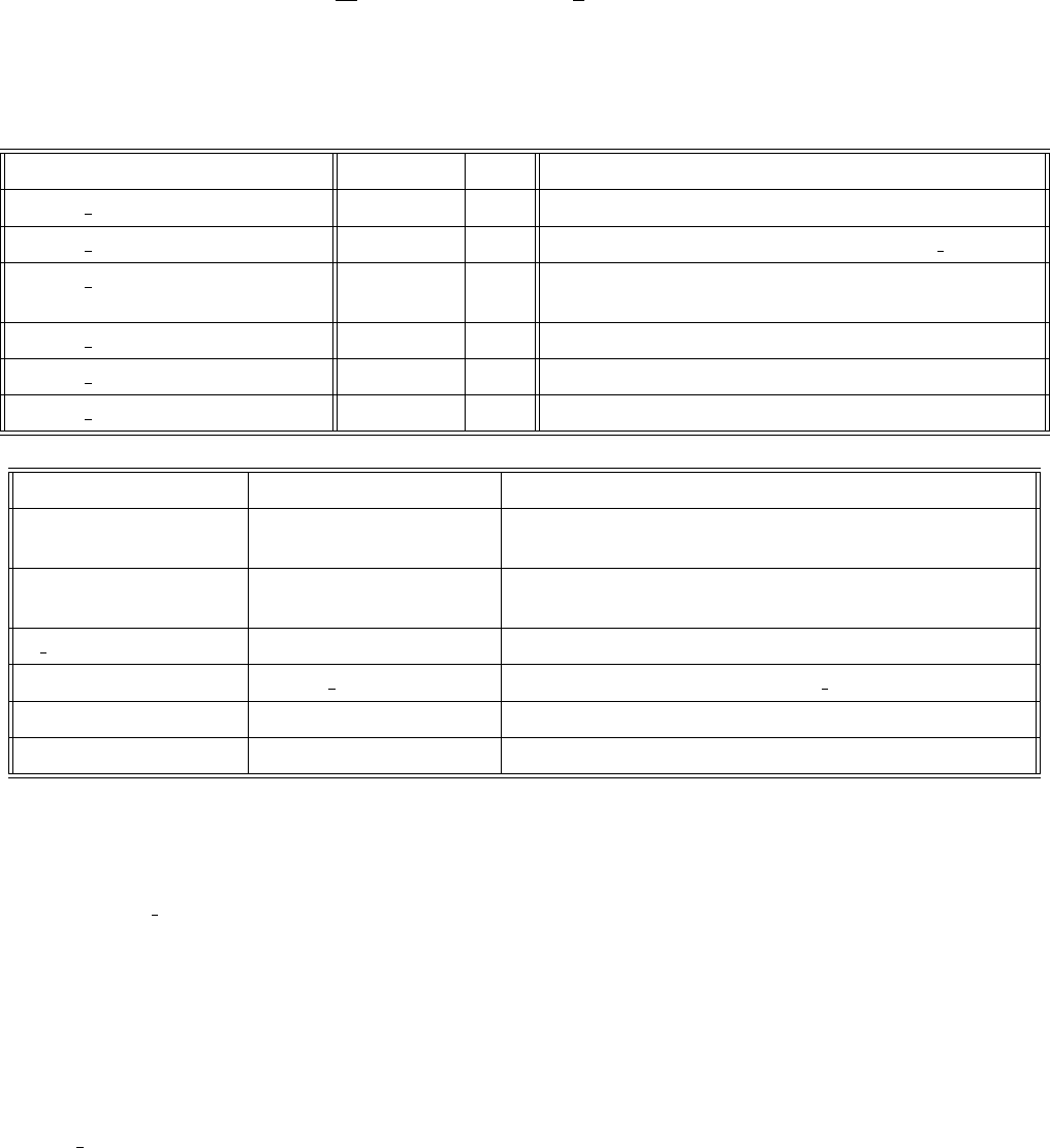
D. Evaluating TMD evolution kernel
The evolution kernel are presented in two types for the evolution from arbitrary point to arbitrary, and for th
evolution from the arbitrary point to the ζ-line. Since all three types of evolution discussed here has different number
of arguments, they could not be confused.
Function solution Evol.type Comments
Evolution from (µf, ζf) to (µi, ζi)
TMDR R(b,muf,zetaf,mui,zetai,mu0,f) improved D1
TMDR R(b,muf,zetaf,mui,zetai,f) improved γ2
Evolution from (µf, ζf) to (µi, ζµi)
TMDR Rzeta(b,muf,zetaf,mui,mu0,f) improved D1
TMDR Rzeta(b,muf,zetaf,mui,f) improved γ2
TMDR Rzeta(b,muf,zetaf,f) fixed µ3 Evolution along ζ. Absolutely fastest.
where
b(real*8) Transverse distance (b > 0) in GeV
zetaf,muf (real*8) hard-factorization scales (ζf, µf) in GeV. Typically, =(Q2, Q)
zetai,mui (real*8) low-factorization scales (ζi, µi) in GeV.
mu0 (real*8) The scale of perturbative definition of rapidity anomalous dimension Dµ0in GeV.
f(integer) parton flavor. 0 for gluon, 6= 0 for quarks.
The parameter evolution type is set in constants-file and is used by TMDs to call particular version of evolution.
Within only the TMDR-module it is not needed.
27
E. Inverted evolution and the lowest available Q
At small values of parameter Q=Q0the point (Q, Q2) crosses the ζ-lines. The value of Q0dependents on b. The
dangerous situation is then hard scale of the process Qis smaller then Q0at large b=b∞. In this case the evolution
kernel R[b∞,(Q, Q2)→ζµ]>1, which is generally implies that it grows to infinity. However, it happens only at
small values of Q. E.g. at NNLO the typical value of Q0is ∼1.5GeV. That should be taken into account during
consideration of low-energy experiment and especially their error-band, since the point (c2Q, Q2) could cross the point
at larger values of Q.
The function LowestQ() returns the values (real*8(1:3)) {Q−1, Q0, Q+1}, which are solution of equation Q2=
ζcQ(b), for (fixed bu) large values of b.Q−1corresponds to c= 0.5, Q0corresponds to c= 1 and Q+1 corresponds to
c= 2.
28
IX. UTMDPDF MODULE
The module uTMDPDF performs the evaluation of the unpolarized TMD PDF at low scale µiin ζ-prescription. It is
given by the following integral
Ff(x, b) = Z1
x
dz
zCf←f0(z, b, c4µOPE)ff0(z
x, c4µOPE)ff
NP (x, z, b, {λ}),(9.1)
where ff(x, µ) is PDF of flavor f,Cis the coefficient function in ζ-prescription, fNP is the non-perturbative function.
The variable c4is used to test the scale variation sensitivity of the TMD PDF. The NNLO coefficient functions used
in the module were evaluated in [5] (please, cite it if use).
List of available commands
Command Type Sec. Short description
uTMDPDF Initialize(order) subrout. IX A Initialization of module.
uTMDPDF SetLambdaNP(..) subrout IX B Set new NP parameters used in FNP and mu OPE.
uTMDPDF lowScale5(x,b,h) (real*8(-5:5)) IX C Returns unpolarized TMD PDF at x,band hadron h.
Gluon flavour undefined.
uTMDPDF lowScale50(x,b,h) (real*8(-5:5)) IX C Returns unpolarized TMD PDF at x,band hadron h.
uTMDPDF SetScaleVariation(c4)) subrout Set new value of c4(default value c4= 1).
uTMDPDF resetGrid(bG,g) subrout IX D Force reset or deconstruct the grid.
List of inputs
Input Setup by Short description
ModelInitialization() write-in Necessary predefinitions by user. E.g. some precalculations
for FNP.
FNP(x,z,b,hadron) write-in NP-model for fNP (x, z, b, {λ}) depends on the hadron. See
sec.IX B
mu OPE(x,bt) write-in The value of µOPE.
lambdaNP uTMDPDF SetLambdaNP(..) NP parameters used in FNP and mu OPE.
asdefined in QCDinput Strong coupling. See sec.II
xf(x) defined in QCDinput Unpolarized PDF. See sec.II
A. Initialization
Prior the usage module is to be initialized (once per run). By
call uTMDPDF Initialize(order)
here order defines the perturbative order of the coefficient function according to the
LO,LO+ =a0
s,NLO,NLO+ =a1
s,NNLO,NNLO+ =a2
s.
B. Definition of non-perturbative part, fN P and parameters
The model for TMD is given by fN P (and in smaller amount by µOP E ). In the current version there is no possibility
to implement b∗-prescription, to be added in future. The definitions of these functions is provided by user in the file
uTMDPDF model.f90, which is located in the scr/model directory.
•The function FNP is dependent on x,z,band λ(and the hadron flavor). It is an array for all flavors (-5:5).
It uses the parameters λ1,2.... which are passed to it by main module. The total number of NP parameters
LambdaNPLength, is declared in the constants-file.

29
•Also user can provide the value of µOPE (or use the default one) in the function mu OPE(x,b). This scale is used
inside the convolution F(x, b) = C(x, b;µOPE)⊗q(x, µOPE). The function could depend on x(the one which
enter f(x) in the convolution), however, this option has not been accurately tested yet..
•Together with the model user can provide the function ReplicaParameters(n), which returns NP parameters
in accordance to input integer number n. These parameters will be set as be current λ1,2.., upon the call
uTMDPDF SetLambdaNP(n), where nis integer number of the replica. It is convenient to specify initializing
values here, or indeed, the values for fit replicas.
To set the values for array lambdaNP use the subroutine
call uTMDPDF SetLambdaNP((/λ1, λ2,.../))
Optional: There exist the overloaded version of uTMDPDF SetLambdaNP, with two additional boolean parameters
call uTMDPDF SetLambdaNP((/λ1, λ2,.../),makeGrid,includeGluons)
If parameter makeGrid=.true. then for this run of non-perturbative parameters the grid for TMD will be evaluated.
Then until new NP parameters set the TMDs are reconstructed from the grid, see sec.IX D.
If parameter includeGluons=.true., the grid is calculated with gluons. If parameter includeGluons=.false.,
the grid is calculated without gluons (but the mixture of quark with gluon is taken into account. The difference is
the same as, e.g. between uTMDPDF lowScale5 and uTMDPDF lowScale50 functions (see next section).
Default version has makeGrid=.false.,includeGluons=.false.. Note, that this command compare new values of
parameters to the old one. If they coincides, the grid is not renewed.
Optional: There exist the overloaded version of uTMDPDF SetLambdaNP(n), with nbeing an integer. It attempt to
load user defined set of NP parameters associated with number n.
C. Evaluating unpolarized TMD PDFs
The expression for unpolarized TMD PDFs is given by the function
uTMDPDF lowScale??(x,b,h)
where
x(real*8) Bjorken-x(0 <x<1)
b(real*8) Transverse distance (b > 0) in GeV
h(integer) The number that indicates the hadron. Since coefficient function is hadron independent, this number
influence the PDF that used, and FNP.
The questions marks stand for a flavor content of TMD-vector. The functions evaluate the TMD PDFs of different
flavours simultaneously.
uTMDPDF lowScale5(x,b,h) returns (real*8) array(-5:5) for ¯
b, ¯c, ¯s, ¯u, ¯
d, ?, d, u, s, c, b. Gluon contribution is un-
defined, but taken into account in the mixing contribution.
uTMDPDF lowScale50(x,b,h) returns (real*8) array(-5:5) for ¯
b, ¯c, ¯s, ¯u, ¯
d, g, d, u, s, c, b. This procedure is slower
(∼10 −50% depending on parameters, mainly on x) in comparison to the previous command. The slowdown
is presented since the gluon coefficient function has 1/x behavior, and requires more iteration to reach the
demanded precision. If gluons are not needed use previous.
Important note: there is no arguments µand ζ, because the arTeMiDe uses the ζ-prescription, where a TMD
distribution is scaleless. The scale of matching procedure µOPE is set in the function mu OPE (see previous
subsection). Note, that the TMD at different then ζ-prescription point can be evaluated within TMDs package
(which uses uTMDPDF in turn).
Additional points:
•In order to avoid possible problems at b= 0, at b < 10−6the value of bis set to b= 10−6. This region is
numerically non-important, since in any cross-section it is suppressed by bn(n>1) within the Fourier integral.

30
•The convolution procedure C⊗fis the most costly procedure in the package. Its timing seriously increases from
NLO to NNLO coefficient function (about 10 times). In the current version we implement the Gauss-Kronrod
adaptive algorithm, with estimation of accuracy as |(G7−K15)/(f(x)fNP (1))|< , where the default value
of is 10−3. According to our checks default estimation guaranties the 4-digit precision of the evaluation. If
integrand does not converge fast enough at z→1 (e.g. for gluon contribution at NNLO, where ln3¯zis presented),
the integral at (x0,1) is replaced by exact integral with constant f(x)fNP . The value of x0is determined by
f0(x0)< and x0>1−. This additional procedure is needed to ensure convergence of the integral. However,
in our experience (which uses only quark TMDs), this extra procedure is not used at all.
D. Grid construction
For fitting procedure one often needs to evaluate TMDs multiple times. For example, for fit performed in [1] the
evaluation of singe χ2entry requires ∼16 ×106calls of uTMDPDF ... Every call of uTMDPDF .. at NNLO order,
requires ∼200 calls of pdfs, depending on x,band λ’s. Therefore, in such situations it is much more cheaper to make
a grid of TMD distributions for given set of non-pertrubative parameters (i.e. the grid is in xand b), and then use
this grid for the interpolation of TMD values.
The griding turns on by the call overloaded version of uTMDPDF SetLambdaNP(lambda,makeGrid,includeGluons)
with makeGrid=.true. (see also sec.IX B). After this call the grid will be built (the corresponding massage will be
shown on the screen, if output level is >1). This grid is used for the interpolation of TMD distribution until the next
call of uTMDPDF SetLambdaNP, which resets/cancels grid.
To speed up the multiple changes of parameters, the packages checks the function FNP onto the x-dependance. If
it is x-independent, then the grid (unless it is forcibly reseted) is not renewed but reweighted with new FNP. It is
possible since in this case FNP does not enter the convolution.
The interpolation is cubic. The grid is build for the finite domain of x∈(xmin,1) and b∈(0, bM). For x < xmin
the program will be terminated (with an error). For b > bMthe extrapolation by the function exp(−α(x)−β(x)b) (or
exp(−α(x)−β(x)b2)) is made (with the common sign equal to sign of TMD at b=bM). In the default set we have
xmin = 10−5, bM= 100.
The default grid is 250×750 (the grid is logarithmic in both xand b, small xand b→0), we have found that it
gives in average 5-6 digit precision. All this parameter can be changed in constants file in the section 3.D. These
parameters have been used to fit a large domain of energies and qT. However, we recommend, to check the obtained
result by exact evaluation without a grid to ensure the precision in particular cases.
The form of the extrapolation (exponential or Gauassian) can be also changed in the file constants, sec. 3.D.
The subroutine uTMDPDF resetGrid(makeGrid,includeGluons) changes the current behaviour (for the meaning
of arguments see uTMDPDF SetLambdaNP). If makeGrid=.true. the grid will be recalculated.
E. Theoretical uncertainties
uTMDPDF SetScaleVariation(c4) changes the scale multiplicative factor c4(see [1], eqn.(2.46)).

31
X. UTMDFF MODULE
The TMDFF functions structurally repeats the TMDPDF functions. Therefore, the module is practically the same
as uTMDFF. The NNLO coefficient functions used in the module were evaluated in [5, 6] (please, cite it if use).
XI. SUPPLEMENTARY CODES
In the arTeMiDe archive you can find the codes which evaluates the cross-sections using our fit parameters.
A. Drell-Yan cross-section
The compile the program for the evaluation of Drell-Yan cross-section evaluate: make dy. As a result of evaluation
in the executable file arTeMiDe DY and the file of input parameters input will be placed in /bin. The program
arTeMiDe DY evaluates the differential cross-section dσ/dQ2dydq2
Tfor the production of Z and γ∗in the Drell-Yan
process (take care that in the current fit we expect agreement with the data for qT<0.2Q). The program also
evaluates various integrals of cross-section such as
ZQ2
Q1
dQ2,Zy2
y1
dy, ZqT2
qT1
dq2
T
qT2−qT1
,(11.1)
and their combinations. It also takes (if necessary) into account lepton cuts. Therefore, can be used to build DY
cross-section for wide range of experiments. To input all these options check the file input, which is self-explanatory.
32
XII. HARPY
The harpy (from combination of Hybrid ARtemide+PYthon)) is an interface to artemide to the python.
It is directly possible to interfacing the artemide to python since artemide is made on fortran95. It uses some of
it features, such as interfaces, and indirect list declarations, which are alien to python. Also I have not found any
convenient way to include several dependent Fortran modules in f2py (if you have suggestion just tell me). Therefore,
I made a wrap module harpy.f90 that call some useful functions from artemide with simple declarations. So, it
could be linked to python by f2py library.
So, in the current realization I create the signature file that declare python module artemide, which has an wrap
module harpy. In python it looks like
>>> import artemide
>>> artemide.harpy.initialize(”NNLO”)
>>> print artemide.harpy.utmdpdf 5 optimal(0.1,1.,1)
Ugly, but it works.
Note, that not all functions of artemide are available in harpy. I have added only the most useful, however, you
can add them by our-self, or write me an e-mail. Here, list the functions from artemide and their synonym in harpy
artemide harpy.f90
module function
General Initialize(order)
TMDX DY TMDX DY SetNPParameters(array) SetLambda(array)
TMDX DY SetNPParameters(integer) SetLambda ByReplica(integer)
TMDX DY SetScaleVariations(c1,c2,c3,c4) SetScaleVariation(c1,c2,c3,c4)
TMDs uTMDPDF 5(x,bt,muf,zetaf,h) uTMDPDF 5 Evolved(x,bt,muf,zetaf,h)
uTMDPDF 50(x,bt,muf,zetaf,h) uTMDPDF 50 Evolved(x,bt,muf,zetaf,h)
uTMDPDF 5(x,bt,h) uTMDPDF 5 Optimal(x,bt,h)
uTMDPDF 50(x,bt,h) uTMDPDF 50 Optimal(x,bt,h)
TMDs inKT uTMDPDF kT 5(x,kt,muf,zetaf,h) uTMDPDF kT 5 Evolved(x,kt,muf,zetaf,h)
uTMDPDF kT 50(x,kt,muf,zetaf,h) uTMDPDF kT 50 Evolved(x,kt,muf,zetaf,h)
uTMDPDF kT 5(x,kt,h) uTMDPDF kT 5 Optimal(x,kt,h)
uTMDPDF kT 50(x,kt,h) uTMDPDF kT 50 Optimal(x,kt,h)
TMDX DY xSec DY(X,proc,s,qT,Q,y,iC,cuts,Num) X=DY xSec Single(proc,s,qT,Q,y,iC,cuts,Num)
xSec DY List(X,proc,s,qT,Q,y,iC,cuts,Num) X=DY xSec List(proc,s,qT,Q,y,iC,cuts,Num)
NOTE: there is no OPTIONAL parameters. All parameters should be defined (it is necessary for f2py).
For convenience I have also created a more user-friendly interface, written on python. It is called harpy.py
and located in /harpy, and can be imported as is.

33
[1] I. Scimemi and A. Vladimirov, Eur. Phys. J. C 78, no. 2, 89 (2018) doi:10.1140/epjc/s10052-018-5557-y [arXiv:1706.01473
[hep-ph]].
[2] L. A. Harland-Lang, A. D. Martin, P. Motylinski and R. S. Thorne, Eur. Phys. J. C 75 (2015) no.5, 204
doi:10.1140/epjc/s10052-015-3397-6 [arXiv:1412.3989 [hep-ph]].
[3] I. Scimemi and A. Vladimirov, JHEP 1808 (2018) 003 doi:10.1007/JHEP08(2018)003 [arXiv:1803.11089 [hep-ph]].
[4] A. Buckley, J. Ferrando, S. Lloyd, K. Nordstrm, B. Page, M. Rfenacht, M. Schnherr and G. Watt, Eur. Phys. J. C 75, 132
(2015) doi:10.1140/epjc/s10052-015-3318-8 [arXiv:1412.7420 [hep-ph]].
[5] M. G. Echevarria, I. Scimemi and A. Vladimirov, JHEP 1609, 004 (2016) doi:10.1007/JHEP09(2016)004 [arXiv:1604.07869
[hep-ph]].
[6] M. G. Echevarria, I. Scimemi and A. Vladimirov, Phys. Rev. D 93, no. 1, 011502 (2016) Erratum: [Phys. Rev. D 94, no.
9, 099904 (2016)] doi:10.1103/PhysRevD.93.011502, 10.1103/PhysRevD.94.099904 [arXiv:1509.06392 [hep-ph]].
[7] M. G. Echevarria, I. Scimemi and A. Vladimirov, Phys. Rev. D 93, no. 5, 054004 (2016) doi:10.1103/PhysRevD.93.054004
[arXiv:1511.05590 [hep-ph]].
[8] A. A. Vladimirov, Phys. Rev. Lett. 118, no. 6, 062001 (2017) doi:10.1103/PhysRevLett.118.062001 [arXiv:1610.05791
[hep-ph]].
[9] A. Vladimirov, JHEP 1804, 045 (2018) doi:10.1007/JHEP04(2018)045 [arXiv:1707.07606 [hep-ph]].
[10] T. Gehrmann, E. W. N. Glover, T. Huber, N. Ikizlerli and C. Studerus, JHEP 1006, 094 (2010)
doi:10.1007/JHEP06(2010)094 [arXiv:1004.3653 [hep-ph]].

34
XIII. VERSION HISTORY
Ver.1.4 – HARPY: Implemented.
– TMDs and sub-modules: Added function SetReplica.
– TMDs: Added interface to optimal TMDs
– TMDs: Added check for length of incoming λNP
– TMDs: Fixed bug with incorrect gluon TMDs in functions 50.
– TMDs inKT: Implemented.
– TMDX DY: Added xSec DY subroutines.
– TMDX DY: Encapsulated process, and cut-parameter variables.
– TMDX DY: Defined p1=2, which corresponds to integration over xF. Removed old functions for xF
integrations.
– TMDX DY: Fixed a bug with variation of c2(introduced in ver.1.3).
– LeptonCutsDY : Old version of function removed, cut-parameters encapsulated into single array variable.
– LeptonCutsDY : asymmetric cuts in pTare introduced.
– LeptonCutsDY : New function CutFactor4, which is analogous to CutFactor3 but with one integral
integrated analytically. Thus, it is more accurate, and faster by 5-20%
– LeptonCutsDY : some rearrangement of variables that makes CutFactor4 and CutFactor3 faster by
20%.
– uTMDPDF &uTMDFF :FN P is now function of (x, z, b, h, λ). For that reason this version in-
compatible with earlier versions.
– uTMDPDF &uTMDFF: The common block of the code is extracted into a separate files. It include
calculation of Mellin convolution and Grid construction.
Ver.1.32 – TMDX DY: Added the routine with lists of y-bins, in addition to the lists of pt-bins.
– TMDX DY: The implementation of parallel computation over the list of cross-sections.
– LeptonCutsDY: The kinematic variables are encapsulated.
– TMDX DY: The kinematic variables are encapsulated (by the cost of small reduction of performance).
– uTMDR: Changed behavior at extremely small-b. Now values of b freeze at b= 10−6.
– uTMDPDF &uTMDFF: Changed behavior at extremely small-b. Now values of b freeze at b= 10−6.
– TMDR: Added NNNLO evolution (only for quarks, Γ3is from 1808.08981). Not tested.
– TMDs: Functions RuPDFuPDF and antiRuPDFuPDF are added.
Ver.1.31 – Global: The module TMDF is split out from TMDX .. modules.
– Global: Constant tables are moved to the folder \tables.
– TMDX ..: Change the structure of process definition.
– TMDF: Fixed bug with throwing exception for failed check of convergence of Ogata quadrature.
– TMDF: Added possibility to vary the Ogata quadrature parameters.
– TMDX DY: The structure of interface to integrated cross-section simplified.
– TMDX DY: Added trigger for exact power-corrected values of x1,2.
– uTMDPDF &uTMDFF: Fixed rare error for exceptional restoration of TMD distribution from grid,
then fNP evaluated to zero.
Ver.1.3 – Global: Complete change of interface. Interface update for all modules.
– uTMDPDF: Added hadron dependence. FNP is now flavour and hadron dependent.
– uTMDPDF: Renormalon correction is removed. As not used.
– TMDR: The grid (and pre-grid) option is removed. Since it was incompatible with new interface. Also
the new evolution (type 3) is faster any previous (with grids).

35
Ver.1.2(unpub.) –TMDR: Older version is changed to uTMDR1. New evolution routine implemented.
–uTMDFF: Implemented.
–uTMDPDF: Fixed bug in evaluation of gluon TMDs, within the evaluation of (..)+part.
– Global: Removed functions for the evaluation of only 3-flavours TMDs. As outdated and not used.
– Global: Number of non-pertrubative parameters is now read from ’constants’-file. Module TMDs initialize
sub-modules with accordance to this set.
– Global: Module TMDX is renamed into TMDX DY, also many functions in it renamed.
–uTMDX SIDIS: Implemented.
–TMDs: As an temporary solution introduced a rigid cut for TMD(µ<mq).
–TMDX: Update of Ogata quadrature, with more accurate estimation of convergence.
Ver.1.1 hotfix Bugs in uTMDPDF and TMDR related to the evaluation of gluon TMDs fixed (thanks to Valerio Bertone).
Ver.1.1 – Global: The physical, numerical and option constant are moved to the file constants, where they are
read during the initialization stage.
–MakeGridsForTMDR: Update of integration procedures to adaptive. Default grids accordingly updated (no
significant effect).
–uTMDPDF: Update of the integration procedure in uTMDPDF, to adaptive Gauss-Kronrod (G7-K15). with
special treatment of the x→1 singularity.
–uTMDPDF: The procedure for evaluation of TMD for individual flavour (uTMDPDF lowScale(f,x,b,mu)) is
removed, as outdated.
–uTMDPDF: Removed argument µ, from uTMDPDF ...(x,b). Added function mu OPE(b), which is used as
µ-definition for TMDs.
–uTMDPDF: Optional griding of TMDs is added. See sec.??
–TMDR: fixed potential error in the ”close-to-Landau-pole” exception.
–TMDs: fixed potential error in the evaluation of the gluon evolution factor.
–TMDX: the name convention of subroutines CalculateXsection ..., changed to CalculateXsec ..., to
shorten the name length.
–TMDX: added functions CalculateXsec PTint Qint YintComplete(X,qtMin,qtMax,QMin,QMax) and
CalculateXsec Qint YintComplete(X,qtMin,qtMax,QMin,QMax).
–TMDX&TMDs&uTMDPDF: the independent variation constant c4is added (in the ver.1 variation of c3and c4
was simultaneous). The corresponding routines are updated.
Ver.1 Release: uTMDPDF,TMDR,TMDs and TMDX modules. Only Drell-Yan-like cross-sections.
36
XIV. BACKUP
TO DO LIST
•Re-check uTMDFF module. Possible mistake in 1/z2factors.
•Add possibility for non-perturbative definition of ζ-line.
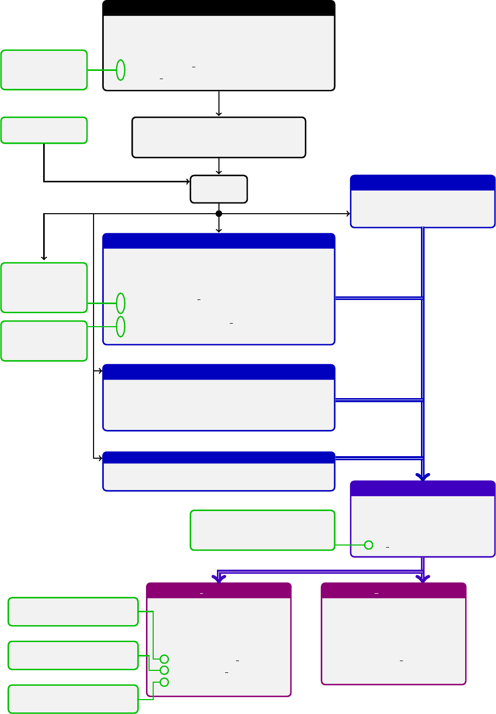
37
A. arTeMiDe structure before v1.3
MakeGridsForTMDR
Precalculated grids for various RGE, see
sec.??.
User defined functions
•InitializeAs byUser
•alphaS ByUser
User defined
as
RGE Grids
Default from MMHT2014[2]
PDF Grids
paths
uTMDPDF
Evaluates unpolarized TMD PDF at low-scale
point. see sec.IX
User defined functions:
•InitializePDF byUser
•xPDF
•ModelInitialization byUser
•FNP
TMDR
Evaluates TMD evolution
factor R. See sec.VIII
User defined
unpolarized
PDF
User defined
fNP
uTMDFF
Evaluates unpolarized TMD FF at low-scale
point.
Not implemented in the ver.1
..
Not implemented in the ver.1
TMDs
Evaluates of TMD distribu-
tions. See sec.VI
User defined functions
•mu LOW
User defined low-
normalization scale µ.
TMDX DY
Evaluates cross-section of
DY-type with TMD distri-
butions. See sec.III
User defined functions
•CutPrefactor byUser
•XPrefactor byUser
•XIntegrand
Fiducial cuts on leptons.
qT-independent part.
Integrand of Fourier.
TMDX SIDIS
Evaluates cross-section of
SIDIS-type with TMD dis-
tributions. See sec.III
User defined functions
•XPrefactor byUser
•XIntegrand
