Manual
User Manual:
Open the PDF directly: View PDF ![]() .
.
Page Count: 9

Unofficial manual version 2.0
September 2018
If you have no idea about this work, please start from the paper
https://arxiv.org/abs/1803.00788
All the code are stored in: C:\Users\CNNplace\Documents\MATLAB\Code
All 227x227 images are stored in:
C:\Users\CNNplace\Documents\MATLAB\SceneImage\OSM_MAPtest
Folder needed to be activate:
For OSM extraction: OSMprocess + johnyf-openstreetmap-v0.2.2-3-gbb37962
For OSM process: OSMprocess + Utility
For GSV/BING images download: OSMprocess + Streetview
Small tip: if you do not have any idea where I put the said functions or scripts, use the
command edit functionOrScriptname or highlight the name in the file → right click → select
‘open *filename*’, and make sure you add all the path above before search it, if not, it will ask
you whether you want to create a new file of not.
•••••
Where to start
Within the code folder, go and check the OSMprocess\1_BasicCommand folder for the basic
file. It contains these operations:
1. Load OSM + corresponding GSV images + construct the static database
(normal/dense)
The basic processes are: read OSM, get the tag of each object, get road points, find intersection
of road and generate connectivity table, for each point, interpret the OSM information, and then
download the corresponding images from GSV.
After that the connectivity table will be used for generating the DB.
● Load OSM
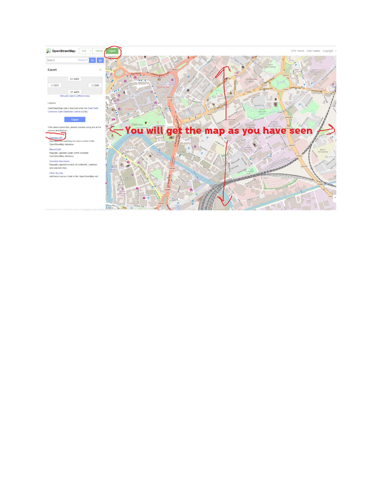
To get .osm file, go to https://www.openstreetmap.org/ and select the region you want → press
‘Export’ → ‘Overpass API’. Then rename the loaded file to .osm

All of my .osm file are in:
C:\Users\CNNplace\Documents\MATLAB\Code\OSMprocess\osmcnn\mymap
I strongly suggest you to open some of them via any text editing tool to get the feel how OSM
store and arrange the data. In brief, it is similar to XML. Try to avoid loading too large map,
MatLab will crash.
Note: Make sure you check the appearance of the OSM map before download. Sometimes
you’d see the blank city with only road; that means there is no information about the building at
all, so you cannot use this for ‘gaps between buildings detection’ process as there is no building.
Also, you can check the tag and label I used from OSMtagSetupInit. Be careful if you would like
to try to load OSM of non-english usage country, there might be a problem caused by the label.
I had tried Japan before and found out that my code could not work due to the face that the
OSM map contains Japanese label and my function cannot read it.
For descriptor generation, you can go and check osmggg\getGGAngletoLines and modify it to
check the finer angle.
Note: the road intersection detection still contains some I-do-not-know-why-it-happened bug. It’s
not usual, but can occur, so go and check: getRoadConn and conRoadTableConn, you might
find where I missed. The effect of this bug is sometime the connection looks funny, they jump to
the next road. This probably might cause by the raw OSM.

● Load Google Streetview
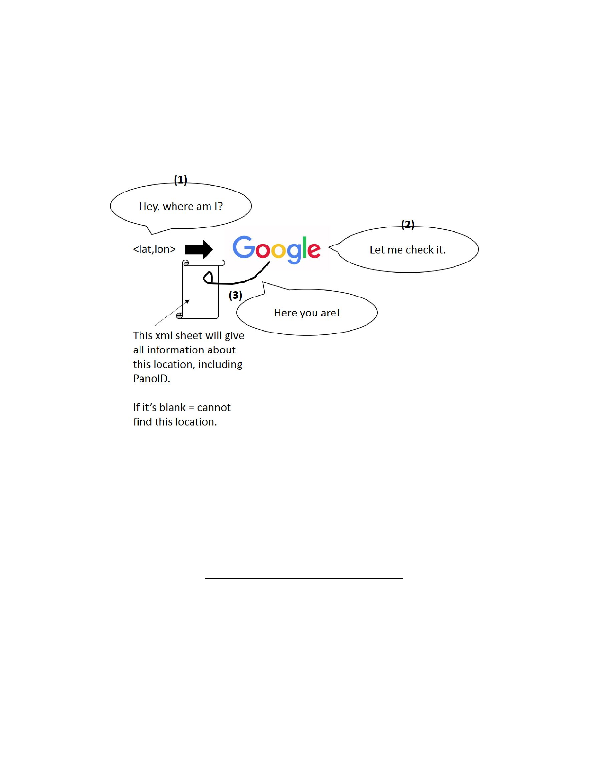
The concept of Google streetview is you send the <lat,lon> → get Panoramic ID of that
panorama and then select where to crop out.
The process from 1-3 are in Streetview\src\streetImagery\checkUsageLL. If you’d like to get
more information, go and modify it. I read XML as a text and retrieve the strings I want. Then,
from this you can get the corresponding PanoID and send to Google again with some
parameters to retrieve the image. In my code, the important information will be stored in pList,
which is a sub-parameter in osmelem.
Also, go and check osmretrieveggg4_NEWSMALL for more information. Note that I have two
separate folder for saving the large images (1240x480) and cropped images (227x227).
However, for the future test, do the train by capture in 227x227 directly. No need to keep in two
separate location. To change this, just get the input for sizeIm2 = [227 227] and remove the
cropped part & filepathS variable from the function.
Note that sometimes by running the GSV scripts/functions in the different time, you might get
the different number of GSV-uniqued road. If there is a crash like the data cannot be download,
maybe you should stop and wait for another day. Sometimes there will be a weird crash like this
using Google API.

There is also the Bing version, check realZhu\BING\osmretrieveBBG4_NEWSMALL to see
how I download images. The basic process of Bing is similar to Google. Also, there are some
other useful functions that you can use all in Streetview folder. This is the legacy code, so there
are things that I have not discovered yet.
Also, on the web, you can get the PanoID from the URL:
https://www.google.com/maps/@51.4568999,-2.6021452,3a,75y,129.66h,93.02t/data=!3m6!1e1
!3m4!1sE0ej1HvN8dzkm3JK6HHbog!2e0!7i13312!8i6656
The PanoID is E0ej1HvN8dzkm3JK6HHbog. It will be after !1s and before the next !, and the
latitude and longitude are highlighted in red.
You can retrieve the XML information by copy and paste this to the web browser:
http://maps.google.com/cbk?output=xml&ll=51.4568999,-2.6021452
If you want to get the panoramic image, use:
I = downloadPanoImage(panoID, zoomfactor);
%default = 3
For example, from osmelem parameter, you can call:
I = downloadPanoImage(osmelem.pList(1).panoID, 3);
There is also a way to get depth information from GSV in case you might need it; I cannot
remember the exact function, but I believe you can find something useful in
\streetImagery\ggstreetview folder.
● Generate DB
For DB, I would suggest you to try the normal construction first. Be careful when you use dense
version, this one is not optimised, it could take days to generate the whole dataset. I encourage
you to look for more practical solution.
In my code I set the sub-section = 4; you can adjust them as you like, or make it more flexible
(for example, the auto-generate function/script that do the auto loop instead of manual like this).
If you change the number, make sure to go and modify the search process.
The database you could play with:
LONDON: I split into 4 sets; they are in the folder → D:\TreeData\Set1 (Set2,Set3 and Set4)
BRISTOL: this one is densed, so I split into ~6000; they are in the folder →
D:\TreeData\realZhu\FullPath_all
Be careful, it’s actually loaded.

Note that the generated routes are not allow to perform revert direction (for this version). You
can (and should, in the future) add them by turning the direction of the descriptor. Please check
genFullBoxNew3 and genFullBoxDesc functions.
Also, please be careful about the format of the descriptor (binary/decimal). If you put it wrong,
you might find that the accuracy of classifier looks very scary (like, 70% error!). Don’t be panic!
Carefully check the format first. For example, in genFullBoxDesc, you need to put the
descriptor in the decimal format. You can modify them into a friendly version if you like; it is so
easy to get confused.
Let say, for one location:
Raw format: 1 1 2 3; when 2 = 0 and 3 = unknown (sometimes the info on the map can be
missing.)
Binary format: 1 1 0 0; I replace 2&3 as 0
Decimal format: 12
For the important parameters: rconnTable
is the road connectivity table, numHops
is the
maximum number of locations within the route you need (try 40), descList
is the list of the BSD
descriptor for each location; in my database: descList_n2
is the raw interpretation from the map
descList_n3
is the binary format, and descList_n4
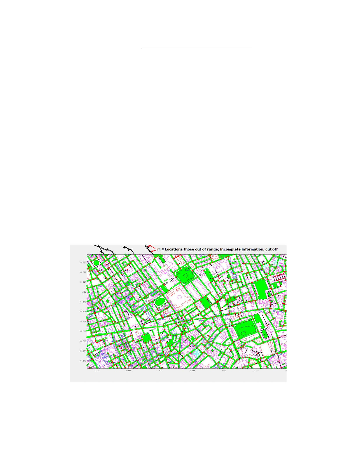
is the decimal format, and m
is the number of
locations those are out of range (says, some location might not appear on the map, and it
means the data might be incomplete so I remove them off).
Go and check OSMFirstprocess for more information about how each parameter has been
genereated.

2. Train the dataset
Each classifier trained separately. The data will be arranged into table format. For more details
of using CNN in Matlab: https://www.mathworks.com/help/nnet/ref/trainnetwork.html
The processes of training are: (1) Generate table of labelled data and (2) Put the table into the
For junction use: [T] = genTableData(filepath,ggSet);
For gaps use: [T] = genTableDataBDJC_cate(filepath,ggSet);
When T is the generated table of labels, and filepath is the location of image corresponding to
the ggSet. For ggSet, you generated them in the previous step (while extracting the OSM).
If you want to use my image data, go and check
C:\Users\CNNplace\Documents\MATLAB\SceneImage\OSM_MAPtest folder, there are tons
of it; their corresponding ggSet has been stored in the
C:\Users\CNNplace\Documents\MATLAB\DataBackup folder and look for _allGG file (ex.
'C:\Users\CNNplace\Documents\MATLAB\DataBackup\20170413_BBLSM_allGG.mat'). It might
be a bit hard to find. If it is too confused, and you need to re-download/retrain it anyway, just do
the step 1 and make sure you properly save the ggSet parameter.
You can also rewrite everything, the training process is simple, you only need matlab table with
2 column: image path and label. For more information:
https://www.mathworks.com/help/matlab/ref/table.html
Also, if you want to try on other semantic features, go and modify the way ggSet has been
interpret the OSM map first and then move to the genTableData for modification,
To test it, follow the code in testing section. Note that I am not sure whether this one is the
newest version or not. You can also write a simple function to check the results. The easiest
way is to turn the test set into the table, put the image into the classifier by:
I = imread(‘Your file path’);
%Optional I = imresize( imread(‘Your file path’), [227 227]);
res = predict(net,I);
The res parameter will return the score for each category, you can add ans_cate = find(res ==
max(res));
to get the answer. In my work, 1 = junction 2 = no junction, and the same as gaps.
To turn the answer to binary, convert 2 into 0.
Then, compare the returned result with the label (ground truth) and count the accuracy.
Note: again, I would suggest you to be careful with the size of the training set; having too large
would freeze the machine (look at ‘MaxEpochs’
and ‘MiniBatchSize’
parameter). Don’t panic,
just restart the computer and try again with a smaller size.

Also, there is some ways you could obtain the backup for each round of the training. From my
setting, see the parameter ‘CheckpointPath’
, in the demo, I put them in 'D:\checkPoints'
. You
can change it to any directory you prefer. This is also loaded, you should go and clear them
when you don’t want them anymore.
For more information about the training process using MatLab, please read:
https://www.mathworks.com/solutions/deep-learning/convolutional-neural-network.html
The examples are good. Make sure you understand it.
For my trained networks in both categories, go for
load('C:\Users\CNNplace\Documents\MATLAB\DataBackup\20180330_NETonly')
3. Sampling + Test + Results
Note: andddd again, I would suggest you to be careful with the size of the test set; having too
large would also freeze the machine. The smart move is 25 or 50, and then you can run several
times to gain numbers.
SamplingAndSearch is the the naive version (run from 2-40 big BD)
SamplingAndSearch_DYNM is the dynamic version; it would start by searching on the full
database, but at some points, it will stop and use the previous results as the base to generate
the new database. Change the number as you like. I would suggest 10-15 depends on the size
of dataset & the accuracy. Too low would cause the fail to detect the correct route.
[Edited] I found some minor bugs for dynamic version and do not have time to fix *sorry*, but the
core function should be okay, you can start by that.
While searching, if the program just closes itself (or crash/ get debug prompt) without any sign, I
advise you to check the balance of the descriptor and the location you load the DB file. The
common problem is the size of descriptors in the database is not the same as you query; this is
the crash of c program. Another possibility is the wrong length of threshold list (ex. You test for
50 keys but put 40 threshold list).
This part still opens for the optimisation process. I’m sure it could do faster.
Note that the turn process has been included after the search, you can find the code in there.
Also, you can change the angle of the turn as you like; one difference from the paper is that I
had changed from turn/not turn to left and right turn. However, I changed this and that a lot to
see the response, and I am not sure which version I left. You might want to ensure the
correctness of the function.

Please keep in mind that sometimes Google frontal angle might have an error (ex. → → ← →
→ ; one location gets reverted frontal angle). I have not remove this yet as it is not a major
problem at this state of work. However, in real world environment, this might affect your result
when applying the turn direction process (as this might cause a fake turn). I’d suggest you to
find a way fix this. Small tips: check the direction along a route to see the sudden changes and
flip the image + viewing position.
4. Visualisation (one route operation only)
Inside basic folder, check New_testConcl\demoDisplayCC, these are the basic operation of
visualisation. To change the value, you can check each function. Sorry for some hardcode and
magic number; I’d tried my best to reduce them.
The convertScores_frameCCGT is the ground-truth integration; this one will guess the current
location by using the information from the previous steps. The original is counting the
n-consecutive overlapped routes.Says, if they appear to be the best answer around the same
location for n times, we guess that’d be our current location.
Sorry that I cannot find the old version, it should be somewhere in my code. This one is the
modified version, so it might be slightly different operation, but you can do the modification
based on this; it is kind of straight-forward process. I left the test route for you. If you would like
the new one, you can generate from step 3.
Also, there is a way to perform all the animation in one frame. Use loop and pause command.
For example:
for numHops = 1:39
if numHops > 1
%not the first round
%Remove the handle of the previous round
delete(AJ);
delete(SJ);
end
[AJ,SJ] =
displayBKCCC_anim_IN(mroadcoord2,convAns2,pathSet2,thresSet(keynum,numHops),numH
ops);
%Go to take a look, the basic operation is similar to my example code
pause(1);
%You can set the time as you like
end
To save frame by frame, you can call:

temp=['Your file path\frame',num2str(keyframe),'.png'];
saveas(gca,temp);
close(gcf);
%This will close the current frame
•••••
Some useful functions
To calculate the distance between two coordinate points: dist = distFrom(coord1,coord2);
To calculate the size of the whole OSM area: [w,h] = getOSMboundM(osmelem.bounds);
To see the whole OSM map: displayOSMinit(osmelem)
•••••
Small tips
I’m sure that you would see a lot of ‘crash’ or ‘freeze’ in this document. It is because each
process is memory consuming; try not to open the other programs or run things in parallel to
reduce the memory usage.
Please bear in mind that you should to save as much as possible to ensure you won’t need to
re-do them, especially the training process; Losing something that you train for 2 days is not fun
at all. Also, I’d love to suggest you to try to do things in script instead of function because if the
function crashes, you cannot take out the intermediate results and need to re-run from the start.
If you are more familiar with other languages, switching to other tools might be much better and
more stable (but, yes, you need to rewrite everything).