Manual

User Manual:

Open the PDF directly: View PDF .
Page Count: 41

User Manual

LRSDAY: Long-read Sequencing Data Analysis for Yeasts

Release v1.1.0

(2018-07-11)

Author Contact:

Jia-Xing Yue (岳家兴)

Email: yuejiaxing@gmail.com

GitHub: yjx1217

Twitter: iAmphioxus

Website: http://www.iamphioxus.org

Table of Contents

INTRODUCTION .......................................................................................................................... 1!

Background+......................................................................................................................................................................................+1!

Overview+of+the+LRSDAY+workflow+.......................................................................................................................................+2!

Comparison+with+other+methods+............................................................................................................................................+3!

Experimental+Design+....................................................................................................................................................................+4!

Limitations+and+potential+adaptation+.................................................................................................................................+8!

Expected+improvements+.............................................................................................................................................................+8!

CITATIONS .................................................................................................................................. 9!

MATERIALS ................................................................................................................................. 9!

Hardware,+operating+system+and+network........................................................................................................................+9!

Software+or+library+requirements+..........................................................................................................................................+9!

Input+data+......................................................................................................................................................................................+10!

Example+data+...............................................................................................................................................................................+10!

PROCEDURE .............................................................................................................................. 12!

Download,+install+and+configure+LRSDAY+++●+TIMING&<1&h+...................................................................................+12!

Run+LRSDAY+with+the+testing+example+●+TIMING&50&h+...........................................................................................+14!

? TROUBLESHOOTING .............................................................................................................. 25!

●

TIMING ................................................................................................................................ 28!

ANTICIPATED RESULTS ............................................................................................................. 29!

REFERENCES ............................................................................................................................. 33!

APPENDIX ................................................................................................................................. 36!

Appendix+1:+Pre-shipped+supporting+data+for+LRSDAY+.............................................................................................+36!

Appendix+2:+Tips+for+adapting+LRSDAY+to+other+eukaryotic+organisms+...........................................................+38!

INTRODUCTION

Background

Twenty years ago, the genome sequence of the budding yeast Saccharomyces cerevisiae was

published1. As the first complete eukaryotic genome ever sequenced, this marked a major

scientific milestone in biology. Since then, the genomes of many model and non-model organisms

have been sequenced, with this process accelerating after the emergence of next-generation

sequencing (NGS) technologies. Despite the notably improved throughputs, NGS technologies

suffer from the limitation of short reads and usually result in highly fragmented genome

assemblies containing numerous gaps and local mis-assemblies. The recently developed long-

read sequencing technologies represented by Pacific Biosciences (PacBio) and Oxford Nanopore

offer compelling alternatives to overcome such hurdles, producing high-quality genome

assemblies with substantially improved continuity and accuracy. Although initially tested in

microbial genome sequencing, their recent applications in complex mammalian and plant

genomes also achieved high-quality results2–6. With such new sequencing technologies,

challenging genomic regions with enriched repetitive elements, strongly biased GC-content, or

complex structural variants can often be correctly resolved. It is therefore anticipated that genome

sequencing projects will routinely adopt long-read-based sequencing technologies in the coming

years to gain insight in these complex genomic regions.

Yeast is a leading model organism with great importance in both basic biomedical research and

biotechnological applications. Its small genome size makes it particularly suitable for long-read-

based high-coverage genome sequencing. The resulting complete genome assembly with fully-

resolved subtelomere structure can in turn illuminate the genetic basis of many complex

phenotypic traits with unprecedented resolution. Recently, we used the long-read sequencing

technologies to generate the first panel of population-level end-to-end reference genomes of 12

yeast strains representing major subpopulations of the partially domesticated S. cerevisiae and

its sister species Saccharomyces paradoxus7. In addition, there have been a number of other

studies carrying out long-read sequencing for many S. cerevisiae strains8–11. Given the vast

genomic and phenotypic diversity of S. cerevisiae, we expect the incoming collection of long-read-

based high-quality genome assemblies of strains from widespread geographic locations and

ecological niches will substantially deepen our understanding in the S. cerevisiae natural genetic

variation and its associated biotechnological values.

Overview of the LRSDAY workflow

Here we present a highly organized and modular computational framework named Long-Read

Sequencing Data Analysis for Yeasts (LRSDAY), which enables automated high-quality yeast

genome assembly and annotation production from raw long-read sequencing data. The prototype

of LRSDAY has been developed to generate the yeast population reference panel (YPRP) in our

previous study7. Under the hood, LRSDAY contains a series of task-specific modules handling

long-read-based de novo genome assembly, short-read-based assembly polishing, reference-

guided assembly scaffolding, as well as comprehensive genomic feature annotations. These

tasks can be run individually, selectively or coordinately depending on users’ needs. LRSDAY

supports both leading long-read sequencing technologies: PacBio and Oxford Nanopore.

Running the full LRSDAY workflow, the final output is a chromosome-level genome assembly with

high-quality annotations of centromeres, protein-coding genes, tRNAs, transposable elements

(TEs; Ty1-Ty5 for S. cerevisiae and S. paradoxus), and telomere associated core X and Y’

elements. LRSDAY is shipped with various auxiliary scripts, configuration files and supporting

data that enable its semi-automatic installation, configuration, and execution with minimal manual

intervention (Appendix 1). This design concept greatly alleviates the technical barrier for bench

biologists with limited bioinformatics experiences. In addition, a real case example and its final

outputs are also provided for users’ test and comparison. All these task-specific modules, auxiliary

files, installed tools, sample outputs, together with the user-created project directories for the

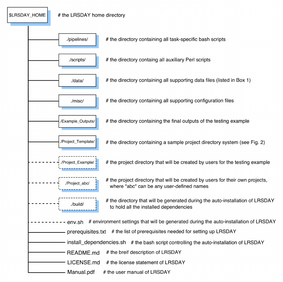
testing example and users’ own data are hosted under the same home directory

($LRSDAY_HOME) in a self-contained fashion (Fig. 1). This design makes LRSDAY well-isolated

from the rest of the system and therefore greatly improves its portability. To sum up, LRSDAY is

a highly transparent, automated and powerful computational framework that handles both

genome assembly and annotation, which suits the needs of the yeast community in performing

long-read-based genome sequencing projects. In the PROCEDURE section of this article, we

provide a step-by-step walkthrough on how to install, configure, and run LRSDAY with our

prepared testing example.

Figure 1. Overview of the LRSDAY directory system. All the top-level directories (boxes, solid

lines) and individual files of LRSDAY are listed and briefly described. Additional directories and

files will be generated during the installation or execution of LRSDAY (boxes, dashed lines).

Comparison with other methods

Genome assembly is a rapidly moving field, co-evolving with the fast-paced development of

sequencing technologies. In recent years, both hybrid (i.e. using both long and short reads) and

native (i.e. using long reads only) assemblers that support long-read sequencing data have been

developed and tested on many different organisms8,12–17. As for gene annotation, there is also a

wide range of choices that perform gene model prediction in an ab initio fashion or based on

additional evidences (e.g. mRNA transcripts, protein-sequence alignment)18–20. Specifically for

yeasts, a web-based gene annotation tool has been developed that combines both approaches21.

However, there is currently no integrated solution that handles both genome assembly and

annotation in a seamless way. To fill this gap, we revamped our original workflow for deriving the

yeast population-level reference genomes7 into a self-contained package to considerably

streamline this process with modular design and automated implementation. Moreover, rather

than simply combining the existing tools for genome assembly and gene annotation, LRSDAY

assembled a well-integrated workflow with many other functionalities (e.g. reference-guided

scaffolding, gene orthology identification, and additional genomic feature annotation) built in,

which makes it a unique one-stop solution for high-quality genome assembly and annotation

production from long-read sequencing data.

Experimental Design

Genome assembly and annotation are complex computational processes with many intermediate

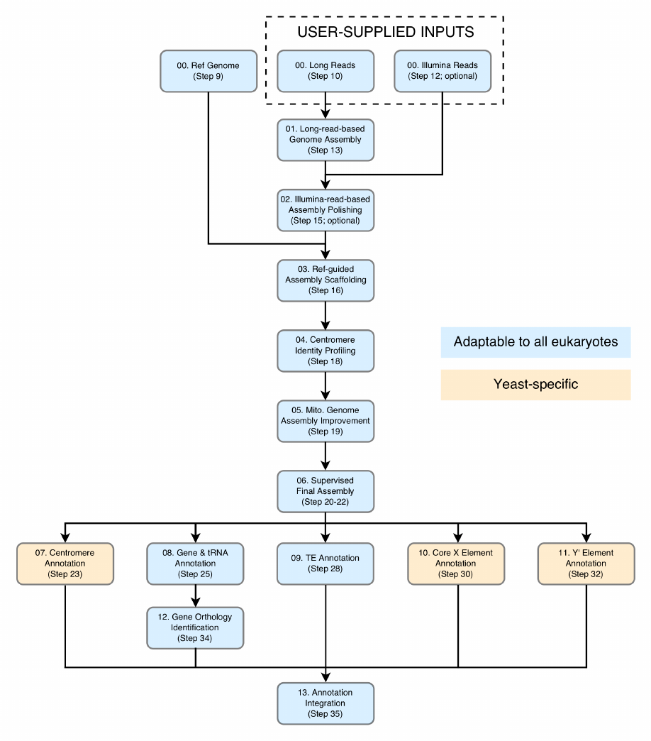
steps and inputs/outputs involved. With LRSDAY, we designed a highly structured project

directory system to help users to run the whole workflow in an organized and modular way (Fig.

2). Within such project directory system, the three subdirectories holding the pre-shipped

reference genome as well as the user-supplied long (PacBio or Oxford Nanopore) and short

(Illumina) reads are numbered as “00” and the task-specific subdirectories are numbered

sequentially from “01” to “13” according to their execution orders. For each subdirectory, a self-

explained name is attached after the number index to help users to navigate through the workflow.

To run each task, users only need to edit (i.e. to specify the input and output file paths and certain

task-specific parameters) and execute the task-specific pipeline scripts pre-placed in these

subdirectories. These pipeline scripts will automatically set environment variables, process the

data, and formulate the results. All computationally intensive tasks can be processed using

multiple threads to substantially save computation time. Although LRSDAY is mainly designed for

yeasts, most of these tasks can be further adapted for the analysis on any eukaryotic organisms

(See Appendix 2 for details). Below we briefly describe the computational processes executed by

each task-specific module in LRSDAY with the corresponding PROCEDURE Step labeled in

parentheses.

01. Long-read-based_Genome_Assembly (Step 13): Long reads generated from PacBio or

Oxford Nanopore technologies are used to perform de novo genome assembly using an

overlap-layout-consensus (OLC) algorithm.

02. Illumina-read-based_Assembly_Polishing (Step 15; optional): Illumina reads are first

clipped and trimmed to remove potential sequencing adapters and low-quality regions.

The cleaned reads are subsequently mapped to the raw long-read-based genome

assembly. The resulting BAM file is further processed for alignment sorting, mate

information and read group fixing, duplicates removal as well as local realignment. Finally,

the processed bam file is used for correcting base-level errors of the long-read-based

assembly.

03. Reference-guided_Assembly_Scaffolding (Step 16): The contigs from the polished

genome assembly are first aligned to the reference genome to identify their shared

sequence homology, based on which reference-guided assembly scaffolding is

subsequently performed. The chromosomal identity of each scaffold is labeled

accordingly. Structural rearrangements captured in the contigs will remain untouched

during the scaffolding.

04. Centromere_Identity_Profiling (Step 18): The pre-shipped S. cerevisiae centromere

sequences are searched against the scaffolded assembly for chromosome-specific

centromere identity profiling.

05. Mitochondrial_Genome_Assembly_Improvement (Step 19): The polished contigs

corresponding to the mitochondrial genome are re-collected from the scaffolded assembly.

The mitochondrial contigs spanning over the designated starting point (the ATP6 gene by

default) are broken into subsegments to prevent assembly problems caused by the

circular organization of the mitochondrial genome. The resulting contigs are then re-

assembled into a single linear sequence, which is further circularized by the designated

ATP6 starting point. The nuclear scaffolds and the circularized mitochondrial sequence

together form the improved genome assembly.

06. Supervised_Final_Assembly (Steps 20-22): A modification list containing the ordering,

orientation and naming information of each sequence from the improved genome

assembly is generated for users to review and to make manual adjustment when needed.

The final genome assembly is further generated based on the user-edited modification

list.

07. Centromere_Annotation (Step 23): The pre-shipped S. cerevisiae centromere

sequences are searched against the final genome assembly for centromere annotation.

08. Gene_Annotation (Step 25): De novo protein-coding and tRNA gene annotations are

performed for the final genome assembly, which are further leveraged by the mRNA

transcripts and protein sequences alignments.

09. TE_Annotation (Step 28): The pre-shipped curated TE library (containing the long

terminal repeats (LTRs) and internal sequences of the S. cerevisiae and S. paradoxus

Ty1-Ty5 by default) is searched against the final genome assembly to identify TEs. The

identified TEs are further curated and classified into the full-length, truncated, and solo-

LTRs of Ty1-Ty5.

10. Core_X_Element_Annotation (Step 30): The pre-shipped curated hidden Markov model

(HMM) of the S. cerevisiae core X elements is searched against the final genome

assembly to annotate core X elements.

11. Y_Prime_Element_Annotation (Step 32): The pre-shipped representative S. cerevisiae

Y’ element sequence is searched against the final genome assembly to annotate Y’

elements. Note that Y’ elements can have long, short or degenerated forms22, and we

used a representative long-form Y’ element as the query to maximize detection power.

12. Gene_Orthology_Identification (Step 34): The annotated protein-coding genes are

compared with the reference protein-coding genes based on both sequence homology

and gene order conservation to identify gene orthology relationship between these two

sets. Based on such gene orthology relationships, the Saccharomyces Genome Database

(SGD; http://www.yeastgenome.org/) systematic names are assigned to the annotated

protein-coding genes.

13. Annotation_Integration (Step 35): The annotations of centromeres, TEs, protein-coding

genes, tRNAs, as well as core X and Y’ elements are combined and sorted to form a final

integrated multi-feature annotation.

Figure 2. The workflow of LRSDAY. Each box represents an individual module. These modules

are numbered according to the tasks described in Experimental Design, with the corresponding

protocol step numbers also indicated. Modules that can be adapted for other eukaryotes are

colored in light blue while those yeast-specific are colored in orange.

Limitations and potential adaptation

In its distributed form, LRSDAY is tailored for the model budding yeast S. cerevisiae and its closely

related sister species S. paradoxus with a number of pre-shipped auxiliary data files configured

accordingly. However, given its modular design, the backbone of LRSDAY can be adapted for

virtually any eukaryotic organisms to perform genome assembly, sequence polishing, reference-

guided scaffolding, protein-coding genes and tRNA annotations, gene orthology identification,

and annotation integration. In Appendix 2, we provide some tips with regard to such adaptation.

Moreover, those assembly polishing, scaffolding and various annotation modules (See

Experimental Design) can also be used to analyze existing genome assemblies derived from any

or any combination of sequencing technologies. Such flexibility makes LRSDAY very useful for

expanded use cases and therefore suits the needs of a broader audience.

Expected improvements

As thousands of yeast strains have been or are currently under sequencing23–26, our knowledge

of the overall genome content diversity27 of this important model organism is expanding rapidly,

revealing a whole new picture of the pan-genome diversity of S. cerevisiae. For example, our lab

is currently working on characterizing the pan-genome of >1,000 S. cerevisiae isolates across the

globe (The 1002 Yeast Genomes Project26; http://1002genomes.u-strasbg.fr/). Future

developments of LRSDAY will incorporate such pan-genome dataset to provide additional

annotation information for those non-reference genes, especially with regard to their evolutionary

origin, population prevalence, and putative functions. Such information will greatly help users to

dissect and interpret complex genotype-phenotype interactions in diverse ecological and

biotechnological settings. An additional potential future direction of our research is the direct

integration with the downstream synteny analysis tools (e.g. CHROnicle28, MCScanX29, etc) to

perform automatic large-scale structural variants discovery, which exploits one of the major

benefits of having a high-quality genome assembly derived from long reads. Finally, we envision

developing a dedicated web-based tool to implement such database and tool integration at a

larger scale towards fully automated genomics analysis for the yeast community in the long run.

CITATIONS

Jia-Xing Yue & Gianni Liti. (2018) Long-read sequencing data analysis for yeasts. Nature

Protocols, 13:1213–1231.

Jia-Xing Yue, Jing Li, Louise Aigrain, Johan Hallin, Karl Persson, Karen Oliver, Anders

Bergström, Paul Coupland, Jonas Warringer, Marco Cosentino Lagomarsino, Gilles Fischer,

Richard Durbin, Gianni Liti. (2017) Contrasting evolutionary genome dynamics between

domesticated and wild yeasts. Nature Genetics, 49:913-924.

MATERIALS

Hardware, operating system and network

This protocol is designed for a desktop or computing server running an x86-64-bit Linux operating

system. Multi-threaded processors are preferred to speed up the process since many steps can

be configured to use multiple threads in parallel. For assembling and analyzing the budding yeast

genomes (genome size = ~12 Mb), at least 16 Gb of RAM and 100 Gb of free disk space are

recommended. When adapted for other eukaryotic organisms with larger genome sizes, the RAM

and disk space consumption will scale up, majorly during de novo genome assembly (performed

by Canu17). Please refer to Canu’s manual (http://canu.readthedocs.io/en/latest/) for suggested

RAM and disk space consumption for assembling large genomes. Stable Internet connection is

required for the installation and configuration of LRSDAY as well as for retrieving the testing data.

Software or library requirements

● Bash (https://www.gnu.org/software/bash/)

● Bzip2 (http://www.bzip.org/)

● Cmake (https://cmake.org/)

● GCC and G++ v4.7 or newer (https://gcc.gnu.org/)

● Ghostscript (https://www.ghostscript.com)

● Git (https://git-scm.com/)

● GNU make (https://www.gnu.org/software/make/)

● Gzip (https://www.gnu.org/software/gzip/)

● Java runtime environment (JRE) v1.8.0 or newer (https://www.java.com)

● Perl v5.12 or newer (https://www.perl.org/)

● Python v2.7.9 or newer (https://www.python.org/)

● Python v3.6 or newer (https://www.python.org/)

● Tar (https://www.gnu.org/software/tar/)

● Unzip (http://infozip.sourceforge.net/UnZip.html)

● Virtualenv v15.1.0 or newer (https://virtualenv.pypa.io)

● Wget (https://www.gnu.org/software/wget/)

● Zlib (https://zlib.net/)

Input data

● Long reads: A single FASTQ file containing PacBio or Oxford Nanopore reads is needed,

which will be used for long-read based de novo genome assembly (Task 01).

● Short reads: Short reads are optional for LRSDAY but LRSDAY could take advantage of

short reads when such data is available to perform additional assembly polishing (Task

02). If paired-end Illumina sequencing is performed, two FASTQ files containing the

forward and reverse Illumina reads respectively are needed. If only single-end Illumina

sequencing data is available, one FASTQ file containing the single-end reads is needed.

● Reference genome: For the budding yeast S. cerevisiae, we pre-shipped two reference

genome files (one original assembly and one with hard-masked subtelomeres and

chromosome-ends based on our previous study7). The masked version is used for

chromosomal scaffolding to minimize the confounding effect due to interchromosomal

subtelomeric rearrangemnets. When working with organisms of which the subtelomeric

regions are undefined, users can just use a single raw reference genome instead. The

reference genome file(s) will be used for reference-guided scaffolding, mitochondrial

genome assembly improvement and supervised final genome assembly (Task 03, 05 and

06 respectively).

● A number of S. cerevisiae-specific auxiliary data have been pre-shipped with LRSDAY for

genomic feature annotation and gene orthology identification (Task 07-12).

Example data

● The S. cerevisiae reference genome pre-shipped with LRSDAY is taken from our

previous study7 with the Genbank accession number GCA_002057635.1

(https://www.ncbi.nlm.nih.gov/assembly/GCA_002057635.1/). The sequencing reads

used for the testing example come from the same study, which consists of both PacBio

and Illumina reads produced from the S. cerevisiae strain SK1. The PacBio reads can be

retrieved with the ENA analysis accession number ERZ448251

(https://www.ebi.ac.uk/ena/data/view/ERZ448251). The Illumina reads can be retrieved

with the SRA sequencing run accession number SRR4074258

(https://www.ncbi.nlm.nih.gov/sra/?term=SRR4074258). In LRSDAY, we have provided

bash scripts to automatically download and setup these data for the testing example.

PROCEDURE

Download, install and configure LRSDAY ● TIMING <1 h

1) Download the latest LRSDAY release (current version: v1.1.0) by entering the following

commands in a terminal window:

$ wget https://github.com/yjx1217/LRSDAY/releases/download/v1.1.0/LRSDAY-v1.1.0.tar.gz

$ tar xvzf LRSDAY-v1.1.0.tar.gz

$ cd LRSDAY-v1.1.0

$ bash install_dependencies.sh

▲CRITICAL STEP Make sure you have a fast and stable Internet connection when

running this step since many tools will be downloaded here. Check that all the

prerequisites (see Software or library requirements in EQUIPMENT or the prerequisite.txt

file in the downloaded LRSDAY directory) have been installed on your system.

▲CRITICAL STEP Upon the successful completion of executing the bash script, you

should see a confirmation message prompted out: “LRSDAY message: This bash script

has been successfully processed! :)”. Otherwise, it means an error has occurred during

the execution of the bash script, which interrupted the automatic installation process. This

also applies to all the bash scripts used in Steps 8-35. Whenever an error is encountered,

please check the error message and refer to the troubleshooting section when available.

When the cause of the error is fixed, re-run this step to initiate a new installation. The

installer will prompt for the confirmation of deleting the build directory generated by the old

run, always answer “yes” to authorize such action so that the new installation can start.

▲CRITICAL STEP Pay attention to the final message prompted by the installation script

for a number of notes with regard to the additional manual setup steps as well as the

licensing information for commercial users.

? TROUBLESHOOTING

2) Load the environment settings for LRSDAY by entering:

$ source env.sh

After loading the pre-configured environment settings, the current directory should be

assigned to the environment variable $LRSDAY_HOME. You can check to see if the full

path to your current directory is displayed after entering:

$ echo $LRSDAY_HOME

▲CRITICAL STEP Although most required tools have been automatically installed and

configured, manual downloading and/or configuration are needed for GATK30 and

RepeatMasker31 due to license restriction of these tools or of their dependent libraries.

Make sure to run this command to load the pre-configured environment settings before

such manual setup (described in Steps 3-7). If you exited your terminal session before or

in the middle of your manual setup, you need to re-load the environment settings before

proceeding. These environment settings will be automatically loaded each time the task-

specific bash pipelines of LRSDAY are executed.

? TROUBLESHOOTING

3) Download and set up GATK3. Go to the official website of GATK

(https://software.broadinstitute.org/gatk/download/archive) and download GATK v3.8 (the

recently released GATK4 will not work). Registration might be needed for unregistered

GATK users. Place the downloaded GATK package (file name: GenomeAnalysisTK-3.8-

1- gf15c1c3ef.tar.bz2) in the GATK installation directory and set up GATK by entering the

following command in terminal:

$ mv GenomeAnalysisTK-3.8-1- gf15c1c3ef.tar.bz2 $LRSDAY_HOME/build/GATK3

$ cd $LRSDAY_HOME/build/GATK3

$ tar xjf GenomeAnalysisTK-3.8-1.tar.bz2

$ mv ./GenomeAnalysisTK-3.8-1*/GenomeAnalysisTK.jar .

$ chmod 755 GenomeAnalysisTK.jar

4) Set up TRF for RepeatMasker. Go to the TRF website

(http://tandem.bu.edu/trf/trf.download.html) to download the TRF v4.09 executable built

for 64-bit Linux. Place the downloaded file (file name: trf409.linux64) in the RepeatMasker

installation directory and set up TRF by entering:

$ mv trf409.linux64 $LRSDAY_HOME/build/RepeatMasker/

$ cd $LRSDAY_HOME/build/RepeatMasker/

$ chmod 755 trf409.linux64

$ ln -s trf409.linux64 trf

5) Set up the RepBase library for RepeatMasker. Go to the RepBase website

(http://www.girinst.org/repbase/) and register a user account (using a non-profit

institutional email address, e.g. the “.com” extension will not work) to download the

RepeatMasker edition of the RepBase library (version: 20170127). Place the downloaded

file (file name: RepBaseRepeatMaskerEdition-20170127.tar.gz) in the RepeatMasker

installation directory and uncompress it by entering:

$ mv RepBaseRepeatMaskerEdition-20170127.tar.gz $LRSDAY_HOME/build/RepeatMasker/

$ cd $LRSDAY_HOME/build/RepeatMasker/

$ tar xzf RepBaseRepeatMaskerEdition-20170127.tar.gz

? TROUBLESHOOTING

6) Get the installation path of TRF and rmblastn/makeblastdb by entering:

$ echo $trf_dir

$ echo $rmblast_dir

Remember these two paths since they will be used for the RepeatMasker configuration in

Step 7.

? TROUBLESHOOTING

7) Run the configuration script for RepeatMasker by entering:

$ perl ./configure

This configuration script will prompt for several questions. Please do the following to

answer these questions. Enter “env” for the question about the installation path of Perl.

Just press enter for the question about the installation path of RepeatMasker. Enter the

first path that you obtained in Step 6 for the question about the installation path of TRF.

Enter “2” for the question about selecting a search engine. Then enter the second path

that you obtained in Step 6 for the question about the installation path of rmblastn and

makeblastdb. Just press enter for the question about the default search engine. And finally

enter “5” to complete the configuration.

Run LRSDAY with the testing example ● TIMING 50 h

8) Create the project directory. When running LRSDAY with your own data, it is

recommended to make a copy of our Project_Template directory to create your own

project directory such as Project_abc, where “abc” can be any string containing letters,

numbers, or underscores. For this testing example, we make a copy of the

Project_Template directory and name it as Project_Example by entering:

$ cd $LRSDAY_HOME

$ cp -r Project_Template Project_Example

▲CRITICAL STEP Before proceeding to your own project, it is advised to first run our

prepared testing example to check if LRSDAY is working properly as well as to get

acquainted with the logic and workflow of LRSDAY.

9) Prepare the reference genome files. When running LRSDAY with your own data, you can

directly put the reference genome (in FASTA format without compression) in the

00.Ref_Genome subdirectory of your project directory (e.g. Project_abc). If your

sequenced organism is S. cerevisiae or S. paradoxus, you can use the reference genome

pre-shipped with LRSDAY. Here we prepare the pre-shipped reference genome for the

testing example by entering:

$ cd ./Project_Example/00.Ref_Genome

$ bash LRSDAY.00.Prepare_Sc_Ref_Genome.sh

10) Prepare the long reads. When running LRSDAY with your own data, you can directly put

the long reads in the 00.Long_Reads subdirectory of your project directory (e.g.

Project_abc). The reads file should be in FASTQ or FASTA format. Compressed files with

file extensions of “.gz”, “.bz2”, and “.xz” are also supported. For this testing example, you

can download the sample long reads by entering:

$ cd ./../00.Long_Reads

$ bash LRSDAY.00.Retrieve_Sample_PacBio_Reads.sh

11) (Optional) If your long reads are generated from the PacBio Sequel platform, your reads

are likely to be in BAM format. In this case, convert it to our supported format (FASTA or

FASTQ) using the following commands:

$ source ./../../env.sh

$ $bedtools_dir/bedtools bamtofastq -i long_reads.bam -fq long_reads.fastq

$ gzip long_reads.fastq

12) (Optional) Prepare the Illumina reads. Like for the long reads, directly put your Illumina

reads in the 00.Illumina_Reads subdirectory of your project directory (e.g. Project_abc)

when running LRSDAY for your own data. The reads file should be in FASTQ format with

“gzip” comprehension (identified by the “.gz” extension). For this testing example, you can

download the Illumina reads by entering:

$ cd ./../00.Illumina_Reads

$ bash LRSDAY.00.Retrieve_Sample_Illumina_Reads.sh

? TROUBLESHOOTING

13) Perform long-read-based de novo genome assembly by running the following commands:

$ cd ./../01. Long-read-based_Genome_Assembly

$ bash LRSDAY.01.Long-read-based_Genome_Assembly.sh

Upon the completion of this step, a summary file (SK1.canu.stats.txt for this testing

example) will be generated to report some basic summary statistics (e.g. total assembly

size, N50 (i.e. the contig length such that 50% of the total assembly size is contained in

contigs of at least this size), L50 (i.e. the number of longest contigs such that 50% of the

total assembly size is contained), GC-content, etc) to assist gauging the genome

assembly quality (Table 1). Two VCF files (SK1.canu.filter.mummer2vcf.SNP.vcf and

SK1.canu.filter.mummer2vcf.INDEL.vcf for the testing example) will also be generated to

report base-level differences between the raw genome assembly and the reference

genome for their uniquely alignable regions, which could also help for assessing the

genome assembly quality.

▲CRITICAL STEP This step can be run with multiple threads to speed up the process.

Depending on the CPU configuration of your Linux server/desktop, you can edit the

“threads=” option in the bash script LRSDAY.01.Long-read-based_Genome_Assembly.sh

to enable multi-threading. You can do the same for all the following tasks whenever the

“threads=” option is provided in the corresponding task-specific bash script. Simple text

editors such as emacs, vim, gedit or pico are highly recommended for such editing. Rich

text editors might not work

▲CRITICAL STEP Note this step will take long to finish (see TIMING), so we recommend

running this step and all the other time-consuming steps with “nohup”

(https://en.wikipedia.org/wiki/Nohup), which allows the process to continue running after

you exit the terminal or logout from the server. As an example, you can run the bash script

using nohup as follows:

$ nohup bash LRSDAY.01.Long-read-based_Genome_Assembly.sh >run_log.txt 2>&1 &

▲CRITICAL STEP Starting from v1.1.0, LRSDAY added the

"customized_canu_parameters” option to support customized parameter settings for the

Canu assembler. In addition, two additional assemblers, Flye and smartdenovo, were

further supported. Based on our test, Flye32 (https://github.com/fenderglass/Flye) and

smartdenovo (https://github.com/ruanjue/smartdenovo) run much faster than Canu but

also came with understandable tradeoff in assembly precision, as reflected by the higher

base-level error rate of their resulting assemblies. Therefore, when assembling with Flye

or smartdenovo, post-assembly polishing is strongly recommended.

▲CRITICAL STEP When running LRSDAY with your own data, modify the bash script to

specify the input reads and reference genome, the input reads type (e.g. “pacbio_raw”,

“pacbio_corrected”, “nanopore_raw” or “nanopore_corrected”), the estimated genome

size for the assembled genome, as well as the prefix for the output data. Remember to do

similar project-specific adjustment for all the following steps.

? TROUBLESHOOTING

14) (Optional) Polishing genome assembly with long-reads. When running LRSDAY for your

own data, if you performed PacBio sequencing and also have access to a locally installed

PacBio SMRT Analysis software package (http://www.pacb.com/products-and-

services/analytical-software/smrt-analysis/), we recommend running the first-pass

polishing for the assembly generated in Step 13 based on raw PacBio reads by using

PacBio’s own Quiver/Arrow pipeline13. If you performed Oxford Nanopore sequencing, we

recommend using nanopolish (https://github.com/jts/nanopolish) or equivalent tools to

perform the assembly polishing based on raw Nanopore reads in this step. We expect to

directly pack nanopolish into LRSDAY in our next release. We will also try to the same for

PacBio’s Quiver/Arrow pipeline but it seems quite challenging. Finally, we also tested

Racon (https://github.com/isovic/racon) for polishing but its performance was not

satisfying.

15) (Optional) Polishing genome assembly with Illumina reads. When Illumina reads are

available, we recommend running this additional polishing step either for the raw assembly

generated in Step 13 (when Step 14 is skipped as in our testing example) or for the long-

read-polished assembly generated in Step 14. Use the following commands to perform

Illumina-read-based assembly polishing. This step can be run with multiple threads.

$ cd ./../02.Illumina-read-based_Assembly_Polishing

$ bash LRSDAY.02.Illumina-read-based_Assembly_Polishing.sh

TABLE 1 | Assembly statistics for the genome of S. cerevisiae strain SK1 assembled in the

testing example.

Assembly statistics

Raw

assembly

Scaffolded

assembly

Final

assembly

Total sequence count

Total sequence length (bp)

12505999

12511058

12489291

Min sequence length (bp)

1248

Max sequence length (bp)

1480196

1480203

Mean sequence length (bp)

357314.26

367972.29

378463.36

Median sequence length (bp)

103703.00

74951.00

84648.00

N50 (bp)

818058

923633

L50

N90 (bp)

341459

341463

L90

GC%

38.27

38.25

38.29

0.00

0.08

0.04

Note

N50: the contig length such that 50% of the total assembly size is contained in contigs of at

least this size.

L50: the number of longest contigs such that 50% of the total assembly size is contained.

N90: the contig length such that 90% of the total assembly size is contained in contigs of at

least this size.

L90: the number of longest contigs such that 90% of the total assembly size is contained.

GC%: the percentage of guanine (G) and cytosine (C) bases in the nucleotide sequences.

N%: the percentage of the N bases in the nucleotide sequence. In genome assembly, the N

bases are usually used to represent scaffolding gaps.

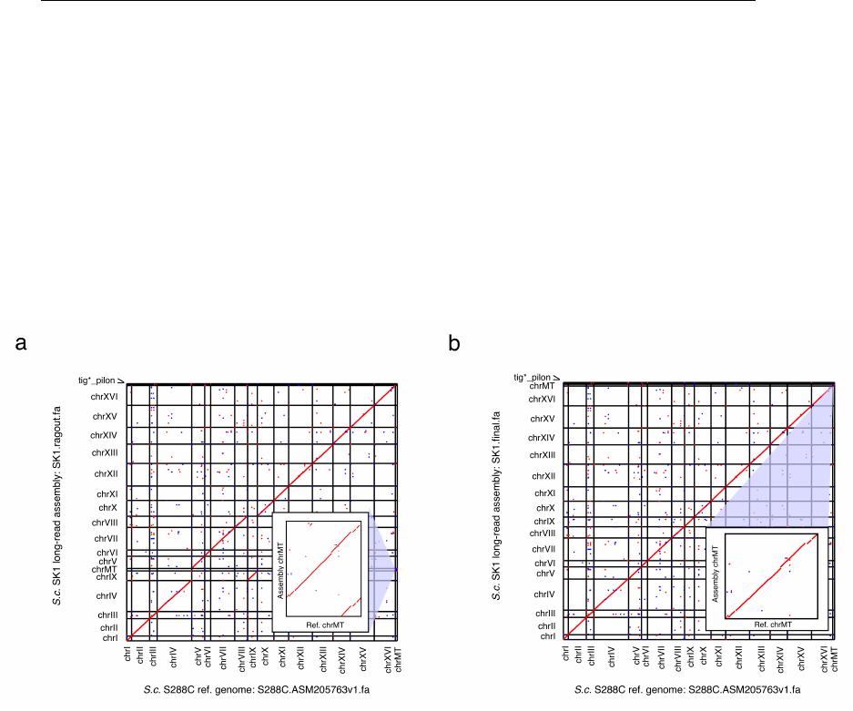
Figure 3. Genome-wide dotplots of the S. cerevisiae SK1 genome assembly generated in

the LRSDAY testing example. Both the raw scaffolded assembly (panel a; generated in Step

16) and the final assembly (panel b, generated in Step 22) are analyzed. The forward and reverse

sequence matches are depicted in red and blue respectively, while the zoomed-in views of the

mitochondrial genome (chrMT) comparison are shown in insets. In addition to the sixteen nuclear

chromosomes and the mitochondrial genome, the scaffolded and final assemblies also contain

some short contigs (named as tig*_pilon) that are derived from highly repetitive regions.

16) Perform chromosome-level scaffolding for the long-read-based assembly. Run the

following commands:

$ cd ./../03.Reference-guided_Assembly_Scaffolding

$ bash LRSDAY.03.Reference-guided_Assembly_Scaffolding.sh

This step can be run with multiple threads. Upon completion, a list of summary statistics

(SK1.ragout.stats.txt for this testing example) will be generated for the scaffolded

assembly (Table 1).

▲CRITICAL STEP Please check the generated genome-wide dotplot

(SK1.ragout.filter.pdf for the testing example) (Fig. 3a) to verify the correctness of

chromosomal identity assignment performed by Ragout33 and apply manual adjustment in

Step 21 when necessary. When running LRSDAY with your own data, you might see a

single scaffold corresponds to more than one reference chromosomes, which could be

due to shared sequence homology between duplicated regions or interchromosomal

rearrangements. Both types of events can be correctly interpreted based on the genome-

wide dotplot generated in this Step. In either case, LRSDAY can correctly assign

chromosomal identity of the corresponding scaffold based on its encompassed

centromere identity as annotated in Step 18. Check the generated AGP file

(SK1.ragout.agp for the testing example) for the details of reference-based scaffolding.

▲CRITICAL STEP Due to the high AT and repeat contents and the circular conformation

of the mitochondrial genome, multiple contigs corresponding to the mitochondrial genome

are often obtained from the raw genome assembly, as shown in the generated

mitochondrial genome dotplot (SK1.ragout.chrMT.filter.pdf for the testing example) (Fig.

3a, inset). A list of such mitochondrial contigs will also be generated (SK1.mt_contig.list

for the testing example), which will be used in Step 19 for improving mitochondrial genome

assembly.

17) (Optional) When running LRSDAY for your own data, if you have strong evidence for mis-

scaffolding based on prior knowledge or other experimental data (e.g. mate-pair libraries

or chromosomal contact data), break the corresponding ragout scaffolds back to contigs

and re-joined them with corrected order using the pre-shipped Perl scripts

break_scaffolds_by_N.pl, join_contigs_by_N.pl and extract_region_from_genome.pl in

the $LRSDAY_HOME/scripts directory by running the following commands:

perl $LRSDAY_HOME/scripts/break_scaffolds_by_N.pl -i <the input FASTA file containing the

scaffold sequence(s) to break> -o < the output FASTA file containing the scaffolds after the

breaking> -g <the minimal length of runs of Ns in the input scaffold(s) for breaking, e.g. 100>

perl $LRSDAY_HOME/scripts/join_contigs_by_N.pl -i <the input FASTA file containing contigs for

joining in a sequential order> -o <the output FASTA file containing scaffold sequence after the

contig joining> –g <gap size, i.e. the number of Ns to be inserted between two joined contigs> -t

perl $LRSDAY_HOME/scripts/extract_region_from_genome.pl -i <the input FASTA file containing

the genome assembly> -o <the output FASTA file containing the extracted query sequence> -q

<specially formatted query string (sequence:start-end:strand) containing the genomic coordinates

for the region to be extracted, e.g. using the query string chrI:1000-4000:+ for extracting the

sequence in the region 1000-4000 bp on the + strand of chrI in the input genome assembly> -f <the

length of flanking sequences to be extracted as well, e.g. 100 for 100-bp flanking region>

A scenario for such use case is when the breakpoints of structural rearrangements are

also the breakpoints of the genome assembly. In this case, the reference-based

scaffolding will arrange contigs according to the reference genome configuration and

therefore un-do the genome rearrangement.

18) Perform centromere profiling for the scaffolded genome assembly by running the following

commands:

$ cd ./../04.Centromere_Identity_Profiling

$ bash LRSDAY.04.Centromere_Identity_Profiling.sh

▲CRITICAL STEP The chromosome-specific centromere identities profiled here will be

used as another layer of information for the final chromosomal identity assignment in Step

21. The profiled centromere identities usually agree well with the chromosomal identities

labeled in Step 16, so that chrI will have the CEN1 centromere and chrII will have the

CEN2 centromere, etc. Exception can occur when interchromosomal rearrangements are

involved in your sequenced genome. In such case, we recommend naming those

rearranged chromosomes according to their encompassed centromeres in Step 21.

19) Perform mitochondrial genome assembly improvement by running the following

commands:

$ cd ./../05.Mitochondrial_Genome_Assembly_Improvement

$ bash LRSDAY.05.Mitochondrial_Genome_Assembly_Improvement.sh

▲CRITICAL STEP Check the generated final mitochondrial genome dotplot

(SK1.mt_improved.chrMT.filter.pdf for the testing example) and compare it with the

mitochondrial genome dotplot generated in Step 16 to see how the mitochondrial genome

assembly has been improved when aligning with the reference mitochondrial genome (Fig.

3b, inset). When running this step for your own data, the degree of such improvement may

vary because it depends on both the complexity of the assembled mitochondrial genome

and the quality of library preparation and sequencing experiments.

? TROUBLESHOOTING

20) Generate the assembly modification list file for performing the final chromosome

assignment by running the following commands:

$ cd ./../06.Supervised_Final_Assembly

$ bash LRSDAY.06.Supervised_Final_Assembly.1.sh

21) Edit the generated assembly modification list file (SK1.modification.list for the testing

example) based on the genome-wide dotplot generated in Step 16 and the centromere

profiles generated in Step 18. The modification list file consists of three comma-separated

columns, which correspond to the original sequence name, sequence orientation, and new

sequence name respectively. With this file, you can do three types of editing:

If you need to change the current sequence order, you can move the corresponding

rows upward or downward to reflect the correct order.

If you need to invert the orientation of a given sequence, you can change its

orientation from “+” to “-” in column 2.

If you need to rename a given sequence, you can specify the new name in the third

column.

For this testing example here, we need to move the row “chrIX,+,chrIX” downward to place

it after the row “chrVIII,+,chrVIII”, so that chrIX will be placed after chrVIII in the final

assembly. Also, we need to change the row “chrMT_Contig1,+,chrMT_Contig1” to

“chrMT_Contig1,+,chrMT” for renaming the assembled sequence corresponding to the

mitochondrial genome.

22) Once all the modifications have been specified, run the following bash script to generate

the final genome assembly as well as the associated genome-wide dotplot (Fig. 3b),

assembly statistics (Table 1), and VCF files:

$ bash LRSDAY.06.Supervised_Final_Assembly.2.sh

23) Re-run centromere annotation for the final genome assembly using the following

commands:

$ cd ./../07.Centromere_Annotation

$ bash LRSDAY.07.Centromere_Annotation.sh

24) (Optional) Customize the configuration file for gene annotation. When running LRSDAY

with your own data, edit the configuration file

$LRSDAY_HOME/misc/maker_opts.customized.ctl if your sequenced organisms is

neither S. cerevisiae nor S. paradoxus (See Appendix 2 for the details). If your sequenced

organism is S. cerevisiae or S. paradoxus, no customization is needed unless you have

native transcriptome or expressed sequence tag (EST) data for the strain that you

sequenced. In this case, you can edit the line 16 of this file to provide the full path of the

native transcriptome or EST assembly for your sequenced strain.

25) Annotate protein-coding genes and tRNAs for the final genome assembly, using the

following commands. This step can be run with multiple threads.

$ cd ./../08.Gene_Annotation

$ bash LRSDAY.08.Gene_Annotation.sh

26) (Optional) A manual checklist file (SK1.EVM.manual_check.list for the testing example)

containing a list of genes with suspicious annotations will be generated in Step 25. As

labeled in this file, these annotated gene models could be fragmented, frameshifted or

containing internal stop codons. Potentially, these genes could be good candidates for

pseudogenes. Manually inspect the annotated gene models of these genes by loading the

annotation result (SK1.EVM.gff3 for the testing example) together with the protein/EST-

alignment evidence files generated during the annotation in Step 25

(SK1.protein_evidence.gff3 and SK1.est_evidence.gff3 for the testing example) into IGV34

to check how well these suspicious gene models are supported by the corresponding

protein/EST-alignment evidence and to tag or remove those truly problematic ones in your

downstream analysis.

27) (Optional) Perform dedicated mitochondrial protein-coding and RNA annotation. If you are

interested in studying mitochondrial genomes, we highly recommend running dedicated

mitochondrial feature annotation with specialized software such as MFannot

(http://megasun.bch.umontreal.ca/cgi-bin/mfannot/mfannotInterface.pl). Although

MFannot does not support local installation so far, you can run MFannot conveniently via

its web portal. Be sure to select the correct genetic code table (e.g. “3 Yeast Mitochondrial”

for annotating yeast mitochondrial genomes) for your analysis.

28) Annotate transposable elements (TEs) for the final genome assembly. This step can be

run with multiple threads using the following commands:

$ cd ./../09.TE_Annotation

$ bash LRSDAY.09.TE_Annotation.sh

29) (Optional) TE activity can be highly dynamic in the genome with many complex cases

such as fragmentation and nested insertion. In LRSDAY, we used REannotate35 to

automatically resolve these complex cases, which works well for most cases but it could

occasionally misjoin two adjacent TEs when they are closely spaced. Further inspect and

curate the LRSDAY TE annotation output (SK1.TE.gff3 for the testing example) by

visualizing it in IGV34 together with the raw REannotate annotation (SK1.REannotate.gff

for the testing example). For each TE found in the LRSDAY TE annotation output, examine

its corresponding LTR and internal region structure based on the raw REannotate

annotation to check for misjoinings. If needed, you can manually edit the corresponding

TE annotation output file to decouple the misjoinings.

30) Annotate yeast telomere-associated core X elements for the final genome assembly, using

the following commands:

$ cd ./../10.Core_X_Element_Annotation

$ bash LRSDAY.10.Core_X_Element_Annotation.sh

31) (Optional) Inspect the alignment file for annotated core X element. In LRSDAY, we label

the identified core X elements to be “partial” if they are shorter than 300 bp. This should

work for most cases but we recommend inspecting the generated alignment file

(SK1.X_element.aln.fa for the testing example) for further curation. Upon the curation,

manually adjust the “partial” labeling in the annotation file (SK1.X_element.gff3 for the

testing example) when needed.

32) Annotate yeast telomere-associated Y’ elements for the final genome assembly by using

the following commands:

$ cd ./../11.Y_Prime_Element_Annotation

$ bash LRSDAY.11.Y_Prime_Element_Annotation.sh

33) (Optional) Inspect the alignment file for annotated Y’ element. Like for the core X element

annotation, we used a hard length cutoff (3500 bp) to label if the identified Y’ elements are

“partial”. We recommend manually inspecting the generated alignment file

(SK1.Y_prime_element.aln.fa for the testing example) to check if the “partial” labeling is

needed and edit the annotation file (SK1.Y_prime_element.gff3 for the testing example)

accordingly.

34) Perform orthology identification for protein coding genes by using the following

commands:

$ cd ./../12.Gene_Orthology_Identification

$ bash LRSDAY12.Gene_Orthology_Identification.sh

In this step, a gene orthology relationship list is created between the annotated proteome

and the SGD S. cerevisiae reference proteome based on both sequence similarity and

synteny conservation. Based on this list, we further attach SGD systematic names to our

gene annotation as shown in the “Name=” field of the generated GFF3 file

(SK1.updated.gff3 for the testing example). For a given annotated gene, when more than

one orthologous gene can be found in the SGD reference proteome, we will label all of its

co-orthologs in the “Name=” filed with “/” between the alternative SGD systematic names

(e.g. “YAR071W/YHR215W”), whereas when no orthologous gene can be found, we will

label its gene name as “Name=NA”. This step can be run with multiple threads.

35) Integrate the annotation of different genomic features into a unified GFF3 file by using the

following commands:

$ cd ./../13.Annotation_Integration

$ bash LRSDAY.13.Annotation_Integration.sh

? TROUBLESHOOTING

Troubleshooting advice can be found in Table 2.

TABLE 2 | Troubleshooting table.

Step

Problem

Possible reason

Solution

Downloading errors or

unresponsive remote

servers

Unstable internet

connection or temporary

problems of the remote

servers where the tools for

downloading are hosted.

Stabilizing the internet connection

and give another try.

Compilation or

installation error for

specific tools.

Prerequisites not satisfied

or corner cases due to

your specific system

settings.

If missing prerequisites are found

(see software and library

requirements in EQUIPMENT),

install the missing prerequisites

and give another try as described

above. Otherwise, record the error

message and email it to the

developers of the problematic tools

or the authors of this protocol for

further problem diagnosis.

Cannot find the file

“env.sh”.

Step 1 has failed.

Check the error message that you

got when running Step 1 and refer

to the troubleshooting for Step 1.

Rejected by RepBase

for the license

registration.

A personal or commercial

email address (e.g. with a

.com extension) was used

for the registration.

Use a non-commercial institutional

email address for the registration

or purchase the commercial

license if you work in a commercial

entity. Also, the installation of

RepBase can be potentially

skipped although not

recommended by RepeatMasker.

Users can still follow the remaining

steps of this protocol even if they

skip the RepBase installation here.

“echo $rmblast_dir”

returns nothing.

Step 2 has failed or your

terminal session got

interrupted before this

step.

Re-load environment settings in

Step 2 and then re-try this step.

Downloading

warnings/errors

encountered.

Temporary SRA server

problems.

Directly download the sample

Illumina reads for the testing

example by running the following

commands:

$ wget

ftp://ftp.sra.ebi.ac.uk/vol1/fastq/SR

R407/008/SRR4074258/SRR4074

258_1.fastq.gz

$ ln -s SRR4074258_1.fastq.gz

SRR4074258_pass_1.fastq.gz

$ wget

ftp://ftp.sra.ebi.ac.uk/vol1/fastq/SR

R407/008/SRR4074258/SRR4074

258_2.fastq.gz

$ ln -s SRR4074258_2.fastq.gz

SRR4074258_pass_2.fastq.gz

The total assembly

size is much smaller

than the expected

value or the assembly

is too fragmented.

Insufficient sequencing

depth of coverage.

Obtain more reads. We

recommend a minimal sequencing

depth of 20X.

Assembly runs too

slow.

This likely will happen for

Canu with high-depth

nanopore reads.

Three options are available:

1) Use the pre-shipped perl

script

subsampling_seqeunces.p

l in the

$LRSDAY_HOME/scripts

directory to downsample

(either randomly or

preferably sampling the

longer ones) the reads.

Example:

perl

subsampling_sequences.p

l -i input.fq(.gz) -f fastq -s

0.1 -m random -p output #

randomly sampling the

10% sequences

perl

subsampling_sequences.p

l -i input.fq(.gz) -f fastq -s

0.1 -m longest -p output #

sampling the 10% longest

sequences

2) Use the customized

parameters as suggested

in the bash script

LRSDAY.01.Long-read-

based_Genome_Assembly

.sh

3) Use alternative

assemblers such as Flye

or smartdenovo for this

step.

Only partial assembly

is obtained for the

mitochondrial genome.

High AT and repeat

content of the

mitochondrial genome is

challenging for de novo

genome assembly.

If the sequencing is done with

PacBio, obtaining more reads

should solve the problem. If

sequencing is done with Oxford

Nanopore data, currently there is

no satisfying solution. Future

improvement of the Oxford

Nanopore sequencing technology

will likely solve this problem given

the rapid development of this

technology.

● TIMING

The following timing information was measured on a Linux computing server with an Intel Xeon

CPU E5-2630L v3 (1.80GHz) using 4 threads. Enabling multithreading can substantially decrease

the processing time. All optional steps except Steps 12 and 15 were not processed when

measuring the computation time.

Steps 1-7, set up LRSDAY: < 1 h.

Step 8, prepare the project directory for the testing example: 5 s.

Step 9, prepare the reference genomes for the testing example: 1 s.

Step 10, prepare the long reads for the testing example: 22 min.

Step 12 (optional), prepare the Illumina reads for the testing example: 20 min.

Step 13, de novo assembly using long-reads: 26 h.

Step 15 (optional), assembly polishing using Illumina reads: 1h.

Step 16, reference-guided scaffolding for the raw assembly: 12 min.

Step 18, centromere identity profiling for the scaffolded assembly: 1 s.

Step 19, mitochondrial genome assembly improvement: 4 min.

Step 20, generate the assembly modification list file: 1s.

Step 21, manual editing the assembly modification list file: 30 s.

Step 22, finalize genome assembly based on the assembly modification list file: 20 s.

Step 23, centromere annotation for the final assembly: 1s.

Step 25, protein-coding gene and tRNA annotation for the final assembly: 19 h.

Step 28, TE annotation for the final assembly: 5 min.

Step 30, core X element annotation for the final assembly: 2 min.

Step 32, Y’ element annotation for the final assembly: 2.5 min.

Step 34, gene orthology identification for the annotated protein-coding genes: 20 min.

Step 35, final annotation integration: 1 min.

ANTICIPATED RESULTS

Upon the completion of the LRSDAY workflow described above, users can expect to obtain a

chromosome-level genome assembly with comprehensive genomic feature annotation, which will

lay a solid foundation for all kinds of downstream genomic and functional analyses. As

demonstrated in Fig. 3b, the final genome assembly is highly continuous, with each chromosome

assembled in an end-to-end fashion. Both genome-wide dotplots (like those shown in Fig. 3) and

summary statistics (like those listed in Table 1) will be generated to help users to evaluate the

genome assembly quality both graphically and quantitatively. As for the annotation, LRSDAY

profiles a full spectrum of genomic features for the assembled yeast genome, which include

centromeres, protein-coding genes, tRNAs, Ty1-Ty5 transposable elements, as well as the

telomere-associated core X and Y’ elements. The availability of such rich information can be very

valuable for users working on diverse biological questions. In Table 3, we further summarized the

major outputs of the testing example. The final genome assembly and annotation outputs

generated with this testing example are also provided in the directory Example_Outputs for users

to make direct comparison with their own results.

TABLE 3 | Major LRSDAY outputs from the testing example.

Task

Step

Output file or directory

Explanation for the output

SK1.canu.fa

The long-read-based de novo genome

assembly containing all the contigs

assembled by Canu17.

SK1.canu.stats.txt

The summary table reporting basic

assembly statistics, such as the number

of the assembled sequences, the total

length of the assembled sequences, the

minimal, maximal, mean and median

lengths of the assembled sequences, the

N50, L50, N90, and L90 of the assembled

sequences, as well as the base

composition (A%, T%, G%, C%, AT%,

GC% and N%) of the assembled

sequences. Users can compare this file

with the similar file generated in Step 16

and Step 22. We also summarized such

comparison in Table 1.

SK1.canu.filter.pdf

The genome-wide dotplot for the

comparison between the raw genome

assembly and the reference genome.

SK1.canu.filter.mummer2vcf.SNP

.vcf

The VCF file showing SNP differences

between the raw genome assembly and

the reference genome. This file can be

used for assessing the raw assembly

quality.

SK1.canu.filter.mummer2vcf.IND

EL.vcf

The VCF file showing INDEL differences

between the raw genome assembly and

the reference genome. This file can be

used for assessing the raw assembly

quality.

SK1_canu_out

the directory containing all the output files

of Canu

SK1.pilon.fa

The polished genome assembly

generated by Pilon36.

SK1.pilon.vcf

The VCF file reporting the variants

identified by Pilon based on short reads

mapping against the input genome

assembly.

SK1.pilon.changes

The space-delimited record of all the

changes that Pilon made during the

assembly polishing. The four columns

are: the original sequence coordinate, the

new sequence coordinate after the

correction, the original base, the new

base after the correction.

SK1.realn.bam

The BAM file of short reads mapping

against the input genome assembly.

SK1.ragout.fa

The scaffolded genome assembly based

on the reference genome.

SK1.ragout.stats.txt

The summary table reporting basic

assembly statistics of the scaffolded

genome assembly. Users can compare

this file with the similar file generated in

Step 13 and Step 22. We also

summarized such comparison in Table 1.

SK1.ragout.agp

the AGP file reporting the order and

orientation of each input contig used

during scaffolding.

SK1_ragout_out

The directory containing all the output

files of Ragout33.

SK1.ragout.filter.pdf

The genome-wide dotplot for the

comparison between the scaffolded

assembly and the reference genome.

SK1.mt_contig.list

The list of assembled contigs

corresponding to the mitochondrial

genome. This file will be used for Step 19.

SK1.mt_contig.fa

The assembled contig sequences

corresponding to the mitochondrial

genome.

SK1.ragout.chrMT.filter.pdf

The dotplot for the comparison between

the scaffolded mitochondrial genome

assembly and the reference mitochondrial

genome.

SK1.centromere.gff3

The profiled centromere identities for the

scaffolded genome assembly.

SK1.mt_improved.fa

The improved genome assembly with

better processing (re-assembling and

circularization) of the mitochondrial

genome.

SK1.mt_improved.chrMT.filter.pdf

The dotplot for the comparison between

the improved mitochondrial genome

assembly and the reference mitochondrial

genome. You should see improved

collinearity in this plot than the similar plot

generated in Step 16.

20-22

SK1.modification.list

The assembly modification list file for

manual editing to guide the final genome

assembly.

SK1.final.fa

The final genome assembly generated by

LRSDAY.

SK1.final.filter.pdf

The genome-wide dotplot for the

comparison between the final genome

assembly and the reference genome.

SK1.final.stats.txt

The summary table reporting basic

assembly statistics of the final genome

assembly. Users can compare this file

with the similar file generated in Step 13

and Step 16. We also summarized such

comparison in Table 1.

SK1.final.filter.mummer2vcf.SNP.

vcf

The VCF file showing SNP differences

between the final genome assembly and

the reference genome. This file can be

used for assessing the final assembly

quality.

SK1.final.filter.mummer2vcf.INDE

L.vcf

The VCF file showing INDEL differences

between the final genome assembly and

the reference genome. This file can be

used for assessing the final assembly

quality.

SK1.centromere.gff3

The centromere annotation for the final

genome assembly.

SK1.maker.raw.gff3

The raw MAKER37 annotation for protein-

coding genes and tRNA genes.

SK1.EVM.gff3

The final EVM38 annotation for protein-

coding genes and tRNA genes with

systematically assigned gene IDs.

SK1.protein_evidence.gff3

The protein-to-genome alignment

evidences generated by MAKER. This file

can be used for manual curation of those

suspicious annotations.

SK1.est_evidence.gff3

The EST-to-genome alignment evidences

generated by MAKER. This file can be

used for manual curation of those

suspicious annotations.

SK1.EVM.trimmed_cds.fa

The CDSs of the final EVM protein-coding

annotation with the out-of-frame parts

trimmed.

SK1.EVM.trimmed_cds.log

The log file of the CDS trimming for the

final EVM protein-coding gene annotation.

SK1.EVM.pep.fa

The translated protein sequences of the

trimmed CDSs derived from the final EVM

protein-coding gene annotation.

SK1.EVM.manual_check.list

The list of suspicious gene annotations for

manual curation.

SK1.EVM.PoFF.gff

The gene synteny information derived

from SK1.EVM.gff3, which will be used for

Task 12 (Step 34).

SK1.EVM.PoFF.ffn

Same as SK1.EVM.trimmed_cds.fa but

with simpler sequence IDs, which could

be used for Task 12 (Step 34).

SK1.EVM.PoFF.ffa

Same as SK1.EVM.pep.fa but with

simpler sequence IDs, which will be used

for Task 12 (Step 34).

SK1.REannotate.gff

The raw TE annotation from REannotate.

This file can be used for further curating

TE annotation.

SK1.TE.gff3

The final TE annotation from LRSDAY.

SK1.X_element.gff3

The final core X element annotation from

LRSDAY.

SK1.X_element.fa

The sequences of all the annotated core

X elements.

SK1.X_element.aln.fa

The sequence alignment of all the

annotated core X elements for further

checking whether the annotated feature is

complete or partial as well as whether this

is consistent with the labeling in the

annotation file SK1.X_element.gff3.

SK1.Y_prime_element.gff3

The final Y’ element annotation from

LRSDAY.

SK1.Y_prime_element.fa

The sequences of all the annotated Y’

elements.

SK1.Y_prime_element.aln.fa

The sequence alignment of all the

annotated Y’ elements for further

checking whether the annotated feature is

complete or partial as well as whether this

is consistent with the labeling in the

annotation file

SK1.Y_prime_element.gff3.

SK1.proteinortho

The gene orthology mapping between the

annotated genes and the reference gene

sets based only on sequence similarity.

SK1.poff

The gene orthology mapping between the

annotated genes and the reference gene

sets based on both sequence similarity

and synteny conservation.

SK1.updated.gff3

The updated gene annotation with

reference-based gene name labeling.

SK1.final.gff3

The final integrated annotation from

LRSDAY.

SK1.final.trimmed_cds.fa

The CDSs of the final protein-coding gene

annotation with the out-of-frame parts

trimmed.

SK1.final.trimmed_cds.log

SK1.final.trimmed_cds.log: the log file of

the CDS trimming for the final protein-

coding gene annotation.

SK1.final.pep.fa

The translated protein sequences of the

trimmed CDSs derived from the final

protein-coding gene annotation.

SK1.final.manual_check.list

The list of suspicious gene annotations for

manual curation.

SK1.final.fa

A copy of the final genome assembly

generated in Task 06 (Step 22).

REFERENCES

1. Goffeau, A. et al. Life with 6000 Genes. Science 274, 546–567 (1996).

2. Gordon, D. et al. Long-read sequence assembly of the gorilla genome. Science 352,

aae0344 (2016).

3. VanBuren, R. et al. Single-molecule sequencing of the desiccation-tolerant grass

Oropetium thomaeum. Nature 527, 508–11 (2015).

4. Bickhart, D. M. et al. Single-molecule sequencing and chromatin conformation capture

enable de novo reference assembly of the domestic goat genome. Nat. Genet. 49, 643–

650 (2017).

5. Badouin, H. et al. The sunflower genome provides insights into oil metabolism, flowering

and Asterid evolution. Nature 546, 148–152 (2017).

6. Jain, M. et al. Nanopore sequencing and assembly of a human genome with ultra-long

reads. Nat. Biotechnol. 36, 338–345 (2018).

7. Yue, J.-X. et al. Contrasting evolutionary genome dynamics between domesticated and

wild yeasts. Nat. Genet. 49, 913–924 (2017).

8. Goodwin, S. et al. Oxford Nanopore sequencing, hybrid error correction, and de novo

assembly of a eukaryotic genome. Genome Res. 25, 1750–1756 (2015).

9. McIlwain, S. J. et al. Genome sequence and analysis of a stress-tolerant, wild-derived

strain of Saccharomyces cerevisiae used in biofuels research. G3 (Bethesda). 6, 1757–

66 (2016).

10. Istace, B. et al. de novo assembly and population genomic survey of natural yeast

isolates with the Oxford Nanopore MinION sequencer. Gigascience 6, 1–13 (2017).

11. Giordano, F. et al. De novo yeast genome assemblies from MinION, PacBio and MiSeq

platforms. Sci. Rep. 7, 3935 (2017).

12. Koren, S. et al. Hybrid error correction and de novo assembly of single-molecule

sequencing reads. Nat. Biotechnol. 30, 693–700 (2012).

13. Chin, C.-S. et al. Nonhybrid, finished microbial genome assemblies from long-read SMRT

sequencing data. Nat. Methods 10, 563–9 (2013).

14. Berlin, K. et al. Assembling large genomes with single-molecule sequencing and locality-

sensitive hashing. Nat. Biotechnol. 33, 623–630 (2015).

15. Chin, C.-S. et al. Phased diploid genome assembly with single-molecule real-time

sequencing. Nat. Methods 13, 1050–1054 (2016).

16. Li, H. Minimap and miniasm: Fast mapping and de novo assembly for noisy long

sequences. Bioinformatics 32, 2103–2110 (2016).

17. Koren, S. et al. Canu: Scalable and accurate long-read assembly via adaptive κ-mer

weighting and repeat separation. Genome Res. 27, 722–736 (2017).

18. Salamov, A. A. & Solovyev, V. V. Ab initio gene finding in Drosophila genomic DNA.

Genome Res. 10, 516–522 (2000).

19. Stanke, M., Steinkamp, R., Waack, S. & Morgenstern, B. AUGUSTUS: A web server for

gene finding in eukaryotes. Nucleic Acids Res. 32, W309–W312 (2004).

20. Besemer, J. & Borodovsky, M. GeneMark: Web software for gene finding in prokaryotes,

eukaryotes and viruses. Nucleic Acids Res. 33, (2005).

21. Proux-Wéra, E., Armisén, D., Byrne, K. P. & Wolfe, K. H. A pipeline for automated

annotation of yeast genome sequences by a conserved-synteny approach. BMC

Bioinformatics 13, 237 (2012).

22. Louis, E. J. & Haber, J. E. The structure and evolution of subtelomeric Y’ repeats in

Saccharomyces cerevisiae. Genetics 131, 559–574 (1992).

23. Strope, P. K. et al. The 100-genomes strains, an S. cerevisiae resource that illuminates

its natural phenotypic and genotypic variation and emergence as an opportunistic

pathogen. Genome Res. 25, 762–774 (2015).

24. Almeida, P. et al. A population genomics insight into the Mediterranean origins of wine

yeast domestication. Mol. Ecol. 24, 5412–5427 (2015).

25. Gallone, B. et al. Domestication and divergence of Saccharomyces cerevisiae beer

yeasts. Cell 166, 1397–1410.e16 (2016).

26. Peter, J. et al. Genome evolution across 1,011 Saccharomyces cerevisiae isolates.

Nature 556, 339–344 (2018).

27. Bergström, A. et al. A high-definition view of functional genetic variation from natural

yeast genomes. Mol. Biol. Evol. 31, 872–888 (2014).

28. Drillon, G., Carbone, A. & Fischer, G. SynChro: A fast and easy tool to reconstruct and

visualize synteny blocks along eukaryotic chromosomes. PLoS One 9, (2014).

29. Wang, Y. et al. MCScanX: A toolkit for detection and evolutionary analysis of gene

synteny and collinearity. Nucleic Acids Res. 40, (2012).

30. McKenna, A. et al. The genome analysis toolkit: A MapReduce framework for analyzing

next-generation DNA sequencing data. Genome Res. 20, 1297–1303 (2010).

31. Smit, A., Hubley, R. & Green, P. RepeatMasker Open-4.0. 2013-2015 .

http://www.repeatmasker.org (2013).

32. Kolmogorov, M., Yuan, J., Lin, Y. & Pevzner, P. Assembly of Long Error-Prone Reads

Using Repeat Graphs. bioRxiv 247148 (2018). doi:10.1101/247148

33. Kolmogorov, M., Raney, B., Paten, B. & Pham, S. Ragout - A reference-assisted

assembly tool for bacterial genomes. Bioinformatics 30, (2014).

34. Robinson, J. T. et al. Integrative genomics viewer. Nat. Biotechnol. 29, 24–26 (2011).

35. Pereira, V. Automated paleontology of repetitive DNA with REANNOTATE. BMC

Genomics 9, 614 (2008).

36. Walker, B. J. et al. Pilon: An integrated tool for comprehensive microbial variant detection

and genome assembly improvement. PLoS One 9, (2014).

37. Holt, C. & Yandell, M. MAKER2: an annotation pipeline and genome-database

management tool for second-generation genome projects. BMC Bioinformatics 12, 491

(2011).

38. Haas, B. J. et al. Automated eukaryotic gene structure annotation using

EVidenceModeler and the program to assemble spliced alignments. Genome Biol. 9, R7

(2008).

39. Lowe, T. M. & Eddy, S. R. A computational screen for methylation guide snoRNAs in

yeast. Science 283, 1168–71 (1999).

40. Minkin, I., Patel, A., Kolmogorov, M., Vyahhi, N. & Pham, S. Sibelia: A scalable and

comprehensive synteny block generation tool for closely related microbial genomes. in

Lecture Notes in Computer Science (including subseries Lecture Notes in Artificial

Intelligence and Lecture Notes in Bioinformatics) 8126 LNBI, 215–229 (2013).

APPENDIX

Appendix 1: Pre-shipped supporting data for LRSDAY

With LRSDAY, we pre-ship the following supporting datasets for the automatic execution of

LRSDAY. Unless labeled otherwise, most of these pre-shipped datasets were either described or

generated in our previous study7.

1) ATP6.cds.fa # The coding sequence (CDS) of the S. cerevisiae S288C ATP6 gene.

2) fuzzy_defragmentation.txt # the fuzzy defragmentation file for REannotate35.

3) Proteome_DB_for_annotation.CDhit_I95.fa # our curated proteome dataset for S.

cerevisiae and other closely related yeast sensu stricto species.

4) query.Y_prime_element.long.fa # the sequence of a representative S. cerevisiae Y’

element.

5) S288C.ASM205763v1.fa.gz # the S. cerevisiae S288C genome assembly.

6) S288C.ASM205763v1.noncore_masked.fa.gz # the S. cerevisiae S288C genome

assembly with subtelomeres and chromosome-ends hard-masked.

7) S288C.centromere.fa # the centromere sequence of S. cerevisiae S288C.

8) S288C.gene.hmm # the hidden Markov model (HMM) for de novo gene annotation based

on S. cerevisiae S288C.

9) S288C.X_element.hmm # the hidden Markov model (HMM) for the core X element

annotation based on S. cerevisiae S288C.

10) Sc-meth.sites # the S. cerevisiae methylation sites (shipped with snoScan39).

11) Sc-rRNA.fa # the S. cerevisiae rRNA sequences (shipped with snoScan39).

12) SGDref.PoFF.faa # the proteinortho proteome file generated for the SGD reference

genome.

13) SGDref.PoFF.ffn # the proteinortho CDS file generated for the SGD reference genome.

14) SGDref.PoFF.gff # the proteinortho gene order gff file generated for the SGD reference

genome.

15) te_proteins.fasta # protein sequences for genes encoded within TEs (shipped with

MAKER37).

16) TY2_specific_region.fa # the sequence of a Ty2 specific regions for differentiating Ty1

and Ty2.

17) TY_lib.Yue_et_al_2017_NG.fa # a custom RepeatMasker library for Ty annotation in S.

cerevisiae and S. paradoxus.

18) TY_lib.Yue_et_al_2017_NG.LTRonly.fa # representative Ty LTR sequences of S.

cerevisiae and S. paradoxus.

Appendix 2: Tips for adapting LRSDAY to other eukaryotic organisms

The backbone modules of LRSDAY can be easily adapted for other eukaryotic organisms. Here

are some tips with regard to this:

1) For Task 01 (long-read-based genome assembly; Step 13), be sure to adjust the genome

size parameter in line 13 of the bash script LRSDAY.01.Long-read-

based_Genome_Assembly.sh based on the estimated genome size of the organism that

you sequenced.

2) For Task 03 (reference-guided assembly scaffolding; Step 16), be sure to modify the bash

script LRSDAY.03.Reference-guided_Assembly_Scaffolding.sh to provide the reference

genome file of your sequenced organisms to guide the scaffolding and chromosome

assignment. It is very likely that the chromosomal cores and subtelomeres of your

reference genome have not been clearly defined. In such case, you can provide the same

reference genome file for both the “ref_genome_raw=” and

“ref_genome_noncore_masked=” parameters. The “chrMT_tag=” and “gap_size=”

parameters should also be adjusted for your own project.

3) By default, Task 03 (reference-guided assembly scaffolding; Step 16) performs reference-

guided scaffolding using the whole genome alignment constructed by Sibelia40. Sibelia is

designed for processing small genomes (<100 Mb). For organisms with large genomes,

you should install Progressive Cactus (https://github.com/glennhickey/progressiveCactus)

and use it to build the whole genome alignment in HAL format and feed it directly to

Ragout33. Please refer to Ragout’s user manual

(http://fenderglass.github.io/Ragout/usage.html) for this advanced usage. We have pre-

shipped the HAL tools (https://github.com/ComparativeGenomicsToolkit/hal) to enable

Ragout to process the HAL file generated by Progressive Cactus.

4) For Task 05 (mitochondrial genome assembly improvement; Step 19), be sure to modify

the “gene_start=”, “ref_genome_raw=”, and “chrMT_tag=” parameters in the bash script

LRSDAY.05.Mitochondrial_Genome_Assembly_Improvement.sh based on your own

project.

5) While many of the genomic feature annotation tasks are S. cerevisiae and S. paradoxus

specific, Task 08 (protein-coding genes and tRNA annotation; Step 25) can be adapted

for any eukaryotic organism. In general, you will need to edit the lines 16, 22, 34, 36, 44,

45, and 68-71 in the $LRSDAY_HOME/misc/maker_opts.customized.ctl file to feed

organism-specific parameters into MAKER. Also, please refer to MAKER’s own Wiki page

(http://weatherby.genetics.utah.edu/MAKER/wiki/index.php/Main_Page) and protocols

(https://www.ncbi.nlm.nih.gov/pmc/articles/PMC4286374/) for technical details and

advanced usage. Similarly, you can learn more about EVM from its website

(http://evidencemodeler.github.io/).

6) While Task 09 (TE annotation; Step 28) is heavily tuned for yeasts, the same tools that

we used here (RepeatMasker31 and REannotate35) can be used for any eukaryotic

organism. We recommend reading their respective manuals (distributed with the

corresponding software) for adapting these tools in your own study.

7) For Task 12 (gene orthology identification; Step 34), you need to edit the “ref_PoFF_faa=”

and “ref_PoFF_gff=” parameters based on the reference gene annotation that you used.

Please check ProteinOrtho’s manual (https://www.bioinf.uni-

leipzig.de/Software/proteinortho/manual.html) for more details on required file formats.

The pre-shipped Perl script prepare_PoFFfaa_simple.pl and prepare_PoFFgff_simple.pl

in the $LRSDAY_HOME/scripts directory should help for this. You can run these two

scripts as follows:

$ source ./../../env.sh

$ perl $LRSDAY_HOME/scripts/prepare_PoFFffn_simple.pl -i prefix.pep.fa -o

prefix.PoFF.faa

$ perl $LRSDAY_HOME/scripts/prepare_PoFFgff_simple.pl -i prefix.raw.gff -o

prefix.PoFF.gff

Manual

Navigation menu

Versions of this User Manual:

Views

Navigation