Manual
User Manual:
Open the PDF directly: View PDF ![]() .
.
Page Count: 50

User’s Manual
Version 1.1
1
MALSAR: Multi-tAsk Learning via StructurAl
Regularization
Version 1.1
Jiayu Zhou, Jianhui Chen, Jieping Ye
Computer Science & Engineering
Center for Evolutionary Medicine and Informatics
The Biodesign Institute
Arizona State University
Tempe, AZ 85287
{jiayu.zhou, jianhui.chen, jieping. ye}@asu.edu
Website:
http://www.MALSAR.org
December 18, 2012
2

Contents
1 Introduction ............................................. 6
1.1 Multi-TaskLearning ...................................... 6
1.2 OptimizationAlgorithm..................................... 7
2 Package and Installation ...................................... 9
3 Interface Specification ........................................ 10
3.1 InputandOutput ........................................ 10
3.2 OptimizationOptions...................................... 11
4 Multi-Task Learning Formulations ................................. 12
4.1 ℓ1-normRegularizedProblems................................. 12
4.1.1 Least Lasso ..................................... 12
4.1.2 Logistic Lasso .................................. 13
4.2 ℓ2,1-normRegularizedProblems ................................ 13
4.2.1 Least L21 ...................................... 13
4.2.2 Logistic L21 .................................... 14
4.3 DirtyModel........................................... 14
4.3.1 Least Dirty ..................................... 15
4.4 GraphRegularizedProblems.................................. 15
4.4.1 Least SRMTL ..................................... 16
4.4.2 Logistic SRMTL .................................. 16
4.5 Trace-norm Regularized Problems . . . . . . . . . . . . . . . . . . . . . . . . . . . . . . . 17
4.5.1 Least Trace ..................................... 18
4.5.2 Logistic Trace .................................. 18
4.5.3 Least SparseTrace ................................ 18
4.6 Clustered Multi-Task Learning . . . . . . . . . . . . . . . . . . . . . . . . . . . . . . . . . 19
4.6.1 Least CMTL ..................................... 20
4.6.2 Logistic CMTL ................................... 20
4.7 Alternating Structure Optimization . . . . . . . . . . . . . . . . . . . . . . . . . . . . . . . 21
4.7.1 Least CASO ..................................... 21
4.7.2 Logistic CASO ................................... 22
4.8 RobustMulti-TaskLearning .................................. 22
4.8.1 Least RMTL ..................................... 23
4.9 Robust Multi-Task Feature Learning . . . . . . . . . . . . . . . . . . . . . . . . . . . . . . 23
4.9.1 Least rMTFL ..................................... 24
4.10 Disease Progression Models . . . . . . . . . . . . . . . . . . . . . . . . . . . . . . . . . . 24
4.10.1 Least TGL ...................................... 26
4.10.2 Logistic TGL .................................... 26
4.10.3 Least CFGLasso .................................. 27
4.10.4 Logistic CFGLasso ................................ 27
4.10.5 Least NCFGLassoF1 ................................ 28
4.10.6 Least NCFGLassoF2 ................................ 28
4.11 Incomplete Multi-Source Data Fusion (iMSF) Models . . . . . . . . . . . . . . . . . . . . . 29
4.11.1 Least iMSF ..................................... 30
4.11.2 Logistic iMSF ................................... 30
4.12 Multi-Stage Multi-Task Feature Learning (MSMTFL) . . . . . . . . . . . . . . . . . . . . . 30
3

4.12.1 Least msmtfl capL1 ............................... 31
4.13 Learning the Shared Subspace for Multi-Task Clustering (LSSMTC) . . . . . . . . . . . . . 31
4.13.1 LSSMTC ........................................ 31
5 Examples ............................................... 33
5.1 Code Usage and Optimization Setup . . . . . . . . . . . . . . . . . . . . . . . . . . . . . . 33
5.2 Training and Testing in Multi-Task Learning . . . . . . . . . . . . . . . . . . . . . . . . . . 33
5.3 ℓ1-normRegularization..................................... 35
5.4 ℓ2,1-normRegularization .................................... 35
5.5 Trace-normRegularization ................................... 36
5.6 GraphRegularization...................................... 38
5.7 RobustMulti-Tasklearning................................... 38
5.8 Robust Multi-Task Feature learning . . . . . . . . . . . . . . . . . . . . . . . . . . . . . . 39
5.9 DirtyMulti-TaskLearning ................................... 39
5.10 Clustered Multi-Task Learning . . . . . . . . . . . . . . . . . . . . . . . . . . . . . . . . . 41
5.11 Incomplete Multi-Source Fusion . . . . . . . . . . . . . . . . . . . . . . . . . . . . . . . . 43
5.12 Multi-Stage Multi-Task Feature Learning . . . . . . . . . . . . . . . . . . . . . . . . . . . 44
5.13Multi-TaskClustering...................................... 45
6 Revision, Citation and Acknowledgement ............................. 47
Bibliography ............................................... 48
List of Figures
1 Illustration of single task learning and multi-task learning . . . . . . . . . . . . . . . . . . . 6
2 The input and output variables . . . . . . . . . . . . . . . . . . . . . . . . . . . . . . . . . 10
3 LearningwithLasso ...................................... 12
4 Learning with ℓ2,1-normGroupLasso ............................. 14
5 Dirty Model for Multi-Task Learning . . . . . . . . . . . . . . . . . . . . . . . . . . . . . . 15
6 Learning Incoherent Sparse and Low-Rank Patterns . . . . . . . . . . . . . . . . . . . . . 17
7 Illustration of clustered tasks . . . . . . . . . . . . . . . . . . . . . . . . . . . . . . . . . . 19
8 Illustration of multi-task learning using a shared feature representation . . . . . . . . . . . . 21
9 Illustration of robust multi-task learning . . . . . . . . . . . . . . . . . . . . . . . . . . . . 23
10 Illustration of robust multi-task feature learning . . . . . . . . . . . . . . . . . . . . . . . . 24
11 Illustration of the temporal group Lasso (TGL) disease progression model . . . . . . . . . . 25
12 Illustration of the multi-task feature learning framework for incomplete multi-source data
fusion(iMSF).......................................... 29
13 Example: Sparsity of Model Learnt from ℓ1-norm regularized MTL . . . . . . . . . . . . . 36
14 Example: Shared Features Learnt from ℓ2,1-norm regularized MTL . . . . . . . . . . . . . . 37
15 Example: Trace-norm and rank of model learnt from trace-norm regularization . . . . . . . 37
16 Example: Outlier Detected by RMTL . . . . . . . . . . . . . . . . . . . . . . . . . . . . . 39
17 Example: Outlier Detected by rMTFL . . . . . . . . . . . . . . . . . . . . . . . . . . . . . 40
18 Example: Dirty Model Learnt from Dirty MTL . . . . . . . . . . . . . . . . . . . . . . . . 41
19 Example: Cluster Structure Learnt from CMTL . . . . . . . . . . . . . . . . . . . . . . . . 42
20 Example: Incomplete Multi-Source Fusion . . . . . . . . . . . . . . . . . . . . . . . . . . 43
21 Example: Performance of Multi-Stage Feature Learning . . . . . . . . . . . . . . . . . . . 44
22 Example: Performance of Multi-Task Clustering . . . . . . . . . . . . . . . . . . . . . . . . 46
4
List of Tables
1 Formulations included in the MALSAR package . . . . . . . . . . . . . . . . . . . . . . . 7
2 Notationsusedinthispaper................................... 8
3 InstallationofMALSAR .................................... 9
5
1 Introduction
1.1 Multi-Task Learning
In many real-world applications we deal with multiple related classification/regression/clustering tasks. For
example, in the prediction of therapy outcome (Bickel et al., 2008), the tasks of predicting the effectiveness
of several combinations of drugs are related. In the prediction of disease progression, the prediction of
outcome at each time point can be considered as a task and these tasks are temporally related (Zhou et al.,
2011b). A simple approach is to solve these tasks independently, ignoring the task relatedness. In multi-
task learning, these related tasks are learnt simultaneously by extracting and utilizing appropriate shared
information across tasks. Learning multiple related tasks simultaneously effectively increases the sample
size for each task, and improves the prediction performance. Thus multi-task learning is especially beneficial
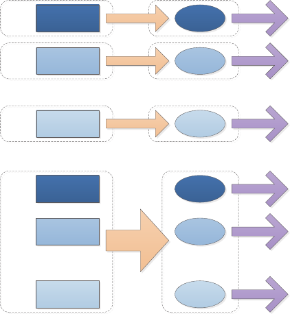
when the training sample size is small for each task. Figure 1 illustrates the difference between traditional
single task learning (STL) and multi-task learning (MTL). In STL, each task is considered to be independent
and learnt independently. In MTL, multiple tasks are learnt simultaneously, by utilizing task relatedness.
Training Data Trained
Model
Task 1
Training Data Trained
Model
Task 2
Training Data Trained
Model
Task t
...
...
Training
Training
Training
Generalization
Generalization
Generalization
Single Task Learning
Training Data Trained
Model
Task 1
Training Data Trained
Model
Task 2
Training Data Trained
Model
Task t
...
...
Training
Generalization
Generalization
Generalization
Multi-Task Learning
Figure 1: Illustration of single task learning (STL) and multi-task learning (MTL). In single task learning
(STL), each task is considered to be independent and learnt independently. In multi-task learning (MTL),
multiple tasks are learnt simultaneously, by utilizing task relatedness.
In data mining and machine learning, a common paradigm for classification and regression is to mini-
mize the penalized empirical loss:
min
WL(W) + Ω(W),(1)
where Wis the parameter to be estimated from the training samples, L(W)is the empirical loss on the
training set, and Ω(W)is the regularization term that encodes task relatedness. Different assumptions on
task relatedness lead to different regularization terms. In the field of multi-task learning, there are many prior
work that model relationships among tasks using novel regularizations (Evgeniou & Pontil, 2004; Ji & Ye,
6

2009; Abernethy et al., 2006; Abernethy et al., 2009; Argyriou et al., 2008a; Obozinski et al., 2010; Chen
et al., 2010; Argyriou et al., 2008b; Agarwal et al., 2010). The formulations implemented in the MALSAR
package is summarized in Table 1. The notations used in this manual (unless otherwise specified) are given
in Table 2. Note, for some formulations, only certain loss versions are included (e.g., squared loss for dirty
model, multi-stage multi-task feature learning). In most cases this is because a theory is associated with the
loss function provided. However, practically, other loss functions can be used. One can always modify the
code according to existing ones to use other loss.
Table 1: Formulations included in the MALSAR package of the following form: minWL(W) + Ω(W).
Name Loss function L(W)Regularization Ω(W)Main Reference
Lasso Least Squares, Logistic ρ1∥W∥1(Tibshirani, 1996)
Mean Regularized Least Squares, Logistic ρ1T
t=1 ∥Wt−1
TT
s=1 Ws∥=
ρ1∥W R∥2
F
(Evgeniou & Pontil, 2004)
Joint Feature Selection Least Squares, Logistic λ∥W∥1,2(Argyriou et al., 2007)
Dirty Model Least Squares ρ1∥P∥1,∞+ρ2∥Q∥1(Jalali et al., 2010)
Graph Structure Least Squares, Logistic ρ1∥W R∥2
F+ρ2∥W∥1
Low Rank Least Squares, Logistic ρ1∥W∥∗(Ji & Ye, 2009)
Sparse+Low Rank Least Squares γ∥P∥1,s.t. W=P+Q, ∥Q∥∗≤τ(Chen et al., 2010)
Relaxed Clustered MTL Least Squares, Logistic ρ1η(1 + η)tr W(ηI +M)−1WT
s.t. tr (M) = k, M ≼I, M ∈
St
+, η =ρ2
ρ1
(Zhou et al., 2011a)
Relaxed ASO Least Squares, Logistic ρ1η(1 + η)tr WT(ηI +M)−1W
s.t. tr (M) = k, M ≼I, M ∈
Sd
+, η =ρ2
ρ1
(Chen et al., 2009)
Robust MTL Least Squares ρ1∥P∥∗+ρ2∥Q∥1,2,s.t. W=P+
W
(Chen et al., 2011)
Robust Feature Learning Least Squares ρ1∥P∥2,1+ρ2∥Q∥1,2,s.t. W=
P+Q
(Gong et al., 2012b)
Temporal Group Lasso Least Squares, Logistic ρ1∥W∥2
F+ρ2∥W R∥2
F+ρ3∥W∥2,1(Zhou et al., 2011b)
Fused Sparse Group Lasso Least Squares, Logistic ρ1∥W∥1+ρ2∥W R∥1+ρ3∥W∥2,1,
ρ1d
i=1 ∥wi∥1+ρ2∥RW T∥1,
ρ1d
i=1 ∥RwT
i∥1+ρ2∥wi∥1
(Zhou et al., 2012)
Incomplete Multi-Source Least Squares, Logistic ρ1S
s=1 ps
k=1
WG(s,k)
2(Yuan et al., 2012)
Multi-Stage Feat. Learn. Least Squares ρ1d
j=1 min(∥wi∥1, θ)(Gong et al., 2012a)
Multi-Task Clustering Sum of Squared Error t
i=1 ∥WTXi−MP T
i∥2
F(Gu & Zhou, 2009)
1.2 Optimization Algorithm
In the MALSAR package, most optimization algorithms are implemented via the accelerated gradient meth-
ods (AGM) (Nemirovski, ; Nemirovski, 2001; Nesterov & Nesterov, 2004; Nesterov, 2005; Nesterov, 2007).
The AGM differs from the traditional gradient method in that every iteration it uses a linear combination of
previous two points as the search point, instead of only using the latest point. The AGM has the conver-
gence speed of O(1/k2), which is the optimal among first order methods. The key subroutine in AGM is to
compute the proximal operator:
W∗= argmin
W
Mγ,S (W) = argmin
W
γ
2∥W−(S−1
γ∇L(W))∥2
F+ Ω(W)(2)
7

Table 2: A list of notations and corresponding Matlab variables (if applicable) used in this manual. Other
usages of the notations may exist and are specified in the context.
Math Notation Meaning Matlab Variable Size
S+symmetric positive semi-definite
∥·∥1ℓ1-norm
∥·∥∞ℓ∞-norm
∥·∥Fℓ2-norm (Frobenius norm)
∥·∥∗trace-norm (sum of singular values)
∥·∥1,2ℓ1,2-norm (row grouped ℓ1)
∥ · ∥1,∞ℓ1,∞-norm (row grouped ℓ1)
∥·∥2,1ℓ2,1-norm (column grouped ℓ1)
ttask number
ddimensionality
nisample size of task i
ρformulation parameters i
Lloss function
Ωregularization terms
Xdata (attributes, features) Xtby 1 cell array
Ytarget (response, label) Ytby 1 cell array
Wmodel (weight, parameter) Wdby tmatrix
P, Q, M model components P, Q, M dby tmatrix
Rstructure variable Rmatrix of varying size
Iidentity matrix Imatrix of varying size
cmodel bias (in logistic loss) c,C1by tvector
Xithe data of the task iX{i}niby dmatrix
Yithe target of the task iY{i}niby 1vector
Withe model of the task iW(:,i) dby 1vector
withe model at i-th feature of all tasks 1by tvector
cithe model bias of the task i(in logistic loss) c,Cscalar
Xi,j the data of the j-th sample of the task iX{i}(i,:) 1by dvector
Yi,j the target of the j-th sample of the task iY{i}(i,:) scalar
optimization options opts struct variable
objective function value funcVal a vector of varying size
where Ω(W, λ)is the non-smooth regularization term, γis the step size, ∇L(·)is the gradient of L(·),Sis
the current search point.
8
2 Package and Installation
The MALSAR package is currently only available for MATLAB1. The user needs MATLAB with 2011a or
higher versions. If you are using lower versions, some functions (such as rng the random number generator
settings may not work properly)
After MATLAB is correctly installed, download the MALSAR package from the software homepage2,
and unzip to a folder. If you are using a Unix-based machines or Mac OS, there is an additional step to build
C libraries: Open MATLAB, navigate to package folder, and run INSTALL.M. A step-by-step installation
guide is given in Table 3.
Table 3: Installation of MALSAR
Step Comment
1. Install MATLAB 2010a or later Required for all functions.
2. Download MALSAR and uncom-
press
Required for all functions.
3. In MATLAB, go to the MALSAR
folder, run INSTALL.M in command
window
Required for non-Windows machines.
The folder structure of MALSAR package is:
•manual. The location of the manual.
•MALSAR. This is the folder containing main functions and libraries.
–utils. This folder contains opts structure initialization and some common libraries. The folder
should be in MATLA path.
–functions. This folder contains all the MATLAB functions and are organized by categories.
–c files. All c files are in this folder. It is not necessary to compile one by one. For Windows
users, there are precompiled binaries for i386 and x64 CPU. For Mac OS X users, binaries for
Intel x64 are included. For Unix users and other Mac OS users, you can perform compilation all
together by running INSTALL.M.
•examples. Many examples are included in this folder for functions implemented in MALSAR. If
you are not familiar with the package, this is the perfect place to start with.
•data. Popular multi-task learning datasets, currently we have included the School data and a part of
the 20 Newsgroups.
1http://www.mathworks.com/products/matlab/
2http://www.public.asu.edu/∼jye02/Software/MALSAR
9
3 Interface Specification
3.1 Input and Output
All functions implemented in MALSAR follow a common specification. For a multi-task learning algorithm
NAME, the input and output of the algorithm are in the following format:
[MODEL VARS, func val, OTHER OUTPUT] = ...
LOSS NAME(X, Y, ρ1, ..., ρp, [opts])
where the name of the loss function is LOSS, and MODEL VARS is the model variables learnt.
In the input fields, Xand Yare two t-dimensional cell arrays. Each cell of Xcontains a ni-by-dmatrix,
where niis the sample size for task iand dis the dimensionality of the feature space. Each cell of Ycontains
the corresponding ni-by-1response. The relationship among X,Yand Wis given in Figure 2. ρ1. . . ρpare
algorithm parameters (e.g., regularization parameters). opts is the optional optimization options that are
elaborated in Sect 3.2.
In the output fields, MODEL VARS are model variables that can be used for predicting unseen data points.
Depending on different loss functions, the model variables may be different. Specifically, the following
format is used under the least squares loss:
[W, func val, OTHER OUTPUT ] = Least NAME (X, Y, ρ1, ..., ρp[opts])
where Wis a d-by-tmatrix, each column of which is a ddimensional parameter vector for the corresponding
task. For a new input xfrom task i, the prediction yis given by
y=xT·W(:, i).
The following format is used under the logistic loss:
[W, c, func val, OTHER OUTPUT ] = ...
Logistic NAME (X, Y, ρ1, ..., ρp[opts])
Learning
Task t
Dimension d
Sample nt
...
Sample n2
Sample n1
Feature X
Task t
Sample nt
...
Sample n2
Sample n1
Response Y
Task t
Dimension d
Model W
Model C
(logistic Regression)
Figure 2: The main input and output variables.
10

where Wis a d-by-tmatrix, each column of which is a ddimensional parameter vector for the corresponding
task, and cis a t-dimensional vector. For a new input xfrom task i, the binary prediction yis given by
y=sign(xT·W(:, i) + c(i)).
These two loss functions are available for most of the algorithms in the package. The output func val is
the objective function values at all iterations of the optimization algorithms. In some algorithms, there are
other output variables that are not directly related to the prediction. For example in convex relaxed ASO,
the optimization also gives the shared feature mapping, which is a low rank matrix. In some scenarios the
user may be interested in such variables. The variables are given in the field %OTHER OUTPUT%.
3.2 Optimization Options
All optimization algorithms in our package are implemented using iterative methods. Users can use the
optional opts input to specify starting points, termination conditions, tolerance, and maximum iteration
number. The input opts is a structure variable. To specify an option, user can add corresponding fields. If
one or more required fields are not specified, or the opts variable is not given, then default values will be
used. The default values can be changed in init opts.m in \MALSAR\utils.
•Starting Point .init. Users can use the field to specify different starting points.
–opts.init = 0. If 0 is specified then the starting points will be initialized to a guess value
computed from data. For example, in the least squares loss, the model W(:, i) for i-th task is
initialized by X{i}*Y{i}.
–opts.init = 1. If 1 is specified then opts.W0 is used. Note that if value 1 is specified in
.init but the field .W0 is not specified, then .init will be forced to the default value.
–opts.init = 2 (default). If 2 is specified, then the starting point will be a zero matrix.
•Termination Condition .tFlag and Tolerance .tol. In this package, there are 4 types of termination
conditions supported for all optimization algorithms.
–opts.tFlag = 0.
–opts.tFlag = 1 (default).
–opts.tFlag = 2.
–opts.tFlag = 3.
•Maximum Iteration .maxIter. When the tolerance and/or termination condition is not properly set,
the algorithms may take an unacceptable long time to stop. In order to prevent this situation, users
can provide the maximum number of iterations allowed for the solver, and the algorithm stops when
the maximum number of iterations is achieved even if the termination condition is not satisfied.
For example, one can use the following code to specify the maximum iteration number of the opti-
mization problem:
opts.maxIter = 1000;
The algorithm will stop after 1000 iteration steps even if the termination condition is not satisfied.
11
4 Multi-Task Learning Formulations
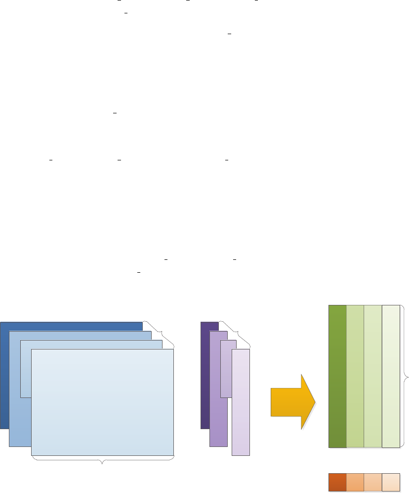
4.1 Sparsity in Multi-Task Learning: ℓ1-norm Regularized Problems
The ℓ1-norm (or Lasso) regularized methods are widely used to introduce sparsity into the model and achieve
the goal of reducing model complexity and feature learning (Tibshirani, 1996). We can easily extend the
ℓ1-norm regularized STL to MTL formulations. A common simplification of Lasso in MTL is that the
parameter controlling the sparsity is shared among all tasks, assuming that different tasks share the same
sparsity parameter. The learnt model is illustrated in Figure 3.
Learning
Task t
Dimension d
Sample nt
...
Sample n2
Sample n1
Feature X
Task t
Sample nt
...
Sample n2
Sample n1
Response Y
Task t
Dimension d
Figure 3: Illustration of multi-task Lasso.
4.1.1 Multi-Task Lasso with Least Squares Loss (Least Lasso)
The function
[W, funcVal] = Least Lasso(X, Y, ρ1, [opts])
solves the ℓ1-norm (and the squared ℓ2-norm ) regularized multi-task least squares problem:
min
W
t
i=1
∥WT
iXi−Yi∥2
F+ρ1∥W∥1+ρL2∥W∥2
F,(3)
where Xidenotes the input matrix of the i-th task, Yidenotes its corresponding label, Wiis the model
for task i, the regularization parameter ρ1controls sparsity, and the optional ρL2regularization parameter
controls the ℓ2-norm penalty. Note that both ℓ1-norm and ℓ2-norm penalties are used in elastic net.
Currently, this function supports the following optional fields:
• Starting Point: opts.init,opts.W0
• Termination: opts.tFlag,opts.tol
• Regularization: opts.rho L2
12

4.1.2 Multi-Task Lasso with Logistic Loss (Logistic Lasso)
The function
[W, c, funcVal] = Logistic Lasso(X, Y, ρ1, [opts])
solves the ℓ1-norm (and the squared ℓ2-norm ) regularized multi-task logistic regression problem:
min
W,c
t
i=1
ni
j=1
log(1 + exp (−Yi,j (WT
jXi,j +ci))) + ρ1∥W∥1+ρL2∥W∥2
F,(4)
where Xi,j denotes sample jof the i-th task, Yi,j denotes its corresponding label, Wiand ciare the model
for task i, the regularization parameter ρ1controls sparsity, and the optional ρL2regularization parameter
controls the ℓ2-norm penalty.
Currently, this function supports the following optional fields:
• Starting Point: opts.init,opts.W0,opts.C0
• Termination: opts.tFlag,opts.tol
• Regularization: opts.rho L2
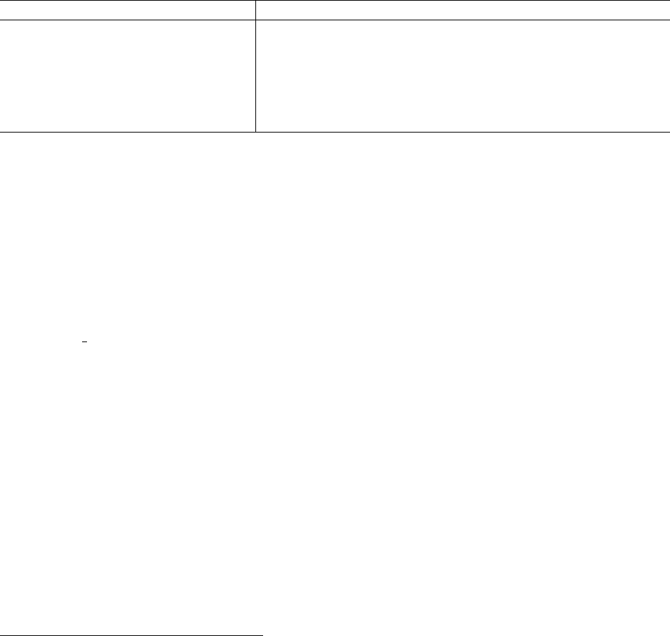
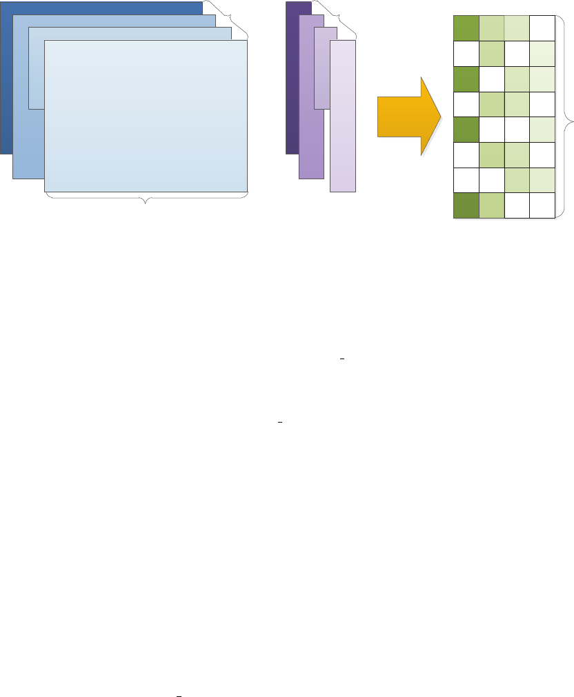
4.2 Joint Feature Selection: ℓ2,1-norm Regularized Problems
One way to capture the task relatedness from multiple related tasks is to constrain all models to share a com-
mon set of features. This motivates the group sparsity, i.e. the ℓ1/ℓ2-norm regularized learning (Argyriou
et al., 2007; Argyriou et al., 2008a; Liu et al., 2009; Nie et al., 2010):
min
WL(W) + λ∥W∥1,2,(5)
where ∥W∥=T
t=1 ∥Wt∥2is the group sparse penalty. Compared to Lasso, the ℓ2,1-norm regularization
results in grouped sparsity, assuming that all tasks share a common set of features. The learnt model is
illustrated in Figure 4.
4.2.1 ℓ2,1-Norm Regularization with Least Squares Loss (Least L21)
The function
[W, funcVal] = Least L21(X, Y, ρ1, [opts])
solves the ℓ2,1-norm (and the squared ℓ2-norm ) regularized multi-task least squares problem:
min
W
t
i=1
∥WT
iXi−Yi∥2
F+ρ1∥W∥2,1+ρL2∥W∥2
F,(6)
where Xidenotes the input matrix of the i-th task, Yidenotes its corresponding label, Wiis the model for
task i, the regularization parameter ρ1controls group sparsity, and the optional ρL2regularization parameter
controls ℓ2-norm penalty.
Currently, this function supports the following optional fields:
• Starting Point: opts.init,opts.W0
• Termination: opts.tFlag,opts.tol
• Regularization: opts.rho L2
13
Learning
Task t
Dimension d
Sample nt
...
Sample n2
Sample n1
Feature X
Task t
Sample nt
...
Sample n2
Sample n1
Response Y
Task t
Dimension d
Figure 4: Illustration of multi-task learning with joint feature selection based on the ℓ2,1-norm regularization.
4.2.2 ℓ2,1-Norm Regularization with Logistic Loss (Logistic L21)
The function
[W, c, funcVal] = Logistic L21(X, Y, ρ1, [opts])
solves the ℓ2,1-norm (and the squared ℓ2-norm ) regularized multi-task logistic regression problem:
min
W,c
t
i=1
ni
j=1
log(1 + exp (−Yi,j (WT
jXi,j +ci))) + ρ1∥W∥2,1+ρL2∥W∥2
F,(7)
where Xi,j denotes sample jof the i-th task, Yi,j denotes its corresponding label, Wiand ciare the model for
task i, the regularization parameter ρ1controls group sparsity, and the optional ρL2regularization parameter
controls ℓ2-norm penalty.
Currently, this function supports the following optional fields:
• Starting Point: opts.init,opts.W0,opts.C0
• Termination: opts.tFlag,opts.tol
• Regularization: opts.rho L2
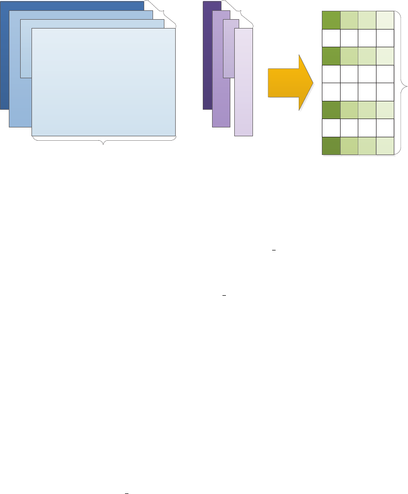
4.3 The Dirty Model for Multi-Task Learning
The joint feature learning using ℓ1/ℓq-norm regularization performs well in idea cases. In practical appli-
cations, however, simply using the ℓ1/ℓq-norm regularization may not be effective for dealing with dirty
data which may not fall into a single structure. To this end, the dirty model for multi-task learning is
proposed (Jalali et al., 2010). The key idea in the dirty model is to decompose the model Winto two
components Pand Q, as shown in Figure 5.
14
+
=
Group Sparse
Component
P
Sparse
Component
Q
Model
W
Figure 5: Illustration of dirty model for multi-task learning.
4.3.1 A Dirty Model for Multi-Task Learning with the Least Squares Loss (Least Dirty)
The function
[W, funcVal, P, Q] = Least Dirty(X, Y, ρ1,ρ2, [opts])
solves the dirty multi-task least squares problem:
min
W
t
i=1
∥WT
iXi−Yi∥2
F+ρ1∥P∥1,∞+ρ2∥Q∥1,(8)
subject to:W=P+Q(9)
where Xidenotes the input matrix of the i-th task, Yidenotes its corresponding label, Wiis the model for
task i,Pis the group sparsity component and Qis the elementwise sparse component, ρ1controls the group
sparsity regularization on P, and ρ2controls the sparsity regularization on Q.
Currently, this function supports the following optional fields:
• Starting Point: opts.init,opts.P0,opts.Q0 (set opts.W0 to any non-empty value)
• Termination: opts.tFlag,opts.tol
• Initial Lipschiz Constant: opts.lFlag
4.4 Encoding Graph Structure: Graph Regularized Problems
In some applications, the task relationship can be represented using a graph where each task is a node, and
two nodes are connected via an edge if they are related. Let Edenote the set of edges, and we denote edge i
as a vector e(i)∈Rtdefined as follows: e(i)
xand e(i)
yare set to 1and −1respectively if the two nodes xand
15

yare connected. The complete graph is encoded in the matrix R= [e(1),e(2),...,e(∥E∥)]∈Rt×∥E∥. The
following regularization penalizes the differences between all pairs connected in the graph:
∥W R∥2
F=
∥E∥
i=1
∥W e(i)∥2
2=
∥E∥
i=1
∥We(i)
x−We(i)
y∥2
2,(10)
which can also be represented in the following matrix form:
∥W R∥2
F=tr (W R)T(W R)=tr W RRTWT=tr WLWT,(11)
where L=RRT, known as the Laplacian matrix, is symmetric and positive definiteness. In (Li & Li, 2008),
the network structure is defined on the features, while in MTL the structure is on the tasks.
In the multi-task learning formulation proposed by (Evgeniou & Pontil, 2004), it assumes all tasks are
related in the way that the models of all tasks are close to their mean:
min
WL(W) + λ
T
t=1
∥Wt−1
T
T
s=1
Ws∥,(12)
where λ > 0is penalty parameter. The regularization term in Eq.(12) penalizes the deviation of each task
from the mean 1
TT
s=1 Ws. This regularization can also be encoded using the structure matrix Rby setting
R = eye(t) - ones(t)/t.
4.4.1 Sparse Graph Regularization with Logistic Loss (Least SRMTL)
The function
[W, funcVal] = Least SRMTL(X, Y, R, ρ1,ρ2, [opts])
solves the graph structure regularized and ℓ1-norm (and the squared ℓ2-norm ) regularized multi-task least
squares problem:
min
W
t
i=1
∥WT
iXi−Yi∥2
F+ρ1∥W R∥2
F+ρ2∥W∥1+ρL2∥W∥2
F,(13)
where Xidenotes the input matrix of the i-th task, Yidenotes its corresponding label, Wiis the model
for task i, the regularization parameter ρ1controls sparsity, and the optional ρL2regularization parameter
controls ℓ2-norm penalty.
Currently, this function supports the following optional fields:
• Starting Point: opts.init,opts.W0
• Termination: opts.tFlag,opts.tol
• Regularization: opts.rho L2
4.4.2 Sparse Graph Regularization with Logistic Loss (Logistic SRMTL)
The function
[W, c, funcVal] = Logistic SRMTL(X, Y, R, ρ1,ρ2, [opts])
16
solves the graph structure regularized and ℓ1-norm (and the squared ℓ2-norm ) regularized multi-task logistic
regression problem:
min
W,c
t
i=1
ni
j=1
log(1 + exp (−Yi,j (WT
jXi,j +ci))) + ρ1∥W R∥2
F+ρ2∥W∥1+ρL2∥W∥2
F,(14)
where Xi,j denotes sample jof the i-th task, Yi,j denotes its corresponding label, Wiand ciare the model
for task i, the regularization parameter ρ1controls sparsity, and the optional ρL2regularization parameter
controls ℓ2-norm penalty.
Currently, this function supports the following optional fields:
• Starting Point: opts.init,opts.W0,opts.C0
• Termination: opts.tFlag,opts.tol
• Regularization: opts.rho L2
4.5 Low Rank Assumption: Trace-norm Regularized Problems
One way to capture the task relationship is to constrain the models from different tasks to share a low-
dimensional subspace, i.e., Wis of low rank, resulting in the following rank minimization problem:
min L(W) + λrank(W).
The above problem is in general NP-hard (Vandenberghe & Boyd, 1996). One popular approach is to replace
the rank function (Fazel, 2002) by the trace norm (or nuclear norm) as follows:
min L(W) + λ∥W∥∗,(15)
where the trace norm is given by the sum of the singular values: ∥W∥∗=iσi(W). The trace norm
regularization has been studied extensively in multi-task learning (Ji & Ye, 2009; Abernethy et al., 2006;
Abernethy et al., 2009; Argyriou et al., 2008a; Obozinski et al., 2010).
Task Models
W
Sparse Component
P+=
Low Rank
Component
Q= X
Figure 6: Learning Incoherent Sparse and Low-Rank Patterns form Multiple Tasks.
The assumption that all models share a common low-dimensional subspace is restrictive in some appli-
cations. To this end, an extension that learns incoherent sparse and low-rank patterns simultaneously was
17

proposed in (Chen et al., 2010). The key idea is to decompose the task models Winto two components: a
sparse part Pand a low-rank part Q, as shown in Figure 6. It solves the following optimization problem:
min
WL(W) + γ∥P∥1
subject to: W=P+Q, ∥Q∥∗≤τ.
4.5.1 Trace-Norm Regularization with Least Squares Loss (Least Trace)
The function
[W, funcVal] = Least Trace(X, Y, ρ1, [opts])
solves the trace-norm regularized multi-task least squares problem:
min
W
t
i=1
∥WT
iXi−Yi∥2
F+ρ1∥W∥∗,(16)
where Xidenotes the input matrix of the i-th task, Yidenotes its corresponding label, Wiis the model for
task i, and the regularization parameter ρ1controls the rank of W.
Currently, this function supports the following optional fields:
• Starting Point: opts.init,opts.W0
• Termination: opts.tFlag,opts.tol
4.5.2 Trace-Norm Regularization with Logistic Loss (Logistic Trace)
The function
[W, c, funcVal] = Logistic Trace(X, Y, ρ1, [opts])
solves the trace-norm regularized multi-task logistic regression problem:
min
W,c
t
i=1
ni
j=1
log(1 + exp (−Yi,j (WT
jXi,j +ci))) + ρ1∥W∥∗,(17)
where Xi,j denotes sample jof the i-th task, Yi,j denotes its corresponding label, Wiand ciare the model
for task i, and the regularization parameter ρ1controls the rank of W.
Currently, this function supports the following optional fields:
• Starting Point: opts.init,opts.W0,opts.C0
• Termination: opts.tFlag,opts.tol
4.5.3 Learning with Incoherent Sparse and Low-Rank Components (Least SparseTrace)
The function
[W, funcVal, P, Q] = Least SparseTrace(X, Y, ρ1,ρ2, [opts])
18
Training Data XĬ
Training Data XĬ
...
Clustered Models
...
Cluster 1 Cluster 2 Cluster k-1 Cluster k
Cluster 1
Cluster 2
Cluster k-1
Cluster k
Figure 7: Illustration of clustered tasks. Tasks with similar colors are similar with each other.
solves the incoherent sparse and low-rank multi-task least squares problem:
min
W
t
i=1
∥WT
iXi−Yi∥2
F+ρ1∥P∥1(18)
subject to: W=P+Q, ∥Q∥∗≤ρ2(19)
where Xidenotes the input matrix of the i-th task, Yidenotes its corresponding label, Wiis the model for
task i, the regularization parameter ρ1controls sparsity of the sparse component P, and the ρ2regularization
parameter controls the rank of Q.
Currently, this function supports the following optional fields:
• Starting Point: opts.init,opts.P0,opts.Q0 (set opts.W0 to any non-empty value)
• Termination: opts.tFlag,opts.tol
4.6 Discovery of Clustered Structure: Clustered Multi-Task Learning
Many multi-task learning algorithms assume that all learning tasks are related. In practical applications,
the tasks may exhibit a more sophisticated group structure where the models of tasks from the same group
are closer to each other than those from a different group. There have been many work along this line
of research (Thrun & O’Sullivan, 1998; Jacob et al., 2008; Wang et al., 2009; Xue et al., 2007; Bakker
& Heskes, 2003; Evgeniou et al., 2006; Zhang & Yeung, 2010), known as clustered multi-task learning
(CMTL). The idea of CMTL is shown in Figure 7.
In (Zhou et al., 2011a) we proposed a CMTL formulation which is based on the spectral relaxed k-means
clustering (Zha et al., 2002):
min
W,F :FTF=Ik
L(W) + αtrWTW−trFTWTW F +βtr(WTW).(20)
where kis the number of clusters and Fcaptures the relaxed cluster assignment information. Since the
formulation in Eq. (20) is not convex, a convex relaxation called cCMTL is also proposed. The formulation
19

of cCMTL is given by:
min
WL(W) + ρ1η(1 + η)tr W(ηI +M)−1WT
subject to: tr (M) = k, M ≼I, M ∈St
+, η =ρ2
ρ1
There are many optimization algorithms for solving the cCMTL formulations (Zhou et al., 2011a). In
our package we include an efficient implementation based on Accelerated Projected Gradient.
4.6.1 Convex Relaxed Clustered Multi-Task Learning with Least Squares Loss (Least CMTL)
The function
[W, funcVal, M] = Least CMTL(X, Y, ρ1,ρ2, k, [opts])
solves the relaxed k-means clustering regularized multi-task least squares problem:
min
W
t
i=1
∥WT
iXi−Yi∥2
F+ρ1η(1 + η)tr W(ηI +M)−1WT,(21)
subject to: tr (M) = k, M ≼I, M ∈St
+, η =ρ2
ρ1(22)
where Xidenotes the input matrix of the i-th task, Yidenotes its corresponding label, Wiis the model for
task i, and ρ1is the regularization parameter. Because of the equality constraint tr (M) = k, the starting
point of Mis initialized to be M0=k/t ×Isatisfying tr (M0) = k.
Currently, this function supports the following optional fields:
• Starting Point: opts.init,opts.W0
• Termination: opts.tFlag,opts.tol
4.6.2 Convex Relaxed Clustered Multi-Task Learning with Logistic Loss (Logistic CMTL)
The function
[W, c, funcVal, M] = Logistic CMTL (X, Y, ρ1,ρ2, k, [opts])
solves the relaxed k-means clustering regularized multi-task logistic regression problem:
min
W,c
t
i=1
ni
j=1
log(1 + exp (−Yi,j (WT
jXi,j +ci))) + ρ1η(1 + η)tr W(ηI +M)−1WT,(23)
subject to: tr (M) = k, M ≼I, M ∈St
+, η =ρ2
ρ1(24)
where Xi,j denotes sample jof the i-th task, Yi,j denotes its corresponding label, Wiand ciare the model
for task i, and ρ1is the regularization parameter. Because of the equality constraint tr (M) = k, the starting
point of Mis initialized to be M0=k/t ×Isatisfying tr (M0) = k.
Currently, this function supports the following optional fields:
• Starting Point: opts.init,opts.W0,opts.C0
• Termination: opts.tFlag,opts.tol
20
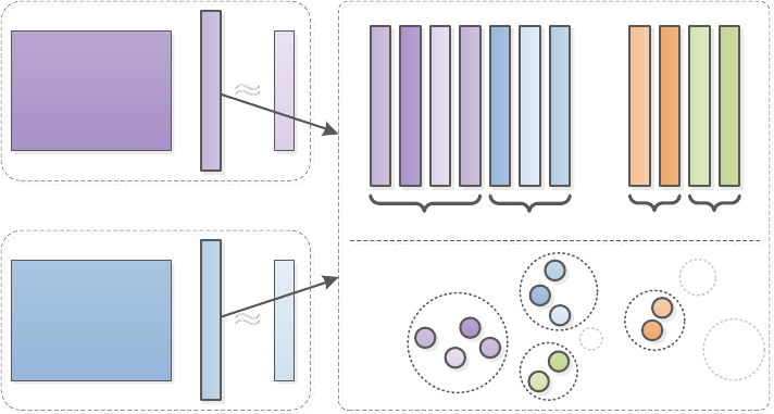
4.7 Discovery of Shared Feature Mapping: Alternating Structure Optimization
The basic idea of alternating structure optimization (ASO) (Ando & Zhang, 2005) is to decompose the pre-
dictive model of each task into two components: the task-specific feature mapping and task-shared feature
mapping, as shown in Figure 8. The ASO formulation for linear predictors is given by:
min
{vt,wt},Θ
T
t=1 1
nt
L(wt) + α∥wt∥2
subject to ΘΘT=I, wt=ut+ ΘTvt,(25)
where Θis the low dimensional feature map across all tasks. The predictor ftfor task tcan be expressed as:
ft(x) = wT
tx=uT
tx+vT
tΘx.
Input XĬ
Task 1
Low-
Dimensional
Feature Map
+ΘT X
u1v1
Input XĬ
Task 2+ΘT X
u2v2
Input XĬ
Task m+ΘT X
umvm
...
ΘT
Figure 8: Illustration of Alternating Structure Optimization. The predictive model of each task includes two
components: the task-specific feature mapping and task-shared feature mapping.
The formulation in Eq.(12) is not convex. A convex relaxation of ASO called cASO is proposed in (Chen
et al., 2009):
min
{wt},M
T
t=1 1
nt
nt
i=1
L(wt)+αη(1 + η)tr WT(ηI +M)−1W
subject to tr(M) = h, M ≼I, M ∈Sd
+(26)
It has been shown in (Zhou et al., 2011a) that there is an equivalence relationship between clustered
multi-task learning in Eq. (20) and cASO when the dimensionality of the shared subspace in cASO is
equivalent to the cluster number in cMTL.
4.7.1 cASO with Least Squares Loss (Least CASO)
The function
21
[W, funcVal, M] = Least CASO(X, Y, ρ1,ρ2, k, [opts])
solves the convex relaxed alternating structure optimization (ASO) multi-task least squares problem:
min
W
t
i=1
∥WT
iXi−Yi∥2
F+ρ1η(1 + η)tr WT(ηI +M)−1W,(27)
subject to: tr (M) = k, M ≼I, M ∈Sd
+, η =ρ2
ρ1(28)
where Xidenotes the input matrix of the i-th task, Yidenotes its corresponding label, Wiis the model for
task i, and ρ1is the regularization parameter. Due to the equality constraint tr (M) = k, the starting point
of Mis initialized to be M0=k/t ×Isatisfying tr (M0) = k.
Currently, this function supports the following optional fields:
• Starting Point: opts.init,opts.W0
• Termination: opts.tFlag,opts.tol
4.7.2 cASO with Logistic Loss (Logistic CASO)
The function
[W, c, funcVal, M] = Logistic CASO(X, Y, ρ1,ρ2, k, [opts])
solves the convex relaxed alternating structure optimization (ASO) multi-task logistic regression problem:
min
W,c
t
i=1
ni
j=1
log(1 + exp (−Yi,j (WT
jXi,j +ci))) + ρ1η(1 + η)tr WT(ηI +M)−1W,(29)
subject to: tr (M) = k, M ≼I, M ∈Sd
+, η =ρ2
ρ1(30)
where Xi,j denotes sample jof the i-th task, Yi,j denotes its corresponding label, Wiand ciare the model
for task i, and ρ1is the regularization parameter. Due to the equality constraint tr (M) = k, the starting
point of Mis initialized to be M0=k/t ×Isatisfying tr (M0) = k.
Currently, this function supports the following optional fields:
• Starting Point: opts.init,opts.W0,opts.C0
• Termination: opts.tFlag,opts.tol
4.8 Dealing with Outlier Tasks: Robust Multi-Task Learning
Most multi-task learning formulations assume that all tasks are relevant, which is however not the case in
many real-world applications. Robust multi-task learning (RMTL) is aimed at identifying irrelevant (outlier)
tasks when learning from multiple tasks.
One approach to perform RMTL is to assume that the model Wcan be decomposed into two com-
ponents: a low rank structure Lthat captures task-relatedness and a group-sparse structure Sthat detects
outliers (Chen et al., 2011). If a task is not an outlier, then it falls into the low rank structure Lwith its corre-
sponding column in Sbeing a zero vector; if not, then the Smatrix has non-zero entries at the corresponding
column. The following formulation learns the two components simultaneously:
min
W=L+SL(W) + ρ1∥L∥∗+β∥S∥1,2(31)
The predictive model of RMTL is illustrated in Figure 9.
22
Task Models
W+=
Low Rank
Component
L= X
Group Sparse
Component
S
Outlier Tasks
Figure 9: Illustration of robust multi-task learning. The predictive model of each task includes two compo-
nents: the low-rank structure Lthat captures task relatedness and the group sparse structure Sthat detects
outliers.
4.8.1 RMTL with Least Squares Loss (Least RMTL)
The function
[W, funcVal, L, S] = Least RMTL(X, Y, ρ1,ρ2, [opts])
solves the incoherent group-sparse and low-rank multi-task least squares problem:
min
W
t
i=1
∥WT
iXi−Yi∥2
F+ρ1∥L∥∗+ρ2∥S∥1,2(32)
subject to: W=L+S(33)
where Xidenotes the input matrix of the i-th task, Yidenotes its corresponding label, Wiis the model for
task i, the regularization parameter ρ1controls the low rank regularization on the structure L, and the ρ2
regularization parameter controls the ℓ2,1-norm penalty on S.
Currently, this function supports the following optional fields:
• Starting Point: opts.init,opts.L0,opts.S0 (set opts.W0 to any non-empty value)
• Termination: opts.tFlag,opts.tol
4.9 Joint Feature Learning with Outlier Tasks: Robust Multi-Task Feature Learning
The joint feature learning formulation in 4.2 selects a common set of features for all tasks. However, it
assumes there is no outlier task, which may not the case in practical applications. To this end, a robust
multi-task feature learning (rMTFL) formulation is proposed in (Gong et al., 2012b). rMTFL assumes that
the model Wcan be decomposed into two components: a shared feature structure Pthat captures task-
relatedness and a group-sparse structure Qthat detects outliers. If the task is not an outlier, then it falls into
the joint feature structure Pwith its corresponding column in Qbeing a zero vector; if not, then the Qmatrix
has non-zero entries at the corresponding column. The following formulation learns the two components
simultaneously:
min
W=P+QL(W) + ρ1∥P∥2,1+β∥QT∥2,1(34)
The predictive model of rMTFL is illustrated in Figure 10.
23
+=
Joint
Selected
Features
Group Sparse
Component
Q
Outlier Tasks
Task Models
W
Group Sparse
Component
P
Figure 10: Illustration of robust multi-task feature learning. The predictive model of each task includes
two components: the joint feature selection structure Pthat captures task relatedness and the group sparse
structure Qthat detects outliers.
4.9.1 RMTL with Least Squares Loss (Least rMTFL)
The function
[W, funcVal, Q, P] = Least rMTFL(X, Y, ρ1,ρ2, [opts])
solves the problem of robust multi-task feature learning with least squares loss:
min
W
t
i=1
∥WT
iXi−Yi∥2
F+ρ1∥P∥2,1+ρ2∥QT∥2,1(35)
subject to: W=P+Q(36)
where Xidenotes the input matrix of the i-th task, Yidenotes its corresponding label, Wiis the model for
task i, the regularization parameter ρ1controls the joint feature learning, and the regularization parameter
ρ2controls the columnwise group sparsity on Qthat detects outliers.
Currently, this function supports the following optional fields:
• Starting Point: opts.init,opts.L0,opts.S0 (set opts.W0 to any non-empty value)
• Termination: opts.tFlag,opts.tol
• Initial Lipschitz constant: opts.lFlag
4.10 Encoding Temporal Information: Disease Progression Models
Disease progression can be modeled using multi-task learning (Zhou et al., 2011b). In many longitudinal
study of diseases, subjects are followed over a period of time and asked to visit the hospital repeatedly.
24
Each visit a variety of biomarkers (e.g. imaging, plasma panels) and disease status (e.g. scores that reflect
cognitive status) are measured from patients. One important task is to build predictive models of future
disease status given biomarker measurements at one or more time points. The prediction of the value of
the disease status at one time point is considered as a task, the prediction models at different time points
may be similar because that they are temporally related. The model encodes the temporal information using
regularization terms. Specifically, the formulation is given by:
min
WL(W) + ρ1∥W∥2
F+ρ2
t−1
i=1
∥Wi−Wi+1∥2
F+ρ3∥W∥2,1,
where the first penalty controls the complexity of the model; the second penalty couples the neighbor tasks,
encouraging every two neighbor tasks to be similar (temporal smoothness); and the third penalty induces the
grouped sparsity, which performs the joint feature selection on the tasks at different time points (longitudinal
feature selection, see Figure 11).
Patient Sample: n
Feature Space: d
Task (Time Point): t
X=
Baseline MRI Volume
Baseline MRI Area
Baseline MRI Surface
Baseline Labtest
Baseline Cognitive Test
Other features
Task (Time Point): t
06 Month
12 Month
24 Month
36 Month
Patient Sample: n
Feature Size: d
06 Month
12 Month
24 Month
36 Month
X Y
W
Removed Feature
Removed Feature
Removed Feature
Removed Feature
Removed Feature
Removed Feature
Figure 11: Illustration of the temporal group Lasso (TGL) disease progression model.
We can understand the temporal information as a type of graph regularization, where neighbor tasks are
coupled via edges. The structure variable Rcan be defined as:
R = zeros(t, t-1); R(1:(t+1):end) = 1; R(2:(t+1):end) = -1;
and the formulation can be written in a simple form:
min
WL(W) + ρ1∥W∥2
F+ρ2∥W R∥2
F+ρ3∥W∥2,1,(37)
Note that the implementation of TGL algorithm can deal with general graph structure in the structure
variable R, but not limited to temporal regularization. Please refer Section 4.4 for specification of the struc-
ture variable R.
One advantage of TGL formulation in Eq. (37) is that the regularization terms are simple to solve and
thus can be efficiently solved. However, the formulation assumes that a biomarker is either selected or is
25

not selected at all time points. The convex fused sparse group Lasso (cFSGL) formulations are proposed to
overcome this issue (Zhou et al., 2012):
min
WL(W) + ρ1∥W∥1+ρ2∥RW T∥1+ρ3∥W∥2,1,(38)
where the fused structure Ris defined in the same way as in TGL. In cFSGL , we aim to select task-shared
and task-specific features using the sparse group Lasso penalty. However, the sparsity-inducing penalties
are known to lead to biased estimates. The paper also discussed two non-convex multi-task regression
formulations for modeling disease progression (Zhou et al., 2012):
[nFSGL1] min
WL(W) + ρ1
d
i=1 ∥wi∥1+ρ2∥RW T∥1,(39)
[nFSGL2] min
WL(W) + ρ1
d
i=1 ∥RwT
i∥1+ρ2∥wi∥1,(40)
where the second term is the summation of the squared root of ℓ1-norm of wi(wiis the ith row of W). For
a detailed discussion and comparison among different disease progression models, the reader is referred to
the paper (Zhou et al., 2012). In the package, we have included all algorithms for the disease progression
models discussed above.
4.10.1 Temporal Group Lasso with Least Squares Loss (Least TGL)
The function
[W, funcVal] = Least TGL (X, Y, R, ρ1,ρ2, [opts])
solves the temporal smoothness regularized (and the squared ℓ2-norm ) regularized multi-task least squares
problem:
min
W
t
i=1
∥WT
iXi−Yi∥2
F+ρ1∥W∥2
F+ρ2∥W R∥2
F+ρ3∥W∥2,1,(41)
where Xidenotes the input matrix of the i-th task, Yidenotes its corresponding label, Wiis the task model
for task i,ρ2is the regularization parameter that controls temporal smoothness, the regularization parameter
ρ3controls group sparsity for joint feature selection, and the ρ1regularization parameter controls ℓ2-norm
penalty and can be set to prevent overfitting.
Currently, this function supports the following optional fields:
• Starting Point: opts.init,opts.W0
• Termination: opts.tFlag,opts.tol
4.10.2 Temporal Group Lasso with Logistic Loss (Logistic TGL)
The function
[W, c, funcVal] = Logistic TGL (X, Y, R, ρ1,ρ2, [opts])
26

solves the temporal smoothness regularized (and the squared ℓ2-norm ) regularized multi-task logistic re-
gression problem:
min
W,c
t
i=1
ni
j=1
log(1 + exp (−Yi,j (WT
jXi,j +ci))) + ρ1∥W∥2
F+ρ2∥W R∥2
F+ρ3∥W∥2,1,(42)
where Xi,j denotes sample jof the i-th task, Yi,j denotes its corresponding label, Wiand ciare the model
parameters for task i,ρ2is the regularization parameter for temporal smoothness the regularization pa-
rameter ρ3controls group sparsity for joint feature selection , and the ρ1regularization parameter controls
ℓ2-norm penalty and can be set to prevent overfitting.
Currently, this function supports the following optional fields:
• Starting Point: opts.init,opts.W0,opts.C0
• Termination: opts.tFlag,opts.tol
4.10.3 Convex Sparse Fused Group Lasso (cFSGL) with Least Squares Loss (Least CFGLasso)
The function
[W, funcVal] = Least CFGLasso (X, Y, ρ1,ρ2,ρ3, [opts])
solves the convex fused sparse group Lasso regularized multi-task least squares problem:
min
W
t
i=1
∥WT
iXi−Yi∥2
F+ρ1∥W∥1+ρ2∥RW T∥1+ρ3∥W∥2,1,(43)
where Xidenotes the input matrix of the i-th task, Yidenotes its corresponding label, Wiis the task model
for task i, the regularization parameter ρ3controls group sparsity for joint feature selection, ρ1and ρ2are
the parameters for the fused Lasso. Specifically, ρ1controls element-wise sparsity and ρ2controls the fused
regularization.
Currently, this function supports the following optional fields:
• Starting Point: opts.init,opts.W0
• Termination: opts.tFlag,opts.tol
4.10.4 Convex Sparse Fused Group Lasso (cFSGL) with Logistic Loss (Logistic CFGLasso)
[W, c, funcVal] = Logistic CFGLasso (X, Y, ρ1,ρ2,ρ3, [opts])
solves the convex fused sparse group Lasso regularized multi-task logistic regression problem:
min
W,c
t
i=1
ni
j=1
log(1 + exp (−Yi,j (WT
jXi,j +ci))) + ρ1∥W∥1+ρ2∥RW T∥1+ρ3∥W∥2,1,(44)
where Xi,j denotes sample jof the i-th task, Yi,j denotes its corresponding label, Wiand ciare the model
parameters for task i, the regularization parameter ρ3controls group sparsity for joint feature selection, ρ1
and ρ2are the parameters for the fused Lasso. Specifically, ρ1controls element-wise sparsity and ρ2controls
the fused regularization.
Currently, this function supports the following optional fields:
• Starting Point: opts.init,opts.W0,opts.C0
• Termination: opts.tFlag,opts.tol
27

4.10.5 Non-Convex Sparse Fused Group Lasso Formulation 1 (nFSGL1) (Least NCFGLassoF1)
The function
[W, funcVal] = Least NCFGLassoF1 (X, Y, ρ1,ρ2, [opts])
solves the non-convex fused sparse group Lasso (nFSGL1) regularized multi-task least squares problem:
min
W
t
i=1
∥WT
iXi−Yi∥2
F+ρ1
d
i=1 ∥wi∥1+ρ2∥RW T∥1(45)
where Xidenotes the input matrix of the i-th task, Yidenotes its corresponding label, Wiis the task model
for task i, the regularization parameter ρ1controls the group sparsity for joint feature selection and also the
element-wise sparsity, ρ2controls the fused regularization. Currently, this function supports the following
optional fields:
• Starting Point: opts.init,opts.W0
• Termination: opts.tFlag,opts.tol
• Outer Loop Max Iteration: opts.max iter
• Outer Loop Tolerance: opts.tol funcVal
Note that this is a multi-stage optimization problem, it is suggested that the outer loop need NOT to converge
to a high precision. Typically a very small max iteration (e.g. 10) is used.
4.10.6 Non-Convex Sparse Fused Group Lasso Formulation 2 (nFSGL2) (Logistic NCFGLassoF2)
The function
[W, funcVal] = Least NCFGLassoF2 (X, Y, ρ1,ρ2, [opts])
solves the non-convex fused sparse group Lasso (nFSGL2) regularized multi-task least squares problem:
min
W
t
i=1
∥WT
iXi−Yi∥2
F+ρ1
d
i=1 ∥RwT
i∥1+ρ2∥wi∥1,(46)
where Xidenotes the input matrix of the i-th task, Yidenotes its corresponding label, Wiis the task model
for task i, the regularization parameter ρ1controls the group sparsity for joint feature selection and also
fused regularization, ρ2controls the element-wise sparsity.
Currently, this function supports the following optional fields:
• Starting Point: opts.init,opts.W0
• Termination: opts.tFlag,opts.tol
• Outer Loop Max Iteration: opts.max iter
• Outer Loop Tolerance: opts.tol funcVal
Note that this is a multi-stage optimization problem, it is suggested that the outer loop need NOT to converge
to a high precision. Typically a very small max iteration (e.g. 10) is used.
28
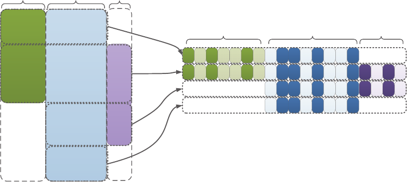
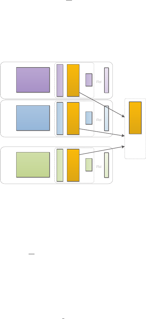
4.11 The Multi-Task Feature Learning Framework for Incomplete Multi-Source Data Fu-
sion (iMSF)
In some learning problems that involve multiple data sources, though all data sources consist of different
features for the same set of samples, it is common that each data source has some missing samples that
are different from each other. When one wants to build predictive models that involve features from more
than one data sources, a common way is to remove the the samples that are missing in any of these data
sources. However, this approach removes too much information that can be potentially useful in the learn-
ing. Recently, a multi-task learning framework for incomplete multi-source data fusion (iMSF) has been
proposed to solve this problem (Yuan et al., 2012). Considering a data set with three sources (CSF, MRI,
PET) and assuming all samples have MRI measures, we first partition the samples into multiple blocks (4 in
this case), one for each combination of data sources available: (1) PET, MRI; (2) PET, MRI, CSF; (3) MRI,
CSF; and (4) MRI. We then build four models, one for each block of data, resulting in four prediction tasks
(Figure 12).
MRIPET
Task I
Task II
Task III
Task IV
Model I
Model II
Model III
Model IV
MRI CSF
CSF
PET
Figure 12: Illustration of the multi-task feature learning framework for incomplete multi-source data fu-
sion (iMSF). In the proposed framework, we first partition the samples into multiple blocks (four blocks in
this case), one for each combination of data sources available: (1) PET, MRI; (2) PET, MRI, CSF; (3) MRI,
CSF; (4) MRI. We then build four models, one for each block of data, resulting in four prediction tasks.
We use a joint feature learning framework that learns all models simultaneously. Specifically, all models
involving a specific source are constrained to select a common set of features for that particular source.
Assume that we have a total of Sdata sources, and the feature dimensionality of the s-th source is
denoted as ps. For notational convenience, we introduce an index function G(s, k)as follows: WG(s,k)
denotes all the model parameters corresponding to the k-th feature in the s-th data source. The iMSF
formulation is:
L(W) + ρ1
S
s=1
ps
k=1
WG(s,k)
2(47)
where L(·)is the loss function.
29

4.11.1 Incomplete Multi-Source Fusion (iMSF) with Least Squares Loss (Least iMSF)
The function
[W, funcVal] = Least iMSF (X, Y, ρ1, [opts])
solves the convex fused sparse group Lasso regularized multi-task least squares problem:
min
W
1
t
t
i=1
1
ni
∥WT
iXi−Yi∥2
F+ρ1
S
s=1
ps
k=1
WG(s,k)
2(48)
where Xidenotes the input matrix of the i-th task, Yidenotes its corresponding label, Wiis the task model
for task i, the regularization parameter ρ1controls group sparsity. Currently, this function supports the
following optional fields:
• Termination: opts.tFlag,opts.tol
4.11.2 Incomplete Multi-Source Fusion (iMSF) with Logistic Loss (Logistic iMSF)
[W, c, funcVal] = Logistic iMSF (X, Y, ρ1, [opts])
solves the convex fused sparse group Lasso regularized multi-task logistic regression problem:
min
W,c
1
t
t
i=1
1
ni
ni
j=1
log(1 + exp (−Yi,j (WT
jXi,j +ci))) + ρ1
S
s=1
ps
k=1
WG(s,k)
2(49)
where Xi,j denotes sample jof the i-th task, Yi,j denotes its corresponding label, Wiand ciare the model
parameters for task i, the regularization parameter ρ1controls group sparsity. Currently, this function sup-
ports the following optional fields:
• Termination: opts.tFlag,opts.tol
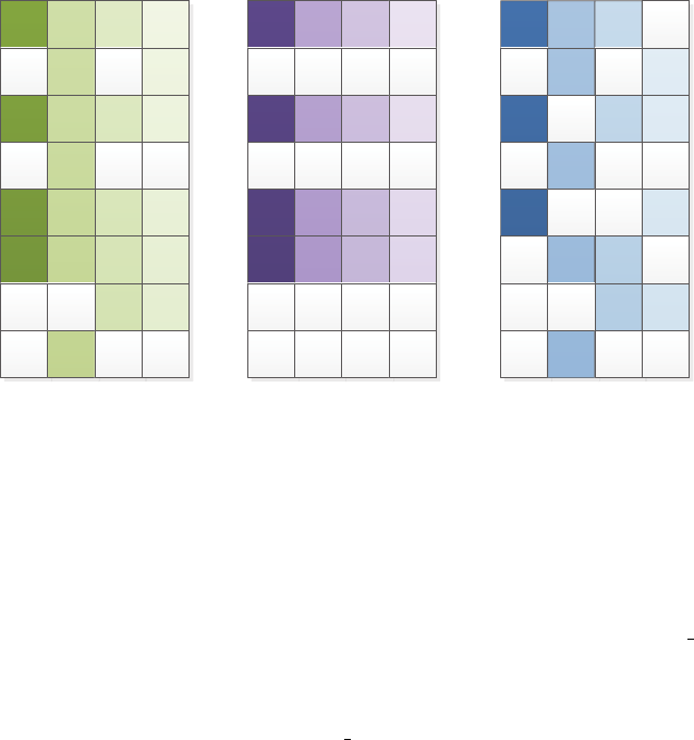
4.12 Multi-Stage Multi-Task Feature Learning (MSMTFL)
In many recent studies of sparse learning, capped vector norms are shown to enjoy better theoretical proper-
ties and better empirical performance than the classic sparsity inducing norms (Zhang, 2010). More recently
the capped norm is used in multi-task feature learning and is shown to possess both theoretical and empirical
improvements on feature learning (Gong et al., 2012a). The method is called multi-stage multi-task feature
learning (MSMTFL), which simultaneously learn the features specific to each task as well as the common
features shared among tasks. The non-convex MSMTFL solves the following formulation
min
W
L(W) + ρ1
d
j=1
min(∥wj∥1, θ)
,
where wjis the j-th row the model W. Using the difference of convex procedures, the optimization of
MSMTFL is to iteratively solve ℓ1-regularized convex problems.
30

4.12.1 Multi-Stage Feature Learning (MSMTFL) with Least Squares Loss (Least msmtfl capL1)
The function
[W, funcVal] = Least msmtfl capL1 (X, Y, ρ1,θ, [opts])
solves the multi-stage multi-task feature learning problem:
min
W
1
t
t
i=1
1
ni
∥WT
iXi−Yi∥2
F+ρ1
d
j=1
min(∥wj∥1, θ),(50)
where Xidenotes the input matrix of the i-th task, Yidenotes its corresponding label, Wiis the task model
for task i,wjis the j-th row the model W, the regularization parameter ρ1controls group sparsity, and θis
the parameter for the capped ℓ1. Currently, this function supports the following optional fields:
• Starting Point: opts.init,opts.W0
• Termination: opts.tFlag,opts.tol
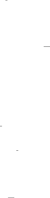
4.13 Learning the Shared Subspace for Multi-Task Clustering (LSSMTC)
Most of the multi-task learning algorithms in the literature fall in the field of supervised learning. However,
multi-task learning can also be used in the unsupervised learning, i.e., clustering (Gu & Zhou, 2009). One
may get confused between the clustered multi-task learning (CMTL) and multi-task clustering (MTC). In
CMTL, the objects to be clustered are model vectors, i.e., columns of the model matrix W(refer Section for
detailed information). In MTC, the objects to be clustered are samples, i.e., rows of the design matrix X.
One way to model task relatedness in the MTC is to assume that the data matrix share a common
subspace, and data points from each task forms cluster in the subspace. In (Gu & Zhou, 2009), an algorithm
for learning the shared subspace for multi-task clustering (LSSMTC) is proposed to address the MTC with
shared subspace. Assume there are tclustering tasks, and each task clusters the samples into cclusters, the
formulation of LSSMTC is given by:
min
M,P,W ρ1
t
i=1
∥Xi−MiPT
i∥2
F+ (1 −ρ1)
t
i=1
∥WTXi−MP T
i∥2
F
subject to: WTW=I, Pi≥0
where Mi∈Rd×cis the matrix for cluster centers of task i,Pi∈Rni×cis the relaxed cluster assignment
of task i,W∈Rd×l, and lis the dimensionality of the shared subspace. The first term is the objective of
relaxed k-means and the second the term is the objective of the relaxed k-means in the shared subspace.
4.13.1 Learning Shared Subspace for Multi-Task Clustering (LSSMTC)
The function
[W, M, P, funcVal, Acc, NMI] = LSSMTC (X, Y, c, l, ρ1, [opts])
solves the following multi-task clustering formulation:
min
M,P,W ρ1
t
i=1
∥Xi−MiPT
i∥2
F+ (1 −ρ1)
t
i=1
∥WTXi−MP T
i∥2
F(51)
subject to: WTW=I, Pi≥0(52)
31
where Xidenotes the input matrix of the i-th task, Yidenotes its corresponding clustering label (the input
is not mandatory, it is only required if the evaluation metric accuracy Acc and/or normalized mutual infor-
mation NMI are needed), Wis the shared subspace, Piis the partition matrix for task i,Miis the matrix that
consists of the centers of clusters of task i,cis the cluster number, lis the dimension of the shared subspace,
and the regularization parameter ρ1controls the importance of the clustering quality in the shared space and
in the original space. Currently, this function supports the following optional fields:
• Termination: opts.tFlag,opts.tol
32

5 Examples
In this section we provide some running examples for some representative multi-task learning formulations
included in the MALSAR package. All figures in these examples can be generated using the corresponding
MATLAB scripts in the examples folder.
5.1 Code Usage and Optimization Setup
The users are recommended to add paths that contains necessary functions at the beginning:
addpath('/MALSAR/functions/Lasso/'); % load function
addpath('/MALSAR/utils/'); % load utilities
addpath(genpath('/MALSAR/c_files/')); % load c-files
An alternative is to add the entire MALSAR package:
addpath(genpath('/MALSAR/'));
The users then need to setup optimization options before calling functions (refer to Section 3.2 for detailed
information about opts ):
opts.init = 0; % compute start point from data.
opts.tFlag = 1; % terminate after relative objective
% value does not changes much.
opts.tol = 10ˆ-5; % tolerance.
opts.maxIter = 1500; % maximum iteration number of optimization.
[W funcVal] = Least_Lasso(data_feature, data_response, lambda, opts);
Note: For efficiency consideration, it is important to set proper tolerance, termination conditions and most
importantly, maximum iterations, especially for large-scale problems.
Note: In many of the following examples we use the following command to control random generator:
rng('default'); % reset random generator.
This command is only available on MATLAB 2011 and later version. If you are using earlier versions,
another command can achieve the same goal reset. Please use the MATLAB help to get more information
about the command.
5.2 Training and Testing in Multi-Task Learning
In multi-task learning (MTL), a set of related tasks are learnt simultaneously by extracting and utilizing
appropriate shared information among tasks. In the supervised multi-task learning, each task has its own
training data and testing data. Though in the training (inference) stage, the training data for all tasks are
inputed in MTL algorithms simultaneously, the algorithms give one model for each task (in our package the
model for task iis given by the i-th column of W). The evaluation of each task is independently performed
on its testing data using the model for the task.
In this example we show the training, testing and model selection using the benchmark dataset - School
data3. In the School data there are 15362 students and their exam scores, and the students are described
by 27 attributes (features). Our goal is to build regression models to predict the exam score of students
3http://www.cs.ucl.ac.uk/staff/A.Argyriou/code/
33

from the attributes. The students come from one of the 139 secondary schools, and we build one regression
model for each school because the regression models are likely to be different for different schools (e.g.,
different textbooks may be used). Therefore we have 139 tasks, and each task is the exam score prediction
for students from one school.
We use the trace-norm regularized multi-task learning formulation in this example (for a detailed ex-
ample designed for understanding this particular formulation, see Sect. 5.5). This formulation has one
data-dependent parameter (the regularization parameter for the trace norm penalty), and we also show how
to estimate the parameter on the training data via cross validation, this process is also known as the model
selection (Kohavi, 1995). The code for this example is included in the example file test script.m in
the train and test subfolder. Firstly we load the School data:
load_data = load('../../data/school.mat');% load sample data.
X = load_data.X;
Y = load_data.Y;
The data file is already prepared in the cell format (for details about input and output format, the users are
referred to Section 3.1). We then perform z-score to normalize Xand add a bias column to the data for each
task to learn the bias. Alternatively, one can choose to normalize the target Yin the training data, and apply
the reverse transformation on the predicted values during testing.
for t = 1: length(X)
X{t} = zscore(X{t}); % normalization
X{t} = [X{t} ones(size(X{t}, 1), 1)]; % add bias.
end
We specify a training percentage to randomly split the data of each task to the training and testing part:
training_percent = 0.3;
[X_tr, Y_tr, X_te, Y_te] = mtSplitPerc(X, Y, training_percent);
The next step is to perform model selection and estimate the best regularization parameter from the data.
In order to perform cross validation, one must specify a criterion for evaluating the parameters. In multi-task
regression, a commonly used criterion is root mean squared error (MSE) given by
t
i=1 ni
j=1(Xi,j ∗Wi−Yi,j )2∗ni
t
i=1 ni
.
We use 5-fold cross validation to estimate the trace norm regularization parameter:
% the function used for evaluation.
eval_func_str = 'eval_MTL_mse';
higher_better = false; % mse is lower the better.
% cross validation fold
cv_fold = 5;
% optimization options
opts = [];
opts.maxIter = 100;
% model parameter range
param_range = [0.001 0.01 0.1 1 10 100 1000 10000];
% cross validation
best_param = CrossValidation1Param( X_tr, Y_tr, 'Least_Trace', opts, param_range, ...
cv_fold, eval_func_str, higher_better);
34

We have included the code for computing MSE and 1-parameter cross validation CrossValidation1Param
in the example folder. After the best parameter is obtained, we can build models using the parameter and
compute performance:
W = Least_Trace(X_te, Y_te, best_param, opts);
final_performance = eval_MTL_mse(Y_te, X_te, W);
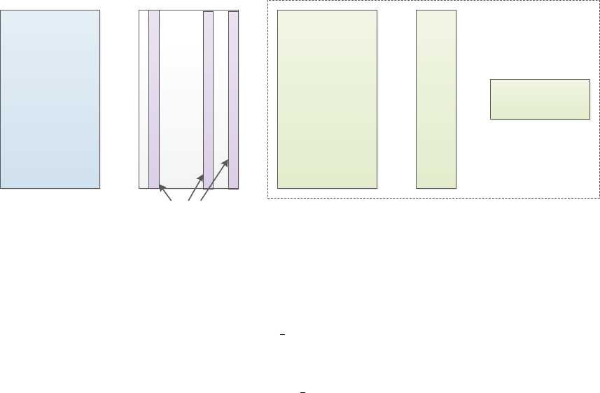
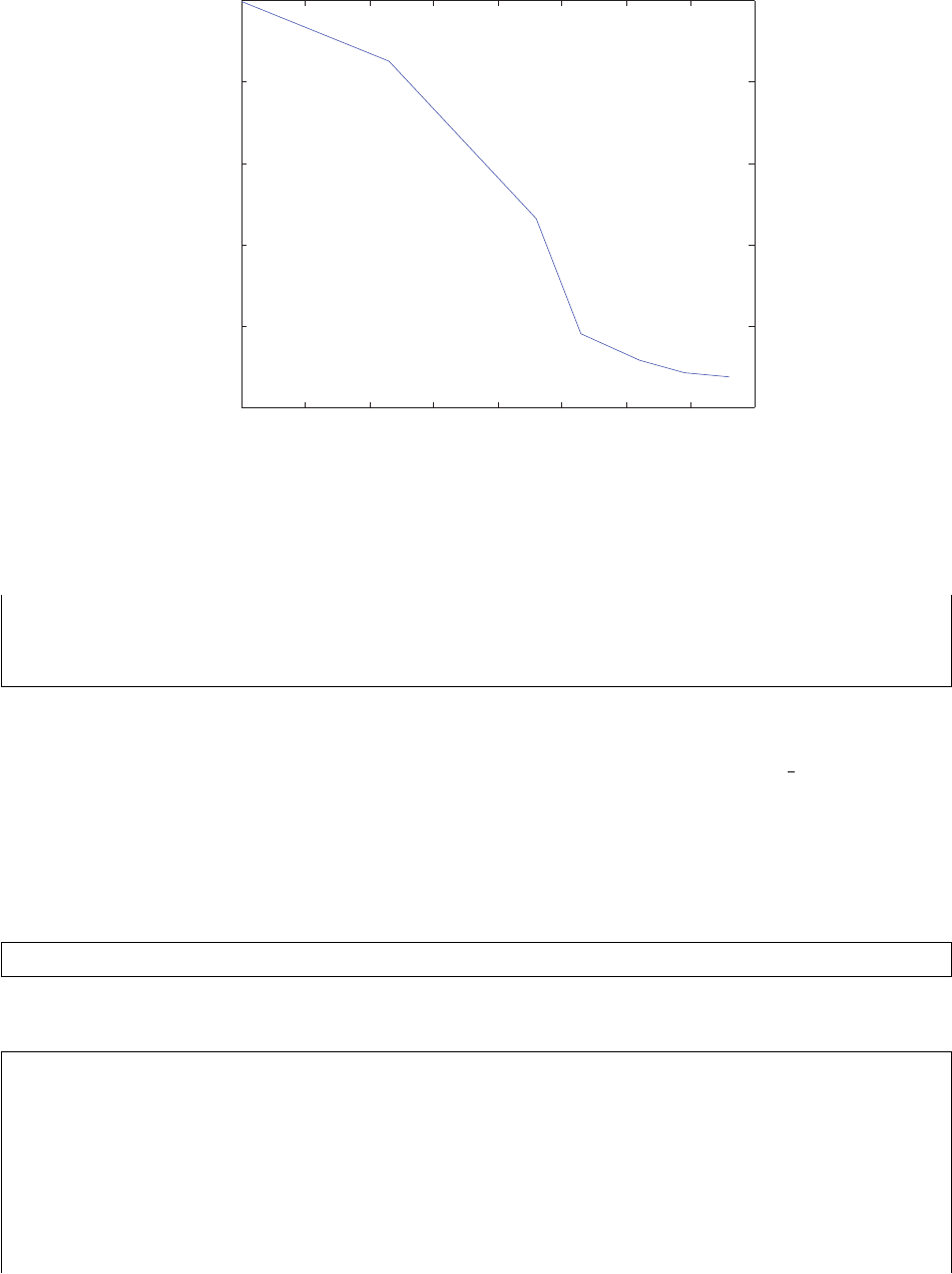
5.3 Sparsity in Multi-Task Learning: ℓ1-norm regularization
In this example, we explore the sparsity of prediction models in ℓ1-norm regularized multi-task learning
using the School data. To use school data, first load it from the data folder.
load('../data/school.mat'); % load sample data.
Define a set of regularization parameters and use pathwise computation:
lambda = [1 10 100 200 500 1000 2000];
sparsity = zeros(length(lambda), 1);
log_lam = log(lambda);
for i = 1: length(lambda)
[W funcVal] = Least_Lasso(X, Y, lambda(i), opts);
% set the solution as the next initial point.
% this gives better efficiency.
opts.init = 1;
opts.W0 = W;
sparsity(i) = nnz(W);
end
The algorithm records the number of non-zero entries in the resulting prediction model W. We show the
change of the sparsity variable against the logarithm of regularization parameters in Figure 13. Clearly,
when the regularization parameter increases, the sparsity of the resulting model increases, or equivalently,
the number of non-zero elements decreases. The code that generates this figure is from the example file
example Lasso.m.
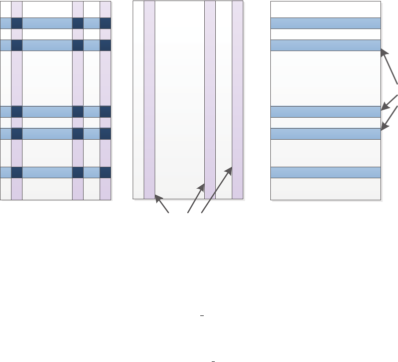
5.4 Joint Feature Selection: ℓ2,1-norm regularization
In this example, we explore the ℓ2,1-norm regularized multi-task learning using the School data from the
data folder:
load('../data/school.mat'); % load sample data.
Define a set of regularization parameters and use pathwise computation:
lambda = [200 :300: 1500];
sparsity = zeros(length(lambda), 1);
log_lam = log(lambda);
for i = 1: length(lambda)
[W funcVal] = Least_L21(X, Y, lambda(i), opts);
% set the solution as the next initial point.
% this gives better efficiency.
35
0 1 2 3 4 5 6 7 8
0
500
1000
1500
2000
2500
log(ρ1)
Sparsity of Model (Non−Zero Elements in W)
Sparsity of Predictive Model when Changing Regularization Parameter
Figure 13: Sparsity of the model Learnt from ℓ1-norm regularized MTL. As the parameter increases, the
number of non-zero elements in Wdecreases, and the model Wbecomes more sparse.
opts.init = 1;
opts.W0 = W;
sparsity(i) = nnz(sum(W,2 )==0)/d;
end
The statement nnz(sum(W,2 )==0) computes the number of features that are not selected for all tasks.
We can observe from Figure 14 that when the regularization parameter increases, the number of selected
features decreases. The code that generates this result is from the example file example L21.m.
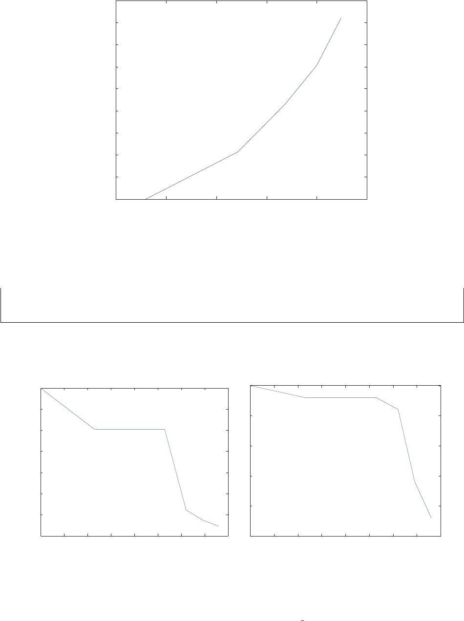
5.5 Low-Rank Structure: Trace norm Regularization
In this example, we explore the trace-norm regularized multi-task learning using the School data from the
data folder:
load('../data/school.mat'); % load sample data.
Define a set of regularization parameters and use pathwise computation:
tn_val = zeros(length(lambda), 1);
rk_val = zeros(length(lambda), 1);
log_lam = log(lambda);
for i = 1: length(lambda)
[W funcVal] = Least_Trace(X, Y, lambda(i), opts);
% set the solution as the next initial point.
% this gives better efficiency.
opts.init = 1;
opts.W0 = W;
36
5 5.5 6 6.5 7 7.5
0
0.1
0.2
0.3
0.4
0.5
0.6
0.7
0.8
0.9
log(ρ1)
Row Sparsity of Model (Percentage of All−Zero Columns)
Row Sparsity of Predictive Model when Changing Regularization Parameter
Figure 14: Joint feature learning via the ℓ2,1-norm regularized MTL. When the regularization parameter
increases, the number of selected features decreases.
tn_val(i) = sum(svd(W));
rk_val(i) = rank(W);
end
In the code we compute the value of trace norm of the prediction model as well as its rank. We gradually
increase the penalty and the results are shown in Figure 15. The code sum(svd(W)) computes the trace
norm (the sum of singular values).
0 1 2 3 4 5 6 7 8
0
200
400
600
800
1000
1200
1400
log(ρ1)
Trace Norm of Model (Sum of Singular Values of W)
Trace Norm of Predictive Model when Changing Regularization Parameter
0 1 2 3 4 5 6 7 8
0
5
10
15
20
25
log(ρ1)
Rank of Model
Rank of Predictive Model when Changing Regularization Parameter
Figure 15: The trace norm and rank of the model learnt from trace norm regularized MTL.
As the trace-norm penalty increases, we observe the monotonic decrease of the trace norm and rank.
The code that generates this result is from the example file example Trace.m.
37

5.6 Graph Structure: Graph Regularization
In this example, we show how to use graph regularized multi-task learning using the SRMTL functions. We
use the School data from the data folder:
load('../data/school.mat'); % load sample data.
For a given graph, we first construct the graph variable Rto encode the graph structure:
% construct graph structure variable.
R = [];
for i = 1: task_num
for j = i + 1: task_num
if graph (i, j) ̸=0
edge = zeros(task_num, 1);
edge(i) = 1;
edge(j) = -1;
R = cat(2, R, edge);
end
end
end
[W_est funcVal] = Least_SRMTL(X, Y, R, 1, 20);
The code that generates this result is from example SRMTL.m and example SRMTL spcov.m.
5.7 Learning with Outlier Tasks: RMTL
In this example, we show how to use robust multi-task learning to detect outlier tasks using synthetic data:
dimension = 500;
sample_size = 50;
task = 50;
X = cell(task ,1);
Y = cell(task ,1);
for i = 1: task
X{i} = rand(sample_size, dimension);
Y{i} = rand(sample_size, 1);
end
To generate reproducible results, we reset the random number generator before we use the rand function.
We then run the following code:
opts.init = 0; % guess start point from data.
opts.tFlag = 1; % terminate after relative objective value does not changes much.
opts.tol = 10ˆ-6; % tolerance.
opts.maxIter = 1500; % maximum iteration number of optimization.
rho_1 = 10;% rho1: low rank component L trace-norm regularization parameter
rho_2 = 30; % rho2: sparse component S L1,2-norm sprasity controlling parameter
[W funcVal L S] = Least_RMTL(X, Y, rho_1, rho_2, opts);
We visualize the matrices Land Sin Figure 16. In the figure, the dark blue color corresponds to a zero entry.
The matrices are transposed since the dimensionality is much larger than the task number. After transpose,
each row corresponds to a task. We see that for the sparse component Shas non-zero rows, corresponding
to the outlier tasks. The code that generates this result is from the example file example Robust.m.
38
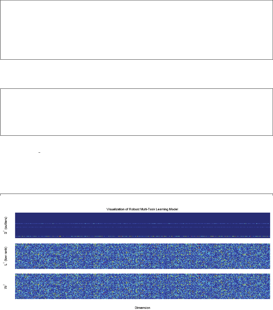
5.8 Joint Feature Learning with Outlier Tasks: rMTFL
In this example, we show how to use robust multi-task learning to detect outlier tasks using synthetic data:
dimension = 500;
sample_size = 50;
task = 50;
X = cell(task ,1);
Y = cell(task ,1);
for i = 1: task
X{i} = rand(sample_size, dimension);
Y{i} = rand(sample_size, 1);
end
To generate reproducible results, we reset the random number generator before we use the rand function.
We then run the following code:
opts.init = 0; % guess start point from data.
opts.tFlag = 1; % terminate after relative objective value does not changes much.
opts.tol = 10ˆ-6; % tolerance.
opts.maxIter = 500; % maximum iteration number of optimization.
rho_1 = 90;% rho1: joint feature learning
rho_2 = 280; % rho2: detect outlier
[W funcVal P Q] = Least_rMTFL(X, Y, rho_1, rho_2, opts);
We visualize the matrices Pand Qin Figure 17. The code that generates this result is from the example
file example rMTFL.m.
5.9 Learning with Dirty Data: Dirty MTL Model
In this example, we show how to use dirty multi-task learning using synthetic data:
Figure 16: Illustration of RMTL. The dark blue color corresponds to a zero entry. The matrices are trans-
posed since the dimensionality is much larger than the task number. After transpose, each row corresponds
to a task. We see that for the sparse component Shas non-zero rows, corresponding to the outlier tasks.
39
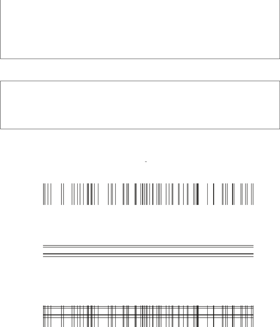
dimension = 500;
sample_size = 50;
task = 50;
X = cell(task ,1);
Y = cell(task ,1);
for i = 1: task
X{i} = rand(sample_size, dimension);
Y{i} = rand(sample_size, 1);
end
We then run the following code:
opts.init = 0; % guess start point from data.
opts.tFlag = 1; % terminate after relative objective value does not changes much.
opts.tol = 10ˆ-4; % tolerance.
opts.maxIter = 500; % maximum iteration number of optimization.
rho_1 = 350;% rho1: group sparsity regularization parameter
rho_2 = 10;% rho2: elementwise sparsity regularization parameter
[W funcVal P Q] = Least_Dirty(X, Y, rho_1, rho_2, opts);
We visualize the non-zero entries in P,Qand Rin Figure 18. The figures are transposed for better
visualization. We see that matrix Phas a clear group sparsity property and it captures the joint-selected
features. The features that do not fit into the group sparsity structure is captured in matrix Q. The code that
generates this result is from the example file example Dirty.m.
Visualization of Robust Multi−Task Feature Learning Model
PT (feature)QT (outliers)
Dimension
WT
Figure 17: Illustration of outlier tasks detected by rMTFL. Black means non-zero entries. The matrices are
transposed because that dimension number is larger than the task number. After transpose, each row denotes
a task.
40
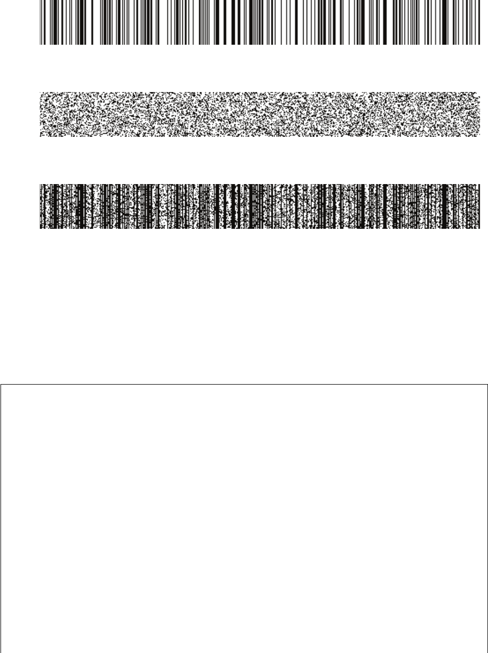
Visualization Non−Zero Entries in Dirty Model
PT
QT
Dimension
WT
Figure 18: The dirty prediction model Wlearnt as well as the joint feature selection component Pand the
element-wise sparse component Q.
5.10 Learning with Clustered Structures: CMTL
In this example, we show how to use clustered multi-task learning (CMTL) functions. we use synthetic data
generated as follows:
clus_var = 900; % cluster variance
task_var = 16; % inter task variance
nois_var = 150; % variance of noise
clus_num = 2; % clusters
clus_task_num = 10; % task number of each cluster
task_num = clus_num *clus_task_num; % total task number.
sample_size = 100;
dimension = 20; % total dimension
comm_dim = 2; % independent dimension for all tasks.
clus_dim = floor((dimension - comm_dim)/2); % dimension of cluster
% generate cluster model
cluster_weight = randn(dimension, clus_num) *clus_var;
for i = 1: clus_num
cluster_weight (randperm(dimension-clus_num)≤clus_dim, i) = 0;
end
cluster_weight (end-comm_dim:end, :) = 0;
W = repmat (cluster_weight, 1, clus_task_num);
cluster_index = repmat (1:clus_num, 1, clus_task_num)';
% generate task and intra-cluster variance
W_it = randn(dimension, task_num) *task_var;
for i = 1: task_num
W_it(cat(1, W(1:end-comm_dim, i)==0, zeros(comm_dim, 1))==1, i) = 0;
end
W = W + W_it;
41
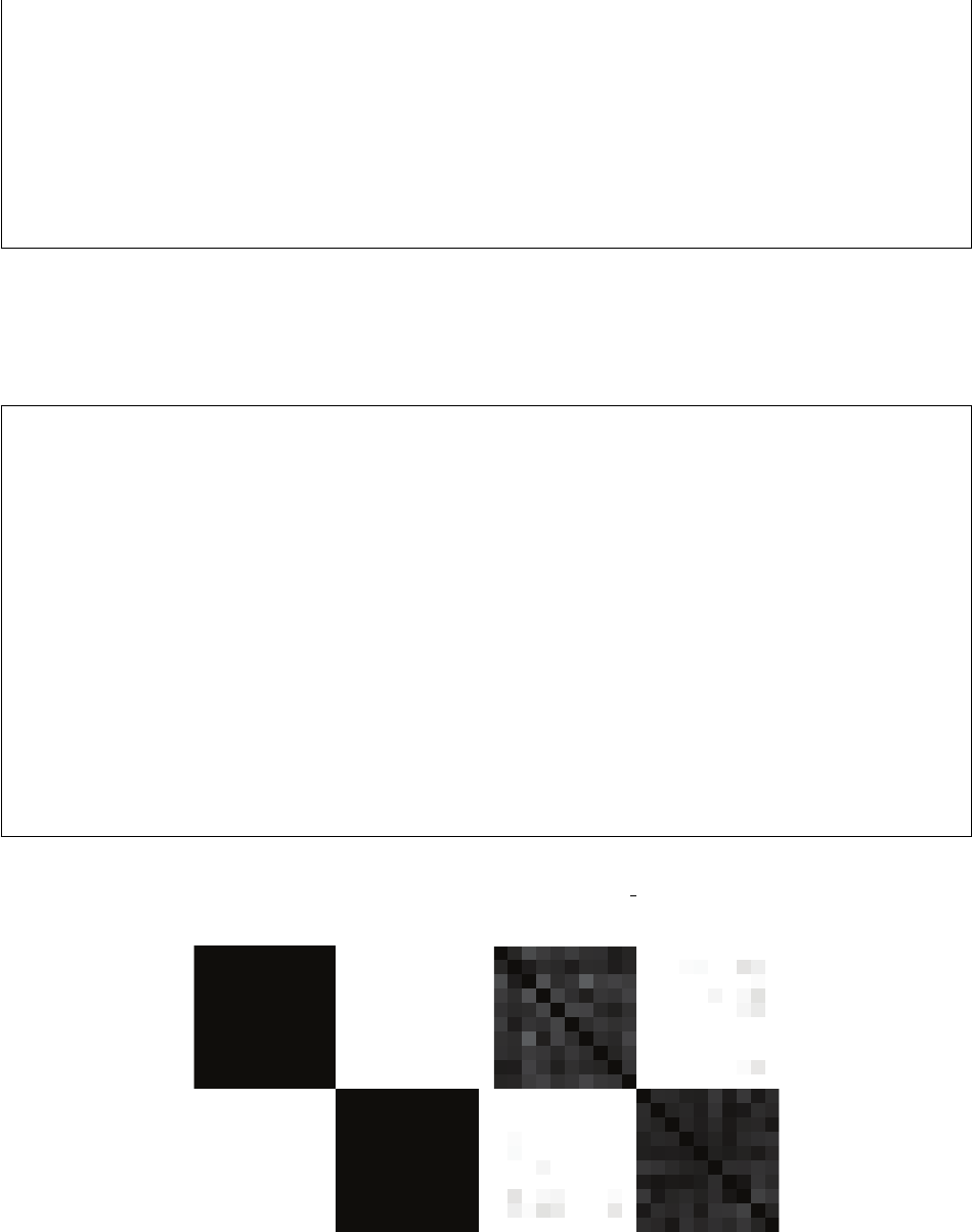
% apply noise;
W = W + randn(dimension, task_num) *nois_var;
% Generate Data Sets
X = cell(task_num, 1);
Y = cell(task_num, 1);
for i = 1: task_num
X{i} = randn(sample_size, dimension);
xw = X{i} *W(:, i);
xw = xw + randn(size(xw)) *nois_var;
Y{i} = sign(xw);
end
We generate a set of tasks as follows: We firstly generate 2 cluster centers with between cluster variance
N(0,900), and for each cluster center we generate 10 tasks with intra-cluster variance N(0,16). We thus
generate a total of 20 task models W. We generate data points with variance N(0,150). After we generate
the data set, we run the following code to learn the CMTL model:
opts.init = 0; % guess start point from data.
opts.tFlag = 1; % terminate after relative objective value does not changes much.
opts.tol = 10ˆ-6; % tolerance.
opts.maxIter = 1500; % maximum iteration number of optimization.
rho_1 = 10;
rho_2 = 10ˆ-1;
W_learn = Least_CMTL(X, Y, rho_1, rho_2, clus_num, opts);
% recover clustered order.
kmCMTL_OrderedModel = zeros(size(W));
OrderedTrueModel = zeros(size(W));
for i = 1: clus_num
clusModel = W_learn (:, i:clus_num:task_num );
kmCMTL_OrderedModel (:, (i-1)*clus_task_num + 1: i*clus_task_num ) = ...
clusModel;
clusModel = W (:, i:clus_num:task_num );
OrderedTrueModel (:, (i-1)*clus_task_num + 1: i*clus_task_num ) = ...
clusModel;
end
We visualize the models in Figure 19. We see that the clustered structure is captured in the learnt model.
The code that generates this result is from the example file example CMTL.m.
Model Correlation: Ground Truth
Model Correlation: Clustered MTL
Figure 19: Illustration of the cluster Structure Learnt from CMTL.
42
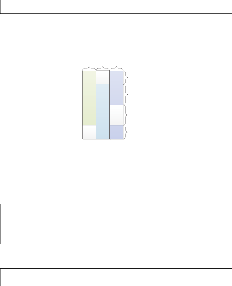
5.11 Learning with Incomplete Data: Incomplete Multi-Source Fusion (iMSF)
In this example we show how to use incomplete multi-source fusion (iMSF). First, we import the path
necessary for running iMSF.
addpath('../MALSAR/utils/')
addpath('../MALSAR/functions/iMSF')
Next, we construct 3 data sources that are block-wise missing. In total there are 50 samples, and the di-
mensions of the three data sources are 45, 55, 50 respectively. In the first data source, we suppose that the
last 20% samples are missing, in the second data source, the first 20% samples are missing, and in the third
data source there are 30% samples are missing. The missing patterns of the data sources are illustrated in
Figure 20. Note that using this dataset for training the iMSF gives 4 models, one for each missing pattern
(and the dimensions of these models are 95, 150, 100,105 respectively).
45 55 50
Model
Dimension 95
Model
Dimension 150
Model
Dimension 100
Model
Dimension 105
Data Source 1
Data Source 2
Data Source 3
Figure 20: Illustration the block-wise missing patterns in the incomplete multi-source fusion.
We use the following code to construct these data sources and block-wise missing patterns:
n = 50; p1 = 45; p2 = 55; p3 = 50;
X1 = randn(n, p1); X2 = randn(n, p2); X3 = randn(n, p3);
X1(round(0.8 *n):end, :) = nan;
X2(1:round(0.2 *n), :) = nan;
X3(round(0.5 *n):round(0.8 *n), :) = nan;
Y = sign(randn(n, 1));
X_Set{1} = X1; X_Set{2} = X2; X_Set{3} = X3;
After the data sets are constructed, one can use the iMSF with logistic loss (or least squares loss) to build
the models.
opts.tol = 1e-6;
opts.maxIter = 5000;
lambda = 0.1;
43

[logistic_Sol, logistic_funVal] = Logistic_iMSF(X_Set, Y, lambda, opts);
5.12 Towards Better Multi-Task Feature Learning: Multi-Stage Multi-Task Feature Learn-
ing
1 2 3 4 5 6 7 8 9 10
0
20
40
60
80
100
120
140
Stage
Parameter estimation error (L2,1)
m=20,n=30,d=200,σ=0.001
α=2.629e−05
α=5.258e−05
α=0.00010516
α=0.0002629
Figure 21: The parameter estimation error (ℓ2,1) of multi-stage feature learning with different number of
stages.
In this example we explore the effectiveness of multi-stages methods in the multi-task feature learning.
We generate data randomly from a given distribution and vary the parameters of the algorithm to demonstrate
the effectiveness of the algorithm evaluated by ℓ2,1-norm between the ground truth and the model estimated
from synthetic data.
We firstly load directories for the function and dependent utilities:
addpath('../MALSAR/functions/msmtfl/'); % load function
addpath('../MALSAR/utils/'); % load utilities
and specify experimental settings:
% problem size
m = 20; % task number
n = 30; % number of samples for each task
samplesize = n*ones(m,1);
d = 200; % dimensionality
repeat_num = 10; % repeat the experiment for 10 times
maxstep = 10; % compare different parameters up to 10 stages.
% distribution for model and data
zerorow_percent = 0.9;
restzero_percent = 0.8;
noiselevel = 0.001;
44

% algorithm property
opts.tol = 1e-5;
opts.lFlag = 0;
opts.init = 1;
opts.W0 = randn(d,m);
opts.tFlag = 1;
% algorithm parameter settings.
scale = 50;
para = [0.00005; 0.0001; 0.0002; 0.0005]*sqrt(log(d*m)/n);
para_num = length(para);
In the experiment, we repeat the following experiments for 10 times and evaluate the average perfor-
mance. We generate synthetic model and data from the given distribution
% generate model
W = rand(d,m)*20 - 10;
permnum = randperm(d);
zerorow = permnum(1:round(d*zerorow_percent));
nonzerorow = permnum(round(d*zerorow_percent)+1:end);
W(zerorow,:) = 0;
Wtemp = W(nonzerorow,:);
permnum = randperm(length(nonzerorow)*m);
Wtemp(permnum(1:round(length(nonzerorow)*m*restzero_percent))) = 0;
W(nonzerorow,:) = Wtemp;
% genetate data
X = cell(m,1);
Y = cell(m,1);
for ii = 1:m
X{ii} = normrnd(0,1,samplesize(ii),d);
X{ii} = normalize(X{ii},samplesize(ii));
Y{ii} = X{ii} *W(:, ii) + noiselevel*normrnd(0,1,samplesize(ii),1);
end
and we study for each given maximum step (stage), the performance of different λand the performance.
opts.maxIter = ii; % given (maximum) stage number.
lambda = para(1)*m*n;
theta = scale(1)*m*lambda;
[W_ms1,¬] = Least_msmtfl_capL1(X,Y,lambda,theta,opts);
and evaluate the performance using the ℓ2,1-norm:
Werror_ms1_21(ii,jj) = norm(sum(abs(W_ms1 - W),2));
A comparison of the performance of different settings is shown in the Figure 21. The code used to
generate the figure can be found in the script example_msmtfl.m in the example folder of the package.
5.13 Unsupervised Multi-Task Learning: Learning Shared Subspace in Multi-Task Clus-
tering (LSSMTC)
In this example we show how to learn shared subspace in multi-task clustering (LSSMTC). We use the 20
Newsgroup data 4, which is a collection of approximately 20k newsgroup documents, partitioned across 20
different newsgroups nearly evenly. In the Data folder we include two cross domain data sets (Rec. vs.
4http://people.csail.mit.edu/jrennie/20Newsgroups
45
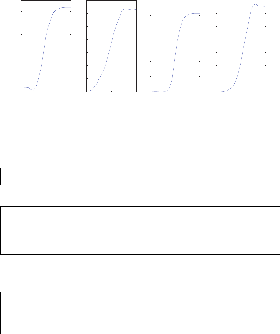
0 5 10 15 20
50
55
60
65
70
75
80
85
90
accuracy
iteration
Task 1
0 5 10 15 20
50
55
60
65
70
75
80
85
accuracy
iteration
Task 2
0 5 10 15 20
0
10
20
30
40
50
60
normalized mutual information
iteration
Task 1
0 5 10 15 20
0
5
10
15
20
25
30
35
normalized mutual information
iteration
Task 2
Figure 22: The accuracy and normalized mutual information for multi-task clustering on the 20 Newsgroups
Computer vs Science dataset.
Talk and Comp. vs. Sci.). We demonstrate the LSSMTC algorithm on Computer vs Science dataset. Firstly
we add paths necessary for running LSSMTC:
addpath('../MALSAR/functions/mutli-task clustering/');
addpath('../MALSAR/utils/');
We then load the clustering tasks into proper data structures:
m = 2; % there are two tasks in this dataset.
cellX = cell(m,1); cellgnd = cell(m,1);
for i=1:m
task_data = load([path 'Task' num2str(i)]);
cellX{i} = task_data.fea';
cellgnd{i} = task_data.gnd;
end
Note that we need the label information only for the computation of performance metric (accuracy and/or
normalized mutual information). In applications where ground truth is unknown, one may set cellgnd=[].
And then we can perform LSSMTC:
opts.tFlag = 2; % termination: run maximum iteration.
opts.maxIter = 20; % maximum iteration.
c = length(unique(cellgnd{1})); % cluster number
l = 2; % subspace dimension
lambda = 0.75; % multi-task regulariation paramter
[W cellM cellP residue cellAcc cellNMI] = LSSMTC(cellX,cellgnd,c,l,lambda,opts);
Note that for the purpose of illustration, for the cluster number cwe use the ground truth, in real applications,
however, the number (and also the dimension of the subspace l) should be estimated from data via cross
validation. The accuracy and normalized mutual information for the two tasks are given in Figure 22. It can
be seen from the results that the multi-task clustering improves the clustering performance for both tasks.
46
6 Revision, Citation and Acknowledgement
Revision
• Version 1.0 was released on April, 2012.
• Version 1.1 was released on December, 2012. There are several improvements and new features:
1. Improved algorithm performance.
2. Added disease progression models (Zhou et al., 2011b; Zhou et al., 2012).
3. Added the incomplete multi-source fusion (iMSF) models (Yuan et al., 2012).
4. Added the multi-stage multi-task feature learning (Gong et al., 2012a).
5. Added the learning shared subspace for multi-task clustering (LSSMTC) algorithm (Gu & Zhou,
2009).
6. Added an example to illustrate training, testing and model selection in multi-task learning.
Citation
In citing MALSAR in your papers, please use the following reference:
[Zhou 2012] J. Zhou, J. Chen, and J. Ye. MALSAR: Multi-tAsk Learning via StructurAl Regularization.
Arizona State University, 2012. http://www.MALSAR.org
Acknowledgement
The MALSAR software project has been supported by research grants from the National Science Founda-
tion (NSF). The authors of MALSAR would like to thank Pinghua Gong, Lei Yuan and Quanquan Gu for
donating their codes.
47
References
Abernethy, J., Bach, F., Evgeniou, T., & Vert, J. (2006). Low-rank matrix factorization with attributes. Arxiv
preprint cs/0611124.
Abernethy, J., Bach, F., Evgeniou, T., & Vert, J. (2009). A new approach to collaborative filtering: Operator
estimation with spectral regularization. The Journal of Machine Learning Research,10, 803–826.
Agarwal, A., Daum´
e III, H., & Gerber, S. (2010). Learning multiple tasks using manifold regularization. .
Ando, R., & Zhang, T. (2005). A framework for learning predictive structures from multiple tasks and
unlabeled data. The Journal of Machine Learning Research,6, 1817–1853.
Argyriou, A., Evgeniou, T., & Pontil, M. (2007). Multi-task feature learning. Advances in neural informa-
tion processing systems,19, 41.
Argyriou, A., Evgeniou, T., & Pontil, M. (2008a). Convex multi-task feature learning. Machine Learning,
73, 243–272.
Argyriou, A., Micchelli, C., Pontil, M., & Ying, Y. (2008b). A spectral regularization framework for multi-
task structure learning. Advances in Neural Information Processing Systems,20, 25–32.
Bakker, B., & Heskes, T. (2003). Task clustering and gating for bayesian multitask learning. The Journal of
Machine Learning Research,4, 83–99.
Bickel, S., Bogojeska, J., Lengauer, T., & Scheffer, T. (2008). Multi-task learning for hiv therapy screening.
Proceedings of the 25th international conference on Machine learning (pp. 56–63).
Chen, J., Liu, J., & Ye, J. (2010). Learning incoherent sparse and low-rank patterns from multiple tasks.
Proceedings of the 16th ACM SIGKDD international conference on Knowledge discovery and data mining
(pp. 1179–1188).
Chen, J., Tang, L., Liu, J., & Ye, J. (2009). A convex formulation for learning shared structures from multiple
tasks. Proceedings of the 26th Annual International Conference on Machine Learning (pp. 137–144).
Chen, J., Zhou, J., & Ye, J. (2011). Integrating low-rank and group-sparse structures for robust multi-task
learning. Proceedings of the tenth ACM SIGKDD international conference on Knowledge discovery and
data mining.
Evgeniou, T., Micchelli, C., & Pontil, M. (2006). Learning multiple tasks with kernel methods. Journal of
Machine Learning Research,6, 615.
Evgeniou, T., & Pontil, M. (2004). Regularized multi–task learning. Proceedings of the tenth ACM SIGKDD
international conference on Knowledge discovery and data mining (pp. 109–117).
Fazel, M. (2002). Matrix rank minimization with applications. Doctoral dissertation, PhD thesis, Stanford
University.
Gong, P., Ye, J., & Zhang, C. (2012a). Multi-stage multi-task feature learning. Advances in Neural Infor-
mation Processing Systems.
Gong, P., Ye, J., & Zhang, C. (2012b). Robust multi-task feature learning. Proceedings of the 18th ACM
SIGKDD international conference on Knowledge discovery and data mining. New York, NY, USA: ACM.
48
Gu, Q., & Zhou, J. (2009). Learning the shared subspace for multi-task clustering and transductive transfer
classification. Data Mining, 2009. ICDM’09. Ninth IEEE International Conference on (pp. 159–168).
Jacob, L., Bach, F., & Vert, J. (2008). Clustered multi-task learning: A convex formulation. Advances in
Neural Information Processing Systems.
Jalali, A., Ravikumar, P., Sanghavi, S., & Ruan, C. (2010). A dirty model for multi-task learning. Proceed-
ings of the Conference on Advances in Neural Information Processing Systems (NIPS).
Ji, S., & Ye, J. (2009). An accelerated gradient method for trace norm minimization. Proceedings of the
26th Annual International Conference on Machine Learning (pp. 457–464).
Kohavi, R. (1995). A study of cross-validation and bootstrap for accuracy estimation and model selection.
International joint Conference on artificial intelligence (pp. 1137–1145).
Li, C., & Li, H. (2008). Network-constrained regularization and variable selection for analysis of genomic
data. Bioinformatics,24, 1175–1182.
Liu, J., Ji, S., & Ye, J. (2009). Multi-task feature learning via efficient l 2, 1-norm minimization. Proceedings
of the Twenty-Fifth Conference on Uncertainty in Artificial Intelligence (pp. 339–348).
Nemirovski, A. Efficient methods in convex programming. Lecture Notes.
Nemirovski, A. (2001). Lectures on modern convex optimization. Society for Industrial and Applied Math-
ematics (SIAM.
Nesterov, Y. (2005). Smooth minimization of non-smooth functions. Mathematical Programming,103,
127–152.
Nesterov, Y. (2007). Gradient methods for minimizing composite objective function. ReCALL,76.
Nesterov, Y., & Nesterov, I. (2004). Introductory lectures on convex optimization: A basic course, vol. 87.
Springer.
Nie, F., Huang, H., Cai, X., & Ding, C. (2010). Efficient and robust feature selection via joint l21-norms
minimization. .
Obozinski, G., Taskar, B., & Jordan, M. (2010). Joint covariate selection and joint subspace selection for
multiple classification problems. Statistics and Computing,20, 231–252.
Thrun, S., & O’Sullivan, J. (1998). Clustering learning tasks and the selective cross-task transfer of knowl-
edge. Learning to learn, 181–209.
Tibshirani, R. (1996). Regression shrinkage and selection via the lasso. Journal of the Royal Statistical
Society. Series B (Methodological), 267–288.
Vandenberghe, L., & Boyd, S. (1996). Semidefinite programming. SIAM review, 49–95.
Wang, F., Wang, X., & Li, T. (2009). Semi-supervised multi-task learning with task regularizations. 2009
Ninth IEEE International Conference on Data Mining (pp. 562–568).
Xue, Y., Liao, X., Carin, L., & Krishnapuram, B. (2007). Multi-task learning for classification with dirichlet
process priors. The Journal of Machine Learning Research,8, 35–63.
49
Yuan, L., Wang, Y., Thompson, M., Narayan, A. V., & Ye, J. (2012). Multi-source learning for joint analysis
of incomplete multi-modality neuroimaging data. Proceedings of the 18th ACM SIGKDD international
conference on Knowledge discovery and data mining. New York, NY, USA: ACM.
Zha, H., He, X., Ding, C., Gu, M., & Simon, H. (2002). Spectral relaxation for k-means clustering. Advances
in Neural Information Processing Systems,2, 1057–1064.
Zhang, T. (2010). Analysis of multi-stage convex relaxation for sparse regularization. The Journal of
Machine Learning Research,11, 1081–1107.
Zhang, Y., & Yeung, D. (2010). A convex formulation for learning task relationships in multi-task learning.
Proceedings of the 26th Conference on Uncertainty in Artificial Intelligence (UAI) (pp. 733–742).
Zhou, J., Chen, J., & Ye, J. (2011a). Clustered multi-task learning via alternating structure optimization.
Advances in Neural Information Processing Systems.
Zhou, J., Liu, J., Narayan, A. V., & Ye, J. (2012). Modeling disease progression via fused sparse group
lasso. Proceedings of the 18th ACM SIGKDD international conference on Knowledge discovery and data
mining. New York, NY, USA: ACM.
Zhou, J., Yuan, L., Liu, J., & Ye, J. (2011b). A multi-task learning formulation for predicting disease
progression. Proceedings of the 17th ACM SIGKDD international conference on Knowledge discovery
and data mining (pp. 814–822). New York, NY, USA: ACM.
50
