Manual

User Manual:

Open the PDF directly: View PDF .
Page Count: 26

Introduction
Electron drift
Gas Amplification
Cosmic Radiation
Measurement Setup
Measurements
Sample Analysis Code:

Manual number:

Physikpraktikum für Vorgerückte (VP)

vp.phys.ethz.ch

Drift Chamber

Instructions

D. Hits, G. Guyer, M. Setz

rev. D. Hits, October 5, 2018

1 Introduction

This manual is contains only brief introduction to the processes occurring in a

drift chamber.In order to gain more complete understanding of the physics of

the drift chamber a references at the end of this manual should be consulted

[1, 2, 3].

Drift chambers belong to the most important measurement devices of

nuclear and particle physics. They are a central aspect of nearly every large

experiment in high energy physics. In this experiment a small drift chamber

is operated and characterized. After that the trajectories of particles from

the cosmic radiation should be reconstructed.

If a charged particle travels through a gas volume, it leaves a trail of

ionized gas atoms and free electrons behind. By applying an electric ﬁeld

the ions and electrons can be separated and generate an electric signal. This

signal, however, is very small. A high-energy particle with an elementary

charge produces only about 100 electron/ion-pairs by going through one cen-

timeter of air. Single particles are therefore only detectable after amplifying

this signal.

In a detector ﬁlled with gas there is a simple way to amplify the signal

inside the detector, even before it is measured on the outside. If the electric

ﬁeld is suﬃciently strong, the free electrons can be accelerated to the energies

large enough to ionize gas atoms and create and avalanche which will result

in an electric signal many times higher than the original one. The required

electric ﬁeld strengths are easily generated around very thin wires. By using

very thin signal wires, one can therefore easily create a detectable signal.

Hence already a simple structure allows the detection of particle radiation.

Many detectors are based on this principle, from a simple Geiger counter up

to time projection chambers in high energy experiments with several thou-

sand wires.

A drift chamber additionally makes use of the fact, that the ampliﬁcation

of the signal only occurs, when the free electrons reach the region of strong

ﬁelds in the immediate proximity to a wire. Before reaching this point the

electrons simply drift along the electric ﬁeld lines, without increasing their

numbers. With a known drift velocity and a measured time diﬀerence be-

tween the arrival of the particle and the detection of the electric signal the

distance between the signal wire and the trajectory of the particle can there-

fore be calculated. The location can be reconstructed in such a chamber

with a resolution to a fraction of a millimeter. By combining the position

measurement of multiple wires, the trajectory of the particle can be recon-

structed. Figure 1.1 shows the general structure of a drift chamber. It is

described in more detail in section 5.2.

Figure 1.2 shows traces of particles, which were being generated by a

electron-proton-collision in the H1-Detector at the HERA storage ring. The

paths are curved, because the detector is inside a strong magnetic ﬁeld. The

curvature is a measure of the charge and momentum of the particles. By

the way the gas inside the H1-Detector is identical to the gas used in our

experiment.

Figure 1.1: General structure of a drift chamber.

Run 248070 Event 1808 Class: 4 8 19 28 29 Date 31/03/1100

H1 Eve nt Di s pl ay 1. 17/ 05

DSN=[ h1uk. h1] t t f / e pdat a/ 99e +/ e ppot _f 2025. A00

E= -27.6 x 920.0 GeV B= 0.0 kG

Run date 99/07/28 15:17

AST = 0

RST = 0

BTOF Gl obal , BG, I A = 000

Figure 1.2: Particle trajectories in the central drift chamber of the H1 experi-

ment. The drift chamber is cylindrical and the anode wires are parallel to the

cylindrical axis, therefore they are perpendicular to the image plane. Each

point represents a wire which detected a signal. The positions are corrected

by means of drift duration.

2 Electron drift

The electrons released by ionization get quickly to thermal equilibrium through

elastic collisions with the gas atoms. The electrons then move in arbitrary,

frequently changing directions. The average kinetic energy is like in an ideal

gas

2mv2>=3

2kT. (1)

At room temperature this correlates to a velocity of 120 km s−1!

Between collisions the electrons get accelerated by the electric ﬁeld over

and over again. Thus the motion of the electron cloud goes along the ﬁeld

lines on average.

For a start we look at a group of electrons all traveling with velocity v.

Along a way dx a fraction Nσdx of the electrons collide with a gas atom. N

is the number of gas atoms per unit volume and σthe total collision cross

section. Let’s call n(t)the number of electrons, which didn’t collide with a

gas atom in a time tsince the last collision. Thus n(t)can be calculated by

dn(t) = −Nσvdt =−v

ldt. (2)

The quantity l≡Nσ is called the mean free path of the electrons in the

gas. Integrating (2) yields

N(t) = n0exp −v

lt.(3)

An electron experiences a constant force e~

Eon the path between two

collisions. Therefore additionally to the free movement the electron covers

the distance

∆s=1

m∆t2(4)

along the ~

E-ﬁeld.

The mean drift velocity for electrons with velocity vis thus

vD(v) = R∆s(t)e−

ltdt

Rte−

ldt

mRt2e−

ltdt

Rte−

ldt =eE

In reality not all electrons are moving at the same velocity, but the veloc-

ities are distributed corresponding to the Maxwell-Boltzmann distribution.

Thus to get the mean drift velocity for the whole electron cloud, one has to

average over the thermal velocities. The drift velocity of the electron cloud

is therefore

vD=eE

m<l

v>=eE

mτ. (5)

Where τis the mean time between two collisions of an electron with a gas

atom.

According to this simple calculation one expects the drift velocity to in-

crease proportional to the electric ﬁeld strength. For small ﬁelds this is

normally the case. The proportionality constant is called the mobility.

3 Gas Ampliﬁcation

If the accelerating electric ﬁeld is strong enough, the electrons can gain

enough energy between two collisions, to ionize a gas atom. The new free

electrons get accelerated themselves to the point where they can ionize a gas

atom and the total number of free electrons increases rapidly in a snowballing

eﬀect.

In a constant and suﬃcient high electric ﬁeld strength the number of

secondary ionizations, which a drifting electron causes, is proportional to the

covered distance. The proportionality factor αis called the ﬁrst Townsend-

coeﬃcient. The factor is dependent on the electric ﬁeld strength. One ﬁnds

an empirical dependency of the form

α=Aexp−B

E,(6)

with coeﬃcients Aand B, which depend on the gas.

Hence the total number of electrons increases along the way dx by

dn =nαdx. (7)

Generally the electric ﬁeld, in which the gas ampliﬁcation occurs, is inhomo-

geneous. Thus αbecomes dependent on position. If the gas ampliﬁcation

starts at a distance r0, the number of electrons which arrive at the signal

wire (radius r2) is

n(x) = n0exp Zr2

α(x)dx. (8)

In principle the characteristics of the electric ﬁeld are dependent on the

form and potentials of all the electrodes. But within immediate distance to

the signal wires, that is for distances which are very much smaller than the

distances to the other electrodes, the ﬁeld proﬁle is always the same. For a

cylindrical geometry the ﬁeld strength can be described by:

E(r) = 1

ln(r2/r1)(9)

Where Vis the voltage between the wire and the other electrode, which is

located at radius r1. From this equation one recognizes, that the ﬁeld goes

like 1/r near the wire and that with small wires one can achieve high ﬁeld

strengths. The signal wires in our chamber have a diameter of 50 µm.

The gas ampliﬁcation or speciﬁcally the number of electrons in the avalanche

arriving at the wire is therefore

M= exp



Zr2

Aexp

−Brln(r2/r1)

V







= exp

AV

ln(r2/r1)exp

−Brln(r2/r1)

V





= exp



ln(r2/r1)α(r2)−α(r0)



The Townsend-coeﬃcient α(r0)at the start of the avalanche is much

smaller, than the one near the wire. From equation (6 it follows that for high

enough ﬁeld strengths αtends to a constant value and thus α(r2)−α(r0)≈

const. The gas ampliﬁcation is therefore dependent on the potential of the

signal wires simply by

M∝eV.(10)

The gas ampliﬁcation increases exponentially with increasing voltage!

However this increase does not go on forever. If the charge of the avalanche

is high enough to aﬀect the electric ﬁeld, the resulting signal is no longer pro-

portional to the originally released charge.

If the voltage gets too high, electric discharges start to occur, where

permanent gas discharges take place and a very high current ﬂows. The

equipment can be damaged in this process.

4 Cosmic Radiation

Particles, in particular protons, coming from the universe and from the sun

constantly impact the earth. The energy of these particles ranges from 109

up to 1020 GeV. The particles loose their energy by colliding with atoms

in the upper atmosphere. In this process they create jets of new particles.

Many of these secondary particles collide with gas atoms themselves and only

a small fraction reaches the surface of the earth.

In the midst of these secondary particles there are also pions, which decay

into muons and neutrinos after only a short amount of time. The neutral

neutrinos only interact via the weak force and are practically undetectable.

The charged muons loose energy due to ionization, but have cross sections

for inelastic collisions with air atoms which are much smaller than the ones

for the strongly interacting protons.

On the earth’s surface the cosmic radiation then consists mostly of muons.

5 Measurement Setup

The mechanism consists of the actual drift chamber, the trigger, the elec-

tronics and a computer for data collection. Figure 5.1 shows a logic diagram

of the setup.

The Figures 5.2 through 5.3b shows the physical view of of some of the

elements in Figure 5.1. It contains the both the trigger logic units and power

supplies from left to right the untis in the Figure 5.2 are:

•Lower voltage power supply for the ampliﬁers of the photomultipliers

(PMTs)

•Discriminator

•Coincidence unit

•Counter/scalar

•Level converter (NIM to TTL)

•High voltage power supply for cathode

•High voltage power supply for anode (positive voltage)

Figure 5.1: Logic diagram of the main parts of the measurement setup.

•High voltage power supply for ﬁeld wires

•Counter/scalar

•Delay unit

5.1 Trigger formation

The even trigger is formed in the following way. The muons crossing the scin-

tillators produce photons in the scintillator. The photons are converted into

electrical pulse by the PMTs futher multiplied and fed into the discrimina-

tor. The discriminator analyzers the signal and if the amplitude of the signal

crosses the set threshold, it outputs a square NIM pulse. The NIM pulses

from each discriminator are then fed into the coincidence unit. This unit,

when the both inputs are set in an AND mode, analyzes whether or not the

input pulses overlap in time. If they do, it outputs another NIM pulse, which

in turn is fed into two duplicating counters. Each of the counters counts the

pulses fed into it. Another output from the coincidence unit is delayed by

the delay unit and converted to TTL pulse. The TTL pulse is then fed into

the trigger input of the 1st DRS4 board. When the signal arrives there it

gives the board a command to output the signals that are at the moment

on the inputs of the DRS4 board to the computer screen and record them

to hard disc, if the SAVE mode is activated. Another trigger output is fed

into external trigger of an oscilloscope. Where one can observe the signals

of the scintillators before and after they fed trough the discriminators. You

are strongly encouraged to explore the setup yourself by tracing the cables.

Understanding the trigger system is an important part of the lab.

The Figures 5.3a and 5.3b show the front and the back of the high voltage

power supply of the scintillator PMTs. Since the operation voltage of each

PMT diﬀers slightly. The output of the high voltage power supply if fed into

the 1st input of the high voltage distributor (Fig. 5.3b). The 1st and the 2nd

outputs of the distributor are then supply voltage individually to the PMTs.

The each output can be individually down regulated by a corresponding

knob on the front panel of the distributor. IMPORTANT: The power supply

requires a few seconds to warm up before the high voltage can be switched

ON. After turning on the power suplly wait until the yellow/white indicator

light is ON before ﬂipping the high voltage switch to ON.

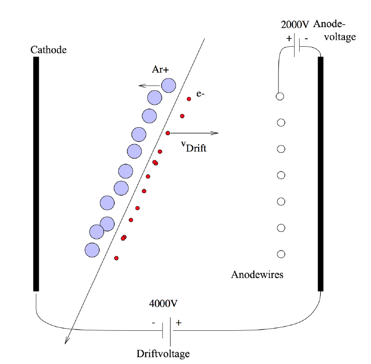
5.2 Drift Chamber

The drift ﬁeld inside of our drift chamber is generated by two parallel elec-

trodes, which have a distance of 100 mm. To have a homogeneous electric

ﬁeld inside the drift chamber, the potential also has to increase linearly from

the cathode to the anode at the edge of the drift chamber. This is approx-

imately achieved with 9 electrodes, which are placed parallel to each other

in a distance of 1 cm and enclose the drift chamber. Their potentials are

linearly graduated with a bleeder chain. The resulting electric ﬁeld looks

similarly to the electric ﬁeld in Figure 5.4.

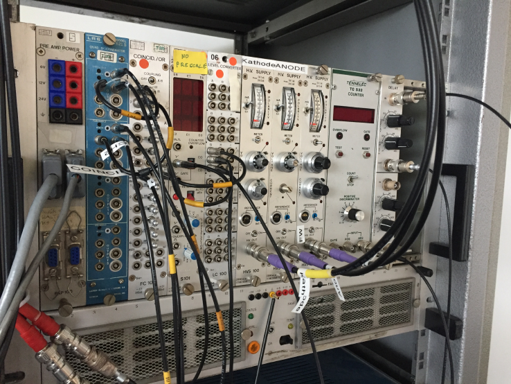
Figure 5.2: NIM crate with the main logic and power supplies.

The Figure 5.5 shows a CAD cross section of the drift camera.

The anode wires, which produce the gas ampliﬁcation, are placed 5 mm in

front of the ground plate. The sensitive region in which the particles can be

detected is between those wires and the cathode and has a length of 9.5 cm.

The 8 wires are arranged parallel to each other and have a distance of

10 mm between each other. Their diameter is only 50 µm, so they can produce

the needed high electric ﬁeld strengths for the gas ampliﬁcation. Between the

anode wires there are ﬁeld wires that make the electric ﬁeld more even. These

ﬁeld wires have an own voltage supply, which can be left at zero though.

The anode wires connected to a charge sensitive ampliﬁer powered by

the low voltage power supply, which ampliﬁes the signal coming from the

wire even further. This ampliﬁer is mounted inside the drift chamber, at the

end of each anode wire. The low voltage power supply is connected to the

ampliﬁer by three jacks at the front of the chamber and has to be turned on

in order of being able to detect the signals on the anode wires.

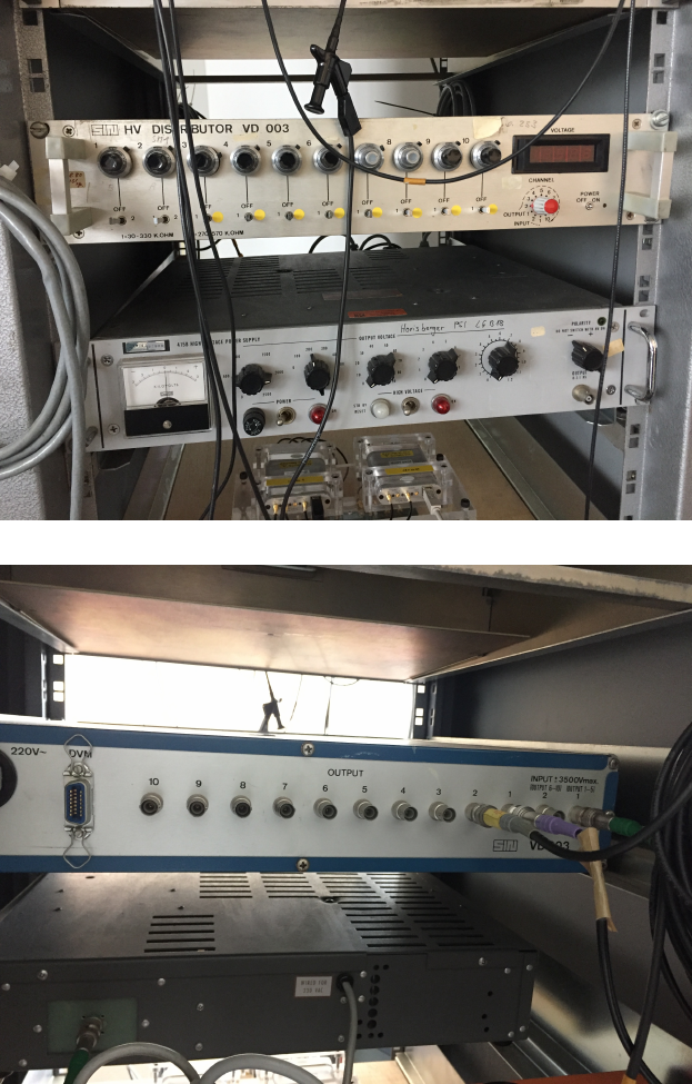
(a)

(b)

Figure 5.3: The front (a) and back (b) of the high voltage power supply and

high voltage distributor for the scintillator PMTs.

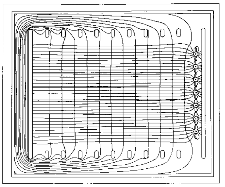
Figure 5.4: Electric ﬁeld lines and equipotential lines inside the drift chamber.

The electrons drift from left to right, where the signal wires are.

The drift chamber is mounted such that the wires are horizontal and the

plane of the wires is vertical. The drift direction for the electrons is thus

horizontal. A particle which travels vertically through the drift chamber will

therefore induce a signal in all wires. Figure 5.6 shows the interior of the

drift chamber with the electrodes and the signal wires.

5.3 The DRS4 unit

To process the incoming data from the signal wires, the wires are connected

to DRS4 boards. These DRS4 boards were designed at the Paul Scherrer

Institute and are capable of digitizing 4 channels each. Two boards are

linked together to process all 8 channels. The DRS4 boards work like a

Figure 5.5: CAD cross section of the drift camera. All the distances shown

are correct. The camera there only 8 anode wires (shown as black dots on

the left side on the picture). On each side of the anode wires the ﬁeld wires

(empty circles) are located equidistantly from each anode neighboring anode

wire. The cathode plate is 94.3 mm right of the anode wires. About 4 mm

To the left of the anode wires the ground plate is located. On the top and on

the bottom of the drift volume the ﬁeld plates are position at roughly equal

distances.

digital oscilloscope. For details on the operation of the DRS4 boards please

refer to the DRS4 manual [4].

The DRS4 unit comes with a computer program called drsosc located

in ~/Desktop/drs-5.0.6/. A softlink to the executable is put in the home

Figure 5.6: A drawing of the drift chamber. One can observe the anode wires

(the ﬁeld wires between the anode wires are not shown), the electrodes which

make a more homogeneous ﬁeld and the cathode and ground plate.

directory. The program can be started from the command line as follows:

1$ . / d r s o s c

It opens a GUI that emulates an oscilloscope interface and can display all

8 channels. The boards have a port for an external trigger which can be con-

nected to the trigger logic. The trigger output of the ﬁrst board is connected

to the second board, so both boards receive the trigger at approximately the

same time.

6 Measurements

The main goal of this experiment is to familiarize oneself with an operation

of a small drift chamber and observe the tracks of the cosmic muons passing

through it. Additionally you will develop your own data analysis technique

using as a provided data conversion program as a starter. You are advised to

perform the following measurements. Start with ﬁnding the working point

of the scintillators. Then study the gas ampliﬁcation dependence on the

anode voltage. Followed by the study of the dependence of the ion drift

velocity on the cathode voltage. Finally, observe a few events and plot the

muon traces. The following sections will give you some hints on how to

perform the measurement. Overall you are encouraged to your own methods

to measure the above parameters. However, if your methods deviate from

the suggested, substantiate them by solid physical arguments.

6.1 Saving and analyzing data

Save data in binary format (remember to add .dat extension to the ﬁle name

as it is not there by default) In the directory ~/Software/driftchamber/code/

there is a program which reads the binary dataﬁle and makes numpy arrays

for each event. Please NOTE that the extantions to the analysis code should

be written by you!

6.2 Finding the working point of the scintillators

To get a good trigger signal you ﬁrst have to ﬁnd the working point of the

two scintillators. For any given discriminator threshold the scintillator has

a speciﬁc voltage, where all incoming signals get detected, but the voltage

isn’t high enough to detect too much background noise. This manifests itself

in a plateau in the counts per second around this working point. You apply

a voltage of about 2 kV on the scintillators and put one of them to "and"

on the coincidence unit. Then you regulate the threshold so that there are

a few counts per second. The threshold voltage can be measured with the

external voltmeter. Now you have to count the triggered signals and calculate

the number of counts per second for diﬀerent applied voltages from around

1.9 kV to 2.1 kV. Plot the counts per second against the voltage and you will

see a plateau. The working point of the scintillator is the highest voltage

of the plateau. Repeat the measurement for the second scintillator. The

working points of the scintillators do not have to be at the same voltage, but

double check if the plateaus are at the same number of counts per second.

6.3 Purifying the gas

The experiment is performed at an atmospheric pressure. The gas inside

the chamber is a mixture of argon and methane (50:50). It is supplied from

the pressurized gas cylinder marked A on Figure 6.1. The chamber is also

connected to a pressure pump (D), which can evacuate the chamber. In order

to evacuate the chamber the valve at the chamber to the pump (B) and the

valve at the pump itself both should be opened. While the valve to the

gas cyllinder (C) should be closed. The ﬁlling of the chamber is performed

by closing the valves (B) and (D) and openning valves (A) and (C). Before

starting the experiment it is wise to empty the chamber and ﬁll it up again

several times, to make sure the gas inside the chamber is pure enough. The

pressure inside the chamber should be at or slightly above 1 bar in the end.

IMPORTANT: When you ﬁnish purifying the gas inside the chamber make

sure that the valve (A) on the gas cyllinder is closed.

Figure 6.1: To evacuate the chamber turn on the pump under the table

and open valve D and B. Do open valve B gently, such that the pressure

doesn’t decrease too fast otherwise it will start to smell inside the room. To

stop evacuating ﬁrst close valve B and then D. To ﬁll the chamber with gas,

ﬁrst open valve A and then gently open valve C until the desired pressure is

achieved. Afterwards close valve C and A.

6.4 Gas Ampliﬁcation

In the next part you want to ﬁnd the optimum anode voltage ampliﬁes

that provides the maximum ampliﬁcation while keeping the frequency of

the sparking (electrostatic discharge) inside the chamber low.

In order to have a high enough count rate, a 90Sr-probe can be put in

the window on top of the drift chamber. This isotope decays in a β-decay

into 90Y, which is also a β-emitter. The electrons from the β-decays have a

wide spectrum up to a maximum energy of 2.28 MeV. The scintillators and

the metal wall of the drift chamber stop these low-energy electrons, which is

why the source has to be placed on the window and the DRS4 board should

be set to trigger on one of the channels.

Then you have to repeat the measurement for increasing anode voltages

and plot the average pulse amplitude against the anode voltage. Be careful

with increasing the voltage, because the actual voltage follows the adjusted

value with some delay. Increase the voltage only in small steps and wait

until it stabilizes. If you see a breakdown on the oscilloscope, immediately

decrease the anode voltage. Figure 6.2 shows how a typical breakdown looks

like on the oscilloscope. Do not increase the anode voltage over 4 kV.

6.5 Drift Velocity

Now set the anode voltage to the optimal value, which was determined in the

previous task. Because we now want to make a time measurement, the exter-

nal trigger should be used. The scintillators must be placed above and below

the drift chamber. The scintillators should be positioned exactly vertically

above each other. In oder to ﬁnd the time electron needs to travel through

the whole chamber (94.3 mm) to the anode wire.The events with the earliest

signals (muon passes next to the anode wire) and the latest signals (muon

passes next to the cathode plate) should be observed. Note that because of

the geometrical acceptance of the scintillator triger, such events have very

low probability. (You are encouraged to estimate this probability). Therefore

a signiﬁcant ammount of events (∼10000) should be recorded. Since the rate

of the muons is low, this measurements should be run overnight.

With the assumption of a constant velocity you can then derive the drift

velocity. Repeat this measurement for several cathode voltages between

500 V and 4000 V to see how the drift velocity depends on the cathode volt-

age. The exact ammount of points you chose will depend on your time and

Figure 6.2: A picture of a typical display of an oscilloscope at the time of

a breakdown. The anode voltage inside the drift chamber gets too high

and electric discharge occurs, which produces this signal. If a breakdown is

visible or audible inside the chamber, the anode voltage has to be decreased

immediately.

curiousity.

6.6 Muon tracking

Now you have all the data to track the muons. You can either collect a small

ammount data at you favourite settings or use a sample of the data from the

drift velocity measurements. The drift velocity will help you to compute the

distance at which the muon passed the signal wire. Then using the vertical

positions wires plot the trajectories.

References

[1] Luigi Rolandi Walter Blum, Werner Riegler. Particle detection with drift

chambers. Wiley, Berlin, 2008.

[2] Gelnn F. Knoll. Radiation detection and measurement. Springer, Hobo-

ken, New Jersey, 2010.

[3] Wikipedia. NIM instrumentation module.

[4] Stefan Ritt. DRS4 evaluation board user’s manual.

A Sample Analysis Code:

The latest analysis code is located at:

https://github.com/dmitryhits/driftchamber/blob/master/code/decode.

Note that at the moment this is the only program that works, but you

are encouraged to make others working as well.

1#! / u sr / bin / env python

2" " "

3S c r i p t to c on v er t b i na ry for ma t t o r o ot f o r DRS4 e v a l u a t i o n

boards .

4http : //www. p s i . ch/ d rs / ev a lu a ti on −board

6Jonas Rembser ( rembserj@phys . e t h z . ch ) , 2016−04−15 based on work

7Gregor Kasieczka , ETHZ, 2014−01−15

8based on decode .C by Dmitry Hi t s

9" " "

11 from sys import argv , e x i t

12 from ROOT import TFile , TTree , TTimeStamp , AddressOf

13 from ROOT. st d import vector

14 from numpy import ar ra y , uin t3 2 , cumsum , r o l l , z er o s , f l o a t 3 2 ,

arange

15 from s t r u c t import unpack

16 import m a t p l o t l i b . p y pl ot a s p l t

18 ########################################

19 # Prepare Input

20 ########################################

22 i f not l e n ( argv ) == 2 :

23 p r i n t (" Wrong number o f argum ents ! " )

24 p r i n t (" Usage : python de code . py f i l e n a m e . da t " )

25 p r i n t (" E xi t in g . . . " )

26 e x i t ( )

28 in p u t_file n a m e = argv [ 1 ]

29 f = open( input_filename , " rb " )

31 ########################################

32 # Prepare Output

33 ########################################

35 # F i l e and Trees

36 o u t f i l e = TFile ( i n put_f i l e name . r e p l a c e ( " . dat " ," . r o o t " ) , ’

recreate ’)

37 o u t t r e e = TTree ( ’ t r e e ’ ,’ t r e e ’ )

39 # Crea te board and even t s e r i a l number and date v a r i a b l e s and

add to t r e e

40 timestamp = TTimeStamp ( )

41 o u t t r e e . Branch ( "EventDateTime " ," TTimeStamp " , AddressOf(

timestamp ) )

42 b o a r d _ s e r i a l s = v e c t o r ( i n t ) ( )

43 o u t t r e e . Branch ( "BoardSerials " , board_serials)

44 e v e n t _ s e r i a l = a rr ay ( [ 0 ] , dtype=u in t3 2 )

45 o u t t r e e . Branch ( " EventNumber " , event_serial , " EventNumber/ i " )

46 # more br anc hes w i l l be added d ynam i cally i n the f i r s t wh i l e

lo o p

48 ########################################

49 # Actual Work

50 ########################################

52 " " "

53 Read i n e f f e c t i v e time width b in s i n ns and c a l c u l a t e the

r e l a t i v e time from

54 the e f f e c t i v e time b in s . This i s j u s t a rough c a l c u l a t i o n be fo re

the correction

55 done f u r t h e r down i n th e code

57 The s c r i p t a l s o g e t s c ha nn el number i n f o r m a t i o n from t h i s

s e c t i o n to c r e a t e

58 t he a p p r o p r i a t e number o f t r e e b ra nc he s .

60 NOTE: the ch a n n e ls 0−3 a r e f o r the f i r s t board and cha n n e ls 4−7

are f o r t he second board

61 " " "

62 # To hold to the t o t a l number o f ch a n ne l s and b oards

63 n_ch = 0

64 n_boards = 0

66 # Empty l i s t s f o r c on t ai n in g t he v a r i a b l e s con ne cte d to the t r e e

branches

67 channels_t = [ ]

68 channels_v = [ ]

70 # L i s t o f numpy a r r a y s t o s t o r e t he time bi n i n f o r m a t i o n

71 timebins = []

72 " " "

73 This l oo p e x t r a c t s t ime i n f o r m a t i o n f o r e ac h DRS4 c e l l

74 " " "

75 while True :

76 he ad er = f . r ea d ( 4 )

77 # For s k i p p i n g t he i n i t i a l time he ad er

78 i f h ea de r == b "TIME" :

79 continue

80 elif hea der . s t a r t s w i t h ( b "C" ) :

81 n_ch = n_ch + 1

82 # Crea te v a r i a b l e s . . .

83 channels_t . append ( z er os ( 102 4 , dtype=f l o a t 3 2 ) )

84 channels_v . append ( z er o s ( 10 2 4 , dtype=f l o a t 3 2 ) )

85 # . . And add t o t r e e

86 o u t t r e e . Branch ( " chn {} _t " .format( n_ch ) , channels_t [ −1] , "

chn {}_t [ 1 0 2 4 ] / F" )

87 o u t t r e e . Branch ( " chn {}_v" .format( n_ch ) , ch an nels_v [ −1] , "

chn {}_v[ 1 0 2 4 ] / F" )

89 # Write ti mebi n s to numpy a r r a y

90 tim e b i ns . append ( a r r a y ( unpack ( ’ f ’ ∗1 02 4 , f . read ( 4 ∗1 0 2 4 ) ) ) )

92 # Increment the number o f boards when s e ei n g a new s e r i a l

number

93 # and s t o r e the s e r i a l numbers i n th e board s e r i a l numbers

vector

94 elif hea der . s t a r t s w i t h ( b "B#" ) :

95 b o a r d _ s e r i a l = unpack ( b ’H ’ , header [ 2 : ] ) [ 0 ]

96 b o a r d _ s e r i a l s . push_back ( b o a r d _ s e r i a l )

97 n_boards = n_boards + 1

99 # End the loop i f h eader i s not CXX or a s e r i a l number

100 elif header == b"EHDR" :

101 break

102

103 " " "

104 # This i s the main l o o p One i t e r a t i o n c or r es p o nd s to r e a di n g one

ch ann e l ever y

105 # few ch an ne l s a new e ven t can s t a r t We know t hat t h i s i f th e

c a s e i f we s e e

106 # "EHDR" i n s t e a d o f " C00x " ( x = 1 .. 4 ) I f we have a new e ve nt : F i l l

the t re e , r e s e t

107 # the branches , i ncr eme nt event c o u n t e r The binary format i s

d e s c r i b e d i n :

108 # h ttp : / /www. p s i . ch/ d rs / DocumentationEN/ manual_rev40 . pdf ( page

24)

109 # What happens when m u l t i p l e b oar ds a r e d a i s y ch a i n ed : a f t e r t he

C004 v o l t a g e s o f

110 # the f i r s t board , t h e r e i s the s e r i a l number o f th e next board

b e f o r e i t s t a r t s

111 # a g a in with C001 .

112 " " "

113

114

115 current_board = 0

116 t c e l l = 0 # c ur re n t t r i g g e r c e l l

117 t_00 = 0 # time i n f i r s t c e l l i n f i r s t ch ann el f o r ali gnm ent

118 is_new_event = True

119

120 info_string = " Reading in e v e nts measurend with {0} ch a n nel s on

{1} board ( s ) . . . "

121 p r i n t (info_string . format( n_ch , n_boards ) )

122

123 while True :

124 # S t a r t o f Event

125 i f is_new_event :

126 e v e n t _ s e r i a l [ 0 ] = unpack ( " I " , f . r ead ( 4 ) ) [ 0 ]

127 p r i n t (" Event : " , e v e n t _ s e r i a l [ 0 ] )

128 is_new_event = Fa l s e

129

130 # Set th e timestamp , where the m i l l i s e c o n d s need to be

converted to

131 # n an os ec on ds t o f i t th e f u n c t i o n arguments

132 d t _ l i s t = unpack ( "H" ∗8 , f . r ea d ( 1 6 ) )

133 timestamp_args = l i s t ( d t _ l i s t [ : −2 ] ) + [ d t _ l i s t [ −2]∗i n t (1

e6 ) , 1 , 0 ]

134 timestamp . Set (∗timestamp_args)

135

136 # F l u f f t he s e r i a l number and read i n t r i g g e r c e l l

137 f l u f f = f . read (4 )

138 t c e l l = unpack ( ’H ’ , f . re ad ( 4 ) [ 2 : ] ) [ 0 ]

139 # R es et c u r r e n t boar d number

140 current_board = 0

141 continue

142

143 # Read the header , t h i s i s e i t h e r

144 # EHDR −> f i n i s h eve nt

145 # C00x −> read the data

146 # " " −> end o f f i l e

147 he ad er = f . r ea d ( 4 )

148

149 # Handle next board

150 i f header . s t a r t s w i t h ( b "B#" ) :

151 current_board = current_board + 1

152 t c e l l = unpack (b ’H ’ , f . read (4 ) [ 2 : ] ) [ 0 ]

153 continue

154

155 # End o f Event

156 elif header == b"EHDR" :

157 # F i l l p r e v i o u s e ve nt

158 o u t t r e e . F i l l ( )

159 is_new_event = True

160

161 # Read and s t o r e data

162 elif hea der . s t a r t s w i t h ( b "C" ) :

163 # the v o l ta ge i n f o i s 1024 f l o a t s with 2−byte precision

164 chn_i = i n t ( header . decode ( ’ a s c i i ’ ) [ −1]) + current_board

∗4

165 s c a l e r = unpack ( ’ I ’ , f . r ead ( 4 ) )

166 v o l t a g e _ i n t s = unpack ( b ’H ’ ∗1 02 4 , f . rea d ( 2 ∗1 0 2 4 ) )

167

168 " " "

169 C a l c u l a t e p r e c i s e t im i ng u s i n g th e tim e b i n s and t r i g g e r

cell

170 s e e p . 24 o f t he DRS4 manual f o r t he e x p l a n a t i o n

171 the f o l l o w i n g l i n e s sum up the t ime s o f a l l c e l l s

s t a r t i n g from the t r i g g e r c e l l

172 to th e i_th c e l l and s e l e c t on ly even members , bec ause

the amplitud e o f the a d ja c e nt c e l l s a r e a veraged .

173 The width o f th e b i n s 1024 −2047 i s i d e n t i c a l to the b i ns

0−1023 , t h at i s why t he a r r a y s a r e s im pl y e xte nd ed

174 b e f o r e p e rf or m in g th e cumsum o p e r a t i o n

175 " " "

176 timebins_full = list( r o l l ( t i meb i n s [ chn_i −1] , −t c e l l ) )+

l i s t ( r o l l ( t i m e bins [ chn_i −1] , −t c e l l ) )

177 t = cumsum( t i m e b i n s _ f u l l ) [ : : 2 ]

178 # time o f f i r s t c e l l f o r c o r r e c t i o n , f i n d th e time o f

the f i r s t c e l l f o r each channel ,

179 # b ec aus e on ly t h e se c e l l s a r e a l i g n e d i n time

180 t_0 = t [(1024 −t c e l l ) %1024]

181 i f chn_i % 4 == 1 :

182 t_00 = t_0

183 # A lig n a l l c h a nnel s with the f i r s t ch anne l

184 t = t −( t_0 −t_00 ) # correction

185 # TODO: i t i s a b i t u nc le a r how to do the c o r r e c t i o n

with

186 # TODO: m u l t i p l e boards , s o t he bo ar ds a re j u s t

c o r r e c t e d i n de pe n de nt l y f o r now

187 # TODO: f i n d th e a lig nme nt o f t he bo ards by s en di ng th e

same s i g n a l t o both boards

188 " " "

189 The f o l l o w i n g l i s t s o f numpy a r ra y s can be p l ot t ed or

used i n the f u r t h e r a n a l y s i s .

190

191 NOTE: the ch a n n e ls 0−3 a r e f o r the f i r s t board and

channels 4−7 are f o r the second board

192 " " "

193 f o r i , x in enumerate( v o l t a g e _ i n t s ) :

194 channels_v [ chn_i −1 ] [ i ] = ( ( x / 6 5 5 3 5 . ) −0 . 5 )

195 channels_t [ chn_i −1] [ i ] = t [ i ]

196

197 # End o f F i l e

198 elif header == b" " :

199 o u t t r e e . F i l l ( )

200 break

201

202 # Clean up

203 f . c l o s e ( )

204 o u t t r e e . Write ( )

205 o u t f i l e . C lose ( )

Manual

Navigation menu

Versions of this User Manual:

Views

Navigation