PTV Balance Manual EN ENG

User Manual:

Open the PDF directly: View PDF .
Page Count: 54

PTV BALANCE

USER MANUAL

PTV Balance Manual EN Contents

 PTV GROUP

All brand or product names in this document are trademarks or registered trademarks of

Legal agreements

The information contained in this documentation is subject to change without notice and

should not be construed as a commitment on the part of PTV AG.

Without the prior written permission of PTV AG, this manual may neither be reproduced or

stored in a retrieval system, nor transmitted in any form or by any means, electronically,

mechanically, photocopying, recording, or otherwise, except for the buyer's personal use

as permitted under the terms of the copyright.

Warranty restriction

The content accuracy is not warranted. We are grateful for any information on errors.

Imprint

PTV AG

Haid-und-Neu-Str. 15

76131 Karlsruhe

Germany

Tel. +49 721 9651-300

Fax +49 721 9651-562

info@vision.ptvgroup.com

www.ptvgroup.com

Last amended: November 2017 EN-US F

PTV Balance Manual EN  Contents 
 
 
 PTV GROUP 

 
 
Contents 
Introduction .................................................................................................. 5 
Functionality ................................................................................................. 6 
1 Architecture and algorithms .............................................................. 6 
1.1 Basic Idea  6 
1.2 Collection of Data  Fehler! Textmarke nicht definiert. 
1.3 Traffic Model  10 
1.4 Determination of Efficiency and Evaluation of Control 
Alternatives  13 
1.5 Optimization process  17 
2 Definition of control groups ............................................................. 24 
3 Changing the Objective Function .................................................... 25 
4 Online-/Offline-System .................................................................... 26 
5 Possibilities for the Local Control .................................................... 26 
5.1 PTV Balance with PTV Epics  26 
5.2 TRENDS-Kernel with normal TRELAN-Logic  26 
5.3 VS-Plus (Verkehrssysteme AG)  26 
5.4 Ring-barrier-controller  27 
5.5 Dynamic Fixed Time Control  27 
5.6 Other Methods  27 
Data Provision ............................................................................................ 28 
1 Guidelines for using PTV Balance within the PTV Vision suite ........ 29 
2 Network and Demand Data ............................................................. 33 
2.1 Network Data  33 
2.2 Demand Data  35 
3 PTV Balance Parameters and Signal Control Data ......................... 36 
3.1 Local Parameters and Signal Control Data  36 
3.2 Global Parameters  40 
Simulation, Calibration and Operation ..................................................... 43 
1 Simulation With PTV Vissim ........................................................... 43 
1.1 Data Provision  43 
1.2 Showing Additional Data in the Signal Times Window  44 

PTV Balance Manual EN Contents

 PTV GROUP

4.1.3 Evaluating Additional Data in the Signal Control Detector

Record 45

4.1.4 PTV Balance and Epics network view 46

4.2 Log Files ......................................................................................... 47

4.2.1 Balance_output_YYYY-MM-DD.log.txt 48

4.2.2 Bxx_summary_YYYY-MM-DD-log.txt 48

4.2.3 Balance_signals_YYYY-MM-DD-log.txt 49

4.3 Calibration ...................................................................................... 50

4.3.1 General 50

4.3.2 Guideline for the Calibration 50

5 Literature .................................................................................................... 53

PTV Balance Manual EN Introduction

 PTV GROUP

1 Introduction

The adaptive network control PTV Balance (“balancing adaptive network control method”)

was originally created within the research projects “Munich Comfort” (Friedrich and Mertz

1996) and “Tabasco” (Friedrich et al. 1998). Numerous other projects followed in which the

system and its algorithms were tested, evaluated and improved, most notably the research

project TRAVOLUTION (2006-2009) with the development of the genetic optimization

algorithm and the projects TRISTAR (2013-2015) and Lublin (2015-2016) that established

Balance in Poland, the latter together with PTV Optima as a comprehensive traffic

management system.

The inner core of PTV Balance consists of four parts:

1. A macroscopic traffic model that estimates flows in accordance with detector data,

2. A control model that emulates the local intersection control,

3. A mesoscopic traffic flow model that calculates the effects of a specific signal plan,

4. And most importantly different optimization algorithms.

Furthermore, it is possible to replace the macroscopic traffic model with external traffic state

estimating programs that are able to take a whole conurbation into account. To this end

Balance can be embedded into PTV Optima, which is the traffic management platform and

decision support system developed by PTV. The main advantages are that Optima is able

to predict traffic, enabling an optimization for the near future, and also allows to take much

more traffic data than just detectors into account, e.g. floating cars and ANPR data.

PTV Balance is independent of the local control method that is used in the field as long as

the local traffic control is able to utilize the frame signal plans calculated by PTV Balance.

The ideal partner is the sister product PTV Epics, as it adds strong local adaption, has full

transit signal priority and is integrated with PTV Balance from a technical and a

methodological point of view already.

PTV Balance is seamlessly embedded into the environment of the PTV Vision suite. The

road network and the traffic demand are modelled in PTV Visum. Signal control related

data and parameters are provided with Vissig, a module of either PTV Visum or PTV

Vissim. PTV Balance’s input formats are shared with PTV Vissim and Vissig, the former

being able to fully simulate the effects of the Balance control, thus enabling an elegant way

of testing, calibrating and evaluating the effects on the road network.

PTV Balance Manual EN Functionality

 PTV GROUP

2 Functionality

2.1 Architecture and algorithms

2.1.1 Basic Idea

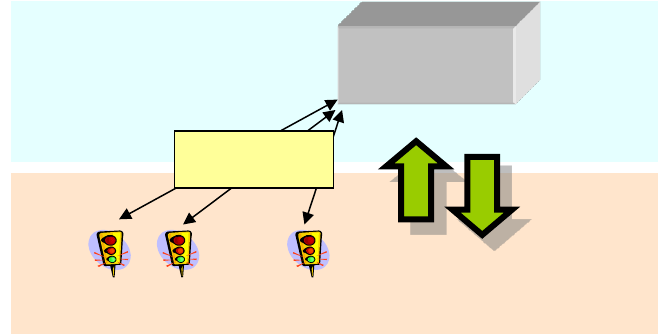
Figure 1: Two-Level-Concept of PTV Balance

The system architecture of Balance is characterized by a two-level-concept, where the

functionality of the traffic light system is divided hierarchically (see Figure 1)

 An efficient microscopic controlling method looks at short-term changes of the traffic

volume, e.g. during the prioritization of public transport, based on the current detector

values and signal status. The local controlling method works usually on a second-by-

second basis or even shorter.

 PTV Balance works as macroscopic system on the tactical level of the adaptive

network control by sending framework signal plans to the intersections every 5

Minutes. A framework signal plan defines static and variable areas for the phases of

the local control for all controllers within a group that have the same cycle time. Inside

the variable areas, the local control can adapt to the current traffic volume by using its

local detection. Nevertheless, a basic structure for the single traffic light systems is

provided by the framework signal plans. The green times of the signal groups can vary

inside this framework.

Any local traffic control system control can be applied, as long as it integrates an interface

for the frame signal plans which are created by PTV Balance. This flexibility was one of

the main goals during the development of PTV Balance, to be able to apply the system

quickly without changing the local traffic light system control. Currently PTV Epics, the

Trelan/Trends-System (Gevas software Systementwicklung und Verkehrinformatik GmbH

2010a/b), the VS-PLUS-Control (Verkehrs-Systeme AG 2012) and the SIEMENS

TL/PDM-System have been used as local control strategy. Tests with the American ring

barrier controller have also been conducted.

The reduction of delay by the traffic adaptive coordination of traffic signal systems among

each other (offset-optimization, green wave) and by the rough adaption of the green times

of the signal groups is processed centrally on the level of the network. A second-by-second

operational level

tactical level

JCt. 1

Jct. 2

Jct. n

intersections

framework

signal plans

Detector

measurings

Signal States

PTV

BALANCE

central

decentral

data transmitting

infrastructure

network

PTV Balance Manual EN Functionality

 PTV GROUP

adaption of the green times is processed in the local controller. If there is no local detection

or traffic responsive control available at the intersection, the Balance framework signal

plans can also be used directly as fix time-program.

A PTV Balance-System can control all intersections of a town, but it is necessary to divide

them into several control groups, with a size of 1-30 intersections in each group. This

additional division is required to distinguish different areas of the network with different

traffic related characteristics. One important point is that Balance selects a signal program

with an adequate cycle time at once for all controllers in a group. Performance issues play

a role here, and a limitation of the search space for optimization is also good to avoid being

stuck in local optima.

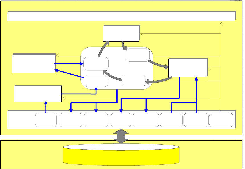
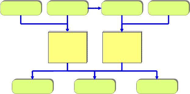
Figure 2: Block-diagram of the PTV Balance network control

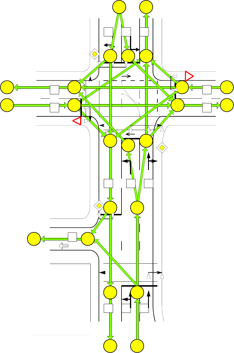
The central database structure in PTV Balance is the network model. The street network is

represented internally as a graph in form of nodes and edges. Figure 3 illustrates this

aspect at the example of a small net with two intersections.

PTV Balance

data preparation

traffic-

Model

data-

Interface

sequence control

detector-

data

traffic-

flows

Impact

signal

states

framework

signal plans

static

data

Program

Switches

cycle-

times

database-server

control-

model

efficiency-

model

network

traffic-

flows

Impact,

actuators

messages

Iteration

PTV Balance Manual EN Functionality

 PTV GROUP

Figure 3: Example of a simple network model

Fv07

D41

D72

D71

D11

Fg53

Fv08

Fv05

Fv04

Fg52

Fv03

Fv02

LZA 5

LZA 7

D75

D21

Fv01

D81

D51

D45

Fv06

Fg51

D61

D31

D35

D65

D95

PTV Balance Manual EN Functionality

 PTV GROUP

The edges are the central container for the traffic data within the PTV Balance-System.

The procedures of the PTV Balance-Controlling system can be divided into five functional

groups:

 Collection and Preparation of data

 Illustration of the traffic

 Determination of efficiency and evaluation of control alternatives

 Creation of the control alternatives

 Data interface

There are more system functions available for the control of the internal process or for

database accesses, etc, but these functions are not discussed in this manual. The next

chapters will shortly describe the functional groups mentioned above.

2.1.2 Detector positioning and data gathering

It is necessary to estimate the current traffic state in the road network as good as possible,

before the optimization of the signal control can start. Local detectors collect the traffic

situation in the controlled area in the form of aggregated or disaggregated measurements

for the current calculation interval. This data is gathered by the controllers and delivered to

the central database. Detectors which are not connected to a traffic light system can also

be utilized by PTV Balance. Additional kinds of dynamic data of the traffic light systems are

also collected. For example, the currently running signal program, the cycle time or different

operation modes of the controller or the detector.

The positioning of detectors for Balance should be done according to the following rules:

1. There should be single- or double loop detectors on every lane that leads to an

intersection controlled by the traffic light. The distance to the stop line should be at

least 20m and not more than 50m. The ideal detector position is 40-50m in front of

the stop line.

2. Every lane has to be detected on its own. No detector may cover more than one

lane.

3. In case of turn-off lanes, the detector should also be placed according to the

distances suggested in 1., if possible. If the turn-off lane is shorter, the detector

should be placed on the turn-off lane so that it is as far as possible from the stop

line and measures all turning vehicles. If this is not possible, the second criterion is

more important. It may be necessary to do an on-site inspection to decide this. In

addition, single loop detectors should be placed on the main lanes 50m in front of

the sop line.

4. At the borders of the area which is selected for the calculation of the traffic state

(usually the main road network), detectors which measure the outflow may be

placed (about 30m behind the stop line) if there are big differences between the

incoming and the outflowing traffic during the day. This improves the quality of the

origin-destination estimation of the network model.

PTV Balance Manual EN Functionality

 PTV GROUP

The detectors which are suggested here are normal single loops which can also be used

for the time gap control or counting purposes. It is also an option to use other means of

detection, but only if it is guaranteed that the cars are reliably counted even under adverse

weather conditions and under heavy saturation.

It is usually not necessary to have more or different detectors for Balance than for Epics.

So, if the junction is controlled by PTV Epics, everything should be fine regarding detection.

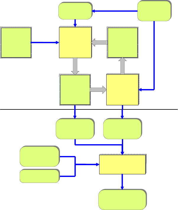
2.1.3 Traffic Model

The PTV Balance-traffic model builds an internal spatial/ chronological representation of

the current traffic situation out of traffic flows measured at different measuring sections. It

consists of three different functional parts which are arranged in two different levels (see

Figure 4):

Figure 4: block diagram of the PTV Balance-traffic model

The first level (see chapter 2.1.3.1) consists of a macroscopic traffic model (Ploss 1993),

which is called only once for every optimization. It consists of:

 An OD-Estimation for the determination of the origin-/destination-relations in the sub-

net and

static

weighting-

matrix

Iteration

1. level

2. level

traffic flow-

model

edge-related

traffic flow profiles

qFl(a, t)

cycle time

status

controller

zust(sg,t)

Origin-/Destination-

Relations

edge-related

traffic flows

qMod(a)

assignment

Origin/

Destination-

Matrix

kl_i

Matrix

dividing-

parameters

akl_i

OD-

Estimation

Cordon-

measurements

cross section-

measurements

q(a)

PTV Balance Manual EN Functionality

 PTV GROUP

 A traffic assignment for the allocation of the traffic flows to the road edges in the

network

The second level (chapter 2.1.3.3) is a mesoscopic traffic flow model, which periodically

generates traffic flow profiles out of the macroscopic traffic parameters of the first level.

This takes place during every step of the signal plan-optimization process inside PTV

Balance.

2.1.3.1 Macroscopic traffic model (1. Level)

An estimation of the matrix (fkl_0) of the traffic flows [veh/h] from an entry-edge k to an exit-

edge l is processed according to a static weighting-matrix (wkl) and to the in- and outflows

at the edges of the net (OD-Estimation). The entropy-maximizing algorithm of (Van Zuylen

and Branston 1982) is used for the OD-Estimation.

In the first step, the in- and outflows at the edges on the border of the controlled area are

estimated. This goal is achieved either by using already existing measurements, or by

estimating the traffic, based on the historic weighting matrix and the measured values which

are available.

The matrix of the origin-destination-relations is the input parameter for the traffic

assignment, which distributes the traffic to the streets in the network using an incremental

multiple-assignment-algorithm. The traffic is assigned to the edges in shares of 10%, 20%,

30% und 40%. After every step, a route-searching algorithm is conducted. This algorithm

calculates the fastest route according to impedances in the net (like travel times) and

assigns the whole traffic of this step to the respective edges (All-Or-Nothing Assignment).

The results of the traffic assignment are the traffic flows qMod(a) [Veh/h] per edge and also

the matrix of the distribution parameters (pakl), that defines which share of the traffic relation

fkl drives over edge a. Therefore, the following correlation exists:



 



Ek Al

akl

ifpaqMod )(

Where

i step of iteration

a index of edge

k, l index of origin/destination

E, A number of entries/exits respectively

origins/destinations in the network

piakl share [0...1,0] of the traffic relation fkl which uses edge

The relative deviation X(a) between traffic model and reality can be calculated with the help

of the estimated traffic flows qMod(a) and the real traffic flows q(a) measured on the edges

a in the network. The deviation is used in combination with the distribution parameters pakl

in order to correct the estimation of the origin-destination relations in an iterative process.

Criteria for the cancellation of the so called internal iteration are the exceeding of a

previously defined number of iterations or the shortfall below a given value of the standard

deviation between measured and estimated value.

PTV Balance Manual EN Functionality

 PTV GROUP

This procedure is repeated until a given number of iterations is reached. The main results

are macroscopic traffic volumes qMod(a) [Veh/h] for all edges a of the network, and

especially for edges where no measured values are available. Other results are the matrix

of the origin-destination relations (fkl) in the network and the distribution parameters (pakl).

2.1.3.2 Embedding into superordinate traffic models

A superordinate traffic model like PTV Optima can also be embedded instead of the

macroscopic traffic model discussed above. PTV Optima’s model is dedicated to traffic

state estimation based on a wider range of detection sources (loops, ANPR, FCD...) and

can calculate the real traffic situation in a network more precisely. As input PTV Balance

requires the traffic volumes for every edge and the turn-off rates at the intersections of the

network control. The values should be delivered at least every 5 minutes.

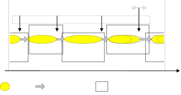
2.1.3.3 Mesoscopic traffic model (2. level)

Traffic flow profiles qFl(a,t) [Veh/sec] are created for all edges based on the data of the

traffic model (1. Level) or a super ordinate traffic model and the states of the signal groups

in the network, given by the control model. The length of the flow profiles represents the

homogeneous cycle time tu of the control group (see Figure 5).

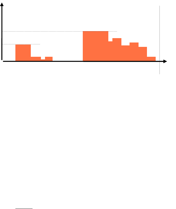
Figure 5: Illustration of the traffic flow profile of the second level of the traffic model

The mesoscopic traffic flow model takes the influence of the traffic lights, the travel times

and the dissolving of the queues through changing speeds on the groups of vehicles into

account. Therefore the outflow zFl(a,t) at the end of an edge a is defined as follows:

With the estimated average

travel time on the edge

tr(a) = len(a) / v(a)

[sec]

The platoon dispersion is modelled over the length of two intervals 2L by moving average

determination









Lt

Ltt

taqFl

)',(

),('

With the given whole-number length of the interval L

q(t)

[Veh/sec]

sg1

sg2

[sec]

















t)(a,qFl't)l(a, otherwise

ssgt)(a,qFl't)l(a,queue the

and t at released issg if

t time in point at release no is there if 0

trttuazFl

))(mod,(

PTV Balance Manual EN Functionality

 PTV GROUP

  

where

t periodical base of time [1... tu sec]

sg index of signal group sg, controlled by edge a

ssg saturation of signal group sg [Veh/sec]

l(a, t) queue length [Veh] on edge a at point in time t

k(a) calibration of the dissolving

len(a) length [m] of edge a

v(a) estimated average speed [m/sec] on edge a

DIV whole-number division

The periodic traffic flow model q(a, t) at the beginning of an edge results from the additive

connection of the outflows zFl(a´, t) of the incoming edges a´. These outflows are

distributed to the following edges, according to their share of the whole traffic volume:







)('

),'(),'(),(

aIna

tazFlaaptaqFl

The distributing factors p(a´, a) contain the share [0...1.0] of the total traffic volume on edge

a, which comes from edge a´. This share is calculated by using the traffic volumes qMod

which were defined in the first level of the traffic model:

 



)'()(

)(

)'(

),'(

aOutaaIna

aqMod

aap

where

In(a) number of entry edges of edge a

Out(a´) number of exit edges of edge a´

qMod(a) modelled traffic volume [Veh/h] on edge a

At the beginning of the traffic flow modelling, the flow profiles are initialized for the cordon-

edges. Here an equally distributed flow profile is assumed:

)...1(

3600

)(

),( tutfor

aqMod

taqFl 

Starting from the edges at the network entrances, this procedure is executed periodically

for all edges in the network. At the end of this process the traffic flow profiles qFl are defined

for all edges in the network. The flow modelling is processed for every edge of the sub-net

during every step of the optimization. Usually there are some thousand optimization-steps

processed during every PTV Balance-call. Therefore the traffic flow model had to be

implemented very efficiently.

2.1.4 Determination of Efficiency and Evaluation of Control

Alternatives

With the help of the effect model, the impact of the control alternatives is calculated for the

next step in time. The control alternatives are evaluated by a performance index. The

PTV Balance Manual EN Functionality

 PTV GROUP

relevant variables for the calculation of the index are: weighted vehicle waiting times,

number of stops of vehicles and queue-lengths.

)),,(),,(),,((),( sgyxLsgyxHsgyxDyxPI sgsg

SGsg



 



where

SG number of signal groups in the sub-net

sg, sg, sg emphasis of waiting time/ stops/ queue-lengths for

signal group sg

D, H, L vehicle waiting times/ stops/ queue-lengths for signal

group sg

x vector of control variables

y vector of traffic related variables

The variables of efficiency are generated by two models: Every second, a high-resolution

mesoscopic model calculates the deterministic share by assuming a steady maximum

speed and saturation flow. The stochastic part at the stop lines is determined by a

macroscopic queue-model that takes overloads into account (see Figure 6).

Figure 6: Block-Image of the PTV Balance-efficiency model

The deterministic effect model is based on the flow profiles of the traffic model qFl(a, t) and

the cycle time, defined green times of the controllers zust(sg,t). It calculates the impact of

the adjacent control alternatives in a numerical, simulative way. The calculation for every

second enables the modelling of the traffic related impact of green time-lengths and offsets

between adjacent signal groups.

The optimization of green times of a signal group in a traffic network always has an impact

on the signal groups which are located downstream. Therefore, the optimization of the

green time is calculated for the whole subnet at the same time. Although this holistic

solution requires a lot of computing capacity, compared to a heuristic procedure, it

considers all relations between the signals and links in the network.

For this it is necessary to use the flow profiles of the links which lead out of the subnet, as

input variables for the signal groups which are located downstream. As described in chapter

2.1.4.3, the traffic flow profiles of the entry-links of a sub-net are initialized with equally

distributed profiles. If there is a traffic flow profile available for an exit-link of an adjacent

waiting time

D(sg)

queue-lengths

L(sg)

stops

H(sg)

green times

tgr(sg)

traffic flow

qMod(a)

signal states

zust(sg, t)

stochastic

effect model

flow profiles

qFl(a, t)

deterministic

effect model

PTV Balance Manual EN Functionality

 PTV GROUP

sub-net, the equally distributed profile will be overwritten. This way it is guaranteed that the

traffic light systems at the links of the sub-nets get realistic traffic flow profiles.

The deterministic effect model is built similar to the models in the well-known planning

system Transyt (Robertson 1969) and the adaptive control SCOOT (Hunt et al. 1981). A

simulation of the impact of the controllers on the traffic flow is processed in order to get the

efficiency variables vehicle waiting time, number of stops and mean queue-length. The

traffic is not modelled as single vehicles (microscopic modelling) but with the help of the

macroscopic parameter traffic volume. However, this parameter is available for every

second (mesoscopic modelling). The applied formulas are described in the following sub-

chapters.

2.1.4.1 Calculation of delay

The signal group-related vehicle delay D results from the summing up of the queue lengths

l(t) which denote the vehicles that have stopped during time frame T. l(t) is defined as the

sum of the inflows Q(t) at an origin or entrance (demand process) and as the sum of the

outflows Z(sp,t) at an exit or destination (service process) until the point in time t :

 







 

where

SG number of signal groups

sp signal plan which is evaluated

Qsg sum of the vehicles which have entered at signal

group sg until t

Zsg sum of the vehicles which have left at signal group sg

until t

Dsg sum of the vehicles waiting times at signal group sg

during time frame T

The following formula defines the request process Q

  



 

with qsg(t) = inflow [Veh/s] to signal group sg at time t.

The inflow profile qsg(t) is the input parameter for the effect model and is defined as

described above.

2.1.4.2 Calculation of the vehicle stops

The following formula represents the sum of vehicles Hsg, which are forced to stop due to

the creation of a signal plan of the length T at a signal group sg







where

PTV Balance Manual EN Functionality

 PTV GROUP

sp signal plan which is evaluated

hsg sum of the vehicles which have to stop at signal group

sg at time t

A vehicle has to stop if it reaches the end of a queue or the stop line while the inflow is

greater than the outflow (normally when the signal is red). Therefore, the stops hsg at point

in time t are defined as follows:

   



2.1.4.3 Calculation of the queue lengths

In case of the queue lengths, time-related-, current-, average- and maximum queue lengths

are distinguished.

The current queue length lsg is calculated by the difference between the incoming and the

leaving traffic:





  

The average queue length L and the maximum queue length Lmax can be derived from

the formula mentioned above:

  



 







The maximum queue length is important for the protection of congestion spaces or to

prevent the congestion to reach into previous intersections. It is the maximum queue length

that is applied in the performance index of PTV Balance.

2.1.4.4 Modelling of stochastic deviations

The analytic queuing model of (Kimber and Hollis 1979) is used to include stochastic

deviations resulting from capacity overloads in the calculation. It only requires the degree

of saturation of an entry as macroscopic input parameter. It is calculated by the average

traffic volume qMod of an entry and the cycle time-related length tgr(sg) [sec] of the green

times of the signal groups:

3600)(

)(

)( tu

ssgtgr

aqMod

sgrsg

Aa 







where

A number of edges which are controlled by signal group

r degree of saturation

tu cycle time [sec]

ssg saturation [Veh/sec] of signal group sg

The results of the macroscopic effect model are the waiting times and average queue

lengths created by the random deviations of the traffic flow. They are added to the waiting

PTV Balance Manual EN Functionality

 PTV GROUP

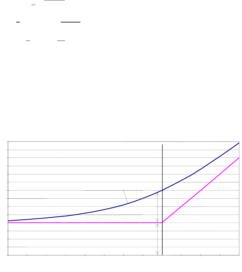
times of the deterministic effect model (Figure 7). The sum of both models serves as input

parameter for the performance index.

The formulas for the stochastic waiting time WKB, sg for signal group sg are defined as

follows:

 

 

  

 



  

 



Where

r= r(sg) the degree of saturation calculated above,

g0 the start queue length before signal group,

C a constant (usually C=0,4 in PTV Balance),

q capacity in [Veh/s] for the signal group (saturation flow

respecting green share)

T the time frame (usually 300 seconds in PTV Balance).

The stochastic delay is added to the deterministic delay for each signal group.

Figure 7: Schematic waiting times with deterministic and stochastic model

2.1.5 Optimization process

The control model of the PTV Balance-network control optimizes the following control

parameters:

 Length of the green times (split)

 Chronological location of the green times according to their equal cycle time (offsets)

 Length of the cycle time

0,2

0,3

0,4

0,5

0,6

0,7

0,8

0,9

1,1

1,2

1,3

1,4

saturation r

waiting time

deterministic model

waiting time

stochastic model

total waiting time

overload area

PTV Balance Manual EN Functionality

 PTV GROUP

PTV Balance was originally designed to use a Hill-Climbing (HC) algorithm for optimization.

In 2008 an additional optimization procedure was developed and implemented in the

German research project TRAVOLUTION: The Genetic Algorithm (GA). One important

advantage of a Genetic Algorithm is its ability to optimize all control parameters at the same

time. The other advantage is that it tends to avoid local optima by applying a parallel search

through the solution space. The research project TRAVOLUTION showed that the GA

significantly improved the optimization quality in terms of a better performance index in

Balance and, more importantly, also on the road. But it also is consuming more calculation

time. This is not so big an issue in a real-world traffic centre, but slows down the speed

when used in conjunction with a micro simulation, e.g. PTV Vissim. That’s why still both

algorithms are contained in Balance. The user can switch between them through an entry

in the initialization file. The GA in Balance has been patent-protected

2.1.5.1 Calculation of split and offset

The Balance control model creates framework signal plans for all traffic lights in the sub-

network every 5 minutes and sends them to the controllers. A framework signal plan (FSP)

contains the length (split) of the green times of all signal groups of the traffic light system

and their chronological location (offset) according to the cycle time which is equal for all

objects in the control group. Both control variables are optimized together in an integrated

approach, which calculates a framework for the starting points of the interstages for every

possible periodical stage cycle (see Figure 8).

Figure 8: Block-Image of the PTV Balance control model

Base of the optimization is the modelling of the relevant control parameters in the control

model. These are:

 The signal groups (index and type)

 The stage definition (index, belonging signal groups)

 The definition of the interstages (index, Start- and target-stage, switch on- /switch off-

points in time of the signal groups, index of belonging signal groups)

Framework signal plan

FSP

creation

framework

signal plan

stage cycle

phab

modification

starting points

stage transitions

creation

signal plan

TLS-Model

start solution

performance-index

PI(phab)

signal states

state (sg, t)

traffic model,

effect model

framework-

conditions

Signal State

traffic flows

qMod

iterative

optimization

PTV Balance Manual EN Functionality

 PTV GROUP

 The signal programs (index, cycle time, type)

 Program-related framework conditions (minimum/maximum green times of the signal

group, earliest and latest starting points of the interstages

The optimization itself is processed for each intersection as a search in the solution space.

The solution space is defined by the parameters described above. At first, a valid starting

solution is created with the current fixed-time program of the traffic light. A valid solution is

represented by a periodical stage cycle. This describes a vector, which consists of the

indexes of the interstages and their starting points:

  

Where

pui index of interstage i

Ti starting point of interstage i [1 ... tu sec]

n length of stage cycle, number of stage transitions

Starting with the start solution phab_0, the control model successively creates new

solutions by changing the local parameters. The starting points are increased for each

interstage of the stage cycle (Figure 9) respectively the modification is interpreted in a way,

which allows the following solutions phab_i to be valid, too. This means, that the solutions

are compliant with the framework conditions and therefore give a valid signal plan for each

traffic light controller.

Figure 9: Example modification of the stage cycle

The stage cycle is transformed into a signal plan sp by the control model. It describes the

states of the signal groups during the cycle time of the control group:















),(...)1,(

.....

),(...)1,( 11

tusgstatesgstate

Where

sgi index of signal group

m number of signal groups

state(sg, t) state [free, blocked] of signal group sg at point in time

t in signal plan sp

stage

stage transition

framework conditions

Starting points of stages

pu1

pu4

pu3

pu2

Modification

PTV Balance Manual EN Functionality

 PTV GROUP

Now the traffic-related impacts of the solutions can be calculated by the traffic model

because the states of the signal groups in relation to cycle time are given by the signal

plan. The solutions can be evaluated by the effect model according to the given

performance index PI (see chapter 2.1.4). Now the goal of the optimization model is to find

the optimal solution according to the PI.

Unfortunately, the problem of traffic network optimization is very complex and not

mathematically solvable. Simple optimization strategies, like the gradient procedure or

linear optimization lead often to suboptimal results or are not applicable at all. Because of

that, the global optimum can only be found securely by an exhaustive search of the solution

space. This procedure is not working if there are too many input parameters (number of

intersections, number of stages per intersection, etc.) because the size of the solution

space is growing exponentially with the number of input parameters, so the calculation time

would grow to infinity regardless of the speed of the computer.

Calculation with the Hill-Climbing Algorithm

The Hill-Climbing approach is a heuristic procedure which moves starting times of

interstages in the cycle and calculates the performance index of the resulting signal plan.

Only solutions which are better than the previous state are accepted. This is done iteratively

for all stages and all controllers. The performance index is always calculated for the whole

network at once, so changes that will deteriorate the downstream traffic will be rejected.

This procedure corresponds to the Hill-Climbing Algorithm (Domschke and Drexl 1998),

which is also used by many other adaptive network control procedures like Scoot (Hunt et

al. 1981) and Transyt (Robertson 1969).

The procedure mentioned above is executed multiple times for each intersection of the

respective control group with a limited number of calculation steps, until no improvement

can be achieved anymore. This best solution for each traffic light, according to the

performance index, is realized with its framework signal plan FSP and sent down to the

controllers. At the local site, stages can also be extended or skipped according to the local

detection.

Calculation of split and offset with the Genetic Algorithm

The Genetic Algorithm was conceived in the Bavarian research project TRAVOLUTION

and tested in the city of Ingolstadt at 50 intersections. It proved an improvement of over

10% in terms of delays and stops in comparison to the Hill-Climbing Algorithm, and over

20% compared to the vehicle-actuated control that was in place before.

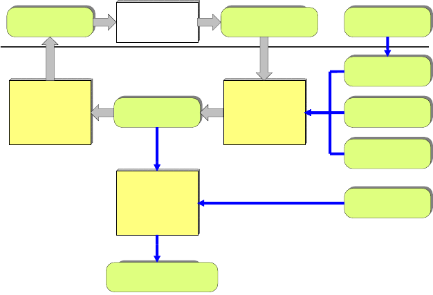
The whole work-flow of the optimization is illustrated in Figure 10. It consists of the following

main components:

 Traffic- and Efficiency-Model

 Objective function

 Optimization procedure

The traffic model creates an internal representation of the current traffic state out of the

traffic volumes measured at the measuring sections. The effect model, which is based on

the traffic model, determines the efficiency parameters, which in turn are the input

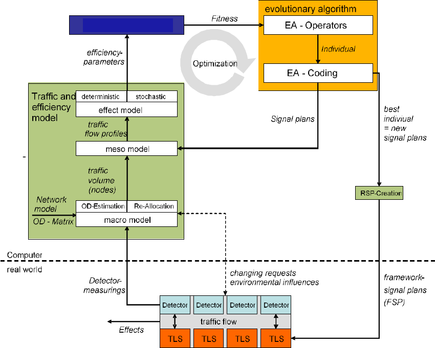
PTV Balance Manual EN Functionality

 PTV GROUP

parameters for the objective function. The result of this function is the fitness of an

individual, which means a scalar quality value for a control alternative (signal plans of the

network). The fitness in turn is the input variable for the optimization procedure which

optimizes the signal plans of the whole network and determines the best control alternative

(=the best individual) for the current traffic flow. All of the main components and the

framework signal plan creation (FSP-Creation) represent the traffic adaptive network

control PTV Balance, which delivers a new framework signal plan every 5 minutes (tactical

level). Based on that, the local control of the traffic light at each intersection reacts on short-

term changes of the traffic flow each second (operational level).

Figure 10: Procedure of online-optimization

The coding of the control parameters has significant meaning for the quality and the

functional ability of the optimization. In case of an evolutionary algorithm, coding means

the translation of signal plans to the individual. In case of the given problem, the following

specific framework conditions are relevant for the coding:

 Conditions of the planning (allowed cycle times, allowed cycle procedures)

 Necessary framework conditions (intergreen times, minimum green times)

 Framework conditions of the local traffic-dependent control

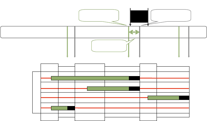
The framework conditions for the time interval control, which is very common in Germany

and the world, are illustrated in Figure 11.

Objective function

PTV Balance Manual EN Functionality

 PTV GROUP

The framework signal plan for the local, measurement-based time-gap control is defined

by the T-Time-Limits (TiA, TiB). The latest starting points of the interstages TiB are optimized

for all traffic lights in the control area. An interval [TiBmin, TiBmax] is defined for TiB in order to

assure the functionality of the local control.

Figure 11: T-Time-Limits of the local control

The optimization procedure GALOP (GALOP-Online – ein Genetischer Algorithmus zur

netzweiten Online-Optimierung der Lichtsignalsteuerung, Braun and Kemper 2008)

represents the control alternatives by the so-called coding of the individuals. An individual

has the following expression:

 

),...,,,,(),...,,...,,,,(),,...,,,,(, 1221222111111 21 n

nmnnnnmm



It contains a gene φ for the cycle time as well as n so called chromosomes for the m

intersections of the network which are to be optimized. Every chromosome consists of

multiple genes: one gene σ for the definition of the stage cycle, one gene ω for the global

offset, one gene ο for the local offset, as well as m genes ϴ for the stage durations

respectively the starting points of the interstages. Every gene has a real value between 0

and 1.

The genes remain inactive for the local and the global offset in the version of the algorithm

which is implemented in TRAVOLUTION because of the offset limits and framework

conditions of the local traffic dependent control. A special sequential coding was

developed. Its principle is described in (Braun and Kemper 2008) and in (Braun 2008) and

is protected by patents. Besides the necessary framework conditions, like the adherence

of intergreen times, it also integrates the framework conditions of the local traffic-dependent

control. The achievement was to create only valid individuals in each optimization.

The arrangements of the operators of the evolutionary algorithm and their parameterization

have a great influence on the quality of the optimization procedure. The operators must be

aligned to the coding because one individual represents all intersections in the network. An

intersection in the individual is illustrated as set of genes (chromosome). During the

recombination, single genes from the parent-individuals are used for the creation of

offspring-individuals by default. The recombination-operator was developed concerning the

probability p that a recombination will also be applied to the complete chromosomes

earliest point in time

for the interstage

framework signal plan

stage 1

stage 4

stage 2

interstage

min

max

interstage

latest point in time

for the interstage

buffer for the

local control

PTV Balance Manual EN Functionality

 PTV GROUP

(intersections). A mutation takes only place inside T-Time-Limits. Therefore, the length of

the steps can either be adjusted individually for each gene or for the whole individual. which

makes an adaption on demand possible.

The Hill-Climbing Algorithm can only optimize the control parameters sequentially in

contrary to the evolutionary algorithm which optimizes all control parameters at the same

time. Therefore, the created control alternative depends on the chosen order. As soon as

no better control alternative can be found for a control parameter in one direction, the

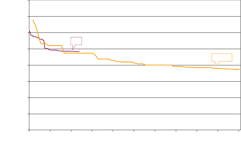
search will be continued for another direction. Figure 12 illustrates an example for the

different behaviour of the Hill-Climbing-Algorithm and the evolutionary algorithm in an

identical network with identical traffic volumes.

Figure 12: Comparison of the development of the fitness of the GA and the HC

The Hill-Climbing-Algorithm starts with the signal plans of the basic control that already

have a good quality. In contrary to that, the evolutionary algorithm begins with a random

start population. The best individual of the first generation (after 175 evaluated individuals)

does not reach that quality yet. However, the Hill-Climbing Algorithm stops after 2.404

evaluated control alternatives with a quality value of 241.742, because it can´t find a better

control alternative (it is stuck in a local optimum). Instead, the evolutionary algorithm has

reached a fitness of 236.556 after 2.300 individuals in the 18th generation. The evolutionary

algorithm has even reached a fitness of 186.559 after 80 generations and 10.050 control

alternatives.

2.1.5.2 Calculation of the ideal cycle time

The calculation of the ideal cycle time is done for all controllers of a control group at the

same time, to achieve an equal cycle time within the group. However, the adaption is

processed more slowly and in larger intervals than the changing of the split and offset

parameters, because a change of cycle time usually requires synchronization at the local

50000

100000

150000

200000

250000

300000

350000

400000

01000 2000 3000 4000 5000 6000 7000 8000 9000 10000

Bewertete Steuerungsalternativen

Beste Fitness (Gütewert)

GALOP

Evaluated alternatives/objective function calls

(Best) Performance index

PTV Balance Manual EN Functionality

 PTV GROUP

controllers. This can take several cycles, is disruptive for the individual traffic and hence

frequent changes should be avoided.

Moreover, this adaption can only be processed in discrete steps, because it is realized on

intersection level by the selection of signal programs with a given cycle time. Only a limited

number of signal programs can be supplied for each controller. Therefore, Balance

determines the signal program that has a cycle time nearest but bigger to the currently

ideal cycle time.

The switching procedure for the traffic-dependent selection of the signal plan automatically

calculates the required cycle time out of the saturation ratio of the signals with an optimized

signal plan from Balance. Considering the green time tgr and the saturation ratio µ for a

signal group, the additional green time necessary to reach a desired saturation α (e.g.

90%) with the same cycle time is determined as follows:

 



If you increase the green time by this value, the cycle time also changes, so that it’s

necessary to adjust the green share again to reach the desired value. This leads to the

following formula for the cycle time change Δt for the whole intersection:

   

  

With ti,gr the green time of the critical signal group in stage i and the additional green

time for stage i determined with above formula (tu is the currently running cycle time). The

intersection that gives the biggest value of Δt in a control group is the most critical

intersection and thus determines the necessary cycle time as tu+Δt. Consideration of the

available signal programs and their cycle times allows to choose the signal program that

has minimum cycle time longer than the desired one. Thresholds can be applied for the

number of repetitions of this calculation, before an actual switch is done in the field. These

thresholds can be set differently for switching into longer or shorter signal programs.

2.2 Definition of control groups

For the network control you should define several control areas marking the traffic light

systems which should be controlled in one go. These control areas are defined according

to the following guidelines:

 Distance between intersections

 Different cycle times

 Coordination areas

There shouldn’t be more than 30 intersections in one signal control, and as few as 1 is

permitted, if the intersection is separated from its surrounding. The greater the number of

intersections, the more degrees of freedom are in the optimization, enhancing the risk to

stick to a local optimum.

The maximum distance between the traffic light systems which belong to one control area

should be in the range of 700-1200m. A larger distance prevents a possible coordination,

because the queue dissolving processes increases with a larger distance.

PTV Balance Manual EN Functionality

 PTV GROUP

Different cycle times in a control area also prevent the coordination of the respective traffic

light systems. A certain coordination is still possible if the different cycle times are a multiple

to each other, like i.e. 60s and 120s. No coordination and therefore no good optimization

of the network can be processed if the cycle times are not uniform.

In order to guarantee a good optimization, it is important not to divide coordination areas

by a control area. A coordination area should be integrated into the control area because

in general, coordination areas already fulfil the first two conditions: the distance between

the intersections and the uniform cycle times.

The groups are defined statically, according to geographical issues and traffic-related

coherences. Because of queue dissolving-processes, it is useless to add traffic light

systems which are far away from the group. Moreover, it has to be regarded, that the traffic

light systems of a group have to run in the same cycle time. The defined groups are

checked and calibrated before the actual operation in the streets by simulations and quality

management plans. The whole system changes by adding a signal controller. Therefore

you would have to check and calibrate the control group again after you have added a

controller, in order to guarantee an error-free operation of the group. Because of that, the

integration of a completely dynamic change of the group compositions would not make

sense.

2.3 Changing the Objective Function

A dynamic change of the objective function is realized by additional master-weights. The

single summands of the objective function are multiplied with additional factors WD, WH,

WL, which are valid for the whole group. Therefore, either single impacts can be

disregarded by the factor 0 or different combinations of impacts can be regarded.

)),,(),,(),,((),( L

SGsg

sg WsgyxLWsgyxHWsgyxDyxPI  





Where

SG all the signal groups in the sub-net



sg,



sg,



sg weighting of waiting times/stops/queue lengths of

signal group sg

D, H, L vehicles waiting times/stops/queue lengths of signal

group sg

WD, WH, WL master-weights Waiting time/stops/queue length

x vector of control parameters (the signal plans of each

intersection)

y vector of traffic parameters (traffic volumes)

These factors can be changed dynamically by the user to create an optimization of the

objective function with the respective weights. The following optimization-possibilities are

available for the user:

 Minimization of the number of stops

 Minimization of delay times (which is the same as minimizing the travel times)

 Minimization of the queue lengths (which is the same as maximizing the traffic flow)

PTV Balance Manual EN Functionality

 PTV GROUP

2.4 Online-/Offline-System

In the previous chapters, the network control was mentioned in combination with the live-,

respectively the online-system. However, it is also possible and useful to build the network

control in an offline system. PTV Vissim (PTV AG 2017a) is serving as simulation software.

PTV Balance is integrated into Vissim systems as a DLL-file. The data provision of PTV

Balance is created by Network-XML-Files which are exported from the data provision tool

PTV Visum and by a signal controller data-file shared with PTV Epics and Vissig. The data

provision itself is done similar to the data provision for the online system. Further

information about this topic can be found in chapters 3 and 4.1.

The offline system offers multiple ways to test the behaviour of the network control because

the functionality of the network control is not affected. It is possible to test possible changes

and calibrate the whole system including the network control. It is important to test changes

at an intersection inside the offline mode before they are applied in the online system,

because the changes at one intersection of the network control could have impact on the

whole system. Therefore, it is important to test changes of the weighting, the objective

function, the control or of the network itself, in a simulation.

2.5 Possibilities for the Local Control

2.5.1 PTV Balance with PTV Epics

It is possible to operate the network control PTV Balance with PTV Epics. PTV Balance as

network-wide system takes the task of overall coordination and traffic control. The model-

based system PTV Epics assumes the local holistic optimization on the node including

public transport. Thus, the traffic-dependent control is realized within seconds and can

react to changes in the traffic very quickly.

2.5.2 TRENDS-Kernel with normal TRELAN-Logic

A further possibility is to combine a rule-based traffic-dependent control by means of

TRELAN-Logic (Gevas software Systementwicklung und Verkehrinformatik GmbH 2010b)

with the network control PTV Balance. Every 5 minutes the frame signal times on which

local traffic-dependent control is based are optimized by PTV Balance. The public transport

is considered only by the local control.

2.5.3 VS-Plus (Verkehrssysteme AG)

It is also possible to couple VS-Plus controlled controllers with PTV Balance. The

parameterized frame signal plan in VS-Plus is replaced by PTV Balance. This way the local

traffic actuated control logic of VS-Plus is preserved. VS-PLUS receives from its

superordinate network control dynamically adapted frame signal plans that improve the

traffic flow throughout the network.

PTV Balance Manual EN Functionality

 PTV GROUP

2.5.4 Ring-barrier-controller

The North American Ring Barrier control system was already equipped with PTV Balance

as a superordinate network control system. This has been tested in a simulation study.

2.5.5 Dynamic Fixed Time Control

In network control is also possible to bypass the local control function and to use a so-

called dynamic fixed time. The earliest and latest starting points of the interstages as part

of the frame are reduced to one point. Is the local control set in a way that the requirements

of PTV Balance are strictly adhered, a dynamic fixed time control is switched that changes

the green times and offsets every 5 Minutes. There is no local traffic dependency needed.

This control method is a valid option if transit signal priority is not used and traffic demand

is rather static.

2.5.6 Other Methods

As you can see, the network control PTV Balance can be coupled with many local control

systems, so there are other connections with other methods open.

PTV Balance Manual EN Data Provision

 PTV GROUP

3 Data Provision

The PTV Vision suite allows data provision for PTV Balance in a seamless way for

simulation and calibration. PTV Balance data provision consists of the following parts:

 A network model of the road network and the traffic demand

PTV Visum provides this information in the anm/anmroutes format. This step uses the

same standard export and import functionalities that are used to convert a PTV Visum

model to PTV Vissim.

 Parameters of PTV Balance and signal control data

 Local parameters e.g. signal control data and parameters that are intersection

The signal controller “Epics/Balance-Local” is used to provide signal control data.

This signal controller is available in PTV Visum and PTV Vissim. Vissig, PTV

Balance and PTV Epics use the same sig-file format that can be shared between

the different models.

 Global parameters e.g. optimization algorithm

Global parameters for PTV Balance are provided using the traffic signal controller

“Balance-Central” in PTV Vissim.

For details regarding PTV Vissim, PTV Visum or PTV Epics please refer to their respective

manuals (PTV AG 2017a/b/c).

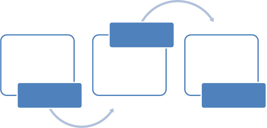
Figure 13: Workflow for data provision in the PTV Vision suite.

•Network Model

•Assignment

•ANM/ANMROUTES-Export

•Provision of signal control

data for PTV Balance/Epics

Modelling in PTV Visum

•Finetuning of the simulation

model

•Provision of signal control

data for PTV Balance/Epics

Modelling in PTV Vissim

•Simulation for testing and

calibration

Simulation of PTV Balance and PTV

Epics

and/or

Field device data provision

PTV Balance Manual EN Data Provision

 PTV GROUP

Hint: PTV Balance is a network control that optimizes signal plans typically every five

minutes. It has local and global parameters. It requires a local signal controller to apply

the optimized signal plans. Therefore, PTV Balance is modelled with two types of signal

controllers - “Epics/Balance-local” and “Balance-Central”. The local controller

“Epics/Balance-local” can accomplish several tasks. It can be a pure executor of PTV

Balance, it can be the local traffic signal optimization PTV Epics and it can be the

combination of both.

For guidelines on using PTV Epics and PTV Balance within the PTV Vision suite, please

see chapter 3.1.

3.1 Guidelines for using PTV Balance within the PTV Vision

suite

This chapter provides guidelines for the data provision for PTV Balance and PTV Epics

within the PTV Vision suite. The guidelines are a recommendation, there are other means

of handling the related tasks and the necessity of specific steps depends on the actual

project.

Step 1: PTV Visum - base model

Provide a suitable base model in PTV Visum in terms of:

 Supply with hourly capacities on links and turns, vehicle restrictions, free flow speeds

etc. and public transport if required for simulations with PTV Epics.

The network needs to be suitable for an anm ex- and import i.e.

 connectors must not be connected to nodes that represent a physical intersection

 every node must not have more than one connector per direction

 every zone must not have more than one connector per direction

 Demand matrices for the relevant days and times of day for which PTV Balance shall

be designed and calibrated (e.g. Mon-Fry morning peak, Mon-Fry mid-day, Sat/Sun

morning peak etc.).

Ideally, these matrices have already been assigned and are corrected with

TFlowFuzzy for hourly counts (see PTV AG 2017b “Matrix correction using

TFlowFuzzy”). See also Step 3: PTV Visum - assignment specifics.

Step 2: PTV Visum - PTV Balance (and PTV Epics) data provision

Hint: Use the Add-In “Preprocess Balance/Epics” in order to create specific user defined

attributes for PTV Balance and load an appropriate layout for the junction editor.

1. Set the PTV Visum project directory for “External control” to the directory of the ver-

file.

2. Provide detailed information for all nodes that shall be controlled by PTV Balance

using the junction editor. For any of these nodes:

 create a signal control of the type “Epics/Balance local”

 edit the signal control “Epics/Balance local” (see chapter 3.3.1 and PTV AG

2017b “Editing a signal control in Vissig”).

PTV Balance Manual EN Data Provision

 PTV GROUP

 add only the signal groups and return to the PTV Visum junction editor

Hint: In the next steps signal groups will be assigned to lane turns. After this step, the

GUI of “Epics/Balance local” can draw direction arrows for the specific signal groups,

making further steps much easier.

 define the geometry of legs, lanes, lane turns and crosswalks

 assign the signal groups to their lane turns

 add detectors to the lanes and assign the appropriate signal control and channel

number

Hint: Log-in detectors for public transport prioritization for PTV Epics can be at a long

distance upstream of the node of the signal control. It is possible that the link approaching

the signalized node is too short and the detector is located on a link further upstream. In

that case, add the detector to the appropriate upstream node and make sure that the

assigned signal control of that detector is correct.

 make sure that allowed traffic systems of turns and lane turns are consistent

 edit the signal control “Epics/Balance local”

 define intergreen matrices, stages, signal programs etc.

 define parameters for PTV Balance and PTV Epics (or do that after Step 5: in

PTV Vissim)

Hint: When signal control design starts from scratch (i.e. no fixed time signal programs

available) you can use the PTV Visum procedures “Signal cycle and split optimization”

and “Signal offset optimization” (PTV AG 2017b) to quickly create good starting signal

programs for a large number of intersections (also see Step 3: PTV Visum - assignment

specifics).

3. Define signal coordination groups and assign the signal controllers to these groups.

4. After finishing the data provision of all signal-controlled nodes, run the Add-In

“Preprocess Balance/Epics” again. This updates the saturation flow rates with

respect to the updated lane turns.

5. Use the network check “Viability for Balance / Epics” and make sure that all checks

are “ok”.

Step 3: PTV Visum - assignment specifics

PTV Balance requires an anm export with an anmroutes-file containing routes. An

anmroutes-file can contain matrices and/or routes. The latter describing an assignment

result from PTV Visum. This in turn means that one has to calculate an assignment in PTV

Visum and export the results via an anmroutes file containing routes to PTV Vissim and

PTV Balance. This is also a very comfortable way of defining vehicle inputs and vehicle

routes in PTV Vissim. All of the below is valid for anmroutes-routes, specifically the

interaction of anmroutes-matrices and time validities is different.

There is no general limitation to the assignment method. However, the following things are

of importance:

PTV Balance Manual EN Data Provision

 PTV GROUP

 Impact of signal control

This can either be considered directly by an assignment with ICA or by suitably

derived capacities on turns e.g. from an assignment with ICA (see PTV AG 2017b

“The procedure of assignment with ICA”).

 Time validity of the demand

Static assignments do not consider whether a demand matrix contains the demand for

1 or for 24 hours, though obviously the capacities of the network have to correspond.

What does matter for PTV Vissim as well as for PTV Balance is that the demand

information of the anmroutes file is connected to an appropriate time interval (see PTV

AG 2017b “Saving an abstract network model”).

In general, it is perfectly fine to use a static assignment that e.g. assigns a 3-hour

demand matrix and map this to a simulation time interval of three hours in PTV Vissim.

However, that way it will neither be possible to use an assignment with ICA, that

requires hourly values nor will it be possible to represent a demand in PTV Vissim that

changes over time e.g. one hour with low demand, then one hour with high demand

and then again one hour with low demand. In order to represent this, use an

assignment with the Dynamic User Equilibrium (see also PTV AG 2017b “Parameters

of Dynamic User Equilibrium (DUE)”). On the other hand, DUE cannot directly

consider the impact of signal control on turn capacities.

Therefore, in order to consider both impact of signal control on capacities and a fluctuation

in demand over time, a combination of an assignment with ICA and DUE is recommended.

The former providing turn capacities for the latter and the latter providing the actual input

for PTV Vissim and PTV Balance. If a simulation time of one hour is sufficient and demand

fluctuations over time are not of interest, then skip sub-steps 5 and 6 in the

recommendation below.

1. In Calculate->General procedure settings->Prt settings->Assignment set Save

paths to As connections.

This allows PTV Visum to save the routes of an assignment in the anmroutes file.

2. (Optional) use an assignment without blocking back and TFlowFuzzy to correct the

demand matrices (see PTV AG 2017b “Matrix correction using TFlowFuzzy”).

3. Use an assignment with ICA for the peak hour demand (see PTV AG 2017b “The

procedure of assignment with ICA”).

4. (Optional)

 Use “Signal cycle and split optimization” and “Signal offset optimization” (see

PTV AG 2017b) to provide new or update existing fixed time signal plans.

 Recalculate the assignment with ICA to respect the updated signal plans.

Hint: While it seems tempting to set up an iterative process around sub-steps 2 to 4, this

has to be avoided, as it is likely that this process has a positive feedback loop and will

yield an unrealistic result.

5. Use the ICA capacities “ICAFINALCAP” as turn capacities. Apply a minimum turn

capacity of 100 Veh/h.

PTV Balance Manual EN Data Provision

 PTV GROUP

6. Use the DUE assignment to calculate the final output for PTV Vissim and PTV

Balance.

Step 4: PTV Visum - anm/anmroutes export

1. Export the network and the result of an assignment as anm/anmroutes-files.

For general information on anm/anmroutes export see PTV AG 2017b “Saving an

abstract network model” and for PTV Balance specific parameters see chapter

3.2.1 and 3.2.2.

Hint: Set the project directory for “External control” of the PTV Visum ver-file and export of

anm/anmroutes-file to the same folder. This way PTV Visum, PTV Vissim, PTV Balance

and PTV Epics will share the same sig-files. Take note, that the anm export will provide a

warning that the external control files will be shared.

In order to simulate large networks with several signal coordination groups in a timely

manner in PTV Vissim, cut subnetworks corresponding to signal coordination groups for

PTV Balance.

In order to simulate several demand scenarios, repeat the process starting from Step 3:

PTV Visum - assignment specifics but only export the anmroutes file and specify a

suitable name.

Step 5: PTV Vissim - anm/anmroutes import

1. Import only the anm-file in PTV Visum (see PTV AG 2017a “Importing ANM data”)

2. Check the result of the anm import and fine tune the network as desired. Typical

tasks are:

 Check detector positions.

 On connectors that reduce additional lanes after an intersection, check if Route-

>Lane change: is short enough to make the vehicles use the additional lanes.

 Depending on the maximum cycle time, adjust the Waiting time before

diffusion of the Driving Behaviors.

 Check conflict areas and positions of links, connectors and crosswalks.

Specifically large intersections are likely to require corrections.

 If desired, apply cosmetic changes e.g. number of splines on connectors, fix the

splines on links (besides “inside intersection corrections”, typically links feeding

the network that lead to an intersection with a central island require fixing) etc.

Take note that, besides slightly changing the lengths of links and connectors,

these changes do not affect the quality of the simulation.

3. Add a signal controller of the type “Balance-Central” and provide parameters (see

chapter 3.3.2).

4. Save, this is your “base” network in PTV Vissim.

5. Import the anmroutes files as desired.

PTV Balance Manual EN Data Provision

 PTV GROUP

Hint: The import of the anmroutes file can be repeated as long as the node structure in

the inpx-file remains stable. This swaps the entire demand and allows a comfortable way

of handling different demand scenarios within one inpx-file. In order to keep track of the

results use the comment of the Simulation Runs list.

It is also possible to “split” and maintain several inpx-files for every demand scenario,

though this makes updates of the network for several inpx-files more tedious.

Step 6: PTV Vissim - simulation and calibration

1. Simulate and calibrate (see chapter 4)

 Make sure that PTV Vissim behaves realistically (specifically due to anm based

network generation).

 Fine tune PTV Balance and/or PTV Epics parameters.

Hint: For PTV Balance the input file that describes the network is the anm-file. Therefore

changes to the network, e.g. saturation flows for PTV Balance, adding detectors (or

correcting the position in terms of placing the detector on another link) etc. anything that

is stored in the anm-file need to be applied in PTV Visum and require a new export of the

anm-file (and the import in PTV Vissim).

This does not apply to PTV Epics.

3.2 Network and Demand Data

3.2.1 Network Data

An anm-file describes the network data (links, turns, number of lanes, detectors etc.).

Create these files with PTV Visum. PTV Vissim can import these files too. The anm-file is

a parameter of the signal control Balance-Central.

The anmroutes-file is used in the same way as for an export to PTV Vissim (see PTV AG

2017b “Saving an abstract network model”). In addition to that, it is required to define

attributes describing the saturation flow for links and turns for the anm export in PTV Visum.

The saturation flow corresponds to the capacity of a link or turn with no signal control.

The PTV Visum Junction Editor and Control add-on is required to model signalized

intersections in the required level of detail.

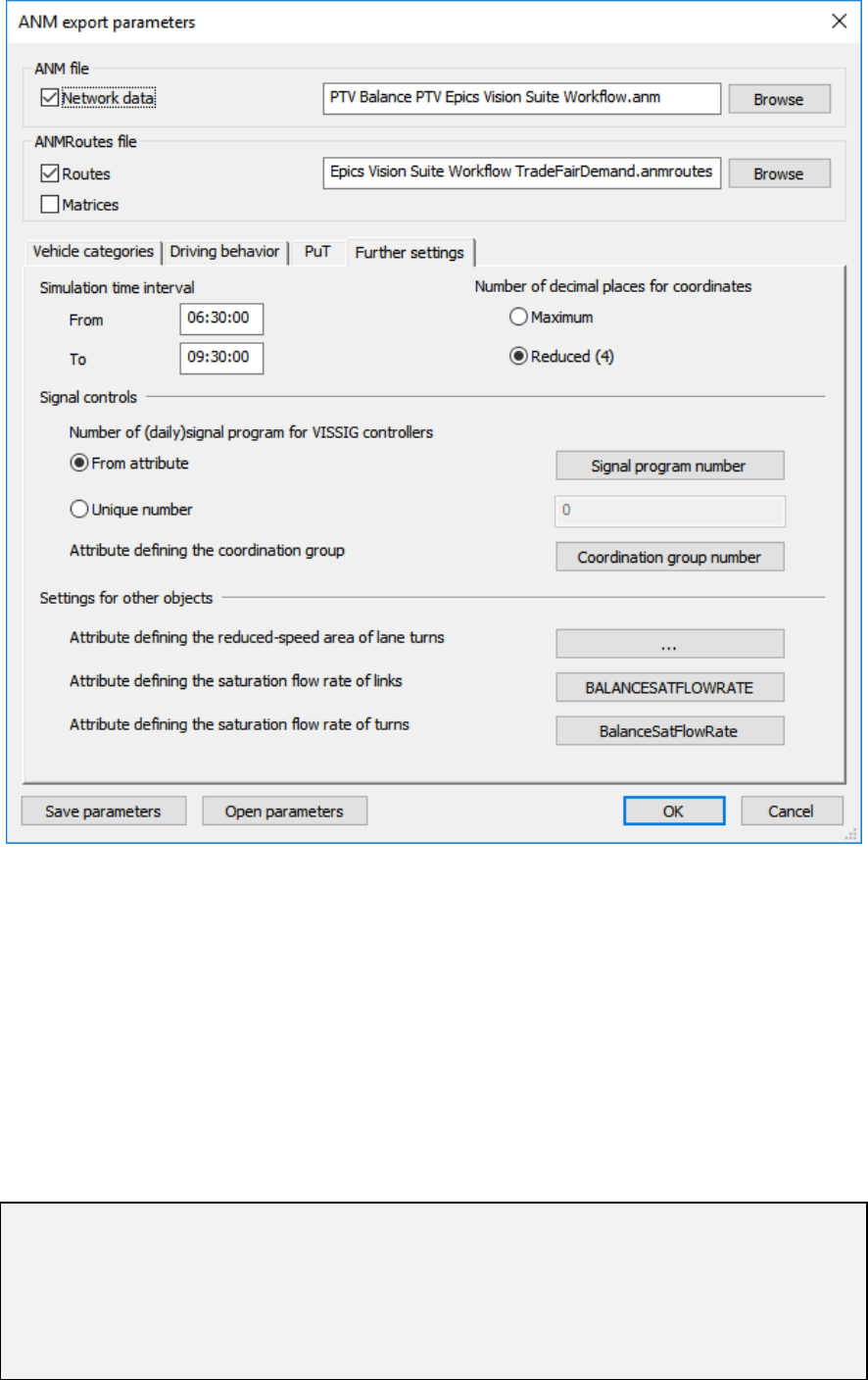
To define the additional parameters in PTV Visum:

1. Open anm export parameters.

2. Click on Further settings.

3. In Signal controls click on the button next to Attribute defining the coordination

group.

4. Choose any attribute.

Fill the chosen attribute with the corresponding values.

PTV Balance Manual EN Data Provision

 PTV GROUP

Element

Description

Attribute defining the

coordination group [-]

Numerical attribute that assigns the signal control to a signal control

group. PTV Balance optimizes all signal controllers of one group

together. Design control groups based on the topology of the network

and runtime restrictions (depending on network size and computational

power usually up to 50 signal controllers are feasible).

It is possible to provide several signal control groups in the same anm-

file. Use the global parameters of PTV Balance in PTV Vissim (see

chapter 3.3.2) to optimize a specific group together with PTV Vissim.

Nevertheless, in order to simulate large networks in a timely manner with

PTV Vissim, cut subnetworks in PTV Visum, that correspond to the

desired signal control groups.

5. In Settings for other objects click on the button next to either Attribute defining

the saturation flow rate of links or Attribute defining the saturation flow rate of

links turns.

6. Choose any attribute.

Fill the chosen attribute with the corresponding values.

Element

Description

Attribute defining the

saturation flow rate of links

[Veh/h]

Saturation flow of the link respecting number of lanes, share of HGV,

slope, etc. standard value is 1800 x number of lanes x reduction factors.

Attribute defining the

saturation flow rate of turns

[Veh/h]

Saturation flow of the turn respecting number of lanes, share of HGV,

slope, direction (right turns tend to require a lower speed than straight

turns) etc. standard value is 1750/1850/1800 (right/straight/left) x number

of lanes x reduction factors.

PTV Balance Manual EN Data Provision

 PTV GROUP

3.2.2 Demand Data

An anmroutes-file describes demand data. Create these files with PTV Visum. PTV Vissim

can import these files too. The anmroutes-file is a parameter of the signal control Balance-

Central.

The anmroutes-file is used in the same way as for an export to PTV Vissim (see PTV AG

2017b “Saving an abstract network model”).

The anmroutes-file must contain only Routes. In PTV Visum Calculate->General

procedure settings->Prt settings->Assignment set Save paths to As connections.

This allows PTV Visum to save the routes of an assignment in the anmroutes file.

Hint: A static assignment in PTV Visum does not have any information about the time.

Therefore, if exporting the result of a static assignment, make sure that the demand and

the Simulation time interval in the ANM export parameters fit together. PTV Vissim

and PTV Balance will respect these settings.

In order to test how PTV Balance reacts to unplanned changes in demand it is possible to

use different anmroutes-files for PTV Vissim and PTV Balance.

PTV Balance Manual EN Data Provision

 PTV GROUP

3.3 PTV Balance Parameters and Signal Control Data

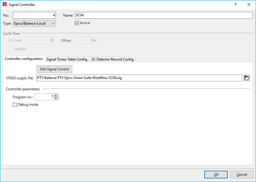
3.3.1 Local Parameters and Signal Control Data

PTV Balance related parameters are provided with the GUI of the signal controller

Epics/Balance-local that is an extended version of Vissig. This manual will only address

additional data that are relevant for PTV Balance. Sections that are not covered are not

required for PTV Balance.

PTV Balance requires a stage based design.

1. From the Signal Control menu, choose > Signal Controllers.

The Signal Controller list opens.

2. Right-click the entry of your choice.

3. From the shortcut menu, choose Edit or Add.

The Signal Control window opens.

4. In the Type field, select > Epics/Balance-Local

5. Edit the desired data:

PTV Balance Manual EN Data Provision

 PTV GROUP

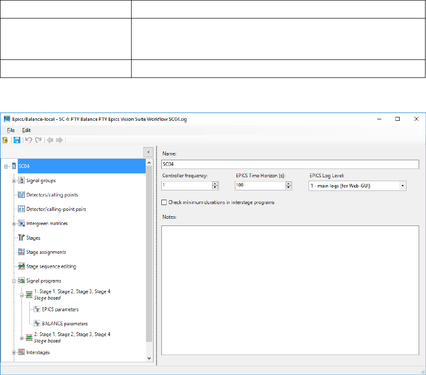
Element

Description

Debug mode

If active, then the local controller creates log-files. Detailed log-files are

created in the subfolder Epics_Log of the directory of the inpx-file. This

significantly increases runtime.

All other elements

Please refer to help on Fixed Time control.

6. Click on Edit Signal Control.

The SC Editor opens.

3.3.1.1 Signal groups

As required for any stage based fixed time control modelled with Vissig.

3.3.1.2 Intergreen matrices

As required for any stage based fixed time control modelled with Vissig.

3.3.1.3 Stages

As required for any stage based fixed time control modelled with Vissig.

3.3.1.4 Stage assignments

As required for any stage based fixed time control modelled with Vissig.

3.3.1.5 Stage sequence editing

As required for any stage based fixed time control modelled with Vissig.

3.3.1.6 Signal programs

As required for any stage based fixed time control modelled with Vissig.

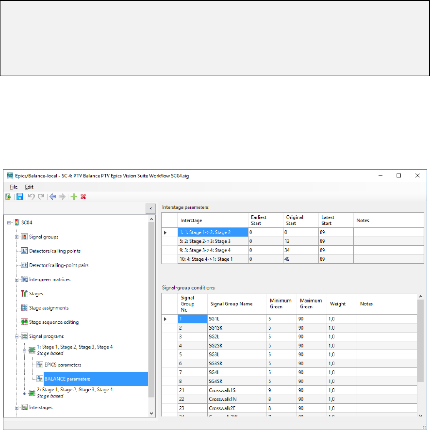
PTV Balance Manual EN Data Provision

 PTV GROUP

Additionally PTV Balance requires the provision of signal program and stage dependent

parameters that define priorities and constraints for the optimization.

Overview of signal program parameters

PTV Balance has parameters concerning time and duration constraints of stages and

allowed interstages. These parameters are signal program dependent and are set to

default values during the automatic creation. Some of the default values are derived from

the fixed-time signal program (e.g. original start of an interstage).

These parameters govern the optimization function of PTV Balance.

Hint: Every parameter for PTV Balance comes with a tooltip providing an explanation of

its meaning. In addition, there are numerous plausibility checks with explanations.

When you have the license for PTV Balance and PTV Epics and you want to use only

PTV Balance, then activate EPICS parameters > BALANCE fixed-time control to force

PTV Epics to follow the results of PTV Balance exactly.

Setting signal program interstage parameters

1. Select a stage based signal program.

2. Expand the Navigator.

3. Select BALANCE parameters.

4. Make the desired changes of the Interstage parameters

PTV Balance Manual EN Data Provision

 PTV GROUP

Element

Description

Interstage

Interstage can be added, removed and changed (see hint).

Earliest Start

Cycle second [s] defining the earliest possible start of the

corresponding interstage.

Original Start

Cycle second [s] defining the original start, typically as defined by the

underlying fixed time signal program, of the corresponding interstage.

Latest End

Cycle second [s] defining the latest possible start of the corresponding

interstage.

Note

Free text.

Hint: The interstages of PTV Balance and the underlying fixed time signal program may

be different.

This is mainly of concern for real-word data provision, where the underlying fixed time

signal program may be used as a fallback by the local controller. As a fallback option the

underlying fixed time signal program must use all stages even e.g. non-regular PuT

prioritization stages. But specifically these non-regular stages are not useful to be

considered in the optimization of PTV Balance.

The PTV Balance interstages are set according to a newly created underlying fixed time

signal program but can be changed manually.

Adding an interstage of a signal program

1. In the table, right-click the table cell.

2. From the context menu, choose Add.

Removing an interstage of a signal program

1. In the table, right-click the desired row.

2. From the context menu, choose the entry Delete.

Resetting interstage parameters of a signal program

1. In any table right-click the desired cell or column.

2. From the context menu, choose either Reset values of table or Reset values of

column ...

This resets either the whole table or the corresponding column to the default

values.

Setting signal program signal-group conditions

1. Select a stage based signal program.

2. Expand the Navigator.

3. Select BALANCE parameters.

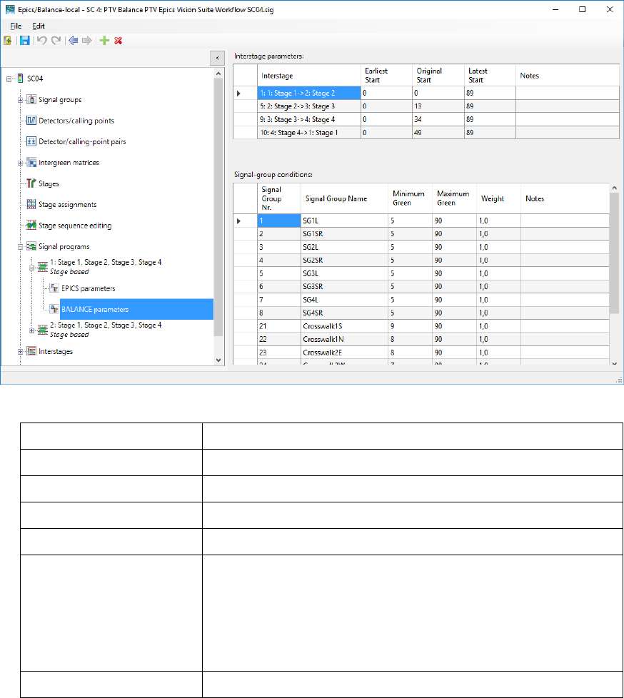
PTV Balance Manual EN Data Provision

 PTV GROUP

4. Make the desired changes of the Signal-group conditions

Element

Description

Signal Group Nr.

Non-editable as defined in signal groups.

Signal Group Name

Non-editable as defined in signal groups.

Minimum Green

The minimum length of the corresponding signal group [s].

Maximum Green

The maximum length of the corresponding signal group [s].

Weight

The weight reflects the importance of the signal group for the objective

function of PTV Balance.

Of specific concern is the relation of the weights of the different signal

groups. If you want to put specific empathizes on a direction or if you

experience queues in front of a specific signal group, increase its

weight in relation to the other signal groups.

Note

Free text.

3.3.1.7 Interstages

As required for any stage based fixed time control modelled with Vissig.

3.3.1.8 Daily signal program lists

Optional but as required for any stage based fixed time control modelled with Vissig.

3.3.2 Global Parameters

Global parameters are set by a signal control of the type Balance-Central. This signal

control is not associated with any signal groups or signal heads. It is a virtual signal control,

which represents the core of PTV Balance. There has to be only one instance of such a

signal control.

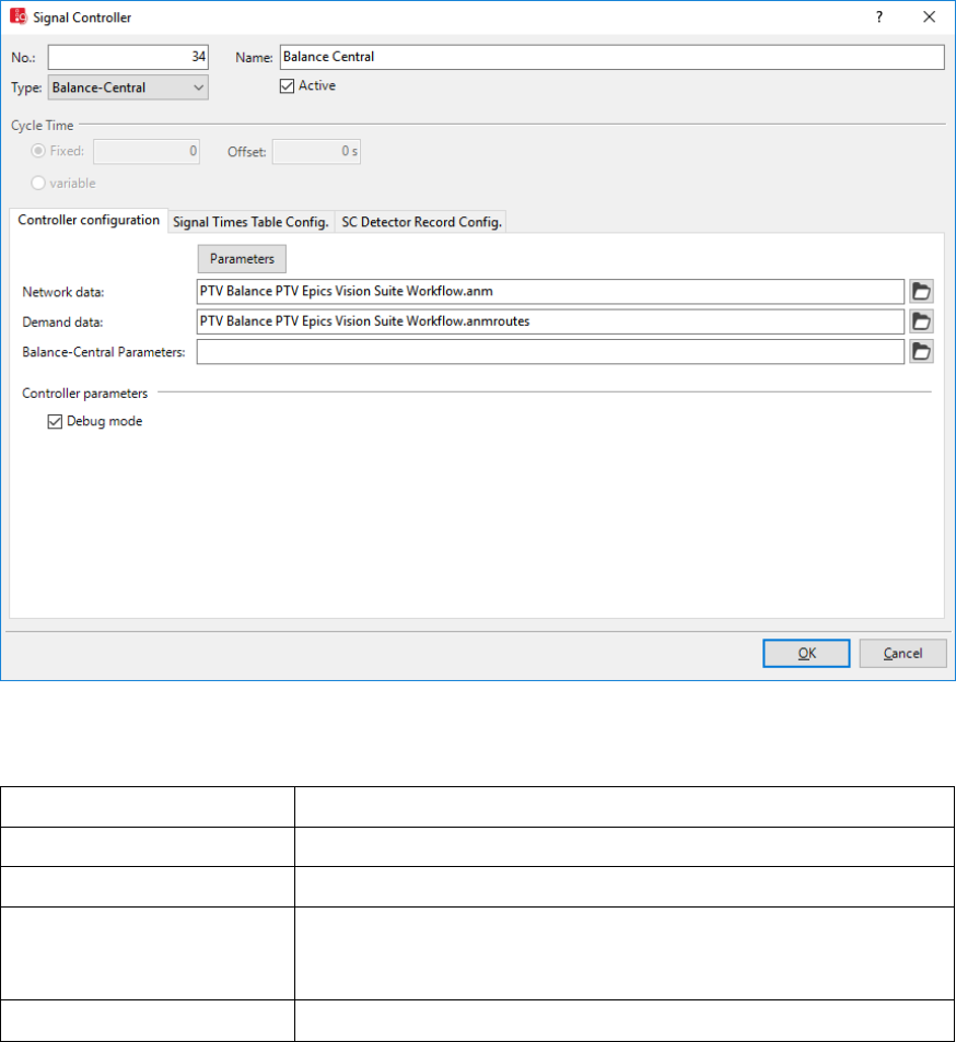
PTV Balance Manual EN Data Provision

 PTV GROUP

1. From the Signal Control menu, choose > Signal Controllers.

The Signal Controller list opens.

2. Right-click the entry of your choice.

3. From the shortcut menu, choose Edit or Add.

The Signal Control window opens.

4. In the Type field, select > Balance-Central

5. Edit the desired data:

Element

Description

Data file 1:

The anm-file describing the network.

Data file 2:

The anmroutes-file describing the demand.

Debug mode

If active, then PTV Balance creates log files (see chapter 4.1.2). The

level of detail of the log files can be set in the Balance-Central Editor.

This influences the number of produced log files. This increases runtime.

All other elements

Please refer to help on Fixed Time control.

6. Click on Parameters

The Balance-Central Editor opens.

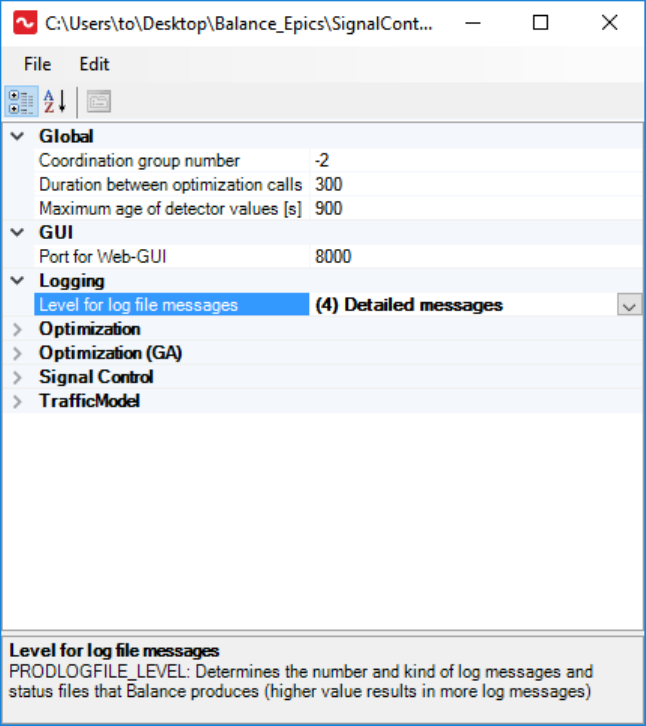
PTV Balance Manual EN Data Provision

 PTV GROUP

7. Edit the desired data.

Categories group the parameters.

The bottom of the figure displays a short description of the currently selected

parameter.

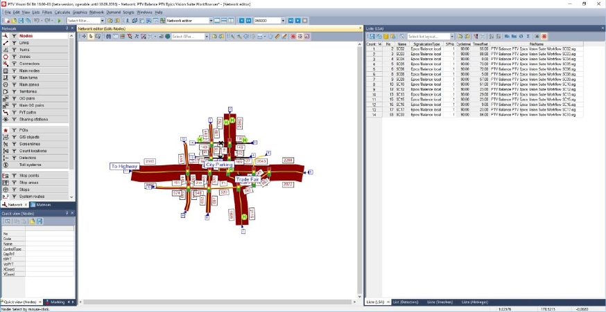
PTV Balance Manual EN Simulation, Calibration and Operation

 PTV GROUP

4 Simulation, Calibration and Operation

Testing the efficiency of an adaptive signal control like PTV Balance is nearly impossible

without a modern simulation environment like PTV Vissim. It is the only way to check

whether all parameters are chosen and calibrated well and if all detectors are correctly

defined

On the other hand a simulation is never 100-percent exact. Therefore the step from the

simulated network to the real road network has to be taken with care – a recalibration might

be necessary, at least for some approaches.

4.1 Simulation With PTV Vissim

4.1.1 Data Provision

The microscopic traffic flow simulation PTV Vissim provides the possibility to test PTV

Balance without access to any online system. PTV Vissim uses the same import/input

format for network and demand data as PTV Balance providing a quick to set up test

environment. PTV Visum, PTV Vissim and PTV Balance share signal control related data

through the sig-files.

PTV Visum and PTV Vissim are the recommended way for data provision and calibration.

See chapter 3.1 for guidelines on how to set up a PTV Balance project with the PTV Vision

suite.

Figure 14: Network in PTV Visum.

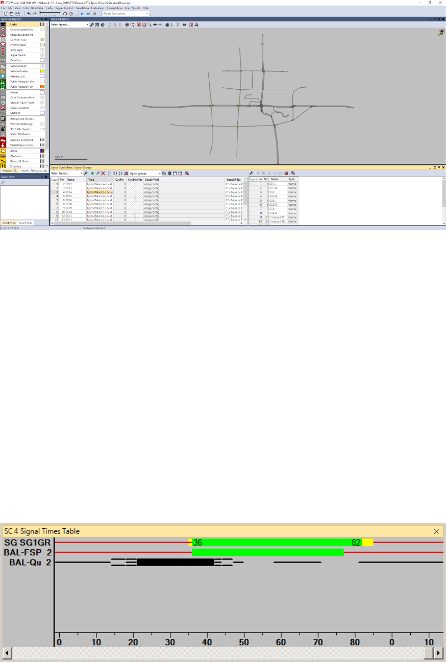
PTV Balance Manual EN Simulation, Calibration and Operation

 PTV GROUP

Figure 15: Network in PTV Vissim using anm-export and import functionalities.

4.1.2 Showing Additional Data in the Signal Times Window

You can show the current signal states and detector states during a simulation or during

interactive tests of signal control logic in a window. Therein, the green times, yellow times

and red times are represented graphically along a horizontal time axis for each selected

signal control.

For details on the standard attributes and configuring the signal times window please refer

the Vissim user manual (PTV AG 2017a).

PTV Balance allows you to show additional attributes that are described below.

Result of evaluation of signal times tables, additional PTV Balance attributes

If you have selected the evaluation, each selected signal control is shown in a window

during a simulation or a test run of the signal times table.

The colors indicate the current state of the respective signal group.

The state of the current time step is represented at the right edge of the window.

If the signal times table also contains PTV Balance frame signal plan BAL-FSP, the colors

indicate the desired signal state of PTV Balance. BAL-FSP does only differ red and green

PTV Balance Manual EN Simulation, Calibration and Operation

 PTV GROUP

states and it is subject to the local control whether the frame signal plan is respected or

not.

If the signal times table also contains PTV Balance queues BAL-Qu, the colors indicate the

queue state of the PTV Balance simulation model.

Queue color

Description of the queue state

nothing

no queue

black line

1-3 vehicles in queue

black frame

4-6 vehicles in queue

black line and black frame

7-8 vehicles in queue

solid black

>8 vehicles in queue

Hint: These attributes are not available before PTV Balance calculated an actual

optimization. On the first call to PTV Balance, the network is empty, detectors have not

yet delivered any data and therefore this initial call, does not yield optimization results.

4.1.3 Evaluating Additional Data in the Signal Control Detector

Record

You can use the SC detector record to check control logic of external control procedures.

For each SC, you can show a freely configurable, precise record of the SC values and

detector values as well as internal parameters of the control procedure.

For details on the standard attributes and configuring the signal control detector record

please refer the Vissim user manual (PTV AG 2017a).

PTV Balance allows you to show additional attributes that are described below.

Result of the SC detector record evaluation, additional PTV Balance attributes

Value type

Meaning

BAL-FSP

PTV Balance Frame Signal Plan

BAL-FSP does only differ red and green states and it is subject to the local

control whether the frame signal plan is respected or not.

State of frame signal plan:

 . red

 I green

BAL-Qu

PTV Balance Queue

Bal-Qu indicates the queue state of the PTV Balance simulation model:

 0-9 vehicles in the queue

 X more than 9 vehicles in the queue

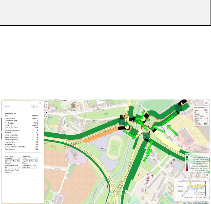
PTV Balance Manual EN Simulation, Calibration and Operation

 PTV GROUP

Hint: These attributes are not available before PTV Balance calculated an actual

optimization. On the first call to PTV Balance, the network is empty, detectors have not

yet delivered any data and therefore this initial call does not yield optimization results but

shows the road network in grey.

4.1.4 PTV Balance and Epics network view

PTV Balance and PTV Epics are distributed with PTV Vissim and their own data

visualization tool “PTV Balance and Epics network view”. This tool is browser-based and

shows many internal data and the results of PTV Balance (and some information of PTV

Epics) and is a useful tool for understanding and calibrating PTV Balance (it is also used

for real-world deployments). It opens automatically when a simulation is started in Vissim

which contains a signal controller of type “Balance central” that has an activated check box

“debug mode“ in its signal controller parameters.

Right after the start of the simulation the Balance GUI can only show the network, but after

the first optimization run it shows the results of the Balance calculation for each link,

controller and signal. The GUI is mouse sensitive and always shows the data for the object

under the mouse cursor. The button in the right upper corner allows to lay an Open Street

Map under the network, if the coordinates fit.

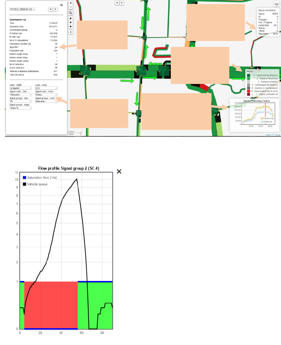
PTV Balance Manual EN Simulation, Calibration and Operation

 PTV GROUP

Clicking on a signal group will display the flow profile that Balance calculated for this

signal: For each second in the cycle, it displays

1. If it is green or red

2. When red, it shows the number of cars

waiting at the stop line

3. When green, it shows the number of cars

passing through the stop line

This allows to check the quality of coordination

as Balance calculated and compare this with the

Vissim “reality”.

The example to the left shows a signal group

with a queue length of 10 cars in total at the

beginning of green. These vehicles have passed

the stop line after 10 seconds of green. Then

there is a gap of 10 seconds. Finally a platoon

arrives from the upstream intersection and

passes the stop line. The majority of cars is

arriving after 20 seconds of red time.

Clicking on an intersection (the square) allows to

see the frame signal plan that Balance

calculated as optimal.

4.2 Log Files

PTV Balance provides several log files. These contain warnings, errors and results. The

log files are an important tool to identify errors in the data provision and for calibration.

The level of detail of the log files can be set in the Balance-Central Editor. This influences

the number of produced log files.

Visualize

performance index

and choose past

optimization runs

Choose what to

display in the

map

Summary of

optimization

run

Calculation

results for

object at

mouse position

Explanation for

color of the

object at

mouse position

PTV Balance Manual EN Simulation, Calibration and Operation

 PTV GROUP

Log files are created in the subfolder of the directory of the inpx-file. The folder has the

name of the anmroutes-file with suffix BAL_Log.

PTV Balance creates a new log file for every calendar day and appends information to

existing log files for every optimization.

Most log files provide a short explanation of its content and their first two columns display

the current time and the simulation time.

PTV Balance creates numerous log files of the following schemes and types:

 Balance_LOGTYPE_YYYY-MM-DD_log.txt

 LOGTYPE identifies the type of the log file. The most important types are described

below.

 YYYY-MM-DD represents the current day.

 json files

These are used internally by the visualization component.

 genetic algorithm files (sav files and last files)

These are used internally to manage the genetic algorithm.

4.2.1 Balance_output_YYYY-MM-DD.log.txt

The main log file. It includes error messages, warnings and information of the initialization

and the optimization.

The first two columns display the time stamp and the log level. The third column denotes

the Balance group that created the message, followed by the message text. A log level of

5 indicates an error and usually prevents an optimization. Messages of log level 4 indicate

a warning and usually do not prevent an optimization but impact the achievable quality of

the results.

4.2.2 Bxx_summary_YYYY-MM-DD-log.txt

This file provides an aggregated summary of every optimization run for group Bxx (with xx

the group number). The summary is split up in the following parts:

 Optimization

Static information about the optimization algorithm and parameters.

Dynamic information about the achieved results and the reason for termination of the

optimization.

 Signal control

Overview of all signal controllers, the active signal program, cycle time and the

saturation of every signal controller. The latter helps to identify critical spots for

calibration.

 Input data

Number of known and active detectors. When PTV Balance is used in combination

with PTV Vissim, these numbers should be identical.

PTV Balance Manual EN Simulation, Calibration and Operation

 PTV GROUP

 Traffic state

The top ten least and most saturated signal groups. The latter helps to identify critical

spots for calibration.

 OD estimation

The top nine signals with the biggest deviation between measured and modelled traffic

flows. Helps to identify critical spots for calibration.

4.2.3 Balance_signals_YYYY-MM-DD-log.txt

An important file for the calibration is the file Balance_signals_YYYY-MM-DD-log.txt. This

file shows the internal state of PTV Balance’s microscopic traffic model.

Column header

Description

Time

current time [hh:mm:ss]

Simulation time

current simulation time [hh:mm:ss]

Group

The number of the traffic control group

SPR

active signal program

LSA

unique ID of the traffic light system

FVSGR

signal group name

Link

unique ID of this object type

LinkGisID

unique ID of this object type

Lanes

number of lanes

Tgr[s]

green time demanded by PTV Balance, based on the latest T-Times

Q[Fz/h]

measured traffic volume

Qmod[Fz/h]

traffic volume calculated by the traffic model

Start queue length

not used

queue length

queue length from queue estimator

Queue length [Fz]

mean queue length

Queue lengthDet[Fz]

mean queue length from the deterministic model

Queue lengthSto (KiHo) [Fz]

mean queue length from the stochastic model

Waiting time[s/tInt]

total waiting time during the calculation interval of the objective function

Waiting time[s/Fz]

mean waiting time per vehicle

Waiting timeDet [s/Fz]

mean waiting time per vehicle from the deterministic model

Waiting timeSto (KiHo)[s/Fz]

mean waiting time per vehicle from the stochastic model

Saturation[-]

saturation of the signal group

MaxCap[Fz/h]

maximum capacity of the lane

NumberStops[/TU]

number of stops during a cycle time

ShareStopingVeh[-]

share of the stopping vehicles

PI(SGrelated)

performance index of the objective function, related to the signal group

Average speed

average speed [km/h]

PTV Balance Manual EN Simulation, Calibration and Operation

 PTV GROUP

4.3 Calibration

4.3.1 General

In order to calibrate PTV Balance it is necessary to know the determining factors and their

effects. If the data provision is correct, the following parameters allow improving the

performance of PTV Balance:

 Saturation flows of the edges and turning movements:

Saturation flows of the edges are a major factor in the calculation of the delay.

Saturation flows represent the capacity of a link or turn considering HGV share, turning

ratio, width, steepness etc. but not green shares of a signal control. The anm file

defines saturation flows for links and turns and can be changed using PTV Visum. For

calibration purposes, one has to consider that in general the real saturation flow is

unknown. Therefore, careful deliberation and ideally measurements are helpful,

especially for turning movements.

 Weights for waiting time, queue length and number of steps for every signal group:

Weights are used in the objective function of PTV Balance (chapter 2.1.4). Specific

local circumstances or objectives to emphasize specific directions within the

optimization are modelled with the weights. In order to get effects from the change of

weights at an intersection, all signal groups and the scale of their effects have to be

considered.

4.3.2 Guideline for the Calibration

In order to assist the calibration process, the following chapters provide an outline of a

structured approach. In general, calibration is an iterative process and it is advised to not

apply too many changes at once.

4.3.2.1 Simulation without optimization

Generally, there is always a With- and Without-Comparison. The simulation runs should

always be started with different random seeds and at least 5 repetitions to guarantee a

solid data base with different traffic situations for assessment.

Bigger traffic related changes like morning peak, off-peak or evening peak should be

simulated in different scenarios. The signal programs can be analysed separately, because

usually different signal programs are used during the different scenarios.

4.3.2.2 Simulation with optimization

In the beginning, the simulation with optimization is not processed with different simulation

random seeds until a useful result is achieved. A soon as a positive result is achieved with

a certain random seed, simulation runs with other random seeds can be tested.

Because PTV Balance is a network control, the delay, travel times and numbers of stops

of the whole network should also be observed and evaluated during any simulation run.

The traffic parameters which should be captured during the simulation are varying

according to the objectives of the control. Because there is a vast array of possibilities for

PTV Balance Manual EN Simulation, Calibration and Operation

 PTV GROUP

the analysis of those data offered in the simulation, almost every objective of the control

can be achieved with these analysing methods. The analyses can be generated and

visualized by PTV Vissim and can be used for the evaluation of the network control.

Depending on the objective of the control, it may also be useful to analyse certain edge

sections apart from the others using additional parameters which can be integrated into the

calibration.

4.3.2.3 Observing the simulation

PTV Vissim offers many parameters for the evaluation of the performance of the network

control. However, one should not rely on these parameters only, but also observe the

simulation visually. It is possible that the overall results are improving due to a queue on

one of the entrances of the network. In conclusion, less vehicles drive into the road network

and the overall result gets better. If there are errors in the data provision or the optimization

the reason can quickly be located by observing the simulation in a heavily congested

network.

4.3.2.4 Analysing log Files

For details on the content of the log files please refer to chapter 4.1.2.

Balance_output_YYYY-MM-DD.log.txt

The main log file has to be checked for messages of log level 4 and 5 that either negatively

affect or prevent an optimization.

Balance_signals_YYYY-MM-DD-log.txt

The values traffic volume, demanded green time, delay, queue length and number of stops

should be compared to the values which have been calculated in the simulation. If there

are significant differences, check the data provision. If the traffic volume is also plausible,

the actual calibration can be started.

Bxx_summary_YYYY-MM-DD-log.txt

The summary of every optimization allows for a quickly identification of critical spots.

Signal controllers and signal groups with the highest saturation should be examined in the

simulation. If the behaviour of the simulation is plausible then these are the most promising

locations to focus the calibration.

Large deviations between measured and modelled vehicle flows indicate either potential

errors in detector data provision (wrong location or vehicles not travelling over a detector)

or a low quality of the provided demand matrix.

4.3.2.5 Result evaluation

Result evaluation depends on the objective. PTV Vissim provides various possibilities to

measure global indicators (e.g. total delay time) or to focus on more specific indicators

(delay time for public transport busses, pedestrians or travel times along a specific

direction). Suitable indicators have to be defined and observed to evaluate changes in the

optimization parameters.

PTV Balance Manual EN Simulation, Calibration and Operation

 PTV GROUP

4.3.2.6 Tweaking calibration parameters

The following circumstances require special attention:

 Mixed lanes

Tweaking saturation flows of edges is especially important if there are right turning

vehicles and straight driving vehicles on the same lane. If the right turning vehicles

progress independent of the straight turn, an estimation of the saturation traffic volume

is difficult. If PTV Balances estimates waiting times significantly different from the

simulation this indicates the need to adjust saturation flows.

 Left turns

Left turns with separate short lanes that are signalled in separate stages can block the

straight turns and deserve special attention.

 If single directions of the signal groups are estimated wrong, it is recommended to

change the weight for the waiting time in order to perform a specific adaption of the

signal group resp. the direction. It is important to consider the scale of the other

weights of this intersection.

 If coordination is one of the most important objectives, the weight for number of stops

should be changed at the respective signal groups. Every intersection should be

checked one by one considering the objectives and the weights should be changed

accordingly. This is an iterative process because changes at a single intersection can

have effects on the whole network.

PTV Balance Manual EN Literature

 PTV GROUP

5 Literature

Braun, R. (2008). Ein echtzeitfähiger Evolutionärer Algorithmus zur netzweiten

Optimierung der Lichtsignalsteuerung. München: Dissertation am Lehrstuhl für

Verkehrstechnik, Technische Universität München.

Braun, R., Kemper, C. (2008). GALOP-Online – ein Genetischer Algorithmus zur

netzweiten Online-Optimierung der Lichtsignalsteuerung. Forschungsgesellschaft für

Straßen- und Verkehrswesen, HEUREKA '08, Optimierung in Verkehr und Transport -

Tagungsband . Köln: FGSV Verlag, ISBN 978-3-939715-48-1.

Domschke, W., Drexl, A. (1998). Einführung in Operations Research. Berlin: Springer, 4.

Auflage.

Domschke, W., Klein, R., Scholl, A. (1996). Taktische Tabus, Tabu -Search - Durch

Verbote schneller optimieren. c`t - Magazin für Computertechnik, Heft 12/1996, S.326-332.

Forschungsgesellschaft für Straßen- und Verkehrswesen (2009). Handbuch für die

Bemessung von Straßenverkehrsanlagen. Köln.

Friedrich, B., Mertz, J. (1996). Abschlußbericht Munich COMFORT Arbeitsbereich 444,

Städtische Verkehrssteuerung. München: Fachgebiet Verkehrstechnik und

Verkehrsplanung, TU-München.

Friedrich, B., Mertz, J., Ernhofer, O., Clark, M., Toomey, C., McLean, T., et al. (1998).

TABASCO Deliverable 9.4: Urban Traffic Control with PT Priority: Final Evaluation Report.

Brüssel.

Gevas software Systementwicklung und Verkehrinformatik GmbH (2010a). TRENDS,

Version 5.0, Benutzerhandbuch. München.

Gevas software Systementwicklung und Verkehrsinformatik GmbH (2010b).

openTRELAN, Version 5.0, Benutzerhandbuch. München.

Gevas software Systementwicklung und Verkehrinformatik GmbH (2012a).

Benutzerhandbuch DRIVERS. München.

Gevas software Systementwicklung und Verkehrinformatik GmbH (2012b).

Benutzerhandbuch Nonstop. München.

Gevas software Systementwicklung und Verkehrsinformatik GmbH (2012c). Projekt Tristar,

Anforderungsspezifikation Detektorpositionierung und betriebliche Aspekte der Detektion.

München.

Hunt, P. B., Robertson, D. I., Bretherton, R. D., Winton, R. I. (1981). SCOOT, A Traffic

Responsive Method of Coordinating Signals, TRRL Report No. LR 1014. Crowthorne UK:

Transport and Road Research Laboratory.

Kimber, R. M., Hollis, E. M. (1979). Traffic Queues and delays at road junctions. TRRL

Laboratory Report 909.

Ploss, G. (1993). EIn dynamisches Verfahren zur Schätzung von Verkehrsbeziehungen

aus Querschnittszählungen. München: Fachgebiet Verkehrstechnik und Verkehrsplanung,

TU München.

PTV AG (2017a). PTV Vissim manual. Karlsruhe.

PTV Balance Manual EN Literature

 PTV GROUP

PTV AG (2017b). PTV Visum manual. Karlsruhe.

PTV AG (2017c). PTV Epics manual. Karlsruhe.

Robertson, D. I. (1969). TRANSYT, A traffic Network Study Tool. TRRL Report No. LR 253

. Crowthorne, UK: Transport and Road Research Laboratory.

Van Zuylen, H. J., Branston, D. (1982). Consistant Link Flow Estimation from Traffic

Counts. Transportation Research B. Vol. 16B.

Verkehrs-Systme AG (2012). VS-Plus. Muttenz.

PTV Balance Manual EN ENG

Navigation menu

Versions of this User Manual:

Views

Navigation