What Is Azure Machine Learning Studio? | Microsoft Docs Manual Azura
User Manual:
Open the PDF directly: View PDF ![]() .
.
Page Count: 421 [warning: Documents this large are best viewed by clicking the View PDF Link!]
- Cover Page
- Machine Learning Studio Documentation
- Overview
- Get Started
- How To
- Set up tools and utilities
- Acquire and understand data
- Develop models
- Operationalize models
- Examples
- Reference
- Related
- Resources

Table of ContentsTable of Contents
Machine Learning Studio Documentation
Overview
Machine Learning Studio
ML Studio capabilities
ML Studio basics (infographic)
Frequently asked questions
What's new?
Get Started
Create your first experiment
Example walkthrough
Create a predictive solution
1 - Create a workspace
2 - Upload data
3 - Create experiment
4 - Train and evaluate
5 - Deploy web service
6 - Access web service
Data Science for Beginners
1 - Five questions
2 - Is your data ready?
3 - Ask the right question
4 - Predict an answer
5 - Copy other people's work
R quick start
How To
Set up tools and utilities
Manage a workspace
Acquire and understand data
Import training data
Develop models
Create and train models
Operationalize models
Overview
Deploy models
Manage web services
Retrain models
Consume models
Examples
Sample experiments
Sample datasets
Customer churn example
Reference
Azure PowerShell module (New)
Azure PowerShell module (Classic)
Algorithm & Module reference
REST management APIs
Web service error codes
Related
Azure AI Gallery
Overview
Industries
Solutions
Experiments
Jupyter Notebooks
Competitions
Competitions FAQ
Tutorials
Collections
Custom Modules
Resources
Azure Roadmap
What is Azure Machine Learning Studio?
4/9/2018 • 9 min to read • Edit Online
NOTENOTE
The Machine Learning Studio interactive workspace
TIPTIP
Microsoft Azure Machine Learning Studio is a collaborative, drag-and-drop tool you can use to build, test, and
deploy predictive analytics solutions on your data. Machine Learning Studio publishes models as web services that
can easily be consumed by custom apps or BI tools such as Excel.
Machine Learning Studio is where data science, predictive analytics, cloud resources, and your data meet.
You can try Azure Machine Learning for free. No credit card or Azure subscription is required. Get started now.
To develop a predictive analysis model, you typically use data from one or more sources, transform and analyze
that data through various data manipulation and statistical functions, and generate a set of results. Developing a
model like this is an iterative process. As you modify the various functions and their parameters, your results
converge until you are satisfied that you have a trained, effective model.
Azure Machine Learning Studio gives you an interactive, visual workspace to easily build, test, and iterate on a
predictive analysis model. You drag-and-drop datasets and analysis modules onto an interactive canvas,
connecting them together to form an experiment, which you run in Machine Learning Studio. To iterate on your
model design, you edit the experiment, save a copy if desired, and run it again. When you're ready, you can convert
your training experiment to a predictive experiment, and then publish it as a web service so that your model
can be accessed by others.
There is no programming required, just visually connecting datasets and modules to construct your predictive
analysis model.
To download and print a diagram that gives an overview of the capabilities of Machine Learning Studio, see Overview
diagram of Azure Machine Learning Studio capabilities.
Get started with Machine Learning Studio
Cortana IntelligenceCortana Intelligence
Azure Machine Learning StudioAzure Machine Learning Studio
GalleryGallery
Components of an experiment
When you first enter Machine Learning Studio you see the Home page. From here you can view documentation,
videos, webinars, and find other valuable resources.
Click the upper-left menu and you'll see several options.
Click Cortana Intelligence and you'll be taken to the home page of the Cortana Intelligence Suite. The Cortana
Intelligence Suite is a fully managed big data and advanced analytics suite to transform your data into intelligent
action. See the Suite home page for full documentation, including customer stories.
There are two options here, Home, the page where you started, and Studio.
Click Studio and you'll be taken to the Azure Machine Learning Studio. First you'll be asked to sign in using
your Microsoft account, or your work or school account. Once signed in, you'll see the following tabs on the left:
PROJECTS - Collections of experiments, datasets, notebooks, and other resources representing a single project
EXPERIMENTS - Experiments that you have created and run or saved as drafts
WEB SERVICES - Web services that you have deployed from your experiments
NOTEBOOKS - Jupyter notebooks that you have created
DATASETS - Datasets that you have uploaded into Studio
TRAINED MODELS - Models that you have trained in experiments and saved in Studio
SETTINGS - A collection of settings that you can use to configure your account and resources.
Click Gallery and you'll be taken to the Azure AI Gallery. The Gallery is a place where a community of data
scientists and developers share solutions created using components of the Cortana Intelligence Suite.
For more information about the Gallery, see Share and discover solutions in the Azure AI Gallery.

DatasetsDatasets
ModulesModules
Deploying a predictive analytics web service
An experiment consists of datasets that provide data to analytical modules, which you connect together to
construct a predictive analysis model. Specifically, a valid experiment has these characteristics:
The experiment has at least one dataset and one module
Datasets may be connected only to modules
Modules may be connected to either datasets or other modules
All input ports for modules must have some connection to the data flow
All required parameters for each module must be set
You can create an experiment from scratch, or you can use an existing sample experiment as a template. For more
information, see Copy example experiments to create new machine learning experiments.
For an example of creating a simple experiment, see Create a simple experiment in Azure Machine Learning
Studio.
For a more complete walkthrough of creating a predictive analytics solution, see Develop a predictive solution with
Azure Machine Learning.
A dataset is data that has been uploaded to Machine Learning Studio so that it can be used in the modeling
process. A number of sample datasets are included with Machine Learning Studio for you to experiment with, and
you can upload more datasets as you need them. Here are some examples of included datasets:
MPG data for various automobiles - Miles per gallon (MPG) values for automobiles identified by number of
cylinders, horsepower, etc.
Breast cancer data - Breast cancer diagnosis data.
Forest fires data - Forest fire sizes in northeast Portugal.
As you build an experiment you can choose from the list of datasets available to the left of the canvas.
For a list of sample datasets included in Machine Learning Studio, see Use the sample data sets in Azure Machine
Learning Studio.
A module is an algorithm that you can perform on your data. Machine Learning Studio has a number of modules
ranging from data ingress functions to training, scoring, and validation processes. Here are some examples of
included modules:
Convert to ARFF - Converts a .NET serialized dataset to Attribute-Relation File Format (ARFF).
Compute Elementary Statistics - Calculates elementary statistics such as mean, standard deviation, etc.
Linear Regression - Creates an online gradient descent-based linear regression model.
Score Model - Scores a trained classification or regression model.
As you build an experiment you can choose from the list of modules available to the left of the canvas.
A module may have a set of parameters that you can use to configure the module's internal algorithms. When you
select a module on the canvas, the module's parameters are displayed in the Properties pane to the right of the
canvas. You can modify the parameters in that pane to tune your model.
For some help navigating through the large library of machine learning algorithms available, see How to choose
algorithms for Microsoft Azure Machine Learning.
Once your predictive analytics model is ready, you can deploy it as a web service right from Machine Learning
Studio. For more details on this process, see Deploy an Azure Machine Learning web service.

Key machine learning terms and concepts
Data exploration, descriptive analytics, and predictive analyticsData exploration, descriptive analytics, and predictive analytics
Supervised and unsupervised learningSupervised and unsupervised learning
Model training and evaluationModel training and evaluation
Training dataTraining data
Evaluation dataEvaluation data
Other common machine learning terms
Machine learning terms can be confusing. Here are definitions of key terms to help you. Use comments following
to tell us about any other term you'd like defined.
Data exploration is the process of gathering information about a large and often unstructured data set in order
to find characteristics for focused analysis.
Data mining refers to automated data exploration.
Descriptive analytics is the process of analyzing a data set in order to summarize what happened. The vast
majority of business analytics - such as sales reports, web metrics, and social networks analysis - are descriptive.
Predictive analytics is the process of building models from historical or current data in order to forecast future
outcomes.
Supervised learning algorithms are trained with labeled data - in other words, data comprised of examples of the
answers wanted. For instance, a model that identifies fraudulent credit card use would be trained from a data set
with labeled data points of known fraudulent and valid charges. Most machine learning is supervised.
Unsupervised learning is used on data with no labels, and the goal is to find relationships in the data. For
instance, you might want to find groupings of customer demographics with similar buying habits.
A machine learning model is an abstraction of the question you are trying to answer or the outcome you want to
predict. Models are trained and evaluated from existing data.
When you train a model from data, you use a known data set and make adjustments to the model based on the
data characteristics to get the most accurate answer. In Azure Machine Learning, a model is built from an
algorithm module that processes training data and functional modules, such as a scoring module.
In supervised learning, if you're training a fraud detection model, you use a set of transactions that are labeled as
either fraudulent or valid. You split your data set randomly, and use part to train the model and part to test or
evaluate the model.
Once you have a trained model, evaluate the model using the remaining test data. You use data you already know
the outcomes for, so that you can tell whether your model predicts accurately.
algorithm: A self-contained set of rules used to solve problems through data processing, math, or automated
reasoning.
anomaly detection: A model that flags unusual events or values and helps you discover problems. For
example, credit card fraud detection looks for unusual purchases.
categorical data: Data that is organized by categories and that can be divided into groups. For example a
categorical data set for autos could specify year, make, model, and price.
classification: A model for organizing data points into categories based on a data set for which category
groupings are already known.
feature engineering: The process of extracting or selecting features related to a data set in order to enhance
the data set and improve outcomes. For instance, airfare data could be enhanced by days of the week and
holidays. See Feature selection and engineering in Azure Machine Learning.
module: A functional part in a Machine Learning Studio model, such as the Enter Data module that enables

Next steps
entering and editing small data sets. An algorithm is also a type of module in Machine Learning Studio.
model: A supervised learning model is the product of a machine learning experiment comprised of training
data, an algorithm module, and functional modules, such as a Score Model module.
numerical data: Data that has meaning as measurements (continuous data) or counts (discrete data). Also
referred to as quantitative data.
partition: The method by which you divide data into samples. See Partition and Sample for more information.
prediction: A prediction is a forecast of a value or values from a machine learning model. You might also see
the term "predicted score." However, predicted scores are not the final output of a model. An evaluation of the
model follows the score.
regression: A model for predicting a value based on independent variables, such as predicting the price of a car
based on its year and make.
score: A predicted value generated from a trained classification or regression model, using the Score Model
module in Machine Learning Studio. Classification models also return a score for the probability of the
predicted value. Once you've generated scores from a model, you can evaluate the model's accuracy using the
Evaluate Model module.
sample: A part of a data set intended to be representative of the whole. Samples can be selected randomly or
based on specific features of the data set.
You can learn the basics of predictive analytics and machine learning using a step-by-step tutorial and by building
on samples.
Overview diagram of Azure Machine Learning Studio
capabilities
3/21/2018 • 1 min to read • Edit Online
NOTENOTE
Download the Machine Learning Studio overview diagram
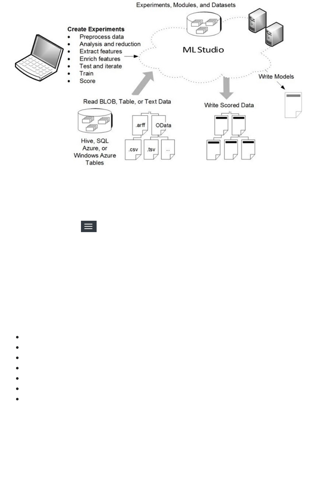
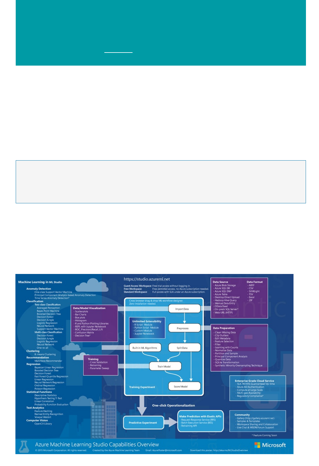
The Microsoft Azure Machine Learning Studio Capabilities Overview diagram gives you a high-level
overview of how you can use Machine Learning Studio to develop a predictive analytics model and operationalize
it in the Azure cloud.
Azure Machine Learning Studio has available a large number of machine learning algorithms, along with modules
that help with data input, output, preparation, and visualization. Using these components you can develop a
predictive analytics experiment, iterate on it, and use it to train your model. Then with one click you can
operationalize your model in the Azure cloud so that it can be used to score new data.
This diagram demonstrates how all those pieces fit together.
See Machine learning algorithm cheat sheet for Microsoft Azure Machine Learning Studio for additional help in navigating
through and choosing the machine learning algorithms available in Machine Learning Studio.
Download the Microsoft Azure Machine Learning Studio Capabilities Overview diagram and get a high-
level view of the capabilities of Machine Learning Studio. To keep it nearby, you can print the diagram in tabloid
size (11 x 17 in.).
Download the diagram here: Microsoft Azure Machine Learning Studio Capabilities Overview

More help with Machine Learning Studio
NOTENOTE
For an overview of Microsoft Azure Machine Learning, see Introduction to machine learning on Microsoft
Azure
For an overview of Machine Learning Studio, see What is Azure Machine Learning Studio?.
For a detailed discussion of the machine learning algorithms available in Machine Learning Studio, see How to
choose algorithms for Microsoft Azure Machine Learning.
You can try Azure Machine Learning for free. No credit card or Azure subscription is required. Get started now.
Downloadable Infographic: Machine learning basics
with algorithm examples
3/21/2018 • 1 min to read • Edit Online
Popular algorithms in Machine Learning Studio
Download the infographic with algorithm examples
More help with algorithms for beginners and advanced users
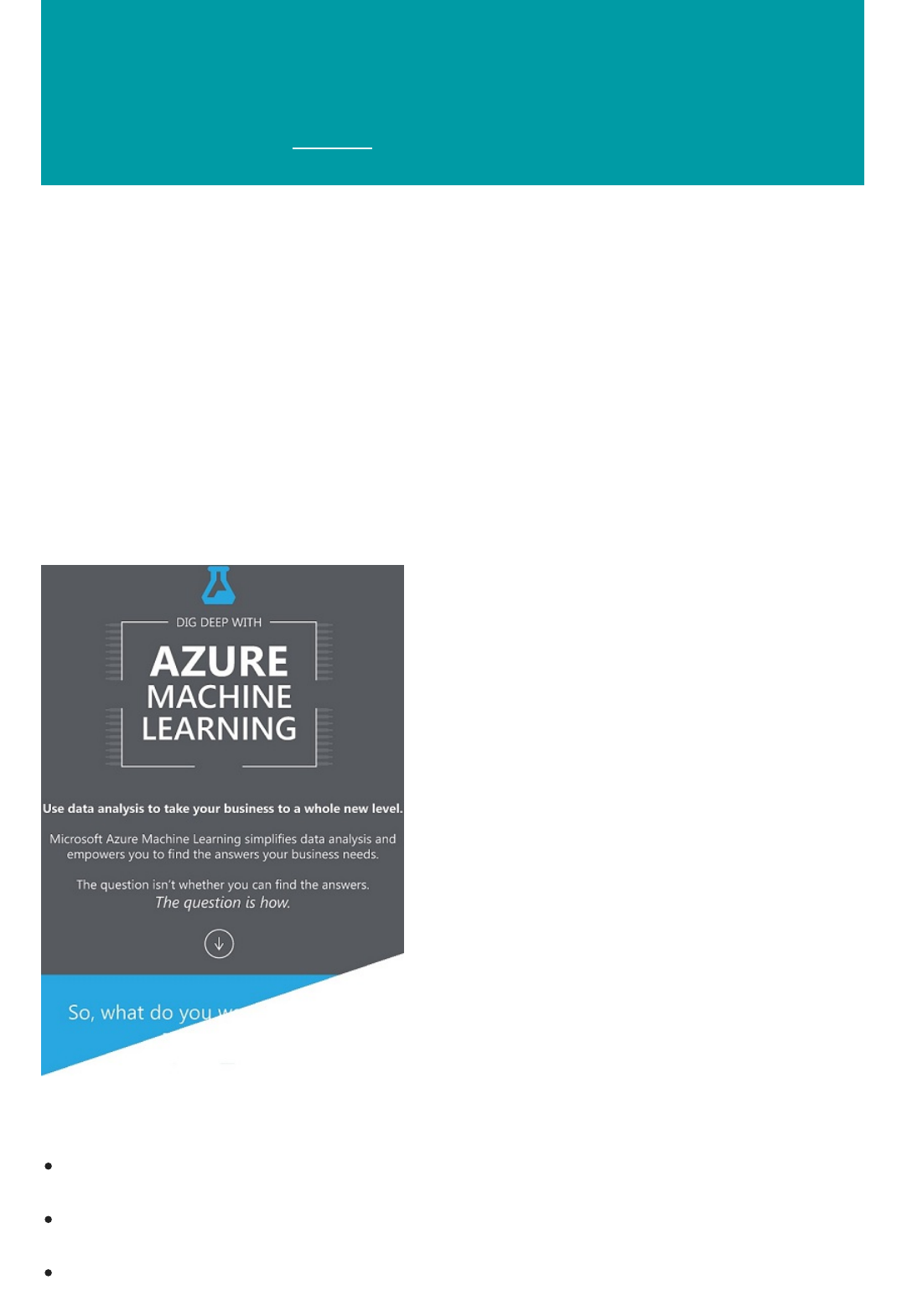
Download this easy-to-understand infographic overview of machine learning basics to learn about popular
algorithms used to answer common machine learning questions. Algorithm examples help the machine learning
beginner understand which algorithms to use and what they're used for.
Azure Machine Learning Studio comes with a large library of algorithms for predictive analytics. The infographic
identifies four popular families of algorithms - regression, anomaly detection, clustering, and classification - and
provides links to working examples in the Azure AI Gallery. The Gallery contains example experiments and
tutorials that demonstrate how these algorithms can be applied in many real-world solutions.
Download: Infographic of machine learning basics with links to algorithm examples (PDF)
For a deeper discussion of the different types of machine learning algorithms, how they're used, and how to
choose the right one for your solution, see How to choose algorithms for Microsoft Azure Machine Learning.
For a list by category of all the machine learning algorithms available in Machine Learning Studio, see Initialize
Model in the Machine Learning Studio Algorithm and Module Help.
For a complete alphabetical list of algorithms and modules in Machine Learning Studio, see A-Z list of Machine
Learning Studio modules in Machine Learning Studio Algorithm and Module Help.

NOTENOTE
To download and print a diagram that gives an overview of the capabilities of Machine Learning Studio, see
Overview diagram of Azure Machine Learning Studio capabilities.
For an overview of the Azure AI Gallery and the many community-generated resources available there, see
Share and discover resources in the Azure AI Gallery.
You can try Azure Machine Learning for free. No credit card or Azure subscription is required. Get started now.
Azure Machine Learning frequently asked questions:
Billing, capabilities, limitations, and support
4/25/2018 • 29 min to read • Edit Online
General questions
NOTENOTE
Here are some frequently asked questions (FAQs) and corresponding answers about Azure Machine Learning, a
cloud service for developing predictive models and operationalizing solutions through web services. These FAQs
provide questions about how to use the service, which includes the billing model, capabilities, limitations, and
support.
Have a question you can't find here?
Azure Machine Learning has a forum on MSDN where members of the data science community can ask questions
about Azure Machine Learning. The Azure Machine Learning team monitors the forum. Go to the Azure Machine
Learning Forum to search for answers or to post a new question of your own.
What is Azure Machine Learning?
Azure Machine Learning is a fully managed service that you can use to create, test, operate, and manage predictive
analytic solutions in the cloud. With only a browser, you can sign in, upload data, and immediately start machine-
learning experiments. Drag-and-drop predictive modeling, a large pallet of modules, and a library of starting
templates make common machine-learning tasks simple and quick. For more information, see the Azure Machine
Learning service overview. For an introduction to machine learning that explains key terminology and concepts,
see Introduction to Azure Machine Learning.
You can try Azure Machine Learning for free. No credit card or Azure subscription is required. Get started now.
What is Machine Learning Studio?
Machine Learning Studio is a workbench environment that you access by using a web browser. Machine Learning
Studio hosts a pallet of modules in a visual composition interface that helps you build an end-to-end, data-science
workflow in the form of an experiment.
For more information about Machine Learning Studio, see What is Machine Learning Studio?
What is the Machine Learning API service?
The Machine Learning API service enables you to deploy predictive models, like those that are built into Machine
Learning Studio, as scalable, fault-tolerant, web services. The web services that the Machine Learning API service
creates are REST APIs that provide an interface for communication between external applications and your
predictive analytics models.
For more information, see How to consume an Azure Machine Learning Web service.
Where are my Classic web services listed? Where are my New (Azure Resource Manager-based) web
services listed?
Web services created using the Classic deployment model and web services created using the New Azure
Resource Manager deployment model are listed in the Microsoft Azure Machine Learning Web Services portal.

Azure Machine Learning questions
Machine Learning Studio questions
Import and export data for Machine LearningImport and export data for Machine Learning
How large can the data set be for my modules?How large can the data set be for my modules?
Classic web services are also listed in Machine Learning Studio on the Web services tab.
What are Azure Machine Learning web services?
Machine Learning web services provide an interface between an application and a Machine Learning workflow
scoring model. An external application can use Azure Machine Learning to communicate with a Machine Learning
workflow scoring model in real time. A call to a Machine Learning web service returns prediction results to an
external application. To make a call to a web service, you pass an API key that was created when you deployed the
web service. A Machine Learning web service is based on REST, a popular architecture choice for web
programming projects.
Azure Machine Learning has two types of web services:
Request-Response Service (RRS): A low latency, highly scalable service that provides an interface to the
stateless models created and deployed by using Machine Learning Studio.
Batch Execution Service (BES): An asynchronous service that scores a batch for data records.
There are several ways to consume the REST API and access the web service. For example, you can write an
application in C#, R, or Python by using the sample code that's generated for you when you deployed the web
service.
The sample code is available on:
The Consume page for the web service in the Azure Machine Learning Web Services portal
The API Help Page in the web service dashboard in Machine Learning Studio
You can also use the sample Microsoft Excel workbook that's created for you and is available in the web service
dashboard in Machine Learning Studio.
What are the main updates to Azure Machine Learning?
For the latest updates, see What's new in Azure Machine Learning.
What data sources does Machine Learning support?
You can download data to a Machine Learning Studio experiment in three ways:
Upload a local file as a dataset
Use a module to import data from cloud data services
Import a dataset saved from another experiment
To learn more about supported file formats, see Import training data into Machine Learning Studio.
Modules in Machine Learning Studio support datasets of up to 10 GB of dense numerical data for common use
cases. If a module takes more than one input, the 10 GB value is the total of all input sizes. You can also sample
larger datasets by using queries from Hive or Azure SQL Database, or you can use Learning by Counts
preprocessing before ingestion.
The following types of data can expand to larger datasets during feature normalization and are limited to less than
10 GB:
Sparse

What are the limits for data upload?What are the limits for data upload?
ModulesModules
Data processingData processing
Categorical
Strings
Binary data
The following modules are limited to datasets less than 10 GB:
Recommender modules
Synthetic Minority Oversampling Technique (SMOTE) module
Scripting modules: R, Python, SQL
Modules where the output data size can be larger than input data size, such as Join or Feature Hashing
Cross-validation, Tune Model Hyperparameters, Ordinal Regression, and One-vs-All Multiclass, when the
number of iterations is very large
For datasets that are larger than a couple GBs, upload data to Azure Storage or Azure SQL Database, or use Azure
HDInsight rather than directly uploading from a local file.
Can I read data from Amazon S3?
If you have a small amount of data and want to expose it via an HTTP URL, then you can use the Import Data
module. For larger amounts of data, transfer it to Azure Storage first, and then use the Import Data module to
bring it into your experiment.
Is there a built-in image input capability?
You can learn about image input capability in the Import Images reference.
The algorithm, data source, data format, or data transformation operation that I am looking for isn't in
Azure Machine Learning Studio. What are my options?
You can go to the user feedback forum to see feature requests that we are tracking. Add your vote to a request if a
capability that you're looking for has already been requested. If the capability that you're looking for doesn't exist,
create a new request. You can view the status of your request in this forum, too. We track this list closely and
update the status of feature availability frequently. In addition, you can use the built-in support for R and Python to
create custom transformations when needed.
Can I bring my existing code into Machine Learning Studio?
Yes, you can bring your existing R or Python code into Machine Learning Studio, run it in the same experiment with
Azure Machine Learning learners, and deploy the solution as a web service via Azure Machine Learning. For more
information, see Extend your experiment with R and Execute Python machine learning scripts in Azure Machine
Learning Studio.
Is it possible to use something like PMML to define a model?
No, Predictive Model Markup Language (PMML) is not supported. You can use custom R and Python code to
define a module.
How many modules can I execute in parallel in my experiment?
You can execute up to four modules in parallel in an experiment.
Is there an ability to visualize data (beyond R visualizations) interactively within the experiment?
Click the output of a module to visualize the data and get statistics.
When previewing results or data in a browser, the number of rows and columns is limited. Why?

AlgorithmsAlgorithms
R moduleR module
Python modulePython module
Because large amounts of data might be sent to a browser, data size is limited to prevent slowing down Machine
Learning Studio. To visualize all the data/results, it's better to download the data and use Excel or another tool.
What existing algorithms are supported in Machine Learning Studio?
Machine Learning Studio provides state-of-the-art algorithms, such as Scalable Boosted Decision trees, Bayesian
Recommendation systems, Deep Neural Networks, and Decision Jungles developed at Microsoft Research.
Scalable open-source machine learning packages, like Vowpal Wabbit, are also included. Machine Learning Studio
supports machine learning algorithms for multiclass and binary classification, regression, and clustering. See the
complete list of Machine Learning Modules.
Do you automatically suggest the right Machine Learning algorithm to use for my data?
No, but Machine Learning Studio has various ways to compare the results of each algorithm to determine the right
one for your problem.
Do you have any guidelines on picking one algorithm over another for the provided algorithms?
See How to choose an algorithm.
Are the provided algorithms written in R or Python?
No, these algorithms are mostly written in compiled languages to provide better performance.
Are any details of the algorithms provided?
The documentation provides some information about the algorithms and parameters for tuning are described to
optimize the algorithm for your use.
Is there any support for online learning?
No, currently only programmatic retraining is supported.
Can I visualize the layers of a Neural Net Model by using the built-in module?
No.
Can I create my own modules in C# or some other language?
Currently, you can only use R to create new custom modules.
What R packages are available in Machine Learning Studio?
Machine Learning Studio supports more than 400 CRAN R packages today, and here is the current list of all
included packages. Also, see Extend your experiment with R to learn how to retrieve this list yourself. If the package
that you want is not in this list, provide the name of the package at the user feedback forum.
Is it possible to build a custom R module?
Yes, see Author custom R modules in Azure Machine Learning for more information.
Is there a REPL environment for R?
No, there is no Read-Eval-Print-Loop (REPL) environment for R in the studio.
Is it possible to build a custom Python module?
Not currently, but you can use one or more Execute Python Script modules to get the same result.

Web service
RetrainRetrain
CreateCreate
UseUse
Is there a REPL environment for Python?
You can use the Jupyter Notebooks in Machine Learning Studio. For more information, see Introducing Jupyter
Notebooks in Azure Machine Learning Studio.
How do I retrain Azure Machine Learning models programmatically?
Use the retraining APIs. For more information, see Retrain Machine Learning models programmatically. Sample
code is also available in the Microsoft Azure Machine Learning Retraining Demo.
Can I deploy the model locally or in an application that doesn't have an Internet connection?
No.
Is there a baseline latency that is expected for all web services?
See the Azure subscription limits.
When would I want to run my predictive model as a Batch Execution service versus a Request Response
service?
The Request Response service (RRS) is a low-latency, high-scale web service that is used to provide an interface to
stateless models that are created and deployed from the experimentation environment. The Batch Execution
service (BES) is a service that asynchronously scores a batch of data records. The input for BES is like data input
that RRS uses. The main difference is that BES reads a block of records from a variety of sources, such as Azure
Blob storage, Azure Table storage, Azure SQL Database, HDInsight (hive query), and HTTP sources. For more
information, see How to consume an Azure Machine Learning Web service.
How do I update the model for the deployed web service?
To update a predictive model for an already deployed service, modify and rerun the experiment that you used to
author and save the trained model. After you have a new version of the trained model available, Machine Learning
Studio asks you if you want to update your web service. For details about how to update a deployed web service,
see Deploy a Machine Learning web service.
You can also use the Retraining APIs. For more information, see Retrain Machine Learning models
programmatically. Sample code is also available in the Microsoft Azure Machine Learning Retraining Demo.
How do I monitor my web service deployed in production?
After you deploy a predictive model, you can monitor it from the Azure Machine Learning Web Services portal.
Each deployed service has its own dashboard where you can see monitoring information for that service. For more
information about how to manage your deployed web services, see Manage a Web service using the Azure
Machine Learning Web Services portal and Manage an Azure Machine Learning workspace.
Is there a place where I can see the output of my RRS/BES?
For RRS, the web service response is typically where you see the result. You can also write it to Azure Blob storage.
For BES, the output is written to a blob by default. You can also write the output to a database or table by using the
Export Data module.
Can I create web services only from models that were created in Machine Learning Studio?
No, you can also create web services directly by using Jupyter Notebooks and RStudio.

Scalability
Security and availability
Where can I find information about error codes?
See Machine Learning Module Error Codes for a list of error codes and descriptions.
What is the scalability of the web service?
Currently, the default endpoint is provisioned with 20 concurrent RRS requests per endpoint. You can scale this to
200 concurrent requests per endpoint, and you can scale each web service to 10,000 endpoints per web service as
described in Scaling a Web Service. For BES, each endpoint can process 40 requests at a time, and additional
requests beyond 40 requests are queued. These queued requests run automatically as the queue drains.
Are R jobs spread across nodes?
No.
How much data can I use for training?
Modules in Machine Learning Studio support datasets of up to 10 GB of dense numerical data for common use
cases. If a module takes more than one input, the total size for all inputs is 10 GB. You can also sample larger
datasets via Hive queries, via Azure SQL Database queries, or by preprocessing with Learning with Counts
modules before ingestion.
The following types of data can expand to larger datasets during feature normalization and are limited to less than
10 GB:
Sparse
Categorical
Strings
Binary data
The following modules are limited to datasets less than 10 GB:
Recommender modules
Synthetic Minority Oversampling Technique (SMOTE) module
Scripting modules: R, Python, SQL
Modules where the output data size can be larger than input data size, such as Join or Feature Hashing
Cross-Validate, Tune Model Hyperparameters, Ordinal Regression, and One-vs-All Multiclass, when number of
iterations is very large
For datasets that are larger than a few GBs, upload data to Azure Storage or Azure SQL Database, or use
HDInsight rather than directly uploading from a local file.
Are there any vector size limitations?
Rows and columns are each limited to the .NET limitation of Max Int: 2,147,483,647.
Can I adjust the size of the virtual machine that runs the web service?
No.
Who can access the http endpoint for the web service by default? How do I restrict access to the
endpoint?
After a web service is deployed, a default endpoint is created for that service. The default endpoint can be called by

Support and training
Billing questions
using its API key. You can add more endpoints with their own keys from the Web Services portal or
programmatically by using the Web Service Management APIs. Access keys are needed to make calls to the web
service. For more information, see How to consume an Azure Machine Learning Web service.
What happens if my Azure storage account can't be found?
Machine Learning Studio relies on a user-supplied Azure storage account to save intermediary data when it
executes the workflow. This storage account is provided to Machine Learning Studio when a workspace is created.
After the workspace is created, if the storage account is deleted and can no longer be found, the workspace will
stop functioning, and all experiments in that workspace will fail.
If you accidentally deleted the storage account, recreate the storage account with the same name in the same
region as the deleted storage account. After that, resync the access key.
What happens if my storage account access key is out of sync?
Machine Learning Studio relies on a user-supplied Azure storage account to store intermediary data when it
executes the workflow. This storage account is provided to Machine Learning Studio when a workspace is created,
and the access keys are associated with that workspace. If the access keys are changed after the workspace is
created, the workspace can no longer access the storage account. It will stop functioning and all experiments in that
workspace will fail.
If you changed storage account access keys, resync the access keys in the workspace by using the Azure portal.
Where can I get training for Azure Machine Learning?
The Azure Machine Learning Documentation Center hosts video tutorials and how-to guides. These step-by-step
guides introduce the services and explain the data science life cycle of importing data, cleaning data, building
predictive models, and deploying them in production by using Azure Machine Learning.
We add new material to the Machine Learning Center on an ongoing basis. You can submit requests for additional
learning material on Machine Learning Center at the user feedback forum.
You can also find training at Microsoft Virtual Academy.
How do I get support for Azure Machine Learning?
To get technical support for Azure Machine Learning, go to Azure Support, and select Machine Learning.
Azure Machine Learning also has a community forum on MSDN where you can ask questions about Azure
Machine Learning. The Azure Machine Learning team monitors the forum. Go to Azure Forum.
How does Machine Learning billing work?
Azure Machine Learning has two components: Machine Learning Studio and Machine Learning web services.
While you are evaluating Machine Learning Studio, you can use the Free billing tier. The Free tier also lets you
deploy a Classic web service that has limited capacity.
If you decide that Azure Machine Learning meets your needs, you can sign up for the Standard tier. To sign up, you
must have a Microsoft Azure subscription.
In the Standard tier, you are billed monthly for each workspace that you define in Machine Learning Studio. When
you run an experiment in the studio, you are billed for compute resources when you are running an experiment.
When you deploy a Classic web service, transactions and compute hours are billed on the Pay As You Go basis.

NOTENOTE
New (Resource Manager-based) web services introduce billing plans that allow for more predictability in costs.
Tiered pricing offers discounted rates to customers who need a large amount of capacity.
When you create a plan, you commit to a fixed cost that comes with an included quantity of API compute hours
and API transactions. If you need more included quantities, you can add instances to your plan. If you need a lot
more included quantities, you can choose a higher tier plan that provides considerably more included quantities
and a better discounted rate.
After the included quantities in existing instances are used up, additional usage is charged at the overage rate that's
associated with the billing plan tier.
Included quantities are reallocated every 30 days, and unused included quantities do not roll over to the next period.
For additional billing and pricing information, see Machine Learning Pricing.
Does Machine Learning have a free trial?
Azure Machine Learning has a free subscription option that's explained in Machine Learning Pricing. Machine
Learning Studio has an eight-hour quick evaluation trial that's available when you sign in to Machine Learning
Studio.
In addition, when you sign up for an Azure free trial, you can try any Azure services for a month. To learn more
about the Azure free trial, visit Azure free trial FAQ.
What is a transaction?
A transaction represents an API call that Azure Machine Learning responds to. Transactions from Request-
Response Service (RRS) and Batch Execution Service (BES) calls are aggregated and charged against your billing
plan.
Can I use the included transaction quantities in a plan for both RRS and BES transactions?
Yes, your transactions from your RRS and BES are aggregated and charged against your billing plan.
What is an API compute hour?
An API compute hour is the billing unit for the time that API calls take to run by using Machine Learning compute
resources. All your calls are aggregated for billing purposes.
How long does a typical production API call take?
Production API call times can vary significantly, generally ranging from hundreds of milliseconds to a few seconds.
Some API calls might require minutes depending on the complexity of the data processing and machine-learning
model. The best way to estimate production API call times is to benchmark a model on the Machine Learning
service.
What is a Studio compute hour?
A Studio compute hour is the billing unit for the aggregate time that your experiments use compute resources in
studio.
In New (Azure Resource Manager-based) web services, what is the Dev/Test tier meant for?
Resource Manager-based web services provide multiple tiers that you can use to provision your billing plan. The
Dev/Test pricing tier provides limited, included quantities that allow you to test your experiment as a web service
without incurring costs. You have the opportunity to see how it works.
Are there separate storage charges?
Management of New (Resource Manager-based) web servicesManagement of New (Resource Manager-based) web services
NOTENOTE
NOTENOTE
NOTENOTE
Sign up for New (Resource Manager-based) web services plansSign up for New (Resource Manager-based) web services plans
The Machine Learning Free tier does not require or allow separate storage. The Machine Learning Standard tier
requires users to have an Azure storage account. Azure Storage is billed separately.
Does Machine Learning support high availability?
Yes. For details, see Machine Learning Pricing for a description of the service level agreement (SL A).
What specific kind of compute resources will my production API calls be run on?
The Machine Learning service is a multitenant service. Actual compute resources that are used on the back end
vary and are optimized for performance and predictability.
What happens if I delete my plan?
The plan is removed from your subscription, and you are billed for prorated usage.
You cannot delete a plan that a web service is using. To delete the plan, you must either assign a new plan to the web service
or delete the web service.
What is a plan instance?
A plan instance is a unit of included quantities that you can add to your billing plan. When you select a billing tier
for your billing plan, it comes with one instance. If you need more included quantities, you can add instances of the
selected billing tier to your plan.
How many plan instances can I add?
You can have one instance of the Dev/Test pricing tier in a subscription.
For Standard S1, Standard S2, and Standard S3 tiers, you can add as many as necessary.
Depending on your anticipated usage, it might be more cost effective to upgrade to a tier that has more included quantities
rather than add instances to the current tier.
What happens when I change plan tiers (upgrade / downgrade)?
The old plan is deleted and the current usage is billed on a prorated basis. A new plan with the full included
quantities of the upgraded/downgraded tier is created for the rest of the period.
Included quantities are allocated per period, and unused quantities do not roll over.
What happens when I increase the instances in a plan?
Quantities are included on a prorated basis and may take 24 hours to be effective.
What happens when I delete an instance of a plan?
The instance is removed from your subscription, and you are billed for prorated usage.
How do I sign up for a plan?

New web services: OveragesNew web services: Overages
You have two ways to create billing plans.
When you first deploy a Resource Manager-based web service, you can choose an existing plan or create a new
plan.
Plans that you create in this manner are in your default region, and your web service will be deployed to that
region.
If you want to deploy services to regions other than your default region, you may want to define your billing plans
before you deploy your service.
In that case, you can sign in to the Azure Machine Learning Web Services portal, and go to the Plans page. From
there, you can add plans, delete plans, and modify existing plans.
Which plan should I choose to start off with?
We recommend you that you start with the Standard S1 tier and monitor your service for usage. If you find that
you are using your included quantities rapidly, you can add instances or move to a higher tier and get better
discounted rates. You can adjust your billing plan as needed throughout your billing cycle.
Which regions are the new plans available in?
The new billing plans are available in the three production regions in which we support the new web services:
South Central US
West Europe
South East Asia
I have web services in multiple regions. Do I need a plan for every region?
Yes. Plan pricing varies by region. When you deploy a web service to another region, you need to assign it a plan
that is specific to that region. For more information, see Products available by region.
How do I check if I exceeded my web service usage?
You can view the usage on all your plans on the Plans page in the Azure Machine Learning Web Services portal.
Sign in to the portal, and then click the Plans menu option.
In the Transactions and Compute columns of the table, you can see the included quantities of the plan and the
percentage used.
What happens when I use up the include quantities in the Dev/Test pricing tier?
Services that have a Dev/Test pricing tier assigned to them are stopped until the next period or until you move
them to a paid tier.
For Classic web services and overages of New (Resource Manager-based) web services, how are prices
calculated for Request Response (RRS) and Batch (BES) workloads?
For an RRS workload, you are charged for every API transaction call that you make and for the compute time
that's associated with those requests. Your RRS production API transaction costs are calculated as the total number
of API calls that you make multiplied by the price per 1,000 transactions (prorated by individual transaction). Your
RRS API production API compute hour costs are calculated as the amount of time required for each API call to run,
multiplied by the total number of API transactions, multiplied by the price per production API compute hour.
For example, for Standard S1 overage, 1,000,000 API transactions that take 0.72 seconds each to run would result
in (1,000,000 * $0.50/1K API transactions) in $500 in production API transaction costs and (1,000,000 * 0.72 sec *
$2/hr) $400 in production API compute hours, for a total of $900.

Azure Machine Learning Classic web servicesAzure Machine Learning Classic web services
Azure Machine Learning Free and Standard tierAzure Machine Learning Free and Standard tier
For a BES workload, you are charged in the same manner. However, the API transaction costs represent the
number of batch jobs that you submit, and the compute costs represent the compute time that's associated with
those batch jobs. Your BES production API transaction costs are calculated as the total number of jobs submitted
multiplied by the price per 1,000 transactions (prorated by individual transaction). Your BES API production API
compute hour costs are calculated as the amount of time required for each row in your job to run multiplied by the
total number of rows in your job multiplied by the total number of jobs multiplied by the price per production API
compute hour. When you use the Machine Learning calculator, the transaction meter represents the number of jobs
that you plan to submit, and the time-per-transaction field represents the combined time that's needed for all rows
in each job to run.
For example, assume Standard S1 overage, and you submit 100 jobs per day that each consist of 500 rows that
take 0.72 seconds each. Your monthly overage costs would be (100 jobs per day = 3,100 jobs/mo * $0.50/1K API
transactions) $1.55 in production API transaction costs and (500 rows * 0.72 sec * 3,100 Jobs * $2/hr) $620 in
production API compute hours, for a total of $621.55.
Is Pay As You Go still available?
Yes, Classic web services are still available in Azure Machine Learning.
What is included in the Azure Machine Learning Free tier?
The Azure Machine Learning Free tier is intended to provide an in-depth introduction to the Azure Machine
Learning Studio. All you need is a Microsoft account to sign up. The Free tier includes free access to one Azure
Machine Learning Studio workspace per Microsoft account. In this tier, you can use up to 10 GB of storage and
operationalize models as staging APIs. Free tier workloads are not covered by an SL A and are intended for
development and personal use only.
Free tier workspaces have the following limitations:
Workloads can't access data by connecting to an on-premises server that runs SQL Server.
You cannot deploy New Resource Manager base web services.
What is included in the Azure Machine Learning Standard tier and plans?
The Azure Machine Learning Standard tier is a paid production version of Azure Machine Learning Studio. The
Azure Machine Learning Studio monthly fee is billed on a per workspace per month basis and prorated for partial
months. Azure Machine Learning Studio experiment hours are billed per compute hour for active experimentation.
Billing is prorated for partial hours.
The Azure Machine Learning API service is billed depending on whether it's a Classic web service or a New
(Resource Manager-based) web service.
The following charges are aggregated per workspace for your subscription.
Machine Learning Workspace Subscription: The Machine Learning workspace subscription is a monthly fee that
provides access to a Machine Learning Studio workspace. The subscription is required to run experiments in the
studio and to utilize the production APIs.
Studio Experiment hours: This meter aggregates all compute charges that are accrued by running experiments
in Machine Learning Studio and running production API calls in the staging environment.
Access data by connecting to an on-premises server that runs SQL Server in your models for your training and
scoring.
For Classic web services:
Production API Compute Hours: This meter includes compute charges that are accrued by web services
running in production.

Production API Transactions (in 1000s): This meter includes charges that are accrued per call to your
production web service.
Apart from the preceding charges, in the case of Resource Manager-based web service, charges are aggregated to
the selected plan:
Standard S1/S2/S3 API Plan (Units): This meter represents the type of instance that's selected for Resource
Manager-based web services.
Standard S1/S2/S3 Overage API Compute Hours: This meter includes compute charges that are accrued by
Resource Manager-based web services that run in production after the included quantities in existing instances
are used up. The additional usage is charged at the overate rate that's associated with S1/S2/S3 plan tier.
Standard S1/S2/S3 Overage API Transactions (in 1,000s): This meter includes charges that are accrued per call
to your production Resource Manager-based web service after the included quantities in existing instances are
used up. The additional usage is charged at the overate rate associated with S1/S2/S3 plan tier.
Included Quantity API Compute Hours: With Resource Manager-based web services, this meter represents the
included quantity of API compute hours.
Included Quantity API Transactions (in 1,000s): With Resource Manager-based web services, this meter
represents the included quantity of API transactions.
How do I sign up for Azure Machine Learning Free tier?
All you need is a Microsoft account. Go to Azure Machine Learning home, and then click Start Now. Sign in with
your Microsoft account and a workspace in Free tier is created for you. You can start to explore and create Machine
Learning experiments right away.
How do I sign up for Azure Machine Learning Standard tier?
You must first have access to an Azure subscription to create a Standard Machine Learning workspace. You can
sign up for a 30-day free trial Azure subscription and later upgrade to a paid Azure subscription, or you can
purchase a paid Azure subscription outright. You can then create a Machine Learning workspace from the
Microsoft Azure portal after you gain access to the subscription. View the step-by-step instructions.
Alternatively, you can be invited by a Standard Machine Learning workspace owner to access the owner's
workspace.
Can I specify my own Azure Blob storage account to use with the Free tier?
No, the Standard tier is equivalent to the version of the Machine Learning service that was available before the
tiers were introduced.
Can I deploy my machine learning models as APIs in the Free tier?
Yes, you can operationalize machine learning models to staging API services as part of the Free tier. To put the
staging API service into production and get a production endpoint for the operationalized service, you must use
the Standard tier.
What is the difference between Azure free trial and Azure Machine Learning Free tier?
The Microsoft Azure free trial offers credits that you can apply to any Azure service for one month. The Azure
Machine Learning Free tier offers continuous access specifically to Azure Machine Learning for non-production
workloads.
How do I move an experiment from the Free tier to the Standard tier?
To copy your experiments from the Free tier to the Standard tier:
1. Sign in to Azure Machine Learning Studio, and make sure that you can see both the Free workspace and the
Standard workspace in the workspace selector in the top navigation bar.

Studio workspaceStudio workspace
Guest AccessGuest Access
2. Switch to Free workspace if you are in the Standard workspace.
3. In the experiment list view, select an experiment that you'd like to copy, and then click the Copy command
button.
4. Select the Standard workspace from the dialog box that opens, and then click the Copy button. All the
associated datasets, trained model, etc. are copied together with the experiment into the Standard workspace.
5. You need to rerun the experiment and republish your web service in the Standard workspace.
Will I see different bills for different workspaces?
Workspace charges are broken out separately for each applicable meter on a single bill.
What specific kind of compute resources will my experiments be run on?
The Machine Learning service is a multitenant service. Actual compute resources that are used on the back end
vary and are optimized for performance and predictability.
What is Guest Access to Azure Machine Learning Studio?
Guest Access is a restricted trial experience. You can create and run experiments in Azure Machine Learning Studio
at no cost and without authentication. Guest sessions are non-persistent (cannot be saved) and limited to eight
hours. Other limitations include lack of support for R and Python, lack of staging APIs, and restricted dataset size
and storage capacity. By comparison, users who choose to sign in with a Microsoft account have full access to the
Free tier of Machine Learning Studio that's described previously, which includes a persistent workspace and more
comprehensive capabilities. To choose your free Machine Learning experience, click Get started on
https://studio.azureml.net, and then select Guess Access or sign in with a Microsoft account.

What's New in Azure Machine Learning
3/21/2018 • 1 min to read • Edit Online
The March 2017 release of Microsoft Azure Machine Learning updates provides the following feature:The March 2017 release of Microsoft Azure Machine Learning updates provides the following feature:
The August 2016 release of Microsoft Azure Machine Learning updates provide the following features:The August 2016 release of Microsoft Azure Machine Learning updates provide the following features:
The July 2016 release of Microsoft Azure Machine Learning updates provide the following features:The July 2016 release of Microsoft Azure Machine Learning updates provide the following features:
Dedicated Capacity for Azure Machine Learning BES Jobs
Machine Learning Batch Pool processing uses the Azure Batch service to provide customer-managed scale
for the Azure Machine Learning Batch Execution Service. Batch Pool processing allows you to create Azure
Batch pools on which you can submit batch jobs and have them execute in a predictable manner.
For more information, see Azure Batch service for Machine Learning jobs.
Classic Web services can now be managed in the new Microsoft Azure Machine Learning Web Services portal
that provides one place to manage all aspects of your Web service.
Which provides web service usage statistics.
Simplifies testing of Azure Machine Learning Remote-Request calls using sample data.
Provides a new Batch Execution Service test page with sample data and job submission history.
Provides easier endpoint management.
Web services are now managed as Azure resources managed through Azure Resource Manager interfaces,
allowing for the following enhancements:
Incorporates a new subscription-based, multi-region web service deployment model using Resource Manager
based APIs leveraging the Resource Manager Resource Provider for Web Services.
Introduces new pricing plans and plan management capabilities using the new Resource Manager RP for
Billing.
Provides web service usage statistics.
Simplifies testing of Azure Machine Learning Remote-Request calls using sample data.
Provides a new Batch Execution Service test page with sample data and job submission history.
There are new REST APIs to deploy and manage your Resource Manager based Web services.
There is a new Microsoft Azure Machine Learning Web Services portal that provides one place to
manage all aspects of your Web service.
You can now deploy your web service to multiple regions without needing to create a subscription in
each region.
In addition, the Machine Learning Studio has been updated to allow you to deploy to the new Web service model
or continue to deploy to the classic Web service model.
Machine learning tutorial: Create your first data
science experiment in Azure Machine Learning
Studio
4/9/2018 • 16 min to read • Edit Online
NOTENOTE
NOTENOTE
How does Machine Learning Studio help?
If you've never used Azure Machine Learning Studio before, this tutorial is for you.
In this tutorial, we'll walk through how to use Studio for the first time to create a machine learning experiment.
The experiment will test an analytical model that predicts the price of an automobile based on different variables
such as make and technical specifications.
This tutorial shows you the basics of how to drag-and-drop modules onto your experiment, connect them together, run
the experiment, and look at the results. We're not going to discuss the general topic of machine learning or how to select
and use the 100+ built-in algorithms and data manipulation modules included in Studio.
If you're new to machine learning, the video series Data Science for Beginners might be a good place to start. This video
series is a great introduction to machine learning using everyday language and concepts.
If you're familiar with machine learning, but you're looking for more general information about Machine Learning Studio,
and the machine learning algorithms it contains, here are some good resources:
What is Machine Learning Studio? - This is a high-level overview of Studio.
Machine learning basics with algorithm examples - This infographic is useful if you want to learn more about the
different types of machine learning algorithms included with Machine Learning Studio.
Machine Learning Guide - This guide covers similar information as the infographic above, but in an interactive format.
Machine learning algorithm cheat sheet and How to choose algorithms for Microsoft Azure Machine Learning - This
downloadable poster and accompanying article discuss the Studio algorithms in depth.
Machine Learning Studio: Algorithm and Module Help - This is the complete reference for all Studio modules, including
machine learning algorithms,
You can try Azure Machine Learning for free. No credit card or Azure subscription is required. Get started now.
Machine Learning Studio makes it easy to set up an experiment using drag-and-drop modules preprogrammed
with predictive modeling techniques.
Using an interactive, visual workspace, you drag-and-drop datasets and analysis modules onto an interactive
canvas. You connect them together to form an experiment that you run in Machine Learning Studio. You create
a model, train the model, and score and test the model.
You can iterate on your model design, editing the experiment and running it until it gives you the results you're
looking for. When your model is ready, you can publish it as a web service so that others can send it new data
and get predictions in return.
Open Machine Learning Studio
Five steps to create an experiment
TIPTIP
Step 1: Get data
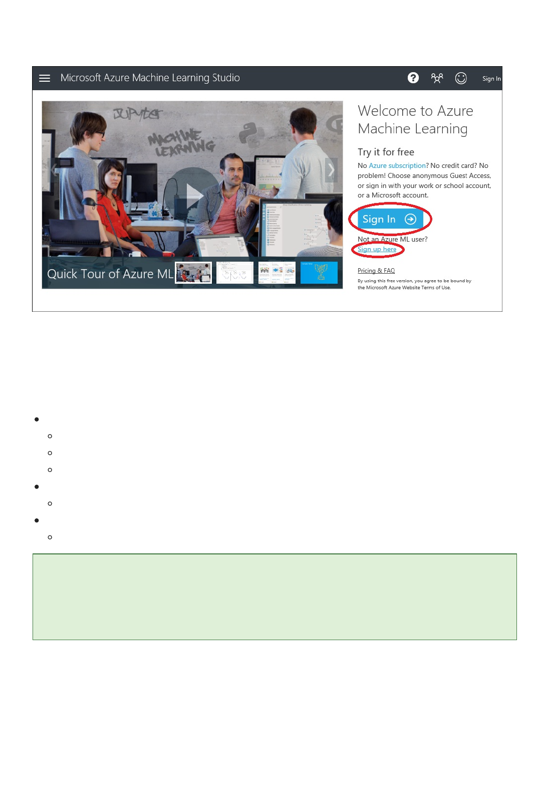
To get started with Studio, go to https://studio.azureml.net. If you’ve signed into Machine Learning Studio before,
click Sign In. Otherwise, click Sign up here and choose between free and paid options.
Sign in to Machine Learning Studio
In this machine learning tutorial, you'll follow five basic steps to build an experiment in Machine Learning Studio
to create, train, and score your model:
Create a model
Train the model
Score and test the model
Step 1: Get data
Step 2: Prepare the data
Step 3: Define features
Step 4: Choose and apply a learning algorithm
Step 5: Predict new automobile prices
You can find a working copy of the following experiment in the Azure AI Gallery. Go to Your first data science
experiment - Automobile price prediction and click Open in Studio to download a copy of the experiment into your
Machine Learning Studio workspace.
The first thing you need to perform machine learning is data. There are several sample datasets included with
Machine Learning Studio that you can use, or you can import data from many sources. For this example, we'll
use the sample dataset, Automobile price data (Raw), that's included in your workspace. This dataset includes
entries for various individual automobiles, including information such as make, model, technical specifications,
and price.
Here's how to get the dataset into your experiment.
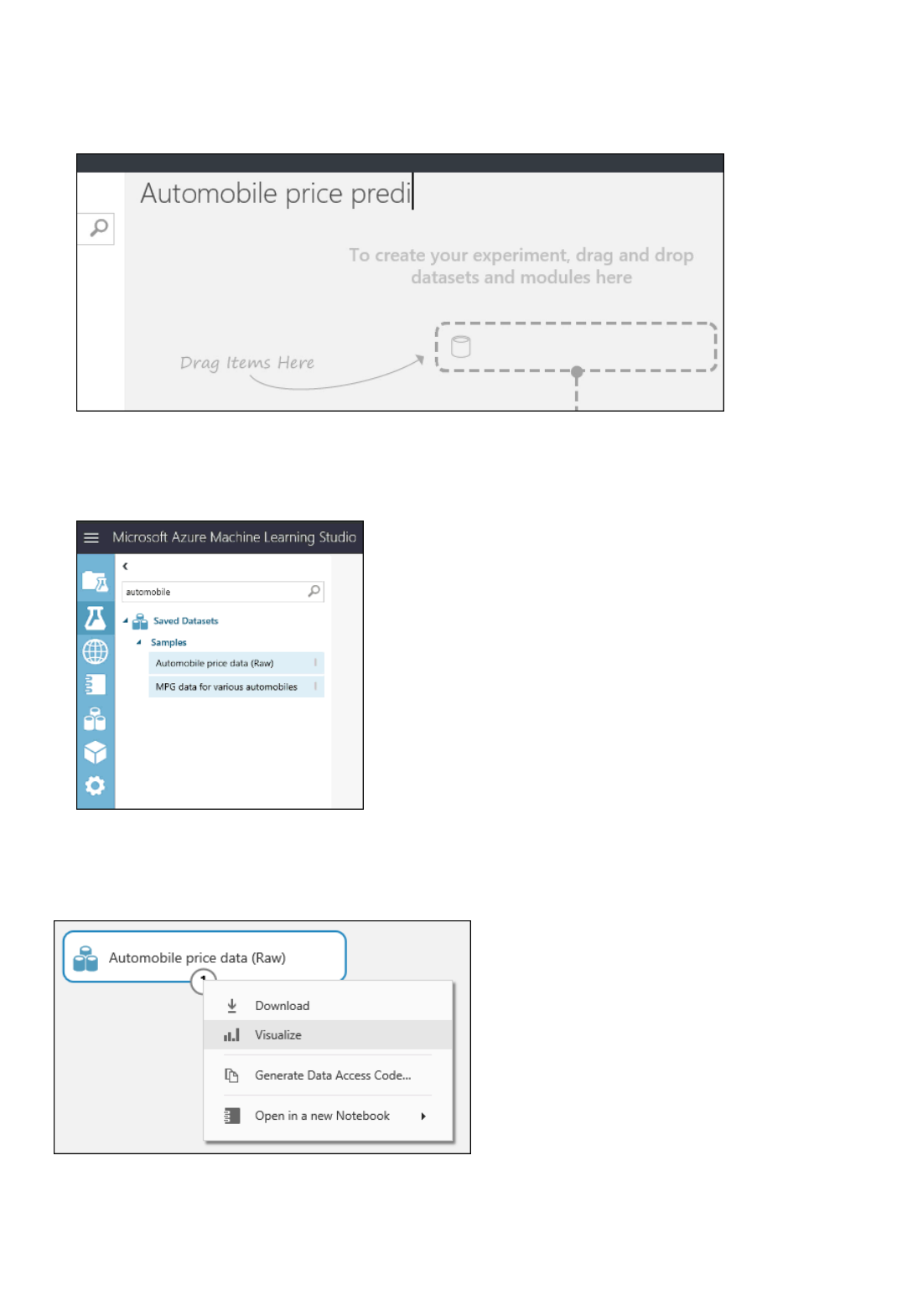
1. Create a new experiment by clicking +NEW at the bottom of the Machine Learning Studio window, select
EXPERIMENT, and then select Blank Experiment.
2. The experiment is given a default name that you can see at the top of the canvas. Select this text and
rename it to something meaningful, for example, Automobile price prediction. The name doesn't need
to be unique.
3. To the left of the experiment canvas is a palette of datasets and modules. Type automobile in the Search
box at the top of this palette to find the dataset labeled Automobile price data (Raw). Drag this dataset
to the experiment canvas.
Find the automobile dataset and drag it onto the experiment canvas
To see what this data looks like, click the output port at the bottom of the automobile dataset, and then select
Visualize.
Click the output port and select "Visualize"
TIPTIP
Step 2: Prepare the data
TIPTIP
Datasets and modules have input and output ports represented by small circles - input ports at the top, output ports at
the bottom. To create a flow of data through your experiment, you'll connect an output port of one module to an input
port of another. At any time, you can click the output port of a dataset or module to see what the data looks like at that
point in the data flow.
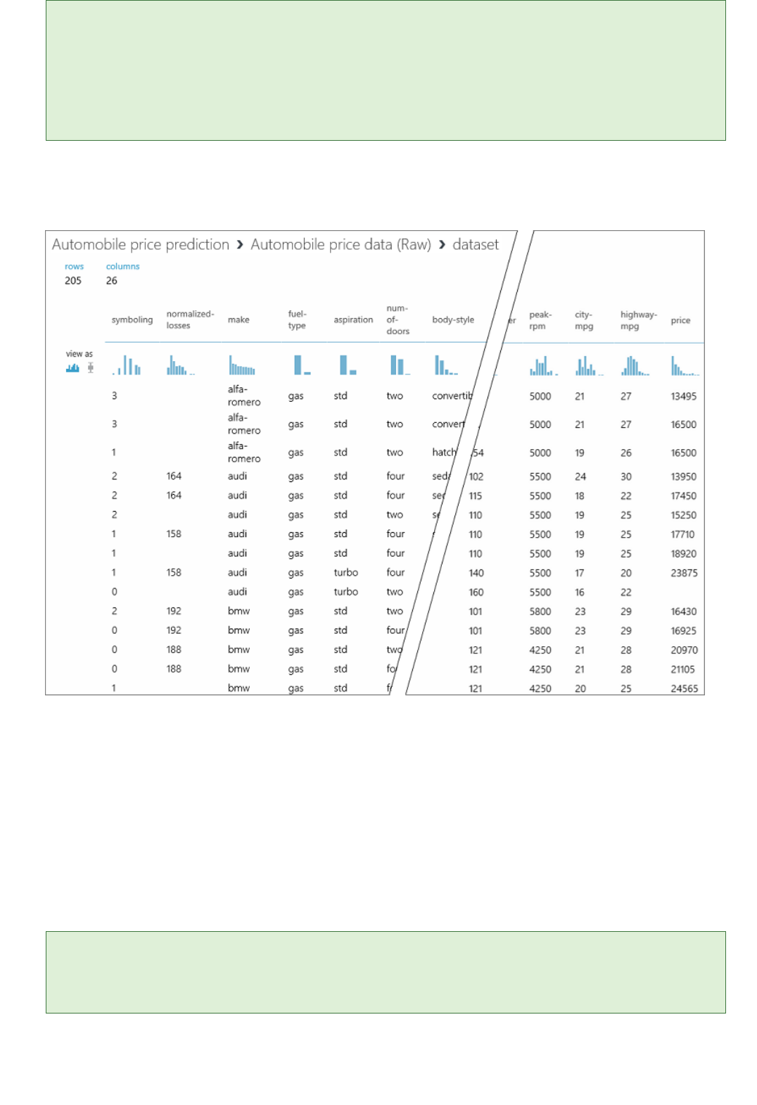
In this sample dataset, each instance of an automobile appears as a row, and the variables associated with each
automobile appear as columns. Given the variables for a specific automobile, we're going to try to predict the
price in far-right column (column 26, titled "price").
View the automobile data in the data visualization window
Close the visualization window by clicking the "x" in the upper-right corner.
A dataset usually requires some preprocessing before it can be analyzed. For example, you might have noticed
the missing values present in the columns of various rows. These missing values need to be cleaned so the
model can analyze the data correctly. In our case, we'll remove any rows that have missing values. Also, the
normalized-losses column has a large proportion of missing values, so we'll exclude that column from the
model altogether.
Cleaning the missing values from input data is a prerequisite for using most of the modules.
First we add a module that removes the normalized-losses column completely, and then we add another
module that removes any row that has missing data.
1. Type select columns in the Search box at the top of the module palette to find the Select Columns in
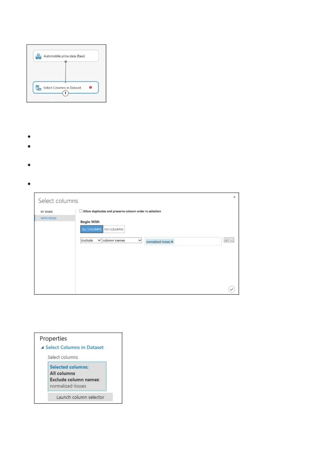
Dataset module, then drag it to the experiment canvas. This module allows us to select which columns of
data we want to include or exclude in the model.
2. Connect the output port of the Automobile price data (Raw) dataset to the input port of the Select
Columns in Dataset module.
Add the "Select Columns in Dataset" module to the experiment canvas and connect it
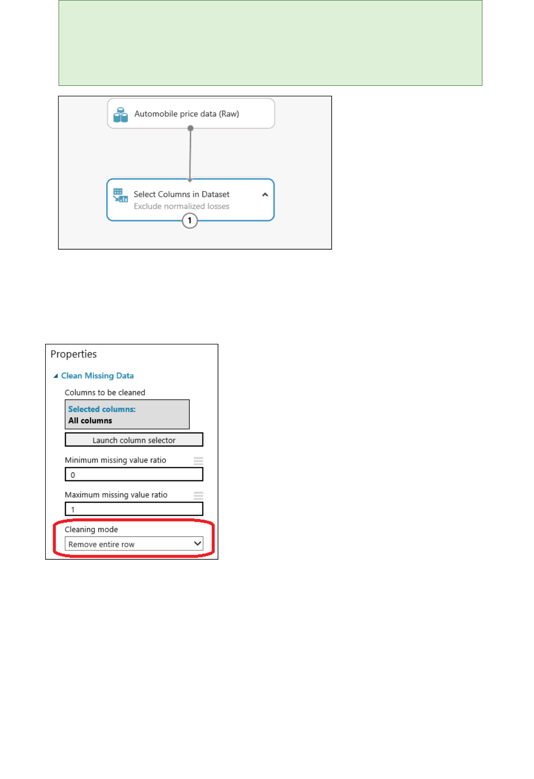
3. Click the Select Columns in Dataset module and click Launch column selector in the Properties pane.
On the left, click With rules
Under Begin With, click All columns. This directs Select Columns in Dataset to pass through all the
columns (except those columns we're about to exclude).
From the drop-downs, select Exclude and column names, and then click inside the text box. A list of
columns is displayed. Select normalized-losses, and it's added to the text box.
Click the check mark (OK) button to close the column selector (on the lower-right).
Launch the column selector and exclude the "normalized-losses" column
Now the properties pane for Select Columns in Dataset indicates that it will pass through all
columns from the dataset except normalized-losses.
The properties pane shows that the "normalized-losses" column is excluded
TIPTIP
You can add a comment to a module by double-clicking the module and entering text. This can help you
see at a glance what the module is doing in your experiment. In this case double-click the Select Columns in
Dataset module and type the comment "Exclude normalized losses."
Double-click a module to add a comment
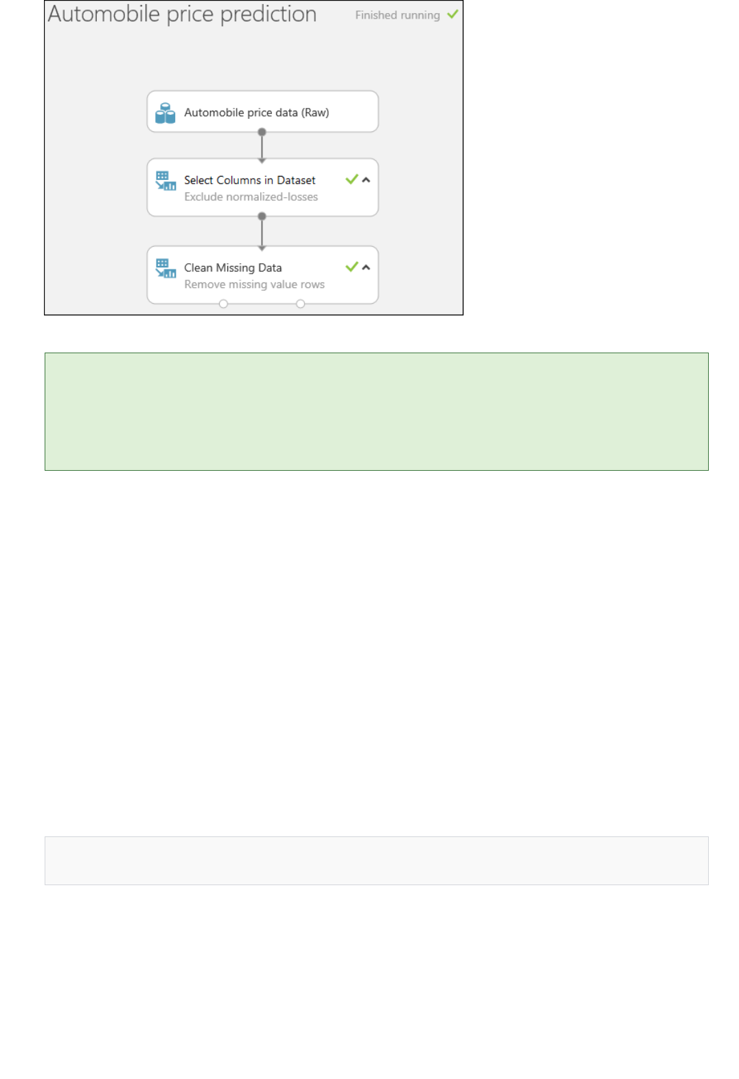
4. Drag the Clean Missing Data module to the experiment canvas and connect it to the Select Columns in
Dataset module. In the Properties pane, select Remove entire row under Cleaning mode. This directs
Clean Missing Data to clean the data by removing rows that have any missing values. Double-click the
module and type the comment "Remove missing value rows."
Set the cleaning mode to "Remove entire row" for the "Clean Missing Data" module
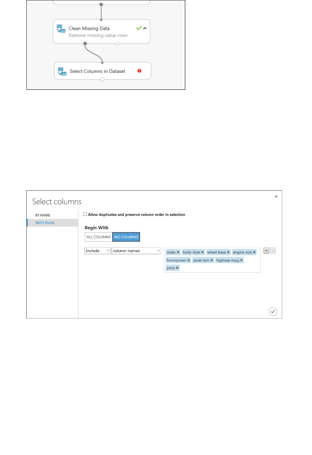
5. Run the experiment by clicking RUN at the bottom of the page.
When the experiment has finished running, all the modules have a green check mark to indicate that they
finished successfully. Notice also the Finished running status in the upper-right corner.
TIPTIP
Step 3: Define features
make, body-style, wheel-base, engine-size, horsepower, peak-rpm, highway-mpg, price
After running it, the experiment should look something like this
Why did we run the experiment now? By running the experiment, the column definitions for our data pass from the
dataset, through the Select Columns in Dataset module, and through the Clean Missing Data module. This means that any
modules we connect to Clean Missing Data will also have this same information.
All we have done in the experiment up to this point is clean the data. If you want to view the cleaned dataset, click
the left output port of the Clean Missing Data module and select Visualize. Notice that the normalized-losses
column is no longer included, and there are no missing values.
Now that the data is clean, we're ready to specify what features we're going to use in the predictive model.
In machine learning, features are individual measurable properties of something you’re interested in. In our
dataset, each row represents one automobile, and each column is a feature of that automobile.
Finding a good set of features for creating a predictive model requires experimentation and knowledge about the
problem you want to solve. Some features are better for predicting the target than others. Also, some features
have a strong correlation with other features and can be removed. For example, city-mpg and highway-mpg are
closely related so we can keep one and remove the other without significantly affecting the prediction.
Let's build a model that uses a subset of the features in our dataset. You can come back later and select different
features, run the experiment again, and see if you get better results. But to start, let's try the following features:
1. Drag another Select Columns in Dataset module to the experiment canvas. Connect the left output port of
the Clean Missing Data module to the input of the Select Columns in Dataset module.
Step 4: Choose and apply a learning algorithm
Connect the "Select Columns in Dataset" module to the "Clean Missing Data" module
2. Double-click the module and type "Select features for prediction."
3. Click Launch column selector in the Properties pane.
4. Click With rules.
5. Under Begin With, click No columns. In the filter row, select Include and column names and select
our list of column names in the text box. This directs the module to not pass through any columns
(features) except the ones that we specify.
6. Click the check mark (OK) button.
Select the columns (features) to include in the prediction
This produces a filtered dataset containing only the features we want to pass to the learning algorithm we'll use
in the next step. Later, you can return and try again with a different selection of features.
Now that the data is ready, constructing a predictive model consists of training and testing. We'll use our data to
train the model, and then we'll test the model to see how closely it's able to predict prices.
Classification and regression are two types of supervised machine learning algorithms. Classification predicts an
answer from a defined set of categories, such as a color (red, blue, or green). Regression is used to predict a
number.
Because we want to predict price, which is a number, we'll use a regression algorithm. For this example, we'll use
a simple linear regression model.
TIPTIP
If you want to learn more about different types of machine learning algorithms and when to use them, you might view the
first video in the Data Science for Beginners series, The five questions data science answers. You might also look at the
infographic Machine learning basics with algorithm examples, or check out the Machine learning algorithm cheat sheet.
We train the model by giving it a set of data that includes the price. The model scans the data and look for
correlations between an automobile's features and its price. Then we'll test the model - we'll give it a set of
features for automobiles we're familiar with and see how close the model comes to predicting the known price.
We'll use our data for both training the model and testing it by splitting the data into separate training and
testing datasets.
TIPTIP
1. Select and drag the Split Data module to the experiment canvas and connect it to the last Select Columns
in Dataset module.
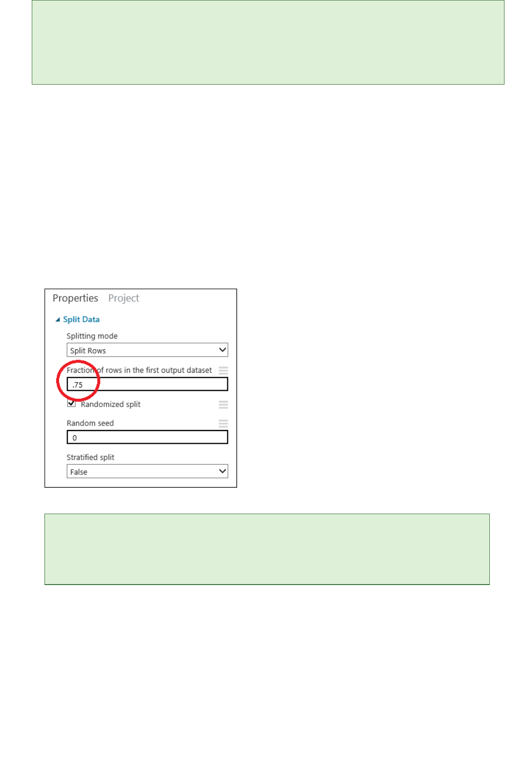
2. Click the Split Data module to select it. Find the Fraction of rows in the first output dataset (in the
Properties pane to the right of the canvas) and set it to 0.75. This way, we'll use 75 percent of the data to
train the model, and hold back 25 percent for testing (later, you can experiment with using different
percentages).
Set the split fraction of the "Split Data" module to 0.75
By changing the Random seed parameter, you can produce different random samples for training and testing.
This parameter controls the seeding of the pseudo-random number generator.
3. Run the experiment. When the experiment is run, the Select Columns in Dataset and Split Data modules
pass column definitions to the modules we'll be adding next.
4. To select the learning algorithm, expand the Machine Learning category in the module palette to the left
of the canvas, and then expand Initialize Model. This displays several categories of modules that can be
used to initialize machine learning algorithms. For this experiment, select the Linear Regression module
under the Regression category, and drag it to the experiment canvas. (You can also find the module by
typing "linear regression" in the palette Search box.)
5. Find and drag the Train Model module to the experiment canvas. Connect the output of the Linear
Regression module to the left input of the Train Model module, and connect the training data output (left
port) of the Split Data module to the right input of the Train Model module.
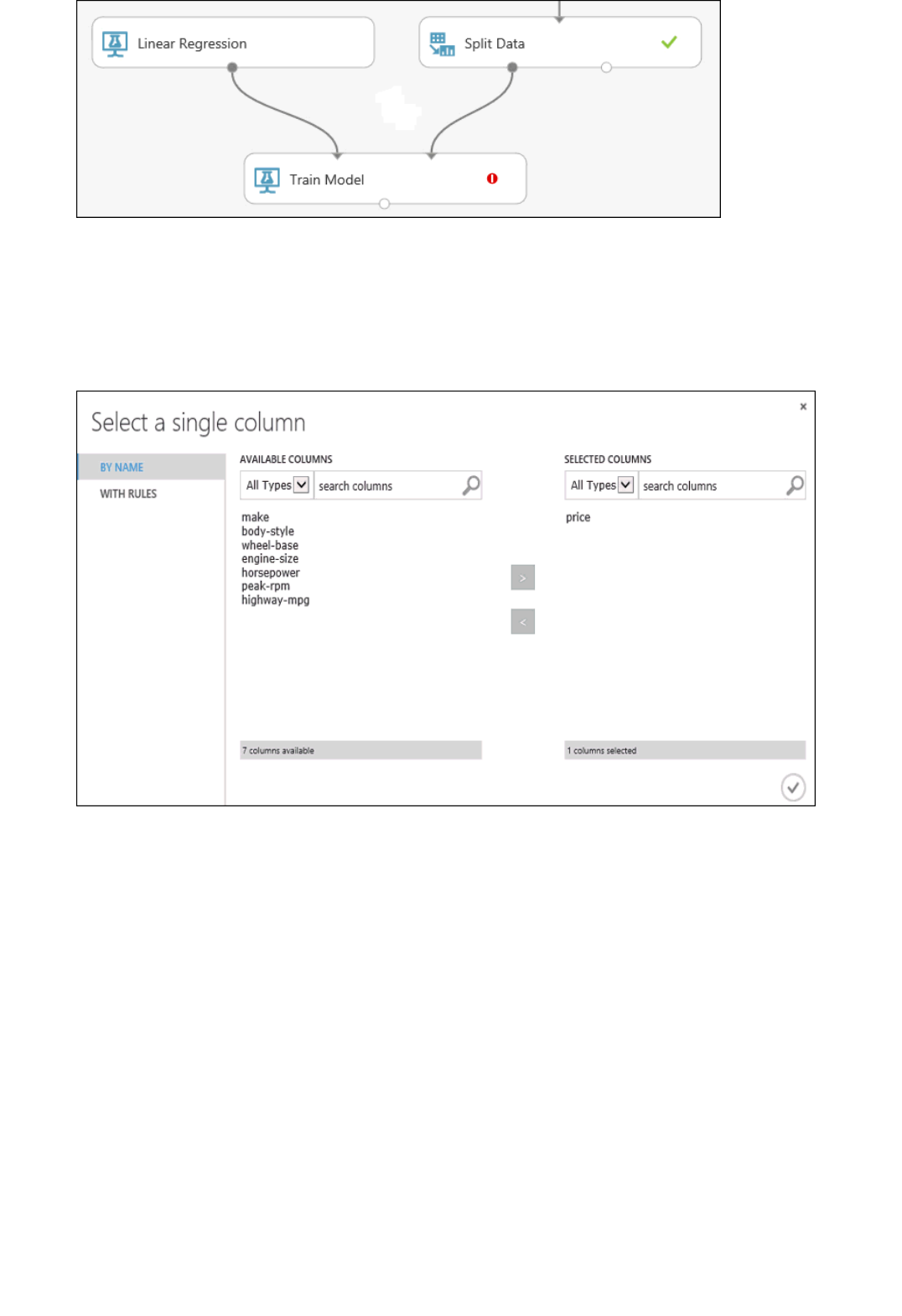
Connect the "Train Model" module to both the "Linear Regression" and "Split Data" modules
6. Click the Train Model module, click Launch column selector in the Properties pane, and then select the
price column. This is the value that our model is going to predict.
You select the price column in the column selector by moving it from the Available columns list to the
Selected columns list.
Select the price column for the "Train Model" module
7. Run the experiment.
We now have a trained regression model that can be used to score new automobile data to make price
predictions.
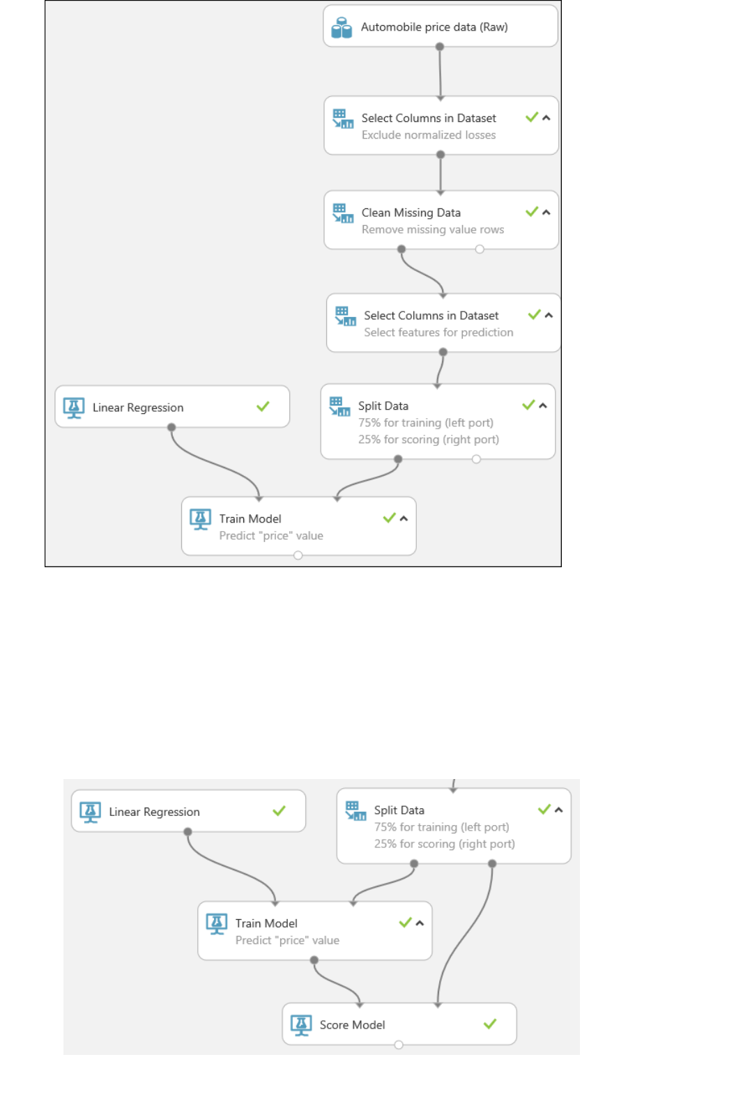
Step 5: Predict new automobile prices
After running, the experiment should now look something like this
Now that we've trained the model using 75 percent of our data, we can use it to score the other 25 percent of the
data to see how well our model functions.
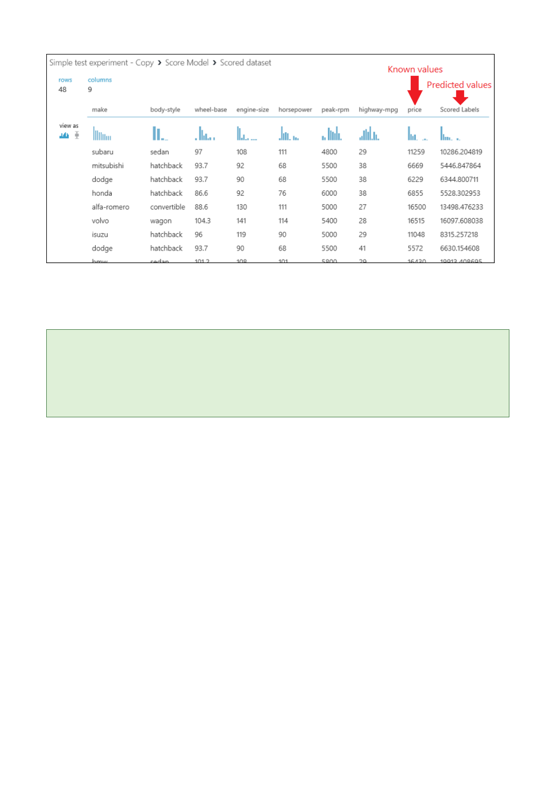
1. Find and drag the Score Model module to the experiment canvas. Connect the output of the Train Model
module to the left input port of Score Model. Connect the test data output (right port) of the Split Data
module to the right input port of Score Model.
Connect the "Score Model" module to both the "Train Model" and "Split Data" modules
TIPTIP
2. Run the experiment and view the output from the Score Model module (click the output port of Score
Model and select Visualize). The output shows the predicted values for price and the known values from
the test data.
Output of the "Score Model" module
3. Finally, we test the quality of the results. Select and drag the Evaluate Model module to the experiment
canvas, and connect the output of the Score Model module to the left input of Evaluate Model.
There are two input ports on the Evaluate Model module because it can be used to compare two models side by
side. Later, you can add another algorithm to the experiment and use Evaluate Model to see which one gives better
results.
4. Run the experiment.
To view the output from the Evaluate Model module, click the output port, and then select Visualize.
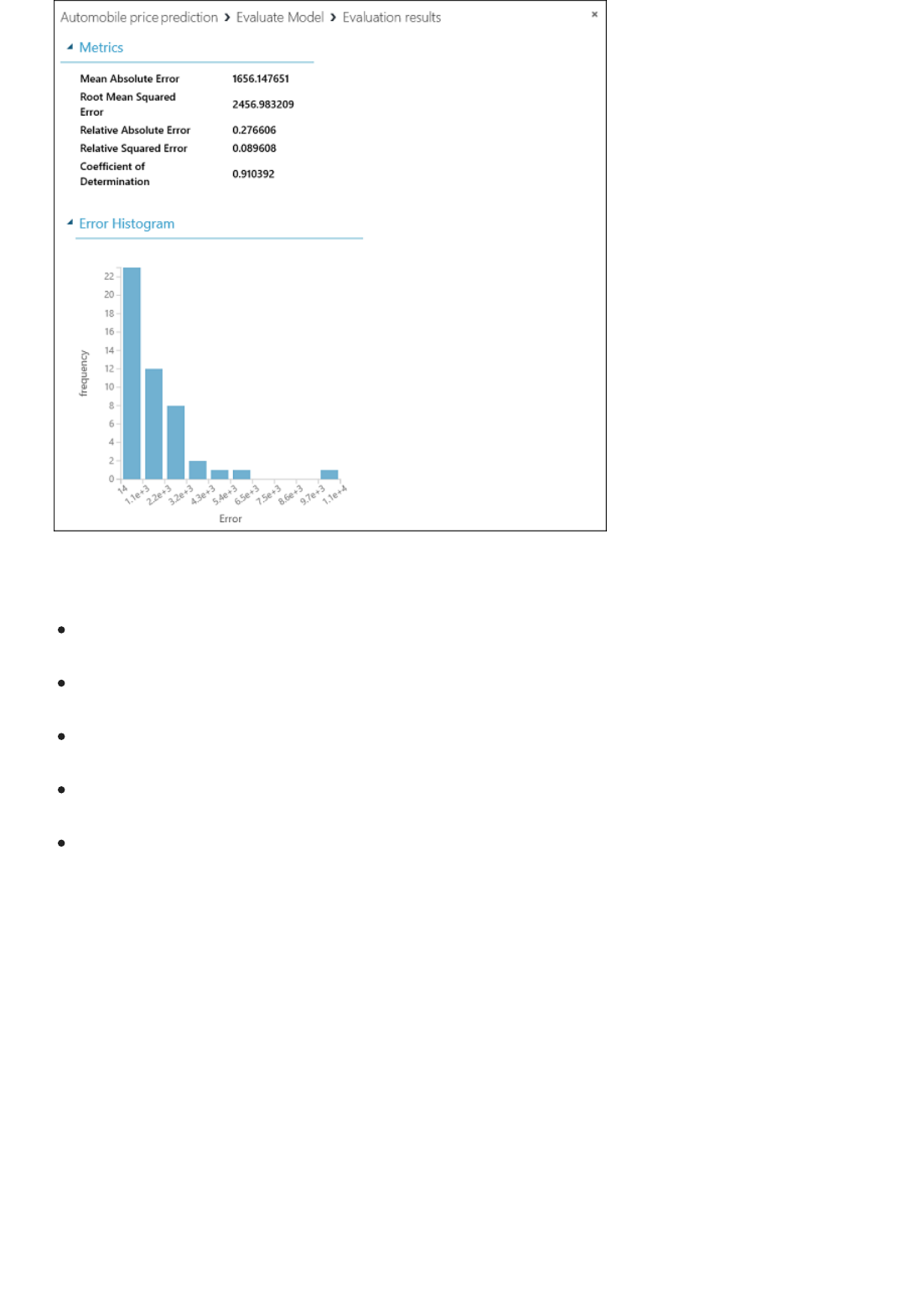
Final experiment
Evaluation results for the experiment
The following statistics are shown for our model:
Mean Absolute Error (MAE): The average of absolute errors (an error is the difference between the
predicted value and the actual value).
Root Mean Squared Error (RMSE): The square root of the average of squared errors of predictions made
on the test dataset.
Relative Absolute Error: The average of absolute errors relative to the absolute difference between actual
values and the average of all actual values.
Relative Squared Error: The average of squared errors relative to the squared difference between the actual
values and the average of all actual values.
Coefficient of Determination: Also known as the R squared value, this is a statistical metric indicating
how well a model fits the data.
For each of the error statistics, smaller is better. A smaller value indicates that the predictions more closely match
the actual values. For Coefficient of Determination, the closer its value is to one (1.0), the better the
predictions.
The final experiment should look something like this:
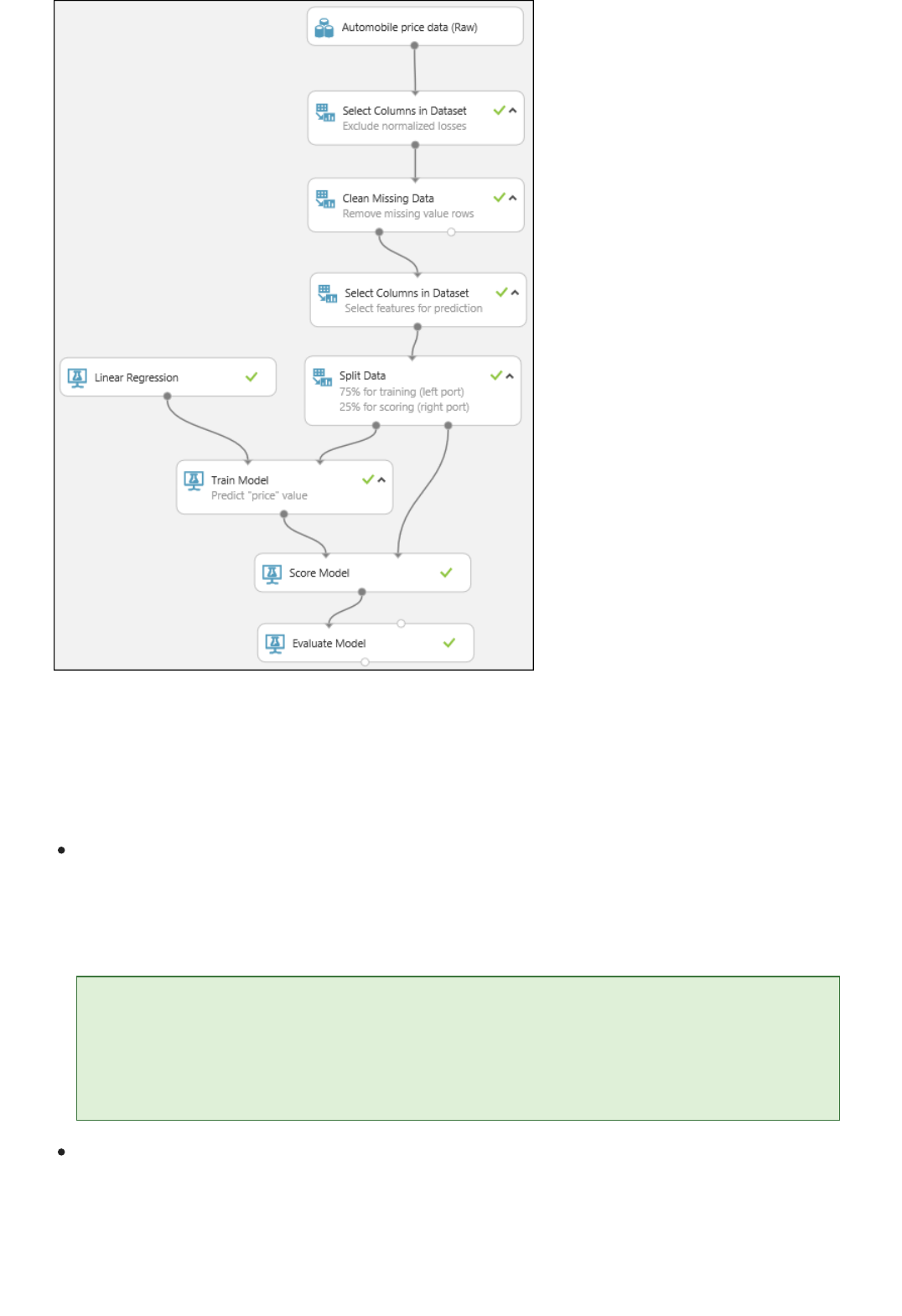
Next steps
The final experiment
Now that you've completed the first machine learning tutorial and have your experiment set up, you can
continue to improve the model and then deploy it as a predictive web service.
TIPTIP
Iterate to try to improve the model - For example, you can change the features you use in your
prediction. Or you can modify the properties of the Linear Regression algorithm or try a different
algorithm altogether. You can even add multiple machine learning algorithms to your experiment at one
time and compare two of them by using the Evaluate Model module. For an example of how to compare
multiple models in a single experiment, see Compare Regressors in the Azure AI Gallery.
To copy any iteration of your experiment, use the SAVE AS button at the bottom of the page. You can see all the
iterations of your experiment by clicking VIEW RUN HISTORY at the bottom of the page. For more details, see
Manage experiment iterations in Azure Machine Learning Studio.
Deploy the model as a predictive web service - When you're satisfied with your model, you can deploy it
as a web service to be used to predict automobile prices by using new data. For more details, see Deploy an
Azure Machine Learning web service.
Want to learn more? For a more extensive and detailed walkthrough of the process of creating, training, scoring,
and deploying a model, see Develop a predictive solution by using Azure Machine Learning.
Walkthrough: Develop a predictive analytics solution
for credit risk assessment in Azure Machine Learning
3/21/2018 • 2 min to read • Edit Online
NOTENOTE
The problem
The solution
In this walkthrough, we take an extended look at the process of developing a predictive analytics solution in
Machine Learning Studio. We develop a simple model in Machine Learning Studio, and then deploy it as an
Azure Machine Learning web service where the model can make predictions using new data.
This walkthrough assumes that you've used Machine Learning Studio at least once before, and that you have
some understanding of machine learning concepts. But it doesn't assume you're an expert in either.
If you've never used Azure Machine Learning Studio before, you might want to start with the tutorial, Create
your first data science experiment in Azure Machine Learning Studio. That tutorial takes you through Machine
Learning Studio for the first time. It shows you the basics of how to drag-and-drop modules onto your
experiment, connect them together, run the experiment, and look at the results. Another tool that may be helpful
for getting started is a diagram that gives an overview of the capabilities of Machine Learning Studio. You can
download and print it from here: Overview diagram of Azure Machine Learning Studio capabilities.
If you're new to the field of machine learning in general, there's a video series that might be helpful to you. It's
called Data Science for Beginners and it can give you a great introduction to machine learning using everyday
language and concepts.
You can try Azure Machine Learning for free. No credit card or Azure subscription is required. Get started now.
Suppose you need to predict an individual's credit risk based on the information they gave on a credit
application.
Credit risk assessment is a complex problem, but we can simplify it a bit for this walkthrough. We'll use it as an
example of how you can create a predictive analytics solution using Microsoft Azure Machine Learning. To do
this, we use Azure Machine Learning Studio and a Machine Learning web service.
In this detailed walkthrough, we start with publicly available credit risk data and develop and train a predictive
model based on that data. Then we deploy the model as a web service so it can be used by others for credit risk
assessment.
To create this credit risk assessment solution, we follow these steps:
1. Create a Machine Learning workspace
2. Upload existing data
3. Create an experiment
4. Train and evaluate the models
5. Deploy the web service
6. Access the web service

TIPTIP
You can find a working copy of the experiment that we develop in this walkthrough in the Azure AI Gallery. Go to
Walkthrough - Credit risk prediction and click Open in Studio to download a copy of the experiment into your
Machine Learning Studio workspace.
This walkthrough is based on a simplified version of the sample experiment, Binary Classification: Credit risk prediction, also
available in the Gallery.
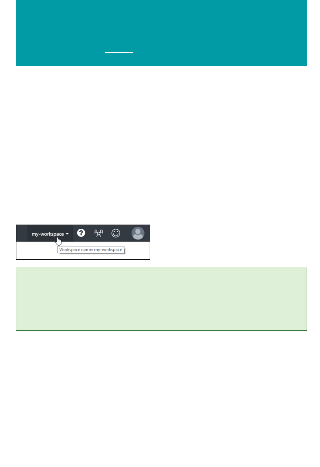
Walkthrough Step 1: Create a Machine Learning
workspace
3/21/2018 • 1 min to read • Edit Online
TIPTIP
This is the first step of the walkthrough, Develop a predictive analytics solution in Azure Machine Learning.
1. Create a Machine Learning workspace
2. Upload existing data
3. Create a new experiment
4. Train and evaluate the models
5. Deploy the Web service
6. Access the Web service
To use Machine Learning Studio, you need to have a Microsoft Azure Machine Learning workspace. This
workspace contains the tools you need to create, manage, and publish experiments.
The administrator for your Azure subscription needs to create the workspace and then add you as an owner or
contributor. For details, see Create and share an Azure Machine Learning workspace.
After your workspace is created, open Machine Learning Studio (https://studio.azureml.net/Home). If you have
more than one workspace, you can select the workspace in the toolbar in the upper-right corner of the window.
If you were made an owner of the workspace, you can share the experiments you're working on by inviting others to the
workspace. You can do this in Machine Learning Studio on the SETTINGS page. You just need the Microsoft account or
organizational account for each user.
On the SETTINGS page, click USERS, then click INVITE MORE USERS at the bottom of the window.
Next: Upload existing data

Walkthrough Step 2: Upload existing data into an
Azure Machine Learning experiment
5/1/2018 • 3 min to read • Edit Online
Convert the dataset format
This is the second step of the walkthrough, Develop a predictive analytics solution in Azure Machine Learning
1. Create a Machine Learning workspace
2. Upload existing data
3. Create a new experiment
4. Train and evaluate the models
5. Deploy the Web service
6. Access the Web service
To develop a predictive model for credit risk, we need data that we can use to train and then test the model. For
this walkthrough, we'll use the "UCI Statlog (German Credit Data) Data Set" from the UC Irvine Machine
Learning repository. You can find it here:
http://archive.ics.uci.edu/ml/datasets/Statlog+(German+Credit+Data)
We'll use the file named german.data. Download this file to your local hard drive.
The german.data dataset contains rows of 20 variables for 1000 past applicants for credit. These 20 variables
represent the dataset's set of features (the feature vector), which provides identifying characteristics for each
credit applicant. An additional column in each row represents the applicant's calculated credit risk, with 700
applicants identified as a low credit risk and 300 as a high risk.
The UCI website provides a description of the attributes of the feature vector for this data. This includes financial
information, credit history, employment status, and personal information. For each applicant, a binary rating has
been given indicating whether they are a low or high credit risk.
We'll use this data to train a predictive analytics model. When we're done, our model should be able to accept a
feature vector for a new individual and predict whether he or she is a low or high credit risk.
Here's an interesting twist. The description of the dataset on the UCI website mentions what it costs if we
misclassify a person's credit risk. If the model predicts a high credit risk for someone who is actually a low credit
risk, the model has made a misclassification. But the reverse misclassification is five times more costly to the
financial institution: if the model predicts a low credit risk for someone who is actually a high credit risk.
So, we want to train our model so that the cost of this latter type of misclassification is five times higher than
misclassifying the other way. One simple way to do this when training the model in our experiment is by
duplicating (five times) those entries that represent someone with a high credit risk. Then, if the model
misclassifies someone as a low credit risk when they're actually a high risk, the model does that same
misclassification five times, once for each duplicate. This will increase the cost of this error in the training results.
The original dataset uses a blank-separated format. Machine Learning Studio works better with a comma-
separated value (CSV) file, so we'll convert the dataset by replacing spaces with commas.
There are many ways to convert this data. One way is by using the following Windows PowerShell command:
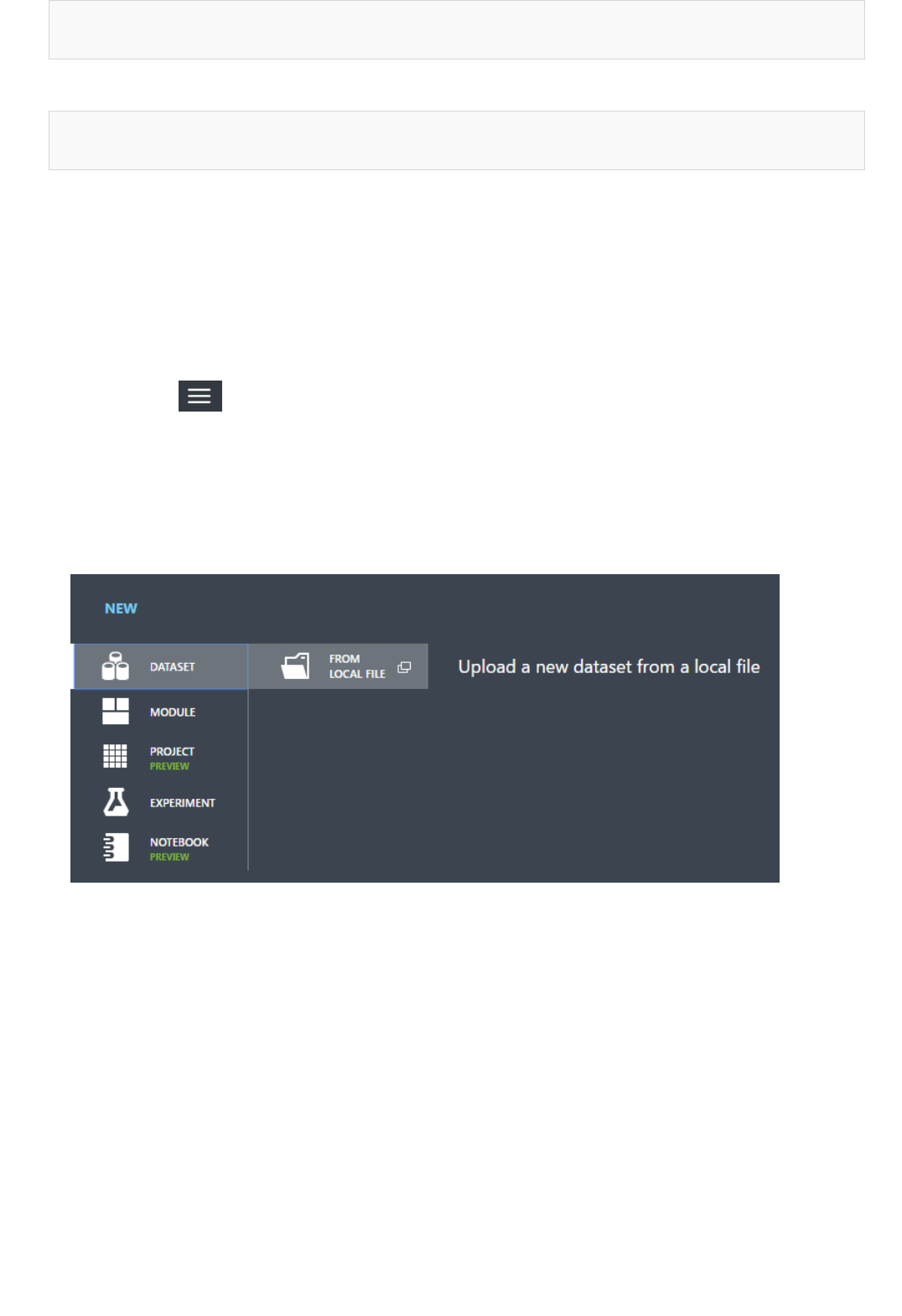
cat german.data | %{$_ -replace " ",","} | sc german.csv
sed 's/ /,/g' german.data > german.csv
Upload the dataset to Machine Learning Studio
Another way is by using the Unix sed command:
In either case, we have created a comma-separated version of the data in a file named german.csv that we can
use in our experiment.
Once the data has been converted to CSV format, we need to upload it into Machine Learning Studio.
1. Open the Machine Learning Studio home page (https://studio.azureml.net).
2. Click the menu in the upper-left corner of the window, click Azure Machine Learning, select
Studio, and sign in.
3. Click +NEW at the bottom of the window.
4. Select DATASET.
5. Select FROM LOCAL FILE.
6. In the Upload a new dataset dialog, click Browse and find the german.csv file you created.
7. Enter a name for the dataset. For this walkthrough, call it "UCI German Credit Card Data".
8. For data type, select Generic CSV File With no header (.nh.csv).
9. Add a description if you’d like.
10. Click the OK check mark.
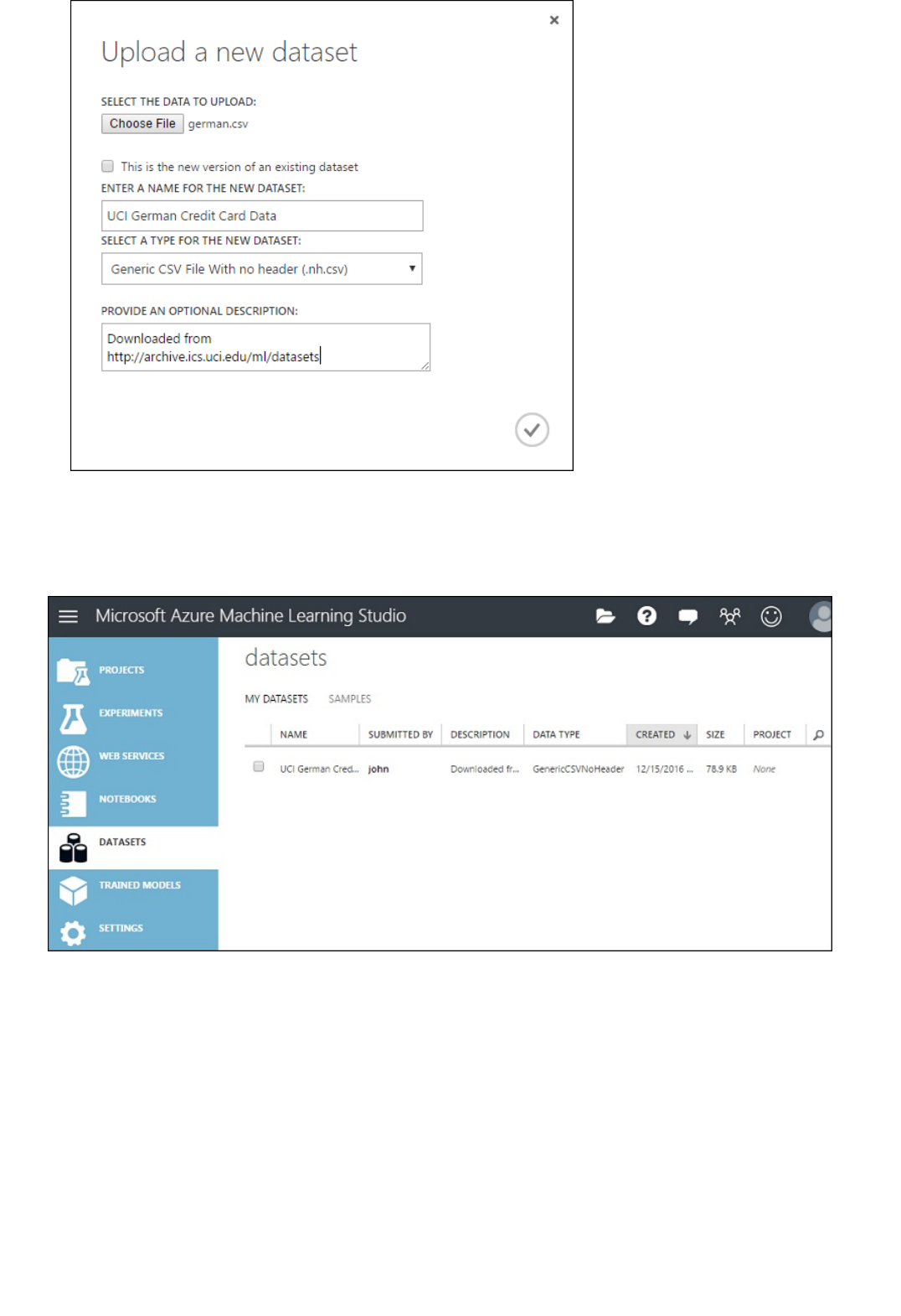
This uploads the data into a dataset module that we can use in an experiment.
You can manage datasets that you've uploaded to Studio by clicking the DATASETS tab to the left of the Studio
window.
For more information about importing other types of data into an experiment, see Import your training data into
Azure Machine Learning Studio.
Next: Create a new experiment
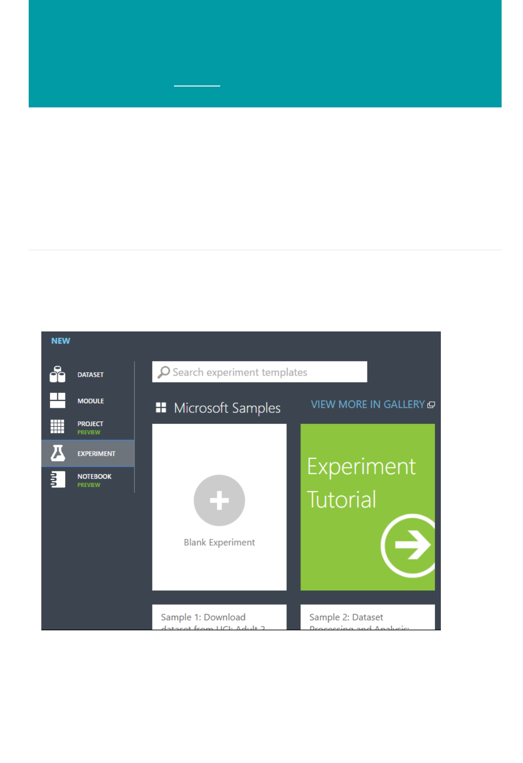
Walkthrough Step 3: Create a new Azure Machine
Learning experiment
3/21/2018 • 6 min to read • Edit Online
This is the third step of the walkthrough, Develop a predictive analytics solution in Azure Machine Learning
1. Create a Machine Learning workspace
2. Upload existing data
3. Create a new experiment
4. Train and evaluate the models
5. Deploy the Web service
6. Access the Web service
The next step in this walkthrough is to create an experiment in Machine Learning Studio that uses the dataset we
uploaded.
1. In Studio, click +NEW at the bottom of the window.
2. Select EXPERIMENT, and then select "Blank Experiment".
3. Select the default experiment name at the top of the canvas and rename it to something meaningful.
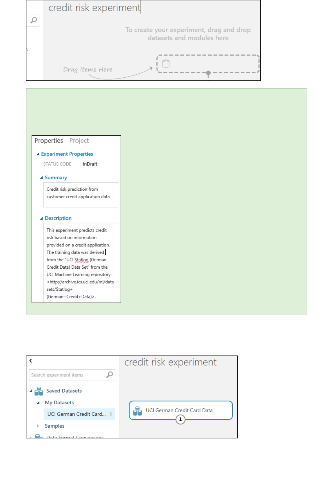
Prepare the data
TIPTIP
4. In the module palette to the left of the experiment canvas, expand Saved Datasets.
It's a good practice to fill in Summary and Description for the experiment in the Properties pane. These
properties give you the chance to document the experiment so that anyone who looks at it later will understand
your goals and methodology.
5. Find the dataset you created under My Datasets and drag it onto the canvas. You can also find the dataset
by entering the name in the Search box above the palette.
You can view the first 100 rows of the data and some statistical information for the whole dataset: Click the
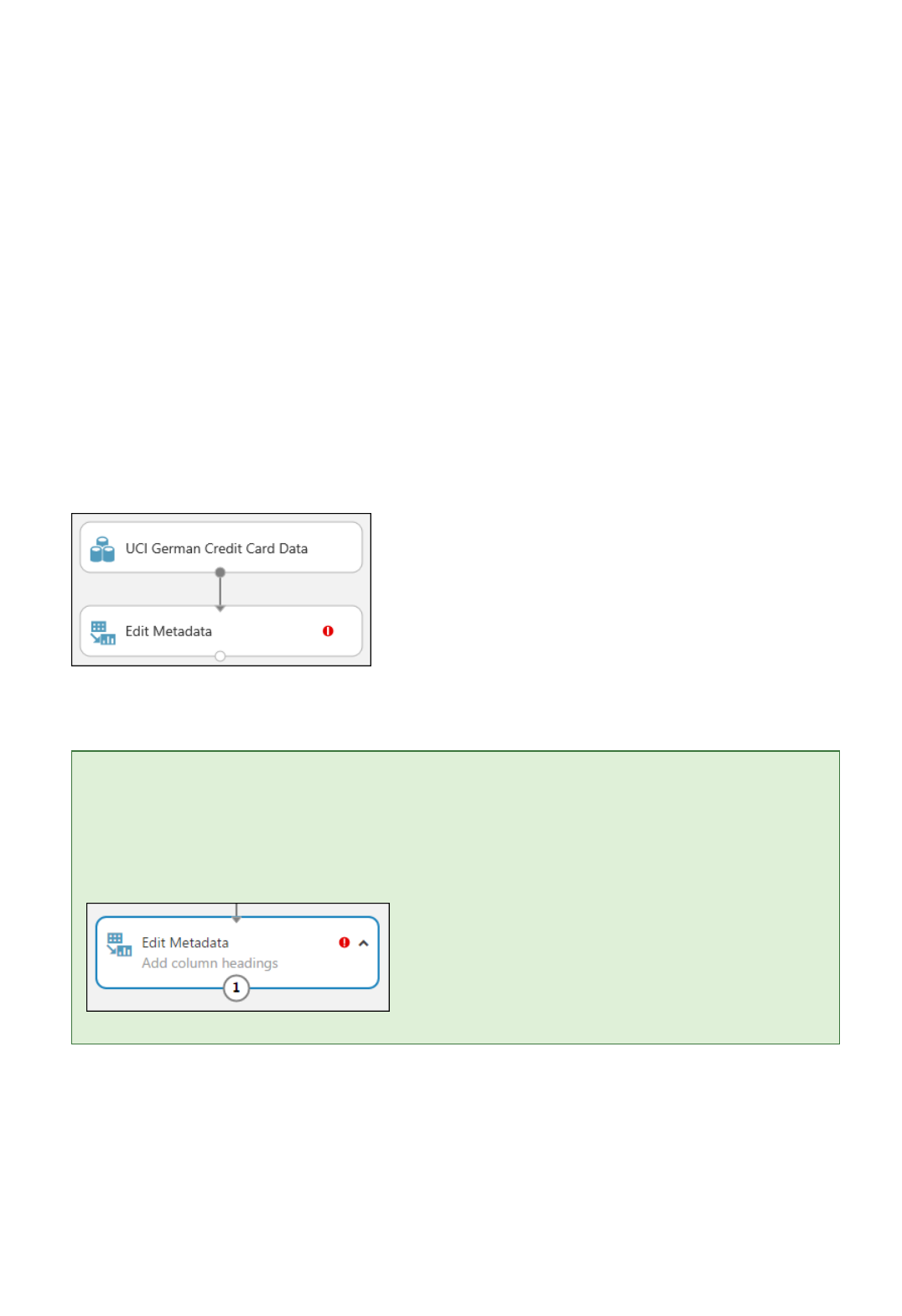
output port of the dataset (the small circle at the bottom) and select Visualize.
Because the data file didn't come with column headings, Studio has provided generic headings (Col1, Col2, etc.).
Good headings aren't essential to creating a model, but they make it easier to work with the data in the
experiment. Also, when we eventually publish this model in a web service, the headings help identify the columns
to the user of the service.
We can add column headings using the Edit Metadata module. You use the Edit Metadata module to change
metadata associated with a dataset. In this case, we use it to provide more friendly names for column headings.
To use Edit Metadata, you first specify which columns to modify (in this case, all of them.) Next, you specify the
action to be performed on those columns (in this case, changing column headings.)
TIPTIP
1. In the module palette, type "metadata" in the Search box. The Edit Metadata appears in the module list.
2. Click and drag the Edit Metadata module onto the canvas and drop it below the dataset we added earlier.
3. Connect the dataset to the Edit Metadata: click the output port of the dataset (the small circle at the bottom
of the dataset), drag to the input port of Edit Metadata (the small circle at the top of the module), then
release the mouse button. The dataset and module remain connected even if you move either around on
the canvas.
The experiment should now look something like this:
The red exclamation mark indicates that we haven't set the properties for this module yet. We'll do that
next.
You can add a comment to a module by double-clicking the module and entering text. This can help you see at a
glance what the module is doing in your experiment. In this case, double-click the Edit Metadata module and type
the comment "Add column headings". Click anywhere else on the canvas to close the text box. To display the
comment, click the down-arrow on the module.
4. Select Edit Metadata, and in the Properties pane to the right of the canvas, click Launch column
selector.
5. In the Select columns dialog, select all the rows in Available Columns and click > to move them to
Selected Columns. The dialog should look like this:
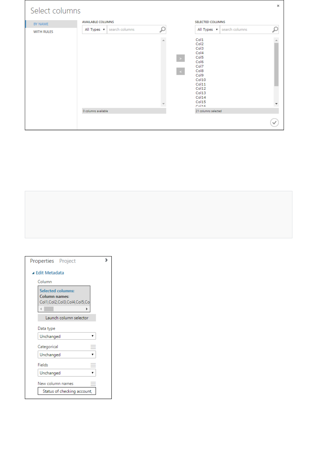
Status of checking account, Duration in months, Credit history, Purpose, Credit amount, Savings
account/bond, Present employment since, Installment rate in percentage of disposable income, Personal
status and sex, Other debtors, Present residence since, Property, Age in years, Other installment
plans, Housing, Number of existing credits, Job, Number of people providing maintenance for,
Telephone, Foreign worker, Credit risk
6. Click the OK check mark.
7. Back in the Properties pane, look for the New column names parameter. In this field, enter a list of
names for the 21 columns in the dataset, separated by commas and in column order. You can obtain the
columns names from the dataset documentation on the UCI website, or for convenience you can copy and
paste the following list:
The Properties pane looks like this:
TIPTIP
Create training and test datasets
If you want to verify the column headings, run the experiment (click RUN below the experiment canvas). When it finishes
running (a green check mark appears on Edit Metadata), click the output port of the Edit Metadata module, and select
Visualize. You can view the output of any module in the same way to view the progress of the data through the
experiment.
We need some data to train the model and some to test it. So in the next step of the experiment, we split the
dataset into two separate datasets: one for training our model and one for testing it.
To do this, we use the Split Data module.
TIPTIP
1. Find the Split Data module, drag it onto the canvas, and connect it to the Edit Metadata module.
2. By default, the split ratio is 0.5 and the Randomized split parameter is set. This means that a random half
of the data is output through one port of the Split Data module, and half through the other. You can adjust
these parameters, as well as the Random seed parameter, to change the split between training and testing
data. For this example, we leave them as-is.
The property Fraction of rows in the first output dataset determines how much of the data is output through
the left output port. For instance, if you set the ratio to 0.7, then 70% of the data is output through the left port
and 30% through the right port.
3. Double-click the Split Data module and enter the comment, "Training/testing data split 50%".
We can use the outputs of the Split Data module however we like, but let's choose to use the left output as
training data and the right output as testing data.
As mentioned in the previous step, the cost of misclassifying a high credit risk as low is five times higher than the
cost of misclassifying a low credit risk as high. To account for this, we generate a new dataset that reflects this cost
function. In the new dataset, each high risk example is replicated five times, while each low risk example is not
replicated.
We can do this replication using R code:
dataset1 <- maml.mapInputPort(1)
data.set<-dataset1[dataset1[,21]==1,]
pos<-dataset1[dataset1[,21]==2,]
for (i in 1:5) data.set<-rbind(data.set,pos)
maml.mapOutputPort("data.set")
1. Find and drag the Execute R Script module onto the experiment canvas.
2. Connect the left output port of the Split Data module to the first input port ("Dataset1") of the Execute R
Script module.
3. Double-click the Execute R Script module and enter the comment, "Set cost adjustment".
4. In the Properties pane, delete the default text in the R Script parameter and enter this script:
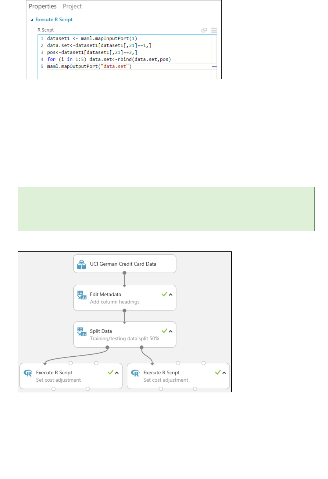
TIPTIP
We need to do this same replication operation for each output of the Split Data module so that the training and
testing data have the same cost adjustment. The easiest way to do this is by duplicating the Execute R Script
module we just made and connecting it to the other output port of the Split Data module.
1. Right-click the Execute R Script module and select Copy.
2. Right-click the experiment canvas and select Paste.
3. Drag the new module into position, and then connect the right output port of the Split Data module to the
first input port of this new Execute R Script module.
4. At the bottom of the canvas, click Run.
The copy of the Execute R Script module contains the same script as the original module. When you copy and paste a
module on the canvas, the copy retains all the properties of the original.
Our experiment now looks something like this:
For more information on using R scripts in your experiments, see Extend your experiment with R.
Next: Train and evaluate the models

Walkthrough Step 4: Train and evaluate the
predictive analytic models
3/21/2018 • 8 min to read • Edit Online
TIPTIP
Train the models
Two-Class Boosted Decision TreeTwo-Class Boosted Decision Tree
This topic contains the fourth step of the walkthrough, Develop a predictive analytics solution in Azure Machine
Learning
1. Create a Machine Learning workspace
2. Upload existing data
3. Create a new experiment
4. Train and evaluate the models
5. Deploy the Web service
6. Access the Web service
One of the benefits of using Azure Machine Learning Studio for creating machine learning models is the ability to
try more than one type of model at a time in a single experiment and compare the results. This type of
experimentation helps you find the best solution for your problem.
In the experiment we're developing in this walkthrough, we'll create two different types of models and then
compare their scoring results to decide which algorithm we want to use in our final experiment.
There are various models we could choose from. To see the models available, expand the Machine Learning
node in the module palette, and then expand Initialize Model and the nodes beneath it. For the purposes of this
experiment, we'll select the Two-Class Support Vector Machine (SVM) and the Two-Class Boosted Decision Tree
modules.
To get help deciding which Machine Learning algorithm best suits the particular problem you're trying to solve, see How to
choose algorithms for Microsoft Azure Machine Learning.
We'll add both the Two-Class Boosted Decision Tree module and Two-Class Support Vector Machine module in
this experiment.
First, let's set up the boosted decision tree model.
1. Find the Two-Class Boosted Decision Tree module in the module palette and drag it onto the canvas.
2. Find the Train Model module, drag it onto the canvas, and then connect the output of the Two-Class
Boosted Decision Tree module to the left input port of the Train Model module.
The Two-Class Boosted Decision Tree module initializes the generic model, and Train Model uses training
data to train the model.
3. Connect the left output of the left Execute R Script module to the right input port of the Train Model
module (we decided in Step 3 of this walkthrough to use the data coming from the left side of the Split
Data module for training).
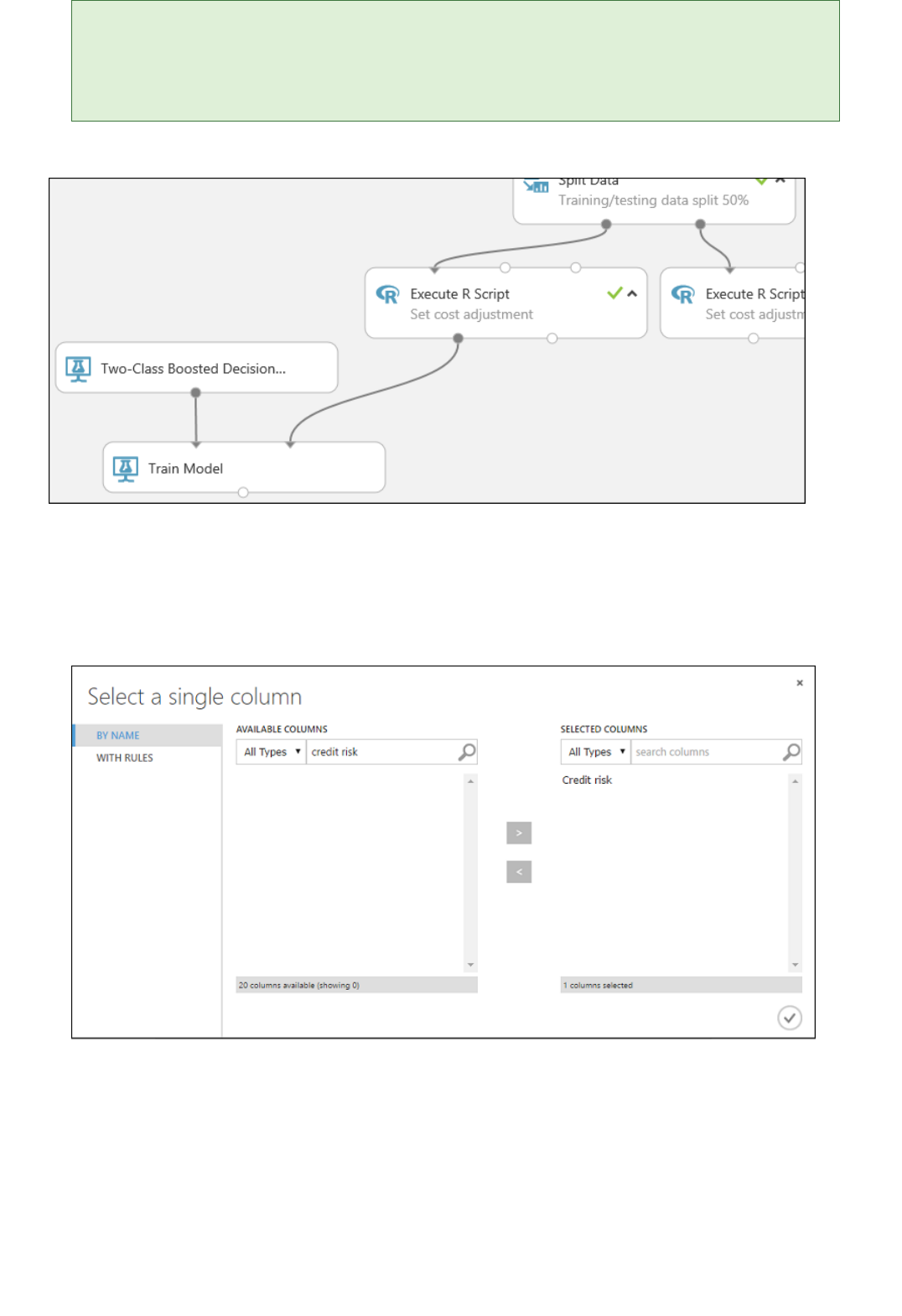
Two-Class Support Vector MachineTwo-Class Support Vector Machine
TIPTIP
We don't need two of the inputs and one of the outputs of the Execute R Script module for this experiment, so we
can leave them unattached.
This portion of the experiment now looks something like this:
Now we need to tell the Train Model module that we want the model to predict the Credit Risk value.
1. Select the Train Model module. In the Properties pane, click Launch column selector.
2. In the Select a single column dialog, type "credit risk" in the search field under Available Columns,
select "Credit risk" below, and click the right arrow button (>) to move "Credit risk" to Selected Columns.
3. Click the OK check mark.
Next, we set up the SVM model.
First, a little explanation about SVM. Boosted decision trees work well with features of any type. However, since
the SVM module generates a linear classifier, the model that it generates has the best test error when all numeric
features have the same scale. To convert all numeric features to the same scale, we use a "Tanh" transformation
(with the Normalize Data module). This transforms our numbers into the [0,1] range. The SVM module converts
string features to categorical features and then to binary 0/1 features, so we don't need to manually transform
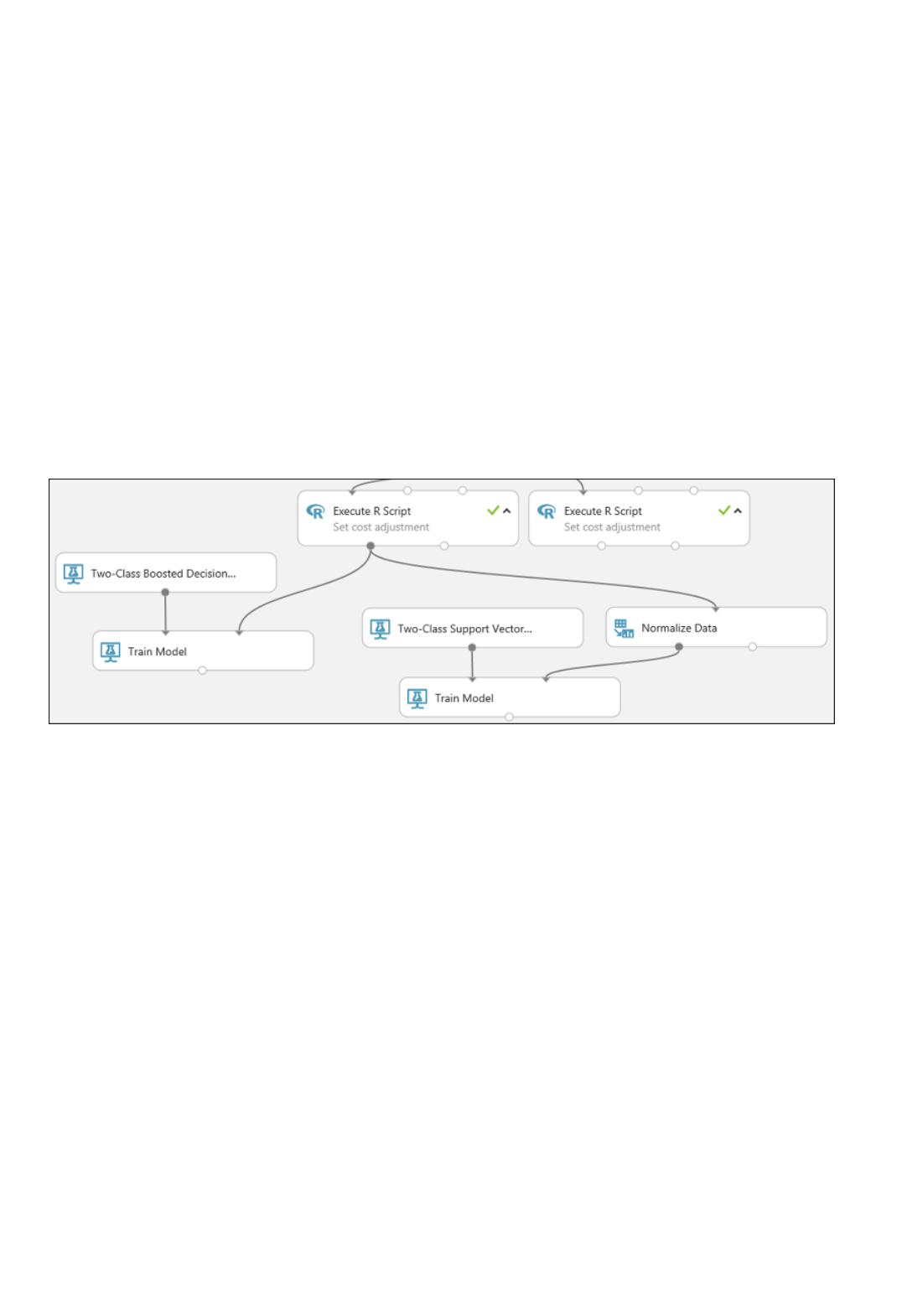
string features. Also, we don't want to transform the Credit Risk column (column 21) - it's numeric, but it's the
value we're training the model to predict, so we need to leave it alone.
To set up the SVM model, do the following:
1. Find the Two-Class Support Vector Machine module in the module palette and drag it onto the canvas.
2. Right-click the Train Model module, select Copy, and then right-click the canvas and select Paste. The copy
of the Train Model module has the same column selection as the original.
3. Connect the output of the Two-Class Support Vector Machine module to the left input port of the second
Train Model module.
4. Find the Normalize Data module and drag it onto the canvas.
5. Connect the left output of the left Execute R Script module to the input of this module (notice that the
output port of a module may be connected to more than one other module).
6. Connect the left output port of the Normalize Data module to the right input port of the second Train
Model module.
This portion of our experiment should now look something like this:
Now configure the Normalize Data module:
1. Click to select the Normalize Data module. In the Properties pane, select Tanh for the Transformation
method parameter.
2. Click Launch column selector, select "No columns" for Begin With, select Include in the first
dropdown, select column type in the second dropdown, and select Numeric in the third dropdown. This
specifies that all the numeric columns (and only numeric) are transformed.
3. Click the plus sign (+) to the right of this row - this creates a row of dropdowns. Select Exclude in the first
dropdown, select column names in the second dropdown, and enter "Credit risk" in the text field. This
specifies that the Credit Risk column should be ignored (we need to do this because this column is
numeric and so would be transformed if we didn't exclude it).
4. Click the OK check mark.
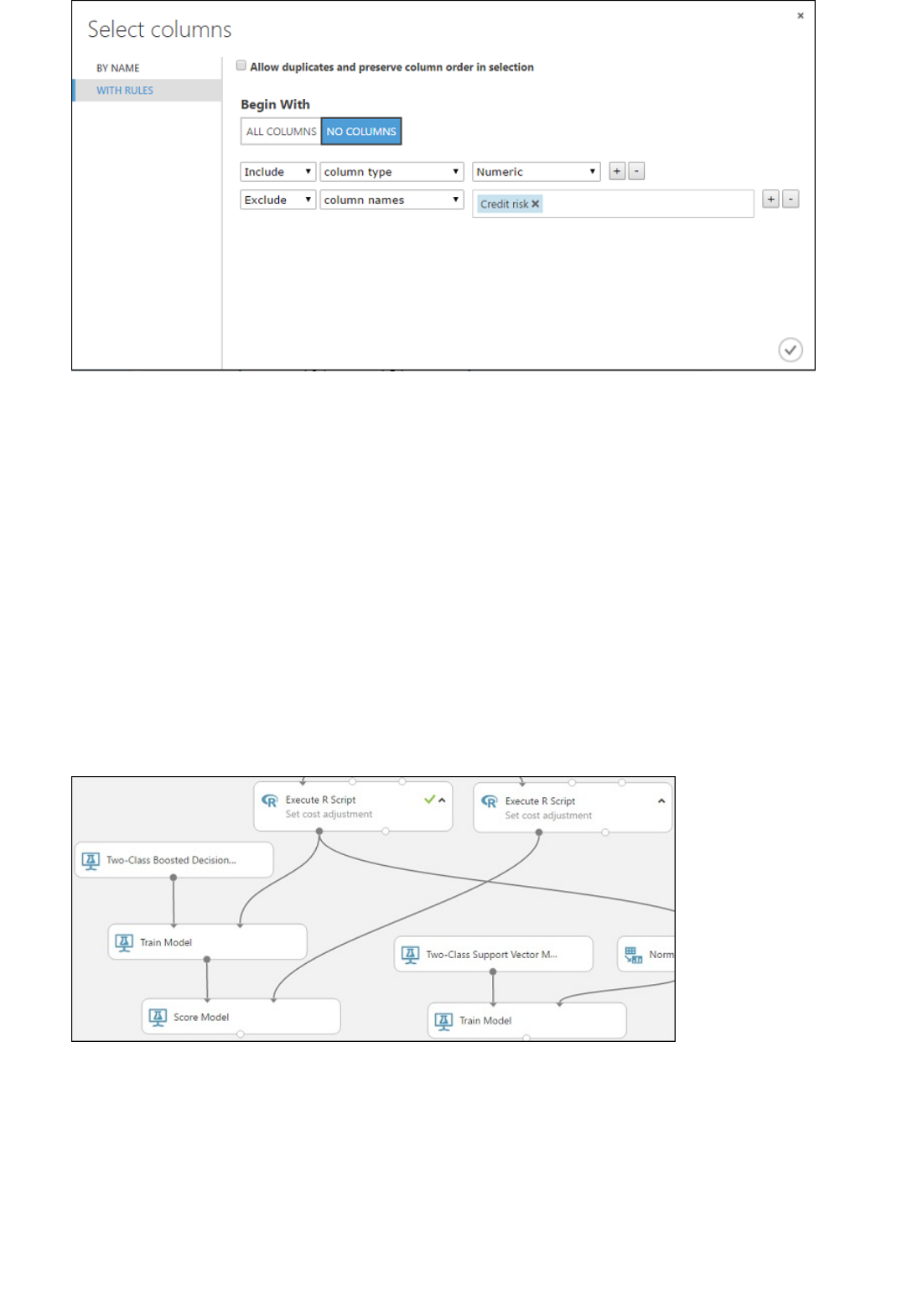
Score and evaluate the models
Add the Score Model modulesAdd the Score Model modules
The Normalize Data module is now set to perform a Tanh transformation on all numeric columns except for the
Credit Risk column.
We use the testing data that was separated out by the Split Data module to score our trained models. We can
then compare the results of the two models to see which generated better results.
1. Find the Score Model module and drag it onto the canvas.
2. Connect the Train Model module that's connected to the Two-Class Boosted Decision Tree module to the
left input port of the Score Model module.
3. Connect the right Execute R Script module (our testing data) to the right input port of the Score Model
module.
The Score Model module can now take the credit information from the testing data, run it through the
model, and compare the predictions the model generates with the actual credit risk column in the testing
data.
4. Copy and paste the Score Model module to create a second copy.
5. Connect the output of the SVM model (that is, the output port of the Train Model module that's connected
to the Two-Class Support Vector Machine module) to the input port of the second Score Model module.
6. For the SVM model, we have to do the same transformation to the test data as we did to the training data.
So copy and paste the Normalize Data module to create a second copy and connect it to the right Execute
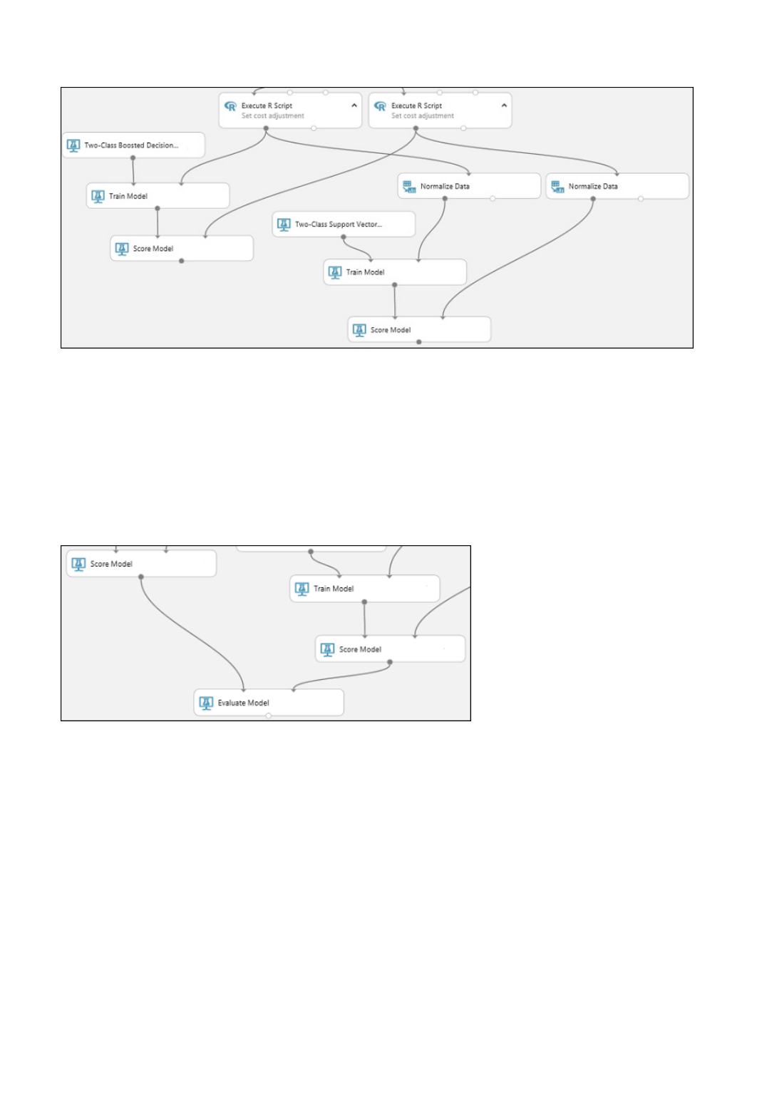
Add the Evaluate Model moduleAdd the Evaluate Model module
Run the experiment and check the resultsRun the experiment and check the results
R Script module.
7. Connect the left output of the second Normalize Data module to the right input port of the second Score
Model module.
To evaluate the two scoring results and compare them, we use an Evaluate Model module.
1. Find the Evaluate Model module and drag it onto the canvas.
2. Connect the output port of the Score Model module associated with the boosted decision tree model to
the left input port of the Evaluate Model module.
3. Connect the other Score Model module to the right input port.
To run the experiment, click the RUN button below the canvas. It may take a few minutes. A spinning indicator on
each module shows that it's running, and then a green check mark shows when the module is finished. When all
the modules have a check mark, the experiment has finished running.
The experiment should now look something like this:
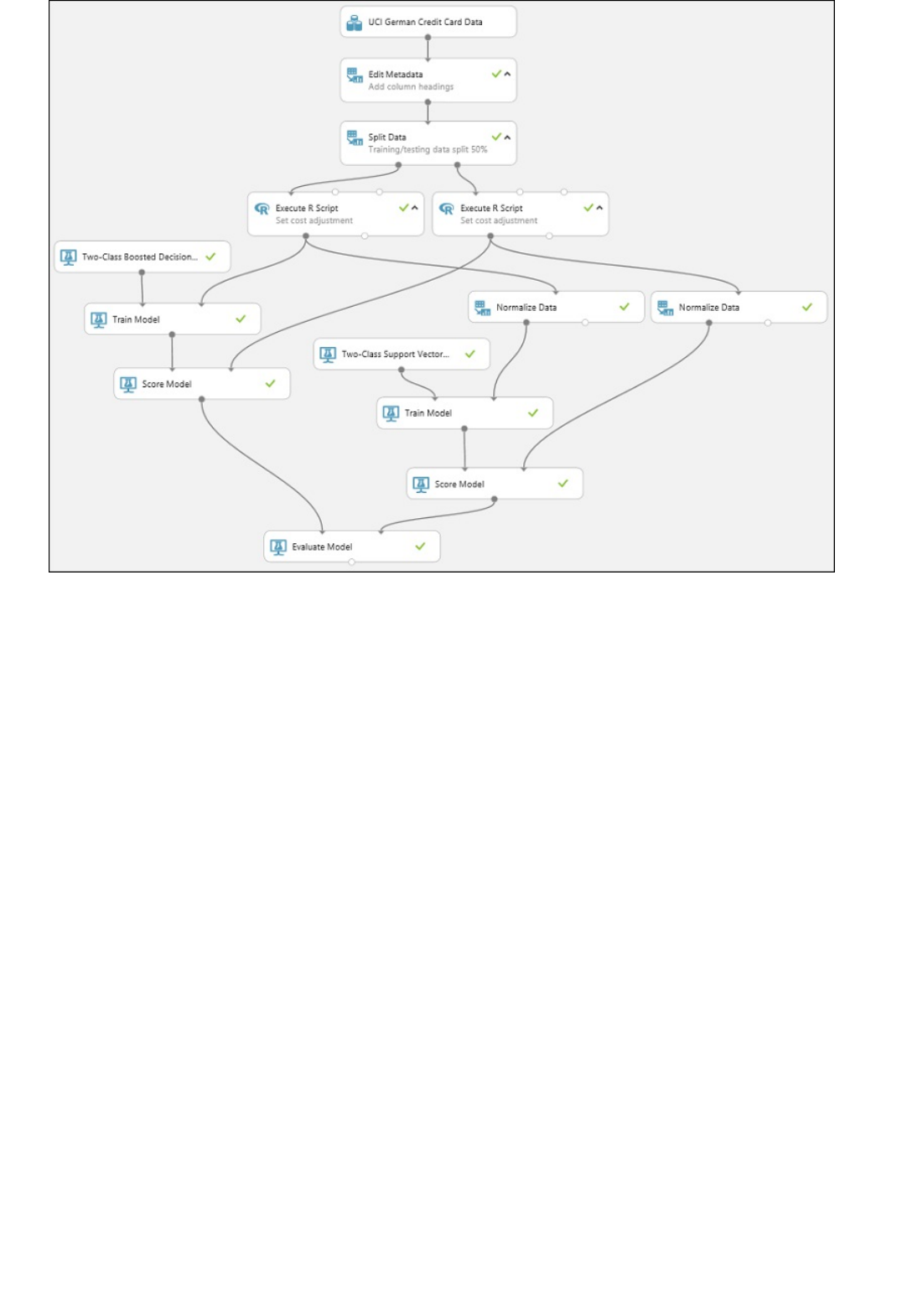
To check the results, click the output port of the Evaluate Model module and select Visualize.
The Evaluate Model module produces a pair of curves and metrics that allow you to compare the results of the
two scored models. You can view the results as Receiver Operator Characteristic (ROC) curves, Precision/Recall
curves, or Lift curves. Additional data displayed includes a confusion matrix, cumulative values for the area under
the curve (AUC), and other metrics. You can change the threshold value by moving the slider left or right and see
how it affects the set of metrics.
To the right of the graph, click Scored dataset or Scored dataset to compare to highlight the associated curve
and to display the associated metrics below. In the legend for the curves, "Scored dataset" corresponds to the left
input port of the Evaluate Model module - in our case, this is the boosted decision tree model. "Scored dataset to
compare" corresponds to the right input port - the SVM model in our case. When you click one of these labels,
the curve for that model is highlighted and the corresponding metrics are displayed, as shown in the following
graphic.
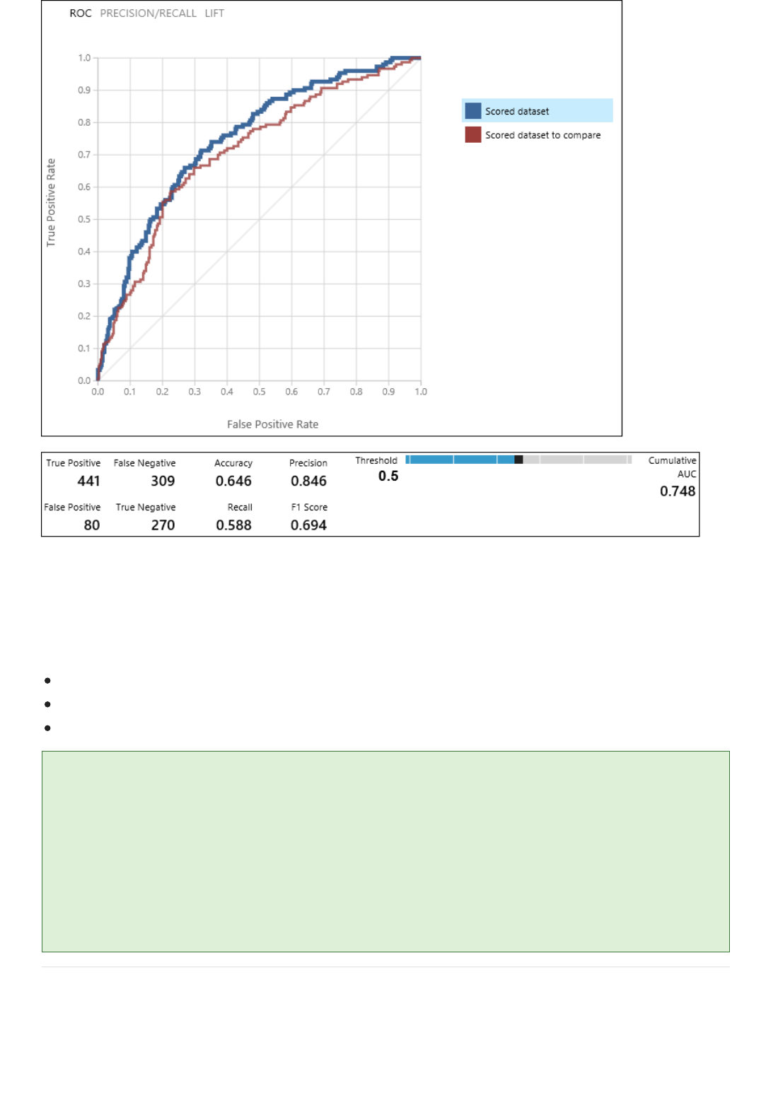
TIPTIP
By examining these values, you can decide which model is closest to giving you the results you're looking for. You
can go back and iterate on your experiment by changing parameter values in the different models.
The science and art of interpreting these results and tuning the model performance is outside the scope of this
walkthrough. For additional help, you might read the following articles:
How to evaluate model performance in Azure Machine Learning
Choose parameters to optimize your algorithms in Azure Machine Learning
Interpret model results in Azure Machine Learning
Each time you run the experiment a record of that iteration is kept in the Run History. You can view these iterations, and
return to any of them, by clicking VIEW RUN HISTORY below the canvas. You can also click Prior Run in the Properties
pane to return to the iteration immediately preceding the one you have open.
You can make a copy of any iteration of your experiment by clicking SAVE AS below the canvas. Use the experiment's
Summary and Description properties to keep a record of what you've tried in your experiment iterations.
For more details, see Manage experiment iterations in Azure Machine Learning Studio.
Next: Deploy the web service

Walkthrough Step 5: Deploy the Azure Machine
Learning web service
4/25/2018 • 9 min to read • Edit Online
Remove one of the models
This is the fifth step of the walkthrough, Develop a predictive analytics solution in Azure Machine Learning
1. Create a Machine Learning workspace
2. Upload existing data
3. Create a new experiment
4. Train and evaluate the models
5. Deploy the web service
6. Access the web service
To give others a chance to use the predictive model we've developed in this walkthrough, we can deploy it as a
web service on Azure.
Up to this point we've been experimenting with training our model. But the deployed service is no longer going
to do training - it's going to generate new predictions by scoring the user's input based on our model. So we're
going to do some preparation to convert this experiment from a training experiment to a predictive
experiment.
This is a three-step process:
1. Remove one of the models
2. Convert the training experiment we've created into a predictive experiment
3. Deploy the predictive experiment as a web service
First, we need to trim this experiment down a little. We currently have two different models in the experiment,
but we only want to use one model when we deploy this as a web service.
Let's say we've decided that the boosted tree model performed better than the SVM model. So the first thing to
do is remove the Two-Class Support Vector Machine module and the modules that were used for training it. You
may want to make a copy of the experiment first by clicking Save As at the bottom of the experiment canvas.
We need to delete the following modules:
Two-Class Support Vector Machine
Train Model and Score Model modules that were connected to it
Normalize Data (both of them)
Evaluate Model (because we're finished evaluating the models)
Select each module and press the Delete key, or right-click the module and select Delete.
Convert the training experiment to a predictive experiment
TIPTIP
NOTENOTE
To get this model ready for deployment, we need to convert this training experiment to a predictive experiment.
This involves three steps:
1. Save the model we've trained and then replace our training modules
2. Trim the experiment to remove modules that were only needed for training
3. Define where the web service will accept input and where it generates the output
We could do this manually, but fortunately all three steps can be accomplished by clicking Set Up Web Service
at the bottom of the experiment canvas (and selecting the Predictive Web Service option).
If you want more details on what happens when you convert a training experiment to a predictive experiment, see How to
prepare your model for deployment in Azure Machine Learning Studio.
When you click Set Up Web Service, several things happen:
The trained model is converted to a single Trained Model module and stored in the module palette to the
left of the experiment canvas (you can find it under Trained Models)
Modules that were used for training are removed; specifically:
The saved trained model is added back into the experiment
Web service input and Web service output modules are added (these identify where the user's data will
enter the model, and what data is returned, when the web service is accessed)
Two-Class Boosted Decision Tree
Train Model
Split Data
the second Execute R Script module that was used for test data
You can see that the experiment is saved in two parts under tabs that have been added at the top of the experiment
canvas. The original training experiment is under the tab Training experiment, and the newly created predictive
experiment is under Predictive experiment. The predictive experiment is the one we'll deploy as a web service.
We need to take one additional step with this particular experiment. We added two Execute R Script modules to
provide a weighting function to the data. That was just a trick we needed for training and testing, so we can take
out those modules in the final model. Machine Learning Studio removed one Execute R Script module when it
removed the Split module. Now we can remove the other and connect Metadata Editor directly to Score Model.
Our experiment should now look like this:

NOTENOTE
Deploy the web service
Deploy as a Classic web serviceDeploy as a Classic web service
You may be wondering why we left the UCI German Credit Card Data dataset in the predictive experiment. The service is
going to score the user's data, not the original dataset, so why leave the original dataset in the model?
It's true that the service doesn't need the original credit card data. But it does need the schema for that data, which
includes information such as how many columns there are and which columns are numeric. This schema information is
necessary to interpret the user's data. We leave these components connected so that the scoring module has the dataset
schema when the service is running. The data isn't used, just the schema.
Run the experiment one last time (click Run.) If you want to verify that the model is still working, click the output
of the Score Model module and select View Results. You can see that the original data is displayed, along with
the credit risk value ("Scored Labels") and the scoring probability value ("Scored Probabilities".)
You can deploy the experiment as either a Classic web service, or as a New web service that's based on Azure
Resource Manager.
To deploy a Classic web service derived from our experiment, click Deploy Web Service below the canvas and
select Deploy Web Service [Classic]. Machine Learning Studio deploys the experiment as a web service and
takes you to the dashboard for that web service. From this page you can return to the experiment (View
snapshot or View latest) and run a simple test of the web service (see Test the web service below). There is
also information here for creating applications that can access the web service (more on that in the next step of
this walkthrough).
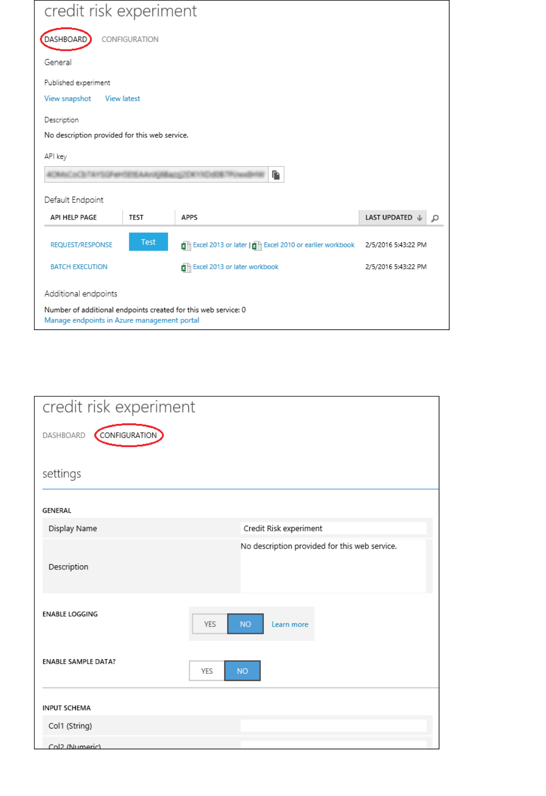
Deploy as a New web serviceDeploy as a New web service
You can configure the service by clicking the CONFIGURATION tab. Here you can modify the service name (it's
given the experiment name by default) and give it a description. You can also give more friendly labels for the
input and output data.
NOTENOTE
TIPTIP
Test the web service
TIPTIP
To deploy a New web service you must have sufficient permissions in the subscription to which you are deploying the web
service. For more information, see Manage a web service using the Azure Machine Learning Web Services portal.
To deploy a New web service derived from our experiment:
1. Click Deploy Web Service below the canvas and select Deploy Web Service [New]. Machine
Learning Studio transfers you to the Azure Machine Learning web services Deploy Experiment page.
2. Enter a name for the web service.
3. For Price Plan, you can select an existing pricing plan, or select "Create new" and give the new plan a
name and select the monthly plan option. The plan tiers default to the plans for your default region and
your web service is deployed to that region.
4. Click Deploy.
After a few minutes, the Quickstart page for your web service opens.
You can configure the service by clicking the Configure tab. Here you can modify the service title and give it a
description.
To test the web service, click the Test tab (see Test the web service below). For information on creating
applications that can access the web service, click the Consume tab (the next step in this walkthrough will go
into more detail).
You can update the web service after you've deployed it. For example, if you want to change your model, then you can edit
the training experiment, tweak the model parameters, and click Deploy Web Service, selecting Deploy Web Service
[Classic] or Deploy Web Service [New]. When you deploy the experiment again, it replaces the web service, now using
your updated model.
When the web service is accessed, the user's data enters through the Web service input module where it's
passed to the Score Model module and scored. The way we've set up the predictive experiment, the model
expects data in the same format as the original credit risk dataset. The results are returned to the user from the
web service through the Web service output module.
The way we have the predictive experiment configured, the entire results from the Score Model module are returned. This
includes all the input data plus the credit risk value and the scoring probability. But you can return something different if
you want - for example, you could return just the credit risk value. To do this, insert a Project Columns module between
Score Model and the Web service output to eliminate columns you don't want the web service to return.
You can test a Classic web service either in Machine Learning Studio or in the Azure Machine Learning
Web Services portal. You can test a New web service only in the Machine Learning Web Services portal.

TIPTIP
Test a Classic web serviceTest a Classic web service
Test in Machine Learning StudioTest in Machine Learning Studio
Test in the Machine Learning Web Services portalTest in the Machine Learning Web Services portal
Test a New web serviceTest a New web service
Manage the web service
When testing in the Azure Machine Learning Web Services portal, you can have the portal create sample data that you
can use to test the Request-Response service. On the Configure page, select "Yes" for Sample Data Enabled?. When you
open the Request-Response tab on the Test page, the portal fills in sample data taken from the original credit risk dataset.
You can test a Classic web service in Machine Learning Studio or in the Machine Learning Web Services portal.
1. On the DASHBOARD page for the web service, click the Test button under Default Endpoint. A dialog
pops up and asks you for the input data for the service. These are the same columns that appeared in the
original credit risk dataset.
2. Enter a set of data and then click OK.
1. On the DASHBOARD page for the web service, click the Test preview link under Default Endpoint.
The test page in the Azure Machine Learning Web Services portal for the web service endpoint opens
and asks you for the input data for the service. These are the same columns that appeared in the original
credit risk dataset.
2. Click Test Request-Response.
You can test a New web service only in the Machine Learning Web Services portal.
1. In the Azure Machine Learning Web Services portal, click Test at the top of the page. The Test page
opens and you can input data for the service. The input fields displayed correspond to the columns that
appeared in the original credit risk dataset.
2. Enter a set of data and then click Test Request-Response.
The results of the test are displayed on the right-hand side of the page in the output column.
Once you've deployed your web service, whether Classic or New, you can manage it from the Microsoft Azure
Machine Learning Web Services portal.
To monitor the performance of your web service:
1. Sign in to the Microsoft Azure Machine Learning Web Services portal
2. Click Web services
3. Click your web service
4. Click the Dashboard
Next: Access the web service

Walkthrough Step 6: Access the Azure Machine
Learning web service
3/21/2018 • 1 min to read • Edit Online
This is the last step of the walkthrough, Develop a predictive analytics solution in Azure Machine Learning
1. Create a Machine Learning workspace
2. Upload existing data
3. Create a new experiment
4. Train and evaluate the models
5. Deploy the Web service
6. Access the Web service
In the previous step in this walkthrough we deployed a web service that uses our credit risk prediction model.
Now users are able to send data to it and receive results.
The Web service is an Azure web service that can receive and return data using REST APIs in one of two ways:
Request/Response - The user sends one or more rows of credit data to the service by using an HTTP
protocol, and the service responds with one or more sets of results.
Batch Execution - The user stores one or more rows of credit data in an Azure blob and then sends the blob
location to the service. The service scores all the rows of data in the input blob, stores the results in another
blob, and returns the URL of that container.
The quickest and easiest way to access a Classic web service is through the Azure ML Request-Response Service
Web App or Azure ML Batch Execution Service Web App Template.
These web app templates can build a custom web app that knows your web service's input data and what it will
return. All you need to do is provide access to your web service and data, and the template does the rest.
For more information on using the web app templates, see Consume an Azure Machine Learning Web service
with a web app template.
You can also develop a custom application to access the web service using starter code provided for you in R, C#,
and Python programming languages.
You can find complete details in How to consume an Azure Machine Learning Web service.

Data Science for Beginners video 1: The 5 questions
data science answers
3/20/2018 • 4 min to read • Edit Online
Other videos in this series
Transcript: The 5 questions data science answers
Question 1: Is this A or B? uses classification algorithms
Get a quick introduction to data science from Data Science for Beginners in five short videos from a top data
scientist. These videos are basic but useful, whether you're interested in doing data science or you work with data
scientists.
This first video is about the kinds of questions that data science can answer. To get the most out of the series,
watch them all. Go to the list of videos
Data Science for Beginners is a quick introduction to data science taking about 25 minutes total. Check out all five
videos:
Video 1: The 5 questions data science answers
Video 2: Is your data ready for data science? (4 min 56 sec)
Video 3: Ask a question you can answer with data (4 min 17 sec)
Video 4: Predict an answer with a simple model (7 min 42 sec)
Video 5: Copy other people's work to do data science (3 min 18 sec)
Hi! Welcome to the video series Data Science for Beginners.
Data Science can be intimidating, so I'll introduce the basics here without any equations or computer
programming jargon.
In this first video, we'll talk about "The 5 questions data science answers."
Data Science uses numbers and names (also known as categories or labels) to predict answers to questions.
It might surprise you, but there are only five questions that data science answers:
Is this A or B?
Is this weird?
How much – or – How many?
How is this organized?
What should I do next?
Each one of these questions is answered by a separate family of machine learning methods, called algorithms.
It's helpful to think about an algorithm as a recipe and your data as the ingredients. An algorithm tells how to
combine and mix the data in order to get an answer. Computers are like a blender. They do most of the hard work
of the algorithm for you and they do it pretty fast.
Let's start with the question: Is this A or B?
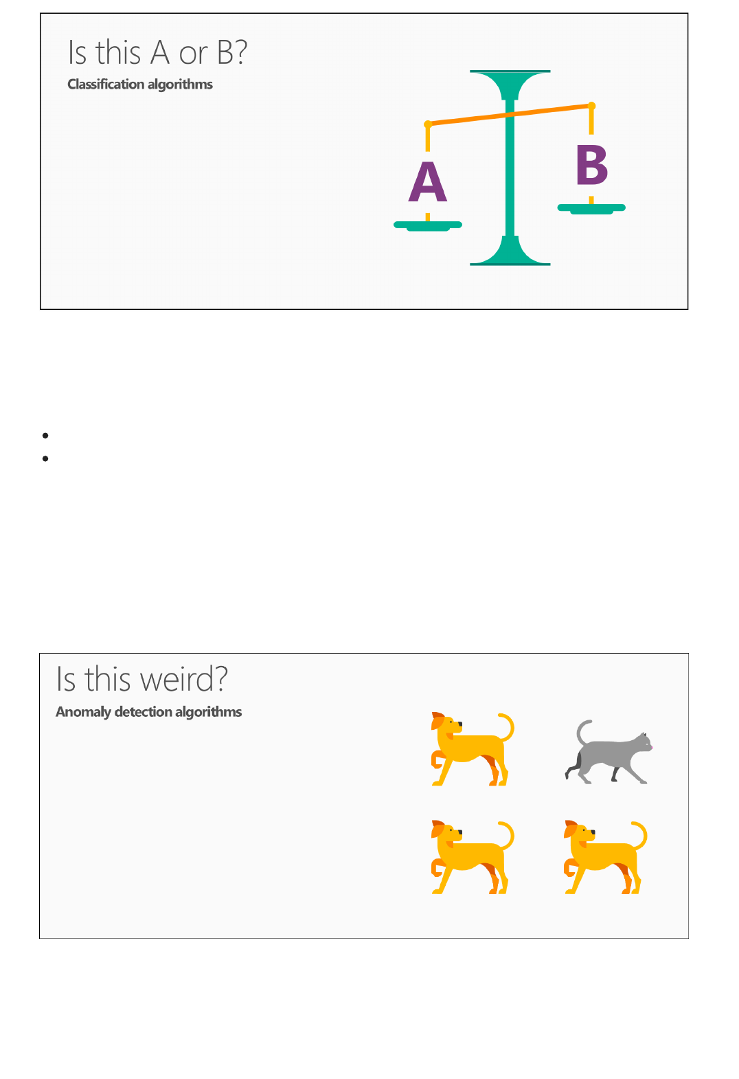
Question 2: Is this weird? uses anomaly detection algorithms
This family of algorithms is called two-class classification.
It's useful for any question that has just two possible answers.
For example:
Will this tire fail in the next 1,000 miles: Yes or no?
Which brings in more customers: a $5 coupon or a 25% discount?
This question can also be rephrased to include more than two options: Is this A or B or C or D, etc.? This is called
multiclass classification and it's useful when you have several — or several thousand — possible answers.
Multiclass classification chooses the most likely one.
The next question data science can answer is: Is this weird? This question is answered by a family of algorithms
called anomaly detection.
If you have a credit card, you’ve already benefited from anomaly detection. Your credit card company analyzes
your purchase patterns, so that they can alert you to possible fraud. Charges that are "weird" might be a purchase
at a store where you don't normally shop or buying an unusually pricey item.
This question can be useful in lots of ways. For instance:
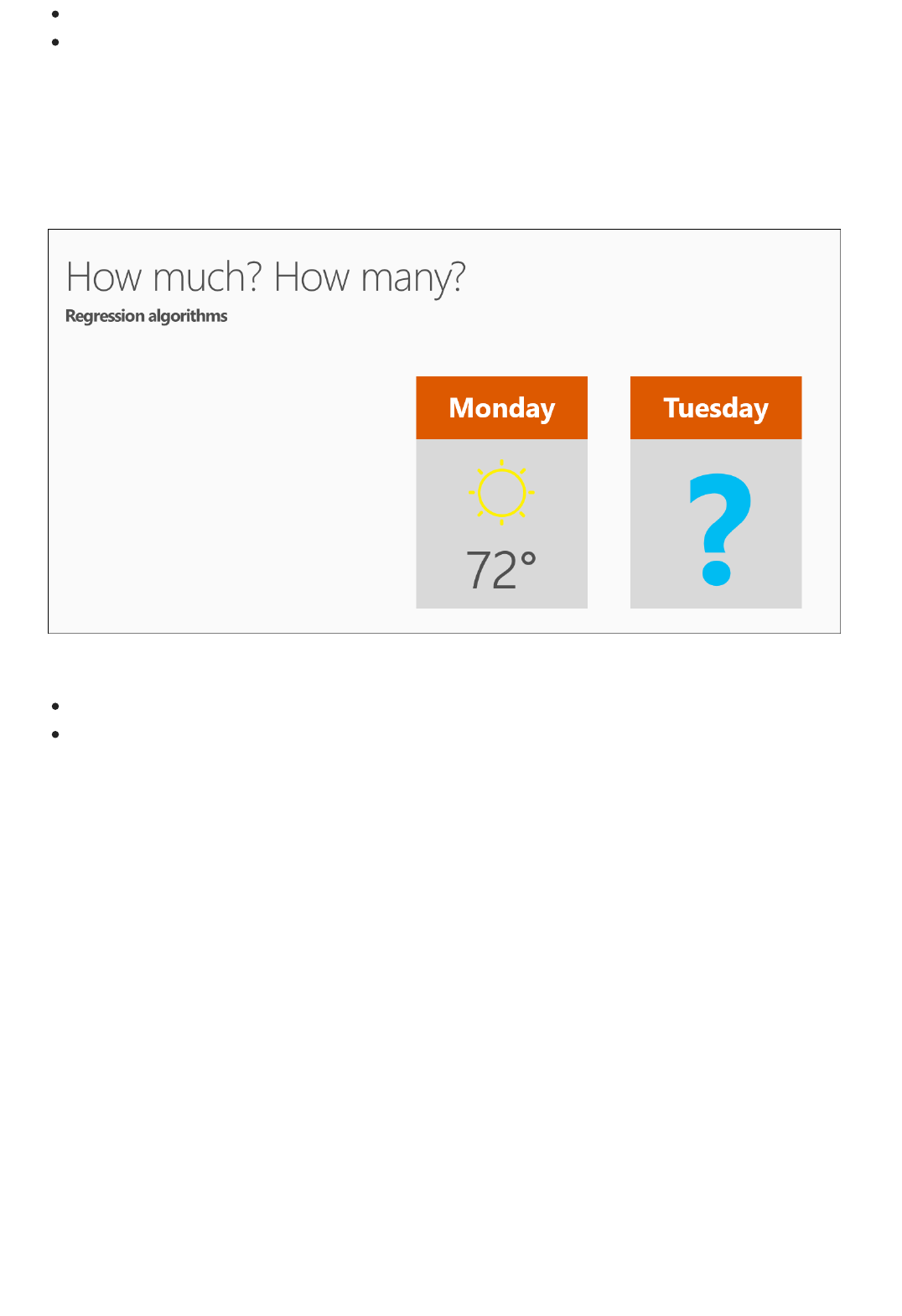
Question 3: How much? or How many? uses regression algorithms
Question 4: How is this organized? uses clustering algorithms
If you have a car with pressure gauges, you might want to know: Is this pressure gauge reading normal?
If you're monitoring the internet, you’d want to know: Is this message from the internet typical?
Anomaly detection flags unexpected or unusual events or behaviors. It gives clues where to look for problems.
Machine learning can also predict the answer to How much? or How many? The algorithm family that answers
this question is called regression.
Regression algorithms make numerical predictions, such as:
What will the temperature be next Tuesday?
What will my fourth quarter sales be?
They help answer any question that asks for a number.
Now the last two questions are a bit more advanced.
Sometimes you want to understand the structure of a data set - How is this organized? For this question, you
don’t have examples that you already know outcomes for.
There are a lot of ways to tease out the structure of data. One approach is clustering. It separates data into natural
"clumps," for easier interpretation. With clustering, there is no one right answer.
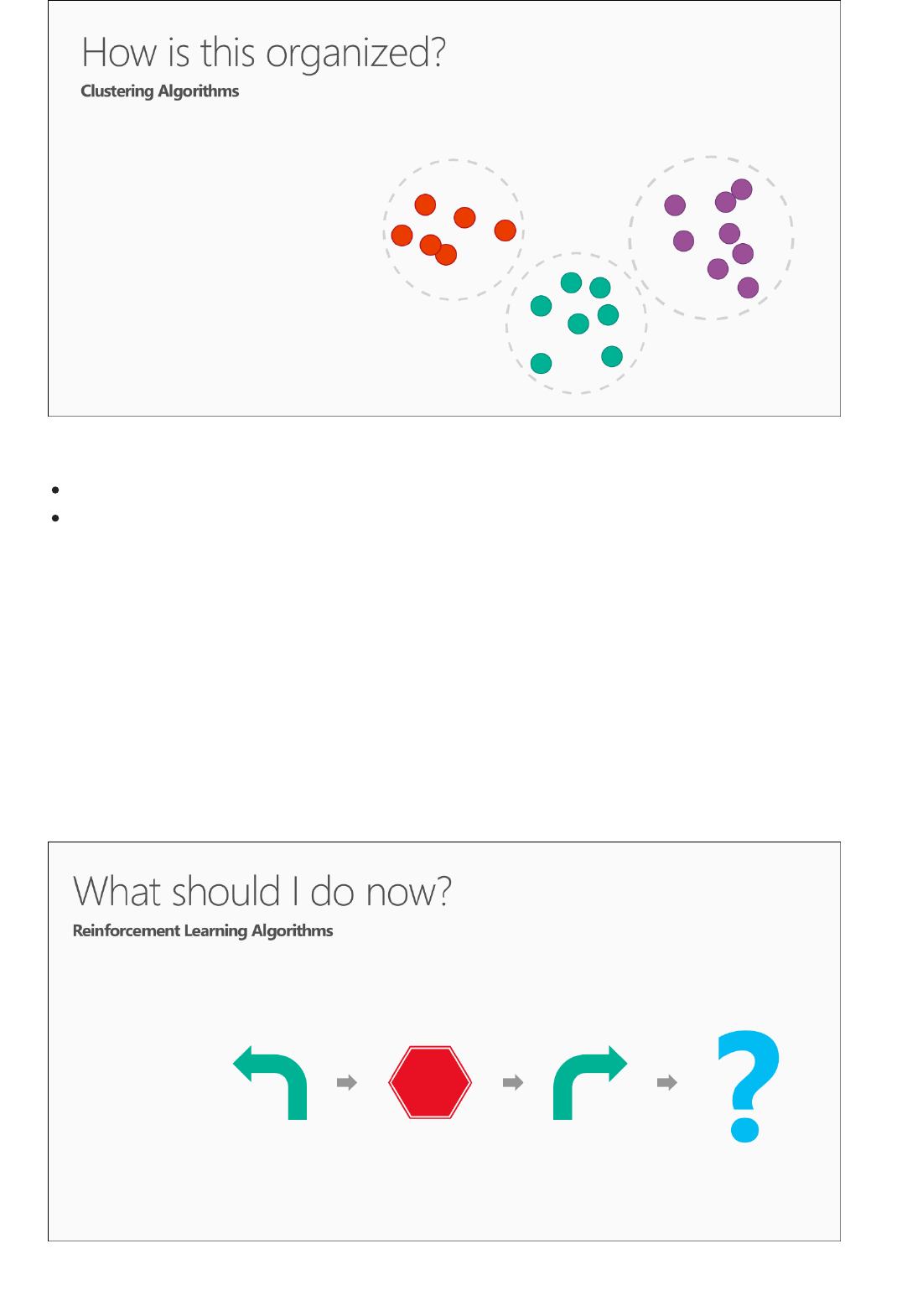
Question 5: What should I do now? uses reinforcement learning
algorithms
Common examples of clustering questions are:
Which viewers like the same types of movies?
Which printer models fail the same way?
By understanding how data is organized, you can better understand - and predict - behaviors and events.
The last question – What should I do now? – uses a family of algorithms called reinforcement learning.
Reinforcement learning was inspired by how the brains of rats and humans respond to punishment and rewards.
These algorithms learn from outcomes, and decide on the next action.
Typically, reinforcement learning is a good fit for automated systems that have to make lots of small decisions
without human guidance.
Questions it answers are always about what action should be taken - usually by a machine or a robot. Examples
are:

Next steps
If I'm a temperature control system for a house: Adjust the temperature or leave it where it is?
If I'm a self-driving car: At a yellow light, brake or accelerate?
For a robot vacuum: Keep vacuuming, or go back to the charging station?
Reinforcement learning algorithms gather data as they go, learning from trial and error.
So that's it - The 5 questions data science can answer.
Try a first data science experiment with Machine Learning Studio
Get an introduction to Machine Learning on Microsoft Azure

Is your data ready for data science?
3/20/2018 • 4 min to read • Edit Online
Video 2: Data Science for Beginners series
Other videos in this series
Transcript: Is your data ready for data science?
Criteria for data
Is your data relevant?
Learn how to evaluate your data to make sure it meets basic criteria to be ready for data science.
To get the most out of the series, watch them all. Go to the list of videos
Data Science for Beginners is a quick introduction to data science in five short videos.
Video 1: The 5 questions data science answers (5 min 14 sec)
Video 2: Is your data ready for data science?
Video 3: Ask a question you can answer with data (4 min 17 sec)
Video 4: Predict an answer with a simple model (7 min 42 sec)
Video 5: Copy other people's work to do data science (3 min 18 sec)
Welcome to "Is your data ready for data science?" the second video in the series Data Science for Beginners.
Before data science can give you the answers you want, you have to give it some high-quality raw materials to
work with. Just like making a pizza, the better the ingredients you start with, the better the final product.
In data science, there are certain ingredients that must be pulled together including:
Relevant
Connected
Accurate
Enough to work with
So the first ingredient - you need data that's relevant.
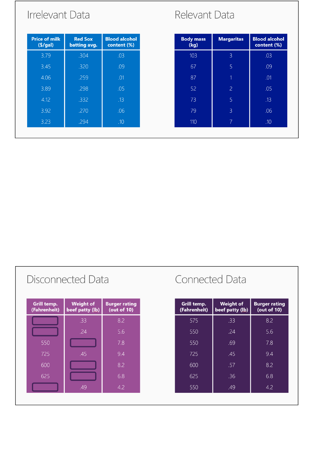
Do you have connected data?
On the left, the table presents the blood alcohol level of seven people tested outside a Boston bar, the Red Sox
batting average in their last game, and the price of milk in the nearest convenience store.
This is all perfectly legitimate data. It’s only fault is that it isn’t relevant. There's no obvious relationship between
these numbers. If someone gave you the current price of milk and the Red Sox batting average, there's no way you
could guess their blood alcohol content.
Now look at the table on the right. This time each person’s body mass was measured as well as the number of
drinks they’ve had. The numbers in each row are now relevant to each other. If I gave you my body mass and the
number of Margaritas I've had, you could make a guess at my blood alcohol content.
The next ingredient is connected data.
Here is some relevant data on the quality of hamburgers: grill temperature, patty weight, and rating in the local
food magazine. But notice the gaps in the table on the left.
Most data sets are missing some values. It's common to have holes like this and there are ways to work around
them. But if there's too much missing, your data begins to look like Swiss cheese.
If you look at the table on the left, there's so much missing data, it's hard to come up with any kind of relationship
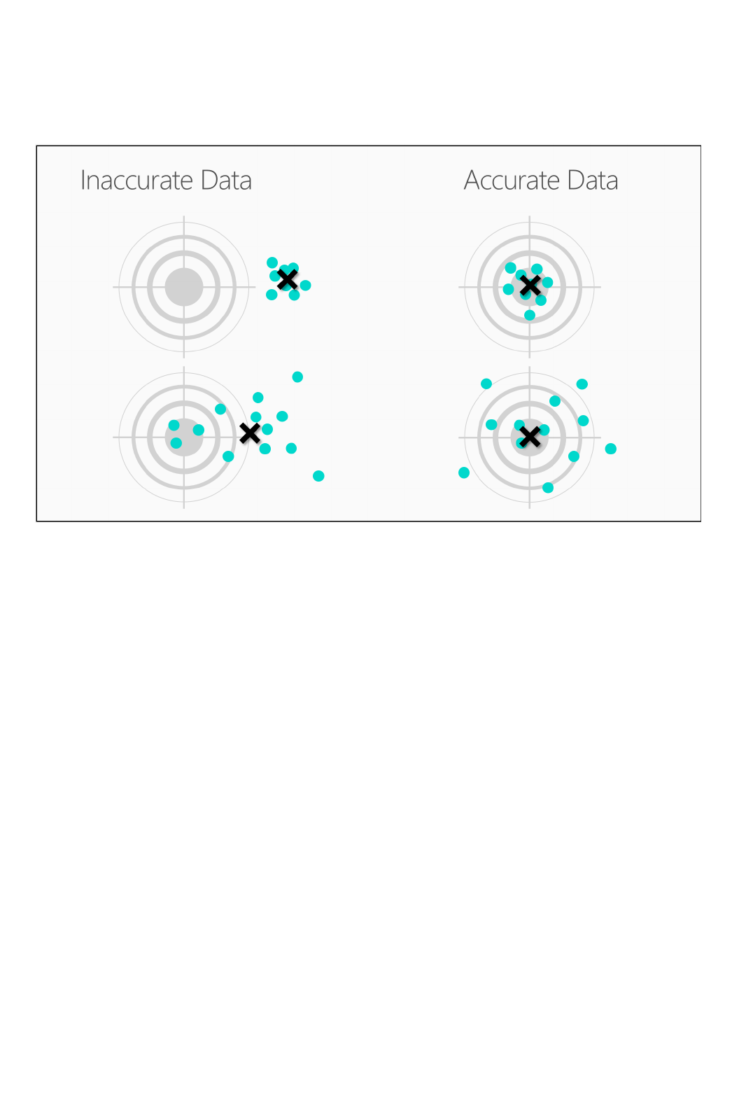
Is your data accurate?
Do you have enough data to work with?
between grill temperature and patty weight. This example shows disconnected data.
The table on the right, though, is full and complete - an example of connected data.
The next ingredient is accuracy. Here are four targets to hit.
Look at the target in the upper right. There is a tight grouping right around the bulls eye. That, of course, is
accurate. Oddly, in the language of data science, performance on the target right below it is also considered
accurate.
If you mapped out the center of these arrows, you'd see that it's very close to the bulls eye. The arrows are spread
out all around the target, so they're considered imprecise, but they're centered around the bulls eye, so they're
considered accurate.
Now look at the upper-left target. Here the arrows hit very close together, a tight grouping. They're precise, but
they're inaccurate because the center is way off the bulls eye. The arrows in the bottom-left target are both
inaccurate and imprecise. This archer needs more practice.
Finally, ingredient #4 is sufficient data.

Next steps
Think of each data point in your table as being a brush stroke in a painting. If you have only a few of them, the
painting can be fuzzy - it's hard to tell what it is.
If you add some more brush strokes, then your painting starts to get a little sharper.
When you have barely enough strokes, you only see enough to make some broad decisions. Is it somewhere I
might want to visit? It looks bright, that looks like clean water – yes, that’s where I’m going on vacation.
As you add more data, the picture becomes clearer and you can make more detailed decisions. Now you can look
at the three hotels on the left bank. You can notice the architectural features of the one in the foreground. You
might even choose to stay on the third floor because of the view.
With data that's relevant, connected, accurate, and enough, you have all the ingredients needed to do some high-
quality data science.
Be sure to check out the other four videos in Data Science for Beginners from Microsoft Azure Machine Learning.
Try a first data science experiment with Machine Learning Studio
Get an introduction to Machine Learning on Microsoft Azure

Ask a question you can answer with data
3/20/2018 • 4 min to read • Edit Online
Video 3: Data Science for Beginners series
Other videos in this series
Transcript: Ask a question you can answer with data
Ask a sharp question
Examples of your answer: Target data
Learn how to formulate a data science problem into a question in Data Science for Beginners video 3. This video
includes a comparison of questions for classification and regression algorithms.
To get the most out of the series, watch them all. Go to the list of videos
Data Science for Beginners is a quick introduction to data science in five short videos.
Video 1: The 5 questions data science answers (5 min 14 sec)
Video 2: Is your data ready for data science? (4 min 56 sec)
Video 3: Ask a question you can answer with data
Video 4: Predict an answer with a simple model (7 min 42 sec)
Video 5: Copy other people's work to do data science (3 min 18 sec)
Welcome to the third video in the series "Data Science for Beginners."
In this one, you'll get some tips for formulating a question you can answer with data.
You might get more out of this video, if you first watch the two earlier videos in this series: "The 5 questions data
science can answer" and "Is your data is ready for data science?"
We've talked about how data science is the process of using names (also called categories or labels) and numbers
to predict an answer to a question. But it can't be just any question; it has to be a sharp question.
A vague question doesn't have to be answered with a name or a number. A sharp question must.
Imagine you found a magic lamp with a genie who will truthfully answer any question you ask. But it's a
mischievous genie, and he'll try to make his answer as vague and confusing as he can get away with. You want to
pin him down with a question so airtight that he can't help but tell you what you want to know.
If you were to ask a vague question, like "What's going to happen with my stock?", the genie might answer, "The
price will change". That's a truthful answer, but it's not very helpful.
But if you were to ask a sharp question, like "What will my stock's sale price be next week?", the genie can't help
but give you a specific answer and predict a sale price.
Once you formulate your question, check to see whether you have examples of the answer in your data.
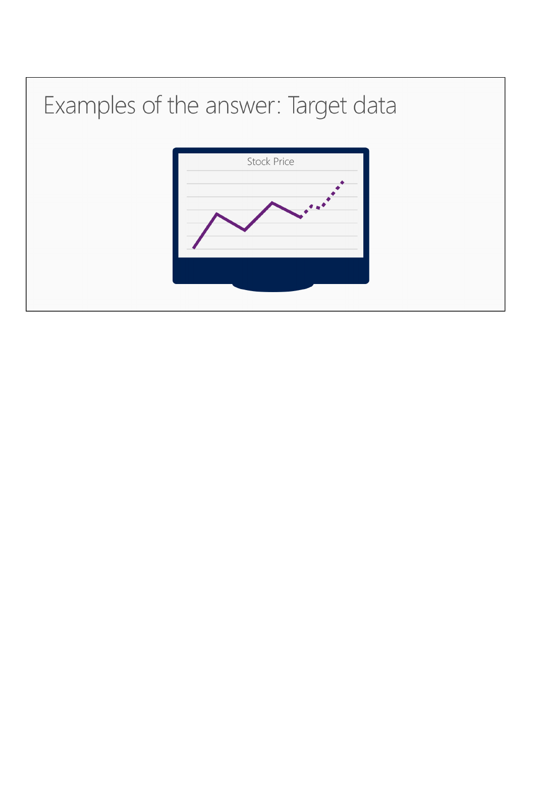
Reformulate your question
If our question is "What will my stock's sale price be next week?" then we have to make sure our data includes the
stock price history.
If our question is "Which car in my fleet is going to fail first?" then we have to make sure our data includes
information about previous failures.
These examples of answers are called a target. A target is what we are trying to predict about future data points,
whether it's a category or a number.
If you don't have any target data, you'll need to get some. You won't be able to answer your question without it.
Sometimes you can reword your question to get a more useful answer.
The question "Is this data point A or B?" predicts the category (or name or label) of something. To answer it, we
use a classification algorithm.
The question "How much?" or "How many?" predicts an amount. To answer it we use a regression algorithm.
To see how we can transform these, let's look at the question, "Which news story is the most interesting to this
reader?" It asks for a prediction of a single choice from many possibilities - in other words "Is this A or B or C or
D?" - and would use a classification algorithm.
But, this question may be easier to answer if you reword it as "How interesting is each story on this list to this
reader?" Now you can give each article a numerical score, and then it's easy to identify the highest-scoring article.
This is a rephrasing of the classification question into a regression question or How much?
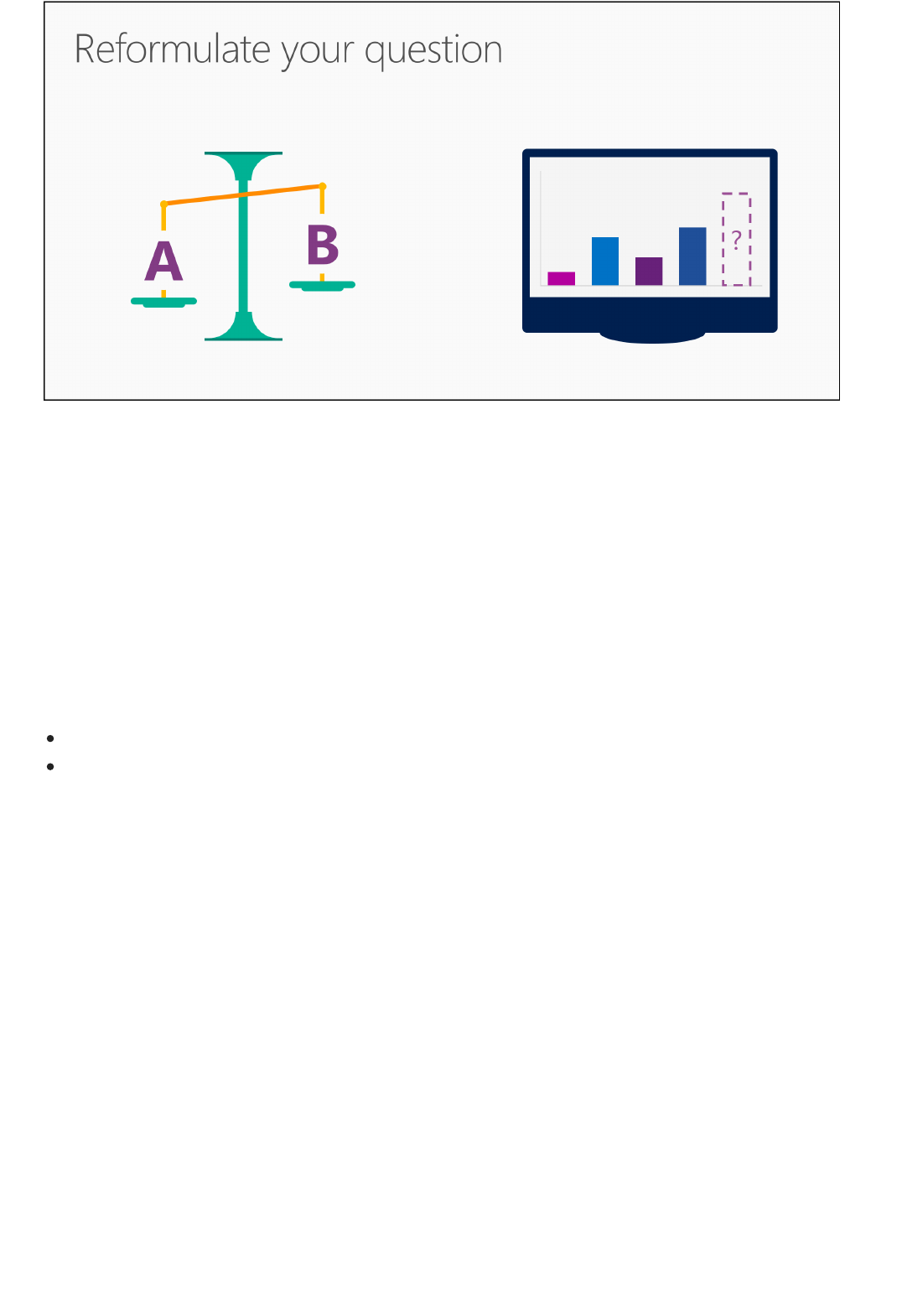
Next steps
How you ask a question is a clue to which algorithm can give you an answer.
You'll find that certain families of algorithms - like the ones in our news story example - are closely related. You
can reformulate your question to use the algorithm that gives you the most useful answer.
But, most important, ask that sharp question - the question that you can answer with data. And be sure you have
the right data to answer it.
We've talked about some basic principles for asking a question you can answer with data.
Be sure to check out the other videos in "Data Science for Beginners" from Microsoft Azure Machine Learning.
Try a first data science experiment with Machine Learning Studio
Get an introduction to Machine Learning on Microsoft Azure

Predict an answer with a simple model
3/20/2018 • 5 min to read • Edit Online
Video 4: Data Science for Beginners series
Other videos in this series
Transcript: Predict an answer with a simple model
Collect relevant, accurate, connected, enough data
Learn how to create a simple regression model to predict the price of a diamond in Data Science for Beginners
video 4. We'll draw a regression model with target data.
To get the most out of the series, watch them all. Go to the list of videos
Data Science for Beginners is a quick introduction to data science in five short videos.
Video 1: The 5 questions data science answers (5 min 14 sec)
Video 2: Is your data ready for data science? (4 min 56 sec)
Video 3: Ask a question you can answer with data (4 min 17 sec)
Video 4: Predict an answer with a simple model
Video 5: Copy other people's work to do data science (3 min 18 sec)
Welcome to the fourth video in the "Data Science for Beginners" series. In this one, we'll build a simple model and
make a prediction.
A model is a simplified story about our data. I'll show you what I mean.
Say I want to shop for a diamond. I have a ring that belonged to my grandmother with a setting for a 1.35 carat
diamond, and I want to get an idea of how much it will cost. I take a notepad and pen into the jewelry store, and I
write down the price of all of the diamonds in the case and how much they weigh in carats. Starting with the first
diamond - it's 1.01 carats and $7,366.
Now I go through and do this for all the other diamonds in the store.
Ask a sharp question
Plot the existing data
Notice that our list has two columns. Each column has a different attribute - weight in carats and price - and each
row is a single data point that represents a single diamond.
We've actually created a small data set here - a table. Notice that it meets our criteria for quality:
The data is relevant - weight is definitely related to price
It's accurate - we double-checked the prices that we write down
It's connected - there are no blank spaces in either of these columns
And, as we'll see, it's enough data to answer our question
Now we'll pose our question in a sharp way: "How much will it cost to buy a 1.35 carat diamond?"
Our list doesn't have a 1.35 carat diamond in it, so we'll have to use the rest of our data to get an answer to the
question.
The first thing we'll do is draw a horizontal number line, called an axis, to chart the weights. The range of the
weights is 0 to 2, so we'll draw a line that covers that range and put ticks for each half carat.
Next we'll draw a vertical axis to record the price and connect it to the horizontal weight axis. This will be in units
of dollars. Now we have a set of coordinate axes.
We're going to take this data now and turn it into a scatter plot. This is a great way to visualize numerical data sets.
For the first data point, we eyeball a vertical line at 1.01 carats. Then, we eyeball a horizontal line at $7,366. Where
they meet, we draw a dot. This represents our first diamond.
Now we go through each diamond on this list and do the same thing. When we're through, this is what we get: a
bunch of dots, one for each diamond.
Draw the model through the data points
Now if you look at the dots and squint, the collection looks like a fat, fuzzy line. We can take our marker and draw
a straight line through it.
By drawing a line, we created a model. Think of this as taking the real world and making a simplistic cartoon
version of it. Now the cartoon is wrong - the line doesn't go through all the data points. But, it's a useful
simplification.
Use the model to find the answer
The fact that all the dots don't go exactly through the line is OK. Data scientists explain this by saying that there's
the model - that's the line - and then each dot has some noise or variance associated with it. There's the underlying
perfect relationship, and then there's the gritty, real world that adds noise and uncertainty.
Because we're trying to answer the question How much? this is called a regression. And because we're using a
straight line, it's a linear regression.
Now we have a model and we ask it our question: How much will a 1.35 carat diamond cost?
To answer our question, we eyeball 1.35 carats and draw a vertical line. Where it crosses the model line, we eyeball
a horizontal line to the dollar axis. It hits right at 10,000. Boom! That's the answer: A 1.35 carat diamond costs
about $10,000.
Create a confidence interval
It's natural to wonder how precise this prediction is. It's useful to know whether the 1.35 carat diamond will be
very close to $10,000, or a lot higher or lower. To figure this out, let's draw an envelope around the regression line
that includes most of the dots. This envelope is called our confidence interval: We're pretty confident that prices
fall within this envelope, because in the past most of them have. We can draw two more horizontal lines from
where the 1.35 carat line crosses the top and the bottom of that envelope.
We're done, with no math or computers
Next steps
Now we can say something about our confidence interval: We can say confidently that the price of a 1.35 carat
diamond is about $10,000 - but it might be as low as $8,000 and it might be as high as $12,000.
We did what data scientists get paid to do, and we did it just by drawing:
We asked a question that we could answer with data
We built a model using linear regression
We made a prediction, complete with a confidence interval
And we didn't use math or computers to do it.
Now if we'd had more information, like...
the cut of the diamond
color variations (how close the diamond is to being white)
the number of inclusions in the diamond
...then we would have had more columns. In that case, math becomes helpful. If you have more than two columns,
it's hard to draw dots on paper. The math lets you fit that line or that plane to your data very nicely.
Also, if instead of just a handful of diamonds, we had two thousand or two million, then you can do that work
much faster with a computer.
Today, we've talked about how to do linear regression, and we made a prediction using data.
Be sure to check out the other videos in "Data Science for Beginners" from Microsoft Azure Machine Learning.
Try a first data science experiment with Machine Learning Studio
Get an introduction to Machine Learning on Microsoft Azure

Copy other people's work to do data science
3/20/2018 • 3 min to read • Edit Online
Video 5: Data Science for Beginners series
IMPORTANTIMPORTANT
Other videos in this series
Transcript: Copy other people's work to do data science
Find examples in the Azure AI Gallery
One of the trade secrets of data science is getting other people to do your work for you. Find a clustering
algorithm example in Azure AI Gallery to use for your own machine learning experiment.
Cortana Intelligence Gallery was renamed Azure AI Gallery. As a result, text and images in this transcript vary slightly
from the video, which uses the former name.
To get the most out of the series, watch them all. Go to the list of videos
Data Science for Beginners is a quick introduction to data science in five short videos.
Video 1: The 5 questions data science answers (5 min 14 sec)
Video 2: Is your data ready for data science? (4 min 56 sec)
Video 3: Ask a question you can answer with data (4 min 17 sec)
Video 4: Predict an answer with a simple model (7 min 42 sec)
Video 5: Copy other people's work to do data science
Welcome to the fifth video in the series "Data Science for Beginners."
In this one, you’ll discover a place to find examples that you can borrow from as a starting point for your own
work. You might get the most out of this video if you first watch the earlier videos in this series.
One of the trade secrets of data science is getting other people to do your work for you.
Microsoft has a cloud-based service called Azure Machine Learning Studio that you're welcome to try for free. It
provides you with a workspace where you can experiment with different machine learning algorithms, and, when
you've got your solution worked out, you can launch it as a web service.
Part of this service is something called the Azure AI Gallery. It contains resources, including a collection of Azure
Machine Learning experiments, or models, that people have built and contributed for others to use. These
experiments are a great way to leverage the thought and hard work of others to get you started on your own
solutions. Everyone is welcome to browse through it.
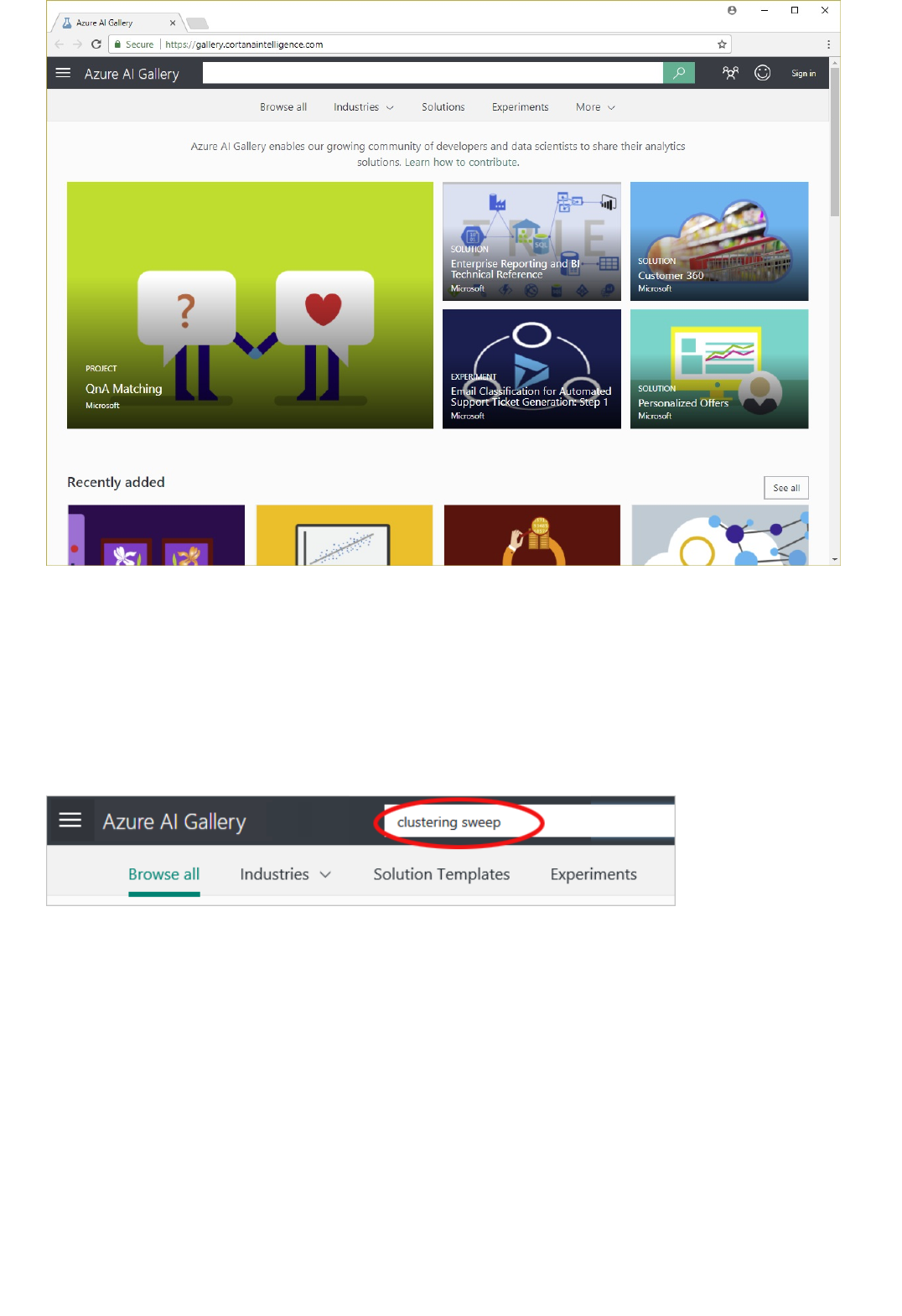
Find and use a clustering algorithm example
If you click Experiments at the top, you'll see a number of the most recent and popular experiments in the
gallery. You can search through the rest of experiments by clicking Browse All at the top of the screen, and there
you can enter search terms and choose search filters.
So, for instance, let's say you want to see an example of how clustering works, so you search for "clustering
sweep" experiments.
Here's an interesting one that someone contributed to the gallery.
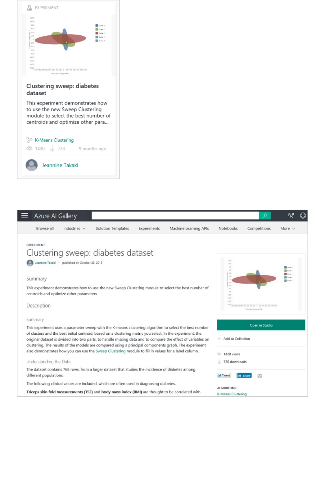
Click on that experiment and you get a web page that describes the work that this contributor did, along with
some of their results.
Notice the link that says Open in Studio.
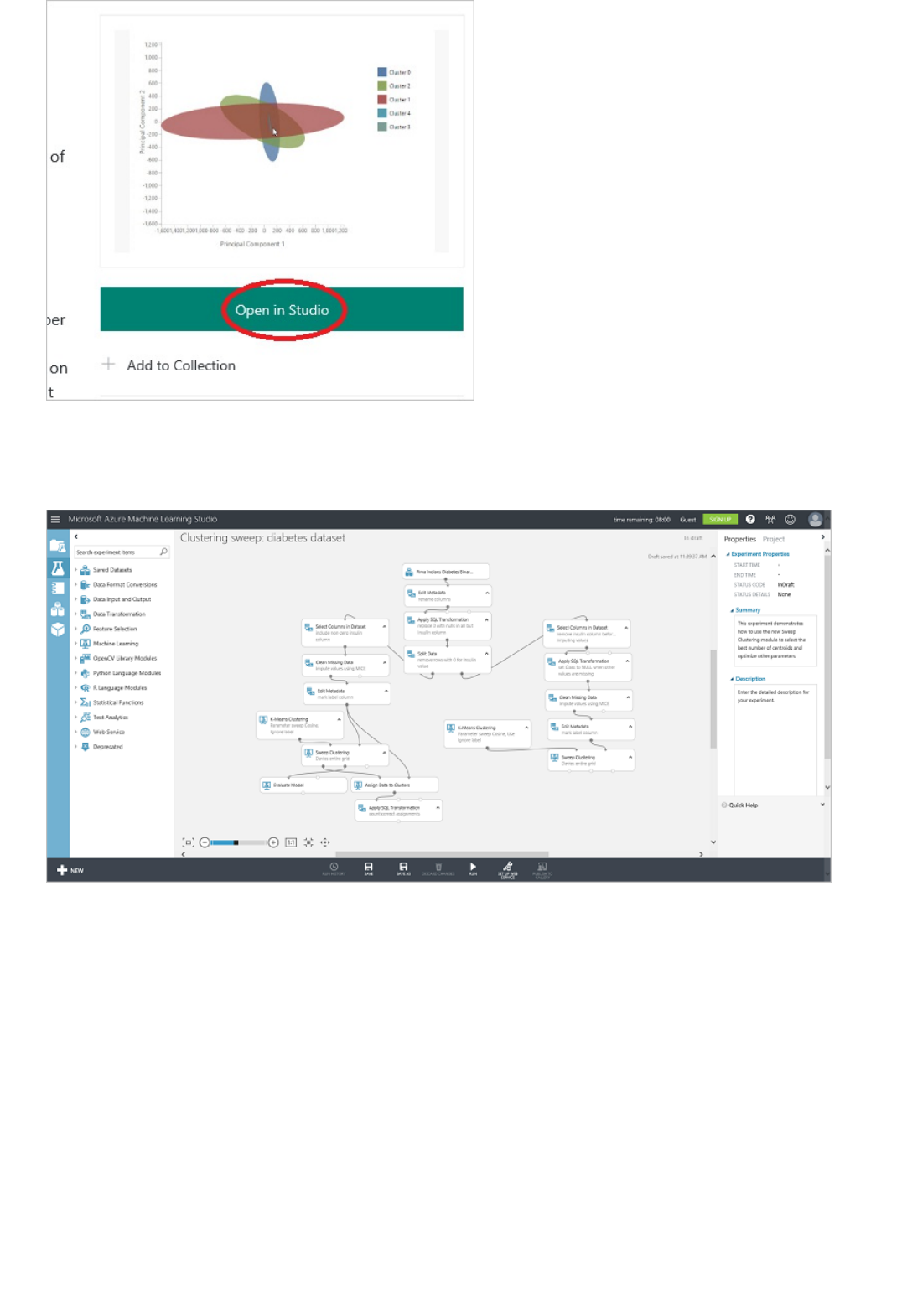
Find experiments that demonstrate machine learning techniques
I can click on that and it takes me right to Azure Machine Learning Studio. It creates a copy of the experiment
and puts it in my own workspace. This includes the contributor's dataset, all the processing that they did, all of the
algorithms that they used, and how they saved out the results.
And now I have a starting point. I can swap out their data for my own and do my own tweaking of the model. This
gives me a running start, and it lets me build on the work of people who really know what they’re doing.
There are other experiments in the Azure AI Gallery that were contributed specifically to provide how-to examples
for people new to data science. For instance, there's an experiment in the gallery that demonstrates how to handle
missing values (Methods for handling missing values). It walks you through 15 different ways of substituting
empty values, and talks about the benefits of each method and when to use it.

Next steps
Azure AI Gallery is a place to find working experiments that you can use as a starting point for your own
solutions.
Be sure to check out the other videos in "Data Science for Beginners" from Microsoft Azure Machine Learning.
Try your first data science experiment with Azure Machine Learning
Get an introduction to Machine Learning on Microsoft Azure
Quickstart tutorial for the R programming language
for Azure Machine Learning
3/21/2018 • 53 min to read • Edit Online
Introduction
NOTENOTE
Forecasting and the datasetForecasting and the dataset
OrganizationOrganization
This quickstart tutorial helps you quickly start extending Azure Machine Learning by using the R programming
language. Follow this R programming tutorial to create, test and execute R code within Azure Machine Learning.
As you work through tutorial, you will create a complete forecasting solution by using the R language in Azure
Machine Learning.
Microsoft Azure Machine Learning contains many powerful machine learning and data manipulation modules. The
powerful R language has been described as the lingua franca of analytics. Happily, analytics and data manipulation
in Azure Machine Learning can be extended by using R. This combination provides the scalability and ease of
deployment of Azure Machine Learning with the flexibility and deep analytics of R.
You can try Azure Machine Learning for free. No credit card or Azure subscription is required. Get started now.
Forecasting is a widely employed and quite useful analytical method. Common uses range from predicting sales of
seasonal items, determining optimal inventory levels, to predicting macroeconomic variables. Forecasting is
typically done with time series models.
Time series data is data in which the values have a time index. The time index can be regular, e.g. every month or
every minute, or irregular. A time series model is based on time series data. The R programming language contains
a flexible framework and extensive analytics for time series data.
In this quickstart guide we will be working with California dairy production and pricing data. This data includes
monthly information on the production of several dairy products and the price of milk fat, a benchmark
commodity.
The data used in this article, along with R scripts, can be downloaded here. This data was originally synthesized
from information available from the University of Wisconsin at http://future.aae.wisc.edu/tab/production.html.
We will progress through several steps as you learn how to create, test and execute analytics and data
manipulation R code in the Azure Machine Learning environment.
First we will explore the basics of using the R language in the Azure Machine Learning Studio environment.
Then we progress to discussing various aspects of I/O for data, R code and graphics in the Azure Machine
Learning environment.
We will then construct the first part of our forecasting solution by creating code for data cleaning and
transformation.
With our data prepared we will perform an analysis of the correlations between several of the variables in our
dataset.
Finally, we will create a seasonal time series forecasting model for milk production.
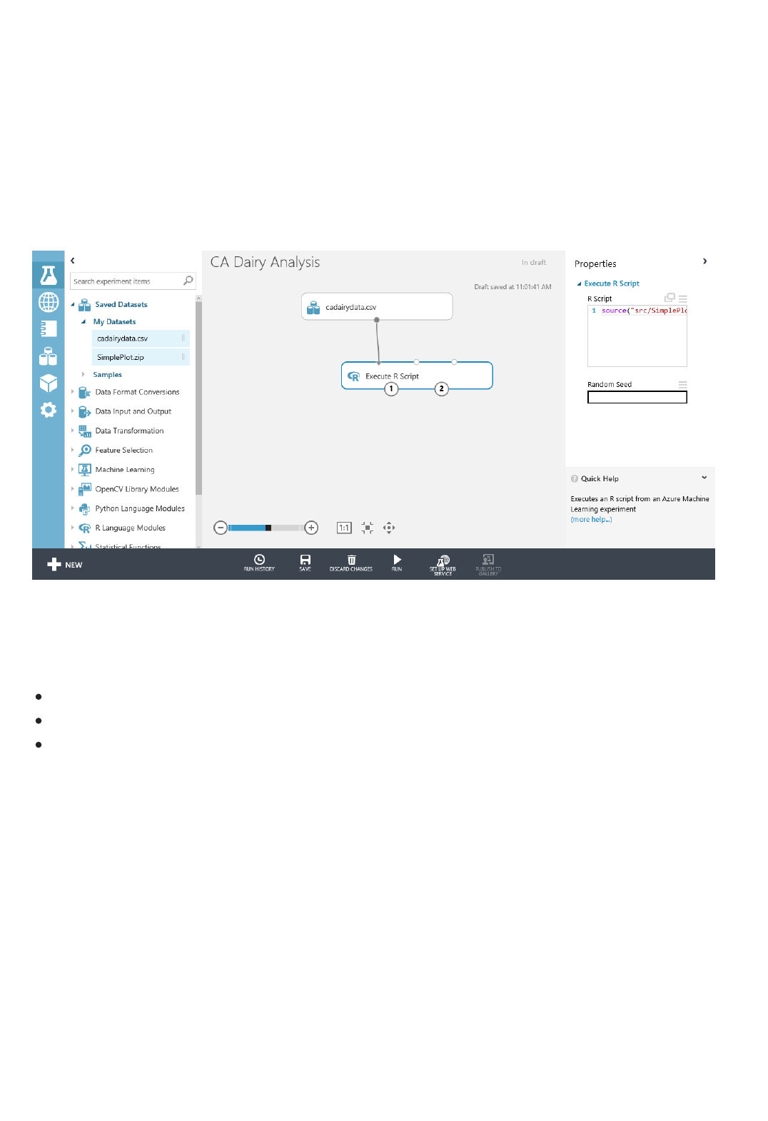
Interact with R language in Machine Learning Studio
The Execute R Script moduleThe Execute R Script module
Execute R codeExecute R code
Defensive R coding for Azure Machine LearningDefensive R coding for Azure Machine Learning
This section takes you through some basics of interacting with the R programming language in the Machine
Learning Studio environment. The R language provides a powerful tool to create customized analytics and data
manipulation modules within the Azure Machine Learning environment.
I will use RStudio to develop, test and debug R code on a small scale. This code is then cut and paste into an
Execute R Script module in Machine Learning Studio ready to run.
Within Machine Learning Studio, R scripts are run within the Execute R Script module. An example of the Execute
R Script module in Machine Learning Studio is shown in Figure 1.
Figure 1. The Machine Learning Studio environment showing the Execute R Script module selected.
Referring to Figure 1, let's look at some of the key parts of the Machine Learning Studio environment for working
with the Execute R Script module.
The modules in the experiment are shown in the center pane.
The upper part of the right pane contains a window to view and edit your R scripts.
The lower part of right pane shows some properties of the Execute R Script. You can view the error and output
logs by clicking on the appropriate spots of this pane.
We will, of course, be discussing the Execute R Script in greater detail in the rest of this document.
When working with complex R functions, I recommend that you edit, test and debug in RStudio. As with any
software development, extend your code incrementally and test it on small simple test cases. Then cut and paste
your functions into the R script window of the Execute R Script module. This approach allows you to harness both
the RStudio integrated development environment (IDE) and the power of Azure Machine Learning.
Any R code in the Execute R Script module will execute when you run the experiment by clicking on the Run
button. When execution has completed, a check mark will appear on the Execute R Script icon.
If you are developing R code for, say, a web service by using Azure Machine Learning, you should definitely plan
how your code will deal with an unexpected data input and exceptions. To maintain clarity, I have not included
much in the way of checking or exception handling in most of the code examples shown. However, as we proceed I
will give you several examples of functions by using R's exception handling capability.
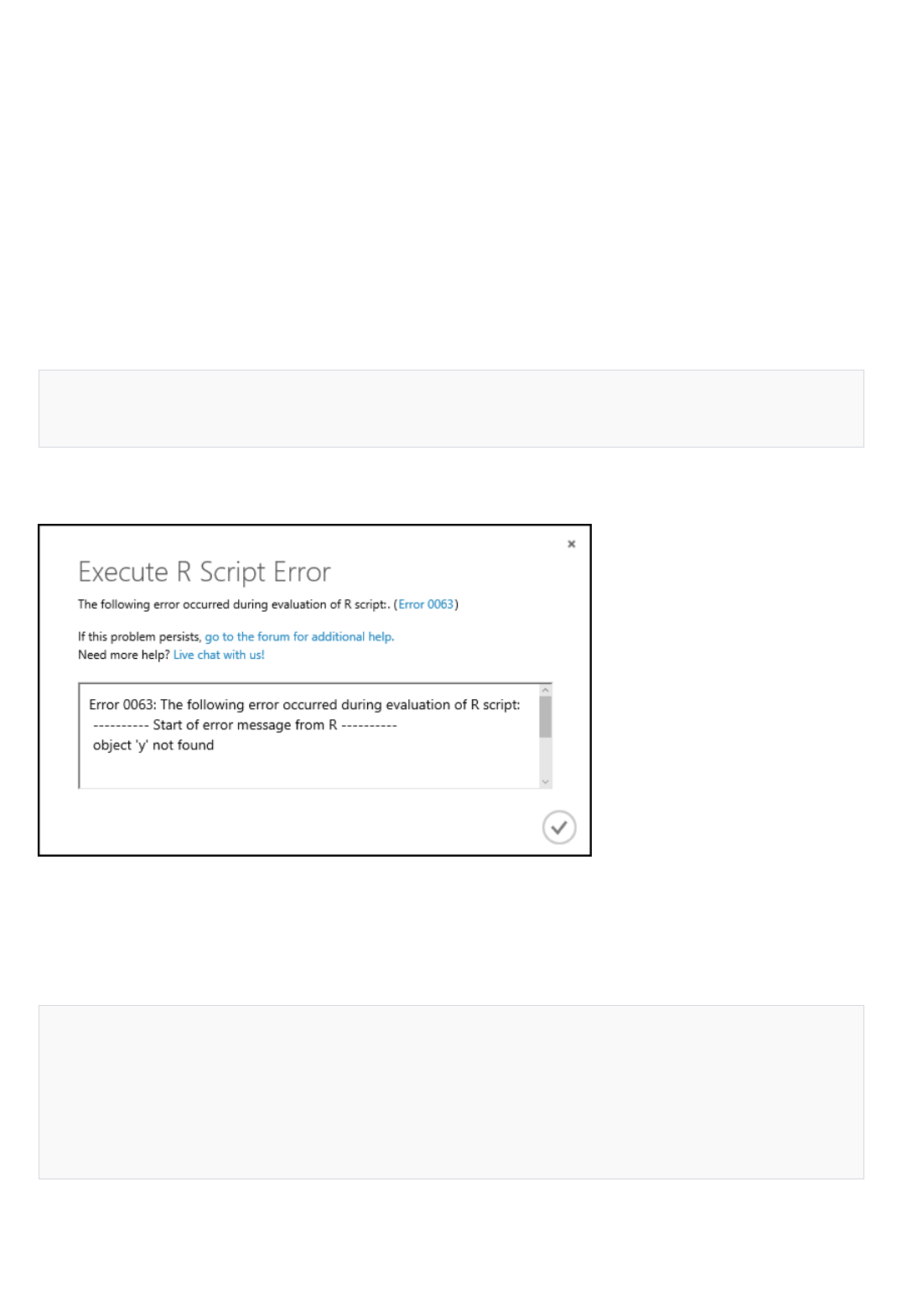
Debug and test R in Machine Learning StudioDebug and test R in Machine Learning Studio
x <- 1.0
z <- x + y
[Critical] Error: Error 0063: The following error occurred during evaluation of R script:
---------- Start of error message from R ----------
object 'y' not found
object 'y' not found
----------- End of error message from R -----------
If you need a more complete treatment of R exception handling, I recommend you read the applicable sections of
the book by Wickham listed in Appendix B - Further Reading.
To reiterate, I recommend you test and debug your R code on a small scale in RStudio. However, there are cases
where you will need to track down R code problems in the Execute R Script itself. In addition, it is good practice to
check your results in Machine Learning Studio.
Output from the execution of your R code and on the Azure Machine Learning platform is found primarily in
output.log. Some additional information will be seen in error.log.
If an error occurs in Machine Learning Studio while running your R code, your first course of action should be to
look at error.log. This file can contain useful error messages to help you understand and correct your error. To view
error.log, click on View error log on the properties pane for the Execute R Script containing the error.
For example, I ran the following R code, with an undefined variable y, in an Execute R Script module:
This code fails to execute, resulting in an error condition. Clicking on View error log on the properties pane
produces the display shown in Figure 2.
Figure 2. Error message pop-up.
It looks like we need to look in output.log to see the R error message. Click on the Execute R Script and then click
on the View output.log item on the properties pane to the right. A new browser window opens, and I see the
following.
This error message contains no surprises and clearly identifies the problem.
To inspect the value of any object in R, you can print these values to the output.log file. The rules for examining
object values are essentially the same as in an interactive R session. For example, if you type a variable name on a
line, the value of the object will be printed to the output.log file.

Packages in Machine Learning StudioPackages in Machine Learning Studio
data.set <- data.frame(installed.packages())
maml.mapOutputPort("data.set")
Introduction to RStudioIntroduction to RStudio
Get data in and out of the Execute R Script module
Load and check data in Machine Learning StudioLoad and check data in Machine Learning Studio
Load the datasetLoad the dataset
Create an experimentCreate an experiment
Azure Machine Learning comes with over 350 preinstalled R language packages. You can use the following code in
the Execute R Script module to retrieve a list of the preinstalled packages.
If you don't understand the last line of this code at the moment, read on. In the rest of this document we will
extensively discuss using R in the Azure Machine Learning environment.
RStudio is a widely used IDE for R. I will use RStudio for editing, testing and debugging some of the R code used
in this quick start guide. Once R code is tested and ready, you simply cut and paste from the RStudio editor into a
Machine Learning Studio Execute R Script module.
If you do not have the R programming language installed on your desktop machine, I recommend you do so now.
Free downloads of open source R language are available at the Comprehensive R Archive Network (CRAN) at
http://www.r-project.org/. There are downloads available for Windows, Mac OS, and Linux/UNIX. Choose a nearby
mirror and follow the download directions. In addition, CRAN contains a wealth of useful analytics and data
manipulation packages.
If you are new to RStudio, you should download and install the desktop version. You can find the RStudio
downloads for Windows, Mac OS, and Linux/UNIX at http://www.rstudio.com/products/RStudio/. Follow the
directions provided to install RStudio on your desktop machine.
A tutorial introduction to RStudio is available at https://support.rstudio.com/hc/sections/200107586-Using-
RStudio.
I provide some additional information on using RStudio in Appendix A.
In this section we will discuss how you get data into and out of the Execute R Script module. We will review how to
handle various data types read into and out of the Execute R Script module.
The complete code for this section is in the zip file you downloaded earlier.
We will start by loading the csdairydata.csv file into Azure Machine Learning Studio.
Start your Azure Machine Learning Studio environment.
Click on + NEW at the lower left of your screen and select Dataset.
Select From Local File, and then Browse to select the file.
Make sure you have selected Generic CSV file with header (.csv) as the type for the dataset.
Click the check mark.
After the dataset has been uploaded, you should see the new dataset by clicking on the Datasets tab.
Now that we have some data in Machine Learning Studio, we need to create an experiment to do the analysis.
Click on + NEW at the lower left and select Experiment, then Blank Experiment.
You can name your experiment by selecting, and modifying, the Experiment created on ... title at the top of
the page. For example, changing it to CA Dairy Analysis.
On the left of the experiment page, expand Saved Datasets, and then My Datasets. You should see the
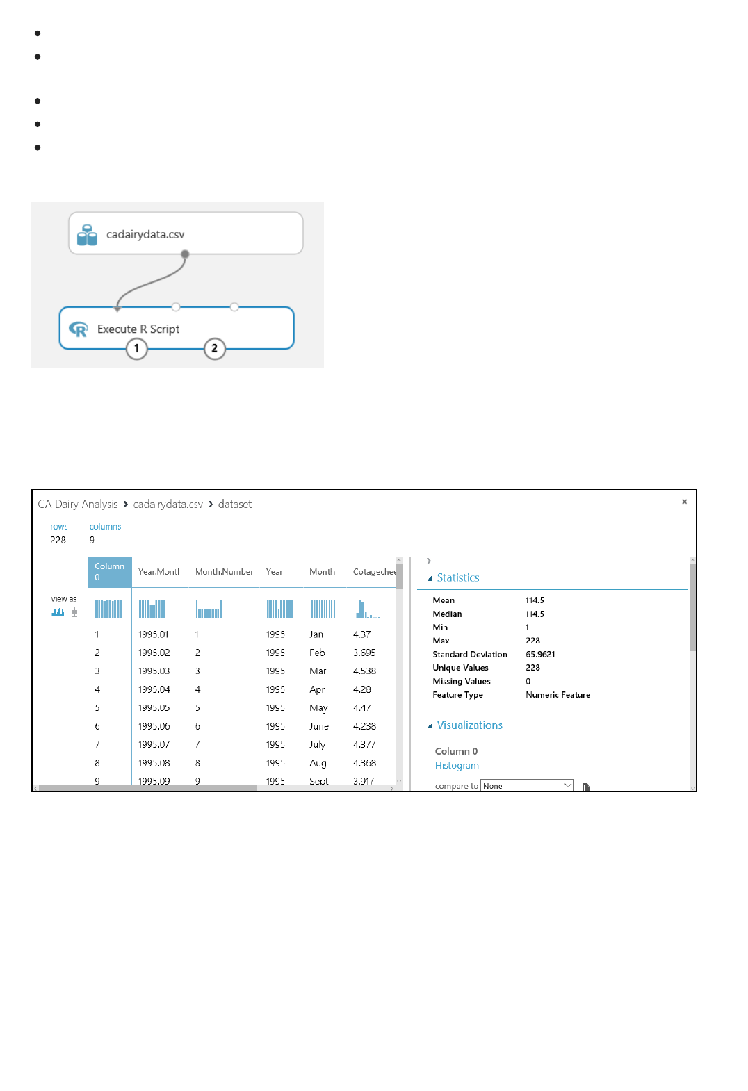
Check on the dataCheck on the data
First R scriptFirst R script
cadairydata.csv that you uploaded earlier.
Drag and drop the csdairydata.csv dataset onto the experiment.
In the Search experiment items box on the top of the left pane, type Execute R Script. You will see the module
appear in the search list.
Drag and drop the Execute R Script module onto your pallet.
Connect the output of the csdairydata.csv dataset to the leftmost input (Dataset1) of the Execute R Script.
Don't forget to click on 'Save'!
At this point your experiment should look something like Figure 3.
Figure 3. The CA Dairy Analysis experiment with dataset and Execute R Script module.
Let's have a look at the data we have loaded into our experiment. In the experiment, click on the output of the
cadairydata.csv dataset and select visualize. You should see something like Figure 4.
Figure 4. Summary of the cadairydata.csv dataset.
In this view we see a lot of useful information. We can see the first several rows of that dataset. If we select a
column, the Statistics section shows more information about the column. For example, the Feature Type row shows
us what data types Azure Machine Learning Studio assigned to the column. Having a quick look like this is a good
sanity check before we start to do any serious work.
Let's create a simple first R script to experiment with in Azure Machine Learning Studio. I have created and tested
the following script in RStudio.
## Only one of the following two lines should be used
## If running in Machine Learning Studio, use the first line with maml.mapInputPort()
## If in RStudio, use the second line with read.csv()
cadairydata <- maml.mapInputPort(1)
# cadairydata <- read.csv("cadairydata.csv", header = TRUE, stringsAsFactors = FALSE)
str(cadairydata)
pairs(~ Cotagecheese.Prod + Icecream.Prod + Milk.Prod + N.CA.Fat.Price, data = cadairydata)
## The following line should be executed only when running in
## Azure Machine Learning Studio
maml.mapOutputPort('cadairydata')
Data input to the Execute R Script moduleData input to the Execute R Script module
Script BundleScript Bundle
source("src/yourfile.R") # Reads a zipped R script
load("src/yourData.rdata") # Reads a zipped R data file
NOTENOTE
Now I need to transfer this script to Azure Machine Learning Studio. I could simply cut and paste. However, in this
case, I will transfer my R script via a zip file.
Let's have a look at the inputs to the Execute R Script module. In this example we will read the California dairy data
into the Execute R Script module.
There are three possible inputs for the Execute R Script module. You may use any one or all of these inputs,
depending on your application. It is also perfectly reasonable to use an R script that takes no input at all.
Let's look at each of these inputs, going from left to right. You can see the names of each of the inputs by placing
your cursor over the input and reading the tooltip.
The Script Bundle input allows you to pass the contents of a zip file into Execute R Script module. You can use one
of the following commands to read the contents of the zip file into your R code.
Azure Machine Learning treats files in the zip as if they are in the src/ directory, so you need to prefix your file names with
this directory name. For example, if the zip contains the files yourfile.R and yourData.rdata in the root of the zip, you
would address these as src/yourfile.R and src/yourData.rdata when using source and load .
We already discussed loading datasets in Loading the dataset. Once you have created and tested the R script
shown in the previous section, do the following:
## Only one of the following two lines should be used
## If running in Machine Learning Studio, use the first line with maml.mapInputPort()
## If in RStudio, use the second line with read.csv()
cadairydata <- maml.mapInputPort(1)
# cadairydata <- read.csv("cadairydata.csv", header = TRUE, stringsAsFactors = FALSE)
str(cadairydata)
pairs(~ Cotagecheese.Prod + Icecream.Prod + Milk.Prod + N.CA.Fat.Price, data = cadairydata)
## The following line should be executed only when running in
## Azure Machine Learning Studio
maml.mapOutputPort('cadairydata')
2. Create a zip file and copy your script into this zip file. On Windows, you can right-click on the file and select
Send to, and then Compressed folder. This will create a new zip file containing the "simpleplot.R" file.
3. Add your file to the datasets in Machine Learning Studio, specifying the type as zip. You should now see the
1. Save the R script into a .R file. I call my script file "simpleplot.R". Here's the contents.
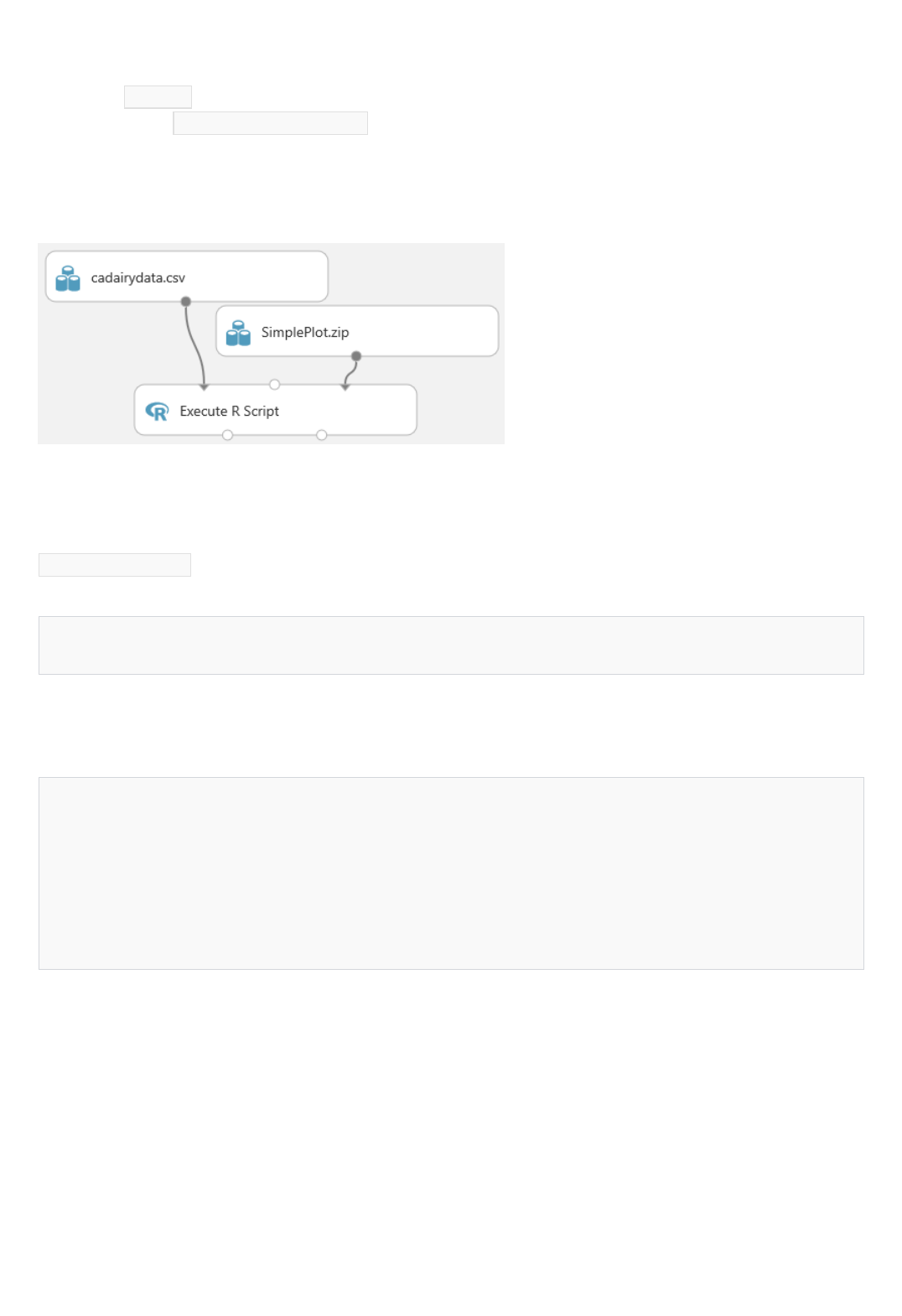
Dataset1Dataset1
cadairydata <- maml.mapInputPort(1)
[ModuleOutput] InputDataStructure
[ModuleOutput]
[ModuleOutput] {
[ModuleOutput] "InputName":Dataset1
[ModuleOutput] "Rows":228
[ModuleOutput] "Cols":9
[ModuleOutput] "ColumnTypes":System.Int32,3,System.Double,5,System.String,1
[ModuleOutput] }
zip file in your datasets.
4. Drag and drop the zip file from datasets onto the ML Studio canvas.
5. Connect the output of the zip data icon to the Script Bundle input of the Execute R Script module.
6. Type the source() function with your zip file name into the code window for the Execute R Script module. In
my case I typed source("src/simpleplot.R") .
7. Make sure you click Save.
Once these steps are complete, the Execute R Script module will execute the R script in the zip file when the
experiment is run. At this point your experiment should look something like Figure 5.
Figure 5. Experiment using zipped R script.
You can pass a rectangular table of data to your R code by using the Dataset1 input. In our simple script the
maml.mapInputPort(1) function reads the data from port 1. This data is then assigned to a dataframe variable name
in your code. In our simple script the first line of code performs the assignment.
Execute your experiment by clicking on the Run button. When the execution finishes, click on the Execute R Script
module and then click View output log on the properties pane. A new page should appear in your browser
showing the contents of the output.log file. When you scroll down you should see something like the following.
Farther down the page is more detailed information on the columns, which will look something like the following.
[ModuleOutput] [1] "Loading variable port1..."
[ModuleOutput]
[ModuleOutput] 'data.frame': 228 obs. of 9 variables:
[ModuleOutput]
[ModuleOutput] $ Column 0 : int 1 2 3 4 5 6 7 8 9 10 ...
[ModuleOutput]
[ModuleOutput] $ Year.Month : num 1995 1995 1995 1995 1995 ...
[ModuleOutput]
[ModuleOutput] $ Month.Number : int 1 2 3 4 5 6 7 8 9 10 ...
[ModuleOutput]
[ModuleOutput] $ Year : int 1995 1995 1995 1995 1995 1995 1995 1995 1995 1995 ...
[ModuleOutput]
[ModuleOutput] $ Month : chr "Jan" "Feb" "Mar" "Apr" ...
[ModuleOutput]
[ModuleOutput] $ Cotagecheese.Prod: num 4.37 3.69 4.54 4.28 4.47 ...
[ModuleOutput]
[ModuleOutput] $ Icecream.Prod : num 51.6 56.1 68.5 65.7 73.7 ...
[ModuleOutput]
[ModuleOutput] $ Milk.Prod : num 2.11 1.93 2.16 2.13 2.23 ...
[ModuleOutput]
[ModuleOutput] $ N.CA.Fat.Price : num 0.98 0.892 0.892 0.897 0.897 ...
NOTENOTE
Dataset2Dataset2
Execute R Script outputsExecute R Script outputs
Output a dataframeOutput a dataframe
maml.mapOutputPort('cadairydata')
These results are mostly as expected, with 228 observations and 9 columns in the dataframe. We can see the
column names, the R data type and a sample of each column.
This same printed output is conveniently available from the R Device output of the Execute R Script module. We will discuss
the outputs of the Execute R Script module in the next section.
The behavior of the Dataset2 input is identical to that of Dataset1. Using this input you can pass a second
rectangular table of data into your R code. The function maml.mapInputPort(2) , with the argument 2, is used to pass
this data.
You can output the contents of an R dataframe as a rectangular table through the Result Dataset1 port by using the
maml.mapOutputPort() function. In our simple R script this is performed by the following line.
After running the experiment, click on the Result Dataset1 output port and then click on Visualize. You should see
something like Figure 6.
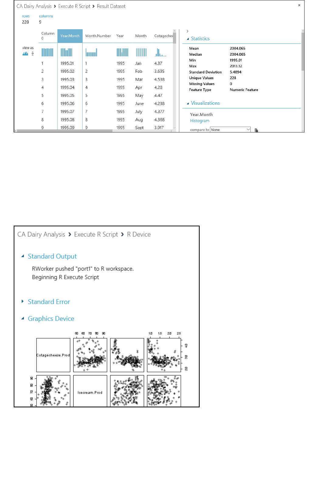
R Device outputR Device output
Figure 6. The visualization of the output of the California dairy data.
This output looks identical to the input, exactly as we expected.
The Device output of the Execute R Script module contains messages and graphics output. Both standard output
and standard error messages from R are sent to the R Device output port.
To view the R Device output, click on the port and then on Visualize. We see the standard output and standard
error from the R script in Figure 7.
Figure 7. Standard output and standard error from the R Device port.
Scrolling down we see the graphics output from our R script in Figure 8.
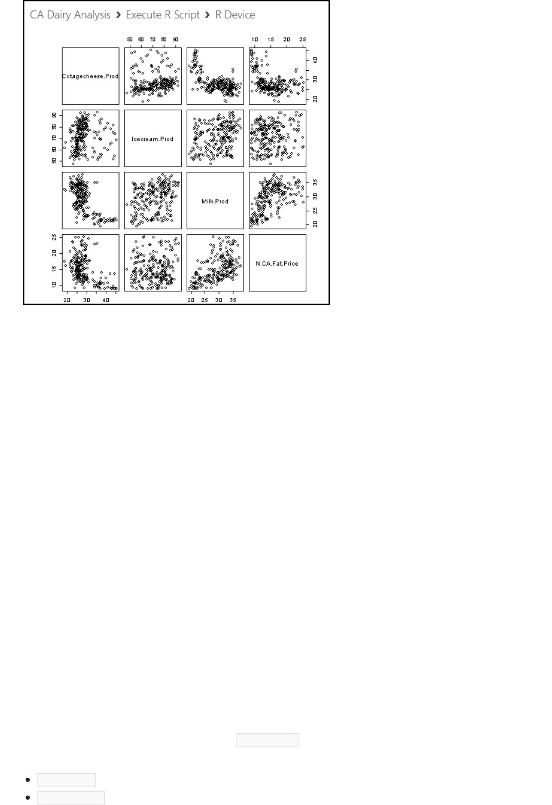
Data filtering and transformation
Type transformationsType transformations
Figure 8. Graphics output from the R Device port.
In this section we will perform some basic data filtering and transformation operations on the California dairy data.
By the end of this section we will have data in a format suitable for building an analytic model.
More specifically, in this section we will perform several common data cleaning and transformation tasks: type
transformation, filtering on dataframes, adding new computed columns, and value transformations. This
background should help you deal with the many variations encountered in real-world problems.
The complete R code for this section is available in the zip file you downloaded earlier.
Now that we can read the California dairy data into the R code in the Execute R Script module, we need to ensure
that the data in the columns has the intended type and format.
R is a dynamically typed language, which means that data types are coerced from one to another as required. The
atomic data types in R include numeric, logical and character. The factor type is used to compactly store categorical
data. You can find much more information on data types in the references in Appendix B - Further reading.
When tabular data is read into R from an external source, it is always a good idea to check the resulting types in the
columns. You may want a column of type character, but in many cases this will show up as factor or vice versa. In
other cases a column you think should be numeric is represented by character data, e.g. '1.23' rather than 1.23 as a
floating point number.
Fortunately, it is easy to convert one type to another, as long as mapping is possible. For example, you cannot
convert 'Nevada' into a numeric value, but you can convert it to a factor (categorical variable). As another example,
you can convert a numeric 1 into a character '1' or a factor.
The syntax for any of these conversions is simple: as.datatype() . These type conversion functions include the
following.
as.numeric()
as.character()
## Only one of the following two lines should be used
## If running in Machine Learning Studio, use the first line with maml.mapInputPort()
## If in RStudio, use the second line with read.csv()
cadairydata <- maml.mapInputPort(1)
# cadairydata <- read.csv("cadairydata.csv", header = TRUE, stringsAsFactors = FALSE)
## Ensure the coding is consistent and convert column to a factor
cadairydata$Month <- as.factor(cadairydata$Month)
str(cadairydata) # Check the result
## The following line should be executed only when running in
## Azure Machine Learning Studio
maml.mapOutputPort('cadairydata')
[ModuleOutput] [1] "Loading variable port1..."
[ModuleOutput]
[ModuleOutput] 'data.frame': 228 obs. of 9 variables:
[ModuleOutput]
[ModuleOutput] $ Column 0 : int 1 2 3 4 5 6 7 8 9 10 ...
[ModuleOutput]
[ModuleOutput] $ Year.Month : num 1995 1995 1995 1995 1995 ...
[ModuleOutput]
[ModuleOutput] $ Month.Number : int 1 2 3 4 5 6 7 8 9 10 ...
[ModuleOutput]
[ModuleOutput] $ Year : int 1995 1995 1995 1995 1995 1995 1995 1995 1995 1995 ...
[ModuleOutput]
[ModuleOutput] $ Month : Factor w/ 14 levels "Apr","April",..: 6 5 9 1 11 8 7 3 14 13 ...
[ModuleOutput]
[ModuleOutput] $ Cotagecheese.Prod: num 4.37 3.69 4.54 4.28 4.47 ...
[ModuleOutput]
[ModuleOutput] $ Icecream.Prod : num 51.6 56.1 68.5 65.7 73.7 ...
[ModuleOutput]
[ModuleOutput] $ Milk.Prod : num 2.11 1.93 2.16 2.13 2.23 ...
[ModuleOutput]
[ModuleOutput] $ N.CA.Fat.Price : num 0.98 0.892 0.892 0.897 0.897 ...
[ModuleOutput]
[ModuleOutput] [1] "Saving variable cadairydata ..."
[ModuleOutput]
[ModuleOutput] [1] "Saving the following item(s): .maml.oport1"
as.logical()
as.factor()
Looking at the data types of the columns we input in the previous section: all columns are of type numeric, except
for the column labeled 'Month', which is of type character. Let's convert this to a factor and test the results.
I have deleted the line that created the scatterplot matrix and added a line converting the 'Month' column to a
factor. In my experiment I will just cut and paste the R code into the code window of the Execute R Script Module.
You could also update the zip file and upload it to Azure Machine Learning Studio, but this takes several steps.
Let's execute this code and look at the output log for the R script. The relevant data from the log is shown in Figure
9.
Figure 9. Summary of the dataframe with a factor variable.
The type for Month should now say 'Factor w/ 14 levels'. This is a problem since there are only 12 months in the
year. You can also check to see that the type in Visualize of the Result Dataset port is 'Categorical'.
The problem is that the 'Month' column has not been coded systematically. In some cases a month is called April
and in others it is abbreviated as Apr. We can solve this problem by trimming the string to 3 characters. The line of
code now looks like the following:
## Ensure the coding is consistent and convert column to a factor
cadairydata$Month <- as.factor(substr(cadairydata$Month, 1, 3))
[ModuleOutput] [1] "Loading variable port1..."
[ModuleOutput]
[ModuleOutput] 'data.frame': 228 obs. of 9 variables:
[ModuleOutput]
[ModuleOutput] $ Column 0 : int 1 2 3 4 5 6 7 8 9 10 ...
[ModuleOutput]
[ModuleOutput] $ Year.Month : num 1995 1995 1995 1995 1995 ...
[ModuleOutput]
[ModuleOutput] $ Month.Number : int 1 2 3 4 5 6 7 8 9 10 ...
[ModuleOutput]
[ModuleOutput] $ Year : int 1995 1995 1995 1995 1995 1995 1995 1995 1995 1995 ...
[ModuleOutput]
[ModuleOutput] $ Month : Factor w/ 12 levels "Apr","Aug","Dec",..: 5 4 8 1 9 7 6 2 12 11 ...
[ModuleOutput]
[ModuleOutput] $ Cotagecheese.Prod: num 4.37 3.69 4.54 4.28 4.47 ...
[ModuleOutput]
[ModuleOutput] $ Icecream.Prod : num 51.6 56.1 68.5 65.7 73.7 ...
[ModuleOutput]
[ModuleOutput] $ Milk.Prod : num 2.11 1.93 2.16 2.13 2.23 ...
[ModuleOutput]
[ModuleOutput] $ N.CA.Fat.Price : num 0.98 0.892 0.892 0.897 0.897 ...
[ModuleOutput]
[ModuleOutput] [1] "Saving variable cadairydata ..."
[ModuleOutput]
[ModuleOutput] [1] "Saving the following item(s): .maml.oport1"
Basic data frame filteringBasic data frame filtering
NOTENOTE
# Remove two columns we do not need
cadairydata <- cadairydata[, c(-1, -2)]
Rerun the experiment and view the output log. The expected results are shown in Figure 10.
Figure 10. Summary of the dataframe with correct number of factor levels.
Our factor variable now has the desired 12 levels.
R dataframes support powerful filtering capabilities. Datasets can be subsetted by using logical filters on either
rows or columns. In many cases, complex filter criteria will be required. The references in Appendix B - Further
reading contain extensive examples of filtering dataframes.
There is one bit of filtering we should do on our dataset. If you look at the columns in the cadairydata dataframe,
you will see two unnecessary columns. The first column just holds a row number, which is not very useful. The
second column, Year.Month, contains redundant information. We can easily exclude these columns by using the
following R code.
From now on in this section, I will just show you the additional code I am adding in the Execute R Script module. I will add
each new line before the str() function. I use this function to verify my results in Azure Machine Learning Studio.
I add the following line to my R code in the Execute R Script module.
Run this code in your experiment and check the result from the output log. These results are shown in Figure 11.

[ModuleOutput] [1] "Loading variable port1..."
[ModuleOutput]
[ModuleOutput] 'data.frame': 228 obs. of 7 variables:
[ModuleOutput]
[ModuleOutput] $ Month.Number : int 1 2 3 4 5 6 7 8 9 10 ...
[ModuleOutput]
[ModuleOutput] $ Year : int 1995 1995 1995 1995 1995 1995 1995 1995 1995 1995 ...
[ModuleOutput]
[ModuleOutput] $ Month : Factor w/ 12 levels "Apr","Aug","Dec",..: 5 4 8 1 9 7 6 2 12 11 ...
[ModuleOutput]
[ModuleOutput] $ Cotagecheese.Prod: num 4.37 3.69 4.54 4.28 4.47 ...
[ModuleOutput]
[ModuleOutput] $ Icecream.Prod : num 51.6 56.1 68.5 65.7 73.7 ...
[ModuleOutput]
[ModuleOutput] $ Milk.Prod : num 2.11 1.93 2.16 2.13 2.23 ...
[ModuleOutput]
[ModuleOutput] $ N.CA.Fat.Price : num 0.98 0.892 0.892 0.897 0.897 ...
[ModuleOutput]
[ModuleOutput] [1] "Saving variable cadairydata ..."
[ModuleOutput]
[ModuleOutput] [1] "Saving the following item(s): .maml.oport1"
Add a new columnAdd a new column
## Create a new column with the month count
## Function to find the number of months from the first
## month of the time series
num.month <- function(Year, Month) {
## Find the starting year
min.year <- min(Year)
## Compute the number of months from the start of the time series
12 * (Year - min.year) + Month - 1
}
## Compute the new column for the dataframe
cadairydata$Month.Count <- num.month(cadairydata$Year, cadairydata$Month.Number)
Figure 11. Summary of the dataframe with two columns removed.
Good news! We get the expected results.
To create time series models it will be convenient to have a column containing the months since the start of the
time series. We will create a new column 'Month.Count'.
To help organize the code we will create our first simple function, num.month() . We will then apply this function to
create a new column in the dataframe. The new code is as follows.
Now run the updated experiment and use the output log to view the results. These results are shown in Figure 12.

[ModuleOutput] [1] "Loading variable port1..."
[ModuleOutput]
[ModuleOutput] 'data.frame': 228 obs. of 8 variables:
[ModuleOutput]
[ModuleOutput] $ Month.Number : int 1 2 3 4 5 6 7 8 9 10 ...
[ModuleOutput]
[ModuleOutput] $ Year : int 1995 1995 1995 1995 1995 1995 1995 1995 1995 1995 ...
[ModuleOutput]
[ModuleOutput] $ Month : Factor w/ 12 levels "Apr","Aug","Dec",..: 5 4 8 1 9 7 6 2 12 11 ...
[ModuleOutput]
[ModuleOutput] $ Cotagecheese.Prod: num 4.37 3.69 4.54 4.28 4.47 ...
[ModuleOutput]
[ModuleOutput] $ Icecream.Prod : num 51.6 56.1 68.5 65.7 73.7 ...
[ModuleOutput]
[ModuleOutput] $ Milk.Prod : num 2.11 1.93 2.16 2.13 2.23 ...
[ModuleOutput]
[ModuleOutput] $ N.CA.Fat.Price : num 0.98 0.892 0.892 0.897 0.897 ...
[ModuleOutput]
[ModuleOutput] $ Month.Count : num 0 1 2 3 4 5 6 7 8 9 ...
[ModuleOutput]
[ModuleOutput] [1] "Saving variable cadairydata ..."
[ModuleOutput]
[ModuleOutput] [1] "Saving the following item(s): .maml.oport1"
Value transformationsValue transformations
Figure 12. Summary of the dataframe with the additional column.
It looks like everything is working. We have the new column with the expected values in our dataframe.
In this section we will perform some simple transformations on the values in some of the columns of our
dataframe. The R language supports nearly arbitrary value transformations. The references in Appendix B -
Further Reading contain extensive examples.
If you look at the values in the summaries of our dataframe you should see something odd here. Is more ice cream
than milk produced in California? No, of course not, as this makes no sense, sad as this fact may be to some of us
ice cream lovers. The units are different. The price is in units of US pounds, milk is in units of 1 M US pounds, ice
cream is in units of 1,000 US gallons, and cottage cheese is in units of 1,000 US pounds. Assuming ice cream
weighs about 6.5 pounds per gallon, we can easily do the multiplication to convert these values so they are all in
equal units of 1,000 pounds.
For our forecasting model we use a multiplicative model for trend and seasonal adjustment of this data. A log
transformation allows us to use a linear model, simplifying this process. We can apply the log transformation in the
same function where the multiplier is applied.
In the following code, I define a new function, log.transform() , and apply it to the rows containing the numerical
values. The R Map() function is used to apply the log.transform() function to the selected columns of the
dataframe. Map() is similar to apply() but allows for more than one list of arguments to the function. Note that a
list of multipliers supplies the second argument to the log.transform() function. The na.omit() function is used
as a bit of cleanup to ensure we do not have missing or undefined values in the dataframe.

log.transform <- function(invec, multiplier = 1) {
## Function for the transformation, which is the log
## of the input value times a multiplier
warningmessages <- c("ERROR: Non-numeric argument encountered in function log.transform",
"ERROR: Arguments to function log.transform must be greate than zero",
"ERROR: Aggurment multiplier to funcition log.transform must be a scaler",
"ERROR: Invalid time seies value encountered in function log.transform"
)
## Check the input arguments
if(!is.numeric(invec) | !is.numeric(multiplier)) {warning(warningmessages[1]); return(NA)}
if(any(invec < 0.0) | any(multiplier < 0.0)) {warning(warningmessages[2]); return(NA)}
if(length(multiplier) != 1) {{warning(warningmessages[3]); return(NA)}}
## Wrap the multiplication in tryCatch
## If there is an exception, print the warningmessage to
## standard error and return NA
tryCatch(log(multiplier * invec),
error = function(e){warning(warningmessages[4]); NA})
}
## Apply the transformation function to the 4 columns
## of the dataframe with production data
multipliers <- list(1.0, 6.5, 1000.0, 1000.0)
cadairydata[, 4:7] <- Map(log.transform, cadairydata[, 4:7], multipliers)
## Get rid of any rows with NA values
cadairydata <- na.omit(cadairydata)
There is quite a bit happening in the log.transform() function. Most of this code is checking for potential
problems with the arguments or dealing with exceptions, which can still arise during the computations. Only a few
lines of this code actually do the computations.
The goal of the defensive programming is to prevent the failure of a single function that prevents processing from
continuing. An abrupt failure of a long-running analysis can be quite frustrating for users. To avoid this situation,
default return values must be chosen that will limit damage to downstream processing. A message is also
produced to alert users that something has gone wrong.
If you are not used to defensive programming in R, all this code may seem a bit overwhelming. I will walk you
through the major steps:
1. A vector of four messages is defined. These messages are used to communicate information about some of the
possible errors and exceptions that can occur with this code.
2. I return a value of NA for each case. There are many other possibilities that might have fewer side effects. I
could return a vector of zeroes, or the original input vector, for example.
3. Checks are run on the arguments to the function. In each case, if an error is detected, a default value is returned
and a message is produced by the warning() function. I am using warning() rather than stop() as the latter
will terminate execution, exactly what I am trying to avoid. Note that I have written this code in a procedural
style, as in this case a functional approach seemed complex and obscure.
4. The log computations are wrapped in tryCatch() so that exceptions will not cause an abrupt halt to processing.
Without tryCatch() most errors raised by R functions result in a stop signal, which does just that.
Execute this R code in your experiment and have a look at the printed output in the output.log file. You will now see
the transformed values of the four columns in the log, as shown in Figure 13.

[ModuleOutput] [1] "Loading variable port1..."
[ModuleOutput]
[ModuleOutput] 'data.frame': 228 obs. of 8 variables:
[ModuleOutput]
[ModuleOutput] $ Month.Number : int 1 2 3 4 5 6 7 8 9 10 ...
[ModuleOutput]
[ModuleOutput] $ Year : int 1995 1995 1995 1995 1995 1995 1995 1995 1995 1995 ...
[ModuleOutput]
[ModuleOutput] $ Month : Factor w/ 12 levels "Apr","Aug","Dec",..: 5 4 8 1 9 7 6 2 12 11 ...
[ModuleOutput]
[ModuleOutput] $ Cotagecheese.Prod: num 1.47 1.31 1.51 1.45 1.5 ...
[ModuleOutput]
[ModuleOutput] $ Icecream.Prod : num 5.82 5.9 6.1 6.06 6.17 ...
[ModuleOutput]
[ModuleOutput] $ Milk.Prod : num 7.66 7.57 7.68 7.66 7.71 ...
[ModuleOutput]
[ModuleOutput] $ N.CA.Fat.Price : num 6.89 6.79 6.79 6.8 6.8 ...
[ModuleOutput]
[ModuleOutput] $ Month.Count : num 0 1 2 3 4 5 6 7 8 9 ...
[ModuleOutput]
[ModuleOutput] [1] "Saving variable cadairydata ..."
[ModuleOutput]
[ModuleOutput] [1] "Saving the following item(s): .maml.oport1"
Time series objects and correlation analysis
Time series objects in RTime series objects in R
Time series object exampleTime series object example
Reading the dataframeReading the dataframe
Figure 13. Summary of the transformed values in the dataframe.
We see the values have been transformed. Milk production now greatly exceeds all other dairy product production,
recalling that we are now looking at a log scale.
At this point our data is cleaned up and we are ready for some modeling. Looking at the visualization summary for
the Result Dataset output of our Execute R Script module, you will see the 'Month' column is 'Categorical' with 12
unique values, again, just as we wanted.
In this section we will explore a few basic R time series objects and analyze the correlations between some of the
variables. Our goal is to output a dataframe containing the pairwise correlation information at several lags.
The complete R code for this section is in the zip file you downloaded earlier.
As already mentioned, time series are a series of data values indexed by time. R time series objects are used to
create and manage the time index. There are several advantages to using time series objects. Time series objects
free you from the many details of managing the time series index values that are encapsulated in the object. In
addition, time series objects allow you to use the many time series methods for plotting, printing, modeling, etc.
The POSIXct time series class is commonly used and is relatively simple. This time series class measures time from
the start of the epoch, January 1, 1970. We will use POSIXct time series objects in this example. Other widely used
R time series object classes include zoo and xts, extensible time series.
Let's get started with our example. Drag and drop a new Execute R Script module into your experiment. Connect
the Result Dataset1 output port of the existing Execute R Script module to the Dataset1 input port of the new
Execute R Script module.
As I did for the first examples, as we progress through the example, at some points I will show only the incremental
additional lines of R code at each step.
As a first step, let's read in a dataframe and make sure we get the expected results. The following code should do

# Comment the following if using RStudio
cadairydata <- maml.mapInputPort(1)
str(cadairydata) # Check the results
[ModuleOutput] [1] "Loading variable port1..."
[ModuleOutput]
[ModuleOutput] 'data.frame': 228 obs. of 8 variables:
[ModuleOutput]
[ModuleOutput] $ Month.Number : int 1 2 3 4 5 6 7 8 9 10 ...
[ModuleOutput]
[ModuleOutput] $ Year : int 1995 1995 1995 1995 1995 1995 1995 1995 1995 1995 ...
[ModuleOutput]
[ModuleOutput] $ Month : Factor w/ 12 levels "Apr","Aug","Dec",..: 5 4 8 1 9 7 6 2 12 11 ...
[ModuleOutput]
[ModuleOutput] $ Cotagecheese.Prod: num 1.47 1.31 1.51 1.45 1.5 ...
[ModuleOutput]
[ModuleOutput] $ Icecream.Prod : num 5.82 5.9 6.1 6.06 6.17 ...
[ModuleOutput]
[ModuleOutput] $ Milk.Prod : num 7.66 7.57 7.68 7.66 7.71 ...
[ModuleOutput]
[ModuleOutput] $ N.CA.Fat.Price : num 6.89 6.79 6.79 6.8 6.8 ...
[ModuleOutput]
[ModuleOutput] $ Month.Count : num 0 1 2 3 4 5 6 7 8 9 ...
Creating a time series objectCreating a time series object
# Comment the following if using RStudio
cadairydata <- maml.mapInputPort(1)
## Create a new column as a POSIXct object
Sys.setenv(TZ = "PST8PDT")
cadairydata$Time <- as.POSIXct(strptime(paste(as.character(cadairydata$Year), "-",
as.character(cadairydata$Month.Number), "-01 00:00:00", sep = ""), "%Y-%m-%d %H:%M:%S"))
str(cadairydata) # Check the results
the job.
Now, run the experiment. The log of the new Execute R Script shape should look like Figure 14.
Figure 14. Summary of the dataframe in the Execute R Script module.
This data is of the expected types and format. Note that the 'Month' column is of type factor and has the expected
number of levels.
We need to add a time series object to our dataframe. Replace the current code with the following, which adds a
new column of class POSIXct.
Now, check the log. It should look like Figure 15.
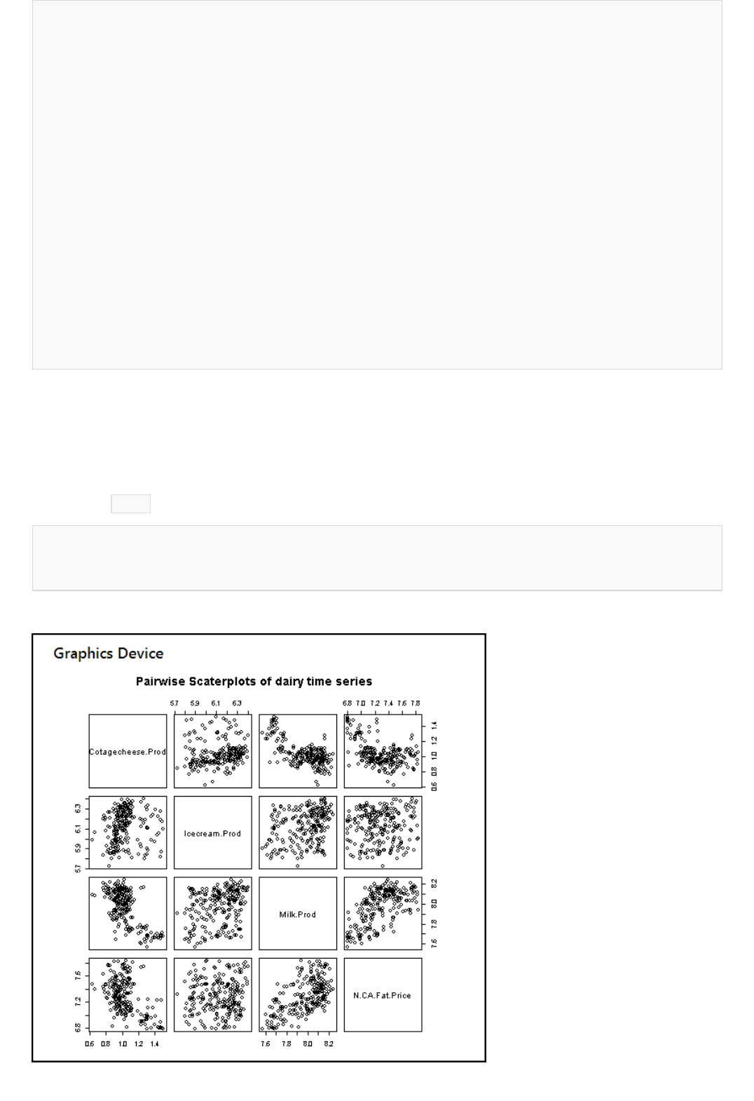
[ModuleOutput] [1] "Loading variable port1..."
[ModuleOutput]
[ModuleOutput] 'data.frame': 228 obs. of 9 variables:
[ModuleOutput]
[ModuleOutput] $ Month.Number : int 1 2 3 4 5 6 7 8 9 10 ...
[ModuleOutput]
[ModuleOutput] $ Year : int 1995 1995 1995 1995 1995 1995 1995 1995 1995 1995 ...
[ModuleOutput]
[ModuleOutput] $ Month : Factor w/ 12 levels "Apr","Aug","Dec",..: 5 4 8 1 9 7 6 2 12 11 ...
[ModuleOutput]
[ModuleOutput] $ Cotagecheese.Prod: num 1.47 1.31 1.51 1.45 1.5 ...
[ModuleOutput]
[ModuleOutput] $ Icecream.Prod : num 5.82 5.9 6.1 6.06 6.17 ...
[ModuleOutput]
[ModuleOutput] $ Milk.Prod : num 7.66 7.57 7.68 7.66 7.71 ...
[ModuleOutput]
[ModuleOutput] $ N.CA.Fat.Price : num 6.89 6.79 6.79 6.8 6.8 ...
[ModuleOutput]
[ModuleOutput] $ Month.Count : num 0 1 2 3 4 5 6 7 8 9 ...
[ModuleOutput]
[ModuleOutput] $ Time : POSIXct, format: "1995-01-01" "1995-02-01" ...
Exploring and transforming the dataExploring and transforming the data
pairs(~ Cotagecheese.Prod + Icecream.Prod + Milk.Prod + N.CA.Fat.Price, data = cadairydata, main = "Pairwise
Scatterplots of dairy time series")
Figure 15. Summary of the dataframe with a time series object.
We can see from the summary that the new column is in fact of class POSIXct.
Let's explore some of the variables in this dataset. A scatterplot matrix is a good way to produce a quick look. I am
replacing the str() function in the previous R code with the following line.
Run this code and see what happens. The plot produced at the R Device port should look like Figure 16.
Figure 16. Scatterplot matrix of selected variables.

Correlation analysisCorrelation analysis
ts.detrend <- function(ts, Time, min.length = 3){
## Function to de-trend and standardize a time series
## Define some messages if they are NULL
messages <- c('ERROR: ts.detrend requires arguments ts and Time to have the same length',
'ERROR: ts.detrend requires argument ts to be of type numeric',
paste('WARNING: ts.detrend has encountered a time series with length less than',
as.character(min.length)),
'ERROR: ts.detrend has encountered a Time argument not of class POSIXct',
'ERROR: Detrend regression has failed in ts.detrend',
'ERROR: Exception occurred in ts.detrend while standardizing time series in function
ts.detrend'
)
# Create a vector of zeros to return as a default in some cases
zerovec <- rep(length(ts), 0.0)
# The input arguments are not of the same length, return ts and quit
if(length(Time) != length(ts)) {warning(messages[1]); return(ts)}
# If the ts is not numeric, just return a zero vector and quit
if(!is.numeric(ts)) {warning(messages[2]); return(zerovec)}
# If the ts is too short, just return it and quit
if((ts.length <- length(ts)) < min.length) {warning(messages[3]); return(ts)}
## Check that the Time variable is of class POSIXct
if(class(cadairydata$Time)[[1]] != "POSIXct") {warning(messages[4]); return(ts)}
## De-trend the time series by using a linear model
ts.frame <- data.frame(ts = ts, Time = Time)
tryCatch({ts <- ts - fitted(lm(ts ~ Time, data = ts.frame))},
error = function(e){warning(messages[5]); zerovec})
tryCatch( {stdev <- sqrt(sum((ts - mean(ts))^2))/(ts.length - 1)
ts <- ts/stdev},
error = function(e){warning(messages[6]); zerovec})
ts
}
## Apply the detrend.ts function to the variables of interest
df.detrend <- data.frame(lapply(cadairydata[, 4:7], ts.detrend, cadairydata$Time))
## Plot the results to look at the relationships
pairs(~ Cotagecheese.Prod + Icecream.Prod + Milk.Prod + N.CA.Fat.Price, data = df.detrend, main = "Pairwise
Scatterplots of detrended standardized time series")
There is some odd-looking structure in the relationships between these variables. Perhaps this arises from trends
in the data and from the fact that we have not standardized the variables.
To perform correlation analysis we need to both de-trend and standardize the variables. We could simply use the R
scale() function, which both centers and scales variables. This function might well run faster. However, I want to
show you an example of defensive programing in R.
The ts.detrend() function shown below performs both of these operations. The following two lines of code de-
trend the data and then standardize the values.
There is quite a bit happening in the ts.detrend() function. Most of this code is checking for potential problems
with the arguments or dealing with exceptions, which can still arise during the computations. Only a few lines of
this code actually do the computations.
We have already discussed an example of defensive programming in Value transformations. Both computation
blocks are wrapped in tryCatch() . For some errors it makes sense to return the original input vector, and in other
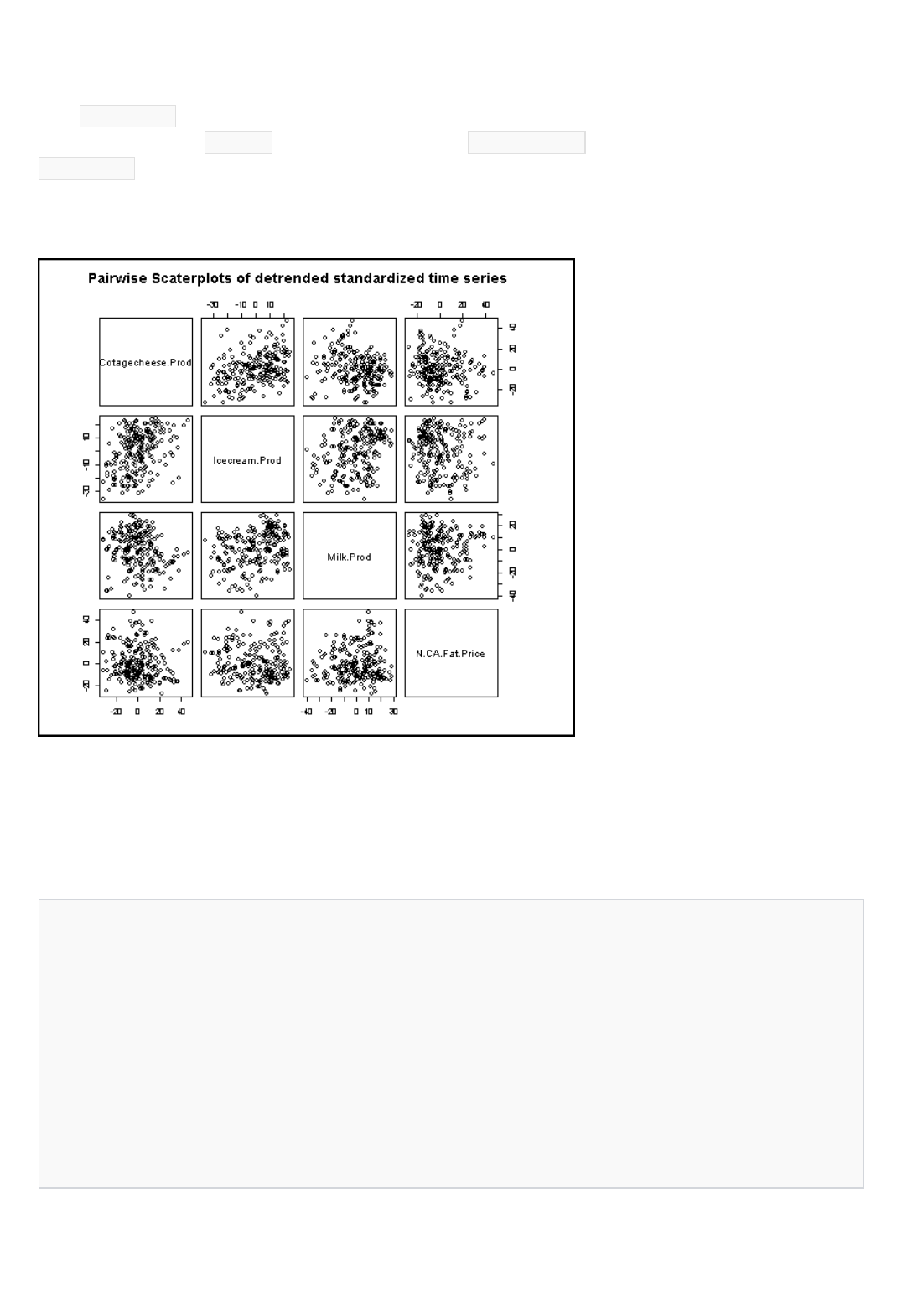
## A function to compute pairwise correlations from a
## list of time series value vectors
pair.cor <- function(pair.ind, ts.list, lag.max = 1, plot = FALSE){
ccf(ts.list[[pair.ind[1]]], ts.list[[pair.ind[2]]], lag.max = lag.max, plot = plot)
}
## A list of the pairwise indices
corpairs <- list(c(1,2), c(1,3), c(1,4), c(2,3), c(2,4), c(3,4))
## Compute the list of ccf objects
cadairycorrelations <- lapply(corpairs, pair.cor, df.detrend)
cadairycorrelations
cases, I return a vector of zeros.
Note that the linear regression used for de-trending is a time series regression. The predictor variable is a time
series object.
Once ts.detrend() is defined we apply it to the variables of interest in our dataframe. We must coerce the
resulting list created by lapply() to data dataframe by using as.data.frame() . Because of defensive aspects of
ts.detrend() , failure to process one of the variables will not prevent correct processing of the others.
The final line of code creates a pairwise scatterplot. After running the R code, the results of the scatterplot are
shown in Figure 17.
Figure 17. Pairwise scatterplot of de-trended and standardized time series.
You can compare these results to those shown in Figure 16. With the trend removed and the variables
standardized, we see a lot less structure in the relationships between these variables.
The code to compute the correlations as R ccf objects is as follows.
Running this code produces the log shown in Figure 18.

[ModuleOutput] Loading objects:
[ModuleOutput] port1
[ModuleOutput] [1] "Loading variable port1..."
[ModuleOutput] [[1]]
[ModuleOutput]
[ModuleOutput]
[ModuleOutput] Autocorrelations of series 'X', by lag
[ModuleOutput]
[ModuleOutput]
[ModuleOutput] -1 0 1
[ModuleOutput] 0.148 0.358 0.317
[ModuleOutput]
[ModuleOutput]
[ModuleOutput] [[2]]
[ModuleOutput]
[ModuleOutput]
[ModuleOutput] Autocorrelations of series 'X', by lag
[ModuleOutput]
[ModuleOutput]
[ModuleOutput] -1 0 1
[ModuleOutput] -0.395 -0.186 -0.238
[ModuleOutput]
[ModuleOutput]
[ModuleOutput] [[3]]
[ModuleOutput]
[ModuleOutput]
[ModuleOutput] Autocorrelations of series 'X', by lag
[ModuleOutput]
[ModuleOutput]
[ModuleOutput] -1 0 1
[ModuleOutput] -0.059 -0.089 -0.127
[ModuleOutput]
[ModuleOutput]
[ModuleOutput] [[4]]
[ModuleOutput]
[ModuleOutput]
[ModuleOutput] Autocorrelations of series 'X', by lag
[ModuleOutput]
[ModuleOutput]
[ModuleOutput] -1 0 1
[ModuleOutput] 0.140 0.294 0.293
[ModuleOutput]
[ModuleOutput]
[ModuleOutput] [[5]]
[ModuleOutput]
[ModuleOutput]
[ModuleOutput] Autocorrelations of series 'X', by lag
[ModuleOutput]
[ModuleOutput]
[ModuleOutput] -1 0 1
[ModuleOutput] -0.002 -0.074 -0.124
Output a dataframeOutput a dataframe
Figure 18. List of ccf objects from the pairwise correlation analysis.
There is a correlation value for each lag. None of these correlation values is large enough to be significant. We can
therefore conclude that we can model each variable independently.
We have computed the pairwise correlations as a list of R ccf objects. This presents a bit of a problem as the Result
Dataset output port really requires a dataframe. Further, the ccf object is itself a list and we want only the values in
the first element of this list, the correlations at the various lags.
The following code extracts the lag values from the list of ccf objects, which are themselves lists.
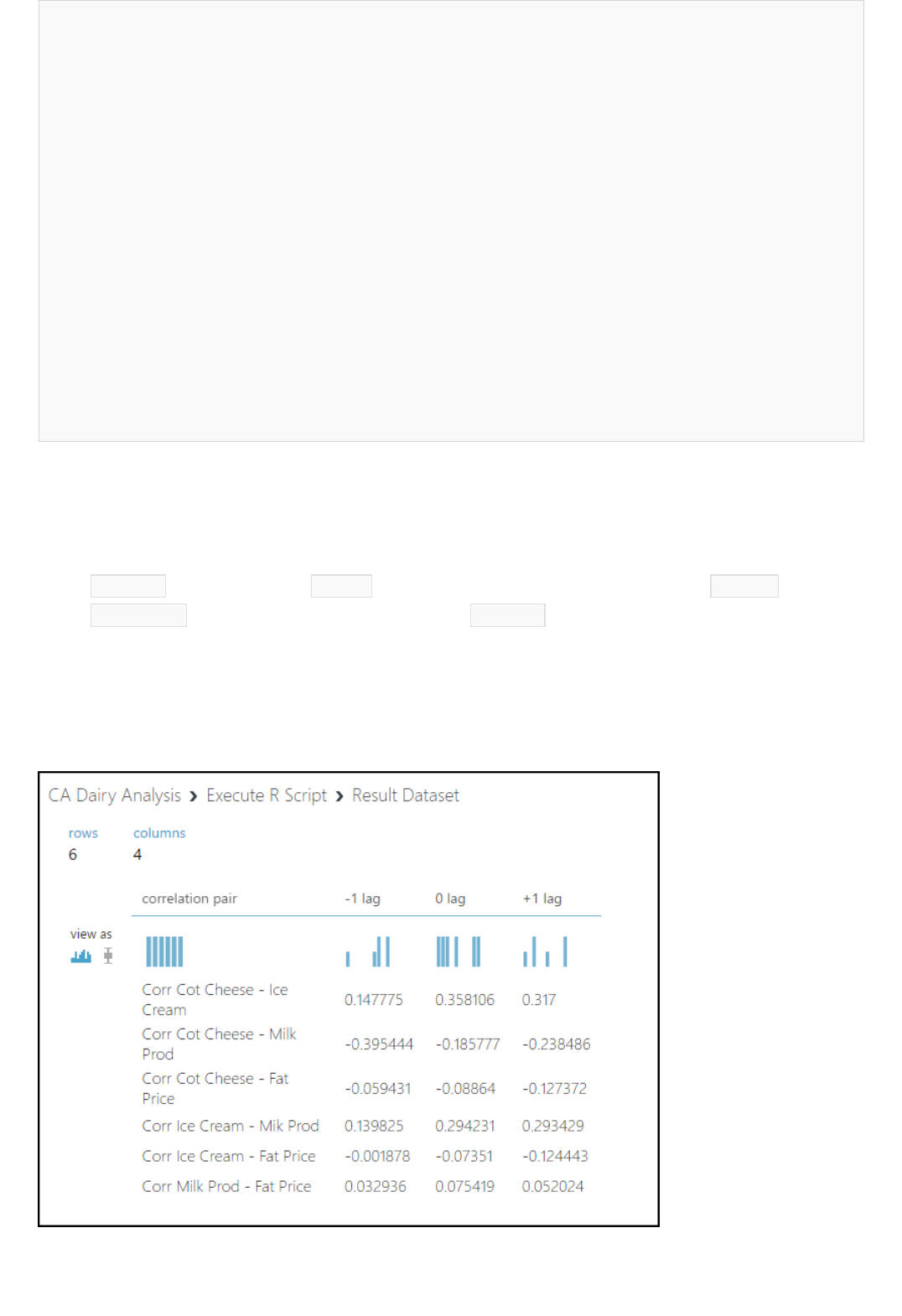
df.correlations <- data.frame(do.call(rbind, lapply(cadairycorrelations, '[[', 1)))
c.names <- c("correlation pair", "-1 lag", "0 lag", "+1 lag")
r.names <- c("Corr Cot Cheese - Ice Cream",
"Corr Cot Cheese - Milk Prod",
"Corr Cot Cheese - Fat Price",
"Corr Ice Cream - Mik Prod",
"Corr Ice Cream - Fat Price",
"Corr Milk Prod - Fat Price")
## Build a dataframe with the row names column and the
## correlation data frame and assign the column names
outframe <- cbind(r.names, df.correlations)
colnames(outframe) <- c.names
outframe
## WARNING!
## The following line works only in Azure Machine Learning
## When running in RStudio, this code will result in an error
#maml.mapOutputPort('outframe')
The first line of code is a bit tricky, and some explanation may help you understand it. Working from the inside out
we have the following:
1. The '[[' operator with the argument '1' selects the vector of correlations at the lags from the first element of the
ccf object list.
2. The do.call() function applies the rbind() function over the elements of the list returns by lapply() .
3. The data.frame() function coerces the result produced by do.call() to a dataframe.
Note that the row names are in a column of the dataframe. Doing so preserves the row names when they are
output from the Execute R Script.
Running the code produces the output shown in Figure 19 when I Visualize the output at the Result Dataset port.
The row names are in the first column, as intended.
Figure 19. Results output from the correlation analysis.
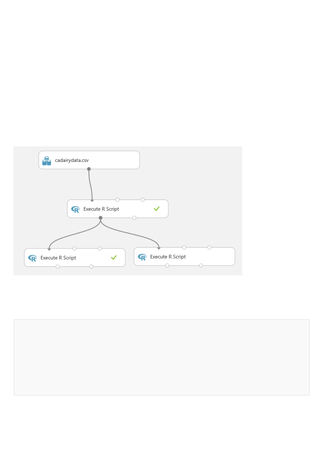
Time series example: seasonal forecasting
Creating the dataframe for analysisCreating the dataframe for analysis
# If running in Machine Learning Studio, uncomment the first line with maml.mapInputPort()
cadairydata <- maml.mapInputPort(1)
## Create a new column as a POSIXct object
Sys.setenv(TZ = "PST8PDT")
cadairydata$Time <- as.POSIXct(strptime(paste(as.character(cadairydata$Year), "-",
as.character(cadairydata$Month.Number), "-01 00:00:00", sep = ""), "%Y-%m-%d %H:%M:%S"))
str(cadairydata)
Our data is now in a form suitable for analysis, and we have determined there are no significant correlations
between the variables. Let's move on and create a time series forecasting model. Using this model we will forecast
California milk production for the 12 months of 2013.
Our forecasting model will have two components, a trend component and a seasonal component. The complete
forecast is the product of these two components. This type of model is known as a multiplicative model. The
alternative is an additive model. We have already applied a log transformation to the variables of interest, which
makes this analysis tractable.
The complete R code for this section is in the zip file you downloaded earlier.
Start by adding a new Execute R Script module to your experiment. Connect the Result Dataset output of the
existing Execute R Script module to the Dataset1 input of the new module. The result should look something like
Figure 20.
Figure 20. The experiment with the new Execute R Script module added.
As with the correlation analysis we just completed, we need to add a column with a POSIXct time series object. The
following code will do just this.
Run this code and look at the log. The result should look like Figure 21.

[ModuleOutput] [1] "Loading variable port1..."
[ModuleOutput]
[ModuleOutput] 'data.frame': 228 obs. of 9 variables:
[ModuleOutput]
[ModuleOutput] $ Month.Number : int 1 2 3 4 5 6 7 8 9 10 ...
[ModuleOutput]
[ModuleOutput] $ Year : int 1995 1995 1995 1995 1995 1995 1995 1995 1995 1995 ...
[ModuleOutput]
[ModuleOutput] $ Month : Factor w/ 12 levels "Apr","Aug","Dec",..: 5 4 8 1 9 7 6 2 12 11 ...
[ModuleOutput]
[ModuleOutput] $ Cotagecheese.Prod: num 1.47 1.31 1.51 1.45 1.5 ...
[ModuleOutput]
[ModuleOutput] $ Icecream.Prod : num 5.82 5.9 6.1 6.06 6.17 ...
[ModuleOutput]
[ModuleOutput] $ Milk.Prod : num 7.66 7.57 7.68 7.66 7.71 ...
[ModuleOutput]
[ModuleOutput] $ N.CA.Fat.Price : num 6.89 6.79 6.79 6.8 6.8 ...
[ModuleOutput]
[ModuleOutput] $ Month.Count : num 0 1 2 3 4 5 6 7 8 9 ...
[ModuleOutput]
[ModuleOutput] $ Time : POSIXct, format: "1995-01-01" "1995-02-01" ...
Create a training datasetCreate a training dataset
cadairytrain <- cadairydata[1:216, ]
Ylabs <- list("Log CA Cotage Cheese Production, 1000s lb",
"Log CA Ice Cream Production, 1000s lb",
"Log CA Milk Production 1000s lb",
"Log North CA Milk Milk Fat Price per 1000 lb")
Map(function(y, Ylabs){plot(cadairytrain$Time, y, xlab = "Time", ylab = Ylabs, type = "l")}, cadairytrain[,
4:7], Ylabs)
Figure 21. A summary of the dataframe.
With this result, we are ready to start our analysis.
With the dataframe constructed we need to create a training dataset. This data will include all of the observations
except the last 12, of the year 2013, which is our test dataset. The following code subsets the dataframe and creates
plots of the dairy production and price variables. I then create plots of the four production and price variables. An
anonymous function is used to define some augments for plot, and then iterate over the list of the other two
arguments with Map() . If you are thinking that a for loop would have worked fine here, you are correct. But, since
R is a functional language I am showing you a functional approach.
Running the code produces the series of time series plots from the R Device output shown in Figure 22. Note that
the time axis is in units of dates, a nice benefit of the time series plot method.
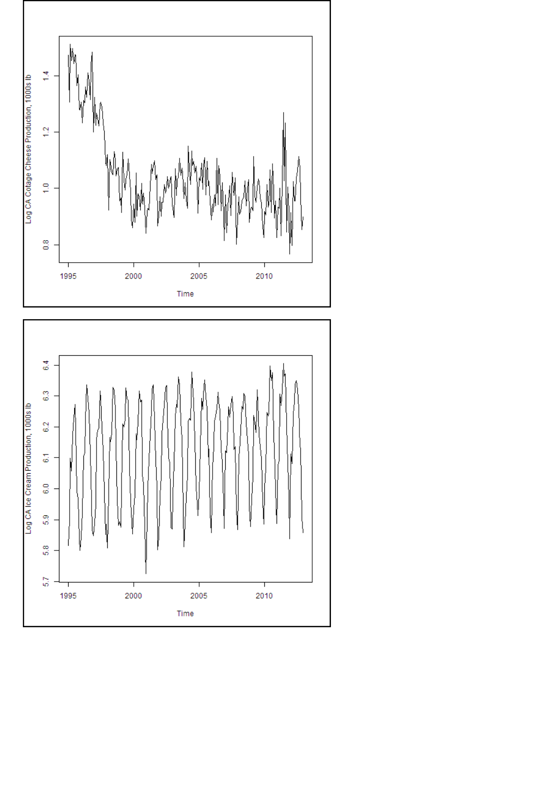
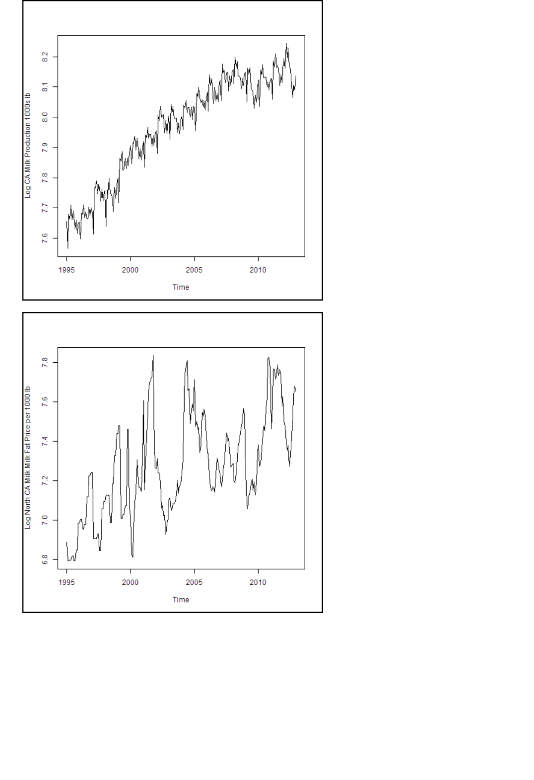
A trend modelA trend model
Figure 22. Time series plots of California dairy production and price data.
Having created a time series object and having had a look at the data, let's start to construct a trend model for the
California milk production data. We can do this with a time series regression. However, it is clear from the plot that
we will need more than a slope and intercept to accurately model the observed trend in the training data.
Given the small scale of the data, I will build the model for trend in RStudio and then cut and paste the resulting
model into Azure Machine Learning. RStudio provides an interactive environment for this type of interactive
analysis.
milk.lm <- lm(Milk.Prod ~ Time + I(Month.Count^2) + I(Month.Count^3), data = cadairytrain)
summary(milk.lm)
##
## Call:
## lm(formula = Milk.Prod ~ Time + I(Month.Count^2) + I(Month.Count^3),
## data = cadairytrain)
##
## Residuals:
## Min 1Q Median 3Q Max
## -0.12667 -0.02730 0.00236 0.02943 0.10586
##
## Coefficients:
## Estimate Std. Error t value Pr(>|t|)
## (Intercept) 6.33e+00 1.45e-01 43.60 <2e-16 ***
## Time 1.63e-09 1.72e-10 9.47 <2e-16 ***
## I(Month.Count^2) -1.71e-06 4.89e-06 -0.35 0.726
## I(Month.Count^3) -3.24e-08 1.49e-08 -2.17 0.031 *
## ---
## Signif. codes: 0 '***' 0.001 '**' 0.01 '*' 0.05 '.' 0.1 ' ' 1
##
## Residual standard error: 0.0418 on 212 degrees of freedom
## Multiple R-squared: 0.941, Adjusted R-squared: 0.94
## F-statistic: 1.12e+03 on 3 and 212 DF, p-value: <2e-16
milk.lm <- update(milk.lm, . ~ . - I(Month.Count^2))
summary(milk.lm)
##
## Call:
## lm(formula = Milk.Prod ~ Time + I(Month.Count^3), data = cadairytrain)
##
## Residuals:
## Min 1Q Median 3Q Max
## -0.12597 -0.02659 0.00185 0.02963 0.10696
##
## Coefficients:
## Estimate Std. Error t value Pr(>|t|)
## (Intercept) 6.38e+00 4.07e-02 156.6 <2e-16 ***
## Time 1.57e-09 4.32e-11 36.3 <2e-16 ***
## I(Month.Count^3) -3.76e-08 2.50e-09 -15.1 <2e-16 ***
## ---
## Signif. codes: 0 '***' 0.001 '**' 0.01 '*' 0.05 '.' 0.1 ' ' 1
##
## Residual standard error: 0.0417 on 213 degrees of freedom
## Multiple R-squared: 0.941, Adjusted R-squared: 0.94
## F-statistic: 1.69e+03 on 2 and 213 DF, p-value: <2e-16
As a first attempt, I will try a polynomial regression with powers up to 3. There is a real danger of over-fitting these
kinds of models. Therefore, it is best to avoid high order terms. The I() function inhibits interpretation of the
contents (interprets the contents 'as is') and allows you to write a literally interpreted function in a regression
equation.
This generates the following.
From P values (Pr(>|t|)) in this output, we can see that the squared term may not be significant. I will use the
update() function to modify this model by dropping the squared term.
This generates the following.
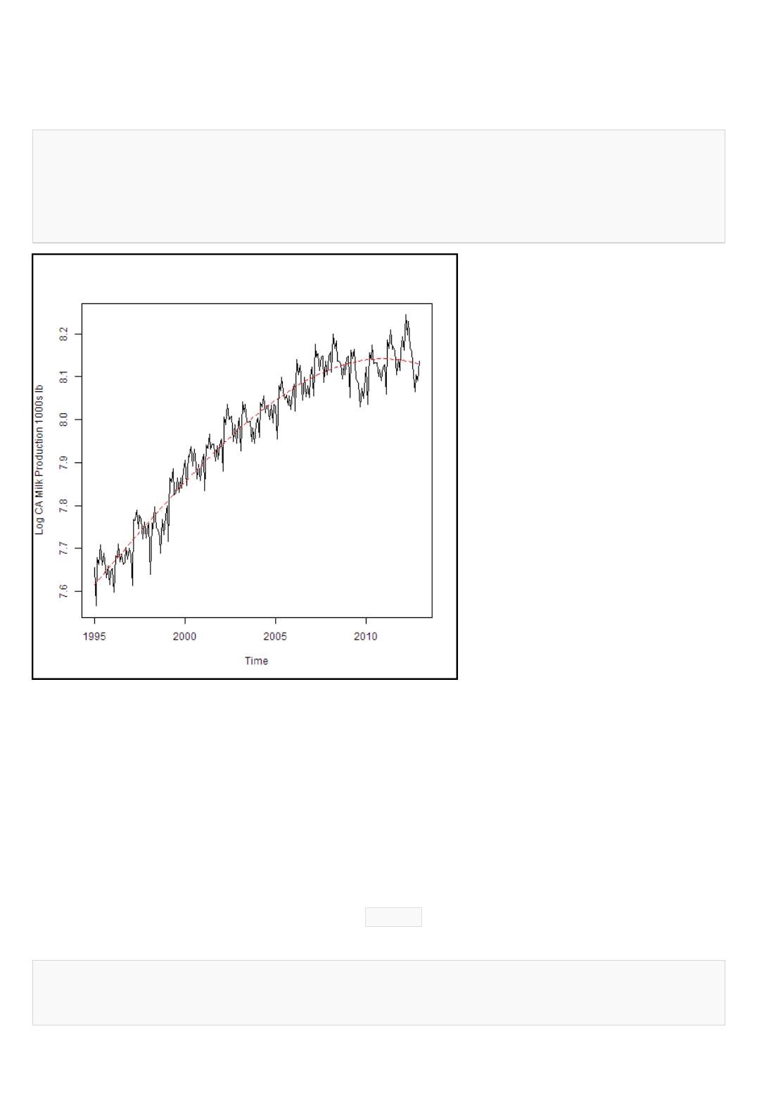
milk.lm <- lm(Milk.Prod ~ Time + I(Month.Count^3), data = cadairytrain)
plot(cadairytrain$Time, cadairytrain$Milk.Prod, xlab = "Time", ylab = "Log CA Milk Production 1000s lb", type =
"l")
lines(cadairytrain$Time, predict(milk.lm, cadairytrain), lty = 2, col = 2)
Seasonal modelSeasonal model
milk.lm2 <- update(milk.lm, . ~ . + Month - 1)
summary(milk.lm2)
This looks better. All of the terms are significant. However, the 2e-16 value is a default value, and should not be
taken too seriously.
As a sanity test, let's make a time series plot of the California dairy production data with the trend curve shown. I
have added the following code in the Azure Machine Learning Execute R Script model (not RStudio) to create the
model and make a plot. The result is shown in Figure 23.
Figure 23. California milk production data with trend model shown.
It looks like the trend model fits the data fairly well. Further, there does not seem to be evidence of over-fitting,
such as odd wiggles in the model curve.
With a trend model in hand, we need to push on and include the seasonal effects. We will use the month of the
year as a dummy variable in the linear model to capture the month-by-month effect. Note that when you introduce
factor variables into a model, the intercept must not be computed. If you do not do this, the formula is over-
specified and R will drop one of the desired factors but keep the intercept term.
Since we have a satisfactory trend model we can use the update() function to add the new terms to the existing
model. The -1 in the update formula drops the intercept term. Continuing in RStudio for the moment:
This generates the following.

##
## Call:
## lm(formula = Milk.Prod ~ Time + I(Month.Count^3) + Month - 1,
## data = cadairytrain)
##
## Residuals:
## Min 1Q Median 3Q Max
## -0.06879 -0.01693 0.00346 0.01543 0.08726
##
## Coefficients:
## Estimate Std. Error t value Pr(>|t|)
## Time 1.57e-09 2.72e-11 57.7 <2e-16 ***
## I(Month.Count^3) -3.74e-08 1.57e-09 -23.8 <2e-16 ***
## MonthApr 6.40e+00 2.63e-02 243.3 <2e-16 ***
## MonthAug 6.38e+00 2.63e-02 242.2 <2e-16 ***
## MonthDec 6.38e+00 2.64e-02 241.9 <2e-16 ***
## MonthFeb 6.31e+00 2.63e-02 240.1 <2e-16 ***
## MonthJan 6.39e+00 2.63e-02 243.1 <2e-16 ***
## MonthJul 6.39e+00 2.63e-02 242.6 <2e-16 ***
## MonthJun 6.38e+00 2.63e-02 242.4 <2e-16 ***
## MonthMar 6.42e+00 2.63e-02 244.2 <2e-16 ***
## MonthMay 6.43e+00 2.63e-02 244.3 <2e-16 ***
## MonthNov 6.34e+00 2.63e-02 240.6 <2e-16 ***
## MonthOct 6.37e+00 2.63e-02 241.8 <2e-16 ***
## MonthSep 6.34e+00 2.63e-02 240.6 <2e-16 ***
## ---
## Signif. codes: 0 '***' 0.001 '**' 0.01 '*' 0.05 '.' 0.1 ' ' 1
##
## Residual standard error: 0.0263 on 202 degrees of freedom
## Multiple R-squared: 1, Adjusted R-squared: 1
## F-statistic: 1.42e+06 on 14 and 202 DF, p-value: <2e-16
milk.lm2 <- lm(Milk.Prod ~ Time + I(Month.Count^3) + Month - 1, data = cadairytrain)
plot(cadairytrain$Time, cadairytrain$Milk.Prod, xlab = "Time", ylab = "Log CA Milk Production 1000s lb", type =
"l")
lines(cadairytrain$Time, predict(milk.lm2, cadairytrain), lty = 2, col = 2)
We see that the model no longer has an intercept term and has 12 significant month factors. This is exactly what
we wanted to see.
Let's make another time series plot of the California dairy production data to see how well the seasonal model is
working. I have added the following code in the Azure Machine Learning Execute R Script to create the model and
make a plot.
Running this code in Azure Machine Learning produces the plot shown in Figure 24.
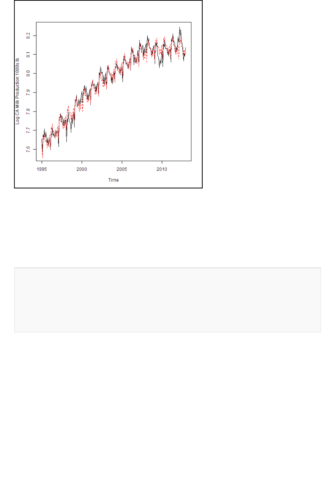
## Compute predictions from our models
predict1 <- predict(milk.lm, cadairydata)
predict2 <- predict(milk.lm2, cadairydata)
## Compute and plot the residuals
residuals <- cadairydata$Milk.Prod - predict2
plot(cadairytrain$Time, residuals[1:216], xlab = "Time", ylab ="Residuals of Seasonal Model")
Figure 24. California milk production with model including seasonal effects.
The fit to the data shown in Figure 24 is rather encouraging. Both the trend and the seasonal effect (monthly
variation) look reasonable.
As another check on our model, let's have a look at the residuals. The following code computes the predicted
values from our two models, computes the residuals for the seasonal model, and then plots these residuals for the
training data.
The residual plot is shown in Figure 25.
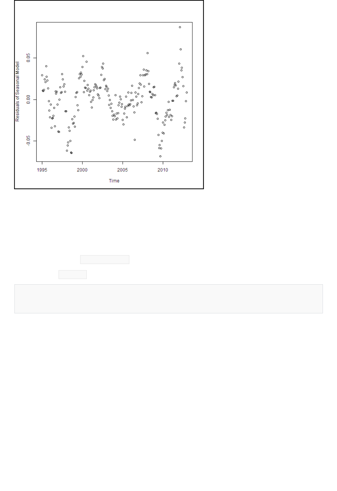
## Show the diagnostic plots for the model
plot(milk.lm2, ask = FALSE)
Figure 25. Residuals of the seasonal model for the training data.
These residuals look reasonable. There is no particular structure, except the effect of the 2008-2009 recession,
which our model does not account for particularly well.
The plot shown in Figure 25 is useful for detecting any time-dependent patterns in the residuals. The explicit
approach of computing and plotting the residuals I used places the residuals in time order on the plot. If, on the
other hand, I had plotted milk.lm$residuals , the plot would not have been in time order.
You can also use plot.lm() to produce a series of diagnostic plots.
This code produces a series of diagnostic plots shown in Figure 26.
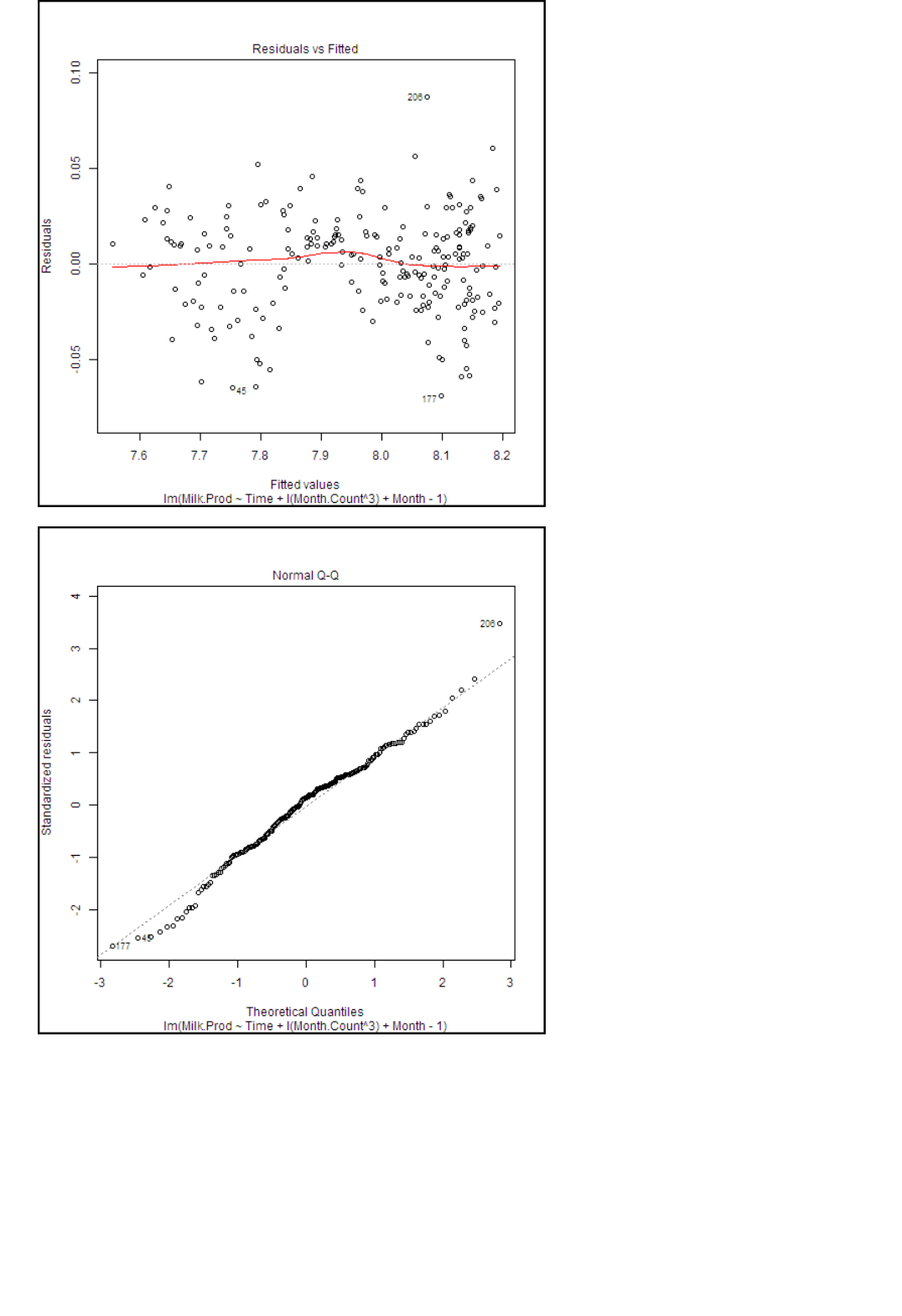
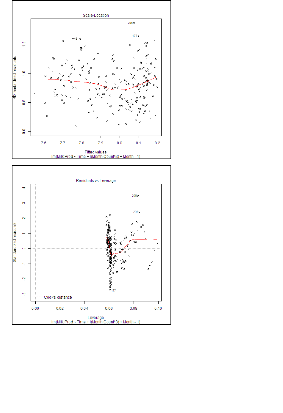
Forecasting and model evaluationForecasting and model evaluation
Figure 26. Diagnostic plots for the seasonal model.
There are a few highly influential points identified in these plots, but nothing to cause great concern. Further, we
can see from the Normal Q-Q plot that the residuals are close to normally distributed, an important assumption
for linear models.
There is just one more thing to do to complete our example. We need to compute forecasts and measure the error
against the actual data. Our forecast will be for the 12 months of 2013. We can compute an error measure for this
forecast to the actual data that is not part of our training dataset. Additionally, we can compare performance on the
18 years of training data to the 12 months of test data.

RMS.error <- function(series1, series2, is.log = TRUE, min.length = 2){
## Function to compute the RMS error or difference between two
## series or vectors
messages <- c("ERROR: Input arguments to function RMS.error of wrong type encountered",
"ERROR: Input vector to function RMS.error is too short",
"ERROR: Input vectors to function RMS.error must be of same length",
"WARNING: Funtion rms.error has received invald input time series.")
## Check the arguments
if(!is.numeric(series1) | !is.numeric(series2) | !is.logical(is.log) | !is.numeric(min.length)) {
warning(messages[1])
return(NA)}
if(length(series1) < min.length) {
warning(messages[2])
return(NA)}
if((length(series1) != length(series2))) {
warning(messages[3])
return(NA)}
## If is.log is TRUE exponentiate the values, else just copy
if(is.log) {
tryCatch( {
temp1 <- exp(series1)
temp2 <- exp(series2) },
error = function(e){warning(messages[4]); NA}
)
} else {
temp1 <- series1
temp2 <- series2
}
## Compute predictions from our models
predict1 <- predict(milk.lm, cadairydata)
predict2 <- predict(milk.lm2, cadairydata)
## Compute the RMS error in a dataframe
tryCatch( {
sqrt(sum((temp1 - temp2)^2) / length(temp1))},
error = function(e){warning(messages[4]); NA})
}
A number of metrics are used to measure the performance of time series models. In our case we will use the root
mean square (RMS) error. The following function computes the RMS error between two series.
As with the log.transform() function we discussed in the "Value transformations" section, there is quite a lot of
error checking and exception recovery code in this function. The principles employed are the same. The work is
done in two places wrapped in tryCatch() . First, the time series are exponentiated, since we have been working
with the logs of the values. Second, the actual RMS error is computed.
Equipped with a function to measure the RMS error, let's build and output a dataframe containing the RMS errors.
We will include terms for the trend model alone and the complete model with seasonal factors. The following code
does the job by using the two linear models we have constructed.
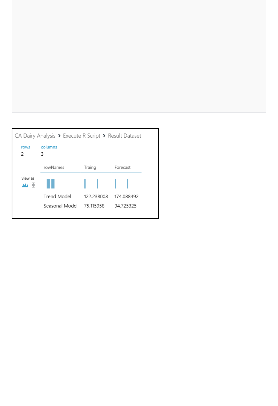
## Compute the RMS error in a dataframe
## Include the row names in the first column so they will
## appear in the output of the Execute R Script
RMS.df <- data.frame(
rowNames = c("Trend Model", "Seasonal Model"),
Traing = c(
RMS.error(predict1[1:216], cadairydata$Milk.Prod[1:216]),
RMS.error(predict2[1:216], cadairydata$Milk.Prod[1:216])),
Forecast = c(
RMS.error(predict1[217:228], cadairydata$Milk.Prod[217:228]),
RMS.error(predict2[217:228], cadairydata$Milk.Prod[217:228]))
)
RMS.df
## The following line should be executed only when running in
## Azure Machine Learning Studio
maml.mapOutputPort('RMS.df')
APPENDIX A: Guide to RStudio
Running this code produces the output shown in Figure 27 at the Result Dataset output port.
Figure 27. Comparison of RMS errors for the models.
From these results, we see that adding the seasonal factors to the model reduces the RMS error significantly. Not
too surprisingly, the RMS error for the training data is a bit less than for the forecast.
RStudio is quite well documented, so in this appendix I will provide some links to the key sections of the RStudio
documentation to get you started.
1. Creating projects
You can organize and manage your R code into projects by using RStudio. The documentation that uses
projects can be found at https://support.rstudio.com/hc/articles/200526207-Using-Projects.
I recommend that you follow these directions and create a project for the R code examples in this document.
2. Editing and executing R code
RStudio provides an integrated environment for editing and executing R code. Documentation can be found
at https://support.rstudio.com/hc/articles/200484448-Editing-and-Executing-Code.
3. Debugging
RStudio includes powerful debugging capabilities. Documentation for these features is at
https://support.rstudio.com/hc/articles/200713843-Debugging-with-RStudio.

APPENDIX B: Further reading
The breakpoint troubleshooting features are documented at
https://support.rstudio.com/hc/articles/200534337-Breakpoint-Troubleshooting.
This R programming tutorial covers the basics of what you need to use the R language with Azure Machine
Learning Studio. If you are not familiar with R, two introductions are available on CRAN:
R for Beginners by Emmanuel Paradis is a good place to start at http://cran.r-project.org/doc/contrib/Paradis-
rdebuts_en.pdf.
An Introduction to R by W. N. Venables et. al. goes into a bit more depth, at http://cran.r-
project.org/doc/manuals/R-intro.html.
There are many books on R that can help you get started. Here are a few I find useful:
The Art of R Programming: A Tour of Statistical Software Design by Norman Matloff is an excellent
introduction to programming in R.
R Cookbook by Paul Teetor provides a problem and solution approach to using R.
R in Action by Robert Kabacoff is another useful introductory book. The companion Quick R website is a useful
resource at http://www.statmethods.net/.
R Inferno by Patrick Burns is a surprisingly humorous book that deals with a number of tricky and difficult
topics that can be encountered when programming in R. The book is available for free at http://www.burns-
stat.com/documents/books/the-r-inferno/.
If you want a deep dive into advanced topics in R, have a look at the book Advanced R by Hadley Wickham. The
online version of this book is available for free at http://adv-r.had.co.nz/.
A catalogue of R time series packages can be found in the CRAN Task View for time series analysis: http://cran.r-
project.org/web/views/TimeSeries.html. For information on specific time series object packages, you should refer
to the documentation for that package.
The book Introductory Time Series with R by Paul Cowpertwait and Andrew Metcalfe provides an introduction to
using R for time series analysis. Many more theoretical texts provide R examples.
Some great internet resources:
DataCamp: DataCamp teaches R in the comfort of your browser with video lessons and coding exercises. There
are interactive tutorials on the latest R techniques and packages. Take the free interactive R tutorial at
https://www.datacamp.com/courses/introduction-to-r
A guide on Getting started with R from Programiz https://www.programiz.com/r-programming
A quick R tutorial by Kelly Black from Clarkson University http://www.cyclismo.org/tutorial/R/
60+ R resources listed at http://www.computerworld.com/article/2497464/business-intelligence-60-r-
resources-to-improve-your-data-skills.html
Create and share an Azure Machine Learning
workspace
3/21/2018 • 2 min to read • Edit Online
NOTENOTE
To create a workspaceTo create a workspace
This menu links to topics that describe how to set up the various data science environments used by the Cortana
Analytics Process (CAPS).
To use Azure Machine Learning Studio, you need to have a Machine Learning workspace. This workspace contains
the tools you need to create, manage, and publish experiments.
You can try Azure Machine Learning for free. No credit card or Azure subscription is required. Get started now.
NOTENOTE
1. Sign in to the Azure portal
To sign in and create a workspace, you need to be an Azure subscription administrator.
2. Click +New
3. In the search box, type Machine Learning Studio Workspace and select the matching item. Then, select
click Create at the bottom of the page.
4. Enter your workspace information:
The workspace name may be up to 260 characters, not ending in a space. The name can't include these
characters: < > * % & : \ ? + /
The web service plan you choose (or create), along with the associated pricing tier you select, is used
if you deploy web services from this workspace.
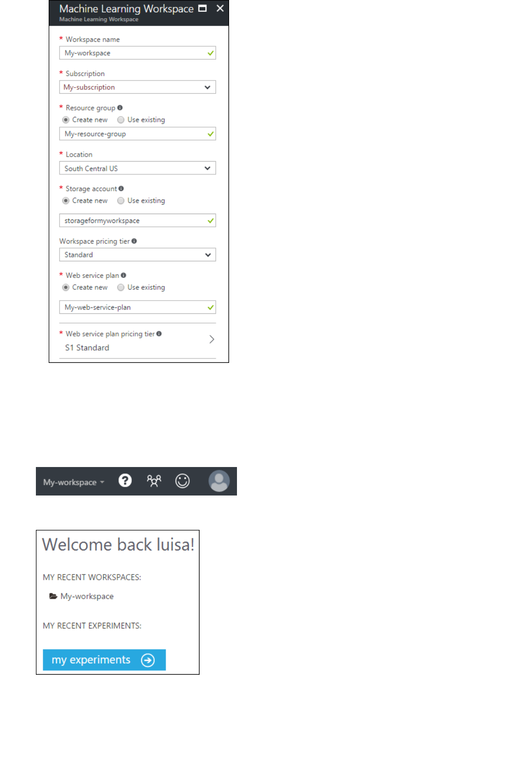
Sharing an Azure Machine Learning workspace
5. Click Create.
Once the workspace is deployed, you can open it in Machine Learning Studio.
1. Browse to Machine Learning Studio at https://studio.azureml.net/.
2. Select your workspace in the upper-right-hand corner.
3. Click my experiments.
For information about managing your workspace, see Manage an Azure Machine Learning workspace. If you
encounter a problem creating your workspace, see Troubleshooting guide: Create and connect to a Machine
Learning workspace.
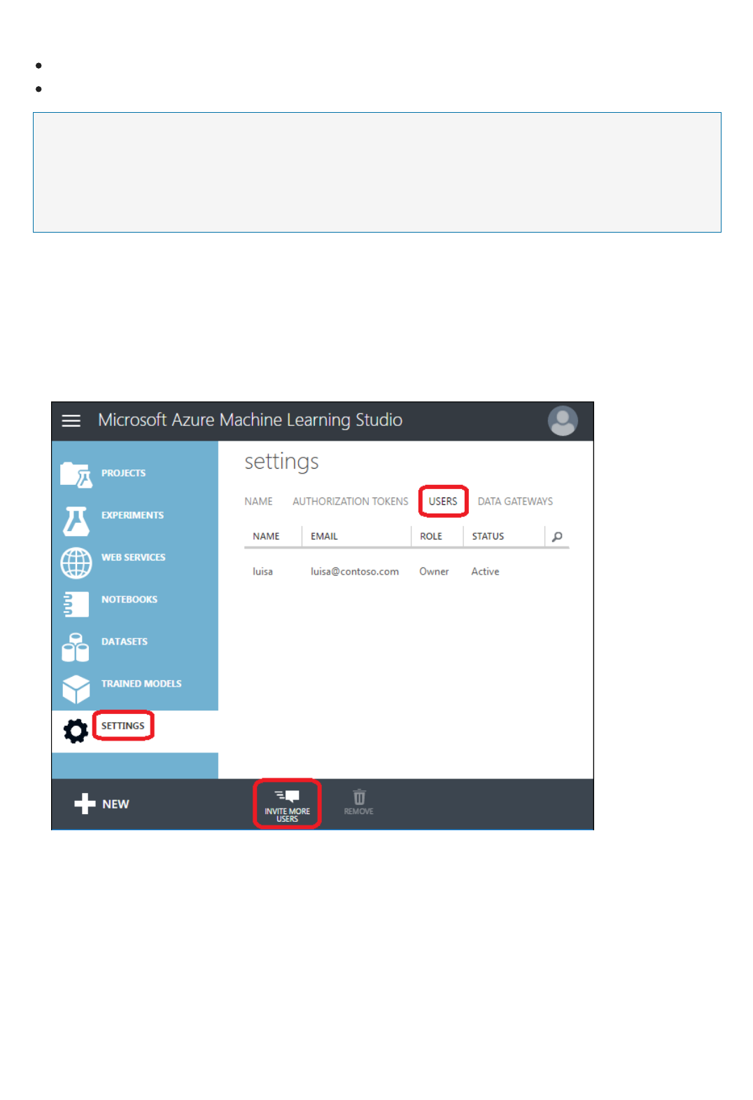
NOTENOTE
To share a workspaceTo share a workspace
Once a Machine Learning workspace is created, you can invite users to your workspace to share access to your
workspace and all its experiments, datasets, notebooks, etc. You can add users in one of two roles:
User - A workspace user can create, open, modify, and delete experiments, datasets, etc. in the workspace.
Owner - An owner can invite and remove users in the workspace, in addition to what a user can do.
The administrator account that creates the workspace is automatically added to the workspace as workspace Owner.
However, other administrators or users in that subscription are not automatically granted access to the workspace - you
need to invite them explicitly.
1. Sign in to Machine Learning Studio at https://studio.azureml.net/Home
2. In the left panel, click SETTINGS
3. Click the USERS tab
4. Click INVITE MORE USERS at the bottom of the page
5. Enter one or more email addresses. The users need a valid Microsoft account or an organizational account
(from Azure Active Directory).
6. Select whether you want to add the users as Owner or User.
7. Click the OK checkmark button.
Each user you add will receive an email with instructions on how to sign in to the shared workspace.

NOTENOTE
For users to be able to deploy or manage web services in this workspace, they must be a contributor or administrator in the
Azure subscription.
Manage an Azure Machine Learning workspace
4/11/2018 • 1 min to read • Edit Online
NOTENOTE
NOTENOTE
Use the Azure portal
NOTENOTE
Next steps
For information on managing Web services in the Machine Learning Web Services portal, see Manage a Web service using
the Azure Machine Learning Web Services portal.
You can manage Machine Learning workspaces in the Azure portal.
You can try Azure Machine Learning for free. No credit card or Azure subscription is required. Get started now.
To manage a workspace in the Azure portal:
1. Sign in to the Azure portal using an Azure subscription administrator account.
2. In the search box at the top of the page, enter "machine learning workspaces" and then select Machine
Learning Workspaces.
3. Click the workspace you want to manage.
In addition to the standard resource management information and options available, you can:
View Properties - This page displays the workspace and resource information, and you can change the
subscription and resource group that this workspace is connected with.
Resync Storage Keys - The workspace maintains keys to the storage account. If the storage account changes
keys, then you can click Resync keys to synchronize the keys with the workspace.
To manage the web services associated with this workspace, use the Machine Learning Web Services portal. See
Manage a Web service using the Azure Machine Learning Web Services portal for complete information.
To deploy or manage New web services you must be assigned a contributor or administrator role on the subscription to
which the web service is deployed. If you invite another user to a machine learning workspace, you must assign them to a
contributor or administrator role on the subscription before they can deploy or manage web services.
For more information on setting access permissions, see View access assignments for users and groups in the Azure portal.
Learn more about deploy Machine Learning with Azure Resource Manager Templates.
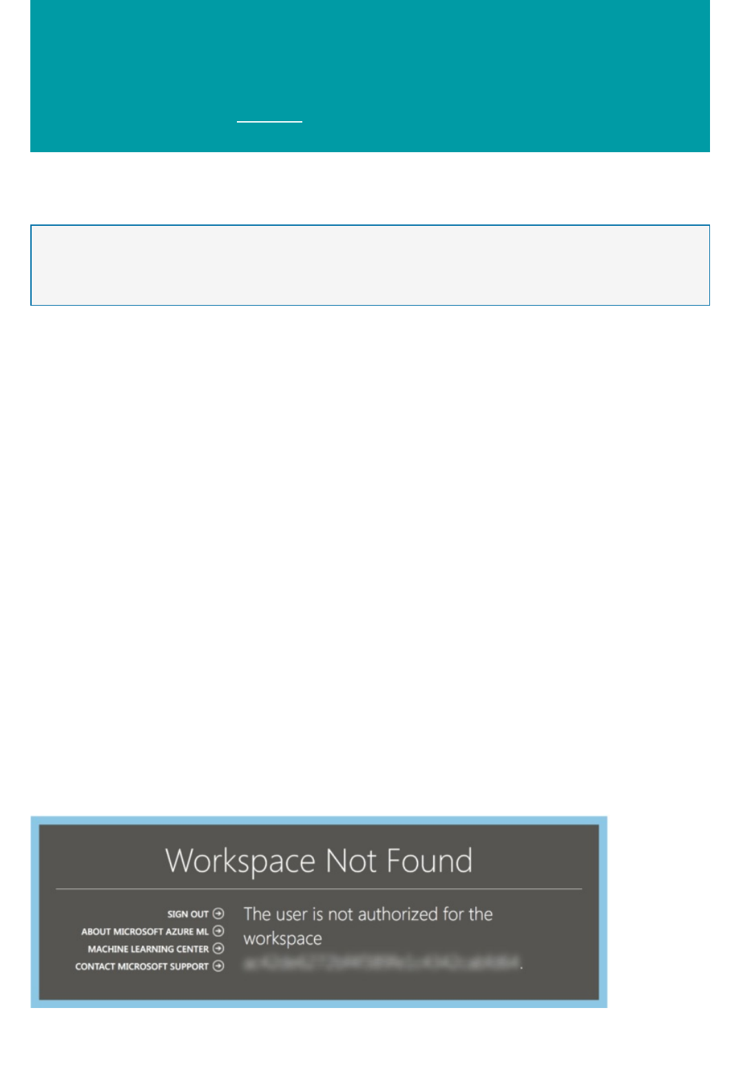
Troubleshooting guide: Create and connect to an
Machine Learning workspace
3/21/2018 • 1 min to read • Edit Online
NOTENOTE
Workspace owner
Allowed regions
Storage account
This guide provides solutions for some frequently encountered challenges when you are setting up Azure Machine
Learning workspaces.
You can try Azure Machine Learning for free. No credit card or Azure subscription is required. Get started now.
To open a workspace in Machine Learning Studio, you must be signed in to the Microsoft Account you used to
create the workspace, or you need to receive an invitation from the owner to join the workspace. From the Azure
portal you can manage the workspace, which includes the ability to configure access.
For more information on managing a workspace, see Manage an Azure Machine Learning workspace.
Machine Learning is currently available in a limited number of regions. If your subscription does not include one of
these regions, you may see the error message, “You have no subscriptions in the allowed regions.”
To request that a region be added to your subscription, create a new Microsoft support request from the Azure
portal, choose Billing as the problem type, and follow the prompts to submit your request.
The Machine Learning service needs a storage account to store data. You can use an existing storage account, or
you can create a new storage account when you create the new Machine Learning workspace (if you have quota to
create a new storage account).
After the new Machine Learning workspace is created, you can sign in to Machine Learning Studio by using the
Microsoft account you used to create the workspace. If you encounter the error message, “Workspace Not Found”
(similar to the following screenshot), please use the following steps to delete your browser cookies.
To delete browser cookies
1. If you use Internet Explorer, click the Tools button in the upper-right corner and select Internet options.
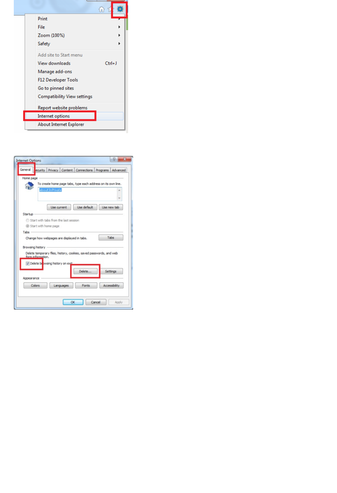
1. Under the General tab, click Delete…
1. In the Delete Browsing History dialog box, make sure Cookies and website data is selected, and click
Delete.
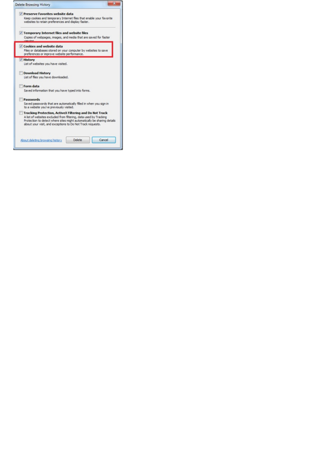
Comments
After the cookies are deleted, restart the browser and then go to the Microsoft Azure Machine Learning page.
When you are prompted for a user name and password, enter the same Microsoft account you used to create the
workspace.
Our goal is to make the Machine Learning experience as seamless as possible. Please post any comments and
issues at the Azure Machine Learning forum to help us serve you better.

Deploy Machine Learning Workspace Using Azure
Resource Manager
4/18/2018 • 3 min to read • Edit Online
Introduction
Step-by-step: create a Machine Learning Workspace
Create an Azure Resource Manager templateCreate an Azure Resource Manager template
Using an Azure Resource Manager deployment template saves you time by giving you a scalable way to deploy
interconnected components with a validation and retry mechanism. To set up Azure Machine Learning
Workspaces, for example, you need to first configure an Azure storage account and then deploy your workspace.
Imagine doing this manually for hundreds of workspaces. An easier alternative is to use an Azure Resource
Manager template to deploy an Azure Machine Learning Workspace and all its dependencies. This article takes you
through this process step-by-step. For a great overview of Azure Resource Manager, see Azure Resource Manager
overview.
We will create an Azure resource group, then deploy a new Azure storage account and a new Azure Machine
Learning Workspace using a Resource Manager template. Once the deployment is complete, we will print out
important information about the workspaces that were created (the primary key, the workspaceID, and the URL to
the workspace).
A Machine Learning Workspace requires an Azure storage account to store the dataset linked to it. The following
template uses the name of the resource group to generate the storage account name and the workspace name. It
also uses the storage account name as a property when creating the workspace.
{
"contentVersion": "1.0.0.0",
"$schema": "http://schema.management.azure.com/schemas/2015-01-01/deploymentTemplate.json#",
"variables": {
"namePrefix": "[resourceGroup().name]",
"location": "[resourceGroup().location]",
"mlVersion": "2016-04-01",
"stgVersion": "2015-06-15",
"storageAccountName": "[concat(variables('namePrefix'),'stg')]",
"mlWorkspaceName": "[concat(variables('namePrefix'),'mlwk')]",
"mlResourceId": "[resourceId('Microsoft.MachineLearning/workspaces', variables('mlWorkspaceName'))]",
"stgResourceId": "[resourceId('Microsoft.Storage/storageAccounts', variables('storageAccountName'))]",
"storageAccountType": "Standard_LRS"
},
"resources": [
{
"apiVersion": "[variables('stgVersion')]",
"name": "[variables('storageAccountName')]",
"type": "Microsoft.Storage/storageAccounts",
"location": "[variables('location')]",
"properties": {
"accountType": "[variables('storageAccountType')]"
}
},
{
"apiVersion": "[variables('mlVersion')]",
"type": "Microsoft.MachineLearning/workspaces",
"name": "[variables('mlWorkspaceName')]",
"location": "[variables('location')]",
"dependsOn": ["[variables('stgResourceId')]"],
"properties": {
"UserStorageAccountId": "[variables('stgResourceId')]"
}
}
],
"outputs": {
"mlWorkspaceObject": {"type": "object", "value": "[reference(variables('mlResourceId'),
variables('mlVersion'))]"},
"mlWorkspaceToken": {"type": "string", "value": "[listWorkspaceKeys(variables('mlResourceId'),
variables('mlVersion')).primaryToken]"},
"mlWorkspaceWorkspaceID": {"type": "string", "value": "[reference(variables('mlResourceId'),
variables('mlVersion')).WorkspaceId]"},
"mlWorkspaceWorkspaceLink": {"type": "string", "value": "
[concat('https://studio.azureml.net/Home/ViewWorkspace/', reference(variables('mlResourceId'),
variables('mlVersion')).WorkspaceId)]"}
}
}
Deploy the resource group, based on the templateDeploy the resource group, based on the template
# Install the Azure Resource Manager modules from the PowerShell Gallery (press “A”)
Install-Module AzureRM -Scope CurrentUser
# Install the Azure Service Management modules from the PowerShell Gallery (press “A”)
Install-Module Azure -Scope CurrentUser
Save this template as mlworkspace.json file under c:\temp.
Open PowerShell
Install modules for Azure Resource Manager and Azure Service Management
These steps download and install the modules necessary to complete the remaining steps. This only needs to be
done once in the environment where you are executing the PowerShell commands.
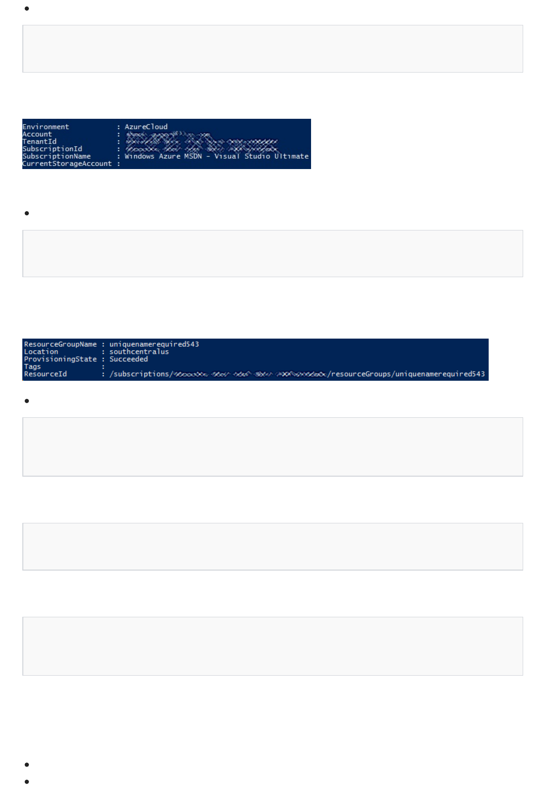
# Authenticate (enter your credentials in the pop-up window)
Connect-AzureRmAccount
$rg = New-AzureRmResourceGroup -Name "uniquenamerequired523" -Location "South Central US"
$rg
# Create a Resource Group, TemplateFile is the location of the JSON template.
$rgd = New-AzureRmResourceGroupDeployment -Name "demo" -TemplateFile "C:\temp\mlworkspace.json" -
ResourceGroupName $rg.ResourceGroupName
# Access Azure ML Workspace Token after its deployment.
$rgd.Outputs.mlWorkspaceToken.Value
# List the primary and secondary tokens of all workspaces
Get-AzureRmResource |? { $_.ResourceType -Like "*MachineLearning/workspaces*"} |% { Invoke-
AzureRmResourceAction -ResourceId $_.ResourceId -Action listworkspacekeys -Force}
Next Steps
Authenticate to Azure
This step needs to be repeated for each session. Once authenticated, your subscription information should be
displayed.
Now that we have access to Azure, we can create the resource group.
Create a resource group
Verify that the resource group is correctly provisioned. ProvisioningState should be “Succeeded.” The resource
group name is used by the template to generate the storage account name. The storage account name must be
between 3 and 24 characters in length and use numbers and lower-case letters only.
Using the resource group deployment, deploy a new Machine Learning Workspace.
Once the deployment is completed, it is straightforward to access properties of the workspace you deployed. For
example, you can access the Primary Key Token.
Another way to retrieve tokens of existing workspace is to use the Invoke-AzureRmResourceAction command. For
example, you can list the primary and secondary tokens of all workspaces.
After the workspace is provisioned, you can also automate many Azure Machine Learning Studio tasks using the
PowerShell Module for Azure Machine Learning.
Learn more about authoring Azure Resource Manager Templates.
Have a look at the Azure Quickstart Templates Repository.

Edit Online
1 min to read •
Import your training data into Azure Machine
Learning Studio from various data sources
3/21/2018 • 3 min to read • Edit Online
NOTENOTE
NOTENOTE
Get data ready for use in Azure Machine Learning Studio
Data formats and data types supported
To use your own data in Machine Learning Studio to develop and train a predictive analytics solution, you can:
upload data from a local file ahead of time from your hard drive to create a dataset module in your
workspace
access data from one of several online data sources while your experiment is running using the Import Data
module
use data from another Azure Machine learning experiment saved as a dataset
use data from an on-premises SQL Server database
Each of these options is described in one of the topics on the menu below. These topics show you how to import
data from these various data sources to use in Machine Learning Studio.
There are a number of sample datasets available in Machine Learning Studio that you can use for training data. For
information on these, see Use the sample datasets in Azure Machine Learning Studio).
This introductory topic also discusses how to get data ready for use in Machine Learning Studio and describes
which data formats and data types are supported.
You can try Azure Machine Learning for free. No credit card or Azure subscription is required. Get started now.
Machine Learning Studio is designed to work with rectangular or tabular data, such as text data that's delimited or
structured data from a database, though in some circumstances non-rectangular data may be used.
It's best if your data is relatively clean. That is, you'll want to take care of issues such as unquoted strings before
you upload the data into your experiment.
However, there are modules available in Machine Learning Studio that enable some manipulation of data within
your experiment. Depending on the machine learning algorithms you'll be using, you may need to decide how
you'll handle data structural issues such as missing values and sparse data, and there are modules that can help
with that. Look in the Data Transformation section of the module palette for modules that perform these
functions.
At any point in your experiment you can view or download the data that's produced by a module by clicking the
output port. Depending on the module, there may be different download options available, or you may be able to
visualize the data within your web browser in Machine Learning Studio.
You can import a number of data types into your experiment, depending on what mechanism you use to import

data and where it's coming from:
Plain text (.txt)
Comma-separated values (CSV) with a header (.csv) or without (.nh.csv)
Tab-separated values (TSV) with a header (.tsv) or without (.nh.tsv)
Excel file
Azure table
Hive table
SQL database table
OData values
SVMLight data (.svmlight) (see the SVMLight definition for format information)
Attribute Relation File Format (ARFF) data (.arff) (see the ARFF definition for format information)
Zip file (.zip)
R object or workspace file (.RData)
If you import data in a format such as ARFF that includes metadata, Machine Learning Studio uses this metadata
to define the heading and data type of each column.
If you import data such as TSV or CSV format that doesn't include this metadata, Machine Learning Studio infers
the data type for each column by sampling the data. If the data also doesn't have column headings, Machine
Learning Studio provides default names.
You can explicitly specify or change the headings and data types for columns using the Edit Metadata.
The following data types are recognized by Machine Learning Studio:
String
Integer
Double
Boolean
DateTime
TimeSpan
Machine Learning Studio uses an internal data type called Data Table to pass data between modules. You can
explicitly convert your data into Data Table format using the Convert to Dataset module.
Any module that accepts formats other than Data Table will convert the data to Data Table silently before passing
it to the next module.
If necessary, you can convert Data Table format back into CSV, TSV, ARFF, or SVMLight format using other
conversion modules. Look in the Data Format Conversions section of the module palette for modules that
perform these functions.
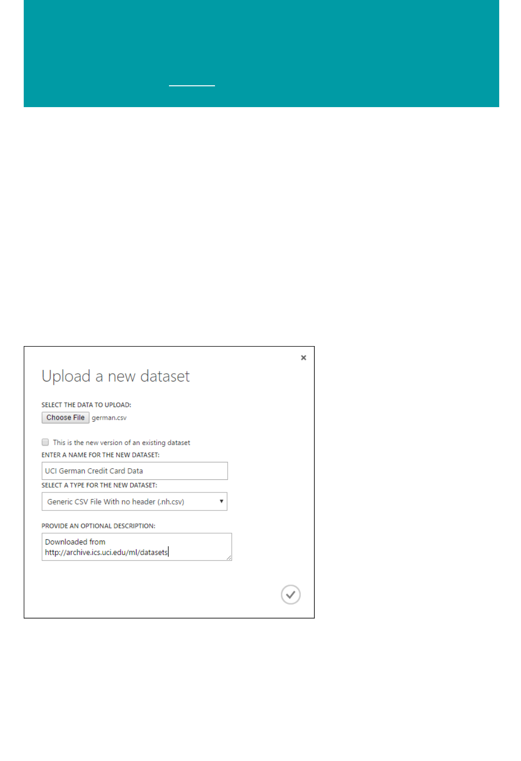
Import training data from a file on your hard drive
into Machine Learning Studio
3/20/2018 • 1 min to read • Edit Online
Steps to import data from a local file
Dataset module is ready for use
Learn how to upload a data file from your hard drive to use as training data in Azure Machine Learning Studio. By
importing the data file, you have a dataset module ready for use in your workspace.
To import data from a local hard drive, do the following:
1. Click +NEW at the bottom of the Machine Learning Studio window.
2. Select DATASET and FROM LOCAL FILE.
3. In the Upload a new dataset dialog, browse to the file you want to upload
4. Enter a name, identify the data type, and optionally enter a description. A description is recommended - it
allows you to record any characteristics about the data that you want to remember when using the data in the
future.
5. The checkbox This is the new version of an existing dataset allows you to update an existing dataset with
new data. Click this checkbox and then enter the name of an existing dataset.
During upload, you'll see a message that your file is being uploaded. Upload time depends on the size of your data
and the speed of your connection to the service. If you know the file will take a long time, you can do other things
inside Machine Learning Studio while you wait. However, closing the browser causes the data upload to fail.
Once your data is uploaded, it's stored in a dataset module and is available to any experiment in your workspace.
When you're editing an experiment, you can find the datasets you've created in the My Datasets list under the

Saved Datasets list in the module palette. You can drag and drop the dataset onto the experiment canvas when
you want to use the dataset for further analytics and machine learning.
Import data into Azure Machine Learning Studio
from various online data sources with the Import
Data module
3/20/2018 • 7 min to read • Edit Online
NOTENOTE
Introduction
IMPORTANTIMPORTANT
This article describes the support for importing online data from various sources and the information needed to
move data from these sources into an Azure Machine Learning experiment.
This article provides general information about the Import Data module. For more detailed information about the types of
data you can access, formats, parameters, and answers to common questions, see the module reference topic for the Import
Data module.
By using the Import Data module, you can access data from one of several online data sources while your
experiment is running in Azure Machine Learning Studio:
A Web URL using HTTP
Hadoop using HiveQL
Azure blob storage
Azure table
Azure SQL database or SQL Server on Azure VM
On-premises SQL Server database
A data feed provider, OData currently
Azure Cosmos DB
To access online data sources in your Studio experiment, add the Import Data module to your, select the Data
source, and then provide the parameters needed to access the data. The online data sources that are supported
are itemized in the table below. This table also summarizes the file formats that are supported and parameters that
are used to access the data.
Note that because this training data is accessed while your experiment is running, it's only available in that
experiment. By comparison, data that has been stored in a dataset module are available to any experiment in your
workspace.
Currently, the Import Data and Export Data modules can read and write data only from Azure storage created using the
Classic deployment model. In other words, the new Azure Blob Storage account type that offers a hot storage access tier or
cool storage access tier is not yet supported.
Generally, any Azure storage accounts that you might have created before this service option became available should not
be affected. If you need to create a new account, select Classic for the Deployment model, or use Resource manager and
select General purpose rather than Blob storage for Account kind.
For more information, see Azure Blob Storage: Hot and Cool Storage Tiers.

Supported online data sources
DATA SOURCE DESCRIPTION PARAMETERS
Web URL via HTTP Reads data in comma-separated values
(CSV), tab-separated values (TSV),
attribute-relation file format (ARFF), and
Support Vector Machines (SVM-light)
formats, from any web URL that uses
HTTP
URL: Specifies the full name of the file,
including the site URL and the file
name, with any extension.
Data format: Specifies one of the
supported data formats: CSV, TSV, ARFF,
or SVM-light. If the data has a header
row, it is used to assign column names.
Hadoop/HDFS Reads data from distributed storage in
Hadoop. You specify the data you want
by using HiveQL, a SQL-like query
language. HiveQL can also be used to
aggregate data and perform data
filtering before you add the data to
Machine Learning Studio.
Hive database query: Specifies the
Hive query used to generate the data.
HCatalog server URI : Specified the
name of your cluster using the format
<your cluster
name>.azurehdinsight.net.
Hadoop user account name: Specifies
the Hadoop user account name used to
provision the cluster.
Hadoop user account password :
Specifies the credentials used when
provisioning the cluster. For more
information, see Create Hadoop clusters
in HDInsight.
Location of output data: Specifies
whether the data is stored in a Hadoop
distributed file system (HDFS) or in
Azure.
Azure Machine Learning Import Data module supports the following data sources:
If you store output data in HDFS,
specify the HDFS server URI. (Be
sure to use the HDInsight cluster
name without the HTTPS:// prefix).
If you store your output data in
Azure, you must specify the Azure
storage account name, Storage
access key and Storage container
name.

SQL database Reads data that is stored in an Azure
SQL database or in a SQL Server
database running on an Azure virtual
machine.
Database server name: Specifies the
name of the server on which the
database is running.
Database name : Specifies the name of
the database on the server.
Server user account name: Specifies a
user name for an account that has
access permissions for the database.
Server user account password:
Specifies the password for the user
account.
Database query:Enter a SQL
statement that describes the data you
want to read.
DATA SOURCE DESCRIPTION PARAMETERS
In case of Azure SQL Database
enter the server name that is
generated. Typically it has the form
<generated_identifier>.database.w
indows.net.
In case of a SQL server hosted on a
Azure Virtual machine enter tcp:
<Virtual Machine DNS Name>,
1433

On-premises SQL database Reads data that is stored in an on-
premises SQL database.
Data gateway: Specifies the name of
the Data Management Gateway
installed on a computer where it can
access your SQL Server database. For
information about setting up the
gateway, see Perform advanced
analytics with Azure Machine Learning
using data from an on-premises SQL
server.
Database server name: Specifies the
name of the server on which the
database is running.
Database name : Specifies the name of
the database on the server.
Server user account name: Specifies a
user name for an account that has
access permissions for the database.
User name and password: Click Enter
values to enter your database
credentials. You can use Windows
Integrated Authentication or SQL
Server Authentication depending upon
how your on-premises SQL Server is
configured.
Database query:Enter a SQL
statement that describes the data you
want to read.
Azure Table Reads data from the Table service in
Azure Storage.
If you read large amounts of data
infrequently, use the Azure Table
Service. It provides a flexible, non-
relational (NoSQL), massively scalable,
inexpensive, and highly available
storage solution.
The options in the Import Data change
depending on whether you are
accessing public information or a
private storage account that requires
login credentials. This is determined by
the Authentication Type which can
have value of "PublicOrSAS" or
"Account", each of which has its own set
of parameters.
Public or Shared Access Signature
(SAS) URI: The parameters are:
DATA SOURCE DESCRIPTION PARAMETERS
Table URI: Specifies the Public or
SAS URL for the table.
Specifies the rows to scan for
property names: The values are
TopN to scan the specified number
of rows, or ScanAll to get all rows
in the table.
If the data is homogeneous and
predictable, it is recommended that
you select TopN and enter a
number for N. For large tables, this
can result in quicker reading times.
If the data is structured with sets of

Private Storage Account: The
parameters are:
DATA SOURCE DESCRIPTION PARAMETERS
properties that vary based on the
depth and position of the table,
choose the ScanAll option to scan
all rows. This ensures the integrity
of your resulting property and
metadata conversion.
Account name: Specifies the name
of the account that contains the
table to read.
Account key: Specifies the storage
key associated with the account.
Table name : Specifies the name of
the table that contains the data to
read.
Rows to scan for property
names: The values are TopN to
scan the specified number of rows,
or ScanAll to get all rows in the
table.
If the data is homogeneous and
predictable, we recommend that
you select TopN and enter a
number for N. For large tables, this
can result in quicker reading times.
If the data is structured with sets of
properties that vary based on the
depth and position of the table,
choose the ScanAll option to scan
all rows. This ensures the integrity
of your resulting property and
metadata conversion.

Azure Blob Storage Reads data stored in the Blob service in
Azure Storage, including images,
unstructured text, or binary data.
You can use the Blob service to publicly
expose data, or to privately store
application data. You can access your
data from anywhere by using HTTP or
HTTPS connections.
The options in the Import Data
module change depending on whether
you are accessing public information or
a private storage account that requires
login credentials. This is determined by
the Authentication Type which can
have a value either of "PublicOrSAS" or
of "Account".
Public or Shared Access Signature
(SAS) URI: The parameters are:
Private Storage Account: The
parameters are:
DATA SOURCE DESCRIPTION PARAMETERS
URI: Specifies the Public or SAS URL
for the storage blob.
File Format: Specifies the format of
the data in the Blob service. The
supported formats are CSV, TSV,
and ARFF.
Account name: Specifies the name
of the account that contains the
blob you want to read.
Account key: Specifies the storage
key associated with the account.
Path to container, directory, or
blob : Specifies the name of the
blob that contains the data to read.
Blob file format: Specifies the
format of the data in the blob
service. The supported data
formats are CSV, TSV, ARFF, CSV
with a specified encoding, and Excel.
If the format is CSV or TSV, be
sure to indicate whether the file
contains a header row.
You can use the Excel option to
read data from Excel
workbooks. In the
Excel data format option,
indicate whether the data is in
an Excel worksheet range, or in
an Excel table. In the
Excel sheet or embedded table
option, specify the name of the
sheet or table that you want to
read from.

Data Feed Provider Reads data from a supported feed
provider. Currently only the Open Data
Protocol (OData) format is supported.
Data content type: Specifies the OData
format.
Source URL: Specifies the full URL for
the data feed.
For example, the following URL reads
from the Northwind sample database:
http://services.odata.org/northwind/nor
thwind.svc/
DATA SOURCE DESCRIPTION PARAMETERS
Next steps
Deploying Azure ML web services that use Data Import and Data Export modules

Import your data into Azure Machine Learning
Studio from another experiment
3/5/2018 • 1 min to read • Edit Online
There will be times when you'll want to take an intermediate result from one experiment and use it as part of
another experiment. To do this, you save the module as a dataset:
1. Click the output of the module that you want to save as a dataset.
2. Click Save as Dataset.
3. When prompted, enter a name and a description that would allow you to identify the dataset easily.
4. Click the OK checkmark.
When the save finishes, the dataset will be available for use within any experiment in your workspace. You can find
it in the Saved Datasets list in the module palette.

Perform advanced analytics with Azure Machine
Learning using data from an on-premises SQL
Server database
3/21/2018 • 9 min to read • Edit Online
NOTENOTE
NOTENOTE
Install the Microsoft Data Management Gateway
Often enterprises that work with on-premises data would like to take advantage of the scale and agility of the
cloud for their machine learning workloads. But they don't want to disrupt their current business processes and
workflows by moving their on-premises data to the cloud. Azure Machine Learning now supports reading your
data from an on-premises SQL Server database and then training and scoring a model with this data. You no
longer have to manually copy and sync the data between the cloud and your on-premises server. Instead, the
Import Data module in Azure Machine Learning Studio can now read directly from your on-premises SQL
Server database for your training and scoring jobs.
This article provides an overview of how to ingress on-premises SQL server data into Azure Machine Learning. It
assumes that you're familiar with Azure Machine Learning concepts like workspaces, modules, datasets,
experiments, etc..
This feature is not available for free workspaces. For more information about Machine Learning pricing and tiers, see Azure
Machine Learning Pricing.
You can try Azure Machine Learning for free. No credit card or Azure subscription is required. Get started now.
To access an on-premises SQL Server database in Azure Machine Learning, you need to download and install the
Microsoft Data Management Gateway. When you configure the gateway connection in Machine Learning Studio,
you have the opportunity to download and install the gateway using the Download and register data gateway
dialog described below.
You also can install the Data Management Gateway ahead of time by downloading and running the MSI setup
package from the Microsoft Download Center. Choose the latest version, selecting either 32-bit or 64-bit as
appropriate for your computer. The MSI can also be used to upgrade an existing Data Management Gateway to
the latest version, with all settings preserved.
The gateway has the following prerequisites:
The supported Windows operating system versions are Windows 7, Windows 8/8.1, Windows 10, Windows
Server 2008 R2, Windows Server 2012, and Windows Server 2012 R2.
The recommended configuration for the gateway machine is at least 2 GHz, 4 cores, 8GB RAM, and 80GB
disk.
If the host machine hibernates, the gateway won’t respond to data requests. Therefore, configure an
appropriate power plan on the computer before installing the gateway. If the machine is configured to
hibernate, the gateway installation displays a message.
Ingress data from your on-premises SQL Server database into Azure
Machine Learning
TIPTIP
Step 1: Create a gatewayStep 1: Create a gateway
Because copy activity occurs at a specific frequency, the resource usage (CPU, memory) on the machine also
follows the same pattern with peak and idle times. Resource utilization also depends heavily on the amount of
data being moved. When multiple copy jobs are in progress, you'll observe resource usage go up during peak
times. While the minimum configuration listed above is technically sufficient, you may want to have a
configuration with more resources than the minimum configuration depending on your specific load for data
movement.
Consider the following when setting up and using a Data Management Gateway:
You can install only one instance of Data Management Gateway on a single computer.
You can use a single gateway for multiple on-premises data sources.
You can connect multiple gateways on different computers to the same on-premises data source.
You configure a gateway for only one workspace at a time. Currently, gateways can’t be shared across
workspaces.
You can configure multiple gateways for a single workspace. For example, you may want to use a gateway
that's connected to your test data sources during development and a production gateway when you're ready to
operationalize.
The gateway does not need to be on the same machine as the data source. But staying closer to the data
source reduces the time for the gateway to connect to the data source. We recommend that you install the
gateway on a machine that's different from the one that hosts the on-premises data source so that the gateway
and data source don't compete for resources.
NOTENOTE
You need to use the Data Management Gateway for Azure Machine Learning even if you are using Azure
ExpressRoute for other data. You should treat your data source as an on-premises data source (that's behind a
firewall) even when you use ExpressRoute. Use the Data Management Gateway to establish connectivity
between Machine Learning and the data source.
If you already have a gateway installed on your computer serving Power BI or Azure Data Factory
scenarios, install a separate gateway for Azure Machine Learning on another computer.
You can't run Data Management Gateway and Power BI Gateway on the same computer.
You can find detailed information on installation prerequisites, installation steps, and troubleshooting tips in the
article Data Management Gateway.
In this walkthrough, you will set up a Data Management Gateway in an Azure Machine Learning workspace,
configure it, and then read data from an on-premises SQL Server database.
Before you start, disable your browser’s pop-up blocker for studio.azureml.net . If you're using the Google Chrome
browser, download and install one of the several plug-ins available at Google Chrome WebStore Click Once App Extension.
The first step is to create and set up the gateway to access your on-premises SQL database.
1. Log in to Azure Machine Learning Studio and select the workspace that you want to work in.
2. Click the SETTINGS blade on the left, and then click the DATA GATEWAYS tab at the top.
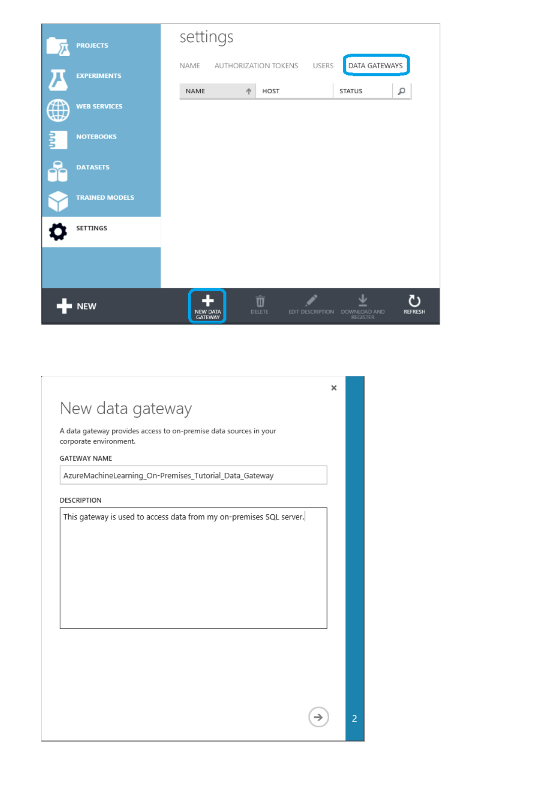
3. Click NEW DATA GATEWAY at the bottom of the screen.
4. In the New data gateway dialog, enter the Gateway Name and optionally add a Description. Click the
arrow on the bottom right-hand corner to go to the next step of the configuration.
5. In the Download and register data gateway dialog, copy the GATEWAY REGISTRATION KEY to the
clipboard.
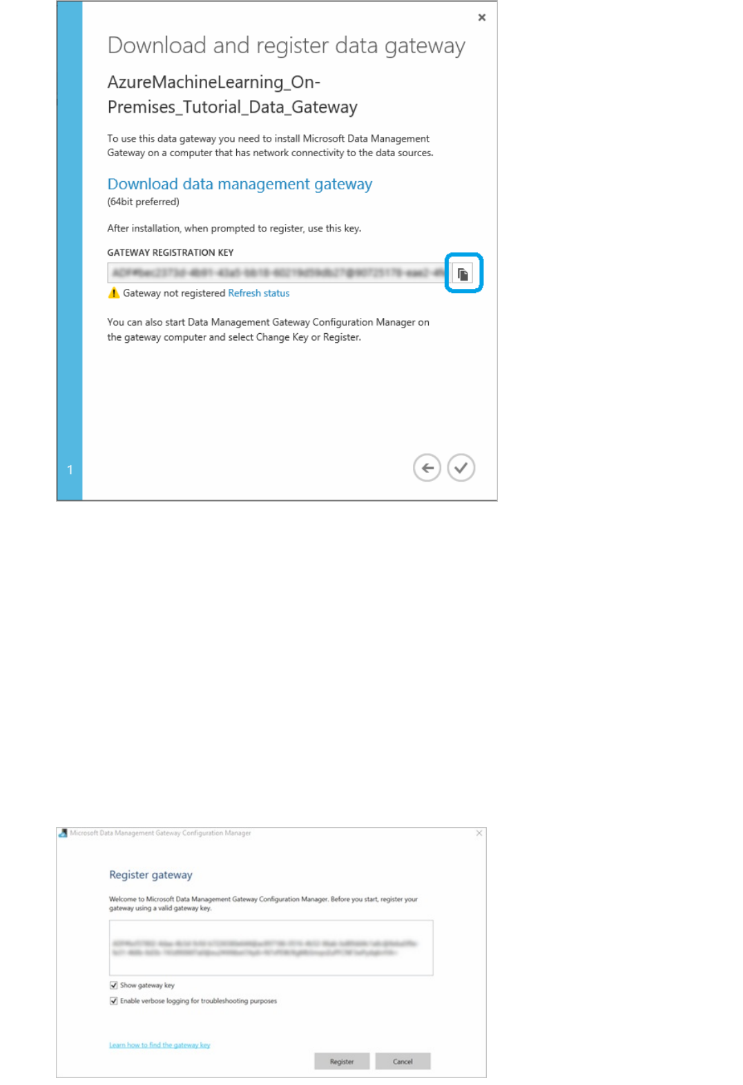
6. If you have not yet downloaded and installed the Microsoft Data Management Gateway, then click Download
data management gateway. This takes you to the Microsoft Download Center where you can select the
gateway version you need, download it, and install it. You can find detailed information on installation
prerequisites, installation steps, and troubleshooting tips in the beginning sections of the article Move data
between on-premises sources and cloud with Data Management Gateway.
7. After the gateway is installed, the Data Management Gateway Configuration Manager will open and the
Register gateway dialog is displayed. Paste the Gateway Registration Key that you copied to the clipboard
and click Register.
8. If you already have a gateway installed, run the Data Management Gateway Configuration Manager. Click
Change key, paste the Gateway Registration Key that you copied to the clipboard in the previous step, and
click OK.
9. When the installation is complete, the Register gateway dialog for Microsoft Data Management Gateway
Configuration Manager is displayed. Paste the GATEWAY REGISTRATION KEY that you copied to the
clipboard in a previous step and click Register.
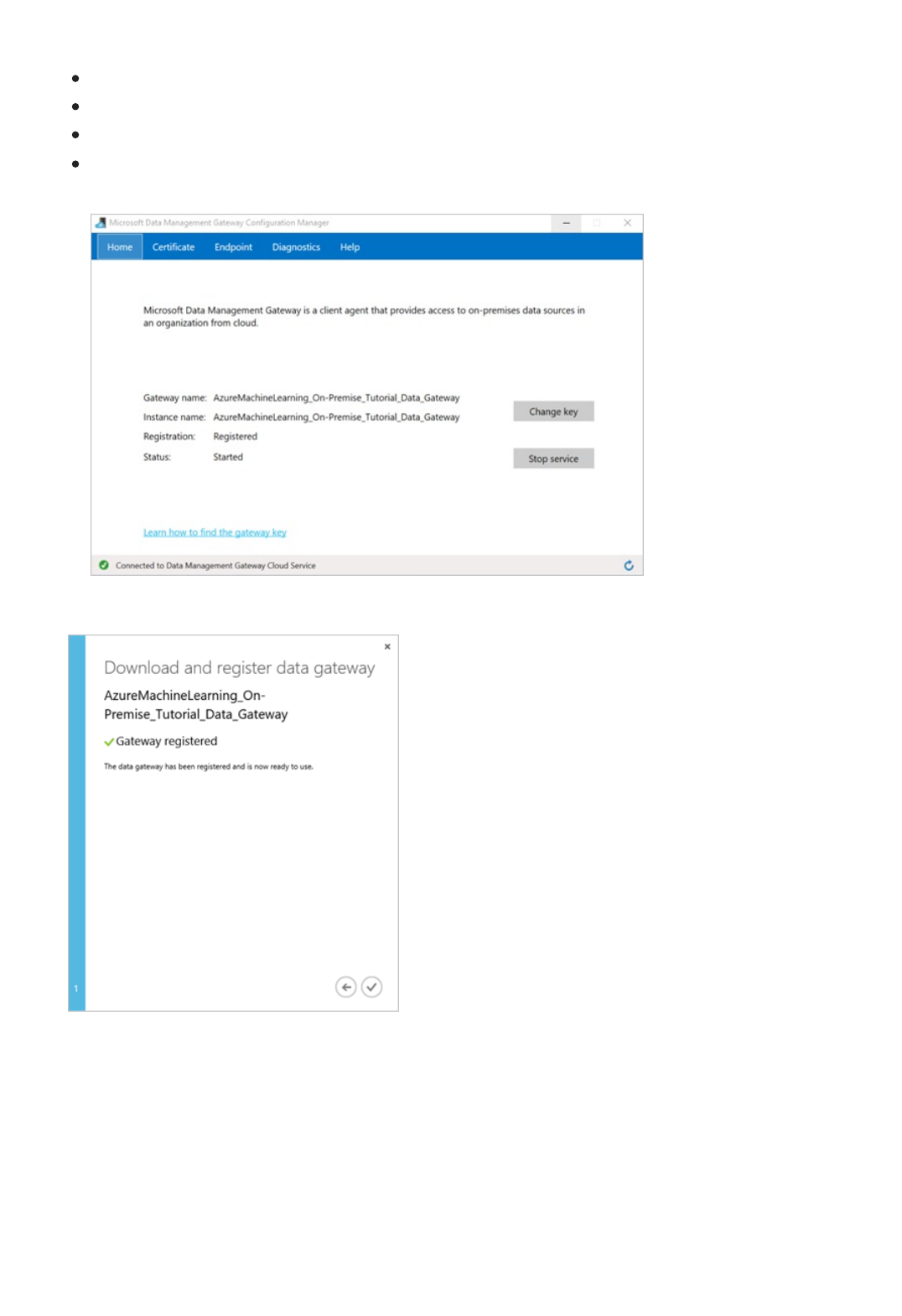
10. The gateway configuration is complete when the following values are set on the Home tab in Microsoft
Data Management Gateway Configuration Manager:
Gateway name and Instance name are set to the name of the gateway.
Registration is set to Registered.
Status is set to Started.
The status bar at the bottom displays Connected to Data Management Gateway Cloud Service
along with a green check mark.
Azure Machine Learning Studio also gets updated when the registration is successful.
11. In the Download and register data gateway dialog, click the check mark to complete the setup. The
Settings page displays the gateway status as "Online". In the right-hand pane, you'll find status and other
useful information.
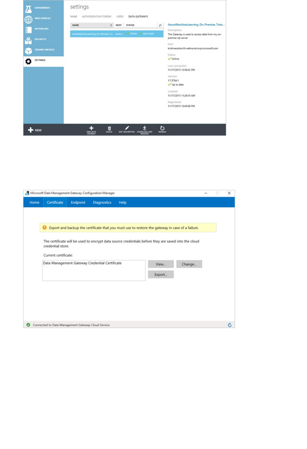
12. In the Microsoft Data Management Gateway Configuration Manager switch to the Certificate tab. The
certificate specified on this tab is used to encrypt/decrypt credentials for the on-premises data store that
you specify in the portal. This certificate is the default certificate. Microsoft recommends changing this to
your own certificate that you back up in your certificate management system. Click Change to use your
own certificate instead.
13. (optional) If you want to enable verbose logging in order to troubleshoot issues with the gateway, in the
Microsoft Data Management Gateway Configuration Manager switch to the Diagnostics tab and check
the Enable verbose logging for troubleshooting purposes option. The logging information can be
found in the Windows Event Viewer under the Applications and Services Logs -> Data Management
Gateway node. You can also use the Diagnostics tab to test the connection to an on-premises data source
using the gateway.
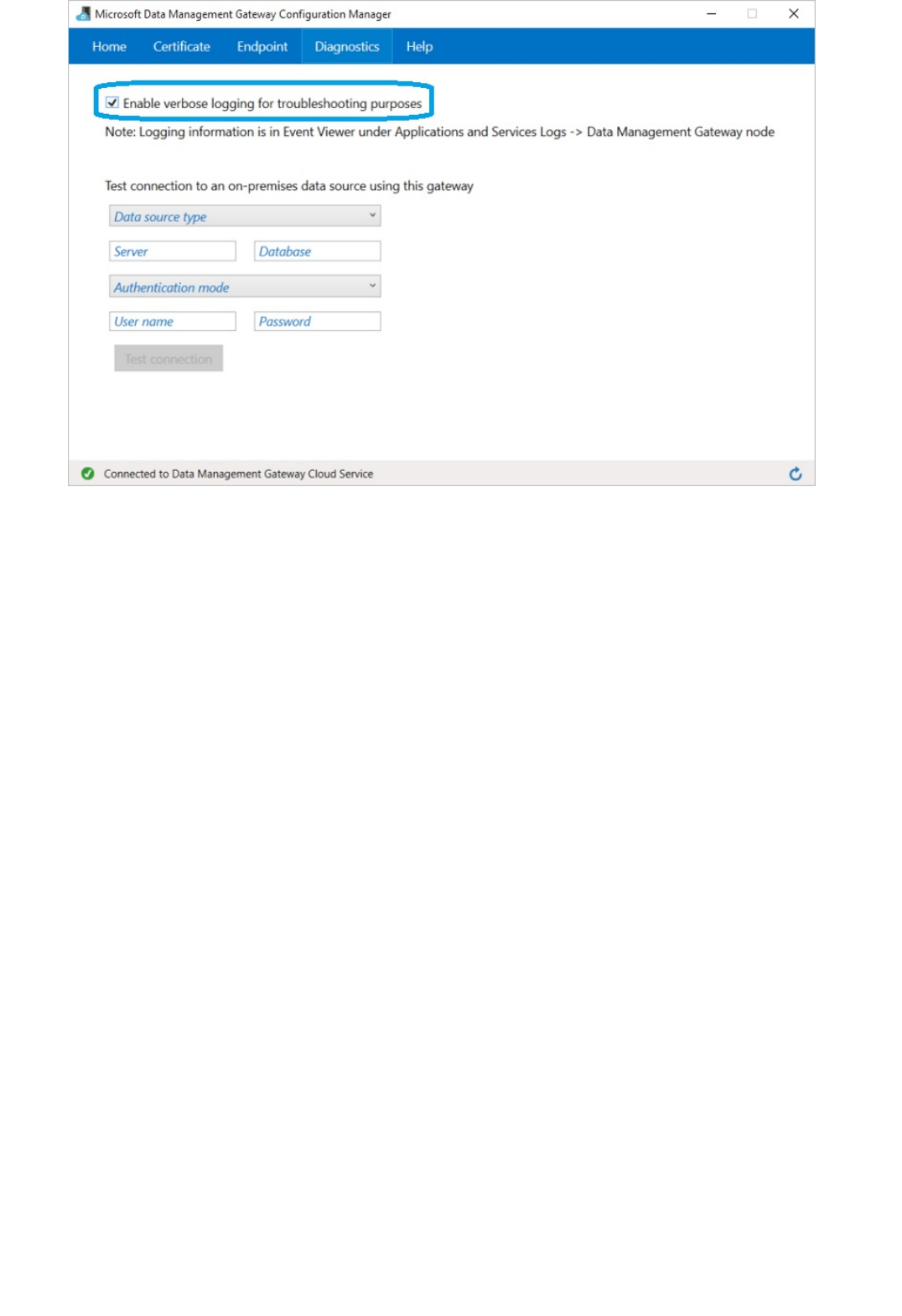
Step 2: Use the gateway to read data from an on-premises data sourceStep 2: Use the gateway to read data from an on-premises data source
This completes the gateway setup process in Azure Machine Learning. You're now ready to use your on-premises
data.
You can create and set up multiple gateways in Studio for each workspace. For example, you may have a gateway
that you want to connect to your test data sources during development, and a different gateway for your
production data sources. Azure Machine Learning gives you the flexibility to set up multiple gateways depending
upon your corporate environment. Currently you can’t share a gateway between workspaces and only one
gateway can be installed on a single computer. For more information, see Move data between on-premises
sources and cloud with Data Management Gateway.
After you set up the gateway, you can add an Import Data module to an experiment that inputs the data from the
on-premises SQL Server database.
1. In Machine Learning Studio, select the EXPERIMENTS tab, click +NEW in the lower-left corner, and select
Blank Experiment (or select one of several sample experiments available).
2. Find and drag the Import Data module to the experiment canvas.
3. Click Save as below the canvas. Enter "Azure Machine Learning On-Premises SQL Server Tutorial" for the
experiment name, select the workspace, and click the OK check mark.
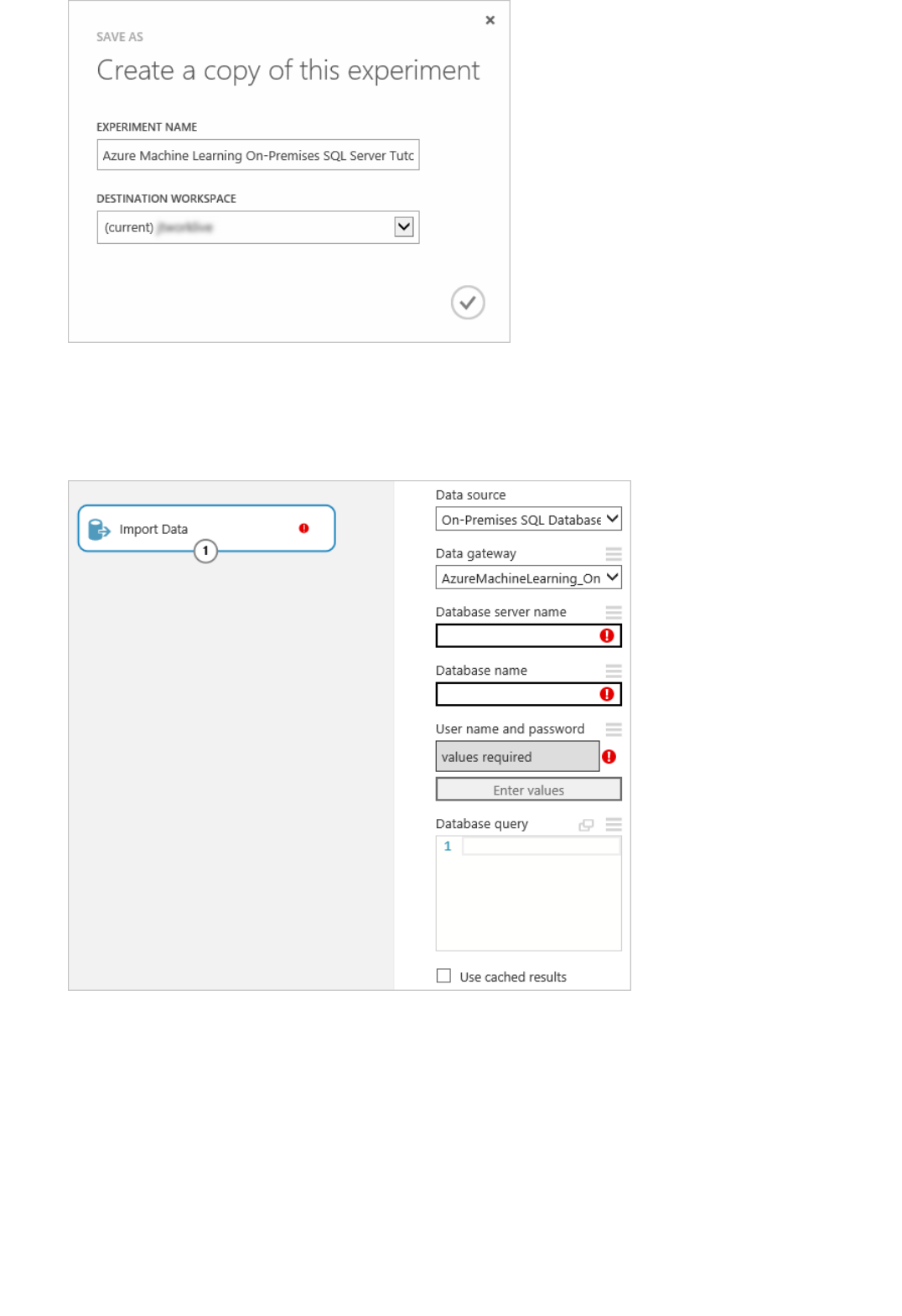
4. Click the Import Data module to select it, then in the Properties pane to the right of the canvas, select "On-
Premises SQL Database" in the Data source dropdown list.
6. Enter the SQL Database server name and Database name, along with the SQL Database query you want
to execute.
5. Select the Data gateway you installed and registered. You can set up another gateway by selecting "(add
new Data Gateway…)".
7. Click Enter values under User name and password and enter your database credentials. You can use
Windows Integrated Authentication or SQL Server Authentication depending upon how your on-premises
SQL Server is configured.
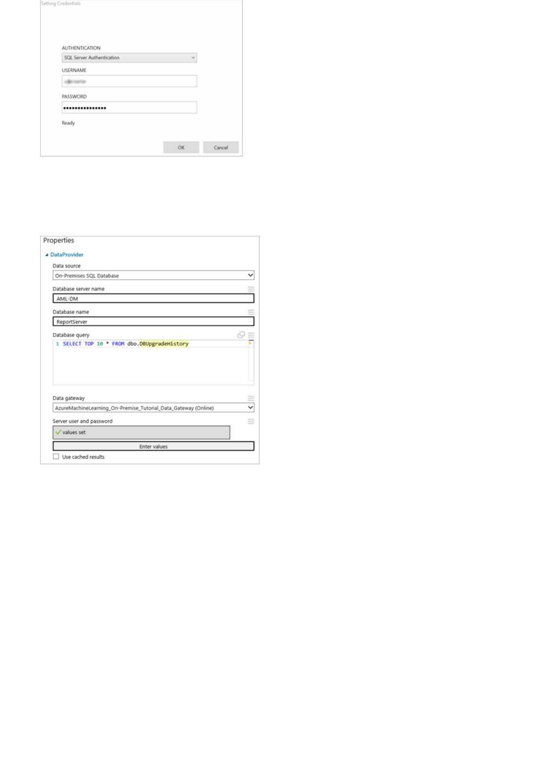
8. Click RUN to run the experiment.
The message "values required" changes to "values set" with a green check mark. You only need to enter the
credentials once unless the database information or password changes. Azure Machine Learning uses the
certificate you provided when you installed the gateway to encrypt the credentials in the cloud. Azure never
stores on-premises credentials without encryption.
Once the experiment finishes running, you can visualize the data you imported from the database by clicking the
output port of the Import Data module and selecting Visualize.
Once you finish developing your experiment, you can deploy and operationalize your model. Using the Batch
Execution Service, data from the on-premises SQL Server database configured in the Import Data module will
be read and used for scoring. While you can use the Request Response Service for scoring on-premises data,
Microsoft recommends using the Excel Add-in instead. Currently, writing to an on-premises SQL Server database
through Export Data is not supported either in your experiments or published web services.
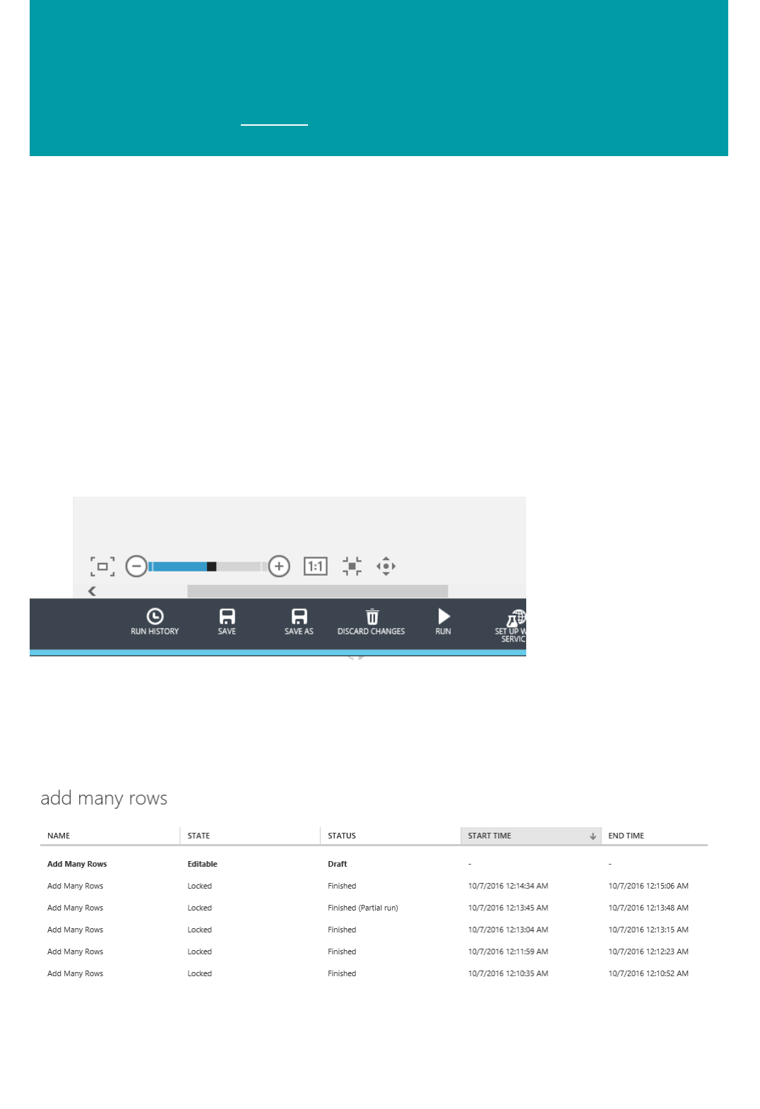
Application Lifecycle Management in Azure Machine
Learning Studio
3/21/2018 • 6 min to read • Edit Online
Versioning experiment
Experiment snapshots using Run HistoryExperiment snapshots using Run History
Azure Machine Learning Studio is a tool for developing machine learning experiments that are operationalized in
the Azure cloud platform. It is like the Visual Studio IDE and scalable cloud service merged into a single platform.
You can incorporate standard Application Lifecycle Management (ALM) practices from versioning various assets to
automated execution and deployment, into Azure Machine Learning Studio. This article discusses some of the
options and approaches.
There are two recommended ways to version your experiments. You can either rely on the built-in run history or
export the experiment in a JSON format so as to manage it externally. Each approach comes with its pros and cons.
In the execution model of the Azure Machine Learning Studio learning experiment, an immutable snapshot of the
experiment is submitted to the job scheduler whenever you click Run in the experiment editor. To view this list of
snapshots, click Run History on the command bar in the experiment editor view.
You can then open the snapshot in Locked mode by clicking the name of the experiment at the time the experiment
was submitted to run and the snapshot was taken. Notice that only the first item in the list, which represents the
current experiment, is in an Editable state. Also notice that each snapshot can be in various Status states as well,
including Finished (Partial run), Failed, Failed (Partial run), or Draft.
After it's opened, you can save the snapshot experiment as a new experiment and then modify it. If your experiment
snapshot contains assets such as trained models, transforms, or datasets that have updated versions, the snapshot
retains the references to the original version when the snapshot was taken. If you save the locked snapshot as a
new experiment, Azure Machine Learning Studio detects the existence of a newer version of these assets, and
automatically updates them in the new experiment.

Export/import experiment in JSON formatExport/import experiment in JSON format
Versioning trained model
Versioning web service
Classic web serviceClassic web service
If you delete the experiment, all snapshots of that experiment are deleted.
The run history snapshots keep an immutable version of the experiment in Azure Machine Learning Studio every
time it is submitted to run. You can also save a local copy of the experiment and check it in to your favorite source
control system, such as Team Foundation Server, and later on re-create an experiment from that local file. You can
use the Azure Machine Learning PowerShell commandlets Export-AmlExperimentGraph and Import-
AmlExperimentGraph to accomplish that.
The JSON file is a textual representation of the experiment graph, which might include a reference to assets in the
workspace such as a dataset or a trained model. It doesn't contain a serialized version of the asset. If you attempt to
import the JSON document back into the workspace, the referenced assets must already exist with the same asset
IDs that are referenced in the experiment. Otherwise you cannot access the imported experiment.
A trained model in Azure Machine Learning is serialized into a format known as an iLearner file (.iLearner ), and is
stored in the Azure Blob storage account associated with the workspace. One way to get a copy of the iLearner file
is through the retraining API. This article explains how the retraining API works. The high-level steps:
1. Set up your training experiment.
2. Add a web service output port to the Train Model module, or the module that produces the trained model, such
as Tune Model Hyperparameter or Create R Model.
3. Run your training experiment and then deploy it as a model training web service.
4. Call the BES endpoint of the training web service, and specify the desired iLearner file name and Blob storage
account location where it will be stored.
5. Harvest the produced iLearner file after the BES call finishes.
Another way to retrieve the iLearner file is through the PowerShell commandlet Download-
AmlExperimentNodeOutput. This might be easier if you just want to get a copy of the iLearner file without the need
to retrain the model programmatically.
After you have the iLearner file containing the trained model, you can then employ your own versioning strategy.
The strategy can be as simple as applying a pre/postfix as a naming convention and just leaving the iLearner file in
Blob storage, or copying/importing it into your version control system.
The saved iLearner file can then be used for scoring through deployed web services.
You can deploy two types of web services from an Azure Machine Learning experiment. The classic web service is
tightly coupled with the experiment as well as the workspace. The new web service uses the Azure Resource
Manager framework, and it is no longer coupled with the original experiment or the workspace.
To version a classic web service, you can take advantage of the web service endpoint construct. Here is a typical
flow:
1. From your predictive experiment, you deploy a new classic web service, which contains a default endpoint.
2. You create a new endpoint named ep2, which exposes the current version of the experiment/trained model.
3. You go back and update your predictive experiment and trained model.
4. You redeploy the predictive experiment, which will then update the default endpoint. But this will not alter ep2.
5. You create an additional endpoint named ep3, which exposes the new version of the experiment and trained
model.

New web serviceNew web service
Automate experiment execution and deployment
Next steps
6. Go back to step 3 if needed.
Over time, you might have many endpoints created in the same web service. Each endpoint represents a point-in-
time copy of the experiment containing the point-in-time version of the trained model. You can then use external
logic to determine which endpoint to call, which effectively means selecting a version of the trained model for the
scoring run.
You can also create many identical web service endpoints, and then patch different versions of the iLearner file to
the endpoint to achieve similar effect. This article explains in more detail how to accomplish that.
If you create a new Azure Resource Manager-based web service, the endpoint construct is no longer available.
Instead, you can generate web service definition (WSD) files, in JSON format, from your predictive experiment by
using the Export-AmlWebServiceDefinitionFromExperiment PowerShell commandlet, or by using the Export-
AzureRmMlWebservice PowerShell commandlet from a deployed Resource Manager-based web service.
After you have the exported WSD file and version control it, you can also deploy the WSD as a new web service in
a different web service plan in a different Azure region. Just make sure you supply the proper storage account
configuration as well as the new web service plan ID. To patch in different iLearner files, you can modify the WSD
file and update the location reference of the trained model, and deploy it as a new web service.
An important aspect of ALM is to be able to automate the execution and deployment process of the application. In
Azure Machine Learning, you can accomplish this by using the PowerShell module. Here is an example of end-to-
end steps that are relevant to a standard ALM automated execution/deployment process by using the Azure
Machine Learning Studio PowerShell module. Each step is linked to one or more PowerShell commandlets that you
can use to accomplish that step.
1. Upload a dataset.
2. Copy a training experiment into the workspace from a workspace or from Gallery, or import an exported
experiment from local disk.
3. Update the dataset in the training experiment.
4. Run the training experiment.
5. Promote the trained model.
6. Copy a predictive experiment into the workspace.
7. Update the trained model in the predictive experiment.
8. Run the predictive experiment.
9. Deploy a web service from the predictive experiment.
10. Test the web service RRS or BES endpoint.
Download the Azure Machine Learning Studio PowerShell module and start to automate your ALM tasks.
Learn how to create and manage large number of ML models by using just a single experiment through
PowerShell and retraining API.
Learn more about deploying Azure Machine Learning web services.

Manage experiment iterations in Azure Machine
Learning Studio
3/21/2018 • 4 min to read • Edit Online
NOTENOTE
NOTENOTE
Viewing the Prior Run
Viewing the Run History
LEARNING RATE VALUE RUN START TIME
0.1 9/11/2014 4:18:58 pm
0.2 9/11/2014 4:24:33 pm
Developing a predictive analysis model is an iterative process - as you modify the various functions and
parameters of your experiment, your results converge until you are satisfied that you have a trained, effective
model. Key to this process is tracking the various iterations of your experiment parameters and configurations.
You can try Azure Machine Learning for free. No credit card or Azure subscription is required. Get started now.
You can review previous runs of your experiments at any time in order to challenge, revisit, and ultimately either
confirm or refine previous assumptions. When you run an experiment, Machine Learning Studio keeps a history of
the run, including dataset, module, and port connections and parameters. This history also captures results,
runtime information such as start and stop times, log messages, and execution status. You can look back at any of
these runs at any time to review the chronology of your experiment and intermediate results. You can even use a
previous run of your experiment to launch into a new phase of inquiry and discovery on your path to creating
simple, complex, or even ensemble modeling solutions.
When you view a previous run of an experiment, that version of the experiment is locked and can't be edited. You can,
however, save a copy of it by clicking SAVE AS and providing a new name for the copy. Machine Learning Studio opens the
new copy, which you can then edit and run. This copy of your experiment is available in the EXPERIMENTS list along with all
your other experiments.
When you have an experiment open that you have run at least once, you can view the preceding run of the
experiment by clicking Prior Run in the properties pane.
For example, suppose you create an experiment and run versions of it at 11:23, 11:42, and 11:55. If you open the
last run of the experiment (11:55) and click Prior Run, the version you ran at 11:42 is opened.
You can view all the previous runs of an experiment by clicking View Run History in an open experiment.
For example, suppose you create an experiment with the Linear Regression module and you want to observe the
effect of changing the value of Learning rate on your experiment results. You run the experiment multiple times
with different values for this parameter, as follows:
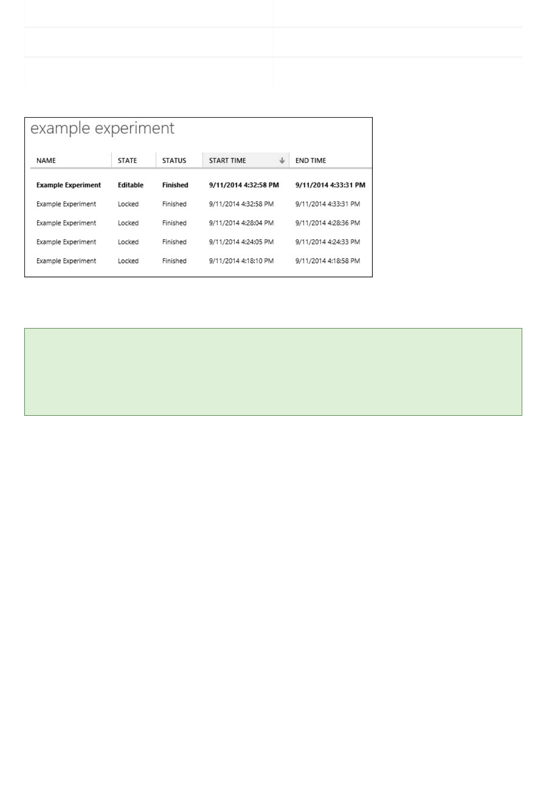
0.4 9/11/2014 4:28:36 pm
0.5 9/11/2014 4:33:31 pm
LEARNING RATE VALUE RUN START TIME
TIPTIP
Iterating on a Previous Run
If you click VIEW RUN HISTORY, you see a list of all these runs:
Click any of these runs to view a snapshot of the experiment at the time you ran it. The configuration, parameter
values, comments, and results are all preserved to give you a complete record of that run of your experiment.
To document your iterations of the experiment, you can modify the title each time you run it, you can update the Summary
of the experiment in the properties pane, and you can add or update comments on individual modules to record your
changes. The title, summary, and module comments are saved with each run of the experiment.
The list of experiments in the EXPERIMENTS tab in Machine Learning Studio always displays the latest version
of an experiment. If you open a previous run of the experiment (using Prior Run or VIEW RUN HISTORY), you
can return to the draft version by clicking VIEW RUN HISTORY and selecting the iteration that has a STATE of
Editable.
When you click Prior Run or VIEW RUN HISTORY and open a previous run, you can view a finished experiment
in read-only mode.
If you want to begin an iteration of your experiment starting with the way you configured it for a previous run, you
can do this by opening the run and clicking SAVE AS. This creates a new experiment, with a new title, an empty
run history, and all the components and parameter values of the previous run. This new experiment is listed in the
EXPERIMENTS tab in the Machine Learning Studio home page, and you can modify and run it, initiating a new
run history for this iteration of your experiment.
For example, suppose you have the experiment run history shown in the previous section. You want to observe
what happens when you set the Learning rate parameter to 0.4, and try different values for the Number of
training epochs parameter.
1. Click VIEW RUN HISTORY and open the iteration of the experiment that you ran at 4:28:36 pm (in which you
set the parameter value to 0.4).
2. Click SAVE AS.
3. Enter a new title and click the OK checkmark. A new copy of the experiment is created.
4. Modify the Number of training epochs parameter.

5. Click RUN.
You can now continue to modify and run this version of your experiment, building a new run history to record your
work.
Create many Machine Learning models and web
service endpoints from one experiment using
PowerShell
3/21/2018 • 9 min to read • Edit Online
NOTENOTE
Set up the training experiment
NOTENOTE
Here's a common machine learning problem: You want to create many models that have the same training
workflow and use the same algorithm. But you want them to have different training datasets as input. This article
shows you how to do this at scale in Azure Machine Learning Studio using just a single experiment.
For example, let's say you own a global bike rental franchise business. You want to build a regression model to
predict the rental demand based on historic data. You have 1,000 rental locations across the world and you've
collected a dataset for each location. They include important features such as date, time, weather, and traffic that
are specific to each location.
You could train your model once using a merged version of all the datasets across all locations. But, each of your
locations has a unique environment. So a better approach would be to train your regression model separately
using the dataset for each location. That way, each trained model could take into account the different store sizes,
volume, geography, population, bike-friendly traffic environment, and more.
That may be the best approach, but you don't want to create 1,000 training experiments in Azure Machine
Learning with each one representing a unique location. Besides being an overwhelming task, it's also seems
inefficient since each experiment would have all the same components except for the training dataset.
Fortunately, you can accomplish this by using the Azure Machine Learning retraining API and automating the task
with Azure Machine Learning PowerShell.
To make your sample run faster, reduce the number of locations from 1,000 to 10. But the same principles and procedures
apply to 1,000 locations. However, if you do want to train from 1,000 datasets you might want to run the following
PowerShell scripts in parallel. How to do that is beyond the scope of this article, but you can find examples of PowerShell
multi-threading on the Internet.
Use the example training experiment that's in the Cortana Intelligence Gallery. Open this experiment in your
Azure Machine Learning Studio workspace.
In order to follow along with this example, you may want to use a standard workspace rather than a free workspace. You
create one endpoint for each customer - for a total of 10 endpoints - and that requires a standard workspace since a free
workspace is limited to 3 endpoints. If you only have a free workspace, just change the scripts to allow for only th locations.
The experiment uses an Import Data module to import the training dataset customer001.csv from an Azure
storage account. Let's assume you have collected training datasets from all bike rental locations and stored them
in the same blob storage location with file names ranging from rentalloc001.csv to rentalloc10.csv.
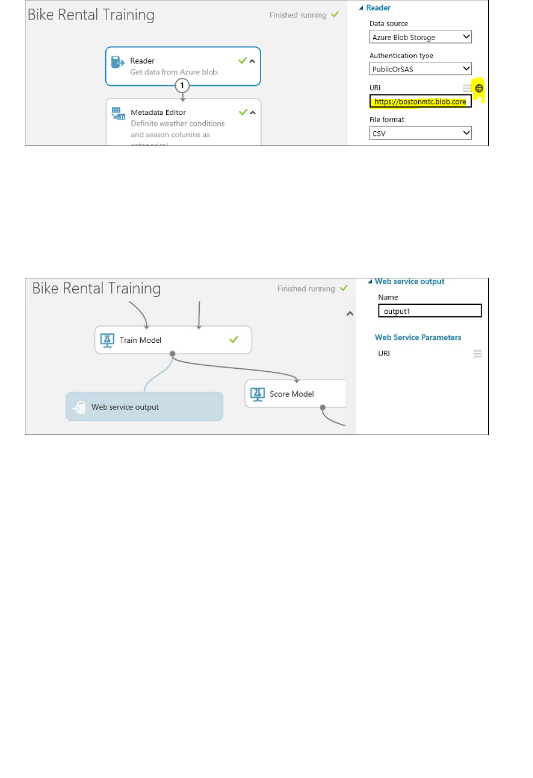
Deploy the training and scoring web services
Create 10 identical web service endpoints with PowerShell
Note that a Web Service Output module has been added to the Train Model module. When this experiment is
deployed as a web service, the endpoint associated with that output returns the trained model in the format of an
.ilearner file.
Also note that you set up a web service parameter that defines the URL that the Import Data module uses. This
allows you to use the parameter to specify individual training datasets to train the model for each location. There
are other ways you could have done this. You can use a SQL query with a web service parameter to get data from
a SQL Azure database. Or you can use a Web Service Input module to pass in a dataset to the web service.
Now, let's run this training experiment using the default value rental001.csv as the training dataset. If you view the
output of the Evaluate module (click the output and select Visualize), you can see you get a decent performance
of AUC = 0.91. At this point, you're ready to deploy a web service out of this training experiment.
To deploy the training web service, click the Set Up Web Service button below the experiment canvas and select
Deploy Web Service. Call this web service ""Bike Rental Training".
Now you need to deploy the scoring web service. To do this, click Set Up Web Service below the canvas and
select Predictive Web Service. This creates a scoring experiment. You need to make a few minor adjustments to
make it work as a web service. Remove the label column "cnt" from the input data and limit the output to only the
instance id and the corresponding predicted value.
To save yourself that work, you can open the predictive experiment in the Gallery that has already been prepared.
To deploy the web service, run the predictive experiment, then click the Deploy Web Service button below the
canvas. Name the scoring web service "Bike Rental Scoring"".
This web service comes with a default endpoint. But you're not as interested in the default endpoint since it can't
be updated. What you need to do is to create 10 additional endpoints, one for each location. You can do this with
PowerShell.
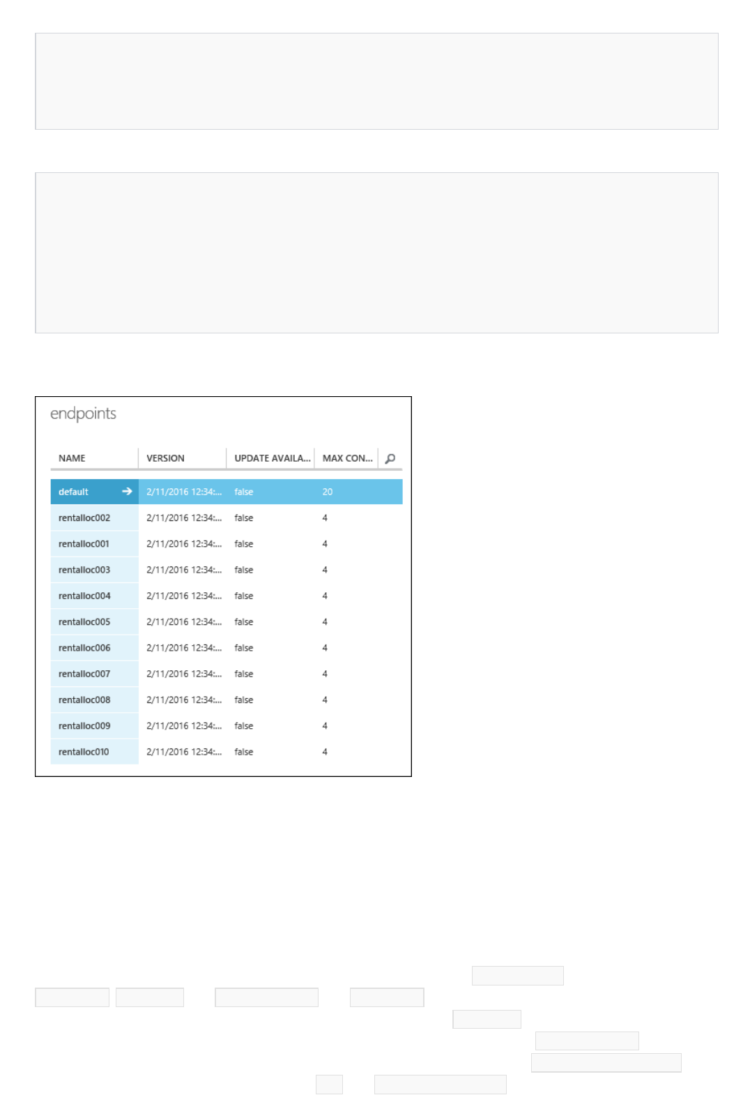
Import-Module .\AzureMLPS.dll
# Assume the default configuration file exists and is properly set to point to the valid Workspace.
$scoringSvc = Get-AmlWebService | where Name -eq 'Bike Rental Scoring'
$trainingSvc = Get-AmlWebService | where Name -eq 'Bike Rental Training'
# Create 10 endpoints on the scoring web service.
For ($i = 1; $i -le 10; $i++){
$seq = $i.ToString().PadLeft(3, '0');
$endpointName = 'rentalloc' + $seq;
Write-Host ('adding endpoint ' + $endpointName + '...')
Add-AmlWebServiceEndpoint -WebServiceId $scoringSvc.Id -EndpointName $endpointName -Description
$endpointName
}
Update the endpoints to use separate training datasets using
PowerShell
First, you set up the PowerShell environment:
Then, run the following PowerShell command:
Now you created 10 endpoints and they all contain the same trained model trained on customer001.csv. You can
view them in the Azure portal.
The next step is to update the endpoints with models uniquely trained on each customer's individual data. But first
you need to produce these models from the Bike Rental Training web service. Let's go back to the Bike Rental
Training web service. You need to call its BES endpoint 10 times with 10 different training datasets in order to
produce 10 different models. Use the InovkeAmlWebServiceBESEndpoint PowerShell cmdlet to do this.
You will also need to provide credentials for your blob storage account into $configContent . Namely, at the fields
AccountName , AccountKey , and RelativeLocation . The AccountName can be one of your account names, as seen in
the Azure portal (Storage tab). Once you click on a storage account, its AccountKey can be found by pressing the
Manage Access Keys button at the bottom and copying the Primary Access Key. The RelativeLocation is the
path relative to your storage where a new model will be stored. For instance, the path hai/retrain/bike_rental/ in
the following script points to a container named hai , and /retrain/bike_rental/ are subfolders. Currently, you
# Invoke the retraining API 10 times
# This is the default (and the only) endpoint on the training web service
$trainingSvcEp = (Get-AmlWebServiceEndpoint -WebServiceId $trainingSvc.Id)[0];
$submitJobRequestUrl = $trainingSvcEp.ApiLocation + '/jobs?api-version=2.0';
$apiKey = $trainingSvcEp.PrimaryKey;
For ($i = 1; $i -le 10; $i++){
$seq = $i.ToString().PadLeft(3, '0');
$inputFileName = 'https://bostonmtc.blob.core.windows.net/hai/retrain/bike_rental/BikeRental' + $seq +
'.csv';
$configContent = '{ "GlobalParameters": { "URI": "' + $inputFileName + '" }, "Outputs": { "output1": {
"ConnectionString": "DefaultEndpointsProtocol=https;AccountName=<myaccount>;AccountKey=<mykey>",
"RelativeLocation": "hai/retrain/bike_rental/model' + $seq + '.ilearner" } } }';
Write-Host ('training regression model on ' + $inputFileName + ' for rental location ' + $seq + '...');
Invoke-AmlWebServiceBESEndpoint -JobConfigString $configContent -SubmitJobRequestUrl $submitJobRequestUrl
-ApiKey $apiKey
}
NOTENOTE
# Patch the 10 endpoints with respective .ilearner models
$baseLoc = 'http://bostonmtc.blob.core.windows.net/'
$sasToken = '<my_blob_sas_token>'
For ($i = 1; $i -le 10; $i++){
$seq = $i.ToString().PadLeft(3, '0');
$endpointName = 'rentalloc' + $seq;
$relativeLoc = 'hai/retrain/bike_rental/model' + $seq + '.ilearner';
Write-Host ('Patching endpoint ' + $endpointName + '...');
Patch-AmlWebServiceEndpoint -WebServiceId $scoringSvc.Id -EndpointName $endpointName -ResourceName 'Bike
Rental [trained model]' -BaseLocation $baseLoc -RelativeLocation $relativeLoc -SasBlobToken $sasToken
}
Full PowerShell script
cannot create subfolders through the portal UI, but there are several Azure Storage Explorers that allow you to do
so. It is recommended that you create a new container in your storage to store the new trained models (.iLearner
files) as follows: from your storage page, click the Add button at the bottom and name it retrain . In summary,
the necessary changes to the following script pertain to AccountName , AccountKey , and RelativeLocation (:
"retrain/model' + $seq + '.ilearner" ).
The BES endpoint is the only supported mode for this operation. RRS cannot be used for producing trained models.
As you can see above, instead of constructing 10 different BES job configuration json files, you dynamically create
the config string instead. Then feed it to the jobConfigString parameter of the
InvokeAmlWebServceBESEndpoint cmdlet. There's really no need to keep a copy on disk.
If everything goes well, after a while you should see 10 .iLearner files, from model001.ilearner to
model010.ilearner, in your Azure storage account. Now you're ready to update the 10 scoring web service
endpoints with these models using the Patch-AmlWebServiceEndpoint PowerShell cmdlet. Remember again
that you can only patch the non-default endpoints you programmatically created earlier.
This should run fairly quickly. When the execution finishes, you'll have successfully created 10 predictive web
service endpoints. Each one will contain a trained model uniquely trained on the dataset specific to a rental
location, all from a single training experiment. To verify this, you can try calling these endpoints using the
InvokeAmlWebServiceRRSEndpoint cmdlet, providing them with the same input data. You should expect to
see different prediction results since the models are trained with different training sets.
Here's the listing of the full source code:

Import-Module .\AzureMLPS.dll
# Assume the default configuration file exists and properly set to point to the valid workspace.
$scoringSvc = Get-AmlWebService | where Name -eq 'Bike Rental Scoring'
$trainingSvc = Get-AmlWebService | where Name -eq 'Bike Rental Training'
# Create 10 endpoints on the scoring web service
For ($i = 1; $i -le 10; $i++){
$seq = $i.ToString().PadLeft(3, '0');
$endpointName = 'rentalloc' + $seq;
Write-Host ('adding endpoint ' + $endpontName + '...')
Add-AmlWebServiceEndpoint -WebServiceId $scoringSvc.Id -EndpointName $endpointName -Description
$endpointName
}
# Invoke the retraining API 10 times to produce 10 regression models in .ilearner format
$trainingSvcEp = (Get-AmlWebServiceEndpoint -WebServiceId $trainingSvc.Id)[0];
$submitJobRequestUrl = $trainingSvcEp.ApiLocation + '/jobs?api-version=2.0';
$apiKey = $trainingSvcEp.PrimaryKey;
For ($i = 1; $i -le 10; $i++){
$seq = $i.ToString().PadLeft(3, '0');
$inputFileName = 'https://bostonmtc.blob.core.windows.net/hai/retrain/bike_rental/BikeRental' + $seq +
'.csv';
$configContent = '{ "GlobalParameters": { "URI": "' + $inputFileName + '" }, "Outputs": { "output1": {
"ConnectionString": "DefaultEndpointsProtocol=https;AccountName=<myaccount>;AccountKey=<mykey>",
"RelativeLocation": "hai/retrain/bike_rental/model' + $seq + '.ilearner" } } }';
Write-Host ('training regression model on ' + $inputFileName + ' for rental location ' + $seq + '...');
Invoke-AmlWebServiceBESEndpoint -JobConfigString $configContent -SubmitJobRequestUrl $submitJobRequestUrl
-ApiKey $apiKey
}
# Patch the 10 endpoints with respective .ilearner models
$baseLoc = 'http://bostonmtc.blob.core.windows.net/'
$sasToken = '?test'
For ($i = 1; $i -le 10; $i++){
$seq = $i.ToString().PadLeft(3, '0');
$endpointName = 'rentalloc' + $seq;
$relativeLoc = 'hai/retrain/bike_rental/model' + $seq + '.ilearner';
Write-Host ('Patching endpoint ' + $endpointName + '...');
Patch-AmlWebServiceEndpoint -WebServiceId $scoringSvc.Id -EndpointName $endpointName -ResourceName 'Bike
Rental [trained model]' -BaseLocation $baseLoc -RelativeLocation $relativeLoc -SasBlobToken $sasToken
}
How to choose algorithms for Microsoft Azure
Machine Learning
3/21/2018 • 15 min to read • Edit Online
The Machine Learning Algorithm Cheat Sheet
NOTENOTE
How to use the cheat sheetHow to use the cheat sheet
TIPTIP
Flavors of machine learning
SupervisedSupervised
The answer to the question "What machine learning algorithm should I use?" is always "It depends." It depends
on the size, quality, and nature of the data. It depends on what you want to do with the answer. It depends on how
the math of the algorithm was translated into instructions for the computer you are using. And it depends on how
much time you have. Even the most experienced data scientists can't tell which algorithm will perform best before
trying them.
The Microsoft Azure Machine Learning Algorithm Cheat Sheet helps you choose the right machine
learning algorithm for your predictive analytics solutions from the Microsoft Azure Machine Learning library of
algorithms. This article walks you through how to use it.
To download the cheat sheet and follow along with this article, go to Machine learning algorithm cheat sheet for Microsoft
Azure Machine Learning Studio.
This cheat sheet has a very specific audience in mind: a beginning data scientist with undergraduate-level
machine learning, trying to choose an algorithm to start with in Azure Machine Learning Studio. That means that
it makes some generalizations and oversimplifications, but it points you in a safe direction. It also means that
there are lots of algorithms not listed here. As Azure Machine Learning grows to encompass a more complete set
of available methods, we'll add them.
These recommendations are compiled feedback and tips from many data scientists and machine learning experts.
We didn't agree on everything, but I've tried to harmonize our opinions into a rough consensus. Most of the
statements of disagreement begin with "It depends…"
Read the path and algorithm labels on the chart as "For <path label>, use <algorithm>." For example, "For
speed, use two class logistic regression." Sometimes more than one branch applies. Sometimes none of them are
a perfect fit. They're intended to be rule-of-thumb recommendations, so don't worry about it being exact. Several
data scientists I talked with said that the only sure way to find the very best algorithm is to try all of them.
Here's an example from the Azure AI Gallery of an experiment that tries several algorithms against the same data
and compares the results: Compare Multi-class Classifiers: Letter recognition.
To download and print a diagram that gives an overview of the capabilities of Machine Learning Studio, see Overview
diagram of Azure Machine Learning Studio capabilities.

UnsupervisedUnsupervised
Reinforcement learningReinforcement learning
Considerations when choosing an algorithm
AccuracyAccuracy
Training timeTraining time
LinearityLinearity
Supervised learning algorithms make predictions based on a set of examples. For instance, historical stock prices
can be used to hazard guesses at future prices. Each example used for training is labeled with the value of interest
—in this case the stock price. A supervised learning algorithm looks for patterns in those value labels. It can use
any information that might be relevant—the day of the week, the season, the company's financial data, the type of
industry, the presence of disruptive geopolitical events—and each algorithm looks for different types of patterns.
After the algorithm has found the best pattern it can, it uses that pattern to make predictions for unlabeled testing
data—tomorrow's prices.
Supervised learning is a popular and useful type of machine learning. With one exception, all the modules in
Azure Machine Learning are supervised learning algorithms. There are several specific types of supervised
learning that are represented within Azure Machine Learning: classification, regression, and anomaly detection.
Classification. When the data are being used to predict a category, supervised learning is also called
classification. This is the case when assigning an image as a picture of either a 'cat' or a 'dog'. When there are
only two choices, it's called two-class or binomial classification. When there are more categories, as when
predicting the winner of the NCAA March Madness tournament, this problem is known as multi-class
classification.
Regression. When a value is being predicted, as with stock prices, supervised learning is called regression.
Anomaly detection. Sometimes the goal is to identify data points that are simply unusual. In fraud detection,
for example, any highly unusual credit card spending patterns are suspect. The possible variations are so
numerous and the training examples so few, that it's not feasible to learn what fraudulent activity looks like.
The approach that anomaly detection takes is to simply learn what normal activity looks like (using a history
non-fraudulent transactions) and identify anything that is significantly different.
In unsupervised learning, data points have no labels associated with them. Instead, the goal of an unsupervised
learning algorithm is to organize the data in some way or to describe its structure. This can mean grouping it into
clusters or finding different ways of looking at complex data so that it appears simpler or more organized.
In reinforcement learning, the algorithm gets to choose an action in response to each data point. The learning
algorithm also receives a reward signal a short time later, indicating how good the decision was. Based on this,
the algorithm modifies its strategy in order to achieve the highest reward. Currently there are no reinforcement
learning algorithm modules in Azure Machine Learning. Reinforcement learning is common in robotics, where
the set of sensor readings at one point in time is a data point, and the algorithm must choose the robot's next
action. It is also a natural fit for Internet of Things applications.
Getting the most accurate answer possible isn't always necessary. Sometimes an approximation is adequate,
depending on what you want to use it for. If that's the case, you may be able to cut your processing time
dramatically by sticking with more approximate methods. Another advantage of more approximate methods is
that they naturally tend to avoid overfitting.
The number of minutes or hours necessary to train a model varies a great deal between algorithms. Training time
is often closely tied to accuracy—one typically accompanies the other. In addition, some algorithms are more
sensitive to the number of data points than others. When time is limited it can drive the choice of algorithm,
especially when the data set is large.
Lots of machine learning algorithms make use of linearity. Linear classification algorithms assume that classes
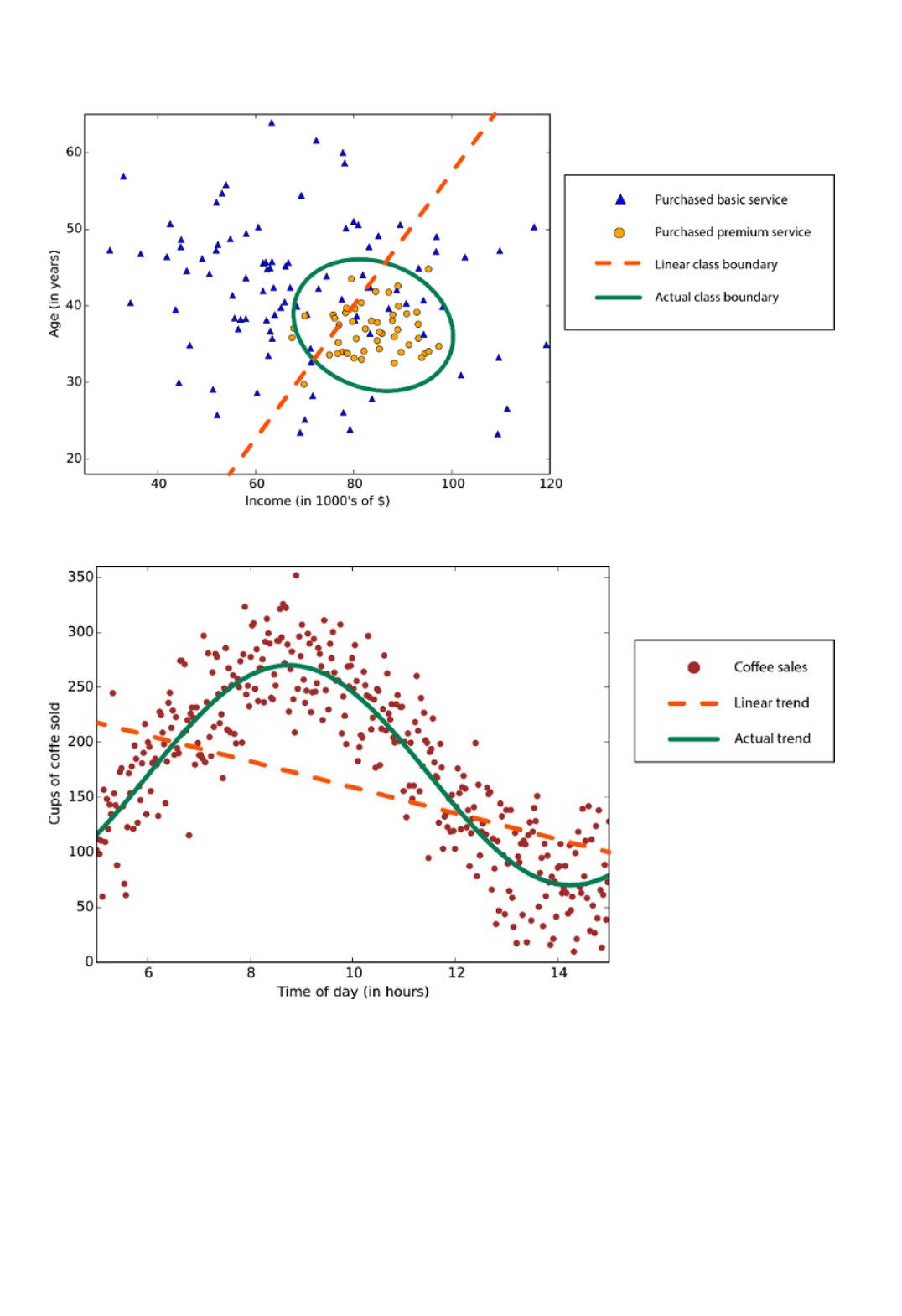
Number of parametersNumber of parameters
can be separated by a straight line (or its higher-dimensional analog). These include logistic regression and
support vector machines (as implemented in Azure Machine Learning). Linear regression algorithms assume that
data trends follow a straight line. These assumptions aren't bad for some problems, but on others they bring
accuracy down.
Non-linear class boundary - relying on a linear classification algorithm would result in low accuracy
Data with a nonlinear trend - using a linear regression method would generate much larger errors than
necessary
Despite their dangers, linear algorithms are very popular as a first line of attack. They tend to be algorithmically
simple and fast to train.
Parameters are the knobs a data scientist gets to turn when setting up an algorithm. They are numbers that affect
the algorithm's behavior, such as error tolerance or number of iterations, or options between variants of how the
algorithm behaves. The training time and accuracy of the algorithm can sometimes be quite sensitive to getting
just the right settings. Typically, algorithms with large numbers parameters require the most trial and error to find
a good combination.

Number of featuresNumber of features
Special casesSpecial cases
ALGORITHM ACCURACY TRAINING TIME LINEARIT Y PARAMETERS NOTES
Two-class
classification
logistic
regression
●●5
decision forest ● ○ 6
decision jungle ● ○ 6 Low memory
footprint
boosted decision
tree
● ○ 6 Large memory
footprint
neural network ● 9 Additional
customization is
possible
averaged
perceptron
○ ○ ● 4
support vector
machine
○ ● 5 Good for large
feature sets
locally deep
support vector
machine
○ 8 Good for large
feature sets
Bayes’ point
machine
○ ● 3
Multi-class
classification
Alternatively, there is a parameter sweeping module block in Azure Machine Learning that automatically tries all
parameter combinations at whatever granularity you choose. While this is a great way to make sure you've
spanned the parameter space, the time required to train a model increases exponentially with the number of
parameters.
The upside is that having many parameters typically indicates that an algorithm has greater flexibility. It can often
achieve very good accuracy. Provided you can find the right combination of parameter settings.
For certain types of data, the number of features can be very large compared to the number of data points. This is
often the case with genetics or textual data. The large number of features can bog down some learning
algorithms, making training time unfeasibly long. Support Vector Machines are particularly well suited to this
case (see below).
Some learning algorithms make particular assumptions about the structure of the data or the desired results. If
you can find one that fits your needs, it can give you more useful results, more accurate predictions, or faster
training times.

logistic
regression
●●5
decision forest ● ○ 6
decision jungle ● ○ 6 Low memory
footprint
neural network ● 9 Additional
customization is
possible
one-v-all ----See properties of
the two-class
method selected
Regression
linear ●●4
Bayesian linear ○ ● 2
decision forest ● ○ 6
boosted decision
tree
● ○ 5 Large memory
footprint
fast forest
quantile
● ○ 9 Distributions
rather than point
predictions
neural network ● 9 Additional
customization is
possible
Poisson ● 5 Technically log-
linear. For
predicting counts
ordinal 0 For predicting
rank-ordering
Anomaly
detection
support vector
machine
○ ○ 2 Especially good
for large feature
sets
PCA-based
anomaly
detection
○ ● 3
ALGORITHM ACCURACY TRAINING TIME LINEARIT Y PARAMETERS NOTES
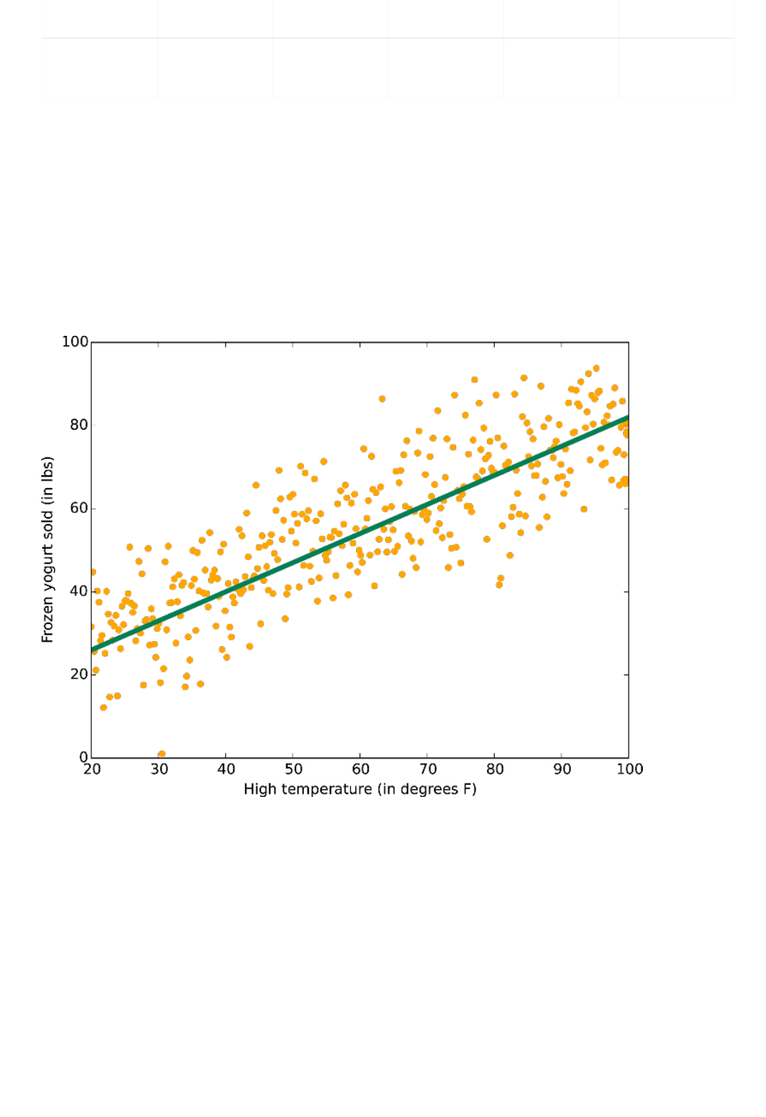
K-means ○ ● 4 A clustering
algorithm
ALGORITHM ACCURACY TRAINING TIME LINEARIT Y PARAMETERS NOTES
Algorithm notes
Linear regressionLinear regression
Logistic regressionLogistic regression
Algorithm properties:
● - shows excellent accuracy, fast training times, and the use of linearity
○ - shows good accuracy and moderate training times
As mentioned previously, linear regression fits a line (or plane, or hyperplane) to the data set. It's a workhorse,
simple and fast, but it may be overly simplistic for some problems. Check here for a linear regression tutorial.
Data with a linear trend
Although it confusingly includes 'regression' in the name, logistic regression is actually a powerful tool for two-
class and multiclass classification. It's fast and simple. The fact that it uses an 'S'-shaped curve instead of a
straight line makes it a natural fit for dividing data into groups. Logistic regression gives linear class boundaries,
so when you use it, make sure a linear approximation is something you can live with.
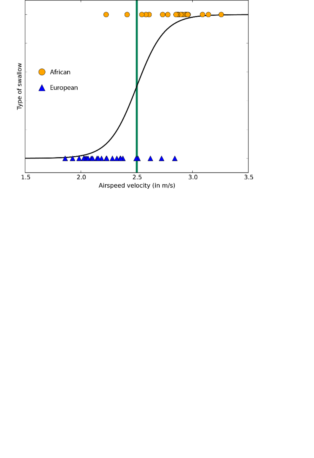
Trees, forests, and junglesTrees, forests, and jungles
A logistic regression to two-class data with just one feature - the class boundary is the point at which the
logistic curve is just as close to both classes
Decision forests (regression, two-class, and multiclass), decision jungles (two-class and multiclass), and boosted
decision trees (regression and two-class) are all based on decision trees, a foundational machine learning concept.
There are many variants of decision trees, but they all do the same thing—subdivide the feature space into
regions with mostly the same label. These can be regions of consistent category or of constant value, depending
on whether you are doing classification or regression.
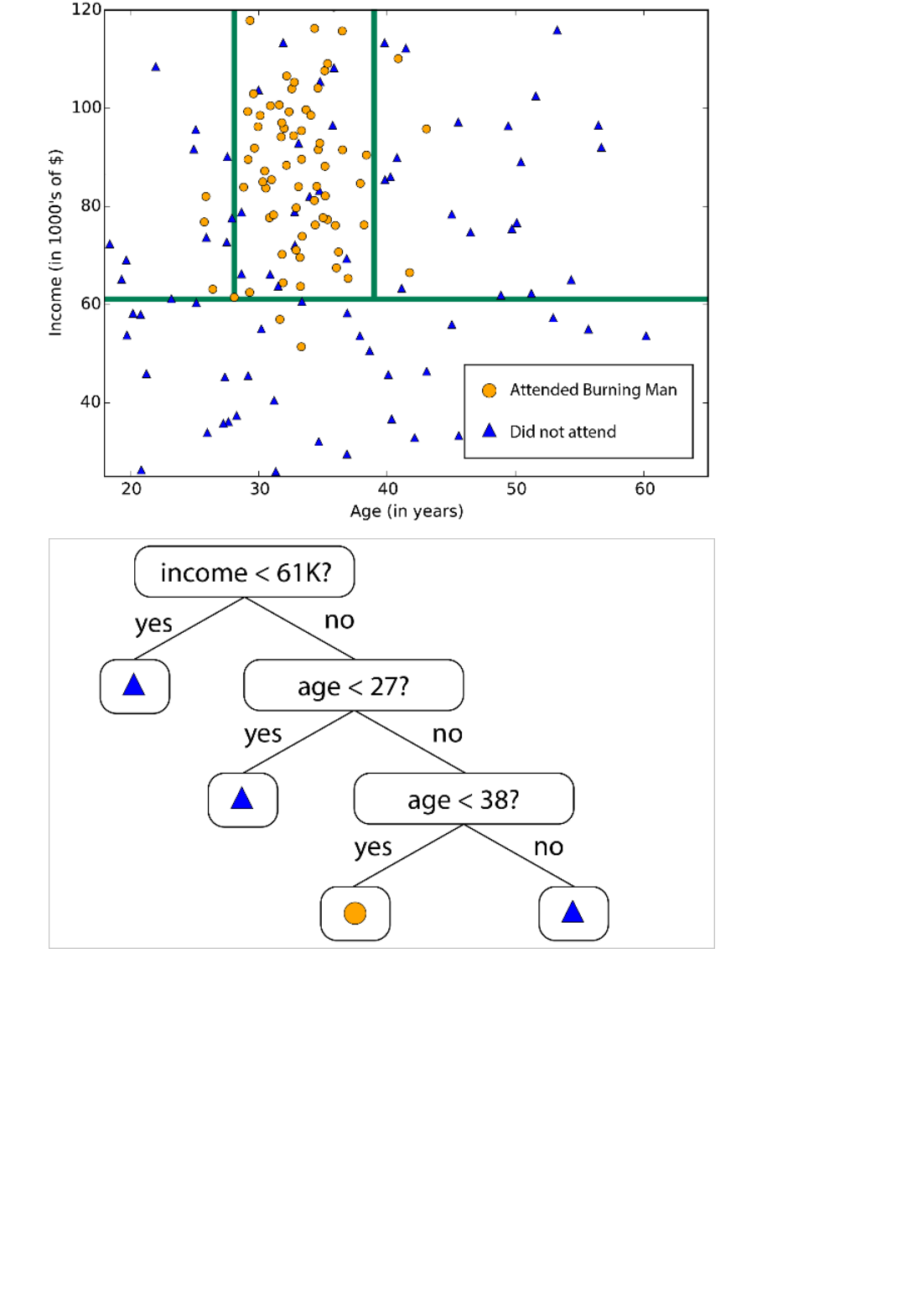
A decision tree subdivides a feature space into regions of roughly uniform values
Because a feature space can be subdivided into arbitrarily small regions, it's easy to imagine dividing it finely
enough to have one data point per region. This is an extreme example of overfitting. In order to avoid this, a large
set of trees are constructed with special mathematical care taken that the trees are not correlated. The average of
this "decision forest" is a tree that avoids overfitting. Decision forests can use a lot of memory. Decision jungles
are a variant that consumes less memory at the expense of a slightly longer training time.
Boosted decision trees avoid overfitting by limiting how many times they can subdivide and how few data points
are allowed in each region. The algorithm constructs a sequence of trees, each of which learns to compensate for
the error left by the tree before. The result is a very accurate learner that tends to use a lot of memory. For the full
technical description, check out Friedman's original paper.
Fast forest quantile regression is a variation of decision trees for the special case where you want to know not
only the typical (median) value of the data within a region, but also its distribution in the form of quantiles.

Neural networks and perceptronsNeural networks and perceptrons
Neural networks are brain-inspired learning algorithms covering multiclass, two-class, and regression problems.
They come in an infinite variety, but the neural networks within Azure Machine Learning are all of the form of
directed acyclic graphs. That means that input features are passed forward (never backward) through a sequence
of layers before being turned into outputs. In each layer, inputs are weighted in various combinations, summed,
and passed on to the next layer. This combination of simple calculations results in the ability to learn sophisticated
class boundaries and data trends, seemingly by magic. Many-layered networks of this sort perform the "deep
learning" that fuels so much tech reporting and science fiction.
This high performance doesn't come for free, though. Neural networks can take a long time to train, particularly
for large data sets with lots of features. They also have more parameters than most algorithms, which means that
parameter sweeping expands the training time a great deal. And for those overachievers who wish to specify their
own network structure, the possibilities are inexhaustible.
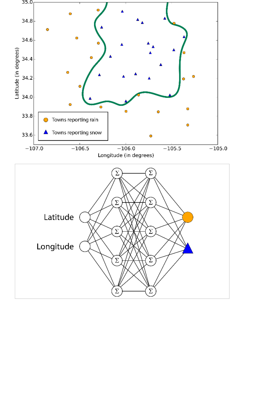
SVMsSVMs
The
boundaries learned by neural networks can be complex and irregular
The two-class averaged perceptron is neural networks' answer to skyrocketing training times. It uses a network
structure that gives linear class boundaries. It is almost primitive by today's standards, but it has a long history of
working robustly and is small enough to learn quickly.
Support vector machines (SVMs) find the boundary that separates classes by as wide a margin as possible. When
the two classes can't be clearly separated, the algorithms find the best boundary they can. As written in Azure
Machine Learning, the two-class SVM does this with a straight line only. (In SVM-speak, it uses a linear kernel.)
Because it makes this linear approximation, it is able to run fairly quickly. Where it really shines is with feature-
intense data, like text or genomic. In these cases SVMs are able to separate classes more quickly and with less
overfitting than most other algorithms, in addition to requiring only a modest amount of memory.
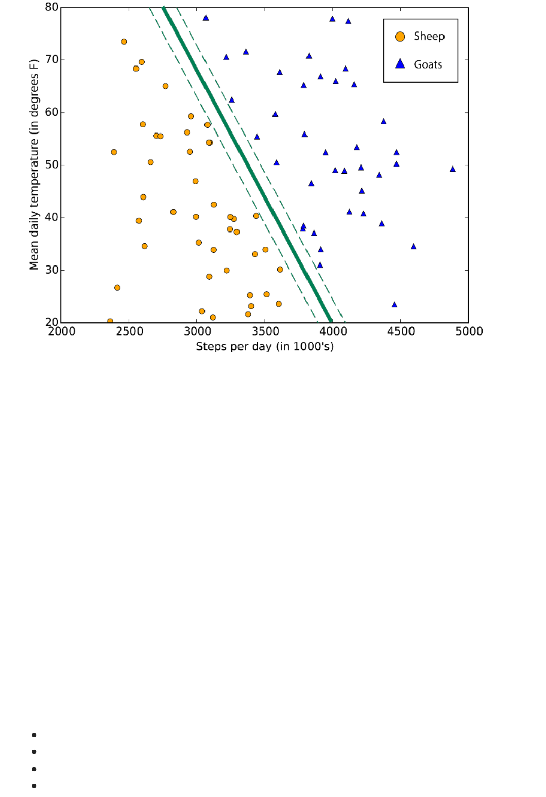
Bayesian methodsBayesian methods
Specialized algorithmsSpecialized algorithms
A typical support vector machine class boundary maximizes the margin separating two classes
Another product of Microsoft Research, the two-class locally deep SVM is a non-linear variant of SVM that
retains most of the speed and memory efficiency of the linear version. It is ideal for cases where the linear
approach doesn't give accurate enough answers. The developers kept it fast by breaking down the problem into a
bunch of small linear SVM problems. Read the full description for the details on how they pulled off this trick.
Using a clever extension of nonlinear SVMs, the one-class SVM draws a boundary that tightly outlines the entire
data set. It is useful for anomaly detection. Any new data points that fall far outside that boundary are unusual
enough to be noteworthy.
Bayesian methods have a highly desirable quality: they avoid overfitting. They do this by making some
assumptions beforehand about the likely distribution of the answer. Another byproduct of this approach is that
they have very few parameters. Azure Machine Learning has both Bayesian algorithms for both classification
(Two-class Bayes' point machine) and regression (Bayesian linear regression). Note that these assume that the
data can be split or fit with a straight line.
On a historical note, Bayes' point machines were developed at Microsoft Research. They have some exceptionally
beautiful theoretical work behind them. The interested student is directed to the original article in JMLR and an
insightful blog by Chris Bishop.
If you have a very specific goal you may be in luck. Within the Azure Machine Learning collection, there are
algorithms that specialize in:
rank prediction (ordinal regression),
count prediction (Poisson regression),
anomaly detection (one based on principal components analysis and one based on support vector machines)
clustering (K-means)
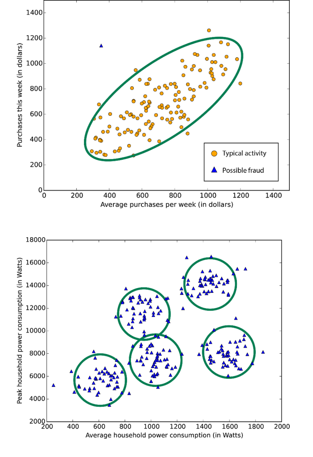
PCA-based anomaly detection - the vast majority of the data falls into a stereotypical distribution; points
deviating dramatically from that distribution are suspect
A data set is grouped into five clusters using K-means
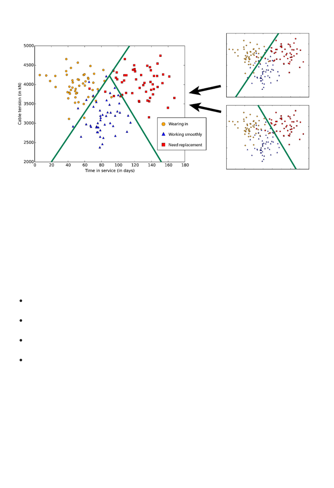
More help with algorithms
There is also an ensemble one-v-all multiclass classifier, which breaks the N-class classification problem into N-1
two-class classification problems. The accuracy, training time, and linearity properties are determined by the two-
class classifiers used.
A pair of two-class classifiers combine to form a three-class classifier
Azure Machine Learning also includes access to a powerful machine learning framework under the title of
Vowpal Wabbit. VW defies categorization here, since it can learn both classification and regression problems and
can even learn from partially unlabeled data. You can configure it to use any one of a number of learning
algorithms, loss functions, and optimization algorithms. It was designed from the ground up to be efficient,
parallel, and extremely fast. It handles ridiculously large feature sets with little apparent effort. Started and led by
Microsoft Research's own John Langford, VW is a Formula One entry in a field of stock car algorithms. Not every
problem fits VW, but if yours does, it may be worth your while to climb the learning curve on its interface. It's also
available as stand-alone open source code in several languages.
For a downloadable infographic that describes algorithms and provides examples, see Downloadable
Infographic: Machine learning basics with algorithm examples.
For a list by category of all the machine learning algorithms available in Azure Machine Learning Studio, see
Initialize Model in the Machine Learning Studio Algorithm and Module Help.
For a complete alphabetical list of algorithms and modules in Azure Machine Learning Studio, see A-Z list of
Machine Learning Studio modules in Machine Learning Studio Algorithm and Module Help.
To download and print a diagram that gives an overview of the capabilities of Azure Machine Learning Studio,
see Overview diagram of Azure Machine Learning Studio capabilities.
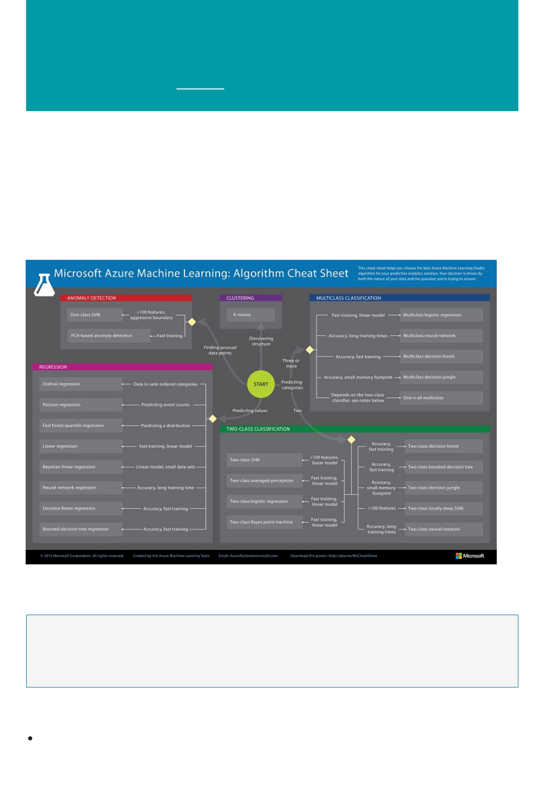
Machine learning algorithm cheat sheet for Microsoft
Azure Machine Learning Studio
3/21/2018 • 5 min to read • Edit Online
Download: Machine learning algorithm cheat sheet
NOTENOTE
More help with algorithms
The Microsoft Azure Machine Learning Algorithm Cheat Sheet helps you choose the right algorithm for a
predictive analytics model.
Azure Machine Learning Studio has a large library of algorithms from the regression, classification, clustering,
and anomaly detection families. Each is designed to address a different type of machine learning problem.
Download the cheat sheet here: Machine Learning Algorithm Cheat Sheet (11x17 in.)
Download and print the Machine Learning Algorithm Cheat Sheet in tabloid size to keep it handy and get help
choosing an algorithm.
See the article How to choose algorithms for Microsoft Azure Machine Learning for a detailed guide to using this cheat
sheet.
For help in using this cheat sheet for choosing the right algorithm, plus a deeper discussion of the different
types of machine learning algorithms and how they're used, see How to choose algorithms for Microsoft Azure
Machine Learning.
NOTENOTE
Notes and terminology definitions for the machine learning algorithm
cheat sheet
For a downloadable infographic that describes algorithms and provides examples, see Downloadable
Infographic: Machine learning basics with algorithm examples.
For a list by category of all the machine learning algorithms available in Machine Learning Studio, see Initialize
Model in the Machine Learning Studio Algorithm and Module Help.
For a complete alphabetical list of algorithms and modules in Machine Learning Studio, see A-Z list of Machine
Learning Studio modules in Machine Learning Studio Algorithm and Module Help.
To download and print a diagram that gives an overview of the capabilities of Machine Learning Studio, see
Overview diagram of Azure Machine Learning Studio capabilities.
You can try Azure Machine Learning for free. No credit card or Azure subscription is required. Get started now.
The suggestions offered in this algorithm cheat sheet are approximate rules-of-thumb. Some can be bent,
and some can be flagrantly violated. This is intended to suggest a starting point. Don’t be afraid to run a
head-to-head competition between several algorithms on your data. There is simply no substitute for
understanding the principles of each algorithm and understanding the system that generated your data.
Every machine learning algorithm has its own style or inductive bias. For a specific problem, several
algorithms may be appropriate and one algorithm may be a better fit than others. But it's not always
possible to know beforehand which is the best fit. In cases like these, several algorithms are listed together
in the cheat sheet. An appropriate strategy would be to try one algorithm, and if the results are not yet
satisfactory, try the others. Here’s an example from the Azure AI Gallery of an experiment that tries several
algorithms against the same data and compares the results: Compare Multi-class Classifiers: Letter
recognition.
There are three main categories of machine learning: supervised learning, unsupervised learning, and
reinforcement learning.
In supervised learning, each data point is labeled or associated with a category or value of interest.
An example of a categorical label is assigning an image as either a ‘cat’ or a ‘dog’. An example of a
value label is the sale price associated with a used car. The goal of supervised learning is to study
many labeled examples like these, and then to be able to make predictions about future data points.
For example, identifying new photos with the correct animal or assigning accurate sale prices to
other used cars. This is a popular and useful type of machine learning. All of the modules in Azure
Machine Learning are supervised learning algorithms except for K-Means Clustering.
In unsupervised learning, data points have no labels associated with them. Instead, the goal of an
unsupervised learning algorithm is to organize the data in some way or to describe its structure. This
can mean grouping it into clusters, as K-means does, or finding different ways of looking at complex
data so that it appears simpler.
In reinforcement learning, the algorithm gets to choose an action in response to each data point. It
is a common approach in robotics, where the set of sensor readings at one point in time is a data
point, and the algorithm must choose the robot’s next action. It's also a natural fit for Internet of
Things applications. The learning algorithm also receives a reward signal a short time later,
indicating how good the decision was. Based on this, the algorithm modifies its strategy in order to
achieve the highest reward. Currently there are no reinforcement learning algorithm modules in
Azure ML.
Bayesian methods make the assumption of statistically independent data points. This means that the

unmodeled variability in one data point is uncorrelated with others, that is, it can’t be predicted. For
example, if the data being recorded is the number of minutes until the next subway train arrives, two
measurements taken a day apart are statistically independent. However, two measurements taken a minute
apart are not statistically independent - the value of one is highly predictive of the value of the other.
Boosted decision tree regression takes advantage of feature overlap or interaction among features. That
means that, in any given data point, the value of one feature is somewhat predictive of the value of another.
For example, in daily high/low temperature data, knowing the low temperature for the day allows you to
make a reasonable guess at the high. The information contained in the two features is somewhat
redundant.
Classifying data into more than two categories can be done by either using an inherently multi-class
classifier, or by combining a set of two-class classifiers into an ensemble. In the ensemble approach, there
is a separate two-class classifier for each class - each one separates the data into two categories: “this class”
and “not this class.” Then these classifiers vote on the correct assignment of the data point. This is the
operational principle behind One-vs-All Multiclass.
Several methods, including logistic regression and the Bayes point machine, assume linear class
boundaries. That is, they assume that the boundaries between classes are approximately straight lines (or
hyperplanes in the more general case). Often this is a characteristic of the data that you don’t know until
after you’ve tried to separate it, but it’s something that typically can be learned by visualizing beforehand. If
the class boundaries look very irregular, stick with decision trees, decision jungles, support vector machines,
or neural networks.
Neural networks can be used with categorical variables by creating a dummy variable for each category,
setting it to 1 in cases where the category applies, 0 where it doesn’t.

Using linear regression in Azure Machine Learning
3/21/2018 • 7 min to read • Edit Online
NOTENOTE
Goal
Achieving predictive performance parity
Create regression model in ExcelCreate regression model in Excel
Create comparable experiment in Azure Machine LearningCreate comparable experiment in Azure Machine Learning
Kate Baroni and Ben Boatman are enterprise solution architects in Microsoft’s Data Insights Center of
Excellence. In this article, they describe their experience migrating an existing regression analysis suite to a
cloud-based solution using Azure Machine Learning.
You can try Azure Machine Learning for free. No credit card or Azure subscription is required. Get started now.
Our project started with two goals in mind:
1. Use predictive analytics to improve the accuracy of our organization’s monthly revenue projections
2. Use Azure Machine Learning to confirm, optimize, increase velocity, and scale of our results.
Like many businesses, our organization goes through a monthly revenue forecasting process. Our small team of
business analysts was tasked with using Azure Machine Learning to support the process and improve forecast
accuracy. The team spent several months collecting data from multiple sources and running the data attributes
through statistical analysis identifying key attributes relevant to services sales forecasting. The next step was to
begin prototyping statistical regression models on the data in Excel. Within a few weeks, we had an Excel
regression model that was outperforming the current field and finance forecasting processes. This became the
baseline prediction result.
We then took the next step to moving our predictive analytics over to Azure Machine Learning to find out how
Machine Learning could improve on predictive performance.
Our first priority was to achieve parity between Machine Learning and Excel regression models. Given the same
data, and the same split for training and testing data, we wanted to achieve predictive performance parity between
Excel and Machine Learning. Initially we failed. The Excel model outperformed the Machine Learning model. The
failure was due to a lack of understanding of the base tool setting in Machine Learning. After a sync with the
Machine Learning product team, we gained a better understanding of the base setting required for our data sets,
and achieved parity between the two models.
Our Excel Regression used the standard linear regression model found in the Excel Analysis ToolPak.
We calculated Mean Absolute % Error and used it as the performance measure for the model. It took 3 months to
arrive at a working model using Excel. We brought much of the learning into the Machine Learning Studio
experiment which ultimately was beneficial in understanding requirements.
We followed these steps to create our experiment in Machine Learning Studio:
1. Uploaded the dataset as a csv file to Machine Learning Studio (very small file)

Review initial resultsReview initial results
EXCEL STUDIO
Performance
0.96 N/A
N/A 0.78
(low accuracy)
Mean Absolute Error $9.5M $ 19.4M
Mean Absolute Error (%)6.03% 12.2%
Mystery solved!Mystery solved!
EXCEL STUDIO (INITIAL)STUDIO W/ LEAST SQUARES
Labeled value Actuals (numeric)same same
Learner Excel -> Data Analysis ->
Regression
Linear Regression. Linear Regression
Learner options N/A Defaults ordinary least squares
L2 = 0.005
Data Set 26 rows, 3 features, 1 label.
All numeric.
same same
2. Created a new experiment and used the Select Columns in Dataset module to select the same data features
used in Excel
3. Used the Split Data module (with Relative Expression mode) to divide the data into the same training datasets
as had been done in Excel
4. Experimented with the Linear Regression module (default options only), documented, and compared the results
to our Excel regression model
At first, the Excel model clearly outperformed the Machine Learning Studio model:
Adjusted R Square
Coefficient of
Determination
When we ran our process and results by the developers and data scientists on the Machine Learning team, they
quickly provided some useful tips.
When you use the Linear Regression module in Machine Learning Studio, two methods are provided:
Consider tweaking the L2 Regularization Weight parameter to improve performance. It is set to 0.001 by
default, but for our small data set we set it to 0.005 to improve performance.
Online Gradient Descent: May be more suitable for larger-scale problems
Ordinary Least Squares: This is the method most people think of when they hear linear regression. For
small datasets, Ordinary Least Squares can be a more optimal choice.
When we applied the recommendations, we achieved the same baseline performance in Machine Learning Studio
as with Excel:
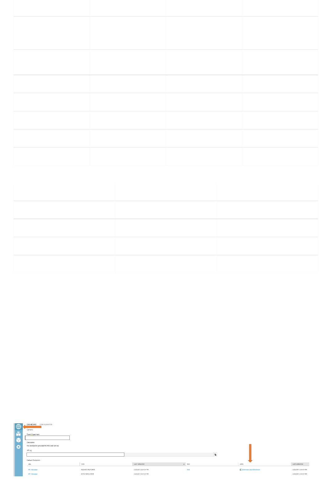
Split: Train Excel trained on the first 18
rows, tested on the last 8
rows.
same same
Split: Test Excel regression formula
applied to the last 8 rows
same same
Performance
Adjusted R Square 0.96 N/A
Coefficient of Determination N/A 0.78 0.952049
Mean Absolute Error $9.5M $ 19.4M $9.5M
Mean Absolute Error (%)6.03% 12.2% 6.03%
EXCEL STUDIO (INITIAL)STUDIO W/ LEAST SQUARES
EXCEL COEFFICIENTS AZURE FEATURE WEIGHTS
Intercept/Bias 19470209.88 19328500
Feature A 0.832653063 0.834156
Feature B 11071967.08 11007300
Feature C 25383318.09 25140800
Next Steps
Integration with ExcelIntegration with Excel
In addition, the Excel coefficients compared well to the feature weights in the Azure trained model:
We wanted to consume the Machine Learning web service within Excel. Our business analysts rely on Excel and we
needed a way to call the Machine Learning web service with a row of Excel data and have it return the predicted
value to Excel.
We also wanted to optimize our model, using the options and algorithms available in Machine Learning Studio.
Our solution was to operationalize our Machine Learning regression model by creating a web service from the
trained model. Within a few minutes, the web service was created and we could call it directly from Excel to return
a predicted revenue value.
The Web Services Dashboard section includes a downloadable Excel workbook. The workbook comes pre-
formatted with the web service API and schema information embedded. When you click Download Excel
Workbook, the workbook opens and you can save it to your local computer.

Optimization and further experimentsOptimization and further experiments
MODEL
MEAN ABSOLUTE
ERROR
ROOT MEAN
SQUARED ERROR
RELATIVE
ABSOLUTE ERROR
RELATIVE
SQUARED ERROR
COEFFICIENT OF
DETERMINATION
Boosted Decision
Tree
0.930113 1.4239 0.106647 0.021662 0.978338
Linear Regression
(Gradient
Descent)
2.035693 2.98006 0.233414 0.094881 0.905119
Neural Network
Regression
1.548195 2.114617 0.177517 0.047774 0.952226
Linear Regression
(Ordinary Least
Squares)
1.428273 1.984461 0.163767 0.042074 0.957926
Key Takeaways
With the workbook open, copy your predefined parameters into the blue Parameter section as shown below. Once
the parameters are entered, Excel calls out to the Machine Learning web service and the predicted scored labels
will display in the green Predicted Values section. The workbook will continue to create predictions for parameters
based on your trained model for all row items entered under Parameters. For more information on how to use this
feature, see Consuming an Azure Machine Learning Web Service from Excel.
Now that we had a baseline with our Excel model, we moved ahead to optimize our Machine Learning Linear
Regression Model. We used the module Filter-Based Feature Selection to improve on our selection of initial data
elements and it helped us achieve a performance improvement of 4.6% Mean Absolute Error. For future projects
we will use this feature which could save us weeks in iterating through data attributes to find the right set of
features to use for modelling.
Next we plan to include additional algorithms like Bayesian or Boosted Decision Trees in our experiment to
compare performance.
If you want to experiment with regression, a good dataset to try is the Energy Efficiency Regression sample dataset,
which has lots of numerical attributes. The dataset is provided as part of the sample datasets in Machine Learning
Studio. You can use a variety of learning modules to predict either Heating Load or Cooling Load. The chart below
is a performance comparison of different regression learns against the Energy Efficiency dataset predicting for the
target variable Cooling Load:
We learned a lot by from running Excel regression and Azure Machine Learning experiments in parallel. Creating
the baseline model in Excel and comparing it to models using Machine Learning Linear Regression helped us learn
Azure Machine Learning, and we discovered opportunities to improve data selection and model performance.
We also found that it is advisable to use Filter-Based Feature Selection to accelerate future prediction projects. By
applying feature selection to your data, you can create an improved model in Machine Learning with better overall
performance.
The ability to transfer the predictive analytic forecasting from Machine Learning to Excel systemically allows a
significant increase in the ability to successfully provide results to a broad business user audience.

Resources
Here are some resources for helping you work with regression:
Regression in Excel. If you’ve never tried regression in Excel, this tutorial makes it easy: http://www.excel-
easy.com/examples/regression.html
Regression vs forecasting. Tyler Chessman wrote a blog article explaining how to do time series forecasting in
Excel, which contains a good beginner’s description of linear regression. http://sqlmag.com/sql-server-analysis-
services/understanding-time-series-forecasting-concepts
Ordinary Least Squares Linear Regression: Flaws, Problems and Pitfalls. For an introduction and discussion of
Regression: http://www.clockbackward.com/2009/06/18/ordinary-least-squares-linear-regression-flaws-
problems-and-pitfalls/
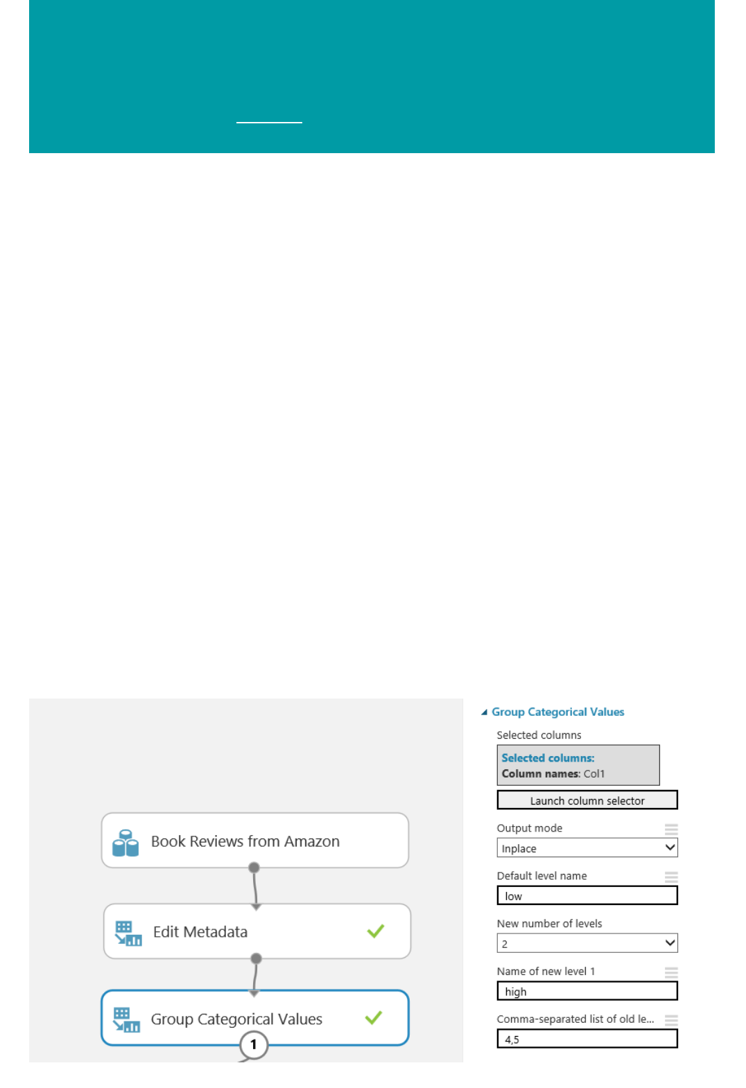
Create text analytics models in Azure Machine
Learning Studio
3/21/2018 • 5 min to read • Edit Online
Step 1: Clean and preprocess text dataset
You can use Azure Machine Learning to build and operationalize text analytics models. These models can help you
solve, for example, document classification or sentiment analysis problems.
In a text analytics experiment, you would typically:
1. Clean and preprocess text dataset
2. Extract numeric feature vectors from pre-processed text
3. Train classification or regression model
4. Score and validate the model
5. Deploy the model to production
In this tutorial, you learn these steps as we walk through a sentiment analysis model using Amazon Book Reviews
dataset (see this research paper “Biographies, Bollywood, Boom-boxes and Blenders: Domain Adaptation for
Sentiment Classification” by John Blitzer, Mark Dredze, and Fernando Pereira; Association of Computational
Linguistics (ACL), 2007.) This dataset consists of review scores (1-2 or 4-5) and a free-form text. The goal is to
predict the review score: low (1-2) or high (4-5).
You can find experiments covered in this tutorial at Azure AI Gallery:
Predict Book Reviews
Predict Book Reviews - Predictive Experiment
We begin the experiment by dividing the review scores into categorical low and high buckets to formulate the
problem as two-class classification. We use Edit Metadata and Group Categorical Values modules.
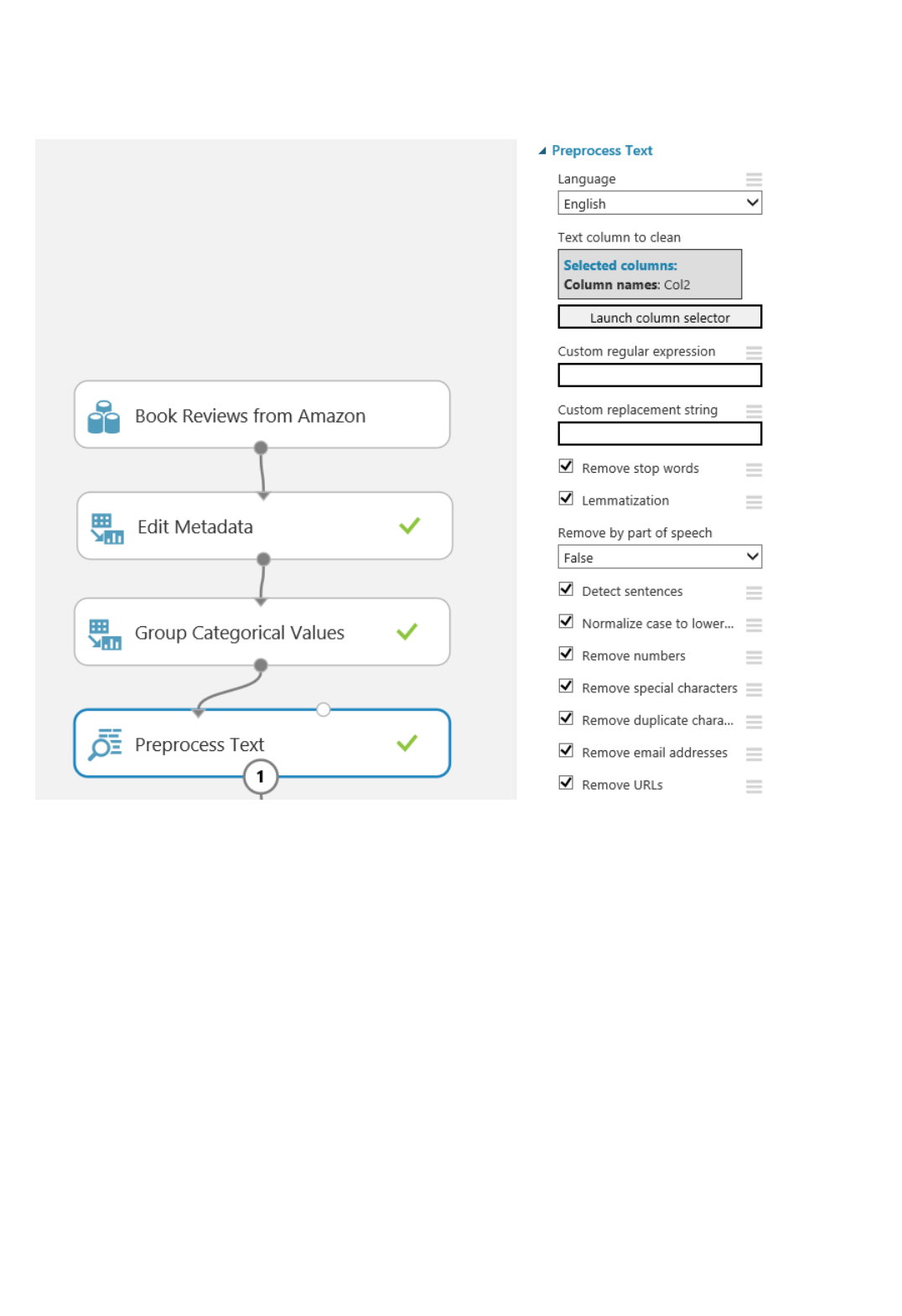
Step 2: Extract numeric feature vectors from pre-processed text
Then, we clean the text using Preprocess Text module. The cleaning reduces the noise in the dataset, help you find
the most important features, and improve the accuracy of the final model. We remove stopwords - common words
such as "the" or "a" - and numbers, special characters, duplicated characters, email addresses, and URLs. We also
convert the text to lowercase, lemmatize the words, and detect sentence boundaries that are then indicated by "|||"
symbol in pre-processed text.
What if you want to use a custom list of stopwords? You can pass it in as optional input. You can also use custom
C# syntax regular expression to replace substrings, and remove words by part of speech: nouns, verbs, or
adjectives.
After the preprocessing is complete, we split the data into train and test sets.
To build a model for text data, you typically have to convert free-form text into numeric feature vectors. In this
example, we use Extract N-Gram Features from Text module to transform the text data to such format. This module
takes a column of whitespace-separated words and computes a dictionary of words, or N-grams of words, that
appear in your dataset. Then, it counts how many times each word, or N-gram, appears in each record, and creates
feature vectors from those counts. In this tutorial, we set N-gram size to 2, so our feature vectors include single
words and combinations of two subsequent words.
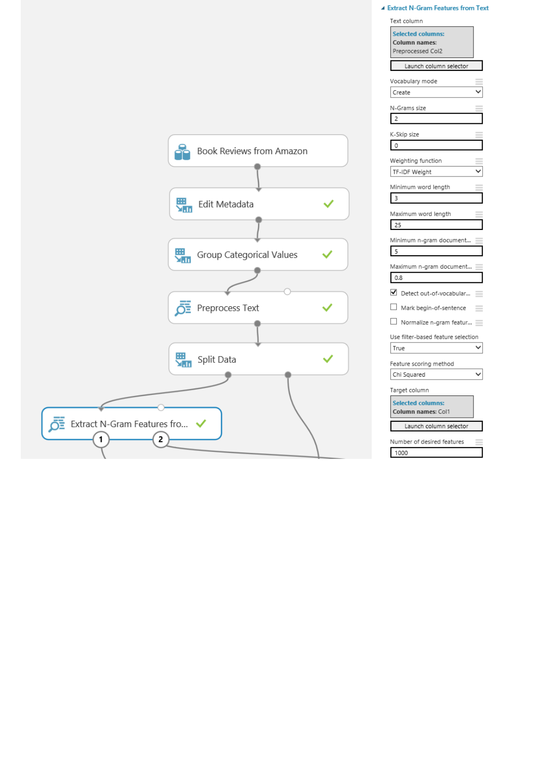
Step 3: Train classification or regression model
We apply TF*IDF (Term Frequency Inverse Document Frequency) weighting to N-gram counts. This approach adds
weight of words that appear frequently in a single record but are rare across the entire dataset. Other options
include binary, TF, and graph weighing.
Such text features often have high dimensionality. For example, if your corpus has 100,000 unique words, your
feature space would have 100,000 dimensions, or more if N-grams are used. The Extract N-Gram Features module
gives you a set of options to reduce the dimensionality. You can choose to exclude words that are short or long, or
too uncommon or too frequent to have significant predictive value. In this tutorial, we exclude N-grams that appear
in fewer than 5 records or in more than 80% of records.
Also, you can use feature selection to select only those features that are the most correlated with your prediction
target. We use Chi-Squared feature selection to select 1000 features. You can view the vocabulary of selected
words or N-grams by clicking the right output of Extract N-grams module.
As an alternative approach to using Extract N-Gram Features, you can use Feature Hashing module. Note though
that Feature Hashing does not have build-in feature selection capabilities, or TF*IDF weighing.
Now the text has been transformed to numeric feature columns. The dataset still contains string columns from
previous stages, so we use Select Columns in Dataset to exclude them.
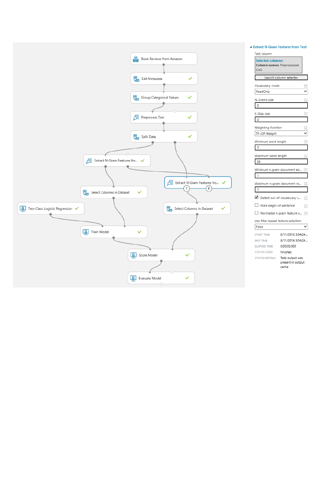
Step 4: Score and validate the model
Step 5: Deploy the model to production
We then use Two-Class Logistic Regression to predict our target: high or low review score. At this point, the text
analytics problem has been transformed into a regular classification problem. You can use the tools available in
Azure Machine Learning to improve the model. For example, you can experiment with different classifiers to find
out how accurate results they give, or use hyperparameter tuning to improve the accuracy.
How would you validate the trained model? We score it against the test dataset and evaluate the accuracy. However,
the model learned the vocabulary of N-grams and their weights from the training dataset. Therefore, we should use
that vocabulary and those weights when extracting features from test data, as opposed to creating the vocabulary
anew. Therefore, we add Extract N-Gram Features module to the scoring branch of the experiment, connect the
output vocabulary from training branch, and set the vocabulary mode to read-only. We also disable the filtering of
N-grams by frequency by setting the minimum to 1 instance and maximum to 100%, and turn off the feature
selection.
After the text column in test data has been transformed to numeric feature columns, we exclude the string columns
from previous stages like in training branch. We then use Score Model module to make predictions and Evaluate
Model module to evaluate the accuracy.
The model is almost ready to be deployed to production. When deployed as web service, it takes free-form text
string as input, and return a prediction "high" or "low." It uses the learned N-gram vocabulary to transform the text
to features, and trained logistic regression model to make a prediction from those features.
To set up the predictive experiment, we first save the N-gram vocabulary as dataset, and the trained logistic
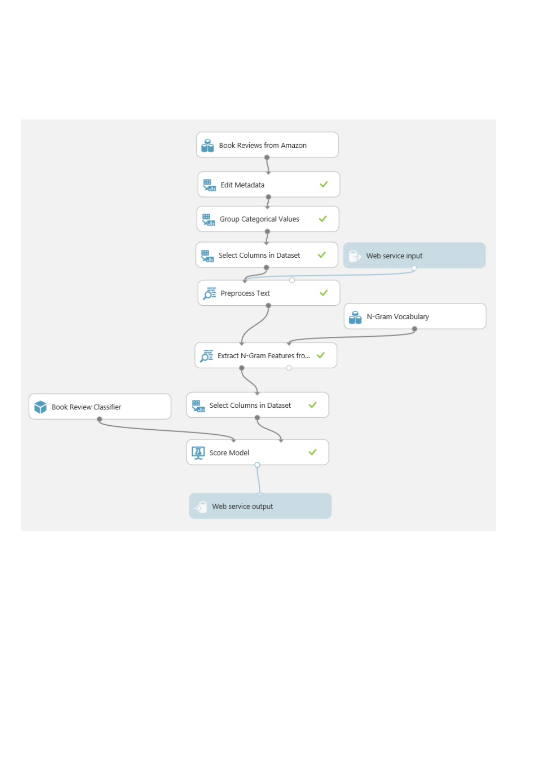
Next Steps
regression model from the training branch of the experiment. Then, we save the experiment using "Save As" to
create an experiment graph for predictive experiment. We remove the Split Data module and the training branch
from the experiment. We then connect the previously saved N-gram vocabulary and model to Extract N-Gram
Features and Score Model modules, respectively. We also remove the Evaluate Model module.
We insert Select Columns in Dataset module before Preprocess Text module to remove the label column, and
unselect "Append score column to dataset" option in Score Module. That way, the web service does not request the
label it is trying to predict, and does not echo the input features in response.
Now we have an experiment that can be published as a web service and called using request-response or batch
execution APIs.
Learn about text analytics modules from MSDN documentation.
How to evaluate model performance in Azure
Machine Learning
3/20/2018 • 12 min to read • Edit Online
NOTENOTE
Evaluation vs. Cross Validation
Evaluating a Regression Model
This article demonstrates how to evaluate the performance of a model in Azure Machine Learning Studio and
provides a brief explanation of the metrics available for this task. Three common supervised learning scenarios are
presented:
regression
binary classification
multiclass classification
You can try Azure Machine Learning for free. No credit card or Azure subscription is required. Get started now.
Evaluating the performance of a model is one of the core stages in the data science process. It indicates how
successful the scoring (predictions) of a dataset has been by a trained model.
Azure Machine Learning supports model evaluation through two of its main machine learning modules: Evaluate
Model and Cross-Validate Model. These modules allow you to see how your model performs in terms of a number
of metrics that are commonly used in machine learning and statistics.
Evaluation and cross validation are standard ways to measure the performance of your model. They both generate
evaluation metrics that you can inspect or compare against those of other models.
Evaluate Model expects a scored dataset as input (or 2 in case you would like to compare the performance of 2
different models). This means that you need to train your model using the Train Model module and make
predictions on some dataset using the Score Model module, before you can evaluate the results. The evaluation is
based on the scored labels/probabilities along with the true labels, all of which are output by the Score Model
module.
Alternatively, you can use cross validation to perform a number of train-score-evaluate operations (10 folds)
automatically on different subsets of the input data. The input data is split into 10 parts, where one is reserved for
testing, and the other 9 for training. This process is repeated 10 times and the evaluation metrics are averaged. This
helps in determining how well a model would generalize to new datasets. The Cross-Validate Model module takes
in an untrained model and some labeled dataset and outputs the evaluation results of each of the 10 folds, in
addition to the averaged results.
In the following sections, we will build simple regression and classification models and evaluate their performance,
using both the Evaluate Model and the Cross-Validate Model modules.
Assume we want to predict a car’s price using some features such as dimensions, horsepower, engine specs, and so
on. This is a typical regression problem, where the target variable (price) is a continuous numeric value. We can fit
a simple linear regression model that, given the feature values of a certain car, can predict the price of that car. This
regression model can be used to score the same dataset we trained on. Once we have the predicted prices for all of
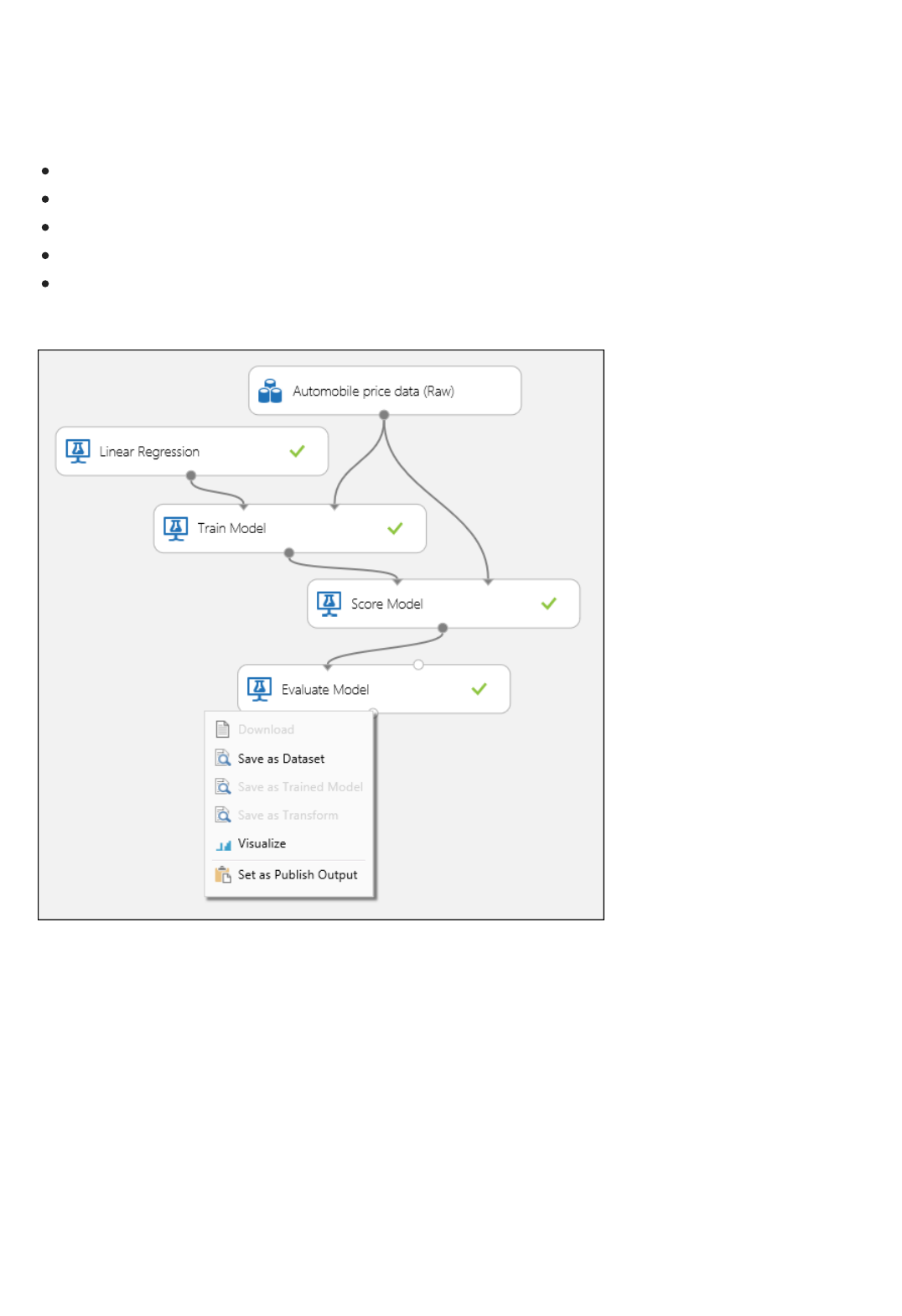
Creating the ExperimentCreating the Experiment
Inspecting the Evaluation ResultsInspecting the Evaluation Results
the cars, we can evaluate the performance of the model by looking at how much the predictions deviate from the
actual prices on average. To illustrate this, we use the Automobile price data (Raw) dataset available in the Saved
Datasets section in Azure Machine Learning Studio.
Add the following modules to your workspace in Azure Machine Learning Studio:
Automobile price data (Raw)
Linear Regression
Train Model
Score Model
Evaluate Model
Connect the ports as shown below in Figure 1 and set the Label column of the Train Model module to price.
Figure 1. Evaluating a Regression Model.
After running the experiment, you can click on the output port of the Evaluate Model module and select Visualize
to see the evaluation results. The evaluation metrics available for regression models are: Mean Absolute Error, Root
Mean Absolute Error, Relative Absolute Error, Relative Squared Error, and the Coefficient of Determination.
The term "error" here represents the difference between the predicted value and the true value. The absolute value
or the square of this difference are usually computed to capture the total magnitude of error across all instances, as
the difference between the predicted and true value could be negative in some cases. The error metrics measure
the predictive performance of a regression model in terms of the mean deviation of its predictions from the true
values. Lower error values mean the model is more accurate in making predictions. An overall error metric of 0
means that the model fits the data perfectly.
The coefficient of determination, which is also known as R squared, is also a standard way of measuring how well
the model fits the data. It can be interpreted as the proportion of variation explained by the model. A higher
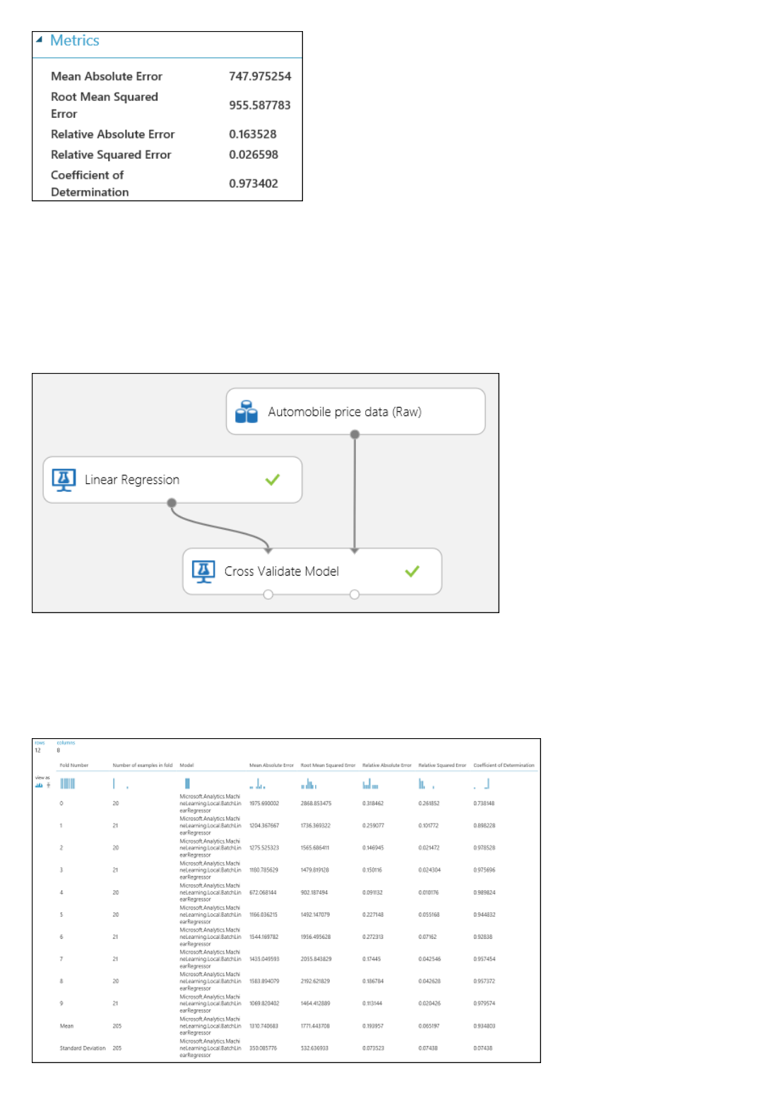
Using Cross ValidationUsing Cross Validation
proportion is better in this case, where 1 indicates a perfect fit.
Figure 2. Linear Regression Evaluation Metrics.
As mentioned earlier, you can perform repeated training, scoring and evaluations automatically using the Cross-
Validate Model module. All you need in this case is a dataset, an untrained model, and a Cross-Validate Model
module (see figure below). Note that you need to set the label column to price in the Cross-Validate Model
module’s properties.
Figure 3. Cross-Validating a Regression Model.
After running the experiment, you can inspect the evaluation results by clicking on the right output port of the
Cross-Validate Model module. This will provide a detailed view of the metrics for each iteration (fold), and the
averaged results of each of the metrics (Figure 4).
Figure 4. Cross-Validation Results of a Regression Model.
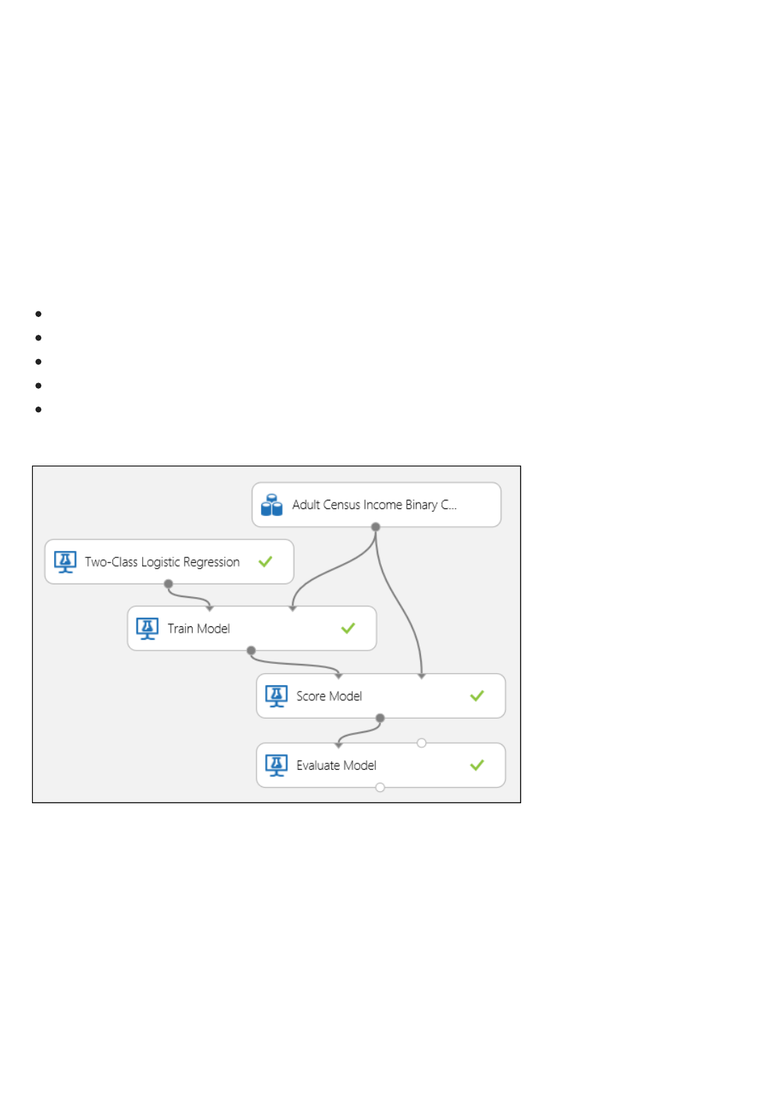
Evaluating a Binary Classification Model
Creating the ExperimentCreating the Experiment
Inspecting the Evaluation ResultsInspecting the Evaluation Results
In a binary classification scenario, the target variable has only two possible outcomes, for example: {0, 1} or {false,
true}, {negative, positive}. Assume you are given a dataset of adult employees with some demographic and
employment variables, and that you are asked to predict the income level, a binary variable with the values
{“<=50K”, “>50K”}. In other words, the negative class represents the employees who make less than or equal to
50K per year, and the positive class represents all other employees. As in the regression scenario, we would train a
model, score some data, and evaluate the results. The main difference here is the choice of metrics Azure Machine
Learning computes and outputs. To illustrate the income level prediction scenario, we will use the Adult dataset to
create an Azure Machine Learning experiment and evaluate the performance of a two-class logistic regression
model, a commonly used binary classifier.
Add the following modules to your workspace in Azure Machine Learning Studio:
Adult Census Income Binary Classification dataset
Two-Class Logistic Regression
Train Model
Score Model
Evaluate Model
Connect the ports as shown below in Figure 5 and set the Label column of the Train Model module to income.
Figure 5. Evaluating a Binary Classification Model.
After running the experiment, you can click on the output port of the Evaluate Model module and select Visualize
to see the evaluation results (Figure 7). The evaluation metrics available for binary classification models are:
Accuracy, Precision, Recall, F1 Score, and AUC. In addition, the module outputs a confusion matrix showing the
number of true positives, false negatives, false positives, and true negatives, as well as ROC, Precision/Recall, and
Lift curves.
Accuracy is simply the proportion of correctly classified instances. It is usually the first metric you look at when
evaluating a classifier. However, when the test data is unbalanced (where most of the instances belong to one of the
classes), or you are more interested in the performance on either one of the classes, accuracy doesn’t really capture
the effectiveness of a classifier. In the income level classification scenario, assume you are testing on some data
where 99% of the instances represent people who earn less than or equal to 50K per year. It is possible to achieve a
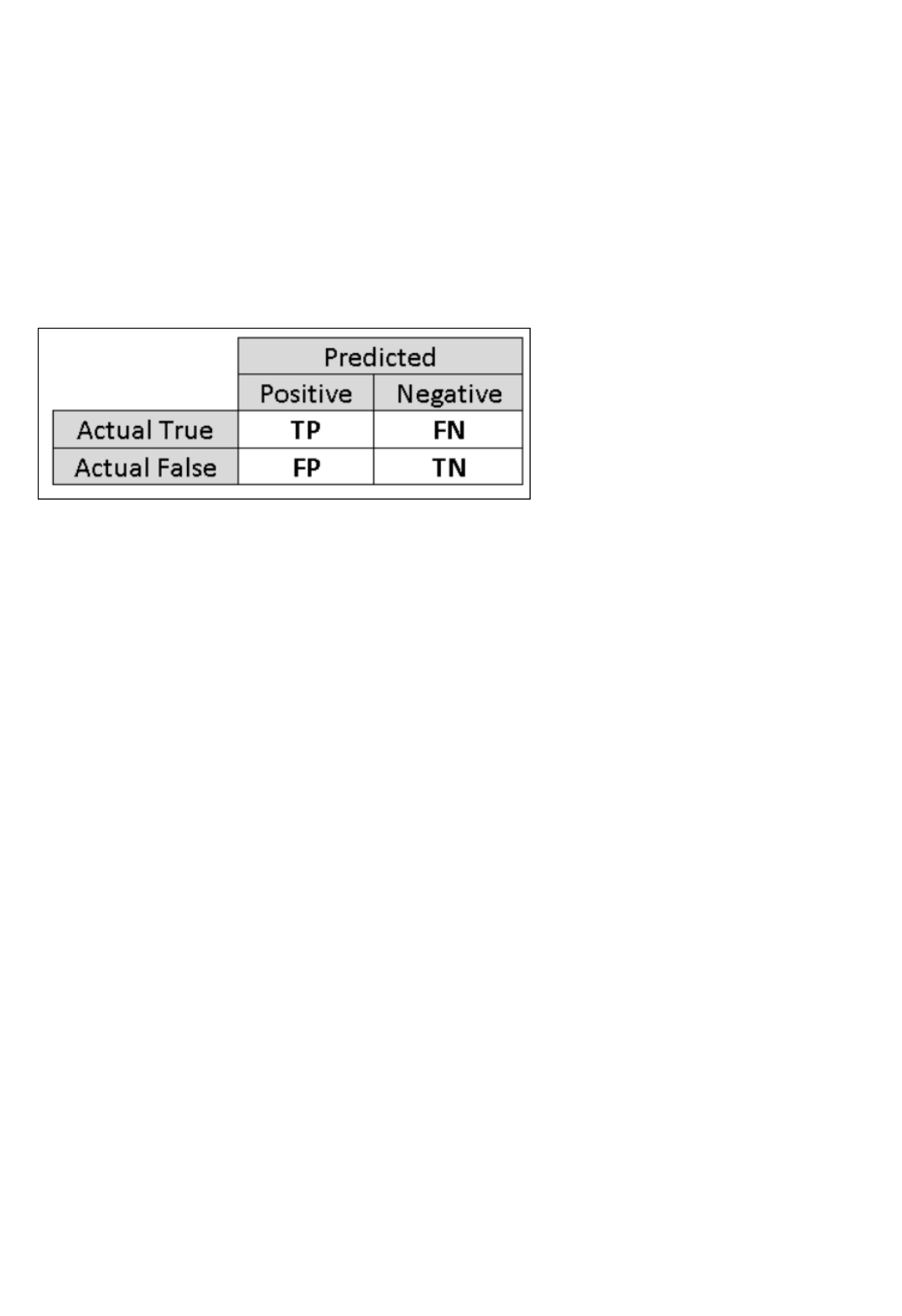
0.99 accuracy by predicting the class “<=50K” for all instances. The classifier in this case appears to be doing a
good job overall, but in reality, it fails to classify any of the high-income individuals (the 1%) correctly.
For that reason, it is helpful to compute additional metrics that capture more specific aspects of the evaluation.
Before going into the details of such metrics, it is important to understand the confusion matrix of a binary
classification evaluation. The class labels in the training set can take on only 2 possible values, which we usually
refer to as positive or negative. The positive and negative instances that a classifier predicts correctly are called true
positives (TP) and true negatives (TN), respectively. Similarly, the incorrectly classified instances are called false
positives (FP) and false negatives (FN). The confusion matrix is simply a table showing the number of instances
that fall under each of these 4 categories. Azure Machine Learning automatically decides which of the two classes
in the dataset is the positive class. If the class labels are Boolean or integers, then the ‘true’ or ‘1’ labeled instances
are assigned the positive class. If the labels are strings, as in the case of the income dataset, the labels are sorted
alphabetically and the first level is chosen to be the negative class while the second level is the positive class.
Figure 6. Binary Classification Confusion Matrix.
Going back to the income classification problem, we would want to ask several evaluation questions that help us
understand the performance of the classifier used. A very natural question is: ‘Out of the individuals whom the
model predicted to be earning >50K (TP+FP), how many were classified correctly (TP)?’ This question can be
answered by looking at the Precision of the model, which is the proportion of positives that are classified
correctly: TP/(TP+FP). Another common question is “Out of all the high earning employees with income >50k
(TP+FN), how many did the classifier classify correctly (TP)”. This is actually the Recall, or the true positive rate:
TP/(TP+FN) of the classifier. You might notice that there is an obvious trade-off between precision and recall. For
example, given a relatively balanced dataset, a classifier that predicts mostly positive instances, would have a high
recall, but a rather low precision as many of the negative instances would be misclassified resulting in a large
number of false positives. To see a plot of how these two metrics vary, you can click on the ‘PRECISION/RECALL’
curve in the evaluation result output page (top left part of Figure 7).
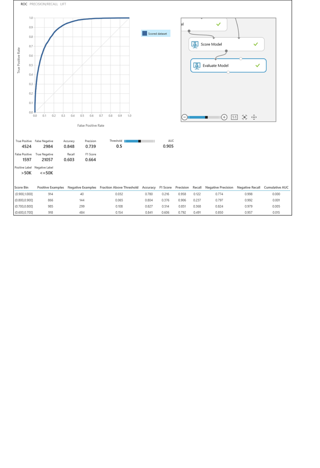
Using Cross ValidationUsing Cross Validation
Figure 7. Binary Classification Evaluation Results.
Another related metric that is often used is the F1 Score, which takes both precision and recall into consideration.
It is the harmonic mean of these 2 metrics and is computed as such: F1 = 2 (precision x recall) / (precision + recall).
The F1 score is a good way to summarize the evaluation in a single number, but it’s always a good practice to look
at both precision and recall together to better understand how a classifier behaves.
In addition, one can inspect the true positive rate vs. the false positive rate in the Receiver Operating
Characteristic (ROC) curve and the corresponding Area Under the Curve (AUC) value. The closer this curve is
to the upper left corner, the better the classifier’s performance is (that is maximizing the true positive rate while
minimizing the false positive rate). Curves that are close to the diagonal of the plot, result from classifiers that tend
to make predictions that are close to random guessing.
As in the regression example, we can perform cross validation to repeatedly train, score and evaluate different
subsets of the data automatically. Similarly, we can use the Cross-Validate Model module, an untrained logistic
regression model, and a dataset. The label column must be set to income in the Cross-Validate Model module’s
properties. After running the experiment and clicking on the right output port of the Cross-Validate Model module,
we can see the binary classification metric values for each fold, in addition to the mean and standard deviation of
each.
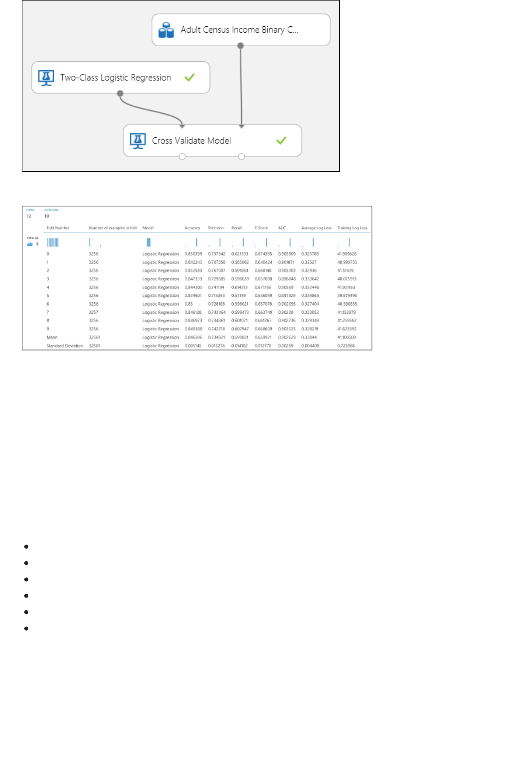
Evaluating a Multiclass Classification Model
Creating the ExperimentCreating the Experiment
Figure 8. Cross-Validating a Binary Classification Model.
Figure 9. Cross-Validation Results of a Binary Classifier.
In this experiment we will use the popular Iris dataset which contains instances of 3 different types (classes) of the
iris plant. There are 4 feature values (sepal length/width and petal length/width) for each instance. In the previous
experiments we trained and tested the models using the same datasets. Here, we will use the Split Data module to
create 2 subsets of the data, train on the first, and score and evaluate on the second. The Iris dataset is publicly
available on the UCI Machine Learning Repository, and can be downloaded using an Import Data module.
Add the following modules to your workspace in Azure Machine Learning Studio:
Import Data
Multiclass Decision Forest
Split Data
Train Model
Score Model
Evaluate Model
Connect the ports as shown below in Figure 10.
Set the Label column index of the Train Model module to 5. The dataset has no header row but we know that the
class labels are in the fifth column.
Click on the Import Data module and set the Data source property to Web URL via HTTP, and the URL to
http://archive.ics.uci.edu/ml/machine-learning-databases/iris/iris.data.
Set the fraction of instances to be used for training in the Split Data module (0.7 for example).
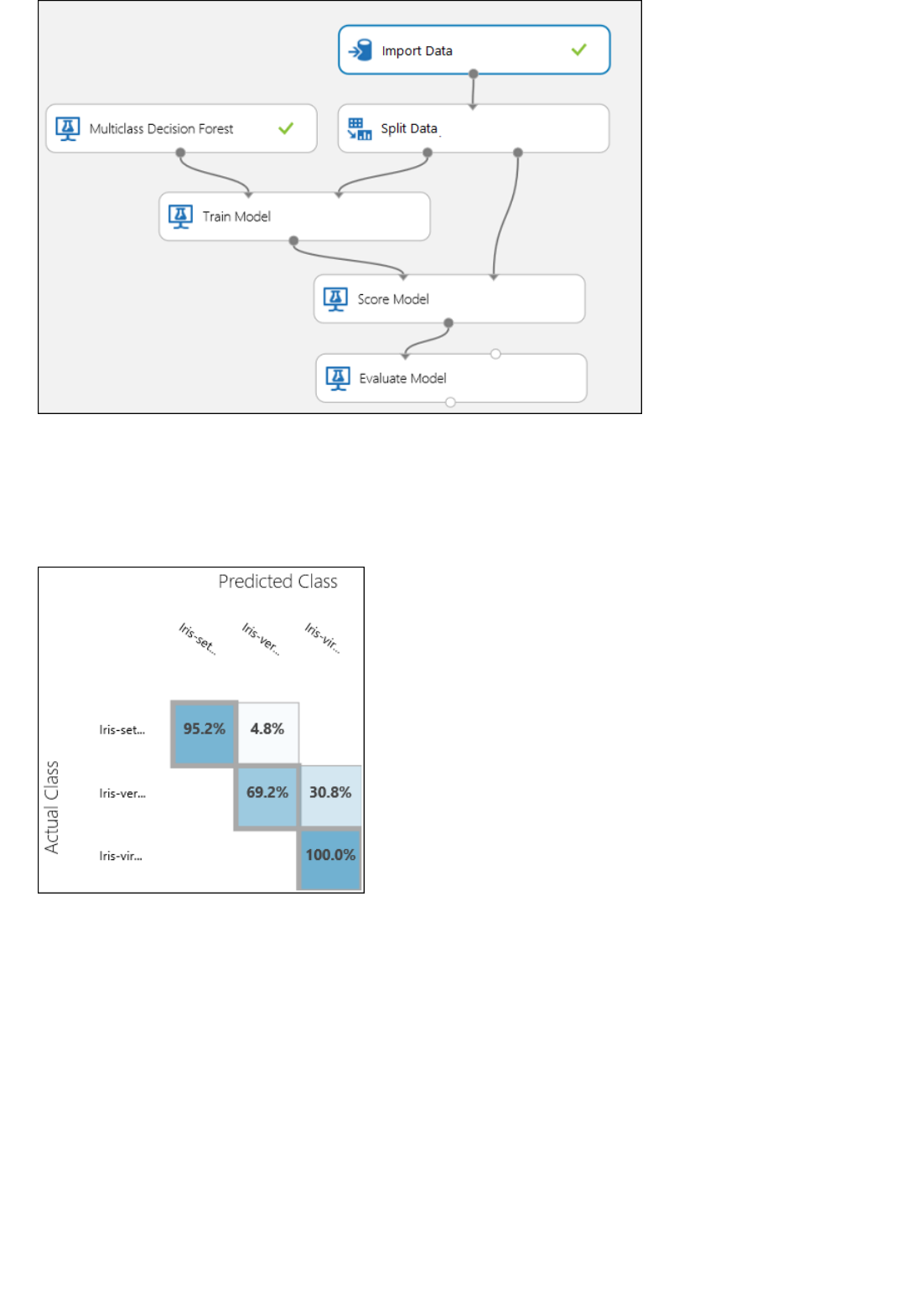
Inspecting the Evaluation ResultsInspecting the Evaluation Results
Using Cross ValidationUsing Cross Validation
Figure 10. Evaluating a Multiclass Classifier
Run the experiment and click on the output port of Evaluate Model. The evaluation results are presented in the
form of a confusion matrix, in this case. The matrix shows the actual vs. predicted instances for all 3 classes.
Figure 11. Multiclass Classification Evaluation Results.
As mentioned earlier, you can perform repeated training, scoring and evaluations automatically using the Cross-
Validate Model module. You would need a dataset, an untrained model, and a Cross-Validate Model module (see
figure below). Again you need to set the label column of the Cross-Validate Model module (column index 5 in this
case). After running the experiment and clicking the right output port of the Cross-Validate Model, you can inspect
the metric values for each fold as well as the mean and standard deviation. The metrics displayed here are the
similar to the ones discussed in the binary classification case. However, note that in multiclass classification,
computing the true positives/negatives and false positives/negatives is done by counting on a per-class basis, as
there is no overall positive or negative class. For example, when computing the precision or recall of the ‘Iris-
setosa’ class, it is assumed that this is the positive class and all others as negative.
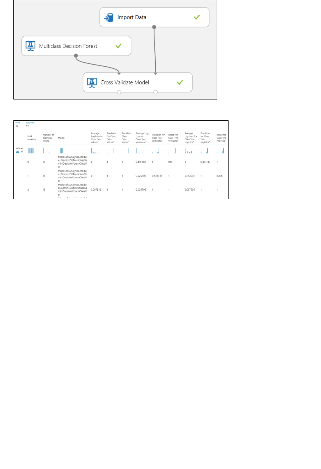
Figure 12. Cross-Validating a Multiclass Classification Model.
Figure 13. Cross-Validation Results of a Multiclass Classification Model.
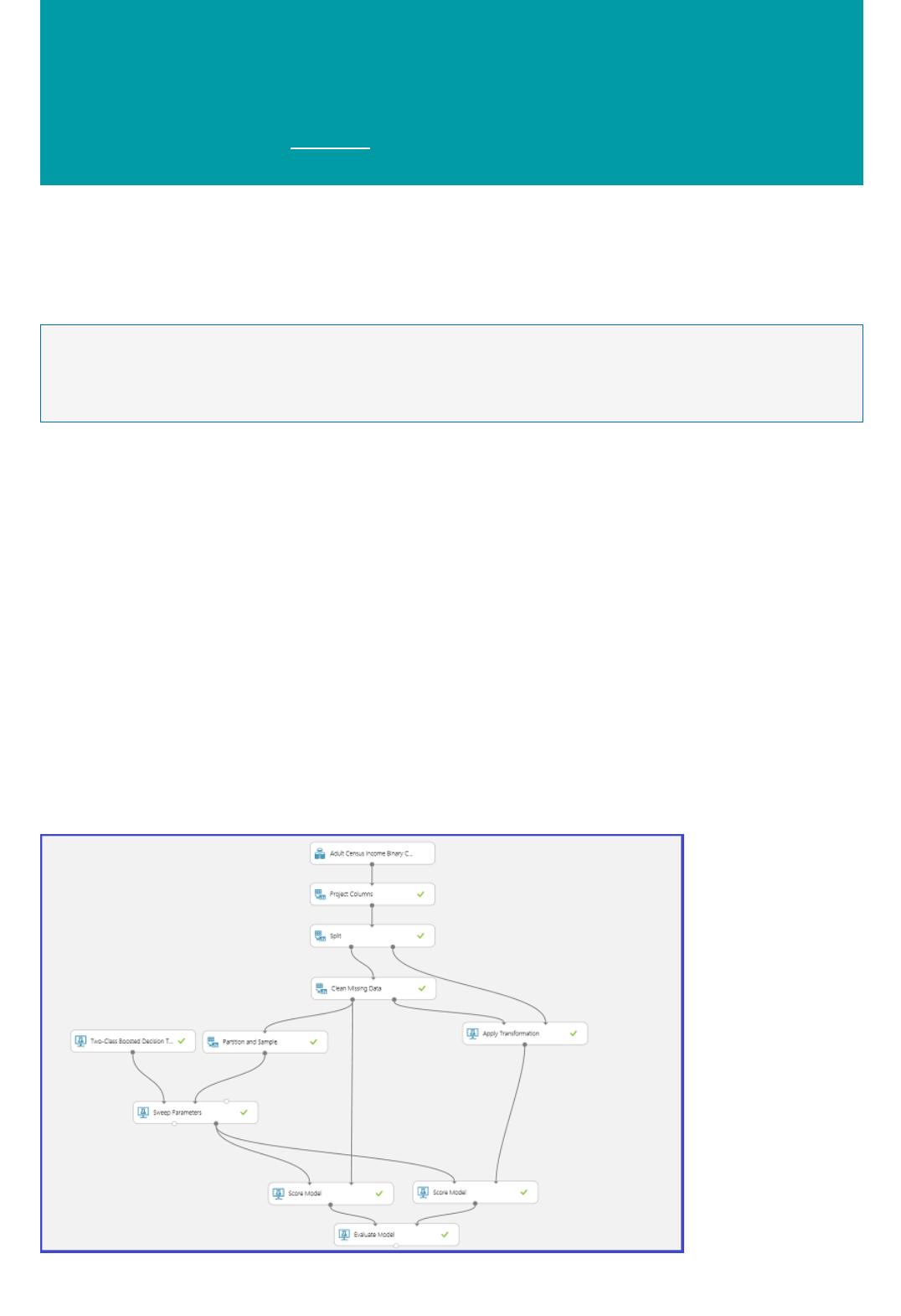
Choose parameters to optimize your algorithms in
Azure Machine Learning
3/20/2018 • 3 min to read • Edit Online
NOTENOTE
This topic describes how to choose the right hyperparameter set for an algorithm in Azure Machine Learning.
Most machine learning algorithms have parameters to set. When you train a model, you need to provide values for
those parameters. The efficacy of the trained model depends on the model parameters that you choose. The
process of finding the optimal set of parameters is known as model selection.
You can try Azure Machine Learning for free. No credit card or Azure subscription is required. Get started now.
There are various ways to do model selection. In machine learning, cross-validation is one of the most widely used
methods for model selection, and it is the default model selection mechanism in Azure Machine Learning. Because
Azure Machine Learning supports both R and Python, you can always implement their own model selection
mechanisms by using either R or Python.
There are four steps in the process of finding the best parameter set:
1. Define the parameter space: For the algorithm, first decide the exact parameter values you want to consider.
2. Define the cross-validation settings: Decide how to choose cross-validation folds for the dataset.
3. Define the metric: Decide what metric to use for determining the best set of parameters, such as accuracy,
root mean squared error, precision, recall, or f-score.
4. Train, evaluate, and compare: For each unique combination of the parameter values, cross-validation is
carried out by and based on the error metric you define. After evaluation and comparison, you can choose the
best-performing model.
The following image illustrates shows how this can be achieved in Azure Machine Learning.
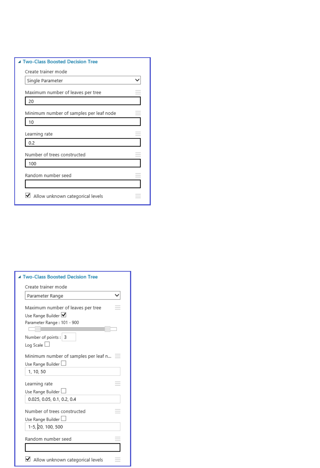
Define the parameter space
You can define the parameter set at the model initialization step. The parameter pane of all machine learning
algorithms has two trainer modes: Single Parameter and Parameter Range. Choose Parameter Range mode. In
Parameter Range mode, you can enter multiple values for each parameter. You can enter comma-separated values
in the text box.
Alternately, you can define the maximum and minimum points of the grid and the total number of points to be
generated with Use Range Builder. By default, the parameter values are generated on a linear scale. But if Log
Scale is checked, the values are generated in the log scale (that is, the ratio of the adjacent points is constant
instead of their difference). For integer parameters, you can define a range by using a hyphen. For example, “1-10”
means that all integers between 1 and 10 (both inclusive) form the parameter set. A mixed mode is also supported.
For example, the parameter set “1-10, 20, 50” would include integers 1-10, 20, and 50.
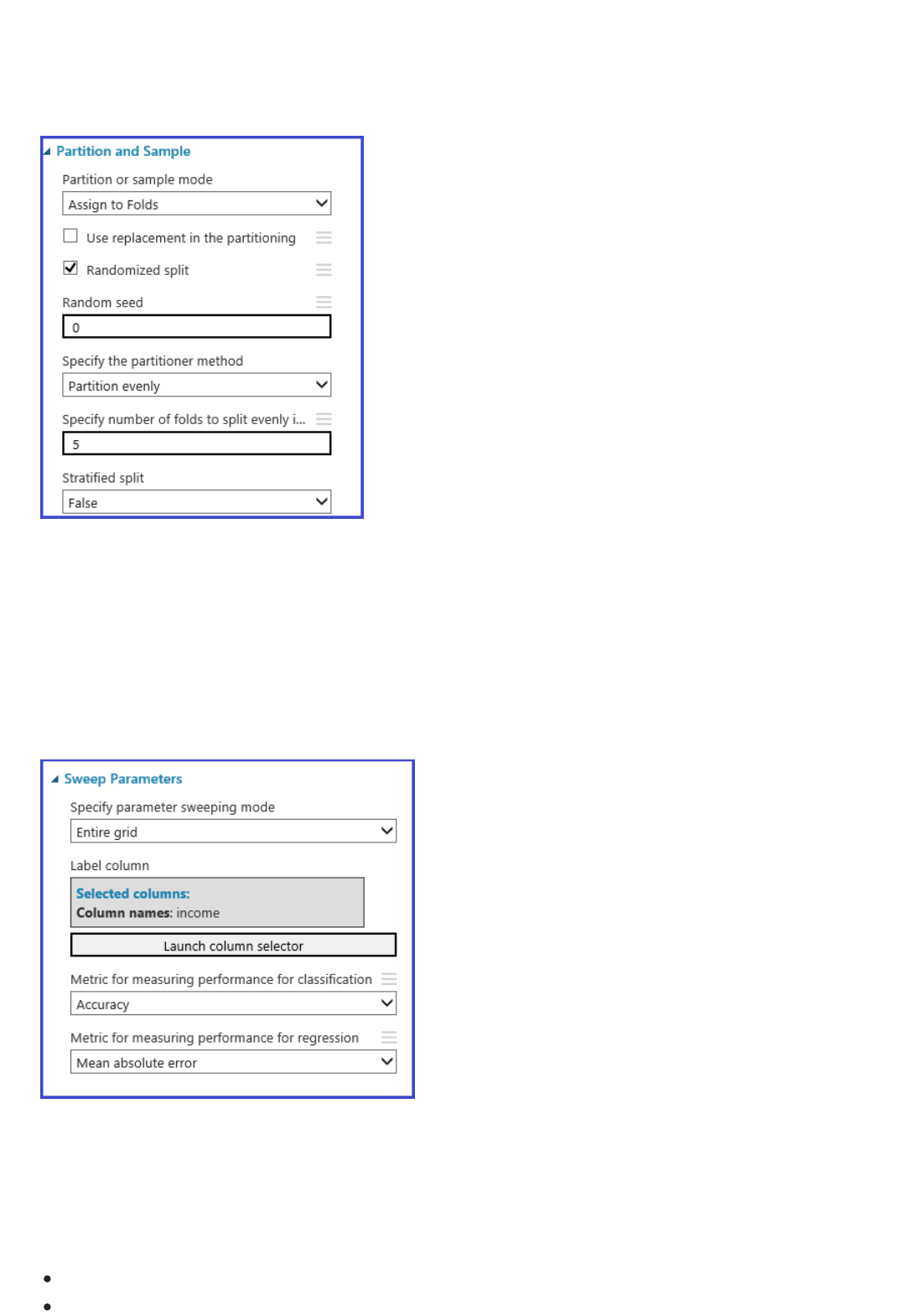
Define cross-validation folds
Define the metric
Train, evaluate, and compare
The Partition and Sample module can be used to randomly assign folds to the data. In the following sample
configuration for the module, we define five folds and randomly assign a fold number to the sample instances.
The Tune Model Hyperparameters module provides support for empirically choosing the best set of parameters
for a given algorithm and dataset. In addition to other information regarding training the model, the Properties
pane of this module includes the metric for determining the best parameter set. It has two different drop-down list
boxes for classification and regression algorithms, respectively. If the algorithm under consideration is a
classification algorithm, the regression metric is ignored and vice versa. In this specific example, the metric is
Accuracy.
The same Tune Model Hyperparameters module trains all the models that correspond to the parameter set,
evaluates various metrics, and then creates the best-trained model based on the metric you choose. This module
has two mandatory inputs:
The untrained learner
The dataset
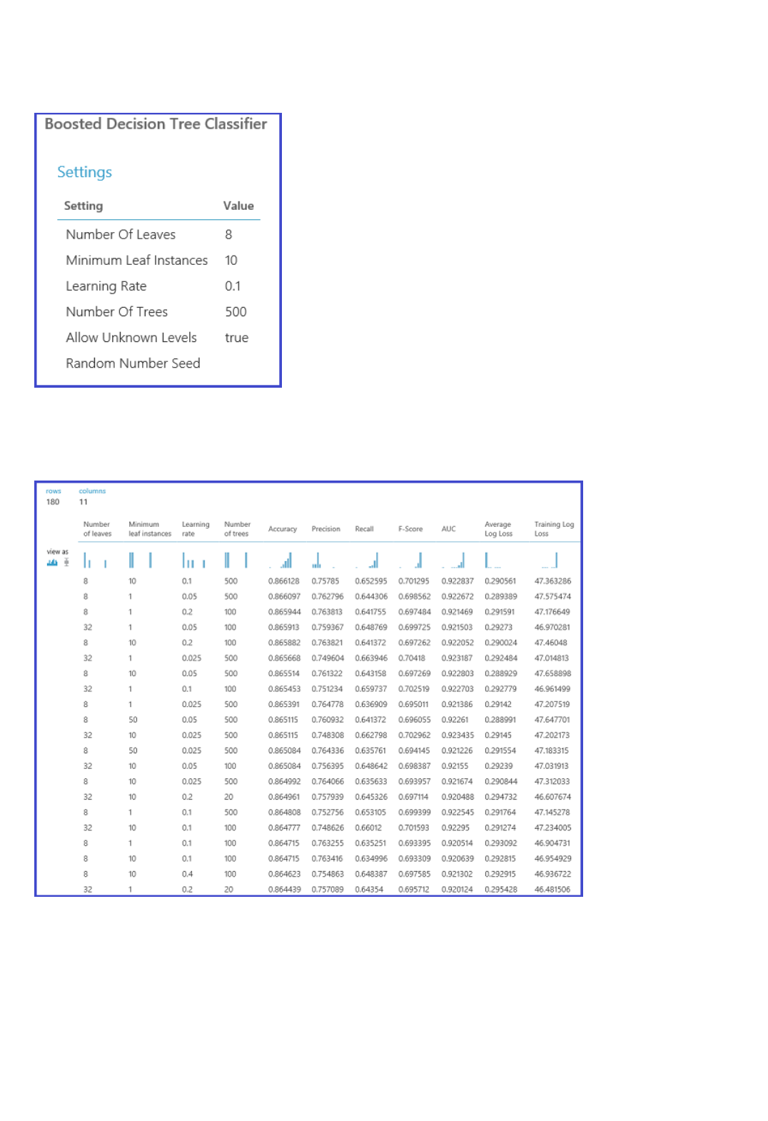
The module also has an optional dataset input. Connect the dataset with fold information to the mandatory dataset
input. If the dataset is not assigned any fold information, then a 10-fold cross-validation is automatically executed
by default. If the fold assignment is not done and a validation dataset is provided at the optional dataset port, then
a train-test mode is chosen and the first dataset is used to train the model for each parameter combination.
The model is then evaluated on the validation dataset. The left output port of the module shows different metrics
as functions of parameter values. The right output port gives the trained model that corresponds to the best-
performing model according to the chosen metric (Accuracy in this case).
You can see the exact parameters chosen by visualizing the right output port. This model can be used in scoring a
test set or in an operationalized web service after saving as a trained model.
Interpret model results in Azure Machine Learning
3/21/2018 • 13 min to read • Edit Online
NOTENOTE
Classification
Two-class classificationTwo-class classification
This topic explains how to visualize and interpret prediction results in Azure Machine Learning Studio. After you
have trained a model and done predictions on top of it ("scored the model"), you need to understand and interpret
the prediction result.
You can try Azure Machine Learning for free. No credit card or Azure subscription is required. Get started now.
There are four major kinds of machine learning models in Azure Machine Learning:
Classification
Clustering
Regression
Recommender systems
The modules used for prediction on top of these models are:
Score Model module for classification and regression
Assign to Clusters module for clustering
Score Matchbox Recommender for recommendation systems
This document explains how to interpret prediction results for each of these modules. For an overview of these
modules, see How to choose parameters to optimize your algorithms in Azure Machine Learning.
This topic addresses prediction interpretation but not model evaluation. For more information about how to
evaluate your model, see How to evaluate model performance in Azure Machine Learning.
If you are new to Azure Machine Learning and need help creating a simple experiment to get started, see Create a
simple experiment in Azure Machine Learning Studio in Azure Machine Learning Studio.
There are two subcategories of classification problems:
Problems with only two classes (two-class or binary classification)
Problems with more than two classes (multi-class classification)
Azure Machine Learning has different modules to deal with each of these types of classification, but the methods
for interpreting their prediction results are similar.
Example experiment
An example of a two-class classification problem is the classification of iris flowers. The task is to classify iris
flowers based on their features. The Iris data set provided in Azure Machine Learning is a subset of the popular Iris
data set containing instances of only two flower species (classes 0 and 1). There are four features for each flower
(sepal length, sepal width, petal length, and petal width).
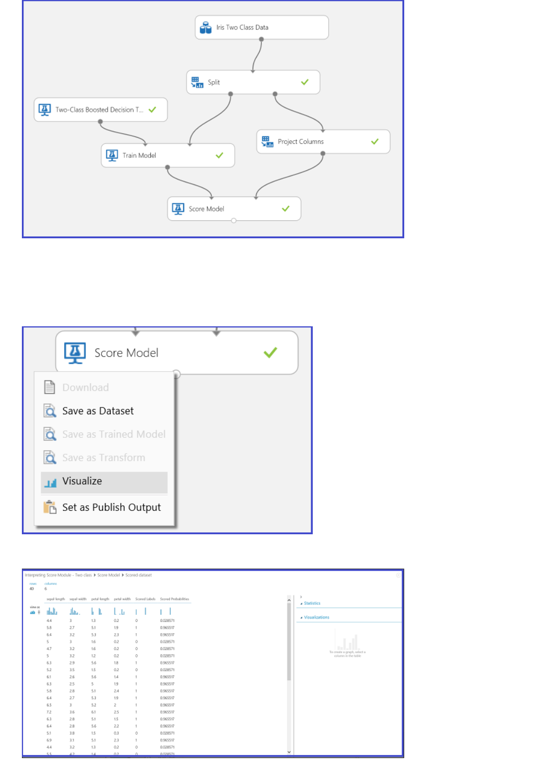
Figure 1. Iris two-class classification problem experiment
An experiment has been performed to solve this problem, as shown in Figure 1. A two-class boosted decision tree
model has been trained and scored. Now you can visualize the prediction results from the Score Model module by
clicking the output port of the Score Model module and then clicking Visualize.
This brings up the scoring results as shown in Figure 2.
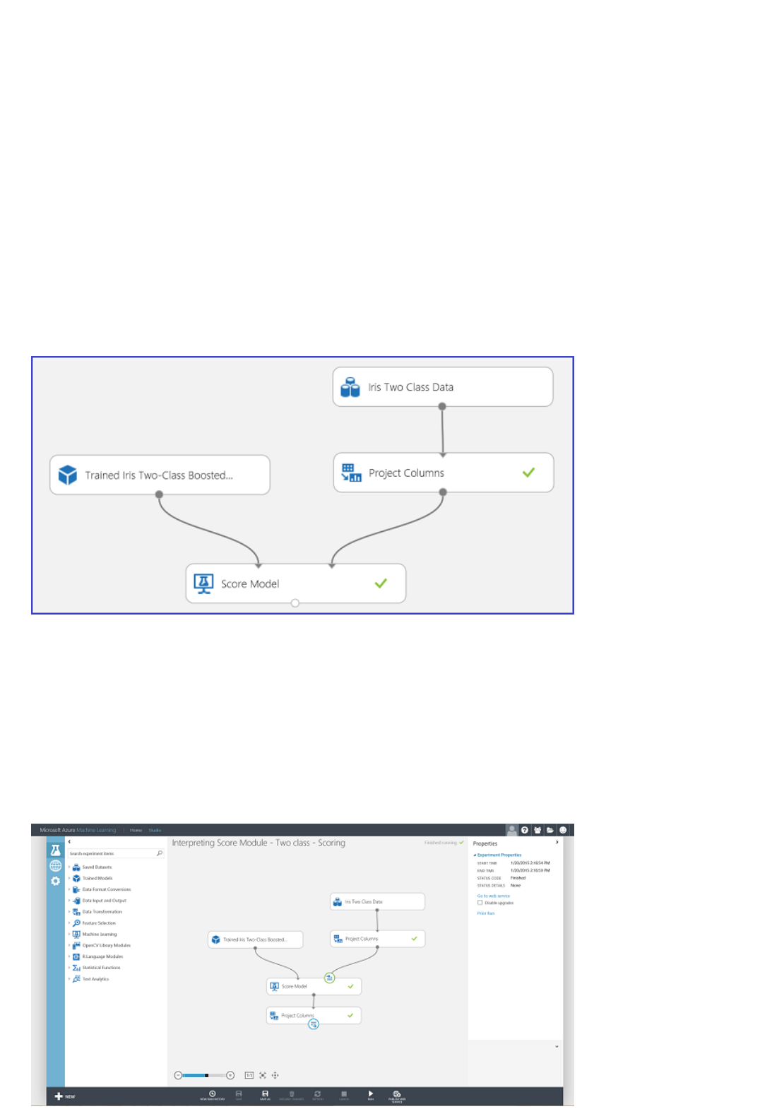
Figure 2. Visualize a score model result in two-class classification
Result interpretation
There are six columns in the results table. The left four columns are the four features. The right two columns,
Scored Labels and Scored Probabilities, are the prediction results. The Scored Probabilities column shows the
probability that a flower belongs to the positive class (Class 1). For example, the first number in the column
(0.028571) means there is 0.028571 probability that the first flower belongs to Class 1. The Scored Labels column
shows the predicted class for each flower. This is based on the Scored Probabilities column. If the scored
probability of a flower is larger than 0.5, it is predicted as Class 1. Otherwise, it is predicted as Class 0.
Web service publication
After the prediction results have been understood and judged sound, the experiment can be published as a web
service so that you can deploy it in various applications and call it to obtain class predictions on any new iris flower.
To learn how to change a training experiment into a scoring experiment and publish it as a web service, see Publish
the Azure Machine Learning web service. This procedure provides you with a scoring experiment as shown in
Figure 3.
Figure 3. Scoring the iris two-class classification problem experiment
Now you need to set the input and output for the web service. The input is the right input port of Score Model,
which is the Iris flower features input. The choice of the output depends on whether you are interested in the
predicted class (scored label), the scored probability, or both. In this example, it is assumed that you are interested
in both. To select the desired output columns, use a Select Columns in Data set module. Click Select Columns in
Data set, click Launch column selector, and select Scored Labels and Scored Probabilities. After setting the
output port of Select Columns in Data set and running it again, you should be ready to publish the scoring
experiment as a web service by clicking PUBLISH WEB SERVICE. The final experiment looks like Figure 4.
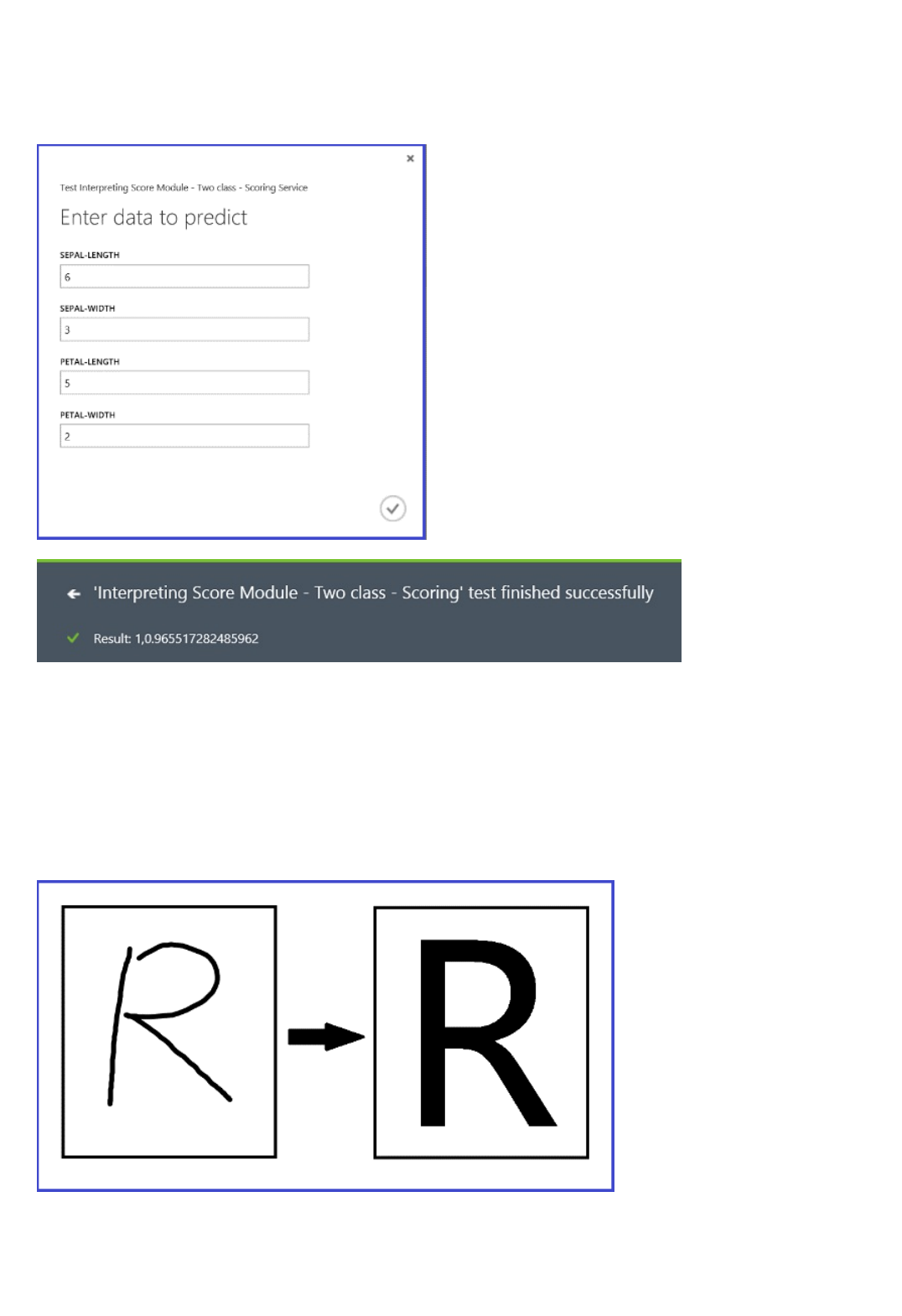
Multi-class classificationMulti-class classification
Figure 4. Final scoring experiment of an iris two-class classification problem
After you run the web service and enter some feature values of a test instance, the result returns two numbers. The
first number is the scored label, and the second is the scored probability. This flower is predicted as Class 1 with
0.9655 probability.
Figure 5. Web service result of iris two-class classification
Example experiment
In this experiment, you perform a letter-recognition task as an example of multiclass classification. The classifier
attempts to predict a certain letter (class) based on some hand-written attribute values extracted from the hand-
written images.
In the training data, there are 16 features extracted from hand-written letter images. The 26 letters form our 26
classes. Figure 6 shows an experiment that will train a multiclass classification model for letter recognition and
predict on the same feature set on a test data set.
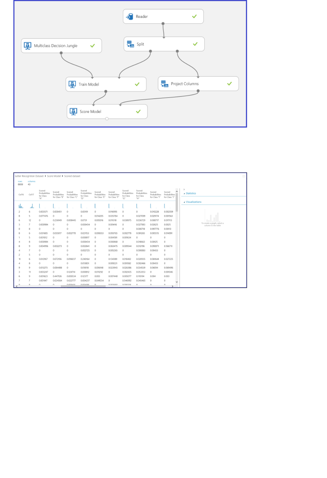
Figure 6. Letter recognition multiclass classification problem experiment
Visualizing the results from the Score Model module by clicking the output port of Score Model module and then
clicking Visualize, you should see content as shown in Figure 7.
Figure 7. Visualize score model results in a multi-class classification
Result interpretation
The left 16 columns represent the feature values of the test set. The columns with names like Scored Probabilities
for Class "XX" are just like the Scored Probabilities column in the two-class case. They show the probability that the
corresponding entry falls into a certain class. For example, for the first entry, there is 0.003571 probability that it is
an “A,” 0.000451 probability that it is a “B,” and so forth. The last column (Scored Labels) is the same as Scored
Labels in the two-class case. It selects the class with the largest scored probability as the predicted class of the
corresponding entry. For example, for the first entry, the scored label is “F” since it has the largest probability to be
an “F” (0.916995).
Web service publication
You can also get the scored label for each entry and the probability of the scored label. The basic logic is to find the
largest probability among all the scored probabilities. To do this, you need to use the Execute R Script module. The
R code is shown in Figure 8, and the result of the experiment is shown in Figure 9.
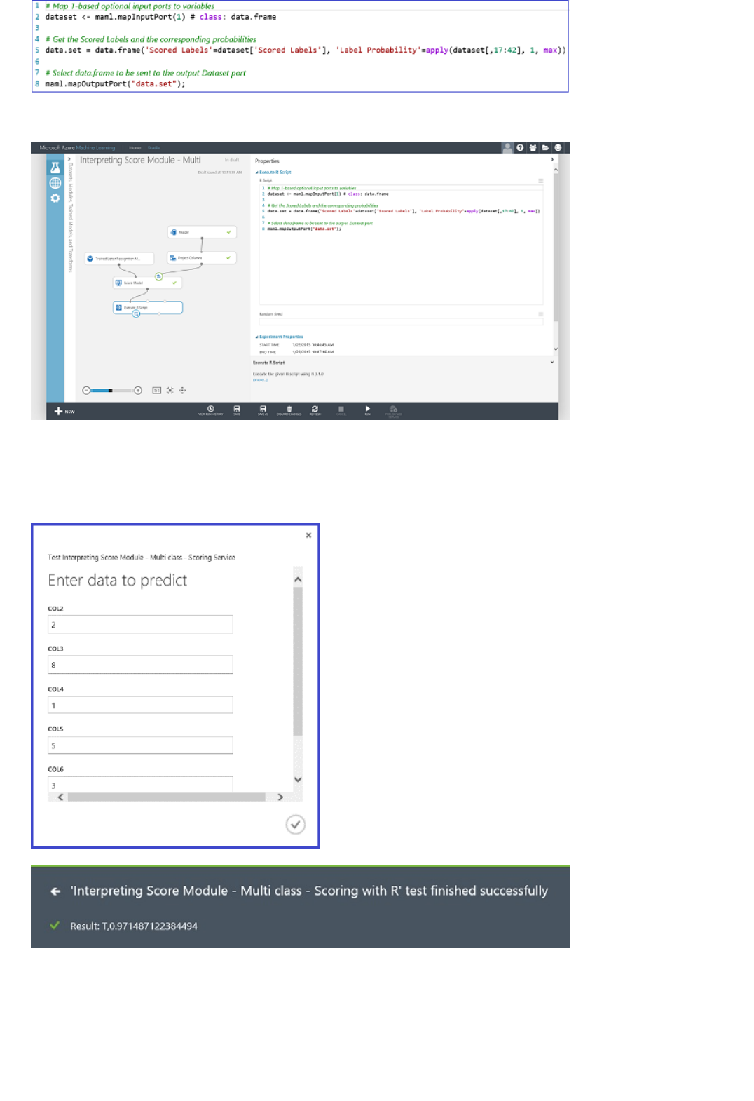
Regression
Figure 8. R code for extracting Scored Labels and the associated probabilities of the labels
Figure 9. Final scoring experiment of the letter-recognition multiclass classification problem
After you publish and run the web service and enter some input feature values, the returned result looks like Figure
10. This hand-written letter, with its extracted 16 features, is predicted to be a “T” with 0.9715 probability.
Figure 10. Web service result of multiclass classification
Regression problems are different from classification problems. In a classification problem, you're trying to predict
discrete classes, such as which class an iris flower belongs to. But as you can see in the following example of a
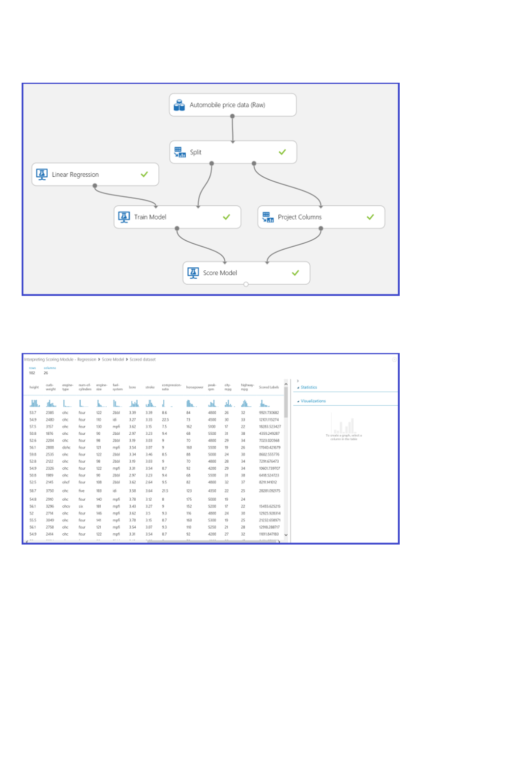
regression problem, you're trying to predict a continuous variable, such as the price of a car.
Example experiment
Use automobile price prediction as your example for regression. You are trying to predict the price of a car based
on its features, including make, fuel type, body type, and drive wheel. The experiment is shown in Figure 11.
Figure 11. Automobile price regression problem experiment
Visualizing the Score Model module, the result looks like Figure 12.
Figure 12. Scoring result for the automobile price prediction problem
Result interpretation
Scored Labels is the result column in this scoring result. The numbers are the predicted price for each car.
Web service publication
You can publish the regression experiment into a web service and call it for automobile price prediction in the same
way as in the two-class classification use case.
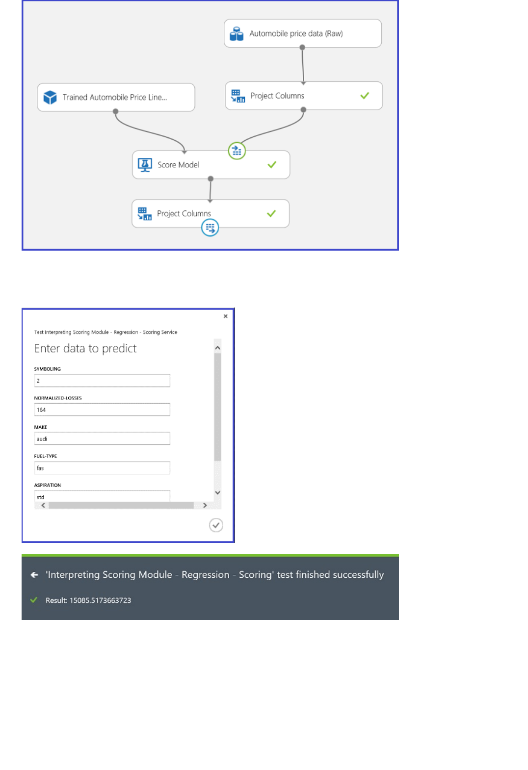
Clustering
Figure 13. Scoring experiment of an automobile price regression problem
Running the web service, the returned result looks like Figure 14. The predicted price for this car is $15,085.52.
Figure 14. Web service result of an automobile price regression problem
Example experiment
Let’s use the Iris data set again to build a clustering experiment. Here you can filter out the class labels in the data
set so that it only has features and can be used for clustering. In this iris use case, specify the number of clusters to
be two during the training process, which means you would cluster the flowers into two classes. The experiment is
shown in Figure 15.
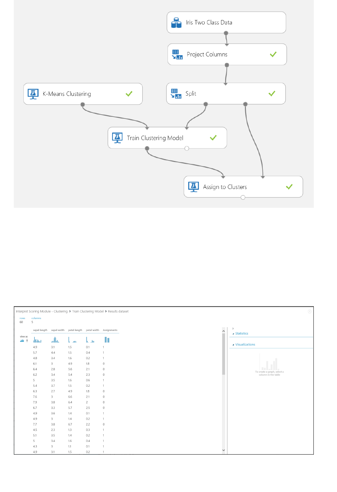
Figure 15. Iris clustering problem experiment
Clustering differs from classification in that the training data set doesn’t have ground-truth labels by itself.
Clustering groups the training data set instances into distinct clusters. During the training process, the model labels
the entries by learning the differences between their features. After that, the trained model can be used to further
classify future entries. There are two parts of the result we are interested in within a clustering problem. The first
part is labeling the training data set, and the second is classifying a new data set with the trained model.
The first part of the result can be visualized by clicking the left output port of Train Clustering Model and then
clicking Visualize. The visualization is shown in Figure 16.
Figure 16. Visualize clustering result for the training data set
The result of the second part, clustering new entries with the trained clustering model, is shown in Figure 17.
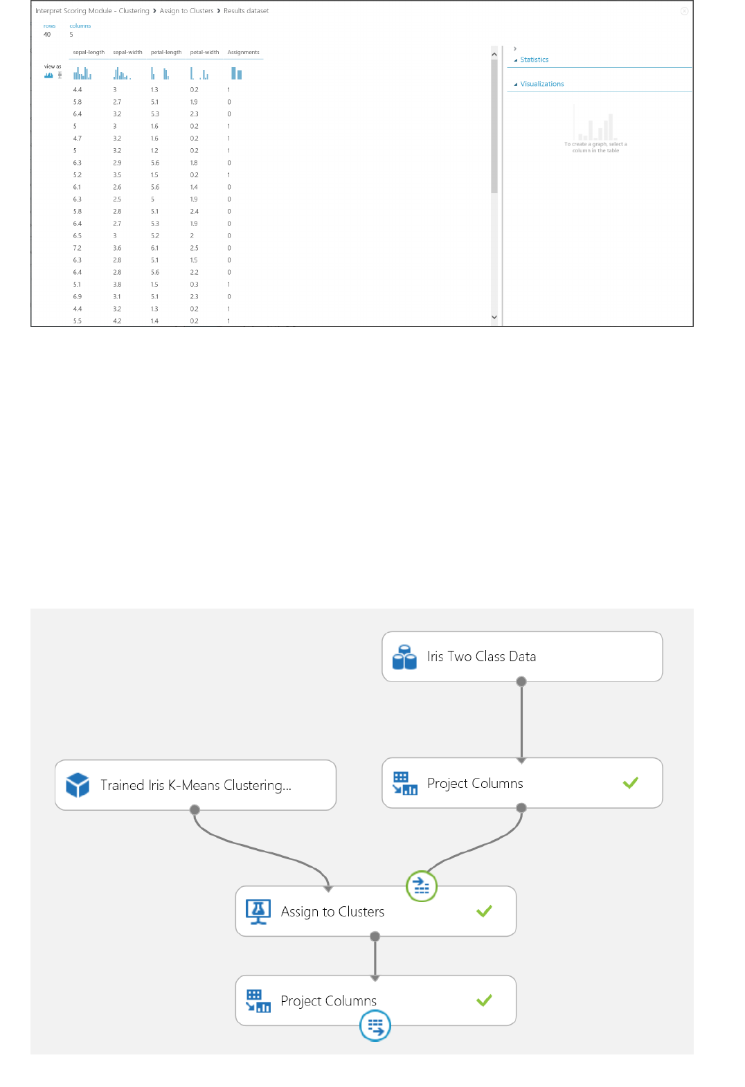
Figure 17. Visualize clustering result on a new data set
Result interpretation
Although the results of the two parts stem from different experiment stages, they look the same and are
interpreted in the same way. The first four columns are features. The last column, Assignments, is the prediction
result. The entries assigned the same number are predicted to be in the same cluster, that is, they share similarities
in some way (this experiment uses the default Euclidean distance metric). Because you specified the number of
clusters to be 2, the entries in Assignments are labeled either 0 or 1.
Web service publication
You can publish the clustering experiment into a web service and call it for clustering predictions the same way as
in the two-class classification use case.
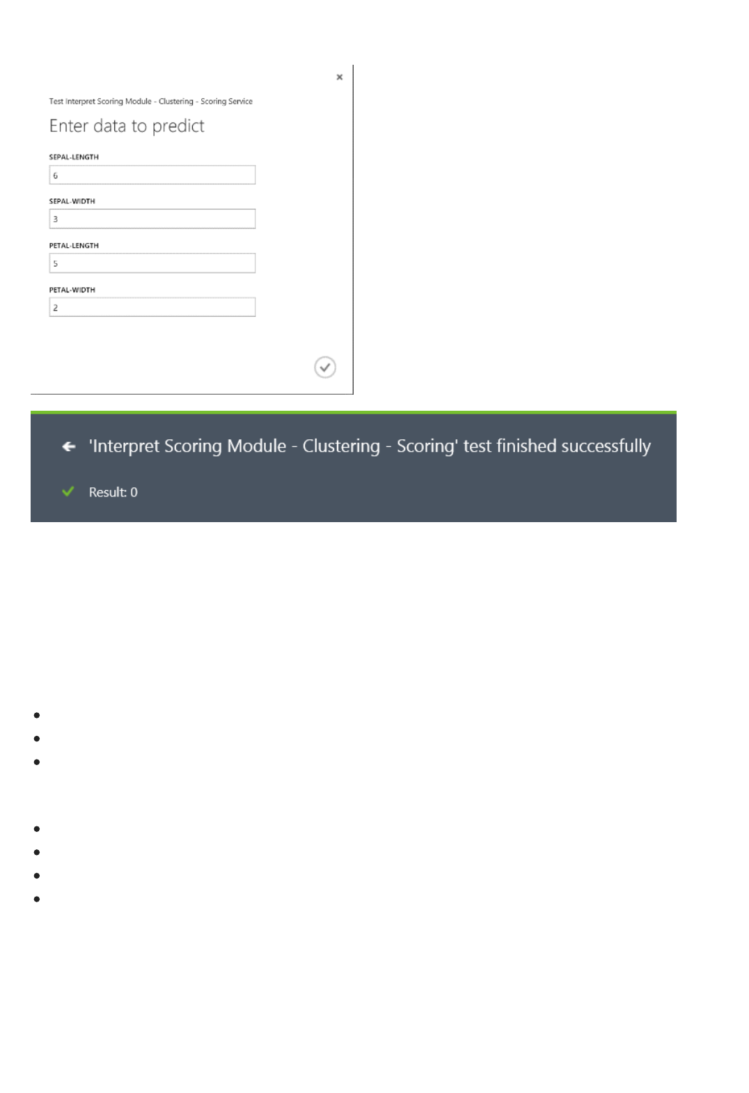
Recommender system
Figure 18. Scoring experiment of an iris clustering problem
After you run the web service, the returned result looks like Figure 19. This flower is predicted to be in cluster 0.
Figure 19. Web service result of iris two-class classification
Example experiment
For recommender systems, you can use the restaurant recommendation problem as an example: you can
recommend restaurants for customers based on their rating history. The input data consists of three parts:
Restaurant ratings from customers
Customer feature data
Restaurant feature data
There are several things we can do with the Train Matchbox Recommender module in Azure Machine Learning:
Predict ratings for a given user and item
Recommend items to a given user
Find users related to a given user
Find items related to a given item
You can choose what you want to do by selecting from the four options in the Recommender prediction kind
menu. Here you can walk through all four scenarios.
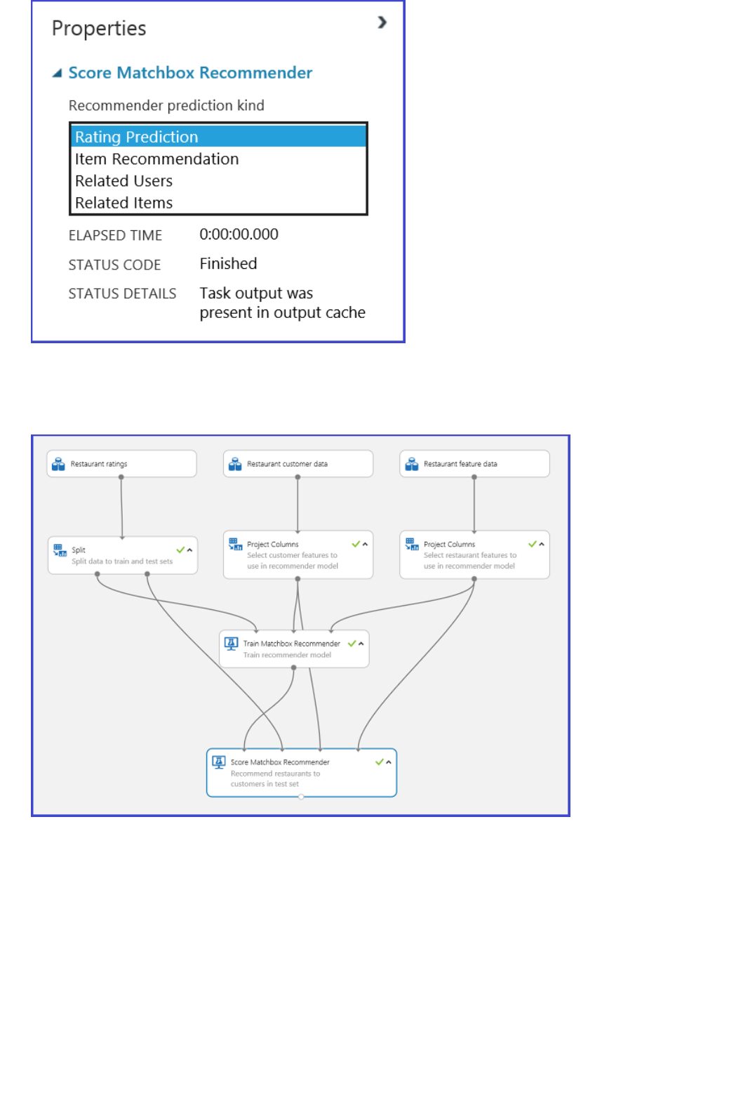
A typical Azure Machine Learning experiment for a recommender system looks like Figure 20. For information
about how to use those recommender system modules, see Train matchbox recommender and Score matchbox
recommender.
Figure 20. Recommender system experiment
Result interpretation
Predict ratings for a given user and item
By selecting Rating Prediction under Recommender prediction kind, you are asking the recommender system
to predict the rating for a given user and item. The visualization of the Score Matchbox Recommender output looks
like Figure 21.
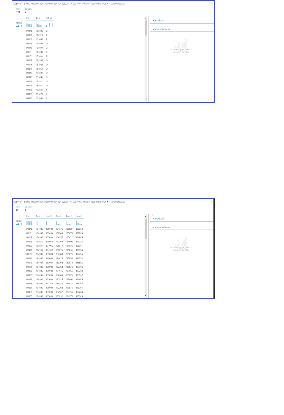
Figure 21. Visualize the score result of the recommender system--rating prediction
The first two columns are the user-item pairs provided by the input data. The third column is the predicted rating of
a user for a certain item. For example, in the first row, customer U1048 is predicted to rate restaurant 135026 as 2.
Recommend items to a given user
By selecting Item Recommendation under Recommender prediction kind, you're asking the recommender
system to recommend items to a given user. The last parameter to choose in this scenario is Recommended item
selection. The option From Rated Items (for model evaluation) is primarily for model evaluation during the
training process. For this prediction stage, we choose From All Items. The visualization of the Score Matchbox
Recommender output looks like Figure 22.
Figure 22. Visualize score result of the recommender system--item recommendation
The first of the six columns represents the given user IDs to recommend items for, as provided by the input data.
The other five columns represent the items recommended to the user in descending order of relevance. For
example, in the first row, the most recommended restaurant for customer U1048 is 134986, followed by 135018,
134975, 135021, and 132862.
Find users related to a given user
By selecting Related Users under Recommender prediction kind, you're asking the recommender system to
find related users to a given user. Related users are the users who have similar preferences. The last parameter to
choose in this scenario is Related user selection. The option From Users That Rated Items (for model
evaluation) is primarily for model evaluation during the training process. Choose From All Users for this
prediction stage. The visualization of the Score Matchbox Recommender output looks like Figure 23.
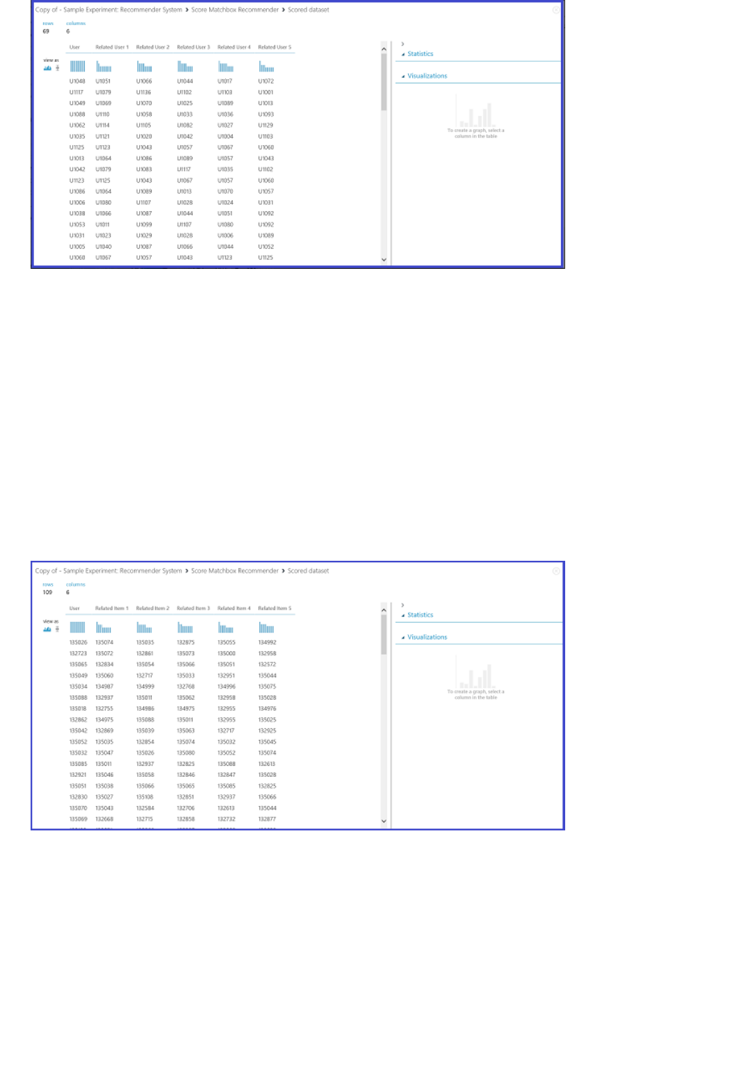
Figure 23. Visualize score results of the recommender system--related users
The first of the six columns shows the given user IDs needed to find related users, as provided by input data. The
other five columns store the predicted related users of the user in descending order of relevance. For example, in
the first row, the most relevant customer for customer U1048 is U1051, followed by U1066, U1044, U1017, and
U1072.
Find items related to a given item
By selecting Related Items under Recommender prediction kind, you are asking the recommender system to
find related items to a given item. Related items are the items most likely to be liked by the same user. The last
parameter to choose in this scenario is Related item selection. The option From Rated Items (for model
evaluation) is primarily for model evaluation during the training process. We choose From All Items for this
prediction stage. The visualization of the Score Matchbox Recommender output looks like Figure 24.
Figure 24. Visualize score results of the recommender system--related items
The first of the six columns represents the given item IDs needed to find related items, as provided by the input
data. The other five columns store the predicted related items of the item in descending order in terms of relevance.
For example, in the first row, the most relevant item for item 135026 is 135074, followed by 135035, 132875,
135055, and 134992.
Web service publication
The process of publishing these experiments as web services to get predictions is similar for each of the four
scenarios. Here we take the second scenario (recommend items to a given user) as an example. You can follow the
same procedure with the other three.
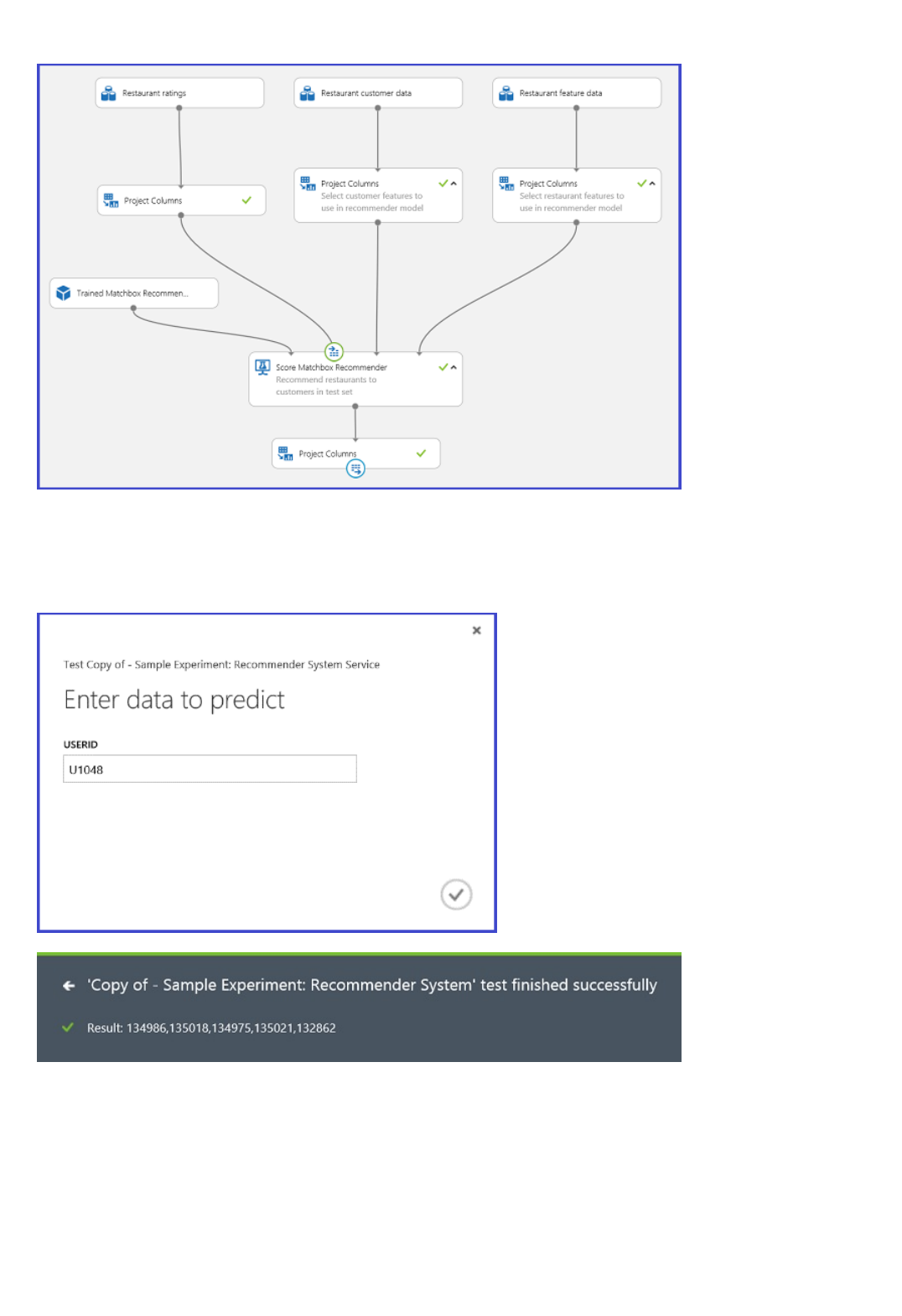
Saving the trained recommender system as a trained model and filtering the input data to a single user ID column
as requested, you can hook up the experiment as in Figure 25 and publish it as a web service.
Figure 25. Scoring experiment of the restaurant recommendation problem
Running the web service, the returned result looks like Figure 26. The five recommended restaurants for user
U1048 are 134986, 135018, 134975, 135021, and 132862.
Figure 26. Web service result of restaurant recommendation problem
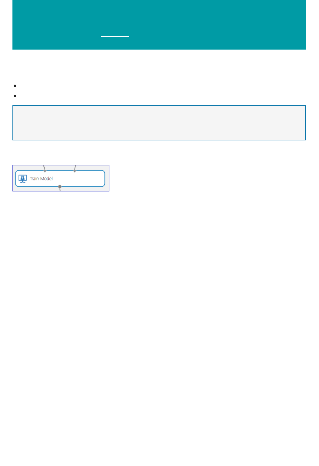
Debug your Model in Azure Machine Learning
3/20/2018 • 2 min to read • Edit Online
NOTENOTE
Train Model Module produces an error
Score Model Module produces incorrect results
This article explains the potential reasons why either of the following two failures might be encountered when
running a model:
the Train Model module produces an error
the Score Model module produces incorrect results
You can try Azure Machine Learning for free. No credit card or Azure subscription is required. Get started now.
The Train Model Module expects two inputs:
1. The type of machine learning model from the collection of models provided by Azure Machine Learning.
2. The training data with a specified Label column which specifies the variable to predict (the other columns are
assumed to be Features).
This module can produce an error in the following cases:
1. The Label column is specified incorrectly. This can happen if either more than one column is selected as the
Label or an incorrect column index is selected. For example, the second case would apply if a column index
of 30 is used with an input dataset which has only 25 columns.
2. The dataset does not contain any Feature columns. For example, if the input dataset has only one column,
which is marked as the Label column, there would be no features with which to build the model. In this case,
the Train Model module produces an error.
3. The input dataset (Features or Label) contains Infinity as a value.

In a typical training/testing experiment for supervised learning, the Split Data module divides the original dataset
into two parts: one part is used to train the model and one part is used to score how well the trained model
performs. The trained model is then used to score the test data, after which the results are evaluated to determine
the accuracy of the model.
The Score Model module requires two inputs:
1. A trained model output from the Train Model module.
2. A scoring dataset that is different from the dataset used to train the model.
It's possible that even though the experiment succeeds, the Score Model module produces incorrect results. Several
scenarios may cause this to happen:
1. If the specified Label is categorical and a regression model is trained on the data, an incorrect output would
be produced by the Score Model module. This is because regression requires a continuous response
variable. In this case, it would be more suitable to use a classification model.
2. Similarly, if a classification model is trained on a dataset having floating point numbers in the Label column,
it may produce undesirable results. This is because classification requires a discrete response variable that
only allows values that range over a finite, and usually somewhat small, set of classes.
3. If the scoring dataset does not contain all the features used to train the model, the Score Model produces an
error.
4. If a row in the scoring dataset contains a missing value or an infinite value for any of its features, the Score
Model will not produce any output corresponding to that row.
5. The Score Model may produce identical outputs for all rows in the scoring dataset. This could occur, for
example, when attempting classification using Decision Forests if the minimum number of samples per leaf
node is chosen to be more than the number of training examples available.
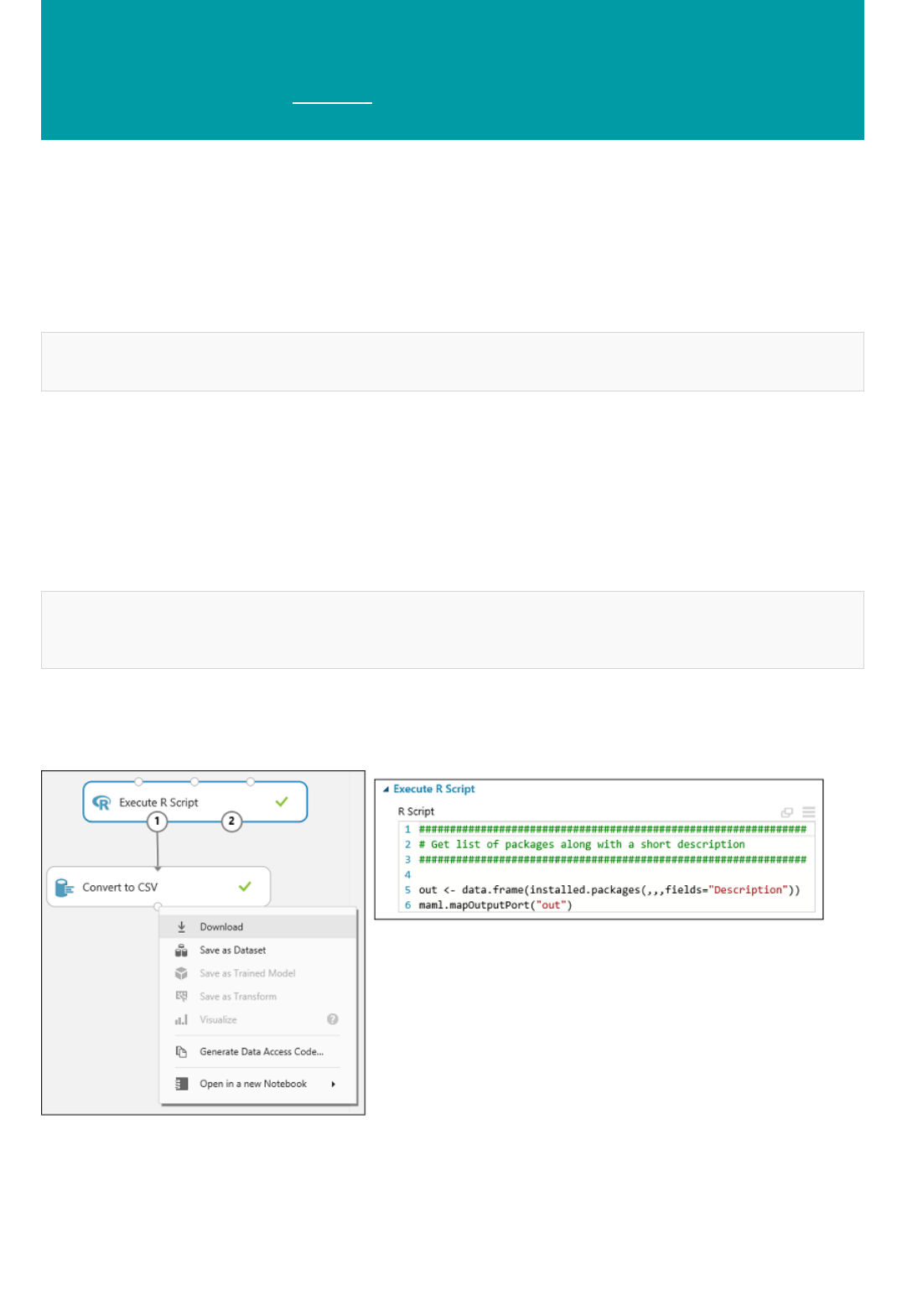
Extend your experiment with R
3/21/2018 • 1 min to read • Edit Online
dataset1 <- maml.mapInputPort(1)
Listing all currently-installed packages
out <- data.frame(installed.packages(,,,fields="Description"))
maml.mapOutputPort("out")
Importing packages
You can extend the functionality of Azure Machine Learning Studio through the R language by using the Execute R
Script module.
This module accepts multiple input datasets and yields a single dataset as output. You can type an R script into the
R Script parameter of the Execute R Script module.
You access each input port of the module by using code similar to the following:
The list of installed packages can change. A list of currently installed packages can be found in R Packages
Supported by Azure Machine Learning.
You also can get the complete, current list of installed packages by entering the following code into the Execute R
Script module:
This sends the list of packages to the output port of the Execute R Script module. To view the package list, connect
a conversion module such as Convert to CSV to the left output of the Execute R Script module, run the
experiment, then click the output of the conversion module and select Download.
You can import packages that are not already installed by using the following commands in the Execute R Script
module:

install.packages("src/my_favorite_package.zip", lib = ".", repos = NULL, verbose = TRUE)
success <- library("my_favorite_package", lib.loc = ".", logical.return = TRUE, verbose = TRUE)
NOTENOTE
where the my_favorite_package.zip file contains your package.
You can try Azure Machine Learning for free. No credit card or Azure subscription is required. Get started now.

Author custom R modules in Azure Machine Learning
3/20/2018 • 16 min to read • Edit Online
NOTENOTE
What is a custom R module?
Files in a custom R module
Quickstart example: define, package, and register a custom R module
The source file
This topic describes how to author and deploy a custom R module in Azure Machine Learning. It explains what
custom R modules are and what files are used to define them. It illustrates how to construct the files that define a
module and how to register the module for deployment in a Machine Learning workspace. The elements and
attributes used in the definition of the custom module are then described in more detail. How to use auxiliary
functionality and files and multiple outputs is also discussed.
You can try Azure Machine Learning for free. No credit card or Azure subscription is required. Get started now.
A custom module is a user-defined module that can be uploaded to your workspace and executed as part of an
Azure Machine Learning experiment. A custom R module is a custom module that executes a user-defined R
function. R is a programming language for statistical computing and graphics that is widely used by statisticians
and data scientists for implementing algorithms. Currently, R is the only language supported in custom modules,
but support for additional languages is scheduled for future releases.
Custom modules have first-class status in Azure Machine Learning in the sense that they can be used just like any
other module. They can be executed with other modules, included in published experiments or in visualizations.
You have control over the algorithm implemented by the module, the input and output ports to be used, the
modeling parameters, and other various runtime behaviors. An experiment that contains custom modules can also
be published into the Azure AI Gallery for easy sharing.
A custom R module is defined by a .zip file that contains, at a minimum, two files:
A source file that implements the R function exposed by the module
An XML definition file that describes the custom module interface
Additional auxiliary files can also be included in the .zip file that provides functionality that can be accessed from
the custom module. This option is discussed in the Arguments part of the reference section Elements in the
XML definition file following the quickstart example.
This example illustrates how to construct the files required by a custom R module, package them into a zip file, and
then register the module in your Machine Learning workspace. The example zip package and sample files can be
downloaded from Download CustomAddRows.zip file.
Consider the example of a Custom Add Rows module that modifies the standard implementation of the Add
Rows module used to concatenate rows (observations) from two datasets (data frames). The standard Add Rows
module appends the rows of the second input dataset to the end of the first input dataset using the rbind
algorithm. The customized CustomAddRows function similarly accepts two datasets, but also accepts a Boolean swap

CustomAddRows <- function(dataset1, dataset2, swap=FALSE)
{
if (swap)
{
return (rbind(dataset2, dataset1));
}
else
{
return (rbind(dataset1, dataset2));
}
}
The XML definition fileThe XML definition file
<!-- Defined a module using an R Script -->
<Module name="Custom Add Rows">
<Owner>Microsoft Corporation</Owner>
<Description>Appends one dataset to another. Dataset 2 is concatenated to Dataset 1 when Swap is FALSE, and
vice versa when Swap is TRUE.</Description>
<!-- Specify the base language, script file and R function to use for this module. -->
<Language name="R"
sourceFile="CustomAddRows.R"
entryPoint="CustomAddRows" />
<!-- Define module input and output ports -->
<!-- Note: The values of the id attributes in the Input and Arg elements must match the parameter names in the
R Function CustomAddRows defined in CustomAddRows.R. -->
<Ports>
<Input id="dataset1" name="Dataset 1" type="DataTable">
<Description>First input dataset</Description>
</Input>
<Input id="dataset2" name="Dataset 2" type="DataTable">
<Description>Second input dataset</Description>
</Input>
<Output id="dataset" name="Dataset" type="DataTable">
<Description>The combined dataset</Description>
</Output>
</Ports>
<!-- Define module parameters -->
<Arguments>
<Arg id="swap" name="Swap" type="bool" >
<Description>Swap input datasets.</Description>
</Arg>
</Arguments>
</Module>
parameter as an additional input. If the swap parameter is set to FALSE, it returns the same data set as the
standard implementation. But if the swap parameter is TRUE, the function appends rows of first input dataset to
the end of the second dataset instead. The CustomAddRows.R file that contains the implementation of the R
CustomAddRows function exposed by the Custom Add Rows module has the following R code.
To expose this CustomAddRows function as an Azure Machine Learning module, an XML definition file must be
created to specify how the Custom Add Rows module should look and behave.
It is critical to note that the value of the id attributes of the Input and Arg elements in the XML file must match the
function parameter names of the R code in the CustomAddRows.R file EXACTLY: (dataset1, dataset2, and swap in
the example). Similarly, the value of the entryPoint attribute of the Language element must match the name of
the function in the R script EXACTLY: (CustomAddRows in the example).
In contrast, the id attribute for the Output element does not correspond to any variables in the R script. When
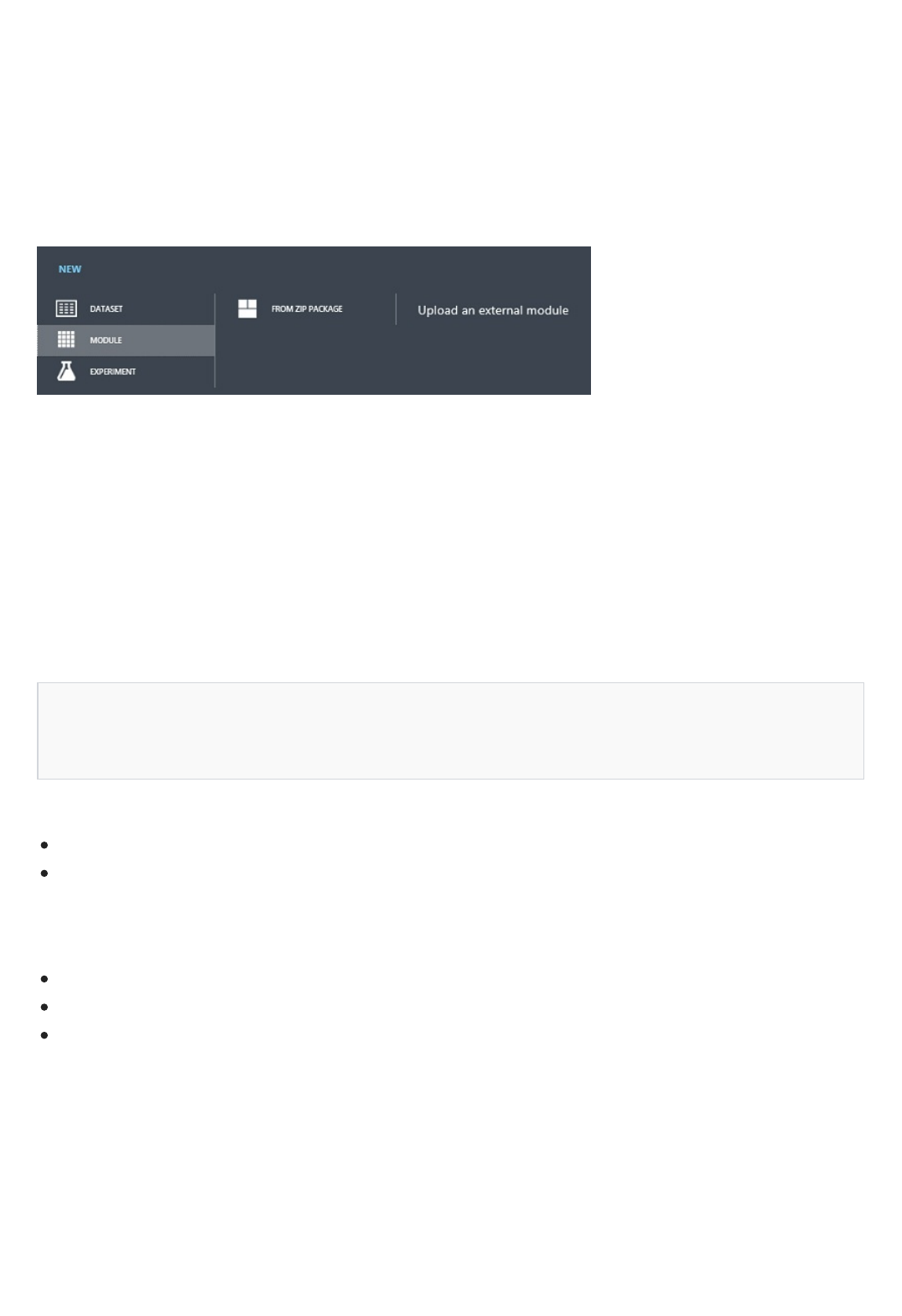
Package and register the modulePackage and register the module
Elements in the XML definition file
Module elementsModule elements
<Module name="Custom Add Rows" isDeterministic="false">
<Owner>Microsoft Corporation</Owner>
<Description>Appends one dataset to another...</Description>/>
more than one output is required, simply return a list from the R function with results placed in the same order as
Outputs elements are declared in the XML file.
Save these two files as CustomAddRows.R and CustomAddRows.xml and then zip the two files together into a
CustomAddRows.zip file.
To register them in your Machine Learning workspace, go to your workspace in the Machine Learning Studio, click
the +NEW button on the bottom and choose MODULE -> FROM ZIP PACKAGE to upload the new Custom
Add Rows module.
The Custom Add Rows module is now ready to be accessed by your Machine Learning experiments.
The Module element is used to define a custom module in the XML file. Multiple modules can be defined in one
XML file using multiple module elements. Each module in your workspace must have a unique name. Register a
custom module with the same name as an existing custom module and it replaces the existing module with the
new one. Custom modules can, however, be registered with the same name as an existing Azure Machine Learning
module. If so, they appear in the Custom category of the module palette.
Within the Module element, you can specify two additional optional elements:
an Owner element that is embedded into the module
a Description element that contains text that is displayed in quick help for the module and when you hover
over the module in the Machine Learning UI.
Rules for characters limits in the Module elements:
The value of the name attribute in the Module element must not exceed 64 characters in length.
The content of the Description element must not exceed 128 characters in length.
The content of the Owner element must not exceed 32 characters in length.
A module's results can be deterministic or nondeterministic.** By default, all modules are considered to be
deterministic. That is, given an unchanging set of input parameters and data, the module should return the same
results eacRAND or a functionh time it is run. Given this behavior, Azure Machine Learning Studio only reruns
modules marked as deterministic if a parameter or the input data has changed. Returning the cached results also
provides much faster execution of experiments.
There are functions that are nondeterministic, such as RAND or a function that returns the current date or time. If
your module uses a nondeterministic function, you can specify that the module is non-deterministic by setting the
optional isDeterministic attribute to FALSE. This insures that the module is rerun whenever the experiment is
run, even if the module input and parameters have not changed.
Language DefinitionLanguage Definition
<Language name="R" sourceFile="CustomAddRows.R" entryPoint="CustomAddRows" />
PortsPorts
Input elementsInput elements
<Input id="dataset1" name="Input 1" type="DataTable" isOptional="false">
<Description>Input Dataset 1</Description>
</Input>
<Input id="zippedData" name="Zip Input" type="Zip" IsOptional="false">
<Description>Zip files to be extracted to the R working directory.</Description>
</Input>
The Language element in your XML definition file is used to specify the custom module language. Currently, R is
the only supported language. The value of the sourceFile attribute must be the name of the R file that contains the
function to call when the module is run. This file must be part of the zip package. The value of the entryPoint
attribute is the name of the function being called and must match a valid function defined with in the source file.
The input and output ports for a custom module are specified in child elements of the Ports section of the XML
definition file. The order of these elements determines the layout experienced (UX) by users. The first child input or
output listed in the Ports element of the XML file becomes the left-most input port in the Machine Learning UX.
Each input and output port may have an optional Description child element that specifies the text shown when
you hover the mouse cursor over the port in the Machine Learning UI.
Ports Rules:
Maximum number of input and output ports is 8 for each.
Input ports allow you to pass data to your R function and workspace. The data types that are supported for input
ports are as follows:
DataTable: This type is passed to your R function as a data.frame. In fact, any types (for example, CSV files or
ARFF files) that are supported by Machine Learning and that are compatible with DataTable are converted to a
data.frame automatically.
The id attribute associated with each DataTable input port must have a unique value and this value must match its
corresponding named parameter in your R function. Optional DataTable ports that are not passed as input in an
experiment have the value NULL passed to the R function and optional zip ports are ignored if the input is not
connected. The isOptional attribute is optional for both the DataTable and Zip types and is false by default.
Zip: Custom modules can accept a zip file as input. This input is unpacked into the R working directory of your
function
For custom R modules, the id for a Zip port does not have to match any parameters of the R function. This is
because the zip file is automatically extracted to the R working directory.
Input Rules:
The value of the id attribute of the Input element must be a valid R variable name.
The value of the id attribute of the Input element must not be longer than 64 characters.
The value of the name attribute of the Input element must not be longer than 64 characters.
The content of the Description element must not be longer than 128 characters
The value of the type attribute of the Input element must be Zip or DataTable.
The value of the isOptional attribute of the Input element is not required (and is false by default when not

Output elementsOutput elements
<Output id="dataset" name="Dataset" type="DataTable">
<Description>Combined dataset</Description>
</Output>
<Ports>
<Output id="dataset" name="Dataset Out" type="DataTable">
<Description>New Dataset</Description>
</Output>
<Output id="dataset1_out" name="Dataset 1 Out" type="DataTable">
<Description>First Dataset</Description>
</Output>
<Output id="dataset2_out" name="Dataset 2 Out" type="DataTable">
<Description>Second Dataset</Description>
</Output>
<Input id="dataset1" name="Dataset 1" type="DataTable">
<Description>First Input Table</Description>
</Input>
<Input id="dataset2" name="Dataset 2" type="DataTable">
<Description>Second Input Table</Description>
</Input>
</Ports>
CustomAddRows <- function(dataset1, dataset2, swap=FALSE) {
if (swap) { dataset <- rbind(dataset2, dataset1)) }
else { dataset <- rbind(dataset1, dataset2))
}
return (list(dataset, dataset1, dataset2))
}
<Output id="deviceOutput" name="View Port" type="Visualization">
<Description>View the R console graphics device output.</Description>
</Output>
specified); but if it is specified, it must be true or false.
Standard output ports: Output ports are mapped to the return values from your R function, which can then be
used by subsequent modules. DataTable is the only standard output port type supported currently. (Support for
Learners and Transforms is forthcoming.) A DataTable output is defined as:
For outputs in custom R modules, the value of the id attribute does not have to correspond with anything in the R
script, but it must be unique. For a single module output, the return value from the R function must be a
data.frame. In order to output more than one object of a supported data type, the appropriate output ports need to
be specified in the XML definition file and the objects need to be returned as a list. The output objects are assigned
to output ports from left to right, reflecting the order in which the objects are placed in the returned list.
For example, if you want to modify the Custom Add Rows module to output the original two datasets, dataset1
and dataset2, in addition to the new joined dataset, dataset, (in an order, from left to right, as: dataset, dataset1,
dataset2), then define the output ports in the CustomAddRows.xml file as follows:
And return the list of objects in a list in the correct order in ‘CustomAddRows.R’:
Visualization output: You can also specify an output port of type Visualization, which displays the output from
the R graphics device and console output. This port is not part of the R function output and does not interfere with
the order of the other output port types. To add a visualization port to the custom modules, add an Output
element with a value of Visualization for its type attribute:
ArgumentsArguments
Arg elementArg element
<Arg id="intValue1" name="Int Param" type="int">
<Properties min="0" max="100" default="0" />
<Description>Integer Parameter</Description>
</Arg>
<Arg id="doubleValue1" name="Double Param" type="double">
<Properties min="0.000" max="0.999" default="0.3" />
<Description>Double Parameter</Description>
</Arg>
<Arg id="boolValue1" name="Boolean Param" type="bool">
<Properties default="true" />
<Description>Boolean Parameter</Description>
</Arg>
Output Rules:
The value of the id attribute of the Output element must be a valid R variable name.
The value of the id attribute of the Output element must not be longer than 32 characters.
The value of the name attribute of the Output element must not be longer than 64 characters.
The value of the type attribute of the Output element must be Visualization.
Additional data can be passed to the R function via module parameters which are defined in the Arguments
element. These parameters appear in the rightmost properties pane of the Machine Learning UI when the module
is selected. Arguments can be any of the supported types or you can create a custom enumeration when needed.
Similar to the Ports elements, Arguments elements can have an optional Description element that specifies the
text that appears when you hover the mouse over the parameter name. Optional properties for a module, such as
defaultValue, minValue, and maxValue can be added to any argument as attributes to a Properties element. Valid
properties for the Properties element depend on the argument type and are described with the supported
argument types in the next section. Arguments with the isOptional property set to "true" do not require the user
to enter a value. If a value is not provided to the argument, then the argument is not passed to the entry point
function. Arguments of the entry point function that are optional need to be explicitly handled by the function, e.g.
assigned a default value of NULL in the entry point function definition. An optional argument will only enforce the
other argument constraints, i.e. min or max, if a value is provided by the user. As with inputs and outputs, it is
critical that each of the parameters have unique id values associated with them. In our quick start example the
associated id/parameter was swap.
A module parameter is defined using the Arg child element of the Arguments section of the XML definition file.
As with the child elements in the Ports section, the ordering of parameters in the Arguments section defines the
layout encountered in the UX. The parameters appear from top down in the UI in the same order in which they are
defined in the XML file. The types supported by Machine Learning for parameters are listed here.
int – an Integer (32-bit) type parameter.
Optional Properties: min, max, default and isOptional
double – a double type parameter.
Optional Properties: min, max, default and isOptional
bool – a Boolean parameter that is represented by a check-box in UX.
Optional Properties: default - false if not set
<Arg id="stringValue1" name="My string Param" type="string">
<Properties isOptional="true" />
<Description>String Parameter 1</Description>
</Arg>
<Arg id="colset" name="Column set" type="ColumnPicker">
<Properties portId="datasetIn1" allowedTypes="Numeric" default="NumericAll"/>
<Description>Column set</Description>
</Arg>
string: a standard string
Optional Properties: default and isOptional
ColumnPicker: a column selection parameter. This type renders in the UX as a column chooser. The Property
element is used here to specify the id of the port from which columns are selected, where the target port type must
be DataTable. The result of the column selection is passed to the R function as a list of strings containing the
selected column names.
Required Properties: portId - matches the id of an Input element with type DataTable.
Optional Properties:
allowedTypes - Filters the column types from which you can pick. Valid values include:
Numeric
Boolean
Categorical
String
Label
Feature
Score
All
default - Valid default selections for the column picker include:
None
NumericFeature
NumericLabel
NumericScore
NumericAll
BooleanFeature
BooleanLabel
BooleanScore
BooleanAll
CategoricalFeature
CategoricalLabel
CategoricalScore
CategoricalAll
StringFeature
StringLabel
StringScore
StringAll
<Arg id="color" name="Color" type="DropDown">
<Properties default="red">
<Item id="red" name="Red Value"/>
<Item id="green" name="Green Value"/>
<Item id="blue" name="Blue Value"/>
</Properties>
<Description>Select a color.</Description>
</Arg>
Auxiliary FilesAuxiliary Files
NOTENOTE
RemoveDupNARows <- function(dataFrame) {
#Remove Duplicate Rows:
dataFrame <- unique(dataFrame)
#Remove Rows with NAs:
finalDataFrame <- dataFrame[complete.cases(dataFrame),]
return(finalDataFrame)
}
CustomAddRows <- function(dataset1, dataset2, swap=FALSE) {
source("src/RemoveDupNARows.R")
if (swap) {
dataset <- rbind(dataset2, dataset1))
} else {
dataset <- rbind(dataset1, dataset2))
}
dataset <- removeDupNARows(dataset)
return (dataset)
}
AllLabel
AllFeature
AllScore
All
DropDown: a user-specified enumerated (dropdown) list. The dropdown items are specified within the Properties
element using an Item element. The id for each Item must be unique and a valid R variable. The value of the
name of an Item serves as both the text that you see and the value that is passed to the R function.
Optional Properties:
default - The value for the default property must correspond with an id value from one of the Item
elements.
Any file that is placed in your custom module ZIP file is going to be available for use during execution time. Any
directory structures present are preserved. This means that file sourcing works the same locally and in Azure
Machine Learning execution.
Notice that all files are extracted to ‘src’ directory so all paths should have ‘src/’ prefix.
For example, say you want to remove any rows with NAs from the dataset, and also remove any duplicate rows,
before outputting it into CustomAddRows, and you’ve already written an R function that does that in a file
RemoveDupNARows.R:
You can source the auxiliary file RemoveDupNARows.R in the CustomAddRows function:

Execution Environment
Next, upload a zip file containing ‘CustomAddRows.R’, ‘CustomAddRows.xml’, and ‘RemoveDupNARows.R’ as a
custom R module.
The execution environment for the R script uses the same version of R as the Execute R Script module and can
use the same default packages. You can also add additional R packages to your custom module by including them
in the custom module zip package. Just load them in your R script as you would in your own R environment.
Limitations of the execution environment include:
Non-persistent file system: Files written when the custom module is run are not persisted across multiple runs
of the same module.
No network access
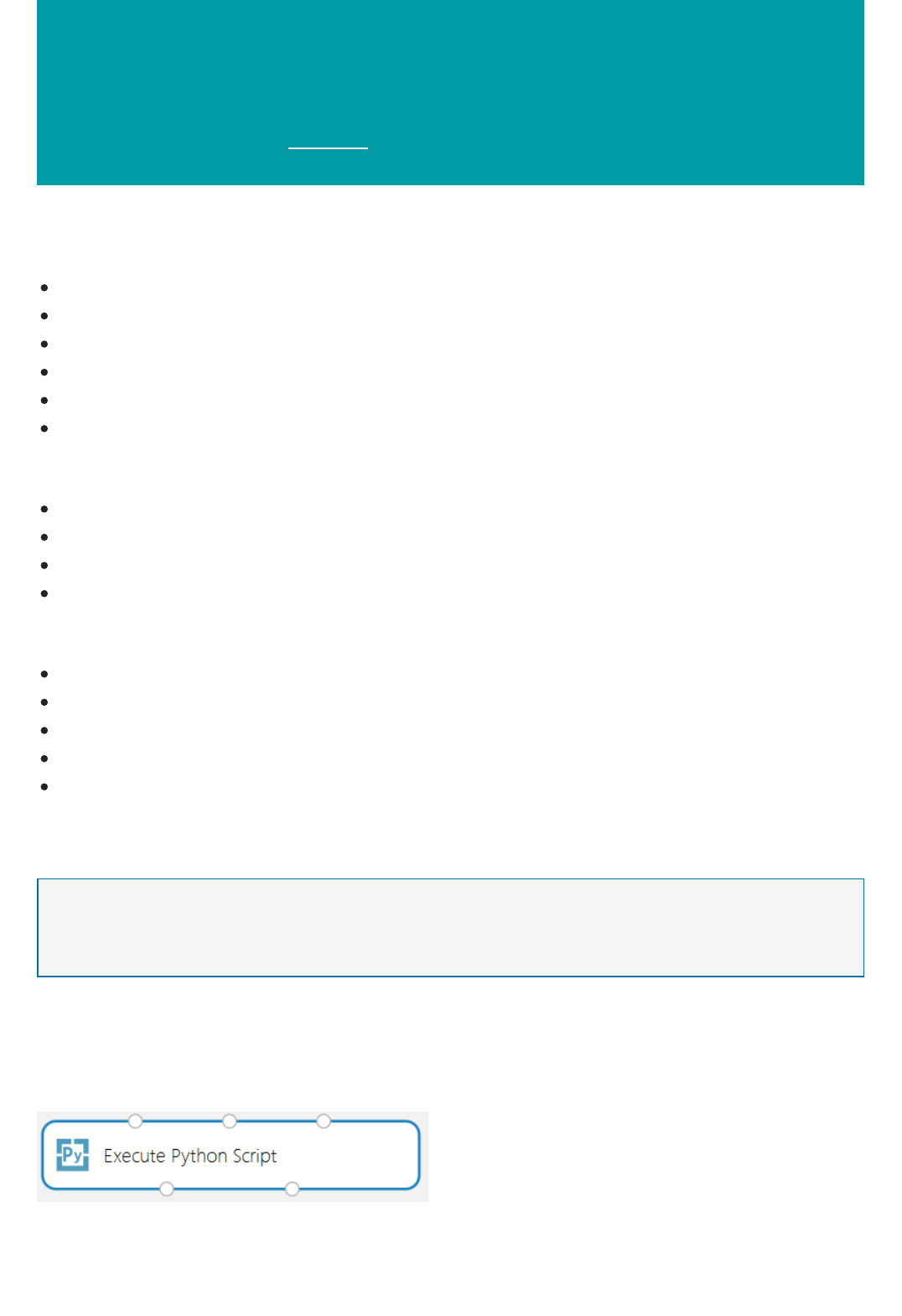
Execute Python machine learning scripts in Azure
Machine Learning Studio
3/20/2018 • 9 min to read • Edit Online
NOTENOTE
Design principles of Python scripts in Machine Learning
This topic describes the design principles underlying the current support for Python scripts in Azure Machine
Learning. The main capabilities provided are also outlined, including:
execute basic usage scenarios
score an experiment in a web service
support for importing existing code
export visualizations
perform supervised feature selection
understand some limitations
Python is an indispensable tool in the tool chest of many data scientists. It has:
an elegant and concise syntax,
cross-platform support,
a vast collection of powerful libraries, and
mature development tools.
Python is being used in all phases of a workflow typically used in machine learning modeling:
data ingest and processing
feature construction
model training
model validation
deployment of the models
Azure Machine Learning Studio supports embedding Python scripts into various parts of a machine learning
experiment and also seamlessly publishing them as web services on Microsoft Azure.
You can try Azure Machine Learning for free. No credit card or Azure subscription is required. Get started now.
The primary interface to Python in Azure Machine Learning Studio is via the Execute Python Script module shown
in Figure 1.
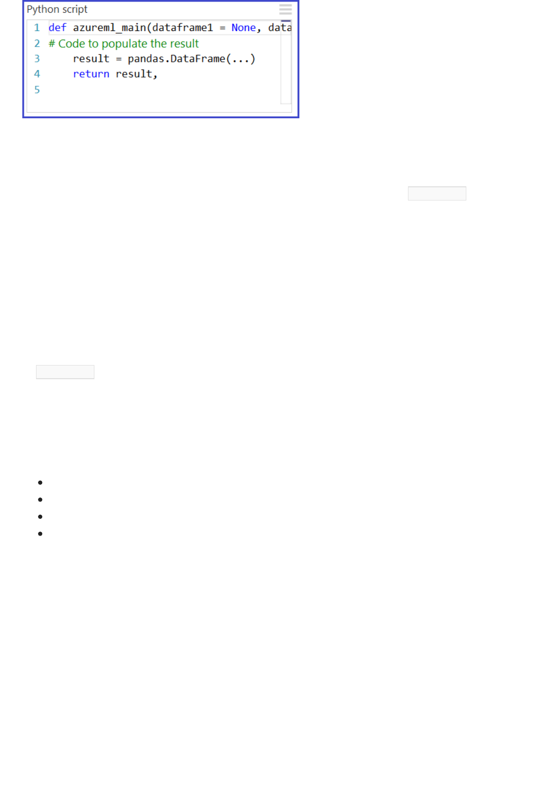
Basic usage scenarios in ML for Python scripts
Figure 1. The Execute Python Script module.
The Execute Python Script module in Azure ML Studio accepts up to three inputs and produces up to two outputs
(discussed in the following section), like its R analogue, the Execute R Script module. The Python code to be
executed is entered into the parameter box as a specially named entry-point function called azureml_main . Here are
the key design principles used to implement this module:
1. Must be idiomatic for Python users. Most Python users factor their code as functions inside modules. So putting
a lot of executable statements in a top-level module is relatively rare. As a result, the script box also takes a
specially named Python function as opposed to just a sequence of statements. The objects exposed in the
function are standard Python library types such as Pandas data frames and NumPy arrays.
2. Must have high-fidelity between local and cloud executions. The backend used to execute the Python code is
based on Anaconda, a widely used cross-platform scientific Python distribution. It comes with close to 200 of
the most common Python packages. Therefore, data scientists can debug and qualify their code on their local
Azure Machine Learning-compatible Anaconda environment. Then use an existing development environment,
such as IPython notebook or Python Tools for Visual Studio, to run it as part of an Azure ML experiment. The
azureml_main entry point is a vanilla Python function and so ****can be authored without Azure ML-specific
code or the SDK installed.
3. Must be seamlessly composable with other Azure Machine Learning modules. The Execute Python Script
module accepts, as inputs and outputs, standard Azure Machine Learning datasets. The underlying framework
transparently and efficiently bridges the Azure ML and Python runtimes. So Python can be used in conjunction
with existing Azure ML workflows, including those that call into R and SQLite. A result, data scientist could
compose workflows that:
use Python and Pandas for data pre-processing and cleaning
feed the data to a SQL transformation, joining multiple datasets to form features
train models using the algorithms in Azure Machine Learning
evaluate and post-process the results using R.
In this section, we survey some of the basic uses of the Execute Python Script module. Inputs to the Python module
are exposed as Pandas data frames. The function must return a single Pandas data frame packaged inside of a
Python sequence such as a tuple, list, or NumPy array. The first element of this sequence is then returned in the
first output port of the module. This scheme is shown in Figure 2.
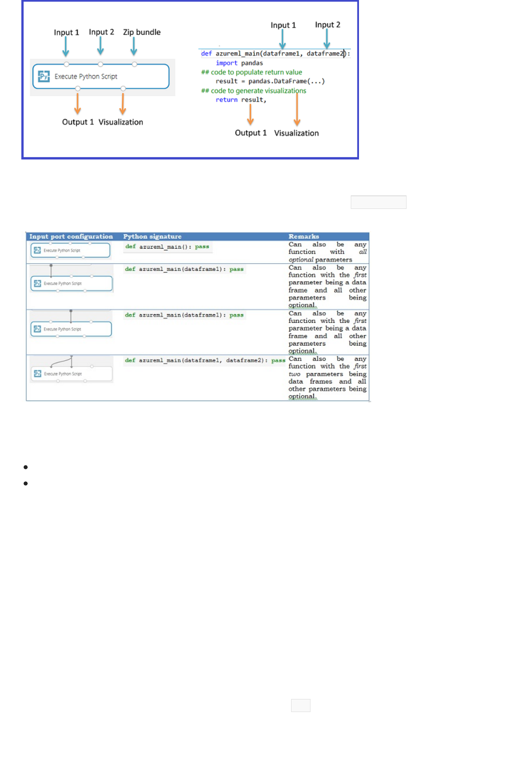
Translation of input and output types
Figure 2. Mapping of input ports to parameters and return value to output port.
More detailed semantics of how the input ports get mapped to parameters of the azureml_main function are
shown in Table 1:
Table 1. Mapping of input ports to function parameters.
The mapping between input ports and function parameters is positional:
The first connected input port is mapped to the first parameter of the function.
The second input (if connected) is mapped to the second parameter of the function.
See Python for Data Analysis (O'Reilly, 2012) by W. McKinney for more information on Python Pandas and on
how it can be used to manipulate data effectively and efficiently.
Input datasets in Azure ML are converted to data frames in Pandas. Output data frames are converted back to
Azure ML datasets. The following conversions are performed:
1. String and numeric columns are converted as-is and missing values in a dataset are converted to ‘NA’ values in
Pandas. The same conversion happens on the way back (NA values in Pandas are converted to missing values
in Azure ML).
2. Index vectors in Pandas are not supported in Azure ML. All input data frames in the Python function always
have a 64-bit numerical index from 0 to the number of rows minus 1.
3. Azure ML datasets cannot have duplicate column names and column names that are not strings. If an output
data frame contains non-numeric columns, the framework calls str on the column names. Likewise, any
duplicate column names are automatically mangled to insure the names are unique. The suffix (2) is added to
the first duplicate, (3) to the second duplicate, and so on.
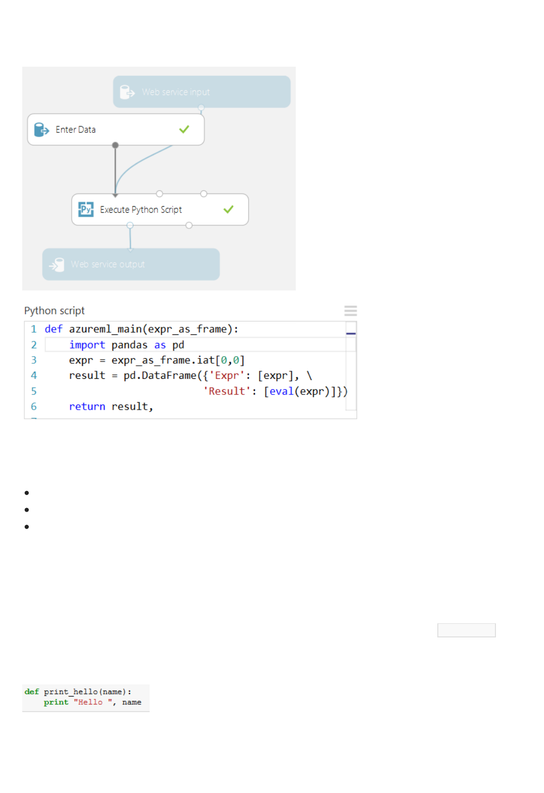
Operationalizing Python scripts
Importing existing Python script modules
Any Execute Python Script modules used in a scoring experiment are called when published as a web service. For
example, Figure 3 shows a scoring experiment that contains the code to evaluate a single Python expression.
Figure 3. Web service for evaluating a Python expression.
A web service created from this experiment:
takes as input a Python expression (as a string)
sends it to the Python interpreter
returns a table containing both the expression and the evaluated result.
A common use-case for many data scientists is to incorporate existing Python scripts into Azure ML experiments.
Instead of requiring that all code be concatenated and pasted into a single script box, the Execute Python Script
module accepts a zip file that contains Python modules at the third input port. The file is unzipped by the execution
framework at runtime and the contents are added to the library path of the Python interpreter. The azureml_main
entry point function can then import these modules directly.
As an example, consider the file Hello.py containing a simple “Hello, World” function.
Figure 4. User-defined function in Hello.py file.
Next, we create a file Hello.zip that contains Hello.py:
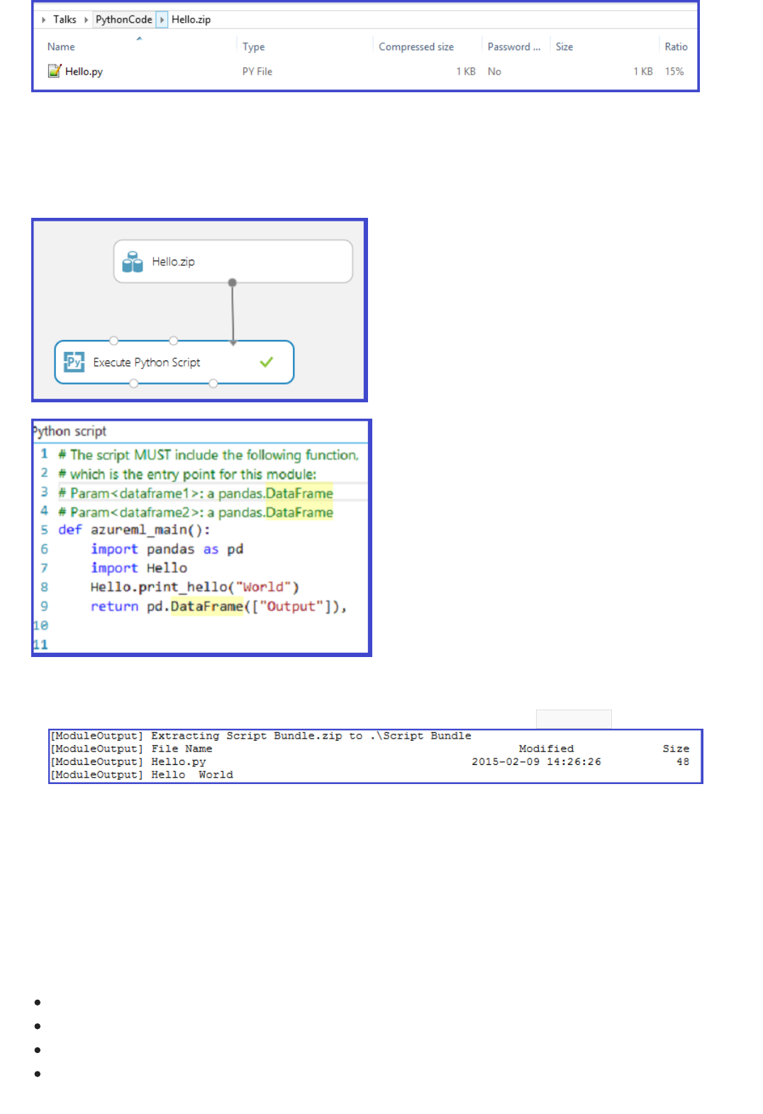
Working with visualizations
Figure 5. Zip file containing user-defined Python code.
Upload the zip file as a dataset into Azure Machine Learning Studio. Then create and run an experiment that uses
the Python code in the Hello.zip file by attaching it to the third input port of the Execute Python Script module,
as shown in this figure.
Figure 6. Sample experiment with user-defined Python code uploaded as a zip file.
The module output shows that the zip file has been unpackaged and that the function print_hello has been run.
Figure 7. User-defined function in use inside the Execute Python Script module.
Plots created using MatplotLib that can be visualized on the browser can be returned by the Execute Python Script.
But the plots are not automatically redirected to images as they are when using R. So the user must explicitly save
any plots to PNG files if they are to be returned back to Azure Machine Learning.
To generate images from MatplotLib, you must complete the following procedure:
switch the backend to “AGG” from the default Qt-based renderer
create a new figure object
get the axis and generate all plots into it
save the figure to a PNG file
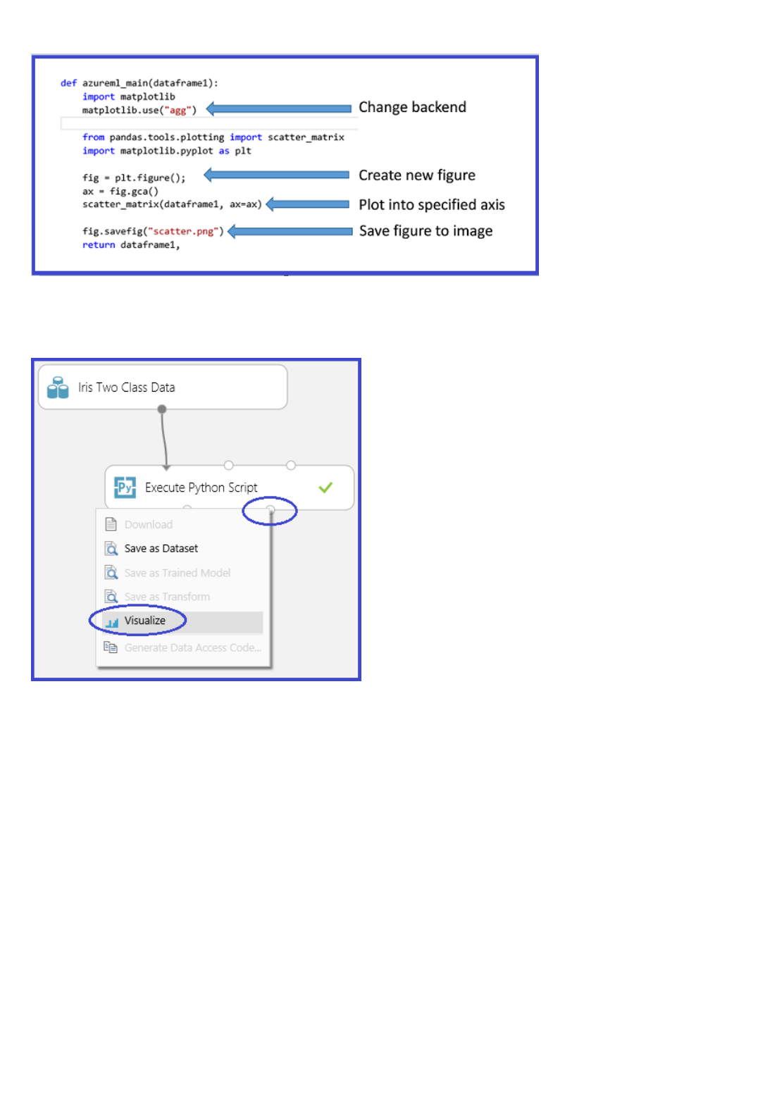
This process is illustrated in the following Figure 8 that creates a scatter plot matrix using the scatter_matrix
function in Pandas.
Figure 8. Code to save MatplotLib figures to images.
Figure 9 shows an experiment that uses the script shown previously to return plots via the second output port.
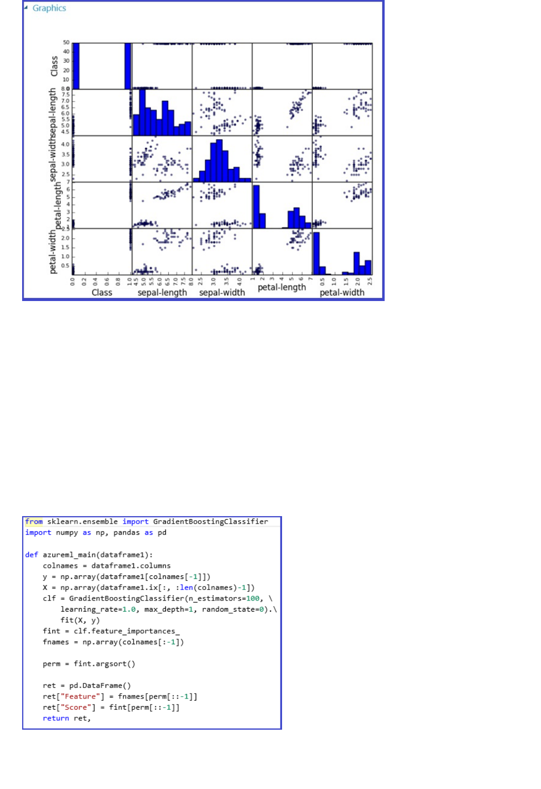
Advanced examples
Figure 9. Visualizing plots generated from Python code.
It is possible to return multiple figures by saving them into different images, the Azure Machine Learning runtime
picks up all images and concatenates them for visualization.
The Anaconda environment installed in Azure Machine Learning contains common packages such as NumPy,
SciPy, and Scikits-Learn. These packages can be effectively used for various data processing tasks in a machine
learning pipeline. As an example, the following experiment and script illustrate the use of ensemble learners in
Scikits-Learn to compute feature importance scores for a dataset. The scores can be used to perform supervised
feature selection before being fed into another ML model.
Here is the Python function used to compute the importance scores and order the features based on the scores:
Figure 10. Function to rank features by scores. The following experiment then computes and returns the
importance scores of features in the “Pima Indian Diabetes” dataset in Azure Machine Learning:
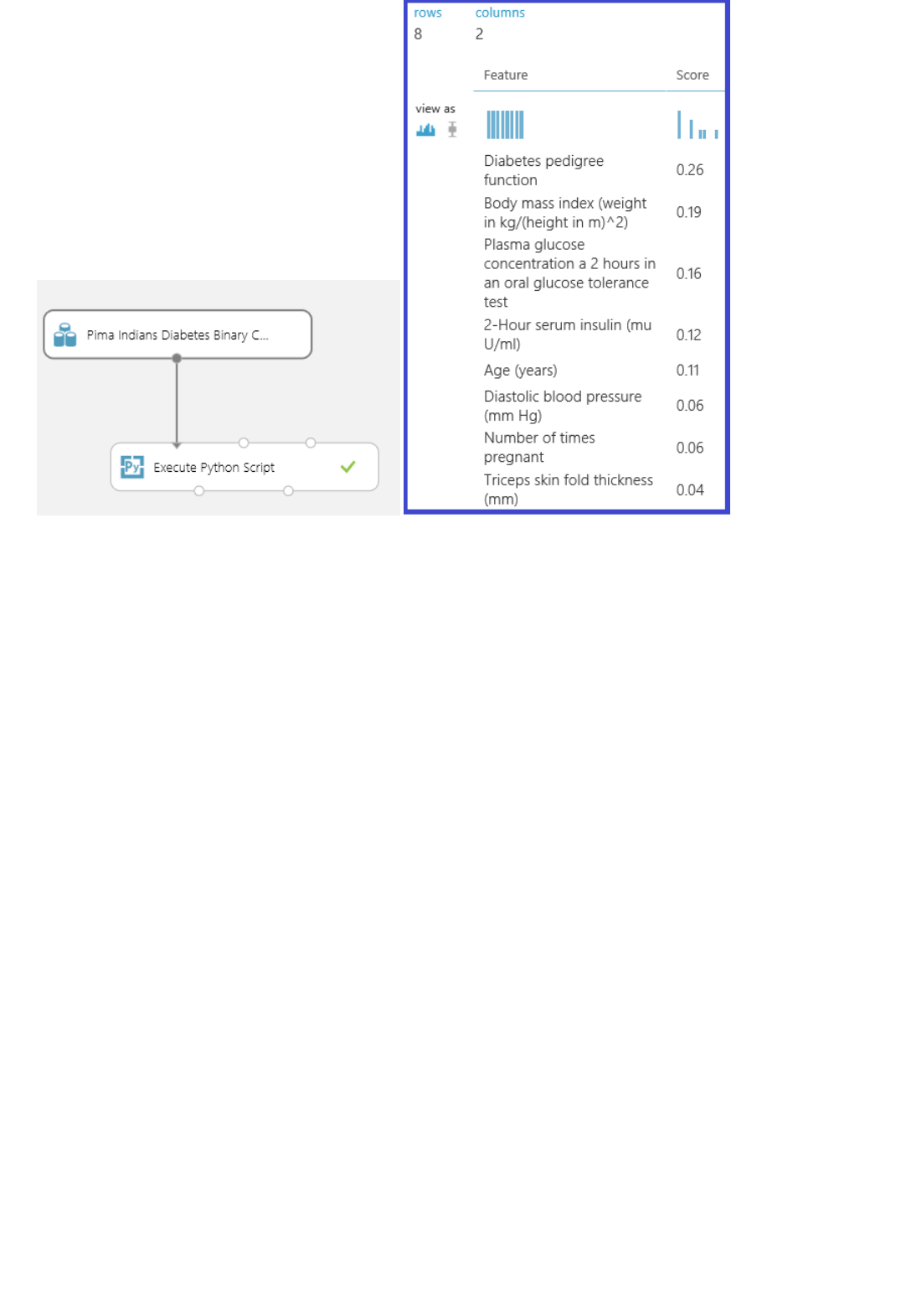
Limitations
Conclusions
Figure 11. Experiment to rank features in the Pima Indian Diabetes dataset.
The Execute Python Script currently has the following limitations:
1. Sandboxed execution. The Python runtime is currently sandboxed and, as a result, does not allow access to the
network or to the local file system in a persistent manner. All files saved locally are isolated and deleted once the
module finishes. The Python code cannot access most directories on the machine it runs on, the exception being
the current directory and its subdirectories.
2. Lack of sophisticated development and debugging support. The Python module currently does not support IDE
features such as intellisense and debugging. Also, if the module fails at runtime, the full Python stack trace is
available. But it must be viewed in the output log for the module. We currently recommend that you develop
and debug Python scripts in an environment such as IPython and then import the code into the module.
3. Single data frame output. The Python entry point is only permitted to return a single data frame as output. It is
not currently possible to return arbitrary Python objects such as trained models directly back to the Azure
Machine Learning runtime. Like Execute R Script, which has the same limitation, it is possible in many cases to
pickle objects into a byte array and then return that inside of a data frame.
4. Inability to customize Python installation. Currently, the only way to add custom Python modules is via the zip
file mechanism described earlier. While this is feasible for small modules, it is cumbersome for large modules
(especially those with native DLLs) or a large number of modules.
The Execute Python Script module allows a data scientist to incorporate existing Python code into cloud-hosted
machine learning workflows in Azure Machine Learning and to seamlessly operationalize them as part of a web
service. The Python script module interoperates naturally with other modules in Azure Machine Learning. The
module can be used for a range of tasks from data exploration to pre-processing and feature extraction, and then to
evaluation and post-processing of the results. The backend runtime used for execution is based on Anaconda, a
well-tested and widely used Python distribution. This backend makes it simple for you to on-board existing code
assets into the cloud.

Next steps
We expect to provide additional functionality to the Execute Python Script module such as the ability to train and
operationalize models in Python and to add better support for the development and debugging code in Azure
Machine Learning Studio.
For more information, see the Python Developer Center.
Azure Machine Learning Web Services: Deployment
and consumption
4/18/2018 • 3 min to read • Edit Online
Deploy a web service
With Azure Machine Learning StudioWith Azure Machine Learning Studio
With web services resource provider APIs (Azure Resource Manager APIs)
With web services resource provider APIs (Azure Resource Manager APIs)
With PowerShell cmdletsWith PowerShell cmdlets
C:\<folder>\GetWSD <experiment-url> <workspace-auth-token>
You can use Azure Machine Learning to deploy machine-learning workflows and models as web services. These
web services can then be used to call the machine-learning models from applications over the Internet to do
predictions in real time or in batch mode. Because the web services are RESTful, you can call them from various
programming languages and platforms, such as .NET and Java, and from applications, such as Excel.
The next sections provide links to walkthroughs, code, and documentation to help get you started.
Machine Learning Studio and the Microsoft Azure Machine Learning Web Services portal help you deploy and
manage a web service without writing code.
The following links provide general Information about how to deploy a new web service:
For an overview about how to deploy a new web service that's based on Azure Resource Manager, see Deploy a
new web service.
For a walkthrough about how to deploy a web service, see Deploy an Azure Machine Learning web service.
For a full walkthrough about how to create and deploy a web service, see Walkthrough Step 1: Create a
Machine Learning workspace.
For specific examples that deploy a web service, see:
Walkthrough Step 5: Deploy the Azure Machine Learning web service
How to deploy a web service to multiple regions
The Azure Machine Learning resource provider for web services enables deployment and management of web
services by using REST API calls. For additional details, see the Machine Learning Web Service (REST) reference.
Azure Machine Learning resource provider for web services enables deployment and management of web services
by using PowerShell cmdlets.
To use the cmdlets, you must first sign in to your Azure account from within the PowerShell environment by using
the Connect-AzureRmAccount cmdlet. If you are unfamiliar with how to call PowerShell commands that are based
on Resource Manager, see Using Azure PowerShell with Azure Resource Manager.
To export your predictive experiment, use this sample code. After you create the .exe file from the code, you can
type:
Running the application creates a web service JSON template. To use the template to deploy a web service, you
must add the following information:
Storage account name and key
"StorageAccount": {
"name": "YourStorageAccountName",
"key": "YourStorageAccountKey"
},
"CommitmentPlan": {
"id":
"subscriptions/YouSubscriptionID/resourceGroups/YourResourceGroupID/providers/Microsoft.MachineLearning/commitm
entPlans/YourPlanName"
}
Consume the web services
From the Azure Machine Learning Web Services UI (Testing)
From the Azure Machine Learning Web Services UI (Testing)
From ExcelFrom Excel
From a REST-based clientFrom a REST-based client
You can get the storage account name and key from the Azure portal.
Commitment plan ID
You can get the plan ID from the Azure Machine Learning Web Services portal by signing in and clicking a
plan name.
Add them to the JSON template as children of the Properties node at the same level as the
MachineLearningWorkspace node.
Here's an example:
See the following articles and sample code for additional details:
Azure Machine Learning Cmdlets reference on MSDN
Sample walkthrough on GitHub
You can test your web service from the Azure Machine Learning Web Services portal. This includes testing the
Request-Response service (RRS) and Batch Execution service (BES) interfaces.
Deploy a new web service
Deploy an Azure Machine Learning web service
Walkthrough Step 5: Deploy the Azure Machine Learning web service
You can download an Excel template that consumes the web service:
Consuming an Azure Machine Learning web service from Excel
Excel add-in for Azure Machine Learning Web Services
Azure Machine Learning Web Services are RESTful APIs. You can consume these APIs from various platforms,
such as .NET, Python, R, Java, etc. The Consume page for your web service on the Microsoft Azure Machine
Learning Web Services portal has sample code that can help you get started. For more information, see How to
consume an Azure Machine Learning Web service.
Deploy an Azure Machine Learning web service
3/21/2018 • 9 min to read • Edit Online
NOTENOTE
Create a training experiment
Convert the training experiment to a predictive experiment
Azure Machine Learning enables you to build, test, and deploy predictive analytic solutions.
From a high-level point-of-view, this is done in three steps:
Create a training experiment - Azure Machine Learning Studio is a collaborative visual development
environment that you use to train and test a predictive analytics model using training data that you supply.
Convert it to a predictive experiment - Once your model has been trained with existing data and you're
ready to use it to score new data, you prepare and streamline your experiment for predictions.
Deploy it as a web service - You can deploy your predictive experiment as a new or classic Azure web
service. Users can send data to your model and receive your model's predictions.
You can try Azure Machine Learning for free. No credit card or Azure subscription is required. Get started now.
To train a predictive analytics model, you use Azure Machine Learning Studio to create a training experiment
where you include various modules to load training data, prepare the data as necessary, apply machine learning
algorithms, and evaluate the results. You can iterate on an experiment and try different machine learning
algorithms to compare and evaluate the results.
The process of creating and managing training experiments is covered more thoroughly elsewhere. For more
information, see these articles:
Create a simple experiment in Azure Machine Learning Studio
Develop a predictive solution with Azure Machine Learning
Import your training data into Azure Machine Learning Studio
Manage experiment iterations in Azure Machine Learning Studio
Once you've trained your model, you're ready to convert your training experiment into a predictive experiment
to score new data.
By converting to a predictive experiment, you're getting your trained model ready to be deployed as a scoring
web service. Users of the web service can send input data to your model and your model will send back the
prediction results. As you convert to a predictive experiment, keep in mind how you expect your model to be
used by others.
To convert your training experiment to a predictive experiment, click Run at the bottom of the experiment
canvas, click Set Up Web Service, then select Predictive Web Service.
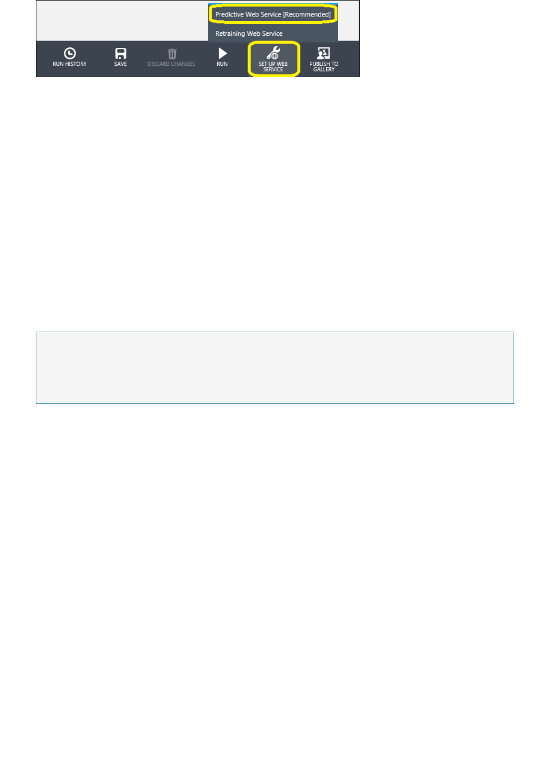
Deploy it as a web service
Deploy the predictive experiment as a New web serviceDeploy the predictive experiment as a New web service
NOTENOTE
Machine Learning Web Service portal Deploy Experiment PageMachine Learning Web Service portal Deploy Experiment Page
Test your New web serviceTest your New web service
For more information on how to perform this conversion, see How to prepare your model for deployment in
Azure Machine Learning Studio.
The following steps describe deploying a predictive experiment as a New web service. You can also deploy the
experiment as Classic web service.
You can deploy the predictive experiment as a New web service or as a Classic web service.
Now that the predictive experiment has been prepared, you can deploy it as a new Azure web service. Using the
web service, users can send data to your model and the model will return its predictions.
To deploy your predictive experiment, click Run at the bottom of the experiment canvas. Once the experiment
has finished running, click Deploy Web Service and select Deploy Web Service New. The deployment page
of the Machine Learning Web Service portal opens.
To deploy a New web service you must have sufficient permissions in the subscription to which you deploying the web
service. For more information see, Manage a Web service using the Azure Machine Learning Web Services portal.
On the Deploy Experiment page, enter a name for the web service. Select a pricing plan. If you have an existing
pricing plan you can select it, otherwise you must create a new price plan for the service.
1. In the Price Plan drop down, select an existing plan or select the Select new plan option.
2. In Plan Name, type a name that will identify the plan on your bill.
3. Select one of the Monthly Plan Tiers. The plan tiers default to the plans for your default region and your
web service is deployed to that region.
Click Deploy and the Quickstart page for your web service opens.
The web service Quickstart page gives you access and guidance on the most common tasks you will perform
after creating a web service. From here, you can easily access both the Test page and Consume page.
To test your new web service, click Test web service under common tasks. On the Test page, you can test your
web service as a Request-Response Service (RRS) or a Batch Execution service (BES).
The RRS test page displays the inputs, outputs, and any global parameters that you have defined for the
experiment. To test the web service, you can manually enter appropriate values for the inputs or supply a
comma separated value (CSV) formatted file containing the test values.
To test using RRS, from the list view mode, enter appropriate values for the inputs and click Test Request-
Response. Your prediction results display in the output column to the left.
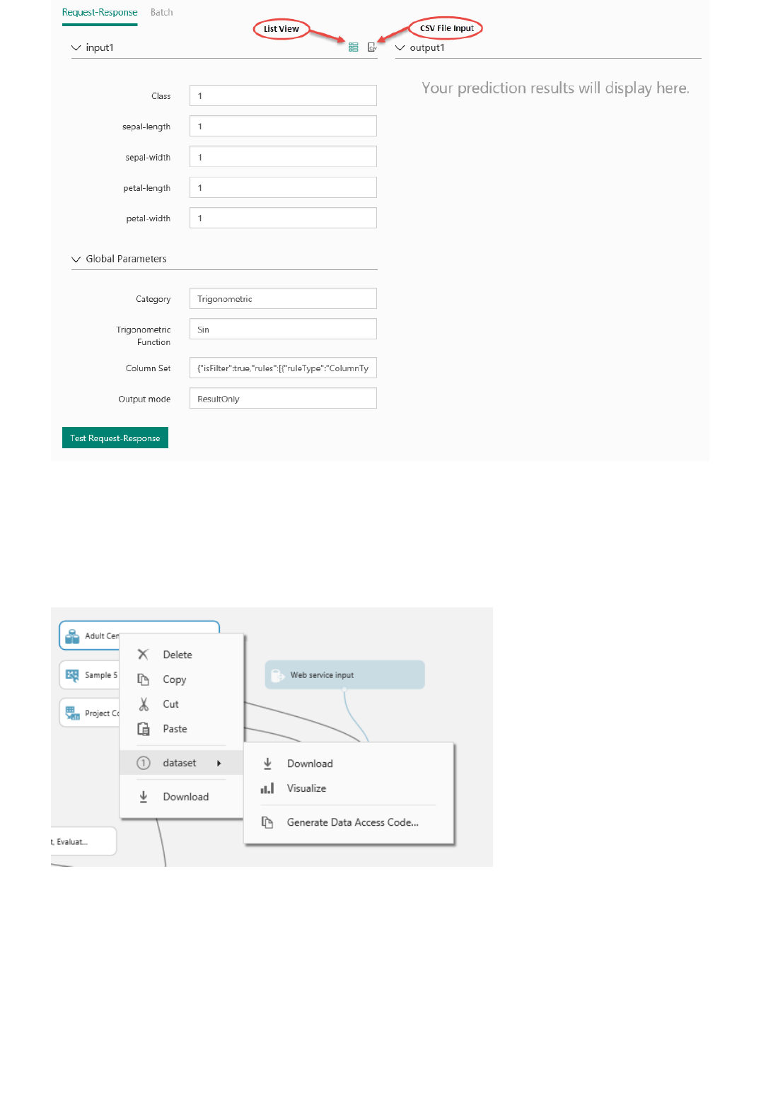
To test your BES, click Batch. On the Batch test page, click Browse under your input and select a CSV file
containing appropriate sample values. If you don't have a CSV file, and you created your predictive experiment
using Machine Learning Studio, you can download the data set for your predictive experiment and use it.
To download the data set, open Machine Learning Studio. Open your predictive experiment and right click the
input for your experiment. From the context menu, select dataset and then select Download.
Click Test. The status of your Batch Execution job displays to the right under Test Batch Jobs.
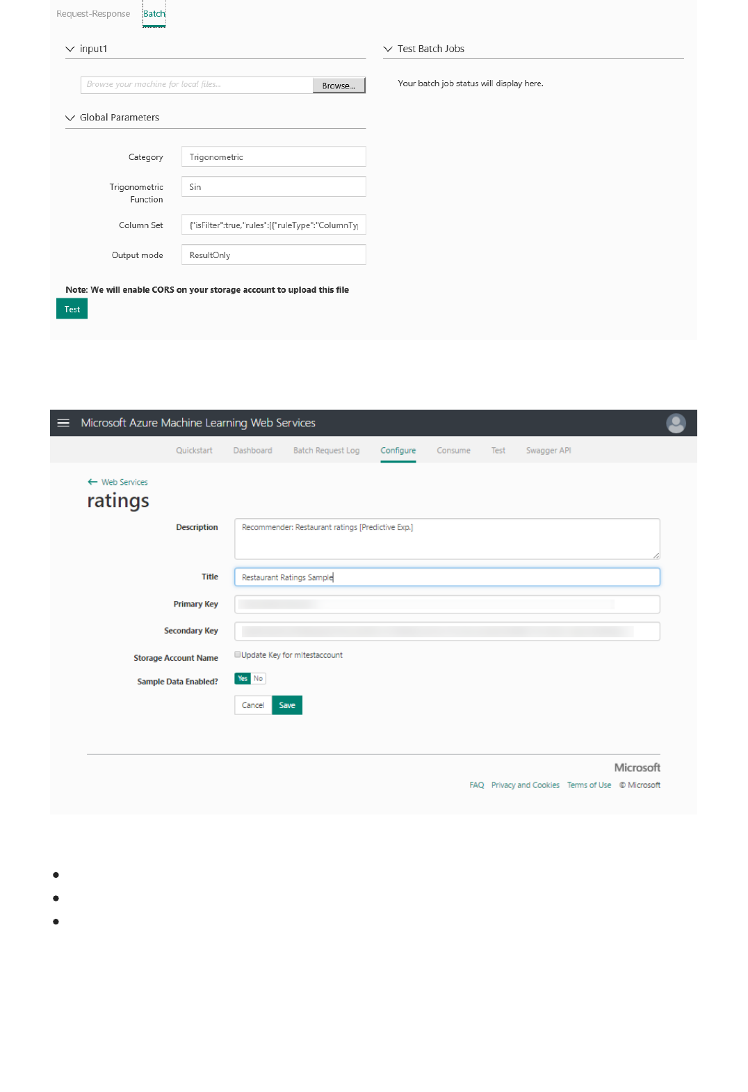
Access your New web serviceAccess your New web service
On the CONFIGURATION page, you can change the description, title, update the storage account key, and
enable sample data for your web service.
Once you've deployed the web service, you can:
Access it through the web service API.
Manage it through Azure Machine Learning web services portal.
Update it if your model changes.
Once you deploy your web service from Machine Learning Studio, you can send data to the service and receive
responses programmatically.
The Consume page provides all the information you need to access your web service. For example, the API key
is provided to allow authorized access to the service.
For more information about accessing a Machine Learning web service, see How to consume an Azure Machine
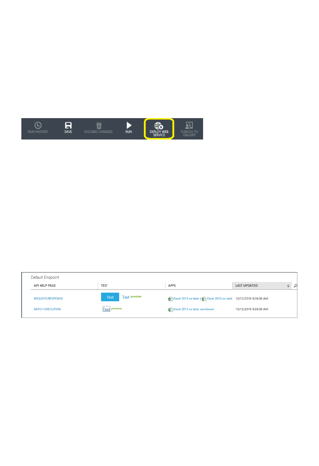
Manage your New web serviceManage your New web service
Deploy the predictive experiment as a Classic web serviceDeploy the predictive experiment as a Classic web service
Test your Classic web serviceTest your Classic web service
Learning Web service.
You can manage your New web services Machine Learning Web Services portal. From the main portal page,
click Web Services. From the web services page, you can delete or copy a service. To monitor a specific service,
click the service and then click Dashboard. To monitor batch jobs associated with the web service, click Batch
Request Log.
Now that the predictive experiment has been sufficiently prepared, you can deploy it as a Classic Azure web
service. Using the web service, users can send data to your model and the model will return its predictions.
To deploy your predictive experiment, click Run at the bottom of the experiment canvas and then click Deploy
Web Service. The web service is set up and you are placed in the web service dashboard.
You can test the web service in either the Machine Learning Web Services portal or Machine Learning Studio.
To test the Request Response web service, click the Test button in the web service dashboard. A dialog pops up
to ask you for the input data for the service. These are the columns expected by the scoring experiment. Enter a
set of data and then click OK. The results generated by the web service are displayed at the bottom of the
dashboard.
You can click the Test preview link to test your service in the Azure Machine Learning Web Services portal as
shown previously in the New web service section.
To test the Batch Execution Service, click Test preview link . On the Batch test page, click Browse under your
input and select a CSV file containing appropriate sample values. If you don't have a CSV file, and you created
your predictive experiment using Machine Learning Studio, you can download the data set for your predictive
experiment and use it.
On the CONFIGURATION page, you can change the display name of the service and give it a description. The
name and description is displayed in the Azure portal where you manage your web services.
You can provide a description for your input data, output data, and web service parameters by entering a string
for each column under INPUT SCHEMA, OUTPUT SCHEMA, and Web SERVICE PARAMETER. These
descriptions are used in the sample code documentation provided for the web service.
You can enable logging to diagnose any failures that you're seeing when your web service is accessed. For more
information, see Enable logging for Machine Learning web services.
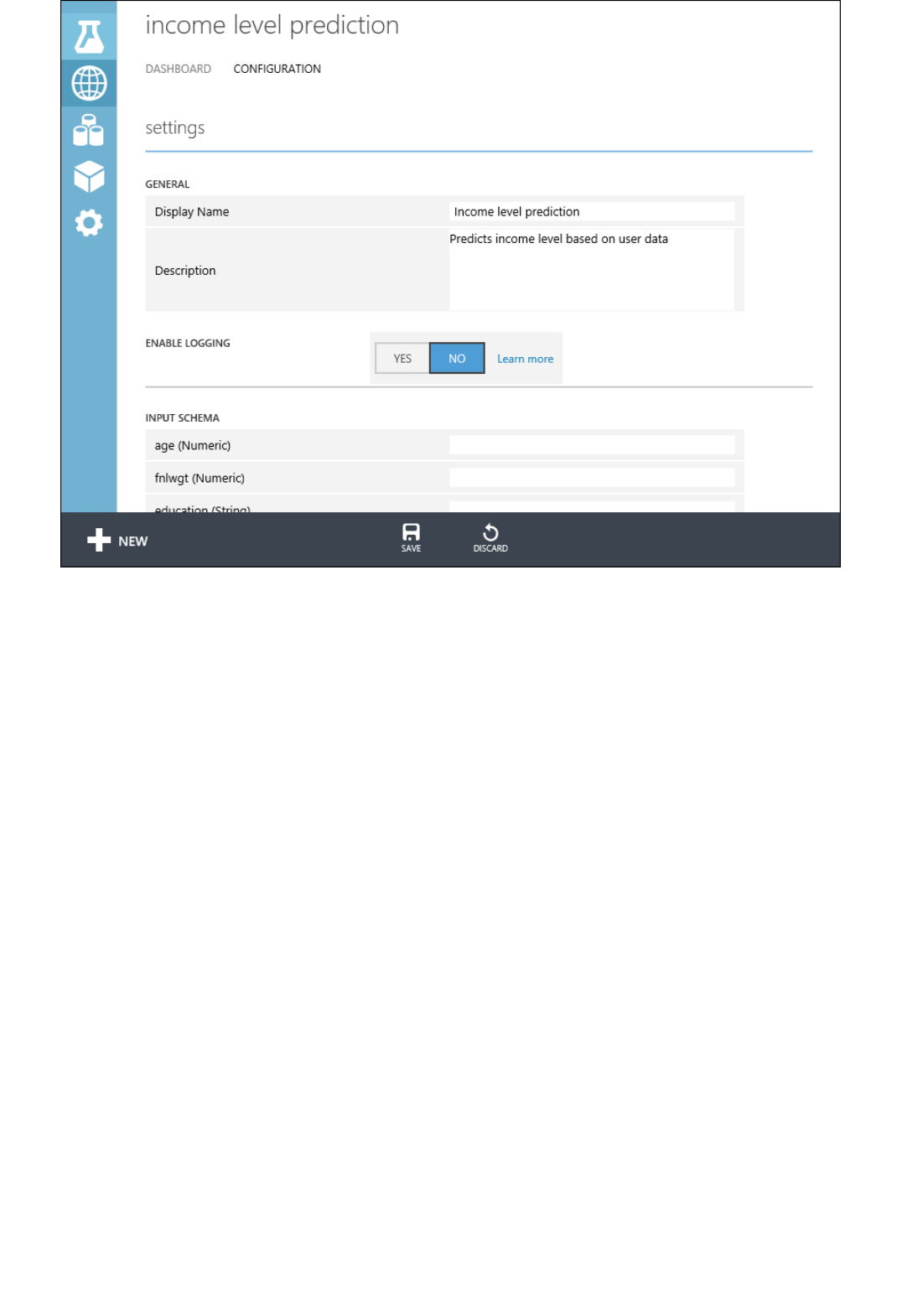
Access your Classic web serviceAccess your Classic web service
Manage your Classic web serviceManage your Classic web service
Update the web service
You can also configure the endpoints for the web service in the Azure Machine Learning Web Services portal
similar to the procedure shown previously in the New web service section. The options are different, you can
add or change the service description, enable logging, and enable sample data for testing.
Once you deploy your web service from Machine Learning Studio, you can send data to the service and receive
responses programmatically.
The dashboard provides all the information you need to access your web service. For example, the API key is
provided to allow authorized access to the service, and API help pages are provided to help you get started
writing your code.
For more information about accessing a Machine Learning web service, see How to consume an Azure Machine
Learning Web service.
There are various of actions you can perform to monitor a web service. You can update it, and delete it. You can
also add additional endpoints to a Classic web service in addition to the default endpoint that is created when
you deploy it.
For more information, see Manage an Azure Machine Learning workspace and Manage a web service using the
Azure Machine Learning Web Services portal.
You can make changes to your web service, such as updating the model with additional training data, and
deploy it again, overwriting the original web service.
To update the web service, open the original predictive experiment you used to deploy the web service and
make an editable copy by clicking SAVE AS. Make your changes and then click Deploy Web Service.
Because you've deployed this experiment before, you are asked if you want to overwrite (Classic Web Service)

NOTENOTE
or update (New web service) the existing service. Clicking YES or Update stops the existing web service and
deploys the new predictive experiment is deployed in its place.
If you made configuration changes in the original web service, for example, entering a new display name or description,
you will need to enter those values again.
One option for updating your web service is to retrain the model programmatically. For more information, see
Retrain Machine Learning models programmatically.
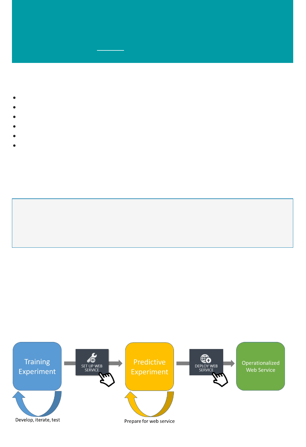
How a Machine Learning model progresses from an
experiment to an operationalized Web service
3/21/2018 • 7 min to read • Edit Online
NOTENOTE
Developing and deploying a predictive Web service
Azure Machine Learning Studio provides an interactive canvas that allows you to develop, run, test, and iterate an
experiment representing a predictive analysis model. There are a wide variety of modules available that can:
Input data into your experiment
Manipulate the data
Train a model using machine learning algorithms
Score the model
Evaluate the results
Output final values
Once you’re satisfied with your experiment, you can deploy it as a Classic Azure Machine Learning Web service
or a New Azure Machine Learning Web service so that users can send it new data and receive back results.
In this article, we give an overview of the mechanics of how your Machine Learning model progresses from a
development experiment to an operationalized Web service.
There are other ways to develop and deploy machine learning models, but this article is focused on how you use Machine
Learning Studio. For example, to read a description of how to create a classic predictive Web service with R, see the blog post
Build & Deploy Predictive Web Apps Using RStudio and Azure ML.
While Azure Machine Learning Studio is designed to help you develop and deploy a predictive analysis model, it’s
possible to use Studio to develop an experiment that doesn’t include a predictive analysis model. For example, an
experiment might just input data, manipulate it, and then output the results. Just like a predictive analysis
experiment, you can deploy this non-predictive experiment as a Web service, but it’s a simpler process because the
experiment isn’t training or scoring a machine learning model. While it’s not the typical to use Studio in this way,
we’ll include it in the discussion so that we can give a complete explanation of how Studio works.
Here are the stages that a typical solution follows as you develop and deploy it using Machine Learning Studio:
Figure 1 - Stages of a typical predictive analysis model
The training experimentThe training experiment
The predictive experimentThe predictive experiment
NOTENOTE
The Web serviceThe Web service
The non-typical case: creating a non-predictive Web service
The training experiment is the initial phase of developing your Web service in Machine Learning Studio. The
purpose of the training experiment is to give you a place to develop, test, iterate, and eventually train a machine
learning model. You can even train multiple models simultaneously as you look for the best solution, but once
you’re done experimenting you’ll select a single trained model and eliminate the rest from the experiment. For an
example of developing a predictive analysis experiment, see Develop a predictive analytics solution for credit risk
assessment in Azure Machine Learning.
Once you have a trained model in your training experiment, click Set Up Web Service and select Predictive Web
Service in Machine Learning Studio to initiate the process of converting your training experiment to a predictive
experiment. The purpose of the predictive experiment is to use your trained model to score new data, with the goal
of eventually becoming operationalized as an Azure Web service.
This conversion is done for you through the following steps:
Convert the set of modules used for training into a single module and save it as a trained model
Eliminate any extraneous modules not related to scoring
Add input and output ports that the eventual Web service will use
There may be more changes you want to make to get your predictive experiment ready to deploy as a Web service.
For example, if you want the Web service to output only a subset of results, you can add a filtering module before
the output port.
In this conversion process, the training experiment is not discarded. When the process is complete, you have two
tabs in Studio: one for the training experiment and one for the predictive experiment. This way you can make
changes to the training experiment before you deploy your Web service and rebuild the predictive experiment. Or
you can save a copy of the training experiment to start another line of experimentation.
When you click Predictive Web Service you start an automatic process to convert your training experiment to a predictive
experiment, and this works well in most cases. If your training experiment is complex (for example, you have multiple paths for
training that you join together), you might prefer to do this conversion manually. For more information, see How to prepare
your model for deployment in Azure Machine Learning Studio.
Once you’re satisfied that your predictive experiment is ready, you can deploy your service as either a Classic Web
service or a New Web service based on Azure Resource Manager. To operationalize your model by deploying it as a
Classic Machine Learning Web service, click Deploy Web Service and select Deploy Web Service [Classic]. To
deploy as New Machine Learning Web service, click Deploy Web Service and select Deploy Web Service
[New]. Users can now send data to your model using the Web service REST API and receive back the results. For
more information, see How to consume an Azure Machine Learning Web service.
If your experiment does not train a predictive analysis model, then you don’t need to create both a training
experiment and a scoring experiment - there’s just one experiment, and you can deploy it as a Web service.
Machine Learning Studio detects whether your experiment contains a predictive model by analyzing the modules
you’ve used.
After you’ve iterated on your experiment and are satisfied with it:
1. Click Set Up Web Service and select Retraining Web Service - input and output nodes are added
automatically

Updating your Web service
Next Steps
2. Click Run
3. Click Deploy Web Service and select Deploy Web Service [Classic] or Deploy Web Service [New]
depending on the environment to which you want to deploy.
Your Web service is now deployed, and you can access and manage it just like a predictive Web service.
Now that you’ve deployed your experiment as a Web service, what if you need to update it?
That depends on what you need to update:
You want to change the input or output, or you want to modify how the Web service manipulates data
If you’re not changing the model, but are just changing how the Web service handles data, you can edit the
predictive experiment and then click Deploy Web Service and select Deploy Web Service [Classic] or Deploy
Web Service [New] again. The Web service is stopped, the updated predictive experiment is deployed, and the
Web service is restarted.
Here’s an example: Suppose your predictive experiment returns the entire row of input data with the predicted
result. You may decide that you want the Web service to just return the result. So you can add a Project Columns
module in the predictive experiment, right before the output port, to exclude columns other than the result. When
you click Deploy Web Service and select Deploy Web Service [Classic] or Deploy Web Service [New] again,
the Web service is updated.
You want to retrain the model with new data
If you want to keep your machine learning model, but you would like to retrain it with new data, you have two
choices:
1. Retrain the model while the Web service is running - If you want to retrain your model while the predictive
Web service is running, you can do this by making a couple modifications to the training experiment to make it
a retraining experiment, then you can deploy it as a retraining web service. For instructions on how to do
this, see Retrain Machine Learning models programmatically.
2. Go back to the original training experiment and use different training data to develop your model
- Your predictive experiment is linked to the Web service, but the training experiment is not directly linked in
this way. If you modify the original training experiment and click Set Up Web Service, it will create a new
predictive experiment which, when deployed, will create a new Web service. It doesn’t just update the
original Web service.
If you need to modify the training experiment, open it and click Save As to make a copy. This will leave intact
the original training experiment, predictive experiment, and Web service. You can now create a new Web
service with your changes. Once you’ve deployed the new Web service you can then decide whether to stop
the previous Web service or keep it running alongside the new one.
You want to train a different model
If you want to make changes to your original predictive experiment, such as selecting a different machine learning
algorithm, trying a different training method, etc., then you need to follow the second procedure described above
for retraining your model: open the training experiment, click Save As to make a copy, and then start down the new
path of developing your model, creating the predictive experiment, and deploying the web service. This will create a
new Web service unrelated to the original one - you can decide which one, or both, to keep running.
For more details on the process of developing and experiment, see the following articles:

converting the experiment - How to prepare your model for deployment in Azure Machine Learning Studio
deploying the Web service - Deploy an Azure Machine Learning web service
retraining the model - Retrain Machine Learning models programmatically
For examples of the whole process, see:
Machine learning tutorial: Create your first experiment in Azure Machine Learning Studio
Walkthrough: Develop a predictive analytics solution for credit risk assessment in Azure Machine Learning
How to prepare your model for deployment in Azure
Machine Learning Studio
3/21/2018 • 7 min to read • Edit Online
NOTENOTE
Overview
TIPTIP
Set Up Web Service button
Azure Machine Learning Studio gives you the tools you need to develop a predictive analytics model and then
operationalize it by deploying it as an Azure web service.
To do this, you use Studio to create an experiment - called a training experiment - where you train, score, and edit
your model. Once you're satisfied, you get your model ready to deploy by converting your training experiment to
a predictive experiment that's configured to score user data.
You can see an example of this process in Walkthrough: Develop a predictive analytics solution for credit risk
assessment in Azure Machine Learning.
This article takes a deep dive into the details of how a training experiment gets converted into a predictive
experiment, and how that predictive experiment is deployed. By understanding these details, you can learn how to
configure your deployed model to make it more effective.
You can try Azure Machine Learning for free. No credit card or Azure subscription is required. Get started now.
The process of converting a training experiment to a predictive experiment involves three steps:
1. Replace the machine learning algorithm modules with your trained model.
2. Trim the experiment to only those modules that are needed for scoring. A training experiment includes a
number of modules that are necessary for training but are not needed once the model is trained.
3. Define how your model will accept data from the web service user, and what data will be returned.
In your training experiment, you've been concerned with training and scoring your model using your own data. But once
deployed, users will send new data to your model and it will return prediction results. So, as you convert your training
experiment to a predictive experiment to get it ready for deployment, keep in mind how the model will be used by others.
After you run your experiment (click RUN at the bottom of the experiment canvas), click the Set Up Web Service
button (select the Predictive Web Service option). Set Up Web Service performs for you the three steps of
converting your training experiment to a predictive experiment:
1. It saves your trained model in the Trained Models section of the module palette (to the left of the experiment
canvas). It then replaces the machine learning algorithm and Train Model modules with the saved trained
model.
2. It analyzes your experiment and removes modules that were clearly used only for training and are no longer
needed.
3. It inserts Web service input and output modules into default locations in your experiment (these modules
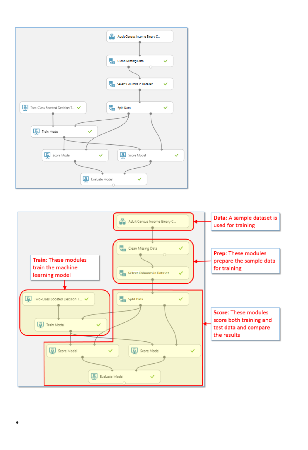
accept and return user data).
For example, the following experiment trains a two-class boosted decision tree model using sample census data:
The modules in this experiment perform basically four different functions:
When you convert this training experiment to a predictive experiment, some of these modules are no longer
needed, or they now serve a different purpose:
Data - The data in this sample dataset is not used during scoring - the user of the web service will supply
the data to be scored. However, the metadata from this dataset, such as data types, is used by the trained
model. So you need to keep the dataset in the predictive experiment so that it can provide this metadata.
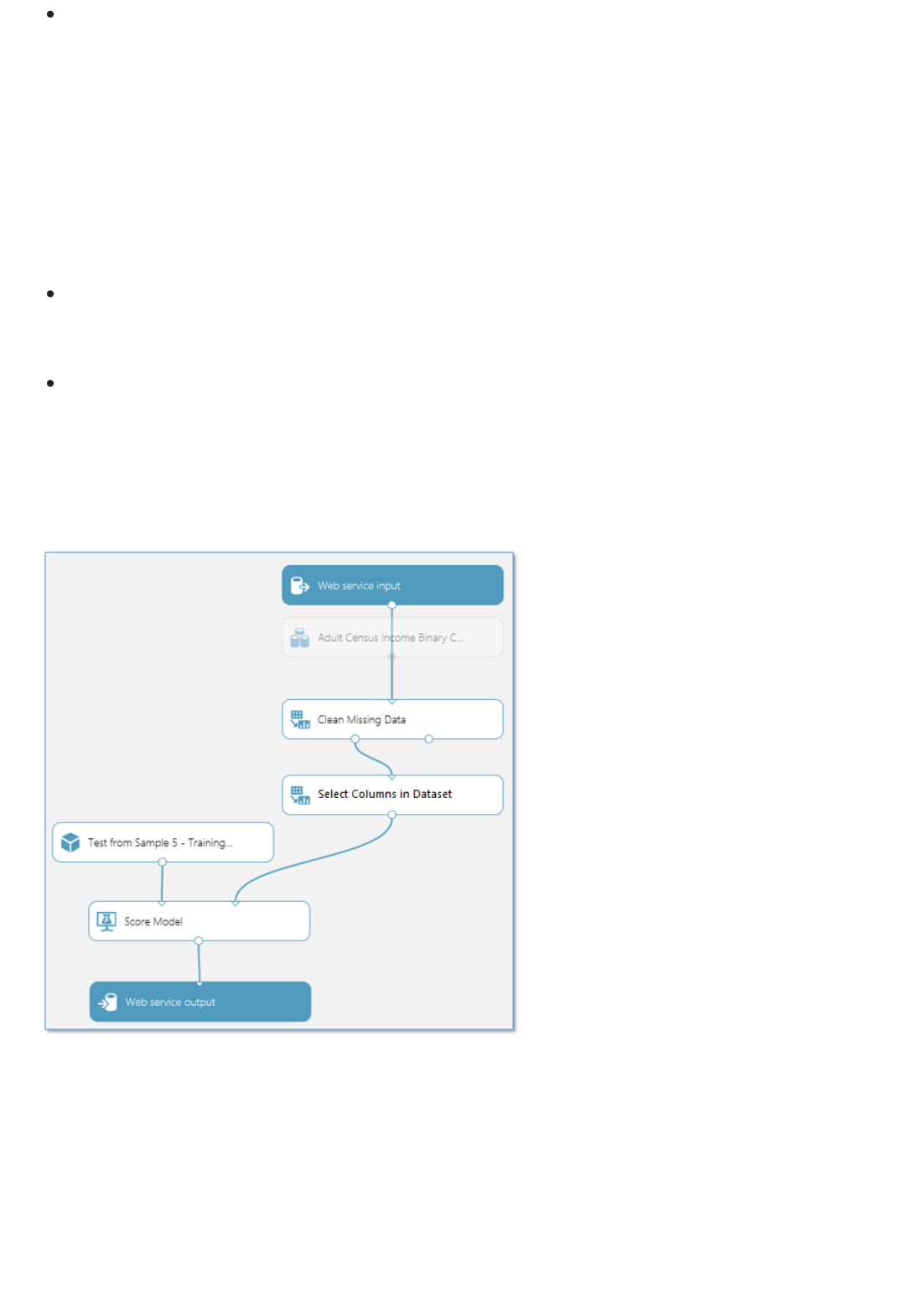
Adjust input and output modulesAdjust input and output modules
Prep - Depending on the user data that will be submitted for scoring, these modules may or may not be
necessary to process the incoming data. The Set Up Web Service button doesn't touch these - you need
to decide how you want to handle them.
For instance, in this example the sample dataset may have missing values, so a Clean Missing Data module
was included to deal with them. Also, the sample dataset includes columns that are not needed to train the
model. So a Select Columns in Dataset module was included to exclude those extra columns from the data
flow. If you know that the data that will be submitted for scoring through the web service will not have
missing values, then you can remove the Clean Missing Data module. However, since the Select Columns in
Dataset module helps define the columns of data that the trained model expects, that module needs to
remain.
Train - These modules are used to train the model. When you click Set Up Web Service, these modules
are replaced with a single module that contains the model you trained. This new module is saved in the
Trained Models section of the module palette.
Score - In this example, the Split Data module is used to divide the data stream into test data and training
data. In the predictive experiment, we're not training anymore, so Split Data can be removed. Similarly, the
second Score Model module and the Evaluate Model module are used to compare results from the test
data, so these modules are not needed in the predictive experiment. The remaining Score Model module,
however, is needed to return a score result through the web service.
Here is how our example looks after clicking Set Up Web Service:
The work done by Set Up Web Service may be sufficient to prepare your experiment to be deployed as a web
service. However, you may want to do some additional work specific to your experiment.
In your training experiment, you used a set of training data and then did some processing to get the data in a form
that the machine learning algorithm needed. If the data you expect to receive through the web service will not
need this processing, you can bypass it: connect the output of the Web service input module to a different
module in your experiment. The user's data will now arrive in the model at this location.
For example, by default Set Up Web Service puts the Web service input module at the top of your data flow, as
shown in the figure above. But we can manually position the Web service input past the data processing
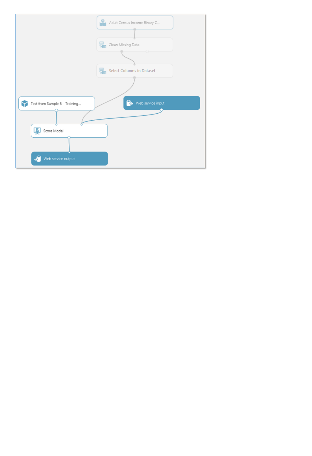
modules:
The input data provided through the web service will now pass directly into the Score Model module without any
preprocessing.
Similarly, by default Set Up Web Service puts the Web service output module at the bottom of your data flow. In
this example, the web service will return to the user the output of the Score Model module, which includes the
complete input data vector plus the scoring results. However, if you would prefer to return something different,
then you can add additional modules before the Web service output module.
For example, to return only the scoring results and not the entire vector of input data, add a Select Columns in
Dataset module to exclude all columns except the scoring results. Then move the Web service output module to
the output of the Select Columns in Dataset module. The experiment looks like this:
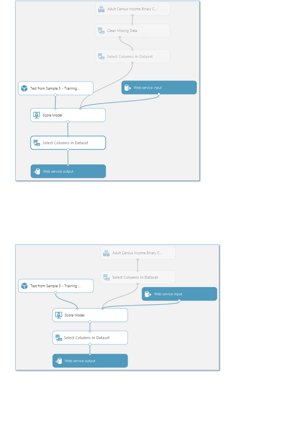
Add or remove additional data processing modulesAdd or remove additional data processing modules
Add optional Web Service ParametersAdd optional Web Service Parameters
If there are more modules in your experiment that you know will not be needed during scoring, these can be
removed. For example, because we moved the Web service input module to a point after the data processing
modules, we can remove the Clean Missing Data module from the predictive experiment.
Our predictive experiment now looks like this:
In some cases, you may want to allow the user of your web service to change the behavior of modules when the
service is accessed. Web Service Parameters allow you to do this.
A common example is setting up an Import Data module so the user of the deployed web service can specify a
different data source when the web service is accessed. Or configuring an Export Data module so that a different
destination can be specified.

Deploy the predictive experiment as a web service
You can define Web Service Parameters and associate them with one or more module parameters, and you can
specify whether they are required or optional. The user of the web service provides values for these parameters
when the service is accessed, and the module actions are modified accordingly.
For more information about what Web Service Parameters are and how to use them, see Using Azure Machine
Learning Web Service Parameters.
Now that the predictive experiment has been sufficiently prepared, you can deploy it as an Azure web service.
Using the web service, users can send data to your model and the model will return its predictions.
For more information on the complete deployment process, see Deploy an Azure Machine Learning web service
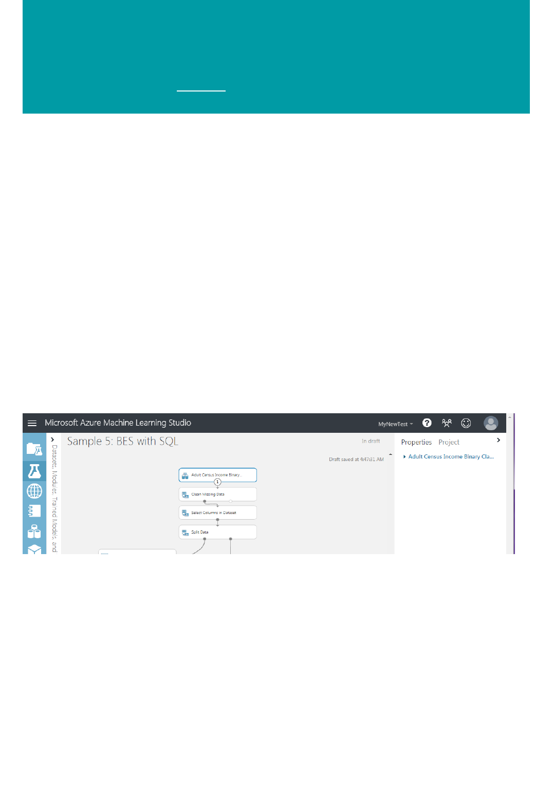
Deploying Azure ML web services that use Data
Import and Data Export modules
3/21/2018 • 6 min to read • Edit Online
Create the training experiment
When you create a predictive experiment, you typically add a web service input and output. When you deploy the
experiment, consumers can send and receive data from the web service through the inputs and outputs. For some
applications, a consumer's data may be available from a data feed or already reside in an external data source such
as Azure Blob storage. In these cases, they do not need read and write data using web service inputs and outputs.
They can, instead, use the Batch Execution Service (BES) to read data from the data source using an Import Data
module and write the scoring results to a different data location using an Export Data module.
The Import Data and Export data modules, can read from and write to various data locations such as a Web URL
via HTTP, a Hive Query, an Azure SQL database, Azure Table storage, Azure Blob storage, a Data Feed provide, or
an on-premises SQL database.
This topic uses the "Sample 5: Train, Test, Evaluate for Binary Classification: Adult Dataset" sample and assumes the
dataset has already been loaded into an Azure SQL table named censusdata.
When you open the "Sample 5: Train, Test, Evaluate for Binary Classification: Adult Dataset" sample it uses the
sample Adult Census Income Binary Classification dataset. And the experiment in the canvas will look similar to
the following image:
To read the data from the Azure SQL table:
1. Delete the dataset module.
2. In the components search box, type import.
3. From the results list, add an Import Data module to the experiment canvas.
4. Connect output of the Import Data module the input of the Clean Missing Data module.
5. In properties pane, select Azure SQL Database in the Data Source dropdown.
6. In the Database server name, Database name, User name, and Password fields, enter the appropriate
information for your database.
7. In the Database query field, enter the following query.
select [age],

Create the predictive experiment
[workclass],
[fnlwgt],
[education],
[education-num],
[marital-status],
[occupation],
[relationship],
[race],
[sex],
[capital-gain],
[capital-loss],
[hours-per-week],
[native-country],
[income]
8. At the bottom of the experiment canvas, click Run.
from dbo.censusdata;
Next you set up the predictive experiment from which you deploy your web service.
1. At the bottom of the experiment canvas, click Set Up Web Service and select Predictive Web Service
[Recommended].
2. Remove the Web Service Input and Web Service Output modules from the predictive experiment.
3. In the components search box, type export.
4. From the results list, add an Export Data module to the experiment canvas.
5. Connect output of the Score Model module the input of the Export Data module.
6. In properties pane, select Azure SQL Database in the data destination dropdown.
7. In the Database server name, Database name, Server user account name, and Server user account
password fields, enter the appropriate information for your database.
8. In the Comma separated list of columns to be saved field, type Scored Labels.
9. In the Data table name field, type dbo.ScoredLabels. If the table does not exist, it is created when the
experiment is run or the web service is called.
10. In the Comma separated list of datatable columns field, type ScoredLabels.
When you write an application that calls the final web service, you may want to specify a different input query or
destination table at run time. To configure these inputs and outputs, use the Web Service Parameters feature to set
the Import Data module Data source property and the Export Data mode data destination property. For more
information on Web Service Parameters, see the AzureML Web Service Parameters entry on the Cortana
Intelligence and Machine Learning Blog.
To configure the Web Service Parameters for the import query and the destination table:
1. In the properties pane for the Import Data module, click the icon at the top right of the Database query field
and select Set as web service parameter.
2. In the properties pane for the Export Data module, click the icon at the top right of the Data table name field
and select Set as web service parameter.
3. At the bottom of the Export Data module properties pane, in the Web Service Parameters section, click
Database query and rename it Query.
4. Click Data table name and rename it Table.
When you are done, your experiment should look similar to the following image:
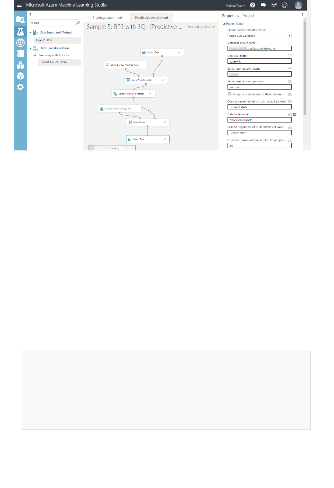
Deploy the web service
Deploy a Classic Web ServiceDeploy a Classic Web Service
Deploy a New Web ServiceDeploy a New Web Service
Now you can deploy the experiment as a web service.
You can deploy to either a Classic or New web service.
To deploy as a Classic Web Service and create an application to consume it:
1. At the bottom of the experiment canvas, click Run.
2. When the run has completed, click Deploy Web Service and select Deploy Web Service [Classic].
3. On the web service dashboard, locate your API key. Copy and save it to use later.
4. In the Default Endpoint table, click the Batch Execution link to open the API Help Page.
5. In Visual Studio, create a C# console application: New > Project > Visual C# > Windows Classic Desktop >
Console App (.NET Framework).
6. On the API Help Page, find the Sample Code section at the bottom of the page.
7. Copy and paste the C# sample code into your Program.cs file, and remove all references to the blob storage.
8. Update the value of the apiKey variable with the API key saved earlier.
var request = new BatchExecutionRequest()
{
GlobalParameters = new Dictionary<string, string>() {
{ "Query", @"select [age], [workclass], [fnlwgt], [education], [education-num], [marital-
status], [occupation], [relationship], [race], [sex], [capital-gain], [capital-loss], [hours-per-week],
[native-country], [income] from dbo.censusdata" },
{ "Table", "dbo.ScoredTable2" },
}
};
10. Run the application.
9. Locate the request declaration and update the values of Web Service Parameters that are passed to the
Import Data and Export Data modules. In this case, you use the original query, but define a new table name.
On completion of the run, a new table is added to the database containing the scoring results.

NOTENOTE
To deploy a New web service you must have sufficient permissions in the subscription to which you deploying the web
service. For more information, see Manage a Web service using the Azure Machine Learning Web Services portal.
To deploy as a New Web Service and create an application to consume it:
1. At the bottom of the experiment canvas, click Run.
2. When the run has completed, click Deploy Web Service and select Deploy Web Service [New].
3. On the Deploy Experiment page, enter a name for your web service, and select a pricing plan, then click
Deploy.
4. On the Quickstart page, click Consume.
5. In the Sample Code section, click Batch.
6. In Visual Studio, create a C# console application: New > Project > Visual C# > Windows Classic Desktop >
Console App (.NET Framework).
7. Copy and paste the C# sample code into your Program.cs file.
8. Update the value of the apiKey variable with the Primary Key located in the Basic consumption info section.
var scoreRequest = new
{
Inputs = new Dictionary<string, StringTable>()
{
},
GlobalParameters = new Dictionary<string, string>() {
{ "Query", @"select [age], [workclass], [fnlwgt], [education], [education-num], [marital-
status], [occupation], [relationship], [race], [sex], [capital-gain], [capital-loss], [hours-per-week],
[native-country], [income] from dbo.censusdata" },
{ "Table", "dbo.ScoredTable3" },
}
};
10. Run the application.
9. Locate the scoreRequest declaration and update the values of Web Service Parameters that are passed to the
Import Data and Export Data modules. In this case, you use the original query, but define a new table name.

How to deploy a Web Service to multiple regions
3/16/2018 • 1 min to read • Edit Online
To create a plan in another region
Deploying the web service to another region
The New Azure Web Services allow you to easily deploy a web service to multiple regions without needing
multiple subscriptions or workspaces.
Pricing is region specific, therefore you must define a billing plan for each region in which you will deploy the web
service.
1. Sign into Microsoft Azure Machine Learning Web Services.
2. Click the Plans menu option.
3. On the Plans over view page, click New.
4. From the Subscription dropdown, select the subscription in which the new plan will reside.
5. From the Region dropdown, select a region for the new plan. The Plan Options for the selected region will
display in the Plan Options section of the page.
6. From the Resource Group dropdown, select a resource group for the plan. From more information on
resource groups, see Azure Resource Manager overview.
7. In Plan Name type the name of the plan.
8. Under Plan Options, click the billing level for the new plan.
9. Click Create.
1. Click the Web Services menu option.
2. Select the Web Service you are deploying to a new region.
3. Click Copy.
4. In Web Service Name, type a new name for the web service.
5. In Web service description, type a description for the web service.
6. From the Subscription dropdown, select the subscription in which the new web service will reside.
7. From the Resource Group dropdown, select a resource group for the web service. From more information on
resource groups, see Azure Resource Manager overview.
8. From the Region dropdown, select the region in which to deploy the web service.
9. From the Storage account dropdown, select a storage account in which to store the web service.
10. From the Price Plan dropdown, select a plan in the region you selected in step 8.
11. Click Copy.
Use Azure Machine Learning Web Service
Parameters
4/13/2018 • 4 min to read • Edit Online
NOTENOTE
How to set and use Web Service Parameters
NOTENOTE
Example
An Azure Machine Learning web service is created by publishing an experiment that contains modules with
configurable parameters. In some cases, you may want to change the module behavior while the web service is
running. Web Service Parameters allow you to do this task.
A common example is setting up the Import Data module so that the user of the published web service can specify
a different data source when the web service is accessed. Or configuring the Export Data module so that a different
destination can be specified. Some other examples include changing the number of bits for the Feature Hashing
module or the number of desired features for the Filter-Based Feature Selection module.
You can set Web Service Parameters and associate them with one or more module parameters in your experiment,
and you can specify whether they are required or optional. The user of the web service can then provide values for
these parameters when they call the web service.
You can try Azure Machine Learning for free. No credit card or Azure subscription is required. Get started now.
You define a Web Service Parameter by clicking the icon next to the parameter for a module and selecting "Set as
web service parameter". This creates a new Web Service Parameter and connects it to that module parameter.
Then, when the web service is accessed, the user can specify a value for the Web Service Parameter and it is
applied to the module parameter.
Once you define a Web Service Parameter, it's available to any other module parameter in the experiment. If you
define a Web Service Parameter associated with a parameter for one module, you can use that same Web Service
Parameter for any other module, as long as the parameter expects the same type of value. For example, if the Web
Service Parameter is a numeric value, then it can only be used for module parameters that expect a numeric value.
When the user sets a value for the Web Service Parameter, it will be applied to all associated module parameters.
You can decide whether to provide a default value for the Web Service Parameter. If you do, then the parameter is
optional for the user of the web service. If you don't provide a default value, then the user is required to enter a
value when the web service is accessed.
The API documentation for the web service includes information for the web service user on how to specify the
Web Service Parameter programmatically when accessing the web service.
The API documentation for a classic web service is provided through the API help page link in the web service
DASHBOARD in Machine Learning Studio. The API documentation for a new web service is provided through the Azure
Machine Learning Web Services portal on the Consume and Swagger API pages for your web service.
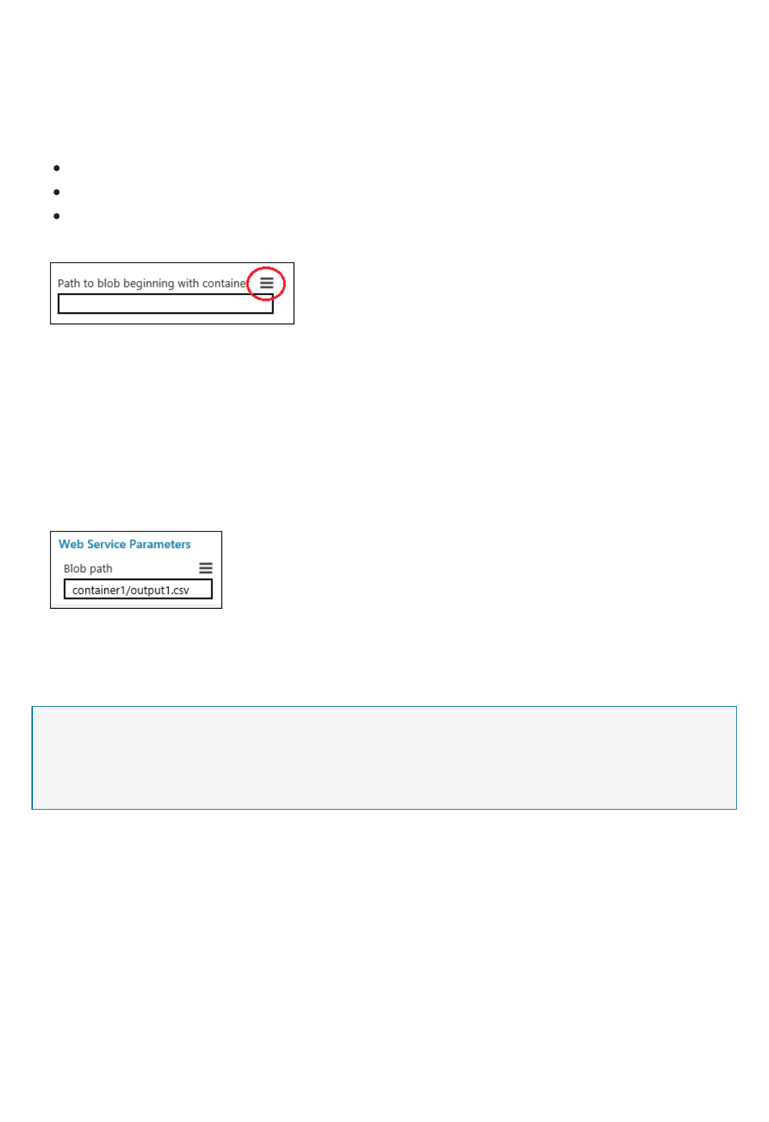
NOTENOTE
More information
As an example, let's assume we have an experiment with an Export Data module that sends information to Azure
blob storage. We'll define a Web Service Parameter named "Blob path" that allows the web service user to change
the path to the blob storage when the service is accessed.
1. In Machine Learning Studio, click the Export Data module to select it. Its properties are shown in the Properties
pane to the right of the experiment canvas.
4. To rename the Web Service Parameter, click the name, enter "Blob path", and press the Enter key.
6. Click Run.
7. Click Deploy Web Service and select Deploy Web Service [Classic] or Deploy Web Service [New] to
deploy the web service.
2. Specify the storage type:
Under Please specify data destination, select "Azure Blob Storage".
Under Please specify authentication type, select "Account".
Enter the account information for the Azure blob storage.
3. Click the icon to the right of the Path to blob beginning with container parameter. It looks like this:
Select "Set as web service parameter".
An entry is added under Web Service Parameters at the bottom of the Properties pane with the name
"Path to blob beginning with container". This is the Web Service Parameter that is now associated with this
Export Data module parameter.
5. To provide a default value for the Web Service Parameter, click the icon to the right of the name, select
"Provide default value", enter a value (for example, "container1/output1.csv"), and press the Enter key.
To deploy a New web service you must have sufficient permissions in the subscription to which you deploying the web
service. For more information see, Manage a Web service using the Azure Machine Learning Web Services portal.
The user of the web service can now specify a new destination for the Export Data module when accessing the web
service.
For a more detailed example, see the Web Service Parameters entry in the Machine Learning Blog.
For more information on accessing a Machine Learning web service, see How to consume an Azure Machine
Learning Web service.
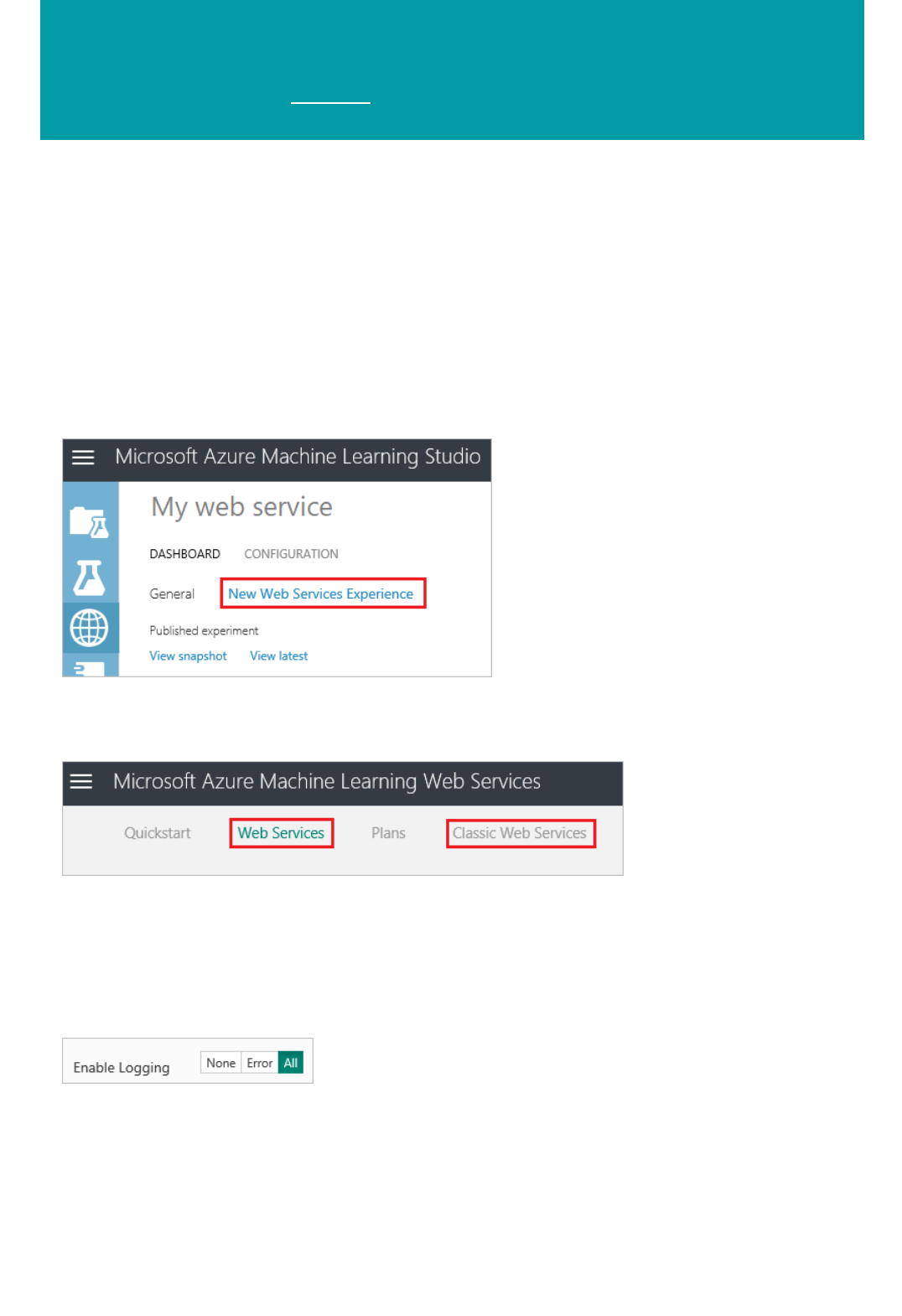
Enable logging for Machine Learning web services
3/21/2018 • 2 min to read • Edit Online
How to enable logging for a Web service
This document provides information on the logging capability of Machine Learning web services. Logging
provides additional information, beyond just an error number and a message, that can help you troubleshoot your
calls to the Machine Learning APIs.
You enable logging from the Azure Machine Learning Web Services portal.
1. Sign in to the Azure Machine Learning Web Services portal at https://services.azureml.net. For a Classic
web service, you can also get to the portal by clicking New Web Services Experience on the Machine
Learning Web Services page in Machine Learning Studio.
2. On the top menu bar, click Web Services for a New web service, or click Classic Web Services for a
Classic web service.
3. For a New web service, click the web service name. For a Classic web service, click the web service name
and then on the next page click the appropriate endpoint.
4. On the top menu bar, click Configure.
5. Set the Enable Logging option to Error (to log only errors) or All (for full logging).
6. Click Save.
7. For Classic web services, create the ml-diagnostics container.
All web service logs are kept in a blob container named ml-diagnostics in the storage account associated
with the web service. For New web services, this container is created the first time you access the web
service. For Classic web services, you need to create the container if it doesn't already exist.
a. In the Azure portal, go to the storage account associated with the web service.
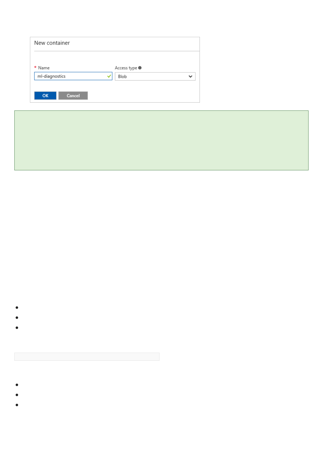
TIPTIP
The effects of enabling logging
Log blob detail information
b. Under Blob Service, click Containers.
c. If the container ml-diagnostics doesn't exist, click +Container, give the container the name "ml-
diagnostics", and select the Access type as "Blob". Click OK.
For a Classic web service, the Web Services Dashboard in Machine Learning Studio also has a switch to enable logging.
However, because logging is now managed through the Web Services portal, you need to enable logging through the portal
as described in this article. If you already enabled logging in Studio, then in the Web Services Portal, disable logging and
enable it again.
When logging is enabled, the diagnostics and errors from the web service endpoint are logged in the ml-
diagnostics blob container in the Azure Storage Account linked with the user’s workspace. This container holds all
the diagnostics information for all the web service endpoints for all the workspaces associated with this storage
account.
The logs can be viewed using any of the several tools available to explore an Azure Storage Account. The easiest
may be to navigate to the storage account in the Azure portal, click Containers, and then click the container ml-
diagnostics.
Each blob in the container holds the diagnostics information for exactly one of the following actions:
An execution of the Batch-Execution method
An execution of the Request-Response method
Initialization of a Request-Response container
The name of each blob has a prefix of the following form:
{Workspace Id}-{Web service Id}-{Endpoint Id}/{Log type}
Where Log type is one of the following values:
batch
score/requests
score/init
Manage a Web service using the Azure Machine
Learning Web Services portal
4/11/2018 • 7 min to read • Edit Online
NOTENOTE
Permissions to manage New Resources Manager based web services
Manage New Web services
You can manage your Machine Learning New and Classic Web services using the Microsoft Azure Machine
Learning Web Services portal. Since Classic Web services and New Web services are based on different
underlying technologies, you have slightly different management capabilities for each of them.
In the Machine Learning Web Services portal you can:
Monitor how the web service is being used.
Configure the description, update the keys for the web service (New only), update your storage account key
(New only), enable logging, and enable or disable sample data.
Delete the web service.
Create, delete, or update billing plans (New only).
Add and delete endpoints (Classic only)
You can try Azure Machine Learning for free. No credit card or Azure subscription is required. Get started now.
New web services are deployed as Azure resources. As such, you must have the correct permissions to deploy
and manage New web services. To deploy or manage New web services you must be assigned a contributor or
administrator role on the subscription to which the web service is deployed. If you invite another user to a
machine learning workspace, you must assign them to a contributor or administrator role on the subscription
before they can deploy or manage web services.
If the user does not have the correct permissions to access resources in the Azure Machine Learning Web
Services portal, they will receive the following error when trying to deploy a web service:
Web Service deployment failed. This account does not have sufficient access to the Azure subscription that
contains the Workspace. In order to deploy a Web Service to Azure, the same account must be invited to the
Workspace and be given access to the Azure subscription that contains the Workspace.
For more information on creating a workspace, see Create and share an Azure Machine Learning workspace.
For more information on setting access permissions, see View access assignments for users and groups in the
Azure portal - Public preview.
To manage your New Web services:
1. Sign in to the Microsoft Azure Machine Learning Web Services portal using your Microsoft Azure account -
use the account that's associated with the Azure subscription.
2. On the menu, click Web Services.
This displays a list of deployed Web services for your subscription.

Monitoring how the web service is being usedMonitoring how the web service is being used
Configuring the web serviceConfiguring the web service
Managing billing plansManaging billing plans
To manage a Web service, click Web Services. From the Web Services page you can:
Click the web service to manage it.
Click the Billing Plan for the web service to update it.
Delete a web service.
Copy a web service and deploy it to another region.
When you click a web service, the web service Quickstart page opens. The web service Quickstart page has two
menu options that allow you to manage your web service:
DASHBOARD - Allows you to view Web service usage.
CONFIGURE - Allows you to add descriptive text, update the key for the storage account associated with the
Web service, and enable or disable sample data.
Click the DASHBOARD tab.
From the dashboard, you can view overall usage of your Web service over a period of time. You can select the
period to view from the Period dropdown menu in the upper right of the usage charts. The dashboard shows
the following information:
Requests Over Time displays a step graph of the number of requests over the selected time period. It can
help identify if you are experiencing spikes in usage.
Request-Response Requests displays the total number of Request-Response calls the service has received
over the selected time period and how many of them failed.
Average Request-Response Compute Time displays an average of the time needed to execute the
received requests.
Batch Requests displays the total number of Batch Requests the service has received over the selected time
period and how many of them failed.
Average Job Latency displays an average of the time needed to execute the received requests.
Errors displays the aggregate number of errors that have occurred on calls to the web service.
Services Costs displays the charges for the billing plan associated with the service.
Click the CONFIGURE menu option.
You can update the following properties:
Description allows you to enter a description for the Web service.
Title allows you to enter a title for the Web service
Keys allows you to rotate your primary and secondary API keys.
Storage account key allows you to update the key for the storage account associated with the Web service
changes.
Enable Sample data allows you to provide sample data that you can use to test the Request-Response
service. If you created the web service in Machine Learning Studio, the sample data is taken from the data
your used to train your model. If you created the service programmatically, the data is taken from the
example data you provided as part of the JSON package.
Click the Plans menu option from the web services Quickstart page. You can also click the plan associated with
specific Web service to manage that plan.
New allows you to create a new plan.
Add/Remove Plan instance allows you to "scale out" an existing plan to add capacity.
Manage Classic Web Services
NOTENOTE
Monitoring how the web service is being usedMonitoring how the web service is being used
Upgrade/DownGrade allows you to "scale up" an existing plan to add capacity.
Delete allows you to delete a plan.
Click a plan to view its dashboard. The dashboard gives you snapshot or plan usage over a selected period of
time. To select the time period to view, click the Period dropdown at the upper right of dashboard.
The plan dashboard provides the following information:
Plan Description displays information about the costs and capacity associated with the plan.
Plan Usage displays the number of transactions and compute hours that have been charged against the
plan.
Web Services displays the number of Web services that are using this plan.
Top Web Service By Calls displays the top four Web services that are making calls that are charged against
the plan.
Top Web Services by Compute Hrs displays the top four Web services that are using compute resources
that are charged against the plan.
The procedures in this section are relevant to managing Classic web services through the Azure Machine Learning Web
Services portal. For information on managing Classic Web services through the Machine Learning Studio and the Azure
portal, see Manage an Azure Machine Learning workspace.
To manage your Classic Web services:
1. Sign in to the Microsoft Azure Machine Learning Web Services portal using your Microsoft Azure account -
use the account that's associated with the Azure subscription.
2. On the menu, click Classic Web Services.
To manage a Classic Web Service, click Classic Web Services. From the Classic Web Services page you can:
Click the web service to view the associated endpoints.
Delete a web service.
When you manage a Classic Web service, you manage each of the endpoints separately. When you click a web
service in the Web Services page, the list of endpoints associated with the service opens.
On the Classic Web Service endpoint page, you can add and delete endpoints on the service. For more
information on adding endpoints, see Creating Endpoints.
Click one of the endpoints to open the web service Quickstart page. On the Quickstart page, there are two
menu options that allow you to manage your web service:
DASHBOARD - Allows you to view Web service usage.
CONFIGURE - Allows you to add descriptive text, turn error logging on and off, update the key for the
storage account associated with the Web service, and enable and disable sample data.
Click the DASHBOARD tab.
From the dashboard, you can view overall usage of your Web service over a period of time. You can select the
period to view from the Period dropdown menu in the upper right of the usage charts. The dashboard shows
the following information:

Configuring the web serviceConfiguring the web service
Requests Over Time displays a step graph of the number of requests over the selected time period. It can
help identify if you are experiencing spikes in usage.
Request-Response Requests displays the total number of Request-Response calls the service has received
over the selected time period and how many of them failed.
Average Request-Response Compute Time displays an average of the time needed to execute the
received requests.
Batch Requests displays the total number of Batch Requests the service has received over the selected time
period and how many of them failed.
Average Job Latency displays an average of the time needed to execute the received requests.
Errors displays the aggregate number of errors that have occurred on calls to the web service.
Services Costs displays the charges for the billing plan associated with the service.
Click the CONFIGURE menu option.
You can update the following properties:
Description allows you to enter a description for the Web service. Description is a required field.
Logging allows you to enable or disable error logging on the endpoint. For more information on Logging,
see Enable logging for Machine Learning web services.
Enable Sample data allows you to provide sample data that you can use to test the Request-Response
service. If you created the web service in Machine Learning Studio, the sample data is taken from the data
your used to train your model. If you created the service programmatically, the data is taken from the
example data you provided as part of the JSON package.

Learn how to manage AzureML web services using
API Management
3/21/2018 • 11 min to read • Edit Online
Overview
What is Azure API Management?
What is AzureML?
Prerequisites
Create an API Management instance
This guide shows you how to quickly get started using API Management to manage your AzureML web services.
Azure API Management is an Azure service that lets you manage your REST API endpoints by defining user
access, usage throttling, and dashboard monitoring. Click here for details on Azure API Management. Click here for
a guide on how to get started with Azure API Management. This other guide, which this guide is based on, covers
more topics, including notification configurations, tier pricing, response handling, user authentication, creating
products, developer subscriptions, and usage dashboarding.
AzureML is an Azure service for machine learning that enables you to easily build, deploy, and share advanced
analytics solutions. Click here for details on AzureML.
To complete this guide, you need:
An Azure account. If you don’t have an Azure account, click here for details on how to create a free trial account.
An AzureML account. If you don’t have an AzureML account, click here for details on how to create a free trial
account.
The workspace, service, and api_key for an AzureML experiment deployed as a web service. Click here for
details on how to create an AzureML experiment. Click here for details on how to deploy an AzureML
experiment as a web service. Alternately, Appendix A has instructions for how to create and test a simple
AzureML experiment and deploy it as a web service.
You can manage your Azure Machine Learning web service with an API Management instance.
1. Sign in to the Azure portal.
2. Select + Create a resource.
3. In the search box, type "API management", then select the "API management" resource.
4. Click Create.
5. The Name value will be used to create a unique URL (this example uses "demoazureml").
6. Select a Subscription, Resource group, and Location for your service instance.
7. Specify a value for Organization name (this example uses "demoazureml").
8. Enter your Administrator email - this email will be used for notifications from the API Management system.
9. Click Create.
It may take up to 30 minutes for a new service to be created.
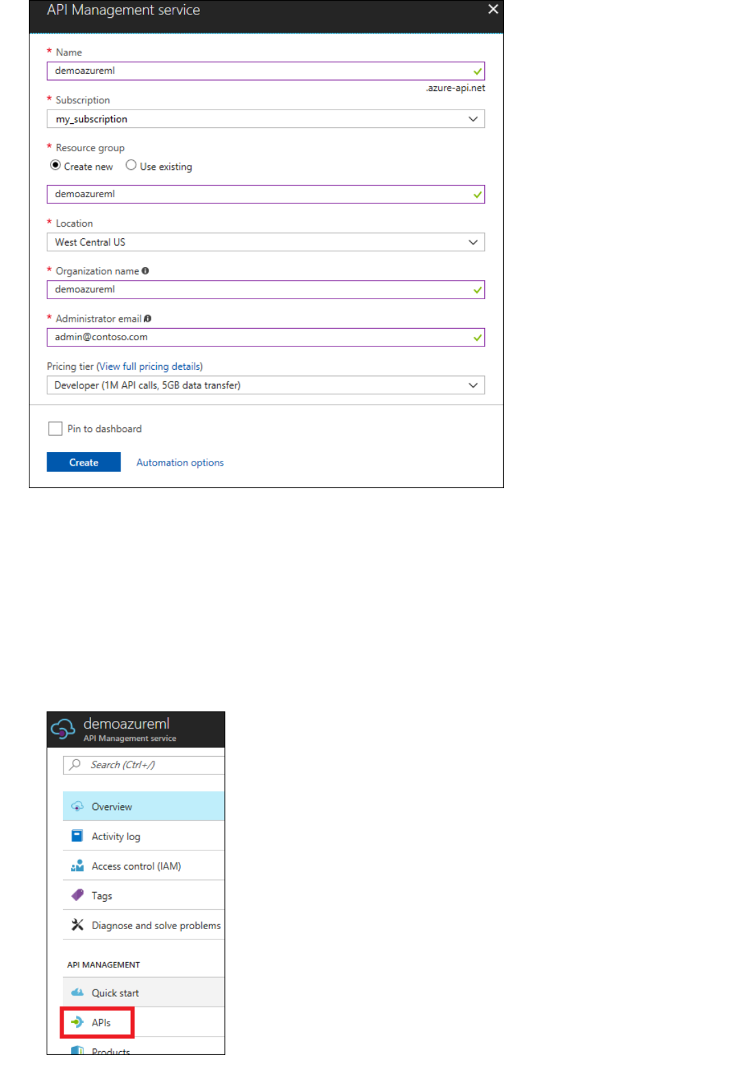
Create the API
Once the service instance is created, the next step is to create the API. An API consists of a set of operations that
can be invoked from a client application. API operations are proxied to existing web services. This guide creates
APIs that proxy to the existing AzureML RRS and BES web services.
To create the API:
1. In the Azure portal, open the service instance you just created.
2. In the left navigation pane, select APIs.
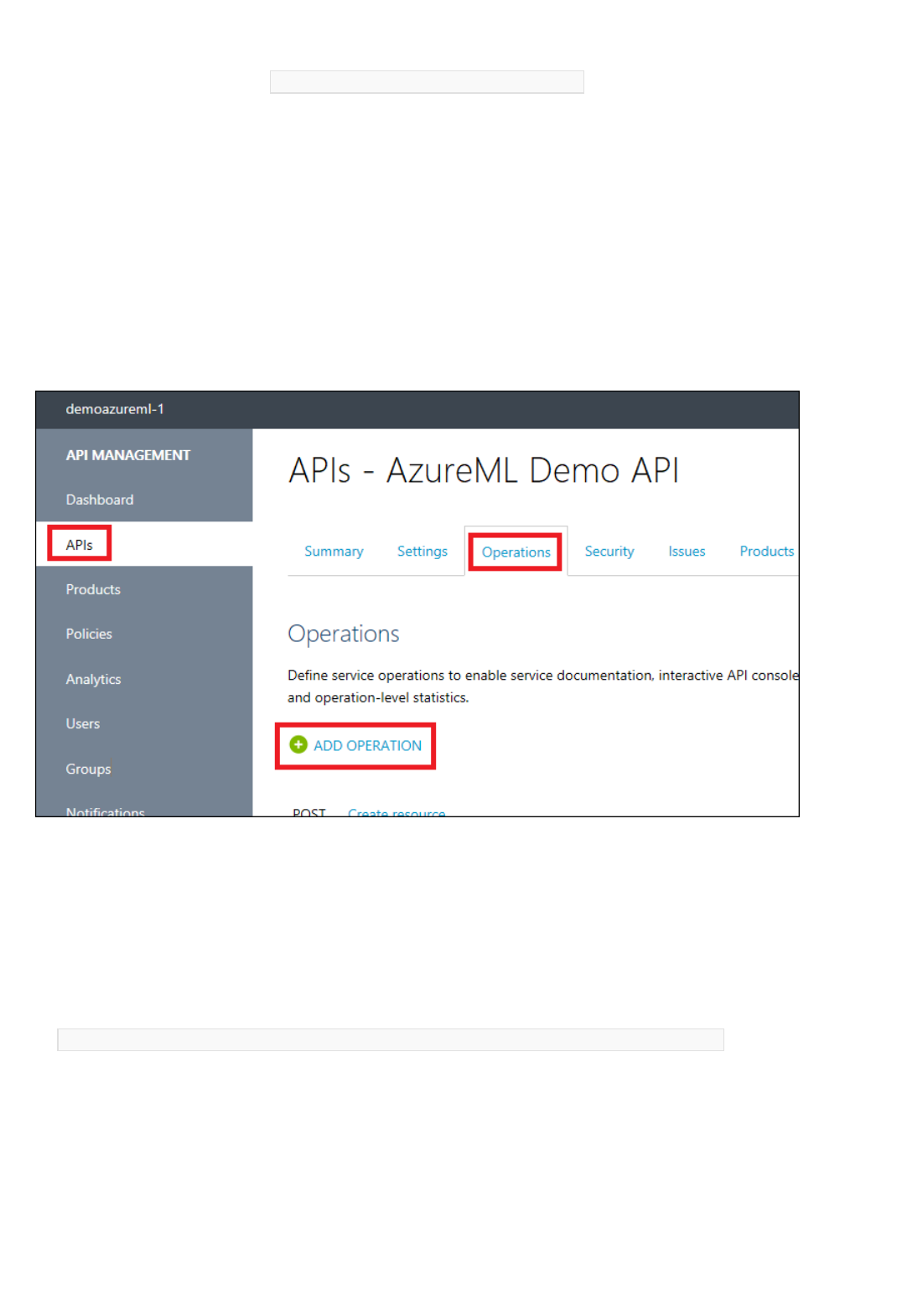
Add the operations
Add RRS Operation
4. Enter a Web API name (this example uses "AzureML Demo API").
5. For Web service URL, enter " https://ussouthcentral.services.azureml.net ".
6. Enter a **Web API URL suffix". This will become the last part of the URL that customers will use for sending
requests to the service instance (this example uses "azureml-demo").
7. For Web API URL scheme, select HTTPS.
8. For Products, select Starter.
9. Click Save.
3. Click Add API.
Operations are added and configured to an API in the publisher portal. To access the publisher portal, click
Publisher portal in the Azure portal for your API Management service, select APIs, Operations, then click Add
operation.
The New operation window will be displayed and the Signature tab will be selected by default.
First create an operation for the AzureML RRS service:
1. For the HTTP verb, select POST.
2. For the URL template, type "
/workspaces/{workspace}/services/{service}/execute?api-version={apiversion}&details={details} ".
3. Enter a Display name (this example uses "RRS Execute").
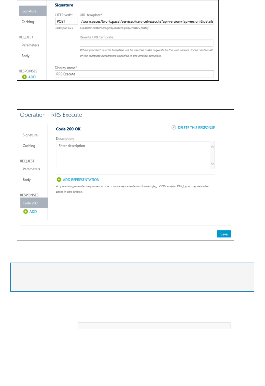
Add BES Operations
NOTENOTE
Submit (but not start) a Batch Execution jobSubmit (but not start) a Batch Execution job
Start a Batch Execution jobStart a Batch Execution job
4. Click Responses > ADD on the left and select 200 OK.
5. Click Save to save this operation.
Screenshots are not included here for the BES operations as they are very similar to those for adding the RRS operation.
1. Click add operation to add a BES operation to the API.
2. For the HTTP verb, select POST.
3. For the URL template, type " /workspaces/{workspace}/services/{service}/jobs?api-version={apiversion} ".
4. Enter a Display name (this example uses "BES Submit").
5. Click Responses > ADD on the left and select 200 OK.
6. Click Save.
1. Click add operation to add a BES operation to the API.
2. For the HTTP verb, select POST.
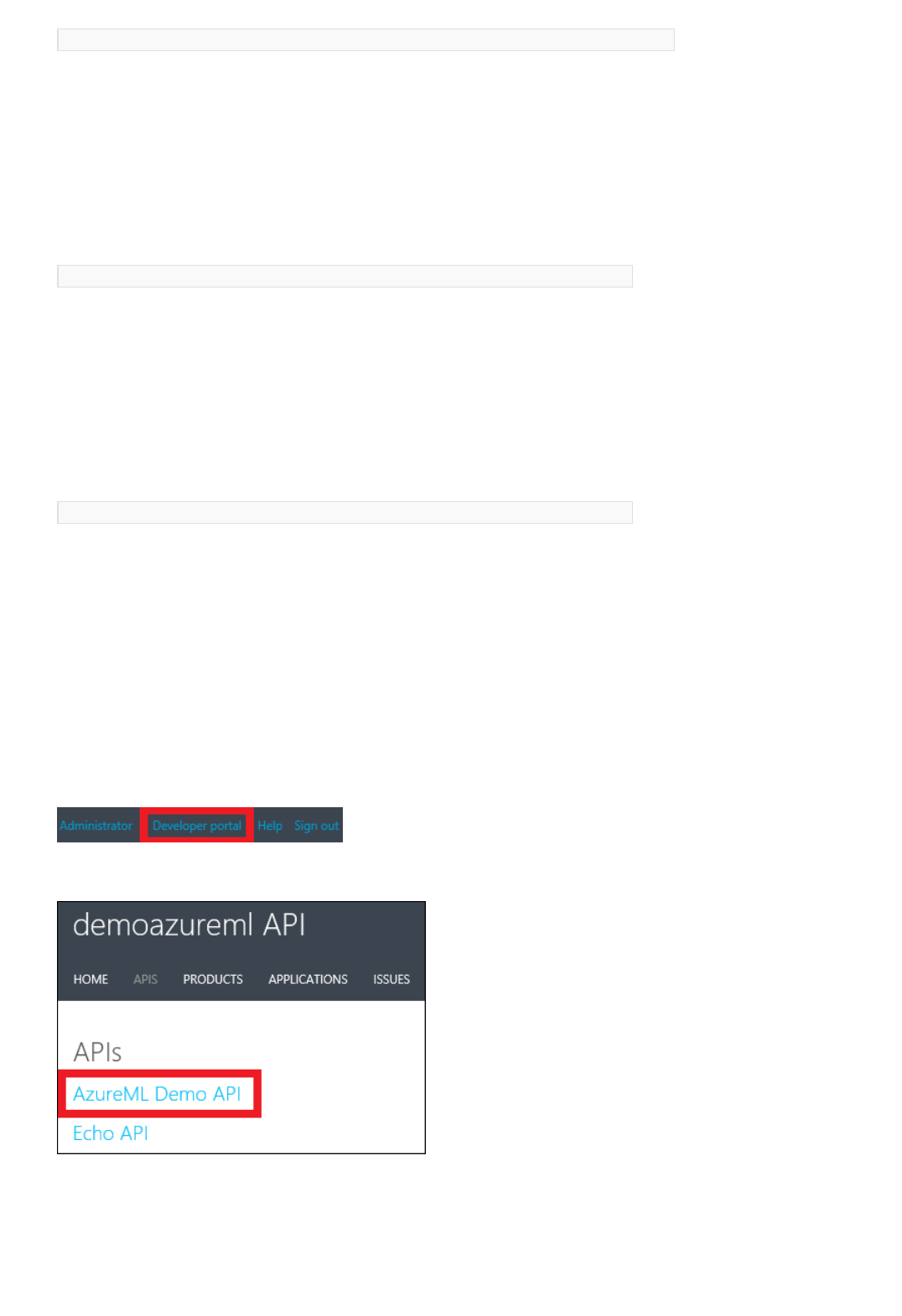
Get the status or result of a Batch Execution jobGet the status or result of a Batch Execution job
Delete a Batch Execution jobDelete a Batch Execution job
Call an operation from the Developer portal
3. For the HTTP verb, type "
/workspaces/{workspace}/services/{service}/jobs/{jobid}/start?api-version={apiversion} ".
4. Enter a Display name (this example uses "BES Start").
5. Click Responses > ADD on the left and select 200 OK.
6. Click Save.
1. Click add operation to add a BES operation to the API.
2. For the HTTP verb, select GET.
3. For the URL template, type "
/workspaces/{workspace}/services/{service}/jobs/{jobid}?api-version={apiversion} ".
4. Enter a Display name (this example uses "BES Status").
5. Click Responses > ADD on the left and select 200 OK.
6. Click Save.
1. Click add operation to add a BES operation to the API.
2. For the HTTP verb, select DELETE.
3. For the URL template, type "
/workspaces/{workspace}/services/{service}/jobs/{jobid}?api-version={apiversion} ".
4. Enter a Display name (this example uses "BES Delete").
5. Click Responses > ADD on the left and select 200 OK.
6. Click Save.
Operations can be called directly from the Developer portal, which provides a convenient way to view and test the
operations of an API. In this step you will call the RRS Execute method that was added to the AzureML Demo
API.
1. Click Developer portal.
2. Click APIs from the top menu, and then click AzureML Demo API to see the operations available.
3. Select RRS Execute for the operation. Click Try It.
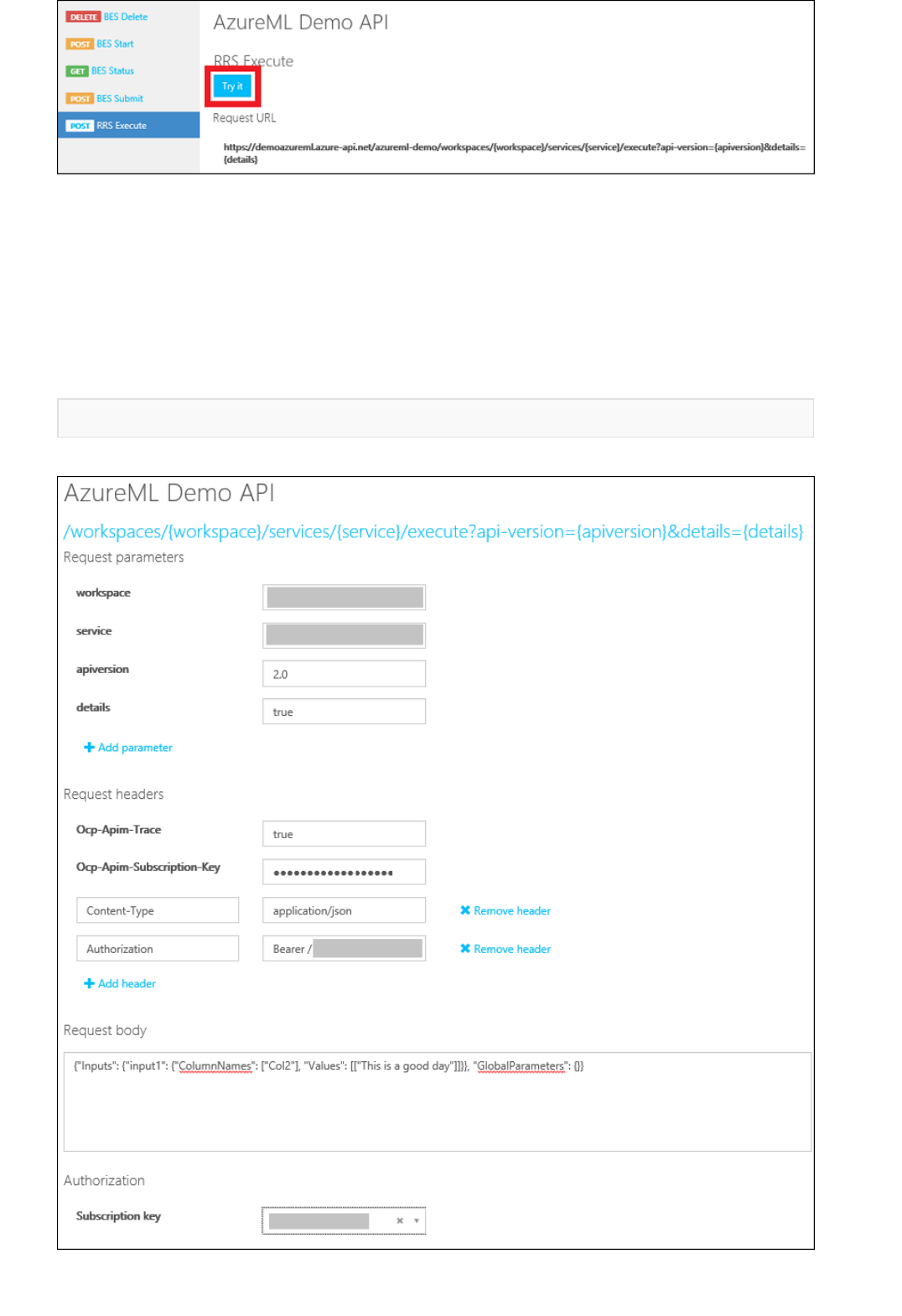
4. For Request parameters, type your workspace and service, type "2.0 for the apiversion, and "true" for
the details. You can find your workspace and service in the AzureML web service dashboard (see Test the
web service in Appendix A).
For Request headers, click Add header and type "Content-Type" and "application/json". Click Add header
again and type "Authorization" and "Bearer <your service API-KEY>". You can find your API-KEY in the
AzureML web service dashboard (see Test the web service in Appendix A).
For Request body, type
{"Inputs": {"input1": {"ColumnNames": ["Col2"], "Values": [["This is a good day"]]}}, "GlobalParameters":
{}}
.
5. Click Send.
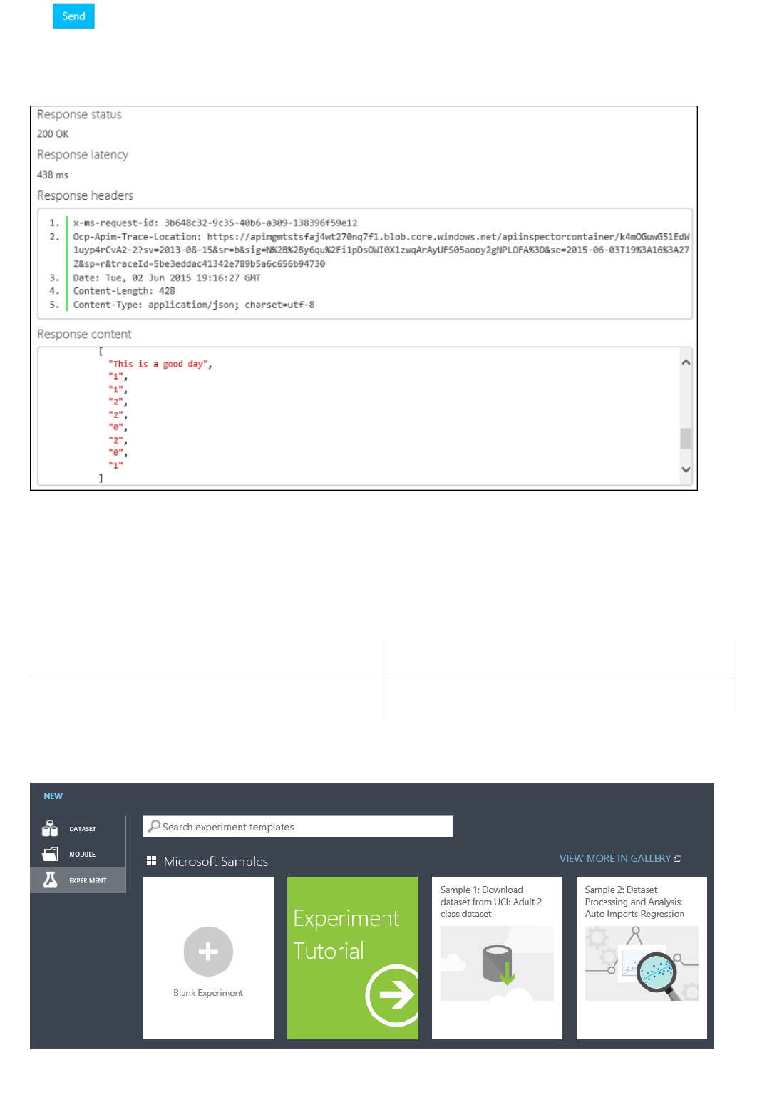
Appendix A - Creating and testing a simple AzureML web service
Creating the experimentCreating the experiment
TEX T HASHED TEX T
This is a good day 1 1 2 2 0 2 0 1
After an operation is invoked, the developer portal displays the Requested URL from the back-end service, the
Response status, the Response headers, and any Response content.
Below are the steps for creating a simple AzureML experiment and deploying it as a web service. The web service
takes as input a column of arbitrary text and returns a set of features represented as integers. For example:
First, using a browser of your choice, navigate to: https://studio.azureml.net/ and enter your credentials to log in.
Next, create a new blank experiment.
Rename it to SimpleFeatureHashingExperiment. Expand Saved Datasets and drag Book Reviews from
Amazon onto your experiment.
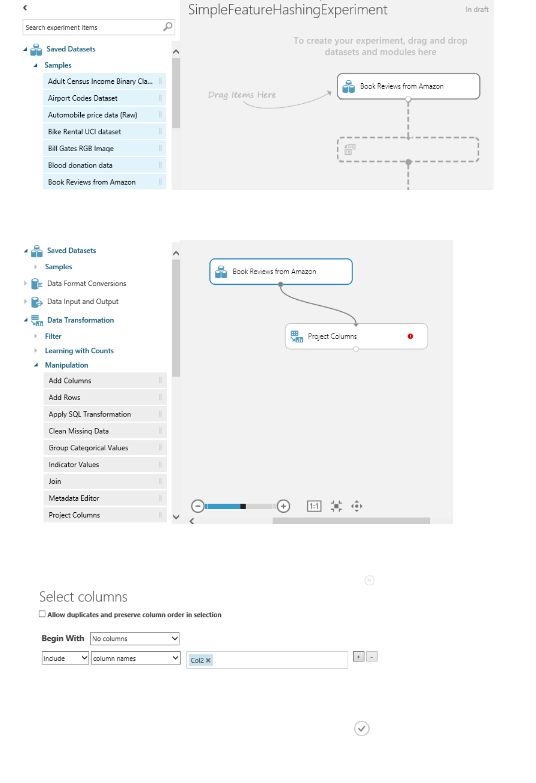
Expand Data Transformation and Manipulation and drag Select Columns in Dataset onto your experiment.
Connect Book Reviews from Amazon to Select Columns in Dataset.
Click Select Columns in Dataset and then click Launch column selector and select Col2. Click the checkmark
to apply these changes.
Expand Text Analytics and drag Feature Hashing onto the experiment. Connect Select Columns in Dataset to
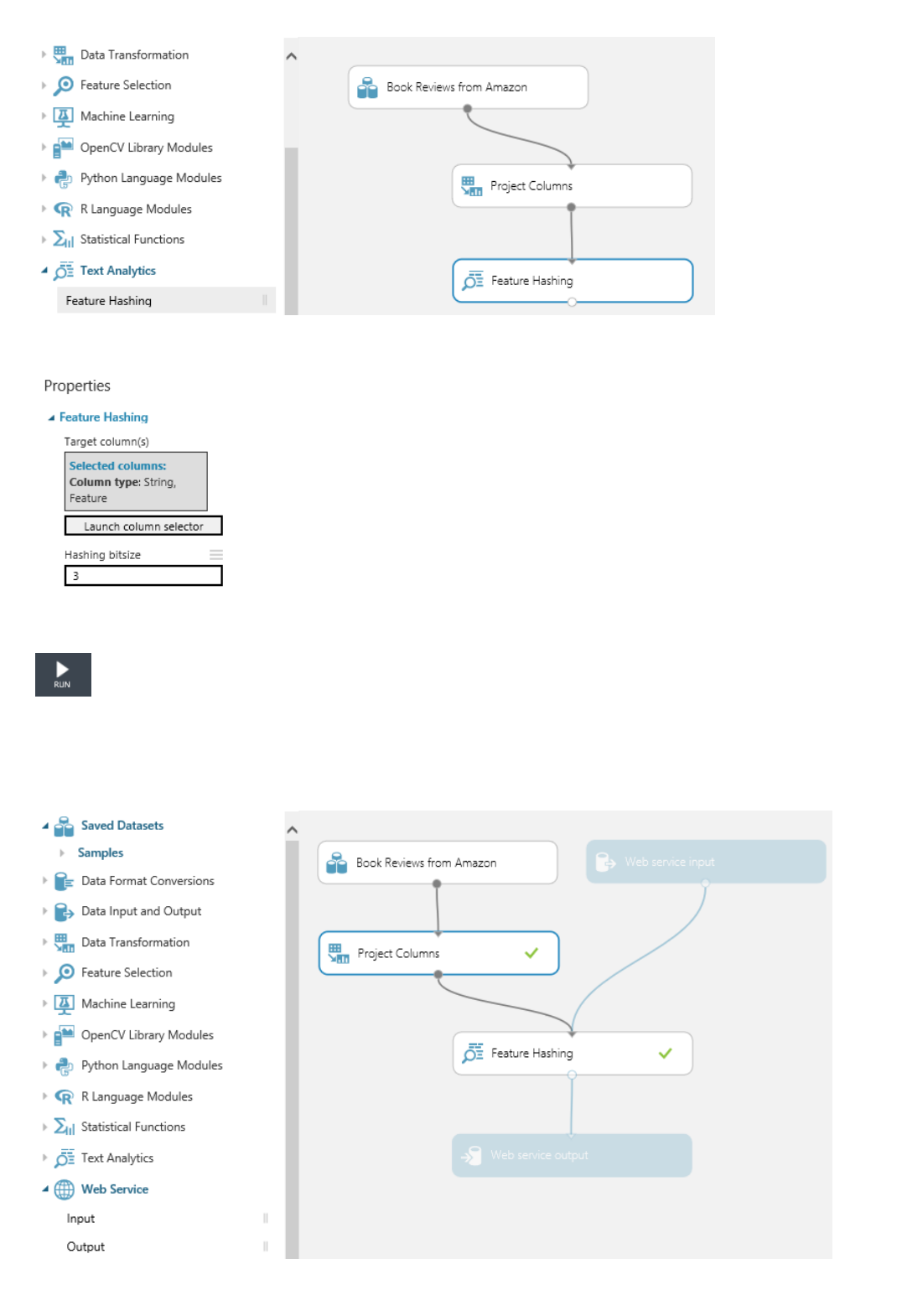
Create a web serviceCreate a web service
Feature Hashing.
Type 3 for the Hashing bitsize. This will create 8 (23) columns.
At this point, you may want to click Run to test the experiment.
Now create a web service. Expand Web Service and drag Input onto your experiment. Connect Input to Feature
Hashing. Also drag output onto your experiment. Connect Output to Feature Hashing.
Click Publish web service.
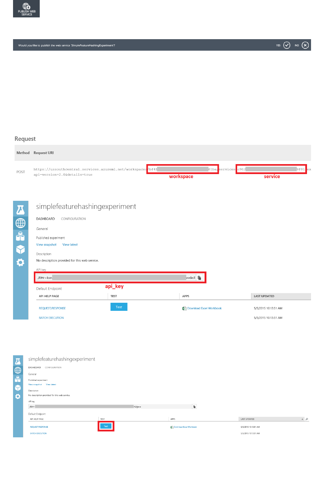
Test the web serviceTest the web service
Test RRS endpointTest RRS endpoint
Te st b u t t o nT e s t b u t t o n
Click Yes to publish the experiment.
An AzureML web service consists of RSS (request/response service) and BES (batch execution service) endpoints.
RSS is for synchronous execution. BES is for asynchronous job execution. To test your web service with the sample
Python source below, you may need to download and install the Azure SDK for Python (see: How to install Python).
You will also need the workspace, service, and api_key of your experiment for the sample source below. You can
find the workspace and service by clicking either Request/Response or Batch Execution for your experiment in
the web service dashboard.
You can find the api_key by clicking your experiment in the web service dashboard.
An easy way to test the RRS endpoint is to click Test on the web service dashboard.
Type This is a good day for col2. Click the checkmark.
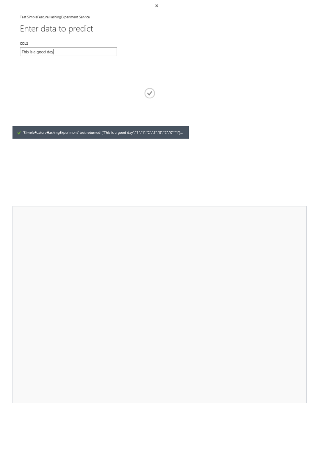
Sa m p l e C o d eSa m p l e C o d e
import urllib2
import json
workspace = "<REPLACE WITH YOUR EXPERIMENT’S WEB SERVICE WORKSPACE ID>"
service = "<REPLACE WITH YOUR EXPERIMENT’S WEB SERVICE SERVICE ID>"
api_key = "<REPLACE WITH YOUR EXPERIMENT’S WEB SERVICE API KEY>"
data = {
"Inputs": {
"input1": {
"ColumnNames": ["Col2"],
"Values": [ [ "This is a good day" ] ]
},
},
"GlobalParameters": { }
}
url = "https://ussouthcentral.services.azureml.net/workspaces/" + workspace + "/services/" + service +
"/execute?api-version=2.0&details=true"
headers = {'Content-Type':'application/json', 'Authorization':('Bearer '+ api_key)}
body = str.encode(json.dumps(data))
try:
req = urllib2.Request(url, body, headers)
response = urllib2.urlopen(req)
result = response.read()
print "result:" + result
except urllib2.HTTPError, error:
print("The request failed with status code: " + str(error.code))
print(error.info())
print(json.loads(error.read()))
Test BES endpointTest BES endpoint
You will see something like
Another way to test your RRS is from your client code. If you click Request/response on the dashboard and scroll
to the bottom, you will see sample code for C#, Python, and R. You will also see the syntax of the RRS request,
including the request URI, headers, and body.
This guide shows a working Python example. You will need to modify it with the workspace, service, and api_key
of your experiment.
Click Batch execution on the dashboard and scroll to the bottom. You will see sample code for C#, Python, and R.
You will also see the syntax of the BES requests to submit a job, start a job, get the status or results of a job, and
delete a job.
This guide shows a working Python example. You need to modify it with the workspace, service, and api_key of
your experiment. Additionally, you need to modify the storage account name, storage account key, and storage

import urllib2
import json
import time
from azure.storage import *
workspace = "<REPLACE WITH YOUR WORKSPACE ID>"
service = "<REPLACE WITH YOUR SERVICE ID>"
api_key = "<REPLACE WITH THE API KEY FOR YOUR WEB SERVICE>"
storage_account_name = "<REPLACE WITH YOUR AZURE STORAGE ACCOUNT NAME>"
storage_account_key = "<REPLACE WITH YOUR AZURE STORAGE KEY>"
storage_container_name = "<REPLACE WITH YOUR AZURE STORAGE CONTAINER NAME>"
input_file = "<REPLACE WITH THE LOCATION OF YOUR INPUT FILE>" # Example: C:\\mydata.csv
output_file = "<REPLACE WITH THE LOCATION OF YOUR OUTPUT FILE>" # Example: C:\\myresults.csv
input_blob_name = "mydatablob.csv"
output_blob_name = "myresultsblob.csv"
def printHttpError(httpError):
print("The request failed with status code: " + str(httpError.code))
print(httpError.info())
print(json.loads(httpError.read()))
return
def saveBlobToFile(blobUrl, resultsLabel):
print("Reading the result from " + blobUrl)
try:
response = urllib2.urlopen(blobUrl)
except urllib2.HTTPError, error:
printHttpError(error)
return
with open(output_file, "w+") as f:
f.write(response.read())
print(resultsLabel + " have been written to the file " + output_file)
return
def processResults(result):
first = True
results = result["Results"]
for outputName in results:
result_blob_location = results[outputName]
sas_token = result_blob_location["SasBlobToken"]
base_url = result_blob_location["BaseLocation"]
relative_url = result_blob_location["RelativeLocation"]
print("The results for " + outputName + " are available at the following Azure Storage location:")
print("BaseLocation: " + base_url)
print("RelativeLocation: " + relative_url)
print("SasBlobToken: " + sas_token)
if (first):
first = False
url3 = base_url + relative_url + sas_token
saveBlobToFile(url3, "The results for " + outputName)
return
def invokeBatchExecutionService():
url = "https://ussouthcentral.services.azureml.net/workspaces/" + workspace +"/services/" + service +"/jobs"
blob_service = BlobService(account_name=storage_account_name, account_key=storage_account_key)
print("Uploading the input to blob storage...")
data_to_upload = open(input_file, "r").read()
blob_service.put_blob(storage_container_name, input_blob_name, data_to_upload, x_ms_blob_type="BlockBlob")
print "Uploaded the input to blob storage"
input_blob_path = "/" + storage_container_name + "/" + input_blob_name
connection_string = "DefaultEndpointsProtocol=https;AccountName=" + storage_account_name + ";AccountKey=" +
storage_account_key
payload = {
"Input": {
"ConnectionString": connection_string,
"RelativeLocation": input_blob_path
},
"Outputs": {
"output1": { "ConnectionString": connection_string, "RelativeLocation": "/" + storage_container_name +
"/" + output_blob_name },
container name. Lastly, you will need to modify the location of the input file and the location of the output file.

"/" + output_blob_name },
},
"GlobalParameters": {
}
}
body = str.encode(json.dumps(payload))
headers = { "Content-Type":"application/json", "Authorization":("Bearer " + api_key)}
print("Submitting the job...")
# submit the job
req = urllib2.Request(url + "?api-version=2.0", body, headers)
try:
response = urllib2.urlopen(req)
except urllib2.HTTPError, error:
printHttpError(error)
return
result = response.read()
job_id = result[1:-1] # remove the enclosing double-quotes
print("Job ID: " + job_id)
# start the job
print("Starting the job...")
req = urllib2.Request(url + "/" + job_id + "/start?api-version=2.0", "", headers)
try:
response = urllib2.urlopen(req)
except urllib2.HTTPError, error:
printHttpError(error)
return
url2 = url + "/" + job_id + "?api-version=2.0"
while True:
print("Checking the job status...")
# If you are using Python 3+, replace urllib2 with urllib.request in the follwing code
req = urllib2.Request(url2, headers = { "Authorization":("Bearer " + api_key) })
try:
response = urllib2.urlopen(req)
except urllib2.HTTPError, error:
printHttpError(error)
return
result = json.loads(response.read())
status = result["StatusCode"]
print "status:" + status
if (status == 0 or status == "NotStarted"):
print("Job " + job_id + " not yet started...")
elif (status == 1 or status == "Running"):
print("Job " + job_id + " running...")
elif (status == 2 or status == "Failed"):
print("Job " + job_id + " failed!")
print("Error details: " + result["Details"])
break
elif (status == 3 or status == "Cancelled"):
print("Job " + job_id + " cancelled!")
break
elif (status == 4 or status == "Finished"):
print("Job " + job_id + " finished!")
processResults(result)
break
time.sleep(1) # wait one second
return
invokeBatchExecutionService()
Creating endpoints
3/21/2018 • 1 min to read • Edit Online
NOTENOTE
NOTENOTE
Adding endpoints to a Web service
NOTENOTE
Adding an endpoint programmatically
Adding an endpoint using the Azure Machine Learning Web Services
portal
This topic describes techniques applicable to a Classic Machine Learning Web service.
When you create Web services that you sell forward to your customers, you need to provide trained models to
each customer that are still linked to the experiment from which the Web service was created. In addition, any
updates to the experiment should be applied selectively to an endpoint without overwriting the customizations.
To accomplish this, Azure Machine Learning allows you to create multiple endpoints for a deployed Web service.
Each endpoint in the Web service is independently addressed, throttled, and managed. Each endpoint is a unique
URL and authorization key that you can distribute to your customers.
You can try Azure Machine Learning for free. No credit card or Azure subscription is required. Get started now.
There are two ways to add an endpoint to a Web service.
Programmatically
Through the Azure Machine Learning Web Services portal
Once the endpoint is created, you can consume it through synchronous APIs, batch APIs, and excel worksheets. In
addition to adding endpoints through this UI, you can also use the Endpoint Management APIs to
programmatically add endpoints.
If you have added additional endpoints to the Web service, you cannot delete the default endpoint.
You can add an endpoint to your Web service programmatically using the AddEndpoint sample code.
1. In Machine Learning Studio, on the left navigation column, click Web Services.
2. At the bottom of the Web service dashboard, click Manage endpoints. The Azure Machine Learning Web
Services portal opens to the endpoints page for the Web service.
3. Click New.
4. Type a name and description for the new endpoint. Endpoint names must be 24 character or less in length, and
must be made up of lower-case alphabets or numbers. Select the logging level and whether sample data is
enabled. For more information on logging, see Enable logging for Machine Learning Web services.

Scaling an Azure Machine Learning web service by
adding additional endpoints
3/21/2018 • 1 min to read • Edit Online
NOTENOTE
This topic describes techniques applicable to a Classic Machine Learning Web service.
By default, each published Web service is configured to support 20 concurrent requests and can be as high as 200
concurrent requests. Azure Machine Learning automatically optimizes the setting to provide the best performance
for your web service and the portal value is ignored.
If you plan to call the API with a higher load than a Max Concurrent Calls value of 200 will support, you should
create multiple endpoints on the same Web service. You can then randomly distribute your load across all of them.
The scaling of a Web service is a common task. Some reasons to scale are to support more than 200 concurrent
requests, increase availability through multiple endpoints, or provide separate endpoints for the web service. You
can increase the scale by adding additional endpoints for the same Web service through the Azure Machine
Learning Web Service portal.
For more information on adding new endpoints, see Creating Endpoints.
Keep in mind that using a high concurrency count can be detrimental if you're not calling the API with a
correspondingly high rate. You might see sporadic timeouts and/or spikes in the latency if you put a relatively low
load on an API configured for high load.
The synchronous APIs are typically used in situations where a low latency is desired. Latency here implies the time
it takes for the API to complete one request, and doesn't account for any network delays. Let's say you have an API
with a 50-ms latency. To fully consume the available capacity with throttle level High and Max Concurrent Calls =
20, you need to call this API 20 * 1000 / 50 = 400 times per second. Extending this further, a Max Concurrent Calls
of 200 allows you to call the API 4000 times per second, assuming a 50-ms latency.
Retrain a Machine Learning Model
3/21/2018 • 3 min to read • Edit Online
Why retrain: defining the problem
NOTENOTE
End-to-end workflow
As part of the process of operationalization of machine learning models in Azure Machine Learning, your model is
trained and saved. You then use it to create a predicative Web service. The Web service can then be consumed in
web sites, dashboards, and mobile apps.
Models you create using Machine Learning are typically not static. As new data becomes available or when the
consumer of the API has their own data the model needs to be retrained.
Retraining may occur frequently. With the Programmatic Retraining API feature, you can programmatically retrain
the model using the Retraining APIs and update the Web service with the newly trained model.
This document describes the retraining process, and shows you how to use the Retraining APIs.
As part of the machine learning training process, a model is trained using a set of data. Models you create using
Machine Learning are typically not static. As new data becomes available or when the consumer of the API has
their own data the model needs to be retrained.
In these scenarios, a programmatic API provides a convenient way to allow you or the consumer of your APIs to
create a client that can, on a one-time or regular basis, retrain the model using their own data. They can then
evaluate the results of retraining, and update the Web service API to use the newly trained model.
If you have an existing Training Experiment and New Web service, you may want to check out Retrain an existing Predictive
Web service instead of following the walkthrough mentioned in the following section.
The process involves the following components: A Training Experiment and a Predictive Experiment published as a
Web service. To enable retraining of a trained model, the Training Experiment must be published as a Web service
with the output of a trained model. This enables API access to the model for retraining.
The following steps apply to both New and Classic Web services:
Create the initial Predictive Web service:
Create a training experiment
Create a predictive web experiment
Deploy a predictive web service
Retrain the Web service:
Update training experiment to allow for retraining
Deploy the retraining web service
Use the Batch Execution Service code to retrain the model
For a walkthrough of the preceding steps, see Retrain Machine Learning models programmatically.
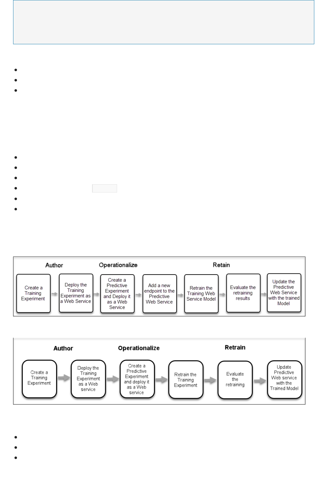
NOTENOTE
Other Resources
To deploy a New web service you must have sufficient permissions in the subscription to which you deploying the web
service. For more information see, Manage a Web service using the Azure Machine Learning Web Services portal.
If you deployed a Classic Web Service:
Create a new Endpoint on the Predictive Web service
Get the PATCH URL and code
Use the PATCH URL to point the new Endpoint at the retrained model
For a walkthrough of the preceding steps, see Retrain a Classic Web service.
If you run into difficulties retraining a Classic Web service, see Troubleshooting the retraining of an Azure Machine
Learning Classic Web service.
If you deployed a New Web service:
Sign in to your Azure Resource Manager account
Get the Web service definition
Export the Web Service Definition as JSON
Update the reference to the ilearner blob in the JSON
Import the JSON into a Web Service Definition
Update the Web service with new Web Service Definition
For a walkthrough of the preceding steps, see Retrain a New Web service using the Machine Learning
Management PowerShell cmdlets.
The process for setting up retraining for a Classic Web service involves the following steps:
The process for setting up retraining for a New Web service involves the following steps:
Retraining and Updating Azure Machine Learning models with Azure Data Factory
Create many Machine Learning models and web service endpoints from one experiment using PowerShell
The AML Retraining Models Using APIs video shows you how to retrain Machine Learning models created in
Azure Machine Learning using the Retraining APIs and PowerShell.

Retrain Machine Learning models programmatically
3/21/2018 • 7 min to read • Edit Online
Create a training experiment
In this walkthrough, you will learn how to programmatically retrain an Azure Machine Learning Web Service
using C# and the Machine Learning Batch Execution service.
Once you have retrained the model, the following walkthroughs show how to update the model in your
predictive web service:
If you deployed a Classic web service in the Machine Learning Web Services portal, see Retrain a Classic web
service.
If you deployed a New web service, see Retrain a New web service using the Machine Learning Management
cmdlets.
For an overview of the retraining process, see Retrain a Machine Learning Model.
If you want to start with your existing New Azure Resource Manager based web service, see Retrain an existing
Predictive web service.
For this example, you will use "Sample 5: Train, Test, Evaluate for Binary Classification: Adult Dataset" from the
Microsoft Azure Machine Learning samples.
To create the experiment:
1. Sign into to Microsoft Azure Machine Learning Studio.
2. On the bottom right corner of the dashboard, click New.
3. From the Microsoft Samples, select Sample 5.
4. To rename the experiment, at the top of the experiment canvas, select the experiment name "Sample 5: Train,
Test, Evaluate for Binary Classification: Adult Dataset".
5. Type Census Model.
6. At the bottom of the experiment canvas, click Run.
7. Click Set Up web service and select Retraining web service.
The following shows the initial experiment.
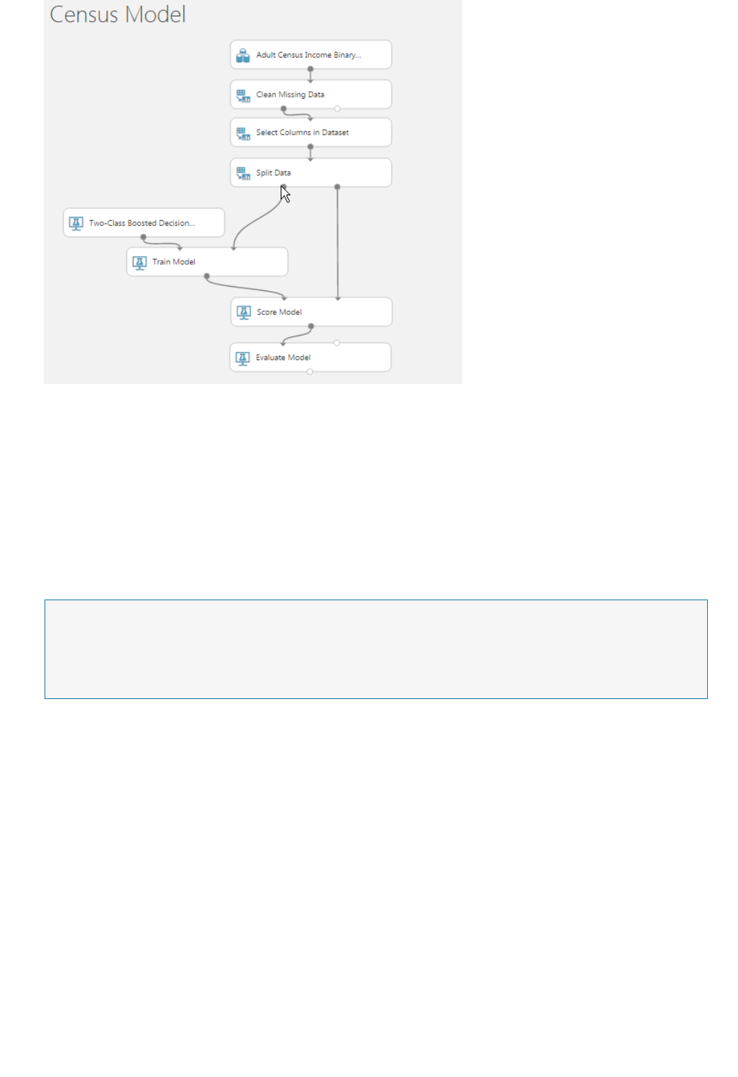
Create a predictive experiment and publish as a web service
NOTENOTE
Deploy the training experiment as a Training web service
Next you create a Predicative Experiment.
1. At the bottom of the experiment canvas, click Set Up Web Service and select Predictive Web Service. This
saves the model as a Trained Model and adds web service Input and Output modules.
2. Click Run.
3. After the experiment has finished running, click Deploy Web Service [Classic] or Deploy Web Service
[New].
To deploy a New web service you must have sufficient permissions in the subscription to which you deploying the web
service. For more information see, Manage a Web service using the Azure Machine Learning Web Services portal.
To retrain the trained model, you must deploy the training experiment that you created as a Retraining web
service. This web service needs a Web Service Output module connected to the Train Model module, to be able
to produce new trained models.
1. To return to the training experiment, click the Experiments icon in the left pane, then click the experiment
named Census Model.
2. In the Search Experiment Items search box, type web service.
3. Drag a Web Service Input module onto the experiment canvas and connect its output to the Clean Missing
Data module. This ensures that your retraining data is processed the same way as your original training data.
4. Drag two web service Output modules onto the experiment canvas. Connect the output of the Train Model
module to one and the output of the Evaluate Model module to the other. The web service output for Train
Model gives us the new trained model. The output attached to Evaluate Model returns that module’s
output, which is the performance results.
5. Click Run.
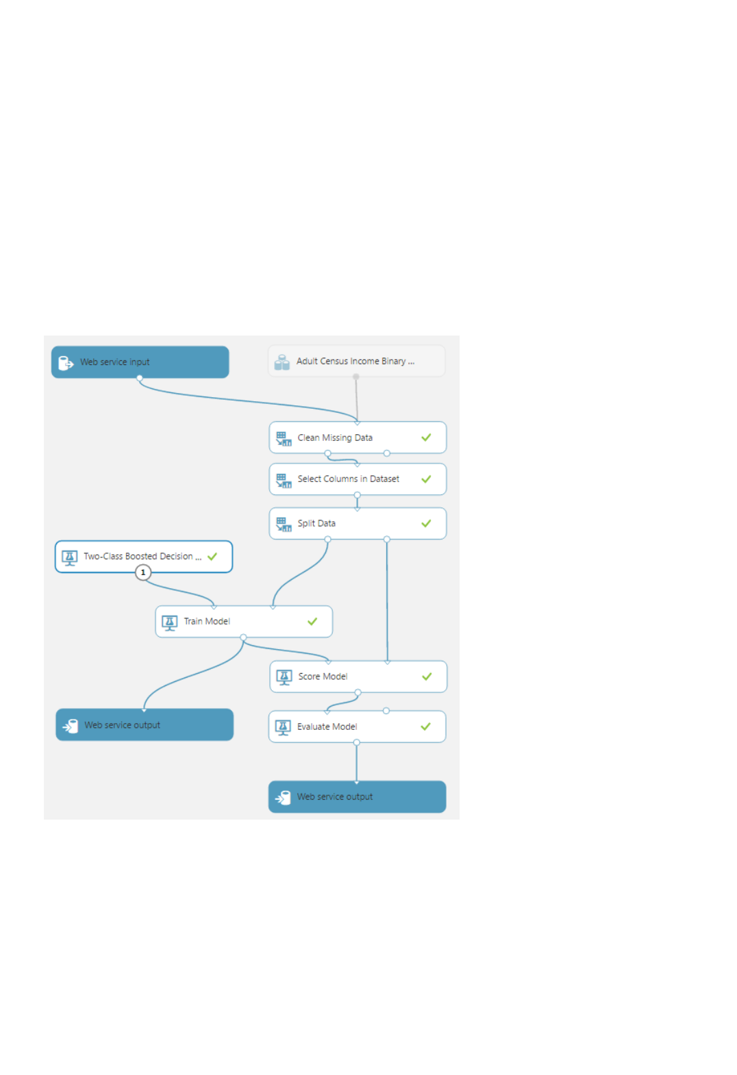
Retrain the model with new data using BES
Next you must deploy the training experiment as a web service that produces a trained model and model
evaluation results. To accomplish this, your next set of actions are dependent on whether you are working with a
Classic web service or a New web service.
Classic web service
At the bottom of the experiment canvas, click Set Up Web Service and select Deploy Web Service [Classic].
The Web Service Dashboard is displayed with the API Key and the API help page for Batch Execution. Only the
Batch Execution method can be used for creating Trained Models.
New web service
At the bottom of the experiment canvas, click Set Up Web Service and select Deploy Web Service [New].
The Web Service Azure Machine Learning Web Services portal opens to the Deploy web service page. Type a
name for your web service and choose a payment plan, then click Deploy. Only the Batch Execution method can
be used for creating Trained Models
In either case, after experiment has completed running, the resulting workflow should look as follows:
For this example, you are using C# to create the retraining application. You can also use the Python or R sample
code to accomplish this task.
To call the Retraining APIs:
1. Create a C# console application in Visual Studio: New > Project > Visual C# > Windows Classic Desktop
> Console App (.NET Framework).
2. Sign in to the Machine Learning Web Service portal.
3. If you are working with a Classic web service, click Classic Web Services.
a. Click the web service you are working with.

Update the apikey declarationUpdate the apikey declaration
const string apiKey = "abc123"; // Replace this with the API key for the web service
Update the Azure Storage informationUpdate the Azure Storage information
const string StorageAccountName = "mystorageacct"; // Replace this with your Azure Storage Account name
const string StorageAccountKey = "a_storage_account_key"; // Replace this with your Azure Storage Key
const string StorageContainerName = "mycontainer"; // Replace this with your Azure Storage Container name
Specify the output locationSpecify the output location
4. If you are working with a New web service, click Web Services.
5. Copy the sample C# code for batch execution and paste it into the Program.cs file, making sure the
namespace remains intact.
b. Click the default endpoint.
c. Click Consume.
d. At the bottom of the Consume page, in the Sample Code section, click Batch.
e. Continue to step 5 of this procedure.
a. Click the web service you are working with.
b. Click Consume.
c. At the bottom of the Consume page, in the Sample Code section, click Batch.
Add the Nuget package Microsoft.AspNet.WebApi.Client as specified in the comments. To add the reference to
Microsoft.WindowsAzure.Storage.dll, you might first need to install the client library for Microsoft Azure storage
services. For more information, see Windows Storage Services.
Locate the apikey declaration.
In the Basic consumption info section of the Consume page, locate the primary key and copy it to the apikey
declaration.
The BES sample code uploads a file from a local drive (For example "C:\temp\CensusIpnput.csv") to Azure
Storage, processes it, and writes the results back to Azure Storage.
To accomplish this task, you must retrieve the Storage account name, key, and container information for your
Storage account from the classic Azure portal and the update corresponding values in the code.
1. Sign in to the classic Azure portal.
2. In the left navigation column, click Storage.
3. From the list of storage accounts, select one to store the retrained model.
4. At the bottom of the page, click Manage Access Keys.
5. Copy and save the Primary Access Key and close the dialog.
6. At the top of the page, click Containers.
7. Select an existing container or create a new one and save the name.
Locate the StorageAccountName, StorageAccountKey, and StorageContainerName declarations and update the
values you saved from the Azure portal.
You also must ensure the input file is available at the location you specify in the code.
When specifying the output location in the Request Payload, the extension of the file specified in
RelativeLocation must be specified as ilearner.
See the following example:
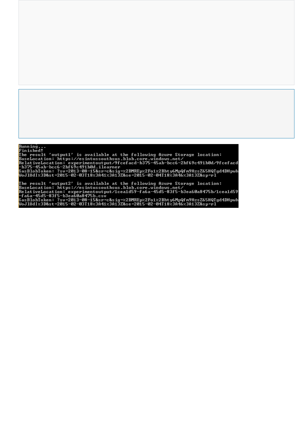
Outputs = new Dictionary<string, AzureBlobDataReference>() {
{
"output1",
new AzureBlobDataReference()
{
ConnectionString = storageConnectionString,
RelativeLocation = string.Format("{0}/output1results.ilearner", StorageContainerName) /*Replace
this with the location you would like to use for your output file, and valid file extension (usually .csv
for scoring results, or .ilearner for trained models)*/
}
},
NOTENOTE
Evaluate the Retraining Results
Next steps
The names of your output locations may be different from the ones in this walkthrough based on the order in which you
added the web service output modules. Since you set up this training experiment with two outputs, the results include
storage location information for both of them.
Diagram 4: Retraining output.
When you run the application, the output includes the URL and SAS token necessary to access the evaluation
results.
You can see the performance results of the retrained model by combining the BaseLocation, RelativeLocation,
and SasBlobToken from the output results for output2 (as shown in the preceding retraining output image) and
pasting the complete URL in the browser address bar.
Examine the results to determine whether the newly trained model performs well enough to replace the existing
one.
Copy the BaseLocation, RelativeLocation, and SasBlobToken from the output results, you will use them during
the retraining process.
If you deployed the predictive web service by clicking Deploy Web Service [Classic], see Retrain a Classic web
service.
If you deployed the predictive web service by clicking Deploy Web Service [New], see Retrain a New web
service using the Machine Learning Management cmdlets.
Retrain a Classic web service
3/21/2018 • 3 min to read • Edit Online
Prerequisites
IMPORTANTIMPORTANT
Add a new endpoint
NOTENOTE
Programmatically add an endpointProgrammatically add an endpoint
Use the Microsoft Azure Web Services portal to add an endpointUse the Microsoft Azure Web Services portal to add an endpoint
Update the added endpoint’s trained model
The Predictive Web Service you deployed is the default scoring endpoint. Default endpoints are kept in sync with
the original training and scoring experiments, and therefore the trained model for the default endpoint cannot be
replaced. To retrain the web service, you must add a new endpoint to the web service.
You must have set up a training experiment and a predictive experiment as shown in Retrain Machine Learning
models programmatically.
The predictive experiment must be deployed as a Classic machine learning web service.
For additional information on Deploying web services, see Deploy an Azure Machine Learning web service.
The Predictive Web Service that you deployed contains a default scoring endpoint that is kept in sync with the
original training and scoring experiments trained model. To update your web service to with a new trained model,
you must create a new scoring endpoint.
To create a new scoring endpoint, on the Predictive Web Service that can be updated with the trained model:
Be sure you are adding the endpoint to the Predictive Web Service, not the Training Web Service. If you have correctly
deployed both a Training and a Predictive Web Service, you should see two separate web services listed. The Predictive Web
Service should end with "[predictive exp.]".
There are two ways in which you can add a new end point to a web service:
1. Programmatically
2. Use the Microsoft Azure Web Services portal
You can add scoring endpoints using the sample code provided in this github repository.
1. In Machine Learning Studio, on the left navigation column, click Web Services.
2. At the bottom of the web service dashboard, click Manage endpoints preview.
3. Click Add.
4. Type a name and description for the new endpoint. Select the logging level and whether sample data is
enabled. For more information on logging, see Enable logging for Machine Learning web services.
To complete the retraining process, you must update the trained model of the new endpoint that you added.

private async Task OverwriteModel()
{
var resourceLocations = new
{
Resources = new[]
{
new
{
Name = "Census Model [trained model]",
Location = new AzureBlobDataReference()
{
BaseLocation = "https://esintussouthsus.blob.core.windows.net/",
RelativeLocation = "your endpoint relative location", //from the output, for example:
“experimentoutput/8946abfd-79d6-4438-89a9-3e5d109183/8946abfd-79d6-4438-89a9-3e5d109183.ilearner”
SasBlobToken = "your endpoint SAS blob token" //from the output, for example: “?sv=2013-
08-15&sr=c&sig=37lTTfngRwxCcf94%3D&st=2015-01-30T22%3A53%3A06Z&se=2015-01-31T22%3A58%3A06Z&sp=rl”
}
}
}
};
using (var client = new HttpClient())
{
client.DefaultRequestHeaders.Authorization = new AuthenticationHeaderValue("Bearer", apiKey);
using (var request = new HttpRequestMessage(new HttpMethod("PATCH"), endpointUrl))
{
request.Content = new StringContent(JsonConvert.SerializeObject(resourceLocations),
System.Text.Encoding.UTF8, "application/json");
HttpResponseMessage response = await client.SendAsync(request);
if (!response.IsSuccessStatusCode)
{
await WriteFailedResponse(response);
}
// Do what you want with a successful response here.
}
}
}
If you added the endpoint using the sample code, this includes location of the help URL identified by the
HelpLocationURL value in the output.
To retrieve the path URL:
1. Copy and paste the URL into your browser.
2. Click the Update Resource link.
3. Copy the POST URL of the PATCH request. For example:
PATCH URL:
https://management.azureml.net/workspaces/00bf70534500b34rebfa1843d6/webservices/af3er32ad3938
52f9b30ac9a35b/endpoints/newendpoint2
You can now use the trained model to update the scoring endpoint that you created previously.
The following sample code shows you how to use the BaseLocation, RelativeLocation, SasBlobToken, and PATCH
URL to update the endpoint.
The apiKey and the endpointUrl for the call can be obtained from endpoint dashboard.
The value of the Name parameter in Resources should match the Resource Name of the saved Trained Model in
the predictive experiment. To get the Resource Name:

Summary
Next steps
1. Sign in to the Azure portal.
2. In the left menu, click Machine Learning.
3. Under Name, click your workspace and then click Web Services.
4. Under Name, click Census Model [predictive exp.].
5. Click the new endpoint you added.
6. On the endpoint dashboard, click Update Resource.
7. On the Update Resource API Documentation page for the web service, you can find the Resource Name
under Updatable Resources.
If your SAS token expires before you finish updating the endpoint, you must perform a GET with the Job Id to
obtain a fresh token.
When the code has successfully run, the new endpoint should start using the retrained model in approximately 30
seconds.
Using the Retraining APIs, you can update the trained model of a predictive Web Service enabling scenarios such
as:
Periodic model retraining with new data.
Distribution of a model to customers with the goal of letting them retrain the model using their own data.
Troubleshooting the retraining of an Azure Machine Learning classic web service
Retrain a New Resource Manager based web service
using the Machine Learning Management PowerShell
cmdlets
4/18/2018 • 3 min to read • Edit Online
Prerequisites
IMPORTANTIMPORTANT
Sign in to your Azure Resource Manager account
Get the Web Service Definition
When you retrain a New web service, you update the predictive web service definition to reference the new
trained model.
You must set up a training experiment and a predictive experiment as shown in Retrain Machine Learning models
programmatically.
The predictive experiment must be deployed as an Azure Resource Manager (New) based machine learning web service. To
deploy a New web service you must have sufficient permissions in the subscription to which you deploying the web service.
For more information, see Manage a Web service using the Azure Machine Learning Web Services portal.
For additional information on Deploying web services, see Deploy an Azure Machine Learning web service.
This process requires that you have installed the Azure Machine Learning Cmdlets. For information installing the
Machine Learning cmdlets, see the Azure Machine Learning Cmdlets reference on MSDN.
Copied the following information from the retraining output:
BaseLocation
RelativeLocation
The steps you take are:
1. Sign in to your Azure Resource Manager account.
2. Get the web service definition
3. Export the Web Service Definition as JSON
4. Update the reference to the ilearner blob in the JSON.
5. Import the JSON into a Web Service Definition
6. Update the web service with new Web Service Definition
You must first sign in to your Azure account from within the PowerShell environment using the Connect-
AzureRmAccount cmdlet.
Next, get the Web Service by calling the Get-AzureRmMlWebService cmdlet. The Web Service Definition is an
internal representation of the trained model of the web service and is not directly modifiable. Make sure that you
are retrieving the Web Service Definition for your Predictive experiment and not your training experiment.

$wsd = Get-AzureRmMlWebService -Name 'RetrainSamplePre.2016.8.17.0.3.51.237' -ResourceGroupName 'Default-
MachineLearning-SouthCentralUS'
Properties : Microsoft.Azure.Management.MachineLearning.WebServices.Models.WebServicePropertiesForGraph
Id : /subscriptions/<subscription ID>/resourceGroups/Default-MachineLearning-
SouthCentralUS/providers/Microsoft.MachineLearning/webServices/RetrainSamplePre.2016.8.17.0.3.51.237
Name : RetrainSamplePre.2016.8.17.0.3.51.237
Location : South Central US
Type : Microsoft.MachineLearning/webServices
Tags : {}
https://services.azureml.net/subscriptions/<subcription ID>/resourceGroups/Default-MachineLearning-
SouthCentralUS/providers/Microsoft.MachineLearning/webServices/RetrainSamplePre.2016.8.17.0.3.51.237
Export the Web Service Definition as JSON
Export-AzureRmMlWebService -WebService $wsd -OutputFile "C:\temp\mlservice_export.json"
Update the reference to the ilearner blob in the JSON.
"asset3": {
"name": "Retrain Samp.le [trained model]",
"type": "Resource",
"locationInfo": {
"uri":
"https://mltestaccount.blob.core.windows.net/azuremlassetscontainer/baca7bca650f46218633552c0bcbba0e.ilearner"
},
"outputPorts": {
"Results dataset": {
"type": "Dataset"
}
}
},
Import the JSON into a Web Service Definition
To determine the resource group name of an existing web service, run the Get-AzureRmMlWebService cmdlet
without any parameters to display the web services in your subscription. Locate the web service, and then look at
its web service ID. The name of the resource group is the fourth element in the ID, just after the resourceGroups
element. In the following example, the resource group name is Default-MachineLearning-SouthCentralUS.
Alternatively, to determine the resource group name of an existing web service, log on to the Microsoft Azure
Machine Learning Web Services portal. Select the web service. The resource group name is the fifth element of
the URL of the web service, just after the resourceGroups element. In the following example, the resource group
name is Default-MachineLearning-SouthCentralUS.
To modify the definition to the trained model to use the newly Trained Model, you must first use the Export-
AzureRmMlWebService cmdlet to export it to a JSON format file.
In the assets, locate the [trained model], update the uri value in the locationInfo node with the URI of the ilearner
blob. The URI is generated by combining the BaseLocation and the RelativeLocation from the output of the BES
retraining call. This updates the path to reference the new trained model.

$wsd = Import-AzureRmMlWebService -InputFile "C:\temp\mlservice_export.json"
Update the web service with new Web Service Definition
Update-AzureRmMlWebService -Name 'RetrainSamplePre.2016.8.17.0.3.51.237' -ResourceGroupName 'Default-
MachineLearning-SouthCentralUS' -ServiceUpdates $wsd
Summary
You must use the Import-AzureRmMlWebService cmdlet to convert the modified JSON file back into a Web
Service Definition that you can use to update the Web Service Definition.
Finally, you use Update-AzureRmMlWebService cmdlet to update the Web Service Definition.
Using the Machine Learning PowerShell management cmdlets, you can update the trained model of a predictive
Web Service enabling scenarios such as:
Periodic model retraining with new data.
Distribution of a model to customers with the goal of letting them retrain the model using their own data.
Retrain an existing predictive web service
4/18/2018 • 7 min to read • Edit Online
NOTENOTE
Deploy the training experiment
This document describes the retraining process for the following scenario:
You have a training experiment and a predictive experiment that you have deployed as an operationalized web
service.
You have new data that you want your predictive web service to use to perform its scoring.
To deploy a New web service you must have sufficient permissions in the subscription to which you deploying the web
service. For more information see, Manage a Web service using the Azure Machine Learning Web Services portal.
Starting with your existing web service and experiments, you need to follow these steps:
1. Update the model.
2. Use the Azure Machine Learning PowerShell cmdlets to update the predictive experiment.
a. Modify your training experiment to allow for web service inputs and outputs.
b. Deploy the training experiment as a retraining web service.
c. Use the training experiment's Batch Execution Service (BES) to retrain the model.
a. Sign in to your Azure Resource Manager account.
b. Get the web service definition.
c. Export the web service definition as JSON.
d. Update the reference to the ilearner blob in the JSON.
e. Import the JSON into a web service definition.
f. Update the web service with a new web service definition.
To deploy the training experiment as a retraining web service, you must add web service inputs and outputs to the
model. By connecting a Web Service Output module to the experiment's Train Model module, you enable the
training experiment to produce a new trained model that you can use in your predictive experiment. If you have an
Evaluate Model module, you can also attach web service output to get the evaluation results as output.
To update your training experiment:
1. Connect a Web Service Input module to your data input (for example, a Clean Missing Data module). Typically,
you want to ensure that your input data is processed in the same way as your original training data.
2. Connect a Web Service Output module to the output of your Train Model module.
3. If you have an Evaluate Model module and you want to output the evaluation results, connect a Web Service
Output module to the output of your Evaluate Model module.
Run your experiment.
Next, you must deploy the training experiment as a web service that produces a trained model and model
evaluation results.
At the bottom of the experiment canvas, click Set Up Web Service, and then select Deploy Web Service [New].
The Azure Machine Learning Web Services portal opens to the Deploy Web Service page. Type a name for your
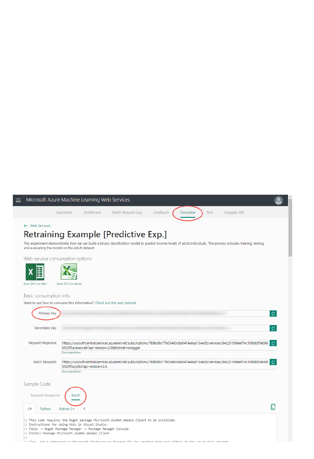
Retrain the model with new data by using BES
Update the apikey declarationUpdate the apikey declaration
web service, choose a payment plan, and then click Deploy. You can only use the Batch Execution method for
creating trained models.
For this example, we're using C# to create the retraining application. You can also use Python or R sample code to
accomplish this task.
To call the retraining APIs:
1. Create a C# console application in Visual Studio: New > Project > Visual C# > Windows Classic Desktop >
Console App (.NET Framework).
2. Sign in to the Machine Learning Web Services portal.
3. Click the web service that you're working with.
4. Click Consume.
5. At the bottom of the Consume page, in the Sample Code section, click Batch.
6. Copy the sample C# code for batch execution and paste it into the Program.cs file. Make sure that the
namespace remains intact.
Add the NuGet package Microsoft.AspNet.WebApi.Client, as specified in the comments. To add the reference to
Microsoft.WindowsAzure.Storage.dll, you might first need to install the client library for Azure Storage services.
The following screenshot shows the Consume page in the Azure Machine Learning Web Services portal.
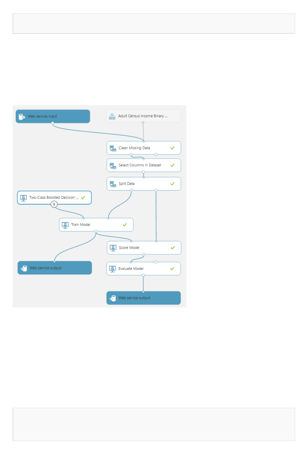
const string apiKey = "abc123"; // Replace this with the API key for the web service
Update the Azure Storage informationUpdate the Azure Storage information
const string StorageAccountName = "mystorageacct"; // Replace this with your Azure storage account name
const string StorageAccountKey = "a_storage_account_key"; // Replace this with your Azure Storage key
const string StorageContainerName = "mycontainer"; // Replace this with your Azure Storage container name
Locate the apikey declaration:
In the Basic consumption info section of the Consume page, locate the primary key and copy it to the apikey
declaration.
The BES sample code uploads a file from a local drive (for example, "C:\temp\CensusIpnput.csv") to Azure Storage,
processes it, and writes the results back to Azure Storage.
After running your experiment, the resulting workflow should be similar to the following:
1. Sign in to the Azure portal.
2. In the left navigation column, click More services, search for Storage accounts, and select it.
3. From the list of storage accounts, select one to store the retrained model.
4. In the left navigation column, click Access keys.
5. Copy and save the Primary Access Key.
6. In the left navigation column, click Containers.
7. Select an existing container, or create a new one and save the name.
Locate the StorageAccountName, StorageAccountKey, and StorageContainerName declarations, and update the
values that you saved from the portal.

Specify the output locationSpecify the output location
Outputs = new Dictionary<string, AzureBlobDataReference>() {
{
"output1",
new AzureBlobDataReference()
{
ConnectionString = storageConnectionString,
RelativeLocation = string.Format("{0}/output1results.ilearner", StorageContainerName) /*Replace
this with the location you want to use for your output file and a valid file extension (usually .csv for
scoring results or .ilearner for trained models)*/
}
},
Evaluate the retraining results
Retrain the web service
Sign in to Azure Resource Manager
Get the Web Service Definition object
You also must ensure that the input file is available at the location that you specify in the code.
When you specify the output location in the Request Payload, the extension of the file that is specified in
RelativeLocation must be specified as ilearner . See the following example:
The following is an example of retraining output:
When you run the application, the output includes the URL and shared access signatures token that are necessary
to access the evaluation results.
You can see the performance results of the retrained model by combining the BaseLocation, RelativeLocation, and
SasBlobToken from the output results for output2 (as shown in the preceding retraining output image) and pasting
the complete URL into the browser address bar.
Examine the results to determine whether the newly trained model performs well enough to replace the existing
one.
Copy the BaseLocation, RelativeLocation, and SasBlobToken from the output results.
When you retrain a new web service, you update the predictive web service definition to reference the new trained
model. The web service definition is an internal representation of the trained model of the web service and is not
directly modifiable. Make sure that you are retrieving the web service definition for your predictive experiment and
not your training experiment.
You must first sign in to your Azure account from within the PowerShell environment by using the Connect-
AzureRmAccount cmdlet.
$wsd = Get-AzureRmMlWebService -Name 'RetrainSamplePre.2016.8.17.0.3.51.237' -ResourceGroupName 'Default-
MachineLearning-SouthCentralUS'
Properties : Microsoft.Azure.Management.MachineLearning.WebServices.Models.WebServicePropertiesForGraph
Id : /subscriptions/<subscription ID>/resourceGroups/Default-MachineLearning-
SouthCentralUS/providers/Microsoft.MachineLearning/webServices/RetrainSamplePre.2016.8.17.0.3.51.237
Name : RetrainSamplePre.2016.8.17.0.3.51.237
Location : South Central US
Type : Microsoft.MachineLearning/webServices
Tags : {}
https://services.azureml.net/subscriptions/<subcription ID>/resourceGroups/Default-MachineLearning-
SouthCentralUS/providers/Microsoft.MachineLearning/webServices/RetrainSamplePre.2016.8.17.0.3.51.237
Export the Web Service Definition object as JSON
Export-AzureRmMlWebService -WebService $wsd -OutputFile "C:\temp\mlservice_export.json"
Update the reference to the ilearner blob
"asset3": {
"name": "Retrain Sample [trained model]",
"type": "Resource",
"locationInfo": {
"uri":
"https://mltestaccount.blob.core.windows.net/azuremlassetscontainer/baca7bca650f46218633552c0bcbba0e.ilearner"
},
"outputPorts": {
"Results dataset": {
"type": "Dataset"
}
}
},
Next, get the Web Service Definition object by calling the Get-AzureRmMlWebService cmdlet.
To determine the resource group name of an existing web service, run the Get-AzureRmMlWebService cmdlet
without any parameters to display the web services in your subscription. Locate the web service, and then look at
its web service ID. The name of the resource group is the fourth element in the ID, just after the resourceGroups
element. In the following example, the resource group name is Default-MachineLearning-SouthCentralUS.
Alternatively, to determine the resource group name of an existing web service, sign in to the Azure Machine
Learning Web Services portal. Select the web service. The resource group name is the fifth element of the URL of
the web service, just after the resourceGroups element. In the following example, the resource group name is
Default-MachineLearning-SouthCentralUS.
To modify the definition of the trained model to use the newly trained model, you must first use the Export-
AzureRmMlWebService cmdlet to export it to a JSON-format file.
In the assets, locate the [trained model], update the uri value in the locationInfo node with the URI of the ilearner
blob. The URI is generated by combining the BaseLocation and the RelativeLocation from the output of the BES
retraining call.

Import the JSON into a Web Service Definition object
$wsd = Import-AzureRmMlWebService -InputFile "C:\temp\mlservice_export.json"
Update the web service
Update-AzureRmMlWebService -Name 'RetrainSamplePre.2016.8.17.0.3.51.237' -ResourceGroupName 'Default-
MachineLearning-SouthCentralUS'
You must use the Import-AzureRmMlWebService cmdlet to convert the modified JSON file back into a Web
Service Definition object that you can use to update the predicative experiment.
Finally, use the Update-AzureRmMlWebService cmdlet to update the predictive experiment.
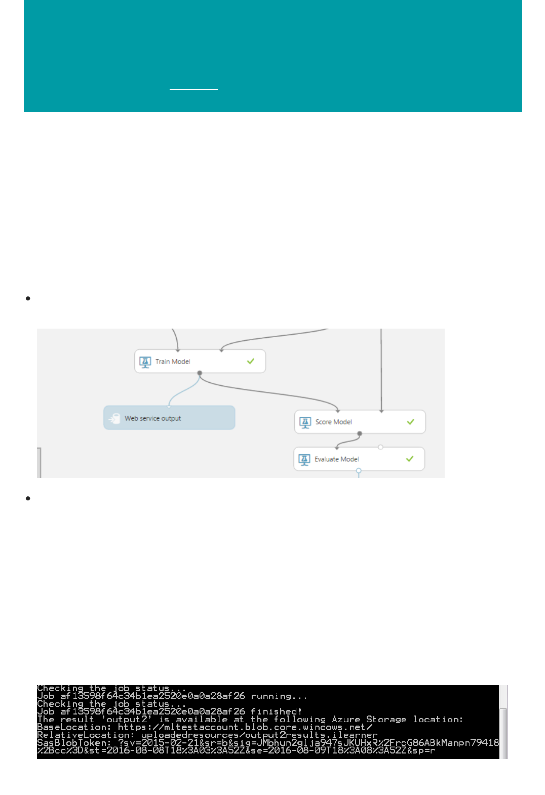
Troubleshooting the retraining of an Azure Machine
Learning Classic web service
5/1/2018 • 3 min to read • Edit Online
Retraining overview
Retraining process
When you deploy a predictive experiment as a scoring web service it is a static model. As new data becomes
available or when the consumer of the API has their own data, the model needs to be retrained.
For a complete walkthrough of the retraining process of a Classic web service, see Retrain Machine Learning
Models Programmatically.
When you need to retrain the web service, you must add some additional pieces:
A new endpoint added to your scoring web service. You can add the endpoint programmatically using the
sample code referenced in the Retrain Machine Learning models programmatically topic or through the Azure
Machine Learning Web Services portal.
A web service deployed from the Training Experiment. The experiment must have a Web Service Output
module attached to the output of the Train Model module.
You can then use the sample C# code from the Training Web Service's API help page to retrain model. Once you
have evaluated the results and are satisfied with them, you update the trained model scoring web service using the
new endpoint that you added.
With all the pieces in place, the major steps you must take to retrain the model are as follows:
1. Call the Training Web Service: The call is to the Batch Execution Service (BES), not the Request Response
Service (RRS). You can use the sample C# code on the API help page to make the call.
2. Find the values for the BaseLocation, RelativeLocation, and SasBlobToken: These values are returned in the
output from your call to the Training Web Service.
3. Update the added endpoint from the scoring web service with the new trained model: Using the sample code
provided in the Retrain Machine Learning models programmatically, update the new endpoint you added to the
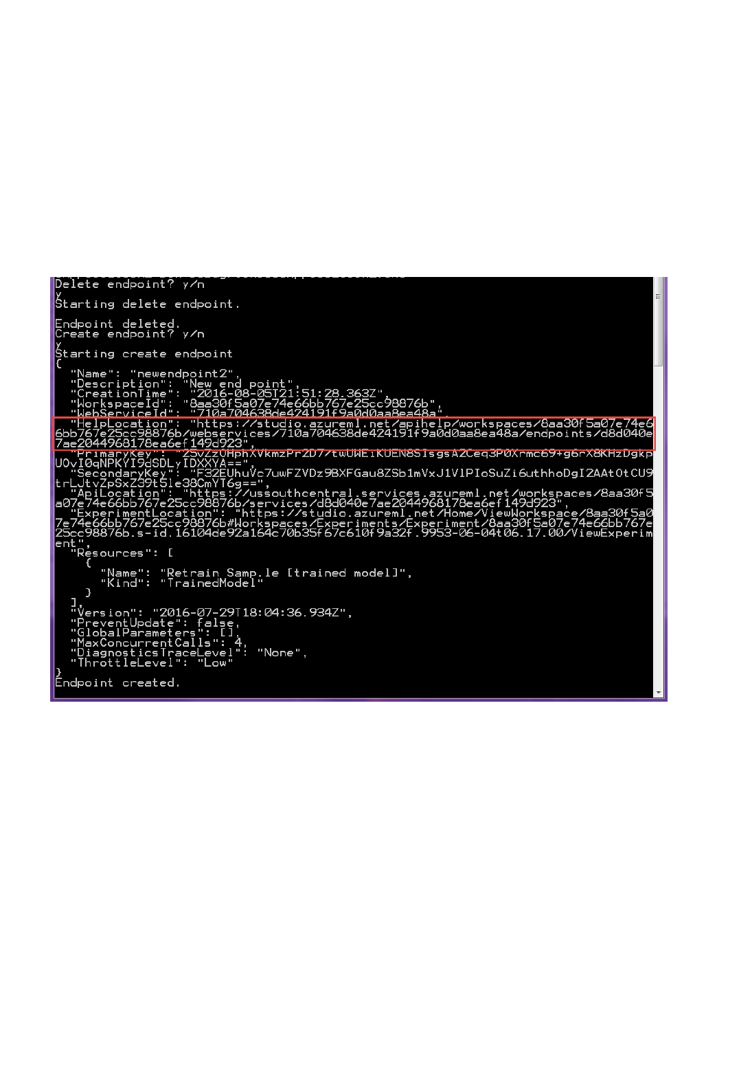
Common obstacles
Check to see if you have the correct PATCH URLCheck to see if you have the correct PATCH URL
scoring model with the newly trained model from the Training Web Service.
The PATCH URL you are using must be the one associated with the new scoring endpoint you added to the scoring
web service. There are a number of ways to obtain the PATCH URL:
Option 1: Programatically
To get the correct PATCH URL:
1. Run the AddEndpoint sample code.
3. Paste the URL into a browser to navigate to a page that provides help links for the web service.
4. Click the Update Resource link to open the patch help page.
2. From the output of AddEndpoint, find the HelpLocation value and copy the URL.
Option 2: Use the Azure Machine Learning Web Services portal
1. Sign in to the Azure Machine Learning Web Services portal.
2. Click Web Services or Classic Web Services at the top.
3. Click the scoring web service you are working with (if you didn't modify the default name of the web service, it
will end in "[Scoring Exp.]").
4. Click +NEW.
5. After the endpoint is added, click the endpoint name.
6. Under the Patch URL, click API Help to open the patching help page.

NOTENOTE
Check to see that you are updating the correct scoring endpointCheck to see that you are updating the correct scoring endpoint
NOTENOTE
Check that your workspace is in the same region as the web serviceCheck that your workspace is in the same region as the web service
If you have added the endpoint to the Training Web Service instead of the Predictive Web Service, you will receive the
following error when you click the Update Resource link: "Sorry, but this feature is not supported or available in this
context. This Web Service has no updatable resources. We apologize for the inconvenience and are working on improving
this workflow."
The PATCH help page contains the PATCH URL you must use and provides sample code you can use to call it.
Do not patch the training web service: The patch operation must be performed on the scoring web service.
Do not patch the default endpoint on the web service: The patch operation must be performed on the new
scoring web service endpoint that you added.
You can verify which web service the endpoint is on by visiting the Web Services portal.
Be sure you are adding the endpoint to the Predictive Web Service, not the Training Web Service. If you have correctly
deployed both a Training and a Predictive Web Service, you should see two separate web services listed. The Predictive Web
Service should end with "[predictive exp.]".
1. Sign in to the Azure Machine Learning Web Services portal.
2. Click Web Services or Classic Web Services.
3. Select your Predictive Web Service.
4. Verify that your new endpoint was added to the web service.
1. Sign in to Machine Learning Studio.
2. At the top, click the drop-down list of your workspaces.
3. Verify the region that your workspace is in.

How to consume an Azure Machine Learning Web
service
3/21/2018 • 8 min to read • Edit Online
NOTENOTE
Overview
Get an Azure Machine Learning authorization key
From the Microsoft Azure Machine Learning Web Services portalFrom the Microsoft Azure Machine Learning Web Services portal
Once you deploy an Azure Machine Learning predictive model as a Web service, you can use a REST API to
send it data and get predictions. You can send the data in real-time or in batch mode.
You can find more information about how to create and deploy a Machine Learning Web service using Machine
Learning Studio here:
For a tutorial on how to create an experiment in Machine Learning Studio, see Create your first experiment.
For details on how to deploy a Web service, see Deploy a Machine Learning Web service.
For more information about Machine Learning in general, visit the Machine Learning Documentation Center.
You can try Azure Machine Learning for free. No credit card or Azure subscription is required. Get started now.
With the Azure Machine Learning Web service, an external application communicates with a Machine Learning
workflow scoring model in real time. A Machine Learning Web service call returns prediction results to an
external application. To make a Machine Learning Web service call, you pass an API key that is created when you
deploy a prediction. The Machine Learning Web service is based on REST, a popular architecture choice for web
programming projects.
Azure Machine Learning has two types of services:
Request-Response Service (RRS) – A low latency, highly scalable service that provides an interface to the
stateless models created and deployed from the Machine Learning Studio.
Batch Execution Service (BES) – An asynchronous service that scores a batch for data records.
For more information about Machine Learning Web services, see Deploy a Machine Learning Web service.
When you deploy your experiment, API keys are generated for the Web service. You can retrieve the keys from
several locations.
Sign in to the Microsoft Azure Machine Learning Web Services portal.
To retrieve the API key for a New Machine Learning Web service:
1. In the Azure Machine Learning Web Services portal, click Web Services the top menu.
2. Click the Web service for which you want to retrieve the key.
3. On the top menu, click Consume.
4. Copy and save the Primary Key.
To retrieve the API key for a Classic Machine Learning Web service:

Classic Web serviceClassic Web service
Machine Learning StudioMachine Learning Studio
Connect to a Machine Learning Web service
C# SampleC# Sample
1. In the Azure Machine Learning Web Services portal, click Classic Web Services the top menu.
2. Click the Web service with which you are working.
3. Click the endpoint for which you want to retrieve the key.
4. On the top menu, click Consume.
5. Copy and save the Primary Key.
You can also retrieve a key for a Classic Web service from Machine Learning Studio.
1. In Machine Learning Studio, click WEB SERVICES on the left.
2. Click a Web service. The API key is on the DASHBOARD tab.
You can connect to a Machine Learning Web service using any programming language that supports HTTP
request and response. You can view examples in C#, Python, and R from a Machine Learning Web service help
page.
Machine Learning API help Machine Learning API help is created when you deploy a Web service. See Azure
Machine Learning Walkthrough- Deploy Web Service. The Machine Learning API help contains details about a
prediction Web service.
1. Click the Web service with which you are working.
2. Click the endpoint for which you want to view the API Help Page.
3. On the top menu, click Consume.
4. Click API help page under either the Request-Response or Batch Execution endpoints.
To view Machine Learning API help for a New Web service
In the Azure Machine Learning Web Services Portal:
1. Click WEB SERVICES on the top menu.
2. Click the Web service for which you want to retrieve the key.
Click Use Web Service to get the URIs for the Request-Reposonse and Batch Execution Services and Sample
code in C#, R, and Python.
Click Swagger API to get Swagger based documentation for the APIs called from the supplied URIs.
To connect to a Machine Learning Web service, use an HttpClient passing ScoreData. ScoreData contains a
FeatureVector, an n-dimensional vector of numerical features that represents the ScoreData. You authenticate to
the Machine Learning service with an API key.
To connect to a Machine Learning Web service, the Microsoft.AspNet.WebApi.Client NuGet package must
be installed.
Install Microsoft.AspNet.WebApi.Client NuGet in Visual Studio
1. Publish the Download dataset from UCI: Adult 2 class dataset Web Service.
2. Click Tools > NuGet Package Manager > Package Manager Console.
3. Choose Install-Package Microsoft.AspNet.WebApi.Client.
To run the code sample
1. Publish "Sample 1: Download dataset from UCI: Adult 2 class dataset" experiment, part of the Machine

using System;
using System.Collections.Generic;
using System.IO;
using System.Net.Http;
using System.Net.Http.Formatting;
using System.Net.Http.Headers;
using System.Text;
using System.Threading.Tasks;
namespace CallRequestResponseService
{
class Program
{
static void Main(string[] args)
{
InvokeRequestResponseService().Wait();
}
static async Task InvokeRequestResponseService()
{
using (var client = new HttpClient())
{
var scoreRequest = new
{
Inputs = new Dictionary<string, List<Dictionary<string, string>>> () {
{
"input1",
// Replace columns labels with those used in your dataset
new List<Dictionary<string, string>>(){new Dictionary<string, string>(){
{
"column1", "value1"
},
{
"column2", "value2"
},
{
"column3", "value3"
}
}
}
},
},
GlobalParameters = new Dictionary<string, string>() {}
};
// Replace these values with your API key and URI found on https://services.azureml.net/
const string apiKey = "<your-api-key>";
const string apiUri = "<your-api-uri>";
client.DefaultRequestHeaders.Authorization = new AuthenticationHeaderValue( "Bearer",
apiKey);
client.BaseAddress = new Uri(apiUri);
// WARNING: The 'await' statement below can result in a deadlock
// if you are calling this code from the UI thread of an ASP.Net application.
// One way to address this would be to call ConfigureAwait(false)
// so that the execution does not attempt to resume on the original context.
// For instance, replace code such as:
// result = await DoSomeTask()
// with the following:
Learning sample collection.
2. Assign apiKey with the key from a Web service. See Get an Azure Machine Learning authorization key
above.
3. Assign serviceUri with the Request URI.
Here is what a complete request will look like.

// with the following:
// result = await DoSomeTask().ConfigureAwait(false)
HttpResponseMessage response = await client.PostAsJsonAsync("", scoreRequest);
if (response.IsSuccessStatusCode)
{
string result = await response.Content.ReadAsStringAsync();
Console.WriteLine("Result: {0}", result);
}
else
{
Console.WriteLine(string.Format("The request failed with status code: {0}",
response.StatusCode));
// Print the headers - they include the requert ID and the timestamp,
// which are useful for debugging the failure
Console.WriteLine(response.Headers.ToString());
string responseContent = await response.Content.ReadAsStringAsync();
Console.WriteLine(responseContent);
}
}
}
}
}
Python SamplePython Sample
To connect to a Machine Learning Web service, use the urllib2 library for Python 2.X and urllib.request library
for Python 3.X. You will pass ScoreData, which contains a FeatureVector, an n-dimensional vector of numerical
features that represents the ScoreData. You authenticate to the Machine Learning service with an API key.
To run the code sample
1. Deploy "Sample 1: Download dataset from UCI: Adult 2 class dataset" experiment, part of the Machine
Learning sample collection.
2. Assign apiKey with the key from a Web service. See the Get an Azure Machine Learning authorization
key section near the beginning of this article.
3. Assign serviceUri with the Request URI.
Here is what a complete request will look like.

import urllib2 # urllib.request for Python 3.X
import json
data = {
"Inputs": {
"input1":
[
{
'column1': "value1",
'column2': "value2",
'column3': "value3"
}
],
},
"GlobalParameters": {}
}
body = str.encode(json.dumps(data))
# Replace this with the URI and API Key for your web service
url = '<your-api-uri>'
api_key = '<your-api-key>'
headers = {'Content-Type':'application/json', 'Authorization':('Bearer '+ api_key)}
# "urllib.request.Request(uri, body, headers)" for Python 3.X
req = urllib2.Request(url, body, headers)
try:
# "urllib.request.urlopen(req)" for Python 3.X
response = urllib2.urlopen(req)
result = response.read()
print(result)
# "urllib.error.HTTPError as error" for Python 3.X
except urllib2.HTTPError, error:
print("The request failed with status code: " + str(error.code))
# Print the headers - they include the requert ID and the timestamp, which are useful for debugging the
failure
print(error.info())
print(json.loads(error.read()))
R SampleR Sample
To connect to a Machine Learning Web Service, use the RCurl and rjson libraries to make the request and
process the returned JSON response. You will pass ScoreData, which contains a FeatureVector, an n-dimensional
vector of numerical features that represents the ScoreData. You authenticate to the Machine Learning service
with an API key.
Here is what a complete request will look like.

library("RCurl")
library("rjson")
# Accept SSL certificates issued by public Certificate Authorities
options(RCurlOptions = list(cainfo = system.file("CurlSSL", "cacert.pem", package = "RCurl")))
h = basicTextGatherer()
hdr = basicHeaderGatherer()
req = list(
Inputs = list(
"input1" = list(
list(
'column1' = "value1",
'column2' = "value2",
'column3' = "value3"
)
)
),
GlobalParameters = setNames(fromJSON('{}'), character(0))
)
body = enc2utf8(toJSON(req))
api_key = "<your-api-key>" # Replace this with the API key for the web service
authz_hdr = paste('Bearer', api_key, sep=' ')
h$reset()
curlPerform(url = "<your-api-uri>",
httpheader=c('Content-Type' = "application/json", 'Authorization' = authz_hdr),
postfields=body,
writefunction = h$update,
headerfunction = hdr$update,
verbose = TRUE
)
headers = hdr$value()
httpStatus = headers["status"]
if (httpStatus >= 400)
{
print(paste("The request failed with status code:", httpStatus, sep=" "))
# Print the headers - they include the requert ID and the timestamp, which are useful for debugging the
failure
print(headers)
}
print("Result:")
result = h$value()
print(fromJSON(result))
JavaScript SampleJavaScript Sample
To connect to a Machine Learning Web Service, use the request npm package in your project. You will also use
the JSON object to format your input and parse the result. Install using npm install request --save , or add
"request": "*" to your package.json under dependencies and run npm install .
Here is what a complete request will look like.

let req = require("request");
const uri = "<your-api-uri>";
const apiKey = "<your-api-key>";
let data = {
"Inputs": {
"input1":
[
{
'column1': "value1",
'column2': "value2",
'column3': "value3"
}
],
},
"GlobalParameters": {}
}
const options = {
uri: uri,
method: "POST",
headers: {
"Content-Type": "application/json",
"Authorization": "Bearer " + apiKey,
},
body: JSON.stringify(data)
}
req(options, (err, res, body) => {
if (!err && res.statusCode == 200) {
console.log(body);
} else {
console.log("The request failed with status code: " + res.statusCode);
}
});
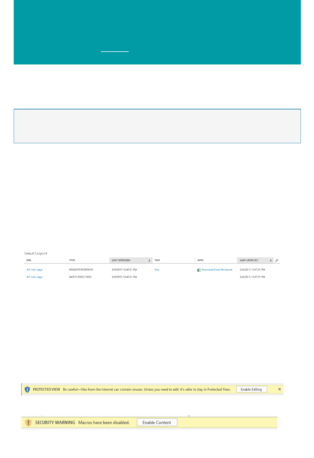
Consuming an Azure Machine Learning Web Service
from Excel
3/21/2018 • 1 min to read • Edit Online
NOTENOTE
Steps
Azure Machine Learning Studio makes it easy to call web services directly from Excel without the need to write any
code.
If you are using Excel 2013 (or later) or Excel Online, then we recommend that you use the Excel Excel add-in.
You can try Azure Machine Learning for free. No credit card or Azure subscription is required. Get started now.
Publish a web service. This page explains how to do it. Currently the Excel workbook feature is only supported for
Request/Response services that have a single output (that is, a single scoring label).
Once you have a web service, click on the WEB SERVICES section on the left of the studio, and then select the
web service to consume from Excel.
Classic Web Service
2. Click on Download Excel Workbook.
1. On the DASHBOARD tab for the web service is a row for the REQUEST/RESPONSE service. If this
service had a single output, you should see the Download Excel Workbook link in that row.
New Web Service
1. In the Azure Machine Learning Web Service portal, select Consume.
2. On the Consume page, in the Web service consumption options section, click the Excel icon.
Using the workbook
1. Open the workbook.
2. A Security Warning appears; click on the Enable Editing button.
3. A Security Warning appears. Click on the Enable Content button to run macros on your spreadsheet.
4. Once macros are enabled, a table is generated. Columns in blue are required as input into the RRS web
service, or PARAMETERS. Note the output of the RRS service, PREDICTED VALUES in green. When all

Sharing your workbook
Automatic updates
5. To score more than one row, fill the second row with data and the predicted values are produced. You can even
paste several rows at once.
columns for a given row are filled, the workbook automatically calls the scoring API, and displays the scored
results.
You can use any of the Excel features (graphs, power map, conditional formatting, etc.) with the predicted values to
help visualize the data.
For the macros to work, your API Key must be part of the spreadsheet. That means that you should share the
workbook only with entities/individuals you trust.
An RRS call is made in these two situations:
1. The first time a row has content in all of its PARAMETERS
2. Any time any of the PARAMETERS changes in a row that had all of its PARAMETERS entered.
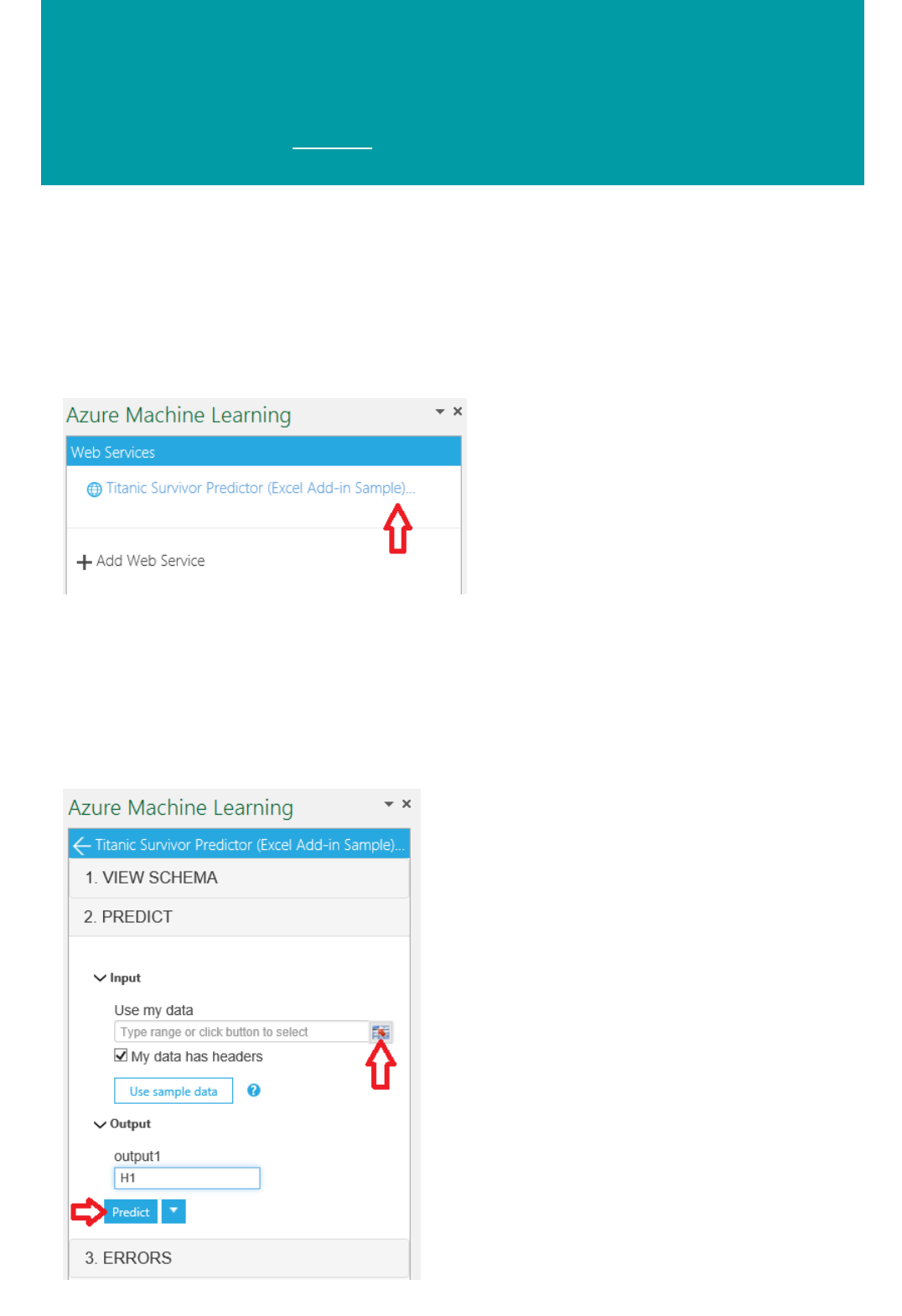
Excel Add-in for Azure Machine Learning web
services
3/21/2018 • 2 min to read • Edit Online
Steps to Use an Existing web service in the Workbook
Excel makes it easy to call web services directly without the need to write any code.
1. Open the sample Excel file, which contains the Excel add-in and data about passengers on the Titanic.
3. This takes you to the Predict section. This workbook already contains sample data, but for a blank workbook
you can select a cell in Excel and click Use sample data.
4. Select the data with headers and click the input data range icon. Make sure the "My data has headers" box is
checked.
5. Under Output, enter the cell number where you want the output to be, for example "H1" here.
2. Choose the web service by clicking it - "Titanic Survivor Predictor (Excel Add-in Sample) [Score]" in this
example.
6. Click Predict.
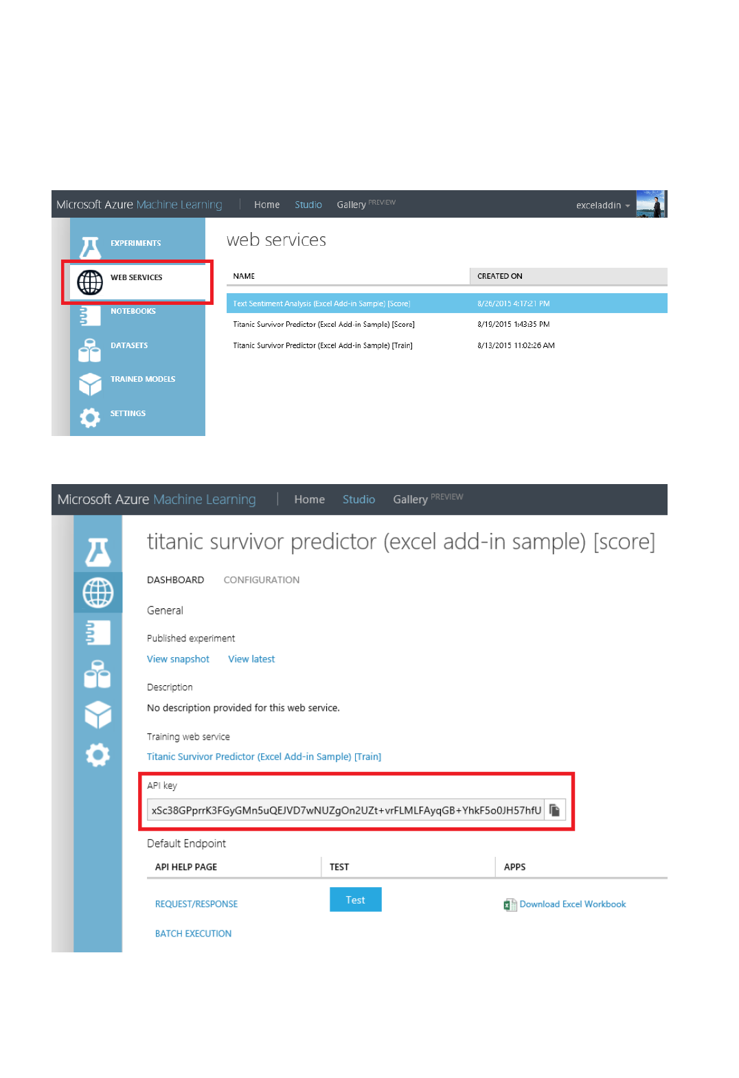
Deploy a web service or use an existing Web service. For more information on deploying a web service, see
Walkthrough Step 5: Deploy the Azure Machine Learning Web service.
Get the API key for your web service. Where you perform this action depends on whether you published a Classic
Machine Learning web service of a New Machine Learning web service.
Use a Classic web service
3. On the DASHBOARD tab for the web service, click the REQUEST/RESPONSE link.
4. Look for the Request URI section. Copy and save the URL.
1. In Machine Learning Studio, click the WEB SERVICES section in the left pane, and then select the web
service.
2. Copy the API key for the web service.
NOTENOTE
Steps to Add a New web service
It is now possible to sign into the Azure Machine Learning Web Services portal to obtain the API key for a Classic Machine
Learning web service.
Use a New web service
1. In the Azure Machine Learning Web Services portal, click Web Services, then select your web service.
2. Click Consume.
3. Look for the Basic consumption info section. Copy and save the Primary Key and the Request-Response
URL.
1. Deploy a web service or use an existing Web service. For more information on deploying a web service, see
Walkthrough Step 5: Deploy the Azure Machine Learning Web service.
2. Click Consume.
3. Look for the Basic consumption info section. Copy and save the Primary Key and the Request-Response
URL.
5. Click Add Web Service.
6. Paste the URL into the Excel add-in text box labeled URL.
7. Paste the API/Primary key into the text box labeled API key.
4. In Excel, go to the Web Services section (if you are in the Predict section, click the back arrow to go to the
list of web services).
8. Click Add.
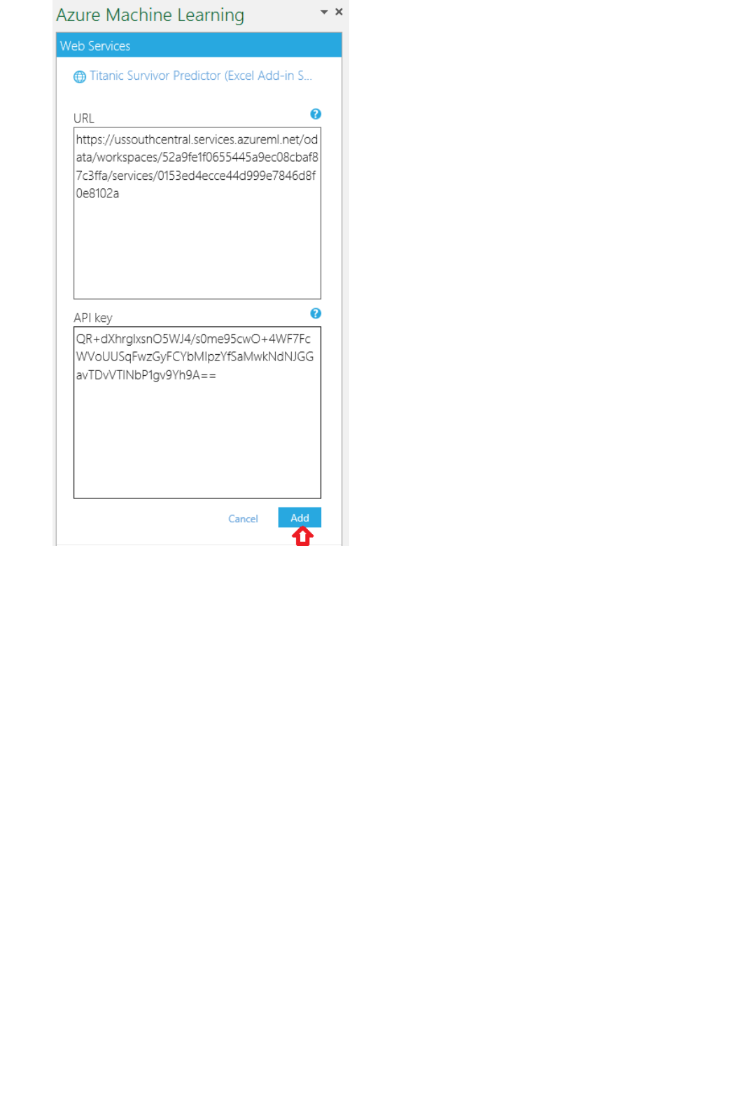
Sharing Your Workbook
9. To use the web service, follow the preceding directions, "Steps to Use an Existing web Service."
If you save your workbook, then the API/Primary key for the web services you have added is also saved. That
means you should only share the workbook with individuals you trust.
Ask any questions in the following comment section or on our forum.
Consume an Azure Machine Learning web service by
using a web app template
3/21/2018 • 5 min to read • Edit Online
NOTENOTE
Azure Machine Learning web app templates
You can develop a predictive model and deploy it as an Azure web service by using:
Azure Machine Learning Studio.
Tools such as R or Python.
After that, you can access the operationalized model by using a REST API.
There are a number of ways to consume the REST API and access the web service. For example, you can write an
application in C#, R, or Python by using the sample code generated for you when you deployed the web service.
(The sample code is available in the Machine Learning Web Services portal or in the web service dashboard in
Machine Learning Studio.) Or you can use the sample Microsoft Excel workbook created for you at the same time.
But the quickest and easiest way to access your web service is through the web app templates available in the
Azure Marketplace.
You can try Azure Machine Learning for free. No credit card or Azure subscription is required. Get started now.
The web app templates available in the Azure Marketplace can build a custom web app that knows your web
service's input data and expected results. All you need to do is give the web app access to your web service and
data, and the template does the rest.
Two templates are available:
Azure ML Request-Response Service Web App Template
Azure ML Batch Execution Service Web App Template
Each template creates a sample ASP.NET application by using the API URI and key for your web service. The
template then deploys the application as a website to Azure.
The Request-Response Service (RRS) template creates a web app that you can use to send a single row of data to
the web service to get a single result. The Batch Execution Service (BES) template creates a web app that you can
use to send many rows of data to get multiple results.
No coding is required to use these templates. You just supply the API key and URI, and the template builds the
application for you.
To get the API key and request URI for a web service:
1. In the Web Services portal, select Web Services at the top. Or for a classic web service, select Classic Web
Services.
2. Select the web service that you want to access.
3. For a classic web service, select the endpoint that you want to access.
4. Select Consume at the top.
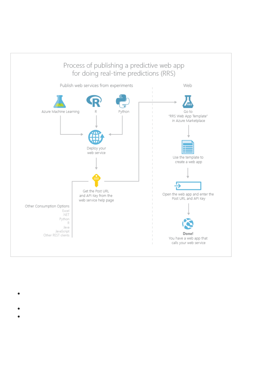
How to use the Request-Response Service template
5. Copy the primary or secondary key and save it.
6. If you're creating an RRS template, copy the Request-Response URI and save it. If you're creating a BES
template, copy the Batch Requests URI and save it.
Follow these steps to use the RRS web app template, as shown in the following diagram.
1. Sign in to the Azure portal.
2. Select New, search for and select Azure ML Request-Response Service Web App, and then select Create.
3. In the Create pane:
Give your web app a unique name. The URL of the web app will be this name followed by
.azurewebsites.net. An example is http://carprediction.azurewebsites.net.
Select the Azure subscription and services under which your web service is running.
Select Create.
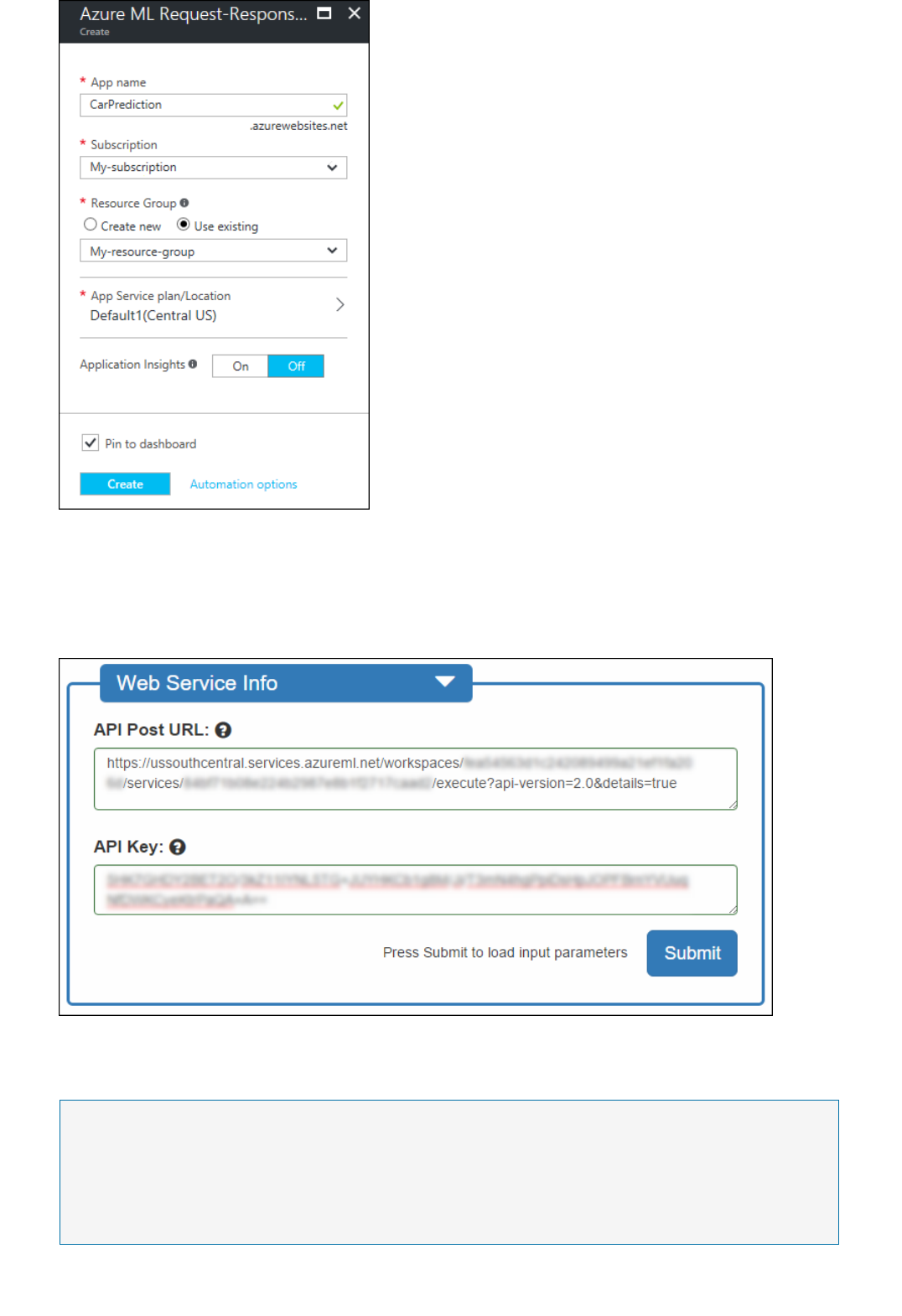
NOTENOTE
4. When Azure has finished deploying the web app, select the URL on the web app settings page in Azure, or
enter the URL in a web browser. For example, enter http://carprediction.azurewebsites.net.
5. When the web app first runs, it asks you for the API Post URL and API Key. Enter the values that you
saved earlier (request URI and API key, respectively). Select Submit.
6. The web app displays its Web App Configuration page with the current web service settings. Here you
can make changes to the settings that the web app uses.
Changing the settings here only changes them for this web app. It doesn't change the default settings of your web
service. For example, if you change the text in Description here, it doesn't change the description shown on the web
service dashboard in Machine Learning Studio.
When you're done, select Save changes, and then select Go to Home Page.
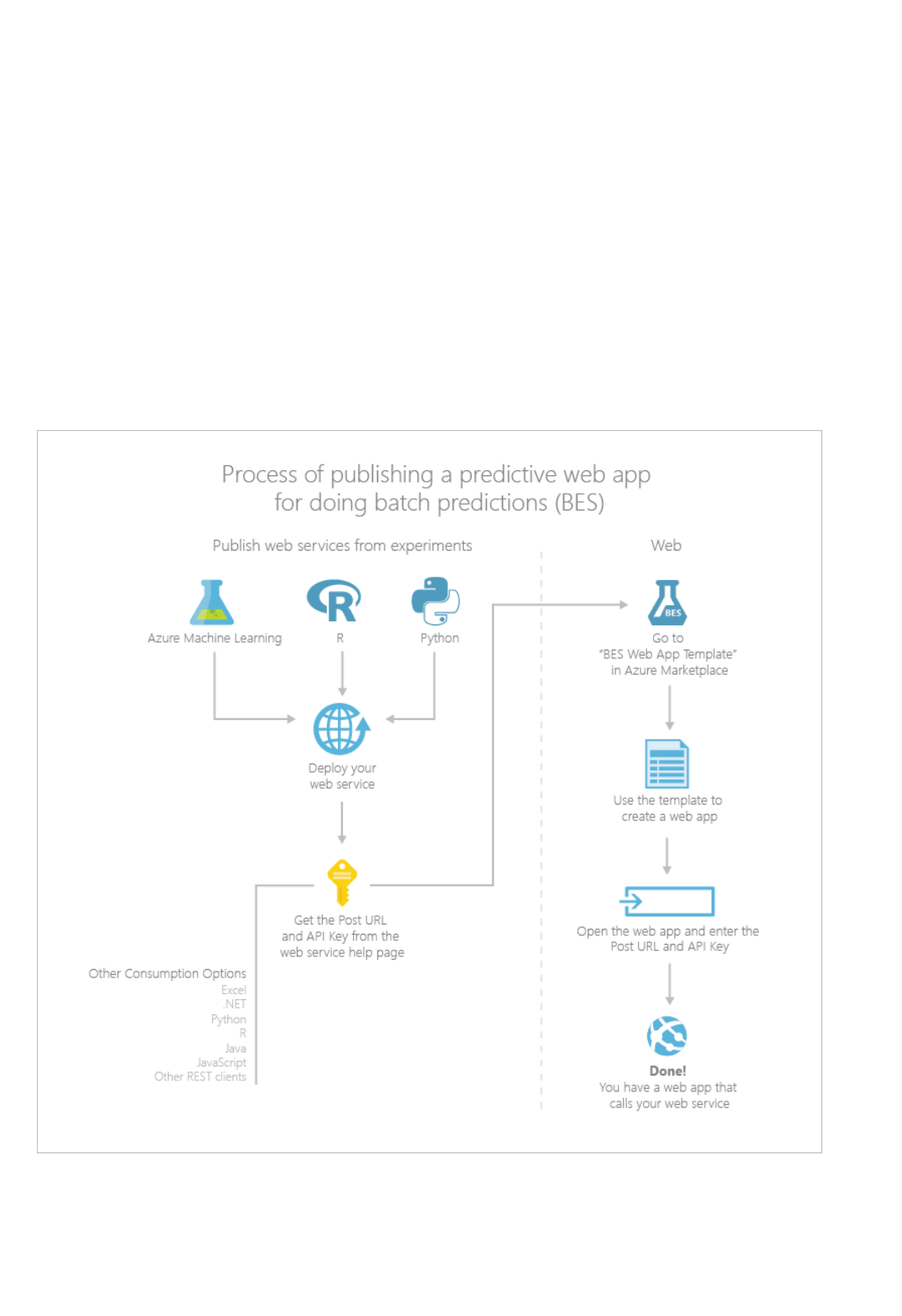
How to use the Batch Execution Service template
7. From the home page, you can enter values to send to your web service. Select Submit when you're done,
and the result will be returned.
If you want to return to the Configuration page, go to the setting.aspx page of the web app. For example, go to
http://carprediction.azurewebsites.net/setting.aspx. You're prompted to enter the API key again. You need
that to access the page and update the settings.
You can stop, restart, or delete the web app in the Azure portal like any other web app. As long as it's running, you
can browse to the home web address and enter new values.
You can use the BES web app template in the same way as the RRS template. The difference is that you can use the
created web app to submit multiple rows of data and receive multiple results.
The input values for a batch execution web service can come from Azure Storage or a local file. The results are
stored in an Azure storage container. So, you need an Azure storage container to hold the results that the web app
returns. You also need to get your input data ready.
1. Follow the same procedure to create the BES web app as for the RRS template. But in this case, go to Azure
ML Batch Execution Service Web App Template to open the BES template in the Azure Marketplace. Select
Create Web App.
2. To specify where you want the results stored, enter the destination container information on the web app's
home page. Also specify where the web app can get the input values: either in a local file or in an Azure
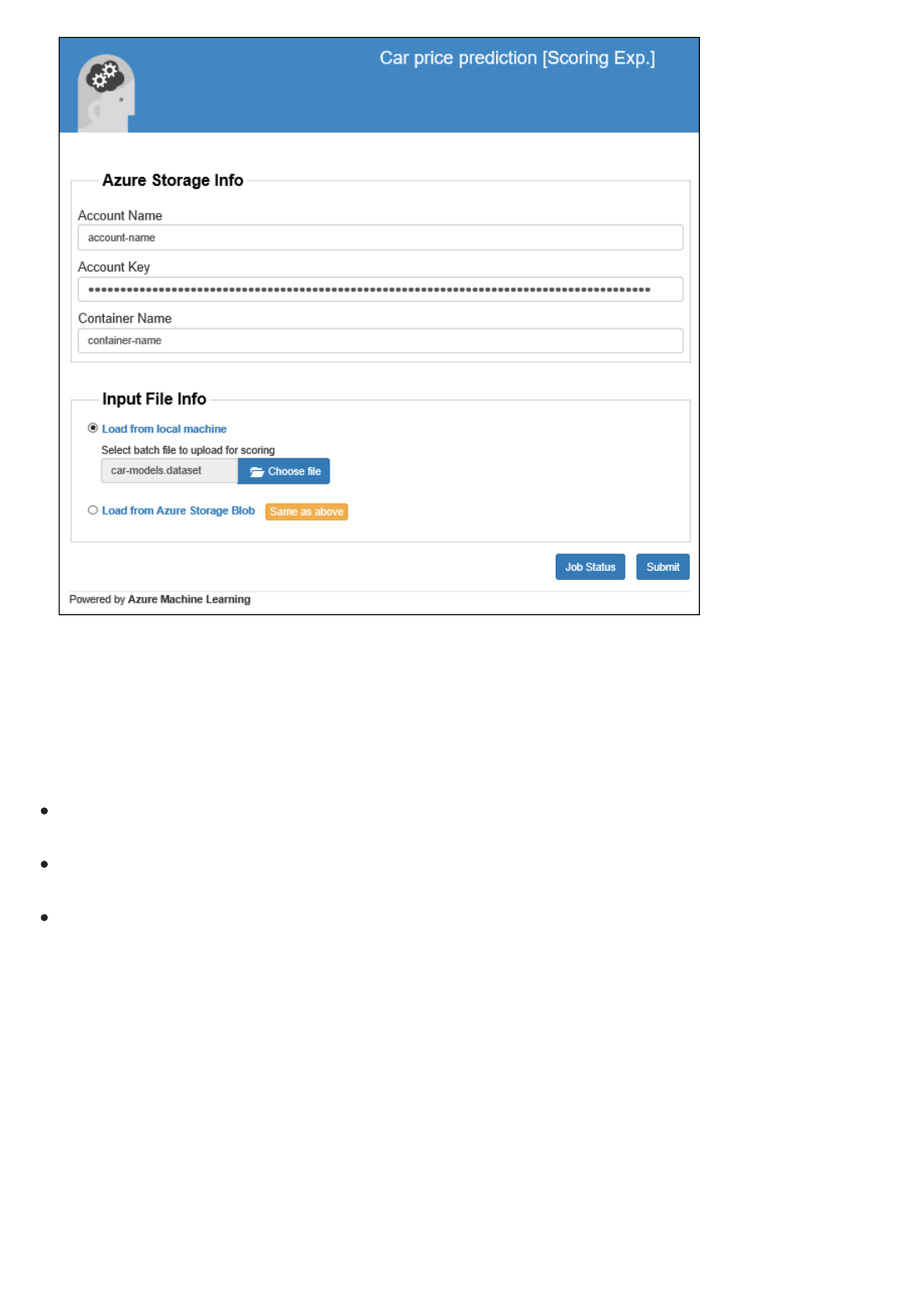
For more information
storage container. Select Submit.
The web app displays a page with job status. When the job is completed, you get the location of the results in Azure
Blob storage. You also have the option of downloading the results to a local file.
To learn more about:
Creating a machine learning experiment with Machine Learning Studio, see Create your first experiment in
Azure Machine Learning Studio.
How to deploy your machine learning experiment as a web service, see Deploy an Azure Machine Learning web
service.
Other ways to access your web service, see How to consume an Azure Machine Learning web service.
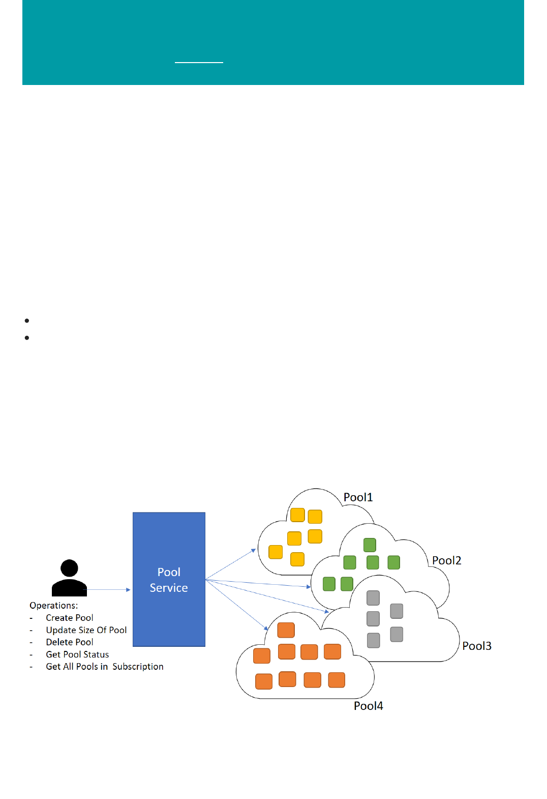
Azure Batch service for Machine Learning jobs
3/21/2018 • 4 min to read • Edit Online
How to use Batch Pool processing
Machine Learning Batch Pool processing provides customer-managed scale for the Azure Machine Learning Batch
Execution Service. Classic batch processing for machine learning takes place in a multi-tenant environment, which
limits the number of concurrent jobs you can submit, and jobs are queued on a first-in-first-out basis. This
uncertainty means that you can't accurately predict when your job will run.
Batch Pool processing allows you to create pools on which you can submit batch jobs. You control the size of the
pool, and to which pool the job is submitted. Your BES job runs in its own processing space providing predictable
processing performance and the ability to create resource pools that correspond to the processing load that you
submit.
Configuration of Batch Pool Processing is not currently available through the Azure portal. To use Batch Pool
processing, you must:
Call CSS to create a Batch Pool Account and obtain a Pool Service URL and an authorization key
Create a New Resource Manager based web service and billing plan
To create your account, call Microsoft Customer Service and Support (CSS) and provide your Subscription ID. CSS
will work with you to determine the appropriate capacity for your scenario. CSS then configures your account with
the maximum number of pools you can create and the maximum number of virtual machines (VMs) that you can
place in each pool. Once your account is configured, you are provided your Pool Service URL and an authorization
key.
After your account is created, you use the Pool Service URL and authorization key to perform pool management
operations on your Batch Pool.
You create pools by calling the Create Pool operation on the pool service URL that CSS provided to you. When you
create a pool, specify the number of VMs and the URL of the swagger.json of a New Resource Manager based
Machine Learning web service. This web service is provided to establish the billing association. The Batch Pool
service uses the swagger.json to associate the pool with a billing plan. You can run any BES web service, both New

Resource Manager based and classic, you choose on the pool.
You can use any New Resource Manager based web service, but be aware that the billing for the jobs are charged
against the billing plan associated with that service. You may want to create a web service and new billing plan
specifically for running Batch Pool jobs.
For more information on creating web services, see Deploy an Azure Machine Learning web service.
Once you have created a pool, you submit the BES job using the Batch Requests URL for the web service. You can
choose to submit it to a pool or to classic batch processing. To submit a job to Batch Pool processing, you add the
following parameter to the job submission request body:
"AzureBatchPoolId":"<pool ID>"
If you do not add the parameter, the job is run in the classic batch process environment. If the pool has available
resources, the job starts running immediately. If the pool does not have free resources, your job is queued until a
resource is available.
If you find that you regularly reach the capacity of your pools, and you need increased capacity, you can call CSS
and work with a representative to increase your quotas.
Example Request:
https://ussouthcentral.services.azureml.net/subscriptions/80c77c7674ba4c8c82294c3b2957990c/services/9fe659
022c9747e3b9b7b923c3830623/jobs?api-version=2.0

{
"Input":{
"ConnectionString":"DefaultEndpointsProtocol=https;BlobEndpoint=https://sampleaccount.blob.core.windows.net/;Ta
bleEndpoint
=https://sampleaccount.table.core.windows.net/;QueueEndpoint=https://sampleaccount.queue.core.windows.net/;File
Endpoint=https://zhguim
l.file.core.windows.net/;AccountName=sampleaccount;AccountKey=<Key>;",
"BaseLocation":null,
"RelativeLocation":"testint/AdultCensusIncomeBinaryClassificationDataset.csv",
"SasBlobToken":null
},
"GlobalParameters":{ },
"Outputs":{
"output1":{
"ConnectionString":"DefaultEndpointsProtocol=https;BlobEndpoint=https://sampleaccount.blob.core.windows.net/;Ta
bleEndpo
int=https://sampleaccount.table.core.windows.net/;QueueEndpoint=https://sampleaccount.queue.core.windows.net/;F
ileEndpoint=https://sampleaccount.file.core.windows.net/;AccountName=sampleaccount;AccountKey=<Key>",
"BaseLocation":null,
"RelativeLocation":"testintoutput/testint\_results.csv",
"SasBlobToken":null
}
},
"AzureBatchPoolId":"8dfc151b0d3e446497b845f3b29ef53b"
}
Considerations when using Batch Pool processing
Batch Pool Processing is an always-on billable service and that requires you to associate it with a Resource
Manager based billing plan. You are only billed for the number of compute hours the pool is running; regardless of
the number of jobs run during that time pool. If you create a pool, you are billed for the compute hours of each
virtual machine in the pool until the pool is deleted, even if no batch jobs are running in the pool. Billing for the
virtual machines starts when they have finished provisioning and stops when they have been deleted. You can use
any of the plans found on the Machine Learning Pricing page.
Billing example:
If you create a Batch Pool with 2 virtual machines and delete it after 24 hours your billing plan is debited 48
compute hours; regardless of how many jobs were run during that period.
If you create a Batch Pool with 4 virtual machines and delete it after 12 hours, your billing plan is also debited 48
compute hours.
We recommend that you poll the job status to determine when jobs complete. When all your jobs have finished

USE BATCH POOL PROCESSING WHEN USE CLASSIC BATCH PROCESSING WHEN
You need to run a large number of jobs
Or
You need to know that your jobs will run immediately
Or
You need guaranteed throughput. For example, you need to
run a number of jobs in a given time frame, and want to scale
out your compute resources to meet your needs.
You are running just a few jobs
And
You don’t need the jobs to run immediately
running, call the Resize Pool operation to set the number of virtual machines in the pool to zero. If you are short on
pool resources and you need to create a new pool, for example to bill against a different billing plan, you can delete
the pool instead when all your jobs have finished running.
Create machine learning experiments from working
examples in Azure AI Gallery
3/21/2018 • 2 min to read • Edit Online
NOTENOTE
Find an experiment to copy in Azure AI Gallery
Find the newest or most popular experimentsFind the newest or most popular experiments
Look for an experiment that meets specific requirementsLook for an experiment that meets specific requirements
Learn how to start with example experiments from Azure AI Gallery instead of creating machine learning
experiments from scratch. You can use the examples to build your own machine learning solution.
The gallery has example experiments by the Microsoft Azure Machine Learning team as well as examples shared
by the Machine Learning community. You also can ask questions or post comments about experiments.
To see how to use the gallery, watch the 3-minute video Copy other people's work to do data science from the
series Data Science for Beginners.
You can try Azure Machine Learning for free. No credit card or Azure subscription is required. Get started now.
To see what experiments are available, go to the Gallery and click Experiments at the top of the page.
On this page, you can see Recently added experiments, or scroll down to look at What's popular or the latest
Popular Microsoft experiments.
To browse all experiments:
1. Click Browse all at the top of the page.
2. On the left-hand side, under Refine by in the Categories section, select Experiment to see all the experiments
in the Gallery.
3. You can find experiments that meet your requirements a couple different ways:
Select filters on the left. For example, to browse experiments that use a PCA-based anomaly detection
algorithm: Under Categories click Experiment. Then, under Algorithms Used, click Show all and in
the dialog box choose PCA-Based Anomaly Detection. You may have to scroll to see it.
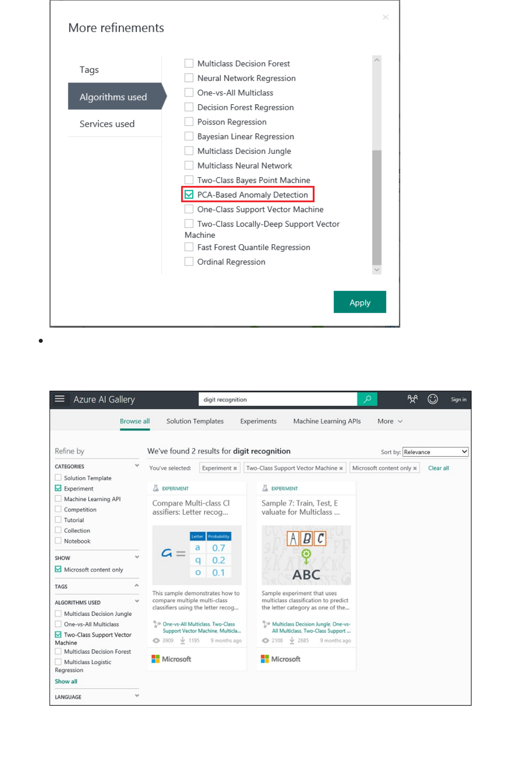
4. Click an experiment to learn more about it.
Use the search box. For example, to find experiments contributed by Microsoft related to digit
recognition that use a two-class support vector machine algorithm, enter "digit recognition" in the search
box. Then, select the filters Experiment, Microsoft content only, and Two-Class Support Vector
Machine:
5. To run and/or modify the experiment, click Open in Studio on the experiment's page.
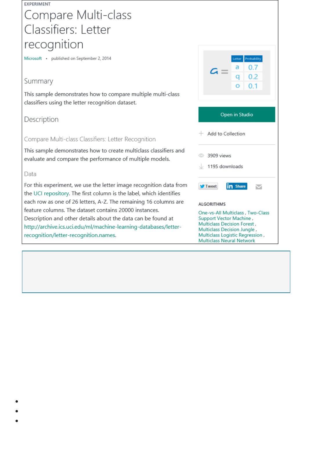
Create a new experiment using an example as a template
Next steps
NOTENOTE
When you open an experiment in Machine Learning Studio for the first time, you can try it for free or buy an Azure
subscription. Learn about the Machine Learning Studio free trial vs. paid service
You also can create a new experiment in Machine Learning Studio using a Gallery example as a template.
1. Sign in with your Microsoft account credentials to the Studio, and then click New to create an experiment.
2. Browse through the example content and click one.
A new experiment is created in your Machine Learning Studio workspace using the example experiment as a
template.
Import data from various sources
Quickstart tutorial for the R language in Machine Learning
Deploy a Machine Learning web service
Use the sample datasets in Azure Machine Learning
Studio
3/21/2018 • 14 min to read • Edit Online
NOTENOTE
DATASET NAME DATASET DESCRIPTION
Adult Census Income Binary Classification dataset A subset of the 1994 Census database, using working adults
over the age of 16 with an adjusted income index of > 100.
Airport Codes Dataset U.S. airport codes.
Automobile price data (Raw)Information about automobiles by make and model, including
the price, features such as the number of cylinders and MPG,
as well as an insurance risk score.
When you create a new workspace in Azure Machine Learning, a number of sample datasets and experiments are
included by default. Many of these sample datasets are used by the sample models in the Azure AI Gallery. Others
are included as examples of various types of data typically used in machine learning.
Some of these datasets are available in Azure Blob storage. For these datasets, the following table provides a
direct link. You can use these datasets in your experiments by using the Import Data module.
The rest of these sample datasets are available in your workspace under Saved Datasets. You can find this in the
module palette to the left of the experiment canvas in Machine Learning Studio. You can use any of these datasets
in your own experiment by dragging it to your experiment canvas.
You can try Azure Machine Learning for free. No credit card or Azure subscription is required. Get started now.
Usage: Classify people using demographics to predict
whether a person earns over 50K a year.
Related Research: Kohavi, R., Becker, B., (1996). UCI
Machine Learning Repository http://archive.ics.uci.edu/ml.
Irvine, CA: University of California, School of Information
and Computer Science
This dataset contains one row for each U.S. airport,
providing the airport ID number and name along with the
location city and state.
The risk score is initially associated with auto price. It is
then adjusted for actual risk in a process known to
actuaries as symboling. A value of +3 indicates that the
auto is risky, and a value of -3 that it is probably safe.
Usage: Predict the risk score by features, using regression
or multivariate classification.
Related Research: Schlimmer, J.C. (1987). UCI Machine
Learning Repository http://archive.ics.uci.edu/ml. Irvine,
CA: University of California, School of Information and
Computer Science

Bike Rental UCI dataset UCI Bike Rental dataset that is based on real data from Capital
Bikeshare company that maintains a bike rental network in
Washington DC.
Bill Gates RGB Image Publicly available image file converted to CSV data.
Blood donation data A subset of data from the blood donor database of the Blood
Transfusion Service Center of Hsin-Chu City, Taiwan.
Breast cancer data One of three cancer-related datasets provided by the
Oncology Institute that appears frequently in machine
learning literature. Combines diagnostic information with
features from laboratory analysis of about 300 tissue samples.
Breast Cancer Features The dataset contains information for 102K suspicious regions
(candidates) of X-ray images, each described by 117 features.
The features are proprietary and their meaning is not revealed
by the dataset creators (Siemens Healthcare).
The dataset has one row for each hour of each day in
2011 and 2012, for a total of 17,379 rows. The range of
hourly bike rentals is from 1 to 977.
The code for converting the image is provided in the
Color quantization using K-Means clustering model
detail page.
Donor data includes the months since last donation), and
frequency, or the total number of donations, time since
last donation, and amount of blood donated.
Usage: The goal is to predict via classification whether the
donor donated blood in March 2007, where 1 indicates a
donor during the target period, and 0 a non-donor.
Related Research: Yeh, I.C., (2008). UCI Machine
Learning Repository http://archive.ics.uci.edu/ml. Irvine,
CA: University of California, School of Information and
Computer Science
Yeh, I-Cheng, Yang, King-Jang, and Ting, Tao-Ming,
"Knowledge discovery on RFM model using Bernoulli
sequence, "Expert Systems with Applications, 2008,
http://dx.doi.org/10.1016/j.eswa.2008.07.018
Usage: Classify the type of cancer, based on 9 attributes,
some of which are linear and some are categorical.
Related Research: Wohlberg, W.H., Street, W.N., &
Mangasarian, O.L. (1995). UCI Machine Learning
Repository http://archive.ics.uci.edu/ml. Irvine, CA:
University of California, School of Information and
Computer Science

Breast Cancer Info The dataset contains additional information for each
suspicious region of X-ray image. Each example provides
information (for example, label, patient ID, coordinates of
patch relative to the whole image) about the corresponding
row number in the Breast Cancer Features dataset. Each
patient has a number of examples. For patients who have a
cancer, some examples are positive and some are negative.
For patients who don't have a cancer, all examples are
negative. The dataset has 102K examples. The dataset is
biased, 0.6% of the points are positive, the rest are negative.
The dataset was made available by Siemens Healthcare.
CRM Appetency Labels Shared Labels from the KDD Cup 2009 customer relationship
prediction challenge (orange_small_train_appetency.labels).
CRM Churn Labels Shared Labels from the KDD Cup 2009 customer relationship
prediction challenge (orange_small_train_churn.labels).
CRM Dataset Shared This data comes from the KDD Cup 2009 customer
relationship prediction challenge (orange_small_train.data.zip).
CRM Upselling Labels Shared Labels from the KDD Cup 2009 customer relationship
prediction challenge (orange_large_train_upselling.labels).
Energy-Efficiency Regression data A collection of simulated energy profiles, based on 12 different
building shapes. The buildings are differentiated by eight
features. This includes glazing area, the glazing area
distribution, and orientation.
Flight Delays Data Passenger flight on-time performance data taken from the
TranStats data collection of the U.S. Department of
Transportation (On-Time).
The dataset contains 50K customers from the French
Telecom company Orange. Each customer has 230
anonymized features, 190 of which are numeric and 40
are categorical. The features are very sparse.
Usage: Use either regression or classification to predict
the energy-efficiency rating based as one of two real
valued responses. For multi-class classification, is round
the response variable to the nearest integer.
Related Research: Xifara, A. & Tsanas, A. (2012). UCI
Machine Learning Repository http://archive.ics.uci.edu/ml.
Irvine, CA: University of California, School of Information
and Computer Science
The dataset covers the time period April-October 2013.
Before uploading to Azure Machine Learning Studio, the
dataset was processed as follows:
The dataset was filtered to cover only the 70 busiest
airports in the continental US
Canceled flights were labeled as delayed by more than
15 minutes
Diverted flights were filtered out
The following columns were selected: Year, Month,
DayofMonth, DayOfWeek, Carrier, OriginAirportID,
DestAirportID, CRSDepTime, DepDelay, DepDel15,
CRSArrTime, ArrDelay, ArrDel15, Canceled

Flight on-time performance (Raw)Records of airplane flight arrivals and departures within United
States from October 2011.
Forest fires data Contains weather data, such as temperature and humidity
indices and wind speed. The data is taken from an area of
northeast Portugal, combined with records of forest fires.
German Credit Card UCI dataset The UCI Statlog (German Credit Card) dataset
(Statlog+German+Credit+Data), using the german.data file.
IMDB Movie Titles The dataset contains information about movies that were
rated in Twitter tweets: IMDB movie ID, movie name, genre,
and production year. There are 17K movies in the dataset. The
dataset was introduced in the paper "S. Dooms, T. De
Pessemier and L. Martens. MovieTweetings: a Movie Rating
Dataset Collected From Twitter. Workshop on Crowdsourcing
and Human Computation for Recommender Systems,
CrowdRec at RecSys 2013."
Iris two class data This is perhaps the best known database to be found in the
pattern recognition literature. The dataset is relatively small,
containing 50 examples each of petal measurements from
three iris varieties.
Usage: Predict flight delays.
Related Research: From US Dept. of Transportation
http://www.transtats.bts.gov/DL_SelectFields.asp?
Table_ID=236&DB_Short_Name=On-Time.
Usage: This is a difficult regression task, where the aim is
to predict the burned area of forest fires.
Related Research: Cortez, P., & Morais, A. (2008). UCI
Machine Learning Repository http://archive.ics.uci.edu/ml.
Irvine, CA: University of California, School of Information
and Computer Science
[Cortez and Morais, 2007] P. Cortez and A. Morais. A Data
Mining Approach to Predict Forest Fires using
Meteorological Data. In J. Neves, M. F. Santos and J.
Machado Eds., New Trends in Artificial Intelligence,
Proceedings of the 13th EPIA 2007 - Portuguese
Conference on Artificial Intelligence, December,
Guimarães, Portugal, pp. 512-523, 2007. APPIA, ISBN-13
978-989-95618-0-9. Available at:
http://www.dsi.uminho.pt/~pcortez/fires.pdf.
The dataset classifies people, described by a set of
attributes, as low or high credit risks. Each example
represents a person. There are 20 features, both
numerical and categorical, and a binary label (the credit
risk value). High credit risk entries have label = 2, low
credit risk entries have label = 1. The cost of misclassifying
a low risk example as high is 1, whereas the cost of
misclassifying a high risk example as low is 5.
Usage: Predict the iris type from the measurements.
Related Research: Fisher, R.A. (1988). UCI Machine
Learning Repository http://archive.ics.uci.edu/ml. Irvine,
CA: University of California, School of Information and
Computer Science

Movie Tweets The dataset is an extended version of the Movie Tweetings
dataset. The dataset has 170K ratings for movies, extracted
from well-structured tweets on Twitter. Each instance
represents a tweet and is a tuple: user ID, IMDB movie ID,
rating, timestamp, numer of favorites for this tweet, and
number of retweets of this tweet. The dataset was made
available by A. Said, S. Dooms, B. Loni and D. Tikk for
Recommender Systems Challenge 2014.
MPG data for various automobiles This dataset is a slightly modified version of the dataset
provided by the StatLib library of Carnegie Mellon University.
The dataset was used in the 1983 American Statistical
Association Exposition.
Pima Indians Diabetes Binary Classification dataset A subset of data from the National Institute of Diabetes and
Digestive and Kidney Diseases database. The dataset was
filtered to focus on female patients of Pima Indian heritage.
The data includes medical data such as glucose and insulin
levels, as well as lifestyle factors.
Restaurant customer data A set of metadata about customers, including demographics
and preferences.
Restaurant feature data A set of metadata about restaurants and their features, such
as food type, dining style, and location.
The data lists fuel consumption for various automobiles in
miles per gallon. It also includes information such as the
number of cylinders, engine displacement, horsepower,
total weight, and acceleration.
Usage: Predict fuel economy based on three multivalued
discrete attributes and five continuous attributes.
Related Research: StatLib, Carnegie Mellon University,
(1993). UCI Machine Learning Repository
http://archive.ics.uci.edu/ml. Irvine, CA: University of
California, School of Information and Computer Science
Usage: Predict whether the subject has diabetes (binary
classification).
Related Research: Sigillito, V. (1990). UCI Machine
Learning Repository http://archive.ics.uci.edu/ml". Irvine,
CA: University of California, School of Information and
Computer Science
Usage: Use this dataset, in combination with the other
two restaurant datasets, to train and test a recommender
system.
Related Research: Bache, K. and Lichman, M. (2013). UCI
Machine Learning Repository http://archive.ics.uci.edu/ml.
Irvine, CA: University of California, School of Information
and Computer Science.

Restaurant ratings Contains ratings given by users to restaurants on a scale from
0 to 2.
Steel Annealing multi-class dataset This dataset contains a series of records from steel annealing
trials. It contains the physical attributes (width, thickness, type
(coil, sheet, etc.) of the resulting steel types.
Usage: Use this dataset, in combination with the other
two restaurant datasets, to train and test a recommender
system.
Related Research: Bache, K. and Lichman, M. (2013). UCI
Machine Learning Repository http://archive.ics.uci.edu/ml.
Irvine, CA: University of California, School of Information
and Computer Science.
Usage: Predict any of two numeric class attributes;
hardness or strength. You might also analyze correlations
among attributes.
Steel grades follow a set standard, defined by SAE and
other organizations. You are looking for a specific 'grade'
(the class variable) and want to understand the values
needed.
Related Research: Sterling, D. & Buntine, W. (NA). UCI
Machine Learning Repository http://archive.ics.uci.edu/ml.
Irvine, CA: University of California, School of Information
and Computer Science
A useful guide to steel grades can be found here:
http://www.outokumpu.com/SiteCollectionDocuments/Ou
tokumpu-steel-grades-properties-global-standards.pdf

Telescope data Record of high energy gamma particle bursts along with
background noise, both simulated using a Monte Carlo
process.
Weather Dataset Hourly land-based weather observations from NOAA (merged
data from 201304 to 201310).
The intent of the simulation was to improve the accuracy
of ground-based atmospheric Cherenkov gamma
telescopes. This is done by using statistical methods to
differentiate between the desired signal (Cherenkov
radiation showers) and background noise (hadronic
showers initiated by cosmic rays in the upper
atmosphere).
The data has been pre-processed to create an elongated
cluster with the long axis is oriented towards the camera
center. The characteristics of this ellipse (often called Hillas
parameters) are among the image parameters that can be
used for discrimination.
Usage: Predict whether image of a shower represents
signal or background noise.
Notes: Simple classification accuracy is not meaningful for
this data, since classifying a background event as signal is
worse than classifying a signal event as background. For
comparison of different classifiers, the ROC graph should
be used. The probability of accepting a background event
as signal must be below one of the following thresholds:
0.01, 0.02, 0.05, 0.1, or 0.2.
Also, note that the number of background events (h, for
hadronic showers) is underestimated. In real
measurements, the h or noise class represents the
majority of events.
Related Research: Bock, R.K. (1995). UCI Machine
Learning Repository http://archive.ics.uci.edu/ml. Irvine,
CA: University of California, School of Information
The weather data covers observations made from airport
weather stations, covering the time period April-October
2013. Before uploading to Azure Machine Learning
Studio, the dataset was processed as follows:
Weather station IDs were mapped to corresponding
airport IDs
Weather stations not associated with the 70 busiest
airports were filtered out
The Date column was split into separate Year, Month,
and Day columns
The following columns were selected: AirportID, Year,
Month, Day, Time, TimeZone, SkyCondition, Visibility,
WeatherType, DryBulbFarenheit, DryBulbCelsius,
WetBulbFarenheit, WetBulbCelsius, DewPointFarenheit,
DewPointCelsius, RelativeHumidity, WindSpeed,
WindDirection, ValueForWindCharacter,
StationPressure, PressureTendency, PressureChange,
SeaLevelPressure, RecordType, HourlyPrecip, Altimeter

Wikipedia SP 500 Dataset Data is derived from Wikipedia (http://www.wikipedia.org/)
based on articles of each S&P 500 company, stored as XML
data.
direct_marketing.csv The dataset contains customer data and indications about
their response to a direct mailing campaign. Each row
represents a customer. The dataset contains nine features
about user demographics and past behavior, and three label
columns (visit, conversion, and spend). Visit is a binary column
that indicates that a customer visited after the marketing
campaign. Conversion indicates a customer purchased
something. Spend is the amount that was spent. The dataset
was made available by Kevin Hillstrom for MineThatData E-
Mail Analytics And Data Mining Challenge.
lyrl2004_tokens_test.csv Features of test examples in the RCV1-V2 Reuters news
dataset. The dataset has 781K news articles along with their
IDs (first column of the dataset). Each article is tokenized,
stopworded, and stemmed. The dataset was made available
by David. D. Lewis.
lyrl2004_tokens_train.csv Features of training examples in the RCV1-V2 Reuters news
dataset. The dataset has 23K news articles along with their
IDs (first column of the dataset). Each article is tokenized,
stopworded, and stemmed. The dataset was made available
by David. D. Lewis.
network_intrusion_detection.csv Dataset from the KDD Cup 1999 Knowledge Discovery and
Data Mining Tools Competition (kddcup99.html).
rcv1-v2.topics.qrels.csv Topic assignments for news articles in the RCV1-V2 Reuters
news dataset. A news article can be assigned to several topics.
The format of each row is "<topic name> <document id> 1".
The dataset contains 2.6M topic assignments. The dataset was
made available by David. D. Lewis.
Before uploading to Azure Machine Learning Studio, the
dataset was processed as follows:
Extract text content for each specific company
Remove wiki formatting
Remove non-alphanumeric characters
Convert all text to lowercase
Known company categories were added
Note that for some companies an article could not be
found, so the number of records is less than 500.
The dataset was downloaded and stored in Azure Blob
storage (network_intrusion_detection.csv) and includes
both training and testing datasets. The training dataset
has approximately 126K rows and 43 columns, including
the labels. Three columns are part of the label
information, and 40 columns, consisting of numeric and
string/categorical features, are available for training the
model. The test data has approximately 22.5K test
examples with the same 43 columns as in the training
data.

student_performance.txt This data comes from the KDD Cup 2010 Student
performance evaluation challenge (student performance
evaluation). The data used is the Algebra_2008_2009 training
set (Stamper, J., Niculescu-Mizil, A., Ritter, S., Gordon, G.J., &
Koedinger, K.R. (2010). Algebra I 2008-2009. Challenge
dataset from KDD Cup 2010 Educational Data Mining
Challenge. Find it at downloads.jsp or algebra_2008_2009.zip.
The dataset was downloaded and stored in Azure Blob
storage (student_performance.txt) and contains log files
from a student tutoring system. The supplied features
include problem ID and its brief description, student ID,
timestamp, and how many attempts the student made
before solving the problem in the right way. The original
dataset has 8.9M records; this dataset has been down-
sampled to the first 100K rows. The dataset has 23 tab-
separated columns of various types: numeric, categorical,
and timestamp.
Analyzing Customer Churn using Azure Machine
Learning
3/20/2018 • 12 min to read • Edit Online
Overview
AcknowledgementsAcknowledgements
NOTENOTE
NOTENOTE
The problem of customer churn
Industry outlook and approaches
This article presents a reference implementation of a customer churn analysis project that is built by using Azure
Machine Learning. In this article, we discuss associated generic models for holistically solving the problem of
industrial customer churn. We also measure the accuracy of models that are built by using Machine Learning, and
assess directions for further development.
This experiment was developed and tested by Serge Berger, Principal Data Scientist at Microsoft, and Roger Barga,
formerly Product Manager for Microsoft Azure Machine Learning. The Azure documentation team gratefully
acknowledges their expertise and thanks them for sharing this white paper.
The data used for this experiment is not publicly available. For an example of how to build a machine learning model for churn
analysis, see: Retail churn model template in Azure AI Gallery
You can try Azure Machine Learning for free. No credit card or Azure subscription is required. Get started now.
Businesses in the consumer market and in all enterprise sectors have to deal with churn. Sometimes churn is
excessive and influences policy decisions. The traditional solution is to predict high-propensity churners and
address their needs via a concierge service, marketing campaigns, or by applying special dispensations. These
approaches can vary from industry to industry. They can even vary from a particular consumer cluster to another
within one industry (for example, telecommunications).
The common factor is that businesses need to minimize these special customer retention efforts. Thus, a natural
methodology would be to score every customer with the probability of churn and address the top N ones. The top
customers might be the most profitable ones. For example, in more sophisticated scenarios a profit function is
employed during the selection of candidates for special dispensation. However, these considerations are only a part
of the complete strategy for dealing with churn. Businesses also have to take into account risk (and associated risk
tolerance), the level and cost of the intervention, and plausible customer segmentation.
Sophisticated handling of churn is a sign of a mature industry. The classic example is the telecommunications
industry where subscribers are known to frequently switch from one provider to another. This voluntary churn is a
prime concern. Moreover, providers have accumulated significant knowledge about churn drivers, which are the
factors that drive customers to switch.
For instance, handset or device choice is a well-known driver of churn in the mobile phone business. As a result, a

Methodology to model customer churn
popular policy is to subsidize the price of a handset for new subscribers and charge a full price to existing
customers for an upgrade. Historically, this policy has led to customers hopping from one provider to another to
get a new discount. This, in turn, has prompted providers to refine their strategies.
High volatility in handset offerings is a factor that quickly invalidates models of churn that are based on current
handset models. Additionally, mobile phones are not only telecommunication devices, they are also fashion
statements (consider the iPhone). These social predictors are outside the scope of regular telecommunications data
sets.
The net result for modeling is that you cannot devise a sound policy simply by eliminating known reasons for
churn. In fact, a continuous modeling strategy, including classic models that quantify categorical variables (such as
decision trees), is mandatory.
Using big data sets on their customers, organizations are performing big data analytics (in particular, churn
detection based on big data) as an effective approach to the problem. You can find more about the big data
approach to the problem of churn in the Recommendations on ETL section.
A common problem-solving process to solve customer churn is depicted in Figures 1-3:
1. A risk model allows you to consider how actions affect probability and risk.
2. An intervention model allows you to consider how the level of intervention could affect the probability of churn
and the amount of customer lifetime value (CLV).
3. This analysis lends itself to a qualitative analysis that is escalated to a proactive marketing campaign that targets
customer segments to deliver the optimal offer.
This forward looking approach is the best way to treat churn, but it comes with complexity: we have to develop a
multi-model archetype and trace dependencies between the models. The interaction among models can be
encapsulated as shown in the following diagram:
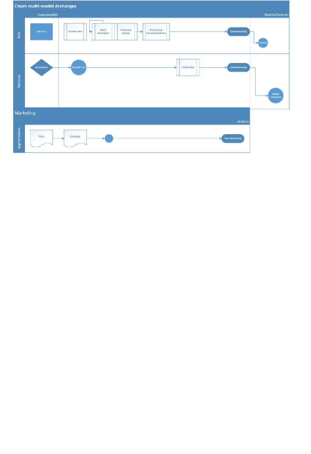
Implementing the modeling archetype in Machine Learning Studio
Figure 4: Unified multi-model archetype
Interaction between the models is key if we are to deliver a holistic approach to customer retention. Each model
necessarily degrades over time; therefore, the architecture is an implicit loop (similar to the archetype set by the
CRISP-DM data mining standard, [3]).
The overall cycle of risk-decision-marketing segmentation/decomposition is still a generalized structure, which is
applicable to many business problems. Churn analysis is simply a strong representative of this group of problems
because it exhibits all the traits of a complex business problem that does not allow a simplified predictive solution.
The social aspects of the modern approach to churn are not particularly highlighted in the approach, but the social
aspects are encapsulated in the modeling archetype, as they would be in any model.
An interesting addition here is big data analytics. Today's telecommunication and retail businesses collect
exhaustive data about their customers, and we can easily foresee that the need for multi-model connectivity will
become a common trend, given emerging trends such as the Internet of Things and ubiquitous devices, which
allow business to employ smart solutions at multiple layers.
Given the problem just described, what is the best way to implement an integrated modeling and scoring
approach? In this section, we will demonstrate how we accomplished this by using Azure Machine Learning Studio.
The multi-model approach is a must when designing a global archetype for churn. Even the scoring (predictive)
part of the approach should be multi-model.
The following diagram shows the prototype we created, which employs four scoring algorithms in Machine
Learning Studio to predict churn. The reason for using a multi-model approach is not only to create an ensemble
classifier to increase accuracy, but also to protect against over-fitting and to improve prescriptive feature selection.
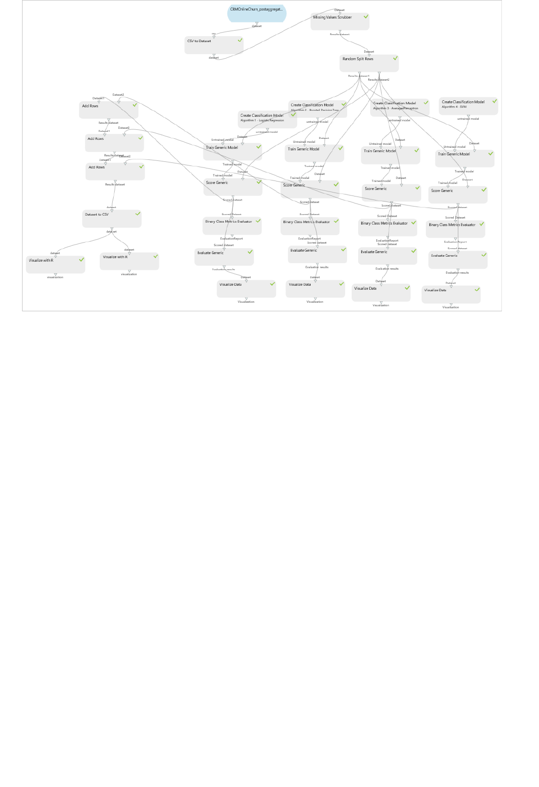
Data selection and preparationData selection and preparation
Figure 5: Prototype of a churn modeling approach
The following sections provide more details about the prototype scoring model that we implemented by using
Machine Learning Studio.
The data used to build the models and score customers was obtained from a CRM vertical solution, with the data
obfuscated to protect customer privacy. The data contains information about 8,000 subscriptions in the U.S., and it
combines three sources: provisioning data (subscription metadata), activity data (usage of the system), and
customer support data. The data does not include any business related information about the customers; for
example, it does not include loyalty metadata or credit scores.
For simplicity, ETL and data cleansing processes are out of scope because we assume that data preparation has
already been done elsewhere.
Feature selection for modeling is based on preliminary significance scoring of the set of predictors, included in the
process that uses the random forest module. For the implementation in Machine Learning Studio, we calculated
the mean, median, and ranges for representative features. For example, we added aggregates for the qualitative
data, such as minimum and maximum values for user activity.
We also captured temporal information for the most recent six months. We analyzed data for one year and we
established that even if there were statistically significant trends, the effect on churn is greatly diminished after six
months.
The most important point is that the entire process, including ETL, feature selection, and modeling was
implemented in Machine Learning Studio, using data sources in Microsoft Azure.
The following diagrams illustrate the data that was used.
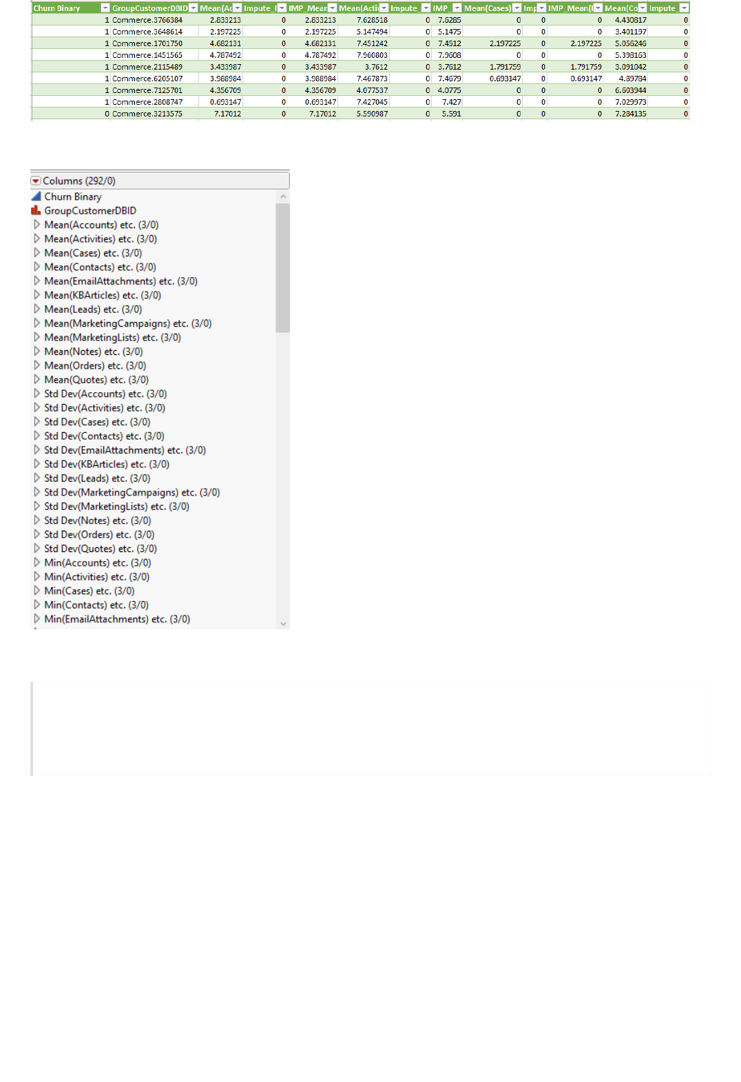
Algorithms used in the prototypeAlgorithms used in the prototype
Figure 6: Excerpt of data source (obfuscated)
Figure 7: Features extracted from data source
Note that this data is private and therefore the model and data cannot be shared. However, for a similar model
using publicly available data, see this sample experiment in the Azure AI Gallery: Telco Customer Churn.
To learn more about how you can implement a churn analysis model using Cortana Intelligence Suite, we also
recommend this video by Senior Program Manager Wee Hyong Tok.
We used the following four machine learning algorithms to build the prototype (no customization):
1. Logistic regression (LR)
2. Boosted decision tree (BT)
3. Averaged perceptron (AP)
4. Support vector machine (SVM)
The following diagram illustrates a portion of the experiment design surface, which indicates the sequence in which
the models were created:
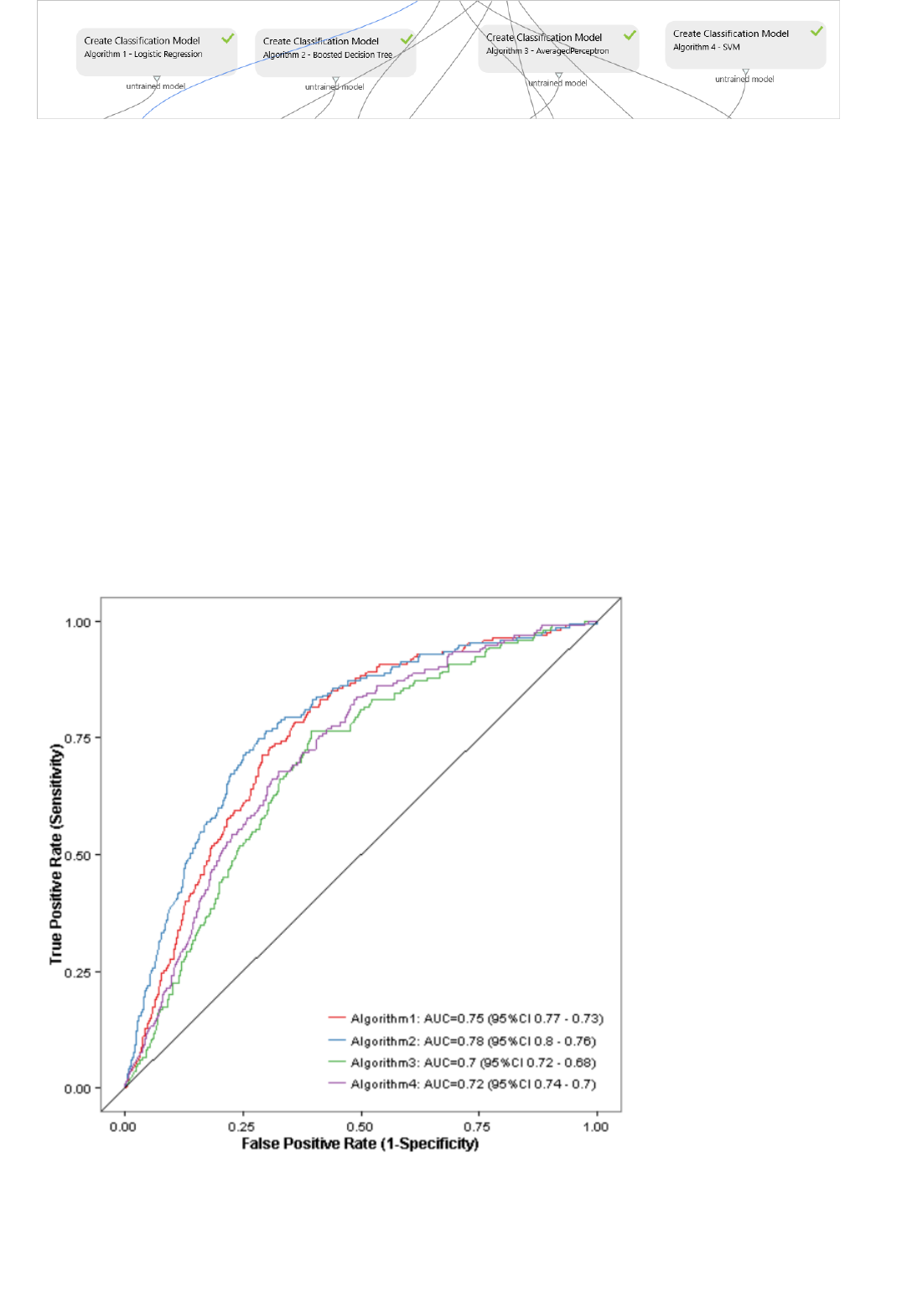
Scoring methodsScoring methods
Results
Accuracy and precision of scoringAccuracy and precision of scoring
Using AUC to compare resultsUsing AUC to compare results
Figure 8: Creating models in Machine Learning Studio
We scored the four models by using a labeled training dataset.
We also submitted the scoring dataset to a comparable model built by using the desktop edition of SAS Enterprise
Miner 12. We measured the accuracy of the SAS model and all four Machine Learning Studio models.
In this section, we present our findings about the accuracy of the models, based on the scoring dataset.
Generally, the implementation in Azure Machine Learning is behind SAS in accuracy by about 10-15% (Area
Under Curve or AUC).
However, the most important metric in churn is the misclassification rate: that is, of the top N churners as predicted
by the classifier, which of them actually did not churn, and yet received special treatment? The following diagram
compares this misclassification rate for all the models:
Figure 9: Passau prototype area under curve
Area Under Curve (AUC) is a metric that represents a global measure of separability between the distributions of
scores for positive and negative populations. It is similar to the traditional Receiver Operator Characteristic (ROC)
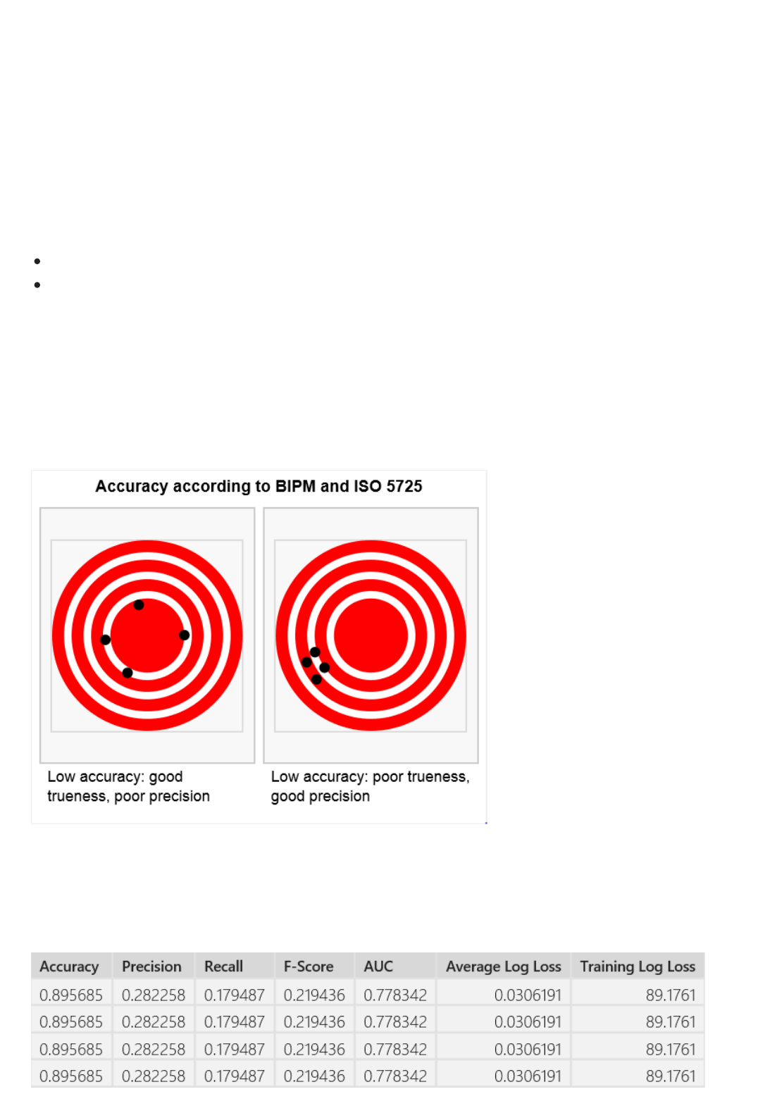
Comparing misclassification ratesComparing misclassification rates
Accuracy and precision results for boosted decision tree modelAccuracy and precision results for boosted decision tree model
graph, but one important difference is that the AUC metric does not require you to choose a threshold value.
Instead, it summarizes the results over all possible choices. In contrast, the traditional ROC graph shows the
positive rate on the vertical axis and the false positive rate on the horizontal axis, and the classification threshold
varies.
AUC is generally used as a measure of worth for different algorithms (or different systems) because it allows
models to be compared by means of their AUC values. This is a popular approach in industries such as
meteorology and biosciences. Thus, AUC represents a popular tool for assessing classifier performance.
We compared the misclassification rates on the dataset in question by using the CRM data of approximately 8,000
subscriptions.
The SAS misclassification rate was 10-15%.
The Machine Learning Studio misclassification rate was 15-20% for the top 200-300 churners.
In the telecommunications industry, it is important to address only those customers who have the highest risk to
churn by offering them a concierge service or other special treatment. In that respect, the Machine Learning Studio
implementation achieves results on par with the SAS model.
By the same token, accuracy is more important than precision because we are mostly interested in correctly
classifying potential churners.
The following diagram from Wikipedia depicts the relationship in a lively, easy-to-understand graphic:
Figure 10: Tradeoff between accuracy and precision
The following chart displays the raw results from scoring using the Machine Learning prototype for the boosted
decision tree model, which happens to be the most accurate among the four models:

Performance comparison
LR BT AP SVM
Average Model The Best Model Underperforming Average Model
Discussion and recommendations
Conclusion
Figure 11: Boosted decision tree model characteristics
We compared the speed at which data was scored using the Machine Learning Studio models and a comparable
model created by using the desktop edition of SAS Enterprise Miner 12.1.
The following table summarizes the performance of the algorithms:
Table 1. General performance (accuracy) of the algorithms
The models hosted in Machine Learning Studio outperformed SAS by 15-25% for speed of execution, but accuracy
was largely on par.
In the telecommunications industry, several practices have emerged to analyze churn, including:
Derive metrics for four fundamental categories:
Use importance to drive feature selection. This implies that the boosted decision tree model is always a
promising approach.
Entity (for example, a subscription). Provision basic information about the subscription and/or
customer that is the subject of churn.
Activity. Obtain all possible usage information that is related to the entity, for example, the number of
logins.
Customer support. Harvest information from customer support logs to indicate whether the
subscription had issues or interactions with customer support.
Competitive and business data. Obtain any information possible about the customer (for example, can
be unavailable or hard to track).
The use of these four categories creates the illusion that a simple deterministic approach, based on indexes formed
on reasonable factors per category, should suffice to identify customers at risk for churn. Unfortunately, although
this notion seems plausible, it is a false understanding. The reason is that churn is a temporal effect and the factors
contributing to churn are usually in transient states. What leads a customer to consider leaving today might be
different tomorrow, and it certainly will be different six months from now. Therefore, a probabilistic model is a
necessity.
This important observation is often overlooked in business, which generally prefers a business intelligence-
oriented approach to analytics, mostly because it is an easier sell and admits straightforward automation.
However, the promise of self-service analytics by using Machine Learning Studio is that the four categories of
information, graded by division or department, become a valuable source for machine learning about churn.
Another exciting capability coming in Azure Machine Learning is the ability to add a custom module to the
repository of predefined modules that are already available. This capability, essentially, creates an opportunity to
select libraries and create templates for vertical markets. It is an important differentiator of Azure Machine
Learning in the market place.
We hope to continue this topic in the future, especially related to big data analytics.

References
Appendix
This paper describes a sensible approach to tackling the common problem of customer churn by using a generic
framework. We considered a prototype for scoring models and implemented it by using Azure Machine Learning.
Finally, we assessed the accuracy and performance of the prototype solution with regard to comparable algorithms
in SAS.
1 Predictive Analytics: Beyond the Predictions, W. McKnight, Information Management, July/August 2011, p.18-20.
2 Wikipedia article: Accuracy and precision
[3] CRISP-DM 1.0: Step-by-Step Data Mining Guide
[4] Big Data Marketing: Engage Your Customers More Effectively and Drive Value
[5] Telco churn model template in Azure AI Gallery
Figure 12: Snapshot of a presentation on churn prototype
PowerShell module for Microsoft Azure Machine
Learning
3/21/2018 • 2 min to read • Edit Online
NOTENOTE
What is the Machine Learning PowerShell module?
What can I do with the PowerShell module?
#Find the first Experiment named “xyz”
$exp = (Get-AmlExperiment | where Description -eq ‘xyz’)[0]
#Run the Experiment
Start-AmlExperiment -ExperimentId $exp.ExperimentId
The PowerShell module for Azure Machine Learning is a powerful tool that allows you to use Windows
PowerShell to manage workspaces, experiments, datasets, Classic web services, and more.
You can view the documentation and download the module, along with the full source code, at
https://aka.ms/amlps.
The Azure Machine Learning PowerShell module is currently in preview mode. The module will continue to be improved and
expanded during this preview period. Keep an eye on the Cortana Intelligence and Machine Learning Blog for news and
information.
The Machine Learning PowerShell module is a .NET-based DLL module that allows you to fully manage Azure
Machine Learning workspaces, experiments, datasets, Classic web services, and Classic web service endpoints
from Windows PowerShell.
Along with the module, you can download the full source code which includes a cleanly separated C# API layer.
You can reference this DLL from your own .NET project and manage Azure Machine Learning through .NET code.
In addition, the DLL depends on underlying REST APIs that you can use directly from your favorite client.
Here are some of the tasks you can perform with this PowerShell module. Check out the full documentation for
these and many more functions.
Provision a new workspace using a management certificate (New-AmlWorkspace)
Export and import a JSON file representing an experiment graph (Export-AmlExperimentGraph and Import-
AmlExperimentGraph)
Run an experiment (Start-AmlExperiment)
Create a web service out of a predictive experiment (New-AmlWebService)
Create an endpoint on a published web service (Add-AmlWebServiceEndpoint)
Invoke an RRS and/or BES web service endpoint (Invoke-AmlWebServiceRRSEndpoint and Invoke-
AmlWebServicBESEndpoint)
Here's a quick example of using PowerShell to run an existing experiment:
For a more in-depth use case, see this article on using the PowerShell module to automate a commonly-requested
task: Create many Machine Learning models and web service endpoints from one experiment using PowerShell.

How do I get started?
Next steps
To get started with Machine Learning PowerShell, download the release package from GitHub and follow the
instructions for installation. The instructions explain how to unblock the downloaded/unzipped DLL and then
import it into your PowerShell environment. Most of the cmdlets require that you supply the workspace ID, the
workspace authorization token, and the Azure region that the workspace is in. The simplest way to provide the
values is through a default config.json file. The instructions also explain how to configure this file.
And if you want, you can clone the git tree, modify the code, and compile it locally using Visual Studio.
You can find the full documentation for the PowerShell module at https://aka.ms/amlps.
For an extended example of how to use the module in a real-world scenario, check out the in-depth use case,
Create many Machine Learning models and web service endpoints from one experiment using PowerShell.

Machine Learning REST API Error Codes
3/21/2018 • 7 min to read • Edit Online
BadArgument (HTTP status code 400)
ERROR CODE USER MESSAGE
BadParameterValue The parameter value supplied does not satisfy the parameter
rule on the parameter
BadSubscriptionId The subscription Id that is used to score is not the one present
in the resource
BadVersionCall Invalid version parameter was passed during the API call: {0}.
Check the API help page for passing the correct version and
try again.
BatchJobInputsNotSpecified The following required input(s) were not specified with the
request: {0}. Please ensure all input data is specified and try
again.
BatchJobInputsTooManySpecified The request specified more inputs than defined in the service.
List of accepted input(s): {0}. Please ensure all input data is
specified correctly and try again.
BlobNameTooLong Azure blob storage path provided for diagnostic output is too
long: {0}. Shorten the path and try again.
BlobNotFound Unable to access the provided Azure blob - {0}. Azure error
message: {1}.
ContainerIsEmpty No Azure storage container name was provided. Provide a
valid container name and try again.
ContainerSegmentInvalid Invalid container name. Provide a valid container name and try
again.
ContainerValidationFailed Blob container validation failed with this error: {0}.
DataTypeNotSupported Unsupported data type provided. Provide valid data type(s)
and try again.
The following error codes could be returned by an operation on an Azure Machine Learning web service.
Invalid argument provided.
This class of errors means an argument provided somewhere was invalid. This could be a credential or location of
Azure storage to something passed to the web service. Please look at the error “code” field in the “details” section
to diagnose which specific argument was invalid.

DuplicateInputInBatchCall The batch request is invalid. Cannot specify both single and
multiple input at the same time. Remove one of these items
from the request and try again.
ExpiryTimeInThePast Expiry time provided is in the past: {0}. Provide a future expiry
time in UTC and try again. To never expire, set expiry time to
NULL.
IncompleteSettings Diagnostics settings are incomplete.
InputBlobRelativeLocationInvalid No Azure storage blob name provided. Provide a valid blob
name and try again.
InvalidBlob Invalid blob specification for blob: {0}. Verify that connection
string / relative path or SAS token specification is correct and
try again.
InvalidBlobConnectionString The connection string specified for one of the input/output
blobs in invalid: {0}. Please correct this and try again.
InvalidBlobExtension The blob reference: {0} has an invalid or missing file extension.
Supported file extensions for this output type are: "{1}".
InvalidInputNames Invalid service input name(s) specified in the request: {0}.
Please map the input data to the correct service inputs and
try again.
InvalidOutputOverrideName Invalid output override name: {0}. The service does not have
an output node with this name. Please pass in a correct
output node name to override (case sensitivity applies).
InvalidQueryParameter Invalid query parameter '{0}'. {1}
MissingInputBlobInformation Missing Azure storage blob information. Provide a valid
connection string and relative path or URI and try again.
MissingJobId No job Id provided. A job Id is returned when a job was
submitted for the first time. Verify the job Id is correct and try
again.
MissingKeys No Keys provided or one of Primary or Secondary Key is not
provided.
MissingModelPackage No model package Id or model package provided. Provide a
valid model package Id or model package and try again.
MissingOutputOverrideSpecification The request is missing the blob specification for output
override {0}. Please specify a valid blob location with the
request, or remove the output specification if no location
override is desired.
MissingRequestInput The web service expects an input, but no input was provided.
Ensure valid inputs are provided based on the published input
ports in the model and try again.
ERROR CODE USER MESSAGE

MissingRequiredGlobalParameters Not all required web service parameter(s) provided. Verify the
parameter(s) expected for the module(s) are correct and try
again.
MissingRequiredOutputOverrides When calling an encrypted service endpoint it is mandatory to
pass in output overrides for all the service's outputs. Missing
overrides at this time for these outputs: {0}
MissingWebServiceGroupId No web service group Id provided. Provide a valid web service
group Id and try again.
MissingWebServiceId No web service Id provided. Provide a valid web service Id and
try again.
MissingWebServicePackage No web Service package provided. Provide a valid web service
package and try again.
MissingWorkspaceId No workspace Id provided. Provide a valid workspace Id and
try again.
ModelConfigurationInvalid Invalid model configuration in the model package. Ensure the
model configuration contains output endpoint(s) definition,
std error endpoint, and std out endpoint and try again.
ModelPackageIdInvalid Invalid model package Id. Verify that the model package Id is
correct and try again.
RequestBodyInvalid No request body provided or error in deserializing the request
body.
RequestIsEmpty No request provided. Provide a valid request and try again.
UnexpectedParameter Unexpected parameters provided. Verify all parameter names
are spelled correctly, only expected parameters are passed, and
try again.
UnknownError Unknown error.
UserParameterInvalid {0}
WebServiceConcurrentRequestRequirementInvalid Cannot change concurrent requests requirements for {0} web
service.
WebServiceIdInvalid Invalid web service id provided. Web service id should be a
valid guid.
WebServiceTooManyConcurrentRequestRequirement Cannot set concurrent request requirement to more than {0}.
WebServiceTypeInvalid Invalid web service type provided. Verify the valid web service
type is correct and try again. Valid web service types: {0}.
ERROR CODE USER MESSAGE
BadUserArgument (HTTP status code 400)

ERROR CODE USER MESSAGE
InputMismatchError Input data does not match input port schema.
InputParseError Parsing of input vector failed. Verify the input vector has the
correct number of columns and data types. Additional details:
{0}.
MissingRequiredGlobalParameters Parameter(s) expected by the web service are missing. Verify all
the required parameters expected by the web service are
correct and try again.
UnexpectedParameter Verify only the required parameters expected by the web
service are passed and try again.
UserParameterInvalid {0}
InvalidOperation (HTTP status code 400)
ERROR CODE USER MESSAGE
CannotStartJob The job cannot be started because it is in {0} state.
IncompatibleModel The model is incompatible with the request version. The
request version only supports single datatable output models.
MultipleInputsNotAllowed The model does not allow multiple inputs.
LibraryExecutionError (HTTP status code 400)
ModuleExecutionError (HTTP status code 400)
WebServicePackageError (HTTP status code 400)
ERROR CODE USER MESSAGE
FormatError The web service package is malformed. Details: {0}
RuntimesError The web service package graph is invalid. Details: {0}
ValidationError The web service package graph is invalid. Details: {0}
Unauthorized (HTTP status code 401)
Invalid user argument provided.
The request is invalid in the current context.
Module execution encountered an internal library error.
Module execution encountered an error.
Invalid web service package. Verify the web service package provided is correct and try again.

ERROR CODE USER MESSAGE
AdminRequestUnauthorized Unauthorized
ManagementRequestUnauthorized Unauthorized
ScoreRequestUnauthorized Invalid credentials provided.
NotFound (HTTP status code 404)
ERROR CODE USER MESSAGE
ModelPackageNotFound Model package not found. Verify the model package Id is
correct and try again.
WebServiceIdNotFoundInWorkspace Web service under this workspace not found. There is a
mismatch between the webServiceId and the workspaceId.
Verify the web service provided is part of the workspace and
try again.
WebServiceNotFound Web service not found. Verify the web service Id is correct and
try again.
WorkspaceNotFound Workspace not found. Verify the workspace Id is correct and
try again.
RequestTimeout (HTTP status code 408)
ERROR CODE USER MESSAGE
RequestCanceled Request was canceled by the client.
ScoreRequestTimeout Execution request timed out.
Conflict (HTTP status code 409)
ERROR CODE USER MESSAGE
ModelOutputMetadataMismatch Invalid output parameter name. Try using the metadata editor
module to rename columns and try again.
MemoryQuotaViolation (HTTP status code 413)
Request is unauthorized to access resource.
Resource not found.
The operation could not be completed within the permitted time.
Resource already exists.
The model had exceeded the memory quota assigned to it.

ERROR CODE USER MESSAGE
OutOfMemoryLimit The model consumed more memory than was appropriated
for it. Maximum allowed memory for the model is {0} MB.
Please check your model for issues.
InternalError (HTTP status code 500)
ERROR CODE USER MESSAGE
AdminAuthenticationFailed
BackendArgumentError
BackendBadRequest
ClusterConfigBlobMisconfigured
ContainerProcessTerminatedWithSystemError The container process crashed with system error
ContainerProcessTerminatedWithUnknownError The container process crashed with unknown error
ContainerValidationFailed Blob container validation failed with this error: {0}.
DeleteWebServiceResourceFailed
ExceptionDeserializationError
FailedGettingApiDocument
FailedStoringWebService
InvalidMemoryConfiguration InvalidMemoryConfiguration, ConfigValue: {0}
InvalidResourceCacheConfiguration
InvalidResourceDownloadConfiguration
InvalidWebServiceResources
MissingTaskInstance No arguments provided. Verify that valid arguments are
passed and try again.
ModelPackageInvalid
ModuleExecutionFailed
ModuleLoadFailed
ModuleObjectCloneFailed
Execution encountered an internal error.

OutputConversionFailed
PortDataTypeNotSupported Port id={0} has an unsupported data type: {1}.
ResourceDownload
ResourceLoadFailed
ServiceUrisNotFound
SwaggerGeneration Swagger generation failed, Details: {0}
UnexpectedScoreStatus
UnknownBackendErrorResponse
UnknownError
UnknownJobStatusCode Unknown job status code {0}.
UnknownModuleError
UpdateWebServiceResourceFailed
WebServiceGroupNotFound
WebServicePackageInvalid InvalidWebServicePackage, Details: {0}
WorkerAuthorizationFailed
WorkerUnreachable
ERROR CODE USER MESSAGE
InternalErrorSystemLowOnMemory (HTTP status code 500)
ModelPackageFormatError (HTTP status code 500)
WebServicePackageInternalError (HTTP status code 500)
ERROR CODE USER MESSAGE
ModuleError The web service package graph is invalid. Details: {0}
InitializingContainers (HTTP status code 503)
Execution encountered an internal error. System low on memory. Please try again.
Invalid model package. Verify the model package provided is correct and try again.
Invalid web service package. Verify the web package provided is correct and try again.

ServiceUnavailable (HTTP status code 503)
ERROR CODE USER MESSAGE
NoMoreResources No resources available for request.
RequestThrottled Request was throttled for {0} endpoint. The maximum
concurrency for the endpoint is {1}.
TooManyConcurrentRequests Too many concurrent requests sent.
TooManyHostsBeingInitialized Too many hosts being initialized at the same time. Consider
throttling / retrying.
TooManyHostsBeingInitializedPerModel Too many hosts being initialized at the same time. Consider
throttling / retrying.
GatewayTimeout (HTTP status code 504)
ERROR CODE USER MESSAGE
BackendInitializationTimeout The web service initialization could not be completed within
the permitted time.
BackendScoreTimeout The web service request execution could not be completed
within the permitted time.
The request cannot execute as the containers are being initialized.
Service is temporarily unavailable.
The operation could not be completed within the permitted time.
Share and discover resources in the Azure AI Gallery
3/21/2018 • 3 min to read • Edit Online
NOTENOTE
What can I find in the Gallery?
Azure AI Gallery is a community-driven site for discovering and sharing solutions built with Cortana Intelligence
Suite. The Gallery has a variety of resources that you can use to develop your own analytics solutions.
You can try Azure Machine Learning for free. No credit card or Azure subscription is required. Get started now.
The Azure AI Gallery contains a variety of resources that you can use to develop your own analytics solutions.
Experiments - The Gallery contains a wide variety of experiments that have been developed in Azure Machine
Learning Studio. These range from quick proof-of-concept experiments that demonstrate a specific machine
learning technique, to fully-developed solutions for complex machine learning problems.
Jupyter Notebooks - Jupyter Notebooks include code, data visualizations, and documentation in a single,
interactive canvas. Notebooks in the Gallery provide tutorials and detailed explanations of advanced machine
learning techniques and solutions.
Solutions - Quickly build Cortana Intelligence Solutions from preconfigured solutions, reference architectures,
and design patterns. Make them your own with the included instructions or with a featured partner.
Tutorials - A number of tutorials are available to walk you through machine learning technologies and
concepts, or to describe advanced methods for solving various machine learning problems.
These basic Gallery resources can be grouped together logically in a couple different ways:
Collections - A collection allows you to group together experiments, APIs, and other Gallery items that
address a specific solution or concept.
Industries - The Industries section of the Gallery brings together various resources that are specific to such
industries as retail, manufacturing, banking, and healthcare.
Finally, Competitions provide an exciting opportunity to compete with the community of data scientsts to solve
complex problems using Cortana Intelligence Suite.
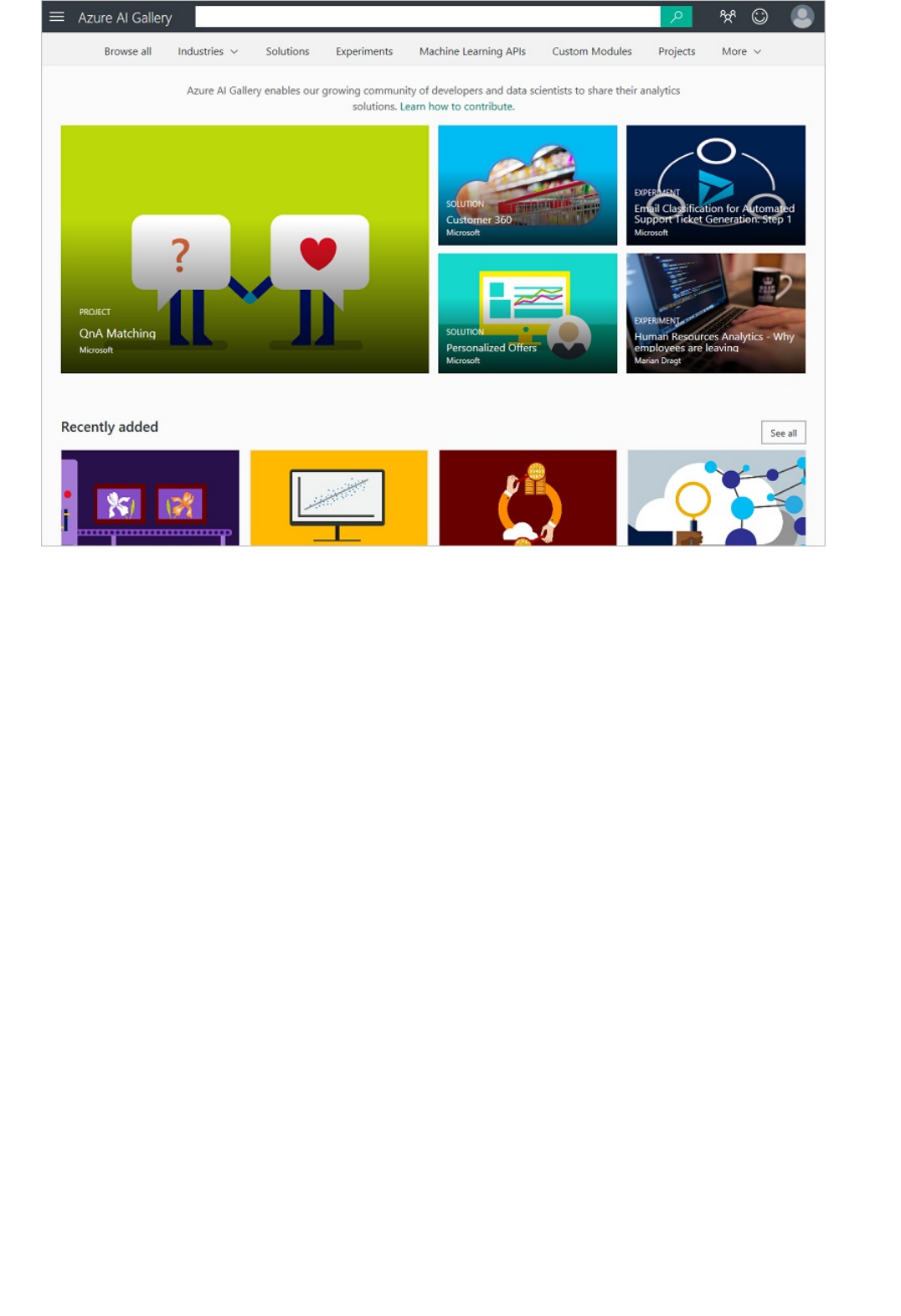
Discover and learn
Anyone can browse and search the different types of resources in the Gallery that have been contributed by
Microsoft and the advanced analytics community. Use these to learn more and get a head start on solving your
own data analysis problems. You can also download experiments and Jupyter notebooks to your own Machine
Learning Studio workspace.
You can easily find recently published and popular resources in the Gallery, or you can search by name, tags,
algorithms, and other attributes. Click Browse all in the Gallery header, and then select search refinements on the
left of the page and enter search terms at the top.
View contributions from a particular author by clicking the author name from within any of the tiles:
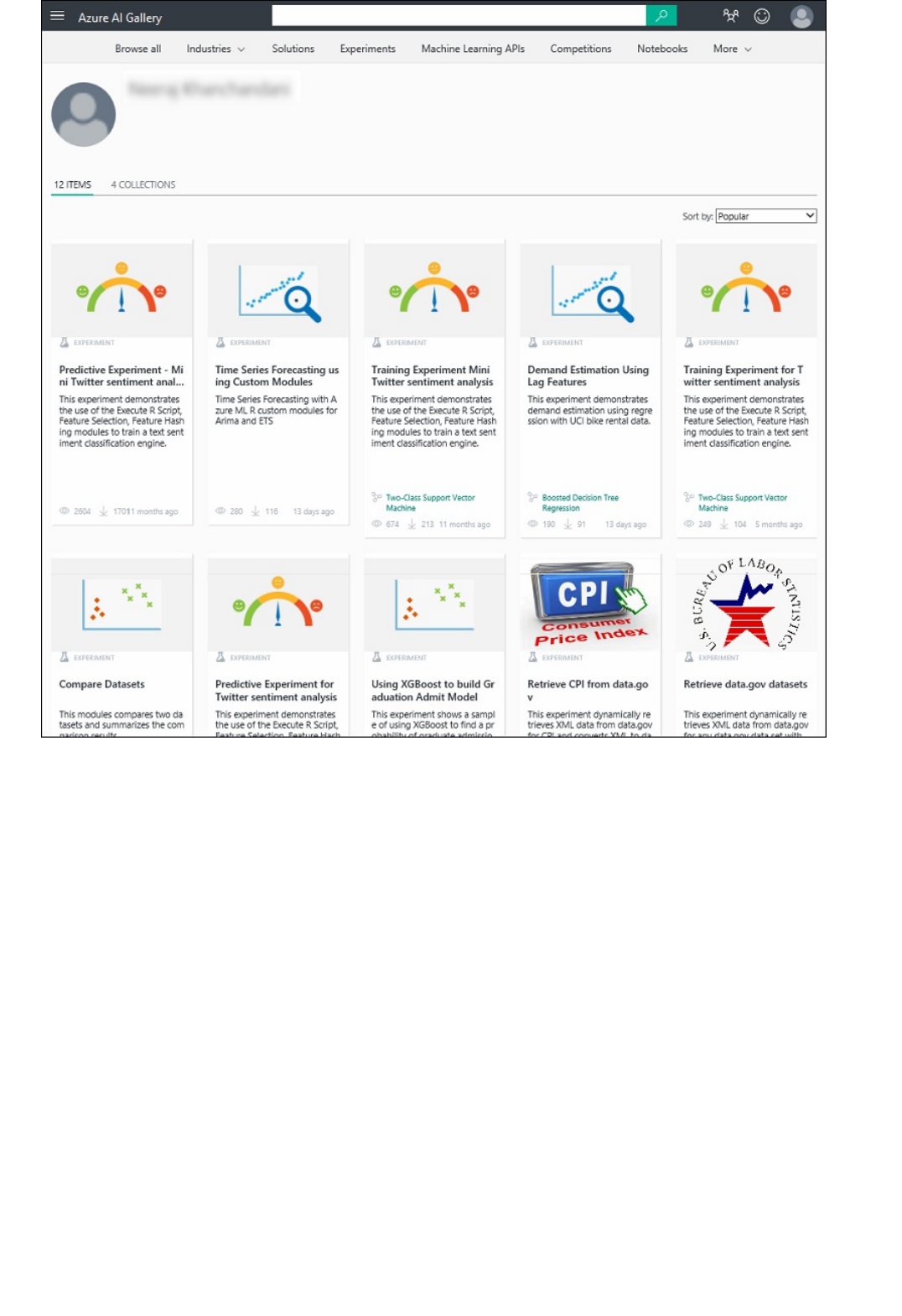
You can comment, provide feedback, or ask questions through the comments section on each resource page. You
can even share a resource of interest with friends or colleagues using the share capabilities of LinkedIn or Twitter.
You may also email links to these resources to invite other users to view the pages.
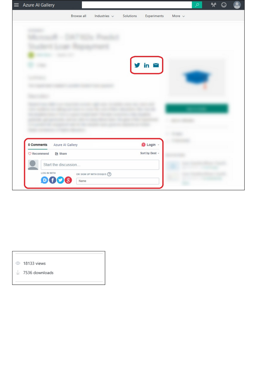
Contribute to the Gallery
When you sign in you become a member of the Gallery community. This allows you to contribute your own
Gallery items so that others can benefit from the solutions you've discovered.
As others come across your contribution in the Gallery, you can follow the number of views and downloads of
your contribution:
Users can also add comments and share your contribution with other members of the data science community.
You can log in with a discussion tool such as Disqus and receive notifications for comments on your contributions.
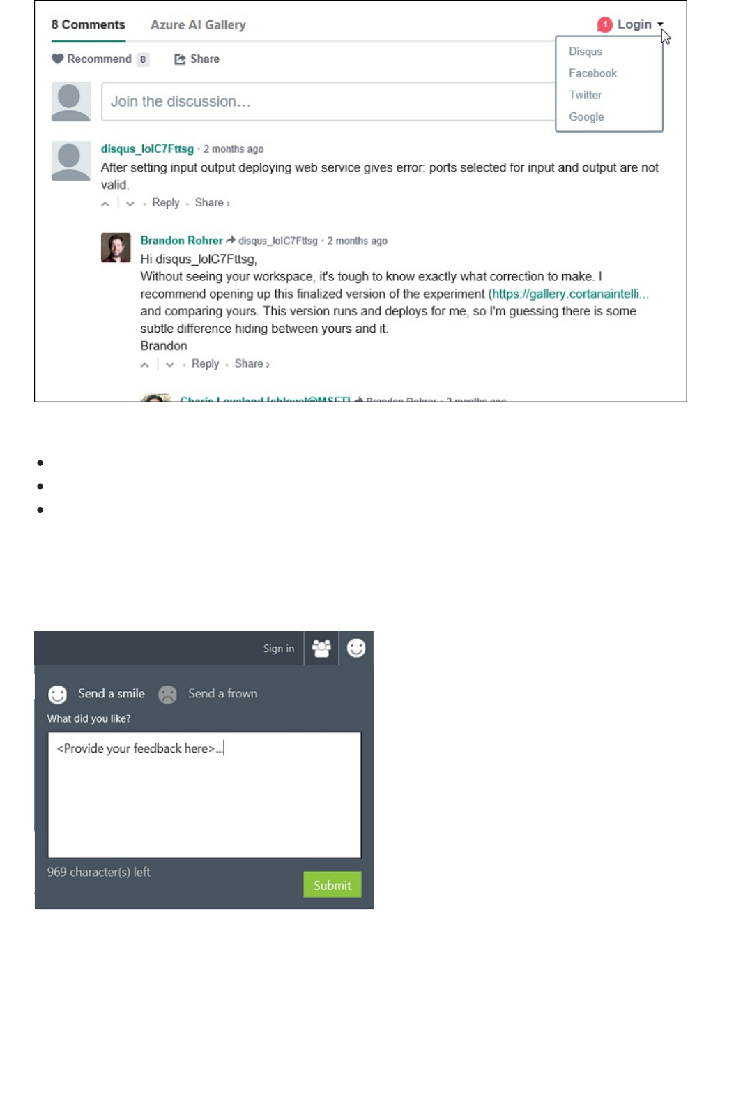
We want to hear from you!
You can contribute the following items to the Gallery - follow these links for more information:
Collections
Experiments
Tutorials
We want the Gallery to be driven by our users and for our users. Use the smiley on the right to tell us what you
love or hate about the Gallery.
TAKE ME TO THE GALLERY >>
Discover industry-specific solutions in the Azure AI
Gallery
2/2/2018 • 1 min to read • Edit Online
Industry-specific Cortana Intelligence solutions
Discover
NOTENOTE
Azure AI Gallery is a community-driven site for discovering and sharing solutions built with Cortana Intelligence
Suite. The Gallery has a variety of resources that you can use to develop your own analytics solutions.
The Industries section of the Gallery brings together various resources that are specific to such industries as
Retail - Find retail solutions such as sales forecasting, predicting customer churn, and developing pricing
models.
Manufacturing - Find manufacturing solutions such as anticipating equipment maintenance and forecasting
energy prices.
Banking - Find banking solutions such as predicting credit risk and monitoring for online fraud.
Healthcare - Find healthcare solutions such as detecting disease, and predicting hospital readmissions.
These resources include experiments, custom modules, APIs, collections, and any other Gallery items that can help
you develop solutions specific to the industry you're working in.
To browse through the industry-specific solutions in the Gallery, open the Gallery, point your mouse at Industries
at the top of the Gallery home page, select a specific industry segment, or select View All to see an overview page
for all industries.
Each industry page displays a list of the most popular Gallery items associated with that industry. Click See all to
view all the industry-specific resources in the Gallery. From this page, you can browse all the resources in the
Gallery. You also can search by selecting filter criteria on the left of the page and entering search terms at the top.
Click any Gallery item to open the item's details page for more information.
TAKE ME TO THE GALLERY >>
You can try Azure Machine Learning for free. No credit card or Azure subscription is required. Get started now.
Discover Solutions in the Azure AI Gallery
3/21/2018 • 1 min to read • Edit Online
Solutions
Discover
Deploy
Azure AI Gallery is a community-driven site for discovering and sharing solutions built with Cortana Intelligence
Suite. The Gallery has a variety of resources that you can use to develop your own analytics solutions.
A Solution in the Gallery provides a jumpstart to quickly build Cortana Intelligence Solutions from preconfigured
solutions, reference architectures, and design patterns. Make them your own with the included instructions or with
a featured partner.
To browse for solutions in the Gallery, open the Gallery and click Solutions at the top of the Gallery home page.
The Solutions page displays a list of the most recently added Solutions. Click See all to view all Solutions. From
this page, you can browse all the Solutions in the Gallery. You also can search by selecting filter criteria on the left
of the page and entering search terms at the top.
Click any Solution to open its details page and read more information. On this page you can comment, provide
feedback, or ask questions through the comments section. You can even share it with friends or colleagues using
the share capabilities of LinkedIn or Twitter. You can also email a link to the Solution to invite other users to view
the page.
If you want to use a Solution, click Deploy. Follow the steps presented to configure and deploy the Solution in
your workspace.

Discover experiments in Azure AI Gallery
3/21/2018 • 8 min to read • Edit Online
Experiments for Machine Learning Studio
NOTENOTE
Discover
Download
Azure AI Gallery is a community-driven site for discovering and sharing solutions built with Cortana Intelligence
Suite. The Gallery has a variety of resources that you can use to develop your own analytics solutions.
The Gallery has a wide variety of experiments that have been developed in Azure Machine Learning Studio.
Experiments range from quick proof-of-concept experiments that demonstrate a specific machine learning
technique, to fully developed solutions for complex machine learning problems.
An experiment is a canvas in Machine Learning Studio that you can use to construct a predictive analysis model. You create
the model by connecting data with various analytical modules. You can try different ideas, do trial runs, and eventually deploy
your model as a web service in Azure. For an example of how to create a basic experiment, see Machine learning tutorial:
Create your first experiment in Azure Machine Learning Studio. For a more comprehensive walkthrough of how to create a
predictive analytics solution, see Walkthrough: Develop a predictive analytics solution for credit risk assessment in Azure
Machine Learning.
To browse experiments in the Gallery, at the top of the Gallery home page, select Experiments.
The Experiments page displays a list of recently added and popular experiments. To see all experiments, select the
See all button. To search for a specific experiment, select See all, and then select filter criteria. You also can enter
search terms in the Search box at the top of the Gallery page.
You can get more information about an experiment on the experiment details page. To open an experiment details
page, select the experiment. On an experiment details page, in the Comments section, you can comment, provide
feedback, or ask questions about the experiment. You can even share the experiment with friends or colleagues on
Twitter or LinkedIn. You also can mail a link to the experiment details page, to invite other users to view the page.
You can download a copy of any experiment in the Gallery to your Machine Learning Studio workspace. Then, you
can modify your copy to create your own solutions.
Azure AI Gallery offers two ways to import a copy of an experiment:
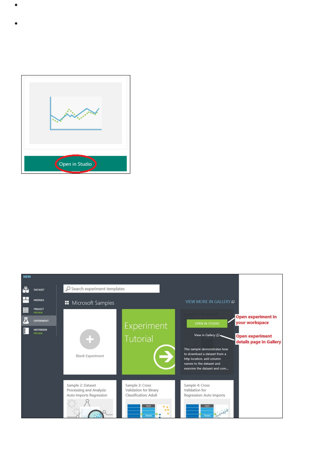
From the GalleryFrom the Gallery
From within Machine Learning StudioFrom within Machine Learning Studio
From the Gallery. If you find an experiment that you like in the Gallery, you can download a copy and then
open it in your Machine Learning Studio workspace.
From within Machine Learning Studio. In Machine Learning Studio, you can use any experiment in the
Gallery as a template to create a new experiment.
1. In the Gallery, open the experiment details page.
2. Select Open in Studio.
When you select Open in Studio, the experiment opens in your Machine Learning Studio workspace. (If you're
not already signed in to Machine Learning Studio, you are prompted to first sign in by using your Microsoft
account.)
1. In Machine Learning Studio, select NEW.
2. Select Experiment. You can choose from a list of Gallery experiments, or find a specific experiment by using
the Search box.
3. Point your mouse at an experiment, and then select Open in Studio. (To see information about the
experiment, select View in Gallery. This takes you to the experiment details page in the Gallery.)
You can customize, iterate, and deploy a downloaded experiment like any other experiment that you create in
Machine Learning Studio.
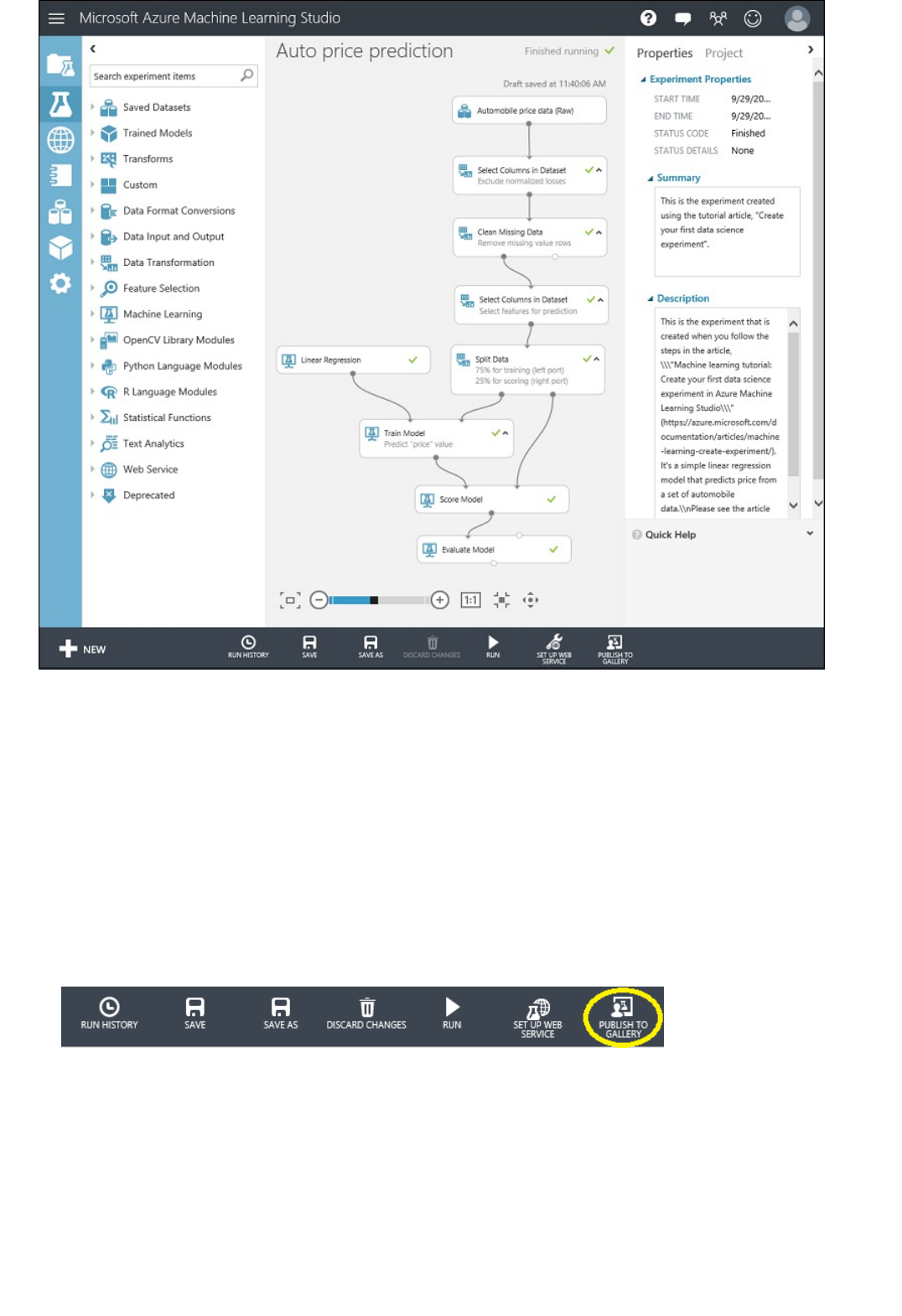
Contribute
Publish your experiment to the GalleryPublish your experiment to the Gallery
When you sign in to the Gallery, you become a member of the Gallery community. As a member of the
community, you can contribute your own experiments, so other users can benefit from the solutions that you've
discovered.
1. Sign in to Machine Learning Studio by using your Microsoft account.
2. Create your experiment, and then run it.
3. When you’re ready to publish your experiment in the Gallery, in the list of actions below the experiment
canvas, select Publish to Gallery.
4. On the Experiment Description page, enter a title and tags. Make the title and tags descriptive. Highlight
the techniques you used or the real-world problem you are solving. An example of a descriptive experiment
title is “Binary Classification: Twitter Sentiment Analysis.”
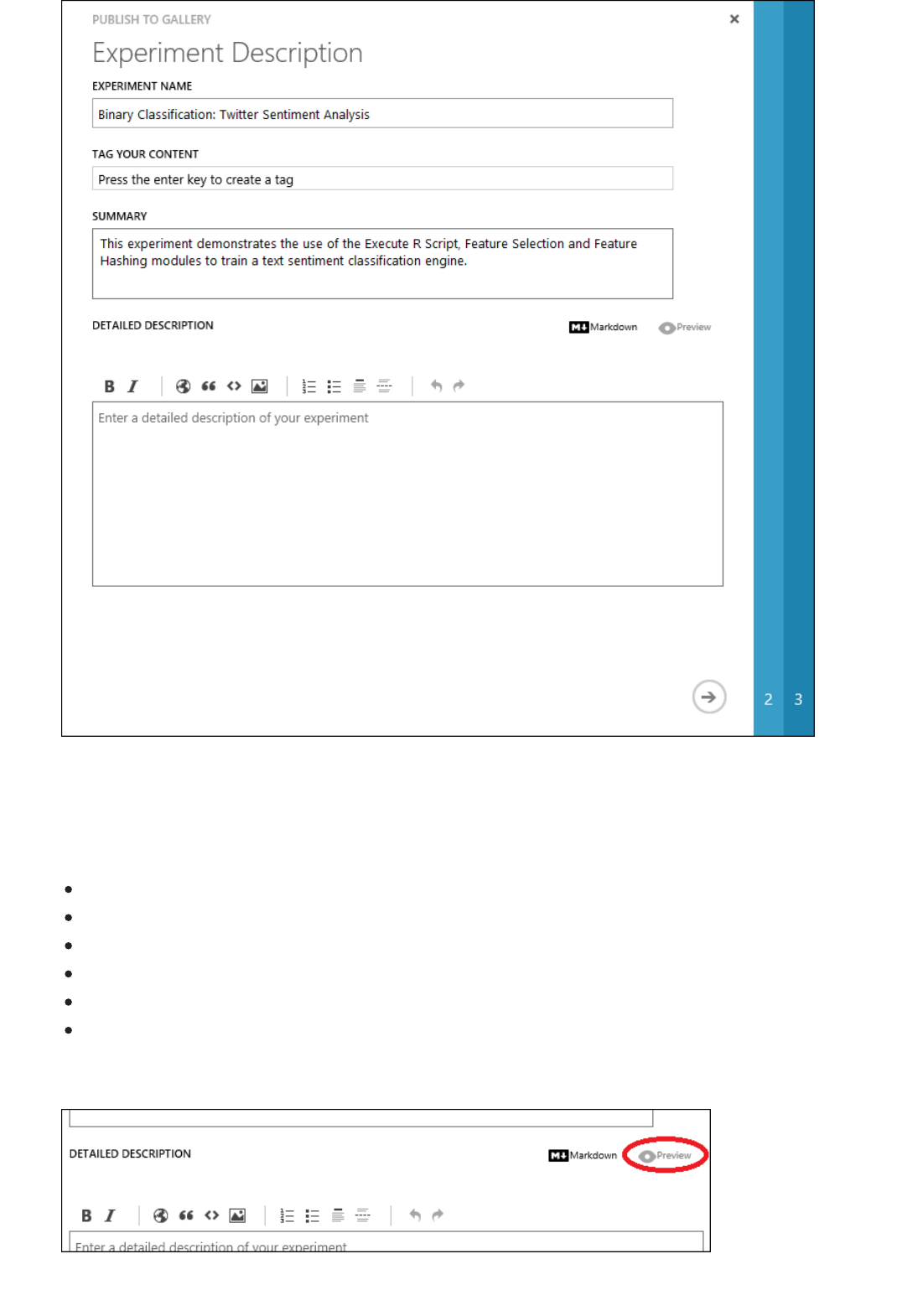
5. In the SUMMARY box, enter a summary of your experiment. Briefly describe the problem the experiment
solves, and how you approached it.
6. In the DETAILED DESCRIPTION box, describe the steps you took in each part of your experiment. Some
useful topics to include are:
Experiment graph screenshot
Data sources and explanation
Data processing
Feature engineering
Model description
Results and evaluation of model performance
You can use markdown to format your description. To see how your entries on the experiment description
page will look when the experiment is published, select Preview.
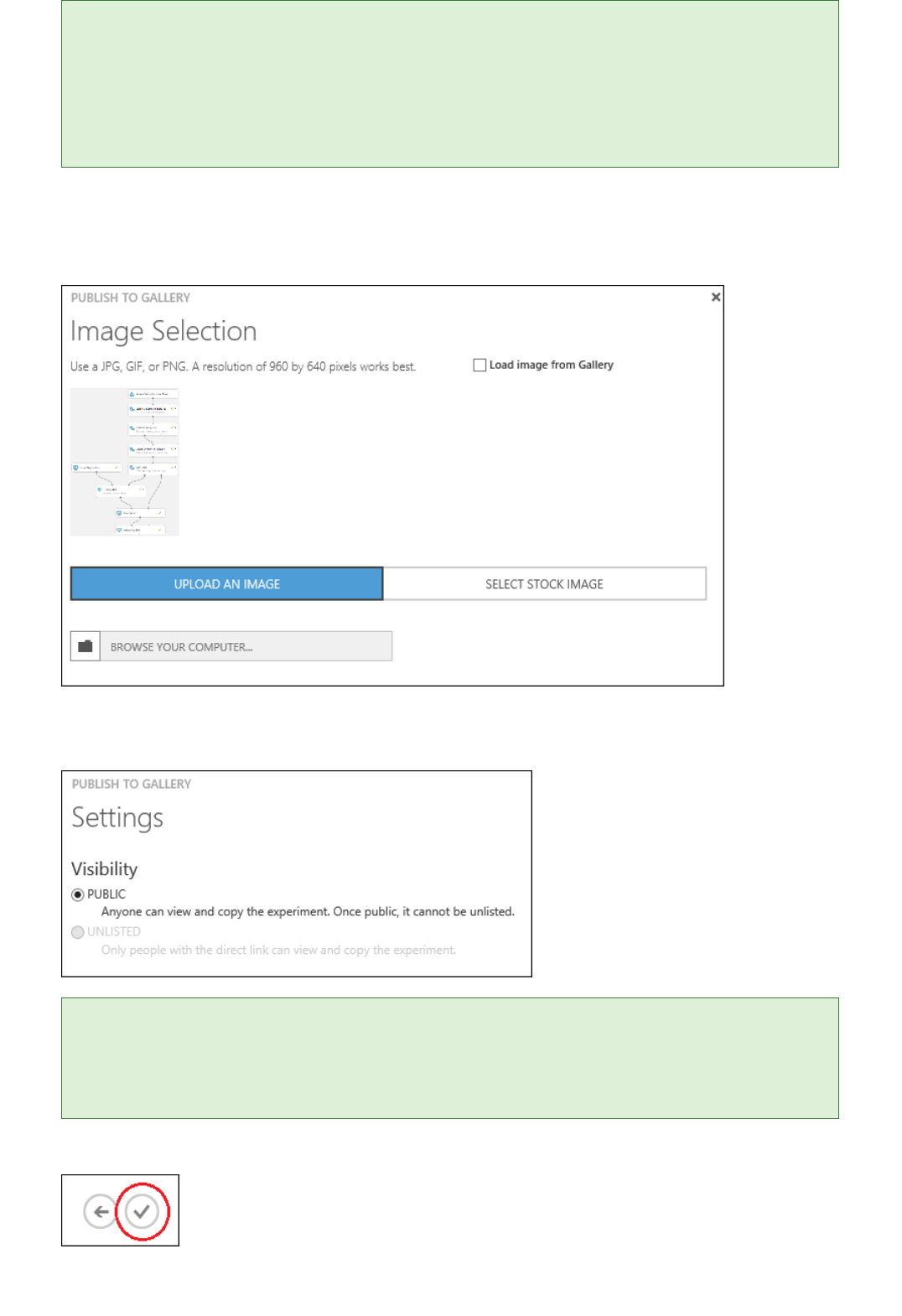
TIPTIP
TIPTIP
The text boxes provided for markdown editing and preview are small. We recommend that you write your experiment
documentation in a markdown editor, copy it, and then paste the completed documentation in the text box in the
Gallery. After you publish your experiment, you can make any corrections by using standard web-based tools that
use markdown for edit and preview.
7. On the Image Selection page, choose a thumbnail image for your experiment. The thumbnail image
appears at the top of the experiment details page and in the experiment tile. Other users will see the
thumbnail image when they browse the Gallery. You can upload an image from your computer, or select a
stock image from the Gallery.
8. On the Settings page, under Visibility, choose whether to publish your content publicly (Public) or to
have it accessible only to people who have a link to the page (Unlisted).
If you want to make sure your documentation looks correct before you release it publicly, you can first publish the
experiment as Unlisted. Later, you can change the visibility setting to Public on the experiment details page.
9. To publish the experiment to the Gallery, select the OK check mark.
For tips on how to publish a high-quality Gallery experiment, see Tips for documenting and publishing your
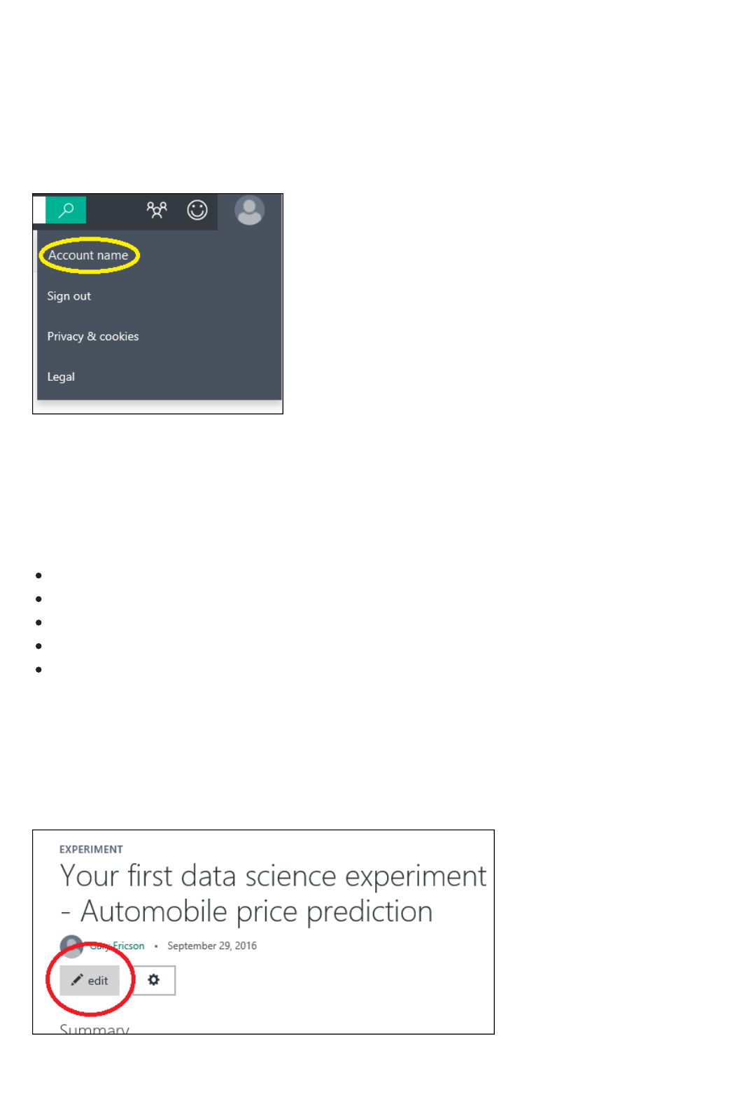
Update your experimentUpdate your experiment
From the experiment details pageFrom the experiment details page
experiment.
That’s it--you’re all done.
You can now view your experiment in the Gallery, and share the link with others. If you published your experiment
by using the Public visibility setting, the experiment shows up in browse and search results in the Gallery. You can
edit your experiment documentation on the experiment details page any time you are signed in to the Gallery.
To see the list of your contributions, select your image in the upper-right corner of any Gallery page. Then, select
your name to open your account page.
If you need to, you can make changes to the workflow (modules, parameters, and so on) in an experiment that you
published to the Gallery. In Machine Learning Studio, make any changes you'd like to make to the experiment, and
then publish again. Your published experiment will be updated with your changes.
You can change any of the following information for your experiment directly in the Gallery:
Experiment name
Summary or description
Tags
Image
Visibility setting (Public or Unlisted)
You also can delete the experiment from the Gallery.
You can make these changes, or delete the experiment, from the experiment details page or from your profile page
in the Gallery.
On the experiment details page, to change the details for your experiment, select Edit.
The details page enters edit mode. To make changes, select Edit next to the experiment name, summary, or tags.
When you're finished making changes, select Done.
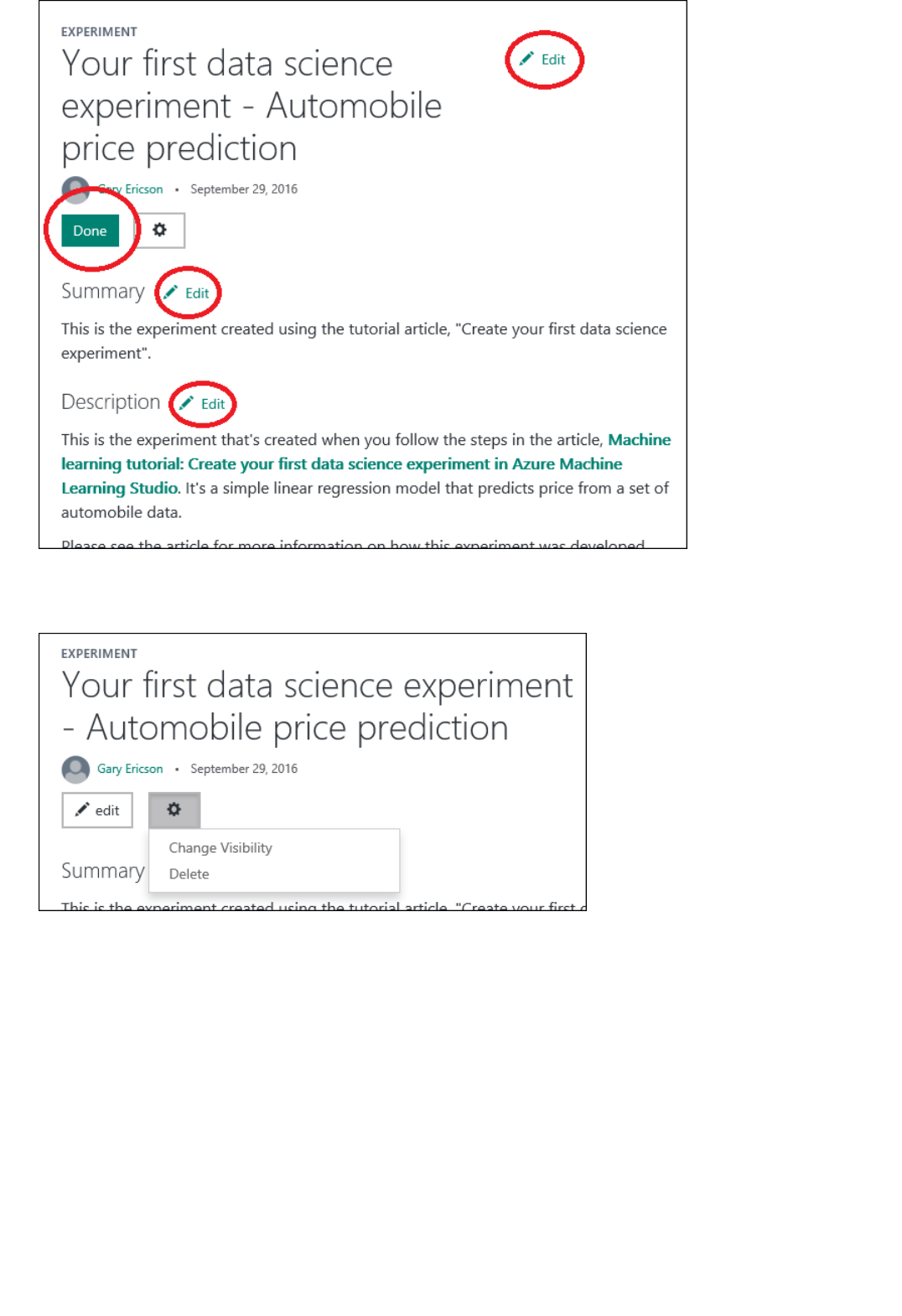
From your profile pageFrom your profile page
To change the visibility settings for the experiment (Public or Unlisted), or to delete the experiment from the
Gallery, select the Settings icon.
On your profile page, select the down arrow for the experiment, and then select Edit. This takes you to the details
page for your experiment, in edit mode. When you are finished making changes, select Done.
To delete the experiment from the Gallery, select Delete.
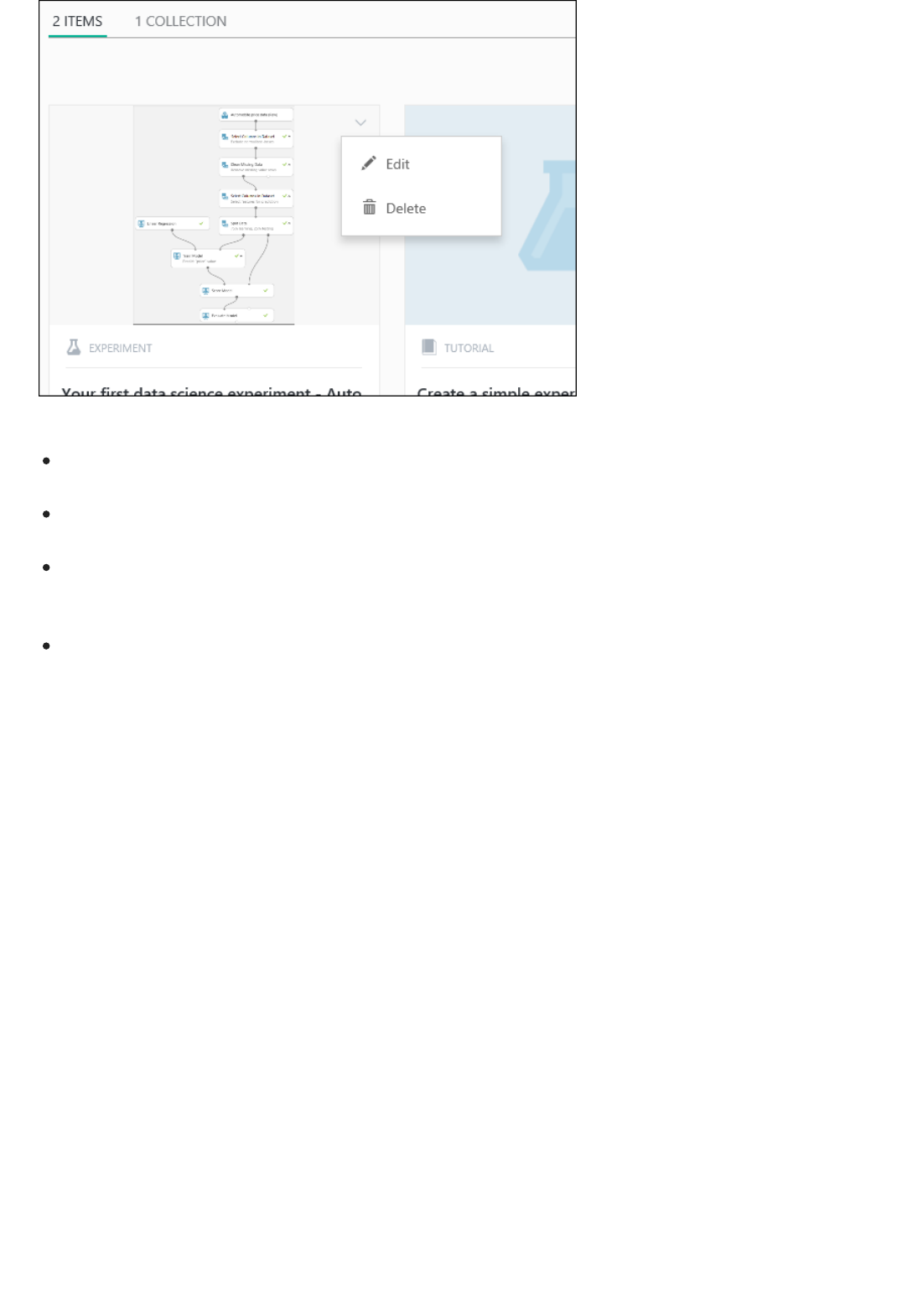
Tips for documenting and publishing your experimentTips for documenting and publishing your experiment
Frequently asked questions
You can assume that the reader has prior data science experience, but it can be helpful to use simple language.
Explain things in detail whenever possible.
Cortana Intelligence Suite is relatively new. Not all readers are familiar with how to use it. Provide enough
information and step-by-step explanations to help readers navigate your experiment.
Visuals can be helpful for readers to interpret and use your experiment documentation correctly. Visuals include
experiment graphs and screenshots of data. For more information about how to include images in your
experiment documentation, see the Publishing Guidelines and Examples collection.
If you include a data set in your experiment (that is, you're not importing the dataset through the Import Data
module), the data set is part of your experiment and is published in the Gallery. Make sure that the data set you
publish has licensing terms that allow sharing and downloading by anyone. Gallery contributions are covered
under the Azure Terms of Use.
What are the requirements for submitting or editing an image for my experiment?
Images that you submit with your experiment are used to create an experiment tile for your contribution. We
recommend that images be smaller than 500 KB, with an aspect ratio of 3:2, and a resolution of 960 × 640.
What happens to the data set I used in the experiment? Is the data set also published in the Gallery?
If your data set is part of your experiment and is not being imported through the Import Data module, the data set
is published in the Gallery as part of your experiment. Make sure that the data set that you publish with your
experiment has the appropriate licensing terms. The licensing terms should allow anyone to share and download
the data.
I have an experiment that uses an Import Data module to pull data from Azure HDInsight or SQL
Server. It uses my credentials to retrieve the data. Can I publish this kind of experiment? How can I be
assured that my credentials won't be shared?
Currently, you cannot publish an experiment that uses credentials in the Gallery.
How do I enter multiple tags?
After you enter a tag, to enter another tag, press the Tab key.
Go to the Gallery
Discover Jupyter Notebooks in the Azure AI Gallery
3/21/2018 • 2 min to read • Edit Online
Jupyter Notebooks
Discover
Download
Download from the GalleryDownload from the Gallery
Azure AI Gallery is a community-driven site for discovering and sharing solutions built with Cortana Intelligence
Suite. The Gallery has a variety of resources that you can use to develop your own analytics solutions.
Jupyter Notebooks include code, data visualizations, and documentation in a single, interactive canvas.
Notebooks in the Gallery provide tutorials and detailed explanations of advanced machine learning techniques and
solutions.
To browse for notebooks in the Gallery, open the Gallery and click Notebooks at the top of the Gallery home
page.
The Jupyter Notebooks page displays a list of the most popular notebooks. Click See all to view all notebooks.
From this page, you can browse all the notebooks in the Gallery. You also can search by selecting filter criteria on
the left of the page and entering search terms at the top.
Click any notebook to open the notebook's details page and read more information. On this page you can
comment, provide feedback, or ask questions through the comments section. You can even share it with friends or
colleagues using the share capabilities of LinkedIn or Twitter. You can also email a link to the notebook to invite
other users to view the page.
You can download a copy of any notebook from the Gallery into your Machine Learning Studio workspace.
To download a copy of a notebook from the Gallery:
1. Open the notebook's details page in the Gallery
2. Click Open in Studio
3. Select the Region and Workspace you want to use
Download in Machine Learning StudioDownload in Machine Learning Studio
NOTENOTE
When you click Open in Studio, the notebook is loaded into your Machine Learning Studio workspace and
opened (if you're not already signed in to Studio, you will be prompted to sign in using your Microsoft account
before the notebook is copied to your workspace). You can find the notebook again later by clicking Notebooks
on the left side of the Studio home page.
You can also open any of the same Gallery notebooks while you're working in Machine Learning Studio:
1. In Machine Learning Studio, click +NEW
2. Select Notebook - a list of notebooks from the Gallery is displayed that you can choose from, or you can find a
specific notebook using the search box
3. Point your mouse at a notebook and select Open Notebook
A copy of the notebook is downloaded and opened in your workspace in the Jupyter Notebooks section of
Machine Learning Studio. The notebook will be listed, along with your other notebooks, on the Notebooks page
of Studio (on the Studio home page, click Notebooks on the left).
TAKE ME TO THE GALLERY >>
You can try Azure Machine Learning for free. No credit card or Azure subscription is required. Get started now.
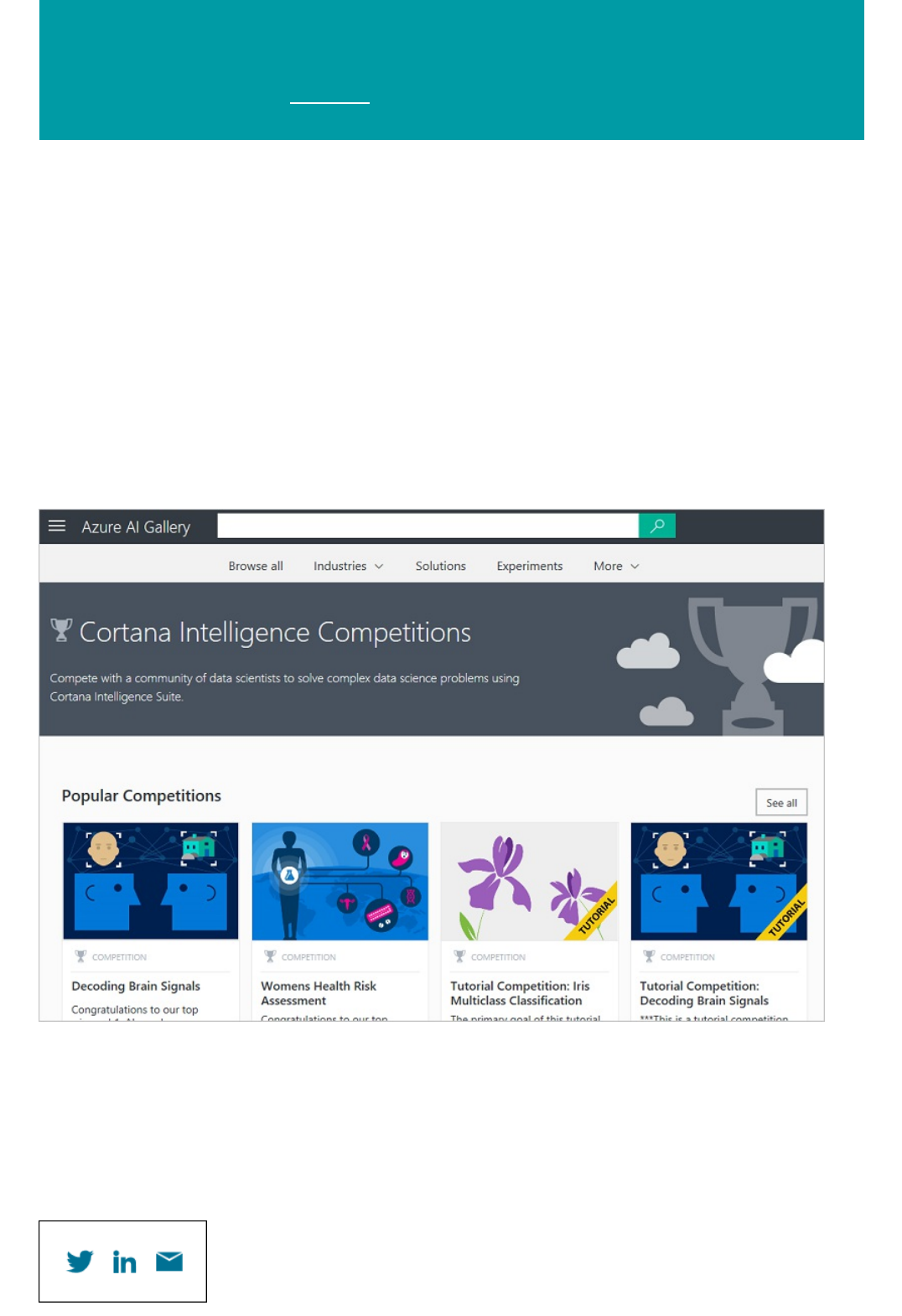
Discover competitions in the Azure AI Gallery
3/20/2018 • 1 min to read • Edit Online
Cortana Intelligence Competitions
Discover
Azure AI Gallery is a community-driven site for discovering and sharing solutions built with Cortana Intelligence
Suite. The Gallery has a variety of resources that you can use to develop your own analytics solutions.
Competitions provide an exciting opportunity to compete with the community of data scientists to solve complex
problems using Cortana Intelligence Suite.
For answers to frequently-asked questions about Competitions, see Microsoft Cortana Intelligence Competitions
FAQ.
The Competitions page (aka.ms/CIComp) displays a list of the most popular competitions.
Click See all to view all competitions. From this page, you can browse all the competitions in the Gallery. You also
can search by selecting filter criteria on the left of the page and entering search terms at the top.
Click any competition to open the competition's details page and read more information. On this page you can
comment, provide feedback, or ask questions through the comments section. You can even share it with friends or
colleagues using the share capabilities of LinkedIn or Twitter. You can also email a link to the competition to invite
other users to view the page.
Enter a competition
NOTENOTE
If the competition is open, the status on the details page is Active. To enter the competition, click Enter
Competition and you will be given instructions on the resources you need and the steps you need to take.
If the competition has been completed, then a list of winners is shown.
TAKE ME TO THE GALLERY >>
You can try Azure Machine Learning for free. No credit card or Azure subscription is required. Get started now.

Microsoft Cortana Intelligence Competitions FAQ
3/21/2018 • 7 min to read • Edit Online
What is Cortana Intelligence Competitions?
The Microsoft Cortana Intelligence Competitions unites a global community of data enthusiasts by collectively
solving some of the world’s most complex data science problems. Cortana Intelligence Competitions allow data
enthusiasts from across the world to compete and build highly accurate and intelligent data science models. These
hosted competitions are based on unique data sets that have been made available publically for the first time.
Participants can win rewards or get recognition via the top 10 public leaderboard. You can access the Competitions
home page at aka.ms/CIComp.
How often will Microsoft release new competitions?
We will be launching 1st-party, Microsoft-owned competitions on a regular basis, approximately every 8-12 weeks.
Where can I ask general questions about data science?
For general questions, you can use the Microsoft Azure Machine Learning forum.
How do I enter a competition?
Access the Competitions home page in the Azure AI Gallery, or go to http://aka.ms/CIComp. The home page lists
all competitions that are currently running. Each competition has detailed instructions and participation rules,
prizes, and duration on its sign-up page.
1. Find the competition you’d like to participate in, read all the instructions and watch the tutorial video. Then
click the Enter Competition button and copy the Starter Experiment into your existing Azure Machine
Learning workspace. If you don’t already have access to a workspace, you must create one beforehand. Run
the Starter Experiment, observe the performance metric, then use your creativity to improve the
performance of the model. You'll likely spend the majority of your time in this step.
2. Create a Predictive Experiment with the trained model out of your Starter Experiment. Then carefully adjust
the input and output schema of the web service to ensure they conform to the requirements specified in the
competition documentation. The tutorial document generally has detailed instructions for this. You can also
watch the tutorial video, if available.
3. Deploy a web service out of your Predictive Experiment. Test your web service using the Test button or the
Excel template automatically created for you to ensure it's working properly.
4. Submit your web service as the competition entry and see your public score in the Azure AI Gallery
competition page. And celebrate if you make it onto the leaderboard!
After you successfully submit an entry, you can go back to your copied Starter Experiment. Then iterate and update
your Predictive Experiment, update the web service, and submit a new entry.
Can I use open-source tools for participating in these competitions?
The competition participants use Azure Machine Learning Studio, a cloud-based service within Cortana
Intelligence Suite, for development of the data science models and to create competition entries for submission.
Machine Learning Studio not only provides a GUI interface for constructing machine learning experiments, it also
allows you to bring your own R and/or Python scripts for native execution. The R and Python runtimes in Studio
come with a rich set of open-source R/Python packages. You can import your own packages as part of the
experiment as well. Studio also has a built-in Jupyter Notebook service for you to do free style data exploration. Of
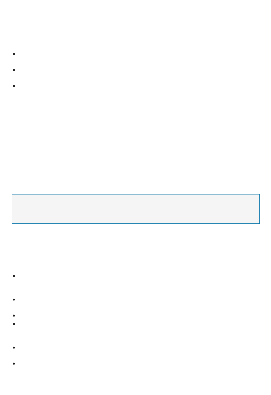
NOTENOTE
course, you can always download the datasets used in the competition and explore it in your favorite tool outside
of Machine Learning Studio.
Do I need to be a data scientist to enter?
No. In fact, we encourage data enthusiasts, anyone curious about data science, and other aspiring data scientists to
enter our contest. We have designed supporting documents to allow everyone to compete. The target audience is:
Data Developers, Data Scientists, BI and Analytics Professionals: those who are responsible for producing
data and analytics content for others to consume
Data Stewards: those who have the knowledge about the data, what it means, and how it's intended to be used
and for which purpose
Students & Researchers: those who are learning and gaining data-related skills via academic programs in
universities, or participants in Massive Open Online Courses (MOOCs)
Can I enter with my colleagues as a team?
The competition platform currently doesn't support team participation. Each competition entry is tied to a single
user identity.
Do I need to pay to participate in a competition?
Competitions are free to participate in. You do, however, need access to an Azure Machine Learning workspace to
participate. You can create a Free workspace without a credit card by simply logging in with a valid Microsoft
account, or an Office 365 account. If you're already an Azure or Cortana Intelligence Suite customer, you can create
and use a Standard workspace under the same Azure subscription. If you'd like to purchase an Azure subscription,
go to the Azure pricing page. Note that the standard rates will apply when using a Standard workspace to
construct experiments. For more information, see Azure Machine Learning pricing information.
You can try Azure Machine Learning for free. No credit card or Azure subscription is required. Get started now.
What are public and private scores?
In most competitions, you'll notice that you'll receive a public score for every submission you make, generally
within 10-20 minutes. But after the competition ends, you'll receive a private score which is used for final ranking.
Here's what happens:
The entire dataset used in the competition is randomly split with stratification into training and testing (the
remaining) data. The random split is stratified to ensure that the distributions of labels in both training and
testing data are consistent.
The training data is uploaded and given to you as part of the Starter Experiment in the Import Data module
configuration.
The testing data is further split into public and private testing data, using the same stratification.
The public testing data is used for the initial round of scoring. The result is referred to as the public score. It's
what you see in your submission history when you submit your entry. This score is calculated for every entry
you submit. This public score is used to rank you on the public leaderboard.
The private testing data is used for the final round of scoring after the competition ends. This is referred to as
private score.
For each participant, a fixed number of entries with the highest public scores are automatically selected to enter
the private scoring round (this number can vary depending on the competition). The entry with the highest
private score is then selected to enter the final ranking, which ultimately determines the prize winners.
Can customers host a competition on our platform?

We welcome 3rd-party organizations to partner with us and host both public and private competitions on our
platform. We have a competition onboarding team who will be happy to discuss the onboarding process for such
competitions. Please get in touch with us at compsupport@microsoft.com for more details.
What are the limitations for submissions?
A typical competition may choose to limit the number of entries you can submit within a 24-hour span (UTC time
00:00:00 to 23:59:59), and the total number of entries you can submit over the duration of the competition. You'll
receive appropriate error messages when a limitation is exceeded.
What happens if I win a competition?
Microsoft will verify the results of the private leaderboard, and then we'll contact you. Please make sure that your
email address in your user profile is up-to-date.
How will I get the prize money if I win a competition?
If you are a competition winner, you will need to sign a declaration of eligibility, license, and release from. This form
reiterates the Competition Rules. Winners need to fill out a US Tax form W-9, or a Form W-8BEN if they are not
US taxpayers. We will contact all winners as part of the rewards disbursement process by using their registration
email. Please refer to our Terms and Conditions for additional details.
What if more than one entry receives the same score?
The submission time is the tie-breaker. The entry submitted earlier outranks the entry submitted later.
Can I participate using guest workspace?
No. You must use a Free or a Standard workspace to participate. You can open the competition starter experiment
in a Guest workspace, but you'll not be able to create a valid entry for submission from that workspace.
Can I participate using a workspace in any Azure region?
Currently, the competition platform only supports entries submitted from a workspace in the South Central US
Azure region. All Free workspaces reside in South Central US, so you can submit an entry from any Free
workspace. If you choose to use a Standard workspace, just ensure that it resides in the South Central US Azure
region, otherwise your submission won't succeed.
Do we keep users’ competitions solutions and entries?
User entries are only retained for evaluation purposes to identify the winning solutions. Please refer to our Terms
and Conditions for specifics.

Discover and share tutorials in Azure AI Gallery
3/21/2018 • 2 min to read • Edit Online
Tutorials
Discover
Contribute
Azure AI Gallery is a community-driven site for discovering and sharing solutions built with Cortana Intelligence
Suite. The Gallery has a variety of resources that you can use to develop your own analytics solutions.
Azure AI Gallery offers several tutorials that can walk you through machine learning technologies and concepts.
Tutorials also might describe advanced methods for solving machine learning problems.
To browse tutorials in the Gallery, under More, select Tutorials.
The Tutorials page displays a list of recently added and popular tutorials. To see all tutorials, select the See all
button. To search for a specific tutorial, select See all, and then select filter criteria. You also can enter search terms
in the Search box at the top of the Gallery page.
You can get more information about a tutorial on the tutorial details page. To open a tutorial details page, select the
tutorial. In the Comments section on a tutorial details page, you can comment, provide feedback, or ask questions
about the tutorial. You can even share the tutorial with friends or colleagues on Twitter or LinkedIn. You also can
email a link to the tutorial details page, to invite other users to view the page.
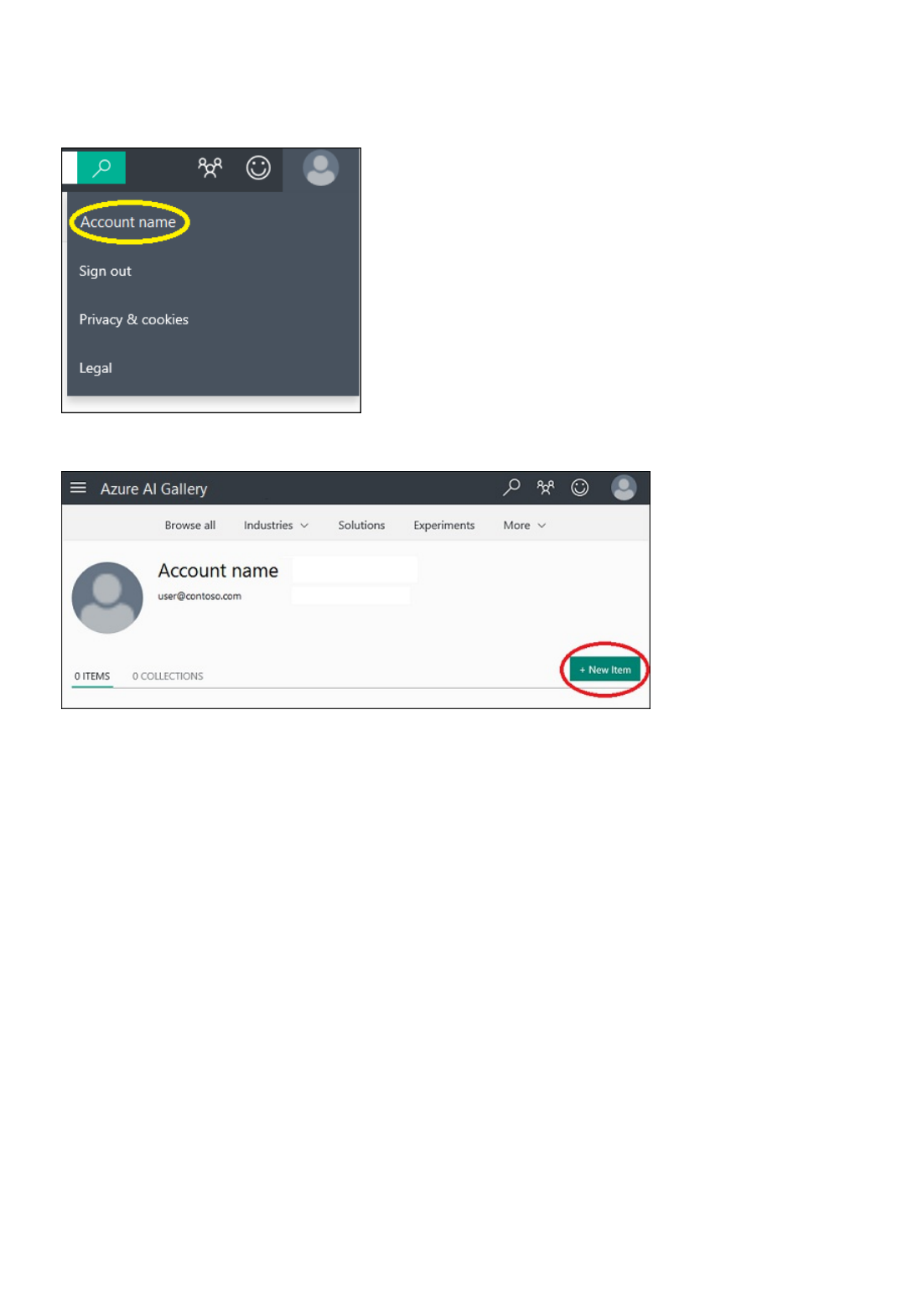
Create a tutorialCreate a tutorial
You can add a tutorial to the Gallery to help other users solve a problem or learn a concept.
1. Sign in to the Gallery by using your Microsoft account.
2. Select your image at the top of the page, and then select your name.
3. Select New Item.
4. On the Description page, for ITEM TYPE, select Tutorial. Enter a name for your tutorial, a brief summary,
a detailed description, and any tags that might help other users find your tutorial.
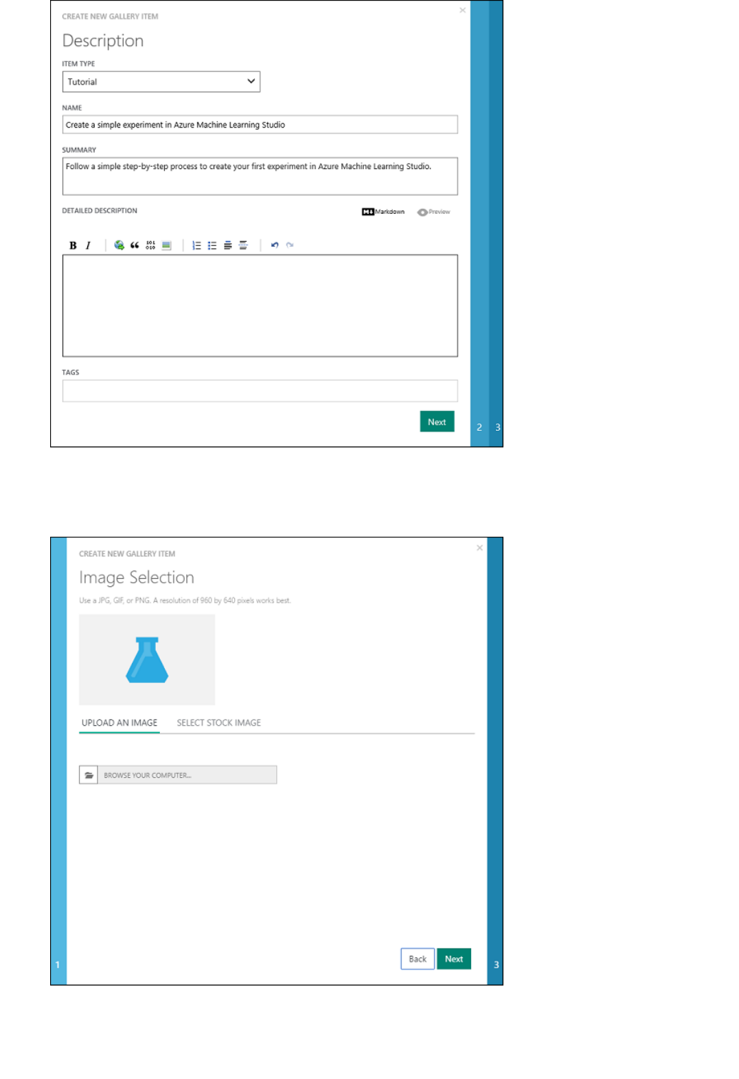
5. On the Image Selection page, select an image that is displayed with the collection. You can upload your
own image file, or select a stock image. Choose an image that might help users identify the content and
purpose of your tutorial.
6. On the Settings page, for Visibility, select whether the collection is Public (anyone can view the tutorial)
or Unlisted (only people with a direct link to the tutorial can view it).
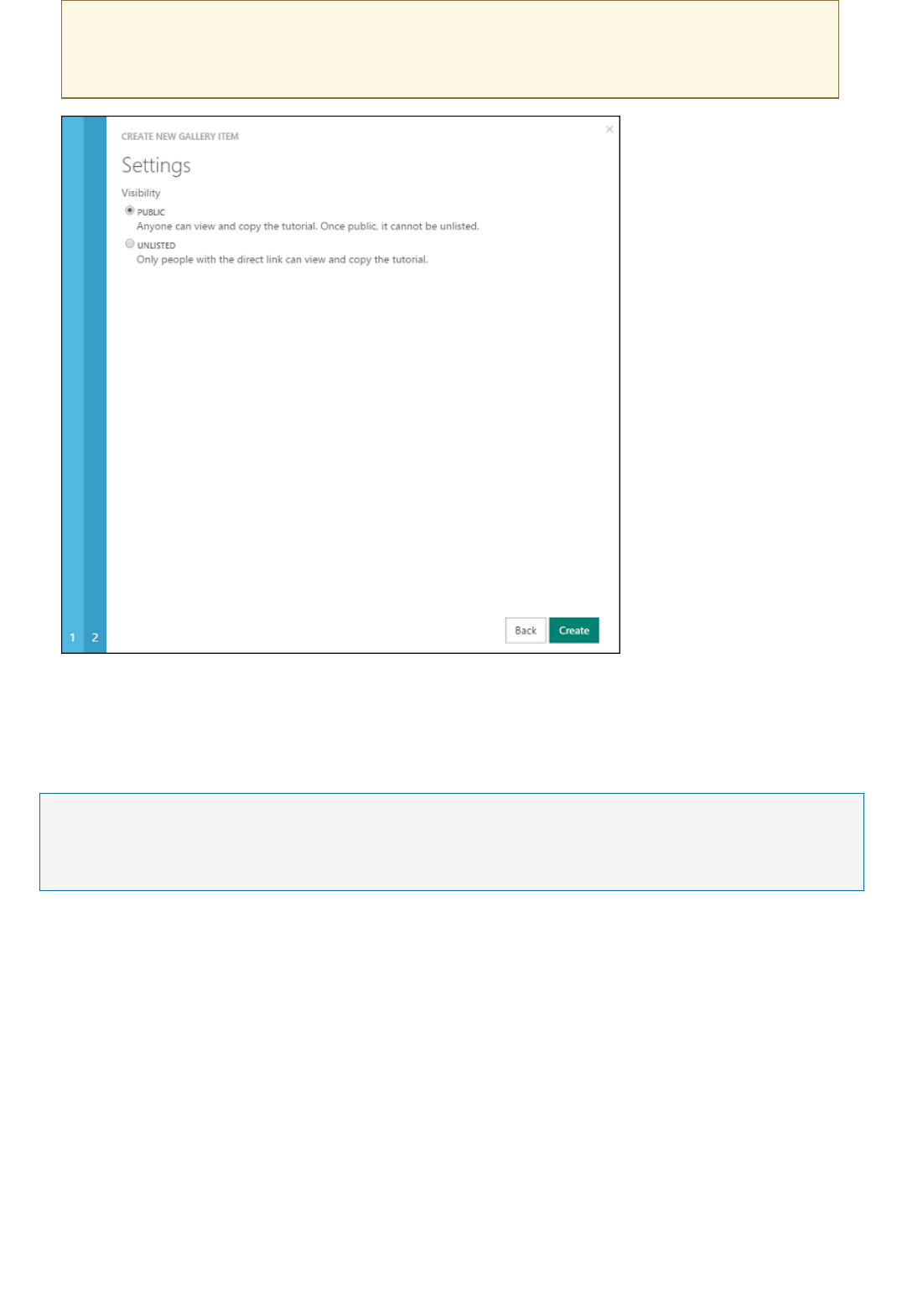
NOTENOTE
IMPORTANTIMPORTANT
After you set a tutorial to Public and then select Create, you cannot later change the tutorial to Unlisted.
7. Select Create.
Your tutorial is now in Azure AI Gallery. Your tutorials are listed on your account page, on the Items tab.
Go to the Gallery
You can try Azure Machine Learning for free. No credit card or Azure subscription is required. Get started now.
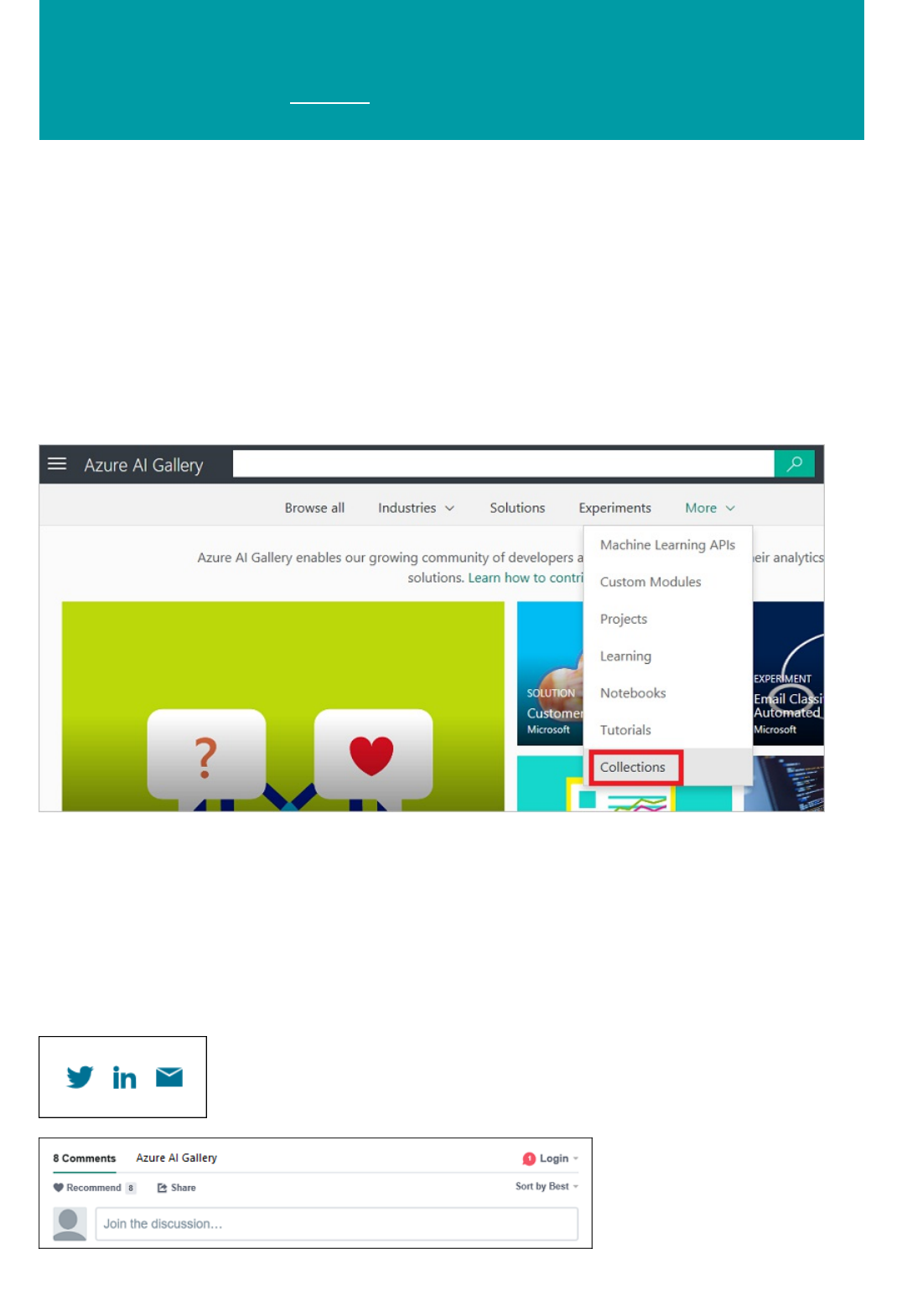
Discover and share collections in Azure AI Gallery
3/20/2018 • 3 min to read • Edit Online
Collections
Discover
Contribute
Azure AI Gallery is a community-driven site for discovering and sharing solutions built with Cortana Intelligence
Suite. The Gallery has a variety of resources that you can use to develop your own analytics solutions.
You can use a collection to group experiments, APIs, and other Gallery items that you use for a specific solution or
concept. You can group them to use, to save for later reference, or to share.
To browse collections in the Gallery, under More, select Collections.
The Collections page displays a list of recently added and popular collections. To view all collections, select See
all. To search for a specific collection, select See all, and then select filter criteria. You also can enter search terms in
the Search box at the top of the Gallery page.
You can get more information about a collection on the collection details page. To open a collection details page,
select the collection. On a collection details page, in the Comments section, you can comment, provide feedback,
or ask questions about the collection. You can even share the collection with friends or colleagues on Twitter or
LinkedIn. You also can email a link to the collection details page, to invite other users to view the page.
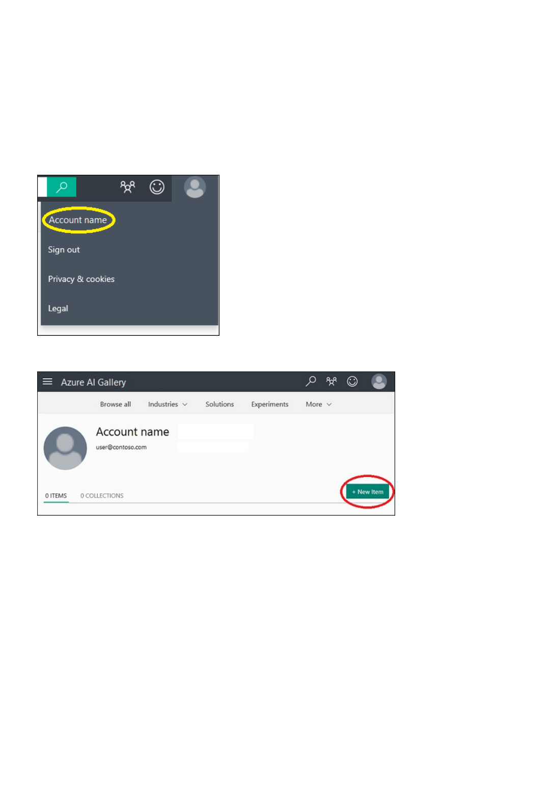
Create a collectionCreate a collection
You can create a collection that has items that you own or items that have been contributed by the community. An
item in a collection can be any Gallery item that addresses a specific solution or concept.
For example, you can use a collection to group items on a specific topic, or you can group a multi-step experiment
that solves a complex problem. The initial collections contributed by Microsoft consist of multi-step machine
learning experiment templates. You can use the templates to help solve real-world problems, such as online fraud
detection, text classification, retail forecasting, or predictive maintenance.
1. Sign in to the Gallery by using your Microsoft account.
2. Select your image at the top of the page, and then select your name.
3. Select New Item.
4. On the Description page, for ITEM TYPE, select Collection. Enter a name for your collection, a brief
summary, a detailed description, and any tags that might help other users find your collection.
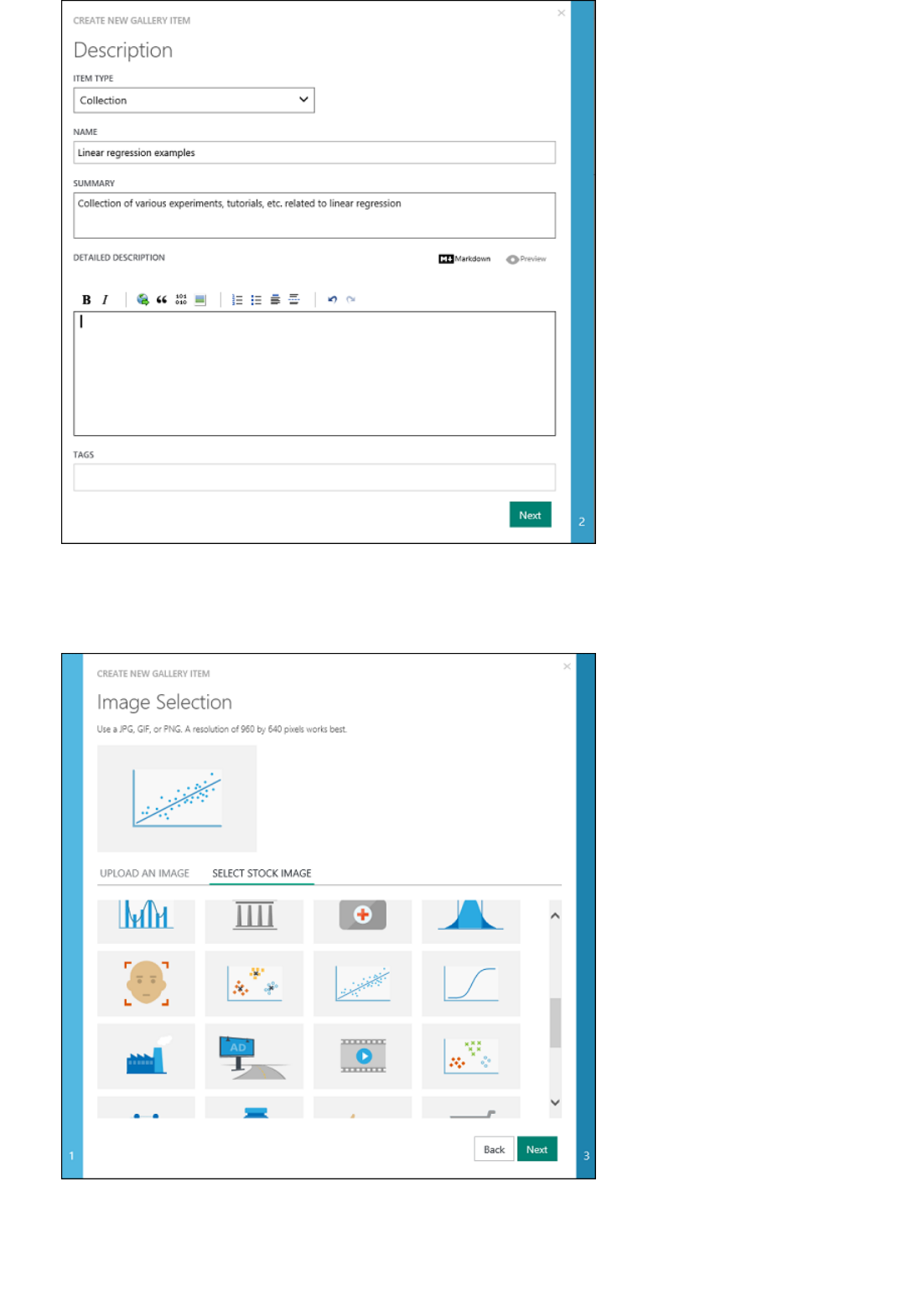
5. On the Image Selection page, select an image that is displayed with the collection. You can upload your
own image file, or select a stock image. Choose an image that might help users identify the content and
purpose of the collection.
6. On the Settings page, for Visibility, select whether the collection is Public (anyone can view the
collection) or Unlisted (only people with a direct link to the collection can view it).
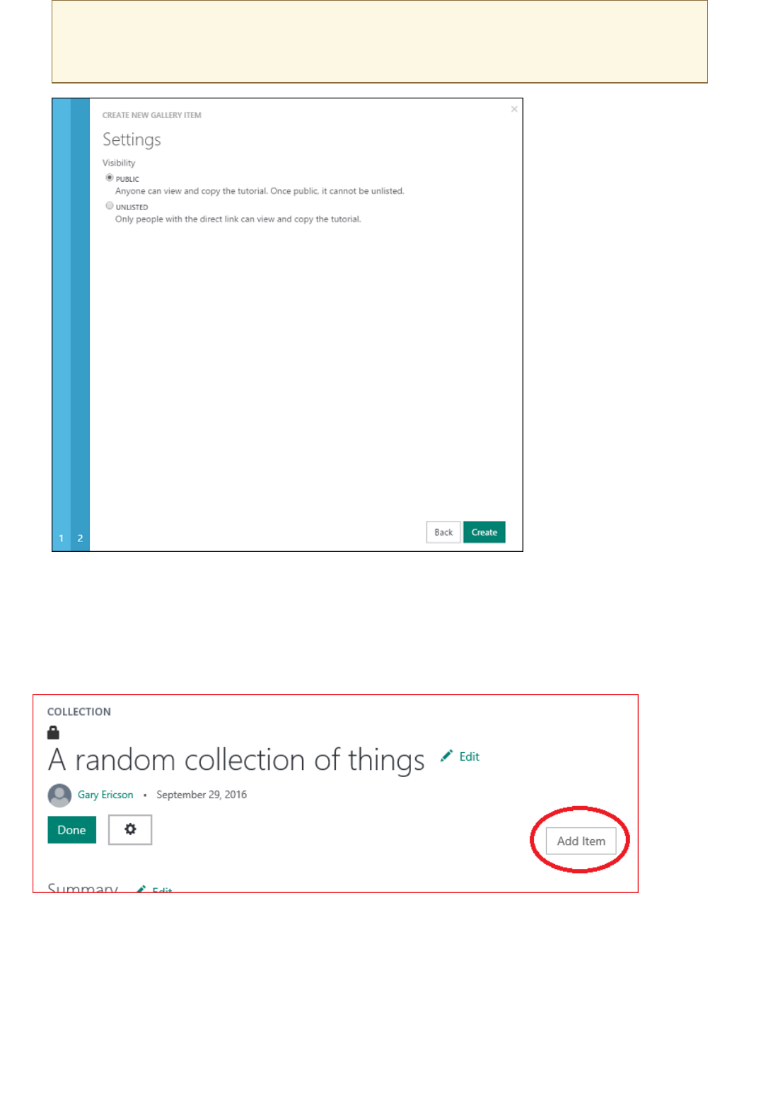
Add items to a collectionAdd items to a collection
IMPORTANTIMPORTANT
7. Select Create.
After you set a collection to Public and then select Create, you cannot later change the collection to Unlisted.
Your collection is now in Azure AI Gallery. Your collections are listed on your account page, on the Collection tab.
To add items to your collection, open the collection, select Edit, and then select Add Item.
A list of items you've contributed to the Gallery is shown on your account page. You also can search the Gallery for
items to add. Select the items that you want to add. Every item that you select is included in the set of items to add.
The Add button indicates how many items you have selected.
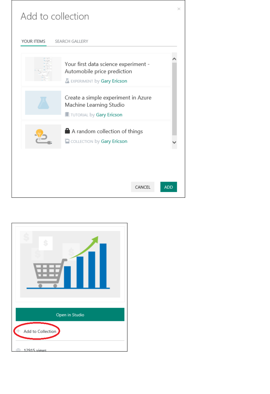
If you find an item that you want to add while you are browsing the Gallery, to open the item, select Add to
collection. Select the collection that you want to add the item to.
To change the summary, description, or tags for your collection, open the collection, and then select Edit.
While you are editing your collection, you can change the order of the items in the collection. Use the arrow
buttons next to an item to move it up or down in the order list.
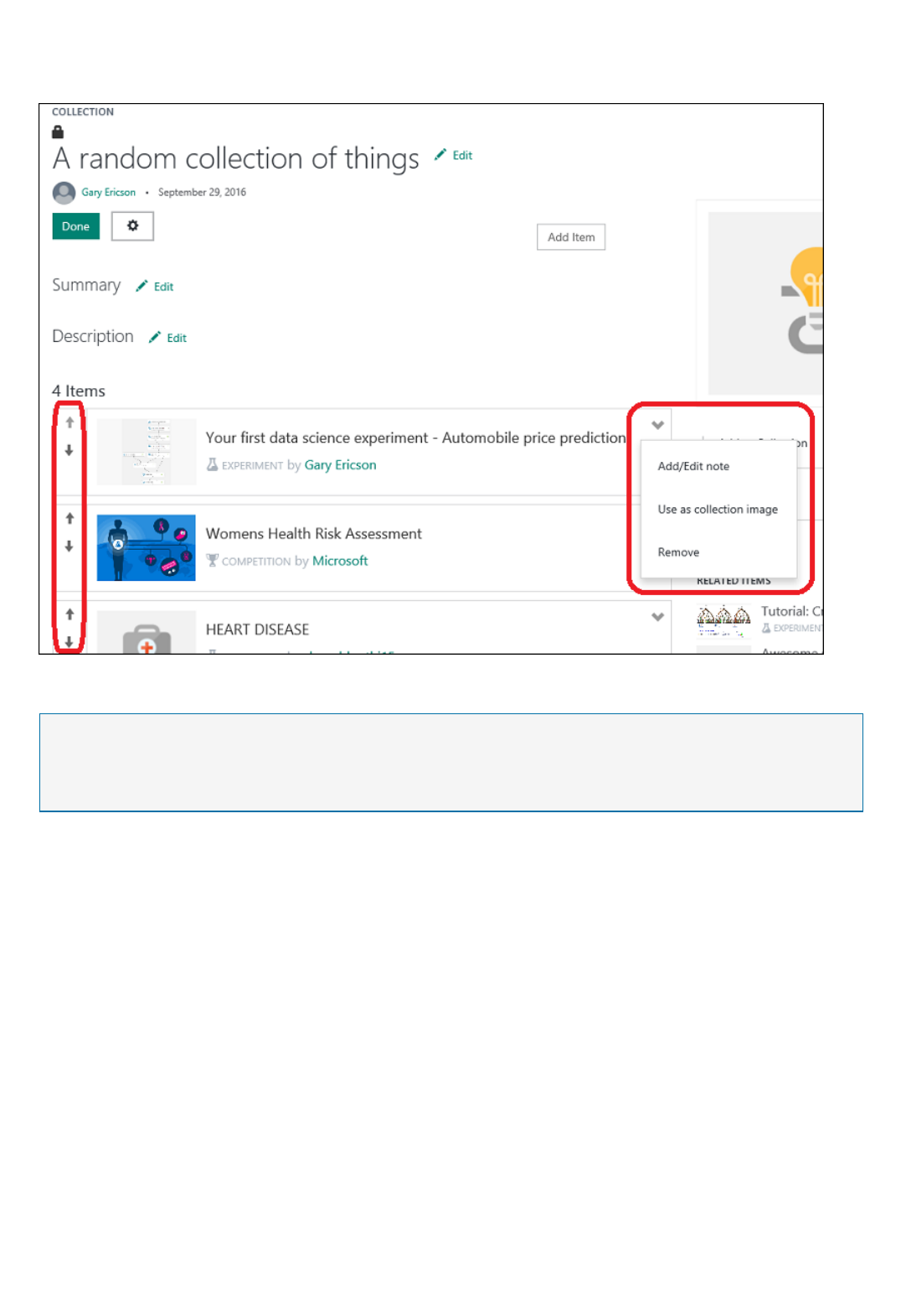
NOTENOTE
To add notes to the items in your collection, select the upper-right corner of an item, and then select Add/Edit
note.
To remove an item from your collection, select Remove.
Go to the Gallery
You can try Azure Machine Learning for free. No credit card or Azure subscription is required. Get started now.
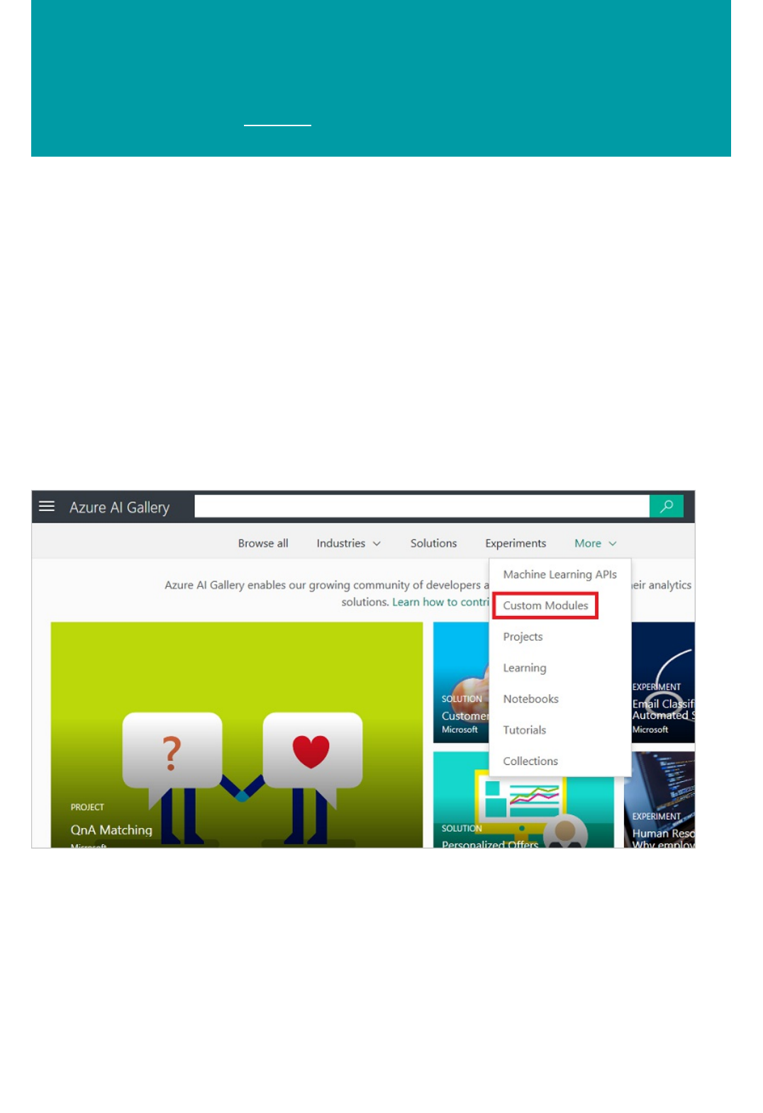
Discover custom machine learning modules in Azure
AI Gallery
3/20/2018 • 3 min to read • Edit Online
Custom modules for Machine Learning Studio
Discover
Azure AI Gallery is a community-driven site for discovering and sharing solutions built with Cortana Intelligence
Suite. The Gallery has a variety of resources that you can use to develop your own analytics solutions.
Azure AI Gallery offers several custom modules that expand the capabilities of Azure Machine Learning Studio.
You can import the modules to use in your experiments, so you can develop even more advanced predictive
analytics solutions.
Currently, the Gallery offers modules on time series analytics, association rules, clustering algorithms (beyond k-
means), and visualizations, and other workhorse utility modules.
To browse custom modules in the Gallery, under More, select Custom Modules.
The Custom Modules page displays a list of recently added and popular modules. To view all custom modules,
select the See all button. To search for a specific custom module, select See all, and then select filter criteria. You
also can enter search terms in the Search box at the top of the Gallery page.
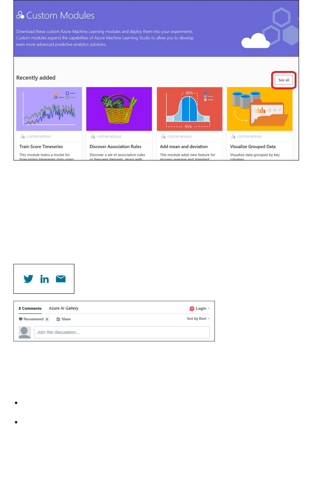
UnderstandUnderstand
Comment and shareComment and share
Import
From the GalleryFrom the Gallery
To understand how a published custom module works, select the custom module to open the module details page.
The details page delivers a consistent and informative learning experience. For example, the details page highlights
the purpose of the module, and it lists expected inputs, outputs, and parameters. The details page also has a link to
the underlying source code, which you can examine and customize.
On a custom module details page, in the Comments section, you can comment, provide feedback, or ask questions
about the module. You can even share the module with friends or colleagues on Twitter or LinkedIn. You also can
email a link to the module details page, to invite other users to view the page.
You can import any custom module from the Gallery to your own experiments.
Azure AI Gallery offers two ways to import a copy of the module:
From the Gallery. When you import a custom module from the Gallery, you also get a sample experiment that
gives you an example of how to use the module.
From within Machine Learning Studio. You can import any custom module while you're working in Machine
Learning Studio (in this case, you don't get the sample experiment).
1. In the Gallery, open the module details page.
2. Select Open in Studio.
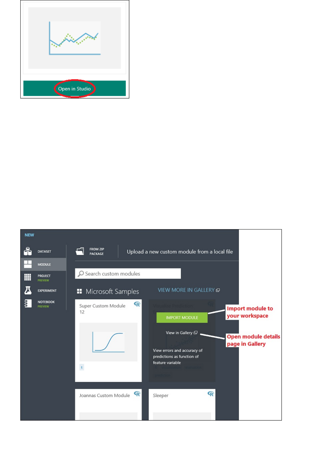
From within Machine Learning StudioFrom within Machine Learning Studio
Each custom module includes a sample experiment that demonstrates how to use the module. When you select
Open in Studio, the sample experiment opens in your Machine Learning Studio workspace. (If you're not already
signed in to Studio, you are prompted to first sign in by using your Microsoft account.)
In addition to the sample experiment, the custom module is copied to your workspace. It's also placed in your
module palette, with all your built-in or custom Machine Learning Studio modules. You can now use it in your own
experiments, like any other module in your workspace.
1. In Machine Learning Studio, select NEW.
2. Select Module. You can choose from a list of Gallery modules, or find a specific module by using the Search
box.
3. Point your mouse at a module, and then select Import Module. (To get information about the module,
select View in Gallery. This takes you to the module details page in the Gallery.)
The custom module is copied to your workspace and placed in your module palette, with your built-in or custom
Machine Learning Studio modules. You can now use it in your own experiments, like any other module in your
workspace.
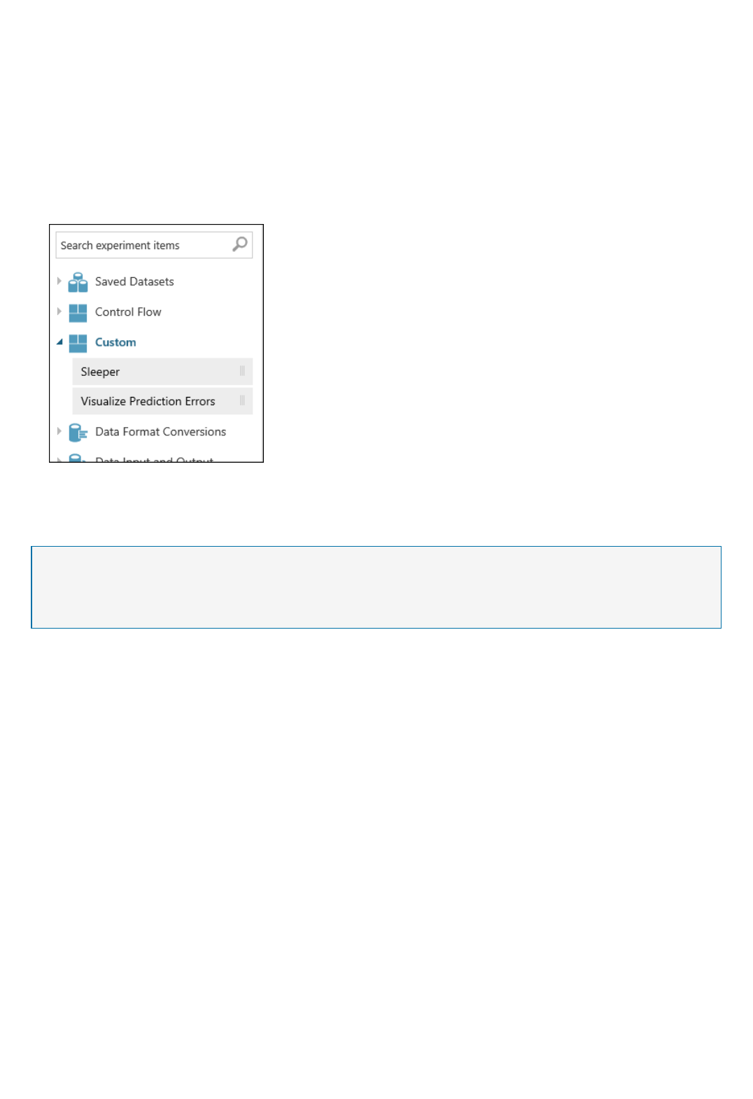
Use
NOTENOTE
Regardless of which method you choose to import a custom module, when you import the module, the module is
placed in your module palette in Machine Learning Studio. From your module palette, you can use the custom
module in any experiment in your workspace, just like any other module.
To use an imported module:
1. Create an experiment, or open an existing experiment.
3. Select the module that you imported, and drag it to your experiment.
2. To expand the list of custom modules in your workspace, in the module palette, select Custom. The module
palette is to the left of the experiment canvas.
Go to the Gallery
You can try Azure Machine Learning for free. No credit card or Azure subscription is required. Get started now.
Guide to Net# neural network specification language
for Azure Machine Learning
3/20/2018 • 23 min to read • Edit Online
NOTENOTE
Neural network basics
Net# is a language developed by Microsoft that is used to define neural network architectures. Using Net# to
define the structure of a neural network makes it possible to define complex structures such as deep neural
networks or convolutions of arbitrary dimensions, which are known to improve learning on data such as image,
audio, or video.
You can use a Net# architecture specification in these contexts:
All neural network modules in Microsoft Azure Machine Learning Studio: Multiclass Neural Network, Two-
Class Neural Network, and Neural Network Regression
Neural network functions in MicrosoftML: NeuralNet and rxNeuralNetfor the R language, and
rx_neural_network for Python.
This article describes the basic concepts and syntax needed to develop a custom neural network using Net#:
Neural network requirements and how to define the primary components
The syntax and keywords of the Net# specification language
Examples of custom neural networks created using Net#
You can try Azure Machine Learning for free. No credit card or Azure subscription is required. Get started now.
A neural network structure consists of nodes that are organized in layers, and weighted connections (or edges)
between the nodes. The connections are directional, and each connection has a source node and a destination node.
Each trainable layer (a hidden or an output layer) has one or more connection bundles. A connection bundle
consists of a source layer and a specification of the connections from that source layer. All the connections in a
given bundle share the same source layer and the same destination layer. In Net#, a connection bundle is
considered as belonging to the bundle's destination layer.
Net# supports various kinds of connection bundles, which lets you customize the way inputs are mapped to hidden
layers and mapped to the outputs.
The default or standard bundle is a full bundle, in which each node in the source layer is connected to every node
in the destination layer.
Additionally, Net# supports the following four kinds of advanced connection bundles:
Filtered bundles. The user can define a predicate by using the locations of the source layer node and the
destination layer node. Nodes are connected whenever the predicate is True.
Convolutional bundles. The user can define small neighborhoods of nodes in the source layer. Each node
in the destination layer is connected to one neighborhood of nodes in the source layer.
Pooling bundles and Response normalization bundles. These are similar to convolutional bundles in
that the user defines small neighborhoods of nodes in the source layer. The difference is that the weights of

Supported customizations
General requirements
Structure specifications
Constant declaration
the edges in these bundles are not trainable. Instead, a predefined function is applied to the source node
values to determine the destination node value.
The architecture of neural network models that you create in Azure Machine Learning can be extensively
customized by using Net#. You can:
Create hidden layers and control the number of nodes in each layer.
Specify how layers are to be connected to each other.
Define special connectivity structures, such as convolutions and weight sharing bundles.
Specify different activation functions.
For details of the specification language syntax, see Structure Specification.
For examples of defining neural networks for some common machine learning tasks, from simplex to complex, see
Examples.
There must be exactly one output layer, at least one input layer, and zero or more hidden layers.
Each layer has a fixed number of nodes, conceptually arranged in a rectangular array of arbitrary dimensions.
Input layers have no associated trained parameters and represent the point where instance data enters the
network.
Trainable layers (the hidden and output layers) have associated trained parameters, known as weights and
biases.
The source and destination nodes must be in separate layers.
Connections must be acyclic; in other words, there cannot be a chain of connections leading back to the initial
source node.
The output layer cannot be a source layer of a connection bundle.
A neural network structure specification is composed of three sections: the constant declaration, the layer
declaration, the connection declaration. There is also an optional share declaration section. The sections can
be specified in any order.
A constant declaration is optional. It provides a means to define values used elsewhere in the neural network
definition. The declaration statement consists of an identifier followed by an equal sign and a value expression.
For example, the following statement defines a constant x:
Const X = 28;
To define two or more constants simultaneously, enclose the identifier names and values in braces, and separate
them by using semicolons. For example:
Const { X = 28; Y = 4; }
The right-hand side of each assignment expression can be an integer, a real number, a Boolean value (True or False),
or a mathematical expression. For example:
Const { X = 17 * 2; Y = true; }
Layer declaration
input Data auto;
hidden Hidden[5,20] from Data all;
output Result[2] from Hidden all;
input Data auto;
hidden Hidden auto from Data all;
output Result auto from Hidden all;
Connection declaration
The layer declaration is required. It defines the size and source of the layer, including its connection bundles and
attributes. The declaration statement starts with the name of the layer (input, hidden, or output), followed by the
dimensions of the layer (a tuple of positive integers). For example:
The product of the dimensions is the number of nodes in the layer. In this example, there are two dimensions
[5,20], which means there are 100 nodes in the layer.
The layers can be declared in any order, with one exception: If more than one input layer is defined, the order in
which they are declared must match the order of features in the input data.
To specify that the number of nodes in a layer be determined automatically, use the auto keyword. The auto
keyword has different effects, depending on the layer:
In an input layer declaration, the number of nodes is the number of features in the input data.
In a hidden layer declaration, the number of nodes is the number that is specified by the parameter value for
Number of hidden nodes.
In an output layer declaration, the number of nodes is 2 for two-class classification, 1 for regression, and equal
to the number of output nodes for multiclass classification.
For example, the following network definition allows the size of all layers to be automatically determined:
A layer declaration for a trainable layer (the hidden or output layers) can optionally include the output function
(also called an activation function), which defaults to sigmoid for classification models, and linear for regression
models. Even if you use the default, you can explicitly state the activation function, if desired for clarity.
The following output functions are supported:
sigmoid
linear
softmax
rlinear
square
sqrt
srlinear
abs
tanh
brlinear
For example, the following declaration uses the softmax function:
output Result [100] softmax from Hidden all;
Immediately after defining the trainable layer, you must declare connections among the layers you have defined.

Full bundles
Filtered bundles
input Pixels [10, 20];
hidden ByRow[10, 12] from Pixels where (s,d) => s[0] == d[0];
hidden ByCol[5, 20] from Pixels where (s,d) => abs(s[1] - d[1]) <= 1;
Convolutional bundles
The connection bundle declaration starts with the keyword from , followed by the name of the bundle's source
layer and the kind of connection bundle to create.
Currently, five kinds of connection bundles are supported:
Full bundles, indicated by the keyword all
Filtered bundles, indicated by the keyword where , followed by a predicate expression
Convolutional bundles, indicated by the keyword convolve , followed by the convolution attributes
Pooling bundles, indicated by the keywords max pool or mean pool
Response normalization bundles, indicated by the keyword response norm
A full connection bundle includes a connection from each node in the source layer to each node in the destination
layer. This is the default network connection type.
A filtered connection bundle specification includes a predicate, expressed syntactically, much like a C# lambda
expression. The following example defines two filtered bundles:
In the predicate for ByRow , s is a parameter representing an index into the rectangular array of nodes of
the input layer, Pixels , and d is a parameter representing an index into the array of nodes of the hidden
layer, ByRow . The type of both s and d is a tuple of integers of length two. Conceptually, s ranges over
all pairs of integers with 0 <= s[0] < 10 and 0 <= s[1] < 20 , and d ranges over all pairs of integers, with
0 <= d[0] < 10 and 0 <= d[1] < 12 .
On the right-hand side of the predicate expression, there is a condition. In this example, for every value of s
and d such that the condition is True, there is an edge from the source layer node to the destination layer
node. Thus, this filter expression indicates that the bundle includes a connection from the node defined by
s to the node defined by d in all cases where s[0] is equal to d[0].
Optionally, you can specify a set of weights for a filtered bundle. The value for the Weights attribute must be a
tuple of floating point values with a length that matches the number of connections defined by the bundle. By
default, weights are randomly generated.
Weight values are grouped by the destination node index. That is, if the first destination node is connected to K
source nodes, the first K elements of the Weights tuple are the weights for the first destination node, in source
index order. The same applies for the remaining destination nodes.
It's possible to specify weights directly as constant values. For example, if you learned the weights previously, you
can specify them as constants using this syntax:
const Weights_1 = [0.0188045055, 0.130500451, ...]
When the training data has a homogeneous structure, convolutional connections are commonly used to learn high-
level features of the data. For example, in image, audio, or video data, spatial or temporal dimensionality can be
fairly uniform.

Convolutional bundles employ rectangular kernels that are slid through the dimensions. Essentially, each kernel
defines a set of weights applied in local neighborhoods, referred to as kernel applications. Each kernel application
corresponds to a node in the source layer, which is referred to as the central node. The weights of a kernel are
shared among many connections. In a convolutional bundle, each kernel is rectangular and all kernel applications
are the same size.
Convolutional bundles support the following attributes:
InputShape defines the dimensionality of the source layer for the purposes of this convolutional bundle. The value
must be a tuple of positive integers. The product of the integers must equal the number of nodes in the source
layer, but otherwise, it does not need to match the dimensionality declared for the source layer. The length of this
tuple becomes the arity value for the convolutional bundle. Typically arity refers to the number of arguments or
operands that a function can take.
To define the shape and locations of the kernels, use the attributes KernelShape, Stride, Padding, LowerPad, and
UpperPad:
KernelShape: (required) Defines the dimensionality of each kernel for the convolutional bundle. The value
must be a tuple of positive integers with a length that equals the arity of the bundle. Each component of this
tuple must be no greater than the corresponding component of InputShape.
Stride: (optional) Defines the sliding step sizes of the convolution (one step size for each dimension), that is
the distance between the central nodes. The value must be a tuple of positive integers with a length that is
the arity of the bundle. Each component of this tuple must be no greater than the corresponding component
of KernelShape. The default value is a tuple with all components equal to one.
Sharing: (optional) Defines the weight sharing for each dimension of the convolution. The value can be a
single Boolean value or a tuple of Boolean values with a length that is the arity of the bundle. A single
Boolean value is extended to be a tuple of the correct length with all components equal to the specified
value. The default value is a tuple that consists of all True values.
MapCount: (optional) Defines the number of feature maps for the convolutional bundle. The value can be a
single positive integer or a tuple of positive integers with a length that is the arity of the bundle. A single
integer value is extended to be a tuple of the correct length with the first components equal to the specified
value and all the remaining components equal to one. The default value is one. The total number of feature
maps is the product of the components of the tuple. The factoring of this total number across the
components determines how the feature map values are grouped in the destination nodes.
Weights: (optional) Defines the initial weights for the bundle. The value must be a tuple of floating point
values with a length that is the number of kernels times the number of weights per kernel, as defined later in
this article. The default weights are randomly generated.
There are two sets of properties that control padding, the properties being mutually exclusive:
Padding: (optional) Determines whether the input should be padded by using a default padding scheme.
The value can be a single Boolean value, or it can be a tuple of Boolean values with a length that is the arity
of the bundle.
A single Boolean value is extended to be a tuple of the correct length with all components equal to the
specified value.
If the value for a dimension is True, the source is logically padded in that dimension with zero-valued cells to
support additional kernel applications, such that the central nodes of the first and last kernels in that
dimension are the first and last nodes in that dimension in the source layer. Thus, the number of "dummy"
nodes in each dimension is determined automatically, to fit exactly (InputShape[d] - 1) / Stride[d] + 1
kernels into the padded source layer.
If the value for a dimension is False, the kernels are defined so that the number of nodes on each side that

Pooling bundles
hidden P1 [5, 12, 12]
from C1 max pool {
InputShape = [ 5, 24, 24];
KernelShape = [ 1, 2, 2];
Stride = [ 1, 2, 2];
}
are left out is the same (up to a difference of 1). The default value of this attribute is a tuple with all
components equal to False.
UpperPad and LowerPad: (optional) Provide greater control over the amount of padding to use.
Important: These attributes can be defined if and only if the Padding property above is not defined. The
values should be integer-valued tuples with lengths that are the arity of the bundle. When these attributes
are specified, "dummy" nodes are added to the lower and upper ends of each dimension of the input layer.
The number of nodes added to the lower and upper ends in each dimension is determined by LowerPad[i]
and UpperPad[i] respectively.
To ensure that kernels correspond only to "real" nodes and not to "dummy" nodes, the following conditions
must be met:
Each component of LowerPad must be strictly less than KernelShape[d]/2 .
Each component of UpperPad must be no greater than KernelShape[d]/2 .
The default value of these attributes is a tuple with all components equal to 0.
The setting Padding = true allows as much padding as is needed to keep the "center" of the kernel
inside the "real" input. This changes the math a bit for computing the output size. Generally, the
output size D is computed as D = (I - K) / S + 1 , where I is the input size, K is the kernel size, S
is the stride, and / is integer division (round toward zero). If you set UpperPad = [1, 1], the input size
I is effectively 29, and thus D = (29 - 5) / 2 + 1 = 13 . However, when Padding = true, essentially
I gets bumped up by K - 1 ; hence D = ((28 + 4) - 5) / 2 + 1 = 27 / 2 + 1 = 13 + 1 = 14 . By
specifying values for UpperPad and LowerPad you get much more control over the padding than if
you just set Padding = true.
For more information about convolutional networks and their applications, see these articles:
http://deeplearning.net/tutorial/lenet.html
http://research.microsoft.com/pubs/68920/icdar03.pdf
http://people.csail.mit.edu/jvb/papers/cnn_tutorial.pdf
A pooling bundle applies geometry similar to convolutional connectivity, but it uses predefined functions to
source node values to derive the destination node value. Hence, pooling bundles have no trainable state (weights
or biases). Pooling bundles support all the convolutional attributes except Sharing, MapCount, and Weights.
Typically, the kernels summarized by adjacent pooling units do not overlap. If Stride[d] is equal to KernelShape[d]
in each dimension, the layer obtained is the traditional local pooling layer, which is commonly employed in
convolutional neural networks. Each destination node computes the maximum or the mean of the activities of its
kernel in the source layer.
The following example illustrates a pooling bundle:
The arity of the bundle is 3: that is, the length of the tuples InputShape , KernelShape , and Stride .
The number of nodes in the source layer is 5 * 24 * 24 = 2880 .
This is a traditional local pooling layer because KernelShape and Stride are equal.
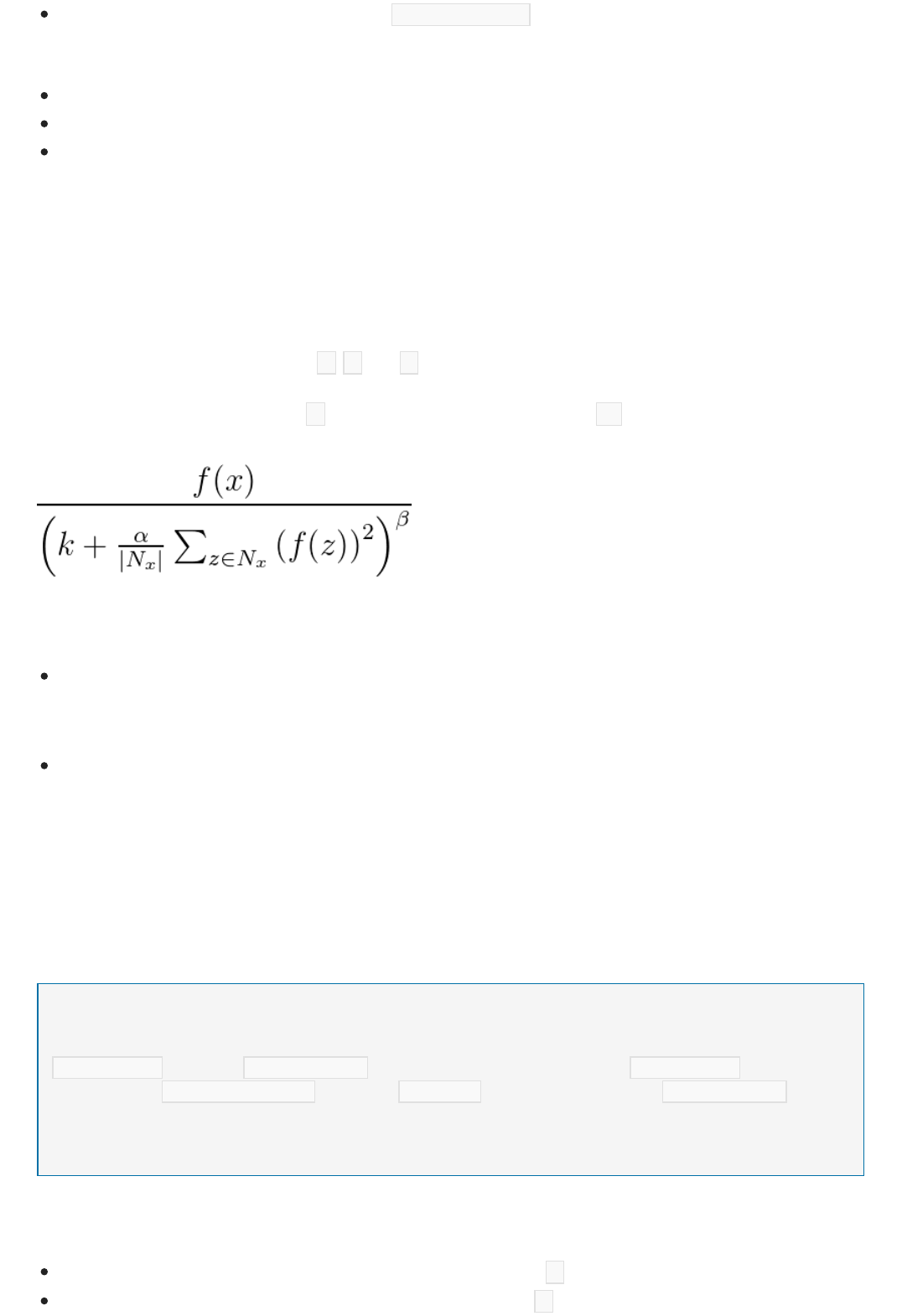
Response normalization bundles
NOTENOTE
The number of nodes in the destination layer is 5 * 12 * 12 = 1440 .
For more information about pooling layers, see these articles:
http://www.cs.toronto.edu/~hinton/absps/imagenet.pdf (Section 3.4)
http://cs.nyu.edu/~koray/publis/lecun-iscas-10.pdf
http://cs.nyu.edu/~koray/publis/jarrett-iccv-09.pdf
Response normalization is a local normalization scheme that was first introduced by Geoffrey Hinton, et al, in the
paper ImageNet Classification with Deep Convolutional Neural Networks.
Response normalization is used to aid generalization in neural nets. When one neuron is firing at a very high
activation level, a local response normalization layer suppresses the activation level of the surrounding neurons.
This is done by using three parameters (α, β, and k) and a convolutional structure (or neighborhood shape).
Every neuron in the destination layer y corresponds to a neuron x in the source layer. The activation level of y is
given by the following formula, where f is the activation level of a neuron, and Nx is the kernel (or the set that
contains the neurons in the neighborhood of x), as defined by the following convolutional structure:
Response normalization bundles support all the convolutional attributes except Sharing, MapCount, and
Weights.
If the kernel contains neurons in the same map as x, the normalization scheme is referred to as same map
normalization. To define same map normalization, the first coordinate in InputShape must have the value
1.
If the kernel contains neurons in the same spatial position as x, but the neurons are in other maps, the
normalization scheme is called across maps normalization. This type of response normalization
implements a form of lateral inhibition inspired by the type found in real neurons, creating competition for
big activation levels amongst neuron outputs computed on different maps. To define across maps
normalization, the first coordinate must be an integer greater than one and no greater than the number of
maps, and the rest of the coordinates must have the value 1.
Because response normalization bundles apply a predefined function to source node values to determine the
destination node value, they have no trainable state (weights or biases).
The nodes in the destination layer correspond to neurons that are the central nodes of the kernels. For example, if
KernelShape[d] is odd, then KernelShape[d]/2 corresponds to the central kernel node. If KernelShape[d] is even, the
central node is at KernelShape[d]/2 - 1 . Therefore, if Padding[d] is False, the first and the last KernelShape[d]/2
nodes do not have corresponding nodes in the destination layer. To avoid this situation, define Padding as [true, true, …,
true].
In addition to the four attributes described earlier, response normalization bundles also support the following
attributes:
Alpha: (required) Specifies a floating-point value that corresponds to α in the previous formula.
Beta: (required) Specifies a floating-point value that corresponds to β in the previous formula.

hidden RN1 [5, 10, 10]
from P1 response norm {
InputShape = [ 5, 12, 12];
KernelShape = [ 1, 3, 3];
Alpha = 0.001;
Beta = 0.75;
}
Share declaration
share-declaration:
share { layer-list }
share { bundle-list }
share { bias-list }
layer-list:
layer-name , layer-name
layer-list , layer-name
bundle-list:
bundle-spec , bundle-spec
bundle-list , bundle-spec
bundle-spec:
layer-name => layer-name
bias-list:
bias-spec , bias-spec
bias-list , bias-spec
bias-spec:
1 => layer-name
layer-name:
identifier
Offset: (optional) Specifies a floating-point value that corresponds to k in the previous formula. It defaults to
1.
The following example defines a response normalization bundle using these attributes:
The source layer includes five maps, each with aof dimension of 12x12, totaling in 1440 nodes.
The value of KernelShape indicates that this is a same map normalization layer, where the neighborhood is a
3x3 rectangle.
The default value of Padding is False, thus the destination layer has only 10 nodes in each dimension. To
include one node in the destination layer that corresponds to every node in the source layer, add Padding =
[true, true, true]; and change the size of RN1 to [5, 12, 12].
Net# optionally supports defining multiple bundles with shared weights. The weights of any two bundles can be
shared if their structures are the same. The following syntax defines bundles with shared weights:
For example, the following share-declaration specifies the layer names, indicating that both weights and biases
should be shared:
Const {
InputSize = 37;
HiddenSize = 50;
}
input {
Data1 [InputSize];
Data2 [InputSize];
}
hidden {
H1 [HiddenSize] from Data1 all;
H2 [HiddenSize] from Data2 all;
}
output Result [2] {
from H1 all;
from H2 all;
}
share { H1, H2 } // share both weights and biases
share { Data1 => H1, Data2 => H2 } // share weights
<!-- -->
share { 1 => H1, 1 => H2 } // share biases
Examples of Net# usage
Define a simple custom neural network: "Hello World" exampleDefine a simple custom neural network: "Hello World" example
input Data auto;
hidden H [200] from Data all;
output Out [10] sigmoid from H all;
Define multiple hidden layers: computer vision exampleDefine multiple hidden layers: computer vision example
The input features are partitioned into two equal sized input layers.
The hidden layers then compute higher level features on the two input layers.
The share-declaration specifies that H1 and H2 must be computed in the same way from their respective inputs.
Alternatively, this could be specified with two separate share-declarations as follows:
You can use the short form only when the layers contain a single bundle. In general, sharing is possible only when
the relevant structure is identical, meaning that they have the same size, same convolutional geometry, and so
forth.
This section provides some examples of how you can use Net# to add hidden layers, define the way that hidden
layers interact with other layers, and build convolutional networks.
This simple example demonstrates how to create a neural network model that has a single hidden layer.
The example illustrates some basic commands as follows:
The first line defines the input layer (named Data ). When you use the auto keyword, the neural network
automatically includes all feature columns in the input examples.
The second line creates the hidden layer. The name H is assigned to the hidden layer, which has 200 nodes. This
layer is fully connected to the input layer.
The third line defines the output layer (named O), which contains 10 output nodes. If the neural network is
used for classification, there is one output node per class. The keyword sigmoid indicates that the output
function is applied to the output layer.
The following example demonstrates how to define a slightly more complex neural network, with multiple custom
// Define the input layers
input Pixels [10, 20];
input MetaData [7];
// Define the first two hidden layers, using data only from the Pixels input
hidden ByRow [10, 12] from Pixels where (s,d) => s[0] == d[0];
hidden ByCol [5, 20] from Pixels where (s,d) => abs(s[1] - d[1]) <= 1;
// Define the third hidden layer, which uses as source the hidden layers ByRow and ByCol
hidden Gather [100]
{
from ByRow all;
from ByCol all;
}
// Define the output layer and its sources
output Result [10]
{
from Gather all;
from MetaData all;
}
Define a convolutional network for multiclass classification: digit recognition exampleDefine a convolutional network for multiclass classification: digit recognition example
input Image [29, 29];
hidden Conv1 [5, 13, 13] from Image convolve
{
InputShape = [29, 29];
KernelShape = [ 5, 5];
Stride = [ 2, 2];
MapCount = 5;
}
hidden Conv2 [50, 5, 5]
from Conv1 convolve
{
InputShape = [ 5, 13, 13];
KernelShape = [ 1, 5, 5];
Stride = [ 1, 2, 2];
Sharing = [false, true, true];
MapCount = 10;
}
hidden Hid3 [100] from Conv2 all;
output Digit [10] from Hid3 all;
hidden layers.
This example illustrates several features of the neural networks specification language:
The structure has two input layers, Pixels and MetaData .
The Pixels layer is a source layer for two connection bundles, with destination layers, ByRow and ByCol .
The layers Gather and Result are destination layers in multiple connection bundles.
The output layer, Result , is a destination layer in two connection bundles; one with the second level hidden
layer Gather as a destination layer, and the other with the input layer MetaData as a destination layer.
The hidden layers, ByRow and ByCol , specify filtered connectivity by using predicate expressions. More
precisely, the node in ByRow at [x, y] is connected to the nodes in Pixels that have the first index coordinate
equal to the node's first coordinate, x. Similarly, the node in ByCol at [x, y] is connected to the nodes in Pixels
that have the second index coordinate within one of the node's second coordinate, y.
The definition of the following network is designed to recognize numbers, and it illustrates some advanced
techniques for customizing a neural network.

Acknowledgements
The structure has a single input layer, Image .
The keyword convolve indicates that the layers named Conv1 and Conv2 are convolutional layers. Each of
these layer declarations is followed by a list of the convolution attributes.
The net has a third hidden layer, Hid3 , which is fully connected to the second hidden layer, Conv2 .
The output layer, Digit , is connected only to the third hidden layer, Hid3 . The keyword all indicates that the
output layer is fully connected to Hid3 .
The arity of the convolution is three: the length of the tuples InputShape , KernelShape , Stride, and Sharing`.
The number of weights per kernel is
1 + KernelShape\[0] * KernelShape\[1] * KernelShape\[2] = 1 + 1 * 5 * 5 = 26 . Or 26 * 50 = 1300 .
Because Sharing[d] is False only for d == 0 , the number of kernels is MapCount * NodeCount\[0] = 10 * 5 = 50 .
You can calculate the nodes in each hidden layer as follows:
NodeCount\[0] = (5 - 1) / 1 + 1 = 5 NodeCount\[1] = (13 - 5) / 2 + 1 = 5
NodeCount\[2] = (13 - 5) / 2 + 1 = 5
The total number of nodes can be calculated by using the declared dimensionality of the layer, [50, 5, 5], as
follows: MapCount * NodeCount\[0] * NodeCount\[1] * NodeCount\[2] = 10 * 5 * 5 * 5
The Net# language for customizing the architecture of neural networks was developed at Microsoft by Shon
Katzenberger (Architect, Machine Learning) and Alexey Kamenev (Software Engineer, Microsoft Research). It is
used internally for machine learning projects and applications ranging from image detection to text analytics. For
more information, see Neural Nets in Azure ML - Introduction to Net#
