CASA CNP Bed Manual
User Manual:
Open the PDF directly: View PDF ![]() .
.
Page Count: 166 [warning: Documents this large are best viewed by clicking the View PDF Link!]

2019
CASA-CNP Model Testbed
March 2019
User’s Manual and Technical Documentation
Lead Authors
Melannie D. Hartman1
William R. Wieder1
Benjamin N. Sulman2
1Climate and Global Dynamics Laboratory,
National Center for Atmospheric Research
Boulder, CO, USA
2 Environmental Sciences Division, Oak Ridge
National Laboratory, Oak Ridge, TN, USA
March 1, 2019
1
1 Table of Contents
1.1 Table of Figures ............................................................................................................................. 4
1.2 List of Tables ................................................................................................................................. 5
2 Overview of the CASA-CNP testbed ...................................................................................................... 6
2.1 Creating input files for the CASA testbed with netcdfTools ....................................................... 11
2.1.1 Meteorological inputs (met*.nc files) ................................................................................. 11
2.1.2 Grid cell locations and PFT coverage (gridinfo_igbpz.csv) .................................................. 11
2.1.3 Grid cell soil properties (gridinfo_soil.csv) .......................................................................... 11
2.1.4 Compiling and running the netcdfTools executable ........................................................... 11
2.1.4.1 Explanation of files.ini content ....................................................................................... 12
2.1.4.2 Executing netcdfTools ..................................................................................................... 12
2.1.4.3 Format of CLM history files and surface data set required by netcdfTools .................... 13
2.2 CASA-CNP Input Files .................................................................................................................. 34
2.2.1 Daily Meteorological Forcings: met*.nc files ...................................................................... 34
2.2.2 Grid Cell Soil and Vegetation Properties ............................................................................. 36
2.2.3 Model-specific parameter files ........................................................................................... 38
2.3 Running the CASA testbed and setting run-time options ........................................................... 38
2.3.1 Specifying parameter file names ........................................................................................ 38
2.3.2 Example run-time options in fcasacnp_clm_testbed.lst file ............................................... 38
2.3.2.1 Specifying simulation type: spinup, transient, transient repeat and using restart files . 41
2.3.2.2 Annual vs. Daily Output files ........................................................................................... 41
2.3.3 Compiling the casaclm_mimics_corpse executable ............................................................ 41
2.3.4 Executing the program ........................................................................................................ 42
2.4 Frequently Asked Questions (FAQ) ............................................................................................. 42
2.4.1 How are PFTs, GPP, and meteorological inputs in the met.nc files aggregated from CLM
output? How are soil properties aggregated? ................................................................................... 42
2.4.2 What needs to be done to change the PFTs on the existing grid? ..................................... 42
2.4.3 What needs to be done to change the soil properties on the existing grid? ..................... 43
2.4.4 What needs to be done to change the grid resolution and/or lat/lon of grid cells? .......... 43
2.4.5 What processes are affected when soil temperature is perturbed in the CASA-CNP
testbed? 43
2.4.6 What processes are affected when air temperature is perturbed in the CASA-CNP
testbed? 43
2.4.7 Are there any input/output file size restraints? ................................................................. 44
March 1, 2019
2
2.4.8 What are the output file options for casaclm_mimics_corpse? ......................................... 44
2.4.9 What is the best way to do two or more simultaneous runs? ........................................... 44
3 Model Descriptions ............................................................................................................................. 44
3.1 CASA-CNP Vegetation Model ...................................................................................................... 44
3.1.1 Plant Functional Types ........................................................................................................ 45
3.2 CASA-CNP Soil Carbon Model ..................................................................................................... 46
3.2.1 Overview of CASA-CNP system of equations for Soil Organic Matter Cycling .................... 47
3.2.2 Partitioning of plant litter inputs into structural and metabolic litter in CASA-CNP .......... 48
3.2.3 CASA-CNP Temperature and Moisture Controls on Decomposition of Litter and SOM..... 54
3.2.3.1 CASA-CNP Temperature Controls on Decomposition ..................................................... 54
3.2.3.2 CASA-CNP Soil Moisture Controls on Decomposition ..................................................... 55
3.2.4 Carbon Stabilization and Destabilization in CASA-CNP ....................................................... 56
3.3 CASA-CNP Soil Layer Structure .................................................................................................... 57
3.3.1 Mapping of CLM 4.5 soil layers to CASA-CNP soil layers .................................................... 58
3.3.2 Mapping of CLM 5.0 soil layers to CASA-CNP soil layers .................................................... 58
3.3.3 Fraction of root biomass in each CASA-CNP soil layer ........................................................ 60
3.4 MIMICS ........................................................................................................................................ 61
3.4.1 Overview of MIMICS system of equations .......................................................................... 63
3.4.2 Partitioning plant litter to metabolic and structural litter pools in MIMICS ....................... 64
3.4.3 Flows to and from MICr: consumption and turnover ......................................................... 64
3.4.4 Flows to and from MICk: consumption and turnover ......................................................... 65
3.4.5 Desorption of physically protected SOM to available SOM ................................................ 66
3.4.6 Oxidation of SOMc to SOMa ............................................................................................... 66
3.4.7 MIMICS Temperature and Moisture Controls on Decomposition of Litter and SOM ........ 66
3.4.7.1 Temperature and moisture sensitive maximum reaction velocities, Vmax(T,Ɵ) ........... 66
3.4.8 Microbial Turnover in MIMICS ............................................................................................ 70
3.4.9 Carbon Stabilization and Destabilization in MIMICS: ......................................................... 71
3.5 CORPSE ........................................................................................................................................ 74
3.5.1 Overview of CORPSE system of equations .......................................................................... 75
3.5.2 Heterotrophic Respiration in CORPSE ................................................................................. 76
3.5.3 CORPSE Temperature and Moisture Controls on Decomposition of Litter and SOM ........ 76
3.5.3.1 CORPSE Temperature Controls on Decomposition of Litter and SOM ........................... 76
3.5.3.2 CORPSE Soil Moisture Controls on Decomposition of Litter and SOM ........................... 77
March 1, 2019
3
3.5.4 Microbial growth and turnover in CORPSE ......................................................................... 78
3.5.5 Carbon Stabilization and Destabilization in CORPSE: ......................................................... 78
4 Detailed Summary of CASA-CNP Subroutines and Biogeochemcial Equations .................................. 80
4.1 Daily biogeochemistry: SUBROUTINE biogeochem .................................................................... 80
4.2 CASA-CNP Dimensions, Constants, and Pointers ........................................................................ 82
4.3 Soil and Litter Decomposition and Heterotrophic Respiration Variables ................................... 83
4.4 CASA-CNP Documentation by Subroutine .................................................................................. 84
4.4.1 Phenology: (1) SUBROUTINE phenology ............................................................................. 84
4.4.2 Average Soil Conditions: (2) SUBROUTINE avgsoil .............................................................. 84
4.4.3 NPP and Autotrophic Respiration: (3) SUBROUTINE casa_rplant ....................................... 85
4.4.4 Carbon Allocation: (4) SUBROUTINE casa_allocation ......................................................... 89
4.4.5 Plant Turnover Rates: (5) SUBROUTINE casa_xrateplant ................................................... 91
4.4.6 Plant Litterfall rate: (6) SUBROUTINE casa_coeffplant ....................................................... 94
4.4.7 Nutrient Limitation on Production: (7) SUBROUTINE casa_xnp ......................................... 97
4.4.8 Soil Temperature and Moisture effects on SOM decomposition: (8) SUBROUTINE
casa_xratesoil .................................................................................................................................... 101
4.4.9 Litter and SOM decomposition rates: (9) SUBROUTINE casa_coeffsoil ............................ 102
4.4.10 Mineralization, Immobilization, N limits on decomposition: (10) SUBROUTINE casa_xkN
106
4.4.11 Plant N uptake: (11) SUBROUTINE casa_nuptake ............................................................. 110
4.4.12 Plant Net C, N, and P fluxes: (13) SUBROUTINE casa_delplant ........................................ 112
4.4.13 Update Litter and Soil Pools: (14) SUBROUTINE casa_delsoil .......................................... 115
4.4.14 Final Daily Update to all Pools: (15) SUBROUTINE casa_cnpcycle .................................... 120
5 Guidelines for adding additional SOM models to the testbed ......................................................... 120
5.1 Overview of subroutine biogeochem with calls to MIMICS and CORPSE models .................... 121
6 Conversions ....................................................................................................................................... 122
6.1 g C m-2 to mg C cm-3 ................................................................................................................... 123
6.2 mg C cm-3 to gC m-2 ................................................................................................................... 123
7 Output NetCDF files .......................................................................................................................... 123
7.1 casaclm_pool_flux.nc ................................................................................................................ 123
7.2 mimics_pool_flux.nc ................................................................................................................. 126
7.3 corpse_pool_flux.nc .................................................................................................................. 128
8 Output Restart Files .......................................................................................................................... 132
8.1 CASA-CNPpool_end.csv............................................................................................................. 132
March 1, 2019
4
8.2 mimicspool_end.csv .................................................................................................................. 133
8.3 corpsepool_end.csv .................................................................................................................. 134
9 Summary of Model Parameters ........................................................................................................ 138
9.1 CASA-CNP parameters in pftlookup_igbp.csv ........................................................................... 138
9.2 MIMICS parameters .................................................................................................................. 154
9.3 CORPSE parameters from corpse_params_new.nml ............................................................... 159
10 References .................................................................................................................................... 161
1.1 Table of Figures
Figure 1. Schematic of the CASA-CNP testbed. ............................................................................................ 8
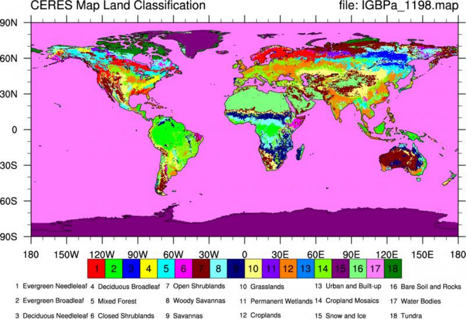
Figure 2. CERES land classification from IGBPa_1198.map.nc. Surface types 1 - 17 correspond to those
defined by IGBP (International Geosphere Biosphere Programme). The 18th surface type (tundra) was
defined for CERES. The IGBP surface type for snow and ice number 15, is for permanent snow and ice.
(Climate Data Guide; D. Shea). https://climatedataguide.ucar.edu/climate-data/ceres-igbp-land-
classification. ................................................................................................................................................. 9
Figure 3. Litter and Soil Organic Mater Pools in the CASA-CNP model. All flows out of any litter or soil
pool are controlled by f(T) and f(Ɵ) as well as the lignin/texture controls shown with the blue arrows.
The blue text refers to the controls on the fraction of the total flow that is transferred from one pool to
another; 1.0 minus these fractions is the portion of the total flow that goes to heterotrophic respiration.
The red arrows indicate that there is no flow from the Passive SOM pool to the Fast (Microbial) or Slow
SOM pools. See equations below. .............................................................................................................. 47
Figure 4. CASA-CNP plant litter transfers to the metabolic and structural litter pools .............................. 50
Figure 5. CASA-CNP soil temperature effect on Soil Organic Matter decomposition (xktemp). ................ 55
Figure 6. CASA-CNP soil moisture effect on SOM decomposition (xkwater). ............................................. 56
Figure 7. The effect of soil clay content (% weight) on the fraction of flows between soil organic matter
pools.The silt fraction was held at a constant 30%.The lower figure is a zoomed in version of the top
figure. .......................................................................................................................................................... 57
Figure 8. Litter and Soil Organic Mater pools in the MIMICS model. Heterotrophic respiration losses
occur with consumption of litter and available pools by the microbes, and with the decomposition of the
CWD pool. ................................................................................................................................................... 62
Figure 9. Temperature sensitive maximum reaction velocities, Vmax(T), for the MIMICS model.. ........... 69
Figure 10. Temperature sensitive half saturation constants, Km(T), for the MIMICS model. .................... 70
Figure 11. Fraction of Microbial Turnover to the protected Soil Organic Matter pool in the MIMICS model
(fPHYS). ....................................................................................................................................................... 72
Figure 12. MIMICS physical protection scalar (Pscalar). The scalar modifies fluxes from available SOM to
microbial pools. ........................................................................................................................................... 74
Figure 13. CORPSE model litter and soil organic matter pools (from Sulman et al. 2014). ........................ 75
Figure 14. The temperature-dependent maximum enzymatic conversion rate Vmax,i(T) (yr-1) in the
CORPSE model. ........................................................................................................................................... 77
March 1, 2019
5
Figure 15. The soil moisture effect on soil organic matter decomposition in the CORPSE model where Ɵl
is the volumetric liquid soil water content, and Ɵsat is the volumetric total soil water content at
saturation (here the volumetric frozen soil water content, Ɵf = 0.0). The corresponding f(Ɵ) effect for
MIMICS is similar but has a maximum value of 1.0. ................................................................................... 78
Figure 16. The effect of soil clay fraction on transfers of C to the protected pools in the CORPSE model.
.................................................................................................................................................................... 79
Figure 17. Order of calculations in subroutine biogeochem in the CASA-CNP model. Subroutine
biogeochem is called once each day and controls daily biogeochemical calculations in CASA-CNP. ........ 81
Figure 18. Maintenance respiration assuming rmplant(pft,leaf) = 0.1/365, rmplant(pft,froot) = 6.0/365,
rmplant(pft,wood) = 10.0/365. ................................................................................................................... 86
Figure 19. The plant growth efficiency (Ygrow). For C only or C+N only, Ygrow = 0.65. ............................ 88
Figure 20. Effect of cold on evergreen leaf tree death rates. In this example for evergreen needle leaves,
xkleafcoldmax = 0.20, xkleafcoldexp = 3.0, TKshed = 268. When xkleafcold = 0.0 (orange line) there is no
death due to cold. Note that the death rate for evergreen needle leaves is lower than the death rate for
deciduous leaves at low temperatures (Figure 21). ................................................................................... 92
Figure 21. Effect of cold on deciduous elaf death rates.In this example for deciduous leaves,
xkleafcoldmax = 0.60, xkleafcoldexp = 3.0, TKshed = 268. When xkleafcold = 0.0 (orange line) there is no
death due to cold. Note that the death rate for deciduous leaves is greater than the death rate for
evergreen needle leaves at low temperatures (Figure 20)......................................................................... 92
Figure 22. Effect of soil dryness on evergreen leaf death rates. In this example for evergreen needle
leaves, xkleafdrymax = 0.1, xkleafdryexp = 3.0. When xkleafdry = 0.0 there is no death due to drought. 93
Figure 23. Effect of soil dryness on deciduous leaf death rates. In this example for deciduous leaves,
xkleafdrymax = 1.0, xkleafdryexp = 3.0. When xkleafdry = 0.0 there is no death due to drought. ............ 94
Figure 24. Carbon fluxes from plant pools to litter pools in the CASA-CNP model. ................................... 96
Figure 25. The N:C ratio of plant parts is bounded by biome-specific parameters ratioNCplantmin and
ratioNCplantmax, and is a function of Nsoilmin, the amount of mineral soil N available (g N m-2). Here
ratioNCplantmin = 0.25 and ratioNCplantmax = 0.5. ................................................................................. 98
Figure 26. Carbon and CO2 fluxes as litter and soil organic matter pools decompose in the CASA-CNP
model. ....................................................................................................................................................... 105
Figure 27. The N:C ratio required by the receiving SOM pool is a function of soil mineral N content. In
this example, ratioNCsoilMin = 0.0, ratioNCsoilMax = 0.2 ....................................................................... 107
Figure 28. Actual N uptake by a plant pool (g N m-2 d-1). In this example, kminN = 0.5, xkNlimiting = 0.8,
Nrequiremin = 0.2, Nrequiremax = 0.5. .................................................................................................... 111
1.2 List of Tables
Table 1. Example of netCDF header from 4.5 CLM history file ................................................................... 13
Table 2. NetCDF file header for CLM 4.5 surface data. ............................................................................... 18
Table 3. Format of daily (h1) CLM 5.0 history file ....................................................................................... 26
Table 4. Partial format of monthly (h0) CCLM 5.0 history file with surface data information. .................. 32
Table 5. Example netcdf header for a forcing file named met_1901_1901.nc (updated January 7, 2019).
.................................................................................................................................................................... 35
Table 6. Example of fcasacnp_clm_testbed.lst file with run-time options................................................. 39
Table 7. IGBP_CERES plant functional types (PFTs) used by the CASA-CNP testbed, from
pftlookup_igbp.csv parameter file. ............................................................................................................. 45
March 1, 2019
6
Table 8. Initial C:N ratios and lignin content of plant parts by plant functional type (PFT). These
parameters can be found in the pftlookup_igbp.csv parameter file. ......................................................... 49
Table 9. CASA-CNP Soil Layer Structure ..................................................................................................... 57
Table 10. CASA-CNP parameters used to calculate fraction of root in each soil layer ............................... 60
Table 11. Fraction of roots in each soil layer by PFT ................................................................................. 61
Table 12. IGBP plant functional types used by the CASA-CNP testbed (pftlookup_igbp.csv). ................. 138
Table 13. Rooting distribution parameters, and ?? by PFT (pftlookup_igbp.csv)..................................... 139
Table 14. Mean residence times (age) for plant, litter, soil organic, and labile plant C pools, and specific
leaf area (SLA) by PFT (pftlookup_igbp.csv). ............................................................................................. 140
Table 15. Carbon allocation fractions and maintenance respiration (rm) parameters by PFT
(pftlookup_igbp.csv). ................................................................................................................................ 141
Table 16. Initial C:N ratios, N retranslocation parameters, and lignin content of plant parts by PFT. The
C:N ratios and lignin fractions are used to compute lignin:N ratios for partitioning plant litter into
structural and metabolic fraction (pftlookup_igbp.csv). .......................................................................... 142
Table 17. Initiial, minimum, and maximum C:N ratios of soil organic pools (icycle ≥ 2)
(pftlookup_igbp.csv). ................................................................................................................................ 143
Table 18. Maximum and minimum LAI values by PFT (pftlookup_igbp.csv). ........................................... 144
Table 19. Initial Carbon values of plant, litter, and soil organic pools for spinup simulations (initcasa=0)
(pftlookup_igbp.csv). ................................................................................................................................ 145
Table 20. Parameters controlling plant death rates with freezing temperatures and water stress
(pftlookup_igbp.csv). ................................................................................................................................ 146
Table 21. Phenology parameters (no longer used) (pftlookup_igbp.csv). ............................................... 147
Table 22. Minimum and Maximum N:C ratios of plant pools, N leaching rates, and N fixation rates (icycle
≥ 2) (pftlookup_igbp.csv). ......................................................................................................................... 148
Table 23. Initial nitrogen pool values for spinup runs (initcasa=0, icycle ≥ 2) (pftlookup_igbp.csv). ....... 149
Table 24. N:P ratios (icycle=3) (pftlookup_igbp.csv). ............................................................................... 150
Table 25. Soil Phosphorous parameters (icycle=3). These apply to all PFTs (pftlookup_igbp.csv). ......... 151
Table 26. Initial Phosphorous Pool values for spinup runs by PFT (initcasa=0, icycle=3)
(pftlookup_igbp.csv). ................................................................................................................................ 152
Table 27. Litter and soil decomposition controls by PFT. Some parameters are only used when icycle ≥ 2
(pftlookup_igbp.csv). ................................................................................................................................ 153
Table 28. MIMICS parameters common to all PFTs. ................................................................................. 154
Table 29. MIMICS PFT-specific soil depths. .............................................................................................. 158
Table 30. CORPSE model parameters common to all PFTs (CORPSE has no PFT-specific parameters). .. 159
2 Overview of the CASA-CNP testbed
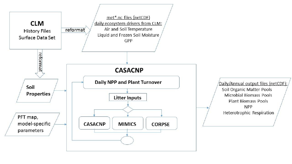
The CASA-CNP testbed (currently named casaclm_mimics_corpse) has been developed to test different
soil organic matter (SOM) cycling models with a common set of environmental conditions and litter
input. At the heart of the testbed is the Carnagie-Aimes-Stanford Approach terrestrial biosphere model
(CASA-CNP) (created by (Potter, Randerson et al. 1993), with modifications by (Randerson, Thompson et
al. 1996, Randerson, Thompson et al. 1997); and with N and P biogeochemistry as implemented by

March 1, 2019
7
(Wang, Law et al. 2010). We use the carbon-only calculations of CASA-CNP to calculate net primary
productivity (NPP), carbon allocation to different tissues (roots, wood, and leaves), as well as the timing
of plant mortality and litterfall. Currently, one of three different SOM cycling models can be selected to
compute organic matter transformations, soil carbon stocks, and heterotrophic respiration (Figure 1).
These SOM models include one first-order model, the SOM cycling model in CASA-CNP (Wang et al.
2010), and two microbial explicit models, the MIcrobial-MIneral Carbon Stabilization (MIMICS) model
(Wieder, Grandy et al. 2014, Wieder, Grandy et al. 2015) and the Carbon, Organisms, Rhizosphere and
Protection in the Soil Environment (CORPSE) model (Sulman, Phillips et al. 2014). If the CASA-CNP SOM
model is selected, the testbed can be run with carbon only, with carbon and nitrogen only, or with
carbon and nitrogen and phosphorus. Currently, the testbed is run in carbon-only mode when either
MIMICS or CORPSE is selected since these models do not yet include N-cycling.
Data inputs were generated by the Community Land Model (CLM version 4.5) using a satellite phenology
scheme forced with the Cru-NCEP climate reanalysis (Koven, Riley et al. 2013, Oleson, Lawrence et al.
2013). This standard configuration of CLM generated globally gridded daily output of gross primary
productivity (GPP), air temperature, along with soil temperature, liquid soil moisture, and frozen soil
moisture in 10 CLM soil layers (top 343 cm of soil) for the historical period (1901-2010). Static soil
property inputs to the testbed including soil texture (sand, silt, clay fractions) and volumetric soil water
content at wilting point, field capacity, and saturation inputs to the testbed were depth-weighted means
in the top 50 cm of soil from the CLM surface data set (Oleson, Lawrence et al. 2013). The testbed
assigned a single plant functional type (PFT) to each 2° x 2° grid cell, computed as the mode from the 1-
km International Geosphere–Biosphere Program Data and Information System (IGBP DISCover) data set
with 18 vegetation types, including grassy tundra (Loveland, Reed et al. 2000) (National Center for
Atmospheric Research Staff (Eds). Last modified 10 Feb 2017. "The Climate Data Guide: CERES: IGBP
Land Classification." Retrieved from https://climatedataguide.ucar.edu/climate-data/ceres-igbp-land-
classification) (Figure 2). CASA-CNP defines biome-specific parameters corresponding to each PFT (Table
12 to
March 1, 2019
8
Table 27).
The daily time-dependent forcings required by the testbed include mean air temperature, atmospheric
nitrogen deposition, Gross Primary Production (GPP), and soil temperature and volumetric soil water
content for five soil layers in the top 150 cm of soil. CASA-CNP computes the depth-weighted mean soil
temperature and depth-weighted volumetric soil water content in the rooting zone using to the PFT-
specific root depth and root distribution to weight the contribution from each soil layer.
The testbed computes average soil temperature, liquid soil moisture, and frozen soil moisture
as depth-weighted means in the rooting zone (50 to 150 cm) according to the PFT-specific root
depth and root distribution within the six CASA-CNP soil layers (section “Fraction of root
biomass in each CASA-CNP soil layer”). The three models in the testbed use only these mean
soil moisture and mean soil temperature for their calculations rather than the vertically-
resolved values. Only liquid soil moisture was considered when computing soil moisture limits
on growth in the CASA-CNP vegetation model and soil moisture decomposition effects for both
CASA-CNP and CORPSE soil organic models. Additionally, CORPSE required frozen soil moisture
to calculate air-filled pore space. MIMICS does not consider soil moisture effects on
decomposition.
Figure 1. Schematic of the CASA-CNP testbed.
Currently the testbed is set up to run the land cells on the 2° x 2° global CLM grid. The grid resolution of
the testbed is flexible and can be modified by updating the resolution of the input files; it can even be
configured to run for a single point or field site. Although CLM defines multiple PFTs in each 2° x 2° grid
March 1, 2019
9
cell, CASA-CNP defines only a single PFT per each grid cell. The testbed does not simulate cells that are
designated as urban, wetlands, water, or ice. The daily GPP forcings are the total daily GPP that CLM
reported for the grid cell even though CLM’s results are the aggregate of multiple PFTs.
Post processing of CLM history files was required to format input data that could be read into the
biogeochemical testbed (Section 2.1. Creating input files for the CASA testbed with netcdfTools). Other
grid cell-specific properties, including Plant Functional Types (PFTs) and timing of phenology, were
derived independent of the CLM model as described below.
Figure 2. CERES land classification from IGBPa_1198.map.nc. Surface types 1 - 17 correspond to those defined by IGBP
(International Geosphere Biosphere Programme). The 18th surface type (tundra) was defined for CERES. The IGBP surface type
for snow and ice number 15, is for permanent snow and ice. (Climate Data Guide; D. Shea).
https://climatedataguide.ucar.edu/climate-data/ceres-igbp-land-classification.
Given daily meteorological inputs and daily gross primary production (GPP) as forcings, the primary
modifications to CASA-CNP to develop this testbed were:
• MIMICS and CORPSE were added as alternative SOM models to the CASA-CNP first-order model
• The testbed specifies soil properties by grid cell instead of assigning a soil type to each grid cell.
Originally CASA-CNP had 9 soil types where each type hard-coded values for soil texture and
water holding capacities.
March 1, 2019
10
• Gridded daily input for meteorological and other time-dependent data is through netCDF
(met.nc) files instead of text files.
• N deposition is a time-dependent daily input instead of a single average annual input.
• The testbed has capability to run transient simulations. Transient simulations read a series of
annual forcing files and maintain the state of the model between each year; no stop/restart is
required. In this way, the model can be driven with a long continuous climate record instead of
recycling a meteorological record with a finite number of years. Transient runs require one
met.nc file for each calendar year of the transient simulation. Non-transient runs require a
single met.nc file that is read over and over; this file can contain up to five complete years of
daily inputs.
• The testbed saves daily or mean annual output each year to netCDf files. Formerly output was
saved at the end of the simulation only to .csv files.
• As with CASA-CNP, the testbed outputs the state of vegetation and soil pools at the end of the
simulation to .csv files. These “restart” files can be used to initialize subsequent runs.
Run-time options for the testbed are specified in a text file (fcasacnp_clm_testbed.lst). These run-time
options include the frequency of output (annual or daily), the names of the model-specific parameter
files, the names of meteorological forcing files, the SOM cycling model to run (i.e. CASA-CNP, MIMICS, or
CORPSE), the type of simulation (spinup or transient), the name of the restart files to initialize the
models, and the names of the output files.
CASA-CNP calculates NPP from GPP by accounting for autotrophic respiration losses and nutrient
limitation (Wang, Law et al. 2010). Nutrient limitation is not relevant when CASA-CNP is run in carbon-
only mode. CASA-CNP computes the exact same NPP and litter inputs regardless of SOM model selected;
in the carbon-only mode there is no feedback of the SOM model to the plant model.
The testbed provides the ability to perturb soil temperatures and/or air temperatures as a step
increment during a simulation. Soil temperature perturbations affect soil organic matter turnover rates
and heterotrophic respiration (all SOM models), root maintenance and growth respiration (and
therefore NPP and litterfall rates), and N mineralization and N leaching when CASA-CNP simulates N
cycling. Air temperature perturbations affect wood maintenance and growth respiration (and therefore
NPP and litterfall rates), labile C (carbohydrate) storage (and therefore NPP and litterfall rates), and cold
effects on leaf litter fall.
The simulations for each SOM model are usually carried out in three steps.
1. Initialize CASA-CNP vegetation pools with a “pre-spin” simulation. We ran the testbed with 1901
climate for 100 years. This pre-spin creates more stable vegetation pools and litter inputs for
subsequent simulations; the microbial pools of MIMICS and CORPSE are sensitive to changes in
litter inputs. The state of the vegetation pools (but not SOM pools) from this pre-spin simulation
is used to initialize spinup runs for all SOM models.
2. We executed spinup simulations by driving each SOM model with 1901-1920 forcings over and
over until organic matter pools reached equilibrium. An SOM model was considered to be in
equilibrium when all three of the following criteria were met between 20-year cycles: global
litter plus soil carbon stocks changed less than 0.01Pg, total litter plus soil carbon in less than 2%
of grid cells changed more than 1 g C m-2, and total litter plus soil carbon in less than 2% of grid
cells changed more than 0.1%. Spinup times varied between models: a) CASA-CNP required
10,000 years of an accelerated spinup followed by 10,00 years of normal spinup in order to
reach equilibrium. The passive pool, the pool with the slowest turnover rate, required the
March 1, 2019
11
longest spinup time. For the accelerated spinup, the decomposition rates were increased 10
times. Pools were multiplied by 10 before starting the normal spinup phase; b) MIMICS organic
matter pools required 12,000 years to reach equilibrium. The physically protected pool
required the longest spinup time; c) CORPSE organic matter pools required 50,000 years to
reach equilibrium. The recalcitrant litter pool required the longest spinup time.
3. Run transient simulations using CRU/NCEP weather from 1901 – 2010. The transient simulations
were initialized from restart files created by the spinup runs.
2.1 Creating input files for the CASA testbed with netcdfTools
The netcdfTools program can be used to create several input files for the testbed by reformatting CLM
history files and surface data. The following are three files that netcdfTools creates. More information
about the format of these files can be found in the next section.
2.1.1 Meteorological inputs (met*.nc files)
The testbed requires meteorological input files in netCDF format (the met*.nc files). These files are
extracted from CLM history files. Non-transient runs require either a single (multi-year) met.nc file or a
subset of consecutive single-year met.nc files that are read over and over. Transient runs require one
met.nc file for each calendar year of the transient simulation. Met.nc files that contain data for the
entire grid are limited to a maximum of 5 years since this amount of data is about 2GB, the maximum
size of a netCDF file. Met.nc files for point simulations can have hundreds of years.
2.1.2 Grid cell locations and PFT coverage (gridinfo_igbpz.csv)
For each grid cell in the CLM grid, this file contains one row with a grid cell id, latitude, longitude, PFT,
land area, and some other information. Note that the Ndep (Nitrogen deposition) column in this file is
now ignored; since August 22, 2016 daily Ndep is stored in the met.nc file.
2.1.3 Grid cell soil properties (gridinfo_soil.csv)
For each grid cell in the CLM grid, this file contains one row with the cell’s soil properties. Soil properties
are derived from the CLM surface data set and include sand, clay, and silt, fractions and volumetric soil
water content at wilting point (wwilt), field capacity (wfiel), and saturation (wsat).
2.1.4 Compiling and running the netcdfTools executable
If the netcdfTools executable does not exist or needs to be recompiled for any reason, change to the
CASACLM/NetCDFTools/SOURCE directory, remove any object files (to be safe), and type the following
“make” command:
cd CASACLM/NetCDFTools/SOURCE
rm *.o *.mod
make -f Makefile.txt netcdfTools
March 1, 2019
12
If the code fails to compile, the makefile, Makefile.txt, may need to be updated with the specifics
(compiler and pathnames) for your system. Next, copy the netcdfTools executable to the location where
it will be run. The Linux chmod command will make it executable in case the file permissions get
changed when it is copied. For example
cp netcdfTools ..
cd ..
chmod 755 netcdfTools
The netcdfTools program reads a text file named files.ini and a .csv file named clmGrid_IGBP.csv. It
creates one met_yyyy_yyyy.nc file (yyyy and yyyy are the starting and ending years of data stored in the
file) and two .csv files (gridinfo_igbpz.csv and gridinfo_soil.csv) per simulation.
Example of files.ini:
h1 ! file type (h0=monthly, h1=daily)
19010101 ! start (yyyymmdd)
19051231 ! end (yyyymmdd)
/project/CASACLM/clm_forcing/CRU_hist/clm4_5_12_r191_CLM45spHIST_CRU.clm2.h1.1901-01-01-
00000.nc
/project/surfdata_1.9x2.5_simyr1850_c130421.nc
/project/fndep_clm_hist_simyr1849-2006_1.9x2.5_c100428.nc
./CO2_1768-2010.txt
2.1.4.1 Explanation of files.ini content
Line 1: Use h1 (daily), h0 no longer works.
Line 2: First day for met_yyyy_yyyy.nc file (best to start Jan. 1st.)
Line 3: Last day for met_yyyy_yyyy.nc file (best to end Dec. 31st, don’t exceed 5 years for 2° x 2° grid)
Line 4: Name of CLM history file for the first year (netCDF format)
Line 5: Name of CLM surface data set (netCDF format)
Line 6: Name of CLM N deposition file (netCDF format)
Line 7: Name of text file with annual global mean CO2 concentrations.
2.1.4.2 Executing netcdfTools
Once the initialization file (files.ini) has been set up, type the following two commands at the command
line prompt. The module load command needs only to be run once for each Linux session.
module load tool/netcdf/4.3.2/gcc
./netcdfTools
An error similar to the following will occur if the module load command is not executed before running
netcdfTools:
./netcdfTools: error while loading shared libraries: libnetcdff.so.6: cannot open shared object file:
No such file or directory
The netcdf module version may change with time. To determine the NetCDF version available, type
“module avail” at the command line to see available modules.

March 1, 2019
13
To create more than one met.nc, one could use a script to create met.nc files in batch. The perl script
run-netcsftools.pl is an example of how to do this. To run this script, update the file paths in the script to
match your directory structure then type the following at the command line:
perl run-netcdftools.pl
2.1.4.3 Format of CLM history files and surface data set required by netcdfTools
The netcdfTools program expects the CLM netCDF files to be in a specific format – it is looking for
specific variable names, dimension names, and dimension orders (Table 1, Table 2). If the format of the
input files is altered, then one will likely need to update the source code and recompile the program to
accommodate the format change. The netcsfTools was originally developed to process CLM 4.5 files
(Table 1 and Table 2), but we recently developed a version that processes CLM 5.0 files (Table 3 and
Table 4).
Table 1. Example of netCDF header from 4.5 CLM history file
netcdf clm4_5_12_r191_CLM45spHIST_CRU.clm2.h1.1850-01-01-00000 {
dimensions:
lon = 144 ;
lat = 96 ;
gridcell = 5663 ;
landunit = 21260 ;
column = 69848 ;
pft = 160456 ;
levgrnd = 15 ;
levurb = 5 ;
levlak = 10 ;
numrad = 2 ;
levsno = 5 ;
ltype = 9 ;
nlevcan = 1 ;
nvegwcs = 4 ;
natpft = 17 ;
string_length = 8 ;
scale_type_string_length = 32 ;
levdcmp = 1 ;
hist_interval = 2 ;
time = UNLIMITED ; // (365 currently)
variables:
float levgrnd(levgrnd) ;
levgrnd:long_name = "coordinate soil levels" ;
levgrnd:units = "m" ;
float levlak(levlak) ;
levlak:long_name = "coordinate lake levels" ;
levlak:units = "m" ;

March 1, 2019
14
float levdcmp(levdcmp) ;
levdcmp:long_name = "coordinate soil levels" ;
levdcmp:units = "m" ;
float time(time) ;
time:long_name = "time" ;
time:units = "days since 1850-01-01 00:00:00" ;
time:calendar = "noleap" ;
time:bounds = "time_bounds" ;
int mcdate(time) ;
mcdate:long_name = "current date (YYYYMMDD)" ;
int mcsec(time) ;
mcsec:long_name = "current seconds of current date" ;
mcsec:units = "s" ;
int mdcur(time) ;
mdcur:long_name = "current day (from base day)" ;
int mscur(time) ;
mscur:long_name = "current seconds of current day" ;
int nstep(time) ;
nstep:long_name = "time step" ;
double time_bounds(time, hist_interval) ;
time_bounds:long_name = "history time interval endpoints" ;
char date_written(time, string_length) ;
char time_written(time, string_length) ;
float lon(lon) ;
lon:long_name = "coordinate longitude" ;
lon:units = "degrees_east" ;
lon:_FillValue = 1.e+36f ;
lon:missing_value = 1.e+36f ;
float lat(lat) ;
lat:long_name = "coordinate latitude" ;
lat:units = "degrees_north" ;
lat:_FillValue = 1.e+36f ;
lat:missing_value = 1.e+36f ;
float area(lat, lon) ;
area:long_name = "grid cell areas" ;
area:units = "km^2" ;
area:_FillValue = 1.e+36f ;
area:missing_value = 1.e+36f ;
float landfrac(lat, lon) ;
landfrac:long_name = "land fraction" ;
landfrac:_FillValue = 1.e+36f ;
landfrac:missing_value = 1.e+36f ;
int landmask(lat, lon) ;
landmask:long_name = "land/ocean mask (0.=ocean and 1.=land)" ;
landmask:_FillValue = -9999 ;
landmask:missing_value = -9999 ;
int pftmask(lat, lon) ;
pftmask:long_name = "pft real/fake mask (0.=fake and 1.=real)" ;

March 1, 2019
15
pftmask:_FillValue = -9999 ;
pftmask:missing_value = -9999 ;
int nbedrock(lat, lon) ;
nbedrock:long_name = "index of shallowest bedrock layer" ;
nbedrock:_FillValue = -9999 ;
nbedrock:missing_value = -9999 ;
float FLDS(time, lat, lon) ;
FLDS:long_name = "atmospheric longwave radiation" ;
FLDS:units = "W/m^2" ;
FLDS:cell_methods = "time: mean" ;
FLDS:_FillValue = 1.e+36f ;
FLDS:missing_value = 1.e+36f ;
float FPSN(time, lat, lon) ;
FPSN:long_name = "photosynthesis" ;
FPSN:units = "umol/m2s" ;
FPSN:cell_methods = "time: mean" ;
FPSN:_FillValue = 1.e+36f ;
FPSN:missing_value = 1.e+36f ;
float FSDS(time, lat, lon) ;
FSDS:long_name = "atmospheric incident solar radiation" ;
FSDS:units = "W/m^2" ;
FSDS:cell_methods = "time: mean" ;
FSDS:_FillValue = 1.e+36f ;
FSDS:missing_value = 1.e+36f ;
float FSDSND(time, lat, lon) ;
FSDSND:long_name = "direct nir incident solar radiation" ;
FSDSND:units = "W/m^2" ;
FSDSND:cell_methods = "time: mean" ;
FSDSND:_FillValue = 1.e+36f ;
FSDSND:missing_value = 1.e+36f ;
float FSDSNI(time, lat, lon) ;
FSDSNI:long_name = "diffuse nir incident solar radiation" ;
FSDSNI:units = "W/m^2" ;
FSDSNI:cell_methods = "time: mean" ;
FSDSNI:_FillValue = 1.e+36f ;
FSDSNI:missing_value = 1.e+36f ;
float FSDSVD(time, lat, lon) ;
FSDSVD:long_name = "direct vis incident solar radiation" ;
FSDSVD:units = "W/m^2" ;
FSDSVD:cell_methods = "time: mean" ;
FSDSVD:_FillValue = 1.e+36f ;
FSDSVD:missing_value = 1.e+36f ;
float FSDSVI(time, lat, lon) ;
FSDSVI:long_name = "diffuse vis incident solar radiation" ;
FSDSVI:units = "W/m^2" ;
FSDSVI:cell_methods = "time: mean" ;
FSDSVI:_FillValue = 1.e+36f ;
FSDSVI:missing_value = 1.e+36f ;

March 1, 2019
16
float H2OSOI(time, levgrnd, lat, lon) ;
H2OSOI:long_name = "volumetric soil water (vegetated landunits only)" ;
H2OSOI:units = "mm3/mm3" ;
H2OSOI:cell_methods = "time: mean" ;
H2OSOI:_FillValue = 1.e+36f ;
H2OSOI:missing_value = 1.e+36f ;
float PBOT(time, lat, lon) ;
PBOT:long_name = "atmospheric pressure" ;
PBOT:units = "Pa" ;
PBOT:cell_methods = "time: mean" ;
PBOT:_FillValue = 1.e+36f ;
PBOT:missing_value = 1.e+36f ;
float QBOT(time, lat, lon) ;
QBOT:long_name = "atmospheric specific humidity" ;
QBOT:units = "kg/kg" ;
QBOT:cell_methods = "time: mean" ;
QBOT:_FillValue = 1.e+36f ;
QBOT:missing_value = 1.e+36f ;
float RAIN(time, lat, lon) ;
RAIN:long_name = "atmospheric rain" ;
RAIN:units = "mm/s" ;
RAIN:cell_methods = "time: mean" ;
RAIN:_FillValue = 1.e+36f ;
RAIN:missing_value = 1.e+36f ;
float SMP(time, levgrnd, lat, lon) ;
SMP:long_name = "soil matric potential (vegetated landunits only)" ;
SMP:units = "mm" ;
SMP:cell_methods = "time: mean" ;
SMP:_FillValue = 1.e+36f ;
SMP:missing_value = 1.e+36f ;
float SNOW(time, lat, lon) ;
SNOW:long_name = "atmospheric snow" ;
SNOW:units = "mm/s" ;
SNOW:cell_methods = "time: mean" ;
SNOW:_FillValue = 1.e+36f ;
SNOW:missing_value = 1.e+36f ;
float SOILICE(time, levgrnd, lat, lon) ;
SOILICE:long_name = "soil ice (vegetated landunits only)" ;
SOILICE:units = "kg/m2" ;
SOILICE:cell_methods = "time: mean" ;
SOILICE:_FillValue = 1.e+36f ;
SOILICE:missing_value = 1.e+36f ;
float SOILLIQ(time, levgrnd, lat, lon) ;
SOILLIQ:long_name = "soil liquid water (vegetated landunits only)" ;
SOILLIQ:units = "kg/m2" ;
SOILLIQ:cell_methods = "time: mean" ;
SOILLIQ:_FillValue = 1.e+36f ;
SOILLIQ:missing_value = 1.e+36f ;

March 1, 2019
17
float SOILPSI(time, levgrnd, lat, lon) ;
SOILPSI:long_name = "soil water potential in each soil layer" ;
SOILPSI:units = "MPa" ;
SOILPSI:cell_methods = "time: mean" ;
SOILPSI:_FillValue = 1.e+36f ;
SOILPSI:missing_value = 1.e+36f ;
float TBOT(time, lat, lon) ;
TBOT:long_name = "atmospheric air temperature" ;
TBOT:units = "K" ;
TBOT:cell_methods = "time: mean" ;
TBOT:_FillValue = 1.e+36f ;
TBOT:missing_value = 1.e+36f ;
float THBOT(time, lat, lon) ;
THBOT:long_name = "atmospheric air potential temperature" ;
THBOT:units = "K" ;
THBOT:cell_methods = "time: mean" ;
THBOT:_FillValue = 1.e+36f ;
THBOT:missing_value = 1.e+36f ;
float TLAI(time, lat, lon) ;
TLAI:long_name = "total projected leaf area index" ;
TLAI:units = "none" ;
TLAI:cell_methods = "time: mean" ;
TLAI:_FillValue = 1.e+36f ;
TLAI:missing_value = 1.e+36f ;
float TSOI(time, levgrnd, lat, lon) ;
TSOI:long_name = "soil temperature (vegetated landunits only)" ;
TSOI:units = "K" ;
TSOI:cell_methods = "time: mean" ;
TSOI:_FillValue = 1.e+36f ;
TSOI:missing_value = 1.e+36f ;
float WIND(time, lat, lon) ;
WIND:long_name = "atmospheric wind velocity magnitude" ;
WIND:units = "m/s" ;
WIND:cell_methods = "time: mean" ;
WIND:_FillValue = 1.e+36f ;
WIND:missing_value = 1.e+36f ;
// global attributes:
:title = "CLM History file information" ;
:comment = "NOTE: None of the variables are weighted by land fraction!" ;
:Conventions = "CF-1.0" ;
:history = "created on 02/17/17 05:30:04" ;
:source = "Community Land Model CLM4.0" ;
:hostname = "yellowstone" ;
:username = "wwieder" ;
:version = "unknown" ;
:revision_id = "$Id: histFileMod.F90 42903 2012-12-21 15:32:10Z muszala $" ;
:case_title = "UNSET" ;

March 1, 2019
18
:case_id = "clm4_5_12_r191_CLM45spHIST_CRU" ;
:Surface_dataset = "surfdata_1.9x2.5_16pfts_simyr1850_c160127.nc" ;
:Initial_conditions_dataset = "clmi.I1850CRUCLM45BGC.0241-01-
01.1.9x2.5_g1v6_simyr1850_c160127.nc" ;
:PFT_physiological_constants_dataset = "clm_params.c160713.nc" ;
:ltype_vegetated_or_bare_soil = 1 ;
:ltype_crop = 2 ;
:ltype_landice = 3 ;
:ltype_landice_multiple_elevation_classes = 4 ;
:ltype_deep_lake = 5 ;
:ltype_wetland = 6 ;
:ltype_urban_tbd = 7 ;
:ltype_urban_hd = 8 ;
:ltype_urban_md = 9 ;
:ctype_vegetated_or_bare_soil = 1 ;
:ctype_crop = 2 ;
:ctype_crop_noncompete = "2*100+m, m=cft_lb,cft_ub" ;
:ctype_landice = 3 ;
:ctype_landice_multiple_elevation_classes = "4*100+m, m=1,glcnec" ;
:ctype_deep_lake = 5 ;
:ctype_wetland = 6 ;
:ctype_urban_roof = 71 ;
:ctype_urban_sunwall = 72 ;
:ctype_urban_shadewall = 73 ;
:ctype_urban_impervious_road = 74 ;
:ctype_urban_pervious_road = 75 ;
}
Table 2. NetCDF file header for CLM 4.5 surface data.
netcdf surfdata_1.9x2.5_simyr1850_c130421_ADDwat4 {
dimensions:
numrad = 2 ;
numurbl = 3 ;
lsmlat = 96 ;
lsmlon = 144 ;
nlevurb = 5 ;
nglcecp1 = 11 ;
time = UNLIMITED ; // (12 currently)
lsmpft = 17 ;
nlevsoi = 10 ;
nglcec = 10 ;
levgrnd = 10 ;
lat = 96 ;
lon = 144 ;
variables:
double ALB_IMPROAD_DIF(numrad, numurbl, lsmlat, lsmlon) ;

March 1, 2019
19
ALB_IMPROAD_DIF:long_name = "diffuse albedo of impervious road" ;
ALB_IMPROAD_DIF:units = "unitless" ;
double ALB_IMPROAD_DIR(numrad, numurbl, lsmlat, lsmlon) ;
ALB_IMPROAD_DIR:long_name = "direct albedo of impervious road" ;
ALB_IMPROAD_DIR:units = "unitless" ;
double ALB_PERROAD_DIF(numrad, numurbl, lsmlat, lsmlon) ;
ALB_PERROAD_DIF:long_name = "diffuse albedo of pervious road" ;
ALB_PERROAD_DIF:units = "unitless" ;
double ALB_PERROAD_DIR(numrad, numurbl, lsmlat, lsmlon) ;
ALB_PERROAD_DIR:long_name = "direct albedo of pervious road" ;
ALB_PERROAD_DIR:units = "unitless" ;
double ALB_ROOF_DIF(numrad, numurbl, lsmlat, lsmlon) ;
ALB_ROOF_DIF:long_name = "diffuse albedo of roof" ;
ALB_ROOF_DIF:units = "unitless" ;
double ALB_ROOF_DIR(numrad, numurbl, lsmlat, lsmlon) ;
ALB_ROOF_DIR:long_name = "direct albedo of roof" ;
ALB_ROOF_DIR:units = "unitless" ;
double ALB_WALL_DIF(numrad, numurbl, lsmlat, lsmlon) ;
ALB_WALL_DIF:long_name = "diffuse albedo of wall" ;
ALB_WALL_DIF:units = "unitless" ;
double ALB_WALL_DIR(numrad, numurbl, lsmlat, lsmlon) ;
ALB_WALL_DIR:long_name = "direct albedo of wall" ;
ALB_WALL_DIR:units = "unitless" ;
double AREA(lsmlat, lsmlon) ;
AREA:long_name = "area" ;
AREA:units = "km^2" ;
double CANYON_HWR(numurbl, lsmlat, lsmlon) ;
CANYON_HWR:long_name = "canyon height to width ratio" ;
CANYON_HWR:units = "unitless" ;
double CV_IMPROAD(nlevurb, numurbl, lsmlat, lsmlon) ;
CV_IMPROAD:long_name = "volumetric heat capacity of impervious road" ;
CV_IMPROAD:units = "J/m^3*K" ;
double CV_ROOF(nlevurb, numurbl, lsmlat, lsmlon) ;
CV_ROOF:long_name = "volumetric heat capacity of roof" ;
CV_ROOF:units = "J/m^3*K" ;
double CV_WALL(nlevurb, numurbl, lsmlat, lsmlon) ;
CV_WALL:long_name = "volumetric heat capacity of wall" ;
CV_WALL:units = "J/m^3*K" ;
double Ds(lsmlat, lsmlon) ;
Ds:long_name = "VIC Ds parameter for the ARNO curve" ;
Ds:units = "unitless" ;
double Dsmax(lsmlat, lsmlon) ;
Dsmax:long_name = "VIC Dsmax parameter for the ARNO curve" ;
Dsmax:units = "mm/day" ;
double EF1_BTR(lsmlat, lsmlon) ;
EF1_BTR:long_name = "EF btr (isoprene)" ;
EF1_BTR:units = "unitless" ;
double EF1_CRP(lsmlat, lsmlon) ;

March 1, 2019
20
EF1_CRP:long_name = "EF crp (isoprene)" ;
EF1_CRP:units = "unitless" ;
double EF1_FDT(lsmlat, lsmlon) ;
EF1_FDT:long_name = "EF fdt (isoprene)" ;
EF1_FDT:units = "unitless" ;
double EF1_FET(lsmlat, lsmlon) ;
EF1_FET:long_name = "EF fet (isoprene)" ;
EF1_FET:units = "unitless" ;
double EF1_GRS(lsmlat, lsmlon) ;
EF1_GRS:long_name = "EF grs (isoprene)" ;
EF1_GRS:units = "unitless" ;
double EF1_SHR(lsmlat, lsmlon) ;
EF1_SHR:long_name = "EF shr (isoprene)" ;
EF1_SHR:units = "unitless" ;
double EM_IMPROAD(numurbl, lsmlat, lsmlon) ;
EM_IMPROAD:long_name = "emissivity of impervious road" ;
EM_IMPROAD:units = "unitless" ;
double EM_PERROAD(numurbl, lsmlat, lsmlon) ;
EM_PERROAD:long_name = "emissivity of pervious road" ;
EM_PERROAD:units = "unitless" ;
double EM_ROOF(numurbl, lsmlat, lsmlon) ;
EM_ROOF:long_name = "emissivity of roof" ;
EM_ROOF:units = "unitless" ;
double EM_WALL(numurbl, lsmlat, lsmlon) ;
EM_WALL:long_name = "emissivity of wall" ;
EM_WALL:units = "unitless" ;
double F0(lsmlat, lsmlon) ;
F0:long_name = "maximum gridcell fractional inundated area" ;
F0:units = "unitless" ;
double FMAX(lsmlat, lsmlon) ;
FMAX:long_name = "maximum fractional saturated area" ;
FMAX:units = "unitless" ;
double GLC_MEC(nglcecp1) ;
GLC_MEC:long_name = "Glacier elevation class" ;
GLC_MEC:units = "m" ;
double HT_ROOF(numurbl, lsmlat, lsmlon) ;
HT_ROOF:long_name = "height of roof" ;
HT_ROOF:units = "meters" ;
double LAKEDEPTH(lsmlat, lsmlon) ;
LAKEDEPTH:long_name = "lake depth" ;
LAKEDEPTH:units = "m" ;
double LANDFRAC_PFT(lsmlat, lsmlon) ;
LANDFRAC_PFT:long_name = "land fraction from pft dataset" ;
LANDFRAC_PFT:units = "unitless" ;
double LATIXY(lsmlat, lsmlon) ;
LATIXY:long_name = "latitude" ;
LATIXY:units = "degrees north" ;
double LONGXY(lsmlat, lsmlon) ;

March 1, 2019
21
LONGXY:long_name = "longitude" ;
LONGXY:units = "degrees east" ;
double MONTHLY_HEIGHT_BOT(time, lsmpft, lsmlat, lsmlon) ;
MONTHLY_HEIGHT_BOT:long_name = "monthly height bottom" ;
MONTHLY_HEIGHT_BOT:units = "meters" ;
double MONTHLY_HEIGHT_TOP(time, lsmpft, lsmlat, lsmlon) ;
MONTHLY_HEIGHT_TOP:long_name = "monthly height top" ;
MONTHLY_HEIGHT_TOP:units = "meters" ;
double MONTHLY_LAI(time, lsmpft, lsmlat, lsmlon) ;
MONTHLY_LAI:long_name = "monthly leaf area index" ;
MONTHLY_LAI:units = "unitless" ;
double MONTHLY_SAI(time, lsmpft, lsmlat, lsmlon) ;
MONTHLY_SAI:long_name = "monthly stem area index" ;
MONTHLY_SAI:units = "unitless" ;
int NLEV_IMPROAD(numurbl, lsmlat, lsmlon) ;
NLEV_IMPROAD:long_name = "number of impervious road layers" ;
NLEV_IMPROAD:units = "unitless" ;
double ORGANIC(nlevsoi, lsmlat, lsmlon) ;
ORGANIC:long_name = "organic matter density at soil levels" ;
ORGANIC:units = "kg/m3 (assumed carbon content 0.58 gC per gOM)" ;
double P3(lsmlat, lsmlon) ;
P3:long_name = "coefficient for qflx_surf_lag for finundated" ;
P3:units = "s/mm" ;
double PCT_CLAY(nlevsoi, lsmlat, lsmlon) ;
PCT_CLAY:long_name = "percent clay" ;
PCT_CLAY:units = "unitless" ;
double PCT_GLACIER(lsmlat, lsmlon) ;
PCT_GLACIER:long_name = "percent glacier" ;
PCT_GLACIER:units = "unitless" ;
double PCT_GLC_GIC(lsmlat, lsmlon) ;
PCT_GLC_GIC:long_name = "percent ice caps/glaciers" ;
PCT_GLC_GIC:units = "unitless" ;
double PCT_GLC_ICESHEET(lsmlat, lsmlon) ;
PCT_GLC_ICESHEET:long_name = "percent ice sheet" ;
PCT_GLC_ICESHEET:units = "unitless" ;
double PCT_GLC_MEC(nglcec, lsmlat, lsmlon) ;
PCT_GLC_MEC:long_name = "percent glacier for each glacier elevation class" ;
PCT_GLC_MEC:units = "unitless" ;
double PCT_GLC_MEC_GIC(nglcec, lsmlat, lsmlon) ;
PCT_GLC_MEC_GIC:long_name = "percent smaller glaciers and ice caps for each
glacier elevation class" ;
PCT_GLC_MEC_GIC:units = "unitless" ;
double PCT_GLC_MEC_ICESHEET(nglcec, lsmlat, lsmlon) ;
PCT_GLC_MEC_ICESHEET:long_name = "percent ice sheet for each glacier elevation
class" ;
PCT_GLC_MEC_ICESHEET:units = "unitless" ;
double PCT_LAKE(lsmlat, lsmlon) ;
PCT_LAKE:long_name = "percent lake" ;

March 1, 2019
22
PCT_LAKE:units = "unitless" ;
double PCT_PFT(lsmpft, lsmlat, lsmlon) ;
PCT_PFT:long_name = "percent plant functional type of gridcell" ;
PCT_PFT:units = "unitless" ;
double PCT_SAND(nlevsoi, lsmlat, lsmlon) ;
PCT_SAND:long_name = "percent sand" ;
PCT_SAND:units = "unitless" ;
double PCT_URBAN(numurbl, lsmlat, lsmlon) ;
PCT_URBAN:long_name = "percent urban for each density type" ;
PCT_URBAN:units = "unitless" ;
double PCT_WETLAND(lsmlat, lsmlon) ;
PCT_WETLAND:long_name = "percent wetland" ;
PCT_WETLAND:units = "unitless" ;
int PFTDATA_MASK(lsmlat, lsmlon) ;
PFTDATA_MASK:long_name = "land mask from pft dataset, indicative of real/fake
points" ;
PFTDATA_MASK:units = "unitless" ;
double SLOPE(lsmlat, lsmlon) ;
SLOPE:long_name = "mean topographic slope" ;
SLOPE:units = "degrees" ;
int SOIL_COLOR(lsmlat, lsmlon) ;
SOIL_COLOR:long_name = "soil color" ;
SOIL_COLOR:units = "unitless" ;
double STD_ELEV(lsmlat, lsmlon) ;
STD_ELEV:long_name = "standard deviation of elevation" ;
STD_ELEV:units = "m" ;
double THICK_ROOF(numurbl, lsmlat, lsmlon) ;
THICK_ROOF:long_name = "thickness of roof" ;
THICK_ROOF:units = "meters" ;
double THICK_WALL(numurbl, lsmlat, lsmlon) ;
THICK_WALL:long_name = "thickness of wall" ;
THICK_WALL:units = "meters" ;
double TK_IMPROAD(nlevurb, numurbl, lsmlat, lsmlon) ;
TK_IMPROAD:long_name = "thermal conductivity of impervious road" ;
TK_IMPROAD:units = "W/m*K" ;
double TK_ROOF(nlevurb, numurbl, lsmlat, lsmlon) ;
TK_ROOF:long_name = "thermal conductivity of roof" ;
TK_ROOF:units = "W/m*K" ;
double TK_WALL(nlevurb, numurbl, lsmlat, lsmlon) ;
TK_WALL:long_name = "thermal conductivity of wall" ;
TK_WALL:units = "W/m*K" ;
double TOPO(lsmlat, lsmlon) ;
TOPO:long_name = "mean elevation on land" ;
TOPO:units = "m" ;
double TOPO_GLC_MEC(nglcec, lsmlat, lsmlon) ;
TOPO_GLC_MEC:long_name = "mean elevation on glacier elevation classes" ;
TOPO_GLC_MEC:units = "m" ;
double T_BUILDING_MAX(numurbl, lsmlat, lsmlon) ;

March 1, 2019
23
T_BUILDING_MAX:long_name = "maximum interior building temperature" ;
T_BUILDING_MAX:units = "K" ;
double T_BUILDING_MIN(numurbl, lsmlat, lsmlon) ;
T_BUILDING_MIN:long_name = "minimum interior building temperature" ;
T_BUILDING_MIN:units = "K" ;
int URBAN_REGION_ID(lsmlat, lsmlon) ;
URBAN_REGION_ID:long_name = "urban region ID" ;
URBAN_REGION_ID:units = "unitless" ;
double WATFC(levgrnd, lat, lon) ;
WATFC:_FillValue = 9.99999961690316e+35 ;
WATFC:cell_methods = "time: mean" ;
WATFC:long_name = "water field capacity" ;
WATFC:missing_value = 1.e+36f ;
WATFC:units = "m^3/m^3" ;
double WATSAT(levgrnd, lat, lon) ;
WATSAT:_FillValue = 9.99999961690316e+35 ;
WATSAT:cell_methods = "time: mean" ;
WATSAT:long_name = "water saturated" ;
WATSAT:missing_value = 1.e+36f ;
WATSAT:units = "m^3/m^3" ;
double WIND_HGT_CANYON(numurbl, lsmlat, lsmlon) ;
WIND_HGT_CANYON:long_name = "height of wind in canyon" ;
WIND_HGT_CANYON:units = "meters" ;
double WTLUNIT_ROOF(numurbl, lsmlat, lsmlon) ;
WTLUNIT_ROOF:long_name = "fraction of roof" ;
WTLUNIT_ROOF:units = "unitless" ;
double WTROAD_PERV(numurbl, lsmlat, lsmlon) ;
WTROAD_PERV:long_name = "fraction of pervious road" ;
WTROAD_PERV:units = "unitless" ;
double Ws(lsmlat, lsmlon) ;
Ws:long_name = "VIC Ws parameter for the ARNO Curve" ;
Ws:units = "unitless" ;
double ZWT0(lsmlat, lsmlon) ;
ZWT0:long_name = "decay factor for finundated" ;
ZWT0:units = "m" ;
int abm(lsmlat, lsmlon) ;
abm:long_name = "agricultural fire peak month" ;
abm:units = "unitless" ;
double binfl(lsmlat, lsmlon) ;
binfl:long_name = "VIC b parameter for the Variable Infiltration Capacity Curve" ;
binfl:units = "unitless" ;
double gdp(lsmlat, lsmlon) ;
gdp:long_name = "gdp" ;
gdp:units = "unitless" ;
int mxsoil_color ;
mxsoil_color:long_name = "maximum numbers of soil colors" ;
mxsoil_color:units = "unitless" ;
double peatf(lsmlat, lsmlon) ;

March 1, 2019
24
peatf:long_name = "peatland fraction" ;
peatf:units = "unitless" ;
int time(time) ;
time:long_name = "Calendar month" ;
time:units = "month" ;
// global attributes:
:Conventions = "CF-1.0" ;
:History_Log = "created on: 04-21-13 22:41:42" ;
:Logname = "erik" ;
:Host = "yslogin3" ;
:Source = "Community Land Model: CLM4" ;
:Version = "$HeadURL: https://svn-ccsm-
models.cgd.ucar.edu/clm2/trunk_tags/clm4_0_74/models/lnd/clm/tools/clm4_5/mksurfdata_map/sr
c/mkfileMod.F90 $" ;
:Revision_Id = "$Id: mkfileMod.F90 46006 2013-04-15 16:04:42Z sacks $" ;
:Compiler_Optimized = "TRUE" ;
:no_inlandwet = "TRUE" ;
:nglcec = 10 ;
:Input_grid_dataset = "map_0.5x0.5_landuse_to_1.9x2.5_aave_da_110307.nc" ;
:Input_gridtype = "global" ;
:VOC_EF_raw_data_file_name = "mksrf_vocef_0.5x0.5_simyr2000.c110531.nc" ;
:Inland_lake_raw_data_file_name =
"mksrf_LakePnDepth_3x3min_simyr2004_c111116.nc" ;
:Inland_wetland_raw_data_file_name = "mksrf_lanwat.050425.nc" ;
:Glacier_raw_data_file_name = "mksrf_glacier_3x3min_simyr2000.c120926.nc" ;
:Urban_Topography_raw_data_file_name = "mksrf_topo.10min.c080912.nc" ;
:Land_Topography_raw_data_file_name = "topodata_10min_USGS_071205.nc" ;
:Urban_raw_data_file_name = "mksrf_urban_0.05x0.05_simyr2000.c120621.nc" ;
:Lai_raw_data_file_name = "mksrf_lai_global_c090506.nc" ;
:agfirepkmon_raw_data_file_name =
"mksrf_abm_0.5x0.5_AVHRR_simyr2000.c130201.nc" ;
:gdp_raw_data_file_name = "mksrf_gdp_0.5x0.5_AVHRR_simyr2000.c130228.nc" ;
:peatland_raw_data_file_name =
"mksrf_peatf_0.5x0.5_AVHRR_simyr2000.c130228.nc" ;
:topography_stats_raw_data_file_name = "mksrf_topostats_1km-merge-
10min_HYDRO1K-merge-nomask_simyr2000.c130402.nc" ;
:vic_raw_data_file_name = "mksrf_vic_0.9x1.25_GRDC_simyr2000.c130307.nc" ;
:ch4_params_raw_data_file_name =
"mksrf_ch4inversion_360x720_cruncep_simyr2000.c130322.nc" ;
:map_pft_file_name = "map_0.5x0.5_landuse_to_1.9x2.5_aave_da_110307.nc" ;
:map_lakwat_file =
"map_3x3min_MODIS_to_1.9x2.5_nomask_aave_da_c111111.nc" ;
:map_wetlnd_file = "map_0.5x0.5_lanwat_to_1.9x2.5_aave_da_110307.nc" ;
:map_glacier_file = "map_3x3min_GLOBE-
Gardner_to_1.9x2.5_nomask_aave_da_c120923.nc" ;
:map_soil_texture_file = "map_5minx5min_soitex_to_1.9x2.5_aave_da_110307.nc" ;
:map_soil_color_file = "map_0.5x0.5_landuse_to_1.9x2.5_aave_da_110307.nc" ;

March 1, 2019
25
:map_soil_organic_file = "map_5x5min_ISRIC-
WISE_to_1.9x2.5_nomask_aave_da_c111115.nc" ;
:map_urban_file =
"map_3x3min_LandScan2004_to_1.9x2.5_nomask_aave_da_c120522.nc" ;
:map_fmax_file = "map_3x3min_USGS_to_1.9x2.5_nomask_aave_da_c120926.nc" ;
:map_VOC_EF_file = "map_0.5x0.5_lanwat_to_1.9x2.5_aave_da_110307.nc" ;
:map_harvest_file = "map_0.5x0.5_landuse_to_1.9x2.5_aave_da_110307.nc" ;
:map_lai_sai_file = "map_0.5x0.5_landuse_to_1.9x2.5_aave_da_110307.nc" ;
:map_urban_topography_file =
"map_10minx10min_topo_to_1.9x2.5_aave_da_110307.nc" ;
:map_land_topography_file =
"map_10minx10min_topo_to_1.9x2.5_aave_da_110307.nc" ;
:map_agfirepkmon_file = "map_0.5x0.5_lanwat_to_1.9x2.5_aave_da_110307.nc" ;
:map_gdp_file = "map_0.5x0.5_lanwat_to_1.9x2.5_aave_da_110307.nc" ;
:map_peatland_file = "map_0.5x0.5_lanwat_to_1.9x2.5_aave_da_110307.nc" ;
:map_topography_stats_file = "map_1km-merge-10min_HYDRO1K-merge-
nomask_to_1.9x2.5_nomask_aave_da_c130405.nc" ;
:map_vic_file = "map_0.9x1.25_GRDC_to_1.9x2.5_nomask_aave_da_c130308.nc" ;
:map_ch4_params_file =
"map_360x720_cruncep_to_1.9x2.5_nomask_aave_da_c130326.nc" ;
:Soil_texture_raw_data_file_name = "mksrf_soitex.10level.c010119.nc" ;
:Soil_color_raw_data_file_name = "mksrf_soilcol_global_c090324.nc" ;
:Fmax_raw_data_file_name = "mksrf_fmax_3x3min_USGS_c120911.nc" ;
:Organic_matter_raw_data_file_name = "mksrf_organic_10level_5x5min_ISRIC-WISE-
NCSCD_nlev7_c120830.nc" ;
:Vegetation_type_raw_data_filename = "mksrf_landuse_rc1850_c090630.nc" ;
:title = "CLM History file information" ;
:comment = "NOTE: None of the variables are weighted by land fraction!" ;
:history = "Fri Mar 17 16:14:08 2017: ncks -d levgrnd,0,9
surfdata_1.9x2.5_simyr1850_c130421_ADDwat3.nc
surfdata_1.9x2.5_simyr1850_c130421_ADDwat4.nc\n",
"Fri Mar 17 13:12:58 2017: ncap2 -s WATSAT=double(WATSAT)
surfdata_1.9x2.5_simyr1850_c130421_ADDwat2.nc
surfdata_1.9x2.5_simyr1850_c130421_ADDwat3.nc\n",
"Fri Mar 17 13:12:39 2017: ncap2 -s WATFC=double(WATFC)
surfdata_1.9x2.5_simyr1850_c130421_ADDwat.nc
surfdata_1.9x2.5_simyr1850_c130421_ADDwat2.nc\n",
"Fri Mar 17 12:58:01 2017: ncrename -v watfc,WATFC
surfdata_1.9x2.5_simyr1850_c130421_ADDwat.nc\n",
"Fri Mar 17 12:57:48 2017: ncrename -v watsat,WATSAT
surfdata_1.9x2.5_simyr1850_c130421_ADDwat.nc\n",
"Fri Mar 17 11:58:03 2017: ncks -v watsat,watfc clm4_5_12_r191_wat2.nc
surfdata_1.9x2.5_simyr1850_c130421_ADDwat.nc\n",
"Fri Mar 17 11:56:06 2017: ncwa -C -v watsat,watfc -a time
clm4_5_12_r191_wat.nc clm4_5_12_r191_wat2.nc\n",
"Fri Mar 17 11:51:37 2017: ncks -v watsat,watfc
clm4_5_12_r191_CLM45spHIST_CRU.clm2.h0.2010-12.nc clm4_5_12_r191_wat.nc\n",
"created on 02/17/17 21:44:43" ;

March 1, 2019
26
:source = "Community Land Model CLM4.0" ;
:hostname = "yellowstone" ;
:username = "wwieder" ;
:version = "unknown" ;
:revision_id = "$Id: histFileMod.F90 42903 2012-12-21 15:32:10Z muszala $" ;
:case_title = "UNSET" ;
:case_id = "clm4_5_12_r191_CLM45spHIST_CRU" ;
:Surface_dataset = "surfdata_1.9x2.5_16pfts_simyr1850_c160127.nc" ;
:Initial_conditions_dataset = "clmi.I1850CRUCLM45BGC.0241-01-
01.1.9x2.5_g1v6_simyr1850_c160127.nc" ;
:PFT_physiological_constants_dataset = "clm_params.c160713.nc" ;
:ltype_vegetated_or_bare_soil = 1 ;
:ltype_crop = 2 ;
:ltype_landice = 3 ;
:ltype_landice_multiple_elevation_classes = 4 ;
:ltype_deep_lake = 5 ;
:ltype_wetland = 6 ;
:ltype_urban_tbd = 7 ;
:ltype_urban_hd = 8 ;
:ltype_urban_md = 9 ;
:ctype_vegetated_or_bare_soil = 1 ;
:ctype_crop = 2 ;
:ctype_crop_noncompete = "2*100+m, m=cft_lb,cft_ub" ;
:ctype_landice = 3 ;
:ctype_landice_multiple_elevation_classes = "4*100+m, m=1,glcnec" ;
:ctype_deep_lake = 5 ;
:ctype_wetland = 6 ;
:ctype_urban_roof = 71 ;
:ctype_urban_sunwall = 72 ;
:ctype_urban_shadewall = 73 ;
:ctype_urban_impervious_road = 74 ;
:ctype_urban_pervious_road = 75 ;
:Time_constant_3Dvars_filename =
"./clm4_5_12_r191_CLM45spHIST_CRU.clm2.h0.1956-01.nc" ;
:Time_constant_3Dvars = "ZSOI:DZSOI:WATSAT:SUCSAT:BSW:HKSAT:ZLAKE:DZLAKE" ;
:NCO = "\"4.5.2\"" ;
:nco_openmp_thread_number = 1 ;
}
Table 3. Format of daily (h1) CLM 5.0 history file
netcdf CLM5sp_HIST_GSWP3.clm2.h1.1901-01-01-00000 {
dimensions:
lon = 144 ;
lat = 96 ;
gridcell = 5663 ;
landunit = 14721 ;

March 1, 2019
27
column = 31736 ;
pft = 111018 ;
levgrnd = 25 ;
levsoi = 20 ;
levurb = 5 ;
levlak = 10 ;
numrad = 2 ;
levsno = 12 ;
ltype = 9 ;
nlevcan = 1 ;
nvegwcs = 4 ;
natpft = 15 ;
cft = 2 ;
glc_nec = 10 ;
elevclas = 11 ;
string_length = 16 ;
scale_type_string_length = 32 ;
levdcmp = 1 ;
hist_interval = 2 ;
time = UNLIMITED ; // (365 currently)
variables:
float levgrnd(levgrnd) ;
levgrnd:long_name = "coordinate soil levels" ;
levgrnd:units = "m" ;
float levlak(levlak) ;
levlak:long_name = "coordinate lake levels" ;
levlak:units = "m" ;
float levdcmp(levdcmp) ;
levdcmp:long_name = "coordinate soil levels" ;
levdcmp:units = "m" ;
float time(time) ;
time:long_name = "time" ;
time:units = "days since 1850-01-01 00:00:00" ;
time:calendar = "noleap" ;
time:bounds = "time_bounds" ;
int mcdate(time) ;
mcdate:long_name = "current date (YYYYMMDD)" ;
int mcsec(time) ;
mcsec:long_name = "current seconds of current date" ;
mcsec:units = "s" ;
int mdcur(time) ;
mdcur:long_name = "current day (from base day)" ;
int mscur(time) ;
mscur:long_name = "current seconds of current day" ;
int nstep(time) ;
nstep:long_name = "time step" ;
double time_bounds(time, hist_interval) ;
time_bounds:long_name = "history time interval endpoints" ;

March 1, 2019
28
char date_written(time, string_length) ;
char time_written(time, string_length) ;
float lon(lon) ;
lon:long_name = "coordinate longitude" ;
lon:units = "degrees_east" ;
lon:_FillValue = 1.e+36f ;
lon:missing_value = 1.e+36f ;
float lat(lat) ;
lat:long_name = "coordinate latitude" ;
lat:units = "degrees_north" ;
lat:_FillValue = 1.e+36f ;
lat:missing_value = 1.e+36f ;
float area(lat, lon) ;
area:long_name = "grid cell areas" ;
area:units = "km^2" ;
area:_FillValue = 1.e+36f ;
area:missing_value = 1.e+36f ;
float landfrac(lat, lon) ;
landfrac:long_name = "land fraction" ;
landfrac:_FillValue = 1.e+36f ;
landfrac:missing_value = 1.e+36f ;
int landmask(lat, lon) ;
landmask:long_name = "land/ocean mask (0.=ocean and 1.=land)" ;
landmask:_FillValue = -9999 ;
landmask:missing_value = -9999 ;
int pftmask(lat, lon) ;
pftmask:long_name = "pft real/fake mask (0.=fake and 1.=real)" ;
pftmask:_FillValue = -9999 ;
pftmask:missing_value = -9999 ;
int nbedrock(lat, lon) ;
nbedrock:long_name = "index of shallowest bedrock layer" ;
nbedrock:_FillValue = -9999 ;
nbedrock:missing_value = -9999 ;
float FLDS(time, lat, lon) ;
FLDS:long_name = "atmospheric longwave radiation (downscaled to columns in
glacier regions)" ;
FLDS:units = "W/m^2" ;
FLDS:cell_methods = "time: mean" ;
FLDS:_FillValue = 1.e+36f ;
FLDS:missing_value = 1.e+36f ;
float FPSN(time, lat, lon) ;
FPSN:long_name = "photosynthesis" ;
FPSN:units = "umol/m2s" ;
FPSN:cell_methods = "time: mean" ;
FPSN:_FillValue = 1.e+36f ;
FPSN:missing_value = 1.e+36f ;
float FSDS(time, lat, lon) ;
FSDS:long_name = "atmospheric incident solar radiation" ;

March 1, 2019
29
FSDS:units = "W/m^2" ;
FSDS:cell_methods = "time: mean" ;
FSDS:_FillValue = 1.e+36f ;
FSDS:missing_value = 1.e+36f ;
float FSDSND(time, lat, lon) ;
FSDSND:long_name = "direct nir incident solar radiation" ;
FSDSND:units = "W/m^2" ;
FSDSND:cell_methods = "time: mean" ;
FSDSND:_FillValue = 1.e+36f ;
FSDSND:missing_value = 1.e+36f ;
float FSDSNI(time, lat, lon) ;
FSDSNI:long_name = "diffuse nir incident solar radiation" ;
FSDSNI:units = "W/m^2" ;
FSDSNI:cell_methods = "time: mean" ;
FSDSNI:_FillValue = 1.e+36f ;
FSDSNI:missing_value = 1.e+36f ;
float FSDSVD(time, lat, lon) ;
FSDSVD:long_name = "direct vis incident solar radiation" ;
FSDSVD:units = "W/m^2" ;
FSDSVD:cell_methods = "time: mean" ;
FSDSVD:_FillValue = 1.e+36f ;
FSDSVD:missing_value = 1.e+36f ;
float FSDSVI(time, lat, lon) ;
FSDSVI:long_name = "diffuse vis incident solar radiation" ;
FSDSVI:units = "W/m^2" ;
FSDSVI:cell_methods = "time: mean" ;
FSDSVI:_FillValue = 1.e+36f ;
FSDSVI:missing_value = 1.e+36f ;
float H2OSOI(time, levsoi, lat, lon) ;
H2OSOI:long_name = "volumetric soil water (vegetated landunits only)" ;
H2OSOI:units = "mm3/mm3" ;
H2OSOI:cell_methods = "time: mean" ;
H2OSOI:_FillValue = 1.e+36f ;
H2OSOI:missing_value = 1.e+36f ;
float PBOT(time, lat, lon) ;
PBOT:long_name = "atmospheric pressure at surface (downscaled to columns in
glacier regions)" ;
PBOT:units = "Pa" ;
PBOT:cell_methods = "time: mean" ;
PBOT:_FillValue = 1.e+36f ;
PBOT:missing_value = 1.e+36f ;
float QBOT(time, lat, lon) ;
QBOT:long_name = "atmospheric specific humidity (downscaled to columns in glacier
regions)" ;
QBOT:units = "kg/kg" ;
QBOT:cell_methods = "time: mean" ;
QBOT:_FillValue = 1.e+36f ;
QBOT:missing_value = 1.e+36f ;

March 1, 2019
30
float RAIN(time, lat, lon) ;
RAIN:long_name = "atmospheric rain, after rain/snow repartitioning based on
temperature" ;
RAIN:units = "mm/s" ;
RAIN:cell_methods = "time: mean" ;
RAIN:_FillValue = 1.e+36f ;
RAIN:missing_value = 1.e+36f ;
float SMP(time, levgrnd, lat, lon) ;
SMP:long_name = "soil matric potential (vegetated landunits only)" ;
SMP:units = "mm" ;
SMP:cell_methods = "time: mean" ;
SMP:_FillValue = 1.e+36f ;
SMP:missing_value = 1.e+36f ;
float SNOW(time, lat, lon) ;
SNOW:long_name = "atmospheric snow, after rain/snow repartitioning based on
temperature" ;
SNOW:units = "mm/s" ;
SNOW:cell_methods = "time: mean" ;
SNOW:_FillValue = 1.e+36f ;
SNOW:missing_value = 1.e+36f ;
float SOILICE(time, levsoi, lat, lon) ;
SOILICE:long_name = "soil ice (vegetated landunits only)" ;
SOILICE:units = "kg/m2" ;
SOILICE:cell_methods = "time: mean" ;
SOILICE:_FillValue = 1.e+36f ;
SOILICE:missing_value = 1.e+36f ;
float SOILLIQ(time, levsoi, lat, lon) ;
SOILLIQ:long_name = "soil liquid water (vegetated landunits only)" ;
SOILLIQ:units = "kg/m2" ;
SOILLIQ:cell_methods = "time: mean" ;
SOILLIQ:_FillValue = 1.e+36f ;
SOILLIQ:missing_value = 1.e+36f ;
float SOILPSI(time, levgrnd, lat, lon) ;
SOILPSI:long_name = "soil water potential in each soil layer" ;
SOILPSI:units = "MPa" ;
SOILPSI:cell_methods = "time: mean" ;
SOILPSI:_FillValue = 1.e+36f ;
SOILPSI:missing_value = 1.e+36f ;
float TBOT(time, lat, lon) ;
TBOT:long_name = "atmospheric air temperature (downscaled to columns in glacier
regions)" ;
TBOT:units = "K" ;
TBOT:cell_methods = "time: mean" ;
TBOT:_FillValue = 1.e+36f ;
TBOT:missing_value = 1.e+36f ;
float THBOT(time, lat, lon) ;
THBOT:long_name = "atmospheric air potential temperature (downscaled to columns
in glacier regions)" ;

March 1, 2019
31
THBOT:units = "K" ;
THBOT:cell_methods = "time: mean" ;
THBOT:_FillValue = 1.e+36f ;
THBOT:missing_value = 1.e+36f ;
float TLAI(time, lat, lon) ;
TLAI:long_name = "total projected leaf area index" ;
TLAI:units = "m^2/m^2" ;
TLAI:cell_methods = "time: mean" ;
TLAI:_FillValue = 1.e+36f ;
TLAI:missing_value = 1.e+36f ;
float TSOI(time, levgrnd, lat, lon) ;
TSOI:long_name = "soil temperature (vegetated landunits only)" ;
TSOI:units = "K" ;
TSOI:cell_methods = "time: mean" ;
TSOI:_FillValue = 1.e+36f ;
TSOI:missing_value = 1.e+36f ;
float WIND(time, lat, lon) ;
WIND:long_name = "atmospheric wind velocity magnitude" ;
WIND:units = "m/s" ;
WIND:cell_methods = "time: mean" ;
WIND:_FillValue = 1.e+36f ;
WIND:missing_value = 1.e+36f ;
// global attributes:
:title = "CLM History file information" ;
:comment = "NOTE: None of the variables are weighted by land fraction!" ;
:Conventions = "CF-1.0" ;
:history = "created on 08/23/18 10:15:50" ;
:source = "Community Land Model CLM4.0" ;
:hostname = "cheyenne" ;
:username = "wwieder" ;
:version = "ctsm1.0.dev004" ;
:revision_id = "$Id: histFileMod.F90 42903 2012-12-21 15:32:10Z muszala $" ;
:case_title = "UNSET" ;
:case_id = "CLM5sp_HIST_GSWP3" ;
:Surface_dataset = "surfdata_1.9x2.5_16pfts_Irrig_CMIP6_simyr1850_c170824.nc" ;
:Initial_conditions_dataset = "finidat_interp_dest.nc" ;
:PFT_physiological_constants_dataset = "clm5_params.c171117.nc" ;
:ltype_vegetated_or_bare_soil = 1 ;
:ltype_crop = 2 ;
:ltype_UNUSED = 3 ;
:ltype_landice_multiple_elevation_classes = 4 ;
:ltype_deep_lake = 5 ;
:ltype_wetland = 6 ;
:ltype_urban_tbd = 7 ;
:ltype_urban_hd = 8 ;
:ltype_urban_md = 9 ;
:ctype_vegetated_or_bare_soil = 1 ;

March 1, 2019
32
:ctype_crop = 2 ;
:ctype_crop_noncompete = "2*100+m, m=cft_lb,cft_ub" ;
:ctype_landice = 3 ;
:ctype_landice_multiple_elevation_classes = "4*100+m, m=1,glcnec" ;
:ctype_deep_lake = 5 ;
:ctype_wetland = 6 ;
:ctype_urban_roof = 71 ;
:ctype_urban_sunwall = 72 ;
:ctype_urban_shadewall = 73 ;
:ctype_urban_impervious_road = 74 ;
:ctype_urban_pervious_road = 75 ;
:cft_c3_crop = 1 ;
:cft_c3_irrigated = 2 ;
:time_period_freq = "day_1" ;
:Time_constant_3Dvars_filename = "./CLM5sp_HIST_GSWP3.clm2.h0.1850-01.nc" ;
:Time_constant_3Dvars = "ZSOI:DZSOI:WATSAT:SUCSAT:BSW:HKSAT:ZLAKE:DZLAKE" ;
}
Table 4. Partial format of monthly (h0) CCLM 5.0 history file with surface data information.
netcdf CLM5sp_HIST_GSWP3.clm2.h0.1850-01 {
dimensions:
lon = 144 ;
lat = 96 ;
gridcell = 5663 ;
landunit = 14721 ;
column = 31736 ;
pft = 111018 ;
levgrnd = 25 ;
levsoi = 20 ;
levurb = 5 ;
levlak = 10 ;
numrad = 2 ;
levsno = 12 ;
ltype = 9 ;
nlevcan = 1 ;
nvegwcs = 4 ;
natpft = 15 ;
cft = 2 ;
glc_nec = 10 ;
elevclas = 11 ;
string_length = 16 ;
scale_type_string_length = 32 ;
levdcmp = 1 ;
hist_interval = 2 ;
time = UNLIMITED ; // (1 currently)
variables:

March 1, 2019
33
float levgrnd(levgrnd) ;
levgrnd:long_name = "coordinate soil levels" ;
levgrnd:units = "m" ;
float cellclay(time, levgrnd, lat, lon) ;
cellclay:long_name = "percent clay" ;
cellclay:units = "precent" ;
cellclay:cell_methods = "time: mean" ;
cellclay:_FillValue = 1.e+36f ;
cellclay:missing_value = 1.e+36f ;
float cellorg(time, levgrnd, lat, lon) ;
cellorg:long_name = "organic matter density at soil levels" ;
cellorg:units = "kg/m3 (assumed carbon content 0.58 gC per gOM)" ;
cellorg:cell_methods = "time: mean" ;
cellorg:_FillValue = 1.e+36f ;
cellorg:missing_value = 1.e+36f ;
float cellsand(time, levgrnd, lat, lon) ;
cellsand:long_name = "percent sand" ;
cellsand:units = "precent" ;
cellsand:cell_methods = "time: mean" ;
cellsand:_FillValue = 1.e+36f ;
cellsand:missing_value = 1.e+36f ;
float watfc(time, levgrnd, lat, lon) ;
watfc:long_name = "water field capacity" ;
watfc:units = "m^3/m^3" ;
watfc:cell_methods = "time: mean" ;
watfc:_FillValue = 1.e+36f ;
watfc:missing_value = 1.e+36f ;
float watsat(time, levgrnd, lat, lon) ;
watsat:long_name = "water saturated" ;
watsat:units = "m^3/m^3" ;
watsat:cell_methods = "time: mean" ;
watsat:_FillValue = 1.e+36f ;
watsat:missing_value = 1.e+36f ;
// global attributes:
:title = "CLM History file information" ;
:comment = "NOTE: None of the variables are weighted by land fraction!" ;
:Conventions = "CF-1.0" ;
:history = "created on 09/24/18 11:41:50" ;
:source = "Community Land Model CLM4.0" ;
:hostname = "cheyenne" ;
:username = "wwieder" ;
:version = "ctsm1.0.dev004" ;
:revision_id = "$Id: histFileMod.F90 42903 2012-12-21 15:32:10Z muszala $" ;
:case_title = "UNSET" ;
:case_id = "CLM5sp_HIST_GSWP3" ;
:Surface_dataset = "surfdata_1.9x2.5_16pfts_Irrig_CMIP6_simyr1850_c170824.nc" ;
:Initial_conditions_dataset = "finidat_interp_dest.nc" ;

March 1, 2019
34
:PFT_physiological_constants_dataset = "clm5_params.c171117.nc" ;
:ltype_vegetated_or_bare_soil = 1 ;
:ltype_crop = 2 ;
:time_period_freq = "month_1" ;
}
2.2 CASA-CNP Input Files
The following input files are required by the testbed.
• met_yyyy_yyyy.nc file – daily meteorological inputs in netCDF format.
• gridinfo_igbpz.csv – for each grid cell in the CLM grid, this file contains a grid cell id, latitude,
longitude, PFT, land area, and some other information.
• gridinfo_soil.csv – soil properties for each grid cell derived from the CLM surface data set.
Netcdftools is a program, separate from the testbed, that can be used to reformat CLM history files and
surface data to create the following input files for the testbed. See section 2.1 for more information.
2.2.1 Daily Meteorological Forcings: met*.nc files
The met*.nc files contain daily meteorological inputs, LAI, and GPP. These files are named
met_yyyy_yyyy_.nc where the first and last calendar years of data in the file are ALWAYS incorporated
in the name. Transient simulations require a series of met*.nc files with only one year of data (in this
case, first calendar year = last calendar year), whereas spinup runs use files with one or more years of
data (5 years of data reaches the file size limit). Formerly CASA-CNP read this information from a single
text file (met.txt), but I decided to store it in NetCDF files to allow for more efficient use of disk space for
large amounts of data. Data for the entire time series is read all at once and assigned to CASA-CNP
variables each day.
• xlai(npt,day) – daily LAI (m2 m-2) read from met.nc file. Not used in latest version of CASA-CNP.
LAI is calculated from the leaf carbon pool.
• xcnpp(npt,day) – daily NPP (g C m-2 d-1) is no longer used by latest version of CASA-CNP. The
value of casaflux%Cnpp(npt) is computed in subroutine casa_rplant called in subroutine
biogeochem.
• xcgpp(npt,day) – daily GPP (g C m-2 d-1) read from met.nc file. Assigned to casaflux%Cgpp(npt)
each day.
• xtairk(npt,day) – mean daily air temperature (K) read from met.nc file. Assigned to
casamet%tairk(npt) each day.
• xtsoil(npt,lyr,day) – mean soil temperature by layer for each day (K) read from met.nc file. This
is CLM soil temperature mapped to the 6 CASA-CNP soil layers. Assigned to
casamet%xtsoil(npt,mlyr) each day. The weighted average soil temperature in these 6 soil layers
(casamet%tsoilavg(npt), K) is computed from casamet%tsoil(*,*) and the fraction of roots in
each soil layer (SUBROUTINE avgsoil).
• xmoist(npt,lyr,day) – mean soil volumetric liquid soil moisture content by layer for each day (0.0
– 1.0) read from met.nc file. Assigned to casamet%moist(npt,mlyr) each day. This is CLM soil
moisture mapped to the 6 CASA-CNP soil layers. The weighted average volumetric soil water
content in these 6 soil layers (casamet%moistavg(npt), 0.0 – 1.0) is computed from
casamet%moist(npt,mlyr) and the fraction of roots in each soil layer (SUBROUTINE avgsoil).

March 1, 2019
35
• xfrznmoist(npt,lyr,day) ) – mean soil volumetric frozen soil moisture content by layer for each
day (0.0 – 1.0) read from met.nc file. Assigned to casamet%frznmoist(npt,mlyr) each day. This is
CLM frozen soil moisture mapped to the 6 CASA-CNP soil layers. The weighted average
volumetric soil water content in these 6 soil layers (casamet%frznmoistavg(npt), 0.0 – 1.0) is
computed from casamet%frznmoist(npt,mlyr) and the fraction of roots in each soil layer
(SUBROUTINE avgsoil).
• xndepDay(time, lat, lon) – daily N deposition (g N m-2 d-1) read from met.nc file. Assigned to
casaflux%Nmindep(npt) each day.
CASA computes nutrient-limited NPP from GPP; therefore, NPP in the met.nc file is just a place holder
and equals GPP/2. Older versions of CASA-CNP required NPP instead of GPP as an input.
The format of the met.nc files can be determined using ncdump (Table 5Table 5). The met.nc files,
regardless of the calendar years contained in them, assume every year has 365 days.
ncdump -h met_1901_1901.nc
Table 5. Example netcdf header for a forcing file named met_1901_1901.nc (updated January 7, 2019).
netcdf met_1901_1901 {
dimensions:
lon = 144 ;
lat = 96 ;
time = 365 ;
nsoilyrs = 6 ;
myear = 1 ;
variables:
float lon(lon) ;
lon:long_name = "coordinate longitude" ;
lon:units = "degrees_east" ;
lon:_FillValue = 1.e+36f ;
lon:missing_value = 1.e+36f ;
float lat(lat) ;
lat:long_name = "coordinate latitude" ;
lat:units = "degrees_north" ;
lat:_FillValue = 1.e+36f ;
lat:missing_value = 1.e+36f ;
int year(myear) ;
year:long_name = "calendar years" ;
float landfrac(lat, lon) ;
landfrac:long_name = "land fraction from pft dataset" ;
landfrac:units = "unitless" ;
landfrac:_FillValue = 1.e+36f ;
landfrac:missing_value = 1.e+36f ;
int cellMissing(lat, lon) ;
cellMissing:long_name = "Missing Data Mask" ;
cellMissing:units = "0=no missing data, 1=missing data" ;

March 1, 2019
36
int cellid(lat, lon) ;
cellid:long_name = "Grid Cell ID" ;
cellid:units = "1..nlat*nlon" ;
float xtairk(time, lat, lon) ;
xtairk:long_name = "average daily air temperature" ;
xtairk:units = "K" ;
xtairk:_FillValue = 1.e+36f ;
xtairk:missing_value = 1.e+36f ;
float ndep(time, lat, lon) ;
ndep:long_name = "daily N deposition derived from annual N deposition" ;
ndep:units = "gN/m2/day" ;
ndep:_FillValue = 1.e+36f ;
ndep:missing_value = 1.e+36f ;
float xcgpp(time, lat, lon) ;
xcgpp:long_name = "gross primary production" ;
xcgpp:units = "gC m-2 day-1" ;
xcgpp:_FillValue = 1.e+36f ;
xcgpp:missing_value = 1.e+36f ;
float xtsoil(time, nsoilyrs, lat, lon) ;
xtsoil:long_name = "average daily soil temperature by layer" ;
xtsoil:units = "K" ;
xtsoil:_FillValue = 1.e+36f ;
xtsoil:missing_value = 1.e+36f ;
float xmoist(time, nsoilyrs, lat, lon) ;
xmoist:long_name = "volumetric soil liquid water content by layer" ;
xmoist:units = "m3/m3" ;
xmoist:_FillValue = 1.e+36f ;
xmoist:missing_value = 1.e+36f ;
float xfrznmoist(time, nsoilyrs, lat, lon) ;
xfrznmoist:long_name = "volumetric soil frozen water content by layer" ;
xfrznmoist:units = "m3/m3" ;
xfrznmoist:_FillValue = 1.e+36f ;
xfrznmoist:missing_value = 1.e+36f ;
// global attributes:
:title = "CLM History file information for CASACNP model" ;
:comment = "NOTE: None of the variables are weighted by land fraction!" ;
:history = "created on 10/01/2018 16:50:54" ;
:source = "CLM Model" ;
}
2.2.2 Grid Cell Soil and Vegetation Properties
gridinfo_soil.csv – this is a new file that was created in order to read soils data derived from CLM. There
is one line for each grid cell simulated (the first 3 columns are identical to the first 3 columns in
gridinfo_igbpz.csv):
• ijcam – index of the grid cell

March 1, 2019
37
• lat – latitude of the grid cell centroid (decimal degrees)
• lon – longitude of the grid cell centroid (decimal degrees)
• soil%sand(npt) – sand content from CLM surface data
• soil%clay(npt) – clay content from CLM surface data
• soil%silt(npt) – silt content from CLM surface data
• soil%swilt(npt) – volumetric soil water content at wilting point. Calculated from sand, clay, and
silt by subroutine hydraulicProperties in netcdfTools.
• soil%sfc(npt) – volumetric soil water content at field capacity. Calculated from sand, clay, and
silt by subroutine hydraulicProperties in netcdfTools.
• soil%ssat(npt) – volumetric soil water content at saturation. Calculated from sand, clay, and silt
by subroutine hydraulicProperties in netcdfTools.
Formerly values soil%sand(*), soil%clay(*), soil%silt(*), soil%swilt(*), soil%sfc(*), soil%ssat(*) were
assigned from hard-coded values based on soil type (1-7), where soil type was specified in
gridinfo_igbpz.csv.
gridinfo_igbpz.csv – this was a file that came with the original CASA-CNP code. There is one line for
each grid cell simulated. The first 3 columns are identical to the first 3 columns in gridinfo_soil.csv.
• We added columns ilat and ilon, the indices for the latitude and longitude on the grid (base 1),
as the rightmost columns of this file. It is necessary to have casamet%ilat(*) and
casamet%ilon(*) so that CASA-CNP output can be remapped to a 2D grid in NetCDF output file.
• Column ist (soil type) is no longer used. Soil properties come from grid_soil.csv now and are not
assigned according to soil type.
• Columns doyP1, doyP2, doyP3, doyP4, and Phase(1) are not used. They are replaced with data
from modis_phenology.txt even before the testbed was linked to CLM inputs.
• Column annNfix, annual N fixation, is ignored (set to zero).
• Column annNdep (g N m-2 yr-1) is set from CLM values. This value is no longer used because N
deposition is read daily from the met.nc file. (If there is a column named Ndep(2001) at the very
right side of the file it is for reference only and is not read by CASA-CNP).
Complete list of gridinfo_igbpz.csv columns:
• ijcam – index of the grid cell
• lat – latitude of the grid cell centroid (decimal degrees)
• lon – longitude of the grid cell centroid (decimal degrees)
• ivt_igbp – IGBP vegetation type (1-18)
• ist – soil type (not used with CLM). Soil properties come from gridinfo_soil.csv now instead of
being assigned according to soil type.
• iso – soil order (1-12) used only when P is simulated (icycle = 3)
• landarea – land area in the grid cell (km2)
• Ndep – annual atmospheric N deposition (g N m-2 yr-1) (not used, see above)
• Nfix – annual N fixation (g N m-2 yr-1) (not used, see above)
• Pwea – annual P inputs from weathering (g P m-2 yr-1) used only when P is simulated (icycle = 3)
• Pdust – annual P inputs from weathering (g P m-2 yr-1) used only when P is simulated (icycle = 3)
• doyP1 – not used (see above)
• doyP2 – not used (see above)

March 1, 2019
38
• doyP3 – not used (see above)
• doyP4 – not used (see above)
• Phase(1) – not used (see above)
• ivcasa – never used with CLM. Only ivt_igbp is used.
• ilat – latitude index for cell (base 1)
• ilon – longitude index for cell (base 1)
laimonth_mod.csv – monthly LAI by gridcell. No longer used by CASA-CNP.
2.2.3 Model-specific parameter files
The CASA-CNP testbed always requires a parameter with biome-specific parameters
(pftlookup_igbp.csv, Section 9.1). Two other files are also required, modis_phenology_wtundra.txt and
co2delta_control.txt (see below).
If the MIMICS model is chosen as the SOM, then the MIMICS parameter file is also required (Section
9.2). If the CORPSE model is chosen as the SOM model, then the CORPSE parameter file is also required
(Section 9.3).
2.3 Running the CASA testbed and setting run-time options
This “list” file, fcasacnp_clm_testbed.lst, contains run-time options and indicates the names of files to
read and output during a testbed simulation. This is an expansion of the original fcasacnp.lst file that
came with the original CASA-CNP code (June 2014). Documentation is included in the file itself.
2.3.1 Specifying parameter file names
The following files may have different names than shown below. Actual names are specified in
fcasacnp_clm_testbed.lst.
• Files required regardless of SOM model chosen
o pftlookup_igbp.csv – contains PFT-specific parameters for CASA-CNP.
o modis_phenology_wtundra.txt – tabulated MODIS-derived leaf phenology data for each
PFT type. The file is organized in rows by ½ degree latitudes from +79.75, +79.25, …, -
55.25). For each PFT across the columns, this file specifies the day of year that GREENUP
and FALL occur. The PHENODAY1 columns specify the phenology stage at the beginning
of the simulation (0=min LAI, after FALL but before GREENUP, mostly northern latitudes;
2=max LAI, after GREENUP but before FALL, mostly southern latitudes). Not all PFTs
have phenology so only 11 of 18 of them are listed in this file.
o co2delta_control.txt – contains options for run-time perturbations. The following is an
example of this file with all perturbation options turned off:
CO2 ppm, dtSoil, dtAir, year to start, NPP_mult
360.0 0.0 0.0 10000 1.0
• Additional files required when running MIMICS
o pftlookup_mimics*.csv - contains MIMICS-specific parameters. The actual name of this
file may vary and is specified in the .lst file.
• Additional files required when running CORPSE

March 1, 2019
39
o corpse_params.nml – contains CORPSE specific parameters in a FORTRAN name-list
format. The actual name of this file may vary and is specified in the .lst file.
2.3.2 Example run-time options in fcasacnp_clm_testbed.lst file
Table 6 shows an example of how runtime-options are specified in the fcasacnp_clm_testbed.lst file. Numeric
options and input/output file names are specified on the first part of the line while comments at the end of the
line are preceded with “!!”. Documentation is also located in the bottom half of the file after line 28. Here, the
file indicates a carbon-only (icycle=1) simulation with the CORPSE model (isomModel=3). The simulation will be
run with metrological inputs for 1901-1920, repeated 100 (mloop=100) times. This is how one may set up a
spin-up run.
Table 6. Example of fcasacnp_clm_testbed.lst file with run-time options.
4299 !! mp, number of points to simulate (formerly 3864)
18 !! mvt, number of vegetation types, =13 for CASA, =18 for IGBP+tundra
100 !! mloop, number of times to cycle through met.nc file
0 !! mdaily, =1 output daily and annual fluxes, =0 output annual fluxes only
3 !! initcasa, =0 spin; =1 restart file; =2 transient (mloop=1); 3= repeated transient (mloop>1)
1901 1920 !! Transient years, contents of this line are ignored if initcasa < 2
3 !! isomModel, SOM model: 1=CASA-CNP, 2=MIMICS, 3=CORPSE
1 !! icycle, =1 for C only, =2 for C+N; =3 for C+N+P
./gridinfo_igbpz.csv !! 9) Input file with grid info
./pftlookup_igbp_updated4.csv !! 10) Input file with CASA PFT parameters
./modis_phenology_wtundra.txt !! 11) Input file with CASA phenonlogy
./gridinfo_soil_clm2.csv !! 12) Input file with soil properties for each grid cell
../INPUT_MET_GRID /met_1901_1901.nc !! 13) Input File for met data
./cnppool_end_prespin_1901_x100.csv !! 14) CASA initial conditions (initcasa > 0 only)
./cnppool_end_1901_1920_spin_x500.csv !! 15) CASA end-of-simulation output file (pools)
./cnpflux_end_1901_1920_spin_x500.csv !! 16) CASA end-of-simulation output file (fluxes)
../OUTPUT_GRID/CORPSE_SPIN/casaclm_pool_yyyy.nc !! 17) CASA annual/daily netcdf output file
./pftlookup_mimics.csv !! 18) MIMICS input parameter file
./mimicspool_init.csv !! 19) MIMICS initial conditions (initcasa > 0 only)
./mimicspool_end_1901_1920_spin_x500.csv !! 20) MIMICS end-of-simulation output file (pools)
../OUTPUT_GRID/MIMICS_SPIN/mimics_pool_yyyy.nc !! 21) MIMICS annual/daily netcdf output file
./corpsepool_init.csv !! 22) CORPSE initial conditions (initcasa > 0 only)
./corpsepool_end_1901_1920_spin_x500.csv !! 23) CORPSE end-of-simulation output file (pools)
./corpse_params_new.nml !! 24) CORPSE input parameter file
../OUTPUT_GRID/CORPSE_SPIN/corpse_pool_yyyy.nc !! 25) CORPSE annual/daily netcdf output file
./co2delta_control.txt !! 26) Input file for perturbations (Tair, Tsoil, NPP)
-1 !! 27) Save daily output for this point. Set to -1 if no daily point file is to be generated.
/project/bgc01/melannie/PointSimulations/ !! 28) Location to write point files (if applicable)
!---------------------------------------------------------------------------------------------------------
!NOTES: text below line 28 is not read by casaclm_mimics_corpse
!Any text following a ' ' or '!' on Lines 9-28 is considered a comment and is not part of the filename
Line 9: Input File. Location of gridinfo file that assigns PFT and area to

March 1, 2019
40
each grid cell. Includes annual N fixation. N deposition amount in this file is ignored
(N deposition is read from met.nc files now).
Internally the file is named filename_cnppoint.
Line 10: Input File. Contains CASA-CNP parameters for each PFT.
Internally the file is named filename_cnpbiome.
Line 11: Input File. Describes phenological stages for each grid cell.
Internally the file is named filename_phen.
Line 12: Input File. Contains soil properties for each grid cell.
Internally the file is named filename_soilprop.
Line 13: Input File. The name of the met file that drives CASA-CNP.
For transient runs (initcasa=2 or 3), the year in the filename is
replaced by the transient year so N deposition can change over time.
Internally the file is named filename_cnpmet.
Line 14: Input (startup) file. Contains initial values for the CASA-CNP pools
when initcasa > 0.
Internally the file is named filename_cnpipool.
Line 15: Output file. End-of-simulation pool values for CASA-CNP.
Can be used to initialize subsequent runs.
Internally the file is named filename_cnpepool.
Line 16: Output file. Average annual CASA-CNP fluxes during the last "myear"
years of the simulation, where myear is the number of years in the
met.nc file. Can be used to initialize subsequent runs.
Internally the file is named filename_cnpflux.
Line 17: Output file. NetCDF file that contains the average daily CASA-CNP pools
during the last "myear" years plus average annual CASA-CNP fluxes during
the last "myear" years of the simulation, where myear is the number of
years in the met.nc file. Each year of the transient run will have an
output file with 1901 replaced by the transient year, 1901 ... 2100 in
this case. Note: for transient simulations, myear = 1.
Internally the file is named filename_ncOut.
Line 18: Input File. Contains MIMICS parameters, some are PFT-specific.
Internally the file named filename_mimicsbiome.
Line 19: Input (startup) file. Initial values for MIMICS pools when initcasa > 0.
Internally the file is named filename_mimicsipool.
Line 20: Output file. End-of-simulation pool values for MIMICS.
Can be used to initialize subsequent runs.
Internally the file is named filename_mimicsepool.
Line 21: Output file. NetCDF file that contains the average daily MIMICS pools
during the last "myear" years plus average annual MIMICS fluxes during
the last "myear" years of the simulation, where myear is the number of
years in the met.nc file. Each year of the transient run will have an
output file with 1901 replaced by the transient year, 1901 ... 2100 in
this case. Note: for transient simulations, myear = 1.
Internally the file is named filename_ncOut_mimics.
Line 22: Input File. Initial CORPSE pool values. Contains initial values for the CORPSE pools
when initcasa > 0. When initcasa=0 use initial_C values (LABILE,RECALCITRANT,PROTECTED)
in corpse_param.nml (filename_corpsenamelist) file.
Internally the file is named filename_corpseipool.

March 1, 2019
41
Line 23: Output file. End-of-simulation pool values for CASA-CNP.
Internally the file is named filename_corpseepool.
Line 24: Input file. Namelist parameters for CORPSE.
Internally the file is named filename_corpsenamelist.
Line 25: Output file. NetCDF file that contains end-of-simulation CORPSE pools and fluxes.
Internally named filename_ncOut_corpse.
Line 26: Input file. Controls changes in air/soil temperature and NPP during the simulation (formerly
co2delta.tx)
Line 27: Save daily output for this point. Set to -1 if no daily point file is to be generated.
TEST_daily_casa_pt.csv and (TEST_daily_mimics_pt.csv or TEST_daily_corpse_pt.csv)
Line 28: Directory for point file output.
2.3.2.1 Specifying simulation type: spinup, transient, transient repeat and using restart files
When initcasa=0, the model computes the initial values of the state variables and cycles the data from a
single met.nc file mloop times. If the initcasa parameter is set to 1, 2, or 3, the model will require a
restart file from a previous simulation to initialize the model (or a file that you have set up with initial
conditions). Restart files contain the state of the model at the very end (Dec. 31st) of a previous
simulation. Restart files do not perfectly reset the model so it is wise not to interrupt runs and restart
them frequently. When initcasa=1, the testbed will repeat meteorogical input from a single met.nc file
mloop times. When initcasa=2, the model will read a series of met.nc file from year1 to year2 (line 6);
always set mloop=1 when initcasa=2. option. When initcasa=3, the met.nc files from year1 to year2
(line 6) will be cycled mloop times.
2.3.2.2 Annual vs. Daily Output files
If the mdaily parameter is set to 0, the model will create netdcf output for each simulation year. Each
variable contains one value per grid cell. For pools, annual values are the MEAN of all daily; for fluxes
they are the annual sum. If the mdaily parameter is set to 1, the model will create netdcf output for
each simulation year. Each variable contains 365 daily values per grid cell. For pools, daily values are the
state of the model at the end of the day, and fluxes are the total daily flux.
2.3.3 Compiling the casaclm_mimics_corpse executable
If the casaclm_mimics_corpse executable does not exist or needs to be recompiled for any reason,
change to the CASACLM/SOURCE_CODE directory, remove any object files (to be safe), and type the
following “make” command:
cd CASACLM/SOURCE_CODE
rm *.o *.mod
make -f Makefile.txt casaclm_mimics_corpse
If the code fails to compile, the makefile, Makefile.txt, may need to be updated with the specifics
(compiler and pathnames) for your system. Next, copy the casaclm_mimics_corpse executable to the
location where it will be run. The Linux chmod command will make it executable in case the file
permissions get changed when it is copied. For example
cp casaclm_mimics_corpse ../GRID/EXAMPLE_GRID
cd casaclm_mimics_corpse ../GRID/EXAMPLE_GRID
March 1, 2019
42
chmod 755 netcdfTools
2.3.4 Executing the program
Once the list file (fcasacnp_clm_testbed.lst) has been set up, type the following two commands at the
command line prompt. The module load command needs only to be run once for each Linux session. It
is best to run the model in the background
module load tool/netcdf/4.3.2/gcc
./casaclm_mimics_corpse &
An error similar to the following will occur if the module load command is not executed before running
casaclm_mimics_corpse:
./ casaclm_mimics_corpse: error while loading shared libraries: libnetcdff.so.6: cannot open
shared object file: No such file or directory
The netcdf module version may change with time. To determine the NetCDF version available, type
“module avail” at the command line to see available modules.
2.4 Frequently Asked Questions (FAQ)
2.4.1 How are PFTs, GPP, and meteorological inputs in the met.nc files aggregated from CLM
output? How are soil properties aggregated?
The testbed is set up to run at the same resolution as defined by CLM history files and surface data (i.e.
2° x 2° gridcells). CLM defines multiple PFTs for each 2° x 2° gridcell, whereas CASA-CNP defines a single
(IGBP) PFT classification per each grid cell. Since CASA-CNP was already parameterized for IGBP
vegetation classifications, and because there was not a good mapping of CLM PFTs to IGBP PFTs, we
determined the dominant IGBP classification for each CLM grid cell (Figure 2).
CASA-CNP requires GPP as an input, and it calculates NPP by accounting for autotrophic respiration
losses and nutrient limitation. Nutrient limitation not relevant when CASA-CNP is run in carbon-only
mode. The GPP values written to the met*.nc files are total GPP that CLM reported for the grid cell even
though CLM’s results are the aggregate of multiple PFT. The NPP written to the met*.nc as a place
holder was calculated as GPP/2, but CASA-CNP does not use this NPP estimate.
The met.nc files contain soil water content and soil temperature for 6 layers in the top 150 cm and are
depth-weighted averages from CLM output. The soil texture data in gridinfo_soil.csv, including sand,
silt, and clay, are also depth-weighted averages in the top 50 cm of soil. Other soil properties in the
gridinfo_soil.csv, including soil water contents at wilting point, field capacity, and saturation (wwilt,
wfiel, and wsat, respectively), were determine from soil texture by the hydraulicProperties subroutine in
netcdfTools (see file CASACLM/NetCDFTools/SOURCE /clm_common.F90).
2.4.2 What needs to be done to change the PFTs on the existing grid?
• netcdfTools:
o Optional: Update the IGBP column in clmGrid_IGBP.csv are rerun netcdfTools to
generate a new gridnfo_igbpz.csv file. The name of this input and the output file are
hardcoded in netcdfTools source code.
March 1, 2019
43
• casaclm_mimics_corpse:
o If you didn’t run netcdfTools to generate a new gridinfo_igbpz.csv as described above,
update the vegetation type code in the ivt_igbp column of “gridnfo_igbpz.csv” (the
actual file name may be different).
o Update the “pftlookup_igbp.csv” file so the parameters for each vegtype correspond
with the new PFTS.
o Similarly, if running MIMICS the “pftlookup_mimics.csv” file also need to be updated.
Currently only soil depth is PFT-specific, but this may change.
o Update the second line in the fCASA-CNP_testbed.lst file to specify the number of PFTs.
2.4.3 What needs to be done to change the soil properties on the existing grid?
Update the sand, silt, clay columns “gridinfo_soil.csv” file. For consistency, one should also update the
volumetric soil water contents at wilting point, field capacity, and saturation (wwilt, wfiel, and wsat)
based on pedometric functions of soil texture.
2.4.4 What needs to be done to change the grid resolution and/or lat/lon of grid cells?
The grid resolution is determined by the CLM history files that were used to create the CASA testbed
input file. One must also set up an input file with the new PFT classification at the new resolution and
rerun netcdf tools. See clmGrid_IGBP.csv for example. There is one header line in this file, plus one row
for each cell defined in the global grid (currently 13,824 grid cells = 144 x 96). This file has 7 columns:
lsmlon – longitude index (1..144)
lsmlat – latitude index (1..96)
LANDFRAC_P – binary field, 1 = cell with land, 0 = cell with no land.
LONGXY – longitude of grid cell centroid (decimal degrees)
LATIXY – latitude of grid cell centroid (decimal degrees)
IGBP – PFT classification
WRTCELL – binary field. 1 = simulate as stand-alone cell.
The netcdfTools program has never been tested for an alternative grid. So if the grid changes and/or the
format of the CLM or other model’s history files change, then one will likely need to make updates to
the netcdfTools code.
2.4.5 What processes are affected when soil temperature is perturbed in the CASA-CNP
testbed?
• Temperature effect on soil organic matter turnover rates and heterotrophic respiration (all SOM
models)
• N mineralization and N leaching (CASA-CNP C+N only)
• Root maintenance and growth respiration (and therefore NPP and litterfall rates)
2.4.6 What processes are affected when air temperature is perturbed in the CASA-CNP
testbed?
• Wood maintenance and growth respiration (and therefore NPP and litterfall rates)
• Labile C (carbohydrate) storage (and therefore NPP and litterfall rates)
• Cold effects on leaf litter fall

March 1, 2019
44
2.4.7 Are there any input/output file size restraints?
The maximum size of a netCDF file is 2GB. The met.nc files for the 2° x 2° CLM grid (4299 cells that had
complete data) with 7 years of daily data are just under this 2GB limit. NetCDF tools will likely fail if one
tries to create a gridded file with more than 7 years. The number of years in a met.nc file will be fewer
for finer-scaled global grids. However, met.nc files for single points can probably contain thousands of
years.
2.4.8 What are the output file options for casaclm_mimics_corpse?
The output timestep is either daily or annual. The testbed outputs at least one netcdf file per year.
Daily netcdf output is saved in annual files with 365 days of results. Annual netcdf output files contain
mean annual pool values and total annual fluxes. If the SOM model is CASA-CNP, then the testbed
outputs netcdf file per year. If the SOM model is MIMICS or CORPSE, then the testbed will output 2
netcdf files per year, one that contains CASA-CNP pools and fluxes, and the other for the pools and
fluxes for the selected SOM model. Note, when MIMICS or CORPSE is the SOM model, then the CASA-
CNP output file will still contain variables for its own SOM model, although the associated fluxes will be
zero and the pools will likely contain non-zero values from the initialization process, so in this case one
must be careful not to use these SOM variables from the CASA-CNP model. The CASA-CNP netcdf files
always contain vegetation pools and fluxes, regardless of the SOM model specified.
Similarly, when the testbed is run with the CASA-CNP SOM model, it will generate one .csv file end-of-
simulation pool values. When the testbed is run with either MIMICS or CORPSE as the SOM model, the
testbed will output two .csv files end-of-simulation pool values; again, in this case, one should ignore the
SOM variables in the CASA-CNP end-of-simulation file.
2.4.9 What is the best way to do two or more simultaneous runs?
You should never run two simulations simultaneously in the same directory, there will be likely
be file conflicts. For example, you should copy the EXAMPLE_GRID folder and start the second
simulation there. Also make sure you aren’t sending netcdf file output to the same directory
where file results from one simulation could overwrite those from another.
3 Model Descriptions
3.1 CASA-CNP Vegetation Model
The CASA-CNP terrestrial biosphere model calculated net primary production (NPP) and
subsequent plant litter inputs to the soil. When run in carbon-only mode, NPP is not nutrient limited.
Daily NPP was daily GPP minus the sum of plant maintenance and growth respiration.
Maintenance respiration for wood and fine roots was a function of their N content. These
respiration rates were zero for air/soil temperatures ≤ 250 K and increased exponentially with
temperature using a fixed biome-specific Q10 (g C g N-1 d-1) (Sitch, Smith et al. 2003). In carbon-only
mode, CASA-CNP determines plant pool N content from fixed biome-specific C:N ratios. Additional
maintenance respiration flux may occur when CASA-CNP is run with N or N+P and is a function of the
size of the labile carbon storage pool; it increases exponentially with temperature using a fixed biome-
specific Q10 (g C d-1) for the labile pool. Maintenance respiration for leaves was set to zero. Growth

March 1, 2019
45
respiration was a fraction (1.0 – growth efficiency) of the quantity GPP minus the sum of maintenance
respiration fluxes. For C only or C+N only, growth efficiency (Ygrow)= 0.65 in C+N+P mode it is less
(Figure 19).
The fraction of NPP allocated to leaf, wood or fine roots depended on leaf phenology (Wang,
Law et al. 2010). Global leaf phenology for all biomes was derived from the estimates of remote sensing
observations (Zhang, Friedl et al. 2006). Leaf growth was divided into four phases. Phase 1 was from leaf
budburst to the start of steady leaf growth and was 14 days long, phase 2 was from the start of steady
leaf growth to the beginning of leaf senescence, phase 3 was the 14-day period of leaf senescence, and
phase 4 was from the end of leaf senescence to the start of leaf bud burst. For evergreen biomes, leaf
phenology remained at phase 2 throughout the year. During maximal leaf growth (phase 1), 80% of C
was allocated to leaves, the remainder of C was allocated to wood and fine roots. During the steady
growth period (phase 2), C allocation to leaves, wood, and fine roots was determined by the fixed
biome-specific fractions, but leaf allocation was adjusted (increased to 80% or reduced to 0%) if LAI was
below or above the theoretical biome-specific minimum and maximum LAI. During leaf growth phase 3
(senescence) and 4 (minimum LAI), no carbon was allocated to leaves and all C is allocated to wood and
fine roots.
Turnover of live leaves, wood, and fine roots occurred daily at biome-specific age-related death
rates, expect that age-related death rates for leaves during Phase 1 were zero. The leaf turnover rate
increased with cold and drought stress, and was modeled following the approach of Arora and Boer
(2005). Drought- and cold-induced leaf death could occur during any phenology phase.
CASA-CNP defines a single International IGBP per each grid cell, and has a set of biome-specific
parameters that control plant growth and turnover, SOM turnover, plant and SOM stoichiometry, and
other processes.
Non-woody plant litter is partitioned into Structural and Metabolic litter material as a function
of the lignin:N ratio of the plant litter. Woody plant litter accumulates in the coarse woody debris (CWD)
pool. CWD decomposes as a function of temperature and soil moisture, with CO2 respiration loss.
Metabolic litter, Structural litter, and decomposing CWD provide C inputs to all soil carbon models in the
testbed.
3.1.1 Plant Functional Types
The 18 plant functional types (PFTs) currently used by the testbed are described in Table 7 below. Ice,
water, and urban types are not simulated by the testbed.
Table 7. IGBP_CERES plant functional types (PFTs) used by the CASA-CNP testbed, from pftlookup_igbp.csv parameter file.
PFT
(ice,water,urban:0)/
grass:1/shrub:2/woody:3
1
3
Evergreen Needleleaf Forest
2
3
Evergreen Broadleaf Forest
3
3
Deciduous Needleleaf Forest
4
3
Deciduous Broadleaf Forest
5
3
Mixed forest

March 1, 2019
46
6
2
Close shrublands
7
2
Open shrublands
8
3
woody savannas
9
3
savannas
10
1
grasslands
11
0
permanent wetlands
12
1
croplands
13
0
urban and built-up
14
1
cropland mosaic (as 12)
15
0
permanent snow and ice
16
1
barren or sparsely vegetated
17
0
ice, water
18
1
tundra
Source: National Center for Atmospheric Research Staff (Eds). Last modified 10 Feb 2017. "The Climate
Data Guide: CERES: IGBP Land Classification." Retrieved from
https://climatedataguide.ucar.edu/climate-data/ceres-igbp-land-classification. The web pages explain
the use of the International Geosphere/Biosphere Programme (IGBP) scene types in the CERES/SARB
surface map. There are 18 surface types used by the SARB group to identify surface properties of a given
region. Scene types were delineated by IGBP. This map is determined using a 1km IGBP scene types
supplied by USGS. An 18th scene type (Tundra) is added to distinguish the rocky/barren scene of
northern climes vs. that of other deserts.
3.2 CASA-CNP Soil Carbon Model
CASA-CNP soil carbon model has two litter pools (Metabolic and Structural) and three soil
organic matter pools (Fast (a.k.a. Microbial), Slow, and Passive) (Figure 3). Live microbial biomass in not
explicitly simulated by CASA-CNP therefore we refer to CASA-CNP’s microbial pool as the Fast pool to
avoid confusion with the live microbial pools of the microbial-explicit SOM models. Non-woody plant
litter is partitioned into Structural and Metabolic litter pools as a function of the lignin:N ratio of the
plant litter. Woody plant litter accumulates in the coarse woody debris (CWD) pool. The decomposition
rates of all pools are controlled by first-order kinetics and modified by soil temperature and moisture
controls. Plant litter pools decompose into Fast and Slow pools as a function leaf/wood lignin, with CO2
respiration loss. The CWD pool decomposes to the Fast and Slow SOM pools, with CO2 respiration loss,
as a function of the wood lignin. Transfers of C from the Fast and Slow pools form the Passive Pool are a
function of soil texture. The passive pool decomposes, with CO2 respiration loss, without transfers of C
to other pools.
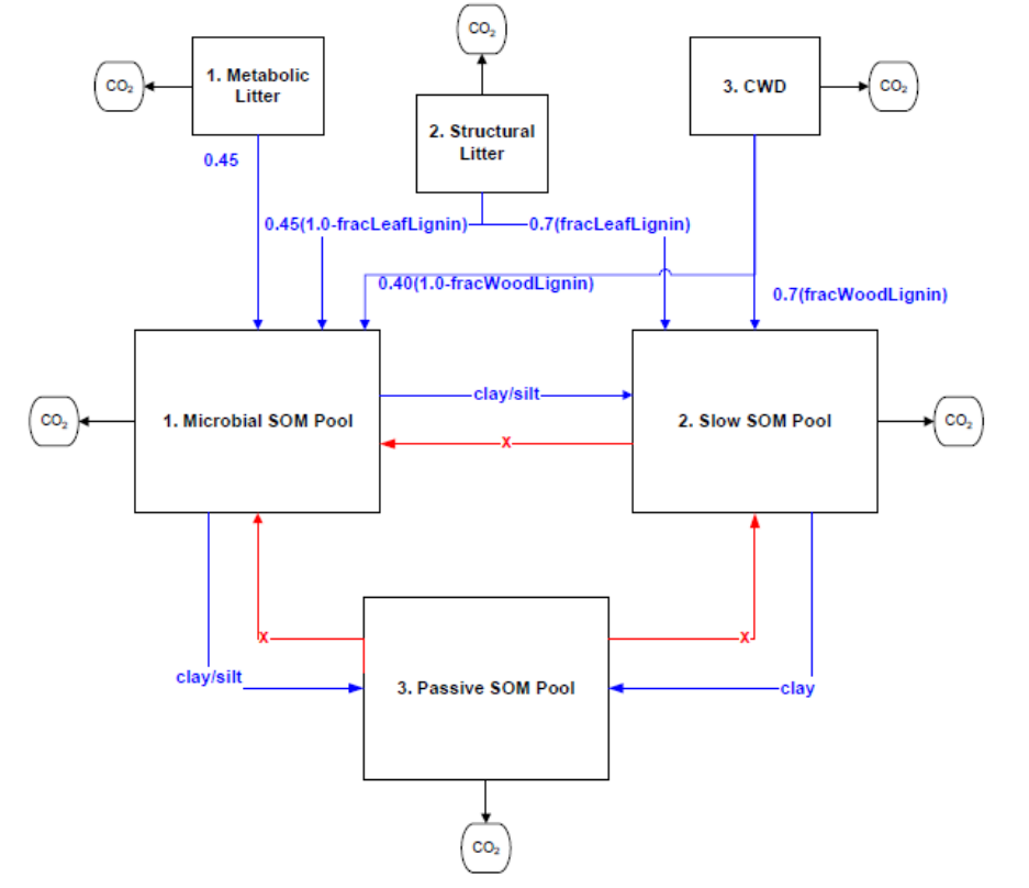
March 1, 2019
47
Figure 3. Litter and Soil Organic Matter Carbon Pools in the CASA-CNP model. All flows out of any litter or soil pool are controlled
by f(T) and f(Ɵ) as well as the lignin/texture controls shown with the blue arrows. The blue text refers to the controls on the
fraction of the total flow that is transferred from one pool to another; 1.0 minus these fractions is the portion of the total flow
that goes to heterotrophic respiration. The red arrows indicate that there is no flow from the Passive SOM pool to the Fast
(Microbial) or Slow SOM pools. See equations below.
3.2.1 Overview of CASA-CNP system of equations for Soil Organic Matter Cycling
The following set of equations summarizes the soil organic matter cycling calculations for CASA-CNP.
More details about the individual inputs and losses to each pool can be found in sections below. Biome-
specific parameters are indicted with “PFT” in parentheses, and these parameters are usually found in
the pftlookup_igbp.csv file. CASA-CNP operates at a daily timestep. Each flow into a soil organic matter
pools has a corresponding heterotrophic respiration flux, except for the passive pool.
March 1, 2019
48
, , ,
, , ,
/
mic metbc mic struc mic cwd
mic metbc mic struc mic cwd
mic C C C
CO2Resp CO2Resp CO2Resp
dC dt +
−
= +
−−
, , ,
, , ,
/
slow slow struc slow cwd slow mic
slow struc slow cwd slow mic
C C C
CO2Resp CO2Resp CO
d
2Resp
C dt ++
−
=
−−
,,
/
pass pass mic pass slow pass
C C CO2RespdC dt +−=
Cmic – microbial (fast) soil organic matter pools (g C m-2)
Cslow – slow soil organic matter pools (g C m-2)
Cpass – passive soil organic matter pools (g C m-2)
Cdestination,source – flow of C from source pool to destination pool (g C m-2 day-1)
CO2Respdestination,source – heterotrophic respiration loss when C flows from source pool to destination pool
(g C m-2 day-1)
3.2.2 Partitioning of plant litter inputs into structural and metabolic litter in CASA-CNP
The Lignin:N ratio (g lignin / g N) of plant biomass is used to partition leaf and fine root litter into
structural and metabolic components. When running CASA-CNP in carbon-only mode, the initial C:N
ratio parameters along with lignin fractions are used to compute lignin:N ratios (Table 8). For plant part i
=leaf, wood, and froot, the lignin:N ratios are the product of the lignin fraction and the C:N ratio:
, , ,
: :
i pft i pft i pft
Lignin N ligninFraction C N ratio=
Table 8. Initial C:N ratios and lignin content of plant parts by plant functional type (PFT). These parameters can be found in the
pftlookup_igbp.csv parameter file.

March 1, 2019
49
vegtype
C:N leaf
C:N wood
C:N froot
lignin leaf
lignin CWD
lignin froot
(PFT)
gC/gN
gC/gN
gC/gN
g lignin /gC
g lignin /gC
g lignin /gC
1
50
250
78
0.25
0.4
0.25
2
25
150
68
0.2
0.4
0.2
3
60
250
41
0.2
0.4
0.2
4
50
175
41
0.2
0.4
0.2
5
50
175
41
0.22
0.4
0.22
6
45
150
41
0.2
0.4
0.2
7
40
150
41
0.2
0.4
0.2
8
25
150
41
0.15
0.4
0.15
9
25
150
41
0.15
0.4
0.15
10
50
150
41
0.1
0.4
0.1
11
30
150
41
0.15
0.4
0.15
12
50
125
41
0.2
0.4
0.2
13
40
150
41
0.15
0.4
0.15
14
30
125
41
0.1
0.4
0.1
15
40
150
41
0.1
0.4
0.1
16
40
150
41
0.15
0.4
0.15
17
40
135
41
0.25
0.4
0.25
18
47.6
150
41
0.166
0.4
0.166
The fraction of leaf and fine root litter allocation to metabolic litter (fracC, 0.0 – 0.85) increases with the
ratio of lignin:N of the plant residue. The remaining fraction is allocated to structural litter (Figure 4).
This partitioning is used by CASA-CNP and CORPSE SOM models. See also “Partitioning of plant litter
inputs in MIMICS”.
( )
( )
( )
( )
max 0.001, 0.85 0.018
max 0.001, 0.85 0.018
1.0
1.0
leaf metb
froot metb
leaf struc leaf metb
froot struc froot metb
w
fracC ratioLignintoN leaf
fracC ratioLignintoN froot
fracC fracC
fracC fracC
fracC
−
−
− −
− −
= −
= −
=−
=−
1.0
ood cwd− =
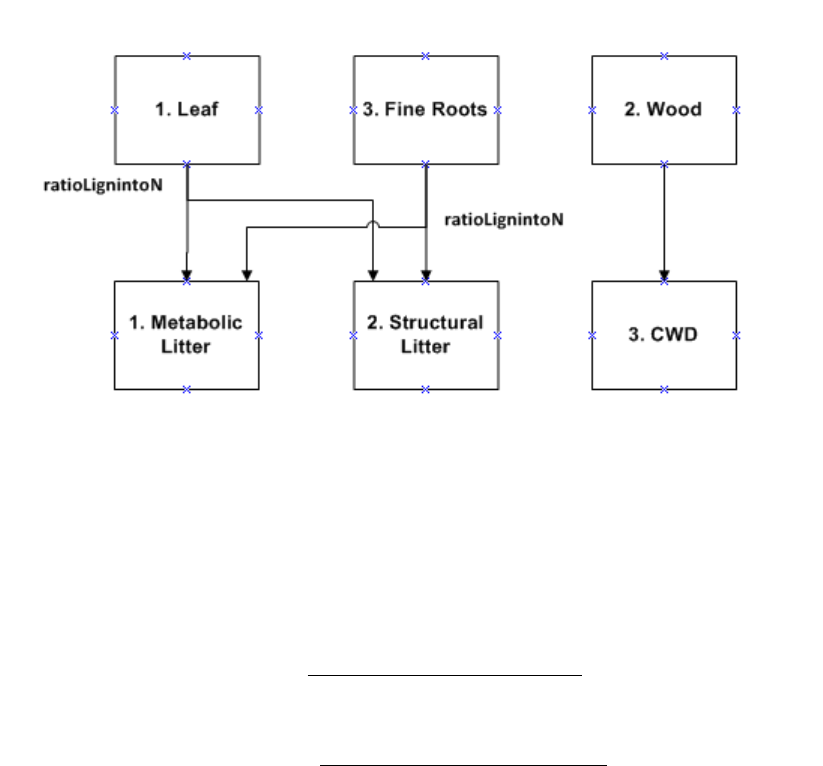
March 1, 2019
50
Figure 4. CASA-CNP plant litter transfers to the metabolic and structural litter pools
The lignin:N ratios are computed from plant C and N pools and biome-specific (PFT) parameters. When
CASA-CNP is run in carbon-only model, plant N pools are determined from fixed biome-specific N:C
ratios.
( ) ( )
( )
,
,
fracLigninplant PFT leaf
ratioLignintoN leaf ratioNCplant PFT np
=
( ) ( )
( )
,
,
fracLigninplant PFT froot
ratioLignintoN froot ratioNCplant PFT froot
=
Where:
fracLigninplant(PFT,*) – biome-specific lignin:N ratio (g lignin / g N)
ratioNCplant(PFT,*) – biome-specific fraction of N:C ratios
Metabolic litter → Fast SOM

March 1, 2019
51
( ) ( )
( )
,0.45
1
365 ( )
mic metbc
age
C xkoptlitter PFT xktemp xkwater
METBC
metbc PFT
=
( ) ( )
( )
,1.0 0.45
1
365 ( )
2 mic metbc
age
CO Resp xkoptlitter PFT xktemp xkwater
METBC
metbc PFT
= −
Structural litter → Fast SOM
( )
( )
( )
( )
,0.45 1.0 ,
1
365 ( )
mic struc
age
C fracLigninplant PFT leaf
xkoptlitter PFT xktemp xkwater STRUC
struc PFT
=−
( )
( )
( )
( )
,1.0 0.45 1.0 ,
1
365 ( )
2 mic struc
age
CO Resp fracLigninplant PFT leaf
xkoptlitter PFT xktemp xkwater STRUC
struc PFT
= − −
Structural litter → Slow SOM
( )
( )
( )
,0.7 ,
1
365 ( )
slow struc
age
C fracLigninplant PFT leaf
xkoptlitter PFT xktemp xkwater
STRUC
struc PFT
=
( )
( )
( )
,1.0 0.7 ,
1
365 ( )
2 slow struc
age
CO Resp fracLigninplant PFT leaf
xkoptlitter PFT xktemp xkwater
STRUC
struc PFT
=−

March 1, 2019
52
Coarse Woody Debris (CWD) → Fast SOM
( )
( )
( )
( )
, 0.40 1.0 ,
1
365 ( )
mic cwd
age
C fracLigninplant PFT wood
xkoptlitter PFT xktemp xkwater
CWD
CWD PFT
=−
( )
( )
( )
( )
, 1.0 0.40 1.0 ,
1
365 ( )
2 mic cwd
age
CO Resp fracLigninplant PFT wood
xkoptlitter PFT xktemp xkwater
CWD
CWD PFT
= − −
Coarse Woody Debris (CWD) → Slow SOM
( )
( )
( )
, 0.7 ,
1
365 ( )
slow cwd
age
C fracLigninplant PFT wood
xkoptlitter PFT xktemp xkwater
CWD
CWD PFT
=
( )
( )
( )
, 1.0 0.7 ,
1*
365 ( )
2 slow cwd
age
CO Resp fracLigninplant PFT wood
xkoptlitter PFT xktemp xkwater
CWD
CWD PFT
=−
Fast SOM → Slow SOM

March 1, 2019
53
( )
( )
( )
( )
( )
,0.85 0.68 0.997 0.032
1
365 ( )
slow mic
mic
age
C clay silt clay
xkoptsoil PFT xktemp xkwater C
MIC PFT
= − + −
( )
( )
( )
( )
( )
,1.0 0.85 0.68 0.997 0.032
1
365 ( )
2 slow mic
mic
age
CO Resp clay silt clay
xkoptsoil PFT xktemp xkwater C
MIC PFT
= − − + −
Fast SOM → Passive SOM
( )
( )
( )
( )
( )
,0.85 0.68 0.003 0.032
1
365 ( )
pass mic
mic
age
C clay silt clay
xkoptsoil PFT xktemp xkwater C
MIC PFT
= − + +
( )
( )
( )
( )
( )
,1.0 0.85 0.68 0.003 0.032
1
365 ( )
2 pass mic
mic
age
CO Resp clay silt clay
xkoptsoil PFT xktemp xkwater C
MIC PFT
= − − + +
Slow SOM → Passive SOM
( )
( )
( )
0.45 0.003 0.009
*
1*
365 ( )
pass,slow
slow
age
C clay
xkoptsoil PFT xktemp xkwater
C
SLOW PFT
=+

March 1, 2019
54
( )
( )
( )
1.0 0.45 0.003 0.009
1
365 ( )
2 pass,slow
slow
age
CO Resp clay
xkoptsoil PFT xktemp xkwater
C
SLOW PFT
= − +
Passive Pool Decomposition
( )
( )
1
365 ( )
2 pass
pass
age
CO Resp xkoptsoil PFT xktemp xkwater
C
PASS PFT
=
3.2.3 CASA-CNP Temperature and Moisture Controls on Decomposition of Litter and SOM
The decomposition of litter or SOM pools is a first order equation. The maximum decomposition rate
(1/pool age) (yr-1) is multiplied by the following factors:
( )
xklitter xkoptlitter PFT xktemp xkwater=
( )
xksoil xkoptsoil PFT xktemp xkwater=
where xkoptlitter(PFT) and xkoptsoil(PFT) are the biome-specific decomposition rate modifiers for litter
and soil, respectively; xktemp is the soil temperature effect on decomposition (0.0-2.0), and xkwater is
the effect of soil moisture (0.0-1.0). In CASA-CNP cropland PFTs have no moisture limitation on soil
organic matter decomposition (xkwater=1.0) and daily turnover rates for the fast, slow, and passive
pools are multiplied by 1.25, 1.5, and 1.5, respectively, to represent increased decomposition rates with
cultivation.
3.2.3.1 CASA-CNP Temperature Controls on Decomposition
The Q10 of the soil temperature function is a biome-specific input, set to 1.72 for all biomes. The value
tsavg is the average soil temperature from the surface to the bottom of the rooting zone (50 – 150 cm)
(K) (Figure 5).
( )
( )
,
0.1 35.0
10 soil
tsavg TKzeroC
xktemp Q PFT −−
=

March 1, 2019
55
Figure 5. CASA-CNP soil temperature effect on Soil Organic Matter decomposition (xktemp).
3.2.3.2 CASA-CNP Soil Moisture Controls on Decomposition
wfpscoefa = 0.55 ! Kelly et al. (2000) JGR, Figure 2b), optimal wfps
wfpscoefb = 1.70 ! Kelly et al. (2000) JGR, Figure 2b)
wfpscoefc = -0.007 ! Kelly et al. (2000) JGR, Figure 2b)
wfpscoefd = 3.22 ! Kelly et al. (2000) JGR, Figure 2b)
wfpscoefe = 6.6481 ! =wfpscoefd*(wfpscoefb-wfpscoefa)/(wfpscoefa-wfpscoefc)
fwps is soil moisture expressed as the fraction of water filled pore space (0.0 – 1.0) (Figure 6).
moistavg
fwps ssat
=
non-cropland
1.0, cropland
,
wfpscoefe wfpscoefd
fwps wfpscoefb fwps wfpscoefc
xkwater wfpscoefa wfpscoefb wfpscoefa wfpscoefc
−−
=−−
0
0.5
1
1.5
2
2.5
-45 -40 -35 -30 -25 -20 -15 -10 -5 0 5 10 15 20 25 30 35 40 45 50 55
soil temperature (deg C)
CASA-CNP soil temperature effect on decomposition
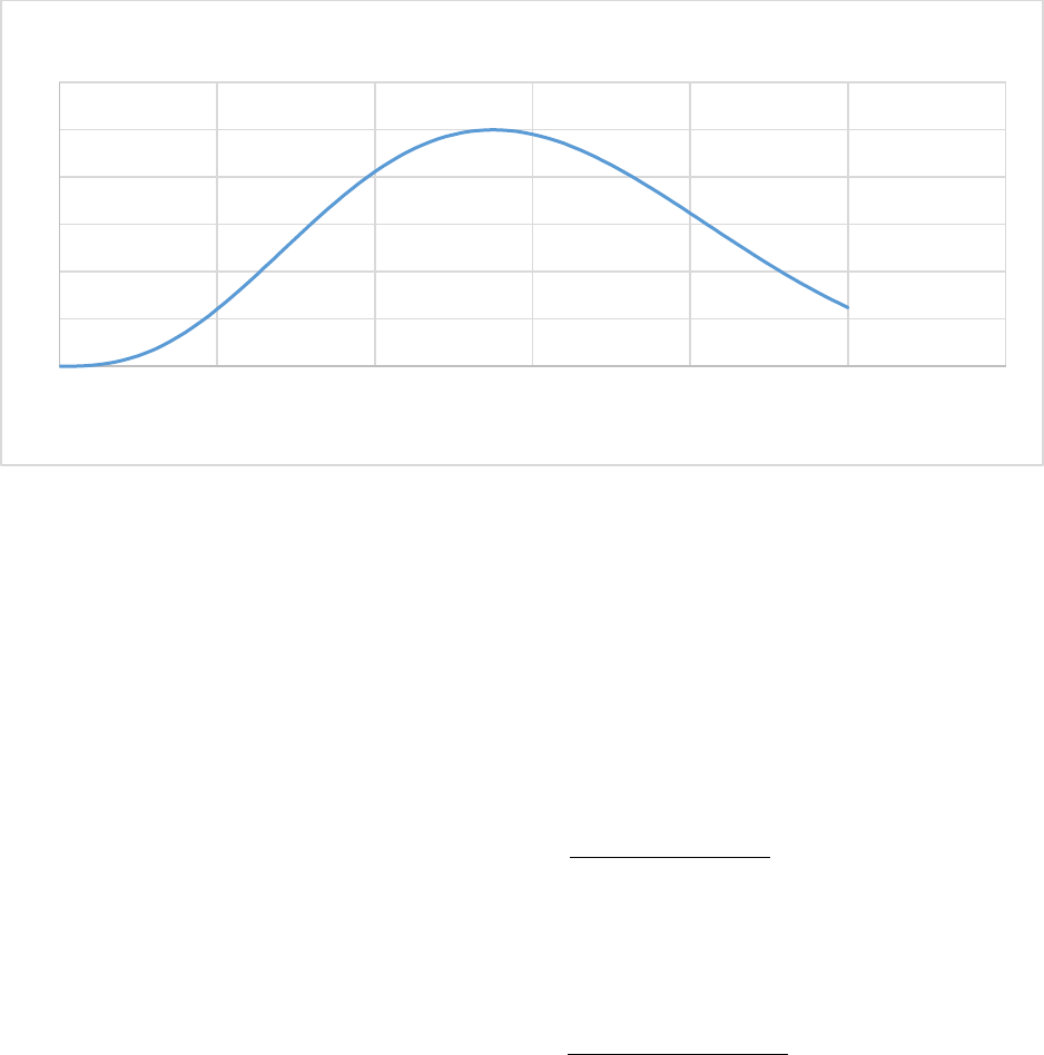
March 1, 2019
56
Figure 6. CASA-CNP soil moisture effect on SOM decomposition (xkwater).
3.2.4 Carbon Stabilization and Destabilization in CASA-CNP
Protected C resides in the Passive SOM pool. The flow of C from the Fast and Slow pools to the Passive
pool is a function of silt and clay (Figure 7).
( )
( )
( )
( )
( )
0.85 0.68 0.003 0.032
1
365 ( )
mic pass
mic
age
C clay silt clay
xkoptsoil PFT xktemp xkwater C
MIC PFT
− = − + +
( )
( )
( )
0.45 0.003 0.009
1
*
365 ( )
slow pass
slow
age
C clay
xkoptsoil PFT xktemp xkwater C
SLOW PFT
− =+
All carbon from the decomposition of the Passive SOM pool is lost as CO2. The intrinsic rate of
decomposition of the passive pool is a biome-specific constant.
0
0.2
0.4
0.6
0.8
1
1.2
0 0.2 0.4 0.6 0.8 1 1.2
Fraction of Soil Water Saturation
CASA-CNP soil moisture effect on decomposition
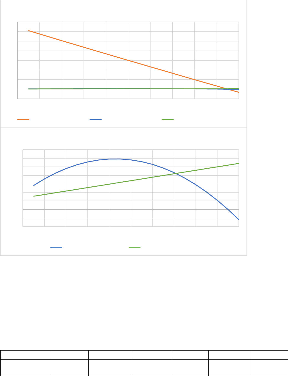
March 1, 2019
57
Figure 7. The effect of soil clay content (% weight) on the fraction of flows between soil organic matter pools.The silt fraction
was held at a constant 30%.The lower figure is a zoomed in version of the top figure.
3.3 CASA-CNP Soil Layer Structure
CASA-CNP defines six soil layers with increasing thicknesses with depth (Table 9). These layer
thicknesses are defined internally and cannot be reset outside of the code.
Table 9. CASA-CNP Soil Layer Structure
Layer Number
1
2
3
4
5
6
Layer Thickness
(m)
0.022
0.058
0.154
0.409
1.085
2.872
-0.1
0
0.1
0.2
0.3
0.4
0.5
0.6
0.7
0 0.1 0.2 0.3 0.4 0.5 0.6 0.7 0.8 0.9 1
fraction of clay
Silt=30%
FracFromStoS(mic->slow) FracFromStoS(mic->pass) FracFromStoS(slow->pass)
-0.002
-0.001
0
0.001
0.002
0.003
0.004
0.005
0.006
0.007
0 0.1 0.2 0.3 0.4 0.5 0.6 0.7 0.8 0.9 1
fraction of clay
Silt=30%
FracFromStoS(mic->pass) FracFromStoS(slow->pass)

March 1, 2019
58
depthsoila (m)
0.000
0.022
0.080
0.234
0.643
1.728
depthsoilb (m)
0.022
0.080
0.234
0.643
1.728
4.600
3.3.1 Mapping of CLM 4.5 soil layers to CASA-CNP soil layers
The casa testbed was developed using CLM 4.5 data. More recent versions of CLM have a different soil
layer structure (see the section below). In order to compute soil moisture and soil temperature for each
of the six CASA-CNP soil layers, the six CASA-CNP soil layers were mapped to ten CLM 4.5 soil layers as
shown in the tables below, based on the lower depth of each soil layer. Soil moisture and soil
temperature of CASA-CNP were the weighted average of the corresponding values in the CLM layers:
CASA-CNP layer 1 to CLM 4.5 layer 1
CASA-CNP layer 2 to CLM 4.5 layers 2 and 3
CASA-CNP layer 3 to CLM 4.5 layers 4 and 5
CASA-CNP layer 4 to CLM 4.5 layers 6 and 7
CASA-CNP layer 5 to CLM 4.5 layers 8 and 9
CASA-CNP layer 6 to CLM 4.5 layer 10
CLM
layer #
z (center
of layer,
m)
∆z (m)
∆z
(cm)
upper
depth
(cm)
lower
depth
(cm)
1
0.0071
0.0175
1.75
0
1.75
2
0.0279
0.0276
2.76
1.75
4.51
3
0.0623
0.0455
4.55
4.51
9.06
4
0.1189
0.075
7.5
9.06
16.56
5
0.2122
0.1236
12.36
16.56
28.92
6
0.3661
0.2038
20.38
28.92
49.3
7
0.6198
0.336
33.6
49.3
82.9
8
1.038
0.5539
55.39
82.9
138.29
9
1.7276
0.9133
91.33
138.29
229.62
10
2.8646
1.137
113.7
229.62
343.32
CASA-
CNP
layer #
∆z (m)
∆z (cm)
upper
depth
(cm)
lower
depth
(cm)
z
(center
of
layer,
cm)
1
0.022
2.2
0
2.2
1.1
2
0.058
5.8
2.2
8
5.1
3
0.154
15.4
8
23.4
15.7
4
0.409
40.9
23.4
64.3
43.85
5
1.085
108.5
64.3
172.8
118.55
6
2.872
287.2
172.8
460
316.4
3.3.2 Mapping of CLM 5.0 soil layers to CASA-CNP soil layers
CLM 5 has a very different soil layer structure than CLM 4.5 (see previous section). To compute soil
moisture and soil temperature for each of the six CASA-CNP soil layers, the six CASA-CNP soil layers were
mapped to twenty-five CLM 5.0 soil layers as shown in the tables below, based on the lower depth of

March 1, 2019
59
each soil layer. Soil moisture and soil temperature of CASA-CNP were the weighted average of the
corresponding values in the CLM layers:
CASA-CNP layer 1 to CLM 5 layers 1 to 1
CASA-CNP layer 2 to CLM 5 layers 2 to 3
CASA-CNP layer 3 to CLM 5 layers 4 to 5
CASA-CNP layer 4 to CLM 5 layers 6 to 7
CASA-CNP layer 5 to CLM 5 layers 8 to 11
CASA-CNP layer 6 to CLM 5 layer 12 to 16
lyr
CLM5
levgrnd
z (center
of layer,
m)
∆z (m)
upper
depth
(cm)
lower
depth
(cm)
∆z (cm)
thickness
aggregate
layer (cm)
z center
of
aggregate
layer (cm)
1
0.01
0.01
0.025
0
2.5
2.50
2.50
1.25
2
0.04
0.04
0.04
2.5
6.5
4.00
3
0.09
0.09
0.06
6.5
12.5
6.00
10.00
7.5
4
0.16
0.16
0.085
12.5
21
8.50
5
0.26
0.26
0.12
21
33
12.00
20.50
22.75
6
0.40
0.4
0.16
33
49
16.00
7
0.58
0.58
0.2
49
69
20.00
36.00
51.00
8
0.80
0.8
0.24
69
93
24.00
9
1.06
1.06
0.28
93
121
28.00
10
1.36
1.36
0.32
121
153
32.00
11
1.70
1.7
0.36
153
189
36.00
120.00
129
12
2.08
2.08
0.4
189
229
40.00
13
2.50
2.5
0.455
229
274.5
45.50
14
2.99
2.99
0.54
274.5
328.5
54.00
15
3.58
3.58
0.64
328.5
392.5
64.00
16
4.27
4.27
0.74
392.5
466.5
74.00
277.50
327.75
17
5.06
5.06
0.84
466.5
550.5
84.00
18
5.95
5.95
0.94
550.5
644.5
94.00
19
6.94
6.94
1.04
644.5
748.5
104.00
20
8.03
8.03
1.4275
748.5
891.25
142.75
21
9.795
9.795
2.648885
891.25
1156.139
264.89
22
13.33
13.32777
4.844065
1156.139
1640.545
484.41
23
19.48313
19.48313
7.771475
1640.545
2417.693
777.15
24
28.87072
28.87072
11.25766
2417.693
3543.458
1125.77
25
41.99844
41.99844
6.56386
3543.458
4199.844
656.39
3733.34

March 1, 2019
60
CASA-
CNP
layer #
∆z (m)
∆z (cm)
upper
depth
(cm)
lower
depth
(cm)
z
(center
of
layer,
cm)
1
0.022
2.2
0
2.2
1.1
2
0.058
5.8
2.2
8
5.1
3
0.154
15.4
8
23.4
15.7
4
0.409
40.9
23.4
64.3
43.85
5
1.085
108.5
64.3
172.8
118.55
6
2.872
287.2
172.8
460
316.4
3.3.3 Fraction of root biomass in each CASA-CNP soil layer
The fraction of root biomass in each of six soil layers (ns=1..6) is determined from three biome-specific
parameters and the following equations (Table 10, Table 11).
( ) ( ) ( )
( )
( )
( ) ( ) ( )
( )
( )
( ) ( ) ( )
( )
( )
1.0 % * %
% * % ,
% * % ,
,
totroot pft exp casabiome kroot casabiome rootdepth pft
exp casabiome kroot min casabiome rootdepth pft depthsoila ns
exp casabiome kroot min casabiome rootdepth pft depthsoilb ns
fracroot pf
pft
pft
p
tft
ns
−= −
−
−−
=
()totroot pft
Table 10. CASA-CNP parameters used to calculate fraction of root in each soil layer
vegtype
Kroot
rootdepth
Krootlen
(PFT)
(1/m)
(m)
(m/g C)
1
5.5
1.5
14.87805
2
3.9
1.5
14.38596
3
5.5
1.5
14.02597
4
3.9
1.5
18.94737
5
2
1.5
16.71642
6
2
0.5
0
7
2
0.5
32.30769
8
2
1.5
120.8
9
2
1.5
120.8
10
5.5
0.5
84
11
5.5
0.5
0
12
5.5
0.5
120.5
13
2
0.5
0
14
5.5
0.5
0
15
5.5
0.5
0

March 1, 2019
61
vegtype
Kroot
rootdepth
Krootlen
(PFT)
(1/m)
(m)
(m/g C)
16
2
0.5
30.76923
17
5.5
1.5
0
18
5.5
0.5
84
Table 11. Fraction of roots in each soil layer by PFT
Vegtype
(PFT)
fracroot(1)
fracroot(2)
fracroot(3)
fracroot(4)
fracroot(5)
fracroot(6)
1
0.11
0.24
0.37
0.25
0.03
0.0
2
0.08
0.19
0.33
0.32
0.08
0.0
3
0.11
0.24
0.37
0.25
0.03
0.0
4
0.08
0.19
0.33
0.32
0.08
0.0
5
0.05
0.11
0.24
0.37
0.24
0.0
6
0.07
0.17
0.36
0.41
0.0
0.0
7
0.07
0.17
0.36
0.41
0.0
0.0
8
0.05
0.11
0.24
0.37
0.24
0.0
9
0.05
0.11
0.24
0.37
0.24
0.0
10
0.12
0.26
0.39
0.23
0.0
0.0
11
0.12
0.26
0.39
0.23
0.0
0.0
12
0.12
0.26
0.39
0.23
0.0
0.0
13
0.07
0.17
0.36
0.41
0.0
0.0
14
0.12
0.26
0.39
0.23
0.0
0.0
15
0.12
0.26
0.39
0.23
0.0
0.0
16
0.07
0.17
0.36
0.41
0.0
0.0
17
0.11
0.24
0.37
0.25
0.03
0.0
18
0.12
0.26
0.39
0.23
0.0
0.0
3.4 MIMICS
MIMICS has two litter pools (Metabolic and Structural), two live microbial biomass pools (r-selected and
K-selected), and three soil organic matter pools (Available, Chemically Protected, and Physically
Protected) (Figure 8). Non-woody plant litter is partitioned into Structural and Metabolic litter pools as a
function of the lignin:N ratio of the plant litter, using a slightly different function that the CASA-CNP
model’s. Decomposing CWD carbon is transferred to the structural litter pool as a function of soil
moisture and temperature, with CO2 respiration loss. The decomposition rates of Metabolic and
Structural litter and Available SOM pools are controlled by reverse Michaelis-Menton kinetics (substrate
limited) and modified by soil temperature controls. The Structural and Metabolic litter pools are
consumed by r-selected and K-selected live microbial pools, with CO2 respiration loss. Microbial
turnover, which is proportional to annual NPP, transfers C to Physically Protected, Chemically Protected,
and Available SOM pools, without CO2 respiration loss. Desorption of the Physically Protected pool, a
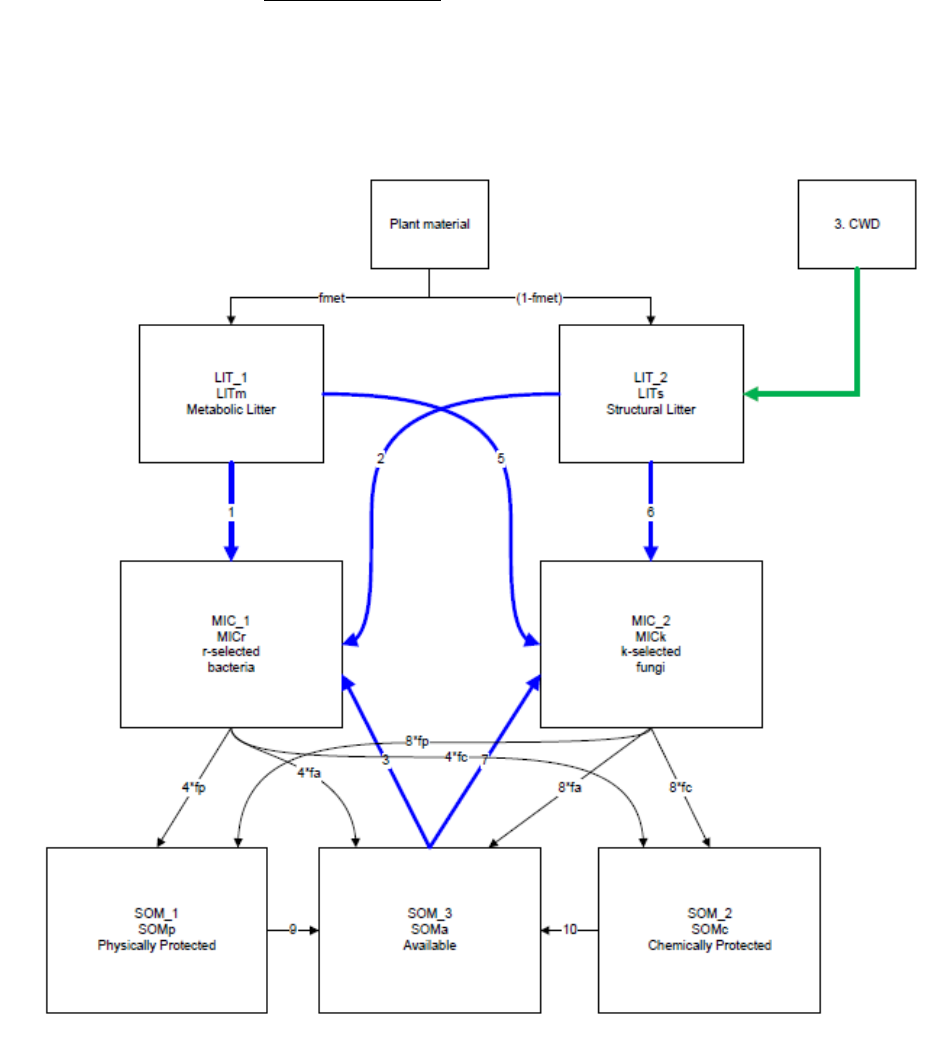
March 1, 2019
62
function of soil clay content, and oxidation of the Chemically Protected pool, transfer C to the Available
pool, without CO2 loss. Carbon in the Available pool is consumed by the two microbial pools, with CO2
respiration loss.
Decomposition of carbon pool (Ci) by microbe pool (MICr/k)
/
/
//
()
rK
rK
r K r K
i i
MIC
CKm T MIC
VmaD x (T)=+
where Vmax(T) is the temperature-sensitive Vmax(T)– temperature sensitive maximum reaction
velocitiy, Km(T) is the temperature-sensitive half-saturation constant.
Figure 8. Litter and Soil Organic Mater pools in the MIMICS model. Heterotrophic respiration losses occur with consumption of
litter and available pools by the microbes, and with the decomposition of the CWD pool.

March 1, 2019
63
3.4.1 Overview of MIMICS system of equations
Hourly changes in MIMICS Litter and SOM pools and heterotrophic respiration losses are summarized as
follows. More details on each equation can be found in the sections below. Within the testbed, MIMICS
operates at an hourly timestep.
( )
/ 1.0 1 3dLITm dt litInput metb Fi metb LITmin LITmin= − − −
( )
( )
3
1
/ 1 1 1 + 2 2 i
dMICr dt MGE LITmin SOMmin MGE LITmin MICtrn i
=
= + −
/ 1 4dSOMp dt litInput metb Fi metb MICtrn MICtrn DEsorb= + + −
( )
/ 1.0 2 4dLITs dt litInput struc Fi struc LITmin LITmin= − − −
( )
( )
6
4
/ 3 3 2 + 4 * 4 i
dMICk dt MGE LITmin SOMmin MGE LITmin MICtrn i
=
= + −
/ 2 5dSOMc dt litInput struc Fi struc MICtrn MICtrn OXIDAT= + + −
/ 3 6 1 2dSOMa dt MICtrn MICtrn DEsorb OXIDAT SOMmin SOMmin= + + + − −
( )
( )
( )
( )
( )
( )
( )
( )
1.0 1 1 1 + 1.0 2 2
1.0 3 3 2 + 1.0 4 4
Rh MGE LITmin SOMmin MGE LITmin
MGE LITmin SOMmin MGE LITmin
= − + −
+ − + −
where:
SOMa – available SOM-C (mg C cm-3)
SOMc – chemically protected SOM-C (mg C cm-3)
SOMp – physically protected SOM-C (mg C cm-3)
LITmin[1..4] – litter C mineralization fluxes (mg C cm-3 hr-1)
MICtrn[1..3] – microbial turnover (mg C cm-3 hr-1)
SOMmin[1..2] – SOM-C mineralization (mg C cm-3 hr-1)
litInput[metb] – litter inputs to metabolic litter (mg C cm-3 hr-1)
litInout[struc] – litter inputs to structural litter (mg C cm-3 hr-1)
Fi[metb] – fraction of metabolic litter inputs transferred to SOMp (0.05), the remainder goes to
the metabolic litter pool.
Fi[struc] – fraction of structural litter inputs transferred to SOMc (0.05), the remainder goes to
the structural litter pool.
MGE[1] – microbial growth efficiency for C fluxes from LITm or SOMa into MICr (0.55, mg mg-1)
MGE[2] – microbial growth efficiency for C fluxes from LITs into MICr (0.25, mg mg-1)
MGE[3] – microbial growth efficiency for C fluxes from LITm or SOMa into MICk (0.75, mg mg-1)
MGE[4] – microbial growth efficiency for C fluxes from LITs into MICk (0.35, mg mg-1)
Rh – total heterotrophic respiration (mg C cm-3 hr-1). Multiple by depth (cm) to get respiration
per unit area.

March 1, 2019
64
3.4.2 Partitioning plant litter to metabolic and structural litter pools in MIMICS
The fraction of plant litter partitioned to metabolic litter ( fmet) is a function the weighted average
lignin:N ratio of all litter inputs (nP=leaf, froot).
( )
, * ( , )
*( , )
()
met
nP
ligninNratio npt nP litterInput npt nP
f = fmetP(1) fmetP(2) fmetP(3)* litterInput npt nP
nP −
where:
fmetP(1) = 0.75 (or as defined in pftlookup_mimics.csv)
fmetP(2) = 0.85 (or as defined in pftlookup_mimics.csv)
fmetP(3) = 0.013 (or as defined in pftlookup_mimics.csv)
The individual flows from pool to pool are summarized below. Variables F1 .. F10 below refer to equations
in Wieder, Grandy et al. (2015).
3.4.3 Flows to and from MICr: consumption and turnover
MICr decomposition of metabolic litter (f1. LITm-->MICr)
1
1
1
1
MICr Vmax r LITm
F LITmin Km r MICr
== +
MICr decomposition of structural litter (f2. LITs-->MICr)
2
2
2
2
MICr Vmax r LITs
F LITmin Km r MICr
== +
MICr turnover to physically protected SOM (f41. MICr-->SOMp)
4.1 11
r
F MICtrn MICr fPHYS
= =
where:
fPHYS[1] – fraction of τr partitioned into SOMp as a function of fclay (0.0 – 1.0)
MICr turnover to chemically protected SOM (f42. MICr-->SOMc)
4.2 21
r
F MICtrn MICr fCHEM
= =
where:
fCHEM[1] – fraction of τr partitioned into SOMc as a function of fmet (0.0 – 1.0)
MICr turnover to available SOM (f43. MICr-->SOMa)

March 1, 2019
65
4.3 31
r
F MICtrn MICr fAVAL
= =
where:
fAVAL[1] –– fraction of τr partitioned into SOMa (0.0 – 1.0)
Decomposition of SOMa by MICr (f3. SOMa-->MICr)
3
3
13
MICr Vmax r SOMa
F SOMmin Km r MICr
== +
3.4.4 Flows to and from MICk: consumption and turnover
MICk decomposition of metabolic litter (f5. LITm -->MICk)
5
1
31
MICk Vmax k LITm
F LITmin Km k MICk
== +
MICk decomposition of structural litter (f6. LITs-->MICk)
6
2
42
MICk Vmax k LITs
F LITmin Km k MICk
== +
MICk turnover to physically protected SOM (f81. MICk-->SOMp)
8.1 4 2
k
F MICtrn MICk fPHYS
= =
where:
fPHYS[2] – fraction of τk partitioned into SOMp as a function of fclay (0.0 – 1.0)
MICk turnover to chemically protected SOM (f82. MICk-->SOMc)
8.2 5 2
k
F MICtrn MICk fCHEM
= =
where:
fCHEM[2] – fraction of τk partitioned into SOMc as a function of fmet (0.0 – 1.0)
MICk turnover to available SOM (f83. MICk->SOMa)
8.3 6 2
k
F MICtrn MICk fAVAL
= =
where:
fAVAL[2] –– fraction of τk partitioned into SOMa (0.0 – 1.0)
Decomposition of SOMa by MICk (f7. SOMa-->MICk)

March 1, 2019
66
7
3
23
MICk Vmax k SOMa
F SOMmin Km k MICk
==+
3.4.5 Desorption of physically protected SOM to available SOM
( )
5
9 1.5*10 exp 1.5 F DEsorb SOMp fclay
−
= = −
3.4.6 Oxidation of SOMc to SOMa
10
22
1 2 2 2
MICr Vmax r SOMc MICk Vmax k SOMc
F OXIDAT KO KM r MICr KO KM k MICk
= = +
+ +
where:
KO[1] – Further modifies Km[r2] for oxidation of SOMc (6.0)
KO[2] – Further modifies Km[k2] for oxidation of SOMc (6.0)
3.4.7 MIMICS Temperature and Moisture Controls on Decomposition of Litter and SOM
In MIMICS, maximum reaction velocities (Vmax) and the Michaelis-Menton half saturation values (Km)
are temperature sensitive. MIMICS has no soil moisture effect on decomposition.
Decomposition is substrate limited (Reverse Michaelis-Menton Kinetics):
/ [ ] /
[ ] /
)
(
r k rk met struc
rk r k
MIC Vmax (T) LIT
Decomposition of litt Km
er pool by microbial p T MI
ol C
o
=+
/ [ ]
[ ] /
SOM ()
r k rk a
rk
a
rk
Decomposition of pool by microbial poo MIC Vmax (T) SOM
Km T C
lMI
=+
Where [rk]=
r1: LITm to MICr flows
r2: LITs to MICr flows
r3: SOMa to MICr flows
k1: LITm to MICk flows
k2: LITs to MICk flows
3.4.7.1 Temperature and moisture sensitive maximum reaction velocities, Vmax(T,Ɵ)

March 1, 2019
67
The MIMICS microbe-specific maximum reaction velocities (Vmax[rk](T,Ɵ), mg C (mg MIC)-1 h-1 ) (Figure 9),
are computed as
( )
[ ] [ ] [ ] [ ]
, exp ( )
[rk] rk soil rk rk rk
Vmax (T ) Vslope T Vint av Vmod f
= +
where:
Tsoil – soil temperature (°C)
Vslope[r1]..Vslope[k3] – 0.063 or as defined in pftlookup_mimics.csv
Vint[r1]..Vint[k3] – 5.47 or as defined in pftlookup_mimics.csv
av[r1]..av[k3] – tuning coefficient (1.25 * 10-8) or as defined in pftlookup_mimics.csv
Vmod[r1]..Vmod[k3] – [10, 2, 10, 3, 3, 2] or as defined in pftlookup_mimics.csv
f(Ɵ) – soil moisture effect on Vmax(T,Ɵ) (0.05-1.0).
The soil moisture effect on Vmax(T,Ɵ) is computed as
( )
3 _
0.05, 1 f
ll
sat sat sat
gas diffusion
fP
= − −
where Ɵl is liquid volumetric soil water content, Ɵf is frozen volumetric soil water content, Ɵsat is
the volumetric soil moisture at saturation, gas_diffusion = 2.5, and P is a scalar (44.247) that sets
the value of the function to a maximum value of 1.0. (This curve is very similar to the one shown
in Figure 15 for CORPSE except that for MIMICS it ranges from 0.05 to 1.0).
3.4.7.1.1 Km(T) – temperature sensitive half saturation constants
The MIMIMCS microbe-specific half saturation constants (Km[rk](T), mg C cm-3) (Figure 10) are computed
as
( )
( ) ( )
( ) ( )
[ ] [ ] [ ] [ ]
[ ] [ ] [ 3] [ ]
[ ] [ ] [ ] [ ]
exp * * /
exp * * / *
exp * * / *
[rk] rk soil rk rk rk
[r3] r3 soil r3 r r3
[k3] k3 soil k3 k3 k3
Km (T) Kslope T Kint ak Kmod
Km (T) Kslope T Kint ak Kmod Pscalar
Km (T) Kslope T Kint ak Kmod Pscalar
=+
=+
=+
where:
Tsoil – soil temperature (°C)
Kslope[r1]..Kslope[k3] – 0.02 or as defined in pftlookup_mimics.csv
Kint[r1]..Kint[k3] – 3.19 or as defined in pftlookup_mimics.csv
ak[r1]..av[k3] – tuning coefficients (0.015625) or as defined in pftlookup_mimics.csv
Kmod[r1]..Kmod[k3] – [8, 2, 4, 2, 4, 6] or as defined in pftlookup_mimics.csv.
Kmod[r3] and Kmod[k3] are multiplied by physical protection scalar (Pscalar, see below).
March 1, 2019
68
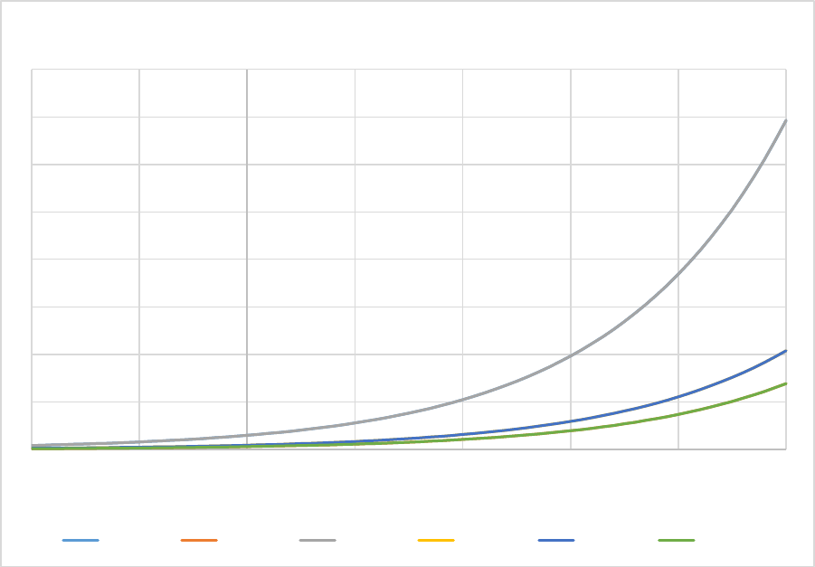
March 1, 2019
69
Figure 9. Temperature sensitive maximum reaction velocities, Vmax(T), for the MIMICS model.
0
0.0001
0.0002
0.0003
0.0004
0.0005
0.0006
0.0007
0.0008
-20 -10 010 20 30 40 50
Soil Temperature (C)
MIMICS Vmax(T)
Vmax_r1 Vmax_r2 Vmax_r3 Vmax_k1 Vmax_k2 Vmax_k3
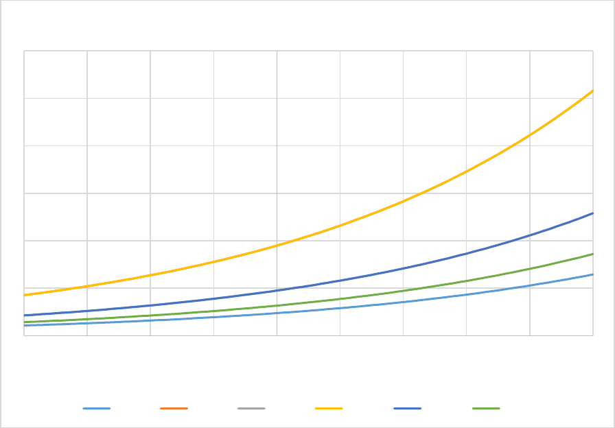
March 1, 2019
70
Figure 10. Temperature sensitive half saturation constants, Km(T), for the MIMICS model.
3.4.8 Microbial Turnover in MIMICS
Microbial biomass turnover rates increase with annual net primary production (NPP).
τr = microbial biomass turnover rate for MICr (hr-1)
τk = microbial biomass turnover rate for MICk (hr-1)
τmod = modifies microbial turnover rate, 0.8 < τmod < 1.2
( ) ( )
( ) ( )
*exp * * *
*exp * * *
met
met
rmod
k mod
tau_r(1) tau_r(2) f f
tau_k(1) tau_k(2) f f
=
=
where:
tau_r(1) = 5.2 * 10-4 (or as defined in pftlookup_mimics.csv)
tau_r(2) = 0.3 (or as defined in pftlookup_mimics.csv)
tau_k(1) = 2.4 * 10-4 (or as defined in pftlookup_mimics.csv)
tau_k(2) = 0.1 (or as defined in pftlookup_mimics.csv)
τmod values changes annually with NPP.
0
0.1
0.2
0.3
0.4
0.5
0.6
-40 -30 -20 -10 010 20 30 40 50
Soil Temperature (C)
MIMICS Km(T)
Km_r1 Km_r2 Km_r3 Km_k1 Km_k2 Km_k3

March 1, 2019
71
f(Ɵ) – soil moisture effect on microbial turnover (0.05-1.0) (see section above titled
“MIMICS Temperature and Moisture Controls on Decomposition of Litter and SOM”).
100
mod NPP
=
where:
NPP – net primary production from the previous growing season (gC m-2 yr-1)
3.4.9 Carbon Stabilization and Destabilization in MIMICS:
Carbon stabilization in the MIMICS model in controlled by clay content and a microbe-specific fPHYS
factor (Figure 11):
τr = microbial biomass turnover rate for MICr (hr-1)
τk = microbial biomass turnover rate for MICk (hr-1)
fPHYS(1) – fraction of τr partitioned into SOMp (0.0 – 1.0)
fPHYS(2) – fraction of τk partitioned into SOMp (0.0 – 1.0)
( )
[1] expfPHYS fPHYSr(1) fPHYSr(2) fclay=
( )
[2] expfPHYS fPHYSk(1) fPHYSk(2) fclay=
where:
fPHYSr(1) = 0.15 (or as defined in pftlookup_mimics.csv)
fPHYSr(2) = 1.3 (or as defined in pftlookup_mimics.csv)
fPHYSk(1) = 0.1 (or as defined in pftlookup_mimics.csv)
fPHYSk(2) = 0.8 (or as defined in pftlookup_mimics.csv)
fclay = fraction of clay in soil (0.0 – 1.0)
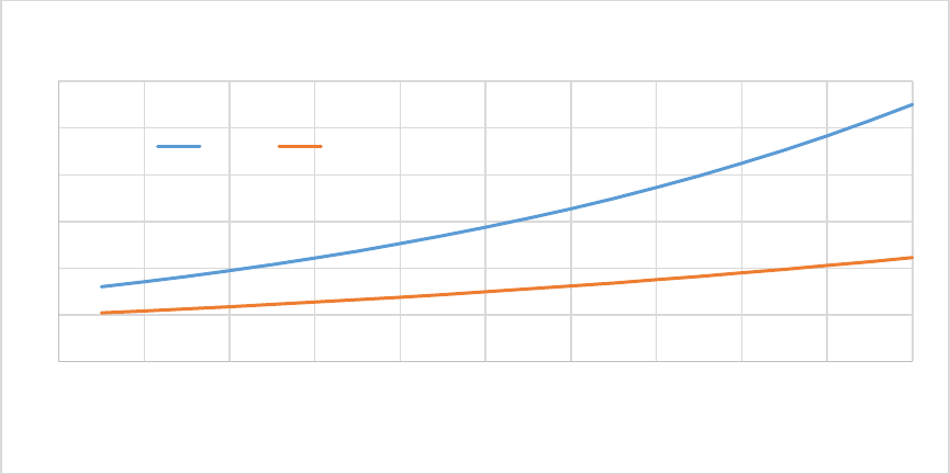
March 1, 2019
72
Figure 11. Fraction of Microbial Turnover to the protected Soil Organic Matter pool in the MIMICS model (fPHYS).
fCHEM(1) – fraction of τr partitioned into SOMc (0.0 – 1.0)
fCHEM(2) – fraction of τk partitioned into SOMc (0.0 – 1.0)
( ) ( )
( )
( )
[1] * 2 31 exp * *fCHEMr ffCHEM fmCHEMr fet CHEMr=
( )
[2] *exp * *fCHEM fCHEMk(1) fCHEMk(2) fmet fCHEMk(3)=
where:
fCHEMr(1) = 0.1 (or as defined in pftlookup_mimics.csv)
fCHEMr(2) = -3.0 (or as defined in pftlookup_mimics.csv)
fCHEMr(3) = 4.0 (or as defined in pftlookup_mimics.csv)
fCHEMk(1) = 0.3 (or as defined in pftlookup_mimics.csv)
fCHEMk(2) = -3.0 (or as defined in pftlookup_mimics.csv)
fCHEMk(3) = 4.0 (or as defined in pftlookup_mimics.csv)
fmet = fraction of plant residue transferred to metabolic litter (0.0 – 1.0)
fAVAL(1) – fraction of τr partitioned into SOMa (0.0 – 1.0)
fAVAL(2) – fraction of τk partitioned into SOMa (0.0 – 1.0)
[1] 1.0 ( [1] [1])fAVAL fPHYS fCHEM= − +
[2] 1.0 ( [2] [2])fAVAL fPHYS fCHEM= − +
As fmet increases, fCHEM[] decreases and fAVAL[] increases.
Desorption of physically protected SOM to available SOM (hr-1)
0
0.1
0.2
0.3
0.4
0.5
0.6
0 0.1 0.2 0.3 0.4 0.5 0.6 0.7 0.8 0.9 1
fraction of clay
Fraction of Microbial Turnover to Protected SOM (fPHYS)
fPHYSr fPHYSk

March 1, 2019
73
( ) ( )
( )
__exp 21fSOM p fSODEsorb SOMp cM ap f l y=
fSOM_p(1) = 1.0 X 10⁻⁵ (or as defined in pftlookup_mimics.csv)
fSOM_p(2)= -2.0 (or as defined in pftlookup_mimics.csv)
Oxidation of SOMc to SOMa
22
1 2 2 2
MICr Vmax r SOMc MICk Vmax k SOMc
OXIDAT KO KM r MICr KO KM k MICk
=+
+ +
where:
KO[1] – Further modifies Km[r2] for oxidation of SOMc (6.0)
KO[2] – Further modifies Km[k2] for oxidation of SOMc (6.0)
Microbial consumption of SOMa
Microbial consumption of the available SOM pool is reduced with the soil clay fraction (Figure 12):
Kmod[r3] – modifies Km[r3] for fluxes from SOMa to MICr (*Pscalar)
Kmod[k3] – modifies Km[k3] for fluxes from SOMa to MICk (*Pscalar)
Pscalar(npt) – physical protection scalar used in Kmod[r3] and Kmod[k3].
( )
[1] exp [2]P physScalar physScalar fclay
scalar =
where:
fclay = soil%clay(npt) – fraction of clay in soil (0.0 – 1.0)
physScalar[1] = 3.0 (or as defined in pftlookup_mimics.csv)
physScalar[2] = -2.0 (or as defined in pftlookup_mimics.csv)
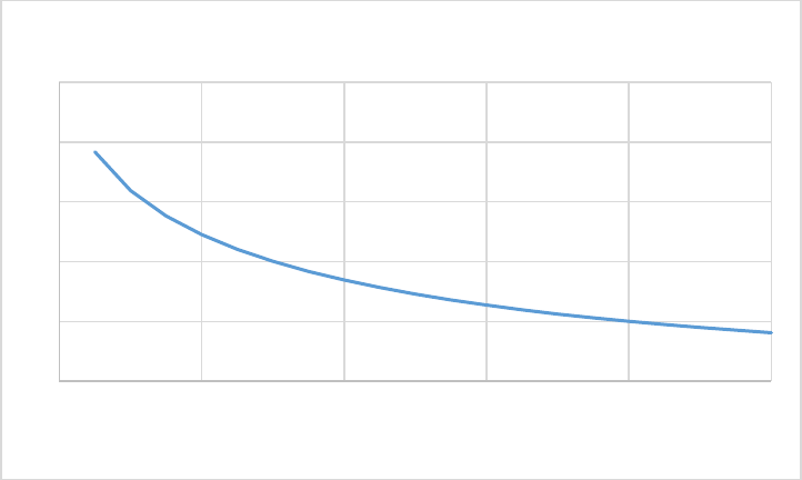
March 1, 2019
74
Figure 12. MIMICS physical protection scalar (Pscalar). The scalar modifies fluxes from available SOM to microbial pools.
3.5 CORPSE
CORPSE has separate surface litter layer pools and soil layer pools, each with three carbon species
(labile, recalcitrant, and dead microbes) and a live microbial biomass pool (Figure 13). The surface litter
pools are unprotected while the soil carbon pools have unprotected and protected counterparts. Leaf
litter is partitioned into Structural and Metabolic material as a function of the lignin:N ratio of the leaf
litter. Metabolic leaf litter is transferred to the Labile surface litter pool and structural leaf litter is
transferred to the Recalcitrant surface litter pool. Similarly, root litter is partitioned into Structural and
Metabolic material as a function of its lignin:N ratio. Metabolic root litter is transferred to the Labile soil
pool and Structural root litter is transferred to the Recalcitrant soil pool. Root exudates also contribute
to the Labile soil pool. Carbon from the decomposing CWD pool is transferred to the Recalcitrant litter
pool, with CO2 respiration loss. The decomposition of unprotected labile, recalcitrant, and dead microbe
litter and SOM pools are controlled by microbial biomass and modified by soil temperature and
moisture controls. The model assumes that the microbial biomass limitation on decomposition is related to
the microbial biomass as a fraction of total carbon. When microbial biomass is much larger than 1% of total
carbon microbes decompose the substrate at their maximum rate, similar to a first-order model. If microbial
biomass is very low, then decomposition rate at any temperature will also be very low. Microbial turnover,
which is proportional to a fixed turnover rate, transfers C to the unprotected dead microbes pool, with
CO2 respiration loss. Microbial death transfers C to the unprotected dead microbes pool, also with CO2
respiration loss. Carbon transfers from the unprotected soil pools to their protected counterparts is a
function of clay and soil porosity (Qmax) and the base protection rate, without CO2 respiration losses.
Loss of protected carbon is proportional to a fixed turnover rate. No carbon is transferred from the
surface litter layer to the soil layer.
0
0.5
1
1.5
2
2.5
0 0.2 0.4 0.6 0.8 1
fraction clay
Pscalar
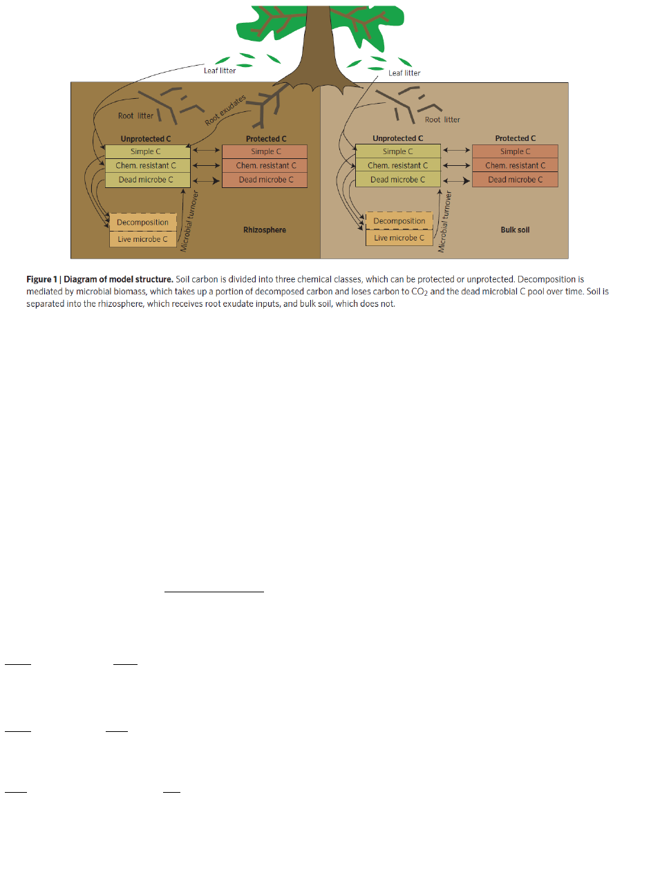
March 1, 2019
75
Figure 13. CORPSE model litter and soil organic matter pools (from Sulman et al. 2014).
3.5.1 Overview of CORPSE system of equations
The following equations summarizes the inputs and outputs from the CORPSE litter and soil pools. More
details on each equation can be found in the sections below. The litter layer contains three unprotected
pools (labile, recalcitrant, and dead microbe) and a live microbial pool. A soil layer contains a live
microbial pool and three unprotected pools (labile, recalcitrant, and dead microbe) and three protected
pools (labile, recalcitrant, and dead microbe) and is portioned into rhizosphere and bulk soil fractions.
Within the CASA-CNP testbed, CORPSE operates at a daily timestep, there is one soil layer defined, and
the litter layer is optional.
( )
,3
1
()
i max i i
ij
j
M
D V T f C
kC C M
=
=
+
ii
imic
dM M
D
dt
=−
ii
ii
dC dP
ID
dt dt
= − −
ii
ii
p
dP P
C Qmax
dt
= −
Di – heterotrophic respiration flux from unprotected pool Ci where i = {labile, recalcitrant, dead microbe}
(kg C m-2 day-1)

March 1, 2019
76
Vmax,i(T) – temperature-dependent maximum enzymatic conversion rate (yr-1)
gas_diffusion = 2.5 (or as defined in corpse_params.nml)
kCi = 1% (or as defined in corpse_params.nml) where i = {labile, recalcitrant, dead microbe}
M – microbial biomass pool (kg C m-2)
εi – microbial uptake efficiency for each pool where i = {labile, recalcitrant, dead microbe} (0.0 – 1.0)
τmic – average turnover rate of the microbial biomass pool (0.25 yr-1)
Ci – unprotected pool where i = {labile, recalcitrant, dead microbe} (kg C m-2)
Ii – inputs into the unprotected pool where i = {labile, recalcitrant, dead microbe} (kg C m-2 day-1)
Pi – protected pool where i = {labile, recalcitrant, dead microbe} (kg C m-2)
Qmax – function of clay and soil porosity (kg C m-3)
Ƭp – residence time of the protected pool (45 years)
ɤ – protection rate of the protected pool (1.5 yr-1)
αi – species-specific multiplier on the protection rate, where i = {0.11, 0.002, and 1.0 for the labile,
recalcitrant, and dead microbe pools, respectively}
f(Ɵ) – the soil moisture effect on soil organic matter decomposition (see section below titled “CORPSE
Soil Moisture Controls on Decomposition of Litter and SOM”)
3.5.2 Heterotrophic Respiration in CORPSE
Decomposition (heterotrophic respiration flux) (Di) of unprotected carbon pool (Ci) by microbe pool (M)
( )
,3
1
()
i max i i
j
j
M
D V T f C
kC C M
=
=
+
where Vmax,i(T) is the temperature-dependent maximum enzymatic conversion rate, f(Ɵ) is the soil
moisture effect on soil organic matter decomposition (see section below titled “CORPSE Soil Moisture
Controls on Decomposition of Litter and SOM”, and kC is 1% (or as define in the corpse_params.nml
file). The rate of change in the unprotected carbon pool is defined as
ii
ii
dC dP
ID
dt dt
= − −
where Ii is the carbon input rate to the pool and Pi is the protected carbon pool for each species. For the
labile pool, Ii comes from metabolic litter inputs. For the recalcitrant pool, Ii comes from structural litter
inputs. For the dead microbe pool, Ii comes from microbial turnover. See the CASA-CNP section titled
“Partitioning of plant litter inputs into structural and metabolic litter in CASA-CNP” for more
information on the portioning of litter into metabolic and structural material.
3.5.3 CORPSE Temperature and Moisture Controls on Decomposition of Litter and SOM
3.5.3.1 CORPSE Temperature Controls on Decomposition of Litter and SOM
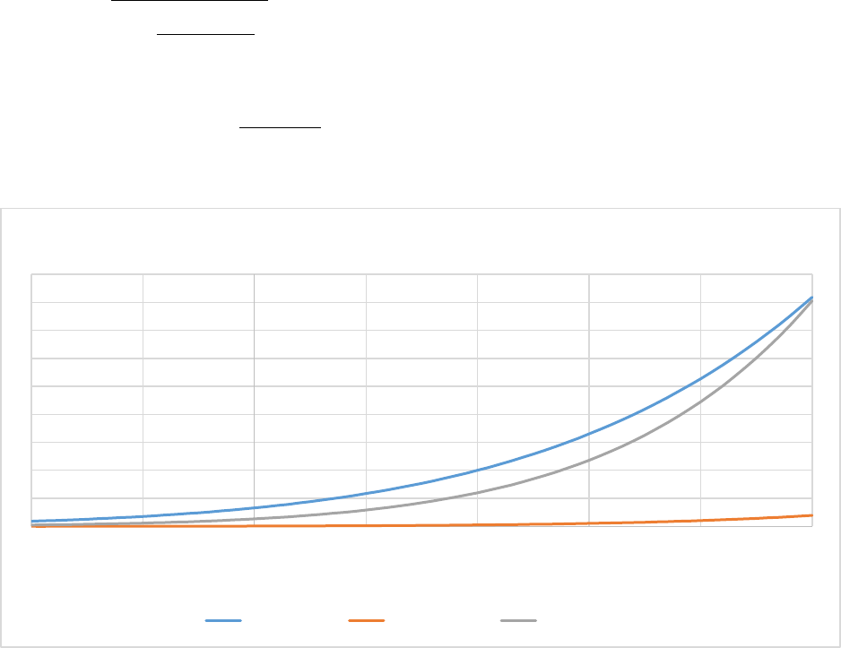
March 1, 2019
77
The decomposition rates of unprotected soil pools are determined by a temperature-dependent
maximum enzymatic conversion rate Vmax,i(T) (yr-1) (Figure 14), where T is the soil temperature (K), Tref is
the reference soil temperature (293.7 K), Vmax,ref,i is the reference Vmax for the species (4500e0, 25e0,
600e0, yr-1), Rugas is the ideal gas constant (8.314472 J-K-1 mol-1), Eαi is the activation energy for the
species (5, 30, 3, kJ mol-1 for labile, recalcitrant, and dead microbe pools, respectively).
,,max ref i
i
i
ref
V
Ea
exp Rugas T
=−
( )
,i
max i i
Ea
V T exp Rugas T
−
=
Figure 14. The temperature-dependent maximum enzymatic conversion rate Vmax,i(T) (yr-1) in the CORPSE model.
3.5.3.2 CORPSE Soil Moisture Controls on Decomposition of Litter and SOM
The soil moisture effect on decomposition of soil organic matter in the CORPSE model (Figure 15) is
defined as:
0
500
1000
1500
2000
2500
3000
3500
4000
4500
-20 -10 010 20 30 40 50
Soil Temperature (°C)
Vmax,i(T) CORPSE
Vmax_labile Vmax_recalct Vmax_deadMic
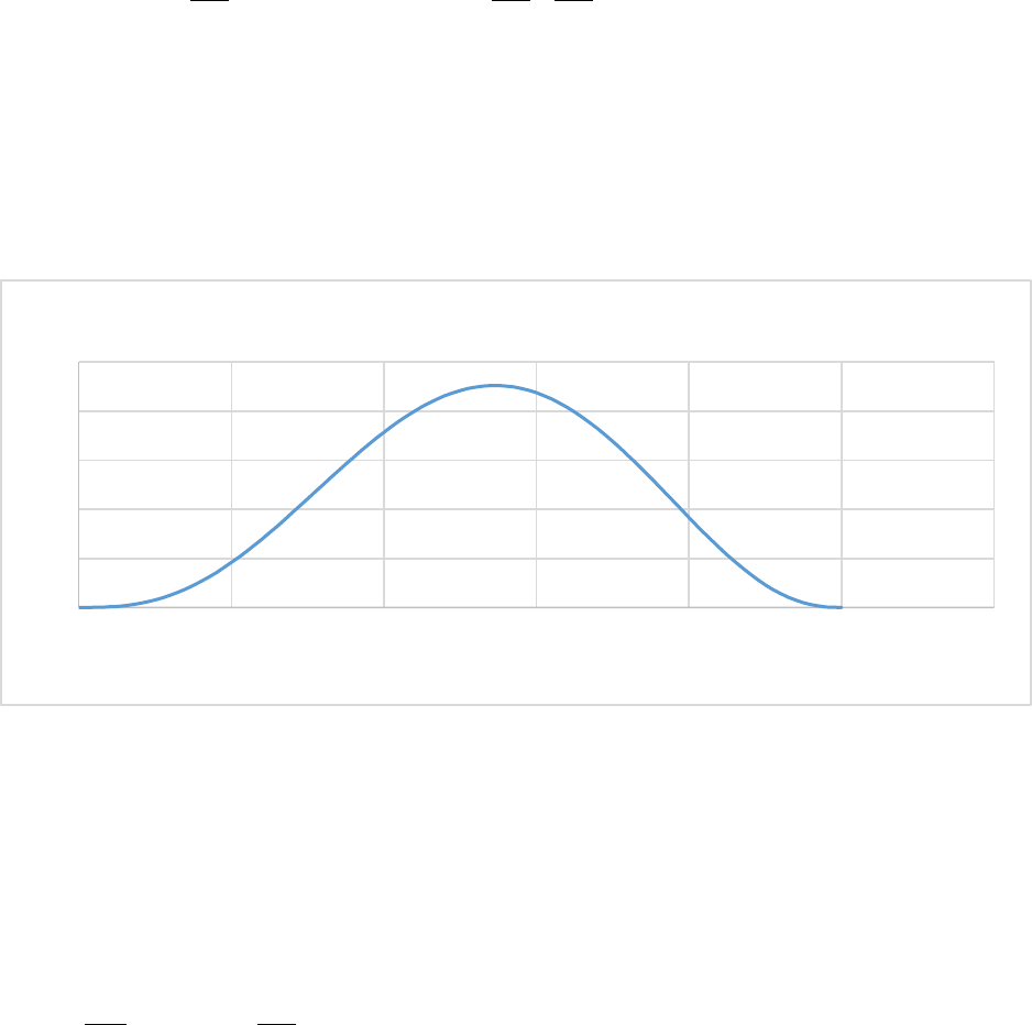
March 1, 2019
78
( )
3 2.5
( ) 0.001 max 1.0 ,
( ) max , ( )
f
ll
sat sat sat
f minAnaerobicRespFactor
f fWmin f
= + − −
=
where Ɵl is the volumetric liquid soil water content (0.0-1.), Ɵf is the volumetric frozen soil water
content (0.0-1.0), and Ɵsat is the volumetric soil moisture at saturation (0.0-1.0), fWmin is the minimum
value of f(Ɵ) (~0.001 as specified in the corpse_params.nml file), and minAnaerobicRespFactor is 0.003.
Figure 15. The soil moisture effect on soil organic matter decomposition in the CORPSE model where Ɵl is the volumetric liquid
soil water content, and Ɵsat is the volumetric total soil water content at saturation (here the volumetric frozen soil water
content, Ɵf = 0.0). The corresponding f(Ɵ) effect for MIMICS is similar but has a maximum value of 1.0.
3.5.4 Microbial growth and turnover in CORPSE
The change in microbial biomass (M) is a balance between uptake of decomposed substrate carbon (Di)
and the loss of biomass through the combination of cell death and maintenance respiration,
ii
imic
dM M
D
dt
=−
where εi is the microbial uptake efficiency for each and τmic is the average turnover rate (0.25 yr-1) for
the microbial community and represents a combination of microbial death and maintenance respiration.
3.5.5 Carbon Stabilization and Destabilization in CORPSE:
Carbon transfers from the unprotected soil pools (Ci) to their protected counterparts (Pi) are
temperature-independent functions of clay and soil porosity (Qmax, kg C m-3) (Figure 16). Loss of
protected carbon is proportional to a fixed turnover rate (1/Ƭp).
0
0.005
0.01
0.015
0.02
0.025
0 0.2 0.4 0.6 0.8 1 1.2
Ɵl/ Ɵsat
CORPSE f(Ɵ)
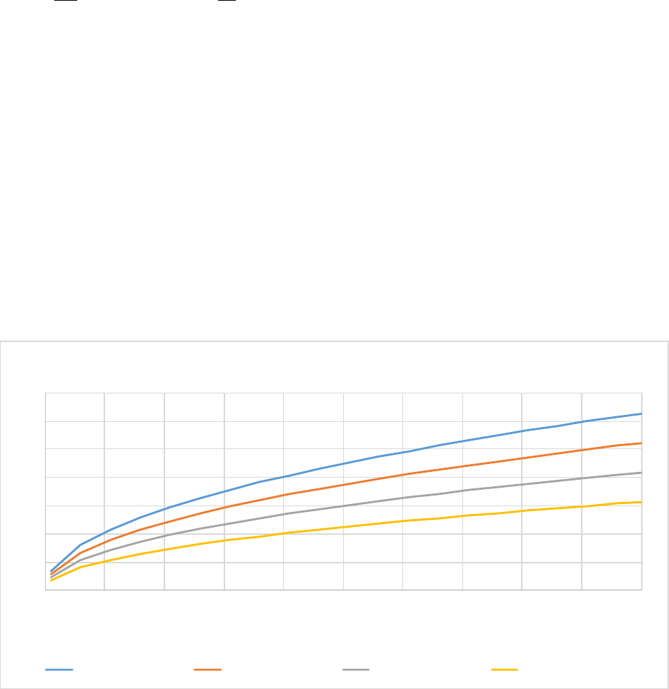
March 1, 2019
79
ii
ii
p
dP P
C Qmax
dt
= −
Ƭp=residence time of the protected pool (45 years)
ɤ (protection rate) = 1.5 yr-1
αi – species-specific multiplier on the protection rate, where i = {0.11, 0.002, and 1.0 for the labile,
recalcitrant, and dead microbe pools, respectively}
The scalar Qmax, originally defined by Mayes et al. 2012, was modified to be a unitless multiplier on the
protection rate. Qmax, which ranges from about 0.2 to 3.0, is normalized to a value of 1.0 at about 10%
clay; therefore, the Qmax function estimates the relative change in protected C formation rate as soil
clay content changes (Figure 16).
( )
( )
( )
( )
6
100.0, 10^ 0.4833 10 % 2.3282 1.0 2650Qmax max log clay porosity −
= + −
Figure 16. The effect of soil clay fraction on transfers of C to the protected pools in the CORPSE model.
0.0
0.5
1.0
1.5
2.0
2.5
3.0
3.5
010 20 30 40 50 60 70 80 90 100
clay (%)
Qmax
Qmax (porosity=0.40) Qmax (porosity=0.50) Qmax (porosity=0.60) Qmax (porosity=0.70)
March 1, 2019
80
4 Detailed Summary of CASA-CNP Subroutines and Biogeochemcial
Equations
4.1 Daily biogeochemistry: SUBROUTINE biogeochem
Subroutine biogeochem, called once each day, controls daily biogeochemical calculations. The numbers
in front of subroutines indicate their calling position in subroutine biogeochem. These subroutines are
found in file casa_cnp.f90 (Figure 17).
1. phenology – Determine current phase for each gridcell: 0=minimalLAI, 1=greenup, 2=steady LAI,
3=senescence
2. avgsoil – Calculate average soil moisture, average soil temperature across soil layers
3. casa_rplant – Calculate maintenance respiration of woody tissue and fine roots, plant growth
respiration, and nutrient unlimited NPP.
4. casa_allocation – Calculate fraction of new C allocated to each plant part.
5. casa_xrateplant – Calculate cold and drought effects on death rate of leaves: xkleafcold,
xkleafdry
6. casa_coeffplant – Calculate plant litter fall rates (1/day) and the transfer coefficients between
plant and litter pools
7. casa_xnp – Calculate nutrient limitation on NPP.
8. casa_xratesoil – Calculate for effects of temperature and water on litter and soil decomposition:
xklitter, xksoil
9. casa_coeffsoil – Calculate the litter and SOM decomposition rates (1/day), respiration rates
(fraction of flow), and the transfer coefficients between litter and soil pools, and between soil
pools.
10. casa_xkN – Calls Nrequire to compute max and min N uptake and translocation by plant part.
Computes the reduction in plant N and P uptake when N is limiting.
11. casa_nuptake – Calls Nrequire to compute max and min N uptake and translocation by plant
part. (1) compute N uptake by plants; (2) allocation of uptaken N to plant pools.
12. casa_puptake – Calls Prequire to compute max and min P uptake and translocation by plant
part. (1) compute P uptake by plants; (2) allocation of uptaken P to plants
13. casa_delplant – Calculate ΔC, ΔN, and ΔP for plant parts and litter pools
14. casa_delsoil – Calculate heterotrophic respiration fluxes from litter and soil decomposition.
Calculate gross and net mineralization.
15. casa_cnpcycle – Update all pool sizes. Reset negative pools to zero by calling poolzero.
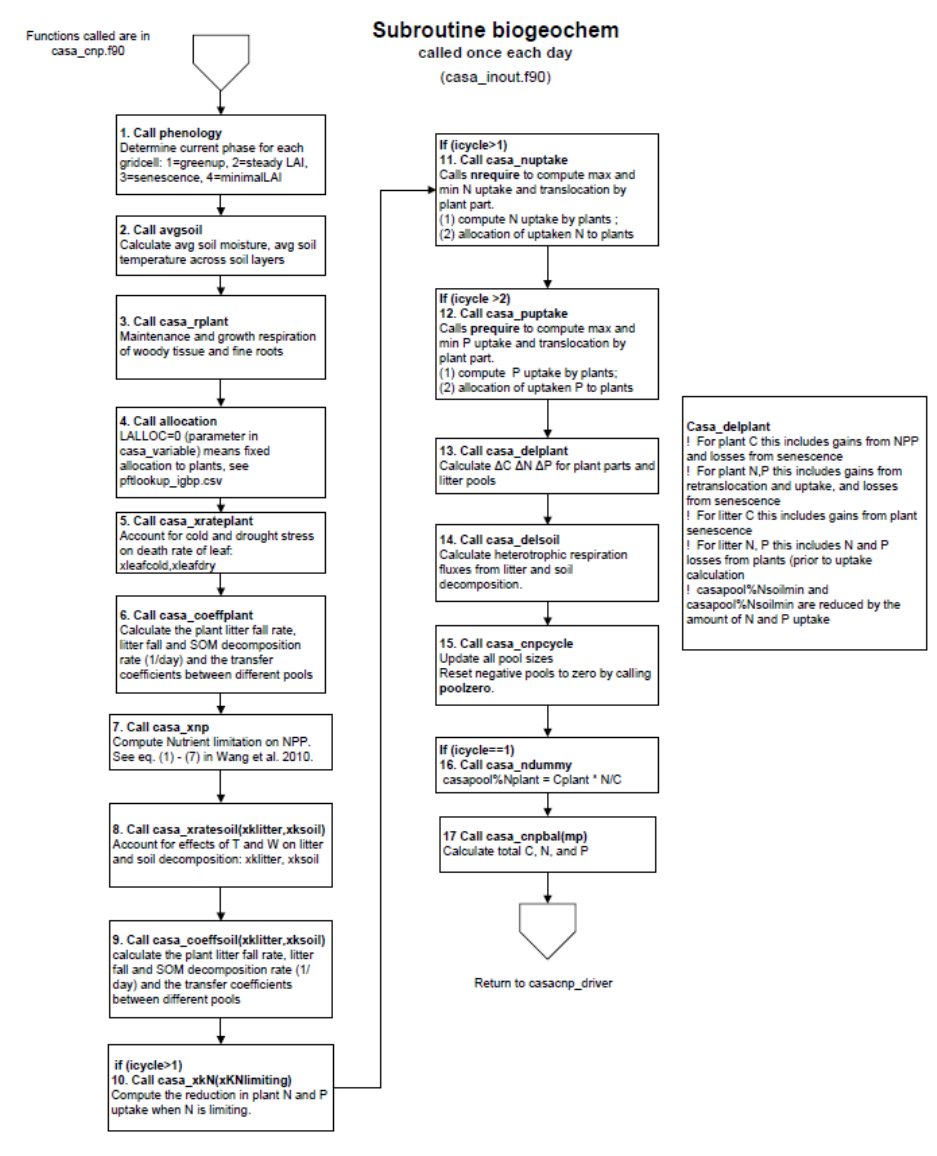
March 1, 2019
81
Figure 17. Order of calculations in subroutine biogeochem in the CASA-CNP model. Subroutine biogeochem is called once each
day and controls daily biogeochemical calculations in CASA-CNP.
March 1, 2019
82
4.2 CASA-CNP Dimensions, Constants, and Pointers
mp = number of grid cells simulated
mplant = number of plant pools (3)
msoil = number of soil pools (3)
mlitter = number of litter pools (3)
ms = number of mineral soil layers (6)
! mineral soil layer thickness (m) defined in SUBROUTINE readbiome
data dzsoil/.022, .058, .154, .409, 1.085, 2.872/
Plant Pools
integer, parameter :: leaf = 1
integer, parameter:: wood = 2
integer, parameter:: froot = 3
Litter Pools
integer, parameter:: metb = 1
integer, parameter:: str = 2
integer, parameter:: cwd = 3
Soil Organic Matter (SOM) pools
integer, parameter:: mic = 1
integer, parameter:: slow = 2
integer, parameter:: pass = 3
Equation documentation shorthand : index (1-18) for biome-specific values
pft = veg%iveg(npt)
The convention in this documentation is that npt iterates through all points (grid cells), nP iterates
through all plant pools, nL iterates through all litter pools, nS and nSS iterate through all soil organic
March 1, 2019
83
matter pools, and nLyr iterates through all soil mineral layers. The indices used in the actual code vary
from this convention.
DO npt=1, mp (iterate through all grid cells)
DO nP=1, mplant (iterate through all 3 plant pools)
DO nL=1, mlitter (iterate through all 3 litter pools)
DO nS=1, msoil (iterate through all 3 soil organic matter pools)
DO nSS=1, msoil (iterate through all 3 soil organic matter pools)
DO nLyr=1, ms (iterate through all 6 mineral soil layers)
pft is the PFT for grid cell npt.
casabiome% is a pointer to PFT specific parameters
casamet% is a pointer to meteorological drivers and soil conditions from the CLM model (read from
met*.nc files).
casaflux% is a pointer to C and N fluxes
casapool% is a pointer to plant, litter, and soil C and N pools. For example:
casapool%cplant(npt,nP) – C content of plant pool nP (g C m-2)
casapool%nplant(npt,nP) – N content of plant pool nP (g N m-2)
casapool%clittert(npt,nL) – C content of litter pool nL (g C m-2)
casapool%nlitter(npt,nL) – N content of litter pool nL (g N m-2)
casapool%csoil (npt,nS) – C content of soil organic matter pool nS (g C m-2)
casapool%nsoil(npt,nS) – N content of soil organic matter pool nS (g N m-2)
If running CASA-CNP as a spinup, C pools are initialized from biome-specific parameters. N pools are
initialized with biome-specific N:C ratios. If extending CASA-CNP from a previous simulation, C and N
pools are initialized from and output file from the previous simulation.
4.3 Soil and Litter Decomposition and Heterotrophic Respiration Variables
casaflux%Crsoil(npt) = casaflux%fluxCtoCO2(npt) (Heterotrophic Respiration)

March 1, 2019
84
fromLtoS(npt,nL,nS): fraction of decomposed litter pool nL that is transferred to soil pool nS
fromStoS(npt,nSS,nS): fraction of decomposed soil C pool nS that is transferred to soil pool nSS
fromLtoCO2(npt,nL): fraction of decomposed litter pool nL emitted as CO2
fromStoCO2(npt,nS): fraction of decomposed soil C pool nS emitted as CO2
casaflux%klitter(npt,nL): decomposition rate of litter pool nL (1/day)
casaflux%ksoil(npt,nS): decomposition rate of soil pool nS (1/day)
4.4 CASA-CNP Documentation by Subroutine
4.4.1 Phenology: (1) SUBROUTINE phenology
This subroutine determines the current phase for each gridcell: 0=minimalLAI, 1=greenup, 2=steady LAI,
3=senescence
CASA-CNP implements a fixed phenology each year, in latitude bands by PFT type, based on MODIS data
that came with the CASA-CNP code (data in modis_phenology.txt).
Phase 0 – minimal LAI
Phase 1 – green up, maximum leaf growth (14 days)
Phase 2 – steady LAI
Phase 3 – senescence (14 days)
• During leaf growth phase 0 (minimum LAI) or 3 (senescence), no carbon is allocated to leaves
and all C is allocated to wood and fine roots.
• During maximal leaf growth phase, 80% of C is allocated to leaves, the remainder of C is
allocated to wood and fine roots.
• During the steady growth period, C allocation to leaves, wood, and fine roots is determined by
the fixed biome-specific fractions, but leaf allocation can be adjusted (increased to 80% or
reduced to 0%) if LAI is below or above the theoretical biome-specific minimum and maximum
LAI.
4.4.2 Average Soil Conditions: (2) SUBROUTINE avgsoil
This subroutine computes average soil temperature and soil moisture conditions in the soil. The values
casamet%tsoilavg(npt) and casamet%moistavg(npt) are used to compute soil and temperature effects
on soil organic matter decomposition rates in subroutine casa_xratesoil. The value
casamet%tsoilavg(npt) is also used to calculate fine root maintenance respiration in subroutine
casa_rplant.

March 1, 2019
85
( ) ( ) ( )
nLyr
casamet%tsoilavg npt = veg%froot npt,nLyr * casamet%tsoil npt,nLyr
( ) ( ) ( ) ( )
( )
% % , *min % , % ,
nLyr
casamet moistavg npt veg froot npt nLyr soil sfc npt casamet moist npt nLyr=
Where froot(npt,nLyr) is the fraction of root biomass in soil layer nLyr, casamet%tsoil(npt,nLyr) is the soil
temperature (K) for layer nLyr (from CLM), soil%fc(npt) is the volumetric field capacity, and
casamet%moist(npt,nLyr) is the volumetric soil moisture content of soil layer nLyr (from CLM).
The value casamet%btran(npt) is the relative water content of the soil used to calculate plant death due
to dryness in subroutine casa_xrateplant.
( ) ( ) ( ) ( )( ) ( )( )
( ) ( )
% , * min % , % , %
%%%
nLyr
veg froot npt nLyr soil sfc npt casamet moist npt nLyr soil swilt npt
casamet btran npt soil sfc npt soil swilt npt
−
=
−
Where froot(npt,nLyr) is the fraction of root biomass in soil layer nLyr, soil%fwilt(npt) is the volumetric
wilting point, soil%fc(npt) is the volumetric field capacity, and casamet%moist(npt,nLyr) is the
volumetric soil moisture content of soil layer nLyr (from CLM).
End SUBROUTINE avgsoil
4.4.3 NPP and Autotrophic Respiration: (3) SUBROUTINE casa_rplant
This subroutine calculates the maintenance respiration of woody tissue and fine roots, the growth
efficiency of the plant, and the total plant growth respiration. It also calculates C losses from the labile
pool.
Plant maintenance respiration: casaflux%crmplant(npt,wood) + casaflux%crmplant(npt,froot)
(maintenance respiration is not calculated for leaves - the code for this calculation was commented out).
Plant growth respiration: casaflux%crgplant(npt)
Maintenance respiration for wood and fine roots increases exponentially with air or soil temperature
using a fixed Q10 that is specific to the PFT (Sitch, Smith et al. 2003).
Maintenance respiration for wood (gC m-2 d-1) (Figure 18):
( )
( )
( )
( )
0, ( ) 250
%,
* % ,
% ,
1.0 1.0
*exp 308.56* 56.02 % 46.02
tairk npt
casabiome rmplant pft wood
casapool nplant npt wood
casaflux crmplant npt wood
casamet tairk npt tkzeroc
=
−+−
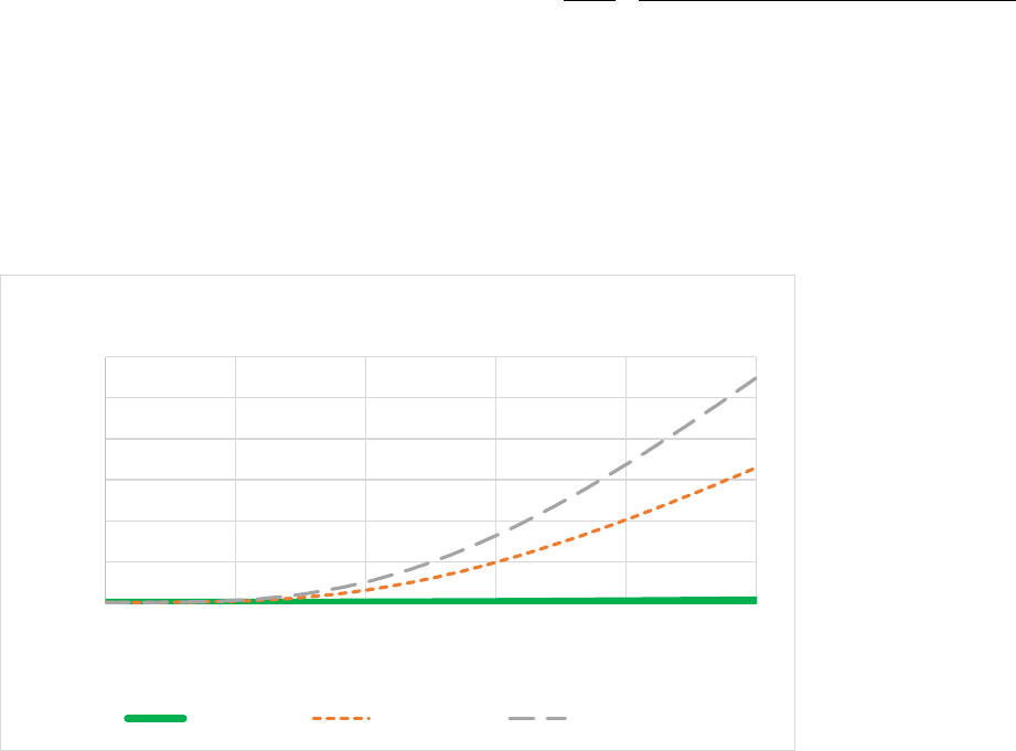
March 1, 2019
86
where casabiome%rmplant(npt,wood) is the daily maintenance respiration rate for wood (PFT-specific
parameter) (g C g N-1 d-1) on a 10 °C base, casapool%nplant(npt,wood) is the N content of wood (g N
m-2), tairk(npt) is the average air temperature (K), and tkzeroc is 273.15 K.
Maintenance respiration for fine roots (gC m-2 d-1) (Figure 18):
( )
( )
( )
( )
0, ( ) 250
%,
* % ,
%,
1.0 1.0
*exp 308.56* 56.02 % 46.02
tsoilavg npt
casabiome rmplant pft froot
casapool nplant npt froot
casaflux crmplant npt froot
casamet tsoilavg npt tkzeroc
=
−+−
where casabiome%rmplant(npt,froot) is the daily maintenance respiration rate for fine roots (PFT-
specific parameter) (g C g N-1 d-1) on a 10 °C base, casapool%nplant(npt,froot) is the N content of fine
roots (g N m-2), tsoilavg(npt) is the average soil temperature (K), and tkzeroc is 273.15 K.
Figure 18. Maintenance respiration assuming rmplant(pft,leaf) = 0.1/365, rmplant(pft,froot) = 6.0/365, rmplant(pft,wood) =
10.0/365.
Respiration losses from the labile C pool, casaflux%clabloss(npt) (g C m-2 d-1)…not sure what this pool is
exactly, plant carbohydrate storage?
0
0.1
0.2
0.3
0.4
0.5
0.6
250 270 290 310 330 350
g C m-2
tair or tsoil (K)
Maintance Respiration per 1 gN m-2 plant N
mresp_leaf mresp_froot mresp_wood

March 1, 2019
87
( )
( )
( )
( )
( )
( )
0, ( ) 250
%%
*max 0.0, %
%
1.0 1.0
*exp 308.56* 56.02 % 46.02
tairk npt
casabiome kclabrate veg iveg npt
casapool Clabile npt
casaflux clabloss npt
casamet tairk npt tkzeroc
=
−
+−
where casabiome%kclabrate(n) is the biome-specific respiration rate for the labile C pool (1/day),
casapool%Clabile(n) is theC content of labile pool (g C m-2), tairk(npt) is the average air temperature (K),
and tkzeroc is 273.15 K.
Growth Efficiency
Growth efficiency correlated to leaf N:P ratio. Q.Zhang @ 22/02/2011
Plant growth efficiency (Ygrow, 0.0 – 1.0) increases with the P/N ratio of leaves, ratioPNplant(npt,leaf).
For C only or C+N only, Ygrow = 0.65 (Figure 19).
% ( , )
( , ) % ( , )
casapool Pplant npt leaf
ratioPNplant npt leaf casapool Nplant npt leaf
=
( ) ( )
( )
,
0.65 0.2* 1.0
,15.0
ratioPNplant npt leaf
Ygrow npt
ratioPNplant npt leaf
=+
+

March 1, 2019
88
Figure 19. The plant growth efficiency (Ygrow). For C only or C+N only, Ygrow = 0.65.
Total growth respiration for the plant, casaflux%crgplant(npt) (g C m-2 d-1)
( ) ( )
( )
( ) ( )
% 1.0
* 0.0, % % ,
nP
casaflux crgplant npt Ygrow npt
MAX casaflux Cgpp npt casaflux crmplant npt nP
=−
−
Total autotrophic respiration (maintenance + growth), casaflux%crgplant(npt) (g C m-2 d-1)
( ) ( ) ( )
% % , %
nP
casaflux Crp npt casaflux crmplant npt nP casaflux crgplant npt=+
Nutrient-unlimited Net Primary Production (GPP minus autotrophic respiration), casaflux%Cnpp(npt)
(g C m-2 d-1)
( ) ( )
( )
( )
%%
%,
%
nP
casaflux Cnpp npt casaflux Cgpp npt
casaflux crmplant npt nP
casaflux crgplant npt
=
−
−
Note: casaflux%Cnpp(npt) will be reduced in subroutine casa_xnp if there is a nutrient limitation.
End SUBROUTINE casa_rplant
0
0.1
0.2
0.3
0.4
0.5
0.6
0.7
0.8
0.9
0 0.2 0.4 0.6 0.8 1
P/N ratio of plant part
Ygrow - plant growth efficiency

March 1, 2019
89
4.4.4 Carbon Allocation: (4) SUBROUTINE casa_allocation
This subroutine computes the fraction of net photosynthate allocated to leaf, wood and froot.
Inputs:
moistavg(mp) – average soil moisture (volumetric fraction) in the rooting zone, calculated in subroutine
avgsoil.
tsoilavg(mp) – average temperature in the rooting zone (K), calculated in subroutine avgsoil.
btran(mp) – relative water content in the rooting zone (0.0 – 1.0), calculated in subroutine avgsoil.
Outputs:
fracCalloc(npt,nP) – fraction of NPP allocated to each plant pool (nP) (0.0 – 1.0).
Fixed allocation fractions based on biome-specific parameters
casaflux%fracCalloc(npt,nP) = casabiome%fracnpptop(pft,nP)
WHERE (phen%phase(npt)==0), Minimum LAI
casaflux%fracCalloc(npt,leaf) = 0.0
( ) ( )
( ) ( )
%,
%, % , % ,
casaflux fracCalloc npt froot
casaflux fracCalloc npt froot casaflux fracCalloc npt froot casaflux fracCalloc npt wood
=+
casaflux%fracCalloc(npt,wood) = 1.0 - casaflux%fracCalloc(npt,froot)
END WHERE
WHERE (phen%phase==1), Greenup
casaflux%fracCalloc(npt,leaf) = 0.8
For woodland or forest
casaflux%fracCalloc(npt,froot) = 0.5*(1.0 - casaflux%fracCalloc(npt,leaf))
casaflux%fracCalloc(npt,wood) = 0.5*(1.0 - casaflux%fracCalloc(npt,leaf))
For grassland, cropland:
casaflux%fracCalloc(npt,froot) = 1.0 - casaflux%fracCalloc(npt,leaf)
casaflux%fracCalloc(npt,wood) = 0.0
END WHERE
WHERE (phen%phase==3), Maximum LAI

March 1, 2019
90
casaflux%fracCalloc(npt,wood) = casabiome%fracnpptop(pft,wood)
casaflux%fracCalloc(npt,froot) = 1.0 - casaflux%fracCalloc(npt,wood)
casaflux%fracCalloc(npt,leaf) = 0.0
ENDWHERE
If prognostic LAI reached glaimax, no C is allocated to leaf. Q.Zhang 17/03/2011
WHERE(casamet%glai(npt) ≥ casabiome%glaimax(pft))
casaflux%fracCalloc(npt,leaf) = 0.0
( ) ( )
( ) ( )
%,
%, % , % ,
casaflux fracCalloc npt froot
casaflux fracCalloc npt froot casaflux fracCalloc npt froot casaflux fracCalloc npt wood
=+
casaflux%fracCalloc(npt,wood) = 1.0 - casaflux%fracCalloc(npt,froot)
ENDWHERE
If prognostic LAI < glaimin, increase allocation to leaves
WHERE(casamet%glai(npt)<casabiome%glaimin(pft))
casaflux%fracCalloc(npt,leaf) = 0.8
For woodland or forest
casaflux%fracCalloc(npt,froot) = 0.5*(1.0-casaflux%fracCalloc(npt,leaf))
casaflux%fracCalloc(npt,wood) = 0.5*(1.0-casaflux%fracCalloc(npt,leaf))
For grassland or cropland
casaflux%fracCalloc(npt,froot) = 1.0 - casaflux%fracCalloc(npt,leaf)
ENDWHERE
Normalization the allocation fraction to ensure they sum up to 1.0
totfracCalloc(npt) = sum(casaflux%fracCalloc(npt,nP))
casaflux%fracCalloc(npt,leaf) = casaflux%fracCalloc(npt,leaf) / totfracCalloc(npt)
casaflux%fracCalloc(npt,wood) = casaflux%fracCalloc(npt,wood) / totfracCalloc(npt)
casaflux%fracCalloc(npt,froot) = casaflux%fracCalloc(npt,froot) / totfracCalloc(npt)

March 1, 2019
91
END SUBROUTINE casa_allocation
4.4.5 Plant Turnover Rates: (5) SUBROUTINE casa_xrateplant
This subroutine calculates xkleafcold and xkleafdry, the effect of cold and drought stress on death rate
of leaves (0.0 – 1.0). These values are 0.0 when there is no death due to cold or drought, and 1.0 when
there is maximum death.
Inputs:
iveg(npt) : biome type (PFT)
phase(npt): leaf growth stage
tairk(npt) : air temperature in K
Outputs:
xkleafcold(npt): cold stress induced leaf senescence rate (1/day)
xkleafdry(npt): drought-induced leaf senescence rate (1/day)
xkleaf(npt): set to 0.0 during maximal leaf growth phase to turn off leaf death due to aging,
1.0 otherwise.
Following the formulation of Arora (2005) on the effect of cold or drought stress on leaf litter fall
calculate cold stress (eqn (18), Arora 2005, GCB 11:39-59, note: the equation in this publication is
missing parentheses around “TKshed-5.0”, corrected below):
Leaf Death Rates Due to Cold (Figure 20, Figure 21).
( )
( ) ( )
( ) ( )
( ) ( )
( ) ( )
( )
( )
1.0, % %
0.0, %
( % 5.0
% 5.0
%,
5.0
min 1.0, max 0.0
)
,
casamet tairk npt phen TKshed pft
xcoldleaf npt casamet tairk npt phen TKshed pft
casamet tairk npt otherwise
xcoldlea
phen TKsh
f npt xcoldleaf np
ed
t
pft
= −
−
=
−
% ( )
( ) % ( )
*(1.0 ( ))casabiome xkleafcoldexp pft
xkleafcold npt casabiome xkleafcoldmax pft
xcoldleaf npt
=
−
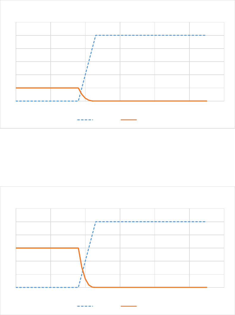
March 1, 2019
92
where phen%TKshed is the air temperature (K) at our below where plants shed their leaves. The
value of xkleafcold(npt) is added to casaflux%kplant(npt,leaf) in subroutine casa_coeffplant to
compute total turnover rate.
Figure 20. Effect of cold on evergreen leaf tree death rates. In this example for evergreen needle leaves, xkleafcoldmax = 0.20,
xkleafcoldexp = 3.0, TKshed = 268. When xkleafcold = 0.0 (orange line) there is no death due to cold. Note that the death rate
for evergreen needle leaves is lower than the death rate for deciduous leaves at low temperatures (Figure 21).
Figure 21. Effect of cold on deciduous elaf death rates.In this example for deciduous leaves, xkleafcoldmax = 0.60, xkleafcoldexp
= 3.0, TKshed = 268. When xkleafcold = 0.0 (orange line) there is no death due to cold. Note that the death rate for deciduous
leaves is greater than the death rate for evergreen needle leaves at low temperatures (Figure 20).
0
0.2
0.4
0.6
0.8
1
1.2
245 255 265 275 285 295 305
Death rates due to cold (evergreen needleleaf)
xcoldleaf xkleafcold
0
0.2
0.4
0.6
0.8
1
1.2
245 255 265 275 285 295 305
Death rates due to cold (deciduous broadleaf)
xcoldleaf xkleafcold

March 1, 2019
93
Leaf Death Rates Due to dryness (Figure 22, Figure 23).
% ( )
( ) % ( )
*(1.0 % ( )) asabiome xkleafdryec xp pft
xkleafdry npt casabiome xkleafdrymax pft
casamet btran npt
=
−
where casamet%btran(npt) is the relative water content of the soil (1.0 ≥ field capacity),
calculated in subroutine avgsoil. The value of xkleafdry(npt) is added to
casaflux%kplant(npt,leaf) in subroutine casa_coeffplant to compute total turnover rate.
Figure 22. Effect of soil dryness on evergreen leaf death rates. In this example for evergreen needle leaves, xkleafdrymax = 0.1,
xkleafdryexp = 3.0. When xkleafdry = 0.0 there is no death due to drought.
0
0.1
0.2
0.3
0.4
0.5
0.6
0.7
0.8
0.9
1
0 0.1 0.2 0.3 0.4 0.5 0.6 0.7 0.8 0.9 1
xkleafdry
btran (relative water content)
Death rates due to dryness (evergreen needleaf)
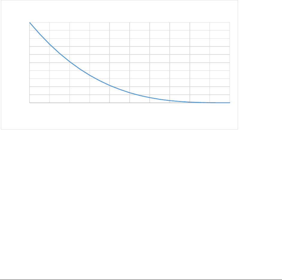
March 1, 2019
94
Figure 23. Effect of soil dryness on deciduous leaf death rates. In this example for deciduous leaves, xkleafdrymax = 1.0,
xkleafdryexp = 3.0. When xkleafdry = 0.0 there is no death due to drought.
The binary value xkleaf(npt) is 1 except during maximal leaf growth phase (greenup). This value
is used to calculate the total turnover rate of leaves, casaflux%kplant(npt,leaf) (see subroutine
casa_coeffplant).
( ) ( )
0.0, % 1
1.0,
phen phase npt
xkleaf npt otherwise
=
=
END SUBROUTINE casa_xrateplant
4.4.6 Plant Litterfall rate: (6) SUBROUTINE casa_coeffplant
This subroutine calculates the plant litter fall rate (1/day) and the transfer coefficients between plant
and litter pools.
Inputs:
xkleafcold(npt): cold stress induced leaf senescence rate (1/day)
xkleafdry(npt): drought-induced leaf senescence rate (1/day)
xkleaf(npt): set to 0.0 during maximal leaf growth phase to turn off leaf death due to aging,
1.0 otherwise.
0
0.1
0.2
0.3
0.4
0.5
0.6
0.7
0.8
0.9
1
0 0.1 0.2 0.3 0.4 0.5 0.6 0.7 0.8 0.9 1
xkleafdry
btran (relative water content)
Death rates due to dryness (deciduous broadleaf)

March 1, 2019
95
casabiome%fracNPtoL(pft,nP): fraction of N or P in plant part nP that is transferred to litter (0.0
– 1.0). The PFT lookup files shows this is about 0.5 for leaves, 0.95 for wood, and 0.90 for fine
roots.
Outputs:
casaflux%kplant(npt,nP): senescence rate of plant pool nP (1/day)
casabiome%fromPtoL(npt,nL,nP): fraction of senesced plant biomass from plant pool nP
transferred to litter pool nL
Partitioning of plant residue to litter pools
The Lignin:N ratio (g lignin / g N) of plant biomass is used to partition litter into structural and metabolic
pools.
( ) ( ) ( )
( ) ( )
% , * % ,
,% , * % ,
casapool Cplant npt leaf casabiome fracLigninplant pft leaf
ratioLignintoN npt leaf casapool Nplant npt leaf casabiome ftransNPtoL pft leaf
=
( ) ( ) ( )
( ) ( )
% , * % ,
,% , * % ,
casapool Cplant npt froot casabiome fracLigninplant pft froot
ratioLignintoN npt froot casapool Nplant npt froot casabiome ftransNPtoL pft froot
=
Where:
casabiome%fracLigninplant(*,nP) – biome-specific lignin:N ratio (g lignin / g N)
casabiome%fransNPtoL(*,nP) – biome-specific fraction of plant N transferred to litter (fraction).
The fraction of leaf and fine root litter allocation to metabolic litter (0.0 – 0.85) increases with the ratio
of lignin:N of the plant residue (similar to DayCent). The remaining fraction is allocated to structural
litter (Figure 24).
( ) ( )
( )
( ) ( )
( )
( )
% , , max 0.001, 0.85 0.018* ,
% , , max 0.001, 0.85 0.018* ,
% , , 1.0
casaflux fromPtoL npt metb leaf ratioLignintoN npt leaf
casaflux fromPtoL npt metb froot ratioLignintoN npt froot
casaflux fromPtoL npt str leaf casaflu
=−
=−
=−
( )
( ) ( )
( )
% , ,
% , , 1.0 % , ,
% , , 1.0
x fromPtoL npt metb leaf
casaflux fromPtoL npt str froot casaflux fromPtoL npt metb froot
casaflux fromPtoL npt cwd wood
=−
=
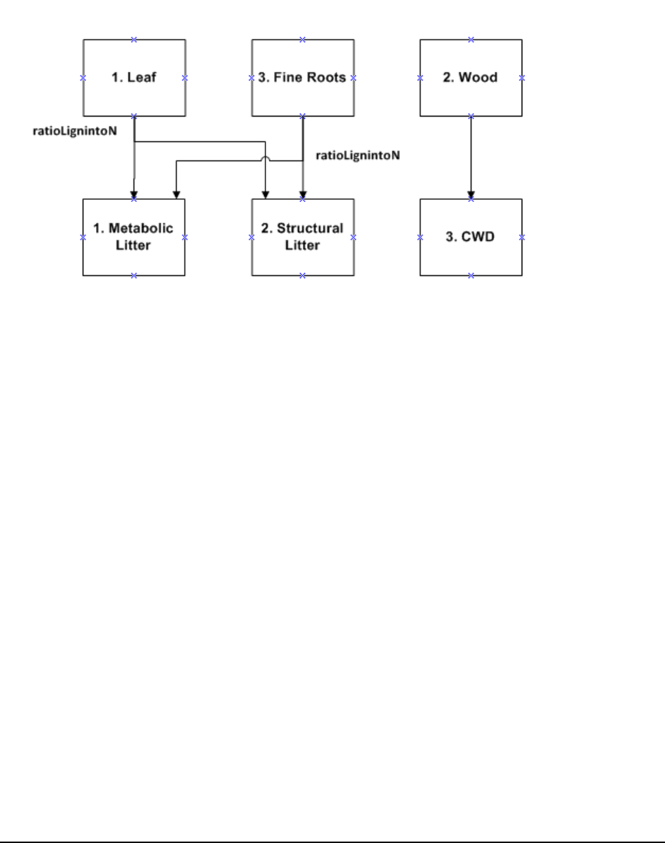
March 1, 2019
96
Figure 24. Carbon fluxes from plant pools to litter pools in the CASA-CNP model.
Plant senescence rates (casaflux%kplant(npt,*))
( ) ( ) ( )
( ) ( )
( ) ( )
( ) ( )
% , % , * :
% , % ,
% , % ,
casaflux kplant npt leaf casabiome plantrate pft leaf xkleaf
xkleafcold npt xkleafdry npt
casaflux kplant npt wood casabiome plantrate pft wood
casaflux kplant npt froot casabiome plantrate pft froot
=
++
=
=
where casabiome%plantrate(pft,nP) is the biome-specific age-related death rate of the plant parts
(1/day), xkleafcold(npt) and xkleafdry(npt) are the leaf death rates due to cold and drought (0.0 – 1.0,
calculated in subroutine casa_xrateplant), and xkleaf(npt) which equals 0 during greenup and 1
otherwise, is calculated in subroutine casa_xrateplant
When glai<glaimin, leaf biomass will not decrease anymore (Q.Zhang 10/03/2011).
If (casamet%glai(npt) ≤ casabiome%glaimin(pft)) casaflux%kplant(npt,leaf) = 0.0
END SUBROUTINE casa_coeffplant

March 1, 2019
97
4.4.7 Nutrient Limitation on Production: (7) SUBROUTINE casa_xnp
This subroutine calculates the effect of soil nutrient limitation on NPP. Note: CASA-CNP is no longer
using N concentration restriction on production as is described in Wang, Law et al. (2010).
If simulating C-only (icycle=1), set nutrient-limiting variables to 1.0:
xnlimit = 1.0
xplimit = 1.0
xnplimit = 1.0
xNuptake = 1.0
xPuptake = 1.0
In addition, all but the final two equations listed below are skipped, and there is no soil nutrient
limitation on NPP: casaflux%fracClabile(npt) = 0.0 and casaflux%Cnpp(npt) is not updated by
this subroutine. See calculations at the end of the subroutine.
This subroutine calls subroutine Nrequire to compute the minimum and maximum plant N
requirements, Nreqmin(npt,*) and Nreqmax(npt,*) (g N m-2 d-1), based on nutrient-unlimited NPP and
minimum and maximum N:C ratios of plant pools, ncplantmin(npt,*) and ncplantmax(npt,*). Minimum
and maximum N:C ratios are a function of biome-specific limits, casabiome%ratioNCplantmin(pft,*) and
casabiome%ratioNCplantmin(pft,*), and the amount of soil mineral N available, casapool%Nsoilmin(npt)
(g N m-2).
If casapool%Nsoilmin(npt) < 2.0 then ncplantmax(npt,*) is less than ratioNCplantmax(*,*)
according to the following relationship (Figure 25):
( ) ( )
( )
( )
( )
()
0.5*
, % ,
%,
%,
* 2.0 1.0
casapool%Nsoilmin npt
ncplantmax npt leaf casabiome ratioNCplantmin pft leaf
casabiome ratioNCplantmax pft leaf
casabiome ratioNCplantmin pft leaf
=
+
−
−
( ) ( )
( )
( )
( )
()
0.5*
, % ,
%,
%,
* 2.0 1.0
casapool%Nsoilmin npt
ncplantmax npt wood casabiome ratioNCplantmin pft wood
casabiome ratioNCplantmax pft wood
casabiome ratioNCplantmin pft wood
=
+
−
−
( ) ( )
( )
( )
( )
()
0.5*
, % ,
%,
%,
* 2.0 1.0
casapool%Nsoilmin npt
ncplantmax npt froot casabiome ratioNCplantmin pft froot
casabiome ratioNCplantmax pft froot
casabiome ratioNCplantmin pft froot
=
+
−
−
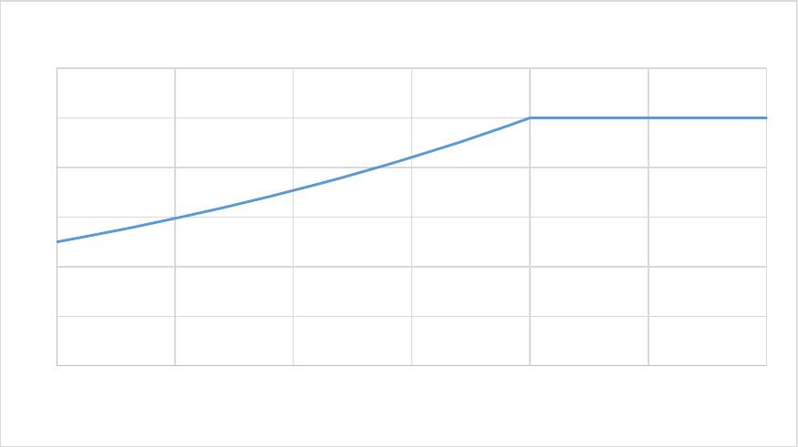
March 1, 2019
98
Else (casapool%Nsoilmin(npt) ≥ 2.0)
ncplantmax(npt,leaf) = casabiome%ratioNCplantmax(pft,leaf)
ncplantmax(npt,wood) = casabiome%ratioNCplantmax(pft,wood)
ncplantmax(npt,froot) = casabiome%ratioNCplantmax(pft,froot)
Figure 25. The N:C ratio of plant parts is bounded by biome-specific parameters ratioNCplantmin and ratioNCplantmax, and is a
function of Nsoilmin, the amount of mineral soil N available (g N m-2). Here ratioNCplantmin = 0.25 and ratioNCplantmax = 0.5.
The maximum N demand by plants (Nreqmax(npt,*), g N m-2 d-1) is a product of the nutrient-unlimited
NPP, the fraction of carbon allocation to each plant part (calculated in subroutine casa_allocation), and
the maximum N:C ratio calculated above.
Nreqmax(npt,leaf) = xnCnpp(npt)* casaflux%fracCalloc(npt,leaf) *ncplantmax(npt,leaf)
Nreqmax(npt,wood) = xnCnpp(npt)* casaflux%fracCalloc(npt,wood) *ncplantmax(npt,wood)
Nreqmax(npt,froot) = xnCnpp(npt)* casaflux%fracCalloc(npt,froot)*ncplantmax(npt,froot)
The minimum N demand by plants (Nreqmin(npt,*), g N m-2 d-1) is a product of the nutrient-unlimited
NPP (xnCnpp, g C m-2 d-1), the fraction of carbon allocation to each plant part (calculated in subroutine
casa_allocation), and the minimum N:C ratio calculated above. Note, when subroutine Nrequire is later
called by subroutine nuptake, xnCnpp has been nutrient-limited.
Nreqmin(npt,leaf) = xnCnpp(npt)* casaflux%fracCalloc(npt,leaf)*
casabiome%ratioNCplantmin(pft,leaf)
Nreqmin(npt,wood) = xnCnpp(npt)* casaflux%fracCalloc(npt,wood)*
casabiome%ratioNCplantmin(pft,wood)
0
0.01
0.02
0.03
0.04
0.05
0.06
0.0 0.5 1.0 1.5 2.0 2.5 3.0
Nsoilmin (g N m-2)
NCplantmax
March 1, 2019
99
Nreqmin(npt,froot) = xnCnpp(npt)* casaflux%fracCalloc(npt,froot)*
casabiome%ratioNCplantmin(pft,froot)
Retranslocation of N from dying plant material to live plant parts (NtransPtoP(npt,*)) is the biome-
specific fraction of N that is not transferred to the litter pools.
NtransPtoP(npt,leaf) = casaflux%kplant(npt,leaf)*casapool%Nplant(npt,leaf)
* (1.0-casabiome%ftransNPtoL(pft,leaf))
NtransPtoP(npt,wood) = casaflux%kplant(npt,wood)*casapool%Nplant(npt,wood)
* (1.0-casabiome%ftransNPtoL(pft,wood))
NtransPtoP(npt,froot) = casaflux%kplant(npt,froot)*casapool%Nplant(npt,froot)
* (1.0-casabiome%ftransNPtoL(pft,froot))
Where:
casabiome%ftransNPtoL(npt,nP) – biome-specific fraction of N transferred from plant poll nP to
litter pools
casaflux%kplant(npt,nP) – senescence rate of plant pool nP (1/day), calculated in subroutine
coeffplant.
The maximum N requirement by each plant part is reduced by the amount of N translocation,
NtransPtoP(npt,*) after plant death (calculated above).
Nreqmax(npt,leaf) = max(0.0,Nreqmax(npt,leaf) - NtransPtoP(npt,leaf))
Nreqmax(npt,wood) = max(0.0,Nreqmax(npt,wood) - NtransPtoP(npt,wood))
Nreqmax(npt,froot) = max(0.0,Nreqmax(npt,froot) - NtransPtoP(npt,froot))
Nreqmin(npt,leaf) = max(0.0,Nreqmin(npt,leaf) - NtransPtoP(npt,leaf))
Nreqmin(npt,wood) = max(0.0,Nreqmin(npt,wood) - NtransPtoP(npt,wood))
Nreqmin(npt,froot) = max(0.0,Nreqmin(npt,froot) - NtransPtoP(npt,froot))
If the N:C ratios of live plant material is > the biome-specific maximum N:C ratio, don’t allow plant N
uptake.
if(casapool%nplant(npt,nP)/(casapool%cplant(npt,nP)+1.0e-10)>casabiome%ratioNCplantmax(pft,nP))
then
Nreqmax(npt,nP) = 0.0
Nreqmin(npt,nP) =0.0
endif
Nutrient limitation on NPP
Sum total minimum and maximum N requirements by plants :

March 1, 2019
100
( ) ( ) ( ) ( )
( ) ( ) ( ) ( )
( ) ( )
( )
, , ,
, , ,
%
0.0, 1.0, *
totNreqmax npt Nreqmax npt leaf Nreqmax npt wood Nreqmax npt froot
totNreqmin npt Nreqmin npt leaf Nreqmin npt wood Nreqmin npt froot
casapool Nsoilmin npt
xNuptake npt MAX MIN totNreqmin npt d
= + +
= + +
=
eltpool
Where deltpool is the time step (1 for daily), and Nsoilmin(npt) in available soil mineral N (g N m-2).
The value xNPuptake(npt) (0.0 – 1.0) is the N/P nutrient limitation on plant production, the minimum of
the N limitation (xNuptake(npt)) and the P limitation (xPuptake(npt)) fractions. The value of
xPuptake(npt) = 1.0 when P is not simulated.
xNPuptake(npt) = min(xNuptake(npt), xPuptake(npt))
If there is a nutrient limitation on production (xNPuptake(npt) < 1.0), calculate the fraction of GPP that is
diverted to the labile pool instead of NPP, fracClabile(npt) (0.0 – 1.0). This fraction is used again in
subroutine casa_delplant.
( ) ( )
( )
( )
( )
%
% 1.0 * %
casaflux Cnpp npt
casaflux fracClabile npt xNPuptake npt casaflux Cgpp npt
=−
( ) ( ) ( ) ( )
% % % * %
( )* ( )
casaflux Cnpp npt casaflux Cnpp npt casaflux fracClabile npt casaflux Cgpp npt
xNPuptake npt Cnpp npt
=−
=
As mentioned at the top of the subroutine, if icycle=1, there is no soil nutrient limitation on NPP:
xNPuptake = 1.0, casaflux%fracClabile(npt) = 0.0, and casaflux%Cnpp(npt) is not updated by this
subroutine.
END SUBROUTINE casa_xnp

March 1, 2019
101
4.4.8 Soil Temperature and Moisture effects on SOM decomposition: (8) SUBROUTINE
casa_xratesoil
This subroutines calculates the effects of soil temperature and soil moisture on litter and soil
decomposition rates: xklitter, xksoil
Inputs:
iveg(npt) : biome type (PFT)
tsoilavg(npt): average soil temperature in the 6 soil layers (K)
moistavg(npt): average volumetric soil moisture in the 6 soil layers (0.0 – 1.0)
Outputs:
xklitter(npt): modifier of litter decomposition rate, similar to a climate decomposition index
(dimensionless)
xksoil(npt): modifier of soil decomposition rate, similar to climate decomposition index
(dimensionless)
Constants:
REAL(r_2), parameter :: wfpscoefa=0.55 ! Kelly et al. (2000) JGR, Figure 2b), optimal wfps
REAL(r_2), parameter :: wfpscoefb=1.70 ! Kelly et al. (2000) JGR, Figure 2b)
REAL(r_2), parameter :: wfpscoefc=-0.007 ! Kelly et al. (2000) JGR, Figure 2b)
REAL(r_2), parameter :: wfpscoefd=3.22 ! Kelly et al. (2000) JGR, Figure 2b)
REAL(r_2), parameter :: wfpscoefe=6.6481 ! =wfpscoefd*(wfpscoefb-wfpscoefa)/(wfpscoefa-wfpscoefc)
Kirschbaum function parameters
REAL(r_2), parameter :: xkalpha=-3.764 ! Kirschbaum (1995, SBB)
REAL(r_2), parameter :: xkbeta=0.204
REAL(r_2), parameter :: xktoptc=36.9
Soil temperature and moisture modifiers on decomposition rates
( ) ( )
( )
( ) ( )
%
%
%
casamet moistavg npt
fwps npt soil ssat npt
tsavg npt casamet tsoilavg npt
=
=

March 1, 2019
102
( ) ( )
( )
( )
()
0.1* 35.0
% % tsavg npt TKzeroC
xktemp npt casabiome q10soil veg iveg npt −−
=
( ) ( ) ( )
* non-cropland
1.0, cropland or cropland2
,
wfpscoefe wfpscoefd
fwps npt wfpscoefb fwps npt wfpscoefc
xkwater npt wfpscoefa wfpscoefb wfpscoefa wfpscoefc
−−
=−−
( ) ( ) ( ) ( )
% * *xklitter npt casabiome xkoptlitter pft xktemp npt xkwater npt=
( ) ( ) ( ) ( )
% * *xksoil npt casabiome xkoptsoil pft xktemp npt xkwater npt=
where casabiome%xkoptlitter and casabiome%xkoptsoil are the biome-specific maximum
decomposition rates (1/day); fwps(npt) is soil moisture expressed as the fraction of water filled pore
space (0.0 – 1.0); tsavg(npt) is the average soil temperature in the 6 soil layers (K).
END SUBROUTINE casa_xratesoil
4.4.9 Litter and SOM decomposition rates: (9) SUBROUTINE casa_coeffsoil
This subroutine calculatse the litter and SOM decomposition rates (1/day), respiration rates (fraction of
flow), and the transfer coefficients between litter and soil pools, and between soil pools.
Inputs:
xkitter and xksoil are calculated in subroutine casa_xratesoil (above)
xklitter(npt): modifier of litter decomposition rate, similar to a climate decomposition index
(dimensionless)
xksoil(npt): modifier of soil decomposition rate, similar to climate decomposition index
(dimensionless)
Outputs:
klitter(npt,mL): decomposition rate of litter pool mL (1/day)
ksoil(npt,mS): decomposition rate of soil pool mS (1/day)
fromLtoS(npt,nL,nS): fraction of decomposed litter pool nL to soil pool nS
fromStoS(npt,nSS,nS): fraction of decomposed soil pool nS to another soil pool nSS
fromLtoCO2(npt,nL): fraction of decomposed litter C pool nL emitted as CO2

March 1, 2019
103
fromStoCO2(npt,nL): fraction of decomposed soil C pool nS emitted as CO2
Litter Decomposition Rates
( ) ( ) ( )
( ) ( ) ( )
( )
( )
( )
% , * % ,
% , * % ,
*exp 3.0* % ,
% ,
casaflux klitter npt metb xklitter npt casabiome litterrate pft metb
casaflux klitter npt str xklitter npt casabiome litterrate pft str
casabiome fracLigninplant pft leaf
casaflux klitter npt cwd x
=
=
−
=
( ) ( )
* % , klitter npt casabiome litterrate pft cwd
( ) ( ) ( )
( )
( ) ( )
( )
( )
( ) ( ) ( )
( )
% , * % % ,
* 1.0 0.75* % %
% , * % % ,
%
casaflux ksoil npt mic xksoil npt casabiome soilrate veg iveg npt mic
soil silt npt soil clay npt
casaflux ksoil npt slow xksoil npt casabiome soilrate veg iveg npt slow
casaflux k
=
−+
=
( ) ( ) ( )
( )
, * % % , soil npt pass xksoil npt casabiome soilrate veg iveg npt pass=
For cultivated land types, increase the rate of soil decomposition
WHERE (pft==cropland)
( ) ( )
( ) ( )
( ) ( )
% , % , *1.25
% , % , *1.5
% , % , *1.5
casaflux ksoil npt mic casaflux ksoil npt mic
casaflux ksoil npt slow casaflux ksoil npt slow
casaflux ksoil npt pass casaflux ksoil npt pass
=
=
=
Litter and Soil Organic Matter Decomposition (Figure 26)
Metabolic litter → Fast SOM
( )
% , , 0.45casaflux fromLtoS npt mic metb =
Structural litter → Fast SOM
( ) ( )
( )
% , , 0.45* 1.0 % , casaflux fromLtoS npt mic str casabiome fracLigninplant pft leaf=−
March 1, 2019
104
Structural litter → Slow SOM
( ) ( )
% , , 0.7* % , casaflux fromLtoS npt slow str casabiome fracLigninplant pft leaf=
Coarse Woody Debris → Fast SOM
( ) ( )
( )
% , , 0.40* 1.0 % ,casaflux fromLtoS npt mic cwd casabiome fracLigninplant pft wood=−
Coarse Woody Debris → Slow SOM
( ) ( )
% , , 0.7* % , casaflux fromLtoS npt slow cwd casabiome fracLigninplant pft wood=
Fast SOM → Slow SOM
( ) ( ) ( )
( )
( )
( )
( )
% , , 0.85 0.68* % %
* 0.997 0.032* %
casaflux fromStoS npt slow mic soil clay npt soil silt npt
soil clay npt
= − +
−
Fast SOM → Passive SOM
( ) ( ) ( )
( )
( )
( )
( )
% , , 0.85 0.68* % %
* 0.003 0.032* % :
casaflux fromStoS npt pass mic soil clay npt soil silt npt
soil clay
= − +
+
Slow SOM → Passive SOM
( ) ( )
( )
% , , 0.45* 0.003 0.009* %casaflux fromStoS npt pass slow soil clay npt=+
Fractions of Litter C pools released as CO2
( ) ( )
% 2 , % , ,
nL nS
casaflux fromLtoCO npt nL casaflux fromLtoS npt nS nL=
( ) ( )
% 2 , 1.0 % 2 ,
nL
casaflux fromLtoCO npt nL casaflux fromLtoCO npt nL=−
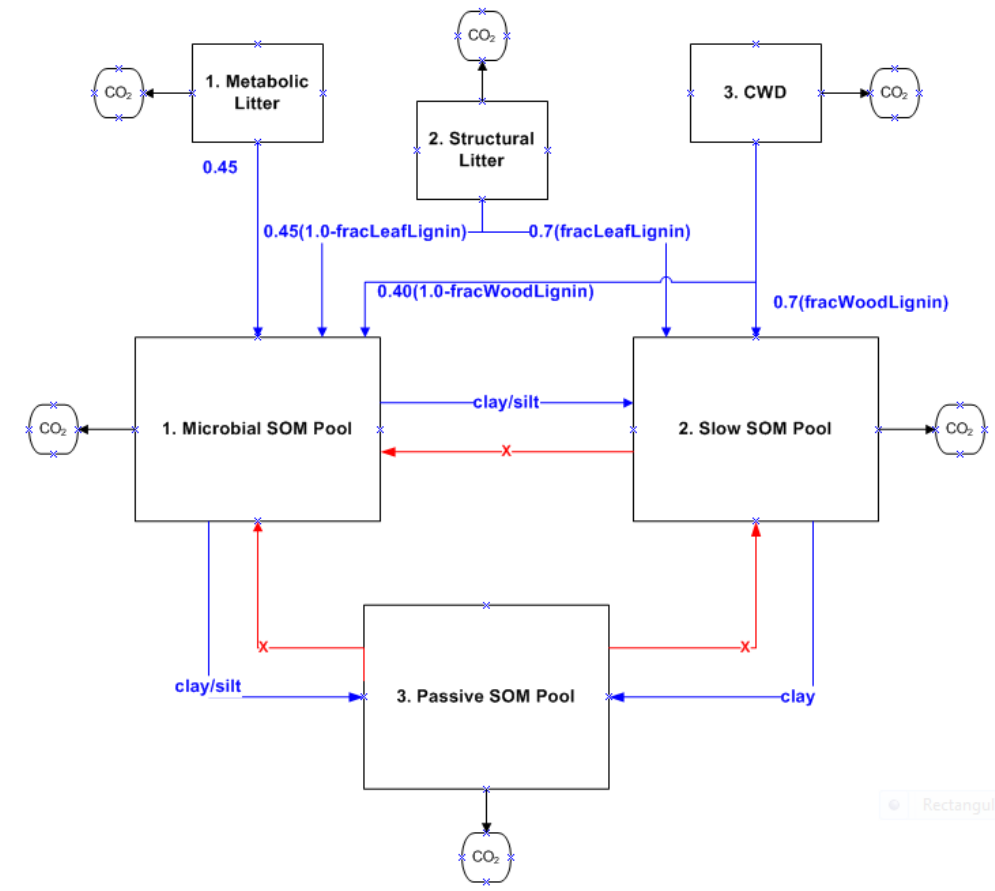
March 1, 2019
105
Fractions of Soil C pools released as CO2
( ) ( )
% 2 , % , ,
nS nSS
casaflux fromStoCO npt nS casaflux fromStoS npt nSS nS=
( ) ( )
% 2 , % 2 , casaflux fromStoCO npt nS casaflux fromStoCO npt nS=−
Figure 26. Carbon and CO2 fluxes as litter and soil organic matter pools decompose in the CASA-CNP model.

March 1, 2019
106
END SUBROUTINE casa_coeffsoil
4.4.10 Mineralization, Immobilization, N limits on decomposition: (10) SUBROUTINE casa_xkN
This subroutine computes the mineralization, immobilization, and the reduction in litter and SOM
decomposition when decomposition rate is N-limiting.
Initialization
xkNlimiting(npt) – multiplier on plant uptake and decomposition rates (0.0 – 1.0). It is < 1.0 when N is
limiting to decomposition. Also defined as the reduction of N uptake by plants (0.0 – 1.0) due to
competition from microbes (1.0 = no reduction). This factor will be used in subroutine casa_nuptake to
reduce N uptake by plants.
Mineral N fluxes (Local Variables)
xFluxNlittermin(npt) – gross mineralization from decomposition of litter pools (positive) (g N m-2 d-1)
xFluxNsoilmin(npt) – gross mineralization from decomposition of soil pools (positive) (g N m-2 d-1)
xFluxNsoilimm(npt) – immobilization from litter and soil C flows to destination soil pools (negative) (g N
m-2 d-1)
xFluxNsoilminnet(npt) – net mineralization (gross mineralization – immobilization), negative for net
microbial uptake and positive for net release of mineral N.
Calculate N:C ratio of newly formed SOM as function of soil mineral N pool (casapool%Nsoilmin(npt),
g N m-2)
This calculation is like the variable C:N ratios in DayCent (Figure 27).
If casapool%Nsoilmin(npt) < 2.0
Limited soil mineral N forces the N:C ratio of new SOM to be below the maximum:
( )
( )
( ) ( )
( )
( )
%,
% ,
% , % ,
%
*2.0
casapool ratioNCsoilnew npt nS
casapool ratioNCsoilmin npt nS
casapool ratioNCsoilmax npt nS casapool ratioNCsoilmin npt nS
casapool Nsoilmin npt
=
+−
If casapool%Nsoilmin(npt) ≥ 2.0
Mineral N unlimited, N:C ratio of new SOM equals the maximum:

March 1, 2019
107
( ) ( )
% , % , casapool ratioNCsoilnew npt nS casapool ratioNCsoilmax npt nS=
where casapool%ratioNCsoilmin(*,*) and casapool%ratioNCsoilmax(*,*) are biome-specific parameters
specifying the minimum and maximum N:C ratios of soil organic matter pools.
Figure 27. The N:C ratio required by the receiving SOM pool is a function of soil mineral N content. In this example,
ratioNCsoilMin = 0.0, ratioNCsoilMax = 0.2
Mineralization of litter and soil pools
( ) ( ) ( )
% , * % ,
nL
xFluxNlittermin npt casaflux klitter npt nL casapool Nlitter npt nL=
( ) ( ) ( )
% , * % ,
nS
xFluxNsoilmin npt casaflux ksoil npt nS casapool Nsoil npt nS=
N immobilization from Litter to Soil
Immobilization from litter pool nL to soil pool nSS (xFluxnsoilimm(npt), gN m-2 d-1) is negative for
microbial uptake.
0
0.05
0.1
0.15
0.2
0.25
0 0.5 1 1.5 2 2.5 3
N/C
Soil Mineral N (NsoilMin, gN m-2)
N/C ratio of new SOM (ratioNCsoilnew)
March 1, 2019
108
( )
( )
( )
( )
( )
% , ,
* % ,
* % ,
* % ,
nL nS
casaflux fromLtoS npt nSS nL
casaflux klitter npt nL
xFluxNsoilimm npt casapool Clitter npt nL
casapool ratioNCsoilnew npt nSS
−
=
Where:
casaflux%fromLtoS(npt,nSS,nL) –fraction of decomposed litter pool nL that flows to soil pool nSS
(0.0 – 1.0)
casaflux%klitter(npt,nL) - turnover rate of litter pool nL (1/day)
casapool%Clitter(npt,nL) – carbon in litter pool nL (g C m-2)
casapool%ratioNCsoilnew(npt,nSS) – the required N:C ratio of the receiving soil pool.
total C flow from litter pool nL to soil pool nSS assuming no N limitation:
casaflux%fromLtoS(npt,nSS,nL)*casaflux%klitter(npt,nL)*casapool%Clitter(npt,nL)
total N flow from litter pool nL to soil pool nSS assuming no N limitation:
casaflux%fromLtoS(npt,nSS,nL)*casaflux%klitter(npt,nL)*casapool%Clitter(npt,nL)*
casapool%ratioNCsoilnew(npt,nSS)
N immobilization from Soil to Soil
Immobilization from soil pool nS to soil pool nSS (added to xFluxnsoilimm(npt), gN m-2 d-1) is negative for
microbial uptake.
( )
( )
( )
( )
( )
% , ,
* % ,
* % ,
* % ,
nS nSS nS
casaflux fromStoS npt nSS nS
casaflux ksoil npt nS
xFluxNsoilimm npt casapool Csoil npt nS
casapool ratioNCsoilnew npt nSS
−
+=
Where:
casaflux%fromStoS(npt,nSS,nS) – fraction of decomposed SOM pool nS that flows to SOM pool
nSS (0.0 – 1.0)
casaflux%ksoil(npt,nS) – turnover rate of SOM pool nS (1/day)
casapool%Csoil(npt,nS) – C in soil pool nS (g C m-2)

March 1, 2019
109
casapool%ratioNCsoilnew(npt,nSS) –required N:C ratio of the receiving soil pool.
total C flow from SOM pool nS to SOM pool nSS. assuming no N limitation:
casaflux%fromStoS(npt,nSS,nS)*casaflux%ksoil(npt,nS)*casapool%Csoil(npt,nS)
total N flowing from SOM pool nS into SOM pool nSS assuming no N limitation:
casaflux%fromStoS(npt,nSS,nS)*casaflux%ksoil(npt,k)*casapool%Csoil(npt,nS)*
casapool%ratioNCsoilnew(npt,nSS)
Check if there is sufficient mineral N. Compute the limit on plant N,P uptake if there is not sufficient
mineral N.
xFluxNsoilminnet (Net mineralization) = N mineralization from source litter pool flow + N mineralization
from source soil pool flow + N immobilization by destination soil pool (negative).
xFluxNsoilminnet(npt) = xFluxNlittermin(npt) + xFluxNsoilmin(npt) + xFluxNsoilimm(npt)
If net mineralization is positive or if there is at least 2.0 g N m-2 after accounting for the N demand by
microbes, xkNlimiting = 1.0.
xkNlimiting(npt) – reduction of N uptake by plants (0.0 – 1.0) due to competition from microbes (1.0 =
no reduction).
if ((xFluxNsoilminnet(npt)*deltpool + (casapool%Nsoilmin(npt) – 2.0)) > 0.0 OR xFluxNsoilminnet(npt) >
0.0)
xkNlimiting(npt) =1.0
Otherwise, 0.0 ≤ xkNlimiting(npt) ≤ 1.0 and is equal to the ratio of available mineral N – 0.5 to the
microbial demand for N
( ) ( )
( )
( )
( )
% 0.5
max 0.0,
*
min 1.0,
casapool Nsoilmin npt
xkNlimiting npt deltpool xFluxNsoilminnet npt
xkNlimiting npt
−
=−
=
If the amount of metabolic + structural litter is > the maximum fine litter + CWD then xkNlimiting = 1.0?
if (sum(casapool%clitter,2) > casabiome%maxfinelitter(pft) + casabiome%maxcwd(pft))
xkNlimiting(npt) = 1.0

March 1, 2019
110
END SUBROUTINE casa_xkN
Note: after this subroutine returns to SUBROUTINE biogeochem (casa_inout.f90), casaflux%klitter(npt,
nL) is multipled by xkNlimiting(npt), but casaflux%ksoil(npt, nS) is not! Why? Then subroutine
casa_nuptake is called.
DO nL=1,mlitter
casaflux%klitter(npt,nL) = casaflux%klitter(npt,nL)* xkNlimiting(npt)
ENDDO
call casa_nuptake(veg, xkNlimiting, casabiome, casapool, casaflux, casamet)
4.4.11 Plant N uptake: (11) SUBROUTINE casa_nuptake
This subroutine computes the total N uptake by plants (casaflux%Nminuptake(npt), g N m-2 d-1) and the
allocation of uptaken N to the 3 plant pools (casaflux%fracNalloc(npt,nP), 0.0 – 1.0).
This subroutine calls subroutine Nrequire to compute the minimum and maximum plant N
requirements, Nreqmin(npt,*) and Nreqmax(npt,*) (g N m-2 d-1), based on nutrient-limited NPP and
minimum and maximum N:C ratios of plant pools, ncplantmin(npt,*) and ncplantmax(npt,*). Minimum
and maximum N:C ratios are a function of biome-specific limits, casabiome%ratioNCplantmin(pft,*) and
casabiome%ratioNCplantmin(pft,*), and the amount of soil mineral N available, casapool%Nsoilmin(npt)
(g N m-2). Equations from subroutine Nrequire are found in documentation for subroutine casa_xnp.
xkNlimiting(npt) – reduction of N uptake by plants (0.0 – 1.0) due to competition from microbes (1.0 =
no reduction). Calculated in subroutine casa_xkN.
Sum total minimum and maximum N requirments by plants (g N m-2 d-1):
( ) ( ) ( ) ( )
( ) ( ) ( ) ( )
, , ,
, , ,
totNreqmax npt Nreqmax npt leaf Nreqmax npt wood Nreqmax npt froot
totNreqmin npt Nreqmin npt leaf Nreqmin npt wood Nreqmin npt froot
= + +
= + +
Note: These are local variables and I don’t think these sums are used anywhere.
N uptake from each plant pool nP, xnuptake(npt,nP) (g N m-2 d-1).
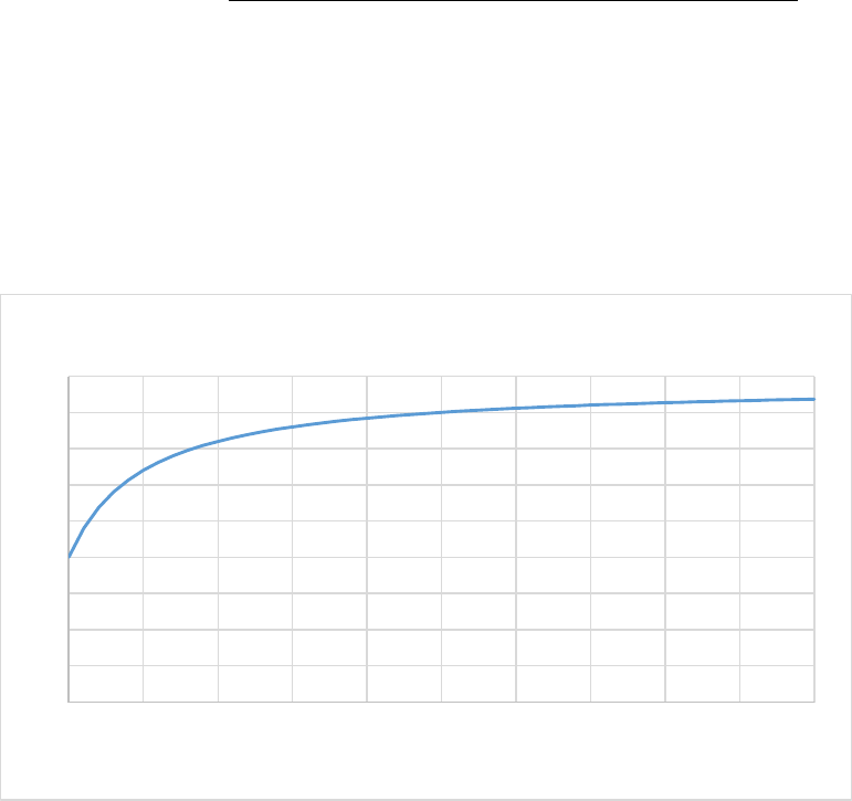
March 1, 2019
111
( ) ( )
( ) ( ) ( )
( )
( )
( ) ( )
, ,
* , ,
%
* %%
xnuptake npt nP Nreqmin npt nP
xkNlimiting npt Nreqmax npt nP Nreqmin npt nP
casapool Nsoilmin npt
casapool Nsoilmin npt casabiome kminN pft
=
+−
+
Where xkNlimiting (0.0 – 1.0) is set in subroutine casa_xkN, casabiome%kminN(pft) (g N m-2) is a biome-
specific parameter, the amount of soil mineral N to reach ½ the maximum N uptake (Figure 28).
Figure 28. Actual N uptake by a plant pool (g N m-2 d-1). In this example, kminN = 0.5, xkNlimiting = 0.8, Nrequiremin = 0.2,
Nrequiremax = 0.5.
Total plant N uptake and N allocation fractions.
These values are used in subroutine casa_delplant.
casaflux%Nminuptake(npt) = xnuptake(npt,leaf) + xnuptake(npt,wood) + xnuptake(npt,froot)
casaflux%fracNalloc(npt,leaf) = xnuptake(npt,leaf) / casaflux%Nminuptake(npt)
casaflux%fracNalloc(npt,wood) = xnuptake(npt,wood) / casaflux%Nminuptake(npt)
casaflux%fracNalloc(npt,froot) = xnuptake(npt,froot) / casaflux%Nminuptake(npt)
0
0.05
0.1
0.15
0.2
0.25
0.3
0.35
0.4
0.45
0.0 0.5 1.0 1.5 2.0 2.5 3.0 3.5 4.0 4.5 5.0
Nsoilmin (g N m-2)
xnuptake (g N m-2 d-1)

March 1, 2019
112
casaflux%Nupland(npt) = casaflux%Nminuptake(npt)
END SUBROUTINE casa_nuptake
4.4.12 Plant Net C, N, and P fluxes: (13) SUBROUTINE casa_delplant
This subroutine calculates the change in plant C, N and P pools. The amount of N uptake by plants is
computed in subroutine casa_nuptake. The dC and dN values calculated here are used by subroutine
CASA-CNPcycle to update the pools.
( ) ( ) ( )
( ) ( )
% , * % ,
% , * % ,
%casapool dcplantdt npt nP casaflux fracCalloc npt nP
casaflux kpl
ca
ant npt nP casapool
safl
cpl
ux
an
Cnp
t np
pn
P
pt
tn
=
−
Calculate fraction C to labile pool as a fraction of GPP, not NPP.
( ) ( ) ( )
( )
% * %
%
%casapool dClabiledt npt casaflux fracClabile npt
casaf
casaf
lux
lux Cgpp np
clab pt
t
loss n
=
−
Where casaflux%fracClabile(npt) was calculated in subroutine casa_xnp, and casaflux%clabloss(npt) was
calculated in subroutine casa_rplant.
Carbon transfers from plant to litter.
These appear to be output variables only and are not used in subsequent calculations.
( ) ( ) ( )
( )
( ) ( ) ( )
( )
% , , * % ,
* % ,
% , , * % ,
* % ,
cleaf2met npt casaflux fromPtoL npt metb leaf casaflux kplant npt leaf
casapool cplant npt leaf
cleaf2str npt casaflux fromPtoL npt str leaf casaflux kplant npt leaf
casapool cplant npt leaf
croot2met n
=
=
( ) ( ) ( )
( )
( ) ( ) ( )
( )
( )
% , , * % ,
* % ,
% , , * % ,
* % ,
pt casaflux fromPtoL npt metb froot casaflux kplant npt froot
casapool cplant npt froot
croot2str npt casaflux fromPtoL npt str froot casaflux kplant npt froot
casapool cplant npt froot
cwood2cwd npt casaflu
=
=
=
( ) ( )
( )
% , , * % ,
* % ,
x fromPtoL npt cwd wood casaflux kplant npt wood
casapool cplant npt wood
Change in plant N pools (icycle > 1 only)
March 1, 2019
113
( )
( ) ( )
( )
( ) ( )
( )
( )
% , * % , ,
if % , 0.0
% , % , * % ,
* % , ,
other
casaflux kplant npt leaf casapool Nplant npt leaf
casaflux fracNalloc npt leaf
casapool dNplantdt npt leaf casaflux kplant npt leaf casapool Nplant npt leaf
casabiome ftransNPtoL iveg npt leaf
−
=
=−
wise
( ) ( ) ( )
( )
( )
% , % , * % ,
* % ,
casapool dNplantdt npt wood casaflux kplant npt wood casapool Nplant npt wood
casabiome ftransNPtoL iveg npt wood
=−
( ) ( ) ( )
( )
( )
% , % , * % ,
* % ,
casapool dNplantdt npt froot casaflux kplant npt froot casapool Nplant npt froot
casabiome ftransNPtoL iveg npt froot
=−
Where casabiome%ftransNPtoL(npt,nP) are biome-specific transfer rates from plant to litter
Nitrogen transfers from plant to litter.
These appear to be output variables only and are not used in subsequent calculations.
( ) ( ) ( )
( )
( ) ( ) ( )
( )
% , , * % ,
* % , *
% , , * % ,
* % , *
nleaf2str npt casaflux fromPtoL npt str leaf casaflux kplant npt leaf
casapool cplant npt leaf ratioNCstrfix
nroot2str npt casaflux fromPtoL npt str froot casaflux kplant npt froot
casapool cplant npt froot
=
=
( ) ( ) ( )
( ) ( ) ( )
( ) ( )
% , 2
% , 2
% ,
ratioNCstrfix
nleaf2met npt casapool dNplantdt npt leaf nleaf str npt
nroot2met npt casapool dNplantdt npt froot nroot str npt
nwood2cwd npt casapool dNplantdt npt wood
= − −
= − −
=−
Where:
ratioNCstrfix – fixed N:C ratio of structural material (1/150)
casaflux%kplant(npt,nP) – senescence rate of plant pool nP (1/day), calculated in
subroutine coeffplant.
casaflux%fromPtoL(npt,nL,nP) – fraction of senesced plant biomass from plant pool nP
transferred to litter pool nL, calculated in subroutine casa_coeffplant.
Total C flux to litter is sum of all transfers of dead plant material to litter.
March 1, 2019
114
( )
( )
( )
( )
% , ,
% , * % ,
* % ,
nL nP
casaflux fromPtoL npt nL nP
casaflux FluxCtolitter npt nL casaflux kplant npt nP
casapool cplant npt nP
=
N fluxes to Litter Pools (icycle > 1 only)
Total N flux to structural and metabolic litter and coarse woody debris is sum of all transfers of dead
plant material to these litter pools.
N flux to structural litter pool
( ) ( )
( )
( )
( )
( )
% , % , ,
* % ,
* % ,
*
% , ,
* % ,
*
casaflux FluxNtolitter npt str casaflux fromPtoL npt str leaf
casaflux kplant npt leaf
casapool cplant npt leaf
ratioNCstrfix
casaflux fromPtoL npt str froot
casaflux kplant npt froot
c
=
+
( )
%,
*
asapool cplant npt froot
ratioNCstrfix
Where:
ratioNCstrfix – fixed N:C ratio of structural material (1/150).
casaflux%kplant(npt,nP) – senescence rate of plant pool nP (1/day), calculated in
subroutine coeffplant.
casaflux%fromPtoL(npt,nL,nP) – fraction of senesced plant biomass from plant pool nP
transferred to litter pool nL, calculated in subroutine casa_coeffplant.
N flux to metabolic litter pool
( ) ( )
( )
( )
% , % ,
% ,
%,
casaflux FluxNtolitter npt metb casapool dNplantdt npt leaf
casapool dNplantdt npt froot
casaflux FluxNtolitter npt str
=−
−
−
N flux to coarse wood debris pool
( ) ( )
% , % ,casaflux FluxNtolitter npt cwd casapool dNplantdt npt wood=−

March 1, 2019
115
N uptake by plants
( ) ( ) ( )
% ,: % * % ,
nP
casapool dNplantdt npt casaflux Nminuptake npt casaflux fracNalloc npt nP=
where casaflux%Nminuptake(npt) is total mineral N uptake calculated in subroutine
casa_nuptake, and casaflux%fracNalloc(npt,nP) is the fraction of N allocation to each plant pool,
calculated in subroutine casa_nuptake.
END SUBROUTINE casa_delplant
4.4.13 Update Litter and Soil Pools: (14) SUBROUTINE casa_delsoil
This subroutine calculates changes in litter and soil pools. The dC and dN values calculated here are used
by subroutine CASA-CNPcycle to update the pools.
Carbon
CO2 fluxes from litter decomposition.
( ) ( )
( ) ( )
% 2 ,
%2 * % , * % ,
nL
casaflux fromLtoCO npt nL
casaflux fluxCtoCO npt casaflux klitter npt nL casapool clitter npt nL
=
C fluxes when a litter pool (nL) decomposes into an SOM pool (nS)
( ) ( )
( ) ( )
% , ,
%,
* % , * % ,
nL
casaflux fromLtoS npt nS nL
casaflux fluxCtosoil npt nS casaflux klitter npt nL casapool clitter npt nL
=
CO2 fluxes when one SOM pool (nSS) decomposes into another SOM pool (nS)
( ) ( )
( ) ( )
% 2 ,
%2 * % , * % ,
nS
casaflux fromStoCO npt nS
casaflux fluxCtoCO npt casaflux ksoil npt nS casapool csoil npt nS
+=
C fluxes when one SOM pool (nSS) decomposes into another SOM pool (nS)

March 1, 2019
116
( ) ( )
( ) ( )
% , ,
%,
* % , * % ,
nSS nS
casaflux fromStoS npt nS nSS
casaflux fluxCtosoil npt nS casaflux ksoil npt nSS casapool csoil npt nSS
+=
Where the following where computed in subroutine casa_coefsoil:
casaflux%klitter(npt,nL): decomposition rate of litter pool nL (1/day)
casaflux%ksoil(npt,nS): decomposition rate of soil pool nS (1/day)
casaflux%fromLtoCO2(npt,nL): fraction of decomposed litter C pool nL emitted as CO2
casaflux%fromLtoS(npt,mL,nS): fraction of decomposed litter pool nL to soil pool nS
casaflux%fromStoCO2(npt,nL): fraction of decomposed soil C pool nS emitted as CO2
casaflux%fromStoS(npt,nSS,nS): fraction of decomposed soil pool nS to another soil pool nSS
Nitrogen (icycle > 1 only)
Many of these calculations are similar to those in subroutine casa_xkN. However, after that function
was called, casaflux%klitter(npt,nL) was multiplied by xkNlimiting(npt) (0.0 – 1.0) to reduce the litter
decomposition rate if N was limiting. The value of casaflux%ksoil(npt,nL) was not changed.
Mineral N fluxes
casaflux%Nlittermin(npt) – gross mineralization from decomposition of litter pools (positive)
(g N m-2 d-1)
casaflux%Nsmin(npt) – gross mineralization from decomposition of soil pools (positive) (g N m-2 d-1)
casaflux%Nsimm(npt) – immobilization from litter and soil C flows to destination soil pools (negative)
(g N m-2 d-1)
casaflux%Nsnet(npt) – net mineralization (gross mineralization – immobilization), negative for net
microbial uptake and positive for net release of mineral N.
Gross mineralization from decomposition of litter
( ) ( ) ( )
% % , * % ,
nL
casaflux Nlittermin npt casaflux klitter npt nL casapool Nlitter npt nL=
Gross mineralization from decomposition of soil organic matter
( ) ( ) ( )
% % , * % ,
nS
casaflux Nsmin npt casaflux ksoil npt nS casapool Nsoil npt nS=
Immobilisation from litter to soil (from mLto nS)

March 1, 2019
117
( )
( )
( )
( )
( )
% , ,
* % ,
% * % ,
* % ,
nS nL
casaflux fromLtoS npt nS nL
casaflux klitter npt nL
casaflux Nsimm npt casapool Clitter npt nL
casapool ratioNCsoilnew npt nS
−
=
Immobilisation from soil to soil (from nSS to nS)
( )
( )
( )
( )
( )
% , ,
* % ,
%
* % ,
* % ,
nS nSS nS
casaflux fromStoS npt nS nSS
casaflux ksoil npt nSS
casaflux Nsimm npt casapool Csoil npt nSS
casapool ratioNCsoilnew npt nS
−
+=
Net mineralization (gross litter mineralization + gross soil mineralization – immobilization)
( ) ( ) ( ) ( )
% % % %casaflux Nsnet npt casaflux Nlittermin npt casaflux Nsmin npt casaflux Nsimm npt= + +
Mineral N losses from volatilization(?) and leaching
IF(casapool%Nsoilmin(npt) > 2.0 AND casamet%tsoilavg(npt) > 273.12) THEN
( ) ( ) ( )
( )
( ) ( ) ( )
( )
% % * 0.0, %
% % * 0.0, %
casaflux Nminloss npt casaflux fNminloss npt MAX casaflux Nsnet npt
casaflux Nminleach npt casaflux fNminleach npt MAX casapool Nsoilmin npt
=
=
ELSE
( ) ( )
( )
( )
( )
% %
* 0.0, %
%
* 0.0, 2.0
casaflux Nminloss npt casaflux fNminloss npt
MAX casaflux npt
casapool
Nsnet
Nsoilmin npt
MAX
=
( ) ( )
( )
( )
( )
% %
* 0.0, %
%
* 0.0, 2.0
casaflux Nminleach npt casaflux fNminleach npt
MAX casapool npt
casapoo
Nsoilmin
Nsoilml npt
MAX in
=

March 1, 2019
118
I have a question about 2 calculations above. Units are (fraction) * (g N m-2 d-1) * (g N m-2)
Where:
casaflux%fNminloss(npt) – biome-specific rate of mineral N loss (fraction) (set to 0.05 for all
biomes)
casaflux%fNminleach(npt) – biome-specific N leaching rate (1/day) (set to 0.05*10/365 for all
biomes)
Total N fluxes to soil organic pools
( )
( )
( )
( )
( )
% , ,
* % ,
%,
* % ,
* % ,
nL nS
casaflux fromLtoS npt nS nL
casaflux klitter npt nL
casaflux FluxNtosoil npt nS casapool Clitter npt nL
casapool ratioNCsoilnew npt nS
=
( )
( )
( )
( )
( )
% , ,
* % ,
% , * % ,
* % ,
nS nSS nS
casaflux fromStoS npt nS nSS
casaflux ksoil npt nSS
casaflux FluxNtosoil npt nS casapool Csoil npt nSS
casapool ratioNCsoilnew npt nS
+=
Change in litter C pools
( ) ( )
( ) ( )
% , % ,
% , * % ,
casapool dClitterdt npt nL casaflux fluxCtolitter npt nL
casaflux klitter npt nL casapool clitter npt nL
=
−
Change in soil C pools
( ) ( )
( ) ( )
% , % ,
% , * % ,
casapool dCsoildt npt nS casaflux fluxCtosoil npt nS
casaflux ksoil npt nS casapool csoil npt nS
=
−
Heterotrophic Respiration
( ) ( )
%%casaflux Crsoil npt casaflux fluxCtoCO2 npt=

March 1, 2019
119
Nitrogen (icycle > 1 only)
Changes to litter and soil organic matter N pools
( ) ( )
( ) ( )
% , % ,
% , * % ,
casapool dNlitterdt npt nL casaflux FluxNtolitter npt nL
casaflux klitter npt nL casapool Nlitter npt nL
=
−
( ) ( )
( ) ( )
% , % ,
% , * % ,
casapool dNsoildt npt nS casaflux FluxNtosoil npt nS
casaflux ksoil npt nS casapool Nsoil npt nS
=
−
Where:
casaflux%FluxNtolitter(npt) – Total N flux to litter, calculated in subroutine casa_delplant which
is called right before this subroutine (g N m-2 d-1)
casaflux%FluxNtosoil(npt) – Total N flux to soil, calculated above (g N m-2 d-1)
Changes to mineral N pool
( ) ( )
( )
( )
( )
( )
( )
%%
%
%
%
%
%
casapool dNsoilmindt npt casaflux Nsnet npt
casaflux Nmindep npt
casaflux Nminfix npt
casaflux Nminloss npt
casaflux Nminleach npt
casaflux Nupland npt
=
+
+
−
−
−
Where:
casaflux%Nsnet(npt) – net mineralization, calculated above (g N m-2 d-1)
casaflux%Nmindep(npt) – atmospheric N deposition rate from CLM (g N m-2 d-1)
casaflux%Nminfix(npt) – biome-specific N fixation rate (g N m-2 d-1)
casaflux%fNminloss(npt) – mineral N losses from volatilization, calculated above (g N m-2 d-1).
casaflux%fNminleach(npt) – mineral N losses from leaching, calculated above (g N m-2 d-1).
casaflux%Nupland(npt) – Total mineral N uptake by plants, calculated in subroutine
casa_nuptake (g N m-2 d-1).

March 1, 2019
120
END SUBROUTINE casa_delsoil
4.4.14 Final Daily Update to all Pools: (15) SUBROUTINE casa_cnpcycle
This subroutine updates all pool sizes. The value of deltpool = 1 (for daily). The dC and dN values are
calculated in subroutine casa_delplant and subroutine casa_delsoil.
Update Plant Carbon Pools
casapool%cplant(npt, nP) = casapool%cplant(npt, nP) + casapool%dCplantdt(npt, nP) * deltpool
casapool%clabile(npt) = casapool%clabile(npt) + casapool%dClabiledt(npt) * deltpool
casamet%glai(npt) = MAX(casabiome%glaimin(pft), casabiome%sla(pft) * casapool%cplant(npt,leaf))
casamet%glai(npt) = MIN(casabiome%glaimax(pft), casamet%glai(npt))
Update Litter and Soil Carbon Pools
casapool%clitter(npt, nL) = casapool%clitter(npt, nL) + casapool%dClitterdt(npt, nL) * deltpool
casapool%csoil(npt, nS) = casapool%csoil(npt, nS) + casapool%dCsoildt(npt, nS) * deltpool
Update Plant Nitrogen Pools (icycle > 1 only)
IF(casapool%cplant(npt,leaf) > 0.0) THEN
casapool%Nplant(npt,:) = casapool%Nplant(npt,:) + casapool%dNplantdt(npt,:)*deltpool
Update Litter and Soil Nitrogen Pools (icycle > 1 only)
casapool%Nlitter(npt, nL) = casapool%Nlitter(npt, nL) + casapool%dNlitterdt(npt, nL) * deltpool
casapool%Nsoil(npt, nS) = casapool%Nsoil(npt, nS) + casapool%dNsoildt(npt, nS) * deltpool
casapool%Nsoilmin(npt) = casapool%Nsoilmin(npt) + casapool%dNsoilmindt(npt) * deltpool
After the above calculations, any negative C or N pools are set to zero without adjusting the N and C
balances. CASA-CNP will also produce a warning message when a negative pool is set to zero.
END SUBROUTINE casa_cnpcycle
5 Guidelines for adding additional SOM models to the testbed
March 1, 2019
121
• Convert all code to FORTRAN 90
• If the model is a point model, then create a structure that will contain all model variables for
each point. This was done for the CORPSE model to avoid modifying the original code (see type
gridcell in corpse_variable.f90)
• Create model-specific versions of casa_coeffplant, casa_xratesoil, casa_delplant, casa_delsoil,
casa_cnpcycle s needed. See “Overview of subroutine biogeochem” below.
• Create model_inout.f90 to
o read model-specific parameter files
o read model restart files to initialize model variables
o compute average annual pools and fluxes before output (once at the end-of-year)
o output model-specific daily and annual variables to netCDF files
5.1 Overview of subroutine biogeochem with calls to MIMICS and CORPSE models
There are several CASA-CNP subroutines that have been modified to work with the MIMICS and CORPSE
models. The numbers in front of subroutines indicate their calling position in subroutine biogeochem
(casa_inout.f90) which is called once a day. The MIMICS subroutines will be found in mimics_cycle.f90,
CORPSE subroutines are found in corpse_cycle.f90, and all CASA-CNP subroutines are found in
casa_cnp.f90.
1. phenology – Determine current phase for each gridcell: 0=minimalLAI, 1=greenup, 2=steady LAI,
3=senescence
2. avgsoil – Calculate average soil moisture, average soil temperature across soil layers
3. casa_rplant – Calculate maintenance respiration of woody tissue and fine roots, plant growth
respiration, and nutrient unlimited NPP.
4. casa_allocation – Compute fraction of new C allocated to each plant part.
5. casa_xrateplant – Account for cold and drought stress on death rate of leaf: xleafcold, xleafdry
6. if running CASA-CNP SOM model (isomModel == 1)
a. casa_coeffplant – Calculate plant litter fall rates (1/day) and the transfer coefficients
between plant and litter pools.
b. casa_xnp – Compute nutrient limitation on NPP.
c. casa_xratesoil – Account for effects of temperature and water on litter and soil
decomposition: xklitter, xksoil
d. casa_coeffsoil – Calculate the litter and SOM decomposition rates (1/day), respiration
rates (fraction of flow), and the transfer coefficients between litter and soil pools, and
between soil pools.
e. These subroutines aren’t used if icycle=1 (C only).
i. casa_xkN – Calls Nrequire to compute max and min N uptake and translocation
by plant part. Computes the reduction in plant N and P uptake when N is
limiting.
ii. casa_nuptake – Calls Nrequire to compute max and min N uptake and
translocation by plant part. (1) compute N uptake by plants; (2) allocation of
uptaken N to plant pools.
iii. casa_puptake – Calls Prequire to compute max and min P uptake and
translocation by plant part. (1) compute P uptake by plants; (2) allocation of
uptaken P to plants
f. casa_delplant – Calculate ΔC, ΔN, and ΔP for plant parts and litter pools
March 1, 2019
122
g. casa_delsoil – Calculate heterotrophic respiration fluxes from litter and soil
decomposition. Calculate gross and net mineralization.
h. casa_cnpcycle – Update all pool sizes. Reset negative pools to zero by calling poolzero.
7. if running MIMICS (isomModel == 2)
a. call mimics subroutines to update all litter, microbial, and SOM pools for the day with an
hourly timestep. Calculate heterotrophic respiration also. Pertinent code was copied
from casa_coeffplant, casa_xratesoil, casa_delplant, casa_delsoil, casa_cnpcycle.
i. call mimics_coeffplant – MIMICS uses some of its own parameters to partition
plant litter into structural and metabolic litter. The computations for
casaflux%fromPtoL(:,metb,leaf) and casaflux%fromPtoL(:,metb,froot) have
therefore been modified.
ii. call mimics_xratesoil – adds the casaflux%fromLtoCO2(npt,cwd) caluation
(fraction of CWD decomposition that goes to heterotrophic respiration) that is
found in casa_coeffsoil
iii. call mimics_delplant – Computes C-only values. Computes MIMICS output
variables for litter inputs. Computes mimicsbiome%fmet(npt). Adds MIMICS
fAVAL, fCHEM, and fPHYS calculations because fCHEM (and therefore fPHYS and
fAVAL) depend on themimicsbiome%fmet(npt) calculation.
iv. call mimics_soil_reverseMM – the MIMICS SOC model. The hourly timestep is
inside this subroutine.
v. call mimics_ccycle – similar to casa_cnpcycle but removes N,P pool updates.
vi. call mimics_caccum – accumulate annual fluxes and convert units from
mgC/cm3 to gC/m2.
8. if running CORPSE (isomModel == 3)
a. call CORPSE subroutines to update all litter, microbial, and SOM pools for the day with a
daily timestep.
i. call casa_coeffplant (uses same subroutine as CASA-CNP)
ii. call mimics_xratesoil (uses same subroutine as mimics)
iii. call corpse_delplant – Computes C-only values. Computes CASA-CNP output
variables for litter inputs.
iv. call corpse_soil – the CORPSE SOC model
calls corpse_caccum - – accumulate annual fluxes
v. call mimics_ccycle (uses same subroutine as mimics)
9. IF (icycle<3) call casa_pdummy(casapool) ! Update Pplant based on N:P ratio
10. IF (icycle<2) call casa_ndummy(casapool) ! Update Nplant based on N:C ratio
11. call casa_cnpbal (casa_input.f90)
12. call casa_cnpflux (casa_input.f90) – Accumulates daily CASA-CNP fluxes. The annual average is
calculated subroutine casa_fluxout*.
13. call casa_cnppool (casa_input.f90) – Accumulates daily CASA-CNP pool values to be averaged at
the end of the year. The annual average is calculated subroutine casa_poolout*.
*MIMICS and CORPSE: mimics_caccum and corpse_caccum are model-specific counterparts to
casa_cnpflux and casa_cnppool. At the end of each simulation year, casa_fluxout, casa_poolout,
mimics_poolfluxout and corpse_poolfluxout are called from subroutine CASA-CNPdriver.
6 Conversions

March 1, 2019
123
6.1 g C m-2 to mg C cm-3
32
2 4 2 3
g C 10 mg C m 1 mg C
* * *
m g C 10 cm depth (cm) cm
=
6.2 mg C cm-3 to gC m-2
42
3 2 3 2
mg C 10 cm g C g C
* * *depth (cm)
cm m 10 mg C m
=
7 Output NetCDF files
The following sections document output produced by “ncdump -h model_pool_flux.nc”, where model =
CASA-CNP, mimics, or corpse. Some of the global attributes are specific to the run-time options
selected.
7.1 casaclm_pool_flux.nc
netcdf casaclm_pool_flux {
dimensions:
lon = 144 ;
lat = 96 ;
time = UNLIMITED ; // (1 currently)
variables:
float lon(lon) ;
lon:long_name = "coordinate longitude" ;
lon:units = "degrees_east" ;
float lat(lat) ;
lat:long_name = "coordinate latitude" ;
lat:units = "degrees_north" ;
float time(time) ;
time:long_name = "coordinate time" ;
time:units = "1..ntimes" ;
int IGBP_PFT(lat, lon) ;
IGBP_PFT:long_name = "IGBP PFT classification" ;
IGBP_PFT:units = "1-18" ;
IGBP_PFT:_FillValue = -9999 ;
IGBP_PFT:missing_value = -9999 ;
float landarea(lat, lon) ;
landarea:long_name = "land area, icewater set to 0.0" ;
landarea:units = "km^2" ;
landarea:_FillValue = 1.e+36f ;
March 1, 2019
124
landarea:missing_value = 1.e+36f ;
int cellMissing(lat, lon) ;
cellMissing:long_name = "Missing Data Mask" ;
cellMissing:units = "0=no missing data, 1=missing data" ;
int cellid(lat, lon) ;
cellid:long_name = "Grid Cell ID" ;
cellid:units = "1..nlat*nlon" ;
float cresp(time, lat, lon) ;
cresp:long_name = "soil heterotrophic respiration" ;
cresp:units = "gC m-2 year-1" ;
cresp:_FillValue = 1.e+36f ;
cresp:missing_value = 1.e+36f ;
float cnpp(time, lat, lon) ;
cnpp:long_name = "net primary production" ;
cnpp:units = "gC m-2 year-1" ;
cnpp:_FillValue = 1.e+36f ;
cnpp:missing_value = 1.e+36f ;
float cgpp(time, lat, lon) ;
cgpp:long_name = "gross primary production" ;
cgpp:units = "gC m-2 year-1" ;
cgpp:_FillValue = 1.e+36f ;
cgpp:missing_value = 1.e+36f ;
float cleaf(time, lat, lon) ;
cleaf:long_name = "leaf carbon" ;
cleaf:units = "gC m-2" ;
cleaf:_FillValue = 1.e+36f ;
cleaf:missing_value = 1.e+36f ;
float nleaf(time, lat, lon) ;
nleaf:long_name = "leaf nitrogen" ;
nleaf:units = "gN m-2" ;
nleaf:_FillValue = 1.e+36f ;
nleaf:missing_value = 1.e+36f ;
float cwood(time, lat, lon) ;
cwood:long_name = "wood carbon" ;
cwood:units = "gC m-2" ;
cwood:_FillValue = 1.e+36f ;
cwood:missing_value = 1.e+36f ;
float nwood(time, lat, lon) ;
nwood:long_name = "wood nitrogen" ;
nwood:units = "gN m-2" ;
nwood:_FillValue = 1.e+36f ;
nwood:missing_value = 1.e+36f ;
float cfroot(time, lat, lon) ;
cfroot:long_name = "fine root carbon" ;
cfroot:units = "gC m-2" ;
cfroot:_FillValue = 1.e+36f ;
cfroot:missing_value = 1.e+36f ;
float nfroot(time, lat, lon) ;
March 1, 2019
125
nfroot:long_name = "fine root nitrogen" ;
nfroot:units = "gN m-2" ;
nfroot:_FillValue = 1.e+36f ;
nfroot:missing_value = 1.e+36f ;
float clitmetb(time, lat, lon) ;
clitmetb:long_name = "metabolic litter carbon" ;
clitmetb:units = "gC m-2" ;
clitmetb:_FillValue = 1.e+36f ;
clitmetb:missing_value = 1.e+36f ;
float nlitmetb(time, lat, lon) ;
nlitmetb:long_name = "metabolic litter nitrogen" ;
nlitmetb:units = "gN m-2" ;
nlitmetb:_FillValue = 1.e+36f ;
nlitmetb:missing_value = 1.e+36f ;
float clitstr(time, lat, lon) ;
clitstr:long_name = "structural litter carbon" ;
clitstr:units = "gC m-2" ;
clitstr:_FillValue = 1.e+36f ;
clitstr:missing_value = 1.e+36f ;
float nlitstr(time, lat, lon) ;
nlitstr:long_name = "structural litter nitrogen" ;
nlitstr:units = "gN m-2" ;
nlitstr:_FillValue = 1.e+36f ;
nlitstr:missing_value = 1.e+36f ;
float clitcwd(time, lat, lon) ;
clitcwd:long_name = "coarse woody debris carbon" ;
clitcwd:units = "gC m-2" ;
clitcwd:_FillValue = 1.e+36f ;
clitcwd:missing_value = 1.e+36f ;
float nlitcwd(time, lat, lon) ;
nlitcwd:long_name = "coarse woody debris nitrogen" ;
nlitcwd:units = "gN m-2" ;
nlitcwd:_FillValue = 1.e+36f ;
nlitcwd:missing_value = 1.e+36f ;
float csoilmic(time, lat, lon) ;
csoilmic:long_name = "microbial soil organic matter carbon" ;
csoilmic:units = "gC m-2" ;
csoilmic:_FillValue = 1.e+36f ;
csoilmic:missing_value = 1.e+36f ;
float nsoilmic(time, lat, lon) ;
nsoilmic:long_name = "microbial soil organic matter nitrogen" ;
nsoilmic:units = "gN m-2" ;
nsoilmic:_FillValue = 1.e+36f ;
nsoilmic:missing_value = 1.e+36f ;
float csoilslow(time, lat, lon) ;
csoilslow:long_name = "slow soil organic matter carbon" ;
csoilslow:units = "gC m-2" ;
csoilslow:_FillValue = 1.e+36f ;
March 1, 2019
126
csoilslow:missing_value = 1.e+36f ;
float nsoilslow(time, lat, lon) ;
nsoilslow:long_name = "slow soil organic matter nitrogen" ;
nsoilslow:units = "gN m-2" ;
nsoilslow:_FillValue = 1.e+36f ;
nsoilslow:missing_value = 1.e+36f ;
float csoilpass(time, lat, lon) ;
csoilpass:long_name = "passive soil organic matter carbon" ;
csoilpass:units = "gC m-2" ;
csoilpass:_FillValue = 1.e+36f ;
csoilpass:missing_value = 1.e+36f ;
float nsoilpass(time, lat, lon) ;
nsoilpass:long_name = "passive soil organic matter nitrogen" ;
nsoilpass:units = "gN m-2" ;
nsoilpass:_FillValue = 1.e+36f ;
nsoilpass:missing_value = 1.e+36f ;
float tairC(time, lat, lon) ;
tairC:long_name = "mean annual air temperature" ;
tairC:units = "degrees C" ;
tairC:_FillValue = 1.e+36f ;
tairC:missing_value = 1.e+36f ;
float tsoilC(time, lat, lon) ;
tsoilC:long_name = "mean annual soil temperature in top 50 cm" ;
tsoilC:units = "degrees C" ;
tsoilC:_FillValue = 1.e+36f ;
tsoilC:missing_value = 1.e+36f ;
float litInptMet(time, lat, lon) ;
litInptMet:long_name = "Metabolic Litter Inputs" ;
litInptMet:units = "gC m-2 yr-1" ;
litInptMet:_FillValue = 1.e+36f ;
litInptMet:missing_value = 1.e+36f ;
float litInptStruc(time, lat, lon) ;
litInptStruc:long_name = "Structural Litter Inputs" ;
litInptStruc:units = "gC m-2 yr-1" ;
litInptStruc:_FillValue = 1.e+36f ;
litInptStruc:missing_value = 1.e+36f ;
// global attributes:
:title = "CASA-CNP model output" ;
:comment = "NOTE: None of the variables are weighted by land fraction!" ;
:history = "created on 03/01/2017 02:36:51" ;
:source = "CASA-CNP Model" ;
:parameters = "./pftlookup_igbp_updated4.csv" ;
}
7.2 mimics_pool_flux.nc
March 1, 2019
127
netcdf mimics_pool_flux {
dimensions:
lon = 144 ;
lat = 96 ;
time = UNLIMITED ; // (1 currently)
variables:
float lon(lon) ;
lon:long_name = "coordinate longitude" ;
lon:units = "degrees_east" ;
float lat(lat) ;
lat:long_name = "coordinate latitude" ;
lat:units = "degrees_north" ;
float time(time) ;
time:long_name = "coordinate time" ;
time:units = "1..ntimes" ;
int IGBP_PFT(lat, lon) ;
IGBP_PFT:long_name = "IGBP PFT classification" ;
IGBP_PFT:units = "1-18" ;
IGBP_PFT:_FillValue = -9999 ;
IGBP_PFT:missing_value = -9999 ;
float landarea(lat, lon) ;
landarea:long_name = "land area, icewater set to 0.0" ;
landarea:units = "km^2" ;
landarea:_FillValue = 1.e+36f ;
landarea:missing_value = 1.e+36f ;
int cellMissing(lat, lon) ;
cellMissing:long_name = "Missing Data Mask" ;
cellMissing:units = "0=no missing data, 1=missing data" ;
int cellid(lat, lon) ;
cellid:long_name = "Grid Cell ID" ;
cellid:units = "1..nlat*nlon" ;
float cLITm(time, lat, lon) ;
cLITm:long_name = "metabolic litter carbon" ;
cLITm:units = "gC m-2" ;
cLITm:_FillValue = 1.e+36f ;
cLITm:missing_value = 1.e+36f ;
float cLITs(time, lat, lon) ;
cLITs:long_name = "structural litter carbon" ;
cLITs:units = "gC m-2" ;
cLITs:_FillValue = 1.e+36f ;
cLITs:missing_value = 1.e+36f ;
float cMICr(time, lat, lon) ;
cMICr:long_name = "r-selected microbial soil organic matter carbon" ;
cMICr:units = "gC m-2" ;
cMICr:_FillValue = 1.e+36f ;
cMICr:missing_value = 1.e+36f ;
float cMICk(time, lat, lon) ;
cMICk:long_name = "k-selected microbial soil organic matter carbon" ;
March 1, 2019
128
cMICk:units = "gC m-2" ;
cMICk:_FillValue = 1.e+36f ;
cMICk:missing_value = 1.e+36f ;
float cSOMa(time, lat, lon) ;
cSOMa:long_name = "active soil organic matter carbon" ;
cSOMa:units = "gC m-2" ;
cSOMa:_FillValue = 1.e+36f ;
cSOMa:missing_value = 1.e+36f ;
float cSOMc(time, lat, lon) ;
cSOMc:long_name = "chemically protected soil organic matter carbon" ;
cSOMc:units = "gC m-2" ;
cSOMc:_FillValue = 1.e+36f ;
cSOMc:missing_value = 1.e+36f ;
float cSOMp(time, lat, lon) ;
cSOMp:long_name = "physically protected soil organic matter carbon" ;
cSOMp:units = "gC m-2" ;
cSOMp:_FillValue = 1.e+36f ;
cSOMp:missing_value = 1.e+36f ;
float cHresp(time, lat, lon) ;
cHresp:long_name = "soil heterotrophic respiration" ;
cHresp:units = "gC m-2 year-1" ;
cHresp:_FillValue = 1.e+36f ;
cHresp:missing_value = 1.e+36f ;
float cLitInput_metbc(time, lat, lon) ;
cLitInput_metbc:long_name = "metabolic litter inputs" ;
cLitInput_metbc:units = "gC m-2 year-1" ;
cLitInput_metbc:_FillValue = 1.e+36f ;
cLitInput_metbc:missing_value = 1.e+36f ;
float cLitInput_struc(time, lat, lon) ;
cLitInput_struc:long_name = "structural litter inputs" ;
cLitInput_struc:units = "gC m-2 year-1" ;
cLitInput_struc:_FillValue = 1.e+36f ;
cLitInput_struc:missing_value = 1.e+36f ;
// global attributes:
:title = "MIMICS model output" ;
:comment = "NOTE: None of the variables are weighted by land fraction!" ;
:history = "created on 03/01/2017 02:36:51" ;
:source = "MIMICS Model" ;
:parameters = "./pftlookup_LIDET-MIM-REV_lowerKM_v11.09.2016_e.csv" ;
}
7.3 corpse_pool_flux.nc
netcdf corpse_pool_flux_6300 {
dimensions:
time = UNLIMITED ; // (1 currently)
March 1, 2019
129
depth = 1 ;
lat = 96 ;
lon = 144 ;
variables:
double lon(lon) ;
lon:long_name = "coordinate longitude" ;
lon:units = "degrees_east" ;
double lat(lat) ;
lat:long_name = "coordinate latitude" ;
lat:units = "degrees_north" ;
double time(time) ;
time:long_name = "simulation time in years" ;
time:units = "1..ntimes" ;
int IGBP_PFT(lat, lon) ;
IGBP_PFT:units = "1-18" ;
IGBP_PFT:_FillValue = -9999 ;
IGBP_PFT:missing_value = -9999 ;
double landarea(lat, lon) ;
landarea:long_name = "land area, icewater set to 0.0" ;
landarea:units = "km^2" ;
landarea:_FillValue = 1.e+36 ;
landarea:missing_value = 1.e+36 ;
int cellMissing(lat, lon) ;
cellMissing:long_name = "Missing Data Mask" ;
cellMissing:units = "0=no missing data, 1=missing data" ;
int cellid(lat, lon) ;
cellid:long_name = "Grid Cell ID" ;
cellid:units = "1..nlat*nlon" ;
double SoilProtected_C1(time, lat, lon) ;
SoilProtected_C1:long_name = "Protected soil labile C" ;
SoilProtected_C1:units = "g C m-2" ;
SoilProtected_C1:_FillValue = 1.e+36 ;
SoilProtected_C1:missing_value = 1.e+36 ;
double SoilProtected_C2(time, lat, lon) ;
SoilProtected_C2:long_name = "Protected soil recalcitrant C" ;
SoilProtected_C2:units = "g C m-2" ;
SoilProtected_C2:_FillValue = 1.e+36 ;
SoilProtected_C2:missing_value = 1.e+36 ;
double SoilProtected_C3(time, lat, lon) ;
SoilProtected_C3:long_name = "Protected soil dead microbe C" ;
SoilProtected_C3:units = "g C m-2" ;
SoilProtected_C3:_FillValue = 1.e+36 ;
SoilProtected_C3:missing_value = 1.e+36 ;
double Soil_C1(time, lat, lon) ;
Soil_C1:long_name = "Unprotected soil labile C" ;
Soil_C1:units = "g C m-2" ;
Soil_C1:_FillValue = 1.e+36 ;
Soil_C1:missing_value = 1.e+36 ;
March 1, 2019
130
double Soil_C2(time, lat, lon) ;
Soil_C2:long_name = "Unprotected soil recalcitrant C" ;
Soil_C2:units = "g C m-2" ;
Soil_C2:_FillValue = 1.e+36 ;
Soil_C2:missing_value = 1.e+36 ;
double Soil_C3(time, lat, lon) ;
Soil_C3:long_name = "Unprotected soil dead microbe C" ;
Soil_C3:units = "g C m-2" ;
Soil_C3:_FillValue = 1.e+36 ;
Soil_C3:missing_value = 1.e+36 ;
double LitterLayer_C1(time, lat, lon) ;
LitterLayer_C1:long_name = "Unprotected litter layer labile C" ;
LitterLayer_C1:units = "g C m-2" ;
LitterLayer_C1:_FillValue = 1.e+36 ;
LitterLayer_C1:missing_value = 1.e+36 ;
double LitterLayer_C2(time, lat, lon) ;
LitterLayer_C2:long_name = "Unprotected litter layer recalcitrant C" ;
LitterLayer_C2:units = "g C m-2" ;
LitterLayer_C2:_FillValue = 1.e+36 ;
LitterLayer_C2:missing_value = 1.e+36 ;
double LitterLayer_C3(time, lat, lon) ;
LitterLayer_C3:long_name = "Unprotected litter layer dead microbe C" ;
LitterLayer_C3:units = "g C m-2" ;
LitterLayer_C3:_FillValue = 1.e+36 ;
LitterLayer_C3:missing_value = 1.e+36 ;
double Soil_LiveMicrobeC(time, lat, lon) ;
Soil_LiveMicrobeC:long_name = "Living soil microbe C" ;
Soil_LiveMicrobeC:units = "g C m-2" ;
Soil_LiveMicrobeC:_FillValue = 1.e+36 ;
Soil_LiveMicrobeC:missing_value = 1.e+36 ;
double Soil_CO2(time, lat, lon) ;
Soil_CO2:long_name = "Mean annual soil CO2-C produced" ;
Soil_CO2:units = "g C m-2" ;
Soil_CO2:_FillValue = 1.e+36 ;
Soil_CO2:missing_value = 1.e+36 ;
double LitterLayer_CO2(time, lat, lon) ;
LitterLayer_CO2:long_name = "Mean annual litter layer CO2-C produced" ;
LitterLayer_CO2:units = "g C m-2" ;
LitterLayer_CO2:_FillValue = 1.e+36 ;
LitterLayer_CO2:missing_value = 1.e+36 ;
double LitterLayer_LiveMicrobeC(time, lat, lon) ;
LitterLayer_LiveMicrobeC:long_name = "Litter layer living microbe C" ;
LitterLayer_LiveMicrobeC:units = "g C m-2" ;
LitterLayer_LiveMicrobeC:_FillValue = 1.e+36 ;
LitterLayer_LiveMicrobeC:missing_value = 1.e+36 ;
double Ts(time, lat, lon) ;
Ts:long_name = "Soil temperature" ;
Ts:units = "K" ;
March 1, 2019
131
Ts:_FillValue = 1.e+36 ;
Ts:missing_value = 1.e+36 ;
double Theta(time, lat, lon) ;
Theta:long_name = "Fraction of Saturation" ;
Theta:units = "0.0-1.0" ;
Theta:_FillValue = 1.e+36 ;
Theta:missing_value = 1.e+36 ;
int ncohorts(time, lat, lon) ;
ncohorts:long_name = "Number of cohorts in layer" ;
ncohorts:units = "1-18" ;
ncohorts:_FillValue = -9999 ;
ncohorts:missing_value = -9999 ;
double Soil_Depth(depth, lat, lon) ;
Soil_Depth:long_name = "Soil depth" ;
Soil_Depth:units = "meters" ;
Soil_Depth:_FillValue = 1.e+36 ;
Soil_Depth:missing_value = 1.e+36 ;
// global attributes:
:title = "CORPSE model output" ;
:comment = "NOTE: None of the variables are weighted by land fraction!" ;
:history = "created on 03/14/2017 09:07:52" ;
:source = "CORPSE Microbial Model" ;
:parameters = "./corpse_params_new.nml" ;
}

March 1, 2019
132
8 Output Restart Files
The following .csv files are output every 100 simulation years and at the end of a testbed simulation. These files contain the values of the pool
and can be used to initialize subsequent simulations when initcasa > 0 in fcasaclm_testbed.lst). The CASA-CNP_pool_end.csv file is always
generated (isomModel=1, 2, or 3 in fcasaclm_testbed.lst). The mimics_pool_end.csv is generated when MIMICS is selected as the SOM model
(isomModel=2) and corpse_pool_end.csv is generated when CORPSE is selected as the SOM model (isomModel=3). These are generic names for
the files; the actual names of the files are specified in fcasaclm_testbed.lst. The files contain one line for each grid cell actually simulated. Some
of the files also have a column header.
8.1 CASA-CNPpool_end.csv
This file currently has no column header in first row.
Column
Variable
Description
Comments
A
ktau
Number of cycles through met.nc file
B
n
grid cell ID
C
veg%iveg(n)
plant functional type (PFT)
D
soil%isoilm(n)
soil type
Not used
E
casamet%isorder(n)
soil order
Not used
F
casamet%lat(n)
latitude (decimal degrees)
G
casamet%lon(n)
longitude (decimal degrees)
H
casamet%areacell(n)
grid cell area (km2)
I
casamet%glai(n)
J
casabiome%sla(veg%iveg(n))
specific leaf area (m2/gC)
K
casapool%clabile(n)
plant labile C (g C m-2)
L
casapool%cplant(n:LEAF)
plant leaf C (g C m-2)
M
casapool%cplant(n:WOOD)
plant wood C (g C m-2)
N
casapool%cplant(n:FROOT)
plant fine root C (g C m-2)
O
casapool%clitter(n:METB)
metabolic litter C (g C m-2)
P
casapool%clitter(n:STR)
structural litter C (g C m-2)
Q
casapool%clitter(n:CWD)
coarse woody debris C (g C m-2)
R
casapool%csoil(n:MIC)
fast (microbial) soil organic C (g C m-2)

March 1, 2019
133
Column
Variable
Description
Comments
S
casapool%csoil(n:SLOW)
slow soil organic C (g C m-2)
T
casapool%csoil(n:PASS)
passive soil organic C (g C m-2)
U
casapool%nplant(n:LEAF)
plant leaf N (g N m-2)
0 unless icyle≥ 2
V
casapool%nplant(n:WOOD)
plant wood N (g N m-2)
0 unless icyle≥ 2
W
casapool%nplant(n:FROOT)
plant fine root N (g N m-2)
0 unless icyle≥ 2
X
casapool%nlitter(n:METB)
metabolic litter N (g N m-2)
0 unless icyle≥ 2
Y
casapool%nlitter(n:STR)
structural litter N (g N m-2)
0 unless icyle≥ 2
Z
casapool%nlitter(n:CWD)
coarse woody debris N (g N m-2)
0 unless icyle≥ 2
AA
casapool%nsoil(n:MIC)
fast (microbial) soil organic N (g N m-2)
0 unless icyle≥ 2
AB
casapool%nsoil(n:SLOW)
slow soil organic N (g N m-2)
0 unless icyle≥ 2
AC
casapool%nsoil(n:PASS)
passive soil organic N (g N m-2)
0 unless icyle≥ 2
AD
casapool%nsoilmin(n)
soil mineral N (g N m-2)
0 unless icyle≥ 2
AE
casapool%pplant(n:LEAF)
plant leaf P (g P m-2)
0 unless icyle≥ 3
AF
casapool%pplant(n:WOOD)
plant wood P (g P m-2)
0 unless icyle≥ 3
AG
casapool%pplant(n:FROOT)
plant fine root P (g P m-2)
0 unless icyle≥ 3
AH
casapool%plitter(n:METB)
metabolic litter P (g P m-2)
0 unless icyle≥ 3
AI
casapool%plitter(n:STR)
structural litter P (g P m-2)
0 unless icyle≥ 3
AJ
casapool%plitter(n:CWD)
coarse woody debris P (g P m-2)
0 unless icyle≥ 3
AK
casapool%psoil(n:MIC)
fast (microbial) soil organic P (g P m-2)
0 unless icyle≥ 3
AL
casapool%psoil(n:SLOW)
slow soil organic P (g P m-2)
0 unless icyle≥ 3
AM
casapool%psoil(n:PASS)
passive soil organic P (g P m-2)
0 unless icyle≥ 3
AN
casapool%psoillab(n)
soil labile mineral P (g P m-2)
0 unless icyle≥ 3
AO
casapool%psoilsorb(n)
soil sorbed mineral P (g P m-2)
0 unless icyle≥ 3
AP
casapool%psoilocc(n)
soil occluded mineral P (g P m-2)
0 unless icyle≥ 3
AQ
casabal%sumcbal(n)
carbon balance (g C m-2)
0 unless icyle≥ 3
AR
casabal%sumnbal(n)
nitrogen balance (g N m-2)
0 unless icyle≥ 2
AS
casabal%sumpbal(n)
phosphorus balance (g P m-2)
0 unless icyle≥ 3
8.2 mimicspool_end.csv

March 1, 2019
134
Column
Variable
Description
Comments
A
iYrCnt
Number of cycles through met.nc file
B
npt
grid cell ID
Column
veg%iveg
plant functional type (PFT)
D
casamet%lat
latitude (decimal degrees)
E
casamet%lon
longitude (decimal degrees)
F
casamet%areacell
grid cell area (km2)
G
mimicspool%LITm
Metabolic Litter (mg C cm-3)
H
mimicspool%LITs
Structural Litter (mg C cm-3)
I
mimicspool%MICr
Live r-selected microbial biomass (mg C cm-3)
J
mimicspool%MICk
Live K-selected microbial biomass (mg C cm-3)
K
mimicspool%SOMa
Available Soil Organic Matter C (mg C cm-3)
L
mimicspool%SOMc
Chemically Protected Soil Organic Matter C (mg C cm-
3)
M
mimicspool%SOMp
Physically Protected Soil Organic Matter C (mg C cm-3)
8.3 corpsepool_end.csv
Colum
n
Variable
Description
Comments
A
pt
grid cell count
B
ijgcm
grid cell ID
C
tcount
timestep count?
D
time
time?
E
lat
latitude (decimal degrees)
F
lon
longitude (decimal degrees)
G
veg
plant functional type (PFT)
H
litlyr_unprotect_rhiz(LABILE)
Litter Layer Unprotected Rhizosphere Labile C (kg C m-2)
I
litlyr_unprotect_rhiz(RECALCTRNT)
Litter Layer Unprotected Rhizosphere Recalcitrant C (kg C
m-2)

March 1, 2019
135
Colum
n
Variable
Description
Comments
J
litlyr_unprotect_rhiz(DEADMICRB)
Litter Layer Unprotected Rhizosphere Dead Microbe C (kg
C m-2)
K
litlyr_unprotect_bulk(LABILE)
Litter Layer Unprotected Bulk Soil Labile C (kg C m-2)
Litter Layer has no bulk
component
L
litlyr_unprotect_bulk(RECALCTRNT)
Litter Layer Unprotected Bulk Soil Recalcitrant C (kg C m-2)
Litter Layer has no bulk
component
M
litlyr_unprotect_bulk(DEADMICRB)
Litter Layer Unprotected Bulk Soil Dead Microbe C (kg C
m-2)
Litter Layer has no bulk
component
N
litlyr_protect_rhiz(LABILE)
Litter Layer Protected Rhizosphere Labile C (kg C m-2)
Litter Layer has no protected
C
O
litlyr_protect_rhiz(RECALCTRNT)
Litter Layer Protected Rhizosphere Recalcitrant C (kg C m-
2)
Litter Layer has no protected
C
P
litlyr_protect_rhiz(DEADMICRB)
Litter Layer Protected Rhizosphere Dead Microbe C (kg C
m-2)
Litter Layer has no protected
C
Q
litlyr_protect_bulk(LABILE)
Litter Layer Protected Bulk Soil Labile C (kg C m-2)
Litter Layer has no protected
C
R
litlyr_protect_bulk(RECALCTRNT)
Litter Layer Protected Bulk Soil Recalcitrant C (kg C m-2)
Litter Layer has no protected
C
S
litlyr_protect_bulk(DEADMICRB)
Litter Layer Protected Bulk Soil Dead Microbe C (kg C m-2)
Litter Layer has no protected
C
T
litlyr_livingMicrobeC_rhiz
Litter Layer Live Microbe Rhizosphere C (kg C m-2)
U
litlyr_livingMicrobeC_bulk
Litter Layer Live Microbe Bulk Soil C (kg C m-2)
Litter Layer has no bulk
component
V
litlyr_CO2_rhiz
Cumulative Litter Layer Rhizosphere Heterotrophic
Respiration (kg C m-2)
W
litlyr_CO2_bulk
Cumulative Litter Layer Bulk Heterotrophic Respiration (kg
C m-2)
Litter Layer has no bulk soil C
X
protection_rate
Rate that carbon becomes protected (yr-1 or yr-1 kg-
microbial-biomass-1 depending on
microbe_driven_protection)
Y
Qmax
Clay protection factor for litter layer
Initialized to zero
Z
litlyr_DOC(LABILE)
Litter Layer Labile DOC (kg C m-2)
Dissolved Organic C not
simulated

March 1, 2019
136
Colum
n
Variable
Description
Comments
AA
litlyr_DOC(RECALCTRNT)
Litter Layer Recalcitrant DOC (kg C m-2)
Dissolved Organic C not
simulated
AB
litlyr_DOC(DEADMICRB)
Litter Layer Dead Microbe DOC (kg C m-2)
Dissolved Organic C not
simulated
AC
soil_1_unprotect_rhiz(LABILE)
Soil Layer 1 Unprotected Rhizosphere Labile C (kg C m-2)
AD
soil_1_unprotect_rhiz(RECALCTRNT)
Soil Layer 1 Unprotected Rhizosphere Recalcitrant C (kg C
m-2)
AE
soil_1_unprotect_rhiz(DEADMICRB)
Soil Layer 1 Unprotected Rhizosphere Dead Microbe C (kg
C m-2)
AF
soil_1_unprotect_bulk(LABILE)
Soil Layer 1 Unprotected Bulk Soil Labile C (kg C m-2)
AG
soil_1_unprotect_bulk(RECALCTRNT)
Soil Layer 1 Unprotected Bulk Soil Recalcitrant C (kg C m-
2)
AH
soil_1_unprotect_bulk(DEADMICRB)
Soil Layer 1 Unprotected Bulk Soil Dead Microbe C (kg C
m-2)
AI
soil_1_protect_rhiz(LABILE)
Soil Layer 1 Protected Rhizosphere Labile C (kg C m-2)
AJ
soil_1_protect_rhiz(RECALCTRNT)
Soil Layer 1 Protected Rhizosphere Recalcitrant C (kg C
m-2)
AK
soil_1_protect_rhiz(DEADMICRB)
Soil Layer 1 Protected Rhizosphere Dead Microbe C (kg C
m-2)
AL
soil_1_protect_bulk(LABILE)
Soil Layer 1 Protected Bulk Soil Labile C (kg C m-2)
AM
soil_1_protect_bulk(RECALCTRNT)
Soil Layer 1 Protected Bulk Soil Recalcitrant C (kg C m-2)
AN
soil_1_protect_bulk(DEADMICRB)
Soil Layer 1 Protected Bulk Soil Dead Microbe C (kg C m-2)
AO
soil_1_livingMicrobeC_rhiz
Soil Layer 1 Live Microbe Rhizosphere C (kg C m-2)
AP
soil_1_livingMicrobeC_bulk
Soil Layer 1 Live Microbe Bulk Soil C (kg C m-2)
AQ
soil_1_CO2_rhiz
Cumulative Litter Layer Rhizosphere Heterotrophic
Respiration (kg C m-2)
AR
soil_1_CO2_bulk
Cumulative Litter Layer Bulk Heterotrophic Respiration (kg
C m-2)
AS
protection_rate
Rate that carbon becomes protected (yr-1 or yr-1 kg-
microbial-biomass-1 depending on
microbe_driven_protection)
AT
Qmax
Clay protection factor for soil layer 1

March 1, 2019
137
Colum
n
Variable
Description
Comments
AU
soil_1_DOC(LABILE)
Soil Layer 1 Labile DOC (kg C m-2)
Dissolved Organic C not
simulated
AV
soil_1_DOC(RECALCTRNT)
Soil Layer 1 Recalcitrant DOC (kg C m-2)
Dissolved Organic C not
simulated
AW
soil_1_DOC(DEADMICRB)
Soil Layer 1 Dead Microbe DOC (kg C m-2)
Dissolved Organic C not
simulated

March 1, 2019
138
9 Summary of Model Parameters
9.1 CASA-CNP parameters in pftlookup_igbp.csv
Table 12. IGBP plant functional types used by the CASA-CNP testbed (pftlookup_igbp.csv).
vegtype (PFT)
(ice,water,urban:0)/
grass:1/shrub:2/woody:3
1
3
Evergreen Needleleaf Forest
2
3
Evergreen Broadleaf Forest
3
3
Deciduous Needleleaf Forest
4
3
Deciduous Broadleaf Forest
5
3
Mixed forest
6
2
Closed shrublands
7
2
Open shrublands
8
3
woody savannas
9
3
savannas
10
1
grasslands
11
0
permanent wetlands
12
1
croplands
13
0
urban and built-up
14
1
cropland mosaic (same as 12)
15
0
permanent snow and ice
16
1
barren or sparsely vegetated
17
0
ice, water
18
1
tundra

March 1, 2019
139
Table 13. Rooting distribution parameters, and ?? by PFT (pftlookup_igbp.csv).
vegtype
Kroot
rootdepth
kuptake
Krootlen
KminN
(icycle ≥2)
Kuplabp
(icycle=3)
frac_herbivore
(PFT)
1/m
m
(not
used)
m/g C
gN/m2
gP/m2
1/year
1
5.5
1.5
2
14.87805
2
0.5
0.068
2
3.9
1.5
1.9
14.38596
2
0.5
0.406
3
5.5
1.5
2
14.02597
2
0.5
0.068
4
3.9
1.5
2
18.94737
2
0.5
0.134
5
2
1.5
2
16.71642
2
0.5
0.137
6
2
0.5
1.9
0
2
0.5
0
7
2
0.5
1.8
32.30769
2
0.5
0.022
8
2
1.5
1.9
120.8
2
0.5
0.35
9
2
1.5
1.9
120.8
2
0.5
0.35
10
5.5
0.5
2
84
2
0.5
0.109
11
5.5
0.5
1.6
0
2
0.5
0
12
5.5
0.5
1.6
120.5
2
0.5
0.14
13
2
0.5
1.8
0
2
0.5
0
14
5.5
0.5
1.6
0
2
0.5
0
15
5.5
0.5
1.8
0
2
0.5
0
16
2
0.5
1.8
30.76923
2
0.5
0.01
17
5.5
1.5
1.8
0
2
0.5
0
18
5.5
0.5
2
84
2
0.5
0.109

March 1, 2019
140
Table 14. Mean residence times (age) for plant, litter, soil organic, and labile plant C pools, and specific leaf area (SLA) by PFT (pftlookup_igbp.csv).
vegtype
leaf age
wood
age
froot age
met age
str age
cwd
age
mic age
slow
age
pass
age
clabile
age
SLA
(PFT)
year
year
year
year
year
year
year
year
year
year
m2/gC
1
2
70
18
0.04
0.23
0.824
0.137
5
222.22
0.2
0.00718
2
1.5
60
10
0.04
0.23
0.824
0.137
5
222.22
0.2
0.01532
3
0.8
80
10
0.04
0.23
0.824
0.137
5
222.22
0.2
0.0231
4
0.8
40
10
0.04
0.23
0.824
0.137
5
222.22
0.2
0.02646
5
1.2
50
10
0.04
0.23
0.824
0.137
5
222.22
0.2
0.01682
6
1
40
5
0.04
0.23
0.824
0.137
5
222.22
0.2
0.00992
7
1
40
5
0.04
0.23
0.824
0.137
5
222.22
0.2
0.00992
8
1.5
40
5
0.04
0.23
0.824
0.137
5
222.22
0.2
0.026308
9
1.5
40
3
0.04
0.23
0.824
0.137
5
222.22
0.2
0.026157
10
1
1
3
0.04
0.23
0.824
0.137
5
222.22
0.2
0.026005
11
1
1
1
0.04
0.23
0.824
0.137
5
222.22
0.2
0.02
12
1
1
0.884227
0.04
0.23
0.824
0.137
5
222.22
0.2
0.026005
13
1
1
1
0.04
0.23
0.824
0.137
5
222.22
0.2
0.02
14
1
1
1
0.04
0.23
0.824
0.137
5
222.22
0.2
0.026005
15
1
1
1
0.04
0.23
0.824
0.137
5
222.22
0.2
0.02
16
1
5
4
0.04
0.23
0.824
0.137
5
222.22
0.2
0.02447
17
1
1
1
0.04
0.23
0.824
0.137
5
222.22
0.2
0.02
18
1
1
3
0.04
0.23
0.824
0.137
5
222.22
0.2
0.026005

March 1, 2019
141
Table 15. Carbon allocation fractions and maintenance respiration (rm) parameters by PFT (pftlookup_igbp.csv).
vegtype
Calloc_leaf
Calloc_wood
Calloc_froot
rmleaf
rmwood
rmfroot
(PFT)
fraction
fraction
fraction
1/year
1/year
1/year
1
0.42
0.33
0.25
0.1
6
6
2
0.25
0.1
0.65
0.1
6
6
3
0.4
0.3
0.3
0.1
6
6
4
0.3
0.2
0.5
0.1
6
6
5
0.35
0.4
0.25
0.1
6
6
6
0.52
0.15
0.33
0.1
6
6
7
0.4
0.15
0.45
0.1
6
6
8
0.3
0.1
0.6
0.1
6
6
9
0.2
0.1
0.7
0.1
6
6
10
0.3
0
0.7
0.1
1
10
11
0.5
0
0.5
0.1
1
10
12
0.3
0
0.7
0.1
1
10
13
0.5
0
0.5
0.1
1
10
14
0.35
0
0.65
0.1
1
10
15
0.5
0
0.5
0.1
1
10
16
0.2
0.2
0.6
0.1
1
10
17
0.6
0.4
0
0.1
1
10
18
0.3
0
0.7
0.1
1
10

March 1, 2019
142
Table 16. Initial C:N ratios, N retranslocation parameters, and lignin content of plant parts by PFT. The C:N ratios and lignin fractions are used to compute lignin:N ratios for
partitioning plant litter into structural and metabolic fraction (pftlookup_igbp.csv).
vegtype
C:N leaf
C:N
wood
C:N
froot
Ntrans_leaf
(icycle ≥ 2)
Ntrans_wood
(icycle ≥ 2)
Ntrans_frt
(icycle ≥ 2)
lignin
leaf
lignin
CWD
lignin
froot
(PFT)
gC/gN
gC/gN
gC/gN
fraction
fraction
fraction
g lignin
/gC
g lignin
/gC
g lignin
/gC
1
50
250
78
0.5
0.95
0.9
0.25
0.4
0.25
2
25
150
68
0.5
0.95
0.9
0.2
0.4
0.2
3
60
250
41
0.5
0.95
0.9
0.2
0.4
0.2
4
50
175
41
0.5
0.95
0.9
0.2
0.4
0.2
5
50
175
41
0.5
0.95
0.9
0.22
0.4
0.22
6
45
150
41
0.5
0.95
0.9
0.2
0.4
0.2
7
40
150
41
0.5
0.95
0.9
0.2
0.4
0.2
8
25
150
41
0.5
0.95
0.9
0.15
0.4
0.15
9
25
150
41
0.5
0.95
0.9
0.15
0.4
0.15
10
50
150
41
0.5
0.95
0.9
0.1
0.4
0.1
11
30
150
41
0.5
0.95
0.9
0.15
0.4
0.15
12
50
125
41
0.5
0.95
0.9
0.2
0.4
0.2
13
40
150
41
0.5
0.95
0.9
0.15
0.4
0.15
14
30
125
41
0.5
0.95
0.9
0.1
0.4
0.1
15
40
150
41
0.5
0.95
0.9
0.1
0.4
0.1
16
40
150
41
0.5
0.95
0.9
0.15
0.4
0.15
17
40
135
41
0.5
0.95
0.9
0.25
0.4
0.25
18
47.6
150
41
0.5
0.95
0.9
0.166
0.4
0.166

March 1, 2019
143
Table 17. Initiial, minimum, and maximum C:N ratios of soil organic pools (icycle ≥ 2) (pftlookup_igbp.csv).
vegtype
C:N mic
C:N
slow
C:N pass
C:Nmic_min
C:Nslow_min
C:Npass_min
C:Nmic_max
C:Nslow_max
C:Npass_max
(PFT)
gC/gN
gC/gN
gC/gN
gC/gN
gC/gN
gC/gN
gC/gN
gC/gN
gC/gN
1
8
16.1
16.1
5.4
26.91
26.91
8
30
30
2
8
12.8
12.8
7.71
13.54
13.54
8
30
30
3
8
24.8
24.8
7.11
26.91
26.91
8
30
30
4
8
30
30
6.69
16.2
16.2
8
30
30
5
8
10.1
10.1
6.045
21.555
21.555
8
30
30
6
8
19.3
19.3
6.17
16.63
16.63
8
20
20
7
8
19.3
19.3
6.17
16.63
16.63
8
20
20
8
8
15
15
6.403333
14.915
14.915
8
28.33333
28.33333
9
8
15
15
6.116667
13.63
13.63
8
26.66667
26.66667
10
8
13.1
13.1
5.83
12.345
12.345
8
25
25
11
8
13.1
13.1
6.51
14.06
14.06
8
20
20
12
8
13.2
13.2
6.34
12.385
12.385
8
20
20
13
8
20
20
6.51
14.06
14.06
8
20
20
14
8
20
20
6.34
12.385
12.385
8
20
20
15
8
20
20
6.51
14.06
14.06
8
20
20
16
8
26.8
26.8
6.51
14.06
14.06
8
20
20
17
8
20
20
6.51
14.06
14.06
8
20
20
18
8
13.1
13.1
5.83
12.345
12.345
8
25
25

March 1, 2019
144
Table 18. Maximum and minimum LAI values by PFT (pftlookup_igbp.csv).
vegtype
Laimax
Laimin
(PFT)
m2/m2
m2/m2
1
7
3
2
7
3
3
7
0.5
4
7
0.5
5
7
0.5
6
3
0.5
7
3
0.1
8
4
0.5
9
4
0.3
10
3
0.2
11
5
0.1
12
6
0.5
13
6
0.5
14
6
0.5
15
0
0
16
1
0.05
17
1
0.1
18
3
0.2

March 1, 2019
145
Table 19. Initial Carbon values of plant, litter, and soil organic pools for spinup simulations (initcasa=0) (pftlookup_igbp.csv).
vegtype
Leaf C
Wood C
Froot C
met C
str C
CWD C
mic C
slow C
pass C
(PFT)
g C/m2
g C/m2
g C/m2
g C/m2
g C/m2
g C/m2
g C/m2
g C/m2
g C/m2
1
384.6037
7865.396
250
6.577021
209.1728
606.0255
528.664
13795.94
4425.396
2
273
11451
2586
44.63457
433.7626
1150.765
11.37765
311.8092
13201.81
3
96.59814
5683.402
220
7.127119
277.7733
776.7331
597.0785
16121.12
5081.802
4
150.2638
10833.74
220
10.97797
312.5492
888.5695
405.5554
11153.25
5041.192
5
166.5077
9583.492
250
14.5634
377.7089
1060.545
467.4273
11896.79
5485.779
6
0
0
0
3.229374
39.44449
111.5864
0
0
0
7
88
372
140
3.229374
39.44449
111.5864
168.0451
4465.478
1386.477
8
177.0966
1972.903
250
31.19319
206.8936
813.0919
174.5109
4782.379
2268.11
9
177.0966
1972.903
250
31.19319
206.8936
813.0919
174.5109
4782.379
2268.11
10
137.1714
0
263
28.57245
50.91091
0
425.6431
5694.437
4179.92
11
0
0
0
0
0
0
0
0
0
12
160
0
240
28.57245
50.91091
0
512.4247
6855.438
5032.137
13
0
0
0
0
0
0
0
0
0
14
0
0
0
28.57245
50.91091
0
0.041325
0.552858
0.405817
15
0
0
0
0
0
0
0
0
0
16
20
17
63
1.457746
4.956338
28.44085
57.77585
1325.052
517.1719
17
0
0
0
0
0
0
0
0
0
18
137.1714
0
263
28.57245
50.91091
0
425.6431
5694.437
4179.92

March 1, 2019
146
Table 20. Parameters controlling plant death rates with freezing temperatures and water stress (pftlookup_igbp.csv).
vegtype
Tkshed
xkleafcoldmax
xkleafcoldexp
xkleafdrymax
xkleafdryexp
(PFT)
K
1/year
1/year
1/year
1/year
1
268
0.2
3
0.1
3
2
260
0.1
3
0.1
3
3
263.15
0.1
3
0.1
3
4
268.15
0.6
3
1
3
5
277.15
0.4
3
0.1
3
6
268.15
0.1
3
0.1
3
7
277.15
1
3
0.1
3
8
275.15
3
3
1.5
3
9
278.15
5
3
2.5
3
10
275.15
0.2
3
0.1
3
11
277.15
0.1
3
0.1
3
12
278.15
0.3
3
0.1
3
13
277.15
0.1
3
0.1
3
14
278.15
0.3
3
0.1
3
15
283.15
0.1
3
0.1
3
16
277.15
0.1
3
0.1
3
17
277.15
0.1
3
0.1
3
18
275.15
0.2
3
0.1
3

March 1, 2019
147
Table 21. Phenology parameters (no longer used) (pftlookup_igbp.csv).
vegtype
Tkchill
Tkwarm
GDD2stdy
nd2onset
nd2grow
nd2dorm
phena
phenb
phenc
(PFT)
K
K
DDK
day
day
day
??
??
??
1
273.15
268.15
200
30
15
10
667
-0.0304
68
2
260
260
200
30
15
10
667
-0.0304
0
3
273.15
268.15
200
30
15
10
667
-0.0304
0
4
273.15
268.15
200
30
15
10
667
-0.0304
0
5
273.15
268.15
200
30
15
10
854
-0.0172
0
6
273.15
268.15
100
30
15
10
638
-0.01
0
7
273.15
268.15
100
30
15
10
638
-0.01
68
8
273.15
268.15
100
30
15
10
638
-0.01
68
9
273.15
268.15
100
30
15
10
638
-0.01
68
10
273.15
268.15
100
30
15
10
638
-0.01
68
11
273.15
268.15
100
30
15
10
638
-0.01
68
12
273.15
268.15
100
30
15
10
638
-0.01
68
13
273.15
268.15
100
30
15
10
638
-0.01
68
14
273.15
268.15
100
30
15
10
638
-0.01
68
15
273.15
268.15
100
30
15
10
638
-0.01
68
16
273.15
268.15
100
30
15
10
638
-0.01
68
17
273.15
268.15
100
30
15
10
638
-0.01
68
18
273.15
268.15
100
30
15
10
638
-0.01
68

March 1, 2019
148
Table 22. Minimum and Maximum N:C ratios of plant pools, N leaching rates, and N fixation rates (icycle ≥ 2) (pftlookup_igbp.csv).
vegtype
N/Cleafmin
N/Cleafmx
N/Cwdmin
N/Cwdmax
N/Cfrtmin
N/Cfrtmax
xNminloss
xNleach
nfixrate
(PFT)
g N/g C
g N/g C
g N/g C
g N/g C
g N/g C
g N/g C
fraction
1/year
gN/m2/yr
1
0.02
0.024
0.004
0.0048
0.012821
0.015385
0.05
0.05
0.08
2
0.025
0.048
0.006667
0.008
0.014706
0.017647
0.05
0.05
2.6
3
0.016667
0.02
0.004
0.0048
0.02439
0.029268
0.05
0.05
0.21
4
0.02
0.024
0.005714
0.006857
0.02439
0.029268
0.05
0.05
1.64
5
0.02
0.024
0.005714
0.006857
0.02439
0.029268
0.05
0.05
1.06
6
0.02
0.026667
0.006667
0.008
0.02439
0.029268
0.05
0.05
0.37
7
0.02
0.03
0.006667
0.008
0.02439
0.029268
0.05
0.05
0.37
8
0.04
0.048
0.006667
0.008
0.02439
0.029268
0.05
0.05
4.06
9
0.04
0.048
0.006667
0.008
0.02439
0.029268
0.05
0.05
4.06
10
0.02
0.024
0.006667
0.008
0.02439
0.029268
0.05
0.05
0.95
11
0.02
0.04
0.006667
0.008
0.02439
0.029268
0.05
0.05
0
12
0.02
0.048
0.008
0.0096
0.02439
0.029268
0.05
0.05
4
13
0.02
0.03
0.006667
0.008
0.02439
0.029268
0.05
0.05
0
14
0.02
0.04
0.008
0.0096
0.02439
0.029268
0.05
0.05
4
15
0.02
0.03
0.006667
0.008
0.02439
0.029268
0.05
0.05
0
16
0.02
0.03
0.006667
0.008
0.02439
0.029268
0.05
0.05
0.35
17
0.02
0.03
0.007407
0.008889
0.02439
0.029268
0.05
0.05
0
18
0.02
0.024
0.006667
0.008
0.02439
0.029268
0.05
0.05
0.95

March 1, 2019
149
Table 23. Initial nitrogen pool values for spinup runs (initcasa=0, icycle ≥ 2) (pftlookup_igbp.csv).
vegtype
N leaf
N wood
N frt
N met
N Str
N cwd
N mic
N slow
N Pass
N Nmin
(PFT)
gN/m2
gN/m2
gN/m2
gN/m2
gN/m2
gN/m2
gN/m2
gN/m2
gN/m2
gN /m2
1
7.541249
31.46159
6.097561
0.064481
1.394485
2.424102
52.8664
919.7293
295.0264
1000
2
9.9
102
38
0.74391
2.891751
8.524183
1.137765
20.78728
880.1209
1000
3
1.609969
22.73361
5.365854
0.059393
1.851822
3.106932
59.70785
1074.741
338.7868
1000
4
3.756594
80.24989
5.365854
0.137225
2.083661
6.581996
40.55554
743.5501
336.0795
1000
5
4.162691
47.91746
6.097561
0.182043
2.51806
5.302723
46.74273
793.1196
365.7186
1000
6
0
0
0
0.040367
0.262963
0.826566
0
0
0
1000
7
2.933333
2.755555
3.414634
0.053823
0.262963
0.826566
16.80451
297.6985
92.4318
1000
8
5.903219
14.6141
6.097561
0.519887
1.379291
6.022903
17.45109
318.8253
151.2073
1000
9
5.903219
14.6141
6.097561
0.519887
1.379291
6.022903
17.45109
318.8253
151.2073
1000
10
4.572381
0
6.414634
0.476208
0.339406
0
42.56431
379.6291
278.6613
1000
11
0
0
0
0
0
0
0
0
0
1000
12
5.333333
0
5.853659
0.476208
0.339406
0
51.24247
457.0292
335.4758
1000
13
0
0
0
0
0
0
0
0
0
1000
14
0
0
0
0.476208
0.339406
0
0.004132
0.036857
0.027055
1000
15
0
0
0
0
0
0
0
0
0
1000
16
0.5
0.125926
1.536585
0.018222
0.033042
0.210673
5.777585
88.33682
34.47813
1000
17
0
0
0
0
0
0
0
0
0
1000
18
4.572381
0
6.414634
0.476208
0.339406
0
42.56431
379.6291
278.6613
1000

March 1, 2019
150
Table 24. N:P ratios (icycle=3) (pftlookup_igbp.csv).
vegtype
N/Pleafmin
N/Pleafmx
N/Pwdmin
N/Pwdmax
N/Pfrtmin
N/Pfrtmax
fpptoL(leaf)
fpptoL(wd)
fpptoL(frt)
(PFT)
gN/gP
gN/gP
gN/gP
gN/gP
gN/gP
gN/gP
fraction
fraction
fraction
1
10
10
15
15
15
15
0.5
0.95
0.9
2
20
20
15
15
15
15
0.5
0.95
0.9
3
8
8
15
15
15
15
0.5
0.95
0.9
4
10
10
15
15
15
15
0.5
0.95
0.9
5
10
10
15
15
15
15
0.5
0.95
0.9
6
8
8
15
15
15
15
0.5
0.95
0.9
7
8
8
15
15
15
15
0.5
0.95
0.9
8
20
20
15
15
15
15
0.5
0.95
0.9
9
20
20
15
15
15
15
0.5
0.95
0.9
10
15
15
15
15
15
15
0.5
0.95
0.9
11
15
15
15
15
15
15
0.5
0.95
0.9
12
10
10
15
15
15
15
0.5
0.95
0.9
13
10
10
15
15
15
15
0.5
0.95
0.9
14
10
10
15
15
15
15
0.5
0.95
0.9
15
10
10
15
15
15
15
0.5
0.95
0.9
16
10
10
15
15
15
15
0.5
0.95
0.9
17
10
10
15
15
15
15
0.5
0.95
0.9
18
15
15
15
15
15
15
0.5
0.95
0.9

March 1, 2019
151
Table 25. Soil Phosphorous parameters (icycle=3). These apply to all PFTs (pftlookup_igbp.csv).
xkmlabp
xpsorbmax
xfpleach
N:Psoil
N:Psoil
N:Psoil
kplab
xkpsorb
kpocc
soilorder
gP/m2
gP/m2
no_dimen
mic
slow
pass
1/year
1/year
1/year
1
74.5408
439.4606
0.0005
0.00137
0.00002
0.00003
2.5
8
8
2
68.1584
937.178
0.0005
0.00137
0.00002
0.00003
2.5
8
8
3
77.952
915.3808
0.0005
0.00137
0.00001
0.00003
2.5
8
8
4
64.41918
600.8843
0.0005
0.00137
0.00001
0.00003
2.5
8
8
5
64.41918
446.9081
0.0005
0.00137
0.00002
0.00003
2.5
8
8
6
70.5856
160.5822
0.0005
0.00137
0.00002
0.00003
2.5
8
8
7
64.5888
249.5358
0.0005
0.00137
0.00002
0.00003
2.5
8
8
8
54.1692
461.3098
0.0005
0.00137
0.00002
0.00003
2.5
8
8
9
9.7704
43.63956
0.0005
0.00137
0.00003
0.00003
2.5
8
8
10
28.29
175.4926
0.0005
0.00137
0.00002
0.00003
2.5
8
8
11
63.963
227.5091
0.0005
0.00137
0.00003
0.00003
2.5
8
8
12
32.402
377.2618
0.0005
0.00137
0.00002
0.00003
2.5
8
8

March 1, 2019
152
Table 26. Initial Phosphorous Pool values for spinup runs by PFT (initcasa=0, icycle=3) (pftlookup_igbp.csv).
vegtype
Pleaf
Pwood
Pfroot
Pmet
Pstr
Pcwd
Pmic
Pslow
Ppass
Plab
Psorb
Pocc
(PFT)
gP/m2
gP/m2
gP/m2
gP/m2
gP/m2
gP/m2
gP/m2
gP/m2
gP/m2
gP/m2
gP/m2
gP/m2
1
0.191648
0.953979
0.076659
0.004385
0.069724
0.101004
6.872632
119.5648
38.35343
26.737
126.73
138.571
2
0.415
5.88
1.95
0.029756
0.144588
0.191794
0.14791
2.702347
114.4157
19.947
92.263
120.374
3
0.115988
0.64438
0.080548
0.004751
0.092591
0.129456
7.762021
139.7164
44.04228
29.107
134.639
138.22
4
0.135453
2.424778
0.141097
0.007319
0.104183
0.148095
5.27222
96.66152
43.69033
30.509
132.012
148.083
5
0.113219
2.634798
0.153318
0.009709
0.125903
0.176757
6.076555
103.1055
47.54342
25.954
143.468
138.823
6
0.022821
0
0.037083
0.002153
0.013148
0.018598
0
0
0
0
0
0
7
0.022821
0
0.037083
0.002153
0.013148
0.018598
2.184586
38.70081
12.01613
23.206
173.47
114.496
8
0.35904
0.923457
0.249333
0.020795
0.068965
0.135515
2.268642
41.44729
19.65695
23.001
125.634
129.469
9
0.35904
0.923457
0.249333
0.020795
0.068965
0.135515
2.268642
41.44729
19.65695
22.114
145.082
130.37
10
0.15125
0
0.15125
0.019048
0.01697
0
5.533361
49.35178
36.22598
25.538
186.207
145.163
11
0
0
0
0
0
0
0
0
0
0
0
0
12
0.15125
0
0.15125
0.019048
0.01697
0
6.661522
59.4138
43.61185
27.729
155.518
158.884
13
0
0
0
0
0
0
0
0
0
0
0
0
14
0.15125
0
0.15125
0.019048
0.01697
0
0.000537
0.004791
0.003517
0
0
0
15
0
0
0
0
0
0
0
0
0
0.103
1.176
0.688
16
0.007
0
0.00875
0.000972
0.001652
0
0.751086
11.48379
4.482157
21.038
255.79
108.897
17
0
0
0
0
0
0
0
0
0
0
0
0
18
0.15125
0
0.15125
0.019048
0.01697
0
5.533361
49.35178
36.22598
25.538
186.207
145.163

March 1, 2019
153
Table 27. Litter and soil decomposition controls by PFT. Some parameters are only used when icycle ≥ 2 (pftlookup_igbp.csv).
vegtype
xnpmax
(icycle ≥ 2)
Q10soil
xkoplitter
xkoptsoil
prodptase
(icycle=3)
cosnpup
(icycle=3)
maxfineL
(icycle ≥ 2)
maxcwd
(icycle ≥ 2)
Nintercept
(not used)
Nslope
(not used)
(PFT)
unitless
unitless
unitless
unitless
year
gN/gP
gC/m2
gC/m2
µmol/m2/s
µmol/m2/s/(gN/m2)
1
1.51086
1.72
0.33
0.33
0.5
40
1524
1795
3.16
9.07
2
1.27916
1.72
0.6
0.6
0.2
25
384
613
4.19
26.19
3
1.59108
1.72
0.15
0.15
0.5
40
1527
1918
6.32
18.15
4
1.420666
1.72
0.6
0.6
0.5
40
887
1164
5.73
29.81
5
1.422382
1.72
0.4
0.495
0.5
40
1205.5
1479.5
4.445
19.44
6
1.422382
1.72
0.4
0.5
0.5
40
157
107
14.71
23.15
7
1.358076
1.72
0.4
0.103435
0.5
40
157
107
14.71
23.15
8
1.303617
1.72
0.4
0.46494
0.5
25
689
884
5.96
28.36667
9
1.259346
1.72
0.4
0.168633
0.5
25
491
604
6.19
26.92333
10
1.456219
1.72
0.4
0.25
0.5
40
293
324
6.42
25.48
11
1.456219
1.72
0.4
1
0.5
40
100
100
14.71
23.15
12
1.210382
1.72
0.4
10
0.5
40
380
455.5
9.71
41.19
13
1.39965
1.72
0.4
0.5
0.5
40
100
100
12.80014
20.14434
14
1.210382
1.72
0.4
0.5
0.5
40
380
455.5
9.71
41.19
15
1
1.72
0.4
1
0.5
40
100
100
14.71
23.15
16
1
1.72
2
2
0.5
40
83
23
14.71
23.15
17
1
1.72
0.4
1
0.5
40
100
100
14.71
23.15
18
1.456219
1.72
0.4
0.25
0.5
40
293
324
6.42
25.48

March 1, 2019
154
9.2 MIMICS parameters
Table 28. MIMICS parameters common to all PFTs.
Vmax(T)– temperature sensitive maximum reaction velocities (mg C (mg MIC)-1 h-1)
( )
[ ] [ ] [ ] [ ]
exp
[rk] rk soil rk rk rk
Vmax (T) Vslope T Vint av Vmod= +
0.063
Vslope(r1)
Vmax regression slope (ln(mg Cs (mg MIC)-1 h-1) C-1)
LITm to MICr
0.063
Vslope(r2)
Vmax regression slope (ln(mg Cs (mg MIC)-1 h-1) C-1)
LITs to MICr
0.063
Vslope(r3)
Vmax regression slope (ln(mg Cs (mg MIC)-1 h-1) C-1)
SOMa to MICr
0.063
Vslope(k1)
Vmax regression slope (ln(mg Cs (mg MIC)-1 h-1) C-1)
LITm to MICk
0.063
Vslope(k2)
Vmax regression slope (ln(mg Cs (mg MIC)-1 h-1) C-1)
LITs to MICk
0.063
Vslope(k3)
Vmax regression slope (ln(mg Cs (mg MIC)-1 h-1) C-1)
SOMa to MICk
5.47
Vint(r1)
Vmax regression intercept (ln(mg Cs (mg MIC)-1 h-1) )
LITm to MICr
5.47
Vint(r2)
Vmax regression intercept (ln(mg Cs (mg MIC)-1 h-1) )
LITs to MICr
5.47
Vint(r3)
Vmax regression intercept (ln(mg Cs (mg MIC)-1 h-1) )
SOMa to MICr
5.47
Vint(k1)
Vmax regression intercept (ln(mg Cs (mg MIC)-1 h-1) )
LITm to MICk
5.47
Vint(k2)
Vmax regression intercept (ln(mg Cs (mg MIC)-1 h-1) )
LITs to MICk
5.47
Vint(k3)
Vmax regression intercept (ln(mg Cs (mg MIC)-1 h-1) )
SOMa to MICk
1.25E-08
av(r1)
Vmax tuning coefficient
LITm to MICr
1.25E-08
av(r2)
Vmax tuning coefficient
LITs to MICr
1.25E-08
av(r3)
Vmax tuning coefficient
SOMa to MICr
1.25E-08
av(k1)
Vmax tuning coefficient
LITm to MICk
1.25E-08
av(k2)
Vmax tuning coefficient
LITs to MICk
1.25E-08
av(k3)
Vmax tuning coefficient
SOMa to MICk
Km(T) – Temperature sensitive reverse Michaelis-Menton half-saturation coefficient
( )
( ) ( )
( ) ( )
[ ] [ ] [ ] [ ]
[ ] [ ] [ 3] [ ]
[ ] [ ] [ ] [ ]
exp * * /
exp * * / *
exp * * / *
[rk] rk soil rk rk rk
[r3] r3 soil r3 r r3
[k3] k3 soil k3 k3 k3
Km (T) Kslope T Kint ak Kmod
Km (T) Kslope T Kint ak Kmod Pscalar
Km (T) Kslope T Kint ak Kmod Pscalar
=+
=+
=+

March 1, 2019
155
0.02
Kslope(r1)
Km regression slope (reverse MM)
LITm to MICr
0.02
Kslope(r2)
Km regression slope (reverse MM)
LITs to MICr
0.02
Kslope(r3)
Km regression slope (reverse MM)
SOMa to MICr
0.02
Kslope(k1)
Km regression slope (reverse MM)
LITm to MICk
0.02
Kslope(k2)
Km regression slope (reverse MM)
LITs to MICk
0.02
Kslope(k3)
Km regression slope (reverse MM)
SOMa to MICk
3.19
Kint(r1)
Km regression intercept
LITm to MICr
3.19
Kint(r2)
Km regression intercept
LITs to MICr
3.19
Kint(r3)
Km regression intercept
SOMa to MICr
3.19
Kint(k1)
Km regression intercept
LITm to MICk
3.19
Kint(k2)
Km regression intercept
LITs to MICk
3.19
Kint(k3)
Km regression intercept
SOMa to MICk
0.015625
ak(r1)
Km tuning coefficient
LITm to MICr
0.015625
ak(r2)
Km tuning coefficient
LITs to MICr
0.015625
ak(r3)
Km tuning coefficient
SOMa to MICr
0.015625
ak(k1)
Km tuning coefficient
LITm to MICk
0.015625
ak(k2)
Km tuning coefficient
LITs to MICk
0.015625
ak(k3)
Km tuning coefficient
SOMa to MICk
Vmax modifier (see Vmax(T) calculation above)
10
Vmod(r1)
modifies Vmax[r1]
LITm to MICr
2
Vmod(r2)
modifies Vmax[r2]
LITs to MICr
10
Vmod(r3)
modifies Vmax[r3]
SOMa to MICr
3
Vmod(k1)
modifies Vmax[k1]
LITm to MICk
3
Vmod(k2)
modifies Vmax[k2]
LITs to MICk
2
Vmod(k3)
modifies Vmax[k3]
SOMa to MICk
Km modifier (see Km(T) calculation above)
8
Kmod(r1)
modifies Km[r1]
LITm to MICr
2
Kmod(r2)
modifies Km[r2]
LITs to MICr
4
Kmod(r3)
modifies Km[r3]
SOMa to MICr
2
Kmod(k1)
modifies Km[k1]
LITm to MICk

March 1, 2019
156
4
Kmod(k2)
modifies Km[k2]
LITs to MICk
6
Kmod(k3)
modifies Km[k3]
SOMa to MICk
Oxidation of SOMc
22
1 2 2 2
MICr Vmax r SOMc MICk Vmax k SOMc
OXIDAT KO Km r MICr KO Km k MICk
=+
+ +
6
KO(1)
modifies Km[r2] for oxidation of SOMc
6
KO(2)
modifies Km[k2] for oxidation of SOMc
Microbial Growth Efficiency
0.5
MGE(1)
microbial growth efficiency for C fluxes from LITm or SOMa into MICr (mg mg-1)
0.25
MGE(2)
microbial growth efficiency for C fluxes from LITs into MICr (mg mg-1)
0.7
MGE(3)
microbial growth efficiency for C fluxes from LITm or SOMa into MICk (mg mg-1)
0.35
MGE(4)
microbial growth efficiency for C fluxes from LITs into MICk (mg mg-1)
Microbial turnover of r-selected and K-selected (tauR and tauK)
0.00052
tau_r(1)
tauR(npt) = tau_r(1) * exp(tau_r(2) * fmet(npt)) * tauMod(npt)
0.3
tau_r(2)
tauR(npt) = tau_r(1) * exp(tau_r(2) * fmet(npt)) * tauMod(npt)
0.00024
tau_k(1)
tauK(npt) = tau_k(1) * exp(tau_k(2) * fmet(npt)) * tauMod(npt)
0.1
tau_k(2)
tauK(npt) = tau_k(1) * exp(tau_k(2) * fmet(npt)) * tauMod(npt)
100
tauModDenom
tauMod(npt) = SQRT(NPPAN(npt)/tauModDenom)
0.6
tauMod_MIN
tauMod(npt) = MAX(tauMod_MIN, tauMod(npt))
1.3
tauMod_MAX
tauMod(npt) = MIN(tauMod_MAX, tauMod(npt))
Fraction of physically protected carbon (fPHYS)
fPHYSr– fraction of τr partitioned into SOMp (0.0 – 1.0)
fPHYSk – fraction of τk partitioned into SOMp (0.0 – 1.0)
0.15
fPHYS_r(1)
fPHYSr(npt,1) = fPHYS_r(1) * exp(fPHYS_r(2) * clay(npt))
1.3
fPHYS_r(2)
fPHYSr(npt,1) = fPHYS_r(1) * exp(fPHYS_r(2) * clay(npt))
0.1
fPHYS_K(1)
fPHYSk(npt,2) = fPHYS_K(1) * exp(fPHYS_K(2) * clay(npt))
0.8
fPHYS_K(2)
fPHYSk(npt,2) = fPHYS_K(1) * exp(fPHYS_K(2) * clay(npt))
fCHEMr – fraction of τr partitioned into SOMc (0.0 – 1.0)
fCHEMk – fraction of τk partitioned into SOMc (0.0 – 1.0)

March 1, 2019
157
0.1
fCHEM_r(1)
fCHEMr(npt) = fCHEM_r(1) * exp(fCHEM_r(2) * fmet(npt)) * fCHEM_r(3)
-3
fCHEM_r(2)
fCHEMr(npt) = fCHEM_r(1) * exp(fCHEM_r(2) * fmet(npt)) * fCHEM_r(3)
3
fCHEM_r(3)
fCHEMr(npt) = fCHEM_r(1) * exp(fCHEM_r(2) * fmet(npt)) * fCHEM_r(3)
0.3
fCHEM_K(1)
fCHEMk(npt) = fCHEM_K(1) * exp(fCHEM_K(2) * fmet(npt)) * fCHEM_K(3)
-3
fCHEM_K(2)
fCHEMk(npt) = fCHEM_K(1) * exp(fCHEM_K(2) * fmet(npt)) * fCHEM_K(3)
3
fCHEM_K(3)
fCHEMk(npt) = fCHEM_K(1) * exp(fCHEM_K(2) * fmet(npt)) * fCHEM_K(3)
Desorption of physically protected SOM to available SOM (hr-1)
( )
5
1.0 10 exp 2.0DEsorb SOMp fclay
−
= −
1.00E-05
fSOM_p(1)
desorb(npt) = fSOM_p(1)* exp(fSOM_p(2) * clay(npt))
-2.0
fSOM_p(2)
desorb(npt) = fSOM_p(1)* exp(fSOM_p(2) * clay(npt))
Physical protection modifier on consumption of SOMa (Pscalar)
See Kmr3(T) and Kmk3(T) calculations above.
3
phys_scalar(1)
Pscalar = phys_scalar(1) * exp(phys_scalar(2)*SQRT(clay(npt)))
-2
phys_scalar(2)
Pscalar = phys_scalar(1) * exp(phys_scalar(2)*SQRT(clay(npt)))
Direct litter transfer to SOMp and SOMc
0.05
FI(metb)
fraction of metabolic litter inputs transferred to SOMp, the remaining goes to the
metabolic litter pool.
0.05
FI(struc)
fraction of structural litter inputs transferred to SOMc, the remaining goes to the
structural litter pool.
fmet = fraction of plant residue transferred to metabolic litter (0.0 – 1.0) (structural litter fraction = 1 – fmet)
0.75
fmet_p(1)
fmet(npt) = fmet_p(1) * (fmet_p(2) - fmet_p(3)* ligninNratioAvg(npt))
0.85
fmet_p(2)
fmet(npt) = fmet_p(1) * (fmet_p(2) - fmet_p(3)* ligninNratioAvg(npt))
0.013
fmet_p(3)
fmet(npt) = fmet_p(1) * (fmet_p(2) - fmet_p(3)* ligninNratioAvg(npt))

March 1, 2019
158
Table 29. MIMICS PFT-specific soil depths.
vegtype (PFT)
SOM depth (cm)
1
100
2
100
3
100
4
100
5
100
6
100
7
100
8
100
9
100
10
100
11
100
12
100
13
100
14
100
15
100
16
100
17
100
18
100

March 1, 2019
159
9.3 CORPSE parameters from corpse_params_new.nml
Table 30. CORPSE model parameters common to all PFTs (CORPSE has no PFT-specific parameters).
soil_carbon_nml
Description
Vmaxref = 4500e0, 25e0, 600e0
Vmax at reference temperature (yr-1) for labile, recalcitrant, and dead microbe pools
Ea = 5e3, 30e3, 3e3
Activation energy (J/mol) for labile, recalcitrant, and dead microbe pools
kC = 0.01, 0.01, 0.01
Michaelis-Menton C parameter (dimensionless microbe fraction of total C) for labile,
recalcitrant, and dead microbe pools
minMicrobeC = 1e-3
Minimum microbial biomass (fraction of total C)
Tmic = 0.25
Microbial turnover rate (yr-1)
eup = 0.6, 0.05, 0.6
Microbial uptake efficiency (dimensionless fraction) for labile, recalcitrant, and dead
microbe pools
protection_rate = 1.5
Rate that carbon becomes protected (yr-1 or yr-1 kg-microbial-biomass-1 depending on
microbe_driven_protection)
microbe_driven_protection = .FALSE.
Whether to use microbial biomass in protection rate
protection_species = 1.0, 0.001, 1.0
Relative protection rate of each carbon species (between 0 and 1) for labile,
recalcitrant, and dead microbe pools
tProtected = 45.0
Turnover time for protected carbon transition back to unprotected pool (years)
protected_carbon_decomp_factor = 0.0
vmaxref for protected carbon is multiplied by this (0.0 if protected C is inaccessible to
microbial decomposition)
soilMaxCohorts = 2
Maximum number of cohorts in each soil carbon pool
gas_diffusion_exp = 2.5
Exponent for gas diffusion power law dependence on theta (Meslin, Adler et al. 2010)
et = 0.6
Fraction of microbial turnover not converted to CO2
leaching_solubility = 0.0
Rate carbon dissolves in soil water at saturated moisture (yr-1)
DOC_deposition_rate = 1.0e10
Rate carbon is deposited from DOC (yr-1) -- currently set very high so there is no
persistent DOC
flavor_relative_solubility = 1.0, 0.1, 1.0
Relative solubility of for labile, recalcitrant, and dead microbe pools (0.0 – 1.0)
protected_relative_solubility = 0.0
Relative solubility of protected carbon (0.0 – 1.0)
litterDensity = 22.0
C density of litter layer (kg/m3) (22.0 roughly from Gaudinsky et al. 2000)
CORPSE_casa_nml
initial_C = 0.0, 2.0, 0.0
Initial C values for labile, recalcitrant, and dead microbe pools (initcasa=0 only)
(kg C /m2)

March 1, 2019
160
soil_carbon_nml
Description
exudate_npp_frac = 0.02, 0.0, 0.0
Fraction of annual NPP going to root exudation for labile, recalcitrant, and dead
microbe pools
rhizosphere_frac = 0.3
Fraction of soil pool located in the rhizosphere (0.0 – 1.0)
litter_option=1
1=use one soil layer only (exclude the litter layer), 2=use one litter & one soil layer

March 1, 2019
161
10 References
National Center for Atmospheric Research Staff (Eds). Last modified 10 Feb 2017. "The Climate Data
Guide: CERES: IGBP Land Classification." Retrieved from https://climatedataguide.ucar.edu/climate-
data/ceres-igbp-land-classification.
Koven, C. D., et al. (2013). "The effect of vertically-resolved soil biogeochemistry and alternate soil C and
N models on C dynamics of CLM4." Biogeosciences 10: 7109-7131.
Loveland, T. R., et al. (2000). "Development of a global land cover characteristics database and IGBP
DISCover from 1 km AVHRR data." International Journal of Remote Sensing 21(6-7): 1303-1330.
Researchers from the U.S. Geological Survey, University of Nebraska-Lincoln and the European
Commission's Joint Research Centre, Ispra, Italy produced a 1 km resolution global land cover
characteristics database for use in a wide range of continental- to global-scale environmental
studies. This database provides a unique view of the broad patterns of the biogeographical and
ecoclimatic diversity of the global land surface, and presents a detailed interpretation of the
extent of human development. The project was carried out as an International Geosphere-
Biosphere Programme, Data and Information Systems (IGBP-DIS) initiative. The IGBP DISCover
global land cover product is an integral component of the global land cover database. DISCover
includes 17 general land cover classes defined to meet the needs of IGBP core science projects.
A formal accuracy assessment of the DISCover data layer will be completed in 1998.
The 1 km global land cover database was developed through a continent-by-continent unsupervised
classification of 1 km monthly Advanced Very High Resolution Radiometer (AVHRR) Normalized
Difference Vegetation Index (NDVI) composites covering 1992-1993. Extensive post-
classification stratification was necessary to resolve spectral/temporal confusion between
disparate land cover types. The complete global database consists of 961 seasonal land cover
regions that capture patterns of land cover, seasonality and relative primary productivity. The
seasonal land cover regions were aggregated to produce seven separate land cover data sets
used for global environmental modelling and assessment. The data sets include IGBP DISCover,
U.S. Geological Survey Anderson System, Simple Biosphere Model, Simple Biosphere Model 2,
Biosphere Atmosphere Transfer Scheme, Olson Ecosystems and Running Global Remote Sensing
Land Cover. The database also includes all digital sources that were used in the classification.
The complete database can be sourced from the website:
http://edcwww.cr.usgs.gov/landdaac/glcc/glcc.html.
Meslin, P. Y., et al. (2010). "Diffusive transport of gases in wet porous media. Application to radon." Soil
Science Society Of America Journal 74: 1871–1885.
Oleson, K., et al. (2013). Technical description of version 4.5 of the Community Land Model (CLM). NCAR
Technical Note NCAR/TN-503+STR: 420.
Oleson, K. W., et al. (2013). Technical description of version 4.5 of the Community Land Model (CLM),
NCAR/TN-503+STR NCAR Technical Note. Boulder, CO, National Center for Atmospheric Research: 420.

March 1, 2019
162
Potter, C. S., et al. (1993). "Terrestrial Ecosystem Production - a Process Model-Based on Global Satellite
and Surface Data." Global Biogeochemical Cycles 7(4): 811-841.
This paper presents a modeling approach aimed at seasonal resolution of global climatic and
edaphic controls on patterns of terrestrial ecosystem production and soil microbial respiration.
We use satellite imagery (Advanced Very High Resolution Radiometer and International Satellite
Cloud Climatology Project solar radiation), along with historical climate (monthly temperature
and precipitation) and soil attributes (texture, C and N contents) from global (1-degrees) data
sets as model inputs. The Carnegie-Ames-Stanford approach (CASA) Biosphere model runs on a
monthly time interval to simulate seasonal patterns in net plant carbon fixation, biomass and
nutrient allocation, litterfall, soil nitrogen mineralization, and microbial CO2 production. The
model estimate of global terrestrial net primary production is 48 Pg C yr-1 with a maximum light
use efficiency of 0.39 g C MJ-1 PAR. Over 70% of terrestrial net production takes place between
30-degrees-N and 30-degrees-S latitude. Steady state pools of standing litter represent global
storage of around 174 Pg C (94 and 80 Pg C in nonwoody and woody pools, respectively),
whereas the pool of soil C in the top 0.3 m that is turning over on decadal time scales comprises
300 Pg C. Seasonal variations in atmospheric CO2 concentrations from three stations in the
Geophysical Monitoring for Climate Change Flask Sampling Network correlate significantly with
estimated net ecosystem production values averaged over 50-degrees-80-degrees-N, 10-
degrees-30-degrees-N, and 0-degrees-10-degrees-N.
Randerson, J. T., et al. (1997). "The contribution of terrestrial sources and sinks to trends in the seasonal
cycle of atmospheric carbon dioxide." Global Biogeochemical Cycles 11(4): 535-560.
We characterized decadal changes in the amplitude and shape of the seasonal cycle of
atmospheric CO2 with three kinds of analysis. First, we calculated the trends in the seasonal
cycle of measured atmospheric CO2 at observation stations in the National Oceanic and
Atmospheric Administration Climate Monitoring and Diagnostic Laboratory network. Second, we
assessed the impact of terrestrial ecosystems in various localities on the mean seasonal cycle of
CO2 at observation stations using the Carnegie-Ames-Stanford Approach terrestrial biosphere
model and the Goddard Institute for Space Studies (GISS) atmospheric tracer transport model.
Third, we used the GISS tracer model to quantify the contribution of terrestrial sources and sinks
to trends in the seasonal cycle of atmospheric CO2 for the period 1961–1990, specifically
examining the effects of biomass burning, emissions from fossil fuel combustion, and regional
increases in net primary production (NPP). Our analysis supports results from previous studies
that indicate a significant positive increase in the amplitude of the seasonal cycle of CO2 at
Arctic and subarctic observation stations. For stations north of 55°N the amplitude increased at
a mean rate of 0.66% yr−1 from 1981 to 1995. From the analysis of ecosystem impacts on the
mean seasonal cycle we find that tundra, boreal forest, and other northern ecosystems are
responsible for most of the seasonal variation in CO2 at stations north of 55°N. The effects of
tropical biomass burning on trends in the seasonal cycle are minimal at these stations, probably
because of strong vertical convection in equatorial regions. From 1981 to 1990, fossil fuel
emissions contributed a trend of 0.20% yr−1 to the seasonal cycle amplitude at Mauna Loa and
less than 0.10% yr−1 at stations north of 55°N. To match the observed amplitude increases at
Arctic and subarctic stations with NPP increases, we find that north of 30°N a 1.7 Pg C yr−1
terrestrial sink would be required. In contrast, over regions south of 30°N, even large NPP

March 1, 2019
163
increases and accompanying terrestrial sinks would be insufficient to account for the increase in
high-latitude amplitudes.
Randerson, J. T., et al. (1996). "Substrate limitations for heterotrophs: Implications for models that
estimate the seasonal cycle of atmospheric CO2." Global Biogeochemical Cycles 10(4): 585-602.
We examine the sensitivity of the seasonal cycle of heterotrophic respiration to model estimates
of litterfall seasonality, herbivory, plant allocation, tissue chemistry, and land use. As a part of
this analysis, we compare heterotrophic respiration models based solely on temperature and
soil moisture controls (zero-order models) with models that depend on available substrate as
well (first-order models). As indicators of regional and global CO2 exchange, we use maps of
monthly global net ecosystem production, growing season net flux (GSNF), and simulated
atmospheric CO2 concentrations from an atmospheric tracer transport model. In one first-order
model, CASA, variations on the representation of the seasonal flow of organic matter from
plants to heterotrophs can increase global GSNF as much as 60% (5.7 Pg C yr−1) above estimates
obtained from a zero-order model. Under a new first-order scheme that includes separate
seasonal dynamics for leaf litterfall, fine root mortality, coarse woody debris, and herbivory, we
observe an increase in GSNF of 8% (0.7 Pg C yr−1) over that predicted by the zero-order model.
The increase in seasonality of CO2 exchange in first-order models reflects the dynamics of labile
litter fractions; specifically, the rapid decomposition of a pulse of labile leaf and fine root litter
that enters the heterotrophic community primarily from the middle to the end of the growing
season shifts respiration outside the growing season. From the perspective of a first-order
model, we then explore the consequences of land use change and winter temperature
anomalies on the amplitude of the seasonal cycle of atmospheric CO2. Agricultural practices
that accelerate decomposition may drive a long-term increase in the amplitude, independent of
human impacts on plant production. Consideration of first-order litter decomposition dynamics
may also help explain year-to-year variation in the amplitude.
Sitch, S., et al. (2003). "Evaluation of ecosystem dynamics, plant geography and terrestrial carbon cycling
in the LPJ dynamic global vegetation model." Global Change Biology 9(2): 161-185.
The Lund–Potsdam–Jena Dynamic Global Vegetation Model (LPJ) combines process-based,
large-scale representations of terrestrial vegetation dynamics and land-atmosphere carbon and
water exchanges in a modular framework. Features include feedback through canopy
conductance between photosynthesis and transpiration and interactive coupling between these
‘fast’ processes and other ecosystem processes including resource competition, tissue turnover,
population dynamics, soil organic matter and litter dynamics and fire disturbance. Ten plants
functional types (PFTs) are differentiated by physiological, morphological, phenological,
bioclimatic and fire-response attributes. Resource competition and differential responses to fire
between PFTs influence their relative fractional cover from year to year. Photosynthesis,
evapotranspiration and soil water dynamics are modelled on a daily time step, while vegetation
structure and PFT population densities are updated annually. Simulations have been made over
the industrial period both for specific sites where field measurements were available for model
evaluation, and globally on a 0.5°° × 0.5°° grid. Modelled vegetation patterns are consistent with
observations, including remotely sensed vegetation structure and phenology. Seasonal cycles of
net ecosystem exchange and soil moisture compare well with local measurements. Global
carbon exchange fields used as input to an atmospheric tracer transport model (TM2) provided

March 1, 2019
164
a good fit to observed seasonal cycles of CO2 concentration at all latitudes. Simulated inter-
annual variability of the global terrestrial carbon balance is in phase with and comparable in
amplitude to observed variability in the growth rate of atmospheric CO2. Global terrestrial
carbon and water cycle parameters (pool sizes and fluxes) lie within their accepted ranges. The
model is being used to study past, present and future terrestrial ecosystem dynamics,
biochemical and biophysical interactions between ecosystems and the atmosphere, and as a
component of coupled Earth system models.
Sulman, B. N., et al. (2014). "Microbe-driven turnover offsets mineral-mediated storage of soil carbon
under elevated CO2." Nature Climate Change 4(12): 1099-1102.
Wang, Y. P., et al. (2010). "A global model of carbon, nitrogen and phosphorus cycles for the terrestrial
biosphere." Biogeosciences 7(7): 2261-2282.
Carbon storage by many terrestrial ecosystems can be limited by nutrients, predominantly
nitrogen (N) and phosphorus (P), in addition to other environmental constraints, water, light and
temperature. However the spatial distribution and the extent of both N and P limitation at the
global scale have not been quantified. Here we have developed a global model of carbon (C),
nitrogen (N) and phosphorus (P) cycles for the terrestrial biosphere. Model estimates of steady
state C and N pool sizes and major fluxes between plant, litter and soil pools, under present
climate conditions, agree well with various independent estimates. The total amount of C in the
terrestrial biosphere is 2767 Gt C, and the C fractions in plant, litter and soil organic matter are
19%, 4% and 77%. The total amount of N is 135 Gt N, with about 94% stored in the soil, 5% in
the plant live biomass, and 1% in litter. We found that the estimates of total soil P and its
partitioning into different pools in soil are quite sensitive to biochemical P mineralization. The
total amount of P (plant biomass, litter and soil) excluding occluded P in soil is 17 Gt P in the
terrestrial biosphere, 33% of which is stored in the soil organic matter if biochemical P
mineralization is modelled, or 31 Gt P with 67% in soil organic matter otherwise. This model was
used to derive the global distribution and uncertainty of N or P limitation on the productivity of
terrestrial ecosystems at steady state under present conditions. Our model estimates that the
net primary productivity of most tropical evergreen broadleaf forests and tropical savannahs is
reduced by about 20% on average by P limitation, and most of the remaining biomes are N
limited; N limitation is strongest in high latitude deciduous needle leaf forests, and reduces its
net primary productivity by up to 40% under present conditions.
Wieder, W. R., et al. (2014). "Integrating microbial physiology and physio-chemical principles in soils
with the MIcrobial-MIneral Carbon Stabilization (MIMICS) model." Biogeosciences 11: 3899–3917.
Wieder, W. R., et al. (2015). "Representing life in the Earth system with soil microbial functional traits in
the MIMICS model." Geoscientific Model Development 8(6): 1789-1808.
Projecting biogeochemical responses to global environmental change requires multi-scaled
perspectives that consider organismal diversity, ecosystem processes, and global fluxes.
However, microbes, the drivers of soil organic matter decomposition and stabilization, remain
notably absent from models used to project carbon (C) cycle-climate feedbacks. We used a
microbial trait-based soil C model with two physiologically distinct microbial communities, and

March 1, 2019
165
evaluate how this model represents soil C storage and response to perturbations. Drawing from
the application of functional traits used to model other ecosystems, we incorporate
copiotrophic and oligotrophic microbial functional groups in the MIcrobial-MIneral Carbon
Stabilization (MIMICS) model; these functional groups are akin to 'gleaner' vs. 'opportunist'
plankton in the ocean, or r- vs. K-strategists in plant and animal communities. Here we compare
MIMICS to a conventional soil C model, DAYCENT (the daily time-step version of the CENTURY
model), in cross-site comparisons of nitrogen (N) enrichment effects on soil C dynamics. MIMICS
more accurately simulates C responses to N enrichment; moreover, it raises important
hypotheses involving the roles of substrate availability, community-level enzyme induction, and
microbial physiological responses in explaining various soil biogeochemical responses to N
enrichment. In global-scale analyses, we show that MIMICS projects much slower rates of soil C
accumulation than a conventional soil biogeochemistry in response to increasing C inputs with
elevated carbon dioxide (CO2) - a finding that would reduce the size of the land C sink estimated
by the Earth system. Our findings illustrate that tradeoffs between theory and utility can be
overcome to develop soil biogeochemistry models that evaluate and advance our theoretical
understanding of microbial dynamics and soil biogeochemical responses to environmental
change.
Zhang, X., et al. (2006). "Global vegetation phenology from Moderate Resolution Imaging
Spectroradiometer (MODIS): Evaluation of global patterns and comparison with in situ measurements."
Journal of Geophysical Research: Biogeosciences 111(G4): n/a-n/a.
In the last two decades the availability of global remote sensing data sets has provided a new
means of studying global patterns and dynamics in vegetation. The vast majority of previous
work in this domain has used data from the Advanced Very High Resolution Radiometer, which
until recently was the primary source of global land remote sensing data. In recent years,
however, a number of new remote sensing data sources have become available that have
significantly improved the capability of remote sensing to monitor global ecosystem dynamics.
In this paper, we describe recent results using data from NASA's Moderate Resolution Imaging
Spectroradiometer to study global vegetation phenology. Using a novel new method based on
fitting piecewise logistic models to time series data from MODIS, key transition dates in the
annual cycle(s) of vegetation growth can be estimated in an ecologically realistic fashion. Using
this method we have produced global maps of seven phenological metrics at 1-km spatial
resolution for all ecosystems exhibiting identifiable annual phenologies. These metrics include
the date of year for (1) the onset of greenness increase (greenup), (2) the onset of greenness
maximum (maturity), (3) the onset of greenness decrease (senescence), and (4) the onset of
greenness minimum (dormancy). The three remaining metrics are the growing season minimum,
maximum, and summation of the enhanced vegetation index derived from MODIS. Comparison
of vegetation phenology retrieved from MODIS with in situ measurements shows that these
metrics provide realistic estimates of the four transition dates identified above. More generally,
the spatial distribution of phenological metrics estimated from MODIS data is qualitatively
realistic, and exhibits strong correspondence with temperature patterns in mid- and high-
latitude climates, with rainfall seasonality in seasonally dry climates, and with cropping patterns
in agricultural areas.
