Manual Jac Dist
User Manual:
Open the PDF directly: View PDF ![]() .
.
Page Count: 265 [warning: Documents this large are best viewed by clicking the View PDF Link!]
- Overview about JAC. Structure of this Manual
- Dirac's hydrogenic atom
- Many-electron atomic interactions, state functions, density operators and statistical tensors
- Electron-electron interaction
- Atomic potentials
- Multi-configuration Dirac-Hartree-Fock (MCDHF) method
- Atomic self-consistent-field and configuration-interaction calculations
- Atomic estimates of quantum-electrodynamic (QED) corrections
- Unitary jjJ-LSJ transformation of atomic states
- Atomic interaction amplitudes
- Atomic density operators
- Parity- and time-violating atomic interactions
- Atomic interactions with the radiation field
- Atomic amplitudes
- Atomic properties
- In JAC implemented level properties
- In JAC partly-implemented level properties
- Energy shifts in plasma environments (PlasmaShift)
- Lande gJ factors and Zeeman splitting of fine-structure levels (LandeZeeman)
- Lande gF factors and Zeeman splitting of hyperfine levels (LandeZeeman)
- Sensitivity of level energies with regard to variations of (AlphaVariation)
- Level-dependent fluorescence and Auger yields (DecayYield)
- Further properties, not yet considered in JAC
- Approximate many-electron Green function for atomic levels (GreenFunction)
- Multipole polarizibilities (MultipolePolarizibility)
- Dispersion coefficients
- Stark shifts and ionization rates in static electric fields
- Dressed atomic (Floquet) states and quasi-energies in slowly varying laser fields
- Fano profiles of continuum-embedded resonances
- Light shifts of atomic levels
- Frequency-dependent ac Stark shifts of atomic levels
- Black-body radiation shifts
- Hyperpolarizibility
- Other topics, related to atomic properties
- Laser cooling, precision spectroscopy and quantum control
- Atomic clocks
- Atomic partition functions
- Atom-atom and atom-ion interaction potentials
- Dispersive interactions in liquid and solids
- Transport coefficients for ion mobility and diffusion in gases
- Polarizibility and optical absorbance of nanoparticles
- Laser-produced plasma
- Plasma diagnostics
- Radial distribution functions for plasma and liquid models
- Average-atom model for warm-dense matter
- Equation-of-state relations for astro physics and condensed matter
- Radiation damage of DNA by electron impact
- Exotic atoms and ions
- Atomic processes
- In JAC implemented processes
- Photo-emission. Transition probabilities (Radiative)
- Photo-excitation (PhotoExcitation)
- Atomic photoionization (PhotoIonization)
- Radiative recombination (PhotoRecombination)
- Auger processes (Auger)
- Dielectronic recombination (Dielectronic)
- Photoexcitation & fluorescence (PhotoExcitationFluores)
- Photoexcitation & autoionization (PhotoExcitationAutoion)
- Rayleigh & Compton scattering of light (RayleighCompton)
- Multi-photon excitation and decay (MultiPhotonDeExcitation)
- Coulomb excitation (CoulombExcitation)
- In JAC partly-implemented processes
- Photoionization & fluorescence (PhotoIonizationFluores)
- Photoionization & autoionization (PhotoIonizationAutoion)
- Dielectronic recombination & fluorescence (DielectronicFluores)
- Electron-impact (de-) excitation (ImpactExcitation)
- Electron-impact excitation & autoionization (ImpactExcitationAutoIon)
- Radiative-Auger decay (RadiativeAuger)
- Multi-photon ionization (MultiPhotonIonization)
- Multi-photon double ionization (MultiPhotonDoubleIon)
- Internal conversion (InternalConversion)
- Electron capture with nuclear decay
- Further processes, not yet considered in JAC
- Other topics closely related to atomic processes
- Atomic database from the literature
- Codes which require atomic data input
- Radiative opacity
- Opacities for astrophysical matter clouds
- Absorption spectra of distinct astrophysical objects
- Ionization equilibria in astrophysical sources
- Photoionized, steady-state plasma
- Plasma light sources for nanolithography
- Synthetic spectra for laser-induced breakdown spectroscopy (LIBS)
- X-ray absorption of solid-state materials
- X-ray quantum optics
- Decay of medical radioisotopes
- Configuration-averaged energies and cross sections
- Mass attenuation coefficients
- In JAC implemented processes
- Atomic cascades
- Field- and collision-induced atomic responses
- Time-evoluation of many-electron atomic state functions and density matrices
- Semiempirical estimates
- Beams of light and particles
- Helmholtz wave equation
- Light beams
- Gaussian beams
- Vortex beams. Characterization and properties
- Vortex beams. Generation
- Hermite-Gaussian beams
- Laguere-Gauss beams
- Bessel beams
- Airy beams
- Necklace ring beams
- Light beams with non-integer OAM
- Vector beams
- Traktor beams
- Polarization radiation
- Manipulation of optical beams
- Optical forces of vortex beams
- Application of optical (vortex) beams
- Electron beams
- References
- Index
JAC: Jena’s Atomic Calculator
— Manual, compendium & theoretical background —
http://www.atomic-theory.uni-jena.de/
Stephan Fritzsche
Helmholtz-Institut Jena &
Theoretisch-Physikalisches Institut, Friedrich-Schiller-Universit¨at Jena, Fr¨obelstieg 3, D-07743 Jena, Germany
(Email: s.fritzsche@gsi.de, Telefon: +49-3641-947606, Raum 204)
Wednesday 6th March, 2019
Contents
1. Overview about JAC. Structure of this Manual 11
1.1. GoalsoftheJACtoolbox ......................................................... 11
1.2. Notations .................................................................. 13
1.3. A quick overview about amplitudes, level properties and processes handled in JAC . . . . . . . . . . . . . . . . . . . . . . . . . . 16
1.4. Short comparison of JAC with other existing codes . . . . . . . . . . . . . . . . . . . . . . . . . . . . . . . . . . . . . . . . . . . 19
1.5. To-do’s, next steps & desired features of the JAC program . . . . . . . . . . . . . . . . . . . . . . . . . . . . . . . . . . . . . . . 24
1.5.a. To-dolists.............................................................. 24
1.5.b. Discussion about (further) implementations . . . . . . . . . . . . . . . . . . . . . . . . . . . . . . . . . . . . . . . . . . . 26
1.5.c. Desired medium- and long-term features of the JAC program . . . . . . . . . . . . . . . . . . . . . . . . . . . . . . . . . . 26
1.6. RemarksontheimplementationofJAC ................................................. 28
2. Dirac’s hydrogenic atom 31
2.1. Energiesandwavefunctions........................................................ 31
2.2. Coulomb-Greenfunction .......................................................... 33
2.3. MatrixelementswithDiracorbitals.................................................... 34
2.3.a. Matrixelementswithradialorbitals................................................ 34
2.3.b. Matrix elements including the angular part of Dirac orbitals . . . . . . . . . . . . . . . . . . . . . . . . . . . . . . . . . . 35
2.4. Frequently applied expansions and identities in atomic theory . . . . . . . . . . . . . . . . . . . . . . . . . . . . . . . . . . . . . 36
2.4.a. Partial-wave expansions of free electrons . . . . . . . . . . . . . . . . . . . . . . . . . . . . . . . . . . . . . . . . . . . . . 36
2.4.b. Expansions including spherical harmonis . . . . . . . . . . . . . . . . . . . . . . . . . . . . . . . . . . . . . . . . . . . . . 36
2.4.c. Usefulidendities .......................................................... 37
2.5. Frequentlyoccuringradialintegrals.................................................... 38
2.6. B-splines................................................................... 39
3
Contents
2.7. Generationofcontinuumorbitals ..................................................... 40
2.7.a. SphericalBesselorbitals ...................................................... 41
2.7.b. Non-relativisticCoulomborbitals ................................................. 41
2.7.c. Asymptotically-correct relativistic Coulomb orbitals . . . . . . . . . . . . . . . . . . . . . . . . . . . . . . . . . . . . . . . 41
2.7.d. Continuum orbitals in an atomic potential: Galerkin method . . . . . . . . . . . . . . . . . . . . . . . . . . . . . . . . . . 42
2.7.e. Normalization and phase of continuum orbitals . . . . . . . . . . . . . . . . . . . . . . . . . . . . . . . . . . . . . . . . . 43
2.8. Nuclearpotentials.............................................................. 44
3. Many-electron atomic interactions, state functions, density operators and statistical tensors 45
3.1. Electron-electroninteraction........................................................ 45
3.2. Atomicpotentials.............................................................. 50
3.2.a. InJACimplementedpotentials .................................................. 50
3.2.b. Further atomic potentials, not yet considered in JAC . . . . . . . . . . . . . . . . . . . . . . . . . . . . . . . . . . . . . . 51
3.3. Multi-configuration Dirac-Hartree-Fock (MCDHF) method . . . . . . . . . . . . . . . . . . . . . . . . . . . . . . . . . . . . . . . 52
3.4. Atomic self-consistent-field and configuration-interaction calculations . . . . . . . . . . . . . . . . . . . . . . . . . . . . . . . . . 54
3.5. Atomic estimates of quantum-electrodynamic (QED) corrections . . . . . . . . . . . . . . . . . . . . . . . . . . . . . . . . . . . . 55
3.5.a. QED model operators & model potentials . . . . . . . . . . . . . . . . . . . . . . . . . . . . . . . . . . . . . . . . . . . . 55
3.5.b. InJACimplementedQEDestimates ............................................... 59
3.6. Unitary jjJ −LSJ transformationofatomicstates........................................... 60
3.6.a. Transformation matrices from jjJ- to LSJ-coupling....................................... 60
3.6.b. Re-couplingcoefficients....................................................... 63
3.6.c. In JAC implemented jjJ −LSJ transformation......................................... 63
3.7. Atomicinteractionamplitudes....................................................... 65
3.8. Atomicdensityoperators.......................................................... 69
3.9. Parity- and time-violating atomic interactions . . . . . . . . . . . . . . . . . . . . . . . . . . . . . . . . . . . . . . . . . . . . . . 70
3.9.a. Interactions beyond the standard model . . . . . . . . . . . . . . . . . . . . . . . . . . . . . . . . . . . . . . . . . . . . . 70
3.9.b. Parity-violating (P-odd, T-even) interactions . . . . . . . . . . . . . . . . . . . . . . . . . . . . . . . . . . . . . . . . . . . 72
3.9.c. Time-reversal violating (P-odd, T-odd) interactions . . . . . . . . . . . . . . . . . . . . . . . . . . . . . . . . . . . . . . . 75
3.9.d. Time-reversal violating atomic electric-dipole moments . . . . . . . . . . . . . . . . . . . . . . . . . . . . . . . . . . . . . 76
4
Contents
4. Atomic interactions with the radiation field 79
4.1. Waveequations&opticalfields ...................................................... 79
4.1.a. Homogeneouswaveequation.................................................... 79
4.1.b. Plane-waveradiation........................................................ 80
4.1.c. Polarization of plane waves in classical electrodynamics . . . . . . . . . . . . . . . . . . . . . . . . . . . . . . . . . . . . . 81
4.2. Representation and parametrization of photons in atomic theory . . . . . . . . . . . . . . . . . . . . . . . . . . . . . . . . . . . . 83
4.2.a. Stokes parametrization and density matrix of a photon . . . . . . . . . . . . . . . . . . . . . . . . . . . . . . . . . . . . . 83
4.2.b. Purepolarizationstatesofphotons ................................................ 86
4.3. Multipole decomposition of the radiation field . . . . . . . . . . . . . . . . . . . . . . . . . . . . . . . . . . . . . . . . . . . . . . 89
4.3.a. Elements from the theory of multipole transitions . . . . . . . . . . . . . . . . . . . . . . . . . . . . . . . . . . . . . . . . 89
4.3.b. Single-electron (reduced) multipole-transition matrix elements . . . . . . . . . . . . . . . . . . . . . . . . . . . . . . . . . 90
4.3.c. Many-electron (reduced) multipole emission and absorption amplitudes . . . . . . . . . . . . . . . . . . . . . . . . . . . . 91
4.4. Electromagneticlightpulses ........................................................ 92
4.4.a. High-intensitypulses ........................................................ 92
4.4.b. Pulseshapesandopticalcycles .................................................. 92
4.4.c. Maximumpulseintensity...................................................... 93
4.4.d. Bichromaticlaserfields....................................................... 94
5. Atomic amplitudes 95
5.1. InJACimplementedamplitudes...................................................... 95
5.1.a. Dipole amplitudes (MultipoleMoment) .............................................. 95
5.1.b. Electro-magnetic multipole transition amplitudes (MultipoleMoment, Radiative) ..................... 95
5.1.c. Electro-magnetic multipole-moment amplitudes (MultipoleMoment) ............................. 96
5.1.d. Momentum transfer amplitudes (FormFactor) .......................................... 97
5.2. InJACpartly-implementedamplitudes.................................................. 98
5.2.a. Parity non-conservation amplitudes (ParityNonConservation) ................................ 98
5.2.b. Schiff-moment amplitudes (ParityNonConservation) ..................................... 99
5.3. Further amplitudes, not yet considered in JAC . . . . . . . . . . . . . . . . . . . . . . . . . . . . . . . . . . . . . . . . . . . . . . 99
5.3.a. Anapole-moment amplitudes (ParityNonConservation) .................................... 99
5.3.b. Scalar-pseudo-scalaramplitudes.................................................. 100
5.3.c. Tensor-pseudo-tensoramplitudes ................................................. 101
5
Contents
5.3.d. Nuclear magnetic-quadrupole-moment amplitudes due to internal B-field ........................... 101
5.4. Composed many-electron amplitudes, not yet considered in JAC . . . . . . . . . . . . . . . . . . . . . . . . . . . . . . . . . . . . 102
5.4.a. Parity-violating (non-diagonal, second-order) amplitudes . . . . . . . . . . . . . . . . . . . . . . . . . . . . . . . . . . . . 102
5.4.b. Charge-parity-violating (diagonal, second-order) amplitudes . . . . . . . . . . . . . . . . . . . . . . . . . . . . . . . . . . 102
5.4.c. Electric-dipole moment enhancement factor . . . . . . . . . . . . . . . . . . . . . . . . . . . . . . . . . . . . . . . . . . . 102
6. Atomic properties 105
6.1. InJACimplementedlevelproperties ................................................... 105
6.1.a. Transition probabilities for a single multiplet (Einstein) .................................... 105
6.1.b. Hyperfine parameters and hyperfine representations (Hfs) ................................... 106
6.1.c. Isotope-shift parameters (IsotopeShift) ............................................ 110
6.1.d. Atomic form & scattering factors and scattering functions (FormFactor) ........................... 113
6.2. In JAC partly-implemented level properties . . . . . . . . . . . . . . . . . . . . . . . . . . . . . . . . . . . . . . . . . . . . . . . 116
6.2.a. Energy shifts in plasma environments (PlasmaShift) ...................................... 116
6.2.b. Lande gJfactors and Zeeman splitting of fine-structure levels (LandeZeeman) ........................ 119
6.2.c. Lande gFfactors and Zeeman splitting of hyperfine levels (LandeZeeman) .......................... 121
6.2.d. Sensitivity of level energies with regard to variations of α(AlphaVariation) ........................ 123
6.2.e. Level-dependent fluorescence and Auger yields (DecayYield) ................................. 124
6.3. Further properties, not yet considered in JAC . . . . . . . . . . . . . . . . . . . . . . . . . . . . . . . . . . . . . . . . . . . . . . 126
6.3.a. Approximate many-electron Green function for atomic levels (GreenFunction) ........................ 126
6.3.b. Multipole polarizibilities (MultipolePolarizibility) ..................................... 126
6.3.c. Dispersioncoefficients ....................................................... 127
6.3.d. Stark shifts and ionization rates in static electric fields . . . . . . . . . . . . . . . . . . . . . . . . . . . . . . . . . . . . . 129
6.3.e. Dressed atomic (Floquet) states and quasi-energies in slowly varying laser fields . . . . . . . . . . . . . . . . . . . . . . . 130
6.3.f. Fano profiles of continuum-embedded resonances . . . . . . . . . . . . . . . . . . . . . . . . . . . . . . . . . . . . . . . . . 131
6.3.g. Lightshiftsofatomiclevels .................................................... 132
6.3.h. Frequency-dependent ac Stark shifts of atomic levels . . . . . . . . . . . . . . . . . . . . . . . . . . . . . . . . . . . . . . 132
6.3.i. Black-bodyradiationshifts..................................................... 132
6.3.j. Hyperpolarizibility ......................................................... 133
6.4. Othertopics,relatedtoatomicproperties................................................. 134
6.4.a. Laser cooling, precision spectroscopy and quantum control . . . . . . . . . . . . . . . . . . . . . . . . . . . . . . . . . . . 134
6
Contents
6.4.b. Atomicclocks............................................................ 135
6.4.c. Atomicpartitionfunctions..................................................... 136
6.4.d. Atom-atom and atom-ion interaction potentials . . . . . . . . . . . . . . . . . . . . . . . . . . . . . . . . . . . . . . . . . 137
6.4.e. Dispersive interactions in liquid and solids . . . . . . . . . . . . . . . . . . . . . . . . . . . . . . . . . . . . . . . . . . . . 139
6.4.f. Transport coefficients for ion mobility and diffusion in gases . . . . . . . . . . . . . . . . . . . . . . . . . . . . . . . . . . 141
6.4.g. Polarizibility and optical absorbance of nanoparticles . . . . . . . . . . . . . . . . . . . . . . . . . . . . . . . . . . . . . . 142
6.4.h. Laser-producedplasma....................................................... 143
6.4.i. Plasmadiagnostics ......................................................... 145
6.4.j. Radial distribution functions for plasma and liquid models . . . . . . . . . . . . . . . . . . . . . . . . . . . . . . . . . . . 148
6.4.k. Average-atom model for warm-dense matter . . . . . . . . . . . . . . . . . . . . . . . . . . . . . . . . . . . . . . . . . . . 148
6.4.l. Equation-of-state relations for astro physics and condensed matter . . . . . . . . . . . . . . . . . . . . . . . . . . . . . . . 150
6.4.m. Radiation damage of DNA by electron impact . . . . . . . . . . . . . . . . . . . . . . . . . . . . . . . . . . . . . . . . . . 151
6.4.n. Exoticatomsandions ....................................................... 152
7. Atomic processes 153
7.1. InJACimplementedprocesses....................................................... 153
7.1.a. Photo-emission. Transition probabilities (Radiative) ...................................... 153
7.1.b. Photo-excitation (PhotoExcitation) ............................................... 157
7.1.c. Atomic photoionization (PhotoIonization) ........................................... 160
7.1.d. Radiative recombination (PhotoRecombination) ........................................ 165
7.1.e. Auger processes (Auger) ...................................................... 169
7.1.f. Dielectronic recombination (Dielectronic) ........................................... 173
7.1.g. Photoexcitation & fluorescence (PhotoExcitationFluores) .................................. 175
7.1.h. Photoexcitation & autoionization (PhotoExcitationAutoion) ................................. 177
7.1.i. Rayleigh & Compton scattering of light (RayleighCompton) .................................. 180
7.1.j. Multi-photon excitation and decay (MultiPhotonDeExcitation) ............................... 182
7.1.k. Coulomb excitation (CoulombExcitation) ............................................ 184
7.2. InJACpartly-implementedprocesses................................................... 189
7.2.a. Photoionization & fluorescence (PhotoIonizationFluores) .................................. 189
7.2.b. Photoionization & autoionization (PhotoIonizationAutoion) ................................. 190
7.2.c. Dielectronic recombination & fluorescence (DielectronicFluores) .............................. 190
7
Contents
7.2.d. Electron-impact (de-) excitation (ImpactExcitation) ..................................... 191
7.2.e. Electron-impact excitation & autoionization (ImpactExcitationAutoIon) .......................... 193
7.2.f. Radiative-Auger decay (RadiativeAuger) ............................................ 193
7.2.g. Multi-photon ionization (MultiPhotonIonization) ....................................... 193
7.2.h. Multi-photon double ionization (MultiPhotonDoubleIon) ................................... 194
7.2.i. Internal conversion (InternalConversion) ........................................... 194
7.2.j. Electroncapturewithnucleardecay................................................ 197
7.3. Further processes, not yet considered in JAC . . . . . . . . . . . . . . . . . . . . . . . . . . . . . . . . . . . . . . . . . . . . . . . 198
7.3.a. Electron-impact ionization (ImpactIonization) ........................................ 198
7.3.b. Electron-impactmultipleionization................................................ 199
7.3.c. Coulomb ionization (CoulombIonization) ............................................ 199
7.3.d. Double-Auger decay (DoubleAuger) ............................................... 200
7.3.e. Radiativedoubleelectroncapture................................................. 200
7.3.f. Interference of multi-photon ionization channels (MultiPhotonInterference) ........................ 200
7.4. Other topics closely related to atomic processes . . . . . . . . . . . . . . . . . . . . . . . . . . . . . . . . . . . . . . . . . . . . . 202
7.4.a. Atomicdatabasefromtheliterature................................................ 202
7.4.b. Codeswhichrequireatomicdatainput.............................................. 203
7.4.c. Radiativeopacity.......................................................... 203
7.4.d. Opacities for astrophysical matter clouds . . . . . . . . . . . . . . . . . . . . . . . . . . . . . . . . . . . . . . . . . . . . . 204
7.4.e. Absorption spectra of distinct astrophysical objects . . . . . . . . . . . . . . . . . . . . . . . . . . . . . . . . . . . . . . . 207
7.4.f. Ionization equilibria in astrophysical sources . . . . . . . . . . . . . . . . . . . . . . . . . . . . . . . . . . . . . . . . . . . 208
7.4.g. Photoionized,steady-stateplasma................................................. 208
7.4.h. Plasma light sources for nanolithography . . . . . . . . . . . . . . . . . . . . . . . . . . . . . . . . . . . . . . . . . . . . . 208
7.4.i. Synthetic spectra for laser-induced breakdown spectroscopy (LIBS) . . . . . . . . . . . . . . . . . . . . . . . . . . . . . . 209
7.4.j. X-ray absorption of solid-state materials . . . . . . . . . . . . . . . . . . . . . . . . . . . . . . . . . . . . . . . . . . . . . 210
7.4.k. X-rayquantumoptics ....................................................... 210
7.4.l. Decayofmedicalradioisotopes................................................... 210
7.4.m. Configuration-averaged energies and cross sections . . . . . . . . . . . . . . . . . . . . . . . . . . . . . . . . . . . . . . . . 211
7.4.n. Massattenuationcoefficients.................................................... 212
8
Contents
8. Atomic cascades 213
8.1. In JAC implemented cascade approximations . . . . . . . . . . . . . . . . . . . . . . . . . . . . . . . . . . . . . . . . . . . . . . . 213
8.2. In JAC partly-implemented cascade approximations . . . . . . . . . . . . . . . . . . . . . . . . . . . . . . . . . . . . . . . . . . . 214
9. Field- and collision-induced atomic responses 215
9.1. Floquettheory ............................................................... 215
9.2. InJACimplementedresponses ...................................................... 216
9.3. InJACpartly-implementedresponses................................................... 216
9.4. Further responses not yet considered in JAC . . . . . . . . . . . . . . . . . . . . . . . . . . . . . . . . . . . . . . . . . . . . . . . 217
9.4.a. Collisional-radiative(CR)models ................................................. 217
10.Time-evoluation of many-electron atomic state functions and density matrices 219
10.1. Time-dependent approximations of many-electron states . . . . . . . . . . . . . . . . . . . . . . . . . . . . . . . . . . . . . . . . 219
10.2.Time-dependentstatisticaltensors..................................................... 219
10.3.Time-integrationofstatisticaltensors................................................... 220
10.4. Time evolution of statistical tensors. Formalism . . . . . . . . . . . . . . . . . . . . . . . . . . . . . . . . . . . . . . . . . . . . . 221
10.4.a. Liouville equation for the atomic density matrix . . . . . . . . . . . . . . . . . . . . . . . . . . . . . . . . . . . . . . . . . 221
10.4.b. Time-dependent statistical tensors of atomic lines . . . . . . . . . . . . . . . . . . . . . . . . . . . . . . . . . . . . . . . . 222
10.5. Observables to be derived from time-dependent statistical tensors . . . . . . . . . . . . . . . . . . . . . . . . . . . . . . . . . . . 223
11.Semiempirical estimates 225
11.1. In JAC implemented estimates for atomic properties and data . . . . . . . . . . . . . . . . . . . . . . . . . . . . . . . . . . . . . 225
11.2. In JAC partly-implemented estimates for atomic properties and data . . . . . . . . . . . . . . . . . . . . . . . . . . . . . . . . . 225
11.2.a.Ionizationenergies ......................................................... 225
11.2.b. Weak-field ionization of effective one-electron atoms . . . . . . . . . . . . . . . . . . . . . . . . . . . . . . . . . . . . . . . 226
11.2.c. Electron-impact ionization. Cross sections . . . . . . . . . . . . . . . . . . . . . . . . . . . . . . . . . . . . . . . . . . . . 227
11.3. Further estimates on atomic properties, not yet considered in JAC . . . . . . . . . . . . . . . . . . . . . . . . . . . . . . . . . . . 227
11.3.a. Electron and positron stopping powers (StoppingPower) .................................... 227
11.3.b. Stark broadening of spectral lines in plasma . . . . . . . . . . . . . . . . . . . . . . . . . . . . . . . . . . . . . . . . . . . 228
11.3.c.Atomicelectron-momentumdensities ............................................... 230
9
Contents
12.Beams of light and particles 231
12.1.Helmholtzwaveequation.......................................................... 231
12.2.Lightbeams................................................................. 232
12.2.a.Gaussianbeams........................................................... 233
12.2.b. Vortex beams. Characterization and properties . . . . . . . . . . . . . . . . . . . . . . . . . . . . . . . . . . . . . . . . . 235
12.2.c.Vortexbeams.Generation..................................................... 237
12.2.d.Hermite-Gaussianbeams...................................................... 239
12.2.e.Laguere-Gaussbeams........................................................ 240
12.2.f.Besselbeams ............................................................ 240
12.2.g.Airybeams ............................................................. 242
12.2.h.Necklaceringbeams ........................................................ 243
12.2.i.Lightbeamswithnon-integerOAM................................................ 243
12.2.j.Vectorbeams ............................................................ 243
12.2.k.Traktorbeams ........................................................... 244
12.2.l.Polarizationradiation........................................................ 244
12.2.m.Manipulationofopticalbeams................................................... 245
12.2.n.Opticalforcesofvortexbeams................................................... 246
12.2.o. Application of optical (vortex) beams . . . . . . . . . . . . . . . . . . . . . . . . . . . . . . . . . . . . . . . . . . . . . . . 246
12.3.Electronbeams ............................................................... 247
12.3.a.Gaussianelectronbeams...................................................... 248
12.3.b.Vortexelectronbeams ....................................................... 248
12.3.c.Generationofvortexelectronbeams ............................................... 248
12.3.d.Besselelectronbeams........................................................ 250
12.3.e.Airyelectronbeams ........................................................ 251
12.3.f. Application of twisted electron beams . . . . . . . . . . . . . . . . . . . . . . . . . . . . . . . . . . . . . . . . . . . . . . . 251
13.References 253
Index 260
10

1. Overview about JAC. Structure of this Manual
1.1. Goals of the JAC toolbox
Purpose of the JAC module:
ãThe Jena Atomic Calculator (Jac) provides tools for performing atomic (structure) calculations at various degrees of complexity and
sophistication. This toolbox has been designed to calculate not only atomic level structures and properties [g-factors, hyperfine and isotope-
shift parameters, etc.] or transition amplitudes between bound-state levels [dipole operator, Schiff moment, parity non-conservation, etc.]
but, in particular, also (atomic) transition probabilities, Auger rates, photoionization cross sections, radiative and dielectronic recombination
rates as well as cross sections and parameters for many other (elementary) processes.
ãJAC also facilitates interactive computations, the simulation of atomic cascades and atomic responses, the time-evolution of statistical
tensors as well as various semi-empirical estimates of atomic properties. It provides a diverse and wide-ranging, yet consistent set of
methods which can be applied in different fields of atomic physics and elsewhere.
ãIn addition, the Jac module has been designed to readily support the display of level energies, electron and photon spectra, radial orbitals
and several others entities.
ãTo find (the details about) individual features of the Jac program, see the index or search for keywords/phrases in this text.
ãIn practice, the design of Jac has been based on an analysis of typical user requirements and a hierarchical structure of the code.
ãSince the theoretical background and data, implemented in Jac, have been extracted from quite many sources, we also hope to develop Jac
asarepository of previous experience with electronic structure calculations of atoms in different environments, and that is to be further
refined, expanded and developed here.
ãThe source code, an extensive documentation as well as a number of tutorials and examples are available from our Web site
https://www.github.com/sfritzsche/JAC.jl.
ãIn order to support all these goals, several types of computation are distinguished within the Jac toolbox.
11

1. Overview about JAC. Structure of this Manual
Types of computations:
ãAtomic computations, based on explicitly specified electron configurations: A typical computation, that is based on explicitly specified
electron configurations, refers to the level energies, atomic states and to either one (or several) atomic properties for levels from a given
multiplet or to the rates and cross sections of just one selected atomic process. For further details, see the supported amplitudes, properties
and processes in Sections 5–7 below.
ãRestricted active-space computations (RAS): A RAS computation refers to systematically-enlarged calculations of atomic states and level
energies due to a specified (and usually restricted) active space of orbitals as well as due to the number and/or kind of virtual excitations
to be included. Such RAS computations are internally performed stepwise in Jac by utilizing the self-consistent field (orbitals) from some
prior step. This type has not yet been properly implemented so far.
ãInteractive computations: In an interactive computation, the functions/methods of the Jac program are applied interactively, either
directly within the REPL or by just a short Julia script, in order to compute energies, expansion coefficients, transition matrices, rates,
cross sections, etc. An interactive computation typically first prepares and generates (instances of) of different data structures of Jac, such
as orbitals, (configuration-state) bases, multiplets, and later applies these computed data to obtain the desired information. More generally,
all methods from Jac and its submodules can be utilized also interactively, although some specialized methods are often available and
may facilitate the computations. Like for other Julia functions, the functions and methods provided by Jac can be seen as (high-level)
language elements in order to perform atomic computations at various degrees of sophistication.
ãAtomic cascade computations: A cascade computation typically refers to three or more charge states of an atom, and which are connected
to each other by different atomic processes, such as photoionization, dielectronic recombination, Auger decay, radiative transitions, etc.
Different (cascade) approaches have been predefined in order to deal with atomic cascades. The particular atomic processes that are to be
taken into account for the inidividual steps of the cascade need to be specified explicitly; these cascade computations have been only partly
implemented so far.
ãAtomic responses: Atomic response computations will support simulations of how atoms respond to an incident (beam of) light pulses and
particles, such as field-induced ionization processes, high-harmonic generation and others. For these responses, the detailed atomic structure
has often not been considered in much detail in the past, though it will become relevant as more elaborate and accurate measurements are
carried out. These response computations have not yet been implemented so far.
ãTime evolution of statistical tensors in (intense) light pusles: A time evolution of statistical tensors always proceeds within a pre-specified
set of sublevels {|αJMi} , i.e. subspace of the many-electron Hilbert space; all further (decay) processes that lead the system out of this
12

1.2. Notations
subspace must be treated by loss rates. Although such a time evolution can deal with pulses of different shape, strength and duration, it
is assumed that they are weak enough not to substantially disturb the level structure and level sequence of the atoms in their neutral or
ionic stage, i.e. that every sublevel can still be characterized by its (total) energy and symmetry. This time-evolution has not yet been
implemented in detail so far. No attempt is made in Jac to solve the time-dependent (many-electron) Schr¨odinger equation explicitly.
ãSemi-empirical estimates of atomic properties, cross sections, asymptotic behaviour, etc.: A semi-empirical ‘estimate’ of atomic data refers
to some simple model computation or to the evaluation of fit functions in order to provide such atomic data, that cannot be generated so
easily by ab-initio computations. These semi-empirical estimates are typically built on — more or less — sophisticated models and external
parameter optimizations, although only a very few of such estimates have been implemented so far.
1.2. Notations
Atomic shells & subshells:
ãAtomic shell model: This model, in which electrons fill a (more or less) regular list of atomic shells or make transitions (quantum jumps)
between different shells, is key and guidance for calculating the electronic structure of atoms, ions and molecules, and most of their
properties.
ãElectron configuration: Describes the occupation of shells within the atomic shell model, for instance, 1s22s22p63s2. In Jac, closed-shell
configurations can often be abbreviated, for instance, by [Ne] 3s2.
ãShells and subshells: Shells and subshells are the building blocks for the atomic shell model. In the relativistic theory, each non-relativistic
n`-shell (apart from the ns-shells) splits into two relativistic subshells due to j=`±1/2 . In Jac, the shell and subshell notations are
therefore used in order to denote the electron configurations, configuration state functions (CSF) and the orbitals of equivalent electrons.
In Jac, there are special data struct’s available to easily deal and communicate the (sub-) shell specification of levels and wave functions.
ãRelativistic angular-momentum quantum number: κ=±(j+ 1/2) for `=j±1/2 carries information about both, the total angular
momentum jand the parity (–1)`of the (single-electron) wavefunction.
13

1. Overview about JAC. Structure of this Manual
Atomic level notations:
ãBound (many-electron) levels and states: |αJi ≡ αJP;|αJMi ≡ αJPM.
Here, the multi-index αrefers to all additional quantum numbers that are needed for a unique specification of some many-electron level
or state. — For instance, we shall often use below |αiJiiand |αfJfiin order to denote the initial and final-ionic bound states of some
atomic amplitude and process.
ã(Many-electron) resonances or scattering states with a single free electron: |(αJ, εκ)Jti ≡ (αJP, εκ)JPt
t
describes a many-electron scattering wave with a single free electron in the partial wave |κi, and where Jtdenotes the overall symmetry
of the many-electron scattering state (level).
Atomic multipoles:
ãThe multipole components (fields) of the radiation field occur at many different places in atomic theory due to the electron-photon
interaction, though often within slightly different contexts. We here use the standard notations for the E1 (electric-dipole), M1 (magnetic-
dipole), E2 (electric-quadrupole), etc. components and refer to them briefly as multipoles Mof the radiation field.
ãThese multipoles or multipole components of the radiation field frequently occurs also in terms of multipole transition operators O(M) and
multipole moment operators Q(M) as well as in summations PM... over such operators and/or the associated transition amplitudes
(matrix elements).
ãA multipole Mis internally characterized by its multipolarity Land its (boolean) character electric (= true/false).
Frequent techical terms used in the manual:
ãAmplitude: Transition amplitudes are the many-electron matrix elements upon which atomic structure and collision theory is usually built
on.
ãBasis: In Jac, a basis refers to a many-electron basis that is specified in terms of a CSF list and the radial orbitals of all (equivalent)
electrons. Each CSF is specified uniquely by a proper set of quantum numbers; here, the (so-called) seniority scheme is applied for the
unique classification of the CSF and the evaluation of all matrix elements.
14
1.2. Notations
ãChannel: Sublines of a given line that need to be distinguished due to the symmetry properties of the multipoles or partial waves in the
decomposition of the many-electron levels or matrix elements.
ãGrid: In Jac, all radial orbital functions are always represented on a grid. Only their grid representation is applied in the evaluation of
all (single- and many-electron) matrix elements. Predefined grids refer to a ’exponential grid’, suitable for bound-state computations, as
well as a log-lin grid, which increases exponentially in the inner part and linearly in the outer part. The latter grid is suitable for collision
processes and for dealing with the electron continuum.
ãLines and transitions: A line referts to an atomic transition that is characterized in terms of a well-defined initial and final level; it frequenty
occurs in the computation of different properties, such as cross sections or rates, angular distribution parameters. Typically, a line contains
various channels (sublines), for instance, due to occurance of multipoles or partial waves in the decomposition of the many-electron matrix
elements
ãMultiplet: Atomic levels are naturally grouped together into (so-called) mutiplets; most often, this term just stands for all fine-structure
levels of one or several given configurations. More generally, multiplets may refer to any group of levels, for instance, to groups levels with
the same total angular momentum Jand/or parity P, or fine-structure levels of closely related configurations, etc.
ãOrbital: In atomic physics, an orbital typically refers to a one-electron function in an radial-spherical representation. Often, only the
radial function(s) are meant. In the relativistic theory, of course, one needs to distinghuish between the large and small components of the
orbital, following Dirac’s theory.
ãPathway: In contrast to an (atomic) line, that is characterized by an initial- and a final-level (and the corresponding multiplets), a pathway
describe a sequence of three or more levels, and which often correspond to different atomic processes. These levels are usually referred
to as initial, (one or several) intermediate and final level. Pathways occur naturally in dielectronic recombination as well as in various
excitation-ionization of excitation-autoioization processes.
ãSettings: In Jac, the control of most, if not all, computations is made by Settings that are associated to particular amplitudes, properties
and processes. These settings are used to specify all details about the requested computation and enable one, for instance, to select individual
levels or lines as well as various physical and technical parameters, such as the multipoles, gauges, etc.
15

1. Overview about JAC. Structure of this Manual
1.3. A quick overview about amplitudes, level properties and processes handled in JAC
In Jac (partly) implemented amplitudes:
ãSelected many-electron (reduced) amplitudes that are accessible within the Jac program. Further details about the call of these amplitudes
can be found below in this manual or interactively by ?<module>.amplitude.
Amplitude Call within Jac Brief explanation
αJ
T(1)
βJ0,αJ
T(2)
βJ0Hfs.amplitude Amplitude for the hyperfine interaction with the magnetic-dipole and electric-
quadrupole field of the nucleus.
αJ
N(1)
βJ0LandeZeeman.amplitude Amplitude for the interaction with an external magnetic field.
αfJf
O(M,emission)
αiJiRadiative.amplitude Transition amplitude for the emission of a multipole (M) photon.
αfJf
O(M,absorption)
αiJiRadiative.amplitude Transition amplitude for the absorption of a multipole (M) photon.
(αfJf, ε κ)Jt
O(M,photoionization)
αiJiPhotoIonization.amplitude Photoionization amplitude for the absorption of a multipole (M) photon and
the release of an electron into the partial wave |ε κi.
αfJf
O(M,recombination)
(αiJi, εκ)JtPhotoRecombination.amplitude Photorecombination amplitude for the emission of a multipole (M) photon and
the capture of an electron that comes in the partial wave |ε κi.
(αfJf, ε κ)Jt
V(Auger)
αiJiAuger.amplitude Auger transition amplitude due to the electron-electron interaction and the
release of an electron into the partial wave |ε κi.
hαfJfkPexp iq·rikαiJiiFormFactor.amplitude Amplitude for a momentrum transfer qwith an external particle of photon
field.
αfJf
H(weak−charge)
αiJiPNC.weakChargeAmplitude Amplitude for the nuclear-spin independent Hamiltonian of the (P-odd, T-
even) internaction.
αfJf
H(Schiff−moment)
αiJiPNC.schiffMomentAmplitude Amplitude for the nuclear Schiff moment of the (P-odd, T-odd) internaction.
αfJf
H(scalar−pseudo−scalar)
αiJiPNC.scalarPseudoScalarAmplitude Amplitude for the scalar-pseudo-scalar (P-odd, T-odd) internaction.
16

1.3. A quick overview about amplitudes, level properties and processes handled in JAC
In Jac (partly) implemented atomic level properties:
ãIn Jac implemented or partly-implememted atomic properties. For these properties, different parameters (observables) can generally
be obtained by performing an Atomic.Computation(..., properties=[id1, id2, ...]), if one or more of the given identifiers are
specified. For each of these properties, moreover, the corresponding (default) Settings can be overwritten by the user in order to control
the detailed computations.
Property id Brief explanation.
|αJi −→ |α(J)FiHFS Hyperfine splitting of an atomic level into hyperfine (sub-) levels with total angular momentum F=|I−J|,
..., I +J−1, I +J; hyperfine Aand Bcoefficients; hyperfine energies and interaction constants; representation
of atomic hyperfine levels in a IJF -coupled basis.
|αJi −→ |αJMiLandeJ Zeeman splitting of an atomic level into Zeeman (sub-) levels; Lande gJ≡g(αJ) and gF≡g(αF) factors for
the atomic and hyperfine levels.
K(MS), F Isotope Isotope shift of an atomic level for two isotopes with mass numbers A, A0: ∆ EAA0=E(αJ;A)−E(αJ;A0) ;
mass-shift parameter K(MS) and field-shift parameter F.
α-variations AlphaX Differential sensitivity of an atomic level |βJiwith regard to variation of the fine-structure constant;
∆E(δα;βJ),∆q(δα;βJ), K(βJ) .
F(q;αJ) FormF Standard and modified atomic form factor of an atomic level |αJiwith a spherical-symmetric charge distribution.
ω(αJ) + a(αJ) = 1 Yields Fluorescence & Auger decay yields of an atomic level, or averaged over an electron configuration.
α(M)(ω) Static and dynamic (ac, multipolar) polarizibilities.
E(αJ; plasma model) Plasma Plasma shift of an atomic level as obtained for different but still rather simple plasma models.
|αiJii −→ |αfJfi+~ωEinsteinX aPhoton emission from an atom or ion; Einstein Aand Bcoefficients and oscillator strength between levels
|αiJii→|αfJfithat belong to a single multiplet (representation).
aAlthough the Einstein coefficients are not the property of a single level, we here still support a quick computation of these coefficients by means of the
Einstein module for pairs of levels that are represented within a single CSF basis.
17

1. Overview about JAC. Structure of this Manual
In Jac (partly) implemented atomic processes:
ãIn Jac implemented or partly-implememted atomic processes. For one process at a time, different parameters (observables) can generally
be obtained by performing an Atomic.Computation(..., process=id), if the corresponding identifier is specified. For this selected
property, moreover, the corresponding (default) Settings can be overwritten by the user in order to control the detailed computations.
Process id Brief explanation
A∗−→ A(∗)+~ωRadiativeX Photon emission from an atom or ion; transition probabilities; oscillator strengths; angular
distributions.
A+~ω−→ A∗PhotoExc Photoexcitation of an atom or ion; alignment parameters; statistical tensors.
A+~ω−→ A+∗+e−
pPhotoIon Photoionization of an atom or ion; cross sections; angular parameters; statistical tensors.
Aq++e−−→ A(q−1)+ +~ωRec Photorecombination of an atom or ion; recombination cross sections; angular parameters.
Aq+∗−→ A(q+1)+(∗)+e−
aAugerX Auger emission (autoionization) of an atom or ion; rates; angular and polarization
parameters.
Aq++e−→A(q−1)+ ∗→A(q−1)+ (∗)+~ωDierec Dielectronic recombination (DR) of an atom or ion; resonance strengths.
A+~ωi−→ A∗−→ A(∗)+~ωfPhotoExcFluor Photoexcitation of an atom or ion with subsequent fluorescence emission.
A+~ω−→ A∗−→ A(∗)+e−
aPhotoExcAuto Photoexcitation & autoionization of an atom or ion.
A+~ωi−→ A(∗)+~ωfCompton Rayleigh or Compton scattering of photons at an atom or ion; angle-differential and total
cross sections.
A+n~ω−→ A∗or
A∗−→ A∗+n~ω
MultiPhoton Multi-photon (de-) excitation of an atom or ion, including two-photon decay, etc.
A+Zp−→ A∗+ZpCoulExc Coulomb excitation of an atom or ion by fast, heavy ions; energy-differential, partial and
total Coulomb excitation cross sections.
A+~ω→A∗+e−
p→A(∗)+e−
p+~ω0PhotoIonFluor Photoionization of an atom or ion with subsequent fluoescence emission.
A+~ω→A∗+e−
p→A(∗)+e−
p+e−
aPhotoIonAuto Photoionization of an atom or ion with subsequent autoionization.
Aq++e−→A(q−1)+ ∗→A(q−1)+ (∗)+~ω
→A(q−1)+ +~ω+~ω0
DierecFluor Dielectronic recombination of an atom or ion with subsequent fluorescence.
18

1.4. Short comparison of JAC with other existing codes
Process id Brief explanation
e−
s+A−→ A∗+e−0
sEimex Electron-impact excitation of an atom or ion; collision strength.
A+e−
s→A∗+e−0
s→A+(∗)+e−0
s+e−
aEimexAuto Electron-impact excitation and subsequent autoionization of an atom or ion.
Aq+∗−→ A(q+1)+(∗)+ (e−
a+~ω) RadAuger Radiative-Auger (autoionization) of an atom or ion.
A+n~ω−→ A(∗)+e−
pMultiIon Multi-photon ionization of an atom or ion.
A+n~ω−→ A(∗)+e−
p1+e−
p1MultiDoubleIon Multi-photon double ionization of an atom or ion.
Aq+[nucleus∗]−→ A(q+1)+∗+e−
cConversion Internal conversion, i.e. electron emission due to nuclear de-excitation.
1.4. Short comparison of JAC with other existing codes
We here compile some (incomplete) information about other existing atomic structure codes for the computation of level energies, transition
rates, cross sections, etc. We remind to some of their special features and briefly summarize how these codes differ from the implementation of
the Jac toolbox.
CATS (Cowan: ’Theory of Atomic Spectra’, 1980):
ãCats relies on a semi-relativistic self-consistent potential and by using either a nonlocal Hartree-Fock (HF) or local Hartree-Fock-Slater
(HFS) approach in order to deal with the exchange interaction.
ãLevel energies & ASF: Since the late 1960s, Cowan’s HFX code has set some standard for many experimentalists and has, together with
his well-known textbook, helped many (atomic) physicist to understand and make use of atomic structure theory. While these earlier
developments are highly appreciated (and are still utilized for various applications), Cats has several severe limitations in the layout and
implementation of the code, which are hard to overcome.The same applies also for the computation of various atomic properties, such at
transition probabilities, photo-excitation and ionization cross sections and Auger rates.
ãCowan’s code has been found a mature tool for identifying new lines, especially if additional information is available from experimental
observations to support empirical adjustments.
19

1. Overview about JAC. Structure of this Manual
ãDisplay of data & spectra: Several tools and facility-programs have been developed for Cats in order to display the computed data and
to compare them with each other and with experiment. The success of some of these tools has or will motivate us for developing some
graphical interfaces for the display of (radial) orbitals, line spectra, etc. also for thte Jac toolbox.
ãSelected advantages of Jac:Jac provides methods to display, for instance, radial functions and line spectra; cf. JAC.display().
GRASP (Grant et al., 1980; J¨onsson et al., 2013; Fischer et al., 2018):
ãLevel energies & ASF: Grasp has originally been devoloped since the late 1960s in order to provide level energies and eigenvectors for
quite general open-shell atoms. Much emphasize during the last two decades was placed upon the systematic improvement of these energies
and representations. While we also provide such level energies and atomic state functions by the Jac toolbox, we do not intent to facilitate
such extensive wave function expansions. Instead, approximate level energies and ASF are mainly considered as the technical preposition
for describing further atomic properties and processes. With the restricted-active space (RAS) computations, however, we shall provide in
Jac useful features for a (more or less) systematic improvement of such ab-initio computations.
ãTransition probabilities & oscillator strength: Apart from the level energies, Grasp has been extensively applied in order to compute and
tabulate transition probabilities for many atoms, ions and isoeletronic sequences throughout the periodic table of elements. With Jac, we
provide analogue or even simpler tools for such computations. Moreover, (the many-electron amplitudes that arise from) the coupling of
the radiation field provides the natural building blocks for a large number of other atomic processes, cf. section 7 on atomic processes below.
ãSelected advantages of Jac:
•Jac supports larger flexibility in handling the output data and, in particular, does not know practically-relevant limitations with
regard to the length of filenames (in contrast, for instance, to 24 letters in grasp2K).
•SCF fields can be generated in Jac at different levels of complexity, including several (local) mean-field potentials as well as, in the
future, the average-level and extended average-level schemes.
•Jac enables one to handle a much larger number of atomic properties and processes as well as atomic cascades and several other types
of computation.
•The use of the Julia language clearly facilitates the coding and maintenance of the Jac code, when compared to previous Fortran
codes.
20

1.4. Short comparison of JAC with other existing codes
RATIP (Fritzsche, 2001, 2012):
ãRelativistic CI (Relci): While Ratip has always used the SCF computations and orbitals from the Grasp code, it also supports
relativistic CI computations. For several years, it helped define a new standard for performing the angular intergration (angular coefficients;
cf. Gaigalas et al., 2002). These angular coefficients are also utilized in Jac by an interface to the Fortran modules of Ratip.
ãAtomic properties and processes: Ratip was (one of) the first codes that made use of Grasp’s systematically improved wave functions in
order to compute a good number of atomic properties and processes, such as relaxed-orbital transition probabilities (Reos; Fritzsche and
Froese Fischer 1999), Auger rates, photoionization cross sections and angular parameters, radiative and dielectronic recombination rates,
electron-impact excitation cross sections, and several others. The experience with Ratip has been found central for the development of
Jac and has find its continuation here.
HULLAC (Bar-Shalom et al., 2001):
ãHullac has been developed as an integrated code for calculating atomic structure and cross sections for collisional and radiative atomic
processes, based on the relativistic configuration interaction method.
ãAll collisional cross sections are calculated in the distorted wave approximation with special emphasis on efficiency.
ãAparametric potential method is applied for the generation of both, the bound and free orbitals, while a (so-called) factorization-
interpolation method is utilized in order to derive all collisional rates.
LADW (Bar-Shalom et al., 2001):
ãLadw, the Los Alamos Distorted-Wave code, has been developed by Sampson and co-workers; it has been further utilized and partly
incorporated into the Laser code.
GEANT4 (Amako et al., 2005):
ãGeant4 is an object-oriented toolkit for analyzing and simulating the passage of particeles through matter that provides a variety of
semi-empirical models to describe the underlying electromagnetic and hadronic interactions. Geant4 combines theorical models with
experimental data or parameterizations of such data.
21

1. Overview about JAC. Structure of this Manual
ãGeant4 is especially based on a number of separate packages to deal with the electromagnetic interactions of (either) electrons, muons,
positrons, photons, hadrons and ions as well as for specific energy range of the processes considered.
ãImplemented processes: The electromagnetic packages of this code include: multiple scattering, ionization, Bremsstrahlung, positron
annihilation, photoelectric effect, Compton and Rayleigh scattering, pair production, synchrotron and transition radiation, Cherenkov
effect, refraction, reflection, absorption, scintillation, fluorescence as well as Auger electron emission (Amako et al., 2005). Less attention
has been placed however on the electronic structure of atoms and ions.
FAC (Gu 2008):
ãFac is a well-known relativistic atomic structure code based on the fit of free parameters in order to define the atomic potentials and is
mainly based on the (standard) Dirac-Fock-Slater method.
ãLevel energies & wave functions: The simplified and more object-oriented treatment of wave functions in the Fac code, when compared
with Grasp, has stimulated the development of the Jac program. While Jac will enable the user to perform also systematic improvements
on the underlying computational models, the support of rather simple approximations is crucial and need to be supported, for example, for
dealing with cascades and time-evolutions.
AUTOSTRUCTURE (Badnell, 2011):
ãAutostructure is a rather general atomic code for the description of free-bound electron and photon collision processes, based on the
original Superstructure code bei Eissner and coworkers.
ãAutostructure supports efficient computations of dielectronic recombination cross sections and rates, especially if large numbers of
highly-excited states are involed in the radiative stabilization of an atom or ion.
ãThe code applies the Breit-Pauli distorted wave method for the electron-impact excitation of atomic ions in order to support problems that
are impractical or even impossible for more sophisticated methods.
ãAutostructure mainly computes (Maxwell-averaged) effective collision strengths at temperatures of broad ionic abundance, rather then
the detailed collision strength at all the energies.
22

1.4. Short comparison of JAC with other existing codes
LASER (Fontes et al., 2015):
ãLaser, i.e. the Los Alamos suite of relativistic atomic physics code, comprises various codes for fundamental atomic structure calculations
as well as for various processes, such as photoexcitation, electron-impact excitation and ionization, photoionization and autoionization,
within a consistent framework. It may help develop atomic physics models in either configuration- average and fine-structure modes, and
by including a proper self-consistency. This suite has been developed for more than 20 years.
ãApplications of the code: The Laser code has been applied to the collisional-radiative modeling of of plasmas, for line identifications
in plasma spectroscopy and for testing relativistic atomic and quantum electro-dynamics (QED) theories. The code has been applied
also for feasibility studies of the collisional-radiative modeling of non-LTE (optically thin) gold plasmas for and to questions from inertial
confinement fusion.
ãApproximations: Laser mainly employs the semi-relativistic theory, similar and often by directly applying Cowan’s atomic structure
code (Cats). The bound-electron wavefunctions are obtained from the semi-relativistic approach in Cats, while the continuum-electron
wavefuctions are obtained as solutions of the Schr¨odinger equation from some specialized routines. Typically, the bound and continuum
radial wave functions are single-component type wavefunctions associated with the Schrdinger equation, rather than the four-component
spinors associated with the Dirac equation.
ãFeatures: Cross sections and other properties can be calculated for five fundamental processes: photo-excitation, photo-ionization, electron-
impact excitation and ionization and autoionization. The code supports the Ipcress (Independent of Platform and Can be Read by Existing
Software Subroutines) random-access binary file format that is used to store large amounts of data, and which can be ported to any platform.
QEDMOD (Shabaev et al., 2015):
ãSelf energy, h(QED) :Computes a model QED operator h(QED) that accounts for the Lamb shift in accurate atomic-structure calculations.
However, there are various difficulties with QedMod which make a direct application of the code and its combination with Grasp or Jac
rather cumbersome.
ãEffective QED Hamiltonian: The QedMod code provides one-electron matrix elements that, in principle could be directly added to any
CI matrix and, hence, to the computation of level energies and multiplets. For the vacuum polarization, it includes automatically both,
the Uehling and Wichmann-Kroll terms.
ãSelected advantages of Jac:A simlified version of the effective QED Hamiltonian from QedMod has been implemented also in Jac.
23

1. Overview about JAC. Structure of this Manual
1.5. To-do’s, next steps & desired features of the JAC program
Encouragement for external users and developers:
ãWhile we (will further) develop Jac for those applications, which are requested frequently by the users, here I shall compile a number of
desired features which will make Jac even more powerful and/or easy to use. For these additional features, I wish to encourage collaboration
with external developers. We welcome in particular all help from outside if the overall style of the program is maintained, and if some prior
consensus exist how to add and implement additional features.
ãNew code developments may concern incremental improvements or also multiple approaches for algorithms and modules in order to provide
well-defined alternatives, for instance, if some particular approach does not work properly.
ãEmphasis will be placed first usually on those applications that receive enough attention by the community.
1.5.a. To-do lists
Urgent to-do’s:
ãBring Jac up to the (public) Github.
ãEstablish the travis-ci system in order to support regular tests on the overall Jac package.
ãVisualize a (given) continuum orbital and its normalization as obtained at sufficiently large r-values.
ãUse of Jac on remote clusters: Work out some prototype example how ’job scripts’ (similar to those from examples) can be exportet and
handled at remote cluster computers and how to re-import the results later on.
ãDocumenter.jl: How to establish a documentation of Jac.
ãGithub: Which license is useful and recommended (MIT) for such a large project ??
24

1.5. To-do’s, next steps & desired features of the JAC program
Short-term to-do’s:
ãImplement ... Jac.modify("level energies: interactive", multiplet::Multiplet)
ãImplement ... Jac.display("level energies: HFS", multiplets::HFSMultiplet[..])
ãImplement ... Jac.display("level energies", multiplets::Multiplet[..])
ãImplement ... Jac.display("configuration list: from basis", basis::Basis)
Medium-term to-do’s:
ãImplement ... Jac.apply("restrictions: CSF list", csfs::CsfR[..], basis::Basis) ... to apply a number of restrictions interac-
tively to a list of CSF. The procedure proceeds in three steps: (i) by taking and applying a restriction to a given CSF list; (ii) showing the
number of CSF to be deleted from the given list; (iii) making this restrictions explicit. The user is requested to enter one restriction after
the other, and until the reduction process is terminated by the user. A csfList::CsfR[] is returned; ...... Here we might adopt the form of
restrictions from the Ratip program.
ãImplement ... Jac.apply("biorthogonal transformation", mplta::Multiplet, mpltb::Multiplet, grid::Radial.Grid)
ãAtoms in plasma environments: Implement 2-3 plasma models in order to deal with atoms in a few (averaged but) different plasma
environments. This usually works via some effective Jac.InteractionStrength.XL BreitXL plasma ionSphere(L::Int64, a::Orbital,
b::Orbital, c::Orbital, d::Orbital, lambda::Float64) that depends on some particular model and plasma parameters; cf. Saha and
Fritzsche, PRE (2004). This will likely require also the set-up of a corresponding Hamiltonian matrix: Jac.compute("matrix: plasma,
ion-sphere model", settings::Plama.Settings, basis::Basis).
ãInterpolation: We might need (from time to time) a proper interpolation of functions from one grid to another, for instance, for using
GRASP-type orbitals that have been generated on a different grid. Implement some function Jac.interpolate("function: for new
radial grid, trapez rule", from::Tuple(rOld::Float64[..],gridOld::Jac.Radial.Grid),
to::Tuple(rNew::Float64[..],gridNew::Jac.Radial.Grid) ).
25

1. Overview about JAC. Structure of this Manual
1.5.b. Discussion about (further) implementations
Issues that need to be discussed:
ãFurther documentation of the code: How can the internal doc-strings be readily combined with the Jac websites ??
ãParallelization and performance of the code: How can one make the code parallel without that the user need to know and provide much
information about the cluster that is used for the computations.
ãModern input forms in scientific computing: Which modern formats do exist ?? Which simple graphical (applet) features exist ?
tomel.jl ??
1.5.c. Desired medium- and long-term features of the JAC program
Plotting and visualization:
ãImplement ... Jac.plot("radial orbitals", orbitals::Orbital[..])
ãImplement ... Jac.plot("spectrum: oscillator strength over energy, emission", lines::RadiativeLine[..];
widths=value::Float64) and Jac.plot("spectrum: oscillator strength over energy, absorption",
lines::RadiativeLine[..]; widths=value::Float64)
ãImplement ... Jac.plot("spectrum: transition rates over energy, Gaussian", lines::RadiativeLine[..];
widths=value::Float64) and Jac.plot("spectrum: transition rates over energy, Lorentzian",
lines::RadiativeLine[..]; widths=value::Float64)
ãVisualize the convergence of energies or other results as function of the size of the computation and/or model space.
ãVisualize the level structure of a given multiplet, for instance, by displaying the level energies in different colors for different (leading)
configurations or groups of such configurations.
ãVisualize the level structure of a given multiplet together with further level or transition properties, such as lifetimes, HFS parameters,
isotope parameters, etc.
26

1.5. To-do’s, next steps & desired features of the JAC program
Excitation and decay cascades:
ãAnalyze (and report) the fine-structure level population following the decay of an inner-shell hole state.
ãCompute and extract the Fano parameters and line-shapes for a given set of autoionizing resonances.
ãFor a given cascade (data), evaluate the ion yields, electron spectra, (fine-structure) level population, fluorescence spectra, etc.
More physics in Jac ?
ãAtomic spectra: Evaluate and display the photoabsorption spectra from calculated photoexcitation and photoionization cross sections.
ãComputation of approximate single-electron properties:
•Subshell-dependent differential and total photoionization cross sections; cf. Eichler and Meyerhof (1995, Eqs. 9.34 and 9.47).
•Nonrelativistic total K-shell or subshell radiative recombination cross sections by using the Stobbe cross section; cf. Eichler & Meyerhof
(1995, Eqs. 9.49, 9.50)
•Dirac energy (subshell); Dirac rkexpectation values; Dirac-matrices; Dirac.Omega(subshell,theta,phi).
•Coulomb-Greens functions for some given hydrogenic orbital.
ãCollisional-radiative models: Such collisonal-radiative models have been frequently applied to describe the evolution of plasma and to
derive information for plasma diagnostics. JAC provides many, if not all, the rates and cross sections to built-up such models for selected
(plasma) environments.
ãElectron-momentum distributions: Provide the expectation values pk, k =−2, ..., 4 of the single-electron radial momentals, i.e. the
radial orbitals in momentum space. These expectation values are frequently applied in crystallography and in studying Compton profiles;
cf. Koga and Thakkar (1996), Eq. (10-11). In the first instance, these expectation values could be readily provided as semi-empirical values
by following the work above.
27

1. Overview about JAC. Structure of this Manual
1.6. Remarks on the implementation of JAC
Why Julia ?
ãHere, we just recall a few remarks from the literature as well as some own experience why Julia have been found helpful for developing
the Jac program. Some of these arguments are directly taken from the work of Bezanson et al. (2017, 2018).
ãJulia is a language for scientific computing that offers many of the features of productivity languages, namely rapid development cycles;
exploratory programming without having to worry about types or memory management; reflective and meta-programming; and language
extensibility via multiple dispatch (Bezanson et al., 2018).
ãProductivity vs. performance: Julia is often said to stand for the combination of productivity and performance through a careful language
design and carefully chosen technologies; it never forces the user to resort to C or Fortran for fast computations. — Julia’s design allows
for gradual learning of modern concepts in scientific computing; from a manner familiar to many users and towards well-structured and
high-performance code.
ãJulia’s productivity features include: dynamic typing, automatic memory management, rich type annotations, and multiple dispatch.
Julia also supports some control of the memory layout and just-in-time compilation in order to eliminate much of the overhead of these
features above (Bezanson et al., 2018).
ãJulia promises scientific programmers the ease of a productivity language at the speed of a performance language (Bezanson et al., 2018).
ãHigh-level languages: Most traditional high-level languages are hampered by the overhead from the interpretor, and which typically results
into more run-time processing of what is strictly necessary. One of these hindrances is (missing) type information, and which then results
in the request for supporting vectorization. Julia is a ’verb’-based language in contrast to most object-oriented ’noun’-based language, in
which the generic functions play a more important role than the datatypes.
ãLanguage design: Julia includes a number of (modern) features that are common to many productivity languages, namely dynamic types,
optional type annotations, reflection, dynamic code loading, and garbage collection (Bezanson et al., 2018).
ãMultiple dispatch: This concept refers to the dynamically selected implementation and to running the right code at the right time. This is
achieved by overloading by means of multiple-argument function, a very powerful abstraction. Multiple dispatch makes it easier to structure
the programs close to the underlying science.
ãMultiple dispatch is perhaps the most prominent feature of Julia’s design and is crucial for the performance of the language and its ability
to inline code efficiently. Another promise of multiple dispatch is that it can be used to extend existing behavior with new features.
28

1.6. Remarks on the implementation of JAC
ãMultiple dispatch: At run-time, a function call is dispatched to the most specific method applicable to the types of its arguments. Julias
type annotations can also be attached to datatype declarations so that they can be checked whenever typed fields are assigned to. Multiple
dispatch also help the programmers to extend the core languages functionalities to their particular needs.
ãMultiple dispatch also reduces the needs for argument checking at the begin of a function. The overloading of functions by multiple
dispatch is also called ad-hoc polymophism. Instead of encapsulating methods inside classes, Julia’s multiple dispatch is a paradigm in
wich methods are defined on combinations of data types (classes). Julia shows that this is remarkably well-suited for numerical computing.
ãJulia’s type system: Julia’s expressive type system allows optional type annotations; this type system supports an agressive code
specializiation against run-time types. To a large extent, however, Julia code can be used without any mentioning of types (in contrast to
C and Fortran); this is achieved by data-flow interference. — User’s own types are also first class in Julia, that is there is no meaningful
distinction between built-in and user-defined types. There are mutable and (default: immutable) composite types.
ãOptimization in Julia:The Julia compiler is built on three strategies that are performed on a high-level intermediate representation,
while all native code generation is later delegated to the LLVM compiler infrastructure. These optimization strategies are: (1) method
inlining which devirtualizes multi-dispatched calls and inline the call target; (2) object unboxing to avoid heap allocation; and (3) method
specialization where code is special cased to its actual argument types (Bezanson et al., 2018).
ãPerformance: There are helpful macros, such as @timing function call(parameters) or @benchmark function call(parameters) to
analyze the performance of the program and to find (and resolve) bottlenecks.
ãData types: Julia distinguishes between concrete data types, that can be instantiated, and abstract types, that can (only) be extended
by subtypes to built up an hierarchy of such types.
ãIn Julia, users are always encouraged to make their programs, whenever possible, type stable. Much of the efficiency of a Julia code
relies on being type stable and on devirtualization and inlining.
ãLAPACK: All of LAPACK is available in Julia, not just the most common functions. LAPACK wrappers are fully implemented by
ccall and can be called directly from the Julia promt.
Requests in building large software packages:
ãThese and further requests have been summarized by Post and Kendall (2004).
ãPhysical models: In general, better physics is more important than better computer science. It is recommended to use modern but well-
proven computer-science techniques, and a ’physics code’ should not be a computer-science research project. Instead, one should use best
29
1. Overview about JAC. Structure of this Manual
engineering practices to improve quality rather than processes. Emphasis should be given to improvements of the physics capabilities. Do
not use the latest computer-science features; let the new ideas mature first. Better physics is the most important product of the code.
ãCode development and evolution: The scale of code-development can become truly immense; a good overview/quantitative database
about (previously) successful software projects in some given field is typically required for good estimation for resources and schedules. It
is easy to loose motivation on a project that last years and which has few incremental deliveries. Continues replacement of code modules
is recommended as better tools and techniques are developed. Every code development typically proceeds in steps: First develop a core
capability (with a small team) and let this small core be tested by users and, if successful, add further capabilities (so-called incremental
delivery).
ãSuccess criteria: One of the important success criteria is the costumer focus. — What do the user really need ?
ãCode specification: Some flexibility in the requirement specification phase is essential because it is difficult to predict when (or if) a new
algorithm/approach will be available. There is a need to pursue multiple approaches for algorithms and modules near to the critical path.
If one approach is not feasible, another one can be used.
ãExternal users and developers: The validation of physics models is a critical issue for all extended software packages and need to be done
with regard to authoritative reference data.
ãDocumentation should be intended to cover all needs of the beginner through to the expert user who wishes to expand the capabilities of
Jac.
30

2. Dirac’s hydrogenic atom
2.1. Energies and wave functions
Notations & application in Jac:
ãIn Jac, non-relativistic hydrogenic orbitals can be easily generated by a call to JAC.HydrogenicIon.radialOrbital().
ãJac also provides approximate radial (relativistic bound-state) orbitals by just applying the kinetic-balance condition to the corresponding
non-relativistic radial orbital and by re-normalizing it afterwards.
Dirac’s (one-electron) energies:
ãRelativistic bound-state energy spectrum: For electrons with principal quantum number nand angular-momentum quantum number κ,
the relativistic bound-state energy spectrum is given by
εnκ =mc2Wnκ =mc2
1 + αZ
n0+s
where αis the fine-structure constant, n0=n− |κ|= 0,1,2, ... is the number of nodes, and s=pκ2−(αZ)2, respectively.
ãSince Wnκ <1 , it can be expanded in terms of (αZ) and written as
Wnκ = 1 −1
2
(αZ)2
n2−1
2
(αZ)4
n31
j+ 1/2−3
4n−...
where the second term, multiplied with mc2, represents the nonrelativistic binding energy of a hydrogenic atom.
31

2. Dirac’s hydrogenic atom
ãFor a given (principal) shell n, the eigenvalues are the same for equal values of jbut are different for equal values of `.For a given value of
`, the spin-orbit splitting between states with j=`+ 1/2 and j=`−1/2 gives rise to the fine-structure in the spectrum of hydrogen-like
atoms. The equation above shows that the relativistic corrections to the one-electron energies decreases rapidly with n. The relativistic
correction to the non-relativistic energy is therefore important, especially for highly-charged ions with rather large Z.
Non-relativistic radial orbitals:
ãThe (radial) function P(r) in the non-relativistic orbital ψ(r, ϑ, ϕ) = P(r)
rY`m(ϑ, ϕ) is known to obey the radial Schr¨odinger equation
and belongs to either the discrete part of the spectrum with the (negative) energies En=−Z2
2n2a.u. < 0 (bound states), or to the
contineous part for all energies E > 0 (the so-called free-electron or continuum states).
ãAn analytic solution of the radial functions P(r) in terms of the confluent hypergeometric function F(α, β;x)are known for both, the
bound-states
Pn`(r) = rl+1 1
(2`+ 1)! s(n+`)!
(n−`−1)! 2n2Z
n3/2+`
e(−Zr
n)F−(n−`−1),2`+ 2; 2Zr
n
as well as for the continuum (E > 0) with k=√2Eand n0=Z/k
PE`(r) = 2√Z
√1−e−2πn0"`
Y
s=1 ps2+n02#(2kr)l
(2`+ 1)! e−ikr F(in0+`+ 1,2`+ 2,2ikr).
Relativistic radial orbitals:
ãAnalogue to the non-relativistic case, the solution ψ(r) of the Dirac equation can be separated for a spherical potential into a radial and
angular part
ψκm(r, ϑ, ϕ) = 1
r P(r) Ωκm(ϑ, ϕ)
i Q(r) Ω−κm(ϑ, ϕ)!,
where Ωκm(ϑ, ϕ) denotes a standard Dirac spin-orbital function, and where κ=±(j+ 1/2 ) for `=j±1/2 is called the relativistic
angular-momentum quantum number.
32

2.2. Coulomb-Green function
ãOwing to the definition of κ=±1,±2, ... , this relativistic quantum number carries information about both, the total angular momentum
jand the parity (–1)`of the wavefunction.
ãLarge & small component: The radial part of a relativistic wavefunctions is given by the two functions P(r) and Q(r), and which are
often called the large and small components.
ãDirac spin-orbital: As usual, the Dirac spin-orbitals can be written in terms of the spin-1/2 Pauli spinors χ±and the spherical harmonics
by
Ωκm(ϑ, ϕ) = X
m`h` ml,1/2, m −m`|jmiY`m`(ϑ, ϕ)χm−m`.
Q(r) = 1
2m c d
dr +κ
rP(r)
2.2. Coulomb-Green function
Relativistic radial Coulomb-Greens function:
ãRadial Green function of the Dirac equation: Following Yerokhin and Shabaev (1999, appendix D), the radial Green function of the Dirac
equation for electrons with the angular-momentum symmetry κcan be written in the form:
Gκ(ω, r1, r2) = −1
Wκ(ω)hφ
φ
φ∞
κ(ω, r1)φ
φ
φ0T
κ(ω, r2) Θ(r1−r2) + φ
φ
φ0
κ(ω, r1)φ
φ
φ∞T
κ(ω, r2) Θ(r2−r1)i
where φ
φ
φ0
κ(ω, r) and φ
φ
φ∞
κ(ω, r) are solutions of the radial Dirac equation, bounded at the origin and at the infinity, and where Wκ(ω) is the
Wronskian.
ãThe functions φ
φ
φ0
κ(ω, r) and φ
φ
φ∞
κ(ω, r) can be calculated in terms of the Whittaker functions of the first and second kind, although special
care has to be taken.
33

2. Dirac’s hydrogenic atom
2.3. Matrix elements with Dirac orbitals
2.3.a. Matrix elements with radial orbitals
Matrix elements with non-relativistic radial orbitals:
ãSpecial non-relativistic rkexpectation values: The following expectation values are displayed by Marxer (1991)
r−1=Z
aon2
r−6=Z
ao635n4−n2[30`(`+ 1) −25] + 3(`−1) `(`+ 1) (`+ 2)
8n7(`−3/2) (`−1) (`−1/2) `(`+ 1/2) (`+ 1) (`+ 3/2) (`+ 2) (`+ 5/2)
r−k−2=Z
aok+2 1
nk+3 `k+1 Pk,` n
`,Pk,`(x) = (2`)k+1 (2`−k)!)
(2`+ 1)! 3F2(−k, k + 1, ` + 1 −` x; 1,2`+ 2; 1)
ãPasternack-Kramers rekursion relation: For k≤0 , the r−kexpectation values of any (n`) level fullfill the relation (Marxer 1991)
r−k−2=4
(2`+ 1)2−k22k−1
kZ
aor−k−1−k−1
kZ2
n2a2
or−k
rk=(2`+k+ 2)!
(2`−k−1)! hn ao
2Zi2k+3 r−k−3
From this relation, explicit formulas for low principal quantum number ncan be computed rather easily.
Matrix elements with relativistic Dirac wavefunctions:
ãAn analytical expression of the matrix elements with operators rke−sr can be found (also) for Dirac’s relativistic wavefunctions. In order
to derive such expressions, it is typically more convenient first to re-write the standard representation of the hydrogenic functions in terms
of a series expansion in ras it was suggested originally by Rose (1961).
34

2.3. Matrix elements with Dirac orbitals
ãAn expression for the corresponding matrix element is given by:
n κ rke−σ rn0κ0=
∞
Z
0
dr e−σr (Pnκ(r)Pn0κ0(r) + Qnκ(r)Qn0κ0(r))
=Nnκ Nn0κ0
n−|κ|
X
ν=0
n0−|κ0|
X
ν0=0 c+
nκ,ν c+
n0κ0,ν0+c−
nκ,ν c−
n0κ0,ν0qs+ν−1q0s0+ν0−1
(q+q0+σ)1+ν+ν0+s+s0+kΓ(ν+ν0+k+s+s0+ 1) ,
c±
nκ,ν =1±p1−q21/2((−n+|κ|)ν2ν)
ν! (2s+ 1)ν
[(ν−n+|κ|)±(αZ/q −κ)]
with (a)νbeing the Pochhammer symbol and where the parameters q, s and the normalization factor Nnκ were defined above.
2.3.b. Matrix elements including the angular part of Dirac orbitals
Matrix elements of spherical tensors:
ãMatrix elements of the CKtensors: Gaidamauskas et al. (2011) use the following definition:
κa
C(K)
κb= (−1)ja+ 1/2[ja, jb]1/2jaK jb
1/2 0 −1/2δ`a+`b+1,even
35

2. Dirac’s hydrogenic atom
2.4. Frequently applied expansions and identities in atomic theory
2.4.a. Partial-wave expansions of free electrons
Partial-wave expansion:
ãPartial-wave components of a plane-wave electron: The computation of partial (and total) ionization cross sections often requires an
integration over all possible angles Ωp= (ϑp, ϕp) of the photoelectrons, emitted in 4π. In practice, this integration over Ωpcan be carried
out rather easily by making use of the decomposition of the free-electron wavefunction |pmsiinto partial-wave components.
ãIn practice, however, this expansion generally depends on the choice of the quantization axis.
ãIf the quantization axis is taken along ez,this expansion is given by
|pmsi=X
κ m
i`e−i∆κhlm`,1/2ms|jmiY∗
`m`(ϑp, ϕp)|εκmi,
and where the summation runs over all partial waves, κ=±1,±2, ... as well as m=−j, ..., j. In this expansion, moreover, ∆κis the
Coulomb phase shift, and the (nonrelativistic orbital angular momentum) quantum number `just distinguishes the parity of the partial
waves.
2.4.b. Expansions including spherical harmonis
Expansions including the spherical harmonics:
ãExpansion of a plane-wave in terms of spherical Bessel functions:
eik·r= 4πX
`m
i`j`(kr)Y∗
`m(ˆ
k)Y∗
`m(ˆr).
ãMultipole expansion of the (transverse-gauge) plane-wave vector potential:
A(transverse)(r, ω) = 4πX
LM p=0,1
iL−pY(p)
LM (ˆ
k)·
a(p)
LM (r),
36

2.4. Frequently applied expansions and identities in atomic theory
where the vector functions a(p)
LM (r) are referred to as multipole potentials, and where only terms with p= 0 (magnetic) and p= 1 (electric)
contribute, since Y(−1)
LM (ˆ
k) is orthogonal to
.
2.4.c. Useful idendities
Useful idendities:
ãDerivative of the spherical Bessel functions:
jn−1(z) = n+ 1
zjn(z) + j0
n(z), jn+1(z) = n
zjn(z)−j0
n(z)
37

2. Dirac’s hydrogenic atom
2.5. Frequently occuring radial integrals
Notation & applications in Jac:
ãIn Jac, all these radial integrals can be directly computed by a call to some function from the RadialIntegrals module.
Grant’s radial integrals for the coupling of the radiation field:
ãGrant (1988) defines the following radial integrals that frequently occur in the coupling of the radiation field
Io
L(q;ab) = Z∞
0
dr jL(qr) [PaQb] = Z∞
0
dr jL(qr) [Pa(r)Qb(r)]
I±
L(q;ab) = Z∞
0
dr jL(qr) [PaQb±QaPb]
JL(q;ab) = Z∞
0
dr jL(qr) [PaPb+QaQb]
ãThese integrals are useful also if the spherical Bessel function occurs in the integrant as jL(qr)/qr , and where the following recursion
relations can be used:
jL(x)
x=1
2L+ 1 [jL−1(x) + jL+1(x) ] .
Further radial integrals for different one-electron spherical tensor operators:
ãIn the treatment of the electron nucleus (hyperfine) interaction and the interaction with an external magnetic field, some radial integrals
38

2.6. B-splines
occur frequently:
I[r]
L(ab)≡[rL]ab =Z∞
0
dr rL[PaQb+QaPb]
J<r>
L(ab) = hrLiab ≡Z∞
0
dr rL[PaPb+QaQb]
ãVinti-Integral: In the treatment of the (relativistic) mass shift, the (so-called) Vinti-Integrals occur
R(Vinti)(a, b) = Z∞
0
dr Pad
dr −κa(κa+ 1) −κb(κb+ 1)
2rPb+Z∞
0
dr Qad
dr −−κa(−κa+ 1) + κb(−κb+ 1)
2rQb.
2.6. B-splines
Properties of B-splines:
ãA B-spline (basis spline) is a spline function with a minimal support and which can be used to express all spline function of any given as a
finite linear combination.
ãIn physics, B-splines are often utilized for curve-fitting and in order to fit derivatives to experimental data.
ãKnot sequence: A sequence of (radial) grid points {t1, t2, ..., tm}with t1≤t2≤... ≤tm.
ãSet of B-splines: Set of piecewise polynomial functions of order k, the so-called B-splines:
nB(k)
1(x), B(k)
2(x), ..., B(k)
n(x)o, B(1)
i(x) = (1 for ti≤x≤ti+1
0 otherwise,i= 1,2, ..., m −1.
ãRecursion relation for the generation of B-splines:
B(k)
i(x) = x−ti
ti+k−1−ti
B(k−1)
i(x) + ti+k−x
ti+k−ti+1
B(k−1)
i+1 (x)i= 1,2, ..., m −k
39

2. Dirac’s hydrogenic atom
The number of B-splines n=m−k(k < m) is determined by the order kand the number of knots m. For B-splines of a given order,
it is therefore sufficient to use the notation B(k)
i(x)
ãEach B-spline is non-negative and is non-zero only for: Bi(x)>0 for ti< x < ti+kand Bi(x) = 0 for x < ti, x > ti+k. —
Essentially, the B-spline Bi(x) starts at tiand ends at ti+kwith only positive values in between.
2.7. Generation of continuum orbitals
Simple approximations in Jac:
ãFor a first estimate of continuum processes, we have implemented a number of (rather) simple approximations/methods for the continuum
orbitals that occur frequently at various places in the program. In Jac, the particular method can be selected by (re-) defining the global
variable JAC CONT SOLUTION by a proper call to Jac.define("method: continuum; ...).
ãIn particular, the following four methods have been implemented: (a) spherical Bessel functions; (b) non-relativistic Coulomb waves for
the large component of the continuum orbital, together with the kinetic-balance condition to obtain a small component; (c) asymptotically
correct, relativistic Coulomb orbital; (d) Galerkin method to solve for continuum orbitals within a B-spline basis and for a given atomic
potential.
ãIn Jac, spherical Bessel orbitals are generated if the global constant JAC CONT SOLUTION = ContBessel; cf. JAC.define().
ãIn Jac, a free nonrelativstic Coulomb orbitals are generated if the global constant is JAC CONT SOLUTION = NonrelativisticCoulomb;
cf. JAC.define().
ãIn Jac, asymptotically-correct relativistic Coulomb orbitals are generated for a potential with a Coulombic tail, if the global constant
JAC CONT SOLUTION = AsymptoticCoulomb; cf. JAC.define() and section 2.7.c.
ãIn Jac, a B-spline representation of the relativistic orbital εκ in a given local potential are generated if the global constant
JAC CONT SOLUTION = BsplineGalerkin; cf. JAC.define() and section 2.7.d.
ãIn Jac, different normalization methods can be selected for all continuum orbitals; a pure-sine normalization for JAC CONT NORMALIZATION =
PureSine, an asymptotic Coulomb normalization for JAC CONT NORMALIZATION = CoulombSine, or a WKB-type normalization for multiply
and highly-charged ions for JAC CONT NORMALIZATION = OngRussek; cf. JAC.define().
ãAt present, no attempt has yet been made to incorporate the exchange interaction of the continuum and bound-state orbitals.
40

2.7. Generation of continuum orbitals
2.7.a. Spherical Bessel orbitals
Implementation and numerical details:
ãGenerating equation and solutions: The spherical Bessel functions j`(|k|r) obey the free radial Schr¨odinger equation for the one-electron
energy εand the corresponding wave number k=√2ε, ρ =kr
Rε`(r) = Pε`
r=N j`(|k|r) = N j`(√2ε r)⇐⇒ j00
`(ρ) + 2 j0
`(ρ)
ρ+1−`(`+ 1)
ρ2j`(ρ) = 0 .
ãWhile the large component of such a continuum (Bessel) orbital |εκiare represented by the Bessel function P=N r j`(|k|r) above,
the small components are here obtained from the kinetic-balance condition.
2.7.b. Non-relativistic Coulomb orbitals
Implementation and numerical details:
ãThe non-relativstic Coulomb orbitals |ε`iare known analytically for ε > 0 and can be utilized to represent the large components of a
relativistic orbital with this (given kinetic) energy, while the small components are here obtained again from the kinetic-balance condition.
ãSee section 2.1 for a representation of a non-relativistic Coulomb orbital with positive energy ε > 0.
2.7.c. Asymptotically-correct relativistic Coulomb orbitals
Implementation and numerical details:
ãRelativistic free Coulomb waves: The free solutions to the radial Dirac equation in a spherical potential with Coulombinc tail satisfy the
41

2. Dirac’s hydrogenic atom
boundary conditions (˚
Aberg and Howat, 1982; Eqs. (19.29-30))
Pε`(0) = Qε`(0) = 0
Pεκ(r→ ∞)'rε+ 2c2
π c2kcos [θκ(ε) + δκ(ε)] , Qε`(r→ ∞)' −rε
π c2ksin [θκ(ε) + δκ(ε)]
θκ(ε) = k r +yln(2k r)−arg Γ(¯γ+i y)−1
2π¯γ+η, k2= 2 ε+ε
c2
¯γ= + κ2−¯
Z2
c21/2
, y =¯
Z(ε+c2)
c2kexp(2i η) = −κ−i y / (ε+c2)
¯γ+i y .
ãThe phase-shift δ`is the non-Coulombic phase shift and is set to δ`= 0 for a pure Coulombic potential.
2.7.d. Continuum orbitals in an atomic potential: Galerkin method
Implementation and numerical details:
ãOne advantages of using B-splines is that solutions of the Schr¨odinger or Dirac equation can be found for any energy ε > 0 by properly
adopting rmax .
ãWhile the Schr¨odinger and Dirac equations have formally a solution for every positive energy ε, a diagonalization in a B-spline representation
only provides a discrete set of solutions due to the boundary condition P(rmax) = Q(rmax) = 0 , and where rmax here denotes the size of
the numerical box.
ãGalerkin method: This method determines an approximate solution of the generalized eigenvalue equations
X
ihBi|(H−ε)|Bjicj=X
i
Aij cj= 0, Aij =hBi|(H−ε)|Bji=Hij −ε Sij.
ãA possible approximation is to compute the smallest eigenvalue of A·c=λc, a more accurate solution follows from a minimization
of |A ψ |2under the contraint |ψ|2= 1 . This variational problem is equivalent to find the smallest eigenvalue of the matrix
A+A:A+A·c=ac. — The eigenvector of the smallest eigenvalue ai>0 is then requested (approximate) solution.
42

2.7. Generation of continuum orbitals
2.7.e. Normalization and phase of continuum orbitals
Pure sine behaviour at large r:
ãAn asymptotic pure sine behaviour ∼sin(kr +ϕ) occurs just for the free radial Schr¨odinger equation without an external potential, while
a pure sine behaviour ∼sin(kr −` π/2 + ϕ) applies for the standard radial Sch¨odinger equation with just a centrifugal potential (but
Z(r) = 0 otherwise).
ãFor this normalization, the large component is assumed to be given with k=√2εby
P(r≈rmax) = r2
π k (sin (kr +ϕ) for `= 0
sin (kr −` π
2+ϕ) for ` > 0.
With this behaviour, the normalization constant Nand phase ϕcan be obtained by means of the logarithmic derivative P/P 0.
Asymptotic Coulomb behaviour at large r:
ãFor this normalization, the large and small components are assumed to be described for all r-values by the asymptotic behaviour as shown
in subsection 2.7.c. With this assumption, the normalization constant Nand phase ϕcan again be obtained by means of the logarithmic
derivative P0/P .
ãInstead of the logarithmic derivative P0/P , one can of course also apply the ratio Q/P ; this option is currently hard-coded in Jac but
need to be further tested.
Normalization for multiply-charged ions due to Ong and Russek (1973):
ãThis normalization scheme has not yet been implemented and tested so far.
43

2. Dirac’s hydrogenic atom
2.8. Nuclear potentials
Nuclear charge distributions:
ãFermi model: For a nucleus with root-mean-square (rms) radius R=phr2i
ρ(r, R) = N
1 + exp[(r−c)/a],Zdr r2ρ(r, R) = 1
where the thickness parameter ais often chosen as a= 2.3/4 ln 3 .
ãWith high accuracy, the parameters Nand ccan be obtained from the analytical formulas
N=3
4π c31 + π2a2
c2−1
, c =r5
3hr2i − 7
3π2a2.
Nuclear potential:
ãPotential of extended nucleus:
V(nuc)(r;R) = −4π α Z Z∞
0
dr0r02ρ(r0, R)
r>
=−4π α Z
rZr
0
dr0r02ρ(r0, R)−4π α Z Z∞
r
dr0r0ρ(r0, R), r>= max(r, r0).
44

3. Many-electron atomic interactions, state functions, density
operators and statistical tensors
3.1. Electron-electron interaction
Motivation:
ãIn the (non-relativistic) limit of a rather slow motion of the electrons, each electron pair just interact by the instantaneous Coulomb
repulsion
1
r12 ≡1
|r1−r2|.
Already this quite simple (interaction) operator results mathematically in various complications and is generally the major source of
electron-electron correlations in all many-electron computations.
ãFor moving charges, Maxwell’s theory also predicts both, current-current and retarded interactions, to which we briefly refer as Breit
interactions in atomic physics. — These relativistic contributions to the electron-electron interactions must be added to the electro-static
Coulomb repulsion.
ãAn effective (relativistic) operator for the electron-electron interaction can be formally derived from QED in perturbation theory with regard
to the number of virtually exchanged photons (Sapirstein 1987, Grant und Quiney 1988), while the same expressions can be obtained also
from heuristic arguments as given, for example, by Bethe and Salpeter (1957) und Johnson (1995).
ãIn practice, the computation of the electron-electron interaction usually requires the largest effort in all electronic-structure codes and,
therefore, deserves special consideration. In atomic physics, a considerable simplification is usually achieved if all electron-electron interaction
operators are represented as spherical tensors.
45

3. Many-electron atomic interactions, state functions, density operators and statistical tensors
ãFor two electrons in orbitals a, b and with energies εa, εb, the interaction energy can be written as difference of a direct and exchange
matrix element of the potential
V(tr) =−1
2πZd3k
k2−ω2eik·(r1−r2)
3
X
i,j=1 δij −kikj
k2α1iα2j
where α1iis the i-th component of the α
α
αmatrix (vector) of the electron at position r1and
ω=(0 direct matrix element
|a−b|
cexchange matrix element
refers to the momentum of the exchanged photon.
ãThe exchange matrix elements of the potential V(tr) is generally complex; while the real part describes an energy shift due to this transverse
interaction, the imaginary part represents a rate for the decay a→bfor a> bor b→avice versa.
ãFrequency-independent Breit interaction: For ω→0 , the transversal Breit interaction gives rise to the frequency-independent Breit
interaction
bo
12 =−1
2r12 α
α
α1·α
α
α2+(α
α
α1·r12) (α
α
α2·r12)
r2
12 ,
which neglects all contributions ∼α4Z3(as well as of higher order in αZ ).
ãTypically, the explicit energy-dependence of the transverse interaction [upon the energy difference of the two electrons] gives rather tiny
corrections, so that, in practice, often no difference is made between the transversal and zero-frequency Breit interaction.
ãGaunt interaction: The first term of the zero-frequency Breit interaction (operator) is known also as Gaunt interaction (Gaunt 1929). This
term describes the current-current interaction due to the motion of the electrons and contributes about 90 % of the total Breit interaction
for closed-shell atoms.
ãFor many elements of the periodic table, the corrections due to the Breit interaction are usually small, when compared with the dominant
Coulomb repulsion. This applies especially for the Breit contributions to the electron-electron correlation.
ãFor describing most processes, it is sufficient, if at all, to include the Breit interaction perturbatively in lowest order. Formally, however,
both terms
v12 =1
r12
+b12 ⇐⇒ V(e−e) =V(Coulomb) +V(Breit)
46

3.1. Electron-electron interaction
are equivalent, and they should be treated simply together for all (super-) heavy elements.
ãIn Jac, only the frequency-independent Breit interaction is currently implemented.
Effective interaction strength X(L)(abcd)of scalar electron-electron interactions:
ãAll operators of the (scalar) electron-electron interaction can be generally represented as spherical tensors in the form:
g12 ≡g(r1,r2) = X
L
gL(r1, r2)T(L)(ϑ1, ϕ1)·T(L)(ϑ2, ϕ2)
hnaκama(1) nbκbmb(2) |g12 |ncκcmc(1) ndκdmd(2)i=X
L M
(−1)L−M+ja−ma+jb−mbjaL jc
−maM mc jbL jd
−mb−M mdX(L)(abcd),
leading to a simple factorization of the two-electron matrix elements, and where the magnetic quantum numbers (i.e. the angular dependence)
of the matrix elements only occurs in the phase and the Wigner 3 −jsymbols.
ãEffective interaction strength X(L)(abcd) of order L:The strengths X(L)(abcd) describe the physical interaction and are specific for every
operator. They are often used as the building blocks in order to handle the electron-electron interactions efficiently in electronic structure
computations.
Effective interaction strength X(L, Coulomb)(abcd)of the Coulomb repulsion:
ãCoulomb repulsion: The decomposition of the Coulomb operator is given by:
1
r12
=∞
X
L=0
UL(r, s)PL(cos(ϑ)) = ∞
X
L=0
UL(r, s)C(L)(ϑ1, ϕ1)·C(L)(ϑ2, ϕ2), UL(r, s) = (rL
sL+1 r < s
sL
rL+1 r > s .
In this expansion, PL(x) denotes a Legendre-polynomial and ϑ=r·s/rs the angle between the two electron coordinates.
47

3. Many-electron atomic interactions, state functions, density operators and statistical tensors
ãEffective interaction strength of the Coulomb repulsion:
X(L, Coulomb)(abcd) = δ(ja, jc, L)δ(jb, jd, L) Πe(κa, κc, L) Πe(κb, κd, L) (−1)Lκa
C(L)
κcκb
C(L)
κdRL(abcd),
δ(ja, jb, jc) =
1|ja−jb| ≤ jc≤ |ja+jb|and cyclic interchanged
0 otherwise ,
and where Πe(κ, κ0, L) represent the angular momentum and parity selection rules.
Effective interaction strength X(L, Breit)(abcd)of the Breit interaction:
ãEffective interaction strength of the zero-frequency Breit: For the zero-frequency interaction, we find
X(L, Breit)(abcd) = (−1)Lκa
C(L)
κcκb
C(L)
κd"Πo(κa, κc, L −1) Πo(κb, κd, L + 1)
8
X
µ=1
sL
µ(abcd)SL
µ(abcd) +
+
L+1
X
ν=L−1
Πo(κa, κc, ν) Π o(κb, κd, ν)
4
X
µ=1
tν,L
µ(abcd)Tν
µ(abcd)#.
Πo(κa, κb, L) = (1 if la+lb+Lodd
0 otherwise.
ãThe constant coefficients sL
µand tν,L
µjust depend on the angular quantum numbers {κa, κb, κc, κd, ν, L}and are diplayed, for example,
by Grant (1988; tables 3 and 4, and where we here use tν,L
µ≡rν,L
µ).
48

3.1. Electron-electron interaction
Table 3.1.: Definition of the integrales Sν
µ(abcd) und Tν
µ(abcd)
Sν
1(abcd) = Sν[ac ||bd]Sν
2(abcd) = Sν[bd ||ac]Tν
1(abcd) = Tν[ac ||bd]
Sν
3(abcd) = Sν[ca ||db]Sν
4(abcd) = Sν[db ||ca]Tν
2(abcd) = Tν[ca ||db]
Sν
5(abcd) = Sν[ac ||db]Sν
6(abcd) = Sν[db ||ac]Tν
3(abcd) = Tν[ac ||db]
Sν
7(abcd) = Sν[ca ||bd]Sν
8(abcd) = Sν[bd ||ca]Tν
4(abcd) = Tν[ca ||bd]
ãThe radial integrals Sν
µ(abcd) and Tν
µ(abcd) are different (linear) combinations of the two integrals [cf. table 3.1]
Sν[ac |bd] = Z∞
0
dr Z∞
0
ds Pa(r)Qc(r)1
2[Wν−1, ν+1, ν (r, s;ωac) + Wν−1, ν+1, ν (r, s;ωbd) ] Pb(s)Qd(s)
Tν[ac |bd] = Z∞
0
dr Z∞
0
ds Pa(r)Qc(r)1
2[Vν(r, s;ωac) + Vν(r, s;ωbd) ] Pb(s)Qd(s)
Vν(r, s;ω) = (−(2ν+ 1) jν(ωr)nν(ωs)r < s
−(2ν+ 1) jν(ωs)nν(ωr)r > s
Wν−1, ν+1, ν (r, s;ω) = (−(2ν+ 1) jν−1(ωr)nν+1(ωs) + 2ν+1
ω2rν−1
sν+2 r < s
−(2ν+ 1) ω jν−1(ωs)nν+1(ωr)r > s .
ãIn these expressions, jν(ωr) and nν(ωr) denote the spherical Bessel functions, and ωac =|a−c|the difference of the corresponding
single-particle energies.
49

3. Many-electron atomic interactions, state functions, density operators and statistical tensors
3.2. Atomic potentials
3.2.a. In JAC implemented potentials
Atomic potentials:
ãCore-Hartree potential:
V(core−Hartree)(r) = Z∞
0
dr0ρc(r0)
r>
, r>= max(r, r0), ρc(r) = X
aP2
a(r) + Q2
a(r),
and where the summation runs over all core orbitals of electron configurations. This potential is applied if just a single valence electron occurs
(alkali atoms). In Jac, this potential can be obtained for a given level from Jac.computePotentialCoreHartree(grid::Radial.Grid,
level::Level).
ãDirac-Fock-Slater potential:
V(DFS)(r) = Z∞
0
dr0ρt(r0)
r>−3
4π2r2ρt(r)1/3
, r>= max(r, r0), ρt(r) = X
aP2
a(r) + Q2
a(r),
and where the summation runs over all orbitals (electrons). In Jac, this potential can be obtained for a given level from
Jac.computePotentialDFS(grid::Radial.Grid, level::Level).
ãHartree potential:
V(Hartree)(r) = −X
a
¯qar Y 0
aa(r)
where ¯qais the generalized occupation number, and where the summation runs over all orbitals here. In Jac, this potential can be obtained
for a given level from Jac.computePotentialHartree(grid::Radial.Grid, level::Level).
ãHartree-Slater potential:
V(HS)(r) = −X
a
¯qaY0
aa(r) + 3
23
4π2r2ρ(r)1/3r
2ρ(r) = X
a
¯qaP2
a(r) + Q2
a(r),
50

3.2. Atomic potentials
and where the summation runs over all orbitals. In Jac, this potential can be obtained for a given level from
Jac.computePotentialDFS(grid::Radial.Grid, level::Level).
ãKohn-Sham potential:
V(Kohn−Sham)(r) = Z∞
0
dr0ρt(r0)
r>−2
3r81
32 π2r ρt(r)1/3
, r>= max(r, r0), ρt(r) = X
aP2
a(r) + Q2
a(r),
and where the summation runs over all orbitals (electrons). In Jac, this potential can be obtained for a given level from
Jac.computePotentialKohnSham(grid::Radial.Grid, level::Level).
3.2.b. Further atomic potentials, not yet considered in JAC
Atomic potentials:
ãTietz (1954) potential:
V(Tietz)(r) = −α Z
rφ(x), φ(x) = 1
(1 + (π/8)2/3x)2, x =r Z1/3
µ, µ =3π
42/3
≈0.8853.
ãModified-Tietz potential: (Neuffer and Commins, 1977)
V(modified−Tietz)(r) = −α
r1 + (Z−1)
(1 + t r)2e−γ r
where γand tare parameters adjusted to fit the low-lying spectra of the atoms under consideration. Johnson et al. (1985) tabulate these
parameters for rhubidium, cesium, gold and thallium.
51

3. Many-electron atomic interactions, state functions, density operators and statistical tensors
3.3. Multi-configuration Dirac-Hartree-Fock (MCDHF) method
Motivation:
ãThe multi-configuration Dirac-Hartree-Fock (MCDHF) method has been found a versatile tool for calculating the level structure and
approximate wave functions for atoms and ions of all elements across the periodic table. Not much need to be said about this method,
which has been presented at several places elsewhere (Grant 1989; Parpia et al. 1996; Fritzsche 2002).
ãAtomic state function (ASF): Similar to the well-known Hartree-Fock (HF) method from non-relativistic quantum theory, in which the
state of a quantum system is approximated by a single (symmetry-adapted) Slater determinant, an atomic state function (ASF) is written
in the MCDHF model as linear combination of configuration state functions (CSF) with well adapted symmetry
|αJMi ≡ ψα(JM) =
nc
X
r=1
cr(α)|γrP JM i.
In this ansatz, ncis the number of CSF, J≡JPthe total angular momentum and parity of the state, and αrefers to all (further)
quantum numbers that are needed to specify the state uniquely. Moreover, {cr(α)}denotes the representation of the atomic state in the
given basis.
ãIn most standard computations, the set of CSF {|γrP JM i} are constructed as antisymmetrized products of a common set of orthonormal
orbitals. In contrast to the HF method, both the radial (one-electron) functions as well as the expansion coefficients {cr(α), r = 1, . . . , nc}
are optimized simultaneously on the basis of the Dirac-Coulomb Hamiltonian. All further relativistic contributions to the energies and
representation of the atomic states, which arise for instance from the (relativistic) interaction among the electrons or with the radiation
field, are then treated in first-order perturbation theory by diagonalizing the Dirac-Coulomb-Breit Hamiltonian matrix.
ãStandard MCDHF calculations give rise to the energies and wave functions (Eα,|αJMi) for one or several selected bound states. From
the symmetry of atoms and ions with regard to a rotation or inversion of the coordinates it is clear, that the Hamiltonian matrix is always
block-diagonal in the total parity and angular momentum quantum numbers, J≡JPand M, respectively.
ãBased on the (one-electron) Dirac Hamiltonian, the MCDHF method enables one to describe consistently the dominant effects of relativity
and correlations within the same framework.
ãOwing to the symmetry of the Hamiltonian, the computational effort of the MCDHF method can be reduced by a rather large factor
(>10) , if the various (total) angular momenta and parities J=JPof the atomic states of interest are considered independently.
52

3.3. Multi-configuration Dirac-Hartree-Fock (MCDHF) method
ãThe decision about the atomic Hamiltonian operator, that is utilized in a particular MCDHF computation, is often made on the basis of
(1) the nuclear charge, (2) the charge state of the atom or ion, (3) its particular shell structure as well as (4) the atomic property under
consideration. Further relativistic and radiative corrections to the (total energies of the) atomic levels can be added in various (effective)
approximations.
ãSteps for practical MCDHF computations: In the MCDHF method and, hence, in Jac, the atomic bound states are typically generated
by a series of steps:
•Definition of the nuclear parameters and the angular structure (and extent) of the CSF basis {|γ P JM i} as used in the MCDHF
ansatz above;
•Algebraic evaluation and computation of the spin-angular integrals (the so-called angular coefficients), based on standard techniques
from Racah’s algebra;
•Initial estimates of all radial orbital functions and self-consistent field (SCF) calculations, based on the Dirac-Coulomb Hamiltonian;
•Configuration interaction (CI) calculations in order to incorporate further relativistic contributions into the Hamiltonian matrix and/or
to enlarge the CSF basis beyond the given SCF model.
Often, these four steps are repeated at several stages by systematically enlarging the one-electron (active) orbital space.
Restricted active spaces:
ãRomplete active space (RAS) method: To include the correlated motion of the bound electrons in a more systematic fashion, the RAS
method has been found useful for simple shell structures and has been applied along various isoelectronic sequences. The idea of this
method is to account for an excitation of the active electrons from the outer shells (into a number of predefined unoccupied orbitals), while
some ‘electronic core’ remains usually fixed in the set-up of the RAS.
ãFor a restricted active space, it is generally supposed that all possible excitations (distributions) of the valence electrons can be taken
into account among the set of active orbitals. In practice, even the concept of a restricted active space is often not only unfeasible but
also unnecessary for predicting many atomic properties, since only those CSF with a “total excitation energy” in the same region as the
reference configurations need often to be taken into account in the MCDHF expansion.
ãThe necessary CSF expansions often increases by one or even several orders of magnitude for open d- or f-shells, and especially if reference
configurations with nearly half-filled shells occur. —With the Jac tools, here we aim for a new generation of atomic structure programs
which enables one to compute the properties of such open d- and f-shell elements with an accuracy comparable to that of simpler shell
structures.
53

3. Many-electron atomic interactions, state functions, density operators and statistical tensors
3.4. Atomic self-consistent-field and configuration-interaction calculations
Hamiltonian matrix elements:
ãFor a given CSF basis, the representation of an atomic state in the MCDHF ansatz above (i.e. the mixing coefficients
c(α)≡(c1(α), c2(α), . . . , cnc(α)) is obtained by solving the secular equation
det ( H−E(nc)
αI) = 0 ,H= (Hrs) = γrP JM |H|γs¯
P¯
J¯
MδP¯
PδJ¯
JδM¯
M
where E(nc)
α(P J) denotes the eigenvalue.
ãThe Hamiltonian matrix is block-diagonal in the total parity and angular momentum of the atom, and is independent of the particular
choice of the electron-electron interaction in the Hamiltonian.
ãSince the Hamiltonian matrix is real and symmetric, all atomic states are orthogonal for Eα6=Eβor can be chosen in this way for
Eα=Eβ. In practice, an efficient decomposition of the many-electron matrix elements Hrs in the Hamiltonian matrix above is central to
every implementation of the MCDHF method.
ãSpin-angular integrals: The integration over the spin-angular variables of all Nelectrons can be performed algebraically and enables one
to write the matrix elements always in the form (Grant, 1989)
Hrs =X
t
urs(atbt)hatkhDkbti+X
t
vLt;rs(atbtctdt)X(Lt)(atbtctdt).
In this expansion, urs(ab) and vL;rs(abcd) are one- and two-particle (scalar) angular coefficients, while the X(L)(abcd) describe the effective
interaction strengths of (formally) the four electrons a, b, c, d that are involved in the interaction. As usual, we here abbreviate the one-
particle quantum numbers a= (na, κa), b = (nb, κ b), . . . to have a compact notation for the subshells of equivalent electrons.
ãReduced one-electron matrix elements of the Dirac Hamiltonian: The reduced matrix element in the first term of the Hamiltonian matrix
elements
hakhDkbi=δκaκbZ∞
0
dr c Qad
dr +κa
rPb+c Pa−d
dr +κa
rQb−2c2QaQb+Vnuc(r) (PaPb+QaQb),
contains the kinetic and potential energy of an electron in subshell a, and can be expressed in terms of the large and small (radial)
components, Pa(r) and Qa(r), of the corresponding one-electron orbital functions.
54

3.5. Atomic estimates of quantum-electrodynamic (QED) corrections
3.5. Atomic estimates of quantum-electrodynamic (QED) corrections
3.5.a. QED model operators & model potentials
Motivation & notations:
ãVarious proposals have been made in the literature to incorporate the (radiative) quantum-electrodynamic corrections by different model
potentials into correlated many-electron methods, such as MCDHF, many-body perturbation theory or coupled-cluster approaches.
ãEffective single-electron QED Hamiltonian: To a good approximation, these QED correction can be included into the (many-electron)
representation {cr(αJ)}of the level |αJiby means of some local single-electron QED Hamiltonian. This Hamiltonian can be separated
into two parts
h(QED) =h(SE) +h(VP),
the self-energy (SE) and vacuum-polarization (VP) Hamiltonians, and which are often written in terms of (effective) potentials.
ãVacuum-polarization: The vacuum-polarization is given by a local potential and can be further splitted into an Uehling and a Wichmann-
Kroll potential; this local potential is rather straightforward to calculate and has already been applied in many applications in the past.
ãSelf-energy Hamiltonian h(SE) :Such a Hamiltonian can be generally represented as sum of a local and non-local potential. These
potentials are typically based on ab initio calculations of the diagonal and nondiagonal matrix elements of the one-loop QED operator with
H-like wave functions (Shabaev et al., 2013).
ãShabaev and coworkers (2013) have shown that the QED corrections can be systematically incorporated into an effective Hamiltonian
that acts in the space of Slater determinants, if these determinants are built from one-electron positive-energy states only and if the total
(many-electron) energies of the system are smaller than the pair-creation energy. This effective QED Hamiltonian can then be added to
the Dirac-Coulomb-Breit Hamiltonian.
ãExplicit calculations of radiative corrections are extremely sophisticated and time-consuming for many-electron systems, if the standard
QED perturbation theory is to be applied. Until the present, such detailed QED computations can be carried out only for highly-charged,
few-electron ions and, still, by using an effective screening potential (instead of the complete perturbation expansion for all electron-electron
pairs).
55

3. Many-electron atomic interactions, state functions, density operators and statistical tensors
Vacuum polarization potentials:
ãUehling potential: This potential is the dominant part of the VP and can be obtained from the direct numerical integration of the
well-known formula
V(Uehling)(r) = −α Z 2α
3πZ∞
0
dr04π r0ρ(r0)Z∞
1
dt 1 + 1
2t2√t2−1
t2
e−2m|r−r0|t−e−2m(r+r0)t
4m r t ,
and where Z ρ(r) denotes the density of the nuclear charge distribution, if normalized to RdV ρ(r) = 1 .
ãApproximate Uehling potential: The Uehling potential can be calculated also by the approximate formula for a point-like nucleus (Flam-
baum and Ginges, 2005)
V(simplified Uehling)(r) = 2α
3πV(r)Z∞
1
dt 1 + 1
2t2√t2−1
t2e−2m r t.
ãWichmann-Kroll potential: A detailed evaluation of the Wichmann-Kroll potential is (much) more sophisticated but can be estimated
again to good accuracy by the approximate formula for a point-like nucleus (Flambaum and Ginges, 2005)
V(simplified WK) =−2α
3πV(r)0.092 Z2α2
1 + (1.62 r/rc)4.
Local self-energy potentials:
ãShabaev et al. (2013) suggest a local but independent part of the self-energy potential for each symmetry block κof the form
V(local SE)
κ(r) = Aκexp −2π r
λc=Aκexp −r
α
56

3.5. Atomic estimates of quantum-electrodynamic (QED) corrections
where the constants Aκare chosen to reproduce the SE shift for the lowest (one-electron, H-like) energy of each given κsymmetry, and
where λC=h/m c is the Compton wavelength of the electron.
ãThese local contributions can also be cast be into the form
V(local SE)(r) = X
κ
AκPκexp −2π r
λc,ha|Pκ|bi=δκ,κaδκ,κb...
ãFollowing the discussion with Volotka (2019), a (single-electron) local self-energy interaction strength for the (local) potential above can be
written
a
h(local SE)
b=ngκ
h(local SE)
ngκ
ngκ
exp −r
α
ngκDa
exp −r
α
bE
where |ngκi={1s1/2,2p1/2,2p3/2,3d3/2, ...}refers to the lowest hydrogenic orbitals of symmetry κand nuclear charge Z.
ãShabaev et al. (2013) have tabulated values for ngκ
h(local SE)
ngκfor selected nuclear charges, which can be readily applied to compute
the self-energy interactions strengths for general many-electron atoms and ions.
Radiative potentials:
ãFlambaum and Ginges (2005) suggest an approximate expression for a (so-called) radiative potential which can be utilized in order to
estimate the radiative corrections in strong Coulomb fields to the energies and electric-dipole transition amplitudes in atomic (many-
electron) computation. This (alternative) potential is claimed to give good QED estimates with an accuracy of a few percent but has been
mainly adopted and applied to (neutral) cesium only.
ãRadiative potential: Flambaum and Ginges (2005) decompose this radiative potential into the terms
V(total QED) =V(simplified Uehling) +V(magnetic form) +V(electric form) +V(low frequency) +V(simplified WK)
and where the individual terms are explained above or below.
ãMagnetic form-factor potential: For the magnetic form-factor contribution, Flambaum and Ginges (2005) give
V(magnetic form) =α
4π m i γ · ∇
γ· ∇
γ· ∇ V(r)Z∞
1
dt exp (−2m r t)
t2√t2−1−1,
57

3. Many-electron atomic interactions, state functions, density operators and statistical tensors
and where γ
γ
γ= (γ1, γ2, γ3) is the vector of gamma matrices
ãLow-frequency potential to the electric form-factor: Flambaum and Ginges (2005) suggest the (low-frequency) expression
V(low frequency) =−B(Z)
eZ4α5mc2exp Z r
aBohr , B(Z) = 0.074 + 0.35 Z α,
and where the function B(Z) has been fitted in order to reproduce the radiative energy shifts for p-levels of selected heavy elements. This
term should be used with some care however.
ãElectric form-factor potential (including high-frequency contributions): Flambaum and Ginges (2005) display a final expression for the
electric form-factor contribution
V(electric form) =−A(Z, r)α
πV(r)Z∞
1
dt exp (−2m r t)
√t2−11−1
2t2ln(t2−1) + 4 ln(1/Zα + 0.5)−3
2+1
t2.
Here, the function A(Z, r) = (1.071 −1.976 x2−2.128 x3+ 0.169 x4)m r / (m r + 0.07 Z2α2) , and with x= (Z−80) α. The detailed
form of A(Z, r) was found by fitting the radiative shifts for the high Coulomb slevels from the literature. This term should be used with
good care again.
58

3.5. Atomic estimates of quantum-electrodynamic (QED) corrections
3.5.b. In JAC implemented QED estimates
Models & applications:
ãIn Jac, the radiative QED corrections can be incorporated into the representation of the wave functions if AsfSettings(..) is initialized
with qedCI = true. This boolean flag tells Jac to include both, the vacuum polarization and the (local) self-energy contributions directly
into the Hamiltonian matrix.
ãIn Jac, two different models are supported for the QED estimates due to the value of the global variable JAC QED MODEL = QedSydney or
JAC QED MODEL = QedPetersburg, respectively. This global variable can be redefined at any time by a call to JAC.define().
Implementation:
ãQedPetersburg model: Here, we add to all matrix elements a
h(1−particle)
bin the many-electron Hamiltonian matrix the (single-
electron) matrix elements
a
h(QED)
b=a
h(local SE)
b+a
h(simplified Uehling)
b
t.
ãQedSydney model: Analogues, here we add to all matrix elements a
h(1−particle)
bin the many-electron Hamiltonian matrix the
(single-electron) matrix elements
a
h(QED)
b=a
h(magnetic form)
b+a
h(electric form)
b+a
h(low frequency)
b+a
h(simplified Uehling)
b.
ãEffective QED operator With the definitions from above, the total QED operator for a many-electron atom includes of course a summation
over all atomic electrons:
H(QED) =H(SE) +H(VP) =X
j
h(QED)
j=X
jh(SE)
j+h(VP)
j
where the h(SE)
jand h(VP)
jrefers to the one-electron operators for electron j.
59

3. Many-electron atomic interactions, state functions, density operators and statistical tensors
3.6. Unitary jjJ −LSJ transformation of atomic states
3.6.a. Transformation matrices from jjJ- to LSJ-coupling
Atomic coupling schemes:
ãCoupling schemes: Atomic and ionic levels are usually identified and labeled by means of quantum numbers of an appropriate coupling
scheme, but which are well-conserved only for cases of pure coupling. LSJ- and jjJcoupling are nowadays the two most frequently applied
coupling schemes in atomic theory.
ãAs usual in quantum mechanics, the transformation from one to another orthogonal basis (coupling scheme) is simply given by a unitary
matrix, even if it is not always so easy to evaluate this matrix for arbitrary shell structures of atoms and ions.
ãLSJ-notation: In atomic spectroscopy, the standard LSJ-notation of the levels is frequently applied for classifying the low-lying level
structures of atoms or ions.
ãLabeling of levels: Atomic energy levels are often labeled by the leading LSJ-coupled CSF in its wave function expansion. However,
special care has to be taken if the same CSF occurs as largest CSF in the expansion of two levels, so that the classification is no longer
unique.
ãThe lack of providing a proper spectroscopic notation in relativistic computations may hamper the spectroscopic level classification of
medium and heavy elements as well as the interpretation and analysis of inner-shell processes.
jjJ −LSJ transformation of subshell states:
ãUnique subshell order: Since each non-relativistic n`-shell (except for ns) is associated with two relativistic subshells with j=`±1/2 ,
the order of the subshell is relevant for the transformation of the many-electron basis and always fixed to n`j=`−1/2, n`j=`+1/2.For the np -
and nd -shells, for example, we therefore use np1/2, np3/2and nd3/2, nd5/2in all formulas below.
ãNon-relativistic subshell states: In the transformation of the non-relativistic shell states n`Nαν LS, we generally have the product of
two (relativistic) subshell states
n−
κ
−
N−
ν−
J, n+
κ
+
N+
ν+
J+, and with −
N++
N=N.
60

3.6. Unitary jjJ −LSJ transformation of atomic states
ãThe transformation between the (sub-) shell states in jjJ- and LSJ-coupling can be expressed with real Fourier coefficients as
(n−
κ
−
N−
ν−
J, n+
κ
+
N+
ν+
J)J+=X
αν LS n`Nαν LSJ*n`Nαν LSJ |(n−
κ
−
N−
ν−
J, n+
κ
+
N+
ν+
J)J+, N =−
N++
N
*n`Nαν LSJ |(n−
κ
−
N−
ν−
J, n+
κ
+
N+
ν+
J)J+=*(n−
κ
−
N−
ν−
J, n+
κ
+
N+
ν+
J)J|n`Nαν LSJ+.
ãThe evaluation of the (unitary) transformation does generally not involve the radial (orbital) functions but depends only on the spin-angular
functions.
ãAlthough the notation of the non-relativistic and relativistic (sub-) shell states is quite similar in LSJ- and jjJ-coupling, these states
generally belong to different irreducible representations of the SO3rotation group. This can be seen already from the splitting of each
non-relativistic shell into two subshells as outlined above.
Transformation of atomic states:
ãLSJ-coupled, non-relativistic CSF:
γ(NR) LSJ=.(n1`N1
1α1ν1L1S1),(n2`N2
2α2ν2L2S2)L12S12,(n3`N3
3α3ν3L3S3)L123S123, ...LSJ
ãjjJ-coupled, relativistic CSF:
γ(R) J= . ((n1−
κ
−
N1
1−
ν1−
J1),(n1
+
κ
+
N1
1
+
ν1
+
J1)) +
X1,(n2−
κ
−
N2
2−
ν2−
J2)!−
X2,(n2
+
κ
+
N2
2
+
ν2
+
J2)!+
X2, ...!J+
ãTo determine the explicit transformation matrix for going from one to another (many-electron) basis, of course, all these quantum numbers
above and their details play an important role in practice. In general, however, it is sufficient here to re-call that the jj-coupled CSF
basis spans a (finite) part of the N-electron Hilbert space and that the matrix γ(NR) LSJ |γ(R) J just represent the (usual) Fourier
coefficients for the expansion of an atomic state with respect to the basis {γ(NR) LSJ}.
ãRepresentation of atomic state functions:
|ψαi=X
r
c(R)
r(α)γ(R)
rJP =X
t
c(NR)
t(α)γ(NR)
t(LtSt)JP E
61
3. Many-electron atomic interactions, state functions, density operators and statistical tensors
ãFormal construction of the jjJ →LSJ transformation matrix: If the |standard −jjJiand |standard −LSJirefer to the basis states
of the (standard) product basis of the (subshell) states in jjJ- and LSJ-coupling, the transformation of a relativistic CSF can be formally
written as
γ(R)
rJ=X
standard−jj |standard −jjJi hstandard −jjJ |γrJP i
=X
standard−jjJ
standard−LSJ
atomic−LSJ
γ(NR)
t(Lt, St)JP E Dγ(NR)
t(Lt, St)JP |standard −LSJEhstandard −LSJ |standard −jjJistandard −jjJ |γ(R)
rJP
=X
Qp,Qrγ(NR)
t(Lt, St)JE×[LSJ −recoupling] ×[product of LSJ −jjJ matrix elements] ×[jjJ −recoupling]
In the last line, the summation runs over the (product basis) quantum numbers Qp= [(α1ν1L1S1),(α2ν2L2S2), ...] as well
as over the (re-coupling) quantum numbers as defined by the [LSJ-recoupling] and [jjJ-recoupling] recoupling coefficients Qp=
[J1, J2, J12, J3, J123, ..., T1, T2, T12, T3, T123, ...] with δJ1,T1δJ2,T2δJ12,T12 ... .
ãRe-coupling from the LSJ-product to the (Lt, St)J-coupled basis:
Dγ(NR)
t(LtSt)JP |standard −LSE= [LSJ −recoupling]
=h(.(.((L1, L2)L12, L3)L123, ...)Lt,(.((S1, S2)S12, S3)S123, ...)St)J|(.(( (L1, S1)T1,(L2, S2)T2)T12,(L3, S3)T3)T123, ...)Ji
ãRe-coupling from the jjJ-product to the jXJ-coupled basis:
standard −jj |γ(R)
rJP = [jjJ −recoupling]
=.(−
J1,+
J1)J1,(−
J2,+
J2)J2J12,(−
J3,+
J3)J3, J123, ...J|.((−
J1,+
J1)+
X1,−
J2)−
X2,+
J2+
X2,−
J3−
X3, ...J
62

3.6. Unitary jjJ −LSJ transformation of atomic states
3.6.b. Re-coupling coefficients
Single open shell:
ãRe-coupling from the LSJ-product to the (Lt, St)J-coupled basis:
[LSJ −recoupling] = h(L1, S1)J|(L1, S1)Ji= 1
ãRe-coupling from the jjJ-product to the jXJ-coupled basis:
[jjJ −recoupling] = (−
J1,+
J1)J|(−
J1,+
J1)J= 1
Two open shells:
ãRe-coupling from the LSJ-product to the (Lt, St)J-coupled basis:
[LSJ −recoupling] = h((L1, L2)Lt,(S1, S2)St)J|((L1, S1)T1,(L2, S2)T2)Ji, Qr= [T1, T2]
ãRe-coupling from the jjJ-product to the jXJ-coupled basis:
[jjJ −recoupling] = (−
J1,+
J1)J1,(−
J2,+
J2)J2J|((−
J1,+
J1)+
X1,−
J2),−
X2,+
J2J, Qr= [J1, J2]
3.6.c. In JAC implemented jjJ −LSJ transformation
Transformation, notations & application:
63

3. Many-electron atomic interactions, state functions, density operators and statistical tensors
ãRepresentation c(NR)
s(α) of atomic states.
|ψαi=X
t
c(NR)
t(α)γ(NR)
tLS JE=X
r
c(R)
r(α)γ(R)
rJ
ãUnique label: ... (n1`1)N12S1+1L1; (n2`2)N22S2+1L22S12+1L12,(n3`3)N32S3+1L3... 2S+1LJ
Such a label is assigned to each selected level, for instance, ...
ãAt present, no jjJ −LSJ transformation has been implemented yet.
ãA proper LSJ spectroscopic notation has been found useful also in order to explain the excitation and decay properties of individual levels,
at least qualitatively.
ãIn Jac, the jj −LS transformation is performed for all selected levels if calcLS = true is set in AsfSettings().
ãIn Jac, a proper LSJ-coupled label is printed by default whenever the (many-electron) Hamiltonian matrix has been (re-) diagonalized
before.
Implementation of jjJ −LSJ transformation:
ãInternally, a jj −LS transformation of selected levels from a given mutliplet is carried out by the following steps:
1 Generate all non-relativistic configurations that contribute to the given multiplet.
2 Generate a unique non-relativistic shell sequence; terminate with an error message if the relativistic subshells of the given multiplet are
ordered in non-standard order, for example, ..., 2p3/2,2p1/2, ... or similar.
3 Calculate either the complete or some proper parts of the jjJ −LSJ transformation matrix.
4 Calculate for each transformation matrix element the recoupling coefficients; at present, only a number of rather simple recoupling coefficients
are implemented explicitly.
"""
‘struct LS_jj_qn‘ ... defines a struct for the generalized quantum numbers (qn) of a LS_jj matrix element.
+ NN ::Int32 ... occupation w = NN
+ QQ ::Int32 ... subshell total quasispin 2*Q = nu
+ LL ::Int32 ... subshell total angular momentum 2*L
+ SS ::Int32 ... subshell total angular momentum 2*S
+ JJ ::Int32 ... subshell total angular momentum 2*J
64

3.7. Atomic interaction amplitudes
+ Nm ::Int32 ... subshell Nm
+ Qm ::Int32 ... subshell quantum number 2*Qm = nu^-
+ Jm ::Int32 ... subshell quantum number 2*Jm
+ Qp ::Int32 ... subshell quantum number 2*Qp = nu^+
+ Jp ::Int32 ... subshell quantum number 2*Jp
"""
3.7. Atomic interaction amplitudes
Concept of interaction amplitudes:
ãHamiltonian matrix: The (scalar) Hamiltonian matrix elements in section ?? below describe the interaction energy between two ASF
|αJMiand |α0J0M0i, and these Hamiltonian matrix elements are perhaps the most simplest (many-electron) interaction amplitudes in
atomic structure theory: hψα|H|ψα0i=hαJMkHkα0J0M0i=Prs c∗
r(α)Hrs cs(α0)δJJ0δM M0δP P 0.
ãIn relativistic atomic structure theory, in particular, Eα=αJ
H(DCB)
αJ≈αJ
H(DC)
αJis the total energy of a given level
|αJi.
ãMany-electron interaction amplitudes: Using time-dependent perturbation theory and Fermi’s Golden rule, most atomic level and transition
properties can be expressed rather similarly as matrix elements of a (so-called) transition or interaction operator T:
hψα|T|ψβi=X
rs
c∗
r(α)Trs cs(β).
ãReduced matrix elements: More often than not, the transition operator Tcan be expressed in terms of spherical tensor operators of rank
K,and, perhaps, with magnetic projections Q=−K, −K+ 1, ..., K, respectively. These spherical tensor operators transform under
rotations like the spherical harmonics YKQ(ϑ, ϕ): T=PKQ a(K, Q)T(K)
Q. – Instead of the complete matrix elements, that include the
magnetic projections Mof the given atomic or configuration states as well as of the tensor operators, one often makes then use of the
reduced matrix elements by applying the Wigner-Eckart theorem:
T(K)
Q, rs ≡DαrJrMrT(K)
QαsJsMsE=hJrMr, KQ |JsMsiαrJr
T(K)
αsJs.
ãAlthough these reduced transition amplitudes are frequently utilized in the literature, for instance in order to discuss and analyze various
atomic processes, not many codes make explicit use of these amplitudes as the natural building blocks for describing the level structure and
65

3. Many-electron atomic interactions, state functions, density operators and statistical tensors
properties of (open-shell) atoms and ions. – More often than not, a prior decomposition of these transition amplitudes into various types
of one- and two-particle (reduced) matrix elements or even directly into radial integrals is made well before any implementation or coding
is considered. This prior decompositon has seriously hampered the modelling of complex processes and is still the reason, why most atomic
structure codes support the computation of just a few properties, cross sections and rates.
ãIndeed, the different techniques, which are employed in the decomposition of the many-electron amplitudes, as well as the large number
of definitions (and notations) of angular- or radial-type integrals in the literature has hampered not only the comparison of different codes
during the last decades but made it difficult also to (re-) use these entities for other properties than those considered by the original program
developers.
ãIn Jac, we attempt to overcome this situation and to make consequent use of the many-electron amplitudes DαrJrMrT(K)
QαsJsMsE
and/or αrJr
T(K)
αsJsas the central building blocks for describing the interaction among the electrons as well as with external
particles and fields.
ãThe concept of these interaction amplitudes has helped to simplify and maintain the code. — Moreover, it (will hopefully) enable us to exploit
the many-electron interaction and transition amplitudes also in second- and higher-order processes, once an appropriate (intermediate) basis
{ψν(P JM )≡ |ανJνMνi, ν = 1, ..., nν}has been constructed for modelling some given process.
Reduced matrix elements of spherical tensor operators for two CSF:
ãFor two CSF of well-defined symmetry, the reduced matrix elements of spherical tensor operators take always the form
γrPrJr
T(K)
γsPsJs=X
t
u(atbt;K)X(atbt;K),T(K)=X
j
t(K)(j;...)... one part.operators
γrPrJr
T(K)
γsPsJs=X
t
v(Lt;atbtctdt;K)XLt(atbtctdt;K),T(K)=X
i<j
T(K)(i, j;...)... symmetric two part.operators,
and where X(atbt;K) and XLt(atbtctdt;K) are one- and two-particle (effective) interaction strengths, cf. section 3.1. These interaction
strengths are specific to the particular transition or interaction operator under consideration, and special care has to be taken that the
same phase convention applies, if different interaction amplitudes are to be combined with each other.
ãIn practice, there are two steps in the computation of the transition amplitudes above for any pair of CSF, which need to be performed
separately: The (pure) angular coefficients are usually calculated by means of some proper program, for instance Anco (Gaigalas et al.,
66

3.7. Atomic interaction amplitudes
2001), for either a pair or a whole set of CSF, and all the non-vanishing coefficients are then returned together to the calling routine. For
these coefficients, the associated one- or two-particle interaction strengths are evaluated and summed up to form the requested matrix
element Trs of the transition matrix.
ãTo decrease the computational effort, these (one- and two-particle) interaction strength are often also stored and re-utilized in various
applications, a feature which has not yet been considered in Jac.
ãA similar decomposition of the many-electron matrix elements (amplitudes) as for the Hamiltonian matrix elements into a sum of angular
coefficient ×interaction strength can be made for every physically relevant (interaction) amplitude, independent of the particular rank of
the corresponding interaction operator. Since most atomic processes can be traced back to just a (very) few of such interaction or transition
amplitudes, we made use of them as the building blocks in the design and implementation of the Jac tools.
Electron-electron interaction:
ãThe interaction among the electrons is described by the scalar operator that occurs in the Dirac-Coulomb-Breit Hamiltonian;
cf. section 3.1
V(e−e) =V(Coulomb) +V(Breit) =X
i<j 1
rij
+bij.
ãThe Dirac-Coulomb-Breit Hamiltonian gives rise to the (reduced) interaction amplitudes
γrPrJr
V(e−e)
γsPsJs=γrPrJr
V(Coulomb)
γsPsJs+γrPrJr
V(Breit)
γsPsJs.
For scalar operators, the full and reduced matrix elements coincide with each other and need not to be distinguished, since the Clebsch-
Gordan coefficient in the Wigner-Eckert theorem then simply evaluates to hJrMr,00 |JsMsi=δJrJsδMrMsfor K=Q= 0.
ãSince the Coulomb and Breit interaction operators are both scalar operators and since they contribute additively to the total electron-
electron interaction, the same (pure) angular coefficients v(Lt;atbtctdt;K= 0) occur in the decompsition of the amplitudes above, although
different angular and parity selection rules apply for the various interaction strengths themselve, cf. section 3.1. In the computation of
these amplitudes, the Breit interaction can therefore be added quite easily to the (usual) instantaneous Coulomb repulsion, if this appears
appropriate for some particular process:
X(L)(abcd) = X(L,Coulomb)(abcd) + X(L,Breit)(abcd).
67

3. Many-electron atomic interactions, state functions, density operators and statistical tensors
ãThe electron-electron interaction amplitudes above are indeed utilized (and calculated) in many components of the Jac tools.
Electron-photon interaction:
ãThe (relativistic) interaction of an electron with the radiation field is central for describing all photo-excition, ionization, emission and
capture processes.
ãThe electron-photon interaction is described by the one-particle operator: Rλ(k) = Piαi· Aλ,i(k) ; cf. chapter 4 below.
Electron-nucleus (hyperfine) interactions:
ãFor a nuclear spin I > 0, the hyperfine interaction describes the interplay of each atomic electron with the electric and magnetic (multipole)
fields of the nucleus, apart from the dominant (electric-monopole) field of the nuclues due to its nuclear charge Ze.
ãThe two dominant contributions to the hyperfine interaction arise from the nuclear magnetic-dipole field A=µ
µ
µ×r
r3and the electric-
quadrupole field Φ(r) = Pij
rirj
2r5Qij, while all higher magnetic and electric multipole fields, that may in principle occur for nuclei with
spin I > 1, are typically negligible.
68

3.8. Atomic density operators
3.8. Atomic density operators
Motivation
ãDensity matrix formalism: In this formalism, the state of a physical system is characterized by means of statistical operators ρwhich
describe a single system or an ensemble of equally prepared collision systems in either a pure quantum state or in a mixture of different
states with any given degree of coherence.
ãThe great benefit of using the (atomic) density matrix theory is that it enables one to “accompany” such an ensemble through one or
several steps of excitation, decay and/or collision process, and without loss of quantum-mechanical information.
ãTransition operators Rof the density-matrix elements If one starts from a well-specified initial state of the system, as described by the
operator ρi, all information about the atomic interactions, that govern the process, simply resides in the (so-called) transition operators
R, and the final state operator just follows from the well-known relation: ρf=R ρiR+.
ãBuilding blocks: The electron-photon, electron-electron interaction and electron-nucleus interaction amplitudes from above are the building
blocks to form the (scattering or) transition matrix for all atomic processes of interest and, hence, the density matrices of the system at
the various steps of some particular excitation or decay process.
ãFor scattering states with a single electron in the continuum, these interaction amplitudes can be readily calculated by means of the Jac
tools.
ãApart from the efficient computation of these building blocks, one also requires a simple book-keeping of these amplitudes in order to set-up
the (atomic) density matrices at the various steps. To facilitate this handling and the book-keeping of these amplitudes, they are typically
provided in Jac by some (amplitude) array, and together with all quantum numbers that are needed for their unique classification.
ãThe prior computation of the many-electron amplitudes enables one to start directly from the amplitudes (for one or several elementary
processes) and to combine them into an appropriate form, in order to support the prediction of different atomic properties and parameters.
ãSet-up of the density matrix: In practice, the computation of all interaction amplitudes is performed within three steps: (i) the generation
of all necessary bound-state wave functions, (ii) the evaluation of the transition amplitudes between bound states and scattering states in
the continuum, and (iii) the set-up and handling of the density matrices, i.e. by applying the formulas from chapter 7.
69

3. Many-electron atomic interactions, state functions, density operators and statistical tensors
Density operator of an atom in level |αJi:
ãMixed states of a level |αJi:For an atom in a well-defined and isolated level (αJ) , a general mixed state with regard to its magnetic
subspace (i.e. its projections M) can always be written as
ˆρ=X
MM 0
cMM 0|αJMihαJM0|.
ãStatistical tensor: Often, it is most convenient to represent the intermediate state of the ions in terms of its so-called statistical tensors
ρkq (αJ) = X
MM 0
(−1)J−M0hJM, J (−M0)|kqi hα JM |ρ|αJM0i.
and which are non-zero only for 0 ≤k≤2Jand −k≤q≤k. These statistical tensors transform like the spherical harmonics.
ãAlthough both, the (reduced, mixed) density matrix and the statistical tensors of some level (αJ) are mathematically equivalent, the latter
form can be transformed more easily and analogue to the spherical harmonics of rank kunder a rotation of the coordinates.
ã(Initial) polarization state of an atom: The polarization state of the initial atom can be characterized by the statistical tensors ρnt
kq (αiJi) ,
if defined with regard to the axis of the (target) polarization nt= (ϑt, ϕt) . While the odd-rank tensors k= 1,3, ... are known to
characterize the orientation of the target atom, the even-rank tensors k= 2,4, ... describe its alignment. The maximal rank of these
tensors is limited by the condition k≤2J.
3.9. Parity- and time-violating atomic interactions
3.9.a. Interactions beyond the standard model
Standard electro-weak model:
ãThe success of the standard electro-weak model of elementary particles is indeed extraordinary. It has been tested by many physical
processes that cover more than ten orders of magnitude in momentum transfer. The standard model also correctly predicted the existence
of new particles, such as the neutral Zboson.
70
3.9. Parity- and time-violating atomic interactions
ãThe standard model is sometimes understood also as a low-energy manifestation of a more complete theory that, perhaps, unifies the four
forces. Many well-motivated extensions to the standard model have been proposed, such as supersymmetric, technicolour and left-right
symmetric models, and they often predictr physical phenomena quite different from those of the standard model.
ãCP symmetry: This symmetry refers to the combined symmetry of charge conjugation C and parity P.
ãViolation of CP symmetry: The violation of CP symmetry was first discovered in 1964 in decays of the neutral K mesons, and this
violation is taken into account by the standard electro-weak model by just a single complex phase in the quark-mixing matrix (the so-called
Kobayashi-Maskawa mechanism).
ãVarious extensions of the standard model, such as supersymmetry, predict considerably larger EDM of the particles. Any observation of
these EDM would therefore lead unambiguously to a hint of new physics.
ãIn addition, the standard model of particle physics is sometimes said to violate time-reversal (T) invariance, but again only through just a
single phase in the Cabibbo-Kobayashi-Maskawa matrix, that mixes the quark flavors.
ãFor a rather long time, K mesons remained the only system in which CP-violation wwere observed explicitly. In 2001, however, the BaBar
and Belle collaborations detected CP violation also for neutral B mesons, although this is still consistent with the predictions of the standard
model.
ãCPT symmetry: The (mathematical) structure of most gauge theories suggest that the combined symmetry of charge conjugation C,
parity change Pand time-reversal violation Thas to be conserved.
ãIf CPT is conserved, as suggested by gauge theories, then CP-violation must be strictly accompanied by T (time-reversal) violation. Until
the present, however, there has been no (undisputed) direct observation of T violation and its detection is of fundamental interest by itself.
A direct detection of T-violation may shed further light also on the origin of CP-violation.
ãPermanent electric dipole moment (EDM) The measurement of a per of neutrons, atoms, or molecule would show explicit evidence of
T-violation.
ãNew physics: theories in physics beyond the standard model predict new sources of T-violation and these sources may lead to EDM
that are many orders of magnitude larger than those from the standard model. This may allow EDM measurements by means of current
experiments. Already the parameter space of quite popular extensions of the standard model, such as such as supersymmetry, multi-Higgs
models, and left-right symmetric models, are strongly restricted by current measurements.
ãSchiff theorem: If an external electric field acts upon a neutral atom, that consists out of non-relativistic point-like charged particles with
some EDM and that only interact via electrostatic forces with each other, the field is screened exactly at each particle. This screening
71

3. Many-electron atomic interactions, state functions, density operators and statistical tensors
arises due to the polarization of the atomic electrons by the external field. Therefore, an external electric field cannot induce an atomic
EDM. As shown by Schiff, however, this schielding is incomplete if magnetic or finite-size effects are taken into account, and this may give
rise in principle to an atomic EDM.
High-precision measurements on fundamental symmetries of atoms:
ãAtomic high-precision experiments: High-precision measurements on the (violation of fundamental) symmetries in atoms are suitable to
test the standard model of elementary particles and to search for new physics beyond it. Such precision experiments in atomic physics
complement measurements in high-energy physics.
ãIndeed, atomic experiments have played an important role in the verification of the standard model for more than 30 years ago already.
While the first evidence for neutral-weak currents, i.e. the existence of the neutral Z boson, was discovered in neutrino scattering, a parity
violation was first established in atomic experiments, and before it was later observed also in high-energy electron scattering.
ãToday, atomic physics plays a major role in the search for new physics beyond the standard model.
ãPNC measurements for cesium: For example, the cesium measurement on parity non-conservation in atomic physics have been found in
excellent agreement with the standard model.
3.9.b. Parity-violating (P-odd, T-even) interactions
Motivation:
ãParity non-conservation (PNC) effects: These effects arise in atoms largely due to the exchange of Z0-bosons between the atomic electrons
and the nucleus.
ãThe exchange of Z0bosons is formally described by the Weinberg-Salam theory and leads to (observable) phenomena, such as circular
dichroism and optical rotation, and which have been investigated in order to detect P-violation in cesium, thallium, bismut and plumbum.
ãThere is also another contribution to atomic parity violation due to the exchange of Z0bosons between each pair of electrons; however,
this effect is negligibly small for heavy atoms and well suppressed by a factor 10−3... 10−4. This contribution is usually neglected in most
PNC studies.
ãPNC effects in atoms can be caused also by nuclear moments, i.e. by parity-violating electromagnetic form factors that occur in addition
to the usual nuclear magnetic-dipole and electric-quadrupole moments (form factors).
72

3.9. Parity- and time-violating atomic interactions
ãRare-earth atoms: Several PNC experiments in rare-earth atoms have been suggested for close-lying levels of opposite parity in order to
enhance the PNC effects. Moreover, rare-earth often have various stable isotopes and, hence, the dependence on atomic theory can be
removed by taking ratios of the measured PNC contributions for different isotopes.
Nuclear-spin independent P-odd electron-nucleus interactions:
ãNuclear-spin independent Hamiltonian: For non-relativistic nucleons, the nuclear-spin independent Hamiltonian for the P-odd electron-
nucleus interaction is given by the effective single-electron operator
H(weak−charge) =−G
√2γ5[Z C1pρp(r) + N C1nρn(r)] ,
where Zand Nare the number of protons and neutrons, and where the proton and neutron densities are normalized to unity, Rdr ρp(r) =
1 = Rdr ρn(r).
ãIf the proton and neutron densities coincide, ρp=ρn≡ρ, the nuclear-spin independent Hamiltonian simplifies and can be described in
terms of a nuclear weak-charge QW,
H(weak−charge) =−G
2√2γ5QWρ .
ãNuclear weak charge QW:This charge is very close to the neutron number and is in lowest order in the electro-weak interaction given by
QW=−N+Z(1 −4 sin2θW)≈ −N .
This value for QWis modified however by radiative corrections.
ãThe nuclear-spin independent electron-neutron interaction is a scalar that mixes levels (states) with the same total electron angular
momentum but different parity.
ãFor heavy atoms, the nuclear-spin independent interaction due to the nuclear weak-charge gives the dominat contribution to parity violation,
when compared to other mechanisms.
73

3. Many-electron atomic interactions, state functions, density operators and statistical tensors
Nuclear-spin dependent P-odd electron-nucleus interactions:
ãP-odd interactions that depend on the nuclear spin I:There are different interactions that depend on the nuclear spin Idue to:
i) the neutral weak current; ii) hyperfine-induced neutral currents; or iii) the nuclear anapole moment.
ãInteraction with the nuclear anapole: The anapole moment gives typically the dominant nuclear-spin dependent P-odd electron-nucleus
interaction. The nuclear anapole moment arises from P-odd interactions inside the nucleus. These interactions manifest themselve in atoms
through a slightly modified electro-magnetic interaction of the nucleus with atomic electrons.
ãThe anapole moment κaincreases with the atomic mass number, κa∝A2/3and, thus, dominates in heavy atoms, when compared to
other nuclear-spin dependent mechanisms listed above.
ãHamiltonian for the electron-anapole (-moment) interaction: For an external nucleon with orbital angular momentum `, the Hamiltonian
is given by (Dzuba et al., 2009)
H(anapole) =G
√2κa
K
I(I+ 1) α·Iρ(r), K = (I+ 1/2) (−1)I+1/2−`.
Anapole moment:
ãThe notion of the anapole moment was introduced by Zel’dovich just after the discovery of parity violation.
ãHowever, an nuclear anapole moment was unambiguously detected only 30 years later. In 1997, a group at Boulder measured a nuclear
anapole moment in 133Cs to an accuracy of 14 % in an atomic experiment. This is considered as the first observation of an electromagnetic
moment that violates fundamental discrete symmetries (Ginges and Flambaum, 2003).
ãA P-odd, T-even anapole moment of the nucleus arises due to the presence of a parity violating weak interaction between nucleons.
ãThe anapole moment is directed along the nuclear spin I:hai=−πhr2ji=aI/I . Since the current vector jchanges its sign under
reflection of coordinates, but not the spin I,an anapole moment need to violate parity but not time-reversal symmetry.
74

3.9. Parity- and time-violating atomic interactions
3.9.c. Time-reversal violating (P-odd, T-odd) interactions
Motivation:
ãTime-reversal symmetry: Many physical systems and processes are asymmetric under time-reversal. In classical mechanics, for example,
a velocity reverses its direction under time reversal, v→ −v, while an acceleration does not. This time-reversal asymmetry is often
associated with some energy dissipation and, hence, with the second law of thermodynamics. Without dissipation, the laws of mechanics
are usually considered to be invariant with regard to time-reversal.
ãIn nuclei, P-odd and T-odd nuclear moments can arise due to an intrinsic EDM of the nucleons, or due to P-odd and T-odd nuclear forces.
The P-odd and T-odd nuclear forces induce larger nuclear moments than a single nucleon EDM.
ãVarious P-odd and T-odd interactions can be considered, especially for heavy atoms and ions. These interaction include the tensor-
pseudotensor electron-nucleon (e-N) interaction, the scalar-pseudoscalar (e-N) interaction, the nuclear Schiff moment and the interaction
of the electron EDM with the internal nuclear magnetic field of the atom.
ãAn atomic EDM can be induced if the nucleus possesses P-odd and T-odd nuclear moments.
P-odd & T-odd Hamiltonians due to electron-nucleus interactions:
ãThe expressions for H(scalar−pseudoscalar) and H(weak charge) as well as H(I−independent) are quite similar.
ãThese electron-nucleus interactions mixes atomic states of opposite parity and induces a static electric-dipole moments in atoms.
P-odd & T-odd nuclear moments:
ãThe operators H(scalar−pseudoscalar) and H(tensor) have both electronic and nuclear components. While these Hamiltonians are overall scalar,
the electronic and nuclear operators can be of any (equal) rank. To obtain any non-zero matrix element, therefore, the triangle rule for
coupling of angular momenta imposes restrictions on the angular momenta of the electron and nuclear states.
ãNuclear moments that violate parity and time-reversal invariance: electric dipole, magnetic quadrupole, electric octupole. For an nuclear
electric-dipole moment, the Hamiltonian must be of the form H(Schiff moment) in order to mix electron states of opposite parity.
ãNuclear electric-dipole (Schiff) moments: If Sis nuclear Schiff moment, the associated P-odd and T-odd Hamiltonian is given by
H(Schiff−moment) =−e φ(Schiff−moment) =−4πe S· ∇δ(r).
Here φ(Schiff−moment) is the electrostatic potential of the nucleus that corresponds to a P-odd and T-odd charge distribution.
75

3. Many-electron atomic interactions, state functions, density operators and statistical tensors
ãNuclear magnetic-quadrupole moments (MQM): A general expression for the nuclear MQM can be constructed in terms of the total
angular momentum of the system I,
Mij =−e3
2
M
I(2I−1) IiIj+IjIi−2
3I(I+ 1)δij.
The quantity Mis conventionally referred to as the nuclear MQM and is defined as the maximum projection of Mij upon the nuclear axis,
M=Mzz. The magnetic quadrupole moment violates parity and time-reversal invariance.
3.9.d. Time-reversal violating atomic electric-dipole moments
Motivation:
ãA non-zero electric-dipole moment (EDM) of atoms require P-odd and T-odd interactions, either among the nucleons or the electrons and
the nucleus.
ãTherefore, the null measurements of EDM in atoms place severe restrictions upon new sources of CP-violation that often arise in models
beyond the standard model, such as supersymmetry.
ãThe nuclear EDM exceeds the EDM of single nucleons by one to two orders of magnitude. P-odd and T-odd nuclear forces generate all
P-odd and T-odd nuclear moments, such as the Schiff and MQM moments. These nuclear moments can be 10-to-100 times larger than
those generated by the presence of a nucleon EDM.
ãIn the standard model, an atomic EDM is suppressed by many orders when compared to predictions from (so-called) new theories. Therefore,
the detection of an EDM would be unambiguous evidence of new physics, even if it contributes only weakly to a very small signal in atomic
parity violation.
ãAn atomic EDM can arise from various P-odd and T-odd mechanisms (Ginges and Flambaum, 2004): i) an intrinsic EDM of an electron;
(ii) a P-odd and T-odd electron-nucleon interaction; (iii) an intrinsic EDM of an external nucleon; (iv) a P-odd and T-odd nucleon-
nucleon interaction.
ãUntil the present, no permanent EDMs in neutrons, atoms or molecules have been detected.
ãThe best limits on the electron electric dipole moment is presently derived from measurements of atomic EDM.
76

3.9. Parity- and time-violating atomic interactions
Physics of the atomic EDM:
ãAn atomic EDM is associated with an atomic level |αJiand arises due to the admixture of levels (states) |νJνiwith opposite-parity
wave functions. This atomic EDM has the form
d(atomic EDM) = 2 X
ν
hαJ|D|νJνiνJνH(PT)αJ
Eα−Eν
=d(atomic EDM) F
F,
where Dis the electric dipole operator, H(PT) the P-odd and T-odd operator that mixes |αJiwith the set of wave functions |ανJνi, and
Fis the total angular momentum of the atom corresponding to the state |αJi.
ãA typical EDM experiment is performed in parallel electric and magnetic fields and can be described by the Hamiltonian
H(em field) =−µ·B−d·E.
ãA linear Stark shift is measured by observing the change in frequency when the electric field is reversed, since it is sensitive to the P-odd
and T-odd term E·B.
ãMeasurements of EDMs in paramagnetic atoms, i.e. for a total electron angular momentum J6= 0 , are most sensitive to leptonic sources
of P- and T-violation, and especially the electron EDM.
ãIn contrast, measurements of EDM in diamagnetic systems with zero total electron angular momentum are most sensitive to P-odd and
T-odd mechanisms in the hadronic sector.
77

4. Atomic interactions with the radiation field
4.1. Wave equations & optical fields
4.1.a. Homogeneous wave equation
General solutions:
ãMonochromatic plane-wave light: Monochromatic plane-wave light is uniquely determined by either the electric (E) or magnetic (B) field.
Without restriction, we here consider a plane-wave along k|| ez.
ãWaves that propagate along the wave vector ±k:We consider the homogenous wave equation (for ψ={E,B,Φ,A, ...}) with the
known solution (proof by substitution and by means of the chain rule), whose wave fronts propagate along ±k
ψ(r, t) = 0 ψ(r, t) = ψ+(k·r+ωt) + ψ−(k·r−ωt)
| {z }
phase
for arbitary functions ψ±(k·r±ωt) , and if they fullfill the dispersion relation ω= (±)c k .
ã(Complex) monochromatic plane waves: If we restrict ourselves to periodic (harmonic) solutions, two obvious solutions are
ψ(r, t) = A−ei(k·r−ωt)or ψ(r, t) = A+ei(k·r+ωt)
ψ= const.for t=to⇐⇒ k·r= const.
Here, the vector kis called the wave or propagation vector and ωthe frequency of the plane waves.
79

4. Atomic interactions with the radiation field
4.1.b. Plane-wave radiation
Plane-wave solutions:
ãPlane waves: Plane waves always propagate into the direction of the wave vector and can be written as
E(r, t) = Eoei(k·r−ωt),B(r, t) = Boei(˜
k·r−˜ωt)
However, since the em field must satisfy not only the homogenous wave equation ψ= 0 but also Maxwell’s equations for the coupling
of the E- und Bfields
rot E =−∂B
∂t ⇐⇒ i(k×Eo)ei(k·r−ωt)=i˜ωBoei(˜
k·r−˜ωt), ω = ˜ω;k=˜
k;k×Eo=ωBo.
Of course, this Maxwell equation need to be fulfilled for all times and places.
ãIf we use of the three other Maxwell equations, we furthermore obtain:
div E = 0 =⇒k·Eo= 0
div B = 0 =⇒k·Bo= 0
rot B =1
c2
∂E
∂t =⇒k×Bo=−ω
c2Eo=⇒(k×Bo)2=k2B2
o=ω2
c4E2
o=⇒E2
o=c2B2
o.
Therefore, the three vectors Eo,Bo,kform (up to any even permutation) an orthogonal and right-handed system, i.e. the vectors Eand
Bare perpendicular on kfor plane waves.
ãVector potential:
A(r, t) = A±ei(k·r±ωt)=X
λ
Ao,λ eλei(k·r±ωt)
ãEquation of a plane: For plane waves, all spatial points rwith k·r= const.have the same value at any time t=to.
ãWave crest: The wave crest of a plane wave is A±ei(k·r±ωt)and propagates into the direction ±k.
80

4.1. Wave equations & optical fields
Conserved properties of plane waves with k || ez:
ã(Linear) momentum:
pk=−i ∂k, px, y A(r, t) = 0, pzA(r, t) = kz.
ãOrbital angular momentum:
`z=−i(x ∂y−y ∂x) = −i∂
∂ ϕ, `zA= 0.
ãSpin (of photons):
sz=−i
0 1 0
−1 0 0
0 0 0
, szA=λA.
ãTotal angular momentum:
jz=`z+sz, jzA=λA.
ãFor plane waves, the (four) good quantum numbers refer to p= (px, py, pz) and λc.
4.1.c. Polarization of plane waves in classical electrodynamics
Polarization of plane-waves beams:
ãApart from the (well-defined) frequency of plane-wave photons, each photon has generally a spin angular momentum ~that can be (partly)
aligned in parallel or antiparallel to the direction of propagation. A full alignment of all photon spins gives then rise to a circularly-polarized
light beam.
81
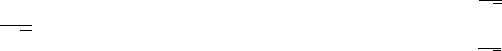
4. Atomic interactions with the radiation field
ãA beam with a circularly-polarized planar wavefront has an azimuthal component of the Poynting vector that is proportional to the radial
intensity gradient, even if it has no orbital angular momentum. This gives rise to a finite value, if integrated over the total cross-section of
the beam.
ãPolarization of the electric field: Polarization is an additional property of (em) waves that describes the orientation of their oscillations;
by convention, the polarization −1≤p≤1 refers to the electric field. The polarization of light is associated with the spin-angular
momentum (density) of the em wave.
ãThe polarisation is said to be linear if p= 0, and is left- or right-circular for p=−1 and p= +1, respectively. For all other values of
−1< p < 1, the wave is said to be elliptically polarized. Sometimes, one also refers to the chirality or handedness of the waves in order
to denote the left- or right-circular polarization of the light beam.
ãVector potential of a circularly-polarized plane wave:
A(r, t) = eλei(kz −ωt);eλ= (ex+i λ ey)(λ= +1 left circular
λ=−1 right circular
ãSpin angular momentum (SAM): The circular polarization of light is usually associated with a well-defined SAM.
ãComplex spherical unit vectors e±:
e±=1
√2(ex±iey)⇐⇒
ex=1
√2(e++e−)
ey=−i
√2(e+−e−).
ãComplex electric field E(c)= (E(c)
x, E(c)
y,0) : Although a complex notation of em fields is often very convinient, the transverse, real
electric field is given by
E(c)
x=|E(c)
x|ei γ
E(c)
y=|E(c)
y|ei(γ+δ))E(c)=<(E(c)
xex+E(c)
yey)ei(k z −ωt)=Exex+Eyey
Ex=|E(c)
x|cos(k z −ωt +γ), Ey=|E(c)
y|cos(k z −ωt +γ+δ
|{z}
!!
)... real.
ãRelative phase δto distinguish different polarization: This relative phase δrefers to the complex field amplitudes E(c)
xand E(c)
y
82

4.2. Representation and parametrization of photons in atomic theory
ãLinear polarization along the angle α:For δ=nπ (n∈N)
E(c)=|E(c)
x|ex± |E(c)
y|eycos(k z −ωt +γ) = |E(c)|eαcos(k z −ωt +γ)
|E(c)|=q|E(c)
x|2+|E(c)
y|2,tan α=±|E(c)
y|
|E(c)
x|...
(+) n= gerade
(−)n= ungerade
eα= cos αex+ sin αey
The angle αdenotes the (polarization-) direction of Ewith regard to the x-axis.
ãGeneral monochromatic plane wave: Any plane wave can always be written as superposition of two components
4.2. Representation and parametrization of photons in atomic theory
4.2.a. Stokes parametrization and density matrix of a photon
Stokes parameters:
ãStokes parameters: These parameters provide a simple and alternative characterization for the polarization of plane waves and are given
in terms of three real parameters that describe the polarization state of (transversal) electromagnetic radiation.
ãStokes parameters P1, P2, P3:The first two Stokes parameters quantify the relative asymmetries between intensities Iχof light that is
linearly polarized under different angles χwith regard to the the reaction plane: P1= (Io−I90)/(Io+I90) and P2= (I45 −I135/(I45 +I135).
The parameter P3reflects the degree of circular polarization of the emitted photons.
ãThe Stokes parameters were defined by George Gabriel Stokes in 1852 as a mathematically convenient alternative to the more common
description of incoherent or partly polarized radiation in terms of its total intensity I, the degree of polarization P, and the orientation of
the (so-called) polarization ellipse.
ãDegree of polarization: The polarization state of the photon is said to be pure if they obey the Stokes parameters obey the restriction
P3
i=1 P2
i= 1.
83

4. Atomic interactions with the radiation field
Table 4.1.: Stokes parametrization of photons for selected polarization of photons with k||ez.
Selected photon polarization P1P2P3
unpolarized 0 0 0
polarized along x-axis 1 0 0
polarized along y-axis -1 0 0
right-circularly polarized 0 0 1
left-circularly polarized 0 0 -1
ãDegree of linear polarization: The parameter P`=pP2
1+P2
2is called the degree of linear polarization.
ãStokes parameters P3=Pc:Photons with λ= +1 are called right-circularly polarized photons, and photons with λ=−1 are called
left-circularly polarized photons.
ãNote that the notation in optics is often opposite to that used in quantum electrodynamics for historical reasons.
Alternative representation of polarized photons:
ãInstead of the Stokes parameters P1and P2, it is often convenient for the analysis of different experimental situations to use the degree of
linear polarization P`and the direction of the principal axis of the polarization ellipse ϕ0.
ãPolarization ellipse: If, in the chosen coordinate frame, the x-axis is directed along the principal axis of a polarized photon beam (ϕ0= 0◦),
the Stokes parameter P1takes the largest value |P1|=P`, while the Stokes parameter P2vanishes. This easily shows that the Stokes
parameters P1and P2depend on the choice of the x-axis even if the z-axis is fixed along the beam, while the degree of linear polarization
P`remains invariant.
ãPolarization ellipse: It is often convenient to introduce the angle ϕ0by the relations
cos 2 ϕ0=P1
P`
,sin 2 ϕ0=P2
P`
84
4.2. Representation and parametrization of photons in atomic theory
ãProbability for measuring a linearly polarized photon along ϕin the xy-plane: For a density matrix with given P`, ϕ0Balashov et al.
(2001) shows the probability distribution
W(ϕ) = 1
2(1 + P`cos 2(ϕ−ϕ0))
for measuring linearly-polarized photon along ϕin the xy-plane.
Figure 4.1.: Laboratory coordinate system.
ãAngle of the polarization vector: The angle ϕ0indicates the principal axis of the polarization ellipse of the photon beam. It describes
the direction of the axis (with regard to the x-axis) which the intensity of the transmitted photon beam is the largest, while it is lowest
intensity perpendicular to this direction.
85

4. Atomic interactions with the radiation field
Photon density matrix:
ãPhoton density matrix in helicity representation: Most naturally, the spin state of an incident photon is expressed within its helicity
representation
ργ=X
λ λ0
cλλ0|kλihkλ0|,
where the helicity λis the spin projection of the photon upon the direction of its propagation, i.e. along the momemtum or wave vector k.
ãSince for a photon (with intrinsic spin s≡1) the helicity just takes the values λ=±1, only three real parameters are required to describe
the spin state of the photons. These parameters in the photon density matrix are closely connected to the Stokes parameters of light (Rose,
1961)
(cλλ0) = hkλ|ργ|kλ0i=1
2 1 + P3P1−iP2
P1+iP21−P3!.
Note that this definition differs from those in Balashov et al. (2005) by a factor −1 for the P1and P2parameters because of the different
convention of the spherical unit vectors e±.
4.2.b. Pure polarization states of photons
Linearly-polarized plane-wave photons with k || ez:
ãIn this section, we consider pure polarization states of an incoming photon, i.e. light with a photon density matrix P2
1+P2
2+P2
3= 1 ,
and which is thus equivalent to a density-matrix with ρ2=ρ.
ãWith this restriction in mind, any polarized state of a transvere photon can be described by the linear combination
|ei=g+e++g−e−,
where eλ(λ=±) are the unit polarization vectors within the circular basis, and with |g+|2+|g−|2= 1 .
86

4.2. Representation and parametrization of photons in atomic theory
ãThe state of a linearly-polarized photon along some given direction ϕ0in the x−yplane can be written in the form
|eϕ0i=−1
√2e−i ϕ0e+−ei ϕ0e−.
ãPure linearly-polarized light with P`= 1 : |g+|=|g−|.
Elliptically-polarized plane-wave photons with k || ez:
ãPhoton density matrix in terms of the g±coefficients: With these notations, an arbitrarely polarized pure state of a (transversal) photon
can be expressed in terms of the g±coefficients by either a 2 ×2 matrix or by means of the corresponding Stokes parameters:
hkλ|ρ|kλ0i= |g+|2g+g∗
−
g∗
+g−|g−|2!, P1=−2<g+g∗
−, P2= 2 =g+g∗
−, P3=|g+|2− |g−|2.
ãPolarization ellipse: The linear polarization can be characterized also by P`and ϕ0with
P`= 2 g+g∗
−= 2 |g+| |g−|cos 2 ϕ0=−<g+g∗
−
|g+g∗
−|,sin 2ϕ0=−=g+g∗
−
|g+g∗
−|.
These simple relations can be used to also find the g±-coefficients for given paramters P`and ϕ0.
ãFully-polarized light with P`6= 1 :
for |g+|>|g−|:|g+|=1
2p1 + P`+p1−P`,|g−|=1
2p1 + P`−p1−P`
for |g+|<|g−1|:|g+|=1
2p1 + P`−p1−P`,|g−|=1
2p1 + P`+p1−P`
ãThe relative phase of the coefficients: g+=|g+|ei ξ+;g−=|g−|ei ξ−can be found from the equation: ξ−−ξ+= 2 ϕ0+π.
ãPolarization vectors
1,
2of elliptical-polarized plane-wave radiation: An alternative representation of the polarization vector is given
by:
j=excos ξj
2+ieysin ξj
2exp i ηj
2,
∗
j=excos ξj
2−ieysin ξj
2exp −i ηj
2, j = 1,2.
87

4. Atomic interactions with the radiation field
ãTwo elliptically-polarized beams with the same angular momentum but opposite helicity: The easist way to describe such a superposition
is ξ1=ξ2=π/2, η1=η2= 0 , and this leads to
1=
2≡
,
∗
1=
∗
2≡
∗,
·
∗= 1,
·
=
∗·
∗= 0 .
ãTwo elliptically-polarized beams with the same helicity and opposite angular momentum: These beams are descroibed by ξ1=−ξ2=
π/2, η1=η2= 0 , and the two polarization vectors then fulfill
1=
∗
2≡
,
∗
1=
2≡
∗,
·
∗= 1,
·
=
∗·
∗= 0 .
Beams of fully-polarized light with k ∦ez:
ãSequences of completely polarized light pulses: In experiments, one often considers a sequence of (fully polarized) photon pulses, which
propagate however into different directions.
ãHierarchy of angles in defining the em pulses: For such a sequence of pulses, all angles are defined with respect to a fixed laboratory frame
Σ = (x, y, z) , and where we assume all coordinate systems to be properly ‘right-handed’.
ãIn the (primed) coordinates Σ0as associated with some given pulse, the polarization cofficients are assumed to be:
g+= 1, g−= 0 (for ‘helicity : +10)
g+= 0, g−= 1 (for ‘helicity : −10)
g+=−1
√2e−i φ0, g−=1
√2ei φ0(for ‘linear0and given φ0).
ãFirst pulse: The wave vector of the first pulse always defines the z-axis and its linear polarization (φ0) the x-axis of the fixed frame Σ ,
i.e. the first pulse defines the x−zscattering plane. For a circularly polarized pulse, the x-axis is defined indirectly due to the definition
of subsequent pulses (see below); it need not to be defined explicitly if there is only a single, circularly-polarized pulse.
88

4.3. Multipole decomposition of the radiation field
ãParameters of the first pulse:
φ1= 0; θ1= 0; (φ1= 0 for circularly polarized light)
4.3. Multipole decomposition of the radiation field
4.3.a. Elements from the theory of multipole transitions
Transition amplitudes:
ãJohnson (2008) provide a systematic decomposition of the transition amplitudes into multipole components.
ãTransition amplitudes due to a transverse-gauge vector potential A(transverse)(r, ω) : For a single-electron atom, the transition amplitude
from state a=|naκamai −→ b=|nbκbmbidue to the interaction with a plane-wave radiation field with the transverse-gauge vector
potential A(transverse)(r, ω) =
eik·r,with
·ez= 0 is
Tba =Zd3rψ∗
bα
α
α·A(transverse)(r, ω)ψa.
Multipole potentials:
ãPlane-wave multipole potentials a(p)
LM (r) : In the multipole expansion of the plane-wave vector potential, the multipole potentials satisfy
both, the Helmholtz equation and transversality condition
∇
∇
∇2a(p)
LM +k2a(p)
LM = 0,∇
∇
∇ · a(p)
LM = 0 p= 0,1.
ãThe multipole potentials a(p)
LM with p= 0 are the magnetic multipole potentials and with p= 1 the electric multipole potentials.
89

4. Atomic interactions with the radiation field
ãElectron-multipole interaction operator: The interaction operator α
α
α·a(p)
LM is an irreducible tensor operator of rank Land parity (−1)L+1−p.
ãThe multipole expansion of the (transverse-gauge) plane-wave vector potential still contains all information about the polarization and
propagation direction of the photons.
ãRepresentation of the multipole potentials: Using the well-known idendities of the spherical Bessel functions, the multipole potentials a(p)
LM
can be expressed as (Johnson, 2007)
a(0)
LM (r) = jL(kr)Y(0)
LM (r),a(1)
LM (r) = j0
L(kr) + jL(kr)
kr Y(1)
LM (r) + pL(L+ 1) jL(kr)
kr Y(−1)
LM (r).
4.3.b. Single-electron (reduced) multipole-transition matrix elements
Johnson’s single-electron reduced multipole-transition matrix elements:
ãTransverse (velocity) gauge: Johnson (2007, section 6.3) derives the reduced multipole-transition matrix elements for M= (L, p)and
q=ω/c as:
a
t(M,magnetic)(ω)
b=−κa
C(L)
κbZ∞
0
dr κa+κb
L+ 1 jL(qr) [PaQb+QaPb]
a
t(M,electric)(ω)
b=κa
C(L)
κbZ∞
0
dr −κa−κb
L+ 1 j0
L(qr) + jL(qr)
qr [PaQb+QaPb] + LjL(qr)
qr [PaQb−QaPb].
ãLength gauge: While the reduced multipole-transition matrix elements are the same in length gauge, Johnson (2007, section 6.3) derives
the reduced multipole-transition matrix elements in length gauge as:
a
t(M,electric)(ω)
b
=κa
C(L)
κbZ∞
0
dr jL(qr) [PaPb+QaQb] + jL+1(qr)κa−κb
L+ 1 [PaQb+QaPb]+[PaQb−QaPb].
90

4.3. Multipole decomposition of the radiation field
Johnson’s frequency-dependent multipole-moment operators:
ãMultipole-moment matrix elements: Following Johnson (2007), the reduced multipole-moment matrix elements can be calculate for the
reduced multipole-transition matrix elements
a
q(M)(ω)
b=(2L+ 1)!!
qLa
t(M)(ω)
b.
4.3.c. Many-electron (reduced) multipole emission and absorption amplitudes
Jac’s (standard) multipole amplitudes for photon absorption and emission:
ãMutipole (absorption) amplitude |αiJii+~ω(M, λ)to |αfJfi:For the absorption of a photon with energy ω, well-defined multipolarity
(angular momentum) Land helicity λ=±1, we always use the notation
αfJf
O(M,absorption)(ω)
αiJi.
ãPhoton emission: from an atom or ion |αiJii −→ |αfJfi+~ω(M).
ãCare has to be taken about the many-electron multipole amplitudes which appear in many expressions. While we need formally to
distinguish between the absorption aλ
Land emission operators aλ+
Loperators, all (one- and many-electron) multipole-transition matrix
elements are always evaluated in absorption.
ãFor any photon emission process, this would then require to ’interchange’ the sequence final-state — operator — initial-state explicitly.
This is a (very) high price however in such a large software project, since such an interchange affects the intuitive description of many
processes in terms of initial-intermediate-final levels as well as still possibly other subsequent (final) states/levels.
91

4. Atomic interactions with the radiation field
4.4. Electromagnetic light pulses
4.4.a. High-intensity pulses
Matter in intense fields:
ãThe exposure of atoms and matter to high-intensity laser fields is known to give rise to high-harmonic generation, above-threshold ionization
and well as laser-induced dissociation and plasma formation, and which are all fundamentally different from processes in the weak-field
regime.
ãThese phenomena are often outside of what is described by (standard) atomic-structure methods since the external field, that acts upon
the electrons in typical strong-field experiments, is then comparable to the Coulomb potential of the nucleus.
ãPump-probe experiments: In these experiments, two short pulses are typically required. While the pump pulse starts the reaction, the
probe pulse investigates the state of the system after a defined time delay. These measurements is repeated several times with increasing
time delays in order to finally obtain a molecular movie.
ãIf the level structure of the atoms is not affected by the (moderately intense) laser pulses, the time-dependent density matrix may allow to
model the (time-dependent) level occupuation and coherences of an atoms and, eventually, all the photoexcitation and ionization processes.
4.4.b. Pulse shapes and optical cycles
Pulse shaping in physics and science:
ãPulse shaping is frequently used in physics, science and technology. Pulse shaping generally refers to the the process of changing the
waveform of a (transmitted) pulse, for instance, in order to make a transmitted signal better suited for a particular communication channel.
In telecommunication, for example, pulse shaping is essential in order to ensure that the signal fit to a given frequency band.
ãIn femtosecond physics and chemistry, pulse shaping describes a technology for generating nearly arbitrary pulses with user defined, ultrafast
optical waveforms, and by controlling its phase, amplitude, and polarization. Here, the most widely applied technique is Fourier transform
pulse shaping.
92

4.4. Electromagnetic light pulses
Frequently applied pulse shapes for time-dependent atomic computations:
ãIn pump- and/or pump-probe experiments, all (symmetric) light pulses are typically defined in terms of a central frequency ωand a (delay)
time Tdfor the arrival of the pulse center with regard to same reference time t0= 0 . Moreover, the shape function is always normalized
to max[fs(t)] = max[f(t)/fo] = 1 and, hence, the intensity of the em field must be captured properly by the constant fo.
ãIn Jac, the following (symmetric) shapes of the em pulses have been pre-defined: "sin^2","sin^2: plateau","sin^2: cycles" and
"gaussian" facilitate the description of experimentally specified pulses. Further pulses shapes might be added if the need arises from the
side of experiment.
ãIt is important to ensure that the pulse-shape function fs(t) (envelope) just contains an integer number of optical cycles. Therefore, one
often starts with an sin2envelope. For example, an envelope function sin210T pulse refers to a pulse with 10 optical cycles.
4.4.c. Maximum pulse intensity
Vector potential:
ãAmplitude of the vector potential: This amplitude need to be derived from the (maximum) intensity of a laser pulses that is typically
given in W/cm2. In general, this relation between intensity and amplitude is non-trivial since the relationship between intensity and the
electric field depends also slightly on the polarization of the pulse. A simple relation only occurs for a linearly-polarized laser beam.
ãAverage intensity of a pulse: If only the average intensity is given, the conversion factor depends also on the particular pulse-shape
function. In practice, however, experimentalists rarely know the intensity accurately and, hence, a simplified normalization procedure can
normally be used.
Intensity and pulse geometry:
ãThe atomic unit of electric field is m2
ee5/~4= 5.1422 ·109V/cm. From this we have: E0[a.u.] = 5.34 ·10−9pI[W/cm2].
93

4. Atomic interactions with the radiation field
4.4.d. Bichromatic laser fields
Bichromatic laser fields:
ãBichromatic laser fields: Of some special interests in light-atom interaction studies are fields with two components of commensurate
frequencies; for instance, the fundamental component ωand one of its low harmonics 2 ωor 3 ω. Moreover, these two components are in
general out of phase by some angle φ.
ãLinearly-polarized bichromatic fields: For such a field, the electric field can be written in a quite general form as
E(t) = F(t)hcos ω t +φ(cep)
1+ηcos 2ω t +φ(cep)
2i
with frequencies ωof the fundamental radiation and 2 ωdue to the second harmonic. Here, the same envelope function F(t) is applied
for both, the fundamental and the second harmonic, while the ratio of the corresponding amplitudes is specified by the real parameter
η(η > 0) . The carrier-envelope phases (CEP) are here denoted by φ(cep)
1and φ(cep)
2, respectively.
94

5. Atomic amplitudes
5.1. In JAC implemented amplitudes
5.1.a. Dipole amplitudes (MultipoleMoment)
Amplitude, notations & application:
ãFormal quantum notation: hαfJfkDkαiJii=hαfJfkPirikαiJiifor Pf6=Pi
ãNote that the full dipole operator is often defined by: D0=−|e|D.
ãUsing Jac: Call MultipoleMoment.dipoleAmplitude(levelf::Level, leveli::Level) or (levelf::Level, leveli::Level;
display=true), if the value of the amplitude needs to be printed to screen.
5.1.b. Electro-magnetic multipole transition amplitudes (MultipoleMoment, Radiative)
Amplitude, notations & application:
ãFormal quantum notation:
αfJf
O(M,emission) (ω)
αiJi=*αiJi
N
X
k=1
α
α
αkap
k, L
αfJf+∗
≡αiJi
O(M, absorption)(ω)
αfJf∗
αfJf
T(M,absorption) (ω)
αiJi
95

5. Atomic amplitudes
which retains the right order of the initial and final levels with regard to absorption or emission and which and can be obtained from
Jac.Radiative.amplitude(); cf. section 4.3.c.
ãUsing Jac: Call Radiative.amplitude("absorption", Mp::Multipole, gauge::EmGauge, omega::Float64, levelf::Level,
leveli::Level) or ("absorption", Mp::Multipole, gauge::EmGauge, omega::Float64, levelf::Level, leveli::Level;
display=true), if the value of the amplitude needs to be printed to screen.
ãUsing Jac: Call MultipoleMoment.transitionAmplitude(Mp::Multipole, gauge::EmGauge, omega::Float64, levelf::Level,
leveli::Level) or (Mp::Multipole, gauge::EmGauge, omega::Float64, levelf::Level, leveli::Level; display=true),
if the value of the amplitude needs to be printed to screen.
Further remarks:
ãA multipole M≡(L, p)≡(L, electric/magnetic) = E1,M1,E2, ... hereby contains all information about its multipolarity (angular
momentum) Land type magnetic (p= 0) or electric (p= 1) , respectively.
ãIn the module Radiative, the multipole-transition amplitudes can be calculated in one of the gauge = {Coulomb, Babushkin, Magnetic}
as appropriate for electric- and magnetic-multipole transitions.
ãJohnson’s multipole-transition operators: Following Johnson (2007), the electron-photon interaction with the multipole fields (M) can be
expressed in terms of a dimensionless multipole-transition operator T(M)
M(ω) = Pjt(M)
M(rj;ω) , an irreducible tensor operator, whose
reduced (single-electron) matrix elements are given in Section 4.3.b. The amplitudes to these operators always describe the absorption of
a photon with a given multipolarity.
ãJohnson’s (2007) multipole-transition amplitudes can be calculated in one of the gauge = {Velocity, Length, Magnetic}as appropriate
for electric- and magnetic-multipole transitions.
5.1.c. Electro-magnetic multipole-moment amplitudes (MultipoleMoment)
Amplitude, notations & application:
ãFormal quantum notation:
αfJf
Q(M)(ω)
αiJi
96

5.1. In JAC implemented amplitudes
ãUsing Jac: Call MultipoleMoment.amplitude(Mp::Multipole, gauge::EmGauge, omega::Float64, levelf::Level,
leveli::Level) or (Mp::Multipole, gauge::EmGauge, omega::Float64, levelf::Level, leveli::Level; display=true),
if the value of the amplitude needs to be printed to screen.
Further remarks:
ãJohnson’s multipole-moment operator: Johnson (2007) also defines a frequency-dependent (irreducible tensor) multipole-moment operator
Q(M)
M(ω) = X
j
q(M)
M(rj;ω)≡(2L+ 1)!!
(ω/c)LX
j
t(M)
M(rj;ω)
ãThese amplitudes are calculated by a call to (Johnson’s) multipole-transition amplitudes from above [cf. section 5.1.b] but by taking the
frequency-dependence into account.
ãElectric multipole-moment amplitudes can be calculated in one of the gauge = {Velocity, Length, Magnetic}as appropriate for electric-
and magnetic-multipole transitions.
5.1.d. Momentum transfer amplitudes (FormFactor)
Amplitude, notations & application:
ãFormal quantum notation: DαfJf
Pjexp (iq·rj)
αiJiE= selection rules
ãUsing Jac: Call FormFactor.amplitude(levelf::Level, leveli::Level, ...) or (levelf::Level, leveli::Level,
...; display=true), if the value of the amplitude needs to be printed to screen.
Further remarks:
ãThe (single-electron) momentum transfer amplitude help describe inelastic scattering processs and is closely related also to the (so-called)
generalized oscillator strength.
97

5. Atomic amplitudes
ãThe (one-electron) momentum-transfer operator T(1)(q) = PN
j=1 exp(iq·rj) can be utilized in order to express the standard form factor
for an atom in a given sublevel |αJMiin terms of an (many-electron) expectation value; cf. 6.1.d.
5.2. In JAC partly-implemented amplitudes
5.2.a. Parity non-conservation amplitudes (ParityNonConservation)
Amplitude, notations & application:
ãFormal quantum notation: αfJf
H(weak−charge)
αiJi
ãUsing Jac: Call ParityNonConservation.weakChargeAmplitude(levelf::Level, leveli::Level, model::Nuclear.Model) or
(levelf::Level, leveli::Level, model::Nuclear.Model; display=true), if the value of the amplitude needs to be printed to screen.
Further remarks:
ãParity non-conservation (PNC) effects arises in atoms mainly because of the exchange of Z0-bosons between atomic electrons and the nucleus.
Various observables due to this parity non-conserving interactions can be described in terms of a nuclear-spin independent Hamiltonian
H(weak−charge) , an effective single-electron operator, if non-relativistic nucleons can be assumed, cf. section 3.9.b.
ãEspecially, if the proton and neutron densities coincide, ρp=ρn=ρ,the general nuclear-spin independent Hamiltonian simplifies and
can be described in terms of a single nuclear- weak charge QW,
H(weak−charge) =−G
2√2QWX
j
γ5,j ρ(rj),
where G= 2.22·10−14 a.u. is the Fermi constant, ρ(r) is the normalized nuclear density with RdV ρ(r) = 1, and QW≈ −N+Z(1−4 sin2θW)
is the nuclear weak charge with θWbeing the Weinberg angle.
98

5.3. Further amplitudes, not yet considered in JAC
5.2.b. Schiff-moment amplitudes (ParityNonConservation)
Amplitude, notations & application:
ãFormal quantum notation: αfJf
H(Schiff−moment)
αiJi=αfJf
H(Schiff−moment)
αiJiδJf,JiPf6=Pi
ãUsing Jac: Call ParityNonConservation.schiffMomentAmplitude(levelf::Level, leveli::Level, model::Nuclear.Model) or
(levelf::Level, leveli::Level, model::Nuclear.Model; display=true), if the value of the amplitude needs to be printed to screen.
Further remarks:
ãNuclear electric-dipole (Schiff) moments: If Sis the P-odd and T-odd nuclear Schiff moment, the associated P-odd and T-odd Hamiltonian
is given by (Dzuba et al., 2009)
H(Schiff−moment) =−e φ(Schiff−moment) =−4πe S· ∇δ(r) = −3S(SM) (I/I)·r
Rρ(r)
where S(SM) (I/I) is the Schiff-moment vector, i.e. the product of the coupling constant S(SM) and the nuclear spin I, and R=R∞
0dr r4ρ(r).
Moreover, φ(Schiff−moment) is the electrostatic potential of the nucleus corresponding to a P-odd and T-odd charge distribution; cf. section
3.9.c.
5.3. Further amplitudes, not yet considered in JAC
5.3.a. Anapole-moment amplitudes (ParityNonConservation)
Amplitude, notations & application:
ãFormal quantum notation: αfJf
H(anapole−moment)
αiJi
99

5. Atomic amplitudes
Further remarks:
ãAP-odd, T-even anapole moment of the nucleus was first introduced by Zel’dovich and arises due to the presence of a parity-violating
weak interaction between nucleons, cf. section 3.9.b. The anapole moment is directed along the nuclear spin I, gives typically the dominant
nuclear-spin dependent electron-nucleus interaction and manifests itself in terms of a slightly modified electro-magnetic interaction between
the nucleus and the atomic electrons.
ãHamiltonian for the interaction of the electrons with the nuclear anapole moment: This Hamiltonian has the form (Dzuba et al., 2009)
H(anapole−moment) =G
√2(I+ 1/2) (−1)I+1/2−`NκAM X
j
I·α
α
αj
I(I+ 1) ρ(rj),
where G= 2.22 ·10−14 a.u. is the Fermi constant, Iis the nuclear spin, `Nthe orbital angular momentum of the outermost nucleon and
κAM is a dimensionless coupling constants for ...
5.3.b. Scalar-pseudo-scalar amplitudes
Amplitude, notations & application:
ãFormal quantum notation: αfJf
H(scalar−pseudo−scalar)
αiJi
Further remarks:
ãHamiltonian for the P-odd, T-odd scalar-pseudo-scalar interaction: In coordinate represetation, this Hamiltonian can be written as (Dzuba
et al., 2009)
H(scalar−pseudo−scalar) =−G
√2
1
2mpcCsX
jγ0
d ρ(r)
dr j
where Gis the Fermi constant, mpis the nucleon mass, Csis a (isotope and) nuclear-state dependent constant, and where hγ0d ρ(r)
dr iis a
scalar term that arises from the scalar product of the ∇-vector with an particularly averaged spin-vector of the nucleus.
100

5.3. Further amplitudes, not yet considered in JAC
5.3.c. Tensor-pseudo-tensor amplitudes
Amplitude, notations & application:
ãFormal quantum notation: αfJf
H(tensor−pseudo−tensor)
αiJi
Further remarks:
ãHamiltonian for the P-odd, T-odd tensor-pseudo-tensor interaction: In coordinate representation, this Hamiltonian can be written as
(Dzuba et al., 2009)
H(tensor−pseudo−tensor) =i√2G CtX
j
[γ ρ(r)]j
where Gis the Fermi constant, Ctis a (isotope and) nuclear-state dependent constant, and where [γ ρ(r)] is a scalar term that arises from
the scalar product of the γ-vector with an averaged spin-vector of the nucleus.
ãTotal P-odd, T-odd electron-nucleus interaction Hamiltonian: H(P−odd,T−odd electron−nucleus) =H(tensor−pseudo−tensor) +H(tensor−pseudo−tensor)
5.3.d. Nuclear magnetic-quadrupole-moment amplitudes due to internal B-field
Amplitude, notations & application:
ãFormal quantum notation: αfJf
H(nuclear−MQM)
αiJi
Further remarks:
ãThis interaction (Hamiltonian) arise from the interaction of the electron EDM dewith the electro-magnetic fields of the nucleus as seen
by the electron. If the treatment is restricted to second order, only the interaction of the electron EDM with the magnetic field B, which
is created by the nuclear magnetic-dipole moment, need to be taken into account.
101

5. Atomic amplitudes
ãNuclear-MQM Hamiltonian: In coordinate representation, this Hamiltonian can be written as (Dzuba et al., 2009)
H(nuclear−MQM) =−i deγ·B
γ·B
γ·B=−i deX
j
γ
γ
γj·∇
∇
∇j×M×rj
r3
>,j
+...
5.4. Composed many-electron amplitudes, not yet considered in JAC
5.4.a. Parity-violating (non-diagonal, second-order) amplitudes
Amplitude, notations & application:
ãParity violation: The (effective) parity-violating interaction is caused by the exchange of Zobosons between the atomic electrons and the
nucleus. The parity-violating interaction typically results in non-vanishing off-diagonal electric-dipole matrix element between two atomic
states of the same parity; cf. section 3.9.b.
5.4.b. Charge-parity-violating (diagonal, second-order) amplitudes
Amplitude, notations & application:
ãCharge-parity violation: An intrinsic electron electric dipole moment deleads to CP-violation in atoms and also induces an atomic electric
dipole moment. cf. section 3.9.d.
5.4.c. Electric-dipole moment enhancement factor
Amplitude, notations & application:
102
5.4. Composed many-electron amplitudes, not yet considered in JAC
ãAn intrinsic electric-dipole moment (EDM) of the electron can enhanced the EDM of the atom. In heavy atoms, in particular, an induced
atomic EDM can be strongly enhanced, when compared to the electron EDM itself.
ãA typical goal is to find the atomic EDM datom =|datom| ≡ datom |F/F |, where F=I+Jis the total angular momentum of an
atomic (hyperfine) level.
ãThe value of the atomic EDM, compared to the electron EDM, is expressed by means of an enhancement factor K=datom/de, and which
increases with nuclear charge Zfaster than Z3.
103

6. Atomic properties
6.1. In JAC implemented level properties
6.1.a. Transition probabilities for a single multiplet (Einstein)
Properties, notations & application:
ãPhoton emission: from an atom or ion A∗−→ A(∗)+~ω
ãFormal quantum notation: |αiJii −→ |αfJfi+~ω
ãUsing Jac: Perform an Atomic.Computation(.., properties=[EinsteinX, ..], configs=[..], einsteinSettings=
Einstein.Settings(..), ..) or call directly functions from the module Einstein.
ãIn the Jac program, the transition probabilities, oscillator strength (in emission) and radiative lifetimes are calculated and tabulated by
default for all selected transitions from a given single multiplet (i.e. list of configurations). Apart from the multipoles, the user can also
specify an overall shift in the photon energies as well as a minimum and maximum transition energy, for which transitions are taken into
account.
ãIn the Einstein module, the emission (transition) amplitudes αfJf
O(M,emission)
αiJior absorption amplitudes
αfJf
O(M,absorption)
αiJican be obtained directly by call of the function Jac.Einstein.amplitude().
Further remarks:
ãEinstein Aand Bcoefficients and oscillator strength for levels |αJifrom a single multiplet are frequently needed for various applications
and in different contexts.
105

6. Atomic properties
ãAlthough these coefficients are no (single) level property, the Einstein module still supports the computation of these coefficients for levels
from a single multiplet, and which is generated by a single CSF basis.
ãAlthough the Einstein module does not allow to include relaxation effects, this module helps obtain either a quick estimate of the Einstein
coefficients between levels from just a few configurations or to deal with cascade computations.
ãJac’s standard multipole amplitudes for photon emission: Although all (one- and many-electron) matrix elements are always evaluated
in absorption within the Jac toolbox, we keep the intuitive description of the matrix elements as final-state – operator – initial-state,
cf. section 4.3.c.
6.1.b. Hyperfine parameters and hyperfine representations (Hfs)
Properties, notations & application:
ãHyperfine splitting of an atomic level into hyperfine (sub-) levels: |αJi −→ |α(J)Fi, F =|I−J|, ..., I +J−1, I +J.
ãFormal quantum notation: |αJi −→ |αFi≡|(I, α0J)Fi≡|α(IJ)Fi≡|α(IJP )Fior
|αJMJi −→ |αFMi≡|(I, α0J)FMi≡|α(IJ)FMi≡|α(IJP )FMi.
ãUsing Jac: Perform an Atomic.Computation(.., properties=[HFS, ..], configs=[..], hfsSettings=Hfs.Settings(..), ..)
or call directly functions from the module Hfs. The Boolean values calcT1 and calcT2 in Hfs.Settings determine which parts of
the hyperfine Hamiltonian are taken into account into the computations.
ãIn the Jac program, the hyperfine Aand Bcoefficients as well as the (electric) hyperfine amplitudes αJ
T(1)
αJ,αJ
T(2)
αJ
are calculated and tabulated by default for all selected levels together with the energy shifts ∆ EFof the hyperfine levels with regard to
the (electronic) level energy EαJ.
ãIn Jac, the hyperfine amplitudes βrJr
T(1)
βsJsand βrJr
T(2)
βsJscan be obtained from the function Jac.Hfs.amplitude().
ãIn Jac, moreover, an explicit representation of a hyperfine multiplet is obtained by diagonalizing the Hamiltonian H=H(DCB) +H(hfs)
within the atomic hyperfine IJF -coupled basis if calcIJFexpansion=true is set in Hfs.Settings.
ãIn Jac, all the (hyperfine) level energies EαFand the energies relative to the lowest (hyperfine) level are tabulated if printDeltaEF=true
in Hfs.Settings.
106

6.1. In JAC implemented level properties
ãIn Jac, all (diagonal and nondiagonal) hyperfine amplitudes are calculated and tabulated explicitly if calcNondiagonal=true in
Hfs.Settings.
Further remarks:
ãFor a nucleus with non-zero spin I > 0, a hyperfine splitting of (all) atomic levels generally occurs since each atomic electron also interacts
with the electric and magnetic (multipole) fields of the nucleus. This is sometimes described also as the interaction of the magnetic moments
of the electrons and nucleus.
ãIn atomic physics, this interaction is better known as ‘hyperfine interaction’ whose two dominant contributions arise from the nuclear
magnetic-dipole field A=µ
µ
µ×r
r3and the electric-quadrupole field Φ(r) = Pij
rirj
2r5Qij, respectively. In these expressions, µ
µ
µis the
nuclear magnetic moment operator and Qij, i, j = 1..3 are the Cartesian components of the nuclear quadrupole operator.
ãApart from the hyperfine parameters A(αJ) and B(αJ), we also provide in Jac arepresentation of the atomic hyperfine levels that
can be utilized, for instance, to compute hyperfine quenched transitions probabilities.
Hyperfine interaction Hamiltonian:
ãRelativistic hyperfine interaction Hamiltonian: For many-electron systems, this Hamiltonian can be written as
H(hfs) =X
K
W(K)·T(K)
where W(K)and T(K)represent the spherical tensor operators of rank Kthat occur in the nucleonic and electronic sectors, respectively.
ãReduced nuclear matrix elements: These matrix elements are determined geometrically by
I
W(1)
I=µIrI+ 1
I,I
W(2)
I=Q
2s(I+ 1) (2I+ 3)
I(2I−1) ,
while, in contrast, the corresponding electronic amplitudes require detailed atomic structure calculations.
ãValues of nuclear magnetic dipole and electric quadrupole moments can be found in the compilation by Stone (2005).
107

6. Atomic properties
ãElectronic tensor operators: For an N-electron atom or ion, these tensor operators are given by (Andersson and J¨onsson, 2008)
T(1) =
N
X
j
t(1)(j) =
N
X
j−i√2α(αjC(1)(j))(1)
r2
j
interaction with the magnetic −dipole field
T(2) =
N
X
j
t(2)(j) =
N
X
j−C(2)(j)
r3
j
interaction with the electric −quadrupole field,
and where αis the fine-structure constant, αjthe vector of Dirac matrices of the j-th electron, and the C(K)are (normalized) spherical
tensors as before.
Atomic (hyperfine) IJF -coupled basis:
ãThis (geometrically fixed) basis is obtained by the standard coupling of the nuclear states |IMIiand the ASF |αJMJi
|α(I, J)FMi ≡ |(I, α0J)FMi=X
MIMJ|IMIi |α0JMJi hIMI, JMJ|F M i.
ãThe atomic (hyperfine) IJF -coupled basis, also called the IJF -coupled ASF basis, is applied internally to represent all hyperfine levels,
see below.
Atomic hyperfine amplitudes and levels:
ãAtomic hyperfine levels: For the combined system ‘nucleus+electrons’, the atomic hyperfine states (magnetic sub-levels) can be formed
as linear combination
|αFMi=X
r=1
˜cr(α)|(I, βrJr)FMi
of hyperfine (basis) states |(I, βrJr)FMiof the same total angular momentum Fand (the same electronic) parity P, and where {˜cr(α)}
denotes the representation of these states in the atomic hyperfine-coupled basis (Johnson, 2010).
108

6.1. In JAC implemented level properties
ãAnalogue as for the ASF |αJiin the standard MCDF ansatz, the representation {˜cr(α)}of an atomic hyperfine state is obtained by
diagonalizing the Hamiltonian H=H(DFB) +H(hfs) of the combined system ‘nucleus+electrons’ in either the IJF -coupled CSF or ASF
basis.
ãIn the IJF -coupled ASF basis, we can make use of H(DFB) |(I, βrJr)FMi=E(βrJr)|(I, βrJr)FMi ≡ EβrJr|(I, βrJr)FMi.
ãFor the hyperfine part of the Hamiltonian, the (reduced) matrix elements can be written after some standard angular momentum algebra
as
(I, βrJr)FMH(hfs) (I, βsJs)F0M0=δM M0(I, βrJr)FH(hfs) (I, βsJs)F0
=δMM 0δFF0(−1)I+Jr+FX
KI JrF
JsI KβrJr
T(K)
βsJsI
W(K)
I,
with δFF0=δP P 0δF F 0, and if all nuclear excitations are ignored right from the beginning.
ãHyperfine amplitudes: These amplitudes refer to the (reduced) electronic matrix elements βrJr
T(K)
βsJs. In the Jac program, we
compute the hyperfine amplitudes for both, the magnetic-dipole and the electric-quadrupole operators of the electron-nucleus interaction.
ãThese hyperfine amplitudes are utilized to set-up and diagonalize the Hamiltonian matrix within the atomic IJF -coupled basis for H=
H(DCB) +H(hfs) in order to determine the representation {˜cr(α)}of the atomic hyperfine states.
Hyperfine energies and interaction constants:
ãHyperfine interaction constants: Usually the hyperfine splitting is considered independently for each atomic level |αJiand without the
need to specify all the hyperfine level energies EαFexplicitly. Instead, the energy splitting of an atomic level |αJiinto hyperfine levels
|αFican be expressed conveniently in terms of the (hyperfine interaction) constants
A(αJ) = µI
I
1
pJ(J+ 1) αJ
T(1)
αJ, B(αJ) = 2QsJ(2J−1)
(J+ 1)(2J+ 3) αJ
T(2)
αJ
ãHyperfine energy splitting: With these constants, the hyperfine energy shifts with regard to the electronic level energy E(αJ) is given by
∆EF=A(αJ)C
2+B(αJ)3/4C(C+ 1) −I(I+ 1) J(J+ 1)
2I(2I−1) J(2J−1) , C =F(F+ 1) −J(J+ 1) −I(I+ 1).
109

6. Atomic properties
6.1.c. Isotope-shift parameters (IsotopeShift)
Properties, notations & application:
ãIsotope shift of an atomic level for two isotopes A, A0with nuclear masses M < M0:E(αJ;A)−→ E(αJ;A0) .
ãFormal quantum notation: ∆E(αJ;A, A0)/ h =M0−M
M M0K(MS) +F δ hr2i.
ãUsing Jac: Perform an Atomic.Computation(.., properties=[Isotope, ..], configs=[..], isotopeSettings=
IsotopeShift.Settings(..), ..) with calcNMS=true, calcNMS=true or calcF=true and/or call directly functions from the module
IsotopeShift in order to include the various contribution of the recoil Hamiltonian.
ãIn Jac, we calculate and tabulate by default the (relativistic) mass-shift parameters K(MS), K (NMS), K (SMS) and the field-shift parameter
Ffor all selected levels.
Further remarks
ãOwing to the conservation of the total momentum, the (total non-relativistic) mass shift is a sum of two parts, the (so-called) normal mass
shift (NMS) and the specific mass shift (SMS):
H(MS,nr) =H(NMS,nr) +H(SMS,nr) =1
2MX
j
p2
j+1
2MX
i6=j
pi·pj
While the normal mass shift operator is obviously a one-particle operator, the specific mass shift is a two-particle operator. The sum of
these two parts is known also as the total recoil operator within the nonrelativistic theory.
Relativistic recoil (Hamilton) operator:
110

6.1. In JAC implemented level properties
ãRecoil Hamiltonian: Within the lowest-order relativistic approximation ( ∼v2/c2) and in first order of m/M for a nucleus with mass
M, the recoil corrections are given by means of the (recoil) Hamiltonian (Tupitsyn et al., 2003):
H(recoil)(M) = 1
2MX
ij pi·pj−α Z
riα
α
αi+(α
α
αi·ri)ri
r2
i·pj
ãThe expectation value of H(recoil)(M) with regard to the relativistic wave function from H(DCB) gives the recoil correction to the energy
of the atomic energy |αJiin first order of m/M .
ãDecomposition of the relativistic recoil Hamiltonian: Similar as in the non-relativistic theory, the (relativistic) recoil operator above can
be written as (Tupitsyn et al., 2003; Gaidamauskas et al., 2011)
H(recoil)(M) = H(NMS,relativistic) +H(SMS,relativistic)
=1
2MX
ip2
i−α Z
riα
α
αi+(α
α
αi·ri)ri
r2
i·pi+1
2MX
i6=jpi·pj−α Z
riα
α
αi+(α
α
αi·ri)ri
r2
i·pj
=1
2MX
ip2
i−α Z
ri
α
α
αi·pi−α Z
ri
(α
α
αi·C(1)
i)C(1)
i·pi+1
2MX
i6=jpi·pj−α Z
ri
α
α
αi·pj−α Z
ri
(α
α
αi·C(1)
i)C(1)
i·pj
=H(NMS) +H(SMS,A) +H(SMS,B) +H(SMS,C)
ãThe relativistic correction to the recoil effect is typically strongly overestimated if the nonrelativistic recoil operator is applied just together
with relativistic wave functions.
ãThe full relativistic theory of the nuclear recoil effect can be formulated only within the framework of quantum electrodynamics. Such a
theory was first formulated by Shabaev (1985), where the complete α Z -dependence of the recoil corrections to an energy level |αJiwas
derived in first order of m/M .
Reduced one-electron matrix elements of the recoil (Hamilton) operator:
111

6. Atomic properties
ãRecoil Hamiltonian: While the normal mass-shift Hamiltonian is a one-particle operator, the specific mass-sift is a (symmetric) two-particle
operator
H(NMS) =X
j
h(NMS)(rj),H(SMS,k) =X
i6=j
h(SMS,k)(ri,rj) = X
i6=j
g(ri, k)g(rj, k)T(1)
i·T(1)
j, k =A, B, C
The particular tensorial structure of the two-particle specific mass-shift Hamiltonian ensures that the reduced (one-electron) matrix elements
can be expressed in terms of the first-rank effective interaction strength X(1; SMS,k) that are specified below for k=A, B, C .
ãReduced one-electron matrix element for the normal mass-shift: With the definition of the angular coefficients in Grasp, this one-electron
matrix element is given with P0=∂P
∂r (Gaidamauskas et al., 2011)
a
h(NMS)
b=δκa,κb
1
2MZ∞
0
dr P0
aP0
b+Q0
aQ0
b+`b(`b+ 1) PaPb+ (2jb−1) 2jbQaQb
r2
−(2αZ)QaP0
b+QbP0
a
r−(αZ)κb−1
r2(QaPb+QbPa)
Parametrization of the isotope shift:
ãMass shift of two isotopes: Within lowest order of m/M , the (isotope) mass shift for an atomic level |αJiis determined by the difference
of the expectation values of H(recoil)(M) for two different isotopes:
∆E(MS) (M, M0) = αJH(recoil)(M)−H(recoil)(M0)αJ=M0−M
M M0K(MS)
K(MS)
M=αJH(recoil) (M)αJ=αJ
H(recoil)(M)
αJ,
and where the Wigner-Eckardt theorem is used here in a special form that is consistent with Grasp and that is utilized for the implemen-
tation of corresponding angular coefficients.
ãThe conversion factor between the mass-shift parameters K(MS) in the frequently applied units is:
K(MS)/[GHz u] = 3609.4824 K(MS)/[a.u.].
112

6.1. In JAC implemented level properties
ãField shift of two isotopes: is caused by their different nuclear charge distributions and can be parametrized by:
∆E(FS)(M, M0) = −*αJ
N
X
j=1 V(nuc)(rj;R0)−V(nuc)(rj;R)
αJ+=*αJ
N
X
j=1
δV(nuc)(rj;R0, R)
+=−F δ r2
F=DαJPjV(nuc)(rj;R0)−V(nuc)(rj;R)αJE
R0−R
where δhr2i=R0−Ris the difference of the root-mean-square (rms) charge radii of the two isotopes with masses M0, M .
6.1.d. Atomic form & scattering factors and scattering functions (FormFactor)
Properties, notations & application:
ãForm factor F(q;αJ)of an atomic level with spherical-symmetric charge distribution:.
ãFormal quantum notation: F(standard)(q;αJ), F (modified)(q;αJ) .
ãUsing Jac: Perform an Atomic.Computation(.., properties=[FormF, ..], configs=[..], formSettings=
FormFactor.Settings(..), ..) or call directly functions from the module FormFactor.
ãIn Jac, the standard and the modified form factors are calculated and tabulated for all selected levels and for all the specified q-values [in
a.u.] in FormFactor.Settings; the default values are q= 0.1,1., 10.
Further remarks:
ãAtomic form factor (known also as atomic scattering factor): These form factors are often taken as a measure of the (scattering) amplitude
for the scattering of some incident quantum wave by an isolated and spherical symmetric atom.
ãIn practice, therefore, the atomic form factor depends on the type of scattering, being elastic or inelastic, as well as on the incident radiation,
such as photons, electrons or neutrons. As usual, we here restrict ourselves to the atomic form factor for photon (x-ray) scattering.
113

6. Atomic properties
ãThe atomic form factor is often written as function of the momentum transfer q=|q|, and this momentum transfer is directly related
to the scattering angle by: ~q= 2ksin(ϑ/2) = 2
λsin(ϑ/2) .
ãMomentum-transfer variable: Instead of the momentum transfer q, many tabulations for x-ray scattering make use of the (so-called)
momentum-transfer variable x= [sin(ϑ/2)] / λ [A] with λ[A] = 12.398520/E [keV].
ãElastic scattering of photons by atoms, ions or molecules has been found important in many fields of physics, such as crystallography,
plasma physics and astrophysics. For high-photon energies (well above the K-shell threshold energy of the atom or ion), the form factor
(FF) or modified form factor (MFF) approximations are widely used and were found moderately succesful in estimating the scattering cross
sections. However, both form factor approximations fail at smaller photon energies.
Definition of atomic form factors:
ãStandard atomic form factor: For an atom in the level |αJiwith a spherically-symmetric charge distribution ρ(r) , the standard atomic
form factor is given by
F(standard)(q;αJ) = 4πZdr r2ρ(r)sin(qr)
q r =αJMT(1)(q)αJM
is just equal to the Fourier transform of the charge density ρ(r) , if this density is normalized by 4πRdr r2ρ(r) = Nto the number of
bound electrons.
ãThis standard form factor can be expressed also as (many-electron) expectation value of the (one-electron) momentum-transfer operator
T(1)(q) = PN
j=1 exp(iq·rj) for a given sublevel |αJMi, see above.
ãModified atomic form factor: For an atom or ion with a spherically-symmetric charge distribution, a modified atomic form factor can be
defined via the charge distributions of the individual (sub-) shells or elements
F(modified)(q;αJ) = 4π
N
X
i=1 Zdr r2ρi(r)sin(qr)
q r
mc2
ε0
i−V(r)
where ρi(r) is the charge density of the i-th electron, ε0
i=εi+mc2its energy (including the rest mass), and V(r) the potential of
the electron at position r. Here, the summation is taken over all electrons, and the charge distribution must fullfill again the constraint
that 4πPiRdr r2ρi(r) = Nis equal to the number of bound electrons.
114

6.1. In JAC implemented level properties
ãGeneralized atomic form factor: A generalized form factor can be defined for any pair of states, often take for the ground state |αoJoMoi
and some excited state |αeJeMei
F(generalized)(q;αeJeMe;αoJoMo) = αeJeMeT(1)(q)αoJoMo.
This generalized atomic form factor help describe inelastic scattering processs and is closely related also to the generalized oscillator strength,
cf. Section 7.3.f
Anomalous scattering factors g0, g00 :
ãAnomalous scattering factor: The real g0(ω) and imaginary g00(ω) anomalous scattering factors are frequently employed in order to
express the coherent (Rayleigh) scattering factor G(ω) , for incident photons with energy ~ω.
ãRayleigh scattering factor: For the photon energy ~ω, the coherent (Rayleigh) scattering factor in forward direction can be written fas
(Zhou et al., 1990)
G(ω) = F(0) + g0(ω) + i g00(ω)
where F(0) = Nis the atomic form factor. Therefore, the (Rayleigh) scattering factors/amplitude can be expressed also in terms of the
standard (atomic) form factor (FF) or with regard to the modified form factor (MFF).
Incoherent scattering function S(q):
ãIncoherent scattering function: This scattering function can be expressed by means of the generalized atomic form factor
S(q;αoJoMo) = X
e6=o|F(generalized) (q;αeJeMe;αoJoMo)|2=αoJoT(2)(q)αoJo− |F(standard)(q;αoJo)|2.
Here, the sum over eincludes a summation over all discrete levels and the integration over the continuum. In the second expression, the
two-electron momentum-transfer operator T(2)(q) = PN
m,n=1 exp[iq·(rm−rn)] need to be applied, although then only matrix elements
are necessary with regard to the ground state |αoJoMoi.
115

6. Atomic properties
6.2. In JAC partly-implemented level properties
6.2.a. Energy shifts in plasma environments (PlasmaShift)
Properties, notations & application:
ãPlasma shift of an atomic level: E(αJ)−→ E(αJ; plasma model and parameters) .
ãFormal quantum notation: ∆E(plasma)(αJ) = E(αJ; plasma model and parameters) −E(αJ; unperturbed) .
ãUsing Jac: Perform an Atomic.Computation(.., properties=[Plasma, ..], configs=[..], plasmaSettings=
PlasmaShift.Settings(..), ..) or call directly functions from the module PlasmaShift.
ãIn Jac, the plasma (energy) shifts are calculated and tabulated by default for a Debye-H¨uckel plasma model with screening parameter
λ= 1. Hereby, the Debye-H¨uckel interaction is incorporated only in first-order perturbation theory within the CI matrix.
Further remarks:
ãSpectral line shifts: The interaction between the plasma and the bound electrons of an ion embedded into the plasma alters the ionic
structure and transition properties. Therefore, a plasma environment generally results in spectral line shifts, line broadening and changes
in the line shapes, when compared with the free ion.
ãFor realistic plasma conditions, the number of bound states of the ions often becomes finite and the electrons less tightly bound by the
nucleus, if the plasma coupling parameter increases.
High-density plasma:
ãRelativistic corrections to the plasma screening may become necessary for a detailed analysis of atomic spectra, especially if lines of
multiply-charged ions are used in some spectral analysis.
ãCollisional-radiative model: The effects of the plasma-environment can be further taken into account also by kinetic or collisional-radiative
models, and where the energy shifts are often introduced by semi-empirically formul, such as the formula by Stewart and Pyatt.
116

6.2. In JAC partly-implemented level properties
ãApplication of simple plasma models: Apart from plasma diagnostics, a proper treatment of a screening potential has been found useful
also in other areas of physics, such as nuclear and elementary particle physics, solid state physics, or even the design of nanostructures.
ãStrongly-coupled plasma: For a strongly-coupled dense plasma the (averaged) electrostatic energy between neighbouring particles in the
plasma exceeds their thermal energy. The coupling parameter Γ = q2/4π0R0kT > 1 is used in order to characterize such a strongly-coupled
plasma. This coupling parameter Γ simply describes the ratio of the electrostatic and the thermal energy of the plasma particles.
ãStrongly-coupled plasma obeys classical statistics and has been observed for a large number of experimental and astrophysical conditions.
In the laboratory, for instance, laser-induced plasma with Γ 1 has been investigated in high-compression fusion experiments. Such
a laser-produced plasma provides a very typical example of a high-density, strongly-coupled plasma with electronic densities well beyond
1024 cm−3.
ãTheoretical (plasma) models for hot and dense plasma are necessary to simulate its properties, such as the equations of state, radiative
transfer coefficients or the conduction coefficients in plasma. These properties are relevant for inertial confinement fusion and astrophysics.
Frequently applied plasma models in atomic structure calculations:
ãDebye-H¨uckel model: This model has been commonly used in order to incorporate plasma effects into atomic structure calculations.
However, the validity of this model is rather questionable because it is valid only when the correlation time of the ion is much longer than
the lifetime of excited atomic states. Therefore, this perturbative approach is at best valid for weakly-coupled plasmas and should not be
applied for modeling of high-density plasmas.
ãCoulomb interaction in the Debye-H¨uckel model: In this model, the (pairwise) Coulomb interaction among the charged particles is modified
(screened) for an ion with nuclear charge Zto
V(DH)(r, λ) = −
N
X
i
Ze−λ ri
ri
+
N
X
i>j
e−λ rij
rij
=
N
X
i
V(e−n,DH)(ri, λ) +
N
X
i>j
V(e−e,DH)(rij , λ).
Here, Nis the number of bound electrons in the ion, riis the distance of the i-th electron from the nucleus, and rij the distance between
the electrons iand j.
ãPlasma screening parameter λ:This parameter is the inverse of the Debye shielding length for a certain plasma environment and can be
117
6. Atomic properties
readily expressed in terms of the electron density neand the temperature Teof the plasma:
λ=4π ne
k Te1
2
.
ãDebye-H¨uckel model: To obtain the modified two-particle integrals due the plasma screening, we can write
V(e−e,DH)(rij , λ) = −λ∞
X
l=0
(2l+ 1) jl(iλ r<)h1
l(iλ r>)Pl(cosθ)
in terms of the larger (r>= max(ri, rj)) and smaller radii (r<= min(ri, rj)) of the one-particle radii riand rj, respectively, and where jl
denotes a spherical Bessel function and h1
la Hankel function of the first kind.
ãDebye-H¨uckel model: While the Debye-H¨uckel screening in the ‘electron-nucleus’ interaction usually destabilizes the binding of the electron,
the screening of the electron-electron repulsion counteracts this trend.
ãIon-sphere model: In this model, the ion is typically enclosed in a spherically symmetric cell that contains the exact number of electrons
in order to ensure neutrality. In the ion-sphere model, one needs to define an electron-density distribution that either obeys self-consistency
equations or need to make some simple hypothesis, such as an uniform density within the cell.
ãIn practice, the ion-sphere model has been extensively used only in its simplest form, in which the free-electron density exactly cancels the
ion densities outside of the Wigner-Seitz sphere, i.e. beyond the ion-sphere radius.
Free-electron distributions in plasma:
ãIn a plasma, the free-electron (radial) density ne(r) can follow different distributions:
ãMaxwell-Boltzmann distribution: The Maxwell-Boltzmann statistics has been often applied to describe the free-electron distribution but
is not well justified for high plasma densities or low plasma temperatures.
ãFermi-Dirac distribution: This distribution is preferable if the free electrons are degenerate
ne(r) = 4
√πZ∞
ro
dr √r
er−ro−µ/k Te+ 1 = 2 λ−3
th F1/2−V(r)
k Te
+µ
k Te
;−V(r)
k Te.
Here µis the chemical potential of the plasma, F1/2(x, y) the incomplete Fermi-Dirac integral and λth =p2π / k Tethe thermal de-Broglie
thermal wavelength.
118

6.2. In JAC partly-implemented level properties
ãUniform electron-gas distribution: This distribution considers a sphere of radius R0around the ion with Nbbound electrons, in which
the ionic charge is completely neutralized by the additional Nf=Z−Nbfree electrons. Although all electrons inside of the sphere will
strongly interact with the embedded ion, the free electrons are here assumed to be distributed uniformly. With this assumption in mind,
the electrostatic potential for the i-th bound electron with radial coordinate riis given by
V(IS)(ri;R0) =
−Z
ri+Z−Nb
2R03−ri
R02for ri≤R0
0 for ri>R0.
In this potential above, the first term describes the interaction of the bound electron with the nucleus, while the second (repulsive) term
arises from the plasma background and always causes a shift of all the level energies towards the continuum.
Gordon-Kim theory:
ãIn the Gordon-Kim theory (1972), the total energy of the system consists out of the direct Coulomb potential energy, the exchange Coulomb
potential energy, the kinetic energy as well as the correlation energy. The direct Coulomb potential energy is calculated by integrating the
Coulomb potential for the (approximated) electron density, while the other contributions to the total energy were calculated by using a
temperature-dependent local density functional (LDA) approach.
6.2.b. Lande gJfactors and Zeeman splitting of fine-structure levels (LandeZeeman)
Properties, notations & application (not yet fully implemented):
ãZeeman splitting of an atomic level into Zeeman (sub-) levels: |αJi −→ |αJMi, M =−J, ..., J −1,+J.
ãFormal quantum notation: |αJMi.
ãUsing Jac: Perform an Atomic.Computation(.., properties=[LandeJ, ..], configs=[..], zeemanSettings=
LandeZeeman.Settings(..), ..) with calcLandeJ=true or call directly functions from the module LandeZeeman.
ãIn Jac, we calculate and tabulate by default the Lande gJ≡g(αJ) factors for the selected fine-structure levels.
119

6. Atomic properties
ãIn the Jac program, the Zeeman amplitudes βrJr
N(1)
βsJsand βrJr
∆N(1)
βsJscan be obtained from the function
Jac.LandeZeeman.amplitude().
Further remarks:
ãThe Zeeman effect describes the (level) splitting of an atomic level |αJiinto its sub-levels |αJMiin the presence of a static magnetic
field.
ãThe various components |αJMiof a Zeeman-splitted line usually have different intensities, and with some of them possibly even forbidden
within the dipole approximation.
ãThe energy splitting of the Zeeman sub-levels depends of course on the magnetic field strength. — Therefore, the Zeeman effect has be
applied for measuring magnetic field strengths, e.g. in astrophysics at the surface of the Sun or in laboratory plasmas.
Zeeman Hamiltonian H(mag):
ãIf the z-axis is chosen along the magnetic field B|| ezand if we neglect diamagnetic contributions, the magnetic (Zeeman) Hamiltonian
can be written in terms of spherical tensors (Andersson and J¨onsson, 2008)
H(mag) =N(1)
0+ ∆ N(1,QED)
0B
N(1) =
N
X
j
n(1)(j) =
N
X
j−i√2
2αrjα
α
αjC(1)(j)(1)
∆N(1) =
N
X
j
∆n(1)(j) =
N
X
j
gs−2
2βjΣ
Σ
Σj,Σ
Σ
Σ = σ
σ
σ0
0σ
σ
σ!,
and where the second term in the magnetic Hamiltonian above is (so-called) Schwinger’s QED correction. Here, gs= 2.00232 is the
g-factor of the electron, including some leading QED corrections.
120

6.2. In JAC partly-implemented level properties
Lande factor gJ≡g(αJ)and Zeeman splitting of an electronic level |αJi:
ãZeeman splitting of an atomic level |αJi:If the energy splitting due to the magnetic field is small, when compared with the fine-structure
splitting, it can be expressed in first-order perturbation theory by
∆E(mag) (αJM) = E(αJM)−E(αJ, M = 0)
=DαJMN(1)
0+ ∆ N(1,QED)
0αJME= (−1)J−MJ1J
−M0M√2J+ 1 αJ
N(1) + ∆ N(1,QED)
αJB
=M
pJ(J+ 1) αJ
N(1) + ∆ N(1,QED)
αJB
and with regard to the unperturbed energy E(αJ, M = 0) = E(αJ, B = 0) .
ãLande gJfactor of an atomic level |αJi:Usually, the dependence on the Mquantum number is factored out and the energy splitting
is expressed for a single level |αJiin terms of its Lande factor gJ≡g(αJ)
∆E(mag) (αJM) = g(αJ)MB
2, g(αJ)≡gJ= 2 αJ
N(1) + ∆ N(1,QED)
αJ
pJ(J+ 1)
6.2.c. Lande gFfactors and Zeeman splitting of hyperfine levels (LandeZeeman)
Properties, notations & application (not yet fully implemented):
ãZeeman splitting of an atomic hyperfine level into Zeeman (sub-) levels: |α(J)Fi −→ |α(J)FMi, M =−F, ..., F −1,+F.
ãFormal quantum notation: |α(J)FMi.
121

6. Atomic properties
ãUsing Jac: Perform an Atomic.Computation(.., properties=[LandeJ, ..], configs=[..], zeemanSettings=
LandeZeeman.Settings(..), ..) with calcLandeF=true or call directly functions from the module LandeZeeman.
ãIn Jac, we calculate and tabulate by default the Lande gF≡g(αF) factors for the selected hyperfine-structure levels.
Further remarks:
ãThe Lande g-factor (also kown as gvalue or dimensionless magnetic moment) is a dimensionless entity that characterizes the gyromagnetic
ratio of an atomic or hyperfine level. The Lande g-factor is basically a proportionality constant how efficient a particle, spin or quantum
state with given total angular momentum scontributes to the splitting in an external magnetic fiel B.
Lande factor gF≡g(αF)of an hyperfine level |αFi:
ãZeeman splitting of an hyperfine level |αFi:If the energy splitting due to the magnetic field is small, when compared with the hyperfine-
splitting, it can be expressed in first-order perturbation theory in terms of the reduced electronic Zeeman amplitudes by
∆E(mag) (αFM) = E(αFM)−E(αF, M = 0)
=D(I, α J)F M N(1)
0+ ∆ N(1,QED)
0(I, α J)F M E
=MF(F+ 1) + J(J+ 1) −I(I+ 1)
2F(F+ 1) DαJ
N(1)
0+ ∆ N(1,QED)
0
αJE
pJ(J+ 1)
=MF(F+ 1) + J(J+ 1) −I(I+ 1)
2F(F+ 1) g(αJ)B
2,
and expressed with regard to the unperturbed hyperfine energy E(αF, M = 0) = E(αF, B = 0) .
ãLande factor gF≡g(αF) and Zeeman energy splitting of an hyperfine level |αFi:
g(αF) = F(F+ 1) + J(J+ 1) −I(I+ 1)
2F(F+ 1) g(αJ) =⇒∆E(mag) (αFM) = g(αF)MB
2
122

6.2. In JAC partly-implemented level properties
6.2.d. Sensitivity of level energies with regard to variations of α(AlphaVariation)
Properties, notations & application (not yet fully implemented):
ãDifferential sensitivity parameter ∆ q(δα;βJ) of an atomic level: For an atomic level |βJi, the level energy depends of course on the
fine-structure constant α. Therefore, an energy shift arises for any variation δα =α−αoof the fine-structure constant and for a non-zero
differential sensitivity parameter ∆ q(δα;βJ) :
∆E(δα;βJ) = ∆ q(δα;βJ)"α
αo2
−1#,
and where αois the (current) reference value of the fine-structure constant.
ãFormal quantum notation: ∆E(δα;βJ),∆q(δα;βJ), K(βJ) .
ãUsing Jac: Perform an Atomic.Computation(.., properties=[AlphaVar, ..], configs=[..], alphaSettings=
AlphaVariation.Settings(..), ..) or call directly functions from the module AlphaVariation.
ãIn Jac, we calculate and tabulate by default the differential sensitivity parameter ∆ q(δα;βJ) and the enhancement factor K(βJ) for
all selected levels.
Further remarks:
ãFine-structure constant α:The dimensionless constant αbecomes dynamical, i.e. explicitly time-dependent, in a number of (quantum-field)
theories that go beyond the standard model and general relativity.
ãSearch for variations of fundamental constants: This search is closely related to several, so-far still unexplained phenomena of the Universe,
such as the nature of dark matter.
ãFrom the individual level-dependent sensitivity parameters ∆ q(δα;βJ) and enhancement factors K(βJ) , the analogue values for any
atomic transition can be simply obtained by taking the sum of the corresponding level parameters.
123

6. Atomic properties
ãExperimentally, a variation of αare currently measured by monitoring for two ions the ratio of (two) clock frequencies with quite different
values of K.
Enhancement and sensitivity of atomic levels with regard to variations of δα :
ãEnhancement of energy shifts due to δα variations: The sensitivy of an atomic level energy E(βJ;α) on δα can be re-written also in
terms of the dimensionless enhancement factor K= 2 ∆q/ ∆Eas:
E(βJ;α)−E(βJ;αo)
E(βJ;αo)=Kα−αo
αo
=Kδα
αo
ãThe reasons for δα variations can be of different type, such as temporal, spatial, slow drift, or of oscillatory nature, and it can depend on
the gravity-potential or others reasons. The theoretical reasoning about such changes is typically outside of atomic theory.
6.2.e. Level-dependent fluorescence and Auger yields (DecayYield)
Properties, notations & application (not yet fully implemented):
ãFluorescence versus Auger decay of an (excited) atomic level: Aq+∗−→
Aq+(∗)+~ω
A(q+1)+(∗)+e−
a
...
.
The corresponding level or configuration-averaged fluorescence and Auger yields just describe the fraction of atoms in a particular level or
configuration that decay by fluorescence or Auger electron emission.
ãFormal quantum notation: |αJi −→
{ |αrJri+~ω({M})}
{ |αaJai+|ε κi }
...
.
ãUsing Jac: Perform an Atomic.Computation(.., properties=[Yields, ..], configs=[..], yieldSettings=
DecayYield.Settings(..), ..) or call directly functions from the module DecayYield.
124

6.2. In JAC partly-implemented level properties
ãIn Jac, we calculate and tabulate by default the fluorescence yields ω(αJ) and the Auger yields a(αJ) for all selected levels.
Further remarks:
ãFluorescence yields ω(αJ) : This yield typically represents the probability of an inner-shell (core) hole to be filled by some radiative decay
process, in contrast and in competition with other nonradiative processes.
ãAuger yields a(αJ) : This yield desribes the (complementary) probability for an inner-shell hole level to decay by an non-radiative
process, hence: ω(αJ) + a(αJ) = 1 . The Auger yield is sometimes further partioned into an Auger and Coster-Kronig yield:
a(αJ) = a(Auger)(αJ) + a(Coster−Kronig)(αJ).
ãIn Jac, all computations of fluorescence and Auger yields are always based on single-step cascade computations within the configuration-
average model, and where only the Coulomb interaction V(Coulomb) is included into the evaluation of the Auger transition amplitudes and
rates.
ãMore often than not, the fluorescence and Auger yields are determined for either K- and L-shell states (holes), and for which usually no
distinction need to be made for different fine-structure levels (αJ).
ãTypically, it is completely sufficient to include only electric-dipole decay channels, although other multipoles can be defined explicitly in
the computations.
125

6. Atomic properties
6.3. Further properties, not yet considered in JAC
6.3.a. Approximate many-electron Green function for atomic levels (GreenFunction)
Properties & notations:
ãGreen function of an atomic level: .
6.3.b. Multipole polarizibilities (MultipolePolarizibility)
Properties & notations:
ãGeneral multipole polarizibility of an atomic level: .
ãDynamic polarizibility of an atomic level: .
Multipole polarizibilities:
ãFrequency-dependent (multipole) polarizibilities are important in various fields of physics.
ãThe ac Stark shift of a clock transition, for example, is determined by the frequency-dependent electric-dipole polarizibilities of the clock
states. The (so-called) magic wavelengths of a clock transition can be determined by finding the frequencies where the ac electric-dipole
polarizabilities of the two clocks states are the same.
ãDynamic multipole (ac 2L-pole) polarizibility: of a level |0iis (Porsev et al., 2018)
α(M)(ω, βoJo) = L+ 1
L
2L+ 1
[(2L+ 1)!!]2(α ω)2L−2X
ν
(Eν−Eo)ανJνT(M)βoJo2
(Eν−Eo)2−ω2
where T(M)is the corresponding multipole operator for E1, M1, ... transitions.
126

6.3. Further properties, not yet considered in JAC
Dynamic electric-dipole polarizibility:
ãThe (dynamic) electric-dipole polarizibility is defined as (Derivianko et al., 1999)
α(E1)(i ω, βoJo) = 2
3X
ν
Eν−Eo
(Eν−Eo)2+ω2|hανJν|R|βoJoi|2
and which includes for α(E1)(ω≡0) the static electric-dipole polarizibility.
Scalar and tensor polarizibility:
ãThe scalar polarizability of a level αJin a light field at frequency ωcan be expressed as the sum over intermediate states that are allowed
by the electric-dipole selection rules (Safronova et al., 2018)
α0(ω) = 2
3 (2J+ 1) X
k
(Eν−Eo)hανJνkDkβoJoi
(Eν−Eo)2−ω2,
and where the frequency ωof the incident light is assumed to be off resonance by at least several linewidths with regard to any of the
intermediate levels {|ανJνi} .
ãThe expression for the tensor polarizability has a similar structure.
6.3.c. Dispersion coefficients
Remarks & notations:
ãLennard-Jones model: This model refers to a mathematically simple potential for describing the interaction between a pair of neutral
atoms or molecules. It was proposed first in 1924 by John Lennard-Jones.
ãThe long-range interactions between atoms and molecules play a prominent role especially in the low-energy and low-temperature collision
experiments.
127

6. Atomic properties
ãDispersion coefficients Cn:The interaction of atoms at large interatomic distances, for instance for cold gases in a cold traps, is usually
described in terms of dispersion (van der Waals) coefficients Cn.
ãAlkaline-earth dimers: For two alkaline-earth atoms in their ground state, the long-range potential as function of the internuclear distance
Rcan be written as (Porsev and Derivianko, 2006)
V(R) = −C6
R6−C8
R8−C10
R10 −....
Atomic computation of dispersion coefficients:
ãAtom-wall coefficient, C3:For an atom in a spherically-symmetric ground state |ψoi=|βoJoMoi, the dispersion coefficient C3of the
Lennar-Jones interaction between an atom and a perfectly conducting wall is given by (Derivianko et al., 1999)
C3=1
4πZ∞
0
dω α(E1)(i ω;βoJoMo) = 1
12 hβoJoMo|R·R|βoJoMoi,R=
N
X
i=1
ri.
ãVan-der-Waals coefficient, C6:For an atom in a spherically-symmetric ground state |ψoi ≡ |βoJoMoi, the dispersion coefficient C6of
the Lennar-Jones interaction can be expressed as integral over the dynamic electric-dipole polarizibility (Derivianko et al., 1999)
C6=3
πZ∞
0
dω [α(E1)(i ω;βoJoMo)]2.
ãSince the van-der-Waals coefficients C6contains the dipole matrix element to the fourth power, these dipole amplitudes must usually be
calculated with high accuracy.
ãLong-range interaction of two atoms: For two atoms aand bin spherical-symmetric ground states, |ψai=|βaJaMaiand |ψbi=
|βbJbMbi, the long-range interaction can be written as (Porsev and Derivianko, 2006)
V(R) = −X
n=3
Cab
2n
R2n, C ab
2n=(2n−2)!
2π
n−2
X
k=1
1
(2k)! (2k0)! Z∞
0
d ω α(E1)
k(iω;ψa)α(E1)
k0(iω;ψb), k0=n−k−1,
and where α(E1)
k(iω;ψc) is the 2k-pole dynamic (electric-dipole) polarizibility of each atom cin its given state |αcJcMci.
128

6.3. Further properties, not yet considered in JAC
6.3.d. Stark shifts and ionization rates in static electric fields
Remarks & notations:
ãLoSurdo-Stark effect: refers to the shifting and broadening of atomic and molecular states under the influence of an external electric field.
(Dynamic) Stark shift: The dynamic Stark shift is caused by the interaction of an atom with the electro-magnetic field.
ãSuch a dynamic (time-dependent) Stark shift can be induced by a laser pulses but also by a single-photon wave packet.
ãKeldish adiabacity parameter γK:Different strong-field ionization mechanisms can be distinguished for different laser frequencies ωL,
(electric) field strength Eo=|Eo|as well as atomic ionization potentials Ip. They are often distinguished by the Keldish adiabacity
parameter, γK=ωp2Ip/Eo.
ãMultiphoton regime, γK1 : This regime is realized at high frequency and low or moderate field strength and gives rise to a a power
law for the ionization rate, Γ ∝En
o.
ãTunnel regime, γK1 : This regime occurs at low laser frequency and high-field strength and gives rise to an exponential dependence
of Γ on Eo.In the tunnel regime, the ionization is often considered as a quasi-static process due to the low frequency, and the total
ionization yield is obtained as integral over the time-dependent field strength:
A= 1 −exp 1−Z∞
−∞
dt Γ (Eo(t)).
ãIn the tunnel regime, atomic structure computation can provide reliable predictions for both, the Stark shifts in an (quasi-static) electric
field as well as for the ionization rates.
ãAmmosov-Delone-Krainov (ADK) formula: This formula for the ionization rate has often been used for many-electron atoms and has been
extended also towards molecules.
ãQuasi-static regime: For γK1 , one often further distinghuishes between the (tunnel ionization and the above-barrier ionization due
to the (semi-classical) field strength E(above−barrier) =I2
p/4 . From a simplified classical viewpoint, the electron can leave the atom without
tunneling for Eo> E (above−barrier) due to the suppression of the (atomic) Coulomb potential. In practice, however, this barrier is not
sharp since an outgoing (scattered) electron is still partly reflected even for a classical suppressed barrier.
ã(Quasi-) Static ionization rates: Within the tunneling regime, a variety of semiempirical expressions exist for the static ionization rates
Γ(Eo) . Many of them are based on Landau’s seminal formula for the ionization rate of the hydrogen atom in its ground state, such as the
ADK rule.
129

6. Atomic properties
6.3.e. Dressed atomic (Floquet) states and quasi-energies in slowly varying laser fields
Remarks & notations:
ãDressed atomic states: In a laser pulse of moderately varying intensity, the dressed states follow adiabatically the temporal evolution of
the intensity during the passage of the pulse. The slow variation of the intensity then results into fairly slow changes in the (coefficients of
the) superposition of the dressed states when compared with the optical period of the laser.
ãQuasi-stationary wave function of dressed states: For sufficiently slow variations of the laser intensity, each dressed state can be written
in the Floquet form, i.e. by means of a space-independent complex exponential multiplied by a time-harmonic function that oscillates with
the same (optical) period as the incident field.
ãFloquet equations: If the incident field is expanded in terms of a Fourier series, the time-dependent Schr¨odinger equation can be decomposed
and re-written as a system of time-independent equations, the (so-called) Floquet equations. For multiphoton ionization, this system should
be solved together with the radiation (Siegert) boundary conditions.
ãThe Floquet ansatz generally enables one to adopt the (time-independent) dressed-state approach to pulses with a sufficiently slowly varying
field intensity, and where the time-dependence in captured by slow changes in the coefficients of the superposition.
ãThe (complex) eigenvalues of the Floquet equations provide both, the quasienergies of the dressed states and the resonance poles of the
scattering amplitudes for laser-assisted scattering.
ãThe Floquet approximation is typically adequate for infrared laser pulses as well as for atoms in either the ground or some Rydberg level.
It has been found inappropriate for UV laser frequencies and for low-lying excited levels because of avoided crossings between the dressed
levels and large non-ponderomotive ac Stark shifts at suchhigh frequencies.
ãThe computation of the widths of quasi-energies often requires to go beyond first-order perturbation theory.
ãQuasi-dressed states of atoms in a constant dc-field of constant intensity and frequency:quad The dressed states of atoms in a field of
constant intensity and frequency refer to particular quasi-stationary solutions of the time-dependent Schr¨odinger equation.
ãIn atomic physics and if the laser pulses are neither ultra-intense nor ultra-short, these pulses can be modeled as a rapidly oscillating electric
field but with a well-defined and slowly varying envelope (field amplitude). For such quasi-constant dc-fields, the behaviour of atoms can
be described in terms of superpositions of dressed bound states that decay under the emission of photoelectrons.
130

6.3. Further properties, not yet considered in JAC
Neutral atoms in direct-current (dc) fields:
ãComplex-eigenvalue Schr¨odinger equation: The system ”neutral atom + dc field” defines a rather complicated many-electron problem.
Because of the (additional) time-dependent field, the discrete spectrum of the atom changes into a resonance spectrum whose states are
obtained as solutions of a complex-eigenvalue Schr¨odinger equation
(H−zo)ψ= 0, H =H(atom) +X
i
F·ri, zo=Eo+ ∆(F)−i
2Γ(F).
ãSolution of the complex eigenvalue equation: This equation can be solved in terms of square-integrable function spaces, if the transformation
ρ=r ei θ is applied.
ãThis coordinate rotation for ρhas been applied to the Hamiltonian operators for the computation of the LoSurdo-Stark ground-state
resonance of hydrogen atoms, and the solution was achieved by direct diagonalization of the non-Hermitian Hamiltonian on a large square-
integrable basis set. However, such a direct diagonalization of the the non-Hermitian Hamiltonian matrix is quite unrealistic for the decaying
states of many-electron atoms and molecules.
6.3.f. Fano profiles of continuum-embedded resonances
Remarks & notations:
ãIn physics, a Fano resonance generally refers to a resonant scattering process (phenomenon), and which gives rise to an asymmetric line-
shape due to the interference between a constant background and a resonant scattering amplitude. Fano-type resonances can be found
across many areas of physics and engineering because resonant scattering is a general wave phenomenon.
ãIn atomic physics, the background amplitude often arise from the direct (ionization) amplitude to the continuum, while the resonant
amplitude arise from the (indirect) coupling of the atom to a discrete, localized state that is embedded into the continuum.
131

6. Atomic properties
6.3.g. Light shifts of atomic levels
Remarks & notations:
ãLight shifts for clock levels: The frequency of an atomic clock can be affected by (i) the thermal bath of blackbody radiation (BBR), (ii)
the electric-quadrupole coupling of the ions to the trapping field and with other residual electro-magnetic fields, (iii) by ambient magnetic
fields as well as (iv) through various Stark shifts (Yudin et al., 2014).
ãIn highly-charged ions, the gross energy intervals nominally grow ∝˜
Z2≡(Z−N)2as ˜
Zincreases. This leads to a substantial suppression
of the ac-Stark and BBR shifts that are ∝1/˜
Z4. Moreover, the quadrupolar moments of the bound-state electronic density scale with
1/˜
Z2and, this also reduces the quadrupolar shifts.
6.3.h. Frequency-dependent ac Stark shifts of atomic levels
Perturbative treatment of ac-Stark shifts En(ω):
ãAtoms and ions in intense laser field: A perturbative description of the ac Stark shift of atoms in fields with intensity I > 1013 W/cm2)
has been a subject of continuing concern.
ãAlthough, perturbation theory is often considered inadequate for the analysis of multiphoton ionization experiments with atoms and ions,
little is known about the breakdown of perturbation theoryt (Pan et al., 1988). Nevertheless, a perturbative treatment of the many-electron
atom in intense fields is still of interest for various scenarios and intensities.
6.3.i. Black-body radiation shifts
Remarks & notations:
ãFrom radiation studies it is known that object emit radiation whose wavelength depends on its temperature.
ãBlack-body radiation shifts: More generally, the interaction with an environment at non-zero absolute temperature causes a level shift in
the atom.
132

6.3. Further properties, not yet considered in JAC
6.3.j. Hyperpolarizibility
Remarks & notations:
ãThe hyperpolarizability of atoms refers to a nonlinear-optical property of matter and is closely related to the second-order electric suscep-
tibility (per unit volume).
ãAny accurate calculation of static hyperpolarizabilities is still a great challenge for atomic theory, and this even applies to simple atoms,
such as lithium with only three electrons. As reported in the literature, both the choice of the basis set (grid) as well as the electronic
correlations can have a large effects upon the (accuracy of the) computed hyperpolarizabilities
ãHyperpolarizibility of closed-shell atoms: For a neutral, closed-shell atom in its ground state |β1S0i, the energy (level) shift in the
presence of a homogeneous static electric field of strength Fis given by (Kassimi and Thakkar, 1994)
E(F;βJ)−Eo=−αF2
2! −γ2
F4
4! −γ4
F6
6! −γ6
F8
8! −....,
where αis the (static) dipole polarizibility and γk, k = 2,4, ... the hyperpolarizibility parameters of the atom.
ãInduced dipole moment µ:In the same field static field F, the dipole moment is then given by
µ(F;βJ) = α F +γ2
F3
3! +γ4
F5
5! +... .
ãFinite-field procedure: In the computational procedure, the polarizabilities and hyperpolarizabilities are obtained from energy and/or
dipole moment calculations of the atom in the presence of an electric fields of various strengths, and by using truncations of the given
expansion above.
133

6. Atomic properties
6.4. Other topics, related to atomic properties
6.4.a. Laser cooling, precision spectroscopy and quantum control
Quantum logic spectroscopy:
ãQuantum logic spectroscopy: Quantum logic is typically implemented by the laser-induced coupling of the internal and external degrees
of freedom of two ions, namely the spectroscopy and the logic ion. By making use of appropriate laser pulses, the information about the
internal state of the spectroscopic ion can then be transferred from the spectroscopic to the logic ion.
ãSuch a quantum-logical transfer scheme can be realized with two ions in a linear Paul trap.
ãQuantum-logic techniques: Many limitations of precision spectroscopy can be overcome if simple quantum-logic techniques are used and
if the spectroscopic and logic ion is controlled together. In this technique, especially, the readily-controllable logic ion provides sympathetic
cooling, internal state preparation and detection of the ion with an interesting spectroscopic transition.
ãSimply speaking, the logic ion can be viewed as both, a remote control and a sensitive quantum sensor for the internal and external state
of the spectroscopy ion.
ãQuantum logic can also be used to laser-cool molecules to near their rotational and vibrational ground state by avoiding spontaneous
emission of photons from the molecule.
Laser cooling and precision spectroscopy:
ãLaser-cooling techniques: The recent development of laser-cooling techniques made cold and ultra-cold atomic samples available for optical
spectroscopy. This development nowadays allowed for long interrogation times and significantly reduced Doppler shifts and gave eventually
rise to an unprecedented uncertainty in atomic clocks, exceeding one part in 10−15 .
ãIn 1995, a controlled-not (cnot) gate between a trapped atomic ion and its motional mode in the trap was first experimentally realized.
Since then, the coherent control over the internal and external degrees of freedom in an atomic system has been demonstrated.
ãIn quantum information processing with trapped ions, precision spectroscopy has lead to new applications, such as teleportation, error-
correction as well as the implementation of the Deutsch-Jozsa and semi-classical Fourier transformation algorithms.
ãInternal vs. motional degrees of freedom: Laser spectroscopy helped develop methods to simultaneously control both, the internal electronic
and motional degrees of freedom of individual atoms, molecules and singly-charged ions in traps with high accuracy.
134

6.4. Other topics, related to atomic properties
ãMost laser spectroscopy with clouds of trapped ions have explored a rather small class of atoms and atomic ions, including hydrogen,
the alkali and alkaline-earth atoms and ions as well as few other species (Schm¨oger et al., 2015). These atoms and ions have electronic
transitions that are suited for laser cooling and that help localize the atoms for precision spectroscopy.
ãCoulomb crystals: A signature for trapped and well-localized ions is the formation of Coulomb crystals, i.e. spatially ordered ensembles
of mutually repelling ions that are confined in a common external trapping potential.
ãCoulomb crystals form when the thermal kinetic energy becomes (much) smaller than the ion-ion electrostatic energy.
ãSympathetic cooling: If atoms and ions do not have a direct cooling transition, sympathetic cooling by use of co-trapped ions has been
found a successful strategy in the past for singly and doubly charged atoms and molecules.
6.4.b. Atomic clocks
Search and application of atomic clocks:
ãAn atomic clock is typically based on an electron transition of either microwave, optical or ultraviolet frequency, and which serves as
frequency standard for its time-keeping element.
ãAtomic clocks are the most accurate time and frequency standards; they are frequnetly applid as primary standards for international time
distribution services, to control the wave frequency of television broadcasts as well as the global navigation satellite systems such as GPS.
ãWhile earlier atomic clocks were based on masers at room temperature, modern clocks are operated near to absolute zero temperature by
probing an atomic fountains in a microwave-filled cavity. The NIST-F1 atomic clock, for example, one of the national primary time and
frequency standards of the United States.
ãRecent developments in the set-up and control of optical atomic clocks has improved their precision by a factor of 1000 in less than two
decades.
ãOne particular goal in developing atomic clocks is to establish a clock with a high sensitivity to the variation of the fundamental fine-structure
constant α.
ãApplications of atomic clocks: Various applications of atomic clocks are now in reach or have already been realized by the improved
precision and the high stability of thse clocks. These applications include: (1) the study of many-body physics and quantum simulations;
(2) relativistic geodesy; (3) very long baseline interferometry; (4) searches for the variation of the fundamental constants; (5) searches for
dark matter candidates; (6) tests of the Lorentz invariance and several others.
135

6. Atomic properties
ãThese and further ideas and applications, such as the use of atomic clocks for gravitational wave detection, will require even more precise
clocks in the future.
Types of optical atomic clocks:
ãThere are currently two types of optical atomic clocks under development: (i) based on neutral atoms in optical lattices or (ii) based on a
single trapped ion. For both types, a similar uncertainty have been reached, namely: 2.1×10¹⁸ for a Sr neutral atom clock (Nicholson et
al., 2015) and 3.2×10¹⁸ for a Yb+trapped ion clock (Huntemann et al., 2016), that have been operated on a particular electric-octupole
(E3) transition.
ãProposals for a Yb atomic clock: The 4f14 6s2 1S0−4f14 6s6p3P0transition in neutral Yb can be induced by hyperfine mixing in
isotopes with nuclear spin I6= 0 and has served already as some frequency standard. However, neutral Yb has still another and very
interesting 4f14 6s6p3P0−4f13 6s25d(J= 2) electric-quadrupole (E2) transition at an easily accessible wavelength of 1695 nm, which
might be suitable as well for the development of another frequency standard in this atom (Safronova et al., 2018).
ã229mTh clock: Thorium has one exceptional nuclear state that is known for the last 40 years and that has a very low energy of presumably
below 10 eV. The currently assumed excitation energy of this isomeric state is 7.8±0.5 eV, or correspondingly 159 ±11 nm or ∼1900
THz. This isomeric state conceptually allows for a direct laser excitation of the nucleus by using solid-state laser technology. This state
has therefore been proposed for the development of a nuclear clock of extremely high stability owing to the expected high resilience against
external influences and its radiative lifetime in the range of minutes to hours (von der Wense et al., 2017).
6.4.c. Atomic partition functions
Motivation:
ãThe atomic partition function U(T) includes a summation over all bound levels of the atom and is defined as
U(T) = X
j
gjexp −Ei
kt .
136

6.4. Other topics, related to atomic properties
6.4.d. Atom-atom and atom-ion interaction potentials
Motivation:
ãInteratomic forces and potentials: Accurate interatomic potentials are of fundamental importance for understanding and modelling the
static and dynamic properties of gases, liquids or even solids.
ãIn particular, a good knowledge of the interatomic forces in (closed-shell) molecules has been found a key for understanding the behavior
of various systems, such as the geometry and stability of molecular solids, the properties of liquids and their phase transitions as well as
collisions between molecules in gases or in molecular beams.
ãWhile the theory of interatomic forces has been developed over the last four decades, fast and reasonably reliable predictions are still often
not easily available, especially if a whole range of intermolecular separations need to be considered.
ãWhile the scattering of charged particles has already a rather long history, collisions of ions and neutral particles at ultracold temperatures
has emerged only recently as an exciting (new) field in AMO physics.
ãIon-atom interactions at cold temperatures: At cold temperatures of just a few Kelvin or even lower, ion-atom interactions are often
affected by (i) rapid energy variations in the potentials as induced by long-range polarization contributions, (ii) the generally large number
of contributing partial waves and (iii) a rather sensitive dependence of the interatomic interactions upon the details of the short-range
potential. Further difficulties may arise from (iv) other weak interactions, such as hyperfine interactions and other.
ãThe standard numerical methods for dealing with intermolecular forces are often not only inefficient in addressing these difficulties but they
sometimes even miss important physics, such as extremely narrow resonances.
ãIon transport coefficients in a gaseous environment: These coefficients can often be derived from the ion-neutral interaction potentials and
such computations are now routine for atomic ion-atom systems.
ãThe (attractive) interatomic interaction is dominated by correlation or dispersion effects at large internuclear distances R,where perturbation
theory gives rise to a series expansion R−2n, n ≥3 . However, this perturbation series is known to be asymptotically divergent and is best
truncated at its smallest term, following the work of Dalgarno and Lewis.
ãBecause of these difficulties, many accurate interatomic potentials have been determined experimentally by combining data from beam
scattering experiments, virial and transport coefficient measurements as well as liquid and solid state properties. In practise, however, the
interatomic potentials are still best probed in the intermediate regions.
137

6. Atomic properties
Gordon-Kim (1972) theory for atom-atom interactions:
ãGordon and Kim (1972) developed a model to calculate the interactions between closed-shell atoms, ions and molecules. In this model, the
electron density of the system is taken as the sum of the two separate densities, and the non-Coulombic part of the interaction potential is
calculated from this density by using energy expressions from the free-electron gas.
ãAssumptions of the Gordon-Kim theory: Three basic assumptions were made by Gordon and Kim (1972):
i) No rearrangement or distortion of the separate atomic densities occurs when the two atoms are brought together and, hence, the total
electron density is just the sum of the two (spherically symmetric) atomic densities. This assumption neglects of course the rearrangement
of the electron density and therefore restricts the theory to systems with a strong chemical bond, including covalent chemical bonds and to
interatomic distances that are smaller than about half of the equilibrium separation.
ii) The interatomic interaction can be evaluated from the combined atomic density, including the Coulomb interactions between all charges.
iii) Gordon and Kim applied originally Hartree-Fock wave-functions in order to obtain the electron densities of the separate atoms, although
other, and perhaps more accurate, wave functions should work as well.
ãTotal interaction of the two (atomic) charge distributions: The total energy includes the contributions from the kinetic, exchange and
correlation energies as well as the (direct) Coulomb interactions energy. Below, we briefly summarize how these contributions can be
calculated by juar using atomic wave functions.
ãApart from the Coulomb interaction of the two (atomic) charge distributions, the kinetic, exchange and correlation energy contributions
to the total interaction energy are obtained from the electron density and the free-electron gas approximation.
ãThe regions around the nuclei (in which the density varies rather rapidly) do overall not contribute much to the interaction energy, even if
they strongly affect the total energy. These contributions to the total energy cancel out if the atomic energies are substracted. Only the
outer regions of the atoms, in which the atomic densities overlap, contribute significantly to the interaction energy. For these reasons, the
uniform electron gas model should be reasonably accurate (Gordon and Kim, 1972).
ãThe rather simple Gordon-Kim potential have been used, for example, in the treatment of ionic compounds such as alkali-halide and
alkaline-earth-dihalide molecules in order to predict (surprisingly) accurate molecular properties (Kim and Gordon, 1974). In this work,
Gordon and Kim made the following two basic assumptions in addition to those assumptions already made for their pair potentials: (a)
the systems are made of free ions; (b) the interactions of ions are pairwise additive, i.e. the total interaction is the sum of all the pair
interactions, neglecting the many-body interactions.
138

6.4. Other topics, related to atomic properties
Perturbative methods:
ãDifferent regions of the molecular potential curves have been investigated by different theoretical methods. Perturbation theory has
been applied, in particular, to describe the long-range attraction, and where the first- and second-order perturbation energies are often
approximated by just the first few terms in a multipole-series expansion of the Coulomb interaction between the molecules.
ãFailure of perturbation theory: However, the perturbation method fails to desribe the potential at short and intermediate distances since
it: (i) does not include exchange interactions between the electrons, (ii) diverges for strong interatomic interactions, and (iii) because a
multipole expansion generally fails when the electron distributions overlap each other.
ãAt intermediate distances, i.e. in the region of the minimum of the intermolecular potential, only SCF computations typically predict the
potentials reasonably well if the molecule does not form strong chemical bonds.
6.4.e. Dispersive interactions in liquid and solids
Dispersive interactions in molecular-dynamics and Monte-Carlo simulations:
ãDispersive interactions: Dispersive forces and interactions in media often refer to contributions to the intermolecular interactions that arise
from the polarization of one the atoms in the (fluctuating) instantaneous multipole field of other atoms. Therefore, dispersive interactions
exist between each pair, triple, etc. of atoms or ions.
ãApplication of dispersive interactions: Apart from inert-gas or crystallized solids of various organic molecules, the dispersive interactions
are small, though not negligible. Reasonable estimates of the magnitude of the dispersion interaction are therefore necessary for many
solid-state studies, such as the cohesion of matter, the behaviour of ionic crystals, for molecular liquids, the adsorption on surfaces or in
porous media (Pellenq and Nicholson, 1998).
ãIn Monte-Carlo and molecular-dynamics simulations, for example, a reasonable accurate potential energy function is required and need to
be based on quantum-mechanical estimates, even if the dynamics of the particles is described classically.
ãFor dense-phase and solid-state systems, full quantum mechanical calculations of the interaction energy are generally not feasible and,
hence, require to describe the interactions by means of inter-molecular or inter-ionic potentials; cf. section 6.4.d.
139

6. Atomic properties
ãExpressions for the dispersion coefficients can be derived from perturbation theory; however, the theory of inter-molecular interaction
also shows clearly that the dispersive interactions in media are generally not pair-additive. Apart from the two-particle interactions, the
three-body terms are known to play a significant role in the thermodynamics of condensed phases.
Two-body dispersive interactions:
ãLong-range dispersive interactions: If we consider two interacting neutral atoms, time-dependent perturbation theory gives rise to a
long-range dispersive interaction due to charge fluctuations of the interacting species.
ãMultipole expansion: For two spherically symmetric atoms or molecules Aand B, that are separated by a distance R, a multipole expansion
is given by (Pellenq and Nicholson, 1998)
V(dispersion,AB)(R) = −C6
R6
+C8
R8
+C10
R10
+....
ãIn this expansion, the dispersion coefficient C6describes the interaction between two instantaneous dipoles, C8the interaction between a
quadrupole and a dipole and C10 both, the interaction between an octopole and a dipole as well as between two quadrupoles.
Three-body dispersive interactions:
ãIn the multipole expansion, the terms with triplets of species A,Band Care obtained from perturbation theory at the third and fourth
orders. For such a triplet, the total dispersion energy is however non-additive:
V(dispersion) =V(dispersion,AB) +V(dispersion,BC) +V(dispersion,CA) +V(dispersion,ABC) +...
where V(dispersion,ABC) represents a sum of several terms describing the three-body interaction.
140

6.4. Other topics, related to atomic properties
6.4.f. Transport coefficients for ion mobility and diffusion in gases
Transport coefficients in gases:
ãIon-mobility spectrometry (IMS): The IMS is an analytical technique that is used to separate and identify ionized molecules in the gas
phase, based on their mobility within a carrier buffer gas.
ãIMS has been heavily employed for military or security purposes, such as detecting drugs and explosives, but also for the analysis of both
small and large biomolecules.
ãIon mobility K:The ion mobility is defined as the proportionality factor between the drift velocity vdof the ions and the applied electric
field E:vd=K E . These ion mobilities are usually reported as reduced (ion) mobilities for a standard gas density n0, i.e. for standard
temperature T= 273 K and pressure po= 1013 hPa.
ãIon mobilities also help in analysis of collision broadening in ion cyclotron resonance, the study of ion-molecule reactions as a function of
electric field strength in flow-drift tubes, and especially the use of mobility data to test or determine ion-neutral interaction potentials.
ãSince the reduced ion mobility just refers to the standard density, it is still temperature dependent Ko=Kn
no= = KTo
T
p
po.
ãKinetic theory of ion mobility in neutral gases: Viehland and Mason (1978) present the first rigorous kinetic theory of ion mobility in
neutral gases which is valid for electric fields of arbitrary strength and without restriction to the ion-neutral mass ratio or interaction
potential. The results have proved useful in a number of applications: the calculation of low-field ion mobilities in high-temperature gases,
if measurements as function of electric field strength were made before in low-temperature gases.
141

6. Atomic properties
6.4.g. Polarizibility and optical absorbance of nanoparticles
Optical properties of nanoparticles:
ãNoble-metal nanoparticles with a size, that is comparable to the wavelength of the incident light, show characteristic colors owing to the
strong absorption and scattering of light in the visible region.
ãLocalized surface plasmon resonance (LSPR). The LSPR are often explained as collective oscillation of free electrons in the nanoparticle
that are induced by the electro-magnetic waves. Therefore, the color of the absorbed light can be tuned by the size, shape, materials as
well as the surrounding environment of the nanoparticles, and with applications in chemistry, physics and biomedical fields.
ãNanoparticles with a size below 10 nm have an extremely high surface-to-volume ratios and, thus, substantially different optical properties
when compared to large nanoparticles or the bulk material. These optical properties also depend on the atomistic structure.
Methods for calculating the polarizibility of nanoparticles:
ãThe polarizability of a discretized medium is in general proportional to its volume.
ãPolarizability of the i-th atom αi:In a given nanoparticle, the polarizability of the i-th atom αican be approximated by multiplying
the polarizability of the free atom α(free) with the relative volume (ratio), i.e. by dividing the effective volume V(eff) by the volume of the
free atom V(free) ,
αi=V(eff)
V(free) α(free) =V(eff)
V(free)
e2
mX
n
fn
ω2
n−ω2−i ω δ
where ωnis the n-th absorption frequency, fnits oscillator strength and where the frequency shift δdepends on the coordination factor
within the nanoparticle.
ãOptical absorbance of nanoparticles: The optical absorbance of the nanoparticle is obtained from the total polarizability by
σ(absorption) =4π ω
c={α(total)(ω)}=4π ω
c=(N
X
i
α(SCF)
i(ω))
142

6.4. Other topics, related to atomic properties
6.4.h. Laser-produced plasma
Properties & applications of laser-produced plasma (LPP):
ãLaser-produced plasmas (LPP) have attracted recent interest because of their use in developing laboratory ion sources and pulsed light
sources at short wavelengths.
ãIn LPP, hot electrons can subsequently ionize the much cooler atoms, forming an x-ray-emitting, high-temperature plasma spark at the
surface of the solid (Murnane et al., 1991).
ãThe emitted x-rays from such a laser-produced plasma are generally incoherent but have a high brightness because of the small size, short
lifetime and the high temperature of the radiating plasma.
ãLPP have been proposed as source of both, x-rays and multiply-charged ions. Whereas x-ray sources aim for a high radiation loss from the
plasma due to the generation of highly stripped atoms, such higher charge states of ions are mainly produced by a high plasma temperature
and a low radiation level (loss).
ãTo determine the properties of a LPP, such as temperature, density or its radiation emission, one needs a proper model for the coupling of
the laser light with the heavy element (solid-state) target.
ãLPP will find applications in extreme ultraviolet (EUV) lithography, EUV metrology as well as in the modification of surfaces.
ãLPP sources have been developed for x-rays in the water window, though with limited conversion efficiency and/or brightness so far. These
plasmas can be used for novel microscope designs as well as for cell tomography.
ãScaling laws for LPP: Scaling laws predict that brighter and more efficient x-ray sources will be obtained if (more) intense laser pulses
are employed. These sources can then be used for time-resolved x-ray scattering studies and for the development of x-ray lasers.
ãScaling laws for LPP: Simple arguments can be used to derive scaling laws predict the response of the LPP if the laser parameters are
varied. If any hydrodynamic expansion is neglected during the interaction with the laser pulse, we can equate the incident heating flux to
the cooling flux that occurs due to classical thermal conduction.
ãScaling laws can be used also to predict the radiation output from a LPP. For a short pulse of about 100 fs, the heat can penetrate for
about 50 nm, and the hot radiating region can be considered as optically thin (Murnane et al., 1991). Therefore, the Planck mean-free
path Xof the radiation is much longer than the characteristic length L, and the plasma radiates as a diluted black body with power
Pr=A σ T 4L / λ , and where σis the Stefan-Boltzmann constant and Athe radiating area.
143

6. Atomic properties
Ultrafast x-ray pulses from laser-produced plasma:
ãA high-temperature plasma is created when an intense laser pulse is focused onto the surface of a solid (Murnane et al., 1991). From such
a plasma, an ultrafast pulse of x-ray radiation is emitted when the laser pulse length is less than about a picosecond.
ãX-ray pulses with a duration of a picosecond or less have been observed, more than an order of magnitude shorter than those produced by
any other x-ray source.
ãA direct comparison of fast x-ray pulses from LPP with other x-ray sources is difficult; in general, however, LPP yield x-rays with much
higher peak power but lower average power than synchrotrons and other high-average power sources such as rotating anode tubes.
Ionization models for LPP:
ãCollisional-radiative (CR) ionization model: A CR model can be applied to LPP with temperatures above a few tens of eV. At these
temperatures, the average ionization stage Aq+of a given element is dominated by the electron plasma temperature due to electron and
photon-impact excitation and ionization processes.
ãIndeed, two main types of excitation and ionization processes occur in LPP: collisional and radiative processes, and where the corresponding
de-excitation and recombination refer to the same types of processes. The ionization-recombination equations for both processes are:
A(q−1)+ +e−←→ Aq++e−
1+e−
2, A(q−1)+ +~ω←→ Aq++e−
p.
ãIonization-recombination equation: In these ionization-recombination equations, one often only considers collisions with (free) electrons
since these collisions are much more efficient than those with heavier particles. Obviously, these equations also neglect autoionization and
its (inverse) dielectronic recombination.
Deflagration models for LPP:
ãDeflagration from the dictionary: Deflagration refers to an explosion in which the speed of burning is lower than the speed of sound in
the surroundings or, in other words, a deflagration is a fire in which a flame travels rapidly, but at subsonic speed, through a gas.
ãThe radiative deflagration (model) describes the rapid interaction of the incident laser radiation with a very thin layer near to the target
surface. In this layer, the electron density reaches a cut-off n(cut−off) = 1021 / λ2[µm].This rapid interaction also leads to a hot plasma
that expands into the vacuum and which vice versa, results in a shock wave into the solid owing to momentum conservation.
144

6.4. Other topics, related to atomic properties
ãThe properties of the hot plasma in the (thin) interaction layer can then be determined mainly from the power density in the focal zone
and the wavelength of the incident radiation.
6.4.i. Plasma diagnostics
Interpretation of line spectra:
ãMore often than not, any detailed interpretation of the line spectra from laboratory plasmas and astrophysical sources has been found a
great challenge since it requires one to go often beyond a local thermodynamical equilibrium (LTE) approach. If no equlibrium is reached,
the spatially-dependent photon emission and absorption need to be taken into account in the solution of the rate equations throughout the
emitting medium.
ãLaboratory versus astrophysical plasma: Laboratory plasmas can differ from astrophysical sources in various ways:
•Laboratory plasmas can be short-lived so that they do not reach statistical equilibrium.
•Even if often much larger densities occur in laboratory plasma, when compared to typical astrophysical sources, still not all lines are
optically thick and, in partiular, the re-bound and free-free transitions (continuum radiation) are usually optically thin.
•In laboratory plasma, most atomic levels are often collisionally rather than radiatively dominated.
•The (large) density of laboratory plasma can dramatically affect the line profiles, and this should be taken into account in the
radiative-transfer calculations.
ãHowever, in order to determine the relevant physical parameters that describe both, the astrophysical and laboratory plasmas, i.e. its
electron temperature, density distribution, ion and element abundances, etc., we need to compare the observed data to a theoretical model
spectra.
ãIn general, any collision between particles cause energy exchange and changes in the state distribution changes.
ãNon-local thermodynamic equilibrium (NLTE): NLTE exists in a wide variety of astrophysical and laboratory-created plasmas. Examples
of NLTE astronomical plasmas are the stellar corona, interstellar nebulae and some other low-density ionized plasmas. In the laboratory,
NLTE exists in laser-produced plasmas, tokamaks and Z-pinch based experiments.
ãX-ray satellites, such as Chandra and Xmm-Newton have provided large amounts of high-resolution spectra from astronomical objects,
and with many of them in NLTE.
145

6. Atomic properties
Diagnostics of astrophysical plasma:
ãHot plasmas are present in the universe in a variety of astrophysical objects, from stellar coronae to the birth of stars and up to the
intergalactic medium in clusters of galaxies. The high-quality data, that have been obtained during the last few decades from space
observatories, like Einstein,Rosat,Asca, and Sax, eneabled one to study in great detail the physical condition of several astrophysical
plasmas.
ãSolar corona plasma: The solar corona plasma is low-density plasma and is believed to be dominated by the spontaneous decay and
radiative recombination. For these two processes, the corresponding decay rates are much higher than the collisional decay and three-body
recombination and, hence, the plasma is not in a local thermodynamic equilibrium and cannot be described by Saha or Boltzmann equations.
ãStatic stellar atmospheres: In the standard models of static stellar atmospheres, the atomic (or ionic) populations, the radiation field, the
temperature and density are calculated self-consistently by means of rate equations and radiative transfer equations but owing to certain
constraints, such as statistical equilibrium, radiative equilibrium or a hydrostatic equilibrium.
Diagnostics of laboratory plasma:
ãFor ITER, various concepts have been developed to reduce the peak heat at the plasma-facing components of the tokamak. Indeed, much
of the current experimental and theoretical work in fusion research focus on the question of how the heat from the plasma need to be
transferred to the walls of the main and divertor chambers.
ãHeat transfer process: To analyse this heat transfer and to enroll the relative importance of the primary atomic processes, simple quasi-
analytic models and refined rate coefficients and cross sections have been utilized. Important heat transfer processes refer to the radiation
losses through bremsstrahlung, impurity radiation losses from the plasma edge, the charge exchange and radiation losses from hydrogen in
outer layer as well as to radiation losses due to impurities in the divertor plasma.
ãIn large fusion devices such as ITER, most of the heating power strikes the divertor plate and results in a high peak-heat loads of all
plasma-facing components.
ãThe ITER divertor has been designed in order to enhance the charge exchange processes, hydrogen and impurity line radiation, ionization,
or elastic collisions between the recycling gas and the plasma in the diverted plasma and, hence, to spread out the heat and momentum
transfer over the device.
146

6.4. Other topics, related to atomic properties
Diagnostics of tungsten plasma:
ãAtomic physics has been crucial for understanding the plasma-energy balance and for diagnostic development. In particular, tungsten is
nowadays very frequently used on present-day tokamaks in preparation for Iter.
ãTungsten has become of high importance since it will be a major constituent of Iter plasmas. Tungsten will be applied as plasma-facing
component that is able to withstand high heat loads and with a lower tritium retention than other possible materials.
ãIter Core Imaging x-ray Spectrometer (CIXS): The CIXS has been designed to measure the ion temperature and the motion of Iters
plasma core, based especially on the x-ray emission of neon-like W64+ ions (Beiersdorfer et al., 2015). The emission from tungsten will be
measured by extreme ultraviolet (EUV) and optical spectrometers in order to determine its concentration in the plasma and to the assess
power loss and the sputtering rate of tungsten.
Diagnostics of lanthanide ions:
ãThe radiative properties of the lanthanide ions have numerous applications in solid-state laser materials, photonics and the lighting industry.
Radiative transitions of lanthanide ions were observed in doped crystals and in solution with small shifts relative to those of the free ions.
ãSuzuki et al. (2018) have systematically observed extreme ultraviolet (EUV) spectra from the highly-charged ions of nine lanthanide
elements with nuclear change Z= 60 .. 70 in optically thin plasmas as produced in the Large Helical Device (LHD). The wavelengths of
the main peaks in the quasi-continuum features were found to agree well previously measured singlet transitions of Pd-like ions as well as
with the discrete spectral lines from Cu-like and Ag-like ions.
ãThe bright emission spectra from highly-charged ions of lanthanide elements (Z= 57 −71) are known to appear in the extreme ultraviolet
(EUV) or soft x-ray wavelength range due to n= 4 −4 transitions of lanthanide ions in the wavelength range of 5-12 nm. These emission
spectra are typically strongly affected by relativistic effects and multi-electron correlations. Likely, these emission spectra will play an
important role in application to the next generation light sources for EUV lithography.
ãObservationos with the Hubble Space Telescope: In astrophysics, observationos with the Hubble Space Telescope of spectra of chemically
peculiar stars have proven the presence of lanthanide ions up to doubly-charged stages. More recently, the shortly delayed observation
of gravitational waves and the emission of electromagnetic waves during a neutron-star merger have renewed the interest for radiative
properties of higher-charged lanthanide ions.
147

6. Atomic properties
6.4.j. Radial distribution functions for plasma and liquid models
General remarks:
ãDistribution functions for plasma: The radial distribution function for a plasma is often required and need to be calculated. In these
computations, quantum effects have to be taken into account for small inter-particle separations, either by using a modified path-integral
technique or, equivalently, by a summation over states, together with the assumption that the charged particles interact via a shielded
Coulomb potential.
ãGeneral expressions for the radial distribution function in an electron-ion plasma outside of an thermal equilibrium have been obtained in
the literature in first-order of the plasma parameters.
ãDistribution functions for fluids: Tadial distribution function and static structure factors have been computed at several places in the
literature. The radial distribution function can be utilized to characterize a fluid, for instance in terms of the pronounced maxima at some
inter-particle distance, and followed by successive minima and maxima with reduced amplitudes.
Quantal hypernetted-chain approximation:
ãHypernetted-chain equation: In statistical mechanics, the hypernetted-chain equation arises as a closure relation in order to solve the
Ornstein-Zernike equation, i.e. a relation between the direct and total correlation functions. The hypernetted-chain equation is commonly
applied in fluid theory in order to obtain, e.g. expressions for the radial distribution function.
ãThe hypernetted-chain approximation is an integral-equation method from statistical physics that arises from the theory of liquids.
ãA quantal version of the hypernetted-chain equation (QHNC) was derived in the literature by using the density-functional method, and
extended to treat a liquid metal and a plasma as an ion-electron mixture.
6.4.k. Average-atom model for warm-dense matter
Warm-dense matter:
ãWarm-dense matter (WDM): This term generally refers to some state of matter under plasma conditions, and which can range from
condensed matter to weakly-coupled plasmas with typical temperatures from a few to a few hundred eV as well as with densities from a
few hundredths to about a hundred times of the solid density.
148

6.4. Other topics, related to atomic properties
ãIn modeling WDM, great challenges arise from the partial ionization of the plasma, the degeneracy of the electron states, the bound-
state level shifts, the pressure ionization in plasma as well as the strong coupling of the ion-ion pairs that must be taken into account
self-consistently.
ãEquation of state: A good understanding of the properties and behaviour of WDM, such as the equation of state, its radiation opacity, or
transport properties, has been found important, for modeling for example astrophysical objects or inertial confinement fusion experiments
(Hou et al., 2015).
ãElectronic structure of impurities: Studies on the electronic structure of impurities within an electron gas have been performed in the
literature as function of their density and temperature. For these investigations, one need to know the dependence of screening effects on
the plasma parameters.
ãFriedel oscillations: At low temperatures and metallic densities, especially, the electron density often exhibits Friedel oscillations as known
also from solid-state physics.
ãHou et al. (2015) combined the average-atom model with the hypernetted chain approximation (to a so-called AAHNC approximation) in
order to describe the electronic and ionic structure in the WDM regime.
Average-atom model:
ãAverage-atom (AA) model: This model divides the plasma into separate neutral Wigner-Seitz cells with a nucleus of charge Zand Zfree
electrons. Various versions of the AA model have been implemented in plasma physics for describing warm- and hot-dense plasma.
ãIn the AA model, each ion or atom is described within a finite (ion) sphere and by using a central-field approximation for the bound
electrons. For heavy atoms and ions, a (radial) Dirac equation can be applied but where the potential V(r) need again to be calculated
self-consistently.
ãElectron density in the AA model: For an isolated atom or ion, the electron density is calculated in the AA model in order to include the
level broadening of the energy levels within a plasma environment. This density is applied also for studying the temperature and density
effects upon the electron distributions within a statistical way.
ãRadial potential in the AA model: (Hou et al., 2015)
V(r) = −Z
r+Zd3r0ρb(r0)
|r−r0|+Vxc[ρb(r) + ρe,0]−Vxc(ρe,0)−ρe,0
βZd3r0Cee(|r−r0|)hie(r0)−ρi,0
βZd3r0Cie(|r−r0|)hii(r0)
149

6. Atomic properties
where the first four terms constitute the contributions from a single ion: electron-nucleus interaction, the electro-static repulsion with the
other bound electrons as well as the exchange and correlation potential, which are often evaluated by using some local density approximation.
The last two terms in this expression represent the interaction of the ion with the surrounding free electrons and with the other ions. Here,
ρe,0=ρ(rb) is the uniform electron density.
Spectral emission from plasma in a non-local thermodynamic equilibirum (NLTE):
ãIn a non-local thermodynamic equilibirum (NLTE), in which the levels of each configuration are in LTE among each other, the population
Naof a given configuation follows as solution of a system of rate equations
∂Na
∂t =−NaX
b
Rab +X
b
Rba Nb,
where Rab is a global transition rate that connects the configurations aand b.
ãMany collisional-radiative models, that are applied for a realistic modelling of NLTE line emission, often account for individual levels
explicitly for spectroscopic reasons, while the levels of other configurations are lumped together. These superlevels have no spectroscopic
meaning but are included to describe the population kinetics.
6.4.l. Equation-of-state relations for astro physics and condensed matter
Equation-of-state:
ãEquation-of-state relations: More often than not, the equation-of-state refers to the pressure-density or pressure-temperature relation for
matter under (more or less) extreme conditions.
ãWhen the atomic density is rather low, we can deal with isolated atoms that are in equilibrium with the surrounding free electrons, while
the statistical or Thomas-Fermi-Dirac model has been found useful for a very high density.
Liberman’s self-consistent model:
ãLiberman (1979) describes a model for condensed matter in which the ions surrounding a particular atom are replaced by a positive charge
distribution which is constant outside of a sphere containing the atom and zero inside. This models enables one to separate the quantities
that pertain to the atom from those of the electron gas (in which it is imbedded) and hence to derive the desired equation-of-state data.
150

6.4. Other topics, related to atomic properties
ãThe model assumes that there are sufficient electrons in the system in order to give overall electrical neutrality together with the (required)
electrical neutrality inside the sphere.
ãInstead of a polyhedral cell, which are surrounded by other identical cells, a nearly equivalent spherical cell is assumed in Liberman’s model,
and surrounded by a uniform electron gas. The density of this electron gas is the same as the mean density of ionic charges. Therefore,
the electron gas outside will not alter the charge distribution inside the cell, if its density is correctly chosen, nor will the atom affect the
electron gas.
6.4.m. Radiation damage of DNA by electron impact
Radiation damage of DNA:
ãRadiation damage: This term often refers to the damage of biological material on rather short time scales, i.e. reactions and processes
that occur within ns or even less following the interaction of a high energy quantum with a living cell. These initial events may ultimately
lead to the collapse of such cells. In practice, they result in the death of the individual cells within hours or days but may affect the matter
also on much longer time scales.
ãLow-energy electrons (LEE) that interact with the DNA: The absorption of high-energetic photons by biological matter often leads to
low-energy electrons (LEE) that interact with the DNA. These LEE can cause specific resonant processes and may lead eventually either
to single- or double-strand breaks in DNA materials, to the damage of its molecular components and possibly even to biological apoptosis
(Bacarelli et al., 2011).
ãSeveral theoretical and computational approaches have been developed for studying the molecular processes that occur in the various steps
of the energy deposition by LEE.
ãIn contrast, an alteration of the genetic expression of DNA may cause the onset of some diseases.
Electron-molecule dynamics:
ãTo understand the electron-impact of bio-molecules, a quite sizeable computational machinery need to be developed. The multiple inelastic
scattering of these electrons will result in a re-distribution in the energy content and may lead to a fragmentation as well as the excitation
of various vibrational modes.
151

6. Atomic properties
6.4.n. Exotic atoms and ions
Muonic atoms and ions:
ãMuonic atom: When a muon is captured by the nucleus, it generally forms a hydrogen-like muonic ion, although it is typically still
surrounded by other atomic electrons.
ãMeasurements of the transition energies in muonic atoms help determine nuclear parameters, such as charge radii, quadrupole moments and
magnetic hyperfine constants. One of the most precise measurements of the nuclear root-mean-square radius by means of muonic atoms
refer to the radius of 208Pb at the 0.2 % level.
ãMuonic hydrogen: In muonic hydrogen, the electron is replaced by a muon µwith a 200 times larger mass. This large mass results orbits
that are 200 times closer to the nuclues, when compared to the electron in regular hydrogen.
ãBecause of the finite extent of the proton, muons in their s-state have therefore some enhanced probability to be inside the proton, and
where it sees also a slightly reduced electric charge of the proton. Therefore, the muon is less bound as larger the proton is.
152

7. Atomic processes
7.1. In JAC implemented processes
7.1.a. Photo-emission. Transition probabilities (Radiative)
Process & notations:
ãPhoton emission: from an atom or ion A∗−→ A(∗)+~ω
ãFormal quantum notation: |αiJii −→ |αfJfi+~ω
ãJac’s standard multipole amplitudes for photon emission: Although all (one- and many-electron) electron-photon interaction matrix
elements are always evaluated in absorption within Jac,we wish to retain the intuitive description of matrix elements as typically applied
in quantum mechanics: hfinal −state |operator |initial −statei. We here therefore introduce an explicit notation for a standard (reduced,
Jac) emission as well as absorption multipole matrix element
αfJf
O(M,emission)
αiJi=*αiJi
N
X
k=1
α
α
αkap
k, L
αfJf+∗
≡αiJi
O(M, absorption)
αfJf∗
which retains the right order and can be obtained from Jac.Radiative.amplitude(); cf. section 4.3.c. A multipole M≡(L, p) =
E1,M1,E2, ... hereby contains all information about its multipolarity (angular momentum) Land type magnetic (p= 0) or electric
(p= 1) .
ãUsing Jac: Perform an Atomic.Computation(.., process=Jac.RadiativeX, processSettings=Radiative.Settings(..), ..) or
call directly functions from the module Radiative.
153

7. Atomic processes
Transition probabilities:
ãWith the notation of the (standard reduced, Jac) emission multipole matrix element from above, the transition probability is given by
Wi→f=8π α ω
2Ji+ 1 X
MαfJf
O(M,emission)
αiJi2
and where the sum over M= E1,M1,E2, ... runs over all requested multipoles for a given computation.
ãIn Jac, the transition probabilities and radiative lifetimes are tabulated by default for all selected transitions i→f.
Angular distribution and anisotropy parameters of the fluorescence radiation:
ãThe fluorescecne (radiation) from an excited atom is characterized not only by its frequency ~ωbut also by the angular distribution
and polarization of the emitted radiation. Both of these properties of the emitted photons depend on the sublevel occupation of the excited
atom or ion and, hence, on its reduced statistical tensors Akq(αiJi) which are associated with the prior excitation process.
ãAngular distribution: For initially unpolarized but aligned atoms, the angular distribution of the (characteristic) fluorescence radiation is
given in perturbation theory by:
W(ϑ) = Wo
4π 1 + X
k=2,4,..
fk(αiJi, αfJf)Ak0(αiJi)Pk(cosϑ)!,
where Wois the total decay rate and ϑthe angle of the photons with regard to the alignment axis (quantization axis).
ãAnisotropy (structure) parameters fk(αiJi, αfJf) : In the angular distribution above, the anisotropy (or structure) parameters
fk(αiJi, αfJf) are independent of the particular excitation process of the level |αiJiiand merely reflects the electronic structure of
the ion in the two levels involved in the fluorescence
fk(αiJi, αfJf) = "X
MαiJi
O(M,emission)
αfJf2#−1√2Ji+ 1
2X
M M0
iL0+p0−L−p(−1)Jf+Ji+1+k[L, L0]1/2hL1, L0−1|k0i
×1+(−1)L+p+L0+p0−kL L0k
JiJiJfαfJf
O(M,emission)
αiJiDαfJf
O(M0,emission)
αiJiE∗,
154

7.1. In JAC implemented processes
ãOf course, there is usually one multipole term that dominates the radiative decay (fluorescence) for any given pair of initial and final-bound
states.
ãIn Jac, the anisotropy (structure) parameters fk(αiJi, αfJf) are calculated and tabulated if the flag calcAnisotropy = true is set in
Radiative.Settings.
Line strength:
ãConversion between gA [1/s] and S:For wavelengths λ[˚
A] (NIST Atomic Spectra Database)
S= 3.707342 ×10⁻¹⁴ λ3g A (M1)
S= 8.928970 ×10⁻¹⁹ λ5g A (M1)
Semi-empirical calculations of transition probabilities:
ãSemi-empirical calculations of transition probabilities are often performed by using Cowan’s code and, especially, the components
RCN/RCN2/RCG/RCE. In a first step, Hartree-Fock calculations of radial integrals are carried out, including relativistic corrections
(HFR) to generate all required atomic orbitals and average energies of configurations. The diagonalization of the Hamiltonian matrix then
leads to approximate energy values and eigenvectors of levels in intermediate coupling.
ãWhen, in addition, also experimental energies are available, RCE is run to perform an iterative least-squares fit and to minimizing the
differences between the calculated and experimental energies, where the radial integrals are applied as fitted parameters. The mean error
of such a fit is defined by ∆ E=rPiE(exp)
i−E(calc)
i2/(Ni−Np) where Niis the number of experimentally known energies and
Npthe number of free parameters.
Unresolved transition arrays (UTA):
ãUnresolved transition arrays: The UTA approach has become the method of choice to calculate the radiative properties of higher Z
elements. Within this approach, a group of lines (i.e. a so-called array) which belongs to the same pair of electron configurations are treated
globally by a Gaussian distributions whose width and position are given by analytical formulae.
155

7. Atomic processes
ãThe UTA approach is computationally efficient and accurate for plasma conditions where the line broadening is such that individual line
profiles merge. This approach has been further extended to a group of arrays in the so-called super-transition array method (STA) where
set of arrays are treated globally.
ãResolved transition arrays (RTA): The RTA method was proposed to overcome the shortcoming of the UTA method that just a few
transitions often dominate the spectral emission distribution of the array. This RTA method improves on the UTA approach by resolving
the transition array into individual lines by using random lines but without performing an explicit atomic structure calculation.
ãUTA method: For a group of lines with known transition energies Eiand corresponding the oscillator strengths gi, the UTA is obtained
by calculating the first two moments for the array of Ntransitions:
µ(1) =PN
igiEi
Pigi
, µ(2) =PN
igiE2
i
Pigi
,
ãThese two moments can be utilized together with the variance σ2=µ(2) −µ(1)2in order to define the spectral distribution of the UTA
f(E) = 1
σ√πexp −(E − µ1)2
2σ2.
ãBy avoiding the explicit calculation of the properties of each line, that belongs to a given array, the UTA method enables one to account
for a large number of transitions for a rather low computational cost.
Two-electron one-photon transitions (TEOP):
ãTwo-electron one-photon transitions were postulated almost 100 years ago and are well-known from the optical region.
ãIn the early 1970s, W¨olfli et al.. reported results for nickel and iron for which high-energetic satellites arose due to two-electron one-photon
transition, where two vacancies in the K-shell were simultaneously filled by two L-shell electrons under the emission of s single photon.
ãSince the interaction with the electromagnetic field is governed by an one-electron operator, however, the contribution of two-electron
one-photon (TEOP) transitions can usually be ignored in comparison to other, allowed one-electron transitions.
156

7.1. In JAC implemented processes
7.1.b. Photo-excitation (PhotoExcitation)
Process & notations:
ãPhoto-excitation of an atom or ion: A+~ω−→ A∗
ãFormal quantum notation: |αiJii+~ω(k, λ)−→ |αfJfi.
ãUsing Jac: Perform an Atomic.Computation(.., process=Jac.PhotoExc, processSettings=PhotoExcitation.Settings(..), ..)
or call directly functions from the module PhotoExcitation.
Photoexcitation cross sections:
ãTotal photoabsorption cross section: For initially unpolarized atoms and incident photons with given (photon) density matrix hkλ|ργ|kλ0i,
the total photoabsorption cross section can be most easily defined in the limit of the zero linewidths as
σ(αiJi→αfJf;ω) = 4π2α
ω(2Ji+ 1) X
MiMf, λλ0hkλ|ργ|kλ0iαfJfMfT(absorption)(k, λ)αiJiMi
×αfJfMfT(absorption)(k, λ0)αiJiMi∗δ(ω+Ei−Ef),
and where T(absorption)(k, λ) formally describes the electron-photon interaction operator for absorbing a photon ~ω(k, λ) .
ãIn order to allow for a finite natural width Γfof the excited level, we need to replace the δ(ω+Ei−Ef) function in the above expression
by a (Lorentzian) spectral distribution
σ(αiJi→αfJf;ω) = 4π2α
ω(2Ji+ 1) X
MiMf, λλ0hkλ|ργ|kλ0iαfJfMfT(absorption)(k, λ)αiJiMi
×αfJfMfT(absorption)(k, λ0)αiJiMi∗1
π
Γf/2
(ω+Ei−Ef)2+ Γ2
f/4
157

7. Atomic processes
ãPhotoexcitation cross sections for initially unpolarized atoms: For incident plane-wave photons with (photon) density matrix (cλ λ0) =
1
2 1 + P3P1−iP2
P1+iP21−P3!, which are resonant to the given transition |αiJii→|αfJfi, the total photoexcitation cross section is
σ(αiJi→αfJf;ω) = 2π3α
ω(2Ji+ 1) X
M, λ
cλ λ αfJf
O(M,absorption)(λ)
αiJi2×
δ(Ei+ω−Ef)
1
π
Γf/2
(Ei+ω−Ef)2+ Γ2
f/4
ãPhotoexcitation cross sections for initially unpolarized atoms and linear-polarized, circularly-polarized or unpolarized photons: For reso-
nant and unpolarized or completely linearly-polarized or circularly-polarized plane-wave photons, especially, the total photoexcitation cross
section is
σ(αiJi→αfJf;ω) = 8π3α
ω(2Ji+ 1) X
MαfJf
O(M,absorption)(λ)
αiJi2×
δ(Ei+ω−Ef)
1
π
Γf/2
(Ei+ω−Ef)2+ Γ2
f/4
ãIn Jac, the photoexcitation cross sections are calculated by default for resonant and completely linearly-polarized plane-wave radiation.
ãIn Jac, the photoexcitation cross sections are calculated also for plane-wave radiation with given Stokes parameters (P1, P2, P3)
if the flag calcStokes = true are set in PhotoExcitation.Settings and if the Stokes parameters are given explicitly by
PhotoExcitation.Settings.stokes.
Final-level statistical tensors and alignment parameters:
ãStatistical tensors: Instead of the (final-level) density matrix above, it is often more convenient to describe the population of the magnetic
sublevels in terms of the (so-called) statistical tensors of the atom or ion
ρkq (αfJf) = X
MfM0
f
(−1)Jf−M0
fJfMf, Jf(−M0
f)|kqαfJfMf|ρ|αfJfM0
f.
and which are non-zero only for 0 ≤k≤2Jfand −k≤q≤k.
158

7.1. In JAC implemented processes
ãReduced statistical tensors: of the excited levels or so-called alignment parameters
Akq (αfJf) = ρkq(αfJf)
ρ00(αfJf).
ãStatistical tensors for initially unpolarized atoms and incident plane-wave radiation For incident plane-wave photons with (photon) density
matrix (cλ λ0) = 1
2 1 + P3P1−iP2
P1+iP21−P3!, which are resonant to the given transition |αiJii→|αfJfi, the reduced statistical tensors
can be written as
ρkq (αfJf) = ...
ãStatistical tensors for initially unpolarized atoms and incident plane-wave radiation with well-defined helicity λ:For incident plane-wave
photons with helicity λ, the reduced statistical tensors can be written as (Surzhykov et al., 2015)
ρkq (αfJf) = δq0CX
M M0
iL+L0[L, L]1/2(i λ)p(−i λ)p0(−1)L0+Jf+Ji+khLλ, L0−λ|kqiL L0k
JfJfJi
×αfJf
O(M,absorption)
αiJiDαfJf
O(M0,absorption)
αiJiE∗
ãIn Jac, the statistical tensors ρkq(αfJf) and the alignment parameters Akq(αfJf) are calculated and tabulated for unpolarized atoms
and plane-wave photons with given Stokes parameters, if the flag calcTensors = true is set in PhotoExcitation.Settings and if the
Stokes parameters are given explicitly by PhotoExcitation.Settings.stokes.
Photoexcitation by twisted light:
ãPhotoexcitation by twisted light:
~ω(twist) +A−→ A∗
ãFor macroscopic targets: computation of sublevel-dependent photoexcitation cross sections σ(twist)
mf=f(ϑk) as well as the cross section
ratio with regard to incoming plane-wave radiation σ(twist)/σ(plane) .
159

7. Atomic processes
ãFor finite, localized targets:
σ(twist)
mf=f(ϑk, ..., b, m),σ(twist)
σ(plane) =f(b,target size),A2, P1=f(b,target size)
ãThe photo excitation of atoms by a Bessel beam of twisted light has been investigated for low-Zhydrogen-like with emphasis on the partial
(subshell) cross sections and the alignment of the excited states if the beam interacts with macroscopic hydrogen target (Markgraf-Scholz
et al. 2014).
7.1.c. Atomic photoionization (PhotoIonization)
Process & notations:
ãPhoto-ionization of an atom or ion: A+~ω−→ A+∗+e−
p
ãFormal quantum notation: |αiJii+~ω(M)−→ |αfJfi+e−
p(p, ms) or |αiJii+~ω(M)−→ |αfJfi+e−
p(ε κ)
ãUsing Jac: Perform an Atomic.Computation(.., process=Jac.Photo, processSettings=PhotoIonization.Settings(..), ..)
or call directly functions from the module PhotoIonization.
Photoionization amplitude:
ãEmission of an electron with asymptotic momentum pand spin projection ms:If the atom undergoes the transition |αiJiMii→|αfJfMfi,
the transition amplitude for the photoionization of an atom or ion by the absorption of a photon with wave vector kand helicity λ=±1
is given by:
M(Mf, ms, λ, Mi) = 4π2α
ω1/2*αfJfMf,pms
N
X
i=1
αiuλeik·ri
αiJiMi+.
ãThe population of the magnetic sublevels |αfJfMfiof the photoion depends (of course) on the spin projection λof the incident photons
as well as the magnetic quantum numbers Mfof the final state of the photoion, while one need to average over the initial sublevel and the
spin projection of the emitted electrons.
160

7.1. In JAC implemented processes
ã(Reduced) photoionization amplitude for a partial-wave decomposition of the outgoing photoelectron and a multipole expansion of the
electron-photon interaction: This amplitude describes the contribution of an individual multipole components of the radiation field to the
formation of a scattering state |(αfJf, ε κ)Jtiwith well-defined total symmetry and electron energy ε
(αfJf, ε κ)Jt
O(M,photoionization)
αiJi=i−`exp(i∆κ)(αfJf, ε κ)Jt
O(M,absorption)
αiJi
Here, the photoioniozation amplitude also accounts for the proper phase (or the asymptotic boundary condition) of the outgoing electron.
ãIn Jac, the reduced matrix elements above are the main building blocks to represent and discuss most photo-ionization properties as they
arise from the interaction of atoms and ions with the radiation field.
Partial and total cross sections:
ãPartial photoionization cross sections for the photoionization of an initially unpolarized atom: For the photoionization of an initially
unpolarized atom from level |αiJii → |αfJfMfiby unpolarized plane-wave photons with wave vector k|| ez(quantization axis), the
partial cross sections can be expressed as:
σ(αiJi→αfJfMf) = 1
2(2Ji+ 1) X
MiλmsZdΩp|M(Mf, ms, λ, Mi)|2
=4π2α
2ω(2Ji+ 1) X
MiλX
κm X
JJ0MhJfMfjm |JMi hJfMfjm |J0Mi*(αfJf, εκ)JM
N
X
i=1
αiuλeik·ri
αiJiMi+
×*(αfJf, εκ)J0M
N
X
i=1
αiuλeik·ri
αiJiMi+∗
.
Obviously, the integration over all the emission angles np= (ϑp, ϕp) of the photoelectron here results into the incoherent summation over
the partial waves of the electron with different κ’s.
ãPartial photoionization cross sections for initially unpolarized atoms by unpolarized plane-wave photons: The partial cross sections from
161

7. Atomic processes
above can be simplified and expressed as
σ(αiJi→αfJfMf) = 8π3α
2ω(2Ji+ 1) X
tλ X
κX
JJ0X
M M0
iL−L0(iλ)p(−iλ)p0(−1)L+L0p(2L+ 1)(2L0+ 1)(2J+ 1)(2J0+ 1)
× hL0λ JfMf|t, λ +Mfi hLλ JfMf|t, λ +Mfi
j J0Jf
J JiL
JfL0t
×(αfJf, εκ)J
O(M,photoionization)
αiJiD(αfJf, εκ)J0
O(M0,photoionization)
αiJiE∗.
ãIn Jac, the total photoionization cross sections are calculated and tabulated by default, while the partial cross sections are calculated if
the flag calcPartialCs = true is set in PhotoIonization.Settings.
Final-state density matrix ’photo-ion + photo-electron’:
ãThe final-state density matrix of the overall system ’photo-ion + photo-electron’ is not so useful in general and is needed only for entangle-
ment studies and related topics. Here, we just summarize some formulas but further work is needed.
ãFinal-state density matrix of the ’photo-ion + photo-electron’: After the absorption of the photon, we have a free electron with asymptotic
linear momentum pand with spin projection ms, while the photoion is left in a fine level |αfJfi. Using a basis with well-defined (angular)
momenta Jiand Jfof the initial as well as the residual ion and the asymptotic linear momentum pand spin projection msof the ejected
electron, the final-state density matrix can be written as
αfJfMf,pms|ρf|αfJfM0
f,pm0
s
=X
MiM0
iλλ0DαfJfMf,pmsˆ
RαiJiMi,kλEhαiJiMi,kλ|ρi|αiJiM0
i,kλ0iDαiJiM0
i,kλ0ˆ
R†αfJfM0
f,pm0
sE
=X
MiM0
iλλ0
cMiM0
icλλ0αfJfMf,pmsα·uλeik·rα0J0M0αfJfM0
f,pm0
sα·uλ0eik·rαiJiM0
i∗,
162

7.1. In JAC implemented processes
where αfJfMf,pmsα·uλeik·rαiJiMirepresents the photo-ionization amplitude from above.
Angular distribution of photoelectrons:
ãIf the detector is not sensitive to the spin state of the photoelectron and the residual photoion, a proper measurement (projection) operator
is obtained if we sum over the electron spin projections msas well as the magnetic quantum numbers Mfof the ion. In the density matrix
formalism, this projection operator for measuring the angular distribution of the emitted photoelectrons therefore is
P=X
Mfms|αfJfMf,pmsihαfJfMf,pms|,
ãWith this operator, the well-known angular distribution of the photoelectrons is just the normal trace of the finsal-state density matrix:
W(ϑ) = Tr (P ρf) = X
MfmshαfJfMf,pms|ρf|αfJfMf,pmsi.
Reduced statistical tensors of the photoion:
ãStatistical tensors of the photo-ion in level |αfJfiafter photoionization of unpolarized atoms by unpolarized plane-wave photons: If the
incident light propagates along the x-axis (quantization axis, because of its typical use in experimental discussions) and if the photoelectron
remains unobserved, the statistical tensors are given by K¨ampfer et al. (2016)
ρkq(αfJf) = π
2Ji+ 1 δq0X
M M0X
κ JJ0X
λ=±1
iL+p−L0−p0λp+p0[L, L0, J, J0]1/2(−1)J+J0+Jf+Ji+j+1 hLλ, L0−λ|kqiJfj J0
J k JfJ0JiL0
L k J
×(αfJf, εκ)J
O(M,photoionization)
αiJiD(αfJf, εκ)J0
O(M0,photoionization)
αiJiE∗,
ãStatistical tensors of the photoion in level |αfJfiafter photoionization of unpolarized atoms by plane-wave photons with given density
matrix (cλλ0) : If the incident plane-wave light with well-defined (photon) density matrix (cλλ0) propagates along the z-axis, the statistical
163

7. Atomic processes
tensors are given more generally by (Sharma et al., 2010)
ρkq (αfJf) = π
2Ji+ 1 X
MM0X
κJJ0X
λλ0
[δλλ0(1 + λP3) + (1 −δλλ0) (P1−iλP2)] iL−L0+p−p0λp(λ0)p0[L, L0, J, J0]1/2
×(−1)(J+J0+Jf+Ji+j+1) hLλL0−λ0|kqiJfj J0
J k Jf:J0JiL0
L k J
×(αfJf, εκ)J
O(M,photoionization)
αiJiD(αfJf, εκ)J0
O(M0,photoionization)
αiJiE∗,
ãIn Jac, the statistical tensors of the photoion are calculated and tabulated for the photoionization of unpolarized atoms by plane-wave
photons with given Stokes parameters, if the flag calcTensors is set in PhotoRecombination.Settings and of the Stokes parameters are
given explicitly in PhotoRecombination.Settings.stokes.
Photoeionization by twisted light:
ãPhotoionization by twisted light:
~ω(twist) +A−→ A++ep
Further information:
ãElectron-electron correlations Often, interesting correlation effects with regard to exchange, interchannel coupling, relaxation and polar-
ization occurs in the vincinity of the photoionization threshold.
ãGiant resonances: The 4dsubshells of xenon and barium are both characterized by a broad and delayed absorption peak with a widths of
approximately 50 eV above of the 4dionization threshold, a so-called giant resonance. Photoelectron spectroscopy measurements in this
region have shown that a significant fraction of the absorption arise for xenon and barium due to satellite and multielectron ionization.
ãDichroism: Conventionally, the dichroism in the photoelectron emission is related to a change in the polarization of the incident light if
the polarization state of the target is kept fixed.
164

7.1. In JAC implemented processes
7.1.d. Radiative recombination (PhotoRecombination)
Process & notations:
ãRadiative recombination of an atom or ion: Aq++e−−→ A(q−1)+ +~ω
ãFormal quantum notation: |αiJii+|εκi −→ |αfJfi+~ω(M) or |αiJii+|pmsi −→ |αfJfi+~ω(M)
ãUsing Jac: Perform an Atomic.Computation(.., process=Jac.Rec, processSettings=PhotoRecombination.Settings(..), ..)
or call directly functions from the module PhotoRecombination.
Motivation
ãThe photorecombination of ions is known also as radiative recombination (RR) or radiative electron capture (REC) in the literature.
ãThe radiative recombination (RR), which can be viewed as the time-reversed photoionization, occurs frequently in stellar and laboratory
plasmas as well as in ion trap and storage ring experiments.
ãIf a highly-charged ion circulates in a storage ring, it may capture electrons from rest-gas atoms in the ring and will then be misbent by
subsequent steering magnets. Therefore, the radiative recombination or electron capture typically results in a loss of the ion from the ring,
and where the lifetime is usually proportional to the inverse of the product of the capture cross section and the target pressure.
ãREC is dominant especially for low-Ztargets in the ring. For these targets, the capture cross sections of projectile ions with low or moderate
energies are proportional to Z5
pand, hence, the lifetimes fall by ten orders of magnitude if Zpincreases by two orders of magnitude. At
(very) high projectile energies, in contrast, the lifetimes increases linearly with γ=p1−β2.
ãIn Jac, the total radiative recombination cross sections and angular anisotropy parameters are calculated and tabulated by default for all
selected recombination lines.
Radiative recombination amplitude
ã(Photo-) recombination amplitude: In first-order perturbation theory, most radiative recombination properties can be traced back to the
evaluation of the (reduced emission) matrix element
αfJf
O(M,recombination)
(αiJi, εκ)Jt=(αiJi, εκ)Jt
O(M,photoionization)
αfJf∗
165

7. Atomic processes
which describes the capture of a free electron with energy εand angular momentum κunder the (simultaneous) emission of a photon with
multipolarity M= (L, p) .
ãIn Jac, these photorecombination amplitudes are the building blocks to obtain most of the properties below.
Final-state density matrix ‘recombined ion + photon’:
ãFinal-state density matrix ‘recombined ion + photon’:
αfJfMf,kλ|ρf|αfJfM0
f,kλ0
=8π
2(2Ji+ 1) X
MM0J J0X
κ κ0X
ν µ1µ2s s0
Dν
µ1µ2(k→ez)iL0−L(iλ0)π0(−iλ)π(−1)1/2+Ji+J0+L+s+s0−M0
J,f [`, `0, L, L0, j, j0, J, J0, s]1/2
×[s0]j01/2`0
` s j j0JiJ0
J s j J L Jf
ν s0L0J J0s
Jfs L0h`00`0|s0iJfMfs0−M0
f|νµ1
×s0s0M0
f|JfM0
fhL0λ0L−λ|νµ2iαfJf
O(M,recombination)
(αiJi, εκ)JDαfJf
O(M00,recombination)
(αiJi, εκ0)JE∗,
and if a nuclear spin I= 0 is assumed.
ãIn Jac, no attempt has been made to implement the density matrix of the overall system ‘recombined ion + photon’ because of its little
relevance for practical computations.
Total recombination cross sections:
ãTotal recombination cross section: If the density of states and the principle of detailed balance between the capture and the (photo-)
ionization of an electron is taken into account, the total cross section reads as
σ(αiJi, αfJf) = 8α3π3ω
(2Ji+ 1)
1
β2γ2"X
MJκ αfJf
O(M,recombination)
(αiJi, εκ)J2#
where β=v/c and γ=p1−β2arise from the Lorentz transformation in going from the projectile into the laboratory frame.
166

7.1. In JAC implemented processes
ãIn Jac, the total recombination cross sections are calculated and tabulated by default for all selected photorecombination lines.
Angular distribution of emitted photons:
ãAngular distribution of emitted photons: For initially unpolarized ions and unpolarized incident electrons, the angular distribution of the
emitted (RR) photons can be readily obtained from the final-state density matrix by taking the trace Tr (Pkρf) :
W(θ) = σ
4π 1 + X
ν=1
Pν(cos θ)β(REC)
ν(αiJi, αfJf)!.
ãAnisotropy parameters of the emitted photons:
β(REC)
ν=−1
2X
JJ0κκ0X
MM0
iL+p−L0−p0(−1)Ji−1/2−Jf[L, L0, `, `0, j, j0, J, J0]1/2h`0, `00|ν0i hL1, L0−1|ν0i1+(−1)L+p+L0+p0−ν
×J J0ν
L0L JfJ J0ν
j0j Jij j0ν
`0`1/2αfJf
O(M,recombination)
(αiJi, εκ)J∗
×DαfJf
O(M0,recombination)
(αiJi, εκ0)J0E"X
Jκ MαfJf
O(M,recombination)
(αiJi, εκ)J2#−1
.
ãIn Jac, the anisotropy parameters β(REC)
ν, ν = 1, ..., 6 are calculated and tabulated for all selected photorecombination lines if the flag
calcAnisotropy = true is set in PhotoRecombination.Settings.
Statistical tensors of the recombined ion in the level |αfJfi:
ãMagnetic sublevel population |αfJfMfiof the recombined ion: The radiative recombination amplitude from above can be used also to
describe the (magnetic) sublevel population of the recombined ion. In the framework of density matrix theory, this sublevel population of
the ionic (or atomic) states is described most conviniently in terms of the statistical tensors ρkq(αfJf) of the recombined ion in its final
level |αfJfi.
ãIn practice, however, the particular expression for the statistical tensors depend on the choice of the quantization axis of the overall system
(z-axis) as well as the geometry of the experiments.
167

7. Atomic processes
ãIn Jac, the statistical tensors for the recombination of unpolarized ions with plane-wave unpolarized electrons are calculated and tabulated
if the flag calcTensors = true is set in PhotoRecombination.Settings.
Photorecombination of twisted electrons:
ãExpressions were derived for the angular distribution and the linear polarization of photons emitted due to the capture of twisted electrons
into the ground state of (hydrogen-like) ions. We show that these angular and polarization distributions are sensitive to both, the transverse
momentum and the topological charge of the electron beam.
ãPhotorecombination with twisted electrons: For twisted electrons with well-defined values of the linear momentum pzand with topological
charge m= 0,±1,±2, the projection of the OAM apon the propagation direction, the initial-state wave function is given by:
ψtw
i(r)≡ψtw
κmpz(r) = Zd2p⊥
(2π)2aκm(p⊥) ei (p⊥·r⊥+pzz)
where aκm(p⊥) refer to the Fourier coefficients that include also the transverse momentum profile of the beam.
ψf(r−b⊥) = e−ip·b⊥ψf(r.
168

7.1. In JAC implemented processes
7.1.e. Auger processes (Auger)
Process & notations:
ãAuger emission (autoionization) of an atom or ion: Aq+∗−→ A(q+1)+(∗)+e−
a
ãFormal quantum notation: |αiJii −→ |αfJfi+|εκi
ãUsing Jac: Perform an Atomic.Computation(.., process=Jac.AugerX, processSettings=Auger.Settings(..), ..) or call di-
rectly functions from the module Auger.
Motivation:
ãAn autoionization of an (inner-shell) excited bound state can occur (only) if the initial level is energetically embedded into the continuum
of the next higher charge state.
ãFormally, an electron emission from such an embedded resonance (level) arise due to its coupling to one or several scattering states that
are degenerate with the initial state and that involve one (or more) free electrons.
ãReaction plane of the Auger emission: For a prior photo-absorption or particle impact, this reaction plane is usually defined by the
directions of the incident photon (particle) beam and the emitted Auger electron.
ãIn Jac, we support the computation of nonradiative (Auger) rates, relative Auger intensities and intrinsic angular anisotropy parameters.
To this end, first the (reduced) Auger amplitudes are calculated for all selected pairs of initial and final levels and, later, these amplitudes
are combined into Auger rates, intrinsic anisotropic as well as (intrinsic) spin-polarization parameters.
ãWhile the Coulomb repulsion in the Auger amplitude above is typically sufficient in order to describe the autoionization of light and medium
elements, the Breit interaction has been found important for electron emission and capture processes of highly-charged ions.
ãThe restriction to the electron-electron interaction in the computation (evaluation) of the Auger amplitudes is quite standard in all presently
available Auger codes, even if the orbital functions of the resonant state |αtJtiand the final-ionic state |αiJiiare not taken orthogonal
to each other.
ãOften, the number of the possible scattering states |(αfJf, ε κ)αtJtiof a system increases rapidly since the free electrons may couple in
quite different ways to the bound-state electrons from the final (Auger) ions.
169

7. Atomic processes
ãThe Auger component of the previous Ratip program (Fritzsche 2012) has been widely used for studying electron emission processes after
inner-shell excitation and the ionization of atoms as well as for analyzing the coherence transfer through Auger cascades.
Auger amplitudes:
ãFollowing ˚
Aberg and Howat (1982), the Auger transition amplitude for the autoionization of an excited bound state |αiJiMiiinto the
final scattering state |αtJtMti, built from an ion in the final level |αfJfi, can be expressed most generally as
(αfJf, ε κ)JtMtV(Auger) αiJiMi=(αfJf, ε κ)Jt
V(Auger)
αiJiδJi,JtδMi,MtδPi,Pt
=h(αfJf, ε κ)JtkH−EkαiJiiδJi,JtδMi,MtδPi,Pt.
This amplitude is independent of the projection Miof the initial state owing to the rotational invariance of free atoms and the scalar
character of the Hamiltonian and/or interelectronic interactions.
ãIn an autoionization process, the final scattering states |αtJtMti≡|(αfJf, ε κ)JtMtiarise from the coupling of the final state
|αfJfMfiof the ion with well-defined symmetry with the partial-wave |ε κ mjiof the outgoing electron with energy εand (one-electron)
angular momentum κ=κ(j, l) as well as magnetic projection mj.
ãIn Jac, as in most other tools for computing autoionization processes, a common set of orthonormal orbitals is often supposed for the
representation of the initial |αiJiiand final (ionic) bound levels |αfJfiin the evaluation of the Auger amplitudes. In this case, the
Auger transition operator V(Auger) ≡H−E≈V(e−e) simplifies to the electron-electron interaction operator and the (reduced) Auger
amplitude becomes
(αfJf, ε κ)Jt
V(Auger)
αiJi'(αfJf, ε κ)Jt
V(e−e)
αiJiδJi,JtδMi,MtδPi,Pt.
Within the framework of the Dirac-Coulomb-Breit Hamiltonian, the interelectronic interaction is the sum of the Coulomb repulsion and
Breit interaction, V(e−e) =V(Coulomb) +V(Breit) 'V(Coulomb) ,although it is often approximated by just the Coulomb part.
ãIn Jac, the partikular kind of the Auger operator V(Auger) can be specified by selecting Auger.Settings.operator = ("Coulomb",
"Breit", "Coulomb+Breit", ...).
170

7.1. In JAC implemented processes
Auger rates:
ãAuger rates: If the (continuum) interaction between the different Auger channels is neglected, the Auger rates are given by
A(i→f) = 2πX
κ(αfJf, ε κ)Ji
V(Auger)
αiJi2,
where the Auger interaction operator V(Auger) still need to be specified due to the (computational) framework and additional approxi-
mations that are made in practice.
ãIn Jac, the Auger rates and (Auger) lifetimes are tabulated by default for all selected (Auger) transitions.
Angular distribution of Auger electrons:
ãAngular distribution of the emitted electrons: If only the Auger electrons are detected from the autoionization of an (inner-shell) excited
ion in level |αiJii, and which is fully characterized by its reduced statistical tensors Akq(αiJi) , the angular distribution of the emitted
electrons of a given Auger transition |αiJii→|αfJfican be written in the general form (Balashov et al. 2000, equation 3.10)
W(ϑ, ϕ;αiJi→αfJf) = A(i→f)
4π"1 +
kmax
X
k= 2,4, ... r4π
2k+ 1 αk(αiJi→αfJf)
k
X
q=−kAkq(αiJi)Ykq(ϑ, ϕ)#,
and where αk(αiJi→αfJf) are the (so-called) intrinsic anisotropy parameters of the electron emission
αk(αiJi→αfJf) = "X
κ(αfJf, ε κ)Ji
V(Auger)
αiJi#−1
(−1)Ji+Jf+k−1/2p2Ji+ 1 X
κκ0
[`, `0, j, j0]1/2h`0, `00|k0i
×Jij Jf
j0Jik` j 1/2
j0`0k(αfJf, ε κ)Ji
V(Auger)
αiJi(αfJf, ε κ0)Ji
V(Auger)
αiJi∗
ãHere, the factor A(i→f) is the total probability of the Auger transition |αiJii→|αfJfi, integrated over the ejection angles. The
anisotropy parameters αk(αiJi→αfJf) contain information about the dynamics of the decay, while the tensors Akq(αiJi) just describe
the polarization properties of the initial level.
171

7. Atomic processes
ãIn Jac, the intrinsic anisotropy parameters are calculated and tabulated if the flag calcAnisotropy = true is set in Auger.Settings.
Spin polarization of Auger electrons:
ãThe spin polarization of Auger electrons is usually described by an polarization vector P.The three components of Pcan be expressed
in terms of the statistical tensors of the initial level and the intrinsic anisotropy parameters of the Auger transition under consideration.
ãTwo coordinate systems, S(XY Z) and S0(X0Y0Z0) are often employed in the description of the spin polarization of Auger electrons;
cf. the figure below and Kabachnik et al. (2007).
Two-electron single Auger emission (TESA):
ãNon-resonant three-electron Auger transitions have been suggested several decades ago, though clear evidence for such TESA transition
were found in Ar only with very low intensity relative to normal Auger.
ãThese TESA transitions usually start with the creation of a double vacancy in an inner shell, and which is filled simultaneously two
outer-shell electrons, while the released energy is passed to a third emitted electron.
ãSuch inner-shell double vacancies are normally at energies above the minimum fourfold ionization energy and can easily be filled also by
two separate successive two-electron Auger transitions involving four electrons in total.
172

7.1. In JAC implemented processes
7.1.f. Dielectronic recombination (Dielectronic)
Process & notations:
ãDielectronic recombination (DR) of an atom or ion: Aq++e−−→ A(q−1)+ ∗−→ A(q−1)+ (∗)+~ω
ãFormal quantum notation: |αiJii+|ε κi −→ |αdJdi −→ |αfJfi+~ω(M) or
|αiJii+|pimii −→ |αdJdi −→ |αfJfi+~ω(M)
ãUsing Jac: Perform an Atomic.Computation(.., process=Jac.Dierec, processSettings=Dielectronic.Settings(..), ..) or
call directly functions from the module Dielectronic.
Motivation:
ãIn most computations, the dielectronic recombination of a N-electron target ion in the (initial) level |αiJiiis typically handled as a
two-step process, in which first an electron is captured resonantly from the continuum into a [(N+ 1)-electron] resonance level |αdJdi,
embedded into the continuum of the initial ion and with often two or more electrons in some excited (one-electron) orbital. In a second step,
then, this excited level |αdJdieither decays radiatively by the emission of photons to some (final) level |αfJfi, below of the ionization
threshold of the ion, or it returns by autoionization back to the ionization stage of the initial target ion.
ãIn practice, the number of the possible scattering states |(αiJi, ε κ),JdMdiof the recombined ion often increases very rapidly since, the
free electrons may couple in many different ways to the bound-state electrons of the initial ion.
ãApart from the computation of proper Auger rates, helpful calculation of DR spectra critically depends on the simple control (and handling)
of the various — radiative and non-radiative — decay branches. In Jac, these branches are treated rather equally within the Dielectronic
module.
ãIn Jac, the individual resonance strength S(i→d→f) and total resonance strengthes S(i→d) are calculated and tabulated by default
for all selected pathways.
ãIn Jac, both the radiative as well as the Auger amplitudes and rates are finally computed by the corresponding modules Radiative and
Auger.
173

7. Atomic processes
Resonance strength of the dielectronic recombination:
ãPartial resonance strength: If the interference between the radiative and dielectronic (nonradiative) capture of the electron is negligible
in the field of the target, the integrated DR cross section for an isolated resonance level |αdJdi, the (so-called) resonance strength, can be
expressed in terms of the Auger and radiative rates of this level by
S(i→d→f)≡Z∞
−∞
dE σ (DR)(E) = 2π2~
k2
i
Aa(i→d)Ar(d→f)
Γd
where kidenotes the wave number of the incident electron and Γdthe half-widths of the resonance level |αdJdi, embedded into the
continuum. Since this resonance strength refers to the area under the DR cross sections, it is usually given in units of: [S] = cm2eV.
ãIn the resonance strength above, Aa(i→d) is the rate for the inverse Auger capture from the initial into the (doubly-excited) resonance
level |αdJdi, while Ar(d→f) refers to the rate for the radiative stabilization to the final level |αfJfiof the N+ 1-electron ion.
ãTotal width of the resonance level |αdJdiThe total width Γdis determined by all possible decay channels of the resonance level |αdJdi
and is given in first-order perturbation theory by
Γd=~ X
j
Aa(d→j) + X
f0
Ar(d→f0)!
by taking the sum over all the individual Auger and radiative rates (widths) of the intermediate level |αdJdi.
ãThe Auger and inverse capture rates Aa(i→d) = gi/gdAa(d→i) are proportional to each other owing to the principle of kinetic
balance, and with the g’s being the statistical factors of the initial and intermediate resonance levels.
ãThe use of the individual resonance strength S(i→d→f) is appropriate especially, if the energy-dependent DR cross section has a
Lorentzian profile
σ(DR)(E) = S
π
Γ/2
(Er−E)2+ Γ2/4
around the resonance energy Er=Ed−Eiand also a natural width less or comparable to the energy spread of the electron beam. In
general, this condition is well fulfilled for most ∆n≥1 resonances (with an excitation of a bound electron from the shell ni→nf, for
which the total widths are small in most cases), but this condition can usually be utilized also for the ∆n= 0 lines if the shape of the
resonances is not to be analyzed in detail.
174

7.1. In JAC implemented processes
ãOwing to the energy of the incident electron [cf. the factor 1/k2
iabove], the resonance strength increases rapidly towards the threshold of
the dielectronic recombination and makes the process sensitive to low kinetic energies of the incoming electrons.
ãTotal resonance strength: At storage rings, the radiative stabilization of the ions in the intermediate resonance level |αdJdiis often not
observed explicitly and, hence, the radiative rate for the individual transition d→fin the resonance strength above has to be replaced by
the total radiative rate of the (doubly-excited) resonance level |αdJdi:
Ar(d→f)−→ X
f0
Ar(d→f0) =⇒S(i→d→f)−→ S(i→d) = X
f0
S(i→d→f0)
ãIn Jac, both the individual S(i→d→f) and total resonance strengthes S(i→d) are calculated and tabulated by default for all selected
pathways.
7.1.g. Photoexcitation & fluorescence (PhotoExcitationFluores)
Process & notations:
ãPhoto excitation of an atom or ion with subsequent fluorescence emission: A+~ωi−→ A∗−→ A(∗)+~ωf
ãFormal quantum notation: |αiJii+~ω(k|| ez, λ;{M})−→ |αeJei −→ |αfJfi+~ωf(Ω; P)
ãUsing Jac: Perform an Atomic.Computation(.., process=PhotoExcFluor, processSettings=PhotoExcitationFluores.
Settings(..), ..) or call directly functions from the module PhotoExcitationFluores.
Motivation:
ãThe photoexcitation and (subsequent) fluorescence emission from atoms and ions has been investigated in good detail for both, incident
plane-wave radiation as well as for twisted Bessel and Laguerre-Gaussian beams.
ãSince the properties of the photo-excited atoms can be calculated by the module PhotoExcitation and those for the radiative emission by
the module Radiative, here we shall focus only upon properties that are related to the overall excitation-fluorescence process, such as the
angular distribution or density matrix of the fluorescence photons.
175

7. Atomic processes
ãIn Jac, the statistical tensors ρkq(αeJe)can be calculated and tabulated by the module PhotoExcitation. These tensors are also required
for describing the excitation-fluorescence process; they are calculated (but not tabulated here) if the flag calcTensors = true is set in
PhotoExcitationFluores.Settings.
Density matrix of the fluorescence photon ~ωf(Ω) :
ã(Reduced) density matrix of the fluorescence photons for the photoemission from an aligned or oriented atom: For photons emitted under
the angle Ω = (ϑ, ϕ) with regard to the propagation direction of the incident plane-wave radiation k|| ez, the (reduced) density matrix
can be readily expressed in terms of the statistical tensors of the excited level ρkq(αeJe) as
k0λρωfk0λ0= 2πX
k, qq0X
M M0
Dk
−qq0(ϕ, ϑ, 0) ρkq(αeJe)iL0+p0−L−pλp(λ0)p0√2L+ 1 √2L0+ 1 (−1)Jf+Je+k+q+1
× hLλ, L0(−λ0)|k−q0iL L0k
JeJeJfαfJf
O(M,emission)(ωf)
αeJeDαfJf
O(M0,emission)(ωf)
αeJeE∗
ãIn Jac, the reduced density matrix of a fluorescence photon can be calculated and tabulated at selected angles {Ω1= (ϑ1, ϕ1),Ω2, ...},if the
flags calcTensors = true and calcPhotonDm = true is set in PhotoExcitationFluores.Settings and if the solid angles are specified
explicitly by PhotoExcitationFluores.Settings.Omegas.
Angular distribution and Stokes parameters of the fluorescence photon ~ωf(Ω; P):
ãAngular distribution of the fluorescence light for the photoemission from a aligned or oriented atom: Most generally, the angular distribution
can be obtained from the photon density matrix above by a summation over the polarization states:
W(ϑ, ϕ) = X
λk0λρωfk0λ.
ãUsing the expressions from above, this angular distribution could be calculated for selected angles {Ω1= (ϑ1, ϕ1),Ω2, ...}.However, the
computation of this angular distribution is currently not (yet) implemented, although this could be readily done.
176

7.1. In JAC implemented processes
ãAngular distribution of the fluorescence light: For initially unpolarized atoms and unpolarized photons in the photo-excitation process,
in particular, this distribution is given by the same formulas as for the photoemission (alone), if the alignment parameters Ak0(αeJe) are
known for the excited level |αeJei.
W(ϑ) = Wo
4π 1 + X
k=2,4,..
fk(αeJe, αfJf)Ak0(αeJe)Pk(cosϑ)!.
ãIn Jac, the alignment parameters of the (intermediate) excited level Akq(αeJe) can be calculated and tabulated by the module
PhotoExcitation, while the structure functions fk(αeJe, αfJf) can be obtained by using the module Radiative.
7.1.h. Photoexcitation & autoionization (PhotoExcitationAutoion)
Process & notations:
ãPhoto-excitation & autoionization of an atom or ion: A+~ω−→ A∗−→ A(∗)+e−
a
ãFormal quantum notation: |αiJii+~ω(M)−→ |αrJri −→ |αfJfi+|εκi
ãUsing Jac: Perform an Atomic.Computation(.., process=PhotoExcAuto, processSettings=PhotoExcitationAutoion.
Settings(..), ..) or call directly functions from the module PhotoExcitationAutoion.
Motivation:
ãThe photoexcitation and (subsequent) autoionization of atoms and ions has been explored in good detail, either as the dominant (photo-)
ionization process within the vincinity of certain (photoionization) resonances or simply as competitive process to atomic photoionization.
ãOften, the photoexcitation-autoionization can be considered independently of the direct photoionization and then leads to partial and total
photoexcitation-autoionization cross sections.
ãIf the direct photoionization is negligible, the photoexcitation-autoionization is the time-reversed process to the dielectronic recombination.
177

7. Atomic processes
ãIn Jac, partial resonance strength S(i→r→f) and total resonance strength S(i→r) are calculated an tabulated by default. Further
implementations are required to obtain also Fano profiles, total photoioniozation cross sections, etc.
Fano profiles in photo-ionization cross sections:
ãFor an isolated resonance, the total photoionization cross section can be (formally) parametrized in the vincinity of the resonant level
|αrJriby the energy-dependent cross section
σ(E) = σ(EA) (q+E)2
1 + E2+σ(D)
where σ(D) is the direct photoionization cross section and σ(EA) the cross section due to the photo-excitation and autoionization of the
resonance. Moreover, E= (Eω−Er)/(Γ/2) indicates the departure of the incident photon energy Eωfrom the resonance energy Er,
in units of the half-width (Γ/2) of the resonance.
ãThe Fano qparameter determines the overall profile of the cross section, ranging from a near-Lorentzian (q→ ∞) , to a window-like
(q→0) , and up to a completely asymmetric resonance (q→ ±1) .
ãIn Jac, no attempt has (yet) been made to calculate the Fano profiles explicitly for selected resonances, although this would be possible
by combining proper calls to functions from the modules PhotoIonization,PhotoExcitation as well as Auger.
Total photoionization amplitudes and cross sections across the resonance level |αrJri:
ãThe photoexcitation and (subsequent) autoionization of atoms and ions obviously contributes to the photoionization and, hence, to its
amplitudes and cross sections.
ãTotal photoionization amplitudes across the resonance level |αrJri:
M(ω; (αfJf, εκ)Jt, αrJr, αiJi)
=(αfJf, εκ)Jt
O(M,photoionzation)
αiJi+(αfJf, εκ)Jt
O(Auger)
αrJrαrJr
O(M,absorption)
αiJi
Ei+ω−Er+iΓr/2
In this notation of the resonant photoionization, we assume the photoelectron to escape by means of the partial wave |ε κiwith kinetic
energy ε=Ei+ω−Efand with well-defined angular momentum and parity.
178

7.1. In JAC implemented processes
ãApart from the direct photoionization amplitude (first term), the total photoionization amplitude now also contains the photoexcitation-
autoionization amplitudes (second term).
ãFrom these amplitudes, the total photoionization cross section (intensity) is obtained as before by the summation over all the possible
scattering states of the final system ‘photoion + electron’:
σ(ω;αiJi, αfJf) = 4π2α ω
3 (2Ji+ 1) X
αrJrκJt| M(ω; (αfJf, εκ)Jt, αrJr, αiJi)|2,
This includes both, the summation over all relevant resonances as well as the summation over the partial waves of the photoelectron and
the total angular momenta and parities of the scattering levels |αtJti.
ãIn Jac, no attempt has yet been made to calculate and tabulate the resonant photoionization cross sections or angular anisotropy parameters,
although this would be possible since all required many-electron matrix elements are internally quite readily available.
Angular distribution of Auger electrons:
ãOf course, the angular distribution of the emitted Auger electrons always critically depend on the (properties of the) prior excitation
process; in this ImpactExcitationAutoIon module, we typically assume a photoexcitation of the atoms or ions for calculating subsequent
properties of Auger electrons. We also assume that the direct photoionization is negligible near to the considered resonance level |αrJri.
ãIf the initial level |αiJiiis axially symmetric along the z-axis, Akq(αiJi)∼δq0, the angular distribution only depends on the angle ϑ
between the symmetry (z-) axis and the linear momentum of the ejected electron, and the angular distribution then simplifies to
W(ϑ;αiJi→αfJf) = Aa(i→f)
4π"1 +
kmax
X
k= 2,4,...
αk(αiJi→αfJf)Ak0(αiJi)Pk(cos ϑ)#.
ãIn Jac, no attempt has (yet) been made to tabulate the angular distribution W(ϑ;αiJi→αfJf) explicitly for selected scenarios;
cf. section 7.1.e.
179

7. Atomic processes
7.1.i. Rayleigh & Compton scattering of light (RayleighCompton)
Process &litude:
ãRayleigh or Compton scattering of photons at an atom or ion: A+~ωi−→ A(∗)+~ωf... including ωi=ωf
ãFormal quantum notation: |αiJiMii+~ωi(ki, λi;{Mi})−→ |αfJfMfi+~ωf(kf, λf;{Mf})
ωi=ωf... for elastic Rayleigh scattering
ãUsing Jac: Perform an Atomic.Computation(.., process=Compton, processSettings=RayleighCompton.Settings(..), ..) or
call directly functions from the module RayleighCompton.
Motivation:
ãThe elastic scattering of light by the bound electrons of an atom or ion is commonly known as Rayleigh scattering and has been found a
versatile tool in the past for studying the electronic structure of atoms and their (chemical) environment.
ãThe inelastic (Compton or Raman) scattering of light on atoms, ions or molecules is associated in contrast with an excitation of the target
and has also been explored since the 1920s, both experimentally and theoretically.
ãFirst theoretical investigations on the elastic scattering of photon by bound electrons date back to the mid-1930s. While initially rather
simple approximations were applied, for instance based on atomic form factors, a more rigorous quantum-electrodynamical (QED) approach
was developed later in terms of the relativistic second-order S-matrix amplitude.
ãIn Jac, the angular-differential cross sections for the elastic Rayleigh and inelastic Compton scattering are calculated and tabulated for all
selected levels of (i→f) line.
Second-order scattering amplitude
ãCompton scattering amplitude: In second-order perturbation theory, the elastic Rayleigh and inelastic Compton process can be described in
terms of the two-photon transition amplitudes for a transition from substates |αiJiMii→|αfJfMfiowing to the absorption and emission
of photons with well-defined wave vectors ki,f and polarization vectors
i,f . This amplitude is given in terms of the electron-photon
180

7.1. In JAC implemented processes
interaction operator by (Jahrsetz et al., 2015)
M(Compton)
fi (αfJfMf, αiJiMi;kf,
f,ki,
i) = X
ανJνMν
DαfJfMfˆ
R†(kf,
f)ανJνMνEDανJνMνˆ
R(ki,
i)αiJiMiE
Ei+ωi−Eν
+DαfJfMfˆ
R(ki,
i)ανJνMνEDανJνMνˆ
R†(kf,
f)αiJiMiE
Ei−ωf−Eν
.
Here, the energies of the photons involved are related by ωf=ωi−Ef+Eito each other and to the energies of the initial and final
states of the atoms or ions.
ãOwing to the time-ordering in (time-dependent) perturbation theory, there are obviously two contributions to this second-order amplitude
for the absorption-emission and emission-absorption of the two photons involved.
ãAlthough these second-order amplitudes can be readily written down, they are less useful for practical computations as they are based on
different representations of the atomic and photon state(s); we therefore first need to perform a multipole expansion of the electron-photon
interaction operators and to do all neccessary simplifications.
ãCompton (scattering) amplitude for the scattering of photons with well-defined helicity and multipolarity:
M(Compton)
fi (αfJfMf, αiJiMi;Mf, λf,Mi, λi) = ...αfJf
O(Mf,emission)
ανJν ανJν
O(Mi,absorption)
αiJi
Ei+ωf−Eν
+...
Angle-differential and total cross sections:
ãAngle-differential cross section for the Compton scattering of unpolarized light by initially unpolarized atoms: For unpolarized incident
plane-wave photons and if the polarization of the scattered photons as well as the magnetic sublevel population of the residual ions both
181

7. Atomic processes
remain unobserved, the angle-differential cross section is given by
dσ (Compton)
dΩ(ϑ;ωi)
=1
2
ωf
ωi
1
2Ji+ 1 X
λiλ0
iλfλ0
fX
Mi, Mf
cλiλ0
iM(Compton)
fi (αfJfMf, αiJiMi;Mf, λf,Mi, λi)M(Compton)
fi (αfJfMf, αiJiMi;Mf, λ0
f,Mi, λ0
i)
Unfortunately, there is no simple parametrization of this angle-differential cross section dσ (Compton)
dΩ(ϑ;ωi) .
ãThe angle-differential Rayleigh cross sections can be obtained from the formulas above by using |αfJfi=|αiJiiin the two-photon
amplitudes and irreducible tensors.
ãIn Jac, the angle-differential Rayleigh and Compton scattering cross sections are calculated by default for all selected initial levels and
(i→f) lines, if a proper spectrum is specified in RayleighCompton.Settings.spectrum.
Further information:
ã
7.1.j. Multi-photon excitation and decay (MultiPhotonDeExcitation)
Process & notations:
ãMulti-photon excitation of an atom or ion: A+n~ω−→ A∗
ãMulti-photon decay of an atom or ion: A∗−→ A∗+n~ω
ãFormal quantum notation: |αiJii+~ω1(k1, λ1;{M1}) + ~ω2(k2, λ2;{M2}) + ... +~ωn(kn, λn;{Mn})−→ |αfJfior
|αiJii −→ |αfJfi+~ω1(k1, λ1;{M1}) + ~ω2(k2, λ2;{M2}) + ... +~ωn(kn, λn;{Mn})
182

7.1. In JAC implemented processes
ãUsing Jac: Perform an Atomic.Computation(.., process=MultiPhoton, processSettings=MultiPhotonDeExcitation.
Settings(..), ..) or call directly functions from the module MultiPhotonDeExcitation.
Motivation:
ãThe two-photon decay of few-electron ions |αiJii −→ |αfJfi+~ω1+~ω2has often been considered, both experimentally and
theoretically. For this two-photon decay, the total decay rate as well as the spectral (energy) distribution of the emittedvphotons have been
explored.
ãIn Jac, only the inital and final levels are tabulated by default, together with their symmetry and total transition energy, while the proper
flags must be set in MultiPhotonDeExcitation.Settings for all further cross section information.
Two-photon decay amplitude and total rate:
ãTwo-photon amplitude for the emission of photons with well-defined helicity and multipolarity:
M(2−emission)
fi (αfJfMf, αiJiMi;M2, λ2,M1, λ1;ω) = αfJf
O(M2,emission)
ανJν ανJν
O(M1,emission)
αiJi
Ei−ω−Eν
ãTwo-photon energy-differential emission rate: For the transition of the atom from level |αiJii→|αfJfican be written as (Goldman
and Drake, 1988; Surzhykov 2005)
dW
dω1
(ω1;αiJi→αfJf) = 4π
2Ji+ 1
ω1ω2
(2π)3c2X
MiMfX
λ1, λ2| Mfi(αfJfMf, αiJiMi;M2, λ2,M1, λ1;ω)|2dΩ1dΩ2
=(4π)5
2Ji+ 1
ω1ω2
(2π)3c2X
M1,M2X
Jν1
2Jν+ 1 |S(2−emission)
Jν(ω1;M2,M1;fi)|2+|S(2−emission)
Jν(ω2;M1,M2;fi)|2
+ 2 X
J0
ν
(−1)Jν+J0
ν+L1+L2JfJ0
νL1
JiJνL2S(2−emission)
Jν(ω2;M1,M2;fi)∗S(2−emission)
Jν(ω1;M2,M1;fi)
183

7. Atomic processes
Here, the summations over Jνand J0
νare restricted, and their allowed values can be quite easily read-off from the standard selection rules
for the multipole matrix elements.
ãReduced two-photon (emission) amplitude:
S(2−emission)
Jν(ω;M2,M1;αfJf, αiJi)≡S(2−emission)
Jν(ω;M2,M1;fi)
=X
αναfJf
O(M2,emission)
ανJνανJν
O(M1,emission)
αiJi
Ei−ω−Eν
=S(2−absorption)
Jν(??? ω;M2,M1;fi ???) = S(2−Compton)
Jν(??? ω;M2,M1;fi ???)
ãIn Jac, the two-photon energy-differential emission rate are calculated and tabulated if ...
7.1.k. Coulomb excitation (CoulombExcitation)
Process & notations:
ãCoulomb excitation of an atom or ion by fast, heavy ions: A+Zp−→ A∗+Zp(projectile remains unaffected)
ãFormal quantum notation: |αiJii+Zp(βp)−→ |αfJfi, βp=vp
c
ãUsing Jac: Perform an Atomic.Computation(.., process=CoulExc, processSettings=CoulombExcitation.Settings(..), ..)
or call directly functions from the module CoulombExcitation.
Motivation
ãIn Coulomb excitation processes, one often assumes that a single electron from a (fast-moving) projectile ion with relative velocity βp=vp/c
(with regard to the target) is excited by a target nucleus at rest.
ãOf course, an analogue process occurs also when we consider the excitation of the target that may occur due to a fast-moving (bare)
projectile ion, and in which case the role of the projectile and target need simply to be interchanged in all formulas below.
184

7.1. In JAC implemented processes
ãThe Coulomb excitation or ionization of the projectile (ion) will be affected, in addition, also by the target electrons (or, vice versa, the
projectile electrons) but such rather small effects are often not considered in detail.
ãThe Coulomb excitation of few-electron ions in fast ion-atom collisions leads to the formation of excited ionic states. In typical ion-atom
collision experiments, a prefared direction is hereby defined for the overall systems, both at storage rings and the EBIT, and this typically
results in an alignment of the excited ions along this distinct direction.
ãThe first step in calculating energy- and angle-differential as well as total Coulomb excitation cross sections usually refers to determining
the impact-parameter dependence of the excitation probability P(b). The weighted K-shell Coulomb excitation probability 2π b P (b) is
known to have a maximum in the vincinity of the K-shell radius. This is quite similar as for the Coulomb ionization probabilities.
ãIn Jac, the partial and total Coulomb excitation cross sections are calculated and tabulated by default for all selected pairs of initial and
final levels.
Coulomb excitation amplitude of few-electron projectile ions in position space
ãCoulomb (excitation) amplitude for the excitation of a (single) projectile electron: If a one-electron projectile moves at a trajectory with
impact parameter b, the amplitude for an excitation from level i→fis given by Eichler & Meyerhof (1995, Eq. 6.2)
M(Coulex)
fi (b) = iγ Zte2
~Zdt exp i
~(Ef−Ei)tZd3r ψ†
f(r)(1 −βpαz)
r0(t)ψi(r),
r0(t) = p(x−b)2+y2+γ2(z−v t)2, βp=vp
c,
where ris the coordinate of the projectile electron, r0(t) its (time-dependent) distance from the target nucleus, and where ψf(r) and ψi(r)
denote the final- and initial-state eigenfunctions of the projectile electron with energies Efand Ei.
ãCoulomb (excitation) amplitude for the excitation of a many-electron projectile (ion): For an Coulomb excitation of a many-electron
projectile from the sublevel |αiJiMii→|αfJfMfi, the excitation amplitude for given impact parameter bcan then be written in
first-order perturbation theory and natural units (~=me=c= 1) as:
M(Coulex)
fi (b;αfJfMf, αiJiMi) = i γ α ZtZdt ei(Ef−Ei)t*αfJfMf
N
X
k=1
1−βpˆαz(k)
r0
k(t)
αiJiMi+.
185

7. Atomic processes
ãFrom this transition amplitude, the cross section for an excitation of the projectile from (sub-) level |αiJii→|αfJfMfican be obtained
by integrating over all the impact parameters band by taking the average over the initial magnetic sublevels Mi.
ãIn Jac, we do not use the Coulomb excitation amplitude in position space but make use of a representation of this amplitude in momentum
space instead, see below.
Coulomb excitation amplitude of few-electron projectile ions in momentum space:
ãCoulomb (excitation) amplitude for the excitation of a (single) projectile electron: To evaluate Coulomb excitation cross sections for
one- and many-electron atoms, it is often more convinient to work in momentum space and to express all properties in terms of the
Fourier transform of the Coulomb excitation amplitude in position space. If we make use of the momentum transfer q= (qb, qz) , the
time-integration in this Coulomb (excitation) amplitude can be carried out explicitly (Eichler & Meyerhof 1995, Eq. 6.4)
M(Coulex)
fi (b) = i νp
πZd2qb
q2
b+ (1 −β2)q2
0
e−iq0·bK(Coulex)
fi (q) ; K(Coulex)
fi (q) = ψf(r)(1 −β αz)eiq·rψi(r).
This formula removes the complicated time dependence in r0(t) and replaces it instead by an explicit wave number (momentum transfer)
dependence.
ãNote, that in momentum space, the (momentum-space) Coulomb excitation amplitude K(Coulex)
fi (q) does no longer depend on the impact
parameter bbut now simply contains an integration over the momentum transfer q, and which starts from the minimum momentum transfer
for the excitation of the initial ion from level |ii→|fi:q0= (Ef−Ei)/vp.
ãIn momentum space, indeed, most Coulomb excitation cross sections can be expressed directly in terms of the momentum-space Coulomb
excitation amplitude K(Coulex)
fi (q) .
ã(Momentum-space) Coulomb excitation amplitude for many-electron projectiles: This amplitude can be further simplified by using the
186

7.1. In JAC implemented processes
Wigner-Eckert theorem (Surzhykov and Fritzsche, 2008)
K(Coulex)
fi (q;αfJfMf, αiJiMi) = *αfJfMf
N
X
k
(1 −β αz(k)) eiq·rk
αiJiMi+
=X
LM
iLY∗
LM (arccos(q0/q),0) *αfJfMf
N
X
k=1
(1 −βpˆαz(k)) jL(q rk)YLM (ϑk, ϕk)
αiJiMi+,
=X
t
1
p2Jf+ 1 hJiMi, t (Mf−Mi)|JfMfiX
L
iLY∗
L, Mf−Mi(arccos(q0/q),0) DαfJf
H(Coulex)
tL (q)
αiJiE
=X
t
1
p2Jf+ 1 hJiMi, t (Mf−Mi)|JfMfiX
L
iLY∗
L, Mf−Mi(arccos(q0/q),0)
×δt L αfJf
K(L,Coulex,jY)
αiJi−βphLM, 10 |tMiαfJf
K(t,Coulex,jT)
αiJi
ãIn Jac, these (momentum-space) Coulomb excitation amplitudes K(Coulex)
fi (q;αfJfMf, αiJiMi) are implemented explicitly and the
integration over qis typically performed by a Gauß-Legendre integration.
Coulomb excitation operators and interaction strength:
ãCoulomb excitation (interaction) strength: The (full) Coulomb excitation amplitude in momentum space above combines two kinds
of reduced (many-electron) matrix elements due to the two interaction operators: PN
k=1 jL(q rk)YL(ϑk, ϕk) of rank Las well as
PN
k=1 jL(q rk)ˆ
α
α
α(k)·TtL(ϑk, ϕk) of rank t,respectively. These two reduced matrix elements are the actual building blocks that are
needed in order to represent and to explore the properties of the target or projectile excitation process.
ãCoulomb excitation (interaction) strength: The building blocks for the computation of the Coulomb excitation and ionization amplitudes
187

7. Atomic processes
are given by the reduced matrix elements
αfJf
K(L,Coulex,jY)
αiJi=*αfJf
N
X
k=1
jL(q rk)YL(ϑk, ϕk)
αiJi+
αfJf
K(t,Coulex,jT)
αiJi=*αfJf
N
X
k=1
jL(q rk)ˆ
α
α
α(k)·T
T
TtL(ϑk, ϕk)
αiJi+
Energie-differential, partial and total Coulomb excitation cross sections:
ãPartial Coulomb excitation cross section: If the Fourier transformation from the position to momentum coordinates is performed, the
integrals over the time tand the impact parameter bcan be evaluated analytically. Then, the partial (excitation) cross section for the
Coulomb excitation from (sub-) levels |αiJii→|αfJfMfican be written as (Surzhykov and Fritzsche, 2008)
σ(αiJi→αfJfMf) = 2π
2Ji+ 1 X
MiZ∞
0
db b M(Coulex)
fi (b;αfJfMf, αiJiMi)
2
= 2π8π Ztα
βp21
2Ji+ 1 X
MiZ∞
q0
dq q
q2−q2
0β2
p2K(Coulex)
fi (q;αfJfMf, αiJiMi)
2.
Alignment of Coulomb-excited ions:
ãAlignment of Coulomb-excited ions in level |αfJfi:For a well-defined ion-atom collision axis, a Coulomb-excited ion in level |αfJfiis
generally aligned; this alignment depends on the partial Coulomb cross sections σ(αfJfMf) can be described in terms of one (or several)
188

7.2. In JAC partly-implemented processes
parameters Ak(αfJf):
Ak(αiJi→αfJf) = p2Jf+ 1
σ(αiJi→αfJf)X
Mf
(−1)Jf−MfhJfMfJf−Mf|k0iσ(αiJi→αfJfMf),
7.2. In JAC partly-implemented processes
7.2.a. Photoionization & fluorescence (PhotoIonizationFluores)
Density operator of the fluorescence photon ~ωf(M):
ãAfter the inner-shell photoionization, the photoion appears to be in an excited level |αeJeithat decays subsequently to some energetically
lower level |αFJfiby the emission of a characteristic photon.
ãCharacteristic photon density matrix in the helicity representation: For this characteristic photon, the density matrix can be expressed in
the form hk0λ|ˆργ|k0λ0i, in which k0≡(ϑ0, ϕ0) denotes the wave vector along the propagation direction of the fluorescence photon and
λ=±1 its helicity. Note that the helicity representation of this density matrix also describes the photon polarization.
Stokes parameter of the fluorescence photon ~ωf(M):
ãThe density matrix of the fluorescence photon ~ωf(M) is usually parametrized in terms of the so-called Stokes parameters (Blum 1981;
Balashov et al., 2001)
k0λˆρωfk0λ0≡cλ,λ0=1
2 1 + P3−P1+iP2
−P1−iP21−P3!,
and which are utilized to characterize both the degree of linear (P1and P2) and circular (P3) polarization of the light.
189

7. Atomic processes
7.2.b. Photoionization & autoionization (PhotoIonizationAutoion)
Process & notations:
ãPhoto ionization of an atom or ion with subsequent autoionization: A+~ω−→ A+,∗+e−
p−→ A(∗)+e−
p+e−
a
ãFormal quantum notation: |αiJii+~ω(M)−→ |αrJri+|εpκpi −→ |αfJfi+|εpκpi+|εaκai
ãUsing Jac: Perform an Atomic.Computation(..., process = Jac.xxx, processSettings = PhotoIonizationAutoion.Settings(),
... or call directly functions from the module PhotoIonizationAutoion.
Motivation:
ãPhotoelectronAuger electron coincidence spectrometry has been found a versatile tool for studying the structure and dynamics of atoms,
molecules and solids. In atomic physics, for example, it has been used to realize a so-called complete experiment in the photoionization of
atoms as well as for exploring small effects of coherence and post-collision interactions in photo-induced Auger processes.
ãFor a full analysis of the photo-ionization & autoionization process, both electrons should be detected in coincidence by measuring the
energy and angular distributions, i.e. the photo-electron – (Auger) electron correlation function.
ãThe photoionization & autoionization process differs from the direct double photoionization by the emission of the two electrons that
proceeds through the formation of a (well-defined) intermediate ionic state and, thus, can usually be considered within a two-step model.
7.2.c. Dielectronic recombination & fluorescence (DielectronicFluores)
Process & notations:
ãDielectronic recombination of an atom or ion with subsequent fluorescence:
Aq++e−
s−→ A(q−1)+ ∗−→ A(q−1)+ (∗)+~ω−→ A(q−1)+ (∗)+~ω+~ω0
ãFormal quantum notation: |αiJii+~ω(M)−→ |αrJri+|εpκpi −→ |αfJfi+|εpκpi+|εaκai
190

7.2. In JAC partly-implemented processes
ãUsing Jac: Perform an Atomic.Computation(..., process=DierecFluor, processSettings=DielectronicFluores.Settings(),
..= or call directly functions from the module DielectronicFluores.
7.2.d. Electron-impact (de-) excitation (ImpactExcitation)
Process & notations:
ãElectron-impact excitation of an atom or ion: e−
s+A−→ A∗+e−0
s
ãFormal quantum notation: |αiJii+|εiκii −→ |αfJfi+|εfκfior |αiJii+|pimii −→ |αfJfi+|pfmfi
ã
ãUsing Jac: Perform an Atomic.Computation(..., process = Jac.xxx, processSettings = ImpactExcitation.Settings(), ...
or call directly functions from the module ImpactExcitation.
Motivation:
ãThe electron-impact excitation of atoms is often described in first-order Born approximation, in which one can easily distinguish individual
excitation channels. This approximation neglects however the coupling of closed channels but which can later be incorperated perturbatively.
ãWe here make use of the distorted-wave Born approximation (DWBA) that accounts for the distortion of the continuum orbitals due
to (local) potential of the nucleus and all remaining electrons. The DWBA typically gives better results than the pure Born or the
Coulomb-Born approximation. The current implementation is similar to the codes by Zhang et al.(1989) as well as to the Fac code (Gu
2008).
ãElectron-impact ionization cross sections are required, for example, for calculating level populations and spectral line intensities of non-
local-thermodynamic-equilibrium (non-LTE) plasmas.
Collision strength and cross sections:
191

7. Atomic processes
ãThe name collision strength was first suggested by Seaton (1953). For a given transition αiJi→αfJf, the collision strength is related to
the cross section Qby
Ω(αiJi, αfJf) = 4π gi
λ2
i
Q(αiJi, αfJf)
The statistical weight giof level |αiJiiensures the relation Ω(αiJi, αfJf) = Ω(αfJf, αiJi) by detailed balance.
ãCollision strength:
Ωif =X
κi, κfX
Jt
[Jt](Jf, f, κf)JtMtVe−e(Ji, i, κi)JtMt2
where |εi, κiiand |εf, κfidenote the partial waves of the incident and scattered electron.
ãA continuum orbital is said to be normalized per unit energy if it has an asymptotic amplitude pk/ (or, p2/k in the non-relativistic
limit) or if it fullfills, equivalently,
Zdr [P(r)P0(r) + Q(r)Q0(r)] = π δ(−0).
ãElectron-impact excitation cross section: If the continuum orbitals are normalized per unit energy, the electron-impact ionization cross
section is obtained from the collision strength Ωif by
σif =π
k2
igi
Ωif
where giis the statistical weight of the initial state and kiis the wavenumber or initial momentum of the incident (scattered) electron.
The wavenumber of the incident electron is related to its energy εiby k2
i= 2 εi1 + ..
.. i.
ãIn the Jac program, the standard decomposition of the electron-electron interaction matrix elements is utilized to compute the collision
strength.
192

7.2. In JAC partly-implemented processes
7.2.e. Electron-impact excitation & autoionization (ImpactExcitationAutoIon)
Process & notations:
ãElectron-impact excitation & autoionization of an atom or ion: ... A+e−
s−→ A∗+e−0
s−→ A+(∗)+e−0
s+e−
a
ãFormal quantum notation: |αiJii+|εiκii −→ |αrJri+|εrκri −→ |αfJfi+|εrκri+|εaκai
ãUsing Jac: Perform an Atomic.Computation(..., process = Jac.xxx, processSettings = ImpactExcitationAutoIon.Settings(),
... or call directly functions from the module ImpactExcitationAutoIon.
7.2.f. Radiative-Auger decay (RadiativeAuger)
Process & notations:
ãRadiative-Auger (autoionization) of an atom or ion: Aq+∗−→ A(q+1)+(∗)+ (e−
a+~ω)
ãFormal quantum notation: |αiJii −→ |αfJfi+~ω(M) + |εaκai
ãUsing Jac: Perform an Atomic.Computation(..., process = Jac.xxx, processSettings = RadiativeAuger.Settings(), ...
or call directly functions from the module RadiativeAuger.
7.2.g. Multi-photon ionization (MultiPhotonIonization)
Process & notations:
ãMulti-photon ionization: of an atom or ion A+n~ω−→ A(∗)+e−
p
ãFormal quantum notation: |αiJii+~ω1(M1) + ~ω2(M2) + ... +~ωn(Mn)−→ |αfJfi+|ε κi
193

7. Atomic processes
ãUsing Jac: Perform an Atomic.Computation(..., process = Jac.xxx, processSettings = MultiPhotonIonization.Settings(),
... or call directly functions from the module MultiPhotonIonization.
Motivation:
ãThe standard models for multi-photon ionization are typically based on a semiclassical time-dependent description of the laser field and on
scattering-theoretical arguments. In these models, the photons and electrons are thus not treated as particles of a truly closed system to
which formal scattering theory would be applicable.
7.2.h. Multi-photon double ionization (MultiPhotonDoubleIon)
Process & notations:
ãMulti-photon double ionization: of an atom or ion A+n~ω−→ A(∗)+e−
p1+e−
p1
ãFormal quantum notation: |αiJii+~ω1(M1) + ~ω2(M2) + ... +~ωn(Mn)−→ |αfJfi+|ε1κ1i+|ε2κ2i
ãUsing Jac: Perform an Atomic.Computation(..., process = Jac.xxx, processSettings = MultiPhotonDoubleIon.Settings(),
... or call directly functions from the module MultiPhotonDoubleIon.
7.2.i. Internal conversion (InternalConversion)
Process & notations:
ãInternal conversion of an atom or ion: Aq++ nucleus∗−→ A(q+1)+∗+e−
c
194

7.2. In JAC partly-implemented processes
ãFormal quantum notation: |αiJii+ nucleus∗({M},E)−→ |αfJfi+e−
c(p, ms) or
|αiJii+ nucleus∗({M},E)−→ |αfJfi+|ε κi, ε =E − (Ei−E−f)
ãHere, the excited nucleus decays by (several) multipoles {M}and releases the energy E, leading to an emitted electron with kinetic energy
ε.
ãUsing Jac: Perform an Atomic.Computation(.., process=Jac.Conversion, processSettings=InternalConversion.Settings(..),
..) or call directly functions from the module InternalConversion.
Motivation:
ãInternal conversion: refers to the (decay) process in which an excited nucleus undergoes a transition to its ground or some lower-lying level
and in which the excitation energy is given to an electron, leading to an ionization of the atom or ion. In general, this internal (energy)
conversion, gamma-ray emission as well as electron-positron pair formation (for nucear excitation energies above 1.022 MeV) are competing
processes.
ãHowever, internal conversion does not constitute a simple photoionization process in which an emitted γphoton leads to the emission of
electrons but it refers to an alternate de-excitation pathway of excited nuclei.
ãThe internal conversion process (ICP) has been found a versatile tool for studying nuclear structure. The measurement and analysis of
conversion electron spectra reveal possible transitions between nuclear levels. By comparing these spectra with calculated internal conversion
coefficients, it is often possible to assign a unique multipolarity to the nuclear gamma radiation and, hence, a total angular momentum and
parity to the excited nuclear states.
ãThe internal conversion coefficients can provide detailed information about the atomic nucleus, if theoretical and experimental values are
compared for transitions of different multipolarity and mixing ratios. A detailed knowledge of these coefficients is needed for determining
absolute transition rates and for the normalization of decay schemes, for M¨ossbauer spectrocopy, for nuclear reaction computations as well
as for the calculation of the decay heat of the fuell cells of nuclear reactors.
General theory:
ãThe internal conversion process can be described by means of the quantum theory of retarded charge interactions.
ãIn particular, the internal conversion is a second-order quantum electrodynamical process in which a virtual photon is exchanged between
the nucleus (proton) and an electron.
195

7. Atomic processes
ãInternal conversion amplitude: The (single-electron) matrix element of the conversion transition can be written as (Listengarten ...; Band
et al., 2002)
fH(conversion) i=−eZd3rψ∗
f(r) [ Φ(r) + α
α
α·A(r) ] ψi(r),
where Φ(r) and A(r) are the time-independent parts of the scalar and vector potentials of the electromagnetic field that arise due to the
nuclear transition charges and currents, and by including the retardation of these interactions.
ãThe retarded potentials in the internal conversion amplitude above are
Φ(r, t) = e−i ω t Φ(r),Φ(r) = Zd3RρR
|r−R|ei k |R−R|=X
LQ
ΦLQ(r)
A(r, t) = e−i ω t A(r),A(r) = 1
cZd3RJr
|R−R|ei k |R−R|=X
LQ
ALQ(r)
with the wavenumber k=ω/c =E/~c, and where r= (r, ϑ, ϕ) and Rare the coordinates of the electron and nucleus (proton),
respectively.
ãHere, we shall not go into the details for the representation of these potentials but just note that these interaction potentials can be written
as sum over multipole contributions as well as in terms of the nuclear charge density ρRand current density Jr , respectively.
Internal conversion coefficients:
ãThe internal conversion coefficient is defined as the ratio of the number of electrons Neejected from the i-th atomic shell to the number of
gamma quanta Nγleaving the atom during the same time:
α(conversion)(αiJi→αfJf) = Ne
Nγ
, α(conversion)(αiJi) = X
f
α(conversion)(αiJi→αfJf)
The total internal conversion coefficient of a given (initial) level α(conversion)(αiJi) is the sum of partial conversion coefficient associated
with all possible ionization channels (lines) of the atom or ion.
196

7.2. In JAC partly-implemented processes
Further information:
ãInternal conversion coefficients have been tabulated in a larger number of tables and compilations; in these tabulations, the screening of
the nuclear electric field by the atomic electrons was often treated in the framework of either some statistical Thomas-Fermi-Dirac or
Dirac-Fock-Slater models.
ãFor different xαpre-factors in the Dirac-Fock-Slater (type) potentials, the differences in the calculated conversion coefficients are typically
small ∼1 % for K-shell electrons but may increase to ∼70 % for outer electrons and even larger when the kinetic energy of the conversion
electron is low (≤1 keV). The question of whether the hole should be incorporated into the potential or not has been explored previously
and lead to a slight preference for noninclusion.
7.2.j. Electron capture with nuclear decay
Process & notations:
ãElectron capture of an atom or ion by nuclear decay: A(Z+ 1) + e−−→ A(Z) + νe
ãFormal quantum notation: Eν=Q+−Ef−Eb>0
ãHere, the nucleus decays by capturing an atomic electron (often from the K-shell) and under the emission of an electron. Q+is the energy
difference due to the rest masses of the parent and daughter nucleus, Efthe energy of the final nuclear state of the daughter nucleus and
Ebthe binding energy of the captured electron. The release energy Eνwill be shared between the emitted neutron and, possible, some
bremsstrahlungs photon or some shaked valence electron.
ãUsing Jac: Perform an Atomic.Computation(.., process=Jac.Conversion, processSettings=InternalConversion.Settings(..),
..) or call directly functions from the module InternalConversion.
Motivation:
ãFor allowed transitions, nearly all vacancies occur in the ns shells, mainly for the K, L1, M1, etc.
197

7. Atomic processes
7.3. Further processes, not yet considered in JAC
7.3.a. Electron-impact ionization (ImpactIonization)
Process & notations:
ãElectron-impact ionization of an atom or ion: e−
s+A−→ A∗+e−0
s+e−
ãFormal quantum notation: |αiJii+|εiκii −→ |αfJfi+|εfκfi+|εaκaiwhere |εcκciis the initially bound atomic electron.
ãUsing Jac: Perform an Atomic.Computation(..., process = Jac.xxx, processSettings = ImpactIonization.Settings(), ...
or call directly functions from the module ImpactIonization.
Motivation:
ãThe electron-impact ionization process is important in all (high-temperature) plasma.
ãWe refer to the three free electrons, that are involved in this process, as incident, (final-) scattered and additional (-ly released) electron,
and with the corresponding indices above.
Cross sections:
ãElectron-impact ionization cross section: These cross sections are obtained similarly as the electron-impact excitation cross section but by
allowing an ionizing transition between fine-structure levels αiJi(N)→αfJf(N−1) (Fontes et al. 2015)
σ(ionization)(αiJi, αfJf) = 8
k2
igiX
Js,Jt
(2Js+ 1) X
κiκfκeZεi−Ip
0
ε0(αfJf, aκa)Jt
V(e−e)
αiJi2
ãThis cross section contains a summation over all possible values Jtof the final ion and the (additionally) released electron due to the
impact of the incident electron εiκi
198

7.3. Further processes, not yet considered in JAC
7.3.b. Electron-impact multiple ionization
Process & notations:
ãElectron-impact multiple ionization of an atom or ion: e−
s+A−→ A∗+e−0
s+e−+......
ãFormal quantum notation: |αiJii+|εiκii −→ |αfJfi+|εfκfi+|εaκai+...... where |εcκciis the initially bound atomic
electron.
ãUsing Jac: Perform an ...
7.3.c. Coulomb ionization (CoulombIonization)
Process & notations:
ãCoulomb ionization by fast, heavy ions: A(q+1)+ +Zp−→ A(q+1)+ (∗)+e−+Z0
p
ãFormal quantum notation: |αiJii+Zp(...)−→ |αfJfi+e−
Motivation:
ãThe projectile ionization leads to a different charge state of ions in matter and determines, for example, the lifetime of ions in storage rings.
ãAt high projectile energies (E≥10 GeV/u), the ion velocity is essentially the speed of light, and the relevant parameter that describes the
kinetic energy is γ. The ion energy per nucleon is given by (γ−1)Mc2, where Mis the mass of the nucleus.
ãIf one of the projectile electrons is ionized, the projectile will be misbent by subsequent steering magnets, resulting in the loss of the ion
from the ring.
199

7. Atomic processes
7.3.d. Double-Auger decay (DoubleAuger)
Process & notations:
ãSimultaneous double Auger (autoionization) of an atom or ion: Aq+∗−→ A(q+2)+(∗)+ (e−
a1+e−
a2)
ãFormal quantum notation: |αiJii −→ |αfJfi+|ε1κ1i+|ε2κ2i
7.3.e. Radiative double electron capture
Process & notations:
ãRadiative double electron capture (RDEC) of an ion:
ãFormal quantum notation: |αiJii+... −→
Motivation:
ãDouble photoionization of atoms has attracted much interest during the last decades as the emission of a second electron is caused by the
electron-electron interaction.
7.3.f. Interference of multi-photon ionization channels (MultiPhotonInterference)
Process & notations:
ãInterference of non-resonant one-photon (2ω) and resonant two-photon (ω) ionization of an atom or ion:
200

7.3. Further processes, not yet considered in JAC
ãFormal quantum notation: |αiJii+... −→
Motivation:
ãTwo-pathway quantum interference process has been manipulated in order to obtain quantum control.
ãSuch quantum control studies were initially stimulated by the small fraction of the second harmonic that typically arise at XFEL and which
is often difficult to be filtered out, though it can strongly influence the experimental from two-photon ionization experiments. Despite the
rather small intensity of the second harmonic, the ionization by photons with frequency 2 ω(second harmonic, first-order process) can
readily compete with, or even dominate, the two-photon ionization by photons with frequency ω.
Interference of non-res. one-photon (2ω) and resonant two-photon (ω) ionization:
ãFor a linearly-polarized bichromatic beam, the interference due to different quantum pathes manifests itself in an asymmetry of the
photoelectron angular distributions (PAD) with respect to the plane that is perpendicular to the electric field of the incident radiation;
cf. Grum-Grzhimailo et al.(2015).
ãPhotoelectron angular distribution (PAD): In the dipole approximation and for an isotropic target, this angular distribution must be
axially symmetric with regard to the polarization direction
dW
dΩ=Wo
4π"1 +
K
X
k=1
βkPk(cos ϑ)#
where ϑis the angle of the photoelectron with regard to the polarization direction (E-field). The βkdenote the anisotropy parameters,
which can expressed in terms of the photoionization amplitudes.
ãFor a combination of one-photon and two-photon ionization paths, all terms with k= 1,2,3,4 should be accounted for in the equation
above. The odd polynomials appear due to coherent creation of photoelectron partial waves with opposite parities by the fundamental and
the second harmonic of the radiation.
201

7. Atomic processes
7.4. Other topics closely related to atomic processes
7.4.a. Atomic database from the literature
CHIANTI: A database for emission lines:
ãChianti is a database of assessed atomic parameters and transition rates needed for the calculation of the line and continuum emission of
optically thin, collisionally-dominated plasma.
ãChianti was first released in 1996 and since then various new releases have been made available in order to expand the database and
improve the quality of the data. Emphasis has been given especially to the line identifications and improvement of the reference wavelengths.
ãFor several ions, the wavelengths and identifications are different from and more accurate than those of the NIST database. Therefore,
Chianti is now often used as a reference atomic database for ions and has been included in several other atomic codes and packages.
ãIn its last version (Del Zanna et al., 2015), the Chianti database includes a large amount of new data and ions which improvement the
soft X-ray, extreme UV (EUV) and UV spectral regions, which several space missions currently cover.
NIST-XCOM:
ãThe Xcom database provides photon scattering data and attenuation coefficients between 1 keV and 100 GeV for all the elements of the
periodic table. It also lists total cross sections, attenuation coefficients and partial interaction coefficients for selected processes, such as
Compton and Rayleigh scattering, photoelectric absorption as well as pair production (Amako et al., 2005).
NIST-ESTAR:
ãThe Estar database provides stopping powers and ranges of electrons as a function of energy between 10 keV and 1 GeV, derived from
the so-called ICRU Report (Amako et al., 2005).
NIST-PSTAR:
ãThe Pstar and Astar databases provide stopping powers and ranges of protons and in the energy intervals 1 keV – 10 GeV and 1 keV –
1 GeV, respectively, and were derived from the so-called ICRU Report 49.
202

7.4. Other topics closely related to atomic processes
7.4.b. Codes which require atomic data input
Codes from astro and plasma physics:
ãRadiative-Collisional code based on Fac,Rcf:This code has been used to simulate steady-state plasmas under non-local thermodynamic
equilibrium condition, especially photoinization-dominated plasmas. RCF takes almost all of the radiative and collisional atomic processes
into a rate equation to interpret the plasmas systematically. The Flexible Atomic Code (FAC) supplies all the atomic data needed for RCF,
which insures calculating completeness and consistency of atomic data.
ãRcf is a steady-state, collisionalradiative, optically thin model. Its rate-equation
dNi,j
ddt = populating process −depopulating process = 0
where Ni,j is the density of the j-th level of the i-th charge state. The processes included are the ionization and recombination between
neighboring charge states as well as the excitation and de-excitation within the same charge state. Their inverse processes are typically
taken into account by the detailed balance principle.
7.4.c. Radiative opacity
Motivation:
ãThe radiative opacity of a plasma is of great significance for various research fields, such as inertial confinement fusion, stellar physics as
well as the development of x-ray lasers. The (so-called) Opacity Project calculated the atomic data for most astrophysically abundant
elements and set a database of opacities.
ãKnowing the opacity of a plasma, the fraction of transmitted radiation with regard to some incident radiation of given intensity can be
expressed as:
F(hν) = exp (−ρ η0(hν)L)
where Lis the path length of the light through the plasma, ρthe mass density and η0(hν) the radiative opacity. This fraction can be
readily determined experimentally and can be obtained theoretically by taking the integral over a Gaussian function, and where the full
width corresponds to the spectrometer resolution.
203

7. Atomic processes
Definition of detailed and mean radiative opacities:
ãFor a plasma in a local thermodynamic equilibirum at temperature T and mass density ρ, the radiative opacity η(~ω)is given by (Cheng
and Jiaolong, 2008)
ρ η(~ω)... =µ(bound−bound)(~ω) + µ(bound−free)(~ω) + µ(free−free)(~ω)1−exp ~ω
kBT +µ(scattering)(~ω)
where µ(bound−bound), µ(bound−free), µ (free−free) and µ(scattering) are the absorption coefficients due to bound-boud, bound-free, free-free and
well as scattering processes, respectively.
ãThe Rosseland and Planck mean opacities are required for many practical applications such as radiative transfer.
ãRosseland mean opacity: With u=~ω
kBT, the Rosseland opacity is defined by
1
K(Rosseland) =Z∞
0
du W(Rosseland)
η(u);W(Rosseland) =15
4π4
u4e−u
(1 −e−u)2
ãPlanck mean opacity:
1
K(Planck) =Z∞
0
du W (Planck) [η(u)−η(scattering)(u)] ; W(Planck) =15
π4
u3e−u
(1 −e−u)
7.4.d. Opacities for astrophysical matter clouds
Neutron star mergers:
ãNeutron stars: Neutron star have been postulated already short after the discovery of the neutron as the ultimate fate of massive stars,
ending in supernova. The existence of neutron stars was later shown in the 1960s due to the observation of first pulsars.
ãToday, the equation of state and the distribution of neutron star masses are believed to be known reasonably well.
204

7.4. Other topics closely related to atomic processes
ãModern simulations of neutron star mergers take into account both, the (elemental) composition of the ejecta as well as the neutrino wind
along the poles.
ãA current question is whether the mergers lead to a robust r-process environment that can produces heavy neutron-rich isotopes with mass
A≥130 , and in proportions similar to solar abundance (Thielemann et al., 2017).
Gravitational-wave astronomy:
ãThe discovery of gravitational waves (GW) from the inspiral and coalescence of binary black holes (BH) and/or neutron stars (NS) by the
Laser Interferometer Gravitational Wave Observatory (LIGO) has opened a new window on the cosmos.
ãIn the neutron-rich ejecta from double neutron star (NS-NS) and BH-NS binaries, in particular, the so-called r-process nucleosynthesis
(rapid neutron capture) is expected to proceed rapidly, leading to many heavy elements like gold, platinum and many others.
ãKilonova Kilonovae are day to week-long thermal, supernova-like transients, which are powered by the radioactive decay of heavy, neutron-
rich elements synthesized in the expanding merger ejecta. The radioactive decay of such unstable neutron-rich nuclei powers a rapid evolution
of a supernova-like transition of stellar matter that is known as kilonova or macronov in the literature. These kilonovae can be understood
also as roughly isotropic electromagnetic counterpart to the GW signal and, thusm provide a unique and direct probe of such r-process
sites (Metzger 2017).
ãIn practice, however, it is not easy to precisely locate the sky positions of the GW sources which need to be determined by triangulating
the arrival times of the GW signals by different detectors. At present, the uncertainties in this triangulation are quite large (initially
≈850 deg2for GW15091 and with a later improvement to ≈250 deg2), though these uncertainties will be reduced to ≈10 −100 deg2,
once Virgo in Italy and, eventually, KAGRA in Japan and LIGO-India will join the network (Metzger 2017).
ãNevertheless, even an localisation of the GW signals within 10 −100 deg2greatly exceed the fields of view of most radio, optical and x-ray
telescopes, and in particular those telescopes that are sensitive enough to detect the electro-magnetic counterparts of NS-NS and BH-NS
mergers.
ãThe discovery of electromagnetic signals in coincidence with chirp at the graviational-wave detectors leads to a better location and a much
richer picture about the merger process. This may allow to extract directly information on the binary formation channels, the age of the
stellar population as well as the dynamics of binary mergers.
205

7. Atomic processes
r-process:
ãBurbidge et al. (1957) and Cameron (1957) realized already more than 60 years ago that approximately half of the elements heavier than
iron are synthesized via the capture of neutrons onto lighter seed nuclei like iron in a dense neutron-rich environment in which the timescale
for neutron capture is shorter than the lifetimes for β-decay.
Astrophysical opacities models:
ãA new astrophysical opacity model (called OPAL) has been developed at the Lawrence Livermore National Laboratory (LLNL) with which
it was shown that ∆ n= 0 transitions results in overlapping lines. This overlap significantly increase the opacity of the iron component
of the mixture and which was suggested also by observation of stellar pulsations
Opacities for ejecta from neutron-star mergers:
ãIn general, the merger of stellar mass BH-BH binaries is not expected to produce luminous electro-magnetic emission because there is not
enough baryonic matter in these systems.
ãDespite of a rather large number of the expected BH-BH mergers during the next few years, a better synthesis and analysis of GW and the
associated electro-magnetic signals will probably come from NS-NS or BH-NS mergers, i.e. if neutron stars are involved.
ãThe ejecta from NS-NS binaries is hot immediately after the merger; however, this thermal energy can initially not escape so easily as
radiation owing to its high optical depth just after the merger (Metzger 2017)
τ=ρκR =3M κ
4π R2∝70 M
10−2M κ
cm2g−1v
0.1c−2t
day−2
where ρ= 3M/(4π R3) is the mean density and κthe opacity, i.e. the cross section per unit mass. When the ejecta expands, the diffusion
time of the photons decreases with t(diffusion) ∝3M κ/4π c vt until the radiation can escape eventually, once we have t(diffusion) =t.
Opacity calculations:
ãRadiative opacities are required for the modeling of astrophysically relevant plasmas under local thermodynamic equilibrium (LTE) con-
ditions. For the computation of these opacities, the atomic structure calculations should be carried out for all fine-structure levels and by
including configuration interactions.
206

7.4. Other topics closely related to atomic processes
ãThree typical example applications for opacity calculations are: (i) iron opacities at conditions of the solar convection zone, (ii) nickel
opacities for modeling various stellar envelopes and (iii) the samarium opacities for the modeling of light curves as produced by neutron
star mergers.
ãIn recent work, the frequency-dependent LTE opacity of iron has been studied for the conditions of the base of the solar convection zone.
These studied revealed rather large (30-400%) differences between experiment and theory for the monochromatic opacity of an neon-like
iron plasma (or nearby charge states). Until the present, the source of this not yet understood and remains an active area of research.
Opacity measurements for homogeneous plasma with uniform density:
ãUniform plasma density: For a uniform density, the transmisison of the sample
T(ω) = I(ω)
Io
= exp (−ρ L κ(ω))
is measured where I(ω) is the attenuated intensity of the probe (backlighter) radiation and Iothe reference intensity. This transmission
is related also to opacity by the Beer-Lambert law if the reabsorption can be neglected in the homogeneous plasma. Here, ρis the density
of the material and Lits thickness.
7.4.e. Absorption spectra of distinct astrophysical objects
Identification of absorption spectra
ãSako et al. (2001) present first results from high-resolution X-ray observation of IRAS 13349+2438 with the XMM-Newton Observatory.
The observed spectrum was obtained with the Reflection Grating Spectrometer (RGS) and shows a wealth of discrete spectral features,
including the (first) astrophysical detection of an unresolved transition array (UTA) due to the 2p−3dinner-shell excitations of M-shell
iron ions. These spectral features could be easily misidentified as an O VII edge when observed with moderate resolution spectrometers.
ãOther prominent features in these spectra were K-shell absorption lines of hydrogen- and helium-like carbon, nitrogen, oxygen and neon,
and L-shell lines of Fe XVII-XX.
207

7. Atomic processes
7.4.f. Ionization equilibria in astrophysical sources
Astrophysical observation of EUV spectra:
ãHigh-quality EUV spectra: The Solar EUV Rocket Telescope and Spectrograph (SERTS, 1992) and the Extreme Ultraviolet Explorer
(EUVE, 1990) spectrometers provided high-quality EUV spectra and helped improve the diagnostics of high temperature plasmas.
ãThe ability to resolve a large number of individual emission lines and to measure accurate intensities over a wide wavelength range have
allowed to analyze the temperatures, densities and abundances of elements in a variety of astrophysical sources (Brickhouse et al., 1995).
ãThe fine structure of (line) multiplets nowadays allow to solve the full rate equations for several atoms in the plasma, including collisions
among all levels and cascades. This enables one to calculate also the emissivities of weak lines that were previously omitted from the
investigation.
7.4.g. Photoionized, steady-state plasma
Ion distributions:
ã
7.4.h. Plasma light sources for nanolithography
EUV light sources:
ãIons with several open shells: The (correlated) electronic structure of medium and heavvy ions with several open shells is both, tedious
and difficult to calculate, and their complex level structure often hampers a straightforward experimental assignment.
ãEUV light at 13.5-nm wavelength: In order to generate extreme ultraviolet (EUV) light at 13.5-nm wavelength by laser-produced plasmas,
the emission of multiply-charged tin ions have been found promising for nanolithographic applications. For these ions, the EUV light is
generated by thousands of transitions that form so-called unresolved transition arrays (UTA) with rather little dependence on the particular
charge state (Winderberger et al., 2016).
208

7.4. Other topics closely related to atomic processes
ãFor multiply charged tin ions with a [Kr] 4dmm= 6..0 configuration, the upper configurations for an EUV emission are [Kr](4p64dm−14f+
4p64dm−15p+ 4p54dm1) (Winderberger et al., 2016).
7.4.i. Synthetic spectra for laser-induced breakdown spectroscopy (LIBS)
Laser-induced breakdown spectroscopy:
ãThe laser-induced breakdown spectroscopy (LIBS) has been found a versatile analytical tool with various applications.
ãIn this technique, a high-power laser beam is typically focused onto the surface of a sample for analysis and, if the laser power exceeds a
certain threshold, an optical breakdown occurs. In practice, the breakdown threshold depends on the wavelength and duration of the laser
pulses as well as the analyzed media.
ãFor a nanosecond laser ablation, for example, the threshold varies from 1.9·108W cm−2for copper up to 1010 .. 11 W cm−2for aqueous
solutions (Yaroshchyk et al. 2006).
ãA plasma, i.e. a gas of highly-ionized atoms, is formed during the breakdown with an electron density of 1016 .. 20 cm−3for typical Nd:YAG
laser-induced plasmas.
Computation of LIBS spectra:
ãCiucci et al. (1999) first estimated within a certain accuracy the composition of a laser-induced plasma by using computational methods
instead of calibration standards. Their computation were based on the assumption that the plasma and sample compositions are the same
and that the plasma is optically thin and in local thermal equilibrium (LTE) during the observation.
ãThe code by Yaroshchyk et al. (2006) is also based on the assumption of a LTE and a well-defined plasma temperature and electron density;
it takes a number of characteristics atomic emission lines as input to create a synthesized theoretical emission spectrum of selected elements
which are compared to the spectra of four separate compact spectrometers covering the spectral region 185–950 nm.
209

7. Atomic processes
7.4.j. X-ray absorption of solid-state materials
Motivation:
ãX-ray near-edge absorption (XANES): XANES as well as the related spectroscopies such as the resonant x-ray scattering (RXS) and x-ray
magnetic circular dichroism (XMCD), are powerful spectroscopic techniques for probing the electronic structure around the absorbing atom
(Bunau and Joly, 2009).
ãIn the near-edge region, one is very sensitive to the surroundings of the absorbing atom. This makes absorption spectroscopies a very useful
tool to investigate geometric and electronic structure.
ãIn x-ray absorption spectroscopy, there has been a great need for codes that help reproduce the near-edge structure within a reasonable
calculation time.
ãThese codes can be classified into two major categories: i) multi-electronic but monoatomic codes which are based on some multiplet theory
and which give rise to a proper parametrized description of the localized electronic state, while the delocalized states can often not be
decribed correctly. ii) multi-atomic but mono-electronic codes which provide correct description of the extended states but fail to account
for the highly correlated state that interact with the core hole (for example, for the calculation of the L2 and L3 edges of the 3delements).
7.4.k. X-ray quantum optics
Motivation:
ã
7.4.l. Decay of medical radioisotopes
Radioisotopes used in clinical therapy:
ãMost radioisotopes that are used in clinical therapy emit βparticles, i.e. ionizing radiation. The biological effect of this radiation is often
characterized by the so-called linear energy transfer (LET) and measured in units of [keV/µm] for the deposited energy along the particle
track.
210

7.4. Other topics closely related to atomic processes
ãA new class of radionuclides including 149Tb, 213Bi, 211Po, 211A, 223Ra, 225Ac, 227Ac, 226Th and 230U, which all emit α, have been considered
for therapy. The LET for most therapeutic αemitters ranges from 25 to 230 [keV/µm].
ãIn addition, electrons and positrons emitted in the nuclear βdecay and the internal conversion processes have kinetic energies ranging from
tens of keV to several MeV and their LET is much lower, typically 0.2 [keV/µm].
7.4.m. Configuration-averaged energies and cross sections
Configuration-averaged energies:
ãCowan (1981)provides a non-relativistic expression for the configuration-averaged energy as it often occurs in the computation of radiative
and collisional rates (Peyrusse, 1999)
Ec=X
a
Nahai+X
ab
Na(Nb−δab)ha, bi
hai=εa+a−V(SCF)(r)−2Z
ra,ha, bi=1
2
ga
ga−δab "R(0)(ab, ab)−1
2X
k`ak `b
0 0 0 2
R(k)(ab, ba)#.
Here, ga= 2(2`a+ 1) is the degeneracy of subshell a,V(SCF)(r)) is the self-consistent atomic potential and Ris the non-relativistic
Slater integral.
Configuration-averaged cross sections:
ãPeyrusse (1999) also provides non-relativistic expressions for the configuration-average radiative rates as well as for the configuration-average
excitation strengths.
211

7. Atomic processes
7.4.n. Mass attenuation coefficients
Attenuation coefficients:
ãThe photon mass attenuation coefficient µ/ρ is calculated from the density ρof the target material and the thickness dof the material
in the direction of the incident photons as
µ
ρ=−1
ρ d ln N
No,
and where No, N are the numbers of incident and transversing photons, respectively.
Theory:
ã
212

8. Atomic cascades
Cascades approaches
ãAverage singe-configuration approach (averageSCA): ... only one ’common set of orbitals’ for all ionization stages of the atom and of
’configuration-averaged’ data throughout the simulations.
ãSinge-configuration approach (SCA): ... applies a common set of orbitals for each ionization stage of the atom.
ãMultiple-configuration approach (MCA): ... incorporates also electron-electron correlations by configuration mixing contributions with
closeby-lying configurations; it ’groups’ the configurations together by using physical insight into the cascade process.
8.1. In JAC implemented cascade approximations
Average singe-configuration approach (averageSCA):
ã... only partly implemented yet.
ãThis approach makes use of only one “common set of orbitals” for all ionization stages of the atom and of “configuration-averaged” data
throughout the simulations; we here use the orbital set from the singly-charged ion to compute all necessary cross sections and rates.
ãApproximate configuration averaged and decay rates are applied throughout by simply averaging over all fine-structure levels, rates and
cross sections.
ãFor dealing with continuum electrons, we use approximate orbitals without exchange and without any relaxation of the electron density
and by only using the first 3-4 (non-vanishing) partial waves in the computation of all photo- and autoionization amplitudes.
213

8. Atomic cascades
8.2. In JAC partly-implemented cascade approximations
Singe-configuration approach (SCA):
ã... not yet implemented.
ãThis approach applies a common set of orbitals for each given ionization stage of the atom.
ãHowever, all fine-structure (many-electron) transitions amplitudes are calculated explicitly for the selected atomic processes.
214

9. Field- and collision-induced atomic responses
Atoms in intense laser pulses
ãAtoms, which are irradiated by intense laser pulses, can emit radiation at multiples of the laser frequency, the (high) so-called harmonics.
ãSuch high-order harmonics, i.e. highly-energetic photons, can be produced by focusing either a high-frequency (excimer) laser or some
low-frequency laser (Nd:glass, Ti:sapphire) into an atomic gas.
ãEspecially for low-frequency lasers, the harmonic spectrum is known to exhibit a characteristic behaviour: A rapid decrease of the yield
for the first few harmonics, followed by a plateau and a rather abrupt cut-off.
9.1. Floquet theory
Motivation:
ãMany time-dependent problems in physics are periodic to a good approximation. For such physical systems, the (time) evolution can be
solved either directly by numerical integration of the (time-dependent) Schr¨odinger, and making use of the time-dependent Hamiltonian.
ãFloquet formalism: For a periodic evolution, time-dependent problems can be transformed also into a time-independent problem by
applying the Floquet formalism, a very desirable transformation as iime-independent problems can often be solved more efficiently.
ãWhile, in applying the Floquet formalism, often the Lindblad and Bloch-Redfield master equations are adapted, we note that these equations
are derived for a time-independent Hamiltonian. In many cases, however, these standard master equations have still been found useful for
solving time-dependent problems.
215

9. Field- and collision-induced atomic responses
Floquet ansatz:
ãVector potential of a linearly-polarized electric field:
A(t) =
Aosin(ωt); Ao=−c Eo
ω E(t) =
Eocos(ωt).
ãFloquet ansatz for the wave function:
ψ(t) = exp(−i Et)∞
X
n=−∞
exp(−i n ωt)ψn, E =<(E)−iΓ/2
where the functions ψnare often called the harmonic components, while Eis the complex quasi-energy of the Siegert state ψ(t)and Γ
the total ionization rate of this state.
9.2. In JAC implemented responses
None.
9.3. In JAC partly-implemented responses
None.
216

9.4. Further responses not yet considered in JAC
9.4. Further responses not yet considered in JAC
9.4.a. Collisional-radiative (CR) models
Basic CR models:
ãCollisional radiative models are sometimes called zero-dimensional plasma models. They are often applied in order to calculate atomic state
distribution functions for one or more atomic species as function of the particle densities and temperatures. Most CR models assume that
the radiative absorption and emission as well as electron-collision processes dominate the plasma and that all other (ion-atom, three-atom,
...) processes are negligible.
ãA CR model can be used to calculate the effective emissivity or the effective ionization and recombination rates as function of electron tem-
perature and density. These rates and results can then be applied in plasma transport model for determining local ionization, recombination
and radiation effects.
ãCR models help determine atomic level population densities of atoms in different plasma environments. Calculations are typically based
on the CR recombination and ionization rate coefficients, radiative energy losses as well as on various individual rate coefficients.
ãDifferent CR models can be distinguished due to the – analytic or numerical – treatment of the rate coefficients as well as the number and
type of processes, for which such rate coefficients are taken into account.
Approximations:
ãCR models are typically built on the level densities n(p) for a serious of levels p1, p2, ..., pN. In general, the relation between the temporal
and spatial distribution of the level density n(p) is given by the diffusion equation
∂ n(p)
∂t CR
=∂ n(p)
∂t +∇
∇
∇ · (n(p)ω
ω
ω(p))
Often, several atomic levels are simply combined into a single (effective) level pe, and where an equal distribution is assumed for all of its
physical levels: n(p) = n(pe)/g(pe) with g(pe) being the statistical weight of the effective level pe.
ãIf changes in the level density are dominated by radiative and collisional (de-) excitation processes, most CR models simply assume
∂ n(p)
∂t CR
= 0 = P(p)−n(p)D(p)
217
9. Field- and collision-induced atomic responses
and just solve a matrix equation. Here, P(p) is the collisional and radiative production rate, and D(p) the (so-called) destructive factor.
The two functions P(p), D(p) can be written in terms of different rate coefficients for electron-impact excitation, ionization as well as for
radiative and three-body recombination.
218

10. Time-evoluation of many-electron atomic state functions
and density matrices
10.1. Time-dependent approximations of many-electron states
Time-evolution of ASF:
ãA reliable description of the time-dependent (TD) many-electron dynamics has attracted recent interest in order to theoretically support
a real-time analysis and control of the ultrafast electronic and nuclear dynamics of atoms and molecules in intense laser pulses.
ãA computational and conceptual simple approach to the many-electron dynamics is the TD configuration-interaction singles (TD-CIS)
method in which only singly excited configurations, relative to the Hartree-Fock ground state, are taken into account in the configuration
interaction expansion.
ãMiyagi and Madsen (2013) make use of the TD-CIS method by performing an optimization of the orbitals as well as the expansion coefficients
at each time step in the evolution. This separate optimization makes it possible to construct a reasonable accurate wave function with just a
relatively small number of electronic configurations. For the optimization, Miyagi and Madsen (2013) utilized the Dirac-Frenkel-McLachlan
TD variational principle.
10.2. Time-dependent statistical tensors
Motivation:
ãIn physics, Liouville’s theorem is known from classical statistical and Hamiltonian mechanics, and it asserts that the phase-space distribution
function is constant along the trajectory of the system.
219

10. Time-evoluation of many-electron atomic state functions and density matrices
ãSimilarly, the quantum-mechanical analog of Liouville equation describes the time evolution of a mixed state. The quantum form can be
obtained by the standard replacements of classical variables with quantum operators and Poisson brackets with commutators.
ãThe Liouville equation for the atomic density matrix ρreads
∂ρ
∂t =−i
~[H, ρ ]−Γρ, H=H(atom) +H(e−γ)
where the first term in the Hamiltonian describes the (inner-) atomic and the atom-photon interactions, and the second term the relaxation
matrix Γ. This relaxation matrix accounts for the atomic spontaneous decay due to either radiative or nonradiative (Auger) processes of
the atom.
10.3. Time-integration of statistical tensors
Motivation:
ãVarious methods can be applies to solve the coupled first-order odg’s for the time-evolution of the statistical tensors. Apart from those
methods which solve the equations with given accuracy (but typically require the evaluation of the rhs at any given time t), we are mainly
interested in shooting or predictor-corrector methods which makes only use of previous solutions of ρand dρ/dt =fon a equidistant
time grid.
Numerical methods:
ãIf we use a step-size hand define ρ(tj) = ρj,dρ
dt (tj) = fj, the following integration formulas can be applied.
ãEuler’s methods:
ρj+1 =ρj+h fj
220

10.4. Time evolution of statistical tensors. Formalism
ãAdams-Bashford methods:
ρj+1 =ρj+h3
2fj−1
2fj−1
ρj+1 =ρj+h23
12 fj−16
12 fj−1+5
12 fj−2
ρj+1 =ρj+h55
24 fj−59
24 fj−1+37
24 fj−2−9
24 fj−3
10.4. Time evolution of statistical tensors. Formalism
10.4.a. Liouville equation for the atomic density matrix
Vector potential and state multipoles:
ãIn the electron-photon interaction, the vector potential of the electromagnetic field is typically chosen to fulfill divA(ri, t) = 0.
ãWhen the electron-photon interaction Hamiltonian H(e−γ)is applied upon the density operator ρ, we shall consider only processes with
one photon.
ãMoreover, we assume a vector potential for a monochromatio field with frequency ωand wave vector k= (ϑk, ϕk) (|k|=ω
c) with regard
to the coordinates in the laboratory system.
ãEnvelope of the vector potential: For a pulse with (real) envelope f(t) , the vector potential then includes two terms
A(r, t) = A(r)f(t)e−iωt +A∗(r)f∗(t)eiωt.
221

10. Time-evoluation of many-electron atomic state functions and density matrices
Liouville equation in the representation of well-defined angular momenta:
ãLiouville equation: In an atomic basis with well-defined total angular momenta and parity, the Liouville equation can be re-written as
∂
∂t hαJαMα|ρ|βJβMβi=−i
~(Eα−Eβ)hαJαMα|ρ|βJβMβi
−i
~X
νJνMναJαMαH(e−γ)νJνMνhνJνMν|ρ|βJβMβi − hαJαMα|ρ|νJνMνiνJνMνH(e−γ)βJβMβ
−X
γJγMγhαJαMα|Γ|γJγMγihγJγMγ|ρ|βJβMβi
10.4.b. Time-dependent statistical tensors of atomic lines
Time-dependent statistical tensors:
ãStatistical tensors: With the substitutions of the statistical tensors from above and the notations [ab...c]≡(2a+ 1)(2b+ 1)...(2c+ 1), the
222

10.5. Observables to be derived from time-dependent statistical tensors
Liouville equation can be written as Grum-Grzhimailo, 2012)
i~˙
˜ρkq(αJα, βJβ) = −2πr~
c k X
νJνKQ
"f(t)e−i(ω−ωαν )tX
LMλ
gλ(−1)Jα+Jβ+K+L[LK]1/2hKQ, LM |kqiJαJβk
K L JνDL
Mλ(ϕk, ϑk,0) DαJα
T(m)
L
νJνE+iλ DαJα
T(e)
L
νJνE ˜ρKQ(νJν, βJβ)
−f∗(t)ei(ω−ωνα)tX
LMλ
g∗
λ(−1)Jβ+k+Jν+L[Lk]1/2hkq, LM |KQiJαJβk
K L JνDL∗
Mλ(ϕk, ϑk,0) DνJν
T(m)
L
αJαE−iλ DνJν
T(e)
L
αJαE ˜ρKQ(νJν, βJβ)
+f(t)e−i(ω−ωνβ )tX
LMλ
gλ(−1)Jα+Jβ+K[LK]1/2hKQ, LM |kqiJαJ beta k
L K JνDL
Mλ(ϕk, ϑk,0) DνJν
T(m)
L
βJβE+iλ DνJν
T(e)
L
βJβE˜ρKQ(αJανJν)
−f∗(t)ei(ω−ωβν )tX
LMλ
g∗
λ(−1)Jα+K+Jν[Lk]1/2hkq, LM |KQiJαJβk
L K JνDL∗
Mλ(ϕk, ϑk,0) DβJβ
T(m)
L
νJνE−iλ DβJβ
T(e)
L
νJνE ˜ρKQ(αJα, νJν)#
−i~X
γJγ
GKQ
kq (αJα, βJβ, γJγ)eiωαγ t˜ρKQ(γJγ, βJβ)
10.5. Observables to be derived from time-dependent statistical tensors
Motivation:
ãIf we solve the set of time-dependent (Liouville) equations for the state multipoles, we can obtain the atomic statistical tensors for
(a) discrete atomic states ρkq (αJα;βJβ) (b) for atomic states with one electron in continuum ρkq(αfJf, εκ :αJα, α0
fJ0
f, ε0κ0:αJα),
(c) nondiagonal elements ρkq (αfJf, εκ :αJα, βJβ) and ρkq(αfJf, εκ :αJα, α0
fJ0
f, ε0κ0:βJβ).
223
11. Semiempirical estimates
11.1. In JAC implemented estimates for atomic properties and data
None.
11.2. In JAC partly-implemented estimates for atomic properties and data
11.2.a. Ionization energies
ãTheir are numerous tabulations for the first and second ionization potentials of (almost) all elements from the periodic table.
ãA simple parametrization for the ionization of inner-shell electrons has been worked out by Thayer Watkins for elements from the n`-shell,
although it seems not to be very reliable
Eb= 10.42924 (Z/n)2+ 1.3716501452−16.76869944 = −11.0053 + 10.31048 (Z/n)2+ 28.83251 (Z/n)−2.88439 `
ãIn Jac, an estimate for the binding energy of an n`-electron in the neutral atom can be obtained from JAC.estimate("ionization
potential: inner-shell", shell::Shell, Z::Int64).
225

11. Semiempirical estimates
11.2.b. Weak-field ionization of effective one-electron atoms
Property & notations:
ãField ionization: by a quasi-static external field: A(∗)+Fez−→ A+∗e−.
ãFormal quantum notation: |αJi −→ ...
ãNot yet implemented.
ãIn Jac, all estimates on the field-ionization rates of atoms are always based on a non-relativistic, single-electron approach. No attempt has
(yet) been made to generalize this approximation towards real many-electron atoms and ions with their fine-structure.
Motivation:
ãIonization of atoms by an external electric field is a fundamental atomic process that plays an important role, for instance, in the formation
of charge-state distributions in (dilute) plasma under strong fields.
ãVice versa: The observations of temporal variations in the line intensities of ions, that are produced by field ionization, can help determine
spectroscopically the macroscopic-field distribution in plasma.
ãSince the field-ionization probability grows (very) rapidly with the electric field strength F, the field strength can be derived from accurate
measurements of the ionization probabilities.
Further information:
ãIonization probabilities are often calculated within the WKB approximation, i.e. in the weak-field limit. In general, field ionization
probability depends critically on the projection of the total orbital angular momentum upon the direction of the field.
ãIn most field-ionization probability computations, a quasi-static and homogeneous electric field is assumed as it occurs, for example, for
macroscopic-scale fields in plasma. This assumption is in contrast to many local fields that may occur at the atomic scale.
226

11.3. Further estimates on atomic properties, not yet considered in JAC
ãFor the case of a single electron with binding energy Ein the valence shell (n `) and outside of closed shells otherwise, the quasi-classical
escape rate is given by (Fisher et al., 1998)
Γ(E, `, m) = B2
n`
(2`+ 1) (`+m)!
2m+1 kmm! (`−m)! 2k2
F2Z/k −m−1
exp −2k3
3F
where Zis the charge of the parent ion as seen by the electron are large r,k=p2|E|is the modulus of the (electron’s) wave vector and
Bn` is the amplitude that characterizes the outgoing electron wave.
11.2.c. Electron-impact ionization. Cross sections
Kolbenstvedt model for the electron-impact ionization:
ãHaque and coworkers (2010) explored a so-called Kolbenstvedt model for the electron-impact ionization of the K-, L- and M-shells of
neutral atoms and ions.
11.3. Further estimates on atomic properties, not yet considered in JAC
11.3.a. Electron and positron stopping powers (StoppingPower)
Property & notations:
ãStopping power: due to the penetration of electrons and positrons through matter: A(∗).. .
Motivation:
ãStopping powers of matter for electrons are important for many applications involving energy deposition. In radiation physics, chemistry,
biology and medicine, it is important to have simple but accurate estimates about the stopping power of energetic electrons in various
media for (G¨um¨us, 2005).
227

11. Semiempirical estimates
ãUntil the present, no simple and practical model exists for the stopping power of electrons with energies below 10 keV.
Approximate stopping power formulas:
ãThe stopping power of materials arise from two types of processes, namely collisional and radiative processes. The collisions of the incident
particles with the target material is most important and mainly arises from collisions between the incident particles and the atomic electrons.
dE
dx =dE
dx (collision)
+dE
dx (radiative)
ãFor incoming electrons, a modified collisional stopping power formula for incoming electrons can be written as given by Sugiyama (1985)
or Rohrlich and Carlson (1954)
ãFull Bethe-Bloch formula:
−dE
dx =e2
4π o4π z2NAZ ρ
mc2β2Aln 2mc2β2
I−ln(1 −β2)−β2
11.3.b. Stark broadening of spectral lines in plasma
Motivation:
ãStark broadening of spectral lines: This broadening has been found very important in (so-called) DA and DB white dwarf atmospheres.
ãApart from white dwarfs, Stark broadening of spectra is also an important pressure-broadening mechanism for arious types of other stars.
ãVarious semi-empirical calculations of the Stark widths and shifts have been performed in the impact approximation by using Griems (1968)
formula.
ãFor selected lines, it was shown that Stark broadening can change the observed widths by 10-45 %.
228

11.3. Further estimates on atomic properties, not yet considered in JAC
Semi-empirical approximations:
ãLorentzian profile of isolated lines: For isolated lines |αiJii→|αfJfiwith level energies Eiand Ef, the line profile is often assumed
to be Lorentzian, shifted by the energy dand with the (total) line widths Γ due to the (plasma) Stark broadening.
F(ω) = (Γ/2π)
(ω−ωif −d)2+ (Γ/2)2, ωif =Ei−Ef
~.
where
ãEnergy shift and (total) widths of the Stard-broadened line: Both, the energy shift das well as the (total) widths Γ can be expressed in
terms of the velocity distribution f(v) of the electrons in the plasma, its density N(elec) , the impact parameter bof the incident electrons
as well as the elastic and inelastic (electron-impact excitation) cross sections for excitations of the initial and final levels to neighboured
levels.
Γ = N(elec) Zdv v f(v)σ(elastic +σ(inelastic;d=N(elec) Zdv v f(v)ZRDebye
R1
db 2π b sin(φp)
and where φpis a plasma-specific phase shift. Further details on the Stark broadening of spectral lines are given by Dimitrijevich and
Sahel-Brechot (1996).
ãIn 1968, Griem suggested simple semiempirical formulas for the Stark line shift and widths in impact approximation which is based on some
original formular by Baranger (1958) as well as an effective Gaunt factor by Seaton (1962) and Regemorter (1962). With these formulas,
the Stark linewidths and Stark line shifts can be obtained by:
Γ
[a.u.]= 8 π
33/2~
m ao
NeEH
k T 1/2"X
i0|hi0|r|ii|2gse E
∆Ei0i+X
f0|hf0|r|fi|2gse E
∆Ef0f#
d
[a.u.]=−8π
33/2~
m ao
NeEH
k T 1/2"X
i0∆Ei0i
|∆Ei0i||hi0|r|ii|2gsh E
∆Ei0i+X
f0∆Ef0f
|∆Ef0f||hf0|r|fi|2gsh E
∆Ef0f#
In these formulae, EHis the hydrogen ionization energy, Neis the free-electron density of the perturber levels, Tis the electron
temperature, E= 3/2kT the mean energy of the perturbing electron and gse, gsh are the effective Gaunt factors which are calculated
229

11. Semiempirical estimates
and tabulated by Griem. These Gaunt factors are slowly varying functions of xj0jwhere xj0j=E/∆Ej0jis the energy difference between
a perturbing level j0and the perturbed initial/upper (final/lower) level j.
ãThe atomic matrix elements need often to be obtained from ab-initio Hartree-Dirac-Fock computations, and the summation over the levels
is obtained by making use of the table by Moore (1958).
11.3.c. Atomic electron-momentum densities
Definition & notations:
ãFor a given atomic level |αJi, the (radial electron) momentum density I(p;αJ) and the one-electron momentum density Πnκ(p;αJ)
and is given by (Koga and Thakkar, 1996)
I(p;αJ) = 4π p2Π(p;αJ),Π(p;αJ) = 1
4π p2
N
X
i=1 hψα|δ(p−pi|ψαi.
ãThe radial one-electron momentum density Iis used to calculate the corresponding moments of the momentum density
pk=Z∞
0
dp pkI(p;αJ),−2≤k≤4
ãThese moments are often applied in:
•density functional theory: since hpi/ π is close to the Dirac-Slater exchange energy;
•x-ray cristallography: since hp3iis roughly proportional to the initial value of the so-called Patterson function
•Compton profiles: since J(q) = 1
2R∞
|q|dp p−1I(p) is twice the peak height of the isotropic Compton profile.
230

12. Beams of light and particles
12.1. Helmholtz wave equation
Propagation of light in free space:
ãHelmholtz wave equation: If we consider the propagation of light in free space, the Maxwell equations simplify and the spatial structure
of their solution satisfy the well-known Helmholtz wave equation, an elliptic partial differential equation
∇2u(r) + k2u(r) = 0 .
This equation follows from the (full) time-dependent wave equations due to the separation of variables.
ãHarmonic solution of the Helmholtz equation:
u(r) = C1eik·r+C2e−ik·r, k =|k|=ω
c.
ãThe solution in time is a linear combination of sine and cosine functions with angular frequency ω, while the form of the spatial solution
of the Helmholtz equation depends rather sensitively on the given boundary conditions.
ãVector potential of optical beams: There exist various expressions to represent the vector potential of optical beams of different kind and
spatial structure, and which are solutions of the Helmholtz equation. These vector potentials represent different spatial structures and
phases.
ãBelow, several of these solution are provided for different beams in terms of the (scalar) amplitudes of the corresponding light fields.
ãSynonym notions of vortex beams: helically phased light beams; optical vortex beams with a field dependence eimϕ , ... .
231

12. Beams of light and particles
Paraxial approximation to the Helmholtz equation:
ãParaxial approximation: The Helmholtz equation still represents a complicated partial differential equation; in the science of optics, one
often has well-defined paraboloidal waves or Gaussian beams in which the field change along the propagation direction is small compared
to the change in perpendicular direction; ∂u/∂z ∂u/∂x, ∂u/∂y.
ãFor these conditions, the Helmholtz equation simplifies to
∇2
⊥u(r)+2ik ∂u
∂z (r) = 0 .
ãConditions for the paraxial approximation: The restrictions upon the variation of the amplitude function uis often also written in the
form
∂u
∂z |k u|and
∂2u
∂z2 |k2u|.
ãThe paraxial approximation is obtained if the ansatz ψ(r) = u(r)eikz is used in the Helmholtz equation and if the term ∼∂2u
∂2zis
neglected, when compared with ∼∂ψ
∂z .
12.2. Light beams
Light beams:
ãCharacterization and properties of beams: In studying light-matter interactions, light beams play a major practical role and, hence, their
characterization and properties are very important in order to understand the details of the interaction.
ãBeams from applications: Light beams are usually formed when the em field from a given source is projected by filters and blends into
a beam. In some lighting devices, lamps or parabolic reflector are used to produce an artificially light beam with a more or less large
divergence (for example, car headlights, spotlights, ect.).
ãExperimental beam parameters: The geometry and behavior of a Gaussian beam are governed by a set of beam parameters which are
defined slightly different for different kinds of beams but which are often used to characterize the beams. These beam parameters include:
232

12.2. Light beams
•Beam width: There are over five definitions of beam width.
•Beam quality: Quantified by the beam quality parameter, M2.
•Beam divergence: This is a measure of how the beam spreads with distance with regard to the focus plane.
•Beam profile: A beam profile is the 2D intensity plot of a beam at a given location along the beam path. A Gaussian or flat-top
profile is often desired for many applications. The beam profile indicates nuisance due to high-order spatial modes in a laser cavity as
well as hot spots in the beam.
•Beam astigmatism: A beam is called astigmatic when the vertical and horizontal focus of the beam is placed at different locations
along the beam path.
•Beam wander or jitter: The amount by which the centroid or peak value of the beam profile moves with time.
Twisted (vortex) light beams:
ãCharles Darwin (1932; 1887-1962) was one of the first who worked on light with a spatial structure of the phase.
ãFor circularly-polarized plane-wave light, the photons carry a projection of the angular momentum ∆ Lz=±~upon the propagation
direction.
ãPolarization state of a light beam: In 1892, Poincare showed that the state of polarization of a light beam can be described as a point on
the surface of a unit sphere now known as the Poincare sphere.
12.2.a. Gaussian beams
Characerization and use:
ãGaussian beam: In optics, a Gaussian beam is a beam of electromagnetic radiation whose transverse electric field amplitude and, hence,
its intensity distributions are approximately described by some Gaussian distribution.
ãBoth, planes waves and Gaussian beams are solutions of the Maxwell equation and the homogenous wave equation they both generally
possess a polarization but can be readily described in terms of complex amplitudes.
233

12. Beams of light and particles
ãComplex-valued electric field amplitude u(r): In a Gaussian beam, the electric field amplitude
u(ρ, z) = u0
w0
w(z)exp −ρ2
w2(z)exp −ikz −ik ρ2
2R(z)+iζ(z)
obeys the paraxial Helmholtz equation. This amplitude is sufficient in order to describe the properties of the beam since the electric field
and magnetic field propagate together and obey the same wave equation.
ãCharacteristic parameters: In the definition of the electric-field amplitude above, we have
•ρ... radial distance from the center axis of the beam;
•z... the axial distance from the beam’s narrowest point (the beam waist),
•k=2π
λ... the wave number (in radians per meter), E0 = |E(0,0)|
•w0=w(0) ... the waist size,
•w(z) ... the radius at which the field amplitude drop to 1/e and, hence, the intensity to 1/e2at axis with regard to w0=w(0),
•R(z) ... the radius of curvature of the beam’s wavefronts,
•ζ(z) ... the Gouy phase shift, an extra contribution to the phase that is seen in Gaussian beams.
ãIn fact, many laser emit beams with roughly a Gaussian profile; these beams are often called the TEM00 fundamental modes of the laser’s
optical resonator. Gaussian beams form a widespread model in laser physics.
234
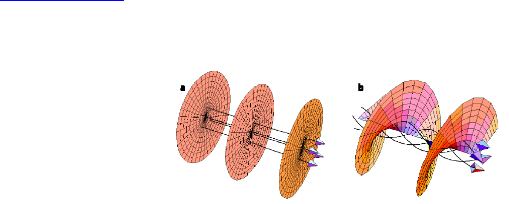
12.2. Light beams
12.2.b. Vortex beams. Characterization and properties
General remarks:
ãThe recent years have seen a tremendous effort in generating and manipulating vortex beams together with a good number of new
or promising applications, including the capture, manipulation and transport of nanoscopic particles (optical tweezer), high-resolution
microsocopy or for data transmission.
Figure 12.1.: Laser beams usually have planar wavefronts with wavevectors parallel to the beam axis. Beams with helical wavefronts have wavevectors
which spiral around the beam axis and give rise to an orbital angular momentum; from Padgett and Allen (2000).
ãTwisted photons carry both, spin angular momentum (SAM) as well as orbital angular momentum (OAM) along their propagation
direction.
ãTopological charge The z-projection of the OAM, m, is often called the topological charge or the winding number of the beam. This
charge describes the number of the 2πwindings of the helical phase around the vortex in one wavelength.
ãSynonym notions of vortex beams: helically phased light beams; optical vortices with a field dependence eimϕ .
ãOptical vortex beams are well-known and have been routinely used for the last 20 years; a first demonstration dates back to Durnin et al.
(1987).
ãFor optical vortices, charge values of m≤5000 have been realized (Shen et al., 2013).
ãReviews on optical vortex beams are given by Allen et al. (1999); Franke-Arnold et al. (2008), Zhan (2009) and Yao and Padgett (2011).
235

12. Beams of light and particles
Characterization of vortex beams:
ãA vortex state of light carries a well-defined projection of the orbital angular momentum (OAM) with respect to the beam axis.
ãWave functions: ∼eimϕ are eigenfunctions of `z=∂
∂ ϕ .
ãPhoton field: For a quantized radiation field, each particle also carries a projection m~of the OAM, that is part of the total angular
momentum. In general, the spin and orbital angular momentum cannot be separated.
ãIn the paraxial approximation, the spin and OAM longitudinal components of the vortex state can be separated from each other. Beyond
the paraxial limit, however, the spin-orbit interaction does not allow a simple separation of the spin and orbital angular momentum.
Properties of vortex beams:
ãFor all points in the beam, the ratio between the azimuthal and z-components of the momentum is found to be `/kr .
ãThe linear momentum of each photon is given by ~k; since the azimuthal component of the wavevector is m/r and is independent of the
wavelength, the orbital angular momentum per photon is
p=~k−→ pϕ=~kφ −→ `=r×pϕ=r×..
r=m~
ãHowever, OAM 6= SAM, despite the rather similar illustrations in the literatur; in particular, there exist also vortex states for spin-less
waves, such as acoustic vortex waves.
236

12.2. Light beams
12.2.c. Vortex beams. Generation
Generation of vortex beams with different photon energies:
ãFor intense, short-wavelength FEL radiation, optical methods can often not be applied due to strong limitations and difficulties in the
fabrications of optical surfaces (Terhalle et al. 2011, Peele et al. 2002).
ãTwisted EUV beams: Ribic and coworkers (2014) proposed an efficient scheme in order to generate intense coherent and twisted OAM
beams in the EUV region. These beams can be realized by means of a seeded FEL, i.e. by using a (seeding) laser pulse with a transverse,
staircaselike phase. For this phase pattern, in particular, the diffraction and mode selection drive the radiation profile towards a dominant
OAM mode at saturation.
ãTwisted x-ray beams: Hemsing an coworkers proposed two clever approaches for generating FEL vortex beams within the x-ray region:
(i) By using the interaction of an electron beam with a seeded laser within a helical undulator (Hemsing et al., 2011);
(ii) by using a so-called echo-enabled harmonic generation (EEHG) scheme, in which two seed lasers and two magnetic chicanes are utilized
in order to produce harmonic microbunches of an electron beam with a corkscrew distribution.
Generation of vortex beams by pitch-fork holograms:
ãThe superposition of a regular phase profile with some proper grating already results in a fork hologram that help generate vortex beams.
ãFork-like or pitch-fork holograms are known to diffract the light and to generate beams with OAM. Such holograms can be generated also
dynamically by using a spatial light modulator and readily controlled by a computer.
ãA pitchfork hologram is obtained adding a twisting and an oblique phase. The width of six 2πphase ramps is highlighted.
Generation of vortex beams by spiral phase plates:
ãA (plane-wave) light beam can acquire a non-zero OAM by crossing a spiral phase plate with an inhomogeneous thickness.
ãSpiral phase plates (SPP): Such a SPP is a transparent dielectric plate with a thickness that varies as a smooth ramp; this variation in
the thickness adds a phase shift to an incident field that increases linear with the azimuthal angle ϕ.
ãLight field: If a SPP is placed into the waist of a Laguerre-Gaussian beam with well-defined quantum numbers, uLG
`p , the complex light
amplitude just behind the plate can be described by means of a phase-plate operator S(ms, α)
hr, ϕ |S(ms, α = 0)|l, pi=uLG
lp (r, ϕ)eimsϕ,
237
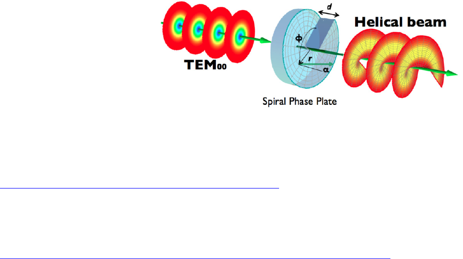
12. Beams of light and particles
and where msis the phase shift per unit angle of the given SPP.
ãSPP help explore high-dimensional entanglement with just two detector, while 6 detectors are required by other popular methods in order
to prove the entanglement of the OAM degree of freedom for two entangled photons (Oemrawsingh et al., 2004).
ãThe figure below shows the transformation of a TEM00 mode into a helical beam.
Figure 12.2.: Experimental scheme for generating light orbital angular momentum with spiral phase plates. Taken from Beijersbergen et al. (1994).
Generation of vortex beams by q-plates:
ãq-plate: A (so-called) q-plate is a device that is realized by means of liquid crystals, polymers or sub-wavelength gratings; this device
exploits a change of sign if the polarization of the incoming light is modified.
Generation of vortex beams by spatial light modulators:
ãxxxxx A spatial light modulator (SLM) is an object that imposes some form of spatially varying modulation on a beam of light. A simple
example is an overhead projector transparency. Usually when the phrase SLM is used, it means that the transparency can be controlled
by a computer. In the 1980s, large SLMs were placed on overhead projectors to project computer monitor contents to the screen. Since
then more modern projectors have been developed where the SLM is built inside the projector. These are commonly used in meetings of
all kinds for presentations.
238
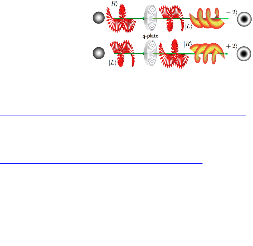
12.2. Light beams
Figure 12.3.: The q-plate effect for left and right-hand circular polarizations.
Generation of vortex beams by cylcindrical mode converters:
ãA Hermite-Gaussian beam can be converted into a Laguerre-Gaussian beam with well-defined OAM by using an astigmatic system with
two well-aligned cylindrical lenses. In this scheme, these lenses are placed at some specific distance in order to introduce a well-defined
relative phase between the horizontal and the vertical Hermite-Gaussian beams.
Generation of vortex beams by helical undulators:
ãX-ray vortex beams with photon energies ~ω≈100 eV have been generated in a helical undulator by Bahrdt et al. (2013) and Hemsing
et al. (2013).
ãAnother interesting approach has been suggested by Ribic and coworkers (2014). These authors proposed to modify he phase mask and to
manipulate directly the seeding laser in order to change the transverse properties of the FEL light.
12.2.d. Hermite-Gaussian beams
Characterization and use:
ãHermite-Gaussian modes HGmn :have a rectangular symmetry and are described by means of two mode indices mand n; these mode
indices give the number of nodes in the xand ydirections respectively.
239

12. Beams of light and particles
ãHermite-Gaussian modes: These modes are a convenient description for the output of lasers whose cavity design is not radially symmetric
but asymmetric in horizontal and vertical directions.
12.2.e. Laguere-Gauss beams
Characterization and use:
ãThe Laguerre-Gaussian (LG) beams carry an intrinsic OAM like the intrinsic SAM for beams with a circular polarization (Allen et al. 1992,
2003). This appeared originally rather surprising as the OAM of LG beams arise from the helical phase distribution about the beam axis,
and which coincides also with a phase singularity (Nye and Berry, 1974).
ãLaguerre-Gaussian modes uLG
`p :For a Laguerre-Gaussian beam with well-defined magnetic and radial quantum numbers (m, p) , the
complex amplitude of the light field in the waist of the beam is defined as in the polar represenation
uLG
`p (r, ϕ) = hr, ϕ |m, pi=Rmp(r) Φm(ϕ) with Φm(ϕ) = eim ϕ
√2π
ãLaguerre-Gaussian modes uLG
`p :If the problem is cylindrically symmetric, these modes are the natural solution of the paraxial wave
equation. They are often written in cylindrical coordinates by using Laguerre polynomials.
12.2.f. Bessel beams
Characterization and use:
ãBessel beams: A Bessel beam refers generally to an electromagnetic field whose amplitude is given by a Bessel function of the first kind. 5
ãAlthough these beams are an idealization, true Bessel beam are monochromatic and non-diffractive and, hence, do not not diffract and
spread out when they propagate. This behaviour is quite in contrast to other typical optical (or sound) waves if they are focused at some
spot.
ãBessel beams are known to be self-healing if they are obstructed at some point, i.e. they reform to a Bessel beam again further down the
beam axis.
240

12.2. Light beams
ãPure Bessel modes generally carry a well-defined OAM; in particular, they typically include three components of the topological charge
since only the (projection of the) total angular momentum is conserved for these beams. For this reason, the z-projections of the orbital
and spin angular momentum are not defined independently.
ãBessel modes |κ, mi:Bessel beams can be written also as a superposition over plane waves with well-defined (fixed) transverse momentum
, longitudinal momentum as well as circular polarization
ψ(r) = e−i ωt +i kzz|κ, mi,|κ, mi ∝ ei mϕ Jm(κ ρ)
ãVector potential: The vector potential of the Bessel beams is often written as Fourierintegral over Bessel states of different projections of
the orbital angular momentum aκ m(k⊥) ,
A=e−i ωt 1
(2π)2Zdk⊥e−ik·raκ m(k⊥)ek,λ, aκ m(k⊥) = r2π
κ(−i)me−imϕkδ(k⊥−κ)
ek,λ =1
√2
cos ϑkcos ϕk−iλ sin ϕk
cos ϑksin ϕk+iλ cos ϕk
−sin ϑk
tan ϑk=κ
kz
and where ek,λ are known as polarization (unit) vector and ϑkas the opening angle of the Bessel beam.
ãPlane-wave expansion: Of course, every monochromatic plane-waves can be expanded also in terms of Bessel waves as they are both just
two different bases in order to describe wave packets
ei(k·r−ωt)=∞
X
m=−∞
e−i ωt +i kzzime−imϕk|κ, mi
ãElectron-photon interaction operator for Bessel beams: For (a Bessel beam of) twisted photons, the transition operator reads as:
V(tw) =αAκmγkzλ(r)p.
Aκmγkzλ(r) = Zekλeikr aκmγ(k⊥)e−ik⊥bd2k⊥
(2π)2, aκmγ(k⊥) = (−i)mγeimγϕkr2π
k⊥
δ(k⊥−κ).
241
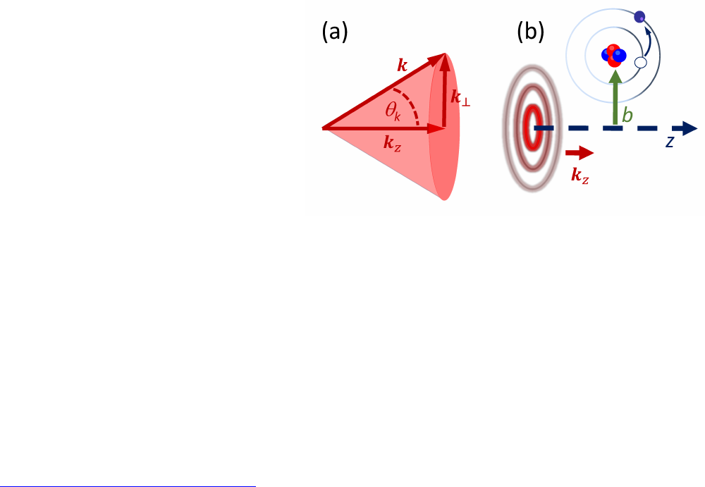
12. Beams of light and particles
Figure 12.4.: (a) In momentum representation, the twisted light can be seen as a coherent superposition of plane waves. These plane waves with wavevectors
kare all lying on a cone with (polar) opening angle ϑk= arctan(|k⊥|/kz) and with polarization vectors ek,λ which are perpendicular to k. (b)
For a given atom, the absorption amplitude depends on the position of the atom in a plane perpendicular to the propagation direction. The
position of the target atom with regard to the beam axis is specified by the impact parameter (vector) b(c-05-photobeam-interaction.eps).
In this expression, the factor e−ik⊥bspecifies the position of a target atom within the incident wave-front, and which refers to the complex
spatial structure of the Bessel beam.
12.2.g. Airy beams
Characterization and use:
ãAiry beams: Similar to Bessel beams, the cross section of an ideal Airy beam has an area of principal intensity and with a series of
adjacent, less luminous areas up to infinity. Airy beams can be derived from the Airy integral that was first developed by George Biddell
Airy in the 180s in order to explain the optical caustics in a rainbow and elsewhere.
ãAn Airy beam preserves its shape of intensity during propagation and forms a parabolic curve, quite analogue to the trajectory of a free
projectile as seen in a plane perpendicular to the propagation.
ãAiry beam are freely accelerating, i.e. they bend to form a parabolic arc as they propagate (Berry and Balazs, 1979; Siviloglou et al., 2007),
although the linear momentum remains conserved for these beams since the intensity centroid of an Airy beam forms a straight line.
242

12.2. Light beams
ãAiry beam do also not diffract, i.e. they do not spread out after focussing.
12.2.h. Necklace ring beams
Characterization and use:
ãNecklace ring beams: These beams refer to optical vector solitons that consist of incoherently coupled self-trapped ‘necklace’ beams; these
beams can carry zero, integer or even some fractional angular momentum.
ãNecklace ring beams exhibit a self-stabilizing mutual attraction between different beam components and a quasistable propagation for much
larger distances than the corresponding scalar vortex solitons
12.2.i. Light beams with non-integer OAM
Characterization and use:
ãBeams with non-integer OAM: These beams refer to structurally propagation invariant light beams carrying non-integer orbital angular
momentum (OAM) using Hermite-Laguerre-Gaussian (HLG) modes.
12.2.j. Vector beams
Characterization and use:
ãVector beams: The vector beams need to be described in the product space of the optical SAM and OAM subspaces and are characterized
by higher-order Stokes parameters.
ãVector beams exhibit a spatially variant polarization.
ãCylindrical vector beams are axially symmetric solution to the full electromagnetic (vector) wave equation.
ãGeneration of vector beams: These beams can be generated via different active and passive methods.
243

12. Beams of light and particles
12.2.k. Traktor beams
Characterization and use:
ãTractor beam: These beams refer to optical fields that help attract one object to another from a distance.
ãThe concept of tractor beams originates from the novel Spacehounds of IPC by E. E. Smith (1931) and by re-coining an earlier ‘attractor
beam’, in contrast to other, ’repulser beams’.
ãTractor beam are defined to use (a negative) nonconservative radiation pressure, that differs from a gradient force, and which is directed
towards the source. This generally requires a continuous redirection of momentum flux (Sukhov and Dogariu, 2010, 2011; Chen et al. 2011).
ãTraktor beams are based on the maximization of forward scattering of light due to interference of different radiation multipoles. It was
shown especially that an simultaneous excitation of multipoles is necessary in the particle in order to realize a negative (pulling) optical
force.
12.2.l. Polarization radiation
Characterization and use:
ãIn electrodynamics, one generally distinguishes two classes of emitted radiation: bremsstrahlung and polarization radiation. While
bremsstrahlung is produced by accelerated charges, polarization radiation can be emitted by a uniformly moving charge, although only in
the presence of a medium.
ãIn dependence on the given medium or target geometry, one distinguishes various forms of polarization radiation: Cherenkov radiation,
transition radiation, diffraction radiation as well as Smith-Purcell radiation.
ãPolarization radiation: Electromagnetic radiation can be emitted not only by accelerated charges but also due to the motion of magnetic
moments and higher multipoles. Until the present, however, this (so-called) polarization radiation has never been verified experimentally
for any frequency of light.
ãThe main experimental difficulty for approving this radiation refers to the (very) small current of a magnetic moment that is suppressed
by ∼10−5w.r.t. a corresponding charge current.
ãA pure quasi-classical treatment of the polarization radiation is inconsistent since quantum corrections are of the same order for this type
of radiation phenomena.
244

12.2. Light beams
12.2.m. Manipulation of optical beams
Optical elements:
ãDove prism: This is a (type of) reflective prism that can be used to invert a given image. These prisms are often shaped from a truncated
right-angle prism.
ãIf a beam enters the prims at one of the sloped faces and parallel to the longitudinal axis, it undergoes total internal reflection at the inside
of the longest (bottom) face, and then leaves the prism at the opposite sloped face. Therefore, any image that passes through the prism is
flipped (mirrored) and also also inverted but not laterally transposed.
ãHologram: A holgram usually refers to a three-dimensional image of an object that is created by holography, i.e. an optical technique
for recording and reconstructing the amplitude and phase distributions of a coherent wave. Holography is often used to produce three-
dimensional images or holograms.
ãHalf-wave plate: A wave plate, sometimes known as a retarder, designates an optical device that alters the polarization state of a light
wave. While a half-wave plate shifts the polarization direction of linearly polarized light, a quarter-wave plate converts linearly-polarized
light into circularly-polarized light and vice versa. Quarter-wave plate can be used also in order to produce elliptically-polarized light.
Mach-Zehnder interferometers:
ãThese interferometers make use of two separate beam splitters in order to split and recombine an input beam but from which the beam
can emerge and detected at two outputs. The optical path lengths in the two arms of the interferometer may be nearly identical or may be
different in order to introduce an extra delay path.
ãIf a beam is sent through the interferometer, the optical powers at the two outputs depends on in practice sensitively on the the precise
difference in optical arm lengths as well as on the wavelength of the light.
ãThe Mach-Zehnder interferometer was first developed by Ludwig Mach and Ludwig Zehnder.
245

12. Beams of light and particles
12.2.n. Optical forces of vortex beams
Optical forces:
ã:
ãA positive radiation force is relatively intuitive and occurs in the backscattering or absorption of the forward-directed momentum of a
beam; it was first reported already by Nichols and Hull (1903).
12.2.o. Application of optical (vortex) beams
Remarks:
ãDifferent applications of optical vortex beams and the angular momentum of light have been envisaged and are currently explored in
research laboratories, although no real commercial application are yet known.
ãFields of applications: Cold atoms, trapped nanoparticles, micro manipulation and detection of spinning objects, remote measurement of
the rotation of mesoscopic particles, entanglement and quantum information, optical data transmission, interaction with matter, microscopy
and astrophysics.
ãX-ray magnetic circular dichromism By using different OAM states in the measurements, the dipole and quadrupole contributions to the
circular dichroism signal can be separated from each other.
Optical tweezer:
ãOptical tweezer: These tweezers usually refer to single-beam gradient force trap that are realized by some highly focused laser beam. These
focused beams provide an attractive or repulsive force on nano- or mesoscopic dielectric objects.
ãOptical tweezers have been utilized to manipulate the orientation of particles or particle aggregates.
ãIn optical tweezers, the forces are typically on the order of piconewtons; they depends on the refractive index of the object.
246

12.3. Electron beams
Optical phasors:
ãPhasor: A complex constant in complex wave notation that encapsulates the amplitude; sometimes known also as sinor or complexor.
Applications in quantum information theory:
ãThe orbital-angular momentum (OAM) of light has recently emerged as a promising candidate for quantum and classical information
systems.
ãIn OAM beams, the spatial degrees of freedom provide a high-dimensional alphabet to quantum information processing which enables one
to use qunits instead of qubits.
ãQuantum information encoding, Higher-dimensional quantum information encoding has been discussed in the literature for possible future
applications in quantum cryptography or quantum computations. The discrete, unbounded state-space of OAM promises in particular vastly
enhanced data rates as well as an increased tolerance to eavesdropping in quantum communication.
12.3. Electron beams
Electron beams:
ãElectron beams are quite frequently applied in physics; such beams may refer, for instance, to some stream of electrons as obtained from
a betatron. Electron beams are generally generated either by heat (thermionic emission), bombardment of surfaces with charged atoms or
particles (secondary electron emission), or by means of strong electric fields (field emission).
ãElectrons may be collimated by holes and slits. Because they are electrically charged, they can also be deflected, focused or accelerated by
electric and magnetic fields.
Twisted electron beams:
ãApart from twisted (vortex) solutions of the Dirac equation, a quais-relativistic wave equation for twisted relativistic electron in arbitrary
electric and magnetic fields can be derived by using a Foldy-Wouthuysen transformation.
247

12. Beams of light and particles
ãThe interaction of twisted (vortex) electrons with electric and magnetic fields can be described quite readily, based on Lorentz transforma-
tions.
12.3.a. Gaussian electron beams
Characterization and use:
ãIt has been demonstrated experimentally that a Gaussian-profile model better describes the (equilibrium) electron beam than a beam with
a uniform-profile model.
12.3.b. Vortex electron beams
General remarks:
ãElectron vortex beams were first realized experimentally by Uchida and Tonomura (2010), Verbeeck, Tian and Schattschneider (2010) and
McMorran et al. (2011). Uchida and Tonomura, in particular, generated an electron vortex beams with (electron) energy E= 300 keV,
a projection of the OAM with m.100 and by focusing the electron beam to a spot size of 1.2 ˚
A.
ãVortex electrons can generally carry a rather large intrinsic projection of the orbital angular momentum (OAM) m∼100 with respect
to their propagation direction. Therefore, the magnetic moment of vortex electrons µ≈m µBis similarly large, when compared with the
Bohr magneton µBdue to the spin motion of the electron.
ãThe magnetic moment of twisted electrons due to their OAM comes in addition to the known magnetic moment due to the spin motion.
ãSince Vortex electrons are sensitive to external magnetic fields, they can be utilized to probe atomic magnetism and, thus, open novel
opportunities for electron microscopy.
ãWhile vortex photon beams have been created and routinely used for several decades already, the vortex states of electrons and charged
particles is a presently emerging field.
248
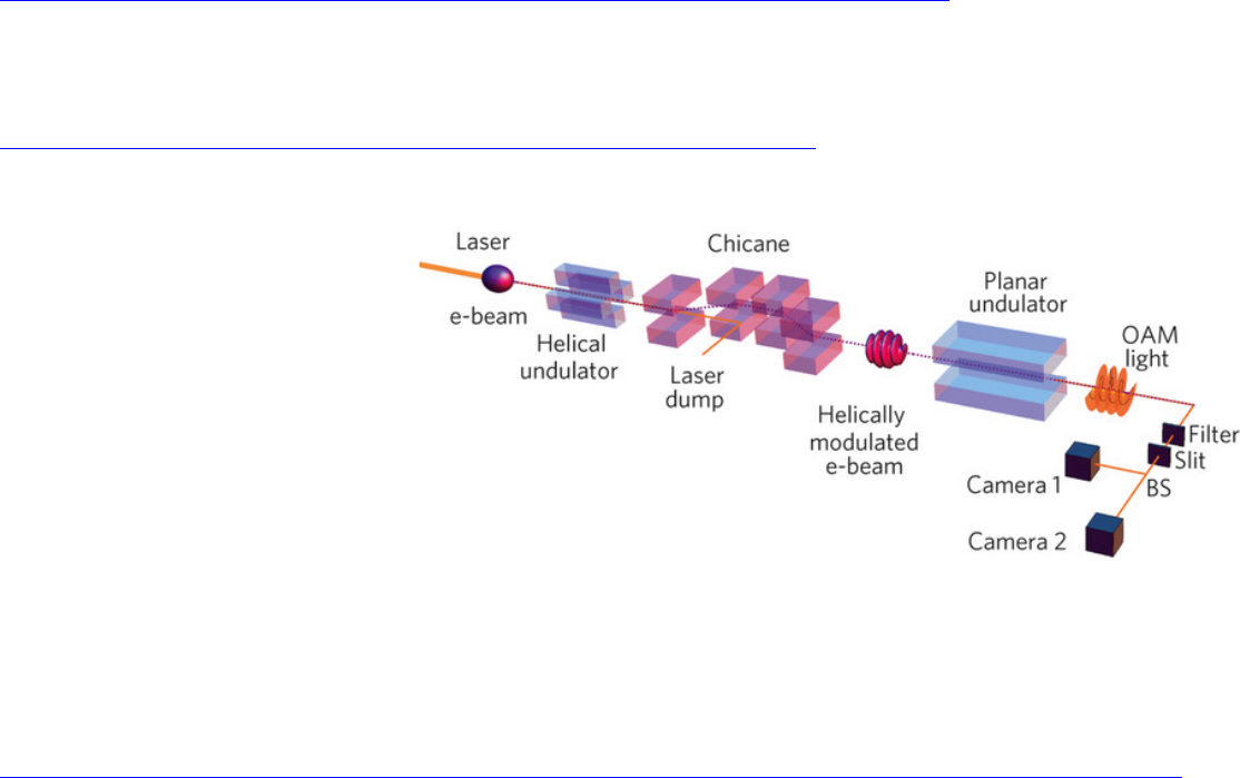
12.3. Electron beams
12.3.c. Generation of vortex electron beams
Generation of vortex electron beams with different energies:
ãIndeed, several new ideas were proposed in the literature in order to create electron vortex beams experimentally.
Generation of vortex electron beams by undulators:
ãElectrons in a helical modulator: cf. Figure 12.3.c
Figure 12.5.: An unmodulated relativistic electron beam interacts with a linearly polarized laser in a helical undulator, which gives the electrons an energy
kick that depends on their position in the focused laser beam.
Generation of vortex electron beams by transmission electron microscopes:
ãVoloch-Bloch et al. (2013) generated Airy electron beams by using a holographic technique within a transmission electron microscope.
Both, self-bending and self-healing features were observed in the experiments if the beam was obstructed by a small object during its
propagation.
249

12. Beams of light and particles
Generation of vortex electron beams by holograms:
ãGrillo et al. (2014) generated an electron Bessel beam by the diffraction of electrons at a nanoscale phase hologram. This hologram imposed
a conical phase structure upon the electron wave-packet. The so obtained beams propagated for 0.6 m without measurable spreading and
could reconstruct also its intensity distributions, if these beams where partly obstructed by an obstacle.
12.3.d. Bessel electron beams
Characterization and use:
ãQuasi-Bessel beams can be obtained within a good approximation, while it is not possible to generate an ideal Bessel beam because they
are not normalizable in their total intensity,
ãWave function of a Bessel electron: In cylindrical coordinates r, ϕ, z, the wave function of electrons in a Bessel beam is given by
ψ(r, ϕ, z;t) = Jm(κ r)ei mϕ e−i(ωt −kzz),
where Jm(x) is the m-th order Bessel function of the first kind and κand kzdenote the transverse and longitudinal components of the wave
vector, respectively.
ãProbability-density distribution of Bessel electron beams: This wave function give rise to a probability-density distribution P=ψ ψ+
that is independent of zand t:
P(r, ϕ, z;t) = P(r, ϕ, 0; 0) = [ Jm(κ r) ]2.
ãThis shows that the probability-density distribution is stationary in the transverse plane and independent of where this plane is taken.
ãThe energy of the electron E=~ωdefines the de Broglie wave length and the modulus of the wave vector by
k2=k2
r+k2
z=2mω
~=2π
λdB 2
.
250

12.3. Electron beams
ãFor Bessel beams with a nonzero mvalue, the electrons possess a non-uniform helical phase front with mdislocations in the phase, and
where the handedness of the phase front is defined by the sign of m.
ãCurrent density of electron Bessel beam: This current density circulates azimuthally in the transverse plane and introduces an (projection
of the total) orbital angular momentum of m~per electron.
ãAn Bessel electron beam with a nonzero mvalue possess exhibit a shape with multiple rings and with a null probability density at the
origin.
ãBessel electron beams can be represented also as a coherent superposition of conical plane waves along a closed ring (circle).
12.3.e. Airy electron beams
Characterization and use:
ãAiry electron beams can be generated by diffraction of electrons through a nanoscale hologram, which imprints a cubic phase modulation
on wavefunction of the electrons in the transverse plane.
12.3.f. Application of twisted electron beams
Remarks:
ãThe scattering of twisted electrons can provide insights into the magnetic structure of the target materials.
ãBeams with non-zero OAM helped explore the vacuum Faraday effect as well as Larmor and Gouy rotations.
ãBessel electron beams have been used in electron microscopy.
251
13. References
1992 Phys. Rev.
˚
Aberg T and Howat G 1982 in Corpuscles and Radiation in Matter I, ed Mehlhorn W (in: Encyclopedia of Physics, vol XXXI; Springer, Berlin, p 469)
Theory of the Auger Effect
Agostinelli S and Geant 4 collaboration 2003 Nuc. Instr. Meth. A506 250 Geant 4 – A simulation toolkit
Allen L, Beijersbergen M W, Spreeuw R J C and Woerdman J P 1992 Phys. Rev. A45 8185 Orbital angular momentum of light and the transforma-
tion of Laguerre-Gaussian laser modes
Allen L, Barnett S M and Padgett M J 2003 Optical Angular Momentum (Institute of Physics Publishing, Bristol)
Allen L, Padgett M J and Babiker M 1999 Progress in Optics 39 291 The orbital angular momentum of light
Ashkin A, Dziedzic J M, Bjorkholm J E and Chu S 1986 Opt. Lett. 11 288 Observation of a single-beam gradient force optical trap for dielectric
particles
Astropy Collaboration 2013 Astronomy & Astrophys. 558 A33 Astropy: A community Python package for astronomy
Avgoustoglou E, Johnson W R, Plante D R, Sapirstein J, Sheinerman S and Blundell S A 1992 Phys. Rev. A46 5478 Many-body perturbation theory
formulas for the energy levels of excited states of closed-shell atoms
Avgoustoglou E, Johnson W R, Liu Z W und Sapirstein J 1995 Phys. Rev. A51 1196 Relativistic many-body calculations of [ 2p53s]excited state
energy levels for neon-like ions
Badnell N R 2011 Comp. Phys. Commun. 182 1528 A Breit-Pauli distorted wave implementation for Autostructure
Bahrdt J, Holldack K, Kuske P, M¨uller R, Scheer M and Schmid P 2013 Phys. Rev. Lett. 111 034801 First observation of photons carrying orbital
angular momentum in undulator radiation
Balashov V V, Grum-Grzhimailo A N and Kabachnik N M 2000 Polarization and Correlation Phenomena in Atomic Collisions (Kluwer Academic
Plenum Publishers, New York)
Band I M, Trzhaskovskaya M B, Nestor Jr N W, Tikkanen P O and Raman S 2002 Atom. Data Nucl. Data Tables 81 1DiracFock internal conver-
sion coefficients
Bazhenov V Y, Vasnetsov M V and Soskin M S 1990 JETP Lett. 52 429 Laser-beams with screw dislocations in their wave-fronts
Beijersbergen M W, Coerwinkel R P C, Kristensen M and Woerdman J P 1994 Opt. Comm. 12 321 Helical-wavefront laser beams produced with a
spiral phase plate
253
13. References
Bethe H A and Salpeter E E 1957 Quantum Mechanics of One- and Two-Electron Systems (Springer-Verlag, Berlin, Gttingen, Heidelberg)
Bezanson J, Edelman A, Karpinski S and Shah V B 2017 SIAM Review 59 65 Julia: A fresh approach to numerical computing
Bezanson J, Chen J, Chung B, Karpinski S, Shah V B, Vitek J and Zoubritzky J 2018 Proceedings of the ACM on Programming Languages 2120 Ju-
lia: Dynamism and performance reconciled by design
Bliokh K Y, Bliokh Y P, Savelev S and Bliokh F N 2007 Phys. Rev. Lett. 99 190404 Semiclassical dynamics of electron wave packet states with phase
vortices
Bliokh K Y, Dennis M R and Franco Nori 2011 Phys. Rev. Lett. 107 174802 Relativistic electron vortex beams: angular momentum and spin-orbit
interaction
Bozinovic N, Yue Y, Ren Y, Tur M, Kristensen P, Huang H, Willner A E, Ramachandran S 2013 Science 340 1545 Terabit-scale orbital angular mo-
mentum mode division multiplexing in fibers
Cai X, Wang J, Strain M J, Johnson-Morris B, Zhu J, Sorel M, O’Brien J L, Thompson M G, Yu S 2012 Science 338 363 Integrated compact optical
vortex beam emitters
Canton-Rogan S E, Wills A A, Gorczyca T W, Wiedenhoeft M, Nayandin O, Liu C-N and Berrah N 2000 Phys. Rev. Lett. 85 3113 Mirroring doubly
excited resonances in argon
Chen J, Ng J, Lin Z and Chan C T 2011 Nat. Photonics 5531 Optical pulling force
Cheng G and Jiaolong Z 2008 Phys. Rev. E78 046407 Spectrally resolved and Rosseland and Planck mean opacities of iron plasmas at temperatures
above 100 eV: A systematic study
Cowan R D 1981 The Theory of Atomic Structure and Spectra (University of California Press, 1981, 731 pages)
Da Pieve F, Fritzsche S, Stefani G and Kabachnik N M 2007 J. Phys. B40 329 Linear magnetic and alignment dichroism in Auger-photoelectron
coincidence spectroscopy
Darwin C G 1932 Proc. R. Soc. Lond. A 136 36 Notes on the theory of radiation
Derevianko A, Johnson W R, Safronova M S and Babb J F 1999 Phys. Rev. Lett. 82 3589 High-precision calculations of dispersion coefficients, static
dipole polarizabilities and atom-wall interaction constants for alkali-metal atoms
Dzuba V A, Flambaum V V and Porsev S G 2009 Phys. Rev. 80 032120 Calculation of (P, T )-odd electric dipole moments for the diamagnetic atoms
129Xe, 171Yb, 199Hg, 211Rn, and 225Ra
Eichler J and Meyerhof W 1995 Relativistic Atomic Collisions (Academic Press, San Diego)
Fisher D, Maron Y and Pitaevskii L P 1998 Phys. Rev. A58 2214 Ionization of many-electron atoms by a quasistatic electric field
Flambaum V V and Ginges J S M 2005 Phys. Rev. A72 052115 Radiative potential and calculations of QED radiative corrections to energy levels
and electromagnetic amplitudes in many-electron atoms
Fontes C J, Zhang H L, Abdallah Jr J, Clark R E H, Kilcrease D P, Colgan J, Cunningham R T, Hakel P, Magee N H and Sherrill M E 2015 J.
Phys. B48 144014 The Los Alamos suite of relativistic atomic physics codes
Franke-Arnold S, Allen L, Padgett M J 2008 Laser and Photonics Reviews 2299 Advances in optical angular momentum
254
Freiburghaus C, Rosswog S and Thielemann F-K 1999 Astrophys. J. 525 L121 r-Process in neutron star mergers
Fritzsche S 2001 J. Electron Spectrosc. Relat. Phenom. 114-116 1155 A toolbox for studying the properties of openshell atoms and ions
Fritzsche S 2002 Phys. Scr. T100 37 Largescale accurate structure calculations for openshell atoms and ions
Fritzsche S, Nikkinen J, Huttula S-M, Aksela H, Huttula M and Aksela S 2007 Phys. Rev. A75 012501 Interferences in the 3p4nl satellite emission
following the excitation of argon across the 2p5
1/24sand 2p5
3/23d J = 1 resonances
Fritzsche S, Fricke B and Sepp W-D 1992 Phys. Rev. A45 1465 Reduced L1level-width and Coster-Kronig yields by relaxation and continuum
interactions in atomic zinc
Furukawa H and Nishihara K 1992 Phys. Rev. A46 6596 Fermi-degeneracy and discrete-ion effects in the spherical-cell model and electron-electron
correlation effects in hot dense plasma
Gaidamauskas E, Naze C, Rynkun P, Gaigalas G, J¨onsson P and Godefroid M 2011 J. Phys. B44 175003 Tensorial form and matrix elements of the
relativistic nuclear recoil operator
Gaigalas G, Froese Fischer C, Rynkun P and J¨onsson P 2017 atoms 56JJ2LSJ: Transformation and unique Labeling for energy levels
Gaigalas G, Zalandauskas T and Fritzsche S 2004 Comp. Phys. Commun. 157 239 Spectroscopic LSJ notation for atomic levels obtained from relativistic
calculations
Gaunt 1929 Proc. R. Soc. A122 513 IV. The triplets of helium
Ginzburg V L and Tsytovich V N 1979 Phys. Rep. 49 1Transition radiation and transition scattering
Goldman S P and Drake G W F 1992 Phys. Rev. Lett. 68 1683 Asymptotic Lamb shifts for helium Rydberg states
Gordon R G and Kim Y S 1972 J. Chem. Phys. 56 3122 Theory for the forces between closed-shell atoms and molecules
Grant I P 1988 in: Methods in Computational Chemistry ed Wilson S, vol 2 (Plenum, New York, p 1) Relativistic effects in atoms and molecules
Grant I P and Pyper N C 1976 J. Phys. B9 761 Breit interaction in multiconfiguration relativistic atomic calculations
Grant I P and Quiney H M 1988 in: Advances in Atomic and Molecular Physics 23 eds D Bates and B Bederson (Academic, New York, p 37) Foundation
of Relativistic Theory of Atomic and Molecular Structure
Griem H 1974 Spectral Line Broadening by Plasmas (Academic Press, New York, London)
Grier D G 2003 Nature 424 810 A revolution in optical manipulation
Grillo V, Gazzadi G-C, Mafakheri E, Frabboni S, Karimi E and Boyd R W 2015 Phys. Rev. Lett. 114 034801 Holographic generation of highly twisted
electron beams
Grum-Grzhimailo A N, Gryzlova E V, Staroselskaya E I, Venzke J and Bartschat K 2015 Phys. Rev. A91 063418 Interfering one-photon and two-
photon ionization by femtosecond VUV pulses in the region of an intermediate resonance
Guo D-S, ˚
Aberg T and Crasemann B 1989 Phys. Rev A40 4997 Scattering theory of multiphoton ionization in strong fields
Guo D-S and Drake G W F 1992 Phys. Rev A45 6622 Multiphoton ionization in circularly polarized standing waves
Haque A K F, Shahjahan M, Uddin M A, Patoary M A R, Basak A K, Saha B C and Malik F B 2010 Phys. Scr. 81 045301 Generalized Kolben-
stvedt model for electron impact ionization of the K-, L- and M-shell ions
255
13. References
Hartgers A, van Dijk J, Jonkers J, van der Mullen J A M 2001 Comp. Phys. Commun. 135 199 CR-Model: A general collisional radiative modeling
code
He H, Friese M E J, Heckenberg N R and Rubinsztein-Dunlop H 1995 Phys. Rev. Lett. 75 826 Direct observation of transfer of angular momentum
to absorptive particles from a laser beam with a phase singularity
Hemsing E, Marinelli A Rosenzweig J B 2011 Phys. Rev. Lett. 106 164803 Generating optical orbital angular momentum in a high-gain free-electron
laser at the first harmonic
Hemsing E and Marinelli A 2012 Phys. Rev. Lett. 109 224801 Echo-enabled x-ray vortex generation
Hemsing E, Knyazik A, Dunning M, Xiang D, Marinelli A, Hast D and Rosenzweig J B 2013 Nature Phys. 9549 Coherent optical vortices from rel-
ativistic electron beams
Hubbell J H, Veigele W J, Briggs E A, Brown R T, Cromer D T and Howerton R J 1992 J. Phys. Chem. Ref. Data 4471 Atomic form factors,
incoherent scattering functions, and photon scattering cross sections
Huntemann N, Sanner C, Lipphardt B, Tamm C and Peik E 2016 Phys. Rev. Lett. 116 063001 Single-ion atomic clock with 3×10¹⁸ systematic
uncertainty
Inal M K, Surzhykov A and Fritzsche S 2005 Phys. Rev. A72 042720 Linear polarization of the 2p53s→2p6lines following the inner-shell photoion-
ization of sodiumlike ions
Inhester L, Burmeister C F, Groenhof G and Grubm¨uller H 1992 J. Chem. Phys. 136 144304 Auger spectrum of a water molecule after single and
double core ionization
Ivanov I P and Karlovets D V 2013 Phys. Rev. Lett. 110 264801 Detecting transition radiation from a magnetic moment
Jahrsetz T, Fritzsche S and Surzhykov A 2015 Phys. Rev. A89 042501 Inelastic Raman scattering of light by hydrogenlike ions
Johnson W R 1995 in: Physics with Multiply Charged Ions ed D Liesen (NATO ASI Series 348, Plenum Press, New York London, p 1 Correlation and
QED for highly-charged ions
Johnson W R 2007 Atomic Structure Theory: Lectures on Atomic Physics (Springer)
Johnson W R, Guo D S, Idrees M and Sapirstein J 1985 Phys. Rev. A32 2093 Weak-interaction effects in heavy atomic systems
J¨onsson P, Gaigalas G, Bieron J, Froese Fischer C and Grant I P 2013 Comp. Phys. Commun. 184 2197 New version: Grasp2K relativistic atomic
structure package
Kabachnik N M 1981 J. Phys. B14 L337
Kabachnik N M, Fritzsche S, Grum-Grzhimailo A N, Meyer M and Ueda K 2007 Phys. Rep. 451 155 Coherence and correlations in photoinduced
Auger and fluorescence cascades in atoms
Kassimi N E and Thakkar A J 1994 Phys. Rev. A50 2948 Static hyperpolarixability of atomic lithium
Kibeedia T, Burrows T W, Trzhaskovskayac M B, Davidsona P M and Nestor Jr C W 2008 Nucl. Instr. Meth. A589 202 Evaluation of theoretical
conversion coefficients using BrIcc
Kim Y S and Gordon R G 1974 Phys. Rev. B9 3548 Theory of binding of ionic crystals: Application to alkali-halide and alkane-earth-dihalide crystals
256
Klar H 1980 J. Phys. B13 4741
Krause M O 1979 J. Phys. Chem. Ref. Data 8329 Atomic radiative and radiationless yields for K and L shells
Koga T and Thakkar A J 1996 J. Phys. B 29 2973 Moments and expansion coefficients of atomic electron momentum densities: numerical Hartree-Fock
calculations for hydrogen to lawrencium
Libermann D A 1979 Phys. Rev. B20 4981 Self-consistent field model for condensed matter
Lindgren I and Rosen A 1974 Case Studies in Atomic Physics 5Relativistic self-consistent-field calculations with application to atomic hyperfine inter-
action. Part I: Relativistic self-consistent fields
Liu C-N and Starace A F 1999 Phys. Rev. A59 1731(R) Mirroring behavior of partial photodetachment and photoionization cross sections in the
neighborhood of a resonance
Liu P F, Liu Y P, Zeng J L and Yuan J M 2014 Phys. Rev. A89 042704 Electron-impact excitation and single- and multiple-ionization cross sections
of heavy ions: Sn13+ as an example
Liu Z, Lee H, Xiong Y, Sun C and Zhang X 2007 Science 315 1686 Far-field optical hyper lens magnifying sub-diffraction-limited objects
Marxer H 1991 Phys. Rev. A 44 1543 Exact correspondence relationship for the expectation values of r−kfor hydrogenlike states
Marxer H 1995 J. Phys. B28 341 Off-diagonal matrix elements n` rkn`0for hydrogen-like states: an exact correspondence relationship in terms of
orthogonal polynomials and the WKB approximation
Matula O, Hayrapetyan A G, Serbo V G, Surzhykov A and Fritzsche S 2013 J. Phys. B46 205002 Atomic ionization of hydrogen-like ions by twisted
photons: angular distribution of emitted electrons
Matula O, Hayrapetyan A G, Serbo V G, Surzhykov A and Fritzsche S 2014 New J. Phys. 16 053016 Radiative capture of twisted electrons by bare
ions
Mazevet S and Abdallah Jr J 2006 J. Phys. B39 3419 Mixed UTA and detailed line treatment for mid-Zopacity and spectral calculations
McGloin D and Dholakia K 2005 Contemp. Phys. 64 15 Bessel Beams: Diffraction in a New Light
McMorran B J, Agrawal A, Anderson I M, Herzing A A, Lezec H J, McClelland J J and Unguris J 2011 Science 331 192 Electron vortex beams with
high quanta of orbital angular momentum
Metzger B D 2017 Living Rev. Relativ. 20 3Kilonovae
Milione G, Sztul H I, Nolan D A and Alfano R R 2011 Phys. Rev. Lett. 107 053601 Higher-order Poincare sphere, Stokes parameters and the angular
momentum of light
Miyagi H and Madsen L B 1992 Phys. Rev. A87 062511 Time-dependent restricted-active-space self-consistent-field theory for laser-driven many-
electron dynamics
Nye J F and Berry M V 1974 Proc. R. Soc. London Ser. A336 165 Dislocations in wave trains
Oemrawsingh S S R, Aiello A, Eliel E R, Nienhuis G and Woerdman J P 2014 Phys. Rev. Lett. 92 217901 How to observe high-dimensional two-
photon entanglement with only two detectors
Pan L, Taylor K T and Clark C W 1988 Phys. Rev. Lett. 61 2673 Computation of the ac Stark effect in the ground state of atomic hydrogen
257
13. References
Parpia F, Froese Fischer C and Grant I P 1996 Comput. Phys. Commun. 94 249 GRASP92: A package for large-scale relativistic atomic structure
calculations
Peele A G, McMahon P J, Paterson D, Tran C Q, Mancuso A P, Nugent K A, Hayes J P, Harvey E, Lai B and McNulty I 2002 Opt. Lett. 27 1752
Observation of an x-ray vortex
Picon A, Mompart J, Vaizquez de Aldana J A, Plaja L, Calvo G F and Roso L 2007 Opt. Express 18 3660 Photoionization with orbital angular mo-
mentum beams
Porsev S G, Kozlov M G and Reimers D 2009 Phys. Rev. A79 032519 Transition frequency shifts with fine-structure constant variation for Fe I and
isotope-shift calculations in Fe I and Fe II
Porsev S G and Derevianko A 2006 J. Exp. Theo. Phys. 102 195 High-accuracy calculations of dipole, quadrupole and octupole electric-dynamic polar-
izabilities and van-der-Waals coefficients C6, C8and C10 for alkaline-earth dimers
Post D E and Kendall R P 2004 Int. J. HPC Applications 18 399 Software project management and quality engineering practices for complex, coupled
...
Potvliege R M 1998 Comput. Phys. Commun. 114 42 STRFLO: A program for time-independent calculations of multiphoton processes in one-electron
atomic systems: I. Quasi-energy spectra and angular distributions
Poynting J H 1909 Proc. R. Soc. A82 560 The wave motion of a revolving shaft, and asuggestion as to the angular momentum in abeam of circularly
polarised light
Radice D, Perego A, Hotokezaka K, Fromm S A, Bernuzzi S and Roberts L F 1992 Astrophys. J. 869 130 Binary neutron star mergers: mass
ejection, electromagnetic counterparts, and nucleosynthesis
Radtke T, Fritzsche S and Surzhykov A 2006 Phys. Rev. A 74 032709 Density-matrix formalism for the photoion-electron entanglement in atomic
photoionization
Ribic P R, Guathier D and De Ninno G 2014 Phys. Rev. Lett. 112 203602 Generation of coherent extreme-ultraviolet radiation carrying orbital angular
momentum
Rohrlich F and Carlson B C 1954 Phys. Rev. 93 38 Positron-electron differences in energy loss and multiple scattering
Rose S J, van Hoof P M M, Jonauskas V, Keenan F P, Kisielius R, Ramsbottom C, Foord M E, Heeter R F and Springer P T 1992 J. Phys. 37
L337 Calculation of photoionized plasmas with an average-atom model
Safronova M S, Porsev S G, Sanner C and Ye J 2018 Phys. Rev. Lett. 120 173001 Two clock transitions in neutral Yb for the highest sensitivity to
variations of the fine-structure constant
Saha B and Fritzsche S 2006 Phys. Rev. E 73 036405 Be I isoelectronic ions embedded in hot plasma
Saha B and Fritzsche S 2007 J. Phys. B40 259 Influence of dense plasma on the low-lying transitions in Be-like ions: relativistic multiconfiguration
DiracFock calculation
Scholz-Marggraf H M, Fritzsche S, Serbo V G, Afanasev A and Surzhykov A 2014 Phys. Rev. A90 013425 Absorption of twisted light by hydrogen-
like atoms
Sapirstein 1987 Phys. Scr. 36 801 Quantum-electrodynamics of many-electron atoms
258
Sasaki S and McNulty I 2008 Phys. Rev. Lett. 100 124801 Proposal for generating brilliant x-ray beams carrying orbital angular momentum
Shabaev V M, Tupitsyn I I and Yerokhin V A 2013 Phys. Rev. A88 012513 Model operator approach to the Lamb shift calculations in relativistic
many-electron atoms
Sharma L, Surzhykov A, Inal M K and Fritzsche S 2010 Phys. Rev. A81 023419 Polarization transfer in the innershell photoionization of sodiumlike
ions
Shen Y, Campbell G T, Hage B, Zou H, Buchler B C and Shen P K L et al. 2013 J. Opt. 15 044005 Generation and interferometric analysis of high
charge optical vortices
Simon A, Warczak A, ElKafrawy T and Tanis J A 2010 Phys. Rev. Lett. 104 123001 Radiative double electron capture in collisions of O8+ ions with
carbon
Stone N J 2005 Atomic Data and Nuclear Data Tables 90 175 Table of nuclear magnetic dipole and electric quadrupole moments
Sukhov S and Dogariu A 2010 Opt. Lett. 35 3847 On the concept of tractor beams
Sukhov S and Dogariu A 2011 Phys. Rev. Lett. 107 203602 Negative nonconservative forces: optical tractor beams for arbitrary objects
Surzhykov A, Radtke T, Indelicato P and Fritzsche S 2009 Eur. J. Phys. Spec. Topics 169 129 Photon polarization in the two-photon decay of heavy
hydrogenlike ions
Surzhykov A, Volotka A, Fratini F, Santos J P, Indelicato P, Plunien G, Sto¨ohlker and Fritzsche S 2008 Phys. Rev. A81 042510 Angular correla-
tions in the twophoton decay of heliumlike heavy ions
Surzhykov A, Jentschura U D, St¨ohlker T and Fritzsche S 2006 Phys. Rev. A73 032716 Radiative electron capture into high-Z few-electron ions:
Alignment of the excited ionic states
Tchang-Brillet W L, Wyart J-F, Meftah A and Mammar S A 2018 atoms 652 Parametric calculations of radiative decay rates for magnetic dipole
and electric quadrupole transitions in Tm IV, Yb V, and Er IV
Torres and Torner (eds) 2011 Twisted photons (Wiley-VCH, Weinheim)
Tupitsyn I I, Shabaev V M, Lopez-Urrutia J R C, Draganic I, Orts R S and Ullrich J 2003 Phys. Rev. A68 022511 Relativistic calculations of isotope
shifts in highly charged ions
Tupitsyn I I, Kozlov M G, Safronova M S, Shabaev V M and Dzuba V A 2016 Phys. Rev. Lett. 117 253001 Quantum electro-dynamical shifts in
multivalent heavy ions
Uchida M and Tonomura A 2010 Nature 467 737 Generation of electron beams carrying orbital angular momentum
van Veenendaal M and McNulty I 2007 Phys. Rev. Lett. 98 157401 Prediction of strong dichroism induced by x rays carrying orbital momentum
Verbeeck J, Tian H and Schattschneider P 2010 Nature 467 301 Production and application of electron vortex beams
Voloch-Bloch N, Lereah Y, Lilach Y, Gover A and Arie A 2013 Nature 494 331 Generation of Electron Airy Beams
Volotka A V, Yerokhin V A, Surzhykov A, St¨ohlker T and Fritzsche S 2016 Phys. Rev. A93 023418 Many-electron effects on x-ray Rayleigh scattering
by highly charged He-like ions
von der Wense, Seiferle B, Stellmer S, Weitenberg J, Kazakov G, Palffy A and Thirolf P G 2017 Phys. Rev. Lett. 119 132503 A laser excitation
259
13. References
scheme for 229mTh
Yao A M and Padgett M J 2011 Adv. Opt. Photon. 3161 Orbital angular momentum: origins, behavior and applications
Yudin V Y, Taichenachev A V and Derevianko A 2014 Phys. Rev. Lett. 113 233003 Magnetic-dipole transitions in highly charged ions as a basis of
ultraprecise optical clocks
Yutsis A P, Levinson I B und Vanagas V V 1962 Mathematical apparatus of the theory of angular momentum. Israel Program for Scientific Translation,
Jerusalem 1962
Zaitsevskii A V und Heully J-L 1992 J. Phys. B25 603 Rayleigh-Schr¨odinger QDPT for hermitian intermediate Hamiltonians by the shift technique
Zambrini R and Barnett S 2006 Phys. Rev. Lett. 96 113901 Quasi-intrinsic angular momentum and the measurement of its spectrum
Zarrabian S, Laidig W D und Bartlett R J 1990 Phys. Rev. A41 4711 Convergence properties of multireference many-body perturbation theory
Zhan Q W 2009 Adv. Opt. Photon. 11Cylindrical vector beams: from mathematical concepts to applications
Zhu X-M and Pu Y-K 2010 J. Phys. D43 015204 A simple collisionalradiative model for low-temperature argon discharges with pressure ranging from
1 Pa to atmospheric pressure: kinetics of Paschen 1sand 2plevels
260
Index
αvariation, 123
differential sensitivity, 123
enhancement, 123
Jac
implementation, 29
alignment
Coulomb excitation, 189
amplitude
absorption, 105
anapole moment, 99
dipole D, 95
emission, 105
form factor, 97
Hamiltonian, 65
magnetic-quadrupole-moment, 101
many-electron, 65
absorption, 91
emission, 91
momentum transfer, 97
multipole, 153
multipole transition, 91, 105
parity violation, 102
PNC, 98
raditive, 105
reduced, 65
scalar-pseudo-scalar, 100
Schiff moment, 99
tensor-pseudo-tensor, 101
ansatz
Floquet, 218
approximation
hypernetted-chain, 148
atomic
density operator, 69
partition function, 136
atomic cascade
yields, 125
atomic clock, 123, 126
nuclear, 136
thorium, 136
ytterbium, 136
atomic clocks
optical, 135
precision, 135
atomic state
density operator, 45
function, 45
autoionization
Auger, 168
bremsstrahlung, 202
inverse, 202
Brillouin theorem, 52
capture
non-radiative, 202
CAS, 52
CI, 54
code
Autostructure, 22
Cats, 19
Fac, 22
Geant4, 21
Grasp, 20
Laser, 23
QedMod, 23
Ratip, 21
HULLAC, 21
LADW, 21
coefficient
spin-angular, 54
collision strength, 192
collision-radiative model, 219
approximations, 219
computation
atomic amplitudes, 12, 16
atomic cascades, 12
261
Index
atomic processes, 12, 18
atomic properties, 12, 17
atomic responses, 12
CI, 54
configuration interaction, 54
interactive, 12
overview, 16
SCF, 54
semi-empirical, 13
time-evolutions, 12
configuration interaction, 54
conversion internal, 195
correlation function
electron-ion, 149
CP-violation, 102
crystal
energy
Gordon-Kim, 139
L¨owdin, 139
d-shell, 52
dark matter, 123
decay
double-Auger, 200
multi-photon, 182
radiative-Auger, 193
two-photon, 183
Dirac orbital
matrix elements, 35
dispersion coefficient, 127
distance
equilibrium internuclear, 139
EDM, 102
atomic, 76
enhancement factor, 102
electron capture
vacuum, 202
electron distribution
Maxwell-Boltzmann, 118
electron gas, 149
electron rearrangement, 52
electron relaxation, 52
element
tungsten, 147
elements
lanthanides, 147
energy
Dirac, 31
dissociation, 139
energy shift
black-body radiation, 132
equation
Lindblad, 217
master, 217
equation-of-state, 150
excitation
Coulomb, 185
alignment, 189
electron-impact, 192
& autoionization, 193
multi-photon, 182
photo, 157
excitation & autoionization, 177
fluorescence, 176
experiment
high-precision, 72
f-shell, 52
Fano
profile, 131
field ionization, 228
weak electric field, 228
fine-structure constant
variation of, 123, 135
form factor
atomic, 113, 115
generalized, 115
standard, 113
formula
Stewart-Pyatt, 116
free electron
partial wave, 36
Friedel oscillations, 149
GOS, 202
Green function
approximate, 126
Greens funtion
Coulomb, relativistic, 33
Hamiltonian
Dirac-Coulomb, 52
Dirac-Coulomb-Breit, 52
hyperfine, 107
magnetic-quadrupole-moment, 101
matrix, 54
P-odd, T-odd, 100
scalar-pseudo-scalar, 100
tensor-pseudo-tensor, 101
Hartree-Fock, 52
262
Index
hyperfine
IJF coupled basis, 108
parameter, 106
hypernetted chain approximation, 149
hypernetted-chain approximation
quantal, 148
integral
spin-angular, 54
interaction potential
atom-atom, 137
cold temperatures, 137
ion-atom, 137
interference
two-pathway, 202
internal conversion
coefficient, 197
electronic amplitude, 196
ionization
above-threshold, 214
Coulomb, 200
amplitude, 200
double
multi-photon, 194
electron-impact, 199
multi-photon, 194, 201
multiple, 199
photo, 160
autoionization, 190
fluorescence, 189
REC, 165
strong-field, 214
two-color, 202
two-photon
non-resonant, 201
resonant, 201
isotope-shift
M, F, 110
parameter, 110
Julia
promises, 28
K-matrix, 52
Lande
gF, 121
gJ, 119, 121
lifetime
radiative, 105
light scattering
Compton, 180
Rayleigh, 180
amplitude, 181
cross section, 182
photon density matrix, 182
light shift
ac, 132
dc, 132
many-electron
density operator, 45
statistical tensor, 45
matrix elements
C(K), 35
matter
equation of state, 148
warm-dense, 148
MCDHF, 52
method
floquet, 217
model
average-atom, 149
radial potential, 149
deflagration, 144
Gordon-Kim, 138
Liberman, 150
Multi-configuration Dirac-Fock, 52
NCDR, 202
notations
atomic level, 14
atomic resonance, 14
atomic symmetry, 14
multipole, 14
scattering state, 14
shell & subshell, 13
technical terms, 14
NRC, 202
nuclear moment
anapole, 74
opacity
computation, 155
Planck mean, 205
radiative, 204
Rosseland mean, 205
open-shell, 52
operator
(em) multipole, 95, 96
263
Index
oscillator strength, 105
generalized, 115, 202
pair annihilation
positron-bound-electron, 202
pair correlation function
ion-electron, 149
pair production, 202
parity non-conservation, 98
partition function, 136
photoionization
ultra-short pulses, 214
plasma
average-atom population, 210
collisional-radiative, 219
energy shift, 116
ion distribution, 210
ion-sphere model, 116
level population, 210
pressure ionization, 148
radial distribution function, 148
screening
non-linear, 149
static structure factor, 148
transport model, 219
Wigner-Seitz cell, 149
plasma model
Debye-H¨uckel, 116, 117
Gordon-Kim theory, 119
ion-sphere, 118
PNC, 102
Idependent, 74
Iindependent, 73
non-diagonal, 102
polarizibility
dynamic, 126
E1, 127
electric-dipole, 126
multipolar, 126
multipole, 126
scalar, 127
static, 126
tensor, 127
potential
atomic, 50
complex absorbing, 214
core-Hartree, 50
Dirac-Fock-Slater, 50
Gordon-Kim, 138
Hartree, 50
Hartree-Slater, 50
Kohn-Sham, 51
modified-Tietz, 51
multipole, 89
Tietz, 51
Uehling, 55, 56
Wichmann-Kroll, 55, 56
process
atomic
implemented, 153
pulse
high-intensity, 92
intensity, 93, 94
optical cycle, 92
shape, 92
vector potential, 93, 94
QED, 52
implementation, 59
local Hamiltonian, 55
many-electron, 55
model, 59
model operator, 55
radiative potential, 57
self-energy potential, 56
Uehling potential, 56
Wichmann-Kroll, 56
radial orbital
continuum, 40
matrix elements, 34
non-relativistic, 32
relativistic, 32
radiation field, 79
radiative correction, 52
radiative transition
angular distribution, 154
structure function, 154
Rayleigh
seelight scattering, 180
re-coupling
jj −LS, 60
atomic states, 60
READI, 202
recombination
dielectronic, 173
fluorescence, 190
negative continuum, 202
radiataive, 165
radiative
264
Index
statistical tensor, 167
radiative & fluorescence, 202
three-body, 202
REDA, 202
restricted active space, 52
scattering
Bhabha, 202
M¨oller, 202
scattering function
incoherent, 115
SCF, 54
Schiff theorem, 71
screening
of charge impurities, 149
sidebands
two-color, 214
Siegert state, 218
slitting
hyperfine, 106
standard model
CP violaton, 70
new physics, 70
T violaton, 70
Stark broadening
energy shift, 230
impact approximation, 231
semi-empirical, 231
spectral lines, 230
Stark widths, 230
temperature dependence, 230
stopping power
electron, 229
Rohrlich-Carlson, 229
strong-field phenomena
frustrated tunnel ionization, 214
stabilization against ionization, 214
STIER, 214
tunnel ionization, 214
symmetry
fundamental, 70
theory
Gordon-Kim, 138
transformation
jj −LS, 60
atomic states, 60
transition
lattice clock, 123
transition array
resolved, 155
super, 155
unresolved, 155
transition probabilities, 105
transition probability, 153, 154
transport coefficients, 137
vector spherical harmonic, 89
warm-dense matter
pair correlation function, 149
wave length
magic, 126
weak-charge, 73
yield
Auger, 124
fluorescence, 124
Zeeman
splitting, 119
265
